Real Estate: Drift Detection

How to use Wallaroo to detect model drift with assays

Tutorial Notebook 4: Observability Part 2 - Drift Detection

In the previous notebook you learned how to add simple validation rules to a pipeline, to monitor whether outputs (or inputs) stray out of some expected range. In this notebook, you will monitor the distribution of the pipeline’s predictions to see if the model, or the environment that it runs it, has changed.

Preliminaries

In the blocks below we will preload some required libraries.

For convenience, the following helper functions are defined to retrieve previously created workspaces, models, and pipelines:

get_workspace(name, client): This takes in the name and the Wallaroo client being used in this session, and returns the workspace matching name. If no workspaces are found matching the name, raises a KeyError and returns None.
get_model_version(model_name, workspace): Retrieves the most recent model version from the model matching the model_name within the provided workspace. If no model matches that name, raises a KeyError and returns None.
get_pipeline(pipeline_name, workspace): Retrieves the most pipeline from the workspace matching the pipeline_name within the provided workspace. If no model matches that name, raises a KeyError and returns None.

# preload needed libraries 

import wallaroo
from wallaroo.object import EntityNotFoundError

from IPython.display import display

# used to display DataFrame information without truncating
from IPython.display import display
import pandas as pd
pd.set_option('display.max_colwidth', None)

import json
import datetime
import time

# used for unique connection names

import string
import random

## convenience functions from the previous notebooks

# return the workspace called <name> through the Wallaroo client.
def get_workspace(name, client):
    workspace = None
    for ws in client.list_workspaces():
        if ws.name() == name:
            workspace= ws
            return workspace
    # if no workspaces were found
    if workspace==None:
        raise KeyError(f"Workspace {name} was not found.")
    return workspace

# returns the most recent model version in a workspace for the matching `model_name`
def get_model_version(model_name, workspace):
    modellist = workspace.models()
    model_version = [m.versions()[-1] for m in modellist if m.name() == model_name]
    # if no models match, return None
    if len(modellist) <= 0:
        raise KeyError(f"Model {mname} not found in this workspace")
        return None
    return model_version[0]

# get a pipeline by name in the workspace
def get_pipeline(pipeline_name, workspace):
    plist = workspace.pipelines()
    pipeline = [p for p in plist if p.name() == pipeline_name]
    if len(pipeline) <= 0:
        raise KeyError(f"Pipeline {pipeline_name} not found in this workspace")
        return None
    return pipeline[0]

Retrieve the previous workspace, model versions, and pipelines used in the previous notebook.

## blank space to log in 

wl = wallaroo.Client()

# retrieve the previous workspace, model, and pipeline version

workspace_name = "tutorial-workspace-john-05"

workspace = get_workspace(workspace_name, wl)

# set your current workspace to the workspace that you just created
wl.set_current_workspace(workspace)

# optionally, examine your current workspace
wl.get_current_workspace()

model_name = 'house-price-prime'

prime_model_version = get_model_version(model_name, workspace)

pipeline_name = 'houseprice-estimator'

pipeline = get_pipeline(pipeline_name, workspace)

display(workspace)
display(prime_model_version)
display(pipeline)

Please log into the following URL in a web browser:
https://doc-test.keycloak.wallarooexample.ai/auth/realms/master/device?user_code=XGEU-SNHK
Login successful!{’name’: ’tutorial-workspace-john-05’, ‘id’: 10, ‘archived’: False, ‘created_by’: ‘fa780cd9-154a-4456-848b-5934f703fcdb’, ‘created_at’: ‘2024-03-11T17:58:57.996784+00:00’, ‘models’: [{’name’: ‘house-price-prime’, ‘versions’: 1, ‘owner_id’: ‘""’, ’last_update_time’: datetime.datetime(2024, 3, 11, 17, 58, 59, 18588, tzinfo=tzutc()), ‘created_at’: datetime.datetime(2024, 3, 11, 17, 58, 59, 18588, tzinfo=tzutc())}], ‘pipelines’: [{’name’: ‘houseprice-estimator’, ‘create_time’: datetime.datetime(2024, 3, 11, 17, 58, 59, 194422, tzinfo=tzutc()), ‘definition’: ‘[]’}]}

Name	house-price-prime
Version	6082ad4c-e034-4bb1-a9e7-dc267b149adc
File Name	xgb_model.onnx
SHA	31e92d6ccb27b041a324a7ac22cf95d9d6cc3aa7e8263a229f7c4aec4938657c
Status	ready
Image Path	None
Updated At	2024-11-Mar 17:58:59

name	houseprice-estimator
created	2024-03-11 17:58:59.194422+00:00
last_updated	2024-03-11 19:09:18.809008+00:00
deployed	True
tags
versions	77ad5fac-733b-40aa-8471-2b623731a1c2, e2c02684-b936-4eaa-ae22-16cc425ac1a7, 90680a22-b46c-4c4c-9c93-cecf87860321, d7ae395c-c5db-41aa-abfa-37aab4050924, e2c920d7-f993-4974-86ff-fdb5230ff590
steps	house-price-prime

Set up the pipeline with the single model step as was done in notebook 1, then deploy it.

Monitoring for Drift: Shift Happens.

In machine learning, you use data and known answers to train a model to make predictions for new previously unseen data. You do this with the assumption that the future unseen data will be similar to the data used during training: the future will look somewhat like the past.
But the conditions that existed when a model was created, trained and tested can change over time, due to various factors.

A good model should be robust to some amount of change in the environment; however, if the environment changes too much, your models may no longer be making the correct decisions. This situation is known as concept drift; too much drift can obsolete your models, requiring periodic retraining.

Let’s consider the example we’ve been working on: home sale price prediction. You may notice over time that there has been a change in the mix of properties in the listings portfolio: for example a dramatic increase or decrease in expensive properties (or more precisely, properties that the model thinks are expensive)

Such a change could be due to many factors: a change in interest rates; the appearance or disappearance of major sources of employment; new housing developments opening up in the area. Whatever the cause, detecting such a change quickly is crucial, so that the business can react quickly in the appropriate manner, whether that means simply retraining the model on fresher data, or a pivot in business strategy.

In Wallaroo you can monitor your housing model for signs of drift through the model monitoring and insight capability called Assays. Assays help you track changes in the environment that your model operates within, which can affect the model’s outcome. It does this by tracking the model’s predictions and/or the data coming into the model against an established baseline. If the distribution of monitored values in the current observation window differs too much from the baseline distribution, the assay will flag it. The figure below shows an example of a running scheduled assay.

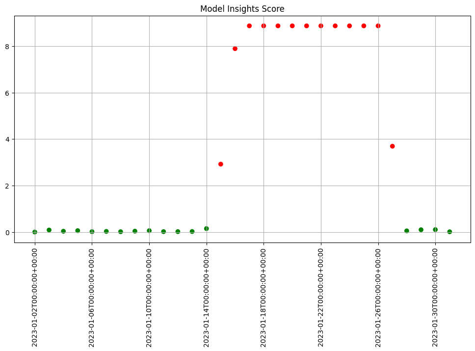
Figure: A daily assay that’s been running for a month. The dots represent the difference between the distribution of values in the daily observation window, and the baseline. When that difference exceeds the specified threshold (indicated by a red dot) an alert is set.

This next set of exercises will walk you through setting up an assay to monitor the predictions of your house price model, in order to detect drift.

NOTE

An assay is a monitoring process that typically runs over an extended, ongoing period of time. For example, one might set up an assay that every day monitors the previous 24 hours’ worth of predictions and compares it to a baseline. For the purposes of these exercises, we’ll be compressing processes what normally would take hours or days into minutes.

Assay DataSet Exercise

Because assays are designed to detect changes in distributions, let’s try to set up data with different distributions to test with. Take your houseprice data and create two sets: a set with lower prices, and a set with higher prices. You can split however you choose.

The idea is we will pretend that the set of lower priced houses represent the “typical” mix of houses in the housing portfolio at the time you set your baseline; you will introduce the higher priced houses later, to represent an environmental change when more expensive houses suddenly enter the market.

If you are using the pre-provided models to do these exercises, you can use the provided data sets lowprice.df.json and highprice.df.json. This is to establish our baseline as a set of known values, so the higher prices will trigger our assay alerts.

lowprice_data = pd.read_json('./data/lowprice.df.json')
highprice_data = pd.read_json('./data/highprice.df.json')

Note that the data in these files are already in the form expected by the models, so you don’t need to use the get_singleton or get_batch convenience functions to infer.

At the end of this exercise, you should have two sets of data to demonstrate assays. In the discussion below, we’ll refer to these sets as lowprice_data and highprice_data.

We will use this data to set up some “historical data” in the house price prediction pipeline that you build in the assay exercises.

Generate Sample Data

Before creating the assays, we will retrieve some sample data. The following files are provided by the instructor, and at this point inferences are run in the same workspace and pipeline that was retrieved.

We’ll retrieve the following variables for use in our assay generation:

small_results_baseline: Used to create the baseline from the numpy values from sample inferences.
assay_baseline_start: When to start the baseline from the inference history.
assay_baseline_end: When to end the baseline from the inference history.
assay_window_start: When to start the assay window period for assay samples.

# not needed for 2023.2
import numpy

baseline_numpy = numpy.load('./small_results_baseline.npy')

# read the assay baseline start datetime

with open('./assay_baseline_start', 'r') as file:
    assay_baseline_start = datetime.datetime.strptime(file.read(), "%d-%b-%Y (%H:%M:%S.%f)")

# read the assay baseline end datetime

with open('./assay_baseline_end', 'r') as file:
    assay_baseline_end = datetime.datetime.strptime(file.read(), "%d-%b-%Y (%H:%M:%S.%f)")

# read the assay window start datetime

with open('./assay_window_start', 'r') as file:
    assay_window_start = datetime.datetime.strptime(file.read(), "%d-%b-%Y (%H:%M:%S.%f)")
assay_window_start

datetime.datetime(2024, 3, 11, 19, 16, 0, 149220)

Model Insights via the Wallaroo Dashboard SDK

Assays generated through the Wallaroo SDK can be previewed, configured, and uploaded to the Wallaroo Ops instance. The following is a condensed version of this process. For full details see the Wallaroo SDK Essentials Guide: Assays Management guide.

Model drift detection with assays using the Wallaroo SDK follows this general process.

Define the Baseline: From either historical inference data for a specific model in a pipeline, or from a pre-determine array of data, a baseline is formed.
Assay Preview: Once the baseline is formed, we preview the assay and configure the different options until we have the the best method of detecting environment or model drift.
Create Assay: With the previews and configuration complete, we upload the assay. The assay will perform an analysis on a regular scheduled based on the configuration.
Get Assay Results: Retrieve the analyses and use them to detect model drift and possible sources.
Pause/Resume Assay: Pause or restart an assay as needed.

Define the Baseline

Assay baselines are defined with the wallaroo.client.build_assay method. Through this process we define the baseline from either a range of dates or pre-generated values.

wallaroo.client.build_assay take the following parameters:

Parameter	Type	Description
assay_name	String (Required) - required	The name of the assay. Assay names must be unique across the Wallaroo instance.
pipeline	wallaroo.pipeline.Pipeline (Required)	The pipeline the assay is monitoring.
model_name	String (Required)	The name of the model to monitor.
iopath	String (Required)	The input/output data for the model being tracked in the format `input/output field index`. Only one value is tracked for any assay. For example, to track the output of the model’s field `house_value` at index `0`, the `iopath` is `'output house_value 0`.
baseline_start	datetime.datetime (Optional)	The start time for the inferences to use as the baseline. Must be included with `baseline_end`. Cannot be included with `baseline_data`.
baseline_end	datetime.datetime (Optional)	The end time of the baseline window. the baseline. Windows start immediately after the baseline window and are run at regular intervals continuously until the assay is deactivated or deleted. Must be included with `baseline_start`. Cannot be included with `baseline_data`..
baseline_data	numpy.array (Optional)	The baseline data in numpy array format. Cannot be included with either `baseline_start` or `baseline_data`.

Baselines are created in one of two ways:

Date Range: The baseline_start and baseline_end retrieves the inference requests and results for the pipeline from the start and end period. This data is summarized and used to create the baseline.
Numpy Values: The baseline_data sets the baseline from a provided numpy array.

Define the Baseline Example

This example shows two methods of defining the baseline for an assay:

"assays from date baseline": This assay uses historical inference requests to define the baseline. This assay is saved to the variable assay_builder_from_dates.
"assays from numpy": This assay uses a pre-generated numpy array to define the baseline. This assay is saved to the variable assay_builder_from_numpy.

In both cases, the following parameters are used:

Parameter	Value
assay_name	`"assays from date baseline"` and `"assays from numpy"`
pipeline	`mainpipeline`: A pipeline with a ML model that predicts house prices. The output field for this model is `variable`.
model_name	`"houseprice-predictor"` - the model name set during model upload.
iopath	These assays monitor the model’s output field variable at index 0. From this, the `iopath` setting is `"output variable 0"`.

The difference between the two assays’ parameters determines how the baseline is generated.

"assays from date baseline": Uses the baseline_start and baseline_end to set the time period of inference requests and results to gather data from.
"assays from numpy": Uses a pre-generated numpy array as for the baseline data.

For each of our assays, we will set the time period of inference data to compare against the baseline data.

# Build the assay, based on the start and end of our baseline time, 
# and tracking the output variable index 0
assay_builder_from_dates = ( wl.build_assay('sample assay from baseline_date', 
                                            pipeline, 
                                            model_name, 
                                            baseline_start=assay_baseline_start, 
                                            baseline_end=assay_baseline_end)
                                            .add_iopath("output variable 0")
                           )

assay_builder_from_dates.add_run_until(datetime.datetime.now())
assay_builder_from_dates.window_builder().add_width(minutes=1).add_interval(minutes=1).add_start(assay_window_start)
assay_config_from_dates = assay_builder_from_dates.build()
assay_results_from_dates = assay_config_from_dates.interactive_run()

# these are for 2023.4 and above

# assay_builder_from_dates = wl.build_assay(assay_name="assays from date baseline", 
#                                           pipeline=pipeline, 
#                                           model_name=model_name, 
#                                           iopath="output variable 0",
#                                           baseline_start=assay_baseline_start, 
#                                           baseline_end=assay_baseline_end)

# # set the width, interval, and time period 
# assay_builder_from_dates.add_run_until(datetime.datetime.now())
# assay_builder_from_dates.window_builder().add_width(minutes=1).add_interval(minutes=1).add_start(assay_window_start)
# assay_config_from_dates = assay_builder_from_dates.build()
# assay_results_from_dates = assay_config_from_dates.interactive_run()

# # assay builder by baseline
# assay_builder_from_numpy = wl.build_assay(assay_name="assays from numpy", 
#                                pipeline=pipeline, 
#                                model_name="house-price-estimator", 
#                                iopath="output variable 0", 
#                                baseline_data = baseline_numpy)

# # set the width, interval, and time period 
# assay_builder_from_numpy.add_run_until(datetime.datetime.now())
# assay_builder_from_numpy.window_builder().add_width(minutes=1).add_interval(minutes=1).add_start(assay_window_start)

# assay_config_from_numpy = assay_builder_from_numpy.build()
# assay_results_from_numpy = assay_config_from_numpy.interactive_run()

Baseline DataFrame

The method wallaroo.assay_config.AssayBuilder.baseline_dataframe returns a DataFrame of the assay baseline generated from the provided parameters. This includes:

metadata: The inference metadata with the model information, inference time, and other related factors.
in data: Each input field assigned with the label in.{input field name}.
out data: Each output field assigned with the label out.{output field name}

Note that for assays generated from numpy values, there is only the out data based on the supplied baseline data.

In the following example, the baseline DataFrame is retrieved.

display(assay_builder_from_dates.baseline_dataframe())

	time	metadata	input_tensor_0	input_tensor_1	input_tensor_2	input_tensor_3	input_tensor_4	input_tensor_5	input_tensor_6	input_tensor_7	...	input_tensor_9	input_tensor_10	input_tensor_11	input_tensor_12	input_tensor_13	input_tensor_14	input_tensor_15	input_tensor_16	input_tensor_17	output_variable_0
0	1710184560113	{'last_model': '{"model_name":"house-price-prime","model_sha":"31e92d6ccb27b041a324a7ac22cf95d9d6cc3aa7e8263a229f7c4aec4938657c"}', 'pipeline_version': '77ad5fac-733b-40aa-8471-2b623731a1c2', 'elapsed': [2926861, 1998356], 'dropped': []}	3.0	2.00	1460.0	9759.0	1.0	0.0	0.0	5.0	...	1460.0	0.0	47.664398	-122.143997	1620.0	8421.0	42.0	0.0	0.0	4.915096e+05
1	1710184560113	{'last_model': '{"model_name":"house-price-prime","model_sha":"31e92d6ccb27b041a324a7ac22cf95d9d6cc3aa7e8263a229f7c4aec4938657c"}', 'pipeline_version': '77ad5fac-733b-40aa-8471-2b623731a1c2', 'elapsed': [2926861, 1998356], 'dropped': []}	4.0	1.00	1750.0	68841.0	1.0	0.0	0.0	3.0	...	1750.0	0.0	47.444199	-122.081001	1550.0	32799.0	72.0	0.0	0.0	3.389258e+05
2	1710184560113	{'last_model': '{"model_name":"house-price-prime","model_sha":"31e92d6ccb27b041a324a7ac22cf95d9d6cc3aa7e8263a229f7c4aec4938657c"}', 'pipeline_version': '77ad5fac-733b-40aa-8471-2b623731a1c2', 'elapsed': [2926861, 1998356], 'dropped': []}	3.0	1.75	1280.0	10716.0	1.0	0.0	0.0	4.0	...	1280.0	0.0	47.475498	-122.144997	1440.0	9870.0	45.0	0.0	0.0	2.832537e+05
3	1710184560113	{'last_model': '{"model_name":"house-price-prime","model_sha":"31e92d6ccb27b041a324a7ac22cf95d9d6cc3aa7e8263a229f7c4aec4938657c"}', 'pipeline_version': '77ad5fac-733b-40aa-8471-2b623731a1c2', 'elapsed': [2926861, 1998356], 'dropped': []}	4.0	2.50	1620.0	8125.0	2.0	0.0	0.0	4.0	...	1620.0	0.0	47.625500	-122.058998	1480.0	8120.0	32.0	0.0	0.0	4.860472e+05
4	1710184560113	{'last_model': '{"model_name":"house-price-prime","model_sha":"31e92d6ccb27b041a324a7ac22cf95d9d6cc3aa7e8263a229f7c4aec4938657c"}', 'pipeline_version': '77ad5fac-733b-40aa-8471-2b623731a1c2', 'elapsed': [2926861, 1998356], 'dropped': []}	4.0	2.50	2810.0	6481.0	2.0	0.0	0.0	3.0	...	2810.0	0.0	47.333000	-122.171997	2660.0	6958.0	17.0	0.0	0.0	3.866570e+05
...	...	...	...	...	...	...	...	...	...	...	...	...	...	...	...	...	...	...	...	...	...
495	1710184560113	{'last_model': '{"model_name":"house-price-prime","model_sha":"31e92d6ccb27b041a324a7ac22cf95d9d6cc3aa7e8263a229f7c4aec4938657c"}', 'pipeline_version': '77ad5fac-733b-40aa-8471-2b623731a1c2', 'elapsed': [2926861, 1998356], 'dropped': []}	4.0	2.25	3310.0	8540.0	1.0	0.0	4.0	4.0	...	1660.0	1650.0	47.560299	-122.157997	3450.0	9566.0	41.0	0.0	0.0	1.001796e+06
496	1710184560113	{'last_model': '{"model_name":"house-price-prime","model_sha":"31e92d6ccb27b041a324a7ac22cf95d9d6cc3aa7e8263a229f7c4aec4938657c"}', 'pipeline_version': '77ad5fac-733b-40aa-8471-2b623731a1c2', 'elapsed': [2926861, 1998356], 'dropped': []}	4.0	2.75	2020.0	7070.0	1.0	0.0	0.0	5.0	...	1010.0	1010.0	47.520199	-122.377998	1390.0	6000.0	56.0	0.0	0.0	4.662758e+05
497	1710184560113	{'last_model': '{"model_name":"house-price-prime","model_sha":"31e92d6ccb27b041a324a7ac22cf95d9d6cc3aa7e8263a229f7c4aec4938657c"}', 'pipeline_version': '77ad5fac-733b-40aa-8471-2b623731a1c2', 'elapsed': [2926861, 1998356], 'dropped': []}	3.0	2.50	2250.0	8076.0	2.0	0.0	0.0	3.0	...	2250.0	0.0	47.366699	-122.041000	2180.0	7244.0	19.0	0.0	0.0	3.643214e+05
498	1710184560113	{'last_model': '{"model_name":"house-price-prime","model_sha":"31e92d6ccb27b041a324a7ac22cf95d9d6cc3aa7e8263a229f7c4aec4938657c"}', 'pipeline_version': '77ad5fac-733b-40aa-8471-2b623731a1c2', 'elapsed': [2926861, 1998356], 'dropped': []}	5.0	4.00	4360.0	8030.0	2.0	0.0	0.0	3.0	...	4360.0	0.0	47.592300	-121.973000	3570.0	6185.0	0.0	0.0	0.0	9.626006e+05
499	1710184560113	{'last_model': '{"model_name":"house-price-prime","model_sha":"31e92d6ccb27b041a324a7ac22cf95d9d6cc3aa7e8263a229f7c4aec4938657c"}', 'pipeline_version': '77ad5fac-733b-40aa-8471-2b623731a1c2', 'elapsed': [2926861, 1998356], 'dropped': []}	4.0	2.50	1960.0	7230.0	2.0	0.0	0.0	3.0	...	1960.0	0.0	47.285500	-122.360001	1850.0	7208.0	12.0	0.0	0.0	2.894587e+05

500 rows × 21 columns

Baseline Stats

The method wallaroo.assay.AssayAnalysis.baseline_stats() returns a pandas.core.frame.DataFrame of the baseline stats.

The baseline stats for each assay are displayed in the examples below.

assay_results_from_dates[0].baseline_stats()

	Baseline
count	500
min	171875.375
max	1908622.5
mean	514227.312437
median	450623.609375
std	277313.851831
start	2024-03-11T19:14:59.997423+00:00
end	2024-03-11T19:16:00.128604+00:00

Baseline Bins

The method wallaroo.assay.AssayAnalysis.baseline_bins a simple dataframe to with the edge/bin data for a baseline.

assay_results_from_dates[0].baseline_bins()

	b_edges	b_edge_names	b_aggregated_values	b_aggregation
0	1.718754e+05	left_outlier	0.000	Density
1	3.061700e+05	q_20	0.204	Density
2	3.938371e+05	q_40	0.196	Density
3	5.016934e+05	q_60	0.202	Density
4	6.670536e+05	q_80	0.198	Density
5	1.908622e+06	q_100	0.200	Density
6	inf	right_outlier	0.000	Density

Baseline Histogram Chart

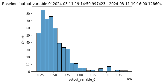
The method wallaroo.assay_config.AssayBuilder.baseline_histogram returns a histogram chart of the assay baseline generated from the provided parameters.

assay_builder_from_dates.baseline_histogram()

Assay Preview

Now that the baseline is defined, we look at different configuration options and view how the assay baseline and results changes. Once we determine what gives us the best method of determining model drift, we can create the assay.

Analysis List Chart Scores

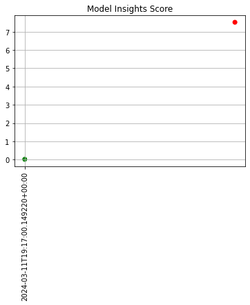
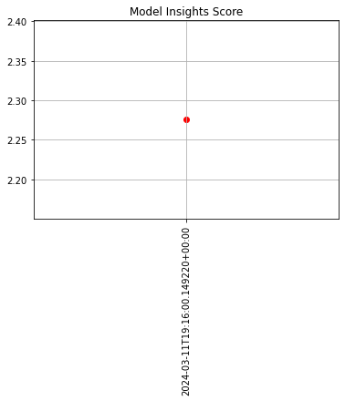
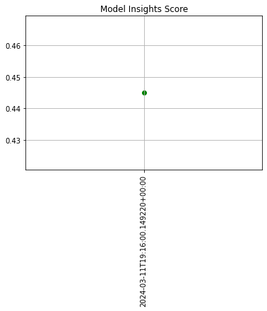
Analysis List scores show the assay scores for each assay result interval in one chart. Values that are outside of the alert threshold are colored red, while scores within the alert threshold are green.

Assay chart scores are displayed with the method wallaroo.assay.AssayAnalysisList.chart_scores(title: Optional[str] = None), with ability to display an optional title with the chart.

The following example shows retrieving the assay results and displaying the chart scores. From our example, we have two windows - the first should be green, and the second is red showing that values were outside the alert threshold.

# Build the assay, based on the start and end of our baseline time, 
# and tracking the output variable index 0
assay_builder_from_dates = ( wl.build_assay('sample assay from baseline_date', 
                                            pipeline, 
                                            model_name, 
                                            baseline_start=assay_baseline_start, 
                                            baseline_end=assay_baseline_end)
                                            .add_iopath("output variable 0")
                           )

assay_builder_from_dates.add_run_until(datetime.datetime.now())
assay_builder_from_dates.window_builder().add_width(minutes=1).add_interval(minutes=1).add_start(assay_window_start)
assay_config_from_dates = assay_builder_from_dates.build()
assay_results_from_dates = assay_config_from_dates.interactive_run()

assay_results_from_dates.chart_scores()

#### Analysis Chart

The method `wallaroo.assay.AssayAnalysis.chart()` displays a comparison between the baseline and an interval of inference data.

This is compared to the [Chart Scores](#analysis-list-chart-scores), which is a **list** of all of the inference data split into intervals, while the **Analysis Chart** shows the breakdown of one set of inference data against the baseline.

Score from the [Analysis List Chart Scores](#analysis-list-chart-scores) and each element from the [Analysis List DataFrame](#analysis-list-dataframe) generates 

The following fields are included.

| Field | Type | Description |
|---|---|---|
| **baseline mean** | **Float** | The mean of the baseline values. |
| **window mean** | **Float** | The mean of the window values. |
| **baseline median** | **Float** | The median of the baseline values. |
| **window median** | **Float** | The median of the window values. |
| **bin_mode** | **String** | The binning mode used for the assay. |
| **aggregation** | **String** | The aggregation mode used for the assay. |
| **metric** | **String** | The metric mode used for the assay. |
| **weighted** | **Bool** | Whether the bins were manually weighted. |
| **score** | **Float** | The score from the assay window. |
| **scores** | **List(Float)** | The score from each assay window bin. |
| **index** | **Integer/None** | The window index.  Interactive assay runs are `None`. |

# Build the assay, based on the start and end of our baseline time, 
# and tracking the output variable index 0
assay_builder_from_dates = ( wl.build_assay('sample assay from baseline_date', 
                                            pipeline, 
                                            model_name, 
                                            baseline_start=assay_baseline_start, 
                                            baseline_end=assay_baseline_end)
                                            .add_iopath("output variable 0")
                           )

assay_builder_from_dates.add_run_until(datetime.datetime.now())
assay_builder_from_dates.window_builder().add_width(minutes=1).add_interval(minutes=1).add_start(assay_window_start)
assay_config_from_dates = assay_builder_from_dates.build()
assay_results_from_dates = assay_config_from_dates.interactive_run()

assay_results_from_dates[0].chart()

baseline mean = 514227.3124375
window mean = 507478.46859375
baseline median = 450623.609375
window median = 445049.296875
bin_mode = Quantile
aggregation = Density
metric = PSI
weighted = False
score = 0.016941317365585698
scores = [0.002748872195622465, 0.0025104927488832605, 0.005438798089551059, 0.003302949120684397, 0.0023179313444721787, 0.0006222738663723384, 0.0]
index = None

Analysis List DataFrame

wallaroo.assay.AssayAnalysisList.to_dataframe() returns a DataFrame showing the assay results for each window aka individual analysis. This DataFrame contains the following fields:

Field	Type	Description
assay_id	Integer/None	The assay id. Only provided from uploaded and executed assays.
name	String/None	The name of the assay. Only provided from uploaded and executed assays.
iopath	String/None	The iopath of the assay. Only provided from uploaded and executed assays.
score	Float	The assay score.
start	DateTime	The DateTime start of the assay window.
min	Float	The minimum value in the assay window.
max	Float	The maximum value in the assay window.
mean	Float	The mean value in the assay window.
median	Float	The median value in the assay window.
std	Float	The standard deviation value in the assay window.
warning_threshold	Float/None	The warning threshold of the assay window.
alert_threshold	Float/None	The alert threshold of the assay window.
status	String	The assay window status. Values are: `OK`: The score is within accepted thresholds. `Warning`: The score has triggered the `warning_threshold` if exists, but not the `alert_threshold`. `Alert`: The score has triggered the the `alert_threshold`.

For this example, the assay analysis list DataFrame is listed.

From this tutorial, we should have 2 windows of dta to look at, each one minute apart. The first window should show status: OK, with the second window with the very large house prices will show status: alert

# Build the assay, based on the start and end of our baseline time, 
# and tracking the output variable index 0
assay_builder_from_dates = ( wl.build_assay('sample assay from baseline_date', 
                                            pipeline, 
                                            model_name, 
                                            baseline_start=assay_baseline_start, 
                                            baseline_end=assay_baseline_end)
                                            .add_iopath("output variable 0")
                           )

assay_builder_from_dates.add_run_until(datetime.datetime.now())
assay_builder_from_dates.window_builder().add_width(minutes=1).add_interval(minutes=1).add_start(assay_window_start)
assay_config_from_dates = assay_builder_from_dates.build()
assay_results_from_dates = assay_config_from_dates.interactive_run()

assay_results_from_dates.to_dataframe()

	assay_id	name	iopath	score	start	min	max	mean	median	std	warning_threshold	alert_threshold	status
0	None		output variable 0	0.016941	2024-03-11T19:17:00.149220+00:00	1.629850e+05	1908622.50	5.074785e+05	4.450493e+05	258215.325866	None	0.25	Ok
1	None		output variable 0	7.517112	2024-03-11T19:19:00.149220+00:00	1.902903e+06	2607629.25	2.244347e+06	2.303257e+06	223017.172706	None	0.25	Alert

Analysis List Full DataFrame

wallaroo.assay.AssayAnalysisList.to_full_dataframe() returns a DataFrame showing all values, including the inputs and outputs from the assay results for each window aka individual analysis. This DataFrame contains the following fields:

pipeline_id	warning_threshold	bin_index	created_at

Field	Type	Description
window_start	DateTime	The date and time when the window period began.
analyzed_at	DateTime	The date and time when the assay analysis was performed.
elapsed_millis	Integer	How long the analysis took to perform in milliseconds.
baseline_summary_count	Integer	The number of data elements from the baseline.
baseline_summary_min	Float	The minimum value from the baseline summary.
baseline_summary_max	Float	The maximum value from the baseline summary.
baseline_summary_mean	Float	The mean value of the baseline summary.
baseline_summary_median	Float	The median value of the baseline summary.
baseline_summary_std	Float	The standard deviation value of the baseline summary.
baseline_summary_edges_{0…n}	Float	The baseline summary edges for each baseline edge from 0 to number of edges.
summarizer_type	String	The type of summarizer used for the baseline. See `wallaroo.assay_config` for other summarizer types.
summarizer_bin_weights	List / None	If baseline bin weights were provided, the list of those weights. Otherwise, `None`.
summarizer_provided_edges	List / None	If baseline bin edges were provided, the list of those edges. Otherwise, `None`.
status	String	The assay window status. Values are: `OK`: The score is within accepted thresholds. `Warning`: The score has triggered the `warning_threshold` if exists, but not the `alert_threshold`. `Alert`: The score has triggered the the `alert_threshold`.
id	Integer/None	The id for the window aka analysis. Only provided from uploaded and executed assays.
assay_id	Integer/None	The assay id. Only provided from uploaded and executed assays.
pipeline_id	Integer/None	The pipeline id. Only provided from uploaded and executed assays.
warning_threshold	Float	The warning threshold set for the assay.
warning_threshold	Float	The warning threshold set for the assay.
bin_index	Integer/None	The bin index for the window aka analysis.
created_at	Datetime/None	The date and time the window aka analysis was generated. Only provided from uploaded and executed assays.

For this example, full DataFrame from an assay preview is generated.

# Build the assay, based on the start and end of our baseline time, 
# and tracking the output variable index 0
assay_builder_from_dates = ( wl.build_assay('sample assay from baseline_date', 
                                            pipeline, 
                                            model_name, 
                                            baseline_start=assay_baseline_start, 
                                            baseline_end=assay_baseline_end)
                                            .add_iopath("output variable 0")
                           )

assay_builder_from_dates.add_run_until(datetime.datetime.now())
assay_builder_from_dates.window_builder().add_width(minutes=1).add_interval(minutes=1).add_start(assay_window_start)
assay_config_from_dates = assay_builder_from_dates.build()
assay_results_from_dates = assay_config_from_dates.interactive_run()

assay_results_from_dates.to_full_dataframe()

	window_start	analyzed_at	elapsed_millis	iopath	baseline_summary_count	baseline_summary_min	baseline_summary_max	baseline_summary_mean	baseline_summary_median	baseline_summary_std	...	summarizer_type	summarizer_bin_weights	summarizer_provided_edges	status	id	assay_id	pipeline_id	warning_threshold	bin_index	created_at
0	2024-03-11T19:17:00.149220+00:00	2024-03-11T21:03:15.699380+00:00	798	output variable 0	500	171875.375	1908622.5	514227.312437	450623.609375	277313.851831	...	UnivariateContinuous	None	None	Ok	None	None	None	None	None	None
1	2024-03-11T19:19:00.149220+00:00	2024-03-11T21:03:15.700061+00:00	794	output variable 0	500	171875.375	1908622.5	514227.312437	450623.609375	277313.851831	...	UnivariateContinuous	None	None	Alert	None	None	None	None	None	None

2 rows × 87 columns

Analysis Compare Basic Stats

The method wallaroo.assay.AssayAnalysis.compare_basic_stats returns a DataFrame comparing one set of inference data against the baseline.

This is compared to the Analysis List DataFrame, which is a list of all of the inference data split into intervals, while the Analysis Compare Basic Stats shows the breakdown of one set of inference data against the baseline.

# Build the assay, based on the start and end of our baseline time, 
# and tracking the output variable index 0
assay_builder_from_dates = ( wl.build_assay('sample assay from baseline_date', 
                                            pipeline, 
                                            model_name, 
                                            baseline_start=assay_baseline_start, 
                                            baseline_end=assay_baseline_end)
                                            .add_iopath("output variable 0")
                           )

assay_builder_from_dates.add_run_until(datetime.datetime.now())
assay_builder_from_dates.window_builder().add_width(minutes=1).add_interval(minutes=1).add_start(assay_window_start)
assay_config_from_dates = assay_builder_from_dates.build()
assay_results_from_dates = assay_config_from_dates.interactive_run()

assay_results_from_dates[0].compare_basic_stats()

	Baseline	Window	diff	pct_diff
count	500.0	1000.0	500.000000	100.000000
min	171875.375	162984.96875	-8890.406250	-5.172589
max	1908622.5	1908622.5	0.000000	0.000000
mean	514227.312437	507478.468594	-6748.843844	-1.312424
median	450623.609375	445049.296875	-5574.312500	-1.237022
std	277313.851831	258215.325866	-19098.525965	-6.886972
start	2024-03-11T19:14:59.997423+00:00	2024-03-11T19:17:00.149220+00:00	NaN	NaN
end	2024-03-11T19:16:00.128604+00:00	2024-03-11T19:18:00.149220+00:00	NaN	NaN

Configure Assays

Before creating the assay, configure the assay and continue to preview it until the best method for detecting drift is set. The following options are available.

Score Metric

The score is a distance between the baseline and the analysis window. The larger the score, the greater the difference between the baseline and the analysis window. The following methods are provided determining the score:

PSI (Default) - Population Stability Index (PSI).
MAXDIFF: Maximum difference between corresponding bins.
SUMDIFF: Mum of differences between corresponding bins.

The metric type used is updated with the wallaroo.assay_config.AssayBuilder.add_metric(metric: wallaroo.assay_config.Metric) method.

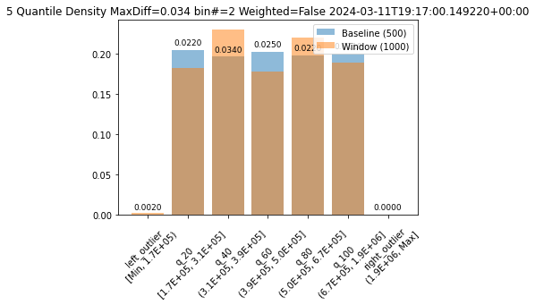
The following three charts use each of the metrics. Note how the scores change based on the score type used.

# Build the assay, based on the start and end of our baseline time, 
# and tracking the output variable index 0
assay_builder_from_dates = ( wl.build_assay('sample assay from baseline_date', 
                                            pipeline, 
                                            model_name, 
                                            baseline_start=assay_baseline_start, 
                                            baseline_end=assay_baseline_end)
                                            .add_iopath("output variable 0")
                           )

# set metric PSI mode
assay_builder_from_dates.summarizer_builder.add_metric(wallaroo.assay_config.Metric.PSI)

assay_builder_from_dates.add_run_until(datetime.datetime.now())
assay_builder_from_dates.window_builder().add_width(minutes=1).add_interval(minutes=1).add_start(assay_window_start)
assay_config_from_dates = assay_builder_from_dates.build()
assay_results_from_dates = assay_config_from_dates.interactive_run()

assay_results_from_dates[0].chart()

baseline mean = 514227.3124375
window mean = 507478.46859375
baseline median = 450623.609375
window median = 445049.296875
bin_mode = Quantile
aggregation = Density
metric = PSI
weighted = False
score = 0.016941317365585698
scores = [0.002748872195622465, 0.0025104927488832605, 0.005438798089551059, 0.003302949120684397, 0.0023179313444721787, 0.0006222738663723384, 0.0]
index = None

# Build the assay, based on the start and end of our baseline time, 
# and tracking the output variable index 0
assay_builder_from_dates = ( wl.build_assay('sample assay from baseline_date', 
                                            pipeline, 
                                            model_name, 
                                            baseline_start=assay_baseline_start, 
                                            baseline_end=assay_baseline_end)
                                            .add_iopath("output variable 0")
                           )

# set metric MAXDIFF mode
assay_builder_from_dates.summarizer_builder.add_metric(wallaroo.assay_config.Metric.MAXDIFF)

assay_builder_from_dates.add_run_until(datetime.datetime.now())
assay_builder_from_dates.window_builder().add_width(minutes=1).add_interval(minutes=1).add_start(assay_window_start)
assay_config_from_dates = assay_builder_from_dates.build()
assay_results_from_dates = assay_config_from_dates.interactive_run()

assay_results_from_dates[0].chart()

baseline mean = 514227.3124375
window mean = 507478.46859375
baseline median = 450623.609375
window median = 445049.296875
bin_mode = Quantile
aggregation = Density
metric = MaxDiff
weighted = False
score = 0.034
scores = [0.002, 0.021999999999999992, 0.034, 0.025000000000000026, 0.021999999999999992, 0.01100000000000001, 0.0]
index = 2

# Build the assay, based on the start and end of our baseline time, 
# and tracking the output variable index 0
assay_builder_from_dates = ( wl.build_assay('sample assay from baseline_date', 
                                            pipeline, 
                                            model_name, 
                                            baseline_start=assay_baseline_start, 
                                            baseline_end=assay_baseline_end)
                                            .add_iopath("output variable 0")
                           )

# set metric SUMDIFF mode
assay_builder_from_dates.summarizer_builder.add_metric(wallaroo.assay_config.Metric.SUMDIFF)

assay_builder_from_dates.add_run_until(datetime.datetime.now())
assay_builder_from_dates.window_builder().add_width(minutes=1).add_interval(minutes=1).add_start(assay_window_start)
assay_config_from_dates = assay_builder_from_dates.build()
assay_results_from_dates = assay_config_from_dates.interactive_run()

assay_results_from_dates[0].chart()

baseline mean = 514227.3124375
window mean = 507478.46859375
baseline median = 450623.609375
window median = 445049.296875
bin_mode = Quantile
aggregation = Density
metric = SumDiff
weighted = False
score = 0.05800000000000001
scores = [0.002, 0.021999999999999992, 0.034, 0.025000000000000026, 0.021999999999999992, 0.01100000000000001, 0.0]
index = None

Alert Threshold

Assay alert thresholds are modified with the wallaroo.assay_config.AssayBuilder.add_alert_threshold(alert_threshold: float) method. By default alert thresholds are 0.1.

The following example updates the alert threshold to 0.5.

# Build the assay, based on the start and end of our baseline time, 
# and tracking the output variable index 0
assay_builder_from_dates = ( wl.build_assay('sample assay from baseline_date', 
                                            pipeline, 
                                            model_name, 
                                            baseline_start=assay_baseline_start, 
                                            baseline_end=assay_baseline_end)
                                            .add_iopath("output variable 0")
                           )

assay_builder_from_dates.add_alert_threshold(0.5)

assay_builder_from_dates.add_run_until(datetime.datetime.now())
assay_builder_from_dates.window_builder().add_width(minutes=1).add_interval(minutes=1).add_start(assay_window_start)
assay_config_from_dates = assay_builder_from_dates.build()
assay_results_from_dates = assay_config_from_dates.interactive_run()

assay_results_from_dates.to_dataframe()

	assay_id	name	iopath	score	start	min	max	mean	median	std	warning_threshold	alert_threshold	status
0	None		output variable 0	0.016941	2024-03-11T19:17:00.149220+00:00	1.629850e+05	1908622.50	5.074785e+05	4.450493e+05	258215.325866	None	0.5	Ok
1	None		output variable 0	7.517112	2024-03-11T19:19:00.149220+00:00	1.902903e+06	2607629.25	2.244347e+06	2.303257e+06	223017.172706	None	0.5	Alert

Number of Bins

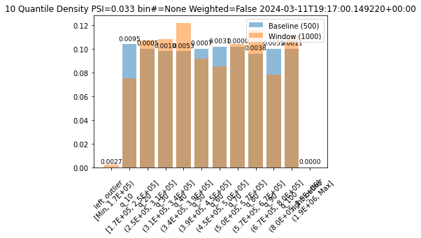
Number of bins sets how the baseline data is partitioned. The total number of bins includes the set number plus the left_outlier and the right_outlier, so the total number of bins will be the total set + 2.

The number of bins is set with the wallaroo.assay_config.UnivariateContinousSummarizerBuilder.add_num_bins(num_bins: int) method.

# Build the assay, based on the start and end of our baseline time, 
# and tracking the output variable index 0
assay_builder_from_dates = ( wl.build_assay('sample assay from baseline_date', 
                                            pipeline, 
                                            model_name, 
                                            baseline_start=assay_baseline_start, 
                                            baseline_end=assay_baseline_end)
                                            .add_iopath("output variable 0")
                           )

# Set the number of bins
# update number of bins here
assay_builder_from_dates.summarizer_builder.add_num_bins(10)

assay_builder_from_dates.add_run_until(datetime.datetime.now())
assay_builder_from_dates.window_builder().add_width(minutes=1).add_interval(minutes=1).add_start(assay_window_start)
assay_config_from_dates = assay_builder_from_dates.build()
assay_results_from_dates = assay_config_from_dates.interactive_run()

assay_results_from_dates[0].chart()

baseline mean = 514227.3124375 window mean = 507478.46859375 baseline median = 450623.609375 window median = 445049.296875 bin_mode = Quantile aggregation = Density metric = PSI weighted = False score = 0.03313589216215494 scores = [0.002748872195622465, 0.009480180782546805, 0.0004736105393167021, 0.0009716374845364762, 0.005257285585504427, 0.0006670528715124097, 0.0030994664654972236, 3.883617171420307e-05, 0.003784839992770567, 0.005466149904566996, 0.0011479601685666688, 0.0] index = None

/opt/conda/lib/python3.9/site-packages/wallaroo/assay.py:317: UserWarning: FixedFormatter should only be used together with FixedLocator ax.set_xticklabels(labels=edge_names, rotation=45)

##### Binning Mode

Binning Mode defines how the bins are separated.  Binning modes are modified through the `wallaroo.assay_config.UnivariateContinousSummarizerBuilder.add_bin_mode(bin_mode: bin_mode: wallaroo.assay_config.BinMode, edges: Optional[List[float]] = None)`.

Available `bin_mode` values from `wallaroo.assay_config.Binmode` are the following:

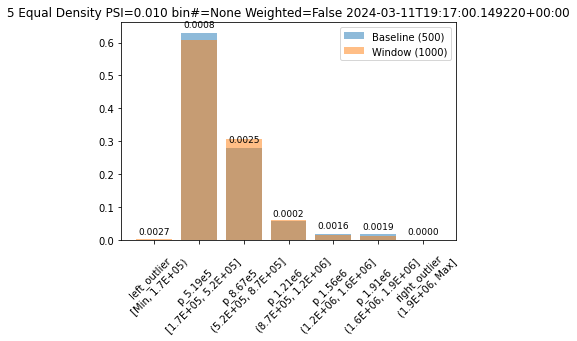
* `QUANTILE` (*Default*): Based on percentages. If `num_bins` is 5 then quintiles so bins are created at the 20%, 40%, 60%, 80% and 100% points.
* `EQUAL`: Evenly spaced bins where each bin is set with the formula `min - max / num_bins`
* `PROVIDED`: The user provides the edge points for the bins.

If `PROVIDED` is supplied, then a List of float values must be provided for the `edges` parameter that matches the number of bins.

The following examples are used to show how each of the binning modes effects the bins.

# Build the assay, based on the start and end of our baseline time, 
# and tracking the output variable index 0
assay_builder_from_dates = ( wl.build_assay('sample assay from baseline_date', 
                                            pipeline, 
                                            model_name, 
                                            baseline_start=assay_baseline_start, 
                                            baseline_end=assay_baseline_end)
                                            .add_iopath("output variable 0")
                           )

# update binning mode here
assay_builder_from_dates.summarizer_builder.add_bin_mode(wallaroo.assay_config.BinMode.QUANTILE)

assay_builder_from_dates.add_run_until(datetime.datetime.now())
assay_builder_from_dates.window_builder().add_width(minutes=1).add_interval(minutes=1).add_start(assay_window_start)
assay_config_from_dates = assay_builder_from_dates.build()
assay_results_from_dates = assay_config_from_dates.interactive_run()

assay_results_from_dates[0].chart()

baseline mean = 514227.3124375
window mean = 507478.46859375
baseline median = 450623.609375
window median = 445049.296875
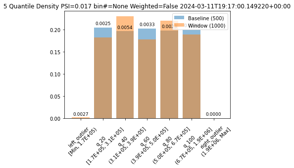
bin_mode = Quantile
aggregation = Density
metric = PSI
weighted = False
score = 0.016941317365585698
scores = [0.002748872195622465, 0.0025104927488832605, 0.005438798089551059, 0.003302949120684397, 0.0023179313444721787, 0.0006222738663723384, 0.0]
index = None

# Build the assay, based on the start and end of our baseline time, 
# and tracking the output variable index 0
assay_builder_from_dates = ( wl.build_assay('sample assay from baseline_date', 
                                            pipeline, 
                                            model_name, 
                                            baseline_start=assay_baseline_start, 
                                            baseline_end=assay_baseline_end)
                                            .add_iopath("output variable 0")
                           )

# update binning mode here
assay_builder_from_dates.summarizer_builder.add_bin_mode(wallaroo.assay_config.BinMode.EQUAL)

assay_builder_from_dates.add_run_until(datetime.datetime.now())
assay_builder_from_dates.window_builder().add_width(minutes=1).add_interval(minutes=1).add_start(assay_window_start)
assay_config_from_dates = assay_builder_from_dates.build()
assay_results_from_dates = assay_config_from_dates.interactive_run()

assay_results_from_dates[0].chart()

baseline mean = 514227.3124375
window mean = 507478.46859375
baseline median = 450623.609375
window median = 445049.296875
bin_mode = Equal
aggregation = Density
metric = PSI
weighted = False
score = 0.009673567227025998
scores = [0.002748872195622465, 0.0007819886232270504, 0.0024855698992845778, 0.00015655725951171053, 0.0016271120021731395, 0.0018734672472070536, 0.0]
index = None

Aggregation Options

Assay aggregation options are modified with the wallaroo.assay_config.AssayBuilder.add_aggregation(aggregation: wallaroo.assay_config.Aggregation) method. The following options are provided:

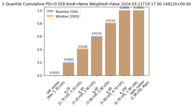
Aggregation.DENSITY (Default): Count the number/percentage of values that fall in each bin.
Aggregation.CUMULATIVE: Empirical Cumulative Density Function style, which keeps a cumulative count of the values/percentages that fall in each bin.

The following example demonstrate the different results between the two.

# Build the assay, based on the start and end of our baseline time, 
# and tracking the output variable index 0
assay_builder_from_dates = ( wl.build_assay('sample assay from baseline_date', 
                                            pipeline, 
                                            model_name, 
                                            baseline_start=assay_baseline_start, 
                                            baseline_end=assay_baseline_end)
                                            .add_iopath("output variable 0")
                           )

assay_builder_from_dates.summarizer_builder.add_aggregation(wallaroo.assay_config.Aggregation.DENSITY)

assay_builder_from_dates.add_run_until(datetime.datetime.now())
assay_builder_from_dates.window_builder().add_width(minutes=1).add_interval(minutes=1).add_start(assay_window_start)
assay_config_from_dates = assay_builder_from_dates.build()
assay_results_from_dates = assay_config_from_dates.interactive_run()

assay_results_from_dates[0].chart()

baseline mean = 514227.3124375
window mean = 507478.46859375
baseline median = 450623.609375
window median = 445049.296875
bin_mode = Quantile
aggregation = Density
metric = PSI
weighted = False
score = 0.016941317365585698
scores = [0.002748872195622465, 0.0025104927488832605, 0.005438798089551059, 0.003302949120684397, 0.0023179313444721787, 0.0006222738663723384, 0.0]
index = None

# Build the assay, based on the start and end of our baseline time, 
# and tracking the output variable index 0
assay_builder_from_dates = ( wl.build_assay('sample assay from baseline_date', 
                                            pipeline, 
                                            model_name, 
                                            baseline_start=assay_baseline_start, 
                                            baseline_end=assay_baseline_end)
                                            .add_iopath("output variable 0")
                           )

assay_builder_from_dates.summarizer_builder.add_aggregation(wallaroo.assay_config.Aggregation.CUMULATIVE)

assay_builder_from_dates.add_run_until(datetime.datetime.now())
assay_builder_from_dates.window_builder().add_width(minutes=1).add_interval(minutes=1).add_start(assay_window_start)
assay_config_from_dates = assay_builder_from_dates.build()
assay_results_from_dates = assay_config_from_dates.interactive_run()

assay_results_from_dates[0].chart()

baseline mean = 514227.3124375
window mean = 507478.46859375
baseline median = 450623.609375
window median = 445049.296875
bin_mode = Quantile
aggregation = Cumulative
metric = PSI
weighted = False
score = 0.05799999999999997
scores = [0.002, 0.01999999999999999, 0.013999999999999955, 0.01100000000000001, 0.01100000000000001, 0.0, 0.0]
index = None

Inference Interval and Inference Width

The inference interval aka window interval sets how often to run the assay analysis. This is set from the wallaroo.assay_config.AssayBuilder.window_builder.add_interval method to collect data expressed in time units: “hours=24”, “minutes=1”, etc.

For example, with an interval of 1 minute, the assay collects data every minute. Within an hour, 60 intervals of data is collected.

We can adjust the interval and see how the assays change based on how frequently they are run.

The width sets the time period from the wallaroo.assay_config.AssayBuilder.window_builder.add_width method to collect data expressed in time units: “hours=24”, “minutes=1”, etc.

For example, an interval of 1 minute and a width of 1 minute collects 1 minutes worth of data every minute. An interval of 1 minute with a width of 5 minutes collects 5 minute of inference data every minute.

By default, the interval and width is 24 hours.

For this example, we’ll adjust the width and interval from 1 minute to 5 minutes and see how the number of analyses and their score changes.

# Build the assay, based on the start and end of our baseline time, 
# and tracking the output variable index 0
assay_builder_from_dates = ( wl.build_assay('sample assay from baseline_date', 
                                            pipeline, 
                                            model_name, 
                                            baseline_start=assay_baseline_start, 
                                            baseline_end=assay_baseline_end)
                                            .add_iopath("output variable 0")
                           )

assay_builder_from_dates.add_run_until(datetime.datetime.now())
assay_builder_from_dates.window_builder().add_width(minutes=1).add_interval(minutes=1).add_start(assay_window_start)
assay_config_from_dates = assay_builder_from_dates.build()
assay_results_from_dates = assay_config_from_dates.interactive_run()

assay_results_from_dates.chart_scores()

# Build the assay, based on the start and end of our baseline time, 
# and tracking the output variable index 0
assay_builder_from_dates = ( wl.build_assay('sample assay from baseline_date', 
                                            pipeline, 
                                            model_name, 
                                            baseline_start=assay_baseline_start, 
                                            baseline_end=assay_baseline_end)
                                            .add_iopath("output variable 0")
                           )

assay_builder_from_dates.add_run_until(datetime.datetime.now())
assay_builder_from_dates.window_builder().add_width(minutes=5).add_interval(minutes=5).add_start(assay_window_start)
assay_config_from_dates = assay_builder_from_dates.build()
assay_results_from_dates = assay_config_from_dates.interactive_run()

assay_results_from_dates.chart_scores()

Create Assay

With the assay previewed and configuration options determined, we officially create it by uploading it to the Wallaroo instance.

Once it is uploaded, the assay runs an analysis based on the window width, interval, and the other settings configured.

Assays are uploaded with the wallaroo.assay_config.upload() method. This uploads the assay into the Wallaroo database with the configurations applied and returns the assay id. Note that assay names must be unique across the Wallaroo instance; attempting to upload an assay with the same name as an existing one will return an error.

wallaroo.assay_config.upload() returns the assay id for the assay.

Typically we would just call wallaroo.assay_config.upload() after configuring the assay. For the example below, we will perform the complete configuration in one window to show all of the configuration steps at once before creating the assay.

# Build the assay, based on the start and end of our baseline time, 
# and tracking the output variable index 0
assay_builder_from_dates = ( wl.build_assay('sample assay from baseline_date', 
                                            pipeline, 
                                            model_name, 
                                            baseline_start=assay_baseline_start, 
                                            baseline_end=assay_baseline_end)
                                            .add_iopath("output variable 0")
                           )

# add other options
assay_builder_from_dates.summarizer_builder.add_aggregation(wallaroo.assay_config.Aggregation.CUMULATIVE)
assay_builder_from_dates.summarizer_builder.add_metric(wallaroo.assay_config.Metric.MAXDIFF)
assay_builder_from_dates.add_alert_threshold(0.5)

assay_builder_from_dates.add_run_until(datetime.datetime.now())
assay_builder_from_dates.window_builder().add_width(minutes=5).add_interval(minutes=5).add_start(assay_window_start)
assay_config_from_dates = assay_builder_from_dates.build()
assay_results_from_dates = assay_config_from_dates.interactive_run()

assay_results_from_dates.chart_scores()

# not doing for the tutorial so we don't have 50 assays running
assay_id = assay_builder_from_dates.upload()

# wait 65 seconds for the first analysis run performed
time.sleep(65)

Get Assay Results

Once an assay is created the assay runs an analysis based on the window width, interval, and the other settings configured.

Assay results are retrieved with the wallaroo.client.get_assay_results method, which takes the following parameters:

Parameter	Type	Description
assay_id	Integer (Required)	The numerical id of the assay.
start	Datetime.Datetime (Required)	The start date and time of historical data from the pipeline to start analyses from.
end	Datetime.Datetime (Required)	The end date and time of historical data from the pipeline to limit analyses to.

IMPORTANT NOTE: This process requires that additional historical data is generated from the time the assay is created to when the results are available. To add additional inference data, use the Assay Test Data section above.

List and Retrieve Assay

If the assay id is not already known, it is retrieved from the wallaroo.client.list_assays() method. Select the assay to retrieve data for and retrieve its id with wallaroo.assay.Assay._id method.

wl.list_assays()

name	active	status	warning_threshold	alert_threshold	pipeline_name
sample assay from baseline_date	True	{"run_at": "2024-03-11T21:28:54.497495392+00:00", "num_ok": 1, "num_warnings": 0, "num_alerts": 0}	None	0.5	houseprice-estimator

retrieved_assay = wl.list_assays()[0]

retrieved_assay._id

live_assay_results = wl.get_assay_results(assay_id=retrieved_assay._id,
                         start=assay_baseline_start,
                         end=datetime.datetime.now()
                    )

len(live_assay_results)
#live_assay_results.chart_scores()

---------------------------------------------------------------------------
Exception                                 Traceback (most recent call last)
/tmp/ipykernel_325/3708687896.py in <module>

5 # retrieved_assay.chart_scores()

6

—-> 7 live_assay_results = wl.get_assay_results(retrieved_assay._id,

8                          start=assay_baseline_start,

9                          end=datetime.datetime.now()
/opt/conda/lib/python3.9/site-packages/wallaroo/client.py in get_assay_results(self, assay_id, start, end)

1830

1831         if not isinstance(res, List):

-> 1832             raise Exception(res.msg)

1833

1834         if len(res) != 0 and not isinstance(
Exception: unknown error.

Cleaning up.

Now that the tutorial is complete, don’t forget to undeploy your pipeline to free up the resources.

# blank space to undeploy your pipeline

pipeline.undeploy()

You have now walked through setting up a basic assay and running it over historical data.

Congratulations!

In this tutorial you have:

Created an assay baseline.
Previewed the assay based on different configurations.
Uploaded the assay.

Great job!