Retail: Upload and Deploy
Tutorial Notebook 1: Deploy a Model
For this tutorial, let’s pretend that you work for a real estate company wants to estimate the likely value of their listings portfolio. You have developed a model to predict the sale price of properties that the company has listed, based on data collected in the company’s listings database.
In this set of exercises, you will used a pre-trained model and deploy it to Wallaroo. This will require understanding the following concepts:
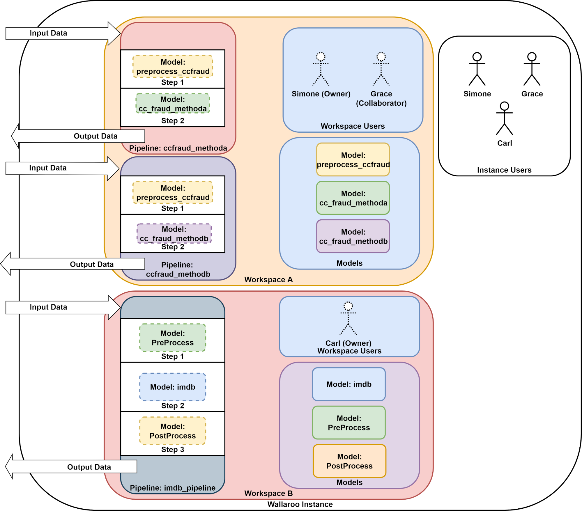
- Wallaroo Workspaces: Workspaces are environments were users upload models, create pipelines and other artifacts. The workspace should be considered the fundamental area where work is done. Workspaces are shared with other users to give them access to the same models, pipelines, etc.
- Wallaroo Model Upload and Registration: ML Models are uploaded to Wallaroo through the SDK or the MLOps API to a workspace. ML models include default runtimes (ONNX, Python Step, and TensorFlow) that are run directly through the Wallaroo engine, and containerized runtimes (Hugging Face, PyTorch, etc) that are run through in a container through the Wallaroo engine.
- Wallaroo Pipelines: Pipelines are used to deploy models for inferencing. Each model is a pipeline step in a pipelines, where the inputs of the previous step are fed into the next. Pipeline steps can be ML models, Python scripts, or Custom Model (these contain necessary models and artifacts for running a model).
For this tutorial, we will be providing pre-trained models in ONNX format. To see how to upload and deploy your particular model, see the Wallaroo Documentation site.
This tutorial includes a helper module CVDemoUtils, which converts images into a DataFrame format that our computer vision model expects.
Preliminary Steps
Before starting this module, ensure that the models have been downloaded.
To download the Wallaroo Computer Vision models, use the following link:
https://storage.googleapis.com/wallaroo-public-data/cv-demo-models/cv-retail-models.zip
Unzip the contents into the directory models.
Before we start, let’s load some libraries that we will need for this notebook (note that this may not be a complete list).
- IMPORTANT NOTE: This tutorial is geared towards a Wallaroo 2023.2.1 environment.
# run this to preload needed libraries

import wallaroo
from wallaroo.object import EntityNotFoundError
from wallaroo.framework import Framework
from IPython.display import display
from IPython.display import Image
import pandas as pd
import json
import datetime
import time
import cv2
import matplotlib.pyplot as plt
import string
import random
import pyarrow as pa
import sys
import asyncio
pd.set_option('display.max_colwidth', None)

import sys

# setting path - only needed when running this from the `with-code` folder.
sys.path.append('../')

import utils
Get ready to work with Wallaroo
With the libraries loaded, you can log into Wallaroo. This will provide access to your workspaces, workspaces shared with you from other users, and all other aspects of the Wallaroo environment.
Logging into Wallaroo via the cluster’s integrated JupyterLab is quite straight forward:
# Login through local Wallaroo instance
wl = wallaroo.Client()
See the documentation if you are logging into Wallaroo some other way such as from a remote location. This tutorial assumes you’re logging in through the Wallaroo JupyterHub service.
Notice that the Wallaroo client connection is stored into a variable called wl. This variable can be anything you want it to be - you can have client = wallaroo.Client() or myWallarooClient = wallaroo.Client().
This variable is about to become your best friend - a lot of the commands you’ll be running will be through this variable, like wl.list_workspaces() to get all of the workspaces available to you in your Wallaroo environment, or wl.list_models() to show all of the models in your current workspace. We’ll go into these commands and more - just make sure you saved that Wallaroo client to a variable so you can use it for the other commands.
When we log into the Wallaroo through the SDK, the Client will provide a url to verify your authentication. Either click it, or copy and past that URL, then authenticate into your Wallaroo instance with your email address and password.
Login to Wallaroo Exercise
Time to login to your Wallaroo instance. By now you should be logged into your Wallaroo JupyterHub service and looking at this notebook.
Copy the code below and place it into the code block and run it. When prompted, select the authentication URL by either clicking it, or copying and pasting it into a browser. Log into your Wallaroo instance, and then the client will be set.
# Login through local Wallaroo instance
wl = wallaroo.Client()
## blank space to put your wallaroo Client login code here.

wl = wallaroo.Client()
Run Client Commands
We’re now logged into our Wallaroo instance, let’s run some commands to get used to working within the environment.
The following are going to be very useful as you work in Wallaroo.
List Workspaces
The command wallaroo.Client.list_workspaces gives a list of all of the workspaces you have access to in the Wallaroo environment. Here’s an example of running it. For this example, our Wallaroo client is stored in the wl variable, but this could have been named wallaroo_client or whatever you like.
wl.list_workspaces()
| Name | Created At | Users | Models | Pipelines |
|---|---|---|---|---|
| john.hummel@wallaroo.ai - Default Workspace | 2023-08-21 19:06:07 | [‘john.hummel@wallaroo.ai’] | 1 | 1 |
| edge-publish-demojohn | 2023-08-21 20:54:35 | [‘john.hummel@wallaroo.ai’] | 1 | 1 |
| biolabsworkspacegomj | 2023-08-22 15:11:11 | [‘john.hummel@wallaroo.ai’] | 1 | 1 |
| biolabsworkspacedtrv | 2023-08-22 16:03:32 | [‘john.hummel@wallaroo.ai’] | 1 | 1 |
| biolabsworkspacejohn | 2023-08-22 16:07:15 | [‘john.hummel@wallaroo.ai’] | 1 | 1 |
Listing the workspaces will show the following fields:
- name: The user created workspace name. Workspace names must be unique across the Wallaroo instance.
- created_at: The date and time the workspace was created.
- users: The users in the workspace. The user who created the workspace is always listed.
- models: The number of models in the workspace.
- pipelines: The number of pipelines in the workspace.
When you first login to Wallaroo, the workspace {your email address} - Default Workspace is created. This is assigned as your current workspace once you have logged into Wallaroo. We’ll cover workspaces in a moment - for now, just remember that every time you do wallaroo.Client(), that your default workspace is set as your current workspace, and any commands you issue will be directed to that workspace.
Notice that in that example above, you only see one default workspace - the one of the user who ran the list_workspaces command. Other users will have their own default workspaces. You can only see workspaces you have access to.
List Users
Users are listed with the wallaroo.Client.list_users command. This shows all of the user’s email addresses and names across the Wallaroo instance.
There’s more commands, but we’ll stop here until we’ve created our workspace and uploaded some models.
Client Commands Exercise
For this exercise, use your Wallaroo client variable and list the current workspaces and current users. You can do this with your Wallaroo client variable you saved in a previous step.
For example, if your Wallaroo client variable is wl, then the following would list the workspaces and then the users:
# list the workspaces available to you
workspaces = wl.list_workspaces()
print(workspaces)

# list the users
users = wl.list_users()
print(users)
## blank space to get workspaces and users

display(wl.list_workspaces())

display(wl.list_users())
| Name | Created At | Users | Models | Pipelines |
|---|---|---|---|---|
| john.hansarick@wallaroo.ai - Default Workspace | 2024-10-29 16:12:39 | ['john.hansarick@wallaroo.ai'] | 0 | 0 |
| tutorial-workspace-john-sentiment-analysis | 2024-10-29 17:03:43 | ['john.hansarick@wallaroo.ai'] | 2 | 1 |
| tutorial-workspace-summarization | 2024-10-29 19:40:06 | ['john.hansarick@wallaroo.ai'] | 1 | 1 |
| tutorial-workspace-forecast | 2024-10-29 20:52:00 | ['john.hansarick@wallaroo.ai'] | 1 | 1 |
| tutorial-finserv-jch | 2024-10-30 21:03:48 | ['john.hansarick@wallaroo.ai'] | 1 | 1 |
| tutorial-finserv-john | 2024-10-31 18:22:53 | ['john.hansarick@wallaroo.ai'] | 1 | 1 |
| tutorial-workspace-sentiment-analysis | 2024-11-01 17:41:05 | ['john.hansarick@wallaroo.ai'] | 2 | 1 |
| tutorial-workspace-cv-yolo-john | 2024-11-04 16:29:07 | ['john.hansarick@wallaroo.ai'] | 1 | 1 |
| tutorial-workspace-john-cv | 2024-11-04 21:08:24 | ['john.hansarick@wallaroo.ai'] | 2 | 3 |
| cv-retail-edge | 2024-11-05 21:36:54 | ['john.hansarick@wallaroo.ai'] | 1 | 1 |
[User({"id": "fca5c4df-37ac-4a78-9602-dd09ca72bc60", "email": "john.hansarick@wallaroo.ai", "username": "john.hansarick@wallaroo.ai", "enabled": "True),
 User({"id": "0e5f6913-ee32-4a03-8c8f-ab6b94d95922", "email": "admin@keycloak", "username": "admin", "enabled": "True)]
Workspace Creation and Management
A Wallaroo workspace is place to organize the deployment artifacts for a project, and to collaborate with other team members. For more information, see the Wallaroo 101.
When you upload a ML model to Wallaroo, you upload it to a workspace. When a pipeline is created and models assigned to it, that pipeline is in side of a workspace. Wallaroo workload orchestrations? They’re assigned to a workspace.
When you first login, the SDK assigns you to your default workspace. Most of the commands issued through your Wallaroo client will target that workspace.
You can see what workspace you are currently in with the wallaroo.Client.get_current_workspace() method.
This shows you the following workspace fields:
- name: The user created workspace name. Workspace names must be unique across the Wallaroo instance.
- id: The numerical identifier of the workspace.
- archived: Whether the workspace was archived or not.
- created_by: The Keycloak ID of the user who created the workspace. This is in UUID format, and is used to identify specific users. Most of the time you’ll refer to users by their email address.
- created_at: The date and time the workspace was created.
- models: The models uploaded to the workspace and their details.
- pipelines: The number of pipelines in the workspace and their details.
Get Current Workspace Exercise
Get your current workspace with the wallaroo.Client.get_current_workspace(). For example, if your Wallaroo client was saved to the variable wl, this command would be:
wl.get_current_workspace()
When done,
## blank space to get your current workspace

wl.get_current_workspace()
{'name': 'john.hansarick@wallaroo.ai - Default Workspace', 'id': 5, 'archived': False, 'created_by': 'john.hansarick@wallaroo.ai', 'created_at': '2024-10-29T16:12:39.233166+00:00', 'models': [], 'pipelines': []}
Create New Workspace
Workspaces are created with the wallaroo.Client.create_workspace(name), where name is the new name of the workspace. When a new workspace is created, the workspace user is assigned to the user that created it (in this case - you). For example, if the Wallaroo client is stored to the variable wl, then the following will create the new workspace ‘sparkly-bunnies, then store the workspace information into the variable workspace`:
workspace = wl.create_workspace('sparkly-bunnies')
Once this is created, this shows you the following workspace fields:
- name: The user created workspace name. Workspace names must be unique across the Wallaroo instance, and must be DNS compliant. So ‘my-cool-workspace’ is ok, but ‘?? workspace’ is not.
-are ok, but_is not. - id: The numerical identifier of the workspace.
- archived: Whether the workspace was archived or not.
- created_by: The Keycloak ID of the user who created the workspace. This is in UUID format, and is used to identify specific users. Most of the time you’ll refer to users by their email address.
- created_at: The date and time the workspace was created.
- models: The models uploaded to the workspace and their details. For a new workspace, this will be empty
[]. - pipelines: The number of pipelines in the workspace and their details. For a new workspace, this will be empty
[].
Workspace names must be unique. So the following will fail:
wl.create_workspace('sparkly-bunnies')
wl.create_workspace('sparkly-bunnies')
Exception: Failed to create workspace.
Create New Workspace Exercise
Now it’s time for us to create our own workspace. To make this easy, we’ll call the workspace ’tutorial-workspace-{firstname}’. If someone else has the same first name and is in this tutorial, each of you decide who should change their name for this to work. Or - if it’s easier - change the firstname to something else like john1.
For example, if your Wallaroo client was saved to the variable wl, then the command to create a new workspace tutorial-workspace-sample is:
wl.create_workspace('tutorial-workspace-sample')
When you’re done, list the workspaces. You did that in a previous step, so you can copy that here.
## blank space to create your workspace

workspace_name = 'tutorial-workspace-john-cv'

print(wl.create_workspace(workspace_name))

# list all the workspaces here

wl.list_workspaces()
{'name': 'tutorial-workspace-john-cv', 'id': 13, 'archived': False, 'created_by': 'john.hansarick@wallaroo.ai', 'created_at': '2024-11-04T21:08:24.55981+00:00', 'models': [{'name': 'mobilenet', 'versions': 1, 'owner_id': '""', 'last_update_time': datetime.datetime(2024, 11, 4, 21, 9, 40, 313224, tzinfo=tzutc()), 'created_at': datetime.datetime(2024, 11, 4, 21, 9, 40, 313224, tzinfo=tzutc())}, {'name': 'cv-pixel-intensity', 'versions': 4, 'owner_id': '""', 'last_update_time': datetime.datetime(2024, 11, 6, 16, 8, 33, 942644, tzinfo=tzutc()), 'created_at': datetime.datetime(2024, 11, 5, 20, 38, 55, 258098, tzinfo=tzutc())}], 'pipelines': [{'name': 'cv-retail', 'create_time': datetime.datetime(2024, 11, 4, 21, 10, 5, 287786, tzinfo=tzutc()), 'definition': '[]'}, {'name': 'cv-retail-observe', 'create_time': datetime.datetime(2024, 11, 5, 20, 35, 25, 831787, tzinfo=tzutc()), 'definition': '[]'}, {'name': 'cv-assays-demo', 'create_time': datetime.datetime(2024, 11, 5, 21, 52, 48, 545484, tzinfo=tzutc()), 'definition': '[]'}]}
| Name | Created At | Users | Models | Pipelines |
|---|---|---|---|---|
| john.hansarick@wallaroo.ai - Default Workspace | 2024-10-29 16:12:39 | ['john.hansarick@wallaroo.ai'] | 0 | 0 |
| tutorial-workspace-john-sentiment-analysis | 2024-10-29 17:03:43 | ['john.hansarick@wallaroo.ai'] | 2 | 1 |
| tutorial-workspace-summarization | 2024-10-29 19:40:06 | ['john.hansarick@wallaroo.ai'] | 1 | 1 |
| tutorial-workspace-forecast | 2024-10-29 20:52:00 | ['john.hansarick@wallaroo.ai'] | 1 | 1 |
| tutorial-finserv-jch | 2024-10-30 21:03:48 | ['john.hansarick@wallaroo.ai'] | 1 | 1 |
| tutorial-finserv-john | 2024-10-31 18:22:53 | ['john.hansarick@wallaroo.ai'] | 1 | 1 |
| tutorial-workspace-sentiment-analysis | 2024-11-01 17:41:05 | ['john.hansarick@wallaroo.ai'] | 2 | 1 |
| tutorial-workspace-cv-yolo-john | 2024-11-04 16:29:07 | ['john.hansarick@wallaroo.ai'] | 1 | 1 |
| tutorial-workspace-john-cv | 2024-11-04 21:08:24 | ['john.hansarick@wallaroo.ai'] | 2 | 3 |
| cv-retail-edge | 2024-11-05 21:36:54 | ['john.hansarick@wallaroo.ai'] | 1 | 1 |
Retrieve Workspace
In the above example, you saw this:
workspace = wl.create_workspace('sparkly-bunnies')
This creates the workspace sparkly-bunnies, then assigns it to the variable workspace. We can display that workspace and see what it looks like. For example:
workspace = wl.create_workspace('sparkly-bunnies')

print(workspace)
{'name': 'sparkly-bunnies', 'id': 9, 'archived': False, 'created_by': '66d3b2c4-9b22-4429-b16e-3bcdc1ac28e3', 'created_at': '2023-08-22T17:30:40.475785+00:00', 'models': [], 'pipelines': []}
If we had created a workspace earlier, and want to work with it, we will have to retrieve it. We do that with the wallaroo.Client.get_workspaces(name, create_if_not_exist) method, which returns the workspace the user has access to that matches the name.
For example, if we’re looking for our workspace sparkly-bunnies:
workspace = wl.get_workspace('sparkly-bunnies')
print(workspace)
{'name': 'sparkly-bunnies', 'id': 9, 'archived': False, 'created_by': '66d3b2c4-9b22-4429-b16e-3bcdc1ac28e3', 'created_at': '2023-08-22T17:30:40.475785+00:00', 'models': [], 'pipelines': []}
Retrieve Workspace Exercise
Retrieve the workspace to a variable you created earlier via the get_workspace method.
## blank space to retrieve your workspace

workspace = wl.get_workspace('tutorial-workspace-john-cv')
print(workspace)
{'name': 'tutorial-workspace-john-cv', 'id': 13, 'archived': False, 'created_by': 'john.hansarick@wallaroo.ai', 'created_at': '2024-11-04T21:08:24.55981+00:00', 'models': [{'name': 'mobilenet', 'versions': 1, 'owner_id': '""', 'last_update_time': datetime.datetime(2024, 11, 4, 21, 9, 40, 313224, tzinfo=tzutc()), 'created_at': datetime.datetime(2024, 11, 4, 21, 9, 40, 313224, tzinfo=tzutc())}, {'name': 'cv-pixel-intensity', 'versions': 4, 'owner_id': '""', 'last_update_time': datetime.datetime(2024, 11, 6, 16, 8, 33, 942644, tzinfo=tzutc()), 'created_at': datetime.datetime(2024, 11, 5, 20, 38, 55, 258098, tzinfo=tzutc())}], 'pipelines': [{'name': 'cv-retail', 'create_time': datetime.datetime(2024, 11, 4, 21, 10, 5, 287786, tzinfo=tzutc()), 'definition': '[]'}, {'name': 'cv-retail-observe', 'create_time': datetime.datetime(2024, 11, 5, 20, 35, 25, 831787, tzinfo=tzutc()), 'definition': '[]'}, {'name': 'cv-assays-demo', 'create_time': datetime.datetime(2024, 11, 5, 21, 52, 48, 545484, tzinfo=tzutc()), 'definition': '[]'}]}
Set the Current Workspace
We mentioned earlier that when you login to Wallaroo, the SDK assigns you to the default workspace - the one named {your email address} - Default Workspace - replacing your email address in the front.
Usually you’ll want to work in some other workspace - perhaps one that you’re a part of with other users, or one you set up yourself for test purposes. It is highly recommended that workspaces be divided by project or some specific goal where the same models are used for different purposes.
We’ve gone over how to create a workspace, and how to retrieve a workspace that was previously created. Now we’ll use that to set our current workspace with the wallaroo.Client.set_current_workspace(workspace).
The current workspace is where your SDK commands are routed to. When you give the upload models command - they are uploaded to your current workspace. Build a pipeline? Associated to the current workspace.
So we’re going to make sure that what we’re doing is done in the right workspace with two commands:
wallaroo.Client.get_current_workspace(): Shows what the current workspace.wallaroo.Client.set_current_workspace(workspace): Sets the current workspace to the target workspace.
For example, if your workspace is saved to a variable as shown in the previous step, we can change from the default workspace and set our current workspace to the new one as follows:
# show the current workspace
print(wl.get_current_workspace())
{'name': 'john.hummel@wallaroo.ai - Default Workspace', 'id': 1, 'archived': False, 'created_by': '66d3b2c4-9b22-4429-b16e-3bcdc1ac28e3', 'created_at': '2023-08-21T19:06:07.404363+00:00', 'models': [{'name': 'm1', 'versions': 1, 'owner_id': '""', 'last_update_time': datetime.datetime(2023, 8, 21, 19, 38, 36, 672465, tzinfo=tzutc()), 'created_at': datetime.datetime(2023, 8, 21, 19, 38, 36, 672465, tzinfo=tzutc())}], 'pipelines': [{'name': 'p1', 'create_time': datetime.datetime(2023, 8, 21, 19, 38, 44, 314377, tzinfo=tzutc()), 'definition': '[]'}]}

# change to the new workspace
wl.set_current_workspace(workspace)

# show the new current workspace
print(wl.get_current_workspace())
{'name': 'tutorial-workspace-john', 'id': 12, 'archived': False, 'created_by': '66d3b2c4-9b22-4429-b16e-3bcdc1ac28e3', 'created_at': '2023-08-22T17:38:13.612187+00:00', 'models': [], 'pipelines': []}
Setting your current workspace to the one you want to work in is an important step. We highly recommend that once a Wallaroo client connection is established, the next task should be setting whatever workspace is the proper one to work in as the current workspace, then proceeding with any other tasks.
Set the Current Workspace Exercise
Previously you created a workspace and retrieved it to a variable. Using the * wallaroo.Client.get_current_workspace() and wallaroo.Client.set_current_workspace(workspace) methods:
- Get your current workspace.
- Set your current workspace to the one created in the previous steps.
- Get your current workspace again to verify that the change was made.
For example, if your Wallaroo client was stored as the variable wl, and your new workspace saved to the variable workspace, you can change your current workspace to the new one with the following:
wl.set_current_workspace(workspace)
wl.get_current_workspace()
## blank space to set current workspace

print(wl.get_current_workspace())
wl.set_current_workspace(workspace)
print(wl.get_current_workspace())
{'name': 'john.hansarick@wallaroo.ai - Default Workspace', 'id': 5, 'archived': False, 'created_by': 'john.hansarick@wallaroo.ai', 'created_at': '2024-10-29T16:12:39.233166+00:00', 'models': [], 'pipelines': []}
{'name': 'tutorial-workspace-john-cv', 'id': 13, 'archived': False, 'created_by': 'john.hansarick@wallaroo.ai', 'created_at': '2024-11-04T21:08:24.55981+00:00', 'models': [{'name': 'mobilenet', 'versions': 1, 'owner_id': '""', 'last_update_time': datetime.datetime(2024, 11, 4, 21, 9, 40, 313224, tzinfo=tzutc()), 'created_at': datetime.datetime(2024, 11, 4, 21, 9, 40, 313224, tzinfo=tzutc())}, {'name': 'cv-pixel-intensity', 'versions': 4, 'owner_id': '""', 'last_update_time': datetime.datetime(2024, 11, 6, 16, 8, 33, 942644, tzinfo=tzutc()), 'created_at': datetime.datetime(2024, 11, 5, 20, 38, 55, 258098, tzinfo=tzutc())}], 'pipelines': [{'name': 'cv-retail', 'create_time': datetime.datetime(2024, 11, 4, 21, 10, 5, 287786, tzinfo=tzutc()), 'definition': '[]'}, {'name': 'cv-retail-observe', 'create_time': datetime.datetime(2024, 11, 5, 20, 35, 25, 831787, tzinfo=tzutc()), 'definition': '[]'}, {'name': 'cv-assays-demo', 'create_time': datetime.datetime(2024, 11, 5, 21, 52, 48, 545484, tzinfo=tzutc()), 'definition': '[]'}]}
Upload a Model
Now that we have our current workspace set, it’s time to start uploading some models.
We already have some ONNX models available in the folder ./models. All three do the same thing: predict house price values based on some values. We have those values stored in the folder ./data.
ML Models are uploaded to the current Wallaroo workspace the wallaroo.Client.upload_model method. Wallaroo supports different model types, as well as Custom Model and containerized models.
For full details, see Wallaroo SDK Essentials Guide: Model Uploads and Registrations.
Wallaroo supports ONNX models as part of the default runtime, so these will run in Wallaroo without additional configurations.
When uploading models, the following is needed:
- The name of the model. This needs to be unique across the workspace.
- The path to the ML model file. For example,
./models/xgb_model.onnx. - The framework of the model. These are listed through the
wallaroo.framework.Frameworklist. For these examples we will be usingwallaroo.framework.Framework.ONNXto specify we are using ONNX models. - The input_schema and output_schema. For ONNX models, we can skip this. For non-native runtime models, that has to be specified in Apache Arrow schema format. See the Wallaroo SDK Essentials Guide: Model Uploads and Registrations for full details.
Here’s an example of uploading a model to a Wallaroo workspace and assigning it the name ‘house-price-prime’, with the Wallaroo client assigned to the variable wl, then retrieving the model version from Wallaroo once the upload it complete:
house_price_model_version = wl.upload_model('house-price-prime',
                                            './models/xgb_model.onnx',
                                            framework=wallaroo.framework.Framework.ONNX)
house_price_model_version
| Name | house-price-prime |
|---|---|
| Version | cc3ba784-ffdf-4a0f-982a-9a8ac4db8ba9 |
| File Name | xgb_model.onnx |
| SHA | 31e92d6ccb27b041a324a7ac22cf95d9d6cc3aa7e8263a229f7c4aec4938657c |
| Status | ready |
| Image Path | None |
| Updated At | 2023-22-Aug 19:55:26 |
We store this new version of a model to the variable house_price_model_version. This is used for later processes involving pipeline deployments, generating assays, and so on.
In Wallaroo, you have the model, which is based on the name parameter. Each model has one or more versions.
IMPORTANT NOTE: Models in Wallaroo are organized by name. If a model is uploaded with the same name, it will create a new version of the model with the same name. For example, the following will create a model named house-price-prime with two versions.
# set the model from the XGB model converted to ONNX
house_price_model_version = wl.upload_model('house-price-prime',
                                            './models/xgb_model.onnx',
                                            framework=wallaroo.framework.Framework.ONNX)
print(house_price_model_version)
{'name': 'house-price-prime', 'version': '83d89260-9aac-41ea-b2b4-79aae48b5a65', 'file_name': 'xgb_model.onnx', 'image_path': None, 'last_update_time': datetime.datetime(2023, 8, 22, 19, 59, 2, 26718, tzinfo=tzutc())}

# create the new model version to the model converted from an RF model
house_price_model_version = wl.upload_model('house-price-prime',
                                            './models/rf_model.onnx',
                                            framework=wallaroo.framework.Framework.ONNX)
print(house_price_model_version)
{'name': 'house-price-prime', 'version': 'c86fd309-7c28-4e95-9d3e-831fefa51a12', 'file_name': 'rf_model.onnx', 'image_path': None, 'last_update_time': datetime.datetime(2023, 8, 22, 19, 59, 3, 381581, tzinfo=tzutc())}
Notice that the model is the same - house-price-prime - but the model version changes each time we do an upload_model. This allows you to change the model version to a totally different flavor and framework if you desire.
Upload a Model Exercise
For this exercise, upload the model /models/mobilenet.pt.onnx and assign it a name, with the framework =wallaroo.framework.Framework.ONNX. Because image size may vary from one image to the next, converting the image to a tensor array may have a different shape from one image to the next. For example, a 640x480 image produces an array of [640][480][3] for 640 rows with 480 columns each, and each pixel has 3 possible color values.
Because the tensor array size may change from image to image, the model upload sets the model’s batch configuration to batch_config="single". See the Wallaroo Data Schema Definitions for more details.
Here’s an example of uploading the mobilenet model.
mobilenet_model = wl.upload_model('mobilenet',
                                  "./models/mobilenet.pt.onnx",
                                  framework=Framework.ONNX).configure('onnx',
                                                                      batch_config="single"
                                                                      )
## blank space to upload the model

mobile_name = "mobilenet"
mobile_file = "../models/mobilenet.pt.onnx"

wl.upload_model(mobile_name,
                mobile_file,
                framework=Framework.ONNX).configure(tensor_fields=['tensor'],
                                                    batch_config="single")
| Name | mobilenet |
| Version | d15d8b9d-9d98-4aa7-8545-ac915862146e |
| File Name | mobilenet.pt.onnx |
| SHA | 9044c970ee061cc47e0c77e20b05e884be37f2a20aa9c0c3ce1993dbd486a830 |
| Status | ready |
| Image Path | None |
| Architecture | x86 |
| Acceleration | none |
| Updated At | 2024-06-Nov 17:10:14 |
| Workspace id | 13 |
| Workspace name | tutorial-workspace-john-cv |
Retrieve Model Version
Once a model is uploaded to Wallaroo, we can list the models in a workspace with the wallaroo.workspace.models() method. This returns a List of all of the models and how many versions are associated with that model.
Here’s an example:
workspace.models()
[{'name': 'house-price-prime', 'versions': 3, 'owner_id': '""', 'last_update_time': datetime.datetime(2023, 8, 22, 19, 59, 3, 381581, tzinfo=tzutc()), 'created_at': datetime.datetime(2023, 8, 22, 19, 55, 26, 603685, tzinfo=tzutc())}]
When a ML model is uploaded, two things happen:
- A Wallaroo model based on the model name field.
- A model version - this is the artifact that is actually deployed.
We retrieve the model version with the method wallaroo.Client.get_model(name, version) which retrieves the most recent model version if no version is specified.
For example, to retrieve the most recent version of the model house-price-prime:
my_model_version = wl.get_model('house-price-prime')
| Name | house-price-prime |
|---|---|
| Version | c86fd309-7c28-4e95-9d3e-831fefa51a12 |
| File Name | rf_model.onnx |
| SHA | e22a0831aafd9917f3cc87a15ed267797f80e2afa12ad7d8810ca58f173b8cc6 |
| Status | ready |
| Image Path | None |
| Updated At | 2023-22-Aug 19:59:03 |
Retrieve Model Version Exercise
This exercise will have you retrieving the model you uploaded earlier. For example, if the Wallaroo client was stored as wl, and the workspace saved to workspace, then the command to get the current model version would be:
my_model_version = wl.get_model('your-model-name')
my_model_version
## blank space to retrieve the model version and store it

my_model_version = wl.get_model("mobilenet")
my_model_version
| Name | mobilenet |
| Version | d15d8b9d-9d98-4aa7-8545-ac915862146e |
| File Name | mobilenet.pt.onnx |
| SHA | 9044c970ee061cc47e0c77e20b05e884be37f2a20aa9c0c3ce1993dbd486a830 |
| Status | ready |
| Image Path | None |
| Architecture | x86 |
| Acceleration | none |
| Updated At | 2024-06-Nov 17:10:14 |
| Workspace id | 13 |
| Workspace name | tutorial-workspace-john-cv |
Upload Post Processing Model
Wallaroo supports ML Models and using Python scripts as models. These are typically used for pre or post-processing data before transmitting the data to the next pipeline step. In this case, we can take the output from the CV model, and average the confidences.
As this is a Python model, we include the input and output data schemas as part of the model upload process. For this exercise, we’ll save the model upload to a variable rather than retrieve it like we did the computer vision model.
Upload Post Processing Model Exercise
Sample code:
input_schema = pa.schema([
    pa.field('boxes', pa.list_(pa.float32())),
    pa.field('classes', pa.list_(pa.int64())),
    pa.field('confidences', pa.list_(pa.float32()))
    ]
)

output_schema = pa.schema([
    pa.field('boxes', pa.list_(pa.float32())),
    pa.field('classes', pa.list_(pa.int64())),
    pa.field('confidences', pa.list_(pa.float32())),
    pa.field('avg_confidence', pa.float32()),
])

module_post_process_model = wl.upload_model("cv-post-process-drift-detection",
                                            "./models/post-process-drift-detection.zip",
                                            framework=Framework.PYTHON,
                                            input_schema=input_schema,
                                            output_schema=output_schema
                                            )
## blank space to upload the post process manual

input_schema = pa.schema([
    pa.field('boxes', pa.list_(pa.float32())),
    pa.field('classes', pa.list_(pa.int64())),
    pa.field('confidences', pa.list_(pa.float32()))
    ]
)

output_schema = pa.schema([
    pa.field('boxes', pa.list_(pa.float32())),
    pa.field('classes', pa.list_(pa.int64())),
    pa.field('confidences', pa.list_(pa.float32())),
    pa.field('avg_confidence', pa.float32()),
])

module_post_process_model = wl.upload_model("cv-post-process-drift-detection",
                                            "../models/post-process-drift-detection.zip",
                                            framework=Framework.PYTHON,
                                            input_schema=input_schema,
                                            output_schema=output_schema
                                            )
Waiting for model loading - this will take up to 10.0min.
Model is pending loading to a container runtime..
Model is attempting loading to a container runtime..successful
Ready
Build a Pipeline
Pipelines are the method of taking submitting data and processing that data through the models. Each pipeline can have one or more steps that submit the data from the previous step to the next one. Information can be submitted to a pipeline as a file, or through the pipeline’s URL.
Each pipeline step is a model version. These can be ML models like we uploaded earlier, or they can be Python scripts that manipulate the data into a format needed for another model in the chain.
When an inference is performed, data is submitted to the pipeline. The pipeline then submits the data to the first step, receives the output, then transmits that data to the next step. When all steps are complete, the pipeline returns the final values to the requesting client.
For this tutorial, we will focus one a very simple pipeline: one ML model.
Pipeline are created in the current workspace with the wallaroo.Client.build_pipeline(name) command, where the name is unique to the workspace. For example, to create the pipeline named houseprice-estimator and the Wallaroo client is saved to wl the command would be:
pipeline = wl.build_pipeline('houseprice-estimator')
pipeline
name | houseprice-estimator
created | 2023-08-22 20:39:35.853683+00:00
last_updated | 2023-08-22 20:39:35.853683+00:00
deployed | (none)
tags |
versions | f42c0457-e4f3-4370-b152-0a220347de11
steps |
Just like models, pipelines have version. Each time pipeline steps are changed, a new version is created.
See Wallaroo SDK Essentials Guide: Pipeline Management for full details.
Build a Pipeline
Build your own pipeline! Use the wallaroo.Client.build_pipeline(name) command and create a pipeline named houseprice-pipeline. Recall that this creates the pipeline in the current workspace, so verify that the current workspace is the one you want to create a pipeline in.
For example, if the Wallaroo client is saved to the variable wl, the command would be:
wl.build_pipeline('cv-retail')
## blank space to create the pipeline

wl.build_pipeline('cv-retail')
| name | cv-retail |
|---|---|
| created | 2024-11-04 21:10:05.287786+00:00 |
| last_updated | 2024-11-06 17:10:38.771050+00:00 |
| deployed | False |
| workspace_id | 13 |
| workspace_name | tutorial-workspace-john-cv |
| arch | x86 |
| accel | none |
| tags | |
| versions | dd5e2f8a-e436-4b35-b2fb-189f6059dacc, 5a0772da-cde1-4fea-afc4-16313fcaa229, 7686f3ea-3781-4a95-aa4c-e99e46b9c47c, 4df9df54-6d12-4577-a970-f544128d0575 |
| steps | mobilenet |
| published | False |
Retrieve a Pipeline
Pipelines that are associated with a workspace are retrieved wallaroo.Client.list_pipelines method - this returns a List of pipelines. From there, a variable is assigned to the pipeline in the list we want to work with.
The list_pipelines method returns a list of pipelines and their details as follows:
wl.list_pipelines()
| name | created | last_updated | deployed | tags | versions | steps |
|---|---|---|---|---|---|---|
| houseprice-estimator | 2023-22-Aug 20:39:35 | 2023-22-Aug 20:39:35 | (unknown) | f42c0457-e4f3-4370-b152-0a220347de11 | ||
| biolabspipeline | 2023-22-Aug 16:07:20 | 2023-22-Aug 16:24:40 | False | 4c6dceb7-e692-4b8b-b615-4f7873eb020b, 59d0babe-bc1d-4dbb-959f-711c74f7b05d, ae834c0d-7a5b-4f87-9e2e-1f06f3cd25e7, 7c438222-28d8-4fca-9a70-eabee8a0fac5 | biolabsmodel | |
| biolabspipeline | 2023-22-Aug 16:03:33 | 2023-22-Aug 16:03:38 | False | 4e103a7d-cd4d-464b-b182-61d4041518a8, ec2a0fd6-21d4-4843-b7c3-65b1e5be1b85, 516f3848-be98-40d7-8564-a1e48eecb7a8 | biolabsmodel | |
| biolabspipelinegomj | 2023-22-Aug 15:11:12 | 2023-22-Aug 15:42:44 | False | 1dc9f89f-82aa-4a71-b21a-75dc8d5e4e51, 152d12f2-1200-46ad-ad04-60078c5aa284, 6ca59ffd-802e-4ad5-bd9a-35146b9fbda5, bdab08cc-3e99-4afc-b22d-657e33b76f29, 3c8feb0d-3124-4018-8dfa-06162156d51e | biolabsmodelgomj | |
| edge-pipeline | 2023-21-Aug 20:54:37 | 2023-22-Aug 19:06:46 | False | 2be013d9-a438-453c-a013-3fd8e6218394, a02b6af5-4235-42af-92c6-5ae678b35be4, e721ccad-11d8-4874-8388-4211c4957d18, d642e766-cffb-451f-b197-e058bedbdd5f, eb586aba-4908-4bff-84e1-bdeb1fa4b7d3, 2163d718-a5ea-41e3-b69f-095efa858462 | ccfraud | |
| p1 | 2023-21-Aug 19:38:44 | 2023-21-Aug 19:38:44 | (unknown) | 5f93e90a-e8d6-4e8a-8a1a-22eee80a3e13, 5f78247f-7bf9-445b-98a6-e146fb22b8e9 |
Just like with a model version, the most recent pipeline version is retrieved with the method wallaroo.Client.get_pipeline(name) method.
Retrieve a Pipeline Exercise
For this exercise, retrieve your the pipeline you built in the previous step and store it into the variable my_pipeline. You’ll need to use get_pipeline(name) method. Here’s an example
my_pipeline = wl.get_pipeline('sample_pipeline')
my_pipeline
## blank space to retrieve your pipeline

my_pipeline = wl.get_pipeline('cv-retail')
my_pipeline
| name | cv-retail |
|---|---|
| created | 2024-11-04 21:10:05.287786+00:00 |
| last_updated | 2024-11-06 17:10:38.771050+00:00 |
| deployed | False |
| workspace_id | 13 |
| workspace_name | tutorial-workspace-john-cv |
| arch | x86 |
| accel | none |
| tags | |
| versions | dd5e2f8a-e436-4b35-b2fb-189f6059dacc, 5a0772da-cde1-4fea-afc4-16313fcaa229, 7686f3ea-3781-4a95-aa4c-e99e46b9c47c, 4df9df54-6d12-4577-a970-f544128d0575 |
| steps | mobilenet |
| published | False |
Add Model Step
Models are added to a pipeline as pipeline steps. There are different kinds of pipeline steps that can host one or more models.
For this tutorial, we will use the method wallaroo.pipeline.add_model_step(model_version). This adds a single step to a Pipeline. Pipeline steps start at 0 and increment from there. We can see the steps in our pipeline with the wallaroo.pipeline.steps() method.
# add modelA as a pipeline steps
pipeline.add_model_step(modelA)

# display the steps
pipeline.steps()

[{'ModelInference': {'models': [{'name': 'house-price-prime', 'version': 'c86fd309-7c28-4e95-9d3e-831fefa51a12', 'sha': 'e22a0831aafd9917f3cc87a15ed267797f80e2afa12ad7d8810ca58f173b8cc6'}]}}]
For now, there’s three commands you should know:
wallaroo.pipelineadd_model_step(model_version): Add a step to a pipeline from a model version.wallaroo.pipeline.steps(): Display the current steps in the pipeline.wallaroo.pipeline.clear(): Clear all pipeline steps.
Pipeline steps are not saved in the Wallaroo instance until the pipeline has been deployed - more on that shortly. So you can add steps, clear them, add new ones - they all stay in your local script until you issue the command to deploy the pipeline. More on that later.
The second thing to watch out for it every time add_model_step is performed on a pipeline, another step is created. For example, if we have a pipeline with two models, modelA and modelB, then the following creates two steps in the same pipelines:
# clear the steps
pipeline.clear()

# add modelA then modelB as pipeline steps
pipeline.add_model_step(modelA)
pipeline.add_model_step(modelB)

# display the steps
pipeline.steps()

[{'ModelInference': {'models': [{'name': 'house-price-prime', 'version': 'c86fd309-7c28-4e95-9d3e-831fefa51a12', 'sha': 'e22a0831aafd9917f3cc87a15ed267797f80e2afa12ad7d8810ca58f173b8cc6'}]}},
 {'ModelInference': {'models': [{'name': 'house-price-gbr', 'version': '248a6eab-b159-4821-830b-22cc137a1ace', 'sha': 'ed6065a79d841f7e96307bb20d5ef22840f15da0b587efb51425c7ad60589d6a'}]}}]
This means the data from the inference is fed first to modelA, and that output is fed into modelB. The problem is if the input data from modelA doesn’t match what modelB expects, the process will fail.
Because of this, check your pipeline steps before you deploy a pipeline, clear them if you need to.
Add Pipeline Step Exercise
We have our model version uploaded from the previous steps, and we have our pipeline. Time to put them together and create a pipeline step with our model version.
Just for practice, do the following:
- Clear the pipeline steps.
- Add the sample model uploaded earlier. In our examples, that was
my_model_version. - Show the current pipeline steps.
Here’s an example with the Wallaroo client stored to wl, with the pipeline my_pipeline and my_model_version, along with the post-processing Python model.
my_pipeline.clear()
my_pipeline.add_model_step(my_model_version)
my_pipeline.add_model_step(module_post_process_model)
my_pipeline.steps()
## blank space to set the model steps and display them

my_pipeline.clear()
my_pipeline.add_model_step(my_model_version)
my_pipeline.add_model_step(module_post_process_model)
my_pipeline.steps()
[{'ModelInference': {'models': [{'name': 'mobilenet', 'version': 'd15d8b9d-9d98-4aa7-8545-ac915862146e', 'sha': '9044c970ee061cc47e0c77e20b05e884be37f2a20aa9c0c3ce1993dbd486a830'}]}},
 {'ModelInference': {'models': [{'name': 'cv-post-process-drift-detection', 'version': 'a335c538-bccf-40b9-b9a4-9296f03e6eb1', 'sha': 'eefc55277b091dd90c45704ff51bbd68dbc0f0f7e686930c5409a606659cefcc'}]}}]
Deploy a Pipeline
Now we reach what we’ve been aiming for: deploying a pipeline.
By now, you’ve seen how workspaces contain the models, pipelines, and other artifacts. You’ve uploaded a model and retrieved the latest version of the model. You’ve built a pipeline and added the model version as a pipeline step.
Now we will deploy the pipeline. Deploying a pipeline allocated resources from the cluster to that pipeline for it’s use. The amount of resources has a default value of 4 CPUs, but for this tutorial we’ll be adjusting that to just 0.5 cpus and 1 GB RAM per pipeline.
- IMPORTANT NOTE: Please stick to these resource configurations when using a Wallaroo instance with other users. Otherwise, pipelines might not deploy if the available resources are used up.
To deploy a pipeline, we do two things:
- Create a deployment configuration: This is an optional step, but we will make it mandatory for this tutorial to allow other users to work in the same Wallaroo instance without running out of resources.
- Deploy the pipeline with the deployment configuration: This is the active step that saves the pipeline steps, and allocates system resources to the pipeline for performing inferences.
Deployment configurations are made with the wallaroo.DeploymentConfigBuilder() class, and then we assign the resource settings from there. This is saved to a variable so we can apply it to our pipeline deployment.
Here’s an example of setting up a deployment with just 0.5 cpu and 1Gi RAM:
deploy_config = wallaroo.DeploymentConfigBuilder().replica_count(1).cpus(0.5).memory("1Gi").build()
Notice the replica_count(1) configuration - this tells Wallaroo to only spin up one replica for this pipeline. In a production environment, we could spin multiple replicas either manually or automatically as more resources are needed to improve performance.
Now we deploy the pipeline with our deployment configuration with the wallaroo.pipeline.deploy(deploy_configuration) method. If our pipeline variable is my_pipeline, then we would deploy it as follows:
deploy_config = wallaroo.DeploymentConfigBuilder().replica_count(1).cpus(0.5).memory("1Gi").build()
my_pipeline.deploy(deployment_config=deploy_config)
We can check the status of the pipeline deployment with the wallaroo.pipeline.status() method:
my_pipeline.status()

{'status': 'Running',
 'details': [],
 'engines': [{'ip': '10.244.3.83',
   'name': 'engine-6d4fccf5cb-dmwfl',
   'status': 'Running',
   'reason': None,
   'details': [],
   'pipeline_statuses': {'pipelines': [{'id': 'houseprice-estimator',
      'status': 'Running'}]},
   'model_statuses': {'models': [{'name': 'house-price-prime',
      'version': 'c86fd309-7c28-4e95-9d3e-831fefa51a12',
      'sha': 'e22a0831aafd9917f3cc87a15ed267797f80e2afa12ad7d8810ca58f173b8cc6',
      'status': 'Running'}]}}],
 'engine_lbs': [{'ip': '10.244.4.100',
   'name': 'engine-lb-584f54c899-sswnw',
   'status': 'Running',
   'reason': None,
   'details': []}],
 'sidekicks': []}
Deploy a Pipeline Exercise
This exercise will have you deploy your pipeline with the deployment settings we listed above. For example, if your pipeline was called my_pipeline, then your deployment will look like this:
deploy_config = wallaroo.DeploymentConfigBuilder().replica_count(1).cpus(0.5).memory("1Gi").build()
my_pipeline.deploy(deployment_config=deploy_config)
If the pipeline doesn’t finish deploying in 45 seconds, we check the status with:
display(my_pipeline.status())
# run the following to set the deployment configuration
deploy_config = wallaroo.DeploymentConfigBuilder().replica_count(1).cpus(1).memory("1Gi").build()
## blank space to deploy the pipeline

my_pipeline.deploy(deployment_config=deploy_config)
## blank space to check the deployment status

display(my_pipeline.status())
{'status': 'Running',
 'details': [],
 'engines': [{'ip': '10.28.3.2',
   'name': 'engine-5f7c4579b6-g55s4',
   'status': 'Running',
   'reason': None,
   'details': [],
   'pipeline_statuses': {'pipelines': [{'id': 'cv-retail',
      'status': 'Running',
      'version': 'd8be019e-2b7c-4c52-9e41-101b20ab0c2a'}]},
   'model_statuses': {'models': [{'name': 'cv-post-process-drift-detection',
      'sha': 'eefc55277b091dd90c45704ff51bbd68dbc0f0f7e686930c5409a606659cefcc',
      'status': 'Running',
      'version': 'a335c538-bccf-40b9-b9a4-9296f03e6eb1'},
     {'name': 'mobilenet',
      'sha': '9044c970ee061cc47e0c77e20b05e884be37f2a20aa9c0c3ce1993dbd486a830',
      'status': 'Running',
      'version': 'd15d8b9d-9d98-4aa7-8545-ac915862146e'}]}}],
 'engine_lbs': [{'ip': '10.28.2.24',
   'name': 'engine-lb-6676794678-58tbj',
   'status': 'Running',
   'reason': None,
   'details': []}],
 'sidekicks': [{'ip': '10.28.2.25',
   'name': 'engine-sidekick-cv-post-process-drift-detection-26-6557db49tmgz',
   'status': 'Running',
   'reason': None,
   'details': [],
   'statuses': '\n'}]}
Pipeline Inference with DataFrames
Wallaroo deployed pipelines accept three types of data:
- pandas DataFrames
- Apache Arrow
We do this with one of two commands on a deployed pipeline.
wallaroo.pipeline.infer(input): Submits either JSON, a DataFrame, or Apache Arrow to the pipeline for inferences.wallaroo.pipeline.infer_from_file(path): Submits either a JSON, a DataFrame in pandas Record format, or an Apache Arrow binary file inferences.
We’ll start with a single DataFrame stored in the file: ./data/singleton.df.json, which contains input data as a tensor:
[
    {
        "tensor": [
            4.0,
            3.0,
            3710.0,
            20000.0,
            2.0,
            0.0,
            2.0,
            5.0,
            10.0,
            2760.0,
            950.0,
            47.6696014404,
            -122.2610015869,
            3970.0,
            20000.0,
            79.0,
            0.0,
            0.0
        ]
    }
]
This translates into a pandas DataFrame, which is submitted with the pipeline.infer method.
df = pd.DataFrame([
    {
        "tensor": [
            4.0,
            3.0,
            3710.0,
            20000.0,
            2.0,
            0.0,
            2.0,
            5.0,
            10.0,
            2760.0,
            950.0,
            47.6696014404,
            -122.2610015869,
            3970.0,
            20000.0,
            79.0,
            0.0,
            0.0
        ]
    }
])

pipeline.infer(df)
When we use infer, Wallaroo determines whether the object is a pandas DataFrame or Apache arrow, and handles the inferences accordingly.
The data received through the SDK is always of the same type submitted: Submit a DataFrame, get a DataFrame with the data back. Submit an Arrow table file, get an Arrow table back. Here’s an example of submitting our sample DataFrame through a pipeline saved to the variable pipeline:
result = pipeline.infer(df)
display(result)
| time | in.tensor | out.variable | check_failures | |
|---|---|---|---|---|
| 0 | 2023-08-23 15:02:41.452 | [4.0, 3.0, 3710.0, 20000.0, 2.0, 0.0, 2.0, 5.0, 10.0, 2760.0, 950.0, 47.6696014404, -122.2610015869, 3970.0, 20000.0, 79.0, 0.0, 0.0] | [1514079.4] | 0 |
Let’s break down each of these fields:
- Index (unnamed): This field doesn’t have a label, but in the example above this is the
index. We only have one submission, so we have one result. If we had 20 inputs, we’d have 20 inference results, and each result would be aligned with each row we sent as an input. - time: The date and time the inference request.
- in.{variable}: Every input to the inference request is listed as
in.{variable_name}. For example, if our inputs werehouse_size_in_square_feetandyear_house_built, then the inputs would be listed asin.house_size_in_square_feetandin.year_house_built. - out.{variable}: Every output to the inference is listed as
out.{variable_name}. Our sample model outputs just one output:variable, but others such might outputestimated_house_price,initial_offer_price, and in the inference result those would be listed asout.estimated_house_priceandout.initial_offer_price. - check_failures: Indicates if any validation checks failed. This is covered in later sessions.
There’s additional data that an inference has that is retrieved by requesting it. For full details, see the Wallaroo SDK Essentials Guide: Inference Management.
Pipeline Inference with Files Exercise
The Computer Vision model for our tutorial uses the CVDemoUtils to convert an image to a pandas DataFrame. Here’s how the code looks:
image = './data/images/input/example/dairy_bottles.png'

width, height = 640, 480
dfImage, resizedImage = cvDemo.loadImageAndConvertToDataframe(image,
                                                              width,
                                                              height
                                                              )
The dfImage is the DataFrame used for inferences. We then perform the inference like any other pipeline inference request, by submitting that DataFrame to the pipeline.infer method.
results = pipeline.infer(dfImage)
The results is too long to show, so feel free to skip displaying it.
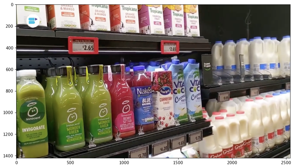
# run the following to display the image

image = cv2.imread('../data/images/example/dairy_bottles.png')
image = cv2.cvtColor(image, cv2.COLOR_BGR2RGB)
plt.figure(figsize=(12,8))
plt.grid(False)
plt.imshow(image)
plt.show()
# run the following to convert the image to a daataframe

width, height = 640, 480
dfImage, resizedImage = utils.loadImageAndConvertToDataframe('../data/images/example/dairy_bottles.png', width, height)
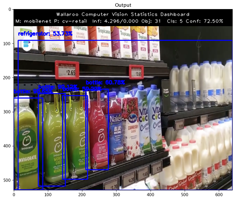
We can take the results and pass them back through our CVDemo that will draw bounding boxes around detected objects. The full details are available through the Wallaroo Tutorials site for those looking for more information. The code below will match the results to the resizedImage to draw the bounding boxes.
Update the model_name and pipeline_name of the code below with the name of your model and pipeline.
## blank space to run the sample inference

startTime = time.time()
infResults = my_pipeline.infer(dfImage, timeout=600)
endTime = time.time()
infResults['out.avg_confidence']
## blank space to run the sample inference

startTime = time.time()
infResults = my_pipeline.infer(dfImage, timeout=600)
endTime = time.time()
infResults['out.avg_confidence']
0    0.289506
Name: out.avg_confidence, dtype: float64
# run the following to display the bounding boxes;
# replace `infResults` and other variables as needed

elapsed = 1.0
results = {
    'model_name' : "mobilenet",
    'pipeline_name' : "cv-retail",
    'width': width,
    'height': height,
    'image' : resizedImage,
    'inf-results' : infResults,
    'confidence-target' : 0.50,
    'inference-time': (endTime-startTime),
    'onnx-time' : int(elapsed) / 1e+9,
    'classes_file': "../models/coco_classes.pickle",
    'color': 'BLUE'
}

image = utils.drawDetectedObjectsFromInference(results)
Batch Inferences through API
For Wallaroo instances that enable external endpoints connections to pipelines, each pipeline has it’s own URL that can be used to perform inferences through an API call.
Performing an inference through an API requires the following:
- The authentication token to authorize the connection to the pipeline.
- The pipeline’s inference URL.
- Inference data to sent to the pipeline - in JSON, DataFrame records format, or Apache Arrow.
Full details are available through the Wallaroo API Connection Guide on how retrieve an authorization token and perform inferences through the pipeline’s API.
For this demonstration, we’ll use some Wallaroo methods to retrieve those items. We’ll use the print command to create the curl command to perform an inference on the pipeline deployment URL.
deploy_url = my_pipeline._deployment._url()

headers = wl.auth.auth_header()

headers['Content-Type']='application/vnd.apache.arrow.file'
headers['Accept']='application/json; format=pandas-records'

data = dfImage.to_json('./sampleimage.df.json', orient="records")

print(f'''
!curl -X POST {deploy_url} \\
    -H "Authorization:{headers['Authorization']}" \\
    -H "Content-Type:{headers['Content-Type']}" \\
    -H "Accept:{headers['Accept']}" \\
    --data-binar
You should have an output that looks similar to this:
!curl -X POST https://doc-test.api.wallarooexample.ai/v1/api/pipelines/infer/houseprice-estimator-89/houseprice-estimator \
    -H "Authorization:Bearer SOME TOKEN STUFF" \
    -H "Content-Type:application/json; format=pandas-records" \
    -H "Accept:application/json; format=pandas-records" \
    --data @../data/test_data.df.json > curl_response.df
Then you can just run the !curl... sample. The inference results will be saved to the file curl_response.df.
Batch Inferences through API Exercise
Perform an inferece request through the curl command. For this example, we’ve converted the file ./data/images/input/example/dairy_bottles.png to an Apache arrow table ./data/dairy_bottles.png.arrow.
deploy_url = my_pipeline._deployment._url()

headers = wl.auth.auth_header()

headers['Content-Type']='application/vnd.apache.arrow.file'
headers['Accept']='application/json; format=pandas-records'

print(f'''
!curl -X POST {deploy_url} \\
    -H "Authorization:{headers['Authorization']}" \\
    -H "Content-Type:{headers['Content-Type']}" \\
    -H "Accept:{headers['Accept']}" \\
    --data-binary @./data/converted-images-to-arrow/dairy_bottles.png.arrow > curl_response.df
      ''')
# run this convert the dfImage to a pandas Record file

dfImage.to_json('../data/inference_inputs/sampleimage.df.json', orient="records")

# run this to generate the curl command

# run the below to generate the curl command

deploy_url = my_pipeline._deployment._url()

headers = wl.auth.auth_header()

headers['Content-Type']='application/json; format=pandas-records'
headers['Accept']='application/json; format=pandas-records'

dataFile = '../data/inference_inputs/sampleimage.df.json'

# test_df = pd.read_json('../data/image_0_21.tif.df.json')
# test_df.to_json('../data/image_0_21.tif.df.json', orient="records")
# display(test_df)

print(f'''
!curl -X POST {deploy_url} \\
    -H "Authorization:{headers['Authorization']}" \\
    -H "Content-Type:{headers['Content-Type']}" \\
    -H "Accept:{headers['Accept']}" \\
    --data @{dataFile} > curl_response.df
      ''')
!curl -X POST https://doc-test.wallarooexample.ai/v1/api/pipelines/infer/cv-retail-8/cv-retail \
    -H "Authorization:Bearer eyJhbGciOiJSUzI1NiIsInR5cCIgOiAiSldUIiwia2lkIiA6ICJvTTJDR1FZTDlPbDNmQTlvN0pqdnVtVk9CeVV3R01IZ3RaNWN3a09WS3pZIn0.eyJleHAiOjE3MzA5MTMxOTksImlhdCI6MTczMDkxMzEzOSwianRpIjoiMTJkZmRiMjUtZjdlOS00OTc0LWIwZTItNjJiMTU2MmNiNDFiIiwiaXNzIjoiaHR0cHM6Ly9kb2MtdGVzdC53YWxsYXJvb2NvbW11bml0eS5uaW5qYS9hdXRoL3JlYWxtcy9tYXN0ZXIiLCJhdWQiOlsibWFzdGVyLXJlYWxtIiwiYWNjb3VudCJdLCJzdWIiOiJmY2E1YzRkZi0zN2FjLTRhNzgtOTYwMi1kZDA5Y2E3MmJjNjAiLCJ0eXAiOiJCZWFyZXIiLCJhenAiOiJzZGstY2xpZW50Iiwic2Vzc2lvbl9zdGF0ZSI6IjY5ODVhMTg2LTcwY2MtNGVlYy1iZGQ1LWQ0ZmY0MmYyOTA4ZCIsImFjciI6IjEiLCJyZWFsbV9hY2Nlc3MiOnsicm9sZXMiOlsiY3JlYXRlLXJlYWxtIiwiZGVmYXVsdC1yb2xlcy1tYXN0ZXIiLCJvZmZsaW5lX2FjY2VzcyIsImFkbWluIiwidW1hX2F1dGhvcml6YXRpb24iXX0sInJlc291cmNlX2FjY2VzcyI6eyJtYXN0ZXItcmVhbG0iOnsicm9sZXMiOlsidmlldy1pZGVudGl0eS1wcm92aWRlcnMiLCJ2aWV3LXJlYWxtIiwibWFuYWdlLWlkZW50aXR5LXByb3ZpZGVycyIsImltcGVyc29uYXRpb24iLCJjcmVhdGUtY2xpZW50IiwibWFuYWdlLXVzZXJzIiwicXVlcnktcmVhbG1zIiwidmlldy1hdXRob3JpemF0aW9uIiwicXVlcnktY2xpZW50cyIsInF1ZXJ5LXVzZXJzIiwibWFuYWdlLWV2ZW50cyIsIm1hbmFnZS1yZWFsbSIsInZpZXctZXZlbnRzIiwidmlldy11c2VycyIsInZpZXctY2xpZW50cyIsIm1hbmFnZS1hdXRob3JpemF0aW9uIiwibWFuYWdlLWNsaWVudHMiLCJxdWVyeS1ncm91cHMiXX0sImFjY291bnQiOnsicm9sZXMiOlsibWFuYWdlLWFjY291bnQiLCJtYW5hZ2UtYWNjb3VudC1saW5rcyIsInZpZXctcHJvZmlsZSJdfX0sInNjb3BlIjoib3BlbmlkIHByb2ZpbGUgZW1haWwiLCJzaWQiOiI2OTg1YTE4Ni03MGNjLTRlZWMtYmRkNS1kNGZmNDJmMjkwOGQiLCJlbWFpbF92ZXJpZmllZCI6dHJ1ZSwiaHR0cHM6Ly9oYXN1cmEuaW8vand0L2NsYWltcyI6eyJ4LWhhc3VyYS11c2VyLWlkIjoiZmNhNWM0ZGYtMzdhYy00YTc4LTk2MDItZGQwOWNhNzJiYzYwIiwieC1oYXN1cmEtdXNlci1lbWFpbCI6ImpvaG4uaGFuc2FyaWNrQHdhbGxhcm9vLmFpIiwieC1oYXN1cmEtZGVmYXVsdC1yb2xlIjoiYWRtaW5fdXNlciIsIngtaGFzdXJhLWFsbG93ZWQtcm9sZXMiOlsidXNlciIsImFkbWluX3VzZXIiXSwieC1oYXN1cmEtdXNlci1ncm91cHMiOiJ7fSJ9LCJwcmVmZXJyZWRfdXNlcm5hbWUiOiJqb2huLmhhbnNhcmlja0B3YWxsYXJvby5haSIsImVtYWlsIjoiam9obi5oYW5zYXJpY2tAd2FsbGFyb28uYWkifQ.UKai1WJ_NfPvSMqL2DovmTQlXnHGrI1IrtA3UsoawacqgUIcCpJ5uLwydklSDAWMb3Yg6PaM5usmKK0Yi3GzsRu9RoSDPP1YkfRtYxiY6yMLHJaRoxvx1be95UTzO58iH3TDhKuZ0hD2qekZJhhevUwEafIWfCOvY21Ig5kZBwEZ9OE-_RDEI-e2267x-bTcS_sq9VY_RjTLsnnsA7pPcNmFFymJak_vApizO0iNMebT1jUX6t5vO-qcWFHVJVOAJgWl4mXFlKc-y8-KL-McE4YcD_R8Ac7sRnf_l-8is6YqlD2dDPpY7VUNJc2i-2hYdaudinL9ngk1VxFIqek09g" \
    -H "Content-Type:application/json; format=pandas-records" \
    -H "Accept:application/json; format=pandas-records" \
    --data @../data/inference_inputs/sampleimage.df.json > curl_response.df
## blank space to run the curl command here

!curl -X POST https://doc-test.wallarooexample.ai/v1/api/pipelines/infer/cv-retail-8/cv-retail \
    -H "Authorization:Bearer eyJhbGciOiJSUzI1NiIsInR5cCIgOiAiSldUIiwia2lkIiA6ICJvTTJDR1FZTDlPbDNmQTlvN0pqdnVtVk9CeVV3R01IZ3RaNWN3a09WS3pZIn0.eyJleHAiOjE3MzA5MTMxOTksImlhdCI6MTczMDkxMzEzOSwianRpIjoiMTJkZmRiMjUtZjdlOS00OTc0LWIwZTItNjJiMTU2MmNiNDFiIiwiaXNzIjoiaHR0cHM6Ly9kb2MtdGVzdC53YWxsYXJvb2NvbW11bml0eS5uaW5qYS9hdXRoL3JlYWxtcy9tYXN0ZXIiLCJhdWQiOlsibWFzdGVyLXJlYWxtIiwiYWNjb3VudCJdLCJzdWIiOiJmY2E1YzRkZi0zN2FjLTRhNzgtOTYwMi1kZDA5Y2E3MmJjNjAiLCJ0eXAiOiJCZWFyZXIiLCJhenAiOiJzZGstY2xpZW50Iiwic2Vzc2lvbl9zdGF0ZSI6IjY5ODVhMTg2LTcwY2MtNGVlYy1iZGQ1LWQ0ZmY0MmYyOTA4ZCIsImFjciI6IjEiLCJyZWFsbV9hY2Nlc3MiOnsicm9sZXMiOlsiY3JlYXRlLXJlYWxtIiwiZGVmYXVsdC1yb2xlcy1tYXN0ZXIiLCJvZmZsaW5lX2FjY2VzcyIsImFkbWluIiwidW1hX2F1dGhvcml6YXRpb24iXX0sInJlc291cmNlX2FjY2VzcyI6eyJtYXN0ZXItcmVhbG0iOnsicm9sZXMiOlsidmlldy1pZGVudGl0eS1wcm92aWRlcnMiLCJ2aWV3LXJlYWxtIiwibWFuYWdlLWlkZW50aXR5LXByb3ZpZGVycyIsImltcGVyc29uYXRpb24iLCJjcmVhdGUtY2xpZW50IiwibWFuYWdlLXVzZXJzIiwicXVlcnktcmVhbG1zIiwidmlldy1hdXRob3JpemF0aW9uIiwicXVlcnktY2xpZW50cyIsInF1ZXJ5LXVzZXJzIiwibWFuYWdlLWV2ZW50cyIsIm1hbmFnZS1yZWFsbSIsInZpZXctZXZlbnRzIiwidmlldy11c2VycyIsInZpZXctY2xpZW50cyIsIm1hbmFnZS1hdXRob3JpemF0aW9uIiwibWFuYWdlLWNsaWVudHMiLCJxdWVyeS1ncm91cHMiXX0sImFjY291bnQiOnsicm9sZXMiOlsibWFuYWdlLWFjY291bnQiLCJtYW5hZ2UtYWNjb3VudC1saW5rcyIsInZpZXctcHJvZmlsZSJdfX0sInNjb3BlIjoib3BlbmlkIHByb2ZpbGUgZW1haWwiLCJzaWQiOiI2OTg1YTE4Ni03MGNjLTRlZWMtYmRkNS1kNGZmNDJmMjkwOGQiLCJlbWFpbF92ZXJpZmllZCI6dHJ1ZSwiaHR0cHM6Ly9oYXN1cmEuaW8vand0L2NsYWltcyI6eyJ4LWhhc3VyYS11c2VyLWlkIjoiZmNhNWM0ZGYtMzdhYy00YTc4LTk2MDItZGQwOWNhNzJiYzYwIiwieC1oYXN1cmEtdXNlci1lbWFpbCI6ImpvaG4uaGFuc2FyaWNrQHdhbGxhcm9vLmFpIiwieC1oYXN1cmEtZGVmYXVsdC1yb2xlIjoiYWRtaW5fdXNlciIsIngtaGFzdXJhLWFsbG93ZWQtcm9sZXMiOlsidXNlciIsImFkbWluX3VzZXIiXSwieC1oYXN1cmEtdXNlci1ncm91cHMiOiJ7fSJ9LCJwcmVmZXJyZWRfdXNlcm5hbWUiOiJqb2huLmhhbnNhcmlja0B3YWxsYXJvby5haSIsImVtYWlsIjoiam9obi5oYW5zYXJpY2tAd2FsbGFyb28uYWkifQ.UKai1WJ_NfPvSMqL2DovmTQlXnHGrI1IrtA3UsoawacqgUIcCpJ5uLwydklSDAWMb3Yg6PaM5usmKK0Yi3GzsRu9RoSDPP1YkfRtYxiY6yMLHJaRoxvx1be95UTzO58iH3TDhKuZ0hD2qekZJhhevUwEafIWfCOvY21Ig5kZBwEZ9OE-_RDEI-e2267x-bTcS_sq9VY_RjTLsnnsA7pPcNmFFymJak_vApizO0iNMebT1jUX6t5vO-qcWFHVJVOAJgWl4mXFlKc-y8-KL-McE4YcD_R8Ac7sRnf_l-8is6YqlD2dDPpY7VUNJc2i-2hYdaudinL9ngk1VxFIqek09g" \
    -H "Content-Type:application/json; format=pandas-records" \
    -H "Accept:application/json; format=pandas-records" \
    --data @../data/inference_inputs/sampleimage.df.json > curl_response.df
  % Total    % Received % Xferd  Average Speed   Time    Time     Time  Current
                                 Dload  Upload   Total   Spent    Left  Speed
100 22.6M  100 11.3M  100 11.3M   849k   849k  0:00:13  0:00:13 --:--:-- 1032k
Undeploying Your Pipeline
You should always undeploy your pipelines when you are done with them, or don’t need them for a while. This releases the resources that the pipeline is using for other processes to use. You can always redeploy the pipeline when you need it again. As a reminder, here are the commands to deploy and undeploy a pipeline:
# when the pipeline is deployed, it's ready to receive data and infer
pipeline.deploy()

# "turn off" the pipeline and releaase its resources
pipeline.undeploy()
If you are continuing on to the next notebook now, you can leave the pipeline deployed to keep working; but if you are taking a break, then you should undeploy.
## blank space to undeploy the pipeline, if needed

my_pipeline.undeploy()
| name | cv-retail |
|---|---|
| created | 2024-11-04 21:10:05.287786+00:00 |
| last_updated | 2024-11-06 17:10:42.759997+00:00 |
| deployed | False |
| workspace_id | 13 |
| workspace_name | tutorial-workspace-john-cv |
| arch | x86 |
| accel | none |
| tags | |
| versions | d8be019e-2b7c-4c52-9e41-101b20ab0c2a, dd5e2f8a-e436-4b35-b2fb-189f6059dacc, 5a0772da-cde1-4fea-afc4-16313fcaa229, 7686f3ea-3781-4a95-aa4c-e99e46b9c47c, 4df9df54-6d12-4577-a970-f544128d0575 |
| steps | mobilenet |
| published | False |
Congratulations!
You have now
- Created a workspace and set it as the current workspace.
- Uploaded an ONNX model.
- Created a Wallaroo pipeline, and set the most recent version of the uploaded model as a pipeline step.
- Successfully send data to your pipeline for inference through the SDK and through an API call.