Classification: Financial Services
1 - Financial Services: Upload and Deploy
Tutorial Notebook 1: Build and Deploy a Model
For this tutorial, let’s pretend that you work for financial institution that determines whether a transaction was more or less likely to be a fraudulent charge based on previous data.
In this set of exercises, you will build a model to predict house sale prices, and deploy it to Wallaroo.
Before we start, let’s load some libraries that we will need for this notebook (note that this may not be a complete list).
- IMPORTANT NOTE: This tutorial is geared towards a Wallaroo 2023.2.1 instance.
# preload needed libraries

import wallaroo
from wallaroo.object import EntityNotFoundError
from wallaroo.framework import Framework

from IPython.display import display

# used to display DataFrame information without truncating
from IPython.display import display
import pandas as pd
pd.set_option('display.max_colwidth', None)

import json

import datetime
import time

# used for unique connection names

import string
import random
Exercise: Build a model
This tutorial is geared towards a ML model that outputs a single array value. For example:
{
“prediction”: [0.75]
}
This represents a 0.75% chance that the financial transaction is fraudulent or not. Use data you have included to product a ML model to output a similar output, or one that you choose.
At the end of the exercise, you should have a notebook and possibly other artifacts to produce a model for predicting house prices. For the purposes of the exercise, please use a framework that can be converted to ONNX, such as scikit-learn or XGBoost.
For assistance converting a model to ONNX, see the Wallaroo Model Conversion Tutorials for some examples.
NOTE
If you prefer to shortcut this step, you can use one of the pre-trained model files in the models subdirectory.
## Blank space for training model, if needed
Getting Ready to deploy
Wallaroo natively supports models in the ONNX and Tensorflow frameworks, and other frameworks via containerization. For this exercise, we assume that you have a model that can be converted to the ONNX framework. The first steps to deploying in Wallaroo, then, is to convert your model to ONNX, and to add some extra functions to your processing modules so Wallaroo can call them.
Exercise: Convert your Model to ONNX
Take the model that you created in the previous exercises, and convert it to ONNX. If you need help, see the Wallaroo Conversion Tutorials, or other conversion documentation.
At the end of this exercise, you should have your model as a standalone artifact, for example, a file called model.onnx.
NOTE
If you prefer to shortcut this exercise, you can use one of the pre-converted onnx files in the models directory.
# Blank space to load for converting model, if needed
Get ready to work with Wallaroo
Now that you have a model ready to go, you can log into Wallaroo and set up a workspace to organize your deployment artifacts. A Wallaroo workspace is place to organize the deployment artifacts for a project, and to collaborate with other team members. For more information, see the Wallaroo 101.
Logging into Wallaroo via the cluster’s integrated JupyterLab is quite straightfoward:
# Login through local Wallaroo instance
wl = wallaroo.Client()
See the documentation if you are logging into Wallaroo some other way.
Once you are logged in, you can create a workspace and set it as your working environment. To make the first exercise easier, here is a convenience function to get or create a workspace:
# return the workspace called <name>, or create it if it does not exist.
# this function assumes your connection to wallaroo is called wl
def get_workspace(name):
    workspace = None
    for ws in wl.list_workspaces():
        if ws.name() == name:
            workspace= ws
    if(workspace == None):
        workspace = wl.create_workspace(name)
    return workspace
Then logging in and creating a workspace looks something like this:
# Login through local Wallaroo instance
wl = wallaroo.Client()
Setting up the workspace may resemble this. Verify that the workspace name is unique across the Wallaroo instance.
# workspace names need to be globally unique, so add a random suffix to insure this
# especially important if the "main" workspace name is potentially a common one

suffix= ''.join(random.choice(string.ascii_lowercase) for i in range(4))
workspace_name = "my-workspace"+suffix

workspace = get_workspace(workspace_name)

# set your current workspace to the workspace that you just created
wl.set_current_workspace(workspace)

# optionally, examine your current workspace
wl.get_current_workspace()
Exercise: Log in and create a workspace
Log into wallaroo, and create a workspace for this tutorial. Then set that new workspace to your current workspace.
Make sure you remember the name that you gave the workspace, as you will need it for later notebooks. Set that workspace to be your working environment.
Notes
- Workspace names must be globally unique, so don’t pick something too common. The “random suffix” trick in the code snippet is one way to try to generate a unique workspace name, if you suspect you are using a common name.
At the end of the exercise, you should be in a new workspace to do further work.
For more information, see Wallaroo SDK Essentials Guide: Workspace Management.
# Login through local Wallaroo instance

wl = wallaroo.Client()
## Blank spot to connect to the workspace

suffix= ''.join(random.choice(string.ascii_lowercase) for i in range(4))
workspace_name = "classification-finserv"

workspace = get_workspace(workspace_name)

# set your current workspace to the workspace that you just created
wl.set_current_workspace(workspace)

# optionally, examine your current workspace
wl.get_current_workspace()
{'name': 'classification-finserv-jch', 'id': 21, 'archived': False, 'created_by': '0a36fba2-ad42-441b-9a8c-bac8c68d13fa', 'created_at': '2023-08-07T16:26:26.779098+00:00', 'models': [{'name': 'ccfraud-model-keras', 'versions': 1, 'owner_id': '""', 'last_update_time': datetime.datetime(2023, 8, 7, 16, 26, 36, 806125, tzinfo=tzutc()), 'created_at': datetime.datetime(2023, 8, 7, 16, 26, 36, 806125, tzinfo=tzutc())}], 'pipelines': [{'name': 'finserv-ccfraud', 'create_time': datetime.datetime(2023, 8, 7, 16, 26, 37, 485326, tzinfo=tzutc()), 'definition': '[]'}]}
Deploy a Simple Single-Step Pipeline
Once your model is in the ONNX format, and you have a workspace to work in, you can easily upload your model to Wallaroo’s production platform with just a few lines of code. For example, if you have a model called model.onnx, and you wish to upload it to Wallaroo with the name mymodel, then upload the model as follows (once you are in the appropriate workspace):
from wallaroo.framework import Framework
my_model = wl.upload_model("mymodel", "model.onnx", framework=Framework.ONNX).configure()
See Wallaroo SDK Essentials Guide: Model Uploads and Registrations: ONNX for full details.
The function upload_model() returns a handle to the uploaded model that you will continue to work with in the SDK.
Once the model has been uploaded, you can create a pipeline that contains the model. The pipeline is the mechanism that manages deployments. A pipeline contains a series of steps - sequential sets of models which take in the data from the preceding step, process it through the model, then return a result. Some pipelines can have just one step, while others may have multiple models with multiple steps or arranged for A/B testing. Deployed pipelines allocate resources and can then process data either through local files or through a deployment URL.
So for your model to accept inferences, you must add it to a pipeline. You can create a single step pipeline called mypipeline as follows.
# create the pipeline
my_pipeline = wl.build_pipeline("mypipeline").add_model_step(my_model)

# deploy the pipeline
my_pipeline = my_pipeline.deploy()
Deploying the pipeline means that resources from the cluster are allocated to the pipeline, and it is ready to accept inferences. You can “turn off” the pipeline with the call pipeline.undeploy(), which returns the resources back to the cluster. This is an important step - leaving pipeline deployed when they’re no longer needed takes up resources that may be needed by other pipelines or services.
See Wallaroo SDK Essentials Guide: Pipeline Management for full details.
More Hints
workspace = wl.get_current_workspace()gives you a handle to the current workspace- then
workspace.models()will return a list of the models in the workspace - and
workspace.pipelines()will return a list of the pipelines in the workspace
Exercise: Upload and deploy your model
Upload and deploy the ONNX model that you created in the previous exercise. For simplicity, do any needed pre-processing in the notebook.
At the end of the exercise, you should have a model and a deployed pipeline in your workspace.
## blank space to upload model, and create the pipeline

from wallaroo.framework import Framework

model = wl.upload_model('ccfraud-model-keras', '../models/keras_ccfraud.onnx', framework=Framework.ONNX)

pipeline = wl.build_pipeline("finserv-ccfraud").add_model_step(model)

pipeline.deploy()
| name | finserv-ccfraud |
|---|---|
| created | 2023-08-07 16:26:37.485326+00:00 |
| last_updated | 2023-08-07 16:28:48.278133+00:00 |
| deployed | True |
| tags | |
| versions | 230d585a-52db-476d-ab28-7b4baed9d023, 192f92e9-9a97-4339-8c1d-f89541ff2cef, 5d2d9c84-13c2-4e35-a41f-ec3c4e8d297b, 41927bef-d8fb-49ee-914e-d106ffc304b3 |
| steps | ccfraud-model-keras |
Sending Data to your Pipeline
ONNX models generally expect their input as an array in a dictionary, keyed by input name. In Wallaroo, the default input name is “tensor”. So (outside of Wallaroo), an ONNX model that expected three numeric values as its input would expect input data similar to the below: (Note: The below examples are only notional, they aren’t intended to work with our example models.)
# one datum
singleton = {'tensor': [[1, 2, 3]] }

# two datums
two_inputs = {'tensor': [[1, 2, 3], [4, 5, 6]] }
In the Wallaroo SDK, you can send a pandas DataFrame representation of this dictionary (pandas record format) to the pipeline, via the pipeline.infer() method.
import pandas as pd

# one datum (notional example)
sdf = pd.DataFrame(singleton)
sdf
#       tensor
# 0  [1, 2, 3]

# send the datum to a pipeline for inference
# notional example - not houseprice model!
result = my_pipeline.infer(sdf)

# two datums
# Note that the value of 'tensor' must be a list, not a numpy array
twodf = pd.DataFrame(two_inputs)
twodf
#      tensor
# 0  [1, 2, 3]
# 1  [4, 5, 6]

# send the data to a pipeline for inference
# notional example, not houseprice model!
result = my_pipeline.infer(twodf)
To send data to a pipeline via the inference URL (for example, via CURL), you need the JSON representation of these data frames.
#
# notional examples, not houseprice model!
#
sdf.to_json(orient='records')
# '[{"tensor":[1,2,3]}]'

twodf.to_json(orient='records')
# '[{"tensor":[1,2,3]},{"tensor":[4,5,6]}]'
If the JSON data is in a file, you can send it to the pipeline from within the SDK via the pipeline.infer_from_file() method.
In either case, a successful inference will return a data frame of inference results. The model inference(s) will be in the column out.<outputname>.
For more details, see Wallaroo SDK Essentials Guide: Inference Management.
Converting from files
If your input data is in a pandas record format (like the cc_data_10k.df.json example data in the data directory), then you need to import it to pandas record format to send the data to your pipeline. See the pandas DataFrame documentation for methods on how to import CSV or JSON files into a pandas DataFrame.
To help with the following exercises, here are some convenience functions you might find useful for doing this conversion. These functions convert input data in standard tabular format (in a pandas DataFrame) to the pandas record format that the model expects.
# pull a single datum from a data frame
# and convert it to the format the model expects
def get_singleton(df, i):
    singleton = df.iloc[i,:].to_numpy().tolist()
    sdict = {'tensor': [singleton]}
    return pd.DataFrame.from_dict(sdict)

# pull a batch of data from a data frame
# and convert to the format the model expects
def get_batch(df, first=0, nrows=1):
    last = first + nrows
    batch = df.iloc[first:last, :].to_numpy().tolist()
    return pd.DataFrame.from_dict({'tensor': batch})
Execute the following code block to see examples of what get_singleton and get_batch do.
# RUN ME!

print('''TOY data for a model that takes inputs var1, var2, var3.
The dataframe is called df.
Pretend the model is in a Wallaroo pipeline called "toypipeline"''')

df = pd.DataFrame({
    'var1': [1, 3, 5],
    'var2': [33, 88, 45],
    'var3': [6, 20, 5]
})

display(df)

# create a model input from the first row
# this is now in the format that a model would accept
singleton = get_singleton(df, 0)

print('''The command "singleton = get_singleton(df, 0)" converts
the first row of the data frame into the format that Wallaroo pipelines accept.
You could now get a prediction by: "toypipeline.infer(singleton)".
''')
display(singleton)

# create a batch of queries from the entire dataframe
batch = get_batch(df, nrows=2)

print('''The command "batch = get_batch(df, nrows=2)" converts
the the first two rows of the data frame into a batch format that Wallaroo pipelines accept.
You could now get a batch prediction by: "toypipeline.infer(batch)".
''')
display(batch)
TOY data for a model that takes inputs var1, var2, var3.
The dataframe is called df.
Pretend the model is in a Wallaroo pipeline called "toypipeline"
| var1 | var2 | var3 | |
|---|---|---|---|
| 0 | 1 | 33 | 6 |
| 1 | 3 | 88 | 20 |
| 2 | 5 | 45 | 5 |
The command "singleton = get_singleton(df, 0)" converts
the first row of the data frame into the format that Wallaroo pipelines accept.
You could now get a prediction by: "toypipeline.infer(singleton)".
| tensor | |
|---|---|
| 0 | [1, 33, 6] |
The command "batch = get_batch(df, nrows=2)" converts
the the first two rows of the data frame into a batch format that Wallaroo pipelines accept.
You could now get a batch prediction by: "toypipeline.infer(batch)".
| tensor | |
|---|---|
| 0 | [1, 33, 6] |
| 1 | [3, 88, 20] |
Exercise: Send data to your pipeline for inference.
Create some test data from the housing data and send it to the pipeline that you deployed in the previous exercise.
If you used the pre-provided models, then you can use
cc_data_10k.df.jsonfrom thedatadirectory. This can be loaded directly into your sample pandas DataFrame - check the pandas documentation for a handy function for doing that. (We mention yours because sometimes people try to use the example code above rather than their own data.)Start easy, with just one datum; retrieve the inference results. You can try small batches, as well. Use the above example as a guide.
Examine the inference results; observe what the model prediction column is called; it should be of the form
out.<outputname>.
For more hints about the different ways of sending data to the pipeline, and to see an example of the inference result format, see the Run Inference through Local Variable.
At the end of the exercise, you should have a set of inference results that you got through the Wallaroo pipeline.
##  blank space to create test data, and send some data to your model

df = pd.read_json('../data/cc_data_10k.df.json')
df.head(5)

singleton = get_singleton(df, 0)
display(singleton)

single_result = pipeline.infer(singleton)
display(single_result)

multiple_batch = get_batch(df, nrows=5)
display(multiple_batch)
multiple_result = pipeline.infer(multiple_batch)
display(multiple_result)
| tensor | |
|---|---|
| 0 | [[-1.0603297501, 2.3544967095000002, -3.5638788326, 5.1387348926, -1.2308457019, -0.7687824608, -3.5881228109, 1.8880837663, -3.2789674274, -3.9563254554, 4.0993439118, -5.6539176395, -0.8775733373, -9.131571192, -0.6093537873, -3.7480276773, -5.0309125017, -0.8748149526000001, 1.9870535692, 0.7005485718000001, 0.9204422758, -0.1041491809, 0.3229564351, -0.7418141657, 0.0384120159, 1.0993439146, 1.2603409756000001, -0.1466244739, -1.4463212439]] |
| time | in.tensor | out.dense_1 | check_failures | |
|---|---|---|---|---|
| 0 | 2023-08-07 17:11:20.715 | [[-1.0603297501, 2.3544967095, -3.5638788326, 5.1387348926, -1.2308457019, -0.7687824608, -3.5881228109, 1.8880837663, -3.2789674274, -3.9563254554, 4.0993439118, -5.6539176395, -0.8775733373, -9.131571192, -0.6093537873, -3.7480276773, -5.0309125017, -0.8748149526, 1.9870535692, 0.7005485718, 0.9204422758, -0.1041491809, 0.3229564351, -0.7418141657, 0.0384120159, 1.0993439146, 1.2603409756, -0.1466244739, -1.4463212439]] | [0.99300325] | 0 |
| tensor | |
|---|---|
| 0 | [[-1.0603297501, 2.3544967095000002, -3.5638788326, 5.1387348926, -1.2308457019, -0.7687824608, -3.5881228109, 1.8880837663, -3.2789674274, -3.9563254554, 4.0993439118, -5.6539176395, -0.8775733373, -9.131571192, -0.6093537873, -3.7480276773, -5.0309125017, -0.8748149526000001, 1.9870535692, 0.7005485718000001, 0.9204422758, -0.1041491809, 0.3229564351, -0.7418141657, 0.0384120159, 1.0993439146, 1.2603409756000001, -0.1466244739, -1.4463212439]] |
| 1 | [[-1.0603297501, 2.3544967095000002, -3.5638788326, 5.1387348926, -1.2308457019, -0.7687824608, -3.5881228109, 1.8880837663, -3.2789674274, -3.9563254554, 4.0993439118, -5.6539176395, -0.8775733373, -9.131571192, -0.6093537873, -3.7480276773, -5.0309125017, -0.8748149526000001, 1.9870535692, 0.7005485718000001, 0.9204422758, -0.1041491809, 0.3229564351, -0.7418141657, 0.0384120159, 1.0993439146, 1.2603409756000001, -0.1466244739, -1.4463212439]] |
| 2 | [[-1.0603297501, 2.3544967095000002, -3.5638788326, 5.1387348926, -1.2308457019, -0.7687824608, -3.5881228109, 1.8880837663, -3.2789674274, -3.9563254554, 4.0993439118, -5.6539176395, -0.8775733373, -9.131571192, -0.6093537873, -3.7480276773, -5.0309125017, -0.8748149526000001, 1.9870535692, 0.7005485718000001, 0.9204422758, -0.1041491809, 0.3229564351, -0.7418141657, 0.0384120159, 1.0993439146, 1.2603409756000001, -0.1466244739, -1.4463212439]] |
| 3 | [[-1.0603297501, 2.3544967095000002, -3.5638788326, 5.1387348926, -1.2308457019, -0.7687824608, -3.5881228109, 1.8880837663, -3.2789674274, -3.9563254554, 4.0993439118, -5.6539176395, -0.8775733373, -9.131571192, -0.6093537873, -3.7480276773, -5.0309125017, -0.8748149526000001, 1.9870535692, 0.7005485718000001, 0.9204422758, -0.1041491809, 0.3229564351, -0.7418141657, 0.0384120159, 1.0993439146, 1.2603409756000001, -0.1466244739, -1.4463212439]] |
| 4 | [[0.5817662108, 0.09788155100000001, 0.1546819424, 0.4754101949, -0.19788623060000002, -0.45043448540000003, 0.016654044700000002, -0.0256070551, 0.0920561602, -0.2783917153, 0.059329944100000004, -0.0196585416, -0.4225083157, -0.12175388770000001, 1.5473094894, 0.2391622864, 0.3553974881, -0.7685165301, -0.7000849355000001, -0.1190043285, -0.3450517133, -1.1065114108, 0.2523411195, 0.0209441826, 0.2199267436, 0.2540689265, -0.0450225094, 0.10867738980000001, 0.2547179311]] |
| time | in.tensor | out.dense_1 | check_failures | |
|---|---|---|---|---|
| 0 | 2023-08-07 17:11:21.172 | [[-1.0603297501, 2.3544967095, -3.5638788326, 5.1387348926, -1.2308457019, -0.7687824608, -3.5881228109, 1.8880837663, -3.2789674274, -3.9563254554, 4.0993439118, -5.6539176395, -0.8775733373, -9.131571192, -0.6093537873, -3.7480276773, -5.0309125017, -0.8748149526, 1.9870535692, 0.7005485718, 0.9204422758, -0.1041491809, 0.3229564351, -0.7418141657, 0.0384120159, 1.0993439146, 1.2603409756, -0.1466244739, -1.4463212439]] | [0.99300325] | 0 |
| 1 | 2023-08-07 17:11:21.172 | [[-1.0603297501, 2.3544967095, -3.5638788326, 5.1387348926, -1.2308457019, -0.7687824608, -3.5881228109, 1.8880837663, -3.2789674274, -3.9563254554, 4.0993439118, -5.6539176395, -0.8775733373, -9.131571192, -0.6093537873, -3.7480276773, -5.0309125017, -0.8748149526, 1.9870535692, 0.7005485718, 0.9204422758, -0.1041491809, 0.3229564351, -0.7418141657, 0.0384120159, 1.0993439146, 1.2603409756, -0.1466244739, -1.4463212439]] | [0.99300325] | 0 |
| 2 | 2023-08-07 17:11:21.172 | [[-1.0603297501, 2.3544967095, -3.5638788326, 5.1387348926, -1.2308457019, -0.7687824608, -3.5881228109, 1.8880837663, -3.2789674274, -3.9563254554, 4.0993439118, -5.6539176395, -0.8775733373, -9.131571192, -0.6093537873, -3.7480276773, -5.0309125017, -0.8748149526, 1.9870535692, 0.7005485718, 0.9204422758, -0.1041491809, 0.3229564351, -0.7418141657, 0.0384120159, 1.0993439146, 1.2603409756, -0.1466244739, -1.4463212439]] | [0.99300325] | 0 |
| 3 | 2023-08-07 17:11:21.172 | [[-1.0603297501, 2.3544967095, -3.5638788326, 5.1387348926, -1.2308457019, -0.7687824608, -3.5881228109, 1.8880837663, -3.2789674274, -3.9563254554, 4.0993439118, -5.6539176395, -0.8775733373, -9.131571192, -0.6093537873, -3.7480276773, -5.0309125017, -0.8748149526, 1.9870535692, 0.7005485718, 0.9204422758, -0.1041491809, 0.3229564351, -0.7418141657, 0.0384120159, 1.0993439146, 1.2603409756, -0.1466244739, -1.4463212439]] | [0.99300325] | 0 |
| 4 | 2023-08-07 17:11:21.172 | [[0.5817662108, 0.097881551, 0.1546819424, 0.4754101949, -0.1978862306, -0.4504344854, 0.0166540447, -0.0256070551, 0.0920561602, -0.2783917153, 0.0593299441, -0.0196585416, -0.4225083157, -0.1217538877, 1.5473094894, 0.2391622864, 0.3553974881, -0.7685165301, -0.7000849355, -0.1190043285, -0.3450517133, -1.1065114108, 0.2523411195, 0.0209441826, 0.2199267436, 0.2540689265, -0.0450225094, 0.1086773898, 0.2547179311]] | [0.0010916889] | 0 |
Undeploying Your Pipeline
You should always undeploy your pipelines when you are done with them, or don’t need them for a while. This releases the resources that the pipeline is using for other processes to use. You can always redeploy the pipeline when you need it again. As a reminder, here are the commands to deploy and undeploy a pipeline:
# when the pipeline is deployed, it's ready to receive data and infer
pipeline.deploy()

# "turn off" the pipeline and release its resources
pipeline.undeploy()
For more information on undeploying a pipeline, see Undeploy a Pipeline.
If you are continuing on to the next notebook now, you can leave the pipeline deployed to keep working; but if you are taking a break, then you should undeploy.
## blank space to undeploy the pipeline, if needed

pipeline.undeploy()
| name | finserv-ccfraud |
|---|---|
| created | 2023-08-07 16:26:37.485326+00:00 |
| last_updated | 2023-08-07 16:28:48.278133+00:00 |
| deployed | False |
| tags | |
| versions | 230d585a-52db-476d-ab28-7b4baed9d023, 192f92e9-9a97-4339-8c1d-f89541ff2cef, 5d2d9c84-13c2-4e35-a41f-ec3c4e8d297b, 41927bef-d8fb-49ee-914e-d106ffc304b3 |
| steps | ccfraud-model-keras |
Congratulations!
You have now
- Successfully trained a model
- Converted your model and uploaded it to Wallaroo
- Created and deployed a simple single-step pipeline
- Successfully send data to your pipeline for inference
In the next notebook, you will look at two different ways to evaluate your model against the real world environment.
2 - Financial Services: Model Experiments
Tutorial Notebook 2: Vetting a Model With Production Experiments
So far, we’ve discussed practices and methods for transitioning an ML model and related artifacts from development to production. However, just the act of pushing a model into production is not the only consideration. In many situations, it’s important to vet a model’s performance in the real world before fully activating it. Real world vetting can surface issues that may not have arisen during the development stage, when models are only checked using hold-out data.
In this notebook, you will learn about two kinds of production ML model validation methods: A/B testing and Shadow Deployments. A/B tests and other types of experimentation are part of the ML lifecycle. The ability to quickly experiment and test new models in the real world helps data scientists to continually learn, innovate, and improve AI-driven decision processes.
Preliminaries
In the blocks below we will preload some required libraries; we will also redefine some of the convenience functions that you saw in the previous notebook.
After that, you should log into Wallaroo and set your working environment to the workspace that you created in the previous notebook.
# preload needed libraries

import wallaroo
from wallaroo.object import EntityNotFoundError
from wallaroo.framework import Framework

from IPython.display import display

# used to display DataFrame information without truncating
from IPython.display import display
import pandas as pd
pd.set_option('display.max_colwidth', None)

import json
import datetime
import time

# used for unique connection names

import string
import random
## convenience functions from the previous notebook

# return the workspace called <name>, or create it if it does not exist.
# this function assumes your connection to wallaroo is called wl
def get_workspace(name):
    workspace = None
    for ws in wl.list_workspaces():
        if ws.name() == name:
            workspace= ws
    if(workspace == None):
        workspace = wl.create_workspace(name)
    return workspace

# pull a single datum from a data frame
# and convert it to the format the model expects
def get_singleton(df, i):
    singleton = df.iloc[i,:].to_numpy().tolist()
    sdict = {'tensor': [singleton]}
    return pd.DataFrame.from_dict(sdict)

# pull a batch of data from a data frame
# and convert to the format the model expects
def get_batch(df, first=0, nrows=1):
    last = first + nrows
    batch = df.iloc[first:last, :].to_numpy().tolist()
    return pd.DataFrame.from_dict({'tensor': batch})
Pre-exercise
If needed, log into Wallaroo and go to the workspace that you created in the previous notebook. Please refer to Notebook 1 to refresh yourself on how to log in and set your working environment to the appropriate workspace.
## blank space to log in and go to the appropriate workspace

wl = wallaroo.Client()

workspace_name = "classification-finserv-jch"

workspace = get_workspace(workspace_name)

# set your current workspace to the workspace that you just created
wl.set_current_workspace(workspace)

# optionally, examine your current workspace
wl.get_current_workspace()
{'name': 'classification-finserv-jch', 'id': 21, 'archived': False, 'created_by': '0a36fba2-ad42-441b-9a8c-bac8c68d13fa', 'created_at': '2023-08-07T16:26:26.779098+00:00', 'models': [{'name': 'ccfraud-model-keras', 'versions': 2, 'owner_id': '""', 'last_update_time': datetime.datetime(2023, 8, 7, 16, 28, 46, 566311, tzinfo=tzutc()), 'created_at': datetime.datetime(2023, 8, 7, 16, 26, 36, 806125, tzinfo=tzutc())}], 'pipelines': [{'name': 'finserv-ccfraud', 'create_time': datetime.datetime(2023, 8, 7, 16, 26, 37, 485326, tzinfo=tzutc()), 'definition': '[]'}]}
A/B Testing
An A/B test, also called a controlled experiment or a randomized control trial, is a statistical method of determining which of a set of variants is the best. A/B tests allow organizations and policy-makers to make smarter, data-driven decisions that are less dependent on guesswork.
In the simplest version of an A/B test, subjects are randomly assigned to either the control group (group A) or the treatment group (group B). Subjects in the treatment group receive the treatment (such as a new medicine, a special offer, or a new web page design) while the control group proceeds as normal without the treatment. Data is then collected on the outcomes and used to study the effects of the treatment.
In data science, A/B tests are often used to choose between two or more candidate models in production, by measuring which model performs best in the real world. In this formulation, the control is often an existing model that is currently in production, sometimes called the champion. The treatment is a new model being considered to replace the old one. This new model is sometimes called the challenger. In our discussion, we’ll use the terms champion and challenger, rather than control and treatment.
When data is sent to a Wallaroo A/B test pipeline for inference, each datum is randomly sent to either the champion or challenger. After enough data has been sent to collect statistics on all the models in the A/B test pipeline, then those outcomes can be analyzed to determine the difference (if any) in the performance of the champion and challenger. Usually, the purpose of an A/B test is to decide whether or not to replace the champion with the challenger.
Keep in mind that in machine learning, the terms experiments and trials also often refer to the process of finding a training configuration that works best for the problem at hand (this is sometimes called hyperparameter optimization). In this guide, we will use the term experiment to refer to the use of A/B tests to compare the performance of different models in production.
Exercise: Create some challenger models and upload them to Wallaroo
Use the house price data from Notebook 1 to create at least one alternate house price prediction model. You can do this by varying the modeling algorithm, the inputs, the feature engineering, or all of the above.
For the purpose of these exercises, please make sure that the predictions from the new model(s) are in the same units as the (champion) model that you created in Chapter 3. For example, if the champion model predicts log price, then the challenger models should also predict log price. If the champion model predicts price in units of $10,000, then the challenger models should, also.
- If you prefer to shortcut this step, you can use some of the pretrained model onnx files in the
modelsdirectory - Upload your new model(s) to Wallaroo, into your workspace
At the end of this exercise, you should have at least one challenger model to compare to your champion model uploaded to your workspace.
# blank space to train, convert, and upload new model

challenger_model = wl.upload_model('ccfraud-model-xgboost', '../models/xgboost_ccfraud.onnx', framework=Framework.ONNX)
There are a number of considerations to designing an A/B test; you can check out the article The What, Why, and How of A/B Testing for more details. In these exercises, we will concentrate on the deployment aspects. You will need a champion model and at least one challenger model. You also need to decide on a data split: for example 50-50 between the champion and challenger, or a 2:1 ratio between champion and challenger (two-thirds of the data to the champion, one-third to the challenger).
As an example of creating an A/B test deployment, suppose you have a champion model called “champion” that you have been running in a one-step pipeline called “pipeline”. You now want to compare it to a challenger model called “challenger”. For your A/B test, you will send two-thirds of the data to the champion, and the other third to the challenger. Both models have already been uploaded.
To help you with the exercises, here some convenience functions to retrieve a models and pipelines that have been previously uploaded to your workspace (in this example, wl is your wallaroo.client() object).
# Get the most recent version of a model.
# Assumes that the most recent version is the first in the list of versions.
# wl.get_current_workspace().models() returns a list of models in the current workspace

def get_model(mname, modellist=wl.get_current_workspace().models()):
    model = [m.versions()[-1] for m in modellist if m.name() == mname]
    if len(model) <= 0:
        raise KeyError(f"model {mname} not found in this workspace")
    return model[0]

# get a pipeline by name in the workspace
def get_pipeline(pname, plist = wl.get_current_workspace().pipelines()):
    pipeline = [p for p in plist if p.name() == pname]
    if len(pipeline) <= 0:
        raise KeyError(f"pipeline {pname} not found in this workspace")
    return pipeline[0]
# use the space here for retrieving the models and pipeline

pipeline = get_pipeline('finserv-ccfraud')

ccfraud_keras_model = get_model('ccfraud-model-keras')
Pipelines may have already been issued with pipeline steps. Pipeline steps can be removed or replaced with other steps.
The easiest way to clear all pipeline steps is with the Pipeline clear() method.
To remove one step, use the Pipeline remove_step(index) method, where index is the step number ordered from zero. For example, if a pipeline has one step, then remove_step(0) would remove that step.
To replace a pipeline step, use the Pipeline replace_with_model_step(index, model), where index is the step number ordered from zero, and the model is the model to be replacing it with.
Updated pipeline steps are not saved until the pipeline is redeployed with the Pipeline deploy() method.
Reference: Wallaroo SDK Essentials Guide: Pipeline Management
.
For A/B testing, pipeline steps are added or replace an existing step.
To add a A/B testing step use the Pipeline add_random_split method with the following parameters:
| Parameter | Type | Description |
|---|---|---|
| champion_weight | Float (Required) | The weight for the champion model. |
| champion_model | Wallaroo.Model (Required) | The uploaded champion model. |
| challenger_weight | Float (Required) | The weight of the challenger model. |
| challenger_model | Wallaroo.Model (Required) | The uploaded challenger model. |
| hash_key | String(Optional) | A key used instead of a random number for model selection. This must be between 0.0 and 1.0. |
Note that multiple challenger models with different weights can be added as the random split step.
In this example, a pipeline will be built with a 2:1 weighted ratio between the champion and a single challenger model.
pipeline.add_random_split([(2, control), (1, challenger)]))
To replace an existing pipeline step with an A/B testing step use the Pipeline replace_with_random_split method.
| Parameter | Type | Description |
|---|---|---|
| index | Integer (Required) | The pipeline step being replaced. |
| champion_weight | Float (Required) | The weight for the champion model. |
| champion_model | Wallaroo.Model (Required) | The uploaded champion model. |
| challenger_weight | Float (Required) | The weight of the challenger model. |
| challenger_model | Wallaroo.Model (Required) | The uploaded challenger model. |
| hash_key | String(Optional) | A key used instead of a random number for model selection. This must be between 0.0 and 1.0. |
This example replaces the first pipeline step with a 2:1 champion to challenger radio.
pipeline.replace_with_random_split(0,[(2, control), (1, challenger)]))
In either case, the random split will randomly send inference data to one model based on the weighted ratio. As more inferences are performed, the ratio between the champion and challengers will align more and more to the ratio specified.
Reference: Wallaroo SDK Essentials Guide: Pipeline Management A/B Testing
.
Then creating an A/B test deployment would look something like this:
First get the models used.
# retrieve handles to the most recent versions
# of the champion and challenger models
champion = get_model("champion")
challenger = get_model("challenger")
# blank space to get the model(s)

ccfraud_xgboost_model = get_model('ccfraud-model-xgboost')
Second step is to retrieve the pipeline created in the previous Notebook, then redeploy it with the A/B testing split step.
Here’s some sample code:
# get an existing single-step pipeline and undeploy it
pipeline = get_pipeline("pipeline")
pipeline.undeploy()

# clear the pipeline and add a random split
pipeline.clear()
pipeline.add_random_split([(2, champion), (1, challenger)])
pipeline.deploy()
The above code clears out all the steps of the pipeline and adds a new step with a A/B test deployment, where the incoming data is randomly sent in a 2:1 ratio to the champion and the challenger, respectively.
You can add multiple challengers to an A/B test::
pipeline.add_random_split([ (2, champion), (1, challenger01), (1, challenger02) ])
This pipeline will distribute data in the ratio 2:1:1 (or half to the champion, a quarter each to the challlengers) to the champion and challenger models, respectively.
You can also create an A/B test deployment from scratch:
pipeline = wl.build_pipeline("pipeline")
pipeline.add_random_split([(2, champion), (1, challenger)])
Exercise: Create an A/B test deployment of your house price models
Use the champion and challenger models that you created in the previous exercises to create an A/B test deployment. You can either create one from scratch, or reconfigure an existing pipeline.
- Send half the data to the champion, and distribute the rest among the challenger(s).
At the end of this exercise, you should have an A/B test deployment and be ready to compare multiple models.
# blank space to retrieve pipeline and redeploy with a/b testing step

pipeline.clear()
pipeline.add_random_split([(2, ccfraud_keras_model), (1, ccfraud_xgboost_model)])
pipeline.deploy()
| name | finserv-ccfraud |
|---|---|
| created | 2023-08-07 16:26:37.485326+00:00 |
| last_updated | 2023-08-07 17:22:20.920743+00:00 |
| deployed | True |
| tags | |
| versions | 36faf126-dac5-419d-b0b1-7d7b698b587e, 230d585a-52db-476d-ab28-7b4baed9d023, 192f92e9-9a97-4339-8c1d-f89541ff2cef, 5d2d9c84-13c2-4e35-a41f-ec3c4e8d297b, 41927bef-d8fb-49ee-914e-d106ffc304b3 |
| steps | ccfraud-model-keras |
The pipeline steps are displayed with the Pipeline steps() method. This is used to verify the current deployed steps in the pipeline.
- IMPORTANT NOTE: Verify that the pipeline is deployed before checking for pipeline steps. Deploying the pipeline sets the steps into the Wallaroo system - until that happens, the steps only exist in the local system as potential steps.
# blank space to get the current pipeline steps

pipeline.steps()
[{'RandomSplit': {'hash_key': None, 'weights': [{'model': {'name': 'ccfraud-model-keras', 'version': '53dbee25-2e64-4acf-8f5b-44feab1de488', 'sha': 'bc85ce596945f876256f41515c7501c399fd97ebcb9ab3dd41bf03f8937b4507'}, 'weight': 2}, {'model': {'name': 'ccfraud-model-xgboost', 'version': 'e71c9c1d-9777-4967-b32c-a074ea8aa467', 'sha': '054810e3e3ebbdd34438d9c1a08ed6a6680ef10bf97b9223f78ebf38e14b3b52'}, 'weight': 1}]}}]
Please note that for batch inferences, the entire batch will be sent to the same model. So in order to verify that your pipeline is distributing inferences in the proportion you specified, you will need to send your queries one datum at a time.
To help with the next exercise, here is another convenience function you might find useful.
# get the names of the inferring models
# from a dataframe of a/b test results
def get_names(resultframe):
    modelcol = resultframe['out._model_split']
    jsonstrs = [mod[0]  for mod in modelcol]
    return [json.loads(jstr)['name'] for jstr in jsonstrs]
Here’s an example of how to send a large number of queries one at a time to your pipeline in the SDK
results = []

# get a list of result frames
for i in range(1000):
    query = get_singleton(testdata, i)
    results.append(pipeline.infer(query))

# make one data frame of all results
allresults = pd.concat(results, ignore_index=True)

# add a column to indicate which model made the inference
allresults['modelname'] = get_names(allresults)

# get the counts of how many inferences were made by each model
allresults.modelname.value_counts()
- NOTE: Performing 1,000 inferences sequentially may take several minutes to complete. Adjust the range for time as required.
As with the single-step pipeline, the model predictions will be in a column named out.<outputname>. In addition, there will be a column named out._model_split that contains information about the model that made a particular prediction. The get_names() convenience function above extracts the model name from the out._model_split column.
Exercise: Send some queries to your A/B test deployment
- Send a single datum to the A/B test pipeline you created in the previous exercise. You can use the same test data set that you created/downloaded in the previous notebook. Observe what the inference result looks like. If you send the singleton through the pipeline multiple times, you should observe that the model making the inference changes.
- Send a large number of queries (at least 100) one at a time to the pipeline.
- Note that approximately half the inferences were made by the champion model.
- The remaining inferences should be distributed as you specified.
The more queries you send, the closer the distribution should be to what you specified.
If you can align the actual house prices from your test data to the predictions, you can also compare the accuracy of the different models.
Don’t forget to undeploy your pipeline after you are done, to free up resources.
## blank space to test one inference

##  blank space to create test data, and send some data to your model

df = pd.read_json('../data/cc_data_10k.df.json')

singleton = get_singleton(df, 0)
display(singleton)

single_result = pipeline.infer(singleton)
display(single_result)

display(get_names(single_result))
| tensor | |
|---|---|
| 0 | [[-1.0603297501, 2.3544967095000002, -3.5638788326, 5.1387348926, -1.2308457019, -0.7687824608, -3.5881228109, 1.8880837663, -3.2789674274, -3.9563254554, 4.0993439118, -5.6539176395, -0.8775733373, -9.131571192, -0.6093537873, -3.7480276773, -5.0309125017, -0.8748149526000001, 1.9870535692, 0.7005485718000001, 0.9204422758, -0.1041491809, 0.3229564351, -0.7418141657, 0.0384120159, 1.0993439146, 1.2603409756000001, -0.1466244739, -1.4463212439]] |
| time | in.tensor | out._model_split | out.dense_1 | check_failures | |
|---|---|---|---|---|---|
| 0 | 2023-08-07 17:24:57.870 | [[-1.0603297501, 2.3544967095, -3.5638788326, 5.1387348926, -1.2308457019, -0.7687824608, -3.5881228109, 1.8880837663, -3.2789674274, -3.9563254554, 4.0993439118, -5.6539176395, -0.8775733373, -9.131571192, -0.6093537873, -3.7480276773, -5.0309125017, -0.8748149526, 1.9870535692, 0.7005485718, 0.9204422758, -0.1041491809, 0.3229564351, -0.7418141657, 0.0384120159, 1.0993439146, 1.2603409756, -0.1466244739, -1.4463212439]] | [{"name":"ccfraud-model-keras","version":"53dbee25-2e64-4acf-8f5b-44feab1de488","sha":"bc85ce596945f876256f41515c7501c399fd97ebcb9ab3dd41bf03f8937b4507"}] | [0.99300325] | 0 |
['ccfraud-model-keras']
# blank space to send queries to A/B test pipeline and examine the results

results = []

# get a list of result frames
for i in range(20):
    query = get_singleton(df, i)
    results.append(pipeline.infer(query))

# make one data frame of all results
allresults = pd.concat(results, ignore_index=True)

# add a column to indicate which model made the inference
allresults['modelname'] = get_names(allresults)

# get the counts of how many inferences were made by each model
allresults.modelname.value_counts()
ccfraud-model-keras      12
ccfraud-model-xgboost     8
Name: modelname, dtype: int64
Shadow Deployments
Another way to vet your new model is to set it up in a shadow deployment. With shadow deployments, all the models in the experiment pipeline get all the data, and all inferences are recorded. However, the pipeline returns only one “official” prediction: the one from default, or champion model.
Shadow deployments are useful for “sanity checking” a model before it goes truly live. For example, you might have built a smaller, leaner version of an existing model using knowledge distillation or other model optimization techniques, as discussed here. A shadow deployment of the new model alongside the original model can help ensure that the new model meets desired accuracy and performance requirements before it’s put into production.
As an example of creating a shadow deployment, suppose you have a champion model called “champion”, that you have been running in a one-step pipeline called “pipeline”. You now want to put a challenger model called “challenger” into a shadow deployment with the champion. Both models have already been uploaded.
Shadow deployments can be added as a pipeline step, or replace an existing pipeline step.
Shadow deployment steps are added with the add_shadow_deploy(champion, [model2, model3,...]) method, where the champion is the model that the inference results will be returned. The array of models listed after are the models where inference data is also submitted with their results displayed as as shadow inference results.
Shadow deployment steps replace an existing pipeline step with the replace_with_shadow_deploy(index, champion, [model2, model3,...]) method. The index is the step being replaced with pipeline steps starting at 0, and the champion is the model that the inference results will be returned. The array of models listed after are the models where inference data is also submitted with their results displayed as as shadow inference results.
Then creating a shadow deployment from a previously created (and deployed) pipeline could look something like this:
# retrieve handles to the most recent versions
# of the champion and challenger models
# see the A/B test section for the definition of get_model()
champion = get_model("champion")
challenger = get_model("challenger")

# get the existing pipeline and undeploy it
# see the A/B test section for the definition of get_pipeline()
pipeline = get_pipeline("pipeline")
pipeline.undeploy()

# clear the pipeline and add a shadow deploy step
pipeline.clear()
pipeline.add_shadow_deploy(champion, [challenger])
pipeline.deploy()
The above code clears the pipeline and adds a shadow deployment. The pipeline will still only return the inferences from the champion model, but it will also run the challenger model in parallel and log the inferences, so that you can compare what all the models do on the same inputs.
You can add multiple challengers to a shadow deploy:
pipeline.add_shadow_deploy(champion, [challenger01, challenger02])
You can also create a shadow deployment from scratch with a new pipeline. This example just uses two models - one champion, one challenger.
newpipeline = wl.build_pipeline("pipeline")
newpipeline.add_shadow_deploy(champion, [challenger])
Exercise: Create a house price model shadow deployment
Use the champion and challenger models that you created in the previous exercises to create a shadow deployment. You can either create one from scratch, or reconfigure an existing pipeline.
At the end of this exercise, you should have a shadow deployment running multiple models in parallel.
For more information, see Pipeline Shadow Deployments
# blank space to create a shadow deployment

pipeline.clear()

pipeline.add_shadow_deploy(ccfraud_keras_model, [ccfraud_xgboost_model])

pipeline.deploy()
| name | finserv-ccfraud |
|---|---|
| created | 2023-08-07 16:26:37.485326+00:00 |
| last_updated | 2023-08-07 17:29:08.595377+00:00 |
| deployed | True |
| tags | |
| versions | 8ff48a62-fd9d-43f5-ba3f-11a7f1bcc474, 36faf126-dac5-419d-b0b1-7d7b698b587e, 230d585a-52db-476d-ab28-7b4baed9d023, 192f92e9-9a97-4339-8c1d-f89541ff2cef, 5d2d9c84-13c2-4e35-a41f-ec3c4e8d297b, 41927bef-d8fb-49ee-914e-d106ffc304b3 |
| steps | ccfraud-model-keras |
Since a shadow deployment returns multiple predictions for a single datum, its inference result will look a little different from those of an A/B test or a single-step pipelne. The next exercise will show you how to examine all the inferences from all the models.
Exercise: Examine shadow deployment inferences
Use the test data that you created in a previous exercise to send a single datum to the shadow deployment that you created in the previous exercise.
- Observe the inference result
- You should see a column called
out.<outputname>; this is the prediction from the champion model. It is the “official” prediction from the pipeline. If you used the same champion model in the A/B test exercise above, and in the single-step pipeline from the previous notebook, you should see the inference results from all those pipelines was also calledout.<outputname>. - You should also see a column called
out_<challengermodel>.<outputname>(or more than one, if you had multiple challengers). These are the predictions from the challenger models.
For example, if your champion model is called “champion”, your challenger model is called “challenger”, and the outputname is “output”,
then you should see the “official” prediction out.output and the shadow prediction out_challenger.output.
Save the datum and the inference result from this exercise. You will need it for the next exercise.
# blank space to send an inference and examine the result
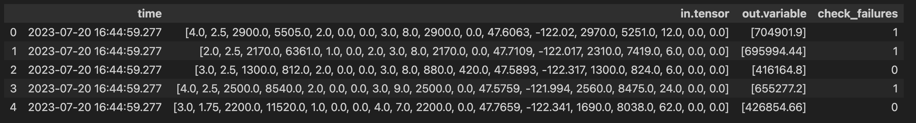
multiple_batch = get_batch(df, nrows=5)
multiple_result = pipeline.infer(multiple_batch)
display(multiple_result)
| time | in.tensor | out.dense_1 | check_failures | out_ccfraud-model-xgboost.variable | |
|---|---|---|---|---|---|
| 0 | 2023-08-07 17:29:16.803 | [[-1.0603297501, 2.3544967095, -3.5638788326, 5.1387348926, -1.2308457019, -0.7687824608, -3.5881228109, 1.8880837663, -3.2789674274, -3.9563254554, 4.0993439118, -5.6539176395, -0.8775733373, -9.131571192, -0.6093537873, -3.7480276773, -5.0309125017, -0.8748149526, 1.9870535692, 0.7005485718, 0.9204422758, -0.1041491809, 0.3229564351, -0.7418141657, 0.0384120159, 1.0993439146, 1.2603409756, -0.1466244739, -1.4463212439]] | [0.99300325] | 0 | [1.0094898] |
| 1 | 2023-08-07 17:29:16.803 | [[-1.0603297501, 2.3544967095, -3.5638788326, 5.1387348926, -1.2308457019, -0.7687824608, -3.5881228109, 1.8880837663, -3.2789674274, -3.9563254554, 4.0993439118, -5.6539176395, -0.8775733373, -9.131571192, -0.6093537873, -3.7480276773, -5.0309125017, -0.8748149526, 1.9870535692, 0.7005485718, 0.9204422758, -0.1041491809, 0.3229564351, -0.7418141657, 0.0384120159, 1.0993439146, 1.2603409756, -0.1466244739, -1.4463212439]] | [0.99300325] | 0 | [1.0094898] |
| 2 | 2023-08-07 17:29:16.803 | [[-1.0603297501, 2.3544967095, -3.5638788326, 5.1387348926, -1.2308457019, -0.7687824608, -3.5881228109, 1.8880837663, -3.2789674274, -3.9563254554, 4.0993439118, -5.6539176395, -0.8775733373, -9.131571192, -0.6093537873, -3.7480276773, -5.0309125017, -0.8748149526, 1.9870535692, 0.7005485718, 0.9204422758, -0.1041491809, 0.3229564351, -0.7418141657, 0.0384120159, 1.0993439146, 1.2603409756, -0.1466244739, -1.4463212439]] | [0.99300325] | 0 | [1.0094898] |
| 3 | 2023-08-07 17:29:16.803 | [[-1.0603297501, 2.3544967095, -3.5638788326, 5.1387348926, -1.2308457019, -0.7687824608, -3.5881228109, 1.8880837663, -3.2789674274, -3.9563254554, 4.0993439118, -5.6539176395, -0.8775733373, -9.131571192, -0.6093537873, -3.7480276773, -5.0309125017, -0.8748149526, 1.9870535692, 0.7005485718, 0.9204422758, -0.1041491809, 0.3229564351, -0.7418141657, 0.0384120159, 1.0993439146, 1.2603409756, -0.1466244739, -1.4463212439]] | [0.99300325] | 0 | [1.0094898] |
| 4 | 2023-08-07 17:29:16.803 | [[0.5817662108, 0.097881551, 0.1546819424, 0.4754101949, -0.1978862306, -0.4504344854, 0.0166540447, -0.0256070551, 0.0920561602, -0.2783917153, 0.0593299441, -0.0196585416, -0.4225083157, -0.1217538877, 1.5473094894, 0.2391622864, 0.3553974881, -0.7685165301, -0.7000849355, -0.1190043285, -0.3450517133, -1.1065114108, 0.2523411195, 0.0209441826, 0.2199267436, 0.2540689265, -0.0450225094, 0.1086773898, 0.2547179311]] | [0.0010916889] | 0 | [-1.9073486e-06] |
After the Experiment: Swapping in New Models
You have seen two methods to validate models in production with test (challenger) models.
The end result of an experiment is a decision about which model becomes the new champion. Let’s say that you have been running the shadow deployment that you created in the previous exercise, and you have decided that you want to replace the model “champion” with the model “challenger”. To do this, you will clear all the steps out of the pipeline, and add only “challenger” back in.
# retrieve a handle to the challenger model
# see the A/B test section for the definition of get_model()
challenger = get_model("challenger")

# get the existing pipeline and undeploy it
# see the A/B test section for the definition of get_pipeline()
pipeline = get_pipeline("pipeline")
pipeline.undeploy()

# clear out all the steps and add the champion back in
pipeline.clear()
pipeline.add_model_step(challenger).deploy()
Exercise: Set a challenger model as the new active model
Pick one of your challenger models as the new champion, and reconfigure your shadow deployment back into a single-step pipeline with the new chosen model.
- Run the test datum from the previous exercise through the reconfigured pipeline.
- Compare the results to the results from the previous exercise.
- Notice that the pipeline predictions are different from the old champion, and consistent with the new one.
At the end of this exercise, you should have a single step pipeline, running a new model.
More information is available through Replace a Pipeline Step.
# Blank space - remove all steps, then redeploy with new champion model

pipeline.clear()

pipeline.add_model_step(ccfraud_xgboost_model)

pipeline.deploy()

singleton = get_singleton(df, 0)
display(singleton)

display(pipeline.steps())

single_result = pipeline.infer(singleton)
display(single_result)
| tensor | |
|---|---|
| 0 | [[-1.0603297501, 2.3544967095000002, -3.5638788326, 5.1387348926, -1.2308457019, -0.7687824608, -3.5881228109, 1.8880837663, -3.2789674274, -3.9563254554, 4.0993439118, -5.6539176395, -0.8775733373, -9.131571192, -0.6093537873, -3.7480276773, -5.0309125017, -0.8748149526000001, 1.9870535692, 0.7005485718000001, 0.9204422758, -0.1041491809, 0.3229564351, -0.7418141657, 0.0384120159, 1.0993439146, 1.2603409756000001, -0.1466244739, -1.4463212439]] |
[{'ModelInference': {'models': [{'name': 'ccfraud-model-xgboost', 'version': 'e71c9c1d-9777-4967-b32c-a074ea8aa467', 'sha': '054810e3e3ebbdd34438d9c1a08ed6a6680ef10bf97b9223f78ebf38e14b3b52'}]}}]
| time | in.tensor | out.dense_1 | check_failures | |
|---|---|---|---|---|
| 0 | 2023-08-07 17:30:17.358 | [[-1.0603297501, 2.3544967095, -3.5638788326, 5.1387348926, -1.2308457019, -0.7687824608, -3.5881228109, 1.8880837663, -3.2789674274, -3.9563254554, 4.0993439118, -5.6539176395, -0.8775733373, -9.131571192, -0.6093537873, -3.7480276773, -5.0309125017, -0.8748149526, 1.9870535692, 0.7005485718, 0.9204422758, -0.1041491809, 0.3229564351, -0.7418141657, 0.0384120159, 1.0993439146, 1.2603409756, -0.1466244739, -1.4463212439]] | [0.99300325] | 0 |
Congratulations!
You have now
- successfully trained new challenger models for the house price prediction problem
- compared your models using an A/B test
- compared your models using a shadow deployment
- replaced your old model for a new one in the house price prediction pipeline
In the next notebook, you will learn how to monitor your production pipeline for “anomalous” or out-of-range behavior.
Cleaning up.
At this point, if you are not continuing on to the next notebook, undeploy your pipeline(s) to give the resources back to the environment.
## blank space to undeploy the pipelines

pipeline.undeploy()
| name | finserv-ccfraud |
|---|---|
| created | 2023-08-07 16:26:37.485326+00:00 |
| last_updated | 2023-08-07 17:30:15.093178+00:00 |
| deployed | False |
| tags | |
| versions | 2513faec-2385-4733-a42d-56a8ae38761a, 10e495af-9b23-4973-913e-4cdebca73461, 782b9edc-d42a-4984-90ca-3bdf35922b87, e80d21a4-21c2-46b8-85d4-6652bbac9506, 8ff48a62-fd9d-43f5-ba3f-11a7f1bcc474, 36faf126-dac5-419d-b0b1-7d7b698b587e, 230d585a-52db-476d-ab28-7b4baed9d023, 192f92e9-9a97-4339-8c1d-f89541ff2cef, 5d2d9c84-13c2-4e35-a41f-ec3c4e8d297b, 41927bef-d8fb-49ee-914e-d106ffc304b3 |
| steps | ccfraud-model-keras |
3 - Financial Services: Validation Rules
Tutorial Notebook 3: Observability Part 1 - Validation Rules
In the previous notebooks you uploaded the models and artifacts, then deployed the models to production through provisioning workspaces and pipelines. Now you’re ready to put your feet up! But to keep your models operational, your work’s not done once the model is in production. You must continue to monitor the behavior and performance of the model to insure that the model provides value to the business.
In this notebook, you will learn about adding validation rules to pipelines.
Preliminaries
In the blocks below we will preload some required libraries; we will also redefine some of the convenience functions that you saw in the previous notebooks.
After that, you should log into Wallaroo and set your working environment to the workspace that you created for this tutorial. Please refer to Notebook 1 to refresh yourself on how to log in and set your working environment to the appropriate workspace.
# preload needed libraries

import wallaroo
from wallaroo.object import EntityNotFoundError
from wallaroo.framework import Framework

from IPython.display import display

# used to display DataFrame information without truncating
from IPython.display import display
import pandas as pd
pd.set_option('display.max_colwidth', None)

import json
import datetime
import time

# used for unique connection names

import string
import random
## convenience functions from the previous notebooks
## these functions assume your connection to wallaroo is called wl

# return the workspace called <name>, or create it if it does not exist.
# this function assumes your connection to wallaroo is called wl
def get_workspace(name):
    workspace = None
    for ws in wl.list_workspaces():
        if ws.name() == name:
            workspace= ws
    if(workspace == None):
        workspace = wl.create_workspace(name)
    return workspace

# pull a single datum from a data frame
# and convert it to the format the model expects
def get_singleton(df, i):
    singleton = df.iloc[i,:].to_numpy().tolist()
    sdict = {'tensor': [singleton]}
    return pd.DataFrame.from_dict(sdict)

# pull a batch of data from a data frame
# and convert to the format the model expects
def get_batch(df, first=0, nrows=1):
    last = first + nrows
    batch = df.iloc[first:last, :].to_numpy().tolist()
    return pd.DataFrame.from_dict({'tensor': batch})

# Get the most recent version of a model in the workspace
# Assumes that the most recent version is the first in the list of versions.
# wl.get_current_workspace().models() returns a list of models in the current workspace

def get_model(mname):
    modellist = wl.get_current_workspace().models()
    model = [m.versions()[-1] for m in modellist if m.name() == mname]
    if len(model) <= 0:
        raise KeyError(f"model {mname} not found in this workspace")
    return model[0]

# get a pipeline by name in the workspace
def get_pipeline(pname):
    plist = wl.get_current_workspace().pipelines()
    pipeline = [p for p in plist if p.name() == pname]
    if len(pipeline) <= 0:
        raise KeyError(f"pipeline {pname} not found in this workspace")
    return pipeline[0]
## blank space to log in and go to correct workspace

wl = wallaroo.Client()

workspace_name = "classification-finserv-jch"

workspace = get_workspace(workspace_name)

# set your current workspace to the workspace that you just created
wl.set_current_workspace(workspace)

# optionally, examine your current workspace
wl.get_current_workspace()
{'name': 'classification-finserv-jch', 'id': 21, 'archived': False, 'created_by': '0a36fba2-ad42-441b-9a8c-bac8c68d13fa', 'created_at': '2023-08-07T16:26:26.779098+00:00', 'models': [{'name': 'ccfraud-model-keras', 'versions': 2, 'owner_id': '""', 'last_update_time': datetime.datetime(2023, 8, 7, 16, 28, 46, 566311, tzinfo=tzutc()), 'created_at': datetime.datetime(2023, 8, 7, 16, 26, 36, 806125, tzinfo=tzutc())}, {'name': 'ccfraud-model-xgboost', 'versions': 1, 'owner_id': '""', 'last_update_time': datetime.datetime(2023, 8, 7, 17, 20, 51, 978426, tzinfo=tzutc()), 'created_at': datetime.datetime(2023, 8, 7, 17, 20, 51, 978426, tzinfo=tzutc())}], 'pipelines': [{'name': 'finserv-ccfraud', 'create_time': datetime.datetime(2023, 8, 7, 16, 26, 37, 485326, tzinfo=tzutc()), 'definition': '[]'}]}
Model Validation Rules
A simple way to try to keep your model’s behavior up to snuff is to make sure that it receives inputs that it expects, and that its output is something that downstream systems can handle. This can entail specifying rules that document what you expect, and either enforcing these rules (by refusing to make a prediction), or at least logging an alert that the expectations described by your validation rules have been violated. As the developer of the model, the data scientist (along with relevant subject matter experts) will often be the person in the best position to specify appropriate validation rules.
In our financial fraud example, supposed you know that confidences from a set of sample data shouldn’t go below 75% likelihood of fraud. Then you might want to set validation rules on your model pipeline to specify that you expect the model’s predictions to also be in that range. That way if the model predicts a value under that range, the pipeline will log that one of the validation checks has failed; this allows you to investigate that instance further.
Note that in this specific example, a model prediction outside the specified range may not necessarily be “wrong”; but out-of-range predictions are likely unusual enough that you may want to “sanity-check” the model’s behavior in these situations.
Wallaroo has functionality for specifying simple validation rules on model input and output values.
pipeline.add_validation(<rulename>, <expression>)
Here, <rulename> is the name of the rule, and <expression> is a simple logical expression that the data scientist expects to be true. This means if the expression proves false, then a check_failure flag is set in the inference results.
To add a validation step to a simple one-step pipeline, you need a handle to the pipeline (here called pipeline), and a handle to the model in the pipeline (here called model). Then you can specify an expected prediction range as follows:
- Get the pipeline.
- Depending on the steps, the pipeline can be cleared and the sample model added as a step.
- Add the validation.
- Deploy the pipeline to set the validation as part of its steps
# get the existing pipeline (in your workspace)
pipeline = get_pipeline("pipeline")

# you also need a handle to the model in this single-step pipeline.
# here are two ways to do it:
#
# (1) If you know the name of the model, you can also just use the get_model() convenience function above.
# In this example, the model has been uploaded to wallaroo with the name "mymodel"

model = get_model("mymodel")

# (2) To get the model without knowing its name (for a single-step pipeline)
model = pipeline.model_configs()[0].model()

# specify the bounds
hi_bnd = 1500000.0 # 1.5M

#
# some examples of validation rules
#

# (1)  validation rule: prediction should be < 1.5 million
pipeline = pipeline.add_validation("less than 1.5m", model.outputs[0][0] < hi_bnd)

# deploy the pipeline to set the steps
pipeline.deploy()
When data is passed to the pipeline for inferences, the pipeline will log a check failure whenever one of the validation expressions evaluates to false. Here are some examples of inference results from a pipeline with the validation rule model.outputs[0][0] < 400000.0.
You can also find check failures in the logs:
logs = pipeline.logs()
logs.loc[logs['check_failures'] > 0]
Exercise: Add validation rules to your model pipeline
Add some simple validation rules to the model pipeline that you created in a previous exercise.
- Add an upper bound or a lower bound to the model predictions
- Try to create predictions that fall both in and out of the specified range
- Look through the logs to find the check failures.
HINT 1: since the purpose of this exercise is try out validation rules, it might be a good idea to take a small data set and make predictions on that data set first, then set the validation rules based on those predictions, so that you can see the check failures trigger.
Don’t forget to undeploy your pipeline after you are done to free up resources.
See Anomaly Testing for more information.
## blank space to get your pipeline and run a small batch of data through it to see the range of predictions

pipeline = get_pipeline('finserv-ccfraud')

ccfraud_keras_model = get_model('ccfraud-model-keras')

pipeline.clear()
pipeline.add_model_step(ccfraud_keras_model)

pipeline.deploy()

df = pd.read_json('../data/cc_data_10k.df.json')

singleton = get_singleton(df, 0)
display(singleton)

single_result = pipeline.infer(singleton)
display(single_result)
| tensor | |
|---|---|
| 0 | [[-1.0603297501, 2.3544967095000002, -3.5638788326, 5.1387348926, -1.2308457019, -0.7687824608, -3.5881228109, 1.8880837663, -3.2789674274, -3.9563254554, 4.0993439118, -5.6539176395, -0.8775733373, -9.131571192, -0.6093537873, -3.7480276773, -5.0309125017, -0.8748149526000001, 1.9870535692, 0.7005485718000001, 0.9204422758, -0.1041491809, 0.3229564351, -0.7418141657, 0.0384120159, 1.0993439146, 1.2603409756000001, -0.1466244739, -1.4463212439]] |
| time | in.tensor | out.dense_1 | check_failures | |
|---|---|---|---|---|
| 0 | 2023-08-07 17:35:16.080 | [[-1.0603297501, 2.3544967095, -3.5638788326, 5.1387348926, -1.2308457019, -0.7687824608, -3.5881228109, 1.8880837663, -3.2789674274, -3.9563254554, 4.0993439118, -5.6539176395, -0.8775733373, -9.131571192, -0.6093537873, -3.7480276773, -5.0309125017, -0.8748149526, 1.9870535692, 0.7005485718, 0.9204422758, -0.1041491809, 0.3229564351, -0.7418141657, 0.0384120159, 1.0993439146, 1.2603409756, -0.1466244739, -1.4463212439]] | [0.99300325] | 0 |
# blank space to set a validation rule on the pipeline and check if it triggers as expected

low_bnd = 0.75

pipeline = pipeline.add_validation("less than 75%", ccfraud_keras_model.outputs[0][0] > low_bnd)

pipeline.deploy()

multiple_batch = get_batch(df, nrows=5)
multiple_result = pipeline.infer(multiple_batch)
display(multiple_result)
| time | in.tensor | out.dense_1 | check_failures | |
|---|---|---|---|---|
| 0 | 2023-08-07 17:35:27.089 | [[-1.0603297501, 2.3544967095, -3.5638788326, 5.1387348926, -1.2308457019, -0.7687824608, -3.5881228109, 1.8880837663, -3.2789674274, -3.9563254554, 4.0993439118, -5.6539176395, -0.8775733373, -9.131571192, -0.6093537873, -3.7480276773, -5.0309125017, -0.8748149526, 1.9870535692, 0.7005485718, 0.9204422758, -0.1041491809, 0.3229564351, -0.7418141657, 0.0384120159, 1.0993439146, 1.2603409756, -0.1466244739, -1.4463212439]] | [0.99300325] | 0 |
| 1 | 2023-08-07 17:35:27.089 | [[-1.0603297501, 2.3544967095, -3.5638788326, 5.1387348926, -1.2308457019, -0.7687824608, -3.5881228109, 1.8880837663, -3.2789674274, -3.9563254554, 4.0993439118, -5.6539176395, -0.8775733373, -9.131571192, -0.6093537873, -3.7480276773, -5.0309125017, -0.8748149526, 1.9870535692, 0.7005485718, 0.9204422758, -0.1041491809, 0.3229564351, -0.7418141657, 0.0384120159, 1.0993439146, 1.2603409756, -0.1466244739, -1.4463212439]] | [0.99300325] | 0 |
| 2 | 2023-08-07 17:35:27.089 | [[-1.0603297501, 2.3544967095, -3.5638788326, 5.1387348926, -1.2308457019, -0.7687824608, -3.5881228109, 1.8880837663, -3.2789674274, -3.9563254554, 4.0993439118, -5.6539176395, -0.8775733373, -9.131571192, -0.6093537873, -3.7480276773, -5.0309125017, -0.8748149526, 1.9870535692, 0.7005485718, 0.9204422758, -0.1041491809, 0.3229564351, -0.7418141657, 0.0384120159, 1.0993439146, 1.2603409756, -0.1466244739, -1.4463212439]] | [0.99300325] | 0 |
| 3 | 2023-08-07 17:35:27.089 | [[-1.0603297501, 2.3544967095, -3.5638788326, 5.1387348926, -1.2308457019, -0.7687824608, -3.5881228109, 1.8880837663, -3.2789674274, -3.9563254554, 4.0993439118, -5.6539176395, -0.8775733373, -9.131571192, -0.6093537873, -3.7480276773, -5.0309125017, -0.8748149526, 1.9870535692, 0.7005485718, 0.9204422758, -0.1041491809, 0.3229564351, -0.7418141657, 0.0384120159, 1.0993439146, 1.2603409756, -0.1466244739, -1.4463212439]] | [0.99300325] | 0 |
| 4 | 2023-08-07 17:35:27.089 | [[0.5817662108, 0.097881551, 0.1546819424, 0.4754101949, -0.1978862306, -0.4504344854, 0.0166540447, -0.0256070551, 0.0920561602, -0.2783917153, 0.0593299441, -0.0196585416, -0.4225083157, -0.1217538877, 1.5473094894, 0.2391622864, 0.3553974881, -0.7685165301, -0.7000849355, -0.1190043285, -0.3450517133, -1.1065114108, 0.2523411195, 0.0209441826, 0.2199267436, 0.2540689265, -0.0450225094, 0.1086773898, 0.2547179311]] | [0.0010916889] | 1 |
Congratulations!
In this tutorial you have
- Set a validation rule on your financial fraud classification pipeline.
- Detected model predictions that failed the validation rule.
In the next notebook, you will learn how to monitor the distribution of model outputs for drift away from expected behavior.
Cleaning up.
At this point, if you are not continuing on to the next notebook, undeploy your pipeline to give the resources back to the environment.
## blank space to undeploy the pipeline

pipeline.undeploy()
| name | finserv-ccfraud |
|---|---|
| created | 2023-08-07 16:26:37.485326+00:00 |
| last_updated | 2023-08-07 17:35:24.149368+00:00 |
| deployed | False |
| tags | |
| versions | 095ef880-06f0-45d5-bfef-ac4e11d2b06c, f9004ecd-7a8c-4963-bebc-e40d1cde357c, 2513faec-2385-4733-a42d-56a8ae38761a, 10e495af-9b23-4973-913e-4cdebca73461, 782b9edc-d42a-4984-90ca-3bdf35922b87, e80d21a4-21c2-46b8-85d4-6652bbac9506, 8ff48a62-fd9d-43f5-ba3f-11a7f1bcc474, 36faf126-dac5-419d-b0b1-7d7b698b587e, 230d585a-52db-476d-ab28-7b4baed9d023, 192f92e9-9a97-4339-8c1d-f89541ff2cef, 5d2d9c84-13c2-4e35-a41f-ec3c4e8d297b, 41927bef-d8fb-49ee-914e-d106ffc304b3 |
| steps | ccfraud-model-keras |
4 - Financial Services: Drift Detection
Tutorial Notebook 4: Observability Part 2 - Drift Detection
In the previous notebook you learned how to add simple validation rules to a pipeline, to monitor whether outputs (or inputs) stray out of some expected range. In this notebook, you will monitor the distribution of the pipeline’s predictions to see if the model, or the environment that it runs it, has changed.
Preliminaries
In the blocks below we will preload some required libraries; we will also redefine some of the convenience functions that you saw in the previous notebooks.
After that, you should log into Wallaroo and set your working environment to the workspace that you created for this tutorial. Please refer to Notebook 1 to refresh yourself on how to log in and set your working environment to the appropriate workspace.
# preload needed libraries

import wallaroo
from wallaroo.object import EntityNotFoundError

from IPython.display import display

# used to display DataFrame information without truncating
from IPython.display import display
import pandas as pd
pd.set_option('display.max_colwidth', None)

import json
import datetime
import time

# used for unique connection names

import string
import random
## convenience functions from the previous notebooks
## these functions assume your connection to wallaroo is called wl

# return the workspace called <name>, or create it if it does not exist.
# this function assumes your connection to wallaroo is called wl
def get_workspace(name):
    workspace = None
    for ws in wl.list_workspaces():
        if ws.name() == name:
            workspace= ws
    if(workspace == None):
        workspace = wl.create_workspace(name)
    return workspace

# pull a single datum from a data frame
# and convert it to the format the model expects
def get_singleton(df, i):
    singleton = df.iloc[i,:].to_numpy().tolist()
    sdict = {'tensor': [singleton]}
    return pd.DataFrame.from_dict(sdict)

# pull a batch of data from a data frame
# and convert to the format the model expects
def get_batch(df, first=0, nrows=1):
    last = first + nrows
    batch = df.iloc[first:last, :].to_numpy().tolist()
    return pd.DataFrame.from_dict({'tensor': batch})

# Get the most recent version of a model in the workspace
# Assumes that the most recent version is the first in the list of versions.
# wl.get_current_workspace().models() returns a list of models in the current workspace

def get_model(mname):
    modellist = wl.get_current_workspace().models()
    model = [m.versions()[-1] for m in modellist if m.name() == mname]
    if len(model) <= 0:
        raise KeyError(f"model {mname} not found in this workspace")
    return model[0]

# get a pipeline by name in the workspace
def get_pipeline(pname):
    plist = wl.get_current_workspace().pipelines()
    pipeline = [p for p in plist if p.name() == pname]
    if len(pipeline) <= 0:
        raise KeyError(f"pipeline {pname} not found in this workspace")
    return pipeline[0]
## blank space to log in and go to correct workspace

wl = wallaroo.Client()

workspace_name = "classification-finserv-jch"

workspace = get_workspace(workspace_name)

# set your current workspace to the workspace that you just created
wl.set_current_workspace(workspace)

# optionally, examine your current workspace
wl.get_current_workspace()
{'name': 'classification-finserv-jch', 'id': 21, 'archived': False, 'created_by': '0a36fba2-ad42-441b-9a8c-bac8c68d13fa', 'created_at': '2023-08-07T16:26:26.779098+00:00', 'models': [{'name': 'ccfraud-model-keras', 'versions': 2, 'owner_id': '""', 'last_update_time': datetime.datetime(2023, 8, 7, 16, 28, 46, 566311, tzinfo=tzutc()), 'created_at': datetime.datetime(2023, 8, 7, 16, 26, 36, 806125, tzinfo=tzutc())}, {'name': 'ccfraud-model-xgboost', 'versions': 1, 'owner_id': '""', 'last_update_time': datetime.datetime(2023, 8, 7, 17, 20, 51, 978426, tzinfo=tzutc()), 'created_at': datetime.datetime(2023, 8, 7, 17, 20, 51, 978426, tzinfo=tzutc())}], 'pipelines': [{'name': 'finserv-ccfraud', 'create_time': datetime.datetime(2023, 8, 7, 16, 26, 37, 485326, tzinfo=tzutc()), 'definition': '[]'}]}
Monitoring for Drift: Shift Happens.
In machine learning, you use data and known answers to train a model to make predictions for new previously unseen data. You do this with the assumption that the future unseen data will be similar to the data used during training: the future will look somewhat like the past.
But the conditions that existed when a model was created, trained and tested can change over time, due to various factors.
A good model should be robust to some amount of change in the environment; however, if the environment changes too much, your models may no longer be making the correct decisions. This situation is known as concept drift; too much drift can obsolete your models, requiring periodic retraining.
Let’s consider the example we’ve been working on: credit card fraud prediction. You may start to notice a large number of transactions that that aren’t coming across as fraudulent compared to historical baselines.
Such a change could be due to many factors: a change in interest rates; the appearance or disappearance of major sources of employment; changes in travel patterns. Whatever the cause, detecting such a change quickly is crucial, so that the business can react quickly in the appropriate manner, whether that means simply retraining the model on fresher data, or a pivot in business strategy.
In Wallaroo you can monitor your housing model for signs of drift through the model monitoring and insight capability called Assays. Assays help you track changes in the environment that your model operates within, which can affect the model’s outcome. It does this by tracking the model’s predictions and/or the data coming into the model against an established baseline. If the distribution of monitored values in the current observation window differs too much from the baseline distribution, the assay will flag it. The figure below shows an example of a running scheduled assay.
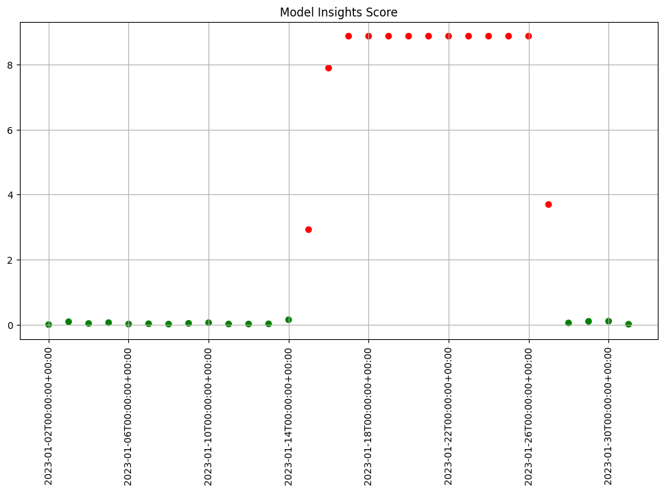
Figure: A daily assay that’s been running for a month. The dots represent the difference between the distribution of values in the daily observation window, and the baseline. When that difference exceeds the specified threshold (indicated by a red dot) an alert is set.
This next set of exercises will walk you through setting up an assay to monitor the predictions of your house price model, in order to detect drift.
NOTE
An assay is a monitoring process that typically runs over an extended, ongoing period of time. For example, one might set up an assay that every day monitors the previous 24 hours’ worth of predictions and compares it to a baseline. For the purposes of these exercises, we’ll be compressing processes what normally would take hours or days into minutes.
Exercise Prep: Create some datasets for demonstrating assays
Because assays are designed to detect changes in distributions, let’s try to set up data with different distributions to test with. Take your financial transaction data and create two sets: a set with lower prices, and a set with higher prices. You can split however you choose.
The idea is we will pretend that the set of transactions less likely to trigger fraud warnings versus a set that is known to have a high likelihood of being evaluated as fraudulent.
- If you are using the pre-provided models to do these exercises, you can use the provided data sets
cc_data_low_confidence.df.jsonandcc_data_high_confidence.df.json. This is to establish our baseline as a set of known values, so the higher prices will trigger our assay alerts.
low_fraud_data = pd.read_json('../data/cc_data_low_confidence.df.json')
high_fraud_data = pd.read_json('../data/cc_data_high_confidence.df.json')
Note that the data in these files are already in the form expected by the models, so you don’t need to use the get_singleton or get_batch convenience functions to infer.
At the end of this exercise, you should have two sets of data to demonstrate assays. In the discussion below, we’ll refer to these sets as low_fraud_data and high_fraud_data.
See Wallaroo SDK Essentials Guide: Assays Management for more details.
# let's start with this - get the 10k of inferences.
# then split them into those < 0.25, and those > 0.75
# blank spot to split or download data

low_fraud_data = pd.read_json('../data/cc_data_low_confidence.df.json')
high_fraud_data = pd.read_json('../data/cc_data_high_confidence.df.json')
We will use this data to set up some “historical data” in the house price prediction pipeline that you build in the assay exercises.
Setting up a baseline for the assay
In order to know whether the distribution of your model’s predictions have changed, you need a baseline to compare them to. This baseline should represent how you expect the model to behave at the time it was trained. This might be approximated by the distribution of the model’s predictions over some “typical” period of time. For example, we might collect the predictions of our model over the first few days after it’s been deployed. For these exercises, we’ll compress that to a few minutes. Currently, to set up a wallaroo assay the pipeline must have been running for some period of time, and the assumption is that this period of time is “typical”, and that the distributions of the inputs and the outputs of the model during this period of time are “typical.”
Exercise Prep: Run some inferences and set some time stamps
Here, we simulate having a pipeline that’s been running for a long enough period of time to set up an assay.
To send enough data through the pipeline to create assays, you execute something like the following code (using the appropriate names for your pipelines and models). Note that this step will take a little while, because of the sleep interval.
You will need the timestamps baseline_start, and baseline_end, for the next exercises.
# get your pipeline (in this example named "mypipeline")

pipeline = get_pipeline("mypipeline")
pipeline.deploy()

## Run some baseline data
# Where the baseline data will start
baseline_start = datetime.datetime.now()

# the number of samples we'll use for the baseline
nsample = 500

# Wait 30 seconds to set this data apart from the rest
# then send the data in batch
time.sleep(30)

# get a sample
lowprice_data_sample = lowprice_data.sample(nsample, replace=True).reset_index(drop=True)
pipeline.infer(lowprice_data_sample)

# Set the baseline end
baseline_end = datetime.datetime.now()
# blank space to get pipeline and set up baseline data

pipeline = get_pipeline('finserv-ccfraud')

ccfraud_keras_model = get_model('ccfraud-model-keras')

pipeline.deploy()
| name | finserv-ccfraud |
|---|---|
| created | 2023-08-07 16:26:37.485326+00:00 |
| last_updated | 2023-08-07 17:55:48.136182+00:00 |
| deployed | True |
| tags | |
| versions | af6809a9-088f-47e5-88a4-2005599fde7a, 095ef880-06f0-45d5-bfef-ac4e11d2b06c, f9004ecd-7a8c-4963-bebc-e40d1cde357c, 2513faec-2385-4733-a42d-56a8ae38761a, 10e495af-9b23-4973-913e-4cdebca73461, 782b9edc-d42a-4984-90ca-3bdf35922b87, e80d21a4-21c2-46b8-85d4-6652bbac9506, 8ff48a62-fd9d-43f5-ba3f-11a7f1bcc474, 36faf126-dac5-419d-b0b1-7d7b698b587e, 230d585a-52db-476d-ab28-7b4baed9d023, 192f92e9-9a97-4339-8c1d-f89541ff2cef, 5d2d9c84-13c2-4e35-a41f-ec3c4e8d297b, 41927bef-d8fb-49ee-914e-d106ffc304b3 |
| steps | ccfraud-model-keras |
Before setting up an assay on this pipeline’s output, we may want to look at the distribution of the predictions over our selected baseline period. To do that, we’ll create an assay_builder that specifies the pipeline, the model in the pipeline, and the baseline period.. We’ll also specify that we want to look at the output of the model, which in the example code is named variable, and would appear as out.variable in the logs.
# print out one of the logs to get the name of the output variable
display(pipeline.logs(limit=1))

# get the model name directly off the pipeline (you could just hard code this, if you know the name)

model_name = pipeline.model_configs()[0].model().name()

assay_builder = ( wl.build_assay(assay_name, pipeline, model_name,
                     baseline_start, baseline_end)
                    .add_iopath("output variable 0") ) # specify that we are looking at the first output of the output variable "variable"
where baseline_start and baseline_end are the beginning and end of the baseline periods as datetime.datetime objects.
You can then examine the distribution of variable over the baseline period:
assay_builder.baseline_histogram()
Exercise: Create an assay builder and set a baseline
Create an assay builder to monitor the output of your house price pipeline. The baseline period should be from baseline_start to baseline_end.
- You will need to know the name of your output variable, and the name of the model in the pipeline.
Examine the baseline distribution.
## Blank space to create an assay builder and examine the baseline distribution

display(pipeline.logs(limit=1))
model_name = pipeline.model_configs()[0].model().name()
display(model_name)

import datetime
import time
baseline_start = datetime.datetime.now()
time.sleep(5)

pipeline.infer(low_fraud_data)

time.sleep(5)

baseline_end = datetime.datetime.now()

assay_builder = ( wl.build_assay('sample finserv assay', pipeline, model_name,
                     baseline_start, baseline_end)
                    .add_iopath("output dense_1 0") )

assay_builder.baseline_histogram()
Warning: There are more logs available. Please set a larger limit or request a file using export_logs.
| time | in.tensor | out.dense_1 | check_failures | |
|---|---|---|---|---|
| 0 | 2023-08-07 17:11:21.172 | [[0.5817662108, 0.097881551, 0.1546819424, 0.4754101949, -0.1978862306, -0.4504344854, 0.0166540447, -0.0256070551, 0.0920561602, -0.2783917153, 0.0593299441, -0.0196585416, -0.4225083157, -0.1217538877, 1.5473094894, 0.2391622864, 0.3553974881, -0.7685165301, -0.7000849355, -0.1190043285, -0.3450517133, -1.1065114108, 0.2523411195, 0.0209441826, 0.2199267436, 0.2540689265, -0.0450225094, 0.1086773898, 0.2547179311]] | [0.0010916889] | 0 |
'ccfraud-model-keras'
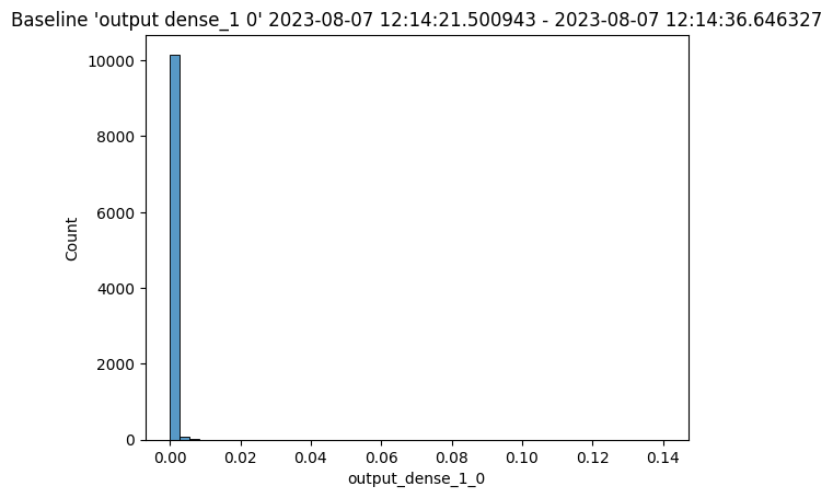
An assay should detect if the distribution of model predictions changes from the above distribution over regularly sampled observation windows. This is called drift.
To show drift, we’ll run more data through the pipeline – first some data drawn from the same distribution as the baseline (lowprice_data). Then, we will gradually introduce more data from a different distribution (highprice_data). We should see the difference between the baseline distribution and the distribution in the observation window increase.
To set up the data, you should do something like the below. It will take a while to run, because of all the sleep intervals.
You will need the assay_window_end for a later exercise.
IMPORTANT NOTE: To generate the data for the assay, this process may take 4-5 minutes. Because the shortest period of time for an assay window is 1 minute, the intervals of inference data are spaced to fall within that time period.
# Set the start for our assay window period.
assay_window_start = datetime.datetime.now()

# Run a set of house values, spread across a "longer" period of time

# run "typical" data
for x in range(4):
    pipeline.infer(low_fraud_data.sample(2*nsample, replace=True).reset_index(drop=True))
    time.sleep(25)

# run a mix
for x in range(3):
    pipeline.infer(low_fraud_data.sample(nsample, replace=True).reset_index(drop=True))
    pipeline.infer(high_fraud_data.sample(nsample, replace=True).reset_index(drop=True))
    time.sleep(25)

# high price houses dominate the sample
for x in range(3):
    pipeline.infer(high_fraud_data.sample(2*nsample, replace=True).reset_index(drop=True))
    time.sleep(25)

# End our assay window period
assay_window_end = datetime.datetime.now()
Exercise Prep: Run some inferences and set some time stamps
Run more data through the pipeline, manifesting a drift, like the example above. It may around 10 minutes depending on how you stagger the inferences.
## Blank space to run more data

assay_window_start = datetime.datetime.now()

# Run a set of house values, spread across a "longer" period of time

nsample = 500

# run "typical" data
for x in range(4):
    pipeline.infer(df.sample(2*nsample, replace=True).reset_index(drop=True))
    time.sleep(25)

# run a mix
for x in range(3):
    pipeline.infer(low_fraud_data.sample(nsample, replace=True).reset_index(drop=True))
    pipeline.infer(high_fraud_data.sample(nsample, replace=True).reset_index(drop=True))
    time.sleep(25)

# high price houses dominate the sample
for x in range(3):
    pipeline.infer(high_fraud_data.sample(2*nsample, replace=True).reset_index(drop=True))
    time.sleep(25)

# End our assay window period
assay_window_end = datetime.datetime.now()
Defining the Assay Parameters
Now we’re finally ready to set up an assay!
The Observation Window
Once a baseline period has been established, you must define the window of observations that will be compared to the baseline. For instance, you might want to set up an assay that runs every 12 hours, collects the previous 24 hours’ predictions and compares the distribution of predictions within that 24 hour window to the baseline. To set such a comparison up would look like this:
assay_builder.window_builder().add_width(hours=24).add_interval(hours=12)
In other words width is the width of the observation window, and interval is how often an assay (comparison) is run. The default value of width is 24 hours; the default value of interval is to set it equal to width. The units can be specified in one of: minutes, hours, days, weeks.
The Comparison Threshold
Given an observation window and a baseline distribution, an assay computes the distribution of predictions in the observation window. It then calculates the “difference” (or “distance”) between the observed distribution and the baseline distribution. For the assay’s default distance metric (which we will use here), a good starting threshold is 0.1. Since a different value may work best for a specific situation, you can try interactive assay runs on historical data to find a good threshold, as we do in these exercises.
To set the assay threshold for the assays to 0.1:
assay_builder.add_alert_threshold(0.1)
Running an Assay on Historical Data
In this exercise, you will build an interactive assay over historical data. To do this, you need an end time (endtime).
Depending on the historical history, the window and interval may need adjusting. If using the previously generated information, an interval window as short as 1 minute may be useful.
Assuming you have an assay builder with the appropriate window parameters and threshold set, you can do an interactive run and look at the results would look like this.
# set the end of the interactive run
assay_builder.add_run_until(endtime)

# set the window

assay_builder.window_builder().add_width(hours=24).add_interval(hours=12)

assay_results = assay_builder.build().interactive_run()
df = assay_results.to_dataframe() # to return the results as a table
assay_results.chart_scores() # to plot the run
Exercise: Create an interactive assay
Use the assay_builder you created in the previous exercise to set up an interactive assay.
- The assay should run every minute, on a window that is a minute wide.
- Set the alert threshold to 0.1.
- You can use
assay_window_end(or a later timestamp) as the end of the interactive run.
Examine the assay results. Do you see any drift?
To try other ways of examining the assay results, see the “Interactive Assay Runs” section of the Model Insights tutorial.
# blank space for setting assay parameters, creating and examining an interactive assay

# set the end of the interactive run
assay_builder.add_run_until(assay_window_end)

# doing minutes to get our previous values in
assay_builder.window_builder().add_width(minutes=1).add_interval(minutes=1)
assay_builder.add_alert_threshold(0.1)
assay_results = assay_builder.build().interactive_run()
df = assay_results.to_dataframe() # to return the results as a table
assay_results.chart_scores() # to plot the run

Scheduling an Assay to run on ongoing data
(We won’t be doing an exercise here, this is for future reference).
Once you are satisfied with the parameters you have set, you can schedule an assay to run regularly .
# create a fresh assay builder with the correct parameters
assay_builder = ( wl.build_assay(assay_name, pipeline, model_name,
                     baseline_start, baseline_end)
                    .add_iopath("output variable 0") )

# this assay runs every 24 hours on a 24 hour window
assay_builder.window_builder().add_width(hours=24)
assay_builder.add_alert_threshold(0.1)

# now schedule the assay
assay_id = assay_builder.upload()
You can use the assay id later to get the assay results.
You have now walked through setting up a basic assay and running it over historical data.
Congratulations!
In this tutorial you have:
- Deployed a single step financial transaction classification pipeline and sent data to it.
- Compared two financial transaction classification models in an A/B test
- Compared two financial transaction classification models in a shadow deployment.
- Swapped the “winner” of the comparisons into the financial transaction classification pipeline.
- Set validation rules on the pipeline.
- Set up an assay on the pipeline to monitor for drift in its predictions.
Great job!
Cleaning up.
Now that the tutorial is complete, don’t forget to undeploy your pipeline to free up the resources.
# blank space to undeploy your pipeline

pipeline.undeploy()
| name | finserv-ccfraud |
|---|---|
| created | 2023-08-07 16:26:37.485326+00:00 |
| last_updated | 2023-08-07 18:11:00.015882+00:00 |
| deployed | False |
| tags | |
| versions | 405d7b12-309e-44a1-968c-744f765b42a2, a665ba59-bc76-4a87-a836-4dd65da8b115, af6809a9-088f-47e5-88a4-2005599fde7a, 095ef880-06f0-45d5-bfef-ac4e11d2b06c, f9004ecd-7a8c-4963-bebc-e40d1cde357c, 2513faec-2385-4733-a42d-56a8ae38761a, 10e495af-9b23-4973-913e-4cdebca73461, 782b9edc-d42a-4984-90ca-3bdf35922b87, e80d21a4-21c2-46b8-85d4-6652bbac9506, 8ff48a62-fd9d-43f5-ba3f-11a7f1bcc474, 36faf126-dac5-419d-b0b1-7d7b698b587e, 230d585a-52db-476d-ab28-7b4baed9d023, 192f92e9-9a97-4339-8c1d-f89541ff2cef, 5d2d9c84-13c2-4e35-a41f-ec3c4e8d297b, 41927bef-d8fb-49ee-914e-d106ffc304b3 |
| steps | ccfraud-model-keras |