The following tutorials demonstrate how to use Wallaroo to test and validation models in production against their target outcomes.
Model Validation and Testing in Wallaroo
Tutorials on using Wallaroo for model testing and validation.
- 1: A/B Testing Tutorial
- 2: Anomaly Testing Tutorial
- 3: House Price Testing Life Cycle
- 4: Shadow Deployment Tutorial
1 - A/B Testing Tutorial
How to use Wallaroo’s A/B Testing feature to evaluate competing ML models.
This tutorial and the assets can be downloaded as part of the Wallaroo Tutorials repository.
A/B Testing
A/B testing is a method that provides the ability to test out ML models for performance, accuracy or other useful benchmarks. A/B testing is contrasted with the Wallaroo Shadow Deployment feature. In both cases, two sets of models are added to a pipeline step:
- Control or Champion model: The model currently used for inferences.
- Challenger model(s): One or more models that are to be compared to the champion model.
The two feature are different in this way:
| Feature | Description |
|---|---|
| A/B Testing | A subset of inferences are submitted to either the champion ML model or a challenger ML model. |
| Shadow Deploy | All inferences are submitted to the champion model and one or more challenger models. |
So to repeat: A/B testing submits some of the inference requests to the champion model, some to the challenger model with one set of outputs, while shadow testing submits all of the inference requests to champion and shadow models, and has separate outputs.
This tutorial demonstrate how to conduct A/B testing in Wallaroo. For this example we will be using an open source model that uses an Aloha CNN LSTM model for classifying Domain names as being either legitimate or being used for nefarious purposes such as malware distribution.
For our example, we will perform the following:
- Create a workspace for our work.
- Upload the Aloha model and a challenger model.
- Create a pipeline that can ingest our submitted data with the champion model and the challenger model set into a A/B step.
- Run a series of sample inferences to display inferences that are run through the champion model versus the challenger model, then determine which is more efficient.
All sample data and models are available through the Wallaroo Quick Start Guide Samples repository.
Prerequisites
- A deployed Wallaroo instance
- The following Python libraries installed:
Steps
Import libraries
Here we will import the libraries needed for this notebook.
import wallaroo
from wallaroo.object import EntityNotFoundError
import os
import pandas as pd
import json
from IPython.display import display

# used to display dataframe information without truncating
from IPython.display import display
pd.set_option('display.max_colwidth', None)
wallaroo.__version__
'2023.2.0rc3'
Connect to the Wallaroo Instance
The first step is to connect to Wallaroo through the Wallaroo client. The Python library is included in the Wallaroo install and available through the Jupyter Hub interface provided with your Wallaroo environment.
This is accomplished using the wallaroo.Client() command, which provides a URL to grant the SDK permission to your specific Wallaroo environment. When displayed, enter the URL into a browser and confirm permissions. Store the connection into a variable that can be referenced later.
If logging into the Wallaroo instance through the internal JupyterHub service, use wl = wallaroo.Client(). For more information on Wallaroo Client settings, see the Client Connection guide.
# Login through local Wallaroo instance

wl = wallaroo.Client()
Create Workspace
We will create a workspace to manage our pipeline and models. The following variables will set the name of our sample workspace then set it as the current workspace for all other commands.
To allow this tutorial to be run multiple times or by multiple users in the same Wallaroo instance, a random 4 character prefix will be added to the workspace, pipeline, and model.
workspace_name = 'abhousetesting'
def get_workspace(name):
    workspace = None
    for ws in wl.list_workspaces():
        if ws.name() == name:
            workspace= ws
    if(workspace == None):
        workspace = wl.create_workspace(name)
    return workspace
workspace = get_workspace(workspace_name)

wl.set_current_workspace(workspace)
{'name': 'abtesting', 'id': 33, 'archived': False, 'created_by': '028c8b48-c39b-4578-9110-0b5bdd3824da', 'created_at': '2023-05-18T13:55:21.887136+00:00', 'models': [], 'pipelines': []}
Set Up the Champion and Challenger Models
Now we upload the Champion and Challenger models to our workspace. We will use two models:
aloha-cnn-lstmmodel.aloha-cnn-lstm-new(a retrained version)
Set the Champion Model
We upload our champion model, labeled as control.
#control =  wl.upload_model("aloha-control",   'models/aloha-cnn-lstm.zip').configure('tensorflow')
control = wl.upload_model("houseprice-control",'models/housing_control.zip', framework=wallaroo.framework.Framework.TENSORFLOW).configure('tensorflow')
Set the Challenger Model
Now we upload the Challenger model, labeled as challenger.
#challenger = wl.upload_model("aloha-challenger",   'models/aloha-cnn-lstm-new.zip').configure('tensorflow')
challenger = wl.upload_model("houseprice-challenger",'models/housing_challenger.zip', framework=wallaroo.framework.Framework.TENSORFLOW).configure('tensorflow')
Define The Pipeline
Here we will configure a pipeline with two models and set the control model with a random split chance of receiving 2/3 of the data. Because this is a random split, it is possible for one model or the other to receive more inferences than a strict 2:1 ratio, but the more inferences are run, the more likely it is for the proper ratio split.
pipeline = (wl.build_pipeline("randomsplitpipeline-demo")
            .add_random_split([(2, control), (1, challenger)], "session_id"))
Deploy the pipeline
Now we deploy the pipeline so we can run our inference through it.
experiment_pipeline = pipeline.deploy()
experiment_pipeline.status()
{'status': 'Running',
 'details': [],
 'engines': [{'ip': '10.244.3.161',
   'name': 'engine-66cbb56b67-4j46k',
   'status': 'Running',
   'reason': None,
   'details': [],
   'pipeline_statuses': {'pipelines': [{'id': 'randomsplitpipeline-demo',
      'status': 'Running'}]},
   'model_statuses': {'models': [{'name': 'aloha-control',
      'version': '7e5d3218-f7ad-4f08-9984-e1a459f6bc1c',
      'sha': 'fd998cd5e4964bbbb4f8d29d245a8ac67df81b62be767afbceb96a03d1a01520',
      'status': 'Running'},
     {'name': 'aloha-challenger',
      'version': 'dcdd8ef9-e30a-4785-ac91-06bc396487ec',
      'sha': '223d26869d24976942f53ccb40b432e8b7c39f9ffcf1f719f3929d7595bceaf3',
      'status': 'Running'}]}}],
 'engine_lbs': [{'ip': '10.244.4.194',
   'name': 'engine-lb-584f54c899-ks6s8',
   'status': 'Running',
   'reason': None,
   'details': []}],
 'sidekicks': []}
Run a single inference
Now we have our deployment set up let’s run a single inference. In the results we will be able to see the inference results as well as which model the inference went to under model_id. We’ll run the inference request 5 times, with the odds are that the challenger model being run at least once.
# use dataframe JSON files
for x in range(5):
    result = experiment_pipeline.infer_from_file("data/data-1.df.json")
    value = result.loc[0]["out.dense_19"]
    model = json.loads(result.loc[0]["out._model_split"][0])['name']
    df = pd.DataFrame({'model': model, 'value': value})
    display(df)
| out._model_split | out.dense_19 | |
|---|---|---|
| 0 | [{"name":"aloha-control","version":"7e5d3218-f7ad-4f08-9984-e1a459f6bc1c","sha":"fd998cd5e4964bbbb4f8d29d245a8ac67df81b62be767afbceb96a03d1a01520"}] | [0.997564] |
| out._model_split | out.dense_19 | |
|---|---|---|
| 0 | [{"name":"aloha-control","version":"7e5d3218-f7ad-4f08-9984-e1a459f6bc1c","sha":"fd998cd5e4964bbbb4f8d29d245a8ac67df81b62be767afbceb96a03d1a01520"}] | [0.997564] |
| out._model_split | out.dense_19 | |
|---|---|---|
| 0 | [{"name":"aloha-challenger","version":"dcdd8ef9-e30a-4785-ac91-06bc396487ec","sha":"223d26869d24976942f53ccb40b432e8b7c39f9ffcf1f719f3929d7595bceaf3"}] | [0.997564] |
| out._model_split | out.dense_19 | |
|---|---|---|
| 0 | [{"name":"aloha-control","version":"7e5d3218-f7ad-4f08-9984-e1a459f6bc1c","sha":"fd998cd5e4964bbbb4f8d29d245a8ac67df81b62be767afbceb96a03d1a01520"}] | [0.997564] |
| out._model_split | out.main | |
|---|---|---|
| 0 | [{"name":"aloha-challenger","version":"dcdd8ef9-e30a-4785-ac91-06bc396487ec","sha":"223d26869d24976942f53ccb40b432e8b7c39f9ffcf1f719f3929d7595bceaf3"}] | [0.997564] |
Run Inference Batch
We will submit 1000 rows of test data through the pipeline, then loop through the responses and display which model each inference was performed in. The results between the control and challenger should be approximately 2:1.
responses = []
test_data = pd.read_json('data/data-1k.df.json')
# For each row, submit that row as a separate dataframe
# Add the results to the responses array
for index, row in test_data.head(1000).iterrows():
    responses.append(experiment_pipeline.infer(row.to_frame('text_input').reset_index()))

#now get our responses for each row
l = [json.loads(r.loc[0]["out._model_split"][0])["name"] for r in responses]
df = pd.DataFrame({'model': l})
display(df.model.value_counts())
aloha-control       666
aloha-challenger    334
Name: model, dtype: int64
Test Challenger
Now we have run a large amount of data we can compare the results.
For this experiment we are looking for a significant change in the fraction of inferences that predicted a probability of the seventh category being high than 0.5 so we can determine whether our challenger model is more “successful” than the champion model at identifying category 7.
control_count = 0
challenger_count = 0

control_success = 0
challenger_success = 0

for r in responses:
    if json.loads(r.loc[0]["out._model_split"][0])["name"] == "aloha-control":
        control_count += 1
        if(r.loc[0]["out.main"][0] > .5):
            control_success += 1
    else:
        challenger_count += 1
        if(r.loc[0]["out.main"][0] > .5):
            challenger_success += 1

print("control class 7 prediction rate: " + str(control_success/control_count))
print("challenger class 7 prediction rate: " + str(challenger_success/challenger_count))
control class 7 prediction rate: 0.972972972972973
challenger class 7 prediction rate: 0.9850299401197605
Logs
Logs can be viewed with the Pipeline method logs(). For this example, only the first 5 logs will be shown. For Arrow enabled environments, the model type can be found in the column out._model_split.
logs = experiment_pipeline.logs(limit=5)
display(logs.loc[:,['time', 'out._model_split', 'out.main']])
Warning: There are more logs available. Please set a larger limit or request a file using export_logs.
| time | out._model_split | out.dense_19 | |
|---|---|---|---|
| 0 | 2023-05-18 14:02:08.525 | [{"name":"aloha-challenger","version":"dcdd8ef9-e30a-4785-ac91-06bc396487ec","sha":"223d26869d24976942f53ccb40b432e8b7c39f9ffcf1f719f3929d7595bceaf3"}] | [0.99999803] |
| 1 | 2023-05-18 14:02:08.141 | [{"name":"aloha-control","version":"7e5d3218-f7ad-4f08-9984-e1a459f6bc1c","sha":"fd998cd5e4964bbbb4f8d29d245a8ac67df81b62be767afbceb96a03d1a01520"}] | [0.9998954] |
| 2 | 2023-05-18 14:02:07.758 | [{"name":"aloha-control","version":"7e5d3218-f7ad-4f08-9984-e1a459f6bc1c","sha":"fd998cd5e4964bbbb4f8d29d245a8ac67df81b62be767afbceb96a03d1a01520"}] | [0.66066873] |
| 3 | 2023-05-18 14:02:07.374 | [{"name":"aloha-control","version":"7e5d3218-f7ad-4f08-9984-e1a459f6bc1c","sha":"fd998cd5e4964bbbb4f8d29d245a8ac67df81b62be767afbceb96a03d1a01520"}] | [0.9999727] |
| 4 | 2023-05-18 14:02:07.021 | [{"name":"aloha-challenger","version":"dcdd8ef9-e30a-4785-ac91-06bc396487ec","sha":"223d26869d24976942f53ccb40b432e8b7c39f9ffcf1f719f3929d7595bceaf3"}] | [0.9999754] |
Undeploy Pipeline
With the testing complete, we undeploy the pipeline to return the resources back to the environment.
experiment_pipeline.undeploy()
| name | randomsplitpipeline-demo |
|---|---|
| created | 2023-05-18 13:55:25.914690+00:00 |
| last_updated | 2023-05-18 13:55:27.144796+00:00 |
| deployed | False |
| tags | |
| versions | 6350d3ee-8b11-4eac-a8f5-e32659ea0dd2, 170fb233-5b26-492a-ba86-e2ee72129d16 |
| steps | aloha-control |
2 - Anomaly Testing Tutorial
How to use Wallaroo’s pipeline validation feature to detect inference anomalies.
This tutorial and the assets can be downloaded as part of the Wallaroo Tutorials repository.
Anomaly Detection
Wallaroo provides multiple methods of analytical analysis to verify that the data received and generated during an inference is accurate. This tutorial will demonstrate how to use anomaly detection to track the outputs from a sample model to verify that the model is outputting acceptable results.
Anomaly detection allows organizations to set validation parameters in a pipeline. A validation is added to a pipeline to test data based on an expression, and flag any inferences where the validation failed inference result and the pipeline logs.
This tutorial will follow this process in setting up a validation to a pipeline and examining the results:
- Create a workspace and upload the sample model.
- Establish a pipeline and add the model as a step.
- Add a validation to the pipeline.
- Perform inferences and display anomalies through the
InferenceResultobject and the pipeline log files.
This tutorial provides the following:
- Housing model:
./models/housingprice.onnx- a pretrained model used to determine standard home prices. - Test Data:
./data- sample data.
Prerequisites
- A deployed Wallaroo instance
- The following Python libraries installed:
Steps
Import libraries
The first step is to import the libraries needed for this notebook.
import wallaroo
from wallaroo.object import EntityNotFoundError
import os
import json

from IPython.display import display

# used to display dataframe information without truncating
from IPython.display import display
import pandas as pd
pd.set_option('display.max_colwidth', None)

import datetime
Connect to the Wallaroo Instance
The first step is to connect to Wallaroo through the Wallaroo client. The Python library is included in the Wallaroo install and available through the Jupyter Hub interface provided with your Wallaroo environment.
This is accomplished using the wallaroo.Client() command, which provides a URL to grant the SDK permission to your specific Wallaroo environment. When displayed, enter the URL into a browser and confirm permissions. Store the connection into a variable that can be referenced later.
If logging into the Wallaroo instance through the internal JupyterHub service, use wl = wallaroo.Client(). For more information on Wallaroo Client settings, see the Client Connection guide.
# Login through local Wallaroo instance

wl = wallaroo.Client()
Create Workspace
We will create a workspace to manage our pipeline and models. The following variables will set the name of our sample workspace then set it as the current workspace.
workspace_name = 'anomalytesting'
pipeline_name = 'anomalytestexample'
model_name = 'anomaly-housing-model'
model_file_name = './models/house_price_keras.onnx'
def get_workspace(name):
    workspace = None
    for ws in wl.list_workspaces():
        if ws.name() == name:
            workspace= ws
    if(workspace == None):
        workspace = wl.create_workspace(name)
    return workspace
workspace = get_workspace(workspace_name)

wl.set_current_workspace(workspace)
{'name': 'anomalytesting', 'id': 145, 'archived': False, 'created_by': '138bd7e6-4dc8-4dc1-a760-c9e721ef3c37', 'created_at': '2023-03-06T19:27:47.219395+00:00', 'models': [{'name': 'anomaly-housing-model', 'versions': 1, 'owner_id': '""', 'last_update_time': datetime.datetime(2023, 3, 13, 16, 39, 41, 683686, tzinfo=tzutc()), 'created_at': datetime.datetime(2023, 3, 13, 16, 39, 41, 683686, tzinfo=tzutc())}], 'pipelines': [{'name': 'anomalyhousing', 'create_time': datetime.datetime(2023, 3, 6, 19, 37, 23, 71334, tzinfo=tzutc()), 'definition': '[]'}]}
Upload The Model
The housing model will be uploaded for use in our pipeline.
housing_model = (wl.upload_model(model_name,
                                 model_file_name,
                                 framework=wallaroo.framework.Framework.ONNX)
                                 .configure(tensor_fields=["tensor"])
                )
Build the Pipeline and Validation
The pipeline anomaly-housing-pipeline will be created and the anomaly-housing-model added as a step. A validation will be created for outputs greater 100.0. This is interpreted as houses with a value greater than $350 thousand with the add_validation method. When houses greater than this value are detected, the InferenceObject will add it in the check_failures array with the message “price too high”.
Once complete, the pipeline will be deployed and ready for inferences.
p = wl.build_pipeline(pipeline_name)
p = p.add_model_step(housing_model)
p = p.add_validation('price too high', housing_model.outputs[0][0] < 35.0)
pipeline = p.deploy()
Testing
Two data points will be fed used for an inference.
The first, labeled response_normal, will not trigger an anomaly detection. The other, labeled response_trigger, will trigger the anomaly detection, which will be shown in the InferenceResult check_failures array.
Note that multiple validations can be created to allow for multiple anomalies detected.
if arrowEnabled is True:
    normal_input = pd.DataFrame.from_records({"tensor": [
                                                [
                                                    0.6752651953165153,
                                                    0.49993424710692347,
                                                    0.7386510547400537,
                                                    1.4527294113261855,
                                                    -0.08666382440547035,
                                                    -0.0713079330077084,
                                                    1.8870291307801872,
                                                    0.9294639723887077,
                                                    -0.305653139057544,
                                                    -0.6285378875598833,
                                                    0.29288456205300767,
                                                    1.181109967163617,
                                                    -0.65605032361317,
                                                    1.1203567680905366,
                                                    -0.20817781526102327,
                                                    0.9695503533113344,
                                                    2.823342771358126
                                                ]
                                            ]
                                        })
else:
    normal_input = {"tensor": [
                                                [
                                                    0.6752651953165153,
                                                    0.49993424710692347,
                                                    0.7386510547400537,
                                                    1.4527294113261855,
                                                    -0.08666382440547035,
                                                    -0.0713079330077084,
                                                    1.8870291307801872,
                                                    0.9294639723887077,
                                                    -0.305653139057544,
                                                    -0.6285378875598833,
                                                    0.29288456205300767,
                                                    1.181109967163617,
                                                    -0.65605032361317,
                                                    1.1203567680905366,
                                                    -0.20817781526102327,
                                                    0.9695503533113344,
                                                    2.823342771358126
                                                ]
                                            ]
                                        }
result = pipeline.infer(normal_input)
display(result)
| time | in.tensor | out.dense_2 | check_failures | |
|---|---|---|---|---|
| 0 | 2023-03-13 20:18:34.677 | [0.6752651953, 0.4999342471, 0.7386510547, 1.4527294113, -0.0866638244, -0.071307933, 1.8870291308, 0.9294639724, -0.3056531391, -0.6285378876, 0.2928845621, 1.1811099672, -0.6560503236, 1.1203567681, -0.2081778153, 0.9695503533, 2.8233427714] | [13.12781] | 0 |
if arrowEnabled is True:
    trigger_input= pd.DataFrame.from_records({"tensor": [
                                                        [0.6752651953165153, -1.4463372267359147, 0.8592227450151407, -1.336883943861539, -0.08666382440547035, 372.11547809844996, -0.26674056237955046, 0.005746226275241667, 2.308796820400806, -0.6285378875598833, -0.5584151415472702, -0.08354305857288258, -0.65605032361317, -1.4648287573778653, -0.20817781526102327, 0.22552571571180896, -0.30338131340656516]
                                                    ]
                                                }
                                            )
else:
    trigger_input= {"tensor": [
                            [0.6752651953165153, -1.4463372267359147, 0.8592227450151407, -1.336883943861539, -0.08666382440547035, 372.11547809844996, -0.26674056237955046, 0.005746226275241667, 2.308796820400806, -0.6285378875598833, -0.5584151415472702, -0.08354305857288258, -0.65605032361317, -1.4648287573778653, -0.20817781526102327, 0.22552571571180896, -0.30338131340656516]
                        ]
                    }
trigger_result = pipeline.infer(trigger_input)
display(trigger_result)
| time | in.tensor | out.dense_2 | check_failures | |
|---|---|---|---|---|
| 0 | 2023-03-13 18:53:50.585 | [0.6752651953, -1.4463372267, 0.859222745, -1.3368839439, -0.0866638244, 372.1154780984, -0.2667405624, 0.0057462263, 2.3087968204, -0.6285378876, -0.5584151415, -0.0835430586, -0.6560503236, -1.4648287574, -0.2081778153, 0.2255257157, -0.3033813134] | [39.575085] | 1 |
Multiple Tests
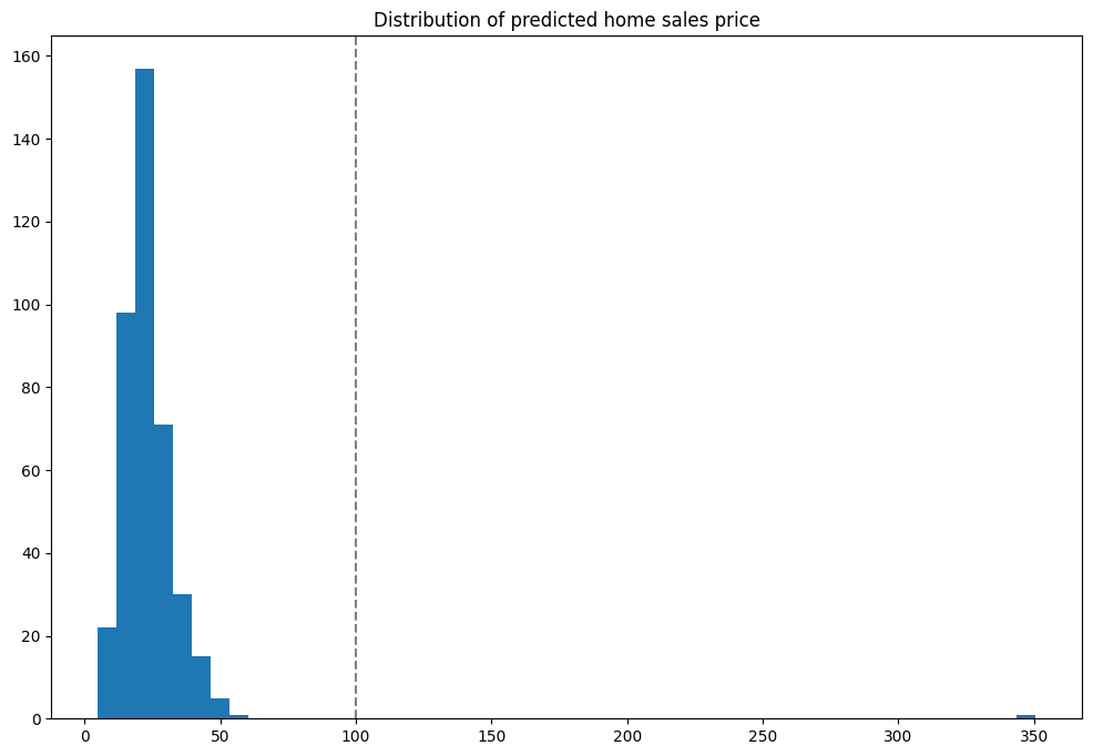
With the initial tests run, we can run the inferences against a larger set of data and identify anomalies that appear versus the expected results. These will be displayed into a graph so we can see where the anomalies occur. In this case with the house that came in at $350 million - outside of our validation range.
Note: Because this is splitting one batch inference into 500 separate inferences for this example, it may take longer to run.
Notice the one result that is outside the normal range - the one lonely result on the far right.
if arrowEnabled is True:
    test_data = pd.read_json("./data/houseprice_inputs_500.json", orient="records")
    responses_anomaly = pd.DataFrame()
    # For the first 1000 rows, submit that row as a separate DataFrame
    # Add the results to the responses_anomaly dataframe
    for index, row in test_data.head(500).iterrows():
        responses_anomaly = responses_anomaly.append(pipeline.infer(row.to_frame('tensor').reset_index()))
else:
    test_data = json.load("./data/houseprice_inputs_500.json")
    responses_anomaly =[]
    for nth in range(500):
        responses_anomaly.extend(pipeline.infer({ "tensor": [test_data['tensor'][0][nth]]}))
import pandas as pd
import matplotlib.pyplot as plt
%matplotlib inline
if arrowEnabled is True:
    houseprices = pd.DataFrame({'sell_price': responses_anomaly['out.dense_2'].apply(lambda x: x[0])})
else:
    houseprices = pd.DataFrame({'sell_price': [r.raw['outputs'][0]['Float']['data'][0] for  r in responses_anomaly]})

houseprices.hist(column='sell_price', bins=75, grid=False, figsize=(12,8))
plt.axvline(x=40, color='gray', ls='--')
_ = plt.title('Distribution of predicted home sales price')
How To Check For Anomalies
There are two primary methods for detecting anomalies with Wallaroo:
- As demonstrated in the example above, from the
InferenceObjectcheck_failuresarray in the output of each inference to see if anything has happened. - The other method is to view pipeline’s logs and see what anomalies have been detected.
View Logs
Anomalies can be displayed through the pipeline logs() method.
For Arrow enabled Wallaroo instances, the logs are returned as a dataframe. Filtering by the column check_failures greater than 0 displays any inferences that had an anomaly triggered.
For Arrow disabled Wallaroo instances, the parameter valid=False will show any validations that were flagged as False - in this case, houses that were above 350 thousand in value.
if arrowEnabled is True:
    logs = pipeline.logs()
    logs = logs.loc[logs['check_failures'] > 0]
else:
    logs = pipeline.logs(valid=False)
display(logs)
Warning: Pipeline log size limit exceeded. Please request logs using export_logs
| time | in.index | in.tensor | out.dense_2 | check_failures | |
|---|---|---|---|---|---|
| 32 | 2023-03-13 19:41:03.596 | tensor | [0.6752651953, -1.4463372267, 0.859222745, -1.3368839439, -0.0866638244, 372.1154780984, -0.2667405624, 0.0057462263, 2.3087968204, -0.6285378876, -0.5584151415, -0.0835430586, -0.6560503236, -1.4648287574, -0.2081778153, 0.2255257157, -0.3033813134] | [39.575085] | 1 |
Undeploy The Pipeline
With the example complete, we undeploy the pipeline to return the resources back to the Wallaroo instance.
pipeline.undeploy()
| name | anomalytestexample |
|---|---|
| created | 2023-03-13 20:18:16.622828+00:00 |
| last_updated | 2023-03-13 20:18:18.995804+00:00 |
| deployed | False |
| tags | |
| versions | dec18ab4-8b71-44c9-a507-c9763803153f, 64246a8b-61a8-4ead-94aa-00f4cf571f74 |
| steps | anomaly-housing-model |
3 - House Price Testing Life Cycle
A comprehensive tutorial on different testing and model comparison techniques for house price prediction.
This tutorial and the assets can be downloaded as part of the Wallaroo Tutorials repository.
House Price Testing Life Cycle Comprehensive Tutorial
This tutorial simulates using Wallaroo for testing a model for inference outliers, potential model drift, and methods to test competitive models against each other and deploy the final version to use. This demonstrates using assays to detect model or data drift, then Wallaroo Shadow Deploy to compare different models to determine which one is most fit for an organization’s needs. These features allow organizations to monitor model performance and accuracy then swap out models as needed.
- IMPORTANT NOTE: This tutorial assumes that the House Price Model Life Cycle Preparation notebook was run before this notebook, and that the workspace, pipeline and models used are the same. This is critical for the section on Assays below. If the preparation notebook has not been run, skip the Assays section as there will be no historical data for the assays to function on.
This tutorial will demonstrate how to:
- Select or create a workspace, pipeline and upload the champion model.
- Add a pipeline step with the champion model, then deploy the pipeline and perform sample inferences.
- Create an assay and set a baseline, then demonstrate inferences that trigger the assay alert threshold.
- Swap out the pipeline step with the champion model with a shadow deploy step that compares the champion model against two competitors.
- Evaluate the results of the champion versus competitor models.
- Change the pipeline step from a shadow deploy step to an A/B testing step, and show the different results.
- Change the A/B testing step back to standard pipeline step with the original control model, then demonstrate hot swapping the control model with a challenger model without undeploying the pipeline.
- Undeploy the pipeline.
This tutorial provides the following:
- Models:
models/rf_model.onnx: The champion model that has been used in this environment for some time.models/xgb_model.onnxandmodels/gbr_model.onnx: Rival models that will be tested against the champion.
- Data:
data/xtest-1.df.jsonanddata/xtest-1k.df.json: DataFrame JSON inference inputs with 1 input and 1,000 inputs.data/xtest-1k.arrow: Apache Arrow inference inputs with 1 input and 1,000 inputs.
Prerequisites
- A deployed Wallaroo instance
- The following Python libraries installed:
Initial Steps
Import libraries
The first step is to import the libraries needed for this notebook.
import wallaroo
from wallaroo.object import EntityNotFoundError
from wallaroo.framework import Framework

from IPython.display import display

# used to display DataFrame information without truncating
from IPython.display import display
import pandas as pd
pd.set_option('display.max_colwidth', None)

import datetime
import time

# used for unique connection names

import string
import random

suffix= ''.join(random.choice(string.ascii_lowercase) for i in range(4))
suffix='baselines'
import json
Connect to the Wallaroo Instance
The first step is to connect to Wallaroo through the Wallaroo client. The Python library is included in the Wallaroo install and available through the Jupyter Hub interface provided with your Wallaroo environment.
This is accomplished using the wallaroo.Client() command, which provides a URL to grant the SDK permission to your specific Wallaroo environment. When displayed, enter the URL into a browser and confirm permissions. Store the connection into a variable that can be referenced later.
If logging into the Wallaroo instance through the internal JupyterHub service, use wl = wallaroo.Client(). For more information on Wallaroo Client settings, see the Client Connection guide.
# Login through local Wallaroo instance

wl = wallaroo.Client()
Create Workspace
We will create a workspace to manage our pipeline and models. The following variables will set the name of our sample workspace then set it as the current workspace.
Workspace, pipeline, and model names should be unique to each user, so we’ll add in a randomly generated suffix so multiple people can run this tutorial in a Wallaroo instance without effecting each other.
workspace_name = f'housepricesagaworkspace{suffix}'
main_pipeline_name = f'housepricesagapipeline'
model_name_control = f'housepricesagacontrol'
model_file_name_control = './models/rf_model.onnx'
def get_workspace(name):
    workspace = None
    for ws in wl.list_workspaces():
        if ws.name() == name:
            workspace= ws
    if(workspace == None):
        workspace = wl.create_workspace(name)
    return workspace

def get_pipeline(name, workspace):
    pipelines = workspace.pipelines()
    pipe_filter = filter(lambda x: x.name() == name, pipelines)
    pipes = list(pipe_filter)
    # we can't have a pipe in the workspace with the same name, so it's always the first
    if pipes:
        pipeline = pipes[0]
    else:
        pipeline = wl.build_pipeline(name)
    return pipeline
workspace = get_workspace(workspace_name)

wl.set_current_workspace(workspace)
{'name': 'housepricesagaworkspacebaselines', 'id': 87, 'archived': False, 'created_by': 'd6a42dd8-1da9-4405-bb80-7c4b42e38b52', 'created_at': '2023-10-31T16:56:03.395454+00:00', 'models': [], 'pipelines': []}
Upload The Champion Model
For our example, we will upload the champion model that has been trained to derive house prices from a variety of inputs. The model file is rf_model.onnx, and is uploaded with the name housingcontrol.
housing_model_control = (wl.upload_model(model_name_control,
                                        model_file_name_control,
                                        framework=Framework.ONNX)
                                        .configure(tensor_fields=["tensor"])
                        )
Standard Pipeline Steps
Build the Pipeline
This pipeline is made to be an example of an existing situation where a model is deployed and being used for inferences in a production environment. We’ll call it housepricepipeline, set housingcontrol as a pipeline step, then run a few sample inferences.
This pipeline will be a simple one - just a single pipeline step.
mainpipeline = get_pipeline(main_pipeline_name, workspace)

# clearing from previous runs and verifying it is undeployed
mainpipeline.clear()
mainpipeline.undeploy()
mainpipeline.add_model_step(housing_model_control)

#minimum deployment config
deploy_config = wallaroo.DeploymentConfigBuilder().replica_count(1).cpus(0.5).memory("1Gi").build()
mainpipeline.deploy(deployment_config = deploy_config)
Waiting for deployment - this will take up to 45s ............. ok
| name | housepricesagapipeline |
|---|---|
| created | 2023-10-31 16:56:07.345831+00:00 |
| last_updated | 2023-10-31 16:56:07.444932+00:00 |
| deployed | True |
| tags | |
| versions | 2ea0cc42-c955-4fc3-bac9-7a2c7c22ddc1, dca84ab2-274a-4391-95dd-a99bda7621e1 |
| steps | housepricesagacontrol |
| published | False |
Testing
We’ll use two inferences as a quick sample test - one that has a house that should be determined around $700k, the other with a house determined to be around $1.5 million. We’ll also save the start and end periods for these events to for later log functionality.
normal_input = pd.DataFrame.from_records({"tensor": [[4.0, 2.5, 2900.0, 5505.0, 2.0, 0.0, 0.0, 3.0, 8.0, 2900.0, 0.0, 47.6063, -122.02, 2970.0, 5251.0, 12.0, 0.0, 0.0]]})
result = mainpipeline.infer(normal_input)
display(result)
| time | in.tensor | out.variable | check_failures | |
|---|---|---|---|---|
| 0 | 2023-10-31 16:57:07.307 | [4.0, 2.5, 2900.0, 5505.0, 2.0, 0.0, 0.0, 3.0, 8.0, 2900.0, 0.0, 47.6063, -122.02, 2970.0, 5251.0, 12.0, 0.0, 0.0] | [718013.7] | 0 |
large_house_input = pd.DataFrame.from_records({'tensor': [[4.0, 3.0, 3710.0, 20000.0, 2.0, 0.0, 2.0, 5.0, 10.0, 2760.0, 950.0, 47.6696, -122.261, 3970.0, 20000.0, 79.0, 0.0, 0.0]]})
large_house_result = mainpipeline.infer(large_house_input)
display(large_house_result)
| time | in.tensor | out.variable | check_failures | |
|---|---|---|---|---|
| 0 | 2023-10-31 16:57:07.746 | [4.0, 3.0, 3710.0, 20000.0, 2.0, 0.0, 2.0, 5.0, 10.0, 2760.0, 950.0, 47.6696, -122.261, 3970.0, 20000.0, 79.0, 0.0, 0.0] | [1514079.4] | 0 |
As one last sample, we’ll run through roughly 1,000 inferences at once and show a few of the results. For this example we’ll use an Apache Arrow table, which has a smaller file size compared to uploading a pandas DataFrame JSON file. The inference result is returned as an arrow table, which we’ll convert into a pandas DataFrame to display the first 20 results.
time.sleep(5)
control_model_start = datetime.datetime.now()
batch_inferences = mainpipeline.infer_from_file('./data/xtest-1k.arrow')

large_inference_result =  batch_inferences.to_pandas()
display(large_inference_result.head(20))
| time | in.tensor | out.variable | check_failures | |
|---|---|---|---|---|
| 0 | 2023-10-31 16:57:13.771 | [4.0, 2.5, 2900.0, 5505.0, 2.0, 0.0, 0.0, 3.0, 8.0, 2900.0, 0.0, 47.6063, -122.02, 2970.0, 5251.0, 12.0, 0.0, 0.0] | [718013.7] | 0 |
| 1 | 2023-10-31 16:57:13.771 | [2.0, 2.5, 2170.0, 6361.0, 1.0, 0.0, 2.0, 3.0, 8.0, 2170.0, 0.0, 47.7109, -122.017, 2310.0, 7419.0, 6.0, 0.0, 0.0] | [615094.6] | 0 |
| 2 | 2023-10-31 16:57:13.771 | [3.0, 2.5, 1300.0, 812.0, 2.0, 0.0, 0.0, 3.0, 8.0, 880.0, 420.0, 47.5893, -122.317, 1300.0, 824.0, 6.0, 0.0, 0.0] | [448627.8] | 0 |
| 3 | 2023-10-31 16:57:13.771 | [4.0, 2.5, 2500.0, 8540.0, 2.0, 0.0, 0.0, 3.0, 9.0, 2500.0, 0.0, 47.5759, -121.994, 2560.0, 8475.0, 24.0, 0.0, 0.0] | [758714.3] | 0 |
| 4 | 2023-10-31 16:57:13.771 | [3.0, 1.75, 2200.0, 11520.0, 1.0, 0.0, 0.0, 4.0, 7.0, 2200.0, 0.0, 47.7659, -122.341, 1690.0, 8038.0, 62.0, 0.0, 0.0] | [513264.66] | 0 |
| 5 | 2023-10-31 16:57:13.771 | [3.0, 2.0, 2140.0, 4923.0, 1.0, 0.0, 0.0, 4.0, 8.0, 1070.0, 1070.0, 47.6902, -122.339, 1470.0, 4923.0, 86.0, 0.0, 0.0] | [668287.94] | 0 |
| 6 | 2023-10-31 16:57:13.771 | [4.0, 3.5, 3590.0, 5334.0, 2.0, 0.0, 2.0, 3.0, 9.0, 3140.0, 450.0, 47.6763, -122.267, 2100.0, 6250.0, 9.0, 0.0, 0.0] | [1004846.56] | 0 |
| 7 | 2023-10-31 16:57:13.771 | [3.0, 2.0, 1280.0, 960.0, 2.0, 0.0, 0.0, 3.0, 9.0, 1040.0, 240.0, 47.602, -122.311, 1280.0, 1173.0, 0.0, 0.0, 0.0] | [684577.25] | 0 |
| 8 | 2023-10-31 16:57:13.771 | [4.0, 2.5, 2820.0, 15000.0, 2.0, 0.0, 0.0, 4.0, 9.0, 2820.0, 0.0, 47.7255, -122.101, 2440.0, 15000.0, 29.0, 0.0, 0.0] | [727898.25] | 0 |
| 9 | 2023-10-31 16:57:13.771 | [3.0, 2.25, 1790.0, 11393.0, 1.0, 0.0, 0.0, 3.0, 8.0, 1790.0, 0.0, 47.6297, -122.099, 2290.0, 11894.0, 36.0, 0.0, 0.0] | [559631.06] | 0 |
| 10 | 2023-10-31 16:57:13.771 | [3.0, 1.5, 1010.0, 7683.0, 1.5, 0.0, 0.0, 5.0, 7.0, 1010.0, 0.0, 47.72, -122.318, 1550.0, 7271.0, 61.0, 0.0, 0.0] | [340764.53] | 0 |
| 11 | 2023-10-31 16:57:13.771 | [3.0, 2.0, 1270.0, 1323.0, 3.0, 0.0, 0.0, 3.0, 8.0, 1270.0, 0.0, 47.6934, -122.342, 1330.0, 1323.0, 8.0, 0.0, 0.0] | [442168.12] | 0 |
| 12 | 2023-10-31 16:57:13.771 | [4.0, 1.75, 2070.0, 9120.0, 1.0, 0.0, 0.0, 4.0, 7.0, 1250.0, 820.0, 47.6045, -122.123, 1650.0, 8400.0, 57.0, 0.0, 0.0] | [630865.5] | 0 |
| 13 | 2023-10-31 16:57:13.771 | [4.0, 1.0, 1620.0, 4080.0, 1.5, 0.0, 0.0, 3.0, 7.0, 1620.0, 0.0, 47.6696, -122.324, 1760.0, 4080.0, 91.0, 0.0, 0.0] | [559631.06] | 0 |
| 14 | 2023-10-31 16:57:13.771 | [4.0, 3.25, 3990.0, 9786.0, 2.0, 0.0, 0.0, 3.0, 9.0, 3990.0, 0.0, 47.6784, -122.026, 3920.0, 8200.0, 10.0, 0.0, 0.0] | [909441.25] | 0 |
| 15 | 2023-10-31 16:57:13.771 | [4.0, 2.0, 1780.0, 19843.0, 1.0, 0.0, 0.0, 3.0, 7.0, 1780.0, 0.0, 47.4414, -122.154, 2210.0, 13500.0, 52.0, 0.0, 0.0] | [313096.0] | 0 |
| 16 | 2023-10-31 16:57:13.771 | [4.0, 2.5, 2130.0, 6003.0, 2.0, 0.0, 0.0, 3.0, 8.0, 2130.0, 0.0, 47.4518, -122.12, 1940.0, 4529.0, 11.0, 0.0, 0.0] | [404040.78] | 0 |
| 17 | 2023-10-31 16:57:13.771 | [3.0, 1.75, 1660.0, 10440.0, 1.0, 0.0, 0.0, 3.0, 7.0, 1040.0, 620.0, 47.4448, -121.77, 1240.0, 10380.0, 36.0, 0.0, 0.0] | [292859.44] | 0 |
| 18 | 2023-10-31 16:57:13.771 | [3.0, 2.5, 2110.0, 4118.0, 2.0, 0.0, 0.0, 3.0, 8.0, 2110.0, 0.0, 47.3878, -122.153, 2110.0, 4044.0, 25.0, 0.0, 0.0] | [338357.88] | 0 |
| 19 | 2023-10-31 16:57:13.771 | [4.0, 2.25, 2200.0, 11250.0, 1.5, 0.0, 0.0, 5.0, 7.0, 1300.0, 900.0, 47.6845, -122.201, 2320.0, 10814.0, 94.0, 0.0, 0.0] | [682284.56] | 0 |
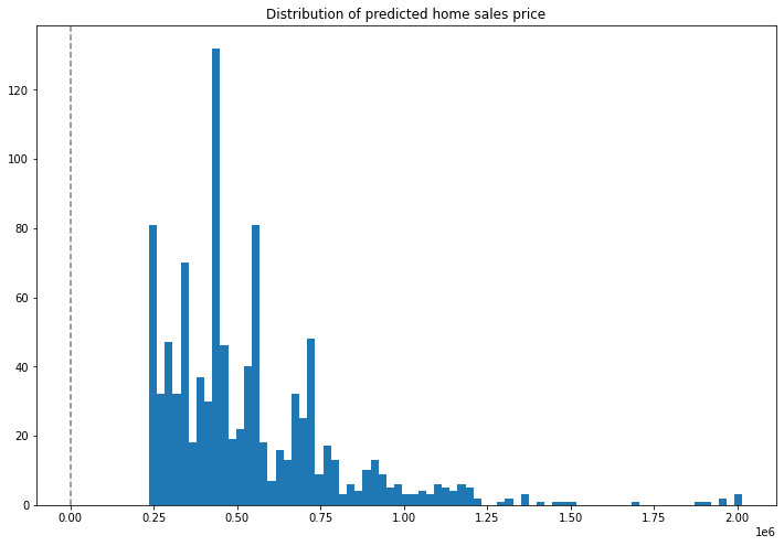
Graph of Prices
Here’s a distribution plot of the inferences to view the values, with the X axis being the house price in millions, and the Y axis the number of houses fitting in a bin grouping. The majority of houses are in the $250,000 to $500,000 range, with some outliers in the far end.
import matplotlib.pyplot as plt
houseprices = pd.DataFrame({'sell_price': large_inference_result['out.variable'].apply(lambda x: x[0])})

houseprices.hist(column='sell_price', bins=75, grid=False, figsize=(12,8))
plt.axvline(x=0, color='gray', ls='--')
_ = plt.title('Distribution of predicted home sales price')
time.sleep(5)
control_model_end = datetime.datetime.now()
Pipeline Logs
Pipeline logs with standard pipeline steps are retrieved either with:
- Pipeline
logswhich returns either a pandas DataFrame or Apache Arrow table. - Pipeline
export_logswhich saves the logs either a pandas DataFrame JSON file or Apache Arrow table.
For full details, see the Wallaroo Documentation Pipeline Log Management guide.
Pipeline Log Methods
The Pipeline logs method accepts the following parameters.
| Parameter | Type | Description |
|---|---|---|
limit | Int (Optional) | Limits how many log records to display. Defaults to 100. If there are more pipeline logs than are being displayed, the Warning message Pipeline log record limit exceeded will be displayed. For example, if 100 log files were requested and there are a total of 1,000, the warning message will be displayed. |
start_datetimert and end_datetime | DateTime (Optional) | Limits logs to all logs between the start_datetime and end_datetime DateTime parameters. Both parameters must be provided. Submitting a logs() request with only start_datetime or end_datetime will generate an exception.If start_datetime and end_datetime are provided as parameters, then the records are returned in chronological order, with the oldest record displayed first. |
arrow | Boolean (Optional) | Defaults to False. If arrow is set to True, then the logs are returned as an Apache Arrow table. If arrow=False, then the logs are returned as a pandas DataFrame. |
The following examples demonstrate displaying the logs, then displaying the logs between the control_model_start and control_model_end periods, then again retrieved as an Arrow table.
# pipeline log retrieval - reverse chronological order

display(mainpipeline.logs())

# pipeline log retrieval between two dates - chronological order

display(mainpipeline.logs(start_datetime=control_model_start, end_datetime=control_model_end))

# pipeline log retrieval limited to the last 5 an an arrow table

display(mainpipeline.logs(arrow=True))
Warning: There are more logs available. Please set a larger limit or request a file using export_logs.
| time | in.tensor | out.variable | check_failures | |
|---|---|---|---|---|
| 0 | 2023-10-31 16:57:13.771 | [3.0, 2.0, 2005.0, 7000.0, 1.0, 0.0, 0.0, 3.0, 7.0, 1605.0, 400.0, 47.6039, -122.298, 1750.0, 4500.0, 34.0, 0.0, 0.0] | [581002.94] | 0 |
| 1 | 2023-10-31 16:57:13.771 | [3.0, 1.75, 2910.0, 37461.0, 1.0, 0.0, 0.0, 4.0, 7.0, 1530.0, 1380.0, 47.7015, -122.164, 2520.0, 18295.0, 47.0, 0.0, 0.0] | [706823.6] | 0 |
| 2 | 2023-10-31 16:57:13.771 | [4.0, 3.25, 2910.0, 1880.0, 2.0, 0.0, 3.0, 5.0, 9.0, 1830.0, 1080.0, 47.616, -122.282, 3100.0, 8200.0, 100.0, 0.0, 0.0] | [1060847.5] | 0 |
| 3 | 2023-10-31 16:57:13.771 | [4.0, 1.75, 2700.0, 7875.0, 1.5, 0.0, 0.0, 4.0, 8.0, 2700.0, 0.0, 47.454, -122.144, 2220.0, 7875.0, 46.0, 0.0, 0.0] | [441960.3] | 0 |
| 4 | 2023-10-31 16:57:13.771 | [3.0, 2.5, 2900.0, 23550.0, 1.0, 0.0, 0.0, 3.0, 10.0, 1490.0, 1410.0, 47.5708, -122.153, 2900.0, 19604.0, 27.0, 0.0, 0.0] | [827411.25] | 0 |
| ... | ... | ... | ... | ... |
| 95 | 2023-10-31 16:57:13.771 | [2.0, 1.5, 1070.0, 1236.0, 2.0, 0.0, 0.0, 3.0, 8.0, 1000.0, 70.0, 47.5619, -122.382, 1170.0, 1888.0, 10.0, 0.0, 0.0] | [435628.72] | 0 |
| 96 | 2023-10-31 16:57:13.771 | [3.0, 2.5, 2830.0, 6000.0, 1.0, 0.0, 3.0, 3.0, 9.0, 1730.0, 1100.0, 47.5751, -122.378, 2040.0, 5300.0, 60.0, 0.0, 0.0] | [981676.7] | 0 |
| 97 | 2023-10-31 16:57:13.771 | [4.0, 1.75, 1720.0, 8750.0, 1.0, 0.0, 0.0, 3.0, 7.0, 860.0, 860.0, 47.726, -122.21, 1790.0, 8750.0, 43.0, 0.0, 0.0] | [437177.97] | 0 |
| 98 | 2023-10-31 16:57:13.771 | [4.0, 2.25, 4470.0, 60373.0, 2.0, 0.0, 0.0, 3.0, 11.0, 4470.0, 0.0, 47.7289, -122.127, 3210.0, 40450.0, 26.0, 0.0, 0.0] | [1208638.1] | 0 |
| 99 | 2023-10-31 16:57:13.771 | [3.0, 1.0, 1150.0, 3000.0, 1.0, 0.0, 0.0, 5.0, 6.0, 1150.0, 0.0, 47.6867, -122.345, 1460.0, 3200.0, 108.0, 0.0, 0.0] | [448627.8] | 0 |
100 rows × 4 columns
Warning: Pipeline log size limit exceeded. Please request logs using export_logs
| time | in.tensor | out.variable | check_failures | |
|---|---|---|---|---|
| 0 | 2023-10-31 16:57:13.771 | [4.0, 2.5, 2900.0, 5505.0, 2.0, 0.0, 0.0, 3.0, 8.0, 2900.0, 0.0, 47.6063, -122.02, 2970.0, 5251.0, 12.0, 0.0, 0.0] | [718013.7] | 0 |
| 1 | 2023-10-31 16:57:13.771 | [2.0, 2.5, 2170.0, 6361.0, 1.0, 0.0, 2.0, 3.0, 8.0, 2170.0, 0.0, 47.7109, -122.017, 2310.0, 7419.0, 6.0, 0.0, 0.0] | [615094.6] | 0 |
| 2 | 2023-10-31 16:57:13.771 | [3.0, 2.5, 1300.0, 812.0, 2.0, 0.0, 0.0, 3.0, 8.0, 880.0, 420.0, 47.5893, -122.317, 1300.0, 824.0, 6.0, 0.0, 0.0] | [448627.8] | 0 |
| 3 | 2023-10-31 16:57:13.771 | [4.0, 2.5, 2500.0, 8540.0, 2.0, 0.0, 0.0, 3.0, 9.0, 2500.0, 0.0, 47.5759, -121.994, 2560.0, 8475.0, 24.0, 0.0, 0.0] | [758714.3] | 0 |
| 4 | 2023-10-31 16:57:13.771 | [3.0, 1.75, 2200.0, 11520.0, 1.0, 0.0, 0.0, 4.0, 7.0, 2200.0, 0.0, 47.7659, -122.341, 1690.0, 8038.0, 62.0, 0.0, 0.0] | [513264.66] | 0 |
| ... | ... | ... | ... | ... |
| 495 | 2023-10-31 16:57:13.771 | [4.0, 2.5, 3550.0, 35689.0, 2.0, 0.0, 0.0, 4.0, 9.0, 3550.0, 0.0, 47.7503, -122.074, 3350.0, 35711.0, 23.0, 0.0, 0.0] | [873315.2] | 0 |
| 496 | 2023-10-31 16:57:13.771 | [4.0, 2.5, 2510.0, 47044.0, 2.0, 0.0, 0.0, 3.0, 9.0, 2510.0, 0.0, 47.7699, -122.085, 2600.0, 42612.0, 27.0, 0.0, 0.0] | [721143.6] | 0 |
| 497 | 2023-10-31 16:57:13.771 | [4.0, 2.5, 4090.0, 11225.0, 2.0, 0.0, 0.0, 3.0, 10.0, 4090.0, 0.0, 47.581, -121.971, 3510.0, 8762.0, 9.0, 0.0, 0.0] | [1048372.44] | 0 |
| 498 | 2023-10-31 16:57:13.771 | [2.0, 1.0, 720.0, 5000.0, 1.0, 0.0, 0.0, 5.0, 6.0, 720.0, 0.0, 47.5195, -122.374, 810.0, 5000.0, 63.0, 0.0, 0.0] | [244566.39] | 0 |
| 499 | 2023-10-31 16:57:13.771 | [4.0, 2.75, 2930.0, 22000.0, 1.0, 0.0, 3.0, 4.0, 9.0, 1580.0, 1350.0, 47.3227, -122.384, 2930.0, 9758.0, 36.0, 0.0, 0.0] | [518869.03] | 0 |
500 rows × 4 columns
    Warning: There are more logs available. Please set a larger limit or request a file using export_logs.

    pyarrow.Table
    time: timestamp[ms]
    in.tensor: list<item: float> not null
      child 0, item: float
    out.variable: list<inner: float not null> not null
      child 0, inner: float not null
    check_failures: int8
    ----
    time: [[2023-10-31 16:57:13.771,2023-10-31 16:57:13.771,2023-10-31 16:57:13.771,2023-10-31 16:57:13.771,2023-10-31 16:57:13.771,...,2023-10-31 16:57:13.771,2023-10-31 16:57:13.771,2023-10-31 16:57:13.771,2023-10-31 16:57:13.771,2023-10-31 16:57:13.771]]
    in.tensor: [[[3,2,2005,7000,1,...,1750,4500,34,0,0],[3,1.75,2910,37461,1,...,2520,18295,47,0,0],...,[4,2.25,4470,60373,2,...,3210,40450,26,0,0],[3,1,1150,3000,1,...,1460,3200,108,0,0]]]
    out.variable: [[[581002.94],[706823.6],...,[1208638.1],[448627.8]]]
    check_failures: [[0,0,0,0,0,...,0,0,0,0,0]]
Anomaly Detection through Validations
Anomaly detection allows organizations to set validation parameters in a pipeline. A validation is added to a pipeline to test data based on an expression, and flag any inferences where the validation failed inference result and the pipeline logs.
Validations are added through the Pipeline add_validation(name, validation) command which uses the following parameters:
| Parameter | Type | Description |
|---|---|---|
| name | String (Required) | The name of the validation. |
| Validation | Expression (Required) | The validation test command in the format model_name.outputs][field][index] {Operation} {Value}. |
For this example, we want to detect the outputs of housing_model_control and validate that values are less than 1,500,000. Any outputs greater than that will trigger a check_failure which is shown in the output.
## Add the validation to the pipeline

mainpipeline = mainpipeline.add_validation('price too high', housing_model_control.outputs[0][0] < 1500000.0)

#minimum deployment config
deploy_config = wallaroo.DeploymentConfigBuilder().replica_count(1).cpus(0.5).memory("1Gi").build()
mainpipeline.deploy(deployment_config = deploy_config)
ok
| name | housepricesagapipeline |
|---|---|
| created | 2023-10-31 16:56:07.345831+00:00 |
| last_updated | 2023-10-31 16:57:24.026392+00:00 |
| deployed | True |
| tags | |
| versions | f7e0deaf-63a2-491a-8ff9-e8148d3cabcb, 2ea0cc42-c955-4fc3-bac9-7a2c7c22ddc1, dca84ab2-274a-4391-95dd-a99bda7621e1 |
| steps | housepricesagacontrol |
| published | False |
Validation Testing
Two validations will be tested:
- One that should return a house value lower than 1,500,000. The validation will pass so
check_failurewill be 0. - The other than should return a house value greater than 1,500,000. The validation will fail, so
check_failurewill be 1.
validation_start = datetime.datetime.now()

# Small value home

normal_input = pd.DataFrame.from_records({
        "tensor": [[
            3.0,
            2.25,
            1620.0,
            997.0,
            2.5,
            0.0,
            0.0,
            3.0,
            8.0,
            1540.0,
            80.0,
            47.5400009155,
            -122.0260009766,
            1620.0,
            1068.0,
            4.0,
            0.0,
            0.0
        ]]
    }
)

small_result = mainpipeline.infer(normal_input)

display(small_result.loc[:,["time", "out.variable", "check_failures"]])
| time | out.variable | check_failures | |
|---|---|---|---|
| 0 | 2023-10-31 16:57:26.205 | [544392.06] | 0 |
# Big value home

big_input = pd.DataFrame.from_records({
        "tensor": [[
            4.0,
            4.5,
            5770.0,
            10050.0,
            1.0,
            0.0,
            3.0,
            5.0,
            9.0,
            3160.0,
            2610.0,
            47.6769981384,
            -122.2750015259,
            2950.0,
            6700.0,
            65.0,
            0.0,
            0.0
        ]]
    }
)

big_result = mainpipeline.infer(big_input)

display(big_result.loc[:,["time", "out.variable", "check_failures"]])
| time | out.variable | check_failures | |
|---|---|---|---|
| 0 | 2023-10-31 16:57:27.138 | [1689843.1] | 1 |
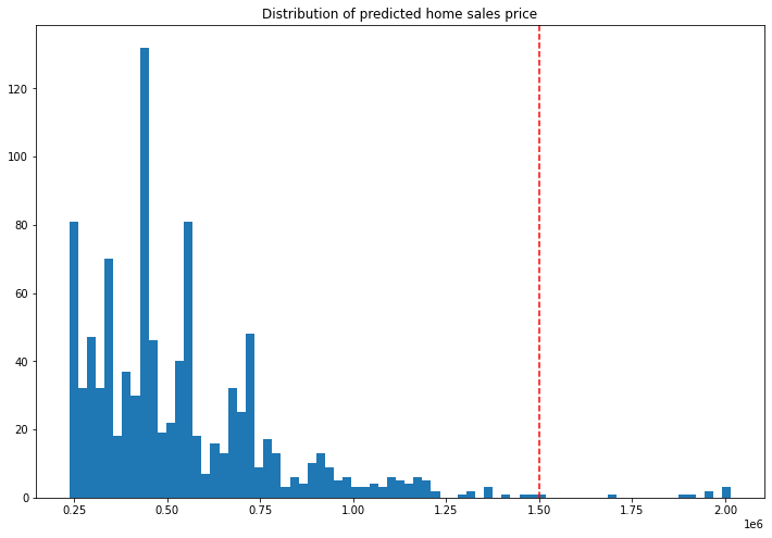
Anomaly Results
We’ll run through our previous batch, this time showing only those results outside of the validation, and a graph showing where the anomalies are against the other results.
batch_inferences = mainpipeline.infer_from_file('./data/xtest-1k.arrow')

large_inference_result =  batch_inferences.to_pandas()
# Display only the anomalous results

display(large_inference_result[large_inference_result["check_failures"] > 0].loc[:,["time", "out.variable", "check_failures"]])
| time | out.variable | check_failures | |
|---|---|---|---|
| 30 | 2023-10-31 16:57:28.974 | [1514079.4] | 1 |
| 248 | 2023-10-31 16:57:28.974 | [1967344.1] | 1 |
| 255 | 2023-10-31 16:57:28.974 | [2002393.6] | 1 |
| 556 | 2023-10-31 16:57:28.974 | [1886959.2] | 1 |
| 698 | 2023-10-31 16:57:28.974 | [1689843.1] | 1 |
| 711 | 2023-10-31 16:57:28.974 | [1946437.8] | 1 |
| 722 | 2023-10-31 16:57:28.974 | [2005883.1] | 1 |
| 782 | 2023-10-31 16:57:28.974 | [1910824.0] | 1 |
| 965 | 2023-10-31 16:57:28.974 | [2016006.1] | 1 |
import matplotlib.pyplot as plt
houseprices = pd.DataFrame({'sell_price': large_inference_result['out.variable'].apply(lambda x: x[0])})

houseprices.hist(column='sell_price', bins=75, grid=False, figsize=(12,8))
plt.axvline(x=1500000, color='red', ls='--')
_ = plt.title('Distribution of predicted home sales price')
Assays
Wallaroo assays provide a method for detecting input or model drift. These can be triggered either when unexpected input is provided for the inference, or when the model needs to be retrained from changing environment conditions.
Wallaroo assays can track either an input field and its index, or an output field and its index. For full details, see the Wallaroo Assays Management Guide.
For this example, we will:
- Perform sample inferences based on lower priced houses.
- Create an assay with the baseline set off those lower priced houses.
- Generate inferences spread across all house values, plus specific set of high priced houses to trigger the assay alert.
- Run an interactive assay to show the detection of values outside the established baseline.
Assay Generation
To start the demonstration, we’ll create a baseline of values from houses with small estimated prices and set that as our baseline. Assays are typically run on a 24 hours interval based on a 24 hour window of data, but we’ll bypass that by setting our baseline time even shorter.
small_houses_inputs = pd.read_json('./data/smallinputs.df.json')
baseline_size = 500

# Where the baseline data will start
baseline_start = datetime.datetime.now()

# These inputs will be random samples of small priced houses.  Around 30,000 is a good number
small_houses = small_houses_inputs.sample(baseline_size, replace=True).reset_index(drop=True)

small_results = mainpipeline.infer(small_houses)

# Set the baseline end

baseline_end = datetime.datetime.now()
# turn the inference results into a numpy array for the baseline

# set the results to a non-array value
small_results_baseline_df = small_results.copy()
small_results_baseline_df['variable']=small_results['out.variable'].map(lambda x: x[0])

# get the numpy values
small_results_baseline = small_results_baseline_df['variable'].to_numpy()
assay_baseline_from_numpy_name = "house price saga assay from numpy"

# assay builder by baseline
assay_builder_from_numpy = wl.build_assay(assay_name=assay_baseline_from_numpy_name,
                               pipeline=mainpipeline,
                               model_name=model_name_control,
                               iopath="output variable 0",
                               baseline_data = small_results_baseline)
# set the width from the recent results
assay_builder_from_numpy.window_builder().add_width(minutes=1)
assay_config_from_numpy = assay_builder_from_numpy.build()
assay_analysis_from_numpy = assay_config_from_numpy.interactive_run()
# get the histogram from the numpy baseline
assay_builder_from_numpy.baseline_histogram()
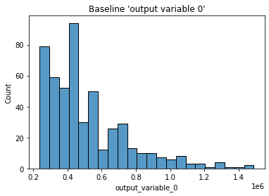
# show the baseline stats
assay_analysis_from_numpy[0].baseline_stats()
| Baseline | |
|---|---|
| count | 500 |
| min | 236238.67 |
| max | 1489624.3 |
| mean | 513762.85694 |
| median | 448627.8 |
| std | 235726.284713 |
| start | None |
| end | None |
Now we’ll perform some inferences with a spread of values, then a larger set with a set of larger house values to trigger our assay alert.
Because our assay windows are 1 minutes, we’ll need to stagger our inference values to be set into the proper windows. This will take about 4 minutes.
By default, assay start date is set to 24 hours from when the assay was created. For this example, we will set the assay.window_builder.add_start to set the assay window to start at the beginning of our data, and assay.add_run_until to set the time period to stop gathering data from.
# Get a spread of house values

time.sleep(35)
# regular_houses_inputs = pd.read_json('./data/xtest-1k.df.json', orient="records")
inference_size = 1000

# regular_houses = regular_houses_inputs.sample(inference_size, replace=True).reset_index(drop=True)

# And a spread of large house values

big_houses_inputs = pd.read_json('./data/biginputs.df.json', orient="records")
big_houses = big_houses_inputs.sample(inference_size, replace=True).reset_index(drop=True)

# Set the start for our assay window period.
assay_window_start = datetime.datetime.now()

mainpipeline.infer(big_houses)

# End our assay window period
time.sleep(35)
assay_window_end = datetime.datetime.now()
assay_builder_from_numpy.add_run_until(assay_window_end)
assay_builder_from_numpy.window_builder().add_width(minutes=1).add_interval(minutes=1).add_start(assay_window_start)
assay_config_from_dates = assay_builder_from_numpy.build()
assay_analysis_from_numpy = assay_config_from_numpy.interactive_run()
# Show how many assay windows were analyzed, then show the chart
print(f"Generated {len(assay_analysis_from_numpy)} analyses")
assay_analysis_from_numpy.chart_scores()
Generated 5 analyses
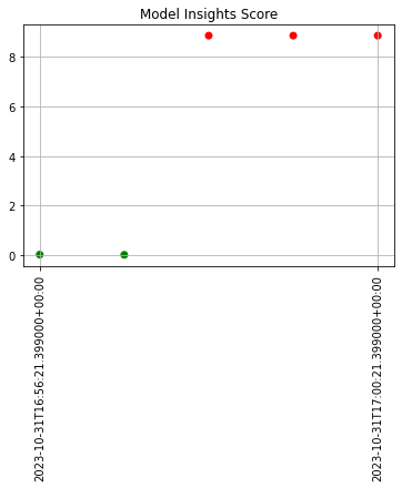
# Display the results as a DataFrame - we're mainly interested in the score and whether the
# alert threshold was triggered
display(assay_analysis_from_numpy.to_dataframe().loc[:, ["score", "start", "alert_threshold", "status"]])
| score | start | alert_threshold | status | |
|---|---|---|---|---|
| 0 | 0.016079 | 2023-10-31T16:56:21.399000+00:00 | 0.25 | Ok |
| 1 | 0.006042 | 2023-10-31T16:57:21.399000+00:00 | 0.25 | Ok |
| 2 | 8.868832 | 2023-10-31T16:58:21.399000+00:00 | 0.25 | Alert |
| 3 | 8.868832 | 2023-10-31T16:59:21.399000+00:00 | 0.25 | Alert |
| 4 | 8.868832 | 2023-10-31T17:00:21.399000+00:00 | 0.25 | Alert |
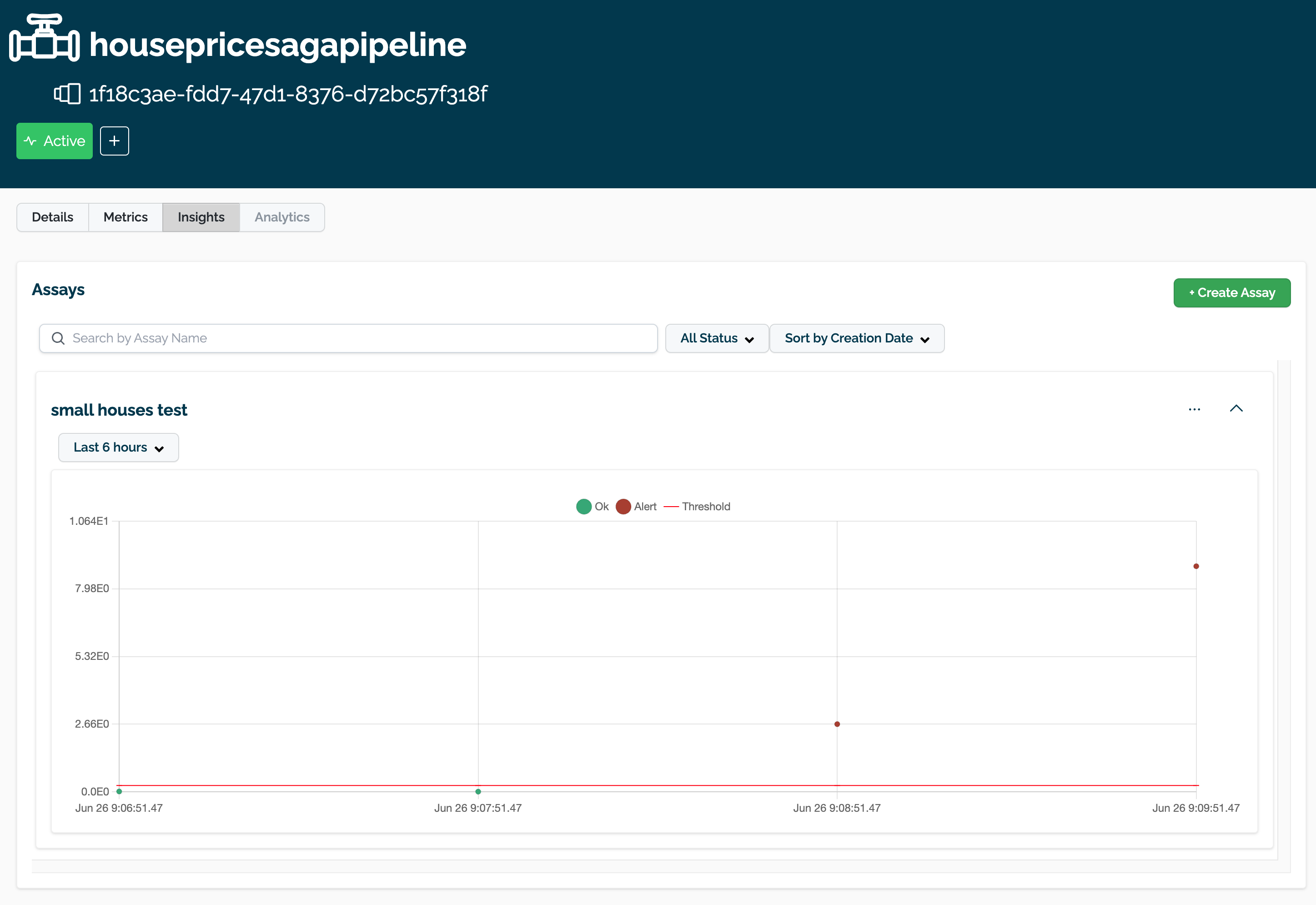
assay_builder_from_numpy.upload()
18
The assay is now visible through the Wallaroo UI by selecting the workspace, then the pipeline, then Insights.
Shadow Deploy
Let’s assume that after analyzing the assay information we want to test two challenger models to our control. We do that with the Shadow Deploy pipeline step.
In Shadow Deploy, the pipeline step is added with the add_shadow_deploy method, with the champion model listed first, then an array of challenger models after. All inference data is fed to all models, with the champion results displayed in the out.variable column, and the shadow results in the format out_{model name}.variable. For example, since we named our challenger models housingchallenger01 and housingchallenger02, the columns out_housingchallenger01.variable and out_housingchallenger02.variable have the shadow deployed model results.
For this example, we will remove the previous pipeline step, then replace it with a shadow deploy step with rf_model.onnx as our champion, and models xgb_model.onnx and gbr_model.onnx as the challengers. We’ll deploy the pipeline and prepare it for sample inferences.
# Upload the challenger models

model_name_challenger01 = 'housingchallenger01'
model_file_name_challenger01 = './models/xgb_model.onnx'

model_name_challenger02 = 'housingchallenger02'
model_file_name_challenger02 = './models/gbr_model.onnx'

housing_model_challenger01 = (wl.upload_model(model_name_challenger01,
                                              model_file_name_challenger01,
                                              framework=Framework.ONNX)
                                              .configure(tensor_fields=["tensor"])
                            )
housing_model_challenger02 = (wl.upload_model(model_name_challenger02,
                                              model_file_name_challenger02,
                                              framework=Framework.ONNX)
                                              .configure(tensor_fields=["tensor"])
                            )
# Undeploy the pipeline
mainpipeline.undeploy()
mainpipeline.clear()
# Add the new shadow deploy step with our challenger models
mainpipeline.add_shadow_deploy(housing_model_control, [housing_model_challenger01, housing_model_challenger02])

# Deploy the pipeline with the new shadow step
#minimum deployment config
deploy_config = wallaroo.DeploymentConfigBuilder().replica_count(1).cpus(0.5).memory("1Gi").build()
mainpipeline.deploy(deployment_config = deploy_config)
Waiting for undeployment - this will take up to 45s ................................... ok
Waiting for deployment - this will take up to 45s ................................. ok
| name | housepricesagapipeline |
|---|---|
| created | 2023-10-31 16:56:07.345831+00:00 |
| last_updated | 2023-10-31 17:04:57.709641+00:00 |
| deployed | True |
| tags | |
| versions | 44d28e3e-094f-4507-8aa1-909c1f151dd5, b9f46ba3-3f14-4e5b-989e-e0b8d166392f, f7e0deaf-63a2-491a-8ff9-e8148d3cabcb, 2ea0cc42-c955-4fc3-bac9-7a2c7c22ddc1, dca84ab2-274a-4391-95dd-a99bda7621e1 |
| steps | housepricesagacontrol |
| published | False |
Shadow Deploy Sample Inference
We’ll now use our same sample data for an inference to our shadow deployed pipeline, then display the first 20 results with just the comparative outputs.
shadow_result = mainpipeline.infer_from_file('./data/xtest-1k.arrow')

shadow_outputs =  shadow_result.to_pandas()
display(shadow_outputs.loc[0:20,['out.variable','out_housingchallenger01.variable','out_housingchallenger02.variable']])
| out.variable | out_housingchallenger01.variable | out_housingchallenger02.variable | |
|---|---|---|---|
| 0 | [718013.7] | [659806.0] | [704901.9] |
| 1 | [615094.6] | [732883.5] | [695994.44] |
| 2 | [448627.8] | [419508.84] | [416164.8] |
| 3 | [758714.3] | [634028.75] | [655277.2] |
| 4 | [513264.66] | [427209.47] | [426854.66] |
| 5 | [668287.94] | [615501.9] | [632556.06] |
| 6 | [1004846.56] | [1139732.4] | [1100465.2] |
| 7 | [684577.25] | [498328.88] | [528278.06] |
| 8 | [727898.25] | [722664.4] | [659439.94] |
| 9 | [559631.06] | [525746.44] | [534331.44] |
| 10 | [340764.53] | [376337.06] | [377187.2] |
| 11 | [442168.12] | [382053.12] | [403964.3] |
| 12 | [630865.5] | [505608.97] | [528991.3] |
| 13 | [559631.06] | [603260.5] | [612201.75] |
| 14 | [909441.25] | [969585.44] | [893874.7] |
| 15 | [313096.0] | [313633.7] | [318054.94] |
| 16 | [404040.78] | [360413.62] | [357816.7] |
| 17 | [292859.44] | [316674.88] | [294034.62] |
| 18 | [338357.88] | [299907.47] | [323254.28] |
| 19 | [682284.56] | [811896.75] | [770916.6] |
| 20 | [583765.94] | [573618.5] | [549141.4] |
A/B Testing
A/B Testing is another method of comparing and testing models. Like shadow deploy, multiple models are compared against the champion or control models. The difference is that instead of submitting the inference data to all models, then tracking the outputs of all of the models, the inference inputs are off of a ratio and other conditions.
For this example, we’ll be using a 1:1:1 ratio with a random split between the champion model and the two challenger models. Each time an inference request is made, there is a random equal chance of any one of them being selected.
When the inference results and log entries are displayed, they include the column out._model_split which displays:
| Field | Type | Description |
|---|---|---|
name | String | The model name used for the inference. |
version | String | The version of the model. |
sha | String | The sha hash of the model version. |
This is used to determine which model was used for the inference request.
# remove the shadow deploy steps
mainpipeline.clear()

# Add the a/b test step to the pipeline
mainpipeline.add_random_split([(1, housing_model_control), (1, housing_model_challenger01), (1, housing_model_challenger02)], "session_id")

mainpipeline.deploy()

# Perform sample inferences of 20 rows and display the results
ab_date_start = datetime.datetime.now()
abtesting_inputs = pd.read_json('./data/xtest-1k.df.json')

df = pd.DataFrame(columns=["model", "value"])

for index, row in abtesting_inputs.sample(20).iterrows():
    result = mainpipeline.infer(row.to_frame('tensor').reset_index())
    value = result.loc[0]["out.variable"]
    model = json.loads(result.loc[0]["out._model_split"][0])['name']
    df = df.append({'model': model, 'value': value}, ignore_index=True)

display(df)
ab_date_end = datetime.datetime.now()
ok
| model | value | |
|---|---|---|
| 0 | housingchallenger01 | [278554.44] |
| 1 | housingchallenger02 | [615955.3] |
| 2 | housepricesagacontrol | [1092273.9] |
| 3 | housepricesagacontrol | [683845.75] |
| 4 | housepricesagacontrol | [682284.56] |
| 5 | housepricesagacontrol | [247792.75] |
| 6 | housingchallenger02 | [315142.44] |
| 7 | housingchallenger02 | [530408.94] |
| 8 | housepricesagacontrol | [340764.53] |
| 9 | housepricesagacontrol | [421153.16] |
| 10 | housingchallenger01 | [395150.63] |
| 11 | housingchallenger02 | [544343.3] |
| 12 | housingchallenger01 | [395284.4] |
| 13 | housepricesagacontrol | [701940.7] |
| 14 | housepricesagacontrol | [448627.8] |
| 15 | housepricesagacontrol | [320863.72] |
| 16 | housingchallenger01 | [558485.3] |
| 17 | housingchallenger02 | [236329.28] |
| 18 | housepricesagacontrol | [559631.06] |
| 19 | housingchallenger01 | [281437.56] |
Model Swap
Now that we’ve completed our testing, we can swap our deployed model in the original housepricingpipeline with one we feel works better.
We’ll start by removing the A/B Testing pipeline step, then going back to the single pipeline step with the champion model and perform a test inference.
When going from a testing step such as A/B Testing or Shadow Deploy, it is best to undeploy the pipeline, change the steps, then deploy the pipeline. In a production environment, there should be two pipelines: One for production, the other for testing models. Since this example uses one pipeline for simplicity, we will undeploy our main pipeline and reset it back to a one-step pipeline with the current champion model as our pipeline step.
Once done, we’ll perform the hot swap with the model gbr_model.onnx, which was labeled housing_model_challenger02 in a previous step. We’ll do an inference with the same data as used with the challenger model. Note that previously, the inference through the original model returned [718013.7].
mainpipeline.undeploy()

# remove the shadow deploy steps
mainpipeline.clear()

mainpipeline.add_model_step(housing_model_control).deploy()

# Inference test
normal_input = pd.DataFrame.from_records({"tensor": [[4.0,
            2.25,
            2200.0,
            11250.0,
            1.5,
            0.0,
            0.0,
            5.0,
            7.0,
            1300.0,
            900.0,
            47.6845,
            -122.201,
            2320.0,
            10814.0,
            94.0,
            0.0,
            0.0]]})
controlresult = mainpipeline.infer(normal_input)
display(controlresult)
 ok
Waiting for deployment - this will take up to 45s ........ ok
| time | in.tensor | out.variable | check_failures | |
|---|---|---|---|---|
| 0 | 2023-10-31 17:08:19.579 | [4.0, 2.25, 2200.0, 11250.0, 1.5, 0.0, 0.0, 5.0, 7.0, 1300.0, 900.0, 47.6845, -122.201, 2320.0, 10814.0, 94.0, 0.0, 0.0] | [682284.56] | 0 |
Now we’ll “hot swap” the control model. We don’t have to deploy the pipeline - we can just swap the model out in that pipeline step and continue with only a millisecond or two lost while the swap was performed.
# Perform hot swap

mainpipeline.replace_with_model_step(0, housing_model_challenger02).deploy()
# wait a moment for the database to be updated.  The swap is near instantaneous but database writes may take a moment
import time
time.sleep(15)

# inference after model swap
normal_input = pd.DataFrame.from_records({"tensor": [[4.0,
            2.25,
            2200.0,
            11250.0,
            1.5,
            0.0,
            0.0,
            5.0,
            7.0,
            1300.0,
            900.0,
            47.6845,
            -122.201,
            2320.0,
            10814.0,
            94.0,
            0.0,
            0.0]]})
challengerresult = mainpipeline.infer(normal_input)
display(challengerresult)
ok
| time | in.tensor | out.variable | check_failures | |
|---|---|---|---|---|
| 0 | 2023-10-31 17:09:23.932 | [4.0, 2.25, 2200.0, 11250.0, 1.5, 0.0, 0.0, 5.0, 7.0, 1300.0, 900.0, 47.6845, -122.201, 2320.0, 10814.0, 94.0, 0.0, 0.0] | [770916.6] | 0 |
# Display the difference between the two

display(f'Original model output: {controlresult.loc[0]["out.variable"]}')
display(f'Hot swapped model  output: {challengerresult.loc[0]["out.variable"]}')
'Original model output: [682284.56]'
‘Hot swapped model  output: [770916.6]’
Undeploy Main Pipeline
With the examples and tutorial complete, we will undeploy the main pipeline and return the resources back to the Wallaroo instance.
mainpipeline.undeploy()
Waiting for undeployment - this will take up to 45s ...................................... ok
| name | housepricesagapipeline |
|---|---|
| created | 2023-10-31 16:56:07.345831+00:00 |
| last_updated | 2023-10-31 17:09:08.758964+00:00 |
| deployed | False |
| tags | |
| versions | 51034ba5-b58e-4475-908d-ec8fae069745, cd0f20e9-6923-4e6f-8114-1137676da5c5, 58274aab-0045-4557-a740-7d085af8574d, 4cf4f0dc-2c42-4f8b-975c-1f5c5d939a98, c5ae5a56-1c7f-4a94-9d4e-f08bf35e7f4f, f652a9d8-a4f6-428a-9b36-b29eec6b5198, 0e7d9d77-02d7-4c13-8062-9c77492145f8, 42b97784-fc16-43be-b89e-2d3dad20dd2b, 7d35285a-f8af-4bed-855b-60258c3435ee, 8b0dc4bb-3340-44f9-85d6-fbd091e19412, 06169fed-59e9-41f8-9dbd-0fc9f80ebb73, 44d28e3e-094f-4507-8aa1-909c1f151dd5, b9f46ba3-3f14-4e5b-989e-e0b8d166392f, f7e0deaf-63a2-491a-8ff9-e8148d3cabcb, 2ea0cc42-c955-4fc3-bac9-7a2c7c22ddc1, dca84ab2-274a-4391-95dd-a99bda7621e1 |
| steps | housepricesagacontrol |
| published | False |
4 - Shadow Deployment Tutorial
The Shadow Deployment Tutorial demonstrates how to use Wallaroo to deploy challenger models to test the performance against champion models.
This tutorial and the assets can be downloaded as part of the Wallaroo Tutorials repository.
Shadow Deployment Tutorial
Wallaroo provides a method of testing the same data against two different models or sets of models at the same time through shadow deployments otherwise known as parallel deployments. This allows data to be submitted to a pipeline with inferences running on two different sets of models. Typically this is performed on a model that is known to provide accurate results - the champion - and a model that is being tested to see if it provides more accurate or faster responses depending on the criteria known as the challengers. Multiple challengers can be tested against a single champion.
As described in the Wallaroo blog post The What, Why, and How of Model A/B Testing:
In data science, A/B tests can also be used to choose between two models in production, by measuring which model performs better in the real world. In this formulation, the control is often an existing model that is currently in production, sometimes called the champion. The treatment is a new model being considered to replace the old one. This new model is sometimes called the challenger….
Keep in mind that in machine learning, the terms experiments and trials also often refer to the process of finding a training configuration that works best for the problem at hand (this is sometimes called hyperparameter optimization).
When a shadow deployment is created, only the inference from the champion is returned in the InferenceResult Object data, while the result data for the shadow deployments is stored in the InferenceResult Object shadow_data.
The following tutorial will demonstrate how:
- Upload champion and challenger models into a Wallaroo instance.
- Create a shadow deployment in a Wallaroo pipeline.
- Perform an inference through a pipeline with a shadow deployment.
- View the
dataandshadow_dataresults from the InferenceResult Object. - View the pipeline logs and pipeline shadow logs.
This tutorial provides the following:
dev_smoke_test.json: Sample test data used for the inference testing.models/keras_ccfraud.onnx: The champion model.models/modelA.onnx: A challenger model.models/xgboost_ccfraud.onnx: A challenger model.
All models are similar to the ones used for the Wallaroo-101 example included in the Wallaroo Tutorials repository.
Prerequisites
- A deployed Wallaroo instance
- The following Python libraries installed:
Steps
Import libraries
The first step is to import the libraries required.
import wallaroo
from wallaroo.object import EntityNotFoundError

# used to display dataframe information without truncating
from IPython.display import display
import pandas as pd
pd.set_option('display.max_colwidth', None)
Connect to the Wallaroo Instance
The first step is to connect to Wallaroo through the Wallaroo client. The Python library is included in the Wallaroo install and available through the Jupyter Hub interface provided with your Wallaroo environment.
This is accomplished using the wallaroo.Client() command, which provides a URL to grant the SDK permission to your specific Wallaroo environment. When displayed, enter the URL into a browser and confirm permissions. Store the connection into a variable that can be referenced later.
If logging into the Wallaroo instance through the internal JupyterHub service, use wl = wallaroo.Client(). For more information on Wallaroo Client settings, see the Client Connection guide.
# Login through local Wallaroo instance

wl = wallaroo.Client()
Set Variables
The following variables are used to create or use existing workspaces, pipelines, and upload the models. Adjust them based on your Wallaroo instance and organization requirements.
import string
import random

suffix= ''.join(random.choice(string.ascii_lowercase) for i in range(4))

workspace_name = f'ccfraudcomparisondemo{suffix}'
pipeline_name = f'ccshadow{suffix}'
champion_model_name = f'ccfraud-lstm{suffix}'
champion_model_file = 'models/keras_ccfraud.onnx'
shadow_model_01_name = f'ccfraud-xgb{suffix}'
shadow_model_01_file = 'models/xgboost_ccfraud.onnx'
shadow_model_02_name = f'ccfraud-rf{suffix}'
shadow_model_02_file = 'models/modelA.onnx'
Workspace and Pipeline
The following creates or connects to an existing workspace based on the variable workspace_name, and creates or connects to a pipeline based on the variable pipeline_name.
def get_workspace(name):
    workspace = None
    for ws in wl.list_workspaces():
        if ws.name() == name:
            workspace= ws
    if(workspace == None):
        workspace = wl.create_workspace(name)
    return workspace

def get_pipeline(name):
    try:
        pipeline = wl.pipelines_by_name(name)[0]
    except EntityNotFoundError:
        pipeline = wl.build_pipeline(name)
    return pipeline
workspace = get_workspace(workspace_name)

wl.set_current_workspace(workspace)

pipeline = get_pipeline(pipeline_name)
pipeline
| name | ccshadowdmyb |
|---|---|
| created | 2023-10-19 18:50:52.588811+00:00 |
| last_updated | 2023-10-19 18:50:52.588811+00:00 |
| deployed | (none) |
| tags | |
| versions | 2d8f9f90-8ced-4e47-b5a6-e2512aeb9d17 |
| steps | |
| published | False |
Load the Models
The models will be uploaded into the current workspace based on the variable names set earlier and listed as the champion, model2 and model3.
champion = (wl.upload_model(champion_model_name,
                            champion_model_file,
                            framework=wallaroo.framework.Framework.ONNX)
                            .configure(tensor_fields=["tensor"])
            )
model2 = (wl.upload_model(shadow_model_01_name,
                          shadow_model_01_file,
                          framework=wallaroo.framework.Framework.ONNX)
                          .configure(tensor_fields=["tensor"])
            )
model3 = (wl.upload_model(shadow_model_02_name,
                          shadow_model_02_file,
                          framework=wallaroo.framework.Framework.ONNX)
                          .configure(tensor_fields=["tensor"])
            )
Create Shadow Deployment
A shadow deployment is created using the add_shadow_deploy(champion, challengers[]) method where:
champion: The model that will be primarily used for inferences run through the pipeline. Inference results will be returned through the Inference Object’sdataelement.challengers[]: An array of models that will be used for inferences iteratively. Inference results will be returned through the Inference Object’sshadow_dataelement.
pipeline.add_shadow_deploy(champion, [model2, model3])
pipeline.deploy()
| name | ccshadowdmyb |
|---|---|
| created | 2023-10-19 18:50:52.588811+00:00 |
| last_updated | 2023-10-19 18:50:58.268275+00:00 |
| deployed | True |
| tags | |
| versions | 1ae1ebe1-f920-4590-a843-bf8429ece205, 2d8f9f90-8ced-4e47-b5a6-e2512aeb9d17 |
| steps | ccfraud-lstmdmyb |
| published | False |
Run Test Inference
Using the data from sample_data_file, a test inference will be made.
For Arrow enabled Wallaroo instances the model outputs are listed by column. The output data is set by the term out, followed by the name of the model. For the default model, this is out.dense_1, while the shadow deployed models are in the format out_{model name}.variable, where {model name} is the name of the shadow deployed model.
For Arrow disabled environments, the output is from the Wallaroo InferenceResult object.### Run Test Inference
Using the data from sample_data_file, a test inference will be made. As mentioned earlier, the inference results from the champion model will be available in the returned InferenceResult Object’s data element, while inference results from each of the challenger models will be in the returned InferenceResult Object’s shadow_data element.
sample_data_file = './smoke_test.df.json'
response = pipeline.infer_from_file(sample_data_file)
display(response)
| time | in.tensor | out.dense_1 | check_failures | out_ccfraud-rfdmyb.variable | out_ccfraud-xgbdmyb.variable | |
|---|---|---|---|---|---|---|
| 0 | 2023-10-19 18:51:10.396 | [1.0678324729, 0.2177810266, -1.7115145262, 0.682285721, 1.0138553067, -0.4335000013, 0.7395859437, -0.2882839595, -0.447262688, 0.5146124988, 0.3791316964, 0.5190619748, -0.4904593222, 1.1656456469, -0.9776307444, -0.6322198963, -0.6891477694, 0.1783317857, 0.1397992467, -0.3554220649, 0.4394217877, 1.4588397512, -0.3886829615, 0.4353492889, 1.7420053483, -0.4434654615, -0.1515747891, -0.2668451725, -1.4549617756] | [0.0014974177] | 0 | [1.0] | [0.0005066991] |
View Pipeline Logs
With the inferences complete, we can retrieve the log data from the pipeline with the pipeline logs method. Note that for each inference request, the logs return one entry per model. For this example, for one inference request three log entries will be created.
pipeline.logs()
| time | in.tensor | out.dense_1 | check_failures | out_ccfraud-rfdmyb.variable | out_ccfraud-xgbdmyb.variable | |
|---|---|---|---|---|---|---|
| 0 | 2023-10-19 18:51:10.396 | [1.0678324729, 0.2177810266, -1.7115145262, 0.682285721, 1.0138553067, -0.4335000013, 0.7395859437, -0.2882839595, -0.447262688, 0.5146124988, 0.3791316964, 0.5190619748, -0.4904593222, 1.1656456469, -0.9776307444, -0.6322198963, -0.6891477694, 0.1783317857, 0.1397992467, -0.3554220649, 0.4394217877, 1.4588397512, -0.3886829615, 0.4353492889, 1.7420053483, -0.4434654615, -0.1515747891, -0.2668451725, -1.4549617756] | [0.0014974177] | 0 | [1.0] | [0.0005066991] |
View Logs Per Model
Another way of displaying the logs would be to specify the model.
For Arrow enabled Wallaroo instances the model outputs are listed by column. The output data is set by the term out, followed by the name of the model. For the default model, this is out.dense_1, while the shadow deployed models are in the format out_{model name}.variable, where {model name} is the name of the shadow deployed model.
For arrow disabled Wallaroo instances, to view the inputs and results for the shadow deployed models, use the pipeline logs_shadow_deploy() method. The results will be grouped by the inputs.
logs = pipeline.logs()
display(logs)
| time | in.tensor | out.dense_1 | check_failures | out_ccfraud-rfdmyb.variable | out_ccfraud-xgbdmyb.variable | |
|---|---|---|---|---|---|---|
| 0 | 2023-10-19 18:51:10.396 | [1.0678324729, 0.2177810266, -1.7115145262, 0.682285721, 1.0138553067, -0.4335000013, 0.7395859437, -0.2882839595, -0.447262688, 0.5146124988, 0.3791316964, 0.5190619748, -0.4904593222, 1.1656456469, -0.9776307444, -0.6322198963, -0.6891477694, 0.1783317857, 0.1397992467, -0.3554220649, 0.4394217877, 1.4588397512, -0.3886829615, 0.4353492889, 1.7420053483, -0.4434654615, -0.1515747891, -0.2668451725, -1.4549617756] | [0.0014974177] | 0 | [1.0] | [0.0005066991] |
Undeploy the Pipeline
With the tutorial complete, we undeploy the pipeline and return the resources back to the system.
pipeline.undeploy()
| name | ccshadowdmyb |
|---|---|
| created | 2023-10-19 18:50:52.588811+00:00 |
| last_updated | 2023-10-19 18:50:58.268275+00:00 |
| deployed | False |
| tags | |
| versions | 1ae1ebe1-f920-4590-a843-bf8429ece205, 2d8f9f90-8ced-4e47-b5a6-e2512aeb9d17 |
| steps | ccfraud-lstmdmyb |
| published | False |