Using Jupyter Notebooks in Production

• 1: Data Exploration And Model Selection
• 2: From Jupyter to Production
• 3: Deploy the Model in Wallaroo
• 4: Regular Batch Inference

1 - Data Exploration And Model Selection

The following tutorials are available from the Wallaroo Tutorials Repository.

Stage 1: Data Exploration And Model Selection

When starting a project, the data scientist focuses on exploration and experimentation, rather than turning the process into an immediate production system. This notebook presents a simplified view of this stage.

Resources

The following resources are used as part of this tutorial:

• data
  • data/seattle_housing_col_description.txt: Describes the columns used as part data analysis.
  • data/seattle_housing.csv: Sample data of the Seattle, Washington housing market between 2014 and 2015.
• code
  • postprocess.py: Formats the data after inference by the model is complete.
  • preprocess.py: Formats the incoming data for the model.
  • simdb.py: A simulated database to demonstrate sending and receiving queries.
  • wallaroo_client.py: Additional methods used with the Wallaroo instance to create workspaces, etc.

Steps

The following steps are part of this process:

• Retrieve Training Data: Connect to the data store and retrieve the training data.
• Data Transformations: Evaluate the data and train the model.
• Model Testing: Evaluate different models and determine which is best suited for the problem.

Import Libraries

First we’ll import the libraries we’ll be using to evaluate the data and test different models.

import numpy as np
import pandas as pd

import sklearn
import sklearn.ensemble

import xgboost as xgb

import seaborn
import matplotlib
import matplotlib.pyplot as plt

import simdb # module for the purpose of this demo to simulate pulling data from a database

matplotlib.rcParams["figure.figsize"] = (12,6)

# ignoring warnings for demonstration
import warnings
warnings.filterwarnings('ignore')

Retrieve Training Data

For training, we will use the data on all houses sold in this market with the last two years. As a reminder, this data pulled from a simulated database as an example of how to pull from an existing data store.

Only a few columns will be shown for display purposes.

conn = simdb.simulate_db_connection()
tablename = simdb.tablename

query = f"select * from {tablename} where date > DATE(DATE(), '-24 month') AND sale_price is not NULL"
print(query)
# read in the data
housing_data = pd.read_sql_query(query, conn)

conn.close()
housing_data.loc[:, ["id", "date", "list_price", "bedrooms", "bathrooms", "sqft_living", "sqft_lot"]]

select * from house_listings where date > DATE(DATE(), '-24 month') AND sale_price is not NULL

20523 rows × 7 columns

Data transformations

To improve relative error performance, we will predict on log10 of the sale price.

Predict on log10 price to try to improve relative error performance

housing_data['logprice'] = np.log10(housing_data.sale_price)

From the data, we will create the following features to evaluate:

• house_age: How old the house is.
• renovated: Whether the house has been renovated or not.
• yrs_since_reno: If the house has been renovated, how long has it been.

import datetime

thisyear = datetime.datetime.now().year

housing_data['house_age'] = thisyear - housing_data['yr_built']
housing_data['renovated'] =  np.where((housing_data['yr_renovated'] > 0), 1, 0) 
housing_data['yrs_since_reno'] =  np.where(housing_data['renovated'], housing_data['yr_renovated'] - housing_data['yr_built'], 0)

housing_data.loc[:, ['yr_built', 'yr_renovated', 'house_age', 'renovated', 'yrs_since_reno']]

20523 rows × 5 columns

Now we pick variables and split training data into training and holdout (test).

vars = ['bedrooms', 'bathrooms', 'sqft_living', 'sqft_lot', 'floors', 'waterfront', 'view',
'condition', 'grade', 'sqft_above', 'sqft_basement', 'lat', 'long', 'sqft_living15', 'sqft_lot15', 'house_age', 'renovated', 'yrs_since_reno']

outcome = 'logprice'

runif = np.random.default_rng(2206222).uniform(0, 1, housing_data.shape[0])
gp = np.where(runif < 0.2, 'test', 'training')

hd_train = housing_data.loc[gp=='training', :].reset_index(drop=True, inplace=False)
hd_test = housing_data.loc[gp=='test', :].reset_index(drop=True, inplace=False)

# split the training into training and val for xgboost
runif = np.random.default_rng(123).uniform(0, 1, hd_train.shape[0])
xgb_gp = np.where(runif < 0.2, 'val', 'train')

# for xgboost, further split into train and val
train_features = np.array(hd_train.loc[xgb_gp=='train', vars])
train_labels = np.array(hd_train.loc[xgb_gp=='train', outcome])

val_features = np.array(hd_train.loc[xgb_gp=='val', vars])
val_labels = np.array(hd_train.loc[xgb_gp=='val', outcome])

Postprocessing

Since we are fitting a model to predict log10 price, we need to convert predictions back into price units. We also want to round to the nearest dollar.

def postprocess(log10price):
    return np.rint(np.power(10, log10price))

Model testing

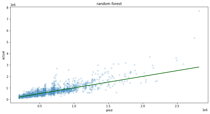
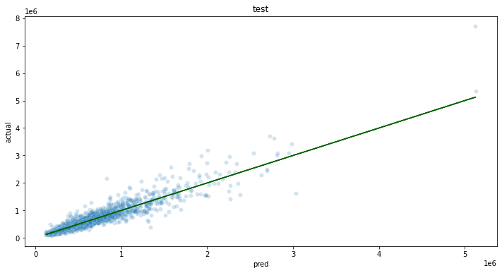
For the purposes of this demo, let’s say that we require a mean absolute percent error (MAPE) of 15% or less, and the we want to try a few models to decide which model we want to use.

One could also hyperparameter tune at this stage; for brevity, we’ll omit that in this demo.

XGBoost

First we will test out using a XGBoost model.

xgb_model = xgb.XGBRegressor(
    objective = 'reg:squarederror', 
    max_depth=5, 
    base_score = np.mean(hd_train[outcome])
    )

xgb_model.fit( 
    train_features,
    train_labels,
    eval_set=[(train_features, train_labels), (val_features, val_labels)],
    verbose=False,
    early_stopping_rounds=35
)

XGBRegressor(base_score=5.666446833601829, booster=None, callbacks=None,
             colsample_bylevel=None, colsample_bynode=None,
             colsample_bytree=None, early_stopping_rounds=None,
             enable_categorical=False, eval_metric=None, feature_types=None,
             gamma=None, gpu_id=None, grow_policy=None, importance_type=None,
             interaction_constraints=None, learning_rate=None, max_bin=None,
             max_cat_threshold=None, max_cat_to_onehot=None,
             max_delta_step=None, max_depth=5, max_leaves=None,
             min_child_weight=None, missing=nan, monotone_constraints=None,
             n_estimators=100, n_jobs=None, num_parallel_tree=None,
             predictor=None, random_state=None, ...)

XGBRegressor(base_score=5.666446833601829, booster=None, callbacks=None,
         colsample_bylevel=None, colsample_bynode=None,
         colsample_bytree=None, early_stopping_rounds=None,
         enable_categorical=False, eval_metric=None, feature_types=None,
         gamma=None, gpu_id=None, grow_policy=None, importance_type=None,
         interaction_constraints=None, learning_rate=None, max_bin=None,
         max_cat_threshold=None, max_cat_to_onehot=None,
         max_delta_step=None, max_depth=5, max_leaves=None,
         min_child_weight=None, missing=nan, monotone_constraints=None,
         n_estimators=100, n_jobs=None, num_parallel_tree=None,
         predictor=None, random_state=None, ...)</pre>
print(xgb_model.best_score)
print(xgb_model.best_iteration)
print(xgb_model.best_ntree_limit)
0.07793614689092423
99
100
XGBoost Evaluate on holdout
With the sample model created, we will test it against the holdout data. Note that we are calling the postprocess function on the data.
test_features = np.array(hd_test.loc[:, vars])
test_labels = np.array(hd_test.loc[:, outcome])

pframe = pd.DataFrame({
    'pred' : postprocess(xgb_model.predict(test_features)),
    'actual' : postprocess(test_labels)
})

ax = seaborn.scatterplot(
    data=pframe,
    x='pred',
    y='actual',
    alpha=0.2
)
matplotlib.pyplot.plot(pframe.pred, pframe.pred, color='DarkGreen')
matplotlib.pyplot.title("test")
plt.show()
pframe['se'] = (pframe.pred - pframe.actual)**2

pframe['pct_err'] = 100*np.abs(pframe.pred - pframe.actual)/pframe.actual
pframe.describe()
pred
actual
se
pct_err
count
4.094000e+03
4.094000e+03
4.094000e+03
4094.000000
mean
5.340824e+05
5.396937e+05
1.657722e+10
12.857674
std
3.413714e+05
3.761666e+05
1.276017e+11
13.512028
min
1.216140e+05
8.200000e+04
1.000000e+00
0.000500
25%
3.167628e+05
3.200000e+05
3.245312e+08
4.252492
50%
4.568700e+05
4.500000e+05
1.602001e+09
9.101485
75%
6.310372e+05
6.355250e+05
6.575385e+09
17.041227
max
5.126706e+06
7.700000e+06
6.637466e+12
252.097895
rmse = np.sqrt(np.mean(pframe.se))
mape = np.mean(pframe.pct_err)

print(f'rmse = {rmse}, mape = {mape}')
rmse = 128752.54982046234, mape = 12.857674005250548
Random Forest
The next model to test is Random Forest.
model_rf = sklearn.ensemble.RandomForestRegressor(n_estimators=100, max_depth=5, n_jobs=2, max_samples=0.8)

train_features = np.array(hd_train.loc[:, vars])
train_labels = np.array(hd_train.loc[:, outcome])

model_rf.fit(train_features, train_labels)
RandomForestRegressor(max_depth=5, max_samples=0.8, n_jobs=2)
In a Jupyter environment, please rerun this cell to show the HTML representation or trust the notebook.
On GitHub, the HTML representation is unable to render, please try loading this page with nbviewer.org.RandomForestRegressor
RandomForestRegressor(max_depth=5, max_samples=0.8, n_jobs=2)
Random Forest Evaluate on holdout
With the Random Forest sample model created, now we can test it against the holdout data.
pframe = pd.DataFrame({
    'pred' : postprocess(model_rf.predict(test_features)),
    'actual' : postprocess(test_labels)
})

ax = seaborn.scatterplot(
    data=pframe,
    x='pred',
    y='actual',
    alpha=0.2
)
matplotlib.pyplot.plot(pframe.pred, pframe.pred, color='DarkGreen')
matplotlib.pyplot.title("random forest")
plt.show()
pframe['se'] = (pframe.pred - pframe.actual)**2

pframe['pct_err'] = 100*np.abs(pframe.pred - pframe.actual)/pframe.actual
pframe.describe()
pred
actual
se
pct_err
count
4.094000e+03
4.094000e+03
4.094000e+03
4094.000000
mean
5.193927e+05
5.396937e+05
3.855718e+10
18.158892
std
2.787917e+05
3.761666e+05
4.146327e+11
17.546377
min
2.035980e+05
8.200000e+04
4.000000e+00
0.000354
25%
3.296550e+05
3.200000e+05
6.581425e+08
6.114513
50%
4.687280e+05
4.500000e+05
3.300043e+09
13.139936
75%
5.871848e+05
6.355250e+05
1.384624e+10
24.662608
max
2.817928e+06
7.700000e+06
2.383463e+13
177.850488
rmse = np.sqrt(np.mean(pframe.se))
mape = np.mean(pframe.pct_err)

print(f'rmse = {rmse}, mape = {mape}')
rmse = 196359.8291940774, mape = 18.158891829018927
Final Decision
At this stage, we decide to go with the xgboost model, with the variables/settings above.
With this stage complete, we can move on to Stage 2: Training Process Automation Setup.

2 - From Jupyter to Production

The following tutorials are available from the Wallaroo Tutorials Repository.

Stage 2: Training Process Automation Setup

Now that we have decided on the type and structure of the model from Stage 1: Data Exploration And Model Selection, this notebook modularizes the various steps of the process in a structure that is compatible with production and with Wallaroo.

We have pulled the preprocessing and postprocessing steps out of the training notebook into individual scripts that can also be used when the model is deployed.

Assuming no changes are made to the structure of the model, this notebook, or a script based on this notebook, can then be scheduled to run on a regular basis, to refresh the model with more recent training data. We’d expect to run this notebook in conjunction with the Stage 3 notebook, 03_deploy_model.ipynb. For clarity in this demo, we have split the training/upload task into two notebooks, 02_automated_training_process.ipynb and 03_deploy_model.ipynb.

Resources

The following resources are used as part of this tutorial:

• data
  • data/seattle_housing_col_description.txt: Describes the columns used as part data analysis.
  • data/seattle_housing.csv: Sample data of the Seattle, Washington housing market between 2014 and 2015.
• code
  • postprocess.py: Formats the data after inference by the model is complete.
  • preprocess.py: Formats the incoming data for the model.
  • simdb.py: A simulated database to demonstrate sending and receiving queries.
  • wallaroo_client.py: Additional methods used with the Wallaroo instance to create workspaces, etc.

Steps

The following steps are part of this process:

• Retrieve Training Data: Connect to the data store and retrieve the training data.
• Data Transformations: Evaluate the data and train the model.
• Generate and Test the Model: Create the model and verify it against the sample test data.
• Pickle The Model: Prepare the model to be uploaded to Wallaroo.

Retrieve Training Data

Note that this connection is simulated to demonstrate how data would be retrieved from an existing data store. For training, we will use the data on all houses sold in this market with the last two years.

import numpy as np
import pandas as pd

import sklearn

import xgboost as xgb

import seaborn
import matplotlib
import matplotlib.pyplot as plt

import pickle

import simdb # module for the purpose of this demo to simulate pulling data from a database

from preprocess import create_features  # our custom preprocessing
from postprocess import postprocess    # our custom postprocessing

matplotlib.rcParams["figure.figsize"] = (12,6)

# ignoring warnings for demonstration
import warnings
warnings.filterwarnings('ignore')

conn = simdb.simulate_db_connection()
tablename = simdb.tablename

query = f"select * from {tablename} where date > DATE(DATE(), '-24 month') AND sale_price is not NULL"
print(query)
# read in the data
housing_data = pd.read_sql_query(query, conn)

conn.close()
housing_data.loc[:, ["id", "date", "list_price", "bedrooms", "bathrooms", "sqft_living", "sqft_lot"]]

select * from house_listings where date > DATE(DATE(), '-24 month') AND sale_price is not NULL

20523 rows × 7 columns

Data transformations

To improve relative error performance, we will predict on log10 of the sale price.

Predict on log10 price to try to improve relative error performance

housing_data['logprice'] = np.log10(housing_data.list_price)

# split data into training and test
outcome = 'logprice'

runif = np.random.default_rng(2206222).uniform(0, 1, housing_data.shape[0])
gp = np.where(runif < 0.2, 'test', 'training')

hd_train = housing_data.loc[gp=='training', :].reset_index(drop=True, inplace=False)
hd_test = housing_data.loc[gp=='test', :].reset_index(drop=True, inplace=False)

# split the training into training and val for xgboost
runif = np.random.default_rng(123).uniform(0, 1, hd_train.shape[0])
xgb_gp = np.where(runif < 0.2, 'val', 'train')

# for xgboost
train_features = hd_train.loc[xgb_gp=='train', :].reset_index(drop=True, inplace=False)
train_features = np.array(create_features(train_features))
train_labels = np.array(hd_train.loc[xgb_gp=='train', outcome])

val_features = hd_train.loc[xgb_gp=='val', :].reset_index(drop=True, inplace=False)
val_features = np.array(create_features(val_features))
val_labels = np.array(hd_train.loc[xgb_gp=='val', outcome])

print(f'train_features: {train_features.shape}, train_labels: {len(train_labels)}')
print(f'val_features: {val_features.shape}, val_labels: {len(val_labels)}')

train_features: (13129, 18), train_labels: 13129
val_features: (3300, 18), val_labels: 3300

Generate and Test the Model

Based on the experimentation and testing performed in Stage 1: Data Exploration And Model Selection, XGBoost was selected as the ML model and the variables for training were selected. The model will be generated and tested against sample data.

xgb_model = xgb.XGBRegressor(
    objective = 'reg:squarederror', 
    max_depth=5, 
    base_score = np.mean(hd_train[outcome])
    )

xgb_model.fit( 
    train_features,
    train_labels,
    eval_set=[(train_features, train_labels), (val_features, val_labels)],
    verbose=False,
    early_stopping_rounds=35
)

XGBRegressor(base_score=5.666446833601829, booster=None, callbacks=None,
             colsample_bylevel=None, colsample_bynode=None,
             colsample_bytree=None, early_stopping_rounds=None,
             enable_categorical=False, eval_metric=None, feature_types=None,
             gamma=None, gpu_id=None, grow_policy=None, importance_type=None,
             interaction_constraints=None, learning_rate=None, max_bin=None,
             max_cat_threshold=None, max_cat_to_onehot=None,
             max_delta_step=None, max_depth=5, max_leaves=None,
             min_child_weight=None, missing=nan, monotone_constraints=None,
             n_estimators=100, n_jobs=None, num_parallel_tree=None,
             predictor=None, random_state=None, ...)

XGBRegressor(base_score=5.666446833601829, booster=None, callbacks=None,
         colsample_bylevel=None, colsample_bynode=None,
         colsample_bytree=None, early_stopping_rounds=None,
         enable_categorical=False, eval_metric=None, feature_types=None,
         gamma=None, gpu_id=None, grow_policy=None, importance_type=None,
         interaction_constraints=None, learning_rate=None, max_bin=None,
         max_cat_threshold=None, max_cat_to_onehot=None,
         max_delta_step=None, max_depth=5, max_leaves=None,
         min_child_weight=None, missing=nan, monotone_constraints=None,
         n_estimators=100, n_jobs=None, num_parallel_tree=None,
         predictor=None, random_state=None, ...)</pre>
print(xgb_model.best_score)
print(xgb_model.best_iteration)
print(xgb_model.best_ntree_limit)
0.07793614689092423
99
100
test_features = np.array(create_features(hd_test.copy()))
test_labels = np.array(hd_test.loc[:, outcome])

pframe = pd.DataFrame({
    'pred' : postprocess(xgb_model.predict(test_features)),
    'actual' : postprocess(test_labels)
})

ax = seaborn.scatterplot(
    data=pframe,
    x='pred',
    y='actual',
    alpha=0.2
)
matplotlib.pyplot.plot(pframe.pred, pframe.pred, color='DarkGreen')
matplotlib.pyplot.title("test")
plt.show()
pframe['se'] = (pframe.pred - pframe.actual)**2

pframe['pct_err'] = 100*np.abs(pframe.pred - pframe.actual)/pframe.actual
pframe.describe()
pred
actual
se
pct_err
count
4.094000e+03
4.094000e+03
4.094000e+03
4094.000000
mean
5.340824e+05
5.396937e+05
1.657722e+10
12.857674
std
3.413714e+05
3.761666e+05
1.276017e+11
13.512028
min
1.216140e+05
8.200000e+04
1.000000e+00
0.000500
25%
3.167628e+05
3.200000e+05
3.245312e+08
4.252492
50%
4.568700e+05
4.500000e+05
1.602001e+09
9.101485
75%
6.310372e+05
6.355250e+05
6.575385e+09
17.041227
max
5.126706e+06
7.700000e+06
6.637466e+12
252.097895
rmse = np.sqrt(np.mean(pframe.se))
mape = np.mean(pframe.pct_err)

print(f'rmse = {rmse}, mape = {mape}')
rmse = 128752.54982046234, mape = 12.857674005250548
Convert the Model to Onnx
This step converts the model to onnx for easy import into Wallaroo.
import onnx
from onnxmltools.convert import convert_xgboost

from skl2onnx.common.data_types import FloatTensorType, DoubleTensorType

import preprocess

# set the number of columns
ncols = len(preprocess._vars)

# derive the opset value

from onnx.defs import onnx_opset_version
from onnxconverter_common.onnx_ex import DEFAULT_OPSET_NUMBER
TARGET_OPSET = min(DEFAULT_OPSET_NUMBER, onnx_opset_version())
# Convert the model to onnx

onnx_model_converted = convert_xgboost(xgb_model, 'tree-based classifier',
                             [('input', FloatTensorType([None, ncols]))],
                             target_opset=TARGET_OPSET)

# Save the model

onnx.save_model(onnx_model_converted, "housing_model_xgb.onnx")
With the model trained and ready, we can now go to Stage 3: Deploy the Model in Wallaroo.

3 - Deploy the Model in Wallaroo

The following tutorials are available from the Wallaroo Tutorials Repository.

Stage 3: Deploy the Model in Wallaroo

In this stage, we upload the trained model and the processing steps to Wallaroo, then set up and deploy the inference pipeline.

Once deployed we can feed the newest batch of data to the pipeline, do the inferences and write the results to a results table.

For clarity in this demo, we have split the training/upload task into two notebooks:

• 02_automated_training_process.ipynb: Train and pickle ML model.
• 03_deploy_model.ipynb: Upload the model to Wallaroo and deploy into a pipeline.

Assuming no changes are made to the structure of the model, these two notebooks, or a script based on them, can then be scheduled to run on a regular basis, to refresh the model with more recent training data and update the inference pipeline.

This notebook is expected to run within the Wallaroo instance’s Jupyter Hub service to provide access to all required Wallaroo libraries and functionality.

Resources

The following resources are used as part of this tutorial:

• data
  • data/seattle_housing_col_description.txt: Describes the columns used as part data analysis.
  • data/seattle_housing.csv: Sample data of the Seattle, Washington housing market between 2014 and 2015.
• code
  • simdb.py: A simulated database to demonstrate sending and receiving queries.
• models
  • housing_model_xgb.onnx: Model created in Stage 2: Training Process Automation Setup.
  • ./models/preprocess_byop.zip.: Formats the incoming data for the model.
  • ./models/postprocess_byop.zip: Formats the outgoing data for the model.

Steps

The process of uploading the model to Wallaroo follows these steps:

• Connect to Wallaroo: Connect to the Wallaroo instance and set up the workspace.
• Upload The Model: Upload the model and autoconvert for use in the Wallaroo engine.
• Upload the Processing Modules: Upload the processing modules.
• Create and Deploy the Pipeline: Create the pipeline with the model and processing modules as steps, then deploy it.
• Test the Pipeline: Verify that the pipeline works with the sample data.

Connect to Wallaroo

First we import the required libraries to connect to the Wallaroo instance, then connect to the Wallaroo instance.

import json
import pickle
import pandas as pd
import numpy as np
import pyarrow as pa

import simdb # module for the purpose of this demo to simulate pulling data from a database

# from wallaroo.ModelConversion import ConvertXGBoostArgs, ModelConversionSource, ModelConversionInputType
import wallaroo
from wallaroo.object import EntityNotFoundError

# used to display dataframe information without truncating
from IPython.display import display
import pandas as pd
pd.set_option('display.max_colwidth', None)

import datetime

Connect to the Wallaroo Instance

The first step is to connect to Wallaroo through the Wallaroo client. The Python library is included in the Wallaroo install and available through the Jupyter Hub interface provided with your Wallaroo environment.

This is accomplished using the wallaroo.Client() command, which provides a URL to grant the SDK permission to your specific Wallaroo environment. When displayed, enter the URL into a browser and confirm permissions. Store the connection into a variable that can be referenced later.

If logging into the Wallaroo instance through the internal JupyterHub service, use wl = wallaroo.Client(). For more information on Wallaroo Client settings, see the Client Connection guide.

# Login through local Wallaroo instance

wl = wallaroo.Client()

def get_workspace(name):
    workspace = None
    for ws in wl.list_workspaces():
        if ws.name() == name:
            workspace= ws
    if(workspace == None):
        workspace = wl.create_workspace(name)
    return workspace

def get_pipeline(name):
    try:
        pipeline = wl.pipelines_by_name(name)[0]
    except EntityNotFoundError:
        pipeline = wl.build_pipeline(name)
    return pipeline

workspace_name = 'housepricing'
model_name = "housepricemodel"
model_file = "./housing_model_xgb.onnx"
pipeline_name = "housing-pipe"

The workspace housepricing will either be created or, if already existing, used and set to the current workspace.

new_workspace = get_workspace(workspace_name)
new_workspace

{'name': 'housepricing', 'id': 5, 'archived': False, 'created_by': '4a24979e-63e9-4f04-bab4-0cf828f15ae7', 'created_at': '2024-03-13T17:58:08.872971+00:00', 'models': [], 'pipelines': []}

_ = wl.set_current_workspace(new_workspace)

Upload The Model

With the connection set and workspace prepared, upload the model created in 02_automated_training_process.ipynb into the current workspace.

To ensure the model input contract matches the provided input, the configuration tensor_fields=["tensor"] is used so regardless of what the model input type is, Wallaroo will ensure inputs of type tensor are accepted.

hpmodel = (wl.upload_model(model_name, 
                           model_file, 
                           framework=wallaroo.framework.Framework.ONNX)
                           .configure(tensor_fields=["tensor"]
                                    )
            )

Upload the Processing Modules

Preprocess model:

input_schema = pa.schema([
    pa.field('id', pa.int64()),
    pa.field('date', pa.string()),
    pa.field('list_price', pa.float64()),
    pa.field('bedrooms', pa.int64()),
    pa.field('bathrooms', pa.float64()),
    pa.field('sqft_living', pa.int64()),
    pa.field('sqft_lot', pa.int64()),
    pa.field('floors', pa.float64()),
    pa.field('waterfront', pa.int64()),
    pa.field('view', pa.int64()),
    pa.field('condition', pa.int64()),
    pa.field('grade', pa.int64()),
    pa.field('sqft_above', pa.int64()),
    pa.field('sqft_basement', pa.int64()),
    pa.field('yr_built', pa.int64()),
    pa.field('yr_renovated', pa.int64()),
    pa.field('zipcode', pa.int64()),
    pa.field('lat', pa.float64()),
    pa.field('long', pa.float64()),
    pa.field('sqft_living15', pa.int64()),
    pa.field('sqft_lot15', pa.int64()),
    pa.field('sale_price', pa.float64())
])

output_schema = pa.schema([
    pa.field('tensor', pa.list_(pa.float32(), list_size=18))
])

preprocess_model = wl.upload_model("preprocess-byop", "./models/preprocess_byop.zip", \
                                   framework=wallaroo.framework.Framework.CUSTOM, \
                                   input_schema=input_schema, output_schema=output_schema)

Waiting for model loading - this will take up to 10.0min.
Model is pending loading to a container runtime..
Model is attempting loading to a container runtime........successful
Ready

Postprocess model:

input_schema = pa.schema([
    pa.field('variable', pa.list_(pa.float32()))
])

output_schema = pa.schema([
    pa.field('variable', pa.list_(pa.float32()))
])

postprocess_model = wl.upload_model("postprocess-byop", "./models/postprocess_byop.zip", \
                                   framework=wallaroo.framework.Framework.CUSTOM, \
                                   input_schema=input_schema, output_schema=output_schema)

Waiting for model loading - this will take up to 10.0min.
Model is pending loading to a container runtime..
Model is attempting loading to a container runtime........successful
Ready

Create and Deploy the Pipeline

Create the pipeline with the preprocess module, housing model, and postprocess module as pipeline steps, then deploy the newpipeline.

pipeline = get_pipeline(pipeline_name)
# clear if the tutorial was run before
pipeline.clear()

pipeline.add_model_step(preprocess_model)
pipeline.add_model_step(hpmodel)
pipeline.add_model_step(postprocess_model)

deploy_config = wallaroo.DeploymentConfigBuilder().replica_count(1).cpus(0.5).memory("1Gi").build()
pipeline.deploy(deployment_config=deploy_config)

pipeline.status()

{'status': 'Running',
 'details': [],
 'engines': [{'ip': '10.28.0.131',
   'name': 'engine-686c9db4fd-jhxf2',
   'status': 'Running',
   'reason': None,
   'details': [],
   'pipeline_statuses': {'pipelines': [{'id': 'housing-pipe',
      'status': 'Running'}]},
   'model_statuses': {'models': [{'name': 'postprocess-byop',
      'version': 'a4f60a10-2097-4b89-ae9b-b97fc3343f12',
      'sha': '7b95b800dd05b11b664ae269820da05de0ba6c99fc7ef270f3d645f330608a05',
      'status': 'Running'},
     {'name': 'preprocess-byop',
      'version': '28e338eb-3dd6-40b8-a57e-f7405840d8c9',
      'sha': '4e5a026b792ec84baf54b04ebf3a5d5cb24079629921efede64872cf6ccde5ca',
      'status': 'Running'},
     {'name': 'housepricemodel',
      'version': 'a5198e1e-5a0e-42b3-86b5-4bcdfd330f2d',
      'sha': 'd8b79e526eed180d39d4653b39bebd9d06e6ae7f68293b5745775a9093a3ae7d',
      'status': 'Running'}]}}],
 'engine_lbs': [{'ip': '10.28.0.130',
   'name': 'engine-lb-d7cc8fc9c-r45rc',
   'status': 'Running',
   'reason': None,
   'details': []}],
 'sidekicks': [{'ip': '10.28.0.129',
   'name': 'engine-sidekick-postprocess-byop-4-c987744bf-82kxx',
   'status': 'Running',
   'reason': None,
   'details': [],
   'statuses': '\n'},
  {'ip': '10.28.2.104',
   'name': 'engine-sidekick-preprocess-byop-3-ff88cfd96-gfmzr',
   'status': 'Running',
   'reason': None,
   'details': [],
   'statuses': '\n'}]}

Test the Pipeline

We will use a single query from the simulated housing_price table and infer. When successful, we will undeploy the pipeline to restore the resources back to the Kubernetes environment.

conn = simdb.simulate_db_connection()

# create the query
query = f"select * from {simdb.tablename} limit 1"
print(query)

# read in the data
singleton = pd.read_sql_query(query, conn)
conn.close()

display(singleton.loc[:, ["id", "date", "list_price", "bedrooms", "bathrooms", "sqft_living", "sqft_lot"]])

select * from house_listings limit 1

result = pipeline.infer(singleton)
display(result.loc[:, ['time', 'out.variable']])

When finished, we undeploy the pipeline to return the resources back to the environment.

pipeline.undeploy()

Waiting for undeployment - this will take up to 45s ..................................... ok

With this stage complete, we can proceed to Stage 4: Regular Batch Inference.

4 - Regular Batch Inference

The following tutorials are available from the Wallaroo Tutorials Repository.

Stage 4: Regular Batch Inference

In Stage 3: Deploy the Model in Wallaroo, the housing model created and tested in Stage 2: Training Process Automation Setup was uploaded to a Wallaroo instance and added to the pipeline housing-pipe in the workspace housepricing. This pipeline can be deployed at any point and time and used with new inferences.

For the purposes of this demo, let’s say that every month we find the newly entered and still-unsold houses and predict their sale price.

The predictions are entered into a staging table, for further inspection before being joined to the primary housing data table.

We show this as a notebook, but this can also be scripted and scheduled, using CRON or some other process.

Resources

The following resources are used as part of this tutorial:

• data
  • data/seattle_housing_col_description.txt: Describes the columns used as part data analysis.
  • data/seattle_housing.csv: Sample data of the Seattle, Washington housing market between 2014 and 2015.
• code
  • simdb.py: A simulated database to demonstrate sending and receiving queries.
• models
  • housing_model_xgb.onnx: Model created in Stage 2: Training Process Automation Setup.
  • ./models/preprocess_byop.zip.: Formats the incoming data for the model.
  • ./models/postprocess_byop.zip: Formats the outgoing data for the model.

Steps

This process will use the following steps:

• Connect to Wallaroo: Connect to the Wallaroo instance and the housepricing workspace.
• Deploy the Pipeline: Deploy the pipeline to prepare it to run inferences.
• Read In New House Listings: Read in the previous month’s house listings and submit them to the pipeline for inference.
• Send Predictions to Results Staging Table: Add the inference results to the results staging table.

Connect to Wallaroo

Connect to the Wallaroo instance and set the housepricing workspace as the current workspace.

import json
import pickle
import wallaroo
import pandas as pd
import numpy as np
import pyarrow as pa
import datetime

import simdb # module for the purpose of this demo to simulate pulling data from a database

from wallaroo_client import get_workspace

# used to display dataframe information without truncating
from IPython.display import display
pd.set_option('display.max_colwidth', None)

Connect to the Wallaroo Instance

The first step is to connect to Wallaroo through the Wallaroo client. The Python library is included in the Wallaroo install and available through the Jupyter Hub interface provided with your Wallaroo environment.

This is accomplished using the wallaroo.Client() command, which provides a URL to grant the SDK permission to your specific Wallaroo environment. When displayed, enter the URL into a browser and confirm permissions. Store the connection into a variable that can be referenced later.

If logging into the Wallaroo instance through the internal JupyterHub service, use wl = wallaroo.Client(). For more information on Wallaroo Client settings, see the Client Connection guide.

# Login through local Wallaroo instance

wl = wallaroo.Client()

def get_workspace(name, client):
    workspace = None
    for ws in client.list_workspaces():
        if ws.name() == name:
            workspace= ws
    if(workspace == None):
        workspace = client.create_workspace(name)
    return workspace

workspace_name = 'housepricing'
model_name = "housepricemodel"
model_file = "./housing_model_xgb.onnx"
pipeline_name = "housing-pipe"

new_workspace = get_workspace(workspace_name, wl)
_ = wl.set_current_workspace(new_workspace)

Deploy the Pipeline

Deploy the housing-pipe workspace established in Stage 3: Deploy the Model in Wallaroo (03_deploy_model.ipynb).

pipeline = new_workspace.pipelines()[0]
pipeline

deploy_config = wallaroo.DeploymentConfigBuilder().replica_count(1).cpus(0.5).memory("1Gi").build()
pipeline.deploy(deployment_config=deploy_config)

Waiting for deployment - this will take up to 45s ................. ok

Read In New House Listings

From the data store, load the previous month’s house listing, prepare it as a DataFrame, then submit it for inferencing.

conn = simdb.simulate_db_connection()

# create the query
query = f"select * from {simdb.tablename} where date > DATE(DATE(), '-1 month') AND sale_price is NULL"
print(query)

# read in the data
# can't have null values - turn them into 0
newbatch = pd.read_sql_query(query, conn)
newbatch['sale_price'] = newbatch.sale_price.apply(lambda x: 0)
display(newbatch.shape)
display(newbatch.head(10).loc[:, ["id", "date", "list_price", "bedrooms", "bathrooms", "sqft_living", "sqft_lot"]])

select * from house_listings where date > DATE(DATE(), '-1 month') AND sale_price is NULL
(843, 22)

# query = {'query': newbatch.to_json()}

result = pipeline.infer(newbatch)

# display(result)
predicted_prices = pd.DataFrame(result['out.variable'].apply(lambda x: x[0])).rename(columns={'out.variable':'prediction'})
display(predicted_prices[0:5])

Send Predictions to Results Staging Table

Take the predicted prices based on the inference results so they can be joined into the house_listings table.

Once complete, undeploy the pipeline to return the resources back to the Kubernetes environment.

result_table = pd.DataFrame({
    'id': newbatch['id'],
    'saleprice_estimate': predicted_prices['prediction']
})

display(result_table)

result_table.to_sql('results_table', conn, index=False, if_exists='append')

843 rows × 2 columns

# Display the top of the table for confirmation
pd.read_sql_query("select * from results_table limit 5", conn)

conn.close()
pipeline.undeploy()

Waiting for undeployment - this will take up to 45s .................................... ok

From here, organizations can automate this process. Other features could be used such as data analysis using Wallaroo assays, or other features such as shadow deployments to test champion and challenger models to find which models provide the best results.