Data Exploration And Model Selection

For more details on this tutorial’s setup and process, see 00_Introduction.ipynb.

Stage 1: Data Exploration And Model Selection

When starting a project, the data scientist focuses on exploration and experimentation, rather than turning the process into an immediate production system. This notebook presents a simplified view of this stage.

Resources

The following resources are used as part of this tutorial:

data
- data/seattle_housing_col_description.txt: Describes the columns used as part data analysis.
- data/seattle_housing.csv: Sample data of the Seattle, Washington housing market between 2014 and 2015.
code
- postprocess.py: Formats the data after inference by the model is complete.
- preprocess.py: Formats the incoming data for the model.
- simdb.py: A simulated database to demonstrate sending and receiving queries.
- wallaroo_client.py: Additional methods used with the Wallaroo instance to create workspaces, etc.

Steps

The following steps are part of this process:

Retrieve Training Data: Connect to the data store and retrieve the training data.
Data Transformations: Evaluate the data and train the model.
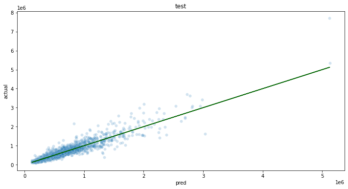
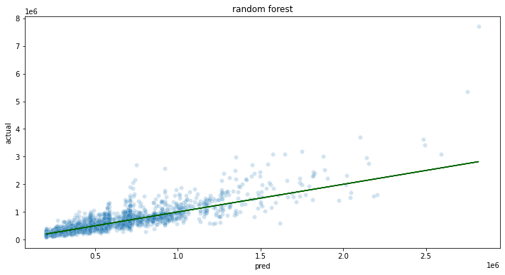
Model Testing: Evaluate different models and determine which is best suited for the problem.

Import Libraries

First we’ll import the libraries we’ll be using to evaluate the data and test different models.

import numpy as np
import pandas as pd

import sklearn
import sklearn.ensemble

import xgboost as xgb

import seaborn
import matplotlib
import matplotlib.pyplot as plt

import simdb # module for the purpose of this demo to simulate pulling data from a database

matplotlib.rcParams["figure.figsize"] = (12,6)

Retrieve Training Data

For training, we will use the data on all houses sold in this market with the last two years. As a reminder, this data pulled from a simulated database as an example of how to pull from an existing data store.

conn = simdb.simulate_db_connection()
tablename = simdb.tablename

query = f"select * from {tablename} where date > DATE(DATE(), '-24 month') AND sale_price is not NULL"
print(query)
# read in the data
housing_data = pd.read_sql_query(query, conn)

conn.close()
housing_data

select * from house_listings where date > DATE(DATE(), '-24 month') AND sale_price is not NULL

id	date	list_price	bedrooms	bathrooms	sqft_living	sqft_lot	floors	waterfront	view	…
0	7129300520	2022-07-11	221900.0	3	1.00	1180	5650	1.0	0	0
1	6414100192	2022-09-06	538000.0	3	2.25	2570	7242	2.0	0	0
2	5631500400	2022-11-23	180000.0	2	1.00	770	10000	1.0	0	0
3	2487200875	2022-09-06	604000.0	4	3.00	1960	5000	1.0	0	0
4	1954400510	2022-11-16	510000.0	3	2.00	1680	8080	1.0	0	0
…	…	…	…	…	…	…	…	…	…	…
20518	263000018	2022-02-16	360000.0	3	2.50	1530	1131	3.0	0	0
20519	6600060120	2022-11-21	400000.0	4	2.50	2310	5813	2.0	0	0
20520	1523300141	2022-03-21	402101.0	2	0.75	1020	1350	2.0	0	0
20521	291310100	2022-10-14	400000.0	3	2.50	1600	2388	2.0	0	0
20522	1523300157	2022-07-13	325000.0	2	0.75	1020	1076	2.0	0	0

20523 rows × 22 columns

Data transformations

To improve relative error performance, we will predict on log10 of the sale price.

Predict on log10 price to try to improve relative error performance

housing_data['logprice'] = np.log10(housing_data.sale_price)

From the data, we will create the following features to evaluate:

house_age: How old the house is.
renovated: Whether the house has been renovated or not.
yrs_since_reno: If the house has been renovated, how long has it been.

import datetime

thisyear = datetime.datetime.now().year

housing_data['house_age'] = thisyear - housing_data['yr_built']
housing_data['renovated'] =  np.where((housing_data['yr_renovated'] > 0), 1, 0) 
housing_data['yrs_since_reno'] =  np.where(housing_data['renovated'], housing_data['yr_renovated'] - housing_data['yr_built'], 0)

housing_data.loc[:, ['yr_built', 'yr_renovated', 'house_age', 'renovated', 'yrs_since_reno']]

	yr_built	yr_renovated	house_age	renovated	yrs_since_reno
0	1955	0	68	0	0
1	1951	1991	72	1	40
2	1933	0	90	0	0
3	1965	0	58	0	0
4	1987	0	36	0	0
...	...	...	...	...	...
20518	2009	0	14	0	0
20519	2014	0	9	0	0
20520	2009	0	14	0	0
20521	2004	0	19	0	0
20522	2008	0	15	0	0

20523 rows × 5 columns

Now we pick variables and split training data into training and holdout (test).

vars = ['bedrooms', 'bathrooms', 'sqft_living', 'sqft_lot', 'floors', 'waterfront', 'view',
'condition', 'grade', 'sqft_above', 'sqft_basement', 'lat', 'long', 'sqft_living15', 'sqft_lot15', 'house_age', 'renovated', 'yrs_since_reno']

outcome = 'logprice'

runif = np.random.default_rng(2206222).uniform(0, 1, housing_data.shape[0])
gp = np.where(runif < 0.2, 'test', 'training')

hd_train = housing_data.loc[gp=='training', :].reset_index(drop=True, inplace=False)
hd_test = housing_data.loc[gp=='test', :].reset_index(drop=True, inplace=False)

# split the training into training and val for xgboost
runif = np.random.default_rng(123).uniform(0, 1, hd_train.shape[0])
xgb_gp = np.where(runif < 0.2, 'val', 'train')

# for xgboost, further split into train and val
train_features = np.array(hd_train.loc[xgb_gp=='train', vars])
train_labels = np.array(hd_train.loc[xgb_gp=='train', outcome])

val_features = np.array(hd_train.loc[xgb_gp=='val', vars])
val_labels = np.array(hd_train.loc[xgb_gp=='val', outcome])

Postprocessing

Since we are fitting a model to predict log10 price, we need to convert predictions back into price units. We also want to round to the nearest dollar.

def postprocess(log10price):
    return np.rint(np.power(10, log10price))

Model testing

For the purposes of this demo, let’s say that we require a mean absolute percent error (MAPE) of 15% or less, and the we want to try a few models to decide which model we want to use.

One could also hyperparameter tune at this stage; for brevity, we’ll omit that in this demo.

XGBoost

First we will test out using a XGBoost model.


xgb_model = xgb.XGBRegressor(
    objective = 'reg:squarederror', 
    max_depth=5, 
    base_score = np.mean(hd_train[outcome])
    )

xgb_model.fit( 
    train_features,
    train_labels,
    eval_set=[(train_features, train_labels), (val_features, val_labels)],
    verbose=False,
    early_stopping_rounds=35
)

print(xgb_model.best_score)
print(xgb_model.best_iteration)
print(xgb_model.best_ntree_limit)

0.07793614689092423
99
100

XGBoost Evaluate on holdout

With the sample model created, we will test it against the holdout data. Note that we are calling the postprocess function on the data.

test_features = np.array(hd_test.loc[:, vars])
test_labels = np.array(hd_test.loc[:, outcome])

pframe = pd.DataFrame({
    'pred' : postprocess(xgb_model.predict(test_features)),
    'actual' : postprocess(test_labels)
})

ax = seaborn.scatterplot(
    data=pframe,
    x='pred',
    y='actual',
    alpha=0.2
)
matplotlib.pyplot.plot(pframe.pred, pframe.pred, color='DarkGreen')
matplotlib.pyplot.title("test")
plt.show()

pframe['se'] = (pframe.pred - pframe.actual)**2

pframe['pct_err'] = 100*np.abs(pframe.pred - pframe.actual)/pframe.actual
pframe.describe()

	pred	actual	se	pct_err
count	4.094000e+03	4.094000e+03	4.094000e+03	4094.000000
mean	5.340824e+05	5.396937e+05	1.657722e+10	12.857674
std	3.413714e+05	3.761666e+05	1.276017e+11	13.512028
min	1.216140e+05	8.200000e+04	1.000000e+00	0.000500
25%	3.167628e+05	3.200000e+05	3.245312e+08	4.252492
50%	4.568700e+05	4.500000e+05	1.602001e+09	9.101485
75%	6.310372e+05	6.355250e+05	6.575385e+09	17.041227
max	5.126706e+06	7.700000e+06	6.637466e+12	252.097895

rmse = np.sqrt(np.mean(pframe.se))
mape = np.mean(pframe.pct_err)

print(f'rmse = {rmse}, mape = {mape}')

rmse = 128752.54982046234, mape = 12.857674005250548

Random Forest

The next model to test is Random Forest.

model_rf = sklearn.ensemble.RandomForestRegressor(n_estimators=100, max_depth=5, n_jobs=2, max_samples=0.8)

train_features = np.array(hd_train.loc[:, vars])
train_labels = np.array(hd_train.loc[:, outcome])

model_rf.fit(train_features, train_labels)

Random Forest Evaluate on holdout

With the Random Forest sample model created, now we can test it against the holdout data.

pframe = pd.DataFrame({
    'pred' : postprocess(model_rf.predict(test_features)),
    'actual' : postprocess(test_labels)
})

ax = seaborn.scatterplot(
    data=pframe,
    x='pred',
    y='actual',
    alpha=0.2
)
matplotlib.pyplot.plot(pframe.pred, pframe.pred, color='DarkGreen')
matplotlib.pyplot.title("random forest")
plt.show()

pframe['se'] = (pframe.pred - pframe.actual)**2

pframe['pct_err'] = 100*np.abs(pframe.pred - pframe.actual)/pframe.actual
pframe.describe()

	pred	actual	se	pct_err
count	4.094000e+03	4.094000e+03	4.094000e+03	4094.000000
mean	5.196958e+05	5.396937e+05	3.881397e+10	18.206029
std	2.801499e+05	3.761666e+05	4.100412e+11	17.623817
min	2.039910e+05	8.200000e+04	7.290000e+02	0.006353
25%	3.295885e+05	3.200000e+05	6.780296e+08	6.115427
50%	4.644340e+05	4.500000e+05	3.304756e+09	13.227328
75%	5.911275e+05	6.355250e+05	1.380760e+10	24.721135
max	2.854540e+06	7.700000e+06	2.347848e+13	175.680235

rmse = np.sqrt(np.mean(pframe.se))
mape = np.mean(pframe.pct_err)

print(f'rmse = {rmse}, mape = {mape}')

rmse = 197012.60307486894, mape = 18.206029369592454

Final Decision

At this stage, we decide to go with the xgboost model, with the variables/settings above.

With this stage complete, we can move on to Stage 2: Training Process Automation Setup.

Next: From Jupyter to Production