This tutorial demonstrates how to use the Wallaroo to detect objects in images through the following models:
rnn mobilenet: A single stage object detector that performs fast inferences. Mobilenet is typically good at identifying objects at a distance.
resnet50: A dual stage object detector with slower inferencing but but is able to detect objects that are closer to each other.
This tutorial series will demonstrate the following:
How to deploy a Wallaroo pipeline with trained rnn mobilenet model and perform sample inferences to detect objects in pictures, then display those objects.
How to deploy a Wallaroo pipeline with a trained resnet50 model and perform sample inferences to detect objects in pictures, then display those objects.
Use the Wallaroo feature shadow deploy to have both models perform inferences, then select the inference result with the higher confidence and show the objects detected.
This tutorial assumes that users have installed the Wallaroo SDK or are running these tutorials from within their Wallaroo instance’s JupyterHub service.
This demonstration should be run within a Wallaroo JupyterHub instance for best results.
Prerequisites
The included OpenCV class is included in this demonstration as CVDemoUtils.py, and requires the following dependencies:
ffmpeg
libsm
libxext
Internal JupyterHub Service
To install these dependencies in the Wallaroo JupyterHub service, use the following commands from a terminal shell via the following procedure:
Launch the JupyterHub Service within the Wallaroo install.
Select File->New->Terminal.
Enter the following:
sudo apt-get update
sudo apt-get install ffmpeg libsm6 libxext6  -y
External SDK Users
For users using the Wallaroo SDK to connect with a remote Wallaroo instance, the following commands will install the required dependancies:
MacOS users can prepare their environments using a package manager such as Brew with the following:
brew install ffmpeg libsm libxext
Libraries and Dependencies
This repository may use large file sizes for the models. Use the Wallaroo Tutorials Releases to download a .zip file of the most recent computer vision tutorial that includes the models.
Import the following Python libraries into your environment:
These can be installed by running the command below in the Wallaroo JupyterHub service. Note the use of pip install torch --no-cache-dir for low memory environments.
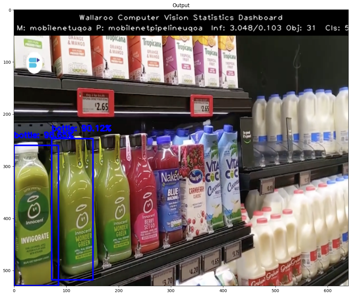
The following tutorial demonstrates how to use a trained mobilenet model deployed in Wallaroo to detect objects. This process will use the following steps:
Create a Wallaroo workspace and pipeline.
Upload a trained mobilenet ML model and add it as a pipeline step.
Deploy the pipeline.
Perform an inference on a sample image.
Draw the detected objects, their bounding boxes, their classifications, and the confidence of the classifications on the provided image.
Review our results.
Steps
Import Libraries
The first step will be to import our libraries. Please check with Step 00: Introduction and Setup and verify that the necessary libraries and applications are added to your environment.
importtorchimportpickleimportwallaroofromwallaroo.objectimportEntityNotFoundErrorfromwallaroo.frameworkimportFrameworkimportnumpyasnpimportjsonimportrequestsimporttimeimportpandasaspdfromCVDemoUtilsimportCVDemo# used to display dataframe information without truncatingfromIPython.displayimportdisplayimportpandasaspdpd.set_option('display.max_colwidth', None)
# used for unique connection namesimportstringimportrandomsuffix=''.join(random.choice(string.ascii_lowercase) foriinrange(4))
suffix=''
Connect to the Wallaroo Instance
The first step is to connect to Wallaroo through the Wallaroo client. The Python library is included in the Wallaroo install and available through the Jupyter Hub interface provided with your Wallaroo environment.
This is accomplished using the wallaroo.Client() command, which provides a URL to grant the SDK permission to your specific Wallaroo environment. When displayed, enter the URL into a browser and confirm permissions. Store the connection into a variable that can be referenced later.
If logging into the Wallaroo instance through the internal JupyterHub service, use wl = wallaroo.Client(). For more information on Wallaroo Client settings, see the Client Connection guide.
# Login through local servicewl=wallaroo.Client()
Set Variables
The following variables and methods are used later to create or connect to an existing workspace, pipeline, and model.
The workspace will be created or connected to, and set as the default workspace for this session. Once that is done, then all models and pipelines will be set in that workspace.
With the model uploaded, we can add it is as a step in the pipeline, then deploy it. Once deployed, resources from the Wallaroo instance will be reserved and the pipeline will be ready to use the model to perform inference requests.
Next we will load a sample image and resize it to the width and height required for the object detector. Once complete, it the image will be converted to a numpy ndim array and added to a dictionary.
# The size the image will be resized towidth=640height=480# Only objects that have a confidence > confidence_target will be displayed on the imagecvDemo=CVDemo()
imagePath='data/images/input/example/dairy_bottles.png'# The image width and height needs to be set to what the model was trained for. In this case 640x480.tensor, resizedImage=cvDemo.loadImageAndResize(imagePath, width, height)
# get npArray from the tensorFloatnpArray=tensor.cpu().numpy()
#creates a dictionary with the wallaroo "tensor" key and the numpy ndim array representing image as the value.dictData= {"tensor":[npArray]}
dataframedata=pd.DataFrame(dictData)
Run Inference
With that done, we can have the model detect the objects on the image by running an inference through the pipeline, and storing the results for the next step.
startTime=time.time()
# pass the dataframe in #infResults = pipeline.infer(dataframedata, dataset=["*", "metadata.elapsed"])infResults=pipeline.infer_from_file('./data/dairy_bottles.df.json', dataset=["*", "metadata.elapsed"])
endTime=time.time()
Draw the Inference Results
With our inference results, we can take them and use the Wallaroo CVDemo class and draw them onto the original image. The bounding boxes and the confidence value will only be drawn on images where the model returned a 90% confidence rate in the object’s identity.
df=pd.DataFrame(columns=['classification','confidence','x','y','width','height'])
pd.options.mode.chained_assignment=None# default='warn'pd.options.display.float_format='{:.2%}'.format# Points to where all the inference results areboxList=infResults.loc[0]["out.boxes"]
# # reshape this to an array of bounding box coordinates converted to intsboxA=np.array(boxList)
boxes=boxA.reshape(-1, 4)
boxes=boxes.astype(int)
df[['x', 'y','width','height']] =pd.DataFrame(boxes)
classes=infResults.loc[0]["out.classes"]
confidences=infResults.loc[0]["out.confidences"]
infResults= {
'model_name' : model_name,
'pipeline_name' : pipeline_name,
'width': width,
'height': height,
'image' : resizedImage,
'boxes' : boxes,
'classes' : classes,
'confidences' : confidences,
'confidence-target' : 0.90,
'inference-time': (endTime-startTime),
'onnx-time' : int(infResults.loc[0]["metadata.elapsed"][1]) /1e+9,
'color':(255,0,0)
}
image=cvDemo.drawAndDisplayDetectedObjectsWithClassification(infResults)
Extract the Inference Information
To show what is going on in the background, we’ll extract the inference results create a dataframe with columns representing the classification, confidence, and bounding boxes of the objects identified.
idx=0foridxinrange(0,len(classes)):
df['classification'][idx] =cvDemo.CLASSES[classes[idx]] # Classes contains the 80 different COCO classificaitonsdf['confidence'][idx] =confidences[idx]
df
classification
confidence
x
y
width
height
0
bottle
98.65%
0
210
85
479
1
bottle
90.12%
72
197
151
468
2
bottle
60.78%
211
184
277
420
3
bottle
59.22%
143
203
216
448
4
refrigerator
53.73%
13
41
640
480
5
bottle
45.13%
106
206
159
463
6
bottle
43.73%
278
1
321
93
7
bottle
43.09%
462
104
510
224
8
bottle
40.85%
310
1
352
94
9
bottle
39.19%
528
268
636
475
10
bottle
35.76%
220
0
258
90
11
bottle
31.81%
552
96
600
233
12
bottle
26.45%
349
0
404
98
13
bottle
23.06%
450
264
619
472
14
bottle
20.48%
261
193
307
408
15
bottle
17.46%
509
101
544
235
16
bottle
17.31%
592
100
633
239
17
bottle
16.00%
475
297
551
468
18
bottle
14.91%
368
163
423
362
19
book
13.66%
120
0
175
81
20
book
13.32%
72
0
143
85
21
bottle
12.22%
271
200
305
274
22
book
12.13%
161
0
213
85
23
bottle
11.96%
162
0
214
83
24
bottle
11.53%
310
190
367
397
25
bottle
9.62%
396
166
441
360
26
cake
8.65%
439
256
640
473
27
bottle
7.84%
544
375
636
472
28
vase
7.23%
272
2
306
96
29
bottle
6.28%
453
303
524
463
30
bottle
5.28%
609
94
635
211
Undeploy the Pipeline
With the inference complete, we can undeploy the pipeline and return the resources back to the Wallaroo instance.
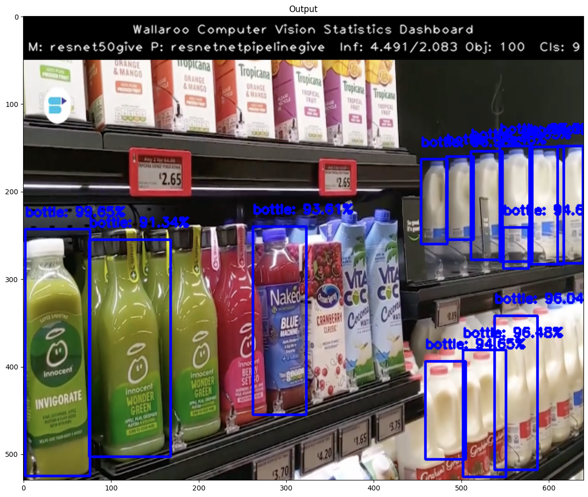
The following tutorial demonstrates how to use a trained mobilenet model deployed in Wallaroo to detect objects. This process will use the following steps:
Create a Wallaroo workspace and pipeline.
Upload a trained resnet50 ML model and add it as a pipeline step.
Deploy the pipeline.
Perform an inference on a sample image.
Draw the detected objects, their bounding boxes, their classifications, and the confidence of the classifications on the provided image.
Review our results.
Steps
Import Libraries
The first step will be to import our libraries. Please check with Step 00: Introduction and Setup and verify that the necessary libraries and applications are added to your environment.
importtorchimportpickleimportwallaroofromwallaroo.objectimportEntityNotFoundErrorfromwallaroo.frameworkimportFrameworkimportnumpyasnpimportjsonimportrequestsimporttimeimportpandasaspdfromCVDemoUtilsimportCVDemo# used to display dataframe information without truncatingfromIPython.displayimportdisplayimportpandasaspdpd.set_option('display.max_colwidth', None)
# used for unique connection namesimportstringimportrandomsuffix=''.join(random.choice(string.ascii_lowercase) foriinrange(4))
Connect to the Wallaroo Instance
The first step is to connect to Wallaroo through the Wallaroo client. The Python library is included in the Wallaroo install and available through the Jupyter Hub interface provided with your Wallaroo environment.
This is accomplished using the wallaroo.Client() command, which provides a URL to grant the SDK permission to your specific Wallaroo environment. When displayed, enter the URL into a browser and confirm permissions. Store the connection into a variable that can be referenced later.
If logging into the Wallaroo instance through the internal JupyterHub service, use wl = wallaroo.Client(). For more information on Wallaroo Client settings, see the Client Connection guide.
# Login through local servicewl=wallaroo.Client()
wl=wallaroo.Client()
Set Variables
The following variables and methods are used later to create or connect to an existing workspace, pipeline, and model. This example has both the resnet model, and a post process script.
The workspace will be created or connected to, and set as the default workspace for this session. Once that is done, then all models and pipelines will be set in that workspace.
With the model uploaded, we can add it is as a step in the pipeline, then deploy it. Once deployed, resources from the Wallaroo instance will be reserved and the pipeline will be ready to use the model to perform inference requests.
Test the pipeline by running inference on a sample image
Prepare input image
Next we will load a sample image and resize it to the width and height required for the object detector.
We will convert the image to a numpy ndim array and add it do a dictionary
#The size the image will be resized towidth=640height=480cvDemo=CVDemo()
imagePath='data/images/input/example/dairy_bottles.png'# The image width and height needs to be set to what the model was trained for. In this case 640x480.tensor, resizedImage=cvDemo.loadImageAndResize(imagePath, width, height)
# get npArray from the tensorFloatnpArray=tensor.cpu().numpy()
dictData= {"tensor":[npArray]}
dataframedata=pd.DataFrame(dictData)
Run Inference
With that done, we can have the model detect the objects on the image by running an inference through the pipeline, and storing the results for the next step.
IMPORTANT NOTE: If necessary, add timeout=60 to the infer method if more time is needed to upload the data file for the inference request.
startTime=time.time()
# pass the dataframe in # infResults = pipeline.infer(dataframedata, dataset=["*", "metadata.elapsed"])infResults=pipeline.infer_from_file('./data/dairy_bottles.df.json', dataset=["*", "metadata.elapsed"])
endTime=time.time()
Draw the Inference Results
With our inference results, we can take them and use the Wallaroo CVDemo class and draw them onto the original image. The bounding boxes and the confidence value will only be drawn on images where the model returned a 50% confidence rate in the object’s identity.
df=pd.DataFrame(columns=['classification','confidence','x','y','width','height'])
pd.options.mode.chained_assignment=None# default='warn'pd.options.display.float_format='{:.2%}'.format# Points to where all the inference results areboxList=infResults.loc[0]["out.boxes"]
# # reshape this to an array of bounding box coordinates converted to intsboxA=np.array(boxList)
boxes=boxA.reshape(-1, 4)
boxes=boxes.astype(int)
df[['x', 'y','width','height']] =pd.DataFrame(boxes)
classes=infResults.loc[0]["out.classes"]
confidences=infResults.loc[0]["out.confidences"]
infResults= {
'model_name' : model_name,
'pipeline_name' : pipeline_name,
'width': width,
'height': height,
'image' : resizedImage,
'boxes' : boxes,
'classes' : classes,
'confidences' : confidences,
'confidence-target' : 0.90,
'inference-time': (endTime-startTime),
'onnx-time' : int(infResults.loc[0]["metadata.elapsed"][1]) /1e+9,
'color':(255,0,0)
}
image=cvDemo.drawAndDisplayDetectedObjectsWithClassification(infResults)
Extract the Inference Information
To show what is going on in the background, we’ll extract the inference results create a dataframe with columns representing the classification, confidence, and bounding boxes of the objects identified.
idx=0foridxinrange(0,len(classes)):
cocoClasses=cvDemo.getCocoClasses()
df['classification'][idx] =cocoClasses[classes[idx]] # Classes contains the 80 different COCO classificaitonsdf['confidence'][idx] =confidences[idx]
df
classification
confidence
x
y
width
height
0
bottle
99.65%
2
193
76
475
1
bottle
98.83%
610
98
639
232
2
bottle
97.00%
544
98
581
230
3
bottle
96.96%
454
113
484
210
4
bottle
96.48%
502
331
551
476
...
...
...
...
...
...
...
95
bottle
5.72%
556
287
580
322
96
refrigerator
5.66%
80
161
638
480
97
bottle
5.60%
455
334
480
349
98
bottle
5.46%
613
267
635
375
99
bottle
5.37%
345
2
395
99
100 rows × 6 columns
Undeploy the Pipeline
With the inference complete, we can undeploy the pipeline and return the resources back to the Wallaroo instance.
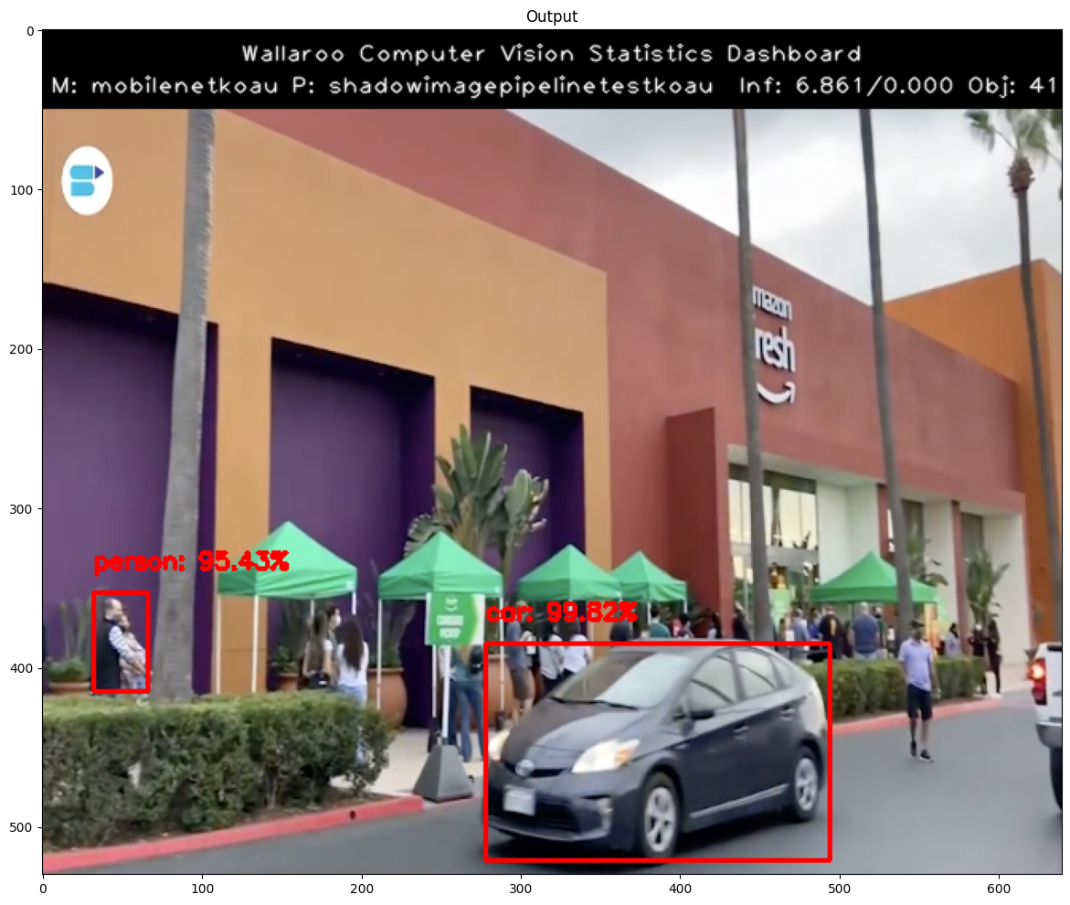
The following tutorial demonstrates how to use two trained models, one based on the resnet50, the other on mobilenet, deployed in Wallaroo to detect objects. This builds on the previous tutorials in this series, Step 01: Detecting Objects Using mobilenet" and “Step 02: Detecting Objects Using resnet50”.
For this tutorial, the Wallaroo feature Shadow Deploy will be used to submit inference requests to both models at once. The mobilnet object detector is the control and the faster-rcnn object detector is the challenger. The results between the two will be compared for their confidence, and that confidence will be used to draw bounding boxes around identified objects.
This process will use the following steps:
Create a Wallaroo workspace and pipeline.
Upload a trained resnet50 ML model and trained mobilenet model and add them as a shadow deployed step with the mobilenet as the control model.
Deploy the pipeline.
Perform an inference on a sample image.
Based on the
Draw the detected objects, their bounding boxes, their classifications, and the confidence of the classifications on the provided image.
Review our results.
Steps
Import Libraries
The first step will be to import our libraries. Please check with Step 00: Introduction and Setup and verify that the necessary libraries and applications are added to your environment.
importtorchimportpickleimportwallaroofromwallaroo.objectimportEntityNotFoundErrorfromwallaroo.frameworkimportFrameworkimportnumpyasnpimportjsonimportrequestsimporttimeimportpandasaspdfromCVDemoUtilsimportCVDemo# used to display dataframe information without truncatingfromIPython.displayimportdisplayimportpandasaspdpd.set_option('display.max_colwidth', None)
# used for unique connection namesimportstringimportrandomsuffix=''.join(random.choice(string.ascii_lowercase) foriinrange(4))
Connect to the Wallaroo Instance
The first step is to connect to Wallaroo through the Wallaroo client. The Python library is included in the Wallaroo install and available through the Jupyter Hub interface provided with your Wallaroo environment.
This is accomplished using the wallaroo.Client() command, which provides a URL to grant the SDK permission to your specific Wallaroo environment. When displayed, enter the URL into a browser and confirm permissions. Store the connection into a variable that can be referenced later.
If logging into the Wallaroo instance through the internal JupyterHub service, use wl = wallaroo.Client(). For more information on Wallaroo Client settings, see the Client Connection guide.
# Login through local servicewl=wallaroo.Client()
wl=wallaroo.Client()
Set Variables
The following variables and methods are used later to create or connect to an existing workspace, pipeline, and model. This example has both the resnet model, and a post process script.
The workspace will be created or connected to, and set as the default workspace for this session. Once that is done, then all models and pipelines will be set in that workspace.
For this step, rather than deploying each model into a separate step, both will be deployed into a single step as a Shadow Deploy step. This will take the inference input data and process it through both pipelines at the same time. The inference results for the control will be stored in it’s ['outputs'] array, while the results for the challenger are stored the ['shadow_data'] array.
Next we will load a sample image and resize it to the width and height required for the object detector.
We will convert the image to a numpy ndim array and add it do a dictionary
imagePath='data/images/input/example/store-front.png'# The image width and height needs to be set to what the model was trained for. In this case 640x480.cvDemo=CVDemo()
# The size the image will be resized to meet the input requirements of the object detectorwidth=640height=480tensor, controlImage=cvDemo.loadImageAndResize(imagePath, width, height)
challengerImage=controlImage.copy()
# get npArray from the tensorFloatnpArray=tensor.cpu().numpy()
#creates a dictionary with the wallaroo "tensor" key and the numpy ndim array representing image as the value.# dictData = {"tensor": npArray.tolist()}dictData= {"tensor":[npArray]}
dataframedata=pd.DataFrame(dictData)
Run Inference using Shadow Deployment
Now lets have the model detect the objects on the image by running inference and extracting the results
First we’ll extract the inference result data for the control model and map it onto the image.
df=pd.DataFrame(columns=['classification','confidence','x','y','width','height'])
pd.options.mode.chained_assignment=None# default='warn'pd.options.display.float_format='{:.2%}'.format# Points to where all the inference results are# boxList = infResults[0]["out.output"]boxList=infResults.loc[0]["out.boxes"]
# # reshape this to an array of bounding box coordinates converted to intsboxA=np.array(boxList)
controlBoxes=boxA.reshape(-1, 4)
controlBoxes=controlBoxes.astype(int)
df[['x', 'y','width','height']] =pd.DataFrame(controlBoxes)
controlClasses=infResults.loc[0]["out.classes"]
controlConfidences=infResults.loc[0]["out.confidences"]
results= {
'model_name' : control.name(),
'pipeline_name' : pipeline.name(),
'width': width,
'height': height,
'image' : controlImage,
'boxes' : controlBoxes,
'classes' : controlClasses,
'confidences' : controlConfidences,
'confidence-target' : 0.9,
'color':CVDemo.RED, # color to draw bounding boxes and the text in the statistics'inference-time': (endTime-startTime),
'onnx-time' : 0,
}
cvDemo.drawAndDisplayDetectedObjectsWithClassification(results)
Display the Control Results
Here we will use the Wallaroo CVDemo helper class to draw the control model results on the image.
The full results will be displayed in a dataframe with columns representing the classification, confidence, and bounding boxes of the objects identified.
Once extracted from the results we will want to reshape the flattened array into an array with 4 elements (x,y,width,height).
idx=0cocoClasses=cvDemo.getCocoClasses()
foridxinrange(0,len(controlClasses)):
df['classification'][idx] =cocoClasses[controlClasses[idx]] # Classes contains the 80 different COCO classificaitonsdf['confidence'][idx] =controlConfidences[idx]
df
classification
confidence
x
y
width
height
0
bottle
98.65%
0
210
85
479
1
bottle
90.12%
72
197
151
468
2
bottle
60.78%
211
184
277
420
3
bottle
59.22%
143
203
216
448
4
refrigerator
53.73%
13
41
640
480
5
bottle
45.13%
106
206
159
463
6
bottle
43.73%
278
1
321
93
7
bottle
43.09%
462
104
510
224
8
bottle
40.85%
310
1
352
94
9
bottle
39.19%
528
268
636
475
10
bottle
35.76%
220
0
258
90
11
bottle
31.81%
552
96
600
233
12
bottle
26.45%
349
0
404
98
13
bottle
23.06%
450
264
619
472
14
bottle
20.48%
261
193
307
408
15
bottle
17.46%
509
101
544
235
16
bottle
17.31%
592
100
633
239
17
bottle
16.00%
475
297
551
468
18
bottle
14.91%
368
163
423
362
19
book
13.66%
120
0
175
81
20
book
13.32%
72
0
143
85
21
bottle
12.22%
271
200
305
274
22
book
12.13%
161
0
213
85
23
bottle
11.96%
162
0
214
83
24
bottle
11.53%
310
190
367
397
25
bottle
9.62%
396
166
441
360
26
cake
8.65%
439
256
640
473
27
bottle
7.84%
544
375
636
472
28
vase
7.23%
272
2
306
96
29
bottle
6.28%
453
303
524
463
30
bottle
5.28%
609
94
635
211
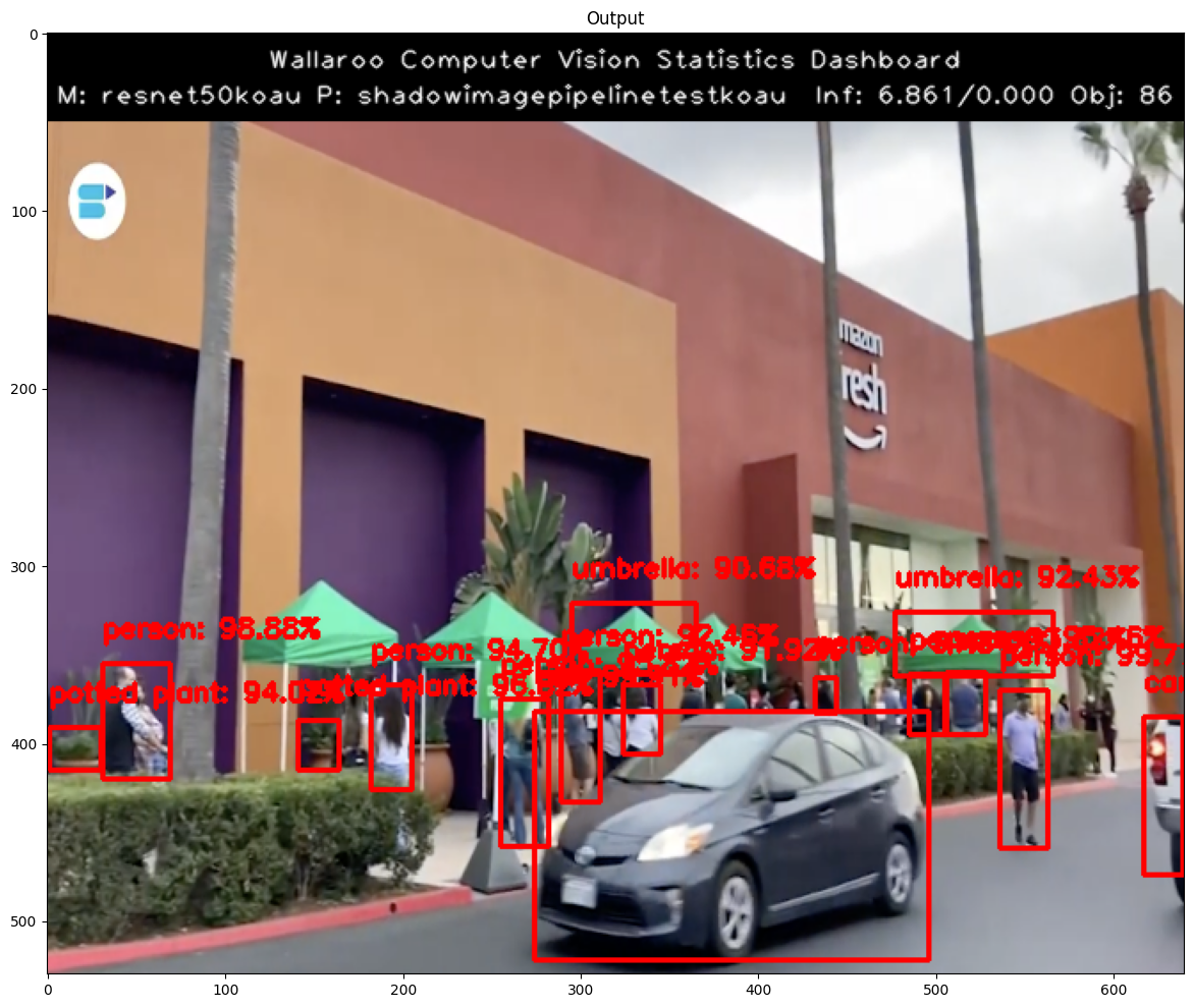
Display the Challenger Results
Here we will use the Wallaroo CVDemo helper class to draw the challenger model results on the input image.
challengerDf=pd.DataFrame(columns=['classification','confidence','x','y','width','height'])
pd.options.mode.chained_assignment=None# default='warn'pd.options.display.float_format='{:.2%}'.format# Points to where all the inference results areboxList=infResults.loc[0][f"out_{challenger_model_name}.boxes"]
# outputs = results['outputs']# boxes = outputs[0]# # reshape this to an array of bounding box coordinates converted to ints# boxList = boxes['Float']['data']boxA=np.array(boxList)
challengerBoxes=boxA.reshape(-1, 4)
challengerBoxes=challengerBoxes.astype(int)
challengerDf[['x', 'y','width','height']] =pd.DataFrame(challengerBoxes)
challengerClasses=infResults.loc[0][f"out_{challenger_model_name}.classes"]
challengerConfidences=infResults.loc[0][f"out_{challenger_model_name}.confidences"]
results= {
'model_name' : challenger.name(),
'pipeline_name' : pipeline.name(),
'width': width,
'height': height,
'image' : challengerImage,
'boxes' : challengerBoxes,
'classes' : challengerClasses,
'confidences' : challengerConfidences,
'confidence-target' : 0.9,
'color':CVDemo.RED, # color to draw bounding boxes and the text in the statistics'inference-time': (endTime-startTime),
'onnx-time' : 0,
}
cvDemo.drawAndDisplayDetectedObjectsWithClassification(results)
Display Challenger Results
The inference results for the objects detected by the challenger model will be displayed including the confidence values. Once extracted from the results we will want to reshape the flattened array into an array with 4 elements (x,y,width,height).
idx=0foridxinrange(0,len(challengerClasses)):
challengerDf['classification'][idx] =cvDemo.CLASSES[challengerClasses[idx]] # Classes contains the 80 different COCO classificaitonschallengerDf['confidence'][idx] =challengerConfidences[idx]
challengerDf
Notice the difference in the control confidence and the challenger confidence. Clearly we can see in this example the challenger resnet50 model is performing better than the control mobilenet model. This is likely due to the fact that frcnn resnet50 model is a 2 stage object detector vs the frcnn mobilenet is a single stage detector.
This completes using Wallaroo’s shadow deployment feature to compare different computer vision models.