The following tutorials are created to highlight specific features in Wallaroo.
Wallaroo Features Tutorials
Tutorials on Wallaroo features.
- 1: Hot Swap Models Tutorial
- 2: Inference URL Tutorials
- 2.1: Wallaroo SDK Inferencing with Pipeline Inference URL Tutorial
- 2.2: Wallaroo MLOps API Inferencing with Pipeline Inference URL Tutorial
- 3: Large Language Model with GPU Pipeline Deployment in Wallaroo Demonstration
- 4: Onnx Deployment with Multi Input-Output Tutorial
- 5: Wallaroo Assays Model Insights Tutorial
- 6: Computer Vision Pipeline Logs MLOps API Tutorial
- 7: Pipeline Logs MLOps API Tutorial
- 8: Pipeline Logs Tutorial
- 9: Statsmodel Forecast with Wallaroo Features
- 9.1: Statsmodel Forecast with Wallaroo Features: Deploy and Test Infer
- 9.2: Statsmodel Forecast with Wallaroo Features: Parallel Inference
- 9.3: Statsmodel Forecast with Wallaroo Features: Data Connection
- 9.4: Statsmodel Forecast with Wallaroo Features: ML Workload Orchestration
- 10: Tags Tutorial
1 - Hot Swap Models Tutorial
How to swap models in a pipeline step while the pipeline is deployed.
This tutorial and the assets can be downloaded as part of the Wallaroo Tutorials repository.
Model Hot Swap Tutorial
One of the biggest challenges facing organizations once they have a model trained is deploying the model: Getting all of the resources together, MLOps configured and systems prepared to allow inferences to run.
The next biggest challenge? Replacing the model while keeping the existing production systems running.
This tutorial demonstrates how Wallaroo model hot swap can update a pipeline step with a new model with one command. This lets organizations keep their production systems running while changing a ML model, with the change taking only milliseconds, and any inference requests in that time are processed after the hot swap is completed.
This example and sample data comes from the Machine Learning Group’s demonstration on Credit Card Fraud detection.
This tutorial provides the following:
- Models:
rf_model.onnx: The champion model that has been used in this environment for some time.xgb_model.onnxandgbr_model.onnx: Rival models that we will swap out from the champion model.
- Data:
- xtest-1.df.json and xtest-1k.df.json: DataFrame JSON inference inputs with 1 input and 1,000 inputs.
- xtest-1.arrow and xtest-1k.arrow: Apache Arrow inference inputs with 1 input and 1,000 inputs.
Reference
For more information about Wallaroo and related features, see the Wallaroo Documentation Site.
Prerequisites
- A deployed Wallaroo instance
- The following Python libraries installed:
Steps
The following steps demonstrate the following:
- Connect to a Wallaroo instance.
- Create a workspace and pipeline.
- Upload both models to the workspace.
- Deploy the pipe with the
rf_model.onnxmodel as a pipeline step. - Perform sample inferences.
- Hot swap and replace the existing model with the
xgb_model.onnxwhile keeping the pipeline deployed. - Conduct additional inferences to demonstrate the model hot swap was successful.
- Hot swap again with gbr_model.onnx, and perform more sample inferences.
- Undeploy the pipeline and return the resources back to the Wallaroo instance.
Load the Libraries
Load the Python libraries used to connect and interact with the Wallaroo instance.
import wallaroo
from wallaroo.object import EntityNotFoundError

# to display dataframe tables
from IPython.display import display
# used to display dataframe information without truncating
import pandas as pd
pd.set_option('display.max_colwidth', None)
import pyarrow as pa
Connect to the Wallaroo Instance
The first step is to connect to Wallaroo through the Wallaroo client. The Python library is included in the Wallaroo install and available through the Jupyter Hub interface provided with your Wallaroo environment.
This is accomplished using the wallaroo.Client() command, which provides a URL to grant the SDK permission to your specific Wallaroo environment. When displayed, enter the URL into a browser and confirm permissions. Store the connection into a variable that can be referenced later.
If logging into the Wallaroo instance through the internal JupyterHub service, use wl = wallaroo.Client(). For more information on Wallaroo Client settings, see the Client Connection guide.
# Login through local Wallaroo instance

wl = wallaroo.Client()
Set the Variables
The following variables are used in the later steps for creating the workspace, pipeline, and uploading the models. Modify them according to your organization’s requirements.
Just for the sake of this tutorial, we’ll use the SDK below to create our workspace , assign as our current workspace, then display all of the workspaces we have at the moment. We’ll also set up for our models and pipelines down the road, so we have one spot to change names to whatever fits your organization’s standards best.
To allow this tutorial to be run multiple times or by multiple users in the same Wallaroo instance, a random 4 character prefix will be added to the workspace, pipeline, and model.
import string
import random

# make a random 4 character prefix
prefix= ''.join(random.choice(string.ascii_lowercase) for i in range(4))

workspace_name = f'{prefix}hotswapworkspace'
pipeline_name = f'{prefix}hotswappipeline'
original_model_name = f'{prefix}housingmodelcontrol'
original_model_file_name = './models/rf_model.onnx'
replacement_model_name01 = f'{prefix}gbrhousingchallenger'
replacement_model_file_name01 = './models/gbr_model.onnx'
replacement_model_name02 = f'{prefix}xgbhousingchallenger'
replacement_model_file_name02 = './models/xgb_model.onnx'
def get_workspace(name):
    workspace = None
    for ws in wl.list_workspaces():
        if ws.name() == name:
            workspace= ws
    if(workspace == None):
        workspace = wl.create_workspace(name)
    return workspace

def get_pipeline(name):
    try:
        pipeline = wl.pipelines_by_name(name)[0]
    except EntityNotFoundError:
        pipeline = wl.build_pipeline(name)
    return pipeline
Create the Workspace
We will create a workspace based on the variable names set above, and set the new workspace as the current workspace. This workspace is where new pipelines will be created in and store uploaded models for this session.
Once set, the pipeline will be created.
workspace = get_workspace(workspace_name)

wl.set_current_workspace(workspace)

pipeline = get_pipeline(pipeline_name)
pipeline
| name | puaehotswappipeline |
|---|---|
| created | 2023-10-31 19:51:30.785109+00:00 |
| last_updated | 2023-10-31 19:51:30.785109+00:00 |
| deployed | (none) |
| arch | None |
| tags | |
| versions | 0f1ccb35-b6c4-4bf6-8467-2e1722c57eb8 |
| steps | |
| published | False |
Upload Models
We can now upload both of the models. In a later step, only one model will be added as a pipeline step, where the pipeline will submit inference requests to the pipeline.
original_model = (wl.upload_model(original_model_name ,
                                  original_model_file_name,
                                  framework=wallaroo.framework.Framework.ONNX)
                                  .configure(tensor_fields=["tensor"])
                    )
replacement_model01 = (wl.upload_model(replacement_model_name01 ,
                                       replacement_model_file_name01,
                                       framework=wallaroo.framework.Framework.ONNX)
                                       .configure(tensor_fields=["tensor"])
                        )
replacement_model02 = (wl.upload_model(replacement_model_name02 ,
                                       replacement_model_file_name02,
                                       framework=wallaroo.framework.Framework.ONNX)
                                       .configure(tensor_fields=["tensor"])
                        )
wl.list_models()
| Name | # of Versions | Owner ID | Last Updated | Created At |
|---|---|---|---|---|
| puaexgbhousingchallenger | 1 | "" | 2023-10-31 19:51:36.363832+00:00 | 2023-10-31 19:51:36.363832+00:00 |
| puaegbrhousingchallenger | 1 | "" | 2023-10-31 19:51:34.715224+00:00 | 2023-10-31 19:51:34.715224+00:00 |
| puaehousingmodelcontrol | 1 | "" | 2023-10-31 19:51:33.070235+00:00 | 2023-10-31 19:51:33.070235+00:00 |
Add Model to Pipeline Step
With the models uploaded, we will add the original model as a pipeline step, then deploy the pipeline so it is available for performing inferences.
pipeline.add_model_step(original_model)
pipeline
| name | puaehotswappipeline |
|---|---|
| created | 2023-10-31 19:51:30.785109+00:00 |
| last_updated | 2023-10-31 19:51:30.785109+00:00 |
| deployed | (none) |
| arch | None |
| tags | |
| versions | 0f1ccb35-b6c4-4bf6-8467-2e1722c57eb8 |
| steps | |
| published | False |
pipeline.deploy()
| name | puaehotswappipeline |
|---|---|
| created | 2023-10-31 19:51:30.785109+00:00 |
| last_updated | 2023-10-31 19:51:39.783255+00:00 |
| deployed | True |
| arch | None |
| tags | |
| versions | b1e80203-be2b-4a78-9e24-3e56d5d10d21, 0f1ccb35-b6c4-4bf6-8467-2e1722c57eb8 |
| steps | puaehousingmodelcontrol |
| published | False |
pipeline.status()
{'status': 'Running',
 'details': [],
 'engines': [{'ip': '10.244.3.81',
   'name': 'engine-696fcc57d7-7m9t7',
   'status': 'Running',
   'reason': None,
   'details': [],
   'pipeline_statuses': {'pipelines': [{'id': 'puaehotswappipeline',
      'status': 'Running'}]},
   'model_statuses': {'models': [{'name': 'puaehousingmodelcontrol',
      'version': 'bc9e5117-5ab0-4da8-971c-06854137243f',
      'sha': 'e22a0831aafd9917f3cc87a15ed267797f80e2afa12ad7d8810ca58f173b8cc6',
      'status': 'Running'}]}}],
 'engine_lbs': [{'ip': '10.244.4.102',
   'name': 'engine-lb-584f54c899-c9z75',
   'status': 'Running',
   'reason': None,
   'details': []}],
 'sidekicks': []}
Verify the Model
The pipeline is deployed with our model. The following will verify that the model is operating correctly. The high_fraud.json file contains data that the model should process as a high likelihood of being a fraudulent transaction.
normal_input = pd.DataFrame.from_records({"tensor": [[4.0, 2.5, 2900.0, 5505.0, 2.0, 0.0, 0.0, 3.0, 8.0, 2900.0, 0.0, 47.6063, -122.02, 2970.0, 5251.0, 12.0, 0.0, 0.0]]})
result = pipeline.infer(normal_input)
display(result)
| time | in.tensor | out.variable | check_failures | |
|---|---|---|---|---|
| 0 | 2023-10-31 19:51:52.769 | [4.0, 2.5, 2900.0, 5505.0, 2.0, 0.0, 0.0, 3.0, 8.0, 2900.0, 0.0, 47.6063, -122.02, 2970.0, 5251.0, 12.0, 0.0, 0.0] | [718013.7] | 0 |
large_house_input = pd.DataFrame.from_records({'tensor': [[4.0, 3.0, 3710.0, 20000.0, 2.0, 0.0, 2.0, 5.0, 10.0, 2760.0, 950.0, 47.6696, -122.261, 3970.0, 20000.0, 79.0, 0.0, 0.0]]})
large_house_result = pipeline.infer(large_house_input)
display(large_house_result)
| time | in.tensor | out.variable | check_failures | |
|---|---|---|---|---|
| 0 | 2023-10-31 19:51:53.171 | [4.0, 3.0, 3710.0, 20000.0, 2.0, 0.0, 2.0, 5.0, 10.0, 2760.0, 950.0, 47.6696, -122.261, 3970.0, 20000.0, 79.0, 0.0, 0.0] | [1514079.4] | 0 |
Replace the Model
The pipeline is currently deployed and is able to handle inferences. The model will now be replaced without having to undeploy the pipeline. This is done using the pipeline method replace_with_model_step(index, model). Steps start at 0, so the method called below will replace step 0 in our pipeline with the replacement model.
As an exercise, this deployment can be performed while inferences are actively being submitted to the pipeline to show how quickly the swap takes place.
pipeline.replace_with_model_step(0, replacement_model01).deploy()
| name | puaehotswappipeline |
|---|---|
| created | 2023-10-31 19:51:30.785109+00:00 |
| last_updated | 2023-10-31 19:51:53.854214+00:00 |
| deployed | True |
| arch | None |
| tags | |
| versions | 90a41e8d-2b33-445c-a8af-411840377674, b1e80203-be2b-4a78-9e24-3e56d5d10d21, 0f1ccb35-b6c4-4bf6-8467-2e1722c57eb8 |
| steps | puaehousingmodelcontrol |
| published | False |
Verify the Swap
To verify the swap, we’ll submit the same inferences and display the result. Note that out.variable has a different output than with the original model.
normal_input = pd.DataFrame.from_records({"tensor": [[4.0, 2.5, 2900.0, 5505.0, 2.0, 0.0, 0.0, 3.0, 8.0, 2900.0, 0.0, 47.6063, -122.02, 2970.0, 5251.0, 12.0, 0.0, 0.0]]})
result02 = pipeline.infer(normal_input)
display(result02)
| time | in.tensor | out.variable | check_failures | |
|---|---|---|---|---|
| 0 | 2023-10-31 19:51:58.130 | [4.0, 2.5, 2900.0, 5505.0, 2.0, 0.0, 0.0, 3.0, 8.0, 2900.0, 0.0, 47.6063, -122.02, 2970.0, 5251.0, 12.0, 0.0, 0.0] | [704901.9] | 0 |
large_house_input = pd.DataFrame.from_records({'tensor': [[4.0, 3.0, 3710.0, 20000.0, 2.0, 0.0, 2.0, 5.0, 10.0, 2760.0, 950.0, 47.6696, -122.261, 3970.0, 20000.0, 79.0, 0.0, 0.0]]})
large_house_result02 = pipeline.infer(large_house_input)
display(large_house_result02)
| time | in.tensor | out.variable | check_failures | |
|---|---|---|---|---|
| 0 | 2023-10-31 19:51:58.541 | [4.0, 3.0, 3710.0, 20000.0, 2.0, 0.0, 2.0, 5.0, 10.0, 2760.0, 950.0, 47.6696, -122.261, 3970.0, 20000.0, 79.0, 0.0, 0.0] | [1981238.0] | 0 |
Replace the Model Again
Let’s do one more hot swap, this time with our replacement_model02, then get some test inferences.
pipeline.replace_with_model_step(0, replacement_model02).deploy()
| name | puaehotswappipeline |
|---|---|
| created | 2023-10-31 19:51:30.785109+00:00 |
| last_updated | 2023-10-31 19:51:59.247708+00:00 |
| deployed | True |
| arch | None |
| tags | |
| versions | ecf69506-b73a-455d-83de-b81a5c815b36, 90a41e8d-2b33-445c-a8af-411840377674, b1e80203-be2b-4a78-9e24-3e56d5d10d21, 0f1ccb35-b6c4-4bf6-8467-2e1722c57eb8 |
| steps | puaehousingmodelcontrol |
| published | False |
normal_input = pd.DataFrame.from_records({"tensor": [[4.0, 2.5, 2900.0, 5505.0, 2.0, 0.0, 0.0, 3.0, 8.0, 2900.0, 0.0, 47.6063, -122.02, 2970.0, 5251.0, 12.0, 0.0, 0.0]]})
result03 = pipeline.infer(normal_input)
display(result03)
| time | in.tensor | out.variable | check_failures | |
|---|---|---|---|---|
| 0 | 2023-10-31 19:52:03.710 | [4.0, 2.5, 2900.0, 5505.0, 2.0, 0.0, 0.0, 3.0, 8.0, 2900.0, 0.0, 47.6063, -122.02, 2970.0, 5251.0, 12.0, 0.0, 0.0] | [659806.0] | 0 |
large_house_input = pd.DataFrame.from_records({'tensor': [[4.0, 3.0, 3710.0, 20000.0, 2.0, 0.0, 2.0, 5.0, 10.0, 2760.0, 950.0, 47.6696, -122.261, 3970.0, 20000.0, 79.0, 0.0, 0.0]]})
large_house_result03 = pipeline.infer(large_house_input)
display(large_house_result03)
| time | in.tensor | out.variable | check_failures | |
|---|---|---|---|---|
| 0 | 2023-10-31 19:52:04.085 | [4.0, 3.0, 3710.0, 20000.0, 2.0, 0.0, 2.0, 5.0, 10.0, 2760.0, 950.0, 47.6696, -122.261, 3970.0, 20000.0, 79.0, 0.0, 0.0] | [2176827.0] | 0 |
Compare Outputs
We’ll display the outputs of our inferences through the different models for comparison.
display([original_model_name, result.loc[0, "out.variable"]])
display([replacement_model_name01, result02.loc[0, "out.variable"]])
display([replacement_model_name02, result03.loc[0, "out.variable"]])
['puaehousingmodelcontrol', [718013.7]]
[‘puaegbrhousingchallenger’, [704901.9]]
[‘puaexgbhousingchallenger’, [659806.0]]
display([original_model_name, large_house_result.loc[0, "out.variable"]])
display([replacement_model_name01, large_house_result02.loc[0, "out.variable"]])
display([replacement_model_name02, large_house_result03.loc[0, "out.variable"]])
['puaehousingmodelcontrol', [1514079.4]]
[‘puaegbrhousingchallenger’, [1981238.0]]
[‘puaexgbhousingchallenger’, [2176827.0]]
Undeploy the Pipeline
With the tutorial complete, the pipeline is undeployed to return the resources back to the Wallaroo instance.
pipeline.undeploy()
| name | puaehotswappipeline |
|---|---|
| created | 2023-10-31 19:51:30.785109+00:00 |
| last_updated | 2023-10-31 19:51:59.247708+00:00 |
| deployed | False |
| arch | None |
| tags | |
| versions | ecf69506-b73a-455d-83de-b81a5c815b36, 90a41e8d-2b33-445c-a8af-411840377674, b1e80203-be2b-4a78-9e24-3e56d5d10d21, 0f1ccb35-b6c4-4bf6-8467-2e1722c57eb8 |
| steps | puaehousingmodelcontrol |
| published | False |
2 - Inference URL Tutorials
How to use the Wallaroo SDK and the Wallaroo MLOps API to perform inferences.
Wallaroo provides multiple methods of performing inferences through a deployed pipeline.
2.1 - Wallaroo SDK Inferencing with Pipeline Inference URL Tutorial
How to use the Wallaroo SDK for inferences via the SDK and API with the Pipeline Inference URL.
This tutorial and the assets can be downloaded as part of the Wallaroo Tutorials repository.
Wallaroo SDK Inference Tutorial
Wallaroo provides the ability to perform inferences through deployed pipelines via the Wallaroo SDK and the Wallaroo MLOps API. This tutorial demonstrates performing inferences using the Wallaroo SDK.
This tutorial provides the following:
ccfraud.onnx: A pre-trained credit card fraud detection model.data/cc_data_1k.arrow,data/cc_data_10k.arrow: Sample testing data in Apache Arrow format with 1,000 and 10,000 records respectively.wallaroo-model-endpoints-sdk.py: A code-only version of this tutorial as a Python script.
This tutorial and sample data comes from the Machine Learning Group’s demonstration on Credit Card Fraud detection.
Prerequisites
The following is required for this tutorial:
- A deployed Wallaroo instance with Model Endpoints Enabled
- The following Python libraries:
Tutorial Goals
This demonstration provides a quick tutorial on performing inferences using the Wallaroo SDK using the Pipeline infer and infer_from_file methods. This following steps will be performed:
- Connect to a Wallaroo instance using environmental variables. This bypasses the browser link confirmation for a seamless login. For more information, see the Wallaroo SDK Essentials Guide: Client Connection.
- Create a workspace for our models and pipelines.
- Upload the
ccfraudmodel. - Create a pipeline and add the
ccfraudmodel as a pipeline step. - Run a sample inference through SDK Pipeline
infermethod. - Run a batch inference through SDK Pipeline
infer_from_filemethod. - Run a DataFrame and Arrow based inference through the pipeline Inference URL.
Open a Connection to Wallaroo
The first step is to connect to Wallaroo through the Wallaroo client. This example will store the user’s credentials into the file ./creds.json which contains the following:
{
    "username": "{Connecting User's Username}",
    "password": "{Connecting User's Password}",
    "email": "{Connecting User's Email Address}"
}
Replace the username, password, and email fields with the user account connecting to the Wallaroo instance. This allows a seamless connection to the Wallaroo instance and bypasses the standard browser based confirmation link. For more information, see the Wallaroo SDK Essentials Guide: Client Connection.
If running this example within the internal Wallaroo JupyterHub service, use the wallaroo.Client(auth_type="user_password") method. If connecting externally via the Wallaroo SDK, use the following to specify the URL of the Wallaroo instance as defined in the Wallaroo DNS Integration Guide, replacing wallarooPrefix. and wallarooSuffix with your Wallaroo instance’s DNS prefix and suffix.
Note the . is part of the prefix. If there is no prefix, then wallarooPrefix = ""
import wallaroo
from wallaroo.object import EntityNotFoundError
import pandas as pd
import os
import pyarrow as pa

# used to display dataframe information without truncating
from IPython.display import display
pd.set_option('display.max_colwidth', None)

import requests

# Used to create unique workspace and pipeline names
import string
import random

# make a random 4 character suffix to prevent workspace and pipeline name clobbering
suffix= ''.join(random.choice(string.ascii_lowercase) for i in range(4))
# Retrieve the login credentials.
os.environ["WALLAROO_SDK_CREDENTIALS"] = './creds.json'

# Client connection from local Wallaroo instance

wl = wallaroo.Client(auth_type="user_password")
Create the Workspace
We will create a workspace to work in and call it the sdkinferenceexampleworkspace, then set it as current workspace environment. We’ll also create our pipeline in advance as sdkinferenceexamplepipeline.
The model to be uploaded and used for inference will be labeled as ccfraud.
workspace_name = f'sdkinferenceexampleworkspace{suffix}'
pipeline_name = f'sdkinferenceexamplepipeline{suffix}'
model_name = f'ccfraud{suffix}'
model_file_name = './ccfraud.onnx'
def get_workspace(name):
    workspace = None
    for ws in wl.list_workspaces():
        if ws.name() == name:
            workspace= ws
    if(workspace == None):
        workspace = wl.create_workspace(name)
    return workspace

def get_pipeline(name):
    try:
        pipeline = wl.pipelines_by_name(name)[0]
    except EntityNotFoundError:
        pipeline = wl.build_pipeline(name)
    return pipeline
workspace = get_workspace(workspace_name)

wl.set_current_workspace(workspace)
{'name': 'sdkinferenceexampleworkspacesrsw', 'id': 47, 'archived': False, 'created_by': 'fec5b97a-934b-487f-b95b-ade7f3b81f9c', 'created_at': '2023-05-19T15:14:02.432103+00:00', 'models': [], 'pipelines': []}
Build Pipeline
In a production environment, the pipeline would already be set up with the model and pipeline steps. We would then select it and use it to perform our inferences.
For this example we will create the pipeline and add the ccfraud model as a pipeline step and deploy it. Deploying a pipeline allocates resources from the Kubernetes cluster hosting the Wallaroo instance and prepares it for performing inferences.
If this process was already completed, it can be commented out and skipped for the next step Select Pipeline.
Then we will list the pipelines and select the one we will be using for the inference demonstrations.
# Create or select the current pipeline

ccfraudpipeline = get_pipeline(pipeline_name)

# Add ccfraud model as the pipeline step

ccfraud_model = (wl.upload_model(model_name,
                                 model_file_name,
                                 framework=wallaroo.framework.Framework.ONNX)
                                 .configure(tensor_fields=["tensor"])
                )

ccfraudpipeline.add_model_step(ccfraud_model).deploy()
| name | sdkinferenceexamplepipelinesrsw |
|---|---|
| created | 2023-05-19 15:14:03.916503+00:00 |
| last_updated | 2023-05-19 15:14:05.162541+00:00 |
| deployed | True |
| tags | |
| versions | 81840bdb-a1bc-48b9-8df0-4c7a196fa79a, 49cfc2cc-16fb-4dfa-8d1b-579fa86dab07 |
| steps | ccfraudsrsw |
Select Pipeline
This step assumes that the pipeline is prepared with ccfraud as the current step. The method pipelines_by_name(name) returns an array of pipelines with names matching the pipeline_name field. This example assumes only one pipeline is assigned the name sdkinferenceexamplepipeline.
# List the pipelines by name in the current workspace - just the first several to save space.

display(wl.list_pipelines()[:5])

# Set the `pipeline` variable to our sample pipeline.

pipeline = wl.pipelines_by_name(pipeline_name)[0]
display(pipeline)
[{'name': 'sdkinferenceexamplepipelinesrsw', 'create_time': datetime.datetime(2023, 5, 19, 15, 14, 3, 916503, tzinfo=tzutc()), 'definition': '[]'},
 {'name': 'ccshadoweonn', 'create_time': datetime.datetime(2023, 5, 19, 15, 13, 48, 963815, tzinfo=tzutc()), 'definition': '[]'},
 {'name': 'ccshadowgozg', 'create_time': datetime.datetime(2023, 5, 19, 15, 8, 23, 58929, tzinfo=tzutc()), 'definition': '[]'}]
| name | sdkinferenceexamplepipelinesrsw |
|---|---|
| created | 2023-05-19 15:14:03.916503+00:00 |
| last_updated | 2023-05-19 15:14:05.162541+00:00 |
| deployed | True |
| tags | |
| versions | 81840bdb-a1bc-48b9-8df0-4c7a196fa79a, 49cfc2cc-16fb-4dfa-8d1b-579fa86dab07 |
| steps | ccfraudsrsw |
Interferences via SDK
Once a pipeline has been deployed, an inference can be run. This will submit data to the pipeline, where it is processed through each of the pipeline’s steps with the output of the previous step providing the input for the next step. The final step will then output the result of all of the pipeline’s steps.
- Inputs are either sent one of the following:
- pandas.DataFrame. The return value will be a pandas.DataFrame.
- Apache Arrow. The return value will be an Apache Arrow table.
- Custom JSON. The return value will be a Wallaroo InferenceResult object.
Inferences are performed through the Wallaroo SDK via the Pipeline infer and infer_from_file methods.
infer Method
Now that the pipeline is deployed we’ll perform an inference using the Pipeline infer method, and submit a pandas DataFrame as our input data. This will return a pandas DataFrame as the inference output.
For more information, see the Wallaroo SDK Essentials Guide: Inferencing: Run Inference through Local Variable.
smoke_test = pd.DataFrame.from_records([
    {
        "tensor":[
            1.0678324729,
            0.2177810266,
            -1.7115145262,
            0.682285721,
            1.0138553067,
            -0.4335000013,
            0.7395859437,
            -0.2882839595,
            -0.447262688,
            0.5146124988,
            0.3791316964,
            0.5190619748,
            -0.4904593222,
            1.1656456469,
            -0.9776307444,
            -0.6322198963,
            -0.6891477694,
            0.1783317857,
            0.1397992467,
            -0.3554220649,
            0.4394217877,
            1.4588397512,
            -0.3886829615,
            0.4353492889,
            1.7420053483,
            -0.4434654615,
            -0.1515747891,
            -0.2668451725,
            -1.4549617756
        ]
    }
])
result = pipeline.infer(smoke_test)
display(result)
| time | in.tensor | out.dense_1 | check_failures | |
|---|---|---|---|---|
| 0 | 2023-05-19 15:14:22.066 | [1.0678324729, 0.2177810266, -1.7115145262, 0.682285721, 1.0138553067, -0.4335000013, 0.7395859437, -0.2882839595, -0.447262688, 0.5146124988, 0.3791316964, 0.5190619748, -0.4904593222, 1.1656456469, -0.9776307444, -0.6322198963, -0.6891477694, 0.1783317857, 0.1397992467, -0.3554220649, 0.4394217877, 1.4588397512, -0.3886829615, 0.4353492889, 1.7420053483, -0.4434654615, -0.1515747891, -0.2668451725, -1.4549617756] | [0.0014974177] | 0 |
infer_from_file Method
This example uses the Pipeline method infer_from_file to submit 10,000 records as a batch using an Apache Arrow table. The method will return an Apache Arrow table. For more information, see the Wallaroo SDK Essentials Guide: Inferencing: Run Inference From A File
The results will be converted into a pandas.DataFrame. The results will be filtered by transactions likely to be credit card fraud.
result = pipeline.infer_from_file('./data/cc_data_10k.arrow')

display(result)
    pyarrow.Table
    time: timestamp[ms]
    in.tensor: list<item: float> not null
      child 0, item: float
    out.dense_1: list<inner: float not null> not null
      child 0, inner: float not null
    check_failures: int8
    ----
    time: [[2023-05-19 15:14:22.851,2023-05-19 15:14:22.851,2023-05-19 15:14:22.851,2023-05-19 15:14:22.851,2023-05-19 15:14:22.851,...,2023-05-19 15:14:22.851,2023-05-19 15:14:22.851,2023-05-19 15:14:22.851,2023-05-19 15:14:22.851,2023-05-19 15:14:22.851]]
    in.tensor: [[[-1.0603298,2.3544967,-3.5638788,5.138735,-1.2308457,...,0.038412016,1.0993439,1.2603409,-0.14662448,-1.4463212],[-1.0603298,2.3544967,-3.5638788,5.138735,-1.2308457,...,0.038412016,1.0993439,1.2603409,-0.14662448,-1.4463212],...,[-2.1694233,-3.1647356,1.2038506,-0.2649221,0.0899006,...,1.8174038,-0.19327773,0.94089776,0.825025,1.6242892],[-0.12405868,0.73698884,1.0311689,0.59917533,0.11831961,...,-0.36567155,-0.87004745,0.41288367,0.49470216,-0.6710689]]]
    out.dense_1: [[[0.99300325],[0.99300325],...,[0.00024175644],[0.0010648072]]]
    check_failures: [[0,0,0,0,0,...,0,0,0,0,0]]
# use pyarrow to convert results to a pandas DataFrame and display only the results with > 0.75

list = [0.75]

outputs =  result.to_pandas()
# display(outputs)
filter = [elt[0] > 0.75 for elt in outputs['out.dense_1']]
outputs = outputs.loc[filter]
display(outputs)
| time | in.tensor | out.dense_1 | check_failures | |
|---|---|---|---|---|
| 0 | 2023-05-19 15:14:22.851 | [-1.0603298, 2.3544967, -3.5638788, 5.138735, -1.2308457, -0.76878244, -3.5881228, 1.8880838, -3.2789674, -3.9563255, 4.099344, -5.653918, -0.8775733, -9.131571, -0.6093538, -3.7480276, -5.0309124, -0.8748149, 1.9870535, 0.7005486, 0.9204423, -0.10414918, 0.32295644, -0.74181414, 0.038412016, 1.0993439, 1.2603409, -0.14662448, -1.4463212] | [0.99300325] | 0 |
| 1 | 2023-05-19 15:14:22.851 | [-1.0603298, 2.3544967, -3.5638788, 5.138735, -1.2308457, -0.76878244, -3.5881228, 1.8880838, -3.2789674, -3.9563255, 4.099344, -5.653918, -0.8775733, -9.131571, -0.6093538, -3.7480276, -5.0309124, -0.8748149, 1.9870535, 0.7005486, 0.9204423, -0.10414918, 0.32295644, -0.74181414, 0.038412016, 1.0993439, 1.2603409, -0.14662448, -1.4463212] | [0.99300325] | 0 |
| 2 | 2023-05-19 15:14:22.851 | [-1.0603298, 2.3544967, -3.5638788, 5.138735, -1.2308457, -0.76878244, -3.5881228, 1.8880838, -3.2789674, -3.9563255, 4.099344, -5.653918, -0.8775733, -9.131571, -0.6093538, -3.7480276, -5.0309124, -0.8748149, 1.9870535, 0.7005486, 0.9204423, -0.10414918, 0.32295644, -0.74181414, 0.038412016, 1.0993439, 1.2603409, -0.14662448, -1.4463212] | [0.99300325] | 0 |
| 3 | 2023-05-19 15:14:22.851 | [-1.0603298, 2.3544967, -3.5638788, 5.138735, -1.2308457, -0.76878244, -3.5881228, 1.8880838, -3.2789674, -3.9563255, 4.099344, -5.653918, -0.8775733, -9.131571, -0.6093538, -3.7480276, -5.0309124, -0.8748149, 1.9870535, 0.7005486, 0.9204423, -0.10414918, 0.32295644, -0.74181414, 0.038412016, 1.0993439, 1.2603409, -0.14662448, -1.4463212] | [0.99300325] | 0 |
| 161 | 2023-05-19 15:14:22.851 | [-9.716793, 9.174981, -14.450761, 8.653825, -11.039951, 0.6602411, -22.825525, -9.919395, -8.064324, -16.737926, 4.852197, -12.563343, -1.0762653, -7.524591, -3.2938414, -9.62102, -15.6501045, -7.089741, 1.7687134, 5.044906, -11.365625, 4.5987034, 4.4777045, 0.31702697, -2.2731977, 0.07944675, -10.052058, -2.024108, -1.0611985] | [1.0] | 0 |
| 941 | 2023-05-19 15:14:22.851 | [-0.50492376, 1.9348029, -3.4217603, 2.2165704, -0.6545315, -1.9004827, -1.6786858, 0.5380051, -2.7229102, -5.265194, 3.504164, -5.4661765, 0.68954825, -8.725291, 2.0267954, -5.4717045, -4.9123807, -1.6131229, 3.8021576, 1.3881834, 1.0676425, 0.28200775, -0.30759808, -0.48498034, 0.9507336, 1.5118006, 1.6385275, 1.072455, 0.7959132] | [0.9873102] | 0 |
| 1445 | 2023-05-19 15:14:22.851 | [-7.615594, 4.659706, -12.057331, 7.975307, -5.1068773, -1.6116138, -12.146941, -0.5952333, -6.4605103, -12.535655, 10.017626, -14.839381, 0.34900802, -14.953928, -0.3901092, -9.342014, -14.285043, -5.758632, 0.7512068, 1.4632998, -3.3777077, 0.9950705, -0.5855211, -1.6528498, 1.9089833, 1.6860862, 5.5044003, -3.703297, -1.4715525] | [1.0] | 0 |
| 2092 | 2023-05-19 15:14:22.851 | [-14.115489, 9.905631, -18.67885, 4.602589, -15.404288, -3.7169847, -15.887272, 15.616176, -3.2883947, -7.0224414, 4.086536, -5.7809114, 1.2251061, -5.4301147, -0.14021407, -6.0200763, -12.957546, -5.545689, 0.86074656, 2.2463796, 2.492611, -2.9649208, -2.265674, 0.27490455, 3.9263225, -0.43438172, 3.1642237, 1.2085277, 0.8223642] | [0.99999] | 0 |
| 2220 | 2023-05-19 15:14:22.851 | [-0.1098309, 2.5842443, -3.5887418, 4.63558, 1.1825614, -1.2139517, -0.7632139, 0.6071841, -3.7244265, -3.501917, 4.3637576, -4.612757, -0.44275254, -10.346612, 0.66243565, -0.33048683, 1.5961986, 2.5439718, 0.8787973, 0.7406088, 0.34268215, -0.68495077, -0.48357907, -1.9404846, -0.059520483, 1.1553137, 0.9918434, 0.7067319, -1.6016251] | [0.91080534] | 0 |
| 4135 | 2023-05-19 15:14:22.851 | [-0.547029, 2.2944348, -4.149202, 2.8648357, -0.31232587, -1.5427867, -2.1489344, 0.9471863, -2.663241, -4.2572775, 2.1116028, -6.2264414, -1.1307784, -6.9296007, 1.0049651, -5.876498, -5.6855297, -1.5800936, 3.567338, 0.5962099, 1.6361043, 1.8584082, -0.08202618, 0.46620172, -2.234368, -0.18116793, 1.744976, 2.1414309, -1.6081295] | [0.98877275] | 0 |
| 4236 | 2023-05-19 15:14:22.851 | [-3.135635, -1.483817, -3.0833669, 1.6626456, -0.59695035, -0.30199608, -3.316563, 1.869609, -1.8006078, -4.5662026, 2.8778172, -4.0887237, -0.43401834, -3.5816982, 0.45171788, -5.725131, -8.982029, -4.0279546, 0.89264476, 0.24721873, 1.8289508, 1.6895254, -2.5555577, -2.4714024, -0.4500012, 0.23333028, 2.2119386, -2.041805, 1.1568314] | [0.95601666] | 0 |
| 5658 | 2023-05-19 15:14:22.851 | [-5.4078765, 3.9039962, -8.98522, 5.128742, -7.373224, -2.946234, -11.033238, 5.914019, -5.669241, -12.041053, 6.950792, -12.488795, 1.2236942, -14.178565, 1.6514667, -12.47019, -22.350504, -8.928755, 4.54775, -0.11478994, 3.130207, -0.70128506, -0.40275285, 0.7511918, -0.1856308, 0.92282087, 0.146656, -1.3761806, 0.42997098] | [1.0] | 0 |
| 6768 | 2023-05-19 15:14:22.851 | [-16.900557, 11.7940855, -21.349983, 4.746453, -17.54182, -3.415758, -19.897173, 13.8569145, -3.570626, -7.388376, 3.0761156, -4.0583425, 1.2901028, -2.7997534, -0.4298746, -4.777225, -11.371295, -5.2725616, 0.0964799, 4.2148075, -0.8343371, -2.3663573, -1.6571938, 0.2110055, 4.438088, -0.49057993, 2.342008, 1.4479793, -1.4715525] | [0.9999745] | 0 |
| 6780 | 2023-05-19 15:14:22.851 | [-0.74893713, 1.3893062, -3.7477517, 2.4144504, -0.11061429, -1.0737498, -3.1504633, 1.2081385, -1.332872, -4.604276, 4.438548, -7.687688, 1.1683422, -5.3296027, -0.19838685, -5.294243, -5.4928794, -1.3254275, 4.387228, 0.68643385, 0.87228596, -0.1154091, -0.8364338, -0.61202216, 0.10518055, 2.2618086, 1.1435078, -0.32623357, -1.6081295] | [0.9852645] | 0 |
| 7133 | 2023-05-19 15:14:22.851 | [-7.5131927, 6.507386, -12.439463, 5.7453, -9.513038, -1.4236209, -17.402607, -3.0903268, -5.378041, -15.169325, 5.7585907, -13.448207, -0.45244268, -8.495097, -2.2323692, -11.429063, -19.578058, -8.367617, 1.8869618, 2.1813896, -4.799091, 2.4388566, 2.9503248, 0.6293566, -2.6906652, -2.1116931, -6.4196434, -1.4523355, -1.4715525] | [1.0] | 0 |
| 7566 | 2023-05-19 15:14:22.851 | [-2.1804514, 1.0243497, -4.3890443, 3.4924, -3.7609894, 0.023624033, -2.7677023, 1.1786921, -2.9450424, -6.8823, 6.1294384, -9.564066, -1.6273017, -10.940607, 0.3062539, -8.854589, -15.382658, -5.419305, 3.2210033, -0.7381137, 0.9632334, 0.6612066, 2.1337948, -0.90536207, 0.7498649, -0.019404415, 5.5950212, 0.26602694, 1.7534728] | [0.9999705] | 0 |
| 7911 | 2023-05-19 15:14:22.851 | [-1.594454, 1.8545462, -2.6311765, 2.759316, -2.6988854, -0.08155677, -3.8566258, -0.04912437, -1.9640644, -4.2058415, 3.391933, -6.471933, -0.9877536, -6.188904, 1.2249585, -8.652863, -11.170872, -6.134417, 2.5400054, -0.29327056, 3.591464, 0.3057127, -0.052313827, 0.06196331, -0.82863224, -0.2595842, 1.0207018, 0.019899422, 1.0935433] | [0.9980203] | 0 |
| 8921 | 2023-05-19 15:14:22.851 | [-0.21756083, 1.786712, -3.4240367, 2.7769134, -1.420116, -2.1018193, -3.4615245, 0.7367844, -2.3844852, -6.3140697, 4.382665, -8.348951, -1.6409378, -10.611383, 1.1813216, -6.251184, -10.577264, -3.5184007, 0.7997489, 0.97915924, 1.081642, -0.7852368, -0.4761941, -0.10635195, 2.066527, -0.4103488, 2.8288178, 1.9340333, -1.4715525] | [0.99950194] | 0 |
| 9244 | 2023-05-19 15:14:22.851 | [-3.314442, 2.4431305, -6.1724143, 3.6737356, -3.81542, -1.5950849, -4.8292923, 2.9850774, -4.22416, -7.5519834, 6.1932964, -8.59886, 0.25443414, -11.834097, -0.39583337, -6.015362, -13.532762, -4.226845, 1.1153877, 0.17989528, 1.3166595, -0.64433384, 0.2305495, -0.5776498, 0.7609739, 2.2197483, 4.01189, -1.2347667, 1.2847253] | [0.9999876] | 0 |
| 10176 | 2023-05-19 15:14:22.851 | [-5.0815525, 3.9294617, -8.4077635, 6.373701, -7.391173, -2.1574461, -10.345097, 5.5896044, -6.3736906, -11.330594, 6.618754, -12.93748, 1.1884484, -13.9628935, 1.0340953, -12.278127, -23.333889, -8.886669, 3.5720036, -0.3243157, 3.4229393, 0.493529, 0.08469851, 0.791218, 0.30968663, 0.6811129, 0.39306796, -1.5204874, 0.9061435] | [1.0] | 0 |
Inferences via HTTP POST
Each pipeline has its own Inference URL that allows HTTP/S POST submissions of inference requests. Full details are available from the Inferencing via the Wallaroo MLOps API.
This example will demonstrate performing inferences with a DataFrame input and an Apache Arrow input.
Request JWT Token
There are two ways to retrieve the JWT token used to authenticate to the Wallaroo MLOps API.
- Wallaroo SDK. This method requires a Wallaroo based user.
- API Clent Secret. This is the recommended method as it is user independent. It allows any valid user to make an inference request.
This tutorial will use the Wallaroo SDK method Wallaroo Client wl.auth.auth_header() method, extracting the Authentication header from the response.
Reference: MLOps API Retrieve Token Through Wallaroo SDK
headers = wl.auth.auth_header()
display(headers)
{'Authorization': 'Bearer eyJhbGciOiJSUzI1NiIsInR5cCIgOiAiSldUIiwia2lkIiA6ICJhSFpPS1RacGhxT1JQVkw4Y19JV25qUDNMU29iSnNZNXBtNE5EQTA1NVZNIn0.eyJleHAiOjE2ODQ1MDkzMDgsImlhdCI6MTY4NDUwOTI0OCwiYXV0aF90aW1lIjoxNjg0NTA4ODUwLCJqdGkiOiJkZmU3ZTIyMS02ODMyLTRiOGItYjJiMS1hYzFkYWY2YjVmMWYiLCJpc3MiOiJodHRwczovL3NwYXJrbHktYXBwbGUtMzAyNi5rZXljbG9hay53YWxsYXJvby5jb21tdW5pdHkvYXV0aC9yZWFsbXMvbWFzdGVyIiwiYXVkIjpbIm1hc3Rlci1yZWFsbSIsImFjY291bnQiXSwic3ViIjoiZmVjNWI5N2EtOTM0Yi00ODdmLWI5NWItYWRlN2YzYjgxZjljIiwidHlwIjoiQmVhcmVyIiwiYXpwIjoic2RrLWNsaWVudCIsInNlc3Npb25fc3RhdGUiOiI5ZTQ0YjNmNC0xYzg2LTRiZmQtOGE3My0yYjc0MjY5ZmNiNGMiLCJhY3IiOiIwIiwicmVhbG1fYWNjZXNzIjp7InJvbGVzIjpbImNyZWF0ZS1yZWFsbSIsImRlZmF1bHQtcm9sZXMtbWFzdGVyIiwib2ZmbGluZV9hY2Nlc3MiLCJhZG1pbiIsInVtYV9hdXRob3JpemF0aW9uIl19LCJyZXNvdXJjZV9hY2Nlc3MiOnsibWFzdGVyLXJlYWxtIjp7InJvbGVzIjpbInZpZXctaWRlbnRpdHktcHJvdmlkZXJzIiwidmlldy1yZWFsbSIsIm1hbmFnZS1pZGVudGl0eS1wcm92aWRlcnMiLCJpbXBlcnNvbmF0aW9uIiwiY3JlYXRlLWNsaWVudCIsIm1hbmFnZS11c2VycyIsInF1ZXJ5LXJlYWxtcyIsInZpZXctYXV0aG9yaXphdGlvbiIsInF1ZXJ5LWNsaWVudHMiLCJxdWVyeS11c2VycyIsIm1hbmFnZS1ldmVudHMiLCJtYW5hZ2UtcmVhbG0iLCJ2aWV3LWV2ZW50cyIsInZpZXctdXNlcnMiLCJ2aWV3LWNsaWVudHMiLCJtYW5hZ2UtYXV0aG9yaXphdGlvbiIsIm1hbmFnZS1jbGllbnRzIiwicXVlcnktZ3JvdXBzIl19LCJhY2NvdW50Ijp7InJvbGVzIjpbIm1hbmFnZS1hY2NvdW50IiwibWFuYWdlLWFjY291bnQtbGlua3MiLCJ2aWV3LXByb2ZpbGUiXX19LCJzY29wZSI6ImVtYWlsIHByb2ZpbGUiLCJzaWQiOiI5ZTQ0YjNmNC0xYzg2LTRiZmQtOGE3My0yYjc0MjY5ZmNiNGMiLCJlbWFpbF92ZXJpZmllZCI6dHJ1ZSwiaHR0cHM6Ly9oYXN1cmEuaW8vand0L2NsYWltcyI6eyJ4LWhhc3VyYS11c2VyLWlkIjoiZmVjNWI5N2EtOTM0Yi00ODdmLWI5NWItYWRlN2YzYjgxZjljIiwieC1oYXN1cmEtZGVmYXVsdC1yb2xlIjoidXNlciIsIngtaGFzdXJhLWFsbG93ZWQtcm9sZXMiOlsidXNlciJdLCJ4LWhhc3VyYS11c2VyLWdyb3VwcyI6Int9In0sInByZWZlcnJlZF91c2VybmFtZSI6ImpvaG4uaHVtbWVsQHdhbGxhcm9vLmFpIiwiZW1haWwiOiJqb2huLmh1bW1lbEB3YWxsYXJvby5haSJ9.YksrXBWIxMHz2Mh0dhM8GVvFUQJH5sCVTfA5qYiMIquME5vROVjqlm72k2FwdHQmRdwbwKGU1fGfuw6ijAfvVvd50lMdhYrT6TInhdaXX6UZ0pqsuuXyC1HxaTfC5JA7yOQo7SGQ3rjVvsSo_tHhf08HW6gmg2FO9Sdsbo3y2cPEqG7xR_vbB93s_lmQHjN6T8lAdq_io2jkDFUlKtAapAQ3Z5d68-Na5behVqtGeYRb6UKJTUoH-dso7zRwZ1RcqX5_3kT2xEL-dfkAndkvzRCfjOz-OJQEjo2j9iJFWpVaNjsUA45FCUhSNfuG1-zYtAOWcSmq8DyxAt6hY-fgaA'}
Retrieve the Pipeline Inference URL
The Pipeline Inference URL is retrieved via the Wallaroo SDK with the Pipeline ._deployment._url() method.
- IMPORTANT NOTE: The
_deployment._url()method will return an internal URL when using Python commands from within the Wallaroo instance - for example, the Wallaroo JupyterHub service. When connecting via an external connection,_deployment._url()returns an external URL.- External URL connections requires the authentication be included in the HTTP request, and Model Endpoints are enabled in the Wallaroo configuration options.
deploy_url = pipeline._deployment._url()
print(deploy_url)
https://sparkly-apple-3026.api.wallaroo.community/v1/api/pipelines/infer/sdkinferenceexamplepipelinesrsw-28/sdkinferenceexamplepipelinesrsw
HTTP Inference with DataFrame Input
The following example performs a HTTP Inference request with a DataFrame input. The request will be made with first a Python requests method, then using curl.
# get authorization header
headers = wl.auth.auth_header()

## Inference through external URL using dataframe

# retrieve the json data to submit
data = pd.DataFrame.from_records([
    {
        "tensor":[
            1.0678324729,
            0.2177810266,
            -1.7115145262,
            0.682285721,
            1.0138553067,
            -0.4335000013,
            0.7395859437,
            -0.2882839595,
            -0.447262688,
            0.5146124988,
            0.3791316964,
            0.5190619748,
            -0.4904593222,
            1.1656456469,
            -0.9776307444,
            -0.6322198963,
            -0.6891477694,
            0.1783317857,
            0.1397992467,
            -0.3554220649,
            0.4394217877,
            1.4588397512,
            -0.3886829615,
            0.4353492889,
            1.7420053483,
            -0.4434654615,
            -0.1515747891,
            -0.2668451725,
            -1.4549617756
        ]
    }
])

# set the content type for pandas records
headers['Content-Type']= 'application/json; format=pandas-records'

# set accept as pandas-records
headers['Accept']='application/json; format=pandas-records'

# submit the request via POST, import as pandas DataFrame
response = pd.DataFrame.from_records(
                requests.post(
                    deploy_url,
                    data=data.to_json(orient="records"),
                    headers=headers)
                .json()
            )
display(response.loc[:,["time", "out"]])
| time | out | |
|---|---|---|
| 0 | 1684509263640 | {'dense_1': [0.0014974177]} |
!curl -X POST {deploy_url} -H "Authorization: {headers['Authorization']}" -H "Content-Type:{headers['Content-Type']}" -H "Accept:{headers['Accept']}" --data '{data.to_json(orient="records")}'
[{"time":1684509264292,"in":{"tensor":[1.0678324729,0.2177810266,-1.7115145262,0.682285721,1.0138553067,-0.4335000013,0.7395859437,-0.2882839595,-0.447262688,0.5146124988,0.3791316964,0.5190619748,-0.4904593222,1.1656456469,-0.9776307444,-0.6322198963,-0.6891477694,0.1783317857,0.1397992467,-0.3554220649,0.4394217877,1.4588397512,-0.3886829615,0.4353492889,1.7420053483,-0.4434654615,-0.1515747891,-0.2668451725,-1.4549617756]},"out":{"dense_1":[0.0014974177]},"check_failures":[],"metadata":{"last_model":"{\"model_name\":\"ccfraudsrsw\",\"model_sha\":\"bc85ce596945f876256f41515c7501c399fd97ebcb9ab3dd41bf03f8937b4507\"}","pipeline_version":"81840bdb-a1bc-48b9-8df0-4c7a196fa79a","elapsed":[62451,212744]}}]
HTTP Inference with Arrow Input
The following example performs a HTTP Inference request with an Apache Arrow input. The request will be made with first a Python requests method, then using curl.
Only the first 5 rows will be displayed for space purposes.
# get authorization header
headers = wl.auth.auth_header()

# Submit arrow file
dataFile="./data/cc_data_10k.arrow"

data = open(dataFile,'rb').read()

# set the content type for Arrow table
headers['Content-Type']= "application/vnd.apache.arrow.file"

# set accept as Apache Arrow
headers['Accept']="application/vnd.apache.arrow.file"

response = requests.post(
                    deploy_url,
                    headers=headers,
                    data=data,
                    verify=True
                )

# Arrow table is retrieved
with pa.ipc.open_file(response.content) as reader:
    arrow_table = reader.read_all()

# convert to Polars DataFrame and display the first 5 rows
display(arrow_table.to_pandas().head(5).loc[:,["time", "out"]])
| time | out | |
|---|---|---|
| 0 | 1684509265142 | {'dense_1': [0.99300325]} |
| 1 | 1684509265142 | {'dense_1': [0.99300325]} |
| 2 | 1684509265142 | {'dense_1': [0.99300325]} |
| 3 | 1684509265142 | {'dense_1': [0.99300325]} |
| 4 | 1684509265142 | {'dense_1': [0.0010916889]} |
!curl -X POST {deploy_url} -H "Authorization: {headers['Authorization']}" -H "Content-Type:{headers['Content-Type']}" -H "Accept:{headers['Accept']}" --data-binary @{dataFile} > curl_response.arrow
  % Total    % Received % Xferd  Average Speed   Time    Time     Time  Current
                                 Dload  Upload   Total   Spent    Left  Speed
100 4200k  100 3037k  100 1162k  1980k   757k  0:00:01  0:00:01 --:--:-- 2766k
Undeploy Pipeline
When finished with our tests, we will undeploy the pipeline so we have the Kubernetes resources back for other tasks.
pipeline.undeploy()
| name | sdkinferenceexamplepipelinesrsw |
|---|---|
| created | 2023-05-19 15:14:03.916503+00:00 |
| last_updated | 2023-05-19 15:14:05.162541+00:00 |
| deployed | False |
| tags | |
| versions | 81840bdb-a1bc-48b9-8df0-4c7a196fa79a, 49cfc2cc-16fb-4dfa-8d1b-579fa86dab07 |
| steps | ccfraudsrsw |
2.2 - Wallaroo MLOps API Inferencing with Pipeline Inference URL Tutorial
How to use the Wallaroo MLOps API for inferences with the Pipeline Inference URL.
This tutorial and the assets can be downloaded as part of the Wallaroo Tutorials repository.
Wallaroo API Inference Tutorial
Wallaroo provides the ability to perform inferences through deployed pipelines via the Wallaroo SDK and the Wallaroo MLOps API. This tutorial demonstrates performing inferences using the Wallaroo MLOps API.
This tutorial provides the following:
ccfraud.onnx: A pre-trained credit card fraud detection model.data/cc_data_1k.arrow,data/cc_data_10k.arrow: Sample testing data in Apache Arrow format with 1,000 and 10,000 records respectively.wallaroo-model-endpoints-api.py: A code-only version of this tutorial as a Python script.
This tutorial and sample data comes from the Machine Learning Group’s demonstration on Credit Card Fraud detection.
Prerequisites
The following is required for this tutorial:
- A deployed Wallaroo instance with Model Endpoints Enabled
- The following Python libraries:
Tutorial Goals
This demonstration provides a quick tutorial on performing inferences using the Wallaroo MLOps API using a deployed pipeline’s Inference URL. This following steps will be performed:
- Connect to a Wallaroo instance using the Wallaroo SDK and environmental variables. This bypasses the browser link confirmation for a seamless login, and provides a simple method of retrieving the JWT token used for Wallaroo MLOps API calls. For more information, see the Wallaroo SDK Essentials Guide: Client Connection and the Wallaroo MLOps API Essentials Guide.
- Create a workspace for our models and pipelines.
- Upload the
ccfraudmodel. - Create a pipeline and add the
ccfraudmodel as a pipeline step. - Run sample inferences with pandas DataFrame inputs and Apache Arrow inputs.
Retrieve Token
There are two methods of retrieving the JWT token used to authenticate to the Wallaroo instance’s API service:
- Wallaroo SDK. This method requires a Wallaroo based user.
- API Client Secret. This is the recommended method as it is user independent. It allows any valid user to make an inference request.
This tutorial will use the Wallaroo SDK method for convenience with environmental variables for a seamless login without browser validation. For more information, see the Wallaroo SDK Essentials Guide: Client Connection.
API Request Methods
All Wallaroo API endpoints follow the format:
https://$URLPREFIX.api.$URLSUFFIX/v1/api$COMMAND
Where $COMMAND is the specific endpoint. For example, for the command to list of workspaces in the Wallaroo instance would use the above format based on these settings:
$URLPREFIX:smooth-moose-1617$URLSUFFIX:example.wallaroo.ai$COMMAND:/workspaces/list
This would create the following API endpoint:
https://smooth-moose-1617.api.example.wallaroo.ai/v1/api/workspaces/list
Connect to Wallaroo
For this example, a connection to the Wallaroo SDK is used. This will be used to retrieve the JWT token for the MLOps API calls.
This example will store the user’s credentials into the file ./creds.json which contains the following:
{
    "username": "{Connecting User's Username}",
    "password": "{Connecting User's Password}",
    "email": "{Connecting User's Email Address}"
}
Replace the username, password, and email fields with the user account connecting to the Wallaroo instance. This allows a seamless connection to the Wallaroo instance and bypasses the standard browser based confirmation link. For more information, see the Wallaroo SDK Essentials Guide: Client Connection.
Update wallarooPrefix = "YOUR PREFIX." and wallarooSuffix = "YOUR SUFFIX" to match the Wallaroo instance used for this demonstration. Note the . is part of the prefix. If there is no prefix, then wallarooPrefix = ""
import wallaroo
from wallaroo.object import EntityNotFoundError

import pandas as pd
import os
import base64

import pyarrow as pa

import requests
from requests.auth import HTTPBasicAuth

# Used to create unique workspace and pipeline names
import string
import random

# make a random 4 character prefix
suffix= ''.join(random.choice(string.ascii_lowercase) for i in range(4))
display(suffix)

import json

# used to display dataframe information without truncating
from IPython.display import display
pd.set_option('display.max_colwidth', None)
'atwc'
# Retrieve the login credentials.
os.environ["WALLAROO_SDK_CREDENTIALS"] = './creds.json.example'

# wl = wallaroo.Client(auth_type="user_password")

# Client connection from local Wallaroo instance
wallarooPrefix = ""
wallarooSuffix = "autoscale-uat-ee.wallaroo.dev"

wl = wallaroo.Client(api_endpoint=f"https://{wallarooPrefix}api.{wallarooSuffix}",
                    auth_endpoint=f"https://{wallarooPrefix}keycloak.{wallarooSuffix}",
                    auth_type="user_password")
wallarooPrefix = "YOUR PREFIX."
wallarooPrefix = "YOUR SUFFIX"

wallarooPrefix = ""
wallarooSuffix = "autoscale-uat-ee.wallaroo.dev"

APIURL=f"https://{wallarooPrefix}api.{wallarooSuffix}"
APIURL
'https://api.autoscale-uat-ee.wallaroo.dev'
Retrieve the JWT Token
As mentioned earlier, there are multiple methods of authenticating to the Wallaroo instance for MLOps API calls. This tutorial will use the Wallaroo SDK method Wallaroo Client wl.auth.auth_header() method, extracting the token from the response.
Reference: MLOps API Retrieve Token Through Wallaroo SDK
# Retrieve the token
headers = wl.auth.auth_header()
display(headers)
{'Authorization': 'Bearer eyJhbGciOiJSUzI1NiIsInR5cCIgOiAiSldUIiwia2lkIiA6ICJEWkc4UE4tOHJ0TVdPdlVGc0V0RWpacXNqbkNjU0tJY3Zyak85X3FxcXc0In0.eyJleHAiOjE2ODg3NTE2NjQsImlhdCI6MTY4ODc1MTYwNCwianRpIjoiNGNmNmFjMzQtMTVjMy00MzU0LWI0ZTYtMGYxOWIzNjg3YmI2IiwiaXNzIjoiaHR0cHM6Ly9rZXljbG9hay5hdXRvc2NhbGUtdWF0LWVlLndhbGxhcm9vLmRldi9hdXRoL3JlYWxtcy9tYXN0ZXIiLCJhdWQiOlsibWFzdGVyLXJlYWxtIiwiYWNjb3VudCJdLCJzdWIiOiJkOWE3MmJkOS0yYTFjLTQ0ZGQtOTg5Zi0zYzdjMTUxMzA4ODUiLCJ0eXAiOiJCZWFyZXIiLCJhenAiOiJzZGstY2xpZW50Iiwic2Vzc2lvbl9zdGF0ZSI6Ijk0MjkxNTAwLWE5MDgtNGU2Ny1hMzBiLTA4MTczMzNlNzYwOCIsImFjciI6IjEiLCJyZWFsbV9hY2Nlc3MiOnsicm9sZXMiOlsiZGVmYXVsdC1yb2xlcy1tYXN0ZXIiLCJvZmZsaW5lX2FjY2VzcyIsInVtYV9hdXRob3JpemF0aW9uIl19LCJyZXNvdXJjZV9hY2Nlc3MiOnsibWFzdGVyLXJlYWxtIjp7InJvbGVzIjpbIm1hbmFnZS11c2VycyIsInZpZXctdXNlcnMiLCJxdWVyeS1ncm91cHMiLCJxdWVyeS11c2VycyJdfSwiYWNjb3VudCI6eyJyb2xlcyI6WyJtYW5hZ2UtYWNjb3VudCIsIm1hbmFnZS1hY2NvdW50LWxpbmtzIiwidmlldy1wcm9maWxlIl19fSwic2NvcGUiOiJwcm9maWxlIGVtYWlsIiwic2lkIjoiOTQyOTE1MDAtYTkwOC00ZTY3LWEzMGItMDgxNzMzM2U3NjA4IiwiZW1haWxfdmVyaWZpZWQiOmZhbHNlLCJodHRwczovL2hhc3VyYS5pby9qd3QvY2xhaW1zIjp7IngtaGFzdXJhLXVzZXItaWQiOiJkOWE3MmJkOS0yYTFjLTQ0ZGQtOTg5Zi0zYzdjMTUxMzA4ODUiLCJ4LWhhc3VyYS1kZWZhdWx0LXJvbGUiOiJ1c2VyIiwieC1oYXN1cmEtYWxsb3dlZC1yb2xlcyI6WyJ1c2VyIl0sIngtaGFzdXJhLXVzZXItZ3JvdXBzIjoie30ifSwibmFtZSI6IkpvaG4gSGFuc2FyaWNrIiwicHJlZmVycmVkX3VzZXJuYW1lIjoiam9obi5odW1tZWxAd2FsbGFyb28uYWkiLCJnaXZlbl9uYW1lIjoiSm9obiIsImZhbWlseV9uYW1lIjoiSGFuc2FyaWNrIiwiZW1haWwiOiJqb2huLmh1bW1lbEB3YWxsYXJvby5haSJ9.QE5WJ6NI5bQob0p2M7KsVXxrAiUUxnsIjZPuHIx7_6kTsDt4zarcCu2b5X6s6wg0EZQDX22oANWUAXnkWRTQd_E6zE7DkKF7H5kodtyu90ewiFM8ULx2iOWy2GkafQTdiuW90-BGDIjAcOiQtOkdHNaNHqJ9go2Lsom1t_b4-FOhh8bAGhMM3aDS0w-Y8dGKClxW_xFSTmOjNLaPxbFs5NCib-_QAsR_PiyfSFNJ_kjIV8f2mdzeyOauj0YOE-w5nXjhbrDvhS1kJ3n_8C2J2eOnEg85OGd3m6VKVzoR7oPzoZH15Jtl8shKTDS6BEUWpzZNfjYjwZdy1KTenCbzAQ'}
Create Workspace
In a production environment, the Wallaroo workspace that contains the pipeline and models would be created and deployed. We will quickly recreate those steps using the MLOps API. If the workspace and pipeline have already been created through the Wallaroo SDK Inference Tutorial, then we can skip directly to Deploy Pipeline.
Workspaces are created through the MLOps API with the /v1/api/workspaces/create command. This requires the workspace name be provided, and that the workspace not already exist in the Wallaroo instance.
Reference: MLOps API Create Workspace
# Retrieve the token
headers = wl.auth.auth_header()

# set Content-Type type
headers['Content-Type']='application/json'

# Create workspace
apiRequest = f"{APIURL}/v1/api/workspaces/create"

workspace_name = f"apiinferenceexampleworkspace{suffix}"

data = {
  "workspace_name": workspace_name
}

response = requests.post(apiRequest, json=data, headers=headers, verify=True).json()
display(response)
# Stored for future examples
workspaceId = response['workspace_id']
{'workspace_id': 374}
Upload Model
The model is uploaded using the /v1/api/models/upload_and_convert command. This uploads a ML Model to a Wallaroo workspace via POST with Content-Type: multipart/form-data and takes the following parameters:
- Parameters
- name - (REQUIRED string): Name of the model
- visibility - (OPTIONAL string): The visibility of the model as either
publicorprivate. - workspace_id - (REQUIRED int): The numerical id of the workspace to upload the model to. Stored earlier as
workspaceId.
Directly after we will use the /models/list_versions to retrieve model details used for later steps.
Reference: Wallaroo MLOps API Essentials Guide: Model Management: Upload Model to Workspace
## upload model

# Retrieve the token
headers = wl.auth.auth_header()

apiRequest = f"{APIURL}/v1/api/models/upload_and_convert"

framework='onnx'

model_name = f"{suffix}ccfraud"

data = {
    "name": model_name,
    "visibility": "public",
    "workspace_id": workspaceId,
    "conversion": {
        "framework": framework,
        "python_version": "3.8",
        "requirements": []
    }
}

files = {
    "metadata": (None, json.dumps(data), "application/json"),
    'file': (model_name, open('./ccfraud.onnx', 'rb'), "application/octet-stream")
    }

response = requests.post(apiRequest, files=files, headers=headers).json()
display(response)
modelId=response['insert_models']['returning'][0]['models'][0]['id']
{'insert_models': {'returning': [{'models': [{'id': 176}]}]}}
# Get the model details

# Retrieve the token
headers = wl.auth.auth_header()

# set Content-Type type
headers['Content-Type']='application/json'

apiRequest = f"{APIURL}/v1/api/models/get_by_id"

data = {
  "id": modelId
}

response = requests.post(apiRequest, json=data, headers=headers, verify=True).json()
display(response)
{'msg': 'The provided model id was not found.', 'code': 400}
# Get the model details

# Retrieve the token
headers = wl.auth.auth_header()

# set Content-Type type
headers['Content-Type']='application/json'

apiRequest = f"{APIURL}/v1/api/models/list_versions"

data = {
  "model_id": model_name,
  "models_pk_id" : modelId
}

response = requests.post(apiRequest, json=data, headers=headers, verify=True).json()
display(response)
[{'sha': 'bc85ce596945f876256f41515c7501c399fd97ebcb9ab3dd41bf03f8937b4507',
  'models_pk_id': 175,
  'model_version': 'fa4c2f8c-769e-4ee1-9a91-fe029a4beffc',
  'owner_id': '""',
  'model_id': 'vsnaccfraud',
  'id': 176,
  'file_name': 'vsnaccfraud',
  'image_path': 'proxy.replicated.com/proxy/wallaroo/ghcr.io/wallaroolabs/mlflow-deploy:v2023.3.0-main-3481',
  'status': 'ready'},
 {'sha': 'bc85ce596945f876256f41515c7501c399fd97ebcb9ab3dd41bf03f8937b4507',
  'models_pk_id': 175,
  'model_version': '701be439-8702-4896-88b5-644bb5cb4d61',
  'owner_id': '""',
  'model_id': 'vsnaccfraud',
  'id': 175,
  'file_name': 'vsnaccfraud',
  'image_path': 'proxy.replicated.com/proxy/wallaroo/ghcr.io/wallaroolabs/mlflow-deploy:v2023.3.0-main-3481',
  'status': 'ready'}]
model_version = response[0]['model_version']
display(model_version)
model_sha = response[0]['sha']
display(model_sha)
'fa4c2f8c-769e-4ee1-9a91-fe029a4beffc'
‘bc85ce596945f876256f41515c7501c399fd97ebcb9ab3dd41bf03f8937b4507’
Create Pipeline
Create Pipeline in a Workspace with the /v1/api/pipelines/create command. This creates a new pipeline in the specified workspace.
- Parameters
- pipeline_id - (REQUIRED string): Name of the new pipeline.
- workspace_id - (REQUIRED int): Numerical id of the workspace for the new pipeline. Stored earlier as
workspaceId. - definition - (REQUIRED string): Pipeline definitions, can be
{}for none.
For our example, we are setting the pipeline steps through the definition field. This will direct inference requests to the model before output.
Reference: Wallaroo MLOps API Essentials Guide: Pipeline Management: Create Pipeline in a Workspace
# Create pipeline

# Retrieve the token
headers = wl.auth.auth_header()

# set Content-Type type
headers['Content-Type']='application/json'

apiRequest = f"{APIURL}/v1/api/pipelines/create"

pipeline_name=f"{suffix}apiinferenceexamplepipeline"

data = {
  "pipeline_id": pipeline_name,
  "workspace_id": workspaceId,
  "definition": {'steps': [{'ModelInference': {'models': [{'name': f'{model_name}', 'version': model_version, 'sha': model_sha}]}}]}
}

response = requests.post(apiRequest, json=data, headers=headers, verify=True).json()

pipeline_id = response['pipeline_pk_id']
pipeline_variant_id=response['pipeline_variant_pk_id']
pipeline_variant_version=['pipeline_variant_version']
Deploy Pipeline
With the pipeline created and the model uploaded into the workspace, the pipeline can be deployed. This will allocate resources from the Kubernetes cluster hosting the Wallaroo instance and prepare the pipeline to process inference requests.
Pipelines are deployed through the MLOps API command /v1/api/pipelines/deploy which takes the following parameters:
- Parameters
- deploy_id (REQUIRED string): The name for the pipeline deployment.
- engine_config (OPTIONAL string): Additional configuration options for the pipeline.
- pipeline_version_pk_id (REQUIRED int): Pipeline version id. Captured earlier as
pipeline_variant_id. - model_configs (OPTIONAL Array int): Ids of model configs to apply.
- model_ids (OPTIONAL Array int): Ids of models to apply to the pipeline. If passed in, model_configs will be created automatically.
- models (OPTIONAL Array models): If the model ids are not available as a pipeline step, the models’ data can be passed to it through this method. The options below are only required if
modelsare provided as a parameter.- name (REQUIRED string): Name of the uploaded model that is in the same workspace as the pipeline. Captured earlier as the
model_namevariable. - version (REQUIRED string): Version of the model to use.
- sha (REQUIRED string): SHA value of the model.
- name (REQUIRED string): Name of the uploaded model that is in the same workspace as the pipeline. Captured earlier as the
- pipeline_id (REQUIRED int): Numerical value of the pipeline to deploy.
- Returns
- id (int): The deployment id.
Reference: Wallaroo MLOps API Essentials Guide: Pipeline Management: Deploy a Pipeline
# Deploy Pipeline

# Retrieve the token
headers = wl.auth.auth_header()

# set Content-Type type
headers['Content-Type']='application/json'

apiRequest = f"{APIURL}/v1/api/pipelines/deploy"

exampleModelDeployId=pipeline_name

data = {
    "deploy_id": exampleModelDeployId,
    "pipeline_version_pk_id": pipeline_variant_id,
    "model_ids": [
        modelId
    ],
    "pipeline_id": pipeline_id
}

response = requests.post(apiRequest, json=data, headers=headers, verify=True).json()
display(response)
exampleModelDeploymentId=response['id']

# wait 45 seconds for the pipeline to complete deployment
import time
time.sleep(45)
{'id': 260}
Get Deployment Status
This returns the deployment status - we’re waiting until the deployment has the status “Ready.”
- Parameters
- name - (REQUIRED string): The deployment in the format {deployment_name}-{deploymnent-id}.
Example: The deployed empty and model pipelines status will be displayed.
# Retrieve the token
headers = wl.auth.auth_header()

# set Content-Type type
headers['Content-Type']='application/json'

# Get model pipeline deployment

api_request = f"{APIURL}/v1/api/status/get_deployment"

data = {
  "name": f"{pipeline_name}-{exampleModelDeploymentId}"
}

response = requests.post(api_request, json=data, headers=headers, verify=True).json()
response
{'status': 'Running',
 'details': [],
 'engines': [{'ip': '10.244.17.3',
   'name': 'engine-f77b5c44b-4j2n5',
   'status': 'Running',
   'reason': None,
   'details': [],
   'pipeline_statuses': {'pipelines': [{'id': 'vsnaapiinferenceexamplepipeline',
      'status': 'Running'}]},
   'model_statuses': {'models': [{'name': 'vsnaccfraud',
      'version': 'fa4c2f8c-769e-4ee1-9a91-fe029a4beffc',
      'sha': 'bc85ce596945f876256f41515c7501c399fd97ebcb9ab3dd41bf03f8937b4507',
      'status': 'Running'}]}}],
 'engine_lbs': [{'ip': '10.244.17.4',
   'name': 'engine-lb-584f54c899-q877m',
   'status': 'Running',
   'reason': None,
   'details': []}],
 'sidekicks': []}
Get External Inference URL
The API command /admin/get_pipeline_external_url retrieves the external inference URL for a specific pipeline in a workspace.
- Parameters
- workspace_id (REQUIRED integer): The workspace integer id.
- pipeline_name (REQUIRED string): The name of the pipeline.
In this example, a list of the workspaces will be retrieved. Based on the setup from the Internal Pipeline Deployment URL Tutorial, the workspace matching urlworkspace will have it’s workspace id stored and used for the /admin/get_pipeline_external_url request with the pipeline urlpipeline.
The External Inference URL will be stored as a variable for the next step.
Reference: Wallaroo MLOps API Essentials Guide: Pipeline Management: Get External Inference URL
# Retrieve the token
headers = wl.auth.auth_header()

# set Content-Type type
headers['Content-Type']='application/json'

## Retrieve the pipeline's External Inference URL

apiRequest = f"{APIURL}/v1/api/admin/get_pipeline_external_url"

data = {
    "workspace_id": workspaceId,
    "pipeline_name": pipeline_name
}

response = requests.post(apiRequest, json=data, headers=headers, verify=True).json()
deployurl = response['url']
deployurl
'https://api.autoscale-uat-ee.wallaroo.dev/v1/api/pipelines/infer/vsnaapiinferenceexamplepipeline-260/vsnaapiinferenceexamplepipeline'
Perform Inference Through External URL
The inference can now be performed through the External Inference URL. This URL will accept the same inference data file that is used with the Wallaroo SDK, or with an Internal Inference URL as used in the Internal Pipeline Inference URL Tutorial.
For this example, the externalUrl retrieved through the Get External Inference URL is used to submit a single inference request through the data file data-1.json.
Reference: Wallaroo MLOps API Essentials Guide: Pipeline Management: Perform Inference Through External URL
# Retrieve the token
headers = wl.auth.auth_header()

# set Content-Type type
headers['Content-Type']='application/json; format=pandas-records'

## Inference through external URL using dataframe

# retrieve the json data to submit
data = [
    {
        "tensor":[
            1.0678324729,
            0.2177810266,
            -1.7115145262,
            0.682285721,
            1.0138553067,
            -0.4335000013,
            0.7395859437,
            -0.2882839595,
            -0.447262688,
            0.5146124988,
            0.3791316964,
            0.5190619748,
            -0.4904593222,
            1.1656456469,
            -0.9776307444,
            -0.6322198963,
            -0.6891477694,
            0.1783317857,
            0.1397992467,
            -0.3554220649,
            0.4394217877,
            1.4588397512,
            -0.3886829615,
            0.4353492889,
            1.7420053483,
            -0.4434654615,
            -0.1515747891,
            -0.2668451725,
            -1.4549617756
        ]
    }
]

# submit the request via POST, import as pandas DataFrame
response = pd.DataFrame.from_records(
    requests.post(
        deployurl,
        json=data,
        headers=headers)
        .json()
    )

display(response.loc[:,["time", "out"]])
| time | out | |
|---|---|---|
| 0 | 1688750664105 | {'dense_1': [0.0014974177]} |
# Retrieve the token
headers = wl.auth.auth_header()

# set Content-Type type
headers['Content-Type']='application/vnd.apache.arrow.file'

# set accept as apache arrow table
headers['Accept']="application/vnd.apache.arrow.file"

# Submit arrow file
dataFile="./data/cc_data_10k.arrow"

data = open(dataFile,'rb').read()

response = requests.post(
                    deployurl,
                    headers=headers,
                    data=data,
                    verify=True
                )

# Arrow table is retrieved
with pa.ipc.open_file(response.content) as reader:
    arrow_table = reader.read_all()

# convert to Polars DataFrame and display the first 5 rows
display(arrow_table.to_pandas().head(5).loc[:,["time", "out"]])
| time | out | |
|---|---|---|
| 0 | 1688750664889 | {'dense_1': [0.99300325]} |
| 1 | 1688750664889 | {'dense_1': [0.99300325]} |
| 2 | 1688750664889 | {'dense_1': [0.99300325]} |
| 3 | 1688750664889 | {'dense_1': [0.99300325]} |
| 4 | 1688750664889 | {'dense_1': [0.0010916889]} |
Undeploy the Pipeline
With the tutorial complete, we’ll undeploy the pipeline with /v1/api/pipelines/undeploy and return the resources back to the Wallaroo instance.
Reference: Wallaroo MLOps API Essentials Guide: Pipeline Management: Undeploy a Pipeline
# Retrieve the token
headers = wl.auth.auth_header()

# set Content-Type type
headers['Content-Type']='application/json'

apiRequest = f"{APIURL}/v1/api/pipelines/undeploy"

data = {
    "pipeline_id": pipeline_id,
    "deployment_id":exampleModelDeploymentId
}

response = requests.post(apiRequest, json=data, headers=headers, verify=True).json()
display(response)
None
Wallaroo supports the ability to perform inferences through the SDK and through the API for each deployed pipeline. For more information on how to use Wallaroo, see the Wallaroo Documentation Site for full details.
3 - Large Language Model with GPU Pipeline Deployment in Wallaroo Demonstration
A demonstration on allocating GPU resources from a cluster for use by a large language model (LLM).
This tutorial and the assets can be downloaded as part of the Wallaroo Tutorials repository.
Large Language Model with GPU Pipeline Deployment in Wallaroo Demonstration
Wallaroo supports the use of GPUs for model deployment and inferences. This demonstration demonstrates using a Hugging Face Large Language Model (LLM) stored in a registry service that creates summaries of larger text strings.
Tutorial Goals
For this demonstration, a cluster with GPU resources will be hosting the Wallaroo instance.
- The containerized model
hf-bart-summarizer3will be registered to a Wallaroo workspace. - The model will be added as a step to a Wallaroo pipeline.
- When the pipeline is deployed, the deployment configuration will specify the allocation of a GPU to the pipeline.
- A sample inference summarizing a set of text is used as an inference input, and the sample results and time period displayed.
Prerequisites
The following is required for this tutorial:
- A Wallaroo Enterprise version 2023.2.1 or greater instance installed into a GPU enabled Kubernetes cluster as described in the Wallaroo Create GPU Nodepools Kubernetes Clusters guide.
- The Wallaroo SDK version 2023.2.1 or greater.
References
- Wallaroo SDK Essentials Guide: Pipeline Deployment Configuration
- Wallaroo SDK Reference wallaroo.deployment_config
Tutorial Steps
Import Libraries
The first step is to import the libraries we’ll be using. These are included by default in the Wallaroo instance’s JupyterHub service.
import json
import os
import pickle

import wallaroo
from wallaroo.pipeline   import Pipeline
from wallaroo.deployment_config import DeploymentConfigBuilder
from wallaroo.framework import Framework

import pyarrow as pa
import numpy as np
import pandas as pd

from sklearn.datasets import load_iris
from sklearn.cluster import KMeans
Connect to the Wallaroo Instance through the User Interface
The next step is to connect to Wallaroo through the Wallaroo client. The Python library is included in the Wallaroo install and available through the Jupyter Hub interface provided with your Wallaroo environment.
This is accomplished using the wallaroo.Client() command, which provides a URL to grant the SDK permission to your specific Wallaroo environment. When displayed, enter the URL into a browser and confirm permissions. Store the connection into a variable that can be referenced later.
If logging into the Wallaroo instance through the internal JupyterHub service, use wl = wallaroo.Client(). For more information on Wallaroo Client settings, see the Client Connection guide.
wl = wallaroo.Client()
Register MLFlow Model in Wallaroo
MLFlow Containerized Model require the input and output schemas be defined in Apache Arrow format. Both the input and output schema is a string.
Once complete, the MLFlow containerized model is registered to the Wallaroo workspace.
input_schema = pa.schema([
    pa.field('inputs', pa.string())
])
output_schema = pa.schema([
    pa.field('summary_text', pa.string()),
])

model = wl.register_model_image(
    name="hf-bart-summarizer3",
    image=f"ghcr.io/wallaroolabs/doc-samples/gpu-hf-summ-official2:1.30"
).configure("mlflow", input_schema=input_schema, output_schema=output_schema)
model
| Name | hf-bart-summarizer3 |
| Version | d511a20c-9612-4112-9368-2d79ae764dec |
| File Name | none |
| SHA | 360dcd343a593e87639106757bad58a7d960899c915bbc9787e7601073bc1121 |
| Status | ready |
| Image Path | proxy.replicated.com/proxy/wallaroo/ghcr.io/wallaroolabs/gpu-hf-summ-official2:1.30 |
| Updated At | 2023-11-Jul 19:23:57 |
Pipeline Deployment With GPU
The registered model will be added to our sample pipeline as a pipeline step. When the pipeline is deployed, a specific resource configuration is applied that allocated a GPU to our MLFlow containerized model.
MLFlow models are run in the Containerized Runtime in the pipeline. As such, the DeploymentConfigBuilder method .sidekick_gpus(model: wallaroo.model.Model, core_count: int) is used to allocate 1 GPU to our model.
The pipeline is then deployed with our deployment configuration, and a GPU from the cluster is allocated for use by this model.
pipeline_name = f"test-gpu7"
pipeline = wl.build_pipeline(pipeline_name)
pipeline.add_model_step(model)

deployment_config = DeploymentConfigBuilder() \
    .cpus(0.25).memory('1Gi').gpus(0) \
    .sidekick_gpus(model, 1) \
    .sidekick_env(model, {"GUNICORN_CMD_ARGS": "--timeout=180 --workers=1"}) \
    .image("ghcr.io/wallaroolabs/doc-samples/gpu-hf-summ-official2:1.30") \
    .build()
deployment_config
{'engine': {'cpu': 0.25,
  'resources': {'limits': {'cpu': 0.25, 'memory': '1Gi', 'nvidia.com/gpu': 0},
   'requests': {'cpu': 0.25, 'memory': '1Gi', 'nvidia.com/gpu': 0}},
  'gpu': 0,
  'image': 'proxy.replicated.com/proxy/wallaroo/ghcr.io/wallaroolabs/fitzroy-mini-cuda:v2023.3.0-josh-fitzroy-gpu-3374'},
 'enginelb': {},
 'engineAux': {'images': {'hf-bart-summarizer3-28': {'resources': {'limits': {'nvidia.com/gpu': 1},
     'requests': {'nvidia.com/gpu': 1}},
    'env': [{'name': 'GUNICORN_CMD_ARGS',
      'value': '--timeout=180 --workers=1'}]}}},
 'node_selector': {}}
pipeline.deploy(deployment_config=deployment_config)
pipeline.status()
Waiting for deployment - this will take up to 90s ................ ok
{‘status’: ‘Running’,

‘details’: [],

’engines’: [{‘ip’: ‘10.244.38.26’,

’name’: ’engine-7457c88db4-42ww6’,

‘status’: ‘Running’,

‘reason’: None,

‘details’: [],

‘pipeline_statuses’: {‘pipelines’: [{‘id’: ’test-gpu7’,

‘status’: ‘Running’}]},

‘model_statuses’: {‘models’: [{’name’: ‘hf-bart-summarizer3’,

‘version’: ‘d511a20c-9612-4112-9368-2d79ae764dec’,

‘sha’: ‘360dcd343a593e87639106757bad58a7d960899c915bbc9787e7601073bc1121’,

‘status’: ‘Running’}]}}],

’engine_lbs’: [{‘ip’: ‘10.244.0.113’,

’name’: ’engine-lb-584f54c899-ht5cd’,

‘status’: ‘Running’,

‘reason’: None,

‘details’: []}],

‘sidekicks’: [{‘ip’: ‘10.244.41.21’,

’name’: ’engine-sidekick-hf-bart-summarizer3-28-f5f8d6567-zzh62’,

‘status’: ‘Running’,

‘reason’: None,

‘details’: [],

‘statuses’: ‘\n’}]}
pipeline.status()
{'status': 'Running',
 'details': [],
 'engines': [{'ip': '10.244.38.26',
   'name': 'engine-7457c88db4-42ww6',
   'status': 'Running',
   'reason': None,
   'details': [],
   'pipeline_statuses': {'pipelines': [{'id': 'test-gpu7',
      'status': 'Running'}]},
   'model_statuses': {'models': [{'name': 'hf-bart-summarizer3',
      'version': 'd511a20c-9612-4112-9368-2d79ae764dec',
      'sha': '360dcd343a593e87639106757bad58a7d960899c915bbc9787e7601073bc1121',
      'status': 'Running'}]}}],
 'engine_lbs': [{'ip': '10.244.0.113',
   'name': 'engine-lb-584f54c899-ht5cd',
   'status': 'Running',
   'reason': None,
   'details': []}],
 'sidekicks': [{'ip': '10.244.41.21',
   'name': 'engine-sidekick-hf-bart-summarizer3-28-f5f8d6567-zzh62',
   'status': 'Running',
   'reason': None,
   'details': [],
   'statuses': '\n'}]}
Sample Text Inference
A sample inference is performed 10 times using the definition of LinkedIn, and the time to completion displayed. In this case, the total time to create a summary of the text multiple times is around 2 seconds per inference request.
input_data = {
    "inputs": ["LinkedIn (/lɪŋktˈɪn/) is a business and employment-focused social media platform that works through websites and mobile apps. It launched on May 5, 2003. It is now owned by Microsoft. The platform is primarily used for professional networking and career development, and allows jobseekers to post their CVs and employers to post jobs. From 2015 most of the company's revenue came from selling access to information about its members to recruiters and sales professionals. Since December 2016, it has been a wholly owned subsidiary of Microsoft. As of March 2023, LinkedIn has more than 900 million registered members from over 200 countries and territories. LinkedIn allows members (both workers and employers) to create profiles and connect with each other in an online social network which may represent real-world professional relationships. Members can invite anyone (whether an existing member or not) to become a connection. LinkedIn can also be used to organize offline events, join groups, write articles, publish job postings, post photos and videos, and more."]
}
dataframe = pd.DataFrame(input_data)
dataframe.to_json('test_data.json', orient='records')
dataframe
| inputs | |
|---|---|
| 0 | LinkedIn (/lɪŋktˈɪn/) is a business and employ... |
import time
start = time.time()

end = time.time()

end - start
2.765655517578125e-05
start = time.time()
elapsed_time = 0
for i in range(10):
    s = time.time()
    res = pipeline.infer_from_file('test_data.json', timeout=120)
    print(res)
    e = time.time()

    el = e-s
    print(el)
end = time.time()

elapsed_time += end - start
print('Execution time:', elapsed_time, 'seconds')
                     time                                          in.inputs  \
0 2023-07-11 19:27:50.806  LinkedIn (/lɪŋktˈɪn/) is a business and employ...
                                out.summary_text  check_failures
0 LinkedIn is a business and employment-focused … 0
2.616016387939453
time in.inputs
0 2023-07-11 19:27:53.421 LinkedIn (/lɪŋktˈɪn/) is a business and employ…                                out.summary_text  check_failures
0 LinkedIn is a business and employment-focused … 0
2.478372097015381
time in.inputs
0 2023-07-11 19:27:55.901 LinkedIn (/lɪŋktˈɪn/) is a business and employ…                                out.summary_text  check_failures
0 LinkedIn is a business and employment-focused … 0
2.453855514526367
time in.inputs
0 2023-07-11 19:27:58.365 LinkedIn (/lɪŋktˈɪn/) is a business and employ…                                out.summary_text  check_failures
0 LinkedIn is a business and employment-focused … 0
2.4600493907928467
time in.inputs
0 2023-07-11 19:28:00.819 LinkedIn (/lɪŋktˈɪn/) is a business and employ…                                out.summary_text  check_failures
0 LinkedIn is a business and employment-focused … 0
2.461345672607422
time in.inputs
0 2023-07-11 19:28:03.273 LinkedIn (/lɪŋktˈɪn/) is a business and employ…                                out.summary_text  check_failures
0 LinkedIn is a business and employment-focused … 0
2.4581406116485596
time in.inputs
0 2023-07-11 19:28:05.732 LinkedIn (/lɪŋktˈɪn/) is a business and employ…                                out.summary_text  check_failures
0 LinkedIn is a business and employment-focused … 0
2.4555394649505615
time in.inputs
0 2023-07-11 19:28:08.192 LinkedIn (/lɪŋktˈɪn/) is a business and employ…                                out.summary_text  check_failures
0 LinkedIn is a business and employment-focused … 0
2.4681003093719482
time in.inputs
0 2023-07-11 19:28:10.657 LinkedIn (/lɪŋktˈɪn/) is a business and employ…                                out.summary_text  check_failures
0 LinkedIn is a business and employment-focused … 0
2.4639062881469727
time in.inputs
0 2023-07-11 19:28:13.120 LinkedIn (/lɪŋktˈɪn/) is a business and employ…                                out.summary_text  check_failures
0 LinkedIn is a business and employment-focused … 0
2.4664926528930664
Execution time: 24.782114267349243 seconds
elapsed_time / 10
2.4782114267349242
Undeploy the Pipeline
With the inferences completed, the pipeline is undeployed. This returns the resources back to the cluster for use by other pipeline.
pipeline.undeploy()
Waiting for undeployment - this will take up to 45s ..............
4 - Onnx Deployment with Multi Input-Output Tutorial
How to deploy an ONNX model with multiple inputs and outputs in Wallaroo.
This tutorial and the assets can be downloaded as part of the Wallaroo Tutorials repository.
ONNX Multiple Input Output Example
The following example demonstrates some of the data and input requirements when working with ONNX models in Wallaroo. This example will:
- Upload an ONNX model trained to accept multiple inputs and return multiple outputs.
- Deploy the model, and show how to format the data for inference requests through a Wallaroo pipeline.
For more information on using ONNX models with Wallaroo, see Wallaroo SDK Essentials Guide: Model Uploads and Registrations: ONNX.
Steps
Import Libraries
The first step is to import the libraries used for our demonstration - primarily the Wallaroo SDK, which is used to connect to the Wallaroo Ops instance, upload models, etc.
- References
import wallaroo
from wallaroo.deployment_config import DeploymentConfigBuilder
from wallaroo.framework import Framework
import pyarrow as pa
import numpy as np
import pandas as pd
Connect to the Wallaroo Instance
The next step is to connect to Wallaroo through the Wallaroo client. The Python library is included in the Wallaroo install and available through the Jupyter Hub interface provided with your Wallaroo environment.
This is accomplished using the wallaroo.Client() command, which provides a URL to grant the SDK permission to your specific Wallaroo environment. When displayed, enter the URL into a browser and confirm permissions. Store the connection into a variable that can be referenced later.
If logging into the Wallaroo instance through the internal JupyterHub service, use wl = wallaroo.Client(). For more information on Wallaroo Client settings, see the Client Connection guide.
# Login through local Wallaroo instance

wl = wallaroo.Client()
Create Workspace
We will create a workspace to manage our pipeline and models. The following variables will set the name of our sample workspace then set it as the current workspace. If this tutorial has been run before, the helper function get_workspace will either create or connect to an existing workspace.
Workspace names must be unique; verify that no other workspaces have the same name when running this tutorial. We then set the current workspace to our new workspace; all model uploads and other requests will use this
def get_workspace(workspace_name, wallaroo_client):
    workspace = None
    for ws in wallaroo_client.list_workspaces():
        if ws.name() == workspace_name:
            workspace= ws
    if(workspace == None):
        workspace = wallaroo_client.create_workspace(workspace_name)
    return workspace
workspace_name = 'onnx-tutorial'

workspace = get_workspace(workspace_name, wl)

wl.set_current_workspace(workspace)
{'name': 'onnx-tutorial', 'id': 9, 'archived': False, 'created_by': '12ea09d1-0f49-405e-bed1-27eb6d10fde4', 'created_at': '2023-11-22T16:24:47.786643+00:00', 'models': [], 'pipelines': []}
Upload Model
The ONNX model ./models/multi_io.onnx will be uploaded with the wallaroo.client.upload_model method. This requires:
- The designated model name.
- The path for the file.
- The framework aka what kind of model it is based on the
wallaroo.framework.Frameworkoptions.
If we wanted to overwrite the name of the input fields, we could use the wallaroo.client.upload_model.configure(tensor_fields[field_names]) option. This ONNX model takes the inputs input_1 and input_2.
model = wl.upload_model('onnx-multi-io-model',
                        "./models/multi_io.onnx",
                        framework=Framework.ONNX)
model
| Name | onnx-multi-io-model |
| Version | 7adb9245-53c2-43b4-95df-2c907bb88161 |
| File Name | multi_io.onnx |
| SHA | bb3e51dfdaa6440359c2396033a84a4248656d0f81ba1f662751520b3f93de27 |
| Status | ready |
| Image Path | None |
| Architecture | None |
| Updated At | 2023-22-Nov 16:24:51 |
Create the Pipeline and Add Steps
A new pipeline ‘multi-io-example’ is created with the wallaroo.client.build_pipeline method that creates a new Wallaroo pipeline within our current workspace. We then add our onnx-multi-io-model as a pipeline step.
pipeline_name = 'multi-io-example'

pipeline = wl.build_pipeline(pipeline_name)

# in case this pipeline was run before
pipeline.clear()
pipeline.add_model_step(model)
| name | multi-io-example |
|---|---|
| created | 2023-11-22 16:24:53.843958+00:00 |
| last_updated | 2023-11-22 16:24:54.523098+00:00 |
| deployed | True |
| arch | None |
| tags | |
| versions | 73c1b57d-3227-471a-8e9b-4a8af62188dd, c8fb97d9-50cd-475d-8f36-1d2290e4c585 |
| steps | onnx-multi-io-model |
| published | False |
Deploy Pipeline
With the model set, deploy the pipeline with a deployment configuration. This sets the number of resources that the pipeline will be allocated from the Wallaroo Ops cluster and makes it available for inference requests.
- References
deployment_config = DeploymentConfigBuilder() \
    .cpus(0.25).memory('1Gi') \
    .build()

pipeline.deploy(deployment_config=deployment_config)
pipeline.status()
{'status': 'Running',
 'details': [],
 'engines': [{'ip': '10.244.3.143',
   'name': 'engine-857444867-nldj5',
   'status': 'Running',
   'reason': None,
   'details': [],
   'pipeline_statuses': {'pipelines': [{'id': 'multi-io-example',
      'status': 'Running'}]},
   'model_statuses': {'models': [{'name': 'onnx-multi-io-model',
      'version': '7adb9245-53c2-43b4-95df-2c907bb88161',
      'sha': 'bb3e51dfdaa6440359c2396033a84a4248656d0f81ba1f662751520b3f93de27',
      'status': 'Running'}]}}],
 'engine_lbs': [{'ip': '10.244.4.155',
   'name': 'engine-lb-584f54c899-h647p',
   'status': 'Running',
   'reason': None,
   'details': []}],
 'sidekicks': []}
Sample Inference
For our inference request, we will create a dummy DataFrame with the following fields:
- input_1: A list of randomly generated numbers.
- input_2: A list of randomly generated numbers.
10 rows will be created.
Inference requests for Wallaroo for ONNX models must meet the following criteria:
- Equal rows constraint: The number of input rows and output rows must match.
- All inputs are tensors: The inputs are tensor arrays with the same shape.
- Data Type Consistency: Data types within each tensor are of the same type.
Note that each input meets these requirements:
- Each input is one row, and will correspond to a single output row.
- Each input is a tensor. Field values are a list contained within their field.
- Each input is the same data type - for example, a list of floats.
For more details, see Wallaroo SDK Essentials Guide: Model Uploads and Registrations: ONNX.
np.random.seed(1)
mock_inference_data = [np.random.rand(10, 10), np.random.rand(10, 5)]
mock_dataframe = pd.DataFrame(
    {
        "input_1": mock_inference_data[0].tolist(),
        "input_2": mock_inference_data[1].tolist(),
    }
)

display(mock_dataframe)
| input_1 | input_2 | |
|---|---|---|
| 0 | [0.417022004702574, 0.7203244934421581, 0.0001... | [0.32664490177209615, 0.5270581022576093, 0.88... |
| 1 | [0.4191945144032948, 0.6852195003967595, 0.204... | [0.6233601157918027, 0.015821242846556283, 0.9... |
| 2 | [0.8007445686755367, 0.9682615757193975, 0.313... | [0.17234050834532855, 0.13713574962887776, 0.9... |
| 3 | [0.0983468338330501, 0.42110762500505217, 0.95... | [0.7554630526024664, 0.7538761884612464, 0.923... |
| 4 | [0.9888610889064947, 0.7481656543798394, 0.280... | [0.01988013383979559, 0.026210986877719278, 0.... |
| 5 | [0.019366957870297075, 0.678835532939891, 0.21... | [0.5388310643416528, 0.5528219786857659, 0.842... |
| 6 | [0.10233442882782584, 0.4140559878195683, 0.69... | [0.5857592714582879, 0.9695957483196745, 0.561... |
| 7 | [0.9034019152878835, 0.13747470414623753, 0.13... | [0.23297427384102043, 0.8071051956187791, 0.38... |
| 8 | [0.8833060912058098, 0.6236722070556089, 0.750... | [0.5562402339904189, 0.13645522566068502, 0.05... |
| 9 | [0.11474597295337519, 0.9494892587070712, 0.44... | [0.1074941291060929, 0.2257093386078547, 0.712... |
We now perform an inference with our sample inference request with the wallaroo.pipeline.infer method. The returning DataFrame displays the input variables as in.{variable_name}, and the output variables as out.{variable_name}. Each inference output row corresponds with an input row.
results = pipeline.infer(mock_dataframe)
results
| time | in.input_1 | in.input_2 | out.output_1 | out.output_2 | check_failures | |
|---|---|---|---|---|---|---|
| 0 | 2023-11-22 16:27:10.632 | [0.4170220047, 0.7203244934, 0.0001143748, 0.3... | [0.3266449018, 0.5270581023, 0.8859420993, 0.3... | [-0.16188532, -0.2735075, -0.10427341] | [-0.18745898, -0.035904408] | 0 |
| 1 | 2023-11-22 16:27:10.632 | [0.4191945144, 0.6852195004, 0.2044522497, 0.8... | [0.6233601158, 0.0158212428, 0.9294372337, 0.6... | [-0.16437894, -0.24449202, -0.10489924] | [-0.17241219, -0.09285815] | 0 |
| 2 | 2023-11-22 16:27:10.632 | [0.8007445687, 0.9682615757, 0.3134241782, 0.6... | [0.1723405083, 0.1371357496, 0.932595463, 0.69... | [-0.1431846, -0.33338487, -0.1858185] | [-0.25035447, -0.095617786] | 0 |
| 3 | 2023-11-22 16:27:10.632 | [0.0983468338, 0.421107625, 0.9578895302, 0.53... | [0.7554630526, 0.7538761885, 0.9230245355, 0.7... | [-0.21010575, -0.38097042, -0.26413786] | [-0.081432916, -0.12933002] | 0 |
| 4 | 2023-11-22 16:27:10.632 | [0.9888610889, 0.7481656544, 0.2804439921, 0.7... | [0.0198801338, 0.0262109869, 0.028306488, 0.24... | [-0.29807547, -0.362104, -0.04459526] | [-0.23403212, 0.019275911] | 0 |
| 5 | 2023-11-22 16:27:10.632 | [0.0193669579, 0.6788355329, 0.211628116, 0.26... | [0.5388310643, 0.5528219787, 0.8420308924, 0.1... | [-0.14283556, -0.29290834, -0.1613777] | [-0.20929304, -0.10064016] | 0 |
| 6 | 2023-11-22 16:27:10.632 | [0.1023344288, 0.4140559878, 0.6944001577, 0.4... | [0.5857592715, 0.9695957483, 0.5610302193, 0.0... | [-0.2372348, -0.29803842, -0.17791237] | [-0.20062584, -0.026013546] | 0 |
| 7 | 2023-11-22 16:27:10.632 | [0.9034019153, 0.1374747041, 0.1392763473, 0.8... | [0.2329742738, 0.8071051956, 0.3878606441, 0.8... | [-0.27525327, -0.46431914, -0.2719731] | [-0.17208403, -0.1618222] | 0 |
| 8 | 2023-11-22 16:27:10.632 | [0.8833060912, 0.6236722071, 0.750942434, 0.34... | [0.556240234, 0.1364552257, 0.0599176895, 0.12... | [-0.3599869, -0.37006766, 0.05214046] | [-0.26465484, 0.08243461] | 0 |
| 9 | 2023-11-22 16:27:10.632 | [0.114745973, 0.9494892587, 0.4499121335, 0.57... | [0.1074941291, 0.2257093386, 0.7129889804, 0.5... | [-0.20812269, -0.3822521, -0.14788152] | [-0.19157144, -0.12436578] | 0 |
Undeploy the Pipeline
With the tutorial complete, we will undeploy the pipeline and return the resources back to the cluster.
pipeline.undeploy()
5 - Wallaroo Assays Model Insights Tutorial
How to use Wallaroo Assays to monitor the environment and know when to retrain the model based on changes to data.
This tutorial and the assets can be downloaded as part of the Wallaroo Tutorials repository.
The Model Insights feature lets you monitor how the environment that your model operates within may be changing in ways that affect it’s predictions so that you can intervene (retrain) in an efficient and timely manner. Changes in the inputs, data drift, can occur due to errors in the data processing pipeline or due to changes in the environment such as user preference or behavior.
The validation framework performs per inference range checks with count frequency based thresholds for alerts and is ideal for catching many errors in input and output data.
In complement to the validation framework model insights focuses on the differences in the distributions of data in a time based window measured against a baseline for a given pipeline and can detect situations where values are still within the expected range but the distribution has shifted. For example, if your model predicts housing prices you might expect the predictions to be between \$200,000 and \$1,000,000 with a distribution centered around \$400,000. If your model suddenly starts predicting prices centered around \$250,000 or \$750,000 the predictions may still be within the expected range but the shift may signal something has changed that should be investigated.
Ideally we’d also monitor the quality of the predictions, concept drift. However this can be difficult as true labels are often not available or are severely delayed in practice. That is there may be a signficant lag between the time the prediction is made and the true (sale price) value is observed.
Consequently, model insights uses data drift detection techniques on both inputs and outputs to detect changes in the distributions of the data.
There are many useful statistical tests for calculating the difference between distributions; however, they typically require assumptions about the underlying distributions or confusing and expensive calculations. We’ve implemented a data drift framework that is easy to understand, fast to compute, runs in an automated fashion and is extensible to many specific use cases.
The methodology currently revolves around calculating the specific percentile-based bins of the baseline distribution and measuring how future distributions fall into these bins. This approach is both visually intuitive and supports an easy to calculate difference score between distributions. Users can tune the scoring mechanism to emphasize different regions of the distribution: for example, you may only care if there is a change in the top 20th percentile of the distribution, compared to the baseline.
You can specify the inputs or outputs that you want to monitor and the data to use for your baselines. You can also specify how often you want to monitor distributions and set parameters to define what constitutes a meaningful change in a distribution for your application.
Once you’ve set up a monitoring task, called an assay, comparisons against your baseline are then run automatically on a scheduled basis. You can be notified if the system notices any abnormally different behavior. The framework also allows you to quickly investigate the cause of any unexpected drifts in your predictions.
The rest of this notebook will shows how to create assays to monitor your pipelines.
NOTE: model insights operates over time and is difficult to demo in a notebook without pre-canned data. We assume you have an active pipeline that has been running and making predictions over time and show you the code you may use to analyze your pipeline.
Prerequisites
- A deployed Wallaroo instance
- The following Python libraries installed:
osdatetimejsonstringrandomnumpymatplotlibwallaroo: The Wallaroo SDK. Included with the Wallaroo JupyterHub service by default.pandas: Pandas, mainly used for Pandas DataFrame.pyarrow: PyArrow for Apache Arrow support.
Workflow
Model Insights has the capability to perform interactive assays so that you can explore the data from a pipeline and learn how the data is behaving. With this information and the knowledge of your particular business use case you can then choose appropriate thresholds for persistent automatic assays as desired.
To get started lets import some libraries we’ll need.
import datetime as dt
from datetime import datetime, timedelta, timezone, tzinfo
import wallaroo
from wallaroo.object import EntityNotFoundError

import wallaroo.assay
from wallaroo.assay_config import BinMode, Aggregation, Metric

import pandas as pd
import matplotlib.pyplot as plt
import matplotlib.patches as mpatches

import json
from IPython.display import display

# used to display dataframe information without truncating
from IPython.display import display
pd.set_option('display.max_colwidth', None)

plt.rcParams["figure.figsize"] = (12,6)
pd.options.display.float_format = '{:,.2f}'.format

# ignoring warnings for demonstration
import warnings
warnings.filterwarnings('ignore')
wallaroo.__version__
'2023.2.0rc3'
Connect to the Wallaroo Instance
The first step is to connect to Wallaroo through the Wallaroo client. The Python library is included in the Wallaroo install and available through the Jupyter Hub interface provided with your Wallaroo environment.
This is accomplished using the wallaroo.Client() command, which provides a URL to grant the SDK permission to your specific Wallaroo environment. When displayed, enter the URL into a browser and confirm permissions. Store the connection into a variable that can be referenced later.
If logging into the Wallaroo instance through the internal JupyterHub service, use wl = wallaroo.Client(). For more information on Wallaroo Client settings, see the Client Connection guide.
# Client connection from local Wallaroo instance

wl = wallaroo.Client()
Connect to Workspace and Pipeline
We will now connect to the existing workspace and pipeline. Update the variables below to match the ones used for past inferences.
workspace_name = 'housepricedrift'
pipeline_name = 'housepricepipe'
model_name = 'housepricemodel'

# Used to generate a unique assay name for each run

import string
import random
# make a random 4 character prefix
prefix= ''.join(random.choice(string.ascii_lowercase) for i in range(4))

assay_name = f"{prefix}example assay"
def get_workspace(name):
    workspace = None
    for ws in wl.list_workspaces():
        if ws.name() == name:
            workspace= ws
    if(workspace == None):
        workspace = wl.create_workspace(name)
    return workspace

def get_pipeline(name):
    try:
        pipeline = wl.pipelines_by_name(name)[0]
    except EntityNotFoundError:
        pipeline = wl.build_pipeline(name)
    return pipeline
workspace = get_workspace(workspace_name)

wl.set_current_workspace(workspace)

pipeline = get_pipeline(pipeline_name)
pipeline
| name | housepricepipe |
|---|---|
| created | 2023-05-17 20:41:50.504206+00:00 |
| last_updated | 2023-05-17 20:41:50.757679+00:00 |
| deployed | False |
| tags | |
| versions | 4d9dfb3b-c9ae-402a-96fc-20ae0a2b2279, fc68f5f2-7bbf-435e-b434-e0c89c28c6a9 |
| steps | housepricemodel |
We assume the pipeline has been running for a while and there is a period of time that is free of errors that we’d like to use as the baseline. Lets note the start and end times. For this example we have 30 days of data from Jan 2023 and well use Jan 1 data as our baseline.
import datetime
baseline_start = datetime.datetime.fromisoformat('2023-01-01T00:00:00+00:00')
baseline_end = datetime.datetime.fromisoformat('2023-01-02T00:00:00+00:00')
last_day = datetime.datetime.fromisoformat('2023-02-01T00:00:00+00:00')
Lets create an assay using that pipeline and the model in the pipeline. We also specify the start end end of the baseline.
It is highly recommended when creating assays to set the input/output path with the add_iopath method. This specifies:
- Whether to track the input or output variables of an inference.
- The name of the field to track.
- The index of the field.
In our example, that is output dense_2 0 for “track the outputs, by the field dense_2, and the index of dense_2 at 0.
assay_builder = wl.build_assay(assay_name=assay_name,
                               pipeline=pipeline,
                               model_name=model_name,
                               iopath="output dense_2 0",
                               baseline_start=baseline_start,
                               baseline_end=last_day)
We don’t know much about our baseline data yet so lets examine the data and create a couple of visual representations. First lets get some basic stats on the baseline data.
baseline_run = assay_builder.build().interactive_run()
baseline_run[0].baseline_stats()
| Baseline | |
|---|---|
| count | 182 |
| min | 12.00 |
| max | 14.97 |
| mean | 12.94 |
| median | 12.88 |
| std | 0.45 |
| start | 2023-01-01T00:00:00Z |
| end | 2023-01-02T00:00:00Z |
Another option is the baseline_dataframe method to retrieve the baseline data with each field as a DataFrame column. To cut down on space, we’ll display just the output_dense_2_0 column, which corresponds to the output output_dense 2 iopath set earlier.
assay_dataframe = assay_builder.baseline_dataframe()
display(assay_dataframe.loc[:, ["time", "metadata", "output_dense_2_0"]])
| time | metadata | output_dense_2_0 | |
|---|---|---|---|
| 0 | 1672531200000 | {'last_model': '{"model_name": "housepricemodel", "model_sha": "test_version"}', 'profile': '{"elapsed_ns": 243}'} | 12.53 |
| 1 | 1672531676753 | {'last_model': '{"model_name": "housepricemodel", "model_sha": "test_version"}', 'profile': '{"elapsed_ns": 216}'} | 13.36 |
| 2 | 1672532153506 | {'last_model': '{"model_name": "housepricemodel", "model_sha": "test_version"}', 'profile': '{"elapsed_ns": 128}'} | 12.80 |
| 3 | 1672532630259 | {'last_model': '{"model_name": "housepricemodel", "model_sha": "test_version"}', 'profile': '{"elapsed_ns": 333}'} | 12.79 |
| 4 | 1672533107013 | {'last_model': '{"model_name": "housepricemodel", "model_sha": "test_version"}', 'profile': '{"elapsed_ns": 53}'} | 13.16 |
| ... | ... | ... | ... |
| 177 | 1672615585332 | {'last_model': '{"model_name": "housepricemodel", "model_sha": "test_version"}', 'profile': '{"elapsed_ns": 228}'} | 12.37 |
| 178 | 1672616062086 | {'last_model': '{"model_name": "housepricemodel", "model_sha": "test_version"}', 'profile': '{"elapsed_ns": 195}'} | 12.96 |
| 179 | 1672616538839 | {'last_model': '{"model_name": "housepricemodel", "model_sha": "test_version"}', 'profile': '{"elapsed_ns": 113}'} | 12.37 |
| 180 | 1672617015592 | {'last_model': '{"model_name": "housepricemodel", "model_sha": "test_version"}', 'profile': '{"elapsed_ns": 94}'} | 12.61 |
| 181 | 1672617492346 | {'last_model': '{"model_name": "housepricemodel", "model_sha": "test_version"}', 'profile': '{"elapsed_ns": 211}'} | 12.47 |
182 rows × 3 columns
Now lets look at a histogram, kernel density estimate (KDE), and Emperical Cumulative Distribution (ecdf) charts of the baseline data. These will give us insite into the distributions of the predictions and features that the assay is configured for.
assay_builder.baseline_histogram()
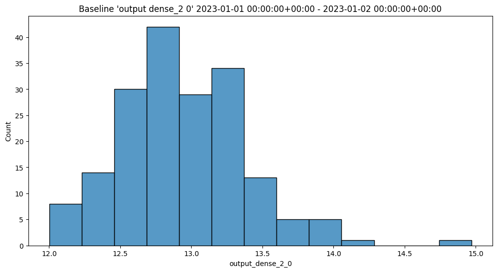
assay_builder.baseline_kde()
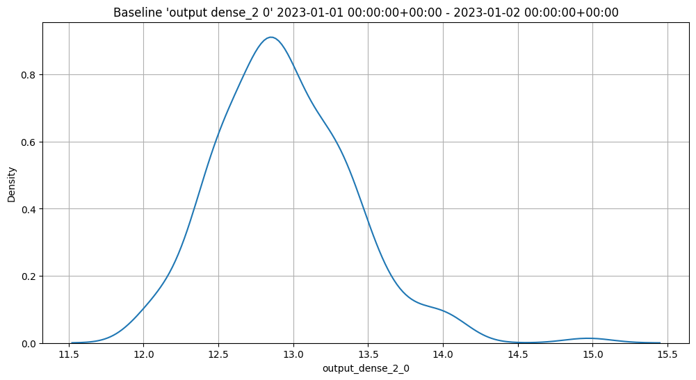
assay_builder.baseline_ecdf()
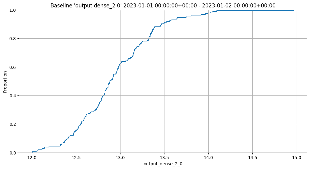
List Assays
Assays are listed through the Wallaroo Client list_assays method.
wl.list_assays()
| name | active | status | warning_threshold | alert_threshold | pipeline_name |
|---|---|---|---|---|---|
| api_assay | True | created | 0.0 | 0.1 | housepricepipe |
Interactive Baseline Runs
We can do an interactive run of just the baseline part to see how the baseline data will be put into bins. This assay uses quintiles so all 5 bins (not counting the outlier bins) have 20% of the predictions. We can see the bin boundaries along the x-axis.
baseline_run.chart()
baseline mean = 12.940910643273655
baseline median = 12.884286880493164
bin_mode = Quantile
aggregation = Density
metric = PSI
weighted = False
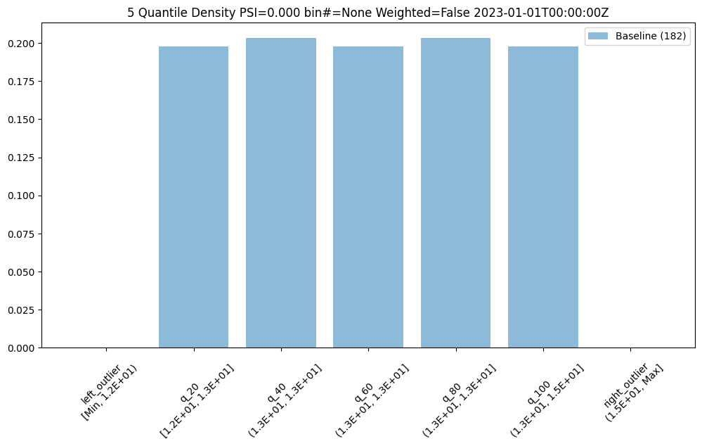
We can also get a dataframe with the bin/edge information.
baseline_run.baseline_bins()
| b_edges | b_edge_names | b_aggregated_values | b_aggregation | |
|---|---|---|---|---|
| 0 | 12.00 | left_outlier | 0.00 | Density |
| 1 | 12.55 | q_20 | 0.20 | Density |
| 2 | 12.81 | q_40 | 0.20 | Density |
| 3 | 12.98 | q_60 | 0.20 | Density |
| 4 | 13.33 | q_80 | 0.20 | Density |
| 5 | 14.97 | q_100 | 0.20 | Density |
| 6 | inf | right_outlier | 0.00 | Density |
The previous assay used quintiles so all of the bins had the same percentage/count of samples. To get bins that are divided equaly along the range of values we can use BinMode.EQUAL.
equal_bin_builder = wl.build_assay(assay_name, pipeline, model_name, baseline_start, baseline_end)
equal_bin_builder.summarizer_builder.add_bin_mode(BinMode.EQUAL)
equal_baseline = equal_bin_builder.build().interactive_baseline_run()
equal_baseline.chart()
baseline mean = 12.940910643273655
baseline median = 12.884286880493164
bin_mode = Equal
aggregation = Density
metric = PSI
weighted = False
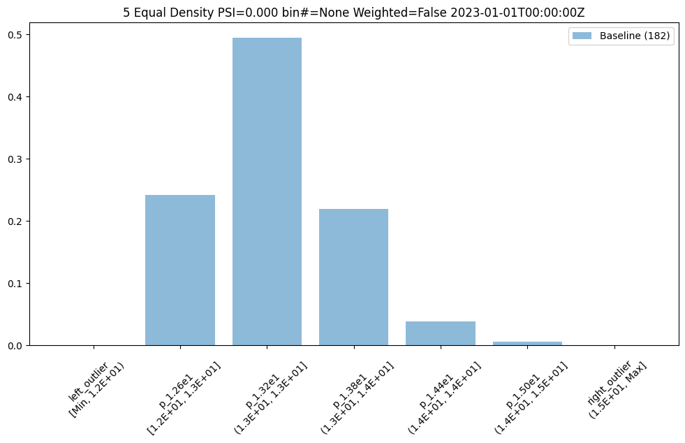
We now see very different bin edges and sample percentages per bin.
equal_baseline.baseline_bins()
| b_edges | b_edge_names | b_aggregated_values | b_aggregation | |
|---|---|---|---|---|
| 0 | 12.00 | left_outlier | 0.00 | Density |
| 1 | 12.60 | p_1.26e1 | 0.24 | Density |
| 2 | 13.19 | p_1.32e1 | 0.49 | Density |
| 3 | 13.78 | p_1.38e1 | 0.22 | Density |
| 4 | 14.38 | p_1.44e1 | 0.04 | Density |
| 5 | 14.97 | p_1.50e1 | 0.01 | Density |
| 6 | inf | right_outlier | 0.00 | Density |
Interactive Assay Runs
By default the assay builder creates an assay with some good starting parameters. In particular the assay is configured to run a new analysis for every 24 hours starting at the end of the baseline period. Additionally, it sets the number of bins to 5 so creates quintiles, and sets the target iopath to "outputs 0 0" which means we want to monitor the first column of the first output/prediction.
We can do an interactive run of just the baseline part to see how the baseline data will be put into bins. This assay uses quintiles so all 5 bins (not counting the outlier bins) have 20% of the predictions. We can see the bin boundaries along the x-axis.
We then run it with interactive_run and convert it to a dataframe for easy analysis with to_dataframe.
Now lets do an interactive run of the first assay as it is configured. Interactive runs don’t save the assay to the database (so they won’t be scheduled in the future) nor do they save the assay results. Instead the results are returned after a short while for further analysis.
assay_builder = wl.build_assay(assay_name, pipeline, model_name, baseline_start, baseline_end)
assay_config = assay_builder.add_run_until(last_day).build()
assay_results = assay_config.interactive_run()
assay_df = assay_results.to_dataframe()
assay_df.loc[:, ~assay_df.columns.isin(['assay_id', 'iopath', 'name', 'warning_threshold'])]
| score | start | min | max | mean | median | std | alert_threshold | status | |
|---|---|---|---|---|---|---|---|---|---|
| 0 | 0.00 | 2023-01-02T00:00:00+00:00 | 12.05 | 14.71 | 12.97 | 12.90 | 0.48 | 0.25 | Ok |
| 1 | 0.09 | 2023-01-03T00:00:00+00:00 | 12.04 | 14.65 | 12.96 | 12.93 | 0.41 | 0.25 | Ok |
| 2 | 0.04 | 2023-01-04T00:00:00+00:00 | 11.87 | 14.02 | 12.98 | 12.95 | 0.46 | 0.25 | Ok |
| 3 | 0.06 | 2023-01-05T00:00:00+00:00 | 11.92 | 14.46 | 12.93 | 12.87 | 0.46 | 0.25 | Ok |
| 4 | 0.02 | 2023-01-06T00:00:00+00:00 | 12.02 | 14.15 | 12.95 | 12.90 | 0.43 | 0.25 | Ok |
| 5 | 0.03 | 2023-01-07T00:00:00+00:00 | 12.18 | 14.58 | 12.96 | 12.93 | 0.44 | 0.25 | Ok |
| 6 | 0.02 | 2023-01-08T00:00:00+00:00 | 12.01 | 14.60 | 12.92 | 12.90 | 0.46 | 0.25 | Ok |
| 7 | 0.04 | 2023-01-09T00:00:00+00:00 | 12.01 | 14.40 | 13.00 | 12.97 | 0.45 | 0.25 | Ok |
| 8 | 0.06 | 2023-01-10T00:00:00+00:00 | 11.99 | 14.79 | 12.94 | 12.91 | 0.46 | 0.25 | Ok |
| 9 | 0.02 | 2023-01-11T00:00:00+00:00 | 11.90 | 14.66 | 12.91 | 12.88 | 0.45 | 0.25 | Ok |
| 10 | 0.02 | 2023-01-12T00:00:00+00:00 | 11.96 | 14.82 | 12.94 | 12.90 | 0.46 | 0.25 | Ok |
| 11 | 0.03 | 2023-01-13T00:00:00+00:00 | 12.07 | 14.61 | 12.96 | 12.93 | 0.47 | 0.25 | Ok |
| 12 | 0.15 | 2023-01-14T00:00:00+00:00 | 12.00 | 14.20 | 13.06 | 13.03 | 0.43 | 0.25 | Ok |
| 13 | 2.92 | 2023-01-15T00:00:00+00:00 | 12.74 | 15.62 | 14.00 | 14.01 | 0.57 | 0.25 | Alert |
| 14 | 7.89 | 2023-01-16T00:00:00+00:00 | 14.64 | 17.19 | 15.91 | 15.87 | 0.63 | 0.25 | Alert |
| 15 | 8.87 | 2023-01-17T00:00:00+00:00 | 16.60 | 19.23 | 17.94 | 17.94 | 0.63 | 0.25 | Alert |
| 16 | 8.87 | 2023-01-18T00:00:00+00:00 | 18.67 | 21.29 | 20.01 | 20.04 | 0.64 | 0.25 | Alert |
| 17 | 8.87 | 2023-01-19T00:00:00+00:00 | 20.72 | 23.57 | 22.17 | 22.18 | 0.65 | 0.25 | Alert |
| 18 | 8.87 | 2023-01-20T00:00:00+00:00 | 23.04 | 25.72 | 24.32 | 24.33 | 0.66 | 0.25 | Alert |
| 19 | 8.87 | 2023-01-21T00:00:00+00:00 | 25.06 | 27.67 | 26.48 | 26.49 | 0.63 | 0.25 | Alert |
| 20 | 8.87 | 2023-01-22T00:00:00+00:00 | 27.21 | 29.89 | 28.63 | 28.58 | 0.65 | 0.25 | Alert |
| 21 | 8.87 | 2023-01-23T00:00:00+00:00 | 29.36 | 32.18 | 30.82 | 30.80 | 0.67 | 0.25 | Alert |
| 22 | 8.87 | 2023-01-24T00:00:00+00:00 | 31.56 | 34.35 | 32.98 | 32.98 | 0.65 | 0.25 | Alert |
| 23 | 8.87 | 2023-01-25T00:00:00+00:00 | 33.68 | 36.44 | 35.14 | 35.14 | 0.66 | 0.25 | Alert |
| 24 | 8.87 | 2023-01-26T00:00:00+00:00 | 35.93 | 38.51 | 37.31 | 37.33 | 0.65 | 0.25 | Alert |
| 25 | 3.69 | 2023-01-27T00:00:00+00:00 | 12.06 | 39.91 | 29.29 | 38.65 | 12.66 | 0.25 | Alert |
| 26 | 0.05 | 2023-01-28T00:00:00+00:00 | 11.87 | 13.88 | 12.92 | 12.90 | 0.38 | 0.25 | Ok |
| 27 | 0.10 | 2023-01-29T00:00:00+00:00 | 12.02 | 14.36 | 12.98 | 12.96 | 0.38 | 0.25 | Ok |
| 28 | 0.11 | 2023-01-30T00:00:00+00:00 | 11.99 | 14.44 | 12.89 | 12.88 | 0.37 | 0.25 | Ok |
| 29 | 0.01 | 2023-01-31T00:00:00+00:00 | 12.00 | 14.64 | 12.92 | 12.89 | 0.40 | 0.25 | Ok |
Basic functionality for creating quick charts is included.
assay_results.chart_scores()
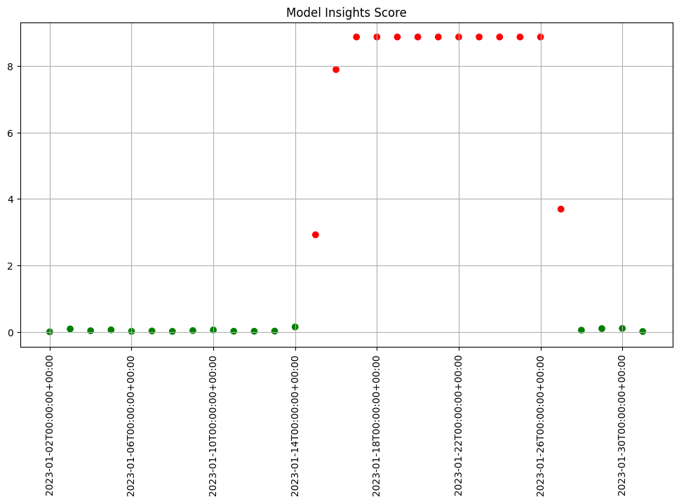
We see that the difference scores are low for a while and then jump up to indicate there is an issue. We can examine that particular window to help us decide if that threshold is set correctly or not.
We can generate a quick chart of the results. This chart shows the 5 quantile bins (quintiles) derived from the baseline data plus one for left outliers and one for right outliers. We also see that the data from the window falls within the baseline quintiles but in a different proportion and is skewing higher. Whether this is an issue or not is specific to your use case.
First lets examine a day that is only slightly different than the baseline. We see that we do see some values that fall outside of the range from the baseline values, the left and right outliers, and that the bin values are different but similar.
assay_results[0].chart()
baseline mean = 12.940910643273655
window mean = 12.969964654406132
baseline median = 12.884286880493164
window median = 12.899214744567873
bin_mode = Quantile
aggregation = Density
metric = PSI
weighted = False
score = 0.0029273068646199748
scores = [0.0, 0.000514261205558409, 0.0002139202456922972, 0.0012617897456473992, 0.0002139202456922972, 0.0007234154220295724, 0.0]
index = None

Other days, however are significantly different.
assay_results[12].chart()
baseline mean = 12.940910643273655
window mean = 13.06380216891949
baseline median = 12.884286880493164
window median = 13.027600288391112
bin_mode = Quantile
aggregation = Density
metric = PSI
weighted = False
score = 0.15060511096978788
scores = [4.6637149189075455e-05, 0.05969428191167242, 0.00806617426854112, 0.008316273402678306, 0.07090885609902021, 0.003572888138686759, 0.0]
index = None

assay_results[13].chart()
baseline mean = 12.940910643273655
window mean = 14.004728427908038
baseline median = 12.884286880493164
window median = 14.009637832641602
bin_mode = Quantile
aggregation = Density
metric = PSI
weighted = False
score = 2.9220486095961196
scores = [0.0, 0.7090936334784107, 0.7130482300184766, 0.33500731896676245, 0.12171058214520876, 0.9038825518183468, 0.1393062931689142]
index = None
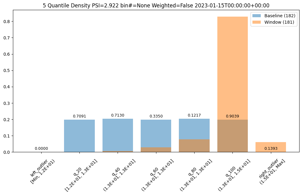
If we want to investigate further, we can run interactive assays on each of the inputs to see if any of them show anything abnormal. In this example we’ll provide the feature labels to create more understandable titles.
The current assay expects continuous data. Sometimes categorical data is encoded as 1 or 0 in a feature and sometimes in a limited number of values such as 1, 2, 3. If one value has high a percentage the analysis emits a warning so that we know the scores for that feature may not behave as we expect.
labels = ['bedrooms', 'bathrooms', 'lat', 'long', 'waterfront', 'sqft_living', 'sqft_lot', 'floors', 'view', 'condition', 'grade', 'sqft_above', 'sqft_basement', 'yr_built', 'yr_renovated', 'sqft_living15', 'sqft_lot15']

topic = wl.get_topic_name(pipeline.id())

all_inferences = wl.get_raw_pipeline_inference_logs(topic, baseline_start, last_day, model_name, limit=1_000_000)

assay_builder = wl.build_assay("Input Assay", pipeline, model_name, baseline_start, baseline_end).add_run_until(last_day)
assay_builder.window_builder().add_width(hours=4)
assay_config = assay_builder.build()
assay_results = assay_config.interactive_input_run(all_inferences, labels)
iadf = assay_results.to_dataframe()
display(iadf.loc[:, ~iadf.columns.isin(['assay_id', 'iopath', 'name', 'warning_threshold'])])
column distinct_vals label           largest_pct
     0            17 bedrooms        0.4244
     1            44 bathrooms       0.2398
     2          3281 lat             0.0014
     3           959 long            0.0066
     4             4 waterfront      0.9156 *** May not be continuous feature
     5          3901 sqft_living     0.0032
     6          3487 sqft_lot        0.0173
     7            11 floors          0.4567
     8            10 view            0.8337
     9             9 condition       0.5915
    10            19 grade           0.3943
    11           745 sqft_above      0.0096
    12           309 sqft_basement   0.5582
    13           224 yr_built        0.0239
    14            77 yr_renovated    0.8889
    15           649 sqft_living15   0.0093
    16          3280 sqft_lot15      0.0199
| score | start | min | max | mean | median | std | alert_threshold | status | |
|---|---|---|---|---|---|---|---|---|---|
| 0 | 0.19 | 2023-01-02T00:00:00+00:00 | -2.54 | 1.75 | 0.21 | 0.68 | 0.99 | 0.25 | Ok |
| 1 | 0.03 | 2023-01-02T04:00:00+00:00 | -1.47 | 2.82 | 0.21 | -0.40 | 0.95 | 0.25 | Ok |
| 2 | 0.09 | 2023-01-02T08:00:00+00:00 | -2.54 | 3.89 | -0.04 | -0.40 | 1.22 | 0.25 | Ok |
| 3 | 0.05 | 2023-01-02T12:00:00+00:00 | -1.47 | 2.82 | -0.12 | -0.40 | 0.94 | 0.25 | Ok |
| 4 | 0.08 | 2023-01-02T16:00:00+00:00 | -1.47 | 1.75 | -0.00 | -0.40 | 0.76 | 0.25 | Ok |
| ... | ... | ... | ... | ... | ... | ... | ... | ... | ... |
| 3055 | 0.08 | 2023-01-31T04:00:00+00:00 | -0.42 | 4.87 | 0.25 | -0.17 | 1.13 | 0.25 | Ok |
| 3056 | 0.58 | 2023-01-31T08:00:00+00:00 | -0.43 | 2.01 | -0.04 | -0.21 | 0.48 | 0.25 | Alert |
| 3057 | 0.13 | 2023-01-31T12:00:00+00:00 | -0.32 | 7.75 | 0.30 | -0.20 | 1.57 | 0.25 | Ok |
| 3058 | 0.26 | 2023-01-31T16:00:00+00:00 | -0.43 | 5.88 | 0.19 | -0.18 | 1.17 | 0.25 | Alert |
| 3059 | 0.84 | 2023-01-31T20:00:00+00:00 | -0.40 | 0.52 | -0.17 | -0.25 | 0.18 | 0.25 | Alert |
3060 rows × 9 columns
We can chart each of the iopaths and do a visual inspection. From the charts we see that if any of the input features had significant differences in the first two days which we can choose to inspect further. Here we choose to show 3 charts just to save space in this notebook.
assay_results.chart_iopaths(labels=labels, selected_labels=['bedrooms', 'lat', 'sqft_living'])
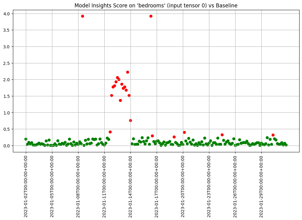
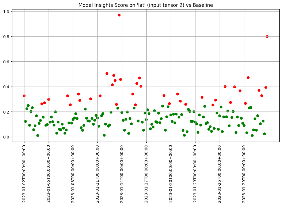
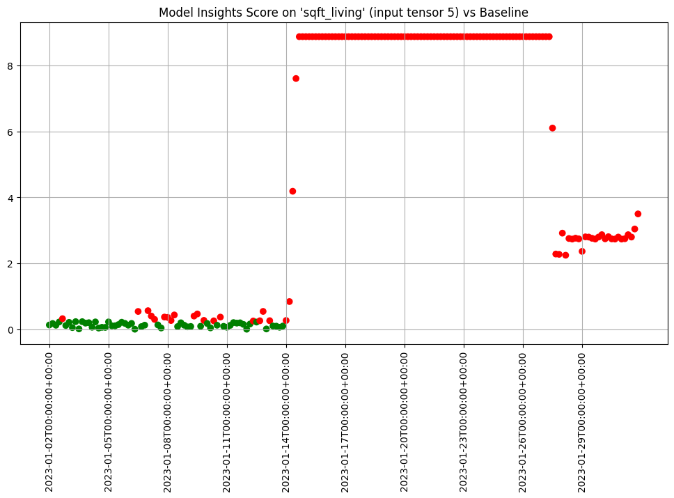
When we are comfortable with what alert threshold should be for our specific purposes we can create and save an assay that will be automatically run on a daily basis.
In this example we’re create an assay that runs everyday against the baseline and has an alert threshold of 0.5.
Once we upload it it will be saved and scheduled for future data as well as run against past data.
alert_threshold = 0.5
import string
import random

prefix= ''.join(random.choice(string.ascii_lowercase) for i in range(4))

assay_name = f"{prefix}example assay"
assay_builder = wl.build_assay(assay_name, pipeline, model_name, baseline_start, baseline_end).add_alert_threshold(alert_threshold)
assay_id = assay_builder.upload()
After a short while, we can get the assay results for further analysis.
When we get the assay results, we see that the assays analysis is similar to the interactive run we started with though the analysis for the third day does not exceed the new alert threshold we set. And since we called upload instead of interactive_run the assay was saved to the system and will continue to run automatically on schedule from now on.
Scheduling Assays
By default assays are scheduled to run every 24 hours starting immediately after the baseline period ends.
However, you can control the start time by setting start and the frequency by setting interval on the window.
So to recap:
- The window width is the size of the window. The default is 24 hours.
- The interval is how often the analysis is run, how far the window is slid into the future based on the last run. The default is the window width.
- The window start is when the analysis should start. The default is the end of the baseline period.
For example to run an analysis every 12 hours on the previous 24 hours of data you’d set the window width to 24 (the default) and the interval to 12.
assay_builder = wl.build_assay(assay_name, pipeline, model_name, baseline_start, baseline_end)
assay_builder = assay_builder.add_run_until(last_day)

assay_builder.window_builder().add_width(hours=24).add_interval(hours=12)

assay_config = assay_builder.build()

assay_results = assay_config.interactive_run()
print(f"Generated {len(assay_results)} analyses")
Generated 59 analyses
assay_results.chart_scores()
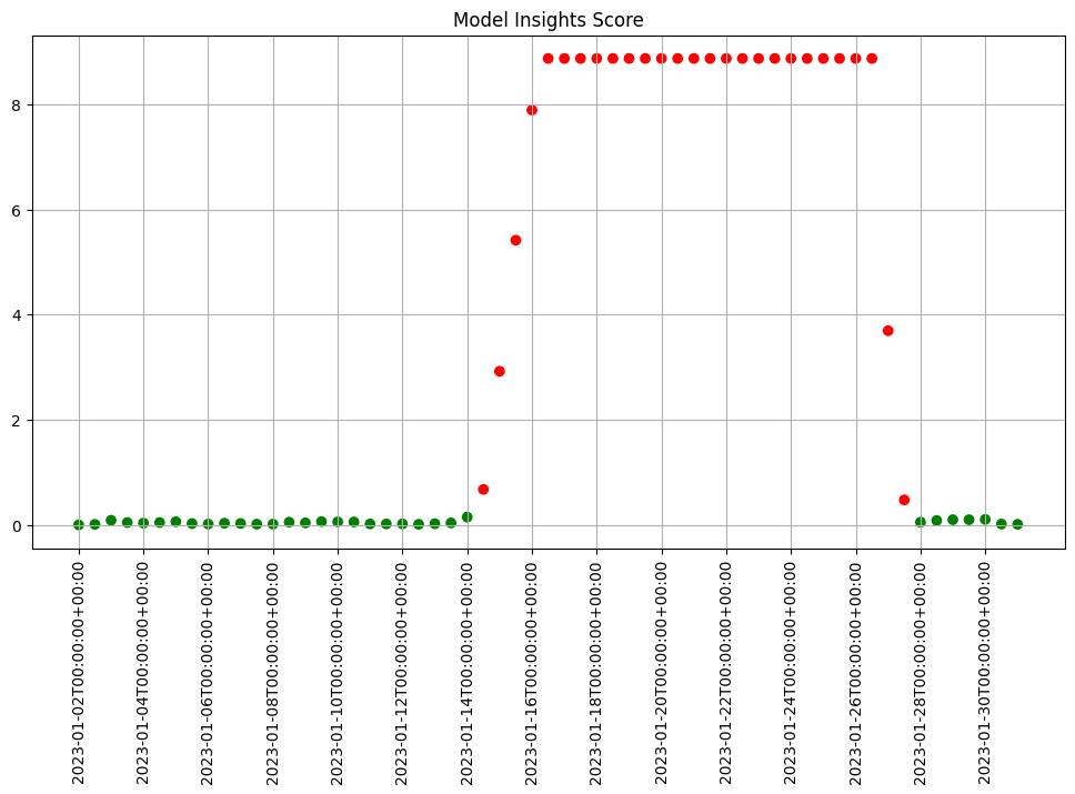
To start a weekly analysis of the previous week on a specific day, set the start date (taking care to specify the desired timezone), and the width and interval to 1 week and of course an analysis won’t be generated till a window is complete.
By default, assay start date is set to 24 hours from when the assay was created. For this example, we will set the assay.window_builder.add_start to set the assay window to start at the beginning of our data, and assay.add_run_until to set the time period to stop gathering data from.
report_start = datetime.datetime.fromisoformat('2022-01-03T00:00:00+00:00')

assay_builder = wl.build_assay(assay_name, pipeline, model_name, baseline_start, baseline_end)
assay_builder = assay_builder.add_run_until(last_day)

assay_builder.window_builder().add_width(weeks=1).add_interval(weeks=1).add_start(report_start)

assay_config = assay_builder.build()

assay_results = assay_config.interactive_run()
print(f"Generated {len(assay_results)} analyses")
Generated 5 analyses
assay_results.chart_scores()
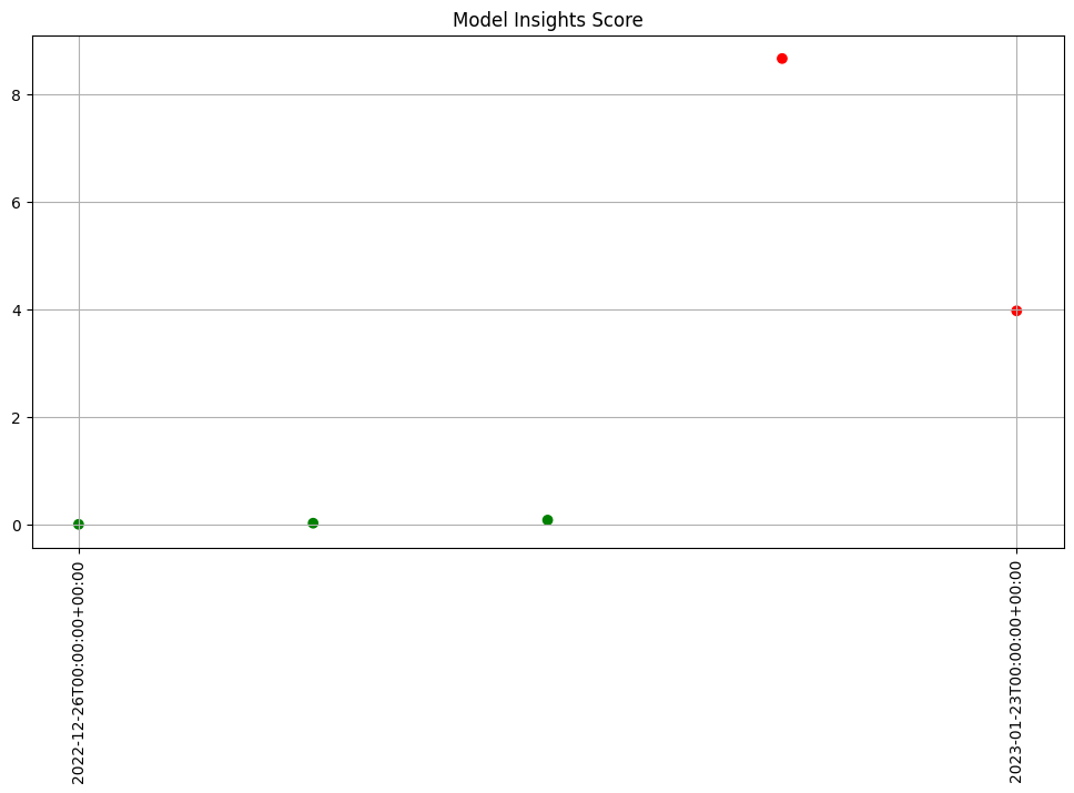
Advanced Configuration
The assay can be configured in a variety of ways to help customize it to your particular needs. Specifically you can:
- change the BinMode to evenly spaced, quantile or user provided
- change the number of bins to use
- provide weights to use when scoring the bins
- calculate the score using the sum of differences, maximum difference or population stability index
- change the value aggregation for the bins to density, cumulative or edges
Lets take a look at these in turn.
Default configuration
First lets look at the default configuration. This is a lot of information but much of it is useful to know where it is available.
We see that the assay is broken up into 4 sections. A top level meta data section, a section for the baseline specification, a section for the window specification and a section that specifies the summarization configuration.
In the meta section we see the name of the assay, that it runs on the first column of the first output "outputs 0 0" and that there is a default threshold of 0.25.
The summarizer section shows us the defaults of Quantile, Density and PSI on 5 bins.
The baseline section shows us that it is configured as a fixed baseline with the specified start and end date times.
And the window tells us what model in the pipeline we are analyzing and how often.
assay_builder = wl.build_assay(assay_name, pipeline, model_name, baseline_start, baseline_end).add_run_until(last_day)
print(assay_builder.build().to_json())
{
    "name": "onmyexample assay",
    "pipeline_id": 1,
    "pipeline_name": "housepricepipe",
    "active": true,
    "status": "created",
    "iopath": "output dense_2 0",
    "baseline": {
        "Fixed": {
            "pipeline": "housepricepipe",
            "model": "housepricemodel",
            "start_at": "2023-01-01T00:00:00+00:00",
            "end_at": "2023-01-02T00:00:00+00:00"
        }
    },
    "window": {
        "pipeline": "housepricepipe",
        "model": "housepricemodel",
        "width": "24 hours",
        "start": null,
        "interval": null
    },
    "summarizer": {
        "type": "UnivariateContinuous",
        "bin_mode": "Quantile",
        "aggregation": "Density",
        "metric": "PSI",
        "num_bins": 5,
        "bin_weights": null,
        "bin_width": null,
        "provided_edges": null,
        "add_outlier_edges": true
    },
    "warning_threshold": null,
    "alert_threshold": 0.25,
    "run_until": "2023-02-01T00:00:00+00:00",
    "workspace_id": 5
}
Defaults
We can run the assay interactively and review the first analysis. The method compare_basic_stats gives us a dataframe with basic stats for the baseline and window data.
assay_results = assay_builder.build().interactive_run()
ar = assay_results[0]

ar.compare_basic_stats()
| Baseline | Window | diff | pct_diff | |
|---|---|---|---|---|
| count | 182.00 | 181.00 | -1.00 | -0.55 |
| min | 12.00 | 12.05 | 0.04 | 0.36 |
| max | 14.97 | 14.71 | -0.26 | -1.71 |
| mean | 12.94 | 12.97 | 0.03 | 0.22 |
| median | 12.88 | 12.90 | 0.01 | 0.12 |
| std | 0.45 | 0.48 | 0.03 | 5.68 |
| start | 2023-01-01T00:00:00+00:00 | 2023-01-02T00:00:00+00:00 | NaN | NaN |
| end | 2023-01-02T00:00:00+00:00 | 2023-01-03T00:00:00+00:00 | NaN | NaN |
The method compare_bins gives us a dataframe with the bin information. Such as the number of bins, the right edges, suggested bin/edge names and the values for each bin in the baseline and the window.
assay_bins = ar.compare_bins()
display(assay_bins.loc[:, assay_bins.columns!='w_aggregation'])
| b_edges | b_edge_names | b_aggregated_values | b_aggregation | w_edges | w_edge_names | w_aggregated_values | diff_in_pcts | |
|---|---|---|---|---|---|---|---|---|
| 0 | 12.00 | left_outlier | 0.00 | Density | 12.00 | left_outlier | 0.00 | 0.00 |
| 1 | 12.55 | q_20 | 0.20 | Density | 12.55 | e_1.26e1 | 0.19 | -0.01 |
| 2 | 12.81 | q_40 | 0.20 | Density | 12.81 | e_1.28e1 | 0.21 | 0.01 |
| 3 | 12.98 | q_60 | 0.20 | Density | 12.98 | e_1.30e1 | 0.18 | -0.02 |
| 4 | 13.33 | q_80 | 0.20 | Density | 13.33 | e_1.33e1 | 0.21 | 0.01 |
| 5 | 14.97 | q_100 | 0.20 | Density | 14.97 | e_1.50e1 | 0.21 | 0.01 |
| 6 | NaN | right_outlier | 0.00 | Density | NaN | right_outlier | 0.00 | 0.00 |
We can also plot the chart to visualize the values of the bins.
ar.chart()
baseline mean = 12.940910643273655
window mean = 12.969964654406132
baseline median = 12.884286880493164
window median = 12.899214744567873
bin_mode = Quantile
aggregation = Density
metric = PSI
weighted = False
score = 0.0029273068646199748
scores = [0.0, 0.000514261205558409, 0.0002139202456922972, 0.0012617897456473992, 0.0002139202456922972, 0.0007234154220295724, 0.0]
index = None
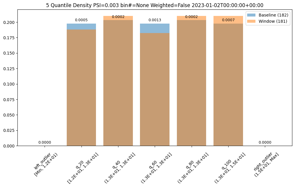
Binning Mode
We can change the bin mode algorithm to equal and see that the bins/edges are partitioned at different points and the bins have different values.
prefix= ''.join(random.choice(string.ascii_lowercase) for i in range(4))

assay_name = f"{prefix}example assay"

assay_builder = wl.build_assay(assay_name, pipeline, model_name, baseline_start, baseline_end).add_run_until(last_day)
assay_builder.summarizer_builder.add_bin_mode(BinMode.EQUAL)
assay_results = assay_builder.build().interactive_run()
assay_results_df = assay_results[0].compare_bins()
display(assay_results_df.loc[:, ~assay_results_df.columns.isin(['b_aggregation', 'w_aggregation'])])
assay_results[0].chart()
| b_edges | b_edge_names | b_aggregated_values | w_edges | w_edge_names | w_aggregated_values | diff_in_pcts | |
|---|---|---|---|---|---|---|---|
| 0 | 12.00 | left_outlier | 0.00 | 12.00 | left_outlier | 0.00 | 0.00 |
| 1 | 12.60 | p_1.26e1 | 0.24 | 12.60 | e_1.26e1 | 0.24 | 0.00 |
| 2 | 13.19 | p_1.32e1 | 0.49 | 13.19 | e_1.32e1 | 0.48 | -0.02 |
| 3 | 13.78 | p_1.38e1 | 0.22 | 13.78 | e_1.38e1 | 0.22 | -0.00 |
| 4 | 14.38 | p_1.44e1 | 0.04 | 14.38 | e_1.44e1 | 0.06 | 0.02 |
| 5 | 14.97 | p_1.50e1 | 0.01 | 14.97 | e_1.50e1 | 0.01 | 0.00 |
| 6 | NaN | right_outlier | 0.00 | NaN | right_outlier | 0.00 | 0.00 |
baseline mean = 12.940910643273655
window mean = 12.969964654406132
baseline median = 12.884286880493164
window median = 12.899214744567873
bin_mode = Equal
aggregation = Density
metric = PSI
weighted = False
score = 0.011074287819376092
scores = [0.0, 7.3591419975306595e-06, 0.000773779195360713, 8.538514991838585e-05, 0.010207597078872246, 1.6725322721660374e-07, 0.0]
index = None
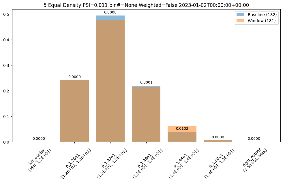
User Provided Bin Edges
The values in this dataset run from ~11.6 to ~15.81. And lets say we had a business reason to use specific bin edges. We can specify them with the BinMode.PROVIDED and specifying a list of floats with the right hand / upper edge of each bin and optionally the lower edge of the smallest bin. If the lowest edge is not specified the threshold for left outliers is taken from the smallest value in the baseline dataset.
edges = [11.0, 12.0, 13.0, 14.0, 15.0, 16.0]
assay_builder = wl.build_assay(assay_name, pipeline, model_name, baseline_start, baseline_end).add_run_until(last_day)
assay_builder.summarizer_builder.add_bin_mode(BinMode.PROVIDED, edges)
assay_results = assay_builder.build().interactive_run()
assay_results_df = assay_results[0].compare_bins()
display(assay_results_df.loc[:, ~assay_results_df.columns.isin(['b_aggregation', 'w_aggregation'])])
assay_results[0].chart()
| b_edges | b_edge_names | b_aggregated_values | w_edges | w_edge_names | w_aggregated_values | diff_in_pcts | |
|---|---|---|---|---|---|---|---|
| 0 | 11.00 | left_outlier | 0.00 | 11.00 | left_outlier | 0.00 | 0.00 |
| 1 | 12.00 | e_1.20e1 | 0.00 | 12.00 | e_1.20e1 | 0.00 | 0.00 |
| 2 | 13.00 | e_1.30e1 | 0.62 | 13.00 | e_1.30e1 | 0.59 | -0.03 |
| 3 | 14.00 | e_1.40e1 | 0.36 | 14.00 | e_1.40e1 | 0.35 | -0.00 |
| 4 | 15.00 | e_1.50e1 | 0.02 | 15.00 | e_1.50e1 | 0.06 | 0.03 |
| 5 | 16.00 | e_1.60e1 | 0.00 | 16.00 | e_1.60e1 | 0.00 | 0.00 |
| 6 | NaN | right_outlier | 0.00 | NaN | right_outlier | 0.00 | 0.00 |
baseline mean = 12.940910643273655
window mean = 12.969964654406132
baseline median = 12.884286880493164
window median = 12.899214744567873
bin_mode = Provided
aggregation = Density
metric = PSI
weighted = False
score = 0.0321620386600679
scores = [0.0, 0.0, 0.0014576920813015586, 3.549754401142936e-05, 0.030668849034754912, 0.0, 0.0]
index = None
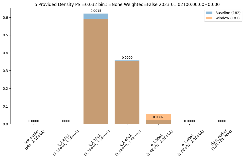
Number of Bins
We could also choose to a different number of bins, lets say 10, which can be evenly spaced or based on the quantiles (deciles).
assay_builder = wl.build_assay(assay_name, pipeline, model_name, baseline_start, baseline_end).add_run_until(last_day)
assay_builder.summarizer_builder.add_bin_mode(BinMode.QUANTILE).add_num_bins(10)
assay_results = assay_builder.build().interactive_run()
assay_results_df = assay_results[1].compare_bins()
display(assay_results_df.loc[:, ~assay_results_df.columns.isin(['b_aggregation', 'w_aggregation'])])
assay_results[1].chart()
| b_edges | b_edge_names | b_aggregated_values | w_edges | w_edge_names | w_aggregated_values | diff_in_pcts | |
|---|---|---|---|---|---|---|---|
| 0 | 12.00 | left_outlier | 0.00 | 12.00 | left_outlier | 0.00 | 0.00 |
| 1 | 12.41 | q_10 | 0.10 | 12.41 | e_1.24e1 | 0.09 | -0.00 |
| 2 | 12.55 | q_20 | 0.10 | 12.55 | e_1.26e1 | 0.04 | -0.05 |
| 3 | 12.72 | q_30 | 0.10 | 12.72 | e_1.27e1 | 0.14 | 0.03 |
| 4 | 12.81 | q_40 | 0.10 | 12.81 | e_1.28e1 | 0.05 | -0.05 |
| 5 | 12.88 | q_50 | 0.10 | 12.88 | e_1.29e1 | 0.12 | 0.02 |
| 6 | 12.98 | q_60 | 0.10 | 12.98 | e_1.30e1 | 0.09 | -0.01 |
| 7 | 13.15 | q_70 | 0.10 | 13.15 | e_1.32e1 | 0.18 | 0.08 |
| 8 | 13.33 | q_80 | 0.10 | 13.33 | e_1.33e1 | 0.14 | 0.03 |
| 9 | 13.47 | q_90 | 0.10 | 13.47 | e_1.35e1 | 0.07 | -0.03 |
| 10 | 14.97 | q_100 | 0.10 | 14.97 | e_1.50e1 | 0.08 | -0.02 |
| 11 | NaN | right_outlier | 0.00 | NaN | right_outlier | 0.00 | 0.00 |
baseline mean = 12.940910643273655
window mean = 12.956829186961135
baseline median = 12.884286880493164
window median = 12.929338455200195
bin_mode = Quantile
aggregation = Density
metric = PSI
weighted = False
score = 0.16591076620684958
scores = [0.0, 0.0002571306027792045, 0.044058279699182114, 0.009441459631493015, 0.03381618572319047, 0.0027335446937028877, 0.0011792419836838435, 0.051023062424253904, 0.009441459631493015, 0.008662563542113508, 0.0052978382749576496, 0.0]
index = None
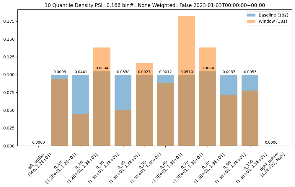
Bin Weights
Now lets say we only care about differences at the higher end of the range. We can use weights to specify that difference in the lower bins should not be counted in the score.
If we stick with 10 bins we can provide 10 a vector of 12 weights. One weight each for the original bins plus one at the front for the left outlier bin and one at the end for the right outlier bin.
Note we still show the values for the bins but the scores for the lower 5 and left outlier are 0 and only the right half is counted and reflected in the score.
weights = [0] * 6
weights.extend([1] * 6)
print("Using weights: ", weights)
assay_builder = wl.build_assay(assay_name, pipeline, model_name, baseline_start, baseline_end).add_run_until(last_day)
assay_builder.summarizer_builder.add_bin_mode(BinMode.QUANTILE).add_num_bins(10).add_bin_weights(weights)
assay_results = assay_builder.build().interactive_run()
assay_results_df = assay_results[1].compare_bins()
display(assay_results_df.loc[:, ~assay_results_df.columns.isin(['b_aggregation', 'w_aggregation'])])
assay_results[1].chart()
Using weights: [0, 0, 0, 0, 0, 0, 1, 1, 1, 1, 1, 1]
| b_edges | b_edge_names | b_aggregated_values | w_edges | w_edge_names | w_aggregated_values | diff_in_pcts | |
|---|---|---|---|---|---|---|---|
| 0 | 12.00 | left_outlier | 0.00 | 12.00 | left_outlier | 0.00 | 0.00 |
| 1 | 12.41 | q_10 | 0.10 | 12.41 | e_1.24e1 | 0.09 | -0.00 |
| 2 | 12.55 | q_20 | 0.10 | 12.55 | e_1.26e1 | 0.04 | -0.05 |
| 3 | 12.72 | q_30 | 0.10 | 12.72 | e_1.27e1 | 0.14 | 0.03 |
| 4 | 12.81 | q_40 | 0.10 | 12.81 | e_1.28e1 | 0.05 | -0.05 |
| 5 | 12.88 | q_50 | 0.10 | 12.88 | e_1.29e1 | 0.12 | 0.02 |
| 6 | 12.98 | q_60 | 0.10 | 12.98 | e_1.30e1 | 0.09 | -0.01 |
| 7 | 13.15 | q_70 | 0.10 | 13.15 | e_1.32e1 | 0.18 | 0.08 |
| 8 | 13.33 | q_80 | 0.10 | 13.33 | e_1.33e1 | 0.14 | 0.03 |
| 9 | 13.47 | q_90 | 0.10 | 13.47 | e_1.35e1 | 0.07 | -0.03 |
| 10 | 14.97 | q_100 | 0.10 | 14.97 | e_1.50e1 | 0.08 | -0.02 |
| 11 | NaN | right_outlier | 0.00 | NaN | right_outlier | 0.00 | 0.00 |
baseline mean = 12.940910643273655
window mean = 12.956829186961135
baseline median = 12.884286880493164
window median = 12.929338455200195
bin_mode = Quantile
aggregation = Density
metric = PSI
weighted = True
score = 0.012600694309416988
scores = [0.0, 0.0, 0.0, 0.0, 0.0, 0.0, 0.00019654033061397393, 0.00850384373737565, 0.0015735766052488358, 0.0014437605903522511, 0.000882973045826275, 0.0]
index = None

Metrics
The score is a distance or dis-similarity measure. The larger it is the less similar the two distributions are. We currently support
summing the differences of each individual bin, taking the maximum difference and a modified Population Stability Index (PSI).
The following three charts use each of the metrics. Note how the scores change. The best one will depend on your particular use case.
assay_builder = wl.build_assay(assay_name, pipeline, model_name, baseline_start, baseline_end).add_run_until(last_day)
assay_results = assay_builder.build().interactive_run()
assay_results[0].chart()
baseline mean = 12.940910643273655
window mean = 12.969964654406132
baseline median = 12.884286880493164
window median = 12.899214744567873
bin_mode = Quantile
aggregation = Density
metric = PSI
weighted = False
score = 0.0029273068646199748
scores = [0.0, 0.000514261205558409, 0.0002139202456922972, 0.0012617897456473992, 0.0002139202456922972, 0.0007234154220295724, 0.0]
index = None

assay_builder = wl.build_assay(assay_name, pipeline, model_name, baseline_start, baseline_end).add_run_until(last_day)
assay_builder.summarizer_builder.add_metric(Metric.SUMDIFF)
assay_results = assay_builder.build().interactive_run()
assay_results[0].chart()
baseline mean = 12.940910643273655
window mean = 12.969964654406132
baseline median = 12.884286880493164
window median = 12.899214744567873
bin_mode = Quantile
aggregation = Density
metric = SumDiff
weighted = False
score = 0.025438649748041997
scores = [0.0, 0.009956893934794486, 0.006648048084512165, 0.01548175581324751, 0.006648048084512165, 0.012142553579017668, 0.0]
index = None

assay_builder = wl.build_assay(assay_name, pipeline, model_name, baseline_start, baseline_end).add_run_until(last_day)
assay_builder.summarizer_builder.add_metric(Metric.MAXDIFF)
assay_results = assay_builder.build().interactive_run()
assay_results[0].chart()
baseline mean = 12.940910643273655
window mean = 12.969964654406132
baseline median = 12.884286880493164
window median = 12.899214744567873
bin_mode = Quantile
aggregation = Density
metric = MaxDiff
weighted = False
score = 0.01548175581324751
scores = [0.0, 0.009956893934794486, 0.006648048084512165, 0.01548175581324751, 0.006648048084512165, 0.012142553579017668, 0.0]
index = 3
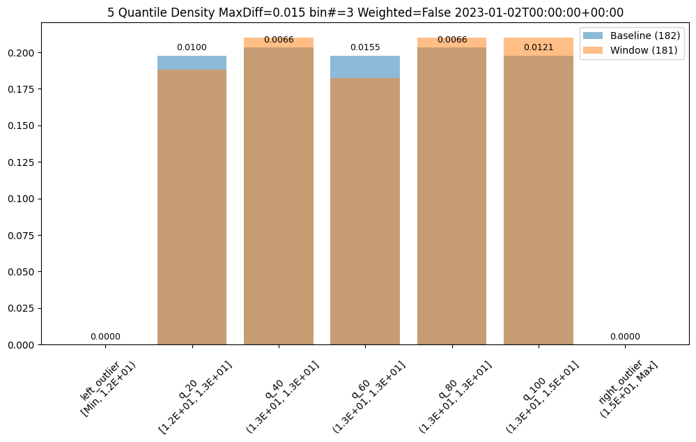
Aggregation Options
Also, bin aggregation can be done in histogram Aggregation.DENSITY style (the default) where we count the number/percentage of values that fall in each bin or Empirical Cumulative Density Function style Aggregation.CUMULATIVE where we keep a cumulative count of the values/percentages that fall in each bin.
assay_builder = wl.build_assay(assay_name, pipeline, model_name, baseline_start, baseline_end).add_run_until(last_day)
assay_builder.summarizer_builder.add_aggregation(Aggregation.DENSITY)
assay_results = assay_builder.build().interactive_run()
assay_results[0].chart()
baseline mean = 12.940910643273655
window mean = 12.969964654406132
baseline median = 12.884286880493164
window median = 12.899214744567873
bin_mode = Quantile
aggregation = Density
metric = PSI
weighted = False
score = 0.0029273068646199748
scores = [0.0, 0.000514261205558409, 0.0002139202456922972, 0.0012617897456473992, 0.0002139202456922972, 0.0007234154220295724, 0.0]
index = None

assay_builder = wl.build_assay(assay_name, pipeline, model_name, baseline_start, baseline_end).add_run_until(last_day)
assay_builder.summarizer_builder.add_aggregation(Aggregation.CUMULATIVE)
assay_results = assay_builder.build().interactive_run()
assay_results[0].chart()
baseline mean = 12.940910643273655
window mean = 12.969964654406132
baseline median = 12.884286880493164
window median = 12.899214744567873
bin_mode = Quantile
aggregation = Cumulative
metric = PSI
weighted = False
score = 0.04419889502762442
scores = [0.0, 0.009956893934794486, 0.0033088458502823492, 0.01879060166352986, 0.012142553579017725, 0.0, 0.0]
index = None
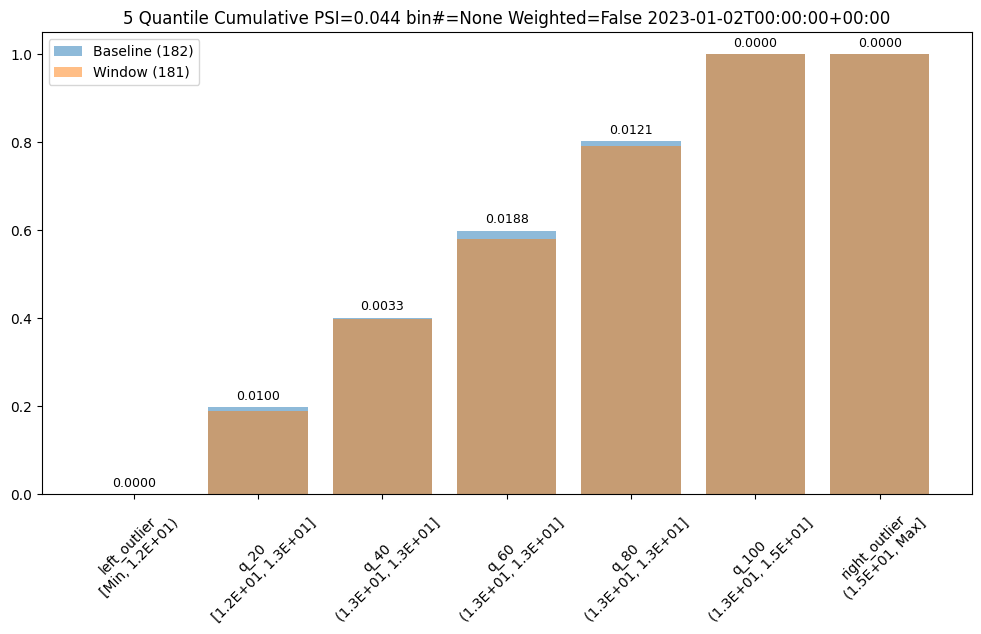
6 - Computer Vision Pipeline Logs MLOps API Tutorial
How to retrieve computer vision oriented pipeline logs through the Wallaroo MLOps API.
This tutorial and the assets can be downloaded as part of the Wallaroo Tutorials repository.
Pipeline API Log Tutorial
This tutorial demonstrates Wallaroo Pipeline MLOps API for pipeline log retrieval for Computer Vision based models.
This tutorial will demonstrate how to:
- Select or create a workspace, pipeline and upload the control model, and additional testing models.
- Add a pipeline step with the champion model, then deploy the pipeline and perform sample inferences for computer vision detection.
- Retrieve the logs via the Wallaroo MLOps API. These steps will be simplified to only show the API log retrieval method. See the Wallaroo Documentation site for full details.
- Use the pipeline logs to display metadata data.
- Undeploy the pipeline.
This tutorial provides the following:
- Models:
models/yolov8n.onnx: A pre-trained Yolov8n model.
- Data:
data/dogbike.png: A PNG image with a dog and bicycle.data/dogbike.df.json: A pandas Record format JSON file of the PNG image converted to numpy array values for inference requests.
Prerequisites
- A deployed Wallaroo instance
- The following Python libraries installed:
wallaroo: The Wallaroo SDK. Included with the Wallaroo JupyterHub service by default.
Initial Steps
Import libraries
The first step is to import the libraries needed for this notebook.
import wallaroo
from wallaroo.object import EntityNotFoundError

import pyarrow as pa

from IPython.display import display

# used to display DataFrame information without truncating
from IPython.display import display
import pandas as pd
pd.set_option('display.max_colwidth', None)

import datetime
import requests
Connect to the Wallaroo Instance
The first step is to connect to Wallaroo through the Wallaroo client. The Python library is included in the Wallaroo install and available through the Jupyter Hub interface provided with your Wallaroo environment.
This is accomplished using the wallaroo.Client() command, which provides a URL to grant the SDK permission to your specific Wallaroo environment. When displayed, enter the URL into a browser and confirm permissions. Store the connection into a variable that can be referenced later.
If logging into the Wallaroo instance through the internal JupyterHub service, use wl = wallaroo.Client(). If logging in externally, update the wallarooPrefix and wallarooSuffix variables with the proper DNS information. For more information on Wallaroo Client settings, see the Client Connection guide.
# Login through local Wallaroo instance

wl = wallaroo.Client()
Wallaroo MLOps API URL
API URL
The variable APIURL is used to specify the connection to the Wallaroo instance’s MLOps API URL, and is composed of the Wallaroo DNS prefix and suffix. For full details, see the Wallaroo API Connection Guide
.
For this demonstration, the following Wallaroo SDK methods are used to generate the API authentication Bearer token, and the MLOps API URL.
For full details on connecting to a Wallaroo instance via MLOps API calls, see the Wallaroo API Connection Guide.
These methods are:
wallaroo.client.auth_header(): Returns the authorization Bearer token for a user authenticated through the Wallaroo SDK.wallaroo.client.api_endpoint: Returns the Wallaroo instance’s api endpoint.
display(wl.auth.auth_header())
display(wl.api_endpoint)
{'Authorization': 'Bearer eyJhbGciOiJSUzI1NiIsInR5cCIgOiAiSldUIiwia2lkIiA6ICJzWThabWtGcm9VWDdDSzFiQjEyS1dwWGtaaUk2R01Gd1ZQUHduWmxxbkVRIn0.eyJleHAiOjE3MDMyNjYxOTIsImlhdCI6MTcwMzI2NjEzMiwiYXV0aF90aW1lIjoxNzAzMjY0OTgxLCJqdGkiOiI0NDdmNmU4YS02NTY0LTRhMDQtODBiYy03MDY1YjViMzM4NTQiLCJpc3MiOiJodHRwczovL2RvYy10ZXN0LmtleWNsb2FrLndhbGxhcm9vY29tbXVuaXR5Lm5pbmphL2F1dGgvcmVhbG1zL21hc3RlciIsImF1ZCI6WyJtYXN0ZXItcmVhbG0iLCJhY2NvdW50Il0sInN1YiI6ImNkOGZkMDYzLTYyZmItNDhkYy05NTg5LTFkZTFiMjlkOTZhNyIsInR5cCI6IkJlYXJlciIsImF6cCI6InNkay1jbGllbnQiLCJzZXNzaW9uX3N0YXRlIjoiMTIxNTg0M2UtMThhNy00NzgyLWE0YjgtODQ4YjIyYWQxYzdmIiwiYWNyIjoiMSIsInJlYWxtX2FjY2VzcyI6eyJyb2xlcyI6WyJkZWZhdWx0LXJvbGVzLW1hc3RlciIsIm9mZmxpbmVfYWNjZXNzIiwidW1hX2F1dGhvcml6YXRpb24iXX0sInJlc291cmNlX2FjY2VzcyI6eyJtYXN0ZXItcmVhbG0iOnsicm9sZXMiOlsibWFuYWdlLXVzZXJzIiwidmlldy11c2VycyIsInF1ZXJ5LWdyb3VwcyIsInF1ZXJ5LXVzZXJzIl19LCJhY2NvdW50Ijp7InJvbGVzIjpbIm1hbmFnZS1hY2NvdW50IiwibWFuYWdlLWFjY291bnQtbGlua3MiLCJ2aWV3LXByb2ZpbGUiXX19LCJzY29wZSI6InByb2ZpbGUgb3BlbmlkIGVtYWlsIiwic2lkIjoiMTIxNTg0M2UtMThhNy00NzgyLWE0YjgtODQ4YjIyYWQxYzdmIiwiZW1haWxfdmVyaWZpZWQiOmZhbHNlLCJodHRwczovL2hhc3VyYS5pby9qd3QvY2xhaW1zIjp7IngtaGFzdXJhLXVzZXItaWQiOiJjZDhmZDA2My02MmZiLTQ4ZGMtOTU4OS0xZGUxYjI5ZDk2YTciLCJ4LWhhc3VyYS1kZWZhdWx0LXJvbGUiOiJ1c2VyIiwieC1oYXN1cmEtYWxsb3dlZC1yb2xlcyI6WyJ1c2VyIl0sIngtaGFzdXJhLXVzZXItZ3JvdXBzIjoie30ifSwibmFtZSI6IkpvaG4gSGFuc2FyaWNrIiwicHJlZmVycmVkX3VzZXJuYW1lIjoiam9obi5odW1tZWxAd2FsbGFyb28uYWkiLCJnaXZlbl9uYW1lIjoiSm9obiIsImZhbWlseV9uYW1lIjoiSGFuc2FyaWNrIiwiZW1haWwiOiJqb2huLmh1bW1lbEB3YWxsYXJvby5haSJ9.W4rshsGTfdHrQnfP03zDcKUJSTEXVHb6HGmci5wDjCSUmqVibauaifoPl1b9mC9XR384-mt9CTEoA4k9JR9YntGzVgifQ2FgSvFtLHaTMMdl1BYulmJmnG_1jxheU7bc0XcgaBpTTQprkVn_UNvipIQuTxIwSsRyJzCmTXofQ8MQB5M1UVz2EQij-w9PzNWUbgDQ0K4IueYFK3idF3VWZCrO3ETEQV-xqySc-GoOmS8IQHWgNBb_WD11SjBYj1wrISYj3PgBAalyCc-hxZKDbdtuWGjjjeexqkGr_aTc4DfxQS3VUki4k9pCJEi5riLeOf0eJvRRYT69GrLrIe7IIA'}
Create Workspace
We will create a workspace to manage our pipeline and models. The following variables will set the name of our sample workspace then set it as the current workspace.
IMPORTANT NOTE: Workspace names must be unique across the Wallaroo instance. To verify unique names, the randomization code below is provided to allow the workspace name to be unique. If this is not required, set
suffixto''.References
import string
import random

# make a random 4 character suffix to prevent overwriting other user's workspaces
suffix= ''.join(random.choice(string.ascii_lowercase) for i in range(4))

suffix=''

workspace_name = f'log-api-cv-workspace{suffix}'
main_pipeline_name = 'log-api-cv'
model_name = 'yolov8n'
model_file_name = './models/yolov8n.onnx'
def get_workspace(name, client):
    workspace = None
    for ws in client.list_workspaces():
        if ws.name() == name:
            workspace= ws
    if(workspace == None):
        workspace = client.create_workspace(name)
    return workspace
workspace = get_workspace(workspace_name, wl)

wl.set_current_workspace(workspace)

workspace_id = workspace.id()
Upload The Computer Vision Model
For our example, we will upload the Yolov8n model, and set the input field to images.
# Upload Retrained Yolo8 Model

yolov8_model = (wl.upload_model(model_name,
                               model_file_name,
                               framework=wallaroo.framework.Framework.ONNX)
                               .configure(tensor_fields=['images'],
                                          batch_config="single"
                                          )
                )
Build the Pipeline
This pipeline is made to be an example of an existing situation where a model is deployed and being used for inferences in a production environment. We’ll call it housepricepipeline, set housingcontrol as a pipeline step, then run a few sample inferences.
mainpipeline = wl.build_pipeline(main_pipeline_name)

# in case this pipeline was run before
mainpipeline.undeploy()
mainpipeline.clear()
mainpipeline.add_model_step(yolov8_model).deploy()
| name | log-api-cv |
|---|---|
| created | 2023-12-22 17:10:06.563220+00:00 |
| last_updated | 2023-12-22 17:55:34.460452+00:00 |
| deployed | True |
| arch | None |
| tags | |
| versions | b1c6d8ea-0259-4a45-aca5-c065a2d59d2d, a8f0adef-5ab9-4695-95eb-e09c256b221c, d174e395-66b5-40bb-bec0-a689e597749f, 4db1d862-0c8d-4394-9009-8aee1324503c, ce598566-83f7-4983-a8e5-4fc779e2c008, b016fb58-d52e-46e1-afc4-31268f471077, 0bd75ecf-1923-42cf-b7e5-6593699465c0 |
| steps | api-sample-model |
| published | False |
Testing
We’ll pass in our DataFrame reference file as an inference request, noting the start and end times for our log retrieval.
dataframe_start = datetime.datetime.now(datetime.timezone.utc)

# run as inference api

# Retrieve the token
headers = wl.auth.auth_header()

# set Content-Type type
headers['Content-Type']='application/json; format=pandas-records'

## Inference through external URL using dataframe

df = pd.read_json('./data/dogbike.df.json')
data = df.to_dict(orient="records")

# submit the request via POST, import as pandas DataFrame
response = pd.DataFrame.from_records(
    requests.post(
        mainpipeline._deployment._url(),
        json=data,
        headers=headers)
        .json()
    )
# just to account for any local versus server time discrepancy
import time
time.sleep(20)
dataframe_end = datetime.datetime.now(datetime.timezone.utc)

# run additional inferences outside the time frame

for i in range(10):
    # submit the request via POST, import as pandas DataFrame
    response = pd.DataFrame.from_records(
        requests.post(
            mainpipeline._deployment._url(),
            json=data,
            headers=headers)
            .json()
        )
Get Pipeline Logs
Pipeline logs are retrieved through the Wallaroo MLOps API with the following request.
- REQUEST URL
v1/api/pipelines/get_logs
- Headers
- Accept:
application/json; format=pandas-records: For the logs returned as pandas DataFrameapplication/vnd.apache.arrow.file: for the logs returned as Apache Arrow
- Accept:
- PARAMETERS
- pipeline_name (String Required): The name of the pipeline.
- workspace_id (Integer Required): The numerical identifier of the workspace.
- cursor (String Optional): Cursor returned with a previous page of results from a pipeline log request, used to retrieve the next page of information.
- order (String Optional Default:
Desc): The order for log inserts returned. Valid values are:Asc: In chronological order of inserts.Desc: In reverse chronological order of inserts.
- page_size (Integer Optional Default:
1000.): Max records per page. - start_time (String Optional): The start time of the period to retrieve logs for in RFC 3339 format for DateTime. Must be combined with
end_time. - end_time (String Optional): The end time of the period to retrieve logs for in RFC 3339 format for DateTime. Must be combined with
start_time.
- RETURNS
- The logs are returned by default as
'application/json; format=pandas-records'format. To request the logs as Apache Arrow tables, set the submission headerAccepttoapplication/vnd.apache.arrow.file. - Headers:
- x-iteration-cursor: Used to retrieve the next page of results. This is not included if
x-iteration-statusisAll. - x-iteration-status: Informs whether there are more records available outside of this log request parameters.
- All: This page includes all logs available from this request. If
x-iteration-statusisAll, thenx-iteration-cursoris not provided. - SchemaChange: A change in the log schema caused by actions such as pipeline version, etc.
- RecordLimited: The number of records exceeded from the page size, more records can be requested as the next page. There may be more records available to retrieve OR the record limit was reached for this request even if no more records are available in next cursor request.
- ByteLimited: The number of records exceeded the pipeline log limit which is around 100K.
- All: This page includes all logs available from this request. If
- x-iteration-cursor: Used to retrieve the next page of results. This is not included if
- The logs are returned by default as
Get Pipeline Logs Example
For our example, we will retrieve the pipeline logs. FIrst by specifying the date and time, then we will request the logs and continue to show them as long as the cursor has another log to display. Because of the size of the input and outputs, most logs may be constrained by the x-iteration-status as ByteLimited.
# retrieve the authorization token
headers = wl.auth.auth_header()

url = f"{wl.api_endpoint}/v1/api/pipelines/get_logs"

# Standard log retrieval

data = {
    'pipeline_name': main_pipeline_name,
    'workspace_id': workspace_id,
    'start_time': dataframe_start.isoformat(),
    'end_time': dataframe_end.isoformat()
}

response = requests.post(url, headers=headers, json=data)
standard_logs = pd.DataFrame.from_records(response.json())

display(len(standard_logs))
display(standard_logs.loc[:, ["time", "out"]])
1
| time | out | |
|---|---|---|
| 0 | 1703267760538 | {'output0': [17.09787, 16.459343, 17.259743, 19.960602, 43.600235, 59.986958, 62.826073, 68.24793, 77.43261, 80.82158, 89.44183, 96.168915, 99.22421, 112.584045, 126.75803, 131.9707, 137.1645, 141.93822, 146.29594, 152.00876, 155.94037, 165.20976, 175.27249, 184.05307, 193.66891, 201.51189, 215.04979, 223.80424, 227.24472, 234.19638, 244.9743, 248.5781, 252.42526, 264.95795, 278.48563, 285.758, 293.1897, 300.48227, 305.47742, 314.46085, 319.89404, 324.83658, 335.99536, 345.1116, 350.31964, 352.41107, 365.44934, 381.30008, 391.52316, 399.29163, 405.78503, 411.33804, 415.93207, 421.6868, 431.67108, 439.9069, 447.71542, 459.38522, 474.13187, 479.32642, 484.49884, 493.5153, 501.29932, 507.7967, 514.26044, 523.1473, 531.3479, 542.5094, 555.619, 557.7229, 564.6408, 571.5525, 572.8373, 587.95703, 604.2997, 609.452, 616.31714, 623.5797, 624.13153, 634.47266, 16.970057, 16.788723, 17.441803, 17.900642, 36.188023, 57.277973, 61.664352, 62.556896, 63.43486, 79.50621, 83.844, 95.983765, 106.166, 115.368454, 123.09253, 124.5821, 128.65866, 139.16113, 142.02315, 143.69855, ...]} |
# retrieve the authorization token
headers = wl.auth.auth_header()

url = f"{wl.api_endpoint}/v1/api/pipelines/get_logs"

# datetime set back one day to get more values

data = {
    'pipeline_name': main_pipeline_name,
    'workspace_id': workspace_id
}

response = requests.post(url, headers=headers, json=data)
standard_logs = pd.DataFrame.from_records(response.json())

display(standard_logs.loc[:, ["time", "out"]])
cursor = response.headers['x-iteration-cursor']

# if there's another record, get the next one

while 'x-iteration-cursor' in response.headers:
    # retrieve the authorization token
    headers = wl.auth.auth_header()

    url = f"{wl.api_endpoint}/v1/api/pipelines/get_logs"

    # datetime set back one day to get more values

    data = {
        'pipeline_name': main_pipeline_name,
        'workspace_id': workspace_id,
        'cursor': response.headers['x-iteration-cursor']
    }

    response = requests.post(url, headers=headers, json=data)
    # if there's no response, the logs are done
    if response.json() != []:
        standard_logs = pd.DataFrame.from_records(response.json())
        display(standard_logs.head(5).loc[:, ["time", "out"]])
| time | out | |
|---|---|---|
| 0 | 1703267304746 | {'output0': [17.09787, 16.459343, 17.259743, 19.960602, 43.600235, 59.986958, 62.826073, 68.24793, 77.43261, 80.82158, 89.44183, 96.168915, 99.22421, 112.584045, 126.75803, 131.9707, 137.1645, 141.93822, 146.29594, 152.00876, 155.94037, 165.20976, 175.27249, 184.05307, 193.66891, 201.51189, 215.04979, 223.80424, 227.24472, 234.19638, 244.9743, 248.5781, 252.42526, 264.95795, 278.48563, 285.758, 293.1897, 300.48227, 305.47742, 314.46085, 319.89404, 324.83658, 335.99536, 345.1116, 350.31964, 352.41107, 365.44934, 381.30008, 391.52316, 399.29163, 405.78503, 411.33804, 415.93207, 421.6868, 431.67108, 439.9069, 447.71542, 459.38522, 474.13187, 479.32642, 484.49884, 493.5153, 501.29932, 507.7967, 514.26044, 523.1473, 531.3479, 542.5094, 555.619, 557.7229, 564.6408, 571.5525, 572.8373, 587.95703, 604.2997, 609.452, 616.31714, 623.5797, 624.13153, 634.47266, 16.970057, 16.788723, 17.441803, 17.900642, 36.188023, 57.277973, 61.664352, 62.556896, 63.43486, 79.50621, 83.844, 95.983765, 106.166, 115.368454, 123.09253, 124.5821, 128.65866, 139.16113, 142.02315, 143.69855, ...]} |
| 1 | 1703267414439 | {'output0': [17.09787, 16.459343, 17.259743, 19.960602, 43.600235, 59.986958, 62.826073, 68.24793, 77.43261, 80.82158, 89.44183, 96.168915, 99.22421, 112.584045, 126.75803, 131.9707, 137.1645, 141.93822, 146.29594, 152.00876, 155.94037, 165.20976, 175.27249, 184.05307, 193.66891, 201.51189, 215.04979, 223.80424, 227.24472, 234.19638, 244.9743, 248.5781, 252.42526, 264.95795, 278.48563, 285.758, 293.1897, 300.48227, 305.47742, 314.46085, 319.89404, 324.83658, 335.99536, 345.1116, 350.31964, 352.41107, 365.44934, 381.30008, 391.52316, 399.29163, 405.78503, 411.33804, 415.93207, 421.6868, 431.67108, 439.9069, 447.71542, 459.38522, 474.13187, 479.32642, 484.49884, 493.5153, 501.29932, 507.7967, 514.26044, 523.1473, 531.3479, 542.5094, 555.619, 557.7229, 564.6408, 571.5525, 572.8373, 587.95703, 604.2997, 609.452, 616.31714, 623.5797, 624.13153, 634.47266, 16.970057, 16.788723, 17.441803, 17.900642, 36.188023, 57.277973, 61.664352, 62.556896, 63.43486, 79.50621, 83.844, 95.983765, 106.166, 115.368454, 123.09253, 124.5821, 128.65866, 139.16113, 142.02315, 143.69855, ...]} |
| 2 | 1703267420527 | {'output0': [17.09787, 16.459343, 17.259743, 19.960602, 43.600235, 59.986958, 62.826073, 68.24793, 77.43261, 80.82158, 89.44183, 96.168915, 99.22421, 112.584045, 126.75803, 131.9707, 137.1645, 141.93822, 146.29594, 152.00876, 155.94037, 165.20976, 175.27249, 184.05307, 193.66891, 201.51189, 215.04979, 223.80424, 227.24472, 234.19638, 244.9743, 248.5781, 252.42526, 264.95795, 278.48563, 285.758, 293.1897, 300.48227, 305.47742, 314.46085, 319.89404, 324.83658, 335.99536, 345.1116, 350.31964, 352.41107, 365.44934, 381.30008, 391.52316, 399.29163, 405.78503, 411.33804, 415.93207, 421.6868, 431.67108, 439.9069, 447.71542, 459.38522, 474.13187, 479.32642, 484.49884, 493.5153, 501.29932, 507.7967, 514.26044, 523.1473, 531.3479, 542.5094, 555.619, 557.7229, 564.6408, 571.5525, 572.8373, 587.95703, 604.2997, 609.452, 616.31714, 623.5797, 624.13153, 634.47266, 16.970057, 16.788723, 17.441803, 17.900642, 36.188023, 57.277973, 61.664352, 62.556896, 63.43486, 79.50621, 83.844, 95.983765, 106.166, 115.368454, 123.09253, 124.5821, 128.65866, 139.16113, 142.02315, 143.69855, ...]} |
| 3 | 1703267426032 | {'output0': [17.09787, 16.459343, 17.259743, 19.960602, 43.600235, 59.986958, 62.826073, 68.24793, 77.43261, 80.82158, 89.44183, 96.168915, 99.22421, 112.584045, 126.75803, 131.9707, 137.1645, 141.93822, 146.29594, 152.00876, 155.94037, 165.20976, 175.27249, 184.05307, 193.66891, 201.51189, 215.04979, 223.80424, 227.24472, 234.19638, 244.9743, 248.5781, 252.42526, 264.95795, 278.48563, 285.758, 293.1897, 300.48227, 305.47742, 314.46085, 319.89404, 324.83658, 335.99536, 345.1116, 350.31964, 352.41107, 365.44934, 381.30008, 391.52316, 399.29163, 405.78503, 411.33804, 415.93207, 421.6868, 431.67108, 439.9069, 447.71542, 459.38522, 474.13187, 479.32642, 484.49884, 493.5153, 501.29932, 507.7967, 514.26044, 523.1473, 531.3479, 542.5094, 555.619, 557.7229, 564.6408, 571.5525, 572.8373, 587.95703, 604.2997, 609.452, 616.31714, 623.5797, 624.13153, 634.47266, 16.970057, 16.788723, 17.441803, 17.900642, 36.188023, 57.277973, 61.664352, 62.556896, 63.43486, 79.50621, 83.844, 95.983765, 106.166, 115.368454, 123.09253, 124.5821, 128.65866, 139.16113, 142.02315, 143.69855, ...]} |
| 4 | 1703267432037 | {'output0': [17.09787, 16.459343, 17.259743, 19.960602, 43.600235, 59.986958, 62.826073, 68.24793, 77.43261, 80.82158, 89.44183, 96.168915, 99.22421, 112.584045, 126.75803, 131.9707, 137.1645, 141.93822, 146.29594, 152.00876, 155.94037, 165.20976, 175.27249, 184.05307, 193.66891, 201.51189, 215.04979, 223.80424, 227.24472, 234.19638, 244.9743, 248.5781, 252.42526, 264.95795, 278.48563, 285.758, 293.1897, 300.48227, 305.47742, 314.46085, 319.89404, 324.83658, 335.99536, 345.1116, 350.31964, 352.41107, 365.44934, 381.30008, 391.52316, 399.29163, 405.78503, 411.33804, 415.93207, 421.6868, 431.67108, 439.9069, 447.71542, 459.38522, 474.13187, 479.32642, 484.49884, 493.5153, 501.29932, 507.7967, 514.26044, 523.1473, 531.3479, 542.5094, 555.619, 557.7229, 564.6408, 571.5525, 572.8373, 587.95703, 604.2997, 609.452, 616.31714, 623.5797, 624.13153, 634.47266, 16.970057, 16.788723, 17.441803, 17.900642, 36.188023, 57.277973, 61.664352, 62.556896, 63.43486, 79.50621, 83.844, 95.983765, 106.166, 115.368454, 123.09253, 124.5821, 128.65866, 139.16113, 142.02315, 143.69855, ...]} |
| 5 | 1703267437567 | {'output0': [17.09787, 16.459343, 17.259743, 19.960602, 43.600235, 59.986958, 62.826073, 68.24793, 77.43261, 80.82158, 89.44183, 96.168915, 99.22421, 112.584045, 126.75803, 131.9707, 137.1645, 141.93822, 146.29594, 152.00876, 155.94037, 165.20976, 175.27249, 184.05307, 193.66891, 201.51189, 215.04979, 223.80424, 227.24472, 234.19638, 244.9743, 248.5781, 252.42526, 264.95795, 278.48563, 285.758, 293.1897, 300.48227, 305.47742, 314.46085, 319.89404, 324.83658, 335.99536, 345.1116, 350.31964, 352.41107, 365.44934, 381.30008, 391.52316, 399.29163, 405.78503, 411.33804, 415.93207, 421.6868, 431.67108, 439.9069, 447.71542, 459.38522, 474.13187, 479.32642, 484.49884, 493.5153, 501.29932, 507.7967, 514.26044, 523.1473, 531.3479, 542.5094, 555.619, 557.7229, 564.6408, 571.5525, 572.8373, 587.95703, 604.2997, 609.452, 616.31714, 623.5797, 624.13153, 634.47266, 16.970057, 16.788723, 17.441803, 17.900642, 36.188023, 57.277973, 61.664352, 62.556896, 63.43486, 79.50621, 83.844, 95.983765, 106.166, 115.368454, 123.09253, 124.5821, 128.65866, 139.16113, 142.02315, 143.69855, ...]} |
| 6 | 1703267442644 | {'output0': [17.09787, 16.459343, 17.259743, 19.960602, 43.600235, 59.986958, 62.826073, 68.24793, 77.43261, 80.82158, 89.44183, 96.168915, 99.22421, 112.584045, 126.75803, 131.9707, 137.1645, 141.93822, 146.29594, 152.00876, 155.94037, 165.20976, 175.27249, 184.05307, 193.66891, 201.51189, 215.04979, 223.80424, 227.24472, 234.19638, 244.9743, 248.5781, 252.42526, 264.95795, 278.48563, 285.758, 293.1897, 300.48227, 305.47742, 314.46085, 319.89404, 324.83658, 335.99536, 345.1116, 350.31964, 352.41107, 365.44934, 381.30008, 391.52316, 399.29163, 405.78503, 411.33804, 415.93207, 421.6868, 431.67108, 439.9069, 447.71542, 459.38522, 474.13187, 479.32642, 484.49884, 493.5153, 501.29932, 507.7967, 514.26044, 523.1473, 531.3479, 542.5094, 555.619, 557.7229, 564.6408, 571.5525, 572.8373, 587.95703, 604.2997, 609.452, 616.31714, 623.5797, 624.13153, 634.47266, 16.970057, 16.788723, 17.441803, 17.900642, 36.188023, 57.277973, 61.664352, 62.556896, 63.43486, 79.50621, 83.844, 95.983765, 106.166, 115.368454, 123.09253, 124.5821, 128.65866, 139.16113, 142.02315, 143.69855, ...]} |
| 7 | 1703267449561 | {'output0': [17.09787, 16.459343, 17.259743, 19.960602, 43.600235, 59.986958, 62.826073, 68.24793, 77.43261, 80.82158, 89.44183, 96.168915, 99.22421, 112.584045, 126.75803, 131.9707, 137.1645, 141.93822, 146.29594, 152.00876, 155.94037, 165.20976, 175.27249, 184.05307, 193.66891, 201.51189, 215.04979, 223.80424, 227.24472, 234.19638, 244.9743, 248.5781, 252.42526, 264.95795, 278.48563, 285.758, 293.1897, 300.48227, 305.47742, 314.46085, 319.89404, 324.83658, 335.99536, 345.1116, 350.31964, 352.41107, 365.44934, 381.30008, 391.52316, 399.29163, 405.78503, 411.33804, 415.93207, 421.6868, 431.67108, 439.9069, 447.71542, 459.38522, 474.13187, 479.32642, 484.49884, 493.5153, 501.29932, 507.7967, 514.26044, 523.1473, 531.3479, 542.5094, 555.619, 557.7229, 564.6408, 571.5525, 572.8373, 587.95703, 604.2997, 609.452, 616.31714, 623.5797, 624.13153, 634.47266, 16.970057, 16.788723, 17.441803, 17.900642, 36.188023, 57.277973, 61.664352, 62.556896, 63.43486, 79.50621, 83.844, 95.983765, 106.166, 115.368454, 123.09253, 124.5821, 128.65866, 139.16113, 142.02315, 143.69855, ...]} |
| 8 | 1703267455734 | {'output0': [17.09787, 16.459343, 17.259743, 19.960602, 43.600235, 59.986958, 62.826073, 68.24793, 77.43261, 80.82158, 89.44183, 96.168915, 99.22421, 112.584045, 126.75803, 131.9707, 137.1645, 141.93822, 146.29594, 152.00876, 155.94037, 165.20976, 175.27249, 184.05307, 193.66891, 201.51189, 215.04979, 223.80424, 227.24472, 234.19638, 244.9743, 248.5781, 252.42526, 264.95795, 278.48563, 285.758, 293.1897, 300.48227, 305.47742, 314.46085, 319.89404, 324.83658, 335.99536, 345.1116, 350.31964, 352.41107, 365.44934, 381.30008, 391.52316, 399.29163, 405.78503, 411.33804, 415.93207, 421.6868, 431.67108, 439.9069, 447.71542, 459.38522, 474.13187, 479.32642, 484.49884, 493.5153, 501.29932, 507.7967, 514.26044, 523.1473, 531.3479, 542.5094, 555.619, 557.7229, 564.6408, 571.5525, 572.8373, 587.95703, 604.2997, 609.452, 616.31714, 623.5797, 624.13153, 634.47266, 16.970057, 16.788723, 17.441803, 17.900642, 36.188023, 57.277973, 61.664352, 62.556896, 63.43486, 79.50621, 83.844, 95.983765, 106.166, 115.368454, 123.09253, 124.5821, 128.65866, 139.16113, 142.02315, 143.69855, ...]} |
| 9 | 1703267462641 | {'output0': [17.09787, 16.459343, 17.259743, 19.960602, 43.600235, 59.986958, 62.826073, 68.24793, 77.43261, 80.82158, 89.44183, 96.168915, 99.22421, 112.584045, 126.75803, 131.9707, 137.1645, 141.93822, 146.29594, 152.00876, 155.94037, 165.20976, 175.27249, 184.05307, 193.66891, 201.51189, 215.04979, 223.80424, 227.24472, 234.19638, 244.9743, 248.5781, 252.42526, 264.95795, 278.48563, 285.758, 293.1897, 300.48227, 305.47742, 314.46085, 319.89404, 324.83658, 335.99536, 345.1116, 350.31964, 352.41107, 365.44934, 381.30008, 391.52316, 399.29163, 405.78503, 411.33804, 415.93207, 421.6868, 431.67108, 439.9069, 447.71542, 459.38522, 474.13187, 479.32642, 484.49884, 493.5153, 501.29932, 507.7967, 514.26044, 523.1473, 531.3479, 542.5094, 555.619, 557.7229, 564.6408, 571.5525, 572.8373, 587.95703, 604.2997, 609.452, 616.31714, 623.5797, 624.13153, 634.47266, 16.970057, 16.788723, 17.441803, 17.900642, 36.188023, 57.277973, 61.664352, 62.556896, 63.43486, 79.50621, 83.844, 95.983765, 106.166, 115.368454, 123.09253, 124.5821, 128.65866, 139.16113, 142.02315, 143.69855, ...]} |
| 10 | 1703267468362 | {'output0': [17.09787, 16.459343, 17.259743, 19.960602, 43.600235, 59.986958, 62.826073, 68.24793, 77.43261, 80.82158, 89.44183, 96.168915, 99.22421, 112.584045, 126.75803, 131.9707, 137.1645, 141.93822, 146.29594, 152.00876, 155.94037, 165.20976, 175.27249, 184.05307, 193.66891, 201.51189, 215.04979, 223.80424, 227.24472, 234.19638, 244.9743, 248.5781, 252.42526, 264.95795, 278.48563, 285.758, 293.1897, 300.48227, 305.47742, 314.46085, 319.89404, 324.83658, 335.99536, 345.1116, 350.31964, 352.41107, 365.44934, 381.30008, 391.52316, 399.29163, 405.78503, 411.33804, 415.93207, 421.6868, 431.67108, 439.9069, 447.71542, 459.38522, 474.13187, 479.32642, 484.49884, 493.5153, 501.29932, 507.7967, 514.26044, 523.1473, 531.3479, 542.5094, 555.619, 557.7229, 564.6408, 571.5525, 572.8373, 587.95703, 604.2997, 609.452, 616.31714, 623.5797, 624.13153, 634.47266, 16.970057, 16.788723, 17.441803, 17.900642, 36.188023, 57.277973, 61.664352, 62.556896, 63.43486, 79.50621, 83.844, 95.983765, 106.166, 115.368454, 123.09253, 124.5821, 128.65866, 139.16113, 142.02315, 143.69855, ...]} |
| time | out | |
|---|---|---|
| 0 | 1703267760538 | {'output0': [17.09787, 16.459343, 17.259743, 19.960602, 43.600235, 59.986958, 62.826073, 68.24793, 77.43261, 80.82158, 89.44183, 96.168915, 99.22421, 112.584045, 126.75803, 131.9707, 137.1645, 141.93822, 146.29594, 152.00876, 155.94037, 165.20976, 175.27249, 184.05307, 193.66891, 201.51189, 215.04979, 223.80424, 227.24472, 234.19638, 244.9743, 248.5781, 252.42526, 264.95795, 278.48563, 285.758, 293.1897, 300.48227, 305.47742, 314.46085, 319.89404, 324.83658, 335.99536, 345.1116, 350.31964, 352.41107, 365.44934, 381.30008, 391.52316, 399.29163, 405.78503, 411.33804, 415.93207, 421.6868, 431.67108, 439.9069, 447.71542, 459.38522, 474.13187, 479.32642, 484.49884, 493.5153, 501.29932, 507.7967, 514.26044, 523.1473, 531.3479, 542.5094, 555.619, 557.7229, 564.6408, 571.5525, 572.8373, 587.95703, 604.2997, 609.452, 616.31714, 623.5797, 624.13153, 634.47266, 16.970057, 16.788723, 17.441803, 17.900642, 36.188023, 57.277973, 61.664352, 62.556896, 63.43486, 79.50621, 83.844, 95.983765, 106.166, 115.368454, 123.09253, 124.5821, 128.65866, 139.16113, 142.02315, 143.69855, ...]} |
| 1 | 1703267788432 | {'output0': [17.09787, 16.459343, 17.259743, 19.960602, 43.600235, 59.986958, 62.826073, 68.24793, 77.43261, 80.82158, 89.44183, 96.168915, 99.22421, 112.584045, 126.75803, 131.9707, 137.1645, 141.93822, 146.29594, 152.00876, 155.94037, 165.20976, 175.27249, 184.05307, 193.66891, 201.51189, 215.04979, 223.80424, 227.24472, 234.19638, 244.9743, 248.5781, 252.42526, 264.95795, 278.48563, 285.758, 293.1897, 300.48227, 305.47742, 314.46085, 319.89404, 324.83658, 335.99536, 345.1116, 350.31964, 352.41107, 365.44934, 381.30008, 391.52316, 399.29163, 405.78503, 411.33804, 415.93207, 421.6868, 431.67108, 439.9069, 447.71542, 459.38522, 474.13187, 479.32642, 484.49884, 493.5153, 501.29932, 507.7967, 514.26044, 523.1473, 531.3479, 542.5094, 555.619, 557.7229, 564.6408, 571.5525, 572.8373, 587.95703, 604.2997, 609.452, 616.31714, 623.5797, 624.13153, 634.47266, 16.970057, 16.788723, 17.441803, 17.900642, 36.188023, 57.277973, 61.664352, 62.556896, 63.43486, 79.50621, 83.844, 95.983765, 106.166, 115.368454, 123.09253, 124.5821, 128.65866, 139.16113, 142.02315, 143.69855, ...]} |
| 2 | 1703267794241 | {'output0': [17.09787, 16.459343, 17.259743, 19.960602, 43.600235, 59.986958, 62.826073, 68.24793, 77.43261, 80.82158, 89.44183, 96.168915, 99.22421, 112.584045, 126.75803, 131.9707, 137.1645, 141.93822, 146.29594, 152.00876, 155.94037, 165.20976, 175.27249, 184.05307, 193.66891, 201.51189, 215.04979, 223.80424, 227.24472, 234.19638, 244.9743, 248.5781, 252.42526, 264.95795, 278.48563, 285.758, 293.1897, 300.48227, 305.47742, 314.46085, 319.89404, 324.83658, 335.99536, 345.1116, 350.31964, 352.41107, 365.44934, 381.30008, 391.52316, 399.29163, 405.78503, 411.33804, 415.93207, 421.6868, 431.67108, 439.9069, 447.71542, 459.38522, 474.13187, 479.32642, 484.49884, 493.5153, 501.29932, 507.7967, 514.26044, 523.1473, 531.3479, 542.5094, 555.619, 557.7229, 564.6408, 571.5525, 572.8373, 587.95703, 604.2997, 609.452, 616.31714, 623.5797, 624.13153, 634.47266, 16.970057, 16.788723, 17.441803, 17.900642, 36.188023, 57.277973, 61.664352, 62.556896, 63.43486, 79.50621, 83.844, 95.983765, 106.166, 115.368454, 123.09253, 124.5821, 128.65866, 139.16113, 142.02315, 143.69855, ...]} |
| 3 | 1703267802339 | {'output0': [17.09787, 16.459343, 17.259743, 19.960602, 43.600235, 59.986958, 62.826073, 68.24793, 77.43261, 80.82158, 89.44183, 96.168915, 99.22421, 112.584045, 126.75803, 131.9707, 137.1645, 141.93822, 146.29594, 152.00876, 155.94037, 165.20976, 175.27249, 184.05307, 193.66891, 201.51189, 215.04979, 223.80424, 227.24472, 234.19638, 244.9743, 248.5781, 252.42526, 264.95795, 278.48563, 285.758, 293.1897, 300.48227, 305.47742, 314.46085, 319.89404, 324.83658, 335.99536, 345.1116, 350.31964, 352.41107, 365.44934, 381.30008, 391.52316, 399.29163, 405.78503, 411.33804, 415.93207, 421.6868, 431.67108, 439.9069, 447.71542, 459.38522, 474.13187, 479.32642, 484.49884, 493.5153, 501.29932, 507.7967, 514.26044, 523.1473, 531.3479, 542.5094, 555.619, 557.7229, 564.6408, 571.5525, 572.8373, 587.95703, 604.2997, 609.452, 616.31714, 623.5797, 624.13153, 634.47266, 16.970057, 16.788723, 17.441803, 17.900642, 36.188023, 57.277973, 61.664352, 62.556896, 63.43486, 79.50621, 83.844, 95.983765, 106.166, 115.368454, 123.09253, 124.5821, 128.65866, 139.16113, 142.02315, 143.69855, ...]} |
| 4 | 1703267810346 | {'output0': [17.09787, 16.459343, 17.259743, 19.960602, 43.600235, 59.986958, 62.826073, 68.24793, 77.43261, 80.82158, 89.44183, 96.168915, 99.22421, 112.584045, 126.75803, 131.9707, 137.1645, 141.93822, 146.29594, 152.00876, 155.94037, 165.20976, 175.27249, 184.05307, 193.66891, 201.51189, 215.04979, 223.80424, 227.24472, 234.19638, 244.9743, 248.5781, 252.42526, 264.95795, 278.48563, 285.758, 293.1897, 300.48227, 305.47742, 314.46085, 319.89404, 324.83658, 335.99536, 345.1116, 350.31964, 352.41107, 365.44934, 381.30008, 391.52316, 399.29163, 405.78503, 411.33804, 415.93207, 421.6868, 431.67108, 439.9069, 447.71542, 459.38522, 474.13187, 479.32642, 484.49884, 493.5153, 501.29932, 507.7967, 514.26044, 523.1473, 531.3479, 542.5094, 555.619, 557.7229, 564.6408, 571.5525, 572.8373, 587.95703, 604.2997, 609.452, 616.31714, 623.5797, 624.13153, 634.47266, 16.970057, 16.788723, 17.441803, 17.900642, 36.188023, 57.277973, 61.664352, 62.556896, 63.43486, 79.50621, 83.844, 95.983765, 106.166, 115.368454, 123.09253, 124.5821, 128.65866, 139.16113, 142.02315, 143.69855, ...]} |
| time | out | |
|---|---|---|
| 0 | 1703266176951 | {'output0': [17.09787, 16.459343, 17.259743, 19.960602, 43.600235, 59.986958, 62.826073, 68.24793, 77.43261, 80.82158, 89.44183, 96.168915, 99.22421, 112.584045, 126.75803, 131.9707, 137.1645, 141.93822, 146.29594, 152.00876, 155.94037, 165.20976, 175.27249, 184.05307, 193.66891, 201.51189, 215.04979, 223.80424, 227.24472, 234.19638, 244.9743, 248.5781, 252.42526, 264.95795, 278.48563, 285.758, 293.1897, 300.48227, 305.47742, 314.46085, 319.89404, 324.83658, 335.99536, 345.1116, 350.31964, 352.41107, 365.44934, 381.30008, 391.52316, 399.29163, 405.78503, 411.33804, 415.93207, 421.6868, 431.67108, 439.9069, 447.71542, 459.38522, 474.13187, 479.32642, 484.49884, 493.5153, 501.29932, 507.7967, 514.26044, 523.1473, 531.3479, 542.5094, 555.619, 557.7229, 564.6408, 571.5525, 572.8373, 587.95703, 604.2997, 609.452, 616.31714, 623.5797, 624.13153, 634.47266, 16.970057, 16.788723, 17.441803, 17.900642, 36.188023, 57.277973, 61.664352, 62.556896, 63.43486, 79.50621, 83.844, 95.983765, 106.166, 115.368454, 123.09253, 124.5821, 128.65866, 139.16113, 142.02315, 143.69855, ...]} |
| 1 | 1703266192757 | {'output0': [17.09787, 16.459343, 17.259743, 19.960602, 43.600235, 59.986958, 62.826073, 68.24793, 77.43261, 80.82158, 89.44183, 96.168915, 99.22421, 112.584045, 126.75803, 131.9707, 137.1645, 141.93822, 146.29594, 152.00876, 155.94037, 165.20976, 175.27249, 184.05307, 193.66891, 201.51189, 215.04979, 223.80424, 227.24472, 234.19638, 244.9743, 248.5781, 252.42526, 264.95795, 278.48563, 285.758, 293.1897, 300.48227, 305.47742, 314.46085, 319.89404, 324.83658, 335.99536, 345.1116, 350.31964, 352.41107, 365.44934, 381.30008, 391.52316, 399.29163, 405.78503, 411.33804, 415.93207, 421.6868, 431.67108, 439.9069, 447.71542, 459.38522, 474.13187, 479.32642, 484.49884, 493.5153, 501.29932, 507.7967, 514.26044, 523.1473, 531.3479, 542.5094, 555.619, 557.7229, 564.6408, 571.5525, 572.8373, 587.95703, 604.2997, 609.452, 616.31714, 623.5797, 624.13153, 634.47266, 16.970057, 16.788723, 17.441803, 17.900642, 36.188023, 57.277973, 61.664352, 62.556896, 63.43486, 79.50621, 83.844, 95.983765, 106.166, 115.368454, 123.09253, 124.5821, 128.65866, 139.16113, 142.02315, 143.69855, ...]} |
| 2 | 1703266198591 | {'output0': [17.09787, 16.459343, 17.259743, 19.960602, 43.600235, 59.986958, 62.826073, 68.24793, 77.43261, 80.82158, 89.44183, 96.168915, 99.22421, 112.584045, 126.75803, 131.9707, 137.1645, 141.93822, 146.29594, 152.00876, 155.94037, 165.20976, 175.27249, 184.05307, 193.66891, 201.51189, 215.04979, 223.80424, 227.24472, 234.19638, 244.9743, 248.5781, 252.42526, 264.95795, 278.48563, 285.758, 293.1897, 300.48227, 305.47742, 314.46085, 319.89404, 324.83658, 335.99536, 345.1116, 350.31964, 352.41107, 365.44934, 381.30008, 391.52316, 399.29163, 405.78503, 411.33804, 415.93207, 421.6868, 431.67108, 439.9069, 447.71542, 459.38522, 474.13187, 479.32642, 484.49884, 493.5153, 501.29932, 507.7967, 514.26044, 523.1473, 531.3479, 542.5094, 555.619, 557.7229, 564.6408, 571.5525, 572.8373, 587.95703, 604.2997, 609.452, 616.31714, 623.5797, 624.13153, 634.47266, 16.970057, 16.788723, 17.441803, 17.900642, 36.188023, 57.277973, 61.664352, 62.556896, 63.43486, 79.50621, 83.844, 95.983765, 106.166, 115.368454, 123.09253, 124.5821, 128.65866, 139.16113, 142.02315, 143.69855, ...]} |
| 3 | 1703266205430 | {'output0': [17.09787, 16.459343, 17.259743, 19.960602, 43.600235, 59.986958, 62.826073, 68.24793, 77.43261, 80.82158, 89.44183, 96.168915, 99.22421, 112.584045, 126.75803, 131.9707, 137.1645, 141.93822, 146.29594, 152.00876, 155.94037, 165.20976, 175.27249, 184.05307, 193.66891, 201.51189, 215.04979, 223.80424, 227.24472, 234.19638, 244.9743, 248.5781, 252.42526, 264.95795, 278.48563, 285.758, 293.1897, 300.48227, 305.47742, 314.46085, 319.89404, 324.83658, 335.99536, 345.1116, 350.31964, 352.41107, 365.44934, 381.30008, 391.52316, 399.29163, 405.78503, 411.33804, 415.93207, 421.6868, 431.67108, 439.9069, 447.71542, 459.38522, 474.13187, 479.32642, 484.49884, 493.5153, 501.29932, 507.7967, 514.26044, 523.1473, 531.3479, 542.5094, 555.619, 557.7229, 564.6408, 571.5525, 572.8373, 587.95703, 604.2997, 609.452, 616.31714, 623.5797, 624.13153, 634.47266, 16.970057, 16.788723, 17.441803, 17.900642, 36.188023, 57.277973, 61.664352, 62.556896, 63.43486, 79.50621, 83.844, 95.983765, 106.166, 115.368454, 123.09253, 124.5821, 128.65866, 139.16113, 142.02315, 143.69855, ...]} |
| 4 | 1703266212538 | {'output0': [17.09787, 16.459343, 17.259743, 19.960602, 43.600235, 59.986958, 62.826073, 68.24793, 77.43261, 80.82158, 89.44183, 96.168915, 99.22421, 112.584045, 126.75803, 131.9707, 137.1645, 141.93822, 146.29594, 152.00876, 155.94037, 165.20976, 175.27249, 184.05307, 193.66891, 201.51189, 215.04979, 223.80424, 227.24472, 234.19638, 244.9743, 248.5781, 252.42526, 264.95795, 278.48563, 285.758, 293.1897, 300.48227, 305.47742, 314.46085, 319.89404, 324.83658, 335.99536, 345.1116, 350.31964, 352.41107, 365.44934, 381.30008, 391.52316, 399.29163, 405.78503, 411.33804, 415.93207, 421.6868, 431.67108, 439.9069, 447.71542, 459.38522, 474.13187, 479.32642, 484.49884, 493.5153, 501.29932, 507.7967, 514.26044, 523.1473, 531.3479, 542.5094, 555.619, 557.7229, 564.6408, 571.5525, 572.8373, 587.95703, 604.2997, 609.452, 616.31714, 623.5797, 624.13153, 634.47266, 16.970057, 16.788723, 17.441803, 17.900642, 36.188023, 57.277973, 61.664352, 62.556896, 63.43486, 79.50621, 83.844, 95.983765, 106.166, 115.368454, 123.09253, 124.5821, 128.65866, 139.16113, 142.02315, 143.69855, ...]} |
Undeploy Main Pipeline
With the examples and tutorial complete, we will undeploy the main pipeline and return the resources back to the Wallaroo instance.
mainpipeline.undeploy()
| name | log-api-cv |
|---|---|
| created | 2023-12-22 17:10:06.563220+00:00 |
| last_updated | 2023-12-22 17:55:34.460452+00:00 |
| deployed | False |
| arch | None |
| tags | |
| versions | b1c6d8ea-0259-4a45-aca5-c065a2d59d2d, a8f0adef-5ab9-4695-95eb-e09c256b221c, d174e395-66b5-40bb-bec0-a689e597749f, 4db1d862-0c8d-4394-9009-8aee1324503c, ce598566-83f7-4983-a8e5-4fc779e2c008, b016fb58-d52e-46e1-afc4-31268f471077, 0bd75ecf-1923-42cf-b7e5-6593699465c0 |
| steps | api-sample-model |
| published | False |
7 - Pipeline Logs MLOps API Tutorial
How to retrieve pipeline logs through the Wallaroo MLOps API.
This tutorial and the assets can be downloaded as part of the Wallaroo Tutorials repository.
Pipeline API Log Tutorial
This tutorial demonstrates Wallaroo Pipeline MLOps API for pipeline log retrieval.
This tutorial will demonstrate how to:
- Select or create a workspace, pipeline and upload the control model, and additional testing models.
- Add a pipeline step with the champion model, then deploy the pipeline and perform sample inferences.
- Retrieve the logs via the Wallaroo MLOps API. These steps will be simplified to only show the API log retrieval method. See the Wallaroo Documentation site for full details.
- Swap out the pipeline step with the champion model with a shadow deploy step that compares the champion model against two competitors.
- Perform sample inferences with a shadow deployed step, then display the log files through the MLOps API for a shadow deployed pipeline.
- Swap out the shadow deployed pipeline step with an A/B pipeline step.
- Perform sample inferences with a A/B pipeline step, then display the log files through the MLOps API for an A/B pipeline step.
- Undeploy the pipeline.
This tutorial provides the following:
- Models:
models/rf_model.onnx: The champion model that has been used in this environment for some time.models/xgb_model.onnxandmodels/gbr_model.onnx: Rival models that will be tested against the champion.
- Data:
data/xtest-1.df.jsonanddata/xtest-1k.df.json: DataFrame JSON inference inputs with 1 input and 1,000 inputs.data/xtest-1k.arrow: Apache Arrow inference inputs with 1 input and 1,000 inputs.
Prerequisites
- A deployed Wallaroo instance
- The following Python libraries installed:
Initial Steps
Import libraries
The first step is to import the libraries needed for this notebook.
import wallaroo
from wallaroo.object import EntityNotFoundError

import pyarrow as pa

from IPython.display import display

# used to display DataFrame information without truncating
from IPython.display import display
import pandas as pd
pd.set_option('display.max_colwidth', None)

import datetime
import requests
Connect to the Wallaroo Instance
The first step is to connect to Wallaroo through the Wallaroo client. The Python library is included in the Wallaroo install and available through the Jupyter Hub interface provided with your Wallaroo environment.
This is accomplished using the wallaroo.Client() command, which provides a URL to grant the SDK permission to your specific Wallaroo environment. When displayed, enter the URL into a browser and confirm permissions. Store the connection into a variable that can be referenced later.
If logging into the Wallaroo instance through the internal JupyterHub service, use wl = wallaroo.Client(). If logging in externally, update the wallarooPrefix and wallarooSuffix variables with the proper DNS information. For more information on Wallaroo Client settings, see the Client Connection guide.
# Login through local Wallaroo instance

wl = wallaroo.Client()
Wallaroo MLOps API URL
API URL
The variable APIURL is used to specify the connection to the Wallaroo instance’s MLOps API URL, and is composed of the Wallaroo DNS prefix and suffix. For full details, see the Wallaroo API Connection Guide
.
For our examples, we will use the Wallaroo SDK to retrieve the API endpoint via the wl.api_endpoint() method.
display(wl.api_endpoint)
'https://doc-test.api.wallarooexample.ai'
Create Workspace
We will create a workspace to manage our pipeline and models. The following variables will set the name of our sample workspace then set it as the current workspace.
workspace_name = 'logapiworkspace'
main_pipeline_name = 'logapipipeline'
model_name_control = 'logapicontrol'
model_file_name_control = './models/rf_model.onnx'
def get_workspace(name, client):
    workspace = None
    for ws in client.list_workspaces():
        if ws.name() == name:
            workspace= ws
    if(workspace == None):
        workspace = client.create_workspace(name)
    return workspace
workspace = get_workspace(workspace_name, wl)

wl.set_current_workspace(workspace)

workspace_id = workspace.id()
Standard Pipeline
Upload The Champion Model
For our example, we will upload the champion model that has been trained to derive house prices from a variety of inputs. The model file is rf_model.onnx, and is uploaded with the name housingcontrol.
housing_model_control = (wl.upload_model(model_name_control,
                                         model_file_name_control,
                                         framework=wallaroo.framework.Framework.ONNX)
                                         .configure(tensor_fields=["tensor"])
                        )
Build the Pipeline
This pipeline is made to be an example of an existing situation where a model is deployed and being used for inferences in a production environment. We’ll call it housepricepipeline, set housingcontrol as a pipeline step, then run a few sample inferences.
mainpipeline = wl.build_pipeline(main_pipeline_name)
mainpipeline.undeploy()
# in case this pipeline was run before
mainpipeline.clear()
mainpipeline.add_model_step(housing_model_control).deploy()
| name | logapipipeline |
|---|---|
| created | 2024-03-07 17:14:00.354660+00:00 |
| last_updated | 2024-03-07 17:14:01.362335+00:00 |
| deployed | True |
| arch | None |
| accel | None |
| tags | |
| versions | c6c4e074-9525-4c51-8496-d2ed4c0ec714, 9739a581-ea94-4ba6-bcef-169e076253d2 |
| steps | logapicontrol |
| published | False |
Testing
We’ll pass in two DataFrame formatted inference requests which are returned as a pandas DataFrame. Then roughly 1,000 inferences as a batch as an Apache Arrow table, which is returned as an arrow table, which we’ll convert into a pandas DataFrame to display the first 20 results.
dataframe_start = datetime.datetime.now(datetime.timezone.utc)

normal_input = pd.DataFrame.from_records({"tensor": [[4.0, 2.5, 2900.0, 5505.0, 2.0, 0.0, 0.0, 3.0, 8.0, 2900.0, 0.0, 47.6063, -122.02, 2970.0, 5251.0, 12.0, 0.0, 0.0]]})
result = mainpipeline.infer(normal_input)
display(result)

large_house_input = pd.DataFrame.from_records({'tensor': [[4.0, 3.0, 3710.0, 20000.0, 2.0, 0.0, 2.0, 5.0, 10.0, 2760.0, 950.0, 47.6696, -122.261, 3970.0, 20000.0, 79.0, 0.0, 0.0]]})
large_house_result = mainpipeline.infer(large_house_input)
display(large_house_result)

import time
time.sleep(10)
dataframe_end = datetime.datetime.now(datetime.timezone.utc)

# generating multiple log entries
batch_inferences = mainpipeline.infer_from_file('./data/xtest-1k.arrow')
batch_inferences = mainpipeline.infer_from_file('./data/xtest-1k.arrow')
batch_inferences = mainpipeline.infer_from_file('./data/xtest-1k.arrow')

large_inference_result = batch_inferences.to_pandas()
display(large_inference_result.head(20))
| time | in.tensor | out.variable | anomaly.count | |
|---|---|---|---|---|
| 0 | 2024-03-07 17:14:17.592 | [4.0, 2.5, 2900.0, 5505.0, 2.0, 0.0, 0.0, 3.0, 8.0, 2900.0, 0.0, 47.6063, -122.02, 2970.0, 5251.0, 12.0, 0.0, 0.0] | [718013.7] | 0 |
| time | in.tensor | out.variable | anomaly.count | |
|---|---|---|---|---|
| 0 | 2024-03-07 17:14:17.811 | [4.0, 3.0, 3710.0, 20000.0, 2.0, 0.0, 2.0, 5.0, 10.0, 2760.0, 950.0, 47.6696, -122.261, 3970.0, 20000.0, 79.0, 0.0, 0.0] | [1514079.4] | 0 |
| time | in.tensor | out.variable | anomaly.count | |
|---|---|---|---|---|
| 0 | 2024-03-07 17:14:28.829 | [4.0, 2.5, 2900.0, 5505.0, 2.0, 0.0, 0.0, 3.0, 8.0, 2900.0, 0.0, 47.6063, -122.02, 2970.0, 5251.0, 12.0, 0.0, 0.0] | [718013.75] | 0 |
| 1 | 2024-03-07 17:14:28.829 | [2.0, 2.5, 2170.0, 6361.0, 1.0, 0.0, 2.0, 3.0, 8.0, 2170.0, 0.0, 47.7109, -122.017, 2310.0, 7419.0, 6.0, 0.0, 0.0] | [615094.56] | 0 |
| 2 | 2024-03-07 17:14:28.829 | [3.0, 2.5, 1300.0, 812.0, 2.0, 0.0, 0.0, 3.0, 8.0, 880.0, 420.0, 47.5893, -122.317, 1300.0, 824.0, 6.0, 0.0, 0.0] | [448627.72] | 0 |
| 3 | 2024-03-07 17:14:28.829 | [4.0, 2.5, 2500.0, 8540.0, 2.0, 0.0, 0.0, 3.0, 9.0, 2500.0, 0.0, 47.5759, -121.994, 2560.0, 8475.0, 24.0, 0.0, 0.0] | [758714.2] | 0 |
| 4 | 2024-03-07 17:14:28.829 | [3.0, 1.75, 2200.0, 11520.0, 1.0, 0.0, 0.0, 4.0, 7.0, 2200.0, 0.0, 47.7659, -122.341, 1690.0, 8038.0, 62.0, 0.0, 0.0] | [513264.7] | 0 |
| 5 | 2024-03-07 17:14:28.829 | [3.0, 2.0, 2140.0, 4923.0, 1.0, 0.0, 0.0, 4.0, 8.0, 1070.0, 1070.0, 47.6902, -122.339, 1470.0, 4923.0, 86.0, 0.0, 0.0] | [668288.0] | 0 |
| 6 | 2024-03-07 17:14:28.829 | [4.0, 3.5, 3590.0, 5334.0, 2.0, 0.0, 2.0, 3.0, 9.0, 3140.0, 450.0, 47.6763, -122.267, 2100.0, 6250.0, 9.0, 0.0, 0.0] | [1004846.5] | 0 |
| 7 | 2024-03-07 17:14:28.829 | [3.0, 2.0, 1280.0, 960.0, 2.0, 0.0, 0.0, 3.0, 9.0, 1040.0, 240.0, 47.602, -122.311, 1280.0, 1173.0, 0.0, 0.0, 0.0] | [684577.2] | 0 |
| 8 | 2024-03-07 17:14:28.829 | [4.0, 2.5, 2820.0, 15000.0, 2.0, 0.0, 0.0, 4.0, 9.0, 2820.0, 0.0, 47.7255, -122.101, 2440.0, 15000.0, 29.0, 0.0, 0.0] | [727898.1] | 0 |
| 9 | 2024-03-07 17:14:28.829 | [3.0, 2.25, 1790.0, 11393.0, 1.0, 0.0, 0.0, 3.0, 8.0, 1790.0, 0.0, 47.6297, -122.099, 2290.0, 11894.0, 36.0, 0.0, 0.0] | [559631.1] | 0 |
| 10 | 2024-03-07 17:14:28.829 | [3.0, 1.5, 1010.0, 7683.0, 1.5, 0.0, 0.0, 5.0, 7.0, 1010.0, 0.0, 47.72, -122.318, 1550.0, 7271.0, 61.0, 0.0, 0.0] | [340764.53] | 0 |
| 11 | 2024-03-07 17:14:28.829 | [3.0, 2.0, 1270.0, 1323.0, 3.0, 0.0, 0.0, 3.0, 8.0, 1270.0, 0.0, 47.6934, -122.342, 1330.0, 1323.0, 8.0, 0.0, 0.0] | [442168.06] | 0 |
| 12 | 2024-03-07 17:14:28.829 | [4.0, 1.75, 2070.0, 9120.0, 1.0, 0.0, 0.0, 4.0, 7.0, 1250.0, 820.0, 47.6045, -122.123, 1650.0, 8400.0, 57.0, 0.0, 0.0] | [630865.6] | 0 |
| 13 | 2024-03-07 17:14:28.829 | [4.0, 1.0, 1620.0, 4080.0, 1.5, 0.0, 0.0, 3.0, 7.0, 1620.0, 0.0, 47.6696, -122.324, 1760.0, 4080.0, 91.0, 0.0, 0.0] | [559631.1] | 0 |
| 14 | 2024-03-07 17:14:28.829 | [4.0, 3.25, 3990.0, 9786.0, 2.0, 0.0, 0.0, 3.0, 9.0, 3990.0, 0.0, 47.6784, -122.026, 3920.0, 8200.0, 10.0, 0.0, 0.0] | [909441.1] | 0 |
| 15 | 2024-03-07 17:14:28.829 | [4.0, 2.0, 1780.0, 19843.0, 1.0, 0.0, 0.0, 3.0, 7.0, 1780.0, 0.0, 47.4414, -122.154, 2210.0, 13500.0, 52.0, 0.0, 0.0] | [313096.0] | 0 |
| 16 | 2024-03-07 17:14:28.829 | [4.0, 2.5, 2130.0, 6003.0, 2.0, 0.0, 0.0, 3.0, 8.0, 2130.0, 0.0, 47.4518, -122.12, 1940.0, 4529.0, 11.0, 0.0, 0.0] | [404040.8] | 0 |
| 17 | 2024-03-07 17:14:28.829 | [3.0, 1.75, 1660.0, 10440.0, 1.0, 0.0, 0.0, 3.0, 7.0, 1040.0, 620.0, 47.4448, -121.77, 1240.0, 10380.0, 36.0, 0.0, 0.0] | [292859.5] | 0 |
| 18 | 2024-03-07 17:14:28.829 | [3.0, 2.5, 2110.0, 4118.0, 2.0, 0.0, 0.0, 3.0, 8.0, 2110.0, 0.0, 47.3878, -122.153, 2110.0, 4044.0, 25.0, 0.0, 0.0] | [338357.88] | 0 |
| 19 | 2024-03-07 17:14:28.829 | [4.0, 2.25, 2200.0, 11250.0, 1.5, 0.0, 0.0, 5.0, 7.0, 1300.0, 900.0, 47.6845, -122.201, 2320.0, 10814.0, 94.0, 0.0, 0.0] | [682284.6] | 0 |
Standard Pipeline Logs
Pipeline logs are retrieved through the Wallaroo MLOps API with the following request.
- REQUEST URL
v1/api/pipelines/get_logs
- Headers
- Accept:
application/json; format=pandas-records: For the logs returned as pandas DataFrameapplication/vnd.apache.arrow.file: for the logs returned as Apache Arrow
- Accept:
- PARAMETERS
- pipeline_name (String Required): The name of the pipeline.
- workspace_id (Integer Required): The numerical identifier of the workspace.
- cursor (String Optional): Cursor returned with a previous page of results from a pipeline log request, used to retrieve the next page of information.
- order (String Optional Default:
Desc): The order for log inserts returned. Valid values are:Asc: In chronological order of inserts.Desc: In reverse chronological order of inserts.
- page_size (Integer Optional Default:
1000.): Max records per page. - start_time (String Optional): The start time of the period to retrieve logs for in RFC 3339 format for DateTime. Must be combined with
end_time. - end_time (String Optional): The end time of the period to retrieve logs for in RFC 3339 format for DateTime. Must be combined with
start_time.
- RETURNS
- The logs are returned by default as
'application/json; format=pandas-records'format. To request the logs as Apache Arrow tables, set the submission headerAccepttoapplication/vnd.apache.arrow.file. - Headers:
- x-iteration-cursor: Used to retrieve the next page of results. This is not included if
x-iteration-statusisAll. - x-iteration-status: Informs whether there are more records available outside of this log request parameters.
- All: This page includes all logs available from this request. If
x-iteration-statusisAll, thenx-iteration-cursoris not provided. - SchemaChange: A change in the log schema caused by actions such as pipeline version, etc.
- RecordLimited: The number of records exceeded from the page size, more records can be requested as the next page. There may be more records available to retrieve OR the record limit was reached for this request even if no more records are available in next cursor request.
- ByteLimited: The number of records exceeded the pipeline log limit which is around 100K.
- All: This page includes all logs available from this request. If
- x-iteration-cursor: Used to retrieve the next page of results. This is not included if
- The logs are returned by default as
# retrieve the authorization token
headers = wl.auth.auth_header()

url = f"{wl.api_endpoint}/v1/api/pipelines/get_logs"

# Standard log retrieval

data = {
    'pipeline_name': main_pipeline_name,
    'workspace_id': workspace_id
}

response = requests.post(url, headers=headers, json=data)
standard_logs = pd.DataFrame.from_records(response.json())

display(len(standard_logs))
display(standard_logs.head(5).loc[:, ["time", "in", "out"]])
cursor = response.headers['x-iteration-cursor']
2
| time | in | out | |
|---|---|---|---|
| 0 | 1709831657592 | {'tensor': [4.0, 2.5, 2900.0, 5505.0, 2.0, 0.0, 0.0, 3.0, 8.0, 2900.0, 0.0, 47.6063, -122.02, 2970.0, 5251.0, 12.0, 0.0, 0.0]} | {'variable': [718013.7]} |
| 1 | 1709831657811 | {'tensor': [4.0, 3.0, 3710.0, 20000.0, 2.0, 0.0, 2.0, 5.0, 10.0, 2760.0, 950.0, 47.6696, -122.261, 3970.0, 20000.0, 79.0, 0.0, 0.0]} | {'variable': [1514079.4]} |
# Get next page of results as an arrow table

# retrieve the authorization token
headers = wl.auth.auth_header()
headers['Accept']="application/vnd.apache.arrow.file"

url = f"{wl.api_endpoint}/v1/api/pipelines/get_logs"

# Standard log retrieval

data = {
    'pipeline_name': main_pipeline_name,
    'workspace_id': workspace_id,
    'cursor': cursor
}

response = requests.post(url, headers=headers, json=data)

# Arrow table is retrieved
with pa.ipc.open_file(response.content) as reader:
    arrow_table = reader.read_all()

# convert to Polars DataFrame and display the first 5 rows
display(arrow_table.to_pandas().head(5).loc[:,["time", "out"]])
| time | out | |
|---|---|---|
| 0 | 1709831668232 | {'variable': [718013.75]} |
| 1 | 1709831668232 | {'variable': [615094.56]} |
| 2 | 1709831668232 | {'variable': [448627.72]} |
| 3 | 1709831668232 | {'variable': [758714.2]} |
| 4 | 1709831668232 | {'variable': [513264.7]} |
# Retrieve logs from specific date/time to only get the two DataFrame input inferences in ascending format

# retrieve the authorization token
headers = wl.auth.auth_header()

url = f"{wl.api_endpoint}/v1/api/pipelines/get_logs"

# Standard log retrieval

data = {
    'pipeline_name': main_pipeline_name,
    'workspace_id': workspace_id,
    'order': 'Asc',
    'start_time': f'{dataframe_start.isoformat()}',
    'end_time': f'{dataframe_end.isoformat()}'
}

response = requests.post(url, headers=headers, json=data)
standard_logs = pd.DataFrame.from_records(response.json())

display(standard_logs.head(5).loc[:, ["time", "in", "out"]])
display(response.headers)
| time | in | out | |
|---|---|---|---|
| 0 | 1709831657592 | {'tensor': [4.0, 2.5, 2900.0, 5505.0, 2.0, 0.0, 0.0, 3.0, 8.0, 2900.0, 0.0, 47.6063, -122.02, 2970.0, 5251.0, 12.0, 0.0, 0.0]} | {'variable': [718013.7]} |
| 1 | 1709831657811 | {'tensor': [4.0, 3.0, 3710.0, 20000.0, 2.0, 0.0, 2.0, 5.0, 10.0, 2760.0, 950.0, 47.6696, -122.261, 3970.0, 20000.0, 79.0, 0.0, 0.0]} | {'variable': [1514079.4]} |
{'content-type': 'application/json; format=pandas-records', 'x-iteration-status': 'All', 'content-length': '877', 'date': 'Thu, 07 Mar 2024 17:14:29 GMT', 'x-envoy-upstream-service-time': '4', 'server': 'envoy'}
Shadow Deploy Pipelines
Let’s assume that after analyzing the assay information we want to test two challenger models to our control. We do that with the Shadow Deploy pipeline step.
In Shadow Deploy, the pipeline step is added with the add_shadow_deploy method, with the champion model listed first, then an array of challenger models after. All inference data is fed to all models, with the champion results displayed in the out.variable column, and the shadow results in the format out_{model name}.variable. For example, since we named our challenger models housingchallenger01 and housingchallenger02, the columns out_housingchallenger01.variable and out_housingchallenger02.variable have the shadow deployed model results.
For this example, we will remove the previous pipeline step, then replace it with a shadow deploy step with rf_model.onnx as our champion, and models xgb_model.onnx and gbr_model.onnx as the challengers. We’ll deploy the pipeline and prepare it for sample inferences.
# Upload the challenger models

model_name_challenger01 = 'logcontrolchallenger01'
model_file_name_challenger01 = './models/xgb_model.onnx'

model_name_challenger02 = 'logcontrolchallenger02'
model_file_name_challenger02 = './models/gbr_model.onnx'

housing_model_challenger01 = (wl.upload_model(model_name_challenger01,
                                              model_file_name_challenger01,
                                              framework=wallaroo.framework.Framework.ONNX)
                                              .configure(tensor_fields=["tensor"])
                            )
housing_model_challenger02 = (wl.upload_model(model_name_challenger02,
                                              model_file_name_challenger02,
                                              framework=wallaroo.framework.Framework.ONNX).configure(tensor_fields=["tensor"])
                                )
# Undeploy the pipeline
mainpipeline.undeploy()

mainpipeline.clear()

# Add the new shadow deploy step with our challenger models
mainpipeline.add_shadow_deploy(housing_model_control, [housing_model_challenger01, housing_model_challenger02])

# Deploy the pipeline with the new shadow step
mainpipeline.deploy()
| name | logapipipeline |
|---|---|
| created | 2024-03-07 17:14:00.354660+00:00 |
| last_updated | 2024-03-07 17:16:26.023654+00:00 |
| deployed | True |
| arch | None |
| accel | None |
| tags | |
| versions | 3690d26a-d9d8-4b48-b0a7-afcac1d7c6b9, c6c4e074-9525-4c51-8496-d2ed4c0ec714, 9739a581-ea94-4ba6-bcef-169e076253d2 |
| steps | logapicontrol |
| published | False |
Shadow Deploy Sample Inference
We’ll now use our same sample data for an inference to our shadow deployed pipeline, then display the first 20 results with just the comparative outputs.
shadow_date_start = datetime.datetime.now(datetime.timezone.utc)

shadow_result = mainpipeline.infer_from_file('./data/xtest-1k.arrow')

shadow_outputs =  shadow_result.to_pandas()
display(shadow_outputs.loc[0:20,['out.variable','out_logcontrolchallenger01.variable','out_logcontrolchallenger02.variable']])

shadow_date_end = datetime.datetime.now(datetime.timezone.utc)
| out.variable | out_logcontrolchallenger01.variable | out_logcontrolchallenger02.variable | |
|---|---|---|---|
| 0 | [718013.75] | [659806.0] | [704901.9] |
| 1 | [615094.56] | [732883.5] | [695994.44] |
| 2 | [448627.72] | [419508.84] | [416164.8] |
| 3 | [758714.2] | [634028.8] | [655277.2] |
| 4 | [513264.7] | [427209.44] | [426854.66] |
| 5 | [668288.0] | [615501.9] | [632556.1] |
| 6 | [1004846.5] | [1139732.5] | [1100465.2] |
| 7 | [684577.2] | [498328.88] | [528278.06] |
| 8 | [727898.1] | [722664.4] | [659439.94] |
| 9 | [559631.1] | [525746.44] | [534331.44] |
| 10 | [340764.53] | [376337.1] | [377187.2] |
| 11 | [442168.06] | [382053.12] | [403964.3] |
| 12 | [630865.6] | [505608.97] | [528991.3] |
| 13 | [559631.1] | [603260.5] | [612201.75] |
| 14 | [909441.1] | [969585.4] | [893874.7] |
| 15 | [313096.0] | [313633.75] | [318054.94] |
| 16 | [404040.8] | [360413.56] | [357816.75] |
| 17 | [292859.5] | [316674.94] | [294034.7] |
| 18 | [338357.88] | [299907.44] | [323254.3] |
| 19 | [682284.6] | [811896.75] | [770916.7] |
| 20 | [583765.94] | [573618.5] | [549141.4] |
Shadow Deploy Logs
Pipelines with a shadow deployed step include the shadow inference result in the same format as the inference result: inference results from shadow deployed models are displayed as out_{model name}.{output variable}.
# Retrieve logs from specific date/time to only get the two DataFrame input inferences in ascending format

# retrieve the authorization token
headers = wl.auth.auth_header()

url = f"{wl.api_endpoint}/v1/api/pipelines/get_logs"

# Standard log retrieval

data = {
    'pipeline_name': main_pipeline_name,
    'workspace_id': workspace_id,
    'order': 'Asc',
    'start_time': f'{shadow_date_start.isoformat()}',
    'end_time': f'{shadow_date_end.isoformat()}'
}

response = requests.post(url, headers=headers, json=data)
standard_logs = pd.DataFrame.from_records(response.json())

display(standard_logs.head(5).loc[:, ["time", "out", "out_logcontrolchallenger01", "out_logcontrolchallenger02"]])
| time | out | out_logcontrolchallenger01 | out_logcontrolchallenger02 | |
|---|---|---|---|---|
| 0 | 1709831801106 | {'variable': [718013.75]} | {'variable': [659806.0]} | {'variable': [704901.9]} |
| 1 | 1709831801106 | {'variable': [615094.56]} | {'variable': [732883.5]} | {'variable': [695994.44]} |
| 2 | 1709831801106 | {'variable': [448627.72]} | {'variable': [419508.84]} | {'variable': [416164.8]} |
| 3 | 1709831801106 | {'variable': [758714.2]} | {'variable': [634028.8]} | {'variable': [655277.2]} |
| 4 | 1709831801106 | {'variable': [513264.7]} | {'variable': [427209.44]} | {'variable': [426854.66]} |
A/B Testing Pipeline
A/B testing allows inference requests to be split between a control model and one or more challenger models. For full details, see the Pipeline Management Guide: A/B Testing.
When the inference results and log entries are displayed, they include the column out._model_split which displays:
| Field | Type | Description |
|---|---|---|
name | String | The model name used for the inference. |
version | String | The version of the model. |
sha | String | The sha hash of the model version. |
For this example, the shadow deployed step will be removed and replaced with an A/B Testing step with the ratio 1:1:1, so the control and each of the challenger models will be split randomly between inference requests. A set of sample inferences will be run, then the pipeline logs displayed.
pipeline = (wl.build_pipeline(“randomsplitpipeline-demo”)
.add_random_split([(2, control), (1, challenger)], “session_id”))
ab_date_start = datetime.datetime.now(datetime.timezone.utc)
mainpipeline.undeploy()

# remove the shadow deploy steps
mainpipeline.clear()

# Add the a/b test step to the pipeline
mainpipeline.add_random_split([(1, housing_model_control), (1, housing_model_challenger01), (1, housing_model_challenger02)], "session_id")

mainpipeline.deploy()

# Perform sample inferences of 20 rows and display the results

abtesting_inputs = pd.read_json('./data/xtest-1k.df.json')

for index, row in abtesting_inputs.sample(20).iterrows():
    display(mainpipeline.infer(row.to_frame('tensor').reset_index()).loc[:,["out._model_split", "out.variable"]])

ab_date_end = datetime.datetime.now(datetime.timezone.utc)
| out._model_split | out.variable | |
|---|---|---|
| 0 | [{"name":"logcontrolchallenger01","version":"1ec4c975-95bf-4f83-8ef8-37c76fd2f861","sha":"31e92d6ccb27b041a324a7ac22cf95d9d6cc3aa7e8263a229f7c4aec4938657c"}] | [224316.13] |
| out._model_split | out.variable | |
|---|---|---|
| 0 | [{"name":"logapicontrol","version":"3a4d6449-64d8-482d-b497-a8c9d9092a8c","sha":"e22a0831aafd9917f3cc87a15ed267797f80e2afa12ad7d8810ca58f173b8cc6"}] | [241330.17] |
| out._model_split | out.variable | |
|---|---|---|
| 0 | [{"name":"logapicontrol","version":"3a4d6449-64d8-482d-b497-a8c9d9092a8c","sha":"e22a0831aafd9917f3cc87a15ed267797f80e2afa12ad7d8810ca58f173b8cc6"}] | [675545.44] |
| out._model_split | out.variable | |
|---|---|---|
| 0 | [{"name":"logcontrolchallenger01","version":"1ec4c975-95bf-4f83-8ef8-37c76fd2f861","sha":"31e92d6ccb27b041a324a7ac22cf95d9d6cc3aa7e8263a229f7c4aec4938657c"}] | [391424.6] |
| out._model_split | out.variable | |
|---|---|---|
| 0 | [{"name":"logcontrolchallenger01","version":"1ec4c975-95bf-4f83-8ef8-37c76fd2f861","sha":"31e92d6ccb27b041a324a7ac22cf95d9d6cc3aa7e8263a229f7c4aec4938657c"}] | [767853.5] |
| out._model_split | out.variable | |
|---|---|---|
| 0 | [{"name":"logcontrolchallenger02","version":"5a205da3-a31f-4758-9626-74da277f060e","sha":"ed6065a79d841f7e96307bb20d5ef22840f15da0b587efb51425c7ad60589d6a"}] | [327108.25] |
| out._model_split | out.variable | |
|---|---|---|
| 0 | [{"name":"logapicontrol","version":"3a4d6449-64d8-482d-b497-a8c9d9092a8c","sha":"e22a0831aafd9917f3cc87a15ed267797f80e2afa12ad7d8810ca58f173b8cc6"}] | [338138.0] |
| out._model_split | out.variable | |
|---|---|---|
| 0 | [{"name":"logcontrolchallenger01","version":"1ec4c975-95bf-4f83-8ef8-37c76fd2f861","sha":"31e92d6ccb27b041a324a7ac22cf95d9d6cc3aa7e8263a229f7c4aec4938657c"}] | [220148.0] |
| out._model_split | out.variable | |
|---|---|---|
| 0 | [{"name":"logapicontrol","version":"3a4d6449-64d8-482d-b497-a8c9d9092a8c","sha":"e22a0831aafd9917f3cc87a15ed267797f80e2afa12ad7d8810ca58f173b8cc6"}] | [291799.84] |
| out._model_split | out.variable | |
|---|---|---|
| 0 | [{"name":"logapicontrol","version":"3a4d6449-64d8-482d-b497-a8c9d9092a8c","sha":"e22a0831aafd9917f3cc87a15ed267797f80e2afa12ad7d8810ca58f173b8cc6"}] | [706407.4] |
| out._model_split | out.variable | |
|---|---|---|
| 0 | [{"name":"logcontrolchallenger02","version":"5a205da3-a31f-4758-9626-74da277f060e","sha":"ed6065a79d841f7e96307bb20d5ef22840f15da0b587efb51425c7ad60589d6a"}] | [231846.72] |
| out._model_split | out.variable | |
|---|---|---|
| 0 | [{"name":"logcontrolchallenger01","version":"1ec4c975-95bf-4f83-8ef8-37c76fd2f861","sha":"31e92d6ccb27b041a324a7ac22cf95d9d6cc3aa7e8263a229f7c4aec4938657c"}] | [428174.94] |
| out._model_split | out.variable | |
|---|---|---|
| 0 | [{"name":"logcontrolchallenger02","version":"5a205da3-a31f-4758-9626-74da277f060e","sha":"ed6065a79d841f7e96307bb20d5ef22840f15da0b587efb51425c7ad60589d6a"}] | [728114.44] |
| out._model_split | out.variable | |
|---|---|---|
| 0 | [{"name":"logcontrolchallenger02","version":"5a205da3-a31f-4758-9626-74da277f060e","sha":"ed6065a79d841f7e96307bb20d5ef22840f15da0b587efb51425c7ad60589d6a"}] | [416164.8] |
| out._model_split | out.variable | |
|---|---|---|
| 0 | [{"name":"logapicontrol","version":"3a4d6449-64d8-482d-b497-a8c9d9092a8c","sha":"e22a0831aafd9917f3cc87a15ed267797f80e2afa12ad7d8810ca58f173b8cc6"}] | [879092.9] |
| out._model_split | out.variable | |
|---|---|---|
| 0 | [{"name":"logapicontrol","version":"3a4d6449-64d8-482d-b497-a8c9d9092a8c","sha":"e22a0831aafd9917f3cc87a15ed267797f80e2afa12ad7d8810ca58f173b8cc6"}] | [441465.72] |
| out._model_split | out.variable | |
|---|---|---|
| 0 | [{"name":"logcontrolchallenger02","version":"5a205da3-a31f-4758-9626-74da277f060e","sha":"ed6065a79d841f7e96307bb20d5ef22840f15da0b587efb51425c7ad60589d6a"}] | [1532461.0] |
| out._model_split | out.variable | |
|---|---|---|
| 0 | [{"name":"logapicontrol","version":"3a4d6449-64d8-482d-b497-a8c9d9092a8c","sha":"e22a0831aafd9917f3cc87a15ed267797f80e2afa12ad7d8810ca58f173b8cc6"}] | [448627.8] |
| out._model_split | out.variable | |
|---|---|---|
| 0 | [{"name":"logapicontrol","version":"3a4d6449-64d8-482d-b497-a8c9d9092a8c","sha":"e22a0831aafd9917f3cc87a15ed267797f80e2afa12ad7d8810ca58f173b8cc6"}] | [713485.7] |
| out._model_split | out.variable | |
|---|---|---|
| 0 | [{"name":"logcontrolchallenger01","version":"1ec4c975-95bf-4f83-8ef8-37c76fd2f861","sha":"31e92d6ccb27b041a324a7ac22cf95d9d6cc3aa7e8263a229f7c4aec4938657c"}] | [1720818.0] |
Retrieve A/B Testing Log Files through API
The log files for A/B Testing pipeline inference results contain the model information with the model outputs in the out field.
# Retrieve logs from specific date/time to only get the two DataFrame input inferences in ascending format

# retrieve the authorization token
headers = wl.auth.auth_header()

url = f"{wl.api_endpoint}/v1/api/pipelines/get_logs"

# Standard log retrieval

data = {
    'pipeline_name': main_pipeline_name,
    'workspace_id': workspace_id,
    'order': 'Asc',
    'start_time': f'{ab_date_start.isoformat()}',
    'end_time': f'{ab_date_end.isoformat()}'
}

response = requests.post(url, headers=headers, json=data)
standard_logs = pd.DataFrame.from_records(response.json())

display(standard_logs.head(5).loc[:, ["time", "out"]])
| time | out | |
|---|---|---|
| 0 | 1709831883585 | {'_model_split': ['{"name":"logcontrolchallenger01","version":"1ec4c975-95bf-4f83-8ef8-37c76fd2f861","sha":"31e92d6ccb27b041a324a7ac22cf95d9d6cc3aa7e8263a229f7c4aec4938657c"}'], 'variable': [224316.13]} |
| 1 | 1709831883828 | {'_model_split': ['{"name":"logapicontrol","version":"3a4d6449-64d8-482d-b497-a8c9d9092a8c","sha":"e22a0831aafd9917f3cc87a15ed267797f80e2afa12ad7d8810ca58f173b8cc6"}'], 'variable': [241330.17]} |
| 2 | 1709831884044 | {'_model_split': ['{"name":"logapicontrol","version":"3a4d6449-64d8-482d-b497-a8c9d9092a8c","sha":"e22a0831aafd9917f3cc87a15ed267797f80e2afa12ad7d8810ca58f173b8cc6"}'], 'variable': [675545.44]} |
| 3 | 1709831884273 | {'_model_split': ['{"name":"logcontrolchallenger01","version":"1ec4c975-95bf-4f83-8ef8-37c76fd2f861","sha":"31e92d6ccb27b041a324a7ac22cf95d9d6cc3aa7e8263a229f7c4aec4938657c"}'], 'variable': [391424.6]} |
| 4 | 1709831884465 | {'_model_split': ['{"name":"logcontrolchallenger01","version":"1ec4c975-95bf-4f83-8ef8-37c76fd2f861","sha":"31e92d6ccb27b041a324a7ac22cf95d9d6cc3aa7e8263a229f7c4aec4938657c"}'], 'variable': [767853.5]} |
Undeploy Main Pipeline
With the examples and tutorial complete, we will undeploy the main pipeline and return the resources back to the Wallaroo instance.
mainpipeline.undeploy()
| name | logapipipeline |
|---|---|
| created | 2024-03-07 17:14:00.354660+00:00 |
| last_updated | 2024-03-07 17:17:33.498224+00:00 |
| deployed | False |
| arch | None |
| accel | None |
| tags | |
| versions | 7fba4700-0076-48d8-924c-bbc18d030f47, 3690d26a-d9d8-4b48-b0a7-afcac1d7c6b9, c6c4e074-9525-4c51-8496-d2ed4c0ec714, 9739a581-ea94-4ba6-bcef-169e076253d2 |
| steps | logapicontrol |
| published | False |
8 - Pipeline Logs Tutorial
How to retrieve pipeline logs as DataFrame, Apache Arrow tables, and saved to files.
This tutorial and the assets can be downloaded as part of the Wallaroo Tutorials repository.
Pipeline Log Tutorial
This tutorial demonstrates Wallaroo Pipeline logs and
This tutorial will demonstrate how to:
- Select or create a workspace, pipeline and upload the control model, then additional models for A/B Testing and Shadow Deploy.
- Add a pipeline step with the champion model, then deploy the pipeline and perform sample inferences.
- Display the various log types for a standard deployed pipeline.
- Swap out the pipeline step with the champion model with a shadow deploy step that compares the champion model against two competitors.
- Perform sample inferences with a shadow deployed step, then display the log files for a shadow deployed pipeline.
- Swap out the shadow deployed pipeline step with an A/B pipeline step.
- Perform sample inferences with a A/B pipeline step, then display the log files for an A/B pipeline step.
- Undeploy the pipeline.
This tutorial provides the following:
- Models:
models/rf_model.onnx: The champion model that has been used in this environment for some time.models/xgb_model.onnxandmodels/gbr_model.onnx: Rival models that will be tested against the champion.
- Data:
data/xtest-1.df.jsonanddata/xtest-1k.df.json: DataFrame JSON inference inputs with 1 input and 1,000 inputs.data/xtest-1k.arrow: Apache Arrow inference inputs with 1 input and 1,000 inputs.
Prerequisites
- A deployed Wallaroo instance
- The following Python libraries installed:
Initial Steps
Import libraries
The first step is to import the libraries needed for this notebook.
import wallaroo
from wallaroo.object import EntityNotFoundError

import pyarrow as pa

from IPython.display import display

# used to display DataFrame information without truncating
from IPython.display import display
import pandas as pd
pd.set_option('display.max_colwidth', None)

import datetime

import os
Connect to the Wallaroo Instance
The first step is to connect to Wallaroo through the Wallaroo client. The Python library is included in the Wallaroo install and available through the Jupyter Hub interface provided with your Wallaroo environment.
This is accomplished using the wallaroo.Client() command, which provides a URL to grant the SDK permission to your specific Wallaroo environment. When displayed, enter the URL into a browser and confirm permissions. Store the connection into a variable that can be referenced later.
If logging into the Wallaroo instance through the internal JupyterHub service, use wl = wallaroo.Client(). For more information on Wallaroo Client settings, see the Client Connection guide.
# Login through local Wallaroo instance

wl = wallaroo.Client()
Create Workspace
We will create a workspace to manage our pipeline and models. The following variables will set the name of our sample workspace then set it as the current workspace.
workspace_name = 'logworkspace'
main_pipeline_name = 'logpipeline-test'
model_name_control = 'logcontrol'
model_file_name_control = './models/rf_model.onnx'
def get_workspace(name):
    workspace = None
    for ws in wl.list_workspaces():
        if ws.name() == name:
            workspace= ws
    if(workspace == None):
        workspace = wl.create_workspace(name)
    return workspace
workspace = get_workspace(workspace_name)

wl.set_current_workspace(workspace)
{'name': 'logworkspace', 'id': 7, 'archived': False, 'created_by': '218d4494-6ef6-4781-be30-9cbea0aa1695', 'created_at': '2023-10-26T16:30:41.605212+00:00', 'models': [], 'pipelines': []}
Standard Pipeline
Upload The Champion Model
For our example, we will upload the champion model that has been trained to derive house prices from a variety of inputs. The model file is rf_model.onnx, and is uploaded with the name housingcontrol.
housing_model_control = (wl.upload_model(model_name_control,
                                         model_file_name_control,
                                         framework=wallaroo.framework.Framework.ONNX)
                                         .configure(tensor_fields=["tensor"])
                        )
Build the Pipeline
This pipeline is made to be an example of an existing situation where a model is deployed and being used for inferences in a production environment. We’ll call it housepricepipeline, set housingcontrol as a pipeline step, then run a few sample inferences.
mainpipeline = wl.build_pipeline(main_pipeline_name)
mainpipeline.undeploy()
# in case this pipeline was run before
mainpipeline.clear()
mainpipeline.add_model_step(housing_model_control).deploy()
| name | logpipeline-test |
|---|---|
| created | 2023-10-26 16:50:50.930771+00:00 |
| last_updated | 2023-10-26 16:50:51.945682+00:00 |
| deployed | True |
| tags | |
| versions | 9aa799f3-bae4-49d5-93ec-82ae91a34ea0, 951f1a15-5aa3-478b-ac64-a1d11a070ab4 |
| steps | logcontrol |
| published | False |
Testing
We’ll use two inferences as a quick sample test - one that has a house that should be determined around $700k, the other with a house determined to be around $1.5 million. We’ll also save the start and end periods for these events to for later log functionality.
dataframe_start = datetime.datetime.now()

normal_input = pd.DataFrame.from_records({"tensor": [
            [
                4.0,
                2.5,
                2900.0,
                5505.0,
                2.0,
                0.0,
                0.0,
                3.0,
                8.0,
                2900.0,
                0.0,
                47.6063,
                -122.02,
                2970.0,
                5251.0,
                12.0,
                0.0,
                0.0
            ]
        ]
    }
)
result = mainpipeline.infer(normal_input)
display(result)
| time | in.tensor | out.variable | check_failures | |
|---|---|---|---|---|
| 0 | 2023-10-26 16:49:34.750 | [4.0, 2.5, 2900.0, 5505.0, 2.0, 0.0, 0.0, 3.0, 8.0, 2900.0, 0.0, 47.6063, -122.02, 2970.0, 5251.0, 12.0, 0.0, 0.0] | [718013.7] | 0 |
large_house_input = pd.DataFrame.from_records(
    {
        'tensor': [
            [
                4.0,
                3.0,
                3710.0,
                20000.0,
                2.0,
                0.0,
                2.0,
                5.0,
                10.0,
                2760.0,
                950.0,
                47.6696,
                -122.261,
                3970.0,
                20000.0,
                79.0,
                0.0,
                0.0
            ]
        ]
    }
)
large_house_result = mainpipeline.infer(large_house_input)
display(large_house_result)

import time
time.sleep(10)
dataframe_end = datetime.datetime.now()
| time | in.tensor | out.variable | check_failures | |
|---|---|---|---|---|
| 0 | 2023-10-26 16:49:35.392 | [4.0, 3.0, 3710.0, 20000.0, 2.0, 0.0, 2.0, 5.0, 10.0, 2760.0, 950.0, 47.6696, -122.261, 3970.0, 20000.0, 79.0, 0.0, 0.0] | [1514079.4] | 0 |
As one last sample, we’ll run through roughly 1,000 inferences at once and show a few of the results. For this example we’ll use an Apache Arrow table, which has a smaller file size compared to uploading a pandas DataFrame JSON file. The inference result is returned as an arrow table, which we’ll convert into a pandas DataFrame to display the first 20 results.
batch_inferences = mainpipeline.infer_from_file('./data/xtest-1k.arrow')

large_inference_result = batch_inferences.to_pandas()
display(large_inference_result.head(20))
| time | in.tensor | out.variable | check_failures | |
|---|---|---|---|---|
| 0 | 2023-10-26 16:51:09.710 | [4.0, 2.5, 2900.0, 5505.0, 2.0, 0.0, 0.0, 3.0, 8.0, 2900.0, 0.0, 47.6063, -122.02, 2970.0, 5251.0, 12.0, 0.0, 0.0] | [718013.75] | 0 |
| 1 | 2023-10-26 16:51:09.710 | [2.0, 2.5, 2170.0, 6361.0, 1.0, 0.0, 2.0, 3.0, 8.0, 2170.0, 0.0, 47.7109, -122.017, 2310.0, 7419.0, 6.0, 0.0, 0.0] | [615094.56] | 0 |
| 2 | 2023-10-26 16:51:09.710 | [3.0, 2.5, 1300.0, 812.0, 2.0, 0.0, 0.0, 3.0, 8.0, 880.0, 420.0, 47.5893, -122.317, 1300.0, 824.0, 6.0, 0.0, 0.0] | [448627.72] | 0 |
| 3 | 2023-10-26 16:51:09.710 | [4.0, 2.5, 2500.0, 8540.0, 2.0, 0.0, 0.0, 3.0, 9.0, 2500.0, 0.0, 47.5759, -121.994, 2560.0, 8475.0, 24.0, 0.0, 0.0] | [758714.2] | 0 |
| 4 | 2023-10-26 16:51:09.710 | [3.0, 1.75, 2200.0, 11520.0, 1.0, 0.0, 0.0, 4.0, 7.0, 2200.0, 0.0, 47.7659, -122.341, 1690.0, 8038.0, 62.0, 0.0, 0.0] | [513264.7] | 0 |
| 5 | 2023-10-26 16:51:09.710 | [3.0, 2.0, 2140.0, 4923.0, 1.0, 0.0, 0.0, 4.0, 8.0, 1070.0, 1070.0, 47.6902, -122.339, 1470.0, 4923.0, 86.0, 0.0, 0.0] | [668288.0] | 0 |
| 6 | 2023-10-26 16:51:09.710 | [4.0, 3.5, 3590.0, 5334.0, 2.0, 0.0, 2.0, 3.0, 9.0, 3140.0, 450.0, 47.6763, -122.267, 2100.0, 6250.0, 9.0, 0.0, 0.0] | [1004846.5] | 0 |
| 7 | 2023-10-26 16:51:09.710 | [3.0, 2.0, 1280.0, 960.0, 2.0, 0.0, 0.0, 3.0, 9.0, 1040.0, 240.0, 47.602, -122.311, 1280.0, 1173.0, 0.0, 0.0, 0.0] | [684577.2] | 0 |
| 8 | 2023-10-26 16:51:09.710 | [4.0, 2.5, 2820.0, 15000.0, 2.0, 0.0, 0.0, 4.0, 9.0, 2820.0, 0.0, 47.7255, -122.101, 2440.0, 15000.0, 29.0, 0.0, 0.0] | [727898.1] | 0 |
| 9 | 2023-10-26 16:51:09.710 | [3.0, 2.25, 1790.0, 11393.0, 1.0, 0.0, 0.0, 3.0, 8.0, 1790.0, 0.0, 47.6297, -122.099, 2290.0, 11894.0, 36.0, 0.0, 0.0] | [559631.1] | 0 |
| 10 | 2023-10-26 16:51:09.710 | [3.0, 1.5, 1010.0, 7683.0, 1.5, 0.0, 0.0, 5.0, 7.0, 1010.0, 0.0, 47.72, -122.318, 1550.0, 7271.0, 61.0, 0.0, 0.0] | [340764.53] | 0 |
| 11 | 2023-10-26 16:51:09.710 | [3.0, 2.0, 1270.0, 1323.0, 3.0, 0.0, 0.0, 3.0, 8.0, 1270.0, 0.0, 47.6934, -122.342, 1330.0, 1323.0, 8.0, 0.0, 0.0] | [442168.06] | 0 |
| 12 | 2023-10-26 16:51:09.710 | [4.0, 1.75, 2070.0, 9120.0, 1.0, 0.0, 0.0, 4.0, 7.0, 1250.0, 820.0, 47.6045, -122.123, 1650.0, 8400.0, 57.0, 0.0, 0.0] | [630865.6] | 0 |
| 13 | 2023-10-26 16:51:09.710 | [4.0, 1.0, 1620.0, 4080.0, 1.5, 0.0, 0.0, 3.0, 7.0, 1620.0, 0.0, 47.6696, -122.324, 1760.0, 4080.0, 91.0, 0.0, 0.0] | [559631.1] | 0 |
| 14 | 2023-10-26 16:51:09.710 | [4.0, 3.25, 3990.0, 9786.0, 2.0, 0.0, 0.0, 3.0, 9.0, 3990.0, 0.0, 47.6784, -122.026, 3920.0, 8200.0, 10.0, 0.0, 0.0] | [909441.1] | 0 |
| 15 | 2023-10-26 16:51:09.710 | [4.0, 2.0, 1780.0, 19843.0, 1.0, 0.0, 0.0, 3.0, 7.0, 1780.0, 0.0, 47.4414, -122.154, 2210.0, 13500.0, 52.0, 0.0, 0.0] | [313096.0] | 0 |
| 16 | 2023-10-26 16:51:09.710 | [4.0, 2.5, 2130.0, 6003.0, 2.0, 0.0, 0.0, 3.0, 8.0, 2130.0, 0.0, 47.4518, -122.12, 1940.0, 4529.0, 11.0, 0.0, 0.0] | [404040.8] | 0 |
| 17 | 2023-10-26 16:51:09.710 | [3.0, 1.75, 1660.0, 10440.0, 1.0, 0.0, 0.0, 3.0, 7.0, 1040.0, 620.0, 47.4448, -121.77, 1240.0, 10380.0, 36.0, 0.0, 0.0] | [292859.5] | 0 |
| 18 | 2023-10-26 16:51:09.710 | [3.0, 2.5, 2110.0, 4118.0, 2.0, 0.0, 0.0, 3.0, 8.0, 2110.0, 0.0, 47.3878, -122.153, 2110.0, 4044.0, 25.0, 0.0, 0.0] | [338357.88] | 0 |
| 19 | 2023-10-26 16:51:09.710 | [4.0, 2.25, 2200.0, 11250.0, 1.5, 0.0, 0.0, 5.0, 7.0, 1300.0, 900.0, 47.6845, -122.201, 2320.0, 10814.0, 94.0, 0.0, 0.0] | [682284.6] | 0 |
Standard Pipeline Logs
Pipeline logs with standard pipeline steps are retrieved either with:
- Pipeline
logswhich returns either a pandas DataFrame or Apache Arrow table. - Pipeline
export_logswhich saves the logs either a pandas DataFrame JSON file or Apache Arrow table.
For full details, see the Wallaroo Documentation Pipeline Log Management guide.
Pipeline Log Method
The Pipeline logs method includes the following parameters. For a complete list, see the Wallaroo SDK Essentials Guide: Pipeline Log Management.
| Parameter | Type | Description |
|---|---|---|
limit | Int (Optional) | Limits how many log records to display. Defaults to 100. If there are more pipeline logs than are being displayed, the Warning message Pipeline log record limit exceeded will be displayed. For example, if 100 log files were requested and there are a total of 1,000, the warning message will be displayed. |
start_datetime and end_datetime | DateTime (Optional) | Limits logs to all logs between the start and end DateTime parameters. Both parameters must be provided. Submitting a logs() request with only start_datetime or end_datetime will generate an exception.If start_datetime and end_datetime are provided as parameters, then the records are returned in chronological order, with the oldest record displayed first. |
dataset | List (OPTIONAL) | The datasets to be returned. The datasets available are:
metadata.elapsed: IMPORTANT NOTE: See Metadata Requests Restrictionsfor specifications on how this dataset can be used with other datasets.
|
arrow | Boolean (Optional) | Defaults to False. If arrow is set to True, then the logs are returned as an Apache Arrow table. If arrow=False, then the logs are returned as a pandas DataFrame. |
Pipeline Log Warnings
If the total number of logs the either the set limit or 10 MB in file size, the following warning is returned:
Warning: There are more logs available. Please set a larger limit or request a file using export_logs.
If the total number of logs requested either through the limit or through the start_datetime and end_datetime request is greater than 10 MB in size, the following error is displayed:
Warning: Pipeline log size limit exceeded. Only displaying 509 log messages. Please request a file using export_logs.
The following examples demonstrate displaying the logs, then displaying the logs between the control_model_start and control_model_end periods, then again retrieved as an Arrow table with the logs limited to only 5 entries.
# pipeline log retrieval - reverse chronological order

regular_logs = mainpipeline.logs()

display("Standard Logs")
display(len(regular_logs))
display(regular_logs)

# Display metadata

metadatalogs = mainpipeline.logs(dataset=["time", "out.variable", "metadata"])
display("Metadata Logs")
# Only showing the pipeline version for space reasons
display(metadatalogs.loc[:, ["time", "out.variable", "metadata.pipeline_version"]])

# Display logs restricted by date and limit

display("Logs restricted by date")
arrow_logs = mainpipeline.logs(start_datetime=dataframe_start, end_datetime=dataframe_end, limit=50)

display(len(arrow_logs))
display(arrow_logs)

# # pipeline log retrieval limited to arrow tables
display(mainpipeline.logs(arrow=True))
Warning: There are more logs available. Please set a larger limit or request a file using export_logs.
‘Standard Logs’
100
| time | in.tensor | out.variable | check_failures | |
|---|---|---|---|---|
| 0 | 2023-10-26 16:32:19.282 | [3.0, 2.0, 2005.0, 7000.0, 1.0, 0.0, 0.0, 3.0, 7.0, 1605.0, 400.0, 47.6039, -122.298, 1750.0, 4500.0, 34.0, 0.0, 0.0] | [581003.0] | 0 |
| 1 | 2023-10-26 16:32:19.282 | [3.0, 1.75, 2910.0, 37461.0, 1.0, 0.0, 0.0, 4.0, 7.0, 1530.0, 1380.0, 47.7015, -122.164, 2520.0, 18295.0, 47.0, 0.0, 0.0] | [706823.56] | 0 |
| 2 | 2023-10-26 16:32:19.282 | [4.0, 3.25, 2910.0, 1880.0, 2.0, 0.0, 3.0, 5.0, 9.0, 1830.0, 1080.0, 47.616, -122.282, 3100.0, 8200.0, 100.0, 0.0, 0.0] | [1060847.5] | 0 |
| 3 | 2023-10-26 16:32:19.282 | [4.0, 1.75, 2700.0, 7875.0, 1.5, 0.0, 0.0, 4.0, 8.0, 2700.0, 0.0, 47.454, -122.144, 2220.0, 7875.0, 46.0, 0.0, 0.0] | [441960.38] | 0 |
| 4 | 2023-10-26 16:32:19.282 | [3.0, 2.5, 2900.0, 23550.0, 1.0, 0.0, 0.0, 3.0, 10.0, 1490.0, 1410.0, 47.5708, -122.153, 2900.0, 19604.0, 27.0, 0.0, 0.0] | [827411.0] | 0 |
| ... | ... | ... | ... | ... |
| 95 | 2023-10-26 16:32:19.282 | [2.0, 1.5, 1070.0, 1236.0, 2.0, 0.0, 0.0, 3.0, 8.0, 1000.0, 70.0, 47.5619, -122.382, 1170.0, 1888.0, 10.0, 0.0, 0.0] | [435628.56] | 0 |
| 96 | 2023-10-26 16:32:19.282 | [3.0, 2.5, 2830.0, 6000.0, 1.0, 0.0, 3.0, 3.0, 9.0, 1730.0, 1100.0, 47.5751, -122.378, 2040.0, 5300.0, 60.0, 0.0, 0.0] | [981676.6] | 0 |
| 97 | 2023-10-26 16:32:19.282 | [4.0, 1.75, 1720.0, 8750.0, 1.0, 0.0, 0.0, 3.0, 7.0, 860.0, 860.0, 47.726, -122.21, 1790.0, 8750.0, 43.0, 0.0, 0.0] | [437177.84] | 0 |
| 98 | 2023-10-26 16:32:19.282 | [4.0, 2.25, 4470.0, 60373.0, 2.0, 0.0, 0.0, 3.0, 11.0, 4470.0, 0.0, 47.7289, -122.127, 3210.0, 40450.0, 26.0, 0.0, 0.0] | [1208638.0] | 0 |
| 99 | 2023-10-26 16:32:19.282 | [3.0, 1.0, 1150.0, 3000.0, 1.0, 0.0, 0.0, 5.0, 6.0, 1150.0, 0.0, 47.6867, -122.345, 1460.0, 3200.0, 108.0, 0.0, 0.0] | [448627.72] | 0 |
100 rows × 4 columns
Warning: There are more logs available. Please set a larger limit or request a file using export_logs.
‘Metadata Logs’
| time | out.variable | metadata.pipeline_version | |
|---|---|---|---|
| 0 | 2023-10-26 16:32:19.282 | [581003.0] | 23b11216-7b04-4e2e-862d-26308055f3cc |
| 1 | 2023-10-26 16:32:19.282 | [706823.56] | 23b11216-7b04-4e2e-862d-26308055f3cc |
| 2 | 2023-10-26 16:32:19.282 | [1060847.5] | 23b11216-7b04-4e2e-862d-26308055f3cc |
| 3 | 2023-10-26 16:32:19.282 | [441960.38] | 23b11216-7b04-4e2e-862d-26308055f3cc |
| 4 | 2023-10-26 16:32:19.282 | [827411.0] | 23b11216-7b04-4e2e-862d-26308055f3cc |
| ... | ... | ... | ... |
| 95 | 2023-10-26 16:32:19.282 | [435628.56] | 23b11216-7b04-4e2e-862d-26308055f3cc |
| 96 | 2023-10-26 16:32:19.282 | [981676.6] | 23b11216-7b04-4e2e-862d-26308055f3cc |
| 97 | 2023-10-26 16:32:19.282 | [437177.84] | 23b11216-7b04-4e2e-862d-26308055f3cc |
| 98 | 2023-10-26 16:32:19.282 | [1208638.0] | 23b11216-7b04-4e2e-862d-26308055f3cc |
| 99 | 2023-10-26 16:32:19.282 | [448627.72] | 23b11216-7b04-4e2e-862d-26308055f3cc |
100 rows × 3 columns
'Logs restricted by date'
2
| time | in.tensor | out.variable | check_failures | |
|---|---|---|---|---|
| 0 | 2023-10-26 16:30:58.396 | [4.0, 2.5, 2900.0, 5505.0, 2.0, 0.0, 0.0, 3.0, 8.0, 2900.0, 0.0, 47.6063, -122.02, 2970.0, 5251.0, 12.0, 0.0, 0.0] | [718013.7] | 0 |
| 1 | 2023-10-26 16:32:08.690 | [4.0, 3.0, 3710.0, 20000.0, 2.0, 0.0, 2.0, 5.0, 10.0, 2760.0, 950.0, 47.6696, -122.261, 3970.0, 20000.0, 79.0, 0.0, 0.0] | [1514079.4] | 0 |
    Warning: There are more logs available. Please set a larger limit or request a file using export_logs.

    pyarrow.Table
    time: timestamp[ms]
    in.tensor: list<item: float> not null
      child 0, item: float
    out.variable: list<inner: float not null> not null
      child 0, inner: float not null
    check_failures: int8
    ----
    time: [[2023-10-26 16:32:19.282,2023-10-26 16:32:19.282,2023-10-26 16:32:19.282,2023-10-26 16:32:19.282,2023-10-26 16:32:19.282,...,2023-10-26 16:32:19.282,2023-10-26 16:32:19.282,2023-10-26 16:32:19.282,2023-10-26 16:32:19.282,2023-10-26 16:32:19.282]]
    in.tensor: [[[3,2,2005,7000,1,...,1750,4500,34,0,0],[3,1.75,2910,37461,1,...,2520,18295,47,0,0],...,[4,2.25,4470,60373,2,...,3210,40450,26,0,0],[3,1,1150,3000,1,...,1460,3200,108,0,0]]]
    out.variable: [[[581003],[706823.56],...,[1208638],[448627.72]]]
    check_failures: [[0,0,0,0,0,...,0,0,0,0,0]]
result = mainpipeline.infer(normal_input, dataset=["*", "metadata.pipeline_version"])
display(result)
| time | in.tensor | out.variable | check_failures | metadata.pipeline_version | |
|---|---|---|---|---|---|
| 0 | 2023-10-26 16:47:45.922 | [4.0, 2.5, 2900.0, 5505.0, 2.0, 0.0, 0.0, 3.0, 8.0, 2900.0, 0.0, 47.6063, -122.02, 2970.0, 5251.0, 12.0, 0.0, 0.0] | [718013.7] | 0 | 23b11216-7b04-4e2e-862d-26308055f3cc |
The following displays the pipeline metadata logs.
Standard Pipeline Steps Log Requests
Effected pipeline steps:
add_model_stepreplace_with_model_step
For log file requests, the following metadata dataset requests for standard pipeline steps are available:
metadata
These must be paired with specific columns. * is not available when paired with metadata.
in: All input fields.out: All output fields.time: The DateTime the inference request was made.in.{input_fields}: Any input fields (tensor, etc.)out.{output_fields}: Any output fields (out.house_price,out.variable, etc.)check_failures: Any validation check failures.
The following requests the metadata, and displays the output variable and last model from the metadata.
# Display metadata

metadatalogs = mainpipeline.logs(dataset=["out","metadata"])
display("Metadata Logs")
display(metadatalogs.loc[:, ['out.variable', 'metadata.last_model']])
Warning: There are more logs available. Please set a larger limit or request a file using export_logs.
‘Metadata Logs’
| out.variable | metadata.last_model | |
|---|---|---|
| 0 | [581003.0] | {"model_name":"logcontrol","model_sha":"e22a0831aafd9917f3cc87a15ed267797f80e2afa12ad7d8810ca58f173b8cc6"} |
| 1 | [706823.56] | {"model_name":"logcontrol","model_sha":"e22a0831aafd9917f3cc87a15ed267797f80e2afa12ad7d8810ca58f173b8cc6"} |
| 2 | [1060847.5] | {"model_name":"logcontrol","model_sha":"e22a0831aafd9917f3cc87a15ed267797f80e2afa12ad7d8810ca58f173b8cc6"} |
| 3 | [441960.38] | {"model_name":"logcontrol","model_sha":"e22a0831aafd9917f3cc87a15ed267797f80e2afa12ad7d8810ca58f173b8cc6"} |
| 4 | [827411.0] | {"model_name":"logcontrol","model_sha":"e22a0831aafd9917f3cc87a15ed267797f80e2afa12ad7d8810ca58f173b8cc6"} |
| ... | ... | ... |
| 95 | [435628.56] | {"model_name":"logcontrol","model_sha":"e22a0831aafd9917f3cc87a15ed267797f80e2afa12ad7d8810ca58f173b8cc6"} |
| 96 | [981676.6] | {"model_name":"logcontrol","model_sha":"e22a0831aafd9917f3cc87a15ed267797f80e2afa12ad7d8810ca58f173b8cc6"} |
| 97 | [437177.84] | {"model_name":"logcontrol","model_sha":"e22a0831aafd9917f3cc87a15ed267797f80e2afa12ad7d8810ca58f173b8cc6"} |
| 98 | [1208638.0] | {"model_name":"logcontrol","model_sha":"e22a0831aafd9917f3cc87a15ed267797f80e2afa12ad7d8810ca58f173b8cc6"} |
| 99 | [448627.72] | {"model_name":"logcontrol","model_sha":"e22a0831aafd9917f3cc87a15ed267797f80e2afa12ad7d8810ca58f173b8cc6"} |
100 rows × 2 columns
Pipeline Limits
In a previous step we performed 10,000 inferences at once. If we attempt to pull them at once, we’ll likely run into the size limit for this pipeline and receive the following warning message indicating that the pipeline size limits were exceeded and we should use export_logs instead.
Warning: Pipeline log size limit exceeded. Only displaying 1000 log messages (of 10000 requested). Please request a file using export_logs.
logs = mainpipeline.logs(limit=10000)
display(logs)
Warning: Pipeline log size limit exceeded. Please request logs using export_logs
| time | in.tensor | out.variable | check_failures | |
|---|---|---|---|---|
| 0 | 2023-10-26 16:51:09.710 | [3.0, 2.0, 2005.0, 7000.0, 1.0, 0.0, 0.0, 3.0, 7.0, 1605.0, 400.0, 47.6039, -122.298, 1750.0, 4500.0, 34.0, 0.0, 0.0] | [581003.0] | 0 |
| 1 | 2023-10-26 16:51:09.710 | [3.0, 1.75, 2910.0, 37461.0, 1.0, 0.0, 0.0, 4.0, 7.0, 1530.0, 1380.0, 47.7015, -122.164, 2520.0, 18295.0, 47.0, 0.0, 0.0] | [706823.56] | 0 |
| 2 | 2023-10-26 16:51:09.710 | [4.0, 3.25, 2910.0, 1880.0, 2.0, 0.0, 3.0, 5.0, 9.0, 1830.0, 1080.0, 47.616, -122.282, 3100.0, 8200.0, 100.0, 0.0, 0.0] | [1060847.5] | 0 |
| 3 | 2023-10-26 16:51:09.710 | [4.0, 1.75, 2700.0, 7875.0, 1.5, 0.0, 0.0, 4.0, 8.0, 2700.0, 0.0, 47.454, -122.144, 2220.0, 7875.0, 46.0, 0.0, 0.0] | [441960.38] | 0 |
| 4 | 2023-10-26 16:51:09.710 | [3.0, 2.5, 2900.0, 23550.0, 1.0, 0.0, 0.0, 3.0, 10.0, 1490.0, 1410.0, 47.5708, -122.153, 2900.0, 19604.0, 27.0, 0.0, 0.0] | [827411.0] | 0 |
| ... | ... | ... | ... | ... |
| 661 | 2023-10-26 16:51:09.710 | [5.0, 3.25, 3160.0, 10587.0, 1.0, 0.0, 0.0, 5.0, 7.0, 2190.0, 970.0, 47.7238, -122.165, 2200.0, 7761.0, 55.0, 0.0, 0.0] | [573403.1] | 0 |
| 662 | 2023-10-26 16:51:09.710 | [3.0, 2.5, 2210.0, 7620.0, 2.0, 0.0, 0.0, 3.0, 8.0, 2210.0, 0.0, 47.6938, -122.13, 1920.0, 7440.0, 20.0, 0.0, 0.0] | [677870.9] | 0 |
| 663 | 2023-10-26 16:51:09.710 | [3.0, 1.75, 1960.0, 8136.0, 1.0, 0.0, 0.0, 3.0, 7.0, 980.0, 980.0, 47.5208, -122.364, 1070.0, 7480.0, 66.0, 0.0, 0.0] | [365436.25] | 0 |
| 664 | 2023-10-26 16:51:09.710 | [3.0, 2.0, 1260.0, 8092.0, 1.0, 0.0, 0.0, 3.0, 7.0, 1260.0, 0.0, 47.3635, -122.054, 1950.0, 8092.0, 28.0, 0.0, 0.0] | [253958.75] | 0 |
| 665 | 2023-10-26 16:51:09.710 | [4.0, 2.5, 2650.0, 18295.0, 2.0, 0.0, 0.0, 3.0, 8.0, 2650.0, 0.0, 47.6075, -122.154, 2230.0, 19856.0, 28.0, 0.0, 0.0] | [706407.4] | 0 |
666 rows × 4 columns
Pipeline export_logs Method
The Pipeline method export_logs returns the Pipeline records as either a DataFrame JSON file, or an Apache Arrow table file. For a complete list, see the Wallaroo SDK Essentials Guide: Pipeline Log Management.
The export_logs method takes the following parameters:
| Parameter | Type | Description |
|---|---|---|
directory | String (Optional) (Default: logs) | Logs are exported to a file from current working directory to directory. |
data_size_limit | String (Optional) ((Default: 100MB) | The maximum size for the exported data in bytes. Note that file size is approximate to the request; a request of 10MiB may return 10.3MB of data. The fields are in the format “{size as number} {unit value}”, and can include a space so “10 MiB” and “10MiB” are the same. The accepted unit values are:
|
file_prefix | String (Optional) (Default: The name of the pipeline) | The name of the exported files. By default, this will the name of the pipeline and is segmented by pipeline version between the limits or the start and end period. For example: ’logpipeline-1.json`, etc. |
limit | Int (Optional) | Limits how many log records to display. Defaults to 100. If there are more pipeline logs than are being displayed, the Warning message Pipeline log record limit exceeded will be displayed. For example, if 100 log files were requested and there are a total of 1,000, the warning message will be displayed. |
start and end | DateTime (Optional) | Limits logs to all logs between the start and end DateTime parameters. Both parameters must be provided. Submitting a logs() request with only start or end will generate an exception.If start and end are provided as parameters, then the records are returned in chronological order, with the oldest record displayed first. |
dataset | List (OPTIONAL) | The datasets to be returned. The datasets available are:
metadata.elapsed: IMPORTANT NOTE: See Metadata Requests Restrictionsfor specifications on how this dataset can be used with other datasets.
|
arrow | Boolean (Optional) | Defaults to False. If arrow is set to True, then the logs are returned as an Apache Arrow table. If arrow=False, then the logs are returned as JSON in pandas DataFrame format. |
The following examples demonstrate saving a DataFrame version of the mainpipeline logs, then an Arrow version.
# Save the DataFrame version of the log file

mainpipeline.export_logs()
display(os.listdir('./logs'))

mainpipeline.export_logs(arrow=True)
display(os.listdir('./logs'))
Warning: There are more logs available. Please set a larger limit to export more data.
[’logpipeline-1.json']
Warning: There are more logs available. Please set a larger limit to export more data.
[’logpipeline-1.arrow’, ’logpipeline-1.json’]
Shadow Deploy Pipelines
Let’s assume that after analyzing the assay information we want to test two challenger models to our control. We do that with the Shadow Deploy pipeline step.
In Shadow Deploy, the pipeline step is added with the add_shadow_deploy method, with the champion model listed first, then an array of challenger models after. All inference data is fed to all models, with the champion results displayed in the out.variable column, and the shadow results in the format out_{model name}.variable. For example, since we named our challenger models housingchallenger01 and housingchallenger02, the columns out_housingchallenger01.variable and out_housingchallenger02.variable have the shadow deployed model results.
For this example, we will remove the previous pipeline step, then replace it with a shadow deploy step with rf_model.onnx as our champion, and models xgb_model.onnx and gbr_model.onnx as the challengers. We’ll deploy the pipeline and prepare it for sample inferences.
# Upload the challenger models

model_name_challenger01 = 'logcontrolchallenger01'
model_file_name_challenger01 = './models/xgb_model.onnx'

model_name_challenger02 = 'logcontrolchallenger02'
model_file_name_challenger02 = './models/gbr_model.onnx'

housing_model_challenger01 = (wl.upload_model(model_name_challenger01,
                                              model_file_name_challenger01,
                                              framework=wallaroo.framework.Framework.ONNX)
                                              .configure(tensor_fields=["tensor"])
                            )
housing_model_challenger02 = (wl.upload_model(model_name_challenger02,
                                              model_file_name_challenger02,
                                              framework=wallaroo.framework.Framework.ONNX)
                                              .configure(tensor_fields=["tensor"])
                            )
# Undeploy the pipeline
mainpipeline.undeploy()

mainpipeline.clear()

# Add the new shadow deploy step with our challenger models
mainpipeline.add_shadow_deploy(housing_model_control, [housing_model_challenger01, housing_model_challenger02])

# Deploy the pipeline with the new shadow step
mainpipeline.deploy()
| name | logpipeline-test |
|---|---|
| created | 2023-10-26 16:50:50.930771+00:00 |
| last_updated | 2023-10-26 17:04:50.279469+00:00 |
| deployed | True |
| tags | |
| versions | b487e3d5-3cff-42de-b4d2-40eab6ad37c3, 9aa799f3-bae4-49d5-93ec-82ae91a34ea0, 951f1a15-5aa3-478b-ac64-a1d11a070ab4 |
| steps | logcontrol |
| published | False |
Shadow Deploy Sample Inference
We’ll now use our same sample data for an inference to our shadow deployed pipeline, then display the first 20 results with just the comparative outputs.
shadow_date_start = datetime.datetime.now()

shadow_result = mainpipeline.infer_from_file('./data/xtest-1k.arrow')

shadow_outputs =  shadow_result.to_pandas()
display(shadow_outputs.loc[0:20,['out.variable','out_logcontrolchallenger01.variable','out_logcontrolchallenger02.variable']])

shadow_date_end = datetime.datetime.now()
| out.variable | out_logcontrolchallenger01.variable | out_logcontrolchallenger02.variable | |
|---|---|---|---|
| 0 | [718013.75] | [659806.0] | [704901.9] |
| 1 | [615094.56] | [732883.5] | [695994.44] |
| 2 | [448627.72] | [419508.84] | [416164.8] |
| 3 | [758714.2] | [634028.8] | [655277.2] |
| 4 | [513264.7] | [427209.44] | [426854.66] |
| 5 | [668288.0] | [615501.9] | [632556.1] |
| 6 | [1004846.5] | [1139732.5] | [1100465.2] |
| 7 | [684577.2] | [498328.88] | [528278.06] |
| 8 | [727898.1] | [722664.4] | [659439.94] |
| 9 | [559631.1] | [525746.44] | [534331.44] |
| 10 | [340764.53] | [376337.1] | [377187.2] |
| 11 | [442168.06] | [382053.12] | [403964.3] |
| 12 | [630865.6] | [505608.97] | [528991.3] |
| 13 | [559631.1] | [603260.5] | [612201.75] |
| 14 | [909441.1] | [969585.4] | [893874.7] |
| 15 | [313096.0] | [313633.75] | [318054.94] |
| 16 | [404040.8] | [360413.56] | [357816.75] |
| 17 | [292859.5] | [316674.94] | [294034.7] |
| 18 | [338357.88] | [299907.44] | [323254.3] |
| 19 | [682284.6] | [811896.75] | [770916.7] |
| 20 | [583765.94] | [573618.5] | [549141.4] |
Shadow Deploy Logs
Pipelines with a shadow deployed step include the shadow inference result in the same format as the inference result: inference results from shadow deployed models are displayed as out_{model name}.{output variable}.
# display logs with shadow deployed steps

display(mainpipeline.logs(start_datetime=shadow_date_start, end_datetime=shadow_date_end).loc[:, ["time", "out.variable", "out_logcontrolchallenger01.variable", "out_logcontrolchallenger02.variable"]])
Warning: Pipeline log size limit exceeded. Please request logs using export_logs
| time | out.variable | out_logcontrolchallenger01.variable | out_logcontrolchallenger02.variable | |
|---|---|---|---|---|
| 0 | 2023-10-26 17:05:08.349 | [718013.75] | [659806.0] | [704901.9] |
| 1 | 2023-10-26 17:05:08.349 | [615094.56] | [732883.5] | [695994.44] |
| 2 | 2023-10-26 17:05:08.349 | [448627.72] | [419508.84] | [416164.8] |
| 3 | 2023-10-26 17:05:08.349 | [758714.2] | [634028.8] | [655277.2] |
| 4 | 2023-10-26 17:05:08.349 | [513264.7] | [427209.44] | [426854.66] |
| ... | ... | ... | ... | ... |
| 663 | 2023-10-26 17:05:08.349 | [642519.75] | [390891.06] | [481425.8] |
| 664 | 2023-10-26 17:05:08.349 | [301714.75] | [406503.62] | [374509.53] |
| 665 | 2023-10-26 17:05:08.349 | [448627.72] | [473771.0] | [478128.03] |
| 666 | 2023-10-26 17:05:08.349 | [544392.1] | [428174.9] | [442408.25] |
| 667 | 2023-10-26 17:05:08.349 | [944006.75] | [902058.6] | [866622.25] |
668 rows × 4 columns
For log file requests, the following metadata dataset requests for testing pipeline steps are available:
metadata
These must be paired with specific columns. * is not available when paired with metadata.
in: All input fields.out: All output fields.time: The DateTime the inference request was made.in.{input_fields}: Any input fields (tensor, etc.).out.{output_fields}: Any output fields matching the specificoutput_field(out.house_price,out.variable, etc.).out_: All shadow deployed challenger steps Any output fields matching the specificoutput_field(out.house_price,out.variable, etc.).check_failures: Any validation check failures.
The following example retrieves the logs from a pipeline with shadow deployed models, and displays the specific shadow deployed model outputs and the metadata.elasped field.
# display logs with shadow deployed steps

display(mainpipeline.logs(start_datetime=shadow_date_start, end_datetime=shadow_date_end).loc[:, ["time",
                                                                                                  "out.variable",
                                                                                                  "out_logcontrolchallenger01.variable",
                                                                                                  "out_logcontrolchallenger02.variable"
                                                                                                  ]
                                                                                        ])
Warning: Pipeline log size limit exceeded. Please request logs using export_logs
| time | out.variable | out_logcontrolchallenger01.variable | out_logcontrolchallenger02.variable | |
|---|---|---|---|---|
| 0 | 2023-10-26 17:07:56.576 | [718013.75] | [659806.0] | [704901.9] |
| 1 | 2023-10-26 17:07:56.576 | [615094.56] | [732883.5] | [695994.44] |
| 2 | 2023-10-26 17:07:56.576 | [448627.72] | [419508.84] | [416164.8] |
| 3 | 2023-10-26 17:07:56.576 | [758714.2] | [634028.8] | [655277.2] |
| 4 | 2023-10-26 17:07:56.576 | [513264.7] | [427209.44] | [426854.66] |
| ... | ... | ... | ... | ... |
| 663 | 2023-10-26 17:07:56.576 | [642519.75] | [390891.06] | [481425.8] |
| 664 | 2023-10-26 17:07:56.576 | [301714.75] | [406503.62] | [374509.53] |
| 665 | 2023-10-26 17:07:56.576 | [448627.72] | [473771.0] | [478128.03] |
| 666 | 2023-10-26 17:07:56.576 | [544392.1] | [428174.9] | [442408.25] |
| 667 | 2023-10-26 17:07:56.576 | [944006.75] | [902058.6] | [866622.25] |
668 rows × 4 columns
metadatalogs = mainpipeline.logs(dataset=["time",
                                          "out_logcontrolchallenger01.variable",
                                          "out_logcontrolchallenger02.variable",
                                          "metadata"
                                          ],
                                start_datetime=shadow_date_start,
                                end_datetime=shadow_date_end
                                )

display(metadatalogs.loc[:, ['out_logcontrolchallenger01.variable',
                             'out_logcontrolchallenger02.variable',
                             'metadata.elapsed'
                             ]
                        ])
Warning: Pipeline log size limit exceeded. Please request logs using export_logs
| out_logcontrolchallenger01.variable | out_logcontrolchallenger02.variable | metadata.elapsed | |
|---|---|---|---|
| 0 | [659806.0] | [704901.9] | [302804, 26900] |
| 1 | [732883.5] | [695994.44] | [302804, 26900] |
| 2 | [419508.84] | [416164.8] | [302804, 26900] |
| 3 | [634028.8] | [655277.2] | [302804, 26900] |
| 4 | [427209.44] | [426854.66] | [302804, 26900] |
| ... | ... | ... | ... |
| 663 | [390891.06] | [481425.8] | [302804, 26900] |
| 664 | [406503.62] | [374509.53] | [302804, 26900] |
| 665 | [473771.0] | [478128.03] | [302804, 26900] |
| 666 | [428174.9] | [442408.25] | [302804, 26900] |
| 667 | [902058.6] | [866622.25] | [302804, 26900] |
668 rows × 3 columns
The following demonstrates exporting the shadow deployed logs to the directory shadow.
# Save shadow deployed log files as pandas DataFrame

mainpipeline.export_logs(directory="shadow", file_prefix="shadowdeploylogs")
display(os.listdir('./shadow'))
Warning: There are more logs available. Please set a larger limit to export more data.
[‘shadowdeploylogs-1.json’]
A/B Testing Pipeline
A/B testing allows inference requests to be split between a control model and one or more challenger models. For full details, see the Pipeline Management Guide: A/B Testing.
When the inference results and log entries are displayed, they include the column out._model_split which displays:
| Field | Type | Description |
|---|---|---|
name | String | The model name used for the inference. |
version | String | The version of the model. |
sha | String | The sha hash of the model version. |
For this example, the shadow deployed step will be removed and replaced with an A/B Testing step with the ratio 1:1:1, so the control and each of the challenger models will be split randomly between inference requests. A set of sample inferences will be run, then the pipeline logs displayed.
pipeline = (wl.build_pipeline(“randomsplitpipeline-demo”)
.add_random_split([(2, control), (1, challenger)], “session_id”))
mainpipeline.undeploy()

# remove the shadow deploy steps
mainpipeline.clear()

# Add the a/b test step to the pipeline
mainpipeline.add_random_split([(1, housing_model_control), (1, housing_model_challenger01), (1, housing_model_challenger02)], "session_id")

mainpipeline.deploy()

# Perform sample inferences of 20 rows and display the results
ab_date_start = datetime.datetime.now()
abtesting_inputs = pd.read_json('./data/xtest-1k.df.json')

for index, row in abtesting_inputs.sample(20).iterrows():
    display(mainpipeline.infer(row.to_frame('tensor').reset_index()).loc[:,["out._model_split", "out.variable"]])

ab_date_end = datetime.datetime.now()
| out._model_split | out.variable | |
|---|---|---|
| 0 | [{"name":"logcontrol","version":"096065f1-2d21-4c8b-b499-0c813bc09c04","sha":"e22a0831aafd9917f3cc87a15ed267797f80e2afa12ad7d8810ca58f173b8cc6"}] | [921695.4] |
| out._model_split | out.variable | |
|---|---|---|
| 0 | [{"name":"logcontrolchallenger01","version":"470363b5-6353-47ae-8c66-1631b783f562","sha":"31e92d6ccb27b041a324a7ac22cf95d9d6cc3aa7e8263a229f7c4aec4938657c"}] | [455095.16] |
| out._model_split | out.variable | |
|---|---|---|
| 0 | [{"name":"logcontrolchallenger01","version":"470363b5-6353-47ae-8c66-1631b783f562","sha":"31e92d6ccb27b041a324a7ac22cf95d9d6cc3aa7e8263a229f7c4aec4938657c"}] | [286100.3] |
| out._model_split | out.variable | |
|---|---|---|
| 0 | [{"name":"logcontrolchallenger02","version":"87a39cd8-1ff5-41a7-b66b-373d49fd2452","sha":"ed6065a79d841f7e96307bb20d5ef22840f15da0b587efb51425c7ad60589d6a"}] | [360863.16] |
| out._model_split | out.variable | |
|---|---|---|
| 0 | [{"name":"logcontrolchallenger02","version":"87a39cd8-1ff5-41a7-b66b-373d49fd2452","sha":"ed6065a79d841f7e96307bb20d5ef22840f15da0b587efb51425c7ad60589d6a"}] | [356897.44] |
| out._model_split | out.variable | |
|---|---|---|
| 0 | [{"name":"logcontrolchallenger02","version":"87a39cd8-1ff5-41a7-b66b-373d49fd2452","sha":"ed6065a79d841f7e96307bb20d5ef22840f15da0b587efb51425c7ad60589d6a"}] | [732620.3] |
| out._model_split | out.variable | |
|---|---|---|
| 0 | [{"name":"logcontrolchallenger01","version":"470363b5-6353-47ae-8c66-1631b783f562","sha":"31e92d6ccb27b041a324a7ac22cf95d9d6cc3aa7e8263a229f7c4aec4938657c"}] | [729163.06] |
| out._model_split | out.variable | |
|---|---|---|
| 0 | [{"name":"logcontrolchallenger02","version":"87a39cd8-1ff5-41a7-b66b-373d49fd2452","sha":"ed6065a79d841f7e96307bb20d5ef22840f15da0b587efb51425c7ad60589d6a"}] | [725518.4] |
| out._model_split | out.variable | |
|---|---|---|
| 0 | [{"name":"logcontrol","version":"096065f1-2d21-4c8b-b499-0c813bc09c04","sha":"e22a0831aafd9917f3cc87a15ed267797f80e2afa12ad7d8810ca58f173b8cc6"}] | [448627.8] |
| out._model_split | out.variable | |
|---|---|---|
| 0 | [{"name":"logcontrolchallenger01","version":"470363b5-6353-47ae-8c66-1631b783f562","sha":"31e92d6ccb27b041a324a7ac22cf95d9d6cc3aa7e8263a229f7c4aec4938657c"}] | [628291.1] |
| out._model_split | out.variable | |
|---|---|---|
| 0 | [{"name":"logcontrol","version":"096065f1-2d21-4c8b-b499-0c813bc09c04","sha":"e22a0831aafd9917f3cc87a15ed267797f80e2afa12ad7d8810ca58f173b8cc6"}] | [340764.53] |
| out._model_split | out.variable | |
|---|---|---|
| 0 | [{"name":"logcontrolchallenger01","version":"470363b5-6353-47ae-8c66-1631b783f562","sha":"31e92d6ccb27b041a324a7ac22cf95d9d6cc3aa7e8263a229f7c4aec4938657c"}] | [491306.7] |
| out._model_split | out.variable | |
|---|---|---|
| 0 | [{"name":"logcontrol","version":"096065f1-2d21-4c8b-b499-0c813bc09c04","sha":"e22a0831aafd9917f3cc87a15ed267797f80e2afa12ad7d8810ca58f173b8cc6"}] | [673288.6] |
| out._model_split | out.variable | |
|---|---|---|
| 0 | [{"name":"logcontrol","version":"096065f1-2d21-4c8b-b499-0c813bc09c04","sha":"e22a0831aafd9917f3cc87a15ed267797f80e2afa12ad7d8810ca58f173b8cc6"}] | [464811.13] |
| out._model_split | out.variable | |
|---|---|---|
| 0 | [{"name":"logcontrolchallenger02","version":"87a39cd8-1ff5-41a7-b66b-373d49fd2452","sha":"ed6065a79d841f7e96307bb20d5ef22840f15da0b587efb51425c7ad60589d6a"}] | [268304.4] |
| out._model_split | out.variable | |
|---|---|---|
| 0 | [{"name":"logcontrol","version":"096065f1-2d21-4c8b-b499-0c813bc09c04","sha":"e22a0831aafd9917f3cc87a15ed267797f80e2afa12ad7d8810ca58f173b8cc6"}] | [1182820.6] |
| out._model_split | out.variable | |
|---|---|---|
| 0 | [{"name":"logcontrolchallenger01","version":"470363b5-6353-47ae-8c66-1631b783f562","sha":"31e92d6ccb27b041a324a7ac22cf95d9d6cc3aa7e8263a229f7c4aec4938657c"}] | [271387.47] |
| out._model_split | out.variable | |
|---|---|---|
| 0 | [{"name":"logcontrol","version":"096065f1-2d21-4c8b-b499-0c813bc09c04","sha":"e22a0831aafd9917f3cc87a15ed267797f80e2afa12ad7d8810ca58f173b8cc6"}] | [637377.0] |
| out._model_split | out.variable | |
|---|---|---|
| 0 | [{"name":"logcontrol","version":"096065f1-2d21-4c8b-b499-0c813bc09c04","sha":"e22a0831aafd9917f3cc87a15ed267797f80e2afa12ad7d8810ca58f173b8cc6"}] | [403520.16] |
| out._model_split | out.variable | |
|---|---|---|
| 0 | [{"name":"logcontrolchallenger01","version":"470363b5-6353-47ae-8c66-1631b783f562","sha":"31e92d6ccb27b041a324a7ac22cf95d9d6cc3aa7e8263a229f7c4aec4938657c"}] | [1165000.1] |
## Get the logs with the a/b testing information

metadatalogs = mainpipeline.logs(dataset=["time",
                                          "out",
                                          "metadata"
                                          ]
                                )

display(metadatalogs.loc[:, ['out.variable', 'metadata.last_model']])
Warning: There are more logs available. Please set a larger limit or request a file using export_logs.
| out.variable | metadata.last_model | |
|---|---|---|
| 0 | [581003.0] | {"model_name":"logcontrol","model_sha":"e22a0831aafd9917f3cc87a15ed267797f80e2afa12ad7d8810ca58f173b8cc6"} |
| 1 | [706823.56] | {"model_name":"logcontrol","model_sha":"e22a0831aafd9917f3cc87a15ed267797f80e2afa12ad7d8810ca58f173b8cc6"} |
| 2 | [1060847.5] | {"model_name":"logcontrol","model_sha":"e22a0831aafd9917f3cc87a15ed267797f80e2afa12ad7d8810ca58f173b8cc6"} |
| 3 | [441960.38] | {"model_name":"logcontrol","model_sha":"e22a0831aafd9917f3cc87a15ed267797f80e2afa12ad7d8810ca58f173b8cc6"} |
| 4 | [827411.0] | {"model_name":"logcontrol","model_sha":"e22a0831aafd9917f3cc87a15ed267797f80e2afa12ad7d8810ca58f173b8cc6"} |
| ... | ... | ... |
| 95 | [435628.56] | {"model_name":"logcontrol","model_sha":"e22a0831aafd9917f3cc87a15ed267797f80e2afa12ad7d8810ca58f173b8cc6"} |
| 96 | [981676.6] | {"model_name":"logcontrol","model_sha":"e22a0831aafd9917f3cc87a15ed267797f80e2afa12ad7d8810ca58f173b8cc6"} |
| 97 | [437177.84] | {"model_name":"logcontrol","model_sha":"e22a0831aafd9917f3cc87a15ed267797f80e2afa12ad7d8810ca58f173b8cc6"} |
| 98 | [1208638.0] | {"model_name":"logcontrol","model_sha":"e22a0831aafd9917f3cc87a15ed267797f80e2afa12ad7d8810ca58f173b8cc6"} |
| 99 | [448627.72] | {"model_name":"logcontrol","model_sha":"e22a0831aafd9917f3cc87a15ed267797f80e2afa12ad7d8810ca58f173b8cc6"} |
100 rows × 2 columns
# Save a/b testing log files as DataFrame

mainpipeline.export_logs(directory="abtesting",
                         file_prefix="abtests",
                         start_datetime=ab_date_start,
                         end_datetime=ab_date_end)
display(os.listdir('./abtesting'))
['abtests-1.json']
The following exports the metadata with the log files.
# Save a/b testing log files as DataFrame

mainpipeline.export_logs(directory="abtesting-metadata",
                         file_prefix="abtests",
                         start_datetime=ab_date_start,
                         end_datetime=ab_date_end,
                         dataset=["time", "out", "metadata"])
display(os.listdir('./abtesting-metadata'))
['abtests-1.json']
Undeploy Main Pipeline
With the examples and tutorial complete, we will undeploy the main pipeline and return the resources back to the Wallaroo instance.
mainpipeline.undeploy()
| name | logpipeline-test |
|---|---|
| created | 2023-10-26 16:50:50.930771+00:00 |
| last_updated | 2023-10-26 17:46:09.340797+00:00 |
| deployed | False |
| tags | |
| versions | 7351b1ab-3038-48e6-81ef-0378a8afc36d, b487e3d5-3cff-42de-b4d2-40eab6ad37c3, 9aa799f3-bae4-49d5-93ec-82ae91a34ea0, 951f1a15-5aa3-478b-ac64-a1d11a070ab4 |
| steps | logcontrol |
| published | False |
9 - Statsmodel Forecast with Wallaroo Features
A life cycle with a Statsmodel forecast model from model creation to automation.
This tutorial series demonstrates how to use Wallaroo to create a Statsmodel forecasting model based on bike rentals. This tutorial series is broken down into the following:
- Create and Train the Model: This first notebook shows how the model is trained from existing data.
- Deploy and Sample Inference: With the model developed, we will deploy it into Wallaroo and perform a sample inference.
- Parallel Infer: A sample of multiple weeks of data will be retrieved and submitted as an asynchronous parallel inference. The results will be collected and uploaded to a sample database.
- External Connection: A sample data connection to Google BigQuery to retrieve input data and store the results in a table.
- ML Workload Orchestration: Take all of the previous steps and automate the request into a single Wallaroo ML Workload Orchestration.
9.1 - Statsmodel Forecast with Wallaroo Features: Deploy and Test Infer
Deploy the sample Statsmodel and perform sample inferences.
This tutorial and the assets can be downloaded as part of the Wallaroo Tutorials repository.
Statsmodel Forecast with Wallaroo Features: Deploy and Test Infer
This tutorial series demonstrates how to use Wallaroo to create a Statsmodel forecasting model based on bike rentals. This tutorial series is broken down into the following:
- Create and Train the Model: This first notebook shows how the model is trained from existing data.
- Deploy and Sample Inference: With the model developed, we will deploy it into Wallaroo and perform a sample inference.
- Parallel Infer: A sample of multiple weeks of data will be retrieved and submitted as an asynchronous parallel inference. The results will be collected and uploaded to a sample database.
- External Connection: A sample data connection to Google BigQuery to retrieve input data and store the results in a table.
- ML Workload Orchestration: Take all of the previous steps and automate the request into a single Wallaroo ML Workload Orchestration.
In the previous step “Statsmodel Forecast with Wallaroo Features: Model Creation”, the statsmodel was trained and saved to the Python file forecast.py. This file will now be uploaded to a Wallaroo instance as a Python model, then used for sample inferences.
Prerequisites
- A Wallaroo instance version 2023.2.1 or greater.
References
- Wallaroo SDK Essentials Guide: Model Uploads and Registrations: Python Models
- Wallaroo SDK Essentials Guide: Pipeline Management
- Wallaroo SDK Essentials: Inference Guide: Parallel Inferences
Tutorial Steps
Import Libraries
The first step is to import the libraries that we will need.
import json
import os
import datetime

import wallaroo
from wallaroo.object import EntityNotFoundError
from wallaroo.framework import Framework

# used to display dataframe information without truncating
from IPython.display import display
import pandas as pd
pd.set_option('display.max_colwidth', None)
wallaroo.__version__
'2023.2.1rc2'
Initialize connection
Start a connect to the Wallaroo instance and save the connection into the variable wl.
# Login through local Wallaroo instance

wl = wallaroo.Client()
Set Configurations
The following will set the workspace, model name, and pipeline that will be used for this example. If the workspace or pipeline already exist, then they will assigned for use in this example. If they do not exist, they will be created based on the names listed below.
Workspace names must be unique. To allow this tutorial to run in the same Wallaroo instance for multiple users, the suffix variable is generated from a random set of 4 ASCII characters. To use the same workspace each time, hard code suffix and verify the workspace name created is is unique across the Wallaroo instance.
# used for unique connection names

import string
import random

suffix= ''.join(random.choice(string.ascii_lowercase) for i in range(4))

workspace_name = f'multiple-replica-forecast-tutorial-{suffix}'
pipeline_name = 'bikedaypipe'
model_name = 'bikedaymodel'
Set the Workspace and Pipeline
The workspace will be either used or created if it does not exist, along with the pipeline.
def get_workspace(name):
    workspace = None
    for ws in wl.list_workspaces():
        if ws.name() == name:
            workspace= ws
    if(workspace == None):
        workspace = wl.create_workspace(name)
    return workspace

def get_pipeline(name):
    try:
        pipeline = wl.pipelines_by_name(name)[0]
    except EntityNotFoundError:
        pipeline = wl.build_pipeline(name)
    return pipeline

workspace = get_workspace(workspace_name)

wl.set_current_workspace(workspace)

pipeline = get_pipeline(pipeline_name)
Upload Model
The Python model created in “Forecast and Parallel Infer with Statsmodel: Model Creation” will now be uploaded. Note that the Framework and runtime are set to python.
model_file_name = 'forecast.py'

bike_day_model = wl.upload_model(model_name, model_file_name, Framework.PYTHON).configure(runtime="python")
Deploy the Pipeline
We will now add the uploaded model as a step for the pipeline, then deploy it. The pipeline configuration will allow for multiple replicas of the pipeline to be deployed and spooled up in the cluster. Each pipeline replica will use 0.25 cpu and 512 Gi RAM.
# Set the deployment to allow for additional engines to run
deploy_config = (wallaroo.DeploymentConfigBuilder()
                        .replica_count(1)
                        .replica_autoscale_min_max(minimum=2, maximum=5)
                        .cpus(0.25)
                        .memory("512Mi")
                        .build()
                    )

pipeline.add_model_step(bike_day_model).deploy(deployment_config = deploy_config)
| name | bikedaypipe |
|---|---|
| created | 2023-07-14 15:50:50.014326+00:00 |
| last_updated | 2023-07-14 15:50:52.029628+00:00 |
| deployed | True |
| tags | |
| versions | 7aae4653-9e9f-468c-b266-4433be652313, 48983f9b-7c43-41fe-9688-df72a6aa55e9 |
| steps | bikedaymodel |
Run Inference
Run a test inference to verify the pipeline is operational from the sample test data stored in ./data/testdata_dict.json.
inferencedata = json.load(open("./data/testdata_dict.json"))

results = pipeline.infer(inferencedata)

display(results)
[{'forecast': [1764, 1749, 1743, 1741, 1740, 1740, 1740]}]
Undeploy the Pipeline
Undeploy the pipeline and return the resources back to the Wallaroo instance.
pipeline.undeploy()
| name | bikedaypipe |
|---|---|
| created | 2023-07-14 15:50:50.014326+00:00 |
| last_updated | 2023-07-14 15:50:52.029628+00:00 |
| deployed | False |
| tags | |
| versions | 7aae4653-9e9f-468c-b266-4433be652313, 48983f9b-7c43-41fe-9688-df72a6aa55e9 |
| steps | bikedaymodel |
9.2 - Statsmodel Forecast with Wallaroo Features: Parallel Inference
Performing parallel inferences against the Statsmodel bike rentals model.
This tutorial and the assets can be downloaded as part of the Wallaroo Tutorials repository.
Statsmodel Forecast with Wallaroo Features: Parallel Inference
This tutorial series demonstrates how to use Wallaroo to create a Statsmodel forecasting model based on bike rentals. This tutorial series is broken down into the following:
- Create and Train the Model: This first notebook shows how the model is trained from existing data.
- Deploy and Sample Inference: With the model developed, we will deploy it into Wallaroo and perform a sample inference.
- Parallel Infer: A sample of multiple weeks of data will be retrieved and submitted as an asynchronous parallel inference. The results will be collected and uploaded to a sample database.
- External Connection: A sample data connection to Google BigQuery to retrieve input data and store the results in a table.
- ML Workload Orchestration: Take all of the previous steps and automate the request into a single Wallaroo ML Workload Orchestration.
This step will use the simulated database simdb to gather 4 weeks of inference data, then submit the inference request through the asynchronous Pipeline method parallel_infer. This receives a List of inference data, submits it to the Wallaroo pipeline, then receives the results as a separate list with each inference matched to the input submitted.
The results are then compared against the actual data to see if the model was accurate.
Prerequisites
- A Wallaroo instance version 2023.2.1 or greater.
References
- Wallaroo SDK Essentials Guide: Model Uploads and Registrations: Python Models
- Wallaroo SDK Essentials Guide: Pipeline Management
- Wallaroo SDK Essentials: Inference Guide: Parallel Inferences
Parallel Infer Steps
Import Libraries
The first step is to import the libraries that we will need.
import json
import os
import datetime

import wallaroo
from wallaroo.object import EntityNotFoundError
from wallaroo.framework import Framework

# used to display dataframe information without truncating
from IPython.display import display
import pandas as pd
import numpy as np

from resources import simdb
from resources import util

pd.set_option('display.max_colwidth', None)
display(wallaroo.__version__)
'2023.2.1rc2'
Initialize connection
Start a connect to the Wallaroo instance and save the connection into the variable wl.
# Login through local Wallaroo instance

wl = wallaroo.Client()
Set Configurations
The following will set the workspace, model name, and pipeline that will be used for this example. If the workspace or pipeline already exist, then they will assigned for use in this example. If they do not exist, they will be created based on the names listed below.
Workspace names must be unique. To allow this tutorial to run in the same Wallaroo instance for multiple users, the suffix variable is generated from a random set of 4 ASCII characters. To use the same workspace across the tutorial notebooks, hard code suffix and verify the workspace name created is is unique across the Wallaroo instance.
# used for unique connection names

import string
import random

suffix= ''.join(random.choice(string.ascii_lowercase) for i in range(4))

workspace_name = f'multiple-replica-forecast-tutorial-{suffix}'
pipeline_name = 'bikedaypipe'
model_name = 'bikedaymodel'
Set the Workspace and Pipeline
The workspace will be either used or created if it does not exist, along with the pipeline.
def get_workspace(name):
    workspace = None
    for ws in wl.list_workspaces():
        if ws.name() == name:
            workspace= ws
    if(workspace == None):
        workspace = wl.create_workspace(name)
    return workspace

def get_pipeline(name):
    try:
        pipeline = wl.pipelines_by_name(name)[0]
    except EntityNotFoundError:
        pipeline = wl.build_pipeline(name)
    return pipeline

workspace = get_workspace(workspace_name)

wl.set_current_workspace(workspace)

pipeline = get_pipeline(pipeline_name)
model_file_name = 'forecast.py'

bike_day_model = wl.upload_model(model_name, model_file_name, Framework.PYTHON).configure(runtime="python")
Upload Model
The Python model created in “Forecast and Parallel Infer with Statsmodel: Model Creation” will now be uploaded. Note that the Framework and runtime are set to python.
pipeline.add_model_step(bike_day_model)
| name | bikedaypipe |
|---|---|
| created | 2023-07-14 15:50:50.014326+00:00 |
| last_updated | 2023-07-14 15:50:52.029628+00:00 |
| deployed | False |
| tags | |
| versions | 7aae4653-9e9f-468c-b266-4433be652313, 48983f9b-7c43-41fe-9688-df72a6aa55e9 |
| steps | bikedaymodel |
Deploy the Pipeline
We will now add the uploaded model as a step for the pipeline, then deploy it. The pipeline configuration will allow for multiple replicas of the pipeline to be deployed and spooled up in the cluster. Each pipeline replica will use 0.25 cpu and 512 Gi RAM.
# Set the deployment to allow for additional engines to run
deploy_config = (wallaroo.DeploymentConfigBuilder()
                        .replica_count(1)
                        .replica_autoscale_min_max(minimum=2, maximum=5)
                        .cpus(0.25)
                        .memory("512Mi")
                        .build()
                    )

pipeline.deploy(deployment_config = deploy_config)
| name | bikedaypipe |
|---|---|
| created | 2023-07-14 15:53:07.284131+00:00 |
| last_updated | 2023-07-14 15:56:07.413409+00:00 |
| deployed | True |
| tags | |
| versions | 9c67dd93-014c-4cc9-9b44-549829e613ad, 258dafaf-c272-4bda-881b-5998a4a9be26 |
| steps | bikedaymodel |
Run Inference
For this example, we will forecast bike rentals by looking back one month from “today” which will be set as 2011-02-22. The data from 2011-01-23 to 2011-01-27 (the 5 days starting from one month back) are used to generate a forecast for what bike sales will be over the next week from “today”, which will be 2011-02-23 to 2011-03-01.
# retrieve forecast schedule
first_day, analysis_days = util.get_forecast_days()

print(f'Running analysis on {first_day}')
Running analysis on 2011-02-22
# connect to SQL data base
conn = simdb.get_db_connection()
print(f'Bike rentals table: {simdb.tablename}')

# create the query and retrieve data
query = util.mk_dt_range_query(tablename=simdb.tablename, forecast_day=first_day)
print(query)
data = pd.read_sql_query(query, conn)
data.head()
Bike rentals table: bikerentals
select cnt from bikerentals where date > DATE(DATE('2011-02-22'), '-1 month') AND date <= DATE('2011-02-22')
| cnt | |
|---|---|
| 0 | 986 |
| 1 | 1416 |
| 2 | 1985 |
| 3 | 506 |
| 4 | 431 |
pd.read_sql_query("select date, cnt from bikerentals where date > DATE(DATE('2011-02-22'), '-1 month') AND date <= DATE('2011-02-22') LIMIT 5", conn)
| date | cnt | |
|---|---|---|
| 0 | 2011-01-23 | 986 |
| 1 | 2011-01-24 | 1416 |
| 2 | 2011-01-25 | 1985 |
| 3 | 2011-01-26 | 506 |
| 4 | 2011-01-27 | 431 |
# send data to model for forecast
results = pipeline.infer(data.to_dict(orient='list'))[0]
results
{'forecast': [1462, 1483, 1497, 1507, 1513, 1518, 1521]}
# annotate with the appropriate dates (the next seven days)
resultframe = pd.DataFrame({
'date' : util.get_forecast_dates(first_day),
'forecast' : results['forecast']
})
# write the new data to the db table "bikeforecast"
resultframe.to_sql('bikeforecast', conn, index=False, if_exists='append')
# display the db table
query = "select date, forecast from bikeforecast"
pd.read_sql_query(query, conn)
| date | forecast | |
|---|---|---|
| 0 | 2011-02-23 | 1462 |
| 1 | 2011-02-24 | 1483 |
| 2 | 2011-02-25 | 1497 |
| 3 | 2011-02-26 | 1507 |
| 4 | 2011-02-27 | 1513 |
| 5 | 2011-02-28 | 1518 |
| 6 | 2011-03-01 | 1521 |
Four Weeks of Inference Data
Now we’ll go back staring at the “current data” of 2011-03-01, and fetch each week’s data across the month. This will be used to submit 5 inference requests through the Pipeline parallel_infer method.
The inference data is saved into the inference_data List - each element in the list will be a separate inference request.
# get our list of items to run through
inference_data = []
content_type = "application/json"
days = []
for day in analysis_days:
print(f"Current date: {day}")
days.append(day)
query = util.mk_dt_range_query(tablename=simdb.tablename, forecast_day=day)
print(query)
data = pd.read_sql_query(query, conn)
inference_data.append(data.to_dict(orient='list'))
Current date: 2011-03-01
select cnt from bikerentals where date > DATE(DATE('2011-03-01'), '-1 month') AND date <= DATE('2011-03-01')
Current date: 2011-03-08
select cnt from bikerentals where date > DATE(DATE('2011-03-08'), '-1 month') AND date <= DATE('2011-03-08')
Current date: 2011-03-15
select cnt from bikerentals where date > DATE(DATE('2011-03-15'), '-1 month') AND date <= DATE('2011-03-15')
Current date: 2011-03-22
select cnt from bikerentals where date > DATE(DATE('2011-03-22'), '-1 month') AND date <= DATE('2011-03-22')
Current date: 2011-03-29
select cnt from bikerentals where date > DATE(DATE('2011-03-29'), '-1 month') AND date <= DATE('2011-03-29')
Parallel Inference Request
The List inference_data will be submitted. Recall that the pipeline deployment can spool up to 5 replicas.
The pipeline parallel_infer(tensor_list, timeout, num_parallel, retries) asynchronous method performs an inference as defined by the pipeline steps and takes the following arguments:
- tensor_list (REQUIRED List): The data submitted to the pipeline for inference as a List of the supported data types:
- pandas.DataFrame: Data submitted as a pandas DataFrame are returned as a pandas DataFrame. For models that output one column based on the models outputs.
- Apache Arrow (Preferred): Data submitted as an Apache Arrow are returned as an Apache Arrow.
- timeout (OPTIONAL int): A timeout in seconds before the inference throws an exception. The default is 15 second per call to accommodate large, complex models. Note that for a batch inference, this is per list item - with 10 inference requests, each would have a default timeout of 15 seconds.
- num_parallel (OPTIONAL int): The number of parallel threads used for the submission. This should be no more than four times the number of pipeline replicas.
- retries (OPTIONAL int): The number of retries per inference request submitted.
parallel_infer is an asynchronous method that returns the Python callback list of tasks. Calling parallel_infer should be called with the await keyword to retrieve the callback results.
For more details, see the Wallaroo parallel inferences guide.
parallel_results = await pipeline.parallel_infer(tensor_list=inference_data, timeout=20, num_parallel=16, retries=2)
display(parallel_results)
[[{'forecast': [1764, 1749, 1743, 1741, 1740, 1740, 1740]}],
[{'forecast': [1735, 1858, 1755, 1841, 1770, 1829, 1780]}],
[{'forecast': [1878, 1851, 1858, 1856, 1857, 1856, 1856]}],
[{'forecast': [2363, 2316, 2277, 2243, 2215, 2192, 2172]}],
[{'forecast': [2225, 2133, 2113, 2109, 2108, 2108, 2108]}]]
Upload into DataBase
With our results, we’ll merge the results we have into the days we were looking to analyze. Then we can upload the results into the sample database and display the results.
# merge the days and the results
days_results = list(zip(days, parallel_results))
# upload to the database
for day_result in days_results:
resultframe = pd.DataFrame({
'date' : util.get_forecast_dates(day_result[0]),
'forecast' : day_result[1][0]['forecast']
})
resultframe.to_sql('bikeforecast', conn, index=False, if_exists='append')
On April 1st, we can compare March forecasts to actuals
query = f'''SELECT bikeforecast.date AS date, forecast, cnt AS actual
FROM bikeforecast LEFT JOIN bikerentals
ON bikeforecast.date = bikerentals.date
WHERE bikeforecast.date >= DATE('2011-03-01')
AND bikeforecast.date < DATE('2011-04-01')
ORDER BY 1'''
print(query)
comparison = pd.read_sql_query(query, conn)
comparison
SELECT bikeforecast.date AS date, forecast, cnt AS actual
FROM bikeforecast LEFT JOIN bikerentals
ON bikeforecast.date = bikerentals.date
WHERE bikeforecast.date >= DATE('2011-03-01')
AND bikeforecast.date < DATE('2011-04-01')
ORDER BY 1
| date | forecast | actual | |
|---|---|---|---|
| 0 | 2011-03-02 | 1764 | 2134 |
| 1 | 2011-03-03 | 1749 | 1685 |
| 2 | 2011-03-04 | 1743 | 1944 |
| 3 | 2011-03-05 | 1741 | 2077 |
| 4 | 2011-03-06 | 1740 | 605 |
| 5 | 2011-03-07 | 1740 | 1872 |
| 6 | 2011-03-08 | 1740 | 2133 |
| 7 | 2011-03-09 | 1735 | 1891 |
| 8 | 2011-03-10 | 1858 | 623 |
| 9 | 2011-03-11 | 1755 | 1977 |
| 10 | 2011-03-12 | 1841 | 2132 |
| 11 | 2011-03-13 | 1770 | 2417 |
| 12 | 2011-03-14 | 1829 | 2046 |
| 13 | 2011-03-15 | 1780 | 2056 |
| 14 | 2011-03-16 | 1878 | 2192 |
| 15 | 2011-03-17 | 1851 | 2744 |
| 16 | 2011-03-18 | 1858 | 3239 |
| 17 | 2011-03-19 | 1856 | 3117 |
| 18 | 2011-03-20 | 1857 | 2471 |
| 19 | 2011-03-21 | 1856 | 2077 |
| 20 | 2011-03-22 | 1856 | 2703 |
| 21 | 2011-03-23 | 2363 | 2121 |
| 22 | 2011-03-24 | 2316 | 1865 |
| 23 | 2011-03-25 | 2277 | 2210 |
| 24 | 2011-03-26 | 2243 | 2496 |
| 25 | 2011-03-27 | 2215 | 1693 |
| 26 | 2011-03-28 | 2192 | 2028 |
| 27 | 2011-03-29 | 2172 | 2425 |
| 28 | 2011-03-30 | 2225 | 1536 |
| 29 | 2011-03-31 | 2133 | 1685 |
Undeploy the Pipeline
Undeploy the pipeline and return the resources back to the Wallaroo instance.
conn.close()
pipeline.undeploy()
| name | bikedaypipe |
|---|---|
| created | 2023-07-14 15:53:07.284131+00:00 |
| last_updated | 2023-07-14 15:56:07.413409+00:00 |
| deployed | False |
| tags | |
| versions | 9c67dd93-014c-4cc9-9b44-549829e613ad, 258dafaf-c272-4bda-881b-5998a4a9be26 |
| steps | bikedaymodel |
9.3 - Statsmodel Forecast with Wallaroo Features: Data Connection
Using an external data connection for inference inputs and results with the bike rental prediction Statsmodel model.
This tutorial and the assets can be downloaded as part of the Wallaroo Tutorials repository.
Statsmodel Forecast with Wallaroo Features: Data Connection
This tutorial series demonstrates how to use Wallaroo to create a Statsmodel forecasting model based on bike rentals. This tutorial series is broken down into the following:
- Create and Train the Model: This first notebook shows how the model is trained from existing data.
- Deploy and Sample Inference: With the model developed, we will deploy it into Wallaroo and perform a sample inference.
- Parallel Infer: A sample of multiple weeks of data will be retrieved and submitted as an asynchronous parallel inference. The results will be collected and uploaded to a sample database.
- External Connection: A sample data connection to Google BigQuery to retrieve input data and store the results in a table.
- ML Workload Orchestration: Take all of the previous steps and automate the request into a single Wallaroo ML Workload Orchestration.
For this step, we will use a Google BigQuery dataset to retrieve the inference information, predict the next month of sales, then store those predictions into another table. This will use the Wallaroo Connection feature to create a Connection, assign it to our workspace, then perform our inferences by using the Connection details to connect to the BigQuery dataset and tables.
Prerequisites
- A Wallaroo instance version 2023.2.1 or greater.
- Install the libraries from
./resources/requirements.txtthat include the following:- google-cloud-bigquery==3.10.0
- google-auth==2.17.3
- db-dtypes==1.1.1
References
- Wallaroo SDK Essentials Guide: Model Uploads and Registrations: Python Models
- Wallaroo SDK Essentials Guide: Pipeline Management
- Wallaroo SDK Essentials: Inference Guide: Parallel Inferences
Statsmodel Forecast Connection Steps
Import Libraries
The first step is to import the libraries that we will need.
import json
import os
import datetime
import wallaroo
from wallaroo.object import EntityNotFoundError
from wallaroo.framework import Framework
# used to display dataframe information without truncating
from IPython.display import display
import pandas as pd
import numpy as np
from resources import simdb
from resources import util
pd.set_option('display.max_colwidth', None)
# for Big Query connections
from google.cloud import bigquery
from google.oauth2 import service_account
import db_dtypes
import time
display(wallaroo.__version__)
'2023.3.0+65834aca6'
Initialize connection
Start a connect to the Wallaroo instance and save the connection into the variable wl.
# Login through local Wallaroo instance
wl = wallaroo.Client()
Set Configurations
The following will set the workspace, model name, and pipeline that will be used for this example. If the workspace or pipeline already exist, then they will assigned for use in this example. If they do not exist, they will be created based on the names listed below.
Workspace names must be unique. To allow this tutorial to run in the same Wallaroo instance for multiple users, the suffix variable is generated from a random set of 4 ASCII characters. To use the same workspace across the tutorial notebooks, hard code suffix and verify the workspace name created is is unique across the Wallaroo instance.
# used for unique connection names
import string
import random
suffix= ''.join(random.choice(string.ascii_lowercase) for i in range(4))
workspace_name = f'multiple-replica-forecast-tutorial-{suffix}'
pipeline_name = 'bikedaypipe'
model_name = 'bikedaymodel'
Set the Workspace and Pipeline
The workspace will be either used or created if it does not exist, along with the pipeline.
def get_workspace(name):
workspace = None
for ws in wl.list_workspaces():
if ws.name() == name:
workspace= ws
if(workspace == None):
workspace = wl.create_workspace(name)
return workspace
def get_pipeline(name):
try:
pipeline = wl.pipelines_by_name(name)[0]
except EntityNotFoundError:
pipeline = wl.build_pipeline(name)
return pipeline
workspace = get_workspace(workspace_name)
wl.set_current_workspace(workspace)
pipeline = get_pipeline(pipeline_name)
Upload Model
The Python model created in “Forecast and Parallel Infer with Statsmodel: Model Creation” will now be uploaded. Note that the Framework and runtime are set to python.
model_file_name = 'forecast.py'
bike_day_model = wl.upload_model(model_name, model_file_name, Framework.PYTHON).configure(runtime="python")
pipeline.add_model_step(bike_day_model)
| name | bikedaypipe |
|---|---|
| created | 2023-06-28 20:11:58.734248+00:00 |
| last_updated | 2023-06-29 21:10:19.250680+00:00 |
| deployed | True |
| tags | |
| versions | 93b113a2-f31a-4e05-883e-66a3d1fa10fb, 7d687c43-a833-4585-b607-7085eff16e9d, 504bb140-d9e2-4964-8f82-27b1d234f7f2, db1a14ad-c40c-41ac-82db-0cdd372172f3, 01d60d1c-7834-4d1f-b9a8-8ad569e114b6, a165cbbb-84d9-42e7-99ec-aa8e244aeb55, 0fefef8b-105e-4a6e-9193-d2e6d61248a1 |
| steps | bikedaymodel |
Deploy the Pipeline
We will now add the uploaded model as a step for the pipeline, then deploy it. The pipeline configuration will allow for multiple replicas of the pipeline to be deployed and spooled up in the cluster. Each pipeline replica will use 0.25 cpu and 512 Gi RAM.
# Set the deployment to allow for additional engines to run
deploy_config = (wallaroo.DeploymentConfigBuilder()
.replica_count(4)
.cpus(0.25)
.memory("512Mi")
.build()
)
pipeline.deploy(deployment_config = deploy_config)
ok
| name | bikedaypipe |
|---|---|
| created | 2023-06-28 20:11:58.734248+00:00 |
| last_updated | 2023-06-29 21:12:00.676013+00:00 |
| deployed | True |
| tags | |
| versions | f5051ddf-1111-49e6-b914-f8d24f1f6a8a, 93b113a2-f31a-4e05-883e-66a3d1fa10fb, 7d687c43-a833-4585-b607-7085eff16e9d, 504bb140-d9e2-4964-8f82-27b1d234f7f2, db1a14ad-c40c-41ac-82db-0cdd372172f3, 01d60d1c-7834-4d1f-b9a8-8ad569e114b6, a165cbbb-84d9-42e7-99ec-aa8e244aeb55, 0fefef8b-105e-4a6e-9193-d2e6d61248a1 |
| steps | bikedaymodel |
Create the Connection
We have already demonstrated through the other notebooks in this series that we can use the statsmodel forecast model to perform an inference through a simulated database. Now we’ll create a Wallaroo connection that will store the credentials to a Google BigQuery database containining the information we’re looking for.
The details of the connection are stored in the file ./resources/bigquery_service_account_statsmodel.json that include the service account key file(SAK) information, as well as the dataset and table used. The details on how to generate the table and data for the sample bike_rentals table are stored in the file ./resources/create_bike_rentals.table, with the data used stored in ./resources/bike_rentals.csv.
Wallaroo connections are created through the Wallaroo Client create_connection(name, type, details) method. See the Wallaroo SDK Essentials Guide: Data Connections Management guide for full details.
With the credentials are three other important fields:
dataset: The BigQuery dataset from the project specified in the service account credentials file.input_table: The table used for inference inputs.output_table: The table used to store results.
We’ll add the helper method get_connection. If the connection already exists, then Wallaroo will return an error. If the connection with the same name already exists, it will retrieve it. Verify that the connection does not already exist in the Wallaroo instance for proper functioning of this tutorial.
forecast_connection_input_name = f'statsmodel-bike-rentals-{suffix}'
forecast_connection_input_type = "BIGQUERY"
forecast_connection_input_argument = json.load(open('./resources/bigquery_service_account_statsmodel.json'))
statsmodel_connection = wl.create_connection(forecast_connection_input_name,
forecast_connection_input_type,
forecast_connection_input_argument)
display(statsmodel_connection)
| Field | Value |
|---|---|
| Name | statsmodel-bike-rentals-jch |
| Connection Type | BIGQUERY |
| Details | ***** |
| Created At | 2023-06-29T19:55:17.866728+00:00 |
| Linked Workspaces | ['multiple-replica-forecast-tutorial-jch'] |
Add Connection to Workspace
We’ll now add the connection to our workspace so it can be retrieved by other workspace users. The method Workspace add_connection(connection_name) adds a Data Connection to a workspace.
workspace.add_connection(forecast_connection_input_name)
Retrieve Connection from Workspace
To simulate a data scientist’s procedural flow, we’ll now retrieve the connection from the workspace.
The method Workspace list_connections() displays a list of connections attached to the workspace. By default the details field is obfuscated. Specific connections are retrieved by specifying their position in the returned list.
forecast_connection = workspace.list_connections()[0]
display(forecast_connection)
| Field | Value |
|---|---|
| Name | statsmodel-bike-rentals-jch |
| Connection Type | BIGQUERY |
| Details | ***** |
| Created At | 2023-06-29T19:55:17.866728+00:00 |
| Linked Workspaces | ['multiple-replica-forecast-tutorial-jch'] |
Run Inference from BigQuery Table
We’ll now retrieve sample data through the Wallaroo connection, and perform a sample inference. The connection details are retrieved through the Connection details() method.
The process is:
- Create the BigQuery credentials.
- Connect to the BigQuery dataset.
- Retrieve the inference data.
bigquery_statsmodel_credentials = service_account.Credentials.from_service_account_info(
forecast_connection.details())
bigquery_statsmodel_client = bigquery.Client(
credentials=bigquery_statsmodel_credentials,
project=forecast_connection.details()['project_id']
)
inference_inputs = bigquery_statsmodel_client.query(
f"""
select dteday as date, cnt FROM {forecast_connection.details()['dataset']}.{forecast_connection.details()['input_table']}
where dteday > DATE_SUB(DATE('2011-02-22'),
INTERVAL 1 month) AND dteday <= DATE('2011-02-22')
ORDER BY dteday
LIMIT 5
"""
).to_dataframe().apply({"date":str, "cnt":int}).to_dict(orient='list')
# the original table sends back the date schema as a date, not text. We'll convert it here.
# inference_inputs = inference_inputs.apply({"date":str, "cnt":int})
display(inference_inputs)
{'date': ['2011-01-23',
'2011-01-24',
'2011-01-25',
'2011-01-26',
'2011-01-27'],
'cnt': [986, 1416, 1985, 506, 431]}
Perform Inference from BigQuery Connection Data
With the data retrieved, we’ll perform an inference through it and display the result.
results = pipeline.infer(inference_inputs)
results
[{'forecast': [1177, 1023, 1082, 1060, 1068, 1065, 1066]}]
Four Weeks of Inference Data
Now we’ll go back staring at the “current data” of the next month in 2011, and fetch the previous month to that date, then use that to predict what sales will be over the next 7 days.
The inference data is saved into the inference_data List - each element in the list will be a separate inference request.
# Start by getting the current month - we'll alway assume we're in 2011 to match the data store
month = datetime.datetime.now().month
month=5
start_date = f"{month+1}-1-2011"
display(start_date)
'6-1-2011'
def get_forecast_days(firstdate) :
days = [i*7 for i in [-1,0,1,2,3,4]]
deltadays = pd.to_timedelta(pd.Series(days), unit='D')
analysis_days = (pd.to_datetime(firstdate) + deltadays).dt.date
analysis_days = [str(day) for day in analysis_days]
analysis_days
seed_day = analysis_days.pop(0)
return analysis_days
forecast_dates = get_forecast_days(start_date)
display(forecast_dates)
['2011-06-01', '2011-06-08', '2011-06-15', '2011-06-22', '2011-06-29']
# get our list of items to run through
inference_data = []
days = []
# get the days from the start date to the end date
def get_forecast_dates(forecast_day: str, nforecast=7):
days = [i for i in range(nforecast)]
deltadays = pd.to_timedelta(pd.Series(days), unit='D')
last_day = pd.to_datetime(forecast_day)
dates = last_day + deltadays
datestr = dates.dt.date.astype(str)
return datestr
# used to generate our queries
def mk_dt_range_query(*, tablename: str, forecast_day: str) -> str:
assert isinstance(tablename, str)
assert isinstance(forecast_day, str)
query = f"""
select cnt from {tablename} where
dteday >= DATE_SUB(DATE('{forecast_day}'), INTERVAL 1 month)
AND dteday < DATE('{forecast_day}')
ORDER BY dteday
"""
return query
for day in forecast_dates:
print(f"Current date: {day}")
day_range=get_forecast_dates(day)
days.append({"date": day_range})
query = mk_dt_range_query(tablename=f"{forecast_connection.details()['dataset']}.{forecast_connection.details()['input_table']}", forecast_day=day)
print(query)
data = bigquery_statsmodel_client.query(query).to_dataframe().apply({"cnt":int}).to_dict(orient='list')
# add the date into the list
inference_data.append(data)
Current date: 2011-06-01
select cnt from release_testing_2023_2.bike_rentals where
dteday >= DATE_SUB(DATE('2011-06-01'), INTERVAL 1 month)
AND dteday < DATE('2011-06-01')
ORDER BY dteday
Current date: 2011-06-08
select cnt from release_testing_2023_2.bike_rentals where
dteday >= DATE_SUB(DATE('2011-06-08'), INTERVAL 1 month)
AND dteday < DATE('2011-06-08')
ORDER BY dteday
Current date: 2011-06-15
select cnt from release_testing_2023_2.bike_rentals where
dteday >= DATE_SUB(DATE('2011-06-15'), INTERVAL 1 month)
AND dteday < DATE('2011-06-15')
ORDER BY dteday
Current date: 2011-06-22
select cnt from release_testing_2023_2.bike_rentals where
dteday >= DATE_SUB(DATE('2011-06-22'), INTERVAL 1 month)
AND dteday < DATE('2011-06-22')
ORDER BY dteday
Current date: 2011-06-29
select cnt from release_testing_2023_2.bike_rentals where
dteday >= DATE_SUB(DATE('2011-06-29'), INTERVAL 1 month)
AND dteday < DATE('2011-06-29')
ORDER BY dteday
parallel_results = await pipeline.parallel_infer(tensor_list=inference_data, timeout=20, num_parallel=16, retries=2)
display(parallel_results)
[[{'forecast': [4373, 4385, 4379, 4382, 4380, 4381, 4380]}],
[{'forecast': [4666, 4582, 4560, 4555, 4553, 4553, 4552]}],
[{'forecast': [4683, 4634, 4625, 4623, 4622, 4622, 4622]}],
[{'forecast': [4732, 4637, 4648, 4646, 4647, 4647, 4647]}],
[{'forecast': [4692, 4698, 4699, 4699, 4699, 4699, 4699]}]]
days_results = list(zip(days, parallel_results))
# merge our parallel results into the predicted date sales
# results_table = pd.DataFrame(list(zip(days, parallel_results)),
# columns=["date", "forecast"])
results_table = pd.DataFrame(columns=["date", "forecast"])
# display(days_results)
for date in days_results:
# display(date)
new_days = date[0]['date'].tolist()
new_forecast = date[1][0]['forecast']
new_results = list(zip(new_days, new_forecast))
results_table = results_table.append(pd.DataFrame(list(zip(new_days, new_forecast)), columns=['date','forecast']))
Based on all of the predictions, here are the results for the next month.
results_table
| date | forecast | |
|---|---|---|
| 0 | 2011-06-01 | 4373 |
| 1 | 2011-06-02 | 4385 |
| 2 | 2011-06-03 | 4379 |
| 3 | 2011-06-04 | 4382 |
| 4 | 2011-06-05 | 4380 |
| 5 | 2011-06-06 | 4381 |
| 6 | 2011-06-07 | 4380 |
| 0 | 2011-06-08 | 4666 |
| 1 | 2011-06-09 | 4582 |
| 2 | 2011-06-10 | 4560 |
| 3 | 2011-06-11 | 4555 |
| 4 | 2011-06-12 | 4553 |
| 5 | 2011-06-13 | 4553 |
| 6 | 2011-06-14 | 4552 |
| 0 | 2011-06-15 | 4683 |
| 1 | 2011-06-16 | 4634 |
| 2 | 2011-06-17 | 4625 |
| 3 | 2011-06-18 | 4623 |
| 4 | 2011-06-19 | 4622 |
| 5 | 2011-06-20 | 4622 |
| 6 | 2011-06-21 | 4622 |
| 0 | 2011-06-22 | 4732 |
| 1 | 2011-06-23 | 4637 |
| 2 | 2011-06-24 | 4648 |
| 3 | 2011-06-25 | 4646 |
| 4 | 2011-06-26 | 4647 |
| 5 | 2011-06-27 | 4647 |
| 6 | 2011-06-28 | 4647 |
| 0 | 2011-06-29 | 4692 |
| 1 | 2011-06-30 | 4698 |
| 2 | 2011-07-01 | 4699 |
| 3 | 2011-07-02 | 4699 |
| 4 | 2011-07-03 | 4699 |
| 5 | 2011-07-04 | 4699 |
| 6 | 2011-07-05 | 4699 |
Upload into DataBase
With our results, we’ll upload the results into the table listed in our connection as the results_table. To save time, we’ll just upload the dataframe directly with the Google Query insert_rows_from_dataframe method.
output_table = bigquery_statsmodel_client.get_table(f"{forecast_connection.details()['dataset']}.{forecast_connection.details()['results_table']}")
bigquery_statsmodel_client.insert_rows_from_dataframe(
output_table,
dataframe=results_table
)
[[]]
We’ll grab the last 5 results from our results table to verify the data was inserted.
# Get the last insert to the output table to verify
# wait 10 seconds for the insert to finish
time.sleep(10)
task_inference_results = bigquery_statsmodel_client.query(
f"""
SELECT *
FROM {forecast_connection.details()['dataset']}.{forecast_connection.details()['results_table']}
ORDER BY date DESC
LIMIT 5
"""
).to_dataframe()
display(task_inference_results)
| date | forecast | |
|---|---|---|
| 0 | 2011-07-05 | 4699 |
| 1 | 2011-07-05 | 4699 |
| 2 | 2011-07-04 | 4699 |
| 3 | 2011-07-04 | 4699 |
| 4 | 2011-07-03 | 4699 |
Undeploy the Pipeline
Undeploy the pipeline and return the resources back to the Wallaroo instance.
pipeline.undeploy()
Waiting for undeployment - this will take up to 45s ..................................... ok
| name | bikedaypipe |
|---|---|
| created | 2023-06-28 20:11:58.734248+00:00 |
| last_updated | 2023-06-29 21:12:00.676013+00:00 |
| deployed | False |
| tags | |
| versions | f5051ddf-1111-49e6-b914-f8d24f1f6a8a, 93b113a2-f31a-4e05-883e-66a3d1fa10fb, 7d687c43-a833-4585-b607-7085eff16e9d, 504bb140-d9e2-4964-8f82-27b1d234f7f2, db1a14ad-c40c-41ac-82db-0cdd372172f3, 01d60d1c-7834-4d1f-b9a8-8ad569e114b6, a165cbbb-84d9-42e7-99ec-aa8e244aeb55, 0fefef8b-105e-4a6e-9193-d2e6d61248a1 |
| steps | bikedaymodel |
9.4 - Statsmodel Forecast with Wallaroo Features: ML Workload Orchestration
Automating the bike rental Statsmodel forecasting model.
This tutorial and the assets can be downloaded as part of the Wallaroo Tutorials repository.
Statsmodel Forecast with Wallaroo Features: ML Workload Orchestration
This tutorial series demonstrates how to use Wallaroo to create a Statsmodel forecasting model based on bike rentals. This tutorial series is broken down into the following:
- Create and Train the Model: This first notebook shows how the model is trained from existing data.
- Deploy and Sample Inference: With the model developed, we will deploy it into Wallaroo and perform a sample inference.
- Parallel Infer: A sample of multiple weeks of data will be retrieved and submitted as an asynchronous parallel inference. The results will be collected and uploaded to a sample database.
- External Connection: A sample data connection to Google BigQuery to retrieve input data and store the results in a table.
- ML Workload Orchestration: Take all of the previous steps and automate the request into a single Wallaroo ML Workload Orchestration.
This step will expand upon using the Connection and create a ML Workload Orchestration that automates requesting the inference data, submitting it in parallel, and storing the results into a database table.
Prerequisites
- A Wallaroo instance version 2023.2.1 or greater.
- Install the libraries from
./resources/requirements.txtthat include the following:- google-cloud-bigquery==3.10.0
- google-auth==2.17.3
- db-dtypes==1.1.1
References
- Wallaroo SDK Essentials Guide: Model Uploads and Registrations: Python Models
- Wallaroo SDK Essentials Guide: Pipeline Management
- Wallaroo SDK Essentials: Inference Guide: Parallel Inferences
Orchestrations, Taks, and Tasks Runs
We’ve details how Wallaroo Connections work. Now we’ll use Orchestrations, Tasks, and Task Runs.
| Item | Description |
|---|---|
| Orchestration | ML Workload orchestration allows data scientists and ML Engineers to automate and scale production ML workflows in Wallaroo to ensure a tight feedback loop and continuous tuning of models from training to production. Wallaroo platform users (data scientists or ML Engineers) have the ability to deploy, automate and scale recurring batch production ML workloads that can ingest data from predefined data sources to run inferences in Wallaroo, chain pipelines, and send inference results to predefined destinations to analyze model insights and assess business outcomes. |
| Task | An implementation of an Orchestration. Tasks can be either Run Once: They run once and upon completion, stop. Run Scheduled: The task runs whenever a specific cron like schedule is reached. Scheduled tasks will run until the kill command is issued. |
| Task Run | The execusion of a task. For Run Once tasks, there will be only one Run Task. A Run Scheduled tasks will have multiple tasks, one for every time the schedule parameter is met. Task Runs have their own log files that can be examined to track progress and results. |
Statsmodel Forecast Connection Steps
Import Libraries
The first step is to import the libraries that we will need.
import json
import os
import datetime
import wallaroo
from wallaroo.object import EntityNotFoundError
from wallaroo.framework import Framework
# used to display dataframe information without truncating
from IPython.display import display
import pandas as pd
import numpy as np
from resources import simdb
from resources import util
pd.set_option('display.max_colwidth', None)
# for Big Query connections
from google.cloud import bigquery
from google.oauth2 import service_account
import db_dtypes
import time
display(wallaroo.__version__)
'2023.3.0+785595cda'
Initialize connection
Start a connect to the Wallaroo instance and save the connection into the variable wl.
# Login through local Wallaroo instance
wl = wallaroo.Client()
Set Configurations
The following will set the workspace, model name, and pipeline that will be used for this example. If the workspace or pipeline already exist, then they will assigned for use in this example. If they do not exist, they will be created based on the names listed below.
Workspace names must be unique. To allow this tutorial to run in the same Wallaroo instance for multiple users, the suffix variable is generated from a random set of 4 ASCII characters. To use the same workspace across the tutorial notebooks, hard code suffix and verify the workspace name created is is unique across the Wallaroo instance.
# used for unique connection names
import string
import random
suffix= ''.join(random.choice(string.ascii_lowercase) for i in range(4))
workspace_name = f'multiple-replica-forecast-tutorial-{suffix}'
pipeline_name = 'bikedaypipe'
connection_name = f'statsmodel-bike-rentals-{suffix}'
Set the Workspace and Pipeline
The workspace will be either used or created if it does not exist, along with the pipeline.
def get_workspace(name):
workspace = None
for ws in wl.list_workspaces():
if ws.name() == name:
workspace= ws
if(workspace == None):
workspace = wl.create_workspace(name)
return workspace
def get_pipeline(name):
try:
pipeline = wl.pipelines_by_name(name)[0]
except EntityNotFoundError:
pipeline = wl.build_pipeline(name)
return pipeline
workspace = get_workspace(workspace_name)
wl.set_current_workspace(workspace)
pipeline = get_pipeline(pipeline_name)
Deploy Pipeline
The pipeline is already set witht the model. For our demo we’ll verify that it’s deployed.
# Set the deployment to allow for additional engines to run
deploy_config = (wallaroo.DeploymentConfigBuilder()
.replica_count(4)
.cpus(0.25)
.memory("512Mi")
.build()
)
pipeline.deploy(deployment_config = deploy_config)
Waiting for deployment - this will take up to 45s .................... ok
| name | bikedaypipe |
|---|---|
| created | 2023-06-30 15:42:56.781150+00:00 |
| last_updated | 2023-06-30 15:45:23.267621+00:00 |
| deployed | True |
| tags | |
| versions | 6552b04e-d074-4773-982b-a2885ce6f9bf, b884c20c-c491-46ec-b438-74384a963acc, 4e8d2a88-1a41-482c-831d-f057a48e18c1 |
| steps | bikedaymodel |
BigQuery Sample Orchestration
The orchestration that will automate this process is ./resources/forecast-bigquer-orchestration.zip. The files used are stored in the directory forecast-bigquery-orchestration, created with the command:
zip -r forecast-bigquery-connection.zip main.py requirements.txt.
This contains the following:
requirements.txt: The Python requirements file to specify the following libraries used:
google-cloud-bigquery==3.10.0
google-auth==2.17.3
db-dtypes==1.1.1
main.py: The entry file that takes the previous statsmodel BigQuery connection and statsmodel Forecast model and uses it to predict the next month’s sales based on the previous month’s performance. The details are listed below. Since we are using the asyncparallel_infer, we’ll use theasynciolibrary to run our samplemainmethod.
import json
import os
import datetime
import asyncio
import wallaroo
from wallaroo.object import EntityNotFoundError
from wallaroo.framework import Framework
import pandas as pd
import numpy as np
pd.set_option('display.max_colwidth', None)
# for Big Query connections
from google.cloud import bigquery
from google.oauth2 import service_account
import db_dtypes
import time
async def main():
wl = wallaroo.Client()
# get the arguments
arguments = wl.task_args()
if "workspace_name" in arguments:
workspace_name = arguments['workspace_name']
else:
workspace_name="multiple-replica-forecast-tutorial"
if "pipeline_name" in arguments:
pipeline_name = arguments['pipeline_name']
else:
pipeline_name="bikedaypipe"
if "bigquery_connection_input_name" in arguments:
bigquery_connection_name = arguments['bigquery_connection_input_name']
else:
bigquery_connection_name = "statsmodel-bike-rentals"
print(bigquery_connection_name)
def get_workspace(name):
workspace = None
for ws in wl.list_workspaces():
if ws.name() == name:
workspace= ws
return workspace
def get_pipeline(name):
try:
pipeline = wl.pipelines_by_name(name)[0]
except EntityNotFoundError:
print(f"Pipeline not found:{name}")
return pipeline
print(f"BigQuery Connection: {bigquery_connection_name}")
forecast_connection = wl.get_connection(bigquery_connection_name)
print(f"Workspace: {workspace_name}")
workspace = get_workspace(workspace_name)
wl.set_current_workspace(workspace)
print(workspace)
# the pipeline is assumed to be deployed
print(f"Pipeline: {pipeline_name}")
pipeline = get_pipeline(pipeline_name)
print(pipeline)
print("Getting date and input query.")
bigquery_statsmodel_credentials = service_account.Credentials.from_service_account_info(
forecast_connection.details())
bigquery_statsmodel_client = bigquery.Client(
credentials=bigquery_statsmodel_credentials,
project=forecast_connection.details()['project_id']
)
print("Get the current month and retrieve next month's forecasts")
month = datetime.datetime.now().month
start_date = f"{month+1}-1-2011"
print(f"Start date: {start_date}")
def get_forecast_days(firstdate) :
days = [i*7 for i in [-1,0,1,2,3,4]]
deltadays = pd.to_timedelta(pd.Series(days), unit='D')
analysis_days = (pd.to_datetime(firstdate) + deltadays).dt.date
analysis_days = [str(day) for day in analysis_days]
analysis_days
seed_day = analysis_days.pop(0)
return analysis_days
forecast_dates = get_forecast_days(start_date)
print(f"Forecast dates: {forecast_dates}")
# get our list of items to run through
inference_data = []
days = []
# get the days from the start date to the end date
def get_forecast_dates(forecast_day: str, nforecast=7):
days = [i for i in range(nforecast)]
deltadays = pd.to_timedelta(pd.Series(days), unit='D')
last_day = pd.to_datetime(forecast_day)
dates = last_day + deltadays
datestr = dates.dt.date.astype(str)
return datestr
# used to generate our queries
def mk_dt_range_query(*, tablename: str, forecast_day: str) -> str:
assert isinstance(tablename, str)
assert isinstance(forecast_day, str)
query = f"""
select cnt from {tablename} where
dteday >= DATE_SUB(DATE('{forecast_day}'), INTERVAL 1 month)
AND dteday < DATE('{forecast_day}')
ORDER BY dteday
"""
return query
for day in forecast_dates:
print(f"Current date: {day}")
day_range=get_forecast_dates(day)
days.append({"date": day_range})
query = mk_dt_range_query(tablename=f"{forecast_connection.details()['dataset']}.{forecast_connection.details()['input_table']}", forecast_day=day)
print(query)
data = bigquery_statsmodel_client.query(query).to_dataframe().apply({"cnt":int}).to_dict(orient='list')
# add the date into the list
inference_data.append(data)
print(inference_data)
parallel_results = await pipeline.parallel_infer(tensor_list=inference_data, timeout=20, num_parallel=16, retries=2)
days_results = list(zip(days, parallel_results))
print(days_results)
# merge our parallel results into the predicted date sales
results_table = pd.DataFrame(columns=["date", "forecast"])
# match the dates to predictions
# display(days_results)
for date in days_results:
# display(date)
new_days = date[0]['date'].tolist()
new_forecast = date[1][0]['forecast']
new_results = list(zip(new_days, new_forecast))
results_table = results_table.append(pd.DataFrame(list(zip(new_days, new_forecast)), columns=['date','forecast']))
print("Uploading results to results table.")
output_table = bigquery_statsmodel_client.get_table(f"{forecast_connection.details()['dataset']}.{forecast_connection.details()['results_table']}")
bigquery_statsmodel_client.insert_rows_from_dataframe(
output_table,
dataframe=results_table
)
asyncio.run(main())
This orchestration allows a user to specify the workspace, pipeline, and data connection. As long as they all match the previous conditions, then the orchestration will run successfully.
Upload the Orchestration
Orchestrations are uploaded with the Wallaroo client upload_orchestration(path) method with the following parameters.
| Parameter | Type | Description |
|---|---|---|
| path | string (Required) | The path to the ZIP file to be uploaded. |
Once uploaded, the deployment will be prepared and any requirements will be downloaded and installed.
For this example, the orchestration ./bigquery_remote_inference/bigquery_remote_inference.zip will be uploaded and saved to the variable orchestration. Then we will loop until the uploaded orchestration’s status displays ready.
orchestration = wl.upload_orchestration(name="statsmodel-orchestration", path="./resources/forecast-bigquery-orchestration.zip")
while orchestration.status() != 'ready':
print(orchestration.status())
time.sleep(5)
pending_packaging
pending_packaging
packaging
packaging
packaging
packaging
packaging
packaging
packaging
packaging
packaging
wl.list_orchestrations()
| id | name | status | filename | sha | created at | updated at |
|---|---|---|---|---|---|---|
| 8211497d-292a-4145-b28b-f6364e12544e | statsmodel-orchestration | packaging | forecast-bigquery-orchestration.zip | 44f591...1fa8d6 | 2023-30-Jun 15:45:48 | 2023-30-Jun 15:45:58 |
| f8f31494-41c4-4336-bfd6-5b3b1607dedc | statsmodel-orchestration | ready | forecast-bigquery-orchestration.zip | 27ad14...306ad1 | 2023-30-Jun 15:51:08 | 2023-30-Jun 15:51:57 |
| fd776f89-ea63-45e9-b8d6-a749074fd579 | statsmodel-orchestration | ready | forecast-bigquery-orchestration.zip | bd6a0e...3a6a09 | 2023-30-Jun 16:45:50 | 2023-30-Jun 16:46:39 |
| 8200995b-3e33-49f4-ac4f-98ea2b1330db | statsmodel-orchestration | ready | forecast-bigquery-orchestration.zip | 8d0c2f...a3c89f | 2023-30-Jun 15:54:14 | 2023-30-Jun 15:55:07 |
| 5449a104-abc5-423d-a973-31a3cfdf8b55 | statsmodel-orchestration | ready | forecast-bigquery-orchestration.zip | e00646...45d2a7 | 2023-30-Jun 16:12:39 | 2023-30-Jun 16:13:29 |
| 9fd1e58c-942d-495b-b3bd-d51f5c03b5ed | statsmodel-orchestration | ready | forecast-bigquery-orchestration.zip | bd6a0e...3a6a09 | 2023-30-Jun 16:48:53 | 2023-30-Jun 16:49:44 |
| 73f2e90a-13ab-4182-bde1-0fe55c4446cf | statsmodel-orchestration | ready | forecast-bigquery-orchestration.zip | f78c26...f494d9 | 2023-30-Jun 16:27:37 | 2023-30-Jun 16:28:31 |
| 64b085c7-5317-4152-81c3-c0c77b4f683b | statsmodel-orchestration | ready | forecast-bigquery-orchestration.zip | 37257f...4b4547 | 2023-30-Jun 16:39:49 | 2023-30-Jun 16:40:38 |
| 4a3a73ab-014c-4aa4-9896-44c313d80daa | statsmodel-orchestration | ready | forecast-bigquery-orchestration.zip | 23bf29...17b780 | 2023-30-Jun 16:52:45 | 2023-30-Jun 16:53:38 |
| b4ef4449-9afe-4fba-aaa0-b7fd49687443 | statsmodel-orchestration | ready | forecast-bigquery-orchestration.zip | d4f02b...0e6c5d | 2023-30-Jun 16:42:29 | 2023-30-Jun 16:43:26 |
Create the Task
The orchestration is now ready to be implemented as a Wallaroo Task. We’ll just run it once as an example. This specific Orchestration that creates the Task assumes that the pipeline is deployed, and accepts the arguments:
- workspace_name
- pipeline_name
- bigquery_connection_name
We’ll supply the workspaces, pipeline and connection created in previous steps and stored in the initial variables above. Verify these exist and match the existing workspace, pipeline and connection used in the previous notebooks in this series.
Tasks are generated and run once with the Orchestration run_once(name, json_args, timeout) method. Any arguments for the orchestration are passed in as a Dict. If there are no arguments, then an empty set {} is passed.
task = orchestration.run_once(name="statsmodel single run", json_args={"workspace_name":workspace_name, "pipeline_name": pipeline_name, "bigquery_connection_input_name":connection_name})
Monitor Run with Task Status
We’ll monitor the run first with it’s status.
For this example, the status of the previously created task will be generated, then looped until it has reached status started.
while task.status() != "started":
display(task.status())
time.sleep(5)
'pending'
‘pending’
display(connection_name)
'statsmodel-bike-rentals-jch'
List Tasks
We’ll use the Wallaroo client list_tasks method to view the tasks currently running.
wl.list_tasks()
| id | name | last run status | type | active | schedule | created at | updated at |
|---|---|---|---|---|---|---|---|
| c7279e5e-e162-42f8-90ce-b7c0c0bb30f8 | statsmodel single run | running | Temporary Run | True | - | 2023-30-Jun 16:53:41 | 2023-30-Jun 16:53:47 |
| a47dbca0-e568-44d3-9715-1fed0f17b9a7 | statsmodel single run | failure | Temporary Run | True | - | 2023-30-Jun 16:49:44 | 2023-30-Jun 16:49:54 |
| 15c80ad0-537f-4e6a-84c6-6c2f35b5f441 | statsmodel single run | failure | Temporary Run | True | - | 2023-30-Jun 16:46:41 | 2023-30-Jun 16:46:51 |
| d0935da6-480a-420d-a70c-570160b0b6b3 | statsmodel single run | failure | Temporary Run | True | - | 2023-30-Jun 16:44:50 | 2023-30-Jun 16:44:56 |
| e510e8c5-048b-43b1-9524-974934a9e4f5 | statsmodel single run | failure | Temporary Run | True | - | 2023-30-Jun 16:43:30 | 2023-30-Jun 16:43:35 |
| 0f62befb-c788-4779-bcfb-0595e3ca6f24 | statsmodel single run | failure | Temporary Run | True | - | 2023-30-Jun 16:40:39 | 2023-30-Jun 16:40:50 |
| f00c6a97-32f9-4124-bf86-34a0068c1314 | statsmodel single run | failure | Temporary Run | True | - | 2023-30-Jun 16:28:32 | 2023-30-Jun 16:28:38 |
| 10c8af33-8ff4-4aae-b08d-89665bcb0481 | statsmodel single run | failure | Temporary Run | True | - | 2023-30-Jun 16:13:30 | 2023-30-Jun 16:13:35 |
| 9ae4e6e6-3849-4039-acfe-6810699edef8 | statsmodel single run | failure | Temporary Run | True | - | 2023-30-Jun 16:00:05 | 2023-30-Jun 16:00:15 |
Display Task Run Results
The Task Run is the implementation of the task - the actual running of the script and it’s results. Tasks that are Run Once will only have one Task Run, while a Task set to Run Scheduled will have a Task Run for each time the task is executed. Each Task Run has its own set of logs and results that are monitoried through the Task Run logs() method.
We’ll wait 30 seconds, then retrieve the task run for our generated task, then start checking the logs for our task run. It may take longer than 30 seconds to launch the task, so be prepared to run the .logs() method again to view the logs.
#wait 30 seconds for the task to finish
time.sleep(30)
statsmodel_task_run = task.last_runs()[0]
statsmodel_task_run.logs()
2023-30-Jun 16:53:57 statsmodel-bike-rentals-jch
2023-30-Jun 16:53:57 BigQuery Connection: statsmodel-bike-rentals-jch
2023-30-Jun 16:53:57 Workspace: multiple-replica-forecast-tutorial-jch
2023-30-Jun 16:53:57 {'name': 'multiple-replica-forecast-tutorial-jch', 'id': 7, 'archived': False, 'created_by': '34b86cac-021e-4cf0-aa30-40da7db5a77f', 'created_at': '2023-06-30T15:42:56.551195+00:00', 'models': [{'name': 'bikedaymodel', 'versions': 1, 'owner_id': '""', 'last_update_time': datetime.datetime(2023, 6, 30, 15, 42, 56, 979723, tzinfo=tzutc()), 'created_at': datetime.datetime(2023, 6, 30, 15, 42, 56, 979723, tzinfo=tzutc())}], 'pipelines': [{'name': 'bikedaypipe', 'create_time': datetime.datetime(2023, 6, 30, 15, 42, 56, 781150, tzinfo=tzutc()), 'definition': '[]'}]}
2023-30-Jun 16:53:57 Pipeline: bikedaypipe
2023-30-Jun 16:53:57 {'name': 'bikedaypipe', 'create_time': datetime.datetime(2023, 6, 30, 15, 42, 56, 781150, tzinfo=tzutc()), 'definition': '[]'}
2023-30-Jun 16:53:57 Getting date and input query.
2023-30-Jun 16:53:57 Get the current month and retrieve next month's forecasts
2023-30-Jun 16:53:57 Start date: 7-1-2011
2023-30-Jun 16:53:57 Forecast dates: ['2011-07-01', '2011-07-08', '2011-07-15', '2011-07-22', '2011-07-29']
2023-30-Jun 16:53:57 Current date: 2011-07-01
2023-30-Jun 16:53:57
2023-30-Jun 16:53:57 select cnt from release_testing_2023_2.bike_rentals where
2023-30-Jun 16:53:57 dteday >= DATE_SUB(DATE('2011-07-01'), INTERVAL 1 month)
2023-30-Jun 16:53:57 AND dteday < DATE('2011-07-01')
2023-30-Jun 16:53:57 ORDER BY dteday
2023-30-Jun 16:53:57 Current date: 2011-07-08
2023-30-Jun 16:53:57
2023-30-Jun 16:53:57
2023-30-Jun 16:53:57 select cnt from release_testing_2023_2.bike_rentals where
2023-30-Jun 16:53:57 dteday >= DATE_SUB(DATE('2011-07-08'), INTERVAL 1 month)
2023-30-Jun 16:53:57 ORDER BY dteday
2023-30-Jun 16:53:57 AND dteday < DATE('2011-07-08')
2023-30-Jun 16:53:57
2023-30-Jun 16:53:57 Current date: 2011-07-15
2023-30-Jun 16:53:57
2023-30-Jun 16:53:57 select cnt from release_testing_2023_2.bike_rentals where
2023-30-Jun 16:53:57 dteday >= DATE_SUB(DATE('2011-07-15'), INTERVAL 1 month)
2023-30-Jun 16:53:57 ORDER BY dteday
2023-30-Jun 16:53:57 AND dteday < DATE('2011-07-15')
2023-30-Jun 16:53:57
2023-30-Jun 16:53:57 Current date: 2011-07-22
2023-30-Jun 16:53:57
2023-30-Jun 16:53:57 select cnt from release_testing_2023_2.bike_rentals where
2023-30-Jun 16:53:57 dteday >= DATE_SUB(DATE('2011-07-22'), INTERVAL 1 month)
2023-30-Jun 16:53:57 AND dteday < DATE('2011-07-22')
2023-30-Jun 16:53:57 ORDER BY dteday
2023-30-Jun 16:53:57
2023-30-Jun 16:53:57 Current date: 2011-07-29
2023-30-Jun 16:53:57 select cnt from release_testing_2023_2.bike_rentals where
2023-30-Jun 16:53:57
2023-30-Jun 16:53:57 dteday >= DATE_SUB(DATE('2011-07-29'), INTERVAL 1 month)
2023-30-Jun 16:53:57 ORDER BY dteday
2023-30-Jun 16:53:57 AND dteday < DATE('2011-07-29')
2023-30-Jun 16:53:57
2023-30-Jun 16:53:57 [({'date': 0 2011-07-01
2023-30-Jun 16:53:57 [{'cnt': [3974, 4968, 5312, 5342, 4906, 4548, 4833, 4401, 3915, 4586, 4966, 4460, 5020, 4891, 5180, 3767, 4844, 5119, 4744, 4010, 4835, 4507, 4790, 4991, 5202, 5305, 4708, 4648, 5225, 5515]}, {'cnt': [4401, 3915, 4586, 4966, 4460, 5020, 4891, 5180, 3767, 4844, 5119, 4744, 4010, 4835, 4507, 4790, 4991, 5202, 5305, 4708, 4648, 5225, 5515, 5362, 5119, 4649, 6043, 4665, 4629, 4592]}, {'cnt': [5180, 3767, 4844, 5119, 4744, 4010, 4835, 4507, 4790, 4991, 5202, 5305, 4708, 4648, 5225, 5515, 5362, 5119, 4649, 6043, 4665, 4629, 4592, 4040, 5336, 4881, 4086, 4258, 4342, 5084]}, {'cnt': [4507, 4790, 4991, 5202, 5305, 4708, 4648, 5225, 5515, 5362, 5119, 4649, 6043, 4665, 4629, 4592, 4040, 5336, 4881, 4086, 4258, 4342, 5084, 5538, 5923, 5302, 4458, 4541, 4332, 3784]}, {'cnt': [5225, 5515, 5362, 5119, 4649, 6043, 4665, 4629, 4592, 4040, 5336, 4881, 4086, 4258, 4342, 5084, 5538, 5923, 5302, 4458, 4541, 4332, 3784, 3387, 3285, 3606, 3840, 4590, 4656, 4390]}]
2023-30-Jun 16:53:57 1 2011-07-02
2023-30-Jun 16:53:57 2 2011-07-03
2023-30-Jun 16:53:57 3 2011-07-04
2023-30-Jun 16:53:57 4 2011-07-05
2023-30-Jun 16:53:57 5 2011-07-06
2023-30-Jun 16:53:57 6 2011-07-07
2023-30-Jun 16:53:57 dtype: object}, [{'forecast': [4894, 4767, 4786, 4783, 4783, 4783, 4783]}]), ({'date': 0 2011-07-08
2023-30-Jun 16:53:57 2 2011-07-10
2023-30-Jun 16:53:57 1 2011-07-09
2023-30-Jun 16:53:57 4 2011-07-12
2023-30-Jun 16:53:57 3 2011-07-11
2023-30-Jun 16:53:57 5 2011-07-13
2023-30-Jun 16:53:57 6 2011-07-14
2023-30-Jun 16:53:57 dtype: object}, [{'forecast': [4842, 4839, 4836, 4833, 4831, 4830, 4828]}]), ({'date': 0 2011-07-15
2023-30-Jun 16:53:57 1 2011-07-16
2023-30-Jun 16:53:57 2 2011-07-17
2023-30-Jun 16:53:57 3 2011-07-18
2023-30-Jun 16:53:57 4 2011-07-19
2023-30-Jun 16:53:57 5 2011-07-20
2023-30-Jun 16:53:57 6 2011-07-21
2023-30-Jun 16:53:57 dtype: object}, [{'forecast': [4895, 4759, 4873, 4777, 4858, 4789, 4848]}]), ({'date': 0 2011-07-22
2023-30-Jun 16:53:57 1 2011-07-23
2023-30-Jun 16:53:57 2 2011-07-24
2023-30-Jun 16:53:57 3 2011-07-25
2023-30-Jun 16:53:57 5 2011-07-27
2023-30-Jun 16:53:57 4 2011-07-26
2023-30-Jun 16:53:57 6 2011-07-28
2023-30-Jun 16:53:57 dtype: object}, [{'forecast': [4559, 4953, 4829, 4868, 4856, 4860, 4858]}]), ({'date': 0 2011-07-29
2023-30-Jun 16:53:57 1 2011-07-30
2023-30-Jun 16:53:57 3 2011-08-01
2023-30-Jun 16:53:57 2 2011-07-31
2023-30-Jun 16:53:57 5 2011-08-03
2023-30-Jun 16:53:57 4 2011-08-02
2023-30-Jun 16:53:57 6 2011-08-04
2023-30-Jun 16:53:57 dtype: object}, [{'forecast': [4490, 4549, 4586, 4610, 4624, 4634, 4640]}])]
2023-30-Jun 16:53:57 Uploading results to results table.Undeploy the Pipeline
Undeploy the pipeline and return the resources back to the Wallaroo instance.
pipeline.undeploy()
Waiting for undeployment - this will take up to 45s ..................................... ok
| name | bikedaypipe |
|---|---|
| created | 2023-06-30 15:42:56.781150+00:00 |
| last_updated | 2023-06-30 15:45:23.267621+00:00 |
| deployed | False |
| tags | |
| versions | 6552b04e-d074-4773-982b-a2885ce6f9bf, b884c20c-c491-46ec-b438-74384a963acc, 4e8d2a88-1a41-482c-831d-f057a48e18c1 |
| steps | bikedaymodel |
10 - Tags Tutorial
How to use create and manage Tags for Wallaroo models and pipelines.
This tutorial and the assets can be downloaded as part of the Wallaroo Tutorials repository.
Wallaroo SDK Tag Tutorial
The following tutorial demonstrates how to use Wallaroo Tags. Tags are applied to either model versions or pipelines. This allows organizations to track different versions of models, and search for what pipelines have been used for specific purposes such as testing versus production use.
The following will be demonstrated:
- List all tags in a Wallaroo instance.
- List all tags applied to a model.
- List all tags applied to a pipeline.
- Apply a tag to a model.
- Remove a tag from a model.
- Apply a tag to a pipeline.
- Remove a tag from a pipeline.
- Search for a model version by a tag.
- Search for a pipeline by a tag.
This demonstration provides the following through the Wallaroo Tutorials Github Repository:
models/ccfraud.onnx: a sample model used as part of the Wallaroo 101 Tutorials.
Prerequisites
- A deployed Wallaroo instance
- The following Python libraries installed:
osstringrandomwallaroo: The Wallaroo SDK. Included with the Wallaroo JupyterHub service by default.
Steps
The following steps are performed use to connect to a Wallaroo instance and demonstrate how to use tags with models and pipelines.
Load Libraries
The first step is to load the libraries used to connect and use a Wallaroo instance.
import wallaroo
from wallaroo.object import EntityNotFoundError
import pandas as pd
# used to display dataframe information without truncating
from IPython.display import display
pd.set_option('display.max_colwidth', None)
Connect to the Wallaroo Instance
The first step is to connect to Wallaroo through the Wallaroo client. The Python library is included in the Wallaroo install and available through the Jupyter Hub interface provided with your Wallaroo environment.
This is accomplished using the wallaroo.Client() command, which provides a URL to grant the SDK permission to your specific Wallaroo environment. When displayed, enter the URL into a browser and confirm permissions. Store the connection into a variable that can be referenced later.
If logging into the Wallaroo instance through the internal JupyterHub service, use wl = wallaroo.Client(). For more information on Wallaroo Client settings, see the Client Connection guide.
# Client connection from local Wallaroo instance
wl = wallaroo.Client()
Set Variables
The following variables are used to create or connect to existing workspace and pipeline. The model name and model file are set as well. Adjust as required for your organization’s needs.
The methods get_workspace and get_pipeline are used to either create a new workspace and pipeline based on the variables below, or connect to an existing workspace and pipeline with the same name. Once complete, the workspace will be set as the current workspace where pipelines and models are used.
To allow this tutorial to be run multiple times or by multiple users in the same Wallaroo instance, a random 4 character prefix will be added to the workspace, pipeline, and model.
import string
import random
# make a random 4 character prefix
prefix= ''.join(random.choice(string.ascii_lowercase) for i in range(4))
workspace_name = f'{prefix}tagtestworkspace'
pipeline_name = f'{prefix}tagtestpipeline'
model_name = f'{prefix}tagtestmodel'
model_file_name = './models/ccfraud.onnx'
def get_workspace(name):
workspace = None
for ws in wl.list_workspaces():
if ws.name() == name:
workspace= ws
if(workspace == None):
workspace = wl.create_workspace(name)
return workspace
def get_pipeline(name):
try:
pipeline = wl.pipelines_by_name(name)[0]
except EntityNotFoundError:
pipeline = wl.build_pipeline(name)
return pipeline
workspace = get_workspace(workspace_name)
wl.set_current_workspace(workspace)
{'name': 'rehqtagtestworkspace', 'id': 24, 'archived': False, 'created_by': '028c8b48-c39b-4578-9110-0b5bdd3824da', 'created_at': '2023-05-17T21:56:18.63721+00:00', 'models': [], 'pipelines': []}
Upload Model and Create Pipeline
The tagtest_model and tagtest_pipeline will be created (or connected if already existing) based on the variables set earlier.
tagtest_model = (wl.upload_model(model_name,
model_file_name,
framework=wallaroo.framework.Framework.ONNX)
.configure(tensor_fields=["tensor"])
)
tagtest_model
{'name': 'rehqtagtestmodel', 'version': '53febe9a-bb4b-4a01-a6a2-a17f943d6652', 'file_name': 'ccfraud.onnx', 'image_path': None, 'last_update_time': datetime.datetime(2023, 5, 17, 21, 56, 20, 208454, tzinfo=tzutc())}
tagtest_pipeline = get_pipeline(pipeline_name)
tagtest_pipeline
| name | rehqtagtestpipeline |
|---|---|
| created | 2023-05-17 21:56:21.405556+00:00 |
| last_updated | 2023-05-17 21:56:21.405556+00:00 |
| deployed | (none) |
| tags | |
| versions | e259f6db-8ce2-45f1-b2d7-a719fde3b18f |
| steps |
List Pipeline and Model Tags
This tutorial assumes that no tags are currently existing, but that can be verified through the Wallaroo client list_pipelines and list_models commands. For this demonstration, it is recommended to use unique tags to verify each example.
wl.list_pipelines()
| name | created | last_updated | deployed | tags | versions | steps |
|---|---|---|---|---|---|---|
| rehqtagtestpipeline | 2023-17-May 21:56:21 | 2023-17-May 21:56:21 | (unknown) | e259f6db-8ce2-45f1-b2d7-a719fde3b18f | ||
| osysapiinferenceexamplepipeline | 2023-17-May 21:54:56 | 2023-17-May 21:54:56 | False | 8f244f23-73f9-4af2-a95e-2a03214dca63 | osysccfraud | |
| fvqusdkinferenceexamplepipeline | 2023-17-May 21:53:14 | 2023-17-May 21:53:15 | False | a987e13f-ffbe-4826-a6f5-9fd8de9f47fa, 0966d243-ce76-4132-aa69-0d287ae9a572 | fvquccfraud | |
| gobtedgepipelineexample | 2023-17-May 21:50:13 | 2023-17-May 21:51:06 | False | dc0238e7-f3e3-4579-9a63-24902cb3e3bd, 5cf788a6-50ff-471f-a3ee-4bfdc24def34, 9efda57b-c18b-4ebb-9681-33647e7d7e66 | gobtalohamodel | |
| logpipeline | 2023-17-May 21:41:06 | 2023-17-May 21:46:51 | False | 66fb765b-d46c-4472-9976-dba2eac5b8ce, 328b2b59-7a57-403b-abd5-70708a67674e, 18eb212d-0af5-4c0b-8bdb-3abbc4907a3e, c39b5215-0535-4006-a26a-d78b1866435b | logcontrol | |
| btffhotswappipeline | 2023-17-May 21:37:16 | 2023-17-May 21:37:39 | False | 438796a3-e320-4a51-9e64-35eb32d57b49, 4fc11650-1003-43c2-bd3a-96b9cdacbb6d, e4b8d7ca-00fa-4e31-8671-3d0a3bf4c16e, 3c5f951b-e815-4bc7-93bf-84de3d46718d | btffhousingmodelcontrol | |
| qjjoccfraudpipeline | 2023-17-May 21:32:06 | 2023-17-May 21:32:08 | False | 89b634d6-f538-4ac6-98a2-fbb9883fdeb6, c0f8551d-cefe-49c8-8701-c2a307c0ad99 | qjjoccfraudmodel | |
| housing-pipe | 2023-17-May 21:26:56 | 2023-17-May 21:29:05 | False | 34e75a0c-01bd-4ca2-a6e8-ebdd25473aab, b7dbd380-e48c-487c-8f23-398a2ba558c3, 5ea6f182-5764-4377-9f83-d363e349ef32 | preprocess | |
| xgboost-regression-autoconvert-pipeline | 2023-17-May 21:21:56 | 2023-17-May 21:21:59 | False | f5337089-2756-469a-871a-1cb9e3416847, 324433ae-db9a-4d43-9563-ff76df59953d | xgb-regression-model | |
| xgboost-classification-autoconvert-pipeline | 2023-17-May 21:21:19 | 2023-17-May 21:21:22 | False | 5f7bb0cc-f60d-4cee-8425-c5e85331ae2f, bbe4dce4-f62a-4f4f-a45c-aebbfce23304 | xgb-class-model | |
| statsmodelpipeline | 2023-17-May 21:19:52 | 2023-17-May 21:19:55 | False | 4af264e3-f427-4b02-b5ad-4f6690b0ee06, 5456dd2a-3167-4b3c-ad3a-85544292a230 | bikedaymodel | |
| isoletpipeline | 2023-17-May 21:17:33 | 2023-17-May 21:17:44 | False | c129b33c-cefc-4873-ad2c-d186fe2b8228, 145b768e-79f2-44fd-ab6b-14d675501b83 | isolettest | |
| externalkerasautoconvertpipeline | 2023-17-May 21:13:27 | 2023-17-May 21:13:30 | False | 7be0dd01-ef82-4335-b60d-6f1cd5287e5b, 3948e0dc-d591-4ff5-a48f-b8d17195a806 | externalsimple-sentiment-model | |
| gcpsdkpipeline | 2023-17-May 21:03:44 | 2023-17-May 21:03:49 | False | 6398cafc-50c4-49e3-9499-6025b7808245, 7c043d3c-c894-4ae9-9ec1-c35518130b90 | gcpsdkmodel | |
| databricksazuresdkpipeline | 2023-17-May 21:02:55 | 2023-17-May 21:02:59 | False | f125dc67-f690-4011-986a-8f6a9a23c48a, 8c4a15b4-2ef0-4da1-8e2d-38088fde8c56 | ccfraudmodel | |
| azuremlsdkpipeline | 2023-17-May 21:01:46 | 2023-17-May 21:01:51 | False | 28a7a5aa-5359-4320-842b-bad84258f7e4, e011272d-c22c-4b2d-ab9f-b17c60099434 | azuremlsdkmodel | |
| copiedmodelpipeline | 2023-17-May 20:54:01 | 2023-17-May 20:54:01 | (unknown) | bcf5994f-1729-4036-a910-00b662946801 | ||
| pipelinemodels | 2023-17-May 20:52:06 | 2023-17-May 20:52:06 | False | 55f45c16-591e-4a16-8082-3ab6d843b484 | apimodel | |
| pipelinenomodel | 2023-17-May 20:52:04 | 2023-17-May 20:52:04 | (unknown) | a6dd2cee-58d6-4d24-9e25-f531dbbb95ad | ||
| sdkquickpipeline | 2023-17-May 20:43:38 | 2023-17-May 20:46:02 | False | 961c909d-f5ae-472a-b8ae-1e6a00fbc36e, bf7c2146-ed14-430b-bf96-1e8b1047eb2e, 2bd5c838-f7cc-4f48-91ea-28a9ce0f7ed8, d72c468a-a0e2-4189-aa7a-4e27127a2f2b | sdkquickmodel | |
| housepricepipe | 2023-17-May 20:41:50 | 2023-17-May 20:41:50 | False | 4d9dfb3b-c9ae-402a-96fc-20ae0a2b2279, fc68f5f2-7bbf-435e-b434-e0c89c28c6a9 | housepricemodel |
wl.list_models()
| Name | # of Versions | Owner ID | Last Updated | Created At |
|---|---|---|---|---|
| rehqtagtestmodel | 1 | "" | 2023-05-17 21:56:20.208454+00:00 | 2023-05-17 21:56:20.208454+00:00 |
Create Tag
Tags are created with the Wallaroo client command create_tag(String tagname). This creates the tag and makes it available for use.
The tag will be saved to the variable currentTag to be used in the rest of these examples.
# Now we create our tag
currentTag = wl.create_tag("My Great Tag")
List Tags
Tags are listed with the Wallaroo client command list_tags(), which shows all tags and what models and pipelines they have been assigned to. Note that if a tag has not been assigned, it will not be displayed.
# List all tags
wl.list_tags()
(no tags)
Assign Tag to a Model
Tags are assigned to a model through the Wallaroo Tag add_to_model(model_id) command, where model_id is the model’s numerical ID number. The tag is applied to the most current version of the model.
For this example, the currentTag will be applied to the tagtest_model. All tags will then be listed to show it has been assigned to this model.
# add tag to model
currentTag.add_to_model(tagtest_model.id())
{'model_id': 29, 'tag_id': 1}
# list all tags to verify
wl.list_tags()
| id | tag | models | pipelines |
|---|---|---|---|
| 1 | My Great Tag | [('rehqtagtestmodel', ['53febe9a-bb4b-4a01-a6a2-a17f943d6652'])] | [] |
Search Models by Tag
Model versions can be searched via tags using the Wallaroo Client method search_models(search_term), where search_term is a string value. All models versions containing the tag will be displayed. In this example, we will be using the text from our tag to list all models that have the text from currentTag in them.
# Search models by tag
wl.search_models('My Great Tag')
| name | version | file_name | image_path | last_update_time |
|---|---|---|---|---|
| rehqtagtestmodel | 53febe9a-bb4b-4a01-a6a2-a17f943d6652 | ccfraud.onnx | None | 2023-05-17 21:56:20.208454+00:00 |
Remove Tag from Model
Tags are removed from models using the Wallaroo Tag remove_from_model(model_id) command.
In this example, the currentTag will be removed from tagtest_model. A list of all tags will be shown with the list_tags command, followed by searching the models for the tag to verify it has been removed.
### remove tag from model
currentTag.remove_from_model(tagtest_model.id())
{'model_id': 29, 'tag_id': 1}
# list all tags to verify it has been removed from `tagtest_model`.
wl.list_tags()
(no tags)
# search models for currentTag to verify it has been removed from `tagtest_model`.
wl.search_models('My Great Tag')
(no model versions)
Add Tag to Pipeline
Tags are added to a pipeline through the Wallaroo Tag add_to_pipeline(pipeline_id) method, where pipeline_id is the pipeline’s integer id.
For this example, we will add currentTag to testtest_pipeline, then verify it has been added through the list_tags command and list_pipelines command.
# add this tag to the pipeline
currentTag.add_to_pipeline(tagtest_pipeline.id())
{'pipeline_pk_id': 45, 'tag_pk_id': 1}
# list tags to verify it was added to tagtest_pipeline
wl.list_tags()
| id | tag | models | pipelines |
|---|---|---|---|
| 1 | My Great Tag | [] | [('rehqtagtestpipeline', ['e259f6db-8ce2-45f1-b2d7-a719fde3b18f'])] |
# get all of the pipelines to show the tag was added to tagtest-pipeline
wl.list_pipelines()
| name | created | last_updated | deployed | tags | versions | steps |
|---|---|---|---|---|---|---|
| rehqtagtestpipeline | 2023-17-May 21:56:21 | 2023-17-May 21:56:21 | (unknown) | My Great Tag | e259f6db-8ce2-45f1-b2d7-a719fde3b18f | |
| osysapiinferenceexamplepipeline | 2023-17-May 21:54:56 | 2023-17-May 21:54:56 | False | 8f244f23-73f9-4af2-a95e-2a03214dca63 | osysccfraud | |
| fvqusdkinferenceexamplepipeline | 2023-17-May 21:53:14 | 2023-17-May 21:53:15 | False | a987e13f-ffbe-4826-a6f5-9fd8de9f47fa, 0966d243-ce76-4132-aa69-0d287ae9a572 | fvquccfraud | |
| gobtedgepipelineexample | 2023-17-May 21:50:13 | 2023-17-May 21:51:06 | False | dc0238e7-f3e3-4579-9a63-24902cb3e3bd, 5cf788a6-50ff-471f-a3ee-4bfdc24def34, 9efda57b-c18b-4ebb-9681-33647e7d7e66 | gobtalohamodel | |
| logpipeline | 2023-17-May 21:41:06 | 2023-17-May 21:46:51 | False | 66fb765b-d46c-4472-9976-dba2eac5b8ce, 328b2b59-7a57-403b-abd5-70708a67674e, 18eb212d-0af5-4c0b-8bdb-3abbc4907a3e, c39b5215-0535-4006-a26a-d78b1866435b | logcontrol | |
| btffhotswappipeline | 2023-17-May 21:37:16 | 2023-17-May 21:37:39 | False | 438796a3-e320-4a51-9e64-35eb32d57b49, 4fc11650-1003-43c2-bd3a-96b9cdacbb6d, e4b8d7ca-00fa-4e31-8671-3d0a3bf4c16e, 3c5f951b-e815-4bc7-93bf-84de3d46718d | btffhousingmodelcontrol | |
| qjjoccfraudpipeline | 2023-17-May 21:32:06 | 2023-17-May 21:32:08 | False | 89b634d6-f538-4ac6-98a2-fbb9883fdeb6, c0f8551d-cefe-49c8-8701-c2a307c0ad99 | qjjoccfraudmodel | |
| housing-pipe | 2023-17-May 21:26:56 | 2023-17-May 21:29:05 | False | 34e75a0c-01bd-4ca2-a6e8-ebdd25473aab, b7dbd380-e48c-487c-8f23-398a2ba558c3, 5ea6f182-5764-4377-9f83-d363e349ef32 | preprocess | |
| xgboost-regression-autoconvert-pipeline | 2023-17-May 21:21:56 | 2023-17-May 21:21:59 | False | f5337089-2756-469a-871a-1cb9e3416847, 324433ae-db9a-4d43-9563-ff76df59953d | xgb-regression-model | |
| xgboost-classification-autoconvert-pipeline | 2023-17-May 21:21:19 | 2023-17-May 21:21:22 | False | 5f7bb0cc-f60d-4cee-8425-c5e85331ae2f, bbe4dce4-f62a-4f4f-a45c-aebbfce23304 | xgb-class-model | |
| statsmodelpipeline | 2023-17-May 21:19:52 | 2023-17-May 21:19:55 | False | 4af264e3-f427-4b02-b5ad-4f6690b0ee06, 5456dd2a-3167-4b3c-ad3a-85544292a230 | bikedaymodel | |
| isoletpipeline | 2023-17-May 21:17:33 | 2023-17-May 21:17:44 | False | c129b33c-cefc-4873-ad2c-d186fe2b8228, 145b768e-79f2-44fd-ab6b-14d675501b83 | isolettest | |
| externalkerasautoconvertpipeline | 2023-17-May 21:13:27 | 2023-17-May 21:13:30 | False | 7be0dd01-ef82-4335-b60d-6f1cd5287e5b, 3948e0dc-d591-4ff5-a48f-b8d17195a806 | externalsimple-sentiment-model | |
| gcpsdkpipeline | 2023-17-May 21:03:44 | 2023-17-May 21:03:49 | False | 6398cafc-50c4-49e3-9499-6025b7808245, 7c043d3c-c894-4ae9-9ec1-c35518130b90 | gcpsdkmodel | |
| databricksazuresdkpipeline | 2023-17-May 21:02:55 | 2023-17-May 21:02:59 | False | f125dc67-f690-4011-986a-8f6a9a23c48a, 8c4a15b4-2ef0-4da1-8e2d-38088fde8c56 | ccfraudmodel | |
| azuremlsdkpipeline | 2023-17-May 21:01:46 | 2023-17-May 21:01:51 | False | 28a7a5aa-5359-4320-842b-bad84258f7e4, e011272d-c22c-4b2d-ab9f-b17c60099434 | azuremlsdkmodel | |
| copiedmodelpipeline | 2023-17-May 20:54:01 | 2023-17-May 20:54:01 | (unknown) | bcf5994f-1729-4036-a910-00b662946801 | ||
| pipelinemodels | 2023-17-May 20:52:06 | 2023-17-May 20:52:06 | False | 55f45c16-591e-4a16-8082-3ab6d843b484 | apimodel | |
| pipelinenomodel | 2023-17-May 20:52:04 | 2023-17-May 20:52:04 | (unknown) | a6dd2cee-58d6-4d24-9e25-f531dbbb95ad | ||
| sdkquickpipeline | 2023-17-May 20:43:38 | 2023-17-May 20:46:02 | False | 961c909d-f5ae-472a-b8ae-1e6a00fbc36e, bf7c2146-ed14-430b-bf96-1e8b1047eb2e, 2bd5c838-f7cc-4f48-91ea-28a9ce0f7ed8, d72c468a-a0e2-4189-aa7a-4e27127a2f2b | sdkquickmodel | |
| housepricepipe | 2023-17-May 20:41:50 | 2023-17-May 20:41:50 | False | 4d9dfb3b-c9ae-402a-96fc-20ae0a2b2279, fc68f5f2-7bbf-435e-b434-e0c89c28c6a9 | housepricemodel |
Search Pipelines by Tag
Pipelines can be searched through the Wallaroo Client search_pipelines(search_term) method, where search_term is a string value for tags assigned to the pipelines.
In this example, the text “My Great Tag” that corresponds to currentTag will be searched for and displayed.
wl.search_pipelines('My Great Tag')
| name | version | creation_time | last_updated_time | deployed | tags | steps |
|---|---|---|---|---|---|---|
| rehqtagtestpipeline | e259f6db-8ce2-45f1-b2d7-a719fde3b18f | 2023-17-May 21:56:21 | 2023-17-May 21:56:21 | (unknown) | My Great Tag |
Remove Tag from Pipeline
Tags are removed from a pipeline with the Wallaroo Tag remove_from_pipeline(pipeline_id) command, where pipeline_id is the integer value of the pipeline’s id.
For this example, currentTag will be removed from tagtest_pipeline. This will be verified through the list_tags and search_pipelines command.
## remove from pipeline
currentTag.remove_from_pipeline(tagtest_pipeline.id())
{'pipeline_pk_id': 45, 'tag_pk_id': 1}
wl.list_tags()
(no tags)
## Verify it was removed
wl.search_pipelines('My Great Tag')
(no pipelines)