Wallaroo Pipeline Management

How to manage your Wallaroo pipelines

1: Wallaroo Pipeline Edge Publication Management
2: Wallaroo Pipeline Tag Management
3: Wallaroo Anomaly Detection
4: Wallaroo Assays Management

Pipelines represent how data is submitted to your uploaded Machine Learning (ML) models. Pipelines allow you to:

Submit information through an uploaded file or through the Pipeline’s Deployment URL.
Have the Pipeline submit the information to one or more models in sequence.
Once complete, output the result from the model(s).
Pipeline Naming Requirements

Pipeline names map onto Kubernetes objects, and must be DNS compliant. Pipeline names must be ASCII alpha-numeric characters or dash (-) only. . and _ are not allowed.

How to Create a Pipeline and Use a Pipeline

Pipelines can be created through the Wallaroo Dashboard and the Wallaroo SDK. For specifics on using the SDK, see the Wallaroo SDK Guide. For more detailed instructions and step-by-step examples with real models and data, see the Wallaroo Tutorials.

The following instructions are focused on how to use the Wallaroo Dashboard for creating, deploying, and undeploying pipelines.

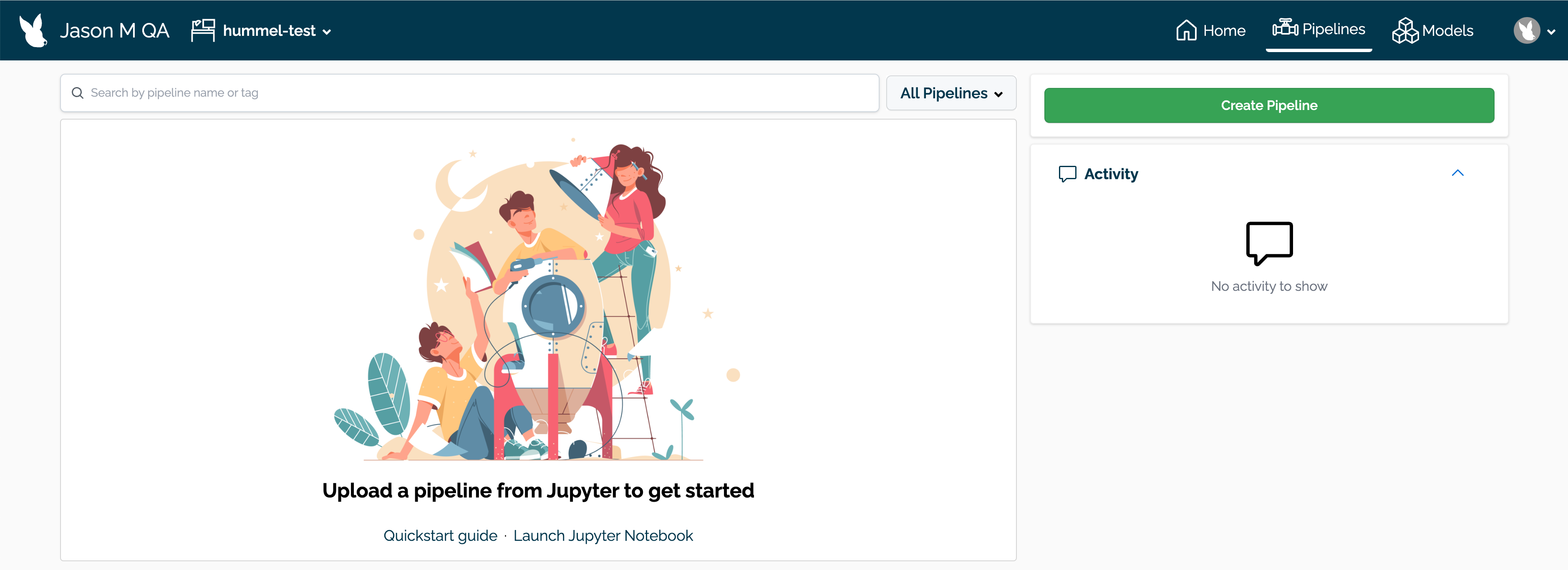
How to Create a Pipeline using the Wallaroo Dashboard

Prerequisites

Before creating a pipeline through the Wallaroo Dashboard, a model must be uploaded into the workspace through the SDK. For more information, see the Wallaroo SDK Essentials Guide.

IMPORTANT NOTICE

Pipeline names are not forced to be unique. You can have 50 pipelines all named my-pipeline, which can cause confusion in determining which pipeline to use.

It is recommended that organizations agree on a naming convention and select pipeline to use rather than creating a new one each time. See the SDK guides for more information on how to select an existing pipeline.

To create a pipeline:

From the Wallaroo Dashboard, set the current workspace from the top left dropdown list.
Select View Pipelines from the pipeline’s row.
From the upper right hand corner, select Create Pipeline.
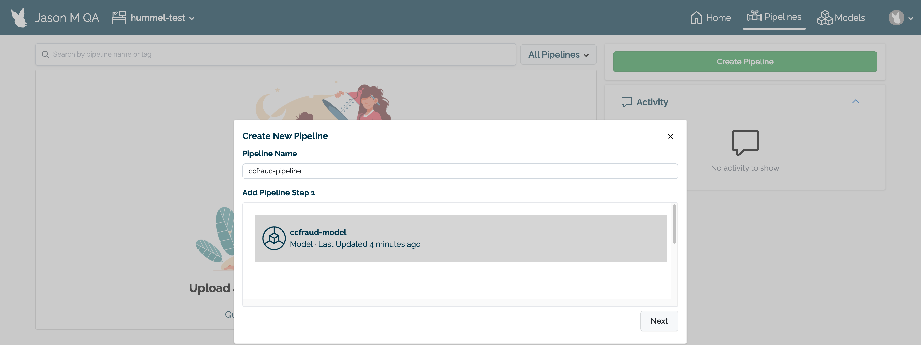
Enter the following:
1. Pipeline Name: The name of the new pipeline. Pipeline names should be unique across the Wallaroo instance.
2. Add Pipeline Step: Select the models to be used as the pipeline steps.
When finished, select Next.
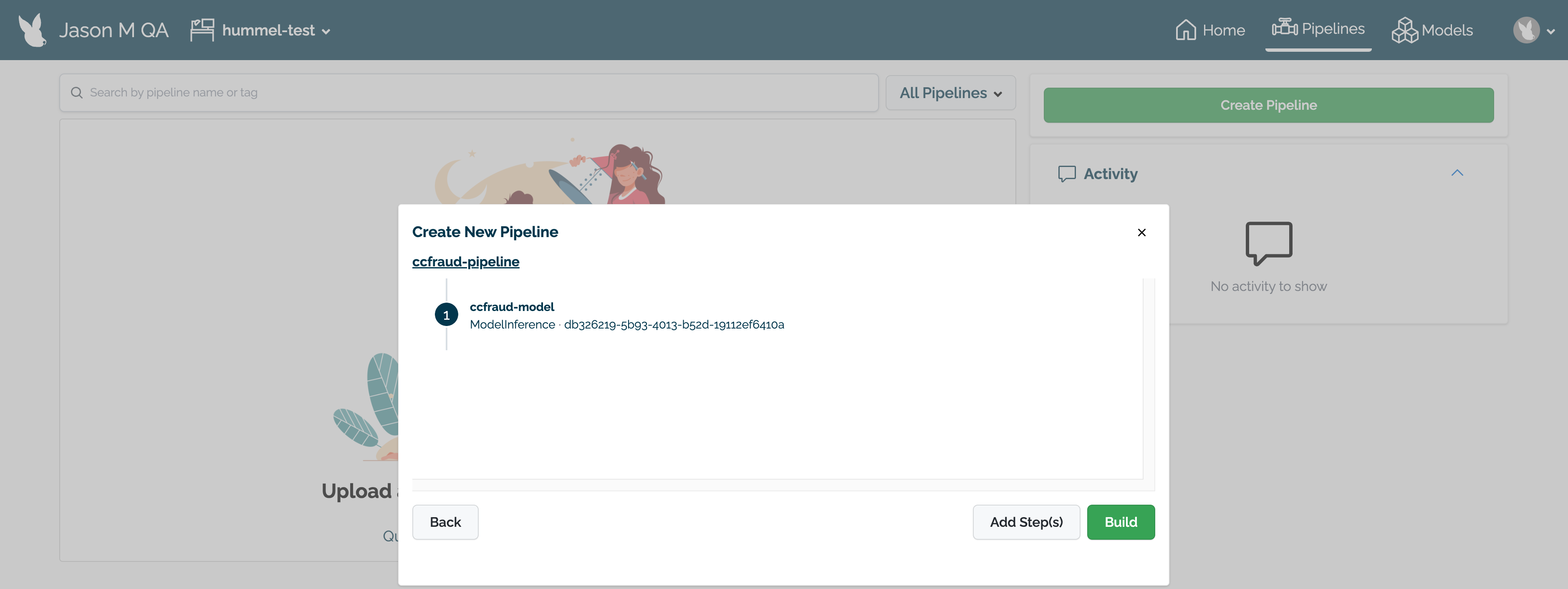
Review the name of the pipeline and the steps. If any adjustments need to be made, select either Back to rename the pipeline or Add Step(s) to change the pipeline’s steps.
When finished, select Build to create the pipeline in this workspace. The pipeline will be built and be ready for deployment within a minute.

How to Deploy and Undeploy a Pipeline using the Wallaroo Dashboard

Deployed pipelines create new namespaces in the Kubernetes environment where the Wallaroo instance is deployed, and allocate resources from the Kubernetes environment to run the pipeline and its steps.

To deploy a pipeline:

From the Wallaroo Dashboard, set the current workspace from the top left dropdown list.
Select View Pipelines from the pipeline’s row.
Select the pipeline to deploy.
From the right navigation panel, select Deploy.
A popup module will request verification to deploy the pipeline. Select Deploy again to deploy the pipeline.

Undeploying a pipeline returns resources back to the Kubernetes environment and removes the namespaces created when the pipeline was deployed.

To undeploy a pipeline:

From the Wallaroo Dashboard, set the current workspace from the top left dropdown list.
Select View Pipelines from the pipeline’s row.
Select the pipeline to deploy.
From the right navigation panel, select Undeploy.
A popup module will request verification to undeploy the pipeline. Select Undeploy again to undeploy the pipeline.

How to View a Pipeline Details and Metrics

To view a pipeline’s details:

From the Wallaroo Dashboard, set the current workspace from the top left dropdown list.
Select View Pipelines from the pipeline’s row.
To view details on the pipeline, select the name of the pipeline.
A list of the pipeline’s details will be displayed.

To view a pipeline’s metrics:

From the Wallaroo Dashboard, set the current workspace from the top left dropdown list.
Select View Pipelines from the pipeline’s row.
To view details on the pipeline, select the name of the pipeline.
A list of the pipeline’s details will be displayed.
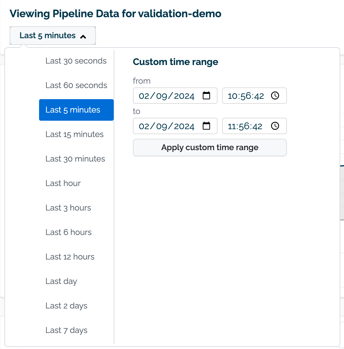
Select Metrics to view the following information. From here you can select the time period to display metrics from through the drop down to display the following:
1. Requests per second
2. Cluster inference rate
3. Inference latency
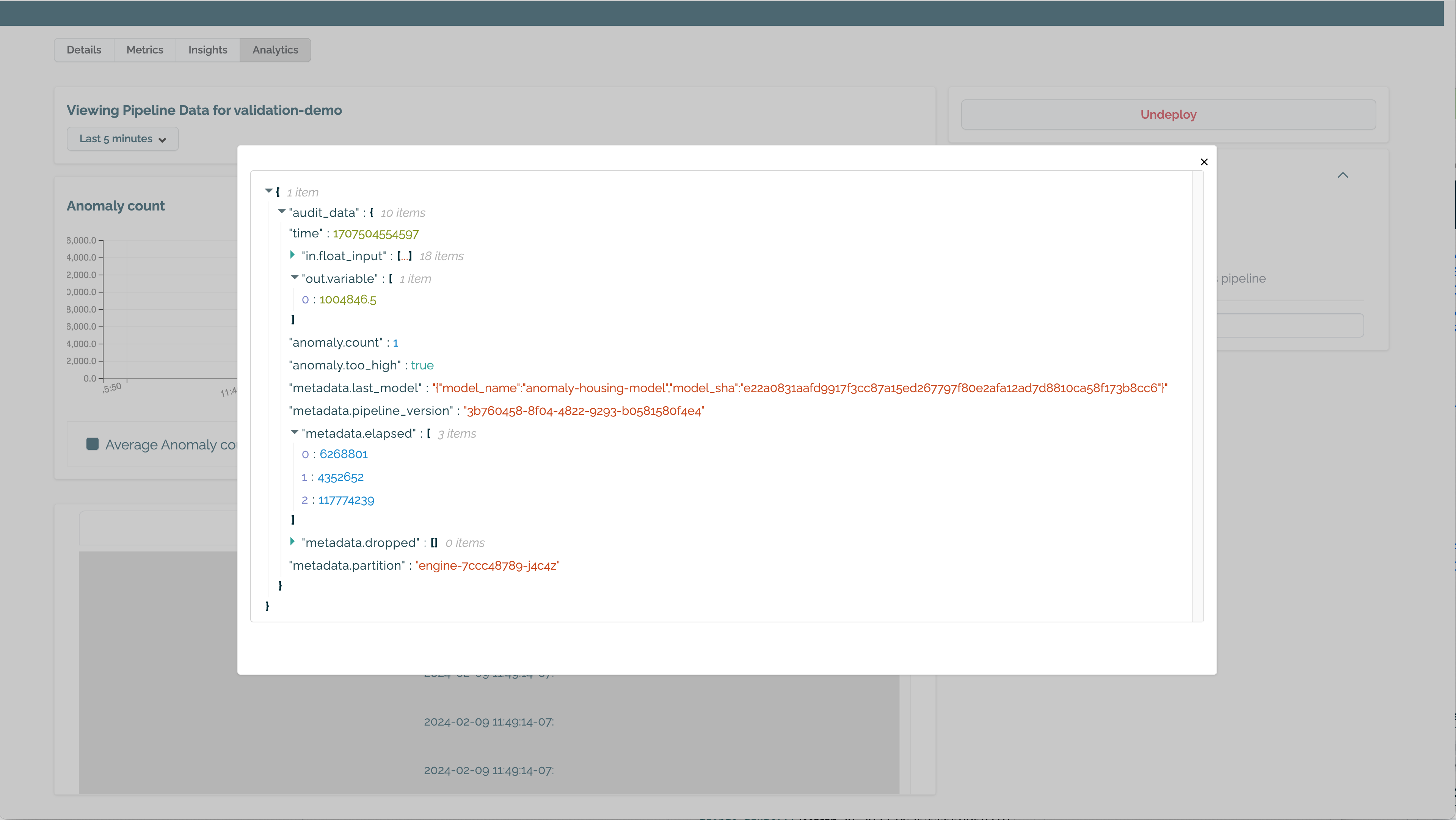
The Audit Log and Anomaly Log are available to view further details of the pipeline’s activities.

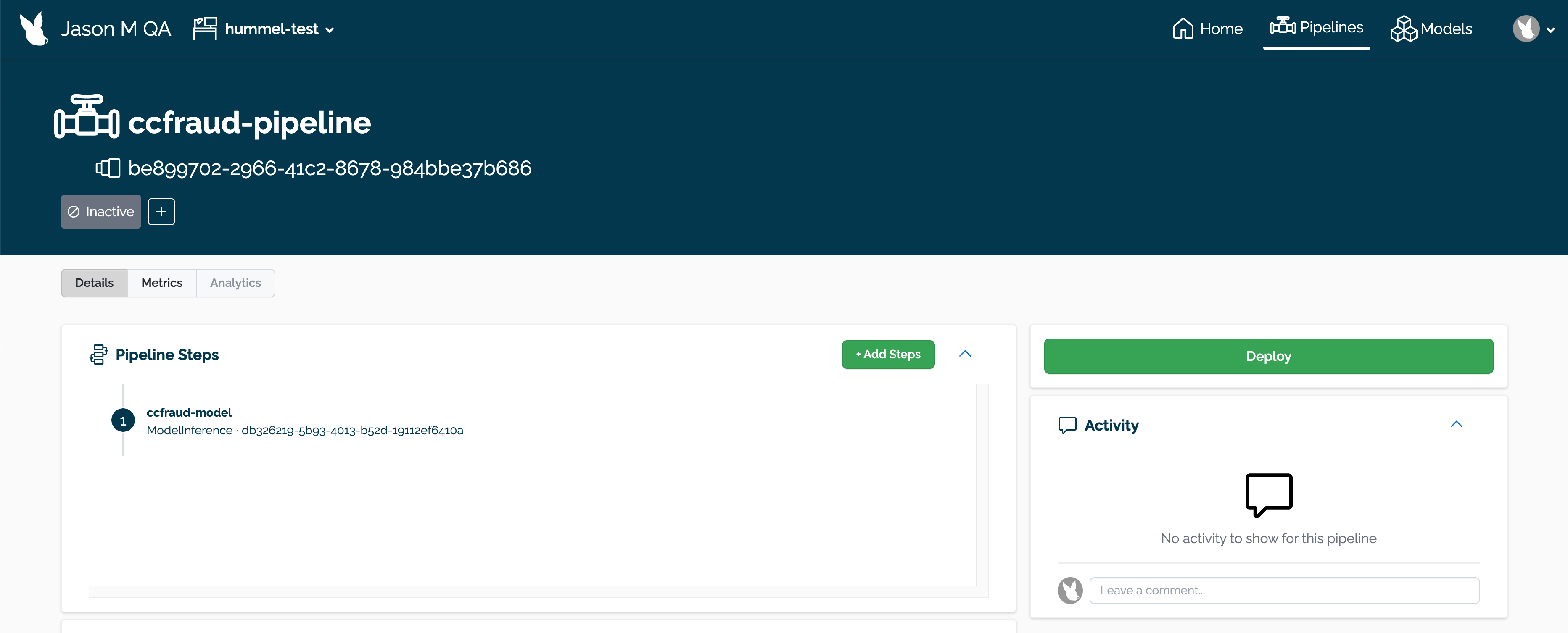
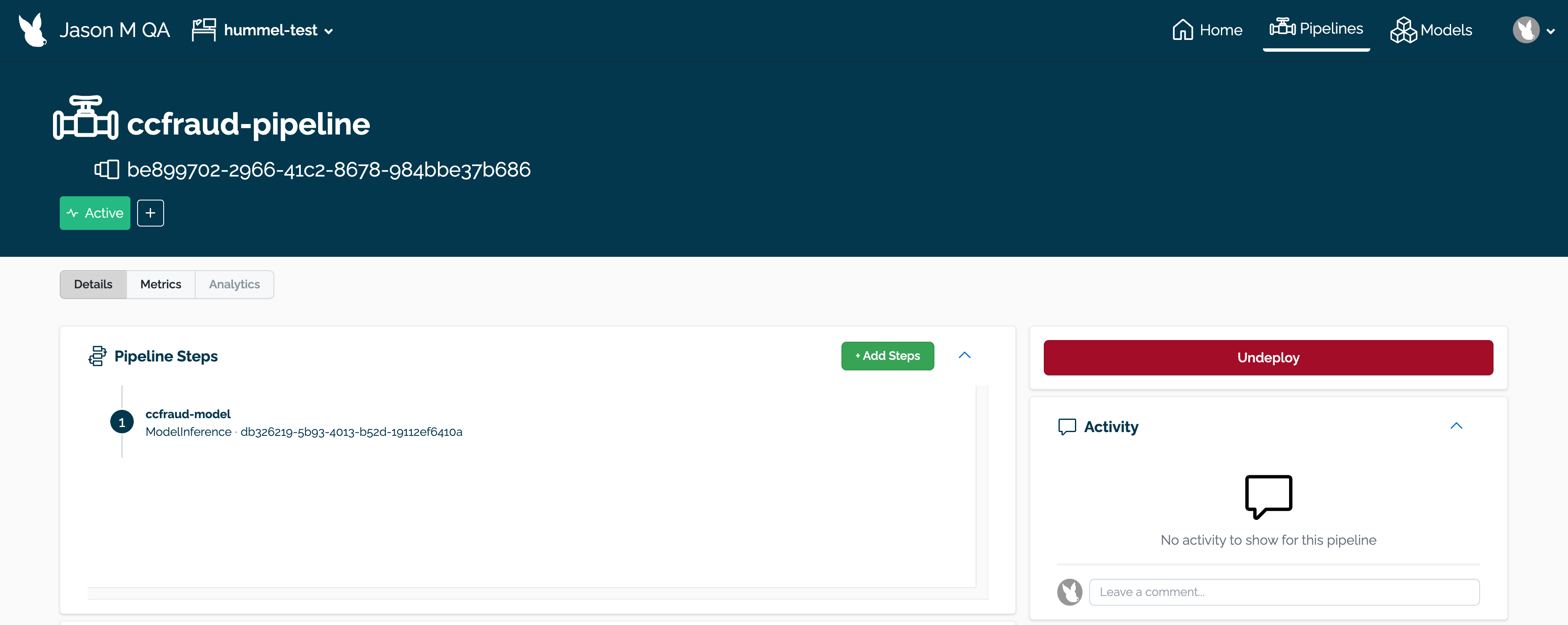
Pipeline Details

The following is available from the Pipeline Details page:

The name of the pipeline.
The pipeline ID: This is in UUID format.
Pipeline steps: The steps and the models in each pipeline step.
Version History: how the pipeline has been updated over time.

1 - Wallaroo Pipeline Edge Publication Management

How to manage pipeline publications

Wallaroo Pipelines are deployed to edge devices by publishing them to Open Container Initiative (OCI) registries. This is managed through the Wallaroo MLOps API, the Wallaroo SDK, and through the Wallaroo Dashboard.

The following describes how to use the Wallaroo Dashboard to:

View published pipeline information
Publish a pipeline to an OCI Registry
Deploy a pipeline to an edge device from an OCI Registry

Wallaroo Dashboard Pipeline Publish Management

Wallaroo pipeline publications are managed through the Wallaroo Dashboard Pipeline pages. This requires that Edge Deployment Registry is enabled.

Wallaroo pipelines are published as containers to OCI registries, and are referred to as publishes.

Access Wallaroo Pipeline Publishes

To view the publishes for a specific pipeline through the Wallaroo Dashboard:

Login to the Wallaroo Dashboard through your browser.
From the Workspace select menu on the upper left, select the workspace the pipeline is associated in.
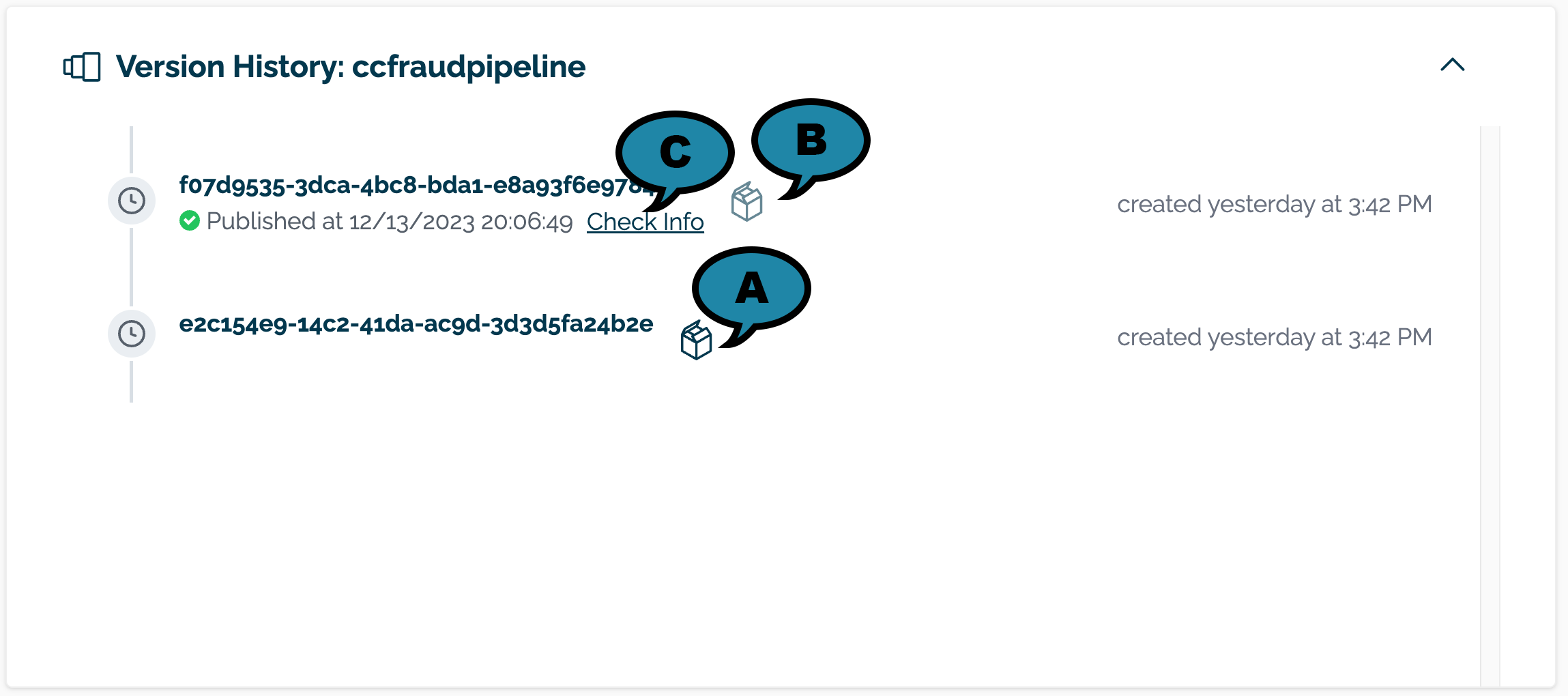
Select the pipeline to view the Pipeline Versions, which contain the Pipeline Publishes for each Pipeline Versions.
The list of pipeline versions are available in the Version History section.
1. Unpublished versions are indicated with a black box (A) to the right of the pipeline version. Published pipelines are indicated with a gray box. (B). Publish details are visible by selecting Check Info (C).
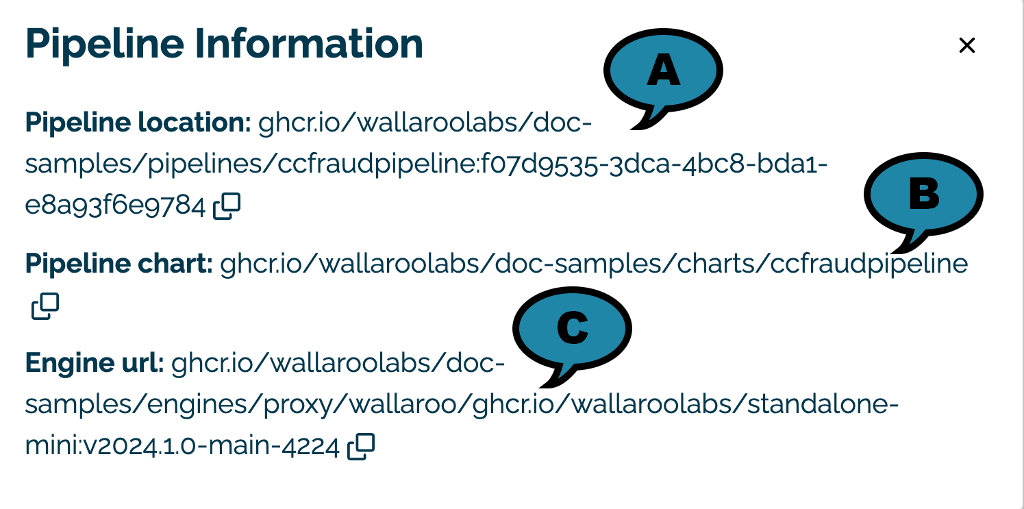
2. Select Check Info to view pipeline details.
  - Pipeline location (A): The URL for the containerized pipeline.
  - PIpeline Chart (B): The URL for the Helm chart of the published pipeline and engine.
  - Engine url (B): The URL for the Wallaroo Engine required to deploy the pipeline and perform inference requests.

Publish a Wallaroo Pipeline Version

To publish a version of the Wallaroo pipeline:

From the Pipeline Versions view:

Select the black box to the right of a Pipeline Version identifier. Grey boxes indicate that the pipeline version is already published.
Wait for the publish to complete. Depending on the number and size of the pipeline steps in the pipeline version, this may take anywhere from 1 to 10 minutes.

DevOps - Pipeline Edge Deployment

Once a pipeline is deployed to the Edge Registry service, it can be deployed in environments such as Docker, Kubernetes, or similar container running services by a DevOps engineer.

Docker Deployment

First, the DevOps engineer must authenticate to the same OCI Registry service used for the Wallaroo Edge Deployment registry.

For more details, check with the documentation on your artifact service. The following are provided for the three major cloud services:

For the deployment, the engine URL is specified with the following environmental variables:

DEBUG (true|false): Whether to include debug output.
OCI_REGISTRY: The URL of the registry service.
CONFIG_CPUS: The number of CPUs to use.
OCI_USERNAME: The edge registry username.
OCI_PASSWORD: The edge registry password or token.
PIPELINE_URL: The published pipeline URL.
EDGE_BUNDLE (Optional): The base64 encoded edge token and other values to connect to the Wallaroo Ops instance. This is used for edge management and transmitting inference results for observability. IMPORTANT NOTE: The token for EDGE_BUNDLE is valid for one deployment. For subsequent deployments, generate a new edge location with its own EDGE_BUNDLE.

Docker Deployment Example

Using our sample environment, here’s sample deployment using Docker with a computer vision ML model, the same used in the Wallaroo Use Case Tutorials Computer Vision: Retail tutorials.

Login through docker to confirm access to the registry service. First, docker login. For example, logging into the artifact registry with the token stored in the variable tok:
```
cat $tok | docker login -u _json_key_base64 --password-stdin https://sample-registry.com
```

Then deploy the Wallaroo published pipeline with an edge added to the pipeline publish through docker run.

IMPORTANT NOTE: Edge deployments with Edge Observability enabled with the EDGE_BUNDLE option include an authentication token that only authenticates once. To store the token long term, include the persistent volume flag -v {path to storage} setting.

Deployment with EDGE_BUNDLE for observability.

docker run -p 8080:8080 \
-v ./data:/persist \
-e DEBUG=true \
-e OCI_REGISTRY=$REGISTRYURL \
-e EDGE_BUNDLE=ZXhwb3J0IEJVTkRMRV9WRVJTSU9OPTEKZXhwb3J0IEVER0VfTkFNRT1lZGdlLWNjZnJhdWQtb2JzZXJ2YWJpbGl0eXlhaWcKZXhwb3J0IEpPSU5fVE9LRU49MjZmYzFjYjgtMjUxMi00YmU3LTk0ZGUtNjQ2NGI1MGQ2MzhiCmV4cG9ydCBPUFNDRU5URVJfSE9TVD1kb2MtdGVzdC5lZGdlLndhbGxhcm9vY29tbXVuaXR5Lm5pbmphCmV4cG9ydCBQSVBFTElORV9VUkw9Z2hjci5pby93YWxsYXJvb2xhYnMvZG9jLXNhbXBsZXMvcGlwZWxpbmVzL2VkZ2Utb2JzZXJ2YWJpbGl0eS1waXBlbGluZTozYjQ5ZmJhOC05NGQ4LTRmY2EtYWVjYy1jNzUyNTdmZDE2YzYKZXhwb3J0IFdPUktTUEFDRV9JRD03 \
-e CONFIG_CPUS=1 \
-e OCI_USERNAME=$REGISTRYUSERNAME \
-e OCI_PASSWORD=$REGISTRYPASSWORD \
-e PIPELINE_URL=ghcr.io/wallaroolabs/doc-samples/pipelines/edge-observability-pipeline:3b49fba8-94d8-4fca-aecc-c75257fd16c6 \
ghcr.io/wallaroolabs/doc-samples/engines/proxy/wallaroo/ghcr.io/wallaroolabs/standalone-mini:v2023.4.0-main-4079

Connection to the Wallaroo Ops instance from edge deployment with EDGE_BUNDLE is verified with the long entry Node attestation was successful.

Deployment without observability.

docker run -p 8080:8080 \
-e DEBUG=true \
-e OCI_REGISTRY=$REGISTRYURL \
-e CONFIG_CPUS=1 \
-e OCI_USERNAME=$REGISTRYUSERNAME \
-e OCI_PASSWORD=$REGISTRYPASSWORD \
-e PIPELINE_URL=ghcr.io/wallaroolabs/doc-samples/pipelines/edge-observability-pipeline:3b49fba8-94d8-4fca-aecc-c75257fd16c6 \
ghcr.io/wallaroolabs/doc-samples/engines/proxy/wallaroo/ghcr.io/wallaroolabs/standalo

Docker Compose Deployment

For users who prefer to use docker compose, the following sample compose.yaml file is used to launch the Wallaroo Edge pipeline. This is the same used in the Wallaroo Use Case Tutorials Computer Vision: Retail tutorials. The volumes tag is used to preserve the login session from the one-time token generated as part of the EDGE_BUNDLE.

EDGE_BUNDLE is only required when adding an edge to a Wallaroo publish for observability. The following is deployed without observability.

services:
  engine:
    image: {Your Engine URL}
    ports:
      - 8080:8080
    environment:
      PIPELINE_URL: {Your Pipeline URL}
      OCI_REGISTRY: {Your Edge Registry URL}
      OCI_USERNAME:  {Your Registry Username}
      OCI_PASSWORD: {Your Token or Password}
      CONFIG_CPUS: 4

The procedure is:

Login through docker to confirm access to the registry service. First, docker login. For example, logging into the artifact registry with the token stored in the variable tok to the registry us-west1-docker.pkg.dev:
```
cat $tok | docker login -u _json_key_base64 --password-stdin https://sample-registry.com
```

Set up the compose.yaml file.

services:
engine:
    image: sample-registry.com/engine:v2023.3.0-main-3707
    ports:
        - 8080:8080
    volumes:
        - ./data:/persist
environment:
    PIPELINE_URL: sample-registry.com/pipelines/edge-cv-retail:bf70eaf7-8c11-4b46-b751-916a43b1a555
    EDGE_BUNDLE: ZXhwb3J0IEJVTkRMRV9WRVJTSU9OPTEKZXhwb3J0IEVER0VfTkFNRT1lZGdlLWNjZnJhdWQtb2JzZXJ2YWJpbGl0eXlhaWcKZXhwb3J0IEpPSU5fVE9LRU49MjZmYzFjYjgtMjUxMi00YmU3LTk0ZGUtNjQ2NGI1MGQ2MzhiCmV4cG9ydCBPUFNDRU5URVJfSE9TVD1kb2MtdGVzdC5lZGdlLndhbGxhcm9vY29tbXVuaXR5Lm5pbmphCmV4cG9ydCBQSVBFTElORV9VUkw9Z2hjci5pby93YWxsYXJvb2xhYnMvZG9jLXNhbXBsZXMvcGlwZWxpbmVzL2VkZ2Utb2JzZXJ2YWJpbGl0eS1waXBlbGluZTozYjQ5ZmJhOC05NGQ4LTRmY2EtYWVjYy1jNzUyNTdmZDE2YzYKZXhwb3J0IFdPUktTUEFDRV9JRD03
    OCI_REGISTRY: sample-registry.com
    OCI_USERNAME:  _json_key_base64
    OCI_PASSWORD: abc123
    CONFIG_CPUS: 4

Then deploy with docker compose up.

Docker Compose Deployment Example

The deployment and undeployment is then just a simple docker compose up and docker compose down. The following shows an example of deploying the Wallaroo edge pipeline using docker compose.

docker compose up
[+] Running 1/1
 ✔ Container cv_data-engine-1  Recreated                                                                                                                                                                 0.5s
Attaching to cv_data-engine-1
cv_data-engine-1  | Wallaroo Engine - Standalone mode
cv_data-engine-1  | Login Succeeded
cv_data-engine-1  | Fetching manifest and config for pipeline: sample-registry.com/pipelines/edge-cv-retail:bf70eaf7-8c11-4b46-b751-916a43b1a555
cv_data-engine-1  | Fetching model layers
cv_data-engine-1  | digest: sha256:c6c8869645962e7711132a7e17aced2ac0f60dcdc2c7faa79b2de73847a87984
cv_data-engine-1  |   filename: c6c8869645962e7711132a7e17aced2ac0f60dcdc2c7faa79b2de73847a87984
cv_data-engine-1  |   name: resnet-50
cv_data-engine-1  |   type: model
cv_data-engine-1  |   runtime: onnx
cv_data-engine-1  |   version: 693e19b5-0dc7-4afb-9922-e3f7feefe66d
cv_data-engine-1  |
cv_data-engine-1  | Fetched
cv_data-engine-1  | Starting engine
cv_data-engine-1  | Looking for preexisting `yaml` files in //modelconfigs
cv_data-engine-1  | Looking for preexisting `yaml` files in //pipelines

Helm Deployment

Published pipelines can be deployed through the use of helm charts.

Helm deployments take up to two steps - the first step is in retrieving the required values.yaml and making updates to override.

IMPORTANT NOTE: Edge deployments with Edge Observability enabled with the EDGE_BUNDLE option include an authentication token that only authenticates once. Helm chart installations automatically add a persistent volume during deployment to store the authentication session data for future deployments.

Login to the registry service with helm registry login. For example, if the token is stored in the variable tok:
```
helm registry login sample-registry.com --username _json_key_base64 --password $tok
```
Pull the helm charts from the published pipeline. The two fields are the Helm Chart URL and the Helm Chart version to specify the OCI . This typically takes the format of:
```
helm pull oci://{published.helm_chart_url} --version {published.helm_chart_version}
```

Extract the tgz file and copy the values.yaml and copy the values used to edit engine allocations, etc. The following are required for the deployment to run:

ociRegistry:
    registry: {your registry service}
    username:  {registry username here}
    password: {registry token here}

For Wallaroo Server deployments with edge location set, the values include edgeBundle as generated when the edge was added to the pipeline publish.

ociRegistry:
    registry: {your registry service}
    username:  {registry username here}
    password: {registry token here}
edgeBundle: abcdefg

Store this into another file, suc as local-values.yaml.

Create the namespace to deploy the pipeline to. For example, the namespace wallaroo-edge-pipeline would be:
```
kubectl create -n wallaroo-edge-pipeline
```

Deploy the helm installation with helm install through one of the following options:

Specify the tgz file that was downloaded and the local values file. For example:

helm install --namespace {namespace} --values {local values file} {helm install name} {tgz path}

Specify the expended directory from the downloaded tgz file.

helm install --namespace {namespace} --values {local values file} {helm install name} {helm directory path}

Specify the Helm Pipeline Helm Chart and the Pipeline Helm Version.

helm install --namespace {namespace} --values {local values file} {helm install name} oci://{published.helm_chart_url} --version {published.helm_chart_version}

Once deployed, the DevOps engineer will have to forward the appropriate ports to the svc/engine-svc service in the specific pipeline. For example, using kubectl port-forward to the namespace ccfraud that would be:
```
kubectl port-forward svc/engine-svc -n ccfraud01 8080 --address 0.0.0.0`
```

Edge Deployment Endpoints

The following endpoints are available for API calls to the edge deployed pipeline.

List Pipelines

The endpoint /pipelines returns:

id (String): The name of the pipeline.
status (String): The status as either Running, or Error if there are any issues.

List Pipelines Example

curl localhost:8080/pipelines
{"pipelines":[{"id":"edge-cv-retail","status":"Running"}]}

List Models

The endpoint /models returns a List of models with the following fields:

name (String): The model name.
sha (String): The sha hash value of the ML model.
status (String): The status of either Running or Error if there are any issues.
version (String): The model version. This matches the version designation used by Wallaroo to track model versions in UUID format.

List Models Example

curl localhost:8080/models
{"models":[{"name":"resnet-50","sha":"c6c8869645962e7711132a7e17aced2ac0f60dcdc2c7faa79b2de73847a87984","status":"Running","version":"693e19b5-0dc7-4afb-9922-e3f7feefe66d"}]}

Edge Inference Endpoint

The inference endpoint takes the following pattern:

/pipelines/{pipeline-name}: The pipeline-name is the same as returned from the /pipelines endpoint as id.

Wallaroo inference endpoint URLs accept the following data inputs through the Content-Type header:

Content-Type: application/vnd.apache.arrow.file: For Apache Arrow tables.
Content-Type: application/json; format=pandas-records: For pandas DataFrame in record format.

Once deployed, we can perform an inference through the deployment URL.

The endpoint returns Content-Type: application/json; format=pandas-records by default with the following fields:

check_failures (List[Integer]): Whether any validation checks were triggered. For more information, see Wallaroo SDK Essentials Guide: Pipeline Management: Anomaly Testing.
elapsed (List[Integer]): A list of time in nanoseconds for:
- [0] The time to serialize the input.
- [1…n] How long each step took.
model_name (String): The name of the model used.
model_version (String): The version of the model in UUID format.
original_data: The original input data. Returns null if the input may be too long for a proper return.
outputs (List): The outputs of the inference result separated by data type, where each data type includes:
- data: The returned values.
- dim (List[Integer]): The dimension shape returned.
- v (Integer): The vector shape of the data.
pipeline_name (String): The name of the pipeline.
shadow_data: Any shadow deployed data inferences in the same format as outputs.
time (Integer): The time since UNIX epoch.

Edge Inference Endpoint Example

The following example demonstrates sending an Apache Arrow table to the Edge deployed pipeline, requesting the inference results back in a pandas DataFrame records format.

curl -X POST localhost:8080/pipelines/edge-cv-retail -H "Content-Type: application/vnd.apache.arrow.file" -H 'Accept: application/json; format=pandas-records'  --data-binary @./data/image_224x224.arrow

Returns:

[{"check_failures":[],"elapsed":[1067541,21209776],"model_name":"resnet-50","model_version":"2e05e1d0-fcb3-4213-bba8-4bac13f53e8d","original_data":null,"outputs":[{"Int64":{"data":[535],"dim":[1],"v":1}},{"Float":{"data":[0.00009498586587142199,0.00009141524787992239,0.0004606838047038764,0.00007667174941161647,0.00008047101437114179,...],"dim":[1,1001],"v":1}}],"pipeline_name":"edge-cv-demo","shadow_data":{},"time":1694205578428}]

Edge Bundle Token Time To Live

When an edge is added to a pipeline publish, the field docker_run_variables contains a JSON value for edge devices to connect to the Wallaroo Ops instance.

The settings are stored in the key EDGE_BUNDLE as a base64 encoded value that include the following:

BUNDLE_VERSION: The current version of the bundled Wallaroo pipeline.
EDGE_NAME: The edge name as defined when created and added to the pipeline publish.
JOIN_TOKEN_: The one time authentication token for authenticating to the Wallaroo Ops instance.
OPSCENTER_HOST: The hostname of the Wallaroo Ops edge service. See Edge Deployment Registry Guide for full details on enabling pipeline publishing and edge observability to Wallaroo.
PIPELINE_URL: The OCI registry URL to the containerized pipeline.
WORKSPACE_ID: The numerical ID of the workspace.

For example:

{'edgeBundle': 'ZXhwb3J0IEJVTkRMRV9WRVJTSU9OPTEKZXhwb3J0IEVER0VfTkFNRT14Z2ItY2NmcmF1ZC1lZGdlLXRlc3QKZXhwb3J0IEpPSU5fVE9LRU49MzE0OGFkYTUtMjg1YS00ZmNhLWIzYjgtYjUwYTQ4ZDc1MTFiCmV4cG9ydCBPUFNDRU5URVJfSE9TVD1kb2MtdGVzdC5lZGdlLndhbGxhcm9vY29tbXVuaXR5Lm5pbmphCmV4cG9ydCBQSVBFTElORV9VUkw9Z2hjci5pby93YWxsYXJvb2xhYnMvZG9jLXNhbXBsZXMvcGlwZWxpbmVzL2VkZ2UtcGlwZWxpbmU6ZjM4OGMxMDktOGQ1Ny00ZWQyLTk4MDYtYWExM2Y4NTQ1NzZiCmV4cG9ydCBXT1JLU1BBQ0VfSUQ9NQ=='}

base64 -D
ZXhwb3J0IEJVTkRMRV9WRVJTSU9OPTEKZXhwb3J0IEVER0VfTkFNRT14Z2ItY2NmcmF1ZC1lZGdlLXRlc3QKZXhwb3J0IEpPSU5fVE9LRU49MzE0OGFkYTUtMjg1YS00ZmNhLWIzYjgtYjUwYTQ4ZDc1MTFiCmV4cG9ydCBPUFNDRU5URVJfSE9TVD1kb2MtdGVzdC5lZGdlLndhbGxhcm9vY29tbXVuaXR5Lm5pbmphCmV4cG9ydCBQSVBFTElORV9VUkw9Z2hjci5pby93YWxsYXJvb2xhYnMvZG9jLXNhbXBsZXMvcGlwZWxpbmVzL2VkZ2UtcGlwZWxpbmU6ZjM4OGMxMDktOGQ1Ny00ZWQyLTk4MDYtYWExM2Y4NTQ1NzZiCmV4cG9ydCBXT1JLU1BBQ0VfSUQ9NQ==^D
export BUNDLE_VERSION=1
export EDGE_NAME=xgb-ccfraud-edge-test
export JOIN_TOKEN=3148ada5-285a-4fca-b3b8-b50a48d7511b
export OPSCENTER_HOST=doc-test.edge.wallaroocommunity.ninja
export PIPELINE_URL=ghcr.io/wallaroolabs/doc-samples/pipelines/edge-pipeline:f388c109-8d57-4ed2-9806-aa13f854576b
export WORKSPACE_ID=5

The JOIN_TOKEN is a one time access token. Once used, a JOIN_TOKEN expires. The authentication session data is stored in persistent volumes. Persistent volumes must be specified for docker and docker compose based deployments of Wallaroo pipelines; helm based deployments automatically provide persistent volumes to store authentication credentials.

The JOIN_TOKEN has the following time to live (TTL) parameters.

Once created, the JOIN_TOKEN is valid for 24 hours. After it expires the edge will not be allowed to contact the OpsCenter the first time and a new edge bundle will have to be created.
After an Edge joins to Wallaroo Ops for the first time with persistent storage, the edge must contact the Wallaroo Ops instance at least once every 7 days.
- If this period is exceeded, the authentication credentials will expire and a new edge bundle must be created with a new and valid JOIN_TOKEN.

Wallaroo edges require unique names. To create a new edge bundle with the same name:

Use the Remove Edge to remove the edge by name.
Use Add Edge to add the edge with the same name. A new EDGE_BUNDLE is generated with a new JOIN_TOKEN.

2 - Wallaroo Pipeline Tag Management

How to manage tags and pipelines.

Tags can be used to label, search, and track pipelines across a Wallaroo instance. The following guide will demonstrate how to:

Create a tag for a specific pipeline.
Remove a tag for a specific pipeline.

The example shown uses the pipeline ccfraudpipeline.

Steps

Add a New Tag to a Pipeline

To set a tag to pipeline using the Wallaroo Dashboard:

Log into your Wallaroo instance.
Select the workspace the pipelines are associated with.
Select View Pipelines.
From the Pipeline Select Dashboard page, select the pipeline to update.
From the Pipeline Dashboard page, select the + icon under the name of the pipeline and it’s hash value.
Enter the name of the new tag. When complete, select Enter. The tag will be set for this pipeline.

Remove a Tag from a Pipeline

To remove a tag from a pipeline:

IMPORTANT NOTE

Once a tag is deleted from a pipeline, it can not be undeleted.

Log into your Wallaroo instance.
Select the workspace the pipelines are associated with.
Select View Pipelines.
From the Pipeline Select Dashboard page, select the pipeline to update.
From the Pipeline Dashboard page, select the select the X for the tag to delete. The tag will be removed from the pipeline.

Wallaroo SDK Tag Management

Tags are applied to either model versions or pipelines. This allows organizations to track different versions of models, and search for what pipelines have been used for specific purposes such as testing versus production use.

Create Tag

Tags are created with the Wallaroo client command create_tag(String tagname). This creates the tag and makes it available for use.

The tag will be saved to the variable currentTag to be used in the rest of these examples.

# Now we create our tag
currentTag = wl.create_tag("My Great Tag")

Tags are listed with the Wallaroo client command list_tags(), which shows all tags and what models and pipelines they have been assigned to.

# List all tags

wl.list_tags()

id	tag	models	pipelines
1	My Great Tag	[('tagtestmodel', ['70169e97-fb7e-4922-82ba-4f5d37e75253'])]	[]

Wallaroo Pipeline Tag Management

Tags are used with pipelines to track different pipelines that are built or deployed with different features or functions.

Add Tag to Pipeline

Tags are added to a pipeline through the Wallaroo Tag add_to_pipeline(pipeline_id) method, where pipeline_id is the pipeline’s integer id.

For this example, we will add currentTag to testtest_pipeline, then verify it has been added through the list_tags command and list_pipelines command.

# add this tag to the pipeline
currentTag.add_to_pipeline(tagtest_pipeline.id())

{'pipeline_pk_id': 1, 'tag_pk_id': 1}

Search Pipelines by Tag

Pipelines can be searched through the Wallaroo Client search_pipelines(search_term) method, where search_term is a string value for tags assigned to the pipelines.

In this example, the text “My Great Tag” that corresponds to currentTag will be searched for and displayed.

wl.search_pipelines('My Great Tag')

name	version	creation_time	last_updated_time	deployed	tags	steps
tagtestpipeline	5a4ff3c7-1a2d-4b0a-ad9f-78941e6f5677	2022-29-Nov 17:15:21	2022-29-Nov 17:15:21	(unknown)	My Great Tag

Remove Tag from Pipeline

Tags are removed from a pipeline with the Wallaroo Tag remove_from_pipeline(pipeline_id) command, where pipeline_id is the integer value of the pipeline’s id.

For this example, currentTag will be removed from tagtest_pipeline. This will be verified through the list_tags and search_pipelines command.

## remove from pipeline
currentTag.remove_from_pipeline(tagtest_pipeline.id())

{'pipeline_pk_id': 1, 'tag_pk_id': 1}

3 - Wallaroo Anomaly Detection

How to use validations to detect data anomalies in data inputs or outputs.

Viewing Detected Anomalies via the Wallaroo Dashboard

Wallaroo provides validations: user defined expressions on model inference input and outputs that determine if data falls outside expected norms. For more details on adding validations to a Wallaroo pipeline, see Detecting Anomalies with Validations via the Wallaroo SDK.

Detected anomaly analytics are available through the Wallaroo Dashboard user interface for each pipeline.

Access the Pipeline Analytics Page

To access a pipeline’s analytics page:

From the Wallaroo Dashboard, select the workspace, then the View Pipelines to view.
Select the pipeline to view.
From the pipeline page, select Analytics.

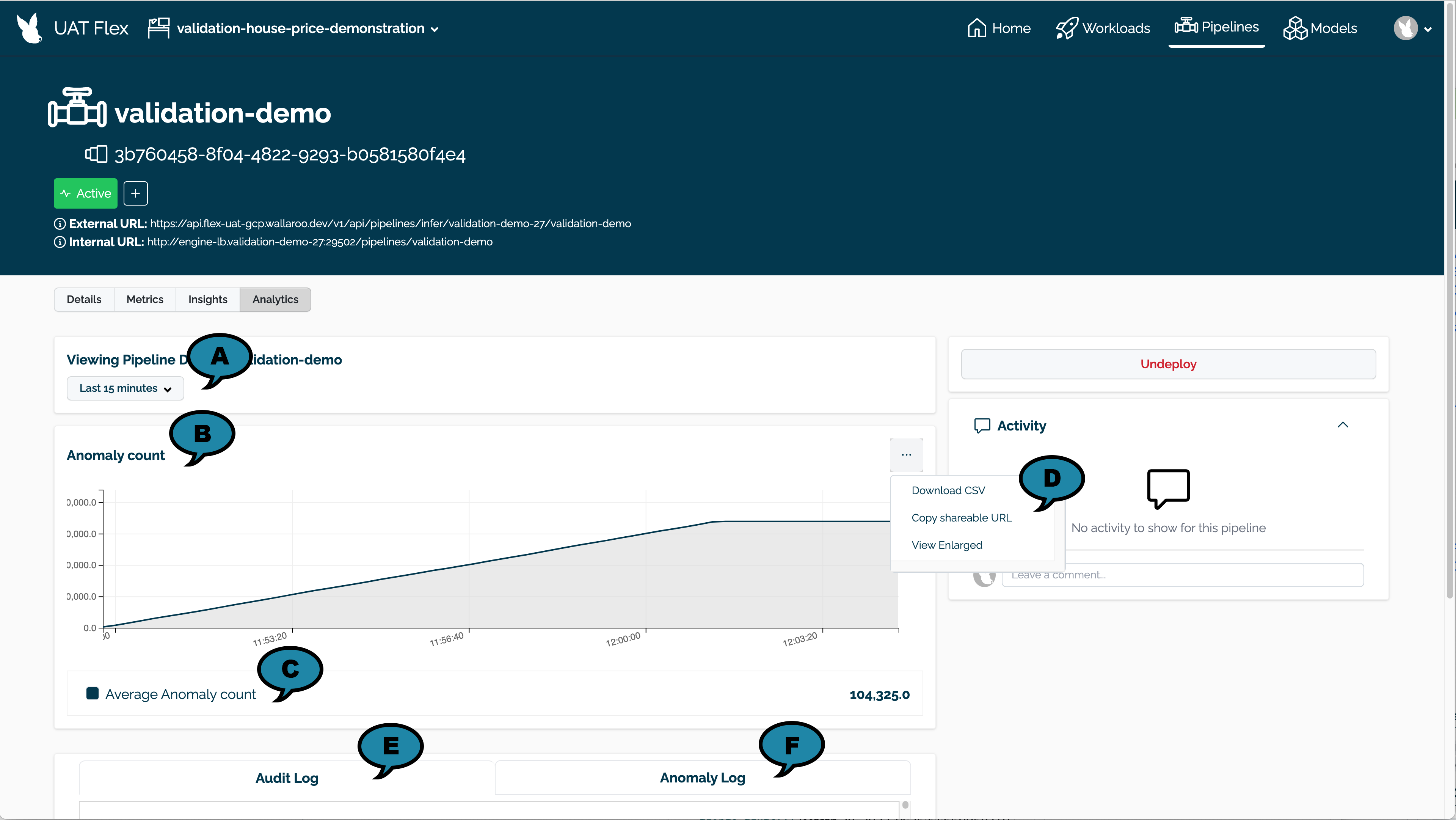
The following analytics options are available.

(A) Time Filter: Select the time range of inference requests to filter.
(B) Anomaly Count: A chart of the count of anomalies detected from inference requests over time.
(C) Average Anomaly Count: The average number of anomaly’s detected over the filtered time range.
(D) Actions: The following actions are available:
- Download CSV: Download a CSV of the anomaly counts shown in the chart.
- Copy sharable URL: Copy a URL of the anomaly count data shared with other registered Wallaroo instance users.
- View Enlarged: View an enlarged version of the anomaly count chart..
(E) Audit Log: Logs of all inference requests over the filtered time period.
(F) Anomaly Log: Logs of inference requests with a detected anomaly over the filtered time period.

Detecting Anomalies with Validations via the Wallaroo SDK

Wallaroo provides validations to detect anomalous data from inference inputs and outputs.

Validations are added to a Wallaroo pipeline with the wallaroo.pipeline.add_validations method.

IMPORTANT NOTE: Validation names must be unique per pipeline. If a validation of the same name is added, both are included in the pipeline validations, but only most recent validation with the same name is displayed with the inference results. Anomalies detected by multiple validations of the same name are added to the anomaly.count inference result field.

Adding validations to a pipeline takes the format:

pipeline.add_validations(
    validation_name_01 = polars.col(in|out.{column_name}) EXPRESSION,
    validation_name_02 = polars.col(in|out.{column_name}) EXPRESSION
    ...{additional rules}
)

validation_name: The user provided name of the validation. The names must match Python variable naming requirements.
- IMPORTANT NOTE: Using the name count as a validation name returns an error. Any validation rules named count are dropped upon request and a warning returned.
polars.col(in|out.{column_name}): Specifies the input or output for a specific field aka “column” in an inference result. Wallaroo inference requests are in the format in.{field_name} for inputs, and out.{field_name} for outputs.
- More than one field can be selected, as long as they follow the rules of the polars 0.18 Expressions library.
EXPRESSION: The expression to validate. When the expression returns True, that indicates an anomaly detected.

The polars library version 0.18.5 is used to create the validation rule. This is installed by default with the Wallaroo SDK. This provides a powerful range of comparisons to organizations tracking anomalous data from their ML models.

When validations are added to a pipeline, inference request outputs return the following fields:

Field	Type	Description
anomaly.count	Integer	The total of all validations that returned True.
anomaly.{validation name}	Bool	The output of the validation `{validation_name}`.

When validation returns True, an anomaly is detected.

For example, adding the validation fraud to the following pipeline returns anomaly.count of 1 when the validation fraud returns True. The validation fraud returns True when the output field dense_1 at index 0 is greater than 0.9.

sample_pipeline = wallaroo.client.build_pipeline("sample-pipeline")
sample_pipeline.add_model_step(ccfraud_model)

# add the validation
sample_pipeline.add_validations(
    fraud=pl.col("out.dense_1").list.get(0) > 0.9,
    )

# deploy the pipeline
sample_pipeline.deploy()

# sample inference
display(sample_pipeline.infer_from_file("dev_high_fraud.json", data_format='pandas-records'))

	time	in.tensor	out.dense_1	anomaly.count	anomaly.fraud
0	2024-02-02 16:05:42.152	[1.0678324729, 18.1555563975, -1.6589551058, 5…]	[0.981199]	1	True

Detecting Anomalies from Inference Request Results

When an inference request is submitted to a Wallaroo pipeline with validations, the following fields are output:

Field	Type	Description
anomaly.count	Integer	The total of all validations that returned True.
anomaly.{validation name}	Bool	The output of each pipeline validation `{validation_name}`.

For example, adding the validation fraud to the following pipeline returns anomaly.count of 1 when the validation fraud returns True.

sample_pipeline = wallaroo.client.build_pipeline("sample-pipeline")
sample_pipeline.add_model_step(ccfraud_model)

# add the validation
sample_pipeline.add_validations(
    fraud=pl.col("out.dense_1").list.get(0) > 0.9,
    )

# deploy the pipeline
sample_pipeline.deploy()

# sample inference
display(sample_pipeline.infer_from_file("dev_high_fraud.json", data_format='pandas-records'))

	time	in.tensor	out.dense_1	anomaly.count	anomaly.fraud
0	2024-02-02 16:05:42.152	[1.0678324729, 18.1555563975, -1.6589551058, 5…]	[0.981199]	1	True

Validation Examples

Common Data Selection Expressions

The following sample expressions demonstrate different methods of selecting which model input or output data to validate.

polars.col(in|out.{column_name}).list.get(index): Returns the index of a specific field. For example, pl.col("out.dense_1") returns from the inference the output the field dense_1, and list.get(0) returns the first value in that list. Most output values from a Wallaroo inference result are a List of at least length 1, making this a common validation expression.
polars.col(in.price_ranges).list.max(): Returns from the inference request the input field price_ranges the maximum value from a list of values.
polars.col(out.price_ranges).mean() returns the mean for all values from the output field price_ranges.

For example, to the following validation fraud detects values for the output of an inference request for the field dense_1 that are greater than 0.9, indicating a transaction has a high likelihood of fraud:

import polars as pl

pipeline.add_validations(
    fraud = fraud=pl.col("out.dense_1").list.get(0) > 0.9
)

The following inference output shows the detected anomaly from an inference output:

	time	in.tensor	out.dense_1	anomaly.count	anomaly.fraud
0	2024-02-02 16:05:42.152	[1.0678324729, 18.1555563975, -1.6589551058, 5…	[0.981199]	1	True

Detecting Input Anomalies

The following validation tests the inputs from sales figures for a week’s worth of sales:

	week	site_id	sales_count
0	[28]	[site0001]	[1357, 1247, 350, 1437, 952, 757, 1831]

To validate that any sales figure does not go below 500 units, the validation is:

import polars as pl

pipeline.add_validations(
    minimum_sales=pl.col("in.sales_count").list.min() < 500
)

pipeline.deploy()

pipeline.infer_from_file(previous_week_sales)

For the input provided, the minimum_sales validation would return True, indicating an anomaly.

	time	out.predicted_sales	anomaly.count	anomaly.minimum_sales
0	2023-10-31 16:57:13.771	[1527]	1	True

Detecting Output Anomalies

The following validation detects an anomaly from a output.

fraud: Detects when an inference output for the field dense_1 at index 0 is greater than 0.9, indicating fraud.

# create the pipeline
sample_pipeline = wallaroo.client.build_pipeline("sample-pipeline")

# add a model step
sample_pipeline.add_model_step(ccfraud_model)

# add validations to the pipeline
sample_pipeline.add_validations(
    fraud=pl.col("out.dense_1").list.get(0) > 0.9
    )
sample_pipeline.deploy()

sample_pipeline.infer_from_file("dev_high_fraud.json")

	time	in.tensor	out.dense_1	anomaly.count	anomaly.fraud
0	2024-02-02 16:05:42.152	[1.0678324729, 18.1555563975, -1.6589551058, 5...	[0.981199]	1	True

Multiple Validations

The following demonstrates multiple validations added to a pipeline at once and their results from inference requests. Two validations that track the same output field and index are applied to a pipeline:

fraud: Detects an anomaly when the inference output field dense_1 at index 0 value is greater than 0.9.
too_low: Detects an anomaly when the inference output field dense_1 at the index 0 value is lower than 0.05.

sample_pipeline.add_validations(
    fraud=pl.col("out.dense_1").list.get(0) > 0.9,
    too_low=pl.col("out.dense_1").list.get(0) < 0.05
    )

Two separate inferences where the output of the first is over 0.9 and the second is under 0.05 would be the following.

sample_pipeline.infer_from_file("high_fraud_example.json")

	time	in.tensor	out.dense_1	anomaly.count	anomaly.fraud	anomaly.too_low
0	2024-02-02 16:05:42.152	[1.0678324729, 18.1555563975, -1.6589551058, 5…	[0.981199]	1	True	False

sample_pipeline.infer_from_file("low_fraud_example.json")

	time	in.tensor	out.dense_1	anomaly.count	anomaly.fraud	anomaly.too_low
0	2024-02-02 16:05:38.452	[1.0678324729, 0.2177810266, -1.7115145262, 0….	[0.0014974177]	1	False	True

The following example tracks two validations for a model that takes the previous week’s sales and projects the next week’s average sales with the field predicted_sales.

minimum_sales=pl.col("in.sales_count").list.min() < 500: The input field sales_count with a range of values has any minimum value under 500.
average_sales_too_low=pl.col("out.predicted_sales").list.get(0) < 500: The output field predicted_sales is less than 500.

The following inputs return the following values. Note how the anomaly.count value changes by the number of validations that detect an anomaly.

Input 1:

In this example, one day had sales under 500, which triggers the minimum_sales validation to return True. The predicted sales are above 500, causing the average_sales_too_low validation to return False.

	week	site_id	sales_count
0	[28]	[site0001]	[1357, 1247, 350, 1437, 952, 757, 1831]

Output 1:

	time	out.predicted_sales	anomaly.count	anomaly.minimum_sales	anomaly.average_sales_too_low
0	2023-10-31 16:57:13.771	[1527]	1	True	False

Input 2:

In this example, multiple days have sales under 500, which triggers the minimum_sales validation to return True. The predicted average sales for the next week are above 500, causing the average_sales_too_low validation to return True.

	week	site_id	sales_count
0	[29]	[site0001]	[497, 617, 350, 200, 150, 400, 110]

Output 2:

	time	out.predicted_sales	anomaly.count	anomaly.minimum_sales	anomaly.average_sales_too_low
0	2023-10-31 16:57:13.771	[325]	2	True	True

Input 3:

In this example, no sales day figures are below 500, which triggers the minimum_sales validation to return False. The predicted sales for the next week is below 500, causing the average_sales_too_low validation to return True.

	week	site_id	sales_count
0	[30]	[site0001]	[617, 525, 513, 517, 622, 757, 508]

Output 3:

	time	out.predicted_sales	anomaly.count	anomaly.minimum_sales	anomaly.average_sales_too_low
0	2023-10-31 16:57:13.771	[497]	1	False	True

Compound Validations

The following combines multiple field checks into a single validation. For this, we will check for values of out.dense_1 that are between 0.05 and 0.9.

Each expression is separated by (). For example:

Expression 1: pl.col("out.dense_1").list.get(0) < 0.9
Expression 2: pl.col("out.dense_1").list.get(0) > 0.001
Compound Expression: (pl.col("out.dense_1").list.get(0) < 0.9) & (pl.col("out.dense_1").list.get(0) > 0.001)

sample_pipeline = sample_pipeline.add_validations(
    in_between_2=(pl.col("out.dense_1").list.get(0) < 0.9) & (pl.col("out.dense_1").list.get(0) > 0.001)
)

results = sample_pipeline.infer_from_file("./data/cc_data_1k.df.json")

results.loc[results['anomaly.in_between_2'] == True]

	time	in.dense_input	out.dense_1	anomaly.count	anomaly.fraud	anomaly.in_between_2	anomaly.too_low
4	2024-02-08 17:48:49.305	[0.5817662108, 0.097881551, 0.1546819424, 0.47...	[0.0010916889]	1	False	True	False
7	2024-02-08 17:48:49.305	[1.0379636346, -0.152987302, -1.0912561862, -0...	[0.0011294782]	1	False	True	False
8	2024-02-08 17:48:49.305	[0.1517283662, 0.6589966337, -0.3323713647, 0....	[0.0018743575]	1	False	True	False
9	2024-02-08 17:48:49.305	[-0.1683100246, 0.7070470317, 0.1875234948, -0...	[0.0011520088]	1	False	True	False
10	2024-02-08 17:48:49.305	[0.6066235674, 0.0631839305, -0.0802961973, 0....	[0.0016568303]	1	False	True	False
...	...	...	...	...	...	...	...
982	2024-02-08 17:48:49.305	[-0.0932906169, 0.2837744937, -0.061094265, 0....	[0.0010192394]	1	False	True	False
983	2024-02-08 17:48:49.305	[0.0991458877, 0.5813808183, -0.3863062246, -0...	[0.0020678043]	1	False	True	False
992	2024-02-08 17:48:49.305	[1.0458395446, 0.2492453605, -1.5260449285, 0....	[0.0013128221]	1	False	True	False
998	2024-02-08 17:48:49.305	[1.0046377125, 0.0343666504, -1.3512533246, 0....	[0.0011070371]	1	False	True	False
1000	2024-02-08 17:48:49.305	[0.6118805301, 0.1726081102, 0.4310545502, 0.5...	[0.0012498498]	1	False	True	False

4 - Wallaroo Assays Management

How to create and use assays to monitor model inputs and outputs.

Model Insights and Interactive Analysis Introduction

Wallaroo provides the ability to perform interactive analysis so organizations can explore the data from a pipeline and learn how the data is behaving. With this information and the knowledge of your particular business use case you can then choose appropriate thresholds for persistent automatic assays as desired.

IMPORTANT NOTE
Model insights operates over time and is difficult to demo in a notebook without pre-canned data. We assume you have an active pipeline that has been running and making predictions over time and show you the code you may use to analyze your pipeline.

Monitoring tasks called assays monitors a model’s predictions or the data coming into the model against an established baseline. Changes in the distribution of this data can be an indication of model drift, or of a change in the environment that the model trained for. This can provide tips on whether a model needs to be retrained or the environment data analyzed for accuracy or other needs.

Assay Details

Assays contain the following attributes:

Attribute	Default	Description
Name		The name of the assay. Assay names must be unique.
Baseline Data		Data that is known to be “typical” (typically distributed) and can be used to determine whether the distribution of new data has changed.
Schedule	Every 24 hours at 1 AM	Configure the start time and frequency of when the new analysis will run. New assays are configured to run a new analysis for every 24 hours starting at the end of the baseline period. This period can be configured through the SDK.
Group Results	Daily	How the results are grouped: Daily (Default), Every Minute, Weekly, or Monthly.
Metric	PSI	Population Stability Index (PSI) is an entropy-based measure of the difference between distributions. Maximum Difference of Bins measures the maximum difference between the baseline and current distributions (as estimated using the bins). Sum of the difference of bins sums up the difference of occurrences in each bin between the baseline and current distributions.
Threshold	0.1	Threshold for deciding the difference between distributions is similar(small) or different(large), as evaluated by the metric. The default of 0.1 is generally a good threshold when using PSI as the metric.
Number of Bins	5	Number of bins used to partition the baseline data. By default, the binning scheme is percentile (quantile) based. The binning scheme can be configured (see Bin Mode, below). Note that the total number of bins will include the set number plus the `left_outlier` and the `right_outlier`, so the total number of bins will be the total set + 2.
Bin Mode	Quantile	Specify the Binning Scheme. Available options are: Quantile binning defines the bins using percentile ranges (each bin holds the same percentage of the baseline data). Equal binning defines the bins using equally spaced data value ranges, like a histogram. Custom allows users to set the range of values for each bin, with the Left Outlier always starting at Min (below the minimum values detected from the baseline) and the Right Outlier always ending at Max (above the maximum values detected from the baseline).
Bin Weight	Equally Weighted	The weight applied to each bin. The bin weights can be either set to Equally Weighted (the default) where each bin is weighted equally, or Custom where the bin weights can be adjusted depending on which are considered more important for detecting model drift.

Manage Assays via the Wallaroo Dashboard

Assays can be created and used via the Wallaroo Dashboard.

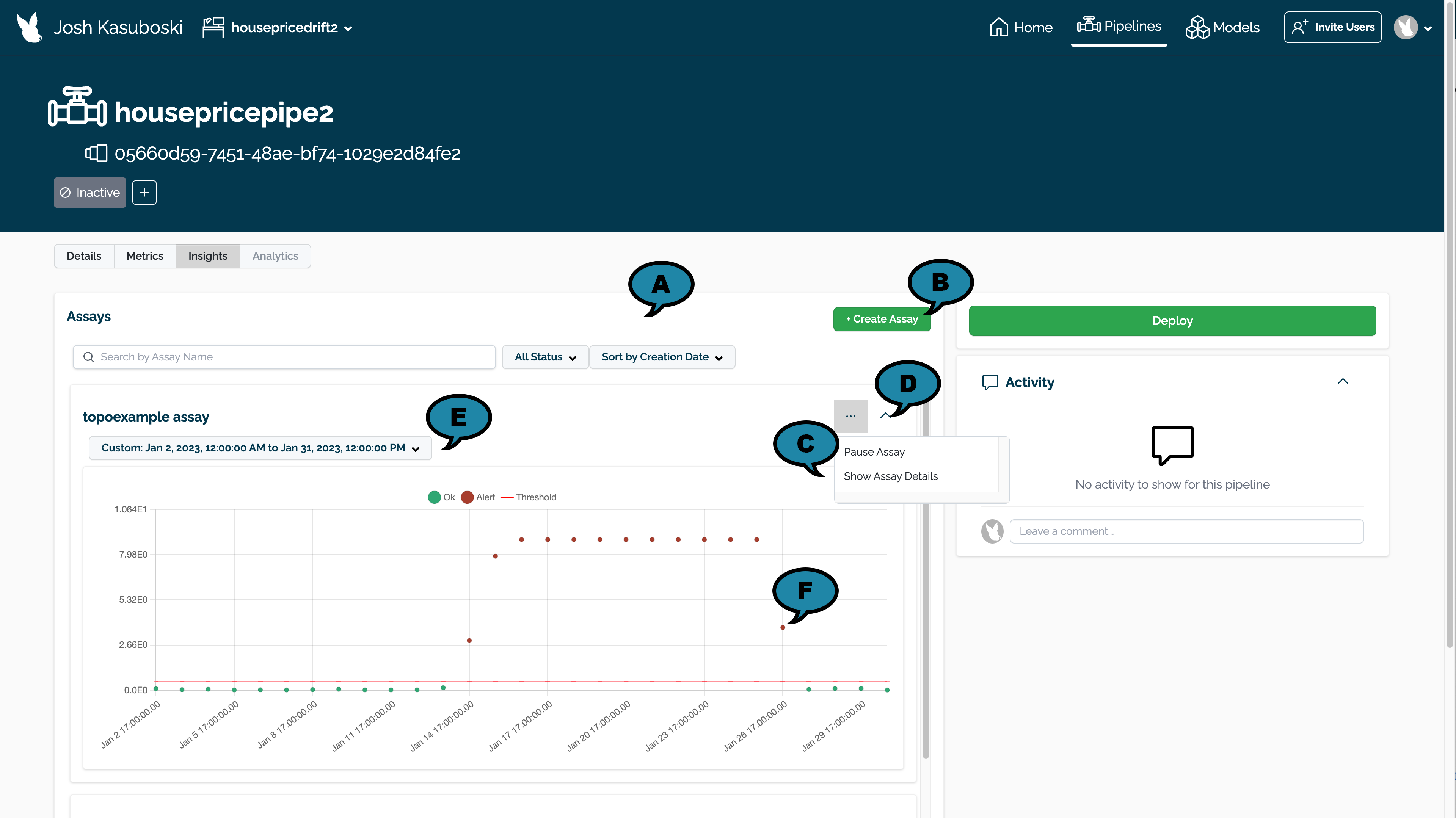
Accessing Assays Through the Pipeline Dashboard

Assays created through the Wallaroo Dashboard are accessed through the Pipeline Dashboard through the following process.

Log into the Wallaroo Dashboard.
Select the workspace containing the pipeline with the models being monitored from the Change Current Workspace and Workspace Management drop down.
Select View Pipelines.
Select the pipeline containing the models being monitored.
Select Insights.

The Wallaroo Assay Dashboard contains the following elements. For more details of each configuration type, see the Model Insights and Assays Introduction.

(A) Filter Assays: Filter assays by the following:
- Name
- Status:
  - Active: The assay is currently running.
  - Paused: The assay is paused until restarted.
  - Drift Detected: One or more drifts have been detected.
- Sort By
  - Sort by Creation Date: Sort by the most recent Assays first.
  - Last Assay Run: Sort by the most recent Assay Last Run date.
(B) Create Assay: Create a new assay.
(C) Assay Controls:
- Pause/Start Assay: Pause a running assay, or start one that was paused.
- Show Assay Details: View assay details. See Assay Details View for more details.
(D) Collapse Assay: Collapse or Expand the assay for view.
(E) Time Period for Assay Data: Set the time period for data to be used in displaying the assay results.
(F) Assay Events: Select an individual assay event to see more details. See View Assay Alert Details for more information.

Assay Details View

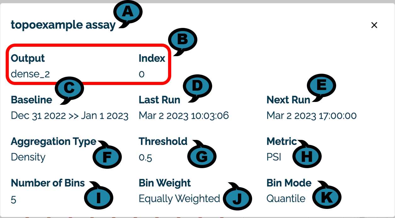
The following details are visible by selecting the Assay View Details icon:

(A) Assay Name: The name of the assay displayed.
(B) Input / Output: The input or output and the index of the element being monitored.
(C) Baseline: The time period used to generate the baseline. For baselines generated from a file, the baseline displayed Uploaded File.
(D) Last Run: The date and time the assay was last run.
(E) Next Run: The future date and time the assay will be run again. NOTE: If the assay is paused, then it will not run at the scheduled time. When unpaused, the date will be updated to the next date and time that the assay will be run.
(F) Aggregation Type: The aggregation type used with the assay.
(G) Threshold: The threshold value used for the assay.
(H) Metric: The metric type used for the assay.
(I) Number of Bins: The number of bins used for the assay.
(J) Bin Weight: The weight applied to each bin.
(K) Bin Mode: The type of bin node applied to each bin.

View Assay Alert Details

To view details on an assay alert:

Select the data with available alert data.
Mouse hover of a specific Assay Event Alert to view the data and time of the event and the alert value.
Select the Assay Event Alert to view the Baseline and Window details of the alert including the left_outlier and right_outlier.

Hover over a bar chart graph to view additional details.

Select the ⊗ symbol to exit the Assay Event Alert details and return to the Assay View.

Build an Assay Through the Pipeline Dashboard

To create a new assay through the Wallaroo Pipeline Dashboard:

Log into the Wallaroo Dashboard.
Select the workspace containing the pipeline with the models being monitored from the Change Current Workspace and Workspace Management drop down.
Select View Pipelines.
Select the pipeline containing the models being monitored.
Select Insights.
Select +Create Assay.
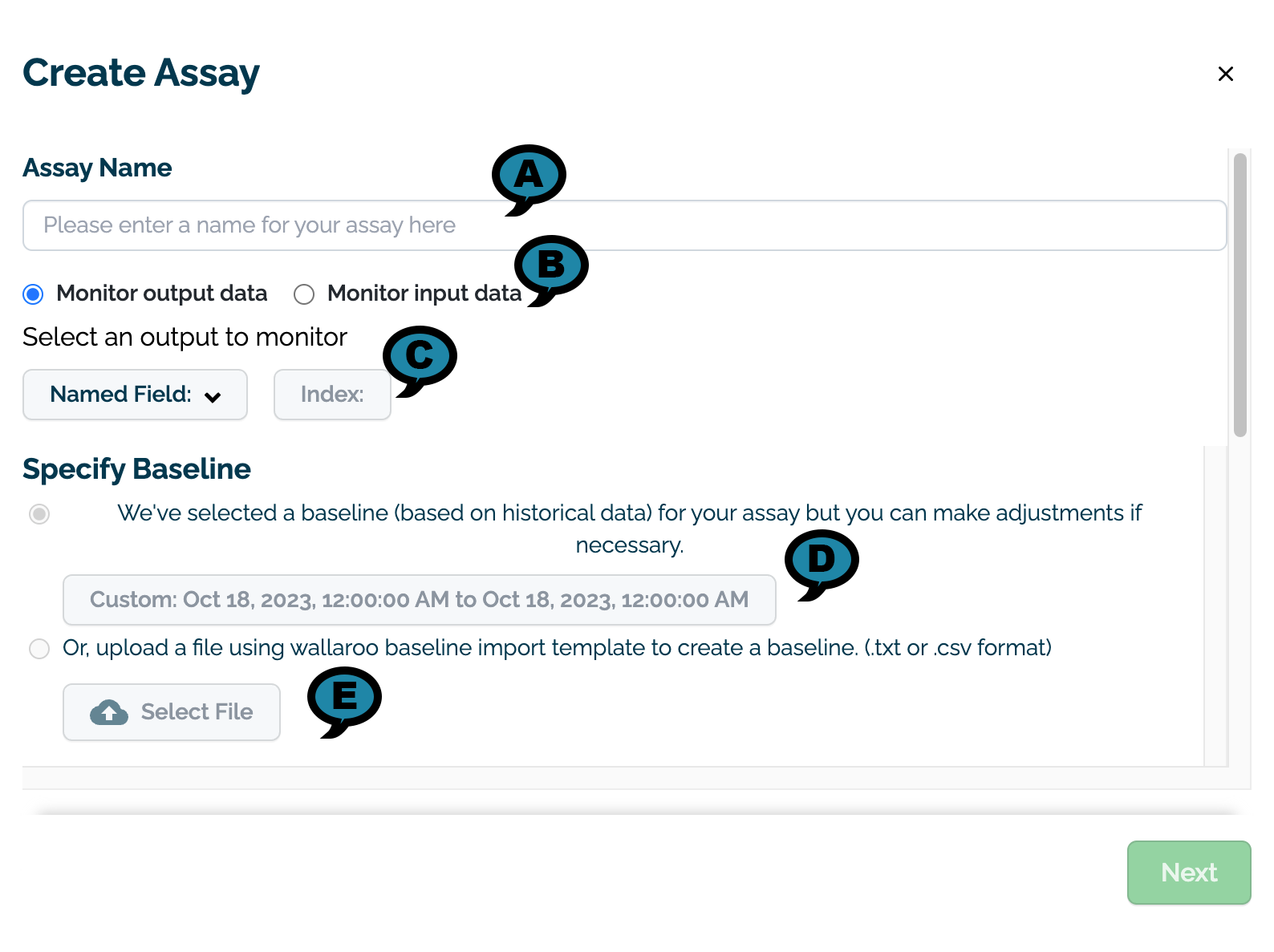
On the Create Assay module, enter the following:
1. On the Assay Name section, enter the following:
2. Assay Name (A): The name of the new assay.
3. Monitor output data or Monitor input data (B): Select whether to monitor input or output data.
4. Select an output/input to monitor (C): Select the input or output to monitor.
  1. Named Field: The name of the field to monitor.
  2. Index: The index of the monitored field.
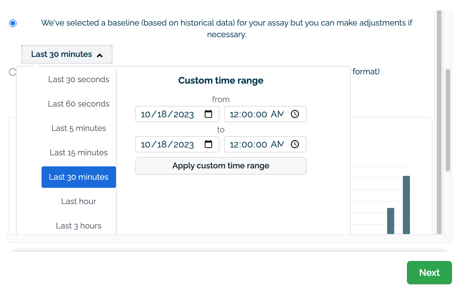
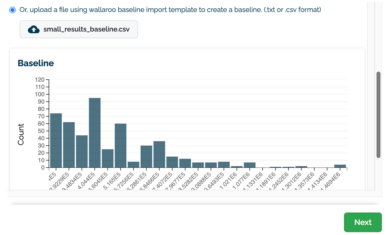
5. On the Specify Baseline section, select one of the following options:
  1. (D) Select the data to use for the baseline. This can either be set with a preset recent time period (last 30 seconds, last 60 seconds, etc) or with a custom date range.
  1. (E) Upload an assay baseline file as either a CSV or TXT file. These assay baselines must be a list of numpy (aka float) values that are comma and newline separated, terminating at the last record with no additional commas or returns.
    For example:
```
684577.200,
921561.500,
705013.440,
725875.900,
684577.200,
379398.300,
266405.600,
256630.310
```
  Once selected, a preview graph of the baseline values will be displayed (C). Note that this may take a few seconds to generate.
6. Select Next to continue.
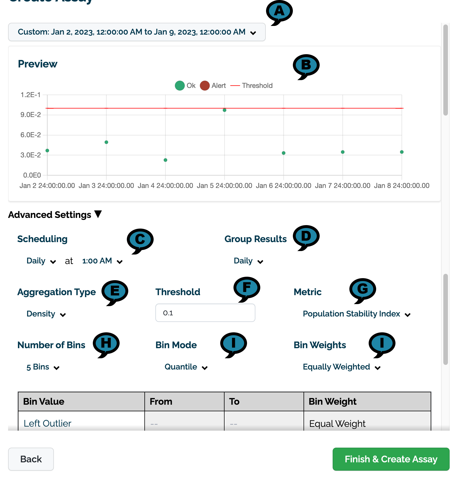
On the Settings Module:
1. Set the date and time range to view values generated by the assay. This can either be set with a preset recent time period (last 30 seconds, last 60 seconds, etc) or with a custom date range.
  New assays are configured to run a new analysis for every 24 hours starting at the end of the baseline period. For information on how to adjust the scheduling period and other settings for the assay scheduling window, see the SDK section on how to Schedule Assay.
2. Set the following Advanced Settings.
  1. (A) Preview Date Range: The date and times to for the preview chart.
  2. (B) Preview: A preview of the assay results will be displayed based on the settings below.
  3. (C) Scheduling: Set the Frequency (Daily, Every Minute, Hourly, Weekly, Default: Daily) and the Time (increments of one hour Default: 1:00 AM).
  4. (D) Group Results: How the results are grouped: Daily (Default), Every Minute, Weekly, or Monthly.
  5. (E) Aggregation Type: Density or Cumulative.
  6. (F) Threshold:
    1. Default: 0.1
  7. (G) Metric:
    1. Default: Population Stability Index
    2. Maximum Difference of Bins
    3. Sum of the Difference of Bins
  8. (H) Number of Bins: From 5 to 14. Default: 5
  9. (F) Bin Mode:
    1. Equally Spaced
    2. Default: Quantile
  10. (I) Bin Weights: The bin weights:
    1. Equally Weighted (Default)
    2. Custom: Users can assign their own bin weights as required.
3. Review the preview chart to verify the settings are correct.
4. Select Build to complete the process and build the new assay.

Once created, it may take a few minutes for the assay to complete compiling data. If needed, reload the Pipeline Dashboard to view changes.

Model Insights via the Wallaroo Dashboard SDK

Assays generated through the Wallaroo SDK can be previewed, configured, and uploaded to the Wallaroo Ops instance. The following is a condensed version of this process. For full details see the Wallaroo SDK Essentials Guide: Assays Management guide.

Model drift detection with assays using the Wallaroo SDK follows this general process.

Define the Baseline: From either historical inference data for a specific model in a pipeline, or from a pre-determine array of data, a baseline is formed.
Assay Preview: Once the baseline is formed, we preview the assay and configure the different options until we have the the best method of detecting environment or model drift.
Create Assay: With the previews and configuration complete, we upload the assay. The assay will perform an analysis on a regular scheduled based on the configuration.
Get Assay Results: Retrieve the analyses and use them to detect model drift and possible sources.
Pause/Resume Assay: Pause or restart an assay as needed.

Define the Baseline

Assay baselines are defined with the wallaroo.client.build_assay method. Through this process we define the baseline from either a range of dates or pre-generated values.

wallaroo.client.build_assay take the following parameters:

Parameter	Type	Description
assay_name	String (Required) - required	The name of the assay. Assay names must be unique across the Wallaroo instance.
pipeline	wallaroo.pipeline.Pipeline (Required)	The pipeline the assay is monitoring.
model_name	String (Required)	The name of the model to monitor.
iopath	String (Required)	The input/output data for the model being tracked in the format `input/output field index`. Only one value is tracked for any assay. For example, to track the output of the model’s field `house_value` at index `0`, the `iopath` is `'output house_value 0`.
baseline_start	datetime.datetime (Optional)	The start time for the inferences to use as the baseline. Must be included with `baseline_end`. Cannot be included with `baseline_data`.
baseline_end	datetime.datetime (Optional)	The end time of the baseline window. the baseline. Windows start immediately after the baseline window and are run at regular intervals continuously until the assay is deactivated or deleted. Must be included with `baseline_start`. Cannot be included with `baseline_data`..
baseline_data	numpy.array (Optional)	The baseline data in numpy array format. Cannot be included with either `baseline_start` or `baseline_data`.

Baselines are created in one of two ways:

Date Range: The baseline_start and baseline_end retrieves the inference requests and results for the pipeline from the start and end period. This data is summarized and used to create the baseline.
Numpy Values: The baseline_data sets the baseline from a provided numpy array.

Define the Baseline Example

This example shows two methods of defining the baseline for an assay:

"assays from date baseline": This assay uses historical inference requests to define the baseline. This assay is saved to the variable assay_builder_from_dates.
"assays from numpy": This assay uses a pre-generated numpy array to define the baseline. This assay is saved to the variable assay_builder_from_numpy.

In both cases, the following parameters are used:

Parameter	Value
assay_name	`"assays from date baseline"` and `"assays from numpy"`
pipeline	`mainpipeline`: A pipeline with a ML model that predicts house prices. The output field for this model is `variable`.
model_name	`"houseprice-predictor"` - the model name set during model upload.
iopath	These assays monitor the model’s output field variable at index 0. From this, the `iopath` setting is `"output variable 0"`.

The difference between the two assays’ parameters determines how the baseline is generated.

"assays from date baseline": Uses the baseline_start and baseline_end to set the time period of inference requests and results to gather data from.
"assays from numpy": Uses a pre-generated numpy array as for the baseline data.

For each of our assays, we will set the time period of inference data to compare against the baseline data.

# Build the assay, based on the start and end of our baseline time, 
# and tracking the output variable index 0
assay_builder_from_dates = wl.build_assay(assay_name="assays from date baseline", 
                                          pipeline=mainpipeline, 
                                          model_name="house-price-estimator", 
                                          iopath="output variable 0",
                                          baseline_start=assay_baseline_start, 
                                          baseline_end=assay_baseline_end)

# set the width, interval, and time period 
assay_builder_from_dates.add_run_until(datetime.datetime.now())
assay_builder_from_dates.window_builder().add_width(minutes=1).add_interval(minutes=1).add_start(assay_window_start)
assay_config_from_dates = assay_builder_from_dates.build()
assay_results_from_dates = assay_config_from_dates.interactive_run()

# assay builder by baseline
assay_builder_from_numpy = wl.build_assay(assay_name="assays from numpy", 
                               pipeline=mainpipeline, 
                               model_name="house-price-estimator", 
                               iopath="output variable 0", 
                               baseline_data = small_results_baseline)

# set the width, interval, and time period 
assay_builder_from_numpy.add_run_until(datetime.datetime.now())
assay_builder_from_numpy.window_builder().add_width(minutes=1).add_interval(minutes=1).add_start(assay_window_start)

assay_config_from_numpy = assay_builder_from_numpy.build()
assay_results_from_numpy = assay_config_from_numpy.interactive_run()

Baseline DataFrame

The method wallaroo.assay_config.AssayBuilder.baseline_dataframe returns a DataFrame of the assay baseline generated from the provided parameters. This includes:

metadata: The inference metadata with the model information, inference time, and other related factors.
in data: Each input field assigned with the label in.{input field name}.
out data: Each output field assigned with the label out.{output field name}

Note that for assays generated from numpy values, there is only the out data based on the supplied baseline data.

In the following example, the baseline DataFrame is retrieved.

display(assay_builder_from_dates.baseline_dataframe())

	time	metadata	input_tensor_0	input_tensor_1	input_tensor_2	input_tensor_3	input_tensor_4	input_tensor_5	input_tensor_6	input_tensor_7	...	input_tensor_9	input_tensor_10	input_tensor_11	input_tensor_12	input_tensor_13	input_tensor_14	input_tensor_15	input_tensor_16	input_tensor_17	output_variable_0
0	1708013922866	{'last_model': '{"model_name":"house-price-estimator","model_sha":"e22a0831aafd9917f3cc87a15ed267797f80e2afa12ad7d8810ca58f173b8cc6"}', 'pipeline_version': '', 'elapsed': [49610, 341497], 'dropped': [], 'partition': 'engine-58b565bf45-29xnm'}	4.0	3.00	3710.0	20000.0	2.0	0.0	2.0	5.0	...	2760.0	950.0	47.669600	-122.261000	3970.0	20000.0	79.0	0.0	0.0	1.514079e+06
1	1708013983808	{'last_model': '{"model_name":"house-price-estimator","model_sha":"e22a0831aafd9917f3cc87a15ed267797f80e2afa12ad7d8810ca58f173b8cc6"}', 'pipeline_version': '', 'elapsed': [2517407, 2287534], 'dropped': [], 'partition': 'engine-58b565bf45-29xnm'}	3.0	2.50	1500.0	7420.0	1.0	0.0	0.0	3.0	...	1000.0	500.0	47.723598	-122.174004	1840.0	7272.0	42.0	0.0	0.0	4.196772e+05
2	1708013983808	{'last_model': '{"model_name":"house-price-estimator","model_sha":"e22a0831aafd9917f3cc87a15ed267797f80e2afa12ad7d8810ca58f173b8cc6"}', 'pipeline_version': '', 'elapsed': [2517407, 2287534], 'dropped': [], 'partition': 'engine-58b565bf45-29xnm'}	4.0	2.50	2009.0	5000.0	2.0	0.0	0.0	3.0	...	2009.0	0.0	47.257702	-122.197998	2009.0	5182.0	0.0	0.0	0.0	3.208637e+05
3	1708013983808	{'last_model': '{"model_name":"house-price-estimator","model_sha":"e22a0831aafd9917f3cc87a15ed267797f80e2afa12ad7d8810ca58f173b8cc6"}', 'pipeline_version': '', 'elapsed': [2517407, 2287534], 'dropped': [], 'partition': 'engine-58b565bf45-29xnm'}	3.0	1.75	1530.0	7245.0	1.0	0.0	0.0	4.0	...	1530.0	0.0	47.730999	-122.191002	1530.0	7490.0	31.0	0.0	0.0	4.319292e+05
4	1708013983808	{'last_model': '{"model_name":"house-price-estimator","model_sha":"e22a0831aafd9917f3cc87a15ed267797f80e2afa12ad7d8810ca58f173b8cc6"}', 'pipeline_version': '', 'elapsed': [2517407, 2287534], 'dropped': [], 'partition': 'engine-58b565bf45-29xnm'}	3.0	1.75	1480.0	4800.0	2.0	0.0	0.0	4.0	...	1140.0	340.0	47.656700	-122.397003	1810.0	4800.0	70.0	0.0	0.0	5.361757e+05
...	...	...	...	...	...	...	...	...	...	...	...	...	...	...	...	...	...	...	...	...	...
496	1708013983808	{'last_model': '{"model_name":"house-price-estimator","model_sha":"e22a0831aafd9917f3cc87a15ed267797f80e2afa12ad7d8810ca58f173b8cc6"}', 'pipeline_version': '', 'elapsed': [2517407, 2287534], 'dropped': [], 'partition': 'engine-58b565bf45-29xnm'}	4.0	2.25	2560.0	12100.0	1.0	0.0	0.0	4.0	...	1760.0	800.0	47.631001	-122.108002	2240.0	12100.0	38.0	0.0	0.0	7.019407e+05
497	1708013983808	{'last_model': '{"model_name":"house-price-estimator","model_sha":"e22a0831aafd9917f3cc87a15ed267797f80e2afa12ad7d8810ca58f173b8cc6"}', 'pipeline_version': '', 'elapsed': [2517407, 2287534], 'dropped': [], 'partition': 'engine-58b565bf45-29xnm'}	2.0	1.00	1160.0	5000.0	1.0	0.0	0.0	4.0	...	1160.0	0.0	47.686501	-122.399002	1750.0	5000.0	77.0	0.0	0.0	4.508677e+05
498	1708013983808	{'last_model': '{"model_name":"house-price-estimator","model_sha":"e22a0831aafd9917f3cc87a15ed267797f80e2afa12ad7d8810ca58f173b8cc6"}', 'pipeline_version': '', 'elapsed': [2517407, 2287534], 'dropped': [], 'partition': 'engine-58b565bf45-29xnm'}	4.0	2.50	1910.0	5000.0	2.0	0.0	0.0	3.0	...	1910.0	0.0	47.360802	-122.036003	2020.0	5000.0	9.0	0.0	0.0	2.962027e+05
499	1708013983808	{'last_model': '{"model_name":"house-price-estimator","model_sha":"e22a0831aafd9917f3cc87a15ed267797f80e2afa12ad7d8810ca58f173b8cc6"}', 'pipeline_version': '', 'elapsed': [2517407, 2287534], 'dropped': [], 'partition': 'engine-58b565bf45-29xnm'}	3.0	1.50	1590.0	8911.0	1.0	0.0	0.0	3.0	...	1590.0	0.0	47.739399	-122.251999	1590.0	9625.0	58.0	0.0	0.0	4.371780e+05
500	1708013983808	{'last_model': '{"model_name":"house-price-estimator","model_sha":"e22a0831aafd9917f3cc87a15ed267797f80e2afa12ad7d8810ca58f173b8cc6"}', 'pipeline_version': '', 'elapsed': [2517407, 2287534], 'dropped': [], 'partition': 'engine-58b565bf45-29xnm'}	4.0	2.75	2640.0	4000.0	2.0	0.0	0.0	5.0	...	1730.0	910.0	47.672699	-122.296997	1530.0	3740.0	89.0	0.0	0.0	7.184457e+05

501 rows × 21 columns

assay_builder_from_numpy.baseline_dataframe()

	output_variable_0
0	419677.20
1	320863.72
2	431929.20
3	536175.70
4	343304.63
...	...
495	701940.70
496	450867.70
497	296202.70
498	437177.97
499	718445.70

500 rows × 1 columns

Baseline Stats

The method wallaroo.assay.AssayAnalysis.baseline_stats() returns a pandas.core.frame.DataFrame of the baseline stats.

The baseline stats for each assay are displayed in the examples below.

assay_results_from_dates[0].baseline_stats()

	Baseline
count	501
min	236238.671875
max	1514079.375
mean	495193.231786
median	442168.125
std	226075.814267
start	None
end	None

assay_results_from_numpy[0].baseline_stats()

	Baseline
count	500
min	236238.67
max	1489624.3
mean	493155.46054
median	441840.425
std	221657.583536
start	None
end	None

Baseline Bins

The method wallaroo.assay.AssayAnalysis.baseline_bins a simple dataframe to with the edge/bin data for a baseline.

assay_results_from_dates[0].baseline_bins()

	b_edges	b_edge_names	b_aggregated_values	b_aggregation
0	2.362387e+05	left_outlier	0.000000	Density
1	2.962027e+05	q_20	0.203593	Density
2	4.159643e+05	q_40	0.195609	Density
3	4.640602e+05	q_60	0.203593	Density
4	6.821819e+05	q_80	0.197605	Density
5	1.514079e+06	q_100	0.199601	Density
6	inf	right_outlier	0.000000	Density

assay_results_from_numpy[0].baseline_bins()

	b_edges	b_edge_names	b_aggregated_values	b_aggregation
0	236238.67	left_outlier	0.000	Density
1	296202.70	q_20	0.204	Density
2	415964.30	q_40	0.196	Density
3	464057.38	q_60	0.200	Density
4	675545.44	q_80	0.200	Density
5	1489624.30	q_100	0.200	Density
6	inf	right_outlier	0.000	Density

Baseline Histogram Chart

The method wallaroo.assay_config.AssayBuilder.baseline_histogram returns a histogram chart of the assay baseline generated from the provided parameters.

assay_builder_from_dates.baseline_histogram()

Baseline KDE Chart

The method wallaroo.assay_config.AssayBuilder.baseline_kde returns a Kernel Density Estimation (KDE) chart of the assay baseline generated from the provided parameters.

assay_builder_from_dates.baseline_kde()

Baseline ECDF Chart

The method wallaroo.assay_config.AssayBuilder.baseline_ecdf returns a Empirical Cumulative Distribution Function (CDF) chart of the assay baseline generated from the provided parameters.

assay_builder_from_dates.baseline_ecdf()

Assay Preview

Now that the baseline is defined, we look at different configuration options and view how the assay baseline and results changes. Once we determine what gives us the best method of determining model drift, we can create the assay.

Analysis List Chart Scores

Analysis List scores show the assay scores for each assay result interval in one chart. Values that are outside of the alert threshold are colored red, while scores within the alert threshold are green.

Assay chart scores are displayed with the method wallaroo.assay.AssayAnalysisList.chart_scores(title: Optional[str] = None), with ability to display an optional title with the chart.

The following example shows retrieving the assay results and displaying the chart scores. From our example, we have two windows - the first should be green, and the second is red showing that values were outside the alert threshold.

# Build the assay, based on the start and end of our baseline time, 
# and tracking the output variable index 0
assay_builder_from_dates = wl.build_assay(assay_name="assays from date baseline", 
                                          pipeline=mainpipeline, 
                                          model_name="house-price-estimator", 
                                          iopath="output variable 0",
                                          baseline_start=assay_baseline_start, 
                                          baseline_end=assay_baseline_end)

# set the width, interval, and time period 
assay_builder_from_dates.add_run_until(datetime.datetime.now())
assay_builder_from_dates.window_builder().add_width(minutes=1).add_interval(minutes=1).add_start(assay_window_start)
assay_config_from_dates = assay_builder_from_dates.build()
assay_results_from_dates = assay_config_from_dates.interactive_run()

assay_results_from_dates.chart_scores()

Analysis Chart

The method wallaroo.assay.AssayAnalysis.chart() displays a comparison between the baseline and an interval of inference data.

This is compared to the Chart Scores, which is a list of all of the inference data split into intervals, while the Analysis Chart shows the breakdown of one set of inference data against the baseline.

Score from the Analysis List Chart Scores and each element from the Analysis List DataFrame generates

The following fields are included.

Field	Type	Description
baseline mean	Float	The mean of the baseline values.
window mean	Float	The mean of the window values.
baseline median	Float	The median of the baseline values.
window median	Float	The median of the window values.
bin_mode	String	The binning mode used for the assay.
aggregation	String	The aggregation mode used for the assay.
metric	String	The metric mode used for the assay.
weighted	Bool	Whether the bins were manually weighted.
score	Float	The score from the assay window.
scores	List(Float)	The score from each assay window bin.
index	Integer/None	The window index. Interactive assay runs are `None`.

# Build the assay, based on the start and end of our baseline time, 
# and tracking the output variable index 0
assay_builder_from_dates = wl.build_assay(assay_name="assays from date baseline", 
                                          pipeline=mainpipeline, 
                                          model_name="house-price-estimator", 
                                          iopath="output variable 0",
                                          baseline_start=assay_baseline_start, 
                                          baseline_end=assay_baseline_end)

# set the width, interval, and time period 
assay_builder_from_dates.add_run_until(datetime.datetime.now())
assay_builder_from_dates.window_builder().add_width(minutes=1).add_interval(minutes=1).add_start(assay_window_start)
assay_config_from_dates = assay_builder_from_dates.build()
assay_results_from_dates = assay_config_from_dates.interactive_run()

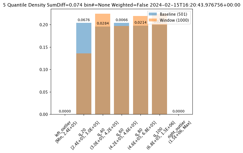
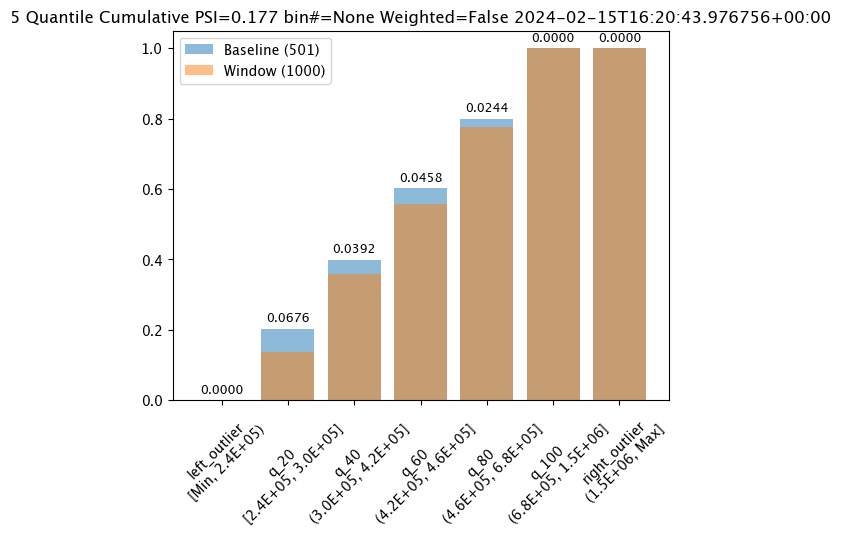
assay_results_from_dates[0].chart()

baseline mean = 495193.23178642715
window mean = 517763.394625
baseline median = 442168.125
window median = 448627.8125
bin_mode = Quantile
aggregation = Density
metric = PSI
weighted = False
score = 0.0363497101644573
scores = [0.0, 0.027271477163285655, 0.003847844548034077, 0.000217023993714693, 0.002199485350158766, 0.0028138791092641195, 0.0]
index = None

Analysis List DataFrame

wallaroo.assay.AssayAnalysisList.to_dataframe() returns a DataFrame showing the assay results for each window aka individual analysis. This DataFrame contains the following fields:

Field	Type	Description
assay_id	Integer/None	The assay id. Only provided from uploaded and executed assays.
name	String/None	The name of the assay. Only provided from uploaded and executed assays.
iopath	String/None	The iopath of the assay. Only provided from uploaded and executed assays.
score	Float	The assay score.
start	DateTime	The DateTime start of the assay window.
min	Float	The minimum value in the assay window.
max	Float	The maximum value in the assay window.
mean	Float	The mean value in the assay window.
median	Float	The median value in the assay window.
std	Float	The standard deviation value in the assay window.
warning_threshold	Float/None	The warning threshold of the assay window.
alert_threshold	Float/None	The alert threshold of the assay window.
status	String	The assay window status. Values are: `OK`: The score is within accepted thresholds. `Warning`: The score has triggered the `warning_threshold` if exists, but not the `alert_threshold`. `Alert`: The score has triggered the the `alert_threshold`.

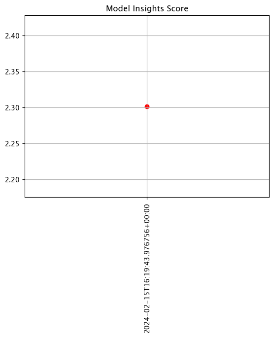
For this example, the assay analysis list DataFrame is listed.

From this tutorial, we should have 2 windows of dta to look at, each one minute apart. The first window should show status: OK, with the second window with the very large house prices will show status: alert

# Build the assay, based on the start and end of our baseline time, 
# and tracking the output variable index 0
assay_builder_from_dates = wl.build_assay(assay_name="assays from date baseline", 
                                          pipeline=mainpipeline, 
                                          model_name="house-price-estimator", 
                                          iopath="output variable 0",
                                          baseline_start=assay_baseline_start, 
                                          baseline_end=assay_baseline_end)

# set the width, interval, and time period 
assay_builder_from_dates.add_run_until(datetime.datetime.now())
assay_builder_from_dates.window_builder().add_width(minutes=1).add_interval(minutes=1).add_start(assay_window_start)
assay_config_from_dates = assay_builder_from_dates.build()
assay_results_from_dates = assay_config_from_dates.interactive_run()

assay_results_from_dates.to_dataframe()

	assay_id	name	iopath	score	start	min	max	mean	median	std	warning_threshold	alert_threshold	status
0	None			0.036350	2024-02-15T16:20:43.976756+00:00	2.362387e+05	1489624.250	5.177634e+05	4.486278e+05	227729.030050	None	0.25	Ok
1	None			8.868614	2024-02-15T16:22:43.976756+00:00	1.514079e+06	2016006.125	1.885772e+06	1.946438e+06	160046.727324	None	0.25	Alert

Analysis List Full DataFrame

wallaroo.assay.AssayAnalysisList.to_full_dataframe() returns a DataFrame showing all values, including the inputs and outputs from the assay results for each window aka individual analysis. This DataFrame contains the following fields:

pipeline_id	warning_threshold	bin_index	created_at

Field	Type	Description
window_start	DateTime	The date and time when the window period began.
analyzed_at	DateTime	The date and time when the assay analysis was performed.
elapsed_millis	Integer	How long the analysis took to perform in milliseconds.
baseline_summary_count	Integer	The number of data elements from the baseline.
baseline_summary_min	Float	The minimum value from the baseline summary.
baseline_summary_max	Float	The maximum value from the baseline summary.
baseline_summary_mean	Float	The mean value of the baseline summary.
baseline_summary_median	Float	The median value of the baseline summary.
baseline_summary_std	Float	The standard deviation value of the baseline summary.
baseline_summary_edges_{0…n}	Float	The baseline summary edges for each baseline edge from 0 to number of edges.
summarizer_type	String	The type of summarizer used for the baseline. See `wallaroo.assay_config` for other summarizer types.
summarizer_bin_weights	List / None	If baseline bin weights were provided, the list of those weights. Otherwise, `None`.
summarizer_provided_edges	List / None	If baseline bin edges were provided, the list of those edges. Otherwise, `None`.
status	String	The assay window status. Values are: `OK`: The score is within accepted thresholds. `Warning`: The score has triggered the `warning_threshold` if exists, but not the `alert_threshold`. `Alert`: The score has triggered the the `alert_threshold`.
id	Integer/None	The id for the window aka analysis. Only provided from uploaded and executed assays.
assay_id	Integer/None	The assay id. Only provided from uploaded and executed assays.
pipeline_id	Integer/None	The pipeline id. Only provided from uploaded and executed assays.
warning_threshold	Float	The warning threshold set for the assay.
warning_threshold	Float	The warning threshold set for the assay.
bin_index	Integer/None	The bin index for the window aka analysis.
created_at	Datetime/None	The date and time the window aka analysis was generated. Only provided from uploaded and executed assays.

For this example, full DataFrame from an assay preview is generated.

# Build the assay, based on the start and end of our baseline time, 
# and tracking the output variable index 0
assay_builder_from_dates = wl.build_assay(assay_name="assays from date baseline", 
                                          pipeline=mainpipeline, 
                                          model_name="house-price-estimator", 
                                          iopath="output variable 0",
                                          baseline_start=assay_baseline_start, 
                                          baseline_end=assay_baseline_end)

# set the width, interval, and time period 
assay_builder_from_dates.add_run_until(datetime.datetime.now())
assay_builder_from_dates.window_builder().add_width(minutes=1).add_interval(minutes=1).add_start(assay_window_start)
assay_config_from_dates = assay_builder_from_dates.build()
assay_results_from_dates = assay_config_from_dates.interactive_run()

assay_results_from_dates.to_full_dataframe()

	window_start	analyzed_at	elapsed_millis	baseline_summary_count	baseline_summary_min	baseline_summary_max	baseline_summary_mean	baseline_summary_median	baseline_summary_std	baseline_summary_edges_0	...	summarizer_type	summarizer_bin_weights	summarizer_provided_edges	status	id	assay_id	pipeline_id	warning_threshold	bin_index	created_at
0	2024-02-15T16:20:43.976756+00:00	2024-02-15T16:26:42.266029+00:00	82	501	236238.671875	1514079.375	495193.231786	442168.125	226075.814267	236238.671875	...	UnivariateContinuous	None	None	Ok	None	None	None	None	None	None
1	2024-02-15T16:22:43.976756+00:00	2024-02-15T16:26:42.266134+00:00	83	501	236238.671875	1514079.375	495193.231786	442168.125	226075.814267	236238.671875	...	UnivariateContinuous	None	None	Alert	None	None	None	None	None	None

2 rows × 86 columns

Analysis Compare Basic Stats

The method wallaroo.assay.AssayAnalysis.compare_basic_stats returns a DataFrame comparing one set of inference data against the baseline.

This is compared to the Analysis List DataFrame, which is a list of all of the inference data split into intervals, while the Analysis Compare Basic Stats shows the breakdown of one set of inference data against the baseline.

# Build the assay, based on the start and end of our baseline time, 
# and tracking the output variable index 0
assay_builder_from_dates = wl.build_assay(assay_name="assays from date baseline", 
                                          pipeline=mainpipeline, 
                                          model_name="house-price-estimator", 
                                          iopath="output variable 0",
                                          baseline_start=assay_baseline_start, 
                                          baseline_end=assay_baseline_end)

# set the width, interval, and time period 
assay_builder_from_dates.add_run_until(datetime.datetime.now())
assay_builder_from_dates.window_builder().add_width(minutes=1).add_interval(minutes=1).add_start(assay_window_start)
assay_config_from_dates = assay_builder_from_dates.build()
assay_results_from_dates = assay_config_from_dates.interactive_run()

assay_results_from_dates[0].compare_basic_stats()

	Baseline	Window	diff	pct_diff
count	501.0	1000.0	499.000000	99.600798
min	236238.671875	236238.671875	0.000000	0.000000
max	1514079.375	1489624.25	-24455.125000	-1.615181
mean	495193.231786	517763.394625	22570.162839	4.557850
median	442168.125	448627.8125	6459.687500	1.460912
std	226075.814267	227729.03005	1653.215783	0.731266
start	None	2024-02-15T16:20:43.976756+00:00	NaN	NaN
end	None	2024-02-15T16:21:43.976756+00:00	NaN	NaN

Configure Assays

Before creating the assay, configure the assay and continue to preview it until the best method for detecting drift is set. The following options are available.

Score Metric

The score is a distance between the baseline and the analysis window. The larger the score, the greater the difference between the baseline and the analysis window. The following methods are provided determining the score:

PSI (Default) - Population Stability Index (PSI).
MAXDIFF: Maximum difference between corresponding bins.
SUMDIFF: Mum of differences between corresponding bins.

The metric type used is updated with the wallaroo.assay_config.AssayBuilder.add_metric(metric: wallaroo.assay_config.Metric) method.

The following three charts use each of the metrics. Note how the scores change based on the score type used.

# Build the assay, based on the start and end of our baseline time, 
# and tracking the output variable index 0
assay_builder_from_dates = wl.build_assay(assay_name="assays from date baseline", 
                                          pipeline=mainpipeline, 
                                          model_name="house-price-estimator", 
                                          iopath="output variable 0",
                                          baseline_start=assay_baseline_start, 
                                          baseline_end=assay_baseline_end)

# set metric PSI mode
assay_builder_from_dates.summarizer_builder.add_metric(wallaroo.assay_config.Metric.PSI)

# set the width, interval, and time period 
assay_builder_from_dates.add_run_until(datetime.datetime.now())
assay_builder_from_dates.window_builder().add_width(minutes=1).add_interval(minutes=1).add_start(assay_window_start)
assay_config_from_dates = assay_builder_from_dates.build()
assay_results_from_dates = assay_config_from_dates.interactive_run()

assay_results_from_dates[0].chart()

baseline mean = 495193.23178642715
window mean = 517763.394625
baseline median = 442168.125
window median = 448627.8125
bin_mode = Quantile
aggregation = Density
metric = PSI
weighted = False
score = 0.0363497101644573
scores = [0.0, 0.027271477163285655, 0.003847844548034077, 0.000217023993714693, 0.002199485350158766, 0.0028138791092641195, 0.0]
index = None

# Build the assay, based on the start and end of our baseline time, 
# and tracking the output variable index 0
assay_builder_from_dates = wl.build_assay(assay_name="assays from date baseline", 
                                          pipeline=mainpipeline, 
                                          model_name="house-price-estimator", 
                                          iopath="output variable 0",
                                          baseline_start=assay_baseline_start, 
                                          baseline_end=assay_baseline_end)

# set metric MAXDIFF mode
assay_builder_from_dates.summarizer_builder.add_metric(wallaroo.assay_config.Metric.MAXDIFF)

# set the width, interval, and time period 
assay_builder_from_dates.add_run_until(datetime.datetime.now())
assay_builder_from_dates.window_builder().add_width(minutes=1).add_interval(minutes=1).add_start(assay_window_start)
assay_config_from_dates = assay_builder_from_dates.build()
assay_results_from_dates = assay_config_from_dates.interactive_run()

assay_results_from_dates[0].chart()

baseline mean = 495193.23178642715
window mean = 517763.394625
baseline median = 442168.125
window median = 448627.8125
bin_mode = Quantile
aggregation = Density
metric = MaxDiff
weighted = False
score = 0.06759281437125747
scores = [0.0, 0.06759281437125747, 0.028391217564870255, 0.006592814371257472, 0.02139520958083832, 0.02439920159680639, 0.0]
index = 1

# Build the assay, based on the start and end of our baseline time, 
# and tracking the output variable index 0
assay_builder_from_dates = wl.build_assay(assay_name="assays from date baseline", 
                                          pipeline=mainpipeline, 
                                          model_name="house-price-estimator", 
                                          iopath="output variable 0",
                                          baseline_start=assay_baseline_start, 
                                          baseline_end=assay_baseline_end)

# set metric SUMDIFF mode
assay_builder_from_dates.summarizer_builder.add_metric(wallaroo.assay_config.Metric.SUMDIFF)

# set the width, interval, and time period 
assay_builder_from_dates.add_run_until(datetime.datetime.now())
assay_builder_from_dates.window_builder().add_width(minutes=1).add_interval(minutes=1).add_start(assay_window_start)
assay_config_from_dates = assay_builder_from_dates.build()
assay_results_from_dates = assay_config_from_dates.interactive_run()

assay_results_from_dates[0].chart()

baseline mean = 495193.23178642715
window mean = 517763.394625
baseline median = 442168.125
window median = 448627.8125
bin_mode = Quantile
aggregation = Density
metric = SumDiff
weighted = False
score = 0.07418562874251496
scores = [0.0, 0.06759281437125747, 0.028391217564870255, 0.006592814371257472, 0.02139520958083832, 0.02439920159680639, 0.0]
index = None

Alert Threshold

Assay alert thresholds are modified with the wallaroo.assay_config.AssayBuilder.add_alert_threshold(alert_threshold: float) method. By default alert thresholds are 0.1.

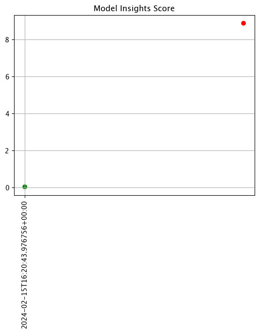
The following example updates the alert threshold to 0.5.

# Build the assay, based on the start and end of our baseline time, 
# and tracking the output variable index 0
assay_builder_from_dates = wl.build_assay(assay_name="assays from date baseline", 
                                          pipeline=mainpipeline, 
                                          model_name="house-price-estimator", 
                                          iopath="output variable 0",
                                          baseline_start=assay_baseline_start, 
                                          baseline_end=assay_baseline_end)

assay_builder_from_dates.add_alert_threshold(0.5)

# set the width, interval, and time period 
assay_builder_from_dates.add_run_until(datetime.datetime.now())
assay_builder_from_dates.window_builder().add_width(minutes=1).add_interval(minutes=1).add_start(assay_window_start)
assay_config_from_dates = assay_builder_from_dates.build()
assay_results_from_dates = assay_config_from_dates.interactive_run()

assay_results_from_dates.to_dataframe()

	assay_id	name	iopath	score	start	min	max	mean	median	std	warning_threshold	alert_threshold	status
0	None			0.036350	2024-02-15T16:20:43.976756+00:00	2.362387e+05	1489624.250	5.177634e+05	4.486278e+05	227729.030050	None	0.5	Ok
1	None			8.868614	2024-02-15T16:22:43.976756+00:00	1.514079e+06	2016006.125	1.885772e+06	1.946438e+06	160046.727324	None	0.5	Alert

Number of Bins

Number of bins sets how the baseline data is partitioned. The total number of bins includes the set number plus the left_outlier and the right_outlier, so the total number of bins will be the total set + 2.

The number of bins is set with the wallaroo.assay_config.UnivariateContinousSummarizerBuilder.add_num_bins(num_bins: int) method.

# Build the assay, based on the start and end of our baseline time, 
# and tracking the output variable index 0
assay_builder_from_dates = wl.build_assay(assay_name="assays from date baseline", 
                                          pipeline=mainpipeline, 
                                          model_name="house-price-estimator", 
                                          iopath="output variable 0",
                                          baseline_start=assay_baseline_start, 
                                          baseline_end=assay_baseline_end)

# Set the number of bins
# update number of bins here
assay_builder_from_dates.summarizer_builder.add_num_bins(10)

# set the width, interval, and time period 
assay_builder_from_dates.add_run_until(datetime.datetime.now())
assay_builder_from_dates.window_builder().add_width(minutes=1).add_interval(minutes=1).add_start(assay_window_start)
assay_config_from_dates = assay_builder_from_dates.build()
assay_results_from_dates = assay_config_from_dates.interactive_run()

assay_results_from_dates[0].chart()

baseline mean = 495193.23178642715
window mean = 517763.394625
baseline median = 442168.125
window median = 448627.8125
bin_mode = Quantile
aggregation = Density
metric = PSI
weighted = False
score = 0.05250979748389363
scores = [0.0, 0.009076998929542533, 0.01924002322223739, 0.0021945246367443406, 0.0016700458183385653, 0.005779503770625584, 0.002393429678215835, 0.002942858220315506, 0.00010651192741915124, 0.00046961759334670583, 0.008636283687108028, 0.0]
index = None

Binning Mode

Binning Mode defines how the bins are separated. Binning modes are modified through the wallaroo.assay_config.UnivariateContinousSummarizerBuilder.add_bin_mode(bin_mode: bin_mode: wallaroo.assay_config.BinMode, edges: Optional[List[float]] = None).

Available bin_mode values from wallaroo.assay_config.Binmode are the following:

QUANTILE (Default): Based on percentages. If num_bins is 5 then quintiles so bins are created at the 20%, 40%, 60%, 80% and 100% points.
EQUAL: Evenly spaced bins where each bin is set with the formula min - max / num_bins
PROVIDED: The user provides the edge points for the bins.

If PROVIDED is supplied, then a List of float values must be provided for the edges parameter that matches the number of bins.

The following examples are used to show how each of the binning modes effects the bins.

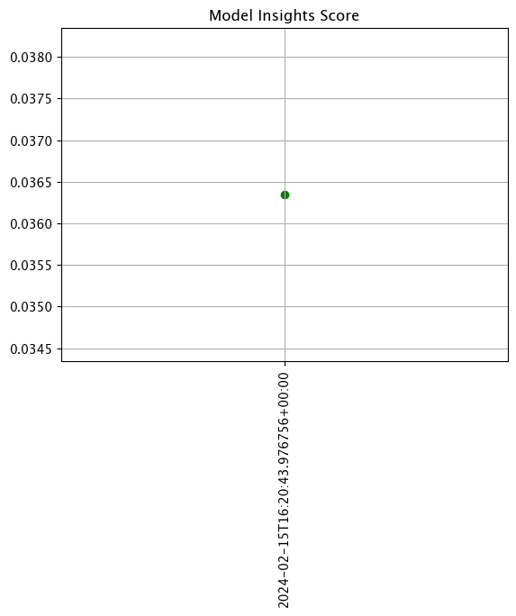
# Build the assay, based on the start and end of our baseline time, 
# and tracking the output variable index 0
assay_builder_from_dates = wl.build_assay(assay_name="assays from date baseline", 
                                          pipeline=mainpipeline, 
                                          model_name="house-price-estimator", 
                                          iopath="output variable 0",
                                          baseline_start=assay_baseline_start, 
                                          baseline_end=assay_baseline_end)

# update binning mode here
assay_builder_from_dates.summarizer_builder.add_bin_mode(wallaroo.assay_config.BinMode.QUANTILE)

# set the width, interval, and time period 
assay_builder_from_dates.add_run_until(datetime.datetime.now())
assay_builder_from_dates.window_builder().add_width(minutes=1).add_interval(minutes=1).add_start(assay_window_start)
assay_config_from_dates = assay_builder_from_dates.build()
assay_results_from_dates = assay_config_from_dates.interactive_run()

assay_results_from_dates[0].chart()

baseline mean = 495193.23178642715
window mean = 517763.394625
baseline median = 442168.125
window median = 448627.8125
bin_mode = Quantile
aggregation = Density
metric = PSI
weighted = False
score = 0.0363497101644573
scores = [0.0, 0.027271477163285655, 0.003847844548034077, 0.000217023993714693, 0.002199485350158766, 0.0028138791092641195, 0.0]
index = None

# Build the assay, based on the start and end of our baseline time, 
# and tracking the output variable index 0
assay_builder_from_dates = wl.build_assay(assay_name="assays from date baseline", 
                                          pipeline=mainpipeline, 
                                          model_name="house-price-estimator", 
                                          iopath="output variable 0",
                                          baseline_start=assay_baseline_start, 
                                          baseline_end=assay_baseline_end)

# update binning mode here
assay_builder_from_dates.summarizer_builder.add_bin_mode(wallaroo.assay_config.BinMode.EQUAL)

# set the width, interval, and time period 
assay_builder_from_dates.add_run_until(datetime.datetime.now())
assay_builder_from_dates.window_builder().add_width(minutes=1).add_interval(minutes=1).add_start(assay_window_start)
assay_config_from_dates = assay_builder_from_dates.build()
assay_results_from_dates = assay_config_from_dates.interactive_run()

assay_results_from_dates[0].chart()

baseline mean = 495193.23178642715
window mean = 517763.394625
baseline median = 442168.125
window median = 448627.8125
bin_mode = Equal
aggregation = Density
metric = PSI
weighted = False
score = 0.013362603453760629
scores = [0.0, 0.0016737762070682225, 1.1166481947075492e-06, 0.011233704798893194, 1.276169365380064e-07, 0.00045387818266796784, 0.0]
index = None

The following example manually sets the bin values.

The values in this dataset run from 200000 to 1500000. We can specify the bins with the BinMode.PROVIDED and specifying a list of floats with the right hand / upper edge of each bin and optionally the lower edge of the smallest bin. If the lowest edge is not specified the threshold for left outliers is taken from the smallest value in the baseline dataset.

# Build the assay, based on the start and end of our baseline time, 
# and tracking the output variable index 0
assay_builder_from_dates = wl.build_assay(assay_name="assays from date baseline", 
                                          pipeline=mainpipeline, 
                                          model_name="house-price-estimator", 
                                          iopath="output variable 0",
                                          baseline_start=assay_baseline_start, 
                                          baseline_end=assay_baseline_end)

edges = [200000.0, 400000.0, 600000.0, 800000.0, 1500000.0, 2000000.0]

# update binning mode here
assay_builder_from_dates.summarizer_builder.add_bin_mode(wallaroo.assay_config.BinMode.PROVIDED, edges)

# set the width, interval, and time period 
assay_builder_from_dates.add_run_until(datetime.datetime.now())
assay_builder_from_dates.window_builder().add_width(minutes=1).add_interval(minutes=1).add_start(assay_window_start)
assay_config_from_dates = assay_builder_from_dates.build()
assay_results_from_dates = assay_config_from_dates.interactive_run()

assay_results_from_dates[0].chart()

baseline mean = 495193.23178642715
window mean = 517763.394625
baseline median = 442168.125
window median = 448627.8125
bin_mode = Provided
aggregation = Density
metric = PSI
weighted = False
score = 0.01005936099521711
scores = [0.0, 0.0030207963288415803, 0.00011480201840874194, 0.00045327555974347976, 0.0037119550613212583, 0.0027585320269020493, 0.0]
index = None

Aggregation Options

Assay aggregation options are modified with the wallaroo.assay_config.AssayBuilder.add_aggregation(aggregation: wallaroo.assay_config.Aggregation) method. The following options are provided:

Aggregation.DENSITY (Default): Count the number/percentage of values that fall in each bin.
Aggregation.CUMULATIVE: Empirical Cumulative Density Function style, which keeps a cumulative count of the values/percentages that fall in each bin.

The following example demonstrate the different results between the two.

#Aggregation.DENSITY - the default

# Build the assay, based on the start and end of our baseline time, 
# and tracking the output variable index 0
assay_builder_from_dates = wl.build_assay(assay_name="assays from date baseline", 
                                          pipeline=mainpipeline, 
                                          model_name="house-price-estimator", 
                                          iopath="output variable 0",
                                          baseline_start=assay_baseline_start, 
                                          baseline_end=assay_baseline_end)

assay_builder_from_dates.summarizer_builder.add_aggregation(wallaroo.assay_config.Aggregation.DENSITY)

# set the width, interval, and time period 
assay_builder_from_dates.add_run_until(datetime.datetime.now())
assay_builder_from_dates.window_builder().add_width(minutes=1).add_interval(minutes=1).add_start(assay_window_start)
assay_config_from_dates = assay_builder_from_dates.build()
assay_results_from_dates = assay_config_from_dates.interactive_run()

assay_results_from_dates[0].chart()

baseline mean = 495193.23178642715
window mean = 517763.394625
baseline median = 442168.125
window median = 448627.8125
bin_mode = Quantile
aggregation = Density
metric = PSI
weighted = False
score = 0.0363497101644573
scores = [0.0, 0.027271477163285655, 0.003847844548034077, 0.000217023993714693, 0.002199485350158766, 0.0028138791092641195, 0.0]
index = None

#Aggregation.CUMULATIVE

# Build the assay, based on the start and end of our baseline time, 
# and tracking the output variable index 0
assay_builder_from_dates = wl.build_assay(assay_name="assays from date baseline", 
                                          pipeline=mainpipeline, 
                                          model_name="house-price-estimator", 
                                          iopath="output variable 0",
                                          baseline_start=assay_baseline_start, 
                                          baseline_end=assay_baseline_end)

assay_builder_from_dates.summarizer_builder.add_aggregation(wallaroo.assay_config.Aggregation.CUMULATIVE)

# set the width, interval, and time period 
assay_builder_from_dates.add_run_until(datetime.datetime.now())
assay_builder_from_dates.window_builder().add_width(minutes=1).add_interval(minutes=1).add_start(assay_window_start)
assay_config_from_dates = assay_builder_from_dates.build()
assay_results_from_dates = assay_config_from_dates.interactive_run()

assay_results_from_dates[0].chart()

baseline mean = 495193.23178642715
window mean = 517763.394625
baseline median = 442168.125
window median = 448627.8125
bin_mode = Quantile
aggregation = Cumulative
metric = PSI
weighted = False
score = 0.17698802395209584
scores = [0.0, 0.06759281437125747, 0.03920159680638724, 0.04579441117764471, 0.02439920159680642, 0.0, 0.0]
index = None

Inference Interval and Inference Width

The inference interval aka window interval sets how often to run the assay analysis. This is set from the wallaroo.assay_config.AssayBuilder.window_builder.add_interval method to collect data expressed in time units: “hours=24”, “minutes=1”, etc.

For example, with an interval of 1 minute, the assay collects data every minute. Within an hour, 60 intervals of data is collected.

We can adjust the interval and see how the assays change based on how frequently they are run.

The width sets the time period from the wallaroo.assay_config.AssayBuilder.window_builder.add_width method to collect data expressed in time units: “hours=24”, “minutes=1”, etc.

For example, an interval of 1 minute and a width of 1 minute collects 1 minutes worth of data every minute. An interval of 1 minute with a width of 5 minutes collects 5 minute of inference data every minute.

By default, the interval and width is 24 hours.

For this example, we’ll adjust the width and interval from 1 minute to 5 minutes and see how the number of analyses and their score changes.

# Build the assay, based on the start and end of our baseline time, 
# and tracking the output variable index 0
assay_builder_from_dates = wl.build_assay(assay_name="assays from date baseline", 
                                          pipeline=mainpipeline, 
                                          model_name="house-price-estimator", 
                                          iopath="output variable 0",
                                          baseline_start=assay_baseline_start, 
                                          baseline_end=assay_baseline_end)

# set the width, interval, and time period 
assay_builder_from_dates.add_run_until(datetime.datetime.now())
assay_builder_from_dates.window_builder().add_width(minutes=1).add_interval(minutes=1).add_start(assay_window_start)
assay_config_from_dates = assay_builder_from_dates.build()
assay_results_from_dates = assay_config_from_dates.interactive_run()

assay_results_from_dates.chart_scores()

# Build the assay, based on the start and end of our baseline time, 
# and tracking the output variable index 0
assay_builder_from_dates = wl.build_assay(assay_name="assays from date baseline", 
                                          pipeline=mainpipeline, 
                                          model_name="house-price-estimator", 
                                          iopath="output variable 0",
                                          baseline_start=assay_baseline_start, 
                                          baseline_end=assay_baseline_end)

# set the width, interval, and time period 
assay_builder_from_dates.add_run_until(datetime.datetime.now())
assay_builder_from_dates.window_builder().add_width(minutes=5).add_interval(minutes=5).add_start(assay_window_start)
assay_config_from_dates = assay_builder_from_dates.build()
assay_results_from_dates = assay_config_from_dates.interactive_run()

assay_results_from_dates.chart_scores()

Add Run Until and Add Inference Start

For previewing assays, setting wallaroo.assay_config.AssayBuilder.add_run_until sets the end date and time for collecting inference data. When an assay is uploaded, this setting is no longer valid - assays run at the Inference Interval until the assay is paused.

Setting the wallaroo.assay_config.WindowBuilder.add_start sets the start date and time to collect inference data. When an assay is uploaded, this setting is included, and assay results will be displayed starting from that start date at the Inference Interval until the assay is paused. By default, add_start begins 24 hours after the assay is uploaded unless set in the assay configuration manually.

For the following example, the add_run_until setting is set to datetime.datetime.now() to collect all inference data from assay_window_start up until now, and the second example limits that example to only two minutes of data.

# inference data that includes all of the data until now 

assay_builder_from_dates = wl.build_assay(assay_name="assays from date baseline", 
                                          pipeline=mainpipeline, 
                                          model_name="house-price-estimator", 
                                          iopath="output variable 0",
                                          baseline_start=assay_baseline_start, 
                                          baseline_end=assay_baseline_end)

# set the width, interval, and time period 
assay_builder_from_dates.add_run_until(datetime.datetime.now())
assay_builder_from_dates.window_builder().add_width(minutes=1).add_interval(minutes=1).add_start(assay_window_start)
assay_config_from_dates = assay_builder_from_dates.build()
assay_results_from_dates = assay_config_from_dates.interactive_run()
assay_results_from_dates.chart_scores()

# inference data that includes all of the data until now 

assay_builder_from_dates = wl.build_assay(assay_name="assays from date baseline", 
                                          pipeline=mainpipeline, 
                                          model_name="house-price-estimator", 
                                          iopath="output variable 0",
                                          baseline_start=assay_baseline_start, 
                                          baseline_end=assay_baseline_end)

# set the width, interval, and time period 
assay_builder_from_dates.add_run_until(assay_window_start+datetime.timedelta(seconds=120))
assay_builder_from_dates.window_builder().add_width(minutes=1).add_interval(minutes=1).add_start(assay_window_start)
assay_config_from_dates = assay_builder_from_dates.build()
assay_results_from_dates = assay_config_from_dates.interactive_run()

assay_results_from_dates.chart_scores()

Create Assay

With the assay previewed and configuration options determined, we officially create it by uploading it to the Wallaroo instance.

Once it is uploaded, the assay runs an analysis based on the window width, interval, and the other settings configured.

Assays are uploaded with the wallaroo.assay_config.upload() method. This uploads the assay into the Wallaroo database with the configurations applied and returns the assay id. Note that assay names must be unique across the Wallaroo instance; attempting to upload an assay with the same name as an existing one will return an error.

wallaroo.assay_config.upload() returns the assay id for the assay.

Typically we would just call wallaroo.assay_config.upload() after configuring the assay. For the example below, we will perform the complete configuration in one window to show all of the configuration steps at once before creating the assay.

# Build the assay, based on the start and end of our baseline time, 
# and tracking the output variable index 0
assay_builder_from_dates = wl.build_assay(assay_name="assays creation example", 
                                          pipeline=mainpipeline, 
                                          model_name="house-price-estimator", 
                                          iopath="output variable 0",
                                          baseline_start=assay_baseline_start, 
                                          baseline_end=assay_baseline_end)

# set the width, interval, and assay start date and time
assay_builder_from_dates.window_builder().add_width(minutes=1).add_interval(minutes=1).add_start(assay_window_start)

# add other options
assay_builder_from_dates.summarizer_builder.add_aggregation(wallaroo.assay_config.Aggregation.CUMULATIVE)
assay_builder_from_dates.summarizer_builder.add_metric(wallaroo.assay_config.Metric.MAXDIFF)
assay_builder_from_dates.add_alert_threshold(0.5)

assay_id = assay_builder_from_dates.upload()

The assay is now visible through the Wallaroo UI by selecting the workspace, then the pipeline, then Insights.

Get Assay Results

Once an assay is created the assay runs an analysis based on the window width, interval, and the other settings configured.

Assay results are retrieved with the wallaroo.client.get_assay_results method, which takes the following parameters:

Parameter	Type	Description
assay_id	Integer (Required)	The numerical id of the assay.
start	Datetime.Datetime (Required)	The start date and time of historical data from the pipeline to start analyses from.
end	Datetime.Datetime (Required)	The end date and time of historical data from the pipeline to limit analyses to.

IMPORTANT NOTE: This process requires that additional historical data is generated from the time the assay is created to when the results are available. To add additional inference data, use the Assay Test Data section above.

assay_results = wl.get_assay_results(assay_id=assay_id,
                     start=assay_window_start,
                     end=datetime.datetime.now())

assay_results.chart_scores()

assay_results[0].chart()

baseline mean = 495193.23178642715
window mean = 517763.394625
baseline median = 442168.125
window median = 448627.8125
bin_mode = Quantile
aggregation = Cumulative
metric = MaxDiff
weighted = False
score = 0.067592815
scores = [0.0, 0.06759281437125747, 0.03920159680638724, 0.04579441117764471, 0.02439920159680642, 0.0, 0.0]
index = 1

List and Retrieve Assay

If the assay id is not already know, it is retrieved from the wallaroo.client.list_assays() method. Select the assay to retrieve data for and retrieve its id with wallaroo.assay.Assay._id method.

wl.list_assays()

name	active	status	warning_threshold	alert_threshold	pipeline_name
assays creation example	True	{"run_at": "2024-02-15T16:40:53.212979206+00:00", "num_ok": 0, "num_warnings": 0, "num_alerts": 0}	None	0.5	assay-demonstration-tutorial

retrieved_assay = wl.list_assays()[0]

live_assay_results = wl.get_assay_results(assay_id=retrieved_assay._id,
                     start=assay_window_start,
                     end=datetime.datetime.now())

live_assay_results.chart_scores()

live_assay_results[0].chart()

baseline mean = 495193.23178642715
window mean = 517763.394625
baseline median = 442168.125
window median = 448627.8125
bin_mode = Quantile
aggregation = Cumulative
metric = MaxDiff
weighted = False
score = 0.067592815
scores = [0.0, 0.06759281437125747, 0.03920159680638724, 0.04579441117764471, 0.02439920159680642, 0.0, 0.0]
index = 1

Pause and Resume Assay

Assays are paused and started with the wallaroo.assay.Assay.turn_off and wallaroo.assay.Assay.turn_on methods.

For the following, we retrieve an assay from the wallaroo instance and pause it, then list the assays to verify its setting Active is False.

display(wl.list_assays())
retrieved_assay = wl.list_assays()[0]

name	active	status	warning_threshold	alert_threshold	pipeline_name
assays creation example	True	{"run_at": "2024-02-15T16:40:53.212979206+00:00", "num_ok": 0, "num_warnings": 0, "num_alerts": 0}	None	0.5	assay-demonstration-tutorial

Now we pause the assay, and show the assay list to verify it is no longer active.

retrieved_assay.turn_off()
display(wl.list_assays())

name	active	status	warning_threshold	alert_threshold	pipeline_name
assays creation example	False	{"run_at": "2024-02-15T16:40:53.212979206+00:00", "num_ok": 0, "num_warnings": 0, "num_alerts": 0}	None	0.5	assay-demonstration-tutorial

We resume the assay and verify its setting Active is True.

retrieved_assay.turn_on()
display(wl.list_assays())

name	active	status	warning_threshold	alert_threshold	pipeline_name
assays creation example	True	{"run_at": "2024-02-15T16:40:53.212979206+00:00", "num_ok": 0, "num_warnings": 0, "num_alerts": 0}	None	0.5	assay-demonstration-tutorial