Wallaroo SDK Essentials Guide: Assays Management
Model Drift Detection with Assays
Wallaroo provides the ability to monitor the input and outputs of models to detect model drift by using model insights. Changes in the inputs or model predictions that fall outside of expected norms, known as data drift, can occur due to errors in the data processing pipeline or due to changes in the environment such as user preference or behavior.
Monitoring tasks called assays provides model insights by comparing a model’s predictions or the input data coming into the model against an established baseline. Changes in the distribution of this data can be an indication of model drift, or of a change in the environment that the model trained for. This can provide tips on whether a model needs to be retrained or the environment data analyzed for accuracy or other needs.
Model Insights provides interactive assays to explore data from a pipeline and learn how the data is behaving. With this information and the knowledge of your particular business use case you can then choose appropriate settings to launch an assay to run on a given frequency as more data is collected.
Assay versions
Wallaroo defaults to Assay V2 for new installations of Wallaroo 2024.4 and above. Assays V2 provides additional performance enhancements and multi-threaded processing of assay runs for realtime drift detection scenarios and offline drift detection scenarios. Except where noted, the Wallaroo SDK calls and returns are the same.
Configuring Assay Version
The assay version is set through platform operations, either during installation or via update. For Wallaroo 2024.4, Assays V2 is the default for a fresh install of Wallaroo; users who upgrade will be on Assays V1 unless they manually change the version via platform operations.
When changing from one assay version to the other, the following effects will follow:
- The Wallaroo Dashboard Pipeline Insights page only displays assays created in the configured assay version.
- For example, if the assay was created in Assays V1, then the Wallaroo instance is configured to Assays V2, only assays created under Assays V2 are displayed in the Wallaroo Dashboard.
- The Wallaroo SDK Assay methods must be set to same configured Wallaroo Assay version.
Organizations should inform ML engineers and other developers on what Wallaroo Assay version is used so they can use the correct SDK settings.
It is highly recommended to set the Wallaroo Assay version at installation time, or before any assays are created. When moving from one Wallaroo Assay version to another, all existing assays should be migrated by recreating them with the same original settings.
Model Insights via the Wallaroo SDK
Assays generated through the Wallaroo SDK can be previewed, configured, and uploaded to the Wallaroo Ops instance. The following is a condensed version of this process. For full details see the Wallaroo SDK Essentials Guide: Assays Management guide.
Model drift detection with assays using the Wallaroo SDK follows this general process.
- Define the Baseline: From either historical inference data for a specific model in a pipeline, or from a pre-determine array of data, a baseline is formed.
- Assay Preview: Once the baseline is formed, we preview the assay and configure the different options until we have the the best method of detecting environment or model drift.
- Create Assay: With the previews and configuration complete, we upload the assay. The assay will perform an analysis on a regular scheduled based on the configuration.
- Get Assay Results: Retrieve the analyses and use them to detect model drift and possible sources.
- Pause/Resume Assay: Pause or restart an assay as needed.
Set the Assay Version
The assay version is set through platform operations, either during installation or via update. Wallaroo platform engineers should inform users which assay version is being used. For Wallaroo 2024.4, Assays V2 is the default.
The Wallaroo SDK is configured to use Assays V2 by setting the following environmental variable:
ASSAYS_V2_ENABLED=True|False
If True (Default), the Wallaroo SDK uses Wallaroo Assay V2. If False, the Wallaroo SDK uses Wallaroo Assays V1. This must match the same Assay setting set for through platform operations. For the Wallaroo 2024.4 SDK, the SDK defaults to Assays V2; no environmental variable is required if using Assays V2.
Define the Baseline
Assay baselines are defined with the wallaroo.client.build_assay method. Through this process we define the baseline from either a range of dates or pre-generated values.
wallaroo.client.build_assay take the following parameters:
| Parameter | Type | Description |
|---|---|---|
| assay_name | String (Required) - required | The name of the assay. Assay names must be unique across the Wallaroo instance. |
| pipeline | wallaroo.pipeline.Pipeline (Required) | The pipeline the assay is monitoring. |
| model_name | String (Optional) / None | The name of the model to monitor. This field should only be used to track the inputs/outputs for a specific model step in a pipeline. If no model_name is to be included, then the parameters must be passed a named parameters not positional ones. |
| iopath | String (Required) | The iopath of the assay in the format "input/output {field_name} {field_index}", where field_index is required for list values and omitted for scalar values. For example, to monitor the output list field house_price at index 0, the iopath is output house_price 0. For scalar and numpy nan support, these data types are only supported in Wallaroo Assay Version V2.For data that are scalar values, no index is passed. For example, the iopath for the input scalar field number_of_houses as an input is 'input number_of_houses'. For more details of scalar and nan support, see Iopath Format and NaN Support. |
| baseline_start | datetime.datetime (Optional) | The start time for the inferences to use as the baseline. Must be included with baseline_end. Cannot be included with baseline_data. |
| baseline_end | datetime.datetime (Optional) | The end time of the baseline window. the baseline. Windows start immediately after the baseline window and are run at regular intervals continuously until the assay is deactivated or deleted. Must be included with baseline_start. Cannot be included with baseline_data.. |
| baseline_data | List(numpy.ndarray) (Optional) | The baseline data in numpy array format. Cannot be included with either baseline_start or baseline_data. |
Note that model_name is an optional parameters when parameters are named. For example:
assay_builder_from_dates = wl.build_assay(assay_name=assay_name,
                                          pipeline=mainpipeline,
                                          iopath="output variable 0",
                                          baseline_start=assay_baseline_start,
                                          baseline_end=assay_baseline_end)
or:
assay_builder_from_dates = wl.build_assay("assays from date baseline",
                                          mainpipeline,
                                          None, ## since we are using positional parameters, `None` must be included for the model parameter
                                          "output variable 0",
                                          assay_baseline_start,
                                          assay_baseline_end)
Baselines are created in one of two mutually exclusive methods:
- Date Range: The
baseline_startandbaseline_endretrieves the inference requests and results for the pipeline from the start and end period. This data is summarized and used to create the baseline. For our examples, we’re using the variablesassay_baseline_startandassay_baseline_endto represent a range of dates, withassay_baseline_startbeing set beforeassay_baseline_end. - Numpy Values: The
baseline_datasets the baseline from a providedList(numpy.ndarray). This allows assay baselines to be created without first performing inferences in Wallaroo.
Iopath Format
The Input/Output Path (iopath) uses the following format.
- Input/Output: Whether the data is input for model, or is model’s output.
- Field: The specific field to monitor.
- Index: The field index to monitor.
- For Assays V2 only, scalar values are represented by passing no index.
The following shows setting the iopath via the Wallaroo SDK for List values and scalars.
| List | Scalar (Assays V2 only) |
|---|---|
| |
NaN Support
For List(numpy.ndarray) data that includes nan aka “Not a Number” (NaN), nan values are treated in Wallaroo assays as follows:
- Visualizations:
nanvalues are not discretely represented in visualizations. These include methods including Analysis Chart. - SDK Calls:
nanvalues in requests and responses are handled as null values. These include the following scenarios:- Baselines imports.
- Querying baseline data.
- Querying assays results in preview mode.
- Querying assay results after assay upload and analysis.
- Baseline metrics: Baseline metrics created from imported values (aka numpy) and date based baselines from the Wallaroo Dashboard and the Wallaroo SDK are treated as follows:
- Baseline stats ignore
nanwhen calculating:mean,median,std dev,min,max. - Baseline stats include
nanwhen calculatingcount.
- Baseline stats ignore
- Baseline binning includes
nanfor:- Score Metrics of
PSI,SUMDIFFandMAXDIFFfor both preview aka “interactive run” and post assay upload analysis factornanvalues into the window score calculation and the associated binning scheme. - NaN’s are treated as negative infinity but included in the left most bin.
- Score Metrics of
Baseline Upload with NaN
When uploading baseline data via the Wallaroo Dashboard, verify that the scalar field is set to None and the imported baseline csv nan values must be one of the following:
- empty double quotes “”
- empty single quotes ‘’
- empty values
The following are examples of NaN within baseline imported data.
nan values as empty values. | nan represented as double quotes: | nan represented as single quotes: |
|---|---|---|
| | |
Define the Baseline Example
This example shows two methods of defining the baseline for an assay:
"assays from date baseline": This assay uses historical inference requests to define the baseline. This assay is saved to the variableassay_builder_from_dates."assays from numpy": This assay uses a pre-generated numpy array to define the baseline. This assay is saved to the variableassay_builder_from_numpy.
In both cases, the following parameters are used:
| Parameter | Value |
|---|---|
| assay_name | "assays from date baseline" and "assays from numpy" |
| pipeline | mainpipeline: A pipeline with a ML model that predicts house prices. The output field for this model is variable. |
| iopath | These assays monitor the model’s output field variable at index 0 for the pipeline. From this, the iopath setting is "output variable 0". |
The difference between the two assays’ parameters determines how the baseline is generated.
"assays from date baseline": Uses thebaseline_startandbaseline_endto set the time period of inference requests and results to gather data from."assays from numpy": Uses a pre-generated numpy array as for the baseline data.
First we generate an assay baseline from a range of historical inferences performed through the specified pipeline deployment.
# Build the assay, based on the start and end of our baseline time,
# and tracking the output variable index 0

# display(assay_baseline_start)
# display(assay_baseline_end)

assay_baseline_from_dates = wl.build_assay(assay_name=assay_name,
                                          pipeline=mainpipeline,
                                          iopath="output variable 0",
                                          baseline_start=assay_baseline_start,
                                          baseline_end=assay_baseline_end)

# create the baseline from the dates
assay_baseline_run_from_dates = assay_baseline_from_dates.build().interactive_baseline_run()
# Build the assay based on the numpy array
# and tracking the output variable index 0

# display(assay_baseline_start)
# display(assay_baseline_end)

assay_baseline_from_numpy = wl.build_assay(assay_name=assay_name,
                                          pipeline=mainpipeline,
                                          iopath="output variable 0",
                                          baseline_data=baseline_results)

# # create the baseline from the dates
assay_baseline_run_from_numpy = assay_baseline_from_numpy.build().interactive_baseline_run()
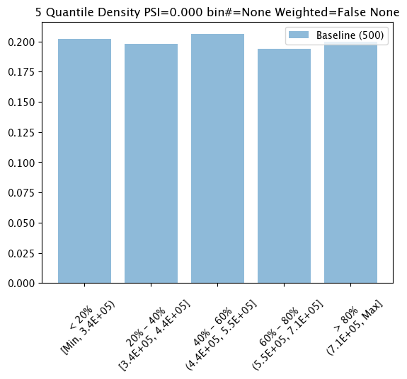
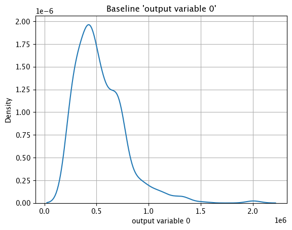
Baseline Chart
The baseline chart is displayed with wallaroo.assay.AssayAnalysis.chart(), which returns a chart with:
- baseline mean: The mean value of the baseline values.
- baseline median: The median value of the baseline values.
- bin_mode: The binning mode. See Binning Mode
- aggregation: The aggregation type. See Aggregation Options
- metric: The assay’s metric type. See Score Metric
- weighted: Whether the binning mode is weighted. See Binning Mode
The first chart is from an assay baseline generated from a set of inferences across a range of dates.
assay_baseline_run_from_dates.chart()
baseline mean = 553768.87409375
baseline median = 452115.8125
bin_mode = Quantile
aggregation = Density
metric = PSI
weighted = False

assay_baseline_run_from_numpy.chart()
baseline mean = 553768.87562
baseline median = 452115.79000000004
bin_mode = Quantile
aggregation = Density
metric = PSI
weighted = False
Baseline DataFrame
The method wallaroo.assay_config.AssayBuilder.baseline_dataframe returns a DataFrame of the assay baseline generated from the provided parameters. This includes:
metadata: The inference metadata with the model information, inference time, and other related factors.indata: Each input field assigned with the labelin.{input field name}.outdata: Each output field assigned with the labelout.{output field name}
Note that for assays generated from numpy values, there is only the out data based on the supplied baseline data.
In the following example, the baseline DataFrame is retrieved.
This baseline DataFrame is from an assay baseline generated from a set of inferences across a range of dates.
display(assay_baseline_from_dates.baseline_dataframe())
| time | metadata | input_tensor_0 | input_tensor_1 | input_tensor_2 | input_tensor_3 | input_tensor_4 | input_tensor_5 | input_tensor_6 | input_tensor_7 | input_tensor_8 | input_tensor_9 | input_tensor_10 | input_tensor_11 | input_tensor_12 | input_tensor_13 | input_tensor_14 | input_tensor_15 | input_tensor_16 | input_tensor_17 | output_variable_0 | |
|---|---|---|---|---|---|---|---|---|---|---|---|---|---|---|---|---|---|---|---|---|---|
| 0 | 1746636429634 | {'last_model': '{"model_name":"house-price-estimator","model_sha":"e22a0831aafd9917f3cc87a15ed267797f80e2afa12ad7d8810ca58f173b8cc6"}', 'pipeline_version': '98812bd0-615c-4acf-8358-93265253450a', 'elapsed': [2139061, 3978743], 'dropped': [], 'partition': 'engine-5577b69f89-vzq2k'} | 5.0 | 1.75 | 2340.0 | 9148.0 | 2.0 | 0.0 | 0.0 | 3.0 | 7.0 | 2340.0 | 0.0 | 47.4232 | -122.324 | 1390.0 | 10019.0 | 57.0 | 0.0 | 0.0 | 385982.06250 |
| 1 | 1746636429634 | {'last_model': '{"model_name":"house-price-estimator","model_sha":"e22a0831aafd9917f3cc87a15ed267797f80e2afa12ad7d8810ca58f173b8cc6"}', 'pipeline_version': '98812bd0-615c-4acf-8358-93265253450a', 'elapsed': [2139061, 3978743], 'dropped': [], 'partition': 'engine-5577b69f89-vzq2k'} | 3.0 | 1.00 | 1220.0 | 3000.0 | 1.5 | 0.0 | 0.0 | 3.0 | 6.0 | 1220.0 | 0.0 | 47.6506 | -122.346 | 1350.0 | 3000.0 | 114.0 | 0.0 | 0.0 | 448627.81250 |
| 2 | 1746636429634 | {'last_model': '{"model_name":"house-price-estimator","model_sha":"e22a0831aafd9917f3cc87a15ed267797f80e2afa12ad7d8810ca58f173b8cc6"}', 'pipeline_version': '98812bd0-615c-4acf-8358-93265253450a', 'elapsed': [2139061, 3978743], 'dropped': [], 'partition': 'engine-5577b69f89-vzq2k'} | 5.0 | 3.25 | 3030.0 | 20446.0 | 2.0 | 0.0 | 2.0 | 3.0 | 9.0 | 2130.0 | 900.0 | 47.6133 | -122.106 | 2890.0 | 20908.0 | 38.0 | 0.0 | 0.0 | 811666.68750 |
| 3 | 1746636429634 | {'last_model': '{"model_name":"house-price-estimator","model_sha":"e22a0831aafd9917f3cc87a15ed267797f80e2afa12ad7d8810ca58f173b8cc6"}', 'pipeline_version': '98812bd0-615c-4acf-8358-93265253450a', 'elapsed': [2139061, 3978743], 'dropped': [], 'partition': 'engine-5577b69f89-vzq2k'} | 3.0 | 2.25 | 1180.0 | 14258.0 | 2.0 | 0.0 | 0.0 | 3.0 | 7.0 | 1180.0 | 0.0 | 47.7112 | -122.238 | 1860.0 | 10390.0 | 27.0 | 0.0 | 0.0 | 340764.53125 |
| 4 | 1746636429634 | {'last_model': '{"model_name":"house-price-estimator","model_sha":"e22a0831aafd9917f3cc87a15ed267797f80e2afa12ad7d8810ca58f173b8cc6"}', 'pipeline_version': '98812bd0-615c-4acf-8358-93265253450a', 'elapsed': [2139061, 3978743], 'dropped': [], 'partition': 'engine-5577b69f89-vzq2k'} | 2.0 | 1.75 | 1670.0 | 6460.0 | 1.0 | 0.0 | 0.0 | 3.0 | 8.0 | 1670.0 | 0.0 | 47.7123 | -122.027 | 2170.0 | 6254.0 | 10.0 | 0.0 | 0.0 | 437177.96875 |
| ... | ... | ... | ... | ... | ... | ... | ... | ... | ... | ... | ... | ... | ... | ... | ... | ... | ... | ... | ... | ... | ... |
| 495 | 1746636429634 | {'last_model': '{"model_name":"house-price-estimator","model_sha":"e22a0831aafd9917f3cc87a15ed267797f80e2afa12ad7d8810ca58f173b8cc6"}', 'pipeline_version': '98812bd0-615c-4acf-8358-93265253450a', 'elapsed': [2139061, 3978743], 'dropped': [], 'partition': 'engine-5577b69f89-vzq2k'} | 3.0 | 2.50 | 1830.0 | 8133.0 | 1.0 | 0.0 | 0.0 | 3.0 | 8.0 | 1390.0 | 440.0 | 47.7478 | -122.247 | 2310.0 | 11522.0 | 19.0 | 0.0 | 0.0 | 437177.96875 |
| 496 | 1746636429634 | {'last_model': '{"model_name":"house-price-estimator","model_sha":"e22a0831aafd9917f3cc87a15ed267797f80e2afa12ad7d8810ca58f173b8cc6"}', 'pipeline_version': '98812bd0-615c-4acf-8358-93265253450a', 'elapsed': [2139061, 3978743], 'dropped': [], 'partition': 'engine-5577b69f89-vzq2k'} | 4.0 | 2.75 | 2930.0 | 22000.0 | 1.0 | 0.0 | 3.0 | 4.0 | 9.0 | 1580.0 | 1350.0 | 47.3227 | -122.384 | 2930.0 | 9758.0 | 36.0 | 0.0 | 0.0 | 518869.03125 |
| 497 | 1746636429634 | {'last_model': '{"model_name":"house-price-estimator","model_sha":"e22a0831aafd9917f3cc87a15ed267797f80e2afa12ad7d8810ca58f173b8cc6"}', 'pipeline_version': '98812bd0-615c-4acf-8358-93265253450a', 'elapsed': [2139061, 3978743], 'dropped': [], 'partition': 'engine-5577b69f89-vzq2k'} | 4.0 | 3.25 | 2050.0 | 5000.0 | 2.0 | 0.0 | 0.0 | 4.0 | 8.0 | 1370.0 | 680.0 | 47.6235 | -122.298 | 1720.0 | 5000.0 | 27.0 | 0.0 | 0.0 | 630865.50000 |
| 498 | 1746636429634 | {'last_model': '{"model_name":"house-price-estimator","model_sha":"e22a0831aafd9917f3cc87a15ed267797f80e2afa12ad7d8810ca58f173b8cc6"}', 'pipeline_version': '98812bd0-615c-4acf-8358-93265253450a', 'elapsed': [2139061, 3978743], 'dropped': [], 'partition': 'engine-5577b69f89-vzq2k'} | 4.0 | 1.75 | 2000.0 | 8700.0 | 1.0 | 0.0 | 0.0 | 5.0 | 7.0 | 1010.0 | 990.0 | 47.3740 | -122.141 | 1490.0 | 7350.0 | 39.0 | 0.0 | 0.0 | 317551.28125 |
| 499 | 1746636429634 | {'last_model': '{"model_name":"house-price-estimator","model_sha":"e22a0831aafd9917f3cc87a15ed267797f80e2afa12ad7d8810ca58f173b8cc6"}', 'pipeline_version': '98812bd0-615c-4acf-8358-93265253450a', 'elapsed': [2139061, 3978743], 'dropped': [], 'partition': 'engine-5577b69f89-vzq2k'} | 4.0 | 2.00 | 2580.0 | 4500.0 | 2.0 | 0.0 | 0.0 | 4.0 | 9.0 | 1850.0 | 730.0 | 47.6245 | -122.316 | 2590.0 | 4100.0 | 110.0 | 0.0 | 0.0 | 964052.62500 |
500 rows × 21 columns
display(assay_baseline_from_numpy.baseline_dataframe())
| output_variable_0 | |
|---|---|
| 0 | 385982.06 |
| 1 | 448627.80 |
| 2 | 811666.70 |
| 3 | 340764.53 |
| 4 | 437177.97 |
| ... | ... |
| 495 | 437177.97 |
| 496 | 518869.03 |
| 497 | 630865.50 |
| 498 | 317551.28 |
| 499 | 964052.60 |
500 rows × 1 columns
Baseline Stats
The method wallaroo.assay.AssayAnalysis.baseline_stats() returns a pandas.core.frame.DataFrame of the baseline stats.
The baseline stats for each assay are displayed in the examples below.
This baseline states DataFrame is from an assay baseline generated from a set of inferences across a range of dates.
assay_baseline_run_from_dates.baseline_stats()
| Baseline | |
|---|---|
| count | 500 |
| min | 236238.671875 |
| max | 2016006.125 |
| mean | 553768.874094 |
| median | 452115.8125 |
| std | 295421.65625 |
| start | None |
| end | None |
assay_baseline_from_numpy.baseline_dataframe()
| output_variable_0 | |
|---|---|
| 0 | 385982.06 |
| 1 | 448627.80 |
| 2 | 811666.70 |
| 3 | 340764.53 |
| 4 | 437177.97 |
| ... | ... |
| 495 | 437177.97 |
| 496 | 518869.03 |
| 497 | 630865.50 |
| 498 | 317551.28 |
| 499 | 964052.60 |
500 rows × 1 columns
Baseline Bins
The method wallaroo.assay.AssayAnalysis.baseline_bins a simple dataframe to with the edge/bin data for a baseline.
These baseline bins DataFrame is from an assay baseline generated from a set of inferences across a range of dates.
assay_baseline_run_from_dates.baseline_bins()
| b_edges | b_edge_names | b_aggregated_values | b_aggregation | |
|---|---|---|---|---|
| 0 | 338418.84375 | < 20% | 0.202 | Aggregation.DENSITY |
| 1 | 443352.375 | 20% - 40% | 0.198 | Aggregation.DENSITY |
| 2 | 546631.9375 | 40% - 60% | 0.206 | Aggregation.DENSITY |
| 3 | 714289.1875 | 60% - 80% | 0.194 | Aggregation.DENSITY |
| 4 | INFINITY | > 80% | 0.200 | Aggregation.DENSITY |
assay_baseline_run_from_numpy.baseline_bins()
| b_edges | b_edge_names | b_aggregated_values | b_aggregation | |
|---|---|---|---|---|
| 0 | 338418.84 | < 20% | 0.202 | Aggregation.DENSITY |
| 1 | 443352.38 | 20% - 40% | 0.198 | Aggregation.DENSITY |
| 2 | 546631.94 | 40% - 60% | 0.206 | Aggregation.DENSITY |
| 3 | 714289.212 | 60% - 80% | 0.194 | Aggregation.DENSITY |
| 4 | INFINITY | > 80% | 0.200 | Aggregation.DENSITY |
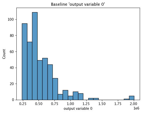
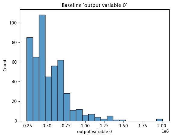
Baseline Histogram Chart
The method wallaroo.assay_config.AssayBuilder.baseline_histogram returns a histogram chart of the assay baseline generated from the provided parameters.
These chart is from an assay baseline generated from a set of inferences across a range of dates.
assay_baseline_from_dates.baseline_histogram()
assay_baseline_from_numpy.baseline_histogram()
Baseline KDE Chart
The method wallaroo.assay_config.AssayBuilder.baseline_kde returns a Kernel Density Estimation (KDE) chart of the assay baseline generated from the provided parameters.
These chart is from an assay baseline generated from a set of inferences across a range of dates.
assay_baseline_from_dates.baseline_kde()
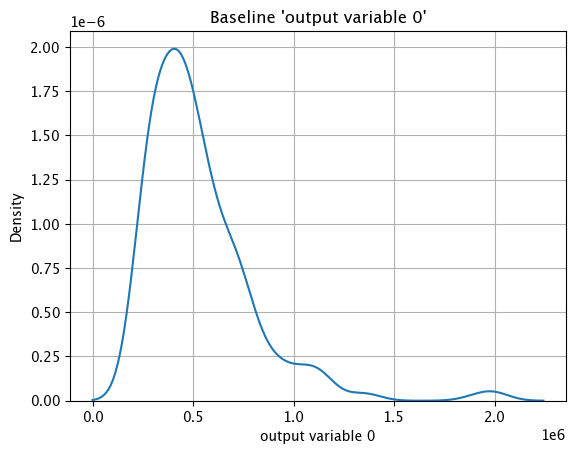
assay_baseline_from_numpy.baseline_kde()
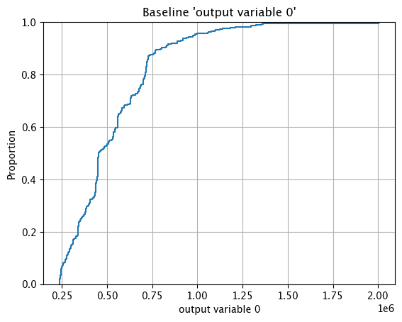
Baseline ECDF Chart
The method wallaroo.assay_config.AssayBuilder.baseline_ecdf returns a Empirical Cumulative Distribution Function (CDF) chart of the assay baseline generated from the provided parameters.
These chart is from an assay baseline generated from a set of inferences across a range of dates.
assay_baseline_from_dates.baseline_ecdf()

assay_baseline_from_numpy.baseline_ecdf()
Assay Preview
Now that the baseline is defined, we look at different configuration options and view how the assay baseline and results changes. Once we determine what gives us the best method of determining model drift, we can create the assay.
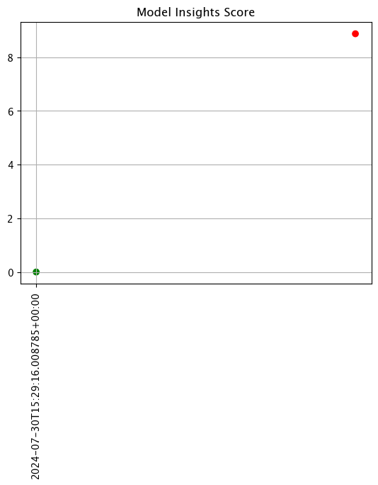
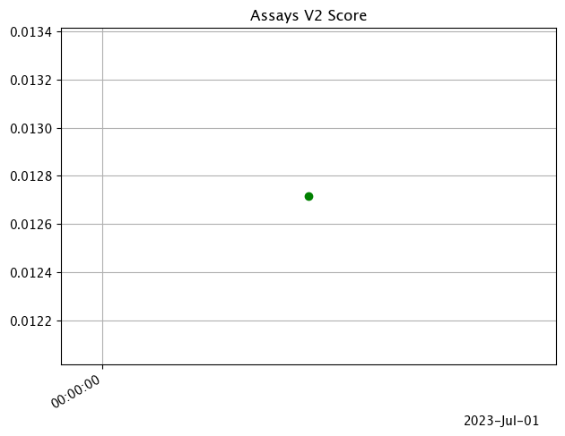
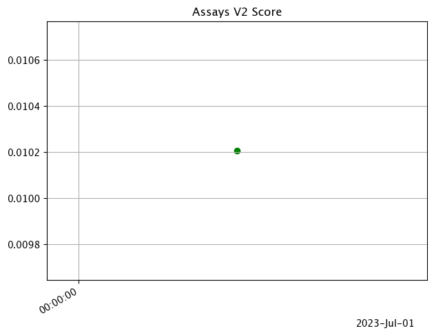
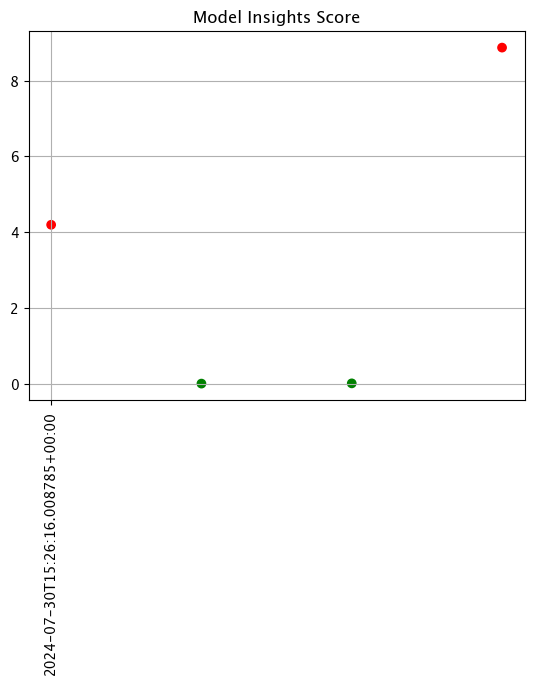
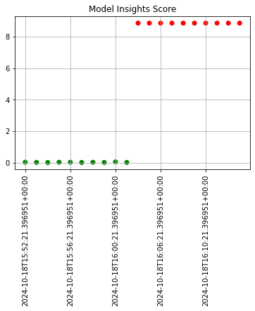
Analysis List Chart Scores
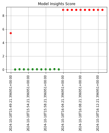
Analysis List scores show the assay scores for each assay result interval in one chart. Values that are outside of the alert threshold are colored red, while scores within the alert threshold are green.
Assay chart scores are displayed with the method wallaroo.assay.AssayAnalysisList.chart_scores, with ability to display an optional title with the chart. This takes the following parameters:
| Parameter | Type | Description |
|---|---|---|
| title | String (Optional) | The title to assign the chart. |
| nth_x_tick | Integer (Optional) (Default: 4) | The density of the x ticks. |
| start | DateTime (Optional) | The start time of the chart. If start is set, the parameter end must be set. |
| end | DateTime (Optional) | The end time of the chart. If end is set, the parameter start must be set. |
The following example shows retrieving the assay results and displaying the chart scores. From our example, we have two windows - the first should be green, and the second is red showing that values were outside the alert threshold.
The following images show how the assay charts change when the nth_x_tick changes from the default to 10. Note that the tutorial code will only generate one data point - these images are for demonstration purposes.

assay_baseline_from_dates = wl.build_assay(assay_name=assay_name,
                                          pipeline=mainpipeline,
                                          iopath="output variable 0",
                                          baseline_start=assay_baseline_start,
                                          baseline_end=assay_baseline_end)

# Set the assay parameters

# The end date to gather inference results
assay_baseline_from_dates.add_run_until(assay_baseline_end)

# Set the interval and window to one minute each, set the start date back 24 hours for gathering inference results
assay_baseline_from_dates.window_builder().add_width(hours=24).add_interval(hours=24).add_start(assay_baseline_start+datetime.timedelta(hours=-24))

# build the assay configuration
assay_config_from_dates = assay_baseline_from_dates.build()

# perform an interactive run and collect inference data
assay_results_from_dates = assay_config_from_dates.interactive_run()

# show the analyses chart
assay_results_from_dates.chart_scores()

assay_baseline_from_numpy = wl.build_assay(assay_name=assay_name,
                                          pipeline=mainpipeline,
                                          iopath="output variable 0",
                                          baseline_data=baseline_results)

# Set the assay parameters

# The end date to gather inference results
assay_baseline_from_numpy.add_run_until(assay_baseline_end)

# Set the interval and window to one minute each, set the start date back 24 hours for gathering inference results
assay_baseline_from_numpy.window_builder().add_width(hours=24).add_interval(hours=24).add_start(assay_baseline_start+datetime.timedelta(hours=-24))

# build the assay configuration
assay_config_from_numpy = assay_baseline_from_numpy.build()

# perform an interactive run and collect inference data
assay_results_from_numpy = assay_config_from_numpy.interactive_run()

# show the analysis chart from the numpy baseline based assay
assay_results_from_numpy.chart_scores()
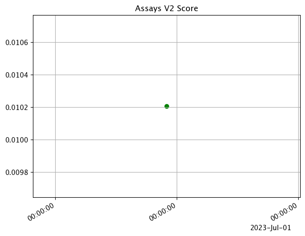
The following chart uses the nth_x_tick setting to space out the x-axis labels further.
# set different nth_x_tick
assay_results_from_dates.chart_scores(nth_x_tick=10)
assay_results_from_numpy.chart_scores(nth_x_tick=10)
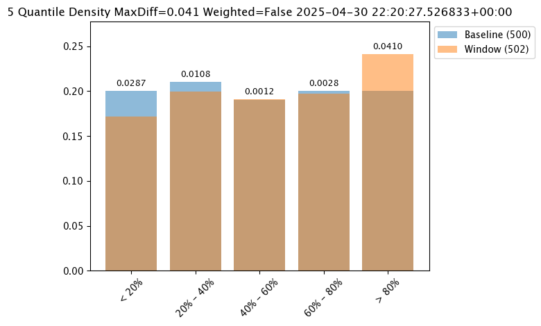
Analysis Chart
The method wallaroo.assay.AssayAnalysis.chart() displays a comparison between the baseline and an interval of inference data.
This is compared to the Chart Scores, which is a list of all of the inference data split into intervals, while the Analysis Chart shows the breakdown of one set of inference data against the baseline.
Score from the Analysis List Chart Scores and each element from the Analysis List DataFrame generates
The following fields are included.
| Field | Type | Description |
|---|---|---|
| baseline mean | Float | The mean of the baseline values. |
| window mean | Float | The mean of the window values. |
| baseline median | Float | The median of the baseline values. |
| window median | Float | The median of the window values. |
| bin_mode | String | The binning mode used for the assay. |
| aggregation | String | The aggregation mode used for the assay. |
| metric | String | The metric mode used for the assay. |
| weighted | Bool | Whether the bins were manually weighted. |
| score | Float | The score from the assay window. |
| scores | List(Float) | The score from each assay window bin. |
| index | Integer/None | The window index. Interactive assay runs are None. |
assay_baseline_from_dates = wl.build_assay(assay_name=assay_name,
                                          pipeline=mainpipeline,
                                          iopath="output variable 0",
                                          baseline_start=assay_baseline_start,
                                          baseline_end=assay_baseline_end)

# Set the assay parameters

# The end date to gather inference results
assay_baseline_from_dates.add_run_until(assay_baseline_end)

# Set the interval and window to one minute each, set the start date back 24 hours for gathering inference results
assay_baseline_from_dates.window_builder().add_width(hours=24).add_interval(hours=24).add_start(assay_baseline_start+datetime.timedelta(hours=-24))

# build the assay configuration
assay_config_from_dates = assay_baseline_from_dates.build()

# perform an interactive run and collect inference data
assay_results_from_dates = assay_config_from_dates.interactive_run()

# display one of the analysis from the total results
assay_results_from_dates[0].chart()

assay_baseline_from_numpy = wl.build_assay(assay_name=assay_name,
                                          pipeline=mainpipeline,
                                          iopath="output variable 0",
                                          baseline_data=baseline_results)

# Set the assay parameters

# The end date to gather inference results
assay_baseline_from_numpy.add_run_until(assay_baseline_end)

# Set the interval and window to one minute each, set the start date back 24 hours for gathering inference results
assay_baseline_from_numpy.window_builder().add_width(hours=24).add_interval(hours=24).add_start(assay_baseline_start+datetime.timedelta(hours=-24))

# build the assay configuration
assay_config_from_numpy = assay_baseline_from_numpy.build()

# perform an interactive run and collect inference data
assay_results_from_numpy = assay_config_from_numpy.interactive_run()

# show the analysis chart from the numpy baseline based assay
assay_results_from_numpy[0].chart()

Analysis List DataFrame
wallaroo.assay.AssayAnalysisList.to_dataframe() returns a DataFrame showing the assay results for each window aka individual analysis. This DataFrame contains the following fields:
| Field | Type | Description |
|---|---|---|
| assay_id | String/None | The assay id in UUID format. Only provided from uploaded and executed assays. |
| name | String/None | The name of the assay. Only provided from uploaded and executed assays. |
| iopath | String/None | The iopath of the assay. Only provided from uploaded and executed assays. |
| score | Float | The assay score. |
| start | DateTime | The DateTime start of the assay window. |
| min | Float | The minimum value in the assay window. |
| max | Float | The maximum value in the assay window. |
| mean | Float | The mean value in the assay window. |
| median | Float | The median value in the assay window. |
| std | Float | The standard deviation value in the assay window. |
| warning_threshold | Float/None | The warning threshold of the assay window. |
| alert_threshold | Float/None | The alert threshold of the assay window. |
| status | String | The assay window status. Values are:
|
For this example, the assay analysis list DataFrame is listed.
From this tutorial, we should have 2 windows of dta to look at, each one minute apart. The first window should show status: OK, with the second window with the very large house prices will show status: alert
assay_baseline_from_dates = wl.build_assay(assay_name=assay_name,
                                          pipeline=mainpipeline,
                                          iopath="output variable 0",
                                          baseline_start=assay_baseline_start,
                                          baseline_end=assay_baseline_end)

# Set the assay parameters

# The end date to gather inference results
assay_baseline_from_dates.add_run_until(assay_baseline_end)

# Set the interval and window to one minute each, set the start date back 24 hours for gathering inference results
assay_baseline_from_dates.window_builder().add_width(hours=24).add_interval(hours=24).add_start(assay_baseline_start+datetime.timedelta(hours=-24))

# build the assay configuration
assay_config_from_dates = assay_baseline_from_dates.build()

# perform an interactive run and collect inference data
assay_results_from_dates = assay_config_from_dates.interactive_run()

# display the dataframe from the analyses
assay_results_from_dates.to_dataframe()
| id | assay_id | assay_name | iopath | pipeline_id | pipeline_name | workspace_id | workspace_name | score | start | min | max | mean | median | std | warning_threshold | alert_threshold | status | |
|---|---|---|---|---|---|---|---|---|---|---|---|---|---|---|---|---|---|---|
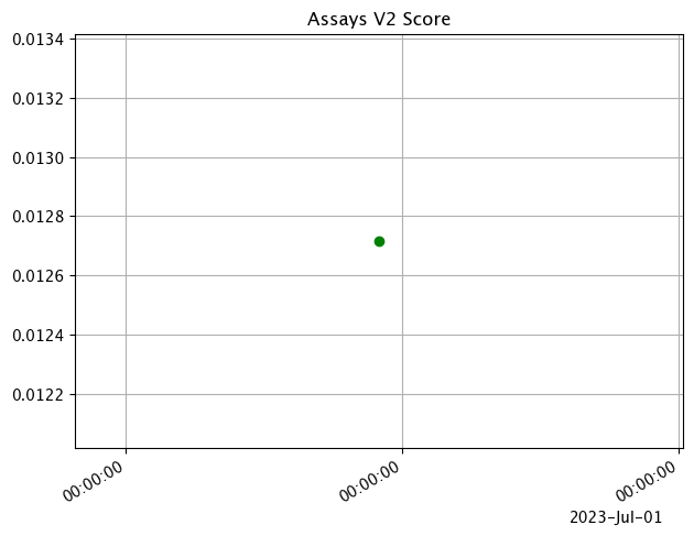
| 0 | 0 | d5aa4404-0509-4e40-ba6c-6b0a96cb508c | assay-demonstration-tutorial assay | out.variable.0 | 1 | assay-demonstration-tutorial | 7 | assay-demonstration-tutorial | 0.012716 | 2025-04-29 22:20:27.526833+00:00 | 236238.671875 | 2005883.125 | 538249.025087 | 453247.0 | 247711.921875 | None | 0.25 | Ok |
assay_baseline_from_numpy = wl.build_assay(assay_name=assay_name,
                                          pipeline=mainpipeline,
                                          iopath="output variable 0",
                                          baseline_data=baseline_results)

# Set the assay parameters

# The end date to gather inference results
assay_baseline_from_numpy.add_run_until(assay_baseline_end)

# Set the interval and window to one minute each, set the start date back 24 hours for gathering inference results
assay_baseline_from_numpy.window_builder().add_width(hours=24).add_interval(hours=24).add_start(assay_baseline_start+datetime.timedelta(hours=-24))

# build the assay configuration
assay_config_from_numpy = assay_baseline_from_numpy.build()

# perform an interactive run and collect inference data
assay_results_from_numpy = assay_config_from_numpy.interactive_run()

assay_results_from_numpy.to_dataframe()
| id | assay_id | assay_name | iopath | pipeline_id | pipeline_name | workspace_id | workspace_name | score | start | min | max | mean | median | std | warning_threshold | alert_threshold | status | |
|---|---|---|---|---|---|---|---|---|---|---|---|---|---|---|---|---|---|---|
| 0 | 0 | d529952d-f817-4e58-a2df-b222cc445869 | assay-demonstration-tutorial assay | out.variable.0 | 1 | assay-demonstration-tutorial | 7 | assay-demonstration-tutorial | 0.010207 | 2025-04-29 22:20:27.526833+00:00 | 236238.671875 | 2005883.125 | 538249.025087 | 453247.0 | 247711.921875 | None | 0.25 | Ok |
Analysis List Full DataFrame
wallaroo.assay.AssayAnalysisList.to_full_dataframe() returns a DataFrame showing all values, including the inputs and outputs from the assay results for each window aka individual analysis. This DataFrame contains the following fields:
pipeline_id warning_threshold bin_index created_at
| Field | Type | Description |
|---|---|---|
| window_start | DateTime | The date and time when the window period began. |
| analyzed_at | DateTime | The date and time when the assay analysis was performed. |
| elapsed_millis | Integer | How long the analysis took to perform in milliseconds. |
| baseline_summary_count | Integer | The number of data elements from the baseline. |
| baseline_summary_min | Float | The minimum value from the baseline summary. |
| baseline_summary_max | Float | The maximum value from the baseline summary. |
| baseline_summary_mean | Float | The mean value of the baseline summary. |
| baseline_summary_median | Float | The median value of the baseline summary. |
| baseline_summary_std | Float | The standard deviation value of the baseline summary. |
| baseline_summary_edges_{0…n} | Float | The baseline summary edges for each baseline edge from 0 to number of edges. |
| summarizer_type | String | The type of summarizer used for the baseline. See wallaroo.assay_config for other summarizer types. |
| summarizer_bin_weights | List / None | If baseline bin weights were provided, the list of those weights. Otherwise, None. |
| summarizer_provided_edges | List / None | If baseline bin edges were provided, the list of those edges. Otherwise, None. |
| status | String | The assay window status. Values are:
|
| id | Integer/None | The id for the window aka analysis. Only provided from uploaded and executed assays. |
| assay_id | String/None | The assay id in UUID format. Only provided from uploaded and executed assays. |
| pipeline_id | Integer/None | The pipeline id. Only provided from uploaded and executed assays. |
| warning_threshold | Float | The warning threshold set for the assay. |
| warning_threshold | Float | The warning threshold set for the assay. |
| bin_index | Integer/None | The bin index for the window aka analysis. |
| created_at | Datetime/None | The date and time the window aka analysis was generated. Only provided from uploaded and executed assays. |
For this example, full DataFrame from an assay preview is generated.
From this tutorial, we should have 2 windows of dta to look at, each one minute apart. The first window should show status: OK, with the second window with the very large house prices will show status: alert
assay_baseline_from_dates = wl.build_assay(assay_name=assay_name,
                                          pipeline=mainpipeline,
                                          iopath="output variable 0",
                                          baseline_start=assay_baseline_start,
                                          baseline_end=assay_baseline_end)

# Set the assay parameters

# The end date to gather inference results
assay_baseline_from_dates.add_run_until(assay_baseline_end)

# Set the interval and window to one minute each, set the start date back 24 hours for gathering inference results
assay_baseline_from_dates.window_builder().add_width(hours=24).add_interval(hours=24).add_start(assay_baseline_start+datetime.timedelta(hours=-24))

# build the assay configuration
assay_config_from_dates = assay_baseline_from_dates.build()

# perform an interactive run and collect inference data
assay_results_from_dates = assay_config_from_dates.interactive_run()

# display the full dataframe from the analyses
assay_results_from_dates.to_full_dataframe()
| id | assay_id | window_start | analyzed_at | elapsed_millis | pipeline_id | workspace_id | workspace_name | baseline_summary_aggregated_values_0 | baseline_summary_aggregated_values_1 | baseline_summary_aggregated_values_2 | baseline_summary_aggregated_values_3 | baseline_summary_aggregated_values_4 | baseline_summary_aggregation | baseline_summary_bins_edges_0 | baseline_summary_bins_edges_1 | baseline_summary_bins_edges_2 | baseline_summary_bins_edges_3 | baseline_summary_bins_edges_4 | baseline_summary_bins_labels_0 | baseline_summary_bins_labels_1 | baseline_summary_bins_labels_2 | baseline_summary_bins_labels_3 | baseline_summary_bins_labels_4 | baseline_summary_bins_mode_Quantile | baseline_summary_name | baseline_summary_statistics_count | baseline_summary_statistics_max | baseline_summary_statistics_mean | baseline_summary_statistics_median | baseline_summary_statistics_min | baseline_summary_statistics_std | baseline_summary_end | baseline_summary_start | window_summary_aggregated_values_0 | window_summary_aggregated_values_1 | window_summary_aggregated_values_2 | window_summary_aggregated_values_3 | window_summary_aggregated_values_4 | window_summary_bins_edges_0 | window_summary_bins_edges_1 | window_summary_bins_edges_2 | window_summary_bins_edges_3 | window_summary_bins_edges_4 | window_summary_bins_labels_0 | window_summary_bins_labels_1 | window_summary_bins_labels_2 | window_summary_bins_labels_3 | window_summary_bins_labels_4 | window_summary_bins_mode_Quantile | window_summary_statistics_count | window_summary_statistics_max | window_summary_statistics_mean | window_summary_statistics_median | window_summary_statistics_min | window_summary_statistics_std | window_summary_end | window_summary_start | warning_threshold | alert_threshold | bin_index | summarizer_UnivariateContinuous_aggregation | summarizer_UnivariateContinuous_bin_mode_Quantile | summarizer_UnivariateContinuous_metric | summarizer_UnivariateContinuous_bin_weights | status | created_at | score | scores_0 | scores_1 | scores_2 | scores_3 | scores_4 | |
|---|---|---|---|---|---|---|---|---|---|---|---|---|---|---|---|---|---|---|---|---|---|---|---|---|---|---|---|---|---|---|---|---|---|---|---|---|---|---|---|---|---|---|---|---|---|---|---|---|---|---|---|---|---|---|---|---|---|---|---|---|---|---|---|---|---|---|---|---|---|---|---|---|---|
| 0 | 0 | 8038ec07-40f0-4c7b-84af-00c6faa72154 | 2025-04-29T22:20:27.526833+00:00 | 2025-04-30 22:28:54.033236+00:00 | 77 | 1 | 7 | assay-demonstration-tutorial | 0.2 | 0.21 | 0.19 | 0.2 | 0.2 | Density | 319918.59375 | 435628.71875 | 535686.0 | 696474.6875 | INFINITY | < 20% | 20% - 40% | 40% - 60% | 60% - 80% | > 80% | 5 | out.variable.0 | 500 | 2005883.125 | 530712.689594 | 448627.8125 | 236238.671875 | 273499.25 | None | None | 0.171315 | 0.199203 | 0.191235 | 0.197211 | 0.241036 | 319918.59375 | 435628.71875 | 535686.0 | 696474.6875 | INFINITY | < 20% | 20% - 40% | 40% - 60% | 60% - 80% | > 80% | 5 | 502 | 2005883.125 | 538249.025087 | 453247.0 | 236238.671875 | 247711.921875 | 2025-04-30T22:20:27.526833+00:00 | 2025-04-29T22:20:27.526833+00:00 | None | 0.25 | None | Density | 5 | PSI | None | Ok | None | 0.012716 | 0.004441 | 0.00057 | 0.000008 | 0.000039 | 0.007658 |
assay_baseline_from_numpy = wl.build_assay(assay_name=assay_name,
                                          pipeline=mainpipeline,
                                          iopath="output variable 0",
                                          baseline_data=baseline_results)

# Set the assay parameters

# The end date to gather inference results
assay_baseline_from_numpy.add_run_until(assay_baseline_end)

# Set the interval and window to one minute each, set the start date back 24 hours for gathering inference results
assay_baseline_from_numpy.window_builder().add_width(hours=24).add_interval(hours=24).add_start(assay_baseline_start+datetime.timedelta(hours=-24))

# build the assay configuration
assay_config_from_numpy = assay_baseline_from_numpy.build()

# perform an interactive run and collect inference data
assay_results_from_numpy = assay_config_from_numpy.interactive_run()

assay_results_from_numpy.to_full_dataframe()
| id | assay_id | window_start | analyzed_at | elapsed_millis | pipeline_id | workspace_id | workspace_name | baseline_summary_aggregated_values_0 | baseline_summary_aggregated_values_1 | baseline_summary_aggregated_values_2 | baseline_summary_aggregated_values_3 | baseline_summary_aggregated_values_4 | baseline_summary_aggregation | baseline_summary_bins_edges_0 | baseline_summary_bins_edges_1 | baseline_summary_bins_edges_2 | baseline_summary_bins_edges_3 | baseline_summary_bins_edges_4 | baseline_summary_bins_labels_0 | baseline_summary_bins_labels_1 | baseline_summary_bins_labels_2 | baseline_summary_bins_labels_3 | baseline_summary_bins_labels_4 | baseline_summary_bins_mode_Quantile | baseline_summary_name | baseline_summary_statistics_count | baseline_summary_statistics_max | baseline_summary_statistics_mean | baseline_summary_statistics_median | baseline_summary_statistics_min | baseline_summary_statistics_std | baseline_summary_end | baseline_summary_start | window_summary_aggregated_values_0 | window_summary_aggregated_values_1 | window_summary_aggregated_values_2 | window_summary_aggregated_values_3 | window_summary_aggregated_values_4 | window_summary_bins_edges_0 | window_summary_bins_edges_1 | window_summary_bins_edges_2 | window_summary_bins_edges_3 | window_summary_bins_edges_4 | window_summary_bins_labels_0 | window_summary_bins_labels_1 | window_summary_bins_labels_2 | window_summary_bins_labels_3 | window_summary_bins_labels_4 | window_summary_bins_mode_Quantile | window_summary_statistics_count | window_summary_statistics_max | window_summary_statistics_mean | window_summary_statistics_median | window_summary_statistics_min | window_summary_statistics_std | window_summary_end | window_summary_start | warning_threshold | alert_threshold | bin_index | summarizer_UnivariateContinuous_aggregation | summarizer_UnivariateContinuous_bin_mode_Quantile | summarizer_UnivariateContinuous_metric | summarizer_UnivariateContinuous_bin_weights | status | created_at | score | scores_0 | scores_1 | scores_2 | scores_3 | scores_4 | |
|---|---|---|---|---|---|---|---|---|---|---|---|---|---|---|---|---|---|---|---|---|---|---|---|---|---|---|---|---|---|---|---|---|---|---|---|---|---|---|---|---|---|---|---|---|---|---|---|---|---|---|---|---|---|---|---|---|---|---|---|---|---|---|---|---|---|---|---|---|---|---|---|---|---|
| 0 | 0 | 7e95f8a4-fd02-48f7-b67e-b41cce829512 | 2025-04-29T22:20:27.526833+00:00 | 2025-04-30 22:29:13.220637+00:00 | 92 | 1 | 7 | assay-demonstration-tutorial | 0.222 | 0.182 | 0.202 | 0.194 | 0.2 | Density | 340764.53 | 444933.25 | 557391.25 | 712519.68 | INFINITY | < 20% | 20% - 40% | 40% - 60% | 60% - 80% | > 80% | 5 | out.variable.0 | 500 | 2005883.1 | 535937.83588 | 451058.3 | 236238.67 | 244197.003014 | None | None | 0.189243 | 0.213147 | 0.201195 | 0.193227 | 0.203187 | 340764.53 | 444933.25 | 557391.25 | 712519.68 | INFINITY | < 20% | 20% - 40% | 40% - 60% | 60% - 80% | > 80% | 5 | 502 | 2005883.125 | 538249.025087 | 453247.0 | 236238.671875 | 247711.921875 | 2025-04-30T22:20:27.526833+00:00 | 2025-04-29T22:20:27.526833+00:00 | None | 0.25 | None | Density | 5 | PSI | None | Ok | None | 0.010207 | 0.005229 | 0.004921 | 0.000003 | 0.000003 | 0.00005 |
Analysis Compare Basic Stats
The method wallaroo.assay.AssayAnalysis.compare_basic_stats returns a DataFrame comparing one set of inference data against the baseline.
This is compared to the Analysis List DataFrame, which is a list of all of the inference data split into intervals, while the Analysis Compare Basic Stats shows the breakdown of one set of inference data against the baseline.
assay_baseline_from_dates = wl.build_assay(assay_name=assay_name,
                                          pipeline=mainpipeline,
                                          iopath="output variable 0",
                                          baseline_start=assay_baseline_start,
                                          baseline_end=assay_baseline_end)

# Set the assay parameters

# The end date to gather inference results
assay_baseline_from_dates.add_run_until(assay_baseline_end)

# Set the interval and window to one minute each, set the start date back 24 hours for gathering inference results
assay_baseline_from_dates.window_builder().add_width(hours=24).add_interval(hours=24).add_start(assay_baseline_start+datetime.timedelta(hours=-24))

# build the assay configuration
assay_config_from_dates = assay_baseline_from_dates.build()

# perform an interactive run and collect inference data
assay_results_from_dates = assay_config_from_dates.interactive_run()

# display one analysis against the baseline
assay_results_from_dates[0].compare_basic_stats()
| Baseline | Window | diff | pct_diff | |
|---|---|---|---|---|
| count | 500.0 | 502.0 | 2.0 | 0.4 |
| max | 2005883.125 | 2005883.125 | 0.0 | 0.0 |
| mean | 530712.689594 | 538249.025087 | 7536.335493 | 1.420041 |
| median | 448627.8125 | 453247.0 | 4619.1875 | 1.029626 |
| min | 236238.671875 | 236238.671875 | 0.0 | 0.0 |
| std | 273499.25 | 247711.921875 | -25787.328125 | -9.428665 |
| start | None | 2025-04-29T22:20:27.526833+00:00 | NaN | NaN |
| end | None | 2025-04-30T22:20:27.526833+00:00 | NaN | NaN |
assay_baseline_from_numpy = wl.build_assay(assay_name=assay_name,
                                          pipeline=mainpipeline,
                                          iopath="output variable 0",
                                          baseline_data=baseline_results)

# Set the assay parameters

# The end date to gather inference results
assay_baseline_from_numpy.add_run_until(assay_baseline_end)

# Set the interval and window to one minute each, set the start date back 24 hours for gathering inference results
assay_baseline_from_numpy.window_builder().add_width(hours=24).add_interval(hours=24).add_start(assay_baseline_start+datetime.timedelta(hours=-24))

# build the assay configuration
assay_config_from_numpy = assay_baseline_from_numpy.build()

# perform an interactive run and collect inference data
assay_results_from_numpy = assay_config_from_numpy.interactive_run()

# assay_results_from_numpy.to_full_dataframe()

assay_results_from_numpy[0].compare_basic_stats()
| Baseline | Window | diff | pct_diff | |
|---|---|---|---|---|
| count | 500.0 | 502.0 | 2.0 | 0.4 |
| max | 2005883.1 | 2005883.125 | 0.025 | 0.000001 |
| mean | 535937.83588 | 538249.025087 | 2311.189207 | 0.431242 |
| median | 451058.3 | 453247.0 | 2188.7 | 0.485237 |
| min | 236238.67 | 236238.671875 | 0.001875 | 0.000001 |
| std | 244197.003014 | 247711.921875 | 3514.918861 | 1.439378 |
| start | None | 2025-04-29T22:20:27.526833+00:00 | NaN | NaN |
| end | None | 2025-04-30T22:20:27.526833+00:00 | NaN | NaN |
Configure Assays
Before creating the assay, configure the assay and continue to preview it until the best method for detecting drift is set. The following options are available.
Inference Interval and Inference Width
The inference interval aka window interval sets how often to run the assay analysis. This is set from the wallaroo.assay_config.AssayBuilder.window_builder.add_interval method to collect data expressed in time units: “hours=24”, “minutes=1”, etc.
For example, with an interval of 1 minute, the assay collects data every minute. Within an hour, 60 intervals of data is collected.
We can adjust the interval and see how the assays change based on how frequently they are run.
The width sets the time period from the wallaroo.assay_config.AssayBuilder.window_builder.add_width method to collect data expressed in time units: “hours=24”, “minutes=1”, etc.
For example, an interval of 1 minute and a width of 1 minute collects 1 minutes worth of data every minute. An interval of 1 minute with a width of 5 minutes collects 5 minute of inference data every minute.
By default, the interval and width is 24 hours.
For this example, we’ll adjust the width and interval from 24 hours to 12 hours.
The following images below demonstrate this change with assay analyses built on a longer historical period. Note that the tutorial code will only generate one data point - these images are for demonstration purposes.
assay_baseline_from_dates = wl.build_assay(assay_name=assay_name,
                                          pipeline=mainpipeline,
                                          iopath="output variable 0",
                                          baseline_start=assay_baseline_start,
                                          baseline_end=assay_baseline_end)

# Set the assay parameters

# The end date to gather inference results
assay_baseline_from_dates.add_run_until(assay_baseline_end)

# Set the interval and window to one minute each, set the start date back 24 hours for gathering inference results
assay_baseline_from_dates.window_builder().add_width(hours=24).add_interval(hours=24).add_start(assay_baseline_start+datetime.timedelta(hours=-24))

# build the assay configuration
assay_config_from_dates = assay_baseline_from_dates.build()

# perform an interactive run and collect inference data
assay_results_from_dates = assay_config_from_dates.interactive_run()

# show the analyses chart
assay_results_from_dates.chart_scores()
assay_baseline_from_dates = wl.build_assay(assay_name=assay_name,
                                          pipeline=mainpipeline,
                                          iopath="output variable 0",
                                          baseline_start=assay_baseline_start,
                                          baseline_end=assay_baseline_end)

# Set the assay parameters

# The end date to gather inference results
assay_baseline_from_dates.add_run_until(assay_baseline_end)

# Set the interval and window to one minute each, set the start date back 24 hours for gathering inference results
assay_baseline_from_dates.window_builder().add_width(hours=12).add_interval(hours=12).add_start(assay_baseline_start+datetime.timedelta(hours=-24))

# build the assay configuration
assay_config_from_dates = assay_baseline_from_dates.build()

# perform an interactive run and collect inference data
assay_results_from_dates = assay_config_from_dates.interactive_run()

# show the analyses chart
assay_results_from_dates.chart_scores()

assay_baseline_from_numpy = wl.build_assay(assay_name=assay_name,
                                          pipeline=mainpipeline,
                                          iopath="output variable 0",
                                          baseline_data=baseline_results)

# The end date to gather inference results
assay_baseline_from_numpy.add_run_until(assay_baseline_end)

# Set the interval and window to one minute each, set the start date back 24 hours for gathering inference results
assay_baseline_from_numpy.window_builder().add_width(hours=24).add_interval(hours=24).add_start(assay_baseline_start+datetime.timedelta(hours=-24))

# create the baseline from the dates
assay_config_from_numpy = assay_baseline_from_numpy.build()

assay_results_from_numpy = assay_config_from_numpy.interactive_baseline_run()

assay_results_from_numpy.compare_basic_stats()
| Baseline | Window | diff | pct_diff | |
|---|---|---|---|---|
| count | 5.000000e+02 | 5.000000e+02 | 0.0 | 0.0 |
| min | 2.362387e+05 | 2.362387e+05 | 0.0 | 0.0 |
| max | 2.005883e+06 | 2.005883e+06 | 0.0 | 0.0 |
| mean | 5.359378e+05 | 5.359378e+05 | 0.0 | 0.0 |
| median | 4.510583e+05 | 4.510583e+05 | 0.0 | 0.0 |
| std | 2.441970e+05 | 2.441970e+05 | 0.0 | 0.0 |
| start | NaN | NaN | NaN | NaN |
| end | NaN | NaN | NaN | NaN |
assay_baseline_from_numpy = wl.build_assay(assay_name=assay_name,
                                          pipeline=mainpipeline,
                                          iopath="output variable 0",
                                          baseline_data=baseline_results)

# The end date to gather inference results
assay_baseline_from_numpy.add_run_until(assay_baseline_end)

# Set the interval and window to one minute each, set the start date back 24 hours for gathering inference results
assay_baseline_from_numpy.window_builder().add_width(hours=12).add_interval(hours=12).add_start(assay_baseline_start+datetime.timedelta(hours=-24))

# create the baseline from the dates
assay_config_from_numpy = assay_baseline_from_numpy.build()

assay_results_from_numpy = assay_config_from_numpy.interactive_baseline_run()

assay_results_from_numpy.compare_basic_stats()
| Baseline | Window | diff | pct_diff | |
|---|---|---|---|---|
| count | 5.000000e+02 | 5.000000e+02 | 0.0 | 0.0 |
| min | 2.362387e+05 | 2.362387e+05 | 0.0 | 0.0 |
| max | 2.005883e+06 | 2.005883e+06 | 0.0 | 0.0 |
| mean | 5.359378e+05 | 5.359378e+05 | 0.0 | 0.0 |
| median | 4.510583e+05 | 4.510583e+05 | 0.0 | 0.0 |
| std | 2.441970e+05 | 2.441970e+05 | 0.0 | 0.0 |
| start | NaN | NaN | NaN | NaN |
| end | NaN | NaN | NaN | NaN |
Add Run Until and Add Inference Start
For previewing assays, setting wallaroo.assay_config.AssayBuilder.add_run_until](https://docs.wallaroo.ai/wallaroo-developer-guides/wallaroo-sdk-guides/wallaroo-sdk-reference-guide/assay_config/#AssayBuilder.add_run_until) sets the end date and time for collecting inference data. When an assay is uploaded, this setting is no longer valid - assays run at the [Inference Interval until the assay is paused.
Setting the wallaroo.assay_config.WindowBuilder.add_start](https://docs.wallaroo.ai/wallaroo-developer-guides/wallaroo-sdk-guides/wallaroo-sdk-reference-guide/assay_config/#WindowBuilder.add_start) sets the start date and time to collect inference data. When an assay is uploaded, this setting is included, and assay results will be displayed starting from that start date at the [Inference Interval until the assay is paused. By default, add_start begins 24 hours after the assay is uploaded unless set in the assay configuration manually.
For the following example, the add_start setting is set to datetime.datetime.now() to collect all inference data from 48 hours ago, then 24 hours ago.
The following images demonstrate assay analyses with historical data with the start and add run until settings changed. Note that the tutorial code will only generate one data point - these images are for demonstration purposes.

assay_baseline_from_dates = wl.build_assay(assay_name=assay_name,
                                          pipeline=mainpipeline,
                                          iopath="output variable 0",
                                          baseline_start=assay_baseline_start,
                                          baseline_end=assay_baseline_end)

# Set the assay parameters

# The end date to gather inference results
assay_baseline_from_dates.add_run_until(assay_baseline_end)

# Set the interval and window to one minute each, set the start date back 24 hours for gathering inference results
assay_baseline_from_dates.window_builder().add_width(hours=12).add_interval(hours=12).add_start(assay_baseline_start+datetime.timedelta(hours=-48))

# build the assay configuration
assay_config_from_dates = assay_baseline_from_dates.build()

# perform an interactive run and collect inference data
assay_results_from_dates = assay_config_from_dates.interactive_run()

assay_results_from_dates.chart_scores()

assay_baseline_from_dates = wl.build_assay(assay_name=assay_name,
                                          pipeline=mainpipeline,
                                          iopath="output variable 0",
                                          baseline_start=assay_baseline_start,
                                          baseline_end=assay_baseline_end)

# Set the assay parameters

# The end date to gather inference results
assay_baseline_from_dates.add_run_until(assay_baseline_end)

# Set the interval and window to one minute each, set the start date back 24 hours for gathering inference results
assay_baseline_from_dates.window_builder().add_width(hours=12).add_interval(hours=12).add_start(assay_baseline_start+datetime.timedelta(hours=-24))

# build the assay configuration
assay_config_from_dates = assay_baseline_from_dates.build()

# perform an interactive run and collect inference data
assay_results_from_dates = assay_config_from_dates.interactive_run()

assay_results_from_dates.chart_scores()

assay_baseline_from_numpy = wl.build_assay(assay_name=assay_name,
                                          pipeline=mainpipeline,
                                          iopath="output variable 0",
                                          baseline_data=baseline_results)

# The end date to gather inference results
assay_baseline_from_numpy.add_run_until(assay_baseline_end)

# Set the interval and window to one minute each, set the start date back 24 hours for gathering inference results
assay_baseline_from_numpy.window_builder().add_width(hours=24).add_interval(hours=24).add_start(assay_baseline_start+datetime.timedelta(hours=-48))

# create the baseline from the dates
assay_config_from_numpy = assay_baseline_from_numpy.build()

assay_results_from_numpy = assay_config_from_numpy.interactive_baseline_run()

assay_results_from_numpy.compare_basic_stats()
| Baseline | Window | diff | pct_diff | |
|---|---|---|---|---|
| count | 5.000000e+02 | 5.000000e+02 | 0.0 | 0.0 |
| min | 2.362387e+05 | 2.362387e+05 | 0.0 | 0.0 |
| max | 2.005883e+06 | 2.005883e+06 | 0.0 | 0.0 |
| mean | 5.359378e+05 | 5.359378e+05 | 0.0 | 0.0 |
| median | 4.510583e+05 | 4.510583e+05 | 0.0 | 0.0 |
| std | 2.441970e+05 | 2.441970e+05 | 0.0 | 0.0 |
| start | NaN | NaN | NaN | NaN |
| end | NaN | NaN | NaN | NaN |
assay_baseline_from_numpy = wl.build_assay(assay_name=assay_name,
                                          pipeline=mainpipeline,
                                          iopath="output variable 0",
                                          baseline_data=baseline_results)

# The end date to gather inference results
assay_baseline_from_numpy.add_run_until(assay_baseline_end)

# Set the interval and window to one minute each, set the start date back 24 hours for gathering inference results
assay_baseline_from_numpy.window_builder().add_width(hours=24).add_interval(hours=24).add_start(assay_baseline_start+datetime.timedelta(hours=-24))

# create the baseline from the dates
assay_config_from_numpy = assay_baseline_from_numpy.build()

assay_results_from_numpy = assay_config_from_numpy.interactive_baseline_run()

assay_results_from_numpy.compare_basic_stats()
| Baseline | Window | diff | pct_diff | |
|---|---|---|---|---|
| count | 5.000000e+02 | 5.000000e+02 | 0.0 | 0.0 |
| min | 2.362387e+05 | 2.362387e+05 | 0.0 | 0.0 |
| max | 2.005883e+06 | 2.005883e+06 | 0.0 | 0.0 |
| mean | 5.359378e+05 | 5.359378e+05 | 0.0 | 0.0 |
| median | 4.510583e+05 | 4.510583e+05 | 0.0 | 0.0 |
| std | 2.441970e+05 | 2.441970e+05 | 0.0 | 0.0 |
| start | NaN | NaN | NaN | NaN |
| end | NaN | NaN | NaN | NaN |
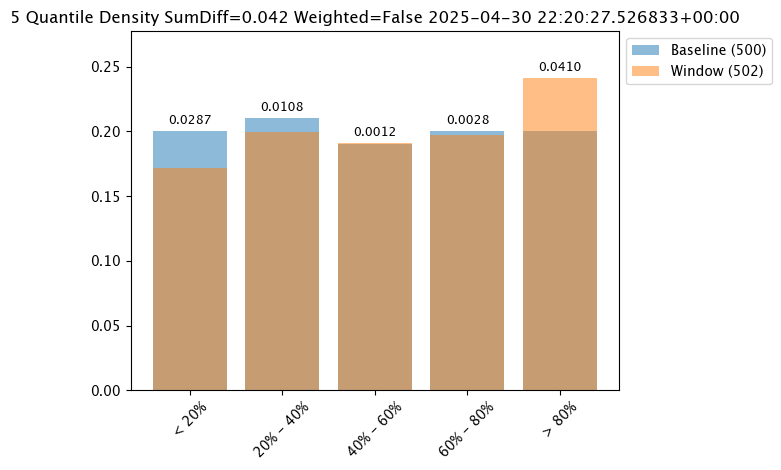
Score Metric
The score is a distance between the baseline and the analysis window. The larger the score, the greater the difference between the baseline and the analysis window. The following methods are provided determining the score:
PSI(Default) - Population Stability Index (PSI).MAXDIFF: Maximum difference between corresponding bins.SUMDIFF: Mum of differences between corresponding bins.
The metric type used is updated with the wallaroo.assay_config.AssayBuilder.add_metric(metric: wallaroo.assay_config.Metric) method.
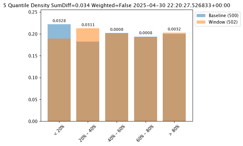
The following three charts use each of the metrics. Note how the scores change based on the score type used.
assay_baseline_from_dates = wl.build_assay(assay_name=assay_name,
                                          pipeline=mainpipeline,
                                          iopath="output variable 0",
                                          baseline_start=assay_baseline_start,
                                          baseline_end=assay_baseline_end)

# Set the assay parameters

# The end date to gather inference results
assay_baseline_from_dates.add_run_until(assay_baseline_end)

# Set the interval and window to one minute each, set the start date back 24 hours for gathering inference results
assay_baseline_from_dates.window_builder().add_width(hours=24).add_interval(hours=24).add_start(assay_baseline_start+datetime.timedelta(hours=-48))

# set metric PSI mode
assay_baseline_from_dates.summarizer_builder.add_metric(wallaroo.assay_config.Metric.PSI)

# build the assay configuration
assay_config_from_dates = assay_baseline_from_dates.build()

# perform an interactive run and collect inference data
assay_results_from_dates = assay_config_from_dates.interactive_run()

# display one analysis from the results
assay_results_from_dates[0].chart()

assay_baseline_from_dates = wl.build_assay(assay_name=assay_name,
                                          pipeline=mainpipeline,
                                          iopath="output variable 0",
                                          baseline_start=assay_baseline_start,
                                          baseline_end=assay_baseline_end)

# Set the assay parameters

# The end date to gather inference results
assay_baseline_from_dates.add_run_until(assay_baseline_end)

# Set the interval and window to one minute each, set the start date back 24 hours for gathering inference results
assay_baseline_from_dates.window_builder().add_width(hours=24).add_interval(hours=24).add_start(assay_baseline_start+datetime.timedelta(hours=-48))

# set metric MAXDIFF mode
assay_baseline_from_dates.summarizer_builder.add_metric(wallaroo.assay_config.Metric.MAXDIFF)

# build the assay configuration
assay_config_from_dates = assay_baseline_from_dates.build()

# perform an interactive run and collect inference data
assay_results_from_dates = assay_config_from_dates.interactive_run()

# display one analysis from the results
assay_results_from_dates[0].chart()
assay_baseline_from_dates = wl.build_assay(assay_name=assay_name,
                                          pipeline=mainpipeline,
                                          iopath="output variable 0",
                                          baseline_start=assay_baseline_start,
                                          baseline_end=assay_baseline_end)

# Set the assay parameters

# The end date to gather inference results
assay_baseline_from_dates.add_run_until(assay_baseline_end)

# Set the interval and window to one minute each, set the start date back 24 hours for gathering inference results
assay_baseline_from_dates.window_builder().add_width(hours=24).add_interval(hours=24).add_start(assay_baseline_start+datetime.timedelta(hours=-48))

# set metric SUMDIFF mode
assay_baseline_from_dates.summarizer_builder.add_metric(wallaroo.assay_config.Metric.SUMDIFF)

# build the assay configuration
assay_config_from_dates = assay_baseline_from_dates.build()

# perform an interactive run and collect inference data
assay_results_from_dates = assay_config_from_dates.interactive_run()

# display one analysis from the results
assay_results_from_dates[0].chart()
assay_baseline_from_numpy = wl.build_assay(assay_name=assay_name,
                                          pipeline=mainpipeline,
                                          iopath="output variable 0",
                                          baseline_data=baseline_results)

# Set the assay parameters

# The end date to gather inference results
assay_baseline_from_numpy.add_run_until(assay_baseline_end)

# Set the interval and window to one minute each, set the start date back 24 hours for gathering inference results
assay_baseline_from_numpy.window_builder().add_width(hours=24).add_interval(hours=24).add_start(assay_baseline_start+datetime.timedelta(hours=-24))

# set metric PSI mode
assay_baseline_from_numpy.summarizer_builder.add_metric(wallaroo.assay_config.Metric.PSI)

# build the assay configuration
assay_config_from_numpy = assay_baseline_from_numpy.build()

# perform an interactive run and collect inference data
assay_results_from_numpy = assay_config_from_numpy.interactive_run()

# show the analysis chart from the numpy baseline based assay
assay_results_from_numpy[0].chart()

assay_baseline_from_numpy = wl.build_assay(assay_name=assay_name,
                                          pipeline=mainpipeline,
                                          iopath="output variable 0",
                                          baseline_data=baseline_results)

# Set the assay parameters

# The end date to gather inference results
assay_baseline_from_numpy.add_run_until(assay_baseline_end)

# Set the interval and window to one minute each, set the start date back 24 hours for gathering inference results
assay_baseline_from_numpy.window_builder().add_width(hours=24).add_interval(hours=24).add_start(assay_baseline_start+datetime.timedelta(hours=-24))

# set metric MAXDIFF mode
assay_baseline_from_numpy.summarizer_builder.add_metric(wallaroo.assay_config.Metric.MAXDIFF)

# build the assay configuration
assay_config_from_numpy = assay_baseline_from_numpy.build()

# perform an interactive run and collect inference data
assay_results_from_numpy = assay_config_from_numpy.interactive_run()

# show the analysis chart from the numpy baseline based assay
assay_results_from_numpy[0].chart()

assay_baseline_from_numpy = wl.build_assay(assay_name=assay_name,
                                          pipeline=mainpipeline,
                                          iopath="output variable 0",
                                          baseline_data=baseline_results)

# Set the assay parameters

# The end date to gather inference results
assay_baseline_from_numpy.add_run_until(assay_baseline_end)

# Set the interval and window to one minute each, set the start date back 24 hours for gathering inference results
assay_baseline_from_numpy.window_builder().add_width(hours=24).add_interval(hours=24).add_start(assay_baseline_start+datetime.timedelta(hours=-24))

# set metric SUMDIFF mode
assay_baseline_from_numpy.summarizer_builder.add_metric(wallaroo.assay_config.Metric.SUMDIFF)

# build the assay configuration
assay_config_from_numpy = assay_baseline_from_numpy.build()

# perform an interactive run and collect inference data
assay_results_from_numpy = assay_config_from_numpy.interactive_run()

# show the analysis chart from the numpy baseline based assay
assay_results_from_numpy[0].chart()
Alert Threshold
Assay alert thresholds are modified with the wallaroo.assay_config.AssayBuilder.add_alert_threshold(alert_threshold: float) method. By default alert thresholds are 0.1.
The following example updates the alert threshold to 0.5.
assay_baseline_from_dates = wl.build_assay(assay_name=assay_name,
                                          pipeline=mainpipeline,
                                          iopath="output variable 0",
                                          baseline_start=assay_baseline_start,
                                          baseline_end=assay_baseline_end)

# Set the assay parameters

# The end date to gather inference results
assay_baseline_from_dates.add_run_until(assay_baseline_end)

# Set the interval and window to one minute each, set the start date back 24 hours for gathering inference results
assay_baseline_from_dates.window_builder().add_width(hours=24).add_interval(hours=24).add_start(assay_baseline_start+datetime.timedelta(hours=-48))

# set the alert threshold
assay_baseline_from_dates.add_alert_threshold(0.5)

# build the assay configuration
assay_config_from_dates = assay_baseline_from_dates.build()

# perform an interactive run and collect inference data
assay_results_from_dates = assay_config_from_dates.interactive_run()

# show the analyses with the alert threshold
assay_results_from_dates.to_dataframe()
| id | assay_id | assay_name | iopath | pipeline_id | pipeline_name | workspace_id | workspace_name | score | start | min | max | mean | median | std | warning_threshold | alert_threshold | status | |
|---|---|---|---|---|---|---|---|---|---|---|---|---|---|---|---|---|---|---|
| 0 | 0 | 03ab3e96-c842-43c6-add4-9b172e5c3b21 | assay-demonstration-tutorial assay | out.variable.0 | 1 | assay-demonstration-tutorial | 7 | assay-demonstration-tutorial | 0.012716 | 2025-04-29 22:20:27.526833+00:00 | 236238.671875 | 2005883.125 | 538249.025087 | 453247.0 | 247711.921875 | None | 0.5 | Ok |
assay_baseline_from_numpy = wl.build_assay(assay_name=assay_name,
                                          pipeline=mainpipeline,
                                          iopath="output variable 0",
                                          baseline_data=baseline_results)

# Set the assay parameters

# The end date to gather inference results
assay_baseline_from_numpy.add_run_until(assay_baseline_end)

# Set the interval and window to one minute each, set the start date back 24 hours for gathering inference results
assay_baseline_from_numpy.window_builder().add_width(hours=24).add_interval(hours=24).add_start(assay_baseline_start+datetime.timedelta(hours=-24))

# set the alert threshold
assay_baseline_from_numpy.add_alert_threshold(0.5)

# build the assay configuration
assay_config_from_numpy = assay_baseline_from_numpy.build()

# perform an interactive run and collect inference data
assay_results_from_numpy = assay_config_from_numpy.interactive_run()

# show the analyses with the alert threshold
assay_results_from_numpy.to_dataframe()
| id | assay_id | assay_name | iopath | pipeline_id | pipeline_name | workspace_id | workspace_name | score | start | min | max | mean | median | std | warning_threshold | alert_threshold | status | |
|---|---|---|---|---|---|---|---|---|---|---|---|---|---|---|---|---|---|---|
| 0 | 0 | 32cf10df-6c85-4131-9148-ffe21c310f94 | assay-demonstration-tutorial assay | out.variable.0 | 1 | assay-demonstration-tutorial | 7 | assay-demonstration-tutorial | 0.010207 | 2025-04-29 22:20:27.526833+00:00 | 236238.671875 | 2005883.125 | 538249.025087 | 453247.0 | 247711.921875 | None | 0.5 | Ok |
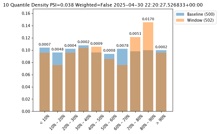
Number of Bins
Number of bins sets how the baseline data is partitioned. The total number of bins includes the set number plus the left_outlier and the right_outlier, so the total number of bins will be the total set + 2.
The number of bins is set with the wallaroo.assay_config.UnivariateContinousSummarizerBuilder.add_num_bins(num_bins: int) method.
assay_baseline_from_dates = wl.build_assay(assay_name=assay_name,
                                          pipeline=mainpipeline,
                                          iopath="output variable 0",
                                          baseline_start=assay_baseline_start,
                                          baseline_end=assay_baseline_end)

# Set the assay parameters

# The end date to gather inference results
assay_baseline_from_dates.add_run_until(assay_baseline_end)

# Set the interval and window to one minute each, set the start date back 24 hours for gathering inference results
assay_baseline_from_dates.window_builder().add_width(hours=24).add_interval(hours=24).add_start(assay_baseline_start+datetime.timedelta(hours=-48))

# update number of bins here
assay_baseline_from_dates.summarizer_builder.add_num_bins(10)

# build the assay configuration
assay_config_from_dates = assay_baseline_from_dates.build()

# perform an interactive run and collect inference data
assay_results_from_dates = assay_config_from_dates.interactive_run()

# show one analysis with the updated bins
assay_results_from_dates[0].chart()
assay_baseline_from_numpy = wl.build_assay(assay_name=assay_name,
                                          pipeline=mainpipeline,
                                          iopath="output variable 0",
                                          baseline_data=baseline_results)

# Set the assay parameters

# The end date to gather inference results
assay_baseline_from_numpy.add_run_until(assay_baseline_end)

# Set the interval and window to one minute each, set the start date back 24 hours for gathering inference results
assay_baseline_from_numpy.window_builder().add_width(hours=24).add_interval(hours=24).add_start(assay_baseline_start+datetime.timedelta(hours=-24))

# update number of bins here
assay_baseline_from_numpy.summarizer_builder.add_num_bins(10)

# build the assay configuration
assay_config_from_numpy = assay_baseline_from_numpy.build()

# perform an interactive run and collect inference data
assay_results_from_numpy = assay_config_from_numpy.interactive_run()

# show one analysis with the updated bins
assay_results_from_numpy[0].chart()
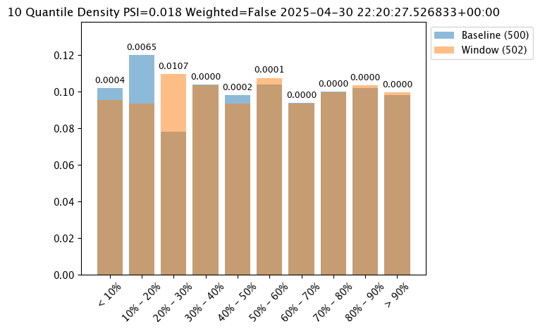
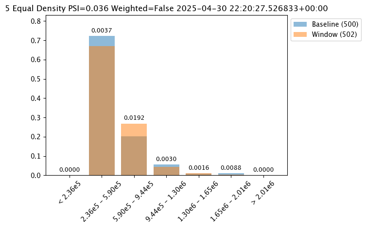
Binning Mode
Binning Mode defines how the bins are separated. Binning modes are modified through the wallaroo.assay_config.UnivariateContinousSummarizerBuilder.add_bin_mode(bin_mode: bin_mode: wallaroo.assay_config.BinMode, edges: Optional[List[float]] = None).
Available bin_mode values from wallaroo.assay_config.Binmode are the following:
QUANTILE(Default): Based on percentages. Ifnum_binsis 5 then quintiles so bins are created at the 20%, 40%, 60%, 80% and 100% points.EQUAL: Evenly spaced bins where each bin is set with the formulamin - max / num_binsPROVIDED: The user provides the edge points for the bins.
If PROVIDED is supplied, then a List of float values must be provided for the edges parameter that matches the number of bins.
The following examples are used to show how each of the binning modes effects the bins.
assay_baseline_from_dates = wl.build_assay(assay_name=assay_name,
                                          pipeline=mainpipeline,
                                          iopath="output variable 0",
                                          baseline_start=assay_baseline_start,
                                          baseline_end=assay_baseline_end)

# Set the assay parameters

# The end date to gather inference results
assay_baseline_from_dates.add_run_until(assay_baseline_end)

# Set the interval and window to one minute each, set the start date back 24 hours for gathering inference results
assay_baseline_from_dates.window_builder().add_width(hours=24).add_interval(hours=24).add_start(assay_baseline_start+datetime.timedelta(hours=-48))

# update binning mode here
assay_baseline_from_dates.summarizer_builder.add_bin_mode(wallaroo.assay_config.BinMode.QUANTILE)

# build the assay configuration
assay_config_from_dates = assay_baseline_from_dates.build()

# perform an interactive run and collect inference data
assay_results_from_dates = assay_config_from_dates.interactive_run()

# show one analysis with the updated bins
assay_results_from_dates[0].chart()

assay_baseline_from_dates = wl.build_assay(assay_name=assay_name,
                                          pipeline=mainpipeline,
                                          iopath="output variable 0",
                                          baseline_start=assay_baseline_start,
                                          baseline_end=assay_baseline_end)

# # Set the assay parameters

# The end date to gather inference results
assay_baseline_from_dates.add_run_until(assay_baseline_end)

# # Set the interval and window to one minute each, set the start date back 24 hours for gathering inference results
assay_baseline_from_dates.window_builder().add_width(hours=24).add_interval(hours=24).add_start(assay_baseline_start+datetime.timedelta(hours=-48))

# # update binning mode here
assay_baseline_from_dates.summarizer_builder.add_bin_mode(wallaroo.assay_config.BinMode.EQUAL)

# # build the assay configuration
assay_config_from_dates = assay_baseline_from_dates.build()

# # perform an interactive run and collect inference data
assay_results_from_dates = assay_config_from_dates.interactive_run()

# # show one analysis with the updated bins
assay_results_from_dates[0].chart()
assay_baseline_from_numpy = wl.build_assay(assay_name=assay_name,
                                          pipeline=mainpipeline,
                                          iopath="output variable 0",
                                          baseline_data=baseline_results)

# Set the assay parameters

# The end date to gather inference results
assay_baseline_from_numpy.add_run_until(assay_baseline_end)

# Set the interval and window to one minute each, set the start date back 24 hours for gathering inference results
assay_baseline_from_numpy.window_builder().add_width(hours=24).add_interval(hours=24).add_start(assay_baseline_start+datetime.timedelta(hours=-24))

# update binning mode here
assay_baseline_from_numpy.summarizer_builder.add_bin_mode(wallaroo.assay_config.BinMode.QUANTILE)

# build the assay configuration
assay_config_from_numpy = assay_baseline_from_numpy.build()

# perform an interactive run and collect inference data
assay_results_from_numpy = assay_config_from_numpy.interactive_run()

# show one analysis with the updated bins
assay_results_from_numpy[0].chart()

assay_baseline_from_numpy = wl.build_assay(assay_name=assay_name,
                                          pipeline=mainpipeline,
                                          iopath="output variable 0",
                                          baseline_data=baseline_results)

# Set the assay parameters

# The end date to gather inference results
assay_baseline_from_numpy.add_run_until(assay_baseline_end)

# Set the interval and window to one minute each, set the start date back 24 hours for gathering inference results
assay_baseline_from_numpy.window_builder().add_width(hours=24).add_interval(hours=24).add_start(assay_baseline_start+datetime.timedelta(hours=-24))

# update binning mode here
assay_baseline_from_numpy.summarizer_builder.add_bin_mode(wallaroo.assay_config.BinMode.EQUAL)

# build the assay configuration
assay_config_from_numpy = assay_baseline_from_numpy.build()

# perform an interactive run and collect inference data
assay_results_from_numpy = assay_config_from_numpy.interactive_run()

# show one analysis with the updated bins
assay_results_from_numpy[0].chart()
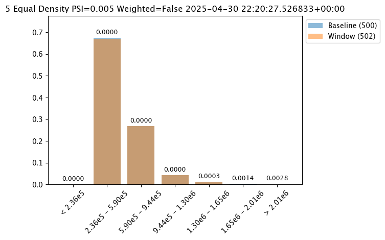
The following example manually sets the bin values.
The values in this dataset run from 200000 to 1500000. We can specify the bins with the BinMode.PROVIDED and specifying a list of floats with the right hand / upper edge of each bin and optionally the lower edge of the smallest bin. If the lowest edge is not specified the threshold for left outliers is taken from the smallest value in the baseline dataset.
assay_baseline_from_dates = wl.build_assay(assay_name=assay_name,
                                          pipeline=mainpipeline,
                                          iopath="output variable 0",
                                          baseline_start=assay_baseline_start,
                                          baseline_end=assay_baseline_end)

# Set the assay parameters

# The end date to gather inference results
assay_baseline_from_dates.add_run_until(assay_baseline_end)

# Set the interval and window to one minute each, set the start date back 24 hours for gathering inference results
assay_baseline_from_dates.window_builder().add_width(hours=24).add_interval(hours=24).add_start(assay_baseline_start+datetime.timedelta(hours=-48))

edges = [200000.0, 400000.0, 600000.0, 800000.0, 1500000.0, 2000000.0]

# update binning mode here
assay_baseline_from_dates.summarizer_builder.add_bin_mode(wallaroo.assay_config.BinMode.PROVIDED, edges)

# build the assay configuration
assay_config_from_dates = assay_baseline_from_dates.build()

# perform an interactive run and collect inference data
assay_results_from_dates = assay_config_from_dates.interactive_run()

# show one analysis with the updated bins
assay_results_from_dates[0].chart()
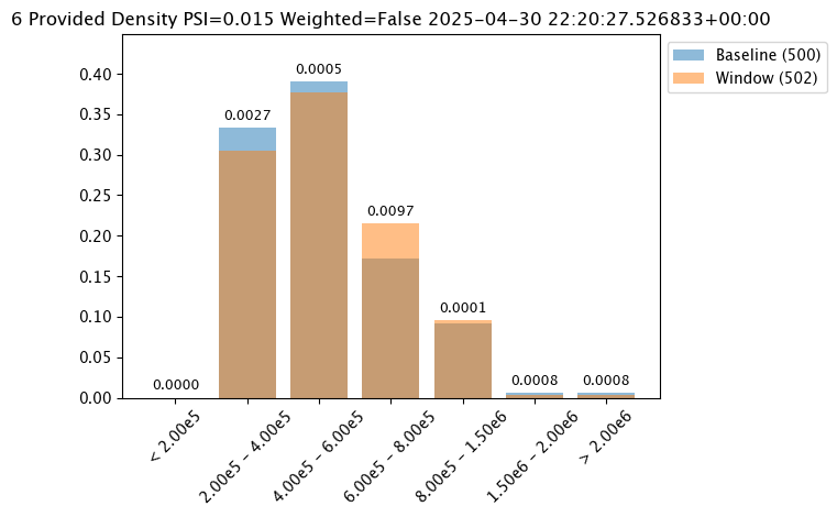
assay_baseline_from_numpy = wl.build_assay(assay_name=assay_name,
                                          pipeline=mainpipeline,
                                          iopath="output variable 0",
                                          baseline_data=baseline_results)

# Set the assay parameters

# The end date to gather inference results
assay_baseline_from_numpy.add_run_until(assay_baseline_end)

# Set the interval and window to one minute each, set the start date back 24 hours for gathering inference results
assay_baseline_from_numpy.window_builder().add_width(hours=24).add_interval(hours=24).add_start(assay_baseline_start+datetime.timedelta(hours=-24))

edges = [200000.0, 400000.0, 600000.0, 800000.0, 1500000.0, 2000000.0]

# update binning mode here
assay_baseline_from_numpy.summarizer_builder.add_bin_mode(wallaroo.assay_config.BinMode.PROVIDED, edges)

# build the assay configuration
assay_config_from_numpy = assay_baseline_from_numpy.build()

# perform an interactive run and collect inference data
assay_results_from_numpy = assay_config_from_numpy.interactive_run()

# show one analysis with the updated bins
assay_results_from_numpy[0].chart()
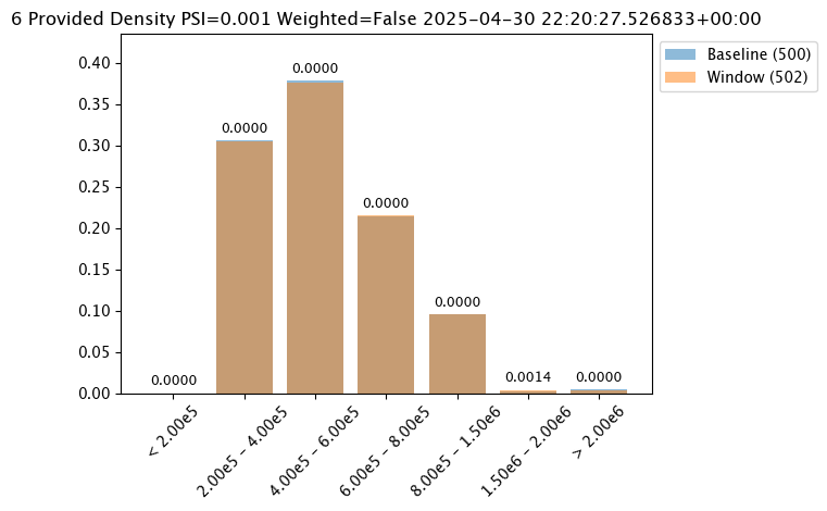
Aggregation Options
Assay aggregation options are modified with the wallaroo.assay_config.AssayBuilder.add_aggregation(aggregation: wallaroo.assay_config.Aggregation) method. The following options are provided:
Aggregation.DENSITY(Default): Count the number/percentage of values that fall in each bin.Aggregation.CUMULATIVE: Empirical Cumulative Density Function style, which keeps a cumulative count of the values/percentages that fall in each bin.
The following example demonstrate the different results between the two.
assay_baseline_from_dates = wl.build_assay(assay_name=assay_name,
                                          pipeline=mainpipeline,
                                          iopath="output variable 0",
                                          baseline_start=assay_baseline_start,
                                          baseline_end=assay_baseline_end)

# Set the assay parameters

# The end date to gather inference results
assay_baseline_from_dates.add_run_until(assay_baseline_end)

# Set the interval and window to one minute each, set the start date back 24 hours for gathering inference results
assay_baseline_from_dates.window_builder().add_width(hours=24).add_interval(hours=24).add_start(assay_baseline_start+datetime.timedelta(hours=-48))

#Aggregation.DENSITY - the default
assay_baseline_from_dates.summarizer_builder.add_aggregation(wallaroo.assay_config.Aggregation.DENSITY)

# build the assay configuration
assay_config_from_dates = assay_baseline_from_dates.build()

# perform an interactive run and collect inference data
assay_results_from_dates = assay_config_from_dates.interactive_run()

# show one analysis with the updated bins
assay_results_from_dates[0].chart()
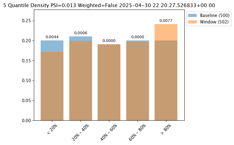
assay_baseline_from_dates = wl.build_assay(assay_name=assay_name,
                                          pipeline=mainpipeline,
                                          iopath="output variable 0",
                                          baseline_start=assay_baseline_start,
                                          baseline_end=assay_baseline_end)

# Set the assay parameters

# The end date to gather inference results
assay_baseline_from_dates.add_run_until(assay_baseline_end)

# Set the interval and window to one minute each, set the start date back 24 hours for gathering inference results
assay_baseline_from_dates.window_builder().add_width(hours=24).add_interval(hours=24).add_start(assay_baseline_start+datetime.timedelta(hours=-48))

#Aggregation.CUMULATIVE - the default
assay_baseline_from_dates.summarizer_builder.add_aggregation(wallaroo.assay_config.Aggregation.CUMULATIVE)

# build the assay configuration
assay_config_from_dates = assay_baseline_from_dates.build()

# perform an interactive run and collect inference data
assay_results_from_dates = assay_config_from_dates.interactive_run()

# show one analysis with the updated bins
assay_results_from_dates[0].chart()
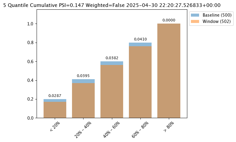
assay_baseline_from_numpy = wl.build_assay(assay_name=assay_name,
                                          pipeline=mainpipeline,
                                          iopath="output variable 0",
                                          baseline_data=baseline_results)

# Set the assay parameters

# The end date to gather inference results
assay_baseline_from_numpy.add_run_until(assay_baseline_end)

# Set the interval and window to one minute each, set the start date back 24 hours for gathering inference results
assay_baseline_from_numpy.window_builder().add_width(hours=24).add_interval(hours=24).add_start(assay_baseline_start+datetime.timedelta(hours=-24))

# Aggregation.DENSITY - the default
assay_baseline_from_numpy.summarizer_builder.add_aggregation(wallaroo.assay_config.Aggregation.DENSITY)

# build the assay configuration
assay_config_from_numpy = assay_baseline_from_numpy.build()

# perform an interactive run and collect inference data
assay_results_from_numpy = assay_config_from_numpy.interactive_run()

# show one analysis with the updated bins
assay_results_from_numpy[0].chart()

assay_baseline_from_numpy = wl.build_assay(assay_name=assay_name,
                                          pipeline=mainpipeline,
                                          iopath="output variable 0",
                                          baseline_data=baseline_results)

# Set the assay parameters

# The end date to gather inference results
assay_baseline_from_numpy.add_run_until(assay_baseline_end)

# Set the interval and window to one minute each, set the start date back 24 hours for gathering inference results
assay_baseline_from_numpy.window_builder().add_width(hours=24).add_interval(hours=24).add_start(assay_baseline_start+datetime.timedelta(hours=-24))

# Aggregation.CUMULATIVE - the default
assay_baseline_from_numpy.summarizer_builder.add_aggregation(wallaroo.assay_config.Aggregation.CUMULATIVE)

# build the assay configuration
assay_config_from_numpy = assay_baseline_from_numpy.build()

# perform an interactive run and collect inference data
assay_results_from_numpy = assay_config_from_numpy.interactive_run()

# show one analysis with the updated bins
assay_results_from_numpy[0].chart()
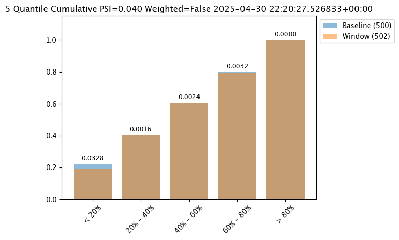
Create Assay
With the assay previewed and configuration options determined, we officially create it by uploading it to the Wallaroo instance.
Once it is uploaded, the assay runs an analysis based on the window width, interval, and the other settings configured.
Assays are uploaded with the wallaroo.assay_config.upload() method. This uploads the assay into the Wallaroo database with the configurations applied and returns the assay id. Note that assay names must be unique across the Wallaroo instance; attempting to upload an assay with the same name as an existing one will return an error.
wallaroo.assay_config.upload() returns the assay id for the assay.
Typically we would just call wallaroo.assay_config.upload() after configuring the assay. For the example below, we will perform the complete configuration in one window to show all of the configuration steps at once before creating the assay.
# Build the assay, based on the start and end of our baseline time,
# and tracking the output variable index 0
assay_baseline = wl.build_assay(assay_name="assays from date baseline tutorial samples",
                                          pipeline=mainpipeline,
                                          iopath="output variable 0",
                                          baseline_start=assay_baseline_start,
                                          baseline_end=assay_baseline_end)

# Set the interval and window to one minute each, set the start date for gathering inference results
assay_baseline.window_builder().add_width(hours=24).add_interval(hours=24).add_start(assay_baseline_start+datetime.timedelta(hours=-24))

# add other options
assay_baseline.summarizer_builder.add_aggregation(wallaroo.assay_config.Aggregation.CUMULATIVE)
assay_baseline.summarizer_builder.add_metric(wallaroo.assay_config.Metric.MAXDIFF)
assay_baseline.add_alert_threshold(0.5)

assay_id = assay_baseline.upload()

# wait 65 seconds for the first analysis run performed
time.sleep(65)
# sample inference to give the assay analysis inference data to work with
baseline_inference_results = mainpipeline.infer(baseline_sample)
The assay is now visible through the Wallaroo UI by selecting the workspace, then the pipeline, then Insights.
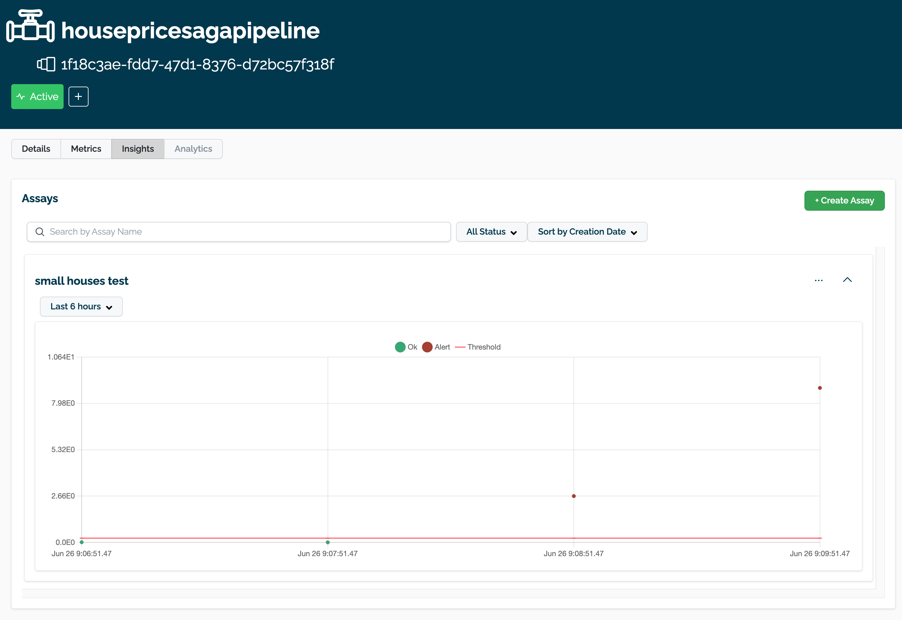
Get Assay Info
Assay information is retrieved with the wallaroo.client.get_assay_info() which takes the following parameters.
| Parameter | Type | Description |
|---|---|---|
| assay_id | String (Required) | The numerical id of the assay in UUID format. |
| workspace_id | (Int) (Optional) | The numerical identifier of the workspace to filter by. |
| workspace_name | (String) (Optional) | The name of the workspace to filter by. |
This returns the following:
| Parameter | Type | Description |
|---|---|---|
| id | String | The id of the assay in UUID format. |
| name | String | The name of the assay. |
| active | Boolean | True: The assay is active and generates analyses based on its configuration. False: The assay is disabled and will not generate new analyses. |
| pipeline_name | String | The name of the pipeline the assay references. |
| last_run | DateTime | The date and time the assay last ran. |
| next_run | DateTime | THe date and time the assay analysis will next run. |
| alert_threshold | Float | The alert threshold setting for the assay. |
| baseline | Dict | The baseline and settings as set from the assay configuration. |
| iopath | String | The iopath setting for the assay. |
| metric | String | The metric setting for the assay. |
| num_bins | Integer | The number of bins for the assay. |
| bin_weights | List/None | The bin weights used if any. |
| bin_mode | String | The binning mode used. |
| workspace_id | (Int) | The numerical identifier of the workspace the assay is associated with. |
| workspace_name | (String) | The name of the workspace the assay is associated with. |
Get Assay Results
Once an assay is created the assay runs an analysis based on the window width, interval, and the other settings configured.
Assay results are retrieved with the wallaroo.client.get_assay_results method which takes the following parameters:
| Parameter | Type | Description |
|---|---|---|
| assay_id | String (Required) | The id of the assay in UUID format. |
| start | Datetime.Datetime (Required) | The start date and time of historical data from the pipeline to start analyses from. |
| end | Datetime.Datetime (Required) | The end date and time of historical data from the pipeline to limit analyses to. |
| workspace_id | (Int) (Optional) | The numerical identifier of the workspace to filter by. |
| workspace_name | (String) (Optional) | The name of the workspace to filter by. |
- IMPORTANT NOTE: This process requires that additional historical data is generated from the time the assay is created to when the results are available. To add additional inference data, use the Assay Test Data section above.
assay_results = wl.get_assay_results(assay_id,
                     start = assay_baseline_start+datetime.timedelta(hours=-24),
                     end = assay_baseline_end)
assay_results[0].chart()
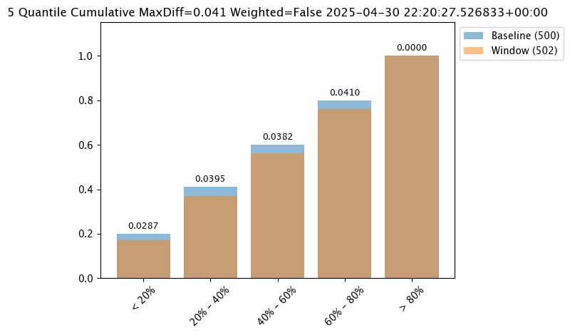
List Assays
A list of assays is retrieved with the wallaroo.client.list_assays() method and takes the following parameters:
| Parameter | Type | Description |
|---|---|---|
| workspace_id | (Int) (Optional) | The numerical identifier of the workspace to filter by. |
| workspace_name | (String) (Optional) | The name of the workspace to filter by. |
This returns a list of assays as filtered in reverse chronological order.
| Parameter | Type | Description |
|---|---|---|
| Assay Id | String | The id of the assay in UUID format. |
| Assay Name | String | The name of the assay. |
| Active | Boolean | True: The assay is active and generates analyses based on its configuration. False: The assay is disabled and will not generate new analyses. |
| Status | Dict | The status of the assay including the |
| Warning Threshold | Float/None | The warning threshold if set. |
| Alert Threshold | Float | The alert threshold for the assay. |
| workspace_id | (Int) | The numerical identifier of the workspace the assay is associated with. |
| workspace_name | (String) | The name of the workspace the assay is associated with. |
The errors for this method include:
- If the parameter
workspace_idis not an integer. - If the parameter
workspace_nameis not a String.
wl.list_assays()
| id | name | active | pipeline | workspace id | workspace name | monitored fields | last_run | next_run | created_at | updated_at |
|---|---|---|---|---|---|---|---|---|---|---|
| 79beecf1-a9ce-41e0-b1e6-da418f3c0aa2 | assays from date baseline tutorial samples | True | assay-demonstration-tutorial | 7 | assay-demonstration-tutorial | ['out.variable.0'] | 2025-30-Apr 22:20:27 | 2025-01-May 22:20:27 | 2025-30-Apr 22:55:43 | 2025-30-Apr 22:55:43 |
Set Assay Active Status
Assays active status is either:
- True: The assay generates analyses based on the assay configuration.
- False: The assay will not generate new analyses.
Assays are set to active or not active with the wallaroo.client.set_assay_active which takes the following parameters.
| Parameter | Type | Description |
|---|---|---|
| assay_id | String | The id of the assay in UUID format. |
| active | Boolean | True: The assay status is set to Active. False: The assay status is Not Active. |
First we will show the current active status.
In the following, set the assay status to False, then set the assay active status back to True.
display(wl.get_assay_info(assay_id))
| Field | Value |
|---|---|
| ID | 79beecf1-a9ce-41e0-b1e6-da418f3c0aa2 |
| Name | assays from date baseline tutorial samples |
| Active | True |
| Pipeline | assay-demonstration-tutorial |
| Workspace ID | 7 |
| Workspace Name | assay-demonstration-tutorial |
| Monitoring | ['out.variable.0'] |
| Window Width | 86400 seconds |
| First Run | 2025-30-Apr 22:20:27 |
| Run Frequency | 24 Hour |
| Bin Mode | 5 Quantile bins |
| Aggregation | Cumulative |
| Metric | MaxDiff |
| Last Run | 2025-30-Apr 22:20:27 |
| Next Run | 2025-01-May 22:20:27 |
| Created At | 2025-30-Apr 22:55:43 |
| Updated At | 2025-30-Apr 22:55:43 |
Now we set the active status to False, and show the assay list to verify it is no longer active.
wl.set_assay_active(assay_id, False)
display(wl.get_assay_info(assay_id))
| Field | Value |
|---|---|
| ID | 79beecf1-a9ce-41e0-b1e6-da418f3c0aa2 |
| Name | assays from date baseline tutorial samples |
| Active | False |
| Pipeline | assay-demonstration-tutorial |
| Workspace ID | 7 |
| Workspace Name | assay-demonstration-tutorial |
| Monitoring | ['out.variable.0'] |
| Window Width | 86400 seconds |
| First Run | 2025-30-Apr 22:20:27 |
| Run Frequency | 24 Hour |
| Bin Mode | 5 Quantile bins |
| Aggregation | Cumulative |
| Metric | MaxDiff |
| Last Run | 2025-30-Apr 22:20:27 |
| Next Run | None |
| Created At | 2025-30-Apr 22:55:43 |
| Updated At | 2025-30-Apr 22:57:04 |
We resume the assay by setting it’s active status to True.
wl.set_assay_active(assay_id, True)
display(wl.get_assay_info(assay_id))
# setting to false to preserve resources
wl.set_assay_active(assay_id, False)
| Field | Value |
|---|---|
| ID | 79beecf1-a9ce-41e0-b1e6-da418f3c0aa2 |
| Name | assays from date baseline tutorial samples |
| Active | True |
| Pipeline | assay-demonstration-tutorial |
| Workspace ID | 7 |
| Workspace Name | assay-demonstration-tutorial |
| Monitoring | ['out.variable.0'] |
| Window Width | 86400 seconds |
| First Run | 2025-30-Apr 22:20:27 |
| Run Frequency | 24 Hour |
| Bin Mode | 5 Quantile bins |
| Aggregation | Cumulative |
| Metric | MaxDiff |
| Last Run | 2025-30-Apr 22:20:27 |
| Next Run | 2025-01-May 22:20:27 |
| Created At | 2025-30-Apr 22:55:43 |
| Updated At | 2025-30-Apr 22:57:06 |
View Assay Filters
The following examples demonstrate various ways of listing assays and retrieving assay details, with filtering options.
List Assays with Filters
List all assays for workspaces the user is a member of.
wl.list_assays()
| id | name | active | pipeline | workspace id | workspace name | monitored fields | last_run | next_run | created_at | updated_at |
|---|---|---|---|---|---|---|---|---|---|---|
| 79beecf1-a9ce-41e0-b1e6-da418f3c0aa2 | assays from date baseline tutorial samples | False | assay-demonstration-tutorial | 7 | assay-demonstration-tutorial | ['out.variable.0'] | 2025-30-Apr 22:20:27 | None | 2025-30-Apr 22:55:43 | 2025-30-Apr 22:57:07 |
List all assays filtered by workspace id.
wl.list_assays(workspace_id=workspace.id())
| id | name | active | pipeline | workspace id | workspace name | monitored fields | last_run | next_run | created_at | updated_at |
|---|---|---|---|---|---|---|---|---|---|---|
| 79beecf1-a9ce-41e0-b1e6-da418f3c0aa2 | assays from date baseline tutorial samples | False | assay-demonstration-tutorial | 7 | assay-demonstration-tutorial | ['out.variable.0'] | 2025-30-Apr 22:20:27 | None | 2025-30-Apr 22:55:43 | 2025-30-Apr 22:57:07 |
List assays filtered by workspace name.
wl.list_assays(workspace_name=workspace_name)
| id | name | active | pipeline | workspace id | workspace name | monitored fields | last_run | next_run | created_at | updated_at |
|---|---|---|---|---|---|---|---|---|---|---|
| 79beecf1-a9ce-41e0-b1e6-da418f3c0aa2 | assays from date baseline tutorial samples | False | assay-demonstration-tutorial | 7 | assay-demonstration-tutorial | ['out.variable.0'] | 2025-30-Apr 22:20:27 | None | 2025-30-Apr 22:55:43 | 2025-30-Apr 22:57:07 |
Get Assay Results with Filters
Get assay results.
assay_results = wl.get_assay_results(assay_id=assay_id,
                     start=assay_baseline_start,
                     end=datetime.datetime.now())

assay_results.chart_scores()

Get assay results filtered by workspace id.
assay_results = wl.get_assay_results(assay_id=assay_id,
                                     workspace_id=workspace.id(),
                                     start=assay_baseline_start+datetime.timedelta(hours=-24),
                                     end=datetime.datetime.now())

assay_results.chart_scores()

Get assay results filtered by workspace name.
assay_results = wl.get_assay_results(assay_id=assay_id,
                                     workspace_name=workspace_name,
                     start=assay_baseline_start,
                     end=datetime.datetime.now())

assay_results.chart_scores()
Get Assay Info with Filter
Get assay info.
wl.get_assay_info(assay_id=assay_id)
| Field | Value |
|---|---|
| ID | 79beecf1-a9ce-41e0-b1e6-da418f3c0aa2 |
| Name | assays from date baseline tutorial samples |
| Active | False |
| Pipeline | assay-demonstration-tutorial |
| Workspace ID | 7 |
| Workspace Name | assay-demonstration-tutorial |
| Monitoring | ['out.variable.0'] |
| Window Width | 86400 seconds |
| First Run | 2025-30-Apr 22:20:27 |
| Run Frequency | 24 Hour |
| Bin Mode | 5 Quantile bins |
| Aggregation | Cumulative |
| Metric | MaxDiff |
| Last Run | 2025-30-Apr 22:20:27 |
| Next Run | None |
| Created At | 2025-30-Apr 22:55:43 |
| Updated At | 2025-30-Apr 22:57:07 |
Get assay info filtered by workspace id.
wl.get_assay_info(assay_id=assay_id,
                 workspace_id=workspace.id())
| Field | Value |
|---|---|
| ID | 79beecf1-a9ce-41e0-b1e6-da418f3c0aa2 |
| Name | assays from date baseline tutorial samples |
| Active | False |
| Pipeline | assay-demonstration-tutorial |
| Workspace ID | 7 |
| Workspace Name | assay-demonstration-tutorial |
| Monitoring | ['out.variable.0'] |
| Window Width | 86400 seconds |
| First Run | 2025-30-Apr 22:20:27 |
| Run Frequency | 24 Hour |
| Bin Mode | 5 Quantile bins |
| Aggregation | Cumulative |
| Metric | MaxDiff |
| Last Run | 2025-30-Apr 22:20:27 |
| Next Run | None |
| Created At | 2025-30-Apr 22:55:43 |
| Updated At | 2025-30-Apr 22:57:07 |
Get assay info filtered by workspace name.
wl.get_assay_info(assay_id=assay_id,
                 workspace_name=workspace_name)
| Field | Value |
|---|---|
| ID | 79beecf1-a9ce-41e0-b1e6-da418f3c0aa2 |
| Name | assays from date baseline tutorial samples |
| Active | False |
| Pipeline | assay-demonstration-tutorial |
| Workspace ID | 7 |
| Workspace Name | assay-demonstration-tutorial |
| Monitoring | ['out.variable.0'] |
| Window Width | 86400 seconds |
| First Run | 2025-30-Apr 22:20:27 |
| Run Frequency | 24 Hour |
| Bin Mode | 5 Quantile bins |
| Aggregation | Cumulative |
| Metric | MaxDiff |
| Last Run | 2025-30-Apr 22:20:27 |
| Next Run | None |
| Created At | 2025-30-Apr 22:55:43 |
| Updated At | 2025-30-Apr 22:57:07 |