Model Drift Detection for Edge Deployments: Demonstration
This tutorial and the assets can be downloaded as part of the Wallaroo Tutorials repository.
Model Drift Detection for Edge Deployments Tutorial: Demonstration
The Model Insights feature lets you monitor how the environment that your model operates within may be changing in ways that affect it’s predictions so that you can intervene (retrain) in an efficient and timely manner. Changes in the inputs, data drift, can occur due to errors in the data processing pipeline or due to changes in the environment such as user preference or behavior.
Wallaroo Run Anywhere allows models to be deployed on edge and other locations, and have their inference result logs uploaded to the Wallaroo Ops center. Wallaroo assays allow for model drift detection to include the inference results from one or more deployment locations and compare any one or multiple locations results against an established baseline.
This notebook is designed to demonstrate the Wallaroo Run Anywhere with Model Drift Observability with Wallaroo Assays. This notebook will walk through the process of:
- Preparation: This notebook focuses on setting up the conditions for model edge deployments to different locations. This includes:
- Setting up a workspace, pipeline, and model for deriving the price of a house based on inputs.
- Performing a sample set of inferences to verify the model deployment.
- Publish the deployed model to an Open Container Initiative (OCI) Registry, and use that to deploy the model to two difference edge locations.
- Model Drift by Location:
- Perform inference requests on each of the model edge deployments.
- Perform the steps in creating an assay:
- Build an assay baseline with a specified location for inference results.
- Preview the assay and show different assay configurations based on selecting the inference data from the Wallaroo Ops model deployment versus the edge deployment.
- Create the assay.
- View assay results.
This notebook focuses on Model Drift by Location.
Goal
Model insights monitors the output of the house price model over a designated time window and compares it to an expected baseline distribution. We measure the performance of model deployments in different locations and compare that to the baseline to detect model drift.
Resources
This tutorial provides the following:
- Models:
models/rf_model.onnx: The champion model that has been used in this environment for some time.- Various inputs:
smallinputs.df.json: A set of house inputs that tends to generate low house price values.biginputs.df.json: A set of house inputs that tends to generate high house price values.
Prerequisites
- A deployed Wallaroo instance with Edge Registry Services and Edge Observability enabled.
- The following Python libraries installed:
- A X64 Docker deployment to deploy the model on an edge location.
- The notebook “Wallaroo Run Anywhere Model Drift Observability with Assays: Preparation” has been run, and the model edge deployments executed.
Steps
- Deploying a sample ML model used to determine house prices based on a set of input parameters.
- Build an assay baseline from a set of baseline start and end dates, and an assay baseline from a numpy array.
- Preview the assay and show different assay configurations.
- Upload the assay.
- View assay results.
- Pause and resume the assay.
This notebook requires the notebook “Wallaroo Run Anywhere Model Drift Observability with Assays: Preparation” has been run, and the model edge deployments executed. The name of the workspaces, pipelines, and edge locations in this notebook must match the same ones in “Wallaroo Run Anywhere Model Drift Observability with Assays: Preparation”.
Import Libraries
The first step will be to import our libraries, and set variables used through this tutorial.
import wallaroo
from wallaroo.object import EntityNotFoundError
from wallaroo.framework import Framework

from IPython.display import display

# used to display DataFrame information without truncating
from IPython.display import display
import pandas as pd
pd.set_option('display.max_colwidth', None)

import datetime
import time
import json

workspace_name = f'run-anywhere-assay-demonstration-tutorial'
main_pipeline_name = f'assay-demonstration-tutorial'
model_name_control = f'house-price-estimator'
model_file_name_control = './models/rf_model.onnx'

# Set the name of the assay
assay_name="ops assay example"
edge_assay_name = "edge assay example"
combined_assay_name = "combined assay example"

# ignoring warnings for demonstration
import warnings
warnings.filterwarnings('ignore')

# used to display DataFrame information without truncating
from IPython.display import display
import pandas as pd
pd.set_option('display.max_colwidth', None)
Connect to the Wallaroo Instance
The first step is to connect to Wallaroo through the Wallaroo client. The Python library is included in the Wallaroo install and available through the Jupyter Hub interface provided with your Wallaroo environment.
This is accomplished using the wallaroo.Client() command, which provides a URL to grant the SDK permission to your specific Wallaroo environment. When displayed, enter the URL into a browser and confirm permissions. Store the connection into a variable that can be referenced later.
If logging into the Wallaroo instance through the internal JupyterHub service, use wl = wallaroo.Client(). For more information on Wallaroo Client settings, see the Client Connection guide.
wl = wallaroo.Client()
Retrieve Workspace and Pipeline
For our example, we will retrieve the same workspace and pipeline that were used to create the edge locations. This requires that the preparation notebook is run first and the same workspace and pipeline names are used.
workspace = wl.get_workspace(name=workspace_name, create_if_not_exist=True)

wl.set_current_workspace(workspace)
{'name': 'run-anywhere-assay-demonstration-tutorial', 'id': 15, 'archived': False, 'created_by': 'fb2916bc-551e-4a76-88e8-0f7d7720a0f9', 'created_at': '2024-07-30T15:55:03.564943+00:00', 'models': [{'name': 'house-price-estimator', 'versions': 1, 'owner_id': '""', 'last_update_time': datetime.datetime(2024, 7, 30, 15, 55, 4, 840192, tzinfo=tzutc()), 'created_at': datetime.datetime(2024, 7, 30, 15, 55, 4, 840192, tzinfo=tzutc())}], 'pipelines': [{'name': 'assay-demonstration-tutorial', 'create_time': datetime.datetime(2024, 7, 30, 15, 55, 5, 574830, tzinfo=tzutc()), 'definition': '[]'}]}
List Pipeline Edges
The pipeline published in the notebook ““Wallaroo Run Anywhere Model Drift Observability with Assays: Preparation” created two edge locations.
We start by retrieving the pipeline, then verifying the pipeline publishes with the wallaroo.pipeline.publishes() methods.
We then list the edges with the wallaroo.pipeline.list_edges methods. This verifies the names of our edge locations, which are used later in the model drift detection by location methods.
mainpipeline = wl.get_pipeline(main_pipeline_name)

# list the publishes

display(mainpipeline.publishes())

# get the edges

display(mainpipeline.list_edges())
| id | pipeline_version_name | engine_url | pipeline_url | created_by | created_at | updated_at |
|---|---|---|---|---|---|---|
| 1 | e1abe92f-82d2-494a-8d96-dbd5810dc198 | ghcr.io/wallaroolabs/doc-samples/engines/proxy/wallaroo/ghcr.io/wallaroolabs/fitzroy-mini:v2024.2.0-main-5455 | ghcr.io/wallaroolabs/doc-samples/pipelines/assay-demonstration-tutorial:e1abe92f-82d2-494a-8d96-dbd5810dc198 | john.hansarick@wallaroo.ai | 2024-30-Jul 15:55:59 | 2024-30-Jul 15:55:59 |
| ID | Name | Tags | SPIFFE ID |
|---|---|---|---|
| e3915807-91dc-4195-8e72-a0d070700c33 | houseprice-edge-demonstration-01 | [] | wallaroo.ai/ns/deployments/edge/e3915807-91dc-4195-8e72-a0d070700c33 |
| 21190ced-17e8-4db4-8263-8cca7f3a2c18 | houseprice-edge-demonstration-02 | [] | wallaroo.ai/ns/deployments/edge/21190ced-17e8-4db4-8263-8cca7f3a2c18 |
Historical Data via Edge Inferences Generation
We will perform sample inference on our edge location. This historical inference data is used later in the drift detection by location examples.
For these example, the edge location is on the hostname HOSTNAME. Change this hostname to the host name of your edge deployment.
We will submit two sets of inferences:
- A normal set of inferences to generate the baseline, and are unlikely to trigger an assay alert when compared against the baseline. These are run through the location
houseprice-edge-01. - A set of inferences that will return large house values that is likely to trigger an assay alert when compared against the baseline. These are run through the location
houseprice-edge-02.
Each of these will use the inference endpoint /infer. For more details, see How to Publish and Deploy AI Workloads for For Edge and Multicloud Model Deployments.
assay_baseline_start = datetime.datetime.now()

time.sleep(65)

small_houses_inputs = pd.read_json('./data/smallinputs.df.json')
baseline_size = 500

# These inputs will be random samples of small priced houses.  Around 500 is a good number
small_houses = small_houses_inputs.sample(baseline_size, replace=True).reset_index(drop=True)
# small_houses.to_dict(orient="records")
data = small_houses.to_dict(orient="records")

!curl -X POST testboy.local:8080/infer \
    -H "Content-Type: Content-Type: application/json; format=pandas-records" \
    --data '{json.dumps(data)}' > results01.df.json

assay_baseline_end = datetime.datetime.now()

time.sleep(65)

# set the start of the assay window period
assay_window_start = datetime.datetime.now()

# generate a set of normal house values
!curl -X POST testboy.local:8080/infer \
    -H "Content-Type: Content-Type: application/json; format=pandas-records" \
    --data @./data/normal-inputs.df.json > results01.df.json
  % Total    % Received % Xferd  Average Speed   Time    Time     Time  Current
                                 Dload  Upload   Total   Spent    Left  Speed
100  316k  100  246k  100 71632   465k   132k --:--:-- --:--:-- --:--:--  598k
  % Total    % Received % Xferd  Average Speed   Time    Time     Time  Current
                                 Dload  Upload   Total   Spent    Left  Speed
100  590k  100  481k  100  108k   574k   129k --:--:-- --:--:-- --:--:--  704k
# set of values for the second edge location

time.sleep(65)

# generate a set of normal house values
!curl -X POST testboy.local:8081/infer \
    -H "Content-Type: application/json; format=pandas-records" \
    --data @./data/normal-inputs.df.json > results02.df.json

time.sleep(65)
# generate a set of large house values that will trigger an assay alert based on our baseline
large_houses_inputs = pd.read_json('./data/biginputs.df.json')
baseline_size = 500

# These inputs will be random samples of small priced houses.  Around 500 is a good number
large_houses = large_houses_inputs.sample(baseline_size, replace=True).reset_index(drop=True)
data = large_houses.to_dict(orient="records")

!curl -X POST testboy.local:8081/infer \
    -H "Content-Type: Content-Type: application/json; format=pandas-records" \
    --data '{json.dumps(data)}' > results02.df.json
  % Total    % Received % Xferd  Average Speed   Time    Time     Time  Current
                                 Dload  Upload   Total   Spent    Left  Speed
100  590k  100  481k  100  108k   394k  91114  0:00:01  0:00:01 --:--:--  483k
  % Total    % Received % Xferd  Average Speed   Time    Time     Time  Current
                                 Dload  Upload   Total   Spent    Left  Speed
100  319k  100  248k  100 73249   492k   142k --:--:-- --:--:-- --:--:--  635k
Model Insights via the Wallaroo SDK
Assays generated through the Wallaroo SDK can be previewed, configured, and uploaded to the Wallaroo Ops instance. The following is a condensed version of this process. For full details see the Wallaroo SDK Essentials Guide: Assays Management guide.
Model drift detection with assays using the Wallaroo SDK follows this general process.
- Define the Baseline: From either historical inference data for a specific model in a pipeline, or from a pre-determine array of data, a baseline is formed.
- Assay Preview: Once the baseline is formed, we preview the assay and configure the different options until we have the the best method of detecting environment or model drift.
- Create Assay: With the previews and configuration complete, we upload the assay. The assay will perform an analysis on a regular scheduled based on the configuration.
- Get Assay Results: Retrieve the analyses and use them to detect model drift and possible sources.
- Pause/Resume Assay: Pause or restart an assay as needed.
Define the Baseline
Assay baselines are defined with the wallaroo.client.build_assay method. Through this process we define the baseline from either a range of dates or pre-generated values.
wallaroo.client.build_assay take the following parameters:
| Parameter | Type | Description |
|---|---|---|
| assay_name | String (Required) - required | The name of the assay. Assay names must be unique across the Wallaroo instance. |
| pipeline | wallaroo.pipeline.Pipeline (Required) | The pipeline the assay is monitoring. |
| model_name | String (Optional) / None | The name of the model to monitor. This field should only be used to track the inputs/outputs for a specific model step in a pipeline. If no model_name is to be included, then the parameters must be passed a named parameters not positional ones. |
| iopath | String (Required) | The iopath of the assay in the format "input/output {field_name} {field_index}". For Assays V1, field_index is required for list values. For Assays V2, the field_index is required for list values and omitted for scaler values. For example, to monitor the output list field house_price at index 0, the iopath is output house_price 0. For data that are scaler values, no index is passed. For example, the iopath for the output scaler field model_confidence is 'output model_confidence', with no index value provided. |
| baseline_start | datetime.datetime (Optional) | The start time for the inferences to use as the baseline. Must be included with baseline_end. Cannot be included with baseline_data. |
| baseline_end | datetime.datetime (Optional) | The end time of the baseline window. the baseline. Windows start immediately after the baseline window and are run at regular intervals continuously until the assay is deactivated or deleted. Must be included with baseline_start. Cannot be included with baseline_data.. |
| baseline_data | numpy.array (Optional) | The baseline data in numpy array format. Cannot be included with either baseline_start or baseline_data. |
Note that model_name is an optional parameters when parameters are named. For example:
assay_builder_from_dates = wl.build_assay(assay_name="assays from date baseline",
                                          pipeline=mainpipeline,
                                          iopath="output variable 0",
                                          baseline_start=assay_baseline_start,
                                          baseline_end=assay_baseline_end)
or:
assay_builder_from_dates = wl.build_assay("assays from date baseline",
                                          mainpipeline,
                                          None, ## since we are using positional parameters, `None` must be included for the model parameter
                                          "output variable 0",
                                          assay_baseline_start,
                                          assay_baseline_end)
Baselines are created in one of two mutually exclusive methods:
- Date Range: The
baseline_startandbaseline_endretrieves the inference requests and results for the pipeline from the start and end period. This data is summarized and used to create the baseline. For our examples, we’re using the variablesassay_baseline_startandassay_baseline_endto represent a range of dates, withassay_baseline_startbeing set beforeassay_baseline_end. - Numpy Values: The
baseline_datasets the baseline from a provided numpy array. This allows assay baselines to be created without first performing inferences in Wallaroo.
Define the Baseline by Location Example
This example shows the assay defined from the date ranges from the inferences performed earlier.
By default, all locations are included in the assay location filters. For our example we use wallaroo.assay_config.WindowBuilder.add_location_filter to specify location_01 for our baseline comparison results.
# edge locations

location_01 = "houseprice-edge-demonstration-01"
location_02 = "houseprice-edge-demonstration-02"
# Build the assay, based on the start and end of our baseline time,
# and tracking the output variable index 0

display(assay_baseline_start)
display(assay_baseline_end)

assay_baseline_from_dates = wl.build_assay(assay_name="assays from date baseline",
                                          pipeline=mainpipeline,
                                          iopath="output variable 0",
                                          baseline_start=assay_baseline_start,
                                          baseline_end=assay_baseline_end)

# set the location to the edge location
assay_baseline_from_dates.window_builder().add_location_filter([location_01])

# create the baseline from the dates
assay_baseline_run_from_dates = assay_baseline_from_dates.build().interactive_baseline_run()
datetime.datetime(2024, 7, 30, 10, 40, 17, 908260)

datetime.datetime(2024, 7, 30, 10, 41, 23, 899451)
Baseline DataFrame
The method wallaroo.assay_config.AssayBuilder.baseline_dataframe returns a DataFrame of the assay baseline generated from the provided parameters. This includes:
metadata: The inference metadata with the model information, inference time, and other related factors.indata: Each input field assigned with the labelin.{input field name}.outdata: Each output field assigned with the labelout.{output field name}
Note that for assays generated from numpy values, there is only the out data based on the supplied baseline data.
In the following example, the baseline DataFrame is retrieved. Note that in this example, the partition is set to houseprice-edge-demonstration-01, the location specified when we set the location when creating the baseline.
display(assay_baseline_from_dates.baseline_dataframe())
| time | metadata | input_tensor_0 | input_tensor_1 | input_tensor_2 | input_tensor_3 | input_tensor_4 | input_tensor_5 | input_tensor_6 | input_tensor_7 | ... | input_tensor_9 | input_tensor_10 | input_tensor_11 | input_tensor_12 | input_tensor_13 | input_tensor_14 | input_tensor_15 | input_tensor_16 | input_tensor_17 | output_variable_0 | |
|---|---|---|---|---|---|---|---|---|---|---|---|---|---|---|---|---|---|---|---|---|---|
| 0 | 1722357683705 | {'last_model': '{"model_name":"house-price-estimator","model_sha":"e22a0831aafd9917f3cc87a15ed267797f80e2afa12ad7d8810ca58f173b8cc6"}', 'pipeline_version': 'e1abe92f-82d2-494a-8d96-dbd5810dc198', 'elapsed': [4641368, 6285033], 'dropped': [], 'partition': 'houseprice-edge-demonstration-01'} | 2.0 | 1.00 | 930.0 | 6098.0 | 1.0 | 0.0 | 0.0 | 4.0 | ... | 930.0 | 0.0 | 47.528900 | -122.029999 | 1730.0 | 9000.0 | 95.0 | 0.0 | 0.0 | 246901.156250 |
| 1 | 1722357683705 | {'last_model': '{"model_name":"house-price-estimator","model_sha":"e22a0831aafd9917f3cc87a15ed267797f80e2afa12ad7d8810ca58f173b8cc6"}', 'pipeline_version': 'e1abe92f-82d2-494a-8d96-dbd5810dc198', 'elapsed': [4641368, 6285033], 'dropped': [], 'partition': 'houseprice-edge-demonstration-01'} | 3.0 | 1.00 | 1120.0 | 7250.0 | 1.0 | 0.0 | 0.0 | 4.0 | ... | 1120.0 | 0.0 | 47.714298 | -122.210999 | 1340.0 | 7302.0 | 42.0 | 0.0 | 0.0 | 340764.531250 |
| 2 | 1722357683705 | {'last_model': '{"model_name":"house-price-estimator","model_sha":"e22a0831aafd9917f3cc87a15ed267797f80e2afa12ad7d8810ca58f173b8cc6"}', 'pipeline_version': 'e1abe92f-82d2-494a-8d96-dbd5810dc198', 'elapsed': [4641368, 6285033], 'dropped': [], 'partition': 'houseprice-edge-demonstration-01'} | 3.0 | 1.75 | 2300.0 | 41900.0 | 1.0 | 0.0 | 0.0 | 4.0 | ... | 1310.0 | 990.0 | 47.477001 | -122.292000 | 1160.0 | 8547.0 | 76.0 | 0.0 | 0.0 | 430252.406250 |
| 3 | 1722357683705 | {'last_model': '{"model_name":"house-price-estimator","model_sha":"e22a0831aafd9917f3cc87a15ed267797f80e2afa12ad7d8810ca58f173b8cc6"}', 'pipeline_version': 'e1abe92f-82d2-494a-8d96-dbd5810dc198', 'elapsed': [4641368, 6285033], 'dropped': [], 'partition': 'houseprice-edge-demonstration-01'} | 2.0 | 2.00 | 1390.0 | 1302.0 | 2.0 | 0.0 | 0.0 | 3.0 | ... | 1390.0 | 0.0 | 47.308899 | -122.330002 | 1390.0 | 1302.0 | 28.0 | 0.0 | 0.0 | 249227.796875 |
| 4 | 1722357683705 | {'last_model': '{"model_name":"house-price-estimator","model_sha":"e22a0831aafd9917f3cc87a15ed267797f80e2afa12ad7d8810ca58f173b8cc6"}', 'pipeline_version': 'e1abe92f-82d2-494a-8d96-dbd5810dc198', 'elapsed': [4641368, 6285033], 'dropped': [], 'partition': 'houseprice-edge-demonstration-01'} | 2.0 | 1.50 | 1440.0 | 725.0 | 2.0 | 0.0 | 0.0 | 3.0 | ... | 1100.0 | 340.0 | 47.560699 | -122.377998 | 1440.0 | 4255.0 | 3.0 | 0.0 | 0.0 | 447192.125000 |
| ... | ... | ... | ... | ... | ... | ... | ... | ... | ... | ... | ... | ... | ... | ... | ... | ... | ... | ... | ... | ... | ... |
| 495 | 1722357683705 | {'last_model': '{"model_name":"house-price-estimator","model_sha":"e22a0831aafd9917f3cc87a15ed267797f80e2afa12ad7d8810ca58f173b8cc6"}', 'pipeline_version': 'e1abe92f-82d2-494a-8d96-dbd5810dc198', 'elapsed': [4641368, 6285033], 'dropped': [], 'partition': 'houseprice-edge-demonstration-01'} | 3.0 | 2.00 | 1340.0 | 4320.0 | 1.0 | 0.0 | 0.0 | 3.0 | ... | 920.0 | 420.0 | 47.299000 | -122.227997 | 980.0 | 6480.0 | 102.0 | 1.0 | 81.0 | 244380.265625 |
| 496 | 1722357683705 | {'last_model': '{"model_name":"house-price-estimator","model_sha":"e22a0831aafd9917f3cc87a15ed267797f80e2afa12ad7d8810ca58f173b8cc6"}', 'pipeline_version': 'e1abe92f-82d2-494a-8d96-dbd5810dc198', 'elapsed': [4641368, 6285033], 'dropped': [], 'partition': 'houseprice-edge-demonstration-01'} | 4.0 | 2.25 | 1920.0 | 8259.0 | 2.0 | 0.0 | 0.0 | 4.0 | ... | 1920.0 | 0.0 | 47.561600 | -122.087997 | 2030.0 | 8910.0 | 35.0 | 0.0 | 0.0 | 553463.375000 |
| 497 | 1722357683705 | {'last_model': '{"model_name":"house-price-estimator","model_sha":"e22a0831aafd9917f3cc87a15ed267797f80e2afa12ad7d8810ca58f173b8cc6"}', 'pipeline_version': 'e1abe92f-82d2-494a-8d96-dbd5810dc198', 'elapsed': [4641368, 6285033], 'dropped': [], 'partition': 'houseprice-edge-demonstration-01'} | 3.0 | 1.75 | 1200.0 | 9266.0 | 1.0 | 0.0 | 0.0 | 4.0 | ... | 1200.0 | 0.0 | 47.313999 | -122.208000 | 1200.0 | 9266.0 | 54.0 | 0.0 | 0.0 | 241330.187500 |
| 498 | 1722357683705 | {'last_model': '{"model_name":"house-price-estimator","model_sha":"e22a0831aafd9917f3cc87a15ed267797f80e2afa12ad7d8810ca58f173b8cc6"}', 'pipeline_version': 'e1abe92f-82d2-494a-8d96-dbd5810dc198', 'elapsed': [4641368, 6285033], 'dropped': [], 'partition': 'houseprice-edge-demonstration-01'} | 3.0 | 2.00 | 1460.0 | 2610.0 | 2.0 | 0.0 | 0.0 | 3.0 | ... | 1460.0 | 0.0 | 47.686401 | -122.345001 | 1320.0 | 3000.0 | 27.0 | 0.0 | 0.0 | 498579.406250 |
| 499 | 1722357683705 | {'last_model': '{"model_name":"house-price-estimator","model_sha":"e22a0831aafd9917f3cc87a15ed267797f80e2afa12ad7d8810ca58f173b8cc6"}', 'pipeline_version': 'e1abe92f-82d2-494a-8d96-dbd5810dc198', 'elapsed': [4641368, 6285033], 'dropped': [], 'partition': 'houseprice-edge-demonstration-01'} | 3.0 | 1.75 | 1050.0 | 9871.0 | 1.0 | 0.0 | 0.0 | 5.0 | ... | 1050.0 | 0.0 | 47.381599 | -122.086998 | 1300.0 | 10794.0 | 46.0 | 0.0 | 0.0 | 236238.656250 |
500 rows × 21 columns
Baseline Stats
The method wallaroo.assay.AssayAnalysis.baseline_stats() returns a pandas.core.frame.DataFrame of the baseline stats.
The baseline stats are displayed in the sample below.
assay_baseline_run_from_dates.baseline_stats()
| Baseline | |
|---|---|
| count | 500 |
| min | 236238.65625 |
| max | 1489624.5 |
| mean | 506095.828812 |
| median | 448627.71875 |
| std | 221374.867932 |
| start | 2024-07-30T16:40:17.908260+00:00 |
| end | 2024-07-30T16:41:23.899260+00:00 |
Baseline Bins
The method wallaroo.assay.AssayAnalysis.baseline_bins a simple dataframe to with the edge/bin data for a baseline.
assay_baseline_run_from_dates.baseline_bins()
| b_edges | b_edge_names | b_aggregated_values | b_aggregation | |
|---|---|---|---|---|
| 0 | 2.362387e+05 | left_outlier | 0.000 | Aggregation.DENSITY |
| 1 | 3.115151e+05 | q_20 | 0.200 | Aggregation.DENSITY |
| 2 | 4.302524e+05 | q_40 | 0.202 | Aggregation.DENSITY |
| 3 | 5.193469e+05 | q_60 | 0.198 | Aggregation.DENSITY |
| 4 | 6.822846e+05 | q_80 | 0.204 | Aggregation.DENSITY |
| 5 | 1.489624e+06 | q_100 | 0.196 | Aggregation.DENSITY |
| 6 | inf | right_outlier | 0.000 | Aggregation.DENSITY |
Baseline Histogram Chart
The method wallaroo.assay_config.AssayBuilder.baseline_histogram returns a histogram chart of the assay baseline generated from the provided parameters.
assay_baseline_from_dates.baseline_histogram()

Assay Preview
Now that the baseline is defined, we look at different configuration options and view how the assay baseline and results changes. Once we determine what gives us the best method of determining model drift, we can create the assay.
The following examples show different methods of previewing the assay, then how to configure the assay by collecting data from different locations.
Analysis List Chart Scores
Analysis List scores show the assay scores for each assay result interval in one chart. Values that are outside of the alert threshold are colored red, while scores within the alert threshold are green.
Assay chart scores are displayed with the method wallaroo.assay.AssayAnalysisList.chart_scores(title: Optional[str] = None), with ability to display an optional title with the chart.
The following example shows retrieving the assay results and displaying the chart scores for each window interval for location_01
# Create the assay baseline
assay_baseline = wl.build_assay(assay_name="assays from date baseline",
                                          pipeline=mainpipeline,
                                          iopath="output variable 0",
                                          baseline_start=assay_baseline_start,
                                          baseline_end=assay_baseline_end)

# Set the assay parameters

# set the location to the edge location
assay_baseline.window_builder().add_location_filter([location_01])

# The end date to gather inference results
assay_baseline.add_run_until(datetime.datetime.now())

# Set the interval and window to one minute each, set the start date for gathering inference results
assay_baseline.window_builder().add_width(minutes=1).add_interval(minutes=1).add_start(assay_window_start)

# build the assay configuration
assay_config = assay_baseline.build()

# perform an interactive run and collect inference data
assay_results = assay_config.interactive_run()

# Preview the assay analyses
assay_results.chart_scores()

# Create the assay baseline
assay_baseline = wl.build_assay(assay_name="assays from date baseline",
                                          pipeline=mainpipeline,
                                          iopath="output variable 0",
                                          baseline_start=assay_baseline_start,
                                          baseline_end=assay_baseline_end)

# Set the assay parameters

# set the location to the edge location
assay_baseline.window_builder().add_location_filter([location_01, location_02])

# The end date to gather inference results
assay_baseline.add_run_until(datetime.datetime.now())

# Set the interval and window to one minute each, set the start date for gathering inference results
assay_baseline.window_builder().add_width(minutes=1).add_interval(minutes=1).add_start(assay_window_start)

# build the assay configuration
assay_config = assay_baseline.build()

# perform an interactive run and collect inference data
assay_results = assay_config.interactive_run()

# Preview the assay analyses
assay_results.chart_scores()

Analysis Chart
The method wallaroo.assay.AssayAnalysis.chart() displays a comparison between the baseline and an interval of inference data.
This is compared to the Chart Scores, which is a list of all of the inference data split into intervals, while the Analysis Chart shows the breakdown of one set of inference data against the baseline.
Score from the Analysis List Chart Scores and each element from the Analysis List DataFrame generates
The following fields are included.
| Field | Type | Description |
|---|---|---|
| baseline mean | Float | The mean of the baseline values. |
| window mean | Float | The mean of the window values. |
| baseline median | Float | The median of the baseline values. |
| window median | Float | The median of the window values. |
| bin_mode | String | The binning mode used for the assay. |
| aggregation | String | The aggregation mode used for the assay. |
| metric | String | The metric mode used for the assay. |
| weighted | Bool | Whether the bins were manually weighted. |
| score | Float | The score from the assay window. |
| scores | List(Float) | The score from each assay window bin. |
| index | Integer/None | The window index. Interactive assay runs are None. |
# Create the assay baseline
assay_baseline = wl.build_assay(assay_name="assays from date baseline",
                                          pipeline=mainpipeline,
                                          iopath="output variable 0",
                                          baseline_start=assay_baseline_start,
                                          baseline_end=assay_baseline_end)

# Set the assay parameters

# set the location to the edge location
assay_baseline.window_builder().add_location_filter([location_01])

# The end date to gather inference results
assay_baseline.add_run_until(datetime.datetime.now())

# Set the interval and window to one minute each, set the start date for gathering inference results
assay_baseline.window_builder().add_width(minutes=1).add_interval(minutes=1).add_start(assay_window_start)

# build the assay configuration
assay_config = assay_baseline.build()

# perform an interactive run and collect inference data
assay_results = assay_config.interactive_run()

# Preview the assay analyses
assay_results[0].chart()
baseline mean = 506095.8288125
window mean = 539489.484203125
baseline median = 448627.71875
window median = 451046.9375
bin_mode = Quantile
aggregation = Density
metric = PSI
weighted = False
score = 0.015462902873991784
scores = [0.0, 0.0059506772863322935, 0.0016799749162599476, 0.0014003069563631675, 7.92105091847181e-05, 0.0040015865462431814, 0.002351146659608475]
index = None

Analysis List DataFrame
wallaroo.assay.AssayAnalysisList.to_dataframe() returns a DataFrame showing the assay results for each window aka individual analysis. This DataFrame contains the following fields:
| Field | Type | Description |
|---|---|---|
| assay_id | Integer/None | The assay id. Only provided from uploaded and executed assays. |
| name | String/None | The name of the assay. Only provided from uploaded and executed assays. |
| iopath | String/None | The iopath of the assay. Only provided from uploaded and executed assays. |
| score | Float | The assay score. |
| start | DateTime | The DateTime start of the assay window. |
| min | Float | The minimum value in the assay window. |
| max | Float | The maximum value in the assay window. |
| mean | Float | The mean value in the assay window. |
| median | Float | The median value in the assay window. |
| std | Float | The standard deviation value in the assay window. |
| warning_threshold | Float/None | The warning threshold of the assay window. |
| alert_threshold | Float/None | The alert threshold of the assay window. |
| status | String | The assay window status. Values are:
|
For this example, the assay analysis list DataFrame is listed.
From this tutorial, we should have 2 windows of dta to look at, each one minute apart.
# Create the assay baseline
assay_baseline = wl.build_assay(assay_name="assays from date baseline",
                                          pipeline=mainpipeline,
                                          iopath="output variable 0",
                                          baseline_start=assay_baseline_start,
                                          baseline_end=assay_baseline_end)

# Set the assay parameters

# set the location to the edge location
assay_baseline.window_builder().add_location_filter([location_01])

# The end date to gather inference results
assay_baseline.add_run_until(datetime.datetime.now())

# Set the interval and window to one minute each, set the start date for gathering inference results
assay_baseline.window_builder().add_width(minutes=1).add_interval(minutes=1).add_start(assay_window_start)

# build the assay configuration
assay_config = assay_baseline.build()

# perform an interactive run and collect inference data
assay_results = assay_config.interactive_run()

# Preview the assay analyses
assay_results.to_dataframe()
| id | assay_id | assay_name | iopath | pipeline_id | pipeline_name | workspace_id | workspace_name | score | start | min | max | mean | median | std | warning_threshold | alert_threshold | status | |
|---|---|---|---|---|---|---|---|---|---|---|---|---|---|---|---|---|---|---|
| 0 | None | None | assays from date baseline | None | None | None | 0.015463 | 2024-07-30T16:42:28.909163+00:00 | 236238.65625 | 2016006.0 | 539489.484203 | 451046.9375 | 264051.044244 | None | 0.25 | Ok |
Configure Assays
Before creating the assay, configure the assay and continue to preview it until the best method for detecting drift is set.
Location Filter
This tutorial focuses on the assay configuration method wallaroo.assay_config.WindowBuilder.add_location_filter.
Location Filter Parameters
add_location_filter takes the following parameters.
| Parameter | Type | Description |
|---|---|---|
| locations | List(String) | The list of model deployment locations for the assay. |
Location Filter Example
By default, the locations parameter includes all locations as part of the pipeline. This is seen in the default where no location filter is set, and of the inference data is shown.
For our examples, we will show different locations and how the assay changes. For the first example, we set the location to location_01 which was used to create the baseline, and included inferences that were likely to not trigger a model drift detection alert.
# Create the assay baseline
assay_baseline = wl.build_assay(assay_name="assays from date baseline",
                                          pipeline=mainpipeline,
                                          iopath="output variable 0",
                                          baseline_start=assay_baseline_start,
                                          baseline_end=assay_baseline_end)

# Set the assay parameters

# set the location to the edge location
assay_baseline.window_builder().add_location_filter([location_01])

# The end date to gather inference results
assay_baseline.add_run_until(datetime.datetime.now())

# Set the interval and window to one minute each, set the start date for gathering inference results
assay_baseline.window_builder().add_width(minutes=1).add_interval(minutes=1).add_start(assay_window_start)

# build the assay configuration
assay_config = assay_baseline.build()

# perform an interactive run and collect inference data
assay_results = assay_config.interactive_run()

# Preview the assay analyses
assay_results.chart_scores()
assay_results.to_dataframe()

| id | assay_id | assay_name | iopath | pipeline_id | pipeline_name | workspace_id | workspace_name | score | start | min | max | mean | median | std | warning_threshold | alert_threshold | status | |
|---|---|---|---|---|---|---|---|---|---|---|---|---|---|---|---|---|---|---|
| 0 | None | None | assays from date baseline | None | None | None | 0.015463 | 2024-07-30T16:42:28.909163+00:00 | 236238.65625 | 2016006.0 | 539489.484203 | 451046.9375 | 264051.044244 | None | 0.25 | Ok |
Now we will set the location to location_02 which had a set of inferences likely to trigger a model drift alert.
# Create the assay baseline
assay_baseline = wl.build_assay(assay_name="assays from date baseline",
                                          pipeline=mainpipeline,
                                          iopath="output variable 0",
                                          baseline_start=assay_baseline_start,
                                          baseline_end=assay_baseline_end)

# Set the assay parameters

# set the location to the edge location
assay_baseline.window_builder().add_location_filter([location_02])

# The end date to gather inference results
assay_baseline.add_run_until(datetime.datetime.now())

# Set the interval and window to one minute each, set the start date for gathering inference results
assay_baseline.window_builder().add_width(minutes=1).add_interval(minutes=1).add_start(assay_window_start)

# build the assay configuration
assay_config = assay_baseline.build()

# perform an interactive run and collect inference data
assay_results = assay_config.interactive_run()

# Preview the assay analyses
assay_results.chart_scores()
assay_results.to_dataframe()

| id | assay_id | assay_name | iopath | pipeline_id | pipeline_name | workspace_id | workspace_name | score | start | min | max | mean | median | std | warning_threshold | alert_threshold | status | |
|---|---|---|---|---|---|---|---|---|---|---|---|---|---|---|---|---|---|---|
| 0 | None | None | assays from date baseline | None | None | None | 0.015463 | 2024-07-30T16:43:28.909163+00:00 | 236238.65625 | 2016006.0 | 539489.484203 | 451046.9375 | 264051.044244 | None | 0.25 | Ok |
The next example includes location_01 and location_02. Since they were performed in distinct times, the model insights scores for each location is seen in the chart.
# Create the assay baseline
assay_baseline = wl.build_assay(assay_name="assays from date baseline",
                                          pipeline=mainpipeline,
                                          iopath="output variable 0",
                                          baseline_start=assay_baseline_start,
                                          baseline_end=assay_baseline_end)

# Set the assay parameters

# set the location to the edge location
assay_baseline.window_builder().add_location_filter([location_01, location_02])

# The end date to gather inference results
assay_baseline.add_run_until(datetime.datetime.now())

# Set the interval and window to one minute each, set the start date for gathering inference results
assay_baseline.window_builder().add_width(minutes=1).add_interval(minutes=1).add_start(assay_window_start)

# build the assay configuration
assay_config = assay_baseline.build()

# perform an interactive run and collect inference data
assay_results = assay_config.interactive_run()

# Preview the assay analyses
assay_results.chart_scores()
assay_results.to_dataframe()

| id | assay_id | assay_name | iopath | pipeline_id | pipeline_name | workspace_id | workspace_name | score | start | min | max | mean | median | std | warning_threshold | alert_threshold | status | |
|---|---|---|---|---|---|---|---|---|---|---|---|---|---|---|---|---|---|---|
| 0 | None | None | assays from date baseline | None | None | None | 0.015463 | 2024-07-30T16:42:28.909163+00:00 | 236238.65625 | 2016006.0 | 539489.484203 | 451046.9375 | 264051.044244 | None | 0.25 | Ok | ||
| 1 | None | None | assays from date baseline | None | None | None | 0.015463 | 2024-07-30T16:43:28.909163+00:00 | 236238.65625 | 2016006.0 | 539489.484203 | 451046.9375 | 264051.044244 | None | 0.25 | Ok |
Create Assay
With the assay previewed and configuration options determined, we officially create it by uploading it to the Wallaroo instance.
Once it is uploaded, the assay runs an analysis based on the window width, interval, and the other settings configured.
Assays are uploaded with the wallaroo.assay_config.upload() method. This uploads the assay into the Wallaroo database with the configurations applied and returns the assay id. Note that assay names must be unique across the Wallaroo instance; attempting to upload an assay with the same name as an existing one will return an error.
wallaroo.assay_config.upload() returns the assay id for the assay.
Typically we would just call wallaroo.assay_config.upload() after configuring the assay. For the example below, we will perform the complete configuration in one window to show all of the configuration steps at once before creating the assay, and narrow the locations to location_01 and location_02. By default, all locations associated with a pipeline are included in the assay results unless the add_location_filter method is applied to specify location(s).
# Create the assay baseline
assay_baseline = wl.build_assay(assay_name="assays from date baseline",
                                          pipeline=mainpipeline,
                                          iopath="output variable 0",
                                          baseline_start=assay_baseline_start,
                                          baseline_end=assay_baseline_end)

# Set the assay parameters

# set the location to the edge location
assay_baseline.window_builder().add_location_filter([location_01])

# The end date to gather inference results
assay_baseline.add_run_until(datetime.datetime.now())

# Set the interval and window to one minute each, set the start date for gathering inference results
assay_baseline.window_builder().add_width(minutes=1).add_interval(minutes=1).add_start(assay_window_start)

assay_id = assay_baseline.upload()
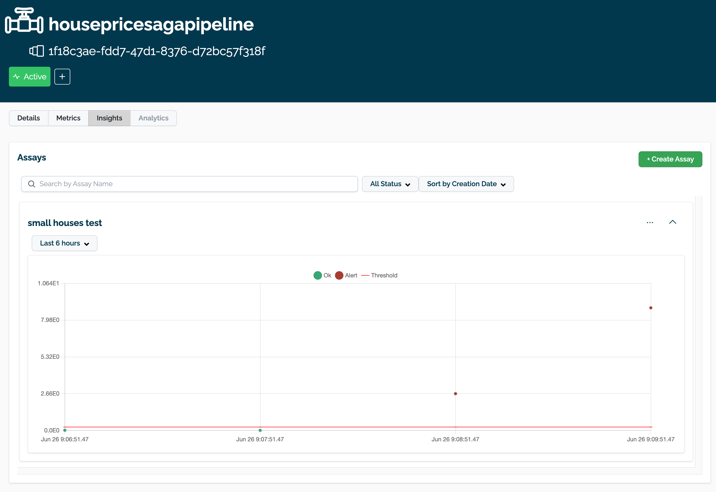
The assay is now visible through the Wallaroo UI by selecting the workspace, then the pipeline, then Insights. The following is an example of another assay in the Wallaroo Dashboard.
Get Assay Info
Assay information is retrieved with the wallaroo.client.get_assay_info() which takes the following parameters.
| Parameter | Type | Description |
|---|---|---|
| assay_id | Integer (Required) | The numerical id of the assay. |
This returns the following:
| Parameter | Type | Description |
|---|---|---|
| id | Integer | The numerical id of the assay. |
| name | String | The name of the assay. |
| active | Boolean | True: The assay is active and generates analyses based on its configuration. False: The assay is disabled and will not generate new analyses. |
| pipeline_name | String | The name of the pipeline the assay references. |
| last_run | DateTime | The date and time the assay last ran. |
| next_run | DateTime | THe date and time the assay analysis will next run. |
| alert_threshold | Float | The alert threshold setting for the assay. |
| baseline | Dict | The baseline and settings as set from the assay configuration. |
| iopath | String | The iopath setting for the assay. |
| metric | String | The metric setting for the assay. |
| num_bins | Integer | The number of bins for the assay. |
| bin_weights | List/None | The bin weights used if any. |
| bin_mode | String | The binning mode used. |
display(wl.get_assay_info(assay_id))
| id | name | active | status | pipeline_name | last_run | next_run | alert_threshold | workspace_id | workspace_name | baseline | iopath | metric | num_bins | bin_weights | bin_mode | |
|---|---|---|---|---|---|---|---|---|---|---|---|---|---|---|---|---|
| 0 | 9 | assays from date baseline | True | created | assay-demonstration-tutorial | None | 2024-07-30T16:44:50.283488+00:00 | 0.25 | 15 | run-anywhere-assay-demonstration-tutorial | Start:2024-07-30T16:40:17.908260+00:00, End:2024-07-30T16:41:23.899260+00:00 | output variable 0 | PSI | 5 | None | Quantile |
To wrap up the tutorial, we’ll disable the assay to save resources.
wl.set_assay_active(assay_id=assay_id, active=False)