Model Observability with Assays

How to use Wallaroo Assays to monitor the environment and know when to retrain the model based on changes to data.

This tutorial and the assets can be downloaded as part of the Wallaroo Tutorials repository.

Model Drift Observability with Assays

The Model Insights feature lets you monitor how the environment that your model operates within may be changing in ways that affect it’s predictions so that you can intervene (retrain) in an efficient and timely manner. Changes in the inputs, data drift, can occur due to errors in the data processing pipeline or due to changes in the environment such as user preference or behavior.

This notebook focuses on interactive exploration over historical data. After you are comfortable with how your data has behaved historically, you can schedule this same analysis (called an assay) to automatically run periodically, looking for indications of data drift or concept drift.

In this notebook, we will be running a drift assay on an ONNX model pre-trained to predict house prices.

Goal

Model insights monitors the output of the spam classifier model over a designated time window and compares it to an expected baseline distribution. We measure the difference between the window distribution and the baseline distribution; large differences indicate that the behavior of the model (or its inputs) has changed from what we expect. This possibly indicates a change that should be accounted for, possibly by retraining the models.

Resources

This tutorial provides the following:

Models:
- models/rf_model.onnx: The champion model that has been used in this environment for some time.
- Various inputs:
  - smallinputs.df.json: A set of house inputs that tends to generate low house price values.
  - biginputs.df.json: A set of house inputs that tends to generate high house price values.

Prerequisites

A deployed Wallaroo instance
The following Python libraries installed:
- wallaroo: The Wallaroo SDK. Included with the Wallaroo JupyterHub service by default.
- pandas: Pandas, mainly used for Pandas DataFrame

Steps

Deploying a sample ML model used to determine house prices based on a set of input parameters.
Build an assay baseline from a set of baseline start and end dates, and an assay baseline from a numpy array.
Preview the assay and show different assay configurations.
Upload the assay.
View assay results.
Pause and resume the assay.

Import Libraries

The first step will be to import our libraries, and set variables used through this tutorial.

import wallaroo
from wallaroo.object import EntityNotFoundError
from wallaroo.framework import Framework

from IPython.display import display

# used to display DataFrame information without truncating
from IPython.display import display
import pandas as pd
pd.set_option('display.max_colwidth', None)

import datetime
import time

workspace_name = f'assay-demonstration-tutorial'
main_pipeline_name = f'assay-demonstration-tutorial'
model_name_control = f'house-price-estimator'
model_file_name_control = './models/rf_model.onnx'

# Set the name of the assay
assay_name=f"house price assay demo"

# ignoring warnings for demonstration
import warnings
warnings.filterwarnings('ignore')

# used to display DataFrame information without truncating
from IPython.display import display
import pandas as pd
pd.set_option('display.max_colwidth', None)

Connect to the Wallaroo Instance

The first step is to connect to Wallaroo through the Wallaroo client. The Python library is included in the Wallaroo install and available through the Jupyter Hub interface provided with your Wallaroo environment.

This is accomplished using the wallaroo.Client() command, which provides a URL to grant the SDK permission to your specific Wallaroo environment. When displayed, enter the URL into a browser and confirm permissions. Store the connection into a variable that can be referenced later.

If logging into the Wallaroo instance through the internal JupyterHub service, use wl = wallaroo.Client(). For more information on Wallaroo Client settings, see the Client Connection guide.

# Login through local Wallaroo instance

wl = wallaroo.Client()

Create Workspace

We will create a workspace to manage our pipeline and models. The following variables will set the name of our sample workspace then set it as the current workspace.

Workspace, pipeline, and model names should be unique to each user, so we’ll add in a randomly generated suffix so multiple people can run this tutorial in a Wallaroo instance without effecting each other.

workspace = wl.get_workspace(name=workspace_name, create_if_not_exist=True)

wl.set_current_workspace(workspace)

{'name': 'assay-demonstration-tutorial', 'id': 9, 'archived': False, 'created_by': '07256c6a-1f1e-4cc8-bff8-94c9fb7cb843', 'created_at': '2024-04-19T16:58:22.5266+00:00', 'models': [], 'pipelines': []}

Upload The Champion Model

For our example, we will upload the champion model that has been trained to derive house prices from a variety of inputs. The model file is rf_model.onnx, and is uploaded with the name house-price-estimator.

housing_model_control = (wl.upload_model(model_name_control, 
                                        model_file_name_control, 
                                        framework=Framework.ONNX)
                                        .configure(tensor_fields=["tensor"])
                        )

Build the Pipeline

This pipeline is made to be an example of an existing situation where a model is deployed and being used for inferences in a production environment. We’ll call it assay-demonstration-tutorial, set housing_model_control as a pipeline step, then run a few sample inferences.

This pipeline will be a simple one - just a single pipeline step.

mainpipeline = wl.build_pipeline(main_pipeline_name)
# clear the steps if used before
mainpipeline.clear()

mainpipeline.add_model_step(housing_model_control)

#minimum deployment config
deploy_config = wallaroo.DeploymentConfigBuilder().replica_count(1).cpus(0.5).memory("1Gi").build()

mainpipeline.deploy(deployment_config = deploy_config)

name	assay-demonstration-tutorial
created	2024-04-19 16:58:24.382145+00:00
last_updated	2024-04-19 16:58:24.760713+00:00
deployed	True
arch	x86
accel	none
tags
versions	b467cbc2-1988-4c04-8ed5-01803f35c1f7, 3155d4db-1650-4bd9-8011-049a7d3a0d96
steps	house-price-estimator
published	False

Testing

We’ll use two inferences as a quick sample test - one that has a house that should be determined around $700k, the other with a house determined to be around $1.5 million.

normal_input = pd.DataFrame.from_records({"tensor": [[4.0, 2.5, 2900.0, 5505.0, 2.0, 0.0, 0.0, 3.0, 8.0, 2900.0, 0.0, 47.6063, -122.02, 2970.0, 5251.0, 12.0, 0.0, 0.0]]})
result = mainpipeline.infer(normal_input)
display(result)

	time	in.tensor	out.variable	anomaly.count
0	2024-04-19 16:58:41.818	[4.0, 2.5, 2900.0, 5505.0, 2.0, 0.0, 0.0, 3.0, 8.0, 2900.0, 0.0, 47.6063, -122.02, 2970.0, 5251.0, 12.0, 0.0, 0.0]	[718013.7]	0

large_house_input = pd.DataFrame.from_records({'tensor': [[4.0, 3.0, 3710.0, 20000.0, 2.0, 0.0, 2.0, 5.0, 10.0, 2760.0, 950.0, 47.6696, -122.261, 3970.0, 20000.0, 79.0, 0.0, 0.0]]})
large_house_result = mainpipeline.infer(large_house_input)
display(large_house_result)

	time	in.tensor	out.variable	anomaly.count
0	2024-04-19 16:58:41.988	[4.0, 3.0, 3710.0, 20000.0, 2.0, 0.0, 2.0, 5.0, 10.0, 2760.0, 950.0, 47.6696, -122.261, 3970.0, 20000.0, 79.0, 0.0, 0.0]	[1514079.4]	0

Generate Sample Data

Before creating the assays, we must generate data for the assays to build from.

For this example, we will:

Perform sample inferences based on lower priced houses and use that as our baseline.
Generate inferences from specific set of high priced houses create inference outputs that will be outside the baseline. This is used in later steps to demonstrate baseline comparison against assay analyses.

Inference Results History Generation

To start the demonstration, we’ll create a set of inferences based on houses with small estimated prices.

We will save the beginning and end periods of inferences to the variables assay_baseline_start and assay_baseline_end. These will be used later to create assay baselines from a range of dates.

small_houses_inputs = pd.read_json('./data/smallinputs.df.json')
baseline_size = 500

# Where the baseline data will start
assay_baseline_start = datetime.datetime.now()

# These inputs will be random samples of small priced houses.  Around 30,000 is a good number
small_houses = small_houses_inputs.sample(baseline_size, replace=True).reset_index(drop=True)

# Wait 60 seconds to set this data apart from the rest
time.sleep(60)
small_results = mainpipeline.infer(small_houses)

# Set the baseline end

assay_baseline_end = datetime.datetime.now()

Generate Numpy Baseline Values

From our inference outputs, we will create an array of numpy values. These are used for assays baselines created from numpy values.

# get the numpy values

# set the results to a non-array value
small_results_baseline_df = small_results.copy()
small_results_baseline_df['variable']=small_results['out.variable'].map(lambda x: x[0])
small_results_baseline_df

# set the numpy array
small_results_baseline = small_results_baseline_df['variable'].to_numpy()

Assay Test Data

The following will generate inference data for us to test against the assay baseline. For this, we will add in house data that generate higher house prices than the baseline data we used earlier.

This process should take 6 minutes to generate the historical data we’ll later use in our assays. We store the DateTime assay_window_start to determine where to start out assay analyses.

# Get a spread of house values

# # Set the start for our assay window period.
assay_window_start = datetime.datetime.now()

time.sleep(65)
inference_size = 1000

# And a spread of large house values

small_houses_inputs = pd.read_json('./data/smallinputs.df.json', orient="records")
small_houses = small_houses_inputs.sample(inference_size, replace=True).reset_index(drop=True)

mainpipeline.infer(small_houses)

time.sleep(65)

# Get a spread of large house values

time.sleep(65)
inference_size = 1000

# And a spread of large house values

big_houses_inputs = pd.read_json('./data/biginputs.df.json', orient="records")
big_houses = big_houses_inputs.sample(inference_size, replace=True).reset_index(drop=True)

mainpipeline.infer(big_houses)

time.sleep(65)

Model Insights via the Wallaroo Dashboard SDK

Assays generated through the Wallaroo SDK can be previewed, configured, and uploaded to the Wallaroo Ops instance. The following is a condensed version of this process. For full details see the Wallaroo SDK Essentials Guide: Assays Management guide.

Model drift detection with assays using the Wallaroo SDK follows this general process.

Define the Baseline: From either historical inference data for a specific model in a pipeline, or from a pre-determine array of data, a baseline is formed.
Assay Preview: Once the baseline is formed, we preview the assay and configure the different options until we have the the best method of detecting environment or model drift.
Create Assay: With the previews and configuration complete, we upload the assay. The assay will perform an analysis on a regular scheduled based on the configuration.
Get Assay Results: Retrieve the analyses and use them to detect model drift and possible sources.
Pause/Resume Assay: Pause or restart an assay as needed.

Define the Baseline

Assay baselines are defined with the wallaroo.client.build_assay method. Through this process we define the baseline from either a range of dates or pre-generated values.

wallaroo.client.build_assay take the following parameters:

Parameter	Type	Description
assay_name	String (Required) - required	The name of the assay. Assay names must be unique across the Wallaroo instance.
pipeline	wallaroo.pipeline.Pipeline (Required)	The pipeline the assay is monitoring.
model_name	String (Optional) / `None`	The name of the model to monitor. This field should only be used to track the inputs/outputs for a specific model step in a pipeline. If no `model_name` is to be included, then the parameters must be passed as named parameters not positional ones.
iopath	String (Required)	The input/output data for the model being tracked in the format `input/output field index`. Only one value is tracked for any assay. For example, to track the output of the model’s field `house_value` at index `0`, the `iopath` is `'output house_value 0`.
baseline_start	datetime.datetime (Optional)	The start time for the inferences to use as the baseline. Must be included with `baseline_end`. Cannot be included with `baseline_data`.
baseline_end	datetime.datetime (Optional)	The end time of the baseline window. the baseline. Windows start immediately after the baseline window and are run at regular intervals continuously until the assay is deactivated or deleted. Must be included with `baseline_start`. Cannot be included with `baseline_data`..
baseline_data	numpy.array (Optional)	The baseline data in numpy array format. Cannot be included with either `baseline_start` or `baseline_data`.

Note that model_name is an optional parameters when parameters are named. For example:

assay_builder_from_dates = wl.build_assay(assay_name="assays from date baseline", 
                                          pipeline=mainpipeline, 
                                          iopath="output variable 0",
                                          baseline_start=assay_baseline_start, 
                                          baseline_end=assay_baseline_end)

or:

assay_builder_from_dates = wl.build_assay("assays from date baseline", 
                                          mainpipeline, 
                                          None, ## since we are using positional parameters, `None` must be included for the model parameter
                                          "output variable 0",
                                          assay_baseline_start, 
                                          assay_baseline_end)

Baselines are created in one of two mutually exclusive methods:

Date Range: The baseline_start and baseline_end retrieves the inference requests and results for the pipeline from the start and end period. This data is summarized and used to create the baseline. For our examples, we’re using the variables assay_baseline_start and assay_baseline_end to represent a range of dates, with assay_baseline_start being set before assay_baseline_end.
Numpy Values: The baseline_data sets the baseline from a provided numpy array. This allows assay baselines to be created without first performing inferences in Wallaroo.

Define the Baseline Example

This example shows two methods of defining the baseline for an assay:

"assays from date baseline": This assay uses historical inference requests to define the baseline. This assay is saved to the variable assay_builder_from_dates.
"assays from numpy": This assay uses a pre-generated numpy array to define the baseline. This assay is saved to the variable assay_builder_from_numpy.

In both cases, the following parameters are used:

Parameter	Value
assay_name	`"assays from date baseline"` and `"assays from numpy"`
pipeline	`mainpipeline`: A pipeline with a ML model that predicts house prices. The output field for this model is `variable`.
iopath	These assays monitor the model’s output field variable at index 0 for the pipeline. From this, the `iopath` setting is `"output variable 0"`.

The difference between the two assays’ parameters determines how the baseline is generated.

"assays from date baseline": Uses the baseline_start and baseline_end to set the time period of inference requests and results to gather data from.
"assays from numpy": Uses a pre-generated numpy array as for the baseline data.

First we generate an assay baseline from a range of historical inferences performed through the specified pipeline deployment.

# Build the assay, based on the start and end of our baseline time, 
# and tracking the output variable index 0

display(assay_baseline_start)
display(assay_baseline_end)

assay_baseline_from_dates = wl.build_assay(assay_name="assays from date baseline", 
                                          pipeline=mainpipeline, 
                                          iopath="output variable 0",
                                          baseline_start=assay_baseline_start, 
                                          baseline_end=assay_baseline_end)

# create the baseline from the dates
assay_baseline_run_from_dates = assay_baseline_from_dates.build().interactive_baseline_run()

datetime.datetime(2024, 4, 19, 10, 58, 41, 956938)
datetime.datetime(2024, 4, 19, 10, 59, 42, 494449)

In this code sample, we generate the assay baseline from a preset numpy array called small_results_baseline.

# build the baseline from the numpy array
display(small_results_baseline[0:5])

# assay builder by baseline
assay_baseline_from_numpy = wl.build_assay(assay_name="assays from numpy", 
                               pipeline=mainpipeline, 
                               iopath="output variable 0", 
                               baseline_data = small_results_baseline)

# create the baseline from the numpy array
assay_baseline_run_from_numpy = assay_baseline_from_numpy.build().interactive_baseline_run()

array([657905.75, 575724.7 , 795841.06, 246901.14, 683845.75])

Baseline Chart

The baseline chart is displayed with wallaroo.assay.AssayAnalysis.chart(), which returns a chart with:

baseline mean: The mean value of the baseline values.
baseline median: The median value of the baseline values.
bin_mode: The binning mode. See Binning Mode
aggregation: The aggregation type. See Aggregation Options
metric: The assay’s metric type. See Score Metric
weighted: Whether the binning mode is weighted. See Binning Mode

The first chart is from an assay baseline generated from a set of inferences across a range of dates.

assay_baseline_run_from_dates.chart()

baseline mean = 535881.168880988
baseline median = 450867.6875
bin_mode = Quantile
aggregation = Density
metric = PSI
weighted = False

This chart is from an assay baseline generated from a set of numpy values.

assay_baseline_run_from_numpy.chart()

baseline mean = 533924.7744999997
baseline median = 450867.7
bin_mode = Quantile
aggregation = Density
metric = PSI
weighted = False

Baseline DataFrame

The method wallaroo.assay_config.AssayBuilder.baseline_dataframe returns a DataFrame of the assay baseline generated from the provided parameters. This includes:

metadata: The inference metadata with the model information, inference time, and other related factors.
in data: Each input field assigned with the label in.{input field name}.
out data: Each output field assigned with the label out.{output field name}

Note that for assays generated from numpy values, there is only the out data based on the supplied baseline data.

In the following example, the baseline DataFrame is retrieved.

This baseline DataFrame is from an assay baseline generated from a set of inferences across a range of dates.

display(assay_baseline_from_dates.baseline_dataframe())

	time	metadata	input_tensor_0	input_tensor_1	input_tensor_2	input_tensor_3	input_tensor_4	input_tensor_5	input_tensor_6	input_tensor_7	...	input_tensor_9	input_tensor_10	input_tensor_11	input_tensor_12	input_tensor_13	input_tensor_14	input_tensor_15	input_tensor_16	input_tensor_17	output_variable_0
0	1713545921988	{'last_model': '{"model_name":"house-price-estimator","model_sha":"e22a0831aafd9917f3cc87a15ed267797f80e2afa12ad7d8810ca58f173b8cc6"}', 'pipeline_version': 'b467cbc2-1988-4c04-8ed5-01803f35c1f7', 'elapsed': [52490, 322610], 'dropped': [], 'partition': 'engine-67fccddd5f-xc79d'}	4.0	3.00	3710.0	20000.0	2.0	0.0	2.0	5.0	...	2760.0	950.0	47.669600	-122.261000	3970.0	20000.0	79.0	0.0	0.0	1.514079e+06
1	1713545982464	{'last_model': '{"model_name":"house-price-estimator","model_sha":"e22a0831aafd9917f3cc87a15ed267797f80e2afa12ad7d8810ca58f173b8cc6"}', 'pipeline_version': 'b467cbc2-1988-4c04-8ed5-01803f35c1f7', 'elapsed': [1547850, 1622690], 'dropped': [], 'partition': 'engine-67fccddd5f-xc79d'}	3.0	2.25	2120.0	9297.0	2.0	0.0	0.0	4.0	...	2120.0	0.0	47.556099	-122.153999	2620.0	10352.0	33.0	0.0	0.0	6.579058e+05
2	1713545982464	{'last_model': '{"model_name":"house-price-estimator","model_sha":"e22a0831aafd9917f3cc87a15ed267797f80e2afa12ad7d8810ca58f173b8cc6"}', 'pipeline_version': 'b467cbc2-1988-4c04-8ed5-01803f35c1f7', 'elapsed': [1547850, 1622690], 'dropped': [], 'partition': 'engine-67fccddd5f-xc79d'}	4.0	2.25	1990.0	7712.0	1.0	0.0	0.0	3.0	...	1210.0	780.0	47.568802	-122.086998	1720.0	7393.0	41.0	0.0	0.0	5.757247e+05
3	1713545982464	{'last_model': '{"model_name":"house-price-estimator","model_sha":"e22a0831aafd9917f3cc87a15ed267797f80e2afa12ad7d8810ca58f173b8cc6"}', 'pipeline_version': 'b467cbc2-1988-4c04-8ed5-01803f35c1f7', 'elapsed': [1547850, 1622690], 'dropped': [], 'partition': 'engine-67fccddd5f-xc79d'}	4.0	2.75	3010.0	7215.0	2.0	0.0	0.0	3.0	...	3010.0	0.0	47.695202	-122.178001	3010.0	7215.0	0.0	0.0	0.0	7.958411e+05
4	1713545982464	{'last_model': '{"model_name":"house-price-estimator","model_sha":"e22a0831aafd9917f3cc87a15ed267797f80e2afa12ad7d8810ca58f173b8cc6"}', 'pipeline_version': 'b467cbc2-1988-4c04-8ed5-01803f35c1f7', 'elapsed': [1547850, 1622690], 'dropped': [], 'partition': 'engine-67fccddd5f-xc79d'}	2.0	1.00	930.0	6098.0	1.0	0.0	0.0	4.0	...	930.0	0.0	47.528900	-122.029999	1730.0	9000.0	95.0	0.0	0.0	2.469011e+05
...	...	...	...	...	...	...	...	...	...	...	...	...	...	...	...	...	...	...	...	...	...
496	1713545982464	{'last_model': '{"model_name":"house-price-estimator","model_sha":"e22a0831aafd9917f3cc87a15ed267797f80e2afa12ad7d8810ca58f173b8cc6"}', 'pipeline_version': 'b467cbc2-1988-4c04-8ed5-01803f35c1f7', 'elapsed': [1547850, 1622690], 'dropped': [], 'partition': 'engine-67fccddd5f-xc79d'}	3.0	1.75	1250.0	3880.0	1.0	0.0	0.0	4.0	...	750.0	500.0	47.686901	-122.391998	1240.0	3880.0	70.0	0.0	0.0	4.486278e+05
497	1713545982464	{'last_model': '{"model_name":"house-price-estimator","model_sha":"e22a0831aafd9917f3cc87a15ed267797f80e2afa12ad7d8810ca58f173b8cc6"}', 'pipeline_version': 'b467cbc2-1988-4c04-8ed5-01803f35c1f7', 'elapsed': [1547850, 1622690], 'dropped': [], 'partition': 'engine-67fccddd5f-xc79d'}	4.0	3.25	3940.0	27591.0	2.0	0.0	3.0	3.0	...	3440.0	500.0	47.515701	-122.115997	3420.0	29170.0	14.0	0.0	0.0	7.367513e+05
498	1713545982464	{'last_model': '{"model_name":"house-price-estimator","model_sha":"e22a0831aafd9917f3cc87a15ed267797f80e2afa12ad7d8810ca58f173b8cc6"}', 'pipeline_version': 'b467cbc2-1988-4c04-8ed5-01803f35c1f7', 'elapsed': [1547850, 1622690], 'dropped': [], 'partition': 'engine-67fccddd5f-xc79d'}	3.0	1.75	1960.0	8136.0	1.0	0.0	0.0	3.0	...	980.0	980.0	47.520802	-122.363998	1070.0	7480.0	66.0	0.0	0.0	3.654362e+05
499	1713545982464	{'last_model': '{"model_name":"house-price-estimator","model_sha":"e22a0831aafd9917f3cc87a15ed267797f80e2afa12ad7d8810ca58f173b8cc6"}', 'pipeline_version': 'b467cbc2-1988-4c04-8ed5-01803f35c1f7', 'elapsed': [1547850, 1622690], 'dropped': [], 'partition': 'engine-67fccddd5f-xc79d'}	2.0	1.00	560.0	7560.0	1.0	0.0	0.0	3.0	...	560.0	0.0	47.527100	-122.375000	990.0	7560.0	70.0	0.0	0.0	2.536796e+05
500	1713545982464	{'last_model': '{"model_name":"house-price-estimator","model_sha":"e22a0831aafd9917f3cc87a15ed267797f80e2afa12ad7d8810ca58f173b8cc6"}', 'pipeline_version': 'b467cbc2-1988-4c04-8ed5-01803f35c1f7', 'elapsed': [1547850, 1622690], 'dropped': [], 'partition': 'engine-67fccddd5f-xc79d'}	5.0	2.75	3430.0	15119.0	2.0	0.0	0.0	3.0	...	3430.0	0.0	47.567799	-122.031998	3430.0	12045.0	17.0	0.0	0.0	9.190315e+05

501 rows × 21 columns

This baseline DataFrame is from an assay baseline generated from an array of numpy values.

display(assay_baseline_from_numpy.baseline_dataframe())

	output_variable_0
0	657905.75
1	575724.70
2	795841.06
3	246901.14
4	683845.75
...	...
495	448627.80
496	736751.30
497	365436.22
498	253679.63
499	919031.50

500 rows × 1 columns

Baseline Stats

The method wallaroo.assay.AssayAnalysis.baseline_stats() returns a pandas.core.frame.DataFrame of the baseline stats.

The baseline stats for each assay are displayed in the examples below.

This baseline states DataFrame is from an assay baseline generated from a set of inferences across a range of dates.

assay_baseline_run_from_dates.baseline_stats()

	Baseline
count	501
min	236238.671875
max	1514079.375
mean	535881.168881
median	450867.6875
std	235998.825739
start	2024-04-19T16:58:41.956938+00:00
end	2024-04-19T16:59:42.493938+00:00

This baseline states DataFrame is from an assay baseline generated from an array of numpy values.

assay_baseline_run_from_numpy.baseline_stats()

	Baseline
count	500
min	236238.67
max	1489624.3
mean	533924.7745
median	450867.7
std	232140.618444
start	None
end	None

Baseline Bins

The method wallaroo.assay.AssayAnalysis.baseline_bins a simple dataframe to with the edge/bin data for a baseline.

These baseline bins DataFrame is from an assay baseline generated from a set of inferences across a range of dates.

assay_baseline_run_from_dates.baseline_bins()

	b_edges	b_edge_names	b_aggregated_values	b_aggregation
0	2.362387e+05	left_outlier	0.000000	Aggregation.DENSITY
1	3.338782e+05	q_20	0.201597	Aggregation.DENSITY
2	4.371780e+05	q_40	0.207585	Aggregation.DENSITY
3	5.512234e+05	q_60	0.191617	Aggregation.DENSITY
4	7.139790e+05	q_80	0.199601	Aggregation.DENSITY
5	1.514079e+06	q_100	0.199601	Aggregation.DENSITY
6	inf	right_outlier	0.000000	Aggregation.DENSITY

These baseline bins DataFrame is from an assay baseline generated from an array of numpy values.

assay_baseline_run_from_numpy.baseline_bins()

	b_edges	b_edge_names	b_aggregated_values	b_aggregation
0	236238.67	left_outlier	0.000	Aggregation.DENSITY
1	333878.22	q_20	0.202	Aggregation.DENSITY
2	437177.97	q_40	0.208	Aggregation.DENSITY
3	550275.10	q_60	0.190	Aggregation.DENSITY
4	713979.00	q_80	0.202	Aggregation.DENSITY
5	1489624.30	q_100	0.198	Aggregation.DENSITY
6	inf	right_outlier	0.000	Aggregation.DENSITY

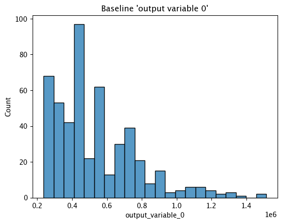
Baseline Histogram Chart

The method wallaroo.assay_config.AssayBuilder.baseline_histogram returns a histogram chart of the assay baseline generated from the provided parameters.

These chart is from an assay baseline generated from a set of inferences across a range of dates.

assay_baseline_from_dates.baseline_histogram()

Baseline KDE Chart

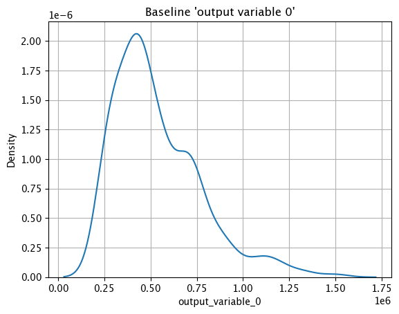
The method wallaroo.assay_config.AssayBuilder.baseline_kde returns a Kernel Density Estimation (KDE) chart of the assay baseline generated from the provided parameters.

These chart is from an assay baseline generated from a set of inferences across a range of dates.

assay_baseline_from_dates.baseline_kde()

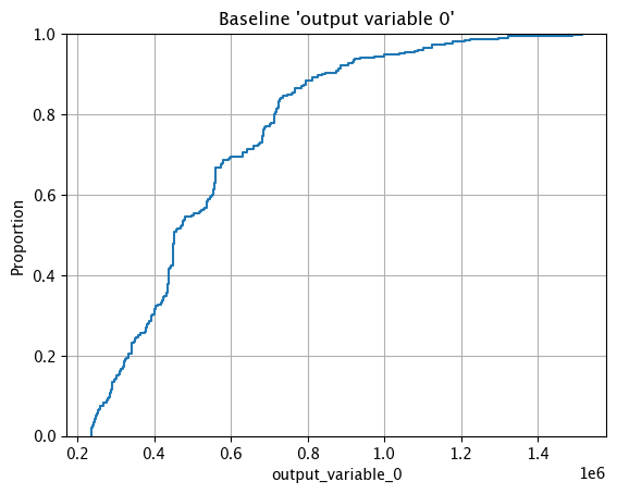
Baseline ECDF Chart

The method wallaroo.assay_config.AssayBuilder.baseline_ecdf returns a Empirical Cumulative Distribution Function (CDF) chart of the assay baseline generated from the provided parameters.

These chart is from an assay baseline generated from a set of inferences across a range of dates.

assay_baseline_from_dates.baseline_ecdf()

Assay Preview

Now that the baseline is defined, we look at different configuration options and view how the assay baseline and results changes. Once we determine what gives us the best method of determining model drift, we can create the assay.

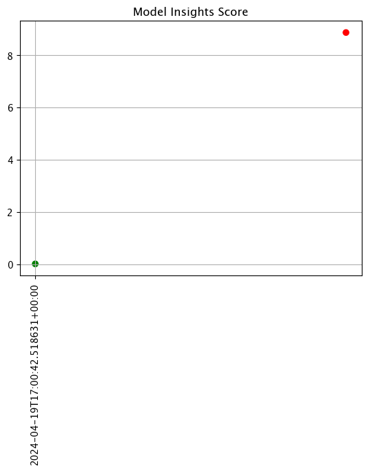
Analysis List Chart Scores

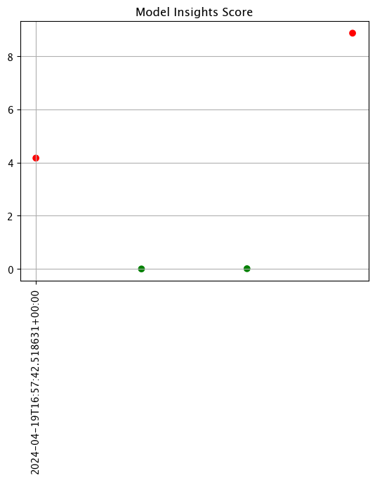
Analysis List scores show the assay scores for each assay result interval in one chart. Values that are outside of the alert threshold are colored red, while scores within the alert threshold are green.

Assay chart scores are displayed with the method wallaroo.assay.AssayAnalysisList.chart_scores(title: Optional[str] = None), with ability to display an optional title with the chart.

The following example shows retrieving the assay results and displaying the chart scores. From our example, we have two windows - the first should be green, and the second is red showing that values were outside the alert threshold.

# Create the assay baseline
assay_baseline = wl.build_assay(assay_name="assays from date baseline", 
                                          pipeline=mainpipeline, 
                                          iopath="output variable 0",
                                          baseline_start=assay_baseline_start, 
                                          baseline_end=assay_baseline_end)

# Set the assay parameters

# The end date to gather inference results
assay_baseline.add_run_until(datetime.datetime.now())

# Set the interval and window to one minute each, set the start date for gathering inference results
assay_baseline.window_builder().add_width(minutes=1).add_interval(minutes=1).add_start(assay_window_start)

# build the assay configuration
assay_config = assay_baseline.build()

# perform an interactive run and collect inference data
assay_results = assay_config.interactive_run()

# Preview the assay analyses
assay_results.chart_scores()

Analysis Chart

The method wallaroo.assay.AssayAnalysis.chart() displays a comparison between the baseline and an interval of inference data.

This is compared to the Chart Scores, which is a list of all of the inference data split into intervals, while the Analysis Chart shows the breakdown of one set of inference data against the baseline.

Score from the Analysis List Chart Scores and each element from the Analysis List DataFrame generates

The following fields are included.

Field	Type	Description
baseline mean	Float	The mean of the baseline values.
window mean	Float	The mean of the window values.
baseline median	Float	The median of the baseline values.
window median	Float	The median of the window values.
bin_mode	String	The binning mode used for the assay.
aggregation	String	The aggregation mode used for the assay.
metric	String	The metric mode used for the assay.
weighted	Bool	Whether the bins were manually weighted.
score	Float	The score from the assay window.
scores	List(Float)	The score from each assay window bin.
index	Integer/None	The window index. Interactive assay runs are `None`.

# Create the assay baseline
assay_baseline = wl.build_assay(assay_name="assays from date baseline", 
                                          pipeline=mainpipeline, 
                                          iopath="output variable 0",
                                          baseline_start=assay_baseline_start, 
                                          baseline_end=assay_baseline_end)

# Set the assay parameters

# The end date to gather inference results
assay_baseline.add_run_until(datetime.datetime.now())

# Set the interval and window to one minute each, set the start date for gathering inference results
assay_baseline.window_builder().add_width(minutes=1).add_interval(minutes=1).add_start(assay_window_start)

# build the assay configuration
assay_config = assay_baseline.build()

# perform an interactive run and collect inference data
assay_results = assay_config.interactive_run()

# display one of the analysis from the total results
assay_results[0].chart()

baseline mean = 535881.168880988
window mean = 525169.808015625
baseline median = 450867.6875
window median = 448627.8125
bin_mode = Quantile
aggregation = Density
metric = PSI
weighted = False
score = 0.00972686088185764
scores = [0.0, 0.0004286769159531457, 0.0003625824754554272, 0.005674527370820431, 0.001819573488386175, 0.0014415006312424594, 0.0]
index = None

Analysis List DataFrame

wallaroo.assay.AssayAnalysisList.to_dataframe() returns a DataFrame showing the assay results for each window aka individual analysis. This DataFrame contains the following fields:

Field	Type	Description
assay_id	Integer/None	The assay id. Only provided from uploaded and executed assays.
name	String/None	The name of the assay. Only provided from uploaded and executed assays.
iopath	String/None	The iopath of the assay. Only provided from uploaded and executed assays.
score	Float	The assay score.
start	DateTime	The DateTime start of the assay window.
min	Float	The minimum value in the assay window.
max	Float	The maximum value in the assay window.
mean	Float	The mean value in the assay window.
median	Float	The median value in the assay window.
std	Float	The standard deviation value in the assay window.
warning_threshold	Float/None	The warning threshold of the assay window.
alert_threshold	Float/None	The alert threshold of the assay window.
status	String	The assay window status. Values are: `OK`: The score is within accepted thresholds. `Warning`: The score has triggered the `warning_threshold` if exists, but not the `alert_threshold`. `Alert`: The score has triggered the the `alert_threshold`.

For this example, the assay analysis list DataFrame is listed.

From this tutorial, we should have 2 windows of dta to look at, each one minute apart. The first window should show status: OK, with the second window with the very large house prices will show status: alert

# Create the assay baseline
assay_baseline = wl.build_assay(assay_name="assays from date baseline", 
                                          pipeline=mainpipeline, 
                                          iopath="output variable 0",
                                          baseline_start=assay_baseline_start, 
                                          baseline_end=assay_baseline_end)

# Set the assay parameters

# The end date to gather inference results
assay_baseline.add_run_until(datetime.datetime.now())

# Set the interval and window to one minute each, set the start date for gathering inference results
assay_baseline.window_builder().add_width(minutes=1).add_interval(minutes=1).add_start(assay_window_start)

# build the assay configuration
assay_config = assay_baseline.build()

# perform an interactive run and collect inference data
assay_results = assay_config.interactive_run()

# display the dataframe from the analyses
assay_results.to_dataframe()

	id	assay_id	assay_name	iopath	pipeline_id	pipeline_name	score	start	min	max	mean	median	std	warning_threshold	alert_threshold	status
0	None	None	assays from date baseline		None		0.009727	2024-04-19T17:00:42.518631+00:00	2.362387e+05	1489624.250	5.251698e+05	4.486278e+05	240871.853496	None	0.25	Ok
1	None	None	assays from date baseline		None		8.868819	2024-04-19T17:02:42.518631+00:00	1.514079e+06	2016006.125	1.878966e+06	1.946438e+06	157729.298871	None	0.25	Alert

Analysis List Full DataFrame

wallaroo.assay.AssayAnalysisList.to_full_dataframe() returns a DataFrame showing all values, including the inputs and outputs from the assay results for each window aka individual analysis. This DataFrame contains the following fields:

pipeline_id	warning_threshold	bin_index	created_at

Field	Type	Description
window_start	DateTime	The date and time when the window period began.
analyzed_at	DateTime	The date and time when the assay analysis was performed.
elapsed_millis	Integer	How long the analysis took to perform in milliseconds.
baseline_summary_count	Integer	The number of data elements from the baseline.
baseline_summary_min	Float	The minimum value from the baseline summary.
baseline_summary_max	Float	The maximum value from the baseline summary.
baseline_summary_mean	Float	The mean value of the baseline summary.
baseline_summary_median	Float	The median value of the baseline summary.
baseline_summary_std	Float	The standard deviation value of the baseline summary.
baseline_summary_edges_{0…n}	Float	The baseline summary edges for each baseline edge from 0 to number of edges.
summarizer_type	String	The type of summarizer used for the baseline. See `wallaroo.assay_config` for other summarizer types.
summarizer_bin_weights	List / None	If baseline bin weights were provided, the list of those weights. Otherwise, `None`.
summarizer_provided_edges	List / None	If baseline bin edges were provided, the list of those edges. Otherwise, `None`.
status	String	The assay window status. Values are: `OK`: The score is within accepted thresholds. `Warning`: The score has triggered the `warning_threshold` if exists, but not the `alert_threshold`. `Alert`: The score has triggered the the `alert_threshold`.
id	Integer/None	The id for the window aka analysis. Only provided from uploaded and executed assays.
assay_id	Integer/None	The assay id. Only provided from uploaded and executed assays.
pipeline_id	Integer/None	The pipeline id. Only provided from uploaded and executed assays.
warning_threshold	Float	The warning threshold set for the assay.
warning_threshold	Float	The warning threshold set for the assay.
bin_index	Integer/None	The bin index for the window aka analysis.
created_at	Datetime/None	The date and time the window aka analysis was generated. Only provided from uploaded and executed assays.

For this example, full DataFrame from an assay preview is generated.

# Create the assay baseline
assay_baseline = wl.build_assay(assay_name="assays from date baseline", 
                                          pipeline=mainpipeline, 
                                          iopath="output variable 0",
                                          baseline_start=assay_baseline_start, 
                                          baseline_end=assay_baseline_end)

# Set the assay parameters

# The end date to gather inference results
assay_baseline.add_run_until(datetime.datetime.now())

# Set the interval and window to one minute each, set the start date for gathering inference results
assay_baseline.window_builder().add_width(minutes=1).add_interval(minutes=1).add_start(assay_window_start)

# build the assay configuration
assay_config = assay_baseline.build()

# perform an interactive run and collect inference data
assay_results = assay_config.interactive_run()

# display the full dataframe from the analyses
assay_results.to_full_dataframe()

	window_start	analyzed_at	elapsed_millis	baseline_summary_count	baseline_summary_min	baseline_summary_max	baseline_summary_mean	baseline_summary_median	baseline_summary_std	baseline_summary_edges_0	...	summarizer_type	summarizer_bin_weights	summarizer_provided_edges	status	id	assay_id	pipeline_id	warning_threshold	bin_index	created_at
0	2024-04-19T17:00:42.518631+00:00	2024-04-19T17:16:29.780623+00:00	86	501	236238.671875	1514079.375	535881.168881	450867.6875	235998.825739	236238.671875	...	UnivariateContinuous	None	None	Ok	None	None	None	None	None	None
1	2024-04-19T17:02:42.518631+00:00	2024-04-19T17:16:29.780753+00:00	87	501	236238.671875	1514079.375	535881.168881	450867.6875	235998.825739	236238.671875	...	UnivariateContinuous	None	None	Alert	None	None	None	None	None	None

2 rows × 86 columns

Analysis Compare Basic Stats

The method wallaroo.assay.AssayAnalysis.compare_basic_stats returns a DataFrame comparing one set of inference data against the baseline.

This is compared to the Analysis List DataFrame, which is a list of all of the inference data split into intervals, while the Analysis Compare Basic Stats shows the breakdown of one set of inference data against the baseline.

# Create the assay baseline
assay_baseline = wl.build_assay(assay_name="assays from date baseline", 
                                          pipeline=mainpipeline, 
                                          iopath="output variable 0",
                                          baseline_start=assay_baseline_start, 
                                          baseline_end=assay_baseline_end)

# Set the assay parameters

# The end date to gather inference results
assay_baseline.add_run_until(datetime.datetime.now())

# Set the interval and window to one minute each, set the start date for gathering inference results
assay_baseline.window_builder().add_width(minutes=1).add_interval(minutes=1).add_start(assay_window_start)

# build the assay configuration
assay_config = assay_baseline.build()

# perform an interactive run and collect inference data
assay_results = assay_config.interactive_run()

# display one analysis against the baseline
assay_results[0].compare_basic_stats()

	Baseline	Window	diff	pct_diff
count	501.0	1000.0	499.000000	99.600798
min	236238.671875	236238.671875	0.000000	0.000000
max	1514079.375	1489624.25	-24455.125000	-1.615181
mean	535881.168881	525169.808016	-10711.360865	-1.998831
median	450867.6875	448627.8125	-2239.875000	-0.496792
std	235998.825739	240871.853496	4873.027757	2.064853
start	2024-04-19T16:58:41.956938+00:00	2024-04-19T17:00:42.518631+00:00	NaN	NaN
end	2024-04-19T16:59:42.493938+00:00	2024-04-19T17:01:42.518631+00:00	NaN	NaN

Configure Assays

Before creating the assay, configure the assay and continue to preview it until the best method for detecting drift is set. The following options are available.

Inference Interval and Inference Width

The inference interval aka window interval sets how often to run the assay analysis. This is set from the wallaroo.assay_config.AssayBuilder.window_builder.add_interval method to collect data expressed in time units: “hours=24”, “minutes=1”, etc.

For example, with an interval of 1 minute, the assay collects data every minute. Within an hour, 60 intervals of data is collected.

We can adjust the interval and see how the assays change based on how frequently they are run.

The width sets the time period from the wallaroo.assay_config.AssayBuilder.window_builder.add_width method to collect data expressed in time units: “hours=24”, “minutes=1”, etc.

For example, an interval of 1 minute and a width of 1 minute collects 1 minutes worth of data every minute. An interval of 1 minute with a width of 5 minutes collects 5 minute of inference data every minute.

By default, the interval and width is 24 hours.

For this example, we’ll adjust the width and interval from 1 minute to 5 minutes and see how the number of analyses and their score changes.

# Create the assay baseline
assay_baseline = wl.build_assay(assay_name="assays from date baseline", 
                                          pipeline=mainpipeline, 
                                          iopath="output variable 0",
                                          baseline_start=assay_baseline_start, 
                                          baseline_end=assay_baseline_end)

# Set the assay parameters

# The end date to gather inference results
assay_baseline.add_run_until(datetime.datetime.now())

# Set the interval and window to one minute each, set the start date for gathering inference results
assay_baseline.window_builder().add_width(minutes=1).add_interval(minutes=1).add_start(assay_window_start)

# build the assay configuration
assay_config = assay_baseline.build()

# perform an interactive run and collect inference data
assay_results = assay_config.interactive_run()

# show the analyses chart
assay_results.chart_scores()

# Create the assay baseline
assay_baseline = wl.build_assay(assay_name="assays from date baseline", 
                                          pipeline=mainpipeline, 
                                          iopath="output variable 0",
                                          baseline_start=assay_baseline_start, 
                                          baseline_end=assay_baseline_end)

# Set the assay parameters

# The end date to gather inference results
assay_baseline.add_run_until(datetime.datetime.now())

# Set the interval and window to five minutes each, set the start date for gathering inference results
assay_baseline.window_builder().add_width(minutes=5).add_interval(minutes=5).add_start(assay_window_start)

# build the assay configuration
assay_config = assay_baseline.build()

# perform an interactive run and collect inference data
assay_results = assay_config.interactive_run()

# show the analyses chart
assay_results.chart_scores()

Add Run Until and Add Inference Start

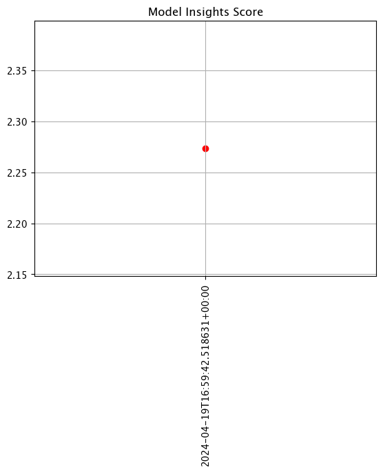
For previewing assays, setting wallaroo.assay_config.AssayBuilder.add_run_until sets the end date and time for collecting inference data. When an assay is uploaded, this setting is no longer valid - assays run at the Inference Interval until the assay is paused.

Setting the wallaroo.assay_config.WindowBuilder.add_start sets the start date and time to collect inference data. When an assay is uploaded, this setting is included, and assay results will be displayed starting from that start date at the Inference Interval until the assay is paused. By default, add_start begins 24 hours after the assay is uploaded unless set in the assay configuration manually.

For the following example, the add_run_until setting is set to datetime.datetime.now() to collect all inference data from assay_window_start up until now, and the second example limits that example to only two minutes of data.

# Create the assay baseline
assay_baseline = wl.build_assay(assay_name="assays from date baseline", 
                                          pipeline=mainpipeline, 
                                          iopath="output variable 0",
                                          baseline_start=assay_baseline_start, 
                                          baseline_end=assay_baseline_end)

# Set the assay parameters

# The end date to gather inference results
assay_baseline.add_run_until(datetime.datetime.now())

# Set the interval and window to one minute each, set the start date for gathering inference results, minus 2 minutes for the period to start gathering analyses
assay_baseline.window_builder().add_width(minutes=1).add_interval(minutes=1).add_start(assay_window_start+datetime.timedelta(seconds=-120))

# build the assay configuration
assay_config = assay_baseline.build()

# perform an interactive run and collect inference data
assay_results = assay_config.interactive_run()

# show the analyses chart
assay_results.chart_scores()

# Create the assay baseline
assay_baseline = wl.build_assay(assay_name="assays from date baseline", 
                                          pipeline=mainpipeline, 
                                          iopath="output variable 0",
                                          baseline_start=assay_baseline_start, 
                                          baseline_end=assay_baseline_end)

# Set the assay parameters

# The end date to gather inference results plus 2 minutes 
assay_baseline.add_run_until(assay_window_start+datetime.timedelta(seconds=120))

# Set the interval and window to one minute each
assay_baseline.window_builder().add_width(minutes=1).add_interval(minutes=1).add_start(assay_window_start)

# build the assay configuration
assay_config = assay_baseline.build()

# perform an interactive run and collect inference data
assay_results = assay_config.interactive_run()

# show the analyses chart
assay_results.chart_scores()

Score Metric

The score is a distance between the baseline and the analysis window. The larger the score, the greater the difference between the baseline and the analysis window. The following methods are provided determining the score:

PSI (Default) - Population Stability Index (PSI).
MAXDIFF: Maximum difference between corresponding bins.
SUMDIFF: Mum of differences between corresponding bins.

The metric type used is updated with the wallaroo.assay_config.AssayBuilder.add_metric(metric: wallaroo.assay_config.Metric) method.

The following three charts use each of the metrics. Note how the scores change based on the score type used.

# Create the assay baseline
assay_baseline = wl.build_assay(assay_name="assays from date baseline", 
                                          pipeline=mainpipeline, 
                                          iopath="output variable 0",
                                          baseline_start=assay_baseline_start, 
                                          baseline_end=assay_baseline_end)

# Set the assay parameters

# The end date to gather inference results
assay_baseline.add_run_until(datetime.datetime.now())

# Set the interval and window to one minute each, set the start date for gathering inference results
assay_baseline.window_builder().add_width(minutes=1).add_interval(minutes=1).add_start(assay_window_start)

# set metric PSI mode
assay_baseline.summarizer_builder.add_metric(wallaroo.assay_config.Metric.PSI)

# build the assay configuration
assay_config = assay_baseline.build()

# perform an interactive run and collect inference data
assay_results = assay_config.interactive_run()

# display one analysis from the results
assay_results[0].chart()

baseline mean = 535881.168880988
window mean = 525169.808015625
baseline median = 450867.6875
window median = 448627.8125
bin_mode = Quantile
aggregation = Density
metric = PSI
weighted = False
score = 0.00972686088185764
scores = [0.0, 0.0004286769159531457, 0.0003625824754554272, 0.005674527370820431, 0.001819573488386175, 0.0014415006312424594, 0.0]
index = None

# Create the assay baseline
assay_baseline = wl.build_assay(assay_name="assays from date baseline", 
                                          pipeline=mainpipeline, 
                                          iopath="output variable 0",
                                          baseline_start=assay_baseline_start, 
                                          baseline_end=assay_baseline_end)

# Set the assay parameters

# The end date to gather inference results
assay_baseline.add_run_until(datetime.datetime.now())

# Set the interval and window to one minute each, set the start date for gathering inference results
assay_baseline.window_builder().add_width(minutes=1).add_interval(minutes=1).add_start(assay_window_start)

# set metric MAXDIFF mode
assay_baseline.summarizer_builder.add_metric(wallaroo.assay_config.Metric.MAXDIFF)

# build the assay configuration
assay_config = assay_baseline.build()

# perform an interactive run and collect inference data
assay_results = assay_config.interactive_run()

# display one analysis from the results
assay_results[0].chart()

baseline mean = 535881.168880988
window mean = 525169.808015625
baseline median = 450867.6875
window median = 448627.8125
bin_mode = Quantile
aggregation = Density
metric = MaxDiff
weighted = False
score = 0.03438323353293413
scores = [0.0, 0.009403193612774446, 0.008584830339321337, 0.03438323353293413, 0.01860079840319362, 0.016600798403193617, 0.0]
index = 3

# Create the assay baseline
assay_baseline = wl.build_assay(assay_name="assays from date baseline", 
                                          pipeline=mainpipeline, 
                                          iopath="output variable 0",
                                          baseline_start=assay_baseline_start, 
                                          baseline_end=assay_baseline_end)

# Set the assay parameters

# The end date to gather inference results
assay_baseline.add_run_until(datetime.datetime.now())

# Set the interval and window to one minute each, set the start date for gathering inference results
assay_baseline.window_builder().add_width(minutes=1).add_interval(minutes=1).add_start(assay_window_start)

# set metric SUMDIFF mode
assay_baseline.summarizer_builder.add_metric(wallaroo.assay_config.Metric.SUMDIFF)

# build the assay configuration
assay_config = assay_baseline.build()

# perform an interactive run and collect inference data
assay_results = assay_config.interactive_run()

# display one analysis from the results
assay_results[0].chart()

baseline mean = 535881.168880988
window mean = 525169.808015625
baseline median = 450867.6875
window median = 448627.8125
bin_mode = Quantile
aggregation = Density
metric = SumDiff
weighted = False
score = 0.04378642714570857
scores = [0.0, 0.009403193612774446, 0.008584830339321337, 0.03438323353293413, 0.01860079840319362, 0.016600798403193617, 0.0]
index = None

Alert Threshold

Assay alert thresholds are modified with the wallaroo.assay_config.AssayBuilder.add_alert_threshold(alert_threshold: float) method. By default alert thresholds are 0.1.

The following example updates the alert threshold to 0.5.

# Create the assay baseline
assay_baseline = wl.build_assay(assay_name="assays from date baseline", 
                                          pipeline=mainpipeline, 
                                          iopath="output variable 0",
                                          baseline_start=assay_baseline_start, 
                                          baseline_end=assay_baseline_end)

# Set the assay parameters

# The end date to gather inference results
assay_baseline.add_run_until(datetime.datetime.now())

# Set the interval and window to one minute each, set the start date for gathering inference results
assay_baseline.window_builder().add_width(minutes=1).add_interval(minutes=1).add_start(assay_window_start)

# set the alert threshold
assay_baseline.add_alert_threshold(0.5)

# build the assay configuration
assay_config = assay_baseline.build()

# perform an interactive run and collect inference data
assay_results = assay_config.interactive_run()

# show the analyses with the alert threshold
assay_results.to_dataframe()

	id	assay_id	assay_name	iopath	pipeline_id	pipeline_name	score	start	min	max	mean	median	std	warning_threshold	alert_threshold	status
0	None	None	assays from date baseline		None		0.009727	2024-04-19T17:00:42.518631+00:00	2.362387e+05	1489624.250	5.251698e+05	4.486278e+05	240871.853496	None	0.5	Ok
1	None	None	assays from date baseline		None		8.868819	2024-04-19T17:02:42.518631+00:00	1.514079e+06	2016006.125	1.878966e+06	1.946438e+06	157729.298871	None	0.5	Alert

Number of Bins

Number of bins sets how the baseline data is partitioned. The total number of bins includes the set number plus the left_outlier and the right_outlier, so the total number of bins will be the total set + 2.

The number of bins is set with the wallaroo.assay_config.UnivariateContinousSummarizerBuilder.add_num_bins(num_bins: int) method.

# Create the assay baseline
assay_baseline = wl.build_assay(assay_name="assays from date baseline", 
                                          pipeline=mainpipeline, 
                                          iopath="output variable 0",
                                          baseline_start=assay_baseline_start, 
                                          baseline_end=assay_baseline_end)

# Set the assay parameters

# The end date to gather inference results
assay_baseline.add_run_until(datetime.datetime.now())

# Set the interval and window to one minute each, set the start date for gathering inference results
assay_baseline.window_builder().add_width(minutes=1).add_interval(minutes=1).add_start(assay_window_start)

# update number of bins here
assay_baseline.summarizer_builder.add_num_bins(10)

# build the assay configuration
assay_config = assay_baseline.build()

# perform an interactive run and collect inference data
assay_results = assay_config.interactive_run()

# show one analysis with the updated bins
assay_results[0].chart()

baseline mean = 535881.168880988
window mean = 525169.808015625
baseline median = 450867.6875
window median = 448627.8125
bin_mode = Quantile
aggregation = Density
metric = PSI
weighted = False
score = 0.03389853094445084
scores = [0.0, 0.002043667046021817, 0.0003632592989260558, 0.004157603807631639, 0.00942419055601088, 0.003861444836884139, 0.0019602905356873607, 0.0009704098768619968, 0.0008494987137215735, 0.009076998929542533, 0.0011911673431628438, 0.0]
index = None

Binning Mode

Binning Mode defines how the bins are separated. Binning modes are modified through the wallaroo.assay_config.UnivariateContinousSummarizerBuilder.add_bin_mode(bin_mode: bin_mode: wallaroo.assay_config.BinMode, edges: Optional[List[float]] = None).

Available bin_mode values from wallaroo.assay_config.Binmode are the following:

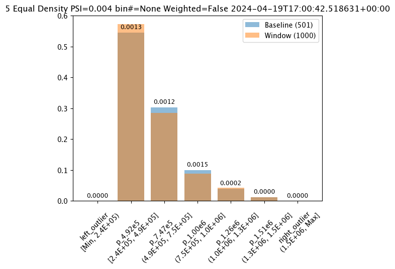
QUANTILE (Default): Based on percentages. If num_bins is 5 then quintiles so bins are created at the 20%, 40%, 60%, 80% and 100% points.
EQUAL: Evenly spaced bins where each bin is set with the formula min - max / num_bins
PROVIDED: The user provides the edge points for the bins.

If PROVIDED is supplied, then a List of float values must be provided for the edges parameter that matches the number of bins.

The following examples are used to show how each of the binning modes effects the bins.

# Create the assay baseline
assay_baseline = wl.build_assay(assay_name="assays from date baseline", 
                                          pipeline=mainpipeline, 
                                          iopath="output variable 0",
                                          baseline_start=assay_baseline_start, 
                                          baseline_end=assay_baseline_end)

# Set the assay parameters

# The end date to gather inference results
assay_baseline.add_run_until(datetime.datetime.now())

# Set the interval and window to one minute each, set the start date for gathering inference results
assay_baseline.window_builder().add_width(minutes=1).add_interval(minutes=1).add_start(assay_window_start)

# update binning mode here
assay_baseline.summarizer_builder.add_bin_mode(wallaroo.assay_config.BinMode.QUANTILE)

# build the assay configuration
assay_config = assay_baseline.build()

# perform an interactive run and collect inference data
assay_results = assay_config.interactive_run()

# show one analysis with the updated bins
assay_results[0].chart()

baseline mean = 535881.168880988
window mean = 525169.808015625
baseline median = 450867.6875
window median = 448627.8125
bin_mode = Quantile
aggregation = Density
metric = PSI
weighted = False
score = 0.00972686088185764
scores = [0.0, 0.0004286769159531457, 0.0003625824754554272, 0.005674527370820431, 0.001819573488386175, 0.0014415006312424594, 0.0]
index = None

# Create the assay baseline
assay_baseline = wl.build_assay(assay_name="assays from date baseline", 
                                          pipeline=mainpipeline, 
                                          iopath="output variable 0",
                                          baseline_start=assay_baseline_start, 
                                          baseline_end=assay_baseline_end)

# Set the assay parameters

# The end date to gather inference results
assay_baseline.add_run_until(datetime.datetime.now())

# Set the interval and window to one minute each, set the start date for gathering inference results
assay_baseline.window_builder().add_width(minutes=1).add_interval(minutes=1).add_start(assay_window_start)

# update binning mode here
assay_baseline.summarizer_builder.add_bin_mode(wallaroo.assay_config.BinMode.EQUAL)

# build the assay configuration
assay_config = assay_baseline.build()

# perform an interactive run and collect inference data
assay_results = assay_config.interactive_run()

# show one analysis with the updated bins
assay_results[0].chart()

baseline mean = 535881.168880988
window mean = 525169.808015625
baseline median = 450867.6875
window median = 448627.8125
bin_mode = Equal
aggregation = Density
metric = PSI
weighted = False
score = 0.0041785105741782205
scores = [0.0, 0.0013143443998693868, 0.0011503211132658463, 0.001484907586077279, 0.0002288896186145055, 4.78563512017524e-08, 0.0]
index = None

The following example manually sets the bin values.

The values in this dataset run from 200000 to 1500000. We can specify the bins with the BinMode.PROVIDED and specifying a list of floats with the right hand / upper edge of each bin and optionally the lower edge of the smallest bin. If the lowest edge is not specified the threshold for left outliers is taken from the smallest value in the baseline dataset.

# Create the assay baseline
assay_baseline = wl.build_assay(assay_name="assays from date baseline", 
                                          pipeline=mainpipeline, 
                                          iopath="output variable 0",
                                          baseline_start=assay_baseline_start, 
                                          baseline_end=assay_baseline_end)

# Set the assay parameters

# The end date to gather inference results
assay_baseline.add_run_until(datetime.datetime.now())

# Set the interval and window to one minute each, set the start date for gathering inference results
assay_baseline.window_builder().add_width(minutes=1).add_interval(minutes=1).add_start(assay_window_start)

edges = [200000.0, 400000.0, 600000.0, 800000.0, 1500000.0, 2000000.0]

# update binning mode here
assay_baseline.summarizer_builder.add_bin_mode(wallaroo.assay_config.BinMode.PROVIDED, edges)

# build the assay configuration
assay_config = assay_baseline.build()

# perform an interactive run and collect inference data
assay_results = assay_config.interactive_run()

# show one analysis with the updated bins
assay_results[0].chart()

baseline mean = 535881.168880988
window mean = 525169.808015625
baseline median = 450867.6875
window median = 448627.8125
bin_mode = Provided
aggregation = Density
metric = PSI
weighted = False
score = 0.009892885637270275
scores = [0.0, 0.0027734668822767096, 9.897111567635928e-05, 0.00402707836473561, 0.00023483724767954655, 0.0027585320269020493, 0.0]
index = None

Aggregation Options

Assay aggregation options are modified with the wallaroo.assay_config.AssayBuilder.add_aggregation(aggregation: wallaroo.assay_config.Aggregation) method. The following options are provided:

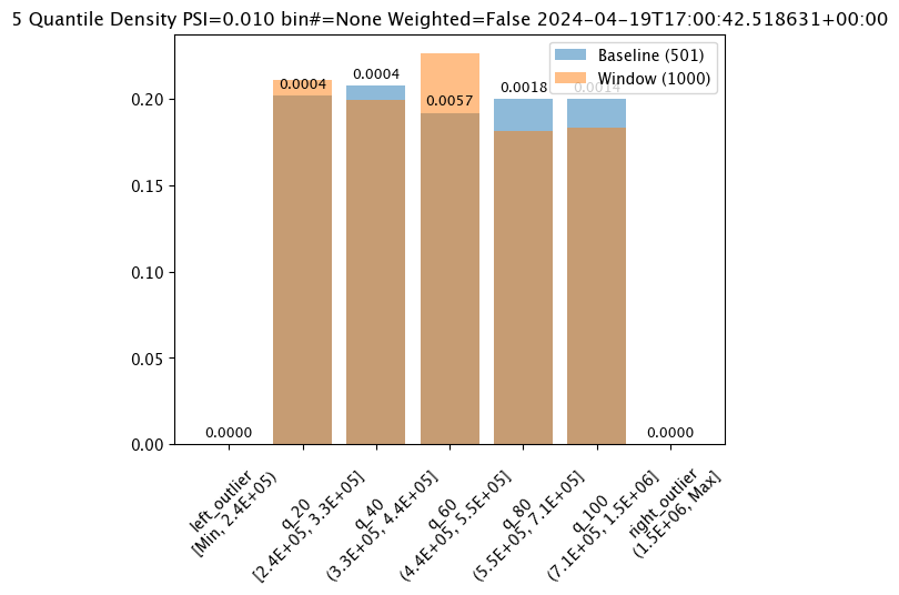
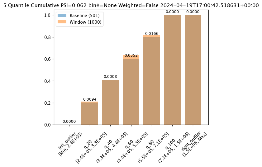
Aggregation.DENSITY (Default): Count the number/percentage of values that fall in each bin.
Aggregation.CUMULATIVE: Empirical Cumulative Density Function style, which keeps a cumulative count of the values/percentages that fall in each bin.

The following example demonstrate the different results between the two.

# Create the assay baseline
assay_baseline = wl.build_assay(assay_name="assays from date baseline", 
                                          pipeline=mainpipeline, 
                                          iopath="output variable 0",
                                          baseline_start=assay_baseline_start, 
                                          baseline_end=assay_baseline_end)

# Set the assay parameters

# The end date to gather inference results
assay_baseline.add_run_until(datetime.datetime.now())

# Set the interval and window to one minute each, set the start date for gathering inference results
assay_baseline.window_builder().add_width(minutes=1).add_interval(minutes=1).add_start(assay_window_start)

#Aggregation.DENSITY - the default
assay_baseline.summarizer_builder.add_aggregation(wallaroo.assay_config.Aggregation.DENSITY)

# build the assay configuration
assay_config = assay_baseline.build()

# perform an interactive run and collect inference data
assay_results = assay_config.interactive_run()

# show one analysis with the updated bins
assay_results[0].chart()

baseline mean = 535881.168880988
window mean = 525169.808015625
baseline median = 450867.6875
window median = 448627.8125
bin_mode = Quantile
aggregation = Density
metric = PSI
weighted = False
score = 0.00972686088185764
scores = [0.0, 0.0004286769159531457, 0.0003625824754554272, 0.005674527370820431, 0.001819573488386175, 0.0014415006312424594, 0.0]
index = None

# Create the assay baseline
assay_baseline = wl.build_assay(assay_name="assays from date baseline", 
                                          pipeline=mainpipeline, 
                                          iopath="output variable 0",
                                          baseline_start=assay_baseline_start, 
                                          baseline_end=assay_baseline_end)

# Set the assay parameters

# The end date to gather inference results
assay_baseline.add_run_until(datetime.datetime.now())

# Set the interval and window to one minute each, set the start date for gathering inference results
assay_baseline.window_builder().add_width(minutes=1).add_interval(minutes=1).add_start(assay_window_start)

#Aggregation.CUMULATIVE
assay_baseline.summarizer_builder.add_aggregation(wallaroo.assay_config.Aggregation.CUMULATIVE)

# build the assay configuration
assay_config = assay_baseline.build()

# perform an interactive run and collect inference data
assay_results = assay_config.interactive_run()

# show one analysis with the updated bins
assay_results[0].chart()

baseline mean = 535881.168880988
window mean = 525169.808015625
baseline median = 450867.6875
window median = 448627.8125
bin_mode = Quantile
aggregation = Cumulative
metric = PSI
weighted = False
score = 0.06202395209580827
scores = [0.0, 0.009403193612774446, 0.0008183632734530821, 0.035201596806387236, 0.016600798403193506, 0.0, 0.0]
index = None

Create Assay

With the assay previewed and configuration options determined, we officially create it by uploading it to the Wallaroo instance.

Once it is uploaded, the assay runs an analysis based on the window width, interval, and the other settings configured.

Assays are uploaded with the wallaroo.assay_config.upload() method. This uploads the assay into the Wallaroo database with the configurations applied and returns the assay id. Note that assay names must be unique across the Wallaroo instance; attempting to upload an assay with the same name as an existing one will return an error.

wallaroo.assay_config.upload() returns the assay id for the assay.

Typically we would just call wallaroo.assay_config.upload() after configuring the assay. For the example below, we will perform the complete configuration in one window to show all of the configuration steps at once before creating the assay.

# Build the assay, based on the start and end of our baseline time, 
# and tracking the output variable index 0
assay_baseline = wl.build_assay(assay_name="assays from date baseline tutorial", 
                                          pipeline=mainpipeline, 
                                          iopath="output variable 0",
                                          baseline_start=assay_baseline_start, 
                                          baseline_end=assay_baseline_end)

# set the width, interval, and assay start date and time
assay_baseline.window_builder().add_width(minutes=1).add_interval(minutes=1).add_start(assay_window_start)

# add other options
assay_baseline.summarizer_builder.add_aggregation(wallaroo.assay_config.Aggregation.CUMULATIVE)
assay_baseline.summarizer_builder.add_metric(wallaroo.assay_config.Metric.MAXDIFF)
assay_baseline.add_alert_threshold(0.5)

assay_id = assay_baseline.upload()

# wait 65 seconds for the first analysis run performed
time.sleep(65)

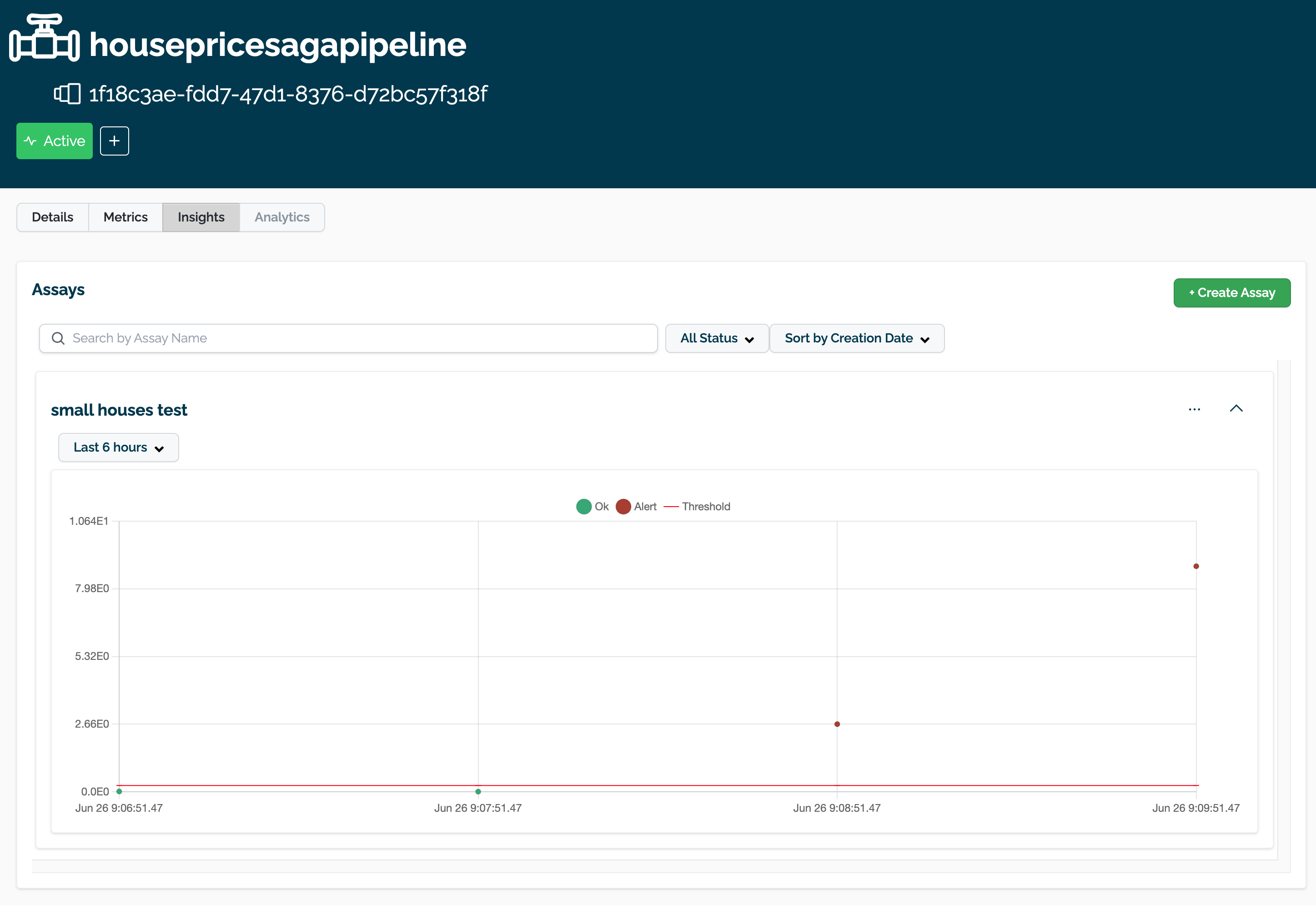
The assay is now visible through the Wallaroo UI by selecting the workspace, then the pipeline, then Insights.

Get Assay Info

Assay information is retrieved with the wallaroo.client.get_assay_info() which takes the following parameters.

Parameter	Type	Description
assay_id	Integer (Required)	The numerical id of the assay.

This returns the following:

Parameter	Type	Description
id	Integer	The numerical id of the assay.
name	String	The name of the assay.
active	Boolean	`True`: The assay is active and generates analyses based on its configuration. `False`: The assay is disabled and will not generate new analyses.
pipeline_name	String	The name of the pipeline the assay references.
last_run	DateTime	The date and time the assay last ran.
next_run	DateTime	THe date and time the assay analysis will next run.
alert_threshold	Float	The alert threshold setting for the assay.
baseline	Dict	The baseline and settings as set from the assay configuration.
iopath	String	The `iopath` setting for the assay.
metric	String	The `metric` setting for the assay.
num_bins	Integer	The number of bins for the assay.
bin_weights	List/None	The bin weights used if any.
bin_mode	String	The binning mode used.

display(wl.get_assay_info(assay_id))

	id	name	active	status	pipeline_name	last_run	next_run	alert_threshold	baseline	iopath	metric	num_bins	bin_weights	bin_mode
0	1	assays from date baseline tutorial	True	{"run_at": "2024-04-19T17:20:50.746019469+00:00", "num_ok": 1, "num_warnings": 0, "num_alerts": 1}	assay-demonstration-tutorial	2024-04-19T17:20:50.746019+00:00	2024-04-19T17:20:42.518631+00:00	0.5	Start:2024-04-19T16:58:41.956938+00:00, End:2024-04-19T16:59:42.493938+00:00	output variable 0	MaxDiff	5	None	Quantile

Get Assay Results

Once an assay is created the assay runs an analysis based on the window width, interval, and the other settings configured.

Assay results are retrieved with the wallaroo.client.get_assay_results method which takes the following parameters:

Parameter	Type	Description
assay_id	Integer (Required)	The numerical id of the assay.
start	Datetime.Datetime (Required)	The start date and time of historical data from the pipeline to start analyses from.
end	Datetime.Datetime (Required)	The end date and time of historical data from the pipeline to limit analyses to.

IMPORTANT NOTE: This process requires that additional historical data is generated from the time the assay is created to when the results are available. To add additional inference data, use the Assay Test Data section above.

assay_results = wl.get_assay_results(assay_id=assay_id,
                     start=assay_window_start,
                     end=datetime.datetime.now())

assay_results.chart_scores()

assay_results[0].chart()

baseline mean = 535881.168880988
window mean = 525169.808015625
baseline median = 450867.6875
window median = 448627.8125
bin_mode = Quantile
aggregation = Cumulative
metric = MaxDiff
weighted = False
score = 0.035201598
scores = [0.0, 0.009403193612774446, 0.0008183632734530821, 0.035201596806387236, 0.016600798403193506, 0.0, 0.0]
index = 3

List Assays

A list of assays is retrieved with the wallaroo.client.list_assays() method.

This returns a Object as a List with the following fields.

Parameter	Type	Description
Assay Id	Integer	The numerical id of the assay.
Assay Name	String	The name of the assay.
Active	Boolean	`True`: The assay is active and generates analyses based on its configuration. `False`: The assay is disabled and will not generate new analyses.
Status	Dict	The status of the assay including the
Warning Threshold	Float/None	The warning threshold if set.
Alert Threshold	Float	The alert threshold for the assay.
Pipeline Id	Integer	The numerical id of the pipeline the assay references.
Pipeline Name	String	The name of the pipeline the assay references.

wl.list_assays()

Assay ID	Assay Name	Active	Status	Warning Threshold	Alert Threshold	Pipeline ID	Pipeline Name
1	assays from date baseline tutorial	True	{"run_at": "2024-04-19T17:20:50.746019469+00:00", "num_ok": 1, "num_warnings": 0, "num_alerts": 1}	None	0.5	1	assay-demonstration-tutorial

Set Assay Active Status

Assays active status is either:

True: The assay generates analyses based on the assay configuration.
False: The assay will not generate new analyses.

Assays are set to active or not active with the wallaroo.client.set_assay_active which takes the following parameters.

Parameter	Type	Description
assay_id	Integer	The numerical id of the assay.
active	Boolean	`True`: The assay status is set to `Active`. `False`: The assay status is `Not Active`.

First we will show the current active status.

In the following, set the assay status to False, then set the assay active status back to True.

display(wl.get_assay_info(assay_id))

	id	name	active	status	pipeline_name	last_run	next_run	alert_threshold	baseline	iopath	metric	num_bins	bin_weights	bin_mode
0	1	assays from date baseline tutorial	True	{"run_at": "2024-04-19T17:20:50.746019469+00:00", "num_ok": 1, "num_warnings": 0, "num_alerts": 1}	assay-demonstration-tutorial	2024-04-19T17:20:50.746019+00:00	2024-04-19T17:20:42.518631+00:00	0.5	Start:2024-04-19T16:58:41.956938+00:00, End:2024-04-19T16:59:42.493938+00:00	output variable 0	MaxDiff	5	None	Quantile

Now we set the active status to False, and show the assay list to verify it is no longer active.

wl.set_assay_active(assay_id, False)
display(wl.get_assay_info(assay_id))

	id	name	active	status	pipeline_name	last_run	next_run	alert_threshold	baseline	iopath	metric	num_bins	bin_weights	bin_mode
0	1	assays from date baseline tutorial	False	{"run_at": "2024-04-19T17:20:50.746019469+00:00", "num_ok": 1, "num_warnings": 0, "num_alerts": 1}	assay-demonstration-tutorial	2024-04-19T17:20:50.746019+00:00	2024-04-19T17:20:42.518631+00:00	0.5	Start:2024-04-19T16:58:41.956938+00:00, End:2024-04-19T16:59:42.493938+00:00	output variable 0	MaxDiff	5	None	Quantile

We resume the assay by setting it’s active status to True.

wl.set_assay_active(assay_id, True)
display(wl.get_assay_info(assay_id))

	id	name	active	status	pipeline_name	last_run	next_run	alert_threshold	baseline	iopath	metric	num_bins	bin_weights	bin_mode
0	1	assays from date baseline tutorial	True	{"run_at": "2024-04-19T17:20:50.746019469+00:00", "num_ok": 1, "num_warnings": 0, "num_alerts": 1}	assay-demonstration-tutorial	2024-04-19T17:20:50.746019+00:00	2024-04-19T17:20:42.518631+00:00	0.5	Start:2024-04-19T16:58:41.956938+00:00, End:2024-04-19T16:59:42.493938+00:00	output variable 0	MaxDiff	5	None	Quantile

Undeploy Main Pipeline

With the examples and tutorial complete, we will undeploy the main pipeline and return the resources back to the Wallaroo instance.

mainpipeline.undeploy()

name	assay-demonstration-tutorial
created	2024-04-19 16:58:24.382145+00:00
last_updated	2024-04-19 16:58:24.760713+00:00
deployed	False
arch	x86
accel	none
tags
versions	b467cbc2-1988-4c04-8ed5-01803f35c1f7, 3155d4db-1650-4bd9-8011-049a7d3a0d96
steps	house-price-estimator
published	False