Wallaroo.AI 101
The Wallaroo 101 tutorial can be downloaded as part of the Wallaroo Tutorials repository.
Introduction
Welcome to the Wallaroo, the fastest, easiest, and most efficient production ready machine learning system.
This tutorial is created to help you get started with Wallaroo right away. We’ll start with a brief explanation of how Wallaroo works, then provide the credit card fraud detection model so you can see it working.
This guide assumes that you’ve installed Wallaroo in your cloud Kubernetes cluster. This can be either:
- Amazon Web Services (AWS)
- Microsoft Azure
- Google Cloud Platform
For instructions on setting up your cloud Kubernetes environment, check out the Wallaroo Environment Setup Guides for your particular cloud provider.
How to Use This Notebook
It is recommended that you run this notebook command at a time so you can see the results and make any changes you need based on your own environment.
Tutorial Goals
This tutorial provides an introductory guide to Wallaroo’s user interface and SDK. Most of the commands will be performed with the SDK, and the user interface version will be shown as a visual example.
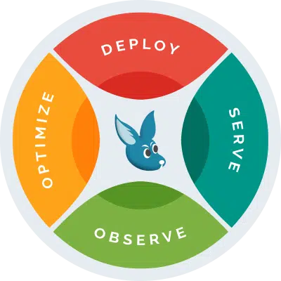
The examples will focus on the four pillars of Wallaroo:
- Deploy
- Run
- Observe
- Optimize
References
- The Wallaroo Documentation Site
- Wallaroo Tutorials Repository
- Request a Demo
- Free License for Wallaroo Community
Prerequisites
- An installed Wallaroo instance.
- The following Python libraries installed:
Tutorial Outline
Wallaroo lets you quickly get your models working with your data and getting results. The typical flow follows these steps:
- Connect: Connect to your Wallaroo Instance.
- Create or Connect to a Workspace: Create a new workspace that will contain your models and pipelines, or connect to an existing one.
- Upload or Use Existing Models: Upload your models to your workspace, or use ones that have already been uploaded.
- Create or Use Existing Pipelines: Create or use an existing pipeline. This is where you’ll set the steps that will ingest your data, submit it through each successive model, then return a result.
- Deploy Your Pipeline: Deploying a pipeline allocates resources from your Kubernetes environment for your models.
- Run an Inference: This is where it all comes together. Submit data through your pipeline either as a file or to your pipeline’s deployment url, and get results.
- Display Pipeline Logs: Observe the recent inference requests from a pipeline to track results and optimize based on an organization’s needs.
- Undeploy Your Pipeline: This returns the Kubernetes resources your pipeline used back to the Kubernetes environment.
For this tutorial, we’ll use the Wallaroo SDK and the Wallaroo User Interface (UI) which is included by default in the Wallaroo JupyterHub service.
For a more detailed rundown of the Wallaroo SDK, see the Wallaroo SDK Essentials Guide.
This example and sample data comes from the Machine Learning Group’s demonstration on Credit Card Fraud detection.
Introduction to Workspaces
A Wallaroo Workspace allows you to manage a set of models and pipelines.
When working within the Wallaroo SDK, the first thing you’ll do after connecting is either create a workspace or set an existing workspace your current workspace. From that point on, all models uploaded and pipelines created or used will be in the context of the current workspace.
Introduction to Models
A Wallaroo model is a trained Machine Learning model that is uploaded to your current workspace. These are the engines that take in data, run it through whatever process they have been trained for, and return a result.
Models don’t work in a vacuum - they are allocated to a pipeline as detailed in the next step.
Introduction to Pipelines
A Wallaroo pipeline is where the real work occurs. A pipeline contains a series of steps - sequential sets of models which take in the data from the preceding step, process it through the model, then return a result. Some models can be simple, such as the cc_fraud example listed below where the pipeline has only one step:
- Step 0: Take in data
- Step 1: Submit data to the model
ccfraudModel. - Step Final: Return a result
Some models can be more complex with a whole series of models - and those results can be submitted to still other pipeline. You can make pipelines as simple or complex as long as it meets your needs.
Once a step is created you can add additional steps, remove a step, or swap one out until everything is running perfectly.
Note: The Community Edition of Wallaroo limits users to two active pipelines, with a maximum of five steps per pipeline.
Import Libraries
The first step is to import the libraries we’ll be using. These are included by default in the Wallaroo instance’s JupyterHub service.
The IPython.display can be ignored in a production script, and is provided for formatting the data in this example.
import wallaroo
from wallaroo.object import EntityNotFoundError

import pyarrow as pa
import pandas as pd

# used to display dataframe information without truncating
from IPython.display import display
pd.set_option('display.max_colwidth', None)
Connect to the Wallaroo Instance through the User Interface
The next step is to connect to Wallaroo through the Wallaroo client. The Python library is included in the Wallaroo install and available through the Jupyter Hub interface provided with your Wallaroo environment.
This is accomplished using the wallaroo.Client() command, which provides a URL to grant the SDK permission to your specific Wallaroo environment. When displayed, enter the URL into a browser and confirm permissions. Store the connection into a variable that can be referenced later.
If logging into the Wallaroo instance through the internal JupyterHub service, use wl = wallaroo.Client(). For more information on Wallaroo Client settings, see the Client Connection guide.
# Login through local Wallaroo instance

wl = wallaroo.Client()
Create a New Workspace
Just for the sake of this tutorial, we’ll use the SDK below to create our workspace , assign as our current workspace, then display all of the workspaces we have at the moment.
When we create our new workspace, we’ll save it in the Python variable workspace so we can refer to it as needed.
workspace_name = f'ccfraudworkspace'
pipeline_name = f'ccfraudpipeline'
model_name = f'ccfraudmodel'
model_file_name = './ccfraud.onnx'
workspace = wl.get_workspace(name=workspace_name, create_if_not_exist=True)
Just to make sure, let’s list our current workspace. If everything is going right, it will show us we’re in the ccfraud-workspace with the appropriate prefix.
wl.set_current_workspace(workspace)
wl.get_current_workspace()
{'name': 'ccfraudworkspace', 'id': 20, 'archived': False, 'created_by': '36e83b1d-b405-4d30-abc5-e7000163d930', 'created_at': '2024-04-11T18:17:24.019263+00:00', 'models': [], 'pipelines': []}
Create a New Workspace via the User Interface
One method of creating new workspace is through the user interface. We did that with the SDK, but here’s an example of doing it through the Wallaroo Dashboard.
The method we’ll introduce below will either create a new workspace if it doesn’t exist, or select an existing workspace.
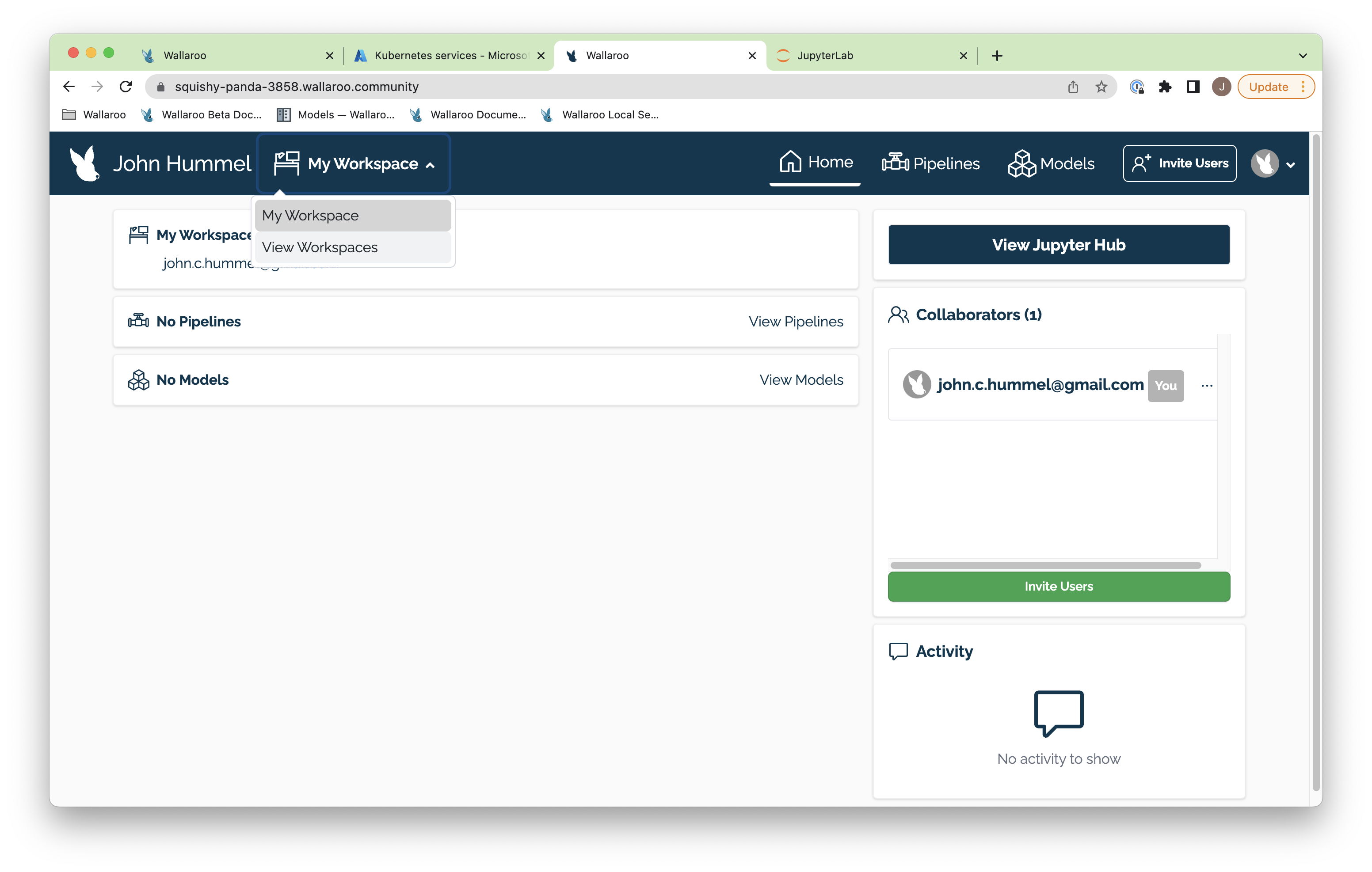
The first part is to return to your Wallaroo Dashboard. In the top navigation panel next to your user name there’s a drop down with your workspaces. In this example it just has My Workspace. Select View Workspaces.
From here, enter the name of our new workspace as ccfraud-workspace. If it already exists, you can skip this step.
- IMPORTANT NOTE: Workspaces do not have forced unique names. It is highly recommended to use an existing workspace when possible, or establish a naming convention for your workspaces to keep their names unique to remove confusion with teams.
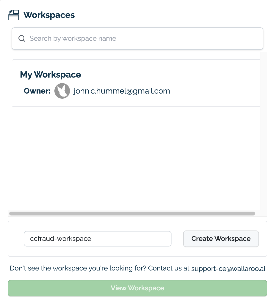
Once complete, you’ll be able to select the workspace from the drop down list in your dashboard.

Upload a model
Our workspace is created. Let’s upload our credit card fraud model to it. This is the file name ccfraud.onnx, and we’ll upload it as ccfraudmodel. The credit card fraud model is trained to detect credit card fraud based on a 0 to 1 model: The closer to 0 the less likely the transactions indicate fraud, while the closer to 1 the more likely the transactions indicate fraud.
Since we’re already in our default workspace ccfraudworkspace, it’ll be uploaded right to there. Once that’s done uploading, we’ll list out all of the models currently deployed so we can see it included.
ccfraud_model = (wl.upload_model(model_name,
                                 model_file_name,
                                 framework=wallaroo.framework.Framework.ONNX)
                                 .configure(tensor_fields=["tensor"])
                )
We can verify that our model was uploaded by listing the models uploaded to our workspace with the Workspace models() command. Note that if we uploaded this model before, we now have different versions of it we can use for our testing.
workspace.models()
[{'name': 'ccfraudmodel', 'versions': 1, 'owner_id': '""', 'last_update_time': datetime.datetime(2024, 4, 11, 18, 17, 25, 503377, tzinfo=tzutc()), 'created_at': datetime.datetime(2024, 4, 11, 18, 17, 25, 503377, tzinfo=tzutc())}]
View the Model through the User Interface
Uploading a model can only be done through the Wallaroo SDK or the Wallaroo MLOps API.
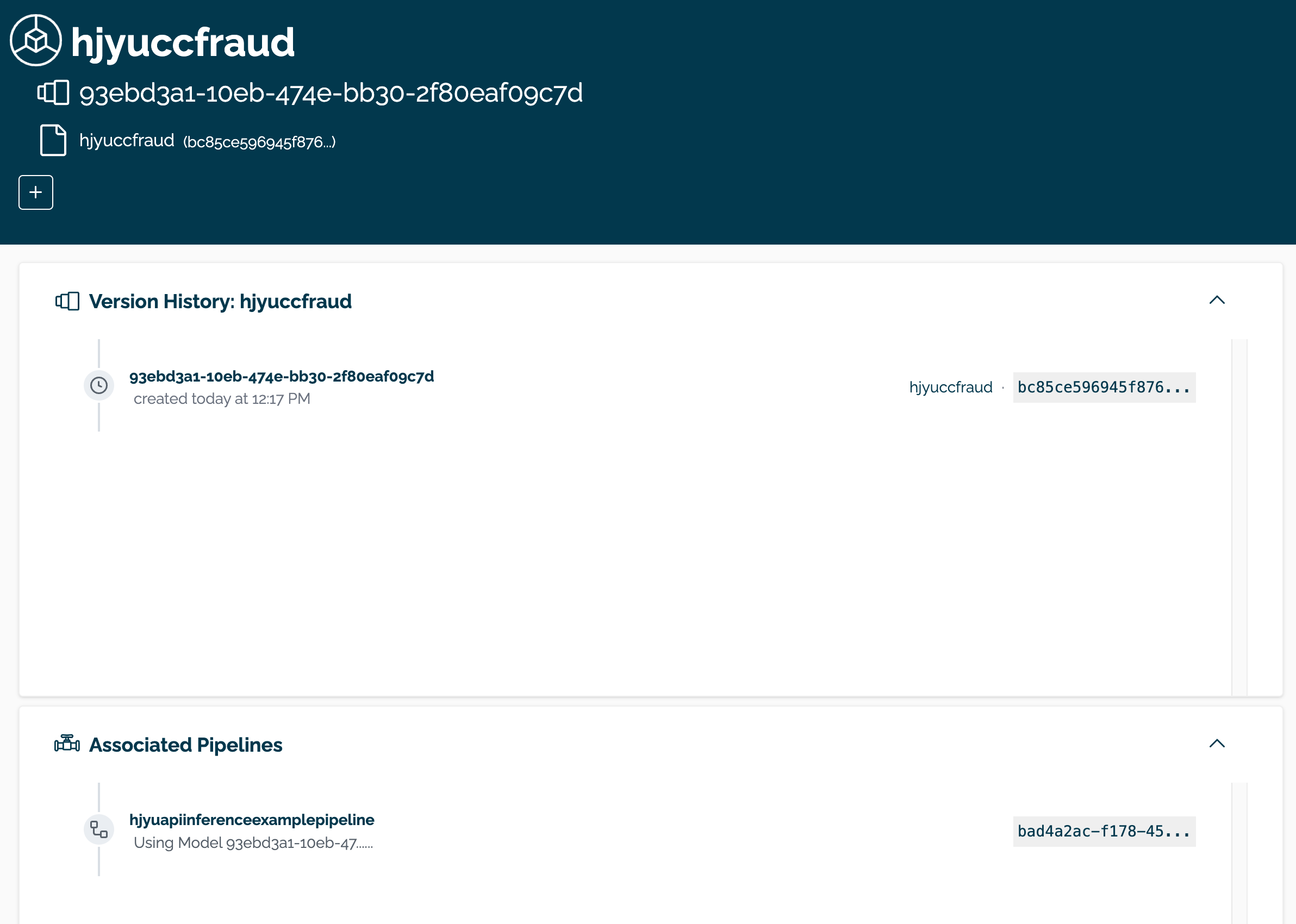
The model can be viewed through the Wallaroo Dashboard by selecting the workspace, then selecting the model. From this display, the model name, version(s), and associates pipeline(s) are displayed.
Create a Pipeline
With our model uploaded, time to create our pipeline and deploy it so it can accept data and process it through our ccfraudmodel. We’ll call our pipeline ccfraudpipeline.
- NOTE: Pipeline names must be unique. If two pipelines are assigned the same name, the new pipeline is created as a new version of the pipeline.
ccfraud_pipeline = wl.build_pipeline(pipeline_name)
ccfraud_pipeline
| name | ccfraudpipeline |
|---|---|
| created | 2024-04-11 18:17:26.376089+00:00 |
| last_updated | 2024-04-11 18:17:26.376089+00:00 |
| deployed | (none) |
| arch | None |
| accel | None |
| tags | |
| versions | 1fa72c2b-f798-457c-8b34-359e08ba348c |
| steps | |
| published | False |
Now our pipeline is set. Let’s add a single step to it - in this case, our ccfraud_model that we uploaded to our workspace.
ccfraud_pipeline.add_model_step(ccfraud_model)
| name | ccfraudpipeline |
|---|---|
| created | 2024-04-11 18:17:26.376089+00:00 |
| last_updated | 2024-04-11 18:17:26.376089+00:00 |
| deployed | (none) |
| arch | None |
| accel | None |
| tags | |
| versions | 1fa72c2b-f798-457c-8b34-359e08ba348c |
| steps | |
| published | False |
And now we can deploy our pipeline and assign resources to it. This typically takes about 45 seconds once the command is issued.
ccfraud_pipeline.deploy()
| name | ccfraudpipeline |
|---|---|
| created | 2024-04-11 18:17:26.376089+00:00 |
| last_updated | 2024-04-11 18:17:27.583651+00:00 |
| deployed | True |
| arch | x86 |
| accel | none |
| tags | |
| versions | 35282a42-08c6-4ce3-80b8-b2bf9e8c6486, 1fa72c2b-f798-457c-8b34-359e08ba348c |
| steps | ccfraudmodel |
| published | False |
We can see our new pipeline with the status() command.
ccfraud_pipeline.status()
{'status': 'Running',
 'details': [],
 'engines': [{'ip': '10.28.0.150',
   'name': 'engine-5f454d68f8-76d4r',
   'status': 'Running',
   'reason': None,
   'details': [],
   'pipeline_statuses': {'pipelines': [{'id': 'ccfraudpipeline',
      'status': 'Running'}]},
   'model_statuses': {'models': [{'name': 'ccfraudmodel',
      'sha': 'bc85ce596945f876256f41515c7501c399fd97ebcb9ab3dd41bf03f8937b4507',
      'status': 'Running',
      'version': 'd32f9869-31a9-4ccc-b9fd-b8414b34289a'}]}}],
 'engine_lbs': [{'ip': '10.28.1.91',
   'name': 'engine-lb-d7cc8fc9c-gcqlr',
   'status': 'Running',
   'reason': None,
   'details': []}],
 'sidekicks': []}
Create Pipeline in the UI
Pipelines can be created and deployed through the user interface through the following process.
Select the workspace from the Wallaroo Dashboard.
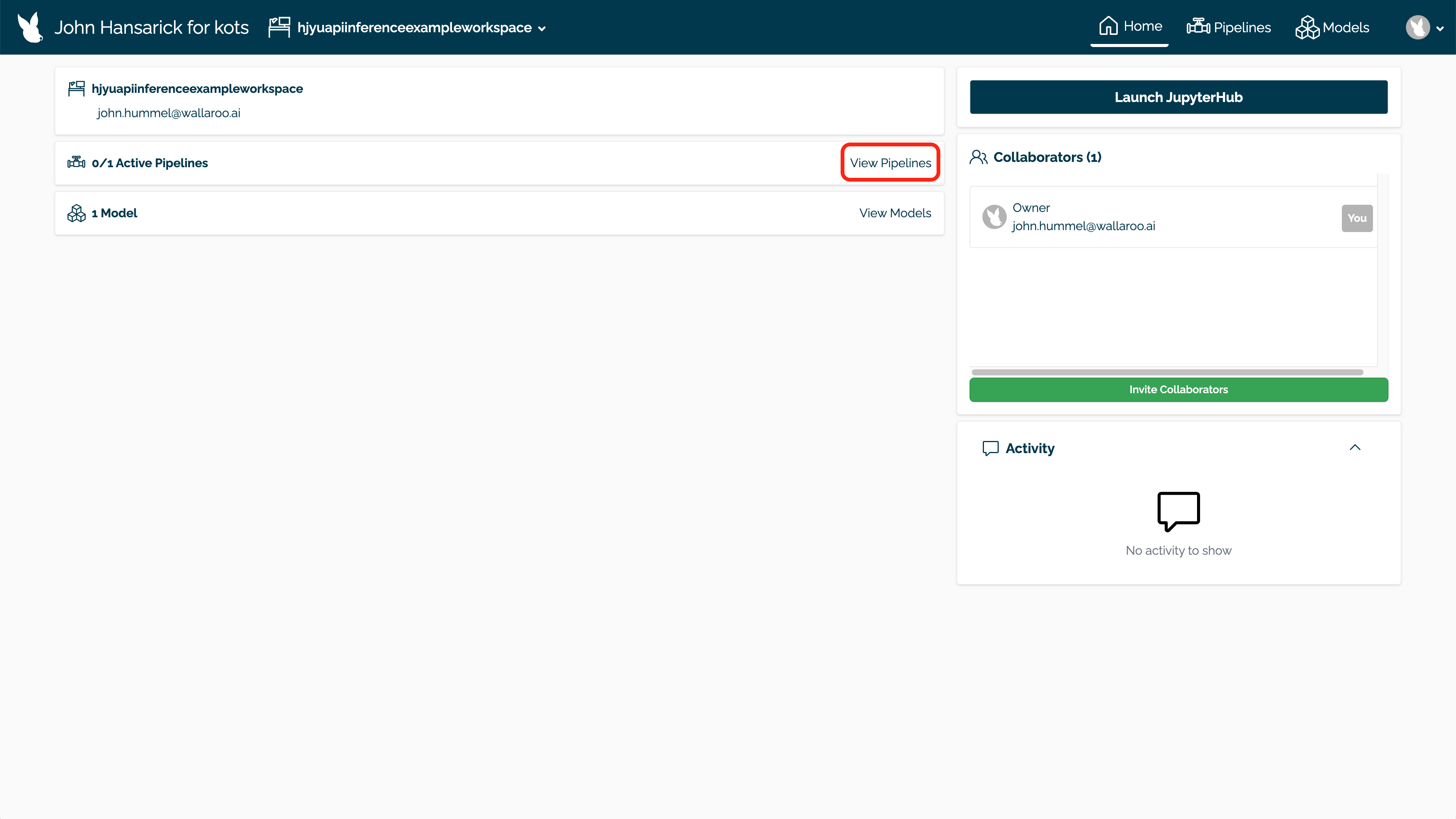
Select View Pipelines.
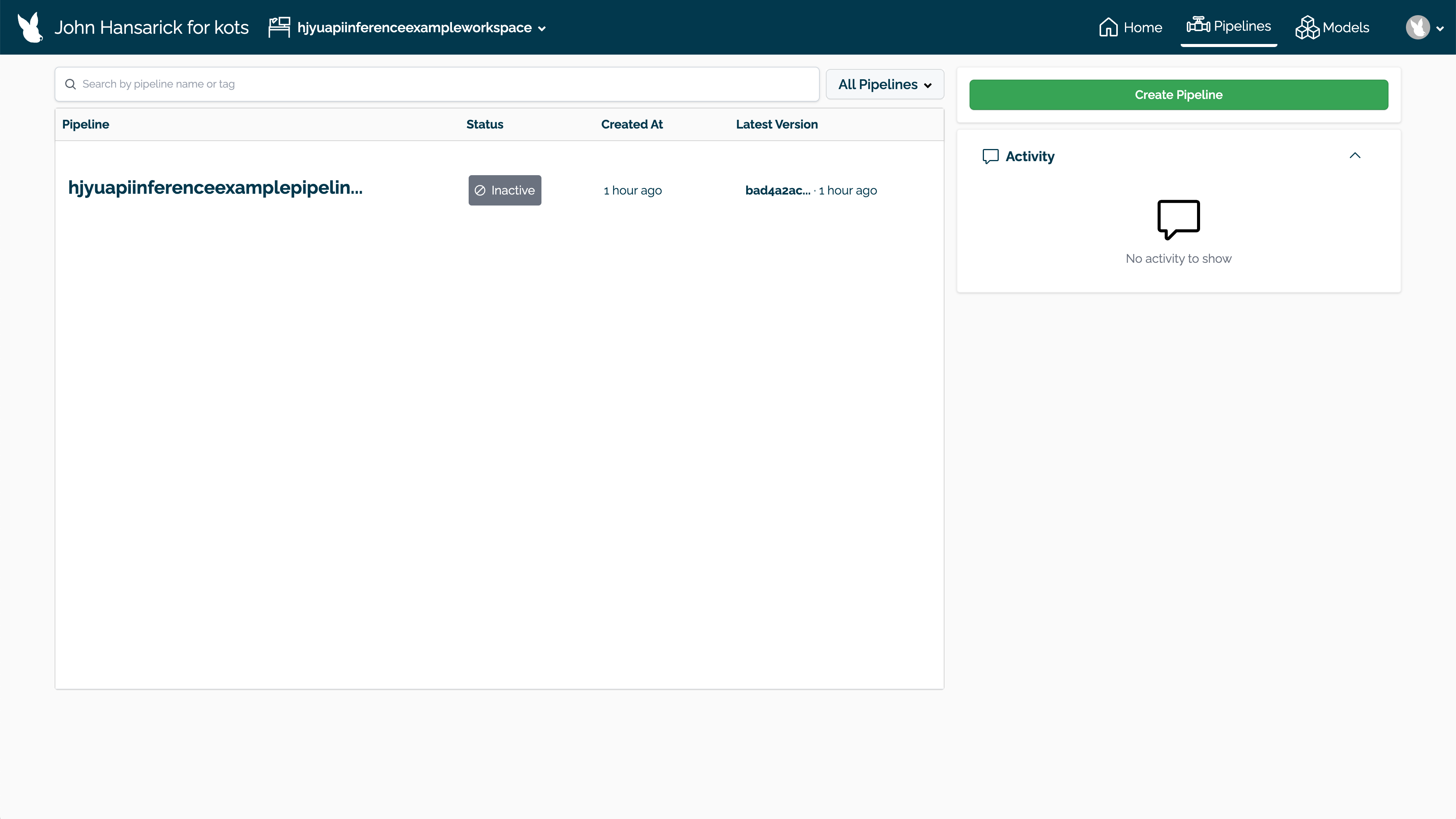
Select Create Pipeline.
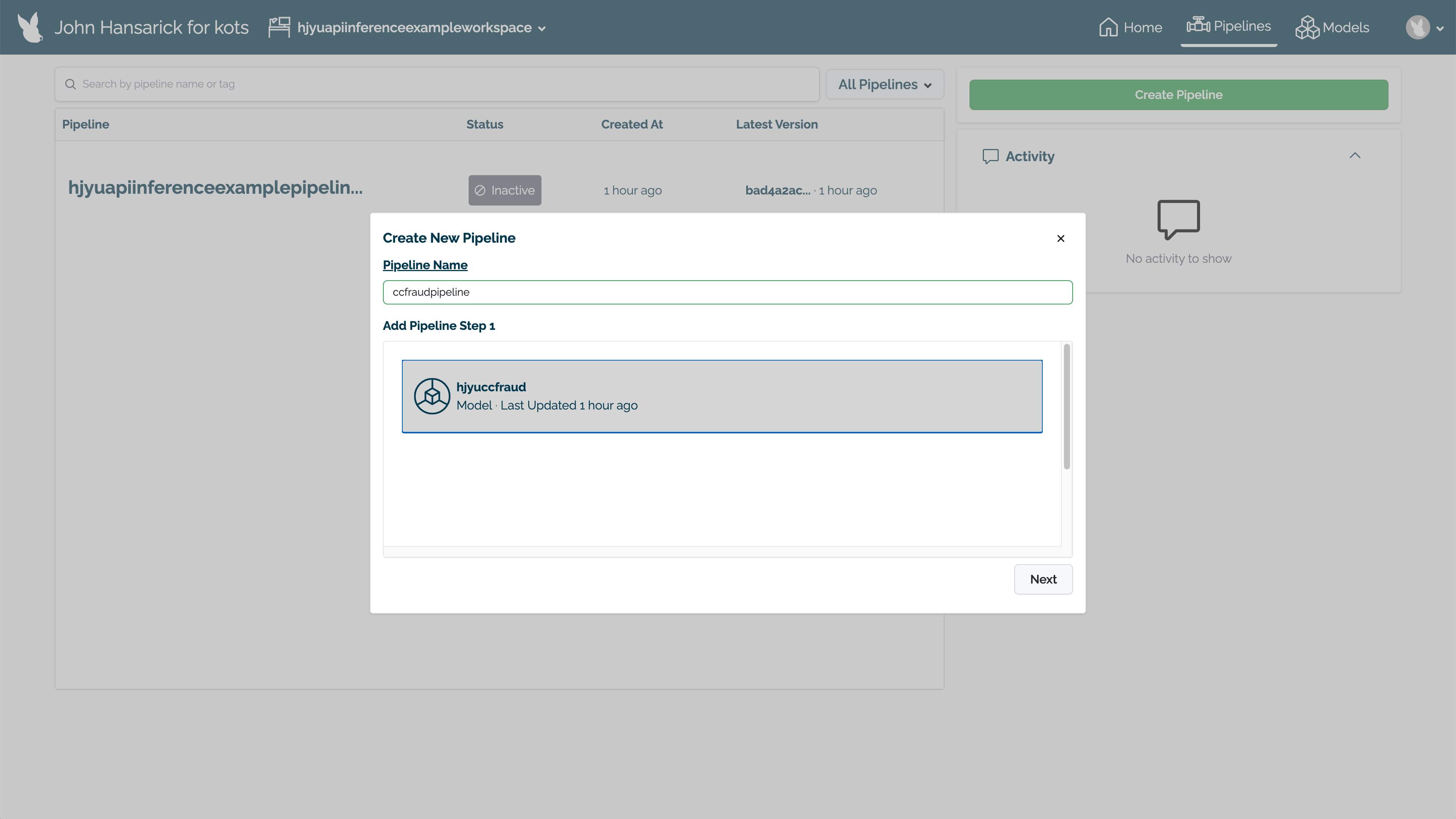
Set the name, then select the model for the pipeline step. Select Next.
With all of the pipeline steps added, select Build. The pipeline will now be available for use.

To deploy the pipeline, select Deploy.
Running Interfences
With our pipeline deployed, let’s run a smoke test to make sure it’s working right. We’ll run an inference through our pipeline from the variable smoke_test and see the results. This should give us a result near 0 - not likely a fraudulent activity.
Wallaroo accepts the following inputs for inferences:
- Apache Arrow tables (Default): Wallaroo highly encourages organizations to use Apache Arrow as their default inference input method for speed and accuracy. This requires the Arrow table schema matches what the model expects.
- Pandas DataFrame: DataFrame inputs are highly useful for data scientists to recognize what data is being input into the pipeline before finalizing to Arrow format.
These first two examples will use a pandas DataFrame record to display a sample input. The rest of the examples will use Arrow tables.
smoke_test = pd.DataFrame.from_records([
    {
        "tensor":[
            1.0678324729,
            0.2177810266,
            -1.7115145262,
            0.682285721,
            1.0138553067,
            -0.4335000013,
            0.7395859437,
            -0.2882839595,
            -0.447262688,
            0.5146124988,
            0.3791316964,
            0.5190619748,
            -0.4904593222,
            1.1656456469,
            -0.9776307444,
            -0.6322198963,
            -0.6891477694,
            0.1783317857,
            0.1397992467,
            -0.3554220649,
            0.4394217877,
            1.4588397512,
            -0.3886829615,
            0.4353492889,
            1.7420053483,
            -0.4434654615,
            -0.1515747891,
            -0.2668451725,
            -1.4549617756
        ]
    }
])
result = ccfraud_pipeline.infer(smoke_test)
display(result)
| time | in.tensor | out.dense_1 | anomaly.count | |
|---|---|---|---|---|
| 0 | 2024-04-11 18:17:50.179 | [1.0678324729, 0.2177810266, -1.7115145262, 0.682285721, 1.0138553067, -0.4335000013, 0.7395859437, -0.2882839595, -0.447262688, 0.5146124988, 0.3791316964, 0.5190619748, -0.4904593222, 1.1656456469, -0.9776307444, -0.6322198963, -0.6891477694, 0.1783317857, 0.1397992467, -0.3554220649, 0.4394217877, 1.4588397512, -0.3886829615, 0.4353492889, 1.7420053483, -0.4434654615, -0.1515747891, -0.2668451725, -1.4549617756] | [0.0014974177] | 0 |
Looks good! Time to run the real test on some real data. Run another inference this time from the file high_fraud.json and let’s see the results. This should give us an output that indicates a high level of fraud - well over 90%.
high_fraud = pd.DataFrame.from_records([
    {
        "tensor":[
            1.0678324729,
            18.1555563975,
            -1.6589551058,
            5.2111788045,
            2.3452470645,
            10.4670835778,
            5.0925820522,
            12.8295153637,
            4.9536770468,
            2.3934736228,
            23.912131818,
            1.759956831,
            0.8561037518,
            1.1656456469,
            0.5395988814,
            0.7784221343,
            6.7580610727,
            3.9274118477,
            12.4621782767,
            12.3075382165,
            13.7879519066,
            1.4588397512,
            3.6818346868,
            1.753914366,
            8.4843550037,
            14.6454097667,
            26.8523774363,
            2.7165292377,
            3.0611957069
        ]
    }
])

result = ccfraud_pipeline.infer(high_fraud)
display(result)
| time | in.tensor | out.dense_1 | anomaly.count | |
|---|---|---|---|---|
| 0 | 2024-04-11 18:17:50.399 | [1.0678324729, 18.1555563975, -1.6589551058, 5.2111788045, 2.3452470645, 10.4670835778, 5.0925820522, 12.8295153637, 4.9536770468, 2.3934736228, 23.912131818, 1.759956831, 0.8561037518, 1.1656456469, 0.5395988814, 0.7784221343, 6.7580610727, 3.9274118477, 12.4621782767, 12.3075382165, 13.7879519066, 1.4588397512, 3.6818346868, 1.753914366, 8.4843550037, 14.6454097667, 26.8523774363, 2.7165292377, 3.0611957069] | [0.981199] | 0 |
Batch Inferences
Now that we’ve tested our pipeline, let’s run it with something larger. We have two batch files - cc_data_1k.arrow that contains 1,000 credit card records to test for fraud. The other is cc_data_10k.arrow which has 10,000 credit card records to test.
Let’s run a batch result for cc_data_10k.arrow and see the results.
With the inference result we’ll output just the cases likely to be fraud.
result = ccfraud_pipeline.infer_from_file('./data/cc_data_10k.arrow')

display(result)

# using pandas conversion, display only the results with > 0.75

list = [0.75]

outputs =  result.to_pandas()
# display(outputs)
filter = [elt[0] > 0.75 for elt in outputs['out.dense_1']]
outputs = outputs.loc[filter]
display(outputs.loc[:,["time", "out.dense_1"]])
pyarrow.Table
time: timestamp[ms]
in.tensor: list<item: float> not null
  child 0, item: float
out.dense_1: list<inner: float not null> not null
  child 0, inner: float not null
anomaly.count: uint32 not null
----
time: [[2024-04-11 18:17:51.027,2024-04-11 18:17:51.027,2024-04-11 18:17:51.027,2024-04-11 18:17:51.027,2024-04-11 18:17:51.027,...,2024-04-11 18:17:51.027,2024-04-11 18:17:51.027,2024-04-11 18:17:51.027,2024-04-11 18:17:51.027,2024-04-11 18:17:51.027]]
in.tensor: [[[-1.0603298,2.3544967,-3.5638788,5.138735,-1.2308457,...,0.038412016,1.0993439,1.2603409,-0.14662448,-1.4463212],[-1.0603298,2.3544967,-3.5638788,5.138735,-1.2308457,...,0.038412016,1.0993439,1.2603409,-0.14662448,-1.4463212],...,[-2.1694233,-3.1647356,1.2038506,-0.2649221,0.0899006,...,1.8174038,-0.19327773,0.94089776,0.825025,1.6242892],[-0.12405868,0.73698884,1.0311689,0.59917533,0.11831961,...,-0.36567155,-0.87004745,0.41288367,0.49470216,-0.6710689]]]
out.dense_1: [[[0.99300325],[0.99300325],...,[0.00024175644],[0.0010648072]]]
anomaly.count: [[0,0,0,0,0,...,0,0,0,0,0]]
| time | out.dense_1 | |
|---|---|---|
| 0 | 2024-04-11 18:17:51.027 | [0.99300325] |
| 1 | 2024-04-11 18:17:51.027 | [0.99300325] |
| 2 | 2024-04-11 18:17:51.027 | [0.99300325] |
| 3 | 2024-04-11 18:17:51.027 | [0.99300325] |
| 161 | 2024-04-11 18:17:51.027 | [1.0] |
| 941 | 2024-04-11 18:17:51.027 | [0.9873102] |
| 1445 | 2024-04-11 18:17:51.027 | [1.0] |
| 2092 | 2024-04-11 18:17:51.027 | [0.99999] |
| 2220 | 2024-04-11 18:17:51.027 | [0.91080534] |
| 4135 | 2024-04-11 18:17:51.027 | [0.98877275] |
| 4236 | 2024-04-11 18:17:51.027 | [0.95601666] |
| 5658 | 2024-04-11 18:17:51.027 | [1.0] |
| 6768 | 2024-04-11 18:17:51.027 | [0.9999745] |
| 6780 | 2024-04-11 18:17:51.027 | [0.9852645] |
| 7133 | 2024-04-11 18:17:51.027 | [1.0] |
| 7566 | 2024-04-11 18:17:51.027 | [0.9999705] |
| 7911 | 2024-04-11 18:17:51.027 | [0.9980203] |
| 8921 | 2024-04-11 18:17:51.027 | [0.99950194] |
| 9244 | 2024-04-11 18:17:51.027 | [0.9999876] |
| 10176 | 2024-04-11 18:17:51.027 | [1.0] |
We can view the inputs either through the in.tensor column from our DataFrame for Arrow enabled environments, or with the InferenceResult object through the input_data() for non-Arrow enabled environments. We’ll display just the first row in either case.
Since our inference results are in a DataFrame, we can map the output column into a percentage value to display or inject
into a database.
predictions = outputs["out.dense_1"].map(lambda x: x[0] * 100)
display(predictions)
0         99.300325
1         99.300325
2         99.300325
3         99.300325
161      100.000000
941       98.731017
1445     100.000000
2092      99.998999
2220      91.080534
4135      98.877275
4236      95.601666
5658     100.000000
6768      99.997449
6780      98.526448
7133     100.000000
7566      99.997050
7911      99.802029
8921      99.950194
9244      99.998760
10176    100.000000
Name: out.dense_1, dtype: float64
Viewing Inference Metrics
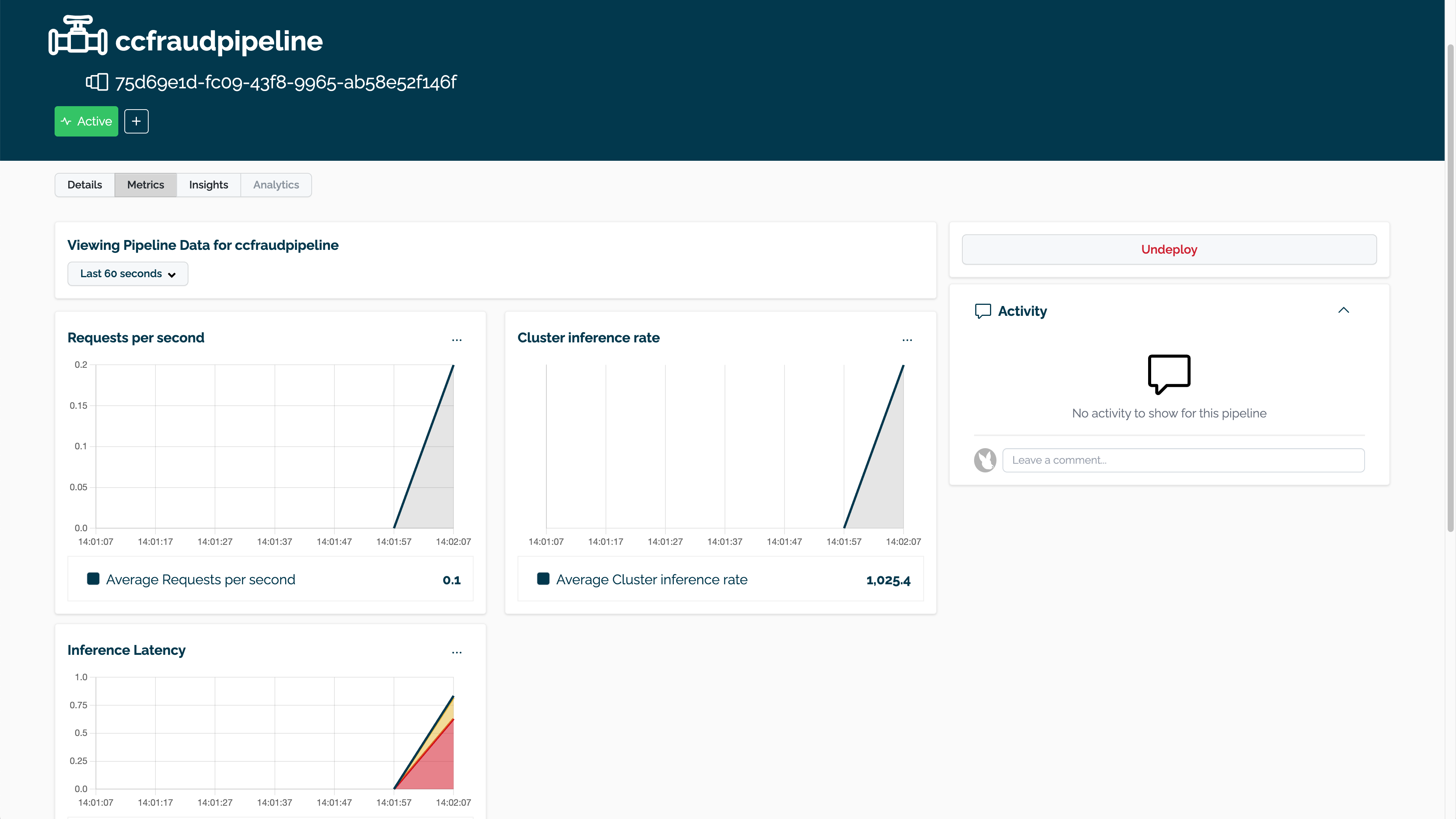
The pipeline metrics are displayed by selecting the pipeline through the Wallaroo Dashboard, then selecting Metrics. This provides a quick visual on how the pipeline is performing with the resources allocated to it.
Batch Deployment through a Pipeline Deployment URL
This next step requires some manual use. We’re going to have ccfraud_pipeline display its deployment url - this allows us to submit data through a HTTP interface and get the results back.
First we’ll request the url with the _deployment._url() method.
- IMPORTANT NOTE: The
_deployment._url()method will return an internal URL when using Python commands from within the Wallaroo instance - for example, the Wallaroo JupyterHub service. When connecting via an external connection,_deployment._url()returns an external URL.- External URL connections requires the authentication be included in the HTTP request, and Model Endpoints are enabled in the Wallaroo configuration options.
The API connection details can be retrieved through the Wallaroo client auth.auth_header() command. This will display the connection URL, bearer token, and other information. The bearer token is available for one hour before it expires.
For this example, the API connection details will be retrieved, then used to submit an inference request through the external inference URL retrieved earlier.
The deploy_url variable will be used to access the pipeline inference URL, Content-Type and Accept parameters will set the submitted values first as a DataFrame record, then the second will use the Python requests library to submit the inference as an Apache Arrow file, and the received values as a Pandas DataFrame.
deploy_url = ccfraud_pipeline._deployment._url()

headers = wl.auth.auth_header()

dataFile="./data/cc_data_10k.df.json"

headers['Content-Type']='application/json; format=pandas-records'
headers['Accept']='application/json; format=pandas-records'
!curl -X POST {deploy_url} \
    -H "Authorization:{headers['Authorization']}" \
    -H "Content-Type:{headers['Content-Type']}" \
    -H "Accept:{headers['Accept']}" \
    --data @{dataFile} > curl_response.df
  % Total    % Received % Xferd  Average Speed   Time    Time     Time  Current
                                 Dload  Upload   Total   Spent    Left  Speed
100 15.0M  100 7697k  100 7743k  2557k  2572k  0:00:03  0:00:03 --:--:-- 5129k1k  0:00:01  0:00:01 --:--:-- 7182k
cc_data_from_file =  pd.read_json('./curl_response.df', orient="records")
display(cc_data_from_file.head(5).loc[:, ["time", "out"]])
| time | out | |
|---|---|---|
| 0 | 1712859473066 | {'dense_1': [0.99300325]} |
| 1 | 1712859473066 | {'dense_1': [0.99300325]} |
| 2 | 1712859473066 | {'dense_1': [0.99300325]} |
| 3 | 1712859473066 | {'dense_1': [0.99300325]} |
| 4 | 1712859473066 | {'dense_1': [0.0010916889]} |
import requests

# Again with Arrow and requests

# Retrieve the token
headers = wl.auth.auth_header()

# set Content-Type type
headers['Content-Type']='application/vnd.apache.arrow.file'

# set accept as pandas-records
headers['Accept']="application/vnd.apache.arrow.file"

# Submit arrow file
dataFile="./data/cc_data_10k.arrow"

data = open(dataFile,'rb').read()

response = requests.post(
                    deploy_url,
                    headers=headers,
                    data=data,
                    verify=True
                )

# Arrow table is retrieved
with pa.ipc.open_file(response.content) as reader:
    arrow_table = reader.read_all()
With the arrow file returned, we’ll show the first five rows for comparison.
# convert to pandas DataFrame and display the first 5 rows
display(arrow_table.to_pandas().head(5).loc[:,["time", "out"]])
| time | out | |
|---|---|---|
| 0 | 1712859475503 | {'dense_1': [0.99300325]} |
| 1 | 1712859475503 | {'dense_1': [0.99300325]} |
| 2 | 1712859475503 | {'dense_1': [0.99300325]} |
| 3 | 1712859475503 | {'dense_1': [0.99300325]} |
| 4 | 1712859475503 | {'dense_1': [0.0010916889]} |
Display Logs
Along with metrics, another method of observability into the Wallaroo pipeline is through pipeline logs, which show when the inference request came in, the inputs used, the outputs, and if there were any validation errors detected.
ccfraud_pipeline.logs()
Warning: There are more logs available. Please set a larger limit or request a file using export_logs.
| time | in.tensor | out.dense_1 | anomaly.count | |
|---|---|---|---|---|
| 0 | 2024-04-11 18:17:55.503 | [-0.12405868, 0.73698884, 1.0311689, 0.59917533, 0.11831961, -0.47327134, 0.67207795, -0.16058543, -0.77808416, -0.2683532, -0.22364272, 0.64049035, 1.5038015, 0.004768592, 1.0683576, -0.3107394, -0.3427847, -0.078522496, 0.5455177, 0.1297957, 0.10491481, 0.4318976, -0.25777233, 0.701442, -0.36567155, -0.87004745, 0.41288367, 0.49470216, -0.6710689] | [0.0010648072] | 0 |
| 1 | 2024-04-11 18:17:55.503 | [-2.1694233, -3.1647356, 1.2038506, -0.2649221, 0.0899006, -0.18928011, -0.3495527, 0.17693162, 0.70965016, 0.19469678, -1.4288249, -1.5722991, -1.8213876, -1.2968907, -0.95062584, 0.8917047, 0.751387, -1.5475872, 0.3787144, 0.7525444, -0.03103788, 0.5858543, 2.6022773, -0.5311059, 1.8174038, -0.19327773, 0.94089776, 0.825025, 1.6242892] | [0.00024175644] | 0 |
| 2 | 2024-04-11 18:17:55.503 | [-0.24798988, 0.40499672, 0.49408177, -0.37252557, -0.412961, -0.38151076, -0.042232547, 0.293104, -2.1088455, 0.49807099, 0.8488427, -0.9078823, -0.89734304, 0.8601335, 0.6696, 0.48890257, 1.0623674, -0.5090369, 3.616667, 0.29580164, 0.43410888, 0.8741068, -0.6503351, 0.034938015, 0.96057385, 0.43238926, -0.1975937, -0.04551184, -0.12277038] | [0.00150159] | 0 |
| 3 | 2024-04-11 18:17:55.503 | [-0.2260837, 0.12802614, -0.8732004, -2.089788, 1.8722432, 2.05272, 0.09746246, 0.49692878, -1.0799059, 0.80176145, -0.26333216, -1.0224636, -0.056668393, -0.060779527, -0.20089072, 1.2798951, -0.55411917, -1.270442, 0.41811302, 0.2239133, 0.3109173, 1.0051724, 0.07736663, 1.7022146, -0.93862903, -0.99493766, -0.68271357, -0.71875495, -1.4715525] | [0.00037947297] | 0 |
| 4 | 2024-04-11 18:17:55.503 | [-0.90164274, -0.50116056, 1.2045985, 0.4078851, 0.2981652, -0.26469636, 0.4460249, 0.16928293, -0.15559517, -0.7641287, -0.8956279, -0.6098771, -0.87228906, 0.158441, 0.7461226, 0.43037805, -0.7037308, 0.7927367, -1.111509, 0.83980113, 0.6249728, 0.7301589, 0.5632024, 1.7966471, 1.5083653, -1.0206859, -0.11091206, 0.37982145, 1.2463697] | [0.0001988411] | 0 |
| ... | ... | ... | ... | ... |
| 95 | 2024-04-11 18:17:55.503 | [-0.1093998, -0.031678658, 0.9885652, -0.6860291, -0.6046543, 0.6653355, -0.6293921, -1.1772763, 1.4608942, -1.1322296, -1.9279546, 1.4049336, 1.2282782, -1.4884002, -3.115575, 0.41227773, -0.47484678, -0.9897973, -1.1200552, -0.66070575, 1.6864017, -1.4189101, -0.70692146, -0.5732528, 1.981664, 1.7516811, 0.28014255, 0.30193287, 0.80388844] | [0.00020942092] | 0 |
| 96 | 2024-04-11 18:17:55.503 | [0.44973943, -0.35288164, 0.5224735, 0.910402, -0.72067416, -0.050270014, -0.3414758, 0.10386056, 0.6459101, -0.019469967, -1.1449441, -0.7871593, -1.2093763, 0.26724637, 1.7972686, 1.0460316, -0.9273358, 0.91270906, -0.69702125, 0.19257616, 0.23213731, 0.08892933, -0.34931126, -0.31643763, 0.583289, -0.6749049, 0.0472516, 0.20378655, 1.0983771] | [0.00031492114] | 0 |
| 97 | 2024-04-11 18:17:55.503 | [0.82174337, -0.50793207, -1.358988, 0.37136176, 0.19260807, -0.60984015, 0.63114387, -0.31723085, 0.34576818, 0.015056487, -0.9967559, -0.037889328, -0.68294096, 0.6202497, -0.32679954, -0.6409717, -0.0055463314, -0.8609782, 0.119142644, 0.3092495, 0.1808159, -0.019580727, -0.20877448, 1.1818781, 0.2868476, 1.1510639, -0.37393016, -0.094152406, 1.2670404] | [0.00081187487] | 0 |
| 98 | 2024-04-11 18:17:55.503 | [1.0252348, 0.37717652, -1.4182774, 0.7057443, 0.36312255, -1.3660663, 0.17341496, -0.3454704, 1.7643102, -1.3501495, 0.9257918, -3.374893, 0.3617876, -0.8583969, 0.5060873, 0.8873245, 2.925866, 2.0265691, -1.1160102, -0.36432365, -0.0936597, 0.25772303, -0.02305712, -0.45073295, 0.37329674, -0.2838264, -0.0411118, 0.006249274, -1.4715525] | [0.001860708] | 0 |
| 99 | 2024-04-11 18:17:55.503 | [-0.36498702, 0.11005125, 0.7734325, 1.0163404, -0.38190573, 0.41608095, 1.4093872, -0.12511922, -0.14253987, -0.093657725, -0.6349157, -0.41843006, -0.91369456, -0.0038188277, 0.3744724, -1.3620936, 0.6263981, -0.57914644, 0.82675296, 0.9850866, 0.08680151, 0.28205827, 0.7979858, 0.065717764, -0.052254554, -0.53277296, 0.40100586, 0.0075293095, 1.3380127] | [0.00064843893] | 0 |
100 rows × 4 columns
With our work in the pipeline done, we’ll undeploy it to get back our resources from the Kubernetes cluster. If we keep the same settings we can redeploy the pipeline with the same configuration in the future.
ccfraud_pipeline.undeploy()
| name | ccfraudpipeline |
|---|---|
| created | 2024-04-11 18:17:26.376089+00:00 |
| last_updated | 2024-04-11 18:17:27.583651+00:00 |
| deployed | False |
| arch | x86 |
| accel | none |
| tags | |
| versions | 35282a42-08c6-4ce3-80b8-b2bf9e8c6486, 1fa72c2b-f798-457c-8b34-359e08ba348c |
| steps | ccfraudmodel |
| published | False |
And there we have it! Feel free to use this as a template for other models, inferences and pipelines that you want to deploy with Wallaroo!