Run Anywhere Model Insights via the Wallaroo SDK
Assays generated through the Wallaroo SDK can be previewed, configured, and uploaded to the Wallaroo Ops instance. The following is a condensed version of this process. For full details see the Model Drift Detection with Model Insights guide.
Model drift detection with assays using the Wallaroo SDK follows this general process.
- Define the Baseline: From either historical inference data for a specific model in a pipeline, or from a pre-determine array of data, a baseline is formed.
- Assay Preview: Once the baseline is formed, we preview the assay and configure the different options until we have the the best method of detecting environment or model drift.
- For this tutorial, we focus on limiting the locations included in the assay analyses.
- Create Assay: With the previews and configuration complete, we upload the assay. The assay will perform an analysis on a regular scheduled based on the configuration.
- Get Assay Results: Retrieve the analyses and use them to detect model drift and possible sources.
- Pause/Resume Assay: Pause or restart an assay as needed.
Define the Baseline
Assay baselines are defined with the wallaroo.client.build_assay method. Through this process we define the baseline from either a range of dates or pre-generated values.
wallaroo.client.build_assay take the following parameters:
| Parameter | Type | Description |
|---|---|---|
| assay_name | String (Required) - required | The name of the assay. Assay names must be unique across the Wallaroo instance. |
| pipeline | wallaroo.pipeline.Pipeline (Required) | The pipeline the assay is monitoring. |
| model_name | String (Required) | The name of the model to monitor. |
| iopath | String (Required) | The input/output data for the model being tracked in the format input/output field index. Only one value is tracked for any assay. For example, to track the output of the model’s field house_value at index 0, the iopath is 'output house_value 0. |
| baseline_start | datetime.datetime (Optional) | The start time for the inferences to use as the baseline. Must be included with baseline_end. Cannot be included with baseline_data. |
| baseline_end | datetime.datetime (Optional) | The end time of the baseline window. the baseline. Windows start immediately after the baseline window and are run at regular intervals continuously until the assay is deactivated or deleted. Must be included with baseline_start. Cannot be included with baseline_data.. |
| baseline_data | numpy.array (Optional) | The baseline data in numpy array format. Cannot be included with either baseline_start or baseline_data. |
Baselines are created in one of two ways:
- Date Range: The
baseline_startandbaseline_endretrieves the inference requests and results for the pipeline from the start and end period. This data is summarized and used to create the baseline. - Numpy Values: The
baseline_datasets the baseline from a provided numpy array.
Define the Baseline Example
This example shows the assay defined from the date ranges from the inferences performed earlier.
The following parameters are used:
| Parameter | Value |
|---|---|
| assay_name | "assays from date baseline" and "assays from numpy" |
| pipeline | mainpipeline: A pipeline with a ML model that predicts house prices. The output field for this model is variable. |
| model_name | "houseprice-predictor" - the model name set during model upload. |
| iopath | These assays monitor the model’s output field variable at index 0. From this, the iopath setting is "output variable 0". |
| baseline_start | The start date for inference requests and results to gather for the baseline. |
| baseline_end | The end date for for inference requests and results to gather for the baseline. |
For each of our assays, we will set the time period of inference data to compare against the baseline data.
# Build the assay, based on the start and end of our baseline time,
# and tracking the output variable index 0
assay_builder_from_dates = wl.build_assay(assay_name="run anywhere from dates",
                                          pipeline=mainpipeline,
                                          model_name="house-price-estimator",
                                          iopath="output variable 0",
                                          baseline_start=assay_baseline_start,
                                          baseline_end=assay_baseline_end)

# set the width, interval, and time period
assay_builder_from_dates.add_run_until(datetime.datetime.now())
assay_builder_from_dates.window_builder().add_width(minutes=1).add_interval(minutes=1).add_start(assay_window_start)
assay_config_from_dates = assay_builder_from_dates.build()
assay_results_from_dates = assay_config_from_dates.interactive_run()
Baseline DataFrame
The method wallaroo.assay_config.AssayBuilder.baseline_dataframe returns a DataFrame of the assay baseline generated from the provided parameters. This includes:
metadata: The inference metadata with the model information, inference time, and other related factors.indata: Each input field assigned with the labelin.{input field name}.outdata: Each output field assigned with the labelout.{output field name}
Note that for assays generated from numpy values, there is only the out data based on the supplied baseline data.
In the following example, the baseline DataFrame is retrieved.
display(assay_builder_from_dates.baseline_dataframe())
| time | metadata | input_tensor_0 | input_tensor_1 | input_tensor_2 | input_tensor_3 | input_tensor_4 | input_tensor_5 | input_tensor_6 | input_tensor_7 | ... | input_tensor_9 | input_tensor_10 | input_tensor_11 | input_tensor_12 | input_tensor_13 | input_tensor_14 | input_tensor_15 | input_tensor_16 | input_tensor_17 | output_variable_0 | |
|---|---|---|---|---|---|---|---|---|---|---|---|---|---|---|---|---|---|---|---|---|---|
| 0 | 1708618266893 | {'last_model': '{"model_name":"house-price-estimator","model_sha":"e22a0831aafd9917f3cc87a15ed267797f80e2afa12ad7d8810ca58f173b8cc6"}', 'pipeline_version': '', 'elapsed': [75799, 482567], 'dropped': [], 'partition': 'engine-666cd7bdf9-4fsbj'} | 4.0 | 3.00 | 3710.0 | 20000.0 | 2.0 | 0.0 | 2.0 | 5.0 | ... | 2760.0 | 950.0 | 47.669600 | -122.261000 | 3970.0 | 20000.0 | 79.0 | 0.0 | 0.0 | 1.514079e+06 |
| 1 | 1708618327651 | {'last_model': '{"model_name":"house-price-estimator","model_sha":"e22a0831aafd9917f3cc87a15ed267797f80e2afa12ad7d8810ca58f173b8cc6"}', 'pipeline_version': '', 'elapsed': [4267763, 4778330], 'dropped': [], 'partition': 'engine-666cd7bdf9-4fsbj'} | 2.0 | 1.75 | 2770.0 | 19700.0 | 2.0 | 0.0 | 0.0 | 3.0 | ... | 1780.0 | 990.0 | 47.758099 | -122.364998 | 2360.0 | 9700.0 | 31.0 | 0.0 | 0.0 | 5.363712e+05 |
| 2 | 1708618327651 | {'last_model': '{"model_name":"house-price-estimator","model_sha":"e22a0831aafd9917f3cc87a15ed267797f80e2afa12ad7d8810ca58f173b8cc6"}', 'pipeline_version': '', 'elapsed': [4267763, 4778330], 'dropped': [], 'partition': 'engine-666cd7bdf9-4fsbj'} | 2.0 | 1.00 | 1290.0 | 3140.0 | 2.0 | 0.0 | 0.0 | 3.0 | ... | 1290.0 | 0.0 | 47.697102 | -122.026001 | 1290.0 | 2628.0 | 6.0 | 0.0 | 0.0 | 4.005612e+05 |
| 3 | 1708618327651 | {'last_model': '{"model_name":"house-price-estimator","model_sha":"e22a0831aafd9917f3cc87a15ed267797f80e2afa12ad7d8810ca58f173b8cc6"}', 'pipeline_version': '', 'elapsed': [4267763, 4778330], 'dropped': [], 'partition': 'engine-666cd7bdf9-4fsbj'} | 3.0 | 1.75 | 1540.0 | 9154.0 | 1.0 | 0.0 | 0.0 | 3.0 | ... | 1540.0 | 0.0 | 47.620701 | -122.042000 | 1990.0 | 10273.0 | 31.0 | 0.0 | 0.0 | 5.552319e+05 |
| 4 | 1708618327651 | {'last_model': '{"model_name":"house-price-estimator","model_sha":"e22a0831aafd9917f3cc87a15ed267797f80e2afa12ad7d8810ca58f173b8cc6"}', 'pipeline_version': '', 'elapsed': [4267763, 4778330], 'dropped': [], 'partition': 'engine-666cd7bdf9-4fsbj'} | 4.0 | 3.25 | 5180.0 | 19850.0 | 2.0 | 0.0 | 3.0 | 3.0 | ... | 3540.0 | 1640.0 | 47.562000 | -122.162003 | 3160.0 | 9750.0 | 9.0 | 0.0 | 0.0 | 1.295532e+06 |
| ... | ... | ... | ... | ... | ... | ... | ... | ... | ... | ... | ... | ... | ... | ... | ... | ... | ... | ... | ... | ... | ... |
| 496 | 1708618327651 | {'last_model': '{"model_name":"house-price-estimator","model_sha":"e22a0831aafd9917f3cc87a15ed267797f80e2afa12ad7d8810ca58f173b8cc6"}', 'pipeline_version': '', 'elapsed': [4267763, 4778330], 'dropped': [], 'partition': 'engine-666cd7bdf9-4fsbj'} | 3.0 | 2.75 | 2600.0 | 12860.0 | 1.0 | 0.0 | 0.0 | 3.0 | ... | 1350.0 | 1250.0 | 47.695000 | -121.917999 | 2260.0 | 12954.0 | 49.0 | 0.0 | 0.0 | 7.032827e+05 |
| 497 | 1708618327651 | {'last_model': '{"model_name":"house-price-estimator","model_sha":"e22a0831aafd9917f3cc87a15ed267797f80e2afa12ad7d8810ca58f173b8cc6"}', 'pipeline_version': '', 'elapsed': [4267763, 4778330], 'dropped': [], 'partition': 'engine-666cd7bdf9-4fsbj'} | 3.0 | 2.50 | 2370.0 | 4200.0 | 2.0 | 0.0 | 0.0 | 3.0 | ... | 2370.0 | 0.0 | 47.369900 | -122.018997 | 2370.0 | 4370.0 | 1.0 | 0.0 | 0.0 | 3.491028e+05 |
| 498 | 1708618327651 | {'last_model': '{"model_name":"house-price-estimator","model_sha":"e22a0831aafd9917f3cc87a15ed267797f80e2afa12ad7d8810ca58f173b8cc6"}', 'pipeline_version': '', 'elapsed': [4267763, 4778330], 'dropped': [], 'partition': 'engine-666cd7bdf9-4fsbj'} | 4.0 | 1.00 | 1750.0 | 68841.0 | 1.0 | 0.0 | 0.0 | 3.0 | ... | 1750.0 | 0.0 | 47.444199 | -122.081001 | 1550.0 | 32799.0 | 72.0 | 0.0 | 0.0 | 3.030022e+05 |
| 499 | 1708618327651 | {'last_model': '{"model_name":"house-price-estimator","model_sha":"e22a0831aafd9917f3cc87a15ed267797f80e2afa12ad7d8810ca58f173b8cc6"}', 'pipeline_version': '', 'elapsed': [4267763, 4778330], 'dropped': [], 'partition': 'engine-666cd7bdf9-4fsbj'} | 2.0 | 1.00 | 1080.0 | 4000.0 | 1.0 | 0.0 | 0.0 | 3.0 | ... | 1080.0 | 0.0 | 47.690201 | -122.387001 | 1530.0 | 4240.0 | 75.0 | 0.0 | 0.0 | 4.486278e+05 |
| 500 | 1708618327651 | {'last_model': '{"model_name":"house-price-estimator","model_sha":"e22a0831aafd9917f3cc87a15ed267797f80e2afa12ad7d8810ca58f173b8cc6"}', 'pipeline_version': '', 'elapsed': [4267763, 4778330], 'dropped': [], 'partition': 'engine-666cd7bdf9-4fsbj'} | 4.0 | 2.00 | 1780.0 | 19843.0 | 1.0 | 0.0 | 0.0 | 3.0 | ... | 1780.0 | 0.0 | 47.441399 | -122.153999 | 2210.0 | 13500.0 | 52.0 | 0.0 | 0.0 | 3.130960e+05 |
501 rows × 21 columns
Baseline Stats
The method wallaroo.assay.AssayAnalysis.baseline_stats() returns a pandas.core.frame.DataFrame of the baseline stats.
The baseline stats for each assay are displayed in the examples below.
assay_results_from_dates[0].baseline_stats()
| Baseline | |
|---|---|
| count | 501 |
| min | 236238.671875 |
| max | 1514079.375 |
| mean | 513088.885697 |
| median | 444408.0 |
| std | 240525.528326 |
| start | None |
| end | None |
Baseline Bins
The method wallaroo.assay.AssayAnalysis.baseline_bins a simple dataframe to with the edge/bin data for a baseline.
assay_results_from_dates[0].baseline_bins()
| b_edges | b_edge_names | b_aggregated_values | b_aggregation | |
|---|---|---|---|---|
| 0 | 2.362387e+05 | left_outlier | 0.000000 | Density |
| 1 | 3.115368e+05 | q_20 | 0.199601 | Density |
| 2 | 4.213066e+05 | q_40 | 0.199601 | Density |
| 3 | 4.801514e+05 | q_60 | 0.203593 | Density |
| 4 | 7.155301e+05 | q_80 | 0.199601 | Density |
| 5 | 1.514079e+06 | q_100 | 0.197605 | Density |
| 6 | inf | right_outlier | 0.000000 | Density |
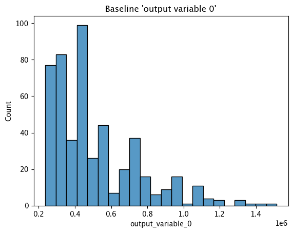
Baseline Histogram Chart
The method wallaroo.assay_config.AssayBuilder.baseline_histogram returns a histogram chart of the assay baseline generated from the provided parameters.
assay_builder_from_dates.baseline_histogram()
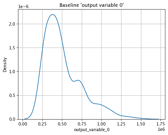
Baseline KDE Chart
The method wallaroo.assay_config.AssayBuilder.baseline_kde returns a Kernel Density Estimation (KDE) chart of the assay baseline generated from the provided parameters.
assay_builder_from_dates.baseline_kde()
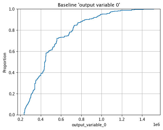
Baseline ECDF Chart
The method wallaroo.assay_config.AssayBuilder.baseline_ecdf returns a Empirical Cumulative Distribution Function (CDF) chart of the assay baseline generated from the provided parameters.
assay_builder_from_dates.baseline_ecdf()
Assay Preview
Now that the baseline is defined, we look at different configuration options and view how the assay baseline and results changes. Once we determine what gives us the best method of determining model drift, we can create the assay.
Analysis List Chart Scores
Analysis List scores show the assay scores for each assay result interval in one chart. Values that are outside of the alert threshold are colored red, while scores within the alert threshold are green.
Assay chart scores are displayed with the method wallaroo.assay.AssayAnalysisList.chart_scores(title: Optional[str] = None), with ability to display an optional title with the chart.
The following example shows retrieving the assay results and displaying the chart scores. From our example, we have two windows - the first should be green, and the second is red showing that values were outside the alert threshold.
# Build the assay, based on the start and end of our baseline time,
# and tracking the output variable index 0
assay_builder_from_dates = wl.build_assay(assay_name="run anywhere from dates",
                                          pipeline=mainpipeline,
                                          model_name="house-price-estimator",
                                          iopath="output variable 0",
                                          baseline_start=assay_baseline_start,
                                          baseline_end=assay_baseline_end)

# set the width, interval, and time period
assay_builder_from_dates.add_run_until(datetime.datetime.now())
assay_builder_from_dates.window_builder().add_width(minutes=1).add_interval(minutes=1).add_start(assay_window_start)
assay_config_from_dates = assay_builder_from_dates.build()
assay_results_from_dates = assay_config_from_dates.interactive_run()

assay_results_from_dates.chart_scores()

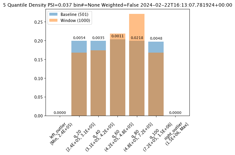
Analysis Chart
The method wallaroo.assay.AssayAnalysis.chart() displays a comparison between the baseline and an interval of inference data.
This is compared to the Chart Scores, which is a list of all of the inference data split into intervals, while the Analysis Chart shows the breakdown of one set of inference data against the baseline.
Score from the Analysis List Chart Scores and each element from the Analysis List DataFrame generates
The following fields are included.
| Field | Type | Description |
|---|---|---|
| baseline mean | Float | The mean of the baseline values. |
| window mean | Float | The mean of the window values. |
| baseline median | Float | The median of the baseline values. |
| window median | Float | The median of the window values. |
| bin_mode | String | The binning mode used for the assay. |
| aggregation | String | The aggregation mode used for the assay. |
| metric | String | The metric mode used for the assay. |
| weighted | Bool | Whether the bins were manually weighted. |
| score | Float | The score from the assay window. |
| scores | List(Float) | The score from each assay window bin. |
| index | Integer/None | The window index. Interactive assay runs are None. |
# Build the assay, based on the start and end of our baseline time,
# and tracking the output variable index 0
assay_builder_from_dates = wl.build_assay(assay_name="run anywhere from dates",
                                          pipeline=mainpipeline,
                                          model_name="house-price-estimator",
                                          iopath="output variable 0",
                                          baseline_start=assay_baseline_start,
                                          baseline_end=assay_baseline_end)

# set the width, interval, and time period
assay_builder_from_dates.add_run_until(datetime.datetime.now())
assay_builder_from_dates.window_builder().add_width(minutes=1).add_interval(minutes=1).add_start(assay_window_start)
assay_config_from_dates = assay_builder_from_dates.build()
assay_results_from_dates = assay_config_from_dates.interactive_run()

assay_results_from_dates[0].chart()
baseline mean = 513088.88569735526
window mean = 523401.741328125
baseline median = 444408.0
window median = 448627.8125
bin_mode = Quantile
aggregation = Density
metric = PSI
weighted = False
score = 0.036723431597836184
scores = [0.0, 0.0054465677587239095, 0.00351406964764097, 0.0011239501647170409, 0.021833837078132627, 0.004805006948621639, 0.0]
index = None
Analysis List DataFrame
wallaroo.assay.AssayAnalysisList.to_dataframe() returns a DataFrame showing the assay results for each window aka individual analysis. This DataFrame contains the following fields:
| Field | Type | Description |
|---|---|---|
| assay_id | Integer/None | The assay id. Only provided from uploaded and executed assays. |
| name | String/None | The name of the assay. Only provided from uploaded and executed assays. |
| iopath | String/None | The iopath of the assay. Only provided from uploaded and executed assays. |
| score | Float | The assay score. |
| start | DateTime | The DateTime start of the assay window. |
| min | Float | The minimum value in the assay window. |
| max | Float | The maximum value in the assay window. |
| mean | Float | The mean value in the assay window. |
| median | Float | The median value in the assay window. |
| std | Float | The standard deviation value in the assay window. |
| warning_threshold | Float/None | The warning threshold of the assay window. |
| alert_threshold | Float/None | The alert threshold of the assay window. |
| status | String | The assay window status. Values are:
|
For this example, the assay analysis list DataFrame is listed.
From this tutorial, we should have 2 windows of dta to look at, each one minute apart. The first window should show status: OK, with the second window with the very large house prices will show status: alert
# Build the assay, based on the start and end of our baseline time,
# and tracking the output variable index 0
assay_builder_from_dates = wl.build_assay(assay_name="assays from date baseline",
                                          pipeline=mainpipeline,
                                          model_name="house-price-estimator",
                                          iopath="output variable 0",
                                          baseline_start=assay_baseline_start,
                                          baseline_end=assay_baseline_end)

# set the width, interval, and time period
assay_builder_from_dates.add_run_until(datetime.datetime.now())
assay_builder_from_dates.window_builder().add_width(minutes=1).add_interval(minutes=1).add_start(assay_window_start)
assay_config_from_dates = assay_builder_from_dates.build()
assay_results_from_dates = assay_config_from_dates.interactive_run()

assay_results_from_dates.to_dataframe()
| assay_id | name | iopath | score | start | min | max | mean | median | std | warning_threshold | alert_threshold | status | |
|---|---|---|---|---|---|---|---|---|---|---|---|---|---|
| 0 | None | 0.036723 | 2024-02-22T16:13:07.781924+00:00 | 2.362387e+05 | 1489624.250 | 5.234017e+05 | 4.486278e+05 | 230914.012105 | None | 0.25 | Ok | ||
| 1 | None | 0.082877 | 2024-02-22T16:15:07.781924+00:00 | 2.362387e+05 | 2016006.125 | 5.473354e+05 | 4.815304e+05 | 260871.745557 | None | 0.25 | Ok | ||
| 2 | None | 0.069016 | 2024-02-22T16:20:07.781924+00:00 | 2.362387e+05 | 2016006.000 | 5.394895e+05 | 4.510469e+05 | 264051.044244 | None | 0.25 | Ok | ||
| 3 | None | 8.868532 | 2024-02-22T16:21:07.781924+00:00 | 1.514079e+06 | 2016006.125 | 1.882197e+06 | 1.946438e+06 | 160686.049379 | None | 0.25 | Alert |
Configure Assays
Before creating the assay, configure the assay and continue to preview it until the best method for detecting drift is set.
Location Filter
This tutorial focuses on the assay configuration method wallaroo.assay_config.WindowBuilder.add_location_filter which takes the following parameters.
| Parameter | Type | Description |
|---|---|---|
| locations | List(String) | The list of model deployment locations for the assay. |
By default, the locations parameter includes all locations as part of the pipeline. This is seen in the default where no location filter is set, and of the inference data is shown.
# Build the assay, based on the start and end of our baseline time,
# and tracking the output variable index 0
assay_builder_from_dates = wl.build_assay(assay_name="run anywhere from dates",
                                          pipeline=mainpipeline,
                                          model_name="house-price-estimator",
                                          iopath="output variable 0",
                                          baseline_start=assay_baseline_start,
                                          baseline_end=assay_baseline_end)

# set the width, interval, and time period
assay_builder_from_dates.add_run_until(datetime.datetime.now())
assay_builder_from_dates.window_builder().add_width(minutes=1).add_interval(minutes=1).add_start(assay_window_start)
assay_config_from_dates = assay_builder_from_dates.build()
assay_results_from_dates = assay_config_from_dates.interactive_run()

assay_results_from_dates.chart_scores()
assay_results_from_dates.to_dataframe()

| assay_id | name | iopath | score | start | min | max | mean | median | std | warning_threshold | alert_threshold | status | |
|---|---|---|---|---|---|---|---|---|---|---|---|---|---|
| 0 | None | 0.036723 | 2024-02-22T16:13:07.781924+00:00 | 2.362387e+05 | 1489624.250 | 5.234017e+05 | 4.486278e+05 | 230914.012105 | None | 0.25 | Ok | ||
| 1 | None | 0.082877 | 2024-02-22T16:15:07.781924+00:00 | 2.362387e+05 | 2016006.125 | 5.473354e+05 | 4.815304e+05 | 260871.745557 | None | 0.25 | Ok | ||
| 2 | None | 0.069016 | 2024-02-22T16:20:07.781924+00:00 | 2.362387e+05 | 2016006.000 | 5.394895e+05 | 4.510469e+05 | 264051.044244 | None | 0.25 | Ok | ||
| 3 | None | 8.868532 | 2024-02-22T16:21:07.781924+00:00 | 1.514079e+06 | 2016006.125 | 1.882197e+06 | 1.946438e+06 | 160686.049379 | None | 0.25 | Alert |
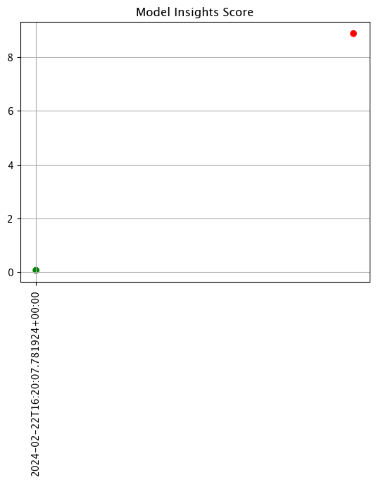
Now we will set the location to the ops center only pipeline and display the results.
# Build the assay, based on the start and end of our baseline time,
# and tracking the output variable index 0
assay_builder_from_dates = wl.build_assay(assay_name="run anywhere from dates",
                                          pipeline=mainpipeline,
                                          model_name="house-price-estimator",
                                          iopath="output variable 0",
                                          baseline_start=assay_baseline_start,
                                          baseline_end=assay_baseline_end)

# set the location to the ops center
assay_builder_from_dates.window_builder().add_location_filter([ops_location])

# set the width, interval, and time period
assay_builder_from_dates.add_run_until(datetime.datetime.now())
assay_builder_from_dates.window_builder().add_width(minutes=1).add_interval(minutes=1).add_start(assay_window_start)
assay_config_from_dates = assay_builder_from_dates.build()
assay_results_from_dates = assay_config_from_dates.interactive_run()

assay_results_from_dates.chart_scores()
assay_results_from_dates.to_dataframe()
| assay_id | name | iopath | score | start | min | max | mean | median | std | warning_threshold | alert_threshold | status | |
|---|---|---|---|---|---|---|---|---|---|---|---|---|---|
| 0 | None | 0.036723 | 2024-02-22T16:13:07.781924+00:00 | 236238.671875 | 1489624.250 | 523401.741328 | 448627.812500 | 230914.012105 | None | 0.25 | Ok | ||
| 1 | None | 0.082877 | 2024-02-22T16:15:07.781924+00:00 | 236238.671875 | 2016006.125 | 547335.355203 | 481530.359375 | 260871.745557 | None | 0.25 | Ok |
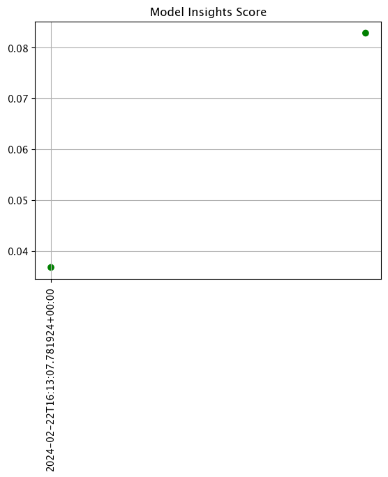
Now we specify only our edge deployment location.
# Build the assay, based on the start and end of our baseline time,
# and tracking the output variable index 0
assay_builder_from_dates = wl.build_assay(assay_name="run anywhere from dates",
                                          pipeline=mainpipeline,
                                          model_name="house-price-estimator",
                                          iopath="output variable 0",
                                          baseline_start=assay_baseline_start,
                                          baseline_end=assay_baseline_end)

# set the location to the the edge location
assay_builder_from_dates.window_builder().add_location_filter([edge_name])

# set the width, interval, and time period
assay_builder_from_dates.add_run_until(datetime.datetime.now())
assay_builder_from_dates.window_builder().add_width(minutes=1).add_interval(minutes=1).add_start(assay_window_start)
assay_config_from_dates = assay_builder_from_dates.build()
assay_results_from_dates = assay_config_from_dates.interactive_run()

assay_results_from_dates.chart_scores()
assay_results_from_dates.to_dataframe()
| assay_id | name | iopath | score | start | min | max | mean | median | std | warning_threshold | alert_threshold | status | |
|---|---|---|---|---|---|---|---|---|---|---|---|---|---|
| 0 | None | 0.069016 | 2024-02-22T16:20:07.781924+00:00 | 2.362387e+05 | 2016006.000 | 5.394895e+05 | 4.510469e+05 | 264051.044244 | None | 0.25 | Ok | ||
| 1 | None | 8.868532 | 2024-02-22T16:21:07.781924+00:00 | 1.514079e+06 | 2016006.125 | 1.882197e+06 | 1.946438e+06 | 160686.049379 | None | 0.25 | Alert |
Now we specify both the Wallaroo Ops deployed pipeline and the edge pipeline.
# Build the assay, based on the start and end of our baseline time,
# and tracking the output variable index 0
assay_builder_from_dates = wl.build_assay(assay_name="run anywhere from dates",
                                          pipeline=mainpipeline,
                                          model_name="house-price-estimator",
                                          iopath="output variable 0",
                                          baseline_start=assay_baseline_start,
                                          baseline_end=assay_baseline_end)

# set the location to both the edge location and ops pipeline
assay_builder_from_dates.window_builder().add_location_filter([ops_location, edge_name])

# set the width, interval, and time period
assay_builder_from_dates.add_run_until(datetime.datetime.now())
assay_builder_from_dates.window_builder().add_width(minutes=1).add_interval(minutes=1).add_start(assay_window_start)
assay_config_from_dates = assay_builder_from_dates.build()
assay_results_from_dates = assay_config_from_dates.interactive_run()

assay_results_from_dates.chart_scores()
assay_results_from_dates.to_dataframe()
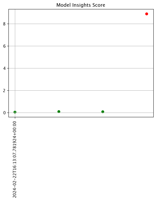
| assay_id | name | iopath | score | start | min | max | mean | median | std | warning_threshold | alert_threshold | status | |
|---|---|---|---|---|---|---|---|---|---|---|---|---|---|
| 0 | None | 0.036723 | 2024-02-22T16:13:07.781924+00:00 | 2.362387e+05 | 1489624.250 | 5.234017e+05 | 4.486278e+05 | 230914.012105 | None | 0.25 | Ok | ||
| 1 | None | 0.082877 | 2024-02-22T16:15:07.781924+00:00 | 2.362387e+05 | 2016006.125 | 5.473354e+05 | 4.815304e+05 | 260871.745557 | None | 0.25 | Ok | ||
| 2 | None | 0.069016 | 2024-02-22T16:20:07.781924+00:00 | 2.362387e+05 | 2016006.000 | 5.394895e+05 | 4.510469e+05 | 264051.044244 | None | 0.25 | Ok | ||
| 3 | None | 8.868532 | 2024-02-22T16:21:07.781924+00:00 | 1.514079e+06 | 2016006.125 | 1.882197e+06 | 1.946438e+06 | 160686.049379 | None | 0.25 | Alert |
Create Assay
With the assay previewed and configuration options determined, we officially create it by uploading it to the Wallaroo instance.
Once it is uploaded, the assay runs an analysis based on the window width, interval, and the other settings configured.
Assays are uploaded with the wallaroo.assay_config.upload() method. This uploads the assay into the Wallaroo database with the configurations applied and returns the assay id. Note that assay names must be unique across the Wallaroo instance; attempting to upload an assay with the same name as an existing one will return an error.
wallaroo.assay_config.upload() returns the assay id for the assay.
Typically we would just call wallaroo.assay_config.upload() after configuring the assay. For the example below, we will perform the complete configuration in one window to show all of the configuration steps at once before creating the assay, and narrow the locations to only the Wallaroo Ops deployed pipeline and the single edge.
# Build the assay, based on the start and end of our baseline time,
# and tracking the output variable index 0
assay_builder_from_dates = wl.build_assay(assay_name="run anywhere from dates",
                                          pipeline=mainpipeline,
                                          model_name="house-price-estimator",
                                          iopath="output variable 0",
                                          baseline_start=assay_baseline_start,
                                          baseline_end=assay_baseline_end)

# set the location to both the edge location and ops pipeline
assay_builder_from_dates.window_builder().add_location_filter([ops_location, edge_name])

# set the width, interval, and time period
assay_builder_from_dates.add_run_until(datetime.datetime.now())
assay_builder_from_dates.window_builder().add_width(minutes=1).add_interval(minutes=1).add_start(assay_window_start)

assay_id = assay_builder_from_dates.upload()
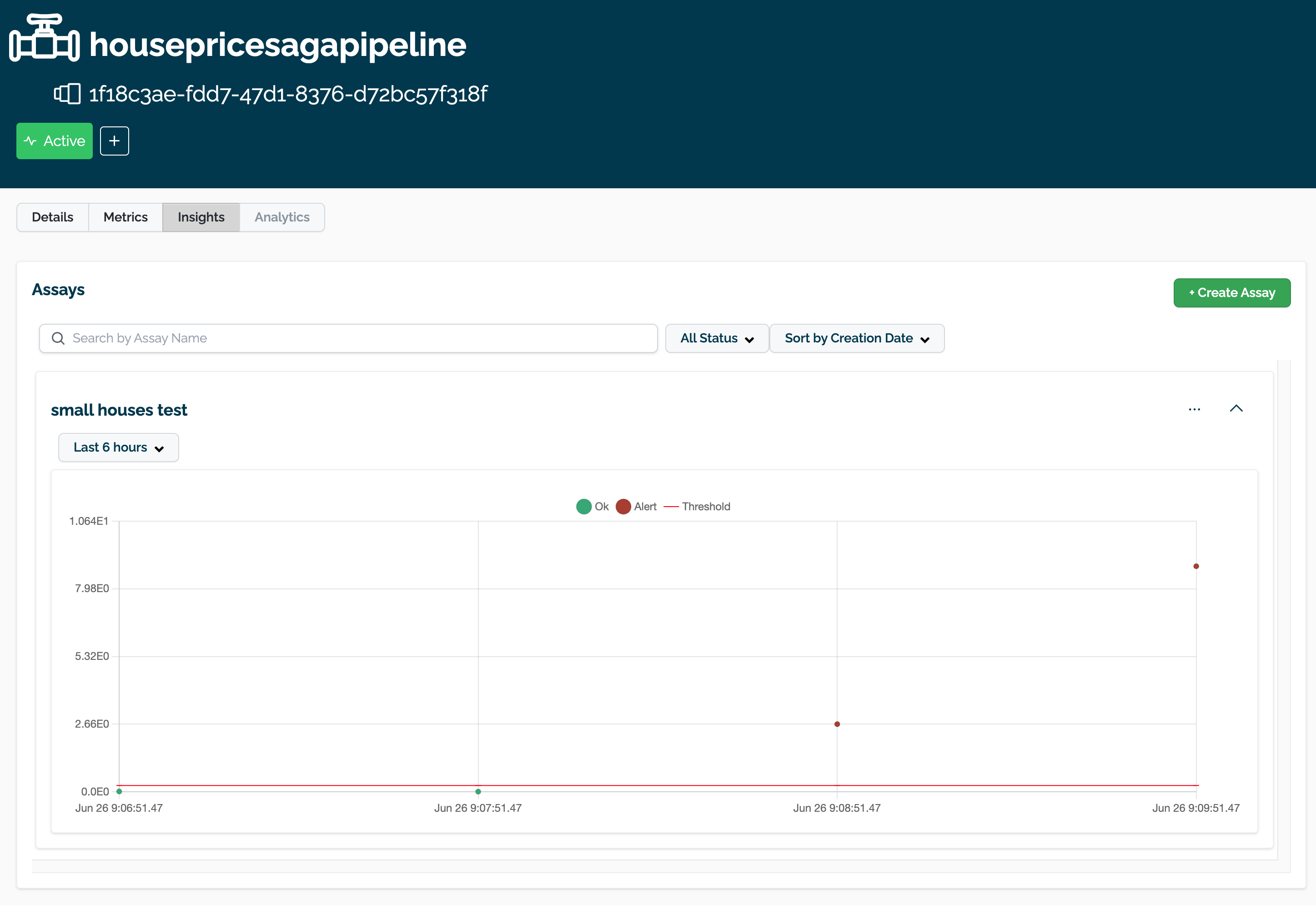
The assay is now visible through the Wallaroo UI by selecting the workspace, then the pipeline, then Insights. The following is an example of another assay in the Wallaroo Dashboard.
Get Assay Results
Once an assay is created the assay runs an analysis based on the window width, interval, and the other settings configured.
Assay results are retrieved with the wallaroo.client.get_assay_results method, which takes the following parameters:
| Parameter | Type | Description |
|---|---|---|
| assay_id | Integer (Required) | The numerical id of the assay. |
| start | Datetime.Datetime (Required) | The start date and time of historical data from the pipeline to start analyses from. |
| end | Datetime.Datetime (Required) | The end date and time of historical data from the pipeline to limit analyses to. |
- IMPORTANT NOTE: This process requires that additional historical data is generated from the time the assay is created to when the results are available. To add additional inference data, use the Assay Test Data section above.
assay_results = wl.get_assay_results(assay_id=assay_id,
                     start=assay_window_start,
                     end=datetime.datetime.now())

assay_results.chart_scores()

assay_results[0].chart()
baseline mean = 513088.88569735526
window mean = 523401.741328125
baseline median = 444408.0
window median = 448627.8125
bin_mode = Quantile
aggregation = Density
metric = PSI
weighted = False
score = 0.03672343
scores = [0.0, 0.0054465677587239095, 0.00351406964764097, 0.0011239501647170409, 0.021833837078132627, 0.004805006948621639, 0.0]
index = None
