Retail: Drift Detection
Tutorial Notebook 3: Observability - Drift Detection
In the previous notebook you learned how to add simple validation rules to a pipeline, to monitor whether outputs (or inputs) stray out of some expected range. In this notebook, you will monitor the distribution of the pipeline’s predictions to see if the model, or the environment that it runs it, has changed.
Preliminaries
In the blocks below we will preload some required libraries; we will also redefine some of the convenience functions that you saw in the previous notebooks.
After that, you should log into Wallaroo and set your working environment to the workspace that you created for this tutorial. Please refer to Notebook 1 to refresh yourself on how to log in and set your working environment to the appropriate workspace.
# preload needed libraries
import wallaroo
from wallaroo.object import EntityNotFoundError
from wallaroo.framework import Framework
from IPython.display import display
# used to display DataFrame information without truncating
from IPython.display import display
import pandas as pd
pd.set_option('display.max_colwidth', None)
import json
import datetime
import time
# used for unique connection names
import string
import random
import pyarrow as pa
import sys
# setting path - only needed when running this from the `with-code` folder.
sys.path.append('../')
from CVDemoUtils import CVDemo
cvDemo = CVDemo()
cvDemo.COCO_CLASSES_PATH = "../models/coco_classes.pickle"
## convenience functions from the previous notebooks
## these functions assume your connection to wallaroo is called wl
# return the workspace called <name>, or create it if it does not exist.
# this function assumes your connection to wallaroo is called wl
def get_workspace(name):
workspace = None
for ws in wl.list_workspaces():
if ws.name() == name:
workspace= ws
if(workspace == None):
workspace = wl.create_workspace(name)
return workspace
# pull a single datum from a data frame
# and convert it to the format the model expects
def get_singleton(df, i):
singleton = df.iloc[i,:].to_numpy().tolist()
sdict = {'tensor': [singleton]}
return pd.DataFrame.from_dict(sdict)
# pull a batch of data from a data frame
# and convert to the format the model expects
def get_batch(df, first=0, nrows=1):
last = first + nrows
batch = df.iloc[first:last, :].to_numpy().tolist()
return pd.DataFrame.from_dict({'tensor': batch})
# Translated a column from a dataframe into a single array
# used for the Statsmodel forecast model
def get_singleton_forecast(df, field):
singleton = pd.DataFrame({field: [df[field].values.tolist()]})
return singleton
# Get the most recent version of a model in the workspace
# Assumes that the most recent version is the first in the list of versions.
# wl.get_current_workspace().models() returns a list of models in the current workspace
def get_model(mname):
modellist = wl.get_current_workspace().models()
model = [m.versions()[-1] for m in modellist if m.name() == mname]
if len(model) <= 0:
raise KeyError(f"model {mname} not found in this workspace")
return model[0]
# get a pipeline by name in the workspace
def get_pipeline(pname):
plist = wl.get_current_workspace().pipelines()
pipeline = [p for p in plist if p.name() == pname]
if len(pipeline) <= 0:
raise KeyError(f"pipeline {pname} not found in this workspace")
return pipeline[0]
## blank space to log in and go to correct workspace
## blank space to log in and go to the appropriate workspace
wl = wallaroo.Client()
import string
import random
suffix= ''.join(random.choice(string.ascii_lowercase) for i in range(4))
workspace_name = f'computer-vision-tutorial'
workspace = get_workspace(workspace_name)
wl.set_current_workspace(workspace)
{'name': 'computer-vision-tutorialjohn', 'id': 20, 'archived': False, 'created_by': '0a36fba2-ad42-441b-9a8c-bac8c68d13fa', 'created_at': '2023-08-04T19:16:04.283819+00:00', 'models': [{'name': 'mobilenet', 'versions': 4, 'owner_id': '""', 'last_update_time': datetime.datetime(2023, 8, 4, 19, 42, 22, 155273, tzinfo=tzutc()), 'created_at': datetime.datetime(2023, 8, 4, 19, 19, 46, 286247, tzinfo=tzutc())}, {'name': 'cv-post-process-drift-detection', 'versions': 3, 'owner_id': '""', 'last_update_time': datetime.datetime(2023, 8, 4, 19, 42, 23, 233883, tzinfo=tzutc()), 'created_at': datetime.datetime(2023, 8, 4, 19, 23, 10, 189958, tzinfo=tzutc())}, {'name': 'resnet', 'versions': 2, 'owner_id': '""', 'last_update_time': datetime.datetime(2023, 8, 5, 17, 25, 35, 579362, tzinfo=tzutc()), 'created_at': datetime.datetime(2023, 8, 5, 17, 20, 21, 886290, tzinfo=tzutc())}], 'pipelines': [{'name': 'cv-retail-pipeline', 'create_time': datetime.datetime(2023, 8, 4, 19, 23, 11, 179176, tzinfo=tzutc()), 'definition': '[]'}]}
Monitoring for Drift: Shift Happens.
In machine learning, you use data and known answers to train a model to make predictions for new previously unseen data. You do this with the assumption that the future unseen data will be similar to the data used during training: the future will look somewhat like the past.
But the conditions that existed when a model was created, trained and tested can change over time, due to various factors.
A good model should be robust to some amount of change in the environment; however, if the environment changes too much, your models may no longer be making the correct decisions. This situation is known as concept drift; too much drift can obsolete your models, requiring periodic retraining.
Let’s consider the example we’ve been working on: computer vision. You may notice over time that there has been a change in the average confidence of recognizing objects in an image. Perhaps the inventory has changed enough that recognizing a bottle of milk isn’t the same as recognizing a bag of milk. Perhaps tne new images are coming in at a lower quality
In Wallaroo you can monitor your housing model for signs of drift through the model monitoring and insight capability called Assays. Assays help you track changes in the environment that your model operates within, which can affect the model’s outcome. It does this by tracking the model’s predictions and/or the data coming into the model against an established baseline. If the distribution of monitored values in the current observation window differs too much from the baseline distribution, the assay will flag it. The figure below shows an example of a running scheduled assay.
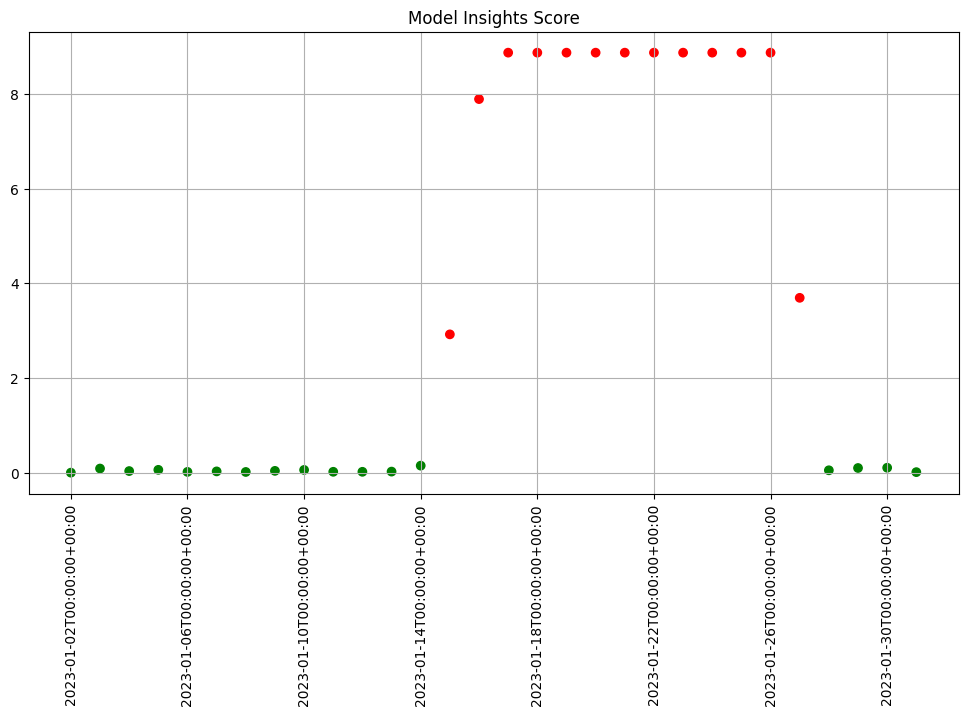
Figure: A daily assay that’s been running for a month. The dots represent the difference between the distribution of values in the daily observation window, and the baseline. When that difference exceeds the specified threshold (indicated by a red dot) an alert is set.
This next set of exercises will walk you through setting up an assay to monitor the predictions of your house price model, in order to detect drift.
NOTE
An assay is a monitoring process that typically runs over an extended, ongoing period of time. For example, one might set up an assay that every day monitors the previous 24 hours’ worth of predictions and compares it to a baseline. For the purposes of these exercises, we’ll be compressing processes what normally would take hours or days into minutes.
Exercise Prep: Create some datasets for demonstrating assays
Because assays are designed to detect changes in distributions, let’s try to set up data with different distributions to test with. Take your houseprice data and create two sets: a set with lower prices, and a set with higher prices. You can split however you choose.
The idea is we will pretend that the set of lower priced houses represent the “typical” mix of houses in the housing portfolio at the time you set your baseline; you will introduce the higher priced houses later, to represent an environmental change when more expensive houses suddenly enter the market.
- If you are using the pre-provided models to do these exercises, you can use the provided data sets of images that show high confidence versus low confidence images. This is to establish our baseline as a set of known values, so the higher prices will trigger our assay alerts.
sample_images = [
"../data/images/input/example/coats-jackets.png",
"../data/images/input/example/dairy_bottles.png",
"../data/images/input/example/dairy_products.png",
"../data/images/input/example/example_01.jpg",
"../data/images/input/example/example_02.jpg",
"../data/images/input/example/example_03.jpg",
"../data/images/input/example/example_04.jpg",
"../data/images/input/example/example_05.jpg",
"../data/images/input/example/example_06.jpg",
"../data/images/input/example/example_09.jpg",
"../data/images/input/example/example_dress.jpg",
"../data/images/input/example/example_shoe.jpg",
"../data/images/input/example/frame5244.jpg",
"../data/images/input/example/frame8744.jpg",
"../data/images/input/example/product_cheeses.png",
"../data/images/input/example/store-front.png",
"../data/images/input/example/vegtables_poor_identification.jpg"
]
# high confidence images
baseline_images = [
"../data/images/input/example/example_02.jpg",
"../data/images/input/example/example_05.jpg",
"../data/images/input/example/example_dress.jpg",
]
# low confidence images
bad_images = [
"../data/images/input/example/coats-jackets.png",
"../data/images/input/example/frame8744.jpg",
]
# blank spot to split or download data
import datetime
import time
startBaseline = datetime.datetime.now()
startTime = time.time()
sample_images = [
"../data/images/input/example/coats-jackets.png",
"../data/images/input/example/dairy_bottles.png",
"../data/images/input/example/dairy_products.png",
"../data/images/input/example/example_01.jpg",
"../data/images/input/example/example_02.jpg",
"../data/images/input/example/example_03.jpg",
"../data/images/input/example/example_04.jpg",
"../data/images/input/example/example_05.jpg",
"../data/images/input/example/example_06.jpg",
"../data/images/input/example/example_09.jpg",
"../data/images/input/example/example_dress.jpg",
"../data/images/input/example/example_shoe.jpg",
"../data/images/input/example/frame5244.jpg",
"../data/images/input/example/frame8744.jpg",
"../data/images/input/example/product_cheeses.png",
"../data/images/input/example/store-front.png",
"../data/images/input/example/vegtables_poor_identification.jpg"
]
baseline_images = [
"../data/images/input/example/example_02.jpg",
"../data/images/input/example/example_05.jpg",
"../data/images/input/example/example_dress.jpg",
]
bad_images = [
"../data/images/input/example/coats-jackets.png",
"../data/images/input/example/frame8744.jpg",
]
We will use this data to set up some “historical data” in the computer vision pipeline that you build in the assay exercises.
Setting up a baseline for the assay
In order to know whether the distribution of your model’s predictions have changed, you need a baseline to compare them to. This baseline should represent how you expect the model to behave at the time it was trained. This might be approximated by the distribution of the model’s predictions over some “typical” period of time. For example, we might collect the predictions of our model over the first few days after it’s been deployed. For these exercises, we’ll compress that to a few minutes. Currently, to set up a wallaroo assay the pipeline must have been running for some period of time, and the assumption is that this period of time is “typical”, and that the distributions of the inputs and the outputs of the model during this period of time are “typical.”
Exercise Prep: Run some inferences and set some time stamps
Here, we simulate having a pipeline that’s been running for a long enough period of time to set up an assay.
To send enough data through the pipeline to create assays, you execute something like the following code (using the appropriate names for your pipelines and models). Note that this step will take a little while, because of the sleep interval.
You will need the timestamps baseline_start, and baseline_end, for the next exercises.
# get your pipeline (in this example named "mypipeline")
pipeline = get_pipeline("mypipeline")
pipeline.deploy()
## Run some baseline data
# Where the baseline data will start
baseline_start = datetime.datetime.now()
# the number of samples we'll use for the baseline
nsample = 500
# Wait 30 seconds to set this data apart from the rest
# then send the data in batch
time.sleep(30)
# get a sample
# convert all of these into a parallel infer list, then one parallel infer to cut down time
for image in baseline_images:
width, height = 640, 480
dfImage, resizedImage = cvDemo.loadImageAndConvertToDataframe(image,
width,
height
)
inference_list.append(dfImage)
parallel_results = await pipeline.parallel_infer(tensor_list=inference_list, timeout=60, num_parallel=2, retries=2)
# Set the baseline end
baseline_end = datetime.datetime.now()
mobilenet_model_name = 'mobilenet'
mobilenet_model_path = "../models/mobilenet.pt.onnx"
mobilenet_model = wl.upload_model(mobilenet_model_name,
mobilenet_model_path,
framework=Framework.ONNX).configure('onnx',
batch_config="single"
)
# upload python step
field_boxes = pa.field('boxes', pa.list_(pa.list_(pa.float64(), 4)))
field_classes = pa.field('classes', pa.list_(pa.int32()))
field_confidences = pa.field('confidences', pa.list_(pa.float64()))
# field_boxes - will have a flattened array of the 4 coordinates representing the boxes. 128 entries
# field_classes - will have 32 entries
# field_confidences - will have 32 entries
input_schema = pa.schema([field_boxes, field_classes, field_confidences])
output_schema = pa.schema([
field_boxes,
field_classes,
field_confidences,
pa.field('avg_conf', pa.list_(pa.float64()))
])
module_post_process_model = wl.upload_model("cv-post-process-drift-detection",
"../models/post-process-drift-detection-arrow.py",
framework=Framework.PYTHON ).configure('python',
input_schema=input_schema,
output_schema=output_schema
)
# set the pipeline step
pipeline.undeploy()
pipeline.clear()
pipeline.add_model_step(mobilenet_model)
pipeline.add_model_step(module_post_process_model)
pipeline.deploy()
pipeline.steps()
[{'ModelInference': {'models': [{'name': 'mobilenet', 'version': '484fffe8-70fe-44b9-937f-e98838bcc245', 'sha': '9044c970ee061cc47e0c77e20b05e884be37f2a20aa9c0c3ce1993dbd486a830'}]}},
{'ModelInference': {'models': [{'name': 'cv-post-process-drift-detection', 'version': '3ae7dfc2-1b3c-44d3-9957-97c5704e3592', 'sha': 'f60c8ca55c6350d23a4e76d24cc3e5922616090686e88c875fadd6e79c403be5'}]}}]
# test inference
image = '../data/images/input/example/dairy_bottles.png'
width, height = 640, 480
dfImage, resizedImage = cvDemo.loadImageAndConvertToDataframe(image,
width,
height
)
results = pipeline.infer(dfImage, timeout=60)
display(results)
| time | in.tensor | out.avg_conf | out.boxes | out.classes | out.confidences | check_failures | |
|---|---|---|---|---|---|---|---|
| 0 | 2023-08-05 18:03:13.810 | [0.9372549057, 0.9529411793, 0.9490196109, 0.9450980425, 0.9450980425, 0.9450980425, 0.9450980425, 0.9450980425, 0.9450980425, 0.9450980425, 0.9450980425, 0.9450980425, 0.9450980425, 0.9450980425, 0.9450980425, 0.9450980425, 0.9450980425, 0.9450980425, 0.9490196109, 0.9490196109, 0.9529411793, 0.9529411793, 0.9490196109, 0.9607843161, 0.9686274529, 0.9647058845, 0.9686274529, 0.9647058845, 0.9568627477, 0.9607843161, 0.9647058845, 0.9647058845, 0.9607843161, 0.9647058845, 0.9725490212, 0.9568627477, 0.9607843161, 0.9176470637, 0.9568627477, 0.9176470637, 0.8784313798, 0.8941176534, 0.8431372643, 0.8784313798, 0.8627451062, 0.850980401, 0.9254902005, 0.8470588326, 0.9686274529, 0.8941176534, 0.8196078539, 0.850980401, 0.9294117689, 0.8666666746, 0.8784313798, 0.8666666746, 0.9647058845, 0.9764705896, 0.980392158, 0.9764705896, 0.9725490212, 0.9725490212, 0.9725490212, 0.9725490212, 0.9725490212, 0.9725490212, 0.980392158, 0.8941176534, 0.4823529422, 0.4627451003, 0.4313725531, 0.270588249, 0.2588235438, 0.2941176593, 0.3450980484, 0.3686274588, 0.4117647111, 0.4549019635, 0.4862745106, 0.5254902244, 0.5607843399, 0.6039215922, 0.6470588446, 0.6862745285, 0.721568644, 0.7450980544, 0.7490196228, 0.7882353067, 0.8666666746, 0.980392158, 0.9882352948, 0.9686274529, 0.9647058845, 0.9686274529, 0.9725490212, 0.9647058845, 0.9607843161, 0.9607843161, 0.9607843161, 0.9607843161, ...] | [0.2895053208114637] | [[0.0, 210.29010009765625, 85.26463317871094, 479.074951171875], [72.03781127929688, 197.32269287109375, 151.44223022460938, 468.4322509765625], [211.2801513671875, 184.72837829589844, 277.2192077636719, 420.4274597167969], [143.23904418945312, 203.83004760742188, 216.85546875, 448.8880920410156], [13.095015525817873, 41.91339111328125, 640.0, 480.0], [106.51464080810548, 206.14498901367188, 159.5464324951172, 463.9675598144531], [278.0636901855469, 1.521723747253418, 321.45782470703125, 93.56348419189452], [462.3183288574219, 104.16201782226562, 510.53961181640625, 224.75314331054688], [310.4559020996094, 1.395981788635254, 352.8512878417969, 94.1238250732422], [528.0485229492188, 268.4224853515625, 636.2671508789062, 475.7666015625], [220.06292724609375, 0.513851165771484, 258.3183288574219, 90.18019104003906], [552.8711547851562, 96.30235290527344, 600.7255859375, 233.53384399414065], [349.24072265625, 0.270343780517578, 404.1732482910156, 98.6802215576172], [450.8934631347656, 264.235595703125, 619.603271484375, 472.6517333984375], [261.51385498046875, 193.4335021972656, 307.17913818359375, 408.7524719238281], [509.2201843261719, 101.16539001464844, 544.1857299804688, 235.7373962402344], [592.482421875, 100.38687133789062, 633.7798461914062, 239.1343231201172], [475.5420837402344, 297.6141052246094, 551.0543823242188, 468.0154724121094], [368.81982421875, 163.61407470703125, 423.909423828125, 362.7887878417969], [120.66899871826172, 0.0, 175.9362030029297, 81.77457427978516], [72.48429107666016, 0.0, 143.5078887939453, 85.46980285644531], [271.1268615722656, 200.891845703125, 305.6260070800781, 274.5953674316406], [161.80728149414062, 0.0, 213.0830841064453, 85.42828369140625], [162.13323974609375, 0.0, 214.6081390380859, 83.81443786621094], [310.8910827636719, 190.9546813964844, 367.3292541503906, 397.2813720703125], [396.67083740234375, 166.49578857421875, 441.5286254882813, 360.07525634765625], [439.2252807617187, 256.26361083984375, 640.0, 473.165771484375], [544.5545654296875, 375.67974853515625, 636.8954467773438, 472.8069458007813], [272.79437255859375, 2.753482818603515, 306.8874206542969, 96.72763061523438], [453.7723388671875, 303.7969665527344, 524.5588989257812, 463.2135009765625], [609.8508911132812, 94.62291717529295, 635.7705078125, 211.13577270507812]] | [44, 44, 44, 44, 82, 44, 44, 44, 44, 44, 44, 44, 44, 44, 44, 44, 44, 44, 44, 84, 84, 44, 84, 44, 44, 44, 61, 44, 86, 44, 44] | [0.98649001121521, 0.9011535644531251, 0.607784628868103, 0.592232286930084, 0.5372903347015381, 0.45131680369377103, 0.43728515505790705, 0.43094053864479004, 0.40848338603973305, 0.39185276627540505, 0.35759133100509605, 0.31812658905982905, 0.26451286673545804, 0.23062895238399503, 0.204820647835731, 0.17462100088596302, 0.173138618469238, 0.159995809197425, 0.14913696050643901, 0.136640205979347, 0.133227065205574, 0.12218642979860302, 0.12130125612020401, 0.11956108361482601, 0.115278266370296, 0.09616333246231001, 0.08654832839965801, 0.078406944870948, 0.07234089076519, 0.06282090395689001, 0.052787985652685006] | 0 |
Before setting up an assay on this pipeline’s output, we may want to look at the distribution of the predictions over our selected baseline period. To do that, we’ll create an assay_builder that specifies the pipeline, the model in the pipeline, and the baseline period.. We’ll also specify that we want to look at the output of the model, which in the example code is named variable, and would appear as out.variable in the logs.
# print out one of the logs to get the name of the output variable
display(pipeline.logs(limit=1))
# get the model name directly off the pipeline (you could just hard code this, if you know the name)
model_name = pipeline.model_configs()[0].model().name()
assay_builder = ( wl.build_assay(assay_name, pipeline, model_name,
baseline_start, baseline_end)
.add_iopath("output variable 0") ) # specify that we are looking at the first output of the output variable "variable"
where baseline_start and baseline_end are the beginning and end of the baseline periods as datetime.datetime objects.
You can then examine the distribution of variable over the baseline period:
assay_builder.baseline_histogram()
Exercise: Create an assay builder and set a baseline
Create an assay builder to monitor the output of your house price pipeline. The baseline period should be from baseline_start to baseline_end.
- You will need to know the name of your output variable, and the name of the model in the pipeline.
Examine the baseline distribution.
## Blank space to create an assay builder and examine the baseline distribution
# now build the actual baseline
# # do an inference off each image
image_confidence = pd.DataFrame(columns=["path", "confidence"])
inference_list = []
# convert all of these into a parallel infer list, then one parallel infer to cut down time
for image in baseline_images:
width, height = 640, 480
dfImage, resizedImage = cvDemo.loadImageAndConvertToDataframe(image,
width,
height
)
inference_list.append(dfImage)
display(inference_list)
startTime = time.time()
parallel_results = await pipeline.parallel_infer(tensor_list=inference_list, timeout=60, num_parallel=2, retries=2)
display(parallel_results)
endTime = time.time()
endBaseline = datetime.datetime.now()
[ tensor
0 [[[[0.18039216 0.18039216 0.18039216 0.18039216 0.18039216 0.18039216\n 0.18039216 0.18039216 0.18039216 0.18039216 0.18039216 0.18039216\n 0.18039216 0.18039216 0.18039216 0.18039216 0.18039216 0.18039216\n 0.18039216 0.18039216 0.18039216 0.18039216 0.18039216 0.18039216\n 0.18039216 0.18039216 0.18039216 0.18039216 0.18039216 0.18039216\n 0.18039216 0.18039216 0.18039216 0.18039216 0.18039216 0.18039216\n 0.18039216 0.18039216 0.18039216 0.18039216 0.18039216 0.18039216\n 0.18431373 0.1882353 0.1882353 0.1882353 0.1882353 0.1882353\n 0.1882353 0.1882353 0.1882353 0.1882353 0.1882353 0.1882353\n 0.1882353 0.1882353 0.18431373 0.18039216 0.18039216 0.18039216\n 0.18039216 0.18039216 0.18039216 0.18039216 0.18039216 0.18039216\n 0.18039216 0.18039216 0.18039216 0.18039216 0.18039216 0.18431373\n 0.18431373 0.18431373 0.18431373 0.18431373 0.18431373 0.18431373\n 0.18431373 0.18431373 0.18431373 0.18431373 0.18431373 0.18431373\n 0.18431373 0.18039216 0.18039216 0.18039216 0.18039216 0.18039216\n 0.18039216 0.18039216 0.18039216 0.18039216 0.18039216 0.18039216\n 0.18039216 0.18039216 0.18039216 0.18431373 0.1882353 0.1882353\n 0.1882353 0.1882353 0.1882353 0.1882353 0.1882353 0.1882353\n 0.1882353 0.1882353 0.1882353 0.1882353 0.1882353 0.1882353\n 0.1882353 0.1882353 0.1882353 0.1882353 0.1882353 0.1882353\n 0.1882353 0.1882353 0.1882353 0.1882353 0.1882353 0.1882353\n 0.1882353 0.1882353 0.1882353 0.1882353 0.1882353 0.1882353\n 0.1882353 0.1882353 0.1882353 0.1882353 0.1882353 0.1882353\n 0.1882353 0.1882353 0.1882353 0.1882353 0.1882353 0.1882353\n 0.1882353 0.1882353 0.1882353 0.1882353 0.1882353 0.1882353\n 0.1882353 0.1882353 0.1882353 0.1882353 0.1882353 0.1882353\n 0.1882353 0.1882353 0.1882353 0.1882353 0.1882353 0.1882353\n 0.1882353 0.1882353 0.1882353 0.1882353 0.1882353 0.1882353\n 0.1882353 0.1882353 0.18431373 0.18431373 0.18431373 0.18431373\n 0.18431373 0.18431373 0.18431373 0.18431373 0.18431373 0.18431373\n 0.18431373 0.18431373 0.18431373 0.18431373 0.18431373 0.18431373\n 0.18431373 0.18431373 0.18431373 0.18431373 0.18431373 0.18431373\n 0.18431373 0.18431373 0.18431373 0.18431373 0.18431373 0.18431373\n 0.18431373 0.18039216 0.18039216 0.18039216 0.18039216 0.18039216\n 0.18039216 0.18039216 0.18039216 0.18039216 0.18039216 0.18039216\n 0.18039216 0.18039216 0.18039216 0.1764706 0.1764706 0.1764706\n 0.1764706 0.1764706 0.1764706 0.1764706 0.1764706 0.1764706\n 0.1764706 0.1764706 0.1764706 0.1764706 0.1764706 0.1764706\n 0.18039216 0.18039216 0.18039216 0.18039216 0.18039216 0.18039216\n 0.18039216 0.18039216 0.18039216 0.18039216 0.18039216 0.18039216\n 0.18039216 0.18039216 0.18039216 0.18039216 0.18039216 0.18039216\n 0.18039216 0.18039216 0.18039216 0.18039216 0.18039216 0.18039216\n 0.18039216 0.18039216 0.18039216 0.18039216 0.1764706 0.1764706\n 0.1764706 0.1764706 0.1764706 0.1764706 0.1764706 0.1764706\n 0.1764706 0.1764706 0.1764706 0.1764706 0.1764706 0.1764706\n 0.1764706 0.1764706 0.1764706 0.1764706 0.1764706 0.1764706\n 0.1764706 0.1764706 0.1764706 0.1764706 0.1764706 0.1764706\n 0.1764706 0.1764706 0.1764706 0.1764706 0.1764706 0.1764706\n 0.1764706 0.1764706 0.1764706 0.1764706 0.1764706 0.1764706\n 0.1764706 0.1764706 0.1764706 0.1764706 0.1764706 0.18039216\n 0.18039216 0.18039216 0.18039216 0.18039216 0.18039216 0.18039216\n 0.18039216 0.18039216 0.18039216 0.18039216 0.18039216 0.18039216\n 0.18039216 0.1764706 0.1764706 0.1764706 0.1764706 0.1764706\n 0.1764706 0.1764706 0.1764706 0.1764706 0.1764706 0.1764706\n 0.1764706 0.1764706 0.1764706 0.1764706 0.1764706 0.1764706\n 0.1764706 0.1764706 0.1764706 0.1764706 0.1764706 0.1764706\n 0.1764706 0.1764706 0.1764706 0.1764706 0.1764706 0.1764706\n 0.1764706 0.1764706 0.1764706 0.1764706 0.1764706 0.1764706\n 0.1764706 0.1764706 0.1764706 0.1764706 0.1764706 0.1764706\n 0.1764706 0.1764706 0.1764706 0.1764706 0.1764706 0.1764706\n 0.1764706 0.1764706 0.1764706 0.1764706 0.1764706 0.1764706\n 0.1764706 0.1764706 0.1764706 0.17254902 0.17254902 0.17254902\n 0.17254902 0.17254902 0.17254902 0.17254902 0.17254902 0.16862746\n 0.16862746 0.16862746 0.16862746 0.16862746 0.16862746 0.16862746\n 0.16862746 0.16862746 0.16862746 0.16862746 0.16862746 0.16862746\n 0.16862746 0.16862746 0.16862746 0.16862746 0.16862746 0.16862746\n 0.16862746 0.16862746 0.16470589 0.16470589 0.16470589 0.16470589\n 0.16470589 0.16470589 0.16470589 0.16470589 0.16470589 0.16470589\n 0.16470589 0.16470589 0.16470589 0.16470589 0.16470589 0.16470589\n 0.16470589 0.16470589 0.16470589 0.16470589 0.16470589 0.16470589\n 0.16470589 0.16470589 0.16470589 0.16470589 0.16470589 0.16470589\n 0.16470589 0.16862746 0.16862746 0.16862746 0.16862746 0.16862746\n 0.16862746 0.16862746 0.16862746 0.16862746 0.16862746 0.16862746\n 0.16862746 0.16862746 0.16862746 0.16470589 0.16470589 0.16470589\n 0.16470589 0.16470589 0.16470589 0.16470589 0.16470589 0.16470589\n 0.16470589 0.16470589 0.16470589 0.16470589 0.16470589 0.16078432\n 0.16078432 0.16078432 0.16078432 0.16078432 0.16078432 0.16078432\n 0.16078432 0.16078432 0.16078432 0.16078432 0.16078432 0.16078432\n 0.16078432 0.16078432 0.16470589 0.16470589 0.16470589 0.16470589\n 0.16470589 0.16470589 0.16470589 0.16470589 0.16470589 0.16470589\n 0.16470589 0.16470589 0.16470589 0.16078432 0.16078432 0.16078432\n 0.16078432 0.16078432 0.16078432 0.16078432 0.16078432 0.16078432\n 0.16078432 0.16078432 0.16078432 0.16078432 0.16078432 0.16078432\n 0.16078432 0.16078432 0.16078432 0.16078432 0.16078432 0.16078432\n 0.16078432 0.16078432 0.16078432 0.16078432 0.16078432 0.16078432\n 0.16078432 0.16078432 0.16078432 0.16078432 0.16078432 0.16078432\n 0.16078432 0.16078432 0.16078432 0.16078432 0.16078432 0.16078432\n 0.16078432 0.16078432 0.16078432 0.16078432 0.15686275 0.15686275\n 0.15294118 0.15294118 0.15294118 0.15294118 0.15294118 0.15294118\n 0.15294118 0.14901961 0.14901961 0.14901961 0.14901961 0.14901961\n 0.14901961 0.14901961 0.14901961 0.14901961 0.14901961 0.14901961\n 0.14901961 0.14901961 0.14901961 0.14901961 0.14901961 0.14901961\n 0.14901961 0.14901961 0.14901961 0.14901961 0.14901961 0.14901961\n 0.14901961 0.14901961 0.14901961 0.14901961 0.14901961 0.14901961\n 0.14901961 0.14901961 0.14901961 0.14901961 0.14901961 0.15294118\n 0.15294118 0.15294118 0.14901961 0.14901961 0.14901961 0.14901961\n 0.14901961 0.14901961 0.14901961 0.14509805 0.14509805 0.14509805\n 0.14509805 0.14901961 0.14901961 0.14901961 0.14901961 0.14901961\n 0.14901961 0.14901961 0.14901961 0.14901961 0.14901961 0.14901961\n 0.14901961 0.14901961 0.14901961 0.14509805 0.14509805 0.14509805\n 0.14509805 0.14509805 0.14117648 0.14117648 0.14117648 0.14117648\n 0.14117648 0.14117648 0.14117648 0.13725491 0.13725491 0.13725491\n 0.13725491 0.13725491 0.13725491 0.13725491 0.13725491 0.13725491\n 0.13333334 0.13333334 0.13333334 0.13333334 0.13333334 0.13333334\n 0.13333334 0.13725491 0.14117648 0.14117648 0.14117648 0.14117648\n 0.14117648 0.14117648 0.14117648 0.14117648 0.14117648 0.14117648\n 0.14117648 0.14117648 0.14117648 0.14117648], [0.18039216 0.18039216 0.18039216 0.18039216 0.18039216 0.18039216\n 0.18039216 0.18039216 0.18039216 0.18039216 0.18039216 0.18039216\n 0.18039216 0.18039216 0.18039216 0.18039216 0.18039216 0.18039216\n 0.18039216 0.18039216 0.18039216 0.18039216 0.18039216 0.18039216\n 0.18039216 0.18039216 0.18039216 0.18039216 0.18039216 0.18039216\n 0.18039216 0.18039216 0.18039216 0.18039216 0.18039216 0.18039216\n 0.18039216 0.18039216 0.18039216 0.18039216 0.18039216 0.18039216\n 0.18431373 0.1882353 0.1882353 0.1882353 0.1882353 0.1882353\n 0.1882353 0.1882353 0.1882353 0.1882353 0.1882353 0.1882353\n 0.1882353 0.1882353 0.18431373 0.18039216 0.18039216 0.18039216\n 0.18039216 0.18039216 0.18039216 0.18039216 0.18039216 0.18039216\n 0.18039216 0.18039216 0.18039216 0.18039216 0.18039216 0.18431373\n 0.18431373 0.18431373 0.18431373 0.18431373 0.18431373 0.18431373\n 0.18431373 0.18431373 0.18431373 0.18431373 0.18431373 0.18431373\n 0.18431373 0.18039216 0.18039216 0.18039216 0.18039216 0.18039216\n 0.18039216 0.18039216 0.18039216 0.18039216 0.18039216 0.18039216\n 0.18039216 0.18039216 0.18039216 0.18431373 0.1882353 0.1882353\n 0.1882353 0.1882353 0.1882353 0.1882353 0.1882353 0.1882353\n 0.1882353 0.1882353 0.1882353 0.1882353 0.1882353 0.1882353\n 0.1882353 0.1882353 0.1882353 0.1882353 0.1882353 0.1882353\n 0.1882353 0.1882353 0.1882353 0.1882353 0.1882353 0.1882353\n 0.1882353 0.1882353 0.1882353 0.1882353 0.1882353 0.1882353\n 0.1882353 0.1882353 0.1882353 0.1882353 0.1882353 0.1882353\n 0.1882353 0.1882353 0.1882353 0.1882353 0.1882353 0.1882353\n 0.1882353 0.1882353 0.1882353 0.1882353 0.1882353 0.1882353\n 0.1882353 0.1882353 0.1882353 0.1882353 0.1882353 0.1882353\n 0.1882353 0.1882353 0.1882353 0.1882353 0.1882353 0.1882353\n 0.1882353 0.1882353 0.1882353 0.1882353 0.1882353 0.1882353\n 0.1882353 0.1882353 0.18431373 0.18431373 0.18431373 0.18431373\n 0.18431373 0.18431373 0.18431373 0.18431373 0.18431373 0.18431373\n 0.18431373 0.18431373 0.18431373 0.18431373 0.18431373 0.18431373\n 0.18431373 0.18431373 0.18431373 0.18431373 0.18431373 0.18431373\n 0.18431373 0.18431373 0.18431373 0.18431373 0.18431373 0.18431373\n 0.18431373 0.18039216 0.18039216 0.18039216 0.18039216 0.18039216\n 0.18039216 0.18039216 0.18039216 0.18039216 0.18039216 0.18039216\n 0.18039216 0.18039216 0.18039216 0.18039216 0.1764706 0.1764706\n 0.1764706 0.1764706 0.1764706 0.1764706 0.1764706 0.1764706\n 0.1764706 0.1764706 0.1764706 0.1764706 0.1764706 0.18039216\n 0.18039216 0.18039216 0.18039216 0.18039216 0.18039216 0.18039216\n 0.18039216 0.18039216 0.18039216 0.18039216 0.18039216 0.18039216\n 0.18039216 0.18039216 0.18039216 0.18039216 0.18039216 0.18039216\n 0.18039216 0.18039216 0.18039216 0.18039216 0.18039216 0.18039216\n 0.18039216 0.18039216 0.18039216 0.18039216 0.1764706 0.1764706\n 0.1764706 0.1764706 0.1764706 0.1764706 0.1764706 0.1764706\n 0.1764706 0.1764706 0.1764706 0.1764706 0.1764706 0.1764706\n 0.1764706 0.1764706 0.1764706 0.1764706 0.1764706 0.1764706\n 0.1764706 0.1764706 0.1764706 0.1764706 0.1764706 0.1764706\n 0.1764706 0.1764706 0.1764706 0.1764706 0.1764706 0.1764706\n 0.1764706 0.1764706 0.1764706 0.1764706 0.1764706 0.1764706\n 0.1764706 0.1764706 0.1764706 0.1764706 0.1764706 0.18039216\n 0.18039216 0.18039216 0.18039216 0.18039216 0.18039216 0.18039216\n 0.18039216 0.18039216 0.18039216 0.18039216 0.18039216 0.18039216\n 0.18039216 0.1764706 0.1764706 0.1764706 0.1764706 0.1764706\n 0.1764706 0.1764706 0.1764706 0.1764706 0.1764706 0.1764706\n 0.1764706 0.1764706 0.1764706 0.1764706 0.1764706 0.1764706\n 0.1764706 0.1764706 0.1764706 0.1764706 0.1764706 0.1764706\n 0.1764706 0.1764706 0.1764706 0.1764706 0.1764706 0.1764706\n 0.1764706 0.1764706 0.1764706 0.1764706 0.1764706 0.1764706\n 0.1764706 0.1764706 0.1764706 0.1764706 0.1764706 0.1764706\n 0.1764706 0.1764706 0.1764706 0.1764706 0.1764706 0.1764706\n 0.1764706 0.1764706 0.1764706 0.1764706 0.1764706 0.1764706\n 0.1764706 0.1764706 0.1764706 0.1764706 0.17254902 0.17254902\n 0.17254902 0.17254902 0.17254902 0.17254902 0.17254902 0.16862746\n 0.16862746 0.16862746 0.16862746 0.16862746 0.16862746 0.16862746\n 0.16862746 0.16862746 0.16862746 0.16862746 0.16862746 0.16862746\n 0.16862746 0.16862746 0.16862746 0.16862746 0.16862746 0.16862746\n 0.16862746 0.16862746 0.16470589 0.16470589 0.16470589 0.16470589\n 0.16470589 0.16470589 0.16470589 0.16470589 0.16470589 0.16470589\n 0.16470589 0.16470589 0.16470589 0.16470589 0.16470589 0.16470589\n 0.16470589 0.16470589 0.16470589 0.16470589 0.16470589 0.16470589\n 0.16470589 0.16470589 0.16470589 0.16470589 0.16470589 0.16470589\n 0.16470589 0.16862746 0.16862746 0.16862746 0.16862746 0.16862746\n 0.16862746 0.16862746 0.16862746 0.16862746 0.16862746 0.16862746\n 0.16862746 0.16862746 0.16862746 0.16470589 0.16470589 0.16470589\n 0.16470589 0.16470589 0.16470589 0.16470589 0.16470589 0.16470589\n 0.16470589 0.16470589 0.16470589 0.16470589 0.16470589 0.16078432\n 0.16078432 0.16078432 0.16078432 0.16078432 0.16078432 0.16078432\n 0.16078432 0.16078432 0.16078432 0.16078432 0.16078432 0.16078432\n 0.16078432 0.16078432 0.16470589 0.16470589 0.16470589 0.16470589\n 0.16470589 0.16470589 0.16470589 0.16470589 0.16470589 0.16470589\n 0.16470589 0.16470589 0.16470589 0.16470589 0.16078432 0.16078432\n 0.16078432 0.16078432 0.16078432 0.16078432 0.16078432 0.16078432\n 0.16078432 0.16078432 0.16078432 0.16078432 0.16078432 0.16078432\n 0.16078432 0.16078432 0.16078432 0.16078432 0.16078432 0.16078432\n 0.16078432 0.16078432 0.16078432 0.16078432 0.16078432 0.16078432\n 0.16078432 0.16078432 0.16078432 0.16078432 0.16078432 0.16078432\n 0.16078432 0.16078432 0.16078432 0.16078432 0.16078432 0.16078432\n 0.16078432 0.16078432 0.16078432 0.16078432 0.15686275 0.15686275\n 0.15294118 0.15294118 0.15294118 0.15294118 0.15294118 0.15294118\n 0.15294118 0.14901961 0.14901961 0.14901961 0.14901961 0.14901961\n 0.14901961 0.14901961 0.14901961 0.14901961 0.14901961 0.14901961\n 0.14901961 0.14901961 0.14901961 0.14901961 0.14901961 0.14901961\n 0.14901961 0.14901961 0.14901961 0.14901961 0.14901961 0.14901961\n 0.14901961 0.14901961 0.14901961 0.14901961 0.14901961 0.14901961\n 0.14901961 0.14901961 0.14901961 0.14901961 0.14901961 0.15294118\n 0.15294118 0.15294118 0.15294118 0.14901961 0.14901961 0.14901961\n 0.14901961 0.14901961 0.14901961 0.14509805 0.14509805 0.14509805\n 0.14509805 0.14901961 0.14901961 0.14901961 0.14901961 0.14901961\n 0.14901961 0.14901961 0.14901961 0.14901961 0.14901961 0.14901961\n 0.14901961 0.14901961 0.14901961 0.14509805 0.14509805 0.14509805\n 0.14509805 0.14509805 0.14509805 0.14117648 0.14117648 0.14117648\n 0.14117648 0.14117648 0.14117648 0.14117648 0.13725491 0.13725491\n 0.13725491 0.13725491 0.13725491 0.13725491 0.13725491 0.13725491\n 0.13333334 0.13333334 0.13333334 0.13333334 0.13333334 0.13333334\n 0.13333334 0.13725491 0.14117648 0.14117648 0.14117648 0.14117648\n 0.14117648 0.14117648 0.14117648 0.14117648 0.14117648 0.14117648\n 0.14117648 0.14117648 0.14117648 0.14117648], [0.18039216 0.18039216 0.18039216 0.18039216 0.18039216 0.18039216\n 0.18039216 0.18039216 0.18039216 0.18039216 0.18039216 0.18039216\n 0.18039216 0.18039216 0.18039216 0.18039216 0.18039216 0.18039216\n 0.18039216 0.18039216 0.18039216 0.18039216 0.18039216 0.18039216\n 0.18039216 0.18039216 0.18039216 0.18039216 0.18039216 0.18039216\n 0.18039216 0.18039216 0.18039216 0.18039216 0.18039216 0.18039216\n 0.18039216 0.18039216 0.18039216 0.18039216 0.18039216 0.18039216\n 0.18431373 0.1882353 0.1882353 0.1882353 0.1882353 0.1882353\n 0.1882353 0.1882353 0.1882353 0.1882353 0.1882353 0.1882353\n 0.1882353 0.1882353 0.18431373 0.18039216 0.18039216 0.18039216\n 0.18039216 0.18039216 0.18039216 0.18039216 0.18039216 0.18039216\n 0.18039216 0.18039216 0.18039216 0.18039216 0.18039216 0.18431373\n 0.18431373 0.18431373 0.18431373 0.18431373 0.18431373 0.18431373\n 0.18431373 0.18431373 0.18431373 0.18431373 0.18431373 0.18431373\n 0.18431373 0.18039216 0.18039216 0.18039216 0.18039216 0.18039216\n 0.18039216 0.18039216 0.18039216 0.18039216 0.18039216 0.18039216\n 0.18039216 0.18039216 0.18039216 0.18431373 0.1882353 0.1882353\n 0.1882353 0.1882353 0.1882353 0.1882353 0.1882353 0.1882353\n 0.1882353 0.1882353 0.1882353 0.1882353 0.1882353 0.1882353\n 0.1882353 0.1882353 0.1882353 0.1882353 0.1882353 0.1882353\n 0.1882353 0.1882353 0.1882353 0.1882353 0.1882353 0.1882353\n 0.1882353 0.1882353 0.1882353 0.1882353 0.1882353 0.1882353\n 0.1882353 0.1882353 0.1882353 0.1882353 0.1882353 0.1882353\n 0.1882353 0.1882353 0.1882353 0.1882353 0.1882353 0.1882353\n 0.1882353 0.1882353 0.1882353 0.1882353 0.1882353 0.1882353\n 0.1882353 0.1882353 0.1882353 0.1882353 0.1882353 0.1882353\n 0.1882353 0.1882353 0.1882353 0.1882353 0.1882353 0.1882353\n 0.1882353 0.1882353 0.1882353 0.1882353 0.1882353 0.1882353\n 0.1882353 0.1882353 0.18431373 0.18431373 0.18431373 0.18431373\n 0.18431373 0.18431373 0.18431373 0.18431373 0.18431373 0.18431373\n 0.18431373 0.18431373 0.18431373 0.18431373 0.18431373 0.18431373\n 0.18431373 0.18431373 0.18431373 0.18431373 0.18431373 0.18431373\n 0.18431373 0.18431373 0.18431373 0.18431373 0.18431373 0.18431373\n 0.18431373 0.18039216 0.18039216 0.18039216 0.18039216 0.18039216\n 0.18039216 0.18039216 0.18039216 0.18039216 0.18039216 0.18039216\n 0.18039216 0.18039216 0.18039216 0.18039216 0.18039216 0.18039216\n 0.18039216 0.18039216 0.18039216 0.18039216 0.18039216 0.18039216\n 0.18039216 0.18039216 0.18039216 0.18039216 0.18039216 0.18039216\n 0.18039216 0.18039216 0.18039216 0.18039216 0.18039216 0.18039216\n 0.18039216 0.18039216 0.18039216 0.18039216 0.18039216 0.18039216\n 0.18039216 0.18039216 0.18039216 0.18039216 0.18039216 0.18039216\n 0.18039216 0.18039216 0.18039216 0.18039216 0.18039216 0.18039216\n 0.18039216 0.18039216 0.18039216 0.18039216 0.1764706 0.1764706\n 0.1764706 0.1764706 0.1764706 0.1764706 0.1764706 0.1764706\n 0.1764706 0.1764706 0.1764706 0.1764706 0.1764706 0.1764706\n 0.1764706 0.1764706 0.1764706 0.1764706 0.1764706 0.1764706\n 0.1764706 0.1764706 0.1764706 0.1764706 0.1764706 0.1764706\n 0.1764706 0.1764706 0.1764706 0.1764706 0.1764706 0.1764706\n 0.1764706 0.1764706 0.1764706 0.1764706 0.1764706 0.1764706\n 0.1764706 0.1764706 0.1764706 0.1764706 0.1764706 0.18039216\n 0.18039216 0.18039216 0.18039216 0.18039216 0.18039216 0.18039216\n 0.18039216 0.18039216 0.18039216 0.18039216 0.18039216 0.18039216\n 0.18039216 0.18039216 0.18039216 0.18039216 0.18039216 0.18039216\n 0.18039216 0.18039216 0.18039216 0.18039216 0.18039216 0.18039216\n 0.18039216 0.18039216 0.18039216 0.18039216 0.18039216 0.18039216\n 0.18039216 0.18039216 0.18039216 0.18039216 0.18039216 0.18039216\n 0.18039216 0.18039216 0.18039216 0.18039216 0.18039216 0.1764706\n 0.1764706 0.1764706 0.1764706 0.1764706 0.1764706 0.1764706\n 0.1764706 0.1764706 0.1764706 0.1764706 0.1764706 0.1764706\n 0.1764706 0.1764706 0.1764706 0.1764706 0.1764706 0.1764706\n 0.1764706 0.1764706 0.1764706 0.1764706 0.1764706 0.1764706\n 0.1764706 0.1764706 0.1764706 0.1764706 0.1764706 0.17254902\n 0.17254902 0.17254902 0.17254902 0.17254902 0.17254902 0.17254902\n 0.16862746 0.16862746 0.16862746 0.16862746 0.16862746 0.16862746\n 0.16862746 0.16862746 0.16862746 0.16862746 0.16862746 0.16862746\n 0.16862746 0.16862746 0.16862746 0.16862746 0.16862746 0.16862746\n 0.16862746 0.16862746 0.16470589 0.16470589 0.16470589 0.16470589\n 0.16470589 0.16470589 0.16470589 0.16470589 0.16470589 0.16470589\n 0.16470589 0.16470589 0.16470589 0.16470589 0.16470589 0.16470589\n 0.16470589 0.16470589 0.16470589 0.16470589 0.16470589 0.16470589\n 0.16470589 0.16470589 0.16470589 0.16470589 0.16470589 0.16470589\n 0.16470589 0.16862746 0.16862746 0.16862746 0.16862746 0.16862746\n 0.16862746 0.16862746 0.16862746 0.16862746 0.16862746 0.16862746\n 0.16862746 0.16862746 0.16862746 0.16470589 0.16470589 0.16470589\n 0.16470589 0.16470589 0.16470589 0.16470589 0.16470589 0.16470589\n 0.16470589 0.16470589 0.16470589 0.16470589 0.16470589 0.16078432\n 0.16078432 0.16078432 0.16078432 0.16078432 0.16078432 0.16078432\n 0.16078432 0.16078432 0.16078432 0.16078432 0.16078432 0.16078432\n 0.16078432 0.16078432 0.16470589 0.16470589 0.16470589 0.16470589\n 0.16470589 0.16470589 0.16470589 0.16470589 0.16470589 0.16470589\n 0.16470589 0.16470589 0.16470589 0.16470589 0.16470589 0.16470589\n 0.16470589 0.16470589 0.16470589 0.16470589 0.16470589 0.16470589\n 0.16470589 0.16470589 0.16470589 0.16470589 0.16470589 0.16078432\n 0.16078432 0.16078432 0.16078432 0.16078432 0.16078432 0.16078432\n 0.16078432 0.16078432 0.16078432 0.16078432 0.16078432 0.16078432\n 0.16078432 0.16078432 0.16078432 0.16078432 0.16078432 0.16078432\n 0.16078432 0.16078432 0.16078432 0.16078432 0.16078432 0.16078432\n 0.16078432 0.16078432 0.16078432 0.16078432 0.15686275 0.15686275\n 0.15686275 0.15294118 0.15294118 0.15294118 0.15294118 0.15294118\n 0.15294118 0.14901961 0.14901961 0.14901961 0.14901961 0.14901961\n 0.14901961 0.14901961 0.14901961 0.14901961 0.14901961 0.14901961\n 0.14901961 0.14901961 0.14901961 0.14901961 0.14901961 0.14901961\n 0.14901961 0.14901961 0.14901961 0.14901961 0.14901961 0.14901961\n 0.14901961 0.14901961 0.14901961 0.14901961 0.14901961 0.14901961\n 0.14901961 0.14901961 0.14901961 0.14901961 0.14901961 0.15294118\n 0.15294118 0.15294118 0.15294118 0.15294118 0.14901961 0.14901961\n 0.14901961 0.14901961 0.14901961 0.14509805 0.14509805 0.14509805\n 0.14509805 0.14901961 0.14901961 0.14901961 0.14901961 0.14901961\n 0.14901961 0.14901961 0.14901961 0.14901961 0.14901961 0.14901961\n 0.14901961 0.14901961 0.14901961 0.14509805 0.14509805 0.14509805\n 0.14509805 0.14509805 0.14509805 0.14509805 0.14117648 0.14117648\n 0.14117648 0.14117648 0.14117648 0.14117648 0.14117648 0.13725491\n 0.13725491 0.13725491 0.13725491 0.13725491 0.13725491 0.13725491\n 0.13333334 0.13333334 0.13333334 0.13333334 0.13333334 0.13333334\n 0.13333334 0.13725491 0.14117648 0.14117648 0.14117648 0.14117648\n 0.14117648 0.14117648 0.14117648 0.14117648 0.14117648 0.14117648\n 0.14117648 0.14117648 0.14117648 0.14117648], [0.18039216 0.18039216 0.18039216 0.18039216 0.18039216 0.18039216\n 0.18039216 0.18039216 0.18039216 0.18039216 0.18039216 0.18039216\n 0.18039216 0.18039216 0.18039216 0.18039216 0.18039216 0.18039216\n 0.18039216 0.18039216 0.18039216 0.18039216 0.18039216 0.18039216\n 0.18039216 0.18039216 0.18039216 0.18039216 0.18039216 0.18039216\n 0.18039216 0.18039216 0.18039216 0.18039216 0.18039216 0.18039216\n 0.18039216 0.18039216 0.18039216 0.18039216 0.18039216 0.18039216\n 0.18431373 0.1882353 0.1882353 0.1882353 0.1882353 0.1882353\n 0.1882353 0.1882353 0.1882353 0.1882353 0.1882353 0.1882353\n 0.1882353 0.1882353 0.18431373 0.18039216 0.18039216 0.18039216\n 0.18039216 0.18039216 0.18039216 0.18039216 0.18039216 0.18039216\n 0.18039216 0.18039216 0.18039216 0.18039216 0.18039216 0.18431373\n 0.18431373 0.18431373 0.18431373 0.18431373 0.18431373 0.18431373\n 0.18431373 0.18431373 0.18431373 0.18431373 0.18431373 0.18431373\n 0.18431373 0.18039216 0.18039216 0.18039216 0.18039216 0.18039216\n 0.18039216 0.18039216 0.18039216 0.18039216 0.18039216 0.18039216\n 0.18039216 0.18039216 0.18039216 0.18431373 0.1882353 0.1882353\n 0.1882353 0.1882353 0.1882353 0.1882353 0.1882353 0.1882353\n 0.1882353 0.1882353 0.1882353 0.1882353 0.1882353 0.1882353\n 0.1882353 0.1882353 0.1882353 0.1882353 0.1882353 0.1882353\n 0.1882353 0.1882353 0.1882353 0.1882353 0.1882353 0.1882353\n 0.1882353 0.1882353 0.1882353 0.1882353 0.1882353 0.1882353\n 0.1882353 0.1882353 0.1882353 0.1882353 0.1882353 0.1882353\n 0.1882353 0.1882353 0.1882353 0.1882353 0.1882353 0.1882353\n 0.1882353 0.1882353 0.1882353 0.1882353 0.1882353 0.1882353\n 0.1882353 0.1882353 0.1882353 0.1882353 0.1882353 0.1882353\n 0.1882353 0.1882353 0.1882353 0.1882353 0.1882353 0.1882353\n 0.1882353 0.1882353 0.1882353 0.1882353 0.1882353 0.1882353\n 0.1882353 0.1882353 0.1882353 0.18431373 0.18431373 0.18431373\n 0.18431373 0.18431373 0.18431373 0.18431373 0.18431373 0.18431373\n 0.18431373 0.18431373 0.18431373 0.18431373 0.18431373 0.18431373\n 0.18431373 0.18431373 0.18431373 0.18431373 0.18431373 0.18431373\n 0.18431373 0.18431373 0.18431373 0.18431373 0.18431373 0.18431373\n 0.18431373 0.18039216 0.18039216 0.18039216 0.18039216 0.18039216\n 0.18039216 0.18039216 0.18039216 0.18039216 0.18039216 0.18039216\n 0.18039216 0.18039216 0.18039216 0.18039216 0.18039216 0.18039216\n 0.18039216 0.18039216 0.18039216 0.18039216 0.18039216 0.18039216\n 0.18039216 0.18039216 0.18039216 0.18039216 0.18039216 0.18039216\n 0.18039216 0.18039216 0.18039216 0.18039216 0.18039216 0.18039216\n 0.18039216 0.18039216 0.18039216 0.18039216 0.18039216 0.18039216\n 0.18039216 0.18039216 0.18039216 0.18039216 0.18039216 0.18039216\n 0.18039216 0.18039216 0.18039216 0.18039216 0.18039216 0.18039216\n 0.18039216 0.18039216 0.18039216 0.18039216 0.1764706 0.1764706\n 0.1764706 0.1764706 0.1764706 0.1764706 0.1764706 0.1764706\n 0.1764706 0.1764706 0.1764706 0.1764706 0.1764706 0.1764706\n 0.1764706 0.1764706 0.1764706 0.1764706 0.1764706 0.1764706\n 0.1764706 0.1764706 0.1764706 0.1764706 0.1764706 0.1764706\n 0.1764706 0.1764706 0.1764706 0.1764706 0.1764706 0.1764706\n 0.1764706 0.1764706 0.1764706 0.1764706 0.1764706 0.1764706\n 0.1764706 0.1764706 0.1764706 0.1764706 0.18039216 0.18039216\n 0.18039216 0.18039216 0.18039216 0.18039216 0.18039216 0.18039216\n 0.18039216 0.18039216 0.18039216 0.18039216 0.18039216 0.18039216\n 0.18039216 0.18039216 0.18039216 0.18039216 0.18039216 0.18039216\n 0.18039216 0.18039216 0.18039216 0.18039216 0.18039216 0.18039216\n 0.18039216 0.18039216 0.18039216 0.18039216 0.18039216 0.18039216\n 0.18039216 0.18039216 0.18039216 0.18039216 0.18039216 0.18039216\n 0.18039216 0.18039216 0.18039216 0.18039216 0.18039216 0.1764706\n 0.1764706 0.1764706 0.1764706 0.1764706 0.1764706 0.1764706\n 0.1764706 0.1764706 0.1764706 0.1764706 0.1764706 0.1764706\n 0.1764706 0.1764706 0.1764706 0.1764706 0.1764706 0.1764706\n 0.1764706 0.1764706 0.1764706 0.1764706 0.1764706 0.1764706\n 0.1764706 0.1764706 0.1764706 0.1764706 0.1764706 0.1764706\n 0.17254902 0.17254902 0.17254902 0.17254902 0.17254902 0.17254902\n 0.17254902 0.16862746 0.16862746 0.16862746 0.16862746 0.16862746\n 0.16862746 0.16862746 0.16862746 0.16862746 0.16862746 0.16862746\n 0.16862746 0.16862746 0.16862746 0.16862746 0.16862746 0.16862746\n 0.16862746 0.16862746 0.16470589 0.16470589 0.16470589 0.16470589\n 0.16470589 0.16470589 0.16470589 0.16470589 0.16470589 0.16470589\n 0.16470589 0.16470589 0.16470589 0.16470589 0.16470589 0.16470589\n 0.16470589 0.16470589 0.16470589 0.16470589 0.16470589 0.16470589\n 0.16470589 0.16470589 0.16470589 0.16470589 0.16470589 0.16470589\n 0.16470589 0.16862746 0.16862746 0.16862746 0.16862746 0.16862746\n 0.16862746 0.16862746 0.16862746 0.16862746 0.16862746 0.16862746\n 0.16862746 0.16862746 0.16862746 0.16470589 0.16470589 0.16470589\n 0.16470589 0.16470589 0.16470589 0.16470589 0.16470589 0.16470589\n 0.16470589 0.16470589 0.16470589 0.16470589 0.16470589 0.16078432\n 0.16078432 0.16078432 0.16078432 0.16078432 0.16078432 0.16078432\n 0.16078432 0.16078432 0.16078432 0.16078432 0.16078432 0.16078432\n 0.16078432 0.16470589 0.16470589 0.16470589 0.16470589 0.16470589\n 0.16470589 0.16470589 0.16470589 0.16470589 0.16470589 0.16470589\n 0.16470589 0.16470589 0.16470589 0.16470589 0.16470589 0.16470589\n 0.16470589 0.16470589 0.16470589 0.16470589 0.16470589 0.16470589\n 0.16470589 0.16470589 0.16470589 0.16470589 0.16470589 0.16078432\n 0.16078432 0.16078432 0.16078432 0.16078432 0.16078432 0.16078432\n 0.16078432 0.16078432 0.16078432 0.16078432 0.16078432 0.16078432\n 0.16078432 0.16078432 0.16078432 0.16078432 0.16078432 0.16078432\n 0.16078432 0.16078432 0.16078432 0.16078432 0.16078432 0.16078432\n 0.16078432 0.16078432 0.16078432 0.16078432 0.15686275 0.15686275\n 0.15686275 0.15686275 0.15294118 0.15294118 0.15294118 0.15294118\n 0.15294118 0.14901961 0.14901961 0.14901961 0.14901961 0.14901961\n 0.14901961 0.14901961 0.14901961 0.14901961 0.14901961 0.14901961\n 0.14901961 0.14901961 0.14901961 0.14901961 0.14901961 0.14901961\n 0.14901961 0.14901961 0.14901961 0.14901961 0.14901961 0.14901961\n 0.14901961 0.14901961 0.14901961 0.14901961 0.14901961 0.14901961\n 0.14901961 0.14901961 0.14901961 0.14901961 0.14901961 0.15294118\n 0.15294118 0.15294118 0.15294118 0.15294118 0.15294118 0.14901961\n 0.14901961 0.14901961 0.14901961 0.14901961 0.14509805 0.14509805\n 0.14509805 0.14901961 0.14901961 0.14901961 0.14901961 0.14901961\n 0.14901961 0.14901961 0.14901961 0.14901961 0.14901961 0.14901961\n 0.14901961 0.14901961 0.14901961 0.14509805 0.14509805 0.14509805\n 0.14509805 0.14509805 0.14509805 0.14509805 0.14117648 0.14117648\n 0.14117648 0.14117648 0.14117648 0.14117648 0.14117648 0.14117648\n 0.13725491 0.13725491 0.13725491 0.13725491 0.13725491 0.13725491\n 0.13725491 0.13333334 0.13333334 0.13333334 0.13333334 0.13333334\n 0.13333334 0.13725491 0.14117648 0.14117648 0.14117648 0.14117648\n 0.14117648 0.14117648 0.14117648 0.14117648 0.14117648 0.14117648\n 0.14117648 0.14117648 0.14117648 0.14117648], [0.18039216 0.18039216 0.18039216 0.18039216 0.18039216 0.18039216\n 0.18039216 0.18039216 0.18039216 0.18039216 0.18039216 0.18039216\n 0.18039216 0.18039216 0.18039216 0.18039216 0.18039216 0.18039216\n 0.18039216 0.18039216 0.18039216 0.18039216 0.18039216 0.18039216\n 0.18039216 0.18039216 0.18039216 0.18039216 0.18039216 0.18039216\n 0.18039216 0.18039216 0.18039216 0.18039216 0.18039216 0.18039216\n 0.18039216 0.18039216 0.18039216 0.18039216 0.18039216 0.18039216\n 0.18431373 0.1882353 0.1882353 0.1882353 0.1882353 0.1882353\n 0.1882353 0.1882353 0.1882353 0.1882353 0.1882353 0.1882353\n 0.1882353 0.1882353 0.18431373 0.18039216 0.18039216 0.18039216\n 0.18039216 0.18039216 0.18039216 0.18039216 0.18039216 0.18039216\n 0.18039216 0.18039216 0.18039216 0.18039216 0.18039216 0.18431373\n 0.18431373 0.18431373 0.18431373 0.18431373 0.18431373 0.18431373\n 0.18431373 0.18431373 0.18431373 0.18431373 0.18431373 0.18431373\n 0.18431373 0.18039216 0.18039216 0.18039216 0.18039216 0.18039216\n 0.18039216 0.18039216 0.18039216 0.18039216 0.18039216 0.18039216\n 0.18039216 0.18039216 0.18039216 0.18431373 0.1882353 0.1882353\n 0.1882353 0.1882353 0.1882353 0.1882353 0.1882353 0.1882353\n 0.1882353 0.1882353 0.1882353 0.1882353 0.1882353 0.1882353\n 0.1882353 0.1882353 0.1882353 0.1882353 0.1882353 0.1882353\n 0.1882353 0.1882353 0.1882353 0.1882353 0.1882353 0.1882353\n 0.1882353 0.1882353 0.1882353 0.1882353 0.1882353 0.1882353\n 0.1882353 0.1882353 0.1882353 0.1882353 0.1882353 0.1882353\n 0.1882353 0.1882353 0.1882353 0.1882353 0.1882353 0.1882353\n 0.1882353 0.1882353 0.1882353 0.1882353 0.1882353 0.1882353\n 0.1882353 0.1882353 0.1882353 0.1882353 0.1882353 0.1882353\n 0.1882353 0.1882353 0.1882353 0.1882353 0.1882353 0.1882353\n 0.1882353 0.1882353 0.1882353 0.1882353 0.1882353 0.1882353\n 0.1882353 0.1882353 0.1882353 0.1882353 0.1882353 0.1882353\n 0.1882353 0.1882353 0.1882353 0.1882353 0.1882353 0.1882353\n 0.1882353 0.1882353 0.1882353 0.1882353 0.1882353 0.18431373\n 0.18431373 0.18431373 0.18431373 0.18431373 0.18431373 0.18431373\n 0.18431373 0.18431373 0.18431373 0.18431373 0.18431373 0.18431373\n 0.18431373 0.18431373 0.18431373 0.18431373 0.18431373 0.18431373\n 0.18431373 0.18431373 0.18431373 0.18431373 0.18431373 0.18431373\n 0.18431373 0.18431373 0.18431373 0.18039216 0.18039216 0.18039216\n 0.18039216 0.18039216 0.18039216 0.18039216 0.18039216 0.18039216\n 0.18039216 0.18039216 0.18039216 0.18039216 0.18039216 0.18039216\n 0.18431373 0.18431373 0.18431373 0.18431373 0.18431373 0.18431373\n 0.18431373 0.18431373 0.18431373 0.18431373 0.18431373 0.18431373\n 0.18431373 0.18431373 0.18431373 0.18431373 0.18431373 0.18431373\n 0.18431373 0.18431373 0.18431373 0.18431373 0.18431373 0.18431373\n 0.18431373 0.18431373 0.18431373 0.18039216 0.18039216 0.18039216\n 0.18039216 0.18039216 0.18039216 0.18039216 0.18039216 0.18039216\n 0.18039216 0.18039216 0.18039216 0.18039216 0.18039216 0.18039216\n 0.18039216 0.18039216 0.18039216 0.18039216 0.18039216 0.18039216\n 0.18039216 0.18039216 0.18039216 0.18039216 0.18039216 0.18039216\n 0.18039216 0.18039216 0.18039216 0.18039216 0.18039216 0.18039216\n 0.18039216 0.18039216 0.18039216 0.18039216 0.18039216 0.18039216\n 0.18039216 0.18039216 0.18039216 0.18039216 0.18039216 0.18039216\n 0.18431373 0.18431373 0.18431373 0.18431373 0.18431373 0.18431373\n 0.18431373 0.18431373 0.18431373 0.18431373 0.18431373 0.18431373\n 0.18431373 0.18039216 0.18039216 0.18039216 0.18039216 0.18039216\n 0.18039216 0.18039216 0.18039216 0.18039216 0.18039216 0.18039216\n 0.18039216 0.18039216 0.18039216 0.18039216 0.18039216 0.18039216\n 0.18039216 0.18039216 0.18039216 0.18039216 0.18039216 0.18039216\n 0.18039216 0.18039216 0.18039216 0.18039216 0.18039216 0.1764706\n 0.1764706 0.1764706 0.1764706 0.1764706 0.1764706 0.1764706\n 0.1764706 0.1764706 0.1764706 0.1764706 0.1764706 0.1764706\n 0.1764706 0.1764706 0.1764706 0.1764706 0.1764706 0.1764706\n 0.1764706 0.1764706 0.1764706 0.1764706 0.1764706 0.1764706\n 0.1764706 0.1764706 0.1764706 0.1764706 0.1764706 0.1764706\n 0.1764706 0.17254902 0.17254902 0.17254902 0.17254902 0.17254902\n 0.17254902 0.17254902 0.16862746 0.16862746 0.16862746 0.16862746\n 0.16862746 0.16862746 0.16862746 0.16862746 0.16862746 0.16862746\n 0.16862746 0.16862746 0.16862746 0.16862746 0.16862746 0.16862746\n 0.16862746 0.16862746 0.16470589 0.16470589 0.16470589 0.16470589\n 0.16470589 0.16470589 0.16470589 0.16470589 0.16470589 0.16470589\n 0.16470589 0.16470589 0.16470589 0.16470589 0.16470589 0.16470589\n 0.16470589 0.16470589 0.16470589 0.16470589 0.16470589 0.16470589\n 0.16470589 0.16470589 0.16470589 0.16470589 0.16470589 0.16470589\n 0.16470589 0.16862746 0.16862746 0.16862746 0.16862746 0.16862746\n 0.16862746 0.16862746 0.16862746 0.16862746 0.16862746 0.16862746\n 0.16862746 0.16862746 0.16862746 0.16862746 0.16862746 0.16862746\n 0.16862746 0.16862746 0.16862746 0.16862746 0.16862746 0.16862746\n 0.16862746 0.16862746 0.16862746 0.16862746 0.16470589 0.16470589\n 0.16470589 0.16470589 0.16470589 0.16470589 0.16470589 0.16470589\n 0.16470589 0.16470589 0.16470589 0.16470589 0.16470589 0.16470589\n 0.16470589 0.16470589 0.16862746 0.16862746 0.16862746 0.16862746\n 0.16862746 0.16862746 0.16862746 0.16862746 0.16862746 0.16862746\n 0.16862746 0.16862746 0.16862746 0.16470589 0.16470589 0.16470589\n 0.16470589 0.16470589 0.16470589 0.16470589 0.16470589 0.16470589\n 0.16470589 0.16470589 0.16470589 0.16470589 0.16470589 0.16078432\n 0.16078432 0.16078432 0.16078432 0.16078432 0.16078432 0.16078432\n 0.16078432 0.16078432 0.16078432 0.16078432 0.16078432 0.16078432\n 0.16078432 0.16078432 0.16078432 0.16078432 0.16078432 0.16078432\n 0.16078432 0.16078432 0.16078432 0.16078432 0.16078432 0.16078432\n 0.16078432 0.16078432 0.16078432 0.16078432 0.15686275 0.15686275\n 0.15686275 0.15686275 0.15686275 0.15294118 0.15294118 0.15294118\n 0.15294118 0.15294118 0.15294118 0.14901961 0.14901961 0.14901961\n 0.14901961 0.14901961 0.14901961 0.14901961 0.14901961 0.14901961\n 0.14901961 0.14901961 0.14901961 0.14901961 0.14901961 0.14901961\n 0.14901961 0.14901961 0.14901961 0.14901961 0.14901961 0.14901961\n 0.14901961 0.14901961 0.14901961 0.14901961 0.14901961 0.14901961\n 0.14901961 0.14901961 0.14901961 0.14901961 0.14901961 0.15294118\n 0.15294118 0.15294118 0.15294118 0.15294118 0.15294118 0.15294118\n 0.14901961 0.14901961 0.14901961 0.14901961 0.14901961 0.14901961\n 0.14901961 0.14509805 0.14509805 0.14509805 0.14509805 0.14509805\n 0.14509805 0.14509805 0.14509805 0.14509805 0.14509805 0.14509805\n 0.14509805 0.14509805 0.14509805 0.14509805 0.14509805 0.14509805\n 0.14509805 0.14509805 0.14509805 0.14509805 0.14117648 0.14117648\n 0.14117648 0.14117648 0.14117648 0.14117648 0.14117648 0.14117648\n 0.14117648 0.14117648 0.14117648 0.13725491 0.13725491 0.13725491\n 0.13725491 0.13725491 0.13333334 0.13333334 0.13333334 0.13333334\n 0.13333334 0.13725491 0.14117648 0.14117648 0.14117648 0.14117648\n 0.14117648 0.14117648 0.14117648 0.14117648 0.14117648 0.14117648\n 0.14117648 0.14117648 0.14117648 0.14117648], [0.18039216 0.18039216 0.18039216 0.18039216 0.18039216 0.18039216\n 0.18039216 0.18039216 0.18039216 0.18039216 0.18039216 0.18039216\n 0.18039216 0.18039216 0.18039216 0.18039216 0.18039216 0.18039216\n 0.18039216 0.18039216 0.18039216 0.18039216 0.18039216 0.18039216\n 0.18039216 0.18039216 0.18039216 0.18039216 0.18039216 0.18039216\n 0.18039216 0.18039216 0.18039216 0.18039216 0.18039216 0.18039216\n 0.18039216 0.18039216 0.18039216 0.18039216 0.18039216 0.18039216\n 0.18431373 0.1882353 0.1882353 0.1882353 0.1882353 0.1882353\n 0.1882353 0.1882353 0.1882353 0.1882353 0.1882353 0.1882353\n 0.1882353 0.1882353 0.1882353 0.18039216 0.18039216 0.18039216\n 0.18039216 0.18039216 0.18039216 0.18039216 0.18039216 0.18039216\n 0.18039216 0.18039216 0.18039216 0.18039216 0.18039216 0.18431373\n 0.18431373 0.18431373 0.18431373 0.18431373 0.18431373 0.18431373\n 0.18431373 0.18431373 0.18431373 0.18431373 0.18431373 0.18431373\n 0.18431373 0.18431373 0.18039216 0.18039216 0.18039216 0.18039216\n 0.18039216 0.18039216 0.18039216 0.18039216 0.18039216 0.18039216\n 0.18039216 0.18039216 0.18039216 0.18431373 0.1882353 0.1882353\n 0.1882353 0.1882353 0.1882353 0.1882353 0.1882353 0.1882353\n 0.1882353 0.1882353 0.1882353 0.1882353 0.1882353 0.1882353\n 0.1882353 0.1882353 0.1882353 0.1882353 0.1882353 0.1882353\n 0.1882353 0.1882353 0.1882353 0.1882353 0.1882353 0.1882353\n 0.1882353 0.1882353 0.1882353 0.1882353 0.1882353 0.1882353\n 0.1882353 0.1882353 0.1882353 0.1882353 0.1882353 0.1882353\n 0.1882353 0.1882353 0.1882353 0.1882353 0.1882353 0.1882353\n 0.1882353 0.1882353 0.1882353 0.1882353 0.1882353 0.1882353\n 0.1882353 0.1882353 0.1882353 0.1882353 0.1882353 0.1882353\n 0.1882353 0.1882353 0.1882353 0.1882353 0.1882353 0.1882353\n 0.1882353 0.1882353 0.1882353 0.1882353 0.1882353 0.1882353\n 0.1882353 0.1882353 0.1882353 0.1882353 0.1882353 0.1882353\n 0.1882353 0.1882353 0.1882353 0.1882353 0.1882353 0.1882353\n 0.1882353 0.1882353 0.1882353 0.1882353 0.1882353 0.18431373\n 0.18431373 0.18431373 0.18431373 0.18431373 0.18431373 0.18431373\n 0.18431373 0.18431373 0.18431373 0.18431373 0.18431373 0.18431373\n 0.18431373 0.18431373 0.18431373 0.18431373 0.18431373 0.18431373\n 0.18431373 0.18431373 0.18431373 0.18431373 0.18431373 0.18431373\n 0.18431373 0.18431373 0.18431373 0.18431373 0.18039216 0.18039216\n 0.18039216 0.18039216 0.18039216 0.18039216 0.18039216 0.18039216\n 0.18039216 0.18039216 0.18039216 0.18039216 0.18039216 0.18431373\n 0.18431373 0.18431373 0.18431373 0.18431373 0.18431373 0.18431373\n 0.18431373 0.18431373 0.18431373 0.18431373 0.18431373 0.18431373\n 0.18431373 0.18431373 0.18431373 0.18431373 0.18431373 0.18431373\n 0.18431373 0.18431373 0.18431373 0.18431373 0.18431373 0.18431373\n 0.18431373 0.18431373 0.18431373 0.18431373 0.18039216 0.18039216\n 0.18039216 0.18039216 0.18039216 0.18039216 0.18039216 0.18039216\n 0.18039216 0.18039216 0.18039216 0.18039216 0.18039216 0.18039216\n 0.18039216 0.18039216 0.18039216 0.18039216 0.18039216 0.18039216\n 0.18039216 0.18039216 0.18039216 0.18039216 0.18039216 0.18039216\n 0.18039216 0.18039216 0.18039216 0.18039216 0.18039216 0.18039216\n 0.18039216 0.18039216 0.18039216 0.18039216 0.18039216 0.18039216\n 0.18039216 0.18039216 0.18039216 0.18039216 0.18039216 0.18431373\n 0.18431373 0.18431373 0.18431373 0.18431373 0.18431373 0.18431373\n 0.18431373 0.18431373 0.18431373 0.18431373 0.18431373 0.18431373\n 0.18431373 0.18039216 0.18039216 0.18039216 0.18039216 0.18039216\n 0.18039216 0.18039216 0.18039216 0.18039216 0.18039216 0.18039216\n 0.18039216 0.18039216 0.18039216 0.18039216 0.18039216 0.18039216\n 0.18039216 0.18039216 0.18039216 0.18039216 0.18039216 0.18039216\n 0.18039216 0.18039216 0.18039216 0.18039216 0.18039216 0.1764706\n 0.1764706 0.1764706 0.1764706 0.1764706 0.1764706 0.1764706\n 0.1764706 0.1764706 0.1764706 0.1764706 0.1764706 0.1764706\n 0.1764706 0.1764706 0.1764706 0.1764706 0.1764706 0.1764706\n 0.1764706 0.1764706 0.1764706 0.1764706 0.1764706 0.1764706\n 0.1764706 0.1764706 0.1764706 0.1764706 0.1764706 0.1764706\n 0.1764706 0.1764706 0.17254902 0.17254902 0.17254902 0.17254902\n 0.17254902 0.17254902 0.17254902 0.16862746 0.16862746 0.16862746\n 0.16862746 0.16862746 0.16862746 0.16862746 0.16862746 0.16862746\n 0.16862746 0.16862746 0.16862746 0.16862746 0.16862746 0.16862746\n 0.16862746 0.16862746 0.16862746 0.16470589 0.16470589 0.16470589\n 0.16470589 0.16470589 0.16470589 0.16470589 0.16470589 0.16470589\n 0.16470589 0.16470589 0.16470589 0.16470589 0.16470589 0.16470589\n 0.16470589 0.16470589 0.16470589 0.16470589 0.16470589 0.16470589\n 0.16470589 0.16470589 0.16470589 0.16470589 0.16470589 0.16470589\n 0.16862746 0.16862746 0.16862746 0.16862746 0.16862746 0.16862746\n 0.16862746 0.16862746 0.16862746 0.16862746 0.16862746 0.16862746\n 0.16862746 0.16862746 0.16862746 0.16862746 0.16862746 0.16862746\n 0.16862746 0.16862746 0.16862746 0.16862746 0.16862746 0.16862746\n 0.16862746 0.16862746 0.16862746 0.16862746 0.16862746 0.16470589\n 0.16470589 0.16470589 0.16470589 0.16470589 0.16470589 0.16470589\n 0.16470589 0.16470589 0.16470589 0.16470589 0.16470589 0.16470589\n 0.16470589 0.16470589 0.16862746 0.16862746 0.16862746 0.16862746\n 0.16862746 0.16862746 0.16862746 0.16862746 0.16862746 0.16862746\n 0.16862746 0.16862746 0.16862746 0.16470589 0.16470589 0.16470589\n 0.16470589 0.16470589 0.16470589 0.16470589 0.16470589 0.16470589\n 0.16470589 0.16470589 0.16470589 0.16470589 0.16470589 0.16078432\n 0.16078432 0.16078432 0.16078432 0.16078432 0.16078432 0.16078432\n 0.16078432 0.16078432 0.16078432 0.16078432 0.16078432 0.16078432\n 0.16078432 0.16078432 0.16078432 0.16078432 0.16078432 0.16078432\n 0.16078432 0.16078432 0.16078432 0.16078432 0.16078432 0.16078432\n 0.16078432 0.16078432 0.16078432 0.16078432 0.15686275 0.15686275\n 0.15686275 0.15686275 0.15686275 0.15686275 0.15294118 0.15294118\n 0.15294118 0.15294118 0.15294118 0.14901961 0.14901961 0.14901961\n 0.14901961 0.14901961 0.14901961 0.14901961 0.14901961 0.14901961\n 0.14901961 0.14901961 0.14901961 0.14901961 0.14901961 0.14901961\n 0.14901961 0.14901961 0.14901961 0.14901961 0.14901961 0.14901961\n 0.14901961 0.14901961 0.14901961 0.14901961 0.14901961 0.14901961\n 0.14901961 0.14901961 0.14901961 0.14901961 0.14901961 0.15294118\n 0.15294118 0.15294118 0.15294118 0.15294118 0.15294118 0.15294118\n 0.14901961 0.14901961 0.14901961 0.14901961 0.14901961 0.14901961\n 0.14901961 0.14509805 0.14509805 0.14509805 0.14509805 0.14509805\n 0.14509805 0.14509805 0.14509805 0.14509805 0.14509805 0.14509805\n 0.14509805 0.14509805 0.14509805 0.14509805 0.14509805 0.14509805\n 0.14509805 0.14509805 0.14509805 0.14509805 0.14509805 0.14117648\n 0.14117648 0.14117648 0.14117648 0.14117648 0.14117648 0.14117648\n 0.14117648 0.14117648 0.14117648 0.13725491 0.13725491 0.13725491\n 0.13725491 0.13725491 0.13725491 0.13333334 0.13333334 0.13333334\n 0.13333334 0.13725491 0.14117648 0.14117648 0.14117648 0.14117648\n 0.14117648 0.14117648 0.14117648 0.14117648 0.14117648 0.14117648\n 0.14117648 0.14117648 0.14117648 0.14117648], [0.18431373 0.18431373 0.18431373 0.18431373 0.18431373 0.18431373\n 0.18431373 0.18431373 0.18431373 0.18431373 0.18431373 0.18431373\n 0.18431373 0.18431373 0.18431373 0.18431373 0.18431373 0.18431373\n 0.18431373 0.18431373 0.18431373 0.18431373 0.18431373 0.18431373\n 0.18431373 0.18431373 0.18431373 0.18431373 0.18431373 0.18431373\n 0.18431373 0.18431373 0.18431373 0.18431373 0.18431373 0.18431373\n 0.18431373 0.18431373 0.18431373 0.18431373 0.18431373 0.18431373\n 0.18431373 0.1882353 0.19215687 0.19215687 0.19215687 0.19215687\n 0.19215687 0.19215687 0.19215687 0.19215687 0.19215687 0.19215687\n 0.19215687 0.19215687 0.1882353 0.18431373 0.18431373 0.18431373\n 0.18431373 0.18431373 0.18431373 0.18431373 0.18431373 0.18431373\n 0.18431373 0.18431373 0.18431373 0.18431373 0.18431373 0.18431373\n 0.18431373 0.18431373 0.18431373 0.18431373 0.18431373 0.18431373\n 0.18431373 0.18431373 0.18431373 0.18431373 0.18431373 0.18431373\n 0.18431373 0.18431373 0.18431373 0.18431373 0.18431373 0.18431373\n 0.18431373 0.18431373 0.18431373 0.18431373 0.18431373 0.18431373\n 0.18431373 0.18431373 0.18431373 0.18431373 0.19215687 0.19215687\n 0.19215687 0.19215687 0.19215687 0.19215687 0.19215687 0.19215687\n 0.19215687 0.19215687 0.19215687 0.19215687 0.19215687 0.19215687\n 0.19215687 0.19215687 0.19215687 0.19215687 0.19215687 0.19215687\n 0.19215687 0.19215687 0.19215687 0.19215687 0.19215687 0.19215687\n 0.19215687 0.19215687 0.19215687 0.19215687 0.19215687 0.19215687\n 0.19215687 0.19215687 0.19215687 0.19215687 0.19215687 0.19215687\n 0.19215687 0.19215687 0.19215687 0.19215687 0.19215687 0.19215687\n 0.19215687 0.19215687 0.19215687 0.19215687 0.19215687 0.19215687\n 0.19215687 0.19215687 0.19215687 0.19215687 0.19215687 0.19215687\n 0.19215687 0.19215687 0.19215687 0.19215687 0.19215687 0.19215687\n 0.19215687 0.19215687 0.19215687 0.19215687 0.19215687 0.19215687\n 0.19215687 0.19215687 0.1882353 0.1882353 0.1882353 0.1882353\n 0.1882353 0.1882353 0.1882353 0.1882353 0.1882353 0.1882353\n 0.1882353 0.1882353 0.1882353 0.1882353 0.1882353 0.1882353\n 0.1882353 0.1882353 0.1882353 0.1882353 0.1882353 0.1882353\n 0.1882353 0.1882353 0.1882353 0.1882353 0.1882353 0.1882353\n 0.1882353 0.18431373 0.18431373 0.18431373 0.18431373 0.18431373\n 0.18431373 0.18431373 0.18431373 0.18431373 0.18431373 0.18431373\n 0.18431373 0.18431373 0.18431373 0.18431373 0.18431373 0.18431373\n 0.18431373 0.18431373 0.18431373 0.18431373 0.18431373 0.18431373\n 0.18431373 0.18431373 0.18431373 0.18431373 0.18431373 0.18431373\n 0.18431373 0.18431373 0.18431373 0.18431373 0.18431373 0.18431373\n 0.18431373 0.18431373 0.18431373 0.18431373 0.18431373 0.18431373\n 0.18431373 0.18431373 0.18431373 0.18431373 0.18431373 0.18431373\n 0.18431373 0.18431373 0.18431373 0.18431373 0.18431373 0.18431373\n 0.18431373 0.18431373 0.18431373 0.18431373 0.18039216 0.18039216\n 0.18039216 0.18039216 0.18039216 0.18039216 0.18039216 0.18039216\n 0.18039216 0.18039216 0.18039216 0.18039216 0.18039216 0.18039216\n 0.18039216 0.18039216 0.18039216 0.18039216 0.18039216 0.18039216\n 0.18039216 0.18039216 0.18039216 0.18039216 0.18039216 0.18039216\n 0.18039216 0.18039216 0.18039216 0.18039216 0.18039216 0.18039216\n 0.18039216 0.18039216 0.18039216 0.18039216 0.18039216 0.18039216\n 0.18039216 0.18039216 0.18039216 0.18039216 0.18039216 0.18431373\n 0.18431373 0.18431373 0.18431373 0.18431373 0.18431373 0.18431373\n 0.18431373 0.18431373 0.18431373 0.18431373 0.18431373 0.18431373\n 0.18431373 0.18039216 0.18039216 0.18039216 0.18039216 0.18039216\n 0.18039216 0.18039216 0.18039216 0.18039216 0.18039216 0.18039216\n 0.18039216 0.18039216 0.18039216 0.18039216 0.18039216 0.18039216\n 0.18039216 0.18039216 0.18039216 0.18039216 0.18039216 0.18039216\n 0.18039216 0.18039216 0.18039216 0.18039216 0.18039216 0.1764706\n 0.1764706 0.1764706 0.1764706 0.1764706 0.1764706 0.1764706\n 0.1764706 0.1764706 0.1764706 0.1764706 0.1764706 0.1764706\n 0.1764706 0.1764706 0.1764706 0.1764706 0.1764706 0.1764706\n 0.1764706 0.1764706 0.1764706 0.1764706 0.1764706 0.1764706\n 0.1764706 0.1764706 0.1764706 0.1764706 0.1764706 0.1764706\n 0.1764706 0.1764706 0.1764706 0.17254902 0.17254902 0.17254902\n 0.17254902 0.17254902 0.17254902 0.17254902 0.16862746 0.16862746\n 0.16862746 0.16862746 0.16862746 0.16862746 0.16862746 0.16862746\n 0.16862746 0.16862746 0.16862746 0.16862746 0.16862746 0.16862746\n 0.16862746 0.16862746 0.16862746 0.16862746 0.16862746 0.16862746\n 0.16862746 0.16862746 0.16862746 0.16862746 0.16862746 0.16862746\n 0.16862746 0.16862746 0.16862746 0.16862746 0.16862746 0.16862746\n 0.16862746 0.16862746 0.16862746 0.16862746 0.16862746 0.16862746\n 0.16862746 0.16862746 0.16862746 0.16862746 0.16862746 0.16862746\n 0.16862746 0.16862746 0.17254902 0.17254902 0.17254902 0.17254902\n 0.17254902 0.17254902 0.17254902 0.17254902 0.17254902 0.17254902\n 0.17254902 0.17254902 0.17254902 0.16862746 0.16862746 0.16862746\n 0.16862746 0.16862746 0.16862746 0.16862746 0.16862746 0.16862746\n 0.16862746 0.16862746 0.16862746 0.16862746 0.16862746 0.16470589\n 0.16470589 0.16470589 0.16470589 0.16470589 0.16470589 0.16470589\n 0.16470589 0.16470589 0.16470589 0.16470589 0.16470589 0.16470589\n 0.16470589 0.16470589 0.16862746 0.16862746 0.16862746 0.16862746\n 0.16862746 0.16862746 0.16862746 0.16862746 0.16862746 0.16862746\n 0.16862746 0.16862746 0.16862746 0.16470589 0.16470589 0.16470589\n 0.16470589 0.16470589 0.16470589 0.16470589 0.16470589 0.16470589\n 0.16470589 0.16470589 0.16470589 0.16470589 0.16470589 0.16078432\n 0.16078432 0.16078432 0.16078432 0.16078432 0.16078432 0.16078432\n 0.16078432 0.16078432 0.16078432 0.16078432 0.16078432 0.16078432\n 0.16078432 0.16078432 0.16078432 0.16078432 0.16078432 0.16078432\n 0.16078432 0.16078432 0.16078432 0.16078432 0.16078432 0.16078432\n 0.16078432 0.16078432 0.16078432 0.16078432 0.15686275 0.15686275\n 0.15686275 0.15686275 0.15686275 0.15686275 0.15686275 0.15294118\n 0.15294118 0.15294118 0.15294118 0.15294118 0.15294118 0.15294118\n 0.15294118 0.15294118 0.15294118 0.15294118 0.15294118 0.15294118\n 0.15294118 0.15294118 0.15294118 0.15294118 0.15294118 0.15294118\n 0.15294118 0.15294118 0.15294118 0.15294118 0.15294118 0.15294118\n 0.15294118 0.15294118 0.15294118 0.15294118 0.15294118 0.15294118\n 0.15294118 0.15294118 0.15294118 0.15294118 0.15294118 0.15294118\n 0.15294118 0.15294118 0.15294118 0.15294118 0.15294118 0.15294118\n 0.15294118 0.14901961 0.14901961 0.14901961 0.14901961 0.14901961\n 0.14901961 0.14509805 0.14509805 0.14509805 0.14509805 0.14509805\n 0.14509805 0.14509805 0.14509805 0.14509805 0.14509805 0.14509805\n 0.14509805 0.14509805 0.14509805 0.14509805 0.14901961 0.14901961\n 0.14901961 0.14509805 0.14509805 0.14509805 0.14509805 0.14509805\n 0.14117648 0.14117648 0.14117648 0.14117648 0.14117648 0.14117648\n 0.14117648 0.14117648 0.14117648 0.14117648 0.14117648 0.13725491\n 0.13725491 0.13725491 0.13725491 0.13725491 0.13333334 0.13333334\n 0.13333334 0.13725491 0.14117648 0.14117648 0.14117648 0.14117648\n 0.14117648 0.14117648 0.14117648 0.14117648 0.14117648 0.14117648\n 0.14117648 0.14117648 0.14117648 0.14117648], [0.18431373 0.18431373 0.18431373 0.18431373 0.18431373 0.18431373\n 0.18431373 0.18431373 0.18431373 0.18431373 0.18431373 0.18431373\n 0.18431373 0.18431373 0.18431373 0.18431373 0.18431373 0.18431373\n 0.18431373 0.18431373 0.18431373 0.18431373 0.18431373 0.18431373\n 0.18431373 0.18431373 0.18431373 0.18431373 0.18431373 0.18431373\n 0.18431373 0.18431373 0.18431373 0.18431373 0.18431373 0.18431373\n 0.18431373 0.18431373 0.18431373 0.18431373 0.18431373 0.18431373\n 0.1882353 0.19215687 0.19215687 0.19215687 0.19215687 0.19215687\n 0.19215687 0.19215687 0.19215687 0.19215687 0.19215687 0.19215687\n 0.19215687 0.19215687 0.1882353 0.18431373 0.18431373 0.18431373\n 0.18431373 0.18431373 0.18431373 0.18431373 0.18431373 0.18431373\n 0.18431373 0.18431373 0.18431373 0.18431373 0.18431373 0.18431373\n 0.18431373 0.18431373 0.18431373 0.18431373 0.18431373 0.18431373\n 0.18431373 0.18431373 0.18431373 0.18431373 0.18431373 0.18431373\n 0.18431373 0.18431373 0.18431373 0.18431373 0.18431373 0.18431373\n 0.18431373 0.18431373 0.18431373 0.18431373 0.18431373 0.18431373\n 0.18431373 0.18431373 0.18431373 0.1882353 0.19215687 0.19215687\n 0.19215687 0.19215687 0.19215687 0.19215687 0.19215687 0.19215687\n 0.19215687 0.19215687 0.19215687 0.19215687 0.19215687 0.19215687\n 0.19215687 0.19215687 0.19215687 0.19215687 0.19215687 0.19215687\n 0.19215687 0.19215687 0.19215687 0.19215687 0.19215687 0.19215687\n 0.19215687 0.19215687 0.19215687 0.19215687 0.19215687 0.19215687\n 0.19215687 0.19215687 0.19215687 0.19215687 0.19215687 0.19215687\n 0.19215687 0.19215687 0.19215687 0.19215687 0.19215687 0.19215687\n 0.19215687 0.19215687 0.19215687 0.19215687 0.19215687 0.19215687\n 0.19215687 0.19215687 0.19215687 0.19215687 0.19215687 0.19215687\n 0.19215687 0.19215687 0.19215687 0.19215687 0.19215687 0.19215687\n 0.19215687 0.19215687 0.19215687 0.19215687 0.19215687 0.19215687\n 0.19215687 0.19215687 0.19215687 0.1882353 0.1882353 0.1882353\n 0.1882353 0.1882353 0.1882353 0.1882353 0.1882353 0.1882353\n 0.1882353 0.1882353 0.1882353 0.1882353 0.1882353 0.1882353\n 0.1882353 0.1882353 0.1882353 0.1882353 0.1882353 0.1882353\n 0.1882353 0.1882353 0.1882353 0.1882353 0.1882353 0.1882353\n 0.1882353 0.18431373 0.18431373 0.18431373 0.18431373 0.18431373\n 0.18431373 0.18431373 0.18431373 0.18431373 0.18431373 0.18431373\n 0.18431373 0.18431373 0.18431373 0.18431373 0.18431373 0.18431373\n 0.18431373 0.18431373 0.18431373 0.18431373 0.18431373 0.18431373\n 0.18431373 0.18431373 0.18431373 0.18431373 0.18431373 0.18431373\n 0.18431373 0.18431373 0.18431373 0.18431373 0.18431373 0.18431373\n 0.18431373 0.18431373 0.18431373 0.18431373 0.18431373 0.18431373\n 0.18431373 0.18431373 0.18431373 0.18431373 0.18431373 0.18431373\n 0.18431373 0.18431373 0.18431373 0.18431373 0.18431373 0.18431373\n 0.18431373 0.18431373 0.18431373 0.18431373 0.18039216 0.18039216\n 0.18039216 0.18039216 0.18039216 0.18039216 0.18039216 0.18039216\n 0.18039216 0.18039216 0.18039216 0.18039216 0.18039216 0.18039216\n 0.18039216 0.18039216 0.18039216 0.18039216 0.18039216 0.18039216\n 0.18039216 0.18039216 0.18039216 0.18039216 0.18039216 0.18039216\n 0.18039216 0.18039216 0.18039216 0.18039216 0.18039216 0.18039216\n 0.18039216 0.18039216 0.18039216 0.18039216 0.18039216 0.18039216\n 0.18039216 0.18039216 0.18039216 0.18039216 0.18039216 0.18431373\n 0.18431373 0.18431373 0.18431373 0.18431373 0.18431373 0.18431373\n 0.18431373 0.18431373 0.18431373 0.18431373 0.18431373 0.18431373\n 0.18431373 0.18039216 0.18039216 0.18039216 0.18039216 0.18039216\n 0.18039216 0.18039216 0.18039216 0.18039216 0.18039216 0.18039216\n 0.18039216 0.18039216 0.18039216 0.18039216 0.18039216 0.18039216\n 0.18039216 0.18039216 0.18039216 0.18039216 0.18039216 0.18039216\n 0.18039216 0.18039216 0.18039216 0.18039216 0.18039216 0.18039216\n 0.1764706 0.1764706 0.1764706 0.1764706 0.1764706 0.1764706\n 0.1764706 0.1764706 0.1764706 0.1764706 0.1764706 0.1764706\n 0.1764706 0.1764706 0.1764706 0.1764706 0.1764706 0.1764706\n 0.1764706 0.1764706 0.1764706 0.1764706 0.1764706 0.1764706\n 0.1764706 0.1764706 0.1764706 0.1764706 0.1764706 0.1764706\n 0.1764706 0.1764706 0.1764706 0.17254902 0.17254902 0.17254902\n 0.17254902 0.17254902 0.17254902 0.17254902 0.17254902 0.16862746\n 0.16862746 0.16862746 0.16862746 0.16862746 0.16862746 0.16862746\n 0.16862746 0.16862746 0.16862746 0.16862746 0.16862746 0.16862746\n 0.16862746 0.16862746 0.16862746 0.16862746 0.16862746 0.16862746\n 0.16862746 0.16862746 0.16862746 0.16862746 0.16862746 0.16862746\n 0.16862746 0.16862746 0.16862746 0.16862746 0.16862746 0.16862746\n 0.16862746 0.16862746 0.16862746 0.16862746 0.16862746 0.16862746\n 0.16862746 0.16862746 0.16862746 0.16862746 0.16862746 0.16862746\n 0.16862746 0.17254902 0.17254902 0.17254902 0.17254902 0.17254902\n 0.17254902 0.17254902 0.17254902 0.17254902 0.17254902 0.17254902\n 0.17254902 0.17254902 0.17254902 0.16862746 0.16862746 0.16862746\n 0.16862746 0.16862746 0.16862746 0.16862746 0.16862746 0.16862746\n 0.16862746 0.16862746 0.16862746 0.16862746 0.16862746 0.16470589\n 0.16470589 0.16470589 0.16470589 0.16470589 0.16470589 0.16470589\n 0.16470589 0.16470589 0.16470589 0.16470589 0.16470589 0.16470589\n 0.16470589 0.16470589 0.16862746 0.16862746 0.16862746 0.16862746\n 0.16862746 0.16862746 0.16862746 0.16862746 0.16862746 0.16862746\n 0.16862746 0.16862746 0.16862746 0.16470589 0.16470589 0.16470589\n 0.16470589 0.16470589 0.16470589 0.16470589 0.16470589 0.16470589\n 0.16470589 0.16470589 0.16470589 0.16470589 0.16470589 0.16470589\n 0.16078432 0.16078432 0.16078432 0.16078432 0.16078432 0.16078432\n 0.16078432 0.16078432 0.16078432 0.16078432 0.16078432 0.16078432\n 0.16078432 0.16078432 0.16078432 0.16078432 0.16078432 0.16078432\n 0.16078432 0.16078432 0.16078432 0.16078432 0.16078432 0.16078432\n 0.16078432 0.16078432 0.16078432 0.16078432 0.16078432 0.15686275\n 0.15686275 0.15686275 0.15686275 0.15686275 0.15686275 0.15686275\n 0.15294118 0.15294118 0.15294118 0.15294118 0.15294118 0.15294118\n 0.15294118 0.15294118 0.15294118 0.15294118 0.15294118 0.15294118\n 0.15294118 0.15294118 0.15294118 0.15294118 0.15294118 0.15294118\n 0.15294118 0.15294118 0.15294118 0.15294118 0.15294118 0.15294118\n 0.15294118 0.15294118 0.15294118 0.15294118 0.15294118 0.15294118\n 0.15294118 0.15294118 0.15294118 0.15294118 0.15294118 0.15686275\n 0.15686275 0.15294118 0.15294118 0.15294118 0.15294118 0.15294118\n 0.15294118 0.15294118 0.14901961 0.14901961 0.14901961 0.14901961\n 0.14901961 0.14509805 0.14509805 0.14509805 0.14509805 0.14509805\n 0.14509805 0.14509805 0.14509805 0.14509805 0.14509805 0.14509805\n 0.14509805 0.14509805 0.14509805 0.14509805 0.14901961 0.14901961\n 0.14901961 0.14509805 0.14509805 0.14509805 0.14509805 0.14509805\n 0.14509805 0.14117648 0.14117648 0.14117648 0.14117648 0.14117648\n 0.14117648 0.14117648 0.14117648 0.14117648 0.14117648 0.13725491\n 0.13725491 0.13725491 0.13725491 0.13725491 0.13725491 0.13333334\n 0.13333334 0.13725491 0.14117648 0.14117648 0.14117648 0.14117648\n 0.14117648 0.14117648 0.14117648 0.14117648 0.14117648 0.14117648\n 0.14117648 0.14117648 0.14117648 0.14117648], [0.18431373 0.18431373 0.18431373 0.18431373 0.18431373 0.18431373\n 0.18431373 0.18431373 0.18431373 0.18431373 0.18431373 0.18431373\n 0.18431373 0.18431373 0.18431373 0.18431373 0.18431373 0.18431373\n 0.18431373 0.18431373 0.18431373 0.18431373 0.18431373 0.18431373\n 0.18431373 0.18431373 0.18431373 0.18431373 0.18431373 0.18431373\n 0.18431373 0.18431373 0.18431373 0.18431373 0.18431373 0.18431373\n 0.18431373 0.18431373 0.18431373 0.18431373 0.18431373 0.18431373\n 0.1882353 0.19215687 0.19215687 0.19215687 0.19215687 0.19215687\n 0.19215687 0.19215687 0.19215687 0.19215687 0.19215687 0.19215687\n 0.19215687 0.19215687 0.1882353 0.18431373 0.18431373 0.18431373\n 0.18431373 0.18431373 0.18431373 0.18431373 0.18431373 0.18431373\n 0.18431373 0.18431373 0.18431373 0.18431373 0.18431373 0.1882353\n 0.1882353 0.1882353 0.1882353 0.1882353 0.1882353 0.1882353\n 0.1882353 0.1882353 0.1882353 0.1882353 0.1882353 0.1882353\n 0.1882353 0.18431373 0.18431373 0.18431373 0.18431373 0.18431373\n 0.18431373 0.18431373 0.18431373 0.18431373 0.18431373 0.18431373\n 0.18431373 0.18431373 0.18431373 0.1882353 0.19215687 0.19215687\n 0.19215687 0.19215687 0.19215687 0.19215687 0.19215687 0.19215687\n 0.19215687 0.19215687 0.19215687 0.19215687 0.19215687 0.19215687\n 0.19215687 0.19215687 0.19215687 0.19215687 0.19215687 0.19215687\n 0.19215687 0.19215687 0.19215687 0.19215687 0.19215687 0.19215687\n 0.19215687 0.19215687 0.19215687 0.19215687 0.19215687 0.19215687\n 0.19215687 0.19215687 0.19215687 0.19215687 0.19215687 0.19215687\n 0.19215687 0.19215687 0.19215687 0.19215687 0.19215687 0.19215687\n 0.19215687 0.19215687 0.19215687 0.19215687 0.19215687 0.19215687\n 0.19215687 0.19215687 0.19215687 0.19215687 0.19215687 0.19215687\n 0.19215687 0.19215687 0.19215687 0.19215687 0.19215687 0.19215687\n 0.19215687 0.19215687 0.19215687 0.19215687 0.19215687 0.19215687\n 0.19215687 0.19215687 0.19215687 0.19215687 0.19215687 0.19215687\n 0.19215687 0.19215687 0.19215687 0.19215687 0.19215687 0.19215687\n 0.19215687 0.19215687 0.19215687 0.19215687 0.19215687 0.1882353\n 0.1882353 0.1882353 0.1882353 0.1882353 0.1882353 0.1882353\n 0.1882353 0.1882353 0.1882353 0.1882353 0.1882353 0.1882353\n 0.1882353 0.18431373 0.18431373 0.18431373 0.18431373 0.18431373\n 0.18431373 0.18431373 0.18431373 0.18431373 0.18431373 0.18431373\n 0.18431373 0.18431373 0.18431373 0.18431373 0.18431373 0.18431373\n 0.18431373 0.18431373 0.18431373 0.18431373 0.18431373 0.18431373\n 0.18431373 0.18431373 0.18431373 0.18431373 0.18431373 0.18431373\n 0.18431373 0.18431373 0.18431373 0.18431373 0.18431373 0.18431373\n 0.18431373 0.18431373 0.18431373 0.18431373 0.18431373 0.18431373\n 0.18431373 0.18431373 0.18431373 0.18431373 0.18431373 0.18431373\n 0.18431373 0.18431373 0.18431373 0.18431373 0.18431373 0.18431373\n 0.18431373 0.18431373 0.18431373 0.18431373 0.18039216 0.18039216\n 0.18039216 0.18039216 0.18039216 0.18039216 0.18039216 0.18039216\n 0.18039216 0.18039216 0.18039216 0.18039216 0.18039216 0.18039216\n 0.18039216 0.18039216 0.18039216 0.18039216 0.18039216 0.18039216\n 0.18039216 0.18039216 0.18039216 0.18039216 0.18039216 0.18039216\n 0.18039216 0.18039216 0.18039216 0.18039216 0.18039216 0.18039216\n 0.18039216 0.18039216 0.18039216 0.18039216 0.18039216 0.18039216\n 0.18039216 0.18039216 0.18039216 0.18039216 0.18039216 0.18431373\n 0.18431373 0.18431373 0.18431373 0.18431373 0.18431373 0.18431373\n 0.18431373 0.18431373 0.18431373 0.18431373 0.18431373 0.18431373\n 0.18431373 0.18039216 0.18039216 0.18039216 0.18039216 0.18039216\n 0.18039216 0.18039216 0.18039216 0.18039216 0.18039216 0.18039216\n 0.18039216 0.18039216 0.18039216 0.18039216 0.18039216 0.18039216\n 0.18039216 0.18039216 0.18039216 0.18039216 0.18039216 0.18039216\n 0.18039216 0.18039216 0.18039216 0.18039216 0.18039216 0.18039216\n 0.18039216 0.18039216 0.18039216 0.18039216 0.18039216 0.18039216\n 0.18039216 0.18039216 0.18039216 0.18039216 0.18039216 0.18039216\n 0.18039216 0.18039216 0.18039216 0.18039216 0.18039216 0.18039216\n 0.18039216 0.18039216 0.18039216 0.18039216 0.18039216 0.18039216\n 0.18039216 0.18039216 0.18039216 0.18039216 0.18039216 0.1764706\n 0.1764706 0.1764706 0.1764706 0.1764706 0.1764706 0.1764706\n 0.17254902 0.17254902 0.17254902 0.17254902 0.17254902 0.17254902\n 0.17254902 0.17254902 0.17254902 0.17254902 0.17254902 0.17254902\n 0.17254902 0.17254902 0.17254902 0.17254902 0.17254902 0.17254902\n 0.17254902 0.17254902 0.16862746 0.16862746 0.16862746 0.16862746\n 0.16862746 0.16862746 0.16862746 0.16862746 0.16862746 0.16862746\n 0.16862746 0.16862746 0.16862746 0.16862746 0.16862746 0.16862746\n 0.16862746 0.16862746 0.16862746 0.16862746 0.16862746 0.16862746\n 0.16862746 0.16862746 0.16862746 0.16862746 0.16862746 0.16862746\n 0.16862746 0.17254902 0.17254902 0.17254902 0.17254902 0.17254902\n 0.17254902 0.17254902 0.17254902 0.17254902 0.17254902 0.17254902\n 0.17254902 0.17254902 0.17254902 0.16862746 0.16862746 0.16862746\n 0.16862746 0.16862746 0.16862746 0.16862746 0.16862746 0.16862746\n 0.16862746 0.16862746 0.16862746 0.16862746 0.16862746 0.16470589\n 0.16470589 0.16470589 0.16470589 0.16470589 0.16470589 0.16470589\n 0.16470589 0.16470589 0.16470589 0.16470589 0.16470589 0.16470589\n 0.16470589 0.16470589 0.16862746 0.16862746 0.16862746 0.16862746\n 0.16862746 0.16862746 0.16862746 0.16862746 0.16862746 0.16862746\n 0.16862746 0.16862746 0.16862746 0.16470589 0.16470589 0.16470589\n 0.16470589 0.16470589 0.16470589 0.16470589 0.16470589 0.16470589\n 0.16470589 0.16470589 0.16470589 0.16470589 0.16470589 0.16470589\n 0.16470589 0.16470589 0.16470589 0.16470589 0.16470589 0.16470589\n 0.16470589 0.16470589 0.16470589 0.16470589 0.16470589 0.16470589\n 0.16470589 0.16470589 0.16470589 0.16470589 0.16470589 0.16470589\n 0.16470589 0.16470589 0.16470589 0.16470589 0.16470589 0.16470589\n 0.16470589 0.16470589 0.16470589 0.16078432 0.16078432 0.16078432\n 0.16078432 0.15686275 0.15686275 0.15686275 0.15686275 0.15686275\n 0.15686275 0.15294118 0.15294118 0.15294118 0.15294118 0.15294118\n 0.15294118 0.15294118 0.15294118 0.15294118 0.15294118 0.15294118\n 0.15294118 0.15294118 0.15294118 0.15294118 0.15294118 0.15294118\n 0.15294118 0.15294118 0.15294118 0.15294118 0.15294118 0.15294118\n 0.15294118 0.15294118 0.15294118 0.15294118 0.15294118 0.15294118\n 0.15294118 0.15294118 0.15294118 0.15294118 0.15294118 0.15686275\n 0.15686275 0.15686275 0.15686275 0.15686275 0.15294118 0.15294118\n 0.15294118 0.15294118 0.15294118 0.14901961 0.14901961 0.14901961\n 0.14901961 0.14509805 0.14509805 0.14509805 0.14509805 0.14509805\n 0.14509805 0.14509805 0.14509805 0.14509805 0.14509805 0.14509805\n 0.14509805 0.14509805 0.14509805 0.14509805 0.14901961 0.14901961\n 0.14901961 0.14901961 0.14509805 0.14509805 0.14509805 0.14509805\n 0.14509805 0.14509805 0.14509805 0.14117648 0.14117648 0.14117648\n 0.14117648 0.14117648 0.14117648 0.14117648 0.14117648 0.14117648\n 0.13725491 0.13725491 0.13725491 0.13725491 0.13725491 0.13725491\n 0.13725491 0.13725491 0.14117648 0.14509805 0.14509805 0.14509805\n 0.14509805 0.14509805 0.14509805 0.14509805 0.14509805 0.14509805\n 0.14509805 0.14509805 0.14509805 0.14509805], [0.18431373 0.18431373 0.18431373 0.18431373 0.18431373 0.18431373\n 0.18431373 0.18431373 0.18431373 0.18431373 0.18431373 0.18431373\n 0.18431373 0.18431373 0.18431373 0.18431373 0.18431373 0.18431373\n 0.18431373 0.18431373 0.18431373 0.18431373 0.18431373 0.18431373\n 0.18431373 0.18431373 0.18431373 0.18431373 0.18431373 0.18431373\n 0.18431373 0.18431373 0.18431373 0.18431373 0.18431373 0.18431373\n 0.18431373 0.18431373 0.18431373 0.18431373 0.18431373 0.18431373\n 0.1882353 0.19215687 0.19215687 0.19215687 0.19215687 0.19215687\n 0.19215687 0.19215687 0.19215687 0.19215687 0.19215687 0.19215687\n 0.19215687 0.19215687 0.1882353 0.18431373 0.18431373 0.18431373\n 0.18431373 0.18431373 0.18431373 0.18431373 0.18431373 0.18431373\n 0.18431373 0.18431373 0.18431373 0.18431373 0.18431373 0.1882353\n 0.1882353 0.1882353 0.1882353 0.1882353 0.1882353 0.1882353\n 0.1882353 0.1882353 0.1882353 0.1882353 0.1882353 0.1882353\n 0.1882353 0.18431373 0.18431373 0.18431373 0.18431373 0.18431373\n 0.18431373 0.18431373 0.18431373 0.18431373 0.18431373 0.18431373\n 0.18431373 0.18431373 0.18431373 0.1882353 0.19215687 0.19215687\n 0.19215687 0.19215687 0.19215687 0.19215687 0.19215687 0.19215687\n 0.19215687 0.19215687 0.19215687 0.19215687 0.19215687 0.19215687\n 0.19215687 0.19215687 0.19215687 0.19215687 0.19215687 0.19215687\n 0.19215687 0.19215687 0.19215687 0.19215687 0.19215687 0.19215687\n 0.19215687 0.19215687 0.19215687 0.19215687 0.19215687 0.19215687\n 0.19215687 0.19215687 0.19215687 0.19215687 0.19215687 0.19215687\n 0.19215687 0.19215687 0.19215687 0.19215687 0.19215687 0.19215687\n 0.19215687 0.19215687 0.19215687 0.19215687 0.19215687 0.19215687\n 0.19215687 0.19215687 0.19215687 0.19215687 0.19215687 0.19215687\n 0.19215687 0.19215687 0.19215687 0.19215687 0.19215687 0.19215687\n 0.19215687 0.19215687 0.19215687 0.19215687 0.19215687 0.19215687\n 0.19215687 0.19215687 0.19215687 0.19215687 0.19215687 0.19215687\n 0.19215687 0.19215687 0.19215687 0.19215687 0.19215687 0.19215687\n 0.19215687 0.19215687 0.19215687 0.19215687 0.19215687 0.1882353\n 0.1882353 0.1882353 0.1882353 0.1882353 0.1882353 0.1882353\n 0.1882353 0.1882353 0.1882353 0.1882353 0.1882353 0.1882353\n 0.1882353 0.18431373 0.18431373 0.18431373 0.18431373 0.18431373\n 0.18431373 0.18431373 0.18431373 0.18431373 0.18431373 0.18431373\n 0.18431373 0.18431373 0.18431373 0.18431373 0.18431373 0.18431373\n 0.18431373 0.18431373 0.18431373 0.18431373 0.18431373 0.18431373\n 0.18431373 0.18431373 0.18431373 0.18431373 0.18431373 0.18431373\n 0.18431373 0.18431373 0.18431373 0.18431373 0.18431373 0.18431373\n 0.18431373 0.18431373 0.18431373 0.18431373 0.18431373 0.18431373\n 0.18431373 0.18431373 0.18431373 0.18431373 0.18431373 0.18431373\n 0.18431373 0.18431373 0.18431373 0.18431373 0.18431373 0.18431373\n 0.18431373 0.18431373 0.18431373 0.18431373 0.18039216 0.18039216\n 0.18039216 0.18039216 0.18039216 0.18039216 0.18039216 0.18039216\n 0.18039216 0.18039216 0.18039216 0.18039216 0.18039216 0.18039216\n 0.18039216 0.18039216 0.18039216 0.18039216 0.18039216 0.18039216\n 0.18039216 0.18039216 0.18039216 0.18039216 0.18039216 0.18039216\n 0.18039216 0.18039216 0.18039216 0.18039216 0.18039216 0.18039216\n 0.18039216 0.18039216 0.18039216 0.18039216 0.18039216 0.18039216\n 0.18039216 0.18039216 0.18039216 0.18039216 0.18431373 0.18431373\n 0.18431373 0.18431373 0.18431373 0.18431373 0.18431373 0.18431373\n 0.18431373 0.18431373 0.18431373 0.18431373 0.18431373 0.18431373\n 0.18431373 0.18039216 0.18039216 0.18039216 0.18039216 0.18039216\n 0.18039216 0.18039216 0.18039216 0.18039216 0.18039216 0.18039216\n 0.18039216 0.18039216 0.18039216 0.18039216 0.18039216 0.18039216\n 0.18039216 0.18039216 0.18039216 0.18039216 0.18039216 0.18039216\n 0.18039216 0.18039216 0.18039216 0.18039216 0.18039216 0.18039216\n 0.18039216 0.18039216 0.18039216 0.18039216 0.18039216 0.18039216\n 0.18039216 0.18039216 0.18039216 0.18039216 0.18039216 0.18039216\n 0.18039216 0.18039216 0.18039216 0.18039216 0.18039216 0.18039216\n 0.18039216 0.18039216 0.18039216 0.18039216 0.18039216 0.18039216\n 0.18039216 0.18039216 0.18039216 0.18039216 0.18039216 0.18039216\n 0.1764706 0.1764706 0.1764706 0.1764706 0.1764706 0.1764706\n 0.1764706 0.17254902 0.17254902 0.17254902 0.17254902 0.17254902\n 0.17254902 0.17254902 0.17254902 0.17254902 0.17254902 0.17254902\n 0.17254902 0.17254902 0.17254902 0.17254902 0.17254902 0.17254902\n 0.17254902 0.17254902 0.16862746 0.16862746 0.16862746 0.16862746\n 0.16862746 0.16862746 0.16862746 0.16862746 0.16862746 0.16862746\n 0.16862746 0.16862746 0.16862746 0.16862746 0.16862746 0.16862746\n 0.16862746 0.16862746 0.16862746 0.16862746 0.16862746 0.16862746\n 0.16862746 0.16862746 0.16862746 0.16862746 0.16862746 0.16862746\n 0.16862746 0.17254902 0.17254902 0.17254902 0.17254902 0.17254902\n 0.17254902 0.17254902 0.17254902 0.17254902 0.17254902 0.17254902\n 0.17254902 0.17254902 0.17254902 0.16862746 0.16862746 0.16862746\n 0.16862746 0.16862746 0.16862746 0.16862746 0.16862746 0.16862746\n 0.16862746 0.16862746 0.16862746 0.16862746 0.16862746 0.16470589\n 0.16470589 0.16470589 0.16470589 0.16470589 0.16470589 0.16470589\n 0.16470589 0.16470589 0.16470589 0.16470589 0.16470589 0.16470589\n 0.16470589 0.16862746 0.16862746 0.16862746 0.16862746 0.16862746\n 0.16862746 0.16862746 0.16862746 0.16862746 0.16862746 0.16862746\n 0.16862746 0.16862746 0.16862746 0.16862746 0.16470589 0.16470589\n 0.16470589 0.16470589 0.16470589 0.16470589 0.16470589 0.16470589\n 0.16470589 0.16470589 0.16470589 0.16470589 0.16470589 0.16470589\n 0.16470589 0.16470589 0.16470589 0.16470589 0.16470589 0.16470589\n 0.16470589 0.16470589 0.16470589 0.16470589 0.16470589 0.16470589\n 0.16470589 0.16470589 0.16470589 0.16470589 0.16470589 0.16470589\n 0.16470589 0.16470589 0.16470589 0.16470589 0.16470589 0.16470589\n 0.16470589 0.16470589 0.16470589 0.16470589 0.16078432 0.16078432\n 0.16078432 0.16078432 0.15686275 0.15686275 0.15686275 0.15686275\n 0.15686275 0.15294118 0.15294118 0.15294118 0.15294118 0.15294118\n 0.15294118 0.15294118 0.15294118 0.15294118 0.15294118 0.15294118\n 0.15294118 0.15294118 0.15294118 0.15294118 0.15294118 0.15294118\n 0.15294118 0.15294118 0.15294118 0.15294118 0.15294118 0.15294118\n 0.15294118 0.15294118 0.15294118 0.15294118 0.15294118 0.15294118\n 0.15294118 0.15294118 0.15294118 0.15294118 0.15294118 0.15686275\n 0.15686275 0.15686275 0.15686275 0.15686275 0.15686275 0.15294118\n 0.15294118 0.15294118 0.15294118 0.15294118 0.14901961 0.14901961\n 0.14901961 0.14509805 0.14509805 0.14509805 0.14509805 0.14509805\n 0.14509805 0.14509805 0.14509805 0.14509805 0.14509805 0.14509805\n 0.14509805 0.14509805 0.14509805 0.14901961 0.14901961 0.14901961\n 0.14901961 0.14901961 0.14901961 0.14509805 0.14509805 0.14509805\n 0.14509805 0.14509805 0.14509805 0.14509805 0.14117648 0.14117648\n 0.14117648 0.14117648 0.14117648 0.14117648 0.14117648 0.14117648\n 0.14117648 0.13725491 0.13725491 0.13725491 0.13725491 0.13725491\n 0.13725491 0.14117648 0.14509805 0.14509805 0.14509805 0.14509805\n 0.14509805 0.14509805 0.14509805 0.14509805 0.14509805 0.14509805\n 0.14509805 0.14509805 0.14509805 0.14509805], [0.18431373 0.18431373 0.18431373 0.18431373 0.18431373 0.18431373\n 0.18431373 0.18431373 0.18431373 0.18431373 0.18431373 0.18431373\n 0.18431373 0.18431373 0.18431373 0.18431373 0.18431373 0.18431373\n 0.18431373 0.18431373 0.18431373 0.18431373 0.18431373 0.18431373\n 0.18431373 0.18431373 0.18431373 0.18431373 0.18431373 0.18431373\n 0.18431373 0.18431373 0.18431373 0.18431373 0.18431373 0.18431373\n 0.18431373 0.18431373 0.18431373 0.18431373 0.18431373 0.18431373\n 0.1882353 0.19215687 0.19215687 0.19215687 0.19215687 0.19215687\n 0.19215687 0.19215687 0.19215687 0.19215687 0.19215687 0.19215687\n 0.19215687 0.19215687 0.1882353 0.18431373 0.18431373 0.18431373\n 0.18431373 0.18431373 0.18431373 0.18431373 0.18431373 0.18431373\n 0.18431373 0.18431373 0.18431373 0.18431373 0.18431373 0.1882353\n 0.1882353 0.1882353 0.1882353 0.1882353 0.1882353 0.1882353\n 0.1882353 0.1882353 0.1882353 0.1882353 0.1882353 0.1882353\n 0.1882353 0.18431373 0.18431373 0.18431373 0.18431373 0.18431373\n 0.18431373 0.18431373 0.18431373 0.18431373 0.18431373 0.18431373\n 0.18431373 0.18431373 0.18431373 0.1882353 0.19215687 0.19215687\n 0.19215687 0.19215687 0.19215687 0.19215687 0.19215687 0.19215687\n 0.19215687 0.19215687 0.19215687 0.19215687 0.19215687 0.19215687\n 0.19215687 0.19215687 0.19215687 0.19215687 0.19215687 0.19215687\n 0.19215687 0.19215687 0.19215687 0.19215687 0.19215687 0.19215687\n 0.19215687 0.19215687 0.19215687 0.19215687 0.19215687 0.19215687\n 0.19215687 0.19215687 0.19215687 0.19215687 0.19215687 0.19215687\n 0.19215687 0.19215687 0.19215687 0.19215687 0.19215687 0.19215687\n 0.19215687 0.19215687 0.19215687 0.19215687 0.19215687 0.19215687\n 0.19215687 0.19215687 0.19215687 0.19215687 0.19215687 0.19215687\n 0.19215687 0.19215687 0.19215687 0.19215687 0.19215687 0.19215687\n 0.19215687 0.19215687 0.19215687 0.19215687 0.19215687 0.19215687\n 0.19215687 0.19215687 0.19215687 0.19607843 0.19607843 0.19607843\n 0.19607843 0.19607843 0.19607843 0.19607843 0.19607843 0.19607843\n 0.19607843 0.19607843 0.19607843 0.19607843 0.19215687 0.1882353\n 0.1882353 0.1882353 0.1882353 0.1882353 0.1882353 0.1882353\n 0.1882353 0.1882353 0.1882353 0.1882353 0.1882353 0.1882353\n 0.1882353 0.1882353 0.1882353 0.1882353 0.1882353 0.1882353\n 0.1882353 0.1882353 0.1882353 0.1882353 0.1882353 0.1882353\n 0.1882353 0.1882353 0.1882353 0.1882353 0.1882353 0.1882353\n 0.1882353 0.1882353 0.1882353 0.1882353 0.1882353 0.1882353\n 0.1882353 0.1882353 0.1882353 0.1882353 0.1882353 0.1882353\n 0.1882353 0.1882353 0.1882353 0.1882353 0.1882353 0.1882353\n 0.1882353 0.1882353 0.1882353 0.1882353 0.1882353 0.1882353\n 0.1882353 0.1882353 0.1882353 0.1882353 0.1882353 0.1882353\n 0.1882353 0.1882353 0.1882353 0.1882353 0.1882353 0.1882353\n 0.1882353 0.1882353 0.1882353 0.18431373 0.18431373 0.18431373\n 0.18431373 0.18431373 0.18431373 0.18431373 0.18431373 0.18431373\n 0.18431373 0.18431373 0.18431373 0.18431373 0.18431373 0.18431373\n 0.18431373 0.18431373 0.18431373 0.18431373 0.18431373 0.18431373\n 0.18431373 0.18431373 0.18431373 0.18431373 0.18431373 0.18431373\n 0.18431373 0.18431373 0.18431373 0.18431373 0.18431373 0.18431373\n 0.18431373 0.18431373 0.18431373 0.18431373 0.18431373 0.18431373\n 0.18431373 0.18431373 0.18431373 0.18431373 0.18431373 0.18431373\n 0.1882353 0.1882353 0.1882353 0.1882353 0.1882353 0.1882353\n 0.1882353 0.1882353 0.1882353 0.1882353 0.1882353 0.1882353\n 0.18431373 0.18431373 0.18431373 0.18431373 0.18431373 0.18431373\n 0.18431373 0.18431373 0.18431373 0.18431373 0.18431373 0.18431373\n 0.18431373 0.18431373 0.18431373 0.18431373 0.18431373 0.18431373\n 0.18431373 0.18431373 0.18431373 0.18431373 0.18431373 0.18431373\n 0.18431373 0.18431373 0.18431373 0.18431373 0.18431373 0.18039216\n 0.18039216 0.18039216 0.18039216 0.18039216 0.18039216 0.18039216\n 0.18039216 0.18039216 0.18039216 0.18039216 0.18039216 0.18039216\n 0.18039216 0.18039216 0.18039216 0.18039216 0.18039216 0.18039216\n 0.18039216 0.18039216 0.18039216 0.18039216 0.18039216 0.18039216\n 0.18039216 0.18039216 0.18039216 0.18039216 0.18039216 0.18039216\n 0.18039216 0.1764706 0.1764706 0.1764706 0.1764706 0.1764706\n 0.1764706 0.1764706 0.17254902 0.17254902 0.17254902 0.17254902\n 0.17254902 0.17254902 0.17254902 0.17254902 0.17254902 0.17254902\n 0.17254902 0.17254902 0.17254902 0.17254902 0.17254902 0.17254902\n 0.17254902 0.17254902 0.16862746 0.16862746 0.16862746 0.16862746\n 0.16862746 0.16862746 0.16862746 0.16862746 0.16862746 0.16862746\n 0.16862746 0.16862746 0.16862746 0.16862746 0.16862746 0.16862746\n 0.16862746 0.16862746 0.16862746 0.16862746 0.16862746 0.16862746\n 0.16862746 0.16862746 0.16862746 0.16862746 0.16862746 0.16862746\n 0.16862746 0.17254902 0.17254902 0.17254902 0.17254902 0.17254902\n 0.17254902 0.17254902 0.17254902 0.17254902 0.17254902 0.17254902\n 0.17254902 0.17254902 0.17254902 0.17254902 0.17254902 0.17254902\n 0.17254902 0.17254902 0.17254902 0.17254902 0.17254902 0.17254902\n 0.17254902 0.17254902 0.17254902 0.17254902 0.16862746 0.16862746\n 0.16862746 0.16862746 0.16862746 0.16862746 0.16862746 0.16862746\n 0.16862746 0.16862746 0.16862746 0.16862746 0.16862746 0.16862746\n 0.16862746 0.16862746 0.17254902 0.17254902 0.17254902 0.17254902\n 0.17254902 0.17254902 0.17254902 0.17254902 0.17254902 0.17254902\n 0.17254902 0.17254902 0.17254902 0.16862746 0.16862746 0.16862746\n 0.16862746 0.16862746 0.16862746 0.16862746 0.16862746 0.16862746\n 0.16862746 0.16862746 0.16862746 0.16862746 0.16862746 0.16470589\n 0.16470589 0.16470589 0.16470589 0.16470589 0.16470589 0.16470589\n 0.16470589 0.16470589 0.16470589 0.16470589 0.16470589 0.16470589\n 0.16470589 0.16470589 0.16470589 0.16470589 0.16470589 0.16470589\n 0.16470589 0.16470589 0.16470589 0.16470589 0.16470589 0.16470589\n 0.16470589 0.16470589 0.16470589 0.16470589 0.16078432 0.16078432\n 0.16078432 0.16078432 0.16078432 0.15686275 0.15686275 0.15686275\n 0.15686275 0.15686275 0.15686275 0.15294118 0.15294118 0.15294118\n 0.15294118 0.15294118 0.15294118 0.15294118 0.15294118 0.15294118\n 0.15294118 0.15294118 0.15294118 0.15294118 0.15294118 0.15294118\n 0.15294118 0.15294118 0.15294118 0.15294118 0.15294118 0.15294118\n 0.15294118 0.15294118 0.15294118 0.15294118 0.15294118 0.15294118\n 0.15294118 0.15294118 0.15294118 0.15294118 0.15294118 0.15686275\n 0.15686275 0.15686275 0.15686275 0.15686275 0.15686275 0.15686275\n 0.15294118 0.15294118 0.15294118 0.15294118 0.15294118 0.15294118\n 0.14901961 0.14901961 0.14901961 0.14901961 0.14901961 0.14901961\n 0.14901961 0.14901961 0.14901961 0.14901961 0.14901961 0.14901961\n 0.14901961 0.14901961 0.14901961 0.14901961 0.14901961 0.14901961\n 0.14901961 0.14901961 0.14901961 0.14901961 0.14509805 0.14509805\n 0.14509805 0.14509805 0.14509805 0.14509805 0.14509805 0.14509805\n 0.14509805 0.14509805 0.14509805 0.14117648 0.14117648 0.14117648\n 0.14117648 0.14117648 0.13725491 0.13725491 0.13725491 0.13725491\n 0.13725491 0.14117648 0.14509805 0.14509805 0.14509805 0.14509805\n 0.14509805 0.14509805 0.14509805 0.14509805 0.14509805 0.14509805\n 0.14509805 0.14509805 0.14509805 0.14509805], [0.18431373 0.18431373 0.18431373 0.18431373 0.18431373 0.18431373\n 0.18431373 0.18431373 0.18431373 0.18431373 0.18431373 0.18431373\n 0.18431373 0.18431373 0.18431373 0.18431373 0.18431373 0.18431373\n 0.18431373 0.18431373 0.18431373 0.18431373 0.18431373 0.18431373\n 0.18431373 0.18431373 0.18431373 0.18431373 0.18431373 0.18431373\n 0.18431373 0.18431373 0.18431373 0.18431373 0.18431373 0.18431373\n 0.18431373 0.18431373 0.18431373 0.18431373 0.18431373 0.18431373\n 0.1882353 0.19215687 0.19215687 0.19215687 0.19215687 0.19215687\n 0.19215687 0.19215687 0.19215687 0.19215687 0.19215687 0.19215687\n 0.19215687 0.19215687 0.19215687 0.18431373 0.18431373 0.18431373\n 0.18431373 0.18431373 0.18431373 0.18431373 0.18431373 0.18431373\n 0.18431373 0.18431373 0.18431373 0.18431373 0.18431373 0.1882353\n 0.1882353 0.1882353 0.1882353 0.1882353 0.1882353 0.1882353\n 0.1882353 0.1882353 0.1882353 0.1882353 0.1882353 0.1882353\n 0.1882353 0.1882353 0.18431373 0.18431373 0.18431373 0.18431373\n 0.18431373 0.18431373 0.18431373 0.18431373 0.18431373 0.18431373\n 0.18431373 0.18431373 0.18431373 0.1882353 0.19215687 0.19215687\n 0.19215687 0.19215687 0.19215687 0.19215687 0.19215687 0.19215687\n 0.19215687 0.19215687 0.19215687 0.19215687 0.19215687 0.19215687\n 0.19215687 0.19215687 0.19215687 0.19215687 0.19215687 0.19215687\n 0.19215687 0.19215687 0.19215687 0.19215687 0.19215687 0.19215687\n 0.19215687 0.19215687 0.19215687 0.19215687 0.19215687 0.19215687\n 0.19215687 0.19215687 0.19215687 0.19215687 0.19215687 0.19215687\n 0.19215687 0.19215687 0.19215687 0.19215687 0.19215687 0.19215687\n 0.19215687 0.19215687 0.19215687 0.19215687 0.19215687 0.19215687\n 0.19215687 0.19215687 0.19215687 0.19215687 0.19215687 0.19215687\n 0.19215687 0.19215687 0.19215687 0.19215687 0.19215687 0.19215687\n 0.19215687 0.19215687 0.19215687 0.19215687 0.19215687 0.19215687\n 0.19215687 0.19215687 0.19607843 0.19607843 0.19607843 0.19607843\n 0.19607843 0.19607843 0.19607843 0.19607843 0.19607843 0.19607843\n 0.19607843 0.19607843 0.19607843 0.19607843 0.19215687 0.1882353\n 0.1882353 0.1882353 0.1882353 0.1882353 0.1882353 0.1882353\n 0.1882353 0.1882353 0.1882353 0.1882353 0.1882353 0.1882353\n 0.1882353 0.1882353 0.1882353 0.1882353 0.1882353 0.1882353\n 0.1882353 0.1882353 0.1882353 0.1882353 0.1882353 0.1882353\n 0.1882353 0.1882353 0.1882353 0.1882353 0.1882353 0.1882353\n 0.1882353 0.1882353 0.1882353 0.1882353 0.1882353 0.1882353\n 0.1882353 0.1882353 0.1882353 0.1882353 0.1882353 0.1882353\n 0.1882353 0.1882353 0.1882353 0.1882353 0.1882353 0.1882353\n 0.1882353 0.1882353 0.1882353 0.1882353 0.1882353 0.1882353\n 0.1882353 0.1882353 0.1882353 0.1882353 0.1882353 0.1882353\n 0.1882353 0.1882353 0.1882353 0.1882353 0.1882353 0.1882353\n 0.1882353 0.1882353 0.1882353 0.1882353 0.18431373 0.18431373\n 0.18431373 0.18431373 0.18431373 0.18431373 0.18431373 0.18431373\n 0.18431373 0.18431373 0.18431373 0.18431373 0.18431373 0.18431373\n 0.18431373 0.18431373 0.18431373 0.18431373 0.18431373 0.18431373\n 0.18431373 0.18431373 0.18431373 0.18431373 0.18431373 0.18431373\n 0.18431373 0.18431373 0.18431373 0.18431373 0.18431373 0.18431373\n 0.18431373 0.18431373 0.18431373 0.18431373 0.18431373 0.18431373\n 0.18431373 0.18431373 0.18431373 0.18431373 0.18431373 0.1882353\n 0.1882353 0.1882353 0.1882353 0.1882353 0.1882353 0.1882353\n 0.1882353 0.1882353 0.1882353 0.1882353 0.1882353 0.1882353\n 0.1882353 0.18431373 0.18431373 0.18431373 0.18431373 0.18431373\n 0.18431373 0.18431373 0.18431373 0.18431373 0.18431373 0.18431373\n 0.18431373 0.18431373 0.18431373 0.18431373 0.18431373 0.18431373\n 0.18431373 0.18431373 0.18431373 0.18431373 0.18431373 0.18431373\n 0.18431373 0.18431373 0.18431373 0.18431373 0.18431373 0.18039216\n 0.18039216 0.18039216 0.18039216 0.18039216 0.18039216 0.18039216\n 0.18039216 0.18039216 0.18039216 0.18039216 0.18039216 0.18039216\n 0.18039216 0.18039216 0.18039216 0.18039216 0.18039216 0.18039216\n 0.18039216 0.18039216 0.18039216 0.18039216 0.18039216 0.18039216\n 0.18039216 0.18039216 0.18039216 0.18039216 0.18039216 0.18039216\n 0.18039216 0.18039216 0.1764706 0.1764706 0.1764706 0.1764706\n 0.1764706 0.1764706 0.1764706 0.17254902 0.17254902 0.17254902\n 0.17254902 0.17254902 0.17254902 0.17254902 0.17254902 0.17254902\n 0.17254902 0.17254902 0.17254902 0.17254902 0.17254902 0.17254902\n 0.17254902 0.17254902 0.17254902 0.16862746 0.16862746 0.16862746\n 0.16862746 0.16862746 0.16862746 0.16862746 0.16862746 0.16862746\n 0.16862746 0.16862746 0.16862746 0.16862746 0.16862746 0.16862746\n 0.16862746 0.16862746 0.16862746 0.16862746 0.16862746 0.16862746\n 0.16862746 0.16862746 0.16862746 0.16862746 0.16862746 0.16862746\n 0.17254902 0.17254902 0.17254902 0.17254902 0.17254902 0.17254902\n 0.17254902 0.17254902 0.17254902 0.17254902 0.17254902 0.17254902\n 0.17254902 0.17254902 0.17254902 0.17254902 0.17254902 0.17254902\n 0.17254902 0.17254902 0.17254902 0.17254902 0.17254902 0.17254902\n 0.17254902 0.17254902 0.17254902 0.17254902 0.17254902 0.16862746\n 0.16862746 0.16862746 0.16862746 0.16862746 0.16862746 0.16862746\n 0.16862746 0.16862746 0.16862746 0.16862746 0.16862746 0.16862746\n 0.16862746 0.16862746 0.17254902 0.17254902 0.17254902 0.17254902\n 0.17254902 0.17254902 0.17254902 0.17254902 0.17254902 0.17254902\n 0.17254902 0.17254902 0.17254902 0.16862746 0.16862746 0.16862746\n 0.16862746 0.16862746 0.16862746 0.16862746 0.16862746 0.16862746\n 0.16862746 0.16862746 0.16862746 0.16862746 0.16862746 0.16470589\n 0.16470589 0.16470589 0.16470589 0.16470589 0.16470589 0.16470589\n 0.16470589 0.16470589 0.16470589 0.16470589 0.16470589 0.16470589\n 0.16470589 0.16470589 0.16470589 0.16470589 0.16470589 0.16470589\n 0.16470589 0.16470589 0.16470589 0.16470589 0.16470589 0.16470589\n 0.16470589 0.16470589 0.16470589 0.16470589 0.16078432 0.16078432\n 0.16078432 0.16078432 0.16078432 0.16078432 0.15686275 0.15686275\n 0.15686275 0.15686275 0.15686275 0.15294118 0.15294118 0.15294118\n 0.15294118 0.15294118 0.15294118 0.15294118 0.15294118 0.15294118\n 0.15294118 0.15294118 0.15294118 0.15294118 0.15294118 0.15294118\n 0.15294118 0.15294118 0.15294118 0.15294118 0.15294118 0.15294118\n 0.15294118 0.15294118 0.15294118 0.15294118 0.15294118 0.15294118\n 0.15294118 0.15294118 0.15294118 0.15294118 0.15294118 0.15686275\n 0.15686275 0.15686275 0.15686275 0.15686275 0.15686275 0.15686275\n 0.15294118 0.15294118 0.15294118 0.15294118 0.15294118 0.15294118\n 0.15294118 0.14901961 0.14901961 0.14901961 0.14901961 0.14901961\n 0.14901961 0.14901961 0.14901961 0.14901961 0.14901961 0.14901961\n 0.14901961 0.14901961 0.14901961 0.14901961 0.14901961 0.14901961\n 0.14901961 0.14901961 0.14901961 0.14901961 0.14901961 0.14509805\n 0.14509805 0.14509805 0.14509805 0.14509805 0.14509805 0.14509805\n 0.14509805 0.14509805 0.14509805 0.14117648 0.14117648 0.14117648\n 0.14117648 0.14117648 0.14117648 0.13725491 0.13725491 0.13725491\n 0.13725491 0.14117648 0.14509805 0.14509805 0.14509805 0.14509805\n 0.14509805 0.14509805 0.14509805 0.14509805 0.14509805 0.14509805\n 0.14509805 0.14509805 0.14509805 0.14509805], [0.1882353 0.1882353 0.1882353 0.1882353 0.1882353 0.1882353\n 0.1882353 0.1882353 0.1882353 0.1882353 0.1882353 0.1882353\n 0.1882353 0.1882353 0.1882353 0.1882353 0.1882353 0.1882353\n 0.1882353 0.1882353 0.1882353 0.1882353 0.1882353 0.1882353\n 0.1882353 0.1882353 0.1882353 0.1882353 0.1882353 0.1882353\n 0.1882353 0.1882353 0.1882353 0.1882353 0.1882353 0.1882353\n 0.1882353 0.1882353 0.1882353 0.1882353 0.1882353 0.1882353\n 0.1882353 0.19215687 0.19607843 0.19607843 0.19607843 0.19607843\n 0.19607843 0.19607843 0.19607843 0.19607843 0.19607843 0.19607843\n 0.19607843 0.19607843 0.19215687 0.1882353 0.1882353 0.1882353\n 0.1882353 0.1882353 0.1882353 0.1882353 0.1882353 0.1882353\n 0.1882353 0.1882353 0.1882353 0.1882353 0.1882353 0.1882353\n 0.1882353 0.1882353 0.1882353 0.1882353 0.1882353 0.1882353\n 0.1882353 0.1882353 0.1882353 0.1882353 0.1882353 0.1882353\n 0.1882353 0.1882353 0.1882353 0.1882353 0.1882353 0.1882353\n 0.1882353 0.1882353 0.1882353 0.1882353 0.1882353 0.1882353\n 0.1882353 0.1882353 0.1882353 0.1882353 0.19607843 0.19607843\n 0.19607843 0.19607843 0.19607843 0.19607843 0.19607843 0.19607843\n 0.19607843 0.19607843 0.19607843 0.19607843 0.19607843 0.19607843\n 0.19607843 0.19607843 0.19607843 0.19607843 0.19607843 0.19607843\n 0.19607843 0.19607843 0.19607843 0.19607843 0.19607843 0.19607843\n 0.19607843 0.19607843 0.19607843 0.19607843 0.19607843 0.19607843\n 0.19607843 0.19607843 0.19607843 0.19607843 0.19607843 0.19607843\n 0.19607843 0.19607843 0.19607843 0.19607843 0.19607843 0.19607843\n 0.19607843 0.19607843 0.19607843 0.19607843 0.19607843 0.19607843\n 0.19607843 0.19607843 0.19607843 0.19607843 0.19607843 0.19607843\n 0.19607843 0.19607843 0.19607843 0.19607843 0.19607843 0.19607843\n 0.19607843 0.19607843 0.19607843 0.19607843 0.19607843 0.19607843\n 0.19607843 0.19607843 0.19607843 0.19607843 0.19607843 0.19607843\n 0.19607843 0.19607843 0.19607843 0.19607843 0.19607843 0.19607843\n 0.19607843 0.19607843 0.19607843 0.19607843 0.19607843 0.19215687\n 0.19215687 0.19215687 0.19215687 0.19215687 0.19215687 0.19215687\n 0.19215687 0.19215687 0.19215687 0.19215687 0.19215687 0.19215687\n 0.19215687 0.1882353 0.1882353 0.1882353 0.1882353 0.1882353\n 0.1882353 0.1882353 0.1882353 0.1882353 0.1882353 0.1882353\n 0.1882353 0.1882353 0.1882353 0.1882353 0.1882353 0.1882353\n 0.1882353 0.1882353 0.1882353 0.1882353 0.1882353 0.1882353\n 0.1882353 0.1882353 0.1882353 0.1882353 0.1882353 0.1882353\n 0.1882353 0.1882353 0.1882353 0.1882353 0.1882353 0.1882353\n 0.1882353 0.1882353 0.1882353 0.1882353 0.1882353 0.1882353\n 0.1882353 0.1882353 0.1882353 0.1882353 0.1882353 0.1882353\n 0.1882353 0.1882353 0.1882353 0.1882353 0.1882353 0.1882353\n 0.1882353 0.1882353 0.1882353 0.1882353 0.18431373 0.18431373\n 0.18431373 0.18431373 0.18431373 0.18431373 0.18431373 0.18431373\n 0.18431373 0.18431373 0.18431373 0.18431373 0.18431373 0.18431373\n 0.18431373 0.18431373 0.18431373 0.18431373 0.18431373 0.18431373\n 0.18431373 0.18431373 0.18431373 0.18431373 0.18431373 0.18431373\n 0.18431373 0.18431373 0.18431373 0.18431373 0.18431373 0.18431373\n 0.18431373 0.18431373 0.18431373 0.18431373 0.18431373 0.18431373\n 0.18431373 0.18431373 0.18431373 0.18431373 0.18431373 0.1882353\n 0.1882353 0.1882353 0.1882353 0.1882353 0.1882353 0.1882353\n 0.1882353 0.1882353 0.1882353 0.1882353 0.1882353 0.1882353\n 0.1882353 0.18431373 0.18431373 0.18431373 0.18431373 0.18431373\n 0.18431373 0.18431373 0.18431373 0.18431373 0.18431373 0.18431373\n 0.18431373 0.18431373 0.18431373 0.18431373 0.18431373 0.18431373\n 0.18431373 0.18431373 0.18431373 0.18431373 0.18431373 0.18431373\n 0.18431373 0.18431373 0.18431373 0.18431373 0.18431373 0.18039216\n 0.18039216 0.18039216 0.18039216 0.18039216 0.18039216 0.18039216\n 0.18039216 0.18039216 0.18039216 0.18039216 0.18039216 0.18039216\n 0.18039216 0.18039216 0.18039216 0.18039216 0.18039216 0.18039216\n 0.18039216 0.18039216 0.18039216 0.18039216 0.18039216 0.18039216\n 0.18039216 0.18039216 0.18039216 0.18039216 0.18039216 0.18039216\n 0.18039216 0.18039216 0.18039216 0.1764706 0.1764706 0.1764706\n 0.1764706 0.1764706 0.1764706 0.1764706 0.17254902 0.17254902\n 0.17254902 0.17254902 0.17254902 0.17254902 0.17254902 0.17254902\n 0.17254902 0.17254902 0.17254902 0.17254902 0.17254902 0.17254902\n 0.17254902 0.17254902 0.17254902 0.17254902 0.17254902 0.17254902\n 0.17254902 0.17254902 0.17254902 0.17254902 0.17254902 0.17254902\n 0.17254902 0.17254902 0.17254902 0.17254902 0.17254902 0.17254902\n 0.17254902 0.17254902 0.17254902 0.17254902 0.17254902 0.17254902\n 0.17254902 0.17254902 0.17254902 0.17254902 0.17254902 0.17254902\n 0.17254902 0.17254902 0.1764706 0.1764706 0.1764706 0.1764706\n 0.1764706 0.1764706 0.1764706 0.1764706 0.1764706 0.1764706\n 0.1764706 0.1764706 0.1764706 0.17254902 0.17254902 0.17254902\n 0.17254902 0.17254902 0.17254902 0.17254902 0.17254902 0.17254902\n 0.17254902 0.17254902 0.17254902 0.17254902 0.17254902 0.16862746\n 0.16862746 0.16862746 0.16862746 0.16862746 0.16862746 0.16862746\n 0.16862746 0.16862746 0.16862746 0.16862746 0.16862746 0.16862746\n 0.16862746 0.16862746 0.17254902 0.17254902 0.17254902 0.17254902\n 0.17254902 0.17254902 0.17254902 0.17254902 0.17254902 0.17254902\n 0.17254902 0.17254902 0.17254902 0.16862746 0.16862746 0.16862746\n 0.16862746 0.16862746 0.16862746 0.16862746 0.16862746 0.16862746\n 0.16862746 0.16862746 0.16862746 0.16862746 0.16862746 0.16470589\n 0.16470589 0.16470589 0.16470589 0.16470589 0.16470589 0.16470589\n 0.16470589 0.16470589 0.16470589 0.16470589 0.16470589 0.16470589\n 0.16470589 0.16470589 0.16470589 0.16470589 0.16470589 0.16470589\n 0.16470589 0.16470589 0.16470589 0.16470589 0.16470589 0.16470589\n 0.16470589 0.16470589 0.16470589 0.16470589 0.16078432 0.16078432\n 0.16078432 0.16078432 0.16078432 0.16078432 0.16078432 0.15686275\n 0.15686275 0.15686275 0.15686275 0.15686275 0.15686275 0.15686275\n 0.15686275 0.15686275 0.15686275 0.15686275 0.15686275 0.15686275\n 0.15686275 0.15686275 0.15686275 0.15686275 0.15686275 0.15686275\n 0.15686275 0.15686275 0.15686275 0.15686275 0.15686275 0.15686275\n 0.15686275 0.15686275 0.15686275 0.15686275 0.15686275 0.15686275\n 0.15686275 0.15686275 0.15686275 0.15686275 0.15686275 0.15686275\n 0.15686275 0.15686275 0.15686275 0.15686275 0.15686275 0.15686275\n 0.15294118 0.15294118 0.15294118 0.15294118 0.15294118 0.15294118\n 0.15294118 0.15294118 0.15294118 0.15294118 0.15294118 0.15294118\n 0.15294118 0.15294118 0.15294118 0.15294118 0.15294118 0.15294118\n 0.15294118 0.15294118 0.15294118 0.15294118 0.15294118 0.15294118\n 0.15294118 0.14901961 0.14901961 0.14901961 0.14901961 0.14901961\n 0.14509805 0.14509805 0.14509805 0.14509805 0.14509805 0.14509805\n 0.14509805 0.14509805 0.14509805 0.14509805 0.14509805 0.14117648\n 0.14117648 0.14117648 0.14117648 0.14117648 0.13725491 0.13725491\n 0.13725491 0.14117648 0.14509805 0.14509805 0.14509805 0.14509805\n 0.14509805 0.14509805 0.14509805 0.14509805 0.14509805 0.14509805\n 0.14509805 0.14509805 0.14509805 0.14509805], [0.1882353 0.1882353 0.1882353 0.1882353 0.1882353 0.1882353\n 0.1882353 0.1882353 0.1882353 0.1882353 0.1882353 0.1882353\n 0.1882353 0.1882353 0.1882353 0.1882353 0.1882353 0.1882353\n 0.1882353 0.1882353 0.1882353 0.1882353 0.1882353 0.1882353\n 0.1882353 0.1882353 0.1882353 0.1882353 0.1882353 0.1882353\n 0.1882353 0.1882353 0.1882353 0.1882353 0.1882353 0.1882353\n 0.1882353 0.1882353 0.1882353 0.1882353 0.1882353 0.1882353\n 0.19215687 0.19607843 0.19607843 0.19607843 0.19607843 0.19607843\n 0.19607843 0.19607843 0.19607843 0.19607843 0.19607843 0.19607843\n 0.19607843 0.19607843 0.19215687 0.1882353 0.1882353 0.1882353\n 0.1882353 0.1882353 0.1882353 0.1882353 0.1882353 0.1882353\n 0.1882353 0.1882353 0.1882353 0.1882353 0.1882353 0.1882353\n 0.1882353 0.1882353 0.1882353 0.1882353 0.1882353 0.1882353\n 0.1882353 0.1882353 0.1882353 0.1882353 0.1882353 0.1882353\n 0.1882353 0.1882353 0.1882353 0.1882353 0.1882353 0.1882353\n 0.1882353 0.1882353 0.1882353 0.1882353 0.1882353 0.1882353\n 0.1882353 0.1882353 0.1882353 0.19215687 0.19607843 0.19607843\n 0.19607843 0.19607843 0.19607843 0.19607843 0.19607843 0.19607843\n 0.19607843 0.19607843 0.19607843 0.19607843 0.19607843 0.19607843\n 0.19607843 0.19607843 0.19607843 0.19607843 0.19607843 0.19607843\n 0.19607843 0.19607843 0.19607843 0.19607843 0.19607843 0.19607843\n 0.19607843 0.19607843 0.19607843 0.19607843 0.19607843 0.19607843\n 0.19607843 0.19607843 0.19607843 0.19607843 0.19607843 0.19607843\n 0.19607843 0.19607843 0.19607843 0.19607843 0.19607843 0.19607843\n 0.19607843 0.19607843 0.19607843 0.19607843 0.19607843 0.19607843\n 0.19607843 0.19607843 0.19607843 0.19607843 0.19607843 0.19607843\n 0.19607843 0.19607843 0.19607843 0.19607843 0.19607843 0.19607843\n 0.19607843 0.19607843 0.19607843 0.19607843 0.19607843 0.19607843\n 0.19607843 0.19607843 0.19607843 0.19607843 0.19607843 0.19607843\n 0.19607843 0.19607843 0.19607843 0.19607843 0.19607843 0.19607843\n 0.19607843 0.19607843 0.19607843 0.19607843 0.19607843 0.19215687\n 0.19215687 0.19215687 0.19215687 0.19215687 0.19215687 0.19215687\n 0.19215687 0.19215687 0.19215687 0.19215687 0.19215687 0.19215687\n 0.19215687 0.1882353 0.1882353 0.1882353 0.1882353 0.1882353\n 0.1882353 0.1882353 0.1882353 0.1882353 0.1882353 0.1882353\n 0.1882353 0.1882353 0.1882353 0.1882353 0.1882353 0.1882353\n 0.1882353 0.1882353 0.1882353 0.1882353 0.1882353 0.1882353\n 0.1882353 0.1882353 0.1882353 0.1882353 0.1882353 0.1882353\n 0.1882353 0.1882353 0.1882353 0.1882353 0.1882353 0.1882353\n 0.1882353 0.1882353 0.1882353 0.1882353 0.1882353 0.1882353\n 0.1882353 0.1882353 0.1882353 0.1882353 0.1882353 0.1882353\n 0.1882353 0.1882353 0.1882353 0.1882353 0.1882353 0.1882353\n 0.1882353 0.1882353 0.1882353 0.1882353 0.18431373 0.18431373\n 0.18431373 0.18431373 0.18431373 0.18431373 0.18431373 0.18431373\n 0.18431373 0.18431373 0.18431373 0.18431373 0.18431373 0.18431373\n 0.18431373 0.18431373 0.18431373 0.18431373 0.18431373 0.18431373\n 0.18431373 0.18431373 0.18431373 0.18431373 0.18431373 0.18431373\n 0.18431373 0.18431373 0.18431373 0.18431373 0.18431373 0.18431373\n 0.18431373 0.18431373 0.18431373 0.18431373 0.18431373 0.18431373\n 0.18431373 0.18431373 0.18431373 0.18431373 0.18431373 0.1882353\n 0.1882353 0.1882353 0.1882353 0.1882353 0.1882353 0.1882353\n 0.1882353 0.1882353 0.1882353 0.1882353 0.1882353 0.1882353\n 0.1882353 0.18431373 0.18431373 0.18431373 0.18431373 0.18431373\n 0.18431373 0.18431373 0.18431373 0.18431373 0.18431373 0.18431373\n 0.18431373 0.18431373 0.18431373 0.18431373 0.18431373 0.18431373\n 0.18431373 0.18431373 0.18431373 0.18431373 0.18431373 0.18431373\n 0.18431373 0.18431373 0.18431373 0.18431373 0.18431373 0.18039216\n 0.18039216 0.18039216 0.18039216 0.18039216 0.18039216 0.18039216\n 0.18039216 0.18039216 0.18039216 0.18039216 0.18039216 0.18039216\n 0.18039216 0.18039216 0.18039216 0.18039216 0.18039216 0.18039216\n 0.18039216 0.18039216 0.18039216 0.18039216 0.18039216 0.18039216\n 0.18039216 0.18039216 0.18039216 0.18039216 0.18039216 0.18039216\n 0.18039216 0.18039216 0.18039216 0.1764706 0.1764706 0.1764706\n 0.1764706 0.1764706 0.1764706 0.1764706 0.1764706 0.17254902\n 0.17254902 0.17254902 0.17254902 0.17254902 0.17254902 0.17254902\n 0.17254902 0.17254902 0.17254902 0.17254902 0.17254902 0.17254902\n 0.17254902 0.17254902 0.17254902 0.17254902 0.17254902 0.17254902\n 0.17254902 0.17254902 0.17254902 0.17254902 0.17254902 0.17254902\n 0.17254902 0.17254902 0.17254902 0.17254902 0.17254902 0.17254902\n 0.17254902 0.17254902 0.17254902 0.17254902 0.17254902 0.17254902\n 0.17254902 0.17254902 0.17254902 0.17254902 0.17254902 0.17254902\n 0.17254902 0.1764706 0.1764706 0.1764706 0.1764706 0.1764706\n 0.1764706 0.1764706 0.1764706 0.1764706 0.1764706 0.1764706\n 0.1764706 0.1764706 0.1764706 0.17254902 0.17254902 0.17254902\n 0.17254902 0.17254902 0.17254902 0.17254902 0.17254902 0.17254902\n 0.17254902 0.17254902 0.17254902 0.17254902 0.17254902 0.16862746\n 0.16862746 0.16862746 0.16862746 0.16862746 0.16862746 0.16862746\n 0.16862746 0.16862746 0.16862746 0.16862746 0.16862746 0.16862746\n 0.16862746 0.16862746 0.17254902 0.17254902 0.17254902 0.17254902\n 0.17254902 0.17254902 0.17254902 0.17254902 0.17254902 0.17254902\n 0.17254902 0.17254902 0.17254902 0.16862746 0.16862746 0.16862746\n 0.16862746 0.16862746 0.16862746 0.16862746 0.16862746 0.16862746\n 0.16862746 0.16862746 0.16862746 0.16862746 0.16862746 0.16470589\n 0.16470589 0.16470589 0.16470589 0.16470589 0.16470589 0.16470589\n 0.16470589 0.16470589 0.16470589 0.16470589 0.16470589 0.16470589\n 0.16470589 0.16470589 0.16470589 0.16470589 0.16470589 0.16470589\n 0.16470589 0.16470589 0.16470589 0.16470589 0.16470589 0.16470589\n 0.16470589 0.16470589 0.16470589 0.16470589 0.16078432 0.16078432\n 0.16078432 0.16078432 0.16078432 0.16078432 0.16078432 0.15686275\n 0.15686275 0.15686275 0.15686275 0.15686275 0.15686275 0.15686275\n 0.15686275 0.15686275 0.15686275 0.15686275 0.15686275 0.15686275\n 0.15686275 0.15686275 0.15686275 0.15686275 0.15686275 0.15686275\n 0.15686275 0.15686275 0.15686275 0.15686275 0.15686275 0.15686275\n 0.15686275 0.15686275 0.15686275 0.15686275 0.15686275 0.15686275\n 0.15686275 0.15686275 0.15686275 0.15686275 0.15686275 0.15686275\n 0.15686275 0.15686275 0.15686275 0.15686275 0.15686275 0.15686275\n 0.15294118 0.15294118 0.15294118 0.15294118 0.15294118 0.15294118\n 0.15294118 0.15294118 0.15294118 0.15294118 0.15294118 0.15294118\n 0.15294118 0.15294118 0.15294118 0.15294118 0.15294118 0.15294118\n 0.15294118 0.15294118 0.15294118 0.15294118 0.15294118 0.15294118\n 0.15294118 0.14901961 0.14901961 0.14901961 0.14901961 0.14901961\n 0.14901961 0.14509805 0.14509805 0.14509805 0.14509805 0.14509805\n 0.14509805 0.14509805 0.14509805 0.14509805 0.14509805 0.14117648\n 0.14117648 0.14117648 0.14117648 0.14117648 0.14117648 0.13725491\n 0.13725491 0.14117648 0.14509805 0.14509805 0.14509805 0.14509805\n 0.14509805 0.14509805 0.14509805 0.14509805 0.14509805 0.14509805\n 0.14509805 0.14509805 0.14509805 0.14509805], [0.1882353 0.1882353 0.1882353 0.1882353 0.1882353 0.1882353\n 0.1882353 0.1882353 0.1882353 0.1882353 0.1882353 0.1882353\n 0.1882353 0.1882353 0.1882353 0.1882353 0.1882353 0.1882353\n 0.1882353 0.1882353 0.1882353 0.1882353 0.1882353 0.1882353\n 0.1882353 0.1882353 0.1882353 0.1882353 0.1882353 0.1882353\n 0.1882353 0.1882353 0.1882353 0.1882353 0.1882353 0.1882353\n 0.1882353 0.1882353 0.1882353 0.1882353 0.1882353 0.1882353\n 0.19215687 0.19607843 0.19607843 0.19607843 0.19607843 0.19607843\n 0.19607843 0.19607843 0.19607843 0.19607843 0.19607843 0.19607843\n 0.19607843 0.19607843 0.19215687 0.1882353 0.1882353 0.1882353\n 0.1882353 0.1882353 0.1882353 0.1882353 0.1882353 0.1882353\n 0.1882353 0.1882353 0.1882353 0.1882353 0.1882353 0.19215687\n 0.19215687 0.19215687 0.19215687 0.19215687 0.19215687 0.19215687\n 0.19215687 0.19215687 0.19215687 0.19215687 0.19215687 0.19215687\n 0.19215687 0.1882353 0.1882353 0.1882353 0.1882353 0.1882353\n 0.1882353 0.1882353 0.1882353 0.1882353 0.1882353 0.1882353\n 0.1882353 0.1882353 0.1882353 0.19215687 0.19607843 0.19607843\n 0.19607843 0.19607843 0.19607843 0.19607843 0.19607843 0.19607843\n 0.19607843 0.19607843 0.19607843 0.19607843 0.19607843 0.19607843\n 0.19607843 0.19607843 0.19607843 0.19607843 0.19607843 0.19607843\n 0.19607843 0.19607843 0.19607843 0.19607843 0.19607843 0.19607843\n 0.19607843 0.19607843 0.19607843 0.19607843 0.19607843 0.19607843\n 0.19607843 0.19607843 0.19607843 0.19607843 0.19607843 0.19607843\n 0.19607843 0.19607843 0.19607843 0.19607843 0.19607843 0.19607843\n 0.19607843 0.19607843 0.19607843 0.19607843 0.19607843 0.19607843\n 0.19607843 0.19607843 0.19607843 0.19607843 0.19607843 0.19607843\n 0.19607843 0.19607843 0.19607843 0.19607843 0.19607843 0.19607843\n 0.19607843 0.19607843 0.19607843 0.19607843 0.19607843 0.19607843\n 0.19607843 0.19607843 0.19607843 0.19607843 0.19607843 0.19607843\n 0.19607843 0.19607843 0.19607843 0.19607843 0.19607843 0.19607843\n 0.19607843 0.19607843 0.19607843 0.19607843 0.19607843 0.19215687\n 0.19215687 0.19215687 0.19215687 0.19215687 0.19215687 0.19215687\n 0.19215687 0.19215687 0.19215687 0.19215687 0.19215687 0.19215687\n 0.19215687 0.1882353 0.1882353 0.1882353 0.1882353 0.1882353\n 0.1882353 0.1882353 0.1882353 0.1882353 0.1882353 0.1882353\n 0.1882353 0.1882353 0.1882353 0.1882353 0.19215687 0.19215687\n 0.19215687 0.19215687 0.19215687 0.19215687 0.19215687 0.19215687\n 0.19215687 0.19215687 0.19215687 0.19215687 0.19215687 0.1882353\n 0.1882353 0.1882353 0.1882353 0.1882353 0.1882353 0.1882353\n 0.1882353 0.1882353 0.1882353 0.1882353 0.1882353 0.1882353\n 0.1882353 0.1882353 0.1882353 0.1882353 0.1882353 0.1882353\n 0.1882353 0.1882353 0.1882353 0.1882353 0.1882353 0.1882353\n 0.1882353 0.1882353 0.1882353 0.1882353 0.18431373 0.18431373\n 0.18431373 0.18431373 0.18431373 0.18431373 0.18431373 0.18431373\n 0.18431373 0.18431373 0.18431373 0.18431373 0.18431373 0.18431373\n 0.18431373 0.18431373 0.18431373 0.18431373 0.18431373 0.18431373\n 0.18431373 0.18431373 0.18431373 0.18431373 0.18431373 0.18431373\n 0.18431373 0.18431373 0.18431373 0.18431373 0.18431373 0.18431373\n 0.18431373 0.18431373 0.18431373 0.18431373 0.18431373 0.18431373\n 0.18431373 0.18431373 0.18431373 0.18431373 0.18431373 0.1882353\n 0.1882353 0.1882353 0.1882353 0.1882353 0.1882353 0.1882353\n 0.1882353 0.1882353 0.1882353 0.1882353 0.1882353 0.1882353\n 0.1882353 0.18431373 0.18431373 0.18431373 0.18431373 0.18431373\n 0.18431373 0.18431373 0.18431373 0.18431373 0.18431373 0.18431373\n 0.18431373 0.18431373 0.18431373 0.18431373 0.18431373 0.18431373\n 0.18431373 0.18431373 0.18431373 0.18431373 0.18431373 0.18431373\n 0.18431373 0.18431373 0.18431373 0.18431373 0.18431373 0.18039216\n 0.18039216 0.18039216 0.18039216 0.18039216 0.18039216 0.18039216\n 0.18039216 0.18039216 0.18039216 0.18039216 0.18039216 0.18039216\n 0.18039216 0.18039216 0.18039216 0.18039216 0.18039216 0.18039216\n 0.18039216 0.18039216 0.18039216 0.18039216 0.18039216 0.18039216\n 0.18039216 0.18039216 0.18039216 0.18039216 0.18039216 0.18039216\n 0.18039216 0.18039216 0.18039216 0.18039216 0.18039216 0.1764706\n 0.1764706 0.1764706 0.1764706 0.1764706 0.1764706 0.1764706\n 0.1764706 0.1764706 0.1764706 0.1764706 0.1764706 0.1764706\n 0.1764706 0.1764706 0.1764706 0.1764706 0.1764706 0.1764706\n 0.1764706 0.1764706 0.17254902 0.17254902 0.17254902 0.17254902\n 0.17254902 0.17254902 0.17254902 0.17254902 0.17254902 0.17254902\n 0.17254902 0.17254902 0.17254902 0.17254902 0.17254902 0.17254902\n 0.17254902 0.17254902 0.17254902 0.17254902 0.17254902 0.17254902\n 0.17254902 0.17254902 0.17254902 0.17254902 0.17254902 0.17254902\n 0.17254902 0.1764706 0.1764706 0.1764706 0.1764706 0.1764706\n 0.1764706 0.1764706 0.1764706 0.1764706 0.1764706 0.1764706\n 0.1764706 0.1764706 0.1764706 0.17254902 0.17254902 0.17254902\n 0.17254902 0.17254902 0.17254902 0.17254902 0.17254902 0.17254902\n 0.17254902 0.17254902 0.17254902 0.17254902 0.17254902 0.16862746\n 0.16862746 0.16862746 0.16862746 0.16862746 0.16862746 0.16862746\n 0.16862746 0.16862746 0.16862746 0.16862746 0.16862746 0.16862746\n 0.16862746 0.16862746 0.17254902 0.17254902 0.17254902 0.17254902\n 0.17254902 0.17254902 0.17254902 0.17254902 0.17254902 0.17254902\n 0.17254902 0.17254902 0.17254902 0.16862746 0.16862746 0.16862746\n 0.16862746 0.16862746 0.16862746 0.16862746 0.16862746 0.16862746\n 0.16862746 0.16862746 0.16862746 0.16862746 0.16862746 0.16470589\n 0.16470589 0.16470589 0.16470589 0.16470589 0.16470589 0.16470589\n 0.16470589 0.16470589 0.16470589 0.16470589 0.16470589 0.16470589\n 0.16470589 0.16470589 0.16470589 0.16470589 0.16470589 0.16470589\n 0.16470589 0.16470589 0.16470589 0.16470589 0.16470589 0.16470589\n 0.16470589 0.16470589 0.16470589 0.16470589 0.16078432 0.16078432\n 0.16078432 0.16078432 0.16078432 0.16078432 0.16078432 0.15686275\n 0.15686275 0.15686275 0.15686275 0.15686275 0.15686275 0.15686275\n 0.15686275 0.15686275 0.15686275 0.15686275 0.15686275 0.15686275\n 0.15686275 0.15686275 0.15686275 0.15686275 0.15686275 0.15686275\n 0.15686275 0.15686275 0.15686275 0.15686275 0.15686275 0.15686275\n 0.15686275 0.15686275 0.15686275 0.15686275 0.15686275 0.15686275\n 0.15686275 0.15686275 0.15686275 0.15686275 0.15686275 0.16078432\n 0.15686275 0.15686275 0.15686275 0.15686275 0.15686275 0.15686275\n 0.15686275 0.15294118 0.15294118 0.15294118 0.15294118 0.15294118\n 0.15294118 0.15686275 0.15686275 0.15686275 0.15686275 0.15686275\n 0.15686275 0.15686275 0.15686275 0.15686275 0.15686275 0.15686275\n 0.15686275 0.15686275 0.15686275 0.15294118 0.15294118 0.15294118\n 0.15294118 0.14901961 0.14901961 0.14901961 0.14901961 0.14901961\n 0.14901961 0.14901961 0.14509805 0.14509805 0.14509805 0.14509805\n 0.14509805 0.14509805 0.14509805 0.14509805 0.14509805 0.14117648\n 0.14117648 0.14117648 0.14117648 0.14117648 0.14117648 0.14117648\n 0.13725491 0.14117648 0.14509805 0.14509805 0.14509805 0.14509805\n 0.14509805 0.14509805 0.14509805 0.14509805 0.14509805 0.14509805\n 0.14509805 0.14509805 0.14509805 0.14509805], [0.1882353 0.1882353 0.1882353 0.1882353 0.1882353 0.1882353\n 0.1882353 0.1882353 0.1882353 0.1882353 0.1882353 0.1882353\n 0.1882353 0.1882353 0.1882353 0.1882353 0.1882353 0.1882353\n 0.1882353 0.1882353 0.1882353 0.1882353 0.1882353 0.1882353\n 0.1882353 0.1882353 0.1882353 0.1882353 0.1882353 0.1882353\n 0.1882353 0.1882353 0.1882353 0.1882353 0.1882353 0.1882353\n 0.1882353 0.1882353 0.1882353 0.1882353 0.1882353 0.1882353\n 0.19215687 0.19215687 0.19607843 0.19607843 0.19607843 0.19607843\n 0.19607843 0.19607843 0.19607843 0.19607843 0.19607843 0.19607843\n 0.19607843 0.19607843 0.19215687 0.1882353 0.1882353 0.1882353\n 0.1882353 0.1882353 0.1882353 0.1882353 0.1882353 0.1882353\n 0.1882353 0.1882353 0.1882353 0.1882353 0.1882353 0.19215687\n 0.19215687 0.19215687 0.19215687 0.19215687 0.19215687 0.19215687\n 0.19215687 0.19215687 0.19215687 0.19215687 0.19215687 0.19215687\n 0.19215687 0.1882353 0.1882353 0.1882353 0.1882353 0.1882353\n 0.1882353 0.1882353 0.1882353 0.1882353 0.1882353 0.1882353\n 0.1882353 0.1882353 0.1882353 0.19215687 0.19607843 0.19607843\n 0.19607843 0.19607843 0.19607843 0.19607843 0.19607843 0.19607843\n 0.19607843 0.19607843 0.19607843 0.19607843 0.19607843 0.19607843\n 0.19607843 0.19607843 0.19607843 0.19607843 0.19607843 0.19607843\n 0.19607843 0.19607843 0.19607843 0.19607843 0.19607843 0.19607843\n 0.19607843 0.19607843 0.19607843 0.19607843 0.19607843 0.19607843\n 0.19607843 0.19607843 0.19607843 0.19607843 0.19607843 0.19607843\n 0.19607843 0.19607843 0.19607843 0.19607843 0.19607843 0.19607843\n 0.19607843 0.19607843 0.19607843 0.19607843 0.19607843 0.19607843\n 0.19607843 0.19607843 0.19607843 0.19607843 0.19607843 0.19607843\n 0.19607843 0.19607843 0.19607843 0.19607843 0.19607843 0.19607843\n 0.19607843 0.19607843 0.19607843 0.19607843 0.19607843 0.19607843\n 0.19607843 0.19607843 0.19607843 0.19607843 0.19607843 0.19607843\n 0.19607843 0.19607843 0.19607843 0.19607843 0.19607843 0.19607843\n 0.19607843 0.19607843 0.19607843 0.19607843 0.19215687 0.19215687\n 0.19215687 0.19215687 0.19215687 0.19215687 0.19215687 0.19215687\n 0.19215687 0.19215687 0.19215687 0.19215687 0.19215687 0.19215687\n 0.19215687 0.1882353 0.1882353 0.1882353 0.1882353 0.1882353\n 0.1882353 0.1882353 0.1882353 0.1882353 0.1882353 0.1882353\n 0.1882353 0.1882353 0.1882353 0.1882353 0.19215687 0.19215687\n 0.19215687 0.19215687 0.19215687 0.19215687 0.19215687 0.19215687\n 0.19215687 0.19215687 0.19215687 0.19215687 0.19215687 0.1882353\n 0.1882353 0.1882353 0.1882353 0.1882353 0.1882353 0.1882353\n 0.1882353 0.1882353 0.1882353 0.1882353 0.1882353 0.1882353\n 0.1882353 0.1882353 0.1882353 0.1882353 0.1882353 0.1882353\n 0.1882353 0.1882353 0.1882353 0.1882353 0.1882353 0.1882353\n 0.1882353 0.1882353 0.1882353 0.1882353 0.18431373 0.18431373\n 0.18431373 0.18431373 0.18431373 0.18431373 0.18431373 0.18431373\n 0.18431373 0.18431373 0.18431373 0.18431373 0.18431373 0.18431373\n 0.18431373 0.1882353 0.1882353 0.1882353 0.1882353 0.1882353\n 0.1882353 0.1882353 0.1882353 0.1882353 0.1882353 0.1882353\n 0.1882353 0.1882353 0.1882353 0.1882353 0.1882353 0.1882353\n 0.1882353 0.1882353 0.1882353 0.1882353 0.1882353 0.1882353\n 0.1882353 0.1882353 0.1882353 0.1882353 0.1882353 0.1882353\n 0.1882353 0.1882353 0.1882353 0.1882353 0.1882353 0.1882353\n 0.1882353 0.1882353 0.1882353 0.1882353 0.1882353 0.1882353\n 0.1882353 0.18431373 0.18431373 0.18431373 0.18431373 0.18431373\n 0.18431373 0.18431373 0.18431373 0.18431373 0.18431373 0.18431373\n 0.18431373 0.18431373 0.18431373 0.18431373 0.18431373 0.18431373\n 0.18431373 0.18431373 0.18431373 0.18431373 0.18431373 0.18431373\n 0.18431373 0.18431373 0.18431373 0.18431373 0.18431373 0.18431373\n 0.18039216 0.18039216 0.18039216 0.18039216 0.18039216 0.18039216\n 0.18039216 0.18039216 0.18039216 0.18039216 0.18039216 0.18039216\n 0.18039216 0.18039216 0.18039216 0.18039216 0.18039216 0.18039216\n 0.18039216 0.18039216 0.18039216 0.18039216 0.18039216 0.18039216\n 0.18039216 0.18039216 0.18039216 0.18039216 0.18039216 0.18039216\n 0.18039216 0.18039216 0.18039216 0.18039216 0.18039216 0.1764706\n 0.1764706 0.1764706 0.1764706 0.1764706 0.1764706 0.1764706\n 0.1764706 0.1764706 0.1764706 0.1764706 0.1764706 0.1764706\n 0.1764706 0.1764706 0.1764706 0.1764706 0.1764706 0.1764706\n 0.1764706 0.1764706 0.1764706 0.17254902 0.17254902 0.17254902\n 0.17254902 0.17254902 0.17254902 0.17254902 0.17254902 0.17254902\n 0.17254902 0.17254902 0.17254902 0.17254902 0.17254902 0.17254902\n 0.17254902 0.17254902 0.17254902 0.17254902 0.17254902 0.17254902\n 0.17254902 0.17254902 0.17254902 0.17254902 0.17254902 0.17254902\n 0.17254902 0.1764706 0.1764706 0.1764706 0.1764706 0.1764706\n 0.1764706 0.1764706 0.1764706 0.1764706 0.1764706 0.1764706\n 0.1764706 0.1764706 0.17254902 0.17254902 0.17254902 0.17254902\n 0.17254902 0.17254902 0.17254902 0.17254902 0.17254902 0.17254902\n 0.17254902 0.17254902 0.17254902 0.17254902 0.17254902 0.16862746\n 0.16862746 0.16862746 0.16862746 0.16862746 0.16862746 0.16862746\n 0.16862746 0.16862746 0.16862746 0.16862746 0.16862746 0.16862746\n 0.16862746 0.16862746 0.17254902 0.17254902 0.17254902 0.17254902\n 0.17254902 0.17254902 0.17254902 0.17254902 0.17254902 0.17254902\n 0.17254902 0.17254902 0.17254902 0.16862746 0.16862746 0.16862746\n 0.16862746 0.16862746 0.16862746 0.16862746 0.16862746 0.16862746\n 0.16862746 0.16862746 0.16862746 0.16862746 0.16862746 0.16470589\n 0.16470589 0.16470589 0.16470589 0.16470589 0.16470589 0.16470589\n 0.16470589 0.16470589 0.16470589 0.16470589 0.16470589 0.16470589\n 0.16470589 0.16470589 0.16470589 0.16470589 0.16470589 0.16470589\n 0.16470589 0.16470589 0.16470589 0.16470589 0.16470589 0.16470589\n 0.16470589 0.16470589 0.16470589 0.16078432 0.16078432 0.16078432\n 0.16078432 0.16078432 0.16078432 0.16078432 0.16078432 0.16078432\n 0.16078432 0.16078432 0.16078432 0.16078432 0.16078432 0.16078432\n 0.15686275 0.15686275 0.15686275 0.15686275 0.15686275 0.15686275\n 0.15686275 0.15686275 0.15686275 0.15686275 0.15686275 0.15686275\n 0.15686275 0.15686275 0.15686275 0.15686275 0.15686275 0.15686275\n 0.15686275 0.15686275 0.15686275 0.15686275 0.15686275 0.15686275\n 0.15686275 0.15686275 0.15686275 0.15686275 0.15686275 0.16078432\n 0.15686275 0.15686275 0.15686275 0.15686275 0.15686275 0.15686275\n 0.15686275 0.15686275 0.15294118 0.15294118 0.15294118 0.15294118\n 0.15294118 0.15686275 0.15686275 0.15686275 0.15686275 0.15686275\n 0.15686275 0.15686275 0.15686275 0.15294118 0.15294118 0.15294118\n 0.15294118 0.15294118 0.15294118 0.15294118 0.15294118 0.15294118\n 0.15294118 0.14901961 0.14901961 0.14901961 0.14901961 0.14901961\n 0.14901961 0.14509805 0.14509805 0.14509805 0.14509805 0.14509805\n 0.14509805 0.14509805 0.14509805 0.14509805 0.14509805 0.14117648\n 0.14117648 0.14117648 0.14117648 0.14117648 0.14117648 0.14117648\n 0.14117648 0.14117648 0.14509805 0.14509805 0.14509805 0.14509805\n 0.14509805 0.14509805 0.14509805 0.14509805 0.14509805 0.14509805\n 0.14509805 0.14509805 0.14509805 0.14509805], [0.1882353 0.1882353 0.1882353 0.1882353 0.1882353 0.1882353\n 0.1882353 0.1882353 0.1882353 0.1882353 0.1882353 0.1882353\n 0.1882353 0.1882353 0.1882353 0.19215687 0.19215687 0.19215687\n 0.19215687 0.19215687 0.19215687 0.19215687 0.19215687 0.19215687\n 0.19215687 0.19215687 0.19215687 0.19215687 0.19215687 0.19215687\n 0.19215687 0.19215687 0.19215687 0.19215687 0.19215687 0.19215687\n 0.19215687 0.19215687 0.19215687 0.19215687 0.19215687 0.19215687\n 0.1882353 0.1882353 0.19215687 0.19215687 0.19215687 0.19215687\n 0.19215687 0.19215687 0.19215687 0.19215687 0.19215687 0.19215687\n 0.19215687 0.19215687 0.1882353 0.1882353 0.1882353 0.1882353\n 0.1882353 0.1882353 0.1882353 0.1882353 0.1882353 0.1882353\n 0.1882353 0.1882353 0.1882353 0.1882353 0.1882353 0.1882353\n 0.1882353 0.1882353 0.1882353 0.1882353 0.1882353 0.1882353\n 0.1882353 0.1882353 0.1882353 0.1882353 0.1882353 0.1882353\n 0.1882353 0.1882353 0.1882353 0.1882353 0.1882353 0.1882353\n 0.1882353 0.1882353 0.1882353 0.1882353 0.1882353 0.1882353\n 0.1882353 0.1882353 0.1882353 0.1882353 0.19215687 0.19215687\n 0.19215687 0.19215687 0.19215687 0.19215687 0.19215687 0.19215687\n 0.19215687 0.19215687 0.19215687 0.19215687 0.19215687 0.19215687\n 0.19215687 0.19215687 0.19215687 0.19215687 0.19215687 0.19215687\n 0.19215687 0.19215687 0.19215687 0.19215687 0.19215687 0.19215687\n 0.19215687 0.19215687 0.19215687 0.19215687 0.19215687 0.19215687\n 0.19215687 0.19215687 0.19215687 0.19215687 0.19215687 0.19215687\n 0.19215687 0.19215687 0.19215687 0.19215687 0.19215687 0.19215687\n 0.19215687 0.19215687 0.19215687 0.19215687 0.19215687 0.19215687\n 0.19215687 0.19215687 0.19215687 0.19215687 0.19215687 0.19215687\n 0.19215687 0.19215687 0.19215687 0.19215687 0.19215687 0.19215687\n 0.19215687 0.19215687 0.19215687 0.19215687 0.19215687 0.19215687\n 0.19215687 0.19215687 0.19215687 0.19215687 0.19215687 0.19215687\n 0.19215687 0.19215687 0.19215687 0.19215687 0.19215687 0.19215687\n 0.19215687 0.19215687 0.19215687 0.19215687 0.1882353 0.1882353\n 0.1882353 0.1882353 0.1882353 0.1882353 0.1882353 0.1882353\n 0.1882353 0.1882353 0.1882353 0.1882353 0.1882353 0.1882353\n 0.1882353 0.1882353 0.1882353 0.1882353 0.1882353 0.1882353\n 0.1882353 0.1882353 0.1882353 0.1882353 0.1882353 0.1882353\n 0.1882353 0.1882353 0.1882353 0.1882353 0.1882353 0.1882353\n 0.1882353 0.1882353 0.1882353 0.1882353 0.1882353 0.1882353\n 0.1882353 0.1882353 0.1882353 0.1882353 0.1882353 0.1882353\n 0.1882353 0.1882353 0.1882353 0.1882353 0.1882353 0.1882353\n 0.1882353 0.1882353 0.1882353 0.1882353 0.1882353 0.1882353\n 0.1882353 0.1882353 0.18431373 0.18431373 0.18431373 0.18431373\n 0.18431373 0.18431373 0.18431373 0.18431373 0.18431373 0.18431373\n 0.18431373 0.18431373 0.18431373 0.18431373 0.18431373 0.18431373\n 0.18431373 0.18431373 0.18431373 0.18431373 0.18431373 0.18431373\n 0.18431373 0.18431373 0.18431373 0.18431373 0.18431373 0.18431373\n 0.1882353 0.19215687 0.19215687 0.19215687 0.19215687 0.19215687\n 0.19215687 0.19215687 0.19215687 0.19215687 0.19215687 0.19215687\n 0.19215687 0.19215687 0.19215687 0.19215687 0.19215687 0.19215687\n 0.19215687 0.19215687 0.19215687 0.19215687 0.19215687 0.19215687\n 0.19215687 0.19215687 0.19215687 0.19215687 0.1882353 0.1882353\n 0.1882353 0.1882353 0.1882353 0.1882353 0.1882353 0.1882353\n 0.1882353 0.1882353 0.1882353 0.1882353 0.1882353 0.1882353\n 0.1882353 0.1882353 0.1882353 0.1882353 0.1882353 0.1882353\n 0.1882353 0.1882353 0.1882353 0.1882353 0.1882353 0.1882353\n 0.1882353 0.1882353 0.1882353 0.1882353 0.1882353 0.1882353\n 0.1882353 0.1882353 0.1882353 0.1882353 0.1882353 0.1882353\n 0.1882353 0.1882353 0.1882353 0.1882353 0.18431373 0.18431373\n 0.18431373 0.18431373 0.18431373 0.18431373 0.18431373 0.18431373\n 0.18431373 0.18431373 0.18431373 0.18431373 0.18431373 0.18431373\n 0.18431373 0.18039216 0.18039216 0.18039216 0.18039216 0.18039216\n 0.18039216 0.1764706 0.1764706 0.1764706 0.1764706 0.1764706\n 0.1764706 0.1764706 0.1764706 0.1764706 0.18431373 0.18431373\n 0.18431373 0.18431373 0.18431373 0.18039216 0.18039216 0.18039216\n 0.18039216 0.18039216 0.18039216 0.18039216 0.1764706 0.1764706\n 0.1764706 0.1764706 0.1764706 0.1764706 0.1764706 0.1764706\n 0.1764706 0.1764706 0.1764706 0.1764706 0.1764706 0.1764706\n 0.1764706 0.1764706 0.1764706 0.1764706 0.1764706 0.1764706\n 0.1764706 0.1764706 0.1764706 0.1764706 0.1764706 0.1764706\n 0.1764706 0.1764706 0.1764706 0.1764706 0.1764706 0.1764706\n 0.1764706 0.1764706 0.1764706 0.1764706 0.1764706 0.1764706\n 0.1764706 0.1764706 0.1764706 0.1764706 0.1764706 0.1764706\n 0.17254902 0.17254902 0.17254902 0.17254902 0.17254902 0.17254902\n 0.17254902 0.17254902 0.17254902 0.17254902 0.17254902 0.17254902\n 0.17254902 0.17254902 0.17254902 0.16862746 0.16862746 0.16862746\n 0.16862746 0.16862746 0.16862746 0.16862746 0.16862746 0.16862746\n 0.16862746 0.16862746 0.16862746 0.16862746 0.16862746 0.16862746\n 0.16862746 0.16862746 0.16862746 0.16862746 0.16862746 0.16862746\n 0.16862746 0.16862746 0.16862746 0.16862746 0.16862746 0.16862746\n 0.16862746 0.16862746 0.17254902 0.17254902 0.17254902 0.17254902\n 0.17254902 0.16862746 0.16862746 0.16862746 0.16862746 0.16862746\n 0.16862746 0.16862746 0.16862746 0.16862746 0.16862746 0.16862746\n 0.16862746 0.16862746 0.16862746 0.16862746 0.16862746 0.16862746\n 0.16862746 0.16862746 0.16862746 0.16862746 0.16862746 0.16470589\n 0.16470589 0.16470589 0.16470589 0.16470589 0.16470589 0.16470589\n 0.16470589 0.16470589 0.16470589 0.16470589 0.16470589 0.16470589\n 0.16470589 0.16470589 0.16470589 0.16470589 0.16470589 0.16470589\n 0.16470589 0.16470589 0.16078432 0.16078432 0.16078432 0.16078432\n 0.16078432 0.16078432 0.16078432 0.15686275 0.16078432 0.16470589\n 0.16470589 0.16470589 0.16470589 0.16470589 0.16470589 0.16470589\n 0.16470589 0.16470589 0.16470589 0.16470589 0.16470589 0.16470589\n 0.16078432 0.16078432 0.16078432 0.16078432 0.16078432 0.16078432\n 0.16078432 0.16078432 0.16078432 0.16078432 0.16078432 0.16078432\n 0.16078432 0.16078432 0.16078432 0.16078432 0.16078432 0.16078432\n 0.16078432 0.16078432 0.16078432 0.16078432 0.16078432 0.16078432\n 0.16078432 0.16078432 0.16078432 0.16078432 0.16078432 0.15686275\n 0.15686275 0.15686275 0.15686275 0.15686275 0.15686275 0.15686275\n 0.15686275 0.15686275 0.15686275 0.15686275 0.15686275 0.15686275\n 0.15686275 0.15294118 0.15294118 0.15294118 0.15294118 0.15294118\n 0.15294118 0.15294118 0.15294118 0.14901961 0.14901961 0.14901961\n 0.14901961 0.14901961 0.14901961 0.14901961 0.14901961 0.14901961\n 0.14901961 0.14901961 0.14901961 0.14509805 0.14509805 0.14509805\n 0.14509805 0.14509805 0.14117648 0.14117648 0.14117648 0.14509805\n 0.14509805 0.14509805 0.14509805 0.14509805 0.14509805 0.14509805\n 0.14509805 0.14509805 0.14509805 0.14509805 0.14509805 0.14509805\n 0.14509805 0.14117648 0.14117648 0.14117648 0.14117648 0.14117648\n 0.14117648 0.14117648 0.14117648 0.14117648 0.14117648 0.14117648\n 0.14117648 0.14117648 0.14117648 0.14117648], [0.1882353 0.1882353 0.1882353 0.1882353 0.1882353 0.1882353\n 0.1882353 0.1882353 0.1882353 0.1882353 0.1882353 0.1882353\n 0.1882353 0.1882353 0.1882353 0.19215687 0.19215687 0.19215687\n 0.19215687 0.19215687 0.19215687 0.19215687 0.19215687 0.19215687\n 0.19215687 0.19215687 0.19215687 0.19215687 0.19215687 0.19215687\n 0.19215687 0.19215687 0.19215687 0.19215687 0.19215687 0.19215687\n 0.19215687 0.19215687 0.19215687 0.19215687 0.19215687 0.19215687\n 0.1882353 0.1882353 0.1882353 0.1882353 0.1882353 0.1882353\n 0.1882353 0.1882353 0.1882353 0.1882353 0.1882353 0.1882353\n 0.1882353 0.1882353 0.1882353 0.1882353 0.1882353 0.1882353\n 0.1882353 0.1882353 0.1882353 0.1882353 0.1882353 0.1882353\n 0.1882353 0.1882353 0.1882353 0.1882353 0.1882353 0.1882353\n 0.1882353 0.1882353 0.1882353 0.1882353 0.1882353 0.1882353\n 0.1882353 0.1882353 0.1882353 0.1882353 0.1882353 0.1882353\n 0.1882353 0.1882353 0.1882353 0.1882353 0.1882353 0.1882353\n 0.1882353 0.1882353 0.1882353 0.1882353 0.1882353 0.1882353\n 0.1882353 0.1882353 0.1882353 0.1882353 0.19215687 0.19215687\n 0.19215687 0.19215687 0.19215687 0.19215687 0.19215687 0.19215687\n 0.19215687 0.19215687 0.19215687 0.19215687 0.19215687 0.19215687\n 0.19215687 0.19215687 0.19215687 0.19215687 0.19215687 0.19215687\n 0.19215687 0.19215687 0.19215687 0.19215687 0.19215687 0.19215687\n 0.19215687 0.19215687 0.1882353 0.1882353 0.1882353 0.1882353\n 0.1882353 0.1882353 0.1882353 0.1882353 0.1882353 0.1882353\n 0.1882353 0.1882353 0.1882353 0.1882353 0.1882353 0.19215687\n 0.19215687 0.19215687 0.19215687 0.19215687 0.19215687 0.19215687\n 0.19215687 0.19215687 0.19215687 0.19215687 0.19215687 0.19215687\n 0.19215687 0.19215687 0.19215687 0.19215687 0.19215687 0.19215687\n 0.19215687 0.19215687 0.19215687 0.19215687 0.19215687 0.19215687\n 0.19215687 0.19215687 0.1882353 0.1882353 0.1882353 0.1882353\n 0.1882353 0.1882353 0.1882353 0.1882353 0.1882353 0.1882353\n 0.1882353 0.1882353 0.1882353 0.1882353 0.1882353 0.1882353\n 0.1882353 0.1882353 0.1882353 0.1882353 0.1882353 0.1882353\n 0.1882353 0.1882353 0.1882353 0.1882353 0.1882353 0.1882353\n 0.1882353 0.1882353 0.1882353 0.1882353 0.1882353 0.1882353\n 0.1882353 0.1882353 0.1882353 0.1882353 0.1882353 0.1882353\n 0.1882353 0.1882353 0.1882353 0.1882353 0.1882353 0.1882353\n 0.1882353 0.1882353 0.1882353 0.1882353 0.1882353 0.1882353\n 0.1882353 0.1882353 0.1882353 0.1882353 0.1882353 0.1882353\n 0.1882353 0.1882353 0.1882353 0.1882353 0.1882353 0.1882353\n 0.1882353 0.1882353 0.1882353 0.1882353 0.1882353 0.1882353\n 0.1882353 0.18431373 0.18431373 0.18431373 0.18431373 0.18431373\n 0.18431373 0.18431373 0.18431373 0.18431373 0.18431373 0.18431373\n 0.18431373 0.18431373 0.18431373 0.18431373 0.18431373 0.18431373\n 0.18431373 0.18431373 0.18431373 0.18431373 0.18431373 0.18431373\n 0.18431373 0.18431373 0.18431373 0.18431373 0.18431373 0.18431373\n 0.1882353 0.19215687 0.19215687 0.19215687 0.19215687 0.19215687\n 0.19215687 0.19215687 0.19215687 0.19215687 0.19215687 0.19215687\n 0.19215687 0.19215687 0.19215687 0.19215687 0.19215687 0.19215687\n 0.19215687 0.19215687 0.19215687 0.19215687 0.19215687 0.19215687\n 0.19215687 0.19215687 0.19215687 0.19215687 0.1882353 0.1882353\n 0.1882353 0.1882353 0.1882353 0.1882353 0.1882353 0.1882353\n 0.1882353 0.1882353 0.1882353 0.1882353 0.1882353 0.1882353\n 0.1882353 0.1882353 0.1882353 0.1882353 0.1882353 0.1882353\n 0.1882353 0.1882353 0.1882353 0.1882353 0.1882353 0.1882353\n 0.1882353 0.1882353 0.1882353 0.1882353 0.1882353 0.1882353\n 0.1882353 0.1882353 0.1882353 0.1882353 0.1882353 0.1882353\n 0.1882353 0.1882353 0.1882353 0.1882353 0.1882353 0.18431373\n 0.18431373 0.18431373 0.18431373 0.18431373 0.18431373 0.18431373\n 0.18431373 0.18431373 0.18431373 0.18431373 0.18431373 0.18431373\n 0.18431373 0.18039216 0.18039216 0.18039216 0.18039216 0.18039216\n 0.18039216 0.1764706 0.1764706 0.1764706 0.1764706 0.1764706\n 0.1764706 0.1764706 0.17254902 0.1764706 0.18431373 0.18431373\n 0.18431373 0.18431373 0.18431373 0.18039216 0.18039216 0.18039216\n 0.18039216 0.18039216 0.18039216 0.18039216 0.18039216 0.1764706\n 0.1764706 0.1764706 0.1764706 0.1764706 0.1764706 0.1764706\n 0.1764706 0.1764706 0.1764706 0.1764706 0.1764706 0.1764706\n 0.1764706 0.1764706 0.1764706 0.1764706 0.1764706 0.1764706\n 0.1764706 0.1764706 0.1764706 0.1764706 0.1764706 0.1764706\n 0.1764706 0.1764706 0.1764706 0.1764706 0.1764706 0.1764706\n 0.1764706 0.1764706 0.1764706 0.1764706 0.1764706 0.1764706\n 0.1764706 0.1764706 0.1764706 0.1764706 0.1764706 0.1764706\n 0.17254902 0.17254902 0.17254902 0.17254902 0.17254902 0.17254902\n 0.17254902 0.17254902 0.17254902 0.17254902 0.17254902 0.17254902\n 0.17254902 0.17254902 0.17254902 0.16862746 0.16862746 0.16862746\n 0.16862746 0.16862746 0.16862746 0.16862746 0.16862746 0.16862746\n 0.16862746 0.16862746 0.16862746 0.16862746 0.16862746 0.16862746\n 0.16862746 0.16862746 0.16862746 0.16862746 0.16862746 0.16862746\n 0.16862746 0.16862746 0.16862746 0.16862746 0.16862746 0.16862746\n 0.16862746 0.16862746 0.17254902 0.17254902 0.17254902 0.17254902\n 0.16862746 0.16862746 0.16862746 0.16862746 0.16862746 0.16862746\n 0.16470589 0.16470589 0.16470589 0.16470589 0.16862746 0.16862746\n 0.16862746 0.16862746 0.16862746 0.16862746 0.16862746 0.16862746\n 0.16862746 0.16862746 0.16862746 0.16862746 0.16862746 0.16470589\n 0.16470589 0.16470589 0.16470589 0.16470589 0.16470589 0.16470589\n 0.16470589 0.16470589 0.16470589 0.16470589 0.16470589 0.16470589\n 0.16470589 0.16470589 0.16470589 0.16470589 0.16470589 0.16470589\n 0.16470589 0.16470589 0.16078432 0.16078432 0.16078432 0.16078432\n 0.16078432 0.16078432 0.16078432 0.15686275 0.16078432 0.16470589\n 0.16470589 0.16470589 0.16470589 0.16470589 0.16470589 0.16470589\n 0.16470589 0.16470589 0.16470589 0.16470589 0.16470589 0.16470589\n 0.16470589 0.16078432 0.16078432 0.16078432 0.16078432 0.16078432\n 0.16078432 0.16078432 0.16078432 0.16078432 0.16078432 0.16078432\n 0.16078432 0.16078432 0.16078432 0.16078432 0.16078432 0.16078432\n 0.16078432 0.16078432 0.16078432 0.16078432 0.16078432 0.16078432\n 0.16078432 0.16078432 0.16078432 0.16078432 0.16078432 0.15686275\n 0.15686275 0.15686275 0.15686275 0.15686275 0.15686275 0.15686275\n 0.15686275 0.15686275 0.15686275 0.15686275 0.15686275 0.15686275\n 0.15686275 0.15294118 0.15294118 0.15294118 0.15294118 0.14901961\n 0.14901961 0.14901961 0.14901961 0.14901961 0.14509805 0.14509805\n 0.14509805 0.14509805 0.14509805 0.14509805 0.14901961 0.14901961\n 0.14901961 0.14901961 0.14901961 0.14509805 0.14509805 0.14509805\n 0.14509805 0.14509805 0.14117648 0.14117648 0.14117648 0.14509805\n 0.14509805 0.14509805 0.14509805 0.14509805 0.14509805 0.14509805\n 0.14509805 0.14509805 0.14509805 0.14509805 0.14509805 0.14509805\n 0.14509805 0.14117648 0.14117648 0.14117648 0.14117648 0.14117648\n 0.14117648 0.14117648 0.14117648 0.14117648 0.14117648 0.14117648\n 0.14117648 0.14117648 0.14117648 0.14117648], [0.1882353 0.1882353 0.1882353 0.1882353 0.1882353 0.1882353\n 0.1882353 0.1882353 0.1882353 0.1882353 0.1882353 0.1882353\n 0.1882353 0.1882353 0.1882353 0.19215687 0.19215687 0.19215687\n 0.19215687 0.19215687 0.19215687 0.19215687 0.19215687 0.19215687\n 0.19215687 0.19215687 0.19215687 0.19215687 0.19215687 0.19215687\n 0.19215687 0.19215687 0.19215687 0.19215687 0.19215687 0.19215687\n 0.19215687 0.19215687 0.19215687 0.19215687 0.19215687 0.19215687\n 0.1882353 0.1882353 0.1882353 0.1882353 0.1882353 0.1882353\n 0.1882353 0.1882353 0.1882353 0.1882353 0.1882353 0.1882353\n 0.1882353 0.1882353 0.1882353 0.1882353 0.1882353 0.1882353\n 0.1882353 0.1882353 0.1882353 0.1882353 0.1882353 0.1882353\n 0.1882353 0.1882353 0.1882353 0.1882353 0.1882353 0.19215687\n 0.19215687 0.19215687 0.19215687 0.19215687 0.19215687 0.19215687\n 0.19215687 0.19215687 0.19215687 0.19215687 0.19215687 0.19215687\n 0.19215687 0.1882353 0.1882353 0.1882353 0.1882353 0.1882353\n 0.1882353 0.1882353 0.1882353 0.1882353 0.1882353 0.1882353\n 0.1882353 0.1882353 0.1882353 0.1882353 0.19215687 0.19215687\n 0.19215687 0.19215687 0.19215687 0.19215687 0.19215687 0.19215687\n 0.19215687 0.19215687 0.19215687 0.19215687 0.19215687 0.19215687\n 0.19215687 0.19215687 0.19215687 0.19215687 0.19215687 0.19215687\n 0.19215687 0.19215687 0.19215687 0.19215687 0.19215687 0.19215687\n 0.19215687 0.19215687 0.1882353 0.1882353 0.1882353 0.1882353\n 0.1882353 0.1882353 0.1882353 0.1882353 0.1882353 0.1882353\n 0.1882353 0.1882353 0.1882353 0.1882353 0.1882353 0.19215687\n 0.19215687 0.19215687 0.19215687 0.19215687 0.19215687 0.19215687\n 0.19215687 0.19215687 0.19215687 0.19215687 0.19215687 0.19215687\n 0.19215687 0.19215687 0.19215687 0.19215687 0.19215687 0.19215687\n 0.19215687 0.19215687 0.19215687 0.19215687 0.19215687 0.19215687\n 0.19215687 0.19215687 0.1882353 0.1882353 0.1882353 0.1882353\n 0.1882353 0.1882353 0.1882353 0.1882353 0.1882353 0.1882353\n 0.1882353 0.1882353 0.1882353 0.1882353 0.1882353 0.1882353\n 0.1882353 0.1882353 0.1882353 0.1882353 0.1882353 0.1882353\n 0.1882353 0.1882353 0.1882353 0.1882353 0.1882353 0.1882353\n 0.1882353 0.1882353 0.1882353 0.1882353 0.1882353 0.1882353\n 0.1882353 0.1882353 0.1882353 0.1882353 0.1882353 0.1882353\n 0.1882353 0.1882353 0.1882353 0.1882353 0.1882353 0.1882353\n 0.1882353 0.1882353 0.1882353 0.1882353 0.1882353 0.1882353\n 0.1882353 0.1882353 0.1882353 0.1882353 0.1882353 0.1882353\n 0.1882353 0.1882353 0.1882353 0.1882353 0.1882353 0.1882353\n 0.1882353 0.1882353 0.1882353 0.1882353 0.1882353 0.1882353\n 0.1882353 0.18431373 0.18431373 0.18431373 0.18431373 0.18431373\n 0.18431373 0.18431373 0.18431373 0.18431373 0.18431373 0.18431373\n 0.18431373 0.18431373 0.18431373 0.18431373 0.18431373 0.18431373\n 0.18431373 0.18431373 0.18431373 0.18431373 0.18431373 0.18431373\n 0.18431373 0.18431373 0.18431373 0.18431373 0.18431373 0.18431373\n 0.1882353 0.19215687 0.19215687 0.19215687 0.19215687 0.19215687\n 0.19215687 0.19215687 0.19215687 0.19215687 0.19215687 0.19215687\n 0.19215687 0.19215687 0.19215687 0.19215687 0.19215687 0.19215687\n 0.19215687 0.19215687 0.19215687 0.19215687 0.19215687 0.19215687\n 0.19215687 0.19215687 0.19215687 0.19215687 0.1882353 0.1882353\n 0.1882353 0.1882353 0.1882353 0.1882353 0.1882353 0.1882353\n 0.1882353 0.1882353 0.1882353 0.1882353 0.1882353 0.1882353\n 0.1882353 0.1882353 0.1882353 0.1882353 0.1882353 0.1882353\n 0.1882353 0.1882353 0.1882353 0.1882353 0.1882353 0.1882353\n 0.1882353 0.1882353 0.1882353 0.1882353 0.1882353 0.1882353\n 0.1882353 0.1882353 0.1882353 0.1882353 0.1882353 0.1882353\n 0.1882353 0.1882353 0.1882353 0.1882353 0.1882353 0.18431373\n 0.18431373 0.18431373 0.18431373 0.18431373 0.18431373 0.18431373\n 0.18431373 0.18431373 0.18431373 0.18431373 0.18431373 0.18431373\n 0.18431373 0.18039216 0.18039216 0.18039216 0.18039216 0.18039216\n 0.18039216 0.18039216 0.1764706 0.1764706 0.1764706 0.1764706\n 0.1764706 0.1764706 0.1764706 0.18039216 0.18431373 0.18431373\n 0.18431373 0.18431373 0.18431373 0.18431373 0.18431373 0.18039216\n 0.18039216 0.18039216 0.18039216 0.18039216 0.18039216 0.18039216\n 0.18039216 0.18039216 0.18039216 0.18039216 0.18039216 0.18039216\n 0.18039216 0.18039216 0.18039216 0.18039216 0.18039216 0.18039216\n 0.18039216 0.18039216 0.1764706 0.1764706 0.1764706 0.1764706\n 0.1764706 0.1764706 0.1764706 0.1764706 0.1764706 0.1764706\n 0.1764706 0.1764706 0.1764706 0.1764706 0.1764706 0.1764706\n 0.1764706 0.1764706 0.1764706 0.1764706 0.1764706 0.1764706\n 0.1764706 0.1764706 0.1764706 0.1764706 0.1764706 0.1764706\n 0.17254902 0.17254902 0.17254902 0.17254902 0.17254902 0.17254902\n 0.17254902 0.17254902 0.17254902 0.17254902 0.17254902 0.17254902\n 0.17254902 0.17254902 0.17254902 0.16862746 0.16862746 0.16862746\n 0.16862746 0.16862746 0.16862746 0.16862746 0.16862746 0.16862746\n 0.16862746 0.16862746 0.16862746 0.16862746 0.16862746 0.16862746\n 0.16862746 0.16862746 0.16862746 0.16862746 0.16862746 0.16862746\n 0.16862746 0.16862746 0.16862746 0.16862746 0.16862746 0.16862746\n 0.16862746 0.16862746 0.17254902 0.17254902 0.17254902 0.17254902\n 0.16862746 0.16862746 0.16862746 0.16862746 0.16862746 0.16862746\n 0.16862746 0.16470589 0.16470589 0.16470589 0.16862746 0.16862746\n 0.16862746 0.16862746 0.16862746 0.16862746 0.16862746 0.16862746\n 0.16862746 0.16862746 0.16862746 0.16862746 0.16862746 0.16470589\n 0.16470589 0.16470589 0.16470589 0.16470589 0.16470589 0.16470589\n 0.16470589 0.16470589 0.16470589 0.16470589 0.16470589 0.16470589\n 0.16470589 0.16470589 0.16470589 0.16470589 0.16470589 0.16470589\n 0.16470589 0.16470589 0.16470589 0.16078432 0.16078432 0.16078432\n 0.16078432 0.16078432 0.16078432 0.16078432 0.16078432 0.16470589\n 0.16470589 0.16470589 0.16470589 0.16470589 0.16470589 0.16470589\n 0.16470589 0.16470589 0.16470589 0.16470589 0.16470589 0.16470589\n 0.16470589 0.16470589 0.16470589 0.16470589 0.16470589 0.16470589\n 0.16470589 0.16470589 0.16470589 0.16470589 0.16470589 0.16470589\n 0.16470589 0.16470589 0.16078432 0.16078432 0.16078432 0.16078432\n 0.16078432 0.16078432 0.16078432 0.16078432 0.16078432 0.16078432\n 0.16078432 0.16078432 0.16078432 0.16078432 0.16078432 0.15686275\n 0.15686275 0.15686275 0.15686275 0.15686275 0.15686275 0.15686275\n 0.15686275 0.15686275 0.15686275 0.15686275 0.15686275 0.15686275\n 0.15686275 0.15294118 0.15294118 0.15294118 0.15294118 0.15294118\n 0.14901961 0.14901961 0.14901961 0.14901961 0.14901961 0.14509805\n 0.14509805 0.14509805 0.14509805 0.14509805 0.14901961 0.14901961\n 0.14901961 0.14901961 0.14901961 0.14901961 0.14509805 0.14509805\n 0.14509805 0.14509805 0.14509805 0.14509805 0.14509805 0.14509805\n 0.14509805 0.14509805 0.14509805 0.14509805 0.14509805 0.14509805\n 0.14509805 0.14509805 0.14509805 0.14509805 0.14509805 0.14509805\n 0.14509805 0.14117648 0.14117648 0.14117648 0.14117648 0.14117648\n 0.14117648 0.14117648 0.14117648 0.14117648 0.14117648 0.14117648\n 0.14117648 0.14117648 0.14117648 0.14117648], [0.1882353 0.1882353 0.1882353 0.1882353 0.1882353 0.1882353\n 0.1882353 0.1882353 0.1882353 0.1882353 0.1882353 0.1882353\n 0.1882353 0.1882353 0.1882353 0.19215687 0.19215687 0.19215687\n 0.19215687 0.19215687 0.19215687 0.19215687 0.19215687 0.19215687\n 0.19215687 0.19215687 0.19215687 0.19215687 0.19215687 0.19215687\n 0.19215687 0.19215687 0.19215687 0.19215687 0.19215687 0.19215687\n 0.19215687 0.19215687 0.19215687 0.19215687 0.19215687 0.19215687\n 0.1882353 0.1882353 0.1882353 0.1882353 0.1882353 0.1882353\n 0.1882353 0.1882353 0.1882353 0.1882353 0.1882353 0.1882353\n 0.1882353 0.1882353 0.1882353 0.1882353 0.1882353 0.1882353\n 0.1882353 0.1882353 0.1882353 0.1882353 0.1882353 0.1882353\n 0.1882353 0.1882353 0.1882353 0.1882353 0.1882353 0.19215687\n 0.19215687 0.19215687 0.19215687 0.19215687 0.19215687 0.19215687\n 0.19215687 0.19215687 0.19215687 0.19215687 0.19215687 0.19215687\n 0.19215687 0.1882353 0.1882353 0.1882353 0.1882353 0.1882353\n 0.1882353 0.1882353 0.1882353 0.1882353 0.1882353 0.1882353\n 0.1882353 0.1882353 0.1882353 0.1882353 0.19215687 0.19215687\n 0.19215687 0.19215687 0.19215687 0.19215687 0.19215687 0.19215687\n 0.19215687 0.19215687 0.19215687 0.19215687 0.19215687 0.19215687\n 0.19215687 0.19215687 0.19215687 0.19215687 0.19215687 0.19215687\n 0.19215687 0.19215687 0.19215687 0.19215687 0.19215687 0.19215687\n 0.19215687 0.19215687 0.1882353 0.1882353 0.1882353 0.1882353\n 0.1882353 0.1882353 0.1882353 0.1882353 0.1882353 0.1882353\n 0.1882353 0.1882353 0.1882353 0.1882353 0.1882353 0.19215687\n 0.19215687 0.19215687 0.19215687 0.19215687 0.19215687 0.19215687\n 0.19215687 0.19215687 0.19215687 0.19215687 0.19215687 0.19215687\n 0.19215687 0.19215687 0.19215687 0.19215687 0.19215687 0.19215687\n 0.19215687 0.19215687 0.19215687 0.19215687 0.19215687 0.19215687\n 0.19215687 0.19215687 0.1882353 0.1882353 0.1882353 0.1882353\n 0.1882353 0.1882353 0.1882353 0.1882353 0.1882353 0.1882353\n 0.1882353 0.1882353 0.1882353 0.1882353 0.1882353 0.1882353\n 0.1882353 0.1882353 0.1882353 0.1882353 0.1882353 0.1882353\n 0.1882353 0.1882353 0.1882353 0.1882353 0.1882353 0.1882353\n 0.1882353 0.1882353 0.1882353 0.1882353 0.1882353 0.1882353\n 0.1882353 0.1882353 0.1882353 0.1882353 0.1882353 0.1882353\n 0.1882353 0.1882353 0.1882353 0.1882353 0.1882353 0.1882353\n 0.1882353 0.1882353 0.1882353 0.1882353 0.1882353 0.1882353\n 0.1882353 0.1882353 0.1882353 0.1882353 0.1882353 0.1882353\n 0.1882353 0.1882353 0.1882353 0.1882353 0.1882353 0.1882353\n 0.1882353 0.1882353 0.1882353 0.1882353 0.1882353 0.1882353\n 0.1882353 0.18431373 0.18431373 0.18431373 0.18431373 0.18431373\n 0.18431373 0.18431373 0.18431373 0.18431373 0.18431373 0.18431373\n 0.18431373 0.18431373 0.18431373 0.18431373 0.18431373 0.18431373\n 0.18431373 0.18431373 0.18431373 0.18431373 0.18431373 0.18431373\n 0.18431373 0.18431373 0.18431373 0.18431373 0.18431373 0.18431373\n 0.1882353 0.19215687 0.19215687 0.19215687 0.19215687 0.19215687\n 0.19215687 0.19215687 0.19215687 0.19215687 0.19215687 0.19215687\n 0.19215687 0.19215687 0.19215687 0.19215687 0.19215687 0.19215687\n 0.19215687 0.19215687 0.19215687 0.19215687 0.19215687 0.19215687\n 0.19215687 0.19215687 0.19215687 0.19215687 0.1882353 0.1882353\n 0.1882353 0.1882353 0.1882353 0.1882353 0.1882353 0.1882353\n 0.1882353 0.1882353 0.1882353 0.1882353 0.1882353 0.1882353\n 0.1882353 0.1882353 0.1882353 0.1882353 0.1882353 0.1882353\n 0.1882353 0.1882353 0.1882353 0.1882353 0.1882353 0.1882353\n 0.1882353 0.1882353 0.1882353 0.1882353 0.1882353 0.1882353\n 0.1882353 0.1882353 0.1882353 0.1882353 0.1882353 0.1882353\n 0.1882353 0.1882353 0.1882353 0.1882353 0.1882353 0.18431373\n 0.18431373 0.18431373 0.18431373 0.18431373 0.18431373 0.18431373\n 0.18431373 0.18431373 0.18431373 0.18431373 0.18431373 0.18431373\n 0.18431373 0.18431373 0.18039216 0.18039216 0.18039216 0.18039216\n 0.18039216 0.18039216 0.18039216 0.1764706 0.1764706 0.1764706\n 0.1764706 0.1764706 0.1764706 0.18039216 0.18431373 0.18431373\n 0.18431373 0.18431373 0.18431373 0.18431373 0.18431373 0.18039216\n 0.18039216 0.18039216 0.18039216 0.18039216 0.18039216 0.18039216\n 0.18039216 0.18039216 0.18039216 0.18039216 0.18039216 0.18039216\n 0.18039216 0.18039216 0.18039216 0.18039216 0.18039216 0.18039216\n 0.18039216 0.18039216 0.1764706 0.1764706 0.1764706 0.1764706\n 0.1764706 0.1764706 0.1764706 0.1764706 0.1764706 0.1764706\n 0.1764706 0.1764706 0.1764706 0.1764706 0.1764706 0.1764706\n 0.1764706 0.1764706 0.1764706 0.1764706 0.1764706 0.1764706\n 0.1764706 0.1764706 0.1764706 0.1764706 0.1764706 0.1764706\n 0.17254902 0.17254902 0.17254902 0.17254902 0.17254902 0.17254902\n 0.17254902 0.17254902 0.17254902 0.17254902 0.17254902 0.17254902\n 0.17254902 0.17254902 0.17254902 0.16862746 0.16862746 0.16862746\n 0.16862746 0.16862746 0.16862746 0.16862746 0.16862746 0.16862746\n 0.16862746 0.16862746 0.16862746 0.16862746 0.16862746 0.16862746\n 0.16862746 0.16862746 0.16862746 0.16862746 0.16862746 0.16862746\n 0.16862746 0.16862746 0.16862746 0.16862746 0.16862746 0.16862746\n 0.16862746 0.17254902 0.17254902 0.17254902 0.17254902 0.17254902\n 0.17254902 0.16862746 0.16862746 0.16862746 0.16862746 0.16862746\n 0.16862746 0.16862746 0.16470589 0.16862746 0.16862746 0.16862746\n 0.16862746 0.16862746 0.16862746 0.16862746 0.16862746 0.16862746\n 0.16862746 0.16862746 0.16862746 0.16862746 0.16862746 0.16862746\n 0.16470589 0.16470589 0.16470589 0.16470589 0.16470589 0.16470589\n 0.16470589 0.16470589 0.16470589 0.16470589 0.16470589 0.16470589\n 0.16470589 0.16470589 0.16470589 0.16470589 0.16470589 0.16470589\n 0.16470589 0.16470589 0.16470589 0.16078432 0.16078432 0.16078432\n 0.16078432 0.16078432 0.16078432 0.16078432 0.16470589 0.16470589\n 0.16470589 0.16470589 0.16470589 0.16470589 0.16470589 0.16470589\n 0.16470589 0.16470589 0.16470589 0.16470589 0.16470589 0.16470589\n 0.16470589 0.16470589 0.16470589 0.16470589 0.16470589 0.16470589\n 0.16470589 0.16470589 0.16470589 0.16470589 0.16470589 0.16470589\n 0.16470589 0.16470589 0.16078432 0.16078432 0.16078432 0.16078432\n 0.16078432 0.16078432 0.16078432 0.16078432 0.16078432 0.16078432\n 0.16078432 0.16078432 0.16078432 0.16078432 0.16078432 0.15686275\n 0.15686275 0.15686275 0.15686275 0.15686275 0.15686275 0.15686275\n 0.15686275 0.15686275 0.15686275 0.15686275 0.15686275 0.15686275\n 0.15686275 0.15294118 0.15294118 0.15294118 0.15294118 0.15294118\n 0.15294118 0.14901961 0.14901961 0.14901961 0.14901961 0.14901961\n 0.14509805 0.14509805 0.14509805 0.14901961 0.14901961 0.14901961\n 0.14901961 0.14901961 0.14901961 0.14901961 0.14901961 0.14509805\n 0.14509805 0.14509805 0.14509805 0.14509805 0.14509805 0.14509805\n 0.14509805 0.14509805 0.14509805 0.14509805 0.14509805 0.14509805\n 0.14509805 0.14509805 0.14509805 0.14509805 0.14509805 0.14509805\n 0.14509805 0.14509805 0.14117648 0.14117648 0.14117648 0.14117648\n 0.14117648 0.14117648 0.14117648 0.14117648 0.14117648 0.14117648\n 0.14117648 0.14117648 0.14117648 0.14117648], [0.1882353 0.1882353 0.1882353 0.1882353 0.1882353 0.1882353\n 0.1882353 0.1882353 0.1882353 0.1882353 0.1882353 0.1882353\n 0.1882353 0.1882353 0.1882353 0.19215687 0.19215687 0.19215687\n 0.19215687 0.19215687 0.19215687 0.19215687 0.19215687 0.19215687\n 0.19215687 0.19215687 0.19215687 0.19215687 0.19215687 0.19215687\n 0.19215687 0.19215687 0.19215687 0.19215687 0.19215687 0.19215687\n 0.19215687 0.19215687 0.19215687 0.19215687 0.19215687 0.19215687\n 0.1882353 0.1882353 0.1882353 0.1882353 0.1882353 0.1882353\n 0.1882353 0.1882353 0.1882353 0.1882353 0.1882353 0.1882353\n 0.1882353 0.1882353 0.1882353 0.1882353 0.1882353 0.1882353\n 0.1882353 0.1882353 0.1882353 0.1882353 0.1882353 0.1882353\n 0.1882353 0.1882353 0.1882353 0.1882353 0.1882353 0.19215687\n 0.19215687 0.19215687 0.19215687 0.19215687 0.19215687 0.19215687\n 0.19215687 0.19215687 0.19215687 0.19215687 0.19215687 0.19215687\n 0.19215687 0.1882353 0.1882353 0.1882353 0.1882353 0.1882353\n 0.1882353 0.1882353 0.1882353 0.1882353 0.1882353 0.1882353\n 0.1882353 0.1882353 0.1882353 0.1882353 0.19215687 0.19215687\n 0.19215687 0.19215687 0.19215687 0.19215687 0.19215687 0.19215687\n 0.19215687 0.19215687 0.19215687 0.19215687 0.19215687 0.19215687\n 0.19215687 0.19215687 0.19215687 0.19215687 0.19215687 0.19215687\n 0.19215687 0.19215687 0.19215687 0.19215687 0.19215687 0.19215687\n 0.19215687 0.19215687 0.1882353 0.1882353 0.1882353 0.1882353\n 0.1882353 0.1882353 0.1882353 0.1882353 0.1882353 0.1882353\n 0.1882353 0.1882353 0.1882353 0.1882353 0.1882353 0.19215687\n 0.19215687 0.19215687 0.19215687 0.19215687 0.19215687 0.19215687\n 0.19215687 0.19215687 0.19215687 0.19215687 0.19215687 0.19215687\n 0.19215687 0.19215687 0.19215687 0.19215687 0.19215687 0.19215687\n 0.19215687 0.19215687 0.19215687 0.19215687 0.19215687 0.19215687\n 0.19215687 0.19215687 0.1882353 0.1882353 0.1882353 0.1882353\n 0.1882353 0.1882353 0.1882353 0.1882353 0.1882353 0.1882353\n 0.1882353 0.1882353 0.1882353 0.1882353 0.1882353 0.1882353\n 0.1882353 0.1882353 0.1882353 0.1882353 0.1882353 0.1882353\n 0.1882353 0.1882353 0.1882353 0.1882353 0.1882353 0.1882353\n 0.1882353 0.1882353 0.1882353 0.1882353 0.1882353 0.1882353\n 0.1882353 0.1882353 0.1882353 0.1882353 0.1882353 0.1882353\n 0.1882353 0.1882353 0.1882353 0.1882353 0.1882353 0.1882353\n 0.1882353 0.1882353 0.1882353 0.1882353 0.1882353 0.1882353\n 0.1882353 0.1882353 0.1882353 0.1882353 0.1882353 0.1882353\n 0.1882353 0.1882353 0.1882353 0.1882353 0.1882353 0.1882353\n 0.1882353 0.1882353 0.1882353 0.1882353 0.1882353 0.1882353\n 0.1882353 0.18431373 0.18431373 0.18431373 0.18431373 0.18431373\n 0.18431373 0.18431373 0.18431373 0.18431373 0.18431373 0.18431373\n 0.18431373 0.18431373 0.18431373 0.18431373 0.18431373 0.18431373\n 0.18431373 0.18431373 0.18431373 0.18431373 0.18431373 0.18431373\n 0.18431373 0.18431373 0.18431373 0.18431373 0.18431373 0.18431373\n 0.1882353 0.19215687 0.19215687 0.19215687 0.19215687 0.19215687\n 0.19215687 0.19215687 0.19215687 0.19215687 0.19215687 0.19215687\n 0.19215687 0.19215687 0.19215687 0.19215687 0.19215687 0.19215687\n 0.19215687 0.19215687 0.19215687 0.19215687 0.19215687 0.19215687\n 0.19215687 0.19215687 0.19215687 0.19215687 0.1882353 0.1882353\n 0.1882353 0.1882353 0.1882353 0.1882353 0.1882353 0.1882353\n 0.1882353 0.1882353 0.1882353 0.1882353 0.1882353 0.1882353\n 0.1882353 0.1882353 0.1882353 0.1882353 0.1882353 0.1882353\n 0.1882353 0.1882353 0.1882353 0.1882353 0.1882353 0.1882353\n 0.1882353 0.1882353 0.1882353 0.1882353 0.1882353 0.1882353\n 0.1882353 0.1882353 0.1882353 0.1882353 0.1882353 0.1882353\n 0.1882353 0.1882353 0.1882353 0.1882353 0.1882353 0.18431373\n 0.18431373 0.18431373 0.18431373 0.18431373 0.18431373 0.18431373\n 0.18431373 0.18431373 0.18431373 0.18431373 0.18431373 0.18431373\n 0.18431373 0.18431373 0.18431373 0.18431373 0.18431373 0.18431373\n 0.18431373 0.18039216 0.18039216 0.18039216 0.18039216 0.18039216\n 0.1764706 0.1764706 0.1764706 0.18039216 0.18431373 0.18431373\n 0.18431373 0.18431373 0.18431373 0.18431373 0.18431373 0.18039216\n 0.18039216 0.18039216 0.18039216 0.18039216 0.18039216 0.18039216\n 0.18039216 0.18039216 0.18039216 0.18039216 0.18039216 0.18039216\n 0.18039216 0.18039216 0.18039216 0.18039216 0.18039216 0.18039216\n 0.18039216 0.18039216 0.1764706 0.1764706 0.1764706 0.1764706\n 0.1764706 0.1764706 0.1764706 0.1764706 0.1764706 0.1764706\n 0.1764706 0.1764706 0.1764706 0.1764706 0.1764706 0.1764706\n 0.1764706 0.1764706 0.1764706 0.1764706 0.1764706 0.1764706\n 0.1764706 0.1764706 0.1764706 0.1764706 0.1764706 0.1764706\n 0.17254902 0.17254902 0.17254902 0.17254902 0.17254902 0.17254902\n 0.17254902 0.17254902 0.17254902 0.17254902 0.17254902 0.17254902\n 0.17254902 0.17254902 0.17254902 0.16862746 0.16862746 0.16862746\n 0.16862746 0.16862746 0.16862746 0.16862746 0.16862746 0.16862746\n 0.16862746 0.16862746 0.16862746 0.16862746 0.16862746 0.16862746\n 0.16862746 0.16862746 0.16862746 0.16862746 0.16862746 0.16862746\n 0.16862746 0.16862746 0.16862746 0.16862746 0.16862746 0.16862746\n 0.16862746 0.17254902 0.1764706 0.1764706 0.1764706 0.17254902\n 0.17254902 0.17254902 0.17254902 0.17254902 0.16862746 0.16862746\n 0.16862746 0.16862746 0.16862746 0.16862746 0.16862746 0.16862746\n 0.16862746 0.16862746 0.16862746 0.16862746 0.16862746 0.16862746\n 0.16862746 0.16862746 0.16862746 0.16862746 0.16862746 0.16862746\n 0.16862746 0.16862746 0.16862746 0.16862746 0.16862746 0.16862746\n 0.16862746 0.16862746 0.16862746 0.16862746 0.16862746 0.16862746\n 0.16862746 0.16862746 0.16470589 0.16470589 0.16470589 0.16470589\n 0.16470589 0.16470589 0.16470589 0.16078432 0.16078432 0.16078432\n 0.16078432 0.16078432 0.16078432 0.16078432 0.16470589 0.16862746\n 0.16862746 0.16862746 0.16862746 0.16862746 0.16862746 0.16862746\n 0.16862746 0.16862746 0.16862746 0.16862746 0.16862746 0.16862746\n 0.16470589 0.16470589 0.16470589 0.16470589 0.16470589 0.16470589\n 0.16470589 0.16470589 0.16470589 0.16470589 0.16470589 0.16470589\n 0.16470589 0.16470589 0.16078432 0.16078432 0.16078432 0.16078432\n 0.16078432 0.16078432 0.16078432 0.16078432 0.16078432 0.16078432\n 0.16078432 0.16078432 0.16078432 0.16078432 0.16078432 0.15686275\n 0.15686275 0.15686275 0.15686275 0.15686275 0.15686275 0.15686275\n 0.15686275 0.15686275 0.15686275 0.15686275 0.15686275 0.15686275\n 0.15686275 0.15686275 0.15686275 0.15294118 0.15294118 0.15294118\n 0.15294118 0.15294118 0.14901961 0.14901961 0.14901961 0.14901961\n 0.14901961 0.14901961 0.14901961 0.14901961 0.15294118 0.15294118\n 0.15294118 0.14901961 0.14901961 0.14901961 0.14901961 0.14901961\n 0.14509805 0.14509805 0.14509805 0.14509805 0.14509805 0.14509805\n 0.14901961 0.14901961 0.14901961 0.14901961 0.14901961 0.14901961\n 0.14901961 0.14901961 0.14901961 0.14901961 0.14901961 0.14901961\n 0.14901961 0.14509805 0.14509805 0.14509805 0.14509805 0.14509805\n 0.14509805 0.14509805 0.14509805 0.14509805 0.14509805 0.14509805\n 0.14509805 0.14509805 0.14509805 0.14509805], [0.1882353 0.1882353 0.1882353 0.1882353 0.1882353 0.1882353\n 0.1882353 0.1882353 0.1882353 0.1882353 0.1882353 0.1882353\n 0.1882353 0.1882353 0.19215687 0.19215687 0.19215687 0.19215687\n 0.19215687 0.19215687 0.19215687 0.19215687 0.19215687 0.19215687\n 0.19215687 0.19215687 0.19215687 0.19215687 0.19215687 0.19215687\n 0.19215687 0.19215687 0.19215687 0.19215687 0.19215687 0.19215687\n 0.19215687 0.19215687 0.19215687 0.19215687 0.19215687 0.19215687\n 0.19215687 0.1882353 0.1882353 0.1882353 0.1882353 0.1882353\n 0.1882353 0.1882353 0.1882353 0.1882353 0.1882353 0.1882353\n 0.1882353 0.1882353 0.1882353 0.1882353 0.1882353 0.1882353\n 0.1882353 0.1882353 0.1882353 0.1882353 0.1882353 0.1882353\n 0.1882353 0.1882353 0.1882353 0.1882353 0.1882353 0.19215687\n 0.19215687 0.19215687 0.19215687 0.19215687 0.19215687 0.19215687\n 0.19215687 0.19215687 0.19215687 0.19215687 0.19215687 0.19215687\n 0.19215687 0.1882353 0.1882353 0.1882353 0.1882353 0.1882353\n 0.1882353 0.1882353 0.1882353 0.1882353 0.1882353 0.1882353\n 0.1882353 0.1882353 0.1882353 0.1882353 0.19215687 0.19215687\n 0.19215687 0.19215687 0.19215687 0.19215687 0.19215687 0.19215687\n 0.19215687 0.19215687 0.19215687 0.19215687 0.19215687 0.19215687\n 0.19215687 0.19215687 0.19215687 0.19215687 0.19215687 0.19215687\n 0.19215687 0.19215687 0.19215687 0.19215687 0.19215687 0.19215687\n 0.19215687 0.19215687 0.1882353 0.1882353 0.1882353 0.1882353\n 0.1882353 0.1882353 0.1882353 0.1882353 0.1882353 0.1882353\n 0.1882353 0.1882353 0.1882353 0.1882353 0.19215687 0.19215687\n 0.19215687 0.19215687 0.19215687 0.19215687 0.19215687 0.19215687\n 0.19215687 0.19215687 0.19215687 0.19215687 0.19215687 0.19215687\n 0.19215687 0.19215687 0.19215687 0.19215687 0.19215687 0.19215687\n 0.19215687 0.19215687 0.19215687 0.19215687 0.19215687 0.19215687\n 0.19215687 0.19215687 0.1882353 0.1882353 0.1882353 0.1882353\n 0.1882353 0.1882353 0.1882353 0.1882353 0.1882353 0.1882353\n 0.1882353 0.1882353 0.1882353 0.1882353 0.1882353 0.1882353\n 0.1882353 0.1882353 0.1882353 0.1882353 0.1882353 0.1882353\n 0.1882353 0.1882353 0.1882353 0.1882353 0.1882353 0.1882353\n 0.1882353 0.1882353 0.1882353 0.1882353 0.1882353 0.1882353\n 0.1882353 0.1882353 0.1882353 0.1882353 0.1882353 0.1882353\n 0.1882353 0.1882353 0.1882353 0.1882353 0.1882353 0.1882353\n 0.1882353 0.1882353 0.1882353 0.1882353 0.1882353 0.1882353\n 0.1882353 0.1882353 0.1882353 0.1882353 0.1882353 0.1882353\n 0.1882353 0.1882353 0.1882353 0.1882353 0.1882353 0.1882353\n 0.1882353 0.1882353 0.1882353 0.1882353 0.1882353 0.1882353\n 0.1882353 0.18431373 0.18431373 0.18431373 0.18431373 0.18431373\n 0.18431373 0.18431373 0.18431373 0.18431373 0.18431373 0.18431373\n 0.18431373 0.18431373 0.18431373 0.18431373 0.18431373 0.18431373\n 0.18431373 0.18431373 0.18431373 0.18431373 0.18431373 0.18431373\n 0.18431373 0.18431373 0.18431373 0.18431373 0.18431373 0.18431373\n 0.1882353 0.19215687 0.19215687 0.19215687 0.19215687 0.19215687\n 0.19215687 0.19215687 0.19215687 0.19215687 0.19215687 0.19215687\n 0.19215687 0.19215687 0.19215687 0.19215687 0.19215687 0.19215687\n 0.19215687 0.19215687 0.19215687 0.19215687 0.19215687 0.19215687\n 0.19215687 0.19215687 0.19215687 0.19215687 0.19215687 0.1882353\n 0.1882353 0.1882353 0.1882353 0.1882353 0.1882353 0.1882353\n 0.1882353 0.1882353 0.1882353 0.1882353 0.1882353 0.1882353\n 0.1882353 0.1882353 0.1882353 0.1882353 0.1882353 0.1882353\n 0.1882353 0.1882353 0.1882353 0.1882353 0.1882353 0.1882353\n 0.1882353 0.1882353 0.1882353 0.1882353 0.1882353 0.1882353\n 0.1882353 0.1882353 0.1882353 0.1882353 0.1882353 0.1882353\n 0.1882353 0.1882353 0.1882353 0.1882353 0.1882353 0.1882353\n 0.18431373 0.18431373 0.18431373 0.18431373 0.18431373 0.18431373\n 0.18431373 0.18431373 0.18431373 0.18431373 0.18431373 0.18431373\n 0.18431373 0.18431373 0.18431373 0.18431373 0.18431373 0.18431373\n 0.18431373 0.18039216 0.18039216 0.18039216 0.18039216 0.18039216\n 0.18039216 0.1764706 0.1764706 0.18039216 0.18431373 0.18431373\n 0.18431373 0.18431373 0.18431373 0.18431373 0.18431373 0.18039216\n 0.18039216 0.18039216 0.18039216 0.18039216 0.18039216 0.18039216\n 0.18039216 0.18039216 0.18039216 0.18039216 0.18039216 0.18039216\n 0.18039216 0.18039216 0.18039216 0.18039216 0.18039216 0.18039216\n 0.18039216 0.18039216 0.1764706 0.1764706 0.1764706 0.1764706\n 0.1764706 0.1764706 0.1764706 0.1764706 0.1764706 0.1764706\n 0.1764706 0.1764706 0.1764706 0.1764706 0.1764706 0.1764706\n 0.1764706 0.1764706 0.1764706 0.1764706 0.1764706 0.1764706\n 0.1764706 0.1764706 0.1764706 0.1764706 0.1764706 0.1764706\n 0.17254902 0.17254902 0.17254902 0.17254902 0.17254902 0.17254902\n 0.17254902 0.17254902 0.17254902 0.17254902 0.17254902 0.17254902\n 0.17254902 0.17254902 0.17254902 0.16862746 0.16862746 0.16862746\n 0.16862746 0.16862746 0.16862746 0.16862746 0.16862746 0.16862746\n 0.16862746 0.16862746 0.16862746 0.16862746 0.16862746 0.16862746\n 0.16862746 0.16862746 0.16862746 0.16862746 0.16862746 0.16862746\n 0.16862746 0.16862746 0.16862746 0.16862746 0.16862746 0.16862746\n 0.16862746 0.17254902 0.1764706 0.1764706 0.1764706 0.17254902\n 0.17254902 0.17254902 0.17254902 0.17254902 0.17254902 0.16862746\n 0.16862746 0.16862746 0.16862746 0.16862746 0.16862746 0.16862746\n 0.16862746 0.16862746 0.16862746 0.16862746 0.16862746 0.16862746\n 0.16862746 0.16862746 0.16862746 0.16862746 0.16862746 0.16862746\n 0.16862746 0.16862746 0.16862746 0.16862746 0.16862746 0.16862746\n 0.16862746 0.16862746 0.16862746 0.16862746 0.16862746 0.16862746\n 0.16862746 0.16862746 0.16470589 0.16470589 0.16470589 0.16470589\n 0.16470589 0.16470589 0.16470589 0.16078432 0.16078432 0.16078432\n 0.16078432 0.16078432 0.16078432 0.16078432 0.16470589 0.16862746\n 0.16862746 0.16862746 0.16862746 0.16862746 0.16862746 0.16862746\n 0.16862746 0.16862746 0.16862746 0.16862746 0.16862746 0.16862746\n 0.16470589 0.16470589 0.16470589 0.16470589 0.16470589 0.16470589\n 0.16470589 0.16470589 0.16470589 0.16470589 0.16470589 0.16470589\n 0.16470589 0.16470589 0.16078432 0.16078432 0.16078432 0.16078432\n 0.16078432 0.16078432 0.16078432 0.16078432 0.16078432 0.16078432\n 0.16078432 0.16078432 0.16078432 0.16078432 0.16078432 0.15686275\n 0.15686275 0.15686275 0.15686275 0.15686275 0.15686275 0.15686275\n 0.15686275 0.15686275 0.15686275 0.15686275 0.15686275 0.15686275\n 0.15686275 0.15686275 0.15686275 0.15294118 0.15294118 0.15294118\n 0.15294118 0.15294118 0.15294118 0.14901961 0.14901961 0.14901961\n 0.14901961 0.14901961 0.14901961 0.14901961 0.15294118 0.15294118\n 0.15294118 0.14901961 0.14901961 0.14901961 0.14901961 0.14901961\n 0.14901961 0.14509805 0.14509805 0.14509805 0.14509805 0.14901961\n 0.14901961 0.14901961 0.14901961 0.14901961 0.14901961 0.14901961\n 0.14901961 0.14901961 0.14901961 0.14901961 0.14901961 0.14901961\n 0.14901961 0.14509805 0.14509805 0.14509805 0.14509805 0.14509805\n 0.14509805 0.14509805 0.14509805 0.14509805 0.14509805 0.14509805\n 0.14509805 0.14509805 0.14509805 0.14509805], [0.19215687 0.19215687 0.19215687 0.19215687 0.19215687 0.19215687\n 0.19215687 0.19215687 0.19215687 0.19215687 0.19215687 0.19215687\n 0.19215687 0.19215687 0.19215687 0.19215687 0.19215687 0.19215687\n 0.19215687 0.19215687 0.19215687 0.19215687 0.19215687 0.19215687\n 0.19215687 0.19215687 0.19215687 0.19215687 0.19215687 0.19215687\n 0.19215687 0.19215687 0.19215687 0.19215687 0.19215687 0.19215687\n 0.19215687 0.19215687 0.19215687 0.19215687 0.19215687 0.19215687\n 0.19215687 0.19215687 0.19215687 0.19215687 0.19215687 0.19215687\n 0.19215687 0.19215687 0.19215687 0.19215687 0.19215687 0.19215687\n 0.19215687 0.19215687 0.19215687 0.19215687 0.19215687 0.19215687\n 0.19215687 0.19215687 0.19215687 0.19215687 0.19215687 0.19215687\n 0.19215687 0.19215687 0.19215687 0.19215687 0.19215687 0.19215687\n 0.19215687 0.19215687 0.19215687 0.19215687 0.19215687 0.19215687\n 0.19215687 0.19215687 0.19215687 0.19215687 0.19215687 0.19215687\n 0.19215687 0.1882353 0.1882353 0.1882353 0.1882353 0.1882353\n 0.1882353 0.1882353 0.1882353 0.1882353 0.1882353 0.1882353\n 0.1882353 0.1882353 0.1882353 0.1882353 0.19215687 0.19215687\n 0.19215687 0.19215687 0.19215687 0.19215687 0.19215687 0.19215687\n 0.19215687 0.19215687 0.19215687 0.19215687 0.19215687 0.19215687\n 0.19215687 0.19215687 0.19215687 0.19215687 0.19215687 0.19215687\n 0.19215687 0.19215687 0.19215687 0.19215687 0.19215687 0.19215687\n 0.19215687 0.19215687 0.19215687 0.19215687 0.19215687 0.19215687\n 0.19215687 0.19215687 0.19215687 0.19215687 0.19215687 0.19215687\n 0.19215687 0.19215687 0.19215687 0.19215687 0.19215687 0.19215687\n 0.19215687 0.19215687 0.19215687 0.19215687 0.19215687 0.19215687\n 0.19215687 0.19215687 0.19215687 0.19215687 0.19215687 0.19215687\n 0.19215687 0.19215687 0.19215687 0.19215687 0.19215687 0.19215687\n 0.19215687 0.19215687 0.19215687 0.19215687 0.19215687 0.19215687\n 0.19215687 0.19215687 0.1882353 0.1882353 0.1882353 0.1882353\n 0.1882353 0.1882353 0.1882353 0.1882353 0.1882353 0.1882353\n 0.1882353 0.1882353 0.1882353 0.1882353 0.1882353 0.1882353\n 0.1882353 0.1882353 0.1882353 0.1882353 0.1882353 0.1882353\n 0.1882353 0.1882353 0.1882353 0.1882353 0.1882353 0.1882353\n 0.1882353 0.1882353 0.1882353 0.1882353 0.1882353 0.1882353\n 0.1882353 0.1882353 0.1882353 0.1882353 0.1882353 0.1882353\n 0.1882353 0.1882353 0.1882353 0.1882353 0.1882353 0.1882353\n 0.1882353 0.1882353 0.1882353 0.1882353 0.1882353 0.1882353\n 0.1882353 0.1882353 0.1882353 0.1882353 0.1882353 0.1882353\n 0.1882353 0.1882353 0.1882353 0.1882353 0.1882353 0.1882353\n 0.1882353 0.1882353 0.1882353 0.1882353 0.1882353 0.1882353\n 0.1882353 0.18431373 0.18431373 0.18431373 0.18431373 0.18431373\n 0.18431373 0.18431373 0.18431373 0.18431373 0.18431373 0.18431373\n 0.18431373 0.18431373 0.18431373 0.18431373 0.18431373 0.18431373\n 0.18431373 0.18431373 0.18431373 0.18431373 0.18431373 0.18431373\n 0.18431373 0.18431373 0.18431373 0.18431373 0.18431373 0.18431373\n 0.1882353 0.19215687 0.19215687 0.19215687 0.19215687 0.19215687\n 0.19215687 0.19215687 0.19215687 0.19215687 0.19215687 0.19215687\n 0.19215687 0.19215687 0.19215687 0.19215687 0.19215687 0.19215687\n 0.19215687 0.19215687 0.19215687 0.19215687 0.19215687 0.19215687\n 0.19215687 0.19215687 0.19215687 0.19215687 0.19215687 0.19215687\n 0.19215687 0.19215687 0.19215687 0.19215687 0.19215687 0.19215687\n 0.19215687 0.19215687 0.19215687 0.19215687 0.19215687 0.19215687\n 0.19215687 0.19215687 0.19215687 0.19215687 0.19215687 0.19215687\n 0.19215687 0.19215687 0.19215687 0.19215687 0.19215687 0.19215687\n 0.19215687 0.19215687 0.19215687 0.19215687 0.19215687 0.19215687\n 0.19215687 0.19215687 0.19215687 0.19215687 0.19215687 0.19215687\n 0.19215687 0.19215687 0.19215687 0.19215687 0.1882353 0.1882353\n 0.1882353 0.1882353 0.1882353 0.1882353 0.1882353 0.1882353\n 0.1882353 0.1882353 0.1882353 0.1882353 0.1882353 0.1882353\n 0.1882353 0.1882353 0.1882353 0.18431373 0.18431373 0.18431373\n 0.18431373 0.18431373 0.18039216 0.18039216 0.18039216 0.18039216\n 0.18039216 0.18039216 0.18039216 0.18039216 0.18431373 0.1882353\n 0.1882353 0.18431373 0.18431373 0.18431373 0.18431373 0.18431373\n 0.18039216 0.18039216 0.18039216 0.18039216 0.18039216 0.18039216\n 0.18039216 0.18039216 0.18039216 0.18039216 0.18039216 0.18039216\n 0.18039216 0.18039216 0.18039216 0.18039216 0.18039216 0.18039216\n 0.18039216 0.18039216 0.1764706 0.1764706 0.1764706 0.1764706\n 0.1764706 0.1764706 0.1764706 0.1764706 0.1764706 0.1764706\n 0.1764706 0.1764706 0.1764706 0.1764706 0.1764706 0.1764706\n 0.1764706 0.1764706 0.1764706 0.1764706 0.1764706 0.1764706\n 0.1764706 0.1764706 0.1764706 0.1764706 0.1764706 0.1764706\n 0.17254902 0.17254902 0.17254902 0.17254902 0.17254902 0.17254902\n 0.17254902 0.17254902 0.17254902 0.17254902 0.17254902 0.17254902\n 0.17254902 0.17254902 0.17254902 0.16862746 0.16862746 0.16862746\n 0.16862746 0.16862746 0.16862746 0.16862746 0.16862746 0.16862746\n 0.16862746 0.16862746 0.16862746 0.16862746 0.16862746 0.16862746\n 0.16862746 0.16862746 0.16862746 0.16862746 0.16862746 0.16862746\n 0.16862746 0.16862746 0.16862746 0.16862746 0.16862746 0.16862746\n 0.16862746 0.17254902 0.1764706 0.1764706 0.1764706 0.1764706\n 0.1764706 0.1764706 0.17254902 0.17254902 0.17254902 0.17254902\n 0.17254902 0.17254902 0.17254902 0.17254902 0.17254902 0.17254902\n 0.17254902 0.17254902 0.17254902 0.17254902 0.17254902 0.17254902\n 0.17254902 0.17254902 0.17254902 0.17254902 0.17254902 0.16862746\n 0.16862746 0.16862746 0.16862746 0.16862746 0.16862746 0.16862746\n 0.16862746 0.16862746 0.16862746 0.16862746 0.16862746 0.16862746\n 0.16862746 0.16862746 0.16862746 0.16862746 0.16862746 0.16470589\n 0.16470589 0.16470589 0.16470589 0.16470589 0.16470589 0.16078432\n 0.16078432 0.16078432 0.16078432 0.16078432 0.16470589 0.16862746\n 0.16862746 0.16862746 0.16862746 0.16862746 0.16862746 0.16862746\n 0.16862746 0.16862746 0.16862746 0.16862746 0.16862746 0.16862746\n 0.16470589 0.16470589 0.16470589 0.16470589 0.16470589 0.16470589\n 0.16470589 0.16470589 0.16470589 0.16470589 0.16470589 0.16470589\n 0.16470589 0.16470589 0.16078432 0.16078432 0.16078432 0.16078432\n 0.16078432 0.16078432 0.16078432 0.16078432 0.16078432 0.16078432\n 0.16078432 0.16078432 0.16078432 0.16078432 0.16078432 0.15686275\n 0.15686275 0.15686275 0.15686275 0.15686275 0.15686275 0.15686275\n 0.15686275 0.15686275 0.15686275 0.15686275 0.15686275 0.15686275\n 0.15686275 0.15686275 0.15686275 0.15686275 0.15686275 0.15686275\n 0.15294118 0.15294118 0.15294118 0.15294118 0.15294118 0.15294118\n 0.15294118 0.14901961 0.14901961 0.14901961 0.15294118 0.15294118\n 0.15294118 0.15294118 0.15294118 0.15294118 0.14901961 0.14901961\n 0.14901961 0.14901961 0.14901961 0.14901961 0.14901961 0.14901961\n 0.14901961 0.14901961 0.14901961 0.14901961 0.14901961 0.14901961\n 0.14901961 0.14901961 0.14901961 0.14901961 0.14901961 0.14901961\n 0.14901961 0.14509805 0.14509805 0.14509805 0.14509805 0.14509805\n 0.14509805 0.14509805 0.14509805 0.14509805 0.14509805 0.14509805\n 0.14509805 0.14509805 0.14509805 0.14509805], [0.19215687 0.19215687 0.19215687 0.19215687 0.19215687 0.19215687\n 0.19215687 0.19215687 0.19215687 0.19215687 0.19215687 0.19215687\n 0.19215687 0.19215687 0.19215687 0.19215687 0.19215687 0.19215687\n 0.19215687 0.19215687 0.19215687 0.19215687 0.19215687 0.19215687\n 0.19215687 0.19215687 0.19215687 0.19215687 0.19215687 0.19215687\n 0.19215687 0.19215687 0.19215687 0.19215687 0.19215687 0.19215687\n 0.19215687 0.19215687 0.19215687 0.19215687 0.19215687 0.19215687\n 0.19215687 0.19215687 0.19215687 0.19215687 0.19215687 0.19215687\n 0.19215687 0.19215687 0.19215687 0.19215687 0.19215687 0.19215687\n 0.19215687 0.19215687 0.19215687 0.19215687 0.19215687 0.19215687\n 0.19215687 0.19215687 0.19215687 0.19215687 0.19215687 0.19215687\n 0.19215687 0.19215687 0.19215687 0.19215687 0.19215687 0.19215687\n 0.19215687 0.19215687 0.19215687 0.19215687 0.19215687 0.19215687\n 0.19215687 0.19215687 0.19215687 0.19215687 0.19215687 0.19215687\n 0.19215687 0.19215687 0.1882353 0.1882353 0.1882353 0.1882353\n 0.1882353 0.1882353 0.1882353 0.1882353 0.1882353 0.1882353\n 0.1882353 0.1882353 0.1882353 0.19215687 0.19215687 0.19215687\n 0.19215687 0.19215687 0.19215687 0.19215687 0.19215687 0.19215687\n 0.19215687 0.19215687 0.19215687 0.19215687 0.19215687 0.19215687\n 0.19215687 0.19215687 0.19215687 0.19215687 0.19215687 0.19215687\n 0.19215687 0.19215687 0.19215687 0.19215687 0.19215687 0.19215687\n 0.19215687 0.19215687 0.19215687 0.19215687 0.19215687 0.19215687\n 0.19215687 0.19215687 0.19215687 0.19215687 0.19215687 0.19215687\n 0.19215687 0.19215687 0.19215687 0.19215687 0.19215687 0.19215687\n 0.19215687 0.19215687 0.19215687 0.19215687 0.19215687 0.19215687\n 0.19215687 0.19215687 0.19215687 0.19215687 0.19215687 0.19215687\n 0.19215687 0.19215687 0.19215687 0.19215687 0.19215687 0.19215687\n 0.19215687 0.19215687 0.19215687 0.19215687 0.19215687 0.19215687\n 0.19215687 0.19215687 0.19215687 0.1882353 0.1882353 0.1882353\n 0.1882353 0.1882353 0.1882353 0.1882353 0.1882353 0.1882353\n 0.1882353 0.1882353 0.1882353 0.1882353 0.1882353 0.1882353\n 0.1882353 0.1882353 0.1882353 0.1882353 0.1882353 0.1882353\n 0.1882353 0.1882353 0.1882353 0.1882353 0.1882353 0.1882353\n 0.1882353 0.1882353 0.1882353 0.1882353 0.1882353 0.1882353\n 0.1882353 0.1882353 0.1882353 0.1882353 0.1882353 0.1882353\n 0.1882353 0.1882353 0.1882353 0.1882353 0.1882353 0.1882353\n 0.1882353 0.1882353 0.1882353 0.1882353 0.1882353 0.1882353\n 0.1882353 0.1882353 0.1882353 0.1882353 0.1882353 0.1882353\n 0.1882353 0.1882353 0.1882353 0.1882353 0.1882353 0.1882353\n 0.1882353 0.1882353 0.1882353 0.1882353 0.1882353 0.1882353\n 0.1882353 0.1882353 0.18431373 0.18431373 0.18431373 0.18431373\n 0.18431373 0.18431373 0.18431373 0.18431373 0.18431373 0.18431373\n 0.18431373 0.18431373 0.18431373 0.18431373 0.18431373 0.18431373\n 0.18431373 0.18431373 0.18431373 0.18431373 0.18431373 0.18431373\n 0.18431373 0.18431373 0.18431373 0.18431373 0.18431373 0.18431373\n 0.1882353 0.19215687 0.19215687 0.19215687 0.19215687 0.19215687\n 0.19215687 0.19215687 0.19215687 0.19215687 0.19215687 0.19215687\n 0.19215687 0.19215687 0.19215687 0.19215687 0.19215687 0.19215687\n 0.19215687 0.19215687 0.19215687 0.19215687 0.19215687 0.19215687\n 0.19215687 0.19215687 0.19215687 0.19215687 0.19215687 0.19215687\n 0.19215687 0.19215687 0.19215687 0.19215687 0.19215687 0.19215687\n 0.19215687 0.19215687 0.19215687 0.19215687 0.19215687 0.19215687\n 0.19215687 0.19215687 0.19215687 0.19215687 0.19215687 0.19215687\n 0.19215687 0.19215687 0.19215687 0.19215687 0.19215687 0.19215687\n 0.19215687 0.19215687 0.19215687 0.19215687 0.19215687 0.19215687\n 0.19215687 0.19215687 0.19215687 0.19215687 0.19215687 0.19215687\n 0.19215687 0.19215687 0.19215687 0.19215687 0.19215687 0.1882353\n 0.1882353 0.1882353 0.1882353 0.1882353 0.1882353 0.1882353\n 0.1882353 0.1882353 0.1882353 0.1882353 0.1882353 0.1882353\n 0.1882353 0.1882353 0.1882353 0.1882353 0.18431373 0.18431373\n 0.18431373 0.18431373 0.18431373 0.18039216 0.18039216 0.18039216\n 0.18039216 0.18039216 0.18039216 0.18431373 0.1882353 0.1882353\n 0.1882353 0.1882353 0.18431373 0.18431373 0.18431373 0.18431373\n 0.18431373 0.18039216 0.18039216 0.18039216 0.18039216 0.18039216\n 0.18039216 0.18039216 0.18039216 0.18039216 0.18039216 0.18039216\n 0.18039216 0.18039216 0.18039216 0.18039216 0.18039216 0.18039216\n 0.18039216 0.18039216 0.18039216 0.1764706 0.1764706 0.1764706\n 0.1764706 0.1764706 0.1764706 0.1764706 0.1764706 0.1764706\n 0.1764706 0.1764706 0.1764706 0.1764706 0.1764706 0.1764706\n 0.1764706 0.1764706 0.1764706 0.1764706 0.1764706 0.1764706\n 0.1764706 0.1764706 0.1764706 0.1764706 0.1764706 0.1764706\n 0.1764706 0.17254902 0.17254902 0.17254902 0.17254902 0.17254902\n 0.17254902 0.17254902 0.17254902 0.17254902 0.17254902 0.17254902\n 0.17254902 0.17254902 0.17254902 0.16862746 0.16862746 0.16862746\n 0.16862746 0.16862746 0.16862746 0.16862746 0.16862746 0.16862746\n 0.16862746 0.16862746 0.16862746 0.16862746 0.16862746 0.16862746\n 0.16862746 0.16862746 0.16862746 0.16862746 0.16862746 0.16862746\n 0.16862746 0.16862746 0.16862746 0.16862746 0.16862746 0.16862746\n 0.16862746 0.17254902 0.1764706 0.1764706 0.1764706 0.1764706\n 0.1764706 0.1764706 0.1764706 0.17254902 0.17254902 0.17254902\n 0.17254902 0.17254902 0.17254902 0.17254902 0.17254902 0.17254902\n 0.17254902 0.17254902 0.17254902 0.17254902 0.17254902 0.17254902\n 0.17254902 0.17254902 0.17254902 0.17254902 0.17254902 0.16862746\n 0.16862746 0.16862746 0.16862746 0.16862746 0.16862746 0.16862746\n 0.16862746 0.16862746 0.16862746 0.16862746 0.16862746 0.16862746\n 0.16862746 0.16862746 0.16862746 0.16862746 0.16862746 0.16862746\n 0.16470589 0.16470589 0.16470589 0.16470589 0.16470589 0.16078432\n 0.16078432 0.16078432 0.16078432 0.16078432 0.16470589 0.16862746\n 0.16862746 0.16862746 0.16862746 0.16862746 0.16862746 0.16862746\n 0.16862746 0.16862746 0.16862746 0.16862746 0.16862746 0.16862746\n 0.16470589 0.16470589 0.16470589 0.16470589 0.16470589 0.16470589\n 0.16470589 0.16470589 0.16470589 0.16470589 0.16470589 0.16470589\n 0.16470589 0.16470589 0.16470589 0.16078432 0.16078432 0.16078432\n 0.16078432 0.16078432 0.16078432 0.16078432 0.16078432 0.16078432\n 0.16078432 0.16078432 0.16078432 0.16078432 0.16078432 0.15686275\n 0.15686275 0.15686275 0.15686275 0.15686275 0.15686275 0.15686275\n 0.15686275 0.15686275 0.15686275 0.15686275 0.15686275 0.15686275\n 0.15686275 0.15686275 0.15686275 0.15686275 0.15686275 0.15686275\n 0.15686275 0.15294118 0.15294118 0.15294118 0.15294118 0.15294118\n 0.15294118 0.15294118 0.14901961 0.15294118 0.15294118 0.15294118\n 0.15294118 0.15294118 0.15294118 0.15294118 0.15294118 0.14901961\n 0.14901961 0.14901961 0.14901961 0.14901961 0.14901961 0.14901961\n 0.14901961 0.14901961 0.14901961 0.14901961 0.14901961 0.14901961\n 0.14901961 0.14901961 0.14901961 0.14901961 0.14901961 0.14901961\n 0.14901961 0.14509805 0.14509805 0.14509805 0.14509805 0.14509805\n 0.14509805 0.14509805 0.14509805 0.14509805 0.14509805 0.14509805\n 0.14509805 0.14509805 0.14509805 0.14509805], [0.19607843 0.19607843 0.19607843 0.19607843 0.19607843 0.19607843\n 0.19607843 0.19607843 0.19607843 0.19607843 0.19607843 0.19607843\n 0.19607843 0.19607843 0.19607843 0.19607843 0.19607843 0.19607843\n 0.19607843 0.19607843 0.19607843 0.19607843 0.19607843 0.19607843\n 0.19607843 0.19607843 0.19607843 0.19607843 0.19607843 0.19607843\n 0.19607843 0.19607843 0.19607843 0.19607843 0.19607843 0.19607843\n 0.19607843 0.19607843 0.19607843 0.19607843 0.19607843 0.19607843\n 0.19607843 0.19607843 0.19607843 0.19607843 0.19607843 0.19607843\n 0.19607843 0.19607843 0.19607843 0.19607843 0.19607843 0.19607843\n 0.19607843 0.19607843 0.19607843 0.19607843 0.19607843 0.19607843\n 0.19607843 0.19607843 0.19607843 0.19607843 0.19607843 0.19607843\n 0.19607843 0.19607843 0.19607843 0.19607843 0.19607843 0.19215687\n 0.19215687 0.19215687 0.19215687 0.19215687 0.19215687 0.19215687\n 0.19215687 0.19215687 0.19215687 0.19215687 0.19215687 0.19215687\n 0.19215687 0.19215687 0.19215687 0.19215687 0.19215687 0.19215687\n 0.19215687 0.19215687 0.19215687 0.19215687 0.19215687 0.19215687\n 0.19215687 0.19215687 0.19215687 0.19215687 0.19607843 0.19607843\n 0.19607843 0.19607843 0.19607843 0.19607843 0.19607843 0.19607843\n 0.19607843 0.19607843 0.19607843 0.19607843 0.19607843 0.19607843\n 0.19607843 0.19607843 0.19607843 0.19607843 0.19607843 0.19607843\n 0.19607843 0.19607843 0.19607843 0.19607843 0.19607843 0.19607843\n 0.19607843 0.19607843 0.19607843 0.19607843 0.19607843 0.19607843\n 0.19607843 0.19607843 0.19607843 0.19607843 0.19607843 0.19607843\n 0.19607843 0.19607843 0.19607843 0.19607843 0.19607843 0.19607843\n 0.19607843 0.19607843 0.19607843 0.19607843 0.19607843 0.19607843\n 0.19607843 0.19607843 0.19607843 0.19607843 0.19607843 0.19607843\n 0.19607843 0.19607843 0.19607843 0.19607843 0.19607843 0.19607843\n 0.19607843 0.19607843 0.19607843 0.19607843 0.19607843 0.19607843\n 0.19607843 0.19607843 0.19215687 0.19215687 0.19215687 0.19215687\n 0.19215687 0.19215687 0.19215687 0.19215687 0.19215687 0.19215687\n 0.19215687 0.19215687 0.19215687 0.19215687 0.19215687 0.19215687\n 0.19215687 0.19215687 0.19215687 0.19215687 0.19215687 0.19215687\n 0.19215687 0.19215687 0.19215687 0.19215687 0.19215687 0.19215687\n 0.19215687 0.19215687 0.19215687 0.19215687 0.19215687 0.19215687\n 0.19215687 0.19215687 0.19215687 0.19215687 0.19215687 0.19215687\n 0.19215687 0.19215687 0.19215687 0.19215687 0.19215687 0.19215687\n 0.19215687 0.19215687 0.19215687 0.19215687 0.19215687 0.19215687\n 0.19215687 0.19215687 0.19215687 0.19215687 0.19215687 0.19215687\n 0.19215687 0.19215687 0.19215687 0.19215687 0.19215687 0.19215687\n 0.19215687 0.19215687 0.19215687 0.19215687 0.19215687 0.19215687\n 0.19215687 0.1882353 0.1882353 0.1882353 0.1882353 0.1882353\n 0.1882353 0.1882353 0.1882353 0.1882353 0.1882353 0.1882353\n 0.1882353 0.1882353 0.1882353 0.1882353 0.1882353 0.1882353\n 0.1882353 0.1882353 0.1882353 0.1882353 0.1882353 0.1882353\n 0.1882353 0.1882353 0.1882353 0.1882353 0.1882353 0.1882353\n 0.19215687 0.19607843 0.19607843 0.19607843 0.19607843 0.19607843\n 0.19607843 0.19607843 0.19607843 0.19607843 0.19607843 0.19607843\n 0.19607843 0.19607843 0.19607843 0.19607843 0.19607843 0.19607843\n 0.19607843 0.19607843 0.19607843 0.19607843 0.19607843 0.19607843\n 0.19607843 0.19607843 0.19607843 0.19607843 0.19215687 0.19215687\n 0.19215687 0.19215687 0.19215687 0.19215687 0.19215687 0.19215687\n 0.19215687 0.19215687 0.19215687 0.19215687 0.19215687 0.19215687\n 0.19215687 0.19215687 0.19215687 0.19215687 0.19215687 0.19215687\n 0.19215687 0.19215687 0.19215687 0.19215687 0.19215687 0.19215687\n 0.19215687 0.19215687 0.19215687 0.19215687 0.19215687 0.19215687\n 0.19215687 0.19215687 0.19215687 0.19215687 0.19215687 0.19215687\n 0.19215687 0.19215687 0.19215687 0.19215687 0.19215687 0.1882353\n 0.1882353 0.1882353 0.1882353 0.1882353 0.1882353 0.1882353\n 0.1882353 0.1882353 0.1882353 0.1882353 0.1882353 0.1882353\n 0.1882353 0.1882353 0.1882353 0.1882353 0.1882353 0.1882353\n 0.1882353 0.1882353 0.18431373 0.18431373 0.18431373 0.18431373\n 0.18431373 0.18431373 0.18039216 0.18431373 0.1882353 0.1882353\n 0.1882353 0.1882353 0.1882353 0.18431373 0.18431373 0.18431373\n 0.18431373 0.18431373 0.18431373 0.18431373 0.18039216 0.18039216\n 0.18039216 0.18039216 0.18039216 0.18039216 0.18039216 0.18039216\n 0.18039216 0.18039216 0.18039216 0.18039216 0.18039216 0.18039216\n 0.18039216 0.18039216 0.18039216 0.18039216 0.18039216 0.18039216\n 0.18039216 0.18039216 0.18039216 0.18039216 0.18039216 0.18039216\n 0.18039216 0.18039216 0.18039216 0.18039216 0.18039216 0.18039216\n 0.18039216 0.18039216 0.18039216 0.18039216 0.18039216 0.18039216\n 0.18039216 0.18039216 0.18039216 0.18039216 0.18039216 0.18039216\n 0.1764706 0.1764706 0.1764706 0.1764706 0.1764706 0.1764706\n 0.1764706 0.1764706 0.1764706 0.1764706 0.1764706 0.1764706\n 0.1764706 0.1764706 0.17254902 0.17254902 0.17254902 0.17254902\n 0.17254902 0.17254902 0.17254902 0.17254902 0.17254902 0.17254902\n 0.17254902 0.17254902 0.17254902 0.17254902 0.17254902 0.17254902\n 0.17254902 0.17254902 0.17254902 0.17254902 0.17254902 0.17254902\n 0.17254902 0.17254902 0.17254902 0.17254902 0.17254902 0.17254902\n 0.17254902 0.1764706 0.18039216 0.18039216 0.18039216 0.18039216\n 0.1764706 0.1764706 0.1764706 0.1764706 0.1764706 0.1764706\n 0.17254902 0.17254902 0.17254902 0.17254902 0.17254902 0.17254902\n 0.17254902 0.17254902 0.17254902 0.17254902 0.17254902 0.17254902\n 0.17254902 0.17254902 0.17254902 0.17254902 0.17254902 0.16862746\n 0.16862746 0.16862746 0.16862746 0.16862746 0.16862746 0.16862746\n 0.16862746 0.16862746 0.16862746 0.16862746 0.16862746 0.16862746\n 0.16862746 0.16862746 0.16862746 0.16862746 0.16862746 0.16862746\n 0.16862746 0.16470589 0.16470589 0.16470589 0.16470589 0.16470589\n 0.16470589 0.16470589 0.16078432 0.16078432 0.16470589 0.16862746\n 0.16862746 0.16862746 0.16862746 0.16862746 0.16862746 0.16862746\n 0.16862746 0.16862746 0.16862746 0.16862746 0.16862746 0.16862746\n 0.16470589 0.16470589 0.16470589 0.16470589 0.16470589 0.16470589\n 0.16470589 0.16470589 0.16470589 0.16470589 0.16470589 0.16470589\n 0.16470589 0.16470589 0.16470589 0.16470589 0.16470589 0.16470589\n 0.16470589 0.16470589 0.16470589 0.16470589 0.16470589 0.16470589\n 0.16470589 0.16470589 0.16470589 0.16470589 0.16078432 0.16078432\n 0.16078432 0.16078432 0.16078432 0.16078432 0.16078432 0.16078432\n 0.16078432 0.16078432 0.16078432 0.16078432 0.16078432 0.16078432\n 0.16078432 0.16078432 0.16078432 0.16078432 0.15686275 0.15686275\n 0.15686275 0.15686275 0.15686275 0.15686275 0.15294118 0.15294118\n 0.15294118 0.15294118 0.15294118 0.15294118 0.15686275 0.15686275\n 0.15686275 0.15686275 0.15294118 0.15294118 0.15294118 0.15294118\n 0.15294118 0.15294118 0.14901961 0.14901961 0.14901961 0.14901961\n 0.14901961 0.14901961 0.14901961 0.14901961 0.14901961 0.14901961\n 0.14901961 0.14901961 0.14901961 0.14901961 0.14901961 0.14901961\n 0.14901961 0.14509805 0.14509805 0.14509805 0.14509805 0.14509805\n 0.14509805 0.14509805 0.14509805 0.14509805 0.14509805 0.14509805\n 0.14509805 0.14509805 0.14509805 0.14509805], [0.19607843 0.19607843 0.19607843 0.19607843 0.19607843 0.19607843\n 0.19607843 0.19607843 0.19607843 0.19607843 0.19607843 0.19607843\n 0.19607843 0.19607843 0.19607843 0.19607843 0.19607843 0.19607843\n 0.19607843 0.19607843 0.19607843 0.19607843 0.19607843 0.19607843\n 0.19607843 0.19607843 0.19607843 0.19607843 0.19607843 0.19607843\n 0.19607843 0.19607843 0.19607843 0.19607843 0.19607843 0.19607843\n 0.19607843 0.19607843 0.19607843 0.19607843 0.19607843 0.19607843\n 0.19607843 0.19607843 0.19607843 0.19607843 0.19607843 0.19607843\n 0.19607843 0.19607843 0.19607843 0.19607843 0.19607843 0.19607843\n 0.19607843 0.19607843 0.19607843 0.19607843 0.19607843 0.19607843\n 0.19607843 0.19607843 0.19607843 0.19607843 0.19607843 0.19607843\n 0.19607843 0.19607843 0.19607843 0.19607843 0.19607843 0.19215687\n 0.19215687 0.19215687 0.19215687 0.19215687 0.19215687 0.19215687\n 0.19215687 0.19215687 0.19215687 0.19215687 0.19215687 0.19215687\n 0.19215687 0.19215687 0.19215687 0.19215687 0.19215687 0.19215687\n 0.19215687 0.19215687 0.19215687 0.19215687 0.19215687 0.19215687\n 0.19215687 0.19215687 0.19215687 0.19607843 0.19607843 0.19607843\n 0.19607843 0.19607843 0.19607843 0.19607843 0.19607843 0.19607843\n 0.19607843 0.19607843 0.19607843 0.19607843 0.19607843 0.19607843\n 0.19607843 0.19607843 0.19607843 0.19607843 0.19607843 0.19607843\n 0.19607843 0.19607843 0.19607843 0.19607843 0.19607843 0.19607843\n 0.19607843 0.19607843 0.19607843 0.19607843 0.19607843 0.19607843\n 0.19607843 0.19607843 0.19607843 0.19607843 0.19607843 0.19607843\n 0.19607843 0.19607843 0.19607843 0.19607843 0.19607843 0.19607843\n 0.19607843 0.19607843 0.19607843 0.19607843 0.19607843 0.19607843\n 0.19607843 0.19607843 0.19607843 0.19607843 0.19607843 0.19607843\n 0.19607843 0.19607843 0.19607843 0.19607843 0.19607843 0.19607843\n 0.19607843 0.19607843 0.19607843 0.19607843 0.19607843 0.19607843\n 0.19607843 0.19607843 0.19215687 0.19215687 0.19215687 0.19215687\n 0.19215687 0.19215687 0.19215687 0.19215687 0.19215687 0.19215687\n 0.19215687 0.19215687 0.19215687 0.19215687 0.19215687 0.19215687\n 0.19215687 0.19215687 0.19215687 0.19215687 0.19215687 0.19215687\n 0.19215687 0.19215687 0.19215687 0.19215687 0.19215687 0.19215687\n 0.19215687 0.19215687 0.19215687 0.19215687 0.19215687 0.19215687\n 0.19215687 0.19215687 0.19215687 0.19215687 0.19215687 0.19215687\n 0.19215687 0.19215687 0.19215687 0.19215687 0.19215687 0.19215687\n 0.19215687 0.19215687 0.19215687 0.19215687 0.19215687 0.19215687\n 0.19215687 0.19215687 0.19215687 0.19215687 0.19215687 0.19215687\n 0.19215687 0.19215687 0.19215687 0.19215687 0.19215687 0.19215687\n 0.19215687 0.19215687 0.19215687 0.19215687 0.19215687 0.19215687\n 0.19215687 0.1882353 0.1882353 0.1882353 0.1882353 0.1882353\n 0.1882353 0.1882353 0.1882353 0.1882353 0.1882353 0.1882353\n 0.1882353 0.1882353 0.1882353 0.1882353 0.1882353 0.1882353\n 0.1882353 0.1882353 0.1882353 0.1882353 0.1882353 0.1882353\n 0.1882353 0.1882353 0.1882353 0.1882353 0.1882353 0.1882353\n 0.19215687 0.19607843 0.19607843 0.19607843 0.19607843 0.19607843\n 0.19607843 0.19607843 0.19607843 0.19607843 0.19607843 0.19607843\n 0.19607843 0.19607843 0.19607843 0.19607843 0.19607843 0.19607843\n 0.19607843 0.19607843 0.19607843 0.19607843 0.19607843 0.19607843\n 0.19607843 0.19607843 0.19607843 0.19607843 0.19215687 0.19215687\n 0.19215687 0.19215687 0.19215687 0.19215687 0.19215687 0.19215687\n 0.19215687 0.19215687 0.19215687 0.19215687 0.19215687 0.19215687\n 0.19215687 0.19215687 0.19215687 0.19215687 0.19215687 0.19215687\n 0.19215687 0.19215687 0.19215687 0.19215687 0.19215687 0.19215687\n 0.19215687 0.19215687 0.19215687 0.19215687 0.19215687 0.19215687\n 0.19215687 0.19215687 0.19215687 0.19215687 0.19215687 0.19215687\n 0.19215687 0.19215687 0.19215687 0.19215687 0.19215687 0.1882353\n 0.1882353 0.1882353 0.1882353 0.1882353 0.1882353 0.1882353\n 0.1882353 0.1882353 0.1882353 0.1882353 0.1882353 0.1882353\n 0.1882353 0.1882353 0.1882353 0.1882353 0.1882353 0.1882353\n 0.1882353 0.1882353 0.1882353 0.18431373 0.18431373 0.18431373\n 0.18431373 0.18431373 0.18039216 0.18431373 0.1882353 0.1882353\n 0.1882353 0.1882353 0.1882353 0.18431373 0.18431373 0.18431373\n 0.18431373 0.18431373 0.18431373 0.18431373 0.18431373 0.18039216\n 0.18039216 0.18039216 0.18039216 0.18039216 0.18039216 0.18039216\n 0.18039216 0.18039216 0.18039216 0.18039216 0.18039216 0.18039216\n 0.18039216 0.18039216 0.18039216 0.18039216 0.18039216 0.18039216\n 0.18039216 0.18039216 0.18039216 0.18039216 0.18039216 0.18039216\n 0.18039216 0.18039216 0.18039216 0.18039216 0.18039216 0.18039216\n 0.18039216 0.18039216 0.18039216 0.18039216 0.18039216 0.18039216\n 0.18039216 0.18039216 0.18039216 0.18039216 0.18039216 0.18039216\n 0.1764706 0.1764706 0.1764706 0.1764706 0.1764706 0.1764706\n 0.1764706 0.1764706 0.1764706 0.1764706 0.1764706 0.1764706\n 0.1764706 0.1764706 0.1764706 0.17254902 0.17254902 0.17254902\n 0.17254902 0.17254902 0.17254902 0.17254902 0.17254902 0.17254902\n 0.17254902 0.17254902 0.17254902 0.17254902 0.17254902 0.17254902\n 0.17254902 0.17254902 0.17254902 0.17254902 0.17254902 0.17254902\n 0.17254902 0.17254902 0.17254902 0.17254902 0.17254902 0.17254902\n 0.17254902 0.1764706 0.18039216 0.18039216 0.18039216 0.18039216\n 0.18039216 0.1764706 0.1764706 0.1764706 0.1764706 0.1764706\n 0.17254902 0.17254902 0.17254902 0.17254902 0.17254902 0.17254902\n 0.17254902 0.17254902 0.17254902 0.17254902 0.17254902 0.17254902\n 0.17254902 0.17254902 0.17254902 0.17254902 0.17254902 0.17254902\n 0.16862746 0.16862746 0.16862746 0.16862746 0.16862746 0.16862746\n 0.16862746 0.16862746 0.16862746 0.16862746 0.16862746 0.16862746\n 0.16862746 0.16862746 0.16862746 0.16862746 0.16862746 0.16862746\n 0.16862746 0.16862746 0.16470589 0.16470589 0.16470589 0.16470589\n 0.16470589 0.16470589 0.16470589 0.16078432 0.16470589 0.16862746\n 0.16862746 0.16862746 0.16862746 0.16862746 0.16862746 0.16862746\n 0.16862746 0.16862746 0.16862746 0.16862746 0.16862746 0.16862746\n 0.16862746 0.16470589 0.16470589 0.16470589 0.16470589 0.16470589\n 0.16470589 0.16470589 0.16470589 0.16470589 0.16470589 0.16470589\n 0.16470589 0.16470589 0.16470589 0.16470589 0.16470589 0.16470589\n 0.16470589 0.16470589 0.16470589 0.16470589 0.16470589 0.16470589\n 0.16470589 0.16470589 0.16470589 0.16470589 0.16470589 0.16078432\n 0.16078432 0.16078432 0.16078432 0.16078432 0.16078432 0.16078432\n 0.16078432 0.16078432 0.16078432 0.16078432 0.16078432 0.16078432\n 0.16078432 0.16078432 0.16078432 0.16078432 0.16078432 0.15686275\n 0.15686275 0.15686275 0.15686275 0.15686275 0.15294118 0.15294118\n 0.15294118 0.15294118 0.15294118 0.15686275 0.15686275 0.15686275\n 0.15686275 0.15686275 0.15686275 0.15294118 0.15294118 0.15294118\n 0.15294118 0.15294118 0.14901961 0.14901961 0.14901961 0.14901961\n 0.14901961 0.14901961 0.14901961 0.14901961 0.14901961 0.14901961\n 0.14901961 0.14901961 0.14901961 0.14901961 0.14901961 0.14901961\n 0.14901961 0.14901961 0.14509805 0.14509805 0.14509805 0.14509805\n 0.14509805 0.14509805 0.14509805 0.14509805 0.14509805 0.14509805\n 0.14509805 0.14509805 0.14509805 0.14509805], [0.19607843 0.19607843 0.19607843 0.19607843 0.19607843 0.19607843\n 0.19607843 0.19607843 0.19607843 0.19607843 0.19607843 0.19607843\n 0.19607843 0.19607843 0.19607843 0.19607843 0.19607843 0.19607843\n 0.19607843 0.19607843 0.19607843 0.19607843 0.19607843 0.19607843\n 0.19607843 0.19607843 0.19607843 0.19607843 0.19607843 0.19607843\n 0.19607843 0.19607843 0.19607843 0.19607843 0.19607843 0.19607843\n 0.19607843 0.19607843 0.19607843 0.19607843 0.19607843 0.19607843\n 0.19607843 0.19607843 0.19607843 0.19607843 0.19607843 0.19607843\n 0.19607843 0.19607843 0.19607843 0.19607843 0.19607843 0.19607843\n 0.19607843 0.19607843 0.19607843 0.19607843 0.19607843 0.19607843\n 0.19607843 0.19607843 0.19607843 0.19607843 0.19607843 0.19607843\n 0.19607843 0.19607843 0.19607843 0.19607843 0.19607843 0.19607843\n 0.19607843 0.19607843 0.19607843 0.19607843 0.19607843 0.19607843\n 0.19607843 0.19607843 0.19607843 0.19607843 0.19607843 0.19607843\n 0.19607843 0.19607843 0.19607843 0.19607843 0.19607843 0.19607843\n 0.19607843 0.19607843 0.19607843 0.19607843 0.19607843 0.19607843\n 0.19607843 0.19607843 0.19607843 0.19607843 0.19607843 0.19607843\n 0.19607843 0.19607843 0.19607843 0.19607843 0.19607843 0.19607843\n 0.19607843 0.19607843 0.19607843 0.19607843 0.19607843 0.19607843\n 0.19607843 0.19607843 0.19607843 0.19607843 0.19607843 0.19607843\n 0.19607843 0.19607843 0.19607843 0.19607843 0.19607843 0.19607843\n 0.19607843 0.19607843 0.19607843 0.19607843 0.19607843 0.19607843\n 0.19607843 0.19607843 0.19607843 0.19607843 0.19607843 0.19607843\n 0.19607843 0.19607843 0.19607843 0.19607843 0.19607843 0.19607843\n 0.19607843 0.19607843 0.19607843 0.19607843 0.19607843 0.19607843\n 0.19607843 0.19607843 0.19607843 0.19607843 0.19607843 0.19607843\n 0.19607843 0.19607843 0.19607843 0.19607843 0.19607843 0.19607843\n 0.19607843 0.19607843 0.19607843 0.19607843 0.19607843 0.19607843\n 0.19607843 0.19607843 0.19215687 0.19215687 0.19215687 0.19215687\n 0.19215687 0.19215687 0.19215687 0.19215687 0.19215687 0.19215687\n 0.19215687 0.19215687 0.19215687 0.19215687 0.19215687 0.19215687\n 0.19215687 0.19215687 0.19215687 0.19215687 0.19215687 0.19215687\n 0.19215687 0.19215687 0.19215687 0.19215687 0.19215687 0.19215687\n 0.19215687 0.19215687 0.19215687 0.19215687 0.19215687 0.19215687\n 0.19215687 0.19215687 0.19215687 0.19215687 0.19215687 0.19215687\n 0.19215687 0.19215687 0.19215687 0.19215687 0.19215687 0.19215687\n 0.19215687 0.19215687 0.19215687 0.19215687 0.19215687 0.19215687\n 0.19215687 0.19215687 0.19215687 0.19215687 0.19215687 0.19215687\n 0.19215687 0.19215687 0.19215687 0.19215687 0.19215687 0.19215687\n 0.19215687 0.19215687 0.19215687 0.19215687 0.19215687 0.19215687\n 0.19215687 0.1882353 0.1882353 0.1882353 0.1882353 0.1882353\n 0.1882353 0.1882353 0.1882353 0.1882353 0.1882353 0.1882353\n 0.1882353 0.1882353 0.1882353 0.1882353 0.1882353 0.1882353\n 0.1882353 0.1882353 0.1882353 0.1882353 0.1882353 0.1882353\n 0.1882353 0.1882353 0.1882353 0.1882353 0.1882353 0.1882353\n 0.19215687 0.19607843 0.19607843 0.19607843 0.19607843 0.19607843\n 0.19607843 0.19607843 0.19607843 0.19607843 0.19607843 0.19607843\n 0.19607843 0.19607843 0.19607843 0.19607843 0.19607843 0.19607843\n 0.19607843 0.19607843 0.19607843 0.19607843 0.19607843 0.19607843\n 0.19607843 0.19607843 0.19607843 0.19607843 0.19215687 0.19215687\n 0.19215687 0.19215687 0.19215687 0.19215687 0.19215687 0.19215687\n 0.19215687 0.19215687 0.19215687 0.19215687 0.19215687 0.19215687\n 0.19215687 0.19215687 0.19215687 0.19215687 0.19215687 0.19215687\n 0.19215687 0.19215687 0.19215687 0.19215687 0.19215687 0.19215687\n 0.19215687 0.19215687 0.19215687 0.19215687 0.19215687 0.19215687\n 0.19215687 0.19215687 0.19215687 0.19215687 0.19215687 0.19215687\n 0.19215687 0.19215687 0.19215687 0.19215687 0.19215687 0.1882353\n 0.1882353 0.1882353 0.1882353 0.1882353 0.1882353 0.1882353\n 0.1882353 0.1882353 0.1882353 0.1882353 0.1882353 0.1882353\n 0.1882353 0.1882353 0.19215687 0.19215687 0.19215687 0.1882353\n 0.1882353 0.1882353 0.1882353 0.1882353 0.18431373 0.18431373\n 0.18431373 0.18431373 0.18431373 0.18431373 0.1882353 0.1882353\n 0.1882353 0.1882353 0.1882353 0.1882353 0.1882353 0.18431373\n 0.18431373 0.18431373 0.18431373 0.18431373 0.18431373 0.18431373\n 0.18431373 0.18431373 0.18431373 0.18431373 0.18431373 0.18431373\n 0.18431373 0.18431373 0.18431373 0.18431373 0.18431373 0.18431373\n 0.18431373 0.18431373 0.18039216 0.18039216 0.18039216 0.18039216\n 0.18039216 0.18039216 0.18039216 0.18039216 0.18039216 0.18039216\n 0.18039216 0.18039216 0.18039216 0.18039216 0.18039216 0.18039216\n 0.18039216 0.18039216 0.18039216 0.18039216 0.18039216 0.18039216\n 0.18039216 0.18039216 0.18039216 0.18039216 0.18039216 0.18039216\n 0.1764706 0.1764706 0.1764706 0.1764706 0.1764706 0.1764706\n 0.1764706 0.1764706 0.1764706 0.1764706 0.1764706 0.1764706\n 0.1764706 0.1764706 0.1764706 0.17254902 0.17254902 0.17254902\n 0.17254902 0.17254902 0.17254902 0.17254902 0.17254902 0.17254902\n 0.17254902 0.17254902 0.17254902 0.17254902 0.17254902 0.17254902\n 0.17254902 0.17254902 0.17254902 0.17254902 0.17254902 0.17254902\n 0.17254902 0.17254902 0.17254902 0.17254902 0.17254902 0.17254902\n 0.17254902 0.18039216 0.18431373 0.18039216 0.18039216 0.18039216\n 0.18039216 0.18039216 0.18039216 0.18039216 0.1764706 0.1764706\n 0.1764706 0.1764706 0.1764706 0.17254902 0.17254902 0.17254902\n 0.17254902 0.17254902 0.17254902 0.17254902 0.17254902 0.17254902\n 0.17254902 0.17254902 0.17254902 0.17254902 0.17254902 0.17254902\n 0.17254902 0.17254902 0.17254902 0.17254902 0.17254902 0.17254902\n 0.17254902 0.17254902 0.17254902 0.17254902 0.17254902 0.17254902\n 0.17254902 0.17254902 0.16862746 0.16862746 0.16862746 0.16862746\n 0.16862746 0.16862746 0.16862746 0.16470589 0.16470589 0.16470589\n 0.16470589 0.16470589 0.16470589 0.16470589 0.16862746 0.17254902\n 0.17254902 0.17254902 0.17254902 0.17254902 0.17254902 0.17254902\n 0.17254902 0.17254902 0.17254902 0.17254902 0.17254902 0.17254902\n 0.16862746 0.16862746 0.16862746 0.16862746 0.16862746 0.16862746\n 0.16862746 0.16862746 0.16862746 0.16862746 0.16862746 0.16862746\n 0.16862746 0.16862746 0.16470589 0.16470589 0.16470589 0.16470589\n 0.16470589 0.16470589 0.16470589 0.16470589 0.16470589 0.16470589\n 0.16470589 0.16470589 0.16470589 0.16470589 0.16470589 0.16078432\n 0.16078432 0.16078432 0.16078432 0.16078432 0.16078432 0.16078432\n 0.16078432 0.16078432 0.16078432 0.16078432 0.16078432 0.16078432\n 0.16078432 0.16078432 0.16078432 0.16078432 0.16078432 0.16078432\n 0.16078432 0.16078432 0.15686275 0.15686275 0.15686275 0.15686275\n 0.15686275 0.15686275 0.15686275 0.15686275 0.16078432 0.16078432\n 0.16078432 0.15686275 0.15686275 0.15686275 0.15686275 0.15686275\n 0.15294118 0.15294118 0.15294118 0.15294118 0.15294118 0.15294118\n 0.15294118 0.15294118 0.15294118 0.15294118 0.15294118 0.15294118\n 0.15294118 0.15294118 0.15294118 0.15294118 0.15294118 0.15294118\n 0.15294118 0.14901961 0.14901961 0.14901961 0.14901961 0.14901961\n 0.14901961 0.14901961 0.14901961 0.14901961 0.14901961 0.14901961\n 0.14901961 0.14901961 0.14901961 0.14901961], [0.19607843 0.19607843 0.19607843 0.19607843 0.19607843 0.19607843\n 0.19607843 0.19607843 0.19607843 0.19607843 0.19607843 0.19607843\n 0.19607843 0.19607843 0.19607843 0.19607843 0.19607843 0.19607843\n 0.19607843 0.19607843 0.19607843 0.19607843 0.19607843 0.19607843\n 0.19607843 0.19607843 0.19607843 0.19607843 0.19607843 0.19607843\n 0.19607843 0.19607843 0.19607843 0.19607843 0.19607843 0.19607843\n 0.19607843 0.19607843 0.19607843 0.19607843 0.19607843 0.19607843\n 0.19607843 0.19607843 0.19607843 0.19607843 0.19607843 0.19607843\n 0.19607843 0.19607843 0.19607843 0.19607843 0.19607843 0.19607843\n 0.19607843 0.19607843 0.19607843 0.19607843 0.19607843 0.19607843\n 0.19607843 0.19607843 0.19607843 0.19607843 0.19607843 0.19607843\n 0.19607843 0.19607843 0.19607843 0.19607843 0.19607843 0.19607843\n 0.19607843 0.19607843 0.19607843 0.19607843 0.19607843 0.19607843\n 0.19607843 0.19607843 0.19607843 0.19607843 0.19607843 0.19607843\n 0.19607843 0.19607843 0.19607843 0.19607843 0.19607843 0.19607843\n 0.19607843 0.19607843 0.19607843 0.19607843 0.19607843 0.19607843\n 0.19607843 0.19607843 0.19607843 0.19607843 0.19607843 0.19607843\n 0.19607843 0.19607843 0.19607843 0.19607843 0.19607843 0.19607843\n 0.19607843 0.19607843 0.19607843 0.19607843 0.19607843 0.19607843\n 0.19607843 0.19607843 0.19607843 0.19607843 0.19607843 0.19607843\n 0.19607843 0.19607843 0.19607843 0.19607843 0.19607843 0.19607843\n 0.19607843 0.19607843 0.19607843 0.19607843 0.19607843 0.19607843\n 0.19607843 0.19607843 0.19607843 0.19607843 0.19607843 0.19607843\n 0.19607843 0.19607843 0.19607843 0.19607843 0.19607843 0.19607843\n 0.19607843 0.19607843 0.19607843 0.19607843 0.19607843 0.19607843\n 0.19607843 0.19607843 0.19607843 0.19607843 0.19607843 0.19607843\n 0.19607843 0.19607843 0.19607843 0.19607843 0.19607843 0.19607843\n 0.19607843 0.19607843 0.19607843 0.19607843 0.19607843 0.19607843\n 0.19607843 0.19607843 0.19215687 0.19215687 0.19215687 0.19215687\n 0.19215687 0.19215687 0.19215687 0.19215687 0.19215687 0.19215687\n 0.19215687 0.19215687 0.19215687 0.19215687 0.19215687 0.19215687\n 0.19215687 0.19215687 0.19215687 0.19215687 0.19215687 0.19215687\n 0.19215687 0.19215687 0.19215687 0.19215687 0.19215687 0.19215687\n 0.19215687 0.19215687 0.19215687 0.19215687 0.19215687 0.19215687\n 0.19215687 0.19215687 0.19215687 0.19215687 0.19215687 0.19215687\n 0.19215687 0.19215687 0.19215687 0.19215687 0.19215687 0.19215687\n 0.19215687 0.19215687 0.19215687 0.19215687 0.19215687 0.19215687\n 0.19215687 0.19215687 0.19215687 0.19215687 0.19215687 0.19215687\n 0.19215687 0.19215687 0.19215687 0.19215687 0.19215687 0.19215687\n 0.19215687 0.19215687 0.19215687 0.19215687 0.19215687 0.19215687\n 0.19215687 0.1882353 0.1882353 0.1882353 0.1882353 0.1882353\n 0.1882353 0.1882353 0.1882353 0.1882353 0.1882353 0.1882353\n 0.1882353 0.1882353 0.1882353 0.1882353 0.1882353 0.1882353\n 0.1882353 0.1882353 0.1882353 0.1882353 0.1882353 0.1882353\n 0.1882353 0.1882353 0.1882353 0.1882353 0.1882353 0.1882353\n 0.19215687 0.19607843 0.19607843 0.19607843 0.19607843 0.19607843\n 0.19607843 0.19607843 0.19607843 0.19607843 0.19607843 0.19607843\n 0.19607843 0.19607843 0.19607843 0.19607843 0.19607843 0.19607843\n 0.19607843 0.19607843 0.19607843 0.19607843 0.19607843 0.19607843\n 0.19607843 0.19607843 0.19607843 0.19607843 0.19607843 0.19215687\n 0.19215687 0.19215687 0.19215687 0.19215687 0.19215687 0.19215687\n 0.19215687 0.19215687 0.19215687 0.19215687 0.19215687 0.19215687\n 0.19215687 0.19215687 0.19215687 0.19215687 0.19215687 0.19215687\n 0.19215687 0.19215687 0.19215687 0.19215687 0.19215687 0.19215687\n 0.19215687 0.19215687 0.19215687 0.19215687 0.19215687 0.19215687\n 0.19215687 0.19215687 0.19215687 0.19215687 0.19215687 0.19215687\n 0.19215687 0.19215687 0.19215687 0.19215687 0.19215687 0.19215687\n 0.1882353 0.1882353 0.1882353 0.1882353 0.1882353 0.1882353\n 0.1882353 0.1882353 0.1882353 0.1882353 0.1882353 0.1882353\n 0.1882353 0.19215687 0.19215687 0.19215687 0.19215687 0.1882353\n 0.1882353 0.1882353 0.1882353 0.1882353 0.1882353 0.18431373\n 0.18431373 0.18431373 0.18431373 0.1882353 0.1882353 0.1882353\n 0.1882353 0.1882353 0.1882353 0.1882353 0.1882353 0.18431373\n 0.18431373 0.18431373 0.18431373 0.18431373 0.18431373 0.18431373\n 0.18431373 0.18431373 0.18431373 0.18431373 0.18431373 0.18431373\n 0.18431373 0.18431373 0.18431373 0.18431373 0.18431373 0.18431373\n 0.18431373 0.18431373 0.18039216 0.18039216 0.18039216 0.18039216\n 0.18039216 0.18039216 0.18039216 0.18039216 0.18039216 0.18039216\n 0.18039216 0.18039216 0.18039216 0.18039216 0.18039216 0.18039216\n 0.18039216 0.18039216 0.18039216 0.18039216 0.18039216 0.18039216\n 0.18039216 0.18039216 0.18039216 0.18039216 0.18039216 0.18039216\n 0.1764706 0.1764706 0.1764706 0.1764706 0.1764706 0.1764706\n 0.1764706 0.1764706 0.1764706 0.1764706 0.1764706 0.1764706\n 0.1764706 0.1764706 0.1764706 0.17254902 0.17254902 0.17254902\n 0.17254902 0.17254902 0.17254902 0.17254902 0.17254902 0.17254902\n 0.17254902 0.17254902 0.17254902 0.17254902 0.17254902 0.17254902\n 0.17254902 0.17254902 0.17254902 0.17254902 0.17254902 0.17254902\n 0.17254902 0.17254902 0.17254902 0.17254902 0.17254902 0.17254902\n 0.17254902 0.18039216 0.18431373 0.18039216 0.18039216 0.18039216\n 0.18039216 0.18039216 0.18039216 0.18039216 0.18039216 0.1764706\n 0.1764706 0.1764706 0.1764706 0.1764706 0.17254902 0.17254902\n 0.17254902 0.17254902 0.17254902 0.17254902 0.17254902 0.17254902\n 0.17254902 0.17254902 0.17254902 0.17254902 0.17254902 0.17254902\n 0.17254902 0.17254902 0.17254902 0.17254902 0.17254902 0.17254902\n 0.17254902 0.17254902 0.17254902 0.17254902 0.17254902 0.17254902\n 0.17254902 0.17254902 0.16862746 0.16862746 0.16862746 0.16862746\n 0.16862746 0.16862746 0.16862746 0.16470589 0.16470589 0.16470589\n 0.16470589 0.16470589 0.16470589 0.16470589 0.16862746 0.17254902\n 0.17254902 0.17254902 0.17254902 0.17254902 0.17254902 0.17254902\n 0.17254902 0.17254902 0.17254902 0.17254902 0.17254902 0.17254902\n 0.16862746 0.16862746 0.16862746 0.16862746 0.16862746 0.16862746\n 0.16862746 0.16862746 0.16862746 0.16862746 0.16862746 0.16862746\n 0.16862746 0.16862746 0.16470589 0.16470589 0.16470589 0.16470589\n 0.16470589 0.16470589 0.16470589 0.16470589 0.16470589 0.16470589\n 0.16470589 0.16470589 0.16470589 0.16470589 0.16470589 0.16078432\n 0.16078432 0.16078432 0.16078432 0.16078432 0.16078432 0.16078432\n 0.16078432 0.16078432 0.16078432 0.16078432 0.16078432 0.16078432\n 0.16078432 0.16078432 0.16078432 0.16078432 0.16078432 0.16078432\n 0.16078432 0.16078432 0.16078432 0.15686275 0.15686275 0.15686275\n 0.15686275 0.15686275 0.15686275 0.15686275 0.16078432 0.16078432\n 0.16078432 0.15686275 0.15686275 0.15686275 0.15686275 0.15686275\n 0.15686275 0.15294118 0.15294118 0.15294118 0.15294118 0.15294118\n 0.15294118 0.15294118 0.15294118 0.15294118 0.15294118 0.15294118\n 0.15294118 0.15294118 0.15294118 0.15294118 0.15294118 0.15294118\n 0.15294118 0.14901961 0.14901961 0.14901961 0.14901961 0.14901961\n 0.14901961 0.14901961 0.14901961 0.14901961 0.14901961 0.14901961\n 0.14901961 0.14901961 0.14901961 0.14901961], [0.2 0.2 0.2 0.2 0.2 0.2\n 0.2 0.2 0.2 0.2 0.2 0.2\n 0.2 0.2 0.19607843 0.19607843 0.19607843 0.19607843\n 0.19607843 0.19607843 0.19607843 0.19607843 0.19607843 0.19607843\n 0.19607843 0.19607843 0.19607843 0.19607843 0.19607843 0.19607843\n 0.19607843 0.19607843 0.19607843 0.19607843 0.19607843 0.19607843\n 0.19607843 0.19607843 0.19607843 0.19607843 0.19607843 0.19607843\n 0.19607843 0.2 0.2 0.2 0.2 0.2\n 0.2 0.2 0.2 0.2 0.2 0.2\n 0.2 0.2 0.2 0.2 0.2 0.2\n 0.2 0.2 0.2 0.2 0.2 0.2\n 0.2 0.2 0.2 0.2 0.2 0.19607843\n 0.19607843 0.19607843 0.19607843 0.19607843 0.19607843 0.19607843\n 0.19607843 0.19607843 0.19607843 0.19607843 0.19607843 0.19607843\n 0.19607843 0.19607843 0.2 0.2 0.2 0.2\n 0.2 0.2 0.2 0.2 0.2 0.2\n 0.2 0.2 0.2 0.19607843 0.19607843 0.19607843\n 0.19607843 0.19607843 0.19607843 0.19607843 0.19607843 0.19607843\n 0.19607843 0.19607843 0.19607843 0.19607843 0.19607843 0.19607843\n 0.19607843 0.19607843 0.19607843 0.19607843 0.19607843 0.19607843\n 0.19607843 0.19607843 0.19607843 0.19607843 0.19607843 0.19607843\n 0.19607843 0.19607843 0.2 0.2 0.2 0.2\n 0.2 0.2 0.2 0.2 0.2 0.2\n 0.2 0.2 0.2 0.2 0.19607843 0.19607843\n 0.19607843 0.19607843 0.19607843 0.19607843 0.19607843 0.19607843\n 0.19607843 0.19607843 0.19607843 0.19607843 0.19607843 0.19607843\n 0.19607843 0.19607843 0.19607843 0.19607843 0.19607843 0.19607843\n 0.19607843 0.19607843 0.19607843 0.19607843 0.19607843 0.19607843\n 0.19607843 0.19607843 0.19215687 0.19215687 0.19215687 0.19215687\n 0.19215687 0.19215687 0.19215687 0.19215687 0.19215687 0.19215687\n 0.19215687 0.19215687 0.19215687 0.19215687 0.19215687 0.19215687\n 0.19215687 0.19215687 0.19215687 0.19215687 0.19215687 0.19215687\n 0.19215687 0.19215687 0.19215687 0.19215687 0.19215687 0.19215687\n 0.19215687 0.19215687 0.19215687 0.19215687 0.19215687 0.19215687\n 0.19215687 0.19215687 0.19215687 0.19215687 0.19215687 0.19215687\n 0.19215687 0.19215687 0.19215687 0.19215687 0.19215687 0.19215687\n 0.19215687 0.19215687 0.19215687 0.19215687 0.19215687 0.19215687\n 0.19215687 0.19215687 0.19215687 0.19215687 0.19215687 0.19215687\n 0.19215687 0.19215687 0.19215687 0.19215687 0.19215687 0.19215687\n 0.19215687 0.19215687 0.19215687 0.19215687 0.19215687 0.19215687\n 0.19215687 0.1882353 0.1882353 0.1882353 0.1882353 0.1882353\n 0.1882353 0.1882353 0.1882353 0.1882353 0.1882353 0.1882353\n 0.1882353 0.1882353 0.1882353 0.1882353 0.1882353 0.1882353\n 0.1882353 0.1882353 0.1882353 0.1882353 0.1882353 0.1882353\n 0.1882353 0.1882353 0.1882353 0.1882353 0.1882353 0.1882353\n 0.19215687 0.19607843 0.19607843 0.19607843 0.19607843 0.19607843\n 0.19607843 0.19607843 0.19607843 0.19607843 0.19607843 0.19607843\n 0.19607843 0.19607843 0.19607843 0.19607843 0.19607843 0.19607843\n 0.19607843 0.19607843 0.19607843 0.19607843 0.19607843 0.19607843\n 0.19607843 0.19607843 0.19607843 0.19607843 0.19607843 0.19607843\n 0.19607843 0.19607843 0.19607843 0.19607843 0.19607843 0.19607843\n 0.19607843 0.19607843 0.19607843 0.19607843 0.19607843 0.19607843\n 0.19607843 0.19607843 0.19607843 0.19607843 0.19607843 0.19607843\n 0.19607843 0.19607843 0.19607843 0.19607843 0.19607843 0.19607843\n 0.19607843 0.19607843 0.19607843 0.19607843 0.19607843 0.19607843\n 0.19607843 0.19607843 0.19607843 0.19607843 0.19607843 0.19607843\n 0.19607843 0.19607843 0.19607843 0.19607843 0.19215687 0.19215687\n 0.19215687 0.19215687 0.19215687 0.19215687 0.19215687 0.19215687\n 0.19215687 0.19215687 0.19215687 0.19215687 0.19215687 0.19215687\n 0.19215687 0.19215687 0.19215687 0.19215687 0.19215687 0.19215687\n 0.19215687 0.19215687 0.1882353 0.1882353 0.1882353 0.1882353\n 0.1882353 0.1882353 0.1882353 0.1882353 0.1882353 0.19215687\n 0.19215687 0.1882353 0.1882353 0.1882353 0.1882353 0.1882353\n 0.18431373 0.18431373 0.18431373 0.18431373 0.18431373 0.18431373\n 0.18431373 0.18431373 0.18431373 0.18431373 0.18431373 0.18431373\n 0.18431373 0.18431373 0.18431373 0.18431373 0.18431373 0.18431373\n 0.18431373 0.18431373 0.18039216 0.18039216 0.18039216 0.18039216\n 0.18039216 0.18039216 0.18039216 0.18039216 0.18039216 0.18039216\n 0.18039216 0.18039216 0.18039216 0.18039216 0.18039216 0.18039216\n 0.18039216 0.18039216 0.18039216 0.18039216 0.18039216 0.18039216\n 0.18039216 0.18039216 0.18039216 0.18039216 0.18039216 0.18039216\n 0.1764706 0.1764706 0.1764706 0.1764706 0.1764706 0.1764706\n 0.1764706 0.1764706 0.1764706 0.1764706 0.1764706 0.1764706\n 0.1764706 0.1764706 0.1764706 0.17254902 0.17254902 0.17254902\n 0.17254902 0.17254902 0.17254902 0.17254902 0.17254902 0.17254902\n 0.17254902 0.17254902 0.17254902 0.17254902 0.17254902 0.17254902\n 0.17254902 0.17254902 0.17254902 0.17254902 0.17254902 0.17254902\n 0.17254902 0.17254902 0.17254902 0.17254902 0.17254902 0.17254902\n 0.17254902 0.18039216 0.18431373 0.18431373 0.18431373 0.18431373\n 0.18039216 0.18039216 0.18039216 0.18039216 0.18039216 0.18039216\n 0.1764706 0.1764706 0.1764706 0.1764706 0.1764706 0.1764706\n 0.1764706 0.1764706 0.1764706 0.1764706 0.1764706 0.1764706\n 0.1764706 0.1764706 0.1764706 0.1764706 0.1764706 0.17254902\n 0.17254902 0.17254902 0.17254902 0.17254902 0.17254902 0.17254902\n 0.17254902 0.17254902 0.17254902 0.17254902 0.17254902 0.17254902\n 0.17254902 0.17254902 0.17254902 0.17254902 0.17254902 0.16862746\n 0.16862746 0.16862746 0.16862746 0.16862746 0.16862746 0.16470589\n 0.16470589 0.16470589 0.16470589 0.16470589 0.16862746 0.17254902\n 0.17254902 0.17254902 0.17254902 0.17254902 0.17254902 0.17254902\n 0.17254902 0.17254902 0.17254902 0.17254902 0.17254902 0.17254902\n 0.16862746 0.16862746 0.16862746 0.16862746 0.16862746 0.16862746\n 0.16862746 0.16862746 0.16862746 0.16862746 0.16862746 0.16862746\n 0.16862746 0.16862746 0.16470589 0.16470589 0.16470589 0.16470589\n 0.16470589 0.16470589 0.16470589 0.16470589 0.16470589 0.16470589\n 0.16470589 0.16470589 0.16470589 0.16470589 0.16470589 0.16078432\n 0.16078432 0.16078432 0.16078432 0.16078432 0.16078432 0.16078432\n 0.16078432 0.16078432 0.16078432 0.16078432 0.16078432 0.16078432\n 0.16078432 0.16470589 0.16470589 0.16470589 0.16470589 0.16470589\n 0.16078432 0.16078432 0.16078432 0.16078432 0.16078432 0.15686275\n 0.15686275 0.15686275 0.15686275 0.15686275 0.16078432 0.16078432\n 0.16078432 0.16078432 0.16078432 0.16078432 0.15686275 0.15686275\n 0.15686275 0.15686275 0.15686275 0.15294118 0.15294118 0.15294118\n 0.15294118 0.15294118 0.15294118 0.15294118 0.15294118 0.15294118\n 0.15294118 0.15294118 0.15294118 0.15294118 0.15294118 0.15294118\n 0.15294118 0.14901961 0.14901961 0.14901961 0.14901961 0.14901961\n 0.14901961 0.14901961 0.14901961 0.14901961 0.14901961 0.14901961\n 0.14901961 0.14901961 0.14901961 0.14901961], [0.2 0.2 0.2 0.2 0.2 0.2\n 0.2 0.2 0.2 0.2 0.2 0.2\n 0.2 0.2 0.19607843 0.19607843 0.19607843 0.19607843\n 0.19607843 0.19607843 0.19607843 0.19607843 0.19607843 0.19607843\n 0.19607843 0.19607843 0.19607843 0.19607843 0.19607843 0.19607843\n 0.19607843 0.19607843 0.19607843 0.19607843 0.19607843 0.19607843\n 0.19607843 0.19607843 0.19607843 0.19607843 0.19607843 0.19607843\n 0.19607843 0.2 0.2 0.2 0.2 0.2\n 0.2 0.2 0.2 0.2 0.2 0.2\n 0.2 0.2 0.2 0.2 0.2 0.2\n 0.2 0.2 0.2 0.2 0.2 0.2\n 0.2 0.2 0.2 0.2 0.2 0.19607843\n 0.19607843 0.19607843 0.19607843 0.19607843 0.19607843 0.19607843\n 0.19607843 0.19607843 0.19607843 0.19607843 0.19607843 0.19607843\n 0.19607843 0.2 0.2 0.2 0.2 0.2\n 0.2 0.2 0.2 0.2 0.2 0.2\n 0.2 0.2 0.2 0.2 0.19607843 0.19607843\n 0.19607843 0.19607843 0.19607843 0.19607843 0.19607843 0.19607843\n 0.19607843 0.19607843 0.19607843 0.19607843 0.19607843 0.19607843\n 0.19607843 0.19607843 0.19607843 0.19607843 0.19607843 0.19607843\n 0.19607843 0.19607843 0.19607843 0.19607843 0.19607843 0.19607843\n 0.19607843 0.19607843 0.2 0.2 0.2 0.2\n 0.2 0.2 0.2 0.2 0.2 0.2\n 0.2 0.2 0.2 0.2 0.19607843 0.19607843\n 0.19607843 0.19607843 0.19607843 0.19607843 0.19607843 0.19607843\n 0.19607843 0.19607843 0.19607843 0.19607843 0.19607843 0.19607843\n 0.19607843 0.19607843 0.19607843 0.19607843 0.19607843 0.19607843\n 0.19607843 0.19607843 0.19607843 0.19607843 0.19607843 0.19607843\n 0.19607843 0.19607843 0.19215687 0.19215687 0.19215687 0.19215687\n 0.19215687 0.19215687 0.19215687 0.19215687 0.19215687 0.19215687\n 0.19215687 0.19215687 0.19215687 0.19215687 0.19215687 0.19215687\n 0.19215687 0.19215687 0.19215687 0.19215687 0.19215687 0.19215687\n 0.19215687 0.19215687 0.19215687 0.19215687 0.19215687 0.19215687\n 0.19215687 0.19215687 0.19215687 0.19215687 0.19215687 0.19215687\n 0.19215687 0.19215687 0.19215687 0.19215687 0.19215687 0.19215687\n 0.19215687 0.19215687 0.19215687 0.19215687 0.19215687 0.19215687\n 0.19215687 0.19215687 0.19215687 0.19215687 0.19215687 0.19215687\n 0.19215687 0.19215687 0.19215687 0.19215687 0.19215687 0.19215687\n 0.19215687 0.19215687 0.19215687 0.19215687 0.19215687 0.19215687\n 0.19215687 0.19215687 0.19215687 0.19215687 0.19215687 0.19215687\n 0.19215687 0.19215687 0.1882353 0.1882353 0.1882353 0.1882353\n 0.1882353 0.1882353 0.1882353 0.1882353 0.1882353 0.1882353\n 0.1882353 0.1882353 0.1882353 0.1882353 0.1882353 0.1882353\n 0.1882353 0.1882353 0.1882353 0.1882353 0.1882353 0.1882353\n 0.1882353 0.1882353 0.1882353 0.1882353 0.1882353 0.1882353\n 0.19215687 0.19607843 0.19607843 0.19607843 0.19607843 0.19607843\n 0.19607843 0.19607843 0.19607843 0.19607843 0.19607843 0.19607843\n 0.19607843 0.19607843 0.19607843 0.19607843 0.19607843 0.19607843\n 0.19607843 0.19607843 0.19607843 0.19607843 0.19607843 0.19607843\n 0.19607843 0.19607843 0.19607843 0.19607843 0.19607843 0.19607843\n 0.19607843 0.19607843 0.19607843 0.19607843 0.19607843 0.19607843\n 0.19607843 0.19607843 0.19607843 0.19607843 0.19607843 0.19607843\n 0.19607843 0.19607843 0.19607843 0.19607843 0.19607843 0.19607843\n 0.19607843 0.19607843 0.19607843 0.19607843 0.19607843 0.19607843\n 0.19607843 0.19607843 0.19607843 0.19607843 0.19607843 0.19607843\n 0.19607843 0.19607843 0.19607843 0.19607843 0.19607843 0.19607843\n 0.19607843 0.19607843 0.19607843 0.19607843 0.19607843 0.19215687\n 0.19215687 0.19215687 0.19215687 0.19215687 0.19215687 0.19215687\n 0.19215687 0.19215687 0.19215687 0.19215687 0.19215687 0.19215687\n 0.19215687 0.19215687 0.19215687 0.19215687 0.19215687 0.19215687\n 0.19215687 0.19215687 0.19215687 0.1882353 0.1882353 0.1882353\n 0.1882353 0.1882353 0.1882353 0.1882353 0.19215687 0.19215687\n 0.19215687 0.1882353 0.1882353 0.1882353 0.1882353 0.1882353\n 0.1882353 0.18431373 0.18431373 0.18431373 0.18431373 0.18431373\n 0.18431373 0.18431373 0.18431373 0.18431373 0.18431373 0.18431373\n 0.18431373 0.18431373 0.18431373 0.18431373 0.18431373 0.18431373\n 0.18431373 0.18431373 0.18039216 0.18039216 0.18039216 0.18039216\n 0.18039216 0.18039216 0.18039216 0.18039216 0.18039216 0.18039216\n 0.18039216 0.18039216 0.18039216 0.18039216 0.18039216 0.18039216\n 0.18039216 0.18039216 0.18039216 0.18039216 0.18039216 0.18039216\n 0.18039216 0.18039216 0.18039216 0.18039216 0.18039216 0.18039216\n 0.1764706 0.1764706 0.1764706 0.1764706 0.1764706 0.1764706\n 0.1764706 0.1764706 0.1764706 0.1764706 0.1764706 0.1764706\n 0.1764706 0.1764706 0.1764706 0.17254902 0.17254902 0.17254902\n 0.17254902 0.17254902 0.17254902 0.17254902 0.17254902 0.17254902\n 0.17254902 0.17254902 0.17254902 0.17254902 0.17254902 0.17254902\n 0.17254902 0.17254902 0.17254902 0.17254902 0.17254902 0.17254902\n 0.17254902 0.17254902 0.17254902 0.17254902 0.17254902 0.17254902\n 0.17254902 0.18039216 0.18431373 0.18431373 0.18431373 0.18431373\n 0.18431373 0.18039216 0.18039216 0.18039216 0.18039216 0.18039216\n 0.1764706 0.1764706 0.1764706 0.1764706 0.1764706 0.1764706\n 0.1764706 0.1764706 0.1764706 0.1764706 0.1764706 0.1764706\n 0.1764706 0.1764706 0.1764706 0.1764706 0.1764706 0.17254902\n 0.17254902 0.17254902 0.17254902 0.17254902 0.17254902 0.17254902\n 0.17254902 0.17254902 0.17254902 0.17254902 0.17254902 0.17254902\n 0.17254902 0.17254902 0.17254902 0.17254902 0.17254902 0.16862746\n 0.16862746 0.16862746 0.16862746 0.16862746 0.16862746 0.16470589\n 0.16470589 0.16470589 0.16470589 0.16470589 0.16862746 0.17254902\n 0.17254902 0.17254902 0.17254902 0.17254902 0.17254902 0.17254902\n 0.17254902 0.17254902 0.17254902 0.17254902 0.17254902 0.17254902\n 0.16862746 0.16862746 0.16862746 0.16862746 0.16862746 0.16862746\n 0.16862746 0.16862746 0.16862746 0.16862746 0.16862746 0.16862746\n 0.16862746 0.16862746 0.16470589 0.16470589 0.16470589 0.16470589\n 0.16470589 0.16470589 0.16470589 0.16470589 0.16470589 0.16470589\n 0.16470589 0.16470589 0.16470589 0.16470589 0.16470589 0.16078432\n 0.16078432 0.16078432 0.16078432 0.16078432 0.16078432 0.16078432\n 0.16078432 0.16078432 0.16078432 0.16078432 0.16078432 0.16078432\n 0.16078432 0.16470589 0.16470589 0.16470589 0.16470589 0.16470589\n 0.16470589 0.16078432 0.16078432 0.16078432 0.16078432 0.16078432\n 0.15686275 0.15686275 0.15686275 0.15686275 0.16078432 0.16078432\n 0.16078432 0.16078432 0.16078432 0.16078432 0.15686275 0.15686275\n 0.15686275 0.15686275 0.15686275 0.15686275 0.15294118 0.15294118\n 0.15294118 0.15294118 0.15294118 0.15294118 0.15294118 0.15294118\n 0.15294118 0.15294118 0.15294118 0.15294118 0.15294118 0.15294118\n 0.15294118 0.14901961 0.14901961 0.14901961 0.14901961 0.14901961\n 0.14901961 0.14901961 0.14901961 0.14901961 0.14901961 0.14901961\n 0.14901961 0.14901961 0.14901961 0.14901961], [0.2 0.2 0.2 0.2 0.2 0.2\n 0.2 0.2 0.2 0.2 0.2 0.2\n 0.2 0.2 0.19607843 0.19607843 0.19607843 0.19607843\n 0.19607843 0.19607843 0.19607843 0.19607843 0.19607843 0.19607843\n 0.19607843 0.19607843 0.19607843 0.19607843 0.19607843 0.19607843\n 0.19607843 0.19607843 0.19607843 0.19607843 0.19607843 0.19607843\n 0.19607843 0.19607843 0.19607843 0.19607843 0.19607843 0.19607843\n 0.19607843 0.2 0.2 0.2 0.2 0.2\n 0.2 0.2 0.2 0.2 0.2 0.2\n 0.2 0.2 0.2 0.2 0.2 0.2\n 0.2 0.2 0.2 0.2 0.2 0.2\n 0.2 0.2 0.2 0.2 0.2 0.19607843\n 0.19607843 0.19607843 0.19607843 0.19607843 0.19607843 0.19607843\n 0.19607843 0.19607843 0.19607843 0.19607843 0.19607843 0.19607843\n 0.19607843 0.2 0.20392157 0.20392157 0.20392157 0.20392157\n 0.20392157 0.20392157 0.20392157 0.20392157 0.20392157 0.20392157\n 0.20392157 0.20392157 0.20392157 0.2 0.19607843 0.19607843\n 0.19607843 0.19607843 0.19607843 0.19607843 0.19607843 0.19607843\n 0.19607843 0.19607843 0.19607843 0.19607843 0.19607843 0.19607843\n 0.19607843 0.19607843 0.19607843 0.19607843 0.19607843 0.19607843\n 0.19607843 0.19607843 0.19607843 0.19607843 0.19607843 0.19607843\n 0.19607843 0.19607843 0.2 0.2 0.2 0.2\n 0.2 0.2 0.2 0.2 0.2 0.2\n 0.2 0.2 0.2 0.2 0.19607843 0.19607843\n 0.19607843 0.19607843 0.19607843 0.19607843 0.19607843 0.19607843\n 0.19607843 0.19607843 0.19607843 0.19607843 0.19607843 0.19607843\n 0.19607843 0.19607843 0.19607843 0.19607843 0.19607843 0.19607843\n 0.19607843 0.19607843 0.19607843 0.19607843 0.19607843 0.19607843\n 0.19607843 0.19607843 0.19215687 0.19215687 0.19215687 0.19215687\n 0.19215687 0.19215687 0.19215687 0.19215687 0.19215687 0.19215687\n 0.19215687 0.19215687 0.19215687 0.19215687 0.19215687 0.19215687\n 0.19215687 0.19215687 0.19215687 0.19215687 0.19215687 0.19215687\n 0.19215687 0.19215687 0.19215687 0.19215687 0.19215687 0.19215687\n 0.19215687 0.19215687 0.19215687 0.19215687 0.19215687 0.19215687\n 0.19215687 0.19215687 0.19215687 0.19215687 0.19215687 0.19215687\n 0.19215687 0.19215687 0.19215687 0.19215687 0.19215687 0.19215687\n 0.19215687 0.19215687 0.19215687 0.19215687 0.19215687 0.19215687\n 0.19215687 0.19215687 0.19215687 0.19215687 0.19215687 0.19215687\n 0.19215687 0.19215687 0.19215687 0.19215687 0.19215687 0.19215687\n 0.19215687 0.19215687 0.19215687 0.19215687 0.19215687 0.19215687\n 0.19215687 0.19215687 0.19215687 0.19215687 0.19215687 0.19215687\n 0.19215687 0.19215687 0.19215687 0.19215687 0.19215687 0.19215687\n 0.19215687 0.19215687 0.19215687 0.19215687 0.19215687 0.19215687\n 0.19215687 0.19215687 0.19215687 0.19215687 0.19215687 0.19215687\n 0.19215687 0.19215687 0.19215687 0.19215687 0.19215687 0.19215687\n 0.19607843 0.2 0.2 0.2 0.2 0.2\n 0.2 0.2 0.2 0.2 0.2 0.2\n 0.2 0.2 0.2 0.2 0.2 0.2\n 0.2 0.2 0.2 0.2 0.2 0.2\n 0.2 0.2 0.2 0.2 0.19607843 0.19607843\n 0.19607843 0.19607843 0.19607843 0.19607843 0.19607843 0.19607843\n 0.19607843 0.19607843 0.19607843 0.19607843 0.19607843 0.19607843\n 0.19607843 0.19607843 0.19607843 0.19607843 0.19607843 0.19607843\n 0.19607843 0.19607843 0.19607843 0.19607843 0.19607843 0.19607843\n 0.19607843 0.19607843 0.19607843 0.19607843 0.19607843 0.19607843\n 0.19607843 0.19607843 0.19607843 0.19607843 0.19607843 0.19607843\n 0.19607843 0.19607843 0.19607843 0.19607843 0.19607843 0.19215687\n 0.19215687 0.19215687 0.19215687 0.19215687 0.19215687 0.19215687\n 0.19215687 0.19215687 0.19215687 0.19215687 0.19215687 0.19215687\n 0.19215687 0.19215687 0.19607843 0.19215687 0.19215687 0.19215687\n 0.19215687 0.19215687 0.19215687 0.19215687 0.1882353 0.1882353\n 0.1882353 0.1882353 0.1882353 0.1882353 0.19215687 0.19215687\n 0.19215687 0.1882353 0.1882353 0.1882353 0.1882353 0.1882353\n 0.1882353 0.1882353 0.18431373 0.18431373 0.18431373 0.18431373\n 0.18431373 0.18431373 0.18431373 0.18431373 0.18431373 0.18431373\n 0.18431373 0.18431373 0.18431373 0.18431373 0.18431373 0.18431373\n 0.18431373 0.18431373 0.18039216 0.18039216 0.18039216 0.18039216\n 0.18039216 0.18039216 0.18039216 0.18039216 0.18039216 0.18039216\n 0.18039216 0.18039216 0.18039216 0.18039216 0.18039216 0.18039216\n 0.18039216 0.18039216 0.18039216 0.18039216 0.18039216 0.18039216\n 0.18039216 0.18039216 0.18039216 0.18039216 0.18039216 0.18039216\n 0.1764706 0.1764706 0.1764706 0.1764706 0.1764706 0.1764706\n 0.1764706 0.1764706 0.1764706 0.1764706 0.1764706 0.1764706\n 0.1764706 0.1764706 0.1764706 0.1764706 0.1764706 0.1764706\n 0.1764706 0.1764706 0.1764706 0.1764706 0.1764706 0.1764706\n 0.1764706 0.1764706 0.1764706 0.1764706 0.1764706 0.1764706\n 0.1764706 0.1764706 0.1764706 0.1764706 0.1764706 0.1764706\n 0.1764706 0.1764706 0.1764706 0.1764706 0.1764706 0.1764706\n 0.1764706 0.18039216 0.18431373 0.18431373 0.18431373 0.18431373\n 0.18431373 0.18431373 0.18039216 0.18039216 0.18039216 0.18039216\n 0.18039216 0.18039216 0.18039216 0.1764706 0.1764706 0.1764706\n 0.1764706 0.1764706 0.1764706 0.1764706 0.1764706 0.1764706\n 0.1764706 0.1764706 0.1764706 0.1764706 0.1764706 0.17254902\n 0.17254902 0.17254902 0.17254902 0.17254902 0.17254902 0.17254902\n 0.17254902 0.17254902 0.17254902 0.17254902 0.17254902 0.17254902\n 0.17254902 0.17254902 0.17254902 0.17254902 0.17254902 0.16862746\n 0.16862746 0.16862746 0.16862746 0.16862746 0.16862746 0.16862746\n 0.16470589 0.16470589 0.16470589 0.16470589 0.16862746 0.17254902\n 0.17254902 0.17254902 0.17254902 0.17254902 0.17254902 0.17254902\n 0.17254902 0.17254902 0.17254902 0.17254902 0.17254902 0.17254902\n 0.16862746 0.16862746 0.16862746 0.16862746 0.16862746 0.16862746\n 0.16862746 0.16862746 0.16862746 0.16862746 0.16862746 0.16862746\n 0.16862746 0.16862746 0.16470589 0.16470589 0.16470589 0.16470589\n 0.16470589 0.16470589 0.16470589 0.16470589 0.16470589 0.16470589\n 0.16470589 0.16470589 0.16470589 0.16470589 0.16470589 0.16078432\n 0.16078432 0.16078432 0.16078432 0.16078432 0.16078432 0.16078432\n 0.16078432 0.16078432 0.16078432 0.16078432 0.16078432 0.16078432\n 0.16078432 0.16470589 0.16470589 0.16470589 0.16470589 0.16470589\n 0.16470589 0.16470589 0.16078432 0.16078432 0.16078432 0.16078432\n 0.16078432 0.15686275 0.15686275 0.15686275 0.16078432 0.16078432\n 0.16078432 0.16078432 0.16078432 0.16078432 0.15686275 0.15686275\n 0.15686275 0.15686275 0.15686275 0.15686275 0.15686275 0.15294118\n 0.15294118 0.15294118 0.15294118 0.15294118 0.15294118 0.15294118\n 0.15294118 0.15294118 0.15294118 0.15294118 0.15294118 0.15294118\n 0.15294118 0.14901961 0.14901961 0.14901961 0.14901961 0.14901961\n 0.14901961 0.14901961 0.14901961 0.14901961 0.14901961 0.14901961\n 0.14901961 0.14901961 0.14901961 0.14901961], [0.2 0.2 0.2 0.2 0.2 0.2\n 0.2 0.2 0.2 0.2 0.2 0.2\n 0.2 0.2 0.2 0.19607843 0.19607843 0.19607843\n 0.19607843 0.19607843 0.19607843 0.19607843 0.19607843 0.19607843\n 0.19607843 0.19607843 0.19607843 0.19607843 0.19607843 0.19607843\n 0.19607843 0.19607843 0.19607843 0.19607843 0.19607843 0.19607843\n 0.19607843 0.19607843 0.19607843 0.19607843 0.19607843 0.19607843\n 0.2 0.2 0.2 0.2 0.2 0.2\n 0.2 0.2 0.2 0.2 0.2 0.2\n 0.2 0.2 0.2 0.2 0.2 0.2\n 0.2 0.2 0.2 0.2 0.2 0.2\n 0.2 0.2 0.2 0.2 0.2 0.19607843\n 0.19607843 0.19607843 0.19607843 0.19607843 0.19607843 0.19607843\n 0.19607843 0.19607843 0.19607843 0.19607843 0.19607843 0.19607843\n 0.19607843 0.2 0.20392157 0.20392157 0.20392157 0.20392157\n 0.20392157 0.20392157 0.20392157 0.20392157 0.20392157 0.20392157\n 0.20392157 0.20392157 0.20392157 0.2 0.19607843 0.19607843\n 0.19607843 0.19607843 0.19607843 0.19607843 0.19607843 0.19607843\n 0.19607843 0.19607843 0.19607843 0.19607843 0.19607843 0.19607843\n 0.19607843 0.19607843 0.19607843 0.19607843 0.19607843 0.19607843\n 0.19607843 0.19607843 0.19607843 0.19607843 0.19607843 0.19607843\n 0.19607843 0.19607843 0.2 0.2 0.2 0.2\n 0.2 0.2 0.2 0.2 0.2 0.2\n 0.2 0.2 0.2 0.2 0.19607843 0.19607843\n 0.19607843 0.19607843 0.19607843 0.19607843 0.19607843 0.19607843\n 0.19607843 0.19607843 0.19607843 0.19607843 0.19607843 0.19607843\n 0.19607843 0.19607843 0.19607843 0.19607843 0.19607843 0.19607843\n 0.19607843 0.19607843 0.19607843 0.19607843 0.19607843 0.19607843\n 0.19607843 0.19607843 0.19215687 0.19215687 0.19215687 0.19215687\n 0.19215687 0.19215687 0.19215687 0.19215687 0.19215687 0.19215687\n 0.19215687 0.19215687 0.19215687 0.19215687 0.19215687 0.19215687\n 0.19215687 0.19215687 0.19215687 0.19215687 0.19215687 0.19215687\n 0.19215687 0.19215687 0.19215687 0.19215687 0.19215687 0.19215687\n 0.19215687 0.19215687 0.19215687 0.19215687 0.19215687 0.19215687\n 0.19215687 0.19215687 0.19215687 0.19215687 0.19215687 0.19215687\n 0.19215687 0.19215687 0.19215687 0.19215687 0.19215687 0.19215687\n 0.19215687 0.19215687 0.19215687 0.19215687 0.19215687 0.19215687\n 0.19215687 0.19215687 0.19215687 0.19215687 0.19215687 0.19215687\n 0.19215687 0.19215687 0.19215687 0.19215687 0.19215687 0.19215687\n 0.19215687 0.19215687 0.19215687 0.19215687 0.19215687 0.19215687\n 0.19215687 0.19215687 0.19215687 0.19215687 0.19215687 0.19215687\n 0.19215687 0.19215687 0.19215687 0.19215687 0.19215687 0.19215687\n 0.19215687 0.19215687 0.19215687 0.19215687 0.19215687 0.19215687\n 0.19215687 0.19215687 0.19215687 0.19215687 0.19215687 0.19215687\n 0.19215687 0.19215687 0.19215687 0.19215687 0.19215687 0.19215687\n 0.19607843 0.2 0.2 0.2 0.2 0.2\n 0.2 0.2 0.2 0.2 0.2 0.2\n 0.2 0.2 0.2 0.2 0.2 0.2\n 0.2 0.2 0.2 0.2 0.2 0.2\n 0.2 0.2 0.2 0.2 0.19607843 0.19607843\n 0.19607843 0.19607843 0.19607843 0.19607843 0.19607843 0.19607843\n 0.19607843 0.19607843 0.19607843 0.19607843 0.19607843 0.19607843\n 0.19607843 0.19607843 0.19607843 0.19607843 0.19607843 0.19607843\n 0.19607843 0.19607843 0.19607843 0.19607843 0.19607843 0.19607843\n 0.19607843 0.19607843 0.19607843 0.19607843 0.19607843 0.19607843\n 0.19607843 0.19607843 0.19607843 0.19607843 0.19607843 0.19607843\n 0.19607843 0.19607843 0.19607843 0.19607843 0.19215687 0.19215687\n 0.19215687 0.19215687 0.19215687 0.19215687 0.19215687 0.19215687\n 0.19215687 0.19215687 0.19215687 0.19215687 0.19215687 0.19215687\n 0.19215687 0.19215687 0.19215687 0.19215687 0.19215687 0.19215687\n 0.19215687 0.19215687 0.19215687 0.19215687 0.1882353 0.1882353\n 0.1882353 0.1882353 0.1882353 0.1882353 0.19215687 0.19215687\n 0.19215687 0.1882353 0.1882353 0.1882353 0.1882353 0.1882353\n 0.1882353 0.1882353 0.18431373 0.18431373 0.18431373 0.18431373\n 0.18431373 0.18431373 0.18431373 0.18431373 0.18431373 0.18431373\n 0.18431373 0.18431373 0.18431373 0.18431373 0.18431373 0.18431373\n 0.18431373 0.18431373 0.18431373 0.18039216 0.18039216 0.18039216\n 0.18039216 0.18039216 0.18039216 0.18039216 0.18039216 0.18039216\n 0.18039216 0.18039216 0.18039216 0.18039216 0.18039216 0.18039216\n 0.18039216 0.18039216 0.18039216 0.18039216 0.18039216 0.18039216\n 0.18039216 0.18039216 0.18039216 0.18039216 0.18039216 0.18039216\n 0.1764706 0.1764706 0.1764706 0.1764706 0.1764706 0.1764706\n 0.1764706 0.1764706 0.1764706 0.1764706 0.1764706 0.1764706\n 0.1764706 0.1764706 0.1764706 0.1764706 0.1764706 0.1764706\n 0.1764706 0.1764706 0.1764706 0.1764706 0.1764706 0.1764706\n 0.1764706 0.1764706 0.1764706 0.1764706 0.1764706 0.1764706\n 0.1764706 0.1764706 0.1764706 0.1764706 0.1764706 0.1764706\n 0.1764706 0.1764706 0.1764706 0.1764706 0.1764706 0.1764706\n 0.1764706 0.18039216 0.18431373 0.18431373 0.18431373 0.18431373\n 0.18431373 0.18431373 0.18039216 0.18039216 0.18039216 0.18039216\n 0.18039216 0.18039216 0.18039216 0.1764706 0.1764706 0.1764706\n 0.1764706 0.1764706 0.1764706 0.1764706 0.1764706 0.1764706\n 0.1764706 0.1764706 0.1764706 0.1764706 0.1764706 0.17254902\n 0.17254902 0.17254902 0.17254902 0.17254902 0.17254902 0.17254902\n 0.17254902 0.17254902 0.17254902 0.17254902 0.17254902 0.17254902\n 0.17254902 0.17254902 0.17254902 0.17254902 0.17254902 0.16862746\n 0.16862746 0.16862746 0.16862746 0.16862746 0.16862746 0.16862746\n 0.16470589 0.16470589 0.16470589 0.16470589 0.16862746 0.17254902\n 0.17254902 0.17254902 0.17254902 0.17254902 0.17254902 0.17254902\n 0.17254902 0.17254902 0.17254902 0.17254902 0.17254902 0.17254902\n 0.16862746 0.16862746 0.16862746 0.16862746 0.16862746 0.16862746\n 0.16862746 0.16862746 0.16862746 0.16862746 0.16862746 0.16862746\n 0.16862746 0.16862746 0.16470589 0.16470589 0.16470589 0.16470589\n 0.16470589 0.16470589 0.16470589 0.16470589 0.16470589 0.16470589\n 0.16470589 0.16470589 0.16470589 0.16470589 0.16470589 0.16078432\n 0.16078432 0.16078432 0.16078432 0.16078432 0.16078432 0.16078432\n 0.16078432 0.16078432 0.16078432 0.16078432 0.16078432 0.16078432\n 0.16078432 0.16470589 0.16470589 0.16470589 0.16470589 0.16470589\n 0.16470589 0.16470589 0.16078432 0.16078432 0.16078432 0.16078432\n 0.16078432 0.16078432 0.15686275 0.16078432 0.16078432 0.16078432\n 0.16078432 0.16078432 0.16078432 0.16078432 0.15686275 0.15686275\n 0.15686275 0.15686275 0.15686275 0.15686275 0.15686275 0.15294118\n 0.15294118 0.15294118 0.15294118 0.15294118 0.15294118 0.15294118\n 0.15294118 0.15294118 0.15294118 0.15294118 0.15294118 0.15294118\n 0.15294118 0.14901961 0.14901961 0.14901961 0.14901961 0.14901961\n 0.14901961 0.14901961 0.14901961 0.14901961 0.14901961 0.14901961\n 0.14901961 0.14901961 0.14901961 0.14901961], [0.2 0.2 0.2 0.2 0.2 0.2\n 0.2 0.2 0.2 0.2 0.2 0.2\n 0.2 0.2 0.2 0.2 0.2 0.2\n 0.2 0.2 0.2 0.2 0.2 0.2\n 0.2 0.2 0.2 0.2 0.2 0.2\n 0.2 0.2 0.2 0.2 0.2 0.2\n 0.2 0.2 0.2 0.2 0.2 0.2\n 0.2 0.2 0.2 0.2 0.2 0.2\n 0.2 0.2 0.2 0.2 0.2 0.2\n 0.2 0.2 0.2 0.2 0.2 0.2\n 0.2 0.2 0.2 0.2 0.2 0.2\n 0.2 0.2 0.2 0.2 0.2 0.2\n 0.2 0.2 0.2 0.2 0.2 0.2\n 0.2 0.2 0.2 0.2 0.2 0.2\n 0.2 0.2 0.2 0.2 0.2 0.2\n 0.2 0.2 0.2 0.2 0.2 0.2\n 0.2 0.2 0.2 0.2 0.2 0.2\n 0.2 0.2 0.2 0.2 0.2 0.2\n 0.2 0.2 0.2 0.2 0.2 0.2\n 0.2 0.2 0.2 0.2 0.2 0.2\n 0.2 0.2 0.2 0.2 0.2 0.2\n 0.2 0.2 0.2 0.2 0.2 0.2\n 0.2 0.2 0.2 0.2 0.2 0.2\n 0.2 0.2 0.2 0.2 0.19607843 0.19607843\n 0.19607843 0.19607843 0.19607843 0.19607843 0.19607843 0.19607843\n 0.19607843 0.19607843 0.19607843 0.19607843 0.19607843 0.19607843\n 0.19607843 0.19607843 0.19607843 0.19607843 0.19607843 0.19607843\n 0.19607843 0.19607843 0.19607843 0.19607843 0.19607843 0.19607843\n 0.19607843 0.19607843 0.19215687 0.19215687 0.19215687 0.19215687\n 0.19215687 0.19215687 0.19215687 0.19215687 0.19215687 0.19215687\n 0.19215687 0.19215687 0.19215687 0.19215687 0.19215687 0.1882353\n 0.1882353 0.1882353 0.1882353 0.1882353 0.1882353 0.1882353\n 0.1882353 0.1882353 0.1882353 0.1882353 0.1882353 0.1882353\n 0.1882353 0.1882353 0.1882353 0.1882353 0.1882353 0.1882353\n 0.1882353 0.1882353 0.1882353 0.1882353 0.1882353 0.1882353\n 0.1882353 0.1882353 0.1882353 0.1882353 0.1882353 0.1882353\n 0.1882353 0.1882353 0.1882353 0.1882353 0.1882353 0.1882353\n 0.1882353 0.1882353 0.1882353 0.1882353 0.1882353 0.1882353\n 0.1882353 0.1882353 0.1882353 0.1882353 0.1882353 0.1882353\n 0.1882353 0.1882353 0.1882353 0.1882353 0.1882353 0.1882353\n 0.1882353 0.1882353 0.1882353 0.1882353 0.1882353 0.1882353\n 0.1882353 0.1882353 0.1882353 0.1882353 0.1882353 0.1882353\n 0.1882353 0.1882353 0.1882353 0.1882353 0.19215687 0.19215687\n 0.19215687 0.19215687 0.19215687 0.19215687 0.19215687 0.19215687\n 0.19215687 0.19215687 0.19215687 0.19215687 0.19215687 0.19215687\n 0.19215687 0.19607843 0.19607843 0.19607843 0.19607843 0.19607843\n 0.19607843 0.19607843 0.19607843 0.19607843 0.19607843 0.19607843\n 0.19607843 0.19607843 0.19607843 0.19607843 0.19607843 0.19607843\n 0.19607843 0.19607843 0.19607843 0.19607843 0.19607843 0.19607843\n 0.19607843 0.19607843 0.19607843 0.19607843 0.19215687 0.19215687\n 0.19215687 0.19215687 0.19215687 0.19215687 0.19215687 0.19215687\n 0.19215687 0.19215687 0.19215687 0.19215687 0.19215687 0.19215687\n 0.19215687 0.19215687 0.19215687 0.19215687 0.19215687 0.19215687\n 0.19215687 0.19215687 0.19215687 0.19215687 0.19215687 0.19215687\n 0.19215687 0.19215687 0.19215687 0.19215687 0.19215687 0.19215687\n 0.19215687 0.19215687 0.19215687 0.19215687 0.19215687 0.19215687\n 0.19215687 0.19215687 0.19215687 0.19215687 0.1882353 0.1882353\n 0.1882353 0.1882353 0.1882353 0.1882353 0.1882353 0.1882353\n 0.1882353 0.1882353 0.1882353 0.1882353 0.1882353 0.1882353\n 0.1882353 0.1882353 0.1882353 0.1882353 0.1882353 0.1882353\n 0.1882353 0.1882353 0.1882353 0.1882353 0.18431373 0.18431373\n 0.18431373 0.18431373 0.18431373 0.18431373 0.19215687 0.19215687\n 0.19215687 0.1882353 0.1882353 0.1882353 0.1882353 0.1882353\n 0.1882353 0.18431373 0.18431373 0.18431373 0.18431373 0.18431373\n 0.1882353 0.1882353 0.1882353 0.1882353 0.1882353 0.1882353\n 0.1882353 0.1882353 0.1882353 0.1882353 0.1882353 0.1882353\n 0.1882353 0.18431373 0.18431373 0.18431373 0.18431373 0.18431373\n 0.18431373 0.18431373 0.18431373 0.18431373 0.18431373 0.18431373\n 0.18431373 0.18431373 0.18431373 0.18431373 0.18039216 0.18039216\n 0.18039216 0.18039216 0.18039216 0.18039216 0.18039216 0.18039216\n 0.18039216 0.18039216 0.18039216 0.18039216 0.18039216 0.18039216\n 0.1764706 0.1764706 0.1764706 0.1764706 0.1764706 0.1764706\n 0.1764706 0.1764706 0.1764706 0.1764706 0.1764706 0.1764706\n 0.1764706 0.1764706 0.1764706 0.18039216 0.18039216 0.18039216\n 0.18039216 0.18039216 0.18039216 0.18039216 0.1764706 0.1764706\n 0.1764706 0.1764706 0.1764706 0.1764706 0.1764706 0.1764706\n 0.1764706 0.1764706 0.1764706 0.1764706 0.1764706 0.1764706\n 0.1764706 0.1764706 0.1764706 0.1764706 0.1764706 0.1764706\n 0.1764706 0.1764706 0.18039216 0.18039216 0.18039216 0.18039216\n 0.18039216 0.18039216 0.1764706 0.1764706 0.1764706 0.1764706\n 0.1764706 0.1764706 0.1764706 0.1764706 0.17254902 0.17254902\n 0.17254902 0.17254902 0.17254902 0.17254902 0.17254902 0.17254902\n 0.17254902 0.17254902 0.17254902 0.17254902 0.17254902 0.17254902\n 0.16862746 0.16862746 0.16862746 0.16862746 0.16862746 0.16862746\n 0.16862746 0.16862746 0.16862746 0.16862746 0.16862746 0.16862746\n 0.16862746 0.16862746 0.16862746 0.16862746 0.16862746 0.16470589\n 0.16470589 0.16470589 0.16470589 0.16470589 0.16470589 0.16470589\n 0.16470589 0.16470589 0.16470589 0.16470589 0.16862746 0.17254902\n 0.17254902 0.17254902 0.16862746 0.16862746 0.16862746 0.16862746\n 0.16862746 0.16862746 0.16862746 0.16862746 0.16862746 0.16862746\n 0.16470589 0.16470589 0.16470589 0.16470589 0.16470589 0.16470589\n 0.16470589 0.16470589 0.16470589 0.16470589 0.16470589 0.16470589\n 0.16470589 0.16470589 0.16470589 0.16470589 0.16470589 0.16470589\n 0.16470589 0.16470589 0.16470589 0.16470589 0.16470589 0.16470589\n 0.16470589 0.16470589 0.16470589 0.16470589 0.16470589 0.16470589\n 0.16470589 0.16470589 0.16470589 0.16470589 0.16078432 0.16078432\n 0.16078432 0.16078432 0.16078432 0.16078432 0.16078432 0.16078432\n 0.15686275 0.16078432 0.16470589 0.16470589 0.16470589 0.16470589\n 0.16470589 0.16470589 0.16078432 0.16078432 0.16078432 0.16078432\n 0.16078432 0.16078432 0.16078432 0.16078432 0.16078432 0.16078432\n 0.16078432 0.16078432 0.16078432 0.16078432 0.15686275 0.15686275\n 0.15686275 0.15686275 0.15686275 0.15686275 0.15686275 0.15294118\n 0.15294118 0.15294118 0.15294118 0.14901961 0.14901961 0.14901961\n 0.14901961 0.14901961 0.14901961 0.14901961 0.14901961 0.14901961\n 0.14901961 0.14509805 0.14509805 0.14509805 0.14509805 0.14509805\n 0.14509805 0.14509805 0.14509805 0.14509805 0.14509805 0.14509805\n 0.14509805 0.14509805 0.14509805 0.14509805], [0.2 0.2 0.2 0.2 0.2 0.2\n 0.2 0.2 0.2 0.2 0.2 0.2\n 0.2 0.2 0.2 0.2 0.2 0.2\n 0.2 0.2 0.2 0.2 0.2 0.2\n 0.2 0.2 0.2 0.2 0.2 0.2\n 0.2 0.2 0.2 0.2 0.2 0.2\n 0.2 0.2 0.2 0.2 0.2 0.2\n 0.2 0.2 0.2 0.2 0.2 0.2\n 0.2 0.2 0.2 0.2 0.2 0.2\n 0.2 0.2 0.2 0.2 0.2 0.2\n 0.2 0.2 0.2 0.2 0.2 0.2\n 0.2 0.2 0.2 0.2 0.2 0.2\n 0.2 0.2 0.2 0.2 0.2 0.2\n 0.2 0.2 0.2 0.2 0.2 0.2\n 0.2 0.2 0.2 0.2 0.2 0.2\n 0.2 0.2 0.2 0.2 0.2 0.2\n 0.2 0.2 0.2 0.2 0.2 0.2\n 0.2 0.2 0.2 0.2 0.2 0.2\n 0.2 0.2 0.2 0.2 0.2 0.2\n 0.2 0.2 0.2 0.2 0.2 0.2\n 0.2 0.2 0.2 0.2 0.2 0.2\n 0.2 0.2 0.2 0.2 0.2 0.2\n 0.2 0.2 0.2 0.2 0.2 0.2\n 0.2 0.2 0.2 0.2 0.19607843 0.19607843\n 0.19607843 0.19607843 0.19607843 0.19607843 0.19607843 0.19607843\n 0.19607843 0.19607843 0.19607843 0.19607843 0.19607843 0.19607843\n 0.19607843 0.19607843 0.19607843 0.19607843 0.19607843 0.19607843\n 0.19607843 0.19607843 0.19607843 0.19607843 0.19607843 0.19607843\n 0.19607843 0.19607843 0.19607843 0.19215687 0.19215687 0.19215687\n 0.19215687 0.19215687 0.19215687 0.19215687 0.19215687 0.19215687\n 0.19215687 0.19215687 0.19215687 0.19215687 0.19215687 0.1882353\n 0.1882353 0.1882353 0.1882353 0.1882353 0.1882353 0.1882353\n 0.1882353 0.1882353 0.1882353 0.1882353 0.1882353 0.1882353\n 0.1882353 0.1882353 0.1882353 0.1882353 0.1882353 0.1882353\n 0.1882353 0.1882353 0.1882353 0.1882353 0.1882353 0.1882353\n 0.1882353 0.1882353 0.1882353 0.1882353 0.1882353 0.1882353\n 0.1882353 0.1882353 0.1882353 0.1882353 0.1882353 0.1882353\n 0.1882353 0.1882353 0.1882353 0.1882353 0.1882353 0.1882353\n 0.1882353 0.1882353 0.1882353 0.1882353 0.1882353 0.1882353\n 0.1882353 0.1882353 0.1882353 0.1882353 0.1882353 0.1882353\n 0.1882353 0.1882353 0.1882353 0.1882353 0.1882353 0.1882353\n 0.1882353 0.1882353 0.1882353 0.1882353 0.1882353 0.1882353\n 0.1882353 0.1882353 0.1882353 0.1882353 0.19215687 0.19215687\n 0.19215687 0.19215687 0.19215687 0.19215687 0.19215687 0.19215687\n 0.19215687 0.19215687 0.19215687 0.19215687 0.19215687 0.19215687\n 0.19215687 0.19215687 0.19215687 0.19215687 0.19215687 0.19215687\n 0.19215687 0.19215687 0.19215687 0.19215687 0.19215687 0.19215687\n 0.19215687 0.19215687 0.19215687 0.19215687 0.19215687 0.19215687\n 0.19215687 0.19215687 0.19215687 0.19215687 0.19215687 0.19215687\n 0.19215687 0.19215687 0.19215687 0.19215687 0.1882353 0.1882353\n 0.1882353 0.1882353 0.1882353 0.1882353 0.1882353 0.1882353\n 0.1882353 0.1882353 0.1882353 0.1882353 0.1882353 0.1882353\n 0.1882353 0.19215687 0.19215687 0.19215687 0.19215687 0.19215687\n 0.19215687 0.19215687 0.19215687 0.19215687 0.19215687 0.19215687\n 0.19215687 0.19215687 0.19215687 0.1882353 0.1882353 0.1882353\n 0.1882353 0.1882353 0.1882353 0.1882353 0.1882353 0.1882353\n 0.1882353 0.1882353 0.1882353 0.1882353 0.1882353 0.1882353\n 0.1882353 0.1882353 0.1882353 0.1882353 0.1882353 0.1882353\n 0.1882353 0.1882353 0.1882353 0.1882353 0.1882353 0.1882353\n 0.1882353 0.1882353 0.1882353 0.1882353 0.18431373 0.18431373\n 0.18431373 0.18431373 0.18431373 0.18431373 0.18039216 0.18039216\n 0.18039216 0.18039216 0.18039216 0.18431373 0.19215687 0.19215687\n 0.19215687 0.1882353 0.1882353 0.1882353 0.1882353 0.1882353\n 0.1882353 0.18431373 0.18431373 0.18431373 0.18431373 0.18431373\n 0.1882353 0.1882353 0.1882353 0.1882353 0.1882353 0.1882353\n 0.1882353 0.1882353 0.1882353 0.1882353 0.1882353 0.1882353\n 0.1882353 0.1882353 0.18431373 0.18431373 0.18431373 0.18431373\n 0.18431373 0.18431373 0.18431373 0.18431373 0.18431373 0.18431373\n 0.18431373 0.18431373 0.18431373 0.18431373 0.18039216 0.18039216\n 0.18039216 0.18039216 0.18039216 0.18039216 0.18039216 0.18039216\n 0.18039216 0.18039216 0.18039216 0.18039216 0.18039216 0.18039216\n 0.18039216 0.1764706 0.1764706 0.1764706 0.1764706 0.1764706\n 0.1764706 0.1764706 0.1764706 0.1764706 0.1764706 0.1764706\n 0.1764706 0.1764706 0.1764706 0.18039216 0.18039216 0.18039216\n 0.18039216 0.18039216 0.18039216 0.18039216 0.1764706 0.1764706\n 0.1764706 0.1764706 0.1764706 0.1764706 0.1764706 0.1764706\n 0.1764706 0.1764706 0.1764706 0.1764706 0.1764706 0.1764706\n 0.1764706 0.1764706 0.1764706 0.1764706 0.1764706 0.1764706\n 0.1764706 0.1764706 0.1764706 0.1764706 0.1764706 0.1764706\n 0.1764706 0.1764706 0.1764706 0.1764706 0.1764706 0.1764706\n 0.1764706 0.1764706 0.1764706 0.17254902 0.17254902 0.17254902\n 0.17254902 0.17254902 0.17254902 0.17254902 0.17254902 0.17254902\n 0.17254902 0.17254902 0.17254902 0.17254902 0.17254902 0.16862746\n 0.16862746 0.16862746 0.16862746 0.16862746 0.16862746 0.16862746\n 0.16862746 0.16862746 0.16862746 0.16862746 0.16862746 0.16862746\n 0.16862746 0.16862746 0.16470589 0.16470589 0.16470589 0.16470589\n 0.16470589 0.16470589 0.16470589 0.16470589 0.16470589 0.16470589\n 0.16470589 0.16470589 0.16470589 0.16470589 0.16862746 0.17254902\n 0.17254902 0.17254902 0.16862746 0.16862746 0.16862746 0.16862746\n 0.16862746 0.16862746 0.16862746 0.16470589 0.16470589 0.16470589\n 0.16470589 0.16470589 0.16470589 0.16470589 0.16470589 0.16470589\n 0.16470589 0.16470589 0.16470589 0.16470589 0.16470589 0.16470589\n 0.16470589 0.16470589 0.16470589 0.16470589 0.16470589 0.16470589\n 0.16470589 0.16470589 0.16470589 0.16470589 0.16470589 0.16470589\n 0.16470589 0.16470589 0.16470589 0.16470589 0.16470589 0.16470589\n 0.16470589 0.16470589 0.16470589 0.16470589 0.16470589 0.16078432\n 0.16078432 0.16078432 0.16078432 0.16078432 0.16078432 0.16078432\n 0.15686275 0.16078432 0.16470589 0.16470589 0.16470589 0.16470589\n 0.16470589 0.16470589 0.16078432 0.16078432 0.16078432 0.16078432\n 0.16078432 0.16078432 0.16078432 0.16078432 0.16078432 0.16078432\n 0.16078432 0.16078432 0.16078432 0.16078432 0.15686275 0.15686275\n 0.15686275 0.15686275 0.15686275 0.15686275 0.15686275 0.15294118\n 0.15294118 0.15294118 0.15294118 0.14901961 0.14901961 0.14901961\n 0.14901961 0.14901961 0.14901961 0.14509805 0.14509805 0.14509805\n 0.14509805 0.14509805 0.14509805 0.14509805 0.14509805 0.14509805\n 0.14509805 0.14509805 0.14509805 0.14509805 0.14509805 0.14509805\n 0.14509805 0.14509805 0.14509805 0.14509805], [0.2 0.2 0.2 0.2 0.2 0.2\n 0.2 0.2 0.2 0.2 0.2 0.2\n 0.2 0.2 0.2 0.2 0.2 0.2\n 0.2 0.2 0.2 0.2 0.2 0.2\n 0.2 0.2 0.2 0.2 0.2 0.2\n 0.2 0.2 0.2 0.2 0.2 0.2\n 0.2 0.2 0.2 0.2 0.2 0.2\n 0.2 0.2 0.2 0.2 0.2 0.2\n 0.2 0.2 0.2 0.2 0.2 0.2\n 0.2 0.2 0.2 0.2 0.2 0.2\n 0.2 0.2 0.2 0.2 0.2 0.2\n 0.2 0.2 0.2 0.2 0.2 0.2\n 0.2 0.2 0.2 0.2 0.2 0.2\n 0.2 0.2 0.2 0.2 0.2 0.2\n 0.2 0.2 0.2 0.2 0.2 0.2\n 0.2 0.2 0.2 0.2 0.2 0.2\n 0.2 0.2 0.2 0.2 0.2 0.2\n 0.2 0.2 0.2 0.2 0.2 0.2\n 0.2 0.2 0.2 0.2 0.2 0.2\n 0.2 0.2 0.2 0.2 0.2 0.2\n 0.2 0.2 0.2 0.2 0.2 0.2\n 0.2 0.2 0.2 0.2 0.2 0.2\n 0.2 0.2 0.2 0.2 0.2 0.2\n 0.2 0.2 0.2 0.2 0.19607843 0.19607843\n 0.19607843 0.19607843 0.19607843 0.19607843 0.19607843 0.19607843\n 0.19607843 0.19607843 0.19607843 0.19607843 0.19607843 0.19607843\n 0.19607843 0.19607843 0.19607843 0.19607843 0.19607843 0.19607843\n 0.19607843 0.19607843 0.19607843 0.19607843 0.19607843 0.19607843\n 0.19607843 0.19607843 0.19607843 0.19607843 0.19607843 0.19607843\n 0.19607843 0.19607843 0.19607843 0.19607843 0.19607843 0.19607843\n 0.19607843 0.19607843 0.19607843 0.19607843 0.19215687 0.19215687\n 0.19215687 0.19215687 0.19215687 0.19215687 0.19215687 0.19215687\n 0.19215687 0.19215687 0.19215687 0.19215687 0.19215687 0.19215687\n 0.19215687 0.19215687 0.19215687 0.19215687 0.19215687 0.19215687\n 0.19215687 0.19215687 0.19215687 0.19215687 0.19215687 0.19215687\n 0.19215687 0.19215687 0.19215687 0.19215687 0.19215687 0.19215687\n 0.19215687 0.19215687 0.19215687 0.19215687 0.19215687 0.19215687\n 0.19215687 0.19215687 0.19215687 0.19215687 0.19215687 0.19215687\n 0.19215687 0.19215687 0.19215687 0.19215687 0.19215687 0.19215687\n 0.19215687 0.19215687 0.19215687 0.19215687 0.19215687 0.19215687\n 0.19215687 0.1882353 0.1882353 0.1882353 0.1882353 0.1882353\n 0.1882353 0.1882353 0.1882353 0.1882353 0.1882353 0.1882353\n 0.1882353 0.1882353 0.1882353 0.1882353 0.19215687 0.19607843\n 0.19607843 0.19607843 0.19607843 0.19607843 0.19607843 0.19607843\n 0.19607843 0.19607843 0.19607843 0.19607843 0.19607843 0.19607843\n 0.19607843 0.19607843 0.19607843 0.19607843 0.19607843 0.19607843\n 0.19607843 0.19607843 0.19607843 0.19607843 0.19607843 0.19607843\n 0.19607843 0.19607843 0.19215687 0.19215687 0.19215687 0.19215687\n 0.19215687 0.19215687 0.19215687 0.19215687 0.19215687 0.19215687\n 0.19215687 0.19215687 0.19215687 0.19215687 0.1882353 0.1882353\n 0.1882353 0.1882353 0.1882353 0.1882353 0.1882353 0.1882353\n 0.1882353 0.1882353 0.1882353 0.1882353 0.1882353 0.1882353\n 0.1882353 0.19215687 0.19215687 0.19215687 0.19215687 0.19215687\n 0.19215687 0.19215687 0.19215687 0.19215687 0.19215687 0.19215687\n 0.19215687 0.19215687 0.19215687 0.1882353 0.1882353 0.1882353\n 0.1882353 0.1882353 0.1882353 0.1882353 0.1882353 0.1882353\n 0.1882353 0.1882353 0.1882353 0.1882353 0.1882353 0.1882353\n 0.1882353 0.1882353 0.1882353 0.1882353 0.1882353 0.1882353\n 0.1882353 0.1882353 0.1882353 0.1882353 0.1882353 0.1882353\n 0.1882353 0.1882353 0.1882353 0.1882353 0.1882353 0.18431373\n 0.18431373 0.18431373 0.18431373 0.18431373 0.18039216 0.18039216\n 0.18039216 0.18039216 0.18039216 0.18431373 0.19215687 0.19215687\n 0.19215687 0.1882353 0.1882353 0.1882353 0.1882353 0.1882353\n 0.1882353 0.1882353 0.18431373 0.18431373 0.18431373 0.18431373\n 0.1882353 0.1882353 0.1882353 0.1882353 0.1882353 0.1882353\n 0.1882353 0.1882353 0.1882353 0.1882353 0.1882353 0.1882353\n 0.1882353 0.1882353 0.18431373 0.18431373 0.18431373 0.18431373\n 0.18431373 0.18431373 0.18431373 0.18431373 0.18431373 0.18431373\n 0.18431373 0.18431373 0.18431373 0.18431373 0.18039216 0.18039216\n 0.18039216 0.18039216 0.18039216 0.18039216 0.18039216 0.18039216\n 0.18039216 0.18039216 0.18039216 0.18039216 0.18039216 0.18039216\n 0.18039216 0.18039216 0.18039216 0.18039216 0.18039216 0.18039216\n 0.18039216 0.18039216 0.18039216 0.18039216 0.18039216 0.18039216\n 0.18039216 0.18039216 0.18039216 0.18039216 0.18039216 0.18039216\n 0.18039216 0.18039216 0.18039216 0.18039216 0.1764706 0.1764706\n 0.1764706 0.1764706 0.1764706 0.1764706 0.1764706 0.1764706\n 0.1764706 0.1764706 0.1764706 0.1764706 0.1764706 0.1764706\n 0.1764706 0.1764706 0.1764706 0.1764706 0.1764706 0.1764706\n 0.1764706 0.1764706 0.1764706 0.1764706 0.1764706 0.1764706\n 0.1764706 0.1764706 0.1764706 0.1764706 0.1764706 0.1764706\n 0.1764706 0.1764706 0.1764706 0.17254902 0.17254902 0.17254902\n 0.17254902 0.17254902 0.17254902 0.17254902 0.17254902 0.17254902\n 0.17254902 0.17254902 0.17254902 0.17254902 0.17254902 0.16862746\n 0.16862746 0.16862746 0.16862746 0.16862746 0.16862746 0.16862746\n 0.16862746 0.16862746 0.16862746 0.16862746 0.16862746 0.16862746\n 0.16862746 0.16862746 0.16470589 0.16470589 0.16470589 0.16470589\n 0.16470589 0.16470589 0.16470589 0.16470589 0.16470589 0.16470589\n 0.16470589 0.16470589 0.16470589 0.16470589 0.16862746 0.17254902\n 0.17254902 0.17254902 0.17254902 0.16862746 0.16862746 0.16862746\n 0.16862746 0.16862746 0.16862746 0.16470589 0.16470589 0.16470589\n 0.16470589 0.16470589 0.16470589 0.16470589 0.16470589 0.16470589\n 0.16470589 0.16470589 0.16470589 0.16470589 0.16470589 0.16470589\n 0.16470589 0.16470589 0.16470589 0.16470589 0.16470589 0.16470589\n 0.16470589 0.16470589 0.16470589 0.16470589 0.16470589 0.16470589\n 0.16470589 0.16470589 0.16470589 0.16470589 0.16470589 0.16470589\n 0.16470589 0.16470589 0.16470589 0.16470589 0.16470589 0.16470589\n 0.16078432 0.16078432 0.16078432 0.16078432 0.16078432 0.16078432\n 0.16078432 0.16470589 0.16470589 0.16470589 0.16470589 0.16470589\n 0.16470589 0.16470589 0.16078432 0.16078432 0.16078432 0.16078432\n 0.16078432 0.16078432 0.16078432 0.16078432 0.16078432 0.16078432\n 0.16078432 0.16078432 0.16078432 0.16078432 0.15686275 0.15686275\n 0.15686275 0.15686275 0.15686275 0.15686275 0.15686275 0.15294118\n 0.15294118 0.15294118 0.15294118 0.15294118 0.15294118 0.14901961\n 0.14901961 0.14901961 0.14901961 0.14901961 0.14509805 0.14509805\n 0.14509805 0.14509805 0.14509805 0.14509805 0.14509805 0.14509805\n 0.14509805 0.14509805 0.14509805 0.14509805 0.14509805 0.14509805\n 0.14509805 0.14509805 0.14509805 0.14509805], [0.2 0.2 0.2 0.2 0.2 0.2\n 0.2 0.2 0.2 0.2 0.2 0.2\n 0.2 0.2 0.2 0.2 0.2 0.2\n 0.2 0.2 0.2 0.2 0.2 0.2\n 0.2 0.2 0.2 0.2 0.2 0.2\n 0.2 0.2 0.2 0.2 0.2 0.2\n 0.2 0.2 0.2 0.2 0.2 0.2\n 0.2 0.2 0.2 0.2 0.2 0.2\n 0.2 0.2 0.2 0.2 0.2 0.2\n 0.2 0.2 0.2 0.2 0.2 0.2\n 0.2 0.2 0.2 0.2 0.2 0.2\n 0.2 0.2 0.2 0.2 0.2 0.2\n 0.2 0.2 0.2 0.2 0.2 0.2\n 0.2 0.2 0.2 0.2 0.2 0.2\n 0.2 0.2 0.2 0.2 0.2 0.2\n 0.2 0.2 0.2 0.2 0.2 0.2\n 0.2 0.2 0.2 0.2 0.2 0.2\n 0.2 0.2 0.2 0.2 0.2 0.2\n 0.2 0.2 0.2 0.2 0.2 0.2\n 0.2 0.2 0.2 0.2 0.2 0.2\n 0.2 0.2 0.2 0.2 0.2 0.2\n 0.2 0.2 0.2 0.2 0.2 0.2\n 0.2 0.2 0.2 0.2 0.2 0.2\n 0.2 0.2 0.2 0.2 0.2 0.19607843\n 0.19607843 0.19607843 0.19607843 0.19607843 0.19607843 0.19607843\n 0.19607843 0.19607843 0.19607843 0.19607843 0.19607843 0.19607843\n 0.19607843 0.19607843 0.19607843 0.19607843 0.19607843 0.19607843\n 0.19607843 0.19607843 0.19607843 0.19607843 0.19607843 0.19607843\n 0.19607843 0.19607843 0.19607843 0.19607843 0.19607843 0.19607843\n 0.19607843 0.19607843 0.19607843 0.19607843 0.19607843 0.19607843\n 0.19607843 0.19607843 0.19607843 0.19607843 0.19607843 0.19215687\n 0.19215687 0.19215687 0.19215687 0.19215687 0.19215687 0.19215687\n 0.19215687 0.19215687 0.19215687 0.19215687 0.19215687 0.19215687\n 0.19215687 0.19215687 0.19215687 0.19215687 0.19215687 0.19215687\n 0.19215687 0.19215687 0.19215687 0.19215687 0.19215687 0.19215687\n 0.19215687 0.19215687 0.19215687 0.19215687 0.19215687 0.19215687\n 0.19215687 0.19215687 0.19215687 0.19215687 0.19215687 0.19215687\n 0.19215687 0.19215687 0.19215687 0.19215687 0.19215687 0.19215687\n 0.19215687 0.19215687 0.19215687 0.19215687 0.19215687 0.19215687\n 0.19215687 0.19215687 0.19215687 0.19215687 0.19215687 0.19215687\n 0.19215687 0.1882353 0.1882353 0.1882353 0.1882353 0.1882353\n 0.1882353 0.1882353 0.1882353 0.1882353 0.1882353 0.1882353\n 0.1882353 0.1882353 0.1882353 0.1882353 0.19215687 0.19607843\n 0.19607843 0.19607843 0.19607843 0.19607843 0.19607843 0.19607843\n 0.19607843 0.19607843 0.19607843 0.19607843 0.19607843 0.19607843\n 0.19607843 0.19607843 0.19607843 0.19607843 0.19607843 0.19607843\n 0.19607843 0.19607843 0.19607843 0.19607843 0.19607843 0.19607843\n 0.19607843 0.19607843 0.19215687 0.19215687 0.19215687 0.19215687\n 0.19215687 0.19215687 0.19215687 0.19215687 0.19215687 0.19215687\n 0.19215687 0.19215687 0.19215687 0.19215687 0.1882353 0.1882353\n 0.1882353 0.1882353 0.1882353 0.1882353 0.1882353 0.1882353\n 0.1882353 0.1882353 0.1882353 0.1882353 0.1882353 0.1882353\n 0.1882353 0.19215687 0.19215687 0.19215687 0.19215687 0.19215687\n 0.19215687 0.19215687 0.19215687 0.19215687 0.19215687 0.19215687\n 0.19215687 0.19215687 0.19215687 0.1882353 0.1882353 0.1882353\n 0.1882353 0.1882353 0.1882353 0.1882353 0.1882353 0.1882353\n 0.1882353 0.1882353 0.1882353 0.1882353 0.1882353 0.1882353\n 0.1882353 0.1882353 0.1882353 0.1882353 0.1882353 0.1882353\n 0.1882353 0.1882353 0.1882353 0.1882353 0.1882353 0.1882353\n 0.1882353 0.1882353 0.1882353 0.1882353 0.1882353 0.18431373\n 0.18431373 0.18431373 0.18431373 0.18431373 0.18431373 0.18039216\n 0.18039216 0.18039216 0.18039216 0.18431373 0.19215687 0.19215687\n 0.19215687 0.19215687 0.1882353 0.1882353 0.1882353 0.1882353\n 0.1882353 0.1882353 0.1882353 0.18431373 0.18431373 0.18431373\n 0.1882353 0.1882353 0.1882353 0.1882353 0.1882353 0.1882353\n 0.1882353 0.1882353 0.1882353 0.1882353 0.1882353 0.1882353\n 0.1882353 0.1882353 0.18431373 0.18431373 0.18431373 0.18431373\n 0.18431373 0.18431373 0.18431373 0.18431373 0.18431373 0.18431373\n 0.18431373 0.18431373 0.18431373 0.18431373 0.18431373 0.18039216\n 0.18039216 0.18039216 0.18039216 0.18039216 0.18039216 0.18039216\n 0.18039216 0.18039216 0.18039216 0.18039216 0.18039216 0.18039216\n 0.18039216 0.18039216 0.18039216 0.18039216 0.18039216 0.18039216\n 0.18039216 0.18039216 0.18039216 0.18039216 0.18039216 0.18039216\n 0.18039216 0.18039216 0.18039216 0.18431373 0.18431373 0.18039216\n 0.18039216 0.18039216 0.18039216 0.18039216 0.1764706 0.1764706\n 0.1764706 0.1764706 0.1764706 0.1764706 0.1764706 0.1764706\n 0.1764706 0.1764706 0.1764706 0.1764706 0.1764706 0.1764706\n 0.1764706 0.1764706 0.1764706 0.1764706 0.1764706 0.1764706\n 0.1764706 0.1764706 0.1764706 0.1764706 0.1764706 0.1764706\n 0.1764706 0.1764706 0.1764706 0.1764706 0.1764706 0.1764706\n 0.1764706 0.1764706 0.1764706 0.17254902 0.17254902 0.17254902\n 0.17254902 0.17254902 0.17254902 0.17254902 0.17254902 0.17254902\n 0.17254902 0.17254902 0.17254902 0.17254902 0.17254902 0.16862746\n 0.16862746 0.16862746 0.16862746 0.16862746 0.16862746 0.16862746\n 0.16862746 0.16862746 0.16862746 0.16862746 0.16862746 0.16862746\n 0.16862746 0.16862746 0.16470589 0.16470589 0.16470589 0.16470589\n 0.16470589 0.16470589 0.16470589 0.16470589 0.16470589 0.16470589\n 0.16470589 0.16470589 0.16470589 0.16470589 0.16862746 0.17254902\n 0.17254902 0.17254902 0.17254902 0.17254902 0.16862746 0.16862746\n 0.16862746 0.16862746 0.16862746 0.16470589 0.16470589 0.16470589\n 0.16470589 0.16470589 0.16470589 0.16470589 0.16470589 0.16470589\n 0.16470589 0.16470589 0.16470589 0.16470589 0.16470589 0.16470589\n 0.16470589 0.16470589 0.16470589 0.16470589 0.16470589 0.16470589\n 0.16470589 0.16470589 0.16470589 0.16470589 0.16470589 0.16470589\n 0.16470589 0.16470589 0.16470589 0.16470589 0.16470589 0.16470589\n 0.16470589 0.16470589 0.16470589 0.16470589 0.16470589 0.16470589\n 0.16078432 0.16078432 0.16078432 0.16078432 0.16078432 0.16078432\n 0.16078432 0.16470589 0.16470589 0.16470589 0.16470589 0.16470589\n 0.16470589 0.16470589 0.16470589 0.16078432 0.16078432 0.16078432\n 0.16078432 0.16078432 0.16078432 0.16078432 0.16078432 0.16078432\n 0.16078432 0.16078432 0.16078432 0.16078432 0.16078432 0.15686275\n 0.15686275 0.15686275 0.15686275 0.15686275 0.15686275 0.15686275\n 0.15294118 0.15294118 0.15294118 0.15294118 0.15294118 0.14901961\n 0.14901961 0.14901961 0.14901961 0.14901961 0.14901961 0.14509805\n 0.14509805 0.14509805 0.14509805 0.14509805 0.14509805 0.14509805\n 0.14509805 0.14509805 0.14509805 0.14509805 0.14509805 0.14509805\n 0.14509805 0.14509805 0.14509805 0.14509805], [0.2 0.2 0.2 0.2 0.2 0.2\n 0.2 0.2 0.2 0.2 0.2 0.2\n 0.2 0.2 0.2 0.2 0.2 0.2\n 0.2 0.2 0.2 0.2 0.2 0.2\n 0.2 0.2 0.2 0.2 0.2 0.2\n 0.2 0.2 0.2 0.2 0.2 0.2\n 0.2 0.2 0.2 0.2 0.2 0.2\n 0.2 0.2 0.2 0.2 0.2 0.2\n 0.2 0.2 0.2 0.2 0.2 0.2\n 0.2 0.2 0.2 0.2 0.2 0.2\n 0.2 0.2 0.2 0.2 0.2 0.2\n 0.2 0.2 0.2 0.2 0.2 0.2\n 0.2 0.2 0.2 0.2 0.2 0.2\n 0.2 0.2 0.2 0.2 0.2 0.2\n 0.2 0.2 0.2 0.2 0.2 0.2\n 0.2 0.2 0.2 0.2 0.2 0.2\n 0.2 0.2 0.2 0.2 0.2 0.2\n 0.2 0.2 0.2 0.2 0.2 0.2\n 0.2 0.2 0.2 0.2 0.2 0.2\n 0.2 0.2 0.2 0.2 0.2 0.2\n 0.2 0.2 0.2 0.2 0.2 0.2\n 0.2 0.2 0.2 0.2 0.2 0.2\n 0.2 0.2 0.2 0.2 0.2 0.2\n 0.2 0.2 0.2 0.2 0.2 0.2\n 0.2 0.2 0.2 0.2 0.2 0.2\n 0.2 0.2 0.2 0.2 0.2 0.2\n 0.2 0.2 0.2 0.2 0.2 0.2\n 0.2 0.2 0.2 0.2 0.2 0.2\n 0.2 0.2 0.19607843 0.19607843 0.19607843 0.19607843\n 0.19607843 0.19607843 0.19607843 0.19607843 0.19607843 0.19607843\n 0.19607843 0.19607843 0.19607843 0.19607843 0.19607843 0.19215687\n 0.19215687 0.19215687 0.19215687 0.19215687 0.19215687 0.19215687\n 0.19215687 0.19215687 0.19215687 0.19215687 0.19215687 0.19215687\n 0.19215687 0.19215687 0.19215687 0.19215687 0.19215687 0.19215687\n 0.19215687 0.19215687 0.19215687 0.19215687 0.19215687 0.19215687\n 0.19215687 0.19215687 0.19215687 0.19215687 0.19215687 0.19215687\n 0.19215687 0.19215687 0.19215687 0.19215687 0.19215687 0.19215687\n 0.19215687 0.19215687 0.19215687 0.19215687 0.19215687 0.19215687\n 0.19215687 0.19215687 0.19215687 0.19215687 0.19215687 0.19215687\n 0.19215687 0.19215687 0.19215687 0.19215687 0.19215687 0.19215687\n 0.19215687 0.1882353 0.1882353 0.1882353 0.1882353 0.1882353\n 0.1882353 0.1882353 0.1882353 0.1882353 0.1882353 0.1882353\n 0.1882353 0.1882353 0.1882353 0.1882353 0.19215687 0.19607843\n 0.19607843 0.19607843 0.19607843 0.19607843 0.19607843 0.19607843\n 0.19607843 0.19607843 0.19607843 0.19607843 0.19607843 0.19607843\n 0.19607843 0.19607843 0.19607843 0.19607843 0.19607843 0.19607843\n 0.19607843 0.19607843 0.19607843 0.19607843 0.19607843 0.19607843\n 0.19607843 0.19607843 0.19215687 0.19215687 0.19215687 0.19215687\n 0.19215687 0.19215687 0.19215687 0.19215687 0.19215687 0.19215687\n 0.19215687 0.19215687 0.19215687 0.19215687 0.1882353 0.1882353\n 0.1882353 0.1882353 0.1882353 0.1882353 0.1882353 0.1882353\n 0.1882353 0.1882353 0.1882353 0.1882353 0.1882353 0.1882353\n 0.1882353 0.19215687 0.19215687 0.19215687 0.19215687 0.19215687\n 0.19215687 0.19215687 0.19215687 0.19215687 0.19215687 0.19215687\n 0.19215687 0.19215687 0.19215687 0.1882353 0.1882353 0.1882353\n 0.1882353 0.1882353 0.1882353 0.1882353 0.1882353 0.1882353\n 0.1882353 0.1882353 0.1882353 0.1882353 0.1882353 0.1882353\n 0.1882353 0.1882353 0.1882353 0.1882353 0.1882353 0.1882353\n 0.1882353 0.1882353 0.1882353 0.1882353 0.1882353 0.1882353\n 0.1882353 0.1882353 0.1882353 0.1882353 0.1882353 0.1882353\n 0.1882353 0.18431373 0.18431373 0.18431373 0.18431373 0.18431373\n 0.18039216 0.18039216 0.18039216 0.18431373 0.19215687 0.19215687\n 0.19215687 0.19215687 0.19215687 0.1882353 0.1882353 0.1882353\n 0.1882353 0.1882353 0.1882353 0.1882353 0.18431373 0.18431373\n 0.1882353 0.1882353 0.1882353 0.1882353 0.1882353 0.1882353\n 0.1882353 0.1882353 0.1882353 0.1882353 0.1882353 0.1882353\n 0.1882353 0.1882353 0.18431373 0.18431373 0.18431373 0.18431373\n 0.18431373 0.18431373 0.18431373 0.18431373 0.18431373 0.18431373\n 0.18431373 0.18431373 0.18431373 0.18431373 0.18431373 0.18431373\n 0.18431373 0.18431373 0.18431373 0.18431373 0.18431373 0.18431373\n 0.18431373 0.18431373 0.18431373 0.18431373 0.18431373 0.18431373\n 0.18039216 0.18039216 0.18039216 0.18039216 0.18039216 0.18039216\n 0.18039216 0.18039216 0.18039216 0.18039216 0.18039216 0.18039216\n 0.18039216 0.18039216 0.18039216 0.18431373 0.18431373 0.18431373\n 0.18431373 0.18431373 0.18039216 0.18039216 0.18039216 0.18039216\n 0.18039216 0.1764706 0.1764706 0.1764706 0.1764706 0.1764706\n 0.1764706 0.1764706 0.1764706 0.1764706 0.1764706 0.1764706\n 0.1764706 0.1764706 0.1764706 0.1764706 0.1764706 0.1764706\n 0.1764706 0.1764706 0.1764706 0.1764706 0.1764706 0.1764706\n 0.1764706 0.1764706 0.1764706 0.1764706 0.1764706 0.1764706\n 0.1764706 0.1764706 0.1764706 0.17254902 0.17254902 0.17254902\n 0.17254902 0.17254902 0.17254902 0.17254902 0.17254902 0.17254902\n 0.17254902 0.17254902 0.17254902 0.17254902 0.17254902 0.16862746\n 0.16862746 0.16862746 0.16862746 0.16862746 0.16862746 0.16862746\n 0.16862746 0.16862746 0.16862746 0.16862746 0.16862746 0.16862746\n 0.16862746 0.16862746 0.16470589 0.16470589 0.16470589 0.16470589\n 0.16470589 0.16470589 0.16470589 0.16470589 0.16470589 0.16470589\n 0.16470589 0.16470589 0.16470589 0.16470589 0.16862746 0.17254902\n 0.17254902 0.17254902 0.17254902 0.17254902 0.17254902 0.16862746\n 0.16862746 0.16862746 0.16862746 0.16862746 0.16862746 0.16862746\n 0.16862746 0.16862746 0.16862746 0.16862746 0.16862746 0.16862746\n 0.16862746 0.16862746 0.16862746 0.16862746 0.16862746 0.16862746\n 0.16862746 0.16862746 0.16862746 0.16862746 0.16862746 0.16862746\n 0.16862746 0.16862746 0.16862746 0.16862746 0.16862746 0.16862746\n 0.16862746 0.16862746 0.16862746 0.16862746 0.16862746 0.16470589\n 0.16470589 0.16470589 0.16470589 0.16470589 0.16470589 0.16470589\n 0.16078432 0.16078432 0.16078432 0.16078432 0.16078432 0.16078432\n 0.16078432 0.16470589 0.16862746 0.16470589 0.16470589 0.16470589\n 0.16470589 0.16470589 0.16470589 0.16470589 0.16078432 0.16078432\n 0.16078432 0.16078432 0.16078432 0.16078432 0.16470589 0.16470589\n 0.16470589 0.16078432 0.16078432 0.16078432 0.16078432 0.16078432\n 0.15686275 0.15686275 0.15686275 0.15686275 0.15686275 0.15686275\n 0.15686275 0.15294118 0.15294118 0.15294118 0.15294118 0.15294118\n 0.14901961 0.14901961 0.14901961 0.14901961 0.14901961 0.14901961\n 0.14901961 0.14901961 0.14901961 0.14901961 0.14901961 0.14901961\n 0.14901961 0.14901961 0.14901961 0.14901961 0.14901961 0.14901961\n 0.14901961 0.14901961 0.14901961 0.14901961], [0.2 0.2 0.2 0.2 0.2 0.2\n 0.2 0.2 0.2 0.2 0.2 0.2\n 0.2 0.2 0.2 0.2 0.2 0.2\n 0.2 0.2 0.2 0.2 0.2 0.2\n 0.2 0.2 0.2 0.2 0.2 0.2\n 0.2 0.2 0.2 0.2 0.2 0.2\n 0.2 0.2 0.2 0.2 0.2 0.2\n 0.2 0.2 0.2 0.2 0.2 0.2\n 0.2 0.2 0.2 0.2 0.2 0.2\n 0.2 0.2 0.2 0.2 0.2 0.2\n 0.2 0.2 0.2 0.2 0.2 0.2\n 0.2 0.2 0.2 0.2 0.2 0.2\n 0.2 0.2 0.2 0.2 0.2 0.2\n 0.2 0.2 0.2 0.2 0.2 0.2\n 0.2 0.2 0.2 0.2 0.2 0.2\n 0.2 0.2 0.2 0.2 0.2 0.2\n 0.2 0.2 0.2 0.2 0.2 0.2\n 0.2 0.2 0.2 0.2 0.2 0.2\n 0.2 0.2 0.2 0.2 0.2 0.2\n 0.2 0.2 0.2 0.2 0.2 0.2\n 0.2 0.2 0.2 0.2 0.2 0.2\n 0.2 0.2 0.2 0.2 0.2 0.2\n 0.2 0.2 0.2 0.2 0.2 0.2\n 0.2 0.2 0.2 0.2 0.2 0.2\n 0.2 0.2 0.2 0.2 0.2 0.2\n 0.2 0.2 0.2 0.2 0.2 0.2\n 0.2 0.2 0.2 0.2 0.2 0.2\n 0.2 0.2 0.2 0.2 0.2 0.2\n 0.2 0.2 0.2 0.19607843 0.19607843 0.19607843\n 0.19607843 0.19607843 0.19607843 0.19607843 0.19607843 0.19607843\n 0.19607843 0.19607843 0.19607843 0.19607843 0.19607843 0.19215687\n 0.19215687 0.19215687 0.19215687 0.19215687 0.19215687 0.19215687\n 0.19215687 0.19215687 0.19215687 0.19215687 0.19215687 0.19215687\n 0.19215687 0.19215687 0.19215687 0.19215687 0.19215687 0.19215687\n 0.19215687 0.19215687 0.19215687 0.19215687 0.19215687 0.19215687\n 0.19215687 0.19215687 0.19215687 0.19215687 0.19215687 0.19215687\n 0.19215687 0.19215687 0.19215687 0.19215687 0.19215687 0.19215687\n 0.19215687 0.19215687 0.19215687 0.19215687 0.19215687 0.19215687\n 0.19215687 0.19215687 0.19215687 0.19215687 0.19215687 0.19215687\n 0.19215687 0.19215687 0.19215687 0.19215687 0.19215687 0.19215687\n 0.19215687 0.19215687 0.1882353 0.1882353 0.1882353 0.1882353\n 0.1882353 0.1882353 0.1882353 0.1882353 0.1882353 0.1882353\n 0.1882353 0.1882353 0.1882353 0.19215687 0.19215687 0.19607843\n 0.19607843 0.19607843 0.19607843 0.19607843 0.19607843 0.19607843\n 0.19607843 0.19607843 0.19607843 0.19607843 0.19607843 0.19607843\n 0.19607843 0.19607843 0.19607843 0.19607843 0.19607843 0.19607843\n 0.19607843 0.19607843 0.19607843 0.19607843 0.19607843 0.19607843\n 0.19607843 0.19607843 0.19607843 0.19215687 0.19215687 0.19215687\n 0.19215687 0.19215687 0.19215687 0.19215687 0.19215687 0.19215687\n 0.19215687 0.19215687 0.19215687 0.19215687 0.19215687 0.1882353\n 0.1882353 0.1882353 0.1882353 0.1882353 0.1882353 0.1882353\n 0.1882353 0.1882353 0.1882353 0.1882353 0.1882353 0.1882353\n 0.1882353 0.19215687 0.19215687 0.19215687 0.19215687 0.19215687\n 0.19215687 0.19215687 0.19215687 0.19215687 0.19215687 0.19215687\n 0.19215687 0.19215687 0.19215687 0.1882353 0.1882353 0.1882353\n 0.1882353 0.1882353 0.1882353 0.1882353 0.1882353 0.1882353\n 0.1882353 0.1882353 0.1882353 0.1882353 0.1882353 0.1882353\n 0.1882353 0.1882353 0.1882353 0.1882353 0.1882353 0.1882353\n 0.1882353 0.1882353 0.1882353 0.1882353 0.1882353 0.1882353\n 0.1882353 0.1882353 0.1882353 0.1882353 0.1882353 0.1882353\n 0.1882353 0.18431373 0.18431373 0.18431373 0.18431373 0.18431373\n 0.18431373 0.18039216 0.18039216 0.18431373 0.19215687 0.19215687\n 0.19215687 0.19215687 0.19215687 0.1882353 0.1882353 0.1882353\n 0.1882353 0.1882353 0.1882353 0.1882353 0.1882353 0.18431373\n 0.1882353 0.1882353 0.1882353 0.1882353 0.1882353 0.1882353\n 0.1882353 0.1882353 0.1882353 0.1882353 0.1882353 0.1882353\n 0.1882353 0.1882353 0.1882353 0.18431373 0.18431373 0.18431373\n 0.18431373 0.18431373 0.18431373 0.18431373 0.18431373 0.18431373\n 0.18431373 0.18431373 0.18431373 0.18431373 0.18431373 0.18431373\n 0.18431373 0.18431373 0.18431373 0.18431373 0.18431373 0.18431373\n 0.18431373 0.18431373 0.18431373 0.18431373 0.18431373 0.18431373\n 0.18431373 0.18039216 0.18039216 0.18039216 0.18039216 0.18039216\n 0.18039216 0.18039216 0.18039216 0.18039216 0.18039216 0.18039216\n 0.18039216 0.18039216 0.18039216 0.18431373 0.18431373 0.18431373\n 0.18431373 0.18431373 0.18431373 0.18039216 0.18039216 0.18039216\n 0.18039216 0.18039216 0.1764706 0.1764706 0.1764706 0.1764706\n 0.1764706 0.1764706 0.1764706 0.1764706 0.1764706 0.1764706\n 0.1764706 0.1764706 0.1764706 0.1764706 0.1764706 0.1764706\n 0.1764706 0.1764706 0.1764706 0.1764706 0.1764706 0.1764706\n 0.1764706 0.1764706 0.1764706 0.1764706 0.1764706 0.1764706\n 0.1764706 0.1764706 0.1764706 0.17254902 0.17254902 0.17254902\n 0.17254902 0.17254902 0.17254902 0.17254902 0.17254902 0.17254902\n 0.17254902 0.17254902 0.17254902 0.17254902 0.17254902 0.16862746\n 0.16862746 0.16862746 0.16862746 0.16862746 0.16862746 0.16862746\n 0.16862746 0.16862746 0.16862746 0.16862746 0.16862746 0.16862746\n 0.16862746 0.16862746 0.16470589 0.16470589 0.16470589 0.16470589\n 0.16470589 0.16470589 0.16470589 0.16470589 0.16470589 0.16470589\n 0.16470589 0.16470589 0.16470589 0.16470589 0.16862746 0.17254902\n 0.17254902 0.17254902 0.17254902 0.17254902 0.17254902 0.17254902\n 0.16862746 0.16862746 0.16862746 0.16862746 0.16862746 0.16862746\n 0.16862746 0.16862746 0.16862746 0.16862746 0.16862746 0.16862746\n 0.16862746 0.16862746 0.16862746 0.16862746 0.16862746 0.16862746\n 0.16862746 0.16862746 0.16862746 0.16862746 0.16862746 0.16862746\n 0.16862746 0.16862746 0.16862746 0.16862746 0.16862746 0.16862746\n 0.16862746 0.16862746 0.16862746 0.16862746 0.16862746 0.16470589\n 0.16470589 0.16470589 0.16470589 0.16470589 0.16470589 0.16470589\n 0.16078432 0.16078432 0.16078432 0.16078432 0.16078432 0.16078432\n 0.16078432 0.16470589 0.16862746 0.16470589 0.16470589 0.16470589\n 0.16470589 0.16470589 0.16470589 0.16470589 0.16078432 0.16078432\n 0.16078432 0.16078432 0.16078432 0.16078432 0.16470589 0.16470589\n 0.16470589 0.16078432 0.16078432 0.16078432 0.16078432 0.16078432\n 0.16078432 0.15686275 0.15686275 0.15686275 0.15686275 0.15686275\n 0.15686275 0.15686275 0.15294118 0.15294118 0.15294118 0.15294118\n 0.15294118 0.14901961 0.14901961 0.14901961 0.14901961 0.14901961\n 0.14901961 0.14901961 0.14901961 0.14901961 0.14901961 0.14901961\n 0.14901961 0.14901961 0.14901961 0.14901961 0.14901961 0.14901961\n 0.14901961 0.14901961 0.14901961 0.14901961], [0.20392157 0.20392157 0.20392157 0.20392157 0.20392157 0.20392157\n 0.20392157 0.20392157 0.20392157 0.20392157 0.20392157 0.20392157\n 0.20392157 0.20392157 0.20392157 0.20392157 0.20392157 0.20392157\n 0.20392157 0.20392157 0.20392157 0.20392157 0.20392157 0.20392157\n 0.20392157 0.20392157 0.20392157 0.20392157 0.20392157 0.20392157\n 0.20392157 0.20392157 0.20392157 0.20392157 0.20392157 0.20392157\n 0.20392157 0.20392157 0.20392157 0.20392157 0.20392157 0.20392157\n 0.20392157 0.20392157 0.20392157 0.20392157 0.20392157 0.20392157\n 0.20392157 0.20392157 0.20392157 0.20392157 0.20392157 0.20392157\n 0.20392157 0.20392157 0.20392157 0.20392157 0.20392157 0.20392157\n 0.20392157 0.20392157 0.20392157 0.20392157 0.20392157 0.20392157\n 0.20392157 0.20392157 0.20392157 0.20392157 0.20392157 0.20392157\n 0.20392157 0.20392157 0.20392157 0.20392157 0.20392157 0.20392157\n 0.20392157 0.20392157 0.20392157 0.20392157 0.20392157 0.20392157\n 0.20392157 0.20392157 0.20392157 0.20392157 0.20392157 0.20392157\n 0.20392157 0.20392157 0.20392157 0.20392157 0.20392157 0.20392157\n 0.20392157 0.20392157 0.20392157 0.20392157 0.20392157 0.20392157\n 0.20392157 0.20392157 0.20392157 0.20392157 0.20392157 0.20392157\n 0.20392157 0.20392157 0.20392157 0.20392157 0.20392157 0.20392157\n 0.20392157 0.20392157 0.20392157 0.20392157 0.20392157 0.20392157\n 0.20392157 0.20392157 0.20392157 0.20392157 0.20392157 0.20392157\n 0.20392157 0.20392157 0.20392157 0.20392157 0.20392157 0.20392157\n 0.20392157 0.20392157 0.20392157 0.20392157 0.20392157 0.20392157\n 0.20392157 0.20392157 0.20392157 0.20392157 0.2 0.2\n 0.2 0.2 0.2 0.2 0.2 0.2\n 0.2 0.2 0.2 0.2 0.2 0.2\n 0.2 0.2 0.2 0.2 0.2 0.2\n 0.2 0.2 0.2 0.2 0.2 0.2\n 0.2 0.2 0.2 0.2 0.2 0.2\n 0.2 0.2 0.2 0.2 0.2 0.2\n 0.2 0.2 0.2 0.2 0.19607843 0.19607843\n 0.19607843 0.19607843 0.19607843 0.19607843 0.19607843 0.19607843\n 0.19607843 0.19607843 0.19607843 0.19607843 0.19607843 0.19607843\n 0.19607843 0.19607843 0.19607843 0.19607843 0.19607843 0.19607843\n 0.19607843 0.19607843 0.19607843 0.19607843 0.19607843 0.19607843\n 0.19607843 0.19607843 0.19607843 0.19607843 0.19607843 0.19607843\n 0.19607843 0.19607843 0.19607843 0.19607843 0.19607843 0.19607843\n 0.19607843 0.19607843 0.19607843 0.19607843 0.19607843 0.19607843\n 0.19607843 0.19607843 0.19607843 0.19607843 0.19607843 0.19607843\n 0.19607843 0.19607843 0.19607843 0.19607843 0.19607843 0.19607843\n 0.19607843 0.19215687 0.19215687 0.19215687 0.19215687 0.19215687\n 0.19215687 0.19215687 0.19215687 0.19215687 0.19215687 0.19215687\n 0.19215687 0.19215687 0.19215687 0.19215687 0.19607843 0.19607843\n 0.19607843 0.19607843 0.19607843 0.19607843 0.19607843 0.19607843\n 0.19607843 0.19607843 0.19607843 0.19607843 0.19607843 0.19607843\n 0.19607843 0.19607843 0.19607843 0.19607843 0.19607843 0.19607843\n 0.19607843 0.19607843 0.19607843 0.19607843 0.19607843 0.19607843\n 0.19607843 0.19607843 0.19607843 0.19607843 0.19607843 0.19607843\n 0.19607843 0.19607843 0.19607843 0.19607843 0.19607843 0.19607843\n 0.19607843 0.19607843 0.19607843 0.19607843 0.19215687 0.19215687\n 0.19215687 0.19215687 0.19215687 0.19215687 0.19215687 0.19215687\n 0.19215687 0.19215687 0.19215687 0.19215687 0.19215687 0.19215687\n 0.19215687 0.19215687 0.19215687 0.19215687 0.19215687 0.19215687\n 0.19215687 0.19215687 0.19215687 0.19215687 0.19215687 0.19215687\n 0.19215687 0.19215687 0.19215687 0.1882353 0.1882353 0.1882353\n 0.1882353 0.1882353 0.1882353 0.1882353 0.1882353 0.1882353\n 0.1882353 0.1882353 0.1882353 0.1882353 0.1882353 0.1882353\n 0.1882353 0.1882353 0.1882353 0.1882353 0.1882353 0.1882353\n 0.1882353 0.1882353 0.1882353 0.1882353 0.1882353 0.1882353\n 0.1882353 0.1882353 0.1882353 0.1882353 0.1882353 0.1882353\n 0.1882353 0.1882353 0.18431373 0.18431373 0.18431373 0.18431373\n 0.18431373 0.18431373 0.18431373 0.1882353 0.19215687 0.19215687\n 0.19215687 0.19215687 0.19215687 0.19215687 0.19215687 0.1882353\n 0.1882353 0.1882353 0.1882353 0.1882353 0.1882353 0.1882353\n 0.1882353 0.19215687 0.19215687 0.19215687 0.19215687 0.19215687\n 0.19215687 0.19215687 0.19215687 0.19215687 0.19215687 0.19215687\n 0.19215687 0.1882353 0.1882353 0.1882353 0.1882353 0.1882353\n 0.1882353 0.1882353 0.1882353 0.1882353 0.1882353 0.1882353\n 0.1882353 0.1882353 0.1882353 0.1882353 0.1882353 0.1882353\n 0.1882353 0.1882353 0.1882353 0.1882353 0.1882353 0.1882353\n 0.1882353 0.1882353 0.1882353 0.1882353 0.1882353 0.1882353\n 0.18431373 0.18431373 0.18431373 0.18431373 0.18431373 0.18431373\n 0.18431373 0.18431373 0.18431373 0.18431373 0.18431373 0.18431373\n 0.18431373 0.18431373 0.18431373 0.18431373 0.1882353 0.1882353\n 0.18431373 0.18431373 0.18431373 0.18431373 0.18431373 0.18039216\n 0.18039216 0.18039216 0.18039216 0.18039216 0.18039216 0.1764706\n 0.1764706 0.1764706 0.1764706 0.1764706 0.1764706 0.1764706\n 0.1764706 0.1764706 0.1764706 0.1764706 0.1764706 0.1764706\n 0.1764706 0.1764706 0.1764706 0.1764706 0.1764706 0.1764706\n 0.1764706 0.1764706 0.1764706 0.1764706 0.1764706 0.1764706\n 0.1764706 0.1764706 0.1764706 0.17254902 0.17254902 0.17254902\n 0.17254902 0.17254902 0.17254902 0.17254902 0.17254902 0.17254902\n 0.17254902 0.17254902 0.17254902 0.17254902 0.17254902 0.16862746\n 0.16862746 0.16862746 0.16862746 0.16862746 0.16862746 0.16862746\n 0.16862746 0.16862746 0.16862746 0.16862746 0.16862746 0.16862746\n 0.16862746 0.16862746 0.16862746 0.16862746 0.16862746 0.16862746\n 0.16862746 0.16862746 0.16862746 0.16862746 0.16862746 0.16862746\n 0.16862746 0.16862746 0.16862746 0.16862746 0.17254902 0.1764706\n 0.17254902 0.17254902 0.17254902 0.17254902 0.17254902 0.17254902\n 0.17254902 0.16862746 0.16862746 0.16862746 0.16862746 0.16862746\n 0.16862746 0.17254902 0.17254902 0.17254902 0.17254902 0.17254902\n 0.17254902 0.17254902 0.17254902 0.17254902 0.17254902 0.17254902\n 0.17254902 0.17254902 0.16862746 0.16862746 0.16862746 0.16862746\n 0.16862746 0.16862746 0.16862746 0.16862746 0.16862746 0.16862746\n 0.16862746 0.16862746 0.16862746 0.16862746 0.16862746 0.16862746\n 0.16862746 0.16862746 0.16470589 0.16470589 0.16470589 0.16470589\n 0.16470589 0.16078432 0.16078432 0.16078432 0.16078432 0.16078432\n 0.16078432 0.16470589 0.16862746 0.16862746 0.16862746 0.16862746\n 0.16470589 0.16470589 0.16470589 0.16470589 0.16470589 0.16078432\n 0.16078432 0.16078432 0.16078432 0.16078432 0.16470589 0.16470589\n 0.16470589 0.16470589 0.16078432 0.16078432 0.16078432 0.16078432\n 0.16078432 0.16078432 0.15686275 0.15686275 0.15686275 0.15686275\n 0.15686275 0.15686275 0.15686275 0.15686275 0.15686275 0.15294118\n 0.15294118 0.15294118 0.15294118 0.15294118 0.15294118 0.15294118\n 0.14901961 0.14901961 0.14901961 0.14901961 0.14901961 0.14901961\n 0.14901961 0.14901961 0.14901961 0.14901961 0.14901961 0.14901961\n 0.14901961 0.14901961 0.14901961 0.14901961], [0.20392157 0.20392157 0.20392157 0.20392157 0.20392157 0.20392157\n 0.20392157 0.20392157 0.20392157 0.20392157 0.20392157 0.20392157\n 0.20392157 0.20392157 0.20392157 0.20392157 0.20392157 0.20392157\n 0.20392157 0.20392157 0.20392157 0.20392157 0.20392157 0.20392157\n 0.20392157 0.20392157 0.20392157 0.20392157 0.20392157 0.20392157\n 0.20392157 0.20392157 0.20392157 0.20392157 0.20392157 0.20392157\n 0.20392157 0.20392157 0.20392157 0.20392157 0.20392157 0.20392157\n 0.20392157 0.20392157 0.20392157 0.20392157 0.20392157 0.20392157\n 0.20392157 0.20392157 0.20392157 0.20392157 0.20392157 0.20392157\n 0.20392157 0.20392157 0.20392157 0.20392157 0.20392157 0.20392157\n 0.20392157 0.20392157 0.20392157 0.20392157 0.20392157 0.20392157\n 0.20392157 0.20392157 0.20392157 0.20392157 0.20392157 0.20392157\n 0.20392157 0.20392157 0.20392157 0.20392157 0.20392157 0.20392157\n 0.20392157 0.20392157 0.20392157 0.20392157 0.20392157 0.20392157\n 0.20392157 0.20392157 0.20392157 0.20392157 0.20392157 0.20392157\n 0.20392157 0.20392157 0.20392157 0.20392157 0.20392157 0.20392157\n 0.20392157 0.20392157 0.20392157 0.20392157 0.20392157 0.20392157\n 0.20392157 0.20392157 0.20392157 0.20392157 0.20392157 0.20392157\n 0.20392157 0.20392157 0.20392157 0.20392157 0.20392157 0.20392157\n 0.20392157 0.20392157 0.20392157 0.20392157 0.20392157 0.20392157\n 0.20392157 0.20392157 0.20392157 0.20392157 0.20392157 0.20392157\n 0.20392157 0.20392157 0.20392157 0.20392157 0.20392157 0.20392157\n 0.20392157 0.20392157 0.20392157 0.20392157 0.20392157 0.20392157\n 0.20392157 0.20392157 0.20392157 0.20392157 0.2 0.2\n 0.2 0.2 0.2 0.2 0.2 0.2\n 0.2 0.2 0.2 0.2 0.2 0.2\n 0.2 0.2 0.2 0.2 0.2 0.2\n 0.2 0.2 0.2 0.2 0.2 0.2\n 0.2 0.2 0.2 0.2 0.2 0.2\n 0.2 0.2 0.2 0.2 0.2 0.2\n 0.2 0.2 0.2 0.2 0.2 0.19607843\n 0.19607843 0.19607843 0.19607843 0.19607843 0.19607843 0.19607843\n 0.19607843 0.19607843 0.19607843 0.19607843 0.19607843 0.19607843\n 0.19607843 0.19607843 0.19607843 0.19607843 0.19607843 0.19607843\n 0.19607843 0.19607843 0.19607843 0.19607843 0.19607843 0.19607843\n 0.19607843 0.19607843 0.19607843 0.19607843 0.19607843 0.19607843\n 0.19607843 0.19607843 0.19607843 0.19607843 0.19607843 0.19607843\n 0.19607843 0.19607843 0.19607843 0.19607843 0.19607843 0.19607843\n 0.19607843 0.19607843 0.19607843 0.19607843 0.19607843 0.19607843\n 0.19607843 0.19607843 0.19607843 0.19607843 0.19607843 0.19607843\n 0.19607843 0.19607843 0.19215687 0.19215687 0.19215687 0.19215687\n 0.19215687 0.19215687 0.19215687 0.19215687 0.19215687 0.19215687\n 0.19215687 0.19215687 0.19215687 0.19215687 0.19607843 0.19607843\n 0.19607843 0.19607843 0.19607843 0.19607843 0.19607843 0.19607843\n 0.19607843 0.19607843 0.19607843 0.19607843 0.19607843 0.19607843\n 0.19607843 0.19607843 0.19607843 0.19607843 0.19607843 0.19607843\n 0.19607843 0.19607843 0.19607843 0.19607843 0.19607843 0.19607843\n 0.19607843 0.19607843 0.19607843 0.19607843 0.19607843 0.19607843\n 0.19607843 0.19607843 0.19607843 0.19607843 0.19607843 0.19607843\n 0.19607843 0.19607843 0.19607843 0.19607843 0.19607843 0.19215687\n 0.19215687 0.19215687 0.19215687 0.19215687 0.19215687 0.19215687\n 0.19215687 0.19215687 0.19215687 0.19215687 0.19215687 0.19215687\n 0.19215687 0.19215687 0.19215687 0.19215687 0.19215687 0.19215687\n 0.19215687 0.19215687 0.19215687 0.19215687 0.19215687 0.19215687\n 0.19215687 0.19215687 0.19215687 0.1882353 0.1882353 0.1882353\n 0.1882353 0.1882353 0.1882353 0.1882353 0.1882353 0.1882353\n 0.1882353 0.1882353 0.1882353 0.1882353 0.1882353 0.1882353\n 0.1882353 0.1882353 0.1882353 0.1882353 0.1882353 0.1882353\n 0.1882353 0.1882353 0.1882353 0.1882353 0.1882353 0.1882353\n 0.1882353 0.1882353 0.1882353 0.1882353 0.1882353 0.1882353\n 0.1882353 0.1882353 0.1882353 0.18431373 0.18431373 0.18431373\n 0.18431373 0.18431373 0.18431373 0.1882353 0.19215687 0.19215687\n 0.19215687 0.19215687 0.19215687 0.19215687 0.19215687 0.1882353\n 0.1882353 0.1882353 0.1882353 0.1882353 0.1882353 0.1882353\n 0.19215687 0.19215687 0.19215687 0.19215687 0.19215687 0.19215687\n 0.19215687 0.19215687 0.19215687 0.19215687 0.19215687 0.19215687\n 0.19215687 0.19215687 0.1882353 0.1882353 0.1882353 0.1882353\n 0.1882353 0.1882353 0.1882353 0.1882353 0.1882353 0.1882353\n 0.1882353 0.1882353 0.1882353 0.1882353 0.1882353 0.1882353\n 0.1882353 0.1882353 0.1882353 0.1882353 0.1882353 0.1882353\n 0.1882353 0.1882353 0.1882353 0.1882353 0.1882353 0.1882353\n 0.18431373 0.18431373 0.18431373 0.18431373 0.18431373 0.18431373\n 0.18431373 0.18431373 0.18431373 0.18431373 0.18431373 0.18431373\n 0.18431373 0.18431373 0.18431373 0.1882353 0.1882353 0.1882353\n 0.1882353 0.18431373 0.18431373 0.18431373 0.18431373 0.18431373\n 0.18039216 0.18039216 0.18039216 0.18039216 0.18039216 0.1764706\n 0.1764706 0.1764706 0.1764706 0.1764706 0.1764706 0.1764706\n 0.1764706 0.1764706 0.1764706 0.1764706 0.1764706 0.1764706\n 0.1764706 0.1764706 0.1764706 0.1764706 0.1764706 0.1764706\n 0.1764706 0.1764706 0.1764706 0.1764706 0.1764706 0.1764706\n 0.1764706 0.1764706 0.1764706 0.1764706 0.17254902 0.17254902\n 0.17254902 0.17254902 0.17254902 0.17254902 0.17254902 0.17254902\n 0.17254902 0.17254902 0.17254902 0.17254902 0.17254902 0.17254902\n 0.16862746 0.16862746 0.16862746 0.16862746 0.16862746 0.16862746\n 0.16862746 0.16862746 0.16862746 0.16862746 0.16862746 0.16862746\n 0.16862746 0.16862746 0.16862746 0.16862746 0.16862746 0.16862746\n 0.16862746 0.16862746 0.16862746 0.16862746 0.16862746 0.16862746\n 0.16862746 0.16862746 0.16862746 0.16862746 0.17254902 0.1764706\n 0.17254902 0.17254902 0.17254902 0.17254902 0.17254902 0.17254902\n 0.17254902 0.16862746 0.16862746 0.16862746 0.16862746 0.16862746\n 0.16862746 0.17254902 0.17254902 0.17254902 0.17254902 0.17254902\n 0.17254902 0.17254902 0.17254902 0.17254902 0.17254902 0.17254902\n 0.17254902 0.17254902 0.16862746 0.16862746 0.16862746 0.16862746\n 0.16862746 0.16862746 0.16862746 0.16862746 0.16862746 0.16862746\n 0.16862746 0.16862746 0.16862746 0.16862746 0.16862746 0.16862746\n 0.16862746 0.16862746 0.16862746 0.16470589 0.16470589 0.16470589\n 0.16470589 0.16470589 0.16078432 0.16078432 0.16078432 0.16078432\n 0.16078432 0.16470589 0.16862746 0.16862746 0.16862746 0.16862746\n 0.16862746 0.16470589 0.16470589 0.16470589 0.16470589 0.16470589\n 0.16078432 0.16078432 0.16078432 0.16470589 0.16470589 0.16470589\n 0.16470589 0.16470589 0.16470589 0.16078432 0.16078432 0.16078432\n 0.16078432 0.16078432 0.15686275 0.15686275 0.15686275 0.15686275\n 0.15686275 0.15686275 0.15686275 0.15686275 0.15686275 0.15294118\n 0.15294118 0.15294118 0.15294118 0.15294118 0.15294118 0.15294118\n 0.14901961 0.14901961 0.14901961 0.14901961 0.14901961 0.14901961\n 0.14901961 0.14901961 0.14901961 0.14901961 0.14901961 0.14901961\n 0.14901961 0.14901961 0.14901961 0.14901961], [0.20392157 0.20392157 0.20392157 0.20392157 0.20392157 0.20392157\n 0.20392157 0.20392157 0.20392157 0.20392157 0.20392157 0.20392157\n 0.20392157 0.20392157 0.20392157 0.20392157 0.20392157 0.20392157\n 0.20392157 0.20392157 0.20392157 0.20392157 0.20392157 0.20392157\n 0.20392157 0.20392157 0.20392157 0.20392157 0.20392157 0.20392157\n 0.20392157 0.20392157 0.20392157 0.20392157 0.20392157 0.20392157\n 0.20392157 0.20392157 0.20392157 0.20392157 0.20392157 0.20392157\n 0.20392157 0.20392157 0.20392157 0.20392157 0.20392157 0.20392157\n 0.20392157 0.20392157 0.20392157 0.20392157 0.20392157 0.20392157\n 0.20392157 0.20392157 0.20392157 0.20392157 0.20392157 0.20392157\n 0.20392157 0.20392157 0.20392157 0.20392157 0.20392157 0.20392157\n 0.20392157 0.20392157 0.20392157 0.20392157 0.20392157 0.20392157\n 0.20392157 0.20392157 0.20392157 0.20392157 0.20392157 0.20392157\n 0.20392157 0.20392157 0.20392157 0.20392157 0.20392157 0.20392157\n 0.20392157 0.20392157 0.20392157 0.20392157 0.20392157 0.20392157\n 0.20392157 0.20392157 0.20392157 0.20392157 0.20392157 0.20392157\n 0.20392157 0.20392157 0.20392157 0.20392157 0.20392157 0.20392157\n 0.20392157 0.20392157 0.20392157 0.20392157 0.20392157 0.20392157\n 0.20392157 0.20392157 0.20392157 0.20392157 0.20392157 0.20392157\n 0.20392157 0.20392157 0.20392157 0.20392157 0.20392157 0.20392157\n 0.20392157 0.20392157 0.20392157 0.20392157 0.20392157 0.20392157\n 0.20392157 0.20392157 0.20392157 0.20392157 0.20392157 0.20392157\n 0.20392157 0.20392157 0.20392157 0.20392157 0.20392157 0.20392157\n 0.20392157 0.20392157 0.20392157 0.20392157 0.2 0.2\n 0.2 0.2 0.2 0.2 0.2 0.2\n 0.2 0.2 0.2 0.2 0.2 0.2\n 0.2 0.2 0.2 0.2 0.2 0.2\n 0.2 0.2 0.2 0.2 0.2 0.2\n 0.2 0.2 0.2 0.2 0.2 0.2\n 0.2 0.2 0.2 0.2 0.2 0.2\n 0.2 0.2 0.2 0.2 0.2 0.19607843\n 0.19607843 0.19607843 0.19607843 0.19607843 0.19607843 0.19607843\n 0.19607843 0.19607843 0.19607843 0.19607843 0.19607843 0.19607843\n 0.19607843 0.19607843 0.19607843 0.19607843 0.19607843 0.19607843\n 0.19607843 0.19607843 0.19607843 0.19607843 0.19607843 0.19607843\n 0.19607843 0.19607843 0.19607843 0.19607843 0.19607843 0.19607843\n 0.19607843 0.19607843 0.19607843 0.19607843 0.19607843 0.19607843\n 0.19607843 0.19607843 0.19607843 0.19607843 0.19607843 0.19607843\n 0.19607843 0.19607843 0.19607843 0.19607843 0.19607843 0.19607843\n 0.19607843 0.19607843 0.19607843 0.19607843 0.19607843 0.19607843\n 0.19607843 0.19607843 0.19607843 0.19607843 0.19607843 0.19607843\n 0.19607843 0.19607843 0.19607843 0.19607843 0.19607843 0.19607843\n 0.19607843 0.19607843 0.19607843 0.19607843 0.19607843 0.19607843\n 0.19607843 0.19607843 0.19607843 0.19607843 0.19607843 0.19607843\n 0.19607843 0.19607843 0.19607843 0.19607843 0.19607843 0.19607843\n 0.19607843 0.19607843 0.19607843 0.19607843 0.19607843 0.19607843\n 0.19607843 0.19607843 0.19607843 0.19607843 0.19607843 0.19607843\n 0.19607843 0.19607843 0.19607843 0.2 0.2 0.2\n 0.2 0.2 0.2 0.2 0.2 0.2\n 0.2 0.2 0.2 0.2 0.19607843 0.19607843\n 0.19607843 0.19607843 0.19607843 0.19607843 0.19607843 0.19607843\n 0.19607843 0.19607843 0.19607843 0.19607843 0.19607843 0.19607843\n 0.19607843 0.19607843 0.19607843 0.19607843 0.19607843 0.19607843\n 0.19607843 0.19607843 0.19607843 0.19607843 0.19607843 0.19607843\n 0.19607843 0.19607843 0.19215687 0.19215687 0.19215687 0.19215687\n 0.19215687 0.19215687 0.19215687 0.19215687 0.19215687 0.19215687\n 0.19215687 0.19215687 0.19215687 0.19215687 0.19215687 0.19215687\n 0.19215687 0.19215687 0.19215687 0.19215687 0.19215687 0.19215687\n 0.19215687 0.19215687 0.19215687 0.19215687 0.19215687 0.19215687\n 0.19215687 0.19215687 0.19215687 0.19215687 0.19215687 0.1882353\n 0.1882353 0.1882353 0.1882353 0.1882353 0.18431373 0.18431373\n 0.18431373 0.18431373 0.18431373 0.1882353 0.19215687 0.19607843\n 0.19607843 0.19215687 0.19215687 0.19215687 0.19215687 0.19215687\n 0.1882353 0.1882353 0.1882353 0.1882353 0.1882353 0.1882353\n 0.19215687 0.19215687 0.19215687 0.19215687 0.19215687 0.19215687\n 0.19215687 0.19215687 0.19215687 0.19215687 0.19215687 0.19215687\n 0.19215687 0.19215687 0.1882353 0.1882353 0.1882353 0.1882353\n 0.1882353 0.1882353 0.1882353 0.1882353 0.1882353 0.1882353\n 0.1882353 0.1882353 0.1882353 0.1882353 0.1882353 0.1882353\n 0.1882353 0.1882353 0.1882353 0.1882353 0.1882353 0.1882353\n 0.1882353 0.1882353 0.1882353 0.1882353 0.1882353 0.1882353\n 0.18431373 0.18431373 0.18431373 0.18431373 0.18431373 0.18431373\n 0.18431373 0.18431373 0.18431373 0.18431373 0.18431373 0.18431373\n 0.18431373 0.18431373 0.18431373 0.1882353 0.1882353 0.1882353\n 0.1882353 0.1882353 0.1882353 0.1882353 0.18431373 0.18431373\n 0.18431373 0.18431373 0.18431373 0.18431373 0.18039216 0.18039216\n 0.18039216 0.18039216 0.18039216 0.18039216 0.18039216 0.18039216\n 0.18039216 0.18039216 0.18039216 0.18039216 0.18039216 0.18039216\n 0.18039216 0.18039216 0.18039216 0.18039216 0.18039216 0.18039216\n 0.18039216 0.18039216 0.18039216 0.18039216 0.18039216 0.18039216\n 0.18039216 0.18039216 0.18039216 0.1764706 0.1764706 0.1764706\n 0.1764706 0.1764706 0.1764706 0.1764706 0.1764706 0.1764706\n 0.1764706 0.1764706 0.1764706 0.1764706 0.1764706 0.17254902\n 0.17254902 0.17254902 0.17254902 0.17254902 0.17254902 0.17254902\n 0.17254902 0.17254902 0.17254902 0.17254902 0.17254902 0.17254902\n 0.17254902 0.17254902 0.16862746 0.16862746 0.16862746 0.16862746\n 0.16862746 0.16862746 0.16862746 0.16862746 0.16862746 0.16862746\n 0.16862746 0.16862746 0.16862746 0.16862746 0.17254902 0.1764706\n 0.1764706 0.1764706 0.1764706 0.17254902 0.17254902 0.17254902\n 0.17254902 0.17254902 0.17254902 0.16862746 0.16862746 0.16862746\n 0.16862746 0.17254902 0.17254902 0.17254902 0.17254902 0.17254902\n 0.17254902 0.17254902 0.17254902 0.17254902 0.17254902 0.17254902\n 0.17254902 0.17254902 0.16862746 0.16862746 0.16862746 0.16862746\n 0.16862746 0.16862746 0.16862746 0.16862746 0.16862746 0.16862746\n 0.16862746 0.16862746 0.16862746 0.16862746 0.16862746 0.16862746\n 0.16862746 0.16862746 0.16862746 0.16862746 0.16470589 0.16470589\n 0.16470589 0.16470589 0.16470589 0.16470589 0.16470589 0.16078432\n 0.16078432 0.16470589 0.16862746 0.16862746 0.16862746 0.16862746\n 0.16862746 0.16862746 0.16470589 0.16470589 0.16470589 0.16470589\n 0.16470589 0.16470589 0.16470589 0.16470589 0.16470589 0.16470589\n 0.16470589 0.16470589 0.16470589 0.16470589 0.16078432 0.16078432\n 0.16078432 0.16078432 0.16078432 0.16078432 0.16078432 0.16078432\n 0.16078432 0.16078432 0.16078432 0.15686275 0.15686275 0.15686275\n 0.15686275 0.15686275 0.15294118 0.15294118 0.15294118 0.15294118\n 0.15294118 0.15294118 0.15294118 0.15294118 0.15294118 0.15294118\n 0.15294118 0.15294118 0.15294118 0.15294118 0.15294118 0.15294118\n 0.15294118 0.15294118 0.15294118 0.15294118], [0.20392157 0.20392157 0.20392157 0.20392157 0.20392157 0.20392157\n 0.20392157 0.20392157 0.20392157 0.20392157 0.20392157 0.20392157\n 0.20392157 0.20392157 0.20392157 0.20392157 0.20392157 0.20392157\n 0.20392157 0.20392157 0.20392157 0.20392157 0.20392157 0.20392157\n 0.20392157 0.20392157 0.20392157 0.20392157 0.20392157 0.20392157\n 0.20392157 0.20392157 0.20392157 0.20392157 0.20392157 0.20392157\n 0.20392157 0.20392157 0.20392157 0.20392157 0.20392157 0.20392157\n 0.20392157 0.20392157 0.20392157 0.20392157 0.20392157 0.20392157\n 0.20392157 0.20392157 0.20392157 0.20392157 0.20392157 0.20392157\n 0.20392157 0.20392157 0.20392157 0.20392157 0.20392157 0.20392157\n 0.20392157 0.20392157 0.20392157 0.20392157 0.20392157 0.20392157\n 0.20392157 0.20392157 0.20392157 0.20392157 0.20392157 0.20392157\n 0.20392157 0.20392157 0.20392157 0.20392157 0.20392157 0.20392157\n 0.20392157 0.20392157 0.20392157 0.20392157 0.20392157 0.20392157\n 0.20392157 0.20392157 0.20392157 0.20392157 0.20392157 0.20392157\n 0.20392157 0.20392157 0.20392157 0.20392157 0.20392157 0.20392157\n 0.20392157 0.20392157 0.20392157 0.20392157 0.20392157 0.20392157\n 0.20392157 0.20392157 0.20392157 0.20392157 0.20392157 0.20392157\n 0.20392157 0.20392157 0.20392157 0.20392157 0.20392157 0.20392157\n 0.20392157 0.20392157 0.20392157 0.20392157 0.20392157 0.20392157\n 0.20392157 0.20392157 0.20392157 0.20392157 0.20392157 0.20392157\n 0.20392157 0.20392157 0.20392157 0.20392157 0.20392157 0.20392157\n 0.20392157 0.20392157 0.20392157 0.20392157 0.20392157 0.20392157\n 0.20392157 0.20392157 0.20392157 0.20392157 0.20392157 0.2\n 0.2 0.2 0.2 0.2 0.2 0.2\n 0.2 0.2 0.2 0.2 0.2 0.2\n 0.2 0.2 0.2 0.2 0.2 0.2\n 0.2 0.2 0.2 0.2 0.2 0.2\n 0.2 0.2 0.2 0.2 0.2 0.2\n 0.2 0.2 0.2 0.2 0.2 0.2\n 0.2 0.2 0.2 0.2 0.2 0.19607843\n 0.19607843 0.19607843 0.19607843 0.19607843 0.19607843 0.19607843\n 0.19607843 0.19607843 0.19607843 0.19607843 0.19607843 0.19607843\n 0.19607843 0.19607843 0.19607843 0.19607843 0.19607843 0.19607843\n 0.19607843 0.19607843 0.19607843 0.19607843 0.19607843 0.19607843\n 0.19607843 0.19607843 0.19607843 0.19607843 0.19607843 0.19607843\n 0.19607843 0.19607843 0.19607843 0.19607843 0.19607843 0.19607843\n 0.19607843 0.19607843 0.19607843 0.19607843 0.19607843 0.19607843\n 0.19607843 0.19607843 0.19607843 0.19607843 0.19607843 0.19607843\n 0.19607843 0.19607843 0.19607843 0.19607843 0.19607843 0.19607843\n 0.19607843 0.19607843 0.19607843 0.19607843 0.19607843 0.19607843\n 0.19607843 0.19607843 0.19607843 0.19607843 0.19607843 0.19607843\n 0.19607843 0.19607843 0.19607843 0.19607843 0.19607843 0.19607843\n 0.19607843 0.19607843 0.19607843 0.19607843 0.19607843 0.19607843\n 0.19607843 0.19607843 0.19607843 0.19607843 0.19607843 0.19607843\n 0.19607843 0.19607843 0.19607843 0.19607843 0.19607843 0.19607843\n 0.19607843 0.19607843 0.19607843 0.19607843 0.19607843 0.19607843\n 0.19607843 0.19607843 0.2 0.2 0.2 0.2\n 0.2 0.2 0.2 0.2 0.2 0.2\n 0.2 0.2 0.2 0.2 0.19607843 0.19607843\n 0.19607843 0.19607843 0.19607843 0.19607843 0.19607843 0.19607843\n 0.19607843 0.19607843 0.19607843 0.19607843 0.19607843 0.19607843\n 0.19607843 0.19607843 0.19607843 0.19607843 0.19607843 0.19607843\n 0.19607843 0.19607843 0.19607843 0.19607843 0.19607843 0.19607843\n 0.19607843 0.19607843 0.19607843 0.19215687 0.19215687 0.19215687\n 0.19215687 0.19215687 0.19215687 0.19215687 0.19215687 0.19215687\n 0.19215687 0.19215687 0.19215687 0.19215687 0.19215687 0.19215687\n 0.19215687 0.19215687 0.19215687 0.19215687 0.19215687 0.19215687\n 0.19215687 0.19215687 0.19215687 0.19215687 0.19215687 0.19215687\n 0.19215687 0.19215687 0.19215687 0.19215687 0.19215687 0.1882353\n 0.1882353 0.1882353 0.1882353 0.1882353 0.1882353 0.18431373\n 0.18431373 0.18431373 0.18431373 0.1882353 0.19607843 0.19607843\n 0.19607843 0.19607843 0.19215687 0.19215687 0.19215687 0.19215687\n 0.19215687 0.1882353 0.1882353 0.1882353 0.1882353 0.1882353\n 0.19215687 0.19215687 0.19215687 0.19215687 0.19215687 0.19215687\n 0.19215687 0.19215687 0.19215687 0.19215687 0.19215687 0.19215687\n 0.19215687 0.19215687 0.1882353 0.1882353 0.1882353 0.1882353\n 0.1882353 0.1882353 0.1882353 0.1882353 0.1882353 0.1882353\n 0.1882353 0.1882353 0.1882353 0.1882353 0.1882353 0.1882353\n 0.1882353 0.1882353 0.1882353 0.1882353 0.1882353 0.1882353\n 0.1882353 0.1882353 0.1882353 0.1882353 0.1882353 0.1882353\n 0.1882353 0.18431373 0.18431373 0.18431373 0.18431373 0.18431373\n 0.18431373 0.18431373 0.18431373 0.18431373 0.18431373 0.18431373\n 0.18431373 0.18431373 0.18431373 0.1882353 0.1882353 0.1882353\n 0.1882353 0.1882353 0.1882353 0.1882353 0.18431373 0.18431373\n 0.18431373 0.18431373 0.18431373 0.18431373 0.18431373 0.18039216\n 0.18039216 0.18039216 0.18039216 0.18039216 0.18039216 0.18039216\n 0.18039216 0.18039216 0.18039216 0.18039216 0.18039216 0.18039216\n 0.18039216 0.18039216 0.18039216 0.18039216 0.18039216 0.18039216\n 0.18039216 0.18039216 0.18039216 0.18039216 0.18039216 0.18039216\n 0.18039216 0.18039216 0.18039216 0.1764706 0.1764706 0.1764706\n 0.1764706 0.1764706 0.1764706 0.1764706 0.1764706 0.1764706\n 0.1764706 0.1764706 0.1764706 0.1764706 0.1764706 0.17254902\n 0.17254902 0.17254902 0.17254902 0.17254902 0.17254902 0.17254902\n 0.17254902 0.17254902 0.17254902 0.17254902 0.17254902 0.17254902\n 0.17254902 0.17254902 0.16862746 0.16862746 0.16862746 0.16862746\n 0.16862746 0.16862746 0.16862746 0.16862746 0.16862746 0.16862746\n 0.16862746 0.16862746 0.16862746 0.16862746 0.17254902 0.1764706\n 0.1764706 0.1764706 0.1764706 0.1764706 0.17254902 0.17254902\n 0.17254902 0.17254902 0.17254902 0.16862746 0.16862746 0.16862746\n 0.17254902 0.17254902 0.17254902 0.17254902 0.17254902 0.17254902\n 0.17254902 0.17254902 0.17254902 0.17254902 0.17254902 0.17254902\n 0.17254902 0.17254902 0.17254902 0.16862746 0.16862746 0.16862746\n 0.16862746 0.16862746 0.16862746 0.16862746 0.16862746 0.16862746\n 0.16862746 0.16862746 0.16862746 0.16862746 0.16862746 0.16862746\n 0.16862746 0.16862746 0.16862746 0.16862746 0.16862746 0.16470589\n 0.16470589 0.16470589 0.16470589 0.16470589 0.16470589 0.16470589\n 0.16078432 0.16862746 0.16862746 0.16862746 0.16862746 0.16862746\n 0.16862746 0.16862746 0.16862746 0.16470589 0.16470589 0.16470589\n 0.16470589 0.16470589 0.16470589 0.16470589 0.16470589 0.16470589\n 0.16470589 0.16470589 0.16470589 0.16470589 0.16470589 0.16078432\n 0.16078432 0.16078432 0.16078432 0.16078432 0.16078432 0.16078432\n 0.16078432 0.16078432 0.16078432 0.15686275 0.15686275 0.15686275\n 0.15686275 0.15686275 0.15686275 0.15294118 0.15294118 0.15294118\n 0.15294118 0.15294118 0.15294118 0.15294118 0.15294118 0.15294118\n 0.15294118 0.15294118 0.15294118 0.15294118 0.15294118 0.15294118\n 0.15294118 0.15294118 0.15294118 0.15294118], [0.20392157 0.20392157 0.20392157 0.20392157 0.20392157 0.20392157\n 0.20392157 0.20392157 0.20392157 0.20392157 0.20392157 0.20392157\n 0.20392157 0.20392157 0.20392157 0.20392157 0.20392157 0.20392157\n 0.20392157 0.20392157 0.20392157 0.20392157 0.20392157 0.20392157\n 0.20392157 0.20392157 0.20392157 0.20392157 0.20392157 0.20392157\n 0.20392157 0.20392157 0.20392157 0.20392157 0.20392157 0.20392157\n 0.20392157 0.20392157 0.20392157 0.20392157 0.20392157 0.20392157\n 0.20392157 0.20392157 0.20392157 0.20392157 0.20392157 0.20392157\n 0.20392157 0.20392157 0.20392157 0.20392157 0.20392157 0.20392157\n 0.20392157 0.20392157 0.20392157 0.20392157 0.20392157 0.20392157\n 0.20392157 0.20392157 0.20392157 0.20392157 0.20392157 0.20392157\n 0.20392157 0.20392157 0.20392157 0.20392157 0.20392157 0.20392157\n 0.20392157 0.20392157 0.20392157 0.20392157 0.20392157 0.20392157\n 0.20392157 0.20392157 0.20392157 0.20392157 0.20392157 0.20392157\n 0.20392157 0.20392157 0.20392157 0.20392157 0.20392157 0.20392157\n 0.20392157 0.20392157 0.20392157 0.20392157 0.20392157 0.20392157\n 0.20392157 0.20392157 0.20392157 0.20392157 0.20392157 0.20392157\n 0.20392157 0.20392157 0.20392157 0.20392157 0.20392157 0.20392157\n 0.20392157 0.20392157 0.20392157 0.20392157 0.20392157 0.20392157\n 0.20392157 0.20392157 0.20392157 0.20392157 0.20392157 0.20392157\n 0.20392157 0.20392157 0.20392157 0.20392157 0.20392157 0.20392157\n 0.20392157 0.20392157 0.20392157 0.20392157 0.20392157 0.20392157\n 0.20392157 0.20392157 0.20392157 0.20392157 0.20392157 0.20392157\n 0.20392157 0.20392157 0.20392157 0.20392157 0.20392157 0.20392157\n 0.20392157 0.20392157 0.20392157 0.20392157 0.20392157 0.20392157\n 0.20392157 0.20392157 0.20392157 0.20392157 0.20392157 0.20392157\n 0.20392157 0.20392157 0.20392157 0.20392157 0.20392157 0.20392157\n 0.20392157 0.20392157 0.20392157 0.20392157 0.20392157 0.20392157\n 0.20392157 0.20392157 0.20392157 0.20392157 0.20392157 0.20392157\n 0.20392157 0.20392157 0.20392157 0.20392157 0.20392157 0.20392157\n 0.20392157 0.20392157 0.20392157 0.20392157 0.2 0.2\n 0.2 0.2 0.2 0.2 0.2 0.2\n 0.2 0.2 0.2 0.2 0.2 0.2\n 0.2 0.2 0.2 0.2 0.2 0.2\n 0.2 0.2 0.2 0.2 0.2 0.2\n 0.2 0.2 0.2 0.2 0.2 0.2\n 0.2 0.2 0.2 0.2 0.2 0.2\n 0.2 0.2 0.2 0.2 0.2 0.2\n 0.2 0.2 0.2 0.2 0.2 0.2\n 0.2 0.2 0.2 0.2 0.2 0.2\n 0.2 0.19607843 0.19607843 0.19607843 0.19607843 0.19607843\n 0.19607843 0.19607843 0.19607843 0.19607843 0.19607843 0.19607843\n 0.19607843 0.19607843 0.19607843 0.19607843 0.2 0.2\n 0.2 0.2 0.2 0.2 0.2 0.2\n 0.2 0.2 0.2 0.2 0.2 0.2\n 0.2 0.2 0.2 0.2 0.2 0.2\n 0.2 0.2 0.2 0.2 0.2 0.2\n 0.2 0.2 0.2 0.2 0.2 0.2\n 0.2 0.2 0.2 0.2 0.2 0.2\n 0.2 0.2 0.2 0.2 0.19607843 0.19607843\n 0.19607843 0.19607843 0.19607843 0.19607843 0.19607843 0.19607843\n 0.19607843 0.19607843 0.19607843 0.19607843 0.19607843 0.19607843\n 0.19607843 0.19607843 0.19607843 0.19607843 0.19607843 0.19607843\n 0.19607843 0.19607843 0.19607843 0.19607843 0.19607843 0.19607843\n 0.19607843 0.19607843 0.19607843 0.19215687 0.19215687 0.19215687\n 0.19215687 0.19215687 0.19215687 0.19215687 0.19215687 0.19215687\n 0.19215687 0.19215687 0.19215687 0.19215687 0.19215687 0.19215687\n 0.19215687 0.19215687 0.19215687 0.19215687 0.19215687 0.19215687\n 0.19215687 0.19215687 0.19215687 0.19215687 0.19215687 0.19215687\n 0.19215687 0.19215687 0.19215687 0.19215687 0.19215687 0.19215687\n 0.19215687 0.1882353 0.1882353 0.1882353 0.1882353 0.1882353\n 0.18431373 0.18431373 0.18431373 0.1882353 0.19607843 0.19607843\n 0.19607843 0.19607843 0.19607843 0.19215687 0.19215687 0.19215687\n 0.19215687 0.19215687 0.19215687 0.19215687 0.1882353 0.1882353\n 0.19215687 0.19215687 0.19215687 0.19215687 0.19215687 0.19215687\n 0.19215687 0.19215687 0.19215687 0.19215687 0.19215687 0.19215687\n 0.19215687 0.19215687 0.1882353 0.1882353 0.1882353 0.1882353\n 0.1882353 0.1882353 0.1882353 0.1882353 0.1882353 0.1882353\n 0.1882353 0.1882353 0.1882353 0.1882353 0.1882353 0.19215687\n 0.19215687 0.19215687 0.19215687 0.19215687 0.19215687 0.19215687\n 0.19215687 0.19215687 0.19215687 0.19215687 0.19215687 0.19215687\n 0.1882353 0.1882353 0.1882353 0.1882353 0.1882353 0.1882353\n 0.1882353 0.1882353 0.1882353 0.1882353 0.1882353 0.1882353\n 0.1882353 0.1882353 0.1882353 0.1882353 0.19215687 0.19215687\n 0.19215687 0.19215687 0.1882353 0.1882353 0.1882353 0.1882353\n 0.1882353 0.18431373 0.18431373 0.18431373 0.18431373 0.18039216\n 0.18039216 0.18039216 0.18039216 0.18039216 0.18039216 0.18039216\n 0.18039216 0.18039216 0.18039216 0.18039216 0.18039216 0.18039216\n 0.18039216 0.18039216 0.18039216 0.18039216 0.18039216 0.18039216\n 0.18039216 0.18039216 0.18039216 0.18039216 0.18039216 0.18039216\n 0.18039216 0.18039216 0.18039216 0.1764706 0.1764706 0.1764706\n 0.1764706 0.1764706 0.1764706 0.1764706 0.1764706 0.1764706\n 0.1764706 0.1764706 0.1764706 0.1764706 0.1764706 0.17254902\n 0.17254902 0.17254902 0.17254902 0.17254902 0.17254902 0.17254902\n 0.17254902 0.17254902 0.17254902 0.17254902 0.17254902 0.17254902\n 0.17254902 0.17254902 0.16862746 0.16862746 0.16862746 0.16862746\n 0.16862746 0.16862746 0.16862746 0.16862746 0.16862746 0.16862746\n 0.16862746 0.16862746 0.16862746 0.16862746 0.17254902 0.1764706\n 0.1764706 0.1764706 0.1764706 0.1764706 0.1764706 0.17254902\n 0.17254902 0.17254902 0.17254902 0.17254902 0.17254902 0.17254902\n 0.17254902 0.1764706 0.1764706 0.1764706 0.1764706 0.1764706\n 0.1764706 0.1764706 0.1764706 0.1764706 0.1764706 0.1764706\n 0.1764706 0.1764706 0.17254902 0.17254902 0.17254902 0.17254902\n 0.17254902 0.17254902 0.17254902 0.17254902 0.17254902 0.17254902\n 0.17254902 0.17254902 0.17254902 0.17254902 0.17254902 0.16862746\n 0.16862746 0.16862746 0.16862746 0.16862746 0.16862746 0.16862746\n 0.16470589 0.16470589 0.16470589 0.16470589 0.16470589 0.16470589\n 0.16470589 0.16862746 0.17254902 0.16862746 0.16862746 0.16862746\n 0.16862746 0.16862746 0.16862746 0.16862746 0.16470589 0.16470589\n 0.16470589 0.16470589 0.16470589 0.16470589 0.16862746 0.16862746\n 0.16862746 0.16470589 0.16470589 0.16470589 0.16470589 0.16470589\n 0.16078432 0.16078432 0.16078432 0.16078432 0.16078432 0.16078432\n 0.16078432 0.16078432 0.16078432 0.16078432 0.16078432 0.16078432\n 0.15686275 0.15686275 0.15686275 0.15686275 0.15686275 0.15686275\n 0.15686275 0.15686275 0.15686275 0.15686275 0.15686275 0.15686275\n 0.15686275 0.15686275 0.15686275 0.15686275 0.15686275 0.15686275\n 0.15686275 0.15686275 0.15686275 0.15686275], [0.20392157 0.20392157 0.20392157 0.20392157 0.20392157 0.20392157\n 0.20392157 0.20392157 0.20392157 0.20392157 0.20392157 0.20392157\n 0.20392157 0.20392157 0.20392157 0.20392157 0.20392157 0.20392157\n 0.20392157 0.20392157 0.20392157 0.20392157 0.20392157 0.20392157\n 0.20392157 0.20392157 0.20392157 0.20392157 0.20392157 0.20392157\n 0.20392157 0.20392157 0.20392157 0.20392157 0.20392157 0.20392157\n 0.20392157 0.20392157 0.20392157 0.20392157 0.20392157 0.20392157\n 0.20392157 0.20392157 0.20392157 0.20392157 0.20392157 0.20392157\n 0.20392157 0.20392157 0.20392157 0.20392157 0.20392157 0.20392157\n 0.20392157 0.20392157 0.20392157 0.20392157 0.20392157 0.20392157\n 0.20392157 0.20392157 0.20392157 0.20392157 0.20392157 0.20392157\n 0.20392157 0.20392157 0.20392157 0.20392157 0.20392157 0.20392157\n 0.20392157 0.20392157 0.20392157 0.20392157 0.20392157 0.20392157\n 0.20392157 0.20392157 0.20392157 0.20392157 0.20392157 0.20392157\n 0.20392157 0.20392157 0.20392157 0.20392157 0.20392157 0.20392157\n 0.20392157 0.20392157 0.20392157 0.20392157 0.20392157 0.20392157\n 0.20392157 0.20392157 0.20392157 0.20392157 0.20392157 0.20392157\n 0.20392157 0.20392157 0.20392157 0.20392157 0.20392157 0.20392157\n 0.20392157 0.20392157 0.20392157 0.20392157 0.20392157 0.20392157\n 0.20392157 0.20392157 0.20392157 0.20392157 0.20392157 0.20392157\n 0.20392157 0.20392157 0.20392157 0.20392157 0.20392157 0.20392157\n 0.20392157 0.20392157 0.20392157 0.20392157 0.20392157 0.20392157\n 0.20392157 0.20392157 0.20392157 0.20392157 0.20392157 0.20392157\n 0.20392157 0.20392157 0.20392157 0.20392157 0.20392157 0.20392157\n 0.20392157 0.20392157 0.20392157 0.20392157 0.20392157 0.20392157\n 0.20392157 0.20392157 0.20392157 0.20392157 0.20392157 0.20392157\n 0.20392157 0.20392157 0.20392157 0.20392157 0.20392157 0.20392157\n 0.20392157 0.20392157 0.20392157 0.20392157 0.20392157 0.20392157\n 0.20392157 0.20392157 0.20392157 0.20392157 0.20392157 0.20392157\n 0.20392157 0.20392157 0.20392157 0.20392157 0.20392157 0.20392157\n 0.20392157 0.20392157 0.20392157 0.20392157 0.20392157 0.2\n 0.2 0.2 0.2 0.2 0.2 0.2\n 0.2 0.2 0.2 0.2 0.2 0.2\n 0.2 0.2 0.2 0.2 0.2 0.2\n 0.2 0.2 0.2 0.2 0.2 0.2\n 0.2 0.2 0.2 0.2 0.2 0.2\n 0.2 0.2 0.2 0.2 0.2 0.2\n 0.2 0.2 0.2 0.2 0.2 0.2\n 0.2 0.2 0.2 0.2 0.2 0.2\n 0.2 0.2 0.2 0.2 0.2 0.2\n 0.2 0.2 0.19607843 0.19607843 0.19607843 0.19607843\n 0.19607843 0.19607843 0.19607843 0.19607843 0.19607843 0.19607843\n 0.19607843 0.19607843 0.19607843 0.19607843 0.2 0.2\n 0.2 0.2 0.2 0.2 0.2 0.2\n 0.2 0.2 0.2 0.2 0.2 0.2\n 0.2 0.2 0.2 0.2 0.2 0.2\n 0.2 0.2 0.2 0.2 0.2 0.2\n 0.2 0.2 0.2 0.2 0.2 0.2\n 0.2 0.2 0.2 0.2 0.2 0.2\n 0.2 0.2 0.2 0.2 0.2 0.19607843\n 0.19607843 0.19607843 0.19607843 0.19607843 0.19607843 0.19607843\n 0.19607843 0.19607843 0.19607843 0.19607843 0.19607843 0.19607843\n 0.19607843 0.19607843 0.19607843 0.19607843 0.19607843 0.19607843\n 0.19607843 0.19607843 0.19607843 0.19607843 0.19607843 0.19607843\n 0.19607843 0.19607843 0.19607843 0.19215687 0.19215687 0.19215687\n 0.19215687 0.19215687 0.19215687 0.19215687 0.19215687 0.19215687\n 0.19215687 0.19215687 0.19215687 0.19215687 0.19215687 0.19215687\n 0.19215687 0.19215687 0.19215687 0.19215687 0.19215687 0.19215687\n 0.19215687 0.19215687 0.19215687 0.19215687 0.19215687 0.19215687\n 0.19215687 0.19215687 0.19215687 0.19215687 0.19215687 0.19215687\n 0.19215687 0.1882353 0.1882353 0.1882353 0.1882353 0.1882353\n 0.1882353 0.18431373 0.18431373 0.1882353 0.19607843 0.19607843\n 0.19607843 0.19607843 0.19607843 0.19215687 0.19215687 0.19215687\n 0.19215687 0.19215687 0.19215687 0.19215687 0.19215687 0.1882353\n 0.19215687 0.19215687 0.19215687 0.19215687 0.19215687 0.19215687\n 0.19215687 0.19215687 0.19215687 0.19215687 0.19215687 0.19215687\n 0.19215687 0.19215687 0.19215687 0.1882353 0.1882353 0.1882353\n 0.1882353 0.1882353 0.1882353 0.1882353 0.1882353 0.1882353\n 0.1882353 0.1882353 0.1882353 0.1882353 0.19215687 0.19215687\n 0.19215687 0.19215687 0.19215687 0.19215687 0.19215687 0.19215687\n 0.19215687 0.19215687 0.19215687 0.19215687 0.19215687 0.19215687\n 0.1882353 0.1882353 0.1882353 0.1882353 0.1882353 0.1882353\n 0.1882353 0.1882353 0.1882353 0.1882353 0.1882353 0.1882353\n 0.1882353 0.1882353 0.1882353 0.19215687 0.19215687 0.19215687\n 0.19215687 0.19215687 0.19215687 0.1882353 0.1882353 0.1882353\n 0.1882353 0.1882353 0.18431373 0.18431373 0.18431373 0.18039216\n 0.18039216 0.18039216 0.18039216 0.18039216 0.18039216 0.18039216\n 0.18039216 0.18039216 0.18039216 0.18039216 0.18039216 0.18039216\n 0.18039216 0.18039216 0.18039216 0.18039216 0.18039216 0.18039216\n 0.18039216 0.18039216 0.18039216 0.18039216 0.18039216 0.18039216\n 0.18039216 0.18039216 0.18039216 0.1764706 0.1764706 0.1764706\n 0.1764706 0.1764706 0.1764706 0.1764706 0.1764706 0.1764706\n 0.1764706 0.1764706 0.1764706 0.1764706 0.1764706 0.17254902\n 0.17254902 0.17254902 0.17254902 0.17254902 0.17254902 0.17254902\n 0.17254902 0.17254902 0.17254902 0.17254902 0.17254902 0.17254902\n 0.17254902 0.17254902 0.16862746 0.16862746 0.16862746 0.16862746\n 0.16862746 0.16862746 0.16862746 0.16862746 0.16862746 0.16862746\n 0.16862746 0.16862746 0.16862746 0.16862746 0.17254902 0.1764706\n 0.1764706 0.1764706 0.1764706 0.1764706 0.1764706 0.17254902\n 0.17254902 0.17254902 0.17254902 0.17254902 0.17254902 0.17254902\n 0.17254902 0.1764706 0.1764706 0.1764706 0.1764706 0.1764706\n 0.1764706 0.1764706 0.1764706 0.1764706 0.1764706 0.1764706\n 0.1764706 0.1764706 0.17254902 0.17254902 0.17254902 0.17254902\n 0.17254902 0.17254902 0.17254902 0.17254902 0.17254902 0.17254902\n 0.17254902 0.17254902 0.17254902 0.17254902 0.17254902 0.16862746\n 0.16862746 0.16862746 0.16862746 0.16862746 0.16862746 0.16862746\n 0.16470589 0.16470589 0.16470589 0.16470589 0.16470589 0.16470589\n 0.16470589 0.16862746 0.17254902 0.16862746 0.16862746 0.16862746\n 0.16862746 0.16862746 0.16862746 0.16862746 0.16470589 0.16470589\n 0.16470589 0.16470589 0.16470589 0.16470589 0.16862746 0.16862746\n 0.16862746 0.16470589 0.16470589 0.16470589 0.16470589 0.16470589\n 0.16470589 0.16078432 0.16078432 0.16078432 0.16078432 0.16078432\n 0.16078432 0.16078432 0.16078432 0.16078432 0.16078432 0.16078432\n 0.16078432 0.15686275 0.15686275 0.15686275 0.15686275 0.15686275\n 0.15686275 0.15686275 0.15686275 0.15686275 0.15686275 0.15686275\n 0.15686275 0.15686275 0.15686275 0.15686275 0.15686275 0.15686275\n 0.15686275 0.15686275 0.15686275 0.15686275], [0.20784314 0.20784314 0.20784314 0.20784314 0.20784314 0.20784314\n 0.20784314 0.20784314 0.20784314 0.20784314 0.20784314 0.20784314\n 0.20784314 0.20784314 0.20784314 0.20784314 0.20784314 0.20784314\n 0.20784314 0.20784314 0.20784314 0.20784314 0.20784314 0.20784314\n 0.20784314 0.20784314 0.20784314 0.20784314 0.20784314 0.20784314\n 0.20784314 0.20784314 0.20784314 0.20784314 0.20784314 0.20784314\n 0.20784314 0.20784314 0.20784314 0.20784314 0.20784314 0.20784314\n 0.20784314 0.20784314 0.20784314 0.20784314 0.20784314 0.20784314\n 0.20784314 0.20784314 0.20784314 0.20784314 0.20784314 0.20784314\n 0.20784314 0.20784314 0.20784314 0.20784314 0.20784314 0.20784314\n 0.20784314 0.20784314 0.20784314 0.20784314 0.20784314 0.20784314\n 0.20784314 0.20784314 0.20784314 0.20784314 0.20784314 0.20784314\n 0.20784314 0.20784314 0.20784314 0.20784314 0.20784314 0.20784314\n 0.20784314 0.20784314 0.20784314 0.20784314 0.20784314 0.20784314\n 0.20784314 0.20784314 0.20784314 0.20784314 0.20784314 0.20784314\n 0.20784314 0.20784314 0.20784314 0.20784314 0.20784314 0.20784314\n 0.20784314 0.20784314 0.20784314 0.20784314 0.20784314 0.20784314\n 0.20784314 0.20784314 0.20784314 0.20784314 0.20784314 0.20784314\n 0.20784314 0.20784314 0.20784314 0.20784314 0.20784314 0.20784314\n 0.20784314 0.20784314 0.20784314 0.20784314 0.20784314 0.20784314\n 0.20784314 0.20784314 0.20784314 0.20784314 0.20784314 0.20784314\n 0.20784314 0.20784314 0.20784314 0.20784314 0.20784314 0.20784314\n 0.20784314 0.20784314 0.20784314 0.20784314 0.20784314 0.20784314\n 0.20784314 0.20784314 0.20784314 0.20784314 0.20392157 0.20392157\n 0.20392157 0.20392157 0.20392157 0.20392157 0.20392157 0.20392157\n 0.20392157 0.20392157 0.20392157 0.20392157 0.20392157 0.20392157\n 0.20392157 0.20392157 0.20392157 0.20392157 0.20392157 0.20392157\n 0.20392157 0.20392157 0.20392157 0.20392157 0.20392157 0.20392157\n 0.20392157 0.20392157 0.20392157 0.20392157 0.20392157 0.20392157\n 0.20392157 0.20392157 0.20392157 0.20392157 0.20392157 0.20392157\n 0.20392157 0.20392157 0.20392157 0.20392157 0.20392157 0.20392157\n 0.20392157 0.20392157 0.20392157 0.20392157 0.20392157 0.20392157\n 0.20392157 0.20392157 0.20392157 0.20392157 0.20392157 0.20392157\n 0.20392157 0.20392157 0.20392157 0.20392157 0.20392157 0.20392157\n 0.20392157 0.20392157 0.20392157 0.20392157 0.20392157 0.20392157\n 0.20392157 0.20392157 0.20392157 0.20392157 0.20392157 0.20392157\n 0.20392157 0.20392157 0.20392157 0.20392157 0.20392157 0.20392157\n 0.20392157 0.20392157 0.20392157 0.20392157 0.20392157 0.20392157\n 0.20392157 0.20392157 0.20392157 0.20392157 0.20392157 0.20392157\n 0.20392157 0.20392157 0.20392157 0.20392157 0.20392157 0.20392157\n 0.20392157 0.2 0.2 0.2 0.2 0.2\n 0.2 0.2 0.2 0.2 0.2 0.2\n 0.2 0.2 0.2 0.2 0.2 0.2\n 0.2 0.2 0.2 0.2 0.2 0.2\n 0.2 0.2 0.2 0.2 0.2 0.2\n 0.2 0.2 0.2 0.2 0.2 0.2\n 0.2 0.2 0.2 0.2 0.2 0.2\n 0.2 0.2 0.2 0.20392157 0.20392157 0.20392157\n 0.20392157 0.20392157 0.20392157 0.20392157 0.20392157 0.20392157\n 0.20392157 0.20392157 0.20392157 0.20392157 0.2 0.2\n 0.2 0.2 0.2 0.2 0.2 0.2\n 0.2 0.2 0.2 0.2 0.2 0.2\n 0.2 0.19607843 0.19607843 0.19607843 0.19607843 0.19607843\n 0.19607843 0.19607843 0.19607843 0.19607843 0.19607843 0.19607843\n 0.19607843 0.19607843 0.19607843 0.19215687 0.19215687 0.19215687\n 0.19215687 0.19215687 0.19215687 0.19215687 0.19215687 0.19215687\n 0.19215687 0.19215687 0.19215687 0.19215687 0.19215687 0.19215687\n 0.19215687 0.19215687 0.19215687 0.19215687 0.19215687 0.19215687\n 0.19215687 0.19215687 0.19215687 0.19215687 0.19215687 0.19215687\n 0.19215687 0.19215687 0.19215687 0.19215687 0.19215687 0.19215687\n 0.19215687 0.19215687 0.1882353 0.1882353 0.1882353 0.1882353\n 0.1882353 0.1882353 0.1882353 0.19215687 0.19607843 0.19607843\n 0.19607843 0.19607843 0.19607843 0.19607843 0.19607843 0.19215687\n 0.19215687 0.19215687 0.19215687 0.19215687 0.19215687 0.19215687\n 0.19215687 0.19607843 0.19607843 0.19607843 0.19607843 0.19607843\n 0.19607843 0.19607843 0.19607843 0.19607843 0.19607843 0.19607843\n 0.19607843 0.19215687 0.19215687 0.19215687 0.19215687 0.19215687\n 0.19215687 0.19215687 0.19215687 0.19215687 0.19215687 0.19215687\n 0.19215687 0.19215687 0.19215687 0.19215687 0.19215687 0.19215687\n 0.19215687 0.19215687 0.19215687 0.19215687 0.19215687 0.19215687\n 0.19215687 0.19215687 0.19215687 0.19215687 0.19215687 0.19215687\n 0.1882353 0.1882353 0.1882353 0.1882353 0.1882353 0.1882353\n 0.1882353 0.1882353 0.1882353 0.1882353 0.1882353 0.1882353\n 0.1882353 0.1882353 0.1882353 0.19215687 0.19215687 0.19215687\n 0.19215687 0.19215687 0.19215687 0.19215687 0.1882353 0.1882353\n 0.1882353 0.1882353 0.1882353 0.1882353 0.18431373 0.18039216\n 0.18039216 0.18039216 0.18039216 0.18039216 0.18039216 0.18039216\n 0.18039216 0.18039216 0.18039216 0.18039216 0.18039216 0.18039216\n 0.18039216 0.18039216 0.18039216 0.18039216 0.18039216 0.18039216\n 0.18039216 0.18039216 0.18039216 0.18039216 0.18039216 0.18039216\n 0.18039216 0.18039216 0.18039216 0.1764706 0.1764706 0.1764706\n 0.1764706 0.1764706 0.1764706 0.1764706 0.1764706 0.1764706\n 0.1764706 0.1764706 0.1764706 0.1764706 0.1764706 0.17254902\n 0.17254902 0.17254902 0.17254902 0.17254902 0.17254902 0.17254902\n 0.17254902 0.17254902 0.17254902 0.17254902 0.17254902 0.17254902\n 0.17254902 0.17254902 0.17254902 0.17254902 0.17254902 0.17254902\n 0.17254902 0.17254902 0.17254902 0.17254902 0.17254902 0.17254902\n 0.17254902 0.17254902 0.17254902 0.17254902 0.17254902 0.1764706\n 0.1764706 0.1764706 0.1764706 0.1764706 0.1764706 0.17254902\n 0.17254902 0.17254902 0.17254902 0.17254902 0.17254902 0.17254902\n 0.17254902 0.1764706 0.1764706 0.1764706 0.1764706 0.1764706\n 0.1764706 0.1764706 0.1764706 0.1764706 0.1764706 0.1764706\n 0.1764706 0.1764706 0.17254902 0.17254902 0.17254902 0.17254902\n 0.17254902 0.17254902 0.17254902 0.17254902 0.17254902 0.17254902\n 0.17254902 0.17254902 0.17254902 0.17254902 0.17254902 0.17254902\n 0.17254902 0.17254902 0.16862746 0.16862746 0.16862746 0.16862746\n 0.16862746 0.16470589 0.16470589 0.16470589 0.16470589 0.16470589\n 0.16470589 0.16862746 0.17254902 0.17254902 0.16862746 0.16862746\n 0.16862746 0.16862746 0.16862746 0.16862746 0.16862746 0.16470589\n 0.16470589 0.16470589 0.16470589 0.16470589 0.16862746 0.16862746\n 0.16862746 0.16862746 0.16470589 0.16470589 0.16470589 0.16470589\n 0.16470589 0.16470589 0.16078432 0.16078432 0.16078432 0.16078432\n 0.16470589 0.16470589 0.16470589 0.16470589 0.16470589 0.16078432\n 0.16078432 0.16078432 0.16078432 0.16078432 0.15686275 0.15686275\n 0.15686275 0.15686275 0.15686275 0.15686275 0.15686275 0.15686275\n 0.15686275 0.15686275 0.15686275 0.15686275 0.15686275 0.15686275\n 0.15686275 0.15686275 0.15686275 0.15686275], [0.20784314 0.20784314 0.20784314 0.20784314 0.20784314 0.20784314\n 0.20784314 0.20784314 0.20784314 0.20784314 0.20784314 0.20784314\n 0.20784314 0.20784314 0.20784314 0.20784314 0.20784314 0.20784314\n 0.20784314 0.20784314 0.20784314 0.20784314 0.20784314 0.20784314\n 0.20784314 0.20784314 0.20784314 0.20784314 0.20784314 0.20784314\n 0.20784314 0.20784314 0.20784314 0.20784314 0.20784314 0.20784314\n 0.20784314 0.20784314 0.20784314 0.20784314 0.20784314 0.20784314\n 0.20784314 0.20784314 0.20784314 0.20784314 0.20784314 0.20784314\n 0.20784314 0.20784314 0.20784314 0.20784314 0.20784314 0.20784314\n 0.20784314 0.20784314 0.20784314 0.20784314 0.20784314 0.20784314\n 0.20784314 0.20784314 0.20784314 0.20784314 0.20784314 0.20784314\n 0.20784314 0.20784314 0.20784314 0.20784314 0.20784314 0.20784314\n 0.20784314 0.20784314 0.20784314 0.20784314 0.20784314 0.20784314\n 0.20784314 0.20784314 0.20784314 0.20784314 0.20784314 0.20784314\n 0.20784314 0.20784314 0.20784314 0.20784314 0.20784314 0.20784314\n 0.20784314 0.20784314 0.20784314 0.20784314 0.20784314 0.20784314\n 0.20784314 0.20784314 0.20784314 0.20784314 0.20784314 0.20784314\n 0.20784314 0.20784314 0.20784314 0.20784314 0.20784314 0.20784314\n 0.20784314 0.20784314 0.20784314 0.20784314 0.20784314 0.20784314\n 0.20784314 0.20784314 0.20784314 0.20784314 0.20784314 0.20784314\n 0.20784314 0.20784314 0.20784314 0.20784314 0.20784314 0.20784314\n 0.20784314 0.20784314 0.20784314 0.20784314 0.20784314 0.20784314\n 0.20784314 0.20784314 0.20784314 0.20784314 0.20784314 0.20784314\n 0.20784314 0.20784314 0.20784314 0.20784314 0.20392157 0.20392157\n 0.20392157 0.20392157 0.20392157 0.20392157 0.20392157 0.20392157\n 0.20392157 0.20392157 0.20392157 0.20392157 0.20392157 0.20392157\n 0.20392157 0.20392157 0.20392157 0.20392157 0.20392157 0.20392157\n 0.20392157 0.20392157 0.20392157 0.20392157 0.20392157 0.20392157\n 0.20392157 0.20392157 0.20392157 0.20392157 0.20392157 0.20392157\n 0.20392157 0.20392157 0.20392157 0.20392157 0.20392157 0.20392157\n 0.20392157 0.20392157 0.20392157 0.20392157 0.20392157 0.20392157\n 0.20392157 0.20392157 0.20392157 0.20392157 0.20392157 0.20392157\n 0.20392157 0.20392157 0.20392157 0.20392157 0.20392157 0.20392157\n 0.20392157 0.20392157 0.20392157 0.20392157 0.20392157 0.20392157\n 0.20392157 0.20392157 0.20392157 0.20392157 0.20392157 0.20392157\n 0.20392157 0.20392157 0.20392157 0.20392157 0.20392157 0.20392157\n 0.20392157 0.20392157 0.20392157 0.20392157 0.20392157 0.20392157\n 0.20392157 0.20392157 0.20392157 0.20392157 0.20392157 0.20392157\n 0.20392157 0.20392157 0.20392157 0.20392157 0.20392157 0.20392157\n 0.20392157 0.20392157 0.20392157 0.20392157 0.20392157 0.20392157\n 0.20392157 0.2 0.2 0.2 0.2 0.2\n 0.2 0.2 0.2 0.2 0.2 0.2\n 0.2 0.2 0.2 0.2 0.2 0.2\n 0.2 0.2 0.2 0.2 0.2 0.2\n 0.2 0.2 0.2 0.2 0.2 0.2\n 0.2 0.2 0.2 0.2 0.2 0.2\n 0.2 0.2 0.2 0.2 0.2 0.2\n 0.2 0.2 0.2 0.20392157 0.20392157 0.20392157\n 0.20392157 0.20392157 0.20392157 0.20392157 0.20392157 0.20392157\n 0.20392157 0.20392157 0.20392157 0.20392157 0.2 0.2\n 0.2 0.2 0.2 0.2 0.2 0.2\n 0.2 0.2 0.2 0.2 0.2 0.2\n 0.2 0.19607843 0.19607843 0.19607843 0.19607843 0.19607843\n 0.19607843 0.19607843 0.19607843 0.19607843 0.19607843 0.19607843\n 0.19607843 0.19607843 0.19607843 0.19215687 0.19215687 0.19215687\n 0.19215687 0.19215687 0.19215687 0.19215687 0.19215687 0.19215687\n 0.19215687 0.19215687 0.19215687 0.19215687 0.19215687 0.19215687\n 0.19215687 0.19215687 0.19215687 0.19215687 0.19215687 0.19215687\n 0.19215687 0.19215687 0.19215687 0.19215687 0.19215687 0.19215687\n 0.19215687 0.19215687 0.19215687 0.19215687 0.19215687 0.19215687\n 0.19215687 0.19215687 0.1882353 0.1882353 0.1882353 0.1882353\n 0.1882353 0.1882353 0.1882353 0.19215687 0.19607843 0.19607843\n 0.19607843 0.19607843 0.19607843 0.19607843 0.19607843 0.19215687\n 0.19215687 0.19215687 0.19215687 0.19215687 0.19215687 0.19215687\n 0.19607843 0.19607843 0.19607843 0.19607843 0.19607843 0.19607843\n 0.19607843 0.19607843 0.19607843 0.19607843 0.19607843 0.19607843\n 0.19607843 0.19607843 0.19215687 0.19215687 0.19215687 0.19215687\n 0.19215687 0.19215687 0.19215687 0.19215687 0.19215687 0.19215687\n 0.19215687 0.19215687 0.19215687 0.19215687 0.19215687 0.19215687\n 0.19215687 0.19215687 0.19215687 0.19215687 0.19215687 0.19215687\n 0.19215687 0.19215687 0.19215687 0.19215687 0.19215687 0.19215687\n 0.19215687 0.1882353 0.1882353 0.1882353 0.1882353 0.1882353\n 0.1882353 0.1882353 0.1882353 0.1882353 0.1882353 0.1882353\n 0.1882353 0.1882353 0.1882353 0.19215687 0.19215687 0.19215687\n 0.19215687 0.19215687 0.19215687 0.19215687 0.1882353 0.1882353\n 0.1882353 0.1882353 0.1882353 0.1882353 0.1882353 0.18039216\n 0.18039216 0.18039216 0.18039216 0.18039216 0.18039216 0.18039216\n 0.18039216 0.18039216 0.18039216 0.18039216 0.18039216 0.18039216\n 0.18039216 0.18039216 0.18039216 0.18039216 0.18039216 0.18039216\n 0.18039216 0.18039216 0.18039216 0.18039216 0.18039216 0.18039216\n 0.18039216 0.18039216 0.18039216 0.1764706 0.1764706 0.1764706\n 0.1764706 0.1764706 0.1764706 0.1764706 0.1764706 0.1764706\n 0.1764706 0.1764706 0.1764706 0.1764706 0.1764706 0.1764706\n 0.17254902 0.17254902 0.17254902 0.17254902 0.17254902 0.17254902\n 0.17254902 0.17254902 0.17254902 0.17254902 0.17254902 0.17254902\n 0.17254902 0.17254902 0.17254902 0.17254902 0.17254902 0.17254902\n 0.17254902 0.17254902 0.17254902 0.17254902 0.17254902 0.17254902\n 0.17254902 0.17254902 0.17254902 0.17254902 0.1764706 0.1764706\n 0.1764706 0.1764706 0.1764706 0.1764706 0.1764706 0.1764706\n 0.17254902 0.17254902 0.17254902 0.17254902 0.17254902 0.17254902\n 0.1764706 0.1764706 0.1764706 0.1764706 0.1764706 0.1764706\n 0.1764706 0.1764706 0.1764706 0.1764706 0.1764706 0.1764706\n 0.1764706 0.1764706 0.1764706 0.17254902 0.17254902 0.17254902\n 0.17254902 0.17254902 0.17254902 0.17254902 0.17254902 0.17254902\n 0.17254902 0.17254902 0.17254902 0.17254902 0.17254902 0.17254902\n 0.17254902 0.17254902 0.16862746 0.16862746 0.16862746 0.16862746\n 0.16862746 0.16862746 0.16470589 0.16470589 0.16470589 0.16470589\n 0.16470589 0.16862746 0.17254902 0.17254902 0.17254902 0.16862746\n 0.16862746 0.16862746 0.16862746 0.16862746 0.16862746 0.16470589\n 0.16470589 0.16470589 0.16470589 0.16470589 0.16862746 0.16862746\n 0.16862746 0.16862746 0.16470589 0.16470589 0.16470589 0.16470589\n 0.16470589 0.16470589 0.16078432 0.16078432 0.16078432 0.16078432\n 0.16470589 0.16470589 0.16470589 0.16470589 0.16470589 0.16078432\n 0.16078432 0.16078432 0.16078432 0.16078432 0.16078432 0.15686275\n 0.15686275 0.15686275 0.15686275 0.15686275 0.15686275 0.15686275\n 0.15686275 0.15686275 0.15686275 0.15686275 0.15686275 0.15686275\n 0.15686275 0.15686275 0.15686275 0.15686275], [0.20784314 0.20784314 0.20784314 0.20784314 0.20784314 0.20784314\n 0.20784314 0.20784314 0.20784314 0.20784314 0.20784314 0.20784314\n 0.20784314 0.20784314 0.20784314 0.20784314 0.20784314 0.20784314\n 0.20784314 0.20784314 0.20784314 0.20784314 0.20784314 0.20784314\n 0.20784314 0.20784314 0.20784314 0.20784314 0.20784314 0.20784314\n 0.20784314 0.20784314 0.20784314 0.20784314 0.20784314 0.20784314\n 0.20784314 0.20784314 0.20784314 0.20784314 0.20784314 0.20784314\n 0.20784314 0.20784314 0.20784314 0.20784314 0.20784314 0.20784314\n 0.20784314 0.20784314 0.20784314 0.20784314 0.20784314 0.20784314\n 0.20784314 0.20784314 0.20784314 0.20784314 0.20784314 0.20784314\n 0.20784314 0.20784314 0.20784314 0.20784314 0.20784314 0.20784314\n 0.20784314 0.20784314 0.20784314 0.20784314 0.20784314 0.20784314\n 0.20784314 0.20784314 0.20784314 0.20784314 0.20784314 0.20784314\n 0.20784314 0.20784314 0.20784314 0.20784314 0.20784314 0.20784314\n 0.20784314 0.20784314 0.20784314 0.20784314 0.20784314 0.20784314\n 0.20784314 0.20784314 0.20784314 0.20784314 0.20784314 0.20784314\n 0.20784314 0.20784314 0.20784314 0.20784314 0.20784314 0.20784314\n 0.20784314 0.20784314 0.20784314 0.20784314 0.20784314 0.20784314\n 0.20784314 0.20784314 0.20784314 0.20784314 0.20784314 0.20784314\n 0.20784314 0.20784314 0.20784314 0.20784314 0.20784314 0.20784314\n 0.20784314 0.20784314 0.20784314 0.20784314 0.20784314 0.20784314\n 0.20784314 0.20784314 0.20784314 0.20784314 0.20784314 0.20784314\n 0.20784314 0.20784314 0.20784314 0.20784314 0.20784314 0.20784314\n 0.20784314 0.20784314 0.20784314 0.20784314 0.20392157 0.20392157\n 0.20392157 0.20392157 0.20392157 0.20392157 0.20392157 0.20392157\n 0.20392157 0.20392157 0.20392157 0.20392157 0.20392157 0.20392157\n 0.20392157 0.20392157 0.20392157 0.20392157 0.20392157 0.20392157\n 0.20392157 0.20392157 0.20392157 0.20392157 0.20392157 0.20392157\n 0.20392157 0.20392157 0.20392157 0.20784314 0.20784314 0.20784314\n 0.20784314 0.20784314 0.20784314 0.20784314 0.20784314 0.20784314\n 0.20784314 0.20784314 0.20784314 0.20784314 0.20784314 0.20392157\n 0.20392157 0.20392157 0.20392157 0.20392157 0.20392157 0.20392157\n 0.20392157 0.20392157 0.20392157 0.20392157 0.20392157 0.20392157\n 0.20392157 0.20392157 0.20392157 0.20392157 0.20392157 0.20392157\n 0.20392157 0.20392157 0.20392157 0.20392157 0.20392157 0.20392157\n 0.20392157 0.20392157 0.20392157 0.20392157 0.20392157 0.20392157\n 0.20392157 0.20392157 0.20392157 0.20392157 0.20392157 0.20392157\n 0.20392157 0.20392157 0.20392157 0.20392157 0.20392157 0.20392157\n 0.20392157 0.20392157 0.20392157 0.20392157 0.20392157 0.20392157\n 0.20392157 0.20392157 0.20392157 0.20392157 0.20392157 0.20392157\n 0.20392157 0.2 0.2 0.2 0.2 0.2\n 0.2 0.2 0.2 0.2 0.2 0.2\n 0.2 0.2 0.2 0.2 0.2 0.2\n 0.2 0.2 0.2 0.2 0.2 0.2\n 0.2 0.2 0.2 0.2 0.2 0.2\n 0.2 0.2 0.2 0.2 0.2 0.2\n 0.2 0.2 0.2 0.2 0.2 0.2\n 0.2 0.2 0.2 0.20392157 0.20392157 0.20392157\n 0.20392157 0.20392157 0.20392157 0.20392157 0.20392157 0.20392157\n 0.20392157 0.20392157 0.20392157 0.20392157 0.2 0.2\n 0.2 0.2 0.2 0.2 0.2 0.2\n 0.2 0.2 0.2 0.2 0.2 0.2\n 0.2 0.19607843 0.19607843 0.19607843 0.19607843 0.19607843\n 0.19607843 0.19607843 0.19607843 0.19607843 0.19607843 0.19607843\n 0.19607843 0.19607843 0.19607843 0.19215687 0.19215687 0.19215687\n 0.19215687 0.19215687 0.19215687 0.19215687 0.19215687 0.19215687\n 0.19215687 0.19215687 0.19215687 0.19215687 0.19215687 0.19215687\n 0.19215687 0.19215687 0.19215687 0.19215687 0.19215687 0.19215687\n 0.19215687 0.19215687 0.19215687 0.19215687 0.19215687 0.19215687\n 0.19215687 0.19215687 0.19215687 0.19215687 0.19215687 0.19215687\n 0.19215687 0.19215687 0.1882353 0.1882353 0.1882353 0.1882353\n 0.1882353 0.1882353 0.1882353 0.19215687 0.19607843 0.19607843\n 0.19607843 0.19607843 0.19607843 0.19607843 0.19607843 0.19215687\n 0.19215687 0.19215687 0.19215687 0.19215687 0.19215687 0.19215687\n 0.19607843 0.19607843 0.19607843 0.19607843 0.19607843 0.19607843\n 0.19607843 0.19607843 0.19607843 0.19607843 0.19607843 0.19607843\n 0.19607843 0.19607843 0.19215687 0.19215687 0.19215687 0.19215687\n 0.19215687 0.19215687 0.19215687 0.19215687 0.19215687 0.19215687\n 0.19215687 0.19215687 0.19215687 0.19215687 0.19215687 0.19607843\n 0.19607843 0.19607843 0.19607843 0.19607843 0.19607843 0.19607843\n 0.19607843 0.19607843 0.19607843 0.19607843 0.19607843 0.19607843\n 0.19215687 0.19215687 0.19215687 0.19215687 0.19215687 0.19215687\n 0.19215687 0.19215687 0.19215687 0.19215687 0.19215687 0.19215687\n 0.19215687 0.19215687 0.19215687 0.19215687 0.19607843 0.19607843\n 0.19215687 0.19215687 0.19215687 0.19215687 0.19215687 0.1882353\n 0.1882353 0.1882353 0.1882353 0.1882353 0.1882353 0.18039216\n 0.18039216 0.18039216 0.18039216 0.18039216 0.18039216 0.18039216\n 0.18039216 0.18039216 0.18039216 0.18039216 0.18039216 0.18039216\n 0.18039216 0.18039216 0.18039216 0.18039216 0.18039216 0.18039216\n 0.18039216 0.18039216 0.18039216 0.18039216 0.18039216 0.18039216\n 0.18039216 0.18039216 0.18039216 0.1764706 0.1764706 0.1764706\n 0.1764706 0.1764706 0.1764706 0.1764706 0.1764706 0.1764706\n 0.1764706 0.1764706 0.1764706 0.1764706 0.1764706 0.1764706\n 0.1764706 0.1764706 0.1764706 0.1764706 0.1764706 0.1764706\n 0.1764706 0.1764706 0.1764706 0.1764706 0.1764706 0.1764706\n 0.1764706 0.1764706 0.17254902 0.17254902 0.17254902 0.17254902\n 0.17254902 0.17254902 0.17254902 0.17254902 0.17254902 0.17254902\n 0.17254902 0.17254902 0.17254902 0.17254902 0.1764706 0.18039216\n 0.1764706 0.1764706 0.1764706 0.1764706 0.1764706 0.1764706\n 0.1764706 0.17254902 0.17254902 0.17254902 0.17254902 0.17254902\n 0.1764706 0.18039216 0.18039216 0.18039216 0.18039216 0.18039216\n 0.18039216 0.18039216 0.18039216 0.18039216 0.18039216 0.18039216\n 0.18039216 0.18039216 0.1764706 0.17254902 0.17254902 0.17254902\n 0.17254902 0.17254902 0.17254902 0.17254902 0.17254902 0.17254902\n 0.17254902 0.17254902 0.17254902 0.17254902 0.17254902 0.17254902\n 0.17254902 0.17254902 0.16862746 0.16862746 0.16862746 0.16862746\n 0.16862746 0.16862746 0.16862746 0.16470589 0.16470589 0.16470589\n 0.16470589 0.16862746 0.17254902 0.17254902 0.17254902 0.17254902\n 0.16862746 0.16862746 0.16862746 0.16862746 0.16862746 0.16470589\n 0.16470589 0.16470589 0.16470589 0.16470589 0.16862746 0.16862746\n 0.16862746 0.16862746 0.16470589 0.16470589 0.16470589 0.16470589\n 0.16470589 0.16470589 0.16470589 0.16078432 0.16078432 0.16078432\n 0.16470589 0.16470589 0.16470589 0.16470589 0.16470589 0.16470589\n 0.16078432 0.16078432 0.16078432 0.16078432 0.16078432 0.16078432\n 0.15686275 0.15686275 0.15686275 0.15686275 0.15686275 0.15686275\n 0.15686275 0.15686275 0.15686275 0.15686275 0.15686275 0.15686275\n 0.15686275 0.15686275 0.15686275 0.15686275], [0.20784314 0.20784314 0.20784314 0.20784314 0.20784314 0.20784314\n 0.20784314 0.20784314 0.20784314 0.20784314 0.20784314 0.20784314\n 0.20784314 0.20784314 0.20784314 0.20784314 0.20784314 0.20784314\n 0.20784314 0.20784314 0.20784314 0.20784314 0.20784314 0.20784314\n 0.20784314 0.20784314 0.20784314 0.20784314 0.20784314 0.20784314\n 0.20784314 0.20784314 0.20784314 0.20784314 0.20784314 0.20784314\n 0.20784314 0.20784314 0.20784314 0.20784314 0.20784314 0.20784314\n 0.20784314 0.20784314 0.20784314 0.20784314 0.20784314 0.20784314\n 0.20784314 0.20784314 0.20784314 0.20784314 0.20784314 0.20784314\n 0.20784314 0.20784314 0.20784314 0.20784314 0.20784314 0.20784314\n 0.20784314 0.20784314 0.20784314 0.20784314 0.20784314 0.20784314\n 0.20784314 0.20784314 0.20784314 0.20784314 0.20784314 0.20784314\n 0.20784314 0.20784314 0.20784314 0.20784314 0.20784314 0.20784314\n 0.20784314 0.20784314 0.20784314 0.20784314 0.20784314 0.20784314\n 0.20784314 0.20784314 0.20784314 0.20784314 0.20784314 0.20784314\n 0.20784314 0.20784314 0.20784314 0.20784314 0.20784314 0.20784314\n 0.20784314 0.20784314 0.20784314 0.20784314 0.20784314 0.20784314\n 0.20784314 0.20784314 0.20784314 0.20784314 0.20784314 0.20784314\n 0.20784314 0.20784314 0.20784314 0.20784314 0.20784314 0.20784314\n 0.20784314 0.20784314 0.20784314 0.20784314 0.20784314 0.20784314\n 0.20784314 0.20784314 0.20784314 0.20784314 0.20784314 0.20784314\n 0.20784314 0.20784314 0.20784314 0.20784314 0.20784314 0.20784314\n 0.20784314 0.20784314 0.20784314 0.20784314 0.20784314 0.20784314\n 0.20784314 0.20784314 0.20784314 0.20784314 0.20784314 0.20392157\n 0.20392157 0.20392157 0.20392157 0.20392157 0.20392157 0.20392157\n 0.20392157 0.20392157 0.20392157 0.20392157 0.20392157 0.20392157\n 0.20392157 0.20392157 0.20392157 0.20392157 0.20392157 0.20392157\n 0.20392157 0.20392157 0.20392157 0.20392157 0.20392157 0.20392157\n 0.20392157 0.20392157 0.20784314 0.20784314 0.20784314 0.20784314\n 0.20784314 0.20784314 0.20784314 0.20784314 0.20784314 0.20784314\n 0.20784314 0.20784314 0.20784314 0.20784314 0.20784314 0.20392157\n 0.20392157 0.20392157 0.20392157 0.20392157 0.20392157 0.20392157\n 0.20392157 0.20392157 0.20392157 0.20392157 0.20392157 0.20392157\n 0.20392157 0.20392157 0.20392157 0.20392157 0.20392157 0.20392157\n 0.20392157 0.20392157 0.20392157 0.20392157 0.20392157 0.20392157\n 0.20392157 0.20392157 0.20392157 0.20392157 0.20392157 0.20392157\n 0.20392157 0.20392157 0.20392157 0.20392157 0.20392157 0.20392157\n 0.20392157 0.20392157 0.20392157 0.20392157 0.20392157 0.20392157\n 0.20392157 0.20392157 0.20392157 0.20392157 0.20392157 0.20392157\n 0.20392157 0.20392157 0.20392157 0.20392157 0.20392157 0.20392157\n 0.20392157 0.2 0.2 0.2 0.2 0.2\n 0.2 0.2 0.2 0.2 0.2 0.2\n 0.2 0.2 0.2 0.2 0.2 0.2\n 0.2 0.2 0.2 0.2 0.2 0.2\n 0.2 0.2 0.2 0.2 0.2 0.2\n 0.2 0.2 0.2 0.2 0.2 0.2\n 0.2 0.2 0.2 0.2 0.2 0.2\n 0.2 0.2 0.2 0.20392157 0.20392157 0.20392157\n 0.20392157 0.20392157 0.20392157 0.20392157 0.20392157 0.20392157\n 0.20392157 0.20392157 0.20392157 0.20392157 0.2 0.2\n 0.2 0.2 0.2 0.2 0.2 0.2\n 0.2 0.2 0.2 0.2 0.2 0.2\n 0.2 0.19607843 0.19607843 0.19607843 0.19607843 0.19607843\n 0.19607843 0.19607843 0.19607843 0.19607843 0.19607843 0.19607843\n 0.19607843 0.19607843 0.19607843 0.19215687 0.19215687 0.19215687\n 0.19215687 0.19215687 0.19215687 0.19215687 0.19215687 0.19215687\n 0.19215687 0.19215687 0.19215687 0.19215687 0.19215687 0.19215687\n 0.19215687 0.19215687 0.19215687 0.19215687 0.19215687 0.19215687\n 0.19215687 0.19215687 0.19215687 0.19215687 0.19215687 0.19215687\n 0.19215687 0.19215687 0.19215687 0.19215687 0.19215687 0.19215687\n 0.19215687 0.19215687 0.1882353 0.1882353 0.1882353 0.1882353\n 0.1882353 0.1882353 0.1882353 0.19215687 0.19215687 0.19607843\n 0.19607843 0.19607843 0.19607843 0.19607843 0.19607843 0.19215687\n 0.19215687 0.19215687 0.19215687 0.19215687 0.19215687 0.19215687\n 0.19215687 0.19607843 0.19607843 0.19607843 0.19607843 0.19607843\n 0.19607843 0.19607843 0.19607843 0.19607843 0.19607843 0.19607843\n 0.19607843 0.19215687 0.19215687 0.19215687 0.19215687 0.19215687\n 0.19215687 0.19215687 0.19215687 0.19215687 0.19215687 0.19215687\n 0.19215687 0.19215687 0.19215687 0.19215687 0.19215687 0.19607843\n 0.19607843 0.19607843 0.19607843 0.19607843 0.19607843 0.19607843\n 0.19607843 0.19607843 0.19607843 0.19607843 0.19607843 0.19607843\n 0.19215687 0.19215687 0.19215687 0.19215687 0.19215687 0.19215687\n 0.19215687 0.19215687 0.19215687 0.19215687 0.19215687 0.19215687\n 0.19215687 0.19215687 0.1882353 0.19215687 0.19215687 0.19215687\n 0.19215687 0.1882353 0.1882353 0.1882353 0.1882353 0.1882353\n 0.1882353 0.1882353 0.1882353 0.1882353 0.18431373 0.18039216\n 0.18039216 0.18039216 0.18039216 0.18039216 0.18039216 0.18039216\n 0.18039216 0.18039216 0.18039216 0.18039216 0.18039216 0.18039216\n 0.18039216 0.18039216 0.18039216 0.18039216 0.18039216 0.18039216\n 0.18039216 0.18039216 0.18039216 0.18039216 0.18039216 0.18039216\n 0.18039216 0.18039216 0.18039216 0.1764706 0.1764706 0.1764706\n 0.1764706 0.1764706 0.1764706 0.1764706 0.1764706 0.1764706\n 0.1764706 0.1764706 0.1764706 0.1764706 0.1764706 0.1764706\n 0.1764706 0.1764706 0.1764706 0.1764706 0.1764706 0.1764706\n 0.1764706 0.1764706 0.1764706 0.1764706 0.1764706 0.1764706\n 0.1764706 0.1764706 0.17254902 0.17254902 0.17254902 0.17254902\n 0.17254902 0.17254902 0.17254902 0.17254902 0.17254902 0.17254902\n 0.17254902 0.17254902 0.17254902 0.17254902 0.1764706 0.1764706\n 0.1764706 0.1764706 0.1764706 0.1764706 0.1764706 0.1764706\n 0.1764706 0.17254902 0.17254902 0.17254902 0.17254902 0.17254902\n 0.1764706 0.18039216 0.18039216 0.18039216 0.18039216 0.18039216\n 0.18039216 0.18039216 0.18039216 0.18039216 0.18039216 0.18039216\n 0.18039216 0.18039216 0.1764706 0.17254902 0.17254902 0.17254902\n 0.17254902 0.17254902 0.17254902 0.17254902 0.17254902 0.17254902\n 0.17254902 0.17254902 0.17254902 0.17254902 0.17254902 0.17254902\n 0.17254902 0.17254902 0.16862746 0.16862746 0.16862746 0.16862746\n 0.16862746 0.16862746 0.16862746 0.16470589 0.16470589 0.16470589\n 0.16470589 0.16862746 0.17254902 0.17254902 0.17254902 0.17254902\n 0.16862746 0.16862746 0.16862746 0.16862746 0.16862746 0.16470589\n 0.16470589 0.16470589 0.16470589 0.16470589 0.16862746 0.16862746\n 0.16862746 0.16862746 0.16470589 0.16470589 0.16470589 0.16470589\n 0.16470589 0.16470589 0.16470589 0.16078432 0.16078432 0.16078432\n 0.16470589 0.16470589 0.16470589 0.16470589 0.16470589 0.16470589\n 0.16078432 0.16078432 0.16078432 0.16078432 0.16078432 0.16078432\n 0.15686275 0.15686275 0.15686275 0.15686275 0.15686275 0.15686275\n 0.15686275 0.15686275 0.15686275 0.15686275 0.15686275 0.15686275\n 0.15686275 0.15686275 0.15686275 0.15686275], [0.20784314 0.20784314 0.20784314 0.20784314 0.20784314 0.20784314\n 0.20784314 0.20784314 0.20784314 0.20784314 0.20784314 0.20784314\n 0.20784314 0.20784314 0.20784314 0.20784314 0.20784314 0.20784314\n 0.20784314 0.20784314 0.20784314 0.20784314 0.20784314 0.20784314\n 0.20784314 0.20784314 0.20784314 0.20784314 0.20784314 0.21176471\n 0.21176471 0.21176471 0.21176471 0.21176471 0.21176471 0.21176471\n 0.21176471 0.21176471 0.21176471 0.21176471 0.21176471 0.21176471\n 0.20784314 0.20784314 0.20784314 0.20784314 0.20784314 0.20784314\n 0.20784314 0.20784314 0.20784314 0.20784314 0.20784314 0.20784314\n 0.20784314 0.20784314 0.20784314 0.20784314 0.20784314 0.20784314\n 0.20784314 0.20784314 0.20784314 0.20784314 0.20784314 0.20784314\n 0.20784314 0.20784314 0.20784314 0.20784314 0.20784314 0.21176471\n 0.21176471 0.21176471 0.21176471 0.21176471 0.21176471 0.21176471\n 0.21176471 0.21176471 0.21176471 0.21176471 0.21176471 0.21176471\n 0.21176471 0.20784314 0.20784314 0.20784314 0.20784314 0.20784314\n 0.20784314 0.20784314 0.20784314 0.20784314 0.20784314 0.20784314\n 0.20784314 0.20784314 0.20784314 0.20784314 0.20784314 0.20784314\n 0.20784314 0.20784314 0.20784314 0.20784314 0.20784314 0.20784314\n 0.20784314 0.20784314 0.20784314 0.20784314 0.20784314 0.20784314\n 0.20784314 0.20784314 0.20784314 0.20784314 0.20784314 0.20784314\n 0.20784314 0.20784314 0.20784314 0.20784314 0.20784314 0.20784314\n 0.20784314 0.20784314 0.20784314 0.20784314 0.20784314 0.20784314\n 0.20784314 0.20784314 0.20784314 0.20784314 0.20784314 0.20784314\n 0.20784314 0.20784314 0.20784314 0.20784314 0.20784314 0.20784314\n 0.20784314 0.20784314 0.20784314 0.20784314 0.20784314 0.20784314\n 0.20784314 0.20784314 0.20784314 0.20784314 0.20784314 0.20784314\n 0.20784314 0.20784314 0.20784314 0.20784314 0.20784314 0.20784314\n 0.20784314 0.20784314 0.20784314 0.20784314 0.20784314 0.20784314\n 0.20784314 0.20784314 0.20784314 0.20784314 0.20784314 0.20784314\n 0.20784314 0.20784314 0.20784314 0.20784314 0.20784314 0.20784314\n 0.20784314 0.20784314 0.20784314 0.20784314 0.20784314 0.20784314\n 0.20784314 0.20784314 0.20784314 0.20784314 0.20784314 0.20784314\n 0.20784314 0.20784314 0.20784314 0.20784314 0.20784314 0.20784314\n 0.20784314 0.20392157 0.20392157 0.20392157 0.20392157 0.20392157\n 0.20392157 0.20392157 0.20392157 0.20392157 0.20392157 0.20392157\n 0.20392157 0.20392157 0.20392157 0.20392157 0.20392157 0.20392157\n 0.20392157 0.20392157 0.20392157 0.20392157 0.20392157 0.20392157\n 0.20392157 0.20392157 0.20392157 0.20392157 0.20392157 0.20392157\n 0.20392157 0.20392157 0.20392157 0.20392157 0.20392157 0.20392157\n 0.20392157 0.20392157 0.20392157 0.20392157 0.20392157 0.20392157\n 0.20392157 0.2 0.2 0.2 0.2 0.2\n 0.2 0.2 0.2 0.2 0.2 0.2\n 0.2 0.2 0.2 0.2 0.20392157 0.20392157\n 0.20392157 0.20392157 0.20392157 0.20392157 0.20392157 0.20392157\n 0.20392157 0.20392157 0.20392157 0.20392157 0.20392157 0.20392157\n 0.2 0.2 0.2 0.2 0.2 0.2\n 0.2 0.2 0.2 0.2 0.2 0.2\n 0.2 0.2 0.2 0.2 0.2 0.2\n 0.2 0.2 0.2 0.2 0.2 0.2\n 0.2 0.2 0.2 0.2 0.2 0.2\n 0.2 0.2 0.2 0.2 0.2 0.2\n 0.2 0.2 0.2 0.2 0.2 0.2\n 0.2 0.2 0.2 0.2 0.2 0.2\n 0.2 0.2 0.2 0.2 0.2 0.2\n 0.2 0.2 0.19607843 0.19607843 0.19607843 0.19607843\n 0.19607843 0.19607843 0.19607843 0.19607843 0.19607843 0.19607843\n 0.19607843 0.19607843 0.19607843 0.19607843 0.19607843 0.19215687\n 0.19215687 0.19215687 0.19215687 0.19215687 0.19215687 0.19215687\n 0.19215687 0.19215687 0.19215687 0.19215687 0.19215687 0.19215687\n 0.19215687 0.19215687 0.1882353 0.1882353 0.1882353 0.1882353\n 0.1882353 0.1882353 0.1882353 0.1882353 0.1882353 0.1882353\n 0.1882353 0.1882353 0.1882353 0.1882353 0.19215687 0.19215687\n 0.19215687 0.19215687 0.19215687 0.19215687 0.19215687 0.19215687\n 0.19215687 0.19215687 0.19215687 0.19215687 0.19215687 0.19215687\n 0.1882353 0.19215687 0.19215687 0.19215687 0.19215687 0.19215687\n 0.19215687 0.19215687 0.19215687 0.19215687 0.19215687 0.19215687\n 0.19215687 0.1882353 0.1882353 0.1882353 0.1882353 0.1882353\n 0.1882353 0.1882353 0.1882353 0.1882353 0.1882353 0.1882353\n 0.1882353 0.1882353 0.1882353 0.1882353 0.1882353 0.19215687\n 0.19215687 0.19215687 0.19215687 0.19215687 0.19215687 0.19215687\n 0.19215687 0.19215687 0.19215687 0.19215687 0.19215687 0.19215687\n 0.1882353 0.1882353 0.1882353 0.1882353 0.1882353 0.1882353\n 0.1882353 0.1882353 0.1882353 0.1882353 0.1882353 0.1882353\n 0.1882353 0.1882353 0.18431373 0.18431373 0.18431373 0.18431373\n 0.18431373 0.18431373 0.18431373 0.18431373 0.18431373 0.18431373\n 0.18431373 0.18431373 0.18431373 0.18431373 0.18039216 0.18431373\n 0.18431373 0.18431373 0.18431373 0.18431373 0.18431373 0.18431373\n 0.18431373 0.18431373 0.18431373 0.18431373 0.18431373 0.18431373\n 0.18431373 0.18039216 0.18039216 0.18039216 0.18039216 0.18039216\n 0.18039216 0.18039216 0.18039216 0.18039216 0.18039216 0.18039216\n 0.18039216 0.18039216 0.18039216 0.1764706 0.17254902 0.17254902\n 0.17254902 0.17254902 0.17254902 0.17254902 0.17254902 0.17254902\n 0.17254902 0.17254902 0.17254902 0.17254902 0.17254902 0.1764706\n 0.1764706 0.1764706 0.1764706 0.1764706 0.1764706 0.1764706\n 0.1764706 0.1764706 0.1764706 0.1764706 0.1764706 0.1764706\n 0.1764706 0.1764706 0.1764706 0.1764706 0.1764706 0.1764706\n 0.1764706 0.1764706 0.1764706 0.1764706 0.1764706 0.1764706\n 0.1764706 0.1764706 0.1764706 0.1764706 0.1764706 0.17254902\n 0.17254902 0.17254902 0.17254902 0.17254902 0.17254902 0.17254902\n 0.17254902 0.17254902 0.17254902 0.17254902 0.17254902 0.17254902\n 0.17254902 0.1764706 0.1764706 0.1764706 0.1764706 0.1764706\n 0.1764706 0.1764706 0.1764706 0.1764706 0.1764706 0.1764706\n 0.1764706 0.1764706 0.17254902 0.16862746 0.16862746 0.16862746\n 0.16862746 0.16862746 0.16862746 0.16862746 0.16862746 0.16862746\n 0.16862746 0.16862746 0.16862746 0.16862746 0.16862746 0.16862746\n 0.16862746 0.16862746 0.16862746 0.16470589 0.16470589 0.16470589\n 0.16470589 0.16470589 0.16470589 0.16078432 0.16078432 0.16078432\n 0.16078432 0.16470589 0.16862746 0.16862746 0.16862746 0.16862746\n 0.16470589 0.16470589 0.16470589 0.16470589 0.16470589 0.16470589\n 0.16470589 0.16470589 0.16470589 0.16470589 0.16862746 0.16862746\n 0.16862746 0.16862746 0.16470589 0.16470589 0.16470589 0.16470589\n 0.16470589 0.16470589 0.16078432 0.16078432 0.16078432 0.16078432\n 0.16078432 0.16078432 0.16078432 0.16078432 0.16078432 0.16078432\n 0.16078432 0.16078432 0.16078432 0.16078432 0.16078432 0.16078432\n 0.16078432 0.15686275 0.15686275 0.15686275 0.15686275 0.15686275\n 0.15686275 0.15686275 0.15686275 0.15686275 0.15686275 0.15686275\n 0.15686275 0.15686275 0.15686275 0.15686275], [0.20784314 0.20784314 0.20784314 0.20784314 0.20784314 0.20784314\n 0.20784314 0.20784314 0.20784314 0.20784314 0.20784314 0.20784314\n 0.20784314 0.20784314 0.20784314 0.20784314 0.20784314 0.20784314\n 0.20784314 0.20784314 0.20784314 0.20784314 0.20784314 0.20784314\n 0.20784314 0.20784314 0.20784314 0.20784314 0.20784314 0.21176471\n 0.21176471 0.21176471 0.21176471 0.21176471 0.21176471 0.21176471\n 0.21176471 0.21176471 0.21176471 0.21176471 0.21176471 0.21176471\n 0.20784314 0.20784314 0.20784314 0.20784314 0.20784314 0.20784314\n 0.20784314 0.20784314 0.20784314 0.20784314 0.20784314 0.20784314\n 0.20784314 0.20784314 0.20784314 0.20784314 0.20784314 0.20784314\n 0.20784314 0.20784314 0.20784314 0.20784314 0.20784314 0.20784314\n 0.20784314 0.20784314 0.20784314 0.20784314 0.20784314 0.21176471\n 0.21176471 0.21176471 0.21176471 0.21176471 0.21176471 0.21176471\n 0.21176471 0.21176471 0.21176471 0.21176471 0.21176471 0.21176471\n 0.21176471 0.20784314 0.20784314 0.20784314 0.20784314 0.20784314\n 0.20784314 0.20784314 0.20784314 0.20784314 0.20784314 0.20784314\n 0.20784314 0.20784314 0.20784314 0.20784314 0.20784314 0.20784314\n 0.20784314 0.20784314 0.20784314 0.20784314 0.20784314 0.20784314\n 0.20784314 0.20784314 0.20784314 0.20784314 0.20784314 0.20784314\n 0.20784314 0.20784314 0.20784314 0.20784314 0.20784314 0.20784314\n 0.20784314 0.20784314 0.20784314 0.20784314 0.20784314 0.20784314\n 0.20784314 0.20784314 0.20784314 0.20784314 0.20784314 0.20784314\n 0.20784314 0.20784314 0.20784314 0.20784314 0.20784314 0.20784314\n 0.20784314 0.20784314 0.20784314 0.20784314 0.20784314 0.20784314\n 0.20784314 0.20784314 0.20784314 0.20784314 0.20784314 0.20784314\n 0.20784314 0.20784314 0.20784314 0.20784314 0.20784314 0.20784314\n 0.20784314 0.20784314 0.20784314 0.20784314 0.20784314 0.20784314\n 0.20784314 0.20784314 0.20784314 0.20784314 0.20784314 0.20784314\n 0.20784314 0.20784314 0.20784314 0.20784314 0.20784314 0.20784314\n 0.20784314 0.20784314 0.20784314 0.20784314 0.20784314 0.20784314\n 0.20784314 0.20784314 0.20784314 0.20784314 0.20784314 0.20784314\n 0.20784314 0.20784314 0.20784314 0.20784314 0.20784314 0.20784314\n 0.20784314 0.20784314 0.20784314 0.20784314 0.20784314 0.20784314\n 0.20784314 0.20392157 0.20392157 0.20392157 0.20392157 0.20392157\n 0.20392157 0.20392157 0.20392157 0.20392157 0.20392157 0.20392157\n 0.20392157 0.20392157 0.20392157 0.20392157 0.20392157 0.20392157\n 0.20392157 0.20392157 0.20392157 0.20392157 0.20392157 0.20392157\n 0.20392157 0.20392157 0.20392157 0.20392157 0.20392157 0.20392157\n 0.20392157 0.20392157 0.20392157 0.20392157 0.20392157 0.20392157\n 0.20392157 0.20392157 0.20392157 0.20392157 0.20392157 0.20392157\n 0.20392157 0.2 0.2 0.2 0.2 0.2\n 0.2 0.2 0.2 0.2 0.2 0.2\n 0.2 0.2 0.2 0.2 0.20392157 0.20392157\n 0.20392157 0.20392157 0.20392157 0.20392157 0.20392157 0.20392157\n 0.20392157 0.20392157 0.20392157 0.20392157 0.20392157 0.20392157\n 0.2 0.2 0.2 0.2 0.2 0.2\n 0.2 0.2 0.2 0.2 0.2 0.2\n 0.2 0.2 0.2 0.2 0.2 0.2\n 0.2 0.2 0.2 0.2 0.2 0.2\n 0.2 0.2 0.2 0.2 0.2 0.2\n 0.2 0.2 0.2 0.2 0.2 0.2\n 0.2 0.2 0.2 0.2 0.2 0.2\n 0.2 0.2 0.2 0.2 0.2 0.2\n 0.2 0.2 0.2 0.2 0.2 0.2\n 0.2 0.2 0.2 0.19607843 0.19607843 0.19607843\n 0.19607843 0.19607843 0.19607843 0.19607843 0.19607843 0.19607843\n 0.19607843 0.19607843 0.19607843 0.19607843 0.19607843 0.19607843\n 0.19215687 0.19215687 0.19215687 0.19215687 0.19215687 0.19215687\n 0.19215687 0.19215687 0.19215687 0.19215687 0.19215687 0.19215687\n 0.19215687 0.19215687 0.1882353 0.1882353 0.1882353 0.1882353\n 0.1882353 0.1882353 0.1882353 0.1882353 0.1882353 0.1882353\n 0.1882353 0.1882353 0.1882353 0.1882353 0.19215687 0.19215687\n 0.19215687 0.19215687 0.19215687 0.19215687 0.19215687 0.19215687\n 0.19215687 0.19215687 0.19215687 0.19215687 0.19215687 0.19215687\n 0.1882353 0.1882353 0.1882353 0.1882353 0.1882353 0.1882353\n 0.1882353 0.1882353 0.1882353 0.1882353 0.1882353 0.1882353\n 0.1882353 0.1882353 0.1882353 0.1882353 0.1882353 0.1882353\n 0.1882353 0.1882353 0.1882353 0.1882353 0.1882353 0.1882353\n 0.1882353 0.1882353 0.1882353 0.1882353 0.1882353 0.1882353\n 0.1882353 0.1882353 0.1882353 0.1882353 0.1882353 0.1882353\n 0.1882353 0.1882353 0.1882353 0.1882353 0.1882353 0.1882353\n 0.18431373 0.18431373 0.18431373 0.18431373 0.18431373 0.18431373\n 0.18431373 0.18431373 0.18431373 0.18431373 0.18431373 0.18431373\n 0.18431373 0.18431373 0.18431373 0.18039216 0.18039216 0.18039216\n 0.18039216 0.18039216 0.18039216 0.18039216 0.18039216 0.18039216\n 0.18039216 0.18039216 0.18039216 0.18039216 0.18039216 0.18431373\n 0.18431373 0.18431373 0.18431373 0.18431373 0.18431373 0.18431373\n 0.18431373 0.18431373 0.18431373 0.18431373 0.18431373 0.18431373\n 0.18431373 0.18039216 0.18039216 0.18039216 0.18039216 0.18039216\n 0.18039216 0.18039216 0.18039216 0.18039216 0.18039216 0.18039216\n 0.18039216 0.18039216 0.18039216 0.1764706 0.17254902 0.17254902\n 0.17254902 0.17254902 0.17254902 0.17254902 0.17254902 0.17254902\n 0.17254902 0.17254902 0.17254902 0.17254902 0.17254902 0.1764706\n 0.1764706 0.1764706 0.1764706 0.1764706 0.1764706 0.1764706\n 0.1764706 0.1764706 0.1764706 0.1764706 0.1764706 0.1764706\n 0.1764706 0.1764706 0.1764706 0.1764706 0.1764706 0.1764706\n 0.1764706 0.1764706 0.1764706 0.1764706 0.1764706 0.1764706\n 0.1764706 0.1764706 0.1764706 0.1764706 0.17254902 0.17254902\n 0.17254902 0.17254902 0.17254902 0.17254902 0.17254902 0.17254902\n 0.17254902 0.17254902 0.17254902 0.17254902 0.17254902 0.17254902\n 0.17254902 0.17254902 0.17254902 0.17254902 0.17254902 0.17254902\n 0.17254902 0.17254902 0.17254902 0.17254902 0.17254902 0.17254902\n 0.17254902 0.17254902 0.16862746 0.16862746 0.16862746 0.16862746\n 0.16862746 0.16862746 0.16862746 0.16862746 0.16862746 0.16862746\n 0.16862746 0.16862746 0.16862746 0.16862746 0.16862746 0.16862746\n 0.16862746 0.16862746 0.16470589 0.16470589 0.16470589 0.16470589\n 0.16470589 0.16470589 0.16078432 0.16078432 0.16078432 0.16078432\n 0.16078432 0.16470589 0.16470589 0.16470589 0.16470589 0.16470589\n 0.16470589 0.16470589 0.16470589 0.16470589 0.16470589 0.16470589\n 0.16470589 0.16470589 0.16470589 0.16470589 0.16862746 0.16862746\n 0.16862746 0.16862746 0.16470589 0.16470589 0.16470589 0.16470589\n 0.16470589 0.16470589 0.16078432 0.16078432 0.16078432 0.16078432\n 0.16078432 0.16078432 0.16078432 0.16078432 0.16078432 0.16078432\n 0.16078432 0.16078432 0.16078432 0.16078432 0.16078432 0.16078432\n 0.16078432 0.16078432 0.15686275 0.15686275 0.15686275 0.15686275\n 0.15686275 0.15686275 0.15686275 0.15686275 0.15686275 0.15686275\n 0.15686275 0.15686275 0.15686275 0.15686275], [0.20784314 0.20784314 0.20784314 0.20784314 0.20784314 0.20784314\n 0.20784314 0.20784314 0.20784314 0.20784314 0.20784314 0.20784314\n 0.20784314 0.20784314 0.20784314 0.20784314 0.20784314 0.20784314\n 0.20784314 0.20784314 0.20784314 0.20784314 0.20784314 0.20784314\n 0.20784314 0.20784314 0.20784314 0.20784314 0.20784314 0.21176471\n 0.21176471 0.21176471 0.21176471 0.21176471 0.21176471 0.21176471\n 0.21176471 0.21176471 0.21176471 0.21176471 0.21176471 0.21176471\n 0.20784314 0.20784314 0.20784314 0.20784314 0.20784314 0.20784314\n 0.20784314 0.20784314 0.20784314 0.20784314 0.20784314 0.20784314\n 0.20784314 0.20784314 0.20784314 0.20784314 0.20784314 0.20784314\n 0.20784314 0.20784314 0.20784314 0.20784314 0.20784314 0.20784314\n 0.20784314 0.20784314 0.20784314 0.20784314 0.20784314 0.21176471\n 0.21176471 0.21176471 0.21176471 0.21176471 0.21176471 0.21176471\n 0.21176471 0.21176471 0.21176471 0.21176471 0.21176471 0.21176471\n 0.21176471 0.20784314 0.20784314 0.20784314 0.20784314 0.20784314\n 0.20784314 0.20784314 0.20784314 0.20784314 0.20784314 0.20784314\n 0.20784314 0.20784314 0.20784314 0.20784314 0.20784314 0.20784314\n 0.20784314 0.20784314 0.20784314 0.20784314 0.20784314 0.20784314\n 0.20784314 0.20784314 0.20784314 0.20784314 0.20784314 0.20784314\n 0.20784314 0.20784314 0.20784314 0.20784314 0.20784314 0.20784314\n 0.20784314 0.20784314 0.20784314 0.20784314 0.20784314 0.20784314\n 0.20784314 0.20784314 0.20784314 0.20784314 0.20784314 0.20784314\n 0.20784314 0.20784314 0.20784314 0.20784314 0.20784314 0.20784314\n 0.20784314 0.20784314 0.20784314 0.20784314 0.20784314 0.20784314\n 0.20784314 0.20784314 0.20784314 0.20784314 0.20784314 0.20784314\n 0.20784314 0.20784314 0.20784314 0.20784314 0.20784314 0.20784314\n 0.20784314 0.20784314 0.20784314 0.20784314 0.20784314 0.20784314\n 0.20784314 0.20784314 0.20784314 0.20784314 0.20784314 0.20784314\n 0.20784314 0.20784314 0.20784314 0.20784314 0.20784314 0.20784314\n 0.20784314 0.20784314 0.20784314 0.20784314 0.20784314 0.20784314\n 0.20784314 0.20784314 0.20784314 0.20784314 0.20784314 0.20784314\n 0.20784314 0.20784314 0.20784314 0.20784314 0.20784314 0.20784314\n 0.20784314 0.20784314 0.20784314 0.20784314 0.20784314 0.20784314\n 0.20784314 0.20392157 0.20392157 0.20392157 0.20392157 0.20392157\n 0.20392157 0.20392157 0.20392157 0.20392157 0.20392157 0.20392157\n 0.20392157 0.20392157 0.20392157 0.20392157 0.20392157 0.20392157\n 0.20392157 0.20392157 0.20392157 0.20392157 0.20392157 0.20392157\n 0.20392157 0.20392157 0.20392157 0.20392157 0.20392157 0.20392157\n 0.20392157 0.20392157 0.20392157 0.20392157 0.20392157 0.20392157\n 0.20392157 0.20392157 0.20392157 0.20392157 0.20392157 0.20392157\n 0.20392157 0.2 0.2 0.2 0.2 0.2\n 0.2 0.2 0.2 0.2 0.2 0.2\n 0.2 0.2 0.2 0.2 0.20392157 0.20392157\n 0.20392157 0.20392157 0.20392157 0.20392157 0.20392157 0.20392157\n 0.20392157 0.20392157 0.20392157 0.20392157 0.20392157 0.20392157\n 0.2 0.2 0.2 0.2 0.2 0.2\n 0.2 0.2 0.2 0.2 0.2 0.2\n 0.2 0.2 0.2 0.2 0.2 0.2\n 0.2 0.2 0.2 0.2 0.2 0.2\n 0.2 0.2 0.2 0.2 0.2 0.2\n 0.2 0.2 0.2 0.2 0.2 0.2\n 0.2 0.2 0.2 0.2 0.2 0.2\n 0.2 0.2 0.2 0.2 0.2 0.2\n 0.2 0.2 0.2 0.2 0.2 0.2\n 0.2 0.2 0.2 0.19607843 0.19607843 0.19607843\n 0.19607843 0.19607843 0.19607843 0.19607843 0.19607843 0.19607843\n 0.19607843 0.19607843 0.19607843 0.19607843 0.19607843 0.19607843\n 0.19607843 0.19607843 0.19607843 0.19607843 0.19607843 0.19607843\n 0.19607843 0.19607843 0.19607843 0.19607843 0.19607843 0.19607843\n 0.19607843 0.19215687 0.1882353 0.1882353 0.1882353 0.1882353\n 0.1882353 0.1882353 0.1882353 0.1882353 0.1882353 0.1882353\n 0.1882353 0.1882353 0.1882353 0.1882353 0.19215687 0.19215687\n 0.19215687 0.19215687 0.19215687 0.19215687 0.19215687 0.19215687\n 0.19215687 0.19215687 0.19215687 0.19215687 0.19215687 0.19215687\n 0.1882353 0.1882353 0.1882353 0.1882353 0.1882353 0.1882353\n 0.1882353 0.1882353 0.1882353 0.1882353 0.1882353 0.1882353\n 0.1882353 0.1882353 0.1882353 0.1882353 0.1882353 0.1882353\n 0.1882353 0.1882353 0.1882353 0.1882353 0.1882353 0.1882353\n 0.1882353 0.1882353 0.1882353 0.1882353 0.1882353 0.1882353\n 0.1882353 0.1882353 0.1882353 0.1882353 0.1882353 0.1882353\n 0.1882353 0.1882353 0.1882353 0.1882353 0.1882353 0.1882353\n 0.18431373 0.18431373 0.18431373 0.18431373 0.18431373 0.18431373\n 0.18431373 0.18431373 0.18431373 0.18431373 0.18431373 0.18431373\n 0.18431373 0.18431373 0.18431373 0.18039216 0.18039216 0.18039216\n 0.18039216 0.18039216 0.18039216 0.18039216 0.18039216 0.18039216\n 0.18039216 0.18039216 0.18039216 0.18039216 0.18039216 0.18431373\n 0.18431373 0.18431373 0.18431373 0.18431373 0.18431373 0.18431373\n 0.18431373 0.18431373 0.18431373 0.18431373 0.18431373 0.18431373\n 0.18431373 0.18039216 0.18039216 0.18039216 0.18039216 0.18039216\n 0.18039216 0.18039216 0.18039216 0.18039216 0.18039216 0.18039216\n 0.18039216 0.18039216 0.18039216 0.1764706 0.1764706 0.1764706\n 0.1764706 0.1764706 0.1764706 0.1764706 0.1764706 0.1764706\n 0.1764706 0.1764706 0.1764706 0.1764706 0.1764706 0.1764706\n 0.1764706 0.18039216 0.18039216 0.18039216 0.18039216 0.18039216\n 0.18039216 0.18039216 0.18039216 0.18039216 0.18039216 0.18039216\n 0.18039216 0.18039216 0.18039216 0.18039216 0.18039216 0.18039216\n 0.18039216 0.18039216 0.18039216 0.18039216 0.18039216 0.18039216\n 0.18039216 0.18039216 0.18039216 0.1764706 0.1764706 0.17254902\n 0.17254902 0.17254902 0.17254902 0.17254902 0.17254902 0.17254902\n 0.17254902 0.17254902 0.17254902 0.17254902 0.17254902 0.17254902\n 0.17254902 0.17254902 0.17254902 0.17254902 0.17254902 0.17254902\n 0.17254902 0.17254902 0.17254902 0.17254902 0.17254902 0.17254902\n 0.17254902 0.17254902 0.16862746 0.16862746 0.16862746 0.16862746\n 0.16862746 0.16862746 0.16862746 0.16862746 0.16862746 0.16862746\n 0.16862746 0.16862746 0.16862746 0.16862746 0.16862746 0.16862746\n 0.16862746 0.16862746 0.16470589 0.16470589 0.16470589 0.16470589\n 0.16470589 0.16470589 0.16470589 0.16078432 0.16078432 0.16078432\n 0.16078432 0.16470589 0.16470589 0.16470589 0.16470589 0.16470589\n 0.16470589 0.16470589 0.16470589 0.16470589 0.16470589 0.16470589\n 0.16470589 0.16470589 0.16470589 0.16470589 0.16862746 0.16862746\n 0.16862746 0.16862746 0.16470589 0.16470589 0.16470589 0.16470589\n 0.16470589 0.16470589 0.16470589 0.16078432 0.16078432 0.16078432\n 0.16470589 0.16470589 0.16470589 0.16470589 0.16470589 0.16470589\n 0.16470589 0.16470589 0.16470589 0.16470589 0.16470589 0.16470589\n 0.16470589 0.16078432 0.15686275 0.15686275 0.15686275 0.15686275\n 0.15686275 0.15686275 0.15686275 0.15686275 0.15686275 0.15686275\n 0.15686275 0.15686275 0.15686275 0.15686275], [0.20784314 0.20784314 0.20784314 0.20784314 0.20784314 0.20784314\n 0.20784314 0.20784314 0.20784314 0.20784314 0.20784314 0.20784314\n 0.20784314 0.20784314 0.20784314 0.20784314 0.20784314 0.20784314\n 0.20784314 0.20784314 0.20784314 0.20784314 0.20784314 0.20784314\n 0.20784314 0.20784314 0.20784314 0.20784314 0.21176471 0.21176471\n 0.21176471 0.21176471 0.21176471 0.21176471 0.21176471 0.21176471\n 0.21176471 0.21176471 0.21176471 0.21176471 0.21176471 0.21176471\n 0.21176471 0.20784314 0.20784314 0.20784314 0.20784314 0.20784314\n 0.20784314 0.20784314 0.20784314 0.20784314 0.20784314 0.20784314\n 0.20784314 0.20784314 0.20784314 0.20784314 0.20784314 0.20784314\n 0.20784314 0.20784314 0.20784314 0.20784314 0.20784314 0.20784314\n 0.20784314 0.20784314 0.20784314 0.20784314 0.20784314 0.21176471\n 0.21176471 0.21176471 0.21176471 0.21176471 0.21176471 0.21176471\n 0.21176471 0.21176471 0.21176471 0.21176471 0.21176471 0.21176471\n 0.21176471 0.21176471 0.20784314 0.20784314 0.20784314 0.20784314\n 0.20784314 0.20784314 0.20784314 0.20784314 0.20784314 0.20784314\n 0.20784314 0.20784314 0.20784314 0.20784314 0.20784314 0.20784314\n 0.20784314 0.20784314 0.20784314 0.20784314 0.20784314 0.20784314\n 0.20784314 0.20784314 0.20784314 0.20784314 0.20784314 0.20784314\n 0.20784314 0.20784314 0.20784314 0.20784314 0.20784314 0.20784314\n 0.20784314 0.20784314 0.20784314 0.20784314 0.20784314 0.20784314\n 0.20784314 0.20784314 0.20784314 0.20784314 0.20784314 0.20784314\n 0.20784314 0.20784314 0.20784314 0.20784314 0.20784314 0.20784314\n 0.20784314 0.20784314 0.20784314 0.20784314 0.20784314 0.20784314\n 0.20784314 0.20784314 0.20784314 0.20784314 0.20784314 0.20784314\n 0.20784314 0.20784314 0.20784314 0.20784314 0.20784314 0.20784314\n 0.20784314 0.20784314 0.20784314 0.20784314 0.20784314 0.20784314\n 0.20784314 0.20784314 0.20784314 0.20784314 0.20784314 0.20784314\n 0.20784314 0.20784314 0.20784314 0.20784314 0.20784314 0.20784314\n 0.20784314 0.20784314 0.20784314 0.20784314 0.20784314 0.20784314\n 0.20784314 0.20784314 0.20784314 0.20784314 0.20784314 0.20784314\n 0.20784314 0.20784314 0.20784314 0.20784314 0.20784314 0.20784314\n 0.20784314 0.20784314 0.20784314 0.20784314 0.20784314 0.20784314\n 0.20784314 0.20392157 0.20392157 0.20392157 0.20392157 0.20392157\n 0.20392157 0.20392157 0.20392157 0.20392157 0.20392157 0.20392157\n 0.20392157 0.20392157 0.20392157 0.20392157 0.20392157 0.20392157\n 0.20392157 0.20392157 0.20392157 0.20392157 0.20392157 0.20392157\n 0.20392157 0.20392157 0.20392157 0.20392157 0.20392157 0.20392157\n 0.20392157 0.20392157 0.20392157 0.20392157 0.20392157 0.20392157\n 0.20392157 0.20392157 0.20392157 0.20392157 0.20392157 0.20392157\n 0.20392157 0.20392157 0.2 0.2 0.2 0.2\n 0.2 0.2 0.2 0.2 0.2 0.2\n 0.2 0.2 0.2 0.2 0.20392157 0.20392157\n 0.20392157 0.20392157 0.20392157 0.20392157 0.20392157 0.20392157\n 0.20392157 0.20392157 0.20392157 0.20392157 0.20392157 0.20392157\n 0.2 0.2 0.2 0.2 0.2 0.2\n 0.2 0.2 0.2 0.2 0.2 0.2\n 0.2 0.2 0.2 0.2 0.2 0.2\n 0.2 0.2 0.2 0.2 0.2 0.2\n 0.2 0.2 0.2 0.2 0.2 0.2\n 0.2 0.2 0.2 0.2 0.2 0.2\n 0.2 0.2 0.2 0.2 0.2 0.2\n 0.2 0.2 0.2 0.2 0.2 0.2\n 0.2 0.2 0.2 0.2 0.2 0.2\n 0.2 0.2 0.2 0.19607843 0.19607843 0.19607843\n 0.19607843 0.19607843 0.19607843 0.19607843 0.19607843 0.19607843\n 0.19607843 0.19607843 0.19607843 0.19607843 0.19607843 0.19607843\n 0.19607843 0.19607843 0.19607843 0.19607843 0.19607843 0.19607843\n 0.19607843 0.19607843 0.19607843 0.19607843 0.19607843 0.19607843\n 0.19607843 0.19215687 0.1882353 0.1882353 0.1882353 0.1882353\n 0.1882353 0.1882353 0.1882353 0.1882353 0.1882353 0.1882353\n 0.1882353 0.1882353 0.1882353 0.1882353 0.19215687 0.19215687\n 0.19215687 0.19215687 0.19215687 0.19215687 0.19215687 0.19215687\n 0.19215687 0.19215687 0.19215687 0.19215687 0.19215687 0.19215687\n 0.1882353 0.1882353 0.1882353 0.1882353 0.1882353 0.1882353\n 0.1882353 0.1882353 0.1882353 0.1882353 0.1882353 0.1882353\n 0.1882353 0.1882353 0.1882353 0.1882353 0.1882353 0.1882353\n 0.1882353 0.1882353 0.1882353 0.1882353 0.1882353 0.1882353\n 0.1882353 0.1882353 0.1882353 0.1882353 0.1882353 0.1882353\n 0.1882353 0.1882353 0.1882353 0.1882353 0.1882353 0.1882353\n 0.1882353 0.1882353 0.1882353 0.1882353 0.1882353 0.1882353\n 0.18431373 0.18431373 0.18431373 0.18431373 0.18431373 0.18431373\n 0.18431373 0.18431373 0.18431373 0.18431373 0.18431373 0.18431373\n 0.18431373 0.18431373 0.18431373 0.18039216 0.18039216 0.18039216\n 0.18039216 0.18039216 0.18039216 0.18039216 0.18039216 0.18039216\n 0.18039216 0.18039216 0.18039216 0.18039216 0.18039216 0.18431373\n 0.18431373 0.18431373 0.18431373 0.18431373 0.18431373 0.18431373\n 0.18431373 0.18431373 0.18431373 0.18431373 0.18431373 0.18431373\n 0.18431373 0.18431373 0.18039216 0.18039216 0.18039216 0.18039216\n 0.18039216 0.18039216 0.18039216 0.18039216 0.18039216 0.18039216\n 0.18039216 0.18039216 0.18039216 0.18039216 0.1764706 0.1764706\n 0.1764706 0.1764706 0.1764706 0.1764706 0.1764706 0.1764706\n 0.1764706 0.1764706 0.1764706 0.1764706 0.1764706 0.1764706\n 0.18039216 0.18039216 0.18039216 0.18039216 0.18039216 0.18039216\n 0.18039216 0.18039216 0.18039216 0.18039216 0.18039216 0.18039216\n 0.18039216 0.18039216 0.18039216 0.18039216 0.18039216 0.18039216\n 0.18039216 0.18039216 0.18039216 0.18039216 0.18039216 0.18039216\n 0.18039216 0.18039216 0.18039216 0.18039216 0.1764706 0.17254902\n 0.17254902 0.17254902 0.17254902 0.17254902 0.17254902 0.17254902\n 0.17254902 0.17254902 0.17254902 0.17254902 0.17254902 0.17254902\n 0.17254902 0.17254902 0.17254902 0.17254902 0.17254902 0.17254902\n 0.17254902 0.17254902 0.17254902 0.17254902 0.17254902 0.17254902\n 0.17254902 0.17254902 0.16862746 0.16862746 0.16862746 0.16862746\n 0.16862746 0.16862746 0.16862746 0.16862746 0.16862746 0.16862746\n 0.16862746 0.16862746 0.16862746 0.16862746 0.16862746 0.16862746\n 0.16862746 0.16862746 0.16862746 0.16470589 0.16470589 0.16470589\n 0.16470589 0.16470589 0.16470589 0.16470589 0.16078432 0.16078432\n 0.16078432 0.16470589 0.16470589 0.16470589 0.16470589 0.16470589\n 0.16470589 0.16470589 0.16470589 0.16470589 0.16470589 0.16470589\n 0.16470589 0.16470589 0.16470589 0.16862746 0.16862746 0.16862746\n 0.16862746 0.16862746 0.16862746 0.16470589 0.16470589 0.16470589\n 0.16470589 0.16470589 0.16470589 0.16470589 0.16078432 0.16470589\n 0.16470589 0.16470589 0.16470589 0.16470589 0.16470589 0.16470589\n 0.16470589 0.16470589 0.16470589 0.16470589 0.16470589 0.16470589\n 0.16470589 0.16078432 0.15686275 0.15686275 0.15686275 0.15686275\n 0.15686275 0.15686275 0.15686275 0.15686275 0.15686275 0.15686275\n 0.15686275 0.15686275 0.15686275 0.15686275], [0.20784314 0.20784314 0.20784314 0.20784314 0.20784314 0.20784314\n 0.20784314 0.20784314 0.20784314 0.20784314 0.20784314 0.20784314\n 0.20784314 0.20784314 0.20784314 0.21176471 0.21176471 0.21176471\n 0.21176471 0.21176471 0.21176471 0.21176471 0.21176471 0.21176471\n 0.21176471 0.21176471 0.21176471 0.21176471 0.21176471 0.21176471\n 0.21176471 0.21176471 0.21176471 0.21176471 0.21176471 0.21176471\n 0.21176471 0.21176471 0.21176471 0.21176471 0.21176471 0.21176471\n 0.21176471 0.21176471 0.21176471 0.21176471 0.21176471 0.21176471\n 0.21176471 0.21176471 0.21176471 0.21176471 0.21176471 0.21176471\n 0.21176471 0.21176471 0.21176471 0.20784314 0.20784314 0.20784314\n 0.20784314 0.20784314 0.20784314 0.20784314 0.20784314 0.20784314\n 0.20784314 0.20784314 0.20784314 0.20784314 0.20784314 0.21176471\n 0.21176471 0.21176471 0.21176471 0.21176471 0.21176471 0.21176471\n 0.21176471 0.21176471 0.21176471 0.21176471 0.21176471 0.21176471\n 0.21176471 0.21176471 0.21176471 0.21176471 0.21176471 0.21176471\n 0.21176471 0.21176471 0.21176471 0.21176471 0.21176471 0.21176471\n 0.21176471 0.21176471 0.21176471 0.21176471 0.21176471 0.21176471\n 0.21176471 0.21176471 0.21176471 0.21176471 0.21176471 0.21176471\n 0.21176471 0.21176471 0.21176471 0.21176471 0.21176471 0.21176471\n 0.21176471 0.21176471 0.21176471 0.21176471 0.21176471 0.21176471\n 0.21176471 0.21176471 0.21176471 0.21176471 0.21176471 0.21176471\n 0.21176471 0.21176471 0.21176471 0.21176471 0.21176471 0.21176471\n 0.21176471 0.21176471 0.21176471 0.21176471 0.21176471 0.21176471\n 0.21176471 0.21176471 0.21176471 0.21176471 0.21176471 0.21176471\n 0.21176471 0.21176471 0.21176471 0.21176471 0.21176471 0.21176471\n 0.21176471 0.21176471 0.21176471 0.21176471 0.21176471 0.21176471\n 0.21176471 0.21176471 0.21176471 0.21176471 0.21176471 0.21176471\n 0.21176471 0.21176471 0.21176471 0.21176471 0.21176471 0.21176471\n 0.21176471 0.21176471 0.20784314 0.20784314 0.20784314 0.20784314\n 0.20784314 0.20784314 0.20784314 0.20784314 0.20784314 0.20784314\n 0.20784314 0.20784314 0.20784314 0.20784314 0.20784314 0.20784314\n 0.20784314 0.20784314 0.20784314 0.20784314 0.20784314 0.20784314\n 0.20784314 0.20784314 0.20784314 0.20784314 0.20784314 0.20784314\n 0.20784314 0.20392157 0.20392157 0.20392157 0.20392157 0.20392157\n 0.20392157 0.20392157 0.20392157 0.20392157 0.20392157 0.20392157\n 0.20392157 0.20392157 0.20392157 0.20392157 0.20392157 0.20392157\n 0.20392157 0.20392157 0.20392157 0.20392157 0.20392157 0.20392157\n 0.20392157 0.20392157 0.20392157 0.20392157 0.20392157 0.20392157\n 0.20392157 0.20392157 0.20392157 0.20392157 0.20392157 0.20392157\n 0.20392157 0.20392157 0.20392157 0.20392157 0.20392157 0.20392157\n 0.20392157 0.20392157 0.20392157 0.20392157 0.20392157 0.20392157\n 0.20392157 0.20392157 0.20392157 0.20392157 0.20392157 0.20392157\n 0.20392157 0.20392157 0.20392157 0.20392157 0.20392157 0.20392157\n 0.20392157 0.20392157 0.20392157 0.20392157 0.20392157 0.20392157\n 0.20392157 0.20392157 0.20392157 0.20392157 0.20392157 0.20392157\n 0.2 0.2 0.2 0.2 0.2 0.2\n 0.2 0.2 0.2 0.2 0.2 0.2\n 0.2 0.2 0.2 0.2 0.2 0.2\n 0.2 0.2 0.2 0.2 0.2 0.2\n 0.2 0.2 0.2 0.2 0.2 0.2\n 0.2 0.2 0.2 0.2 0.2 0.2\n 0.2 0.2 0.2 0.2 0.2 0.2\n 0.2 0.2 0.2 0.2 0.2 0.2\n 0.2 0.2 0.2 0.2 0.2 0.2\n 0.2 0.2 0.2 0.2 0.2 0.2\n 0.2 0.2 0.2 0.2 0.2 0.2\n 0.2 0.2 0.2 0.2 0.2 0.19607843\n 0.19607843 0.19607843 0.19607843 0.19607843 0.19607843 0.19607843\n 0.19607843 0.19607843 0.19607843 0.19607843 0.19607843 0.19607843\n 0.19607843 0.19215687 0.1882353 0.1882353 0.1882353 0.1882353\n 0.1882353 0.1882353 0.1882353 0.1882353 0.1882353 0.1882353\n 0.1882353 0.1882353 0.1882353 0.1882353 0.19215687 0.19215687\n 0.19215687 0.19215687 0.19215687 0.19215687 0.19215687 0.19215687\n 0.19215687 0.19215687 0.19215687 0.19215687 0.19215687 0.19215687\n 0.1882353 0.1882353 0.1882353 0.1882353 0.1882353 0.1882353\n 0.1882353 0.1882353 0.1882353 0.1882353 0.1882353 0.1882353\n 0.1882353 0.1882353 0.1882353 0.1882353 0.1882353 0.1882353\n 0.1882353 0.1882353 0.1882353 0.1882353 0.1882353 0.1882353\n 0.1882353 0.1882353 0.1882353 0.1882353 0.1882353 0.1882353\n 0.1882353 0.1882353 0.1882353 0.1882353 0.1882353 0.1882353\n 0.1882353 0.1882353 0.1882353 0.1882353 0.1882353 0.1882353\n 0.18431373 0.18431373 0.18431373 0.18431373 0.18431373 0.18431373\n 0.18431373 0.18431373 0.18431373 0.18431373 0.18431373 0.18431373\n 0.18431373 0.18431373 0.18431373 0.18039216 0.18039216 0.18039216\n 0.18039216 0.18039216 0.18039216 0.18039216 0.18039216 0.18039216\n 0.18039216 0.18039216 0.18039216 0.18039216 0.18039216 0.18431373\n 0.18431373 0.18431373 0.18431373 0.18431373 0.18431373 0.18431373\n 0.18431373 0.18431373 0.18431373 0.18431373 0.18431373 0.18431373\n 0.18431373 0.18431373 0.18431373 0.18431373 0.18431373 0.18431373\n 0.18431373 0.18431373 0.18431373 0.18431373 0.18431373 0.18431373\n 0.18431373 0.18431373 0.18431373 0.18039216 0.1764706 0.1764706\n 0.1764706 0.1764706 0.1764706 0.1764706 0.1764706 0.1764706\n 0.1764706 0.1764706 0.1764706 0.1764706 0.1764706 0.1764706\n 0.18039216 0.18039216 0.18039216 0.18039216 0.18039216 0.18039216\n 0.18039216 0.18039216 0.18039216 0.18039216 0.18039216 0.18039216\n 0.18039216 0.18039216 0.18039216 0.18039216 0.18039216 0.18039216\n 0.18039216 0.18039216 0.18039216 0.18039216 0.18039216 0.18039216\n 0.18039216 0.18039216 0.18039216 0.18039216 0.1764706 0.17254902\n 0.17254902 0.17254902 0.17254902 0.17254902 0.17254902 0.17254902\n 0.17254902 0.17254902 0.17254902 0.17254902 0.17254902 0.17254902\n 0.17254902 0.17254902 0.17254902 0.17254902 0.17254902 0.17254902\n 0.17254902 0.17254902 0.17254902 0.17254902 0.17254902 0.17254902\n 0.17254902 0.17254902 0.16862746 0.16862746 0.16862746 0.16862746\n 0.16862746 0.16862746 0.16862746 0.16862746 0.16862746 0.16862746\n 0.16862746 0.16862746 0.16862746 0.16862746 0.16862746 0.16862746\n 0.16862746 0.16862746 0.16862746 0.16862746 0.16470589 0.16470589\n 0.16470589 0.16470589 0.16470589 0.16470589 0.16470589 0.16078432\n 0.16078432 0.16470589 0.16862746 0.16862746 0.16862746 0.16862746\n 0.16862746 0.16862746 0.16862746 0.16862746 0.16862746 0.16862746\n 0.16862746 0.16862746 0.16862746 0.16862746 0.16862746 0.16862746\n 0.16862746 0.16862746 0.16862746 0.16862746 0.16470589 0.16470589\n 0.16470589 0.16470589 0.16470589 0.16470589 0.16470589 0.16470589\n 0.16470589 0.16470589 0.16470589 0.16470589 0.16470589 0.16470589\n 0.16470589 0.16470589 0.16470589 0.16470589 0.16470589 0.16470589\n 0.16470589 0.16078432 0.15686275 0.15686275 0.15686275 0.15686275\n 0.15686275 0.15686275 0.15686275 0.15686275 0.15686275 0.15686275\n 0.15686275 0.15686275 0.15686275 0.15686275], [0.20784314 0.20784314 0.20784314 0.20784314 0.20784314 0.20784314\n 0.20784314 0.20784314 0.20784314 0.20784314 0.20784314 0.20784314\n 0.20784314 0.20784314 0.21176471 0.21176471 0.21176471 0.21176471\n 0.21176471 0.21176471 0.21176471 0.21176471 0.21176471 0.21176471\n 0.21176471 0.21176471 0.21176471 0.21176471 0.21176471 0.21176471\n 0.21176471 0.21176471 0.21176471 0.21176471 0.21176471 0.21176471\n 0.21176471 0.21176471 0.21176471 0.21176471 0.21176471 0.21176471\n 0.21176471 0.21176471 0.21176471 0.21176471 0.21176471 0.21176471\n 0.21176471 0.21176471 0.21176471 0.21176471 0.21176471 0.21176471\n 0.21176471 0.21176471 0.21176471 0.20784314 0.20784314 0.20784314\n 0.20784314 0.20784314 0.20784314 0.20784314 0.20784314 0.20784314\n 0.20784314 0.20784314 0.20784314 0.20784314 0.20784314 0.21176471\n 0.21176471 0.21176471 0.21176471 0.21176471 0.21176471 0.21176471\n 0.21176471 0.21176471 0.21176471 0.21176471 0.21176471 0.21176471\n 0.21176471 0.21176471 0.21176471 0.21176471 0.21176471 0.21176471\n 0.21176471 0.21176471 0.21176471 0.21176471 0.21176471 0.21176471\n 0.21176471 0.21176471 0.21176471 0.21176471 0.21176471 0.21176471\n 0.21176471 0.21176471 0.21176471 0.21176471 0.21176471 0.21176471\n 0.21176471 0.21176471 0.21176471 0.21176471 0.21176471 0.21176471\n 0.21176471 0.21176471 0.21176471 0.21176471 0.21176471 0.21176471\n 0.21176471 0.21176471 0.21176471 0.21176471 0.21176471 0.21176471\n 0.21176471 0.21176471 0.21176471 0.21176471 0.21176471 0.21176471\n 0.21176471 0.21176471 0.21176471 0.21176471 0.21176471 0.21176471\n 0.21176471 0.21176471 0.21176471 0.21176471 0.21176471 0.21176471\n 0.21176471 0.21176471 0.21176471 0.21176471 0.21176471 0.21176471\n 0.21176471 0.21176471 0.21176471 0.21176471 0.21176471 0.21176471\n 0.21176471 0.21176471 0.21176471 0.21176471 0.21176471 0.21176471\n 0.21176471 0.21176471 0.21176471 0.21176471 0.21176471 0.21176471\n 0.21176471 0.21176471 0.20784314 0.20784314 0.20784314 0.20784314\n 0.20784314 0.20784314 0.20784314 0.20784314 0.20784314 0.20784314\n 0.20784314 0.20784314 0.20784314 0.20784314 0.20784314 0.20784314\n 0.20784314 0.20784314 0.20784314 0.20784314 0.20784314 0.20784314\n 0.20784314 0.20784314 0.20784314 0.20784314 0.20784314 0.20784314\n 0.20784314 0.20392157 0.20392157 0.20392157 0.20392157 0.20392157\n 0.20392157 0.20392157 0.20392157 0.20392157 0.20392157 0.20392157\n 0.20392157 0.20392157 0.20392157 0.20392157 0.20392157 0.20392157\n 0.20392157 0.20392157 0.20392157 0.20392157 0.20392157 0.20392157\n 0.20392157 0.20392157 0.20392157 0.20392157 0.20392157 0.20392157\n 0.20392157 0.20392157 0.20392157 0.20392157 0.20392157 0.20392157\n 0.20392157 0.20392157 0.20392157 0.20392157 0.20392157 0.20392157\n 0.20392157 0.20392157 0.20392157 0.20392157 0.20392157 0.20392157\n 0.20392157 0.20392157 0.20392157 0.20392157 0.20392157 0.20392157\n 0.20392157 0.20392157 0.20392157 0.20392157 0.20392157 0.20392157\n 0.20392157 0.20392157 0.20392157 0.20392157 0.20392157 0.20392157\n 0.20392157 0.20392157 0.20392157 0.20392157 0.20392157 0.20392157\n 0.20392157 0.2 0.2 0.2 0.2 0.2\n 0.2 0.2 0.2 0.2 0.2 0.2\n 0.2 0.2 0.2 0.2 0.2 0.2\n 0.2 0.2 0.2 0.2 0.2 0.2\n 0.2 0.2 0.2 0.2 0.2 0.2\n 0.2 0.2 0.2 0.2 0.2 0.2\n 0.2 0.2 0.2 0.2 0.2 0.2\n 0.2 0.2 0.2 0.2 0.2 0.2\n 0.2 0.2 0.2 0.2 0.2 0.2\n 0.2 0.2 0.2 0.2 0.2 0.2\n 0.2 0.2 0.2 0.2 0.2 0.2\n 0.2 0.2 0.2 0.2 0.2 0.2\n 0.19607843 0.19607843 0.19607843 0.19607843 0.19607843 0.19607843\n 0.19607843 0.19607843 0.19607843 0.19607843 0.19607843 0.19607843\n 0.19607843 0.19215687 0.1882353 0.1882353 0.1882353 0.1882353\n 0.1882353 0.1882353 0.1882353 0.1882353 0.1882353 0.1882353\n 0.1882353 0.1882353 0.1882353 0.19215687 0.19215687 0.19215687\n 0.19215687 0.19215687 0.19215687 0.19215687 0.19215687 0.19215687\n 0.19215687 0.19215687 0.19215687 0.19215687 0.19215687 0.19215687\n 0.1882353 0.1882353 0.1882353 0.1882353 0.1882353 0.1882353\n 0.1882353 0.1882353 0.1882353 0.1882353 0.1882353 0.1882353\n 0.1882353 0.1882353 0.1882353 0.1882353 0.1882353 0.1882353\n 0.1882353 0.1882353 0.1882353 0.1882353 0.1882353 0.1882353\n 0.1882353 0.1882353 0.1882353 0.1882353 0.1882353 0.1882353\n 0.1882353 0.1882353 0.1882353 0.1882353 0.1882353 0.1882353\n 0.1882353 0.1882353 0.1882353 0.1882353 0.1882353 0.1882353\n 0.18431373 0.18431373 0.18431373 0.18431373 0.18431373 0.18431373\n 0.18431373 0.18431373 0.18431373 0.18431373 0.18431373 0.18431373\n 0.18431373 0.18431373 0.18431373 0.18039216 0.18039216 0.18039216\n 0.18039216 0.18039216 0.18039216 0.18039216 0.18039216 0.18039216\n 0.18039216 0.18039216 0.18039216 0.18039216 0.18039216 0.18431373\n 0.18431373 0.18431373 0.18431373 0.18431373 0.18431373 0.18431373\n 0.18431373 0.18431373 0.18431373 0.18431373 0.18431373 0.18431373\n 0.18431373 0.18431373 0.18431373 0.18431373 0.18431373 0.18431373\n 0.18431373 0.18431373 0.18431373 0.18431373 0.18431373 0.18431373\n 0.18431373 0.18431373 0.18431373 0.18039216 0.1764706 0.1764706\n 0.1764706 0.1764706 0.1764706 0.1764706 0.1764706 0.1764706\n 0.1764706 0.1764706 0.1764706 0.1764706 0.1764706 0.18039216\n 0.18039216 0.18039216 0.18039216 0.18039216 0.18039216 0.18039216\n 0.18039216 0.18039216 0.18039216 0.18039216 0.18039216 0.18039216\n 0.18039216 0.18039216 0.18039216 0.18039216 0.18039216 0.18039216\n 0.18039216 0.18039216 0.18039216 0.18039216 0.18039216 0.18039216\n 0.18039216 0.18039216 0.18039216 0.18039216 0.1764706 0.17254902\n 0.17254902 0.17254902 0.17254902 0.17254902 0.17254902 0.17254902\n 0.17254902 0.17254902 0.17254902 0.17254902 0.17254902 0.17254902\n 0.17254902 0.17254902 0.17254902 0.17254902 0.17254902 0.17254902\n 0.17254902 0.17254902 0.17254902 0.17254902 0.17254902 0.17254902\n 0.17254902 0.17254902 0.16862746 0.16862746 0.16862746 0.16862746\n 0.16862746 0.16862746 0.16862746 0.16862746 0.16862746 0.16862746\n 0.16862746 0.16862746 0.16862746 0.16862746 0.16862746 0.16862746\n 0.16862746 0.16862746 0.16862746 0.16862746 0.16862746 0.16470589\n 0.16470589 0.16470589 0.16470589 0.16470589 0.16470589 0.16470589\n 0.16078432 0.16862746 0.16862746 0.16862746 0.16862746 0.16862746\n 0.16862746 0.16862746 0.16862746 0.16862746 0.16862746 0.16862746\n 0.16862746 0.16862746 0.16862746 0.16862746 0.16862746 0.16862746\n 0.16862746 0.16862746 0.16862746 0.16862746 0.16862746 0.16470589\n 0.16470589 0.16470589 0.16470589 0.16470589 0.16470589 0.16470589\n 0.16470589 0.16470589 0.16470589 0.16470589 0.16470589 0.16470589\n 0.16470589 0.16470589 0.16470589 0.16470589 0.16470589 0.16470589\n 0.16470589 0.16078432 0.15686275 0.15686275 0.15686275 0.15686275\n 0.15686275 0.15686275 0.15686275 0.15686275 0.15686275 0.15686275\n 0.15686275 0.15686275 0.15686275 0.15686275], [0.21176471 0.21176471 0.21176471 0.21176471 0.21176471 0.21176471\n 0.21176471 0.21176471 0.21176471 0.21176471 0.21176471 0.21176471\n 0.21176471 0.21176471 0.21176471 0.21176471 0.21176471 0.21176471\n 0.21176471 0.21176471 0.21176471 0.21176471 0.21176471 0.21176471\n 0.21176471 0.21176471 0.21176471 0.21176471 0.21176471 0.21176471\n 0.21176471 0.21176471 0.21176471 0.21176471 0.21176471 0.21176471\n 0.21176471 0.21176471 0.21176471 0.21176471 0.21176471 0.21176471\n 0.21176471 0.21176471 0.21176471 0.21176471 0.21176471 0.21176471\n 0.21176471 0.21176471 0.21176471 0.21176471 0.21176471 0.21176471\n 0.21176471 0.21176471 0.21176471 0.21176471 0.21176471 0.21176471\n 0.21176471 0.21176471 0.21176471 0.21176471 0.21176471 0.21176471\n 0.21176471 0.21176471 0.21176471 0.21176471 0.21176471 0.21176471\n 0.21568628 0.21568628 0.21568628 0.21568628 0.21568628 0.21568628\n 0.21568628 0.21568628 0.21568628 0.21568628 0.21568628 0.21568628\n 0.21568628 0.21176471 0.21176471 0.21176471 0.21176471 0.21176471\n 0.21176471 0.21176471 0.21176471 0.21176471 0.21176471 0.21176471\n 0.21176471 0.21176471 0.21176471 0.21176471 0.21176471 0.21176471\n 0.21176471 0.21176471 0.21176471 0.21176471 0.21176471 0.21176471\n 0.21176471 0.21176471 0.21176471 0.21176471 0.21176471 0.21176471\n 0.21176471 0.21176471 0.21176471 0.21176471 0.21176471 0.21176471\n 0.21176471 0.21176471 0.21176471 0.21176471 0.21176471 0.21176471\n 0.21176471 0.21176471 0.21176471 0.21176471 0.21176471 0.21176471\n 0.21176471 0.21176471 0.21176471 0.21176471 0.21176471 0.21176471\n 0.21176471 0.21176471 0.21176471 0.21176471 0.21176471 0.21176471\n 0.21176471 0.21176471 0.21176471 0.21176471 0.21176471 0.21176471\n 0.21176471 0.21176471 0.21176471 0.21176471 0.21176471 0.21176471\n 0.21176471 0.21176471 0.21176471 0.21176471 0.21176471 0.21176471\n 0.21176471 0.21176471 0.21176471 0.21176471 0.21176471 0.21176471\n 0.21176471 0.21176471 0.20784314 0.20784314 0.20784314 0.20784314\n 0.20784314 0.20784314 0.20784314 0.20784314 0.20784314 0.20784314\n 0.20784314 0.20784314 0.20784314 0.20784314 0.20784314 0.20784314\n 0.20784314 0.20784314 0.20784314 0.20784314 0.20784314 0.20784314\n 0.20784314 0.20784314 0.20784314 0.20784314 0.20784314 0.20784314\n 0.20784314 0.20784314 0.20784314 0.20784314 0.20784314 0.20784314\n 0.20784314 0.20784314 0.20784314 0.20784314 0.20784314 0.20784314\n 0.20784314 0.20784314 0.20784314 0.20784314 0.20784314 0.20784314\n 0.20784314 0.20784314 0.20784314 0.20784314 0.20784314 0.20784314\n 0.20784314 0.20784314 0.20784314 0.20784314 0.20784314 0.20784314\n 0.20784314 0.20784314 0.20784314 0.20784314 0.20784314 0.20784314\n 0.20784314 0.20784314 0.20784314 0.20784314 0.20784314 0.20784314\n 0.20784314 0.20392157 0.20392157 0.20392157 0.20392157 0.20392157\n 0.20392157 0.20392157 0.20392157 0.20392157 0.20392157 0.20392157\n 0.20392157 0.20392157 0.20392157 0.20392157 0.20784314 0.20784314\n 0.20784314 0.20784314 0.20784314 0.20784314 0.20784314 0.20784314\n 0.20784314 0.20784314 0.20784314 0.20784314 0.20784314 0.20392157\n 0.20392157 0.20392157 0.20392157 0.20392157 0.20392157 0.20392157\n 0.20392157 0.20392157 0.20392157 0.20392157 0.20392157 0.20392157\n 0.20392157 0.20392157 0.20392157 0.20392157 0.20392157 0.20392157\n 0.20392157 0.20392157 0.20392157 0.20392157 0.20392157 0.20392157\n 0.20392157 0.20392157 0.20392157 0.20392157 0.20392157 0.20392157\n 0.20392157 0.20392157 0.20392157 0.20392157 0.20392157 0.20392157\n 0.20392157 0.20392157 0.20392157 0.20392157 0.20392157 0.20392157\n 0.20392157 0.20392157 0.20392157 0.20392157 0.20392157 0.20392157\n 0.20392157 0.20392157 0.20392157 0.20392157 0.20392157 0.20392157\n 0.20392157 0.20392157 0.20392157 0.2 0.2 0.2\n 0.2 0.2 0.2 0.2 0.2 0.2\n 0.2 0.2 0.2 0.2 0.2 0.2\n 0.2 0.2 0.2 0.2 0.2 0.2\n 0.2 0.2 0.2 0.2 0.2 0.2\n 0.2 0.19607843 0.19215687 0.19215687 0.19215687 0.19215687\n 0.19215687 0.19215687 0.19215687 0.19215687 0.19215687 0.19215687\n 0.19215687 0.19215687 0.19215687 0.19215687 0.19215687 0.19215687\n 0.19215687 0.19215687 0.19215687 0.19215687 0.19215687 0.19215687\n 0.19215687 0.19215687 0.19215687 0.19215687 0.19215687 0.19215687\n 0.1882353 0.1882353 0.1882353 0.1882353 0.1882353 0.1882353\n 0.1882353 0.1882353 0.1882353 0.1882353 0.1882353 0.1882353\n 0.1882353 0.1882353 0.1882353 0.1882353 0.1882353 0.1882353\n 0.1882353 0.1882353 0.1882353 0.1882353 0.1882353 0.1882353\n 0.1882353 0.1882353 0.1882353 0.1882353 0.1882353 0.1882353\n 0.1882353 0.1882353 0.1882353 0.1882353 0.1882353 0.1882353\n 0.1882353 0.1882353 0.1882353 0.1882353 0.1882353 0.1882353\n 0.18431373 0.18431373 0.18431373 0.18431373 0.18431373 0.18431373\n 0.18431373 0.18431373 0.18431373 0.18431373 0.18431373 0.18431373\n 0.18431373 0.18431373 0.18431373 0.18431373 0.18431373 0.18431373\n 0.18431373 0.18431373 0.18431373 0.18431373 0.18431373 0.18431373\n 0.18431373 0.18431373 0.18431373 0.18431373 0.18431373 0.18431373\n 0.1882353 0.1882353 0.1882353 0.1882353 0.1882353 0.1882353\n 0.1882353 0.1882353 0.1882353 0.1882353 0.1882353 0.1882353\n 0.1882353 0.1882353 0.1882353 0.1882353 0.1882353 0.1882353\n 0.1882353 0.1882353 0.1882353 0.1882353 0.1882353 0.1882353\n 0.1882353 0.1882353 0.1882353 0.18431373 0.18039216 0.18039216\n 0.18039216 0.18039216 0.18039216 0.18039216 0.18039216 0.18039216\n 0.18039216 0.18039216 0.18039216 0.18039216 0.18039216 0.18039216\n 0.18039216 0.18431373 0.18431373 0.18431373 0.18431373 0.18431373\n 0.18431373 0.18431373 0.18431373 0.18431373 0.18431373 0.18431373\n 0.18431373 0.18431373 0.18039216 0.18039216 0.18039216 0.18039216\n 0.18039216 0.18039216 0.18039216 0.18039216 0.18039216 0.18039216\n 0.18039216 0.18039216 0.18039216 0.18039216 0.1764706 0.17254902\n 0.17254902 0.17254902 0.17254902 0.17254902 0.17254902 0.17254902\n 0.17254902 0.17254902 0.17254902 0.17254902 0.17254902 0.17254902\n 0.17254902 0.17254902 0.17254902 0.17254902 0.17254902 0.17254902\n 0.17254902 0.17254902 0.17254902 0.17254902 0.17254902 0.17254902\n 0.17254902 0.17254902 0.16862746 0.16862746 0.16862746 0.16862746\n 0.16862746 0.16862746 0.16862746 0.16862746 0.16862746 0.16862746\n 0.16862746 0.16862746 0.16862746 0.16862746 0.16862746 0.16862746\n 0.16862746 0.16862746 0.16862746 0.16862746 0.16862746 0.16862746\n 0.16470589 0.16470589 0.16470589 0.16470589 0.16470589 0.16470589\n 0.16470589 0.16862746 0.17254902 0.17254902 0.17254902 0.17254902\n 0.17254902 0.17254902 0.17254902 0.17254902 0.17254902 0.17254902\n 0.17254902 0.17254902 0.17254902 0.17254902 0.17254902 0.17254902\n 0.17254902 0.16862746 0.16862746 0.16862746 0.16862746 0.16862746\n 0.16470589 0.16470589 0.16470589 0.16470589 0.16470589 0.16470589\n 0.16470589 0.16470589 0.16470589 0.16470589 0.16470589 0.16470589\n 0.16470589 0.16470589 0.16470589 0.16470589 0.16470589 0.16470589\n 0.16470589 0.16078432 0.16078432 0.16078432 0.16078432 0.16078432\n 0.16078432 0.16078432 0.16078432 0.16078432 0.16078432 0.16078432\n 0.16078432 0.16078432 0.16078432 0.16078432], [0.21176471 0.21176471 0.21176471 0.21176471 0.21176471 0.21176471\n 0.21176471 0.21176471 0.21176471 0.21176471 0.21176471 0.21176471\n 0.21176471 0.21176471 0.21176471 0.21176471 0.21176471 0.21176471\n 0.21176471 0.21176471 0.21176471 0.21176471 0.21176471 0.21176471\n 0.21176471 0.21176471 0.21176471 0.21176471 0.21176471 0.21176471\n 0.21176471 0.21176471 0.21176471 0.21176471 0.21176471 0.21176471\n 0.21176471 0.21176471 0.21176471 0.21176471 0.21176471 0.21176471\n 0.21176471 0.21176471 0.21176471 0.21176471 0.21176471 0.21176471\n 0.21176471 0.21176471 0.21176471 0.21176471 0.21176471 0.21176471\n 0.21176471 0.21176471 0.21176471 0.21176471 0.21176471 0.21176471\n 0.21176471 0.21176471 0.21176471 0.21176471 0.21176471 0.21176471\n 0.21176471 0.21176471 0.21176471 0.21176471 0.21176471 0.21568628\n 0.21568628 0.21568628 0.21568628 0.21568628 0.21568628 0.21568628\n 0.21568628 0.21568628 0.21568628 0.21568628 0.21568628 0.21568628\n 0.21568628 0.21568628 0.21176471 0.21176471 0.21176471 0.21176471\n 0.21176471 0.21176471 0.21176471 0.21176471 0.21176471 0.21176471\n 0.21176471 0.21176471 0.21176471 0.21176471 0.21176471 0.21176471\n 0.21176471 0.21176471 0.21176471 0.21176471 0.21176471 0.21176471\n 0.21176471 0.21176471 0.21176471 0.21176471 0.21176471 0.21176471\n 0.21176471 0.21176471 0.21176471 0.21176471 0.21176471 0.21176471\n 0.21176471 0.21176471 0.21176471 0.21176471 0.21176471 0.21176471\n 0.21176471 0.21176471 0.21176471 0.21176471 0.21176471 0.21176471\n 0.21176471 0.21176471 0.21176471 0.21176471 0.21176471 0.21176471\n 0.21176471 0.21176471 0.21176471 0.21176471 0.21176471 0.21176471\n 0.21176471 0.21176471 0.21176471 0.21176471 0.21176471 0.21176471\n 0.21176471 0.21176471 0.21176471 0.21176471 0.21176471 0.21176471\n 0.21176471 0.21176471 0.21176471 0.21176471 0.21176471 0.21176471\n 0.21176471 0.21176471 0.21176471 0.21176471 0.21176471 0.21176471\n 0.21176471 0.21176471 0.21176471 0.20784314 0.20784314 0.20784314\n 0.20784314 0.20784314 0.20784314 0.20784314 0.20784314 0.20784314\n 0.20784314 0.20784314 0.20784314 0.20784314 0.20784314 0.20784314\n 0.20784314 0.20784314 0.20784314 0.20784314 0.20784314 0.20784314\n 0.20784314 0.20784314 0.20784314 0.20784314 0.20784314 0.20784314\n 0.20784314 0.20784314 0.20784314 0.20784314 0.20784314 0.20784314\n 0.20784314 0.20784314 0.20784314 0.20784314 0.20784314 0.20784314\n 0.20784314 0.20784314 0.20784314 0.20784314 0.20784314 0.20784314\n 0.20784314 0.20784314 0.20784314 0.20784314 0.20784314 0.20784314\n 0.20784314 0.20784314 0.20784314 0.20784314 0.20784314 0.20784314\n 0.20784314 0.20784314 0.20784314 0.20784314 0.20784314 0.20784314\n 0.20784314 0.20784314 0.20784314 0.20784314 0.20784314 0.20784314\n 0.20784314 0.20784314 0.20392157 0.20392157 0.20392157 0.20392157\n 0.20392157 0.20392157 0.20392157 0.20392157 0.20392157 0.20392157\n 0.20392157 0.20392157 0.20392157 0.20392157 0.20784314 0.20784314\n 0.20784314 0.20784314 0.20784314 0.20784314 0.20784314 0.20784314\n 0.20784314 0.20784314 0.20784314 0.20784314 0.20784314 0.20784314\n 0.20392157 0.20392157 0.20392157 0.20392157 0.20392157 0.20392157\n 0.20392157 0.20392157 0.20392157 0.20392157 0.20392157 0.20392157\n 0.20392157 0.20392157 0.20392157 0.20392157 0.20392157 0.20392157\n 0.20392157 0.20392157 0.20392157 0.20392157 0.20392157 0.20392157\n 0.20392157 0.20392157 0.20392157 0.20392157 0.20392157 0.20392157\n 0.20392157 0.20392157 0.20392157 0.20392157 0.20392157 0.20392157\n 0.20392157 0.20392157 0.20392157 0.20392157 0.20392157 0.20392157\n 0.20392157 0.20392157 0.20392157 0.20392157 0.20392157 0.20392157\n 0.20392157 0.20392157 0.20392157 0.20392157 0.20392157 0.20392157\n 0.20392157 0.20392157 0.20392157 0.2 0.2 0.2\n 0.2 0.2 0.2 0.2 0.2 0.2\n 0.2 0.2 0.2 0.2 0.2 0.2\n 0.2 0.2 0.2 0.2 0.2 0.2\n 0.2 0.2 0.2 0.2 0.2 0.2\n 0.2 0.19607843 0.19215687 0.19215687 0.19215687 0.19215687\n 0.19215687 0.19215687 0.19215687 0.19215687 0.19215687 0.19215687\n 0.19215687 0.19215687 0.19215687 0.19215687 0.19215687 0.19215687\n 0.19215687 0.19215687 0.19215687 0.19215687 0.19215687 0.19215687\n 0.19215687 0.19215687 0.19215687 0.19215687 0.19215687 0.19215687\n 0.1882353 0.1882353 0.1882353 0.1882353 0.1882353 0.1882353\n 0.1882353 0.1882353 0.1882353 0.1882353 0.1882353 0.1882353\n 0.1882353 0.1882353 0.1882353 0.1882353 0.1882353 0.1882353\n 0.1882353 0.1882353 0.1882353 0.1882353 0.1882353 0.1882353\n 0.1882353 0.1882353 0.1882353 0.1882353 0.1882353 0.1882353\n 0.1882353 0.1882353 0.1882353 0.1882353 0.1882353 0.1882353\n 0.1882353 0.1882353 0.1882353 0.1882353 0.1882353 0.1882353\n 0.1882353 0.18431373 0.18431373 0.18431373 0.18431373 0.18431373\n 0.18431373 0.18431373 0.18431373 0.18431373 0.18431373 0.18431373\n 0.18431373 0.18431373 0.18431373 0.18431373 0.18431373 0.18431373\n 0.18431373 0.18431373 0.18431373 0.18431373 0.18431373 0.18431373\n 0.18431373 0.18431373 0.18431373 0.18431373 0.18431373 0.1882353\n 0.1882353 0.1882353 0.1882353 0.1882353 0.1882353 0.1882353\n 0.1882353 0.1882353 0.1882353 0.1882353 0.1882353 0.1882353\n 0.1882353 0.1882353 0.1882353 0.1882353 0.1882353 0.1882353\n 0.1882353 0.1882353 0.1882353 0.1882353 0.1882353 0.1882353\n 0.1882353 0.1882353 0.1882353 0.18431373 0.18039216 0.18039216\n 0.18039216 0.18039216 0.18039216 0.18039216 0.18039216 0.18039216\n 0.18039216 0.18039216 0.18039216 0.18039216 0.18039216 0.18039216\n 0.18431373 0.18431373 0.18431373 0.18431373 0.18431373 0.18431373\n 0.18431373 0.18431373 0.18431373 0.18431373 0.18431373 0.18431373\n 0.18431373 0.18431373 0.18039216 0.18039216 0.18039216 0.18039216\n 0.18039216 0.18039216 0.18039216 0.18039216 0.18039216 0.18039216\n 0.18039216 0.18039216 0.18039216 0.18039216 0.1764706 0.17254902\n 0.17254902 0.17254902 0.17254902 0.17254902 0.17254902 0.17254902\n 0.17254902 0.17254902 0.17254902 0.17254902 0.17254902 0.17254902\n 0.17254902 0.17254902 0.17254902 0.17254902 0.17254902 0.17254902\n 0.17254902 0.17254902 0.17254902 0.17254902 0.17254902 0.17254902\n 0.17254902 0.17254902 0.17254902 0.16862746 0.16862746 0.16862746\n 0.16862746 0.16862746 0.16862746 0.16862746 0.16862746 0.16862746\n 0.16862746 0.16862746 0.16862746 0.16862746 0.16862746 0.16862746\n 0.16862746 0.16862746 0.16862746 0.16862746 0.16862746 0.16862746\n 0.16470589 0.16470589 0.16470589 0.16470589 0.16470589 0.16470589\n 0.16470589 0.16862746 0.17254902 0.17254902 0.17254902 0.17254902\n 0.17254902 0.17254902 0.17254902 0.17254902 0.17254902 0.17254902\n 0.17254902 0.17254902 0.17254902 0.17254902 0.17254902 0.17254902\n 0.17254902 0.16862746 0.16862746 0.16862746 0.16862746 0.16862746\n 0.16862746 0.16470589 0.16470589 0.16470589 0.16470589 0.16470589\n 0.16470589 0.16470589 0.16470589 0.16470589 0.16470589 0.16470589\n 0.16470589 0.16470589 0.16470589 0.16470589 0.16470589 0.16470589\n 0.16470589 0.16470589 0.16078432 0.16078432 0.16078432 0.16078432\n 0.16078432 0.16078432 0.16078432 0.16078432 0.16078432 0.16078432\n 0.16078432 0.16078432 0.16078432 0.16078432], [0.21568628 0.21568628 0.21568628 0.21568628 0.21568628 0.21568628\n 0.21568628 0.21568628 0.21568628 0.21568628 0.21568628 0.21568628\n 0.21568628 0.21568628 0.21568628 0.21568628 0.21568628 0.21568628\n 0.21568628 0.21568628 0.21568628 0.21568628 0.21568628 0.21568628\n 0.21568628 0.21568628 0.21568628 0.21568628 0.21568628 0.21568628\n 0.21568628 0.21568628 0.21568628 0.21568628 0.21568628 0.21568628\n 0.21568628 0.21568628 0.21568628 0.21568628 0.21568628 0.21568628\n 0.21568628 0.21568628 0.21568628 0.21568628 0.21568628 0.21568628\n 0.21568628 0.21568628 0.21568628 0.21568628 0.21568628 0.21568628\n 0.21568628 0.21568628 0.21568628 0.21568628 0.21568628 0.21568628\n 0.21568628 0.21568628 0.21568628 0.21568628 0.21568628 0.21568628\n 0.21568628 0.21568628 0.21568628 0.21568628 0.21568628 0.21568628\n 0.21960784 0.21960784 0.21960784 0.21960784 0.21960784 0.21960784\n 0.21960784 0.21960784 0.21960784 0.21960784 0.21960784 0.21960784\n 0.21568628 0.21568628 0.21568628 0.21568628 0.21568628 0.21568628\n 0.21568628 0.21568628 0.21568628 0.21568628 0.21568628 0.21568628\n 0.21568628 0.21568628 0.21568628 0.21568628 0.21568628 0.21568628\n 0.21568628 0.21568628 0.21568628 0.21568628 0.21568628 0.21568628\n 0.21568628 0.21568628 0.21568628 0.21568628 0.21568628 0.21568628\n 0.21568628 0.21568628 0.21568628 0.21568628 0.21568628 0.21568628\n 0.21568628 0.21568628 0.21568628 0.21568628 0.21568628 0.21568628\n 0.21568628 0.21568628 0.21568628 0.21568628 0.21568628 0.21568628\n 0.21568628 0.21568628 0.21568628 0.21568628 0.21568628 0.21568628\n 0.21568628 0.21568628 0.21568628 0.21568628 0.21568628 0.21568628\n 0.21568628 0.21568628 0.21568628 0.21568628 0.21568628 0.21568628\n 0.21568628 0.21568628 0.21568628 0.21568628 0.21568628 0.21568628\n 0.21568628 0.21568628 0.21568628 0.21568628 0.21568628 0.21568628\n 0.21568628 0.21568628 0.21568628 0.21568628 0.21568628 0.21568628\n 0.21568628 0.21568628 0.21176471 0.21176471 0.21176471 0.21176471\n 0.21176471 0.21176471 0.21176471 0.21176471 0.21176471 0.21176471\n 0.21176471 0.21176471 0.21176471 0.21176471 0.21176471 0.21176471\n 0.21176471 0.21176471 0.21176471 0.21176471 0.21176471 0.21176471\n 0.21176471 0.21176471 0.21176471 0.21176471 0.21176471 0.21176471\n 0.21176471 0.20784314 0.20784314 0.20784314 0.20784314 0.20784314\n 0.20784314 0.20784314 0.20784314 0.20784314 0.20784314 0.20784314\n 0.20784314 0.20784314 0.20784314 0.20784314 0.20784314 0.20784314\n 0.20784314 0.20784314 0.20784314 0.20784314 0.20784314 0.20784314\n 0.20784314 0.20784314 0.20784314 0.20784314 0.20784314 0.20784314\n 0.20784314 0.20784314 0.20784314 0.20784314 0.20784314 0.20784314\n 0.20784314 0.20784314 0.20784314 0.20784314 0.20784314 0.20784314\n 0.20784314 0.20784314 0.20784314 0.20784314 0.20784314 0.20784314\n 0.20784314 0.20784314 0.20784314 0.20784314 0.20784314 0.20784314\n 0.20784314 0.20784314 0.20784314 0.20784314 0.20784314 0.20784314\n 0.20784314 0.20784314 0.20784314 0.20784314 0.20784314 0.20784314\n 0.20784314 0.20784314 0.20784314 0.20784314 0.20784314 0.20784314\n 0.20392157 0.20392157 0.20392157 0.20392157 0.20392157 0.20392157\n 0.20392157 0.20392157 0.20392157 0.20392157 0.20392157 0.20392157\n 0.20392157 0.20392157 0.20392157 0.20392157 0.20392157 0.20392157\n 0.20392157 0.20392157 0.20392157 0.20392157 0.20392157 0.20392157\n 0.20392157 0.20392157 0.20392157 0.20392157 0.20392157 0.20392157\n 0.20392157 0.20392157 0.20392157 0.20392157 0.20392157 0.20392157\n 0.20392157 0.20392157 0.20392157 0.20392157 0.20392157 0.20392157\n 0.20392157 0.20392157 0.20392157 0.20392157 0.20392157 0.20392157\n 0.20392157 0.20392157 0.20392157 0.20392157 0.20392157 0.20392157\n 0.20392157 0.20392157 0.20392157 0.2 0.2 0.2\n 0.2 0.2 0.2 0.2 0.2 0.2\n 0.2 0.2 0.2 0.2 0.2 0.2\n 0.2 0.2 0.2 0.2 0.2 0.2\n 0.2 0.2 0.2 0.2 0.2 0.2\n 0.2 0.19607843 0.19607843 0.19607843 0.19607843 0.19607843\n 0.19607843 0.19607843 0.19607843 0.19607843 0.19607843 0.19607843\n 0.19607843 0.19607843 0.19607843 0.19607843 0.19607843 0.19607843\n 0.19607843 0.19607843 0.19607843 0.19607843 0.19607843 0.19607843\n 0.19607843 0.19607843 0.19607843 0.19607843 0.19607843 0.19215687\n 0.19215687 0.19215687 0.19215687 0.19215687 0.19215687 0.19215687\n 0.19215687 0.19215687 0.19215687 0.19215687 0.19215687 0.19215687\n 0.19215687 0.19215687 0.19215687 0.19215687 0.19215687 0.19215687\n 0.19215687 0.19215687 0.19215687 0.19215687 0.19215687 0.19215687\n 0.19215687 0.19215687 0.19215687 0.19215687 0.19215687 0.19215687\n 0.19215687 0.19215687 0.19215687 0.19215687 0.19215687 0.19215687\n 0.19215687 0.19215687 0.19215687 0.19215687 0.19215687 0.19215687\n 0.1882353 0.1882353 0.1882353 0.1882353 0.1882353 0.1882353\n 0.1882353 0.1882353 0.1882353 0.1882353 0.1882353 0.1882353\n 0.1882353 0.1882353 0.1882353 0.18431373 0.18431373 0.18431373\n 0.18431373 0.18431373 0.18431373 0.18431373 0.18431373 0.18431373\n 0.18431373 0.18431373 0.18431373 0.18431373 0.18431373 0.1882353\n 0.1882353 0.1882353 0.1882353 0.1882353 0.1882353 0.1882353\n 0.1882353 0.1882353 0.1882353 0.1882353 0.1882353 0.1882353\n 0.1882353 0.1882353 0.1882353 0.1882353 0.1882353 0.1882353\n 0.1882353 0.1882353 0.1882353 0.1882353 0.1882353 0.1882353\n 0.1882353 0.1882353 0.1882353 0.18431373 0.18039216 0.18039216\n 0.18039216 0.18039216 0.18039216 0.18039216 0.18039216 0.18039216\n 0.18039216 0.18039216 0.18039216 0.18039216 0.18039216 0.18039216\n 0.18431373 0.18431373 0.18431373 0.18431373 0.18431373 0.18431373\n 0.18431373 0.18431373 0.18431373 0.18431373 0.18431373 0.18431373\n 0.18431373 0.18431373 0.18039216 0.18039216 0.18039216 0.18039216\n 0.18039216 0.18039216 0.18039216 0.18039216 0.18039216 0.18039216\n 0.18039216 0.18039216 0.18039216 0.18039216 0.1764706 0.1764706\n 0.1764706 0.1764706 0.1764706 0.1764706 0.1764706 0.1764706\n 0.1764706 0.1764706 0.1764706 0.1764706 0.1764706 0.1764706\n 0.1764706 0.1764706 0.1764706 0.1764706 0.1764706 0.1764706\n 0.1764706 0.1764706 0.1764706 0.1764706 0.1764706 0.1764706\n 0.1764706 0.1764706 0.17254902 0.17254902 0.17254902 0.17254902\n 0.17254902 0.17254902 0.17254902 0.17254902 0.17254902 0.17254902\n 0.17254902 0.17254902 0.17254902 0.17254902 0.17254902 0.17254902\n 0.17254902 0.17254902 0.16862746 0.16862746 0.16862746 0.16862746\n 0.16862746 0.16470589 0.16470589 0.16470589 0.16470589 0.16470589\n 0.16470589 0.16862746 0.17254902 0.17254902 0.17254902 0.17254902\n 0.17254902 0.17254902 0.17254902 0.17254902 0.17254902 0.17254902\n 0.17254902 0.17254902 0.17254902 0.17254902 0.17254902 0.17254902\n 0.17254902 0.17254902 0.16862746 0.16862746 0.16862746 0.16862746\n 0.16862746 0.16862746 0.16470589 0.16470589 0.16470589 0.16470589\n 0.16470589 0.16470589 0.16470589 0.16470589 0.16470589 0.16470589\n 0.16470589 0.16470589 0.16470589 0.16470589 0.16470589 0.16470589\n 0.16470589 0.16470589 0.16470589 0.16470589 0.16470589 0.16470589\n 0.16470589 0.16470589 0.16470589 0.16470589 0.16470589 0.16470589\n 0.16470589 0.16470589 0.16470589 0.16470589], [0.21568628 0.21568628 0.21568628 0.21568628 0.21568628 0.21568628\n 0.21568628 0.21568628 0.21568628 0.21568628 0.21568628 0.21568628\n 0.21568628 0.21568628 0.21568628 0.21568628 0.21568628 0.21568628\n 0.21568628 0.21568628 0.21568628 0.21568628 0.21568628 0.21568628\n 0.21568628 0.21568628 0.21568628 0.21568628 0.21568628 0.21568628\n 0.21568628 0.21568628 0.21568628 0.21568628 0.21568628 0.21568628\n 0.21568628 0.21568628 0.21568628 0.21568628 0.21568628 0.21568628\n 0.21568628 0.21568628 0.21568628 0.21568628 0.21568628 0.21568628\n 0.21568628 0.21568628 0.21568628 0.21568628 0.21568628 0.21568628\n 0.21568628 0.21568628 0.21568628 0.21568628 0.21568628 0.21568628\n 0.21568628 0.21568628 0.21568628 0.21568628 0.21568628 0.21568628\n 0.21568628 0.21568628 0.21568628 0.21568628 0.21568628 0.21960784\n 0.21960784 0.21960784 0.21960784 0.21960784 0.21960784 0.21960784\n 0.21960784 0.21960784 0.21960784 0.21960784 0.21960784 0.21960784\n 0.21960784 0.21568628 0.21568628 0.21568628 0.21568628 0.21568628\n 0.21568628 0.21568628 0.21568628 0.21568628 0.21568628 0.21568628\n 0.21568628 0.21568628 0.21568628 0.21568628 0.21568628 0.21568628\n 0.21568628 0.21568628 0.21568628 0.21568628 0.21568628 0.21568628\n 0.21568628 0.21568628 0.21568628 0.21568628 0.21568628 0.21568628\n 0.21568628 0.21568628 0.21568628 0.21568628 0.21568628 0.21568628\n 0.21568628 0.21568628 0.21568628 0.21568628 0.21568628 0.21568628\n 0.21568628 0.21568628 0.21568628 0.21568628 0.21568628 0.21568628\n 0.21568628 0.21568628 0.21568628 0.21568628 0.21568628 0.21568628\n 0.21568628 0.21568628 0.21568628 0.21568628 0.21568628 0.21568628\n 0.21568628 0.21568628 0.21568628 0.21568628 0.21568628 0.21568628\n 0.21568628 0.21568628 0.21568628 0.21568628 0.21568628 0.21568628\n 0.21568628 0.21568628 0.21568628 0.21568628 0.21568628 0.21568628\n 0.21568628 0.21568628 0.21568628 0.21568628 0.21568628 0.21568628\n 0.21568628 0.21568628 0.21176471 0.21176471 0.21176471 0.21176471\n 0.21176471 0.21176471 0.21176471 0.21176471 0.21176471 0.21176471\n 0.21176471 0.21176471 0.21176471 0.21176471 0.21176471 0.21176471\n 0.21176471 0.21176471 0.21176471 0.21176471 0.21176471 0.21176471\n 0.21176471 0.21176471 0.21176471 0.21176471 0.21176471 0.21176471\n 0.21176471 0.20784314 0.20784314 0.20784314 0.20784314 0.20784314\n 0.20784314 0.20784314 0.20784314 0.20784314 0.20784314 0.20784314\n 0.20784314 0.20784314 0.20784314 0.20784314 0.20784314 0.20784314\n 0.20784314 0.20784314 0.20784314 0.20784314 0.20784314 0.20784314\n 0.20784314 0.20784314 0.20784314 0.20784314 0.20784314 0.20784314\n 0.20784314 0.20784314 0.20784314 0.20784314 0.20784314 0.20784314\n 0.20784314 0.20784314 0.20784314 0.20784314 0.20784314 0.20784314\n 0.20784314 0.20784314 0.20784314 0.20784314 0.20784314 0.20784314\n 0.20784314 0.20784314 0.20784314 0.20784314 0.20784314 0.20784314\n 0.20784314 0.20784314 0.20784314 0.20784314 0.20784314 0.20784314\n 0.20784314 0.20784314 0.20784314 0.20784314 0.20784314 0.20784314\n 0.20784314 0.20784314 0.20784314 0.20784314 0.20784314 0.20784314\n 0.20392157 0.20392157 0.20392157 0.20392157 0.20392157 0.20392157\n 0.20392157 0.20392157 0.20392157 0.20392157 0.20392157 0.20392157\n 0.20392157 0.20392157 0.20392157 0.20392157 0.20392157 0.20392157\n 0.20392157 0.20392157 0.20392157 0.20392157 0.20392157 0.20392157\n 0.20392157 0.20392157 0.20392157 0.20392157 0.20392157 0.20392157\n 0.20392157 0.20392157 0.20392157 0.20392157 0.20392157 0.20392157\n 0.20392157 0.20392157 0.20392157 0.20392157 0.20392157 0.20392157\n 0.20392157 0.20392157 0.20392157 0.20392157 0.20392157 0.20392157\n 0.20392157 0.20392157 0.20392157 0.20392157 0.20392157 0.20392157\n 0.20392157 0.20392157 0.20392157 0.2 0.2 0.2\n 0.2 0.2 0.2 0.2 0.2 0.2\n 0.2 0.2 0.2 0.2 0.2 0.2\n 0.2 0.2 0.2 0.2 0.2 0.2\n 0.2 0.2 0.2 0.2 0.2 0.2\n 0.2 0.2 0.19607843 0.19607843 0.19607843 0.19607843\n 0.19607843 0.19607843 0.19607843 0.19607843 0.19607843 0.19607843\n 0.19607843 0.19607843 0.19607843 0.19607843 0.19607843 0.19607843\n 0.19607843 0.19607843 0.19607843 0.19607843 0.19607843 0.19607843\n 0.19607843 0.19607843 0.19607843 0.19607843 0.19607843 0.19607843\n 0.19215687 0.19215687 0.19215687 0.19215687 0.19215687 0.19215687\n 0.19215687 0.19215687 0.19215687 0.19215687 0.19215687 0.19215687\n 0.19215687 0.19215687 0.19215687 0.19215687 0.19215687 0.19215687\n 0.19215687 0.19215687 0.19215687 0.19215687 0.19215687 0.19215687\n 0.19215687 0.19215687 0.19215687 0.19215687 0.19215687 0.19215687\n 0.19215687 0.19215687 0.19215687 0.19215687 0.19215687 0.19215687\n 0.19215687 0.19215687 0.19215687 0.19215687 0.19215687 0.19215687\n 0.1882353 0.1882353 0.1882353 0.1882353 0.1882353 0.1882353\n 0.1882353 0.1882353 0.1882353 0.1882353 0.1882353 0.1882353\n 0.1882353 0.1882353 0.1882353 0.18431373 0.18431373 0.18431373\n 0.18431373 0.18431373 0.18431373 0.18431373 0.18431373 0.18431373\n 0.18431373 0.18431373 0.18431373 0.18431373 0.18431373 0.1882353\n 0.1882353 0.1882353 0.1882353 0.1882353 0.1882353 0.1882353\n 0.1882353 0.1882353 0.1882353 0.1882353 0.1882353 0.1882353\n 0.1882353 0.1882353 0.1882353 0.1882353 0.1882353 0.1882353\n 0.1882353 0.1882353 0.1882353 0.1882353 0.1882353 0.1882353\n 0.1882353 0.1882353 0.1882353 0.18431373 0.18039216 0.18039216\n 0.18039216 0.18039216 0.18039216 0.18039216 0.18039216 0.18039216\n 0.18039216 0.18039216 0.18039216 0.18039216 0.18039216 0.18431373\n 0.18431373 0.18431373 0.18431373 0.18431373 0.18431373 0.18431373\n 0.18431373 0.18431373 0.18431373 0.18431373 0.18431373 0.18431373\n 0.18431373 0.18431373 0.18039216 0.18039216 0.18039216 0.18039216\n 0.18039216 0.18039216 0.18039216 0.18039216 0.18039216 0.18039216\n 0.18039216 0.18039216 0.18039216 0.18039216 0.1764706 0.1764706\n 0.1764706 0.1764706 0.1764706 0.1764706 0.1764706 0.1764706\n 0.1764706 0.1764706 0.1764706 0.1764706 0.1764706 0.1764706\n 0.1764706 0.1764706 0.1764706 0.1764706 0.1764706 0.1764706\n 0.1764706 0.1764706 0.1764706 0.1764706 0.1764706 0.1764706\n 0.1764706 0.1764706 0.17254902 0.17254902 0.17254902 0.17254902\n 0.17254902 0.17254902 0.17254902 0.17254902 0.17254902 0.17254902\n 0.17254902 0.17254902 0.17254902 0.17254902 0.17254902 0.17254902\n 0.17254902 0.17254902 0.17254902 0.16862746 0.16862746 0.16862746\n 0.16862746 0.16862746 0.16470589 0.16470589 0.16470589 0.16470589\n 0.16470589 0.17254902 0.17254902 0.17254902 0.17254902 0.17254902\n 0.17254902 0.17254902 0.17254902 0.17254902 0.17254902 0.17254902\n 0.17254902 0.17254902 0.17254902 0.17254902 0.17254902 0.17254902\n 0.17254902 0.17254902 0.17254902 0.16862746 0.16862746 0.16862746\n 0.16862746 0.16862746 0.16470589 0.16470589 0.16470589 0.16470589\n 0.16470589 0.16470589 0.16470589 0.16470589 0.16470589 0.16470589\n 0.16470589 0.16470589 0.16470589 0.16470589 0.16470589 0.16470589\n 0.16470589 0.16470589 0.16470589 0.16470589 0.16470589 0.16470589\n 0.16470589 0.16470589 0.16470589 0.16470589 0.16470589 0.16470589\n 0.16470589 0.16470589 0.16470589 0.16470589], [0.21568628 0.21568628 0.21568628 0.21568628 0.21568628 0.21568628\n 0.21568628 0.21568628 0.21568628 0.21568628 0.21568628 0.21568628\n 0.21568628 0.21568628 0.21568628 0.21568628 0.21568628 0.21568628\n 0.21568628 0.21568628 0.21568628 0.21568628 0.21568628 0.21568628\n 0.21568628 0.21568628 0.21568628 0.21568628 0.21568628 0.21568628\n 0.21568628 0.21568628 0.21568628 0.21568628 0.21568628 0.21568628\n 0.21568628 0.21568628 0.21568628 0.21568628 0.21568628 0.21568628\n 0.21568628 0.21568628 0.21568628 0.21568628 0.21568628 0.21568628\n 0.21568628 0.21568628 0.21568628 0.21568628 0.21568628 0.21568628\n 0.21568628 0.21568628 0.21568628 0.21568628 0.21568628 0.21568628\n 0.21568628 0.21568628 0.21568628 0.21568628 0.21568628 0.21568628\n 0.21568628 0.21568628 0.21568628 0.21568628 0.21568628 0.21960784\n 0.21960784 0.21960784 0.21960784 0.21960784 0.21960784 0.21960784\n 0.21960784 0.21960784 0.21960784 0.21960784 0.21960784 0.21960784\n 0.21960784 0.21568628 0.21568628 0.21568628 0.21568628 0.21568628\n 0.21568628 0.21568628 0.21568628 0.21568628 0.21568628 0.21568628\n 0.21568628 0.21568628 0.21568628 0.21568628 0.21568628 0.21568628\n 0.21568628 0.21568628 0.21568628 0.21568628 0.21568628 0.21568628\n 0.21568628 0.21568628 0.21568628 0.21568628 0.21568628 0.21568628\n 0.21568628 0.21568628 0.21568628 0.21568628 0.21568628 0.21568628\n 0.21568628 0.21568628 0.21568628 0.21568628 0.21568628 0.21568628\n 0.21568628 0.21568628 0.21568628 0.21568628 0.21568628 0.21568628\n 0.21568628 0.21568628 0.21568628 0.21568628 0.21568628 0.21568628\n 0.21568628 0.21568628 0.21568628 0.21568628 0.21568628 0.21568628\n 0.21568628 0.21568628 0.21568628 0.21568628 0.21568628 0.21568628\n 0.21568628 0.21568628 0.21568628 0.21568628 0.21568628 0.21568628\n 0.21568628 0.21568628 0.21568628 0.21568628 0.21568628 0.21568628\n 0.21568628 0.21568628 0.21568628 0.21568628 0.21568628 0.21568628\n 0.21568628 0.21568628 0.21176471 0.21176471 0.21176471 0.21176471\n 0.21176471 0.21176471 0.21176471 0.21176471 0.21176471 0.21176471\n 0.21176471 0.21176471 0.21176471 0.21176471 0.21176471 0.21176471\n 0.21176471 0.21176471 0.21176471 0.21176471 0.21176471 0.21176471\n 0.21176471 0.21176471 0.21176471 0.21176471 0.21176471 0.21176471\n 0.21176471 0.20784314 0.20784314 0.20784314 0.20784314 0.20784314\n 0.20784314 0.20784314 0.20784314 0.20784314 0.20784314 0.20784314\n 0.20784314 0.20784314 0.20784314 0.20784314 0.20784314 0.20784314\n 0.20784314 0.20784314 0.20784314 0.20784314 0.20784314 0.20784314\n 0.20784314 0.20784314 0.20784314 0.20784314 0.20784314 0.20784314\n 0.20784314 0.20784314 0.20784314 0.20784314 0.20784314 0.20784314\n 0.20784314 0.20784314 0.20784314 0.20784314 0.20784314 0.20784314\n 0.20784314 0.20784314 0.21176471 0.21176471 0.21176471 0.21176471\n 0.21176471 0.21176471 0.21176471 0.21176471 0.21176471 0.21176471\n 0.21176471 0.21176471 0.21176471 0.21176471 0.20784314 0.20784314\n 0.20784314 0.20784314 0.20784314 0.20784314 0.20784314 0.20784314\n 0.20784314 0.20784314 0.20784314 0.20784314 0.20784314 0.20784314\n 0.20392157 0.20392157 0.20392157 0.20392157 0.20392157 0.20392157\n 0.20392157 0.20392157 0.20392157 0.20392157 0.20392157 0.20392157\n 0.20392157 0.20392157 0.20392157 0.20392157 0.20392157 0.20392157\n 0.20392157 0.20392157 0.20392157 0.20392157 0.20392157 0.20392157\n 0.20392157 0.20392157 0.20392157 0.20392157 0.20392157 0.20392157\n 0.20392157 0.20392157 0.20392157 0.20392157 0.20392157 0.20392157\n 0.20392157 0.20392157 0.20392157 0.20392157 0.20392157 0.20392157\n 0.20392157 0.20392157 0.20392157 0.20392157 0.20392157 0.20392157\n 0.20392157 0.20392157 0.20392157 0.20392157 0.20392157 0.20392157\n 0.20392157 0.20392157 0.20392157 0.20392157 0.20392157 0.20392157\n 0.20392157 0.20392157 0.20392157 0.20392157 0.20392157 0.20392157\n 0.20392157 0.20392157 0.20392157 0.20392157 0.20392157 0.20392157\n 0.20392157 0.20392157 0.20392157 0.20392157 0.20392157 0.20392157\n 0.20392157 0.20392157 0.20392157 0.20392157 0.20392157 0.20392157\n 0.20392157 0.2 0.19607843 0.19607843 0.19607843 0.19607843\n 0.19607843 0.19607843 0.19607843 0.19607843 0.19607843 0.19607843\n 0.19607843 0.19607843 0.19607843 0.19607843 0.19607843 0.19607843\n 0.19607843 0.19607843 0.19607843 0.19607843 0.19607843 0.19607843\n 0.19607843 0.19607843 0.19607843 0.19607843 0.19607843 0.19607843\n 0.19215687 0.19215687 0.19215687 0.19215687 0.19215687 0.19215687\n 0.19215687 0.19215687 0.19215687 0.19215687 0.19215687 0.19215687\n 0.19215687 0.19215687 0.19215687 0.19215687 0.19215687 0.19215687\n 0.19215687 0.19215687 0.19215687 0.19215687 0.19215687 0.19215687\n 0.19215687 0.19215687 0.19215687 0.19215687 0.19215687 0.19215687\n 0.19215687 0.19215687 0.19215687 0.19215687 0.19215687 0.19215687\n 0.19215687 0.19215687 0.19215687 0.19215687 0.19215687 0.19215687\n 0.1882353 0.1882353 0.1882353 0.1882353 0.1882353 0.1882353\n 0.1882353 0.1882353 0.1882353 0.1882353 0.1882353 0.1882353\n 0.1882353 0.1882353 0.1882353 0.18431373 0.18431373 0.18431373\n 0.18431373 0.18431373 0.18431373 0.18431373 0.18431373 0.18431373\n 0.18431373 0.18431373 0.18431373 0.18431373 0.18431373 0.1882353\n 0.1882353 0.1882353 0.1882353 0.1882353 0.1882353 0.1882353\n 0.1882353 0.1882353 0.1882353 0.1882353 0.1882353 0.1882353\n 0.1882353 0.1882353 0.19215687 0.19215687 0.19215687 0.19215687\n 0.19215687 0.19215687 0.19215687 0.19215687 0.19215687 0.19215687\n 0.19215687 0.19215687 0.19215687 0.1882353 0.18431373 0.18431373\n 0.18431373 0.18431373 0.18431373 0.18431373 0.18431373 0.18431373\n 0.18431373 0.18431373 0.18431373 0.18431373 0.18431373 0.18431373\n 0.18431373 0.1882353 0.1882353 0.1882353 0.1882353 0.1882353\n 0.1882353 0.1882353 0.1882353 0.1882353 0.1882353 0.1882353\n 0.1882353 0.18431373 0.18431373 0.18431373 0.18431373 0.18431373\n 0.18431373 0.18431373 0.18431373 0.18431373 0.18431373 0.18431373\n 0.18431373 0.18431373 0.18431373 0.18039216 0.18039216 0.1764706\n 0.1764706 0.1764706 0.1764706 0.1764706 0.1764706 0.1764706\n 0.1764706 0.1764706 0.1764706 0.1764706 0.1764706 0.1764706\n 0.1764706 0.1764706 0.1764706 0.1764706 0.1764706 0.1764706\n 0.1764706 0.1764706 0.1764706 0.1764706 0.1764706 0.1764706\n 0.1764706 0.1764706 0.17254902 0.17254902 0.17254902 0.17254902\n 0.17254902 0.17254902 0.17254902 0.17254902 0.17254902 0.17254902\n 0.17254902 0.17254902 0.17254902 0.17254902 0.17254902 0.17254902\n 0.17254902 0.17254902 0.17254902 0.17254902 0.16862746 0.16862746\n 0.16862746 0.16862746 0.16862746 0.16862746 0.16862746 0.16470589\n 0.16470589 0.17254902 0.1764706 0.1764706 0.1764706 0.1764706\n 0.1764706 0.1764706 0.1764706 0.1764706 0.1764706 0.1764706\n 0.1764706 0.1764706 0.1764706 0.17254902 0.17254902 0.17254902\n 0.17254902 0.17254902 0.17254902 0.17254902 0.16862746 0.16862746\n 0.16862746 0.16862746 0.16862746 0.16862746 0.16862746 0.16862746\n 0.16862746 0.16862746 0.16862746 0.16862746 0.16862746 0.16862746\n 0.16862746 0.16862746 0.16862746 0.16862746 0.16862746 0.16862746\n 0.16862746 0.16470589 0.16470589 0.16470589 0.16470589 0.16470589\n 0.16470589 0.16470589 0.16470589 0.16470589 0.16470589 0.16470589\n 0.16470589 0.16470589 0.16470589 0.16470589], [0.21568628 0.21568628 0.21568628 0.21568628 0.21568628 0.21568628\n 0.21568628 0.21568628 0.21568628 0.21568628 0.21568628 0.21568628\n 0.21568628 0.21568628 0.21568628 0.21568628 0.21568628 0.21568628\n 0.21568628 0.21568628 0.21568628 0.21568628 0.21568628 0.21568628\n 0.21568628 0.21568628 0.21568628 0.21568628 0.21568628 0.21568628\n 0.21568628 0.21568628 0.21568628 0.21568628 0.21568628 0.21568628\n 0.21568628 0.21568628 0.21568628 0.21568628 0.21568628 0.21568628\n 0.21568628 0.21568628 0.21568628 0.21568628 0.21568628 0.21568628\n 0.21568628 0.21568628 0.21568628 0.21568628 0.21568628 0.21568628\n 0.21568628 0.21568628 0.21568628 0.21568628 0.21568628 0.21568628\n 0.21568628 0.21568628 0.21568628 0.21568628 0.21568628 0.21568628\n 0.21568628 0.21568628 0.21568628 0.21568628 0.21568628 0.21960784\n 0.21960784 0.21960784 0.21960784 0.21960784 0.21960784 0.21960784\n 0.21960784 0.21960784 0.21960784 0.21960784 0.21960784 0.21960784\n 0.21960784 0.21960784 0.21568628 0.21568628 0.21568628 0.21568628\n 0.21568628 0.21568628 0.21568628 0.21568628 0.21568628 0.21568628\n 0.21568628 0.21568628 0.21568628 0.21568628 0.21568628 0.21568628\n 0.21568628 0.21568628 0.21568628 0.21568628 0.21568628 0.21568628\n 0.21568628 0.21568628 0.21568628 0.21568628 0.21568628 0.21568628\n 0.21568628 0.21568628 0.21568628 0.21568628 0.21568628 0.21568628\n 0.21568628 0.21568628 0.21568628 0.21568628 0.21568628 0.21568628\n 0.21568628 0.21568628 0.21568628 0.21568628 0.21568628 0.21568628\n 0.21568628 0.21568628 0.21568628 0.21568628 0.21568628 0.21568628\n 0.21568628 0.21568628 0.21568628 0.21568628 0.21568628 0.21568628\n 0.21568628 0.21568628 0.21568628 0.21568628 0.21568628 0.21568628\n 0.21568628 0.21568628 0.21568628 0.21568628 0.21568628 0.21568628\n 0.21568628 0.21568628 0.21568628 0.21568628 0.21568628 0.21568628\n 0.21568628 0.21568628 0.21568628 0.21568628 0.21568628 0.21568628\n 0.21568628 0.21568628 0.21568628 0.21176471 0.21176471 0.21176471\n 0.21176471 0.21176471 0.21176471 0.21176471 0.21176471 0.21176471\n 0.21176471 0.21176471 0.21176471 0.21176471 0.21176471 0.21176471\n 0.21176471 0.21176471 0.21176471 0.21176471 0.21176471 0.21176471\n 0.21176471 0.21176471 0.21176471 0.21176471 0.21176471 0.21176471\n 0.21176471 0.20784314 0.20784314 0.20784314 0.20784314 0.20784314\n 0.20784314 0.20784314 0.20784314 0.20784314 0.20784314 0.20784314\n 0.20784314 0.20784314 0.20784314 0.20784314 0.20784314 0.20784314\n 0.20784314 0.20784314 0.20784314 0.20784314 0.20784314 0.20784314\n 0.20784314 0.20784314 0.20784314 0.20784314 0.20784314 0.20784314\n 0.20784314 0.20784314 0.20784314 0.20784314 0.20784314 0.20784314\n 0.20784314 0.20784314 0.20784314 0.20784314 0.20784314 0.20784314\n 0.20784314 0.21176471 0.21176471 0.21176471 0.21176471 0.21176471\n 0.21176471 0.21176471 0.21176471 0.21176471 0.21176471 0.21176471\n 0.21176471 0.21176471 0.21176471 0.21176471 0.20784314 0.20784314\n 0.20784314 0.20784314 0.20784314 0.20784314 0.20784314 0.20784314\n 0.20784314 0.20784314 0.20784314 0.20784314 0.20784314 0.20784314\n 0.20784314 0.20392157 0.20392157 0.20392157 0.20392157 0.20392157\n 0.20392157 0.20392157 0.20392157 0.20392157 0.20392157 0.20392157\n 0.20392157 0.20392157 0.20392157 0.20392157 0.20392157 0.20392157\n 0.20392157 0.20392157 0.20392157 0.20392157 0.20392157 0.20392157\n 0.20392157 0.20392157 0.20392157 0.20392157 0.20392157 0.20392157\n 0.20392157 0.20392157 0.20392157 0.20392157 0.20392157 0.20392157\n 0.20392157 0.20392157 0.20392157 0.20392157 0.20392157 0.20392157\n 0.20392157 0.20392157 0.20392157 0.20392157 0.20392157 0.20392157\n 0.20392157 0.20392157 0.20392157 0.20392157 0.20392157 0.20392157\n 0.20392157 0.20392157 0.20392157 0.20392157 0.20392157 0.20392157\n 0.20392157 0.20392157 0.20392157 0.20392157 0.20392157 0.20392157\n 0.20392157 0.20392157 0.20392157 0.20392157 0.20392157 0.20392157\n 0.20392157 0.20392157 0.20392157 0.20392157 0.20392157 0.20392157\n 0.20392157 0.20392157 0.20392157 0.20392157 0.20392157 0.20392157\n 0.20392157 0.2 0.19607843 0.19607843 0.19607843 0.19607843\n 0.19607843 0.19607843 0.19607843 0.19607843 0.19607843 0.19607843\n 0.19607843 0.19607843 0.19607843 0.19607843 0.19607843 0.19607843\n 0.19607843 0.19607843 0.19607843 0.19607843 0.19607843 0.19607843\n 0.19607843 0.19607843 0.19607843 0.19607843 0.19607843 0.19607843\n 0.19215687 0.19215687 0.19215687 0.19215687 0.19215687 0.19215687\n 0.19215687 0.19215687 0.19215687 0.19215687 0.19215687 0.19215687\n 0.19215687 0.19215687 0.19215687 0.19215687 0.19215687 0.19215687\n 0.19215687 0.19215687 0.19215687 0.19215687 0.19215687 0.19215687\n 0.19215687 0.19215687 0.19215687 0.19215687 0.19215687 0.19215687\n 0.19215687 0.19215687 0.19215687 0.19215687 0.19215687 0.19215687\n 0.19215687 0.19215687 0.19215687 0.19215687 0.19215687 0.19215687\n 0.1882353 0.1882353 0.1882353 0.1882353 0.1882353 0.1882353\n 0.1882353 0.1882353 0.1882353 0.1882353 0.1882353 0.1882353\n 0.1882353 0.1882353 0.1882353 0.18431373 0.18431373 0.18431373\n 0.18431373 0.18431373 0.18431373 0.18431373 0.18431373 0.18431373\n 0.18431373 0.18431373 0.18431373 0.18431373 0.18431373 0.1882353\n 0.1882353 0.1882353 0.1882353 0.1882353 0.1882353 0.1882353\n 0.1882353 0.1882353 0.1882353 0.1882353 0.1882353 0.1882353\n 0.1882353 0.19215687 0.19215687 0.19215687 0.19215687 0.19215687\n 0.19215687 0.19215687 0.19215687 0.19215687 0.19215687 0.19215687\n 0.19215687 0.19215687 0.19215687 0.1882353 0.18431373 0.18431373\n 0.18431373 0.18431373 0.18431373 0.18431373 0.18431373 0.18431373\n 0.18431373 0.18431373 0.18431373 0.18431373 0.18431373 0.1882353\n 0.1882353 0.1882353 0.1882353 0.1882353 0.1882353 0.1882353\n 0.1882353 0.1882353 0.1882353 0.1882353 0.1882353 0.1882353\n 0.1882353 0.1882353 0.18431373 0.18431373 0.18431373 0.18431373\n 0.18431373 0.18431373 0.18431373 0.18431373 0.18431373 0.18431373\n 0.18431373 0.18431373 0.18431373 0.18431373 0.18039216 0.1764706\n 0.1764706 0.1764706 0.1764706 0.1764706 0.1764706 0.1764706\n 0.1764706 0.1764706 0.1764706 0.1764706 0.1764706 0.1764706\n 0.1764706 0.1764706 0.1764706 0.1764706 0.1764706 0.1764706\n 0.1764706 0.1764706 0.1764706 0.1764706 0.1764706 0.1764706\n 0.1764706 0.1764706 0.17254902 0.17254902 0.17254902 0.17254902\n 0.17254902 0.17254902 0.17254902 0.17254902 0.17254902 0.17254902\n 0.17254902 0.17254902 0.17254902 0.17254902 0.17254902 0.17254902\n 0.17254902 0.17254902 0.17254902 0.17254902 0.17254902 0.16862746\n 0.16862746 0.16862746 0.16862746 0.16862746 0.16862746 0.16862746\n 0.16862746 0.17254902 0.1764706 0.1764706 0.1764706 0.1764706\n 0.1764706 0.1764706 0.1764706 0.1764706 0.1764706 0.1764706\n 0.1764706 0.1764706 0.1764706 0.1764706 0.17254902 0.17254902\n 0.17254902 0.17254902 0.17254902 0.17254902 0.17254902 0.16862746\n 0.16862746 0.16862746 0.16862746 0.16862746 0.16862746 0.16862746\n 0.16862746 0.16862746 0.16862746 0.16862746 0.16862746 0.16862746\n 0.16862746 0.16862746 0.16862746 0.16862746 0.16862746 0.16862746\n 0.16862746 0.16862746 0.16470589 0.16470589 0.16470589 0.16470589\n 0.16470589 0.16470589 0.16470589 0.16470589 0.16470589 0.16470589\n 0.16470589 0.16470589 0.16470589 0.16470589], [0.21960784 0.21960784 0.21960784 0.21960784 0.21960784 0.21960784\n 0.21960784 0.21960784 0.21960784 0.21960784 0.21960784 0.21960784\n 0.21960784 0.21960784 0.21960784 0.21960784 0.21960784 0.21960784\n 0.21960784 0.21960784 0.21960784 0.21960784 0.21960784 0.21960784\n 0.21960784 0.21960784 0.21960784 0.21960784 0.21568628 0.21568628\n 0.21568628 0.21568628 0.21568628 0.21568628 0.21568628 0.21568628\n 0.21568628 0.21568628 0.21568628 0.21568628 0.21568628 0.21568628\n 0.21568628 0.21960784 0.21960784 0.21960784 0.21960784 0.21960784\n 0.21960784 0.21960784 0.21960784 0.21960784 0.21960784 0.21960784\n 0.21960784 0.21960784 0.21960784 0.21960784 0.21960784 0.21960784\n 0.21960784 0.21960784 0.21960784 0.21960784 0.21960784 0.21960784\n 0.21960784 0.21960784 0.21960784 0.21960784 0.21960784 0.21960784\n 0.22352941 0.22352941 0.22352941 0.22352941 0.22352941 0.22352941\n 0.22352941 0.22352941 0.22352941 0.22352941 0.22352941 0.22352941\n 0.21960784 0.21960784 0.21960784 0.21960784 0.21960784 0.21960784\n 0.21960784 0.21960784 0.21960784 0.21960784 0.21960784 0.21960784\n 0.21960784 0.21960784 0.21960784 0.21960784 0.21960784 0.21960784\n 0.21960784 0.21960784 0.21960784 0.21960784 0.21960784 0.21960784\n 0.21960784 0.21960784 0.21960784 0.21960784 0.21960784 0.21960784\n 0.21960784 0.21960784 0.21960784 0.21960784 0.21960784 0.21960784\n 0.21960784 0.21960784 0.21960784 0.21960784 0.21960784 0.21960784\n 0.21960784 0.21960784 0.21960784 0.21960784 0.21960784 0.21960784\n 0.21960784 0.21960784 0.21960784 0.21960784 0.21960784 0.21960784\n 0.21960784 0.21960784 0.21960784 0.21960784 0.21960784 0.21960784\n 0.21960784 0.21960784 0.21960784 0.21960784 0.21960784 0.21960784\n 0.21960784 0.21960784 0.21960784 0.21960784 0.21960784 0.21960784\n 0.21960784 0.21960784 0.21960784 0.21960784 0.21960784 0.21960784\n 0.21960784 0.21960784 0.21960784 0.21960784 0.21960784 0.21960784\n 0.21960784 0.21960784 0.21568628 0.21176471 0.21176471 0.21176471\n 0.21176471 0.21176471 0.21176471 0.21176471 0.21176471 0.21176471\n 0.21176471 0.21176471 0.21176471 0.21176471 0.21176471 0.21176471\n 0.21176471 0.21176471 0.21176471 0.21176471 0.21176471 0.21176471\n 0.21176471 0.21176471 0.21176471 0.21176471 0.21176471 0.21176471\n 0.21176471 0.21176471 0.21176471 0.21176471 0.21176471 0.21176471\n 0.21176471 0.21176471 0.21176471 0.21176471 0.21176471 0.21176471\n 0.21176471 0.21176471 0.21176471 0.21176471 0.21176471 0.21176471\n 0.21176471 0.21176471 0.21176471 0.21176471 0.21176471 0.21176471\n 0.21176471 0.21176471 0.21176471 0.21176471 0.21176471 0.21176471\n 0.21176471 0.21176471 0.21176471 0.21176471 0.21176471 0.21176471\n 0.21176471 0.21176471 0.21176471 0.21176471 0.21176471 0.21176471\n 0.21176471 0.21176471 0.21176471 0.21176471 0.21176471 0.21176471\n 0.21176471 0.21176471 0.21176471 0.21176471 0.21176471 0.21176471\n 0.21176471 0.21176471 0.21176471 0.21176471 0.21176471 0.21176471\n 0.21176471 0.21176471 0.21176471 0.21176471 0.21176471 0.21176471\n 0.21176471 0.21176471 0.21176471 0.21176471 0.21176471 0.20784314\n 0.20784314 0.20784314 0.20784314 0.20784314 0.20784314 0.20784314\n 0.20784314 0.20784314 0.20784314 0.20784314 0.20784314 0.20784314\n 0.20784314 0.20784314 0.20784314 0.20784314 0.20784314 0.20784314\n 0.20784314 0.20784314 0.20784314 0.20784314 0.20784314 0.20784314\n 0.20784314 0.20784314 0.20784314 0.20784314 0.20784314 0.20784314\n 0.20784314 0.20784314 0.20784314 0.20784314 0.20784314 0.20784314\n 0.20784314 0.20784314 0.20784314 0.20784314 0.20784314 0.20784314\n 0.20784314 0.20784314 0.20784314 0.20784314 0.20784314 0.20784314\n 0.20784314 0.20784314 0.20784314 0.20784314 0.20784314 0.20784314\n 0.20784314 0.20784314 0.20784314 0.20392157 0.20392157 0.20392157\n 0.20392157 0.20392157 0.20392157 0.20392157 0.20392157 0.20392157\n 0.20392157 0.20392157 0.20392157 0.20392157 0.20392157 0.20392157\n 0.20392157 0.20392157 0.20392157 0.20392157 0.20392157 0.20392157\n 0.20392157 0.20392157 0.20392157 0.20392157 0.20392157 0.20392157\n 0.20392157 0.2 0.2 0.2 0.2 0.2\n 0.2 0.2 0.2 0.2 0.2 0.2\n 0.2 0.2 0.2 0.19607843 0.19607843 0.19607843\n 0.19607843 0.19607843 0.19607843 0.19607843 0.19607843 0.19607843\n 0.19607843 0.19607843 0.19607843 0.19607843 0.19607843 0.19607843\n 0.19215687 0.19215687 0.19215687 0.19215687 0.19215687 0.19215687\n 0.19215687 0.19215687 0.19215687 0.19215687 0.19215687 0.19215687\n 0.19215687 0.19215687 0.19215687 0.19215687 0.19215687 0.19215687\n 0.19215687 0.19215687 0.19215687 0.19215687 0.19215687 0.19215687\n 0.19215687 0.19215687 0.19215687 0.19215687 0.19215687 0.19215687\n 0.19215687 0.19215687 0.19215687 0.19215687 0.19215687 0.19215687\n 0.19215687 0.19215687 0.19215687 0.19215687 0.19215687 0.19215687\n 0.1882353 0.1882353 0.1882353 0.1882353 0.1882353 0.1882353\n 0.1882353 0.1882353 0.1882353 0.1882353 0.1882353 0.1882353\n 0.1882353 0.1882353 0.1882353 0.1882353 0.1882353 0.1882353\n 0.1882353 0.1882353 0.1882353 0.1882353 0.1882353 0.1882353\n 0.1882353 0.1882353 0.1882353 0.1882353 0.1882353 0.1882353\n 0.19215687 0.19215687 0.19215687 0.19215687 0.19215687 0.19215687\n 0.19215687 0.19215687 0.19215687 0.19215687 0.19215687 0.19215687\n 0.19215687 0.19215687 0.19215687 0.19215687 0.19215687 0.19215687\n 0.19215687 0.19215687 0.19215687 0.19215687 0.19215687 0.19215687\n 0.19215687 0.19215687 0.19215687 0.1882353 0.1882353 0.1882353\n 0.1882353 0.1882353 0.1882353 0.1882353 0.1882353 0.1882353\n 0.1882353 0.1882353 0.1882353 0.1882353 0.1882353 0.1882353\n 0.1882353 0.19215687 0.19215687 0.19215687 0.19215687 0.19215687\n 0.19215687 0.19215687 0.19215687 0.19215687 0.19215687 0.19215687\n 0.19215687 0.1882353 0.18431373 0.18431373 0.18431373 0.18431373\n 0.18431373 0.18431373 0.18431373 0.18431373 0.18431373 0.18431373\n 0.18431373 0.18431373 0.18431373 0.18431373 0.18039216 0.1764706\n 0.1764706 0.1764706 0.1764706 0.1764706 0.1764706 0.1764706\n 0.1764706 0.1764706 0.1764706 0.1764706 0.1764706 0.1764706\n 0.1764706 0.1764706 0.1764706 0.1764706 0.1764706 0.1764706\n 0.1764706 0.1764706 0.1764706 0.1764706 0.1764706 0.1764706\n 0.1764706 0.1764706 0.17254902 0.17254902 0.17254902 0.17254902\n 0.17254902 0.17254902 0.17254902 0.17254902 0.17254902 0.17254902\n 0.17254902 0.17254902 0.17254902 0.17254902 0.17254902 0.17254902\n 0.17254902 0.17254902 0.17254902 0.17254902 0.17254902 0.17254902\n 0.16862746 0.16862746 0.16862746 0.16862746 0.16862746 0.16862746\n 0.16862746 0.17254902 0.1764706 0.1764706 0.1764706 0.1764706\n 0.1764706 0.1764706 0.1764706 0.1764706 0.1764706 0.1764706\n 0.1764706 0.1764706 0.1764706 0.1764706 0.1764706 0.17254902\n 0.17254902 0.17254902 0.17254902 0.17254902 0.17254902 0.17254902\n 0.16862746 0.16862746 0.16862746 0.16862746 0.16862746 0.16862746\n 0.16862746 0.16862746 0.16862746 0.16862746 0.16862746 0.16862746\n 0.16862746 0.16862746 0.16862746 0.16862746 0.16862746 0.16862746\n 0.16862746 0.16862746 0.16862746 0.16862746 0.16862746 0.16862746\n 0.16862746 0.16862746 0.16862746 0.16862746 0.16862746 0.16862746\n 0.16862746 0.16862746 0.16862746 0.16862746], [0.21960784 0.21960784 0.21960784 0.21960784 0.21960784 0.21960784\n 0.21960784 0.21960784 0.21960784 0.21960784 0.21960784 0.21960784\n 0.21960784 0.21960784 0.21960784 0.21960784 0.21960784 0.21960784\n 0.21960784 0.21960784 0.21960784 0.21960784 0.21960784 0.21960784\n 0.21960784 0.21960784 0.21960784 0.21960784 0.21568628 0.21568628\n 0.21568628 0.21568628 0.21568628 0.21568628 0.21568628 0.21568628\n 0.21568628 0.21568628 0.21568628 0.21568628 0.21568628 0.21568628\n 0.21568628 0.21960784 0.21960784 0.21960784 0.21960784 0.21960784\n 0.21960784 0.21960784 0.21960784 0.21960784 0.21960784 0.21960784\n 0.21960784 0.21960784 0.21960784 0.21960784 0.21960784 0.21960784\n 0.21960784 0.21960784 0.21960784 0.21960784 0.21960784 0.21960784\n 0.21960784 0.21960784 0.21960784 0.21960784 0.21960784 0.22352941\n 0.22352941 0.22352941 0.22352941 0.22352941 0.22352941 0.22352941\n 0.22352941 0.22352941 0.22352941 0.22352941 0.22352941 0.22352941\n 0.22352941 0.21960784 0.21960784 0.21960784 0.21960784 0.21960784\n 0.21960784 0.21960784 0.21960784 0.21960784 0.21960784 0.21960784\n 0.21960784 0.21960784 0.21960784 0.21960784 0.21960784 0.21960784\n 0.21960784 0.21960784 0.21960784 0.21960784 0.21960784 0.21960784\n 0.21960784 0.21960784 0.21960784 0.21960784 0.21960784 0.21960784\n 0.21960784 0.21960784 0.21960784 0.21960784 0.21960784 0.21960784\n 0.21960784 0.21960784 0.21960784 0.21960784 0.21960784 0.21960784\n 0.21960784 0.21960784 0.21960784 0.21960784 0.21960784 0.21960784\n 0.21960784 0.21960784 0.21960784 0.21960784 0.21960784 0.21960784\n 0.21960784 0.21960784 0.21960784 0.21960784 0.21960784 0.21960784\n 0.21960784 0.21960784 0.21960784 0.21960784 0.21960784 0.21960784\n 0.21960784 0.21960784 0.21960784 0.21960784 0.21960784 0.21960784\n 0.21960784 0.21960784 0.21960784 0.21960784 0.21960784 0.21960784\n 0.21960784 0.21960784 0.21960784 0.21960784 0.21960784 0.21960784\n 0.21960784 0.21960784 0.21568628 0.21176471 0.21176471 0.21176471\n 0.21176471 0.21176471 0.21176471 0.21176471 0.21176471 0.21176471\n 0.21176471 0.21176471 0.21176471 0.21176471 0.21176471 0.21176471\n 0.21176471 0.21176471 0.21176471 0.21176471 0.21176471 0.21176471\n 0.21176471 0.21176471 0.21176471 0.21176471 0.21176471 0.21176471\n 0.21176471 0.21176471 0.21176471 0.21176471 0.21176471 0.21176471\n 0.21176471 0.21176471 0.21176471 0.21176471 0.21176471 0.21176471\n 0.21176471 0.21176471 0.21176471 0.21176471 0.21176471 0.21176471\n 0.21176471 0.21176471 0.21176471 0.21176471 0.21176471 0.21176471\n 0.21176471 0.21176471 0.21176471 0.21176471 0.21176471 0.21176471\n 0.21176471 0.21176471 0.21176471 0.21176471 0.21176471 0.21176471\n 0.21176471 0.21176471 0.21176471 0.21176471 0.21176471 0.21176471\n 0.21176471 0.21176471 0.21176471 0.21176471 0.21176471 0.21176471\n 0.21176471 0.21176471 0.21176471 0.21176471 0.21176471 0.21176471\n 0.21176471 0.21176471 0.21176471 0.21176471 0.21176471 0.21176471\n 0.21176471 0.21176471 0.21176471 0.21176471 0.21176471 0.21176471\n 0.21176471 0.21176471 0.21176471 0.21176471 0.21176471 0.21176471\n 0.20784314 0.20784314 0.20784314 0.20784314 0.20784314 0.20784314\n 0.20784314 0.20784314 0.20784314 0.20784314 0.20784314 0.20784314\n 0.20784314 0.20784314 0.20784314 0.20784314 0.20784314 0.20784314\n 0.20784314 0.20784314 0.20784314 0.20784314 0.20784314 0.20784314\n 0.20784314 0.20784314 0.20784314 0.20784314 0.20784314 0.20784314\n 0.20784314 0.20784314 0.20784314 0.20784314 0.20784314 0.20784314\n 0.20784314 0.20784314 0.20784314 0.20784314 0.20784314 0.20784314\n 0.20784314 0.20784314 0.20784314 0.20784314 0.20784314 0.20784314\n 0.20784314 0.20784314 0.20784314 0.20784314 0.20784314 0.20784314\n 0.20784314 0.20784314 0.20784314 0.20392157 0.20392157 0.20392157\n 0.20392157 0.20392157 0.20392157 0.20392157 0.20392157 0.20392157\n 0.20392157 0.20392157 0.20392157 0.20392157 0.20392157 0.20392157\n 0.20392157 0.20392157 0.20392157 0.20392157 0.20392157 0.20392157\n 0.20392157 0.20392157 0.20392157 0.20392157 0.20392157 0.20392157\n 0.20392157 0.20392157 0.2 0.2 0.2 0.2\n 0.2 0.2 0.2 0.2 0.2 0.2\n 0.2 0.2 0.2 0.19607843 0.19607843 0.19607843\n 0.19607843 0.19607843 0.19607843 0.19607843 0.19607843 0.19607843\n 0.19607843 0.19607843 0.19607843 0.19607843 0.19607843 0.19607843\n 0.19215687 0.19215687 0.19215687 0.19215687 0.19215687 0.19215687\n 0.19215687 0.19215687 0.19215687 0.19215687 0.19215687 0.19215687\n 0.19215687 0.19215687 0.19215687 0.19215687 0.19215687 0.19215687\n 0.19215687 0.19215687 0.19215687 0.19215687 0.19215687 0.19215687\n 0.19215687 0.19215687 0.19215687 0.19215687 0.19215687 0.19215687\n 0.19215687 0.19215687 0.19215687 0.19215687 0.19215687 0.19215687\n 0.19215687 0.19215687 0.19215687 0.19215687 0.19215687 0.19215687\n 0.19215687 0.1882353 0.1882353 0.1882353 0.1882353 0.1882353\n 0.1882353 0.1882353 0.1882353 0.1882353 0.1882353 0.1882353\n 0.1882353 0.1882353 0.1882353 0.1882353 0.1882353 0.1882353\n 0.1882353 0.1882353 0.1882353 0.1882353 0.1882353 0.1882353\n 0.1882353 0.1882353 0.1882353 0.1882353 0.1882353 0.19215687\n 0.19215687 0.19215687 0.19215687 0.19215687 0.19215687 0.19215687\n 0.19215687 0.19215687 0.19215687 0.19215687 0.19215687 0.19215687\n 0.19215687 0.19215687 0.19215687 0.19215687 0.19215687 0.19215687\n 0.19215687 0.19215687 0.19215687 0.19215687 0.19215687 0.19215687\n 0.19215687 0.19215687 0.19215687 0.19215687 0.1882353 0.1882353\n 0.1882353 0.1882353 0.1882353 0.1882353 0.1882353 0.1882353\n 0.1882353 0.1882353 0.1882353 0.1882353 0.1882353 0.1882353\n 0.19215687 0.19215687 0.19215687 0.19215687 0.19215687 0.19215687\n 0.19215687 0.19215687 0.19215687 0.19215687 0.19215687 0.19215687\n 0.19215687 0.1882353 0.18431373 0.18431373 0.18431373 0.18431373\n 0.18431373 0.18431373 0.18431373 0.18431373 0.18431373 0.18431373\n 0.18431373 0.18431373 0.18431373 0.18431373 0.18039216 0.1764706\n 0.1764706 0.1764706 0.1764706 0.1764706 0.1764706 0.1764706\n 0.1764706 0.1764706 0.1764706 0.1764706 0.1764706 0.1764706\n 0.1764706 0.1764706 0.1764706 0.1764706 0.1764706 0.1764706\n 0.1764706 0.1764706 0.1764706 0.1764706 0.1764706 0.1764706\n 0.1764706 0.1764706 0.1764706 0.17254902 0.17254902 0.17254902\n 0.17254902 0.17254902 0.17254902 0.17254902 0.17254902 0.17254902\n 0.17254902 0.17254902 0.17254902 0.17254902 0.17254902 0.17254902\n 0.17254902 0.17254902 0.17254902 0.17254902 0.17254902 0.17254902\n 0.16862746 0.16862746 0.16862746 0.16862746 0.16862746 0.16862746\n 0.16862746 0.1764706 0.1764706 0.1764706 0.1764706 0.1764706\n 0.1764706 0.1764706 0.1764706 0.1764706 0.1764706 0.1764706\n 0.1764706 0.1764706 0.1764706 0.1764706 0.1764706 0.17254902\n 0.17254902 0.17254902 0.17254902 0.17254902 0.17254902 0.17254902\n 0.16862746 0.16862746 0.16862746 0.16862746 0.16862746 0.16862746\n 0.16862746 0.16862746 0.16862746 0.16862746 0.16862746 0.16862746\n 0.16862746 0.16862746 0.16862746 0.16862746 0.16862746 0.16862746\n 0.16862746 0.16862746 0.16862746 0.16862746 0.16862746 0.16862746\n 0.16862746 0.16862746 0.16862746 0.16862746 0.16862746 0.16862746\n 0.16862746 0.16862746 0.16862746 0.16862746], [0.21960784 0.21960784 0.21960784 0.21960784 0.21960784 0.21960784\n 0.21960784 0.21960784 0.21960784 0.21960784 0.21960784 0.21960784\n 0.21960784 0.21960784 0.21960784 0.21960784 0.21960784 0.21960784\n 0.21960784 0.21960784 0.21960784 0.21960784 0.21960784 0.21960784\n 0.21960784 0.21960784 0.21960784 0.21960784 0.21568628 0.21568628\n 0.21568628 0.21568628 0.21568628 0.21568628 0.21568628 0.21568628\n 0.21568628 0.21568628 0.21568628 0.21568628 0.21568628 0.21568628\n 0.21568628 0.21960784 0.21960784 0.21960784 0.21960784 0.21960784\n 0.21960784 0.21960784 0.21960784 0.21960784 0.21960784 0.21960784\n 0.21960784 0.21960784 0.21960784 0.21960784 0.21960784 0.21960784\n 0.21960784 0.21960784 0.21960784 0.21960784 0.21960784 0.21960784\n 0.21960784 0.21960784 0.21960784 0.21960784 0.21960784 0.22352941\n 0.22352941 0.22352941 0.22352941 0.22352941 0.22352941 0.22352941\n 0.22352941 0.22352941 0.22352941 0.22352941 0.22352941 0.22352941\n 0.22352941 0.21960784 0.21960784 0.21960784 0.21960784 0.21960784\n 0.21960784 0.21960784 0.21960784 0.21960784 0.21960784 0.21960784\n 0.21960784 0.21960784 0.21960784 0.21960784 0.21960784 0.21960784\n 0.21960784 0.21960784 0.21960784 0.21960784 0.21960784 0.21960784\n 0.21960784 0.21960784 0.21960784 0.21960784 0.21960784 0.21960784\n 0.21960784 0.21960784 0.21960784 0.21960784 0.21960784 0.21960784\n 0.21960784 0.21960784 0.21960784 0.21960784 0.21960784 0.21960784\n 0.21960784 0.21960784 0.21960784 0.21960784 0.21960784 0.21960784\n 0.21960784 0.21960784 0.21960784 0.21960784 0.21960784 0.21960784\n 0.21960784 0.21960784 0.21960784 0.21960784 0.21960784 0.21960784\n 0.21960784 0.21960784 0.21960784 0.21960784 0.21960784 0.21960784\n 0.21960784 0.21960784 0.21960784 0.21960784 0.21960784 0.21960784\n 0.21960784 0.21960784 0.21960784 0.21960784 0.21960784 0.21960784\n 0.21960784 0.21960784 0.21960784 0.21960784 0.21960784 0.21960784\n 0.21960784 0.21960784 0.21568628 0.21568628 0.21568628 0.21568628\n 0.21568628 0.21568628 0.21568628 0.21568628 0.21568628 0.21568628\n 0.21568628 0.21568628 0.21568628 0.21568628 0.21568628 0.21568628\n 0.21568628 0.21568628 0.21568628 0.21568628 0.21568628 0.21568628\n 0.21568628 0.21568628 0.21568628 0.21568628 0.21568628 0.21568628\n 0.21568628 0.21176471 0.21176471 0.21176471 0.21176471 0.21176471\n 0.21176471 0.21176471 0.21176471 0.21176471 0.21176471 0.21176471\n 0.21176471 0.21176471 0.21176471 0.21176471 0.21176471 0.21176471\n 0.21176471 0.21176471 0.21176471 0.21176471 0.21176471 0.21176471\n 0.21176471 0.21176471 0.21176471 0.21176471 0.21176471 0.21176471\n 0.21176471 0.21176471 0.21176471 0.21176471 0.21176471 0.21176471\n 0.21176471 0.21176471 0.21176471 0.21176471 0.21176471 0.21176471\n 0.21176471 0.21176471 0.21176471 0.21176471 0.21176471 0.21176471\n 0.21176471 0.21176471 0.21176471 0.21176471 0.21176471 0.21176471\n 0.21176471 0.21176471 0.21176471 0.21176471 0.21176471 0.21176471\n 0.21176471 0.21176471 0.21176471 0.21176471 0.21176471 0.21176471\n 0.21176471 0.21176471 0.21176471 0.21176471 0.21176471 0.21176471\n 0.20784314 0.20784314 0.20784314 0.20784314 0.20784314 0.20784314\n 0.20784314 0.20784314 0.20784314 0.20784314 0.20784314 0.20784314\n 0.20784314 0.20784314 0.20784314 0.20784314 0.20784314 0.20784314\n 0.20784314 0.20784314 0.20784314 0.20784314 0.20784314 0.20784314\n 0.20784314 0.20784314 0.20784314 0.20784314 0.20784314 0.20784314\n 0.20784314 0.20784314 0.20784314 0.20784314 0.20784314 0.20784314\n 0.20784314 0.20784314 0.20784314 0.20784314 0.20784314 0.20784314\n 0.20784314 0.20784314 0.20784314 0.20784314 0.20784314 0.20784314\n 0.20784314 0.20784314 0.20784314 0.20784314 0.20784314 0.20784314\n 0.20784314 0.20784314 0.20784314 0.20392157 0.20392157 0.20392157\n 0.20392157 0.20392157 0.20392157 0.20392157 0.20392157 0.20392157\n 0.20392157 0.20392157 0.20392157 0.20392157 0.20392157 0.20392157\n 0.20784314 0.20784314 0.20784314 0.20784314 0.20784314 0.20784314\n 0.20784314 0.20784314 0.20784314 0.20784314 0.20784314 0.20784314\n 0.20784314 0.20392157 0.2 0.2 0.2 0.2\n 0.2 0.2 0.2 0.2 0.2 0.2\n 0.2 0.2 0.2 0.19607843 0.19607843 0.19607843\n 0.19607843 0.19607843 0.19607843 0.19607843 0.19607843 0.19607843\n 0.19607843 0.19607843 0.19607843 0.19607843 0.19607843 0.19607843\n 0.19215687 0.19215687 0.19215687 0.19215687 0.19215687 0.19215687\n 0.19215687 0.19215687 0.19215687 0.19215687 0.19215687 0.19215687\n 0.19215687 0.19215687 0.19215687 0.19215687 0.19215687 0.19215687\n 0.19215687 0.19215687 0.19215687 0.19215687 0.19215687 0.19215687\n 0.19215687 0.19215687 0.19215687 0.19215687 0.19215687 0.19215687\n 0.19215687 0.19215687 0.19215687 0.19215687 0.19215687 0.19215687\n 0.19215687 0.19215687 0.19215687 0.19215687 0.19215687 0.19215687\n 0.19215687 0.19215687 0.19215687 0.19215687 0.19215687 0.19215687\n 0.19215687 0.19215687 0.19215687 0.19215687 0.19215687 0.19215687\n 0.19215687 0.19215687 0.19215687 0.1882353 0.1882353 0.1882353\n 0.1882353 0.1882353 0.1882353 0.1882353 0.1882353 0.1882353\n 0.1882353 0.1882353 0.1882353 0.1882353 0.1882353 0.19215687\n 0.19215687 0.19215687 0.19215687 0.19215687 0.19215687 0.19215687\n 0.19215687 0.19215687 0.19215687 0.19215687 0.19215687 0.19215687\n 0.19215687 0.19215687 0.19607843 0.19607843 0.19607843 0.19607843\n 0.19607843 0.19607843 0.19607843 0.19607843 0.19607843 0.19607843\n 0.19607843 0.19607843 0.19607843 0.19215687 0.1882353 0.1882353\n 0.1882353 0.1882353 0.1882353 0.1882353 0.1882353 0.1882353\n 0.1882353 0.1882353 0.1882353 0.1882353 0.1882353 0.1882353\n 0.19215687 0.19215687 0.19215687 0.19215687 0.19215687 0.19215687\n 0.19215687 0.19215687 0.19215687 0.19215687 0.19215687 0.19215687\n 0.19215687 0.1882353 0.18431373 0.18431373 0.18431373 0.18431373\n 0.18431373 0.18431373 0.18431373 0.18431373 0.18431373 0.18431373\n 0.18431373 0.18431373 0.18431373 0.18431373 0.18039216 0.1764706\n 0.1764706 0.1764706 0.1764706 0.1764706 0.1764706 0.1764706\n 0.1764706 0.1764706 0.1764706 0.1764706 0.1764706 0.1764706\n 0.1764706 0.1764706 0.1764706 0.1764706 0.1764706 0.1764706\n 0.1764706 0.1764706 0.1764706 0.1764706 0.1764706 0.1764706\n 0.1764706 0.1764706 0.1764706 0.1764706 0.1764706 0.1764706\n 0.1764706 0.1764706 0.1764706 0.1764706 0.1764706 0.1764706\n 0.1764706 0.1764706 0.1764706 0.1764706 0.1764706 0.17254902\n 0.17254902 0.17254902 0.17254902 0.17254902 0.17254902 0.17254902\n 0.16862746 0.16862746 0.16862746 0.16862746 0.16862746 0.16862746\n 0.16862746 0.1764706 0.18039216 0.18039216 0.18039216 0.18039216\n 0.18039216 0.18039216 0.18039216 0.18039216 0.18039216 0.18039216\n 0.18039216 0.18039216 0.18039216 0.1764706 0.1764706 0.1764706\n 0.1764706 0.17254902 0.17254902 0.17254902 0.17254902 0.17254902\n 0.16862746 0.16862746 0.16862746 0.16862746 0.16862746 0.16862746\n 0.16862746 0.16862746 0.16862746 0.16862746 0.16862746 0.16862746\n 0.16862746 0.16862746 0.16862746 0.16862746 0.16862746 0.16862746\n 0.16862746 0.16862746 0.16862746 0.16862746 0.16862746 0.16862746\n 0.16862746 0.16862746 0.16862746 0.16862746 0.16862746 0.16862746\n 0.16862746 0.16862746 0.16862746 0.16862746], [0.21960784 0.21960784 0.21960784 0.21960784 0.21960784 0.21960784\n 0.21960784 0.21960784 0.21960784 0.21960784 0.21960784 0.21960784\n 0.21960784 0.21568628 0.21568628 0.21568628 0.21568628 0.21568628\n 0.21568628 0.21568628 0.21568628 0.21568628 0.21568628 0.21568628\n 0.21568628 0.21568628 0.21568628 0.21568628 0.21568628 0.21568628\n 0.21568628 0.21568628 0.21568628 0.21568628 0.21568628 0.21568628\n 0.21568628 0.21568628 0.21568628 0.21568628 0.21568628 0.21568628\n 0.21568628 0.21568628 0.21568628 0.21568628 0.21568628 0.21568628\n 0.21568628 0.21568628 0.21568628 0.21568628 0.21568628 0.21568628\n 0.21568628 0.21568628 0.21568628 0.21568628 0.21960784 0.21960784\n 0.21960784 0.21960784 0.21960784 0.21960784 0.21960784 0.21960784\n 0.21960784 0.21960784 0.21960784 0.21960784 0.21960784 0.21960784\n 0.21960784 0.21960784 0.21960784 0.21960784 0.21960784 0.21960784\n 0.21960784 0.21960784 0.21960784 0.21960784 0.21960784 0.21960784\n 0.21960784 0.21960784 0.21568628 0.21568628 0.21568628 0.21568628\n 0.21568628 0.21568628 0.21568628 0.21568628 0.21568628 0.21568628\n 0.21568628 0.21568628 0.21568628 0.21568628 0.21568628 0.21568628\n 0.21568628 0.21568628 0.21568628 0.21568628 0.21568628 0.21568628\n 0.21568628 0.21568628 0.21568628 0.21568628 0.21568628 0.21568628\n 0.21568628 0.21568628 0.21568628 0.21568628 0.21568628 0.21568628\n 0.21568628 0.21568628 0.21568628 0.21568628 0.21568628 0.21568628\n 0.21568628 0.21568628 0.21568628 0.21960784 0.21960784 0.21960784\n 0.21960784 0.21960784 0.21960784 0.21960784 0.21960784 0.21960784\n 0.21960784 0.21960784 0.21960784 0.21568628 0.21568628 0.21568628\n 0.21568628 0.21568628 0.21568628 0.21568628 0.21568628 0.21568628\n 0.21568628 0.21568628 0.21568628 0.21568628 0.21568628 0.21568628\n 0.21568628 0.21568628 0.21568628 0.21568628 0.21568628 0.21568628\n 0.21568628 0.21568628 0.21568628 0.21568628 0.21568628 0.21568628\n 0.21568628 0.21568628 0.21568628 0.21568628 0.21568628 0.21568628\n 0.21568628 0.21568628 0.21568628 0.21568628 0.21568628 0.21568628\n 0.21568628 0.21568628 0.21568628 0.21568628 0.21568628 0.21568628\n 0.21568628 0.21568628 0.21568628 0.21568628 0.21568628 0.21568628\n 0.21568628 0.21568628 0.21568628 0.21568628 0.21568628 0.21568628\n 0.21568628 0.21176471 0.21176471 0.21176471 0.21176471 0.21176471\n 0.21176471 0.21176471 0.21176471 0.21176471 0.21176471 0.21176471\n 0.21176471 0.21176471 0.21176471 0.21176471 0.21176471 0.21176471\n 0.21176471 0.21176471 0.21176471 0.21176471 0.21176471 0.21176471\n 0.21176471 0.21176471 0.21176471 0.21176471 0.21176471 0.21176471\n 0.21176471 0.21176471 0.21176471 0.21176471 0.21176471 0.21176471\n 0.21176471 0.21176471 0.21176471 0.21176471 0.21176471 0.21176471\n 0.21176471 0.21176471 0.21176471 0.21176471 0.21176471 0.21176471\n 0.21176471 0.21176471 0.21176471 0.21176471 0.21176471 0.21176471\n 0.21176471 0.21176471 0.21176471 0.21176471 0.21176471 0.21176471\n 0.21176471 0.21176471 0.21176471 0.21176471 0.21176471 0.21176471\n 0.21176471 0.21176471 0.21176471 0.21176471 0.21176471 0.21176471\n 0.20784314 0.20784314 0.20784314 0.20784314 0.20784314 0.20784314\n 0.20784314 0.20784314 0.20784314 0.20784314 0.20784314 0.20784314\n 0.20784314 0.20784314 0.20784314 0.20784314 0.20784314 0.20784314\n 0.20784314 0.20784314 0.20784314 0.20784314 0.20784314 0.20784314\n 0.20784314 0.20784314 0.20784314 0.20784314 0.20784314 0.20784314\n 0.20784314 0.20784314 0.20784314 0.20784314 0.20784314 0.20784314\n 0.20784314 0.20784314 0.20784314 0.20784314 0.20784314 0.20784314\n 0.20784314 0.20784314 0.20784314 0.20784314 0.20784314 0.20784314\n 0.20784314 0.20784314 0.20784314 0.20784314 0.20784314 0.20784314\n 0.20784314 0.20784314 0.20784314 0.20392157 0.20392157 0.20392157\n 0.20392157 0.20392157 0.20392157 0.20392157 0.20392157 0.20392157\n 0.20392157 0.20392157 0.20392157 0.20392157 0.20392157 0.20392157\n 0.20784314 0.20784314 0.20784314 0.20784314 0.20784314 0.20784314\n 0.20784314 0.20784314 0.20784314 0.20784314 0.20784314 0.20784314\n 0.20784314 0.20392157 0.2 0.2 0.2 0.2\n 0.2 0.2 0.2 0.2 0.2 0.2\n 0.2 0.2 0.2 0.2 0.19607843 0.19607843\n 0.19607843 0.19607843 0.19607843 0.19607843 0.19607843 0.19607843\n 0.19607843 0.19607843 0.19607843 0.19607843 0.19607843 0.19607843\n 0.19215687 0.19215687 0.19215687 0.19215687 0.19215687 0.19215687\n 0.19215687 0.19215687 0.19215687 0.19215687 0.19215687 0.19215687\n 0.19215687 0.19215687 0.19215687 0.19215687 0.19215687 0.19215687\n 0.19215687 0.19215687 0.19215687 0.19215687 0.19215687 0.19215687\n 0.19215687 0.19215687 0.19215687 0.19215687 0.19215687 0.19215687\n 0.19215687 0.19215687 0.19215687 0.19215687 0.19215687 0.19215687\n 0.19215687 0.19215687 0.19215687 0.19215687 0.19215687 0.19215687\n 0.19215687 0.19215687 0.19215687 0.19215687 0.19215687 0.19215687\n 0.19215687 0.19215687 0.19215687 0.19215687 0.19215687 0.19215687\n 0.19215687 0.19215687 0.1882353 0.1882353 0.1882353 0.1882353\n 0.1882353 0.1882353 0.1882353 0.1882353 0.1882353 0.1882353\n 0.1882353 0.1882353 0.1882353 0.1882353 0.1882353 0.19215687\n 0.19215687 0.19215687 0.19215687 0.19215687 0.19215687 0.19215687\n 0.19215687 0.19215687 0.19215687 0.19215687 0.19215687 0.19215687\n 0.19215687 0.19215687 0.19607843 0.19607843 0.19607843 0.19607843\n 0.19607843 0.19607843 0.19607843 0.19607843 0.19607843 0.19607843\n 0.19607843 0.19607843 0.19607843 0.19215687 0.1882353 0.1882353\n 0.1882353 0.1882353 0.1882353 0.1882353 0.1882353 0.1882353\n 0.1882353 0.1882353 0.1882353 0.1882353 0.1882353 0.1882353\n 0.1882353 0.19215687 0.19215687 0.19215687 0.19215687 0.19215687\n 0.19215687 0.19215687 0.19215687 0.19215687 0.19215687 0.19215687\n 0.19215687 0.1882353 0.18431373 0.18431373 0.18431373 0.18431373\n 0.18431373 0.18431373 0.18431373 0.18431373 0.18431373 0.18431373\n 0.18431373 0.18431373 0.18431373 0.18431373 0.18039216 0.1764706\n 0.1764706 0.1764706 0.1764706 0.1764706 0.1764706 0.1764706\n 0.1764706 0.1764706 0.1764706 0.1764706 0.1764706 0.1764706\n 0.1764706 0.1764706 0.1764706 0.1764706 0.1764706 0.1764706\n 0.1764706 0.1764706 0.1764706 0.1764706 0.1764706 0.1764706\n 0.1764706 0.1764706 0.1764706 0.1764706 0.1764706 0.1764706\n 0.1764706 0.1764706 0.1764706 0.1764706 0.1764706 0.1764706\n 0.1764706 0.1764706 0.1764706 0.1764706 0.1764706 0.17254902\n 0.17254902 0.17254902 0.17254902 0.17254902 0.17254902 0.17254902\n 0.16862746 0.16862746 0.16862746 0.16862746 0.16862746 0.16862746\n 0.17254902 0.1764706 0.18039216 0.18039216 0.18039216 0.18039216\n 0.18039216 0.1764706 0.1764706 0.1764706 0.1764706 0.1764706\n 0.1764706 0.1764706 0.1764706 0.1764706 0.1764706 0.1764706\n 0.17254902 0.17254902 0.17254902 0.17254902 0.17254902 0.16862746\n 0.16862746 0.16862746 0.16862746 0.16862746 0.16862746 0.16862746\n 0.16862746 0.16862746 0.16862746 0.16862746 0.16862746 0.16862746\n 0.16862746 0.16862746 0.16862746 0.16862746 0.16862746 0.16862746\n 0.16862746 0.16862746 0.16862746 0.16862746 0.16862746 0.16862746\n 0.16862746 0.16862746 0.16862746 0.16862746 0.16862746 0.16862746\n 0.16862746 0.16862746 0.16862746 0.16862746], [0.21568628 0.21568628 0.21568628 0.21568628 0.21568628 0.21568628\n 0.21568628 0.21568628 0.21568628 0.21568628 0.21568628 0.21568628\n 0.21568628 0.21176471 0.21176471 0.21176471 0.21176471 0.21176471\n 0.21176471 0.21176471 0.21176471 0.21176471 0.21176471 0.21176471\n 0.21176471 0.21176471 0.21176471 0.21176471 0.21176471 0.21176471\n 0.21176471 0.21176471 0.21176471 0.21176471 0.21176471 0.21176471\n 0.21176471 0.21176471 0.21176471 0.21176471 0.21176471 0.21176471\n 0.21176471 0.21176471 0.21176471 0.21176471 0.21176471 0.21176471\n 0.21176471 0.21176471 0.21176471 0.21176471 0.21176471 0.21176471\n 0.21176471 0.21176471 0.21176471 0.21176471 0.21568628 0.21568628\n 0.21568628 0.21568628 0.21568628 0.21568628 0.21568628 0.21568628\n 0.21568628 0.21568628 0.21568628 0.21568628 0.21568628 0.21568628\n 0.21568628 0.21568628 0.21568628 0.21568628 0.21568628 0.21568628\n 0.21568628 0.21568628 0.21568628 0.21568628 0.21568628 0.21568628\n 0.21176471 0.21176471 0.21176471 0.21176471 0.21176471 0.21176471\n 0.21176471 0.21176471 0.21176471 0.21176471 0.21176471 0.21176471\n 0.21176471 0.21176471 0.21176471 0.21176471 0.21176471 0.21176471\n 0.21176471 0.21176471 0.21176471 0.21176471 0.21176471 0.21176471\n 0.21176471 0.21176471 0.21176471 0.21176471 0.21176471 0.21176471\n 0.21176471 0.21176471 0.21176471 0.21176471 0.21176471 0.21176471\n 0.21176471 0.21176471 0.21176471 0.21176471 0.21176471 0.21176471\n 0.21176471 0.21176471 0.21176471 0.21568628 0.21568628 0.21568628\n 0.21568628 0.21568628 0.21568628 0.21568628 0.21568628 0.21568628\n 0.21568628 0.21568628 0.21568628 0.21176471 0.21176471 0.21176471\n 0.21176471 0.21176471 0.21176471 0.21176471 0.21176471 0.21176471\n 0.21176471 0.21176471 0.21176471 0.21176471 0.21176471 0.21176471\n 0.21176471 0.21176471 0.21176471 0.21176471 0.21176471 0.21176471\n 0.21176471 0.21176471 0.21176471 0.21176471 0.21176471 0.21176471\n 0.21176471 0.21176471 0.21176471 0.21176471 0.21176471 0.21176471\n 0.21176471 0.21176471 0.21176471 0.21176471 0.21176471 0.21176471\n 0.21176471 0.21176471 0.21176471 0.21176471 0.21176471 0.21176471\n 0.21176471 0.21176471 0.21176471 0.21176471 0.21176471 0.21176471\n 0.21176471 0.21176471 0.21176471 0.21176471 0.21176471 0.21176471\n 0.21176471 0.21176471 0.21176471 0.21176471 0.21176471 0.21176471\n 0.21176471 0.21176471 0.21176471 0.21176471 0.21176471 0.21176471\n 0.21176471 0.21176471 0.21176471 0.21176471 0.21176471 0.21176471\n 0.21176471 0.21176471 0.21176471 0.21176471 0.21176471 0.21176471\n 0.21176471 0.21176471 0.21176471 0.21176471 0.21176471 0.21176471\n 0.21176471 0.21176471 0.21176471 0.21176471 0.21176471 0.21176471\n 0.21176471 0.21176471 0.21176471 0.21176471 0.21176471 0.21176471\n 0.21176471 0.21176471 0.21176471 0.21176471 0.21176471 0.21176471\n 0.21176471 0.21176471 0.21176471 0.21176471 0.21176471 0.21176471\n 0.21176471 0.21176471 0.21176471 0.21176471 0.20784314 0.20784314\n 0.20784314 0.20784314 0.20784314 0.20784314 0.20784314 0.20784314\n 0.20784314 0.20784314 0.20784314 0.20784314 0.20784314 0.20784314\n 0.20784314 0.20784314 0.20784314 0.20784314 0.20784314 0.20784314\n 0.20784314 0.20784314 0.20784314 0.20784314 0.20784314 0.20784314\n 0.20784314 0.20784314 0.20784314 0.21176471 0.21176471 0.21176471\n 0.21176471 0.21176471 0.21176471 0.21176471 0.21176471 0.21176471\n 0.21176471 0.21176471 0.21176471 0.21176471 0.20784314 0.20784314\n 0.20784314 0.20784314 0.20784314 0.20784314 0.20784314 0.20784314\n 0.20784314 0.20784314 0.20784314 0.20784314 0.20784314 0.20784314\n 0.20784314 0.20784314 0.20784314 0.20784314 0.20784314 0.20784314\n 0.20784314 0.20784314 0.20784314 0.20784314 0.20784314 0.20784314\n 0.20784314 0.20784314 0.20784314 0.20392157 0.20392157 0.20392157\n 0.20392157 0.20392157 0.20392157 0.20392157 0.20392157 0.20392157\n 0.20392157 0.20392157 0.20392157 0.20392157 0.20392157 0.20392157\n 0.20784314 0.20784314 0.20784314 0.20784314 0.20784314 0.20784314\n 0.20784314 0.20784314 0.20784314 0.20784314 0.20784314 0.20784314\n 0.20784314 0.20392157 0.2 0.2 0.2 0.2\n 0.2 0.2 0.2 0.2 0.2 0.2\n 0.2 0.2 0.2 0.2 0.2 0.2\n 0.2 0.2 0.2 0.19607843 0.19607843 0.19607843\n 0.19607843 0.19607843 0.19607843 0.19215687 0.19215687 0.19215687\n 0.19215687 0.19215687 0.19215687 0.19215687 0.19215687 0.19215687\n 0.19215687 0.19215687 0.19215687 0.19215687 0.19215687 0.19215687\n 0.19215687 0.19215687 0.19215687 0.19215687 0.19215687 0.19215687\n 0.19215687 0.19215687 0.19215687 0.19215687 0.19215687 0.19215687\n 0.19215687 0.19215687 0.19215687 0.19215687 0.19215687 0.1882353\n 0.1882353 0.1882353 0.1882353 0.1882353 0.1882353 0.1882353\n 0.1882353 0.1882353 0.1882353 0.1882353 0.1882353 0.1882353\n 0.19215687 0.19215687 0.19215687 0.19215687 0.19215687 0.19215687\n 0.19215687 0.19215687 0.1882353 0.1882353 0.1882353 0.1882353\n 0.1882353 0.1882353 0.1882353 0.18431373 0.18431373 0.18431373\n 0.18431373 0.18431373 0.18431373 0.18431373 0.18431373 0.18431373\n 0.18431373 0.18431373 0.18431373 0.18431373 0.18431373 0.1882353\n 0.19215687 0.19215687 0.19215687 0.19215687 0.19215687 0.19215687\n 0.19215687 0.19215687 0.19215687 0.19215687 0.19215687 0.19215687\n 0.19215687 0.19215687 0.19215687 0.19215687 0.19215687 0.19215687\n 0.19215687 0.19215687 0.19215687 0.19215687 0.19215687 0.19215687\n 0.19215687 0.19215687 0.19215687 0.1882353 0.18431373 0.18431373\n 0.18431373 0.18431373 0.18431373 0.18431373 0.18431373 0.18431373\n 0.18431373 0.18431373 0.18431373 0.18431373 0.18431373 0.1882353\n 0.1882353 0.1882353 0.1882353 0.1882353 0.1882353 0.1882353\n 0.1882353 0.1882353 0.1882353 0.1882353 0.1882353 0.1882353\n 0.1882353 0.1882353 0.18431373 0.18431373 0.18431373 0.18431373\n 0.18431373 0.18431373 0.18431373 0.18431373 0.18431373 0.18431373\n 0.18431373 0.18431373 0.18431373 0.18431373 0.18039216 0.1764706\n 0.1764706 0.1764706 0.1764706 0.1764706 0.1764706 0.1764706\n 0.1764706 0.1764706 0.1764706 0.1764706 0.1764706 0.1764706\n 0.1764706 0.17254902 0.17254902 0.17254902 0.17254902 0.17254902\n 0.17254902 0.17254902 0.17254902 0.17254902 0.17254902 0.17254902\n 0.17254902 0.17254902 0.17254902 0.17254902 0.17254902 0.17254902\n 0.17254902 0.17254902 0.17254902 0.17254902 0.17254902 0.17254902\n 0.17254902 0.17254902 0.17254902 0.17254902 0.17254902 0.1764706\n 0.1764706 0.1764706 0.1764706 0.1764706 0.1764706 0.17254902\n 0.17254902 0.17254902 0.17254902 0.17254902 0.17254902 0.17254902\n 0.17254902 0.17254902 0.1764706 0.1764706 0.1764706 0.1764706\n 0.1764706 0.17254902 0.17254902 0.17254902 0.17254902 0.17254902\n 0.17254902 0.17254902 0.17254902 0.17254902 0.17254902 0.17254902\n 0.16862746 0.16862746 0.16862746 0.16862746 0.16862746 0.16862746\n 0.16862746 0.16470589 0.16470589 0.16470589 0.16470589 0.16862746\n 0.16862746 0.16862746 0.16862746 0.16862746 0.16862746 0.16470589\n 0.16470589 0.16470589 0.16470589 0.16470589 0.16470589 0.16470589\n 0.16470589 0.16470589 0.16470589 0.16470589 0.16470589 0.16470589\n 0.16470589 0.16470589 0.16470589 0.16470589 0.16470589 0.16470589\n 0.16470589 0.16470589 0.16470589 0.16470589], [0.21176471 0.21176471 0.21176471 0.21176471 0.21176471 0.21176471\n 0.21176471 0.21176471 0.21176471 0.21176471 0.21176471 0.21176471\n 0.21176471 0.21176471 0.21176471 0.20784314 0.20784314 0.20784314\n 0.20784314 0.20784314 0.20784314 0.20784314 0.20784314 0.20784314\n 0.20784314 0.20784314 0.20784314 0.20784314 0.20784314 0.20784314\n 0.20784314 0.20784314 0.20784314 0.20784314 0.20784314 0.20784314\n 0.20784314 0.20784314 0.20784314 0.20784314 0.20784314 0.20784314\n 0.20784314 0.20784314 0.20784314 0.20784314 0.20784314 0.20784314\n 0.20784314 0.20784314 0.20784314 0.20784314 0.20784314 0.20784314\n 0.20784314 0.20784314 0.20784314 0.21176471 0.21176471 0.21176471\n 0.21176471 0.21176471 0.21176471 0.21176471 0.21176471 0.21176471\n 0.21176471 0.21176471 0.21176471 0.21176471 0.21176471 0.21176471\n 0.21176471 0.21176471 0.21176471 0.21176471 0.21176471 0.21176471\n 0.21176471 0.21176471 0.21176471 0.21176471 0.21176471 0.21176471\n 0.21176471 0.21176471 0.20784314 0.20784314 0.20784314 0.20784314\n 0.20784314 0.20784314 0.20784314 0.20784314 0.20784314 0.20784314\n 0.20784314 0.20784314 0.20784314 0.20784314 0.20784314 0.20784314\n 0.20784314 0.20784314 0.20784314 0.20784314 0.20784314 0.20784314\n 0.20784314 0.20784314 0.20784314 0.20784314 0.20784314 0.20784314\n 0.20784314 0.20784314 0.20784314 0.20784314 0.20784314 0.20784314\n 0.20784314 0.20784314 0.20784314 0.20784314 0.20784314 0.20784314\n 0.20784314 0.20784314 0.21176471 0.21176471 0.21176471 0.21176471\n 0.21176471 0.21176471 0.21176471 0.21176471 0.21176471 0.21176471\n 0.21176471 0.21176471 0.21176471 0.21176471 0.21176471 0.20784314\n 0.20784314 0.20784314 0.20784314 0.20784314 0.20784314 0.20784314\n 0.20784314 0.20784314 0.20784314 0.20784314 0.20784314 0.20784314\n 0.20784314 0.20784314 0.20784314 0.20784314 0.20784314 0.20784314\n 0.20784314 0.20784314 0.20784314 0.20784314 0.20784314 0.20784314\n 0.20784314 0.20784314 0.21176471 0.21176471 0.21176471 0.21176471\n 0.21176471 0.21176471 0.21176471 0.21176471 0.21176471 0.21176471\n 0.21176471 0.21176471 0.21176471 0.21176471 0.21176471 0.21176471\n 0.21176471 0.21176471 0.21176471 0.21176471 0.21176471 0.21176471\n 0.21176471 0.21176471 0.21176471 0.21176471 0.21176471 0.21176471\n 0.21176471 0.21176471 0.21176471 0.21176471 0.21176471 0.21176471\n 0.21176471 0.21176471 0.21176471 0.21176471 0.21176471 0.21176471\n 0.21176471 0.21176471 0.21176471 0.21176471 0.21176471 0.21176471\n 0.21176471 0.21176471 0.21176471 0.21176471 0.21176471 0.21176471\n 0.21176471 0.21176471 0.21176471 0.21176471 0.21176471 0.21176471\n 0.21176471 0.21176471 0.21176471 0.21176471 0.21176471 0.21176471\n 0.21176471 0.21176471 0.21176471 0.21176471 0.21176471 0.21176471\n 0.21176471 0.21176471 0.21176471 0.21176471 0.21176471 0.21176471\n 0.21176471 0.21176471 0.21176471 0.21176471 0.21176471 0.21176471\n 0.21176471 0.21176471 0.21176471 0.21176471 0.20784314 0.20784314\n 0.20784314 0.20784314 0.20784314 0.20784314 0.20784314 0.20784314\n 0.20784314 0.20784314 0.20784314 0.20784314 0.20784314 0.20784314\n 0.20784314 0.20784314 0.20784314 0.20784314 0.20784314 0.20784314\n 0.20784314 0.20784314 0.20784314 0.20784314 0.20784314 0.20784314\n 0.20784314 0.20784314 0.20784314 0.21176471 0.21176471 0.21176471\n 0.21176471 0.21176471 0.21176471 0.21176471 0.21176471 0.21176471\n 0.21176471 0.21176471 0.21176471 0.21176471 0.20784314 0.20784314\n 0.20784314 0.20784314 0.20784314 0.20784314 0.20784314 0.20784314\n 0.20784314 0.20784314 0.20784314 0.20784314 0.20784314 0.20784314\n 0.20784314 0.20784314 0.20784314 0.20784314 0.20784314 0.20784314\n 0.20784314 0.20784314 0.20784314 0.20784314 0.20784314 0.20784314\n 0.20784314 0.20784314 0.20784314 0.20392157 0.20392157 0.20392157\n 0.20392157 0.20392157 0.20392157 0.20392157 0.20392157 0.20392157\n 0.20392157 0.20392157 0.20392157 0.20392157 0.20392157 0.20392157\n 0.20784314 0.20784314 0.20784314 0.20784314 0.20784314 0.20784314\n 0.20784314 0.20784314 0.20784314 0.20784314 0.20784314 0.20784314\n 0.20784314 0.20392157 0.2 0.2 0.2 0.2\n 0.2 0.2 0.2 0.2 0.2 0.2\n 0.2 0.2 0.2 0.2 0.2 0.2\n 0.2 0.2 0.2 0.19607843 0.19607843 0.19607843\n 0.19607843 0.19607843 0.19607843 0.19215687 0.19215687 0.19215687\n 0.19215687 0.19215687 0.19215687 0.19215687 0.19215687 0.19215687\n 0.19215687 0.19215687 0.19215687 0.19215687 0.19215687 0.19215687\n 0.19215687 0.19215687 0.19215687 0.19215687 0.19215687 0.19215687\n 0.19215687 0.19215687 0.19215687 0.19215687 0.19215687 0.19215687\n 0.19215687 0.19215687 0.19215687 0.19215687 0.19215687 0.1882353\n 0.1882353 0.1882353 0.1882353 0.1882353 0.1882353 0.1882353\n 0.1882353 0.1882353 0.1882353 0.1882353 0.1882353 0.1882353\n 0.19215687 0.19215687 0.19215687 0.19215687 0.19215687 0.19215687\n 0.19215687 0.1882353 0.1882353 0.1882353 0.1882353 0.1882353\n 0.1882353 0.1882353 0.1882353 0.18431373 0.18431373 0.18431373\n 0.18431373 0.18431373 0.18431373 0.18431373 0.18431373 0.18431373\n 0.18431373 0.18431373 0.18431373 0.18431373 0.18431373 0.1882353\n 0.19215687 0.19215687 0.19215687 0.19215687 0.19215687 0.19215687\n 0.19215687 0.19215687 0.19215687 0.19215687 0.19215687 0.19215687\n 0.19215687 0.1882353 0.1882353 0.1882353 0.1882353 0.1882353\n 0.1882353 0.1882353 0.1882353 0.1882353 0.1882353 0.1882353\n 0.1882353 0.1882353 0.1882353 0.18431373 0.18431373 0.18431373\n 0.18431373 0.18431373 0.18431373 0.18431373 0.18431373 0.18431373\n 0.18431373 0.18431373 0.18431373 0.18431373 0.18431373 0.18431373\n 0.1882353 0.1882353 0.1882353 0.1882353 0.1882353 0.1882353\n 0.1882353 0.1882353 0.1882353 0.1882353 0.1882353 0.1882353\n 0.1882353 0.1882353 0.18431373 0.18431373 0.18431373 0.18431373\n 0.18431373 0.18431373 0.18431373 0.18431373 0.18431373 0.18431373\n 0.18431373 0.18431373 0.18431373 0.18431373 0.18039216 0.1764706\n 0.1764706 0.1764706 0.1764706 0.1764706 0.1764706 0.1764706\n 0.1764706 0.1764706 0.1764706 0.1764706 0.1764706 0.1764706\n 0.1764706 0.17254902 0.17254902 0.17254902 0.17254902 0.17254902\n 0.17254902 0.17254902 0.17254902 0.17254902 0.17254902 0.17254902\n 0.17254902 0.17254902 0.17254902 0.17254902 0.17254902 0.17254902\n 0.17254902 0.17254902 0.17254902 0.17254902 0.17254902 0.17254902\n 0.17254902 0.17254902 0.17254902 0.17254902 0.17254902 0.1764706\n 0.1764706 0.1764706 0.1764706 0.1764706 0.1764706 0.1764706\n 0.17254902 0.17254902 0.17254902 0.17254902 0.17254902 0.17254902\n 0.17254902 0.17254902 0.17254902 0.17254902 0.17254902 0.17254902\n 0.17254902 0.17254902 0.17254902 0.16862746 0.16862746 0.16862746\n 0.16862746 0.16862746 0.16862746 0.16862746 0.17254902 0.16862746\n 0.16862746 0.16862746 0.16862746 0.16862746 0.16862746 0.16862746\n 0.16470589 0.16470589 0.16470589 0.16470589 0.16470589 0.16470589\n 0.16862746 0.16862746 0.16862746 0.16862746 0.16862746 0.16470589\n 0.16470589 0.16470589 0.16470589 0.16470589 0.16470589 0.16078432\n 0.16078432 0.16470589 0.16470589 0.16470589 0.16470589 0.16470589\n 0.16470589 0.16470589 0.16470589 0.16470589 0.16470589 0.16470589\n 0.16470589 0.16470589 0.16470589 0.16470589], [0.21176471 0.21176471 0.21176471 0.21176471 0.21176471 0.21176471\n 0.21176471 0.21176471 0.21176471 0.21176471 0.21176471 0.21176471\n 0.21176471 0.21176471 0.21176471 0.21176471 0.21176471 0.21176471\n 0.21176471 0.21176471 0.21176471 0.21176471 0.21176471 0.21176471\n 0.21176471 0.21176471 0.21176471 0.21176471 0.21176471 0.21176471\n 0.21176471 0.21176471 0.21176471 0.21176471 0.21176471 0.21176471\n 0.21176471 0.21176471 0.21176471 0.21176471 0.21176471 0.21176471\n 0.21176471 0.21176471 0.21176471 0.21176471 0.21176471 0.21176471\n 0.21176471 0.21176471 0.21176471 0.21176471 0.21176471 0.21176471\n 0.21176471 0.21176471 0.21176471 0.21176471 0.21176471 0.21176471\n 0.21176471 0.21176471 0.21176471 0.21176471 0.21176471 0.21176471\n 0.21176471 0.21176471 0.21176471 0.21176471 0.21176471 0.21176471\n 0.21176471 0.21176471 0.21176471 0.21176471 0.21176471 0.21176471\n 0.21176471 0.21176471 0.21176471 0.21176471 0.21176471 0.21176471\n 0.21176471 0.21176471 0.21176471 0.21176471 0.21176471 0.21176471\n 0.21176471 0.21176471 0.21176471 0.21176471 0.21176471 0.21176471\n 0.21176471 0.21176471 0.21176471 0.21176471 0.21176471 0.21176471\n 0.21176471 0.21176471 0.21176471 0.21176471 0.21176471 0.21176471\n 0.21176471 0.21176471 0.21176471 0.21176471 0.21176471 0.21176471\n 0.21176471 0.21176471 0.21176471 0.21176471 0.21176471 0.21176471\n 0.21176471 0.21176471 0.21176471 0.21176471 0.21176471 0.21176471\n 0.21176471 0.21176471 0.21176471 0.21176471 0.21176471 0.21176471\n 0.21176471 0.21176471 0.21176471 0.21176471 0.21176471 0.21176471\n 0.21176471 0.21176471 0.21176471 0.21176471 0.21176471 0.21176471\n 0.21176471 0.21176471 0.21176471 0.21176471 0.21176471 0.21176471\n 0.21176471 0.21176471 0.21176471 0.21176471 0.21176471 0.21176471\n 0.21176471 0.21176471 0.21176471 0.21176471 0.21176471 0.21176471\n 0.21176471 0.21176471 0.21176471 0.21176471 0.21176471 0.21176471\n 0.21176471 0.21176471 0.21176471 0.21176471 0.21568628 0.21568628\n 0.21568628 0.21568628 0.21568628 0.21568628 0.21568628 0.21568628\n 0.21568628 0.21568628 0.21568628 0.21568628 0.21568628 0.21568628\n 0.21568628 0.21568628 0.21568628 0.21568628 0.21568628 0.21568628\n 0.21568628 0.21568628 0.21568628 0.21568628 0.21568628 0.21568628\n 0.21568628 0.21176471 0.21176471 0.21176471 0.21176471 0.21176471\n 0.21176471 0.21176471 0.21176471 0.21176471 0.21176471 0.21176471\n 0.21176471 0.21176471 0.21176471 0.21176471 0.21176471 0.21176471\n 0.21176471 0.21176471 0.21176471 0.21176471 0.21176471 0.21176471\n 0.21176471 0.21176471 0.21176471 0.21176471 0.21176471 0.21176471\n 0.21568628 0.21568628 0.21568628 0.21568628 0.21568628 0.21568628\n 0.21568628 0.21568628 0.21568628 0.21568628 0.21568628 0.21568628\n 0.21568628 0.21568628 0.21568628 0.21568628 0.21568628 0.21568628\n 0.21568628 0.21568628 0.21568628 0.21568628 0.21568628 0.21568628\n 0.21568628 0.21568628 0.21568628 0.21176471 0.20784314 0.20784314\n 0.20784314 0.20784314 0.20784314 0.20784314 0.20784314 0.20784314\n 0.20784314 0.20784314 0.20784314 0.20784314 0.20784314 0.20784314\n 0.20784314 0.20784314 0.20784314 0.20784314 0.20784314 0.20784314\n 0.20784314 0.20784314 0.20784314 0.20784314 0.20784314 0.20784314\n 0.20784314 0.20784314 0.20784314 0.21176471 0.21176471 0.21176471\n 0.21176471 0.21176471 0.21176471 0.21176471 0.21176471 0.21176471\n 0.21176471 0.21176471 0.21176471 0.21176471 0.20784314 0.20784314\n 0.20784314 0.20784314 0.20784314 0.20784314 0.20784314 0.20784314\n 0.20784314 0.20784314 0.20784314 0.20784314 0.20784314 0.20784314\n 0.20784314 0.20784314 0.20784314 0.20784314 0.20784314 0.20784314\n 0.20784314 0.20784314 0.20784314 0.20784314 0.20784314 0.20784314\n 0.20784314 0.20784314 0.20784314 0.20392157 0.20392157 0.20392157\n 0.20392157 0.20392157 0.20392157 0.20392157 0.20392157 0.20392157\n 0.20392157 0.20392157 0.20392157 0.20392157 0.20392157 0.20392157\n 0.20784314 0.20784314 0.20784314 0.20784314 0.20784314 0.20784314\n 0.20784314 0.20784314 0.20784314 0.20784314 0.20784314 0.20784314\n 0.20784314 0.20392157 0.2 0.2 0.2 0.2\n 0.2 0.2 0.2 0.2 0.2 0.2\n 0.2 0.2 0.2 0.2 0.2 0.2\n 0.2 0.2 0.2 0.2 0.2 0.19607843\n 0.19607843 0.19607843 0.19607843 0.19607843 0.19607843 0.19607843\n 0.19607843 0.19607843 0.19607843 0.19607843 0.19607843 0.19607843\n 0.19607843 0.19607843 0.19607843 0.19607843 0.19607843 0.19607843\n 0.19607843 0.19607843 0.19607843 0.19607843 0.19607843 0.19607843\n 0.19607843 0.19607843 0.19607843 0.19607843 0.19607843 0.19607843\n 0.19607843 0.19607843 0.19607843 0.19607843 0.19215687 0.19215687\n 0.19215687 0.19215687 0.19215687 0.19215687 0.19215687 0.19215687\n 0.19215687 0.19215687 0.19215687 0.19215687 0.19215687 0.19215687\n 0.19215687 0.19215687 0.19215687 0.19215687 0.19215687 0.19215687\n 0.19215687 0.1882353 0.1882353 0.1882353 0.1882353 0.1882353\n 0.1882353 0.1882353 0.1882353 0.18431373 0.18431373 0.18431373\n 0.18431373 0.18431373 0.18431373 0.18431373 0.18431373 0.18431373\n 0.18431373 0.18431373 0.18431373 0.18431373 0.18431373 0.1882353\n 0.19215687 0.19215687 0.19215687 0.19215687 0.19215687 0.19215687\n 0.19215687 0.19215687 0.19215687 0.19215687 0.19215687 0.19215687\n 0.19215687 0.1882353 0.1882353 0.1882353 0.1882353 0.1882353\n 0.1882353 0.1882353 0.1882353 0.1882353 0.1882353 0.1882353\n 0.1882353 0.1882353 0.1882353 0.18431373 0.18431373 0.18431373\n 0.18431373 0.18431373 0.18431373 0.18431373 0.18431373 0.18431373\n 0.18431373 0.18431373 0.18431373 0.18431373 0.18431373 0.18431373\n 0.1882353 0.1882353 0.1882353 0.1882353 0.1882353 0.1882353\n 0.1882353 0.1882353 0.1882353 0.1882353 0.1882353 0.1882353\n 0.1882353 0.1882353 0.18431373 0.18431373 0.18431373 0.18431373\n 0.18431373 0.18431373 0.18431373 0.18431373 0.18431373 0.18431373\n 0.18431373 0.18431373 0.18431373 0.18431373 0.18039216 0.18039216\n 0.18039216 0.18039216 0.18039216 0.18039216 0.18039216 0.18039216\n 0.18039216 0.18039216 0.18039216 0.18039216 0.18039216 0.18039216\n 0.1764706 0.1764706 0.1764706 0.1764706 0.1764706 0.1764706\n 0.1764706 0.1764706 0.1764706 0.1764706 0.1764706 0.1764706\n 0.1764706 0.1764706 0.1764706 0.1764706 0.1764706 0.1764706\n 0.1764706 0.1764706 0.1764706 0.1764706 0.1764706 0.1764706\n 0.1764706 0.1764706 0.1764706 0.1764706 0.1764706 0.1764706\n 0.1764706 0.1764706 0.1764706 0.1764706 0.1764706 0.1764706\n 0.17254902 0.17254902 0.17254902 0.17254902 0.17254902 0.17254902\n 0.17254902 0.1764706 0.1764706 0.17254902 0.17254902 0.17254902\n 0.17254902 0.17254902 0.17254902 0.17254902 0.16862746 0.16862746\n 0.16862746 0.16862746 0.16862746 0.16862746 0.17254902 0.17254902\n 0.17254902 0.16862746 0.16862746 0.16862746 0.16862746 0.16862746\n 0.16470589 0.16470589 0.16470589 0.16470589 0.16470589 0.16470589\n 0.16862746 0.16862746 0.16862746 0.16862746 0.16862746 0.16862746\n 0.16470589 0.16470589 0.16470589 0.16470589 0.16470589 0.16470589\n 0.16470589 0.16470589 0.16470589 0.16470589 0.16470589 0.16470589\n 0.16470589 0.16470589 0.16470589 0.16470589 0.16470589 0.16470589\n 0.16470589 0.16470589 0.16470589 0.16470589], [0.21176471 0.21176471 0.21176471 0.21176471 0.21176471 0.21176471\n 0.21176471 0.21176471 0.21176471 0.21176471 0.21176471 0.21176471\n 0.21176471 0.21176471 0.21176471 0.21176471 0.21176471 0.21176471\n 0.21176471 0.21176471 0.21176471 0.21176471 0.21176471 0.21176471\n 0.21176471 0.21176471 0.21176471 0.21176471 0.21176471 0.21176471\n 0.21176471 0.21176471 0.21176471 0.21176471 0.21176471 0.21176471\n 0.21176471 0.21176471 0.21176471 0.21176471 0.21176471 0.21176471\n 0.21176471 0.21176471 0.21176471 0.21176471 0.21176471 0.21176471\n 0.21176471 0.21176471 0.21176471 0.21176471 0.21176471 0.21176471\n 0.21176471 0.21176471 0.21176471 0.21176471 0.21176471 0.21176471\n 0.21176471 0.21176471 0.21176471 0.21176471 0.21176471 0.21176471\n 0.21176471 0.21176471 0.21176471 0.21176471 0.21176471 0.21176471\n 0.21176471 0.21176471 0.21176471 0.21176471 0.21176471 0.21176471\n 0.21176471 0.21176471 0.21176471 0.21176471 0.21176471 0.21176471\n 0.21176471 0.21176471 0.21176471 0.21176471 0.21176471 0.21176471\n 0.21176471 0.21176471 0.21176471 0.21176471 0.21176471 0.21176471\n 0.21176471 0.21176471 0.21176471 0.21176471 0.21176471 0.21176471\n 0.21176471 0.21176471 0.21176471 0.21176471 0.21176471 0.21176471\n 0.21176471 0.21176471 0.21176471 0.21176471 0.21176471 0.21176471\n 0.21176471 0.21176471 0.21176471 0.21176471 0.21176471 0.21176471\n 0.21176471 0.21176471 0.21176471 0.21176471 0.21176471 0.21176471\n 0.21176471 0.21176471 0.21176471 0.21176471 0.21176471 0.21176471\n 0.21176471 0.21176471 0.21176471 0.21176471 0.21176471 0.21176471\n 0.21176471 0.21176471 0.21176471 0.21176471 0.21176471 0.21176471\n 0.21176471 0.21176471 0.21176471 0.21176471 0.21176471 0.21176471\n 0.21176471 0.21176471 0.21176471 0.21176471 0.21176471 0.21176471\n 0.21176471 0.21176471 0.21176471 0.21176471 0.21176471 0.21176471\n 0.21176471 0.21176471 0.21176471 0.21176471 0.21176471 0.21176471\n 0.21176471 0.21176471 0.21176471 0.21568628 0.21568628 0.21568628\n 0.21568628 0.21568628 0.21568628 0.21568628 0.21568628 0.21568628\n 0.21568628 0.21568628 0.21568628 0.21568628 0.21568628 0.21568628\n 0.21568628 0.21568628 0.21568628 0.21568628 0.21568628 0.21568628\n 0.21568628 0.21568628 0.21568628 0.21568628 0.21568628 0.21568628\n 0.21568628 0.21176471 0.21176471 0.21176471 0.21176471 0.21176471\n 0.21176471 0.21176471 0.21176471 0.21176471 0.21176471 0.21176471\n 0.21176471 0.21176471 0.21176471 0.21176471 0.21176471 0.21176471\n 0.21176471 0.21176471 0.21176471 0.21176471 0.21176471 0.21176471\n 0.21176471 0.21176471 0.21176471 0.21176471 0.21176471 0.21176471\n 0.21568628 0.21568628 0.21568628 0.21568628 0.21568628 0.21568628\n 0.21568628 0.21568628 0.21568628 0.21568628 0.21568628 0.21568628\n 0.21568628 0.21568628 0.21568628 0.21568628 0.21568628 0.21568628\n 0.21568628 0.21568628 0.21568628 0.21568628 0.21568628 0.21568628\n 0.21568628 0.21568628 0.21568628 0.21176471 0.20784314 0.20784314\n 0.20784314 0.20784314 0.20784314 0.20784314 0.20784314 0.20784314\n 0.20784314 0.20784314 0.20784314 0.20784314 0.20784314 0.20784314\n 0.20784314 0.20784314 0.20784314 0.20784314 0.20784314 0.20784314\n 0.20784314 0.20784314 0.20784314 0.20784314 0.20784314 0.20784314\n 0.20784314 0.20784314 0.20784314 0.21176471 0.21176471 0.21176471\n 0.21176471 0.21176471 0.21176471 0.21176471 0.21176471 0.21176471\n 0.21176471 0.21176471 0.21176471 0.21176471 0.20784314 0.20784314\n 0.20784314 0.20784314 0.20784314 0.20784314 0.20784314 0.20784314\n 0.20784314 0.20784314 0.20784314 0.20784314 0.20784314 0.20784314\n 0.20784314 0.20784314 0.20784314 0.20784314 0.20784314 0.20784314\n 0.20784314 0.20784314 0.20784314 0.20784314 0.20784314 0.20784314\n 0.20784314 0.20784314 0.20784314 0.20392157 0.20392157 0.20392157\n 0.20392157 0.20392157 0.20392157 0.20392157 0.20392157 0.20392157\n 0.20392157 0.20392157 0.20392157 0.20392157 0.20392157 0.20784314\n 0.20784314 0.20784314 0.20784314 0.20784314 0.20784314 0.20784314\n 0.20784314 0.20784314 0.20784314 0.20784314 0.20784314 0.20784314\n 0.20784314 0.20392157 0.2 0.2 0.2 0.2\n 0.2 0.2 0.2 0.2 0.2 0.2\n 0.2 0.2 0.2 0.2 0.2 0.2\n 0.2 0.2 0.2 0.2 0.2 0.19607843\n 0.19607843 0.19607843 0.19607843 0.19607843 0.19607843 0.19607843\n 0.19607843 0.19607843 0.19607843 0.19607843 0.19607843 0.19607843\n 0.19607843 0.19607843 0.19607843 0.19607843 0.19607843 0.19607843\n 0.19607843 0.19607843 0.19607843 0.19607843 0.19607843 0.19607843\n 0.19607843 0.19607843 0.19607843 0.19607843 0.19607843 0.19607843\n 0.19607843 0.19607843 0.19607843 0.19607843 0.19215687 0.19215687\n 0.19215687 0.19215687 0.19215687 0.19215687 0.19215687 0.19215687\n 0.19215687 0.19215687 0.19215687 0.19215687 0.19215687 0.19215687\n 0.19215687 0.19607843 0.19607843 0.19215687 0.19215687 0.19215687\n 0.19215687 0.19215687 0.1882353 0.1882353 0.1882353 0.1882353\n 0.1882353 0.1882353 0.1882353 0.18431373 0.18431373 0.18431373\n 0.18431373 0.18431373 0.18431373 0.18431373 0.18431373 0.18431373\n 0.18431373 0.18431373 0.18431373 0.18431373 0.18431373 0.1882353\n 0.19215687 0.19215687 0.19215687 0.19215687 0.19215687 0.19215687\n 0.19215687 0.19215687 0.19215687 0.19215687 0.19215687 0.19215687\n 0.19215687 0.1882353 0.1882353 0.1882353 0.1882353 0.1882353\n 0.1882353 0.1882353 0.1882353 0.1882353 0.1882353 0.1882353\n 0.1882353 0.1882353 0.1882353 0.18431373 0.18431373 0.18431373\n 0.18431373 0.18431373 0.18431373 0.18431373 0.18431373 0.18431373\n 0.18431373 0.18431373 0.18431373 0.18431373 0.18431373 0.18431373\n 0.1882353 0.1882353 0.1882353 0.1882353 0.1882353 0.1882353\n 0.1882353 0.1882353 0.1882353 0.1882353 0.1882353 0.1882353\n 0.1882353 0.1882353 0.18431373 0.18431373 0.18431373 0.18431373\n 0.18431373 0.18431373 0.18431373 0.18431373 0.18431373 0.18431373\n 0.18431373 0.18431373 0.18431373 0.18431373 0.18039216 0.18039216\n 0.18039216 0.18039216 0.18039216 0.18039216 0.18039216 0.18039216\n 0.18039216 0.18039216 0.18039216 0.18039216 0.18039216 0.18039216\n 0.1764706 0.1764706 0.1764706 0.1764706 0.1764706 0.1764706\n 0.1764706 0.1764706 0.1764706 0.1764706 0.1764706 0.1764706\n 0.1764706 0.1764706 0.1764706 0.1764706 0.1764706 0.1764706\n 0.1764706 0.1764706 0.1764706 0.1764706 0.1764706 0.1764706\n 0.1764706 0.1764706 0.1764706 0.1764706 0.1764706 0.1764706\n 0.1764706 0.1764706 0.1764706 0.1764706 0.1764706 0.1764706\n 0.17254902 0.17254902 0.17254902 0.17254902 0.17254902 0.17254902\n 0.17254902 0.1764706 0.1764706 0.17254902 0.17254902 0.17254902\n 0.17254902 0.17254902 0.17254902 0.17254902 0.16862746 0.16862746\n 0.16862746 0.16862746 0.16862746 0.16862746 0.17254902 0.17254902\n 0.17254902 0.16862746 0.16862746 0.16862746 0.16862746 0.16862746\n 0.16862746 0.16470589 0.16470589 0.16470589 0.16470589 0.16470589\n 0.16862746 0.16862746 0.16862746 0.16862746 0.16862746 0.16862746\n 0.16862746 0.16470589 0.16470589 0.16470589 0.16470589 0.16470589\n 0.16470589 0.16470589 0.16470589 0.16470589 0.16470589 0.16470589\n 0.16470589 0.16470589 0.16470589 0.16470589 0.16470589 0.16470589\n 0.16470589 0.16470589 0.16470589 0.16470589], [0.21568628 0.21568628 0.21568628 0.21568628 0.21568628 0.21568628\n 0.21568628 0.21568628 0.21568628 0.21568628 0.21568628 0.21568628\n 0.21568628 0.21568628 0.21176471 0.21176471 0.21176471 0.21176471\n 0.21176471 0.21176471 0.21176471 0.21176471 0.21176471 0.21176471\n 0.21176471 0.21176471 0.21176471 0.21176471 0.21176471 0.21176471\n 0.21176471 0.21176471 0.21176471 0.21176471 0.21176471 0.21176471\n 0.21176471 0.21176471 0.21176471 0.21176471 0.21176471 0.21176471\n 0.21176471 0.21176471 0.21176471 0.21176471 0.21176471 0.21176471\n 0.21176471 0.21176471 0.21176471 0.21176471 0.21176471 0.21176471\n 0.21176471 0.21176471 0.21176471 0.21568628 0.21568628 0.21568628\n 0.21568628 0.21568628 0.21568628 0.21568628 0.21568628 0.21568628\n 0.21568628 0.21568628 0.21568628 0.21568628 0.21568628 0.21568628\n 0.21568628 0.21568628 0.21568628 0.21568628 0.21568628 0.21568628\n 0.21568628 0.21568628 0.21568628 0.21568628 0.21568628 0.21568628\n 0.21568628 0.21176471 0.21176471 0.21176471 0.21176471 0.21176471\n 0.21176471 0.21176471 0.21176471 0.21176471 0.21176471 0.21176471\n 0.21176471 0.21176471 0.21176471 0.21176471 0.21176471 0.21176471\n 0.21176471 0.21176471 0.21176471 0.21176471 0.21176471 0.21176471\n 0.21176471 0.21176471 0.21176471 0.21176471 0.21176471 0.21176471\n 0.21176471 0.21176471 0.21176471 0.21176471 0.21176471 0.21176471\n 0.21176471 0.21176471 0.21176471 0.21176471 0.21176471 0.21176471\n 0.21176471 0.21176471 0.21568628 0.21568628 0.21568628 0.21568628\n 0.21568628 0.21568628 0.21568628 0.21568628 0.21568628 0.21568628\n 0.21568628 0.21568628 0.21568628 0.21568628 0.21176471 0.21176471\n 0.21176471 0.21176471 0.21176471 0.21176471 0.21176471 0.21176471\n 0.21176471 0.21176471 0.21176471 0.21176471 0.21176471 0.21176471\n 0.21176471 0.21176471 0.21176471 0.21176471 0.21176471 0.21176471\n 0.21176471 0.21176471 0.21176471 0.21176471 0.21176471 0.21176471\n 0.21176471 0.21176471 0.21176471 0.21568628 0.21568628 0.21568628\n 0.21568628 0.21568628 0.21568628 0.21568628 0.21568628 0.21568628\n 0.21568628 0.21568628 0.21568628 0.21568628 0.21568628 0.21568628\n 0.21568628 0.21568628 0.21568628 0.21568628 0.21568628 0.21568628\n 0.21568628 0.21568628 0.21568628 0.21568628 0.21568628 0.21568628\n 0.21568628 0.21176471 0.21176471 0.21176471 0.21176471 0.21176471\n 0.21176471 0.21176471 0.21176471 0.21176471 0.21176471 0.21176471\n 0.21176471 0.21176471 0.21176471 0.21176471 0.21176471 0.21176471\n 0.21176471 0.21176471 0.21176471 0.21176471 0.21176471 0.21176471\n 0.21176471 0.21176471 0.21176471 0.21176471 0.21176471 0.21176471\n 0.21568628 0.21568628 0.21568628 0.21568628 0.21568628 0.21568628\n 0.21568628 0.21568628 0.21568628 0.21568628 0.21568628 0.21568628\n 0.21568628 0.21568628 0.21568628 0.21568628 0.21568628 0.21568628\n 0.21568628 0.21568628 0.21568628 0.21568628 0.21568628 0.21568628\n 0.21568628 0.21568628 0.21568628 0.21176471 0.20784314 0.20784314\n 0.20784314 0.20784314 0.20784314 0.20784314 0.20784314 0.20784314\n 0.20784314 0.20784314 0.20784314 0.20784314 0.20784314 0.20784314\n 0.20784314 0.20784314 0.20784314 0.20784314 0.20784314 0.20784314\n 0.20784314 0.20784314 0.20784314 0.20784314 0.20784314 0.20784314\n 0.20784314 0.20784314 0.20784314 0.21176471 0.21176471 0.21176471\n 0.21176471 0.21176471 0.21176471 0.21176471 0.21176471 0.21176471\n 0.21176471 0.21176471 0.21176471 0.21176471 0.20784314 0.20784314\n 0.20784314 0.20784314 0.20784314 0.20784314 0.20784314 0.20784314\n 0.20784314 0.20784314 0.20784314 0.20784314 0.20784314 0.20784314\n 0.20784314 0.21176471 0.21176471 0.21176471 0.21176471 0.21176471\n 0.21176471 0.21176471 0.21176471 0.21176471 0.21176471 0.21176471\n 0.21176471 0.21176471 0.20784314 0.20784314 0.20784314 0.20784314\n 0.20784314 0.20784314 0.20784314 0.20784314 0.20784314 0.20784314\n 0.20784314 0.20784314 0.20784314 0.20784314 0.20784314 0.20784314\n 0.20784314 0.20784314 0.20784314 0.20784314 0.20784314 0.20784314\n 0.20784314 0.20784314 0.20784314 0.20784314 0.20784314 0.20784314\n 0.20784314 0.20392157 0.20392157 0.20392157 0.20392157 0.20392157\n 0.20392157 0.20392157 0.20392157 0.20392157 0.20392157 0.20392157\n 0.20392157 0.20392157 0.20392157 0.20392157 0.20392157 0.20392157\n 0.20392157 0.2 0.2 0.2 0.2 0.2\n 0.19607843 0.19607843 0.19607843 0.19607843 0.19607843 0.19607843\n 0.19607843 0.19607843 0.19607843 0.19607843 0.19607843 0.19607843\n 0.19607843 0.19607843 0.19607843 0.19607843 0.19607843 0.19607843\n 0.19607843 0.19607843 0.19607843 0.19607843 0.19607843 0.19607843\n 0.19607843 0.19607843 0.19607843 0.19607843 0.19607843 0.19607843\n 0.19607843 0.19607843 0.19607843 0.19607843 0.19215687 0.19215687\n 0.19215687 0.19215687 0.19215687 0.19215687 0.19215687 0.19215687\n 0.19215687 0.19215687 0.19215687 0.19215687 0.19215687 0.19215687\n 0.19215687 0.19607843 0.19607843 0.19607843 0.19607843 0.19607843\n 0.19215687 0.19215687 0.19215687 0.19215687 0.19215687 0.1882353\n 0.1882353 0.1882353 0.1882353 0.18431373 0.18431373 0.18431373\n 0.18431373 0.18431373 0.18431373 0.18431373 0.18431373 0.18431373\n 0.18431373 0.18431373 0.18431373 0.18431373 0.18431373 0.1882353\n 0.19215687 0.19215687 0.19215687 0.19215687 0.19215687 0.19215687\n 0.19215687 0.19215687 0.19215687 0.19215687 0.19215687 0.19215687\n 0.19215687 0.1882353 0.1882353 0.1882353 0.1882353 0.1882353\n 0.1882353 0.1882353 0.1882353 0.1882353 0.1882353 0.1882353\n 0.1882353 0.1882353 0.1882353 0.18431373 0.18431373 0.18431373\n 0.18431373 0.18431373 0.18431373 0.18431373 0.18431373 0.18431373\n 0.18431373 0.18431373 0.18431373 0.18431373 0.18431373 0.18431373\n 0.1882353 0.1882353 0.1882353 0.1882353 0.1882353 0.1882353\n 0.1882353 0.1882353 0.1882353 0.1882353 0.1882353 0.1882353\n 0.1882353 0.1882353 0.18431373 0.18431373 0.18431373 0.18431373\n 0.18431373 0.18431373 0.18431373 0.18431373 0.18431373 0.18431373\n 0.18431373 0.18431373 0.18431373 0.18431373 0.18039216 0.18039216\n 0.18039216 0.18039216 0.18039216 0.18039216 0.18039216 0.18039216\n 0.18039216 0.18039216 0.18039216 0.18039216 0.18039216 0.18039216\n 0.1764706 0.1764706 0.1764706 0.1764706 0.1764706 0.1764706\n 0.1764706 0.1764706 0.1764706 0.1764706 0.1764706 0.1764706\n 0.1764706 0.1764706 0.1764706 0.1764706 0.1764706 0.1764706\n 0.1764706 0.1764706 0.1764706 0.1764706 0.1764706 0.1764706\n 0.1764706 0.1764706 0.1764706 0.1764706 0.1764706 0.18039216\n 0.18039216 0.18039216 0.1764706 0.1764706 0.1764706 0.1764706\n 0.1764706 0.17254902 0.17254902 0.17254902 0.17254902 0.17254902\n 0.17254902 0.1764706 0.1764706 0.1764706 0.17254902 0.17254902\n 0.17254902 0.17254902 0.17254902 0.17254902 0.17254902 0.16862746\n 0.16862746 0.16862746 0.16862746 0.16862746 0.17254902 0.17254902\n 0.17254902 0.17254902 0.16862746 0.16862746 0.16862746 0.16862746\n 0.16862746 0.16862746 0.16470589 0.16470589 0.16470589 0.16862746\n 0.17254902 0.17254902 0.17254902 0.16862746 0.16862746 0.16862746\n 0.16862746 0.16862746 0.16470589 0.16470589 0.16470589 0.16470589\n 0.16470589 0.16470589 0.16862746 0.16862746 0.16862746 0.16862746\n 0.16862746 0.16862746 0.16862746 0.16862746 0.16862746 0.16862746\n 0.16862746 0.16862746 0.16862746 0.16862746], [0.21568628 0.21568628 0.21568628 0.21568628 0.21568628 0.21568628\n 0.21568628 0.21568628 0.21568628 0.21568628 0.21568628 0.21568628\n 0.21568628 0.21568628 0.21568628 0.21176471 0.21176471 0.21176471\n 0.21176471 0.21176471 0.21176471 0.21176471 0.21176471 0.21176471\n 0.21176471 0.21176471 0.21176471 0.21176471 0.21176471 0.21176471\n 0.21176471 0.21176471 0.21176471 0.21176471 0.21176471 0.21176471\n 0.21176471 0.21176471 0.21176471 0.21176471 0.21176471 0.21176471\n 0.21176471 0.21176471 0.21176471 0.21176471 0.21176471 0.21176471\n 0.21176471 0.21176471 0.21176471 0.21176471 0.21176471 0.21176471\n 0.21176471 0.21176471 0.21176471 0.21568628 0.21568628 0.21568628\n 0.21568628 0.21568628 0.21568628 0.21568628 0.21568628 0.21568628\n 0.21568628 0.21568628 0.21568628 0.21568628 0.21568628 0.21568628\n 0.21568628 0.21568628 0.21568628 0.21568628 0.21568628 0.21568628\n 0.21568628 0.21568628 0.21568628 0.21568628 0.21568628 0.21568628\n 0.21568628 0.21568628 0.21176471 0.21176471 0.21176471 0.21176471\n 0.21176471 0.21176471 0.21176471 0.21176471 0.21176471 0.21176471\n 0.21176471 0.21176471 0.21176471 0.21176471 0.21176471 0.21176471\n 0.21176471 0.21176471 0.21176471 0.21176471 0.21176471 0.21176471\n 0.21176471 0.21176471 0.21176471 0.21176471 0.21176471 0.21176471\n 0.21176471 0.21176471 0.21176471 0.21176471 0.21176471 0.21176471\n 0.21176471 0.21176471 0.21176471 0.21176471 0.21176471 0.21176471\n 0.21176471 0.21176471 0.21568628 0.21568628 0.21568628 0.21568628\n 0.21568628 0.21568628 0.21568628 0.21568628 0.21568628 0.21568628\n 0.21568628 0.21568628 0.21568628 0.21568628 0.21568628 0.21176471\n 0.21176471 0.21176471 0.21176471 0.21176471 0.21176471 0.21176471\n 0.21176471 0.21176471 0.21176471 0.21176471 0.21176471 0.21176471\n 0.21176471 0.21176471 0.21176471 0.21176471 0.21176471 0.21176471\n 0.21176471 0.21176471 0.21176471 0.21176471 0.21176471 0.21176471\n 0.21176471 0.21176471 0.21568628 0.21568628 0.21568628 0.21568628\n 0.21568628 0.21568628 0.21568628 0.21568628 0.21568628 0.21568628\n 0.21568628 0.21568628 0.21568628 0.21568628 0.21568628 0.21568628\n 0.21568628 0.21568628 0.21568628 0.21568628 0.21568628 0.21568628\n 0.21568628 0.21568628 0.21568628 0.21568628 0.21568628 0.21568628\n 0.21568628 0.21176471 0.21176471 0.21176471 0.21176471 0.21176471\n 0.21176471 0.21176471 0.21176471 0.21176471 0.21176471 0.21176471\n 0.21176471 0.21176471 0.21176471 0.21176471 0.21176471 0.21176471\n 0.21176471 0.21176471 0.21176471 0.21176471 0.21176471 0.21176471\n 0.21176471 0.21176471 0.21176471 0.21176471 0.21176471 0.21568628\n 0.21568628 0.21568628 0.21568628 0.21568628 0.21568628 0.21568628\n 0.21568628 0.21568628 0.21568628 0.21568628 0.21568628 0.21568628\n 0.21568628 0.21568628 0.21568628 0.21568628 0.21568628 0.21568628\n 0.21568628 0.21568628 0.21568628 0.21568628 0.21568628 0.21568628\n 0.21568628 0.21568628 0.21568628 0.21176471 0.21176471 0.20784314\n 0.20784314 0.20784314 0.20784314 0.20784314 0.20784314 0.20784314\n 0.20784314 0.20784314 0.20784314 0.20784314 0.20784314 0.20784314\n 0.20784314 0.20784314 0.20784314 0.20784314 0.20784314 0.20784314\n 0.20784314 0.20784314 0.20784314 0.20784314 0.20784314 0.20784314\n 0.20784314 0.20784314 0.21176471 0.21176471 0.21176471 0.21176471\n 0.21176471 0.21176471 0.21176471 0.21176471 0.21176471 0.21176471\n 0.21176471 0.21176471 0.21176471 0.21176471 0.20784314 0.20784314\n 0.20784314 0.20784314 0.20784314 0.20784314 0.20784314 0.20784314\n 0.20784314 0.20784314 0.20784314 0.20784314 0.20784314 0.20784314\n 0.20784314 0.21176471 0.21176471 0.21176471 0.21176471 0.21176471\n 0.21176471 0.21176471 0.21176471 0.21176471 0.21176471 0.21176471\n 0.21176471 0.21176471 0.21176471 0.20784314 0.20784314 0.20784314\n 0.20784314 0.20784314 0.20784314 0.20784314 0.20784314 0.20784314\n 0.20784314 0.20784314 0.20784314 0.20784314 0.20784314 0.20784314\n 0.20784314 0.20784314 0.20784314 0.20784314 0.20784314 0.20784314\n 0.20784314 0.20784314 0.20784314 0.20784314 0.20784314 0.20784314\n 0.20784314 0.20392157 0.20392157 0.20392157 0.20392157 0.20392157\n 0.20392157 0.20392157 0.20392157 0.20392157 0.20392157 0.20392157\n 0.20392157 0.20392157 0.20392157 0.20392157 0.20392157 0.20392157\n 0.20392157 0.20392157 0.2 0.2 0.2 0.2\n 0.2 0.19607843 0.19607843 0.19607843 0.19607843 0.19607843\n 0.19607843 0.19607843 0.19607843 0.19607843 0.19607843 0.19607843\n 0.19607843 0.19607843 0.19607843 0.19607843 0.19607843 0.19607843\n 0.19607843 0.19607843 0.19607843 0.19607843 0.19607843 0.19607843\n 0.19607843 0.19607843 0.19607843 0.19607843 0.19607843 0.19607843\n 0.19607843 0.19607843 0.19607843 0.19607843 0.19607843 0.19215687\n 0.19215687 0.19215687 0.19215687 0.19215687 0.19215687 0.19215687\n 0.19215687 0.19215687 0.19215687 0.19215687 0.19215687 0.19215687\n 0.19607843 0.19607843 0.19607843 0.19607843 0.19607843 0.19607843\n 0.19215687 0.19215687 0.19215687 0.19215687 0.19215687 0.19215687\n 0.1882353 0.1882353 0.1882353 0.18431373 0.18431373 0.18431373\n 0.18431373 0.18431373 0.18431373 0.18431373 0.18431373 0.18431373\n 0.18431373 0.18431373 0.18431373 0.18431373 0.18431373 0.1882353\n 0.19215687 0.19215687 0.19215687 0.19215687 0.19215687 0.19215687\n 0.19215687 0.19215687 0.19215687 0.19215687 0.19215687 0.19215687\n 0.19215687 0.1882353 0.1882353 0.1882353 0.1882353 0.1882353\n 0.1882353 0.1882353 0.1882353 0.1882353 0.1882353 0.1882353\n 0.1882353 0.1882353 0.1882353 0.18431373 0.18431373 0.18431373\n 0.18431373 0.18431373 0.18431373 0.18431373 0.18431373 0.18431373\n 0.18431373 0.18431373 0.18431373 0.18431373 0.18431373 0.18431373\n 0.1882353 0.1882353 0.1882353 0.1882353 0.1882353 0.1882353\n 0.1882353 0.1882353 0.1882353 0.1882353 0.1882353 0.1882353\n 0.1882353 0.1882353 0.18431373 0.18431373 0.18431373 0.18431373\n 0.18431373 0.18431373 0.18431373 0.18431373 0.18431373 0.18431373\n 0.18431373 0.18431373 0.18431373 0.18431373 0.18431373 0.18039216\n 0.18039216 0.18039216 0.18039216 0.18039216 0.18039216 0.18039216\n 0.18039216 0.18039216 0.18039216 0.18039216 0.18039216 0.18039216\n 0.18039216 0.1764706 0.1764706 0.1764706 0.1764706 0.1764706\n 0.1764706 0.1764706 0.1764706 0.1764706 0.1764706 0.1764706\n 0.1764706 0.1764706 0.1764706 0.1764706 0.1764706 0.1764706\n 0.1764706 0.1764706 0.1764706 0.1764706 0.1764706 0.1764706\n 0.1764706 0.1764706 0.1764706 0.1764706 0.1764706 0.18039216\n 0.18039216 0.18039216 0.18039216 0.1764706 0.1764706 0.1764706\n 0.1764706 0.1764706 0.17254902 0.17254902 0.17254902 0.17254902\n 0.17254902 0.1764706 0.1764706 0.1764706 0.1764706 0.17254902\n 0.17254902 0.17254902 0.17254902 0.17254902 0.17254902 0.17254902\n 0.16862746 0.16862746 0.16862746 0.16862746 0.17254902 0.17254902\n 0.17254902 0.17254902 0.17254902 0.16862746 0.16862746 0.16862746\n 0.16862746 0.16862746 0.16470589 0.16470589 0.16470589 0.16862746\n 0.17254902 0.17254902 0.17254902 0.16862746 0.16862746 0.16862746\n 0.16862746 0.16862746 0.16862746 0.16470589 0.16470589 0.16470589\n 0.16470589 0.16862746 0.16862746 0.16862746 0.16862746 0.16862746\n 0.16862746 0.16862746 0.16862746 0.16862746 0.16862746 0.16862746\n 0.16862746 0.16862746 0.16862746 0.16862746], [0.21960784 0.21960784 0.21960784 0.21960784 0.21960784 0.21960784\n 0.21960784 0.21960784 0.21960784 0.21960784 0.21960784 0.21960784\n 0.21960784 0.21568628 0.21568628 0.21568628 0.21568628 0.21568628\n 0.21568628 0.21568628 0.21568628 0.21568628 0.21568628 0.21568628\n 0.21568628 0.21568628 0.21568628 0.21568628 0.21568628 0.21568628\n 0.21568628 0.21568628 0.21568628 0.21568628 0.21568628 0.21568628\n 0.21568628 0.21568628 0.21568628 0.21568628 0.21568628 0.21568628\n 0.21568628 0.21568628 0.21568628 0.21568628 0.21568628 0.21568628\n 0.21568628 0.21568628 0.21568628 0.21568628 0.21568628 0.21568628\n 0.21568628 0.21568628 0.21568628 0.21568628 0.21568628 0.21568628\n 0.21568628 0.21568628 0.21568628 0.21568628 0.21568628 0.21568628\n 0.21568628 0.21568628 0.21568628 0.21568628 0.21568628 0.21960784\n 0.21960784 0.21960784 0.21960784 0.21960784 0.21960784 0.21960784\n 0.21960784 0.21960784 0.21960784 0.21960784 0.21960784 0.21960784\n 0.21568628 0.21568628 0.21568628 0.21568628 0.21568628 0.21568628\n 0.21568628 0.21568628 0.21568628 0.21568628 0.21568628 0.21568628\n 0.21568628 0.21568628 0.21568628 0.21568628 0.21568628 0.21568628\n 0.21568628 0.21568628 0.21568628 0.21568628 0.21568628 0.21568628\n 0.21568628 0.21568628 0.21568628 0.21568628 0.21568628 0.21568628\n 0.21568628 0.21568628 0.21568628 0.21568628 0.21568628 0.21568628\n 0.21568628 0.21568628 0.21568628 0.21568628 0.21568628 0.21568628\n 0.21568628 0.21568628 0.21568628 0.21568628 0.21568628 0.21568628\n 0.21568628 0.21568628 0.21568628 0.21568628 0.21568628 0.21568628\n 0.21568628 0.21568628 0.21568628 0.21568628 0.21568628 0.21568628\n 0.21568628 0.21568628 0.21568628 0.21568628 0.21568628 0.21568628\n 0.21568628 0.21568628 0.21568628 0.21568628 0.21568628 0.21568628\n 0.21568628 0.21568628 0.21568628 0.21568628 0.21568628 0.21568628\n 0.21568628 0.21568628 0.21568628 0.21568628 0.21568628 0.21568628\n 0.21568628 0.21568628 0.21568628 0.21568628 0.21960784 0.21960784\n 0.21960784 0.21960784 0.21960784 0.21960784 0.21960784 0.21960784\n 0.21960784 0.21960784 0.21960784 0.21960784 0.21960784 0.21568628\n 0.21568628 0.21568628 0.21568628 0.21568628 0.21568628 0.21568628\n 0.21568628 0.21568628 0.21568628 0.21568628 0.21568628 0.21568628\n 0.21568628 0.21568628 0.21568628 0.21568628 0.21568628 0.21568628\n 0.21568628 0.21568628 0.21568628 0.21568628 0.21568628 0.21568628\n 0.21568628 0.21568628 0.21568628 0.21568628 0.21568628 0.21568628\n 0.21568628 0.21568628 0.21568628 0.21568628 0.21568628 0.21568628\n 0.21568628 0.21568628 0.21568628 0.21568628 0.21568628 0.21568628\n 0.21568628 0.21568628 0.21568628 0.21568628 0.21568628 0.21568628\n 0.21568628 0.21568628 0.21568628 0.21568628 0.21568628 0.21568628\n 0.21568628 0.21568628 0.21568628 0.21568628 0.21568628 0.21568628\n 0.21568628 0.21568628 0.21568628 0.21568628 0.21568628 0.21568628\n 0.21568628 0.21568628 0.21568628 0.21568628 0.21176471 0.21176471\n 0.21176471 0.21176471 0.21176471 0.21176471 0.21176471 0.21176471\n 0.21176471 0.21176471 0.21176471 0.21176471 0.21176471 0.21176471\n 0.21176471 0.21176471 0.21176471 0.21176471 0.21176471 0.21176471\n 0.21176471 0.21176471 0.21176471 0.21176471 0.21176471 0.21176471\n 0.21176471 0.21176471 0.21176471 0.21176471 0.21176471 0.21176471\n 0.21176471 0.21176471 0.21176471 0.21176471 0.21176471 0.21176471\n 0.21176471 0.21176471 0.21176471 0.21176471 0.20784314 0.20784314\n 0.20784314 0.20784314 0.20784314 0.20784314 0.20784314 0.20784314\n 0.20784314 0.20784314 0.20784314 0.20784314 0.20784314 0.20784314\n 0.20784314 0.21176471 0.21176471 0.21176471 0.21176471 0.21176471\n 0.21176471 0.21176471 0.21176471 0.21176471 0.21176471 0.21176471\n 0.21176471 0.21176471 0.21176471 0.20784314 0.20784314 0.20784314\n 0.20784314 0.20784314 0.20784314 0.20784314 0.20784314 0.20784314\n 0.20784314 0.20784314 0.20784314 0.20784314 0.20784314 0.20784314\n 0.20784314 0.20784314 0.20784314 0.20784314 0.20784314 0.20784314\n 0.20784314 0.20784314 0.20784314 0.20784314 0.20784314 0.20784314\n 0.20784314 0.20392157 0.20392157 0.20392157 0.20392157 0.20392157\n 0.20392157 0.20392157 0.20392157 0.20392157 0.20392157 0.20392157\n 0.20392157 0.20392157 0.20392157 0.20392157 0.20392157 0.20392157\n 0.20392157 0.20392157 0.20392157 0.20392157 0.20392157 0.2\n 0.2 0.2 0.2 0.2 0.2 0.2\n 0.2 0.2 0.2 0.2 0.2 0.2\n 0.2 0.2 0.2 0.2 0.2 0.2\n 0.2 0.2 0.2 0.2 0.2 0.2\n 0.2 0.2 0.2 0.2 0.2 0.2\n 0.2 0.2 0.2 0.2 0.19607843 0.19607843\n 0.19607843 0.19607843 0.19607843 0.19607843 0.19607843 0.19607843\n 0.19607843 0.19607843 0.19607843 0.19607843 0.19607843 0.19607843\n 0.19607843 0.19607843 0.2 0.2 0.19607843 0.19607843\n 0.19607843 0.19607843 0.19607843 0.19215687 0.19215687 0.19215687\n 0.19215687 0.19215687 0.1882353 0.1882353 0.1882353 0.1882353\n 0.1882353 0.1882353 0.1882353 0.1882353 0.1882353 0.1882353\n 0.1882353 0.1882353 0.1882353 0.1882353 0.1882353 0.19215687\n 0.19215687 0.19215687 0.19215687 0.19215687 0.19215687 0.19215687\n 0.19215687 0.19215687 0.19215687 0.19215687 0.19215687 0.19215687\n 0.19215687 0.1882353 0.1882353 0.1882353 0.1882353 0.1882353\n 0.1882353 0.1882353 0.1882353 0.1882353 0.1882353 0.1882353\n 0.1882353 0.1882353 0.1882353 0.18431373 0.18431373 0.18431373\n 0.18431373 0.18431373 0.18431373 0.18431373 0.18431373 0.18431373\n 0.18431373 0.18431373 0.18431373 0.18431373 0.18431373 0.1882353\n 0.1882353 0.19215687 0.19215687 0.19215687 0.19215687 0.19215687\n 0.19215687 0.19215687 0.19215687 0.19215687 0.19215687 0.19215687\n 0.19215687 0.1882353 0.1882353 0.1882353 0.1882353 0.1882353\n 0.1882353 0.1882353 0.1882353 0.1882353 0.1882353 0.1882353\n 0.1882353 0.1882353 0.1882353 0.18431373 0.18431373 0.18431373\n 0.18431373 0.18431373 0.18431373 0.18431373 0.18431373 0.18431373\n 0.18431373 0.18431373 0.18431373 0.18431373 0.18431373 0.18431373\n 0.18039216 0.18039216 0.18039216 0.18039216 0.18039216 0.18039216\n 0.18039216 0.18039216 0.18039216 0.18039216 0.18039216 0.18039216\n 0.18039216 0.18039216 0.18039216 0.18039216 0.18039216 0.18039216\n 0.18039216 0.18039216 0.18039216 0.18039216 0.18039216 0.18039216\n 0.18039216 0.18039216 0.18039216 0.18039216 0.18039216 0.18039216\n 0.18039216 0.18039216 0.18039216 0.18039216 0.1764706 0.1764706\n 0.1764706 0.1764706 0.1764706 0.17254902 0.17254902 0.17254902\n 0.17254902 0.1764706 0.1764706 0.1764706 0.1764706 0.1764706\n 0.17254902 0.17254902 0.17254902 0.17254902 0.17254902 0.17254902\n 0.17254902 0.16862746 0.16862746 0.16862746 0.17254902 0.17254902\n 0.17254902 0.17254902 0.17254902 0.17254902 0.16862746 0.16862746\n 0.16862746 0.16862746 0.16862746 0.16862746 0.16862746 0.16862746\n 0.17254902 0.17254902 0.17254902 0.17254902 0.17254902 0.17254902\n 0.16862746 0.16862746 0.16862746 0.16862746 0.16862746 0.16862746\n 0.16862746 0.16862746 0.16862746 0.16862746 0.16862746 0.16862746\n 0.16862746 0.16862746 0.16862746 0.16862746 0.16862746 0.16862746\n 0.16862746 0.16862746 0.16862746 0.16862746], [0.21960784 0.21960784 0.21960784 0.21960784 0.21960784 0.21960784\n 0.21960784 0.21960784 0.21960784 0.21960784 0.21960784 0.21960784\n 0.21960784 0.21960784 0.21568628 0.21568628 0.21568628 0.21568628\n 0.21568628 0.21568628 0.21568628 0.21568628 0.21568628 0.21568628\n 0.21568628 0.21568628 0.21568628 0.21568628 0.21568628 0.21568628\n 0.21568628 0.21568628 0.21568628 0.21568628 0.21568628 0.21568628\n 0.21568628 0.21568628 0.21568628 0.21568628 0.21568628 0.21568628\n 0.21568628 0.21568628 0.21568628 0.21568628 0.21568628 0.21568628\n 0.21568628 0.21568628 0.21568628 0.21568628 0.21568628 0.21568628\n 0.21568628 0.21568628 0.21568628 0.21568628 0.21568628 0.21568628\n 0.21568628 0.21568628 0.21568628 0.21568628 0.21568628 0.21568628\n 0.21568628 0.21568628 0.21568628 0.21568628 0.21568628 0.21960784\n 0.21960784 0.21960784 0.21960784 0.21960784 0.21960784 0.21960784\n 0.21960784 0.21960784 0.21960784 0.21960784 0.21960784 0.21960784\n 0.21960784 0.21568628 0.21568628 0.21568628 0.21568628 0.21568628\n 0.21568628 0.21568628 0.21568628 0.21568628 0.21568628 0.21568628\n 0.21568628 0.21568628 0.21568628 0.21568628 0.21568628 0.21568628\n 0.21568628 0.21568628 0.21568628 0.21568628 0.21568628 0.21568628\n 0.21568628 0.21568628 0.21568628 0.21568628 0.21568628 0.21568628\n 0.21568628 0.21568628 0.21568628 0.21568628 0.21568628 0.21568628\n 0.21568628 0.21568628 0.21568628 0.21568628 0.21568628 0.21568628\n 0.21568628 0.21568628 0.21568628 0.21568628 0.21568628 0.21568628\n 0.21568628 0.21568628 0.21568628 0.21568628 0.21568628 0.21568628\n 0.21568628 0.21568628 0.21568628 0.21568628 0.21568628 0.21568628\n 0.21568628 0.21568628 0.21568628 0.21568628 0.21568628 0.21568628\n 0.21568628 0.21568628 0.21568628 0.21568628 0.21568628 0.21568628\n 0.21568628 0.21568628 0.21568628 0.21568628 0.21568628 0.21568628\n 0.21568628 0.21568628 0.21568628 0.21568628 0.21568628 0.21568628\n 0.21568628 0.21568628 0.21568628 0.21960784 0.21960784 0.21960784\n 0.21960784 0.21960784 0.21960784 0.21960784 0.21960784 0.21960784\n 0.21960784 0.21960784 0.21960784 0.21960784 0.21960784 0.21568628\n 0.21568628 0.21568628 0.21568628 0.21568628 0.21568628 0.21568628\n 0.21568628 0.21568628 0.21568628 0.21568628 0.21568628 0.21568628\n 0.21568628 0.21568628 0.21568628 0.21568628 0.21568628 0.21568628\n 0.21568628 0.21568628 0.21568628 0.21568628 0.21568628 0.21568628\n 0.21568628 0.21568628 0.21568628 0.21568628 0.21568628 0.21568628\n 0.21568628 0.21568628 0.21568628 0.21568628 0.21568628 0.21568628\n 0.21568628 0.21568628 0.21568628 0.21568628 0.21568628 0.21568628\n 0.21568628 0.21568628 0.21568628 0.21568628 0.21568628 0.21568628\n 0.21568628 0.21568628 0.21568628 0.21568628 0.21568628 0.21568628\n 0.21568628 0.21568628 0.21568628 0.21568628 0.21568628 0.21568628\n 0.21568628 0.21568628 0.21568628 0.21568628 0.21568628 0.21568628\n 0.21568628 0.21568628 0.21568628 0.21568628 0.21176471 0.21176471\n 0.21176471 0.21176471 0.21176471 0.21176471 0.21176471 0.21176471\n 0.21176471 0.21176471 0.21176471 0.21176471 0.21176471 0.21176471\n 0.21176471 0.21176471 0.21176471 0.21176471 0.21176471 0.21176471\n 0.21176471 0.21176471 0.21176471 0.21176471 0.21176471 0.21176471\n 0.21176471 0.21176471 0.21176471 0.21176471 0.21176471 0.21176471\n 0.21176471 0.21176471 0.21176471 0.21176471 0.21176471 0.21176471\n 0.21176471 0.21176471 0.21176471 0.21176471 0.21176471 0.20784314\n 0.20784314 0.20784314 0.20784314 0.20784314 0.20784314 0.20784314\n 0.20784314 0.20784314 0.20784314 0.20784314 0.20784314 0.20784314\n 0.20784314 0.21176471 0.21176471 0.21176471 0.21176471 0.21176471\n 0.21176471 0.21176471 0.21176471 0.21176471 0.21176471 0.21176471\n 0.21176471 0.21176471 0.21176471 0.20784314 0.20784314 0.20784314\n 0.20784314 0.20784314 0.20784314 0.20784314 0.20784314 0.20784314\n 0.20784314 0.20784314 0.20784314 0.20784314 0.20784314 0.20784314\n 0.20784314 0.20784314 0.20784314 0.20784314 0.20784314 0.20784314\n 0.20784314 0.20784314 0.20784314 0.20784314 0.20784314 0.20784314\n 0.20784314 0.20784314 0.20392157 0.20392157 0.20392157 0.20392157\n 0.20392157 0.20392157 0.20392157 0.20392157 0.20392157 0.20392157\n 0.20392157 0.20392157 0.20392157 0.20392157 0.20392157 0.20392157\n 0.20392157 0.20392157 0.20392157 0.20392157 0.20392157 0.2\n 0.2 0.2 0.2 0.2 0.2 0.2\n 0.2 0.2 0.2 0.2 0.2 0.2\n 0.2 0.2 0.2 0.2 0.2 0.2\n 0.2 0.2 0.2 0.2 0.2 0.2\n 0.2 0.2 0.2 0.2 0.2 0.2\n 0.2 0.2 0.2 0.2 0.19607843 0.19607843\n 0.19607843 0.19607843 0.19607843 0.19607843 0.19607843 0.19607843\n 0.19607843 0.19607843 0.19607843 0.19607843 0.19607843 0.19607843\n 0.19607843 0.2 0.2 0.2 0.2 0.19607843\n 0.19607843 0.19607843 0.19607843 0.19607843 0.19215687 0.19215687\n 0.19215687 0.19215687 0.19215687 0.1882353 0.1882353 0.1882353\n 0.1882353 0.1882353 0.1882353 0.1882353 0.1882353 0.1882353\n 0.1882353 0.1882353 0.1882353 0.1882353 0.1882353 0.19215687\n 0.19215687 0.19215687 0.19215687 0.19215687 0.19215687 0.19215687\n 0.19215687 0.19215687 0.19215687 0.19215687 0.19215687 0.19215687\n 0.19215687 0.19215687 0.1882353 0.1882353 0.1882353 0.1882353\n 0.1882353 0.1882353 0.1882353 0.1882353 0.1882353 0.1882353\n 0.1882353 0.1882353 0.1882353 0.1882353 0.18431373 0.18431373\n 0.18431373 0.18431373 0.18431373 0.18431373 0.18431373 0.18431373\n 0.18431373 0.18431373 0.18431373 0.18431373 0.18431373 0.1882353\n 0.19215687 0.19215687 0.19215687 0.19215687 0.19215687 0.19215687\n 0.19215687 0.19215687 0.19215687 0.19215687 0.19215687 0.19215687\n 0.19215687 0.19215687 0.1882353 0.1882353 0.1882353 0.1882353\n 0.1882353 0.1882353 0.1882353 0.1882353 0.1882353 0.1882353\n 0.1882353 0.1882353 0.1882353 0.1882353 0.18431373 0.18431373\n 0.18431373 0.18431373 0.18431373 0.18431373 0.18431373 0.18431373\n 0.18431373 0.18431373 0.18431373 0.18431373 0.18431373 0.18431373\n 0.18039216 0.18039216 0.18039216 0.18039216 0.18039216 0.18039216\n 0.18039216 0.18039216 0.18039216 0.18039216 0.18039216 0.18039216\n 0.18039216 0.18039216 0.18039216 0.18039216 0.18039216 0.18039216\n 0.18039216 0.18039216 0.18039216 0.18039216 0.18039216 0.18039216\n 0.18039216 0.18039216 0.18039216 0.18039216 0.18039216 0.18039216\n 0.18039216 0.18039216 0.18039216 0.18039216 0.18039216 0.1764706\n 0.1764706 0.1764706 0.1764706 0.1764706 0.17254902 0.17254902\n 0.17254902 0.1764706 0.1764706 0.1764706 0.1764706 0.1764706\n 0.1764706 0.17254902 0.17254902 0.17254902 0.17254902 0.17254902\n 0.17254902 0.17254902 0.16862746 0.17254902 0.17254902 0.17254902\n 0.17254902 0.17254902 0.17254902 0.17254902 0.17254902 0.16862746\n 0.16862746 0.16862746 0.16862746 0.16862746 0.16862746 0.16862746\n 0.17254902 0.17254902 0.17254902 0.17254902 0.17254902 0.17254902\n 0.17254902 0.16862746 0.16862746 0.16862746 0.16862746 0.16862746\n 0.16862746 0.16862746 0.16862746 0.16862746 0.16862746 0.16862746\n 0.16862746 0.16862746 0.16862746 0.16862746 0.16862746 0.16862746\n 0.16862746 0.16862746 0.16862746 0.16862746], [0.21960784 0.21960784 0.21960784 0.21960784 0.21960784 0.21960784\n 0.21960784 0.21960784 0.21960784 0.21960784 0.21960784 0.21960784\n 0.21960784 0.21960784 0.21568628 0.21568628 0.21568628 0.21568628\n 0.21568628 0.21568628 0.21568628 0.21568628 0.21568628 0.21568628\n 0.21568628 0.21568628 0.21568628 0.21568628 0.21568628 0.21568628\n 0.21568628 0.21568628 0.21568628 0.21568628 0.21568628 0.21568628\n 0.21568628 0.21568628 0.21568628 0.21568628 0.21568628 0.21568628\n 0.21568628 0.21568628 0.21568628 0.21568628 0.21568628 0.21568628\n 0.21568628 0.21568628 0.21568628 0.21568628 0.21568628 0.21568628\n 0.21568628 0.21568628 0.21568628 0.21568628 0.21568628 0.21568628\n 0.21568628 0.21568628 0.21568628 0.21568628 0.21568628 0.21568628\n 0.21568628 0.21568628 0.21568628 0.21568628 0.21568628 0.21960784\n 0.21960784 0.21960784 0.21960784 0.21960784 0.21960784 0.21960784\n 0.21960784 0.21960784 0.21960784 0.21960784 0.21960784 0.21960784\n 0.21960784 0.21568628 0.21568628 0.21568628 0.21568628 0.21568628\n 0.21568628 0.21568628 0.21568628 0.21568628 0.21568628 0.21568628\n 0.21568628 0.21568628 0.21568628 0.21568628 0.21568628 0.21568628\n 0.21568628 0.21568628 0.21568628 0.21568628 0.21568628 0.21568628\n 0.21568628 0.21568628 0.21568628 0.21568628 0.21568628 0.21568628\n 0.21568628 0.21568628 0.21568628 0.21568628 0.21568628 0.21568628\n 0.21568628 0.21568628 0.21568628 0.21568628 0.21568628 0.21568628\n 0.21568628 0.21568628 0.21568628 0.21568628 0.21568628 0.21568628\n 0.21568628 0.21568628 0.21568628 0.21568628 0.21568628 0.21568628\n 0.21568628 0.21568628 0.21568628 0.21568628 0.21568628 0.21568628\n 0.21568628 0.21568628 0.21568628 0.21568628 0.21568628 0.21568628\n 0.21568628 0.21568628 0.21568628 0.21568628 0.21568628 0.21568628\n 0.21568628 0.21568628 0.21568628 0.21568628 0.21568628 0.21568628\n 0.21568628 0.21568628 0.21568628 0.21568628 0.21568628 0.21568628\n 0.21568628 0.21568628 0.21568628 0.21960784 0.21960784 0.21960784\n 0.21960784 0.21960784 0.21960784 0.21960784 0.21960784 0.21960784\n 0.21960784 0.21960784 0.21960784 0.21960784 0.21960784 0.21568628\n 0.21568628 0.21568628 0.21568628 0.21568628 0.21568628 0.21568628\n 0.21568628 0.21568628 0.21568628 0.21568628 0.21568628 0.21568628\n 0.21568628 0.21960784 0.21960784 0.21960784 0.21960784 0.21960784\n 0.21960784 0.21960784 0.21960784 0.21960784 0.21960784 0.21960784\n 0.21960784 0.21960784 0.21960784 0.21960784 0.21960784 0.21960784\n 0.21960784 0.21960784 0.21960784 0.21960784 0.21960784 0.21960784\n 0.21960784 0.21960784 0.21960784 0.21960784 0.21960784 0.21568628\n 0.21568628 0.21568628 0.21568628 0.21568628 0.21568628 0.21568628\n 0.21568628 0.21568628 0.21568628 0.21568628 0.21568628 0.21568628\n 0.21568628 0.21568628 0.21568628 0.21568628 0.21568628 0.21568628\n 0.21568628 0.21568628 0.21568628 0.21568628 0.21568628 0.21568628\n 0.21568628 0.21568628 0.21568628 0.21568628 0.21568628 0.21568628\n 0.21568628 0.21568628 0.21568628 0.21568628 0.21568628 0.21568628\n 0.21568628 0.21568628 0.21568628 0.21568628 0.21568628 0.21568628\n 0.21568628 0.21568628 0.21568628 0.21568628 0.21568628 0.21568628\n 0.21568628 0.21568628 0.21568628 0.21568628 0.21568628 0.21568628\n 0.21568628 0.21568628 0.21568628 0.21568628 0.21568628 0.21568628\n 0.21568628 0.21568628 0.21568628 0.21568628 0.21568628 0.21568628\n 0.21568628 0.21568628 0.21568628 0.21568628 0.21176471 0.21176471\n 0.21176471 0.21176471 0.21176471 0.21176471 0.21176471 0.21176471\n 0.21176471 0.21176471 0.21176471 0.21176471 0.21176471 0.21176471\n 0.21176471 0.21176471 0.21568628 0.21568628 0.21568628 0.21568628\n 0.21568628 0.21568628 0.21568628 0.21568628 0.21568628 0.21568628\n 0.21568628 0.21568628 0.21176471 0.21176471 0.21176471 0.21176471\n 0.21176471 0.21176471 0.21176471 0.21176471 0.21176471 0.21176471\n 0.21176471 0.21176471 0.21176471 0.21176471 0.21176471 0.21176471\n 0.21176471 0.21176471 0.21176471 0.21176471 0.21176471 0.21176471\n 0.21176471 0.21176471 0.21176471 0.21176471 0.21176471 0.21176471\n 0.21176471 0.20784314 0.20784314 0.20784314 0.20784314 0.20784314\n 0.20784314 0.20784314 0.20784314 0.20784314 0.20784314 0.20784314\n 0.20784314 0.20784314 0.20784314 0.20784314 0.20784314 0.20784314\n 0.20784314 0.20784314 0.20784314 0.20392157 0.20392157 0.20392157\n 0.20392157 0.20392157 0.2 0.2 0.2 0.2\n 0.2 0.2 0.2 0.2 0.2 0.2\n 0.2 0.2 0.2 0.2 0.2 0.2\n 0.2 0.2 0.2 0.2 0.2 0.2\n 0.2 0.2 0.2 0.2 0.2 0.2\n 0.2 0.2 0.2 0.2 0.19607843 0.19607843\n 0.19607843 0.19607843 0.19607843 0.19607843 0.19607843 0.19607843\n 0.19607843 0.19607843 0.19607843 0.19607843 0.19607843 0.19607843\n 0.19607843 0.2 0.2 0.2 0.2 0.2\n 0.2 0.19607843 0.19607843 0.19607843 0.19607843 0.19607843\n 0.19607843 0.19607843 0.19215687 0.19215687 0.19215687 0.19215687\n 0.19215687 0.19215687 0.19215687 0.19215687 0.19215687 0.19215687\n 0.19215687 0.19215687 0.19215687 0.19215687 0.19215687 0.19215687\n 0.19607843 0.19607843 0.19607843 0.19607843 0.19607843 0.19607843\n 0.19607843 0.19607843 0.19607843 0.19607843 0.19607843 0.19607843\n 0.19215687 0.19215687 0.19215687 0.19215687 0.19215687 0.19215687\n 0.19215687 0.19215687 0.19215687 0.19215687 0.19215687 0.19215687\n 0.19215687 0.19215687 0.19215687 0.1882353 0.1882353 0.1882353\n 0.1882353 0.1882353 0.1882353 0.1882353 0.1882353 0.1882353\n 0.1882353 0.1882353 0.1882353 0.1882353 0.1882353 0.1882353\n 0.19215687 0.19215687 0.19215687 0.19215687 0.19215687 0.19215687\n 0.19215687 0.19215687 0.19215687 0.19215687 0.19215687 0.19215687\n 0.19215687 0.19215687 0.1882353 0.1882353 0.1882353 0.1882353\n 0.1882353 0.1882353 0.1882353 0.1882353 0.1882353 0.1882353\n 0.1882353 0.1882353 0.1882353 0.1882353 0.18431373 0.18431373\n 0.18431373 0.18431373 0.18431373 0.18431373 0.18431373 0.18431373\n 0.18431373 0.18431373 0.18431373 0.18431373 0.18431373 0.18431373\n 0.18039216 0.18039216 0.18039216 0.18039216 0.18039216 0.18039216\n 0.18039216 0.18039216 0.18039216 0.18039216 0.18039216 0.18039216\n 0.18039216 0.18039216 0.18039216 0.18039216 0.18039216 0.18039216\n 0.18039216 0.18039216 0.18039216 0.18039216 0.18039216 0.18039216\n 0.18039216 0.18039216 0.18039216 0.18039216 0.18039216 0.18039216\n 0.18039216 0.18039216 0.18039216 0.18039216 0.18039216 0.18039216\n 0.1764706 0.1764706 0.1764706 0.1764706 0.1764706 0.1764706\n 0.1764706 0.1764706 0.18039216 0.1764706 0.1764706 0.1764706\n 0.1764706 0.1764706 0.1764706 0.1764706 0.17254902 0.17254902\n 0.17254902 0.17254902 0.17254902 0.17254902 0.1764706 0.1764706\n 0.1764706 0.17254902 0.17254902 0.17254902 0.17254902 0.17254902\n 0.16862746 0.16862746 0.16862746 0.16862746 0.16862746 0.17254902\n 0.1764706 0.1764706 0.1764706 0.1764706 0.1764706 0.17254902\n 0.17254902 0.17254902 0.17254902 0.17254902 0.16862746 0.16862746\n 0.16862746 0.16862746 0.16862746 0.16862746 0.16862746 0.16862746\n 0.16862746 0.16862746 0.16862746 0.16862746 0.16862746 0.16862746\n 0.16862746 0.16862746 0.16862746 0.16862746], [0.21960784 0.21960784 0.21960784 0.21960784 0.21960784 0.21960784\n 0.21960784 0.21960784 0.21960784 0.21960784 0.21960784 0.21960784\n 0.21960784 0.21960784 0.21960784 0.21568628 0.21568628 0.21568628\n 0.21568628 0.21568628 0.21568628 0.21568628 0.21568628 0.21568628\n 0.21568628 0.21568628 0.21568628 0.21568628 0.21568628 0.21568628\n 0.21568628 0.21568628 0.21568628 0.21568628 0.21568628 0.21568628\n 0.21568628 0.21568628 0.21568628 0.21568628 0.21568628 0.21568628\n 0.21568628 0.21568628 0.21568628 0.21568628 0.21568628 0.21568628\n 0.21568628 0.21568628 0.21568628 0.21568628 0.21568628 0.21568628\n 0.21568628 0.21568628 0.21568628 0.21568628 0.21568628 0.21568628\n 0.21568628 0.21568628 0.21568628 0.21568628 0.21568628 0.21568628\n 0.21568628 0.21568628 0.21568628 0.21568628 0.21568628 0.21960784\n 0.21960784 0.21960784 0.21960784 0.21960784 0.21960784 0.21960784\n 0.21960784 0.21960784 0.21960784 0.21960784 0.21960784 0.21960784\n 0.21960784 0.21960784 0.21568628 0.21568628 0.21568628 0.21568628\n 0.21568628 0.21568628 0.21568628 0.21568628 0.21568628 0.21568628\n 0.21568628 0.21568628 0.21568628 0.21568628 0.21568628 0.21568628\n 0.21568628 0.21568628 0.21568628 0.21568628 0.21568628 0.21568628\n 0.21568628 0.21568628 0.21568628 0.21568628 0.21568628 0.21568628\n 0.21568628 0.21568628 0.21568628 0.21568628 0.21568628 0.21568628\n 0.21568628 0.21568628 0.21568628 0.21568628 0.21568628 0.21568628\n 0.21568628 0.21568628 0.21568628 0.21568628 0.21568628 0.21568628\n 0.21568628 0.21568628 0.21568628 0.21568628 0.21568628 0.21568628\n 0.21568628 0.21568628 0.21568628 0.21568628 0.21568628 0.21568628\n 0.21568628 0.21568628 0.21568628 0.21568628 0.21568628 0.21568628\n 0.21568628 0.21568628 0.21568628 0.21568628 0.21568628 0.21568628\n 0.21568628 0.21568628 0.21568628 0.21568628 0.21568628 0.21568628\n 0.21568628 0.21568628 0.21568628 0.21568628 0.21568628 0.21568628\n 0.21568628 0.21568628 0.21960784 0.21960784 0.21960784 0.21960784\n 0.21960784 0.21960784 0.21960784 0.21960784 0.21960784 0.21960784\n 0.21960784 0.21960784 0.21960784 0.21960784 0.21960784 0.21568628\n 0.21568628 0.21568628 0.21568628 0.21568628 0.21568628 0.21568628\n 0.21568628 0.21568628 0.21568628 0.21568628 0.21568628 0.21568628\n 0.21568628 0.21960784 0.21960784 0.21960784 0.21960784 0.21960784\n 0.21960784 0.21960784 0.21960784 0.21960784 0.21960784 0.21960784\n 0.21960784 0.21960784 0.21960784 0.21960784 0.21960784 0.21960784\n 0.21960784 0.21960784 0.21960784 0.21960784 0.21960784 0.21960784\n 0.21960784 0.21960784 0.21960784 0.21960784 0.21960784 0.21960784\n 0.21568628 0.21568628 0.21568628 0.21568628 0.21568628 0.21568628\n 0.21568628 0.21568628 0.21568628 0.21568628 0.21568628 0.21568628\n 0.21568628 0.21568628 0.21568628 0.21568628 0.21568628 0.21568628\n 0.21568628 0.21568628 0.21568628 0.21568628 0.21568628 0.21568628\n 0.21568628 0.21568628 0.21568628 0.21568628 0.21568628 0.21568628\n 0.21568628 0.21568628 0.21568628 0.21568628 0.21568628 0.21568628\n 0.21568628 0.21568628 0.21568628 0.21568628 0.21568628 0.21568628\n 0.21568628 0.21568628 0.21568628 0.21568628 0.21568628 0.21568628\n 0.21568628 0.21568628 0.21568628 0.21568628 0.21568628 0.21568628\n 0.21568628 0.21568628 0.21568628 0.21568628 0.21568628 0.21568628\n 0.21568628 0.21568628 0.21568628 0.21568628 0.21568628 0.21568628\n 0.21568628 0.21568628 0.21568628 0.21568628 0.21176471 0.21176471\n 0.21176471 0.21176471 0.21176471 0.21176471 0.21176471 0.21176471\n 0.21176471 0.21176471 0.21176471 0.21176471 0.21176471 0.21176471\n 0.21176471 0.21568628 0.21568628 0.21568628 0.21568628 0.21568628\n 0.21568628 0.21568628 0.21568628 0.21568628 0.21568628 0.21568628\n 0.21568628 0.21568628 0.21568628 0.21176471 0.21176471 0.21176471\n 0.21176471 0.21176471 0.21176471 0.21176471 0.21176471 0.21176471\n 0.21176471 0.21176471 0.21176471 0.21176471 0.21176471 0.21176471\n 0.21176471 0.21176471 0.21176471 0.21176471 0.21176471 0.21176471\n 0.21176471 0.21176471 0.21176471 0.21176471 0.21176471 0.21176471\n 0.21176471 0.21176471 0.20784314 0.20784314 0.20784314 0.20784314\n 0.20784314 0.20784314 0.20784314 0.20784314 0.20784314 0.20784314\n 0.20784314 0.20784314 0.20784314 0.20784314 0.20784314 0.20784314\n 0.20784314 0.20784314 0.20784314 0.20392157 0.20392157 0.20392157\n 0.20392157 0.20392157 0.20392157 0.2 0.2 0.2\n 0.2 0.2 0.2 0.2 0.2 0.2\n 0.2 0.2 0.2 0.2 0.2 0.2\n 0.2 0.2 0.2 0.2 0.2 0.2\n 0.2 0.2 0.2 0.2 0.2 0.2\n 0.2 0.2 0.2 0.2 0.2 0.19607843\n 0.19607843 0.19607843 0.19607843 0.19607843 0.19607843 0.19607843\n 0.19607843 0.19607843 0.19607843 0.19607843 0.19607843 0.19607843\n 0.2 0.2 0.2 0.2 0.2 0.2\n 0.2 0.2 0.19607843 0.19607843 0.19607843 0.19607843\n 0.19607843 0.19607843 0.19607843 0.19215687 0.19215687 0.19215687\n 0.19215687 0.19215687 0.19215687 0.19215687 0.19215687 0.19215687\n 0.19215687 0.19215687 0.19215687 0.19215687 0.19215687 0.19607843\n 0.19607843 0.19607843 0.19607843 0.19607843 0.19607843 0.19607843\n 0.19607843 0.19607843 0.19607843 0.19607843 0.19607843 0.19607843\n 0.19607843 0.19215687 0.19215687 0.19215687 0.19215687 0.19215687\n 0.19215687 0.19215687 0.19215687 0.19215687 0.19215687 0.19215687\n 0.19215687 0.19215687 0.19215687 0.1882353 0.1882353 0.1882353\n 0.1882353 0.1882353 0.1882353 0.1882353 0.1882353 0.1882353\n 0.1882353 0.1882353 0.1882353 0.1882353 0.1882353 0.1882353\n 0.19215687 0.19215687 0.19215687 0.19215687 0.19215687 0.19215687\n 0.19215687 0.19215687 0.19215687 0.19215687 0.19215687 0.19215687\n 0.19215687 0.19215687 0.1882353 0.1882353 0.1882353 0.1882353\n 0.1882353 0.1882353 0.1882353 0.1882353 0.1882353 0.1882353\n 0.1882353 0.1882353 0.1882353 0.1882353 0.1882353 0.18431373\n 0.18431373 0.18431373 0.18431373 0.18431373 0.18431373 0.18431373\n 0.18431373 0.18431373 0.18431373 0.18431373 0.18431373 0.18431373\n 0.18431373 0.18039216 0.18039216 0.18039216 0.18039216 0.18039216\n 0.18039216 0.18039216 0.18039216 0.18039216 0.18039216 0.18039216\n 0.18039216 0.18039216 0.18039216 0.18039216 0.18039216 0.18039216\n 0.18039216 0.18039216 0.18039216 0.18039216 0.18039216 0.18039216\n 0.18039216 0.18039216 0.18039216 0.18039216 0.18039216 0.18039216\n 0.18039216 0.18039216 0.18039216 0.18039216 0.18039216 0.18039216\n 0.1764706 0.1764706 0.1764706 0.1764706 0.1764706 0.1764706\n 0.1764706 0.18039216 0.18039216 0.1764706 0.1764706 0.1764706\n 0.1764706 0.1764706 0.1764706 0.1764706 0.17254902 0.17254902\n 0.17254902 0.17254902 0.17254902 0.17254902 0.1764706 0.1764706\n 0.1764706 0.17254902 0.17254902 0.17254902 0.17254902 0.17254902\n 0.17254902 0.16862746 0.16862746 0.16862746 0.16862746 0.17254902\n 0.1764706 0.1764706 0.1764706 0.1764706 0.1764706 0.17254902\n 0.17254902 0.17254902 0.17254902 0.17254902 0.17254902 0.16862746\n 0.16862746 0.16862746 0.16862746 0.16862746 0.16862746 0.16862746\n 0.16862746 0.16862746 0.16862746 0.16862746 0.16862746 0.16862746\n 0.16862746 0.16862746 0.16862746 0.16862746], [0.22352941 0.22352941 0.22352941 0.22352941 0.22352941 0.22352941\n 0.22352941 0.22352941 0.22352941 0.22352941 0.22352941 0.22352941\n 0.22352941 0.21960784 0.21960784 0.21960784 0.21960784 0.21960784\n 0.21960784 0.21960784 0.21960784 0.21960784 0.21960784 0.21960784\n 0.21960784 0.21960784 0.21960784 0.21960784 0.21960784 0.21960784\n 0.21960784 0.21960784 0.21960784 0.21960784 0.21960784 0.21960784\n 0.21960784 0.21960784 0.21960784 0.21960784 0.21960784 0.21960784\n 0.21960784 0.21960784 0.21960784 0.21960784 0.21960784 0.21960784\n 0.21960784 0.21960784 0.21960784 0.21960784 0.21960784 0.21960784\n 0.21960784 0.21960784 0.21960784 0.21960784 0.21960784 0.21960784\n 0.21960784 0.21960784 0.21960784 0.21960784 0.21960784 0.21960784\n 0.21960784 0.21960784 0.21960784 0.21960784 0.21960784 0.21960784\n 0.22352941 0.22352941 0.22352941 0.22352941 0.22352941 0.22352941\n 0.22352941 0.22352941 0.22352941 0.22352941 0.22352941 0.22352941\n 0.21960784 0.21960784 0.21960784 0.21960784 0.21960784 0.21960784\n 0.21960784 0.21960784 0.21960784 0.21960784 0.21960784 0.21960784\n 0.21960784 0.21960784 0.21960784 0.21960784 0.21960784 0.21960784\n 0.21960784 0.21960784 0.21960784 0.21960784 0.21960784 0.21960784\n 0.21960784 0.21960784 0.21960784 0.21960784 0.21960784 0.21960784\n 0.21960784 0.21960784 0.21960784 0.21960784 0.21960784 0.21960784\n 0.21960784 0.21960784 0.21960784 0.21960784 0.21960784 0.21960784\n 0.21960784 0.21960784 0.21960784 0.21960784 0.21960784 0.21960784\n 0.21960784 0.21960784 0.21960784 0.21960784 0.21960784 0.21960784\n 0.21960784 0.21960784 0.21960784 0.21960784 0.21960784 0.21960784\n 0.21960784 0.21960784 0.21960784 0.21960784 0.21960784 0.21960784\n 0.21960784 0.21960784 0.21960784 0.21960784 0.21960784 0.21960784\n 0.21960784 0.21960784 0.21960784 0.21960784 0.21960784 0.21960784\n 0.21960784 0.21960784 0.21960784 0.21960784 0.21960784 0.21960784\n 0.21960784 0.21960784 0.21960784 0.21960784 0.22352941 0.22352941\n 0.22352941 0.22352941 0.22352941 0.22352941 0.22352941 0.22352941\n 0.22352941 0.22352941 0.22352941 0.22352941 0.21960784 0.21960784\n 0.21960784 0.21960784 0.21960784 0.21960784 0.21960784 0.21960784\n 0.21960784 0.21960784 0.21960784 0.21960784 0.21960784 0.21960784\n 0.21960784 0.21960784 0.21960784 0.21960784 0.21960784 0.21960784\n 0.21960784 0.21960784 0.21960784 0.21960784 0.21960784 0.21960784\n 0.21960784 0.21960784 0.21960784 0.21960784 0.21960784 0.21960784\n 0.21960784 0.21960784 0.21960784 0.21960784 0.21960784 0.21960784\n 0.21960784 0.21960784 0.21960784 0.21960784 0.21960784 0.21960784\n 0.21960784 0.21960784 0.21960784 0.21960784 0.21960784 0.21960784\n 0.21960784 0.21960784 0.21960784 0.21960784 0.21960784 0.21960784\n 0.21960784 0.21960784 0.21960784 0.21960784 0.21960784 0.21960784\n 0.21960784 0.21960784 0.21960784 0.21960784 0.21960784 0.21960784\n 0.21960784 0.21960784 0.21960784 0.21960784 0.21568628 0.21568628\n 0.21568628 0.21568628 0.21568628 0.21568628 0.21568628 0.21568628\n 0.21568628 0.21568628 0.21568628 0.21568628 0.21568628 0.21568628\n 0.21568628 0.21568628 0.21568628 0.21568628 0.21568628 0.21568628\n 0.21568628 0.21568628 0.21568628 0.21568628 0.21568628 0.21568628\n 0.21568628 0.21568628 0.21568628 0.21568628 0.21568628 0.21568628\n 0.21568628 0.21568628 0.21568628 0.21568628 0.21568628 0.21568628\n 0.21568628 0.21568628 0.21568628 0.21568628 0.21176471 0.21176471\n 0.21176471 0.21176471 0.21176471 0.21176471 0.21176471 0.21176471\n 0.21176471 0.21176471 0.21176471 0.21176471 0.21176471 0.21176471\n 0.21176471 0.21568628 0.21568628 0.21568628 0.21568628 0.21568628\n 0.21568628 0.21568628 0.21568628 0.21568628 0.21568628 0.21568628\n 0.21568628 0.21568628 0.21568628 0.21568628 0.21568628 0.21568628\n 0.21568628 0.21568628 0.21568628 0.21568628 0.21568628 0.21568628\n 0.21568628 0.21568628 0.21568628 0.21568628 0.21568628 0.21176471\n 0.21176471 0.21176471 0.21176471 0.21176471 0.21176471 0.21176471\n 0.21176471 0.21176471 0.21176471 0.21176471 0.21176471 0.21176471\n 0.21176471 0.21176471 0.21176471 0.21176471 0.21176471 0.21176471\n 0.21176471 0.21176471 0.21176471 0.21176471 0.21176471 0.21176471\n 0.21176471 0.21176471 0.21176471 0.21176471 0.21176471 0.21176471\n 0.21176471 0.20784314 0.20784314 0.20784314 0.20784314 0.20784314\n 0.20392157 0.20392157 0.20392157 0.20392157 0.20392157 0.20392157\n 0.20392157 0.20392157 0.20392157 0.20392157 0.20392157 0.20392157\n 0.20392157 0.20392157 0.20392157 0.20392157 0.20392157 0.20392157\n 0.20392157 0.20392157 0.20392157 0.20392157 0.20392157 0.20392157\n 0.20392157 0.20392157 0.20392157 0.20392157 0.20392157 0.20392157\n 0.20392157 0.20392157 0.20392157 0.20392157 0.2 0.2\n 0.2 0.2 0.2 0.2 0.2 0.2\n 0.2 0.2 0.2 0.2 0.2 0.2\n 0.2 0.2 0.20392157 0.20392157 0.20392157 0.20392157\n 0.2 0.2 0.2 0.2 0.2 0.19607843\n 0.19607843 0.19607843 0.19607843 0.19215687 0.19215687 0.19215687\n 0.19215687 0.19215687 0.19215687 0.19215687 0.19215687 0.19215687\n 0.19215687 0.19215687 0.19215687 0.19215687 0.19215687 0.19607843\n 0.19607843 0.19607843 0.19607843 0.19607843 0.19607843 0.19607843\n 0.19607843 0.19607843 0.19607843 0.19607843 0.19607843 0.19607843\n 0.19607843 0.19215687 0.19215687 0.19215687 0.19215687 0.19215687\n 0.19215687 0.19215687 0.19215687 0.19215687 0.19215687 0.19215687\n 0.19215687 0.19215687 0.19215687 0.1882353 0.1882353 0.1882353\n 0.1882353 0.1882353 0.1882353 0.1882353 0.1882353 0.1882353\n 0.1882353 0.1882353 0.1882353 0.1882353 0.1882353 0.1882353\n 0.19215687 0.19215687 0.19215687 0.19215687 0.19215687 0.19215687\n 0.19215687 0.19215687 0.19215687 0.19215687 0.19215687 0.19215687\n 0.19215687 0.19215687 0.1882353 0.1882353 0.1882353 0.1882353\n 0.1882353 0.1882353 0.1882353 0.1882353 0.1882353 0.1882353\n 0.1882353 0.1882353 0.1882353 0.1882353 0.1882353 0.1882353\n 0.1882353 0.1882353 0.1882353 0.1882353 0.1882353 0.1882353\n 0.1882353 0.1882353 0.1882353 0.1882353 0.1882353 0.1882353\n 0.18431373 0.18431373 0.18431373 0.18431373 0.18431373 0.18431373\n 0.18431373 0.18431373 0.18431373 0.18431373 0.18431373 0.18431373\n 0.18431373 0.18431373 0.18431373 0.18431373 0.18431373 0.18431373\n 0.18431373 0.18431373 0.18431373 0.18431373 0.18431373 0.18431373\n 0.18431373 0.18431373 0.18431373 0.18431373 0.18431373 0.18431373\n 0.18431373 0.18431373 0.18039216 0.18039216 0.18039216 0.18039216\n 0.18039216 0.1764706 0.1764706 0.1764706 0.1764706 0.1764706\n 0.1764706 0.18039216 0.18039216 0.18039216 0.1764706 0.1764706\n 0.1764706 0.1764706 0.1764706 0.1764706 0.1764706 0.17254902\n 0.17254902 0.17254902 0.17254902 0.17254902 0.1764706 0.1764706\n 0.1764706 0.1764706 0.17254902 0.17254902 0.17254902 0.17254902\n 0.17254902 0.17254902 0.16862746 0.16862746 0.16862746 0.17254902\n 0.18039216 0.18039216 0.18039216 0.1764706 0.1764706 0.1764706\n 0.1764706 0.1764706 0.17254902 0.17254902 0.17254902 0.17254902\n 0.17254902 0.17254902 0.17254902 0.17254902 0.17254902 0.17254902\n 0.17254902 0.17254902 0.17254902 0.17254902 0.17254902 0.17254902\n 0.17254902 0.17254902 0.17254902 0.17254902], [0.22352941 0.22352941 0.22352941 0.22352941 0.22352941 0.22352941\n 0.22352941 0.22352941 0.22352941 0.22352941 0.22352941 0.22352941\n 0.22352941 0.22352941 0.21960784 0.21960784 0.21960784 0.21960784\n 0.21960784 0.21960784 0.21960784 0.21960784 0.21960784 0.21960784\n 0.21960784 0.21960784 0.21960784 0.21960784 0.21960784 0.21960784\n 0.21960784 0.21960784 0.21960784 0.21960784 0.21960784 0.21960784\n 0.21960784 0.21960784 0.21960784 0.21960784 0.21960784 0.21960784\n 0.21960784 0.21960784 0.21960784 0.21960784 0.21960784 0.21960784\n 0.21960784 0.21960784 0.21960784 0.21960784 0.21960784 0.21960784\n 0.21960784 0.21960784 0.21960784 0.21960784 0.21960784 0.21960784\n 0.21960784 0.21960784 0.21960784 0.21960784 0.21960784 0.21960784\n 0.21960784 0.21960784 0.21960784 0.21960784 0.21960784 0.22352941\n 0.22352941 0.22352941 0.22352941 0.22352941 0.22352941 0.22352941\n 0.22352941 0.22352941 0.22352941 0.22352941 0.22352941 0.22352941\n 0.22352941 0.21960784 0.21960784 0.21960784 0.21960784 0.21960784\n 0.21960784 0.21960784 0.21960784 0.21960784 0.21960784 0.21960784\n 0.21960784 0.21960784 0.21960784 0.21960784 0.21960784 0.21960784\n 0.21960784 0.21960784 0.21960784 0.21960784 0.21960784 0.21960784\n 0.21960784 0.21960784 0.21960784 0.21960784 0.21960784 0.21960784\n 0.21960784 0.21960784 0.21960784 0.21960784 0.21960784 0.21960784\n 0.21960784 0.21960784 0.21960784 0.21960784 0.21960784 0.21960784\n 0.21960784 0.21960784 0.21960784 0.21960784 0.21960784 0.21960784\n 0.21960784 0.21960784 0.21960784 0.21960784 0.21960784 0.21960784\n 0.21960784 0.21960784 0.21960784 0.21960784 0.21960784 0.21960784\n 0.21960784 0.21960784 0.21960784 0.21960784 0.21960784 0.21960784\n 0.21960784 0.21960784 0.21960784 0.21960784 0.21960784 0.21960784\n 0.21960784 0.21960784 0.21960784 0.21960784 0.21960784 0.21960784\n 0.21960784 0.21960784 0.21960784 0.21960784 0.21960784 0.21960784\n 0.21960784 0.21960784 0.21960784 0.22352941 0.22352941 0.22352941\n 0.22352941 0.22352941 0.22352941 0.22352941 0.22352941 0.22352941\n 0.22352941 0.22352941 0.22352941 0.22352941 0.22352941 0.21960784\n 0.21960784 0.21960784 0.21960784 0.21960784 0.21960784 0.21960784\n 0.21960784 0.21960784 0.21960784 0.21960784 0.21960784 0.21960784\n 0.21960784 0.21960784 0.21960784 0.21960784 0.21960784 0.21960784\n 0.21960784 0.21960784 0.21960784 0.21960784 0.21960784 0.21960784\n 0.21960784 0.21960784 0.21960784 0.21960784 0.21960784 0.21960784\n 0.21960784 0.21960784 0.21960784 0.21960784 0.21960784 0.21960784\n 0.21960784 0.21960784 0.21960784 0.21960784 0.21960784 0.21960784\n 0.21960784 0.21960784 0.21960784 0.21960784 0.21960784 0.21960784\n 0.21960784 0.21960784 0.21960784 0.21960784 0.21960784 0.21960784\n 0.21960784 0.21960784 0.21960784 0.21960784 0.21960784 0.21960784\n 0.21960784 0.21960784 0.21960784 0.21960784 0.21960784 0.21960784\n 0.21960784 0.21960784 0.21960784 0.21960784 0.21568628 0.21568628\n 0.21568628 0.21568628 0.21568628 0.21568628 0.21568628 0.21568628\n 0.21568628 0.21568628 0.21568628 0.21568628 0.21568628 0.21568628\n 0.21568628 0.21568628 0.21568628 0.21568628 0.21568628 0.21568628\n 0.21568628 0.21568628 0.21568628 0.21568628 0.21568628 0.21568628\n 0.21568628 0.21568628 0.21568628 0.21568628 0.21568628 0.21568628\n 0.21568628 0.21568628 0.21568628 0.21568628 0.21568628 0.21568628\n 0.21568628 0.21568628 0.21568628 0.21568628 0.21176471 0.21176471\n 0.21176471 0.21176471 0.21176471 0.21176471 0.21176471 0.21176471\n 0.21176471 0.21176471 0.21176471 0.21176471 0.21176471 0.21176471\n 0.21176471 0.21568628 0.21568628 0.21568628 0.21568628 0.21568628\n 0.21568628 0.21568628 0.21568628 0.21568628 0.21568628 0.21568628\n 0.21568628 0.21568628 0.21568628 0.21568628 0.21568628 0.21568628\n 0.21568628 0.21568628 0.21568628 0.21568628 0.21568628 0.21568628\n 0.21568628 0.21568628 0.21568628 0.21568628 0.21568628 0.21176471\n 0.21176471 0.21176471 0.21176471 0.21176471 0.21176471 0.21176471\n 0.21176471 0.21176471 0.21176471 0.21176471 0.21176471 0.21176471\n 0.21176471 0.21176471 0.21176471 0.21176471 0.21176471 0.21176471\n 0.21176471 0.21176471 0.21176471 0.21176471 0.21176471 0.21176471\n 0.21176471 0.21176471 0.21176471 0.21176471 0.21176471 0.21176471\n 0.21176471 0.21176471 0.20784314 0.20784314 0.20784314 0.20784314\n 0.20784314 0.20392157 0.20392157 0.20392157 0.20392157 0.20392157\n 0.20392157 0.20392157 0.20392157 0.20392157 0.20392157 0.20392157\n 0.20392157 0.20392157 0.20392157 0.20392157 0.20392157 0.20392157\n 0.20392157 0.20392157 0.20392157 0.20392157 0.20392157 0.20392157\n 0.20392157 0.20392157 0.20392157 0.20392157 0.20392157 0.20392157\n 0.20392157 0.20392157 0.20392157 0.20392157 0.20392157 0.2\n 0.2 0.2 0.2 0.2 0.2 0.2\n 0.2 0.2 0.2 0.2 0.2 0.2\n 0.20392157 0.20392157 0.20392157 0.20392157 0.20392157 0.20392157\n 0.2 0.2 0.2 0.2 0.2 0.2\n 0.19607843 0.19607843 0.19607843 0.19215687 0.19215687 0.19215687\n 0.19215687 0.19215687 0.19215687 0.19215687 0.19215687 0.19215687\n 0.19215687 0.19215687 0.19215687 0.19215687 0.19215687 0.19607843\n 0.19607843 0.19607843 0.19607843 0.19607843 0.19607843 0.19607843\n 0.19607843 0.19607843 0.19607843 0.19607843 0.19607843 0.19607843\n 0.19607843 0.19215687 0.19215687 0.19215687 0.19215687 0.19215687\n 0.19215687 0.19215687 0.19215687 0.19215687 0.19215687 0.19215687\n 0.19215687 0.19215687 0.19215687 0.1882353 0.1882353 0.1882353\n 0.1882353 0.1882353 0.1882353 0.1882353 0.1882353 0.1882353\n 0.1882353 0.1882353 0.1882353 0.1882353 0.1882353 0.1882353\n 0.19215687 0.19215687 0.19215687 0.19215687 0.19215687 0.19215687\n 0.19215687 0.19215687 0.19215687 0.19215687 0.19215687 0.19215687\n 0.19215687 0.19215687 0.1882353 0.1882353 0.1882353 0.1882353\n 0.1882353 0.1882353 0.1882353 0.1882353 0.1882353 0.1882353\n 0.1882353 0.1882353 0.1882353 0.1882353 0.1882353 0.1882353\n 0.1882353 0.1882353 0.1882353 0.1882353 0.1882353 0.1882353\n 0.1882353 0.1882353 0.1882353 0.1882353 0.1882353 0.1882353\n 0.1882353 0.18431373 0.18431373 0.18431373 0.18431373 0.18431373\n 0.18431373 0.18431373 0.18431373 0.18431373 0.18431373 0.18431373\n 0.18431373 0.18431373 0.18431373 0.18431373 0.18431373 0.18431373\n 0.18431373 0.18431373 0.18431373 0.18431373 0.18431373 0.18431373\n 0.18431373 0.18431373 0.18431373 0.18431373 0.18431373 0.18431373\n 0.18431373 0.18431373 0.18431373 0.18039216 0.18039216 0.18039216\n 0.18039216 0.18039216 0.1764706 0.1764706 0.1764706 0.1764706\n 0.1764706 0.18039216 0.18039216 0.18039216 0.18039216 0.1764706\n 0.1764706 0.1764706 0.1764706 0.1764706 0.1764706 0.1764706\n 0.17254902 0.17254902 0.17254902 0.17254902 0.1764706 0.1764706\n 0.1764706 0.1764706 0.1764706 0.17254902 0.17254902 0.17254902\n 0.17254902 0.17254902 0.16862746 0.16862746 0.16862746 0.17254902\n 0.18039216 0.18039216 0.18039216 0.1764706 0.1764706 0.1764706\n 0.1764706 0.1764706 0.1764706 0.17254902 0.17254902 0.17254902\n 0.17254902 0.17254902 0.17254902 0.17254902 0.17254902 0.17254902\n 0.17254902 0.17254902 0.17254902 0.17254902 0.17254902 0.17254902\n 0.17254902 0.17254902 0.17254902 0.17254902], [0.22352941 0.22352941 0.22352941 0.22352941 0.22352941 0.22352941\n 0.22352941 0.22352941 0.22352941 0.22352941 0.22352941 0.22352941\n 0.22352941 0.22352941 0.21960784 0.21960784 0.21960784 0.21960784\n 0.21960784 0.21960784 0.21960784 0.21960784 0.21960784 0.21960784\n 0.21960784 0.21960784 0.21960784 0.21960784 0.21960784 0.21960784\n 0.21960784 0.21960784 0.21960784 0.21960784 0.21960784 0.21960784\n 0.21960784 0.21960784 0.21960784 0.21960784 0.21960784 0.21960784\n 0.21960784 0.21960784 0.21960784 0.21960784 0.21960784 0.21960784\n 0.21960784 0.21960784 0.21960784 0.21960784 0.21960784 0.21960784\n 0.21960784 0.21960784 0.21960784 0.21960784 0.21960784 0.21960784\n 0.21960784 0.21960784 0.21960784 0.21960784 0.21960784 0.21960784\n 0.21960784 0.21960784 0.21960784 0.21960784 0.21960784 0.22352941\n 0.22352941 0.22352941 0.22352941 0.22352941 0.22352941 0.22352941\n 0.22352941 0.22352941 0.22352941 0.22352941 0.22352941 0.22352941\n 0.22352941 0.21960784 0.21960784 0.21960784 0.21960784 0.21960784\n 0.21960784 0.21960784 0.21960784 0.21960784 0.21960784 0.21960784\n 0.21960784 0.21960784 0.21960784 0.21960784 0.21960784 0.21960784\n 0.21960784 0.21960784 0.21960784 0.21960784 0.21960784 0.21960784\n 0.21960784 0.21960784 0.21960784 0.21960784 0.21960784 0.21960784\n 0.21960784 0.21960784 0.21960784 0.21960784 0.21960784 0.21960784\n 0.21960784 0.21960784 0.21960784 0.21960784 0.21960784 0.21960784\n 0.21960784 0.21960784 0.21960784 0.21960784 0.21960784 0.21960784\n 0.21960784 0.21960784 0.21960784 0.21960784 0.21960784 0.21960784\n 0.21960784 0.21960784 0.21960784 0.21960784 0.21960784 0.21960784\n 0.21960784 0.21960784 0.21960784 0.21960784 0.21960784 0.21960784\n 0.21960784 0.21960784 0.21960784 0.21960784 0.21960784 0.21960784\n 0.21960784 0.21960784 0.21960784 0.21960784 0.21960784 0.21960784\n 0.21960784 0.21960784 0.21960784 0.21960784 0.21960784 0.21960784\n 0.21960784 0.21960784 0.22352941 0.22352941 0.22745098 0.22745098\n 0.22745098 0.22745098 0.22745098 0.22745098 0.22745098 0.22745098\n 0.22745098 0.22745098 0.22745098 0.22745098 0.22352941 0.21960784\n 0.21960784 0.21960784 0.21960784 0.21960784 0.21960784 0.21960784\n 0.21960784 0.21960784 0.21960784 0.21960784 0.21960784 0.21960784\n 0.21960784 0.22352941 0.22352941 0.22352941 0.22352941 0.22352941\n 0.22352941 0.22352941 0.22352941 0.22352941 0.22352941 0.22352941\n 0.22352941 0.22352941 0.22352941 0.22352941 0.22352941 0.22352941\n 0.22352941 0.22352941 0.22352941 0.22352941 0.22352941 0.22352941\n 0.22352941 0.22352941 0.22352941 0.22352941 0.22352941 0.21960784\n 0.21960784 0.21960784 0.21960784 0.21960784 0.21960784 0.21960784\n 0.21960784 0.21960784 0.21960784 0.21960784 0.21960784 0.21960784\n 0.21960784 0.21960784 0.21960784 0.21960784 0.21960784 0.21960784\n 0.21960784 0.21960784 0.21960784 0.21960784 0.21960784 0.21960784\n 0.21960784 0.21960784 0.21960784 0.21960784 0.21960784 0.21960784\n 0.21960784 0.21960784 0.21960784 0.21960784 0.21960784 0.21960784\n 0.21960784 0.21960784 0.21960784 0.21960784 0.21960784 0.21960784\n 0.21960784 0.21960784 0.21960784 0.21960784 0.21960784 0.21960784\n 0.21960784 0.21960784 0.21960784 0.21960784 0.21960784 0.21960784\n 0.21960784 0.21960784 0.21568628 0.21568628 0.21568628 0.21568628\n 0.21568628 0.21568628 0.21568628 0.21568628 0.21568628 0.21568628\n 0.21568628 0.21568628 0.21568628 0.21568628 0.21176471 0.21176471\n 0.21176471 0.21176471 0.21176471 0.21176471 0.21176471 0.21176471\n 0.21176471 0.21176471 0.21176471 0.21176471 0.21176471 0.21176471\n 0.21176471 0.21568628 0.21960784 0.21960784 0.21960784 0.21960784\n 0.21960784 0.21960784 0.21960784 0.21960784 0.21960784 0.21960784\n 0.21960784 0.21960784 0.21960784 0.21568628 0.21568628 0.21568628\n 0.21568628 0.21568628 0.21568628 0.21568628 0.21568628 0.21568628\n 0.21568628 0.21568628 0.21568628 0.21568628 0.21568628 0.21176471\n 0.21176471 0.21176471 0.21176471 0.21176471 0.21176471 0.21176471\n 0.21176471 0.21176471 0.21176471 0.21176471 0.21176471 0.21176471\n 0.21176471 0.21176471 0.21176471 0.21176471 0.21176471 0.21176471\n 0.21176471 0.21176471 0.21176471 0.21176471 0.21176471 0.21176471\n 0.21176471 0.21176471 0.21176471 0.21176471 0.21176471 0.21176471\n 0.21176471 0.21176471 0.21176471 0.21176471 0.21176471 0.20784314\n 0.20784314 0.20784314 0.20784314 0.20784314 0.20392157 0.20392157\n 0.20392157 0.20392157 0.20392157 0.20392157 0.20392157 0.20392157\n 0.20392157 0.20392157 0.20392157 0.20392157 0.20392157 0.20392157\n 0.20392157 0.20392157 0.20392157 0.20392157 0.20392157 0.20392157\n 0.20392157 0.20392157 0.20392157 0.20392157 0.20392157 0.20392157\n 0.20392157 0.20392157 0.20392157 0.20392157 0.20392157 0.20392157\n 0.20392157 0.20392157 0.20392157 0.20392157 0.20392157 0.20392157\n 0.20392157 0.20392157 0.20392157 0.20392157 0.20392157 0.20392157\n 0.20392157 0.20392157 0.20392157 0.20392157 0.20392157 0.20392157\n 0.20392157 0.2 0.2 0.2 0.2 0.2\n 0.2 0.2 0.19607843 0.19607843 0.19607843 0.19607843\n 0.19607843 0.19607843 0.19607843 0.19607843 0.19607843 0.19607843\n 0.19607843 0.19607843 0.19607843 0.19607843 0.19607843 0.19607843\n 0.19607843 0.19607843 0.19607843 0.19607843 0.19607843 0.19607843\n 0.19607843 0.19607843 0.19607843 0.19607843 0.19607843 0.19607843\n 0.19607843 0.19215687 0.19215687 0.19215687 0.19215687 0.19215687\n 0.19215687 0.19215687 0.19215687 0.19215687 0.19215687 0.19215687\n 0.19215687 0.19215687 0.19215687 0.1882353 0.1882353 0.1882353\n 0.1882353 0.1882353 0.1882353 0.1882353 0.1882353 0.1882353\n 0.1882353 0.1882353 0.1882353 0.1882353 0.1882353 0.19215687\n 0.19215687 0.19607843 0.19607843 0.19607843 0.19607843 0.19607843\n 0.19607843 0.19607843 0.19607843 0.19607843 0.19607843 0.19607843\n 0.19607843 0.19215687 0.19215687 0.19215687 0.19215687 0.19215687\n 0.19215687 0.19215687 0.19215687 0.19215687 0.19215687 0.19215687\n 0.19215687 0.19215687 0.19215687 0.19215687 0.1882353 0.1882353\n 0.1882353 0.1882353 0.1882353 0.1882353 0.1882353 0.1882353\n 0.1882353 0.1882353 0.1882353 0.1882353 0.1882353 0.1882353\n 0.1882353 0.1882353 0.1882353 0.1882353 0.1882353 0.1882353\n 0.1882353 0.1882353 0.1882353 0.1882353 0.1882353 0.1882353\n 0.1882353 0.1882353 0.1882353 0.1882353 0.1882353 0.1882353\n 0.1882353 0.1882353 0.1882353 0.1882353 0.1882353 0.1882353\n 0.1882353 0.1882353 0.1882353 0.1882353 0.1882353 0.18431373\n 0.18431373 0.18431373 0.18431373 0.18431373 0.18039216 0.18039216\n 0.18039216 0.18039216 0.18039216 0.1764706 0.1764706 0.1764706\n 0.1764706 0.18039216 0.18039216 0.18039216 0.18039216 0.18039216\n 0.1764706 0.1764706 0.1764706 0.1764706 0.1764706 0.1764706\n 0.1764706 0.17254902 0.17254902 0.17254902 0.1764706 0.1764706\n 0.1764706 0.1764706 0.1764706 0.1764706 0.17254902 0.17254902\n 0.17254902 0.17254902 0.17254902 0.17254902 0.17254902 0.1764706\n 0.18039216 0.18039216 0.18039216 0.18039216 0.18039216 0.18039216\n 0.1764706 0.1764706 0.1764706 0.1764706 0.1764706 0.1764706\n 0.17254902 0.17254902 0.17254902 0.17254902 0.17254902 0.17254902\n 0.17254902 0.17254902 0.17254902 0.17254902 0.17254902 0.17254902\n 0.17254902 0.17254902 0.17254902 0.17254902], [0.22352941 0.22352941 0.22352941 0.22352941 0.22352941 0.22352941\n 0.22352941 0.22352941 0.22352941 0.22352941 0.22352941 0.22352941\n 0.22352941 0.22352941 0.22352941 0.21960784 0.21960784 0.21960784\n 0.21960784 0.21960784 0.21960784 0.21960784 0.21960784 0.21960784\n 0.21960784 0.21960784 0.21960784 0.21960784 0.21960784 0.21960784\n 0.21960784 0.21960784 0.21960784 0.21960784 0.21960784 0.21960784\n 0.21960784 0.21960784 0.21960784 0.21960784 0.21960784 0.21960784\n 0.21960784 0.21960784 0.21960784 0.21960784 0.21960784 0.21960784\n 0.21960784 0.21960784 0.21960784 0.21960784 0.21960784 0.21960784\n 0.21960784 0.21960784 0.21960784 0.21960784 0.21960784 0.21960784\n 0.21960784 0.21960784 0.21960784 0.21960784 0.21960784 0.21960784\n 0.21960784 0.21960784 0.21960784 0.21960784 0.21960784 0.22352941\n 0.22352941 0.22352941 0.22352941 0.22352941 0.22352941 0.22352941\n 0.22352941 0.22352941 0.22352941 0.22352941 0.22352941 0.22352941\n 0.22352941 0.22352941 0.21960784 0.21960784 0.21960784 0.21960784\n 0.21960784 0.21960784 0.21960784 0.21960784 0.21960784 0.21960784\n 0.21960784 0.21960784 0.21960784 0.21960784 0.21960784 0.21960784\n 0.21960784 0.21960784 0.21960784 0.21960784 0.21960784 0.21960784\n 0.21960784 0.21960784 0.21960784 0.21960784 0.21960784 0.21960784\n 0.21960784 0.21960784 0.21960784 0.21960784 0.21960784 0.21960784\n 0.21960784 0.21960784 0.21960784 0.21960784 0.21960784 0.21960784\n 0.21960784 0.21960784 0.21960784 0.21960784 0.21960784 0.21960784\n 0.21960784 0.21960784 0.21960784 0.21960784 0.21960784 0.21960784\n 0.21960784 0.21960784 0.21960784 0.21960784 0.21960784 0.21960784\n 0.21960784 0.21960784 0.21960784 0.21960784 0.21960784 0.21960784\n 0.21960784 0.21960784 0.21960784 0.21960784 0.21960784 0.21960784\n 0.21960784 0.21960784 0.21960784 0.21960784 0.21960784 0.21960784\n 0.21960784 0.21960784 0.21960784 0.21960784 0.21960784 0.21960784\n 0.21960784 0.21960784 0.22352941 0.22745098 0.22745098 0.22745098\n 0.22745098 0.22745098 0.22745098 0.22745098 0.22745098 0.22745098\n 0.22745098 0.22745098 0.22745098 0.22745098 0.22352941 0.21960784\n 0.21960784 0.21960784 0.21960784 0.21960784 0.21960784 0.21960784\n 0.21960784 0.21960784 0.21960784 0.21960784 0.21960784 0.21960784\n 0.21960784 0.22352941 0.22352941 0.22352941 0.22352941 0.22352941\n 0.22352941 0.22352941 0.22352941 0.22352941 0.22352941 0.22352941\n 0.22352941 0.22352941 0.22352941 0.22352941 0.22352941 0.22352941\n 0.22352941 0.22352941 0.22352941 0.22352941 0.22352941 0.22352941\n 0.22352941 0.22352941 0.22352941 0.22352941 0.22352941 0.21960784\n 0.21960784 0.21960784 0.21960784 0.21960784 0.21960784 0.21960784\n 0.21960784 0.21960784 0.21960784 0.21960784 0.21960784 0.21960784\n 0.21960784 0.21960784 0.21960784 0.21960784 0.21960784 0.21960784\n 0.21960784 0.21960784 0.21960784 0.21960784 0.21960784 0.21960784\n 0.21960784 0.21960784 0.21960784 0.21960784 0.21960784 0.21960784\n 0.21960784 0.21960784 0.21960784 0.21960784 0.21960784 0.21960784\n 0.21960784 0.21960784 0.21960784 0.21960784 0.21960784 0.21960784\n 0.21960784 0.21960784 0.21960784 0.21960784 0.21960784 0.21960784\n 0.21960784 0.21960784 0.21960784 0.21960784 0.21960784 0.21960784\n 0.21960784 0.21960784 0.21568628 0.21568628 0.21568628 0.21568628\n 0.21568628 0.21568628 0.21568628 0.21568628 0.21568628 0.21568628\n 0.21568628 0.21568628 0.21568628 0.21568628 0.21176471 0.21176471\n 0.21176471 0.21176471 0.21176471 0.21176471 0.21176471 0.21176471\n 0.21176471 0.21176471 0.21176471 0.21176471 0.21176471 0.21176471\n 0.21176471 0.21960784 0.21960784 0.21960784 0.21960784 0.21960784\n 0.21960784 0.21960784 0.21960784 0.21960784 0.21960784 0.21960784\n 0.21960784 0.21960784 0.21960784 0.21568628 0.21568628 0.21568628\n 0.21568628 0.21568628 0.21568628 0.21568628 0.21568628 0.21568628\n 0.21568628 0.21568628 0.21568628 0.21568628 0.21568628 0.21568628\n 0.21176471 0.21176471 0.21176471 0.21176471 0.21176471 0.21176471\n 0.21176471 0.21176471 0.21176471 0.21176471 0.21176471 0.21176471\n 0.21176471 0.21176471 0.21176471 0.21176471 0.21176471 0.21176471\n 0.21176471 0.21176471 0.21176471 0.21176471 0.21176471 0.21176471\n 0.21176471 0.21176471 0.21176471 0.21176471 0.21176471 0.21176471\n 0.21176471 0.21176471 0.21176471 0.21176471 0.21176471 0.20784314\n 0.20784314 0.20784314 0.20784314 0.20784314 0.20784314 0.20392157\n 0.20392157 0.20392157 0.20392157 0.20392157 0.20392157 0.20392157\n 0.20392157 0.20392157 0.20392157 0.20392157 0.20392157 0.20392157\n 0.20392157 0.20392157 0.20392157 0.20392157 0.20392157 0.20392157\n 0.20392157 0.20392157 0.20392157 0.20392157 0.20392157 0.20392157\n 0.20392157 0.20392157 0.20392157 0.20392157 0.20392157 0.20392157\n 0.20392157 0.20392157 0.20392157 0.20392157 0.20392157 0.20392157\n 0.20392157 0.20392157 0.20392157 0.20392157 0.20392157 0.20392157\n 0.20392157 0.20392157 0.20392157 0.20392157 0.20392157 0.20392157\n 0.20392157 0.20392157 0.2 0.2 0.2 0.2\n 0.2 0.2 0.2 0.19607843 0.19607843 0.19607843\n 0.19607843 0.19607843 0.19607843 0.19607843 0.19607843 0.19607843\n 0.19607843 0.19607843 0.19607843 0.19607843 0.19607843 0.19607843\n 0.19607843 0.19607843 0.19607843 0.19607843 0.19607843 0.19607843\n 0.19607843 0.19607843 0.19607843 0.19607843 0.19607843 0.19607843\n 0.19607843 0.19215687 0.19215687 0.19215687 0.19215687 0.19215687\n 0.19215687 0.19215687 0.19215687 0.19215687 0.19215687 0.19215687\n 0.19215687 0.19215687 0.19215687 0.19215687 0.1882353 0.1882353\n 0.1882353 0.1882353 0.1882353 0.1882353 0.1882353 0.1882353\n 0.1882353 0.1882353 0.1882353 0.1882353 0.1882353 0.19215687\n 0.19607843 0.19607843 0.19607843 0.19607843 0.19607843 0.19607843\n 0.19607843 0.19607843 0.19607843 0.19607843 0.19607843 0.19607843\n 0.19607843 0.19607843 0.19215687 0.19215687 0.19215687 0.19215687\n 0.19215687 0.19215687 0.19215687 0.19215687 0.19215687 0.19215687\n 0.19215687 0.19215687 0.19215687 0.19215687 0.19215687 0.1882353\n 0.1882353 0.1882353 0.1882353 0.1882353 0.1882353 0.1882353\n 0.1882353 0.1882353 0.1882353 0.1882353 0.1882353 0.1882353\n 0.1882353 0.1882353 0.1882353 0.1882353 0.1882353 0.1882353\n 0.1882353 0.1882353 0.1882353 0.1882353 0.1882353 0.1882353\n 0.1882353 0.1882353 0.1882353 0.1882353 0.1882353 0.1882353\n 0.1882353 0.1882353 0.1882353 0.1882353 0.1882353 0.1882353\n 0.1882353 0.1882353 0.1882353 0.1882353 0.1882353 0.18431373\n 0.18431373 0.18431373 0.18431373 0.18431373 0.18039216 0.18039216\n 0.18039216 0.18039216 0.18039216 0.18039216 0.1764706 0.1764706\n 0.1764706 0.18039216 0.18039216 0.18039216 0.18039216 0.18039216\n 0.18039216 0.1764706 0.1764706 0.1764706 0.1764706 0.1764706\n 0.1764706 0.1764706 0.17254902 0.1764706 0.1764706 0.1764706\n 0.1764706 0.1764706 0.1764706 0.1764706 0.17254902 0.17254902\n 0.17254902 0.17254902 0.17254902 0.17254902 0.17254902 0.1764706\n 0.18039216 0.18039216 0.18039216 0.18039216 0.18039216 0.18039216\n 0.1764706 0.1764706 0.1764706 0.1764706 0.1764706 0.1764706\n 0.17254902 0.17254902 0.17254902 0.17254902 0.17254902 0.17254902\n 0.17254902 0.17254902 0.17254902 0.17254902 0.17254902 0.17254902\n 0.17254902 0.17254902 0.17254902 0.17254902], [0.22745098 0.22745098 0.22745098 0.22745098 0.22745098 0.22745098\n 0.22745098 0.22745098 0.22745098 0.22745098 0.22745098 0.22745098\n 0.22745098 0.22352941 0.22352941 0.22352941 0.22352941 0.22352941\n 0.22352941 0.22352941 0.22352941 0.22352941 0.22352941 0.22352941\n 0.22352941 0.22352941 0.22352941 0.22352941 0.22352941 0.22352941\n 0.22352941 0.22352941 0.22352941 0.22352941 0.22352941 0.22352941\n 0.22352941 0.22352941 0.22352941 0.22352941 0.22352941 0.22352941\n 0.22352941 0.22352941 0.22352941 0.22352941 0.22352941 0.22352941\n 0.22352941 0.22352941 0.22352941 0.22352941 0.22352941 0.22352941\n 0.22352941 0.22352941 0.22352941 0.21960784 0.21960784 0.21960784\n 0.21960784 0.21960784 0.21960784 0.21960784 0.21960784 0.21960784\n 0.21960784 0.21960784 0.21960784 0.21960784 0.21960784 0.22352941\n 0.22745098 0.22745098 0.22745098 0.22745098 0.22745098 0.22745098\n 0.22745098 0.22745098 0.22745098 0.22745098 0.22745098 0.22745098\n 0.22352941 0.22352941 0.22352941 0.22352941 0.22352941 0.22352941\n 0.22352941 0.22352941 0.22352941 0.22352941 0.22352941 0.22352941\n 0.22352941 0.22352941 0.22352941 0.22352941 0.22352941 0.22352941\n 0.22352941 0.22352941 0.22352941 0.22352941 0.22352941 0.22352941\n 0.22352941 0.22352941 0.22352941 0.22352941 0.22352941 0.22352941\n 0.22352941 0.22352941 0.22352941 0.22352941 0.22352941 0.22352941\n 0.22352941 0.22352941 0.22352941 0.22352941 0.22352941 0.22352941\n 0.22352941 0.22352941 0.21960784 0.21960784 0.21960784 0.21960784\n 0.21960784 0.21960784 0.21960784 0.21960784 0.21960784 0.21960784\n 0.21960784 0.21960784 0.21960784 0.21960784 0.21960784 0.22352941\n 0.22352941 0.22352941 0.22352941 0.22352941 0.22352941 0.22352941\n 0.22352941 0.22352941 0.22352941 0.22352941 0.22352941 0.22352941\n 0.22352941 0.22352941 0.22352941 0.22352941 0.22352941 0.22352941\n 0.22352941 0.22352941 0.22352941 0.22352941 0.22352941 0.22352941\n 0.22352941 0.22352941 0.22352941 0.22745098 0.22745098 0.22745098\n 0.22745098 0.22745098 0.22745098 0.22745098 0.22745098 0.22745098\n 0.22745098 0.22745098 0.22745098 0.22745098 0.22352941 0.21960784\n 0.21960784 0.21960784 0.21960784 0.21960784 0.21960784 0.21960784\n 0.21960784 0.21960784 0.21960784 0.21960784 0.21960784 0.21960784\n 0.21960784 0.22352941 0.22352941 0.22352941 0.22352941 0.22352941\n 0.22352941 0.22352941 0.22352941 0.22352941 0.22352941 0.22352941\n 0.22352941 0.22352941 0.22352941 0.22352941 0.22352941 0.22352941\n 0.22352941 0.22352941 0.22352941 0.22352941 0.22352941 0.22352941\n 0.22352941 0.22352941 0.22352941 0.22352941 0.22352941 0.21960784\n 0.21960784 0.21960784 0.21960784 0.21960784 0.21960784 0.21960784\n 0.21960784 0.21960784 0.21960784 0.21960784 0.21960784 0.21960784\n 0.21960784 0.21960784 0.21960784 0.21960784 0.21960784 0.21960784\n 0.21960784 0.21960784 0.21960784 0.21960784 0.21960784 0.21960784\n 0.21960784 0.21960784 0.21960784 0.21960784 0.21960784 0.21960784\n 0.21960784 0.21960784 0.21960784 0.21960784 0.21960784 0.21960784\n 0.21960784 0.21960784 0.21960784 0.21960784 0.21960784 0.21960784\n 0.21960784 0.21960784 0.21960784 0.21960784 0.21960784 0.21960784\n 0.21960784 0.21960784 0.21960784 0.21960784 0.21960784 0.21960784\n 0.21960784 0.21960784 0.21568628 0.21568628 0.21568628 0.21568628\n 0.21568628 0.21568628 0.21568628 0.21568628 0.21568628 0.21568628\n 0.21568628 0.21568628 0.21568628 0.21568628 0.21176471 0.21176471\n 0.21176471 0.21176471 0.21176471 0.21176471 0.21176471 0.21176471\n 0.21176471 0.21176471 0.21176471 0.21176471 0.21176471 0.21176471\n 0.21176471 0.21960784 0.21960784 0.21960784 0.21960784 0.21960784\n 0.21960784 0.21960784 0.21960784 0.21960784 0.21960784 0.21960784\n 0.21960784 0.21960784 0.21960784 0.21568628 0.21568628 0.21568628\n 0.21568628 0.21568628 0.21568628 0.21568628 0.21568628 0.21568628\n 0.21568628 0.21568628 0.21568628 0.21568628 0.21568628 0.21568628\n 0.21568628 0.21568628 0.21568628 0.21568628 0.21568628 0.21568628\n 0.21568628 0.21568628 0.21568628 0.21568628 0.21568628 0.21568628\n 0.21568628 0.21176471 0.21176471 0.21176471 0.21176471 0.21176471\n 0.21176471 0.21176471 0.21176471 0.21176471 0.21176471 0.21176471\n 0.21176471 0.21176471 0.21176471 0.21176471 0.21176471 0.21176471\n 0.21176471 0.21176471 0.21176471 0.21176471 0.21176471 0.20784314\n 0.20784314 0.20784314 0.20784314 0.20784314 0.20784314 0.20784314\n 0.20784314 0.20784314 0.20784314 0.20784314 0.20784314 0.20784314\n 0.20784314 0.20784314 0.20784314 0.20784314 0.20784314 0.20784314\n 0.20784314 0.20784314 0.20784314 0.20784314 0.20784314 0.20784314\n 0.20784314 0.20784314 0.20784314 0.20784314 0.20784314 0.20784314\n 0.20784314 0.20784314 0.20784314 0.20784314 0.20392157 0.20392157\n 0.20392157 0.20392157 0.20392157 0.20392157 0.20392157 0.20392157\n 0.20392157 0.20392157 0.20392157 0.20392157 0.20392157 0.20392157\n 0.20392157 0.20784314 0.20784314 0.20784314 0.20392157 0.20392157\n 0.20392157 0.20392157 0.20392157 0.2 0.2 0.2\n 0.2 0.2 0.2 0.19607843 0.19607843 0.19607843\n 0.19607843 0.19607843 0.19607843 0.19607843 0.19607843 0.19607843\n 0.19607843 0.19607843 0.19607843 0.19607843 0.19607843 0.19607843\n 0.19607843 0.19607843 0.19607843 0.19607843 0.19607843 0.19607843\n 0.19607843 0.19607843 0.19607843 0.19607843 0.19607843 0.19607843\n 0.19607843 0.19215687 0.19215687 0.19215687 0.19215687 0.19215687\n 0.19215687 0.19215687 0.19215687 0.19215687 0.19215687 0.19215687\n 0.19215687 0.19215687 0.19215687 0.19215687 0.19215687 0.19215687\n 0.19215687 0.19215687 0.19215687 0.19215687 0.19215687 0.19215687\n 0.19215687 0.19215687 0.19215687 0.19215687 0.19215687 0.19215687\n 0.19607843 0.19607843 0.19607843 0.19607843 0.19607843 0.19607843\n 0.19607843 0.19607843 0.19607843 0.19607843 0.19607843 0.19607843\n 0.19607843 0.19607843 0.19215687 0.19215687 0.19215687 0.19215687\n 0.19215687 0.19215687 0.19215687 0.19215687 0.19215687 0.19215687\n 0.19215687 0.19215687 0.19215687 0.19215687 0.19215687 0.19215687\n 0.19215687 0.19215687 0.19215687 0.19215687 0.19215687 0.19215687\n 0.19215687 0.19215687 0.19215687 0.19215687 0.19215687 0.19215687\n 0.1882353 0.1882353 0.1882353 0.1882353 0.1882353 0.1882353\n 0.1882353 0.1882353 0.1882353 0.1882353 0.1882353 0.1882353\n 0.1882353 0.1882353 0.1882353 0.1882353 0.1882353 0.1882353\n 0.1882353 0.1882353 0.1882353 0.1882353 0.1882353 0.1882353\n 0.1882353 0.1882353 0.1882353 0.1882353 0.1882353 0.18431373\n 0.18431373 0.18431373 0.18431373 0.18431373 0.18039216 0.18039216\n 0.18039216 0.18039216 0.18039216 0.18039216 0.18039216 0.1764706\n 0.1764706 0.18039216 0.18039216 0.18039216 0.18039216 0.18039216\n 0.18039216 0.18039216 0.1764706 0.1764706 0.1764706 0.1764706\n 0.1764706 0.1764706 0.1764706 0.1764706 0.1764706 0.1764706\n 0.1764706 0.1764706 0.1764706 0.1764706 0.17254902 0.17254902\n 0.17254902 0.17254902 0.17254902 0.17254902 0.17254902 0.1764706\n 0.18039216 0.18039216 0.18039216 0.18039216 0.18039216 0.18039216\n 0.1764706 0.1764706 0.1764706 0.1764706 0.1764706 0.1764706\n 0.1764706 0.17254902 0.17254902 0.17254902 0.17254902 0.17254902\n 0.17254902 0.17254902 0.17254902 0.17254902 0.17254902 0.17254902\n 0.17254902 0.17254902 0.17254902 0.17254902], [0.22745098 0.22745098 0.22745098 0.22745098 0.22745098 0.22745098\n 0.22745098 0.22745098 0.22745098 0.22745098 0.22745098 0.22745098\n 0.22745098 0.22745098 0.22745098 0.22352941 0.22352941 0.22352941\n 0.22352941 0.22352941 0.22352941 0.22352941 0.22352941 0.22352941\n 0.22352941 0.22352941 0.22352941 0.22352941 0.22352941 0.22352941\n 0.22352941 0.22352941 0.22352941 0.22352941 0.22352941 0.22352941\n 0.22352941 0.22352941 0.22352941 0.22352941 0.22352941 0.22352941\n 0.22352941 0.22352941 0.22352941 0.22352941 0.22352941 0.22352941\n 0.22352941 0.22352941 0.22352941 0.22352941 0.22352941 0.22352941\n 0.22352941 0.22352941 0.22352941 0.21960784 0.21960784 0.21960784\n 0.21960784 0.21960784 0.21960784 0.21960784 0.21960784 0.21960784\n 0.21960784 0.21960784 0.21960784 0.21960784 0.21960784 0.22352941\n 0.22745098 0.22745098 0.22745098 0.22745098 0.22745098 0.22745098\n 0.22745098 0.22745098 0.22745098 0.22745098 0.22745098 0.22745098\n 0.22745098 0.22352941 0.22352941 0.22352941 0.22352941 0.22352941\n 0.22352941 0.22352941 0.22352941 0.22352941 0.22352941 0.22352941\n 0.22352941 0.22352941 0.22352941 0.22352941 0.22352941 0.22352941\n 0.22352941 0.22352941 0.22352941 0.22352941 0.22352941 0.22352941\n 0.22352941 0.22352941 0.22352941 0.22352941 0.22352941 0.22352941\n 0.22352941 0.22352941 0.22352941 0.22352941 0.22352941 0.22352941\n 0.22352941 0.22352941 0.22352941 0.22352941 0.22352941 0.22352941\n 0.22352941 0.22352941 0.21960784 0.22352941 0.22352941 0.22352941\n 0.22352941 0.22352941 0.22352941 0.22352941 0.22352941 0.22352941\n 0.22352941 0.22352941 0.22352941 0.22352941 0.22352941 0.22352941\n 0.22352941 0.22352941 0.22352941 0.22352941 0.22352941 0.22352941\n 0.22352941 0.22352941 0.22352941 0.22352941 0.22352941 0.22352941\n 0.22352941 0.22352941 0.22352941 0.22352941 0.22352941 0.22352941\n 0.22352941 0.22352941 0.22352941 0.22352941 0.22352941 0.22352941\n 0.22352941 0.22352941 0.22352941 0.22352941 0.22745098 0.22745098\n 0.22745098 0.22745098 0.22745098 0.22745098 0.22745098 0.22745098\n 0.22745098 0.22745098 0.22745098 0.22745098 0.22352941 0.21960784\n 0.21960784 0.21960784 0.21960784 0.21960784 0.21960784 0.21960784\n 0.21960784 0.21960784 0.21960784 0.21960784 0.21960784 0.21960784\n 0.21960784 0.21960784 0.22352941 0.22352941 0.22352941 0.22352941\n 0.22352941 0.22352941 0.22352941 0.22352941 0.22352941 0.22352941\n 0.22352941 0.22352941 0.22352941 0.22352941 0.22352941 0.22352941\n 0.22352941 0.22352941 0.22352941 0.22352941 0.22352941 0.22352941\n 0.22352941 0.22352941 0.22352941 0.22352941 0.22352941 0.21960784\n 0.21960784 0.21960784 0.21960784 0.21960784 0.21960784 0.21960784\n 0.21960784 0.21960784 0.21960784 0.21960784 0.21960784 0.21960784\n 0.21960784 0.21960784 0.21960784 0.21960784 0.21960784 0.21960784\n 0.21960784 0.21960784 0.21960784 0.21960784 0.21960784 0.21960784\n 0.21960784 0.21960784 0.21960784 0.21960784 0.21960784 0.21960784\n 0.21960784 0.21960784 0.21960784 0.21960784 0.21960784 0.21960784\n 0.21960784 0.21960784 0.21960784 0.21960784 0.21960784 0.21960784\n 0.21960784 0.21960784 0.21960784 0.21960784 0.21960784 0.21960784\n 0.21960784 0.21960784 0.21960784 0.21960784 0.21960784 0.21960784\n 0.21960784 0.21960784 0.21568628 0.21568628 0.21568628 0.21568628\n 0.21568628 0.21568628 0.21568628 0.21568628 0.21568628 0.21568628\n 0.21568628 0.21568628 0.21568628 0.21568628 0.21176471 0.21176471\n 0.21176471 0.21176471 0.21176471 0.21176471 0.21176471 0.21176471\n 0.21176471 0.21176471 0.21176471 0.21176471 0.21176471 0.21176471\n 0.21176471 0.21568628 0.21568628 0.21568628 0.21568628 0.21568628\n 0.21568628 0.21568628 0.21568628 0.21568628 0.21568628 0.21568628\n 0.21568628 0.21568628 0.21568628 0.21568628 0.21568628 0.21568628\n 0.21568628 0.21568628 0.21568628 0.21568628 0.21568628 0.21568628\n 0.21568628 0.21568628 0.21568628 0.21568628 0.21568628 0.21568628\n 0.21568628 0.21568628 0.21568628 0.21568628 0.21568628 0.21568628\n 0.21568628 0.21568628 0.21568628 0.21568628 0.21568628 0.21568628\n 0.21568628 0.21176471 0.21176471 0.21176471 0.21176471 0.21176471\n 0.21176471 0.21176471 0.21176471 0.21176471 0.21176471 0.21176471\n 0.21176471 0.21176471 0.21176471 0.21176471 0.21176471 0.21176471\n 0.21176471 0.21176471 0.21176471 0.21176471 0.21176471 0.20784314\n 0.20784314 0.20784314 0.20784314 0.20784314 0.20784314 0.20784314\n 0.20784314 0.20784314 0.20784314 0.20784314 0.20784314 0.20784314\n 0.20784314 0.20784314 0.20784314 0.20784314 0.20784314 0.20784314\n 0.20784314 0.20784314 0.20784314 0.20784314 0.20784314 0.20784314\n 0.20784314 0.20784314 0.20784314 0.20784314 0.20784314 0.20784314\n 0.20784314 0.20784314 0.20784314 0.20784314 0.20784314 0.20392157\n 0.20392157 0.20392157 0.20392157 0.20392157 0.20392157 0.20392157\n 0.20392157 0.20392157 0.20392157 0.20392157 0.20392157 0.20392157\n 0.20392157 0.20784314 0.20784314 0.20784314 0.20392157 0.20392157\n 0.20392157 0.20392157 0.20392157 0.20392157 0.2 0.2\n 0.2 0.2 0.2 0.2 0.2 0.2\n 0.2 0.2 0.2 0.2 0.2 0.2\n 0.2 0.2 0.2 0.2 0.19607843 0.19607843\n 0.19607843 0.19607843 0.19607843 0.19607843 0.19607843 0.19607843\n 0.19607843 0.19607843 0.19607843 0.19607843 0.19607843 0.19607843\n 0.19607843 0.19215687 0.19215687 0.19215687 0.19215687 0.19215687\n 0.19215687 0.19215687 0.19215687 0.19215687 0.19215687 0.19215687\n 0.19215687 0.19215687 0.19215687 0.19215687 0.19215687 0.19215687\n 0.19215687 0.19215687 0.19215687 0.19215687 0.19215687 0.19215687\n 0.19215687 0.19215687 0.19215687 0.19215687 0.19215687 0.19215687\n 0.19215687 0.19607843 0.19607843 0.19607843 0.19607843 0.19607843\n 0.19607843 0.19607843 0.19607843 0.19607843 0.19607843 0.19607843\n 0.19607843 0.19215687 0.19215687 0.19215687 0.19215687 0.19215687\n 0.19215687 0.19215687 0.19215687 0.19215687 0.1882353 0.1882353\n 0.1882353 0.1882353 0.1882353 0.1882353 0.1882353 0.19215687\n 0.19215687 0.19215687 0.19215687 0.19215687 0.19215687 0.19215687\n 0.19215687 0.19215687 0.19215687 0.19215687 0.19215687 0.19215687\n 0.1882353 0.1882353 0.1882353 0.1882353 0.1882353 0.1882353\n 0.1882353 0.1882353 0.1882353 0.1882353 0.1882353 0.1882353\n 0.1882353 0.1882353 0.1882353 0.1882353 0.1882353 0.1882353\n 0.1882353 0.1882353 0.1882353 0.1882353 0.1882353 0.1882353\n 0.1882353 0.1882353 0.1882353 0.1882353 0.18431373 0.18431373\n 0.18431373 0.18431373 0.18431373 0.18431373 0.18431373 0.18039216\n 0.18039216 0.18039216 0.18039216 0.18039216 0.18039216 0.18039216\n 0.1764706 0.18039216 0.18039216 0.18039216 0.18039216 0.18039216\n 0.18039216 0.18039216 0.1764706 0.1764706 0.1764706 0.1764706\n 0.1764706 0.1764706 0.1764706 0.1764706 0.1764706 0.1764706\n 0.1764706 0.1764706 0.1764706 0.1764706 0.17254902 0.17254902\n 0.17254902 0.17254902 0.17254902 0.17254902 0.17254902 0.1764706\n 0.18039216 0.18039216 0.18039216 0.18039216 0.18039216 0.18039216\n 0.1764706 0.1764706 0.1764706 0.1764706 0.1764706 0.1764706\n 0.1764706 0.17254902 0.17254902 0.17254902 0.17254902 0.17254902\n 0.17254902 0.17254902 0.17254902 0.17254902 0.17254902 0.17254902\n 0.17254902 0.17254902 0.17254902 0.17254902], [0.22745098 0.22745098 0.22745098 0.22745098 0.22745098 0.22745098\n 0.22745098 0.22745098 0.22745098 0.22745098 0.22745098 0.22745098\n 0.22745098 0.22745098 0.22745098 0.22745098 0.22745098 0.22745098\n 0.22745098 0.22745098 0.22745098 0.22745098 0.22745098 0.22745098\n 0.22745098 0.22745098 0.22745098 0.22745098 0.22352941 0.22352941\n 0.22352941 0.22352941 0.22352941 0.22352941 0.22352941 0.22352941\n 0.22352941 0.22352941 0.22352941 0.22352941 0.22352941 0.22352941\n 0.22352941 0.22745098 0.22745098 0.22745098 0.22745098 0.22745098\n 0.22745098 0.22745098 0.22745098 0.22745098 0.22745098 0.22745098\n 0.22745098 0.22745098 0.22352941 0.22352941 0.22352941 0.22352941\n 0.22352941 0.22352941 0.22352941 0.22352941 0.22352941 0.22352941\n 0.22352941 0.22352941 0.22352941 0.22352941 0.22352941 0.22352941\n 0.22352941 0.22352941 0.22352941 0.22352941 0.22352941 0.22352941\n 0.22352941 0.22352941 0.22352941 0.22352941 0.22352941 0.22352941\n 0.22352941 0.22352941 0.22745098 0.22745098 0.22745098 0.22745098\n 0.22745098 0.22745098 0.22745098 0.22745098 0.22745098 0.22745098\n 0.22745098 0.22745098 0.22745098 0.22352941 0.22352941 0.22352941\n 0.22352941 0.22352941 0.22352941 0.22352941 0.22352941 0.22352941\n 0.22352941 0.22352941 0.22352941 0.22352941 0.22352941 0.22352941\n 0.22352941 0.22352941 0.22352941 0.22352941 0.22352941 0.22352941\n 0.22352941 0.22352941 0.22352941 0.22352941 0.22352941 0.22352941\n 0.22352941 0.22352941 0.22352941 0.22745098 0.22745098 0.22745098\n 0.22745098 0.22745098 0.22745098 0.22745098 0.22745098 0.22745098\n 0.22745098 0.22745098 0.22745098 0.22745098 0.22745098 0.22745098\n 0.22745098 0.22745098 0.22745098 0.22745098 0.22745098 0.22745098\n 0.22745098 0.22745098 0.22745098 0.22745098 0.22745098 0.22745098\n 0.22352941 0.22352941 0.22352941 0.22352941 0.22352941 0.22352941\n 0.22352941 0.22352941 0.22352941 0.22352941 0.22352941 0.22352941\n 0.22352941 0.22352941 0.22352941 0.21960784 0.22352941 0.22352941\n 0.22352941 0.22352941 0.22352941 0.22352941 0.22352941 0.22352941\n 0.22352941 0.22352941 0.22352941 0.22352941 0.21960784 0.21960784\n 0.21960784 0.21960784 0.21960784 0.21960784 0.21960784 0.21960784\n 0.21960784 0.21960784 0.21960784 0.21960784 0.21960784 0.21960784\n 0.21960784 0.21568628 0.21960784 0.21960784 0.21960784 0.21960784\n 0.21960784 0.21960784 0.21960784 0.21960784 0.21960784 0.21960784\n 0.21960784 0.21960784 0.21960784 0.21960784 0.21960784 0.21960784\n 0.21960784 0.21960784 0.21960784 0.21960784 0.21960784 0.21960784\n 0.21960784 0.21960784 0.21960784 0.21960784 0.21960784 0.21568628\n 0.21568628 0.21568628 0.21568628 0.21568628 0.21568628 0.21568628\n 0.21568628 0.21568628 0.21568628 0.21568628 0.21568628 0.21568628\n 0.21568628 0.21568628 0.21568628 0.21568628 0.21568628 0.21568628\n 0.21568628 0.21568628 0.21568628 0.21568628 0.21568628 0.21568628\n 0.21568628 0.21568628 0.21568628 0.21568628 0.21568628 0.21568628\n 0.21568628 0.21568628 0.21568628 0.21568628 0.21568628 0.21568628\n 0.21568628 0.21568628 0.21568628 0.21568628 0.21568628 0.21568628\n 0.21568628 0.21568628 0.21568628 0.21568628 0.21568628 0.21568628\n 0.21568628 0.21568628 0.21568628 0.21568628 0.21568628 0.21568628\n 0.21568628 0.21568628 0.21568628 0.21568628 0.21568628 0.21568628\n 0.21568628 0.21568628 0.21568628 0.21568628 0.21568628 0.21568628\n 0.21568628 0.21568628 0.21568628 0.21568628 0.21176471 0.20784314\n 0.20784314 0.20784314 0.20784314 0.20784314 0.20784314 0.20784314\n 0.20784314 0.20784314 0.20784314 0.20784314 0.20784314 0.20784314\n 0.20784314 0.21176471 0.21176471 0.21176471 0.21176471 0.21176471\n 0.21176471 0.21176471 0.21176471 0.21176471 0.21176471 0.21176471\n 0.21176471 0.21176471 0.21176471 0.21568628 0.21568628 0.21568628\n 0.21568628 0.21568628 0.21568628 0.21568628 0.21568628 0.21568628\n 0.21568628 0.21568628 0.21568628 0.21568628 0.21568628 0.21568628\n 0.21176471 0.21176471 0.21176471 0.21176471 0.21176471 0.21176471\n 0.21176471 0.21176471 0.21176471 0.21176471 0.21176471 0.21176471\n 0.21176471 0.21176471 0.21176471 0.21176471 0.21176471 0.21176471\n 0.21176471 0.21176471 0.21176471 0.21176471 0.21176471 0.21176471\n 0.21176471 0.21176471 0.21176471 0.21176471 0.21568628 0.21176471\n 0.21176471 0.21176471 0.21176471 0.21176471 0.21176471 0.20784314\n 0.20784314 0.20784314 0.20784314 0.20784314 0.20784314 0.20784314\n 0.20784314 0.20784314 0.20784314 0.20784314 0.20784314 0.20784314\n 0.20784314 0.20784314 0.20784314 0.20784314 0.20784314 0.20784314\n 0.20784314 0.20784314 0.20784314 0.20784314 0.20784314 0.20784314\n 0.20784314 0.20784314 0.20784314 0.20784314 0.20784314 0.20784314\n 0.20784314 0.20784314 0.20784314 0.20784314 0.20784314 0.20784314\n 0.20784314 0.20784314 0.20784314 0.20784314 0.20784314 0.20784314\n 0.20784314 0.20392157 0.20392157 0.20392157 0.20392157 0.20392157\n 0.20392157 0.20392157 0.20392157 0.20392157 0.20392157 0.20392157\n 0.20392157 0.20392157 0.20392157 0.20392157 0.20392157 0.20392157\n 0.20392157 0.20392157 0.20392157 0.20392157 0.20392157 0.20392157\n 0.20392157 0.20392157 0.20392157 0.20392157 0.20392157 0.20392157\n 0.20392157 0.20392157 0.20392157 0.20392157 0.2 0.19607843\n 0.19607843 0.19607843 0.19607843 0.19607843 0.19607843 0.19607843\n 0.19607843 0.19607843 0.19607843 0.19607843 0.19607843 0.19607843\n 0.19607843 0.19215687 0.1882353 0.1882353 0.1882353 0.1882353\n 0.1882353 0.1882353 0.1882353 0.1882353 0.1882353 0.1882353\n 0.1882353 0.1882353 0.1882353 0.1882353 0.1882353 0.1882353\n 0.1882353 0.1882353 0.1882353 0.1882353 0.1882353 0.1882353\n 0.1882353 0.1882353 0.1882353 0.1882353 0.1882353 0.1882353\n 0.1882353 0.19215687 0.19215687 0.19215687 0.19215687 0.19215687\n 0.19215687 0.19215687 0.19215687 0.19215687 0.19215687 0.19215687\n 0.19215687 0.1882353 0.1882353 0.1882353 0.1882353 0.1882353\n 0.1882353 0.1882353 0.1882353 0.1882353 0.18431373 0.18431373\n 0.18431373 0.18431373 0.18431373 0.18431373 0.18431373 0.1882353\n 0.1882353 0.1882353 0.1882353 0.1882353 0.1882353 0.1882353\n 0.1882353 0.1882353 0.1882353 0.1882353 0.1882353 0.1882353\n 0.18431373 0.18431373 0.18431373 0.18431373 0.18431373 0.18431373\n 0.18431373 0.18431373 0.18431373 0.18431373 0.18431373 0.18431373\n 0.18431373 0.18431373 0.18431373 0.18431373 0.18431373 0.18431373\n 0.18431373 0.18431373 0.18431373 0.18431373 0.18431373 0.18431373\n 0.18431373 0.18431373 0.18431373 0.18431373 0.18039216 0.18431373\n 0.18431373 0.18431373 0.18431373 0.18431373 0.18431373 0.18431373\n 0.18431373 0.18431373 0.18431373 0.18431373 0.18431373 0.18431373\n 0.18039216 0.18039216 0.18039216 0.18039216 0.18039216 0.18039216\n 0.18039216 0.1764706 0.1764706 0.1764706 0.1764706 0.1764706\n 0.1764706 0.1764706 0.17254902 0.1764706 0.1764706 0.1764706\n 0.1764706 0.1764706 0.1764706 0.1764706 0.17254902 0.17254902\n 0.17254902 0.17254902 0.17254902 0.17254902 0.17254902 0.17254902\n 0.1764706 0.1764706 0.1764706 0.1764706 0.1764706 0.1764706\n 0.1764706 0.17254902 0.17254902 0.17254902 0.17254902 0.17254902\n 0.17254902 0.17254902 0.16862746 0.16862746 0.16862746 0.16862746\n 0.16862746 0.16862746 0.16862746 0.16862746 0.16862746 0.16862746\n 0.16862746 0.16862746 0.16862746 0.16862746], [0.22745098 0.22745098 0.22745098 0.22745098 0.22745098 0.22745098\n 0.22745098 0.22745098 0.22745098 0.22745098 0.22745098 0.22745098\n 0.22745098 0.22745098 0.22745098 0.22745098 0.22745098 0.22745098\n 0.22745098 0.22745098 0.22745098 0.22745098 0.22745098 0.22745098\n 0.22745098 0.22745098 0.22745098 0.22745098 0.22352941 0.22352941\n 0.22352941 0.22352941 0.22352941 0.22352941 0.22352941 0.22352941\n 0.22352941 0.22352941 0.22352941 0.22352941 0.22352941 0.22352941\n 0.22352941 0.22745098 0.22745098 0.22745098 0.22745098 0.22745098\n 0.22745098 0.22745098 0.22745098 0.22745098 0.22745098 0.22745098\n 0.22745098 0.22745098 0.22745098 0.22352941 0.22352941 0.22352941\n 0.22352941 0.22352941 0.22352941 0.22352941 0.22352941 0.22352941\n 0.22352941 0.22352941 0.22352941 0.22352941 0.22352941 0.22352941\n 0.22352941 0.22352941 0.22352941 0.22352941 0.22352941 0.22352941\n 0.22352941 0.22352941 0.22352941 0.22352941 0.22352941 0.22352941\n 0.22352941 0.22352941 0.22745098 0.22745098 0.22745098 0.22745098\n 0.22745098 0.22745098 0.22745098 0.22745098 0.22745098 0.22745098\n 0.22745098 0.22745098 0.22745098 0.22352941 0.22352941 0.22352941\n 0.22352941 0.22352941 0.22352941 0.22352941 0.22352941 0.22352941\n 0.22352941 0.22352941 0.22352941 0.22352941 0.22352941 0.22352941\n 0.22352941 0.22352941 0.22352941 0.22352941 0.22352941 0.22352941\n 0.22352941 0.22352941 0.22352941 0.22352941 0.22352941 0.22352941\n 0.22352941 0.22352941 0.22745098 0.22745098 0.22745098 0.22745098\n 0.22745098 0.22745098 0.22745098 0.22745098 0.22745098 0.22745098\n 0.22745098 0.22745098 0.22745098 0.22745098 0.22745098 0.22745098\n 0.22745098 0.22745098 0.22745098 0.22745098 0.22745098 0.22745098\n 0.22745098 0.22745098 0.22745098 0.22745098 0.22745098 0.22745098\n 0.22352941 0.22352941 0.22352941 0.22352941 0.22352941 0.22352941\n 0.22352941 0.22352941 0.22352941 0.22352941 0.22352941 0.22352941\n 0.22352941 0.22352941 0.21960784 0.21960784 0.21960784 0.21960784\n 0.21960784 0.21960784 0.21960784 0.21960784 0.21960784 0.21960784\n 0.21960784 0.21960784 0.21960784 0.21960784 0.21960784 0.21960784\n 0.21960784 0.21960784 0.21960784 0.21960784 0.21960784 0.21960784\n 0.21960784 0.21960784 0.21960784 0.21960784 0.21960784 0.21960784\n 0.21960784 0.21568628 0.21568628 0.21568628 0.21568628 0.21568628\n 0.21568628 0.21568628 0.21568628 0.21568628 0.21568628 0.21568628\n 0.21568628 0.21568628 0.21568628 0.21568628 0.21568628 0.21568628\n 0.21568628 0.21568628 0.21568628 0.21568628 0.21568628 0.21568628\n 0.21568628 0.21568628 0.21568628 0.21568628 0.21568628 0.21568628\n 0.21568628 0.21568628 0.21568628 0.21568628 0.21568628 0.21568628\n 0.21568628 0.21568628 0.21568628 0.21568628 0.21568628 0.21568628\n 0.21568628 0.21568628 0.21568628 0.21568628 0.21568628 0.21568628\n 0.21568628 0.21568628 0.21568628 0.21568628 0.21568628 0.21568628\n 0.21568628 0.21568628 0.21568628 0.21568628 0.21176471 0.21176471\n 0.21176471 0.21176471 0.21176471 0.21176471 0.21176471 0.21176471\n 0.21176471 0.21176471 0.21176471 0.21176471 0.21176471 0.21176471\n 0.21176471 0.21568628 0.21568628 0.21568628 0.21568628 0.21568628\n 0.21568628 0.21568628 0.21568628 0.21568628 0.21568628 0.21568628\n 0.21568628 0.21568628 0.21568628 0.21568628 0.21568628 0.21568628\n 0.21568628 0.21568628 0.21568628 0.21568628 0.21568628 0.21568628\n 0.21568628 0.21568628 0.21568628 0.21568628 0.21176471 0.20784314\n 0.20784314 0.20784314 0.20784314 0.20784314 0.20784314 0.20784314\n 0.20784314 0.20784314 0.20784314 0.20784314 0.20784314 0.20784314\n 0.20784314 0.20784314 0.20784314 0.20784314 0.20784314 0.20784314\n 0.20784314 0.20784314 0.20784314 0.20784314 0.20784314 0.20784314\n 0.20784314 0.20784314 0.20784314 0.21568628 0.21568628 0.21568628\n 0.21568628 0.21568628 0.21568628 0.21568628 0.21568628 0.21568628\n 0.21568628 0.21568628 0.21568628 0.21568628 0.21568628 0.21568628\n 0.21176471 0.21176471 0.21176471 0.21176471 0.21176471 0.21176471\n 0.21176471 0.21176471 0.21176471 0.21176471 0.21176471 0.21176471\n 0.21176471 0.21176471 0.21176471 0.21176471 0.21176471 0.21176471\n 0.21176471 0.21176471 0.21176471 0.21176471 0.21176471 0.21176471\n 0.21176471 0.21176471 0.21176471 0.21568628 0.21568628 0.21568628\n 0.21176471 0.21176471 0.21176471 0.21176471 0.21176471 0.20784314\n 0.20784314 0.20784314 0.20784314 0.20784314 0.20784314 0.20784314\n 0.20784314 0.20784314 0.20784314 0.20784314 0.20784314 0.20784314\n 0.20784314 0.20784314 0.20784314 0.20784314 0.20784314 0.20784314\n 0.20784314 0.20784314 0.20784314 0.20784314 0.20784314 0.20784314\n 0.20784314 0.20784314 0.20784314 0.20784314 0.20784314 0.20784314\n 0.20784314 0.20784314 0.20784314 0.20784314 0.20784314 0.21176471\n 0.21176471 0.20784314 0.20784314 0.20784314 0.20784314 0.20784314\n 0.20784314 0.20392157 0.20392157 0.20392157 0.20392157 0.20392157\n 0.20392157 0.20392157 0.20392157 0.20392157 0.20392157 0.20392157\n 0.20392157 0.20392157 0.20392157 0.20392157 0.20392157 0.20392157\n 0.20392157 0.20392157 0.20392157 0.20392157 0.20392157 0.20392157\n 0.20392157 0.20392157 0.20392157 0.20392157 0.20392157 0.20392157\n 0.20392157 0.20392157 0.20392157 0.20392157 0.20392157 0.19607843\n 0.19607843 0.19607843 0.19607843 0.19607843 0.19607843 0.19607843\n 0.19607843 0.19607843 0.19607843 0.19607843 0.19607843 0.19607843\n 0.19607843 0.19215687 0.1882353 0.1882353 0.1882353 0.1882353\n 0.1882353 0.1882353 0.1882353 0.1882353 0.1882353 0.1882353\n 0.1882353 0.1882353 0.1882353 0.1882353 0.1882353 0.1882353\n 0.1882353 0.1882353 0.1882353 0.1882353 0.1882353 0.1882353\n 0.1882353 0.1882353 0.1882353 0.1882353 0.1882353 0.1882353\n 0.1882353 0.1882353 0.1882353 0.1882353 0.1882353 0.1882353\n 0.1882353 0.1882353 0.1882353 0.1882353 0.1882353 0.1882353\n 0.1882353 0.1882353 0.1882353 0.1882353 0.1882353 0.1882353\n 0.18431373 0.18431373 0.18431373 0.18431373 0.18431373 0.18039216\n 0.18039216 0.18039216 0.18039216 0.18039216 0.18039216 0.18431373\n 0.18431373 0.18431373 0.18431373 0.18431373 0.18431373 0.18431373\n 0.18431373 0.18431373 0.18431373 0.18431373 0.18431373 0.18431373\n 0.18431373 0.18431373 0.18431373 0.18431373 0.18431373 0.18431373\n 0.18431373 0.18431373 0.18431373 0.18431373 0.18431373 0.18431373\n 0.18431373 0.18431373 0.18039216 0.18039216 0.18039216 0.18039216\n 0.18039216 0.18039216 0.18039216 0.18039216 0.18039216 0.18039216\n 0.18039216 0.18039216 0.18039216 0.18039216 0.18039216 0.18431373\n 0.18431373 0.18431373 0.18431373 0.18431373 0.18431373 0.18431373\n 0.18431373 0.18431373 0.18431373 0.18431373 0.18431373 0.18431373\n 0.18431373 0.18039216 0.18039216 0.18039216 0.18039216 0.18039216\n 0.18039216 0.1764706 0.1764706 0.1764706 0.1764706 0.1764706\n 0.1764706 0.1764706 0.17254902 0.1764706 0.1764706 0.1764706\n 0.1764706 0.1764706 0.1764706 0.1764706 0.1764706 0.17254902\n 0.17254902 0.17254902 0.17254902 0.17254902 0.17254902 0.17254902\n 0.1764706 0.1764706 0.1764706 0.1764706 0.1764706 0.1764706\n 0.17254902 0.17254902 0.17254902 0.17254902 0.17254902 0.17254902\n 0.17254902 0.16862746 0.16862746 0.16862746 0.16862746 0.16862746\n 0.16862746 0.16862746 0.16862746 0.16862746 0.16862746 0.16862746\n 0.16862746 0.16862746 0.16862746 0.16862746], [0.22745098 0.22745098 0.22745098 0.22745098 0.22745098 0.22745098\n 0.22745098 0.22745098 0.22745098 0.22745098 0.22745098 0.22745098\n 0.22745098 0.22745098 0.22745098 0.22745098 0.22745098 0.22745098\n 0.22745098 0.22745098 0.22745098 0.22745098 0.22745098 0.22745098\n 0.22745098 0.22745098 0.22745098 0.22745098 0.22352941 0.22352941\n 0.22352941 0.22352941 0.22352941 0.22352941 0.22352941 0.22352941\n 0.22352941 0.22352941 0.22352941 0.22352941 0.22352941 0.22352941\n 0.22352941 0.22745098 0.22745098 0.22745098 0.22745098 0.22745098\n 0.22745098 0.22745098 0.22745098 0.22745098 0.22745098 0.22745098\n 0.22745098 0.22745098 0.22745098 0.22352941 0.22352941 0.22352941\n 0.22352941 0.22352941 0.22352941 0.22352941 0.22352941 0.22352941\n 0.22352941 0.22352941 0.22352941 0.22352941 0.22352941 0.22352941\n 0.22352941 0.22352941 0.22352941 0.22352941 0.22352941 0.22352941\n 0.22352941 0.22352941 0.22352941 0.22352941 0.22352941 0.22352941\n 0.22352941 0.22352941 0.22745098 0.22745098 0.22745098 0.22745098\n 0.22745098 0.22745098 0.22745098 0.22745098 0.22745098 0.22745098\n 0.22745098 0.22745098 0.22745098 0.22352941 0.22352941 0.22352941\n 0.22352941 0.22352941 0.22352941 0.22352941 0.22352941 0.22352941\n 0.22352941 0.22352941 0.22352941 0.22352941 0.22352941 0.22352941\n 0.22352941 0.22352941 0.22352941 0.22352941 0.22352941 0.22352941\n 0.22352941 0.22352941 0.22352941 0.22352941 0.22352941 0.22352941\n 0.22352941 0.22352941 0.22745098 0.22745098 0.22745098 0.22745098\n 0.22745098 0.22745098 0.22745098 0.22745098 0.22745098 0.22745098\n 0.22745098 0.22745098 0.22745098 0.22745098 0.22745098 0.22745098\n 0.22745098 0.22745098 0.22745098 0.22745098 0.22745098 0.22745098\n 0.22745098 0.22745098 0.22745098 0.22745098 0.22745098 0.22745098\n 0.22352941 0.22352941 0.22352941 0.22352941 0.22352941 0.22352941\n 0.22352941 0.22352941 0.22352941 0.22352941 0.22352941 0.22352941\n 0.22352941 0.22352941 0.21960784 0.21960784 0.21960784 0.21960784\n 0.21960784 0.21960784 0.21960784 0.21960784 0.21960784 0.21960784\n 0.21960784 0.21960784 0.21960784 0.21960784 0.21960784 0.21960784\n 0.21960784 0.21960784 0.21960784 0.21960784 0.21960784 0.21960784\n 0.21960784 0.21960784 0.21960784 0.21960784 0.21960784 0.21960784\n 0.21960784 0.21568628 0.21568628 0.21568628 0.21568628 0.21568628\n 0.21568628 0.21568628 0.21568628 0.21568628 0.21568628 0.21568628\n 0.21568628 0.21568628 0.21568628 0.21568628 0.21568628 0.21568628\n 0.21568628 0.21568628 0.21568628 0.21568628 0.21568628 0.21568628\n 0.21568628 0.21568628 0.21568628 0.21568628 0.21568628 0.21568628\n 0.21568628 0.21568628 0.21568628 0.21568628 0.21568628 0.21568628\n 0.21568628 0.21568628 0.21568628 0.21568628 0.21568628 0.21568628\n 0.21568628 0.21568628 0.21568628 0.21568628 0.21568628 0.21568628\n 0.21568628 0.21568628 0.21568628 0.21568628 0.21568628 0.21568628\n 0.21568628 0.21568628 0.21568628 0.21568628 0.21176471 0.21176471\n 0.21176471 0.21176471 0.21176471 0.21176471 0.21176471 0.21176471\n 0.21176471 0.21176471 0.21176471 0.21176471 0.21176471 0.21176471\n 0.21176471 0.21568628 0.21568628 0.21568628 0.21568628 0.21568628\n 0.21568628 0.21568628 0.21568628 0.21568628 0.21568628 0.21568628\n 0.21568628 0.21568628 0.21568628 0.21568628 0.21568628 0.21568628\n 0.21568628 0.21568628 0.21568628 0.21568628 0.21568628 0.21568628\n 0.21568628 0.21568628 0.21568628 0.21568628 0.21176471 0.21176471\n 0.21176471 0.21176471 0.21176471 0.21176471 0.21176471 0.21176471\n 0.21176471 0.21176471 0.21176471 0.21176471 0.21176471 0.21176471\n 0.21176471 0.21176471 0.21176471 0.21176471 0.21176471 0.21176471\n 0.21176471 0.21176471 0.21176471 0.21176471 0.21176471 0.21176471\n 0.21176471 0.21176471 0.21176471 0.21568628 0.21960784 0.21960784\n 0.21960784 0.21960784 0.21960784 0.21960784 0.21960784 0.21960784\n 0.21960784 0.21960784 0.21960784 0.21960784 0.21568628 0.21568628\n 0.21568628 0.21568628 0.21568628 0.21568628 0.21568628 0.21568628\n 0.21568628 0.21568628 0.21568628 0.21568628 0.21568628 0.21568628\n 0.21568628 0.21568628 0.21568628 0.21568628 0.21568628 0.21568628\n 0.21568628 0.21568628 0.21568628 0.21568628 0.21568628 0.21568628\n 0.21568628 0.21568628 0.21568628 0.21568628 0.21568628 0.21568628\n 0.21568628 0.21176471 0.21176471 0.21176471 0.21176471 0.21176471\n 0.20784314 0.20784314 0.20784314 0.20784314 0.20784314 0.20784314\n 0.20784314 0.20784314 0.20784314 0.20784314 0.20784314 0.20784314\n 0.20784314 0.20784314 0.20784314 0.20784314 0.20784314 0.20784314\n 0.20784314 0.20784314 0.20784314 0.20784314 0.20784314 0.20784314\n 0.20784314 0.20784314 0.20784314 0.20784314 0.20784314 0.20784314\n 0.20784314 0.20784314 0.20784314 0.20784314 0.20784314 0.21176471\n 0.21176471 0.21176471 0.20784314 0.20784314 0.20784314 0.20784314\n 0.20784314 0.20392157 0.20392157 0.20392157 0.20392157 0.20392157\n 0.20392157 0.20392157 0.20392157 0.20392157 0.20392157 0.20392157\n 0.20392157 0.20392157 0.20392157 0.20392157 0.20392157 0.20392157\n 0.20392157 0.20392157 0.20392157 0.20392157 0.20392157 0.20392157\n 0.20392157 0.20392157 0.20392157 0.20392157 0.20392157 0.20392157\n 0.20392157 0.20392157 0.20392157 0.20392157 0.20392157 0.19607843\n 0.19607843 0.19607843 0.19607843 0.19607843 0.19607843 0.19607843\n 0.19607843 0.19607843 0.19607843 0.19607843 0.19607843 0.19607843\n 0.19607843 0.19215687 0.19215687 0.19215687 0.19215687 0.19215687\n 0.19215687 0.19215687 0.19215687 0.19215687 0.19215687 0.19215687\n 0.19215687 0.19215687 0.19215687 0.1882353 0.1882353 0.1882353\n 0.1882353 0.1882353 0.1882353 0.1882353 0.1882353 0.1882353\n 0.1882353 0.1882353 0.1882353 0.1882353 0.1882353 0.1882353\n 0.1882353 0.1882353 0.1882353 0.1882353 0.1882353 0.1882353\n 0.1882353 0.1882353 0.1882353 0.1882353 0.1882353 0.1882353\n 0.1882353 0.1882353 0.1882353 0.1882353 0.1882353 0.1882353\n 0.1882353 0.18431373 0.18431373 0.18431373 0.18431373 0.18431373\n 0.18039216 0.18039216 0.18039216 0.18039216 0.18039216 0.18431373\n 0.18431373 0.18431373 0.18431373 0.18431373 0.18431373 0.18431373\n 0.18431373 0.18431373 0.18431373 0.18431373 0.18431373 0.18431373\n 0.18431373 0.18431373 0.18431373 0.18431373 0.18431373 0.18431373\n 0.18431373 0.18431373 0.18431373 0.18431373 0.18431373 0.18431373\n 0.18431373 0.18431373 0.18039216 0.18039216 0.18039216 0.18039216\n 0.18039216 0.18039216 0.18039216 0.18039216 0.18039216 0.18039216\n 0.18039216 0.18039216 0.18039216 0.18039216 0.18039216 0.18431373\n 0.18431373 0.18431373 0.18431373 0.18431373 0.18431373 0.18431373\n 0.18431373 0.18431373 0.18431373 0.18431373 0.18431373 0.18431373\n 0.18431373 0.18039216 0.18039216 0.18039216 0.18039216 0.18039216\n 0.18039216 0.18039216 0.1764706 0.1764706 0.1764706 0.1764706\n 0.1764706 0.1764706 0.1764706 0.1764706 0.18039216 0.18039216\n 0.18039216 0.1764706 0.1764706 0.1764706 0.1764706 0.1764706\n 0.17254902 0.17254902 0.17254902 0.17254902 0.17254902 0.17254902\n 0.1764706 0.1764706 0.1764706 0.1764706 0.1764706 0.1764706\n 0.17254902 0.17254902 0.17254902 0.17254902 0.17254902 0.17254902\n 0.17254902 0.16862746 0.16862746 0.16862746 0.16862746 0.16862746\n 0.16862746 0.16862746 0.16862746 0.16862746 0.16862746 0.16862746\n 0.16862746 0.16862746 0.16862746 0.16862746], [0.22745098 0.22745098 0.22745098 0.22745098 0.22745098 0.22745098\n 0.22745098 0.22745098 0.22745098 0.22745098 0.22745098 0.22745098\n 0.22745098 0.22745098 0.22745098 0.22745098 0.22745098 0.22745098\n 0.22745098 0.22745098 0.22745098 0.22745098 0.22745098 0.22745098\n 0.22745098 0.22745098 0.22745098 0.22745098 0.22745098 0.22352941\n 0.22352941 0.22352941 0.22352941 0.22352941 0.22352941 0.22352941\n 0.22352941 0.22352941 0.22352941 0.22352941 0.22352941 0.22352941\n 0.22745098 0.22745098 0.22745098 0.22745098 0.22745098 0.22745098\n 0.22745098 0.22745098 0.22745098 0.22745098 0.22745098 0.22745098\n 0.22745098 0.22745098 0.22745098 0.22352941 0.22352941 0.22352941\n 0.22352941 0.22352941 0.22352941 0.22352941 0.22352941 0.22352941\n 0.22352941 0.22352941 0.22352941 0.22352941 0.22352941 0.22352941\n 0.22352941 0.22352941 0.22352941 0.22352941 0.22352941 0.22352941\n 0.22352941 0.22352941 0.22352941 0.22352941 0.22352941 0.22352941\n 0.22352941 0.22745098 0.22745098 0.22745098 0.22745098 0.22745098\n 0.22745098 0.22745098 0.22745098 0.22745098 0.22745098 0.22745098\n 0.22745098 0.22745098 0.22745098 0.22745098 0.22352941 0.22352941\n 0.22352941 0.22352941 0.22352941 0.22352941 0.22352941 0.22352941\n 0.22352941 0.22352941 0.22352941 0.22352941 0.22352941 0.22352941\n 0.22352941 0.22352941 0.22352941 0.22352941 0.22352941 0.22352941\n 0.22352941 0.22352941 0.22352941 0.22352941 0.22352941 0.22352941\n 0.22352941 0.22352941 0.22745098 0.22745098 0.22745098 0.22745098\n 0.22745098 0.22745098 0.22745098 0.22745098 0.22745098 0.22745098\n 0.22745098 0.22745098 0.22745098 0.22745098 0.22745098 0.22745098\n 0.22745098 0.22745098 0.22745098 0.22745098 0.22745098 0.22745098\n 0.22745098 0.22745098 0.22745098 0.22745098 0.22745098 0.22745098\n 0.22352941 0.22352941 0.22352941 0.22352941 0.22352941 0.22352941\n 0.22352941 0.22352941 0.22352941 0.22352941 0.22352941 0.22352941\n 0.22352941 0.22352941 0.22352941 0.21960784 0.21960784 0.21960784\n 0.21960784 0.21960784 0.21960784 0.21960784 0.21960784 0.21960784\n 0.21960784 0.21960784 0.21960784 0.21960784 0.21960784 0.21960784\n 0.21960784 0.21960784 0.21960784 0.21960784 0.21960784 0.21960784\n 0.21960784 0.21960784 0.21960784 0.21960784 0.21960784 0.21960784\n 0.21960784 0.21568628 0.21568628 0.21568628 0.21568628 0.21568628\n 0.21568628 0.21568628 0.21568628 0.21568628 0.21568628 0.21568628\n 0.21568628 0.21568628 0.21568628 0.21568628 0.21568628 0.21568628\n 0.21568628 0.21568628 0.21568628 0.21568628 0.21568628 0.21568628\n 0.21568628 0.21568628 0.21568628 0.21568628 0.21568628 0.21568628\n 0.21568628 0.21568628 0.21568628 0.21568628 0.21568628 0.21568628\n 0.21568628 0.21568628 0.21568628 0.21568628 0.21568628 0.21568628\n 0.21568628 0.21568628 0.21568628 0.21568628 0.21568628 0.21568628\n 0.21568628 0.21568628 0.21568628 0.21568628 0.21568628 0.21568628\n 0.21568628 0.21568628 0.21568628 0.21568628 0.21176471 0.21176471\n 0.21176471 0.21176471 0.21176471 0.21176471 0.21176471 0.21176471\n 0.21176471 0.21176471 0.21176471 0.21176471 0.21176471 0.21176471\n 0.21568628 0.21568628 0.21568628 0.21568628 0.21568628 0.21568628\n 0.21568628 0.21568628 0.21568628 0.21568628 0.21568628 0.21568628\n 0.21568628 0.21568628 0.21568628 0.21568628 0.21568628 0.21568628\n 0.21568628 0.21568628 0.21568628 0.21568628 0.21568628 0.21568628\n 0.21568628 0.21568628 0.21568628 0.21568628 0.21176471 0.21176471\n 0.21176471 0.21176471 0.21176471 0.21176471 0.21176471 0.21176471\n 0.21176471 0.21176471 0.21176471 0.21176471 0.21176471 0.21176471\n 0.21176471 0.21176471 0.21176471 0.21176471 0.21176471 0.21176471\n 0.21176471 0.21176471 0.21176471 0.21176471 0.21176471 0.21176471\n 0.21176471 0.21176471 0.21176471 0.21568628 0.21960784 0.21960784\n 0.21960784 0.21960784 0.21960784 0.21960784 0.21960784 0.21960784\n 0.21960784 0.21960784 0.21960784 0.21960784 0.21960784 0.21568628\n 0.21568628 0.21568628 0.21568628 0.21568628 0.21568628 0.21568628\n 0.21568628 0.21568628 0.21568628 0.21568628 0.21568628 0.21568628\n 0.21568628 0.21568628 0.21568628 0.21568628 0.21568628 0.21568628\n 0.21568628 0.21568628 0.21568628 0.21568628 0.21568628 0.21568628\n 0.21568628 0.21568628 0.21568628 0.21568628 0.21568628 0.21568628\n 0.21568628 0.21568628 0.21176471 0.21176471 0.21176471 0.21176471\n 0.21176471 0.20784314 0.20784314 0.20784314 0.20784314 0.20784314\n 0.20784314 0.20784314 0.20784314 0.20784314 0.20784314 0.20784314\n 0.20784314 0.20784314 0.20784314 0.20784314 0.20784314 0.20784314\n 0.20784314 0.20784314 0.20784314 0.20784314 0.20784314 0.20784314\n 0.20784314 0.20784314 0.20784314 0.20784314 0.20784314 0.20784314\n 0.20784314 0.20784314 0.20784314 0.20784314 0.20784314 0.21176471\n 0.21176471 0.21176471 0.20784314 0.20784314 0.20784314 0.20784314\n 0.20784314 0.20784314 0.20392157 0.20392157 0.20392157 0.20392157\n 0.20392157 0.20392157 0.20392157 0.20392157 0.20392157 0.20392157\n 0.20392157 0.20392157 0.20392157 0.20392157 0.20392157 0.20392157\n 0.20392157 0.20392157 0.20392157 0.20392157 0.20392157 0.20392157\n 0.20392157 0.20392157 0.20392157 0.20392157 0.20392157 0.20392157\n 0.20392157 0.20392157 0.20392157 0.20392157 0.20392157 0.2\n 0.19607843 0.19607843 0.19607843 0.19607843 0.19607843 0.19607843\n 0.19607843 0.19607843 0.19607843 0.19607843 0.19607843 0.19607843\n 0.19607843 0.19215687 0.19215687 0.19215687 0.19215687 0.19215687\n 0.19215687 0.19215687 0.19215687 0.19215687 0.19215687 0.19215687\n 0.19215687 0.19215687 0.19215687 0.1882353 0.1882353 0.1882353\n 0.1882353 0.1882353 0.1882353 0.1882353 0.1882353 0.1882353\n 0.1882353 0.1882353 0.1882353 0.1882353 0.1882353 0.1882353\n 0.1882353 0.1882353 0.1882353 0.1882353 0.1882353 0.1882353\n 0.1882353 0.1882353 0.1882353 0.1882353 0.1882353 0.1882353\n 0.1882353 0.1882353 0.1882353 0.1882353 0.1882353 0.1882353\n 0.1882353 0.1882353 0.18431373 0.18431373 0.18431373 0.18431373\n 0.18431373 0.18039216 0.18039216 0.18039216 0.18431373 0.18431373\n 0.18431373 0.18431373 0.18431373 0.18431373 0.18431373 0.18431373\n 0.18431373 0.18431373 0.18431373 0.18431373 0.18431373 0.18431373\n 0.18431373 0.18431373 0.18431373 0.18431373 0.18431373 0.18431373\n 0.18431373 0.18431373 0.18431373 0.18431373 0.18431373 0.18431373\n 0.18431373 0.18431373 0.18039216 0.18039216 0.18039216 0.18039216\n 0.18039216 0.18039216 0.18039216 0.18039216 0.18039216 0.18039216\n 0.18039216 0.18039216 0.18039216 0.18039216 0.18039216 0.18431373\n 0.18431373 0.18431373 0.18431373 0.18431373 0.18431373 0.18431373\n 0.18431373 0.18431373 0.18431373 0.18431373 0.18431373 0.18431373\n 0.18431373 0.18039216 0.18039216 0.18039216 0.18039216 0.18039216\n 0.18039216 0.18039216 0.18039216 0.1764706 0.1764706 0.1764706\n 0.1764706 0.1764706 0.1764706 0.1764706 0.18039216 0.18039216\n 0.18039216 0.1764706 0.1764706 0.1764706 0.1764706 0.1764706\n 0.1764706 0.17254902 0.17254902 0.17254902 0.17254902 0.17254902\n 0.1764706 0.1764706 0.1764706 0.1764706 0.1764706 0.1764706\n 0.1764706 0.17254902 0.17254902 0.17254902 0.17254902 0.17254902\n 0.17254902 0.17254902 0.16862746 0.16862746 0.16862746 0.16862746\n 0.16862746 0.16862746 0.16862746 0.16862746 0.16862746 0.16862746\n 0.16862746 0.16862746 0.16862746 0.16862746], [0.22745098 0.22745098 0.22745098 0.22745098 0.22745098 0.22745098\n 0.22745098 0.22745098 0.22745098 0.22745098 0.22745098 0.22745098\n 0.22745098 0.22745098 0.22745098 0.22745098 0.22745098 0.22745098\n 0.22745098 0.22745098 0.22745098 0.22745098 0.22745098 0.22745098\n 0.22745098 0.22745098 0.22745098 0.22745098 0.22745098 0.22745098\n 0.22745098 0.22745098 0.22745098 0.22745098 0.22745098 0.22745098\n 0.22745098 0.22745098 0.22745098 0.22745098 0.22745098 0.22745098\n 0.22745098 0.22745098 0.22745098 0.22745098 0.22745098 0.22745098\n 0.22745098 0.22745098 0.22745098 0.22745098 0.22745098 0.22745098\n 0.22745098 0.22745098 0.22745098 0.22745098 0.22745098 0.22745098\n 0.22745098 0.22745098 0.22745098 0.22745098 0.22745098 0.22745098\n 0.22745098 0.22745098 0.22745098 0.22745098 0.22745098 0.22745098\n 0.22745098 0.22745098 0.22745098 0.22745098 0.22745098 0.22745098\n 0.22745098 0.22745098 0.22745098 0.22745098 0.22745098 0.22745098\n 0.22745098 0.22745098 0.22745098 0.22745098 0.22745098 0.22745098\n 0.22745098 0.22745098 0.22745098 0.22745098 0.22745098 0.22745098\n 0.22745098 0.22745098 0.22745098 0.22745098 0.22745098 0.22745098\n 0.22745098 0.22745098 0.22745098 0.22745098 0.22745098 0.22745098\n 0.22745098 0.22745098 0.22745098 0.22745098 0.22745098 0.22745098\n 0.22745098 0.22745098 0.22745098 0.22745098 0.22745098 0.22745098\n 0.22745098 0.22745098 0.22745098 0.22745098 0.22745098 0.22745098\n 0.22745098 0.22745098 0.22745098 0.22745098 0.22745098 0.22745098\n 0.22745098 0.22745098 0.22745098 0.22745098 0.22745098 0.22745098\n 0.22745098 0.22745098 0.22745098 0.22745098 0.22745098 0.22745098\n 0.22745098 0.22745098 0.22745098 0.22745098 0.22745098 0.22745098\n 0.22745098 0.22745098 0.22745098 0.22745098 0.22745098 0.22745098\n 0.22352941 0.22352941 0.22352941 0.22352941 0.22352941 0.22352941\n 0.22352941 0.22352941 0.22352941 0.22352941 0.22352941 0.22352941\n 0.22352941 0.22352941 0.22352941 0.22352941 0.22352941 0.22352941\n 0.22352941 0.22352941 0.22352941 0.22352941 0.22352941 0.22352941\n 0.22352941 0.22352941 0.22352941 0.22352941 0.22352941 0.21960784\n 0.21960784 0.21960784 0.21960784 0.21960784 0.21960784 0.21960784\n 0.21960784 0.21960784 0.21960784 0.21960784 0.21960784 0.21960784\n 0.21960784 0.21960784 0.21960784 0.21960784 0.21960784 0.21960784\n 0.21960784 0.21960784 0.21960784 0.21960784 0.21960784 0.21960784\n 0.21960784 0.21960784 0.21960784 0.21960784 0.21960784 0.21960784\n 0.21960784 0.21960784 0.21960784 0.21960784 0.21960784 0.21960784\n 0.21960784 0.21960784 0.21960784 0.21960784 0.21960784 0.21960784\n 0.21960784 0.21960784 0.21960784 0.21960784 0.21960784 0.21960784\n 0.21960784 0.21960784 0.21960784 0.21960784 0.21960784 0.21960784\n 0.21960784 0.21960784 0.21960784 0.21960784 0.21960784 0.21960784\n 0.21960784 0.21960784 0.21960784 0.21960784 0.21960784 0.21960784\n 0.21960784 0.21960784 0.21960784 0.21568628 0.21568628 0.21568628\n 0.21568628 0.21568628 0.21568628 0.21568628 0.21568628 0.21568628\n 0.21568628 0.21568628 0.21568628 0.21568628 0.21568628 0.21568628\n 0.21568628 0.21568628 0.21568628 0.21568628 0.21568628 0.21568628\n 0.21568628 0.21568628 0.21568628 0.21568628 0.21568628 0.21568628\n 0.21568628 0.21568628 0.21568628 0.21568628 0.21568628 0.21568628\n 0.21568628 0.21568628 0.21568628 0.21568628 0.21568628 0.21568628\n 0.21568628 0.21568628 0.21568628 0.21568628 0.21176471 0.21176471\n 0.21176471 0.21176471 0.21176471 0.21176471 0.21176471 0.21176471\n 0.21176471 0.21176471 0.21176471 0.21176471 0.21176471 0.21176471\n 0.21176471 0.21176471 0.21176471 0.21176471 0.21176471 0.21176471\n 0.21176471 0.21176471 0.21176471 0.21176471 0.21176471 0.21176471\n 0.21176471 0.21176471 0.21176471 0.21568628 0.21960784 0.21960784\n 0.21960784 0.21960784 0.21960784 0.21960784 0.21960784 0.21960784\n 0.21960784 0.21960784 0.21960784 0.21960784 0.21960784 0.21568628\n 0.21568628 0.21568628 0.21568628 0.21568628 0.21568628 0.21568628\n 0.21568628 0.21568628 0.21568628 0.21568628 0.21568628 0.21568628\n 0.21568628 0.21568628 0.21568628 0.21568628 0.21568628 0.21568628\n 0.21568628 0.21568628 0.21568628 0.21568628 0.21568628 0.21568628\n 0.21568628 0.21568628 0.21568628 0.21568628 0.21568628 0.21568628\n 0.21568628 0.21568628 0.21568628 0.21568628 0.21568628 0.21176471\n 0.21176471 0.21176471 0.21176471 0.21176471 0.21176471 0.21176471\n 0.21176471 0.21176471 0.21176471 0.21176471 0.21176471 0.21176471\n 0.21176471 0.21176471 0.21176471 0.21176471 0.21176471 0.21176471\n 0.21176471 0.21176471 0.20784314 0.20784314 0.20784314 0.20784314\n 0.20784314 0.20784314 0.20784314 0.20784314 0.20784314 0.20784314\n 0.20784314 0.20784314 0.20784314 0.20784314 0.20784314 0.21176471\n 0.21176471 0.21176471 0.21176471 0.20784314 0.20784314 0.20784314\n 0.20784314 0.20784314 0.20784314 0.20392157 0.20392157 0.20392157\n 0.20392157 0.20392157 0.20392157 0.20392157 0.20392157 0.20392157\n 0.20392157 0.20392157 0.20392157 0.20392157 0.20392157 0.20392157\n 0.20392157 0.20392157 0.20392157 0.20392157 0.20392157 0.20392157\n 0.20392157 0.20392157 0.20392157 0.20392157 0.20392157 0.20392157\n 0.20392157 0.20392157 0.20392157 0.20392157 0.20392157 0.2\n 0.2 0.2 0.2 0.2 0.2 0.2\n 0.2 0.2 0.2 0.2 0.2 0.2\n 0.19607843 0.19607843 0.19215687 0.19215687 0.19215687 0.19215687\n 0.19215687 0.19215687 0.19215687 0.19215687 0.19215687 0.19215687\n 0.19215687 0.19215687 0.19215687 0.1882353 0.1882353 0.1882353\n 0.1882353 0.1882353 0.1882353 0.1882353 0.1882353 0.1882353\n 0.1882353 0.1882353 0.1882353 0.1882353 0.1882353 0.1882353\n 0.1882353 0.1882353 0.1882353 0.1882353 0.1882353 0.1882353\n 0.1882353 0.1882353 0.1882353 0.1882353 0.1882353 0.1882353\n 0.1882353 0.1882353 0.1882353 0.1882353 0.1882353 0.1882353\n 0.1882353 0.1882353 0.1882353 0.18431373 0.18431373 0.18431373\n 0.18431373 0.18431373 0.18431373 0.18431373 0.18431373 0.18431373\n 0.18431373 0.18431373 0.18431373 0.18431373 0.18431373 0.18431373\n 0.18431373 0.18431373 0.18431373 0.18431373 0.18431373 0.18431373\n 0.18431373 0.18431373 0.18431373 0.18431373 0.18431373 0.18431373\n 0.18431373 0.18431373 0.18431373 0.18431373 0.18431373 0.18431373\n 0.18431373 0.18431373 0.18039216 0.18039216 0.18039216 0.18039216\n 0.18039216 0.18039216 0.18039216 0.18039216 0.18039216 0.18039216\n 0.18039216 0.18039216 0.18039216 0.18039216 0.18039216 0.18431373\n 0.18431373 0.18431373 0.18431373 0.18431373 0.18431373 0.18431373\n 0.18431373 0.18431373 0.18431373 0.18431373 0.18431373 0.18431373\n 0.18431373 0.18431373 0.18431373 0.18431373 0.18431373 0.18431373\n 0.18039216 0.18039216 0.18039216 0.18039216 0.18039216 0.1764706\n 0.1764706 0.1764706 0.1764706 0.1764706 0.18039216 0.18039216\n 0.18039216 0.18039216 0.1764706 0.1764706 0.1764706 0.1764706\n 0.1764706 0.1764706 0.1764706 0.17254902 0.17254902 0.1764706\n 0.18039216 0.18039216 0.18039216 0.1764706 0.1764706 0.1764706\n 0.1764706 0.1764706 0.17254902 0.17254902 0.17254902 0.17254902\n 0.17254902 0.17254902 0.17254902 0.17254902 0.17254902 0.17254902\n 0.17254902 0.17254902 0.17254902 0.17254902 0.17254902 0.17254902\n 0.17254902 0.17254902 0.17254902 0.17254902], [0.22745098 0.22745098 0.22745098 0.22745098 0.22745098 0.22745098\n 0.22745098 0.22745098 0.22745098 0.22745098 0.22745098 0.22745098\n 0.22745098 0.22745098 0.22745098 0.22745098 0.22745098 0.22745098\n 0.22745098 0.22745098 0.22745098 0.22745098 0.22745098 0.22745098\n 0.22745098 0.22745098 0.22745098 0.22745098 0.22745098 0.22745098\n 0.22745098 0.22745098 0.22745098 0.22745098 0.22745098 0.22745098\n 0.22745098 0.22745098 0.22745098 0.22745098 0.22745098 0.22745098\n 0.22745098 0.22745098 0.22745098 0.22745098 0.22745098 0.22745098\n 0.22745098 0.22745098 0.22745098 0.22745098 0.22745098 0.22745098\n 0.22745098 0.22745098 0.22745098 0.22745098 0.22745098 0.22745098\n 0.22745098 0.22745098 0.22745098 0.22745098 0.22745098 0.22745098\n 0.22745098 0.22745098 0.22745098 0.22745098 0.22745098 0.22745098\n 0.22745098 0.22745098 0.22745098 0.22745098 0.22745098 0.22745098\n 0.22745098 0.22745098 0.22745098 0.22745098 0.22745098 0.22745098\n 0.22745098 0.22745098 0.22745098 0.22745098 0.22745098 0.22745098\n 0.22745098 0.22745098 0.22745098 0.22745098 0.22745098 0.22745098\n 0.22745098 0.22745098 0.22745098 0.22745098 0.22745098 0.22745098\n 0.22745098 0.22745098 0.22745098 0.22745098 0.22745098 0.22745098\n 0.22745098 0.22745098 0.22745098 0.22745098 0.22745098 0.22745098\n 0.22745098 0.22745098 0.22745098 0.22745098 0.22745098 0.22745098\n 0.22745098 0.22745098 0.22745098 0.22745098 0.22745098 0.22745098\n 0.22745098 0.22745098 0.22745098 0.22745098 0.22745098 0.22745098\n 0.22745098 0.22745098 0.22745098 0.22745098 0.22745098 0.22745098\n 0.22745098 0.22745098 0.22745098 0.22745098 0.22745098 0.22745098\n 0.22745098 0.22745098 0.22745098 0.22745098 0.22745098 0.22745098\n 0.22745098 0.22745098 0.22745098 0.22745098 0.22745098 0.22745098\n 0.22352941 0.22352941 0.22352941 0.22352941 0.22352941 0.22352941\n 0.22352941 0.22352941 0.22352941 0.22352941 0.22352941 0.22352941\n 0.22352941 0.22352941 0.22352941 0.22352941 0.22352941 0.22352941\n 0.22352941 0.22352941 0.22352941 0.22352941 0.22352941 0.22352941\n 0.22352941 0.22352941 0.22352941 0.22352941 0.22352941 0.21960784\n 0.21960784 0.21960784 0.21960784 0.21960784 0.21960784 0.21960784\n 0.21960784 0.21960784 0.21960784 0.21960784 0.21960784 0.21960784\n 0.21960784 0.21960784 0.21960784 0.21960784 0.21960784 0.21960784\n 0.21960784 0.21960784 0.21960784 0.21960784 0.21960784 0.21960784\n 0.21960784 0.21960784 0.21960784 0.21960784 0.21960784 0.21960784\n 0.21960784 0.21960784 0.21960784 0.21960784 0.21960784 0.21960784\n 0.21960784 0.21960784 0.21960784 0.21960784 0.21960784 0.21960784\n 0.21960784 0.21960784 0.21960784 0.21960784 0.21960784 0.21960784\n 0.21960784 0.21960784 0.21960784 0.21960784 0.21960784 0.21960784\n 0.21960784 0.21960784 0.21960784 0.21960784 0.21960784 0.21960784\n 0.21960784 0.21960784 0.21960784 0.21960784 0.21960784 0.21960784\n 0.21960784 0.21960784 0.21960784 0.21960784 0.21568628 0.21568628\n 0.21568628 0.21568628 0.21568628 0.21568628 0.21568628 0.21568628\n 0.21568628 0.21568628 0.21568628 0.21568628 0.21568628 0.21568628\n 0.21568628 0.21568628 0.21568628 0.21568628 0.21568628 0.21568628\n 0.21568628 0.21568628 0.21568628 0.21568628 0.21568628 0.21568628\n 0.21568628 0.21568628 0.21568628 0.21568628 0.21568628 0.21568628\n 0.21568628 0.21568628 0.21568628 0.21568628 0.21568628 0.21568628\n 0.21568628 0.21568628 0.21568628 0.21568628 0.21568628 0.21176471\n 0.21176471 0.21176471 0.21176471 0.21176471 0.21176471 0.21176471\n 0.21176471 0.21176471 0.21176471 0.21176471 0.21176471 0.21176471\n 0.21176471 0.21176471 0.21176471 0.21176471 0.21176471 0.21176471\n 0.21176471 0.21176471 0.21176471 0.21176471 0.21176471 0.21176471\n 0.21176471 0.21176471 0.21176471 0.21960784 0.21960784 0.21960784\n 0.21960784 0.21960784 0.21960784 0.21960784 0.21960784 0.21960784\n 0.21960784 0.21960784 0.21960784 0.21960784 0.21960784 0.21960784\n 0.21568628 0.21568628 0.21568628 0.21568628 0.21568628 0.21568628\n 0.21568628 0.21568628 0.21568628 0.21568628 0.21568628 0.21568628\n 0.21568628 0.21568628 0.21568628 0.21568628 0.21568628 0.21568628\n 0.21568628 0.21568628 0.21568628 0.21568628 0.21568628 0.21568628\n 0.21568628 0.21568628 0.21568628 0.21568628 0.21568628 0.21568628\n 0.21568628 0.21568628 0.21568628 0.21568628 0.21568628 0.21176471\n 0.21176471 0.21176471 0.21176471 0.21176471 0.21176471 0.21176471\n 0.21176471 0.21176471 0.21176471 0.21176471 0.21176471 0.21176471\n 0.21176471 0.21176471 0.21176471 0.21176471 0.21176471 0.21176471\n 0.21176471 0.21176471 0.20784314 0.20784314 0.20784314 0.20784314\n 0.20784314 0.20784314 0.20784314 0.20784314 0.20784314 0.20784314\n 0.20784314 0.20784314 0.20784314 0.20784314 0.20784314 0.21176471\n 0.21176471 0.21176471 0.21176471 0.21176471 0.20784314 0.20784314\n 0.20784314 0.20784314 0.20784314 0.20392157 0.20392157 0.20392157\n 0.20392157 0.20392157 0.20392157 0.20392157 0.20392157 0.20392157\n 0.20392157 0.20392157 0.20392157 0.20392157 0.20392157 0.20392157\n 0.20392157 0.20392157 0.20392157 0.20392157 0.20392157 0.20392157\n 0.20392157 0.20392157 0.20392157 0.20392157 0.20392157 0.20392157\n 0.20392157 0.20392157 0.20392157 0.20392157 0.20392157 0.2\n 0.2 0.2 0.2 0.2 0.2 0.2\n 0.2 0.2 0.2 0.2 0.2 0.2\n 0.2 0.19607843 0.19215687 0.19215687 0.19215687 0.19215687\n 0.19215687 0.19215687 0.19215687 0.19215687 0.19215687 0.19215687\n 0.19215687 0.19215687 0.19215687 0.19215687 0.1882353 0.1882353\n 0.1882353 0.1882353 0.1882353 0.1882353 0.1882353 0.1882353\n 0.1882353 0.1882353 0.1882353 0.1882353 0.1882353 0.1882353\n 0.1882353 0.1882353 0.1882353 0.1882353 0.1882353 0.1882353\n 0.1882353 0.1882353 0.1882353 0.1882353 0.1882353 0.1882353\n 0.1882353 0.1882353 0.1882353 0.1882353 0.1882353 0.1882353\n 0.1882353 0.1882353 0.1882353 0.18431373 0.18431373 0.18431373\n 0.18431373 0.18431373 0.18431373 0.18431373 0.18431373 0.18431373\n 0.18431373 0.18431373 0.18431373 0.18431373 0.18431373 0.18431373\n 0.18431373 0.18431373 0.18431373 0.18431373 0.18431373 0.18431373\n 0.18431373 0.18431373 0.18431373 0.18431373 0.18431373 0.18431373\n 0.18431373 0.18431373 0.18431373 0.18431373 0.18431373 0.18431373\n 0.18431373 0.18431373 0.18431373 0.18039216 0.18039216 0.18039216\n 0.18039216 0.18039216 0.18039216 0.18039216 0.18039216 0.18039216\n 0.18039216 0.18039216 0.18039216 0.18039216 0.18039216 0.18431373\n 0.18431373 0.18431373 0.18431373 0.18431373 0.18431373 0.18431373\n 0.18431373 0.18431373 0.18431373 0.18431373 0.18431373 0.18431373\n 0.18431373 0.18431373 0.18431373 0.18431373 0.18431373 0.18431373\n 0.18431373 0.18039216 0.18039216 0.18039216 0.18039216 0.18039216\n 0.1764706 0.1764706 0.1764706 0.18039216 0.18039216 0.18039216\n 0.18039216 0.18039216 0.18039216 0.1764706 0.1764706 0.1764706\n 0.1764706 0.1764706 0.1764706 0.1764706 0.17254902 0.1764706\n 0.18039216 0.18039216 0.18039216 0.1764706 0.1764706 0.1764706\n 0.1764706 0.1764706 0.1764706 0.17254902 0.17254902 0.17254902\n 0.17254902 0.17254902 0.17254902 0.17254902 0.17254902 0.17254902\n 0.17254902 0.17254902 0.17254902 0.17254902 0.17254902 0.17254902\n 0.17254902 0.17254902 0.17254902 0.17254902], [0.23137255 0.23137255 0.23137255 0.23137255 0.23137255 0.23137255\n 0.23137255 0.23137255 0.23137255 0.23137255 0.23137255 0.23137255\n 0.23137255 0.23137255 0.22745098 0.22745098 0.22745098 0.22745098\n 0.22745098 0.22745098 0.22745098 0.22745098 0.22745098 0.22745098\n 0.22745098 0.22745098 0.22745098 0.22745098 0.22745098 0.22745098\n 0.22745098 0.22745098 0.22745098 0.22745098 0.22745098 0.22745098\n 0.22745098 0.22745098 0.22745098 0.22745098 0.22745098 0.22745098\n 0.22745098 0.22745098 0.22745098 0.22745098 0.22745098 0.22745098\n 0.22745098 0.22745098 0.22745098 0.22745098 0.22745098 0.22745098\n 0.22745098 0.22745098 0.22745098 0.22745098 0.22745098 0.22745098\n 0.22745098 0.22745098 0.22745098 0.22745098 0.22745098 0.22745098\n 0.22745098 0.22745098 0.22745098 0.22745098 0.22745098 0.22745098\n 0.22745098 0.22745098 0.22745098 0.22745098 0.22745098 0.22745098\n 0.22745098 0.22745098 0.22745098 0.22745098 0.22745098 0.22745098\n 0.22745098 0.22745098 0.22745098 0.22745098 0.22745098 0.22745098\n 0.22745098 0.22745098 0.22745098 0.22745098 0.22745098 0.22745098\n 0.22745098 0.22745098 0.22745098 0.22745098 0.22745098 0.22745098\n 0.22745098 0.22745098 0.22745098 0.22745098 0.22745098 0.22745098\n 0.22745098 0.22745098 0.22745098 0.22745098 0.22745098 0.22745098\n 0.22745098 0.22745098 0.22745098 0.22745098 0.22745098 0.22745098\n 0.22745098 0.22745098 0.22745098 0.22745098 0.22745098 0.22745098\n 0.22745098 0.22745098 0.22745098 0.22745098 0.22745098 0.22745098\n 0.22745098 0.22745098 0.22745098 0.22745098 0.22745098 0.22745098\n 0.22745098 0.22745098 0.22745098 0.22745098 0.22745098 0.22745098\n 0.22745098 0.22745098 0.22745098 0.22745098 0.22745098 0.22745098\n 0.22745098 0.22745098 0.22745098 0.22745098 0.22745098 0.22745098\n 0.22352941 0.22352941 0.22352941 0.22352941 0.22352941 0.22352941\n 0.22352941 0.22352941 0.22352941 0.22352941 0.22352941 0.22352941\n 0.22352941 0.22352941 0.22352941 0.22352941 0.22352941 0.22352941\n 0.22352941 0.22352941 0.22352941 0.22352941 0.22352941 0.22352941\n 0.22352941 0.22352941 0.22352941 0.22352941 0.22352941 0.22352941\n 0.22352941 0.22352941 0.22352941 0.22352941 0.22352941 0.22352941\n 0.22352941 0.22352941 0.22352941 0.22352941 0.22352941 0.22352941\n 0.22352941 0.21960784 0.21960784 0.21960784 0.21960784 0.21960784\n 0.21960784 0.21960784 0.21960784 0.21960784 0.21960784 0.21960784\n 0.21960784 0.21960784 0.21960784 0.21960784 0.21960784 0.21960784\n 0.21960784 0.21960784 0.21960784 0.21960784 0.21960784 0.21960784\n 0.21960784 0.21960784 0.21960784 0.21960784 0.21960784 0.21960784\n 0.21960784 0.21960784 0.21960784 0.21960784 0.21960784 0.21960784\n 0.21960784 0.21960784 0.21960784 0.21960784 0.21960784 0.21960784\n 0.21960784 0.21960784 0.21960784 0.21960784 0.21960784 0.21960784\n 0.21960784 0.21960784 0.21960784 0.21960784 0.21960784 0.21960784\n 0.21960784 0.21960784 0.21960784 0.21960784 0.21960784 0.21960784\n 0.21960784 0.21960784 0.21960784 0.21960784 0.21960784 0.21960784\n 0.21960784 0.21960784 0.21960784 0.21960784 0.21960784 0.21960784\n 0.21960784 0.21960784 0.21960784 0.21960784 0.21960784 0.21960784\n 0.21960784 0.21960784 0.21960784 0.21960784 0.21960784 0.21960784\n 0.21960784 0.21960784 0.21960784 0.21960784 0.21960784 0.21960784\n 0.21960784 0.21960784 0.21960784 0.21960784 0.21960784 0.21960784\n 0.21960784 0.21960784 0.21960784 0.21960784 0.21568628 0.21568628\n 0.21568628 0.21568628 0.21568628 0.21568628 0.21568628 0.21568628\n 0.21568628 0.21568628 0.21568628 0.21568628 0.21568628 0.21568628\n 0.21568628 0.21568628 0.21568628 0.21568628 0.21568628 0.21568628\n 0.21568628 0.21568628 0.21568628 0.21568628 0.21568628 0.21568628\n 0.21568628 0.21568628 0.21568628 0.21960784 0.22352941 0.22352941\n 0.22352941 0.22352941 0.22352941 0.22352941 0.22352941 0.22352941\n 0.22352941 0.22352941 0.22352941 0.22352941 0.21960784 0.21960784\n 0.21960784 0.21960784 0.21960784 0.21960784 0.21960784 0.21960784\n 0.21960784 0.21960784 0.21960784 0.21960784 0.21960784 0.21960784\n 0.21960784 0.21568628 0.21568628 0.21568628 0.21568628 0.21568628\n 0.21568628 0.21568628 0.21568628 0.21568628 0.21568628 0.21568628\n 0.21568628 0.21568628 0.21568628 0.21568628 0.21960784 0.21960784\n 0.21960784 0.21960784 0.21960784 0.21568628 0.21568628 0.21568628\n 0.21568628 0.21568628 0.21176471 0.21176471 0.21176471 0.21176471\n 0.21176471 0.21176471 0.21176471 0.21176471 0.21176471 0.21176471\n 0.21176471 0.21176471 0.21176471 0.21176471 0.21176471 0.21176471\n 0.21176471 0.21176471 0.20784314 0.20784314 0.20784314 0.20784314\n 0.20784314 0.20784314 0.20784314 0.20784314 0.20784314 0.20784314\n 0.20784314 0.20784314 0.20784314 0.20784314 0.20784314 0.21176471\n 0.21176471 0.21176471 0.21176471 0.21176471 0.21176471 0.20784314\n 0.20784314 0.20784314 0.20784314 0.20784314 0.20784314 0.20784314\n 0.20784314 0.20784314 0.20784314 0.20784314 0.20784314 0.20784314\n 0.20784314 0.20784314 0.20784314 0.20784314 0.20784314 0.20784314\n 0.20784314 0.20784314 0.20784314 0.20784314 0.20784314 0.20784314\n 0.20784314 0.20784314 0.20784314 0.20784314 0.20784314 0.20784314\n 0.20784314 0.20784314 0.20784314 0.20784314 0.20392157 0.2\n 0.2 0.2 0.2 0.2 0.2 0.2\n 0.2 0.2 0.2 0.2 0.2 0.2\n 0.2 0.19607843 0.19607843 0.19607843 0.19607843 0.19607843\n 0.19607843 0.19607843 0.19607843 0.19607843 0.19607843 0.19607843\n 0.19607843 0.19607843 0.19607843 0.19215687 0.19215687 0.19215687\n 0.19215687 0.19215687 0.19215687 0.19215687 0.19215687 0.19215687\n 0.19215687 0.19215687 0.19215687 0.19215687 0.19215687 0.19215687\n 0.19215687 0.19215687 0.19215687 0.19215687 0.19215687 0.19215687\n 0.19215687 0.19215687 0.19215687 0.19215687 0.19215687 0.19215687\n 0.19215687 0.19215687 0.19215687 0.19215687 0.19215687 0.19215687\n 0.19215687 0.1882353 0.1882353 0.1882353 0.1882353 0.1882353\n 0.18431373 0.18431373 0.18431373 0.18431373 0.18431373 0.18431373\n 0.18431373 0.18431373 0.18431373 0.18431373 0.18431373 0.18431373\n 0.18431373 0.18431373 0.18431373 0.18431373 0.18431373 0.18431373\n 0.18431373 0.18431373 0.18431373 0.18431373 0.18431373 0.18431373\n 0.18431373 0.18431373 0.18431373 0.18431373 0.18431373 0.18431373\n 0.18431373 0.18431373 0.18431373 0.18431373 0.18431373 0.18431373\n 0.18431373 0.18431373 0.18431373 0.18431373 0.18431373 0.18431373\n 0.18431373 0.18431373 0.18431373 0.18431373 0.18431373 0.18431373\n 0.1882353 0.1882353 0.1882353 0.1882353 0.1882353 0.1882353\n 0.1882353 0.1882353 0.1882353 0.1882353 0.1882353 0.1882353\n 0.1882353 0.1882353 0.1882353 0.18431373 0.18431373 0.18431373\n 0.18431373 0.18431373 0.18039216 0.18039216 0.18039216 0.18039216\n 0.18039216 0.18039216 0.18039216 0.18039216 0.18431373 0.18431373\n 0.18431373 0.18039216 0.18039216 0.18039216 0.18039216 0.18039216\n 0.1764706 0.1764706 0.1764706 0.1764706 0.1764706 0.1764706\n 0.18039216 0.18039216 0.18039216 0.18039216 0.18039216 0.1764706\n 0.1764706 0.1764706 0.1764706 0.1764706 0.17254902 0.17254902\n 0.17254902 0.17254902 0.17254902 0.17254902 0.17254902 0.17254902\n 0.17254902 0.17254902 0.17254902 0.17254902 0.17254902 0.17254902\n 0.17254902 0.17254902 0.17254902 0.17254902], [0.23137255 0.23137255 0.23137255 0.23137255 0.23137255 0.23137255\n 0.23137255 0.23137255 0.23137255 0.23137255 0.23137255 0.23137255\n 0.23137255 0.23137255 0.23137255 0.22745098 0.22745098 0.22745098\n 0.22745098 0.22745098 0.22745098 0.22745098 0.22745098 0.22745098\n 0.22745098 0.22745098 0.22745098 0.22745098 0.22745098 0.22745098\n 0.22745098 0.22745098 0.22745098 0.22745098 0.22745098 0.22745098\n 0.22745098 0.22745098 0.22745098 0.22745098 0.22745098 0.22745098\n 0.22745098 0.22745098 0.22745098 0.22745098 0.22745098 0.22745098\n 0.22745098 0.22745098 0.22745098 0.22745098 0.22745098 0.22745098\n 0.22745098 0.22745098 0.22745098 0.22745098 0.22745098 0.22745098\n 0.22745098 0.22745098 0.22745098 0.22745098 0.22745098 0.22745098\n 0.22745098 0.22745098 0.22745098 0.22745098 0.22745098 0.22745098\n 0.22745098 0.22745098 0.22745098 0.22745098 0.22745098 0.22745098\n 0.22745098 0.22745098 0.22745098 0.22745098 0.22745098 0.22745098\n 0.22745098 0.22745098 0.22745098 0.22745098 0.22745098 0.22745098\n 0.22745098 0.22745098 0.22745098 0.22745098 0.22745098 0.22745098\n 0.22745098 0.22745098 0.22745098 0.22745098 0.22745098 0.22745098\n 0.22745098 0.22745098 0.22745098 0.22745098 0.22745098 0.22745098\n 0.22745098 0.22745098 0.22745098 0.22745098 0.22745098 0.22745098\n 0.22745098 0.22745098 0.22745098 0.22745098 0.22745098 0.22745098\n 0.22745098 0.22745098 0.22745098 0.22745098 0.22745098 0.22745098\n 0.22745098 0.22745098 0.22745098 0.22745098 0.22745098 0.22745098\n 0.22745098 0.22745098 0.22745098 0.22745098 0.22745098 0.22745098\n 0.22745098 0.22745098 0.22745098 0.22745098 0.22745098 0.22745098\n 0.22745098 0.22745098 0.22745098 0.22745098 0.22745098 0.22745098\n 0.22745098 0.22745098 0.22745098 0.22745098 0.22745098 0.22745098\n 0.22745098 0.22352941 0.22352941 0.22352941 0.22352941 0.22352941\n 0.22352941 0.22352941 0.22352941 0.22352941 0.22352941 0.22352941\n 0.22352941 0.22352941 0.22352941 0.22352941 0.22352941 0.22352941\n 0.22352941 0.22352941 0.22352941 0.22352941 0.22352941 0.22352941\n 0.22352941 0.22352941 0.22352941 0.22352941 0.22352941 0.22352941\n 0.22352941 0.22352941 0.22352941 0.22352941 0.22352941 0.22352941\n 0.22352941 0.22352941 0.22352941 0.22352941 0.22352941 0.22352941\n 0.22352941 0.21960784 0.21960784 0.21960784 0.21960784 0.21960784\n 0.21960784 0.21960784 0.21960784 0.21960784 0.21960784 0.21960784\n 0.21960784 0.21960784 0.21960784 0.21960784 0.21960784 0.21960784\n 0.21960784 0.21960784 0.21960784 0.21960784 0.21960784 0.21960784\n 0.21960784 0.21960784 0.21960784 0.21960784 0.21960784 0.21960784\n 0.21960784 0.21960784 0.21960784 0.21960784 0.21960784 0.21960784\n 0.21960784 0.21960784 0.21960784 0.21960784 0.21960784 0.21960784\n 0.21960784 0.21960784 0.21960784 0.21960784 0.21960784 0.21960784\n 0.21960784 0.21960784 0.21960784 0.21960784 0.21960784 0.21960784\n 0.21960784 0.21960784 0.21960784 0.21960784 0.21960784 0.21960784\n 0.21960784 0.21960784 0.21960784 0.21960784 0.21960784 0.21960784\n 0.21960784 0.21960784 0.21960784 0.21960784 0.21960784 0.21960784\n 0.21960784 0.21960784 0.21960784 0.21960784 0.21960784 0.21960784\n 0.21960784 0.21960784 0.21960784 0.21960784 0.21960784 0.21960784\n 0.21960784 0.21960784 0.21960784 0.21960784 0.21960784 0.21960784\n 0.21960784 0.21960784 0.21960784 0.21960784 0.21960784 0.21960784\n 0.21960784 0.21960784 0.21960784 0.21960784 0.21568628 0.21568628\n 0.21568628 0.21568628 0.21568628 0.21568628 0.21568628 0.21568628\n 0.21568628 0.21568628 0.21568628 0.21568628 0.21568628 0.21568628\n 0.21568628 0.21568628 0.21568628 0.21568628 0.21568628 0.21568628\n 0.21568628 0.21568628 0.21568628 0.21568628 0.21568628 0.21568628\n 0.21568628 0.21568628 0.21568628 0.21960784 0.22352941 0.22352941\n 0.22352941 0.22352941 0.22352941 0.22352941 0.22352941 0.22352941\n 0.22352941 0.22352941 0.22352941 0.22352941 0.22352941 0.21960784\n 0.21960784 0.21960784 0.21960784 0.21960784 0.21960784 0.21960784\n 0.21960784 0.21960784 0.21960784 0.21960784 0.21960784 0.21960784\n 0.21960784 0.21568628 0.21568628 0.21568628 0.21568628 0.21568628\n 0.21568628 0.21568628 0.21568628 0.21568628 0.21568628 0.21568628\n 0.21568628 0.21568628 0.21568628 0.21568628 0.21960784 0.21960784\n 0.21960784 0.21960784 0.21960784 0.21568628 0.21568628 0.21568628\n 0.21568628 0.21568628 0.21568628 0.21176471 0.21176471 0.21176471\n 0.21176471 0.21176471 0.21176471 0.21176471 0.21176471 0.21176471\n 0.21176471 0.21176471 0.21176471 0.21176471 0.21176471 0.21176471\n 0.21176471 0.21176471 0.21176471 0.20784314 0.20784314 0.20784314\n 0.20784314 0.20784314 0.20784314 0.20784314 0.20784314 0.20784314\n 0.20784314 0.20784314 0.20784314 0.20784314 0.21176471 0.21176471\n 0.21176471 0.21176471 0.21176471 0.21176471 0.21176471 0.21176471\n 0.20784314 0.20784314 0.20784314 0.20784314 0.20784314 0.20784314\n 0.20784314 0.20784314 0.20784314 0.20784314 0.20784314 0.20784314\n 0.20784314 0.20784314 0.20784314 0.20784314 0.20784314 0.20784314\n 0.20784314 0.20784314 0.20784314 0.20784314 0.20784314 0.20784314\n 0.20784314 0.20784314 0.20784314 0.20784314 0.20784314 0.20784314\n 0.20784314 0.20784314 0.20784314 0.20784314 0.20784314 0.2\n 0.2 0.2 0.2 0.2 0.2 0.2\n 0.2 0.2 0.2 0.2 0.2 0.2\n 0.2 0.19607843 0.19607843 0.19607843 0.19607843 0.19607843\n 0.19607843 0.19607843 0.19607843 0.19607843 0.19607843 0.19607843\n 0.19607843 0.19607843 0.19607843 0.19607843 0.19215687 0.19215687\n 0.19215687 0.19215687 0.19215687 0.19215687 0.19215687 0.19215687\n 0.19215687 0.19215687 0.19215687 0.19215687 0.19215687 0.19215687\n 0.19215687 0.19215687 0.19215687 0.19215687 0.19215687 0.19215687\n 0.19215687 0.19215687 0.19215687 0.19215687 0.19215687 0.19215687\n 0.19215687 0.19215687 0.19215687 0.19215687 0.19215687 0.19215687\n 0.19215687 0.19215687 0.1882353 0.1882353 0.1882353 0.1882353\n 0.1882353 0.18431373 0.18431373 0.18431373 0.18431373 0.18431373\n 0.18431373 0.18431373 0.18431373 0.18431373 0.18431373 0.18431373\n 0.18431373 0.18431373 0.18431373 0.18431373 0.18431373 0.18431373\n 0.18431373 0.18431373 0.18431373 0.18431373 0.18431373 0.18431373\n 0.18431373 0.18431373 0.18431373 0.18431373 0.18431373 0.18431373\n 0.18431373 0.18431373 0.18431373 0.18431373 0.18431373 0.18431373\n 0.18431373 0.18431373 0.18431373 0.18431373 0.18431373 0.18431373\n 0.18431373 0.18431373 0.18431373 0.18431373 0.18431373 0.1882353\n 0.1882353 0.1882353 0.1882353 0.1882353 0.1882353 0.1882353\n 0.1882353 0.1882353 0.1882353 0.1882353 0.1882353 0.1882353\n 0.1882353 0.1882353 0.1882353 0.18431373 0.18431373 0.18431373\n 0.18431373 0.18431373 0.18431373 0.18039216 0.18039216 0.18039216\n 0.18039216 0.18039216 0.18039216 0.18039216 0.18431373 0.18431373\n 0.18431373 0.18039216 0.18039216 0.18039216 0.18039216 0.18039216\n 0.18039216 0.1764706 0.1764706 0.1764706 0.1764706 0.18039216\n 0.18039216 0.18039216 0.18039216 0.18039216 0.18039216 0.1764706\n 0.1764706 0.1764706 0.1764706 0.1764706 0.1764706 0.17254902\n 0.17254902 0.17254902 0.17254902 0.17254902 0.17254902 0.17254902\n 0.17254902 0.17254902 0.17254902 0.17254902 0.17254902 0.17254902\n 0.17254902 0.17254902 0.17254902 0.17254902], [0.23529412 0.23529412 0.23529412 0.23529412 0.23529412 0.23529412\n 0.23529412 0.23529412 0.23529412 0.23529412 0.23529412 0.23529412\n 0.23529412 0.23137255 0.23137255 0.23137255 0.23137255 0.23137255\n 0.23137255 0.23137255 0.23137255 0.23137255 0.23137255 0.23137255\n 0.23137255 0.23137255 0.23137255 0.23137255 0.23137255 0.23137255\n 0.23137255 0.23137255 0.23137255 0.23137255 0.23137255 0.23137255\n 0.23137255 0.23137255 0.23137255 0.23137255 0.23137255 0.23137255\n 0.23137255 0.23137255 0.23137255 0.23137255 0.23137255 0.23137255\n 0.23137255 0.23137255 0.23137255 0.23137255 0.23137255 0.23137255\n 0.23137255 0.23137255 0.23137255 0.23137255 0.23137255 0.23137255\n 0.23137255 0.23137255 0.23137255 0.23137255 0.23137255 0.23137255\n 0.23137255 0.23137255 0.23137255 0.23137255 0.23137255 0.23137255\n 0.23137255 0.23137255 0.23137255 0.23137255 0.23137255 0.23137255\n 0.23137255 0.23137255 0.23137255 0.23137255 0.23137255 0.23137255\n 0.23137255 0.23137255 0.23137255 0.23137255 0.23137255 0.23137255\n 0.23137255 0.23137255 0.23137255 0.23137255 0.23137255 0.23137255\n 0.23137255 0.23137255 0.23137255 0.23137255 0.23137255 0.23137255\n 0.23137255 0.23137255 0.23137255 0.23137255 0.23137255 0.23137255\n 0.23137255 0.23137255 0.23137255 0.23137255 0.23137255 0.23137255\n 0.23137255 0.23137255 0.23137255 0.23137255 0.23137255 0.23137255\n 0.23137255 0.23137255 0.23137255 0.23137255 0.23137255 0.23137255\n 0.23137255 0.23137255 0.23137255 0.23137255 0.23137255 0.23137255\n 0.23137255 0.23137255 0.23137255 0.23137255 0.23137255 0.23137255\n 0.23137255 0.23137255 0.23137255 0.23137255 0.23137255 0.23137255\n 0.23137255 0.23137255 0.23137255 0.23137255 0.23137255 0.23137255\n 0.23137255 0.23137255 0.23137255 0.23137255 0.23137255 0.23137255\n 0.22745098 0.22745098 0.22745098 0.22745098 0.22745098 0.22745098\n 0.22745098 0.22745098 0.22745098 0.22745098 0.22745098 0.22745098\n 0.22745098 0.22745098 0.22745098 0.22745098 0.22745098 0.22745098\n 0.22745098 0.22745098 0.22745098 0.22745098 0.22745098 0.22745098\n 0.22745098 0.22745098 0.22745098 0.22745098 0.22745098 0.22352941\n 0.22352941 0.22352941 0.22352941 0.22352941 0.22352941 0.22352941\n 0.22352941 0.22352941 0.22352941 0.22352941 0.22352941 0.22352941\n 0.22352941 0.22352941 0.22352941 0.22352941 0.22352941 0.22352941\n 0.22352941 0.22352941 0.22352941 0.22352941 0.22352941 0.22352941\n 0.22352941 0.22352941 0.22352941 0.22352941 0.22352941 0.22352941\n 0.22352941 0.22352941 0.22352941 0.22352941 0.22352941 0.22352941\n 0.22352941 0.22352941 0.22352941 0.22352941 0.22352941 0.22352941\n 0.22352941 0.22352941 0.22352941 0.22352941 0.22352941 0.22352941\n 0.22352941 0.22352941 0.22352941 0.22352941 0.22352941 0.22352941\n 0.22352941 0.22352941 0.22352941 0.22352941 0.22352941 0.22352941\n 0.22352941 0.22352941 0.22352941 0.22352941 0.22352941 0.22352941\n 0.22352941 0.22352941 0.22352941 0.22352941 0.21960784 0.21960784\n 0.21960784 0.21960784 0.21960784 0.21960784 0.21960784 0.21960784\n 0.21960784 0.21960784 0.21960784 0.21960784 0.21960784 0.21960784\n 0.21960784 0.21960784 0.21960784 0.21960784 0.21960784 0.21960784\n 0.21960784 0.21960784 0.21960784 0.21960784 0.21960784 0.21960784\n 0.21960784 0.21960784 0.21960784 0.21960784 0.21960784 0.21960784\n 0.21960784 0.21960784 0.21960784 0.21960784 0.21960784 0.21960784\n 0.21960784 0.21960784 0.21960784 0.21960784 0.21568628 0.21568628\n 0.21568628 0.21568628 0.21568628 0.21568628 0.21568628 0.21568628\n 0.21568628 0.21568628 0.21568628 0.21568628 0.21568628 0.21568628\n 0.21568628 0.21568628 0.21568628 0.21568628 0.21568628 0.21568628\n 0.21568628 0.21568628 0.21568628 0.21568628 0.21568628 0.21568628\n 0.21568628 0.21568628 0.21568628 0.21960784 0.22352941 0.22352941\n 0.22352941 0.22352941 0.22352941 0.22352941 0.22352941 0.22352941\n 0.22352941 0.22352941 0.22352941 0.22352941 0.22352941 0.21960784\n 0.21960784 0.21960784 0.21960784 0.21960784 0.21960784 0.21960784\n 0.21960784 0.21960784 0.21960784 0.21960784 0.21960784 0.21960784\n 0.21960784 0.21568628 0.21568628 0.21568628 0.21568628 0.21568628\n 0.21568628 0.21568628 0.21568628 0.21568628 0.21568628 0.21568628\n 0.21568628 0.21568628 0.21568628 0.21960784 0.21960784 0.21960784\n 0.21960784 0.21960784 0.21960784 0.21960784 0.21960784 0.21960784\n 0.21568628 0.21568628 0.21568628 0.21568628 0.21568628 0.21568628\n 0.21568628 0.21568628 0.21568628 0.21568628 0.21568628 0.21568628\n 0.21568628 0.21568628 0.21568628 0.21568628 0.21568628 0.21568628\n 0.21568628 0.21176471 0.21176471 0.21176471 0.21176471 0.21176471\n 0.21176471 0.21176471 0.21176471 0.21176471 0.21176471 0.21176471\n 0.21176471 0.21176471 0.21176471 0.21176471 0.21176471 0.21568628\n 0.21568628 0.21568628 0.21176471 0.21176471 0.21176471 0.21176471\n 0.21176471 0.20784314 0.20784314 0.20784314 0.20784314 0.20784314\n 0.20784314 0.20784314 0.20784314 0.20784314 0.20784314 0.20784314\n 0.20784314 0.20784314 0.20784314 0.20784314 0.20784314 0.20784314\n 0.20784314 0.20784314 0.20784314 0.20784314 0.20784314 0.20784314\n 0.20784314 0.20784314 0.20784314 0.20784314 0.20784314 0.20784314\n 0.20784314 0.20784314 0.20784314 0.20784314 0.20784314 0.2\n 0.2 0.2 0.2 0.2 0.2 0.2\n 0.2 0.2 0.2 0.2 0.2 0.2\n 0.2 0.19607843 0.19607843 0.19607843 0.19607843 0.19607843\n 0.19607843 0.19607843 0.19607843 0.19607843 0.19607843 0.19607843\n 0.19607843 0.19607843 0.19607843 0.19607843 0.19607843 0.19607843\n 0.19607843 0.19607843 0.19607843 0.19607843 0.19607843 0.19607843\n 0.19607843 0.19607843 0.19607843 0.19607843 0.19607843 0.19607843\n 0.19607843 0.19607843 0.19607843 0.19607843 0.19607843 0.19607843\n 0.19607843 0.19607843 0.19607843 0.19607843 0.19607843 0.19607843\n 0.19607843 0.19607843 0.19607843 0.19607843 0.19607843 0.19215687\n 0.19215687 0.19215687 0.19215687 0.19215687 0.19215687 0.1882353\n 0.1882353 0.1882353 0.1882353 0.1882353 0.1882353 0.1882353\n 0.1882353 0.1882353 0.1882353 0.1882353 0.1882353 0.1882353\n 0.1882353 0.1882353 0.1882353 0.1882353 0.1882353 0.1882353\n 0.1882353 0.1882353 0.1882353 0.1882353 0.1882353 0.1882353\n 0.1882353 0.1882353 0.1882353 0.1882353 0.1882353 0.1882353\n 0.1882353 0.1882353 0.18431373 0.18431373 0.18431373 0.18431373\n 0.18431373 0.18431373 0.18431373 0.18431373 0.18431373 0.18431373\n 0.18431373 0.18431373 0.18431373 0.18431373 0.18431373 0.1882353\n 0.1882353 0.1882353 0.1882353 0.1882353 0.1882353 0.1882353\n 0.1882353 0.1882353 0.1882353 0.1882353 0.1882353 0.1882353\n 0.1882353 0.1882353 0.1882353 0.1882353 0.1882353 0.1882353\n 0.1882353 0.18431373 0.18431373 0.18431373 0.18431373 0.18431373\n 0.18431373 0.18039216 0.18039216 0.18039216 0.18431373 0.18431373\n 0.18431373 0.18431373 0.18431373 0.18431373 0.18039216 0.18039216\n 0.18039216 0.18039216 0.18039216 0.18039216 0.18039216 0.18039216\n 0.18039216 0.18039216 0.18039216 0.18039216 0.18039216 0.18039216\n 0.1764706 0.1764706 0.1764706 0.1764706 0.1764706 0.1764706\n 0.1764706 0.1764706 0.1764706 0.1764706 0.1764706 0.1764706\n 0.1764706 0.1764706 0.1764706 0.1764706 0.1764706 0.1764706\n 0.1764706 0.1764706 0.1764706 0.1764706 ], [0.23529412 0.23529412 0.23529412 0.23529412 0.23529412 0.23529412\n 0.23529412 0.23529412 0.23529412 0.23529412 0.23529412 0.23529412\n 0.23529412 0.23529412 0.23137255 0.23137255 0.23137255 0.23137255\n 0.23137255 0.23137255 0.23137255 0.23137255 0.23137255 0.23137255\n 0.23137255 0.23137255 0.23137255 0.23137255 0.23137255 0.23137255\n 0.23137255 0.23137255 0.23137255 0.23137255 0.23137255 0.23137255\n 0.23137255 0.23137255 0.23137255 0.23137255 0.23137255 0.23137255\n 0.23137255 0.23137255 0.23137255 0.23137255 0.23137255 0.23137255\n 0.23137255 0.23137255 0.23137255 0.23137255 0.23137255 0.23137255\n 0.23137255 0.23137255 0.23137255 0.23137255 0.23137255 0.23137255\n 0.23137255 0.23137255 0.23137255 0.23137255 0.23137255 0.23137255\n 0.23137255 0.23137255 0.23137255 0.23137255 0.23137255 0.23137255\n 0.23137255 0.23137255 0.23137255 0.23137255 0.23137255 0.23137255\n 0.23137255 0.23137255 0.23137255 0.23137255 0.23137255 0.23137255\n 0.23137255 0.23137255 0.23137255 0.23137255 0.23137255 0.23137255\n 0.23137255 0.23137255 0.23137255 0.23137255 0.23137255 0.23137255\n 0.23137255 0.23137255 0.23137255 0.23137255 0.23137255 0.23137255\n 0.23137255 0.23137255 0.23137255 0.23137255 0.23137255 0.23137255\n 0.23137255 0.23137255 0.23137255 0.23137255 0.23137255 0.23137255\n 0.23137255 0.23137255 0.23137255 0.23137255 0.23137255 0.23137255\n 0.23137255 0.23137255 0.23137255 0.23137255 0.23137255 0.23137255\n 0.23137255 0.23137255 0.23137255 0.23137255 0.23137255 0.23137255\n 0.23137255 0.23137255 0.23137255 0.23137255 0.23137255 0.23137255\n 0.23137255 0.23137255 0.23137255 0.23137255 0.23137255 0.23137255\n 0.23137255 0.23137255 0.23137255 0.23137255 0.23137255 0.23137255\n 0.23137255 0.23137255 0.23137255 0.23137255 0.23137255 0.23137255\n 0.22745098 0.22745098 0.22745098 0.22745098 0.22745098 0.22745098\n 0.22745098 0.22745098 0.22745098 0.22745098 0.22745098 0.22745098\n 0.22745098 0.22745098 0.22745098 0.22745098 0.22745098 0.22745098\n 0.22745098 0.22745098 0.22745098 0.22745098 0.22745098 0.22745098\n 0.22745098 0.22745098 0.22745098 0.22745098 0.22745098 0.22352941\n 0.22352941 0.22352941 0.22352941 0.22352941 0.22352941 0.22352941\n 0.22352941 0.22352941 0.22352941 0.22352941 0.22352941 0.22352941\n 0.22352941 0.22352941 0.22352941 0.22352941 0.22352941 0.22352941\n 0.22352941 0.22352941 0.22352941 0.22352941 0.22352941 0.22352941\n 0.22352941 0.22352941 0.22352941 0.22352941 0.22352941 0.22352941\n 0.22352941 0.22352941 0.22352941 0.22352941 0.22352941 0.22352941\n 0.22352941 0.22352941 0.22352941 0.22352941 0.22352941 0.22352941\n 0.22352941 0.22352941 0.22352941 0.22352941 0.22352941 0.22352941\n 0.22352941 0.22352941 0.22352941 0.22352941 0.22352941 0.22352941\n 0.22352941 0.22352941 0.22352941 0.22352941 0.22352941 0.22352941\n 0.22352941 0.22352941 0.22352941 0.22352941 0.22352941 0.22352941\n 0.22352941 0.22352941 0.22352941 0.22352941 0.21960784 0.21960784\n 0.21960784 0.21960784 0.21960784 0.21960784 0.21960784 0.21960784\n 0.21960784 0.21960784 0.21960784 0.21960784 0.21960784 0.21960784\n 0.21960784 0.21960784 0.21960784 0.21960784 0.21960784 0.21960784\n 0.21960784 0.21960784 0.21960784 0.21960784 0.21960784 0.21960784\n 0.21960784 0.21960784 0.21960784 0.21960784 0.21960784 0.21960784\n 0.21960784 0.21960784 0.21960784 0.21960784 0.21960784 0.21960784\n 0.21960784 0.21960784 0.21960784 0.21960784 0.21960784 0.21568628\n 0.21568628 0.21568628 0.21568628 0.21568628 0.21568628 0.21568628\n 0.21568628 0.21568628 0.21568628 0.21568628 0.21568628 0.21568628\n 0.21568628 0.21568628 0.21568628 0.21568628 0.21568628 0.21568628\n 0.21568628 0.21568628 0.21568628 0.21568628 0.21568628 0.21568628\n 0.21568628 0.21568628 0.21568628 0.22352941 0.22352941 0.22352941\n 0.22352941 0.22352941 0.22352941 0.22352941 0.22352941 0.22352941\n 0.22352941 0.22352941 0.22352941 0.22352941 0.22352941 0.22352941\n 0.21960784 0.21960784 0.21960784 0.21960784 0.21960784 0.21960784\n 0.21960784 0.21960784 0.21960784 0.21960784 0.21960784 0.21960784\n 0.21960784 0.21960784 0.21568628 0.21568628 0.21568628 0.21568628\n 0.21568628 0.21568628 0.21568628 0.21568628 0.21568628 0.21568628\n 0.21568628 0.21568628 0.21568628 0.21960784 0.22352941 0.22352941\n 0.21960784 0.21960784 0.21960784 0.21960784 0.21960784 0.21960784\n 0.21960784 0.21568628 0.21568628 0.21568628 0.21568628 0.21568628\n 0.21568628 0.21568628 0.21568628 0.21568628 0.21568628 0.21568628\n 0.21568628 0.21568628 0.21568628 0.21568628 0.21568628 0.21568628\n 0.21568628 0.21568628 0.21176471 0.21176471 0.21176471 0.21176471\n 0.21176471 0.21176471 0.21176471 0.21176471 0.21176471 0.21176471\n 0.21176471 0.21176471 0.21176471 0.21176471 0.21176471 0.21568628\n 0.21568628 0.21568628 0.21176471 0.21176471 0.21176471 0.21176471\n 0.21176471 0.21176471 0.20784314 0.20784314 0.20784314 0.20784314\n 0.20784314 0.20784314 0.20784314 0.20784314 0.20784314 0.20784314\n 0.20784314 0.20784314 0.20784314 0.20784314 0.20784314 0.20784314\n 0.20784314 0.20784314 0.20784314 0.20784314 0.20784314 0.20784314\n 0.20784314 0.20784314 0.20784314 0.20784314 0.20784314 0.20784314\n 0.20784314 0.20784314 0.20784314 0.20784314 0.20784314 0.20392157\n 0.2 0.2 0.2 0.2 0.2 0.2\n 0.2 0.2 0.2 0.2 0.2 0.2\n 0.2 0.2 0.19607843 0.19607843 0.19607843 0.19607843\n 0.19607843 0.19607843 0.19607843 0.19607843 0.19607843 0.19607843\n 0.19607843 0.19607843 0.19607843 0.19607843 0.19607843 0.19607843\n 0.19607843 0.19607843 0.19607843 0.19607843 0.19607843 0.19607843\n 0.19607843 0.19607843 0.19607843 0.19607843 0.19607843 0.19607843\n 0.19607843 0.19607843 0.19607843 0.19607843 0.19607843 0.19607843\n 0.19607843 0.19607843 0.19607843 0.19607843 0.19607843 0.19607843\n 0.19607843 0.19607843 0.19607843 0.19607843 0.19607843 0.19607843\n 0.19215687 0.19215687 0.19215687 0.19215687 0.19215687 0.1882353\n 0.1882353 0.1882353 0.1882353 0.1882353 0.1882353 0.1882353\n 0.1882353 0.1882353 0.1882353 0.1882353 0.1882353 0.1882353\n 0.1882353 0.1882353 0.1882353 0.1882353 0.1882353 0.1882353\n 0.1882353 0.1882353 0.1882353 0.1882353 0.1882353 0.1882353\n 0.1882353 0.1882353 0.1882353 0.1882353 0.1882353 0.1882353\n 0.1882353 0.1882353 0.18431373 0.18431373 0.18431373 0.18431373\n 0.18431373 0.18431373 0.18431373 0.18431373 0.18431373 0.18431373\n 0.18431373 0.18431373 0.18431373 0.18431373 0.18431373 0.1882353\n 0.1882353 0.1882353 0.1882353 0.1882353 0.1882353 0.1882353\n 0.1882353 0.1882353 0.1882353 0.1882353 0.1882353 0.1882353\n 0.1882353 0.1882353 0.1882353 0.1882353 0.1882353 0.1882353\n 0.1882353 0.1882353 0.1882353 0.18431373 0.18431373 0.18431373\n 0.18431373 0.18431373 0.18039216 0.18431373 0.18431373 0.18431373\n 0.18431373 0.18431373 0.18431373 0.18431373 0.18431373 0.18039216\n 0.18039216 0.18039216 0.18039216 0.18039216 0.18039216 0.18039216\n 0.18039216 0.18039216 0.18039216 0.18039216 0.18039216 0.18039216\n 0.18039216 0.1764706 0.1764706 0.1764706 0.1764706 0.1764706\n 0.1764706 0.1764706 0.1764706 0.1764706 0.1764706 0.1764706\n 0.1764706 0.1764706 0.1764706 0.1764706 0.1764706 0.1764706\n 0.1764706 0.1764706 0.1764706 0.1764706 ], [0.23529412 0.23529412 0.23529412 0.23529412 0.23529412 0.23529412\n 0.23529412 0.23529412 0.23529412 0.23529412 0.23529412 0.23529412\n 0.23529412 0.23529412 0.23137255 0.23137255 0.23137255 0.23137255\n 0.23137255 0.23137255 0.23137255 0.23137255 0.23137255 0.23137255\n 0.23137255 0.23137255 0.23137255 0.23137255 0.23137255 0.23137255\n 0.23137255 0.23137255 0.23137255 0.23137255 0.23137255 0.23137255\n 0.23137255 0.23137255 0.23137255 0.23137255 0.23137255 0.23137255\n 0.23137255 0.23137255 0.23137255 0.23137255 0.23137255 0.23137255\n 0.23137255 0.23137255 0.23137255 0.23137255 0.23137255 0.23137255\n 0.23137255 0.23137255 0.23137255 0.23137255 0.23137255 0.23137255\n 0.23137255 0.23137255 0.23137255 0.23137255 0.23137255 0.23137255\n 0.23137255 0.23137255 0.23137255 0.23137255 0.23137255 0.23137255\n 0.23137255 0.23137255 0.23137255 0.23137255 0.23137255 0.23137255\n 0.23137255 0.23137255 0.23137255 0.23137255 0.23137255 0.23137255\n 0.23137255 0.23137255 0.23137255 0.23137255 0.23137255 0.23137255\n 0.23137255 0.23137255 0.23137255 0.23137255 0.23137255 0.23137255\n 0.23137255 0.23137255 0.23137255 0.23137255 0.23137255 0.23137255\n 0.23137255 0.23137255 0.23137255 0.23137255 0.23137255 0.23137255\n 0.23137255 0.23137255 0.23137255 0.23137255 0.23137255 0.23137255\n 0.23137255 0.23137255 0.23137255 0.23137255 0.23137255 0.23137255\n 0.23137255 0.23137255 0.23137255 0.23137255 0.23137255 0.23137255\n 0.23137255 0.23137255 0.23137255 0.23137255 0.23137255 0.23137255\n 0.23137255 0.23137255 0.23137255 0.23137255 0.23137255 0.23137255\n 0.23137255 0.23137255 0.23137255 0.23137255 0.23137255 0.23137255\n 0.23137255 0.23137255 0.23137255 0.23137255 0.23137255 0.23137255\n 0.23137255 0.23137255 0.23137255 0.23137255 0.23137255 0.23137255\n 0.22745098 0.22745098 0.22745098 0.22745098 0.22745098 0.22745098\n 0.22745098 0.22745098 0.22745098 0.22745098 0.22745098 0.22745098\n 0.22745098 0.22745098 0.22745098 0.23137255 0.23137255 0.23137255\n 0.23137255 0.23137255 0.23137255 0.23137255 0.23137255 0.23137255\n 0.23137255 0.23137255 0.23137255 0.23137255 0.22745098 0.22352941\n 0.22352941 0.22352941 0.22352941 0.22352941 0.22352941 0.22352941\n 0.22352941 0.22352941 0.22352941 0.22352941 0.22352941 0.22352941\n 0.22352941 0.22745098 0.22745098 0.22745098 0.22745098 0.22745098\n 0.22745098 0.22745098 0.22745098 0.22745098 0.22745098 0.22745098\n 0.22745098 0.22745098 0.22745098 0.22745098 0.22745098 0.22745098\n 0.22745098 0.22745098 0.22745098 0.22745098 0.22745098 0.22745098\n 0.22745098 0.22745098 0.22745098 0.22745098 0.22745098 0.22745098\n 0.22745098 0.22745098 0.22745098 0.22745098 0.22745098 0.22745098\n 0.22745098 0.22745098 0.22745098 0.22745098 0.22745098 0.22745098\n 0.22745098 0.22745098 0.22745098 0.22745098 0.22745098 0.22745098\n 0.22745098 0.22745098 0.22745098 0.22745098 0.22745098 0.22745098\n 0.22745098 0.22745098 0.22745098 0.22352941 0.22352941 0.22352941\n 0.22352941 0.22352941 0.22352941 0.22352941 0.22352941 0.22352941\n 0.22352941 0.22352941 0.22352941 0.22352941 0.22352941 0.22352941\n 0.21960784 0.21960784 0.21960784 0.21960784 0.21960784 0.21960784\n 0.21960784 0.21960784 0.21960784 0.21960784 0.21960784 0.21960784\n 0.21960784 0.21960784 0.21960784 0.21960784 0.21960784 0.21960784\n 0.21960784 0.21960784 0.21960784 0.21960784 0.21960784 0.21960784\n 0.21960784 0.21960784 0.21960784 0.21960784 0.21960784 0.21960784\n 0.21960784 0.21960784 0.21960784 0.21960784 0.21960784 0.21960784\n 0.21960784 0.21960784 0.21960784 0.21960784 0.21960784 0.21960784\n 0.21960784 0.21960784 0.21960784 0.21960784 0.21960784 0.21960784\n 0.21960784 0.21960784 0.21960784 0.21960784 0.21960784 0.21960784\n 0.21960784 0.21960784 0.21960784 0.22352941 0.22745098 0.22745098\n 0.22745098 0.22745098 0.22745098 0.22745098 0.22745098 0.22745098\n 0.22745098 0.22745098 0.22745098 0.22745098 0.22352941 0.22352941\n 0.22352941 0.22352941 0.22352941 0.22352941 0.22352941 0.22352941\n 0.22352941 0.22352941 0.22352941 0.22352941 0.22352941 0.22352941\n 0.22352941 0.21960784 0.21960784 0.21960784 0.21960784 0.21960784\n 0.21960784 0.21960784 0.21960784 0.21960784 0.21960784 0.21960784\n 0.21960784 0.21960784 0.21960784 0.21960784 0.22352941 0.22352941\n 0.22352941 0.22352941 0.22352941 0.22352941 0.22352941 0.21960784\n 0.21960784 0.21960784 0.21960784 0.21960784 0.21568628 0.21568628\n 0.21568628 0.21568628 0.21568628 0.21568628 0.21568628 0.21568628\n 0.21568628 0.21568628 0.21568628 0.21568628 0.21568628 0.21568628\n 0.21568628 0.21568628 0.21176471 0.21176471 0.21176471 0.21176471\n 0.21176471 0.21176471 0.21176471 0.21176471 0.21176471 0.21176471\n 0.21176471 0.21176471 0.21176471 0.21176471 0.21176471 0.21568628\n 0.21568628 0.21568628 0.21568628 0.21176471 0.21176471 0.21176471\n 0.21176471 0.21176471 0.21176471 0.20784314 0.20784314 0.20784314\n 0.20784314 0.20784314 0.20784314 0.20784314 0.20784314 0.20784314\n 0.20784314 0.20784314 0.20784314 0.20784314 0.20784314 0.20784314\n 0.20784314 0.20784314 0.20784314 0.20784314 0.20784314 0.20784314\n 0.20784314 0.20784314 0.20784314 0.20784314 0.20784314 0.20784314\n 0.20784314 0.20784314 0.20784314 0.20784314 0.20784314 0.20392157\n 0.20392157 0.20392157 0.20392157 0.20392157 0.20392157 0.20392157\n 0.20392157 0.20392157 0.20392157 0.20392157 0.20392157 0.20392157\n 0.2 0.2 0.2 0.2 0.2 0.2\n 0.2 0.2 0.2 0.2 0.2 0.2\n 0.2 0.2 0.2 0.19607843 0.19607843 0.19607843\n 0.19607843 0.19607843 0.19607843 0.19607843 0.19607843 0.19607843\n 0.19607843 0.19607843 0.19607843 0.19607843 0.19607843 0.19607843\n 0.19607843 0.19607843 0.19607843 0.19607843 0.19607843 0.19607843\n 0.19607843 0.19607843 0.19607843 0.19607843 0.19607843 0.19607843\n 0.19607843 0.19607843 0.19607843 0.19607843 0.19607843 0.19607843\n 0.19607843 0.19607843 0.19607843 0.19215687 0.19215687 0.19215687\n 0.19215687 0.19215687 0.19215687 0.19215687 0.1882353 0.1882353\n 0.1882353 0.1882353 0.1882353 0.1882353 0.1882353 0.1882353\n 0.1882353 0.1882353 0.1882353 0.1882353 0.1882353 0.1882353\n 0.1882353 0.1882353 0.1882353 0.1882353 0.1882353 0.1882353\n 0.1882353 0.1882353 0.1882353 0.1882353 0.1882353 0.1882353\n 0.1882353 0.1882353 0.18431373 0.18431373 0.18431373 0.18431373\n 0.18431373 0.18431373 0.18431373 0.18431373 0.18431373 0.18431373\n 0.18431373 0.18431373 0.18431373 0.18431373 0.18431373 0.1882353\n 0.1882353 0.1882353 0.1882353 0.1882353 0.1882353 0.1882353\n 0.1882353 0.1882353 0.1882353 0.1882353 0.1882353 0.1882353\n 0.1882353 0.19215687 0.19215687 0.19215687 0.1882353 0.1882353\n 0.1882353 0.1882353 0.1882353 0.1882353 0.18431373 0.18431373\n 0.18431373 0.18431373 0.18431373 0.18431373 0.1882353 0.1882353\n 0.1882353 0.1882353 0.18431373 0.18431373 0.18431373 0.18431373\n 0.18431373 0.18431373 0.18039216 0.18039216 0.18039216 0.18039216\n 0.18431373 0.18431373 0.18431373 0.18039216 0.18039216 0.18039216\n 0.18039216 0.18039216 0.1764706 0.1764706 0.1764706 0.1764706\n 0.1764706 0.1764706 0.1764706 0.1764706 0.1764706 0.1764706\n 0.1764706 0.1764706 0.1764706 0.1764706 0.1764706 0.1764706\n 0.1764706 0.1764706 0.1764706 0.1764706 ], [0.23529412 0.23529412 0.23529412 0.23529412 0.23529412 0.23529412\n 0.23529412 0.23529412 0.23529412 0.23529412 0.23529412 0.23529412\n 0.23529412 0.23529412 0.23137255 0.23137255 0.23137255 0.23137255\n 0.23137255 0.23137255 0.23137255 0.23137255 0.23137255 0.23137255\n 0.23137255 0.23137255 0.23137255 0.23137255 0.23137255 0.23137255\n 0.23137255 0.23137255 0.23137255 0.23137255 0.23137255 0.23137255\n 0.23137255 0.23137255 0.23137255 0.23137255 0.23137255 0.23137255\n 0.23137255 0.23137255 0.23137255 0.23137255 0.23137255 0.23137255\n 0.23137255 0.23137255 0.23137255 0.23137255 0.23137255 0.23137255\n 0.23137255 0.23137255 0.23137255 0.23137255 0.23137255 0.23137255\n 0.23137255 0.23137255 0.23137255 0.23137255 0.23137255 0.23137255\n 0.23137255 0.23137255 0.23137255 0.23137255 0.23137255 0.23137255\n 0.23137255 0.23137255 0.23137255 0.23137255 0.23137255 0.23137255\n 0.23137255 0.23137255 0.23137255 0.23137255 0.23137255 0.23137255\n 0.23137255 0.23137255 0.23137255 0.23137255 0.23137255 0.23137255\n 0.23137255 0.23137255 0.23137255 0.23137255 0.23137255 0.23137255\n 0.23137255 0.23137255 0.23137255 0.23137255 0.23137255 0.23137255\n 0.23137255 0.23137255 0.23137255 0.23137255 0.23137255 0.23137255\n 0.23137255 0.23137255 0.23137255 0.23137255 0.23137255 0.23137255\n 0.23137255 0.23137255 0.23137255 0.23137255 0.23137255 0.23137255\n 0.23137255 0.23137255 0.23137255 0.23137255 0.23137255 0.23137255\n 0.23137255 0.23137255 0.23137255 0.23137255 0.23137255 0.23137255\n 0.23137255 0.23137255 0.23137255 0.23137255 0.23137255 0.23137255\n 0.23137255 0.23137255 0.23137255 0.23137255 0.23137255 0.23137255\n 0.23137255 0.23137255 0.23137255 0.23137255 0.23137255 0.23137255\n 0.23137255 0.23137255 0.23137255 0.23137255 0.23137255 0.23137255\n 0.22745098 0.22745098 0.22745098 0.22745098 0.22745098 0.22745098\n 0.22745098 0.22745098 0.22745098 0.22745098 0.22745098 0.22745098\n 0.22745098 0.22745098 0.22745098 0.23137255 0.23137255 0.23137255\n 0.23137255 0.23137255 0.23137255 0.23137255 0.23137255 0.23137255\n 0.23137255 0.23137255 0.23137255 0.23137255 0.22745098 0.22352941\n 0.22352941 0.22352941 0.22352941 0.22352941 0.22352941 0.22352941\n 0.22352941 0.22352941 0.22352941 0.22352941 0.22352941 0.22352941\n 0.22352941 0.22745098 0.22745098 0.22745098 0.22745098 0.22745098\n 0.22745098 0.22745098 0.22745098 0.22745098 0.22745098 0.22745098\n 0.22745098 0.22745098 0.22745098 0.22745098 0.22745098 0.22745098\n 0.22745098 0.22745098 0.22745098 0.22745098 0.22745098 0.22745098\n 0.22745098 0.22745098 0.22745098 0.22745098 0.22745098 0.22745098\n 0.22745098 0.22745098 0.22745098 0.22745098 0.22745098 0.22745098\n 0.22745098 0.22745098 0.22745098 0.22745098 0.22745098 0.22745098\n 0.22745098 0.22745098 0.22745098 0.22745098 0.22745098 0.22745098\n 0.22745098 0.22745098 0.22745098 0.22745098 0.22745098 0.22745098\n 0.22745098 0.22745098 0.22745098 0.22745098 0.22352941 0.22352941\n 0.22352941 0.22352941 0.22352941 0.22352941 0.22352941 0.22352941\n 0.22352941 0.22352941 0.22352941 0.22352941 0.22352941 0.22352941\n 0.22352941 0.21960784 0.21960784 0.21960784 0.21960784 0.21960784\n 0.21960784 0.21960784 0.21960784 0.21960784 0.21960784 0.21960784\n 0.21960784 0.21960784 0.21960784 0.21960784 0.21960784 0.21960784\n 0.21960784 0.21960784 0.21960784 0.21960784 0.21960784 0.21960784\n 0.21960784 0.21960784 0.21960784 0.21960784 0.21960784 0.21960784\n 0.21960784 0.21960784 0.21960784 0.21960784 0.21960784 0.21960784\n 0.21960784 0.21960784 0.21960784 0.21960784 0.21960784 0.21960784\n 0.21960784 0.21960784 0.21960784 0.21960784 0.21960784 0.21960784\n 0.21960784 0.21960784 0.21960784 0.21960784 0.21960784 0.21960784\n 0.21960784 0.21960784 0.21960784 0.22352941 0.22745098 0.22745098\n 0.22745098 0.22745098 0.22745098 0.22745098 0.22745098 0.22745098\n 0.22745098 0.22745098 0.22745098 0.22745098 0.22745098 0.22745098\n 0.22352941 0.22352941 0.22352941 0.22352941 0.22352941 0.22352941\n 0.22352941 0.22352941 0.22352941 0.22352941 0.22352941 0.22352941\n 0.22352941 0.22352941 0.21960784 0.21960784 0.21960784 0.21960784\n 0.21960784 0.21960784 0.21960784 0.21960784 0.21960784 0.21960784\n 0.21960784 0.21960784 0.21960784 0.21960784 0.22352941 0.22352941\n 0.22352941 0.22352941 0.22352941 0.22352941 0.22352941 0.21960784\n 0.21960784 0.21960784 0.21960784 0.21960784 0.21960784 0.21568628\n 0.21568628 0.21568628 0.21568628 0.21568628 0.21568628 0.21568628\n 0.21568628 0.21568628 0.21568628 0.21568628 0.21568628 0.21568628\n 0.21568628 0.21568628 0.21176471 0.21176471 0.21176471 0.21176471\n 0.21176471 0.21176471 0.21176471 0.21176471 0.21176471 0.21176471\n 0.21176471 0.21176471 0.21176471 0.21176471 0.21176471 0.21568628\n 0.21568628 0.21568628 0.21568628 0.21568628 0.21176471 0.21176471\n 0.21176471 0.21176471 0.21176471 0.20784314 0.20784314 0.20784314\n 0.20784314 0.20784314 0.20784314 0.20784314 0.20784314 0.20784314\n 0.20784314 0.20784314 0.20784314 0.20784314 0.20784314 0.20784314\n 0.20784314 0.20784314 0.20784314 0.20784314 0.20784314 0.20784314\n 0.20784314 0.20784314 0.20784314 0.20784314 0.20784314 0.20784314\n 0.20784314 0.20784314 0.20784314 0.20784314 0.20784314 0.20392157\n 0.20392157 0.20392157 0.20392157 0.20392157 0.20392157 0.20392157\n 0.20392157 0.20392157 0.20392157 0.20392157 0.20392157 0.20392157\n 0.20392157 0.20392157 0.2 0.2 0.2 0.2\n 0.2 0.2 0.2 0.2 0.2 0.2\n 0.2 0.2 0.2 0.2 0.19607843 0.19607843\n 0.19607843 0.19607843 0.19607843 0.19607843 0.19607843 0.19607843\n 0.19607843 0.19607843 0.19607843 0.19607843 0.19607843 0.19607843\n 0.19607843 0.19607843 0.19607843 0.19607843 0.19607843 0.19607843\n 0.19607843 0.19607843 0.19607843 0.19607843 0.19607843 0.19607843\n 0.19607843 0.19607843 0.19607843 0.19607843 0.19607843 0.19607843\n 0.19607843 0.19607843 0.19607843 0.19215687 0.19215687 0.19215687\n 0.19215687 0.19215687 0.19215687 0.19215687 0.1882353 0.1882353\n 0.1882353 0.1882353 0.1882353 0.1882353 0.1882353 0.1882353\n 0.1882353 0.1882353 0.1882353 0.1882353 0.1882353 0.1882353\n 0.1882353 0.1882353 0.1882353 0.1882353 0.1882353 0.1882353\n 0.1882353 0.1882353 0.1882353 0.1882353 0.1882353 0.1882353\n 0.1882353 0.1882353 0.1882353 0.18431373 0.18431373 0.18431373\n 0.18431373 0.18431373 0.18431373 0.18431373 0.18431373 0.18431373\n 0.18431373 0.18431373 0.18431373 0.18431373 0.18431373 0.1882353\n 0.1882353 0.1882353 0.1882353 0.1882353 0.1882353 0.1882353\n 0.1882353 0.1882353 0.1882353 0.1882353 0.1882353 0.1882353\n 0.1882353 0.19215687 0.19215687 0.19215687 0.19215687 0.1882353\n 0.1882353 0.1882353 0.1882353 0.1882353 0.18431373 0.18431373\n 0.18431373 0.18431373 0.18431373 0.1882353 0.1882353 0.1882353\n 0.1882353 0.1882353 0.1882353 0.18431373 0.18431373 0.18431373\n 0.18431373 0.18431373 0.18039216 0.18039216 0.18039216 0.18431373\n 0.18431373 0.18431373 0.18431373 0.18039216 0.18039216 0.18039216\n 0.18039216 0.18039216 0.18039216 0.1764706 0.1764706 0.1764706\n 0.1764706 0.1764706 0.1764706 0.1764706 0.1764706 0.1764706\n 0.1764706 0.1764706 0.1764706 0.1764706 0.1764706 0.1764706\n 0.1764706 0.1764706 0.1764706 0.1764706 ], [0.23921569 0.23921569 0.23921569 0.23921569 0.23921569 0.23921569\n 0.23921569 0.23921569 0.23921569 0.23921569 0.23921569 0.23921569\n 0.23921569 0.23529412 0.23529412 0.23137255 0.23137255 0.23137255\n 0.23137255 0.23137255 0.23137255 0.23137255 0.23137255 0.23137255\n 0.23137255 0.23137255 0.23137255 0.23137255 0.23137255 0.23529412\n 0.23529412 0.23529412 0.23529412 0.23529412 0.23529412 0.23529412\n 0.23529412 0.23529412 0.23529412 0.23529412 0.23529412 0.23529412\n 0.23137255 0.23137255 0.23137255 0.23137255 0.23137255 0.23137255\n 0.23137255 0.23137255 0.23137255 0.23137255 0.23137255 0.23137255\n 0.23137255 0.23137255 0.23137255 0.23529412 0.23529412 0.23529412\n 0.23529412 0.23529412 0.23529412 0.23529412 0.23529412 0.23529412\n 0.23529412 0.23529412 0.23529412 0.23529412 0.23529412 0.23529412\n 0.23529412 0.23529412 0.23529412 0.23529412 0.23529412 0.23529412\n 0.23529412 0.23529412 0.23529412 0.23529412 0.23529412 0.23529412\n 0.23529412 0.23137255 0.23137255 0.23137255 0.23137255 0.23137255\n 0.23137255 0.23137255 0.23137255 0.23137255 0.23137255 0.23137255\n 0.23137255 0.23137255 0.23137255 0.23137255 0.23529412 0.23529412\n 0.23529412 0.23529412 0.23529412 0.23529412 0.23529412 0.23529412\n 0.23529412 0.23529412 0.23529412 0.23529412 0.23529412 0.23529412\n 0.23529412 0.23529412 0.23529412 0.23529412 0.23529412 0.23529412\n 0.23529412 0.23529412 0.23529412 0.23529412 0.23529412 0.23529412\n 0.23529412 0.23529412 0.23137255 0.23137255 0.23137255 0.23137255\n 0.23137255 0.23137255 0.23137255 0.23137255 0.23137255 0.23137255\n 0.23137255 0.23137255 0.23137255 0.23137255 0.23137255 0.23137255\n 0.23137255 0.23137255 0.23137255 0.23137255 0.23137255 0.23137255\n 0.23137255 0.23137255 0.23137255 0.23137255 0.23137255 0.23137255\n 0.22745098 0.22745098 0.22745098 0.22745098 0.22745098 0.22745098\n 0.22745098 0.22745098 0.22745098 0.22745098 0.22745098 0.22745098\n 0.22745098 0.22745098 0.22745098 0.23137255 0.23137255 0.23137255\n 0.23137255 0.23137255 0.23137255 0.23137255 0.23137255 0.23137255\n 0.23137255 0.23137255 0.23137255 0.23137255 0.23137255 0.22745098\n 0.22745098 0.22745098 0.22745098 0.22745098 0.22745098 0.22745098\n 0.22745098 0.22745098 0.22745098 0.22745098 0.22745098 0.22745098\n 0.22745098 0.22745098 0.22745098 0.22745098 0.22745098 0.22745098\n 0.22745098 0.22745098 0.22745098 0.22745098 0.22745098 0.22745098\n 0.22745098 0.22745098 0.22745098 0.22745098 0.22745098 0.22745098\n 0.22745098 0.22745098 0.22745098 0.22745098 0.22745098 0.22745098\n 0.22745098 0.22745098 0.22745098 0.22745098 0.22745098 0.22745098\n 0.22745098 0.22745098 0.22745098 0.22745098 0.22745098 0.22745098\n 0.22745098 0.22745098 0.22745098 0.22745098 0.22745098 0.22745098\n 0.22745098 0.22745098 0.22745098 0.22745098 0.22745098 0.22745098\n 0.22745098 0.22745098 0.22745098 0.22745098 0.22745098 0.22745098\n 0.22745098 0.22745098 0.22745098 0.22745098 0.22352941 0.22352941\n 0.22352941 0.22352941 0.22352941 0.22352941 0.22352941 0.22352941\n 0.22352941 0.22352941 0.22352941 0.22352941 0.22352941 0.22352941\n 0.22352941 0.22352941 0.22352941 0.22352941 0.22352941 0.22352941\n 0.22352941 0.22352941 0.22352941 0.22352941 0.22352941 0.22352941\n 0.22352941 0.22352941 0.22352941 0.22352941 0.22352941 0.22352941\n 0.22352941 0.22352941 0.22352941 0.22352941 0.22352941 0.22352941\n 0.22352941 0.22352941 0.22352941 0.22352941 0.21960784 0.21960784\n 0.21960784 0.21960784 0.21960784 0.21960784 0.21960784 0.21960784\n 0.21960784 0.21960784 0.21960784 0.21960784 0.21960784 0.21960784\n 0.21960784 0.21960784 0.21960784 0.21960784 0.21960784 0.21960784\n 0.21960784 0.21960784 0.21960784 0.21960784 0.21960784 0.21960784\n 0.21960784 0.21960784 0.21960784 0.22352941 0.22745098 0.22745098\n 0.22745098 0.22745098 0.22745098 0.22745098 0.22745098 0.22745098\n 0.22745098 0.22745098 0.22745098 0.22745098 0.22745098 0.22745098\n 0.22745098 0.22745098 0.22745098 0.22745098 0.22745098 0.22745098\n 0.22745098 0.22745098 0.22745098 0.22745098 0.22745098 0.22745098\n 0.22745098 0.22352941 0.21960784 0.21960784 0.21960784 0.21960784\n 0.21960784 0.21960784 0.21960784 0.21960784 0.21960784 0.21960784\n 0.21960784 0.21960784 0.21960784 0.22352941 0.22352941 0.22745098\n 0.22745098 0.22352941 0.22352941 0.22352941 0.22352941 0.22352941\n 0.21960784 0.21960784 0.21960784 0.21960784 0.21960784 0.21960784\n 0.21960784 0.21960784 0.21960784 0.21960784 0.21960784 0.21960784\n 0.21960784 0.21960784 0.21960784 0.21960784 0.21960784 0.21960784\n 0.21960784 0.21568628 0.21568628 0.21176471 0.21176471 0.21176471\n 0.21176471 0.21176471 0.21176471 0.21176471 0.21176471 0.21176471\n 0.21176471 0.21176471 0.21176471 0.21176471 0.21176471 0.21568628\n 0.21568628 0.21568628 0.21568628 0.21568628 0.21568628 0.21176471\n 0.21176471 0.21176471 0.21176471 0.21176471 0.21176471 0.21176471\n 0.21176471 0.21176471 0.21176471 0.21176471 0.21176471 0.21176471\n 0.21176471 0.21176471 0.21176471 0.21176471 0.21176471 0.21176471\n 0.21176471 0.21176471 0.21176471 0.21176471 0.21176471 0.21176471\n 0.21176471 0.21176471 0.21176471 0.21176471 0.21176471 0.21176471\n 0.21176471 0.21176471 0.21176471 0.21176471 0.20784314 0.20392157\n 0.20392157 0.20392157 0.20392157 0.20392157 0.20392157 0.20392157\n 0.20392157 0.20392157 0.20392157 0.20392157 0.20392157 0.20392157\n 0.20392157 0.20392157 0.20392157 0.20392157 0.20392157 0.20392157\n 0.20392157 0.20392157 0.20392157 0.20392157 0.20392157 0.20392157\n 0.20392157 0.20392157 0.20392157 0.2 0.2 0.2\n 0.2 0.2 0.2 0.2 0.2 0.2\n 0.2 0.2 0.2 0.2 0.2 0.2\n 0.2 0.2 0.2 0.2 0.2 0.2\n 0.2 0.2 0.2 0.2 0.2 0.2\n 0.2 0.2 0.2 0.2 0.2 0.19607843\n 0.19607843 0.19607843 0.19607843 0.19607843 0.19607843 0.19215687\n 0.19215687 0.19215687 0.19215687 0.19215687 0.1882353 0.1882353\n 0.1882353 0.1882353 0.1882353 0.1882353 0.1882353 0.1882353\n 0.1882353 0.1882353 0.1882353 0.1882353 0.1882353 0.1882353\n 0.1882353 0.1882353 0.1882353 0.1882353 0.1882353 0.1882353\n 0.1882353 0.1882353 0.1882353 0.1882353 0.1882353 0.1882353\n 0.1882353 0.1882353 0.1882353 0.1882353 0.1882353 0.1882353\n 0.1882353 0.1882353 0.1882353 0.1882353 0.1882353 0.1882353\n 0.1882353 0.1882353 0.1882353 0.1882353 0.1882353 0.1882353\n 0.19215687 0.19215687 0.19215687 0.19215687 0.19215687 0.19215687\n 0.19215687 0.19215687 0.19215687 0.19215687 0.19215687 0.19215687\n 0.19215687 0.19215687 0.19215687 0.19215687 0.19215687 0.19215687\n 0.19215687 0.19215687 0.1882353 0.1882353 0.1882353 0.1882353\n 0.1882353 0.1882353 0.1882353 0.1882353 0.19215687 0.1882353\n 0.1882353 0.1882353 0.1882353 0.1882353 0.1882353 0.1882353\n 0.18431373 0.18431373 0.18431373 0.18431373 0.18431373 0.18431373\n 0.18431373 0.18431373 0.18431373 0.18431373 0.18431373 0.18039216\n 0.18039216 0.18039216 0.18039216 0.18039216 0.1764706 0.1764706\n 0.1764706 0.1764706 0.18039216 0.18039216 0.18039216 0.18039216\n 0.18039216 0.18039216 0.18039216 0.18039216 0.18039216 0.18039216\n 0.18039216 0.18039216 0.18039216 0.18039216], [0.23921569 0.23921569 0.23921569 0.23921569 0.23921569 0.23921569\n 0.23921569 0.23921569 0.23921569 0.23921569 0.23921569 0.23921569\n 0.23921569 0.23921569 0.23529412 0.23137255 0.23137255 0.23137255\n 0.23137255 0.23137255 0.23137255 0.23137255 0.23137255 0.23137255\n 0.23137255 0.23137255 0.23137255 0.23137255 0.23137255 0.23529412\n 0.23529412 0.23529412 0.23529412 0.23529412 0.23529412 0.23529412\n 0.23529412 0.23529412 0.23529412 0.23529412 0.23529412 0.23529412\n 0.23137255 0.23137255 0.23137255 0.23137255 0.23137255 0.23137255\n 0.23137255 0.23137255 0.23137255 0.23137255 0.23137255 0.23137255\n 0.23137255 0.23137255 0.23137255 0.23529412 0.23529412 0.23529412\n 0.23529412 0.23529412 0.23529412 0.23529412 0.23529412 0.23529412\n 0.23529412 0.23529412 0.23529412 0.23529412 0.23529412 0.23529412\n 0.23529412 0.23529412 0.23529412 0.23529412 0.23529412 0.23529412\n 0.23529412 0.23529412 0.23529412 0.23529412 0.23529412 0.23529412\n 0.23529412 0.23137255 0.23137255 0.23137255 0.23137255 0.23137255\n 0.23137255 0.23137255 0.23137255 0.23137255 0.23137255 0.23137255\n 0.23137255 0.23137255 0.23137255 0.23137255 0.23529412 0.23529412\n 0.23529412 0.23529412 0.23529412 0.23529412 0.23529412 0.23529412\n 0.23529412 0.23529412 0.23529412 0.23529412 0.23529412 0.23529412\n 0.23529412 0.23529412 0.23529412 0.23529412 0.23529412 0.23529412\n 0.23529412 0.23529412 0.23529412 0.23529412 0.23529412 0.23529412\n 0.23529412 0.23529412 0.23137255 0.23137255 0.23137255 0.23137255\n 0.23137255 0.23137255 0.23137255 0.23137255 0.23137255 0.23137255\n 0.23137255 0.23137255 0.23137255 0.23137255 0.23137255 0.23137255\n 0.23137255 0.23137255 0.23137255 0.23137255 0.23137255 0.23137255\n 0.23137255 0.23137255 0.23137255 0.23137255 0.23137255 0.23137255\n 0.23137255 0.22745098 0.22745098 0.22745098 0.22745098 0.22745098\n 0.22745098 0.22745098 0.22745098 0.22745098 0.22745098 0.22745098\n 0.22745098 0.22745098 0.23137255 0.23137255 0.23137255 0.23137255\n 0.23137255 0.23137255 0.23137255 0.23137255 0.23137255 0.23137255\n 0.23137255 0.23137255 0.23137255 0.23137255 0.23137255 0.22745098\n 0.22745098 0.22745098 0.22745098 0.22745098 0.22745098 0.22745098\n 0.22745098 0.22745098 0.22745098 0.22745098 0.22745098 0.22745098\n 0.22745098 0.22745098 0.22745098 0.22745098 0.22745098 0.22745098\n 0.22745098 0.22745098 0.22745098 0.22745098 0.22745098 0.22745098\n 0.22745098 0.22745098 0.22745098 0.22745098 0.22745098 0.22745098\n 0.22745098 0.22745098 0.22745098 0.22745098 0.22745098 0.22745098\n 0.22745098 0.22745098 0.22745098 0.22745098 0.22745098 0.22745098\n 0.22745098 0.22745098 0.22745098 0.22745098 0.22745098 0.22745098\n 0.22745098 0.22745098 0.22745098 0.22745098 0.22745098 0.22745098\n 0.22745098 0.22745098 0.22745098 0.22745098 0.22745098 0.22745098\n 0.22745098 0.22745098 0.22745098 0.22745098 0.22745098 0.22745098\n 0.22745098 0.22745098 0.22745098 0.22745098 0.22352941 0.22352941\n 0.22352941 0.22352941 0.22352941 0.22352941 0.22352941 0.22352941\n 0.22352941 0.22352941 0.22352941 0.22352941 0.22352941 0.22352941\n 0.22352941 0.22352941 0.22352941 0.22352941 0.22352941 0.22352941\n 0.22352941 0.22352941 0.22352941 0.22352941 0.22352941 0.22352941\n 0.22352941 0.22352941 0.22352941 0.22352941 0.22352941 0.22352941\n 0.22352941 0.22352941 0.22352941 0.22352941 0.22352941 0.22352941\n 0.22352941 0.22352941 0.22352941 0.22352941 0.22352941 0.21960784\n 0.21960784 0.21960784 0.21960784 0.21960784 0.21960784 0.21960784\n 0.21960784 0.21960784 0.21960784 0.21960784 0.21960784 0.21960784\n 0.21960784 0.21960784 0.21960784 0.21960784 0.21960784 0.21960784\n 0.21960784 0.21960784 0.21960784 0.21960784 0.21960784 0.21960784\n 0.21960784 0.21960784 0.21960784 0.22745098 0.22745098 0.22745098\n 0.22745098 0.22745098 0.22745098 0.22745098 0.22745098 0.22745098\n 0.22745098 0.22745098 0.22745098 0.22745098 0.22745098 0.22745098\n 0.22745098 0.22745098 0.22745098 0.22745098 0.22745098 0.22745098\n 0.22745098 0.22745098 0.22745098 0.22745098 0.22745098 0.22745098\n 0.22745098 0.22352941 0.21960784 0.21960784 0.21960784 0.21960784\n 0.21960784 0.21960784 0.21960784 0.21960784 0.21960784 0.21960784\n 0.21960784 0.21960784 0.21960784 0.22352941 0.22745098 0.22745098\n 0.22745098 0.22745098 0.22352941 0.22352941 0.22352941 0.22352941\n 0.22352941 0.21960784 0.21960784 0.21960784 0.21960784 0.21960784\n 0.21960784 0.21960784 0.21960784 0.21960784 0.21960784 0.21960784\n 0.21960784 0.21960784 0.21960784 0.21960784 0.21960784 0.21960784\n 0.21960784 0.21960784 0.21568628 0.21176471 0.21176471 0.21176471\n 0.21176471 0.21176471 0.21176471 0.21176471 0.21176471 0.21176471\n 0.21176471 0.21176471 0.21176471 0.21176471 0.21568628 0.21568628\n 0.21568628 0.21568628 0.21568628 0.21568628 0.21568628 0.21176471\n 0.21176471 0.21176471 0.21176471 0.21176471 0.21176471 0.21176471\n 0.21176471 0.21176471 0.21176471 0.21176471 0.21176471 0.21176471\n 0.21176471 0.21176471 0.21176471 0.21176471 0.21176471 0.21176471\n 0.21176471 0.21176471 0.21176471 0.21176471 0.21176471 0.21176471\n 0.21176471 0.21176471 0.21176471 0.21176471 0.21176471 0.21176471\n 0.21176471 0.21176471 0.21176471 0.21176471 0.21176471 0.20392157\n 0.20392157 0.20392157 0.20392157 0.20392157 0.20392157 0.20392157\n 0.20392157 0.20392157 0.20392157 0.20392157 0.20392157 0.20392157\n 0.20392157 0.20392157 0.20392157 0.20392157 0.20392157 0.20392157\n 0.20392157 0.20392157 0.20392157 0.20392157 0.20392157 0.20392157\n 0.20392157 0.20392157 0.20392157 0.2 0.2 0.2\n 0.2 0.2 0.2 0.2 0.2 0.2\n 0.2 0.2 0.2 0.2 0.2 0.2\n 0.2 0.2 0.2 0.2 0.2 0.2\n 0.2 0.2 0.2 0.2 0.2 0.2\n 0.2 0.2 0.2 0.2 0.2 0.2\n 0.19607843 0.19607843 0.19607843 0.19607843 0.19607843 0.19215687\n 0.19215687 0.19215687 0.19215687 0.19215687 0.19215687 0.1882353\n 0.1882353 0.1882353 0.1882353 0.1882353 0.1882353 0.1882353\n 0.1882353 0.1882353 0.1882353 0.1882353 0.1882353 0.1882353\n 0.1882353 0.1882353 0.1882353 0.1882353 0.1882353 0.1882353\n 0.1882353 0.1882353 0.1882353 0.1882353 0.1882353 0.1882353\n 0.1882353 0.1882353 0.1882353 0.1882353 0.1882353 0.1882353\n 0.1882353 0.1882353 0.1882353 0.1882353 0.1882353 0.1882353\n 0.1882353 0.1882353 0.1882353 0.1882353 0.1882353 0.19215687\n 0.19215687 0.19215687 0.19215687 0.19215687 0.19215687 0.19215687\n 0.19215687 0.19215687 0.19215687 0.19215687 0.19215687 0.19215687\n 0.19215687 0.19215687 0.19215687 0.19215687 0.19215687 0.19215687\n 0.19215687 0.19215687 0.19215687 0.1882353 0.1882353 0.1882353\n 0.1882353 0.1882353 0.1882353 0.1882353 0.19215687 0.1882353\n 0.1882353 0.1882353 0.1882353 0.1882353 0.1882353 0.1882353\n 0.18431373 0.18431373 0.18431373 0.18431373 0.18431373 0.18431373\n 0.18431373 0.18431373 0.18431373 0.18431373 0.18431373 0.18039216\n 0.18039216 0.18039216 0.18039216 0.18039216 0.18039216 0.1764706\n 0.1764706 0.1764706 0.18039216 0.18039216 0.18039216 0.18039216\n 0.18039216 0.18039216 0.18039216 0.18039216 0.18039216 0.18039216\n 0.18039216 0.18039216 0.18039216 0.18039216], [0.23921569 0.23921569 0.23921569 0.23921569 0.23921569 0.23921569\n 0.23921569 0.23921569 0.23921569 0.23921569 0.23921569 0.23921569\n 0.23921569 0.23921569 0.23529412 0.23137255 0.23137255 0.23137255\n 0.23137255 0.23137255 0.23137255 0.23137255 0.23137255 0.23137255\n 0.23137255 0.23137255 0.23137255 0.23137255 0.23137255 0.23529412\n 0.23529412 0.23529412 0.23529412 0.23529412 0.23529412 0.23529412\n 0.23529412 0.23529412 0.23529412 0.23529412 0.23529412 0.23529412\n 0.23137255 0.23137255 0.23137255 0.23137255 0.23137255 0.23137255\n 0.23137255 0.23137255 0.23137255 0.23137255 0.23137255 0.23137255\n 0.23137255 0.23137255 0.23137255 0.23529412 0.23529412 0.23529412\n 0.23529412 0.23529412 0.23529412 0.23529412 0.23529412 0.23529412\n 0.23529412 0.23529412 0.23529412 0.23529412 0.23529412 0.23529412\n 0.23529412 0.23529412 0.23529412 0.23529412 0.23529412 0.23529412\n 0.23529412 0.23529412 0.23529412 0.23529412 0.23529412 0.23529412\n 0.23529412 0.23137255 0.23137255 0.23137255 0.23137255 0.23137255\n 0.23137255 0.23137255 0.23137255 0.23137255 0.23137255 0.23137255\n 0.23137255 0.23137255 0.23137255 0.23137255 0.23529412 0.23529412\n 0.23529412 0.23529412 0.23529412 0.23529412 0.23529412 0.23529412\n 0.23529412 0.23529412 0.23529412 0.23529412 0.23529412 0.23529412\n 0.23529412 0.23529412 0.23529412 0.23529412 0.23529412 0.23529412\n 0.23529412 0.23529412 0.23529412 0.23529412 0.23529412 0.23529412\n 0.23529412 0.23529412 0.23137255 0.23137255 0.23137255 0.23137255\n 0.23137255 0.23137255 0.23137255 0.23137255 0.23137255 0.23137255\n 0.23137255 0.23137255 0.23137255 0.23137255 0.23137255 0.23137255\n 0.23137255 0.23137255 0.23137255 0.23137255 0.23137255 0.23137255\n 0.23137255 0.23137255 0.23137255 0.23137255 0.23137255 0.23137255\n 0.23137255 0.23137255 0.23137255 0.23137255 0.23137255 0.23137255\n 0.23137255 0.23137255 0.23137255 0.23137255 0.23137255 0.23137255\n 0.23137255 0.23137255 0.23137255 0.23137255 0.23137255 0.23137255\n 0.23137255 0.23137255 0.23137255 0.23137255 0.23137255 0.23137255\n 0.23137255 0.23137255 0.23137255 0.23137255 0.23137255 0.22745098\n 0.22745098 0.22745098 0.22745098 0.22745098 0.22745098 0.22745098\n 0.22745098 0.22745098 0.22745098 0.22745098 0.22745098 0.22745098\n 0.22745098 0.22745098 0.22745098 0.22745098 0.22745098 0.22745098\n 0.22745098 0.22745098 0.22745098 0.22745098 0.22745098 0.22745098\n 0.22745098 0.22745098 0.22745098 0.22745098 0.22745098 0.22745098\n 0.22745098 0.22745098 0.22745098 0.22745098 0.22745098 0.22745098\n 0.22745098 0.22745098 0.22745098 0.22745098 0.22745098 0.22745098\n 0.22745098 0.22745098 0.22745098 0.22745098 0.22745098 0.22745098\n 0.22745098 0.22745098 0.22745098 0.22745098 0.22745098 0.22745098\n 0.22745098 0.22745098 0.22745098 0.22745098 0.22745098 0.22745098\n 0.22745098 0.22745098 0.22745098 0.22745098 0.22745098 0.22745098\n 0.22745098 0.22745098 0.22745098 0.22745098 0.22745098 0.22745098\n 0.22745098 0.22745098 0.22745098 0.22745098 0.22745098 0.22745098\n 0.22745098 0.22745098 0.22745098 0.22745098 0.22745098 0.22745098\n 0.22352941 0.22352941 0.22352941 0.22352941 0.22352941 0.22352941\n 0.22352941 0.22352941 0.22352941 0.22352941 0.22352941 0.22352941\n 0.22352941 0.22352941 0.22352941 0.22352941 0.22352941 0.22352941\n 0.22352941 0.22352941 0.22352941 0.22352941 0.22352941 0.22352941\n 0.22352941 0.22352941 0.22352941 0.22352941 0.22352941 0.22352941\n 0.22352941 0.22352941 0.22352941 0.22352941 0.22352941 0.22352941\n 0.22352941 0.22352941 0.22352941 0.22352941 0.22352941 0.22352941\n 0.22352941 0.22352941 0.22352941 0.22352941 0.22352941 0.22352941\n 0.22352941 0.22352941 0.22352941 0.22352941 0.22352941 0.22352941\n 0.22352941 0.22352941 0.22352941 0.22745098 0.23137255 0.23137255\n 0.23137255 0.23137255 0.23137255 0.23137255 0.23137255 0.23137255\n 0.23137255 0.23137255 0.23137255 0.23137255 0.23137255 0.22745098\n 0.22745098 0.22745098 0.22745098 0.22745098 0.22745098 0.22745098\n 0.22745098 0.22745098 0.22745098 0.22745098 0.22745098 0.22745098\n 0.22745098 0.22352941 0.21960784 0.21960784 0.21960784 0.21960784\n 0.21960784 0.21960784 0.21960784 0.21960784 0.21960784 0.21960784\n 0.21960784 0.21960784 0.21960784 0.22352941 0.22745098 0.22745098\n 0.22745098 0.22745098 0.22745098 0.22352941 0.22352941 0.22352941\n 0.22352941 0.22352941 0.21960784 0.21960784 0.21960784 0.21960784\n 0.21960784 0.21960784 0.21960784 0.21960784 0.21960784 0.21960784\n 0.21960784 0.21960784 0.21960784 0.21960784 0.21960784 0.21960784\n 0.21960784 0.21960784 0.21568628 0.21568628 0.21568628 0.21568628\n 0.21568628 0.21568628 0.21568628 0.21568628 0.21568628 0.21568628\n 0.21568628 0.21568628 0.21568628 0.21568628 0.21568628 0.21568628\n 0.21568628 0.21568628 0.21568628 0.21568628 0.21568628 0.21176471\n 0.21176471 0.21176471 0.21176471 0.21176471 0.21176471 0.21176471\n 0.21176471 0.21176471 0.21176471 0.21176471 0.21176471 0.21176471\n 0.21176471 0.21176471 0.21176471 0.21176471 0.21176471 0.21176471\n 0.21176471 0.21176471 0.21176471 0.21176471 0.21176471 0.21176471\n 0.21176471 0.21176471 0.21176471 0.21176471 0.21176471 0.21176471\n 0.21176471 0.21176471 0.21176471 0.21176471 0.21176471 0.20392157\n 0.20392157 0.20392157 0.20392157 0.20392157 0.20392157 0.20392157\n 0.20392157 0.20392157 0.20392157 0.20392157 0.20392157 0.20392157\n 0.20392157 0.20392157 0.20392157 0.20392157 0.20392157 0.20392157\n 0.20392157 0.20392157 0.20392157 0.20392157 0.20392157 0.20392157\n 0.20392157 0.20392157 0.20392157 0.2 0.2 0.2\n 0.2 0.2 0.2 0.2 0.2 0.2\n 0.2 0.2 0.2 0.2 0.2 0.2\n 0.2 0.2 0.2 0.2 0.2 0.2\n 0.2 0.2 0.2 0.2 0.2 0.2\n 0.2 0.2 0.2 0.2 0.2 0.2\n 0.2 0.19607843 0.19607843 0.19607843 0.19607843 0.19607843\n 0.19215687 0.19215687 0.19215687 0.19215687 0.19215687 0.19215687\n 0.19215687 0.19215687 0.19215687 0.19215687 0.19215687 0.19215687\n 0.19215687 0.19215687 0.19215687 0.19215687 0.19215687 0.19215687\n 0.19215687 0.19215687 0.19215687 0.19215687 0.19215687 0.19215687\n 0.19215687 0.19215687 0.19215687 0.19215687 0.19215687 0.19215687\n 0.19215687 0.19215687 0.1882353 0.1882353 0.1882353 0.1882353\n 0.1882353 0.1882353 0.1882353 0.1882353 0.1882353 0.1882353\n 0.1882353 0.1882353 0.1882353 0.1882353 0.1882353 0.19215687\n 0.19215687 0.19215687 0.19215687 0.19215687 0.19215687 0.19215687\n 0.19215687 0.19215687 0.19215687 0.19215687 0.19215687 0.19215687\n 0.19215687 0.19607843 0.19607843 0.19215687 0.19215687 0.19215687\n 0.19215687 0.19215687 0.19215687 0.19215687 0.1882353 0.1882353\n 0.1882353 0.1882353 0.1882353 0.1882353 0.19215687 0.19215687\n 0.19215687 0.1882353 0.1882353 0.1882353 0.1882353 0.1882353\n 0.18431373 0.18431373 0.18431373 0.18431373 0.18431373 0.18431373\n 0.18431373 0.18431373 0.18431373 0.18431373 0.18431373 0.18039216\n 0.18039216 0.18039216 0.18039216 0.18039216 0.18039216 0.18039216\n 0.1764706 0.1764706 0.18039216 0.18039216 0.18039216 0.18039216\n 0.18039216 0.18039216 0.18039216 0.18039216 0.18039216 0.18039216\n 0.18039216 0.18039216 0.18039216 0.18039216], [0.23921569 0.23921569 0.23921569 0.23921569 0.23921569 0.23921569\n 0.23921569 0.23921569 0.23921569 0.23921569 0.23921569 0.23921569\n 0.23921569 0.23529412 0.23529412 0.23137255 0.23137255 0.23137255\n 0.23137255 0.23137255 0.23137255 0.23137255 0.23137255 0.23137255\n 0.23137255 0.23137255 0.23137255 0.23137255 0.23137255 0.23529412\n 0.23529412 0.23529412 0.23529412 0.23529412 0.23529412 0.23529412\n 0.23529412 0.23529412 0.23529412 0.23529412 0.23529412 0.23529412\n 0.23137255 0.23137255 0.23137255 0.23137255 0.23137255 0.23137255\n 0.23137255 0.23137255 0.23137255 0.23137255 0.23137255 0.23137255\n 0.23137255 0.23137255 0.23137255 0.23529412 0.23529412 0.23529412\n 0.23529412 0.23529412 0.23529412 0.23529412 0.23529412 0.23529412\n 0.23529412 0.23529412 0.23529412 0.23529412 0.23529412 0.23529412\n 0.23529412 0.23529412 0.23529412 0.23529412 0.23529412 0.23529412\n 0.23529412 0.23529412 0.23529412 0.23529412 0.23529412 0.23529412\n 0.23529412 0.23529412 0.23137255 0.23137255 0.23137255 0.23137255\n 0.23137255 0.23137255 0.23137255 0.23137255 0.23137255 0.23137255\n 0.23137255 0.23137255 0.23137255 0.23529412 0.23529412 0.23529412\n 0.23529412 0.23529412 0.23529412 0.23529412 0.23529412 0.23529412\n 0.23529412 0.23529412 0.23529412 0.23529412 0.23529412 0.23529412\n 0.23529412 0.23529412 0.23529412 0.23529412 0.23529412 0.23529412\n 0.23529412 0.23529412 0.23529412 0.23529412 0.23529412 0.23529412\n 0.23529412 0.23529412 0.23137255 0.23137255 0.23137255 0.23137255\n 0.23137255 0.23137255 0.23137255 0.23137255 0.23137255 0.23137255\n 0.23137255 0.23137255 0.23137255 0.23137255 0.23137255 0.23137255\n 0.23137255 0.23137255 0.23137255 0.23137255 0.23137255 0.23137255\n 0.23137255 0.23137255 0.23137255 0.23137255 0.23137255 0.23137255\n 0.23137255 0.23137255 0.23137255 0.23137255 0.23137255 0.23137255\n 0.23137255 0.23137255 0.23137255 0.23137255 0.23137255 0.23137255\n 0.23137255 0.23137255 0.23137255 0.23137255 0.23137255 0.23137255\n 0.23137255 0.23137255 0.23137255 0.23137255 0.23137255 0.23137255\n 0.23137255 0.23137255 0.23137255 0.23137255 0.23137255 0.22745098\n 0.22745098 0.22745098 0.22745098 0.22745098 0.22745098 0.22745098\n 0.22745098 0.22745098 0.22745098 0.22745098 0.22745098 0.22745098\n 0.22745098 0.22745098 0.22745098 0.22745098 0.22745098 0.22745098\n 0.22745098 0.22745098 0.22745098 0.22745098 0.22745098 0.22745098\n 0.22745098 0.22745098 0.22745098 0.22745098 0.22745098 0.22745098\n 0.22745098 0.22745098 0.22745098 0.22745098 0.22745098 0.22745098\n 0.22745098 0.22745098 0.22745098 0.22745098 0.22745098 0.22745098\n 0.22745098 0.22745098 0.22745098 0.22745098 0.22745098 0.22745098\n 0.22745098 0.22745098 0.22745098 0.22745098 0.22745098 0.22745098\n 0.22745098 0.22745098 0.22745098 0.22745098 0.22745098 0.22745098\n 0.22745098 0.22745098 0.22745098 0.22745098 0.22745098 0.22745098\n 0.22745098 0.22745098 0.22745098 0.22745098 0.22745098 0.22745098\n 0.22745098 0.22745098 0.22745098 0.22745098 0.22745098 0.22745098\n 0.22745098 0.22745098 0.22745098 0.22745098 0.22745098 0.22745098\n 0.22745098 0.22352941 0.22352941 0.22352941 0.22352941 0.22352941\n 0.22352941 0.22352941 0.22352941 0.22352941 0.22352941 0.22352941\n 0.22352941 0.22352941 0.22352941 0.22352941 0.22352941 0.22352941\n 0.22352941 0.22352941 0.22352941 0.22352941 0.22352941 0.22352941\n 0.22352941 0.22352941 0.22352941 0.22352941 0.22352941 0.22352941\n 0.22352941 0.22352941 0.22352941 0.22352941 0.22352941 0.22352941\n 0.22352941 0.22352941 0.22352941 0.22352941 0.22352941 0.22352941\n 0.22352941 0.22352941 0.22352941 0.22352941 0.22352941 0.22352941\n 0.22352941 0.22352941 0.22352941 0.22352941 0.22352941 0.22352941\n 0.22352941 0.22352941 0.22352941 0.22745098 0.23137255 0.23137255\n 0.23137255 0.23137255 0.23137255 0.23137255 0.23137255 0.23137255\n 0.23137255 0.23137255 0.23137255 0.23137255 0.22745098 0.22745098\n 0.22745098 0.22745098 0.22745098 0.22745098 0.22745098 0.22745098\n 0.22745098 0.22745098 0.22745098 0.22745098 0.22745098 0.22745098\n 0.22745098 0.22352941 0.21960784 0.21960784 0.21960784 0.21960784\n 0.21960784 0.21960784 0.21960784 0.21960784 0.21960784 0.21960784\n 0.21960784 0.21960784 0.21960784 0.21960784 0.22352941 0.22352941\n 0.22352941 0.22352941 0.22352941 0.21960784 0.21960784 0.21960784\n 0.21960784 0.21960784 0.21960784 0.21960784 0.21960784 0.21960784\n 0.21960784 0.21960784 0.21960784 0.21960784 0.21960784 0.21960784\n 0.21960784 0.21960784 0.21960784 0.21960784 0.21960784 0.21960784\n 0.21960784 0.21568628 0.21568628 0.21568628 0.21568628 0.21568628\n 0.21568628 0.21568628 0.21568628 0.21568628 0.21568628 0.21568628\n 0.21568628 0.21568628 0.21568628 0.21568628 0.21568628 0.21568628\n 0.21568628 0.21568628 0.21568628 0.21568628 0.21568628 0.21176471\n 0.21176471 0.21176471 0.21176471 0.21176471 0.21176471 0.21176471\n 0.21176471 0.21176471 0.21176471 0.21176471 0.21176471 0.21176471\n 0.21176471 0.21176471 0.21176471 0.21176471 0.21176471 0.21176471\n 0.21176471 0.21176471 0.21176471 0.21176471 0.21176471 0.21176471\n 0.21176471 0.21176471 0.21176471 0.21176471 0.21176471 0.21176471\n 0.21176471 0.21176471 0.21176471 0.21176471 0.21176471 0.20784314\n 0.20392157 0.20392157 0.20392157 0.20392157 0.20392157 0.20392157\n 0.20392157 0.20392157 0.20392157 0.20392157 0.20392157 0.20392157\n 0.20392157 0.20392157 0.20392157 0.20392157 0.20392157 0.20392157\n 0.20392157 0.20392157 0.20392157 0.20392157 0.20392157 0.20392157\n 0.20392157 0.20392157 0.20392157 0.20392157 0.2 0.2\n 0.2 0.2 0.2 0.2 0.2 0.2\n 0.2 0.2 0.2 0.2 0.2 0.2\n 0.2 0.2 0.2 0.2 0.2 0.2\n 0.2 0.2 0.2 0.2 0.2 0.2\n 0.2 0.2 0.2 0.2 0.2 0.2\n 0.2 0.19607843 0.19607843 0.19607843 0.19607843 0.19607843\n 0.19215687 0.19215687 0.19215687 0.19215687 0.19215687 0.19215687\n 0.19215687 0.19215687 0.19215687 0.19215687 0.19215687 0.19215687\n 0.19215687 0.19215687 0.19215687 0.19215687 0.19215687 0.19215687\n 0.19215687 0.19215687 0.19215687 0.19215687 0.19215687 0.19215687\n 0.19215687 0.19215687 0.19215687 0.19215687 0.19215687 0.19215687\n 0.19215687 0.19215687 0.1882353 0.1882353 0.1882353 0.1882353\n 0.1882353 0.1882353 0.1882353 0.1882353 0.1882353 0.1882353\n 0.1882353 0.1882353 0.1882353 0.1882353 0.1882353 0.19215687\n 0.19215687 0.19215687 0.19215687 0.19215687 0.19215687 0.19215687\n 0.19215687 0.19215687 0.19215687 0.19215687 0.19215687 0.19215687\n 0.19215687 0.19215687 0.19215687 0.19215687 0.19215687 0.19215687\n 0.19215687 0.19215687 0.19215687 0.1882353 0.1882353 0.1882353\n 0.1882353 0.1882353 0.1882353 0.1882353 0.19215687 0.19215687\n 0.19215687 0.1882353 0.1882353 0.1882353 0.1882353 0.1882353\n 0.18431373 0.18431373 0.18431373 0.18431373 0.18431373 0.18431373\n 0.18431373 0.18431373 0.18431373 0.18431373 0.18431373 0.18039216\n 0.18039216 0.18039216 0.18039216 0.18039216 0.18039216 0.18039216\n 0.1764706 0.1764706 0.1764706 0.18039216 0.18039216 0.18039216\n 0.18039216 0.18039216 0.18039216 0.18039216 0.18039216 0.18039216\n 0.18039216 0.18039216 0.18039216 0.18039216], [0.23529412 0.23529412 0.23529412 0.23529412 0.23529412 0.23529412\n 0.23529412 0.23529412 0.23529412 0.23529412 0.23529412 0.23529412\n 0.23529412 0.23529412 0.23137255 0.23137255 0.23137255 0.23137255\n 0.23137255 0.23137255 0.23137255 0.23137255 0.23137255 0.23137255\n 0.23137255 0.23137255 0.23137255 0.23137255 0.23137255 0.23137255\n 0.23137255 0.23137255 0.23137255 0.23137255 0.23137255 0.23137255\n 0.23137255 0.23137255 0.23137255 0.23137255 0.23137255 0.23137255\n 0.23137255 0.23529412 0.23529412 0.23529412 0.23529412 0.23529412\n 0.23529412 0.23529412 0.23529412 0.23529412 0.23529412 0.23529412\n 0.23529412 0.23529412 0.23529412 0.23529412 0.23529412 0.23529412\n 0.23529412 0.23529412 0.23529412 0.23529412 0.23529412 0.23529412\n 0.23529412 0.23529412 0.23529412 0.23529412 0.23529412 0.23529412\n 0.23529412 0.23529412 0.23529412 0.23529412 0.23529412 0.23529412\n 0.23529412 0.23529412 0.23529412 0.23529412 0.23529412 0.23529412\n 0.23529412 0.23529412 0.23529412 0.23529412 0.23529412 0.23529412\n 0.23529412 0.23529412 0.23529412 0.23529412 0.23529412 0.23529412\n 0.23529412 0.23529412 0.23529412 0.23529412 0.23529412 0.23529412\n 0.23529412 0.23529412 0.23529412 0.23529412 0.23529412 0.23529412\n 0.23529412 0.23529412 0.23529412 0.23529412 0.23529412 0.23529412\n 0.23137255 0.23137255 0.23137255 0.23137255 0.23137255 0.23137255\n 0.23137255 0.23137255 0.23137255 0.23137255 0.23137255 0.23137255\n 0.23137255 0.23137255 0.23137255 0.23137255 0.23137255 0.23137255\n 0.23137255 0.23137255 0.23137255 0.23137255 0.23137255 0.23137255\n 0.23137255 0.23137255 0.23137255 0.23137255 0.23137255 0.23137255\n 0.23137255 0.23137255 0.23137255 0.23137255 0.23137255 0.23137255\n 0.23137255 0.23137255 0.23137255 0.23137255 0.23137255 0.23137255\n 0.23137255 0.22745098 0.22745098 0.22745098 0.22745098 0.22745098\n 0.22745098 0.22745098 0.22745098 0.22745098 0.22745098 0.22745098\n 0.22745098 0.22745098 0.22745098 0.22745098 0.22745098 0.22745098\n 0.22745098 0.22745098 0.22745098 0.22745098 0.22745098 0.22745098\n 0.22745098 0.22745098 0.22745098 0.22745098 0.22745098 0.22745098\n 0.22745098 0.22745098 0.22745098 0.22745098 0.22745098 0.22745098\n 0.22745098 0.22745098 0.22745098 0.22745098 0.22745098 0.22745098\n 0.22745098 0.22745098 0.22745098 0.22745098 0.22745098 0.22745098\n 0.22745098 0.22745098 0.22745098 0.22745098 0.22745098 0.22745098\n 0.22745098 0.22745098 0.22745098 0.22745098 0.22745098 0.22745098\n 0.22745098 0.22745098 0.22745098 0.22745098 0.22745098 0.22745098\n 0.22745098 0.22745098 0.22745098 0.22745098 0.22745098 0.22745098\n 0.22745098 0.22745098 0.22745098 0.22745098 0.22745098 0.22745098\n 0.22745098 0.22745098 0.22745098 0.22745098 0.22745098 0.22745098\n 0.22745098 0.22745098 0.22745098 0.22745098 0.22745098 0.22745098\n 0.22745098 0.22745098 0.22745098 0.22352941 0.22352941 0.22352941\n 0.22352941 0.22352941 0.22352941 0.22352941 0.22745098 0.22745098\n 0.22745098 0.22745098 0.22745098 0.22745098 0.22745098 0.22745098\n 0.22745098 0.22745098 0.22745098 0.22745098 0.22745098 0.22745098\n 0.22745098 0.22745098 0.22745098 0.22745098 0.22745098 0.22745098\n 0.22745098 0.22745098 0.22745098 0.22745098 0.22745098 0.22745098\n 0.22745098 0.22745098 0.22745098 0.22745098 0.22745098 0.22745098\n 0.22745098 0.22745098 0.22745098 0.22745098 0.22745098 0.22745098\n 0.22745098 0.22745098 0.22745098 0.22745098 0.22745098 0.22745098\n 0.22745098 0.22745098 0.22745098 0.22745098 0.22745098 0.22745098\n 0.22745098 0.22745098 0.22745098 0.22745098 0.22745098 0.22745098\n 0.22745098 0.22352941 0.22352941 0.22352941 0.22352941 0.22352941\n 0.22352941 0.22352941 0.22352941 0.22352941 0.22352941 0.22352941\n 0.22352941 0.22352941 0.22352941 0.22352941 0.22745098 0.22745098\n 0.22745098 0.22745098 0.22745098 0.22745098 0.22745098 0.22745098\n 0.22745098 0.22745098 0.22745098 0.22745098 0.22352941 0.22352941\n 0.22352941 0.22352941 0.22352941 0.22352941 0.22352941 0.22352941\n 0.22352941 0.22352941 0.22352941 0.22352941 0.22352941 0.22352941\n 0.22352941 0.21960784 0.21960784 0.21960784 0.21960784 0.21960784\n 0.21960784 0.21568628 0.21568628 0.21568628 0.21568628 0.21568628\n 0.21568628 0.21568628 0.21568628 0.21568628 0.21568628 0.21568628\n 0.21568628 0.21568628 0.21568628 0.21568628 0.21568628 0.21568628\n 0.21568628 0.21568628 0.21568628 0.21568628 0.21568628 0.21568628\n 0.21568628 0.21568628 0.21568628 0.21568628 0.21568628 0.21568628\n 0.21568628 0.21568628 0.21568628 0.21568628 0.21568628 0.21568628\n 0.21568628 0.21568628 0.21568628 0.21176471 0.21176471 0.21176471\n 0.21176471 0.21176471 0.21176471 0.21176471 0.21176471 0.21176471\n 0.21176471 0.21176471 0.21176471 0.21176471 0.21176471 0.21176471\n 0.21176471 0.21176471 0.21176471 0.21176471 0.21176471 0.21176471\n 0.21176471 0.21176471 0.21176471 0.21176471 0.21176471 0.21176471\n 0.21176471 0.21176471 0.21176471 0.21176471 0.21176471 0.21176471\n 0.21176471 0.21176471 0.21176471 0.21176471 0.21176471 0.21176471\n 0.21176471 0.21176471 0.21176471 0.20784314 0.20784314 0.20784314\n 0.20784314 0.20784314 0.20784314 0.20784314 0.20784314 0.20784314\n 0.20784314 0.20784314 0.20784314 0.20784314 0.20784314 0.20784314\n 0.20784314 0.20784314 0.20784314 0.20784314 0.20784314 0.20784314\n 0.20784314 0.20784314 0.20784314 0.20784314 0.20784314 0.20784314\n 0.20784314 0.20392157 0.20392157 0.20392157 0.20392157 0.20392157\n 0.20392157 0.20392157 0.20392157 0.20392157 0.20392157 0.20392157\n 0.20392157 0.20392157 0.20392157 0.20392157 0.20392157 0.20392157\n 0.20392157 0.20392157 0.20392157 0.2 0.2 0.2\n 0.2 0.2 0.2 0.19607843 0.19607843 0.2\n 0.20392157 0.20392157 0.20392157 0.20392157 0.20392157 0.20392157\n 0.20392157 0.20392157 0.20392157 0.20392157 0.20392157 0.20392157\n 0.20392157 0.20392157 0.2 0.2 0.2 0.2\n 0.2 0.19607843 0.19607843 0.19607843 0.19607843 0.19607843\n 0.19215687 0.19215687 0.19215687 0.19215687 0.19215687 0.19215687\n 0.19215687 0.19215687 0.19215687 0.19215687 0.19215687 0.19215687\n 0.1882353 0.1882353 0.1882353 0.1882353 0.1882353 0.1882353\n 0.1882353 0.1882353 0.1882353 0.1882353 0.1882353 0.1882353\n 0.1882353 0.1882353 0.1882353 0.1882353 0.1882353 0.1882353\n 0.1882353 0.1882353 0.1882353 0.1882353 0.1882353 0.1882353\n 0.1882353 0.1882353 0.1882353 0.1882353 0.1882353 0.1882353\n 0.1882353 0.1882353 0.1882353 0.1882353 0.1882353 0.19215687\n 0.19215687 0.1882353 0.1882353 0.1882353 0.1882353 0.1882353\n 0.1882353 0.1882353 0.1882353 0.1882353 0.1882353 0.1882353\n 0.1882353 0.1882353 0.1882353 0.1882353 0.1882353 0.1882353\n 0.1882353 0.1882353 0.1882353 0.18431373 0.18431373 0.18431373\n 0.18431373 0.18431373 0.18431373 0.1882353 0.19215687 0.19215687\n 0.19215687 0.1882353 0.1882353 0.1882353 0.1882353 0.1882353\n 0.18431373 0.18431373 0.18431373 0.18431373 0.18431373 0.18431373\n 0.18431373 0.18431373 0.18431373 0.18431373 0.18431373 0.18039216\n 0.18039216 0.18039216 0.18039216 0.18039216 0.18039216 0.1764706\n 0.1764706 0.1764706 0.17254902 0.1764706 0.1764706 0.1764706\n 0.1764706 0.1764706 0.1764706 0.1764706 0.1764706 0.1764706\n 0.1764706 0.1764706 0.1764706 0.1764706 ], [0.23529412 0.23529412 0.23529412 0.23529412 0.23529412 0.23529412\n 0.23529412 0.23529412 0.23529412 0.23529412 0.23529412 0.23529412\n 0.23529412 0.23529412 0.23529412 0.23137255 0.23137255 0.23137255\n 0.23137255 0.23137255 0.23137255 0.23137255 0.23137255 0.23137255\n 0.23137255 0.23137255 0.23137255 0.23137255 0.23137255 0.23137255\n 0.23137255 0.23137255 0.23137255 0.23137255 0.23137255 0.23137255\n 0.23137255 0.23137255 0.23137255 0.23137255 0.23137255 0.23137255\n 0.23529412 0.23529412 0.23529412 0.23529412 0.23529412 0.23529412\n 0.23529412 0.23529412 0.23529412 0.23529412 0.23529412 0.23529412\n 0.23529412 0.23529412 0.23529412 0.23529412 0.23529412 0.23529412\n 0.23529412 0.23529412 0.23529412 0.23529412 0.23529412 0.23529412\n 0.23529412 0.23529412 0.23529412 0.23529412 0.23529412 0.23529412\n 0.23529412 0.23529412 0.23529412 0.23529412 0.23529412 0.23529412\n 0.23529412 0.23529412 0.23529412 0.23529412 0.23529412 0.23529412\n 0.23529412 0.23529412 0.23529412 0.23529412 0.23529412 0.23529412\n 0.23529412 0.23529412 0.23529412 0.23529412 0.23529412 0.23529412\n 0.23529412 0.23529412 0.23529412 0.23529412 0.23529412 0.23529412\n 0.23529412 0.23529412 0.23529412 0.23529412 0.23529412 0.23529412\n 0.23529412 0.23529412 0.23529412 0.23529412 0.23529412 0.23529412\n 0.23137255 0.23137255 0.23137255 0.23137255 0.23137255 0.23137255\n 0.23137255 0.23137255 0.23137255 0.23137255 0.23137255 0.23137255\n 0.23137255 0.23137255 0.23137255 0.23137255 0.23137255 0.23137255\n 0.23137255 0.23137255 0.23137255 0.23137255 0.23137255 0.23137255\n 0.23137255 0.23137255 0.23137255 0.23137255 0.23137255 0.23137255\n 0.23137255 0.23137255 0.23137255 0.23137255 0.23137255 0.23137255\n 0.23137255 0.23137255 0.23137255 0.23137255 0.23137255 0.23137255\n 0.23137255 0.22745098 0.22745098 0.22745098 0.22745098 0.22745098\n 0.22745098 0.22745098 0.22745098 0.22745098 0.22745098 0.22745098\n 0.22745098 0.22745098 0.22745098 0.22745098 0.22745098 0.22745098\n 0.22745098 0.22745098 0.22745098 0.22745098 0.22745098 0.22745098\n 0.22745098 0.22745098 0.22745098 0.22745098 0.22745098 0.22745098\n 0.22745098 0.22745098 0.22745098 0.22745098 0.22745098 0.22745098\n 0.22745098 0.22745098 0.22745098 0.22745098 0.22745098 0.22745098\n 0.22745098 0.22745098 0.22745098 0.22745098 0.22745098 0.22745098\n 0.22745098 0.22745098 0.22745098 0.22745098 0.22745098 0.22745098\n 0.22745098 0.22745098 0.22745098 0.22745098 0.22745098 0.22745098\n 0.22745098 0.22745098 0.22745098 0.22745098 0.22745098 0.22745098\n 0.22745098 0.22745098 0.22745098 0.22745098 0.22745098 0.22745098\n 0.22745098 0.22745098 0.22745098 0.22745098 0.22745098 0.22745098\n 0.22745098 0.22745098 0.22745098 0.22745098 0.22745098 0.22745098\n 0.22745098 0.22745098 0.22745098 0.22745098 0.22745098 0.22745098\n 0.22745098 0.22745098 0.22745098 0.22352941 0.22352941 0.22352941\n 0.22352941 0.22352941 0.22352941 0.22352941 0.22745098 0.22745098\n 0.22745098 0.22745098 0.22745098 0.22745098 0.22745098 0.22745098\n 0.22745098 0.22745098 0.22745098 0.22745098 0.22745098 0.22745098\n 0.22745098 0.22745098 0.22745098 0.22745098 0.22745098 0.22745098\n 0.22745098 0.22745098 0.22745098 0.22745098 0.22745098 0.22745098\n 0.22745098 0.22745098 0.22745098 0.22745098 0.22745098 0.22745098\n 0.22745098 0.22745098 0.22745098 0.22745098 0.22745098 0.22745098\n 0.22745098 0.22745098 0.22745098 0.22745098 0.22745098 0.22745098\n 0.22745098 0.22745098 0.22745098 0.22745098 0.22745098 0.22745098\n 0.22745098 0.22745098 0.22745098 0.22745098 0.22745098 0.22745098\n 0.22745098 0.22352941 0.22352941 0.22352941 0.22352941 0.22352941\n 0.22352941 0.22352941 0.22352941 0.22352941 0.22352941 0.22352941\n 0.22352941 0.22352941 0.22352941 0.22352941 0.22352941 0.22352941\n 0.22352941 0.22352941 0.22352941 0.22352941 0.22352941 0.22352941\n 0.22352941 0.22352941 0.22352941 0.22352941 0.22352941 0.21960784\n 0.21960784 0.21960784 0.21960784 0.21960784 0.21960784 0.21960784\n 0.21960784 0.21960784 0.21960784 0.21960784 0.21960784 0.21960784\n 0.21960784 0.21960784 0.21960784 0.21960784 0.21960784 0.21960784\n 0.21960784 0.21568628 0.21568628 0.21568628 0.21568628 0.21568628\n 0.21568628 0.21176471 0.21176471 0.21176471 0.21176471 0.21176471\n 0.21176471 0.21176471 0.21176471 0.21176471 0.21176471 0.21176471\n 0.21176471 0.21176471 0.21176471 0.21176471 0.21176471 0.21176471\n 0.21568628 0.21568628 0.21568628 0.21568628 0.21568628 0.21568628\n 0.21568628 0.21568628 0.21568628 0.21568628 0.21568628 0.21568628\n 0.21568628 0.21568628 0.21568628 0.21176471 0.21176471 0.21176471\n 0.21176471 0.21176471 0.21176471 0.21176471 0.21176471 0.21176471\n 0.21176471 0.21176471 0.21176471 0.21176471 0.21176471 0.21176471\n 0.21176471 0.21176471 0.21176471 0.21176471 0.21176471 0.21176471\n 0.21176471 0.21176471 0.21176471 0.21176471 0.21176471 0.21176471\n 0.21176471 0.21176471 0.21176471 0.21176471 0.21176471 0.21176471\n 0.21176471 0.21176471 0.21176471 0.21176471 0.21176471 0.21176471\n 0.21176471 0.21176471 0.21176471 0.20784314 0.20784314 0.20784314\n 0.20784314 0.20784314 0.20784314 0.20784314 0.20784314 0.20784314\n 0.20784314 0.20784314 0.20784314 0.20784314 0.20784314 0.20784314\n 0.20784314 0.20784314 0.20784314 0.20784314 0.20784314 0.20784314\n 0.20784314 0.20784314 0.20784314 0.20784314 0.20784314 0.20784314\n 0.20784314 0.20392157 0.20392157 0.20392157 0.20392157 0.20392157\n 0.20392157 0.20392157 0.20392157 0.20392157 0.20392157 0.20392157\n 0.20392157 0.20392157 0.20392157 0.20392157 0.20392157 0.20392157\n 0.20392157 0.20392157 0.20392157 0.2 0.2 0.2\n 0.2 0.2 0.2 0.19607843 0.19607843 0.2\n 0.20392157 0.20392157 0.20392157 0.20392157 0.20392157 0.20392157\n 0.20392157 0.20392157 0.20392157 0.20392157 0.20392157 0.20392157\n 0.20392157 0.20392157 0.2 0.2 0.2 0.2\n 0.2 0.2 0.19607843 0.19607843 0.19607843 0.19607843\n 0.19607843 0.19215687 0.19215687 0.19215687 0.19215687 0.19215687\n 0.19215687 0.19215687 0.19215687 0.19215687 0.19215687 0.1882353\n 0.1882353 0.1882353 0.1882353 0.1882353 0.1882353 0.1882353\n 0.1882353 0.1882353 0.1882353 0.1882353 0.1882353 0.1882353\n 0.1882353 0.1882353 0.1882353 0.1882353 0.1882353 0.1882353\n 0.1882353 0.1882353 0.1882353 0.1882353 0.1882353 0.1882353\n 0.1882353 0.1882353 0.1882353 0.1882353 0.1882353 0.1882353\n 0.1882353 0.1882353 0.1882353 0.1882353 0.1882353 0.19215687\n 0.19215687 0.1882353 0.1882353 0.1882353 0.1882353 0.1882353\n 0.18431373 0.18431373 0.18431373 0.18431373 0.18431373 0.18431373\n 0.18431373 0.1882353 0.1882353 0.1882353 0.1882353 0.18431373\n 0.18431373 0.18431373 0.18431373 0.18431373 0.18039216 0.18039216\n 0.18039216 0.18039216 0.18039216 0.1882353 0.19215687 0.19215687\n 0.19215687 0.1882353 0.1882353 0.1882353 0.1882353 0.1882353\n 0.1882353 0.18431373 0.18431373 0.18431373 0.18431373 0.18431373\n 0.18431373 0.18431373 0.18431373 0.18431373 0.18431373 0.18039216\n 0.18039216 0.18039216 0.18039216 0.18039216 0.18039216 0.1764706\n 0.1764706 0.1764706 0.17254902 0.17254902 0.17254902 0.17254902\n 0.17254902 0.17254902 0.17254902 0.17254902 0.17254902 0.17254902\n 0.17254902 0.17254902 0.17254902 0.17254902], [0.23529412 0.23529412 0.23529412 0.23529412 0.23529412 0.23529412\n 0.23529412 0.23529412 0.23529412 0.23529412 0.23529412 0.23529412\n 0.23529412 0.23529412 0.23529412 0.23529412 0.23529412 0.23529412\n 0.23529412 0.23529412 0.23529412 0.23529412 0.23529412 0.23529412\n 0.23529412 0.23529412 0.23529412 0.23529412 0.23529412 0.23529412\n 0.23529412 0.23529412 0.23529412 0.23529412 0.23529412 0.23529412\n 0.23529412 0.23529412 0.23529412 0.23529412 0.23529412 0.23529412\n 0.23529412 0.23529412 0.23529412 0.23529412 0.23529412 0.23529412\n 0.23529412 0.23529412 0.23529412 0.23529412 0.23529412 0.23529412\n 0.23529412 0.23529412 0.23529412 0.23529412 0.23529412 0.23529412\n 0.23529412 0.23529412 0.23529412 0.23529412 0.23529412 0.23529412\n 0.23529412 0.23529412 0.23529412 0.23529412 0.23529412 0.23529412\n 0.23529412 0.23529412 0.23529412 0.23529412 0.23529412 0.23529412\n 0.23529412 0.23529412 0.23529412 0.23529412 0.23529412 0.23529412\n 0.23529412 0.23529412 0.23529412 0.23529412 0.23529412 0.23529412\n 0.23529412 0.23529412 0.23529412 0.23529412 0.23529412 0.23529412\n 0.23529412 0.23529412 0.23529412 0.23529412 0.23529412 0.23529412\n 0.23529412 0.23529412 0.23529412 0.23529412 0.23529412 0.23529412\n 0.23529412 0.23529412 0.23529412 0.23529412 0.23529412 0.23529412\n 0.23529412 0.23529412 0.23529412 0.23529412 0.23529412 0.23529412\n 0.23529412 0.23529412 0.23529412 0.23529412 0.23529412 0.23529412\n 0.23529412 0.23529412 0.23529412 0.23529412 0.23529412 0.23529412\n 0.23529412 0.23529412 0.23529412 0.23529412 0.23529412 0.23529412\n 0.23529412 0.23529412 0.23529412 0.23529412 0.23529412 0.23529412\n 0.23529412 0.23529412 0.23529412 0.23529412 0.23529412 0.23529412\n 0.23529412 0.23529412 0.23529412 0.23529412 0.23529412 0.23529412\n 0.23137255 0.23137255 0.23137255 0.23137255 0.23137255 0.23137255\n 0.23137255 0.23137255 0.23137255 0.23137255 0.23137255 0.23137255\n 0.23137255 0.23137255 0.23137255 0.23137255 0.23137255 0.23137255\n 0.23137255 0.23137255 0.23137255 0.23137255 0.23137255 0.23137255\n 0.23137255 0.23137255 0.23137255 0.23137255 0.23137255 0.23137255\n 0.23137255 0.23137255 0.23137255 0.23137255 0.23137255 0.23137255\n 0.23137255 0.23137255 0.23137255 0.23137255 0.23137255 0.23137255\n 0.23137255 0.22745098 0.22745098 0.22745098 0.22745098 0.22745098\n 0.22745098 0.22745098 0.22745098 0.22745098 0.22745098 0.22745098\n 0.22745098 0.22745098 0.22745098 0.22745098 0.22745098 0.22745098\n 0.22745098 0.22745098 0.22745098 0.22745098 0.22745098 0.22745098\n 0.22745098 0.22745098 0.22745098 0.22745098 0.22745098 0.22745098\n 0.22745098 0.22745098 0.22745098 0.22745098 0.22745098 0.22745098\n 0.22745098 0.22745098 0.22745098 0.22745098 0.22745098 0.22745098\n 0.22745098 0.22745098 0.23137255 0.23137255 0.23137255 0.22745098\n 0.22745098 0.22745098 0.22745098 0.22745098 0.22352941 0.22352941\n 0.22352941 0.22352941 0.22352941 0.22352941 0.22745098 0.22745098\n 0.22745098 0.22745098 0.22745098 0.22745098 0.22745098 0.22745098\n 0.22745098 0.22745098 0.22745098 0.22745098 0.22745098 0.22745098\n 0.22745098 0.22745098 0.22745098 0.22745098 0.22745098 0.22745098\n 0.22745098 0.22745098 0.22745098 0.22745098 0.22745098 0.22745098\n 0.22745098 0.22745098 0.22745098 0.22745098 0.22745098 0.22745098\n 0.22745098 0.22745098 0.22745098 0.22745098 0.22745098 0.22745098\n 0.22745098 0.22745098 0.22745098 0.22745098 0.22745098 0.22745098\n 0.22745098 0.22745098 0.22745098 0.22745098 0.22745098 0.22745098\n 0.22745098 0.22745098 0.22745098 0.22745098 0.22745098 0.22745098\n 0.22745098 0.22352941 0.22352941 0.22352941 0.22352941 0.22352941\n 0.22352941 0.22352941 0.22352941 0.22352941 0.22352941 0.22352941\n 0.22352941 0.22352941 0.22352941 0.22352941 0.22352941 0.22352941\n 0.22352941 0.22352941 0.22352941 0.22352941 0.22352941 0.22352941\n 0.22352941 0.22352941 0.22352941 0.22352941 0.22352941 0.21960784\n 0.21960784 0.21960784 0.21960784 0.21960784 0.21960784 0.21960784\n 0.21960784 0.21960784 0.21960784 0.21960784 0.21960784 0.21960784\n 0.21960784 0.21960784 0.21960784 0.21960784 0.21960784 0.21960784\n 0.21960784 0.21568628 0.21568628 0.21568628 0.21568628 0.21568628\n 0.21568628 0.21568628 0.21176471 0.21176471 0.21176471 0.21176471\n 0.21176471 0.21176471 0.21176471 0.21176471 0.21176471 0.21176471\n 0.21176471 0.21176471 0.21176471 0.21176471 0.21176471 0.21176471\n 0.21568628 0.21960784 0.21960784 0.21960784 0.21960784 0.21960784\n 0.21960784 0.21960784 0.21960784 0.21960784 0.21960784 0.21960784\n 0.21960784 0.21568628 0.21568628 0.21568628 0.21568628 0.21568628\n 0.21568628 0.21568628 0.21568628 0.21568628 0.21568628 0.21568628\n 0.21568628 0.21568628 0.21568628 0.21568628 0.21568628 0.21568628\n 0.21568628 0.21568628 0.21568628 0.21568628 0.21568628 0.21568628\n 0.21568628 0.21568628 0.21568628 0.21568628 0.21568628 0.21568628\n 0.21176471 0.21176471 0.21176471 0.21176471 0.21176471 0.21176471\n 0.21176471 0.21176471 0.21176471 0.21176471 0.21176471 0.21176471\n 0.21176471 0.21176471 0.21176471 0.20784314 0.20784314 0.20784314\n 0.20784314 0.20784314 0.20784314 0.20784314 0.20784314 0.20784314\n 0.20784314 0.20784314 0.20784314 0.20784314 0.20784314 0.20784314\n 0.20784314 0.20784314 0.20784314 0.20784314 0.20784314 0.20784314\n 0.20784314 0.20784314 0.20784314 0.20784314 0.20784314 0.20784314\n 0.20784314 0.20392157 0.20392157 0.20392157 0.20392157 0.20392157\n 0.20392157 0.20392157 0.20392157 0.20392157 0.20392157 0.20392157\n 0.20392157 0.20392157 0.20392157 0.20392157 0.20392157 0.20392157\n 0.20392157 0.20392157 0.20392157 0.2 0.2 0.2\n 0.2 0.2 0.2 0.2 0.19607843 0.2\n 0.20392157 0.20392157 0.20392157 0.20392157 0.20392157 0.20392157\n 0.20392157 0.20392157 0.20392157 0.20392157 0.20392157 0.20392157\n 0.20392157 0.20392157 0.2 0.2 0.2 0.2\n 0.2 0.2 0.2 0.19607843 0.19607843 0.19607843\n 0.19607843 0.19607843 0.19607843 0.19607843 0.19607843 0.19607843\n 0.19215687 0.19215687 0.19215687 0.19215687 0.19215687 0.1882353\n 0.1882353 0.1882353 0.1882353 0.1882353 0.1882353 0.1882353\n 0.1882353 0.19215687 0.19215687 0.19215687 0.19215687 0.19215687\n 0.19215687 0.19215687 0.19215687 0.19215687 0.19215687 0.19215687\n 0.19215687 0.19215687 0.1882353 0.1882353 0.1882353 0.1882353\n 0.1882353 0.1882353 0.1882353 0.1882353 0.1882353 0.1882353\n 0.1882353 0.1882353 0.1882353 0.1882353 0.1882353 0.19215687\n 0.19215687 0.19215687 0.1882353 0.1882353 0.1882353 0.1882353\n 0.1882353 0.18431373 0.18431373 0.18431373 0.18431373 0.18431373\n 0.18431373 0.1882353 0.1882353 0.1882353 0.1882353 0.1882353\n 0.18431373 0.18431373 0.18431373 0.18431373 0.18431373 0.18039216\n 0.18039216 0.18039216 0.18039216 0.1882353 0.19215687 0.19215687\n 0.19215687 0.1882353 0.1882353 0.1882353 0.1882353 0.1882353\n 0.1882353 0.1882353 0.18431373 0.18431373 0.18431373 0.18431373\n 0.18431373 0.18431373 0.18431373 0.18431373 0.18431373 0.18431373\n 0.18039216 0.18039216 0.18039216 0.18039216 0.18039216 0.18039216\n 0.18039216 0.1764706 0.1764706 0.1764706 0.1764706 0.1764706\n 0.1764706 0.1764706 0.1764706 0.1764706 0.1764706 0.1764706\n 0.1764706 0.1764706 0.1764706 0.1764706 ], [0.23529412 0.23529412 0.23529412 0.23529412 0.23529412 0.23529412\n 0.23529412 0.23529412 0.23529412 0.23529412 0.23529412 0.23529412\n 0.23529412 0.23529412 0.23529412 0.23529412 0.23529412 0.23529412\n 0.23529412 0.23529412 0.23529412 0.23529412 0.23529412 0.23529412\n 0.23529412 0.23529412 0.23529412 0.23529412 0.23529412 0.23529412\n 0.23529412 0.23529412 0.23529412 0.23529412 0.23529412 0.23529412\n 0.23529412 0.23529412 0.23529412 0.23529412 0.23529412 0.23529412\n 0.23529412 0.23529412 0.23529412 0.23529412 0.23529412 0.23529412\n 0.23529412 0.23529412 0.23529412 0.23529412 0.23529412 0.23529412\n 0.23529412 0.23529412 0.23529412 0.23529412 0.23529412 0.23529412\n 0.23529412 0.23529412 0.23529412 0.23529412 0.23529412 0.23529412\n 0.23529412 0.23529412 0.23529412 0.23529412 0.23529412 0.23529412\n 0.23529412 0.23529412 0.23529412 0.23529412 0.23529412 0.23529412\n 0.23529412 0.23529412 0.23529412 0.23529412 0.23529412 0.23529412\n 0.23529412 0.23529412 0.23529412 0.23529412 0.23529412 0.23529412\n 0.23529412 0.23529412 0.23529412 0.23529412 0.23529412 0.23529412\n 0.23529412 0.23529412 0.23529412 0.23529412 0.23529412 0.23529412\n 0.23529412 0.23529412 0.23529412 0.23529412 0.23529412 0.23529412\n 0.23529412 0.23529412 0.23529412 0.23529412 0.23529412 0.23529412\n 0.23529412 0.23529412 0.23529412 0.23529412 0.23529412 0.23529412\n 0.23529412 0.23529412 0.23529412 0.23529412 0.23529412 0.23529412\n 0.23529412 0.23529412 0.23529412 0.23529412 0.23529412 0.23529412\n 0.23529412 0.23529412 0.23529412 0.23529412 0.23529412 0.23529412\n 0.23529412 0.23529412 0.23529412 0.23529412 0.23529412 0.23529412\n 0.23529412 0.23529412 0.23529412 0.23529412 0.23529412 0.23529412\n 0.23529412 0.23529412 0.23529412 0.23529412 0.23529412 0.23529412\n 0.23137255 0.23137255 0.23137255 0.23137255 0.23137255 0.23137255\n 0.23137255 0.23137255 0.23137255 0.23137255 0.23137255 0.23137255\n 0.23137255 0.23137255 0.23137255 0.23137255 0.23137255 0.23137255\n 0.23137255 0.23137255 0.23137255 0.23137255 0.23137255 0.23137255\n 0.23137255 0.23137255 0.23137255 0.23137255 0.23137255 0.23137255\n 0.23137255 0.23137255 0.23137255 0.23137255 0.23137255 0.23137255\n 0.23137255 0.23137255 0.23137255 0.23137255 0.23137255 0.23137255\n 0.23137255 0.22745098 0.22745098 0.22745098 0.22745098 0.22745098\n 0.22745098 0.22745098 0.22745098 0.22745098 0.22745098 0.22745098\n 0.22745098 0.22745098 0.22745098 0.22745098 0.22745098 0.22745098\n 0.22745098 0.22745098 0.22745098 0.22745098 0.22745098 0.22745098\n 0.22745098 0.22745098 0.22745098 0.22745098 0.22745098 0.22745098\n 0.22745098 0.22745098 0.22745098 0.22745098 0.22745098 0.22745098\n 0.22745098 0.22745098 0.22745098 0.22745098 0.22745098 0.22745098\n 0.22745098 0.22745098 0.23137255 0.23137255 0.23137255 0.23137255\n 0.22745098 0.22745098 0.22745098 0.22745098 0.22745098 0.22352941\n 0.22352941 0.22352941 0.22352941 0.22352941 0.22745098 0.22745098\n 0.22745098 0.22745098 0.22745098 0.22745098 0.22745098 0.22745098\n 0.22745098 0.22745098 0.22745098 0.22745098 0.22745098 0.22745098\n 0.22745098 0.22745098 0.22745098 0.22745098 0.22745098 0.22745098\n 0.22745098 0.22745098 0.22745098 0.22745098 0.22745098 0.22745098\n 0.22745098 0.22745098 0.22745098 0.22745098 0.22745098 0.22745098\n 0.22745098 0.22745098 0.22745098 0.22745098 0.22745098 0.22745098\n 0.22745098 0.22745098 0.22745098 0.22745098 0.22745098 0.22745098\n 0.22745098 0.22745098 0.22745098 0.22745098 0.22745098 0.22745098\n 0.22745098 0.22745098 0.22745098 0.22745098 0.22745098 0.22745098\n 0.22745098 0.22352941 0.22352941 0.22352941 0.22352941 0.22352941\n 0.22352941 0.22352941 0.22352941 0.22352941 0.22352941 0.22352941\n 0.22352941 0.22352941 0.22352941 0.22352941 0.22352941 0.22352941\n 0.22352941 0.22352941 0.22352941 0.22352941 0.22352941 0.22352941\n 0.22352941 0.22352941 0.22352941 0.22352941 0.22352941 0.22352941\n 0.21960784 0.21960784 0.21960784 0.21960784 0.21960784 0.21960784\n 0.21960784 0.21960784 0.21960784 0.21960784 0.21960784 0.21960784\n 0.21960784 0.21960784 0.21960784 0.21960784 0.21960784 0.21960784\n 0.21960784 0.21568628 0.21568628 0.21568628 0.21568628 0.21568628\n 0.21568628 0.21568628 0.21176471 0.21176471 0.21176471 0.21176471\n 0.21176471 0.21176471 0.21176471 0.21176471 0.21176471 0.21176471\n 0.21176471 0.21176471 0.21176471 0.21176471 0.21176471 0.21568628\n 0.21568628 0.21960784 0.21960784 0.21960784 0.21960784 0.21960784\n 0.21960784 0.21960784 0.21960784 0.21960784 0.21960784 0.21960784\n 0.21960784 0.21960784 0.21568628 0.21568628 0.21568628 0.21568628\n 0.21568628 0.21568628 0.21568628 0.21568628 0.21568628 0.21568628\n 0.21568628 0.21568628 0.21568628 0.21568628 0.21568628 0.21568628\n 0.21568628 0.21568628 0.21568628 0.21568628 0.21568628 0.21568628\n 0.21568628 0.21568628 0.21568628 0.21568628 0.21568628 0.21568628\n 0.21176471 0.21176471 0.21176471 0.21176471 0.21176471 0.21176471\n 0.21176471 0.21176471 0.21176471 0.21176471 0.21176471 0.21176471\n 0.21176471 0.21176471 0.21176471 0.20784314 0.20784314 0.20784314\n 0.20784314 0.20784314 0.20784314 0.20784314 0.20784314 0.20784314\n 0.20784314 0.20784314 0.20784314 0.20784314 0.20784314 0.20784314\n 0.20784314 0.20784314 0.20784314 0.20784314 0.20784314 0.20784314\n 0.20784314 0.20784314 0.20784314 0.20784314 0.20784314 0.20784314\n 0.20784314 0.20784314 0.20392157 0.20392157 0.20392157 0.20392157\n 0.20392157 0.20392157 0.20392157 0.20392157 0.20392157 0.20392157\n 0.20392157 0.20392157 0.20392157 0.20392157 0.20392157 0.20392157\n 0.20392157 0.20392157 0.20392157 0.2 0.2 0.2\n 0.2 0.2 0.2 0.2 0.19607843 0.2\n 0.20392157 0.20392157 0.20392157 0.20392157 0.20392157 0.20392157\n 0.20392157 0.20392157 0.20392157 0.20392157 0.20392157 0.20392157\n 0.20392157 0.20392157 0.2 0.2 0.2 0.2\n 0.2 0.2 0.2 0.19607843 0.19607843 0.19607843\n 0.19607843 0.19607843 0.19607843 0.19607843 0.19607843 0.19607843\n 0.19215687 0.19215687 0.19215687 0.19215687 0.19215687 0.19215687\n 0.1882353 0.1882353 0.1882353 0.1882353 0.1882353 0.1882353\n 0.1882353 0.19215687 0.19215687 0.19215687 0.19215687 0.19215687\n 0.19215687 0.19215687 0.19215687 0.19215687 0.19215687 0.19215687\n 0.19215687 0.19215687 0.1882353 0.1882353 0.1882353 0.1882353\n 0.1882353 0.1882353 0.1882353 0.1882353 0.1882353 0.1882353\n 0.1882353 0.1882353 0.1882353 0.1882353 0.1882353 0.19215687\n 0.19215687 0.19215687 0.19215687 0.1882353 0.1882353 0.1882353\n 0.1882353 0.1882353 0.18431373 0.18431373 0.18431373 0.18431373\n 0.18431373 0.1882353 0.1882353 0.1882353 0.1882353 0.1882353\n 0.1882353 0.18431373 0.18431373 0.18431373 0.18431373 0.18431373\n 0.18039216 0.18039216 0.18039216 0.1882353 0.19215687 0.19215687\n 0.19215687 0.1882353 0.1882353 0.1882353 0.1882353 0.1882353\n 0.1882353 0.1882353 0.18431373 0.18431373 0.18431373 0.18431373\n 0.18431373 0.18431373 0.18431373 0.18431373 0.18431373 0.18431373\n 0.18431373 0.18039216 0.18039216 0.18039216 0.18039216 0.18039216\n 0.18039216 0.1764706 0.1764706 0.1764706 0.1764706 0.1764706\n 0.1764706 0.1764706 0.1764706 0.1764706 0.1764706 0.1764706\n 0.1764706 0.1764706 0.1764706 0.1764706 ], ...], [[0.32941177 0.32941177 0.32941177 0.32941177 0.32941177 0.32941177\n 0.32941177 0.32941177 0.32941177 0.32941177 0.32941177 0.32941177\n 0.32941177 0.32941177 0.32941177 0.32941177 0.32941177 0.32941177\n 0.32941177 0.32941177 0.32941177 0.32941177 0.32941177 0.32941177\n 0.32941177 0.32941177 0.32941177 0.32941177 0.32941177 0.32941177\n 0.32941177 0.32941177 0.32941177 0.32941177 0.32941177 0.32941177\n 0.32941177 0.32941177 0.32941177 0.32941177 0.32941177 0.32941177\n 0.32941177 0.32941177 0.32941177 0.32941177 0.32941177 0.32941177\n 0.32941177 0.32941177 0.32941177 0.32941177 0.32941177 0.32941177\n 0.32941177 0.32941177 0.32941177 0.32941177 0.32941177 0.32941177\n 0.32941177 0.32941177 0.32941177 0.32941177 0.32941177 0.32941177\n 0.32941177 0.32941177 0.32941177 0.32941177 0.32941177 0.33333334\n 0.33333334 0.33333334 0.33333334 0.33333334 0.33333334 0.33333334\n 0.33333334 0.33333334 0.33333334 0.33333334 0.33333334 0.33333334\n 0.33333334 0.32941177 0.32941177 0.32941177 0.32941177 0.32941177\n 0.32941177 0.32941177 0.32941177 0.32941177 0.32941177 0.32941177\n 0.32941177 0.32941177 0.32941177 0.32941177 0.32941177 0.32941177\n 0.32941177 0.32941177 0.32941177 0.32941177 0.32941177 0.32941177\n 0.32941177 0.32941177 0.32941177 0.32941177 0.32941177 0.32941177\n 0.32941177 0.32941177 0.32941177 0.32941177 0.32941177 0.32941177\n 0.32941177 0.32941177 0.32941177 0.32941177 0.32941177 0.32941177\n 0.32941177 0.32941177 0.32941177 0.32941177 0.32941177 0.32941177\n 0.32941177 0.32941177 0.32941177 0.32941177 0.32941177 0.32941177\n 0.32941177 0.32941177 0.32941177 0.32941177 0.32941177 0.32941177\n 0.32941177 0.32941177 0.32941177 0.32941177 0.32941177 0.32941177\n 0.32941177 0.32941177 0.32941177 0.32941177 0.32941177 0.32941177\n 0.32941177 0.32941177 0.32941177 0.32941177 0.32941177 0.32941177\n 0.32941177 0.32941177 0.32941177 0.32941177 0.32941177 0.32941177\n 0.32941177 0.32941177 0.3254902 0.3254902 0.3254902 0.3254902\n 0.3254902 0.3254902 0.3254902 0.3254902 0.3254902 0.3254902\n 0.3254902 0.3254902 0.3254902 0.3254902 0.3254902 0.3254902\n 0.3254902 0.3254902 0.3254902 0.3254902 0.3254902 0.3254902\n 0.3254902 0.3254902 0.3254902 0.3254902 0.3254902 0.3254902\n 0.3254902 0.32156864 0.32156864 0.32156864 0.32156864 0.32156864\n 0.32156864 0.32156864 0.32156864 0.32156864 0.32156864 0.32156864\n 0.32156864 0.32156864 0.32156864 0.31764707 0.31764707 0.31764707\n 0.31764707 0.31764707 0.31764707 0.31764707 0.31764707 0.31764707\n 0.31764707 0.31764707 0.31764707 0.31764707 0.31764707 0.31764707\n 0.32156864 0.32156864 0.32156864 0.32156864 0.32156864 0.32156864\n 0.32156864 0.32156864 0.32156864 0.32156864 0.32156864 0.32156864\n 0.32156864 0.32156864 0.32156864 0.32156864 0.32156864 0.32156864\n 0.32156864 0.32156864 0.32156864 0.32156864 0.32156864 0.32156864\n 0.32156864 0.32156864 0.32156864 0.32156864 0.31764707 0.31764707\n 0.31764707 0.31764707 0.31764707 0.31764707 0.31764707 0.31764707\n 0.31764707 0.31764707 0.31764707 0.31764707 0.31764707 0.31764707\n 0.31764707 0.31764707 0.31764707 0.31764707 0.31764707 0.31764707\n 0.31764707 0.31764707 0.31764707 0.31764707 0.31764707 0.31764707\n 0.31764707 0.31764707 0.31764707 0.31764707 0.31764707 0.31764707\n 0.31764707 0.31764707 0.31764707 0.31764707 0.31764707 0.31764707\n 0.31764707 0.31764707 0.31764707 0.31764707 0.3137255 0.3137255\n 0.3137255 0.3137255 0.3137255 0.3137255 0.3137255 0.3137255\n 0.3137255 0.3137255 0.3137255 0.3137255 0.3137255 0.3137255\n 0.3137255 0.30980393 0.30980393 0.30980393 0.30980393 0.30980393\n 0.30980393 0.30980393 0.30980393 0.30980393 0.30980393 0.30980393\n 0.30980393 0.30980393 0.30980393 0.30980393 0.30980393 0.30980393\n 0.30980393 0.30980393 0.30980393 0.30980393 0.30980393 0.30980393\n 0.30980393 0.30980393 0.30980393 0.30980393 0.30980393 0.30980393\n 0.30980393 0.30980393 0.30980393 0.30980393 0.30980393 0.30980393\n 0.30980393 0.30980393 0.30980393 0.30980393 0.30980393 0.30980393\n 0.30980393 0.30980393 0.3137255 0.3137255 0.3137255 0.3137255\n 0.3137255 0.3137255 0.3137255 0.3137255 0.3137255 0.3137255\n 0.3137255 0.3137255 0.3137255 0.30980393 0.30980393 0.30980393\n 0.30980393 0.30980393 0.30980393 0.30980393 0.30980393 0.30588236\n 0.30588236 0.30588236 0.30588236 0.30588236 0.30588236 0.30588236\n 0.30588236 0.30588236 0.30588236 0.30588236 0.30588236 0.30588236\n 0.30588236 0.30588236 0.30588236 0.30588236 0.30588236 0.30588236\n 0.30588236 0.30588236 0.3019608 0.3019608 0.3019608 0.3019608\n 0.3019608 0.3019608 0.3019608 0.3019608 0.3019608 0.3019608\n 0.3019608 0.3019608 0.3019608 0.3019608 0.3019608 0.3019608\n 0.3019608 0.3019608 0.3019608 0.3019608 0.3019608 0.3019608\n 0.3019608 0.3019608 0.3019608 0.3019608 0.3019608 0.3019608\n 0.29803923 0.29411766 0.29411766 0.29411766 0.29411766 0.29411766\n 0.29411766 0.29411766 0.29411766 0.29411766 0.29411766 0.29411766\n 0.29411766 0.29411766 0.29411766 0.2901961 0.2901961 0.2901961\n 0.2901961 0.2901961 0.2901961 0.2901961 0.2901961 0.2901961\n 0.2901961 0.2901961 0.2901961 0.2901961 0.2901961 0.28627452\n 0.28627452 0.28627452 0.28627452 0.28627452 0.28627452 0.28627452\n 0.28627452 0.28627452 0.28627452 0.28627452 0.28627452 0.28627452\n 0.28627452 0.28627452 0.28627452 0.28627452 0.28627452 0.28627452\n 0.28627452 0.28627452 0.28627452 0.28627452 0.28627452 0.28627452\n 0.28627452 0.28627452 0.28627452 0.28235295 0.28235295 0.28235295\n 0.28235295 0.28235295 0.28235295 0.28235295 0.28235295 0.28235295\n 0.28235295 0.28235295 0.28235295 0.28235295 0.28235295 0.28235295\n 0.28235295 0.28235295 0.28235295 0.28235295 0.28235295 0.28235295\n 0.28235295 0.28235295 0.28235295 0.28235295 0.28235295 0.28235295\n 0.28235295 0.28235295 0.28235295 0.28235295 0.28235295 0.28235295\n 0.28235295 0.28235295 0.28235295 0.28235295 0.28235295 0.28235295\n 0.28235295 0.28235295 0.28235295 0.28235295 0.2784314 0.2784314\n 0.27450982 0.27450982 0.27450982 0.27450982 0.27450982 0.27450982\n 0.27450982 0.27058825 0.27058825 0.27058825 0.27058825 0.27058825\n 0.27058825 0.27058825 0.27058825 0.27058825 0.27058825 0.27058825\n 0.27058825 0.27058825 0.27058825 0.27058825 0.27058825 0.27058825\n 0.27058825 0.27058825 0.27058825 0.27058825 0.27058825 0.27058825\n 0.27058825 0.27058825 0.27058825 0.27058825 0.27058825 0.27058825\n 0.27058825 0.27058825 0.27058825 0.27058825 0.27058825 0.26666668\n 0.26666668 0.26666668 0.2627451 0.2627451 0.2627451 0.2627451\n 0.2627451 0.2627451 0.2627451 0.25882354 0.25882354 0.25882354\n 0.25882354 0.2627451 0.26666668 0.26666668 0.26666668 0.26666668\n 0.26666668 0.26666668 0.26666668 0.26666668 0.26666668 0.26666668\n 0.26666668 0.26666668 0.26666668 0.2627451 0.2627451 0.2627451\n 0.2627451 0.2627451 0.25882354 0.25882354 0.25882354 0.25882354\n 0.25882354 0.25882354 0.25882354 0.25490198 0.25490198 0.25490198\n 0.25490198 0.25490198 0.25490198 0.25490198 0.25490198 0.25490198\n 0.2509804 0.2509804 0.2509804 0.2509804 0.2509804 0.2509804\n 0.2509804 0.24705882 0.24705882 0.24705882 0.24705882 0.24705882\n 0.24705882 0.24705882 0.24705882 0.24705882 0.24705882 0.24705882\n 0.24705882 0.24705882 0.24705882 0.24705882], [0.32941177 0.32941177 0.32941177 0.32941177 0.32941177 0.32941177\n 0.32941177 0.32941177 0.32941177 0.32941177 0.32941177 0.32941177\n 0.32941177 0.32941177 0.32941177 0.32941177 0.32941177 0.32941177\n 0.32941177 0.32941177 0.32941177 0.32941177 0.32941177 0.32941177\n 0.32941177 0.32941177 0.32941177 0.32941177 0.32941177 0.32941177\n 0.32941177 0.32941177 0.32941177 0.32941177 0.32941177 0.32941177\n 0.32941177 0.32941177 0.32941177 0.32941177 0.32941177 0.32941177\n 0.32941177 0.32941177 0.32941177 0.32941177 0.32941177 0.32941177\n 0.32941177 0.32941177 0.32941177 0.32941177 0.32941177 0.32941177\n 0.32941177 0.32941177 0.32941177 0.32941177 0.32941177 0.32941177\n 0.32941177 0.32941177 0.32941177 0.32941177 0.32941177 0.32941177\n 0.32941177 0.32941177 0.32941177 0.32941177 0.32941177 0.33333334\n 0.33333334 0.33333334 0.33333334 0.33333334 0.33333334 0.33333334\n 0.33333334 0.33333334 0.33333334 0.33333334 0.33333334 0.33333334\n 0.33333334 0.32941177 0.32941177 0.32941177 0.32941177 0.32941177\n 0.32941177 0.32941177 0.32941177 0.32941177 0.32941177 0.32941177\n 0.32941177 0.32941177 0.32941177 0.32941177 0.32941177 0.32941177\n 0.32941177 0.32941177 0.32941177 0.32941177 0.32941177 0.32941177\n 0.32941177 0.32941177 0.32941177 0.32941177 0.32941177 0.32941177\n 0.32941177 0.32941177 0.32941177 0.32941177 0.32941177 0.32941177\n 0.32941177 0.32941177 0.32941177 0.32941177 0.32941177 0.32941177\n 0.32941177 0.32941177 0.32941177 0.32941177 0.32941177 0.32941177\n 0.32941177 0.32941177 0.32941177 0.32941177 0.32941177 0.32941177\n 0.32941177 0.32941177 0.32941177 0.32941177 0.32941177 0.32941177\n 0.32941177 0.32941177 0.32941177 0.32941177 0.32941177 0.32941177\n 0.32941177 0.32941177 0.32941177 0.32941177 0.32941177 0.32941177\n 0.32941177 0.32941177 0.32941177 0.32941177 0.32941177 0.32941177\n 0.32941177 0.32941177 0.32941177 0.32941177 0.32941177 0.32941177\n 0.32941177 0.32941177 0.3254902 0.3254902 0.3254902 0.3254902\n 0.3254902 0.3254902 0.3254902 0.3254902 0.3254902 0.3254902\n 0.3254902 0.3254902 0.3254902 0.3254902 0.3254902 0.3254902\n 0.3254902 0.3254902 0.3254902 0.3254902 0.3254902 0.3254902\n 0.3254902 0.3254902 0.3254902 0.3254902 0.3254902 0.3254902\n 0.3254902 0.32156864 0.32156864 0.32156864 0.32156864 0.32156864\n 0.32156864 0.32156864 0.32156864 0.32156864 0.32156864 0.32156864\n 0.32156864 0.32156864 0.32156864 0.32156864 0.31764707 0.31764707\n 0.31764707 0.31764707 0.31764707 0.31764707 0.31764707 0.31764707\n 0.31764707 0.31764707 0.31764707 0.31764707 0.31764707 0.32156864\n 0.32156864 0.32156864 0.32156864 0.32156864 0.32156864 0.32156864\n 0.32156864 0.32156864 0.32156864 0.32156864 0.32156864 0.32156864\n 0.32156864 0.32156864 0.32156864 0.32156864 0.32156864 0.32156864\n 0.32156864 0.32156864 0.32156864 0.32156864 0.32156864 0.32156864\n 0.32156864 0.32156864 0.32156864 0.32156864 0.31764707 0.31764707\n 0.31764707 0.31764707 0.31764707 0.31764707 0.31764707 0.31764707\n 0.31764707 0.31764707 0.31764707 0.31764707 0.31764707 0.31764707\n 0.31764707 0.31764707 0.31764707 0.31764707 0.31764707 0.31764707\n 0.31764707 0.31764707 0.31764707 0.31764707 0.31764707 0.31764707\n 0.31764707 0.31764707 0.31764707 0.31764707 0.31764707 0.31764707\n 0.31764707 0.31764707 0.31764707 0.31764707 0.31764707 0.31764707\n 0.31764707 0.31764707 0.31764707 0.31764707 0.3137255 0.3137255\n 0.3137255 0.3137255 0.3137255 0.3137255 0.3137255 0.3137255\n 0.3137255 0.3137255 0.3137255 0.3137255 0.3137255 0.3137255\n 0.3137255 0.30980393 0.30980393 0.30980393 0.30980393 0.30980393\n 0.30980393 0.30980393 0.30980393 0.30980393 0.30980393 0.30980393\n 0.30980393 0.30980393 0.30980393 0.30980393 0.30980393 0.30980393\n 0.30980393 0.30980393 0.30980393 0.30980393 0.30980393 0.30980393\n 0.30980393 0.30980393 0.30980393 0.30980393 0.30980393 0.30980393\n 0.30980393 0.30980393 0.30980393 0.30980393 0.30980393 0.30980393\n 0.30980393 0.30980393 0.30980393 0.30980393 0.30980393 0.30980393\n 0.30980393 0.30980393 0.3137255 0.3137255 0.3137255 0.3137255\n 0.3137255 0.3137255 0.3137255 0.3137255 0.3137255 0.3137255\n 0.3137255 0.3137255 0.3137255 0.3137255 0.30980393 0.30980393\n 0.30980393 0.30980393 0.30980393 0.30980393 0.30980393 0.30588236\n 0.30588236 0.30588236 0.30588236 0.30588236 0.30588236 0.30588236\n 0.30588236 0.30588236 0.30588236 0.30588236 0.30588236 0.30588236\n 0.30588236 0.30588236 0.30588236 0.30588236 0.30588236 0.30588236\n 0.30588236 0.30588236 0.3019608 0.3019608 0.3019608 0.3019608\n 0.3019608 0.3019608 0.3019608 0.3019608 0.3019608 0.3019608\n 0.3019608 0.3019608 0.3019608 0.3019608 0.3019608 0.3019608\n 0.3019608 0.3019608 0.3019608 0.3019608 0.3019608 0.3019608\n 0.3019608 0.3019608 0.3019608 0.3019608 0.3019608 0.3019608\n 0.29803923 0.29411766 0.29411766 0.29411766 0.29411766 0.29411766\n 0.29411766 0.29411766 0.29411766 0.29411766 0.29411766 0.29411766\n 0.29411766 0.29411766 0.29411766 0.2901961 0.2901961 0.2901961\n 0.2901961 0.2901961 0.2901961 0.2901961 0.2901961 0.2901961\n 0.2901961 0.2901961 0.2901961 0.2901961 0.2901961 0.28627452\n 0.28627452 0.28627452 0.28627452 0.28627452 0.28627452 0.28627452\n 0.28627452 0.28627452 0.28627452 0.28627452 0.28627452 0.28627452\n 0.28627452 0.28627452 0.28627452 0.28627452 0.28627452 0.28627452\n 0.28627452 0.28627452 0.28627452 0.28627452 0.28627452 0.28627452\n 0.28627452 0.28627452 0.28627452 0.28627452 0.28235295 0.28235295\n 0.28235295 0.28235295 0.28235295 0.28235295 0.28235295 0.28235295\n 0.28235295 0.28235295 0.28235295 0.28235295 0.28235295 0.28235295\n 0.28235295 0.28235295 0.28235295 0.28235295 0.28235295 0.28235295\n 0.28235295 0.28235295 0.28235295 0.28235295 0.28235295 0.28235295\n 0.28235295 0.28235295 0.28235295 0.28235295 0.28235295 0.28235295\n 0.28235295 0.28235295 0.28235295 0.28235295 0.28235295 0.28235295\n 0.28235295 0.28235295 0.28235295 0.28235295 0.2784314 0.2784314\n 0.27450982 0.27450982 0.27450982 0.27450982 0.27450982 0.27450982\n 0.27450982 0.27058825 0.27058825 0.27058825 0.27058825 0.27058825\n 0.27058825 0.27058825 0.27058825 0.27058825 0.27058825 0.27058825\n 0.27058825 0.27058825 0.27058825 0.27058825 0.27058825 0.27058825\n 0.27058825 0.27058825 0.27058825 0.27058825 0.27058825 0.27058825\n 0.27058825 0.27058825 0.27058825 0.27058825 0.27058825 0.27058825\n 0.27058825 0.27058825 0.27058825 0.27058825 0.27058825 0.26666668\n 0.26666668 0.26666668 0.26666668 0.2627451 0.2627451 0.2627451\n 0.2627451 0.2627451 0.2627451 0.25882354 0.25882354 0.25882354\n 0.25882354 0.2627451 0.26666668 0.26666668 0.26666668 0.26666668\n 0.26666668 0.26666668 0.26666668 0.26666668 0.26666668 0.26666668\n 0.26666668 0.26666668 0.26666668 0.2627451 0.2627451 0.2627451\n 0.2627451 0.2627451 0.2627451 0.25882354 0.25882354 0.25882354\n 0.25882354 0.25882354 0.25882354 0.25882354 0.25490198 0.25490198\n 0.25490198 0.25490198 0.25490198 0.25490198 0.25490198 0.25490198\n 0.2509804 0.2509804 0.2509804 0.2509804 0.2509804 0.2509804\n 0.2509804 0.24705882 0.24705882 0.24705882 0.24705882 0.24705882\n 0.24705882 0.24705882 0.24705882 0.24705882 0.24705882 0.24705882\n 0.24705882 0.24705882 0.24705882 0.24705882], [0.32941177 0.32941177 0.32941177 0.32941177 0.32941177 0.32941177\n 0.32941177 0.32941177 0.32941177 0.32941177 0.32941177 0.32941177\n 0.32941177 0.32941177 0.32941177 0.32941177 0.32941177 0.32941177\n 0.32941177 0.32941177 0.32941177 0.32941177 0.32941177 0.32941177\n 0.32941177 0.32941177 0.32941177 0.32941177 0.32941177 0.32941177\n 0.32941177 0.32941177 0.32941177 0.32941177 0.32941177 0.32941177\n 0.32941177 0.32941177 0.32941177 0.32941177 0.32941177 0.32941177\n 0.32941177 0.32941177 0.32941177 0.32941177 0.32941177 0.32941177\n 0.32941177 0.32941177 0.32941177 0.32941177 0.32941177 0.32941177\n 0.32941177 0.32941177 0.32941177 0.32941177 0.32941177 0.32941177\n 0.32941177 0.32941177 0.32941177 0.32941177 0.32941177 0.32941177\n 0.32941177 0.32941177 0.32941177 0.32941177 0.32941177 0.33333334\n 0.33333334 0.33333334 0.33333334 0.33333334 0.33333334 0.33333334\n 0.33333334 0.33333334 0.33333334 0.33333334 0.33333334 0.33333334\n 0.33333334 0.32941177 0.32941177 0.32941177 0.32941177 0.32941177\n 0.32941177 0.32941177 0.32941177 0.32941177 0.32941177 0.32941177\n 0.32941177 0.32941177 0.32941177 0.32941177 0.32941177 0.32941177\n 0.32941177 0.32941177 0.32941177 0.32941177 0.32941177 0.32941177\n 0.32941177 0.32941177 0.32941177 0.32941177 0.32941177 0.32941177\n 0.32941177 0.32941177 0.32941177 0.32941177 0.32941177 0.32941177\n 0.32941177 0.32941177 0.32941177 0.32941177 0.32941177 0.32941177\n 0.32941177 0.32941177 0.32941177 0.32941177 0.32941177 0.32941177\n 0.32941177 0.32941177 0.32941177 0.32941177 0.32941177 0.32941177\n 0.32941177 0.32941177 0.32941177 0.32941177 0.32941177 0.32941177\n 0.32941177 0.32941177 0.32941177 0.32941177 0.32941177 0.32941177\n 0.32941177 0.32941177 0.32941177 0.32941177 0.32941177 0.32941177\n 0.32941177 0.32941177 0.32941177 0.32941177 0.32941177 0.32941177\n 0.32941177 0.32941177 0.32941177 0.32941177 0.32941177 0.32941177\n 0.32941177 0.32941177 0.3254902 0.3254902 0.3254902 0.3254902\n 0.3254902 0.3254902 0.3254902 0.3254902 0.3254902 0.3254902\n 0.3254902 0.3254902 0.3254902 0.3254902 0.3254902 0.3254902\n 0.3254902 0.3254902 0.3254902 0.3254902 0.3254902 0.3254902\n 0.3254902 0.3254902 0.3254902 0.3254902 0.3254902 0.3254902\n 0.3254902 0.32156864 0.32156864 0.32156864 0.32156864 0.32156864\n 0.32156864 0.32156864 0.32156864 0.32156864 0.32156864 0.32156864\n 0.32156864 0.32156864 0.32156864 0.32156864 0.32156864 0.32156864\n 0.32156864 0.32156864 0.32156864 0.32156864 0.32156864 0.32156864\n 0.32156864 0.32156864 0.32156864 0.32156864 0.32156864 0.32156864\n 0.32156864 0.32156864 0.32156864 0.32156864 0.32156864 0.32156864\n 0.32156864 0.32156864 0.32156864 0.32156864 0.32156864 0.32156864\n 0.32156864 0.32156864 0.32156864 0.32156864 0.32156864 0.32156864\n 0.32156864 0.32156864 0.32156864 0.32156864 0.32156864 0.32156864\n 0.32156864 0.32156864 0.32156864 0.32156864 0.31764707 0.31764707\n 0.31764707 0.31764707 0.31764707 0.31764707 0.31764707 0.31764707\n 0.31764707 0.31764707 0.31764707 0.31764707 0.31764707 0.31764707\n 0.31764707 0.31764707 0.31764707 0.31764707 0.31764707 0.31764707\n 0.31764707 0.31764707 0.31764707 0.31764707 0.31764707 0.31764707\n 0.31764707 0.31764707 0.31764707 0.31764707 0.31764707 0.31764707\n 0.31764707 0.31764707 0.31764707 0.31764707 0.31764707 0.31764707\n 0.31764707 0.31764707 0.31764707 0.31764707 0.3137255 0.3137255\n 0.3137255 0.3137255 0.3137255 0.3137255 0.3137255 0.3137255\n 0.3137255 0.3137255 0.3137255 0.3137255 0.3137255 0.3137255\n 0.3137255 0.3137255 0.3137255 0.3137255 0.3137255 0.3137255\n 0.3137255 0.3137255 0.3137255 0.3137255 0.3137255 0.3137255\n 0.3137255 0.3137255 0.3137255 0.3137255 0.3137255 0.3137255\n 0.3137255 0.3137255 0.3137255 0.3137255 0.3137255 0.3137255\n 0.3137255 0.3137255 0.3137255 0.3137255 0.3137255 0.30980393\n 0.30980393 0.30980393 0.30980393 0.30980393 0.30980393 0.30980393\n 0.30980393 0.30980393 0.30980393 0.30980393 0.30980393 0.30980393\n 0.30980393 0.30980393 0.3137255 0.3137255 0.3137255 0.3137255\n 0.3137255 0.3137255 0.3137255 0.3137255 0.3137255 0.3137255\n 0.3137255 0.3137255 0.3137255 0.3137255 0.3137255 0.30980393\n 0.30980393 0.30980393 0.30980393 0.30980393 0.30980393 0.30980393\n 0.30588236 0.30588236 0.30588236 0.30588236 0.30588236 0.30588236\n 0.30588236 0.30588236 0.30588236 0.30588236 0.30588236 0.30588236\n 0.30588236 0.30588236 0.30588236 0.30588236 0.30588236 0.30588236\n 0.30588236 0.30588236 0.3019608 0.3019608 0.3019608 0.3019608\n 0.3019608 0.3019608 0.3019608 0.3019608 0.3019608 0.3019608\n 0.3019608 0.3019608 0.3019608 0.3019608 0.3019608 0.3019608\n 0.3019608 0.3019608 0.3019608 0.3019608 0.3019608 0.3019608\n 0.3019608 0.3019608 0.3019608 0.3019608 0.3019608 0.3019608\n 0.29803923 0.29411766 0.29411766 0.29411766 0.29411766 0.29411766\n 0.29411766 0.29411766 0.29411766 0.29411766 0.29411766 0.29411766\n 0.29411766 0.29411766 0.29411766 0.2901961 0.2901961 0.2901961\n 0.2901961 0.2901961 0.2901961 0.2901961 0.2901961 0.2901961\n 0.2901961 0.2901961 0.2901961 0.2901961 0.2901961 0.28627452\n 0.28627452 0.28627452 0.28627452 0.28627452 0.28627452 0.28627452\n 0.28627452 0.28627452 0.28627452 0.28627452 0.28627452 0.28627452\n 0.28627452 0.28627452 0.28627452 0.28627452 0.28627452 0.28627452\n 0.28627452 0.28627452 0.28627452 0.28627452 0.28627452 0.28627452\n 0.28627452 0.28627452 0.28627452 0.28627452 0.28627452 0.28627452\n 0.28627452 0.28627452 0.28627452 0.28627452 0.28627452 0.28627452\n 0.28627452 0.28627452 0.28627452 0.28627452 0.28627452 0.28235295\n 0.28235295 0.28235295 0.28235295 0.28235295 0.28235295 0.28235295\n 0.28235295 0.28235295 0.28235295 0.28235295 0.28235295 0.28235295\n 0.28235295 0.28235295 0.28235295 0.28235295 0.28235295 0.28235295\n 0.28235295 0.28235295 0.28235295 0.28235295 0.28235295 0.28235295\n 0.28235295 0.28235295 0.28235295 0.28235295 0.2784314 0.2784314\n 0.2784314 0.27450982 0.27450982 0.27450982 0.27450982 0.27450982\n 0.27450982 0.27058825 0.27058825 0.27058825 0.27058825 0.27058825\n 0.27058825 0.27058825 0.27058825 0.27058825 0.27058825 0.27058825\n 0.27058825 0.27058825 0.27058825 0.27058825 0.27058825 0.27058825\n 0.27058825 0.27058825 0.27058825 0.27058825 0.27058825 0.27058825\n 0.27058825 0.27058825 0.27058825 0.27058825 0.27058825 0.27058825\n 0.27058825 0.27058825 0.27058825 0.27058825 0.27058825 0.26666668\n 0.26666668 0.26666668 0.26666668 0.26666668 0.2627451 0.2627451\n 0.2627451 0.2627451 0.2627451 0.25882354 0.25882354 0.25882354\n 0.25882354 0.2627451 0.26666668 0.26666668 0.26666668 0.26666668\n 0.26666668 0.26666668 0.26666668 0.26666668 0.26666668 0.26666668\n 0.26666668 0.26666668 0.26666668 0.2627451 0.2627451 0.2627451\n 0.2627451 0.2627451 0.2627451 0.2627451 0.25882354 0.25882354\n 0.25882354 0.25882354 0.25882354 0.25882354 0.25882354 0.25490198\n 0.25490198 0.25490198 0.25490198 0.25490198 0.25490198 0.25490198\n 0.2509804 0.2509804 0.2509804 0.2509804 0.2509804 0.2509804\n 0.2509804 0.24705882 0.24705882 0.24705882 0.24705882 0.24705882\n 0.24705882 0.24705882 0.24705882 0.24705882 0.24705882 0.24705882\n 0.24705882 0.24705882 0.24705882 0.24705882], [0.32941177 0.32941177 0.32941177 0.32941177 0.32941177 0.32941177\n 0.32941177 0.32941177 0.32941177 0.32941177 0.32941177 0.32941177\n 0.32941177 0.32941177 0.32941177 0.32941177 0.32941177 0.32941177\n 0.32941177 0.32941177 0.32941177 0.32941177 0.32941177 0.32941177\n 0.32941177 0.32941177 0.32941177 0.32941177 0.32941177 0.32941177\n 0.32941177 0.32941177 0.32941177 0.32941177 0.32941177 0.32941177\n 0.32941177 0.32941177 0.32941177 0.32941177 0.32941177 0.32941177\n 0.32941177 0.32941177 0.32941177 0.32941177 0.32941177 0.32941177\n 0.32941177 0.32941177 0.32941177 0.32941177 0.32941177 0.32941177\n 0.32941177 0.32941177 0.32941177 0.32941177 0.32941177 0.32941177\n 0.32941177 0.32941177 0.32941177 0.32941177 0.32941177 0.32941177\n 0.32941177 0.32941177 0.32941177 0.32941177 0.32941177 0.33333334\n 0.33333334 0.33333334 0.33333334 0.33333334 0.33333334 0.33333334\n 0.33333334 0.33333334 0.33333334 0.33333334 0.33333334 0.33333334\n 0.33333334 0.32941177 0.32941177 0.32941177 0.32941177 0.32941177\n 0.32941177 0.32941177 0.32941177 0.32941177 0.32941177 0.32941177\n 0.32941177 0.32941177 0.32941177 0.32941177 0.32941177 0.32941177\n 0.32941177 0.32941177 0.32941177 0.32941177 0.32941177 0.32941177\n 0.32941177 0.32941177 0.32941177 0.32941177 0.32941177 0.32941177\n 0.32941177 0.32941177 0.32941177 0.32941177 0.32941177 0.32941177\n 0.32941177 0.32941177 0.32941177 0.32941177 0.32941177 0.32941177\n 0.32941177 0.32941177 0.32941177 0.32941177 0.32941177 0.32941177\n 0.32941177 0.32941177 0.32941177 0.32941177 0.32941177 0.32941177\n 0.32941177 0.32941177 0.32941177 0.32941177 0.32941177 0.32941177\n 0.32941177 0.32941177 0.32941177 0.32941177 0.32941177 0.32941177\n 0.32941177 0.32941177 0.32941177 0.32941177 0.32941177 0.32941177\n 0.32941177 0.32941177 0.32941177 0.32941177 0.32941177 0.32941177\n 0.32941177 0.32941177 0.32941177 0.32941177 0.32941177 0.32941177\n 0.32941177 0.32941177 0.32941177 0.3254902 0.3254902 0.3254902\n 0.3254902 0.3254902 0.3254902 0.3254902 0.3254902 0.3254902\n 0.3254902 0.3254902 0.3254902 0.3254902 0.3254902 0.3254902\n 0.3254902 0.3254902 0.3254902 0.3254902 0.3254902 0.3254902\n 0.3254902 0.3254902 0.3254902 0.3254902 0.3254902 0.3254902\n 0.3254902 0.32156864 0.32156864 0.32156864 0.32156864 0.32156864\n 0.32156864 0.32156864 0.32156864 0.32156864 0.32156864 0.32156864\n 0.32156864 0.32156864 0.32156864 0.32156864 0.32156864 0.32156864\n 0.32156864 0.32156864 0.32156864 0.32156864 0.32156864 0.32156864\n 0.32156864 0.32156864 0.32156864 0.32156864 0.32156864 0.32156864\n 0.32156864 0.32156864 0.32156864 0.32156864 0.32156864 0.32156864\n 0.32156864 0.32156864 0.32156864 0.32156864 0.32156864 0.32156864\n 0.32156864 0.32156864 0.32156864 0.32156864 0.32156864 0.32156864\n 0.32156864 0.32156864 0.32156864 0.32156864 0.32156864 0.32156864\n 0.32156864 0.32156864 0.32156864 0.32156864 0.31764707 0.31764707\n 0.31764707 0.31764707 0.31764707 0.31764707 0.31764707 0.31764707\n 0.31764707 0.31764707 0.31764707 0.31764707 0.31764707 0.31764707\n 0.31764707 0.31764707 0.31764707 0.31764707 0.31764707 0.31764707\n 0.31764707 0.31764707 0.31764707 0.31764707 0.31764707 0.31764707\n 0.31764707 0.31764707 0.31764707 0.31764707 0.31764707 0.31764707\n 0.31764707 0.31764707 0.31764707 0.31764707 0.31764707 0.31764707\n 0.31764707 0.31764707 0.31764707 0.31764707 0.31764707 0.3137255\n 0.3137255 0.3137255 0.3137255 0.3137255 0.3137255 0.3137255\n 0.3137255 0.3137255 0.3137255 0.3137255 0.3137255 0.3137255\n 0.3137255 0.3137255 0.3137255 0.3137255 0.3137255 0.3137255\n 0.3137255 0.3137255 0.3137255 0.3137255 0.3137255 0.3137255\n 0.3137255 0.3137255 0.3137255 0.3137255 0.3137255 0.3137255\n 0.3137255 0.3137255 0.3137255 0.3137255 0.3137255 0.3137255\n 0.3137255 0.3137255 0.3137255 0.3137255 0.3137255 0.30980393\n 0.30980393 0.30980393 0.30980393 0.30980393 0.30980393 0.30980393\n 0.30980393 0.30980393 0.30980393 0.30980393 0.30980393 0.30980393\n 0.30980393 0.30980393 0.3137255 0.3137255 0.3137255 0.3137255\n 0.3137255 0.3137255 0.3137255 0.3137255 0.3137255 0.3137255\n 0.3137255 0.3137255 0.3137255 0.3137255 0.3137255 0.3137255\n 0.30980393 0.30980393 0.30980393 0.30980393 0.30980393 0.30980393\n 0.30980393 0.30588236 0.30588236 0.30588236 0.30588236 0.30588236\n 0.30588236 0.30588236 0.30588236 0.30588236 0.30588236 0.30588236\n 0.30588236 0.30588236 0.30588236 0.30588236 0.30588236 0.30588236\n 0.30588236 0.30588236 0.3019608 0.3019608 0.3019608 0.3019608\n 0.3019608 0.3019608 0.3019608 0.3019608 0.3019608 0.3019608\n 0.3019608 0.3019608 0.3019608 0.3019608 0.3019608 0.3019608\n 0.3019608 0.3019608 0.3019608 0.3019608 0.3019608 0.3019608\n 0.3019608 0.3019608 0.3019608 0.3019608 0.3019608 0.3019608\n 0.29803923 0.29411766 0.29411766 0.29411766 0.29411766 0.29411766\n 0.29411766 0.29411766 0.29411766 0.29411766 0.29411766 0.29411766\n 0.29411766 0.29411766 0.29411766 0.2901961 0.2901961 0.2901961\n 0.2901961 0.2901961 0.2901961 0.2901961 0.2901961 0.2901961\n 0.2901961 0.2901961 0.2901961 0.2901961 0.2901961 0.28627452\n 0.28627452 0.28627452 0.28627452 0.28627452 0.28627452 0.28627452\n 0.28627452 0.28627452 0.28627452 0.28627452 0.28627452 0.28627452\n 0.28627452 0.28627452 0.28627452 0.28627452 0.28627452 0.28627452\n 0.28627452 0.28627452 0.28627452 0.28627452 0.28627452 0.28627452\n 0.28627452 0.28627452 0.28627452 0.28627452 0.28627452 0.28627452\n 0.28627452 0.28627452 0.28627452 0.28627452 0.28627452 0.28627452\n 0.28627452 0.28627452 0.28627452 0.28627452 0.28627452 0.28235295\n 0.28235295 0.28235295 0.28235295 0.28235295 0.28235295 0.28235295\n 0.28235295 0.28235295 0.28235295 0.28235295 0.28235295 0.28235295\n 0.28235295 0.28235295 0.28235295 0.28235295 0.28235295 0.28235295\n 0.28235295 0.28235295 0.28235295 0.28235295 0.28235295 0.28235295\n 0.28235295 0.28235295 0.28235295 0.28235295 0.2784314 0.2784314\n 0.2784314 0.2784314 0.27450982 0.27450982 0.27450982 0.27450982\n 0.27450982 0.27058825 0.27058825 0.27058825 0.27058825 0.27058825\n 0.27058825 0.27058825 0.27058825 0.27058825 0.27058825 0.27058825\n 0.27058825 0.27058825 0.27058825 0.27058825 0.27058825 0.27058825\n 0.27058825 0.27058825 0.27058825 0.27058825 0.27058825 0.27058825\n 0.27058825 0.27058825 0.27058825 0.27058825 0.27058825 0.27058825\n 0.27058825 0.27058825 0.27058825 0.27058825 0.27058825 0.26666668\n 0.26666668 0.26666668 0.26666668 0.26666668 0.26666668 0.2627451\n 0.2627451 0.2627451 0.2627451 0.2627451 0.25882354 0.25882354\n 0.25882354 0.2627451 0.26666668 0.26666668 0.26666668 0.26666668\n 0.26666668 0.26666668 0.26666668 0.26666668 0.26666668 0.26666668\n 0.26666668 0.26666668 0.26666668 0.2627451 0.2627451 0.2627451\n 0.2627451 0.2627451 0.2627451 0.2627451 0.25882354 0.25882354\n 0.25882354 0.25882354 0.25882354 0.25882354 0.25882354 0.25882354\n 0.25490198 0.25490198 0.25490198 0.25490198 0.25490198 0.25490198\n 0.25490198 0.2509804 0.2509804 0.2509804 0.2509804 0.2509804\n 0.2509804 0.24705882 0.24705882 0.24705882 0.24705882 0.24705882\n 0.24705882 0.24705882 0.24705882 0.24705882 0.24705882 0.24705882\n 0.24705882 0.24705882 0.24705882 0.24705882], [0.32941177 0.32941177 0.32941177 0.32941177 0.32941177 0.32941177\n 0.32941177 0.32941177 0.32941177 0.32941177 0.32941177 0.32941177\n 0.32941177 0.32941177 0.32941177 0.32941177 0.32941177 0.32941177\n 0.32941177 0.32941177 0.32941177 0.32941177 0.32941177 0.32941177\n 0.32941177 0.32941177 0.32941177 0.32941177 0.32941177 0.32941177\n 0.32941177 0.32941177 0.32941177 0.32941177 0.32941177 0.32941177\n 0.32941177 0.32941177 0.32941177 0.32941177 0.32941177 0.32941177\n 0.32941177 0.32941177 0.32941177 0.32941177 0.32941177 0.32941177\n 0.32941177 0.32941177 0.32941177 0.32941177 0.32941177 0.32941177\n 0.32941177 0.32941177 0.32941177 0.32941177 0.32941177 0.32941177\n 0.32941177 0.32941177 0.32941177 0.32941177 0.32941177 0.32941177\n 0.32941177 0.32941177 0.32941177 0.32941177 0.32941177 0.33333334\n 0.33333334 0.33333334 0.33333334 0.33333334 0.33333334 0.33333334\n 0.33333334 0.33333334 0.33333334 0.33333334 0.33333334 0.33333334\n 0.33333334 0.32941177 0.32941177 0.32941177 0.32941177 0.32941177\n 0.32941177 0.32941177 0.32941177 0.32941177 0.32941177 0.32941177\n 0.32941177 0.32941177 0.32941177 0.32941177 0.32941177 0.32941177\n 0.32941177 0.32941177 0.32941177 0.32941177 0.32941177 0.32941177\n 0.32941177 0.32941177 0.32941177 0.32941177 0.32941177 0.32941177\n 0.32941177 0.32941177 0.32941177 0.32941177 0.32941177 0.32941177\n 0.32941177 0.32941177 0.32941177 0.32941177 0.32941177 0.32941177\n 0.32941177 0.32941177 0.32941177 0.32941177 0.32941177 0.32941177\n 0.32941177 0.32941177 0.32941177 0.32941177 0.32941177 0.32941177\n 0.32941177 0.32941177 0.32941177 0.32941177 0.32941177 0.32941177\n 0.32941177 0.32941177 0.32941177 0.32941177 0.32941177 0.32941177\n 0.32941177 0.32941177 0.32941177 0.32941177 0.32941177 0.32941177\n 0.32941177 0.32941177 0.32941177 0.32941177 0.32941177 0.32941177\n 0.32941177 0.32941177 0.32941177 0.32941177 0.32941177 0.32941177\n 0.32941177 0.32941177 0.32941177 0.32941177 0.32941177 0.32941177\n 0.32941177 0.32941177 0.32941177 0.32941177 0.32941177 0.32941177\n 0.32941177 0.32941177 0.32941177 0.32941177 0.32941177 0.3254902\n 0.3254902 0.3254902 0.3254902 0.3254902 0.3254902 0.3254902\n 0.3254902 0.3254902 0.3254902 0.3254902 0.3254902 0.3254902\n 0.3254902 0.3254902 0.3254902 0.3254902 0.3254902 0.3254902\n 0.3254902 0.3254902 0.3254902 0.3254902 0.3254902 0.3254902\n 0.3254902 0.3254902 0.3254902 0.32156864 0.32156864 0.32156864\n 0.32156864 0.32156864 0.32156864 0.32156864 0.32156864 0.32156864\n 0.32156864 0.32156864 0.32156864 0.32156864 0.32156864 0.32156864\n 0.3254902 0.3254902 0.3254902 0.3254902 0.3254902 0.3254902\n 0.3254902 0.3254902 0.3254902 0.3254902 0.3254902 0.3254902\n 0.3254902 0.3254902 0.3254902 0.3254902 0.3254902 0.3254902\n 0.3254902 0.3254902 0.3254902 0.3254902 0.3254902 0.3254902\n 0.3254902 0.3254902 0.3254902 0.32156864 0.32156864 0.32156864\n 0.32156864 0.32156864 0.32156864 0.32156864 0.32156864 0.32156864\n 0.32156864 0.32156864 0.32156864 0.32156864 0.32156864 0.32156864\n 0.32156864 0.32156864 0.32156864 0.32156864 0.32156864 0.32156864\n 0.32156864 0.32156864 0.32156864 0.32156864 0.32156864 0.32156864\n 0.32156864 0.32156864 0.32156864 0.32156864 0.32156864 0.32156864\n 0.32156864 0.32156864 0.32156864 0.32156864 0.32156864 0.32156864\n 0.32156864 0.32156864 0.32156864 0.32156864 0.31764707 0.31764707\n 0.31764707 0.31764707 0.31764707 0.31764707 0.31764707 0.31764707\n 0.31764707 0.31764707 0.31764707 0.31764707 0.31764707 0.31764707\n 0.31764707 0.3137255 0.3137255 0.3137255 0.3137255 0.3137255\n 0.3137255 0.3137255 0.3137255 0.3137255 0.3137255 0.3137255\n 0.3137255 0.3137255 0.3137255 0.3137255 0.3137255 0.3137255\n 0.3137255 0.3137255 0.3137255 0.3137255 0.3137255 0.3137255\n 0.3137255 0.3137255 0.3137255 0.3137255 0.3137255 0.30980393\n 0.30980393 0.30980393 0.30980393 0.30980393 0.30980393 0.30980393\n 0.30980393 0.30980393 0.30980393 0.30980393 0.30980393 0.30980393\n 0.30980393 0.30980393 0.3137255 0.3137255 0.3137255 0.3137255\n 0.3137255 0.3137255 0.3137255 0.3137255 0.3137255 0.3137255\n 0.3137255 0.3137255 0.3137255 0.3137255 0.3137255 0.3137255\n 0.3137255 0.30980393 0.30980393 0.30980393 0.30980393 0.30980393\n 0.30980393 0.30980393 0.30588236 0.30588236 0.30588236 0.30588236\n 0.30588236 0.30588236 0.30588236 0.30588236 0.30588236 0.30588236\n 0.30588236 0.30588236 0.30588236 0.30588236 0.30588236 0.30588236\n 0.30588236 0.30588236 0.3019608 0.3019608 0.3019608 0.3019608\n 0.3019608 0.3019608 0.3019608 0.3019608 0.3019608 0.3019608\n 0.3019608 0.3019608 0.3019608 0.3019608 0.3019608 0.3019608\n 0.3019608 0.3019608 0.3019608 0.3019608 0.3019608 0.3019608\n 0.3019608 0.3019608 0.3019608 0.3019608 0.3019608 0.3019608\n 0.29803923 0.29411766 0.29411766 0.29411766 0.29411766 0.29411766\n 0.29411766 0.29411766 0.29411766 0.29411766 0.29411766 0.29411766\n 0.29411766 0.29411766 0.29411766 0.29411766 0.29411766 0.29411766\n 0.29411766 0.29411766 0.29411766 0.29411766 0.29411766 0.29411766\n 0.29411766 0.29411766 0.29411766 0.29411766 0.2901961 0.2901961\n 0.2901961 0.2901961 0.2901961 0.2901961 0.2901961 0.2901961\n 0.2901961 0.2901961 0.2901961 0.2901961 0.2901961 0.2901961\n 0.2901961 0.2901961 0.2901961 0.2901961 0.2901961 0.2901961\n 0.2901961 0.2901961 0.2901961 0.2901961 0.2901961 0.2901961\n 0.2901961 0.2901961 0.2901961 0.28627452 0.28627452 0.28627452\n 0.28627452 0.28627452 0.28627452 0.28627452 0.28627452 0.28627452\n 0.28627452 0.28627452 0.28627452 0.28627452 0.28627452 0.28235295\n 0.28235295 0.28235295 0.28235295 0.28235295 0.28235295 0.28235295\n 0.28235295 0.28235295 0.28235295 0.28235295 0.28235295 0.28235295\n 0.28235295 0.28235295 0.28235295 0.28235295 0.28235295 0.28235295\n 0.28235295 0.28235295 0.28235295 0.28235295 0.28235295 0.28235295\n 0.28235295 0.28235295 0.28235295 0.28235295 0.2784314 0.2784314\n 0.2784314 0.2784314 0.2784314 0.27450982 0.27450982 0.27450982\n 0.27450982 0.27450982 0.27450982 0.27058825 0.27058825 0.27058825\n 0.27058825 0.27058825 0.27058825 0.27058825 0.27058825 0.27058825\n 0.27058825 0.27058825 0.27058825 0.27058825 0.27058825 0.27058825\n 0.27058825 0.27058825 0.27058825 0.27058825 0.27058825 0.27058825\n 0.27058825 0.27058825 0.27058825 0.27058825 0.27058825 0.27058825\n 0.27058825 0.27058825 0.27058825 0.27058825 0.27058825 0.26666668\n 0.26666668 0.26666668 0.26666668 0.26666668 0.26666668 0.26666668\n 0.2627451 0.2627451 0.2627451 0.2627451 0.2627451 0.2627451\n 0.2627451 0.2627451 0.2627451 0.2627451 0.2627451 0.2627451\n 0.2627451 0.2627451 0.2627451 0.2627451 0.2627451 0.2627451\n 0.2627451 0.2627451 0.2627451 0.2627451 0.2627451 0.2627451\n 0.2627451 0.2627451 0.2627451 0.2627451 0.25882354 0.25882354\n 0.25882354 0.25882354 0.25882354 0.25882354 0.25882354 0.25882354\n 0.25882354 0.25882354 0.25882354 0.25490198 0.25490198 0.25490198\n 0.25490198 0.25490198 0.2509804 0.2509804 0.2509804 0.2509804\n 0.2509804 0.24705882 0.24705882 0.24705882 0.24705882 0.24705882\n 0.24705882 0.24705882 0.24705882 0.24705882 0.24705882 0.24705882\n 0.24705882 0.24705882 0.24705882 0.24705882], [0.32941177 0.32941177 0.32941177 0.32941177 0.32941177 0.32941177\n 0.32941177 0.32941177 0.32941177 0.32941177 0.32941177 0.32941177\n 0.32941177 0.32941177 0.32941177 0.32941177 0.32941177 0.32941177\n 0.32941177 0.32941177 0.32941177 0.32941177 0.32941177 0.32941177\n 0.32941177 0.32941177 0.32941177 0.32941177 0.32941177 0.32941177\n 0.32941177 0.32941177 0.32941177 0.32941177 0.32941177 0.32941177\n 0.32941177 0.32941177 0.32941177 0.32941177 0.32941177 0.32941177\n 0.32941177 0.32941177 0.32941177 0.32941177 0.32941177 0.32941177\n 0.32941177 0.32941177 0.32941177 0.32941177 0.32941177 0.32941177\n 0.32941177 0.32941177 0.32941177 0.32941177 0.32941177 0.32941177\n 0.32941177 0.32941177 0.32941177 0.32941177 0.32941177 0.32941177\n 0.32941177 0.32941177 0.32941177 0.32941177 0.32941177 0.33333334\n 0.33333334 0.33333334 0.33333334 0.33333334 0.33333334 0.33333334\n 0.33333334 0.33333334 0.33333334 0.33333334 0.33333334 0.33333334\n 0.33333334 0.33333334 0.32941177 0.32941177 0.32941177 0.32941177\n 0.32941177 0.32941177 0.32941177 0.32941177 0.32941177 0.32941177\n 0.32941177 0.32941177 0.32941177 0.32941177 0.32941177 0.32941177\n 0.32941177 0.32941177 0.32941177 0.32941177 0.32941177 0.32941177\n 0.32941177 0.32941177 0.32941177 0.32941177 0.32941177 0.32941177\n 0.32941177 0.32941177 0.32941177 0.32941177 0.32941177 0.32941177\n 0.32941177 0.32941177 0.32941177 0.32941177 0.32941177 0.32941177\n 0.32941177 0.32941177 0.32941177 0.32941177 0.32941177 0.32941177\n 0.32941177 0.32941177 0.32941177 0.32941177 0.32941177 0.32941177\n 0.32941177 0.32941177 0.32941177 0.32941177 0.32941177 0.32941177\n 0.32941177 0.32941177 0.32941177 0.32941177 0.32941177 0.32941177\n 0.32941177 0.32941177 0.32941177 0.32941177 0.32941177 0.32941177\n 0.32941177 0.32941177 0.32941177 0.32941177 0.32941177 0.32941177\n 0.32941177 0.32941177 0.32941177 0.32941177 0.32941177 0.32941177\n 0.32941177 0.32941177 0.32941177 0.32941177 0.32941177 0.32941177\n 0.32941177 0.32941177 0.32941177 0.32941177 0.32941177 0.32941177\n 0.32941177 0.32941177 0.32941177 0.32941177 0.32941177 0.3254902\n 0.3254902 0.3254902 0.3254902 0.3254902 0.3254902 0.3254902\n 0.3254902 0.3254902 0.3254902 0.3254902 0.3254902 0.3254902\n 0.3254902 0.3254902 0.3254902 0.3254902 0.3254902 0.3254902\n 0.3254902 0.3254902 0.3254902 0.3254902 0.3254902 0.3254902\n 0.3254902 0.3254902 0.3254902 0.3254902 0.32156864 0.32156864\n 0.32156864 0.32156864 0.32156864 0.32156864 0.32156864 0.32156864\n 0.32156864 0.32156864 0.32156864 0.32156864 0.32156864 0.3254902\n 0.3254902 0.3254902 0.3254902 0.3254902 0.3254902 0.3254902\n 0.3254902 0.3254902 0.3254902 0.3254902 0.3254902 0.3254902\n 0.3254902 0.3254902 0.3254902 0.3254902 0.3254902 0.3254902\n 0.3254902 0.3254902 0.3254902 0.3254902 0.3254902 0.3254902\n 0.3254902 0.3254902 0.3254902 0.3254902 0.32156864 0.32156864\n 0.32156864 0.32156864 0.32156864 0.32156864 0.32156864 0.32156864\n 0.32156864 0.32156864 0.32156864 0.32156864 0.32156864 0.32156864\n 0.32156864 0.32156864 0.32156864 0.32156864 0.32156864 0.32156864\n 0.32156864 0.32156864 0.32156864 0.32156864 0.32156864 0.32156864\n 0.32156864 0.32156864 0.32156864 0.32156864 0.32156864 0.32156864\n 0.32156864 0.32156864 0.32156864 0.32156864 0.32156864 0.32156864\n 0.32156864 0.32156864 0.32156864 0.32156864 0.31764707 0.31764707\n 0.31764707 0.31764707 0.31764707 0.31764707 0.31764707 0.31764707\n 0.31764707 0.31764707 0.31764707 0.31764707 0.31764707 0.31764707\n 0.31764707 0.3137255 0.3137255 0.3137255 0.3137255 0.3137255\n 0.3137255 0.3137255 0.3137255 0.3137255 0.3137255 0.3137255\n 0.3137255 0.3137255 0.3137255 0.3137255 0.3137255 0.3137255\n 0.3137255 0.3137255 0.3137255 0.3137255 0.3137255 0.3137255\n 0.3137255 0.3137255 0.3137255 0.3137255 0.3137255 0.30980393\n 0.30980393 0.30980393 0.30980393 0.30980393 0.30980393 0.30980393\n 0.30980393 0.30980393 0.30980393 0.30980393 0.30980393 0.30980393\n 0.30980393 0.30980393 0.3137255 0.3137255 0.3137255 0.3137255\n 0.3137255 0.3137255 0.3137255 0.3137255 0.3137255 0.3137255\n 0.3137255 0.3137255 0.3137255 0.3137255 0.3137255 0.3137255\n 0.3137255 0.3137255 0.30980393 0.30980393 0.30980393 0.30980393\n 0.30980393 0.30980393 0.30980393 0.30588236 0.30588236 0.30588236\n 0.30588236 0.30588236 0.30588236 0.30588236 0.30588236 0.30588236\n 0.30588236 0.30588236 0.30588236 0.30588236 0.30588236 0.30588236\n 0.30588236 0.30588236 0.30588236 0.3019608 0.3019608 0.3019608\n 0.3019608 0.3019608 0.3019608 0.3019608 0.3019608 0.3019608\n 0.3019608 0.3019608 0.3019608 0.3019608 0.3019608 0.3019608\n 0.3019608 0.3019608 0.3019608 0.3019608 0.3019608 0.3019608\n 0.3019608 0.3019608 0.3019608 0.3019608 0.3019608 0.3019608\n 0.29803923 0.29411766 0.29411766 0.29411766 0.29411766 0.29411766\n 0.29411766 0.29411766 0.29411766 0.29411766 0.29411766 0.29411766\n 0.29411766 0.29411766 0.29411766 0.29411766 0.29411766 0.29411766\n 0.29411766 0.29411766 0.29411766 0.29411766 0.29411766 0.29411766\n 0.29411766 0.29411766 0.29411766 0.29411766 0.29411766 0.2901961\n 0.2901961 0.2901961 0.2901961 0.2901961 0.2901961 0.2901961\n 0.2901961 0.2901961 0.2901961 0.2901961 0.2901961 0.2901961\n 0.2901961 0.2901961 0.2901961 0.2901961 0.2901961 0.2901961\n 0.2901961 0.2901961 0.2901961 0.2901961 0.2901961 0.2901961\n 0.2901961 0.2901961 0.2901961 0.28627452 0.28627452 0.28627452\n 0.28627452 0.28627452 0.28627452 0.28627452 0.28627452 0.28627452\n 0.28627452 0.28627452 0.28627452 0.28627452 0.28627452 0.28235295\n 0.28235295 0.28235295 0.28235295 0.28235295 0.28235295 0.28235295\n 0.28235295 0.28235295 0.28235295 0.28235295 0.28235295 0.28235295\n 0.28235295 0.28235295 0.28235295 0.28235295 0.28235295 0.28235295\n 0.28235295 0.28235295 0.28235295 0.28235295 0.28235295 0.28235295\n 0.28235295 0.28235295 0.28235295 0.28235295 0.2784314 0.2784314\n 0.2784314 0.2784314 0.2784314 0.2784314 0.27450982 0.27450982\n 0.27450982 0.27450982 0.27450982 0.27058825 0.27058825 0.27058825\n 0.27058825 0.27058825 0.27058825 0.27058825 0.27058825 0.27058825\n 0.27058825 0.27058825 0.27058825 0.27058825 0.27058825 0.27058825\n 0.27058825 0.27058825 0.27058825 0.27058825 0.27058825 0.27058825\n 0.27058825 0.27058825 0.27058825 0.27058825 0.27058825 0.27058825\n 0.27058825 0.27058825 0.27058825 0.27058825 0.27058825 0.26666668\n 0.26666668 0.26666668 0.26666668 0.26666668 0.26666668 0.26666668\n 0.2627451 0.2627451 0.2627451 0.2627451 0.2627451 0.2627451\n 0.2627451 0.2627451 0.2627451 0.2627451 0.2627451 0.2627451\n 0.2627451 0.2627451 0.2627451 0.2627451 0.2627451 0.2627451\n 0.2627451 0.2627451 0.2627451 0.2627451 0.2627451 0.2627451\n 0.2627451 0.2627451 0.2627451 0.2627451 0.2627451 0.25882354\n 0.25882354 0.25882354 0.25882354 0.25882354 0.25882354 0.25882354\n 0.25882354 0.25882354 0.25882354 0.25490198 0.25490198 0.25490198\n 0.25490198 0.25490198 0.25490198 0.2509804 0.2509804 0.2509804\n 0.2509804 0.24705882 0.24705882 0.24705882 0.24705882 0.24705882\n 0.24705882 0.24705882 0.24705882 0.24705882 0.24705882 0.24705882\n 0.24705882 0.24705882 0.24705882 0.24705882], [0.33333334 0.33333334 0.33333334 0.33333334 0.33333334 0.33333334\n 0.33333334 0.33333334 0.33333334 0.33333334 0.33333334 0.33333334\n 0.33333334 0.33333334 0.33333334 0.33333334 0.33333334 0.33333334\n 0.33333334 0.33333334 0.33333334 0.33333334 0.33333334 0.33333334\n 0.33333334 0.33333334 0.33333334 0.33333334 0.33333334 0.33333334\n 0.33333334 0.33333334 0.33333334 0.33333334 0.33333334 0.33333334\n 0.33333334 0.33333334 0.33333334 0.33333334 0.33333334 0.33333334\n 0.33333334 0.33333334 0.33333334 0.33333334 0.33333334 0.33333334\n 0.33333334 0.33333334 0.33333334 0.33333334 0.33333334 0.33333334\n 0.33333334 0.33333334 0.33333334 0.33333334 0.33333334 0.33333334\n 0.33333334 0.33333334 0.33333334 0.33333334 0.33333334 0.33333334\n 0.33333334 0.33333334 0.33333334 0.33333334 0.33333334 0.33333334\n 0.33333334 0.33333334 0.33333334 0.33333334 0.33333334 0.33333334\n 0.33333334 0.33333334 0.33333334 0.33333334 0.33333334 0.33333334\n 0.33333334 0.33333334 0.33333334 0.33333334 0.33333334 0.33333334\n 0.33333334 0.33333334 0.33333334 0.33333334 0.33333334 0.33333334\n 0.33333334 0.33333334 0.33333334 0.33333334 0.33333334 0.33333334\n 0.33333334 0.33333334 0.33333334 0.33333334 0.33333334 0.33333334\n 0.33333334 0.33333334 0.33333334 0.33333334 0.33333334 0.33333334\n 0.33333334 0.33333334 0.33333334 0.33333334 0.33333334 0.33333334\n 0.33333334 0.33333334 0.33333334 0.33333334 0.33333334 0.33333334\n 0.33333334 0.33333334 0.33333334 0.33333334 0.33333334 0.33333334\n 0.33333334 0.33333334 0.33333334 0.33333334 0.33333334 0.33333334\n 0.33333334 0.33333334 0.33333334 0.33333334 0.33333334 0.33333334\n 0.33333334 0.33333334 0.33333334 0.33333334 0.33333334 0.33333334\n 0.33333334 0.33333334 0.33333334 0.33333334 0.33333334 0.33333334\n 0.33333334 0.33333334 0.33333334 0.33333334 0.33333334 0.33333334\n 0.33333334 0.33333334 0.33333334 0.33333334 0.33333334 0.33333334\n 0.33333334 0.33333334 0.32941177 0.32941177 0.32941177 0.32941177\n 0.32941177 0.32941177 0.32941177 0.32941177 0.32941177 0.32941177\n 0.32941177 0.32941177 0.32941177 0.32941177 0.32941177 0.32941177\n 0.32941177 0.32941177 0.32941177 0.32941177 0.32941177 0.32941177\n 0.32941177 0.32941177 0.32941177 0.32941177 0.32941177 0.32941177\n 0.32941177 0.3254902 0.3254902 0.3254902 0.3254902 0.3254902\n 0.3254902 0.3254902 0.3254902 0.3254902 0.3254902 0.3254902\n 0.3254902 0.3254902 0.3254902 0.3254902 0.3254902 0.3254902\n 0.3254902 0.3254902 0.3254902 0.3254902 0.3254902 0.3254902\n 0.3254902 0.3254902 0.3254902 0.3254902 0.3254902 0.3254902\n 0.3254902 0.3254902 0.3254902 0.3254902 0.3254902 0.3254902\n 0.3254902 0.3254902 0.3254902 0.3254902 0.3254902 0.3254902\n 0.3254902 0.3254902 0.3254902 0.3254902 0.3254902 0.3254902\n 0.3254902 0.3254902 0.3254902 0.3254902 0.3254902 0.3254902\n 0.3254902 0.3254902 0.3254902 0.3254902 0.32156864 0.32156864\n 0.32156864 0.32156864 0.32156864 0.32156864 0.32156864 0.32156864\n 0.32156864 0.32156864 0.32156864 0.32156864 0.32156864 0.32156864\n 0.32156864 0.32156864 0.32156864 0.32156864 0.32156864 0.32156864\n 0.32156864 0.32156864 0.32156864 0.32156864 0.32156864 0.32156864\n 0.32156864 0.32156864 0.32156864 0.32156864 0.32156864 0.32156864\n 0.32156864 0.32156864 0.32156864 0.32156864 0.32156864 0.32156864\n 0.32156864 0.32156864 0.32156864 0.32156864 0.31764707 0.31764707\n 0.31764707 0.31764707 0.31764707 0.31764707 0.31764707 0.31764707\n 0.31764707 0.31764707 0.31764707 0.31764707 0.31764707 0.31764707\n 0.31764707 0.3137255 0.3137255 0.3137255 0.3137255 0.3137255\n 0.3137255 0.3137255 0.3137255 0.3137255 0.3137255 0.3137255\n 0.3137255 0.3137255 0.3137255 0.3137255 0.3137255 0.3137255\n 0.3137255 0.3137255 0.3137255 0.3137255 0.3137255 0.3137255\n 0.3137255 0.3137255 0.3137255 0.3137255 0.3137255 0.30980393\n 0.30980393 0.30980393 0.30980393 0.30980393 0.30980393 0.30980393\n 0.30980393 0.30980393 0.30980393 0.30980393 0.30980393 0.30980393\n 0.30980393 0.30980393 0.3137255 0.3137255 0.3137255 0.3137255\n 0.3137255 0.3137255 0.3137255 0.3137255 0.3137255 0.3137255\n 0.3137255 0.3137255 0.3137255 0.3137255 0.3137255 0.3137255\n 0.3137255 0.3137255 0.3137255 0.30980393 0.30980393 0.30980393\n 0.30980393 0.30980393 0.30980393 0.30980393 0.30588236 0.30588236\n 0.30588236 0.30588236 0.30588236 0.30588236 0.30588236 0.30588236\n 0.30588236 0.30588236 0.30588236 0.30588236 0.30588236 0.30588236\n 0.30588236 0.30588236 0.30588236 0.30588236 0.30588236 0.30588236\n 0.30588236 0.30588236 0.30588236 0.30588236 0.30588236 0.30588236\n 0.30588236 0.30588236 0.30588236 0.30588236 0.30588236 0.30588236\n 0.30588236 0.30588236 0.30588236 0.30588236 0.30588236 0.30588236\n 0.30588236 0.30588236 0.30588236 0.30588236 0.30588236 0.30588236\n 0.3019608 0.29803923 0.29803923 0.29803923 0.29803923 0.29803923\n 0.29803923 0.29803923 0.29803923 0.29803923 0.29803923 0.29803923\n 0.29803923 0.29803923 0.29803923 0.29411766 0.29411766 0.29411766\n 0.29411766 0.29411766 0.29411766 0.29411766 0.29411766 0.29411766\n 0.29411766 0.29411766 0.29411766 0.29411766 0.29411766 0.2901961\n 0.2901961 0.2901961 0.2901961 0.2901961 0.2901961 0.2901961\n 0.2901961 0.2901961 0.2901961 0.2901961 0.2901961 0.2901961\n 0.2901961 0.2901961 0.2901961 0.2901961 0.2901961 0.2901961\n 0.2901961 0.2901961 0.2901961 0.2901961 0.2901961 0.2901961\n 0.2901961 0.2901961 0.2901961 0.28627452 0.28627452 0.28627452\n 0.28627452 0.28627452 0.28627452 0.28627452 0.28627452 0.28627452\n 0.28627452 0.28627452 0.28627452 0.28627452 0.28627452 0.28235295\n 0.28235295 0.28235295 0.28235295 0.28235295 0.28235295 0.28235295\n 0.28235295 0.28235295 0.28235295 0.28235295 0.28235295 0.28235295\n 0.28235295 0.28235295 0.28235295 0.28235295 0.28235295 0.28235295\n 0.28235295 0.28235295 0.28235295 0.28235295 0.28235295 0.28235295\n 0.28235295 0.28235295 0.28235295 0.28235295 0.2784314 0.2784314\n 0.2784314 0.2784314 0.2784314 0.2784314 0.2784314 0.27450982\n 0.27450982 0.27450982 0.27450982 0.27450982 0.27450982 0.27450982\n 0.27450982 0.27450982 0.27450982 0.27450982 0.27450982 0.27450982\n 0.27450982 0.27450982 0.27450982 0.27450982 0.27450982 0.27450982\n 0.27450982 0.27450982 0.27450982 0.27450982 0.27450982 0.27450982\n 0.27450982 0.27450982 0.27450982 0.27450982 0.27450982 0.27450982\n 0.27450982 0.27450982 0.27450982 0.27450982 0.27058825 0.27058825\n 0.26666668 0.26666668 0.26666668 0.26666668 0.26666668 0.26666668\n 0.26666668 0.2627451 0.2627451 0.2627451 0.2627451 0.2627451\n 0.2627451 0.2627451 0.2627451 0.2627451 0.2627451 0.2627451\n 0.2627451 0.2627451 0.2627451 0.2627451 0.2627451 0.2627451\n 0.2627451 0.2627451 0.2627451 0.2627451 0.26666668 0.26666668\n 0.26666668 0.2627451 0.2627451 0.2627451 0.2627451 0.2627451\n 0.25882354 0.25882354 0.25882354 0.25882354 0.25882354 0.25882354\n 0.25882354 0.25882354 0.25882354 0.25882354 0.25882354 0.25490198\n 0.25490198 0.25490198 0.25490198 0.25490198 0.2509804 0.2509804\n 0.2509804 0.24705882 0.24705882 0.24705882 0.24705882 0.24705882\n 0.24705882 0.24705882 0.24705882 0.24705882 0.24705882 0.24705882\n 0.24705882 0.24705882 0.24705882 0.24705882], [0.33333334 0.33333334 0.33333334 0.33333334 0.33333334 0.33333334\n 0.33333334 0.33333334 0.33333334 0.33333334 0.33333334 0.33333334\n 0.33333334 0.33333334 0.33333334 0.33333334 0.33333334 0.33333334\n 0.33333334 0.33333334 0.33333334 0.33333334 0.33333334 0.33333334\n 0.33333334 0.33333334 0.33333334 0.33333334 0.33333334 0.33333334\n 0.33333334 0.33333334 0.33333334 0.33333334 0.33333334 0.33333334\n 0.33333334 0.33333334 0.33333334 0.33333334 0.33333334 0.33333334\n 0.33333334 0.33333334 0.33333334 0.33333334 0.33333334 0.33333334\n 0.33333334 0.33333334 0.33333334 0.33333334 0.33333334 0.33333334\n 0.33333334 0.33333334 0.33333334 0.33333334 0.33333334 0.33333334\n 0.33333334 0.33333334 0.33333334 0.33333334 0.33333334 0.33333334\n 0.33333334 0.33333334 0.33333334 0.33333334 0.33333334 0.33333334\n 0.33333334 0.33333334 0.33333334 0.33333334 0.33333334 0.33333334\n 0.33333334 0.33333334 0.33333334 0.33333334 0.33333334 0.33333334\n 0.33333334 0.33333334 0.33333334 0.33333334 0.33333334 0.33333334\n 0.33333334 0.33333334 0.33333334 0.33333334 0.33333334 0.33333334\n 0.33333334 0.33333334 0.33333334 0.33333334 0.33333334 0.33333334\n 0.33333334 0.33333334 0.33333334 0.33333334 0.33333334 0.33333334\n 0.33333334 0.33333334 0.33333334 0.33333334 0.33333334 0.33333334\n 0.33333334 0.33333334 0.33333334 0.33333334 0.33333334 0.33333334\n 0.33333334 0.33333334 0.33333334 0.33333334 0.33333334 0.33333334\n 0.33333334 0.33333334 0.33333334 0.33333334 0.33333334 0.33333334\n 0.33333334 0.33333334 0.33333334 0.33333334 0.33333334 0.33333334\n 0.33333334 0.33333334 0.33333334 0.33333334 0.33333334 0.33333334\n 0.33333334 0.33333334 0.33333334 0.33333334 0.33333334 0.33333334\n 0.33333334 0.33333334 0.33333334 0.33333334 0.33333334 0.33333334\n 0.33333334 0.33333334 0.33333334 0.33333334 0.33333334 0.33333334\n 0.33333334 0.33333334 0.33333334 0.33333334 0.33333334 0.33333334\n 0.33333334 0.33333334 0.33333334 0.32941177 0.32941177 0.32941177\n 0.32941177 0.32941177 0.32941177 0.32941177 0.32941177 0.32941177\n 0.32941177 0.32941177 0.32941177 0.32941177 0.32941177 0.32941177\n 0.32941177 0.32941177 0.32941177 0.32941177 0.32941177 0.32941177\n 0.32941177 0.32941177 0.32941177 0.32941177 0.32941177 0.32941177\n 0.32941177 0.3254902 0.3254902 0.3254902 0.3254902 0.3254902\n 0.3254902 0.3254902 0.3254902 0.3254902 0.3254902 0.3254902\n 0.3254902 0.3254902 0.3254902 0.3254902 0.3254902 0.3254902\n 0.3254902 0.3254902 0.3254902 0.3254902 0.3254902 0.3254902\n 0.3254902 0.3254902 0.3254902 0.3254902 0.3254902 0.3254902\n 0.3254902 0.3254902 0.3254902 0.3254902 0.3254902 0.3254902\n 0.3254902 0.3254902 0.3254902 0.3254902 0.3254902 0.3254902\n 0.3254902 0.3254902 0.3254902 0.3254902 0.3254902 0.3254902\n 0.3254902 0.3254902 0.3254902 0.3254902 0.3254902 0.3254902\n 0.3254902 0.3254902 0.3254902 0.3254902 0.32156864 0.32156864\n 0.32156864 0.32156864 0.32156864 0.32156864 0.32156864 0.32156864\n 0.32156864 0.32156864 0.32156864 0.32156864 0.32156864 0.32156864\n 0.32156864 0.32156864 0.32156864 0.32156864 0.32156864 0.32156864\n 0.32156864 0.32156864 0.32156864 0.32156864 0.32156864 0.32156864\n 0.32156864 0.32156864 0.32156864 0.32156864 0.32156864 0.32156864\n 0.32156864 0.32156864 0.32156864 0.32156864 0.32156864 0.32156864\n 0.32156864 0.32156864 0.32156864 0.32156864 0.31764707 0.31764707\n 0.31764707 0.31764707 0.31764707 0.31764707 0.31764707 0.31764707\n 0.31764707 0.31764707 0.31764707 0.31764707 0.31764707 0.31764707\n 0.31764707 0.3137255 0.3137255 0.3137255 0.3137255 0.3137255\n 0.3137255 0.3137255 0.3137255 0.3137255 0.3137255 0.3137255\n 0.3137255 0.3137255 0.3137255 0.3137255 0.3137255 0.3137255\n 0.3137255 0.3137255 0.3137255 0.3137255 0.3137255 0.3137255\n 0.3137255 0.3137255 0.3137255 0.3137255 0.3137255 0.3137255\n 0.30980393 0.30980393 0.30980393 0.30980393 0.30980393 0.30980393\n 0.30980393 0.30980393 0.30980393 0.30980393 0.30980393 0.30980393\n 0.30980393 0.3137255 0.3137255 0.3137255 0.3137255 0.3137255\n 0.3137255 0.3137255 0.3137255 0.3137255 0.3137255 0.3137255\n 0.3137255 0.3137255 0.3137255 0.3137255 0.3137255 0.3137255\n 0.3137255 0.3137255 0.3137255 0.30980393 0.30980393 0.30980393\n 0.30980393 0.30980393 0.30980393 0.30980393 0.30980393 0.30588236\n 0.30588236 0.30588236 0.30588236 0.30588236 0.30588236 0.30588236\n 0.30588236 0.30588236 0.30588236 0.30588236 0.30588236 0.30588236\n 0.30588236 0.30588236 0.30588236 0.30588236 0.30588236 0.30588236\n 0.30588236 0.30588236 0.30588236 0.30588236 0.30588236 0.30588236\n 0.30588236 0.30588236 0.30588236 0.30588236 0.30588236 0.30588236\n 0.30588236 0.30588236 0.30588236 0.30588236 0.30588236 0.30588236\n 0.30588236 0.30588236 0.30588236 0.30588236 0.30588236 0.30588236\n 0.3019608 0.29803923 0.29803923 0.29803923 0.29803923 0.29803923\n 0.29803923 0.29803923 0.29803923 0.29803923 0.29803923 0.29803923\n 0.29803923 0.29803923 0.29803923 0.29411766 0.29411766 0.29411766\n 0.29411766 0.29411766 0.29411766 0.29411766 0.29411766 0.29411766\n 0.29411766 0.29411766 0.29411766 0.29411766 0.29411766 0.2901961\n 0.2901961 0.2901961 0.2901961 0.2901961 0.2901961 0.2901961\n 0.2901961 0.2901961 0.2901961 0.2901961 0.2901961 0.2901961\n 0.2901961 0.2901961 0.2901961 0.2901961 0.2901961 0.2901961\n 0.2901961 0.2901961 0.2901961 0.2901961 0.2901961 0.2901961\n 0.2901961 0.2901961 0.2901961 0.28627452 0.28627452 0.28627452\n 0.28627452 0.28627452 0.28627452 0.28627452 0.28627452 0.28627452\n 0.28627452 0.28627452 0.28627452 0.28627452 0.28627452 0.28627452\n 0.28235295 0.28235295 0.28235295 0.28235295 0.28235295 0.28235295\n 0.28235295 0.28235295 0.28235295 0.28235295 0.28235295 0.28235295\n 0.28235295 0.28235295 0.28235295 0.28235295 0.28235295 0.28235295\n 0.28235295 0.28235295 0.28235295 0.28235295 0.28235295 0.28235295\n 0.28235295 0.28235295 0.28235295 0.28235295 0.28235295 0.2784314\n 0.2784314 0.2784314 0.2784314 0.2784314 0.2784314 0.2784314\n 0.27450982 0.27450982 0.27450982 0.27450982 0.27450982 0.27450982\n 0.27450982 0.27450982 0.27450982 0.27450982 0.27450982 0.27450982\n 0.27450982 0.27450982 0.27450982 0.27450982 0.27450982 0.27450982\n 0.27450982 0.27450982 0.27450982 0.27450982 0.27450982 0.27450982\n 0.27450982 0.27450982 0.27450982 0.27450982 0.27450982 0.27450982\n 0.27450982 0.27450982 0.27450982 0.27450982 0.27450982 0.27058825\n 0.27058825 0.26666668 0.26666668 0.26666668 0.26666668 0.26666668\n 0.26666668 0.26666668 0.2627451 0.2627451 0.2627451 0.2627451\n 0.2627451 0.2627451 0.2627451 0.2627451 0.2627451 0.2627451\n 0.2627451 0.2627451 0.2627451 0.2627451 0.2627451 0.2627451\n 0.2627451 0.2627451 0.2627451 0.2627451 0.26666668 0.26666668\n 0.26666668 0.2627451 0.2627451 0.2627451 0.2627451 0.2627451\n 0.2627451 0.25882354 0.25882354 0.25882354 0.25882354 0.25882354\n 0.25882354 0.25882354 0.25882354 0.25882354 0.25882354 0.25490198\n 0.25490198 0.25490198 0.25490198 0.25490198 0.25490198 0.2509804\n 0.2509804 0.2509804 0.24705882 0.24705882 0.24705882 0.24705882\n 0.24705882 0.24705882 0.24705882 0.24705882 0.24705882 0.24705882\n 0.24705882 0.24705882 0.24705882 0.24705882], [0.33333334 0.33333334 0.33333334 0.33333334 0.33333334 0.33333334\n 0.33333334 0.33333334 0.33333334 0.33333334 0.33333334 0.33333334\n 0.33333334 0.33333334 0.33333334 0.33333334 0.33333334 0.33333334\n 0.33333334 0.33333334 0.33333334 0.33333334 0.33333334 0.33333334\n 0.33333334 0.33333334 0.33333334 0.33333334 0.33333334 0.33333334\n 0.33333334 0.33333334 0.33333334 0.33333334 0.33333334 0.33333334\n 0.33333334 0.33333334 0.33333334 0.33333334 0.33333334 0.33333334\n 0.33333334 0.33333334 0.33333334 0.33333334 0.33333334 0.33333334\n 0.33333334 0.33333334 0.33333334 0.33333334 0.33333334 0.33333334\n 0.33333334 0.33333334 0.33333334 0.33333334 0.33333334 0.33333334\n 0.33333334 0.33333334 0.33333334 0.33333334 0.33333334 0.33333334\n 0.33333334 0.33333334 0.33333334 0.33333334 0.33333334 0.3372549\n 0.3372549 0.3372549 0.3372549 0.3372549 0.3372549 0.3372549\n 0.3372549 0.3372549 0.3372549 0.3372549 0.3372549 0.3372549\n 0.3372549 0.33333334 0.33333334 0.33333334 0.33333334 0.33333334\n 0.33333334 0.33333334 0.33333334 0.33333334 0.33333334 0.33333334\n 0.33333334 0.33333334 0.33333334 0.33333334 0.33333334 0.33333334\n 0.33333334 0.33333334 0.33333334 0.33333334 0.33333334 0.33333334\n 0.33333334 0.33333334 0.33333334 0.33333334 0.33333334 0.33333334\n 0.33333334 0.33333334 0.33333334 0.33333334 0.33333334 0.33333334\n 0.33333334 0.33333334 0.33333334 0.33333334 0.33333334 0.33333334\n 0.33333334 0.33333334 0.33333334 0.33333334 0.33333334 0.33333334\n 0.33333334 0.33333334 0.33333334 0.33333334 0.33333334 0.33333334\n 0.33333334 0.33333334 0.33333334 0.33333334 0.33333334 0.33333334\n 0.33333334 0.33333334 0.33333334 0.33333334 0.33333334 0.33333334\n 0.33333334 0.33333334 0.33333334 0.33333334 0.33333334 0.33333334\n 0.33333334 0.33333334 0.33333334 0.33333334 0.33333334 0.33333334\n 0.33333334 0.33333334 0.33333334 0.33333334 0.33333334 0.33333334\n 0.33333334 0.33333334 0.33333334 0.33333334 0.33333334 0.33333334\n 0.33333334 0.33333334 0.33333334 0.33333334 0.33333334 0.33333334\n 0.33333334 0.33333334 0.33333334 0.33333334 0.33333334 0.32941177\n 0.32941177 0.32941177 0.32941177 0.32941177 0.32941177 0.32941177\n 0.32941177 0.32941177 0.32941177 0.32941177 0.32941177 0.32941177\n 0.32941177 0.3254902 0.3254902 0.3254902 0.3254902 0.3254902\n 0.3254902 0.3254902 0.3254902 0.3254902 0.3254902 0.3254902\n 0.3254902 0.3254902 0.3254902 0.3254902 0.3254902 0.3254902\n 0.3254902 0.3254902 0.3254902 0.3254902 0.3254902 0.3254902\n 0.3254902 0.3254902 0.3254902 0.3254902 0.3254902 0.3254902\n 0.3254902 0.3254902 0.3254902 0.3254902 0.3254902 0.3254902\n 0.3254902 0.3254902 0.3254902 0.3254902 0.3254902 0.3254902\n 0.3254902 0.3254902 0.3254902 0.3254902 0.3254902 0.3254902\n 0.3254902 0.3254902 0.3254902 0.3254902 0.3254902 0.3254902\n 0.3254902 0.3254902 0.3254902 0.3254902 0.32156864 0.32156864\n 0.32156864 0.32156864 0.32156864 0.32156864 0.32156864 0.32156864\n 0.32156864 0.32156864 0.32156864 0.32156864 0.32156864 0.32156864\n 0.32156864 0.32156864 0.32156864 0.32156864 0.32156864 0.32156864\n 0.32156864 0.32156864 0.32156864 0.32156864 0.32156864 0.32156864\n 0.32156864 0.32156864 0.32156864 0.32156864 0.32156864 0.32156864\n 0.32156864 0.32156864 0.32156864 0.32156864 0.32156864 0.32156864\n 0.32156864 0.32156864 0.32156864 0.32156864 0.31764707 0.31764707\n 0.31764707 0.31764707 0.31764707 0.31764707 0.31764707 0.31764707\n 0.31764707 0.31764707 0.31764707 0.31764707 0.31764707 0.31764707\n 0.31764707 0.3137255 0.3137255 0.3137255 0.3137255 0.3137255\n 0.3137255 0.3137255 0.3137255 0.3137255 0.3137255 0.3137255\n 0.3137255 0.3137255 0.3137255 0.3137255 0.3137255 0.3137255\n 0.3137255 0.3137255 0.3137255 0.3137255 0.3137255 0.3137255\n 0.3137255 0.3137255 0.3137255 0.3137255 0.3137255 0.3137255\n 0.3137255 0.3137255 0.3137255 0.3137255 0.3137255 0.3137255\n 0.3137255 0.3137255 0.3137255 0.3137255 0.3137255 0.3137255\n 0.3137255 0.3137255 0.31764707 0.31764707 0.31764707 0.31764707\n 0.31764707 0.31764707 0.31764707 0.31764707 0.31764707 0.31764707\n 0.31764707 0.31764707 0.31764707 0.31764707 0.31764707 0.3137255\n 0.3137255 0.3137255 0.3137255 0.3137255 0.3137255 0.3137255\n 0.30980393 0.30980393 0.30980393 0.30980393 0.30980393 0.30980393\n 0.30980393 0.30980393 0.30980393 0.30980393 0.30980393 0.30980393\n 0.30980393 0.30980393 0.30980393 0.30980393 0.30980393 0.30980393\n 0.30980393 0.30980393 0.30588236 0.30588236 0.30588236 0.30588236\n 0.30588236 0.30588236 0.30588236 0.30588236 0.30588236 0.30588236\n 0.30588236 0.30588236 0.30588236 0.30588236 0.30588236 0.30588236\n 0.30588236 0.30588236 0.30588236 0.30588236 0.30588236 0.30588236\n 0.30588236 0.30588236 0.30588236 0.30588236 0.30588236 0.30588236\n 0.3019608 0.29803923 0.29803923 0.29803923 0.29803923 0.29803923\n 0.29803923 0.29803923 0.29803923 0.29803923 0.29803923 0.29803923\n 0.29803923 0.29803923 0.29803923 0.29411766 0.29411766 0.29411766\n 0.29411766 0.29411766 0.29411766 0.29411766 0.29411766 0.29411766\n 0.29411766 0.29411766 0.29411766 0.29411766 0.29411766 0.2901961\n 0.2901961 0.2901961 0.2901961 0.2901961 0.2901961 0.2901961\n 0.2901961 0.2901961 0.2901961 0.2901961 0.2901961 0.2901961\n 0.2901961 0.2901961 0.2901961 0.2901961 0.2901961 0.2901961\n 0.2901961 0.2901961 0.2901961 0.2901961 0.2901961 0.2901961\n 0.2901961 0.2901961 0.2901961 0.28627452 0.28627452 0.28627452\n 0.28627452 0.28627452 0.28627452 0.28627452 0.28627452 0.28627452\n 0.28627452 0.28627452 0.28627452 0.28627452 0.28627452 0.28627452\n 0.28627452 0.28627452 0.28627452 0.28627452 0.28627452 0.28627452\n 0.28627452 0.28627452 0.28627452 0.28627452 0.28627452 0.28627452\n 0.28627452 0.28627452 0.28627452 0.28627452 0.28627452 0.28627452\n 0.28627452 0.28627452 0.28627452 0.28627452 0.28627452 0.28627452\n 0.28627452 0.28627452 0.28627452 0.28235295 0.28235295 0.28235295\n 0.28235295 0.2784314 0.2784314 0.2784314 0.2784314 0.2784314\n 0.2784314 0.27450982 0.27450982 0.27450982 0.27450982 0.27450982\n 0.27450982 0.27450982 0.27450982 0.27450982 0.27450982 0.27450982\n 0.27450982 0.27450982 0.27450982 0.27450982 0.27450982 0.27450982\n 0.27450982 0.27450982 0.27450982 0.27450982 0.27450982 0.27450982\n 0.27450982 0.27450982 0.27450982 0.27450982 0.27450982 0.27450982\n 0.27450982 0.27450982 0.27450982 0.27450982 0.27450982 0.27058825\n 0.27058825 0.27058825 0.27058825 0.27058825 0.26666668 0.26666668\n 0.26666668 0.26666668 0.26666668 0.2627451 0.2627451 0.2627451\n 0.2627451 0.2627451 0.2627451 0.2627451 0.2627451 0.2627451\n 0.2627451 0.2627451 0.2627451 0.2627451 0.2627451 0.2627451\n 0.2627451 0.2627451 0.2627451 0.2627451 0.26666668 0.26666668\n 0.26666668 0.26666668 0.2627451 0.2627451 0.2627451 0.2627451\n 0.2627451 0.2627451 0.2627451 0.25882354 0.25882354 0.25882354\n 0.25882354 0.25882354 0.25882354 0.25882354 0.25882354 0.25882354\n 0.25490198 0.25490198 0.25490198 0.25490198 0.25490198 0.25490198\n 0.25490198 0.2509804 0.2509804 0.2509804 0.2509804 0.2509804\n 0.2509804 0.2509804 0.2509804 0.2509804 0.2509804 0.2509804\n 0.2509804 0.2509804 0.2509804 0.2509804 ], [0.33333334 0.33333334 0.33333334 0.33333334 0.33333334 0.33333334\n 0.33333334 0.33333334 0.33333334 0.33333334 0.33333334 0.33333334\n 0.33333334 0.33333334 0.33333334 0.33333334 0.33333334 0.33333334\n 0.33333334 0.33333334 0.33333334 0.33333334 0.33333334 0.33333334\n 0.33333334 0.33333334 0.33333334 0.33333334 0.33333334 0.33333334\n 0.33333334 0.33333334 0.33333334 0.33333334 0.33333334 0.33333334\n 0.33333334 0.33333334 0.33333334 0.33333334 0.33333334 0.33333334\n 0.33333334 0.33333334 0.33333334 0.33333334 0.33333334 0.33333334\n 0.33333334 0.33333334 0.33333334 0.33333334 0.33333334 0.33333334\n 0.33333334 0.33333334 0.33333334 0.33333334 0.33333334 0.33333334\n 0.33333334 0.33333334 0.33333334 0.33333334 0.33333334 0.33333334\n 0.33333334 0.33333334 0.33333334 0.33333334 0.33333334 0.3372549\n 0.3372549 0.3372549 0.3372549 0.3372549 0.3372549 0.3372549\n 0.3372549 0.3372549 0.3372549 0.3372549 0.3372549 0.3372549\n 0.3372549 0.33333334 0.33333334 0.33333334 0.33333334 0.33333334\n 0.33333334 0.33333334 0.33333334 0.33333334 0.33333334 0.33333334\n 0.33333334 0.33333334 0.33333334 0.33333334 0.33333334 0.33333334\n 0.33333334 0.33333334 0.33333334 0.33333334 0.33333334 0.33333334\n 0.33333334 0.33333334 0.33333334 0.33333334 0.33333334 0.33333334\n 0.33333334 0.33333334 0.33333334 0.33333334 0.33333334 0.33333334\n 0.33333334 0.33333334 0.33333334 0.33333334 0.33333334 0.33333334\n 0.33333334 0.33333334 0.33333334 0.33333334 0.33333334 0.33333334\n 0.33333334 0.33333334 0.33333334 0.33333334 0.33333334 0.33333334\n 0.33333334 0.33333334 0.33333334 0.33333334 0.33333334 0.33333334\n 0.33333334 0.33333334 0.33333334 0.33333334 0.33333334 0.33333334\n 0.33333334 0.33333334 0.33333334 0.33333334 0.33333334 0.33333334\n 0.33333334 0.33333334 0.33333334 0.33333334 0.33333334 0.33333334\n 0.33333334 0.33333334 0.33333334 0.33333334 0.33333334 0.33333334\n 0.33333334 0.33333334 0.33333334 0.33333334 0.33333334 0.33333334\n 0.33333334 0.33333334 0.33333334 0.33333334 0.33333334 0.33333334\n 0.33333334 0.33333334 0.33333334 0.33333334 0.33333334 0.32941177\n 0.32941177 0.32941177 0.32941177 0.32941177 0.32941177 0.32941177\n 0.32941177 0.32941177 0.32941177 0.32941177 0.32941177 0.32941177\n 0.32941177 0.3254902 0.3254902 0.3254902 0.3254902 0.3254902\n 0.3254902 0.3254902 0.3254902 0.3254902 0.3254902 0.3254902\n 0.3254902 0.3254902 0.3254902 0.3254902 0.3254902 0.3254902\n 0.3254902 0.3254902 0.3254902 0.3254902 0.3254902 0.3254902\n 0.3254902 0.3254902 0.3254902 0.3254902 0.3254902 0.3254902\n 0.3254902 0.3254902 0.3254902 0.3254902 0.3254902 0.3254902\n 0.3254902 0.3254902 0.3254902 0.3254902 0.3254902 0.3254902\n 0.3254902 0.3254902 0.3254902 0.3254902 0.3254902 0.3254902\n 0.3254902 0.3254902 0.3254902 0.3254902 0.3254902 0.3254902\n 0.3254902 0.3254902 0.3254902 0.3254902 0.32156864 0.32156864\n 0.32156864 0.32156864 0.32156864 0.32156864 0.32156864 0.32156864\n 0.32156864 0.32156864 0.32156864 0.32156864 0.32156864 0.32156864\n 0.32156864 0.32156864 0.32156864 0.32156864 0.32156864 0.32156864\n 0.32156864 0.32156864 0.32156864 0.32156864 0.32156864 0.32156864\n 0.32156864 0.32156864 0.32156864 0.32156864 0.32156864 0.32156864\n 0.32156864 0.32156864 0.32156864 0.32156864 0.32156864 0.32156864\n 0.32156864 0.32156864 0.32156864 0.32156864 0.32156864 0.31764707\n 0.31764707 0.31764707 0.31764707 0.31764707 0.31764707 0.31764707\n 0.31764707 0.31764707 0.31764707 0.31764707 0.31764707 0.31764707\n 0.31764707 0.3137255 0.3137255 0.3137255 0.3137255 0.3137255\n 0.3137255 0.3137255 0.3137255 0.3137255 0.3137255 0.3137255\n 0.3137255 0.3137255 0.3137255 0.3137255 0.3137255 0.3137255\n 0.3137255 0.3137255 0.3137255 0.3137255 0.3137255 0.3137255\n 0.3137255 0.3137255 0.3137255 0.3137255 0.3137255 0.3137255\n 0.3137255 0.3137255 0.3137255 0.3137255 0.3137255 0.3137255\n 0.3137255 0.3137255 0.3137255 0.3137255 0.3137255 0.3137255\n 0.3137255 0.3137255 0.31764707 0.31764707 0.31764707 0.31764707\n 0.31764707 0.31764707 0.31764707 0.31764707 0.31764707 0.31764707\n 0.31764707 0.31764707 0.31764707 0.31764707 0.31764707 0.31764707\n 0.3137255 0.3137255 0.3137255 0.3137255 0.3137255 0.3137255\n 0.3137255 0.30980393 0.30980393 0.30980393 0.30980393 0.30980393\n 0.30980393 0.30980393 0.30980393 0.30980393 0.30980393 0.30980393\n 0.30980393 0.30980393 0.30980393 0.30980393 0.30980393 0.30980393\n 0.30980393 0.30980393 0.30588236 0.30588236 0.30588236 0.30588236\n 0.30588236 0.30588236 0.30588236 0.30588236 0.30588236 0.30588236\n 0.30588236 0.30588236 0.30588236 0.30588236 0.30588236 0.30588236\n 0.30588236 0.30588236 0.30588236 0.30588236 0.30588236 0.30588236\n 0.30588236 0.30588236 0.30588236 0.30588236 0.30588236 0.30588236\n 0.3019608 0.29803923 0.29803923 0.29803923 0.29803923 0.29803923\n 0.29803923 0.29803923 0.29803923 0.29803923 0.29803923 0.29803923\n 0.29803923 0.29803923 0.29803923 0.29411766 0.29411766 0.29411766\n 0.29411766 0.29411766 0.29411766 0.29411766 0.29411766 0.29411766\n 0.29411766 0.29411766 0.29411766 0.29411766 0.29411766 0.2901961\n 0.2901961 0.2901961 0.2901961 0.2901961 0.2901961 0.2901961\n 0.2901961 0.2901961 0.2901961 0.2901961 0.2901961 0.2901961\n 0.2901961 0.2901961 0.2901961 0.2901961 0.2901961 0.2901961\n 0.2901961 0.2901961 0.2901961 0.2901961 0.2901961 0.2901961\n 0.2901961 0.2901961 0.2901961 0.2901961 0.28627452 0.28627452\n 0.28627452 0.28627452 0.28627452 0.28627452 0.28627452 0.28627452\n 0.28627452 0.28627452 0.28627452 0.28627452 0.28627452 0.28627452\n 0.28627452 0.28627452 0.28627452 0.28627452 0.28627452 0.28627452\n 0.28627452 0.28627452 0.28627452 0.28627452 0.28627452 0.28627452\n 0.28627452 0.28627452 0.28627452 0.28627452 0.28627452 0.28627452\n 0.28627452 0.28627452 0.28627452 0.28627452 0.28627452 0.28627452\n 0.28627452 0.28627452 0.28627452 0.28627452 0.28235295 0.28235295\n 0.28235295 0.28235295 0.2784314 0.2784314 0.2784314 0.2784314\n 0.2784314 0.27450982 0.27450982 0.27450982 0.27450982 0.27450982\n 0.27450982 0.27450982 0.27450982 0.27450982 0.27450982 0.27450982\n 0.27450982 0.27450982 0.27450982 0.27450982 0.27450982 0.27450982\n 0.27450982 0.27450982 0.27450982 0.27450982 0.27450982 0.27450982\n 0.27450982 0.27450982 0.27450982 0.27450982 0.27450982 0.27450982\n 0.27450982 0.27450982 0.27450982 0.27450982 0.27450982 0.27058825\n 0.27058825 0.27058825 0.27058825 0.27058825 0.27058825 0.26666668\n 0.26666668 0.26666668 0.26666668 0.26666668 0.2627451 0.2627451\n 0.2627451 0.2627451 0.2627451 0.2627451 0.2627451 0.2627451\n 0.2627451 0.2627451 0.2627451 0.2627451 0.2627451 0.2627451\n 0.2627451 0.2627451 0.2627451 0.26666668 0.26666668 0.26666668\n 0.26666668 0.26666668 0.26666668 0.2627451 0.2627451 0.2627451\n 0.2627451 0.2627451 0.2627451 0.2627451 0.25882354 0.25882354\n 0.25882354 0.25882354 0.25882354 0.25882354 0.25882354 0.25882354\n 0.25882354 0.25490198 0.25490198 0.25490198 0.25490198 0.25490198\n 0.25490198 0.2509804 0.2509804 0.2509804 0.2509804 0.2509804\n 0.2509804 0.2509804 0.2509804 0.2509804 0.2509804 0.2509804\n 0.2509804 0.2509804 0.2509804 0.2509804 ], [0.33333334 0.33333334 0.33333334 0.33333334 0.33333334 0.33333334\n 0.33333334 0.33333334 0.33333334 0.33333334 0.33333334 0.33333334\n 0.33333334 0.33333334 0.33333334 0.33333334 0.33333334 0.33333334\n 0.33333334 0.33333334 0.33333334 0.33333334 0.33333334 0.33333334\n 0.33333334 0.33333334 0.33333334 0.33333334 0.33333334 0.33333334\n 0.33333334 0.33333334 0.33333334 0.33333334 0.33333334 0.33333334\n 0.33333334 0.33333334 0.33333334 0.33333334 0.33333334 0.33333334\n 0.33333334 0.33333334 0.33333334 0.33333334 0.33333334 0.33333334\n 0.33333334 0.33333334 0.33333334 0.33333334 0.33333334 0.33333334\n 0.33333334 0.33333334 0.33333334 0.33333334 0.33333334 0.33333334\n 0.33333334 0.33333334 0.33333334 0.33333334 0.33333334 0.33333334\n 0.33333334 0.33333334 0.33333334 0.33333334 0.33333334 0.3372549\n 0.3372549 0.3372549 0.3372549 0.3372549 0.3372549 0.3372549\n 0.3372549 0.3372549 0.3372549 0.3372549 0.3372549 0.3372549\n 0.3372549 0.33333334 0.33333334 0.33333334 0.33333334 0.33333334\n 0.33333334 0.33333334 0.33333334 0.33333334 0.33333334 0.33333334\n 0.33333334 0.33333334 0.33333334 0.33333334 0.33333334 0.33333334\n 0.33333334 0.33333334 0.33333334 0.33333334 0.33333334 0.33333334\n 0.33333334 0.33333334 0.33333334 0.33333334 0.33333334 0.33333334\n 0.33333334 0.33333334 0.33333334 0.33333334 0.33333334 0.33333334\n 0.33333334 0.33333334 0.33333334 0.33333334 0.33333334 0.33333334\n 0.33333334 0.33333334 0.33333334 0.33333334 0.33333334 0.33333334\n 0.33333334 0.33333334 0.33333334 0.33333334 0.33333334 0.33333334\n 0.33333334 0.33333334 0.33333334 0.33333334 0.33333334 0.33333334\n 0.33333334 0.33333334 0.33333334 0.33333334 0.33333334 0.33333334\n 0.33333334 0.33333334 0.33333334 0.33333334 0.33333334 0.33333334\n 0.33333334 0.33333334 0.33333334 0.33333334 0.33333334 0.33333334\n 0.33333334 0.33333334 0.33333334 0.33333334 0.33333334 0.33333334\n 0.33333334 0.33333334 0.33333334 0.3372549 0.3372549 0.3372549\n 0.3372549 0.3372549 0.3372549 0.3372549 0.3372549 0.3372549\n 0.3372549 0.3372549 0.3372549 0.3372549 0.33333334 0.32941177\n 0.32941177 0.32941177 0.32941177 0.32941177 0.32941177 0.32941177\n 0.32941177 0.32941177 0.32941177 0.32941177 0.32941177 0.32941177\n 0.32941177 0.32941177 0.32941177 0.32941177 0.32941177 0.32941177\n 0.32941177 0.32941177 0.32941177 0.32941177 0.32941177 0.32941177\n 0.32941177 0.32941177 0.32941177 0.32941177 0.32941177 0.32941177\n 0.32941177 0.32941177 0.32941177 0.32941177 0.32941177 0.32941177\n 0.32941177 0.32941177 0.32941177 0.32941177 0.32941177 0.32941177\n 0.32941177 0.32941177 0.32941177 0.32941177 0.32941177 0.32941177\n 0.32941177 0.32941177 0.32941177 0.32941177 0.32941177 0.32941177\n 0.32941177 0.32941177 0.32941177 0.32941177 0.32941177 0.32941177\n 0.32941177 0.32941177 0.32941177 0.32941177 0.32941177 0.32941177\n 0.32941177 0.32941177 0.32941177 0.3254902 0.3254902 0.3254902\n 0.3254902 0.3254902 0.3254902 0.3254902 0.3254902 0.3254902\n 0.3254902 0.3254902 0.3254902 0.3254902 0.3254902 0.3254902\n 0.3254902 0.3254902 0.3254902 0.3254902 0.3254902 0.3254902\n 0.3254902 0.3254902 0.3254902 0.3254902 0.3254902 0.3254902\n 0.3254902 0.3254902 0.3254902 0.3254902 0.3254902 0.3254902\n 0.3254902 0.3254902 0.3254902 0.3254902 0.3254902 0.3254902\n 0.3254902 0.3254902 0.3254902 0.3254902 0.32156864 0.32156864\n 0.32156864 0.32156864 0.32156864 0.32156864 0.32156864 0.32156864\n 0.32156864 0.32156864 0.32156864 0.32156864 0.32156864 0.32156864\n 0.31764707 0.31764707 0.31764707 0.31764707 0.31764707 0.31764707\n 0.31764707 0.31764707 0.31764707 0.31764707 0.31764707 0.31764707\n 0.31764707 0.31764707 0.31764707 0.31764707 0.31764707 0.31764707\n 0.31764707 0.31764707 0.31764707 0.31764707 0.31764707 0.31764707\n 0.31764707 0.31764707 0.31764707 0.31764707 0.31764707 0.3137255\n 0.3137255 0.3137255 0.3137255 0.3137255 0.3137255 0.3137255\n 0.3137255 0.3137255 0.3137255 0.3137255 0.3137255 0.3137255\n 0.3137255 0.3137255 0.31764707 0.31764707 0.31764707 0.31764707\n 0.31764707 0.31764707 0.31764707 0.31764707 0.31764707 0.31764707\n 0.31764707 0.31764707 0.31764707 0.31764707 0.31764707 0.31764707\n 0.31764707 0.3137255 0.3137255 0.3137255 0.3137255 0.3137255\n 0.3137255 0.3137255 0.30980393 0.30980393 0.30980393 0.30980393\n 0.30980393 0.30980393 0.30980393 0.30980393 0.30980393 0.30980393\n 0.30980393 0.30980393 0.30980393 0.30980393 0.30980393 0.30980393\n 0.30980393 0.30980393 0.30588236 0.30588236 0.30588236 0.30588236\n 0.30588236 0.30588236 0.30588236 0.30588236 0.30588236 0.30588236\n 0.30588236 0.30588236 0.30588236 0.30588236 0.30588236 0.30588236\n 0.30588236 0.30588236 0.30588236 0.30588236 0.30588236 0.30588236\n 0.30588236 0.30588236 0.30588236 0.30588236 0.30588236 0.30588236\n 0.3019608 0.29803923 0.29803923 0.29803923 0.29803923 0.29803923\n 0.29803923 0.29803923 0.29803923 0.29803923 0.29803923 0.29803923\n 0.29803923 0.29803923 0.29803923 0.29803923 0.29803923 0.29803923\n 0.29803923 0.29803923 0.29803923 0.29803923 0.29803923 0.29803923\n 0.29803923 0.29803923 0.29803923 0.29803923 0.29411766 0.29411766\n 0.29411766 0.29411766 0.29411766 0.29411766 0.29411766 0.29411766\n 0.29411766 0.29411766 0.29411766 0.29411766 0.29411766 0.29411766\n 0.29411766 0.29411766 0.29411766 0.29411766 0.29411766 0.29411766\n 0.29411766 0.29411766 0.29411766 0.29411766 0.29411766 0.29411766\n 0.29411766 0.29411766 0.29411766 0.2901961 0.2901961 0.2901961\n 0.2901961 0.2901961 0.2901961 0.2901961 0.2901961 0.2901961\n 0.2901961 0.2901961 0.2901961 0.2901961 0.2901961 0.28627452\n 0.28627452 0.28627452 0.28627452 0.28627452 0.28627452 0.28627452\n 0.28627452 0.28627452 0.28627452 0.28627452 0.28627452 0.28627452\n 0.28627452 0.28627452 0.28627452 0.28627452 0.28627452 0.28627452\n 0.28627452 0.28627452 0.28627452 0.28627452 0.28627452 0.28627452\n 0.28627452 0.28627452 0.28627452 0.28627452 0.28235295 0.28235295\n 0.28235295 0.28235295 0.28235295 0.2784314 0.2784314 0.2784314\n 0.2784314 0.2784314 0.2784314 0.27450982 0.27450982 0.27450982\n 0.27450982 0.27450982 0.27450982 0.27450982 0.27450982 0.27450982\n 0.27450982 0.27450982 0.27450982 0.27450982 0.27450982 0.27450982\n 0.27450982 0.27450982 0.27450982 0.27450982 0.27450982 0.27450982\n 0.27450982 0.27450982 0.27450982 0.27450982 0.27450982 0.27450982\n 0.27450982 0.27450982 0.27450982 0.27450982 0.27450982 0.27058825\n 0.27058825 0.27058825 0.27058825 0.27058825 0.27058825 0.27058825\n 0.26666668 0.26666668 0.26666668 0.26666668 0.26666668 0.26666668\n 0.26666668 0.26666668 0.26666668 0.26666668 0.26666668 0.26666668\n 0.26666668 0.26666668 0.26666668 0.26666668 0.26666668 0.26666668\n 0.26666668 0.26666668 0.26666668 0.26666668 0.26666668 0.26666668\n 0.26666668 0.26666668 0.26666668 0.26666668 0.2627451 0.2627451\n 0.2627451 0.2627451 0.2627451 0.2627451 0.2627451 0.2627451\n 0.2627451 0.2627451 0.2627451 0.25882354 0.25882354 0.25882354\n 0.25882354 0.25882354 0.25490198 0.25490198 0.25490198 0.25490198\n 0.25490198 0.2509804 0.2509804 0.2509804 0.2509804 0.2509804\n 0.2509804 0.2509804 0.2509804 0.2509804 0.2509804 0.2509804\n 0.2509804 0.2509804 0.2509804 0.2509804 ], [0.33333334 0.33333334 0.33333334 0.33333334 0.33333334 0.33333334\n 0.33333334 0.33333334 0.33333334 0.33333334 0.33333334 0.33333334\n 0.33333334 0.33333334 0.33333334 0.33333334 0.33333334 0.33333334\n 0.33333334 0.33333334 0.33333334 0.33333334 0.33333334 0.33333334\n 0.33333334 0.33333334 0.33333334 0.33333334 0.33333334 0.33333334\n 0.33333334 0.33333334 0.33333334 0.33333334 0.33333334 0.33333334\n 0.33333334 0.33333334 0.33333334 0.33333334 0.33333334 0.33333334\n 0.33333334 0.33333334 0.33333334 0.33333334 0.33333334 0.33333334\n 0.33333334 0.33333334 0.33333334 0.33333334 0.33333334 0.33333334\n 0.33333334 0.33333334 0.33333334 0.33333334 0.33333334 0.33333334\n 0.33333334 0.33333334 0.33333334 0.33333334 0.33333334 0.33333334\n 0.33333334 0.33333334 0.33333334 0.33333334 0.33333334 0.3372549\n 0.3372549 0.3372549 0.3372549 0.3372549 0.3372549 0.3372549\n 0.3372549 0.3372549 0.3372549 0.3372549 0.3372549 0.3372549\n 0.3372549 0.3372549 0.33333334 0.33333334 0.33333334 0.33333334\n 0.33333334 0.33333334 0.33333334 0.33333334 0.33333334 0.33333334\n 0.33333334 0.33333334 0.33333334 0.33333334 0.33333334 0.33333334\n 0.33333334 0.33333334 0.33333334 0.33333334 0.33333334 0.33333334\n 0.33333334 0.33333334 0.33333334 0.33333334 0.33333334 0.33333334\n 0.33333334 0.33333334 0.33333334 0.33333334 0.33333334 0.33333334\n 0.33333334 0.33333334 0.33333334 0.33333334 0.33333334 0.33333334\n 0.33333334 0.33333334 0.33333334 0.33333334 0.33333334 0.33333334\n 0.33333334 0.33333334 0.33333334 0.33333334 0.33333334 0.33333334\n 0.33333334 0.33333334 0.33333334 0.33333334 0.33333334 0.33333334\n 0.33333334 0.33333334 0.33333334 0.33333334 0.33333334 0.33333334\n 0.33333334 0.33333334 0.33333334 0.33333334 0.33333334 0.33333334\n 0.33333334 0.33333334 0.33333334 0.33333334 0.33333334 0.33333334\n 0.33333334 0.33333334 0.33333334 0.33333334 0.33333334 0.33333334\n 0.33333334 0.33333334 0.3372549 0.3372549 0.3372549 0.3372549\n 0.3372549 0.3372549 0.3372549 0.3372549 0.3372549 0.3372549\n 0.3372549 0.3372549 0.3372549 0.3372549 0.33333334 0.32941177\n 0.32941177 0.32941177 0.32941177 0.32941177 0.32941177 0.32941177\n 0.32941177 0.32941177 0.32941177 0.32941177 0.32941177 0.32941177\n 0.32941177 0.32941177 0.32941177 0.32941177 0.32941177 0.32941177\n 0.32941177 0.32941177 0.32941177 0.32941177 0.32941177 0.32941177\n 0.32941177 0.32941177 0.32941177 0.32941177 0.32941177 0.32941177\n 0.32941177 0.32941177 0.32941177 0.32941177 0.32941177 0.32941177\n 0.32941177 0.32941177 0.32941177 0.32941177 0.32941177 0.32941177\n 0.32941177 0.32941177 0.32941177 0.32941177 0.32941177 0.32941177\n 0.32941177 0.32941177 0.32941177 0.32941177 0.32941177 0.32941177\n 0.32941177 0.32941177 0.32941177 0.32941177 0.32941177 0.32941177\n 0.32941177 0.32941177 0.32941177 0.32941177 0.32941177 0.32941177\n 0.32941177 0.32941177 0.32941177 0.32941177 0.3254902 0.3254902\n 0.3254902 0.3254902 0.3254902 0.3254902 0.3254902 0.3254902\n 0.3254902 0.3254902 0.3254902 0.3254902 0.3254902 0.3254902\n 0.3254902 0.3254902 0.3254902 0.3254902 0.3254902 0.3254902\n 0.3254902 0.3254902 0.3254902 0.3254902 0.3254902 0.3254902\n 0.3254902 0.3254902 0.3254902 0.3254902 0.3254902 0.3254902\n 0.3254902 0.3254902 0.3254902 0.3254902 0.3254902 0.3254902\n 0.3254902 0.3254902 0.3254902 0.3254902 0.32156864 0.32156864\n 0.32156864 0.32156864 0.32156864 0.32156864 0.32156864 0.32156864\n 0.32156864 0.32156864 0.32156864 0.32156864 0.32156864 0.32156864\n 0.32156864 0.31764707 0.31764707 0.31764707 0.31764707 0.31764707\n 0.31764707 0.31764707 0.31764707 0.31764707 0.31764707 0.31764707\n 0.31764707 0.31764707 0.31764707 0.31764707 0.31764707 0.31764707\n 0.31764707 0.31764707 0.31764707 0.31764707 0.31764707 0.31764707\n 0.31764707 0.31764707 0.31764707 0.31764707 0.31764707 0.3137255\n 0.3137255 0.3137255 0.3137255 0.3137255 0.3137255 0.3137255\n 0.3137255 0.3137255 0.3137255 0.3137255 0.3137255 0.3137255\n 0.3137255 0.3137255 0.31764707 0.31764707 0.31764707 0.31764707\n 0.31764707 0.31764707 0.31764707 0.31764707 0.31764707 0.31764707\n 0.31764707 0.31764707 0.31764707 0.31764707 0.31764707 0.31764707\n 0.31764707 0.31764707 0.3137255 0.3137255 0.3137255 0.3137255\n 0.3137255 0.3137255 0.3137255 0.30980393 0.30980393 0.30980393\n 0.30980393 0.30980393 0.30980393 0.30980393 0.30980393 0.30980393\n 0.30980393 0.30980393 0.30980393 0.30980393 0.30980393 0.30980393\n 0.30980393 0.30980393 0.30980393 0.30588236 0.30588236 0.30588236\n 0.30588236 0.30588236 0.30588236 0.30588236 0.30588236 0.30588236\n 0.30588236 0.30588236 0.30588236 0.30588236 0.30588236 0.30588236\n 0.30588236 0.30588236 0.30588236 0.30588236 0.30588236 0.30588236\n 0.30588236 0.30588236 0.30588236 0.30588236 0.30588236 0.30588236\n 0.3019608 0.29803923 0.29803923 0.29803923 0.29803923 0.29803923\n 0.29803923 0.29803923 0.29803923 0.29803923 0.29803923 0.29803923\n 0.29803923 0.29803923 0.29803923 0.29803923 0.29803923 0.29803923\n 0.29803923 0.29803923 0.29803923 0.29803923 0.29803923 0.29803923\n 0.29803923 0.29803923 0.29803923 0.29803923 0.29803923 0.29411766\n 0.29411766 0.29411766 0.29411766 0.29411766 0.29411766 0.29411766\n 0.29411766 0.29411766 0.29411766 0.29411766 0.29411766 0.29411766\n 0.29411766 0.29411766 0.29411766 0.29411766 0.29411766 0.29411766\n 0.29411766 0.29411766 0.29411766 0.29411766 0.29411766 0.29411766\n 0.29411766 0.29411766 0.29411766 0.2901961 0.2901961 0.2901961\n 0.2901961 0.2901961 0.2901961 0.2901961 0.2901961 0.2901961\n 0.2901961 0.2901961 0.2901961 0.2901961 0.2901961 0.28627452\n 0.28627452 0.28627452 0.28627452 0.28627452 0.28627452 0.28627452\n 0.28627452 0.28627452 0.28627452 0.28627452 0.28627452 0.28627452\n 0.28627452 0.28627452 0.28627452 0.28627452 0.28627452 0.28627452\n 0.28627452 0.28627452 0.28627452 0.28627452 0.28627452 0.28627452\n 0.28627452 0.28627452 0.28627452 0.28627452 0.28235295 0.28235295\n 0.28235295 0.28235295 0.28235295 0.28235295 0.2784314 0.2784314\n 0.2784314 0.2784314 0.2784314 0.27450982 0.27450982 0.27450982\n 0.27450982 0.27450982 0.27450982 0.27450982 0.27450982 0.27450982\n 0.27450982 0.27450982 0.27450982 0.27450982 0.27450982 0.27450982\n 0.27450982 0.27450982 0.27450982 0.27450982 0.27450982 0.27450982\n 0.27450982 0.27450982 0.27450982 0.27450982 0.27450982 0.27450982\n 0.27450982 0.27450982 0.27450982 0.27450982 0.27450982 0.27058825\n 0.27058825 0.27058825 0.27058825 0.27058825 0.27058825 0.27058825\n 0.26666668 0.26666668 0.26666668 0.26666668 0.26666668 0.26666668\n 0.26666668 0.26666668 0.26666668 0.26666668 0.26666668 0.26666668\n 0.26666668 0.26666668 0.26666668 0.26666668 0.26666668 0.26666668\n 0.26666668 0.26666668 0.26666668 0.26666668 0.26666668 0.26666668\n 0.26666668 0.26666668 0.26666668 0.26666668 0.26666668 0.2627451\n 0.2627451 0.2627451 0.2627451 0.2627451 0.2627451 0.2627451\n 0.2627451 0.2627451 0.2627451 0.25882354 0.25882354 0.25882354\n 0.25882354 0.25882354 0.25882354 0.25490198 0.25490198 0.25490198\n 0.25490198 0.2509804 0.2509804 0.2509804 0.2509804 0.2509804\n 0.2509804 0.2509804 0.2509804 0.2509804 0.2509804 0.2509804\n 0.2509804 0.2509804 0.2509804 0.2509804 ], [0.3372549 0.3372549 0.3372549 0.3372549 0.3372549 0.3372549\n 0.3372549 0.3372549 0.3372549 0.3372549 0.3372549 0.3372549\n 0.3372549 0.3372549 0.3372549 0.3372549 0.3372549 0.3372549\n 0.3372549 0.3372549 0.3372549 0.3372549 0.3372549 0.3372549\n 0.3372549 0.3372549 0.3372549 0.3372549 0.3372549 0.3372549\n 0.3372549 0.3372549 0.3372549 0.3372549 0.3372549 0.3372549\n 0.3372549 0.3372549 0.3372549 0.3372549 0.3372549 0.3372549\n 0.3372549 0.3372549 0.3372549 0.3372549 0.3372549 0.3372549\n 0.3372549 0.3372549 0.3372549 0.3372549 0.3372549 0.3372549\n 0.3372549 0.3372549 0.3372549 0.3372549 0.3372549 0.3372549\n 0.3372549 0.3372549 0.3372549 0.3372549 0.3372549 0.3372549\n 0.3372549 0.3372549 0.3372549 0.3372549 0.3372549 0.3372549\n 0.3372549 0.3372549 0.3372549 0.3372549 0.3372549 0.3372549\n 0.3372549 0.3372549 0.3372549 0.3372549 0.3372549 0.3372549\n 0.3372549 0.3372549 0.3372549 0.3372549 0.3372549 0.3372549\n 0.3372549 0.3372549 0.3372549 0.3372549 0.3372549 0.3372549\n 0.3372549 0.3372549 0.3372549 0.3372549 0.3372549 0.3372549\n 0.3372549 0.3372549 0.3372549 0.3372549 0.3372549 0.3372549\n 0.3372549 0.3372549 0.3372549 0.3372549 0.3372549 0.3372549\n 0.3372549 0.3372549 0.3372549 0.3372549 0.3372549 0.3372549\n 0.3372549 0.3372549 0.3372549 0.3372549 0.3372549 0.3372549\n 0.3372549 0.3372549 0.3372549 0.3372549 0.3372549 0.3372549\n 0.3372549 0.3372549 0.3372549 0.3372549 0.3372549 0.3372549\n 0.3372549 0.3372549 0.3372549 0.3372549 0.3372549 0.3372549\n 0.3372549 0.3372549 0.3372549 0.3372549 0.3372549 0.3372549\n 0.3372549 0.3372549 0.3372549 0.3372549 0.3372549 0.3372549\n 0.3372549 0.3372549 0.3372549 0.3372549 0.3372549 0.3372549\n 0.3372549 0.3372549 0.3372549 0.3372549 0.3372549 0.3372549\n 0.3372549 0.3372549 0.3372549 0.3372549 0.3372549 0.3372549\n 0.3372549 0.3372549 0.3372549 0.3372549 0.3372549 0.3372549\n 0.3372549 0.3372549 0.3372549 0.3372549 0.3372549 0.33333334\n 0.33333334 0.33333334 0.33333334 0.33333334 0.33333334 0.33333334\n 0.33333334 0.33333334 0.33333334 0.33333334 0.33333334 0.33333334\n 0.33333334 0.32941177 0.32941177 0.32941177 0.32941177 0.32941177\n 0.32941177 0.32941177 0.32941177 0.32941177 0.32941177 0.32941177\n 0.32941177 0.32941177 0.32941177 0.32941177 0.32941177 0.32941177\n 0.32941177 0.32941177 0.32941177 0.32941177 0.32941177 0.32941177\n 0.32941177 0.32941177 0.32941177 0.32941177 0.32941177 0.32941177\n 0.32941177 0.32941177 0.32941177 0.32941177 0.32941177 0.32941177\n 0.32941177 0.32941177 0.32941177 0.32941177 0.32941177 0.32941177\n 0.32941177 0.32941177 0.32941177 0.32941177 0.32941177 0.32941177\n 0.32941177 0.32941177 0.32941177 0.32941177 0.32941177 0.32941177\n 0.32941177 0.32941177 0.32941177 0.32941177 0.3254902 0.3254902\n 0.3254902 0.3254902 0.3254902 0.3254902 0.3254902 0.3254902\n 0.3254902 0.3254902 0.3254902 0.3254902 0.3254902 0.3254902\n 0.3254902 0.3254902 0.3254902 0.3254902 0.3254902 0.3254902\n 0.3254902 0.3254902 0.3254902 0.3254902 0.3254902 0.3254902\n 0.3254902 0.3254902 0.3254902 0.3254902 0.3254902 0.3254902\n 0.3254902 0.3254902 0.3254902 0.3254902 0.3254902 0.3254902\n 0.3254902 0.3254902 0.3254902 0.3254902 0.32156864 0.32156864\n 0.32156864 0.32156864 0.32156864 0.32156864 0.32156864 0.32156864\n 0.32156864 0.32156864 0.32156864 0.32156864 0.32156864 0.32156864\n 0.32156864 0.31764707 0.31764707 0.31764707 0.31764707 0.31764707\n 0.31764707 0.31764707 0.31764707 0.31764707 0.31764707 0.31764707\n 0.31764707 0.31764707 0.31764707 0.31764707 0.31764707 0.31764707\n 0.31764707 0.31764707 0.31764707 0.31764707 0.31764707 0.31764707\n 0.31764707 0.31764707 0.31764707 0.31764707 0.31764707 0.3137255\n 0.3137255 0.3137255 0.3137255 0.3137255 0.3137255 0.3137255\n 0.3137255 0.3137255 0.3137255 0.3137255 0.3137255 0.3137255\n 0.3137255 0.3137255 0.31764707 0.31764707 0.31764707 0.31764707\n 0.31764707 0.31764707 0.31764707 0.31764707 0.31764707 0.31764707\n 0.31764707 0.31764707 0.31764707 0.31764707 0.31764707 0.31764707\n 0.31764707 0.31764707 0.31764707 0.3137255 0.3137255 0.3137255\n 0.3137255 0.3137255 0.3137255 0.3137255 0.30980393 0.30980393\n 0.30980393 0.30980393 0.30980393 0.30980393 0.30980393 0.30980393\n 0.30980393 0.30980393 0.30980393 0.30980393 0.30980393 0.30980393\n 0.30980393 0.30980393 0.30980393 0.30980393 0.30980393 0.30980393\n 0.30980393 0.30980393 0.30980393 0.30980393 0.30980393 0.30980393\n 0.30980393 0.30980393 0.30980393 0.30980393 0.30980393 0.30980393\n 0.30980393 0.30980393 0.30980393 0.30980393 0.30980393 0.30980393\n 0.30980393 0.30980393 0.30980393 0.30980393 0.30980393 0.30980393\n 0.30588236 0.3019608 0.3019608 0.3019608 0.3019608 0.3019608\n 0.3019608 0.3019608 0.3019608 0.3019608 0.3019608 0.3019608\n 0.3019608 0.3019608 0.3019608 0.29803923 0.29803923 0.29803923\n 0.29803923 0.29803923 0.29803923 0.29803923 0.29803923 0.29803923\n 0.29803923 0.29803923 0.29803923 0.29803923 0.29803923 0.29411766\n 0.29411766 0.29411766 0.29411766 0.29411766 0.29411766 0.29411766\n 0.29411766 0.29411766 0.29411766 0.29411766 0.29411766 0.29411766\n 0.29411766 0.29411766 0.29411766 0.29411766 0.29411766 0.29411766\n 0.29411766 0.29411766 0.29411766 0.29411766 0.29411766 0.29411766\n 0.29411766 0.29411766 0.29411766 0.2901961 0.2901961 0.2901961\n 0.2901961 0.2901961 0.2901961 0.2901961 0.2901961 0.2901961\n 0.2901961 0.2901961 0.2901961 0.2901961 0.2901961 0.28627452\n 0.28627452 0.28627452 0.28627452 0.28627452 0.28627452 0.28627452\n 0.28627452 0.28627452 0.28627452 0.28627452 0.28627452 0.28627452\n 0.28627452 0.28627452 0.28627452 0.28627452 0.28627452 0.28627452\n 0.28627452 0.28627452 0.28627452 0.28627452 0.28627452 0.28627452\n 0.28627452 0.28627452 0.28627452 0.28627452 0.28235295 0.28235295\n 0.28235295 0.28235295 0.28235295 0.28235295 0.28235295 0.2784314\n 0.2784314 0.2784314 0.2784314 0.2784314 0.2784314 0.2784314\n 0.2784314 0.2784314 0.2784314 0.2784314 0.2784314 0.2784314\n 0.2784314 0.2784314 0.2784314 0.2784314 0.2784314 0.2784314\n 0.2784314 0.2784314 0.2784314 0.2784314 0.2784314 0.2784314\n 0.2784314 0.2784314 0.2784314 0.2784314 0.2784314 0.2784314\n 0.2784314 0.2784314 0.2784314 0.2784314 0.27450982 0.27058825\n 0.27058825 0.27058825 0.27058825 0.27058825 0.27058825 0.27058825\n 0.26666668 0.26666668 0.26666668 0.26666668 0.26666668 0.26666668\n 0.26666668 0.27058825 0.27058825 0.27058825 0.27058825 0.27058825\n 0.27058825 0.27058825 0.27058825 0.27058825 0.27058825 0.27058825\n 0.27058825 0.27058825 0.27058825 0.27058825 0.27058825 0.27058825\n 0.27058825 0.26666668 0.26666668 0.26666668 0.26666668 0.26666668\n 0.2627451 0.2627451 0.2627451 0.2627451 0.2627451 0.2627451\n 0.2627451 0.2627451 0.2627451 0.2627451 0.2627451 0.25882354\n 0.25882354 0.25882354 0.25882354 0.25882354 0.25490198 0.25490198\n 0.25490198 0.2509804 0.2509804 0.2509804 0.2509804 0.2509804\n 0.2509804 0.2509804 0.2509804 0.2509804 0.2509804 0.2509804\n 0.2509804 0.2509804 0.2509804 0.2509804 ], [0.3372549 0.3372549 0.3372549 0.3372549 0.3372549 0.3372549\n 0.3372549 0.3372549 0.3372549 0.3372549 0.3372549 0.3372549\n 0.3372549 0.3372549 0.3372549 0.3372549 0.3372549 0.3372549\n 0.3372549 0.3372549 0.3372549 0.3372549 0.3372549 0.3372549\n 0.3372549 0.3372549 0.3372549 0.3372549 0.3372549 0.3372549\n 0.3372549 0.3372549 0.3372549 0.3372549 0.3372549 0.3372549\n 0.3372549 0.3372549 0.3372549 0.3372549 0.3372549 0.3372549\n 0.3372549 0.3372549 0.3372549 0.3372549 0.3372549 0.3372549\n 0.3372549 0.3372549 0.3372549 0.3372549 0.3372549 0.3372549\n 0.3372549 0.3372549 0.3372549 0.3372549 0.3372549 0.3372549\n 0.3372549 0.3372549 0.3372549 0.3372549 0.3372549 0.3372549\n 0.3372549 0.3372549 0.3372549 0.3372549 0.3372549 0.3372549\n 0.3372549 0.3372549 0.3372549 0.3372549 0.3372549 0.3372549\n 0.3372549 0.3372549 0.3372549 0.3372549 0.3372549 0.3372549\n 0.3372549 0.3372549 0.3372549 0.3372549 0.3372549 0.3372549\n 0.3372549 0.3372549 0.3372549 0.3372549 0.3372549 0.3372549\n 0.3372549 0.3372549 0.3372549 0.3372549 0.3372549 0.3372549\n 0.3372549 0.3372549 0.3372549 0.3372549 0.3372549 0.3372549\n 0.3372549 0.3372549 0.3372549 0.3372549 0.3372549 0.3372549\n 0.3372549 0.3372549 0.3372549 0.3372549 0.3372549 0.3372549\n 0.3372549 0.3372549 0.3372549 0.3372549 0.3372549 0.3372549\n 0.3372549 0.3372549 0.3372549 0.3372549 0.3372549 0.3372549\n 0.3372549 0.3372549 0.3372549 0.3372549 0.3372549 0.3372549\n 0.3372549 0.3372549 0.3372549 0.3372549 0.3372549 0.3372549\n 0.3372549 0.3372549 0.3372549 0.3372549 0.3372549 0.3372549\n 0.3372549 0.3372549 0.3372549 0.3372549 0.3372549 0.3372549\n 0.3372549 0.3372549 0.3372549 0.3372549 0.3372549 0.3372549\n 0.3372549 0.3372549 0.3372549 0.3372549 0.3372549 0.3372549\n 0.3372549 0.3372549 0.3372549 0.3372549 0.3372549 0.3372549\n 0.3372549 0.3372549 0.3372549 0.3372549 0.3372549 0.3372549\n 0.3372549 0.3372549 0.3372549 0.3372549 0.3372549 0.33333334\n 0.33333334 0.33333334 0.33333334 0.33333334 0.33333334 0.33333334\n 0.33333334 0.33333334 0.33333334 0.33333334 0.33333334 0.33333334\n 0.33333334 0.32941177 0.32941177 0.32941177 0.32941177 0.32941177\n 0.32941177 0.32941177 0.32941177 0.32941177 0.32941177 0.32941177\n 0.32941177 0.32941177 0.32941177 0.32941177 0.32941177 0.32941177\n 0.32941177 0.32941177 0.32941177 0.32941177 0.32941177 0.32941177\n 0.32941177 0.32941177 0.32941177 0.32941177 0.32941177 0.32941177\n 0.32941177 0.32941177 0.32941177 0.32941177 0.32941177 0.32941177\n 0.32941177 0.32941177 0.32941177 0.32941177 0.32941177 0.32941177\n 0.32941177 0.32941177 0.32941177 0.32941177 0.32941177 0.32941177\n 0.32941177 0.32941177 0.32941177 0.32941177 0.32941177 0.32941177\n 0.32941177 0.32941177 0.32941177 0.32941177 0.3254902 0.3254902\n 0.3254902 0.3254902 0.3254902 0.3254902 0.3254902 0.3254902\n 0.3254902 0.3254902 0.3254902 0.3254902 0.3254902 0.3254902\n 0.3254902 0.3254902 0.3254902 0.3254902 0.3254902 0.3254902\n 0.3254902 0.3254902 0.3254902 0.3254902 0.3254902 0.3254902\n 0.3254902 0.3254902 0.3254902 0.3254902 0.3254902 0.3254902\n 0.3254902 0.3254902 0.3254902 0.3254902 0.3254902 0.3254902\n 0.3254902 0.3254902 0.3254902 0.3254902 0.32156864 0.32156864\n 0.32156864 0.32156864 0.32156864 0.32156864 0.32156864 0.32156864\n 0.32156864 0.32156864 0.32156864 0.32156864 0.32156864 0.32156864\n 0.32156864 0.31764707 0.31764707 0.31764707 0.31764707 0.31764707\n 0.31764707 0.31764707 0.31764707 0.31764707 0.31764707 0.31764707\n 0.31764707 0.31764707 0.31764707 0.31764707 0.31764707 0.31764707\n 0.31764707 0.31764707 0.31764707 0.31764707 0.31764707 0.31764707\n 0.31764707 0.31764707 0.31764707 0.31764707 0.31764707 0.3137255\n 0.3137255 0.3137255 0.3137255 0.3137255 0.3137255 0.3137255\n 0.3137255 0.3137255 0.3137255 0.3137255 0.3137255 0.3137255\n 0.3137255 0.3137255 0.31764707 0.31764707 0.31764707 0.31764707\n 0.31764707 0.31764707 0.31764707 0.31764707 0.31764707 0.31764707\n 0.31764707 0.31764707 0.31764707 0.31764707 0.31764707 0.31764707\n 0.31764707 0.31764707 0.31764707 0.3137255 0.3137255 0.3137255\n 0.3137255 0.3137255 0.3137255 0.3137255 0.3137255 0.30980393\n 0.30980393 0.30980393 0.30980393 0.30980393 0.30980393 0.30980393\n 0.30980393 0.30980393 0.30980393 0.30980393 0.30980393 0.30980393\n 0.30980393 0.30980393 0.30980393 0.30980393 0.30980393 0.30980393\n 0.30980393 0.30980393 0.30980393 0.30980393 0.30980393 0.30980393\n 0.30980393 0.30980393 0.30980393 0.30980393 0.30980393 0.30980393\n 0.30980393 0.30980393 0.30980393 0.30980393 0.30980393 0.30980393\n 0.30980393 0.30980393 0.30980393 0.30980393 0.30980393 0.30980393\n 0.30588236 0.3019608 0.3019608 0.3019608 0.3019608 0.3019608\n 0.3019608 0.3019608 0.3019608 0.3019608 0.3019608 0.3019608\n 0.3019608 0.3019608 0.3019608 0.29803923 0.29803923 0.29803923\n 0.29803923 0.29803923 0.29803923 0.29803923 0.29803923 0.29803923\n 0.29803923 0.29803923 0.29803923 0.29803923 0.29803923 0.29411766\n 0.29411766 0.29411766 0.29411766 0.29411766 0.29411766 0.29411766\n 0.29411766 0.29411766 0.29411766 0.29411766 0.29411766 0.29411766\n 0.29411766 0.29411766 0.29411766 0.29411766 0.29411766 0.29411766\n 0.29411766 0.29411766 0.29411766 0.29411766 0.29411766 0.29411766\n 0.29411766 0.29411766 0.29411766 0.2901961 0.2901961 0.2901961\n 0.2901961 0.2901961 0.2901961 0.2901961 0.2901961 0.2901961\n 0.2901961 0.2901961 0.2901961 0.2901961 0.2901961 0.28627452\n 0.28627452 0.28627452 0.28627452 0.28627452 0.28627452 0.28627452\n 0.28627452 0.28627452 0.28627452 0.28627452 0.28627452 0.28627452\n 0.28627452 0.28627452 0.28627452 0.28627452 0.28627452 0.28627452\n 0.28627452 0.28627452 0.28627452 0.28627452 0.28627452 0.28627452\n 0.28627452 0.28627452 0.28627452 0.28627452 0.28235295 0.28235295\n 0.28235295 0.28235295 0.28235295 0.28235295 0.28235295 0.2784314\n 0.2784314 0.2784314 0.2784314 0.2784314 0.2784314 0.2784314\n 0.2784314 0.2784314 0.2784314 0.2784314 0.2784314 0.2784314\n 0.2784314 0.2784314 0.2784314 0.2784314 0.2784314 0.2784314\n 0.2784314 0.2784314 0.2784314 0.2784314 0.2784314 0.2784314\n 0.2784314 0.2784314 0.2784314 0.2784314 0.2784314 0.2784314\n 0.2784314 0.2784314 0.2784314 0.2784314 0.27450982 0.27058825\n 0.27058825 0.27058825 0.27058825 0.27058825 0.27058825 0.27058825\n 0.26666668 0.26666668 0.26666668 0.26666668 0.26666668 0.26666668\n 0.26666668 0.27058825 0.27058825 0.27058825 0.27058825 0.27058825\n 0.27058825 0.27058825 0.27058825 0.27058825 0.27058825 0.27058825\n 0.27058825 0.27058825 0.27058825 0.27058825 0.27058825 0.27058825\n 0.27058825 0.26666668 0.26666668 0.26666668 0.26666668 0.26666668\n 0.26666668 0.2627451 0.2627451 0.2627451 0.2627451 0.2627451\n 0.2627451 0.2627451 0.2627451 0.2627451 0.2627451 0.25882354\n 0.25882354 0.25882354 0.25882354 0.25882354 0.25882354 0.25490198\n 0.25490198 0.2509804 0.2509804 0.2509804 0.2509804 0.2509804\n 0.2509804 0.2509804 0.2509804 0.2509804 0.2509804 0.2509804\n 0.2509804 0.2509804 0.2509804 0.2509804 ], [0.3372549 0.3372549 0.3372549 0.3372549 0.3372549 0.3372549\n 0.3372549 0.3372549 0.3372549 0.3372549 0.3372549 0.3372549\n 0.3372549 0.3372549 0.3372549 0.3372549 0.3372549 0.3372549\n 0.3372549 0.3372549 0.3372549 0.3372549 0.3372549 0.3372549\n 0.3372549 0.3372549 0.3372549 0.3372549 0.3372549 0.3372549\n 0.3372549 0.3372549 0.3372549 0.3372549 0.3372549 0.3372549\n 0.3372549 0.3372549 0.3372549 0.3372549 0.3372549 0.3372549\n 0.3372549 0.3372549 0.3372549 0.3372549 0.3372549 0.3372549\n 0.3372549 0.3372549 0.3372549 0.3372549 0.3372549 0.3372549\n 0.3372549 0.3372549 0.3372549 0.3372549 0.3372549 0.3372549\n 0.3372549 0.3372549 0.3372549 0.3372549 0.3372549 0.3372549\n 0.3372549 0.3372549 0.3372549 0.3372549 0.3372549 0.34117648\n 0.34117648 0.34117648 0.34117648 0.34117648 0.34117648 0.34117648\n 0.34117648 0.34117648 0.34117648 0.34117648 0.34117648 0.34117648\n 0.34117648 0.3372549 0.3372549 0.3372549 0.3372549 0.3372549\n 0.3372549 0.3372549 0.3372549 0.3372549 0.3372549 0.3372549\n 0.3372549 0.3372549 0.3372549 0.3372549 0.3372549 0.3372549\n 0.3372549 0.3372549 0.3372549 0.3372549 0.3372549 0.3372549\n 0.3372549 0.3372549 0.3372549 0.3372549 0.3372549 0.3372549\n 0.3372549 0.3372549 0.3372549 0.3372549 0.3372549 0.3372549\n 0.3372549 0.3372549 0.3372549 0.3372549 0.3372549 0.3372549\n 0.3372549 0.3372549 0.3372549 0.3372549 0.3372549 0.3372549\n 0.3372549 0.3372549 0.3372549 0.3372549 0.3372549 0.3372549\n 0.3372549 0.3372549 0.3372549 0.3372549 0.3372549 0.3372549\n 0.3372549 0.3372549 0.3372549 0.3372549 0.3372549 0.3372549\n 0.3372549 0.3372549 0.3372549 0.3372549 0.3372549 0.3372549\n 0.3372549 0.3372549 0.3372549 0.3372549 0.3372549 0.3372549\n 0.3372549 0.3372549 0.3372549 0.3372549 0.3372549 0.3372549\n 0.3372549 0.3372549 0.3372549 0.3372549 0.3372549 0.3372549\n 0.3372549 0.3372549 0.3372549 0.3372549 0.3372549 0.3372549\n 0.3372549 0.3372549 0.3372549 0.3372549 0.3372549 0.33333334\n 0.33333334 0.33333334 0.33333334 0.33333334 0.33333334 0.33333334\n 0.33333334 0.33333334 0.33333334 0.33333334 0.33333334 0.33333334\n 0.33333334 0.32941177 0.32941177 0.32941177 0.32941177 0.32941177\n 0.32941177 0.32941177 0.32941177 0.32941177 0.32941177 0.32941177\n 0.32941177 0.32941177 0.32941177 0.32941177 0.33333334 0.33333334\n 0.33333334 0.33333334 0.33333334 0.33333334 0.33333334 0.33333334\n 0.33333334 0.33333334 0.33333334 0.33333334 0.33333334 0.32941177\n 0.32941177 0.32941177 0.32941177 0.32941177 0.32941177 0.32941177\n 0.32941177 0.32941177 0.32941177 0.32941177 0.32941177 0.32941177\n 0.32941177 0.32941177 0.32941177 0.32941177 0.32941177 0.32941177\n 0.32941177 0.32941177 0.32941177 0.32941177 0.32941177 0.32941177\n 0.32941177 0.32941177 0.32941177 0.32941177 0.3254902 0.3254902\n 0.3254902 0.3254902 0.3254902 0.3254902 0.3254902 0.3254902\n 0.3254902 0.3254902 0.3254902 0.3254902 0.3254902 0.3254902\n 0.3254902 0.3254902 0.3254902 0.3254902 0.3254902 0.3254902\n 0.3254902 0.3254902 0.3254902 0.3254902 0.3254902 0.3254902\n 0.3254902 0.3254902 0.3254902 0.3254902 0.3254902 0.3254902\n 0.3254902 0.3254902 0.3254902 0.3254902 0.3254902 0.3254902\n 0.3254902 0.3254902 0.3254902 0.3254902 0.32156864 0.32156864\n 0.32156864 0.32156864 0.32156864 0.32156864 0.32156864 0.32156864\n 0.32156864 0.32156864 0.32156864 0.32156864 0.32156864 0.32156864\n 0.32156864 0.31764707 0.31764707 0.31764707 0.31764707 0.31764707\n 0.31764707 0.31764707 0.31764707 0.31764707 0.31764707 0.31764707\n 0.31764707 0.31764707 0.31764707 0.31764707 0.31764707 0.31764707\n 0.31764707 0.31764707 0.31764707 0.31764707 0.31764707 0.31764707\n 0.31764707 0.31764707 0.31764707 0.31764707 0.31764707 0.3137255\n 0.3137255 0.3137255 0.3137255 0.3137255 0.3137255 0.3137255\n 0.3137255 0.3137255 0.3137255 0.3137255 0.3137255 0.3137255\n 0.3137255 0.3137255 0.31764707 0.31764707 0.31764707 0.31764707\n 0.31764707 0.31764707 0.31764707 0.31764707 0.31764707 0.31764707\n 0.31764707 0.31764707 0.31764707 0.31764707 0.31764707 0.31764707\n 0.31764707 0.31764707 0.31764707 0.31764707 0.31764707 0.3137255\n 0.3137255 0.3137255 0.3137255 0.3137255 0.3137255 0.3137255\n 0.3137255 0.3137255 0.3137255 0.3137255 0.3137255 0.3137255\n 0.3137255 0.3137255 0.3137255 0.3137255 0.3137255 0.3137255\n 0.3137255 0.3137255 0.30980393 0.30980393 0.30980393 0.30980393\n 0.30980393 0.30980393 0.30980393 0.30980393 0.30980393 0.30980393\n 0.30980393 0.30980393 0.30980393 0.30980393 0.30980393 0.30980393\n 0.30980393 0.30980393 0.30980393 0.30980393 0.30980393 0.30980393\n 0.30980393 0.30980393 0.30980393 0.30980393 0.30980393 0.30980393\n 0.30588236 0.3019608 0.3019608 0.3019608 0.3019608 0.3019608\n 0.3019608 0.3019608 0.3019608 0.3019608 0.3019608 0.3019608\n 0.3019608 0.3019608 0.3019608 0.29803923 0.29803923 0.29803923\n 0.29803923 0.29803923 0.29803923 0.29803923 0.29803923 0.29803923\n 0.29803923 0.29803923 0.29803923 0.29803923 0.29803923 0.29411766\n 0.29411766 0.29411766 0.29411766 0.29411766 0.29411766 0.29411766\n 0.29411766 0.29411766 0.29411766 0.29411766 0.29411766 0.29411766\n 0.29411766 0.29411766 0.29411766 0.29411766 0.29411766 0.29411766\n 0.29411766 0.29411766 0.29411766 0.29411766 0.29411766 0.29411766\n 0.29411766 0.29411766 0.29411766 0.2901961 0.2901961 0.2901961\n 0.2901961 0.2901961 0.2901961 0.2901961 0.2901961 0.2901961\n 0.2901961 0.2901961 0.2901961 0.2901961 0.2901961 0.28627452\n 0.28627452 0.28627452 0.28627452 0.28627452 0.28627452 0.28627452\n 0.28627452 0.28627452 0.28627452 0.28627452 0.28627452 0.28627452\n 0.28627452 0.28627452 0.28627452 0.28627452 0.28627452 0.28627452\n 0.28627452 0.28627452 0.28627452 0.28627452 0.28627452 0.28627452\n 0.28627452 0.28627452 0.28627452 0.28627452 0.28235295 0.28235295\n 0.28235295 0.28235295 0.28235295 0.28235295 0.28235295 0.2784314\n 0.2784314 0.2784314 0.2784314 0.2784314 0.2784314 0.2784314\n 0.2784314 0.2784314 0.2784314 0.2784314 0.2784314 0.2784314\n 0.2784314 0.2784314 0.2784314 0.2784314 0.2784314 0.2784314\n 0.2784314 0.2784314 0.2784314 0.2784314 0.2784314 0.2784314\n 0.2784314 0.2784314 0.2784314 0.2784314 0.2784314 0.2784314\n 0.2784314 0.2784314 0.2784314 0.2784314 0.2784314 0.27450982\n 0.27058825 0.27058825 0.27058825 0.27058825 0.27058825 0.27058825\n 0.27058825 0.26666668 0.26666668 0.26666668 0.26666668 0.26666668\n 0.26666668 0.27058825 0.27450982 0.27450982 0.27450982 0.27450982\n 0.27450982 0.27450982 0.27450982 0.27450982 0.27450982 0.27450982\n 0.27450982 0.27450982 0.27450982 0.27058825 0.27058825 0.27058825\n 0.27058825 0.26666668 0.26666668 0.26666668 0.26666668 0.26666668\n 0.26666668 0.26666668 0.2627451 0.2627451 0.2627451 0.2627451\n 0.2627451 0.2627451 0.2627451 0.2627451 0.2627451 0.25882354\n 0.25882354 0.25882354 0.25882354 0.25882354 0.25882354 0.25882354\n 0.25490198 0.2509804 0.2509804 0.2509804 0.2509804 0.2509804\n 0.2509804 0.2509804 0.2509804 0.2509804 0.2509804 0.2509804\n 0.2509804 0.2509804 0.2509804 0.2509804 ], [0.34117648 0.34117648 0.34117648 0.34117648 0.34117648 0.34117648\n 0.34117648 0.34117648 0.34117648 0.34117648 0.34117648 0.34117648\n 0.34117648 0.3372549 0.3372549 0.3372549 0.3372549 0.3372549\n 0.3372549 0.3372549 0.3372549 0.3372549 0.3372549 0.3372549\n 0.3372549 0.3372549 0.3372549 0.3372549 0.3372549 0.3372549\n 0.3372549 0.3372549 0.3372549 0.3372549 0.3372549 0.3372549\n 0.3372549 0.3372549 0.3372549 0.3372549 0.3372549 0.3372549\n 0.3372549 0.3372549 0.3372549 0.3372549 0.3372549 0.3372549\n 0.3372549 0.3372549 0.3372549 0.3372549 0.3372549 0.3372549\n 0.3372549 0.3372549 0.3372549 0.3372549 0.34117648 0.34117648\n 0.34117648 0.34117648 0.34117648 0.34117648 0.34117648 0.34117648\n 0.34117648 0.34117648 0.34117648 0.34117648 0.34117648 0.34117648\n 0.34117648 0.34117648 0.34117648 0.34117648 0.34117648 0.34117648\n 0.34117648 0.34117648 0.34117648 0.34117648 0.34117648 0.34117648\n 0.34117648 0.3372549 0.3372549 0.3372549 0.3372549 0.3372549\n 0.3372549 0.3372549 0.3372549 0.3372549 0.3372549 0.3372549\n 0.3372549 0.3372549 0.3372549 0.3372549 0.3372549 0.3372549\n 0.3372549 0.3372549 0.3372549 0.3372549 0.3372549 0.3372549\n 0.3372549 0.3372549 0.3372549 0.3372549 0.3372549 0.3372549\n 0.3372549 0.3372549 0.3372549 0.3372549 0.3372549 0.3372549\n 0.3372549 0.3372549 0.3372549 0.3372549 0.3372549 0.3372549\n 0.3372549 0.3372549 0.3372549 0.3372549 0.3372549 0.3372549\n 0.3372549 0.3372549 0.3372549 0.3372549 0.3372549 0.3372549\n 0.3372549 0.3372549 0.3372549 0.3372549 0.3372549 0.3372549\n 0.3372549 0.3372549 0.3372549 0.3372549 0.3372549 0.3372549\n 0.3372549 0.3372549 0.3372549 0.3372549 0.3372549 0.3372549\n 0.3372549 0.3372549 0.3372549 0.3372549 0.3372549 0.3372549\n 0.3372549 0.3372549 0.3372549 0.3372549 0.3372549 0.3372549\n 0.3372549 0.3372549 0.3372549 0.3372549 0.3372549 0.3372549\n 0.3372549 0.3372549 0.3372549 0.3372549 0.3372549 0.3372549\n 0.3372549 0.3372549 0.3372549 0.3372549 0.3372549 0.33333334\n 0.33333334 0.33333334 0.33333334 0.33333334 0.33333334 0.33333334\n 0.33333334 0.33333334 0.33333334 0.33333334 0.33333334 0.33333334\n 0.33333334 0.33333334 0.33333334 0.33333334 0.33333334 0.33333334\n 0.33333334 0.33333334 0.33333334 0.33333334 0.33333334 0.33333334\n 0.33333334 0.33333334 0.33333334 0.33333334 0.33333334 0.33333334\n 0.33333334 0.33333334 0.33333334 0.33333334 0.33333334 0.33333334\n 0.33333334 0.33333334 0.33333334 0.33333334 0.33333334 0.33333334\n 0.33333334 0.33333334 0.33333334 0.33333334 0.33333334 0.33333334\n 0.33333334 0.33333334 0.33333334 0.33333334 0.33333334 0.33333334\n 0.33333334 0.33333334 0.32941177 0.32941177 0.32941177 0.32941177\n 0.32941177 0.32941177 0.32941177 0.32941177 0.32941177 0.32941177\n 0.32941177 0.32941177 0.32941177 0.32941177 0.32941177 0.32941177\n 0.32941177 0.32941177 0.32941177 0.32941177 0.32941177 0.32941177\n 0.32941177 0.32941177 0.32941177 0.32941177 0.32941177 0.32941177\n 0.32941177 0.32941177 0.32941177 0.32941177 0.32941177 0.32941177\n 0.32941177 0.32941177 0.32941177 0.32941177 0.32941177 0.32941177\n 0.32941177 0.32941177 0.32941177 0.32941177 0.32941177 0.32941177\n 0.32941177 0.32941177 0.32941177 0.32941177 0.32941177 0.32941177\n 0.32941177 0.32941177 0.32941177 0.32941177 0.3254902 0.3254902\n 0.3254902 0.3254902 0.3254902 0.3254902 0.3254902 0.3254902\n 0.3254902 0.3254902 0.3254902 0.3254902 0.3254902 0.3254902\n 0.32156864 0.32156864 0.32156864 0.32156864 0.32156864 0.32156864\n 0.32156864 0.32156864 0.32156864 0.32156864 0.32156864 0.32156864\n 0.32156864 0.32156864 0.32156864 0.32156864 0.32156864 0.32156864\n 0.32156864 0.32156864 0.32156864 0.32156864 0.32156864 0.32156864\n 0.32156864 0.32156864 0.32156864 0.32156864 0.31764707 0.31764707\n 0.31764707 0.31764707 0.31764707 0.31764707 0.31764707 0.31764707\n 0.31764707 0.31764707 0.31764707 0.31764707 0.31764707 0.31764707\n 0.31764707 0.31764707 0.31764707 0.31764707 0.31764707 0.31764707\n 0.31764707 0.31764707 0.31764707 0.31764707 0.31764707 0.31764707\n 0.31764707 0.31764707 0.31764707 0.31764707 0.31764707 0.31764707\n 0.31764707 0.31764707 0.31764707 0.31764707 0.31764707 0.3137255\n 0.3137255 0.3137255 0.3137255 0.3137255 0.3137255 0.3137255\n 0.3137255 0.3137255 0.3137255 0.3137255 0.3137255 0.3137255\n 0.3137255 0.3137255 0.3137255 0.3137255 0.3137255 0.3137255\n 0.3137255 0.3137255 0.30980393 0.30980393 0.30980393 0.30980393\n 0.30980393 0.30980393 0.30980393 0.30980393 0.30980393 0.30980393\n 0.30980393 0.30980393 0.30980393 0.30980393 0.30980393 0.30980393\n 0.30980393 0.30980393 0.30980393 0.30980393 0.30980393 0.30980393\n 0.30980393 0.30980393 0.30980393 0.30980393 0.30980393 0.30980393\n 0.30588236 0.30588236 0.30588236 0.30588236 0.30588236 0.30588236\n 0.30588236 0.30588236 0.30588236 0.30588236 0.30588236 0.30588236\n 0.30588236 0.30588236 0.3019608 0.3019608 0.3019608 0.3019608\n 0.3019608 0.3019608 0.3019608 0.3019608 0.3019608 0.3019608\n 0.3019608 0.3019608 0.3019608 0.3019608 0.29803923 0.29803923\n 0.29803923 0.29803923 0.29803923 0.29803923 0.29803923 0.29803923\n 0.29803923 0.29803923 0.29803923 0.29803923 0.29803923 0.29803923\n 0.29803923 0.29411766 0.29411766 0.29411766 0.29411766 0.29411766\n 0.29411766 0.29411766 0.29411766 0.29411766 0.29411766 0.29411766\n 0.29411766 0.29411766 0.29411766 0.2901961 0.2901961 0.2901961\n 0.2901961 0.2901961 0.2901961 0.2901961 0.2901961 0.2901961\n 0.2901961 0.2901961 0.2901961 0.2901961 0.2901961 0.2901961\n 0.28627452 0.28627452 0.28627452 0.28627452 0.28627452 0.28627452\n 0.28627452 0.28627452 0.28627452 0.28627452 0.28627452 0.28627452\n 0.28627452 0.28627452 0.28627452 0.28627452 0.28627452 0.28627452\n 0.28627452 0.28627452 0.28627452 0.28627452 0.28627452 0.28627452\n 0.28627452 0.28627452 0.28627452 0.28627452 0.28235295 0.28235295\n 0.28235295 0.28235295 0.28235295 0.28235295 0.28235295 0.28235295\n 0.28235295 0.28235295 0.28235295 0.28235295 0.28235295 0.28235295\n 0.2784314 0.2784314 0.2784314 0.2784314 0.2784314 0.2784314\n 0.2784314 0.2784314 0.2784314 0.2784314 0.2784314 0.2784314\n 0.2784314 0.2784314 0.2784314 0.2784314 0.2784314 0.2784314\n 0.2784314 0.2784314 0.2784314 0.2784314 0.2784314 0.2784314\n 0.2784314 0.2784314 0.2784314 0.2784314 0.2784314 0.27450982\n 0.27450982 0.27450982 0.27450982 0.27450982 0.27450982 0.27450982\n 0.27450982 0.27058825 0.27058825 0.27058825 0.27058825 0.27058825\n 0.27058825 0.27450982 0.27450982 0.27450982 0.27450982 0.27450982\n 0.27450982 0.27450982 0.27450982 0.27450982 0.27450982 0.27450982\n 0.27450982 0.27450982 0.27058825 0.27058825 0.27058825 0.27058825\n 0.26666668 0.26666668 0.26666668 0.26666668 0.26666668 0.26666668\n 0.26666668 0.2627451 0.2627451 0.2627451 0.2627451 0.2627451\n 0.2627451 0.2627451 0.2627451 0.2627451 0.2627451 0.25882354\n 0.25882354 0.25882354 0.25882354 0.25882354 0.25882354 0.25882354\n 0.25882354 0.25490198 0.25490198 0.25490198 0.25490198 0.25490198\n 0.25490198 0.25490198 0.25490198 0.25490198 0.25490198 0.25490198\n 0.25490198 0.25490198 0.25490198 0.25490198], [0.34509805 0.34509805 0.34509805 0.34509805 0.34509805 0.34509805\n 0.34509805 0.34509805 0.34509805 0.34509805 0.34509805 0.34509805\n 0.34509805 0.34117648 0.34117648 0.34117648 0.34117648 0.34117648\n 0.34117648 0.34117648 0.34117648 0.34117648 0.34117648 0.34117648\n 0.34117648 0.34117648 0.34117648 0.34117648 0.34117648 0.34117648\n 0.34117648 0.34117648 0.34117648 0.34117648 0.34117648 0.34117648\n 0.34117648 0.34117648 0.34117648 0.34117648 0.34117648 0.34117648\n 0.3372549 0.3372549 0.3372549 0.3372549 0.3372549 0.3372549\n 0.3372549 0.3372549 0.3372549 0.3372549 0.3372549 0.3372549\n 0.3372549 0.3372549 0.3372549 0.34117648 0.34509805 0.34509805\n 0.34509805 0.34509805 0.34509805 0.34509805 0.34509805 0.34509805\n 0.34509805 0.34509805 0.34509805 0.34509805 0.34509805 0.34509805\n 0.34509805 0.34509805 0.34509805 0.34509805 0.34509805 0.34509805\n 0.34509805 0.34509805 0.34509805 0.34509805 0.34509805 0.34509805\n 0.34117648 0.34117648 0.3372549 0.3372549 0.3372549 0.3372549\n 0.3372549 0.3372549 0.3372549 0.3372549 0.3372549 0.3372549\n 0.3372549 0.3372549 0.3372549 0.3372549 0.34117648 0.34117648\n 0.34117648 0.34117648 0.34117648 0.34117648 0.34117648 0.34117648\n 0.34117648 0.34117648 0.34117648 0.34117648 0.34117648 0.34117648\n 0.34117648 0.34117648 0.34117648 0.34117648 0.34117648 0.34117648\n 0.34117648 0.34117648 0.34117648 0.34117648 0.34117648 0.34117648\n 0.34117648 0.34117648 0.3372549 0.3372549 0.3372549 0.3372549\n 0.3372549 0.3372549 0.3372549 0.3372549 0.3372549 0.3372549\n 0.3372549 0.3372549 0.3372549 0.3372549 0.3372549 0.34117648\n 0.34117648 0.34117648 0.34117648 0.34117648 0.34117648 0.34117648\n 0.34117648 0.34117648 0.34117648 0.34117648 0.34117648 0.34117648\n 0.34117648 0.34117648 0.34117648 0.34117648 0.34117648 0.34117648\n 0.34117648 0.34117648 0.34117648 0.34117648 0.34117648 0.34117648\n 0.34117648 0.34117648 0.3372549 0.3372549 0.3372549 0.3372549\n 0.3372549 0.3372549 0.3372549 0.3372549 0.3372549 0.3372549\n 0.3372549 0.3372549 0.3372549 0.3372549 0.3372549 0.3372549\n 0.3372549 0.3372549 0.3372549 0.3372549 0.3372549 0.3372549\n 0.3372549 0.3372549 0.3372549 0.3372549 0.3372549 0.3372549\n 0.3372549 0.3372549 0.3372549 0.3372549 0.3372549 0.3372549\n 0.3372549 0.3372549 0.3372549 0.3372549 0.3372549 0.3372549\n 0.3372549 0.3372549 0.3372549 0.3372549 0.3372549 0.3372549\n 0.3372549 0.3372549 0.3372549 0.3372549 0.3372549 0.3372549\n 0.3372549 0.3372549 0.3372549 0.3372549 0.3372549 0.3372549\n 0.3372549 0.3372549 0.3372549 0.3372549 0.3372549 0.3372549\n 0.3372549 0.3372549 0.3372549 0.3372549 0.3372549 0.3372549\n 0.3372549 0.3372549 0.33333334 0.33333334 0.33333334 0.33333334\n 0.33333334 0.33333334 0.33333334 0.33333334 0.33333334 0.33333334\n 0.33333334 0.33333334 0.33333334 0.33333334 0.33333334 0.33333334\n 0.33333334 0.33333334 0.33333334 0.33333334 0.33333334 0.33333334\n 0.33333334 0.33333334 0.33333334 0.33333334 0.33333334 0.33333334\n 0.33333334 0.33333334 0.33333334 0.33333334 0.33333334 0.33333334\n 0.33333334 0.33333334 0.33333334 0.33333334 0.33333334 0.33333334\n 0.33333334 0.33333334 0.33333334 0.33333334 0.33333334 0.33333334\n 0.33333334 0.33333334 0.33333334 0.33333334 0.33333334 0.33333334\n 0.33333334 0.33333334 0.33333334 0.33333334 0.32941177 0.32941177\n 0.32941177 0.32941177 0.32941177 0.32941177 0.32941177 0.32941177\n 0.32941177 0.32941177 0.32941177 0.32941177 0.32941177 0.32941177\n 0.3254902 0.3254902 0.3254902 0.3254902 0.3254902 0.3254902\n 0.3254902 0.3254902 0.3254902 0.3254902 0.3254902 0.3254902\n 0.3254902 0.3254902 0.3254902 0.3254902 0.3254902 0.3254902\n 0.3254902 0.3254902 0.3254902 0.3254902 0.3254902 0.3254902\n 0.3254902 0.3254902 0.3254902 0.3254902 0.3254902 0.3254902\n 0.32156864 0.32156864 0.32156864 0.32156864 0.32156864 0.32156864\n 0.32156864 0.32156864 0.32156864 0.32156864 0.32156864 0.32156864\n 0.32156864 0.32156864 0.32156864 0.32156864 0.32156864 0.32156864\n 0.32156864 0.31764707 0.31764707 0.31764707 0.31764707 0.31764707\n 0.31764707 0.31764707 0.3137255 0.31764707 0.31764707 0.31764707\n 0.31764707 0.31764707 0.31764707 0.3137255 0.3137255 0.3137255\n 0.3137255 0.3137255 0.3137255 0.3137255 0.3137255 0.30980393\n 0.30980393 0.30980393 0.30980393 0.30980393 0.30980393 0.30980393\n 0.30980393 0.30980393 0.30980393 0.30980393 0.30980393 0.30980393\n 0.30980393 0.30980393 0.30980393 0.30980393 0.30980393 0.30980393\n 0.30980393 0.30980393 0.30980393 0.30980393 0.30980393 0.30980393\n 0.30980393 0.30980393 0.30980393 0.30980393 0.30980393 0.3137255\n 0.3137255 0.3137255 0.3137255 0.3137255 0.3137255 0.3137255\n 0.3137255 0.3137255 0.3137255 0.3137255 0.3137255 0.3137255\n 0.30980393 0.30980393 0.30980393 0.30980393 0.30980393 0.30980393\n 0.30980393 0.30980393 0.30980393 0.30980393 0.30980393 0.30980393\n 0.30980393 0.30980393 0.30588236 0.30588236 0.30588236 0.30588236\n 0.30588236 0.30588236 0.30588236 0.30588236 0.30588236 0.30588236\n 0.30588236 0.30588236 0.30588236 0.30588236 0.3019608 0.3019608\n 0.3019608 0.3019608 0.3019608 0.3019608 0.3019608 0.3019608\n 0.3019608 0.3019608 0.3019608 0.3019608 0.3019608 0.3019608\n 0.3019608 0.29803923 0.29803923 0.29803923 0.29803923 0.29803923\n 0.29411766 0.29411766 0.29411766 0.29411766 0.29411766 0.29411766\n 0.2901961 0.2901961 0.2901961 0.2901961 0.29411766 0.29411766\n 0.29411766 0.29411766 0.29411766 0.29411766 0.29411766 0.29411766\n 0.29411766 0.29411766 0.29411766 0.29411766 0.29411766 0.2901961\n 0.2901961 0.2901961 0.2901961 0.2901961 0.2901961 0.2901961\n 0.2901961 0.2901961 0.2901961 0.2901961 0.2901961 0.2901961\n 0.2901961 0.2901961 0.2901961 0.2901961 0.2901961 0.2901961\n 0.2901961 0.28627452 0.28627452 0.28627452 0.28627452 0.28627452\n 0.28627452 0.28627452 0.28627452 0.28235295 0.28235295 0.28627452\n 0.28627452 0.28627452 0.28627452 0.28627452 0.28627452 0.28627452\n 0.28627452 0.28627452 0.28627452 0.28627452 0.28627452 0.28627452\n 0.28235295 0.28235295 0.28235295 0.28235295 0.28235295 0.28235295\n 0.28235295 0.28235295 0.28235295 0.28235295 0.28235295 0.28235295\n 0.28235295 0.28235295 0.28235295 0.28235295 0.28235295 0.28235295\n 0.28235295 0.28235295 0.28235295 0.28235295 0.28235295 0.28235295\n 0.28235295 0.28235295 0.28235295 0.28235295 0.2784314 0.2784314\n 0.2784314 0.2784314 0.2784314 0.2784314 0.2784314 0.2784314\n 0.2784314 0.27450982 0.27450982 0.27450982 0.27450982 0.27450982\n 0.27450982 0.27450982 0.27450982 0.27450982 0.27450982 0.27058825\n 0.27058825 0.27058825 0.27058825 0.27058825 0.27058825 0.27058825\n 0.27058825 0.27058825 0.26666668 0.26666668 0.26666668 0.26666668\n 0.2627451 0.2627451 0.2627451 0.2627451 0.2627451 0.2627451\n 0.2627451 0.25882354 0.25882354 0.25882354 0.25882354 0.25882354\n 0.2627451 0.2627451 0.2627451 0.2627451 0.2627451 0.2627451\n 0.2627451 0.2627451 0.2627451 0.2627451 0.2627451 0.2627451\n 0.2627451 0.25882354 0.25882354 0.25882354 0.25882354 0.25882354\n 0.25882354 0.25882354 0.25882354 0.25882354 0.25882354 0.25882354\n 0.25882354 0.25882354 0.25882354 0.25882354], [0.34509805 0.34509805 0.34509805 0.34509805 0.34509805 0.34509805\n 0.34509805 0.34509805 0.34509805 0.34509805 0.34509805 0.34509805\n 0.34509805 0.34509805 0.34117648 0.34117648 0.34117648 0.34117648\n 0.34117648 0.34117648 0.34117648 0.34117648 0.34117648 0.34117648\n 0.34117648 0.34117648 0.34117648 0.34117648 0.34117648 0.34117648\n 0.34117648 0.34117648 0.34117648 0.34117648 0.34117648 0.34117648\n 0.34117648 0.34117648 0.34117648 0.34117648 0.34117648 0.34117648\n 0.3372549 0.3372549 0.3372549 0.3372549 0.3372549 0.3372549\n 0.3372549 0.3372549 0.3372549 0.3372549 0.3372549 0.3372549\n 0.3372549 0.3372549 0.3372549 0.34509805 0.34509805 0.34509805\n 0.34509805 0.34509805 0.34509805 0.34509805 0.34509805 0.34509805\n 0.34509805 0.34509805 0.34509805 0.34509805 0.34509805 0.34509805\n 0.34509805 0.34509805 0.34509805 0.34509805 0.34509805 0.34509805\n 0.34509805 0.34509805 0.34509805 0.34509805 0.34509805 0.34509805\n 0.34509805 0.34117648 0.3372549 0.3372549 0.3372549 0.3372549\n 0.3372549 0.3372549 0.3372549 0.3372549 0.3372549 0.3372549\n 0.3372549 0.3372549 0.3372549 0.3372549 0.34117648 0.34117648\n 0.34117648 0.34117648 0.34117648 0.34117648 0.34117648 0.34117648\n 0.34117648 0.34117648 0.34117648 0.34117648 0.34117648 0.34117648\n 0.34117648 0.34117648 0.34117648 0.34117648 0.34117648 0.34117648\n 0.34117648 0.34117648 0.34117648 0.34117648 0.34117648 0.34117648\n 0.34117648 0.34117648 0.3372549 0.3372549 0.3372549 0.3372549\n 0.3372549 0.3372549 0.3372549 0.3372549 0.3372549 0.3372549\n 0.3372549 0.3372549 0.3372549 0.3372549 0.3372549 0.34117648\n 0.34117648 0.34117648 0.34117648 0.34117648 0.34117648 0.34117648\n 0.34117648 0.34117648 0.34117648 0.34117648 0.34117648 0.34117648\n 0.34117648 0.34117648 0.34117648 0.34117648 0.34117648 0.34117648\n 0.34117648 0.34117648 0.34117648 0.34117648 0.34117648 0.34117648\n 0.34117648 0.34117648 0.3372549 0.3372549 0.3372549 0.3372549\n 0.3372549 0.3372549 0.3372549 0.3372549 0.3372549 0.3372549\n 0.3372549 0.3372549 0.3372549 0.3372549 0.3372549 0.3372549\n 0.3372549 0.3372549 0.3372549 0.3372549 0.3372549 0.3372549\n 0.3372549 0.3372549 0.3372549 0.3372549 0.3372549 0.3372549\n 0.3372549 0.3372549 0.3372549 0.3372549 0.3372549 0.3372549\n 0.3372549 0.3372549 0.3372549 0.3372549 0.3372549 0.3372549\n 0.3372549 0.3372549 0.3372549 0.3372549 0.3372549 0.3372549\n 0.3372549 0.3372549 0.3372549 0.3372549 0.3372549 0.3372549\n 0.3372549 0.3372549 0.3372549 0.3372549 0.3372549 0.3372549\n 0.34117648 0.34117648 0.34117648 0.34117648 0.34117648 0.34117648\n 0.34117648 0.34117648 0.34117648 0.34117648 0.34117648 0.34117648\n 0.34117648 0.3372549 0.33333334 0.33333334 0.33333334 0.33333334\n 0.33333334 0.33333334 0.33333334 0.33333334 0.33333334 0.33333334\n 0.33333334 0.33333334 0.33333334 0.33333334 0.33333334 0.33333334\n 0.33333334 0.33333334 0.33333334 0.33333334 0.33333334 0.33333334\n 0.33333334 0.33333334 0.33333334 0.33333334 0.33333334 0.33333334\n 0.33333334 0.33333334 0.33333334 0.33333334 0.33333334 0.33333334\n 0.33333334 0.33333334 0.33333334 0.33333334 0.33333334 0.33333334\n 0.33333334 0.33333334 0.33333334 0.33333334 0.33333334 0.33333334\n 0.33333334 0.33333334 0.33333334 0.33333334 0.33333334 0.33333334\n 0.33333334 0.33333334 0.33333334 0.33333334 0.32941177 0.32941177\n 0.32941177 0.32941177 0.32941177 0.32941177 0.32941177 0.32941177\n 0.32941177 0.32941177 0.32941177 0.32941177 0.32941177 0.32941177\n 0.32941177 0.32941177 0.32941177 0.32941177 0.32941177 0.32941177\n 0.32941177 0.32941177 0.32941177 0.32941177 0.32941177 0.32941177\n 0.32941177 0.32941177 0.32941177 0.32941177 0.32941177 0.32941177\n 0.32941177 0.32941177 0.32941177 0.32941177 0.32941177 0.32941177\n 0.32941177 0.32941177 0.32941177 0.32941177 0.32941177 0.3254902\n 0.3254902 0.3254902 0.3254902 0.3254902 0.3254902 0.3254902\n 0.3254902 0.3254902 0.3254902 0.3254902 0.3254902 0.3254902\n 0.3254902 0.32156864 0.32156864 0.32156864 0.32156864 0.32156864\n 0.32156864 0.31764707 0.31764707 0.31764707 0.31764707 0.31764707\n 0.31764707 0.31764707 0.3137255 0.31764707 0.31764707 0.31764707\n 0.31764707 0.31764707 0.31764707 0.3137255 0.3137255 0.3137255\n 0.3137255 0.3137255 0.3137255 0.3137255 0.3137255 0.30980393\n 0.30980393 0.30980393 0.30980393 0.30980393 0.30980393 0.30980393\n 0.30980393 0.30980393 0.30980393 0.30980393 0.30980393 0.30980393\n 0.30980393 0.30980393 0.30980393 0.30980393 0.30980393 0.30980393\n 0.30980393 0.30980393 0.30980393 0.30980393 0.30980393 0.30980393\n 0.30980393 0.30980393 0.30980393 0.30980393 0.30980393 0.3137255\n 0.3137255 0.3137255 0.3137255 0.3137255 0.3137255 0.3137255\n 0.3137255 0.3137255 0.3137255 0.3137255 0.3137255 0.3137255\n 0.30980393 0.30980393 0.30980393 0.30980393 0.30980393 0.30980393\n 0.30980393 0.30980393 0.30980393 0.30980393 0.30980393 0.30980393\n 0.30980393 0.30980393 0.30980393 0.30588236 0.30588236 0.30588236\n 0.30588236 0.30588236 0.30588236 0.30588236 0.30588236 0.30588236\n 0.30588236 0.30588236 0.30588236 0.30588236 0.30588236 0.30588236\n 0.30588236 0.30588236 0.30588236 0.30588236 0.30588236 0.30588236\n 0.30588236 0.30588236 0.30588236 0.30588236 0.30588236 0.30588236\n 0.30588236 0.3019608 0.29803923 0.29803923 0.29803923 0.29803923\n 0.29411766 0.29411766 0.29411766 0.29411766 0.29411766 0.29411766\n 0.2901961 0.2901961 0.2901961 0.2901961 0.29411766 0.29411766\n 0.29411766 0.29411766 0.29411766 0.29411766 0.29411766 0.29411766\n 0.29411766 0.29411766 0.29411766 0.29411766 0.29411766 0.2901961\n 0.2901961 0.2901961 0.2901961 0.2901961 0.2901961 0.2901961\n 0.2901961 0.2901961 0.2901961 0.2901961 0.2901961 0.2901961\n 0.2901961 0.2901961 0.2901961 0.2901961 0.2901961 0.2901961\n 0.2901961 0.2901961 0.28627452 0.28627452 0.28627452 0.28627452\n 0.28627452 0.28627452 0.28627452 0.28235295 0.28627452 0.28627452\n 0.28627452 0.28627452 0.28627452 0.28627452 0.28627452 0.28627452\n 0.28627452 0.28627452 0.28627452 0.28627452 0.28627452 0.28627452\n 0.28627452 0.28235295 0.28235295 0.28235295 0.28235295 0.28235295\n 0.28235295 0.28235295 0.28235295 0.28235295 0.28235295 0.28235295\n 0.28235295 0.28235295 0.28235295 0.28235295 0.28235295 0.28235295\n 0.28235295 0.28235295 0.28235295 0.28235295 0.28235295 0.28235295\n 0.28235295 0.28235295 0.28235295 0.28235295 0.28235295 0.2784314\n 0.2784314 0.2784314 0.2784314 0.2784314 0.2784314 0.2784314\n 0.2784314 0.2784314 0.2784314 0.2784314 0.2784314 0.2784314\n 0.2784314 0.27450982 0.27450982 0.27450982 0.27450982 0.27058825\n 0.27058825 0.27058825 0.27058825 0.27058825 0.26666668 0.26666668\n 0.26666668 0.26666668 0.26666668 0.2627451 0.2627451 0.2627451\n 0.2627451 0.2627451 0.2627451 0.25882354 0.25882354 0.25882354\n 0.25882354 0.25882354 0.25490198 0.25490198 0.25490198 0.25882354\n 0.2627451 0.2627451 0.2627451 0.2627451 0.2627451 0.2627451\n 0.2627451 0.2627451 0.2627451 0.2627451 0.2627451 0.2627451\n 0.2627451 0.25882354 0.25882354 0.25882354 0.25882354 0.25882354\n 0.25882354 0.25882354 0.25882354 0.25882354 0.25882354 0.25882354\n 0.25882354 0.25882354 0.25882354 0.25882354], [0.34509805 0.34509805 0.34509805 0.34509805 0.34509805 0.34509805\n 0.34509805 0.34509805 0.34509805 0.34509805 0.34509805 0.34509805\n 0.34509805 0.34509805 0.34117648 0.34117648 0.34117648 0.34117648\n 0.34117648 0.34117648 0.34117648 0.34117648 0.34117648 0.34117648\n 0.34117648 0.34117648 0.34117648 0.34117648 0.34117648 0.34117648\n 0.34117648 0.34117648 0.34117648 0.34117648 0.34117648 0.34117648\n 0.34117648 0.34117648 0.34117648 0.34117648 0.34117648 0.34117648\n 0.3372549 0.3372549 0.3372549 0.3372549 0.3372549 0.3372549\n 0.3372549 0.3372549 0.3372549 0.3372549 0.3372549 0.3372549\n 0.3372549 0.3372549 0.3372549 0.34509805 0.34509805 0.34509805\n 0.34509805 0.34509805 0.34509805 0.34509805 0.34509805 0.34509805\n 0.34509805 0.34509805 0.34509805 0.34509805 0.34509805 0.34901962\n 0.34901962 0.34901962 0.34901962 0.34901962 0.34901962 0.34901962\n 0.34901962 0.34901962 0.34901962 0.34901962 0.34901962 0.34901962\n 0.34509805 0.34117648 0.3372549 0.3372549 0.3372549 0.3372549\n 0.3372549 0.3372549 0.3372549 0.3372549 0.3372549 0.3372549\n 0.3372549 0.3372549 0.3372549 0.3372549 0.34117648 0.34117648\n 0.34117648 0.34117648 0.34117648 0.34117648 0.34117648 0.34117648\n 0.34117648 0.34117648 0.34117648 0.34117648 0.34117648 0.34117648\n 0.34117648 0.34117648 0.34117648 0.34117648 0.34117648 0.34117648\n 0.34117648 0.34117648 0.34117648 0.34117648 0.34117648 0.34117648\n 0.34117648 0.34117648 0.3372549 0.3372549 0.3372549 0.3372549\n 0.3372549 0.3372549 0.3372549 0.3372549 0.3372549 0.3372549\n 0.3372549 0.3372549 0.3372549 0.3372549 0.3372549 0.34117648\n 0.34117648 0.34117648 0.34117648 0.34117648 0.34117648 0.34117648\n 0.34117648 0.34117648 0.34117648 0.34117648 0.34117648 0.34117648\n 0.34117648 0.34117648 0.34117648 0.34117648 0.34117648 0.34117648\n 0.34117648 0.34117648 0.34117648 0.34117648 0.34117648 0.34117648\n 0.34117648 0.34117648 0.3372549 0.3372549 0.3372549 0.3372549\n 0.3372549 0.3372549 0.3372549 0.3372549 0.3372549 0.3372549\n 0.3372549 0.3372549 0.3372549 0.3372549 0.3372549 0.3372549\n 0.3372549 0.3372549 0.3372549 0.3372549 0.3372549 0.3372549\n 0.3372549 0.3372549 0.3372549 0.3372549 0.3372549 0.3372549\n 0.3372549 0.3372549 0.3372549 0.3372549 0.3372549 0.3372549\n 0.3372549 0.3372549 0.3372549 0.3372549 0.3372549 0.3372549\n 0.3372549 0.3372549 0.3372549 0.3372549 0.3372549 0.3372549\n 0.3372549 0.3372549 0.3372549 0.3372549 0.3372549 0.3372549\n 0.3372549 0.3372549 0.3372549 0.3372549 0.3372549 0.3372549\n 0.34117648 0.34117648 0.34117648 0.34117648 0.34117648 0.34117648\n 0.34117648 0.34117648 0.34117648 0.34117648 0.34117648 0.34117648\n 0.34117648 0.3372549 0.33333334 0.33333334 0.33333334 0.33333334\n 0.33333334 0.33333334 0.33333334 0.33333334 0.33333334 0.33333334\n 0.33333334 0.33333334 0.33333334 0.33333334 0.33333334 0.33333334\n 0.33333334 0.33333334 0.33333334 0.33333334 0.33333334 0.33333334\n 0.33333334 0.33333334 0.33333334 0.33333334 0.33333334 0.33333334\n 0.33333334 0.33333334 0.33333334 0.33333334 0.33333334 0.33333334\n 0.33333334 0.33333334 0.33333334 0.33333334 0.33333334 0.33333334\n 0.33333334 0.33333334 0.33333334 0.33333334 0.33333334 0.33333334\n 0.33333334 0.33333334 0.33333334 0.33333334 0.33333334 0.33333334\n 0.33333334 0.33333334 0.33333334 0.33333334 0.32941177 0.32941177\n 0.32941177 0.32941177 0.32941177 0.32941177 0.32941177 0.32941177\n 0.32941177 0.32941177 0.32941177 0.32941177 0.32941177 0.32941177\n 0.32941177 0.32941177 0.32941177 0.32941177 0.32941177 0.32941177\n 0.32941177 0.32941177 0.32941177 0.32941177 0.32941177 0.32941177\n 0.32941177 0.32941177 0.32941177 0.32941177 0.32941177 0.32941177\n 0.32941177 0.32941177 0.32941177 0.32941177 0.32941177 0.32941177\n 0.32941177 0.32941177 0.32941177 0.32941177 0.32941177 0.3254902\n 0.3254902 0.3254902 0.3254902 0.3254902 0.3254902 0.3254902\n 0.3254902 0.3254902 0.3254902 0.3254902 0.3254902 0.3254902\n 0.3254902 0.32156864 0.32156864 0.32156864 0.32156864 0.32156864\n 0.32156864 0.32156864 0.31764707 0.31764707 0.31764707 0.31764707\n 0.31764707 0.31764707 0.31764707 0.31764707 0.31764707 0.31764707\n 0.31764707 0.31764707 0.31764707 0.31764707 0.31764707 0.3137255\n 0.3137255 0.3137255 0.3137255 0.3137255 0.3137255 0.3137255\n 0.3137255 0.3137255 0.3137255 0.3137255 0.3137255 0.3137255\n 0.3137255 0.3137255 0.3137255 0.3137255 0.3137255 0.3137255\n 0.3137255 0.3137255 0.30980393 0.30980393 0.30980393 0.30980393\n 0.30980393 0.30980393 0.30980393 0.30980393 0.30980393 0.30980393\n 0.30980393 0.30980393 0.30980393 0.30980393 0.30980393 0.3137255\n 0.3137255 0.3137255 0.3137255 0.3137255 0.3137255 0.3137255\n 0.3137255 0.3137255 0.3137255 0.3137255 0.3137255 0.3137255\n 0.30980393 0.30980393 0.30980393 0.30980393 0.30980393 0.30980393\n 0.30980393 0.30980393 0.30980393 0.30980393 0.30980393 0.30980393\n 0.30980393 0.30980393 0.30980393 0.30588236 0.30588236 0.30588236\n 0.30588236 0.30588236 0.30588236 0.30588236 0.30588236 0.30588236\n 0.30588236 0.30588236 0.30588236 0.30588236 0.30588236 0.30588236\n 0.30588236 0.30588236 0.30588236 0.30588236 0.30588236 0.30588236\n 0.30588236 0.30588236 0.30588236 0.30588236 0.30588236 0.30588236\n 0.30588236 0.3019608 0.29803923 0.29803923 0.29803923 0.29803923\n 0.29411766 0.29411766 0.29411766 0.29411766 0.29411766 0.29411766\n 0.29411766 0.2901961 0.2901961 0.2901961 0.29411766 0.29411766\n 0.29411766 0.29411766 0.29411766 0.29411766 0.29411766 0.29411766\n 0.29411766 0.29411766 0.29411766 0.29411766 0.29411766 0.2901961\n 0.2901961 0.2901961 0.2901961 0.2901961 0.2901961 0.2901961\n 0.2901961 0.2901961 0.2901961 0.2901961 0.2901961 0.2901961\n 0.2901961 0.2901961 0.2901961 0.2901961 0.2901961 0.2901961\n 0.2901961 0.2901961 0.2901961 0.28627452 0.28627452 0.28627452\n 0.28627452 0.28627452 0.28627452 0.28627452 0.28627452 0.28627452\n 0.28627452 0.28627452 0.28627452 0.28627452 0.28627452 0.28627452\n 0.28627452 0.28627452 0.28627452 0.28627452 0.28627452 0.28627452\n 0.28627452 0.28627452 0.28627452 0.28627452 0.28627452 0.28627452\n 0.28627452 0.28627452 0.28627452 0.28627452 0.28627452 0.28627452\n 0.28627452 0.28627452 0.28235295 0.28235295 0.28235295 0.28235295\n 0.28235295 0.28235295 0.28235295 0.28235295 0.28235295 0.28235295\n 0.28235295 0.28235295 0.28235295 0.28235295 0.28235295 0.2784314\n 0.2784314 0.2784314 0.2784314 0.2784314 0.2784314 0.2784314\n 0.2784314 0.2784314 0.2784314 0.2784314 0.2784314 0.2784314\n 0.2784314 0.27450982 0.27450982 0.27450982 0.27450982 0.27450982\n 0.27058825 0.27058825 0.27058825 0.27058825 0.27058825 0.26666668\n 0.26666668 0.26666668 0.26666668 0.2627451 0.2627451 0.2627451\n 0.2627451 0.2627451 0.2627451 0.2627451 0.25882354 0.25882354\n 0.25882354 0.25882354 0.25882354 0.25882354 0.25882354 0.25882354\n 0.2627451 0.2627451 0.2627451 0.2627451 0.2627451 0.2627451\n 0.2627451 0.2627451 0.2627451 0.2627451 0.2627451 0.2627451\n 0.2627451 0.25882354 0.25882354 0.25882354 0.25882354 0.25882354\n 0.25882354 0.25882354 0.25882354 0.25882354 0.25882354 0.25882354\n 0.25882354 0.25882354 0.25882354 0.25882354], [0.34509805 0.34509805 0.34509805 0.34509805 0.34509805 0.34509805\n 0.34509805 0.34509805 0.34509805 0.34509805 0.34509805 0.34509805\n 0.34509805 0.34509805 0.34117648 0.34117648 0.34117648 0.34117648\n 0.34117648 0.34117648 0.34117648 0.34117648 0.34117648 0.34117648\n 0.34117648 0.34117648 0.34117648 0.34117648 0.34117648 0.34117648\n 0.34117648 0.34117648 0.34117648 0.34117648 0.34117648 0.34117648\n 0.34117648 0.34117648 0.34117648 0.34117648 0.34117648 0.34117648\n 0.3372549 0.3372549 0.3372549 0.3372549 0.3372549 0.3372549\n 0.3372549 0.3372549 0.3372549 0.3372549 0.3372549 0.3372549\n 0.3372549 0.3372549 0.3372549 0.34509805 0.34509805 0.34509805\n 0.34509805 0.34509805 0.34509805 0.34509805 0.34509805 0.34509805\n 0.34509805 0.34509805 0.34509805 0.34509805 0.34509805 0.34901962\n 0.34901962 0.34901962 0.34901962 0.34901962 0.34901962 0.34901962\n 0.34901962 0.34901962 0.34901962 0.34901962 0.34901962 0.34901962\n 0.34901962 0.34117648 0.3372549 0.3372549 0.3372549 0.3372549\n 0.3372549 0.3372549 0.3372549 0.3372549 0.3372549 0.3372549\n 0.3372549 0.3372549 0.3372549 0.3372549 0.34117648 0.34117648\n 0.34117648 0.34117648 0.34117648 0.34117648 0.34117648 0.34117648\n 0.34117648 0.34117648 0.34117648 0.34117648 0.34117648 0.34117648\n 0.34117648 0.34117648 0.34117648 0.34117648 0.34117648 0.34117648\n 0.34117648 0.34117648 0.34117648 0.34117648 0.34117648 0.34117648\n 0.34117648 0.34117648 0.3372549 0.3372549 0.3372549 0.3372549\n 0.3372549 0.3372549 0.3372549 0.3372549 0.3372549 0.3372549\n 0.3372549 0.3372549 0.3372549 0.3372549 0.3372549 0.34117648\n 0.34117648 0.34117648 0.34117648 0.34117648 0.34117648 0.34117648\n 0.34117648 0.34117648 0.34117648 0.34117648 0.34117648 0.34117648\n 0.34117648 0.34117648 0.34117648 0.34117648 0.34117648 0.34117648\n 0.34117648 0.34117648 0.34117648 0.34117648 0.34117648 0.34117648\n 0.34117648 0.34117648 0.3372549 0.3372549 0.3372549 0.3372549\n 0.3372549 0.3372549 0.3372549 0.3372549 0.3372549 0.3372549\n 0.3372549 0.3372549 0.3372549 0.3372549 0.3372549 0.3372549\n 0.3372549 0.3372549 0.3372549 0.3372549 0.3372549 0.3372549\n 0.3372549 0.3372549 0.3372549 0.3372549 0.3372549 0.3372549\n 0.3372549 0.3372549 0.3372549 0.3372549 0.3372549 0.3372549\n 0.3372549 0.3372549 0.3372549 0.3372549 0.3372549 0.3372549\n 0.3372549 0.3372549 0.3372549 0.3372549 0.3372549 0.3372549\n 0.3372549 0.3372549 0.3372549 0.3372549 0.3372549 0.3372549\n 0.3372549 0.3372549 0.3372549 0.3372549 0.3372549 0.3372549\n 0.34117648 0.34117648 0.34117648 0.34117648 0.34117648 0.34117648\n 0.34117648 0.34117648 0.34117648 0.34117648 0.34117648 0.34117648\n 0.34117648 0.3372549 0.33333334 0.33333334 0.33333334 0.33333334\n 0.33333334 0.33333334 0.33333334 0.33333334 0.33333334 0.33333334\n 0.33333334 0.33333334 0.33333334 0.33333334 0.33333334 0.33333334\n 0.33333334 0.33333334 0.33333334 0.33333334 0.33333334 0.33333334\n 0.33333334 0.33333334 0.33333334 0.33333334 0.33333334 0.33333334\n 0.33333334 0.33333334 0.33333334 0.33333334 0.33333334 0.33333334\n 0.33333334 0.33333334 0.33333334 0.33333334 0.33333334 0.33333334\n 0.33333334 0.33333334 0.33333334 0.33333334 0.33333334 0.33333334\n 0.33333334 0.33333334 0.33333334 0.33333334 0.33333334 0.33333334\n 0.33333334 0.33333334 0.33333334 0.33333334 0.32941177 0.32941177\n 0.32941177 0.32941177 0.32941177 0.32941177 0.32941177 0.32941177\n 0.32941177 0.32941177 0.32941177 0.32941177 0.32941177 0.32941177\n 0.32941177 0.32941177 0.32941177 0.32941177 0.32941177 0.32941177\n 0.32941177 0.32941177 0.32941177 0.32941177 0.32941177 0.32941177\n 0.32941177 0.32941177 0.32941177 0.32941177 0.32941177 0.32941177\n 0.32941177 0.32941177 0.32941177 0.32941177 0.32941177 0.32941177\n 0.32941177 0.32941177 0.32941177 0.32941177 0.32941177 0.3254902\n 0.3254902 0.3254902 0.3254902 0.3254902 0.3254902 0.3254902\n 0.3254902 0.3254902 0.3254902 0.3254902 0.3254902 0.3254902\n 0.3254902 0.3254902 0.32156864 0.32156864 0.32156864 0.32156864\n 0.32156864 0.32156864 0.32156864 0.31764707 0.31764707 0.31764707\n 0.31764707 0.31764707 0.31764707 0.31764707 0.31764707 0.31764707\n 0.31764707 0.31764707 0.31764707 0.31764707 0.31764707 0.3137255\n 0.3137255 0.3137255 0.3137255 0.3137255 0.3137255 0.3137255\n 0.3137255 0.3137255 0.3137255 0.3137255 0.3137255 0.3137255\n 0.3137255 0.3137255 0.3137255 0.3137255 0.3137255 0.3137255\n 0.3137255 0.3137255 0.30980393 0.30980393 0.30980393 0.30980393\n 0.30980393 0.30980393 0.30980393 0.30980393 0.30980393 0.30980393\n 0.30980393 0.30980393 0.30980393 0.30980393 0.30980393 0.3137255\n 0.3137255 0.3137255 0.3137255 0.3137255 0.3137255 0.3137255\n 0.3137255 0.3137255 0.3137255 0.3137255 0.3137255 0.3137255\n 0.30980393 0.30980393 0.30980393 0.30980393 0.30980393 0.30980393\n 0.30980393 0.30980393 0.30980393 0.30980393 0.30980393 0.30980393\n 0.30980393 0.30980393 0.30980393 0.30588236 0.30588236 0.30588236\n 0.30588236 0.30588236 0.30588236 0.30588236 0.30588236 0.30588236\n 0.30588236 0.30588236 0.30588236 0.30588236 0.30588236 0.30588236\n 0.30588236 0.30588236 0.30588236 0.30588236 0.30588236 0.30588236\n 0.30588236 0.30588236 0.30588236 0.30588236 0.30588236 0.30588236\n 0.30588236 0.3019608 0.29803923 0.29803923 0.29803923 0.29803923\n 0.29803923 0.29411766 0.29411766 0.29411766 0.29411766 0.29411766\n 0.29411766 0.29411766 0.2901961 0.29411766 0.29411766 0.29411766\n 0.29411766 0.29411766 0.29411766 0.29411766 0.29411766 0.29411766\n 0.29411766 0.29411766 0.29411766 0.29411766 0.29411766 0.29411766\n 0.2901961 0.2901961 0.2901961 0.2901961 0.2901961 0.2901961\n 0.2901961 0.2901961 0.2901961 0.2901961 0.2901961 0.2901961\n 0.2901961 0.2901961 0.2901961 0.2901961 0.2901961 0.2901961\n 0.2901961 0.2901961 0.2901961 0.28627452 0.28627452 0.28627452\n 0.28627452 0.28627452 0.28627452 0.28627452 0.28627452 0.28627452\n 0.28627452 0.28627452 0.28627452 0.28627452 0.28627452 0.28627452\n 0.28627452 0.28627452 0.28627452 0.28627452 0.28627452 0.28627452\n 0.28627452 0.28627452 0.28627452 0.28627452 0.28627452 0.28627452\n 0.28627452 0.28627452 0.28627452 0.28627452 0.28627452 0.28627452\n 0.28627452 0.28627452 0.28235295 0.28235295 0.28235295 0.28235295\n 0.28235295 0.28235295 0.28235295 0.28235295 0.28235295 0.28235295\n 0.28235295 0.28235295 0.28235295 0.28235295 0.28235295 0.2784314\n 0.2784314 0.2784314 0.2784314 0.2784314 0.2784314 0.2784314\n 0.2784314 0.2784314 0.2784314 0.2784314 0.2784314 0.2784314\n 0.2784314 0.27450982 0.27450982 0.27450982 0.27450982 0.27450982\n 0.27450982 0.27058825 0.27058825 0.27058825 0.27058825 0.27058825\n 0.26666668 0.26666668 0.26666668 0.26666668 0.2627451 0.2627451\n 0.2627451 0.2627451 0.2627451 0.2627451 0.2627451 0.25882354\n 0.25882354 0.25882354 0.25882354 0.25882354 0.25882354 0.25882354\n 0.2627451 0.2627451 0.2627451 0.2627451 0.2627451 0.2627451\n 0.2627451 0.2627451 0.2627451 0.2627451 0.2627451 0.2627451\n 0.2627451 0.2627451 0.25882354 0.25882354 0.25882354 0.25882354\n 0.25882354 0.25882354 0.25882354 0.25882354 0.25882354 0.25882354\n 0.25882354 0.25882354 0.25882354 0.25882354], [0.34509805 0.34509805 0.34509805 0.34509805 0.34509805 0.34509805\n 0.34509805 0.34509805 0.34509805 0.34509805 0.34509805 0.34509805\n 0.34509805 0.34509805 0.34117648 0.34117648 0.34117648 0.34117648\n 0.34117648 0.34117648 0.34117648 0.34117648 0.34117648 0.34117648\n 0.34117648 0.34117648 0.34117648 0.34117648 0.34117648 0.34117648\n 0.34117648 0.34117648 0.34117648 0.34117648 0.34117648 0.34117648\n 0.34117648 0.34117648 0.34117648 0.34117648 0.34117648 0.34117648\n 0.3372549 0.3372549 0.3372549 0.3372549 0.3372549 0.3372549\n 0.3372549 0.3372549 0.3372549 0.3372549 0.3372549 0.3372549\n 0.3372549 0.3372549 0.3372549 0.34509805 0.34509805 0.34509805\n 0.34509805 0.34509805 0.34509805 0.34509805 0.34509805 0.34509805\n 0.34509805 0.34509805 0.34509805 0.34509805 0.34509805 0.34901962\n 0.34901962 0.34901962 0.34901962 0.34901962 0.34901962 0.34901962\n 0.34901962 0.34901962 0.34901962 0.34901962 0.34901962 0.34901962\n 0.34901962 0.34117648 0.3372549 0.3372549 0.3372549 0.3372549\n 0.3372549 0.3372549 0.3372549 0.3372549 0.3372549 0.3372549\n 0.3372549 0.3372549 0.3372549 0.3372549 0.34117648 0.34117648\n 0.34117648 0.34117648 0.34117648 0.34117648 0.34117648 0.34117648\n 0.34117648 0.34117648 0.34117648 0.34117648 0.34117648 0.34117648\n 0.34117648 0.34117648 0.34117648 0.34117648 0.34117648 0.34117648\n 0.34117648 0.34117648 0.34117648 0.34117648 0.34117648 0.34117648\n 0.34117648 0.34117648 0.3372549 0.3372549 0.3372549 0.3372549\n 0.3372549 0.3372549 0.3372549 0.3372549 0.3372549 0.3372549\n 0.3372549 0.3372549 0.3372549 0.3372549 0.3372549 0.34117648\n 0.34117648 0.34117648 0.34117648 0.34117648 0.34117648 0.34117648\n 0.34117648 0.34117648 0.34117648 0.34117648 0.34117648 0.34117648\n 0.34117648 0.34117648 0.34117648 0.34117648 0.34117648 0.34117648\n 0.34117648 0.34117648 0.34117648 0.34117648 0.34117648 0.34117648\n 0.34117648 0.34117648 0.3372549 0.3372549 0.3372549 0.3372549\n 0.3372549 0.3372549 0.3372549 0.3372549 0.3372549 0.3372549\n 0.3372549 0.3372549 0.3372549 0.3372549 0.3372549 0.3372549\n 0.3372549 0.3372549 0.3372549 0.3372549 0.3372549 0.3372549\n 0.3372549 0.3372549 0.3372549 0.3372549 0.3372549 0.3372549\n 0.3372549 0.3372549 0.3372549 0.3372549 0.3372549 0.3372549\n 0.3372549 0.3372549 0.3372549 0.3372549 0.3372549 0.3372549\n 0.3372549 0.3372549 0.3372549 0.3372549 0.3372549 0.3372549\n 0.3372549 0.3372549 0.3372549 0.3372549 0.3372549 0.3372549\n 0.3372549 0.3372549 0.3372549 0.3372549 0.3372549 0.3372549\n 0.34117648 0.34117648 0.34117648 0.34117648 0.34117648 0.34117648\n 0.34117648 0.34117648 0.34117648 0.34117648 0.34117648 0.34117648\n 0.34117648 0.3372549 0.33333334 0.33333334 0.33333334 0.33333334\n 0.33333334 0.33333334 0.33333334 0.33333334 0.33333334 0.33333334\n 0.33333334 0.33333334 0.33333334 0.33333334 0.33333334 0.33333334\n 0.33333334 0.33333334 0.33333334 0.33333334 0.33333334 0.33333334\n 0.33333334 0.33333334 0.33333334 0.33333334 0.33333334 0.33333334\n 0.33333334 0.33333334 0.33333334 0.33333334 0.33333334 0.33333334\n 0.33333334 0.33333334 0.33333334 0.33333334 0.33333334 0.33333334\n 0.33333334 0.33333334 0.33333334 0.33333334 0.33333334 0.33333334\n 0.33333334 0.33333334 0.33333334 0.33333334 0.33333334 0.33333334\n 0.33333334 0.33333334 0.33333334 0.33333334 0.32941177 0.32941177\n 0.32941177 0.32941177 0.32941177 0.32941177 0.32941177 0.32941177\n 0.32941177 0.32941177 0.32941177 0.32941177 0.32941177 0.32941177\n 0.32941177 0.32941177 0.32941177 0.32941177 0.32941177 0.32941177\n 0.32941177 0.32941177 0.32941177 0.32941177 0.32941177 0.32941177\n 0.32941177 0.32941177 0.32941177 0.32941177 0.32941177 0.32941177\n 0.32941177 0.32941177 0.32941177 0.32941177 0.32941177 0.32941177\n 0.32941177 0.32941177 0.32941177 0.32941177 0.32941177 0.3254902\n 0.3254902 0.3254902 0.3254902 0.3254902 0.3254902 0.3254902\n 0.3254902 0.3254902 0.3254902 0.3254902 0.3254902 0.3254902\n 0.3254902 0.3254902 0.3254902 0.3254902 0.3254902 0.3254902\n 0.3254902 0.32156864 0.32156864 0.32156864 0.32156864 0.32156864\n 0.31764707 0.31764707 0.31764707 0.31764707 0.31764707 0.31764707\n 0.31764707 0.31764707 0.31764707 0.31764707 0.31764707 0.3137255\n 0.3137255 0.3137255 0.3137255 0.3137255 0.3137255 0.3137255\n 0.3137255 0.3137255 0.3137255 0.3137255 0.3137255 0.3137255\n 0.3137255 0.3137255 0.3137255 0.3137255 0.3137255 0.3137255\n 0.3137255 0.3137255 0.30980393 0.30980393 0.30980393 0.30980393\n 0.30980393 0.30980393 0.30980393 0.30980393 0.30980393 0.30980393\n 0.30980393 0.30980393 0.30980393 0.30980393 0.30980393 0.3137255\n 0.3137255 0.3137255 0.3137255 0.3137255 0.3137255 0.3137255\n 0.3137255 0.3137255 0.3137255 0.3137255 0.3137255 0.3137255\n 0.30980393 0.30980393 0.30980393 0.30980393 0.30980393 0.30980393\n 0.30980393 0.30980393 0.30980393 0.30980393 0.30980393 0.30980393\n 0.30980393 0.30980393 0.30980393 0.30588236 0.30588236 0.30588236\n 0.30588236 0.30588236 0.30588236 0.30588236 0.30588236 0.30588236\n 0.30588236 0.30588236 0.30588236 0.30588236 0.30588236 0.30588236\n 0.30588236 0.30588236 0.30588236 0.30588236 0.30588236 0.30588236\n 0.30588236 0.30588236 0.30588236 0.30588236 0.30588236 0.30588236\n 0.30588236 0.3019608 0.3019608 0.3019608 0.3019608 0.29803923\n 0.29803923 0.29803923 0.29803923 0.29803923 0.29411766 0.29411766\n 0.29411766 0.29411766 0.29411766 0.29411766 0.29411766 0.29411766\n 0.29411766 0.29411766 0.29411766 0.29411766 0.29411766 0.29411766\n 0.29411766 0.29411766 0.29411766 0.29411766 0.29411766 0.29411766\n 0.29411766 0.29411766 0.29411766 0.29411766 0.29411766 0.29411766\n 0.29411766 0.29411766 0.29411766 0.29411766 0.29411766 0.29411766\n 0.29411766 0.29411766 0.2901961 0.2901961 0.2901961 0.2901961\n 0.2901961 0.2901961 0.2901961 0.28627452 0.28627452 0.28627452\n 0.28627452 0.28627452 0.28627452 0.28627452 0.28627452 0.2901961\n 0.2901961 0.2901961 0.2901961 0.2901961 0.2901961 0.2901961\n 0.2901961 0.2901961 0.2901961 0.2901961 0.2901961 0.2901961\n 0.28627452 0.28627452 0.28627452 0.28627452 0.28627452 0.28627452\n 0.28627452 0.28627452 0.28627452 0.28627452 0.28627452 0.28627452\n 0.28627452 0.28627452 0.28235295 0.28235295 0.28235295 0.28235295\n 0.28235295 0.28235295 0.28235295 0.28235295 0.28235295 0.28235295\n 0.28235295 0.28235295 0.28235295 0.28235295 0.28235295 0.2784314\n 0.2784314 0.2784314 0.2784314 0.2784314 0.2784314 0.2784314\n 0.2784314 0.2784314 0.2784314 0.2784314 0.2784314 0.2784314\n 0.2784314 0.2784314 0.2784314 0.27450982 0.27450982 0.27450982\n 0.27450982 0.27450982 0.27058825 0.27058825 0.27058825 0.27058825\n 0.27058825 0.27058825 0.26666668 0.26666668 0.26666668 0.26666668\n 0.26666668 0.2627451 0.2627451 0.2627451 0.2627451 0.2627451\n 0.25882354 0.25882354 0.25882354 0.25882354 0.25882354 0.2627451\n 0.26666668 0.26666668 0.26666668 0.26666668 0.26666668 0.26666668\n 0.26666668 0.26666668 0.26666668 0.26666668 0.26666668 0.26666668\n 0.26666668 0.2627451 0.2627451 0.2627451 0.2627451 0.2627451\n 0.2627451 0.2627451 0.2627451 0.2627451 0.2627451 0.2627451\n 0.2627451 0.2627451 0.2627451 0.2627451 ], [0.34509805 0.34509805 0.34509805 0.34509805 0.34509805 0.34509805\n 0.34509805 0.34509805 0.34509805 0.34509805 0.34509805 0.34509805\n 0.34509805 0.34509805 0.34117648 0.34117648 0.34117648 0.34117648\n 0.34117648 0.34117648 0.34117648 0.34117648 0.34117648 0.34117648\n 0.34117648 0.34117648 0.34117648 0.34117648 0.34117648 0.34117648\n 0.34117648 0.34117648 0.34117648 0.34117648 0.34117648 0.34117648\n 0.34117648 0.34117648 0.34117648 0.34117648 0.34117648 0.34117648\n 0.34117648 0.3372549 0.3372549 0.3372549 0.3372549 0.3372549\n 0.3372549 0.3372549 0.3372549 0.3372549 0.3372549 0.3372549\n 0.3372549 0.3372549 0.34117648 0.34509805 0.34509805 0.34509805\n 0.34509805 0.34509805 0.34509805 0.34509805 0.34509805 0.34509805\n 0.34509805 0.34509805 0.34509805 0.34509805 0.34509805 0.34901962\n 0.34901962 0.34901962 0.34901962 0.34901962 0.34901962 0.34901962\n 0.34901962 0.34901962 0.34901962 0.34901962 0.34901962 0.34901962\n 0.34901962 0.34117648 0.3372549 0.3372549 0.3372549 0.3372549\n 0.3372549 0.3372549 0.3372549 0.3372549 0.3372549 0.3372549\n 0.3372549 0.3372549 0.3372549 0.3372549 0.34117648 0.34117648\n 0.34117648 0.34117648 0.34117648 0.34117648 0.34117648 0.34117648\n 0.34117648 0.34117648 0.34117648 0.34117648 0.34117648 0.34117648\n 0.34117648 0.34117648 0.34117648 0.34117648 0.34117648 0.34117648\n 0.34117648 0.34117648 0.34117648 0.34117648 0.34117648 0.34117648\n 0.34117648 0.34117648 0.3372549 0.3372549 0.3372549 0.3372549\n 0.3372549 0.3372549 0.3372549 0.3372549 0.3372549 0.3372549\n 0.3372549 0.3372549 0.3372549 0.3372549 0.34117648 0.34117648\n 0.34117648 0.34117648 0.34117648 0.34117648 0.34117648 0.34117648\n 0.34117648 0.34117648 0.34117648 0.34117648 0.34117648 0.34117648\n 0.34117648 0.34117648 0.34117648 0.34117648 0.34117648 0.34117648\n 0.34117648 0.34117648 0.34117648 0.34117648 0.34117648 0.34117648\n 0.34117648 0.34117648 0.3372549 0.3372549 0.3372549 0.3372549\n 0.3372549 0.3372549 0.3372549 0.3372549 0.3372549 0.3372549\n 0.3372549 0.3372549 0.3372549 0.3372549 0.3372549 0.3372549\n 0.3372549 0.3372549 0.3372549 0.3372549 0.3372549 0.3372549\n 0.3372549 0.3372549 0.3372549 0.3372549 0.3372549 0.3372549\n 0.3372549 0.3372549 0.3372549 0.3372549 0.3372549 0.3372549\n 0.3372549 0.3372549 0.3372549 0.3372549 0.3372549 0.3372549\n 0.3372549 0.3372549 0.3372549 0.3372549 0.3372549 0.3372549\n 0.3372549 0.3372549 0.3372549 0.3372549 0.3372549 0.3372549\n 0.3372549 0.3372549 0.3372549 0.3372549 0.3372549 0.3372549\n 0.34117648 0.34117648 0.34117648 0.34117648 0.34117648 0.34117648\n 0.34117648 0.34117648 0.34117648 0.34117648 0.34117648 0.34117648\n 0.34117648 0.3372549 0.33333334 0.33333334 0.33333334 0.33333334\n 0.33333334 0.33333334 0.33333334 0.33333334 0.33333334 0.33333334\n 0.33333334 0.33333334 0.33333334 0.33333334 0.33333334 0.33333334\n 0.33333334 0.33333334 0.33333334 0.33333334 0.33333334 0.33333334\n 0.33333334 0.33333334 0.33333334 0.33333334 0.33333334 0.33333334\n 0.33333334 0.33333334 0.33333334 0.33333334 0.33333334 0.33333334\n 0.33333334 0.33333334 0.33333334 0.33333334 0.33333334 0.33333334\n 0.33333334 0.33333334 0.33333334 0.33333334 0.33333334 0.33333334\n 0.33333334 0.33333334 0.33333334 0.33333334 0.33333334 0.33333334\n 0.33333334 0.33333334 0.33333334 0.33333334 0.33333334 0.32941177\n 0.32941177 0.32941177 0.32941177 0.32941177 0.32941177 0.32941177\n 0.32941177 0.32941177 0.32941177 0.32941177 0.32941177 0.32941177\n 0.32941177 0.32941177 0.32941177 0.32941177 0.32941177 0.32941177\n 0.32941177 0.32941177 0.32941177 0.32941177 0.32941177 0.32941177\n 0.32941177 0.32941177 0.32941177 0.32941177 0.32941177 0.32941177\n 0.32941177 0.32941177 0.32941177 0.32941177 0.32941177 0.32941177\n 0.32941177 0.32941177 0.32941177 0.32941177 0.32941177 0.32941177\n 0.3254902 0.3254902 0.3254902 0.3254902 0.3254902 0.3254902\n 0.3254902 0.3254902 0.3254902 0.3254902 0.3254902 0.3254902\n 0.3254902 0.3254902 0.3254902 0.3254902 0.3254902 0.3254902\n 0.3254902 0.32156864 0.32156864 0.32156864 0.32156864 0.32156864\n 0.32156864 0.31764707 0.31764707 0.31764707 0.31764707 0.31764707\n 0.31764707 0.31764707 0.31764707 0.31764707 0.31764707 0.3137255\n 0.3137255 0.3137255 0.3137255 0.3137255 0.3137255 0.3137255\n 0.3137255 0.3137255 0.3137255 0.3137255 0.3137255 0.3137255\n 0.3137255 0.3137255 0.3137255 0.3137255 0.3137255 0.3137255\n 0.3137255 0.3137255 0.30980393 0.30980393 0.30980393 0.30980393\n 0.30980393 0.30980393 0.30980393 0.30980393 0.30980393 0.30980393\n 0.30980393 0.30980393 0.30980393 0.30980393 0.30980393 0.3137255\n 0.3137255 0.3137255 0.3137255 0.3137255 0.3137255 0.3137255\n 0.3137255 0.3137255 0.3137255 0.3137255 0.3137255 0.3137255\n 0.30980393 0.30980393 0.30980393 0.30980393 0.30980393 0.30980393\n 0.30980393 0.30980393 0.30980393 0.30980393 0.30980393 0.30980393\n 0.30980393 0.30980393 0.30980393 0.30588236 0.30588236 0.30588236\n 0.30588236 0.30588236 0.30588236 0.30588236 0.30588236 0.30588236\n 0.30588236 0.30588236 0.30588236 0.30588236 0.30588236 0.30588236\n 0.30588236 0.30588236 0.30588236 0.30588236 0.30588236 0.30588236\n 0.30588236 0.30588236 0.30588236 0.30588236 0.30588236 0.30588236\n 0.30588236 0.3019608 0.3019608 0.3019608 0.3019608 0.29803923\n 0.29803923 0.29803923 0.29803923 0.29803923 0.29803923 0.29411766\n 0.29411766 0.29411766 0.29411766 0.29411766 0.29411766 0.29411766\n 0.29411766 0.29411766 0.29411766 0.29411766 0.29411766 0.29411766\n 0.29411766 0.29411766 0.29411766 0.29411766 0.29411766 0.29411766\n 0.29411766 0.29411766 0.29411766 0.29411766 0.29411766 0.29411766\n 0.29411766 0.29411766 0.29411766 0.29411766 0.29411766 0.29411766\n 0.29411766 0.29411766 0.2901961 0.2901961 0.2901961 0.2901961\n 0.2901961 0.2901961 0.2901961 0.28627452 0.28627452 0.28627452\n 0.28627452 0.28627452 0.28627452 0.28627452 0.28627452 0.2901961\n 0.2901961 0.2901961 0.2901961 0.2901961 0.2901961 0.2901961\n 0.2901961 0.2901961 0.2901961 0.2901961 0.2901961 0.2901961\n 0.28627452 0.28627452 0.28627452 0.28627452 0.28627452 0.28627452\n 0.28627452 0.28627452 0.28627452 0.28627452 0.28627452 0.28627452\n 0.28627452 0.28627452 0.28235295 0.28235295 0.28235295 0.28235295\n 0.28235295 0.28235295 0.28235295 0.28235295 0.28235295 0.28235295\n 0.28235295 0.28235295 0.28235295 0.28235295 0.28235295 0.2784314\n 0.2784314 0.2784314 0.2784314 0.2784314 0.2784314 0.2784314\n 0.2784314 0.2784314 0.2784314 0.2784314 0.2784314 0.2784314\n 0.2784314 0.2784314 0.2784314 0.27450982 0.27450982 0.27450982\n 0.27450982 0.27450982 0.27450982 0.27058825 0.27058825 0.27058825\n 0.27058825 0.27058825 0.27058825 0.26666668 0.26666668 0.26666668\n 0.26666668 0.2627451 0.2627451 0.2627451 0.2627451 0.2627451\n 0.2627451 0.25882354 0.25882354 0.25882354 0.25882354 0.2627451\n 0.26666668 0.26666668 0.26666668 0.26666668 0.26666668 0.26666668\n 0.26666668 0.26666668 0.26666668 0.26666668 0.26666668 0.26666668\n 0.26666668 0.2627451 0.2627451 0.2627451 0.2627451 0.2627451\n 0.2627451 0.2627451 0.2627451 0.2627451 0.2627451 0.2627451\n 0.2627451 0.2627451 0.2627451 0.2627451 ], [0.34901962 0.34901962 0.34901962 0.34901962 0.34901962 0.34901962\n 0.34901962 0.34901962 0.34901962 0.34901962 0.34901962 0.34901962\n 0.34901962 0.34509805 0.34509805 0.34117648 0.34117648 0.34117648\n 0.34117648 0.34117648 0.34117648 0.34117648 0.34117648 0.34117648\n 0.34117648 0.34117648 0.34117648 0.34117648 0.34117648 0.34117648\n 0.34117648 0.34117648 0.34117648 0.34117648 0.34117648 0.34117648\n 0.34117648 0.34117648 0.34117648 0.34117648 0.34117648 0.34117648\n 0.34117648 0.34117648 0.34117648 0.34117648 0.34117648 0.34117648\n 0.34117648 0.34117648 0.34117648 0.34117648 0.34117648 0.34117648\n 0.34117648 0.34117648 0.34117648 0.34509805 0.34901962 0.34901962\n 0.34901962 0.34901962 0.34901962 0.34901962 0.34901962 0.34901962\n 0.34901962 0.34901962 0.34901962 0.34901962 0.34901962 0.34901962\n 0.34901962 0.34901962 0.34901962 0.34901962 0.34901962 0.34901962\n 0.34901962 0.34901962 0.34901962 0.34901962 0.34901962 0.34901962\n 0.34901962 0.34117648 0.3372549 0.3372549 0.3372549 0.3372549\n 0.3372549 0.3372549 0.3372549 0.3372549 0.3372549 0.3372549\n 0.3372549 0.3372549 0.3372549 0.3372549 0.34117648 0.34117648\n 0.34117648 0.34117648 0.34117648 0.34117648 0.34117648 0.34117648\n 0.34117648 0.34117648 0.34117648 0.34117648 0.34117648 0.34117648\n 0.34117648 0.34117648 0.34117648 0.34117648 0.34117648 0.34117648\n 0.34117648 0.34117648 0.34117648 0.34117648 0.34117648 0.34117648\n 0.34117648 0.34117648 0.34117648 0.34117648 0.34117648 0.34117648\n 0.34117648 0.34117648 0.34117648 0.34117648 0.34117648 0.34117648\n 0.34117648 0.34117648 0.34117648 0.34117648 0.34117648 0.34117648\n 0.34117648 0.34117648 0.34117648 0.34117648 0.34117648 0.34117648\n 0.34117648 0.34117648 0.34117648 0.34117648 0.34117648 0.34117648\n 0.34117648 0.34117648 0.34117648 0.34117648 0.34117648 0.34117648\n 0.34117648 0.34117648 0.34117648 0.34117648 0.34117648 0.34117648\n 0.34117648 0.34117648 0.3372549 0.3372549 0.3372549 0.3372549\n 0.3372549 0.3372549 0.3372549 0.3372549 0.3372549 0.3372549\n 0.3372549 0.3372549 0.3372549 0.3372549 0.3372549 0.3372549\n 0.3372549 0.3372549 0.3372549 0.3372549 0.3372549 0.3372549\n 0.3372549 0.3372549 0.3372549 0.3372549 0.3372549 0.3372549\n 0.3372549 0.3372549 0.3372549 0.3372549 0.3372549 0.3372549\n 0.3372549 0.3372549 0.3372549 0.3372549 0.3372549 0.3372549\n 0.3372549 0.3372549 0.3372549 0.3372549 0.3372549 0.3372549\n 0.3372549 0.3372549 0.3372549 0.3372549 0.3372549 0.3372549\n 0.3372549 0.3372549 0.3372549 0.3372549 0.3372549 0.3372549\n 0.3372549 0.3372549 0.3372549 0.3372549 0.3372549 0.3372549\n 0.3372549 0.3372549 0.3372549 0.3372549 0.3372549 0.3372549\n 0.3372549 0.3372549 0.33333334 0.33333334 0.33333334 0.33333334\n 0.33333334 0.33333334 0.33333334 0.33333334 0.33333334 0.33333334\n 0.33333334 0.33333334 0.33333334 0.33333334 0.33333334 0.33333334\n 0.33333334 0.33333334 0.33333334 0.33333334 0.33333334 0.33333334\n 0.33333334 0.33333334 0.33333334 0.33333334 0.33333334 0.33333334\n 0.33333334 0.33333334 0.33333334 0.33333334 0.33333334 0.33333334\n 0.33333334 0.33333334 0.33333334 0.33333334 0.33333334 0.33333334\n 0.33333334 0.33333334 0.33333334 0.33333334 0.33333334 0.33333334\n 0.33333334 0.33333334 0.33333334 0.33333334 0.33333334 0.33333334\n 0.33333334 0.33333334 0.33333334 0.33333334 0.33333334 0.33333334\n 0.33333334 0.33333334 0.33333334 0.33333334 0.33333334 0.33333334\n 0.33333334 0.33333334 0.33333334 0.33333334 0.33333334 0.33333334\n 0.33333334 0.33333334 0.33333334 0.33333334 0.33333334 0.33333334\n 0.33333334 0.33333334 0.33333334 0.33333334 0.33333334 0.33333334\n 0.33333334 0.33333334 0.33333334 0.33333334 0.33333334 0.33333334\n 0.33333334 0.33333334 0.33333334 0.33333334 0.33333334 0.33333334\n 0.33333334 0.33333334 0.33333334 0.33333334 0.32941177 0.32941177\n 0.32941177 0.32941177 0.32941177 0.32941177 0.32941177 0.32941177\n 0.32941177 0.32941177 0.32941177 0.32941177 0.32941177 0.32941177\n 0.32941177 0.32941177 0.32941177 0.3254902 0.3254902 0.3254902\n 0.3254902 0.3254902 0.32156864 0.32156864 0.32156864 0.32156864\n 0.32156864 0.32156864 0.32156864 0.32156864 0.32156864 0.32156864\n 0.32156864 0.31764707 0.31764707 0.31764707 0.31764707 0.31764707\n 0.3137255 0.3137255 0.3137255 0.3137255 0.3137255 0.3137255\n 0.3137255 0.3137255 0.3137255 0.3137255 0.3137255 0.3137255\n 0.3137255 0.3137255 0.3137255 0.3137255 0.3137255 0.3137255\n 0.3137255 0.3137255 0.30980393 0.30980393 0.30980393 0.30980393\n 0.30980393 0.30980393 0.30980393 0.30980393 0.30980393 0.30980393\n 0.30980393 0.30980393 0.30980393 0.30980393 0.30980393 0.3137255\n 0.3137255 0.3137255 0.3137255 0.3137255 0.3137255 0.3137255\n 0.3137255 0.3137255 0.3137255 0.3137255 0.3137255 0.3137255\n 0.30980393 0.30980393 0.30980393 0.30980393 0.30980393 0.30980393\n 0.30980393 0.30980393 0.30980393 0.30980393 0.30980393 0.30980393\n 0.30980393 0.30980393 0.30980393 0.30588236 0.30588236 0.30588236\n 0.30588236 0.30588236 0.30588236 0.30588236 0.30588236 0.30588236\n 0.30588236 0.30588236 0.30588236 0.30588236 0.30588236 0.30588236\n 0.30588236 0.30588236 0.30588236 0.30588236 0.30588236 0.30588236\n 0.30588236 0.30588236 0.30588236 0.30588236 0.30588236 0.30588236\n 0.30588236 0.3019608 0.3019608 0.3019608 0.3019608 0.3019608\n 0.3019608 0.3019608 0.29803923 0.29803923 0.29803923 0.29803923\n 0.29803923 0.29803923 0.29803923 0.29803923 0.29803923 0.29803923\n 0.29803923 0.29803923 0.29803923 0.29803923 0.29803923 0.29803923\n 0.29803923 0.29803923 0.29803923 0.29803923 0.29803923 0.29411766\n 0.29411766 0.29411766 0.29411766 0.29411766 0.29411766 0.29411766\n 0.29411766 0.29411766 0.29411766 0.29411766 0.29411766 0.29411766\n 0.29411766 0.29411766 0.29411766 0.29411766 0.29411766 0.2901961\n 0.2901961 0.2901961 0.2901961 0.2901961 0.2901961 0.28627452\n 0.28627452 0.28627452 0.28627452 0.28627452 0.28627452 0.2901961\n 0.2901961 0.2901961 0.2901961 0.2901961 0.2901961 0.2901961\n 0.2901961 0.2901961 0.2901961 0.2901961 0.2901961 0.2901961\n 0.28627452 0.28627452 0.28627452 0.28627452 0.28627452 0.28627452\n 0.28627452 0.28627452 0.28627452 0.28627452 0.28627452 0.28627452\n 0.28627452 0.28627452 0.28235295 0.28235295 0.28235295 0.28235295\n 0.28235295 0.28235295 0.28235295 0.28235295 0.28235295 0.28235295\n 0.28235295 0.28235295 0.28235295 0.28235295 0.28235295 0.2784314\n 0.2784314 0.2784314 0.2784314 0.2784314 0.2784314 0.2784314\n 0.2784314 0.2784314 0.2784314 0.2784314 0.2784314 0.2784314\n 0.2784314 0.2784314 0.2784314 0.2784314 0.2784314 0.2784314\n 0.27450982 0.27450982 0.27450982 0.27450982 0.27450982 0.27450982\n 0.27450982 0.27058825 0.27058825 0.26666668 0.26666668 0.26666668\n 0.26666668 0.26666668 0.26666668 0.26666668 0.2627451 0.2627451\n 0.2627451 0.2627451 0.2627451 0.2627451 0.2627451 0.2627451\n 0.26666668 0.26666668 0.26666668 0.26666668 0.26666668 0.26666668\n 0.26666668 0.26666668 0.26666668 0.26666668 0.26666668 0.26666668\n 0.26666668 0.2627451 0.2627451 0.2627451 0.2627451 0.2627451\n 0.2627451 0.2627451 0.2627451 0.2627451 0.2627451 0.2627451\n 0.2627451 0.2627451 0.2627451 0.2627451 ], [0.34901962 0.34901962 0.34901962 0.34901962 0.34901962 0.34901962\n 0.34901962 0.34901962 0.34901962 0.34901962 0.34901962 0.34901962\n 0.34901962 0.34901962 0.34509805 0.34117648 0.34117648 0.34117648\n 0.34117648 0.34117648 0.34117648 0.34117648 0.34117648 0.34117648\n 0.34117648 0.34117648 0.34117648 0.34117648 0.34117648 0.34117648\n 0.34117648 0.34117648 0.34117648 0.34117648 0.34117648 0.34117648\n 0.34117648 0.34117648 0.34117648 0.34117648 0.34117648 0.34117648\n 0.34117648 0.34117648 0.34117648 0.34117648 0.34117648 0.34117648\n 0.34117648 0.34117648 0.34117648 0.34117648 0.34117648 0.34117648\n 0.34117648 0.34117648 0.34509805 0.34901962 0.34901962 0.34901962\n 0.34901962 0.34901962 0.34901962 0.34901962 0.34901962 0.34901962\n 0.34901962 0.34901962 0.34901962 0.34901962 0.34901962 0.34901962\n 0.34901962 0.34901962 0.34901962 0.34901962 0.34901962 0.34901962\n 0.34901962 0.34901962 0.34901962 0.34901962 0.34901962 0.34901962\n 0.34901962 0.34117648 0.3372549 0.3372549 0.3372549 0.3372549\n 0.3372549 0.3372549 0.3372549 0.3372549 0.3372549 0.3372549\n 0.3372549 0.3372549 0.3372549 0.34117648 0.34117648 0.34117648\n 0.34117648 0.34117648 0.34117648 0.34117648 0.34117648 0.34117648\n 0.34117648 0.34117648 0.34117648 0.34117648 0.34117648 0.34117648\n 0.34117648 0.34117648 0.34117648 0.34117648 0.34117648 0.34117648\n 0.34117648 0.34117648 0.34117648 0.34117648 0.34117648 0.34117648\n 0.34117648 0.34117648 0.34117648 0.34117648 0.34117648 0.34117648\n 0.34117648 0.34117648 0.34117648 0.34117648 0.34117648 0.34117648\n 0.34117648 0.34117648 0.34117648 0.34117648 0.34117648 0.34117648\n 0.34117648 0.34117648 0.34117648 0.34117648 0.34117648 0.34117648\n 0.34117648 0.34117648 0.34117648 0.34117648 0.34117648 0.34117648\n 0.34117648 0.34117648 0.34117648 0.34117648 0.34117648 0.34117648\n 0.34117648 0.34117648 0.34117648 0.34117648 0.34117648 0.34117648\n 0.34117648 0.34117648 0.34117648 0.3372549 0.3372549 0.3372549\n 0.3372549 0.3372549 0.3372549 0.3372549 0.3372549 0.3372549\n 0.3372549 0.3372549 0.3372549 0.3372549 0.3372549 0.3372549\n 0.3372549 0.3372549 0.3372549 0.3372549 0.3372549 0.3372549\n 0.3372549 0.3372549 0.3372549 0.3372549 0.3372549 0.3372549\n 0.3372549 0.3372549 0.3372549 0.3372549 0.3372549 0.3372549\n 0.3372549 0.3372549 0.3372549 0.3372549 0.3372549 0.3372549\n 0.3372549 0.3372549 0.3372549 0.3372549 0.3372549 0.3372549\n 0.3372549 0.3372549 0.3372549 0.3372549 0.3372549 0.3372549\n 0.3372549 0.3372549 0.3372549 0.3372549 0.3372549 0.3372549\n 0.3372549 0.3372549 0.3372549 0.3372549 0.3372549 0.3372549\n 0.3372549 0.3372549 0.3372549 0.3372549 0.3372549 0.3372549\n 0.3372549 0.3372549 0.33333334 0.33333334 0.33333334 0.33333334\n 0.33333334 0.33333334 0.33333334 0.33333334 0.33333334 0.33333334\n 0.33333334 0.33333334 0.33333334 0.33333334 0.33333334 0.33333334\n 0.33333334 0.33333334 0.33333334 0.33333334 0.33333334 0.33333334\n 0.33333334 0.33333334 0.33333334 0.33333334 0.33333334 0.33333334\n 0.33333334 0.33333334 0.33333334 0.33333334 0.33333334 0.33333334\n 0.33333334 0.33333334 0.33333334 0.33333334 0.33333334 0.33333334\n 0.33333334 0.33333334 0.33333334 0.33333334 0.33333334 0.33333334\n 0.33333334 0.33333334 0.33333334 0.33333334 0.33333334 0.33333334\n 0.33333334 0.33333334 0.33333334 0.33333334 0.33333334 0.33333334\n 0.33333334 0.33333334 0.33333334 0.33333334 0.33333334 0.33333334\n 0.33333334 0.33333334 0.33333334 0.33333334 0.33333334 0.33333334\n 0.33333334 0.33333334 0.33333334 0.33333334 0.33333334 0.33333334\n 0.33333334 0.33333334 0.33333334 0.33333334 0.33333334 0.33333334\n 0.33333334 0.33333334 0.33333334 0.33333334 0.33333334 0.33333334\n 0.33333334 0.33333334 0.33333334 0.33333334 0.33333334 0.33333334\n 0.33333334 0.33333334 0.33333334 0.33333334 0.33333334 0.32941177\n 0.32941177 0.32941177 0.32941177 0.32941177 0.32941177 0.32941177\n 0.32941177 0.32941177 0.32941177 0.32941177 0.32941177 0.32941177\n 0.32941177 0.32941177 0.32941177 0.32941177 0.3254902 0.3254902\n 0.3254902 0.3254902 0.3254902 0.32156864 0.32156864 0.32156864\n 0.32156864 0.32156864 0.32156864 0.32156864 0.32156864 0.32156864\n 0.32156864 0.32156864 0.31764707 0.31764707 0.31764707 0.31764707\n 0.31764707 0.3137255 0.3137255 0.3137255 0.3137255 0.3137255\n 0.3137255 0.3137255 0.3137255 0.3137255 0.3137255 0.3137255\n 0.3137255 0.3137255 0.3137255 0.3137255 0.3137255 0.3137255\n 0.3137255 0.3137255 0.3137255 0.30980393 0.30980393 0.30980393\n 0.30980393 0.30980393 0.30980393 0.30980393 0.30980393 0.30980393\n 0.30980393 0.30980393 0.30980393 0.30980393 0.3137255 0.3137255\n 0.3137255 0.3137255 0.3137255 0.3137255 0.3137255 0.3137255\n 0.3137255 0.3137255 0.3137255 0.3137255 0.3137255 0.3137255\n 0.3137255 0.30980393 0.30980393 0.30980393 0.30980393 0.30980393\n 0.30980393 0.30980393 0.30980393 0.30980393 0.30980393 0.30980393\n 0.30980393 0.30980393 0.30980393 0.30588236 0.30588236 0.30588236\n 0.30588236 0.30588236 0.30588236 0.30588236 0.30588236 0.30588236\n 0.30588236 0.30588236 0.30588236 0.30588236 0.30588236 0.30588236\n 0.30588236 0.30588236 0.30588236 0.30588236 0.30588236 0.30588236\n 0.30588236 0.30588236 0.30588236 0.30588236 0.30588236 0.30588236\n 0.30588236 0.30588236 0.3019608 0.3019608 0.3019608 0.3019608\n 0.3019608 0.3019608 0.3019608 0.29803923 0.29803923 0.29803923\n 0.29803923 0.29803923 0.29803923 0.29803923 0.29803923 0.29803923\n 0.29803923 0.29803923 0.29803923 0.29803923 0.29803923 0.29803923\n 0.29803923 0.29803923 0.29803923 0.29803923 0.29803923 0.29411766\n 0.29411766 0.29411766 0.29411766 0.29411766 0.29411766 0.29411766\n 0.29411766 0.29411766 0.29411766 0.29411766 0.29411766 0.29411766\n 0.29411766 0.29411766 0.29411766 0.29411766 0.29411766 0.29411766\n 0.2901961 0.2901961 0.2901961 0.2901961 0.2901961 0.28627452\n 0.28627452 0.28627452 0.28627452 0.28627452 0.28627452 0.2901961\n 0.2901961 0.2901961 0.2901961 0.2901961 0.2901961 0.2901961\n 0.2901961 0.2901961 0.2901961 0.2901961 0.2901961 0.2901961\n 0.28627452 0.28627452 0.28627452 0.28627452 0.28627452 0.28627452\n 0.28627452 0.28627452 0.28627452 0.28627452 0.28627452 0.28627452\n 0.28627452 0.28627452 0.28627452 0.28235295 0.28235295 0.28235295\n 0.28235295 0.28235295 0.28235295 0.28235295 0.28235295 0.28235295\n 0.28235295 0.28235295 0.28235295 0.28235295 0.28235295 0.2784314\n 0.2784314 0.2784314 0.2784314 0.2784314 0.2784314 0.2784314\n 0.2784314 0.2784314 0.2784314 0.2784314 0.2784314 0.2784314\n 0.2784314 0.2784314 0.2784314 0.2784314 0.2784314 0.2784314\n 0.2784314 0.27450982 0.27450982 0.27450982 0.27450982 0.27450982\n 0.27450982 0.27450982 0.27058825 0.27058825 0.26666668 0.26666668\n 0.26666668 0.26666668 0.26666668 0.26666668 0.26666668 0.2627451\n 0.2627451 0.2627451 0.2627451 0.2627451 0.2627451 0.2627451\n 0.26666668 0.26666668 0.26666668 0.26666668 0.26666668 0.26666668\n 0.26666668 0.26666668 0.26666668 0.26666668 0.26666668 0.26666668\n 0.26666668 0.2627451 0.2627451 0.2627451 0.2627451 0.2627451\n 0.2627451 0.2627451 0.2627451 0.2627451 0.2627451 0.2627451\n 0.2627451 0.2627451 0.2627451 0.2627451 ], [0.3529412 0.3529412 0.3529412 0.3529412 0.3529412 0.3529412\n 0.3529412 0.3529412 0.3529412 0.3529412 0.3529412 0.3529412\n 0.3529412 0.34901962 0.34509805 0.34509805 0.34509805 0.34509805\n 0.34509805 0.34509805 0.34509805 0.34509805 0.34509805 0.34509805\n 0.34509805 0.34509805 0.34509805 0.34509805 0.34509805 0.34509805\n 0.34509805 0.34509805 0.34509805 0.34509805 0.34509805 0.34509805\n 0.34509805 0.34509805 0.34509805 0.34509805 0.34509805 0.34509805\n 0.34509805 0.34509805 0.34509805 0.34509805 0.34509805 0.34509805\n 0.34509805 0.34509805 0.34509805 0.34509805 0.34509805 0.34509805\n 0.34509805 0.34509805 0.34509805 0.34901962 0.3529412 0.3529412\n 0.3529412 0.3529412 0.3529412 0.3529412 0.3529412 0.3529412\n 0.3529412 0.3529412 0.3529412 0.3529412 0.3529412 0.34901962\n 0.34901962 0.34901962 0.34901962 0.34901962 0.34901962 0.34901962\n 0.34901962 0.34901962 0.34901962 0.34901962 0.34901962 0.34901962\n 0.34901962 0.34509805 0.34117648 0.34117648 0.34117648 0.34117648\n 0.34117648 0.34117648 0.34117648 0.34117648 0.34117648 0.34117648\n 0.34117648 0.34117648 0.34117648 0.34117648 0.34509805 0.34509805\n 0.34509805 0.34509805 0.34509805 0.34509805 0.34509805 0.34509805\n 0.34509805 0.34509805 0.34509805 0.34509805 0.34509805 0.34509805\n 0.34509805 0.34509805 0.34509805 0.34509805 0.34509805 0.34509805\n 0.34509805 0.34509805 0.34509805 0.34509805 0.34509805 0.34509805\n 0.34509805 0.34509805 0.34509805 0.34509805 0.34509805 0.34509805\n 0.34509805 0.34509805 0.34509805 0.34509805 0.34509805 0.34509805\n 0.34509805 0.34509805 0.34509805 0.34509805 0.34509805 0.34509805\n 0.34509805 0.34509805 0.34509805 0.34509805 0.34509805 0.34509805\n 0.34509805 0.34509805 0.34509805 0.34509805 0.34509805 0.34509805\n 0.34509805 0.34509805 0.34509805 0.34509805 0.34509805 0.34509805\n 0.34509805 0.34509805 0.34509805 0.34509805 0.34509805 0.34509805\n 0.34509805 0.34509805 0.34117648 0.34117648 0.34117648 0.34117648\n 0.34117648 0.34117648 0.34117648 0.34117648 0.34117648 0.34117648\n 0.34117648 0.34117648 0.34117648 0.34117648 0.34117648 0.34117648\n 0.34117648 0.34117648 0.34117648 0.34117648 0.34117648 0.34117648\n 0.34117648 0.34117648 0.34117648 0.34117648 0.34117648 0.34117648\n 0.34117648 0.34117648 0.34117648 0.34117648 0.34117648 0.34117648\n 0.34117648 0.34117648 0.34117648 0.34117648 0.34117648 0.34117648\n 0.34117648 0.34117648 0.34117648 0.34117648 0.34117648 0.34117648\n 0.34117648 0.34117648 0.34117648 0.34117648 0.34117648 0.34117648\n 0.34117648 0.34117648 0.34117648 0.34117648 0.34117648 0.34117648\n 0.34117648 0.34117648 0.34117648 0.34117648 0.34117648 0.34117648\n 0.34117648 0.34117648 0.34117648 0.34117648 0.34117648 0.34117648\n 0.34117648 0.3372549 0.3372549 0.3372549 0.3372549 0.3372549\n 0.3372549 0.3372549 0.3372549 0.3372549 0.3372549 0.3372549\n 0.3372549 0.3372549 0.3372549 0.3372549 0.3372549 0.3372549\n 0.3372549 0.3372549 0.3372549 0.3372549 0.3372549 0.3372549\n 0.3372549 0.3372549 0.3372549 0.3372549 0.3372549 0.3372549\n 0.3372549 0.3372549 0.3372549 0.3372549 0.3372549 0.3372549\n 0.3372549 0.3372549 0.3372549 0.3372549 0.3372549 0.3372549\n 0.3372549 0.3372549 0.3372549 0.3372549 0.3372549 0.3372549\n 0.3372549 0.3372549 0.3372549 0.3372549 0.3372549 0.3372549\n 0.3372549 0.3372549 0.3372549 0.3372549 0.33333334 0.33333334\n 0.33333334 0.33333334 0.33333334 0.33333334 0.33333334 0.33333334\n 0.33333334 0.33333334 0.33333334 0.33333334 0.33333334 0.33333334\n 0.33333334 0.33333334 0.33333334 0.33333334 0.33333334 0.33333334\n 0.33333334 0.33333334 0.33333334 0.33333334 0.33333334 0.33333334\n 0.33333334 0.33333334 0.33333334 0.33333334 0.33333334 0.33333334\n 0.33333334 0.33333334 0.33333334 0.33333334 0.33333334 0.33333334\n 0.33333334 0.33333334 0.33333334 0.33333334 0.33333334 0.32941177\n 0.32941177 0.32941177 0.32941177 0.32941177 0.32941177 0.32941177\n 0.32941177 0.32941177 0.32941177 0.32941177 0.32941177 0.32941177\n 0.32941177 0.32941177 0.32941177 0.32941177 0.32941177 0.32941177\n 0.32941177 0.32941177 0.3254902 0.3254902 0.3254902 0.3254902\n 0.3254902 0.3254902 0.32156864 0.32156864 0.32156864 0.32156864\n 0.32156864 0.32156864 0.32156864 0.31764707 0.31764707 0.31764707\n 0.31764707 0.31764707 0.31764707 0.31764707 0.3137255 0.3137255\n 0.3137255 0.3137255 0.3137255 0.3137255 0.3137255 0.3137255\n 0.3137255 0.3137255 0.3137255 0.3137255 0.3137255 0.3137255\n 0.3137255 0.3137255 0.3137255 0.3137255 0.3137255 0.3137255\n 0.3137255 0.3137255 0.3137255 0.3137255 0.3137255 0.3137255\n 0.3137255 0.3137255 0.3137255 0.3137255 0.3137255 0.31764707\n 0.31764707 0.31764707 0.31764707 0.31764707 0.31764707 0.31764707\n 0.31764707 0.31764707 0.31764707 0.31764707 0.31764707 0.31764707\n 0.3137255 0.3137255 0.3137255 0.3137255 0.3137255 0.3137255\n 0.3137255 0.3137255 0.3137255 0.3137255 0.3137255 0.3137255\n 0.3137255 0.3137255 0.30980393 0.30980393 0.30980393 0.30980393\n 0.30980393 0.30980393 0.30980393 0.30980393 0.30980393 0.30980393\n 0.30980393 0.30980393 0.30980393 0.30980393 0.30980393 0.30980393\n 0.30980393 0.30980393 0.30980393 0.30980393 0.30980393 0.30980393\n 0.30980393 0.30980393 0.30980393 0.30980393 0.30980393 0.30980393\n 0.30588236 0.30588236 0.30588236 0.30588236 0.30588236 0.30588236\n 0.3019608 0.3019608 0.3019608 0.3019608 0.3019608 0.3019608\n 0.29803923 0.29803923 0.29803923 0.29803923 0.29803923 0.29803923\n 0.29803923 0.29803923 0.29803923 0.29803923 0.29803923 0.29803923\n 0.29803923 0.29803923 0.29803923 0.29803923 0.29803923 0.29411766\n 0.29411766 0.29411766 0.29411766 0.29411766 0.29411766 0.29411766\n 0.29411766 0.29411766 0.29411766 0.29411766 0.29411766 0.29411766\n 0.29411766 0.29411766 0.29411766 0.29411766 0.29411766 0.29411766\n 0.29411766 0.2901961 0.2901961 0.2901961 0.2901961 0.2901961\n 0.2901961 0.2901961 0.28627452 0.28627452 0.28627452 0.2901961\n 0.2901961 0.2901961 0.2901961 0.2901961 0.2901961 0.2901961\n 0.2901961 0.2901961 0.2901961 0.2901961 0.2901961 0.2901961\n 0.28627452 0.28627452 0.28627452 0.28627452 0.28627452 0.28627452\n 0.28627452 0.28627452 0.28627452 0.28627452 0.28627452 0.28627452\n 0.28627452 0.28627452 0.28627452 0.28627452 0.28627452 0.28627452\n 0.28627452 0.28627452 0.28627452 0.28627452 0.28627452 0.28627452\n 0.28627452 0.28627452 0.28627452 0.28627452 0.28235295 0.28235295\n 0.28235295 0.28235295 0.28235295 0.28235295 0.28235295 0.28235295\n 0.28235295 0.28235295 0.28235295 0.28235295 0.28235295 0.28235295\n 0.28235295 0.28235295 0.28235295 0.28235295 0.2784314 0.2784314\n 0.2784314 0.2784314 0.2784314 0.2784314 0.27450982 0.27450982\n 0.27450982 0.27450982 0.27058825 0.27058825 0.27058825 0.27058825\n 0.27058825 0.27058825 0.26666668 0.26666668 0.26666668 0.26666668\n 0.26666668 0.26666668 0.2627451 0.2627451 0.2627451 0.2627451\n 0.26666668 0.26666668 0.26666668 0.26666668 0.26666668 0.26666668\n 0.26666668 0.26666668 0.26666668 0.26666668 0.26666668 0.26666668\n 0.26666668 0.2627451 0.2627451 0.2627451 0.2627451 0.2627451\n 0.2627451 0.2627451 0.2627451 0.2627451 0.2627451 0.2627451\n 0.2627451 0.2627451 0.2627451 0.2627451 ], [0.3529412 0.3529412 0.3529412 0.3529412 0.3529412 0.3529412\n 0.3529412 0.3529412 0.3529412 0.3529412 0.3529412 0.3529412\n 0.3529412 0.3529412 0.34901962 0.34509805 0.34509805 0.34509805\n 0.34509805 0.34509805 0.34509805 0.34509805 0.34509805 0.34509805\n 0.34509805 0.34509805 0.34509805 0.34509805 0.34509805 0.34509805\n 0.34509805 0.34509805 0.34509805 0.34509805 0.34509805 0.34509805\n 0.34509805 0.34509805 0.34509805 0.34509805 0.34509805 0.34509805\n 0.34509805 0.34509805 0.34509805 0.34509805 0.34509805 0.34509805\n 0.34509805 0.34509805 0.34509805 0.34509805 0.34509805 0.34509805\n 0.34509805 0.34509805 0.34509805 0.3529412 0.3529412 0.3529412\n 0.3529412 0.3529412 0.3529412 0.3529412 0.3529412 0.3529412\n 0.3529412 0.3529412 0.3529412 0.3529412 0.3529412 0.34901962\n 0.34901962 0.34901962 0.34901962 0.34901962 0.34901962 0.34901962\n 0.34901962 0.34901962 0.34901962 0.34901962 0.34901962 0.34901962\n 0.34901962 0.34509805 0.34117648 0.34117648 0.34117648 0.34117648\n 0.34117648 0.34117648 0.34117648 0.34117648 0.34117648 0.34117648\n 0.34117648 0.34117648 0.34117648 0.34509805 0.34509805 0.34509805\n 0.34509805 0.34509805 0.34509805 0.34509805 0.34509805 0.34509805\n 0.34509805 0.34509805 0.34509805 0.34509805 0.34509805 0.34509805\n 0.34509805 0.34509805 0.34509805 0.34509805 0.34509805 0.34509805\n 0.34509805 0.34509805 0.34509805 0.34509805 0.34509805 0.34509805\n 0.34509805 0.34509805 0.34509805 0.34509805 0.34509805 0.34509805\n 0.34509805 0.34509805 0.34509805 0.34509805 0.34509805 0.34509805\n 0.34509805 0.34509805 0.34509805 0.34509805 0.34509805 0.34509805\n 0.34509805 0.34509805 0.34509805 0.34509805 0.34509805 0.34509805\n 0.34509805 0.34509805 0.34509805 0.34509805 0.34509805 0.34509805\n 0.34509805 0.34509805 0.34509805 0.34509805 0.34509805 0.34509805\n 0.34509805 0.34509805 0.34509805 0.34509805 0.34509805 0.34509805\n 0.34509805 0.34509805 0.34117648 0.34117648 0.34117648 0.34117648\n 0.34117648 0.34117648 0.34117648 0.34117648 0.34117648 0.34117648\n 0.34117648 0.34117648 0.34117648 0.34117648 0.34117648 0.34117648\n 0.34117648 0.34117648 0.34117648 0.34117648 0.34117648 0.34117648\n 0.34117648 0.34117648 0.34117648 0.34117648 0.34117648 0.34117648\n 0.34117648 0.34117648 0.34117648 0.34117648 0.34117648 0.34117648\n 0.34117648 0.34117648 0.34117648 0.34117648 0.34117648 0.34117648\n 0.34117648 0.34117648 0.34117648 0.34117648 0.34117648 0.34117648\n 0.34117648 0.34117648 0.34117648 0.34117648 0.34117648 0.34117648\n 0.34117648 0.34117648 0.34117648 0.34117648 0.34117648 0.34117648\n 0.34117648 0.34117648 0.34117648 0.34117648 0.34117648 0.34117648\n 0.34117648 0.34117648 0.34117648 0.34117648 0.34117648 0.34117648\n 0.34117648 0.3372549 0.3372549 0.3372549 0.3372549 0.3372549\n 0.3372549 0.3372549 0.3372549 0.3372549 0.3372549 0.3372549\n 0.3372549 0.3372549 0.3372549 0.3372549 0.3372549 0.3372549\n 0.3372549 0.3372549 0.3372549 0.3372549 0.3372549 0.3372549\n 0.3372549 0.3372549 0.3372549 0.3372549 0.3372549 0.3372549\n 0.3372549 0.3372549 0.3372549 0.3372549 0.3372549 0.3372549\n 0.3372549 0.3372549 0.3372549 0.3372549 0.3372549 0.3372549\n 0.3372549 0.3372549 0.3372549 0.3372549 0.3372549 0.3372549\n 0.3372549 0.3372549 0.3372549 0.3372549 0.3372549 0.3372549\n 0.3372549 0.3372549 0.3372549 0.3372549 0.33333334 0.33333334\n 0.33333334 0.33333334 0.33333334 0.33333334 0.33333334 0.33333334\n 0.33333334 0.33333334 0.33333334 0.33333334 0.33333334 0.33333334\n 0.33333334 0.33333334 0.33333334 0.33333334 0.33333334 0.33333334\n 0.33333334 0.33333334 0.33333334 0.33333334 0.33333334 0.33333334\n 0.33333334 0.33333334 0.33333334 0.33333334 0.33333334 0.33333334\n 0.33333334 0.33333334 0.33333334 0.33333334 0.33333334 0.33333334\n 0.33333334 0.33333334 0.33333334 0.33333334 0.33333334 0.32941177\n 0.32941177 0.32941177 0.32941177 0.32941177 0.32941177 0.32941177\n 0.32941177 0.32941177 0.32941177 0.32941177 0.32941177 0.32941177\n 0.32941177 0.32941177 0.32941177 0.32941177 0.32941177 0.32941177\n 0.32941177 0.32941177 0.32941177 0.3254902 0.3254902 0.3254902\n 0.3254902 0.3254902 0.32156864 0.32156864 0.32156864 0.32156864\n 0.32156864 0.32156864 0.32156864 0.31764707 0.31764707 0.31764707\n 0.31764707 0.31764707 0.31764707 0.31764707 0.31764707 0.3137255\n 0.3137255 0.3137255 0.3137255 0.3137255 0.3137255 0.3137255\n 0.3137255 0.3137255 0.3137255 0.3137255 0.3137255 0.3137255\n 0.3137255 0.3137255 0.3137255 0.3137255 0.3137255 0.3137255\n 0.3137255 0.3137255 0.3137255 0.3137255 0.3137255 0.3137255\n 0.3137255 0.3137255 0.3137255 0.3137255 0.3137255 0.31764707\n 0.31764707 0.31764707 0.31764707 0.31764707 0.31764707 0.31764707\n 0.31764707 0.31764707 0.31764707 0.31764707 0.31764707 0.31764707\n 0.3137255 0.3137255 0.3137255 0.3137255 0.3137255 0.3137255\n 0.3137255 0.3137255 0.3137255 0.3137255 0.3137255 0.3137255\n 0.3137255 0.3137255 0.30980393 0.30980393 0.30980393 0.30980393\n 0.30980393 0.30980393 0.30980393 0.30980393 0.30980393 0.30980393\n 0.30980393 0.30980393 0.30980393 0.30980393 0.30980393 0.30980393\n 0.30980393 0.30980393 0.30980393 0.30980393 0.30980393 0.30980393\n 0.30980393 0.30980393 0.30980393 0.30980393 0.30980393 0.30980393\n 0.30980393 0.30980393 0.30588236 0.30588236 0.30588236 0.30588236\n 0.30588236 0.3019608 0.3019608 0.3019608 0.3019608 0.3019608\n 0.29803923 0.29803923 0.29803923 0.29803923 0.29803923 0.29803923\n 0.29803923 0.29803923 0.29803923 0.29803923 0.29803923 0.29803923\n 0.29803923 0.29803923 0.29803923 0.29803923 0.29803923 0.29803923\n 0.29411766 0.29411766 0.29411766 0.29411766 0.29411766 0.29411766\n 0.29411766 0.29411766 0.29411766 0.29411766 0.29411766 0.29411766\n 0.29411766 0.29411766 0.29411766 0.29411766 0.29411766 0.29411766\n 0.29411766 0.29411766 0.2901961 0.2901961 0.2901961 0.2901961\n 0.2901961 0.2901961 0.2901961 0.28627452 0.2901961 0.2901961\n 0.2901961 0.2901961 0.2901961 0.2901961 0.2901961 0.2901961\n 0.2901961 0.2901961 0.2901961 0.2901961 0.2901961 0.2901961\n 0.2901961 0.28627452 0.28627452 0.28627452 0.28627452 0.28627452\n 0.28627452 0.28627452 0.28627452 0.28627452 0.28627452 0.28627452\n 0.28627452 0.28627452 0.28627452 0.28627452 0.28627452 0.28627452\n 0.28627452 0.28627452 0.28627452 0.28627452 0.28627452 0.28627452\n 0.28627452 0.28627452 0.28627452 0.28627452 0.28627452 0.28235295\n 0.28235295 0.28235295 0.28235295 0.28235295 0.28235295 0.28235295\n 0.28235295 0.28235295 0.28235295 0.28235295 0.28235295 0.28235295\n 0.28235295 0.28235295 0.28235295 0.28235295 0.28235295 0.2784314\n 0.2784314 0.2784314 0.2784314 0.2784314 0.27450982 0.27450982\n 0.27450982 0.27450982 0.27450982 0.27450982 0.27058825 0.27058825\n 0.27058825 0.27058825 0.27058825 0.26666668 0.26666668 0.26666668\n 0.26666668 0.26666668 0.2627451 0.2627451 0.2627451 0.26666668\n 0.26666668 0.26666668 0.26666668 0.26666668 0.26666668 0.26666668\n 0.26666668 0.26666668 0.26666668 0.26666668 0.26666668 0.26666668\n 0.26666668 0.26666668 0.2627451 0.2627451 0.2627451 0.2627451\n 0.2627451 0.2627451 0.2627451 0.2627451 0.2627451 0.2627451\n 0.2627451 0.2627451 0.2627451 0.2627451 ], [0.3529412 0.3529412 0.3529412 0.3529412 0.3529412 0.3529412\n 0.3529412 0.3529412 0.3529412 0.3529412 0.3529412 0.3529412\n 0.3529412 0.3529412 0.34901962 0.34509805 0.34509805 0.34509805\n 0.34509805 0.34509805 0.34509805 0.34509805 0.34509805 0.34509805\n 0.34509805 0.34509805 0.34509805 0.34509805 0.34509805 0.34509805\n 0.34509805 0.34509805 0.34509805 0.34509805 0.34509805 0.34509805\n 0.34509805 0.34509805 0.34509805 0.34509805 0.34509805 0.34509805\n 0.34509805 0.34509805 0.34509805 0.34509805 0.34509805 0.34509805\n 0.34509805 0.34509805 0.34509805 0.34509805 0.34509805 0.34509805\n 0.34509805 0.34509805 0.34509805 0.3529412 0.3529412 0.3529412\n 0.3529412 0.3529412 0.3529412 0.3529412 0.3529412 0.3529412\n 0.3529412 0.3529412 0.3529412 0.3529412 0.3529412 0.3529412\n 0.3529412 0.3529412 0.3529412 0.3529412 0.3529412 0.3529412\n 0.3529412 0.3529412 0.3529412 0.3529412 0.3529412 0.3529412\n 0.34901962 0.34509805 0.34509805 0.34509805 0.34509805 0.34509805\n 0.34509805 0.34509805 0.34509805 0.34509805 0.34509805 0.34509805\n 0.34509805 0.34509805 0.34509805 0.34509805 0.34509805 0.34509805\n 0.34509805 0.34509805 0.34509805 0.34509805 0.34509805 0.34509805\n 0.34509805 0.34509805 0.34509805 0.34509805 0.34509805 0.34509805\n 0.34509805 0.34509805 0.34509805 0.34509805 0.34509805 0.34509805\n 0.34509805 0.34509805 0.34509805 0.34509805 0.34509805 0.34509805\n 0.34509805 0.34509805 0.34509805 0.34509805 0.34509805 0.34509805\n 0.34509805 0.34509805 0.34509805 0.34509805 0.34509805 0.34509805\n 0.34509805 0.34509805 0.34509805 0.34509805 0.34509805 0.34509805\n 0.34509805 0.34509805 0.34509805 0.34509805 0.34509805 0.34509805\n 0.34509805 0.34509805 0.34509805 0.34509805 0.34509805 0.34509805\n 0.34509805 0.34509805 0.34509805 0.34509805 0.34509805 0.34509805\n 0.34509805 0.34509805 0.34509805 0.34509805 0.34509805 0.34509805\n 0.34509805 0.34509805 0.34117648 0.34117648 0.34117648 0.34117648\n 0.34117648 0.34117648 0.34117648 0.34117648 0.34117648 0.34117648\n 0.34117648 0.34117648 0.34117648 0.34117648 0.34117648 0.34117648\n 0.34117648 0.34117648 0.34117648 0.34117648 0.34117648 0.34117648\n 0.34117648 0.34117648 0.34117648 0.34117648 0.34117648 0.34117648\n 0.34117648 0.34117648 0.34117648 0.34117648 0.34117648 0.34117648\n 0.34117648 0.34117648 0.34117648 0.34117648 0.34117648 0.34117648\n 0.34117648 0.34117648 0.34117648 0.34117648 0.34117648 0.34117648\n 0.34117648 0.34117648 0.34117648 0.34117648 0.34117648 0.34117648\n 0.34117648 0.34117648 0.34117648 0.34117648 0.34117648 0.34117648\n 0.34117648 0.34117648 0.34117648 0.34117648 0.34117648 0.34117648\n 0.34117648 0.34117648 0.34117648 0.34117648 0.34117648 0.34117648\n 0.34117648 0.3372549 0.3372549 0.3372549 0.3372549 0.3372549\n 0.3372549 0.3372549 0.3372549 0.3372549 0.3372549 0.3372549\n 0.3372549 0.3372549 0.3372549 0.3372549 0.3372549 0.3372549\n 0.3372549 0.3372549 0.3372549 0.3372549 0.3372549 0.3372549\n 0.3372549 0.3372549 0.3372549 0.3372549 0.3372549 0.3372549\n 0.3372549 0.3372549 0.3372549 0.3372549 0.3372549 0.3372549\n 0.3372549 0.3372549 0.3372549 0.3372549 0.3372549 0.3372549\n 0.3372549 0.3372549 0.3372549 0.3372549 0.3372549 0.3372549\n 0.3372549 0.3372549 0.3372549 0.3372549 0.3372549 0.3372549\n 0.3372549 0.3372549 0.3372549 0.3372549 0.33333334 0.33333334\n 0.33333334 0.33333334 0.33333334 0.33333334 0.33333334 0.33333334\n 0.33333334 0.33333334 0.33333334 0.33333334 0.33333334 0.33333334\n 0.33333334 0.33333334 0.33333334 0.33333334 0.33333334 0.33333334\n 0.33333334 0.33333334 0.33333334 0.33333334 0.33333334 0.33333334\n 0.33333334 0.33333334 0.33333334 0.33333334 0.33333334 0.33333334\n 0.33333334 0.33333334 0.33333334 0.33333334 0.33333334 0.33333334\n 0.33333334 0.33333334 0.33333334 0.33333334 0.33333334 0.32941177\n 0.32941177 0.32941177 0.32941177 0.32941177 0.32941177 0.32941177\n 0.32941177 0.32941177 0.32941177 0.32941177 0.32941177 0.32941177\n 0.32941177 0.32941177 0.33333334 0.33333334 0.33333334 0.32941177\n 0.32941177 0.32941177 0.32941177 0.32941177 0.3254902 0.3254902\n 0.3254902 0.3254902 0.3254902 0.32156864 0.32156864 0.32156864\n 0.32156864 0.32156864 0.32156864 0.32156864 0.32156864 0.31764707\n 0.31764707 0.31764707 0.31764707 0.31764707 0.31764707 0.31764707\n 0.31764707 0.31764707 0.31764707 0.31764707 0.31764707 0.31764707\n 0.31764707 0.31764707 0.31764707 0.31764707 0.31764707 0.31764707\n 0.31764707 0.31764707 0.3137255 0.3137255 0.3137255 0.3137255\n 0.3137255 0.3137255 0.3137255 0.3137255 0.3137255 0.3137255\n 0.3137255 0.3137255 0.3137255 0.3137255 0.3137255 0.31764707\n 0.31764707 0.31764707 0.31764707 0.31764707 0.31764707 0.31764707\n 0.31764707 0.31764707 0.31764707 0.31764707 0.31764707 0.31764707\n 0.3137255 0.30980393 0.30980393 0.30980393 0.30980393 0.30980393\n 0.30980393 0.30980393 0.30980393 0.30980393 0.30980393 0.30980393\n 0.30980393 0.30980393 0.30980393 0.30588236 0.30588236 0.30588236\n 0.30588236 0.30588236 0.30588236 0.30588236 0.30588236 0.30588236\n 0.30588236 0.30588236 0.30588236 0.30588236 0.30588236 0.30980393\n 0.30980393 0.30980393 0.30980393 0.30980393 0.30980393 0.30980393\n 0.30980393 0.30980393 0.30980393 0.30980393 0.30980393 0.30980393\n 0.30980393 0.30980393 0.30980393 0.30588236 0.30588236 0.30588236\n 0.30588236 0.30588236 0.30588236 0.30588236 0.3019608 0.3019608\n 0.3019608 0.3019608 0.3019608 0.29803923 0.29803923 0.29803923\n 0.29803923 0.29803923 0.29803923 0.29803923 0.29803923 0.29803923\n 0.29803923 0.29803923 0.29803923 0.29803923 0.29803923 0.29803923\n 0.29803923 0.29803923 0.29803923 0.29803923 0.29803923 0.29803923\n 0.29803923 0.29803923 0.29803923 0.29803923 0.29803923 0.29803923\n 0.29803923 0.29803923 0.29411766 0.29411766 0.29411766 0.29411766\n 0.29411766 0.29411766 0.29411766 0.2901961 0.2901961 0.2901961\n 0.2901961 0.2901961 0.2901961 0.2901961 0.2901961 0.29411766\n 0.29411766 0.29411766 0.29411766 0.29411766 0.29411766 0.29411766\n 0.29411766 0.29411766 0.29411766 0.29411766 0.29411766 0.29411766\n 0.2901961 0.2901961 0.2901961 0.2901961 0.2901961 0.2901961\n 0.2901961 0.2901961 0.2901961 0.2901961 0.2901961 0.2901961\n 0.2901961 0.2901961 0.28627452 0.28627452 0.28627452 0.28627452\n 0.28627452 0.28627452 0.28627452 0.28627452 0.28627452 0.28627452\n 0.28627452 0.28627452 0.28627452 0.28627452 0.28627452 0.28235295\n 0.28235295 0.28235295 0.28235295 0.28235295 0.28235295 0.28235295\n 0.28235295 0.28235295 0.28235295 0.28235295 0.28235295 0.28235295\n 0.28235295 0.28235295 0.28235295 0.28235295 0.28235295 0.28235295\n 0.28235295 0.28235295 0.2784314 0.2784314 0.2784314 0.2784314\n 0.2784314 0.2784314 0.27450982 0.27450982 0.27450982 0.27450982\n 0.27450982 0.27058825 0.27058825 0.27058825 0.27058825 0.27058825\n 0.26666668 0.26666668 0.26666668 0.26666668 0.26666668 0.26666668\n 0.27058825 0.27058825 0.27058825 0.27058825 0.27058825 0.27058825\n 0.27058825 0.27058825 0.27058825 0.27058825 0.27058825 0.27058825\n 0.27058825 0.26666668 0.26666668 0.26666668 0.26666668 0.26666668\n 0.26666668 0.26666668 0.26666668 0.26666668 0.26666668 0.26666668\n 0.26666668 0.26666668 0.26666668 0.26666668], [0.3529412 0.3529412 0.3529412 0.3529412 0.3529412 0.3529412\n 0.3529412 0.3529412 0.3529412 0.3529412 0.3529412 0.3529412\n 0.3529412 0.3529412 0.34901962 0.34509805 0.34509805 0.34509805\n 0.34509805 0.34509805 0.34509805 0.34509805 0.34509805 0.34509805\n 0.34509805 0.34509805 0.34509805 0.34509805 0.34509805 0.34509805\n 0.34509805 0.34509805 0.34509805 0.34509805 0.34509805 0.34509805\n 0.34509805 0.34509805 0.34509805 0.34509805 0.34509805 0.34509805\n 0.34509805 0.34509805 0.34509805 0.34509805 0.34509805 0.34509805\n 0.34509805 0.34509805 0.34509805 0.34509805 0.34509805 0.34509805\n 0.34509805 0.34509805 0.34901962 0.3529412 0.3529412 0.3529412\n 0.3529412 0.3529412 0.3529412 0.3529412 0.3529412 0.3529412\n 0.3529412 0.3529412 0.3529412 0.3529412 0.3529412 0.3529412\n 0.3529412 0.3529412 0.3529412 0.3529412 0.3529412 0.3529412\n 0.3529412 0.3529412 0.3529412 0.3529412 0.3529412 0.3529412\n 0.3529412 0.34901962 0.34509805 0.34509805 0.34509805 0.34509805\n 0.34509805 0.34509805 0.34509805 0.34509805 0.34509805 0.34509805\n 0.34509805 0.34509805 0.34509805 0.34509805 0.34509805 0.34509805\n 0.34509805 0.34509805 0.34509805 0.34509805 0.34509805 0.34509805\n 0.34509805 0.34509805 0.34509805 0.34509805 0.34509805 0.34509805\n 0.34509805 0.34509805 0.34509805 0.34509805 0.34509805 0.34509805\n 0.34509805 0.34509805 0.34509805 0.34509805 0.34509805 0.34509805\n 0.34509805 0.34509805 0.34509805 0.34509805 0.34509805 0.34509805\n 0.34509805 0.34509805 0.34509805 0.34509805 0.34509805 0.34509805\n 0.34509805 0.34509805 0.34509805 0.34509805 0.34509805 0.34509805\n 0.34509805 0.34509805 0.34509805 0.34509805 0.34509805 0.34509805\n 0.34509805 0.34509805 0.34509805 0.34509805 0.34509805 0.34509805\n 0.34509805 0.34509805 0.34509805 0.34509805 0.34509805 0.34509805\n 0.34509805 0.34509805 0.34509805 0.34509805 0.34509805 0.34509805\n 0.34509805 0.34509805 0.34117648 0.34117648 0.34117648 0.34117648\n 0.34117648 0.34117648 0.34117648 0.34117648 0.34117648 0.34117648\n 0.34117648 0.34117648 0.34117648 0.34117648 0.34117648 0.34117648\n 0.34117648 0.34117648 0.34117648 0.34117648 0.34117648 0.34117648\n 0.34117648 0.34117648 0.34117648 0.34117648 0.34117648 0.34117648\n 0.34117648 0.34117648 0.34117648 0.34117648 0.34117648 0.34117648\n 0.34117648 0.34117648 0.34117648 0.34117648 0.34117648 0.34117648\n 0.34117648 0.34117648 0.34117648 0.34117648 0.34117648 0.34117648\n 0.34117648 0.34117648 0.34117648 0.34117648 0.34117648 0.34117648\n 0.34117648 0.34117648 0.34117648 0.34117648 0.34117648 0.34117648\n 0.34117648 0.34117648 0.34117648 0.34117648 0.34117648 0.34117648\n 0.34117648 0.34117648 0.34117648 0.34117648 0.34117648 0.34117648\n 0.34117648 0.3372549 0.3372549 0.3372549 0.3372549 0.3372549\n 0.3372549 0.3372549 0.3372549 0.3372549 0.3372549 0.3372549\n 0.3372549 0.3372549 0.3372549 0.3372549 0.3372549 0.3372549\n 0.3372549 0.3372549 0.3372549 0.3372549 0.3372549 0.3372549\n 0.3372549 0.3372549 0.3372549 0.3372549 0.3372549 0.3372549\n 0.3372549 0.3372549 0.3372549 0.3372549 0.3372549 0.3372549\n 0.3372549 0.3372549 0.3372549 0.3372549 0.3372549 0.3372549\n 0.3372549 0.3372549 0.3372549 0.3372549 0.3372549 0.3372549\n 0.3372549 0.3372549 0.3372549 0.3372549 0.3372549 0.3372549\n 0.3372549 0.3372549 0.3372549 0.3372549 0.3372549 0.33333334\n 0.33333334 0.33333334 0.33333334 0.33333334 0.33333334 0.33333334\n 0.33333334 0.33333334 0.33333334 0.33333334 0.33333334 0.33333334\n 0.33333334 0.33333334 0.33333334 0.33333334 0.33333334 0.33333334\n 0.33333334 0.33333334 0.33333334 0.33333334 0.33333334 0.33333334\n 0.33333334 0.33333334 0.33333334 0.33333334 0.33333334 0.33333334\n 0.33333334 0.33333334 0.33333334 0.33333334 0.33333334 0.33333334\n 0.33333334 0.33333334 0.33333334 0.33333334 0.33333334 0.33333334\n 0.32941177 0.32941177 0.32941177 0.32941177 0.32941177 0.32941177\n 0.32941177 0.32941177 0.32941177 0.32941177 0.32941177 0.32941177\n 0.32941177 0.33333334 0.33333334 0.33333334 0.33333334 0.32941177\n 0.32941177 0.32941177 0.32941177 0.32941177 0.32941177 0.3254902\n 0.3254902 0.3254902 0.3254902 0.3254902 0.32156864 0.32156864\n 0.32156864 0.32156864 0.32156864 0.32156864 0.32156864 0.31764707\n 0.31764707 0.31764707 0.31764707 0.31764707 0.31764707 0.31764707\n 0.31764707 0.31764707 0.31764707 0.31764707 0.31764707 0.31764707\n 0.31764707 0.31764707 0.31764707 0.31764707 0.31764707 0.31764707\n 0.31764707 0.31764707 0.3137255 0.3137255 0.3137255 0.3137255\n 0.3137255 0.3137255 0.3137255 0.3137255 0.3137255 0.3137255\n 0.3137255 0.3137255 0.3137255 0.3137255 0.3137255 0.31764707\n 0.31764707 0.31764707 0.31764707 0.31764707 0.31764707 0.31764707\n 0.31764707 0.31764707 0.31764707 0.31764707 0.31764707 0.31764707\n 0.3137255 0.30980393 0.30980393 0.30980393 0.30980393 0.30980393\n 0.30980393 0.30980393 0.30980393 0.30980393 0.30980393 0.30980393\n 0.30980393 0.30980393 0.30980393 0.30588236 0.30588236 0.30588236\n 0.30588236 0.30588236 0.30588236 0.30588236 0.30588236 0.30588236\n 0.30588236 0.30588236 0.30588236 0.30588236 0.30588236 0.30980393\n 0.30980393 0.30980393 0.30980393 0.30980393 0.30980393 0.30980393\n 0.30980393 0.30980393 0.30980393 0.30980393 0.30980393 0.30980393\n 0.30980393 0.30980393 0.30980393 0.30588236 0.30588236 0.30588236\n 0.30588236 0.30588236 0.30588236 0.30588236 0.30588236 0.3019608\n 0.3019608 0.3019608 0.3019608 0.3019608 0.29803923 0.29803923\n 0.29803923 0.29803923 0.29803923 0.29803923 0.29803923 0.29803923\n 0.29803923 0.29803923 0.29803923 0.29803923 0.29803923 0.29803923\n 0.29803923 0.29803923 0.29803923 0.29803923 0.29803923 0.29803923\n 0.29803923 0.29803923 0.29803923 0.29803923 0.29803923 0.29803923\n 0.29803923 0.29803923 0.29411766 0.29411766 0.29411766 0.29411766\n 0.29411766 0.29411766 0.29411766 0.2901961 0.2901961 0.2901961\n 0.2901961 0.2901961 0.2901961 0.2901961 0.2901961 0.29411766\n 0.29411766 0.29411766 0.29411766 0.29411766 0.29411766 0.29411766\n 0.29411766 0.29411766 0.29411766 0.29411766 0.29411766 0.29411766\n 0.2901961 0.2901961 0.2901961 0.2901961 0.2901961 0.2901961\n 0.2901961 0.2901961 0.2901961 0.2901961 0.2901961 0.2901961\n 0.2901961 0.2901961 0.28627452 0.28627452 0.28627452 0.28627452\n 0.28627452 0.28627452 0.28627452 0.28627452 0.28627452 0.28627452\n 0.28627452 0.28627452 0.28627452 0.28627452 0.28627452 0.28235295\n 0.28235295 0.28235295 0.28235295 0.28235295 0.28235295 0.28235295\n 0.28235295 0.28235295 0.28235295 0.28235295 0.28235295 0.28235295\n 0.28235295 0.28235295 0.28235295 0.28235295 0.28235295 0.28235295\n 0.28235295 0.28235295 0.28235295 0.2784314 0.2784314 0.2784314\n 0.2784314 0.2784314 0.2784314 0.27450982 0.27450982 0.27450982\n 0.27450982 0.27058825 0.27058825 0.27058825 0.27058825 0.27058825\n 0.27058825 0.26666668 0.26666668 0.26666668 0.26666668 0.26666668\n 0.27058825 0.27058825 0.27058825 0.27058825 0.27058825 0.27058825\n 0.27058825 0.27058825 0.27058825 0.27058825 0.27058825 0.27058825\n 0.27058825 0.26666668 0.26666668 0.26666668 0.26666668 0.26666668\n 0.26666668 0.26666668 0.26666668 0.26666668 0.26666668 0.26666668\n 0.26666668 0.26666668 0.26666668 0.26666668], [0.35686275 0.35686275 0.35686275 0.35686275 0.35686275 0.35686275\n 0.35686275 0.35686275 0.35686275 0.35686275 0.35686275 0.35686275\n 0.35686275 0.3529412 0.34901962 0.34509805 0.34509805 0.34509805\n 0.34509805 0.34509805 0.34509805 0.34509805 0.34509805 0.34509805\n 0.34509805 0.34509805 0.34509805 0.34509805 0.34509805 0.34509805\n 0.34509805 0.34509805 0.34509805 0.34509805 0.34509805 0.34509805\n 0.34509805 0.34509805 0.34509805 0.34509805 0.34509805 0.34509805\n 0.34509805 0.34901962 0.34901962 0.34901962 0.34901962 0.34901962\n 0.34901962 0.34901962 0.34901962 0.34901962 0.34901962 0.34901962\n 0.34901962 0.34901962 0.34901962 0.3529412 0.35686275 0.35686275\n 0.35686275 0.35686275 0.35686275 0.35686275 0.35686275 0.35686275\n 0.35686275 0.35686275 0.35686275 0.35686275 0.35686275 0.3529412\n 0.3529412 0.3529412 0.3529412 0.3529412 0.3529412 0.3529412\n 0.3529412 0.3529412 0.3529412 0.3529412 0.3529412 0.3529412\n 0.3529412 0.34901962 0.34901962 0.34901962 0.34901962 0.34901962\n 0.34901962 0.34901962 0.34901962 0.34901962 0.34901962 0.34901962\n 0.34901962 0.34901962 0.34901962 0.34509805 0.34509805 0.34509805\n 0.34509805 0.34509805 0.34509805 0.34509805 0.34509805 0.34509805\n 0.34509805 0.34509805 0.34509805 0.34509805 0.34509805 0.34509805\n 0.34509805 0.34509805 0.34509805 0.34509805 0.34509805 0.34509805\n 0.34509805 0.34509805 0.34509805 0.34509805 0.34509805 0.34509805\n 0.34509805 0.34509805 0.34901962 0.34901962 0.34901962 0.34901962\n 0.34901962 0.34901962 0.34901962 0.34901962 0.34901962 0.34901962\n 0.34901962 0.34901962 0.34901962 0.34901962 0.34509805 0.34509805\n 0.34509805 0.34509805 0.34509805 0.34509805 0.34509805 0.34509805\n 0.34509805 0.34509805 0.34509805 0.34509805 0.34509805 0.34509805\n 0.34509805 0.34509805 0.34509805 0.34509805 0.34509805 0.34509805\n 0.34509805 0.34509805 0.34509805 0.34509805 0.34509805 0.34509805\n 0.34509805 0.34509805 0.34117648 0.34117648 0.34117648 0.34117648\n 0.34117648 0.34117648 0.34117648 0.34117648 0.34117648 0.34117648\n 0.34117648 0.34117648 0.34117648 0.34117648 0.34117648 0.34117648\n 0.34117648 0.34117648 0.34117648 0.34117648 0.34117648 0.34117648\n 0.34117648 0.34117648 0.34117648 0.34117648 0.34117648 0.34117648\n 0.34117648 0.34117648 0.34117648 0.34117648 0.34117648 0.34117648\n 0.34117648 0.34117648 0.34117648 0.34117648 0.34117648 0.34117648\n 0.34117648 0.34117648 0.34117648 0.34117648 0.34117648 0.34117648\n 0.34117648 0.34117648 0.34117648 0.34117648 0.34117648 0.34117648\n 0.34117648 0.34117648 0.34117648 0.34117648 0.34117648 0.34117648\n 0.34117648 0.34117648 0.34117648 0.34117648 0.34117648 0.34117648\n 0.34117648 0.34117648 0.34117648 0.34117648 0.34117648 0.34117648\n 0.34117648 0.3372549 0.3372549 0.3372549 0.3372549 0.3372549\n 0.3372549 0.3372549 0.3372549 0.3372549 0.3372549 0.3372549\n 0.3372549 0.3372549 0.3372549 0.3372549 0.3372549 0.3372549\n 0.3372549 0.3372549 0.3372549 0.3372549 0.3372549 0.3372549\n 0.3372549 0.3372549 0.3372549 0.3372549 0.3372549 0.3372549\n 0.3372549 0.3372549 0.3372549 0.3372549 0.3372549 0.3372549\n 0.3372549 0.3372549 0.3372549 0.3372549 0.3372549 0.3372549\n 0.3372549 0.3372549 0.3372549 0.3372549 0.3372549 0.3372549\n 0.3372549 0.3372549 0.3372549 0.3372549 0.3372549 0.3372549\n 0.3372549 0.3372549 0.3372549 0.3372549 0.3372549 0.3372549\n 0.3372549 0.3372549 0.3372549 0.3372549 0.3372549 0.3372549\n 0.3372549 0.3372549 0.3372549 0.3372549 0.3372549 0.3372549\n 0.3372549 0.3372549 0.3372549 0.3372549 0.3372549 0.3372549\n 0.3372549 0.3372549 0.3372549 0.3372549 0.3372549 0.3372549\n 0.3372549 0.3372549 0.3372549 0.3372549 0.3372549 0.3372549\n 0.3372549 0.3372549 0.3372549 0.3372549 0.3372549 0.3372549\n 0.3372549 0.3372549 0.3372549 0.3372549 0.33333334 0.33333334\n 0.33333334 0.33333334 0.33333334 0.33333334 0.33333334 0.33333334\n 0.33333334 0.33333334 0.33333334 0.33333334 0.33333334 0.33333334\n 0.33333334 0.33333334 0.33333334 0.33333334 0.33333334 0.33333334\n 0.33333334 0.33333334 0.32941177 0.32941177 0.32941177 0.32941177\n 0.32941177 0.32941177 0.32941177 0.3254902 0.3254902 0.3254902\n 0.3254902 0.32156864 0.32156864 0.32156864 0.32156864 0.32156864\n 0.31764707 0.31764707 0.31764707 0.31764707 0.31764707 0.31764707\n 0.31764707 0.31764707 0.31764707 0.31764707 0.31764707 0.31764707\n 0.31764707 0.31764707 0.31764707 0.31764707 0.31764707 0.31764707\n 0.31764707 0.31764707 0.3137255 0.3137255 0.3137255 0.3137255\n 0.3137255 0.3137255 0.3137255 0.3137255 0.3137255 0.3137255\n 0.3137255 0.3137255 0.3137255 0.3137255 0.3137255 0.31764707\n 0.31764707 0.31764707 0.31764707 0.31764707 0.31764707 0.31764707\n 0.31764707 0.31764707 0.31764707 0.31764707 0.31764707 0.31764707\n 0.3137255 0.30980393 0.30980393 0.30980393 0.30980393 0.30980393\n 0.30980393 0.30980393 0.30980393 0.30980393 0.30980393 0.30980393\n 0.30980393 0.30980393 0.30980393 0.30588236 0.30588236 0.30588236\n 0.30588236 0.30588236 0.30588236 0.30588236 0.30588236 0.30588236\n 0.30588236 0.30588236 0.30588236 0.30588236 0.30588236 0.30980393\n 0.30980393 0.30980393 0.30980393 0.30980393 0.30980393 0.30980393\n 0.30980393 0.30980393 0.30980393 0.30980393 0.30980393 0.30980393\n 0.30980393 0.30980393 0.30980393 0.30980393 0.30980393 0.30980393\n 0.30588236 0.30588236 0.30588236 0.30588236 0.30588236 0.30588236\n 0.3019608 0.3019608 0.3019608 0.3019608 0.3019608 0.3019608\n 0.3019608 0.3019608 0.3019608 0.3019608 0.3019608 0.3019608\n 0.3019608 0.3019608 0.3019608 0.3019608 0.3019608 0.29803923\n 0.29803923 0.29803923 0.29803923 0.29803923 0.29803923 0.29803923\n 0.29803923 0.29803923 0.29803923 0.29803923 0.29803923 0.29803923\n 0.29803923 0.29803923 0.29803923 0.29803923 0.29803923 0.29411766\n 0.29411766 0.29411766 0.29411766 0.29411766 0.29411766 0.2901961\n 0.2901961 0.2901961 0.2901961 0.2901961 0.2901961 0.29411766\n 0.29411766 0.29411766 0.29411766 0.29411766 0.29411766 0.29411766\n 0.29411766 0.29411766 0.29411766 0.29411766 0.29411766 0.29411766\n 0.2901961 0.2901961 0.2901961 0.2901961 0.2901961 0.2901961\n 0.2901961 0.2901961 0.2901961 0.2901961 0.2901961 0.2901961\n 0.2901961 0.2901961 0.28627452 0.28627452 0.28627452 0.28627452\n 0.28627452 0.28627452 0.28627452 0.28627452 0.28627452 0.28627452\n 0.28627452 0.28627452 0.28627452 0.28627452 0.28627452 0.28235295\n 0.28235295 0.28235295 0.28235295 0.28235295 0.28235295 0.28235295\n 0.28235295 0.28235295 0.28235295 0.28235295 0.28235295 0.28235295\n 0.28235295 0.28627452 0.28627452 0.28627452 0.28627452 0.28627452\n 0.28235295 0.28235295 0.28235295 0.28235295 0.28235295 0.2784314\n 0.2784314 0.2784314 0.2784314 0.27450982 0.27450982 0.27450982\n 0.27450982 0.27450982 0.27450982 0.27450982 0.27058825 0.27058825\n 0.27058825 0.27058825 0.27058825 0.26666668 0.26666668 0.26666668\n 0.27058825 0.27058825 0.27058825 0.27058825 0.27058825 0.27058825\n 0.27058825 0.27058825 0.27058825 0.27058825 0.27058825 0.27058825\n 0.27058825 0.26666668 0.26666668 0.26666668 0.26666668 0.26666668\n 0.26666668 0.26666668 0.26666668 0.26666668 0.26666668 0.26666668\n 0.26666668 0.26666668 0.26666668 0.26666668], [0.35686275 0.35686275 0.35686275 0.35686275 0.35686275 0.35686275\n 0.35686275 0.35686275 0.35686275 0.35686275 0.35686275 0.35686275\n 0.35686275 0.35686275 0.34901962 0.34509805 0.34509805 0.34509805\n 0.34509805 0.34509805 0.34509805 0.34509805 0.34509805 0.34509805\n 0.34509805 0.34509805 0.34509805 0.34509805 0.34509805 0.34509805\n 0.34509805 0.34509805 0.34509805 0.34509805 0.34509805 0.34509805\n 0.34509805 0.34509805 0.34509805 0.34509805 0.34509805 0.34509805\n 0.34509805 0.34901962 0.34901962 0.34901962 0.34901962 0.34901962\n 0.34901962 0.34901962 0.34901962 0.34901962 0.34901962 0.34901962\n 0.34901962 0.34901962 0.34901962 0.35686275 0.35686275 0.35686275\n 0.35686275 0.35686275 0.35686275 0.35686275 0.35686275 0.35686275\n 0.35686275 0.35686275 0.35686275 0.35686275 0.35686275 0.3529412\n 0.3529412 0.3529412 0.3529412 0.3529412 0.3529412 0.3529412\n 0.3529412 0.3529412 0.3529412 0.3529412 0.3529412 0.3529412\n 0.3529412 0.3529412 0.34901962 0.34901962 0.34901962 0.34901962\n 0.34901962 0.34901962 0.34901962 0.34901962 0.34901962 0.34901962\n 0.34901962 0.34901962 0.34901962 0.34901962 0.34509805 0.34509805\n 0.34509805 0.34509805 0.34509805 0.34509805 0.34509805 0.34509805\n 0.34509805 0.34509805 0.34509805 0.34509805 0.34509805 0.34509805\n 0.34509805 0.34509805 0.34509805 0.34509805 0.34509805 0.34509805\n 0.34509805 0.34509805 0.34509805 0.34509805 0.34509805 0.34509805\n 0.34509805 0.34509805 0.34901962 0.34901962 0.34901962 0.34901962\n 0.34901962 0.34901962 0.34901962 0.34901962 0.34901962 0.34901962\n 0.34901962 0.34901962 0.34901962 0.34901962 0.34509805 0.34509805\n 0.34509805 0.34509805 0.34509805 0.34509805 0.34509805 0.34509805\n 0.34509805 0.34509805 0.34509805 0.34509805 0.34509805 0.34509805\n 0.34509805 0.34509805 0.34509805 0.34509805 0.34509805 0.34509805\n 0.34509805 0.34509805 0.34509805 0.34509805 0.34509805 0.34509805\n 0.34509805 0.34509805 0.34117648 0.34117648 0.34117648 0.34117648\n 0.34117648 0.34117648 0.34117648 0.34117648 0.34117648 0.34117648\n 0.34117648 0.34117648 0.34117648 0.34117648 0.34117648 0.34117648\n 0.34117648 0.34117648 0.34117648 0.34117648 0.34117648 0.34117648\n 0.34117648 0.34117648 0.34117648 0.34117648 0.34117648 0.34117648\n 0.34117648 0.34117648 0.34117648 0.34117648 0.34117648 0.34117648\n 0.34117648 0.34117648 0.34117648 0.34117648 0.34117648 0.34117648\n 0.34117648 0.34117648 0.34117648 0.34117648 0.34117648 0.34117648\n 0.34117648 0.34117648 0.34117648 0.34117648 0.34117648 0.34117648\n 0.34117648 0.34117648 0.34117648 0.34117648 0.34117648 0.34117648\n 0.34117648 0.34117648 0.34117648 0.34117648 0.34117648 0.34117648\n 0.34117648 0.34117648 0.34117648 0.34117648 0.34117648 0.34117648\n 0.34117648 0.34117648 0.3372549 0.3372549 0.3372549 0.3372549\n 0.3372549 0.3372549 0.3372549 0.3372549 0.3372549 0.3372549\n 0.3372549 0.3372549 0.3372549 0.3372549 0.3372549 0.3372549\n 0.3372549 0.3372549 0.3372549 0.3372549 0.3372549 0.3372549\n 0.3372549 0.3372549 0.3372549 0.3372549 0.3372549 0.3372549\n 0.3372549 0.3372549 0.3372549 0.3372549 0.3372549 0.3372549\n 0.3372549 0.3372549 0.3372549 0.3372549 0.3372549 0.3372549\n 0.3372549 0.3372549 0.3372549 0.3372549 0.3372549 0.3372549\n 0.3372549 0.3372549 0.3372549 0.3372549 0.3372549 0.3372549\n 0.3372549 0.3372549 0.3372549 0.3372549 0.3372549 0.3372549\n 0.3372549 0.3372549 0.3372549 0.3372549 0.3372549 0.3372549\n 0.3372549 0.3372549 0.3372549 0.3372549 0.3372549 0.3372549\n 0.3372549 0.3372549 0.3372549 0.3372549 0.3372549 0.3372549\n 0.3372549 0.3372549 0.3372549 0.3372549 0.3372549 0.3372549\n 0.3372549 0.3372549 0.3372549 0.3372549 0.3372549 0.3372549\n 0.3372549 0.3372549 0.3372549 0.3372549 0.3372549 0.3372549\n 0.3372549 0.3372549 0.3372549 0.3372549 0.3372549 0.33333334\n 0.33333334 0.33333334 0.33333334 0.33333334 0.33333334 0.33333334\n 0.33333334 0.33333334 0.33333334 0.33333334 0.33333334 0.33333334\n 0.33333334 0.33333334 0.33333334 0.33333334 0.33333334 0.33333334\n 0.33333334 0.33333334 0.33333334 0.32941177 0.32941177 0.32941177\n 0.32941177 0.32941177 0.32941177 0.3254902 0.3254902 0.3254902\n 0.3254902 0.32156864 0.32156864 0.32156864 0.32156864 0.32156864\n 0.32156864 0.31764707 0.31764707 0.31764707 0.31764707 0.31764707\n 0.31764707 0.31764707 0.31764707 0.31764707 0.31764707 0.31764707\n 0.31764707 0.31764707 0.31764707 0.31764707 0.31764707 0.31764707\n 0.31764707 0.31764707 0.3137255 0.3137255 0.3137255 0.3137255\n 0.3137255 0.3137255 0.3137255 0.3137255 0.3137255 0.3137255\n 0.3137255 0.3137255 0.3137255 0.3137255 0.3137255 0.31764707\n 0.31764707 0.31764707 0.31764707 0.31764707 0.31764707 0.31764707\n 0.31764707 0.31764707 0.31764707 0.31764707 0.31764707 0.31764707\n 0.3137255 0.30980393 0.30980393 0.30980393 0.30980393 0.30980393\n 0.30980393 0.30980393 0.30980393 0.30980393 0.30980393 0.30980393\n 0.30980393 0.30980393 0.30980393 0.30588236 0.30588236 0.30588236\n 0.30588236 0.30588236 0.30588236 0.30588236 0.30588236 0.30588236\n 0.30588236 0.30588236 0.30588236 0.30588236 0.30588236 0.30980393\n 0.30980393 0.30980393 0.30980393 0.30980393 0.30980393 0.30980393\n 0.30980393 0.30980393 0.30980393 0.30980393 0.30980393 0.30980393\n 0.30980393 0.30980393 0.30980393 0.30980393 0.30980393 0.30980393\n 0.30980393 0.30588236 0.30588236 0.30588236 0.30588236 0.30588236\n 0.3019608 0.3019608 0.3019608 0.3019608 0.3019608 0.3019608\n 0.3019608 0.3019608 0.3019608 0.3019608 0.3019608 0.3019608\n 0.3019608 0.3019608 0.3019608 0.3019608 0.3019608 0.29803923\n 0.29803923 0.29803923 0.29803923 0.29803923 0.29803923 0.29803923\n 0.29803923 0.29803923 0.29803923 0.29803923 0.29803923 0.29803923\n 0.29803923 0.29803923 0.29803923 0.29803923 0.29803923 0.29411766\n 0.29411766 0.29411766 0.29411766 0.29411766 0.29411766 0.2901961\n 0.2901961 0.2901961 0.2901961 0.2901961 0.2901961 0.29411766\n 0.29411766 0.29411766 0.29411766 0.29411766 0.29411766 0.29411766\n 0.29411766 0.29411766 0.29411766 0.29411766 0.29411766 0.29411766\n 0.2901961 0.2901961 0.2901961 0.2901961 0.2901961 0.2901961\n 0.2901961 0.2901961 0.2901961 0.2901961 0.2901961 0.2901961\n 0.2901961 0.2901961 0.28627452 0.28627452 0.28627452 0.28627452\n 0.28627452 0.28627452 0.28627452 0.28627452 0.28627452 0.28627452\n 0.28627452 0.28627452 0.28627452 0.28627452 0.28627452 0.28235295\n 0.28235295 0.28235295 0.28235295 0.28235295 0.28235295 0.28235295\n 0.28235295 0.28235295 0.28235295 0.28235295 0.28235295 0.28235295\n 0.28235295 0.28627452 0.28627452 0.28627452 0.28627452 0.28627452\n 0.28627452 0.28235295 0.28235295 0.28235295 0.28235295 0.28235295\n 0.2784314 0.2784314 0.2784314 0.27450982 0.27450982 0.27450982\n 0.27450982 0.27450982 0.27450982 0.27450982 0.27058825 0.27058825\n 0.27058825 0.27058825 0.27058825 0.27058825 0.26666668 0.27058825\n 0.27058825 0.27058825 0.27058825 0.27058825 0.27058825 0.27058825\n 0.27058825 0.27058825 0.27058825 0.27058825 0.27058825 0.27058825\n 0.27058825 0.26666668 0.26666668 0.26666668 0.26666668 0.26666668\n 0.26666668 0.26666668 0.26666668 0.26666668 0.26666668 0.26666668\n 0.26666668 0.26666668 0.26666668 0.26666668], [0.35686275 0.35686275 0.35686275 0.35686275 0.35686275 0.35686275\n 0.35686275 0.35686275 0.35686275 0.35686275 0.35686275 0.35686275\n 0.35686275 0.35686275 0.34901962 0.34509805 0.34509805 0.34509805\n 0.34509805 0.34509805 0.34509805 0.34509805 0.34509805 0.34509805\n 0.34509805 0.34509805 0.34509805 0.34509805 0.34509805 0.34509805\n 0.34509805 0.34509805 0.34509805 0.34509805 0.34509805 0.34509805\n 0.34509805 0.34509805 0.34509805 0.34509805 0.34509805 0.34509805\n 0.34509805 0.34901962 0.34901962 0.34901962 0.34901962 0.34901962\n 0.34901962 0.34901962 0.34901962 0.34901962 0.34901962 0.34901962\n 0.34901962 0.34901962 0.34901962 0.35686275 0.35686275 0.35686275\n 0.35686275 0.35686275 0.35686275 0.35686275 0.35686275 0.35686275\n 0.35686275 0.35686275 0.35686275 0.35686275 0.35686275 0.3529412\n 0.3529412 0.3529412 0.3529412 0.3529412 0.3529412 0.3529412\n 0.3529412 0.3529412 0.3529412 0.3529412 0.3529412 0.3529412\n 0.3529412 0.3529412 0.3529412 0.3529412 0.3529412 0.3529412\n 0.3529412 0.3529412 0.3529412 0.3529412 0.3529412 0.3529412\n 0.3529412 0.3529412 0.3529412 0.34901962 0.34509805 0.34509805\n 0.34509805 0.34509805 0.34509805 0.34509805 0.34509805 0.34509805\n 0.34509805 0.34509805 0.34509805 0.34509805 0.34509805 0.34509805\n 0.34509805 0.34509805 0.34509805 0.34509805 0.34509805 0.34509805\n 0.34509805 0.34509805 0.34509805 0.34509805 0.34509805 0.34509805\n 0.34509805 0.34509805 0.34901962 0.34901962 0.34901962 0.34901962\n 0.34901962 0.34901962 0.34901962 0.34901962 0.34901962 0.34901962\n 0.34901962 0.34901962 0.34901962 0.34901962 0.34509805 0.34509805\n 0.34509805 0.34509805 0.34509805 0.34509805 0.34509805 0.34509805\n 0.34509805 0.34509805 0.34509805 0.34509805 0.34509805 0.34509805\n 0.34509805 0.34509805 0.34509805 0.34509805 0.34509805 0.34509805\n 0.34509805 0.34509805 0.34509805 0.34509805 0.34509805 0.34509805\n 0.34509805 0.34509805 0.34117648 0.34117648 0.34117648 0.34117648\n 0.34117648 0.34117648 0.34117648 0.34117648 0.34117648 0.34117648\n 0.34117648 0.34117648 0.34117648 0.34117648 0.34117648 0.34117648\n 0.34117648 0.34117648 0.34117648 0.34117648 0.34117648 0.34117648\n 0.34117648 0.34117648 0.34117648 0.34117648 0.34117648 0.34117648\n 0.34117648 0.34117648 0.34117648 0.34117648 0.34117648 0.34117648\n 0.34117648 0.34117648 0.34117648 0.34117648 0.34117648 0.34117648\n 0.34117648 0.34117648 0.34117648 0.34117648 0.34117648 0.34117648\n 0.34117648 0.34117648 0.34117648 0.34117648 0.34117648 0.34117648\n 0.34117648 0.34117648 0.34117648 0.34117648 0.34117648 0.34117648\n 0.34117648 0.34117648 0.34117648 0.34117648 0.34117648 0.34117648\n 0.34117648 0.34117648 0.34117648 0.34117648 0.34117648 0.34117648\n 0.34117648 0.34117648 0.34117648 0.34117648 0.34117648 0.34117648\n 0.34117648 0.34117648 0.34117648 0.34117648 0.34117648 0.34117648\n 0.34117648 0.34117648 0.34117648 0.34117648 0.34117648 0.34117648\n 0.34117648 0.34117648 0.34117648 0.34117648 0.34117648 0.34117648\n 0.34117648 0.34117648 0.34117648 0.34117648 0.34117648 0.34117648\n 0.34117648 0.34117648 0.34117648 0.34117648 0.34117648 0.34117648\n 0.34117648 0.34117648 0.34117648 0.34117648 0.34117648 0.34117648\n 0.34117648 0.34117648 0.34117648 0.34117648 0.34117648 0.34117648\n 0.34117648 0.34117648 0.34117648 0.34117648 0.34117648 0.34117648\n 0.34117648 0.34117648 0.34117648 0.34117648 0.3372549 0.3372549\n 0.3372549 0.3372549 0.3372549 0.3372549 0.3372549 0.3372549\n 0.3372549 0.3372549 0.3372549 0.3372549 0.3372549 0.3372549\n 0.3372549 0.3372549 0.3372549 0.3372549 0.3372549 0.3372549\n 0.3372549 0.3372549 0.3372549 0.3372549 0.3372549 0.3372549\n 0.3372549 0.3372549 0.3372549 0.3372549 0.3372549 0.3372549\n 0.3372549 0.3372549 0.3372549 0.3372549 0.3372549 0.3372549\n 0.3372549 0.3372549 0.3372549 0.3372549 0.3372549 0.33333334\n 0.33333334 0.33333334 0.33333334 0.33333334 0.33333334 0.33333334\n 0.33333334 0.33333334 0.33333334 0.33333334 0.33333334 0.33333334\n 0.33333334 0.33333334 0.3372549 0.33333334 0.33333334 0.33333334\n 0.33333334 0.33333334 0.33333334 0.33333334 0.32941177 0.32941177\n 0.32941177 0.32941177 0.32941177 0.3254902 0.3254902 0.3254902\n 0.3254902 0.32156864 0.32156864 0.32156864 0.32156864 0.32156864\n 0.32156864 0.32156864 0.31764707 0.31764707 0.31764707 0.31764707\n 0.31764707 0.31764707 0.31764707 0.31764707 0.31764707 0.31764707\n 0.31764707 0.31764707 0.31764707 0.31764707 0.31764707 0.31764707\n 0.31764707 0.31764707 0.3137255 0.3137255 0.3137255 0.3137255\n 0.3137255 0.3137255 0.3137255 0.3137255 0.3137255 0.3137255\n 0.3137255 0.3137255 0.3137255 0.3137255 0.3137255 0.31764707\n 0.31764707 0.31764707 0.31764707 0.31764707 0.31764707 0.31764707\n 0.31764707 0.31764707 0.31764707 0.31764707 0.31764707 0.31764707\n 0.3137255 0.30980393 0.30980393 0.30980393 0.30980393 0.30980393\n 0.30980393 0.30980393 0.30980393 0.30980393 0.30980393 0.30980393\n 0.30980393 0.30980393 0.30980393 0.30980393 0.30980393 0.30980393\n 0.30980393 0.30980393 0.30980393 0.30980393 0.30980393 0.30980393\n 0.30980393 0.30980393 0.30980393 0.30980393 0.30980393 0.30980393\n 0.3137255 0.3137255 0.3137255 0.3137255 0.3137255 0.3137255\n 0.3137255 0.3137255 0.3137255 0.3137255 0.3137255 0.3137255\n 0.3137255 0.30980393 0.30980393 0.30980393 0.30980393 0.30980393\n 0.30980393 0.30980393 0.30588236 0.30588236 0.30588236 0.30588236\n 0.30588236 0.30588236 0.30588236 0.3019608 0.3019608 0.3019608\n 0.3019608 0.3019608 0.3019608 0.3019608 0.3019608 0.3019608\n 0.3019608 0.3019608 0.3019608 0.3019608 0.3019608 0.29803923\n 0.29803923 0.29803923 0.29803923 0.29803923 0.29803923 0.29803923\n 0.29803923 0.29803923 0.29803923 0.29803923 0.29803923 0.29803923\n 0.29803923 0.29803923 0.29803923 0.29803923 0.29803923 0.29411766\n 0.29411766 0.29411766 0.29411766 0.29411766 0.29411766 0.29411766\n 0.2901961 0.2901961 0.2901961 0.2901961 0.2901961 0.29411766\n 0.29411766 0.29411766 0.29411766 0.29411766 0.29411766 0.29411766\n 0.29411766 0.29411766 0.29411766 0.29411766 0.29411766 0.29411766\n 0.2901961 0.2901961 0.2901961 0.2901961 0.2901961 0.2901961\n 0.2901961 0.2901961 0.2901961 0.2901961 0.2901961 0.2901961\n 0.2901961 0.2901961 0.28627452 0.28627452 0.28627452 0.28627452\n 0.28627452 0.28627452 0.28627452 0.28627452 0.28627452 0.28627452\n 0.28627452 0.28627452 0.28627452 0.28627452 0.28627452 0.28235295\n 0.28235295 0.28235295 0.28235295 0.28235295 0.28235295 0.28235295\n 0.28235295 0.28235295 0.28235295 0.28235295 0.28235295 0.28235295\n 0.28235295 0.28627452 0.28627452 0.28627452 0.28627452 0.28627452\n 0.28627452 0.28627452 0.28235295 0.28235295 0.28235295 0.28235295\n 0.28235295 0.2784314 0.2784314 0.27450982 0.27450982 0.27450982\n 0.27450982 0.27450982 0.27450982 0.27450982 0.27058825 0.27058825\n 0.27058825 0.27058825 0.27058825 0.27058825 0.27058825 0.27058825\n 0.27058825 0.27058825 0.27058825 0.27058825 0.27058825 0.27058825\n 0.27058825 0.27058825 0.27058825 0.27058825 0.27058825 0.27058825\n 0.27058825 0.26666668 0.26666668 0.26666668 0.26666668 0.26666668\n 0.26666668 0.26666668 0.26666668 0.26666668 0.26666668 0.26666668\n 0.26666668 0.26666668 0.26666668 0.26666668], [0.35686275 0.35686275 0.35686275 0.35686275 0.35686275 0.35686275\n 0.35686275 0.35686275 0.35686275 0.35686275 0.35686275 0.35686275\n 0.35686275 0.35686275 0.34901962 0.34901962 0.34901962 0.34901962\n 0.34901962 0.34901962 0.34901962 0.34901962 0.34901962 0.34901962\n 0.34901962 0.34901962 0.34901962 0.34901962 0.34901962 0.34901962\n 0.34901962 0.34901962 0.34901962 0.34901962 0.34901962 0.34901962\n 0.34901962 0.34901962 0.34901962 0.34901962 0.34901962 0.34901962\n 0.34901962 0.34901962 0.3529412 0.3529412 0.3529412 0.3529412\n 0.3529412 0.3529412 0.3529412 0.3529412 0.3529412 0.3529412\n 0.3529412 0.3529412 0.3529412 0.35686275 0.35686275 0.35686275\n 0.35686275 0.35686275 0.35686275 0.35686275 0.35686275 0.35686275\n 0.35686275 0.35686275 0.35686275 0.35686275 0.35686275 0.3529412\n 0.3529412 0.3529412 0.3529412 0.3529412 0.3529412 0.3529412\n 0.3529412 0.3529412 0.3529412 0.3529412 0.3529412 0.3529412\n 0.3529412 0.3529412 0.3529412 0.3529412 0.3529412 0.3529412\n 0.3529412 0.3529412 0.3529412 0.3529412 0.3529412 0.3529412\n 0.3529412 0.3529412 0.3529412 0.3529412 0.34901962 0.34901962\n 0.34901962 0.34901962 0.34901962 0.34901962 0.34901962 0.34901962\n 0.34901962 0.34901962 0.34901962 0.34901962 0.34901962 0.34901962\n 0.34901962 0.34901962 0.34901962 0.34901962 0.34901962 0.34901962\n 0.34901962 0.34901962 0.34901962 0.34901962 0.34901962 0.34901962\n 0.34901962 0.34901962 0.34901962 0.3529412 0.3529412 0.3529412\n 0.3529412 0.3529412 0.3529412 0.3529412 0.3529412 0.3529412\n 0.3529412 0.3529412 0.3529412 0.34901962 0.34901962 0.34901962\n 0.34901962 0.34901962 0.34901962 0.34901962 0.34901962 0.34901962\n 0.34901962 0.34901962 0.34901962 0.34901962 0.34901962 0.34901962\n 0.34901962 0.34901962 0.34901962 0.34901962 0.34901962 0.34901962\n 0.34901962 0.34901962 0.34901962 0.34901962 0.34901962 0.34901962\n 0.34901962 0.34901962 0.34509805 0.34509805 0.34509805 0.34509805\n 0.34509805 0.34509805 0.34509805 0.34509805 0.34509805 0.34509805\n 0.34509805 0.34509805 0.34509805 0.34509805 0.34117648 0.34117648\n 0.34117648 0.34117648 0.34117648 0.34117648 0.34117648 0.34117648\n 0.34117648 0.34117648 0.34117648 0.34117648 0.34117648 0.34117648\n 0.34117648 0.34117648 0.34117648 0.34117648 0.34117648 0.34117648\n 0.34117648 0.34117648 0.34117648 0.34117648 0.34117648 0.34117648\n 0.34117648 0.34117648 0.34117648 0.34117648 0.34117648 0.34117648\n 0.34117648 0.34117648 0.34117648 0.34117648 0.34117648 0.34117648\n 0.34117648 0.34117648 0.34117648 0.34117648 0.34117648 0.34117648\n 0.34117648 0.34117648 0.34117648 0.34117648 0.34117648 0.34117648\n 0.34117648 0.34117648 0.34117648 0.34117648 0.34117648 0.34117648\n 0.34117648 0.34117648 0.34117648 0.34117648 0.34117648 0.34117648\n 0.34117648 0.34117648 0.34117648 0.34117648 0.34117648 0.34117648\n 0.34117648 0.34117648 0.34117648 0.34117648 0.34117648 0.34117648\n 0.34117648 0.34117648 0.34117648 0.34117648 0.34117648 0.34117648\n 0.34117648 0.34117648 0.34117648 0.34117648 0.34117648 0.34117648\n 0.34117648 0.34117648 0.34117648 0.34117648 0.34117648 0.34117648\n 0.34117648 0.34117648 0.34117648 0.34117648 0.34117648 0.34117648\n 0.34117648 0.34117648 0.34117648 0.34117648 0.34117648 0.34117648\n 0.34117648 0.34117648 0.34117648 0.34117648 0.34117648 0.34117648\n 0.34117648 0.34117648 0.34117648 0.34117648 0.3372549 0.3372549\n 0.3372549 0.3372549 0.3372549 0.3372549 0.3372549 0.3372549\n 0.3372549 0.3372549 0.3372549 0.3372549 0.3372549 0.3372549\n 0.3372549 0.3372549 0.3372549 0.3372549 0.3372549 0.3372549\n 0.3372549 0.3372549 0.3372549 0.3372549 0.3372549 0.3372549\n 0.3372549 0.3372549 0.3372549 0.3372549 0.3372549 0.3372549\n 0.3372549 0.3372549 0.3372549 0.3372549 0.3372549 0.3372549\n 0.3372549 0.3372549 0.3372549 0.3372549 0.3372549 0.3372549\n 0.33333334 0.33333334 0.33333334 0.33333334 0.33333334 0.33333334\n 0.33333334 0.33333334 0.33333334 0.33333334 0.33333334 0.33333334\n 0.33333334 0.3372549 0.3372549 0.33333334 0.33333334 0.33333334\n 0.33333334 0.33333334 0.33333334 0.33333334 0.32941177 0.32941177\n 0.32941177 0.32941177 0.32941177 0.32941177 0.3254902 0.32941177\n 0.3254902 0.3254902 0.3254902 0.3254902 0.3254902 0.3254902\n 0.32156864 0.32156864 0.32156864 0.32156864 0.32156864 0.32156864\n 0.32156864 0.32156864 0.32156864 0.32156864 0.32156864 0.32156864\n 0.32156864 0.32156864 0.32156864 0.32156864 0.32156864 0.32156864\n 0.32156864 0.31764707 0.31764707 0.31764707 0.31764707 0.31764707\n 0.31764707 0.31764707 0.31764707 0.31764707 0.31764707 0.31764707\n 0.31764707 0.31764707 0.31764707 0.31764707 0.31764707 0.31764707\n 0.31764707 0.31764707 0.31764707 0.31764707 0.31764707 0.31764707\n 0.31764707 0.31764707 0.31764707 0.31764707 0.31764707 0.31764707\n 0.3137255 0.3137255 0.3137255 0.3137255 0.3137255 0.3137255\n 0.3137255 0.3137255 0.3137255 0.3137255 0.3137255 0.3137255\n 0.3137255 0.3137255 0.30980393 0.30980393 0.30980393 0.30980393\n 0.30980393 0.30980393 0.30980393 0.30980393 0.30980393 0.30980393\n 0.30980393 0.30980393 0.30980393 0.30980393 0.30980393 0.3137255\n 0.3137255 0.3137255 0.3137255 0.3137255 0.3137255 0.3137255\n 0.3137255 0.3137255 0.3137255 0.3137255 0.3137255 0.3137255\n 0.3137255 0.30980393 0.30980393 0.30980393 0.30980393 0.30980393\n 0.30980393 0.30980393 0.30980393 0.30588236 0.30588236 0.30588236\n 0.30588236 0.30588236 0.30588236 0.30588236 0.30588236 0.30588236\n 0.30588236 0.30588236 0.30588236 0.30588236 0.30588236 0.30588236\n 0.30588236 0.30588236 0.30588236 0.30588236 0.30588236 0.3019608\n 0.3019608 0.3019608 0.3019608 0.3019608 0.3019608 0.3019608\n 0.3019608 0.3019608 0.3019608 0.3019608 0.3019608 0.3019608\n 0.3019608 0.29803923 0.29803923 0.29803923 0.29803923 0.29803923\n 0.29803923 0.29803923 0.29803923 0.29803923 0.29803923 0.29803923\n 0.29411766 0.29411766 0.29411766 0.29411766 0.29411766 0.29411766\n 0.29411766 0.29411766 0.29411766 0.29411766 0.29411766 0.29411766\n 0.29411766 0.29411766 0.29411766 0.29411766 0.29411766 0.29411766\n 0.2901961 0.2901961 0.2901961 0.2901961 0.2901961 0.2901961\n 0.2901961 0.2901961 0.2901961 0.2901961 0.2901961 0.2901961\n 0.2901961 0.2901961 0.2901961 0.28627452 0.28627452 0.28627452\n 0.28627452 0.28627452 0.28627452 0.28627452 0.28627452 0.28627452\n 0.28627452 0.28627452 0.28627452 0.28627452 0.28627452 0.28627452\n 0.28627452 0.28627452 0.28627452 0.28235295 0.28235295 0.28235295\n 0.28235295 0.28235295 0.28235295 0.28235295 0.28235295 0.28235295\n 0.28235295 0.28627452 0.28627452 0.28627452 0.28627452 0.28627452\n 0.28627452 0.28627452 0.28235295 0.28235295 0.28235295 0.28235295\n 0.28235295 0.28235295 0.2784314 0.2784314 0.2784314 0.2784314\n 0.2784314 0.2784314 0.2784314 0.2784314 0.27450982 0.27450982\n 0.27450982 0.27450982 0.27450982 0.27450982 0.27450982 0.27058825\n 0.27058825 0.27058825 0.27058825 0.27058825 0.27058825 0.27058825\n 0.27058825 0.27058825 0.27058825 0.27058825 0.27058825 0.27058825\n 0.27058825 0.26666668 0.26666668 0.26666668 0.26666668 0.26666668\n 0.26666668 0.26666668 0.26666668 0.26666668 0.26666668 0.26666668\n 0.26666668 0.26666668 0.26666668 0.26666668], [0.3529412 0.3529412 0.3529412 0.3529412 0.3529412 0.3529412\n 0.3529412 0.3529412 0.3529412 0.3529412 0.3529412 0.3529412\n 0.3529412 0.3529412 0.3529412 0.3529412 0.3529412 0.3529412\n 0.3529412 0.3529412 0.3529412 0.3529412 0.3529412 0.3529412\n 0.3529412 0.3529412 0.3529412 0.3529412 0.3529412 0.3529412\n 0.3529412 0.3529412 0.3529412 0.3529412 0.3529412 0.3529412\n 0.3529412 0.3529412 0.3529412 0.3529412 0.3529412 0.3529412\n 0.3529412 0.3529412 0.35686275 0.35686275 0.35686275 0.35686275\n 0.35686275 0.35686275 0.35686275 0.35686275 0.35686275 0.35686275\n 0.35686275 0.35686275 0.35686275 0.35686275 0.35686275 0.35686275\n 0.35686275 0.35686275 0.35686275 0.35686275 0.35686275 0.35686275\n 0.35686275 0.35686275 0.35686275 0.35686275 0.35686275 0.35686275\n 0.35686275 0.35686275 0.35686275 0.35686275 0.35686275 0.35686275\n 0.35686275 0.35686275 0.35686275 0.35686275 0.35686275 0.35686275\n 0.35686275 0.35686275 0.35686275 0.35686275 0.35686275 0.35686275\n 0.35686275 0.35686275 0.35686275 0.35686275 0.35686275 0.35686275\n 0.35686275 0.35686275 0.35686275 0.35686275 0.3529412 0.3529412\n 0.3529412 0.3529412 0.3529412 0.3529412 0.3529412 0.3529412\n 0.3529412 0.3529412 0.3529412 0.3529412 0.3529412 0.3529412\n 0.3529412 0.3529412 0.3529412 0.3529412 0.3529412 0.3529412\n 0.3529412 0.3529412 0.3529412 0.3529412 0.3529412 0.3529412\n 0.3529412 0.3529412 0.3529412 0.35686275 0.35686275 0.35686275\n 0.35686275 0.35686275 0.35686275 0.35686275 0.35686275 0.35686275\n 0.35686275 0.35686275 0.35686275 0.3529412 0.3529412 0.3529412\n 0.3529412 0.3529412 0.3529412 0.3529412 0.3529412 0.3529412\n 0.3529412 0.3529412 0.3529412 0.3529412 0.3529412 0.3529412\n 0.3529412 0.3529412 0.3529412 0.3529412 0.3529412 0.3529412\n 0.3529412 0.3529412 0.3529412 0.3529412 0.3529412 0.3529412\n 0.3529412 0.3529412 0.34901962 0.34901962 0.34901962 0.34901962\n 0.34901962 0.34901962 0.34901962 0.34901962 0.34901962 0.34901962\n 0.34901962 0.34901962 0.34901962 0.34901962 0.34509805 0.34509805\n 0.34509805 0.34509805 0.34509805 0.34509805 0.34509805 0.34509805\n 0.34509805 0.34509805 0.34509805 0.34509805 0.34509805 0.34509805\n 0.34509805 0.34509805 0.34509805 0.34509805 0.34509805 0.34509805\n 0.34509805 0.34509805 0.34509805 0.34509805 0.34509805 0.34509805\n 0.34509805 0.34509805 0.34509805 0.34509805 0.34509805 0.34509805\n 0.34509805 0.34509805 0.34509805 0.34509805 0.34509805 0.34509805\n 0.34509805 0.34509805 0.34509805 0.34509805 0.34509805 0.34509805\n 0.34509805 0.34509805 0.34509805 0.34509805 0.34509805 0.34509805\n 0.34509805 0.34509805 0.34509805 0.34509805 0.34509805 0.34509805\n 0.34509805 0.34509805 0.34509805 0.34509805 0.34509805 0.34509805\n 0.34509805 0.34509805 0.34509805 0.34509805 0.34509805 0.34509805\n 0.34509805 0.34509805 0.34509805 0.34509805 0.34117648 0.34117648\n 0.34117648 0.34117648 0.34117648 0.34117648 0.34117648 0.34117648\n 0.34117648 0.34117648 0.34117648 0.34117648 0.34117648 0.34117648\n 0.34117648 0.34117648 0.34117648 0.34117648 0.34117648 0.34117648\n 0.34117648 0.34117648 0.34117648 0.34117648 0.34117648 0.34117648\n 0.34117648 0.34117648 0.34117648 0.34117648 0.34117648 0.34117648\n 0.34117648 0.34117648 0.34117648 0.34117648 0.34117648 0.34117648\n 0.34117648 0.34117648 0.34117648 0.34117648 0.3372549 0.3372549\n 0.3372549 0.3372549 0.3372549 0.3372549 0.3372549 0.3372549\n 0.3372549 0.3372549 0.3372549 0.3372549 0.3372549 0.3372549\n 0.3372549 0.34117648 0.34117648 0.34117648 0.34117648 0.34117648\n 0.34117648 0.34117648 0.34117648 0.34117648 0.34117648 0.34117648\n 0.34117648 0.34117648 0.34117648 0.3372549 0.3372549 0.3372549\n 0.3372549 0.3372549 0.3372549 0.3372549 0.3372549 0.3372549\n 0.3372549 0.3372549 0.3372549 0.3372549 0.3372549 0.3372549\n 0.3372549 0.3372549 0.3372549 0.3372549 0.3372549 0.3372549\n 0.3372549 0.3372549 0.3372549 0.3372549 0.3372549 0.3372549\n 0.3372549 0.3372549 0.3372549 0.33333334 0.33333334 0.33333334\n 0.33333334 0.33333334 0.33333334 0.33333334 0.32941177 0.32941177\n 0.32941177 0.32941177 0.32941177 0.32941177 0.32941177 0.33333334\n 0.32941177 0.32941177 0.32941177 0.32941177 0.32941177 0.32941177\n 0.3254902 0.3254902 0.3254902 0.3254902 0.3254902 0.3254902\n 0.3254902 0.3254902 0.3254902 0.3254902 0.3254902 0.3254902\n 0.3254902 0.3254902 0.3254902 0.3254902 0.3254902 0.3254902\n 0.3254902 0.3254902 0.3254902 0.32156864 0.32156864 0.32156864\n 0.32156864 0.32156864 0.32156864 0.32156864 0.32156864 0.32156864\n 0.32156864 0.32156864 0.32156864 0.32156864 0.32156864 0.32156864\n 0.32156864 0.32156864 0.32156864 0.32156864 0.32156864 0.32156864\n 0.32156864 0.32156864 0.32156864 0.32156864 0.32156864 0.32156864\n 0.31764707 0.31764707 0.31764707 0.31764707 0.31764707 0.31764707\n 0.31764707 0.31764707 0.31764707 0.31764707 0.31764707 0.31764707\n 0.31764707 0.31764707 0.3137255 0.3137255 0.3137255 0.3137255\n 0.3137255 0.3137255 0.3137255 0.3137255 0.30980393 0.30980393\n 0.30980393 0.30980393 0.30980393 0.30980393 0.30980393 0.30980393\n 0.30980393 0.30980393 0.30980393 0.30980393 0.30980393 0.30980393\n 0.30980393 0.30980393 0.30980393 0.30980393 0.30980393 0.30980393\n 0.30980393 0.30980393 0.30980393 0.30980393 0.30980393 0.30980393\n 0.30980393 0.30980393 0.30980393 0.30980393 0.30980393 0.30980393\n 0.30980393 0.30980393 0.30980393 0.30980393 0.30980393 0.30980393\n 0.30980393 0.30980393 0.30980393 0.30980393 0.30980393 0.30980393\n 0.30980393 0.30980393 0.30980393 0.30980393 0.30980393 0.30588236\n 0.30588236 0.30588236 0.30588236 0.30588236 0.30588236 0.30588236\n 0.30588236 0.30588236 0.30588236 0.30588236 0.30588236 0.30588236\n 0.30588236 0.3019608 0.3019608 0.3019608 0.3019608 0.3019608\n 0.3019608 0.3019608 0.3019608 0.3019608 0.3019608 0.3019608\n 0.29803923 0.29803923 0.29803923 0.29803923 0.29803923 0.29803923\n 0.29803923 0.29411766 0.29411766 0.29411766 0.29411766 0.29411766\n 0.29411766 0.29411766 0.29411766 0.2901961 0.2901961 0.2901961\n 0.2901961 0.2901961 0.2901961 0.2901961 0.2901961 0.2901961\n 0.2901961 0.2901961 0.2901961 0.2901961 0.2901961 0.2901961\n 0.2901961 0.2901961 0.2901961 0.2901961 0.2901961 0.2901961\n 0.2901961 0.2901961 0.2901961 0.2901961 0.2901961 0.2901961\n 0.2901961 0.2901961 0.2901961 0.2901961 0.2901961 0.2901961\n 0.2901961 0.2901961 0.2901961 0.28627452 0.28627452 0.28627452\n 0.28627452 0.28627452 0.28627452 0.28627452 0.28627452 0.28235295\n 0.28235295 0.28627452 0.28627452 0.28627452 0.28627452 0.28627452\n 0.28627452 0.28627452 0.28235295 0.28235295 0.28235295 0.28235295\n 0.28235295 0.28235295 0.28235295 0.28235295 0.28235295 0.28235295\n 0.28235295 0.28235295 0.28235295 0.28235295 0.2784314 0.2784314\n 0.2784314 0.2784314 0.2784314 0.2784314 0.2784314 0.27450982\n 0.27450982 0.27450982 0.27450982 0.27058825 0.27058825 0.27058825\n 0.27058825 0.27058825 0.27058825 0.26666668 0.26666668 0.26666668\n 0.26666668 0.26666668 0.26666668 0.26666668 0.26666668 0.26666668\n 0.26666668 0.26666668 0.26666668 0.26666668 0.26666668 0.26666668\n 0.26666668 0.26666668 0.26666668 0.26666668], [0.3529412 0.3529412 0.3529412 0.3529412 0.3529412 0.3529412\n 0.3529412 0.3529412 0.3529412 0.3529412 0.3529412 0.3529412\n 0.3529412 0.3529412 0.3529412 0.35686275 0.35686275 0.35686275\n 0.35686275 0.35686275 0.35686275 0.35686275 0.35686275 0.35686275\n 0.35686275 0.35686275 0.35686275 0.35686275 0.35686275 0.35686275\n 0.35686275 0.35686275 0.35686275 0.35686275 0.35686275 0.35686275\n 0.35686275 0.35686275 0.35686275 0.35686275 0.35686275 0.35686275\n 0.35686275 0.35686275 0.35686275 0.35686275 0.35686275 0.35686275\n 0.35686275 0.35686275 0.35686275 0.35686275 0.35686275 0.35686275\n 0.35686275 0.35686275 0.35686275 0.35686275 0.35686275 0.35686275\n 0.35686275 0.35686275 0.35686275 0.35686275 0.35686275 0.35686275\n 0.35686275 0.35686275 0.35686275 0.35686275 0.35686275 0.35686275\n 0.35686275 0.35686275 0.35686275 0.35686275 0.35686275 0.35686275\n 0.35686275 0.35686275 0.35686275 0.35686275 0.35686275 0.35686275\n 0.35686275 0.35686275 0.35686275 0.35686275 0.35686275 0.35686275\n 0.35686275 0.35686275 0.35686275 0.35686275 0.35686275 0.35686275\n 0.35686275 0.35686275 0.35686275 0.35686275 0.35686275 0.35686275\n 0.35686275 0.35686275 0.35686275 0.35686275 0.35686275 0.35686275\n 0.35686275 0.35686275 0.35686275 0.35686275 0.35686275 0.35686275\n 0.35686275 0.35686275 0.35686275 0.35686275 0.35686275 0.35686275\n 0.35686275 0.35686275 0.35686275 0.35686275 0.35686275 0.35686275\n 0.35686275 0.35686275 0.35686275 0.35686275 0.35686275 0.35686275\n 0.35686275 0.35686275 0.35686275 0.35686275 0.35686275 0.35686275\n 0.35686275 0.35686275 0.35686275 0.35686275 0.3529412 0.3529412\n 0.3529412 0.3529412 0.3529412 0.3529412 0.3529412 0.3529412\n 0.3529412 0.3529412 0.3529412 0.3529412 0.3529412 0.3529412\n 0.3529412 0.3529412 0.3529412 0.3529412 0.3529412 0.3529412\n 0.3529412 0.3529412 0.3529412 0.3529412 0.3529412 0.3529412\n 0.3529412 0.3529412 0.3529412 0.34901962 0.34901962 0.34901962\n 0.34901962 0.34901962 0.34901962 0.34901962 0.34901962 0.34901962\n 0.34901962 0.34901962 0.34901962 0.34901962 0.34901962 0.34509805\n 0.34509805 0.34509805 0.34509805 0.34509805 0.34509805 0.34509805\n 0.34509805 0.34509805 0.34509805 0.34509805 0.34509805 0.34509805\n 0.34509805 0.34509805 0.34509805 0.34509805 0.34509805 0.34509805\n 0.34509805 0.34509805 0.34509805 0.34509805 0.34509805 0.34509805\n 0.34509805 0.34509805 0.34509805 0.34509805 0.34509805 0.34509805\n 0.34509805 0.34509805 0.34509805 0.34509805 0.34509805 0.34509805\n 0.34509805 0.34509805 0.34509805 0.34509805 0.34509805 0.34509805\n 0.34509805 0.34509805 0.34509805 0.34509805 0.34509805 0.34509805\n 0.34509805 0.34509805 0.34509805 0.34509805 0.34509805 0.34509805\n 0.34509805 0.34509805 0.34509805 0.34509805 0.34509805 0.34509805\n 0.34509805 0.34509805 0.34509805 0.34509805 0.34509805 0.34509805\n 0.34509805 0.34509805 0.34509805 0.34509805 0.34117648 0.34117648\n 0.34117648 0.34117648 0.34117648 0.34117648 0.34117648 0.34117648\n 0.34117648 0.34117648 0.34117648 0.34117648 0.34117648 0.34117648\n 0.34117648 0.34117648 0.34117648 0.34117648 0.34117648 0.34117648\n 0.34117648 0.34117648 0.34117648 0.34117648 0.34117648 0.34117648\n 0.34117648 0.34117648 0.34117648 0.34117648 0.34117648 0.34117648\n 0.34117648 0.34117648 0.34117648 0.34117648 0.34117648 0.34117648\n 0.34117648 0.34117648 0.34117648 0.34117648 0.3372549 0.3372549\n 0.3372549 0.3372549 0.3372549 0.3372549 0.3372549 0.3372549\n 0.3372549 0.3372549 0.3372549 0.3372549 0.3372549 0.3372549\n 0.3372549 0.34117648 0.34117648 0.34117648 0.34117648 0.34117648\n 0.34117648 0.34117648 0.34117648 0.34117648 0.34117648 0.34117648\n 0.34117648 0.34117648 0.34117648 0.3372549 0.3372549 0.3372549\n 0.3372549 0.3372549 0.3372549 0.3372549 0.3372549 0.3372549\n 0.3372549 0.3372549 0.3372549 0.3372549 0.3372549 0.3372549\n 0.3372549 0.3372549 0.3372549 0.3372549 0.3372549 0.3372549\n 0.3372549 0.3372549 0.3372549 0.3372549 0.3372549 0.3372549\n 0.3372549 0.3372549 0.3372549 0.3372549 0.33333334 0.33333334\n 0.33333334 0.33333334 0.33333334 0.33333334 0.32941177 0.32941177\n 0.32941177 0.32941177 0.32941177 0.32941177 0.33333334 0.33333334\n 0.33333334 0.32941177 0.32941177 0.32941177 0.32941177 0.32941177\n 0.32941177 0.3254902 0.3254902 0.3254902 0.3254902 0.3254902\n 0.32941177 0.32941177 0.32941177 0.32941177 0.32941177 0.32941177\n 0.32941177 0.32941177 0.32941177 0.32941177 0.32941177 0.32941177\n 0.32941177 0.32941177 0.3254902 0.3254902 0.3254902 0.3254902\n 0.3254902 0.3254902 0.3254902 0.3254902 0.3254902 0.3254902\n 0.3254902 0.3254902 0.3254902 0.3254902 0.32156864 0.32156864\n 0.32156864 0.32156864 0.32156864 0.32156864 0.32156864 0.32156864\n 0.32156864 0.32156864 0.32156864 0.32156864 0.32156864 0.32156864\n 0.32156864 0.31764707 0.31764707 0.31764707 0.31764707 0.31764707\n 0.31764707 0.31764707 0.31764707 0.31764707 0.31764707 0.31764707\n 0.31764707 0.31764707 0.31764707 0.3137255 0.3137255 0.3137255\n 0.3137255 0.3137255 0.3137255 0.3137255 0.30980393 0.30980393\n 0.30980393 0.30980393 0.30980393 0.30980393 0.30980393 0.30980393\n 0.30980393 0.30980393 0.30980393 0.30980393 0.30980393 0.30980393\n 0.30980393 0.30980393 0.30980393 0.30980393 0.30980393 0.30980393\n 0.30980393 0.30980393 0.30980393 0.30980393 0.30980393 0.30980393\n 0.30980393 0.30980393 0.30980393 0.30980393 0.30980393 0.30980393\n 0.30980393 0.30980393 0.30980393 0.30980393 0.30980393 0.30980393\n 0.30980393 0.30980393 0.30980393 0.30980393 0.30980393 0.30980393\n 0.30980393 0.30980393 0.30980393 0.30980393 0.30980393 0.30588236\n 0.30588236 0.30588236 0.30588236 0.30588236 0.30588236 0.30588236\n 0.30588236 0.30588236 0.30588236 0.30588236 0.30588236 0.30588236\n 0.30588236 0.30588236 0.3019608 0.3019608 0.3019608 0.3019608\n 0.3019608 0.3019608 0.3019608 0.3019608 0.3019608 0.3019608\n 0.3019608 0.3019608 0.3019608 0.3019608 0.29803923 0.29803923\n 0.29803923 0.29803923 0.29411766 0.29411766 0.29411766 0.29411766\n 0.29411766 0.29411766 0.29411766 0.2901961 0.2901961 0.2901961\n 0.2901961 0.2901961 0.2901961 0.2901961 0.2901961 0.2901961\n 0.2901961 0.2901961 0.2901961 0.2901961 0.2901961 0.2901961\n 0.2901961 0.2901961 0.2901961 0.2901961 0.2901961 0.2901961\n 0.2901961 0.2901961 0.2901961 0.2901961 0.2901961 0.2901961\n 0.2901961 0.2901961 0.2901961 0.2901961 0.2901961 0.2901961\n 0.2901961 0.2901961 0.2901961 0.2901961 0.2901961 0.28627452\n 0.28627452 0.28627452 0.28627452 0.28627452 0.28627452 0.28627452\n 0.28235295 0.28627452 0.28627452 0.28627452 0.28627452 0.28627452\n 0.28627452 0.28627452 0.28235295 0.28235295 0.28235295 0.28235295\n 0.28235295 0.28235295 0.28235295 0.28235295 0.28235295 0.28235295\n 0.28235295 0.28235295 0.28235295 0.28235295 0.2784314 0.2784314\n 0.2784314 0.2784314 0.2784314 0.2784314 0.2784314 0.27450982\n 0.27450982 0.27450982 0.27450982 0.27058825 0.27058825 0.27058825\n 0.27058825 0.27058825 0.27058825 0.26666668 0.26666668 0.26666668\n 0.26666668 0.26666668 0.26666668 0.26666668 0.26666668 0.26666668\n 0.26666668 0.26666668 0.26666668 0.26666668 0.26666668 0.26666668\n 0.26666668 0.26666668 0.26666668 0.26666668], [0.3529412 0.3529412 0.3529412 0.3529412 0.3529412 0.3529412\n 0.3529412 0.3529412 0.3529412 0.3529412 0.3529412 0.3529412\n 0.3529412 0.3529412 0.3529412 0.35686275 0.35686275 0.35686275\n 0.35686275 0.35686275 0.35686275 0.35686275 0.35686275 0.35686275\n 0.35686275 0.35686275 0.35686275 0.35686275 0.35686275 0.35686275\n 0.35686275 0.35686275 0.35686275 0.35686275 0.35686275 0.35686275\n 0.35686275 0.35686275 0.35686275 0.35686275 0.35686275 0.35686275\n 0.35686275 0.35686275 0.35686275 0.35686275 0.35686275 0.35686275\n 0.35686275 0.35686275 0.35686275 0.35686275 0.35686275 0.35686275\n 0.35686275 0.35686275 0.35686275 0.35686275 0.35686275 0.35686275\n 0.35686275 0.35686275 0.35686275 0.35686275 0.35686275 0.35686275\n 0.35686275 0.35686275 0.35686275 0.35686275 0.35686275 0.35686275\n 0.35686275 0.35686275 0.35686275 0.35686275 0.35686275 0.35686275\n 0.35686275 0.35686275 0.35686275 0.35686275 0.35686275 0.35686275\n 0.35686275 0.35686275 0.35686275 0.35686275 0.35686275 0.35686275\n 0.35686275 0.35686275 0.35686275 0.35686275 0.35686275 0.35686275\n 0.35686275 0.35686275 0.35686275 0.35686275 0.35686275 0.35686275\n 0.35686275 0.35686275 0.35686275 0.35686275 0.35686275 0.35686275\n 0.35686275 0.35686275 0.35686275 0.35686275 0.35686275 0.35686275\n 0.35686275 0.35686275 0.35686275 0.35686275 0.35686275 0.35686275\n 0.35686275 0.35686275 0.35686275 0.35686275 0.35686275 0.35686275\n 0.35686275 0.35686275 0.35686275 0.35686275 0.35686275 0.35686275\n 0.35686275 0.35686275 0.35686275 0.35686275 0.35686275 0.35686275\n 0.35686275 0.35686275 0.35686275 0.35686275 0.3529412 0.3529412\n 0.3529412 0.3529412 0.3529412 0.3529412 0.3529412 0.3529412\n 0.3529412 0.3529412 0.3529412 0.3529412 0.3529412 0.3529412\n 0.3529412 0.3529412 0.3529412 0.3529412 0.3529412 0.3529412\n 0.3529412 0.3529412 0.3529412 0.3529412 0.3529412 0.3529412\n 0.3529412 0.3529412 0.3529412 0.3529412 0.3529412 0.3529412\n 0.3529412 0.3529412 0.3529412 0.3529412 0.3529412 0.3529412\n 0.3529412 0.3529412 0.3529412 0.3529412 0.34901962 0.34901962\n 0.34901962 0.34901962 0.34901962 0.34901962 0.34901962 0.34901962\n 0.34901962 0.34901962 0.34901962 0.34901962 0.34901962 0.34901962\n 0.34901962 0.34901962 0.34901962 0.34901962 0.34901962 0.34901962\n 0.34901962 0.34901962 0.34901962 0.34901962 0.34901962 0.34901962\n 0.34901962 0.34901962 0.34901962 0.34901962 0.34901962 0.34901962\n 0.34901962 0.34901962 0.34901962 0.34901962 0.34901962 0.34901962\n 0.34901962 0.34901962 0.34901962 0.34901962 0.34901962 0.34901962\n 0.34901962 0.34901962 0.34901962 0.34901962 0.34901962 0.34901962\n 0.34901962 0.34901962 0.34901962 0.34901962 0.34901962 0.34901962\n 0.34901962 0.34509805 0.34509805 0.34509805 0.34509805 0.34509805\n 0.34509805 0.34509805 0.34509805 0.34509805 0.34509805 0.34509805\n 0.34509805 0.34509805 0.34509805 0.34509805 0.34509805 0.34509805\n 0.34509805 0.34509805 0.34509805 0.34509805 0.34509805 0.34509805\n 0.34509805 0.34509805 0.34509805 0.34509805 0.34509805 0.34509805\n 0.34509805 0.34509805 0.34509805 0.34509805 0.34509805 0.34509805\n 0.34509805 0.34509805 0.34509805 0.34509805 0.34509805 0.34509805\n 0.34509805 0.34509805 0.34117648 0.34117648 0.34117648 0.34117648\n 0.34117648 0.34117648 0.34117648 0.34117648 0.34117648 0.34117648\n 0.34117648 0.34117648 0.34117648 0.34117648 0.3372549 0.3372549\n 0.3372549 0.3372549 0.3372549 0.3372549 0.3372549 0.3372549\n 0.3372549 0.3372549 0.3372549 0.3372549 0.3372549 0.3372549\n 0.3372549 0.34117648 0.34117648 0.34117648 0.34117648 0.34117648\n 0.34117648 0.34117648 0.34117648 0.34117648 0.34117648 0.34117648\n 0.34117648 0.34117648 0.34117648 0.3372549 0.3372549 0.3372549\n 0.3372549 0.3372549 0.3372549 0.3372549 0.3372549 0.3372549\n 0.3372549 0.3372549 0.3372549 0.3372549 0.3372549 0.3372549\n 0.3372549 0.3372549 0.3372549 0.3372549 0.3372549 0.3372549\n 0.3372549 0.3372549 0.3372549 0.3372549 0.3372549 0.3372549\n 0.3372549 0.3372549 0.3372549 0.3372549 0.3372549 0.33333334\n 0.33333334 0.33333334 0.33333334 0.33333334 0.32941177 0.32941177\n 0.32941177 0.32941177 0.32941177 0.32941177 0.33333334 0.33333334\n 0.33333334 0.32941177 0.32941177 0.32941177 0.32941177 0.32941177\n 0.32941177 0.32941177 0.3254902 0.3254902 0.3254902 0.3254902\n 0.32941177 0.32941177 0.32941177 0.32941177 0.32941177 0.32941177\n 0.32941177 0.32941177 0.32941177 0.32941177 0.32941177 0.32941177\n 0.32941177 0.32941177 0.3254902 0.3254902 0.3254902 0.3254902\n 0.3254902 0.3254902 0.3254902 0.3254902 0.3254902 0.3254902\n 0.3254902 0.3254902 0.3254902 0.3254902 0.32156864 0.32156864\n 0.32156864 0.32156864 0.32156864 0.32156864 0.32156864 0.32156864\n 0.32156864 0.32156864 0.32156864 0.32156864 0.32156864 0.32156864\n 0.32156864 0.32156864 0.32156864 0.32156864 0.32156864 0.32156864\n 0.32156864 0.32156864 0.32156864 0.32156864 0.32156864 0.32156864\n 0.32156864 0.32156864 0.31764707 0.31764707 0.3137255 0.3137255\n 0.3137255 0.3137255 0.3137255 0.3137255 0.30980393 0.30980393\n 0.30980393 0.30980393 0.30980393 0.30980393 0.30980393 0.30980393\n 0.30980393 0.30980393 0.30980393 0.30980393 0.30980393 0.30980393\n 0.30980393 0.30980393 0.30980393 0.30980393 0.30980393 0.30980393\n 0.30980393 0.30980393 0.30980393 0.30980393 0.30980393 0.30980393\n 0.30980393 0.30980393 0.30980393 0.30980393 0.30980393 0.30980393\n 0.30980393 0.30980393 0.30980393 0.30980393 0.30980393 0.30980393\n 0.30980393 0.30980393 0.30980393 0.30980393 0.30980393 0.30980393\n 0.30980393 0.30980393 0.30980393 0.30980393 0.30980393 0.30588236\n 0.30588236 0.30588236 0.30588236 0.30588236 0.30588236 0.30588236\n 0.30588236 0.30588236 0.30588236 0.30588236 0.30588236 0.30588236\n 0.30588236 0.30588236 0.3019608 0.3019608 0.3019608 0.3019608\n 0.3019608 0.3019608 0.3019608 0.3019608 0.3019608 0.3019608\n 0.3019608 0.3019608 0.3019608 0.3019608 0.29803923 0.29803923\n 0.29803923 0.29803923 0.29803923 0.29411766 0.29411766 0.29411766\n 0.29411766 0.29411766 0.29411766 0.2901961 0.2901961 0.2901961\n 0.2901961 0.2901961 0.2901961 0.2901961 0.2901961 0.2901961\n 0.2901961 0.2901961 0.2901961 0.2901961 0.2901961 0.2901961\n 0.2901961 0.2901961 0.2901961 0.2901961 0.2901961 0.2901961\n 0.2901961 0.2901961 0.2901961 0.2901961 0.2901961 0.2901961\n 0.2901961 0.2901961 0.2901961 0.2901961 0.2901961 0.2901961\n 0.2901961 0.2901961 0.2901961 0.2901961 0.2901961 0.2901961\n 0.28627452 0.28627452 0.28627452 0.28627452 0.28627452 0.28627452\n 0.28627452 0.28627452 0.28627452 0.28627452 0.28627452 0.28627452\n 0.28627452 0.28627452 0.28235295 0.28235295 0.28235295 0.28235295\n 0.28235295 0.28235295 0.28235295 0.28235295 0.28235295 0.28235295\n 0.28235295 0.28235295 0.28235295 0.28235295 0.2784314 0.2784314\n 0.2784314 0.2784314 0.2784314 0.2784314 0.2784314 0.27450982\n 0.27450982 0.27450982 0.27450982 0.27450982 0.27450982 0.27058825\n 0.27058825 0.27058825 0.27058825 0.27058825 0.26666668 0.26666668\n 0.26666668 0.26666668 0.26666668 0.26666668 0.26666668 0.26666668\n 0.26666668 0.26666668 0.26666668 0.26666668 0.26666668 0.26666668\n 0.26666668 0.26666668 0.26666668 0.26666668], [0.3529412 0.3529412 0.3529412 0.3529412 0.3529412 0.3529412\n 0.3529412 0.3529412 0.3529412 0.3529412 0.3529412 0.3529412\n 0.3529412 0.3529412 0.3529412 0.35686275 0.35686275 0.35686275\n 0.35686275 0.35686275 0.35686275 0.35686275 0.35686275 0.35686275\n 0.35686275 0.35686275 0.35686275 0.35686275 0.35686275 0.35686275\n 0.35686275 0.35686275 0.35686275 0.35686275 0.35686275 0.35686275\n 0.35686275 0.35686275 0.35686275 0.35686275 0.35686275 0.35686275\n 0.35686275 0.35686275 0.35686275 0.35686275 0.35686275 0.35686275\n 0.35686275 0.35686275 0.35686275 0.35686275 0.35686275 0.35686275\n 0.35686275 0.35686275 0.35686275 0.35686275 0.35686275 0.35686275\n 0.35686275 0.35686275 0.35686275 0.35686275 0.35686275 0.35686275\n 0.35686275 0.35686275 0.35686275 0.35686275 0.35686275 0.35686275\n 0.35686275 0.35686275 0.35686275 0.35686275 0.35686275 0.35686275\n 0.35686275 0.35686275 0.35686275 0.35686275 0.35686275 0.35686275\n 0.35686275 0.35686275 0.35686275 0.35686275 0.35686275 0.35686275\n 0.35686275 0.35686275 0.35686275 0.35686275 0.35686275 0.35686275\n 0.35686275 0.35686275 0.35686275 0.35686275 0.35686275 0.35686275\n 0.35686275 0.35686275 0.35686275 0.35686275 0.35686275 0.35686275\n 0.35686275 0.35686275 0.35686275 0.35686275 0.35686275 0.35686275\n 0.35686275 0.35686275 0.35686275 0.35686275 0.35686275 0.35686275\n 0.35686275 0.35686275 0.35686275 0.35686275 0.35686275 0.35686275\n 0.35686275 0.35686275 0.35686275 0.35686275 0.35686275 0.35686275\n 0.35686275 0.35686275 0.35686275 0.35686275 0.35686275 0.35686275\n 0.35686275 0.35686275 0.35686275 0.35686275 0.35686275 0.3529412\n 0.3529412 0.3529412 0.3529412 0.3529412 0.3529412 0.3529412\n 0.3529412 0.3529412 0.3529412 0.3529412 0.3529412 0.3529412\n 0.3529412 0.3529412 0.3529412 0.3529412 0.3529412 0.3529412\n 0.3529412 0.3529412 0.3529412 0.3529412 0.3529412 0.3529412\n 0.3529412 0.3529412 0.3529412 0.3529412 0.3529412 0.3529412\n 0.3529412 0.3529412 0.3529412 0.3529412 0.3529412 0.3529412\n 0.3529412 0.3529412 0.3529412 0.3529412 0.3529412 0.34901962\n 0.34901962 0.34901962 0.34901962 0.34901962 0.34901962 0.34901962\n 0.34901962 0.34901962 0.34901962 0.34901962 0.34901962 0.34901962\n 0.34901962 0.34901962 0.34901962 0.34901962 0.34901962 0.34901962\n 0.34901962 0.34901962 0.34901962 0.34901962 0.34901962 0.34901962\n 0.34901962 0.34901962 0.34901962 0.34901962 0.34901962 0.34901962\n 0.34901962 0.34901962 0.34901962 0.34901962 0.34901962 0.34901962\n 0.34901962 0.34901962 0.34901962 0.34901962 0.34901962 0.34901962\n 0.34901962 0.34901962 0.34901962 0.34901962 0.34901962 0.34901962\n 0.34901962 0.34901962 0.34901962 0.34901962 0.34901962 0.34901962\n 0.34901962 0.34509805 0.34509805 0.34509805 0.34509805 0.34509805\n 0.34509805 0.34509805 0.34509805 0.34509805 0.34509805 0.34509805\n 0.34509805 0.34509805 0.34509805 0.34509805 0.34509805 0.34509805\n 0.34509805 0.34509805 0.34509805 0.34509805 0.34509805 0.34509805\n 0.34509805 0.34509805 0.34509805 0.34509805 0.34509805 0.34509805\n 0.34509805 0.34509805 0.34509805 0.34509805 0.34509805 0.34509805\n 0.34509805 0.34509805 0.34509805 0.34509805 0.34509805 0.34509805\n 0.34509805 0.34509805 0.34117648 0.34117648 0.34117648 0.34117648\n 0.34117648 0.34117648 0.34117648 0.34117648 0.34117648 0.34117648\n 0.34117648 0.34117648 0.34117648 0.34117648 0.3372549 0.3372549\n 0.3372549 0.3372549 0.3372549 0.3372549 0.3372549 0.3372549\n 0.3372549 0.3372549 0.3372549 0.3372549 0.3372549 0.3372549\n 0.3372549 0.34117648 0.34117648 0.34117648 0.34117648 0.34117648\n 0.34117648 0.34117648 0.34117648 0.34117648 0.34117648 0.34117648\n 0.34117648 0.34117648 0.34117648 0.3372549 0.3372549 0.3372549\n 0.3372549 0.3372549 0.3372549 0.3372549 0.3372549 0.3372549\n 0.3372549 0.3372549 0.3372549 0.3372549 0.3372549 0.3372549\n 0.3372549 0.3372549 0.3372549 0.3372549 0.3372549 0.3372549\n 0.3372549 0.3372549 0.3372549 0.3372549 0.3372549 0.3372549\n 0.3372549 0.3372549 0.3372549 0.3372549 0.3372549 0.33333334\n 0.33333334 0.33333334 0.33333334 0.33333334 0.33333334 0.32941177\n 0.32941177 0.32941177 0.32941177 0.32941177 0.33333334 0.33333334\n 0.33333334 0.33333334 0.32941177 0.32941177 0.32941177 0.32941177\n 0.32941177 0.32941177 0.32941177 0.3254902 0.3254902 0.3254902\n 0.32941177 0.32941177 0.32941177 0.32941177 0.32941177 0.32941177\n 0.32941177 0.32941177 0.32941177 0.32941177 0.32941177 0.32941177\n 0.32941177 0.32941177 0.3254902 0.3254902 0.3254902 0.3254902\n 0.3254902 0.3254902 0.3254902 0.3254902 0.3254902 0.3254902\n 0.3254902 0.3254902 0.3254902 0.3254902 0.3254902 0.32156864\n 0.32156864 0.32156864 0.32156864 0.32156864 0.32156864 0.32156864\n 0.32156864 0.32156864 0.32156864 0.32156864 0.32156864 0.32156864\n 0.32156864 0.32156864 0.32156864 0.32156864 0.32156864 0.32156864\n 0.32156864 0.32156864 0.32156864 0.32156864 0.32156864 0.32156864\n 0.32156864 0.32156864 0.32156864 0.31764707 0.31764707 0.3137255\n 0.3137255 0.3137255 0.3137255 0.3137255 0.30980393 0.30980393\n 0.30980393 0.30980393 0.30980393 0.30980393 0.30980393 0.30980393\n 0.30980393 0.30980393 0.30980393 0.30980393 0.30980393 0.30980393\n 0.30980393 0.30980393 0.30980393 0.30980393 0.30980393 0.30980393\n 0.30980393 0.30980393 0.30980393 0.30980393 0.30980393 0.30980393\n 0.30980393 0.30980393 0.30980393 0.30980393 0.30980393 0.30980393\n 0.30980393 0.30980393 0.30980393 0.30980393 0.30980393 0.30980393\n 0.30980393 0.30980393 0.30980393 0.30980393 0.30980393 0.30980393\n 0.30980393 0.30980393 0.30980393 0.30980393 0.30980393 0.30588236\n 0.30588236 0.30588236 0.30588236 0.30588236 0.30588236 0.30588236\n 0.30588236 0.30588236 0.30588236 0.30588236 0.30588236 0.30588236\n 0.30588236 0.30588236 0.3019608 0.3019608 0.3019608 0.3019608\n 0.3019608 0.3019608 0.3019608 0.3019608 0.3019608 0.3019608\n 0.3019608 0.3019608 0.3019608 0.3019608 0.29803923 0.29803923\n 0.29803923 0.29803923 0.29803923 0.29803923 0.29411766 0.29411766\n 0.29411766 0.29411766 0.29411766 0.2901961 0.2901961 0.2901961\n 0.2901961 0.2901961 0.2901961 0.2901961 0.2901961 0.2901961\n 0.2901961 0.2901961 0.2901961 0.2901961 0.2901961 0.2901961\n 0.2901961 0.2901961 0.2901961 0.2901961 0.2901961 0.2901961\n 0.2901961 0.2901961 0.2901961 0.2901961 0.2901961 0.2901961\n 0.2901961 0.2901961 0.2901961 0.2901961 0.2901961 0.2901961\n 0.2901961 0.2901961 0.2901961 0.2901961 0.2901961 0.2901961\n 0.28627452 0.28627452 0.28627452 0.28627452 0.28627452 0.28627452\n 0.28627452 0.28627452 0.28627452 0.28627452 0.28627452 0.28627452\n 0.28627452 0.28627452 0.28627452 0.28235295 0.28235295 0.28235295\n 0.28235295 0.28235295 0.28235295 0.28235295 0.28235295 0.28235295\n 0.28235295 0.28235295 0.28235295 0.28235295 0.28235295 0.2784314\n 0.2784314 0.2784314 0.2784314 0.2784314 0.2784314 0.2784314\n 0.27450982 0.27450982 0.27450982 0.27450982 0.27450982 0.27058825\n 0.27058825 0.27058825 0.27058825 0.27058825 0.27058825 0.26666668\n 0.26666668 0.26666668 0.26666668 0.26666668 0.26666668 0.26666668\n 0.26666668 0.26666668 0.26666668 0.26666668 0.26666668 0.26666668\n 0.26666668 0.26666668 0.26666668 0.26666668], [0.3529412 0.3529412 0.3529412 0.3529412 0.3529412 0.3529412\n 0.3529412 0.3529412 0.3529412 0.3529412 0.3529412 0.3529412\n 0.3529412 0.3529412 0.3529412 0.35686275 0.35686275 0.35686275\n 0.35686275 0.35686275 0.35686275 0.35686275 0.35686275 0.35686275\n 0.35686275 0.35686275 0.35686275 0.35686275 0.35686275 0.35686275\n 0.35686275 0.35686275 0.35686275 0.35686275 0.35686275 0.35686275\n 0.35686275 0.35686275 0.35686275 0.35686275 0.35686275 0.35686275\n 0.35686275 0.35686275 0.35686275 0.35686275 0.35686275 0.35686275\n 0.35686275 0.35686275 0.35686275 0.35686275 0.35686275 0.35686275\n 0.35686275 0.35686275 0.35686275 0.35686275 0.35686275 0.35686275\n 0.35686275 0.35686275 0.35686275 0.35686275 0.35686275 0.35686275\n 0.35686275 0.35686275 0.35686275 0.35686275 0.35686275 0.35686275\n 0.35686275 0.35686275 0.35686275 0.35686275 0.35686275 0.35686275\n 0.35686275 0.35686275 0.35686275 0.35686275 0.35686275 0.35686275\n 0.35686275 0.35686275 0.35686275 0.35686275 0.35686275 0.35686275\n 0.35686275 0.35686275 0.35686275 0.35686275 0.35686275 0.35686275\n 0.35686275 0.35686275 0.35686275 0.35686275 0.35686275 0.35686275\n 0.35686275 0.35686275 0.35686275 0.35686275 0.35686275 0.35686275\n 0.35686275 0.35686275 0.35686275 0.35686275 0.35686275 0.35686275\n 0.35686275 0.35686275 0.35686275 0.35686275 0.35686275 0.35686275\n 0.35686275 0.35686275 0.35686275 0.35686275 0.35686275 0.35686275\n 0.35686275 0.35686275 0.35686275 0.35686275 0.35686275 0.35686275\n 0.35686275 0.35686275 0.35686275 0.35686275 0.35686275 0.35686275\n 0.35686275 0.35686275 0.35686275 0.35686275 0.35686275 0.35686275\n 0.35686275 0.35686275 0.35686275 0.35686275 0.35686275 0.35686275\n 0.35686275 0.35686275 0.35686275 0.35686275 0.35686275 0.35686275\n 0.35686275 0.35686275 0.35686275 0.35686275 0.35686275 0.35686275\n 0.35686275 0.35686275 0.35686275 0.35686275 0.35686275 0.35686275\n 0.35686275 0.35686275 0.3529412 0.3529412 0.3529412 0.3529412\n 0.3529412 0.3529412 0.3529412 0.3529412 0.3529412 0.3529412\n 0.3529412 0.3529412 0.3529412 0.3529412 0.3529412 0.34901962\n 0.34901962 0.34901962 0.34901962 0.34901962 0.34901962 0.34901962\n 0.34901962 0.34901962 0.34901962 0.34901962 0.34901962 0.34901962\n 0.34901962 0.34901962 0.34901962 0.34901962 0.34901962 0.34901962\n 0.34901962 0.34901962 0.34901962 0.34901962 0.34901962 0.34901962\n 0.34901962 0.34901962 0.34901962 0.34901962 0.34901962 0.34901962\n 0.34901962 0.34901962 0.34901962 0.34901962 0.34901962 0.34901962\n 0.34901962 0.34901962 0.34901962 0.34901962 0.34901962 0.34901962\n 0.34901962 0.34901962 0.34901962 0.34901962 0.34901962 0.34901962\n 0.34901962 0.34901962 0.34901962 0.34901962 0.34901962 0.34901962\n 0.34901962 0.34509805 0.34509805 0.34509805 0.34509805 0.34509805\n 0.34509805 0.34509805 0.34509805 0.34509805 0.34509805 0.34509805\n 0.34509805 0.34509805 0.34509805 0.34509805 0.34509805 0.34509805\n 0.34509805 0.34509805 0.34509805 0.34509805 0.34509805 0.34509805\n 0.34509805 0.34509805 0.34509805 0.34509805 0.34509805 0.34509805\n 0.34509805 0.34509805 0.34509805 0.34509805 0.34509805 0.34509805\n 0.34509805 0.34509805 0.34509805 0.34509805 0.34509805 0.34509805\n 0.34509805 0.34509805 0.34117648 0.34117648 0.34117648 0.34117648\n 0.34117648 0.34117648 0.34117648 0.34117648 0.34117648 0.34117648\n 0.34117648 0.34117648 0.34117648 0.34117648 0.3372549 0.3372549\n 0.3372549 0.3372549 0.3372549 0.3372549 0.3372549 0.3372549\n 0.3372549 0.3372549 0.3372549 0.3372549 0.3372549 0.3372549\n 0.3372549 0.34117648 0.34117648 0.34117648 0.34117648 0.34117648\n 0.34117648 0.34117648 0.34117648 0.34117648 0.34117648 0.34117648\n 0.34117648 0.34117648 0.34117648 0.3372549 0.3372549 0.3372549\n 0.3372549 0.3372549 0.3372549 0.3372549 0.3372549 0.3372549\n 0.3372549 0.3372549 0.3372549 0.3372549 0.3372549 0.3372549\n 0.3372549 0.3372549 0.3372549 0.3372549 0.3372549 0.3372549\n 0.3372549 0.3372549 0.3372549 0.3372549 0.3372549 0.3372549\n 0.3372549 0.3372549 0.3372549 0.3372549 0.3372549 0.3372549\n 0.3372549 0.33333334 0.33333334 0.33333334 0.33333334 0.33333334\n 0.32941177 0.32941177 0.32941177 0.32941177 0.33333334 0.33333334\n 0.33333334 0.33333334 0.33333334 0.32941177 0.32941177 0.32941177\n 0.32941177 0.32941177 0.32941177 0.32941177 0.3254902 0.3254902\n 0.32941177 0.32941177 0.32941177 0.32941177 0.32941177 0.32941177\n 0.32941177 0.32941177 0.32941177 0.32941177 0.32941177 0.32941177\n 0.32941177 0.32941177 0.3254902 0.3254902 0.3254902 0.3254902\n 0.3254902 0.3254902 0.3254902 0.3254902 0.3254902 0.3254902\n 0.3254902 0.3254902 0.3254902 0.3254902 0.3254902 0.3254902\n 0.3254902 0.3254902 0.3254902 0.3254902 0.3254902 0.3254902\n 0.3254902 0.3254902 0.3254902 0.3254902 0.3254902 0.3254902\n 0.32156864 0.32156864 0.32156864 0.32156864 0.32156864 0.32156864\n 0.32156864 0.32156864 0.32156864 0.32156864 0.32156864 0.32156864\n 0.32156864 0.32156864 0.32156864 0.31764707 0.31764707 0.31764707\n 0.31764707 0.31764707 0.3137255 0.3137255 0.3137255 0.3137255\n 0.3137255 0.30980393 0.30980393 0.30980393 0.30980393 0.30980393\n 0.30980393 0.30980393 0.30980393 0.30980393 0.30980393 0.30980393\n 0.30980393 0.30980393 0.30980393 0.30980393 0.30980393 0.30980393\n 0.30980393 0.30980393 0.30980393 0.30980393 0.30980393 0.30980393\n 0.30980393 0.30980393 0.30980393 0.30980393 0.30980393 0.30980393\n 0.30980393 0.30980393 0.30980393 0.30980393 0.30980393 0.30980393\n 0.30980393 0.30980393 0.30980393 0.30980393 0.30980393 0.30980393\n 0.30980393 0.30980393 0.30980393 0.30980393 0.30980393 0.30588236\n 0.30588236 0.30588236 0.30588236 0.30588236 0.30588236 0.30588236\n 0.30588236 0.30588236 0.30588236 0.30588236 0.30588236 0.30588236\n 0.30588236 0.30588236 0.3019608 0.3019608 0.3019608 0.3019608\n 0.3019608 0.3019608 0.3019608 0.3019608 0.3019608 0.3019608\n 0.3019608 0.3019608 0.3019608 0.3019608 0.29803923 0.29803923\n 0.29803923 0.29803923 0.29803923 0.29803923 0.29803923 0.29411766\n 0.29411766 0.29411766 0.29411766 0.29411766 0.29411766 0.29411766\n 0.29411766 0.29411766 0.29411766 0.29411766 0.29411766 0.29411766\n 0.29411766 0.29411766 0.29411766 0.29411766 0.29411766 0.29411766\n 0.29411766 0.29411766 0.29411766 0.29411766 0.29411766 0.29411766\n 0.29411766 0.29411766 0.29411766 0.29411766 0.29411766 0.29411766\n 0.29411766 0.29411766 0.29411766 0.29411766 0.29411766 0.2901961\n 0.2901961 0.2901961 0.2901961 0.2901961 0.2901961 0.2901961\n 0.28627452 0.28627452 0.28627452 0.28627452 0.28627452 0.28627452\n 0.28627452 0.2901961 0.2901961 0.28627452 0.28627452 0.28627452\n 0.28627452 0.28627452 0.28627452 0.28627452 0.28235295 0.28235295\n 0.28235295 0.28235295 0.28235295 0.28235295 0.28627452 0.28627452\n 0.28627452 0.28235295 0.28235295 0.28235295 0.28235295 0.28235295\n 0.2784314 0.2784314 0.2784314 0.2784314 0.2784314 0.2784314\n 0.2784314 0.27450982 0.27450982 0.27450982 0.27450982 0.27450982\n 0.27058825 0.27058825 0.27058825 0.27058825 0.27058825 0.27058825\n 0.27058825 0.27058825 0.27058825 0.27058825 0.27058825 0.27058825\n 0.27058825 0.27058825 0.27058825 0.27058825 0.27058825 0.27058825\n 0.27058825 0.27058825 0.27058825 0.27058825], [0.3529412 0.3529412 0.3529412 0.3529412 0.3529412 0.3529412\n 0.3529412 0.3529412 0.3529412 0.3529412 0.3529412 0.3529412\n 0.3529412 0.3529412 0.35686275 0.35686275 0.35686275 0.35686275\n 0.35686275 0.35686275 0.35686275 0.35686275 0.35686275 0.35686275\n 0.35686275 0.35686275 0.35686275 0.35686275 0.35686275 0.35686275\n 0.35686275 0.35686275 0.35686275 0.35686275 0.35686275 0.35686275\n 0.35686275 0.35686275 0.35686275 0.35686275 0.35686275 0.35686275\n 0.35686275 0.35686275 0.35686275 0.35686275 0.35686275 0.35686275\n 0.35686275 0.35686275 0.35686275 0.35686275 0.35686275 0.35686275\n 0.35686275 0.35686275 0.35686275 0.35686275 0.35686275 0.35686275\n 0.35686275 0.35686275 0.35686275 0.35686275 0.35686275 0.35686275\n 0.35686275 0.35686275 0.35686275 0.35686275 0.35686275 0.35686275\n 0.35686275 0.35686275 0.35686275 0.35686275 0.35686275 0.35686275\n 0.35686275 0.35686275 0.35686275 0.35686275 0.35686275 0.35686275\n 0.35686275 0.35686275 0.35686275 0.35686275 0.35686275 0.35686275\n 0.35686275 0.35686275 0.35686275 0.35686275 0.35686275 0.35686275\n 0.35686275 0.35686275 0.35686275 0.35686275 0.35686275 0.35686275\n 0.35686275 0.35686275 0.35686275 0.35686275 0.35686275 0.35686275\n 0.35686275 0.35686275 0.35686275 0.35686275 0.35686275 0.35686275\n 0.35686275 0.35686275 0.35686275 0.35686275 0.35686275 0.35686275\n 0.35686275 0.35686275 0.35686275 0.35686275 0.35686275 0.35686275\n 0.35686275 0.35686275 0.35686275 0.35686275 0.35686275 0.35686275\n 0.35686275 0.35686275 0.35686275 0.35686275 0.35686275 0.35686275\n 0.35686275 0.35686275 0.35686275 0.35686275 0.35686275 0.35686275\n 0.35686275 0.35686275 0.35686275 0.35686275 0.35686275 0.35686275\n 0.35686275 0.35686275 0.35686275 0.35686275 0.35686275 0.35686275\n 0.35686275 0.35686275 0.35686275 0.35686275 0.35686275 0.35686275\n 0.35686275 0.35686275 0.35686275 0.35686275 0.35686275 0.35686275\n 0.35686275 0.35686275 0.35686275 0.3529412 0.3529412 0.3529412\n 0.3529412 0.3529412 0.3529412 0.3529412 0.3529412 0.3529412\n 0.3529412 0.3529412 0.3529412 0.3529412 0.3529412 0.34901962\n 0.34901962 0.34901962 0.34901962 0.34901962 0.34901962 0.34901962\n 0.34901962 0.34901962 0.34901962 0.34901962 0.34901962 0.34901962\n 0.34901962 0.34901962 0.34901962 0.34901962 0.34901962 0.34901962\n 0.34901962 0.34901962 0.34901962 0.34901962 0.34901962 0.34901962\n 0.34901962 0.34901962 0.34901962 0.34901962 0.34901962 0.34901962\n 0.34901962 0.34901962 0.34901962 0.34901962 0.34901962 0.34901962\n 0.34901962 0.34901962 0.34901962 0.34901962 0.34901962 0.34901962\n 0.34901962 0.34901962 0.34901962 0.34901962 0.34901962 0.34901962\n 0.34901962 0.34901962 0.34901962 0.34901962 0.34901962 0.34901962\n 0.34901962 0.34901962 0.34509805 0.34509805 0.34509805 0.34509805\n 0.34509805 0.34509805 0.34509805 0.34509805 0.34509805 0.34509805\n 0.34509805 0.34509805 0.34509805 0.34509805 0.34509805 0.34509805\n 0.34509805 0.34509805 0.34509805 0.34509805 0.34509805 0.34509805\n 0.34509805 0.34509805 0.34509805 0.34509805 0.34509805 0.34509805\n 0.34509805 0.34509805 0.34509805 0.34509805 0.34509805 0.34509805\n 0.34509805 0.34509805 0.34509805 0.34509805 0.34509805 0.34509805\n 0.34509805 0.34509805 0.34509805 0.34117648 0.34117648 0.34117648\n 0.34117648 0.34117648 0.34117648 0.34117648 0.34117648 0.34117648\n 0.34117648 0.34117648 0.34117648 0.34117648 0.34117648 0.3372549\n 0.3372549 0.3372549 0.3372549 0.3372549 0.3372549 0.3372549\n 0.3372549 0.3372549 0.3372549 0.3372549 0.3372549 0.3372549\n 0.3372549 0.34117648 0.34117648 0.34117648 0.34117648 0.34117648\n 0.34117648 0.34117648 0.34117648 0.34117648 0.34117648 0.34117648\n 0.34117648 0.34117648 0.34117648 0.3372549 0.3372549 0.3372549\n 0.3372549 0.3372549 0.3372549 0.3372549 0.3372549 0.3372549\n 0.3372549 0.3372549 0.3372549 0.3372549 0.3372549 0.3372549\n 0.3372549 0.3372549 0.3372549 0.3372549 0.3372549 0.3372549\n 0.3372549 0.3372549 0.3372549 0.3372549 0.3372549 0.3372549\n 0.3372549 0.3372549 0.3372549 0.3372549 0.3372549 0.3372549\n 0.3372549 0.33333334 0.33333334 0.33333334 0.33333334 0.33333334\n 0.33333334 0.32941177 0.32941177 0.33333334 0.33333334 0.33333334\n 0.33333334 0.33333334 0.33333334 0.32941177 0.32941177 0.32941177\n 0.32941177 0.32941177 0.32941177 0.32941177 0.32941177 0.3254902\n 0.32941177 0.32941177 0.32941177 0.32941177 0.32941177 0.32941177\n 0.32941177 0.32941177 0.32941177 0.32941177 0.32941177 0.32941177\n 0.32941177 0.32941177 0.32941177 0.3254902 0.3254902 0.3254902\n 0.3254902 0.3254902 0.3254902 0.3254902 0.3254902 0.3254902\n 0.3254902 0.3254902 0.3254902 0.3254902 0.3254902 0.3254902\n 0.3254902 0.3254902 0.3254902 0.3254902 0.3254902 0.3254902\n 0.3254902 0.3254902 0.3254902 0.3254902 0.3254902 0.3254902\n 0.3254902 0.32156864 0.32156864 0.32156864 0.32156864 0.32156864\n 0.32156864 0.32156864 0.32156864 0.32156864 0.32156864 0.32156864\n 0.32156864 0.32156864 0.32156864 0.31764707 0.31764707 0.31764707\n 0.31764707 0.31764707 0.31764707 0.3137255 0.3137255 0.3137255\n 0.3137255 0.3137255 0.30980393 0.30980393 0.30980393 0.30980393\n 0.30980393 0.30980393 0.30980393 0.30980393 0.30980393 0.30980393\n 0.30980393 0.30980393 0.30980393 0.30980393 0.30980393 0.30980393\n 0.30980393 0.30980393 0.30980393 0.30980393 0.30980393 0.30980393\n 0.30980393 0.30980393 0.30980393 0.30980393 0.30980393 0.30980393\n 0.30980393 0.30980393 0.30980393 0.30980393 0.30980393 0.30980393\n 0.30980393 0.30980393 0.30980393 0.30980393 0.30980393 0.30980393\n 0.30980393 0.30980393 0.30980393 0.30980393 0.30980393 0.30588236\n 0.30588236 0.30588236 0.30588236 0.30588236 0.30588236 0.30588236\n 0.30588236 0.30588236 0.30588236 0.30588236 0.30588236 0.30588236\n 0.30588236 0.30588236 0.3019608 0.3019608 0.3019608 0.3019608\n 0.3019608 0.3019608 0.3019608 0.3019608 0.3019608 0.3019608\n 0.3019608 0.3019608 0.3019608 0.3019608 0.3019608 0.29803923\n 0.29803923 0.29803923 0.29803923 0.29803923 0.29803923 0.29803923\n 0.29411766 0.29411766 0.29411766 0.29411766 0.29411766 0.29411766\n 0.29411766 0.29411766 0.29411766 0.29411766 0.29411766 0.29411766\n 0.29411766 0.29411766 0.29411766 0.29411766 0.29411766 0.29411766\n 0.29411766 0.29411766 0.29411766 0.29411766 0.29411766 0.29411766\n 0.29411766 0.29411766 0.29411766 0.29411766 0.29411766 0.29411766\n 0.29411766 0.29411766 0.29411766 0.29411766 0.29411766 0.2901961\n 0.2901961 0.2901961 0.2901961 0.2901961 0.2901961 0.2901961\n 0.28627452 0.28627452 0.28627452 0.28627452 0.28627452 0.28627452\n 0.28627452 0.2901961 0.2901961 0.28627452 0.28627452 0.28627452\n 0.28627452 0.28627452 0.28627452 0.28627452 0.28235295 0.28235295\n 0.28235295 0.28235295 0.28235295 0.28235295 0.28627452 0.28627452\n 0.28627452 0.28235295 0.28235295 0.28235295 0.28235295 0.28235295\n 0.28235295 0.2784314 0.2784314 0.2784314 0.2784314 0.2784314\n 0.2784314 0.2784314 0.27450982 0.27450982 0.27450982 0.27450982\n 0.27450982 0.27058825 0.27058825 0.27058825 0.27058825 0.27058825\n 0.27058825 0.27058825 0.27058825 0.27058825 0.27058825 0.27058825\n 0.27058825 0.27058825 0.27058825 0.27058825 0.27058825 0.27058825\n 0.27058825 0.27058825 0.27058825 0.27058825], [0.35686275 0.35686275 0.35686275 0.35686275 0.35686275 0.35686275\n 0.35686275 0.35686275 0.35686275 0.35686275 0.35686275 0.35686275\n 0.35686275 0.35686275 0.35686275 0.36078432 0.36078432 0.36078432\n 0.36078432 0.36078432 0.36078432 0.36078432 0.36078432 0.36078432\n 0.36078432 0.36078432 0.36078432 0.36078432 0.36078432 0.36078432\n 0.36078432 0.36078432 0.36078432 0.36078432 0.36078432 0.36078432\n 0.36078432 0.36078432 0.36078432 0.36078432 0.36078432 0.36078432\n 0.36078432 0.36078432 0.36078432 0.36078432 0.36078432 0.36078432\n 0.36078432 0.36078432 0.36078432 0.36078432 0.36078432 0.36078432\n 0.36078432 0.36078432 0.36078432 0.36078432 0.36078432 0.36078432\n 0.36078432 0.36078432 0.36078432 0.36078432 0.36078432 0.36078432\n 0.36078432 0.36078432 0.36078432 0.36078432 0.36078432 0.36078432\n 0.36078432 0.36078432 0.36078432 0.36078432 0.36078432 0.36078432\n 0.36078432 0.36078432 0.36078432 0.36078432 0.36078432 0.36078432\n 0.36078432 0.36078432 0.36078432 0.36078432 0.36078432 0.36078432\n 0.36078432 0.36078432 0.36078432 0.36078432 0.36078432 0.36078432\n 0.36078432 0.36078432 0.36078432 0.36078432 0.36078432 0.36078432\n 0.36078432 0.36078432 0.36078432 0.36078432 0.36078432 0.36078432\n 0.36078432 0.36078432 0.36078432 0.36078432 0.36078432 0.36078432\n 0.36078432 0.36078432 0.36078432 0.36078432 0.36078432 0.36078432\n 0.36078432 0.36078432 0.36078432 0.36078432 0.36078432 0.36078432\n 0.36078432 0.36078432 0.36078432 0.36078432 0.36078432 0.36078432\n 0.36078432 0.36078432 0.36078432 0.36078432 0.36078432 0.36078432\n 0.36078432 0.36078432 0.36078432 0.36078432 0.35686275 0.35686275\n 0.35686275 0.35686275 0.35686275 0.35686275 0.35686275 0.35686275\n 0.35686275 0.35686275 0.35686275 0.35686275 0.35686275 0.35686275\n 0.35686275 0.35686275 0.35686275 0.35686275 0.35686275 0.35686275\n 0.35686275 0.35686275 0.35686275 0.35686275 0.35686275 0.35686275\n 0.35686275 0.35686275 0.35686275 0.35686275 0.35686275 0.35686275\n 0.35686275 0.35686275 0.35686275 0.35686275 0.35686275 0.35686275\n 0.35686275 0.35686275 0.35686275 0.35686275 0.3529412 0.3529412\n 0.3529412 0.3529412 0.3529412 0.3529412 0.3529412 0.3529412\n 0.3529412 0.3529412 0.3529412 0.3529412 0.3529412 0.3529412\n 0.3529412 0.3529412 0.3529412 0.3529412 0.3529412 0.3529412\n 0.3529412 0.3529412 0.3529412 0.3529412 0.3529412 0.3529412\n 0.3529412 0.3529412 0.3529412 0.3529412 0.3529412 0.3529412\n 0.3529412 0.3529412 0.3529412 0.3529412 0.3529412 0.3529412\n 0.3529412 0.3529412 0.3529412 0.3529412 0.3529412 0.3529412\n 0.3529412 0.3529412 0.3529412 0.3529412 0.3529412 0.3529412\n 0.3529412 0.3529412 0.3529412 0.3529412 0.3529412 0.3529412\n 0.3529412 0.34901962 0.34901962 0.34901962 0.34901962 0.34901962\n 0.34901962 0.34901962 0.34901962 0.34901962 0.34901962 0.34901962\n 0.34901962 0.34901962 0.34901962 0.34901962 0.34509805 0.34509805\n 0.34509805 0.34509805 0.34509805 0.34509805 0.34509805 0.34509805\n 0.34509805 0.34509805 0.34509805 0.34509805 0.34509805 0.34509805\n 0.34509805 0.34509805 0.34509805 0.34509805 0.34509805 0.34509805\n 0.34509805 0.34509805 0.34509805 0.34509805 0.34509805 0.34509805\n 0.34509805 0.34509805 0.34509805 0.34509805 0.34509805 0.34509805\n 0.34509805 0.34509805 0.34509805 0.34509805 0.34509805 0.34509805\n 0.34509805 0.34509805 0.34509805 0.34509805 0.34117648 0.34117648\n 0.34117648 0.34117648 0.34117648 0.34117648 0.34117648 0.34117648\n 0.34117648 0.34117648 0.34117648 0.34117648 0.34117648 0.34117648\n 0.34117648 0.34117648 0.34117648 0.34117648 0.34117648 0.34117648\n 0.34117648 0.34117648 0.34117648 0.34117648 0.34117648 0.34117648\n 0.34117648 0.34117648 0.34117648 0.3372549 0.3372549 0.3372549\n 0.3372549 0.3372549 0.3372549 0.3372549 0.3372549 0.3372549\n 0.3372549 0.3372549 0.3372549 0.3372549 0.3372549 0.3372549\n 0.3372549 0.3372549 0.3372549 0.3372549 0.3372549 0.3372549\n 0.3372549 0.3372549 0.3372549 0.3372549 0.3372549 0.3372549\n 0.3372549 0.3372549 0.3372549 0.3372549 0.3372549 0.3372549\n 0.3372549 0.3372549 0.33333334 0.33333334 0.33333334 0.33333334\n 0.33333334 0.33333334 0.33333334 0.33333334 0.33333334 0.33333334\n 0.33333334 0.33333334 0.33333334 0.33333334 0.33333334 0.32941177\n 0.32941177 0.32941177 0.32941177 0.32941177 0.32941177 0.32941177\n 0.32941177 0.33333334 0.33333334 0.33333334 0.33333334 0.33333334\n 0.33333334 0.33333334 0.33333334 0.33333334 0.33333334 0.33333334\n 0.33333334 0.32941177 0.32941177 0.32941177 0.32941177 0.32941177\n 0.32941177 0.32941177 0.32941177 0.32941177 0.32941177 0.32941177\n 0.32941177 0.32941177 0.32941177 0.32941177 0.32941177 0.32941177\n 0.32941177 0.32941177 0.32941177 0.32941177 0.32941177 0.32941177\n 0.32941177 0.32941177 0.32941177 0.32941177 0.32941177 0.32941177\n 0.3254902 0.3254902 0.3254902 0.3254902 0.3254902 0.3254902\n 0.3254902 0.3254902 0.3254902 0.3254902 0.3254902 0.3254902\n 0.3254902 0.3254902 0.32156864 0.32156864 0.32156864 0.32156864\n 0.31764707 0.31764707 0.31764707 0.31764707 0.31764707 0.3137255\n 0.3137255 0.3137255 0.3137255 0.3137255 0.3137255 0.30980393\n 0.30980393 0.30980393 0.30980393 0.30980393 0.30980393 0.30980393\n 0.30980393 0.30980393 0.30980393 0.30980393 0.30980393 0.30980393\n 0.30980393 0.30980393 0.30980393 0.30980393 0.30980393 0.30980393\n 0.30980393 0.30980393 0.30980393 0.30980393 0.30980393 0.30980393\n 0.30980393 0.30980393 0.30980393 0.30980393 0.30980393 0.30980393\n 0.30980393 0.30980393 0.30980393 0.30980393 0.30980393 0.30980393\n 0.30980393 0.30980393 0.30980393 0.30980393 0.30980393 0.30588236\n 0.30588236 0.30588236 0.30588236 0.30588236 0.30588236 0.30588236\n 0.30588236 0.30588236 0.30588236 0.30588236 0.30588236 0.30588236\n 0.30588236 0.30588236 0.30588236 0.30588236 0.30588236 0.30588236\n 0.30588236 0.30588236 0.30588236 0.30588236 0.30588236 0.30588236\n 0.30588236 0.30588236 0.30588236 0.3019608 0.3019608 0.3019608\n 0.29803923 0.29803923 0.29803923 0.29803923 0.29803923 0.29803923\n 0.29803923 0.29411766 0.29411766 0.29411766 0.29411766 0.29411766\n 0.29411766 0.29803923 0.29803923 0.29803923 0.29803923 0.29803923\n 0.29803923 0.29803923 0.29803923 0.29803923 0.29803923 0.29803923\n 0.29803923 0.29803923 0.29411766 0.29411766 0.29411766 0.29411766\n 0.29411766 0.29411766 0.29411766 0.29411766 0.29411766 0.29411766\n 0.29411766 0.29411766 0.29411766 0.29411766 0.29411766 0.29411766\n 0.29411766 0.29411766 0.2901961 0.2901961 0.2901961 0.2901961\n 0.2901961 0.28627452 0.28627452 0.28627452 0.28627452 0.28627452\n 0.28627452 0.2901961 0.2901961 0.2901961 0.2901961 0.2901961\n 0.28627452 0.28627452 0.28627452 0.28627452 0.28627452 0.28235295\n 0.28235295 0.28235295 0.28235295 0.28235295 0.28627452 0.28627452\n 0.28627452 0.28627452 0.28235295 0.28235295 0.28235295 0.28235295\n 0.28235295 0.28235295 0.2784314 0.2784314 0.2784314 0.2784314\n 0.2784314 0.2784314 0.2784314 0.2784314 0.2784314 0.27450982\n 0.27450982 0.27450982 0.27450982 0.27450982 0.27450982 0.27450982\n 0.27058825 0.27058825 0.27058825 0.27058825 0.27058825 0.27058825\n 0.27058825 0.27058825 0.27058825 0.27058825 0.27058825 0.27058825\n 0.27058825 0.27058825 0.27058825 0.27058825], [0.35686275 0.35686275 0.35686275 0.35686275 0.35686275 0.35686275\n 0.35686275 0.35686275 0.35686275 0.35686275 0.35686275 0.35686275\n 0.35686275 0.35686275 0.35686275 0.36078432 0.36078432 0.36078432\n 0.36078432 0.36078432 0.36078432 0.36078432 0.36078432 0.36078432\n 0.36078432 0.36078432 0.36078432 0.36078432 0.36078432 0.36078432\n 0.36078432 0.36078432 0.36078432 0.36078432 0.36078432 0.36078432\n 0.36078432 0.36078432 0.36078432 0.36078432 0.36078432 0.36078432\n 0.36078432 0.36078432 0.36078432 0.36078432 0.36078432 0.36078432\n 0.36078432 0.36078432 0.36078432 0.36078432 0.36078432 0.36078432\n 0.36078432 0.36078432 0.36078432 0.36078432 0.36078432 0.36078432\n 0.36078432 0.36078432 0.36078432 0.36078432 0.36078432 0.36078432\n 0.36078432 0.36078432 0.36078432 0.36078432 0.36078432 0.36078432\n 0.36078432 0.36078432 0.36078432 0.36078432 0.36078432 0.36078432\n 0.36078432 0.36078432 0.36078432 0.36078432 0.36078432 0.36078432\n 0.36078432 0.36078432 0.36078432 0.36078432 0.36078432 0.36078432\n 0.36078432 0.36078432 0.36078432 0.36078432 0.36078432 0.36078432\n 0.36078432 0.36078432 0.36078432 0.36078432 0.36078432 0.36078432\n 0.36078432 0.36078432 0.36078432 0.36078432 0.36078432 0.36078432\n 0.36078432 0.36078432 0.36078432 0.36078432 0.36078432 0.36078432\n 0.36078432 0.36078432 0.36078432 0.36078432 0.36078432 0.36078432\n 0.36078432 0.36078432 0.36078432 0.36078432 0.36078432 0.36078432\n 0.36078432 0.36078432 0.36078432 0.36078432 0.36078432 0.36078432\n 0.36078432 0.36078432 0.36078432 0.36078432 0.36078432 0.36078432\n 0.36078432 0.36078432 0.36078432 0.36078432 0.35686275 0.35686275\n 0.35686275 0.35686275 0.35686275 0.35686275 0.35686275 0.35686275\n 0.35686275 0.35686275 0.35686275 0.35686275 0.35686275 0.35686275\n 0.35686275 0.35686275 0.35686275 0.35686275 0.35686275 0.35686275\n 0.35686275 0.35686275 0.35686275 0.35686275 0.35686275 0.35686275\n 0.35686275 0.35686275 0.35686275 0.35686275 0.35686275 0.35686275\n 0.35686275 0.35686275 0.35686275 0.35686275 0.35686275 0.35686275\n 0.35686275 0.35686275 0.35686275 0.35686275 0.35686275 0.3529412\n 0.3529412 0.3529412 0.3529412 0.3529412 0.3529412 0.3529412\n 0.3529412 0.3529412 0.3529412 0.3529412 0.3529412 0.3529412\n 0.3529412 0.3529412 0.3529412 0.3529412 0.3529412 0.3529412\n 0.3529412 0.3529412 0.3529412 0.3529412 0.3529412 0.3529412\n 0.3529412 0.3529412 0.3529412 0.3529412 0.3529412 0.3529412\n 0.3529412 0.3529412 0.3529412 0.3529412 0.3529412 0.3529412\n 0.3529412 0.3529412 0.3529412 0.3529412 0.3529412 0.3529412\n 0.3529412 0.3529412 0.3529412 0.3529412 0.3529412 0.3529412\n 0.3529412 0.3529412 0.3529412 0.3529412 0.3529412 0.3529412\n 0.3529412 0.3529412 0.34901962 0.34901962 0.34901962 0.34901962\n 0.34901962 0.34901962 0.34901962 0.34901962 0.34901962 0.34901962\n 0.34901962 0.34901962 0.34901962 0.34901962 0.34509805 0.34509805\n 0.34509805 0.34509805 0.34509805 0.34509805 0.34509805 0.34509805\n 0.34509805 0.34509805 0.34509805 0.34509805 0.34509805 0.34509805\n 0.34509805 0.34509805 0.34509805 0.34509805 0.34509805 0.34509805\n 0.34509805 0.34509805 0.34509805 0.34509805 0.34509805 0.34509805\n 0.34509805 0.34509805 0.34509805 0.34509805 0.34509805 0.34509805\n 0.34509805 0.34509805 0.34509805 0.34509805 0.34509805 0.34509805\n 0.34509805 0.34509805 0.34509805 0.34509805 0.34509805 0.34117648\n 0.34117648 0.34117648 0.34117648 0.34117648 0.34117648 0.34117648\n 0.34117648 0.34117648 0.34117648 0.34117648 0.34117648 0.34117648\n 0.34117648 0.34117648 0.34117648 0.34117648 0.34117648 0.34117648\n 0.34117648 0.34117648 0.34117648 0.34117648 0.34117648 0.34117648\n 0.34117648 0.34117648 0.34117648 0.3372549 0.3372549 0.3372549\n 0.3372549 0.3372549 0.3372549 0.3372549 0.3372549 0.3372549\n 0.3372549 0.3372549 0.3372549 0.3372549 0.3372549 0.3372549\n 0.3372549 0.3372549 0.3372549 0.3372549 0.3372549 0.3372549\n 0.3372549 0.3372549 0.3372549 0.3372549 0.3372549 0.3372549\n 0.3372549 0.3372549 0.3372549 0.3372549 0.3372549 0.3372549\n 0.3372549 0.3372549 0.3372549 0.33333334 0.33333334 0.33333334\n 0.33333334 0.33333334 0.33333334 0.33333334 0.33333334 0.33333334\n 0.33333334 0.33333334 0.33333334 0.33333334 0.33333334 0.32941177\n 0.32941177 0.32941177 0.32941177 0.32941177 0.32941177 0.32941177\n 0.33333334 0.33333334 0.33333334 0.33333334 0.33333334 0.33333334\n 0.33333334 0.33333334 0.33333334 0.33333334 0.33333334 0.33333334\n 0.33333334 0.33333334 0.32941177 0.32941177 0.32941177 0.32941177\n 0.32941177 0.32941177 0.32941177 0.32941177 0.32941177 0.32941177\n 0.32941177 0.32941177 0.32941177 0.32941177 0.32941177 0.32941177\n 0.32941177 0.32941177 0.32941177 0.32941177 0.32941177 0.32941177\n 0.32941177 0.32941177 0.32941177 0.32941177 0.32941177 0.32941177\n 0.3254902 0.3254902 0.3254902 0.3254902 0.3254902 0.3254902\n 0.3254902 0.3254902 0.3254902 0.3254902 0.3254902 0.3254902\n 0.3254902 0.3254902 0.3254902 0.32156864 0.32156864 0.32156864\n 0.32156864 0.31764707 0.31764707 0.31764707 0.31764707 0.31764707\n 0.3137255 0.3137255 0.3137255 0.3137255 0.3137255 0.30980393\n 0.30980393 0.30980393 0.30980393 0.30980393 0.30980393 0.30980393\n 0.30980393 0.30980393 0.30980393 0.30980393 0.30980393 0.30980393\n 0.30980393 0.30980393 0.30980393 0.30980393 0.30980393 0.30980393\n 0.30980393 0.30980393 0.30980393 0.30980393 0.30980393 0.30980393\n 0.30980393 0.30980393 0.30980393 0.30980393 0.30980393 0.30980393\n 0.30980393 0.30980393 0.30980393 0.30980393 0.30980393 0.30980393\n 0.30980393 0.30980393 0.30980393 0.30980393 0.30980393 0.30980393\n 0.30588236 0.30588236 0.30588236 0.30588236 0.30588236 0.30588236\n 0.30588236 0.30588236 0.30588236 0.30588236 0.30588236 0.30588236\n 0.30588236 0.30588236 0.30588236 0.30588236 0.30588236 0.30588236\n 0.30588236 0.30588236 0.30588236 0.30588236 0.30588236 0.30588236\n 0.30588236 0.30588236 0.30588236 0.30588236 0.3019608 0.3019608\n 0.29803923 0.29803923 0.29803923 0.29803923 0.29803923 0.29803923\n 0.29803923 0.29411766 0.29411766 0.29411766 0.29411766 0.29411766\n 0.29411766 0.29803923 0.29803923 0.29803923 0.29803923 0.29803923\n 0.29803923 0.29803923 0.29803923 0.29803923 0.29803923 0.29803923\n 0.29803923 0.29803923 0.29411766 0.29411766 0.29411766 0.29411766\n 0.29411766 0.29411766 0.29411766 0.29411766 0.29411766 0.29411766\n 0.29411766 0.29411766 0.29411766 0.29411766 0.29411766 0.29411766\n 0.29411766 0.29411766 0.29411766 0.2901961 0.2901961 0.2901961\n 0.2901961 0.2901961 0.28627452 0.28627452 0.28627452 0.28627452\n 0.28627452 0.2901961 0.2901961 0.2901961 0.2901961 0.2901961\n 0.2901961 0.28627452 0.28627452 0.28627452 0.28627452 0.28627452\n 0.28235295 0.28235295 0.28235295 0.28627452 0.28627452 0.28627452\n 0.28627452 0.28627452 0.28627452 0.28235295 0.28235295 0.28235295\n 0.28235295 0.28235295 0.2784314 0.2784314 0.2784314 0.2784314\n 0.2784314 0.2784314 0.2784314 0.2784314 0.2784314 0.27450982\n 0.27450982 0.27450982 0.27450982 0.27450982 0.27450982 0.27450982\n 0.27058825 0.27058825 0.27058825 0.27058825 0.27058825 0.27058825\n 0.27058825 0.27058825 0.27058825 0.27058825 0.27058825 0.27058825\n 0.27058825 0.27058825 0.27058825 0.27058825], [0.35686275 0.35686275 0.35686275 0.35686275 0.35686275 0.35686275\n 0.35686275 0.35686275 0.35686275 0.35686275 0.35686275 0.35686275\n 0.35686275 0.35686275 0.35686275 0.36078432 0.36078432 0.36078432\n 0.36078432 0.36078432 0.36078432 0.36078432 0.36078432 0.36078432\n 0.36078432 0.36078432 0.36078432 0.36078432 0.36078432 0.36078432\n 0.36078432 0.36078432 0.36078432 0.36078432 0.36078432 0.36078432\n 0.36078432 0.36078432 0.36078432 0.36078432 0.36078432 0.36078432\n 0.36078432 0.36078432 0.36078432 0.36078432 0.36078432 0.36078432\n 0.36078432 0.36078432 0.36078432 0.36078432 0.36078432 0.36078432\n 0.36078432 0.36078432 0.36078432 0.36078432 0.36078432 0.36078432\n 0.36078432 0.36078432 0.36078432 0.36078432 0.36078432 0.36078432\n 0.36078432 0.36078432 0.36078432 0.36078432 0.36078432 0.36078432\n 0.36078432 0.36078432 0.36078432 0.36078432 0.36078432 0.36078432\n 0.36078432 0.36078432 0.36078432 0.36078432 0.36078432 0.36078432\n 0.36078432 0.36078432 0.36078432 0.36078432 0.36078432 0.36078432\n 0.36078432 0.36078432 0.36078432 0.36078432 0.36078432 0.36078432\n 0.36078432 0.36078432 0.36078432 0.36078432 0.36078432 0.36078432\n 0.36078432 0.36078432 0.36078432 0.36078432 0.36078432 0.36078432\n 0.36078432 0.36078432 0.36078432 0.36078432 0.36078432 0.36078432\n 0.36078432 0.36078432 0.36078432 0.36078432 0.36078432 0.36078432\n 0.36078432 0.36078432 0.36078432 0.36078432 0.36078432 0.36078432\n 0.36078432 0.36078432 0.36078432 0.36078432 0.36078432 0.36078432\n 0.36078432 0.36078432 0.36078432 0.36078432 0.36078432 0.36078432\n 0.36078432 0.36078432 0.36078432 0.36078432 0.35686275 0.35686275\n 0.35686275 0.35686275 0.35686275 0.35686275 0.35686275 0.35686275\n 0.35686275 0.35686275 0.35686275 0.35686275 0.35686275 0.35686275\n 0.35686275 0.35686275 0.35686275 0.35686275 0.35686275 0.35686275\n 0.35686275 0.35686275 0.35686275 0.35686275 0.35686275 0.35686275\n 0.35686275 0.35686275 0.35686275 0.35686275 0.35686275 0.35686275\n 0.35686275 0.35686275 0.35686275 0.35686275 0.35686275 0.35686275\n 0.35686275 0.35686275 0.35686275 0.35686275 0.35686275 0.3529412\n 0.3529412 0.3529412 0.3529412 0.3529412 0.3529412 0.3529412\n 0.3529412 0.3529412 0.3529412 0.3529412 0.3529412 0.3529412\n 0.3529412 0.3529412 0.3529412 0.3529412 0.3529412 0.3529412\n 0.3529412 0.3529412 0.3529412 0.3529412 0.3529412 0.3529412\n 0.3529412 0.3529412 0.3529412 0.3529412 0.3529412 0.3529412\n 0.3529412 0.3529412 0.3529412 0.3529412 0.3529412 0.3529412\n 0.3529412 0.3529412 0.3529412 0.3529412 0.3529412 0.3529412\n 0.3529412 0.3529412 0.3529412 0.3529412 0.3529412 0.3529412\n 0.3529412 0.3529412 0.3529412 0.3529412 0.3529412 0.3529412\n 0.3529412 0.3529412 0.3529412 0.3529412 0.3529412 0.3529412\n 0.3529412 0.3529412 0.3529412 0.3529412 0.3529412 0.3529412\n 0.3529412 0.3529412 0.3529412 0.34901962 0.34509805 0.34509805\n 0.34509805 0.34509805 0.34509805 0.34509805 0.34509805 0.34509805\n 0.34509805 0.34509805 0.34509805 0.34509805 0.34509805 0.34509805\n 0.34509805 0.34509805 0.34509805 0.34509805 0.34509805 0.34509805\n 0.34509805 0.34509805 0.34509805 0.34509805 0.34509805 0.34509805\n 0.34509805 0.34509805 0.34509805 0.34901962 0.34901962 0.34901962\n 0.34901962 0.34901962 0.34901962 0.34901962 0.34901962 0.34901962\n 0.34901962 0.34901962 0.34901962 0.34901962 0.34509805 0.34509805\n 0.34509805 0.34509805 0.34509805 0.34509805 0.34509805 0.34509805\n 0.34509805 0.34509805 0.34509805 0.34509805 0.34509805 0.34509805\n 0.34509805 0.34509805 0.34509805 0.34509805 0.34509805 0.34509805\n 0.34509805 0.34509805 0.34509805 0.34509805 0.34509805 0.34509805\n 0.34509805 0.34509805 0.34117648 0.34117648 0.34117648 0.34117648\n 0.34117648 0.34117648 0.34117648 0.34117648 0.34117648 0.34117648\n 0.34117648 0.34117648 0.34117648 0.34117648 0.34117648 0.34117648\n 0.34117648 0.34117648 0.34117648 0.34117648 0.34117648 0.34117648\n 0.34117648 0.34117648 0.34117648 0.34117648 0.34117648 0.34117648\n 0.34117648 0.34117648 0.34117648 0.34117648 0.34117648 0.3372549\n 0.3372549 0.3372549 0.3372549 0.3372549 0.33333334 0.33333334\n 0.33333334 0.33333334 0.33333334 0.33333334 0.3372549 0.3372549\n 0.3372549 0.33333334 0.33333334 0.33333334 0.33333334 0.33333334\n 0.32941177 0.32941177 0.32941177 0.32941177 0.32941177 0.32941177\n 0.33333334 0.33333334 0.33333334 0.33333334 0.33333334 0.33333334\n 0.33333334 0.33333334 0.33333334 0.33333334 0.33333334 0.33333334\n 0.33333334 0.33333334 0.32941177 0.32941177 0.32941177 0.32941177\n 0.32941177 0.32941177 0.32941177 0.32941177 0.32941177 0.32941177\n 0.32941177 0.32941177 0.32941177 0.32941177 0.32941177 0.32941177\n 0.32941177 0.32941177 0.32941177 0.32941177 0.32941177 0.32941177\n 0.32941177 0.32941177 0.32941177 0.32941177 0.32941177 0.32941177\n 0.3254902 0.3254902 0.3254902 0.3254902 0.3254902 0.3254902\n 0.3254902 0.3254902 0.3254902 0.3254902 0.3254902 0.3254902\n 0.3254902 0.3254902 0.3254902 0.32156864 0.32156864 0.32156864\n 0.32156864 0.32156864 0.32156864 0.32156864 0.31764707 0.31764707\n 0.31764707 0.31764707 0.31764707 0.31764707 0.3137255 0.3137255\n 0.3137255 0.3137255 0.3137255 0.3137255 0.3137255 0.3137255\n 0.3137255 0.3137255 0.3137255 0.3137255 0.3137255 0.3137255\n 0.3137255 0.3137255 0.3137255 0.3137255 0.3137255 0.3137255\n 0.3137255 0.3137255 0.3137255 0.3137255 0.3137255 0.3137255\n 0.3137255 0.3137255 0.3137255 0.3137255 0.3137255 0.3137255\n 0.3137255 0.3137255 0.3137255 0.3137255 0.3137255 0.3137255\n 0.3137255 0.3137255 0.3137255 0.3137255 0.3137255 0.30980393\n 0.30980393 0.30980393 0.30980393 0.30980393 0.30980393 0.30980393\n 0.30980393 0.30980393 0.30980393 0.30980393 0.30980393 0.30980393\n 0.30980393 0.30980393 0.30588236 0.30588236 0.30588236 0.30588236\n 0.30588236 0.30588236 0.30588236 0.30588236 0.30588236 0.30588236\n 0.30588236 0.30588236 0.30588236 0.30588236 0.3019608 0.3019608\n 0.3019608 0.3019608 0.3019608 0.29803923 0.29803923 0.29803923\n 0.29803923 0.29803923 0.29803923 0.29411766 0.29411766 0.29411766\n 0.29411766 0.29803923 0.29803923 0.29803923 0.29803923 0.29803923\n 0.29803923 0.29803923 0.29803923 0.29803923 0.29803923 0.29803923\n 0.29803923 0.29803923 0.29411766 0.29411766 0.29411766 0.29411766\n 0.29411766 0.29411766 0.29411766 0.29411766 0.29411766 0.29411766\n 0.29411766 0.29411766 0.29411766 0.29411766 0.29411766 0.29411766\n 0.29411766 0.29411766 0.29411766 0.29411766 0.2901961 0.2901961\n 0.2901961 0.2901961 0.2901961 0.2901961 0.2901961 0.28627452\n 0.28627452 0.2901961 0.2901961 0.2901961 0.2901961 0.2901961\n 0.2901961 0.2901961 0.28627452 0.28627452 0.28627452 0.28627452\n 0.28627452 0.28627452 0.28627452 0.28627452 0.28627452 0.28627452\n 0.28627452 0.28627452 0.28627452 0.28627452 0.28235295 0.28235295\n 0.28235295 0.28235295 0.28235295 0.28235295 0.28235295 0.28235295\n 0.28235295 0.28235295 0.28235295 0.2784314 0.2784314 0.2784314\n 0.2784314 0.2784314 0.27450982 0.27450982 0.27450982 0.27450982\n 0.27450982 0.27450982 0.27450982 0.27450982 0.27450982 0.27450982\n 0.27450982 0.27450982 0.27450982 0.27450982 0.27450982 0.27450982\n 0.27450982 0.27450982 0.27450982 0.27450982], [0.35686275 0.35686275 0.35686275 0.35686275 0.35686275 0.35686275\n 0.35686275 0.35686275 0.35686275 0.35686275 0.35686275 0.35686275\n 0.35686275 0.35686275 0.35686275 0.36078432 0.36078432 0.36078432\n 0.36078432 0.36078432 0.36078432 0.36078432 0.36078432 0.36078432\n 0.36078432 0.36078432 0.36078432 0.36078432 0.36078432 0.36078432\n 0.36078432 0.36078432 0.36078432 0.36078432 0.36078432 0.36078432\n 0.36078432 0.36078432 0.36078432 0.36078432 0.36078432 0.36078432\n 0.36078432 0.36078432 0.36078432 0.36078432 0.36078432 0.36078432\n 0.36078432 0.36078432 0.36078432 0.36078432 0.36078432 0.36078432\n 0.36078432 0.36078432 0.36078432 0.36078432 0.36078432 0.36078432\n 0.36078432 0.36078432 0.36078432 0.36078432 0.36078432 0.36078432\n 0.36078432 0.36078432 0.36078432 0.36078432 0.36078432 0.36078432\n 0.36078432 0.36078432 0.36078432 0.36078432 0.36078432 0.36078432\n 0.36078432 0.36078432 0.36078432 0.36078432 0.36078432 0.36078432\n 0.36078432 0.36078432 0.36078432 0.36078432 0.36078432 0.36078432\n 0.36078432 0.36078432 0.36078432 0.36078432 0.36078432 0.36078432\n 0.36078432 0.36078432 0.36078432 0.36078432 0.36078432 0.36078432\n 0.36078432 0.36078432 0.36078432 0.36078432 0.36078432 0.36078432\n 0.36078432 0.36078432 0.36078432 0.36078432 0.36078432 0.36078432\n 0.36078432 0.36078432 0.36078432 0.36078432 0.36078432 0.36078432\n 0.36078432 0.36078432 0.36078432 0.36078432 0.36078432 0.36078432\n 0.36078432 0.36078432 0.36078432 0.36078432 0.36078432 0.36078432\n 0.36078432 0.36078432 0.36078432 0.36078432 0.36078432 0.36078432\n 0.36078432 0.36078432 0.36078432 0.36078432 0.36078432 0.35686275\n 0.35686275 0.35686275 0.35686275 0.35686275 0.35686275 0.35686275\n 0.35686275 0.35686275 0.35686275 0.35686275 0.35686275 0.35686275\n 0.35686275 0.35686275 0.35686275 0.35686275 0.35686275 0.35686275\n 0.35686275 0.35686275 0.35686275 0.35686275 0.35686275 0.35686275\n 0.35686275 0.35686275 0.35686275 0.35686275 0.35686275 0.35686275\n 0.35686275 0.35686275 0.35686275 0.35686275 0.35686275 0.35686275\n 0.35686275 0.35686275 0.35686275 0.35686275 0.35686275 0.3529412\n 0.3529412 0.3529412 0.3529412 0.3529412 0.3529412 0.3529412\n 0.3529412 0.3529412 0.3529412 0.3529412 0.3529412 0.3529412\n 0.3529412 0.3529412 0.3529412 0.3529412 0.3529412 0.3529412\n 0.3529412 0.3529412 0.3529412 0.3529412 0.3529412 0.3529412\n 0.3529412 0.3529412 0.3529412 0.3529412 0.3529412 0.3529412\n 0.3529412 0.3529412 0.3529412 0.3529412 0.3529412 0.3529412\n 0.3529412 0.3529412 0.3529412 0.3529412 0.3529412 0.3529412\n 0.3529412 0.3529412 0.3529412 0.3529412 0.3529412 0.3529412\n 0.3529412 0.3529412 0.3529412 0.3529412 0.3529412 0.3529412\n 0.3529412 0.3529412 0.3529412 0.3529412 0.3529412 0.3529412\n 0.3529412 0.3529412 0.3529412 0.3529412 0.3529412 0.3529412\n 0.3529412 0.3529412 0.3529412 0.34901962 0.34901962 0.34509805\n 0.34509805 0.34509805 0.34509805 0.34509805 0.34509805 0.34509805\n 0.34509805 0.34509805 0.34509805 0.34509805 0.34509805 0.34509805\n 0.34509805 0.34509805 0.34509805 0.34509805 0.34509805 0.34509805\n 0.34509805 0.34509805 0.34509805 0.34509805 0.34509805 0.34509805\n 0.34509805 0.34509805 0.34901962 0.34901962 0.34901962 0.34901962\n 0.34901962 0.34901962 0.34901962 0.34901962 0.34901962 0.34901962\n 0.34901962 0.34901962 0.34901962 0.34901962 0.34509805 0.34509805\n 0.34509805 0.34509805 0.34509805 0.34509805 0.34509805 0.34509805\n 0.34509805 0.34509805 0.34509805 0.34509805 0.34509805 0.34509805\n 0.34509805 0.34509805 0.34509805 0.34509805 0.34509805 0.34509805\n 0.34509805 0.34509805 0.34509805 0.34509805 0.34509805 0.34509805\n 0.34509805 0.34509805 0.34509805 0.34117648 0.34117648 0.34117648\n 0.34117648 0.34117648 0.34117648 0.34117648 0.34117648 0.34117648\n 0.34117648 0.34117648 0.34117648 0.34117648 0.34117648 0.34117648\n 0.34117648 0.34117648 0.34117648 0.34117648 0.34117648 0.34117648\n 0.34117648 0.34117648 0.34117648 0.34117648 0.34117648 0.34117648\n 0.34117648 0.34117648 0.34117648 0.34117648 0.34117648 0.3372549\n 0.3372549 0.3372549 0.3372549 0.3372549 0.3372549 0.33333334\n 0.33333334 0.33333334 0.33333334 0.33333334 0.3372549 0.3372549\n 0.3372549 0.3372549 0.33333334 0.33333334 0.33333334 0.33333334\n 0.33333334 0.32941177 0.32941177 0.32941177 0.32941177 0.32941177\n 0.33333334 0.33333334 0.33333334 0.33333334 0.33333334 0.33333334\n 0.33333334 0.33333334 0.33333334 0.33333334 0.33333334 0.33333334\n 0.33333334 0.33333334 0.32941177 0.32941177 0.32941177 0.32941177\n 0.32941177 0.32941177 0.32941177 0.32941177 0.32941177 0.32941177\n 0.32941177 0.32941177 0.32941177 0.32941177 0.32941177 0.32941177\n 0.32941177 0.32941177 0.32941177 0.32941177 0.32941177 0.32941177\n 0.32941177 0.32941177 0.32941177 0.32941177 0.32941177 0.32941177\n 0.32941177 0.3254902 0.3254902 0.3254902 0.3254902 0.3254902\n 0.3254902 0.3254902 0.3254902 0.3254902 0.3254902 0.3254902\n 0.3254902 0.3254902 0.3254902 0.32156864 0.32156864 0.32156864\n 0.32156864 0.32156864 0.32156864 0.32156864 0.31764707 0.31764707\n 0.31764707 0.31764707 0.31764707 0.31764707 0.31764707 0.3137255\n 0.3137255 0.3137255 0.3137255 0.3137255 0.3137255 0.3137255\n 0.3137255 0.3137255 0.3137255 0.3137255 0.3137255 0.3137255\n 0.3137255 0.3137255 0.3137255 0.3137255 0.3137255 0.3137255\n 0.3137255 0.3137255 0.3137255 0.3137255 0.3137255 0.3137255\n 0.3137255 0.3137255 0.3137255 0.3137255 0.3137255 0.3137255\n 0.3137255 0.3137255 0.3137255 0.3137255 0.3137255 0.3137255\n 0.3137255 0.3137255 0.3137255 0.3137255 0.3137255 0.30980393\n 0.30980393 0.30980393 0.30980393 0.30980393 0.30980393 0.30980393\n 0.30980393 0.30980393 0.30980393 0.30980393 0.30980393 0.30980393\n 0.30980393 0.30980393 0.30588236 0.30588236 0.30588236 0.30588236\n 0.30588236 0.30588236 0.30588236 0.30588236 0.30588236 0.30588236\n 0.30588236 0.30588236 0.30588236 0.30588236 0.3019608 0.3019608\n 0.3019608 0.3019608 0.3019608 0.3019608 0.29803923 0.29803923\n 0.29803923 0.29803923 0.29803923 0.29411766 0.29411766 0.29411766\n 0.29803923 0.29803923 0.29803923 0.29803923 0.29803923 0.29803923\n 0.29803923 0.29803923 0.29803923 0.29803923 0.29803923 0.29803923\n 0.29803923 0.29803923 0.29803923 0.29411766 0.29411766 0.29411766\n 0.29411766 0.29411766 0.29411766 0.29411766 0.29411766 0.29411766\n 0.29411766 0.29411766 0.29411766 0.29411766 0.29411766 0.29411766\n 0.29411766 0.29411766 0.29411766 0.29411766 0.29411766 0.2901961\n 0.2901961 0.2901961 0.2901961 0.2901961 0.2901961 0.2901961\n 0.28627452 0.2901961 0.2901961 0.2901961 0.2901961 0.2901961\n 0.2901961 0.2901961 0.2901961 0.28627452 0.28627452 0.28627452\n 0.28627452 0.28627452 0.28627452 0.28627452 0.28627452 0.28627452\n 0.28627452 0.28627452 0.28627452 0.28627452 0.28627452 0.28235295\n 0.28235295 0.28235295 0.28235295 0.28235295 0.28235295 0.28235295\n 0.28235295 0.28235295 0.28235295 0.2784314 0.2784314 0.2784314\n 0.2784314 0.2784314 0.2784314 0.27450982 0.27450982 0.27450982\n 0.27450982 0.27450982 0.27450982 0.27450982 0.27450982 0.27450982\n 0.27450982 0.27450982 0.27450982 0.27450982 0.27450982 0.27450982\n 0.27450982 0.27450982 0.27450982 0.27450982], [0.35686275 0.35686275 0.35686275 0.35686275 0.35686275 0.35686275\n 0.35686275 0.35686275 0.35686275 0.35686275 0.35686275 0.35686275\n 0.35686275 0.35686275 0.35686275 0.36078432 0.36078432 0.36078432\n 0.36078432 0.36078432 0.36078432 0.36078432 0.36078432 0.36078432\n 0.36078432 0.36078432 0.36078432 0.36078432 0.36078432 0.36078432\n 0.36078432 0.36078432 0.36078432 0.36078432 0.36078432 0.36078432\n 0.36078432 0.36078432 0.36078432 0.36078432 0.36078432 0.36078432\n 0.36078432 0.36078432 0.36078432 0.36078432 0.36078432 0.36078432\n 0.36078432 0.36078432 0.36078432 0.36078432 0.36078432 0.36078432\n 0.36078432 0.36078432 0.36078432 0.36078432 0.36078432 0.36078432\n 0.36078432 0.36078432 0.36078432 0.36078432 0.36078432 0.36078432\n 0.36078432 0.36078432 0.36078432 0.36078432 0.36078432 0.36078432\n 0.36078432 0.36078432 0.36078432 0.36078432 0.36078432 0.36078432\n 0.36078432 0.36078432 0.36078432 0.36078432 0.36078432 0.36078432\n 0.36078432 0.36078432 0.36078432 0.36078432 0.36078432 0.36078432\n 0.36078432 0.36078432 0.36078432 0.36078432 0.36078432 0.36078432\n 0.36078432 0.36078432 0.36078432 0.36078432 0.36078432 0.36078432\n 0.36078432 0.36078432 0.36078432 0.36078432 0.36078432 0.36078432\n 0.36078432 0.36078432 0.36078432 0.36078432 0.36078432 0.36078432\n 0.36078432 0.36078432 0.36078432 0.36078432 0.36078432 0.36078432\n 0.36078432 0.36078432 0.36078432 0.36078432 0.36078432 0.36078432\n 0.36078432 0.36078432 0.36078432 0.36078432 0.36078432 0.36078432\n 0.36078432 0.36078432 0.36078432 0.36078432 0.36078432 0.36078432\n 0.36078432 0.36078432 0.36078432 0.36078432 0.36078432 0.36078432\n 0.36078432 0.36078432 0.36078432 0.36078432 0.36078432 0.36078432\n 0.36078432 0.36078432 0.36078432 0.36078432 0.36078432 0.36078432\n 0.36078432 0.36078432 0.36078432 0.36078432 0.36078432 0.36078432\n 0.36078432 0.36078432 0.36078432 0.36078432 0.36078432 0.36078432\n 0.36078432 0.36078432 0.36078432 0.36078432 0.36078432 0.36078432\n 0.36078432 0.36078432 0.36078432 0.36078432 0.36078432 0.36078432\n 0.36078432 0.36078432 0.36078432 0.36078432 0.35686275 0.35686275\n 0.35686275 0.35686275 0.35686275 0.35686275 0.35686275 0.35686275\n 0.35686275 0.35686275 0.35686275 0.35686275 0.35686275 0.35686275\n 0.35686275 0.35686275 0.35686275 0.35686275 0.35686275 0.35686275\n 0.35686275 0.35686275 0.35686275 0.35686275 0.35686275 0.35686275\n 0.35686275 0.35686275 0.35686275 0.35686275 0.35686275 0.35686275\n 0.35686275 0.35686275 0.35686275 0.35686275 0.35686275 0.35686275\n 0.35686275 0.35686275 0.35686275 0.35686275 0.35686275 0.35686275\n 0.35686275 0.35686275 0.35686275 0.35686275 0.35686275 0.35686275\n 0.35686275 0.35686275 0.35686275 0.35686275 0.35686275 0.35686275\n 0.35686275 0.3529412 0.3529412 0.3529412 0.3529412 0.3529412\n 0.3529412 0.3529412 0.3529412 0.3529412 0.3529412 0.3529412\n 0.3529412 0.3529412 0.3529412 0.3529412 0.34901962 0.34901962\n 0.34901962 0.34901962 0.34901962 0.34901962 0.34901962 0.34901962\n 0.34901962 0.34901962 0.34901962 0.34901962 0.34901962 0.34901962\n 0.34901962 0.34901962 0.34901962 0.34901962 0.34901962 0.34901962\n 0.34901962 0.34901962 0.34901962 0.34901962 0.34901962 0.34901962\n 0.34901962 0.34901962 0.34901962 0.34901962 0.34901962 0.34901962\n 0.34901962 0.34901962 0.34901962 0.34901962 0.34901962 0.34901962\n 0.34901962 0.34901962 0.34901962 0.34901962 0.34509805 0.34509805\n 0.34509805 0.34509805 0.34509805 0.34509805 0.34509805 0.34509805\n 0.34509805 0.34509805 0.34509805 0.34509805 0.34509805 0.34509805\n 0.34509805 0.34509805 0.34509805 0.34509805 0.34509805 0.34509805\n 0.34509805 0.34509805 0.34509805 0.34509805 0.34509805 0.34509805\n 0.34509805 0.34509805 0.34509805 0.34117648 0.34117648 0.34117648\n 0.34117648 0.34117648 0.34117648 0.34117648 0.34117648 0.34117648\n 0.34117648 0.34117648 0.34117648 0.34117648 0.34117648 0.34117648\n 0.34117648 0.34117648 0.34117648 0.34117648 0.34117648 0.34117648\n 0.34117648 0.34117648 0.34117648 0.34117648 0.34117648 0.34117648\n 0.34117648 0.34117648 0.34117648 0.34117648 0.34117648 0.34117648\n 0.34117648 0.3372549 0.3372549 0.3372549 0.3372549 0.3372549\n 0.33333334 0.33333334 0.33333334 0.33333334 0.3372549 0.3372549\n 0.3372549 0.3372549 0.3372549 0.33333334 0.33333334 0.33333334\n 0.33333334 0.33333334 0.33333334 0.33333334 0.32941177 0.32941177\n 0.33333334 0.33333334 0.33333334 0.33333334 0.33333334 0.33333334\n 0.33333334 0.33333334 0.33333334 0.33333334 0.33333334 0.33333334\n 0.33333334 0.33333334 0.32941177 0.32941177 0.32941177 0.32941177\n 0.32941177 0.32941177 0.32941177 0.32941177 0.32941177 0.32941177\n 0.32941177 0.32941177 0.32941177 0.32941177 0.32941177 0.33333334\n 0.33333334 0.33333334 0.33333334 0.33333334 0.33333334 0.33333334\n 0.33333334 0.33333334 0.33333334 0.33333334 0.33333334 0.33333334\n 0.32941177 0.32941177 0.32941177 0.32941177 0.32941177 0.32941177\n 0.32941177 0.32941177 0.32941177 0.32941177 0.32941177 0.32941177\n 0.32941177 0.32941177 0.3254902 0.3254902 0.3254902 0.3254902\n 0.3254902 0.3254902 0.32156864 0.32156864 0.32156864 0.32156864\n 0.32156864 0.31764707 0.31764707 0.31764707 0.31764707 0.3137255\n 0.3137255 0.3137255 0.3137255 0.3137255 0.3137255 0.3137255\n 0.3137255 0.3137255 0.3137255 0.3137255 0.3137255 0.3137255\n 0.3137255 0.3137255 0.3137255 0.3137255 0.3137255 0.3137255\n 0.3137255 0.3137255 0.3137255 0.3137255 0.3137255 0.3137255\n 0.3137255 0.3137255 0.3137255 0.3137255 0.3137255 0.3137255\n 0.3137255 0.3137255 0.3137255 0.3137255 0.3137255 0.3137255\n 0.3137255 0.3137255 0.3137255 0.3137255 0.3137255 0.30980393\n 0.30980393 0.30980393 0.30980393 0.30980393 0.30980393 0.30980393\n 0.30980393 0.30980393 0.30980393 0.30980393 0.30980393 0.30980393\n 0.30980393 0.30980393 0.30588236 0.30588236 0.30588236 0.30588236\n 0.30588236 0.30588236 0.30588236 0.30588236 0.30588236 0.30588236\n 0.30588236 0.30588236 0.30588236 0.30588236 0.3019608 0.3019608\n 0.3019608 0.3019608 0.3019608 0.3019608 0.3019608 0.29803923\n 0.29803923 0.29803923 0.29803923 0.29803923 0.29803923 0.29803923\n 0.29803923 0.3019608 0.3019608 0.3019608 0.3019608 0.3019608\n 0.3019608 0.3019608 0.3019608 0.3019608 0.3019608 0.3019608\n 0.3019608 0.3019608 0.29803923 0.29803923 0.29803923 0.29803923\n 0.29803923 0.29803923 0.29803923 0.29803923 0.29803923 0.29803923\n 0.29803923 0.29803923 0.29803923 0.29803923 0.29803923 0.29411766\n 0.29411766 0.29411766 0.29411766 0.29411766 0.29411766 0.29411766\n 0.2901961 0.2901961 0.2901961 0.2901961 0.2901961 0.2901961\n 0.2901961 0.2901961 0.29411766 0.2901961 0.2901961 0.2901961\n 0.2901961 0.2901961 0.2901961 0.2901961 0.28627452 0.28627452\n 0.28627452 0.28627452 0.28627452 0.28627452 0.2901961 0.2901961\n 0.2901961 0.28627452 0.28627452 0.28627452 0.28627452 0.28627452\n 0.28235295 0.28235295 0.28235295 0.28235295 0.28235295 0.28235295\n 0.28235295 0.28235295 0.28235295 0.28235295 0.28235295 0.28235295\n 0.2784314 0.2784314 0.2784314 0.2784314 0.2784314 0.2784314\n 0.2784314 0.2784314 0.2784314 0.2784314 0.2784314 0.2784314\n 0.2784314 0.2784314 0.2784314 0.2784314 0.2784314 0.2784314\n 0.2784314 0.2784314 0.2784314 0.2784314 ], [0.35686275 0.35686275 0.35686275 0.35686275 0.35686275 0.35686275\n 0.35686275 0.35686275 0.35686275 0.35686275 0.35686275 0.35686275\n 0.35686275 0.35686275 0.36078432 0.36078432 0.36078432 0.36078432\n 0.36078432 0.36078432 0.36078432 0.36078432 0.36078432 0.36078432\n 0.36078432 0.36078432 0.36078432 0.36078432 0.36078432 0.36078432\n 0.36078432 0.36078432 0.36078432 0.36078432 0.36078432 0.36078432\n 0.36078432 0.36078432 0.36078432 0.36078432 0.36078432 0.36078432\n 0.36078432 0.36078432 0.36078432 0.36078432 0.36078432 0.36078432\n 0.36078432 0.36078432 0.36078432 0.36078432 0.36078432 0.36078432\n 0.36078432 0.36078432 0.36078432 0.36078432 0.36078432 0.36078432\n 0.36078432 0.36078432 0.36078432 0.36078432 0.36078432 0.36078432\n 0.36078432 0.36078432 0.36078432 0.36078432 0.36078432 0.36078432\n 0.36078432 0.36078432 0.36078432 0.36078432 0.36078432 0.36078432\n 0.36078432 0.36078432 0.36078432 0.36078432 0.36078432 0.36078432\n 0.36078432 0.36078432 0.36078432 0.36078432 0.36078432 0.36078432\n 0.36078432 0.36078432 0.36078432 0.36078432 0.36078432 0.36078432\n 0.36078432 0.36078432 0.36078432 0.36078432 0.36078432 0.36078432\n 0.36078432 0.36078432 0.36078432 0.36078432 0.36078432 0.36078432\n 0.36078432 0.36078432 0.36078432 0.36078432 0.36078432 0.36078432\n 0.36078432 0.36078432 0.36078432 0.36078432 0.36078432 0.36078432\n 0.36078432 0.36078432 0.36078432 0.36078432 0.36078432 0.36078432\n 0.36078432 0.36078432 0.36078432 0.36078432 0.36078432 0.36078432\n 0.36078432 0.36078432 0.36078432 0.36078432 0.36078432 0.36078432\n 0.36078432 0.36078432 0.36078432 0.36078432 0.36078432 0.36078432\n 0.36078432 0.36078432 0.36078432 0.36078432 0.36078432 0.36078432\n 0.36078432 0.36078432 0.36078432 0.36078432 0.36078432 0.36078432\n 0.36078432 0.36078432 0.36078432 0.36078432 0.36078432 0.36078432\n 0.36078432 0.36078432 0.36078432 0.36078432 0.36078432 0.36078432\n 0.36078432 0.36078432 0.36078432 0.36078432 0.36078432 0.36078432\n 0.36078432 0.36078432 0.36078432 0.36078432 0.36078432 0.36078432\n 0.36078432 0.36078432 0.36078432 0.36078432 0.36078432 0.35686275\n 0.35686275 0.35686275 0.35686275 0.35686275 0.35686275 0.35686275\n 0.35686275 0.35686275 0.35686275 0.35686275 0.35686275 0.35686275\n 0.35686275 0.35686275 0.35686275 0.35686275 0.35686275 0.35686275\n 0.35686275 0.35686275 0.35686275 0.35686275 0.35686275 0.35686275\n 0.35686275 0.35686275 0.35686275 0.35686275 0.35686275 0.35686275\n 0.35686275 0.35686275 0.35686275 0.35686275 0.35686275 0.35686275\n 0.35686275 0.35686275 0.35686275 0.35686275 0.35686275 0.35686275\n 0.35686275 0.35686275 0.35686275 0.35686275 0.35686275 0.35686275\n 0.35686275 0.35686275 0.35686275 0.35686275 0.35686275 0.35686275\n 0.35686275 0.35686275 0.3529412 0.3529412 0.3529412 0.3529412\n 0.3529412 0.3529412 0.3529412 0.3529412 0.3529412 0.3529412\n 0.3529412 0.3529412 0.3529412 0.3529412 0.34901962 0.34901962\n 0.34901962 0.34901962 0.34901962 0.34901962 0.34901962 0.34901962\n 0.34901962 0.34901962 0.34901962 0.34901962 0.34901962 0.34901962\n 0.34901962 0.34901962 0.34901962 0.34901962 0.34901962 0.34901962\n 0.34901962 0.34901962 0.34901962 0.34901962 0.34901962 0.34901962\n 0.34901962 0.34901962 0.34901962 0.34901962 0.34901962 0.34901962\n 0.34901962 0.34901962 0.34901962 0.34901962 0.34901962 0.34901962\n 0.34901962 0.34901962 0.34901962 0.34901962 0.34901962 0.34509805\n 0.34509805 0.34509805 0.34509805 0.34509805 0.34509805 0.34509805\n 0.34509805 0.34509805 0.34509805 0.34509805 0.34509805 0.34509805\n 0.34509805 0.34509805 0.34509805 0.34509805 0.34509805 0.34509805\n 0.34509805 0.34509805 0.34509805 0.34509805 0.34509805 0.34509805\n 0.34509805 0.34509805 0.34509805 0.34117648 0.34117648 0.34117648\n 0.34117648 0.34117648 0.34117648 0.34117648 0.34117648 0.34117648\n 0.34117648 0.34117648 0.34117648 0.34117648 0.34117648 0.34117648\n 0.34117648 0.34117648 0.34117648 0.34117648 0.34117648 0.34117648\n 0.34117648 0.34117648 0.34117648 0.34117648 0.34117648 0.34117648\n 0.34117648 0.34117648 0.34117648 0.34117648 0.34117648 0.34117648\n 0.34117648 0.3372549 0.3372549 0.3372549 0.3372549 0.3372549\n 0.3372549 0.33333334 0.33333334 0.3372549 0.3372549 0.3372549\n 0.3372549 0.3372549 0.3372549 0.33333334 0.33333334 0.33333334\n 0.33333334 0.33333334 0.33333334 0.33333334 0.33333334 0.32941177\n 0.33333334 0.33333334 0.33333334 0.33333334 0.33333334 0.33333334\n 0.33333334 0.33333334 0.33333334 0.33333334 0.33333334 0.33333334\n 0.33333334 0.33333334 0.33333334 0.32941177 0.32941177 0.32941177\n 0.32941177 0.32941177 0.32941177 0.32941177 0.32941177 0.32941177\n 0.32941177 0.32941177 0.32941177 0.32941177 0.33333334 0.33333334\n 0.33333334 0.33333334 0.33333334 0.33333334 0.33333334 0.33333334\n 0.33333334 0.33333334 0.33333334 0.33333334 0.33333334 0.33333334\n 0.32941177 0.32941177 0.32941177 0.32941177 0.32941177 0.32941177\n 0.32941177 0.32941177 0.32941177 0.32941177 0.32941177 0.32941177\n 0.32941177 0.32941177 0.32941177 0.3254902 0.3254902 0.3254902\n 0.3254902 0.3254902 0.3254902 0.32156864 0.32156864 0.32156864\n 0.32156864 0.32156864 0.31764707 0.31764707 0.31764707 0.3137255\n 0.3137255 0.3137255 0.3137255 0.3137255 0.3137255 0.3137255\n 0.3137255 0.3137255 0.3137255 0.3137255 0.3137255 0.3137255\n 0.3137255 0.3137255 0.3137255 0.3137255 0.3137255 0.3137255\n 0.3137255 0.3137255 0.3137255 0.3137255 0.3137255 0.3137255\n 0.3137255 0.3137255 0.3137255 0.3137255 0.3137255 0.3137255\n 0.3137255 0.3137255 0.3137255 0.3137255 0.3137255 0.3137255\n 0.3137255 0.3137255 0.3137255 0.3137255 0.3137255 0.30980393\n 0.30980393 0.30980393 0.30980393 0.30980393 0.30980393 0.30980393\n 0.30980393 0.30980393 0.30980393 0.30980393 0.30980393 0.30980393\n 0.30980393 0.30980393 0.30588236 0.30588236 0.30588236 0.30588236\n 0.30588236 0.30588236 0.30588236 0.30588236 0.30588236 0.30588236\n 0.30588236 0.30588236 0.30588236 0.30588236 0.3019608 0.3019608\n 0.3019608 0.3019608 0.3019608 0.3019608 0.3019608 0.29803923\n 0.29803923 0.29803923 0.29803923 0.29803923 0.29803923 0.29803923\n 0.29803923 0.3019608 0.3019608 0.3019608 0.3019608 0.3019608\n 0.3019608 0.3019608 0.3019608 0.3019608 0.3019608 0.3019608\n 0.3019608 0.3019608 0.29803923 0.29803923 0.29803923 0.29803923\n 0.29803923 0.29803923 0.29803923 0.29803923 0.29803923 0.29803923\n 0.29803923 0.29803923 0.29803923 0.29803923 0.29803923 0.29411766\n 0.29411766 0.29411766 0.29411766 0.29411766 0.29411766 0.29411766\n 0.2901961 0.2901961 0.2901961 0.2901961 0.2901961 0.2901961\n 0.2901961 0.29411766 0.29411766 0.2901961 0.2901961 0.2901961\n 0.2901961 0.2901961 0.2901961 0.2901961 0.28627452 0.28627452\n 0.28627452 0.28627452 0.28627452 0.28627452 0.2901961 0.2901961\n 0.2901961 0.28627452 0.28627452 0.28627452 0.28627452 0.28627452\n 0.28627452 0.28235295 0.28235295 0.28235295 0.28235295 0.28235295\n 0.28235295 0.28235295 0.28235295 0.28235295 0.28235295 0.28235295\n 0.28235295 0.2784314 0.2784314 0.2784314 0.2784314 0.2784314\n 0.2784314 0.2784314 0.2784314 0.2784314 0.2784314 0.2784314\n 0.2784314 0.2784314 0.2784314 0.2784314 0.2784314 0.2784314\n 0.2784314 0.2784314 0.2784314 0.2784314 ], [0.36078432 0.36078432 0.36078432 0.36078432 0.36078432 0.36078432\n 0.36078432 0.36078432 0.36078432 0.36078432 0.36078432 0.36078432\n 0.36078432 0.36078432 0.36078432 0.3647059 0.3647059 0.3647059\n 0.3647059 0.3647059 0.3647059 0.3647059 0.3647059 0.3647059\n 0.3647059 0.3647059 0.3647059 0.3647059 0.3647059 0.3647059\n 0.3647059 0.3647059 0.3647059 0.3647059 0.3647059 0.3647059\n 0.3647059 0.3647059 0.3647059 0.3647059 0.3647059 0.3647059\n 0.3647059 0.3647059 0.3647059 0.3647059 0.3647059 0.3647059\n 0.3647059 0.3647059 0.3647059 0.3647059 0.3647059 0.3647059\n 0.3647059 0.3647059 0.3647059 0.3647059 0.3647059 0.3647059\n 0.3647059 0.3647059 0.3647059 0.3647059 0.3647059 0.3647059\n 0.3647059 0.3647059 0.3647059 0.3647059 0.3647059 0.3647059\n 0.3647059 0.3647059 0.3647059 0.3647059 0.3647059 0.3647059\n 0.3647059 0.3647059 0.3647059 0.3647059 0.3647059 0.3647059\n 0.3647059 0.3647059 0.3647059 0.3647059 0.3647059 0.3647059\n 0.3647059 0.3647059 0.3647059 0.3647059 0.3647059 0.3647059\n 0.3647059 0.3647059 0.3647059 0.3647059 0.3647059 0.3647059\n 0.3647059 0.3647059 0.3647059 0.3647059 0.3647059 0.3647059\n 0.3647059 0.3647059 0.3647059 0.3647059 0.3647059 0.3647059\n 0.3647059 0.3647059 0.3647059 0.3647059 0.3647059 0.3647059\n 0.3647059 0.3647059 0.3647059 0.3647059 0.3647059 0.3647059\n 0.3647059 0.3647059 0.3647059 0.3647059 0.3647059 0.3647059\n 0.3647059 0.3647059 0.3647059 0.3647059 0.3647059 0.3647059\n 0.3647059 0.3647059 0.3647059 0.3647059 0.36078432 0.36078432\n 0.36078432 0.36078432 0.36078432 0.36078432 0.36078432 0.36078432\n 0.36078432 0.36078432 0.36078432 0.36078432 0.36078432 0.36078432\n 0.36078432 0.36078432 0.36078432 0.36078432 0.36078432 0.36078432\n 0.36078432 0.36078432 0.36078432 0.36078432 0.36078432 0.36078432\n 0.36078432 0.36078432 0.36078432 0.36078432 0.36078432 0.36078432\n 0.36078432 0.36078432 0.36078432 0.36078432 0.36078432 0.36078432\n 0.36078432 0.36078432 0.36078432 0.36078432 0.36078432 0.36078432\n 0.36078432 0.36078432 0.36078432 0.36078432 0.36078432 0.36078432\n 0.36078432 0.36078432 0.36078432 0.36078432 0.36078432 0.36078432\n 0.36078432 0.36078432 0.36078432 0.36078432 0.36078432 0.36078432\n 0.36078432 0.36078432 0.36078432 0.36078432 0.36078432 0.36078432\n 0.36078432 0.36078432 0.36078432 0.36078432 0.36078432 0.36078432\n 0.36078432 0.36078432 0.36078432 0.36078432 0.36078432 0.36078432\n 0.36078432 0.36078432 0.36078432 0.36078432 0.36078432 0.36078432\n 0.36078432 0.36078432 0.36078432 0.36078432 0.36078432 0.36078432\n 0.36078432 0.36078432 0.36078432 0.36078432 0.36078432 0.36078432\n 0.36078432 0.35686275 0.35686275 0.35686275 0.35686275 0.35686275\n 0.35686275 0.35686275 0.35686275 0.35686275 0.35686275 0.35686275\n 0.35686275 0.35686275 0.35686275 0.3529412 0.34901962 0.34901962\n 0.34901962 0.34901962 0.34901962 0.34901962 0.34901962 0.34901962\n 0.34901962 0.34901962 0.34901962 0.34901962 0.34901962 0.34901962\n 0.34901962 0.34901962 0.34901962 0.34901962 0.34901962 0.34901962\n 0.34901962 0.34901962 0.34901962 0.34901962 0.34901962 0.34901962\n 0.34901962 0.34901962 0.34901962 0.3529412 0.3529412 0.3529412\n 0.3529412 0.3529412 0.3529412 0.3529412 0.3529412 0.3529412\n 0.3529412 0.3529412 0.3529412 0.3529412 0.34901962 0.34901962\n 0.34901962 0.34901962 0.34901962 0.34901962 0.34901962 0.34901962\n 0.34901962 0.34901962 0.34901962 0.34901962 0.34901962 0.34901962\n 0.34901962 0.34509805 0.34509805 0.34509805 0.34509805 0.34509805\n 0.34509805 0.34509805 0.34509805 0.34509805 0.34509805 0.34509805\n 0.34509805 0.34509805 0.34509805 0.34117648 0.34117648 0.34117648\n 0.34117648 0.34117648 0.34117648 0.34117648 0.34117648 0.34117648\n 0.34117648 0.34117648 0.34117648 0.34117648 0.34117648 0.34117648\n 0.34117648 0.34117648 0.34117648 0.34117648 0.34117648 0.34117648\n 0.34117648 0.34117648 0.34117648 0.34117648 0.34117648 0.34117648\n 0.34117648 0.34117648 0.34117648 0.34117648 0.34117648 0.34117648\n 0.34117648 0.34117648 0.3372549 0.3372549 0.3372549 0.3372549\n 0.3372549 0.3372549 0.3372549 0.3372549 0.3372549 0.3372549\n 0.3372549 0.3372549 0.3372549 0.3372549 0.3372549 0.33333334\n 0.33333334 0.33333334 0.33333334 0.33333334 0.33333334 0.33333334\n 0.33333334 0.3372549 0.3372549 0.3372549 0.3372549 0.3372549\n 0.3372549 0.3372549 0.3372549 0.3372549 0.3372549 0.3372549\n 0.3372549 0.33333334 0.33333334 0.33333334 0.33333334 0.33333334\n 0.33333334 0.33333334 0.33333334 0.33333334 0.33333334 0.33333334\n 0.33333334 0.33333334 0.33333334 0.33333334 0.33333334 0.33333334\n 0.33333334 0.33333334 0.33333334 0.33333334 0.33333334 0.33333334\n 0.33333334 0.33333334 0.33333334 0.33333334 0.33333334 0.33333334\n 0.32941177 0.32941177 0.32941177 0.32941177 0.32941177 0.32941177\n 0.32941177 0.32941177 0.32941177 0.32941177 0.32941177 0.32941177\n 0.32941177 0.32941177 0.32941177 0.3254902 0.3254902 0.3254902\n 0.3254902 0.3254902 0.3254902 0.3254902 0.32156864 0.32156864\n 0.32156864 0.32156864 0.32156864 0.32156864 0.31764707 0.3137255\n 0.3137255 0.3137255 0.3137255 0.3137255 0.3137255 0.3137255\n 0.3137255 0.3137255 0.3137255 0.3137255 0.3137255 0.3137255\n 0.3137255 0.3137255 0.3137255 0.3137255 0.3137255 0.3137255\n 0.3137255 0.3137255 0.3137255 0.3137255 0.3137255 0.3137255\n 0.3137255 0.3137255 0.3137255 0.3137255 0.3137255 0.3137255\n 0.3137255 0.3137255 0.3137255 0.3137255 0.3137255 0.3137255\n 0.3137255 0.3137255 0.3137255 0.3137255 0.3137255 0.30980393\n 0.30980393 0.30980393 0.30980393 0.30980393 0.30980393 0.30980393\n 0.30980393 0.30980393 0.30980393 0.30980393 0.30980393 0.30980393\n 0.30980393 0.30980393 0.30980393 0.30980393 0.30980393 0.30980393\n 0.30980393 0.30980393 0.30980393 0.30980393 0.30980393 0.30980393\n 0.30980393 0.30980393 0.30980393 0.30588236 0.30588236 0.3019608\n 0.3019608 0.3019608 0.3019608 0.3019608 0.3019608 0.29803923\n 0.29803923 0.29803923 0.29803923 0.29803923 0.29803923 0.29803923\n 0.29803923 0.3019608 0.3019608 0.3019608 0.3019608 0.3019608\n 0.3019608 0.3019608 0.3019608 0.3019608 0.3019608 0.3019608\n 0.3019608 0.3019608 0.29803923 0.29803923 0.29803923 0.29803923\n 0.29803923 0.29803923 0.29803923 0.29803923 0.29803923 0.29803923\n 0.29803923 0.29803923 0.29803923 0.29803923 0.29803923 0.29803923\n 0.29803923 0.29803923 0.29411766 0.29411766 0.29411766 0.29411766\n 0.29411766 0.2901961 0.2901961 0.2901961 0.2901961 0.2901961\n 0.2901961 0.29411766 0.29411766 0.29411766 0.2901961 0.2901961\n 0.2901961 0.2901961 0.2901961 0.2901961 0.2901961 0.28627452\n 0.28627452 0.28627452 0.28627452 0.28627452 0.2901961 0.2901961\n 0.2901961 0.2901961 0.28627452 0.28627452 0.28627452 0.28627452\n 0.28627452 0.28627452 0.28235295 0.28235295 0.28235295 0.28235295\n 0.28627452 0.28627452 0.28627452 0.28627452 0.28627452 0.28235295\n 0.28235295 0.28235295 0.28235295 0.28235295 0.2784314 0.2784314\n 0.2784314 0.2784314 0.2784314 0.2784314 0.2784314 0.2784314\n 0.2784314 0.2784314 0.2784314 0.2784314 0.2784314 0.2784314\n 0.2784314 0.2784314 0.2784314 0.2784314 ], [0.36078432 0.36078432 0.36078432 0.36078432 0.36078432 0.36078432\n 0.36078432 0.36078432 0.36078432 0.36078432 0.36078432 0.36078432\n 0.36078432 0.36078432 0.36078432 0.3647059 0.3647059 0.3647059\n 0.3647059 0.3647059 0.3647059 0.3647059 0.3647059 0.3647059\n 0.3647059 0.3647059 0.3647059 0.3647059 0.3647059 0.3647059\n 0.3647059 0.3647059 0.3647059 0.3647059 0.3647059 0.3647059\n 0.3647059 0.3647059 0.3647059 0.3647059 0.3647059 0.3647059\n 0.3647059 0.3647059 0.3647059 0.3647059 0.3647059 0.3647059\n 0.3647059 0.3647059 0.3647059 0.3647059 0.3647059 0.3647059\n 0.3647059 0.3647059 0.3647059 0.3647059 0.3647059 0.3647059\n 0.3647059 0.3647059 0.3647059 0.3647059 0.3647059 0.3647059\n 0.3647059 0.3647059 0.3647059 0.3647059 0.3647059 0.3647059\n 0.3647059 0.3647059 0.3647059 0.3647059 0.3647059 0.3647059\n 0.3647059 0.3647059 0.3647059 0.3647059 0.3647059 0.3647059\n 0.3647059 0.3647059 0.3647059 0.3647059 0.3647059 0.3647059\n 0.3647059 0.3647059 0.3647059 0.3647059 0.3647059 0.3647059\n 0.3647059 0.3647059 0.3647059 0.3647059 0.3647059 0.3647059\n 0.3647059 0.3647059 0.3647059 0.3647059 0.3647059 0.3647059\n 0.3647059 0.3647059 0.3647059 0.3647059 0.3647059 0.3647059\n 0.3647059 0.3647059 0.3647059 0.3647059 0.3647059 0.3647059\n 0.3647059 0.3647059 0.3647059 0.3647059 0.3647059 0.3647059\n 0.3647059 0.3647059 0.3647059 0.3647059 0.3647059 0.3647059\n 0.3647059 0.3647059 0.3647059 0.3647059 0.3647059 0.3647059\n 0.3647059 0.3647059 0.3647059 0.3647059 0.36078432 0.36078432\n 0.36078432 0.36078432 0.36078432 0.36078432 0.36078432 0.36078432\n 0.36078432 0.36078432 0.36078432 0.36078432 0.36078432 0.36078432\n 0.36078432 0.36078432 0.36078432 0.36078432 0.36078432 0.36078432\n 0.36078432 0.36078432 0.36078432 0.36078432 0.36078432 0.36078432\n 0.36078432 0.36078432 0.36078432 0.36078432 0.36078432 0.36078432\n 0.36078432 0.36078432 0.36078432 0.36078432 0.36078432 0.36078432\n 0.36078432 0.36078432 0.36078432 0.36078432 0.36078432 0.36078432\n 0.36078432 0.36078432 0.36078432 0.36078432 0.36078432 0.36078432\n 0.36078432 0.36078432 0.36078432 0.36078432 0.36078432 0.36078432\n 0.36078432 0.36078432 0.36078432 0.36078432 0.36078432 0.36078432\n 0.36078432 0.36078432 0.36078432 0.36078432 0.36078432 0.36078432\n 0.36078432 0.36078432 0.36078432 0.36078432 0.36078432 0.36078432\n 0.36078432 0.36078432 0.36078432 0.36078432 0.36078432 0.36078432\n 0.36078432 0.36078432 0.36078432 0.36078432 0.36078432 0.36078432\n 0.36078432 0.36078432 0.36078432 0.36078432 0.36078432 0.36078432\n 0.36078432 0.36078432 0.36078432 0.36078432 0.36078432 0.36078432\n 0.36078432 0.35686275 0.35686275 0.35686275 0.35686275 0.35686275\n 0.35686275 0.35686275 0.35686275 0.35686275 0.35686275 0.35686275\n 0.35686275 0.35686275 0.35686275 0.3529412 0.34901962 0.34901962\n 0.34901962 0.34901962 0.34901962 0.34901962 0.34901962 0.34901962\n 0.34901962 0.34901962 0.34901962 0.34901962 0.34901962 0.34901962\n 0.34901962 0.34901962 0.34901962 0.34901962 0.34901962 0.34901962\n 0.34901962 0.34901962 0.34901962 0.34901962 0.34901962 0.34901962\n 0.34901962 0.34901962 0.34901962 0.3529412 0.3529412 0.3529412\n 0.3529412 0.3529412 0.3529412 0.3529412 0.3529412 0.3529412\n 0.3529412 0.3529412 0.3529412 0.3529412 0.34901962 0.34901962\n 0.34901962 0.34901962 0.34901962 0.34901962 0.34901962 0.34901962\n 0.34901962 0.34901962 0.34901962 0.34901962 0.34901962 0.34901962\n 0.34901962 0.34509805 0.34509805 0.34509805 0.34509805 0.34509805\n 0.34509805 0.34509805 0.34509805 0.34509805 0.34509805 0.34509805\n 0.34509805 0.34509805 0.34509805 0.34117648 0.34117648 0.34117648\n 0.34117648 0.34117648 0.34117648 0.34117648 0.34117648 0.34117648\n 0.34117648 0.34117648 0.34117648 0.34117648 0.34117648 0.34117648\n 0.34117648 0.34117648 0.34117648 0.34117648 0.34117648 0.34117648\n 0.34117648 0.34117648 0.34117648 0.34117648 0.34117648 0.34117648\n 0.34117648 0.34117648 0.34117648 0.34117648 0.34117648 0.34117648\n 0.34117648 0.34117648 0.3372549 0.3372549 0.3372549 0.3372549\n 0.3372549 0.3372549 0.3372549 0.3372549 0.3372549 0.3372549\n 0.3372549 0.3372549 0.3372549 0.3372549 0.3372549 0.33333334\n 0.33333334 0.33333334 0.33333334 0.33333334 0.33333334 0.33333334\n 0.3372549 0.3372549 0.3372549 0.3372549 0.3372549 0.3372549\n 0.3372549 0.3372549 0.3372549 0.3372549 0.3372549 0.3372549\n 0.3372549 0.3372549 0.33333334 0.33333334 0.33333334 0.33333334\n 0.33333334 0.33333334 0.33333334 0.33333334 0.33333334 0.33333334\n 0.33333334 0.33333334 0.33333334 0.33333334 0.33333334 0.33333334\n 0.33333334 0.33333334 0.33333334 0.33333334 0.33333334 0.33333334\n 0.33333334 0.33333334 0.33333334 0.33333334 0.33333334 0.33333334\n 0.33333334 0.32941177 0.32941177 0.32941177 0.32941177 0.32941177\n 0.32941177 0.32941177 0.32941177 0.32941177 0.32941177 0.32941177\n 0.32941177 0.32941177 0.32941177 0.3254902 0.3254902 0.3254902\n 0.3254902 0.3254902 0.3254902 0.3254902 0.32156864 0.32156864\n 0.32156864 0.32156864 0.32156864 0.32156864 0.32156864 0.3137255\n 0.3137255 0.3137255 0.3137255 0.3137255 0.3137255 0.3137255\n 0.3137255 0.3137255 0.3137255 0.3137255 0.3137255 0.3137255\n 0.3137255 0.3137255 0.3137255 0.3137255 0.3137255 0.3137255\n 0.3137255 0.3137255 0.3137255 0.3137255 0.3137255 0.3137255\n 0.3137255 0.3137255 0.3137255 0.3137255 0.3137255 0.3137255\n 0.3137255 0.3137255 0.3137255 0.3137255 0.3137255 0.3137255\n 0.3137255 0.3137255 0.3137255 0.3137255 0.3137255 0.3137255\n 0.30980393 0.30980393 0.30980393 0.30980393 0.30980393 0.30980393\n 0.30980393 0.30980393 0.30980393 0.30980393 0.30980393 0.30980393\n 0.30980393 0.30980393 0.30980393 0.30980393 0.30980393 0.30980393\n 0.30980393 0.30980393 0.30980393 0.30980393 0.30980393 0.30980393\n 0.30980393 0.30980393 0.30980393 0.30980393 0.30588236 0.3019608\n 0.3019608 0.3019608 0.3019608 0.3019608 0.3019608 0.3019608\n 0.29803923 0.29803923 0.29803923 0.29803923 0.29803923 0.29803923\n 0.3019608 0.3019608 0.3019608 0.3019608 0.3019608 0.3019608\n 0.3019608 0.3019608 0.3019608 0.3019608 0.3019608 0.3019608\n 0.3019608 0.3019608 0.3019608 0.29803923 0.29803923 0.29803923\n 0.29803923 0.29803923 0.29803923 0.29803923 0.29803923 0.29803923\n 0.29803923 0.29803923 0.29803923 0.29803923 0.29803923 0.29803923\n 0.29803923 0.29803923 0.29411766 0.29411766 0.29411766 0.29411766\n 0.29411766 0.29411766 0.2901961 0.2901961 0.2901961 0.2901961\n 0.2901961 0.29411766 0.29411766 0.29411766 0.29411766 0.2901961\n 0.2901961 0.2901961 0.2901961 0.2901961 0.2901961 0.28627452\n 0.28627452 0.28627452 0.28627452 0.28627452 0.2901961 0.2901961\n 0.2901961 0.2901961 0.28627452 0.28627452 0.28627452 0.28627452\n 0.28627452 0.28627452 0.28235295 0.28235295 0.28235295 0.28235295\n 0.28627452 0.28627452 0.28627452 0.28627452 0.28627452 0.28235295\n 0.28235295 0.28235295 0.28235295 0.28235295 0.28235295 0.2784314\n 0.2784314 0.2784314 0.2784314 0.2784314 0.2784314 0.2784314\n 0.2784314 0.2784314 0.2784314 0.2784314 0.2784314 0.2784314\n 0.2784314 0.2784314 0.2784314 0.2784314 ], [0.36078432 0.36078432 0.36078432 0.36078432 0.36078432 0.36078432\n 0.36078432 0.36078432 0.36078432 0.36078432 0.36078432 0.36078432\n 0.36078432 0.36078432 0.36078432 0.3647059 0.3647059 0.3647059\n 0.3647059 0.3647059 0.3647059 0.3647059 0.3647059 0.3647059\n 0.3647059 0.3647059 0.3647059 0.3647059 0.3647059 0.3647059\n 0.3647059 0.3647059 0.3647059 0.3647059 0.3647059 0.3647059\n 0.3647059 0.3647059 0.3647059 0.3647059 0.3647059 0.3647059\n 0.3647059 0.3647059 0.3647059 0.3647059 0.3647059 0.3647059\n 0.3647059 0.3647059 0.3647059 0.3647059 0.3647059 0.3647059\n 0.3647059 0.3647059 0.3647059 0.3647059 0.3647059 0.3647059\n 0.3647059 0.3647059 0.3647059 0.3647059 0.3647059 0.3647059\n 0.3647059 0.3647059 0.3647059 0.3647059 0.3647059 0.3647059\n 0.3647059 0.3647059 0.3647059 0.3647059 0.3647059 0.3647059\n 0.3647059 0.3647059 0.3647059 0.3647059 0.3647059 0.3647059\n 0.3647059 0.3647059 0.3647059 0.3647059 0.3647059 0.3647059\n 0.3647059 0.3647059 0.3647059 0.3647059 0.3647059 0.3647059\n 0.3647059 0.3647059 0.3647059 0.3647059 0.3647059 0.3647059\n 0.3647059 0.3647059 0.3647059 0.3647059 0.3647059 0.3647059\n 0.3647059 0.3647059 0.3647059 0.3647059 0.3647059 0.3647059\n 0.3647059 0.3647059 0.3647059 0.3647059 0.3647059 0.3647059\n 0.3647059 0.3647059 0.3647059 0.3647059 0.3647059 0.3647059\n 0.3647059 0.3647059 0.3647059 0.3647059 0.3647059 0.3647059\n 0.3647059 0.3647059 0.3647059 0.3647059 0.3647059 0.3647059\n 0.3647059 0.3647059 0.3647059 0.3647059 0.36078432 0.36078432\n 0.36078432 0.36078432 0.36078432 0.36078432 0.36078432 0.36078432\n 0.36078432 0.36078432 0.36078432 0.36078432 0.36078432 0.36078432\n 0.36078432 0.36078432 0.36078432 0.36078432 0.36078432 0.36078432\n 0.36078432 0.36078432 0.36078432 0.36078432 0.36078432 0.36078432\n 0.36078432 0.36078432 0.36078432 0.3647059 0.3647059 0.3647059\n 0.3647059 0.3647059 0.3647059 0.3647059 0.3647059 0.3647059\n 0.3647059 0.3647059 0.3647059 0.3647059 0.3647059 0.36078432\n 0.36078432 0.36078432 0.36078432 0.36078432 0.36078432 0.36078432\n 0.36078432 0.36078432 0.36078432 0.36078432 0.36078432 0.36078432\n 0.36078432 0.36078432 0.36078432 0.36078432 0.36078432 0.36078432\n 0.36078432 0.36078432 0.36078432 0.36078432 0.36078432 0.36078432\n 0.36078432 0.36078432 0.36078432 0.36078432 0.36078432 0.36078432\n 0.36078432 0.36078432 0.36078432 0.36078432 0.36078432 0.36078432\n 0.36078432 0.36078432 0.36078432 0.36078432 0.36078432 0.36078432\n 0.36078432 0.36078432 0.36078432 0.36078432 0.36078432 0.36078432\n 0.36078432 0.36078432 0.36078432 0.36078432 0.36078432 0.36078432\n 0.36078432 0.35686275 0.35686275 0.35686275 0.35686275 0.35686275\n 0.35686275 0.35686275 0.35686275 0.35686275 0.35686275 0.35686275\n 0.35686275 0.35686275 0.35686275 0.3529412 0.34901962 0.34901962\n 0.34901962 0.34901962 0.34901962 0.34901962 0.34901962 0.34901962\n 0.34901962 0.34901962 0.34901962 0.34901962 0.34901962 0.34901962\n 0.34901962 0.34901962 0.34901962 0.34901962 0.34901962 0.34901962\n 0.34901962 0.34901962 0.34901962 0.34901962 0.34901962 0.34901962\n 0.34901962 0.34901962 0.34901962 0.3529412 0.3529412 0.3529412\n 0.3529412 0.3529412 0.3529412 0.3529412 0.3529412 0.3529412\n 0.3529412 0.3529412 0.3529412 0.3529412 0.34901962 0.34901962\n 0.34901962 0.34901962 0.34901962 0.34901962 0.34901962 0.34901962\n 0.34901962 0.34901962 0.34901962 0.34901962 0.34901962 0.34901962\n 0.34901962 0.34509805 0.34509805 0.34509805 0.34509805 0.34509805\n 0.34509805 0.34509805 0.34509805 0.34509805 0.34509805 0.34509805\n 0.34509805 0.34509805 0.34509805 0.34117648 0.34117648 0.34117648\n 0.34117648 0.34117648 0.34117648 0.34117648 0.34117648 0.34117648\n 0.34117648 0.34117648 0.34117648 0.34117648 0.34117648 0.34117648\n 0.34117648 0.34117648 0.34117648 0.34117648 0.34117648 0.34117648\n 0.34117648 0.34117648 0.34117648 0.34117648 0.34117648 0.34117648\n 0.34117648 0.34117648 0.34117648 0.34117648 0.34117648 0.34117648\n 0.34117648 0.34117648 0.3372549 0.3372549 0.3372549 0.3372549\n 0.3372549 0.3372549 0.3372549 0.3372549 0.3372549 0.3372549\n 0.3372549 0.3372549 0.3372549 0.3372549 0.3372549 0.33333334\n 0.33333334 0.33333334 0.33333334 0.33333334 0.33333334 0.33333334\n 0.3372549 0.3372549 0.3372549 0.3372549 0.3372549 0.3372549\n 0.3372549 0.3372549 0.3372549 0.3372549 0.3372549 0.3372549\n 0.3372549 0.3372549 0.33333334 0.33333334 0.33333334 0.33333334\n 0.33333334 0.33333334 0.33333334 0.33333334 0.33333334 0.33333334\n 0.33333334 0.33333334 0.33333334 0.33333334 0.33333334 0.3372549\n 0.3372549 0.3372549 0.3372549 0.3372549 0.3372549 0.3372549\n 0.3372549 0.3372549 0.3372549 0.3372549 0.3372549 0.3372549\n 0.33333334 0.33333334 0.33333334 0.33333334 0.33333334 0.33333334\n 0.33333334 0.33333334 0.33333334 0.33333334 0.33333334 0.33333334\n 0.33333334 0.33333334 0.32941177 0.32941177 0.32941177 0.32941177\n 0.3254902 0.3254902 0.3254902 0.3254902 0.3254902 0.32156864\n 0.32156864 0.32156864 0.32156864 0.32156864 0.32156864 0.3137255\n 0.3137255 0.3137255 0.3137255 0.3137255 0.3137255 0.3137255\n 0.3137255 0.3137255 0.3137255 0.3137255 0.3137255 0.3137255\n 0.3137255 0.3137255 0.3137255 0.3137255 0.3137255 0.3137255\n 0.3137255 0.3137255 0.3137255 0.3137255 0.3137255 0.3137255\n 0.3137255 0.3137255 0.3137255 0.3137255 0.3137255 0.3137255\n 0.3137255 0.3137255 0.3137255 0.3137255 0.3137255 0.3137255\n 0.3137255 0.3137255 0.3137255 0.3137255 0.3137255 0.3137255\n 0.3137255 0.3137255 0.3137255 0.3137255 0.3137255 0.3137255\n 0.3137255 0.3137255 0.3137255 0.3137255 0.3137255 0.3137255\n 0.3137255 0.3137255 0.30980393 0.30980393 0.30980393 0.30980393\n 0.30980393 0.30980393 0.30980393 0.30980393 0.30980393 0.30980393\n 0.30980393 0.30980393 0.30980393 0.30980393 0.30588236 0.30588236\n 0.3019608 0.3019608 0.3019608 0.3019608 0.3019608 0.3019608\n 0.3019608 0.29803923 0.29803923 0.29803923 0.29803923 0.29803923\n 0.3019608 0.30588236 0.30588236 0.30588236 0.30588236 0.30588236\n 0.30588236 0.30588236 0.30588236 0.30588236 0.30588236 0.30588236\n 0.30588236 0.30588236 0.3019608 0.29803923 0.29803923 0.29803923\n 0.29803923 0.29803923 0.29803923 0.29803923 0.29803923 0.29803923\n 0.29803923 0.29803923 0.29803923 0.29803923 0.29803923 0.29803923\n 0.29803923 0.29803923 0.29411766 0.29411766 0.29411766 0.29411766\n 0.29411766 0.29411766 0.29411766 0.2901961 0.2901961 0.2901961\n 0.2901961 0.29411766 0.29411766 0.29411766 0.29411766 0.29411766\n 0.2901961 0.2901961 0.2901961 0.2901961 0.2901961 0.28627452\n 0.28627452 0.28627452 0.28627452 0.28627452 0.2901961 0.2901961\n 0.2901961 0.2901961 0.28627452 0.28627452 0.28627452 0.28627452\n 0.28627452 0.28627452 0.28627452 0.28235295 0.28235295 0.28235295\n 0.28627452 0.28627452 0.28627452 0.28627452 0.28627452 0.28627452\n 0.28235295 0.28235295 0.28235295 0.28235295 0.28235295 0.28235295\n 0.2784314 0.2784314 0.2784314 0.2784314 0.2784314 0.2784314\n 0.2784314 0.2784314 0.2784314 0.2784314 0.2784314 0.2784314\n 0.2784314 0.2784314 0.2784314 0.2784314 ], [0.3647059 0.3647059 0.3647059 0.3647059 0.3647059 0.3647059\n 0.3647059 0.3647059 0.3647059 0.3647059 0.3647059 0.3647059\n 0.3647059 0.36078432 0.36078432 0.3647059 0.3647059 0.3647059\n 0.3647059 0.3647059 0.3647059 0.3647059 0.3647059 0.3647059\n 0.3647059 0.3647059 0.3647059 0.3647059 0.3647059 0.3647059\n 0.3647059 0.3647059 0.3647059 0.3647059 0.3647059 0.3647059\n 0.3647059 0.3647059 0.3647059 0.3647059 0.3647059 0.3647059\n 0.3647059 0.3647059 0.3647059 0.3647059 0.3647059 0.3647059\n 0.3647059 0.3647059 0.3647059 0.3647059 0.3647059 0.3647059\n 0.3647059 0.3647059 0.3647059 0.3647059 0.3647059 0.3647059\n 0.3647059 0.3647059 0.3647059 0.3647059 0.3647059 0.3647059\n 0.3647059 0.3647059 0.3647059 0.3647059 0.3647059 0.3647059\n 0.3647059 0.3647059 0.3647059 0.3647059 0.3647059 0.3647059\n 0.3647059 0.3647059 0.3647059 0.3647059 0.3647059 0.3647059\n 0.3647059 0.3647059 0.3647059 0.3647059 0.3647059 0.3647059\n 0.3647059 0.3647059 0.3647059 0.3647059 0.3647059 0.3647059\n 0.3647059 0.3647059 0.3647059 0.3647059 0.3647059 0.3647059\n 0.3647059 0.3647059 0.3647059 0.3647059 0.3647059 0.3647059\n 0.3647059 0.3647059 0.3647059 0.3647059 0.3647059 0.3647059\n 0.3647059 0.3647059 0.3647059 0.3647059 0.3647059 0.3647059\n 0.3647059 0.3647059 0.3647059 0.3647059 0.3647059 0.3647059\n 0.3647059 0.3647059 0.3647059 0.3647059 0.3647059 0.3647059\n 0.3647059 0.3647059 0.3647059 0.3647059 0.3647059 0.3647059\n 0.3647059 0.3647059 0.3647059 0.3647059 0.36078432 0.36078432\n 0.36078432 0.36078432 0.36078432 0.36078432 0.36078432 0.36078432\n 0.36078432 0.36078432 0.36078432 0.36078432 0.36078432 0.36078432\n 0.36078432 0.36078432 0.36078432 0.36078432 0.36078432 0.36078432\n 0.36078432 0.36078432 0.36078432 0.36078432 0.36078432 0.36078432\n 0.36078432 0.36078432 0.36078432 0.3647059 0.3647059 0.3647059\n 0.3647059 0.3647059 0.3647059 0.3647059 0.3647059 0.3647059\n 0.3647059 0.3647059 0.3647059 0.3647059 0.3647059 0.36078432\n 0.36078432 0.36078432 0.36078432 0.36078432 0.36078432 0.36078432\n 0.36078432 0.36078432 0.36078432 0.36078432 0.36078432 0.36078432\n 0.36078432 0.36078432 0.36078432 0.36078432 0.36078432 0.36078432\n 0.36078432 0.36078432 0.36078432 0.36078432 0.36078432 0.36078432\n 0.36078432 0.36078432 0.36078432 0.36078432 0.36078432 0.36078432\n 0.36078432 0.36078432 0.36078432 0.36078432 0.36078432 0.36078432\n 0.36078432 0.36078432 0.36078432 0.36078432 0.36078432 0.36078432\n 0.36078432 0.36078432 0.36078432 0.36078432 0.36078432 0.36078432\n 0.36078432 0.36078432 0.36078432 0.36078432 0.36078432 0.36078432\n 0.36078432 0.35686275 0.35686275 0.35686275 0.35686275 0.35686275\n 0.35686275 0.35686275 0.35686275 0.35686275 0.35686275 0.35686275\n 0.35686275 0.35686275 0.35686275 0.35686275 0.3529412 0.3529412\n 0.3529412 0.3529412 0.3529412 0.3529412 0.3529412 0.3529412\n 0.3529412 0.3529412 0.3529412 0.3529412 0.3529412 0.3529412\n 0.3529412 0.3529412 0.3529412 0.3529412 0.3529412 0.3529412\n 0.3529412 0.3529412 0.3529412 0.3529412 0.3529412 0.3529412\n 0.3529412 0.3529412 0.3529412 0.3529412 0.3529412 0.3529412\n 0.3529412 0.3529412 0.3529412 0.3529412 0.3529412 0.3529412\n 0.3529412 0.3529412 0.3529412 0.3529412 0.3529412 0.3529412\n 0.3529412 0.3529412 0.3529412 0.3529412 0.3529412 0.3529412\n 0.3529412 0.3529412 0.3529412 0.3529412 0.3529412 0.3529412\n 0.34901962 0.34901962 0.34901962 0.34901962 0.34901962 0.34901962\n 0.34901962 0.34901962 0.34901962 0.34901962 0.34901962 0.34901962\n 0.34901962 0.34901962 0.34509805 0.34509805 0.34509805 0.34509805\n 0.34509805 0.34509805 0.34509805 0.34509805 0.34509805 0.34509805\n 0.34509805 0.34509805 0.34509805 0.34509805 0.34509805 0.34509805\n 0.34509805 0.34509805 0.34509805 0.34509805 0.34509805 0.34509805\n 0.34509805 0.34509805 0.34509805 0.34509805 0.34509805 0.34509805\n 0.34509805 0.34117648 0.34117648 0.34117648 0.34117648 0.34117648\n 0.34117648 0.34117648 0.34117648 0.34117648 0.34117648 0.34117648\n 0.34117648 0.34117648 0.34117648 0.3372549 0.3372549 0.3372549\n 0.3372549 0.3372549 0.3372549 0.3372549 0.3372549 0.3372549\n 0.3372549 0.3372549 0.3372549 0.3372549 0.3372549 0.33333334\n 0.3372549 0.3372549 0.3372549 0.3372549 0.3372549 0.3372549\n 0.3372549 0.3372549 0.3372549 0.3372549 0.3372549 0.3372549\n 0.3372549 0.3372549 0.3372549 0.33333334 0.33333334 0.33333334\n 0.33333334 0.33333334 0.33333334 0.33333334 0.33333334 0.33333334\n 0.33333334 0.33333334 0.33333334 0.33333334 0.3372549 0.3372549\n 0.3372549 0.3372549 0.3372549 0.3372549 0.3372549 0.3372549\n 0.3372549 0.3372549 0.3372549 0.3372549 0.3372549 0.3372549\n 0.33333334 0.33333334 0.33333334 0.33333334 0.33333334 0.33333334\n 0.33333334 0.33333334 0.33333334 0.33333334 0.33333334 0.33333334\n 0.33333334 0.33333334 0.33333334 0.32941177 0.32941177 0.32941177\n 0.32941177 0.3254902 0.3254902 0.3254902 0.3254902 0.3254902\n 0.3254902 0.3254902 0.3254902 0.3254902 0.32156864 0.31764707\n 0.31764707 0.31764707 0.31764707 0.31764707 0.31764707 0.31764707\n 0.31764707 0.31764707 0.31764707 0.31764707 0.31764707 0.31764707\n 0.31764707 0.31764707 0.31764707 0.31764707 0.31764707 0.31764707\n 0.31764707 0.31764707 0.31764707 0.31764707 0.31764707 0.31764707\n 0.31764707 0.31764707 0.31764707 0.3137255 0.3137255 0.3137255\n 0.3137255 0.3137255 0.3137255 0.3137255 0.3137255 0.3137255\n 0.3137255 0.3137255 0.3137255 0.3137255 0.3137255 0.3137255\n 0.3137255 0.3137255 0.3137255 0.3137255 0.3137255 0.3137255\n 0.3137255 0.3137255 0.3137255 0.3137255 0.3137255 0.3137255\n 0.3137255 0.3137255 0.30980393 0.30980393 0.30980393 0.30980393\n 0.30980393 0.30980393 0.30980393 0.30980393 0.30980393 0.30980393\n 0.30980393 0.30980393 0.30980393 0.30980393 0.30588236 0.30588236\n 0.3019608 0.3019608 0.3019608 0.3019608 0.3019608 0.3019608\n 0.3019608 0.3019608 0.3019608 0.3019608 0.3019608 0.3019608\n 0.3019608 0.30588236 0.30588236 0.30588236 0.30588236 0.30588236\n 0.30588236 0.30588236 0.30588236 0.30588236 0.30588236 0.30588236\n 0.30588236 0.30588236 0.3019608 0.3019608 0.3019608 0.3019608\n 0.3019608 0.3019608 0.3019608 0.3019608 0.3019608 0.3019608\n 0.3019608 0.3019608 0.3019608 0.3019608 0.3019608 0.3019608\n 0.3019608 0.3019608 0.29803923 0.29803923 0.29803923 0.29803923\n 0.29803923 0.29411766 0.29411766 0.29411766 0.29411766 0.29411766\n 0.2901961 0.29411766 0.29411766 0.29411766 0.29411766 0.29411766\n 0.2901961 0.2901961 0.2901961 0.2901961 0.2901961 0.2901961\n 0.28627452 0.28627452 0.28627452 0.2901961 0.2901961 0.2901961\n 0.2901961 0.2901961 0.2901961 0.28627452 0.28627452 0.28627452\n 0.28627452 0.28627452 0.28627452 0.28627452 0.28235295 0.28235295\n 0.28627452 0.28627452 0.28627452 0.28627452 0.28627452 0.28627452\n 0.28235295 0.28235295 0.28235295 0.28235295 0.28235295 0.28235295\n 0.2784314 0.2784314 0.2784314 0.2784314 0.2784314 0.2784314\n 0.2784314 0.2784314 0.2784314 0.2784314 0.2784314 0.2784314\n 0.2784314 0.2784314 0.2784314 0.2784314 ], [0.36862746 0.36862746 0.36862746 0.36862746 0.36862746 0.36862746\n 0.36862746 0.36862746 0.36862746 0.36862746 0.36862746 0.36862746\n 0.36862746 0.3647059 0.3647059 0.36078432 0.36078432 0.36078432\n 0.36078432 0.36078432 0.36078432 0.36078432 0.36078432 0.36078432\n 0.36078432 0.36078432 0.36078432 0.36078432 0.3647059 0.3647059\n 0.3647059 0.3647059 0.3647059 0.3647059 0.3647059 0.3647059\n 0.3647059 0.3647059 0.3647059 0.3647059 0.3647059 0.3647059\n 0.3647059 0.36078432 0.36078432 0.36078432 0.36078432 0.36078432\n 0.36078432 0.36078432 0.36078432 0.36078432 0.36078432 0.36078432\n 0.36078432 0.36078432 0.3647059 0.36862746 0.36862746 0.36862746\n 0.36862746 0.36862746 0.36862746 0.36862746 0.36862746 0.36862746\n 0.36862746 0.36862746 0.36862746 0.36862746 0.36862746 0.3647059\n 0.3647059 0.3647059 0.3647059 0.3647059 0.3647059 0.3647059\n 0.3647059 0.3647059 0.3647059 0.3647059 0.3647059 0.3647059\n 0.3647059 0.3647059 0.36078432 0.36078432 0.36078432 0.36078432\n 0.36078432 0.36078432 0.36078432 0.36078432 0.36078432 0.36078432\n 0.36078432 0.36078432 0.36078432 0.36078432 0.36078432 0.36078432\n 0.36078432 0.36078432 0.36078432 0.36078432 0.36078432 0.36078432\n 0.36078432 0.36078432 0.36078432 0.36078432 0.36078432 0.36078432\n 0.36078432 0.36078432 0.36078432 0.36078432 0.36078432 0.36078432\n 0.36078432 0.36078432 0.36078432 0.36078432 0.36078432 0.36078432\n 0.36078432 0.36078432 0.36078432 0.36078432 0.36078432 0.36078432\n 0.36078432 0.36078432 0.36078432 0.36078432 0.36078432 0.36078432\n 0.36078432 0.36078432 0.36078432 0.36078432 0.36078432 0.36078432\n 0.36078432 0.36078432 0.36078432 0.36078432 0.36078432 0.36078432\n 0.36078432 0.36078432 0.36078432 0.36078432 0.36078432 0.36078432\n 0.36078432 0.36078432 0.36078432 0.36078432 0.36078432 0.36078432\n 0.36078432 0.36078432 0.36078432 0.36078432 0.36078432 0.36078432\n 0.36078432 0.36078432 0.36078432 0.3647059 0.3647059 0.3647059\n 0.3647059 0.3647059 0.3647059 0.3647059 0.3647059 0.3647059\n 0.3647059 0.3647059 0.3647059 0.3647059 0.3647059 0.3647059\n 0.3647059 0.3647059 0.3647059 0.3647059 0.3647059 0.3647059\n 0.3647059 0.3647059 0.3647059 0.3647059 0.3647059 0.3647059\n 0.3647059 0.36078432 0.36078432 0.36078432 0.36078432 0.36078432\n 0.36078432 0.36078432 0.36078432 0.36078432 0.36078432 0.36078432\n 0.36078432 0.36078432 0.36078432 0.36078432 0.36078432 0.36078432\n 0.36078432 0.36078432 0.36078432 0.36078432 0.36078432 0.36078432\n 0.36078432 0.36078432 0.36078432 0.36078432 0.36078432 0.36078432\n 0.36078432 0.36078432 0.36078432 0.36078432 0.36078432 0.36078432\n 0.36078432 0.36078432 0.36078432 0.36078432 0.36078432 0.36078432\n 0.36078432 0.35686275 0.35686275 0.35686275 0.35686275 0.35686275\n 0.35686275 0.35686275 0.35686275 0.35686275 0.35686275 0.35686275\n 0.35686275 0.35686275 0.35686275 0.35686275 0.35686275 0.35686275\n 0.35686275 0.35686275 0.35686275 0.35686275 0.35686275 0.35686275\n 0.35686275 0.35686275 0.35686275 0.35686275 0.35686275 0.35686275\n 0.35686275 0.35686275 0.35686275 0.35686275 0.35686275 0.35686275\n 0.35686275 0.35686275 0.35686275 0.35686275 0.35686275 0.35686275\n 0.35686275 0.35686275 0.35686275 0.35686275 0.35686275 0.35686275\n 0.35686275 0.35686275 0.35686275 0.35686275 0.35686275 0.35686275\n 0.35686275 0.35686275 0.35686275 0.35686275 0.35686275 0.35686275\n 0.35686275 0.35686275 0.35686275 0.35686275 0.35686275 0.35686275\n 0.35686275 0.35686275 0.35686275 0.35686275 0.35686275 0.35686275\n 0.3529412 0.3529412 0.3529412 0.3529412 0.3529412 0.3529412\n 0.3529412 0.3529412 0.3529412 0.3529412 0.3529412 0.3529412\n 0.3529412 0.3529412 0.3529412 0.34901962 0.34901962 0.34901962\n 0.34901962 0.34901962 0.34901962 0.34901962 0.34901962 0.34901962\n 0.34901962 0.34901962 0.34901962 0.34901962 0.34901962 0.34901962\n 0.34901962 0.34901962 0.34901962 0.34901962 0.34901962 0.34901962\n 0.34901962 0.34901962 0.34901962 0.34901962 0.34901962 0.34901962\n 0.34901962 0.34509805 0.34509805 0.34509805 0.34509805 0.34509805\n 0.34509805 0.34509805 0.34509805 0.34509805 0.34509805 0.34509805\n 0.34509805 0.34509805 0.34509805 0.34117648 0.34117648 0.34117648\n 0.34117648 0.34117648 0.34117648 0.34117648 0.34117648 0.34117648\n 0.34117648 0.34117648 0.34117648 0.34117648 0.34117648 0.3372549\n 0.3372549 0.3372549 0.3372549 0.3372549 0.3372549 0.3372549\n 0.3372549 0.3372549 0.3372549 0.3372549 0.3372549 0.3372549\n 0.3372549 0.3372549 0.3372549 0.3372549 0.3372549 0.3372549\n 0.3372549 0.3372549 0.3372549 0.3372549 0.3372549 0.3372549\n 0.3372549 0.3372549 0.3372549 0.3372549 0.3372549 0.3372549\n 0.3372549 0.3372549 0.3372549 0.3372549 0.3372549 0.3372549\n 0.3372549 0.3372549 0.3372549 0.3372549 0.3372549 0.3372549\n 0.33333334 0.33333334 0.33333334 0.33333334 0.33333334 0.33333334\n 0.33333334 0.33333334 0.33333334 0.33333334 0.33333334 0.33333334\n 0.33333334 0.33333334 0.33333334 0.32941177 0.32941177 0.32941177\n 0.32941177 0.32941177 0.32941177 0.32941177 0.32941177 0.32941177\n 0.32941177 0.32941177 0.32941177 0.32941177 0.3254902 0.32156864\n 0.32156864 0.32156864 0.32156864 0.32156864 0.32156864 0.32156864\n 0.32156864 0.32156864 0.32156864 0.32156864 0.32156864 0.32156864\n 0.32156864 0.32156864 0.32156864 0.32156864 0.32156864 0.32156864\n 0.32156864 0.32156864 0.32156864 0.32156864 0.32156864 0.32156864\n 0.32156864 0.32156864 0.32156864 0.31764707 0.3137255 0.3137255\n 0.3137255 0.3137255 0.3137255 0.3137255 0.3137255 0.3137255\n 0.3137255 0.3137255 0.3137255 0.3137255 0.3137255 0.3137255\n 0.30980393 0.30980393 0.30980393 0.30980393 0.30980393 0.30980393\n 0.30980393 0.30980393 0.30980393 0.30980393 0.30980393 0.30980393\n 0.30980393 0.30980393 0.30980393 0.30980393 0.30980393 0.30980393\n 0.30980393 0.30980393 0.30980393 0.30980393 0.30980393 0.30980393\n 0.30980393 0.30980393 0.30980393 0.30980393 0.30588236 0.30588236\n 0.30588236 0.30588236 0.30588236 0.30588236 0.30588236 0.30588236\n 0.30588236 0.30588236 0.30588236 0.30588236 0.30588236 0.30588236\n 0.30588236 0.30980393 0.30980393 0.30980393 0.30980393 0.30980393\n 0.30980393 0.30980393 0.30980393 0.30980393 0.30980393 0.30980393\n 0.30980393 0.30980393 0.30588236 0.30588236 0.30588236 0.30588236\n 0.30588236 0.30588236 0.30588236 0.30588236 0.30588236 0.30588236\n 0.30588236 0.30588236 0.30588236 0.30588236 0.30588236 0.30588236\n 0.30588236 0.30588236 0.3019608 0.3019608 0.3019608 0.3019608\n 0.3019608 0.29803923 0.29803923 0.29803923 0.29803923 0.29803923\n 0.29411766 0.2901961 0.2901961 0.2901961 0.2901961 0.2901961\n 0.2901961 0.2901961 0.2901961 0.2901961 0.2901961 0.2901961\n 0.2901961 0.2901961 0.2901961 0.2901961 0.29411766 0.29411766\n 0.29411766 0.29411766 0.2901961 0.2901961 0.2901961 0.2901961\n 0.2901961 0.2901961 0.28627452 0.28627452 0.28627452 0.28235295\n 0.28235295 0.28235295 0.28235295 0.28235295 0.28235295 0.28235295\n 0.28235295 0.28235295 0.28235295 0.28235295 0.28235295 0.28235295\n 0.28235295 0.2784314 0.2784314 0.2784314 0.2784314 0.2784314\n 0.2784314 0.2784314 0.2784314 0.2784314 0.2784314 0.2784314\n 0.2784314 0.2784314 0.2784314 0.2784314 ], [0.36862746 0.36862746 0.36862746 0.36862746 0.36862746 0.36862746\n 0.36862746 0.36862746 0.36862746 0.36862746 0.36862746 0.36862746\n 0.36862746 0.36862746 0.3647059 0.36078432 0.36078432 0.36078432\n 0.36078432 0.36078432 0.36078432 0.36078432 0.36078432 0.36078432\n 0.36078432 0.36078432 0.36078432 0.36078432 0.36078432 0.3647059\n 0.3647059 0.3647059 0.3647059 0.3647059 0.3647059 0.3647059\n 0.3647059 0.3647059 0.3647059 0.3647059 0.3647059 0.3647059\n 0.36078432 0.36078432 0.36078432 0.36078432 0.36078432 0.36078432\n 0.36078432 0.36078432 0.36078432 0.36078432 0.36078432 0.36078432\n 0.36078432 0.36078432 0.36078432 0.36862746 0.36862746 0.36862746\n 0.36862746 0.36862746 0.36862746 0.36862746 0.36862746 0.36862746\n 0.36862746 0.36862746 0.36862746 0.36862746 0.36862746 0.3647059\n 0.3647059 0.3647059 0.3647059 0.3647059 0.3647059 0.3647059\n 0.3647059 0.3647059 0.3647059 0.3647059 0.3647059 0.3647059\n 0.3647059 0.36078432 0.36078432 0.36078432 0.36078432 0.36078432\n 0.36078432 0.36078432 0.36078432 0.36078432 0.36078432 0.36078432\n 0.36078432 0.36078432 0.36078432 0.36078432 0.36078432 0.36078432\n 0.36078432 0.36078432 0.36078432 0.36078432 0.36078432 0.36078432\n 0.36078432 0.36078432 0.36078432 0.36078432 0.36078432 0.36078432\n 0.36078432 0.36078432 0.36078432 0.36078432 0.36078432 0.36078432\n 0.36078432 0.36078432 0.36078432 0.36078432 0.36078432 0.36078432\n 0.36078432 0.36078432 0.36078432 0.36078432 0.36078432 0.36078432\n 0.36078432 0.36078432 0.36078432 0.36078432 0.36078432 0.36078432\n 0.36078432 0.36078432 0.36078432 0.36078432 0.36078432 0.36078432\n 0.36078432 0.36078432 0.36078432 0.36078432 0.36078432 0.36078432\n 0.36078432 0.36078432 0.36078432 0.36078432 0.36078432 0.36078432\n 0.36078432 0.36078432 0.36078432 0.36078432 0.36078432 0.36078432\n 0.36078432 0.36078432 0.36078432 0.36078432 0.36078432 0.36078432\n 0.36078432 0.36078432 0.36078432 0.3647059 0.3647059 0.3647059\n 0.3647059 0.3647059 0.3647059 0.3647059 0.3647059 0.3647059\n 0.3647059 0.3647059 0.3647059 0.3647059 0.3647059 0.3647059\n 0.3647059 0.3647059 0.3647059 0.3647059 0.3647059 0.3647059\n 0.3647059 0.3647059 0.3647059 0.3647059 0.3647059 0.3647059\n 0.3647059 0.36078432 0.36078432 0.36078432 0.36078432 0.36078432\n 0.36078432 0.36078432 0.36078432 0.36078432 0.36078432 0.36078432\n 0.36078432 0.36078432 0.36078432 0.36078432 0.36078432 0.36078432\n 0.36078432 0.36078432 0.36078432 0.36078432 0.36078432 0.36078432\n 0.36078432 0.36078432 0.36078432 0.36078432 0.36078432 0.36078432\n 0.36078432 0.36078432 0.36078432 0.36078432 0.36078432 0.36078432\n 0.36078432 0.36078432 0.36078432 0.36078432 0.36078432 0.36078432\n 0.36078432 0.35686275 0.35686275 0.35686275 0.35686275 0.35686275\n 0.35686275 0.35686275 0.35686275 0.35686275 0.35686275 0.35686275\n 0.35686275 0.35686275 0.35686275 0.35686275 0.36078432 0.36078432\n 0.36078432 0.36078432 0.36078432 0.36078432 0.36078432 0.36078432\n 0.36078432 0.36078432 0.36078432 0.36078432 0.36078432 0.36078432\n 0.35686275 0.35686275 0.35686275 0.35686275 0.35686275 0.35686275\n 0.35686275 0.35686275 0.35686275 0.35686275 0.35686275 0.35686275\n 0.35686275 0.35686275 0.35686275 0.35686275 0.35686275 0.35686275\n 0.35686275 0.35686275 0.35686275 0.35686275 0.35686275 0.35686275\n 0.35686275 0.35686275 0.35686275 0.35686275 0.35686275 0.35686275\n 0.35686275 0.35686275 0.35686275 0.35686275 0.35686275 0.35686275\n 0.35686275 0.35686275 0.35686275 0.35686275 0.35686275 0.35686275\n 0.35686275 0.35686275 0.35686275 0.35686275 0.35686275 0.35686275\n 0.35686275 0.35686275 0.35686275 0.35686275 0.35686275 0.35686275\n 0.35686275 0.35686275 0.35686275 0.3529412 0.3529412 0.3529412\n 0.3529412 0.3529412 0.3529412 0.3529412 0.3529412 0.3529412\n 0.3529412 0.3529412 0.3529412 0.3529412 0.3529412 0.3529412\n 0.34901962 0.34901962 0.34901962 0.34901962 0.34901962 0.34901962\n 0.34901962 0.34901962 0.34901962 0.34901962 0.34901962 0.34901962\n 0.34901962 0.34901962 0.34509805 0.34509805 0.34509805 0.34509805\n 0.34509805 0.34509805 0.34509805 0.34509805 0.34509805 0.34509805\n 0.34509805 0.34509805 0.34509805 0.34117648 0.34117648 0.34117648\n 0.34117648 0.34117648 0.34117648 0.34117648 0.34117648 0.34117648\n 0.34117648 0.34117648 0.34117648 0.34117648 0.34117648 0.34117648\n 0.3372549 0.3372549 0.3372549 0.3372549 0.3372549 0.3372549\n 0.3372549 0.3372549 0.3372549 0.3372549 0.3372549 0.3372549\n 0.3372549 0.3372549 0.3372549 0.3372549 0.3372549 0.3372549\n 0.3372549 0.3372549 0.3372549 0.3372549 0.3372549 0.3372549\n 0.3372549 0.3372549 0.3372549 0.3372549 0.3372549 0.3372549\n 0.3372549 0.3372549 0.3372549 0.3372549 0.3372549 0.3372549\n 0.3372549 0.3372549 0.3372549 0.3372549 0.3372549 0.3372549\n 0.33333334 0.33333334 0.33333334 0.33333334 0.33333334 0.33333334\n 0.33333334 0.33333334 0.33333334 0.33333334 0.33333334 0.33333334\n 0.33333334 0.33333334 0.33333334 0.32941177 0.32941177 0.32941177\n 0.32941177 0.32941177 0.32941177 0.32941177 0.32941177 0.32941177\n 0.32941177 0.32941177 0.32941177 0.32941177 0.32941177 0.3254902\n 0.3254902 0.3254902 0.3254902 0.3254902 0.3254902 0.3254902\n 0.3254902 0.3254902 0.3254902 0.3254902 0.3254902 0.3254902\n 0.3254902 0.32156864 0.32156864 0.32156864 0.32156864 0.32156864\n 0.32156864 0.32156864 0.32156864 0.32156864 0.32156864 0.32156864\n 0.32156864 0.32156864 0.32156864 0.31764707 0.3137255 0.3137255\n 0.3137255 0.3137255 0.3137255 0.3137255 0.3137255 0.3137255\n 0.3137255 0.3137255 0.3137255 0.3137255 0.3137255 0.3137255\n 0.30980393 0.30980393 0.30980393 0.30980393 0.30980393 0.30980393\n 0.30980393 0.30980393 0.30980393 0.30980393 0.30980393 0.30980393\n 0.30980393 0.30980393 0.30980393 0.30980393 0.30980393 0.30980393\n 0.30980393 0.30980393 0.30980393 0.30980393 0.30980393 0.30980393\n 0.30980393 0.30980393 0.30980393 0.30980393 0.30588236 0.30588236\n 0.30588236 0.30588236 0.30588236 0.30588236 0.30588236 0.30588236\n 0.30588236 0.30588236 0.30588236 0.30588236 0.30588236 0.30588236\n 0.30588236 0.30980393 0.30980393 0.30980393 0.30980393 0.30980393\n 0.30980393 0.30980393 0.30980393 0.30980393 0.30980393 0.30980393\n 0.30980393 0.30980393 0.30588236 0.30588236 0.30588236 0.30588236\n 0.30588236 0.30588236 0.30588236 0.30588236 0.30588236 0.30588236\n 0.30588236 0.30588236 0.30588236 0.30588236 0.30588236 0.30588236\n 0.30588236 0.30588236 0.3019608 0.3019608 0.3019608 0.3019608\n 0.3019608 0.3019608 0.29803923 0.29803923 0.29803923 0.29803923\n 0.29803923 0.2901961 0.2901961 0.2901961 0.2901961 0.2901961\n 0.2901961 0.2901961 0.2901961 0.2901961 0.2901961 0.2901961\n 0.2901961 0.2901961 0.2901961 0.2901961 0.29411766 0.29411766\n 0.29411766 0.29411766 0.2901961 0.2901961 0.2901961 0.2901961\n 0.2901961 0.2901961 0.28627452 0.28627452 0.28627452 0.28627452\n 0.28235295 0.28235295 0.28235295 0.28235295 0.28235295 0.28235295\n 0.28235295 0.28235295 0.28235295 0.28235295 0.28235295 0.28235295\n 0.28235295 0.28235295 0.2784314 0.2784314 0.2784314 0.2784314\n 0.2784314 0.2784314 0.2784314 0.2784314 0.2784314 0.2784314\n 0.2784314 0.2784314 0.2784314 0.2784314 ], [0.36862746 0.36862746 0.36862746 0.36862746 0.36862746 0.36862746\n 0.36862746 0.36862746 0.36862746 0.36862746 0.36862746 0.36862746\n 0.36862746 0.36862746 0.3647059 0.36078432 0.36078432 0.36078432\n 0.36078432 0.36078432 0.36078432 0.36078432 0.36078432 0.36078432\n 0.36078432 0.36078432 0.36078432 0.36078432 0.36078432 0.3647059\n 0.3647059 0.3647059 0.3647059 0.3647059 0.3647059 0.3647059\n 0.3647059 0.3647059 0.3647059 0.3647059 0.3647059 0.3647059\n 0.36078432 0.36078432 0.36078432 0.36078432 0.36078432 0.36078432\n 0.36078432 0.36078432 0.36078432 0.36078432 0.36078432 0.36078432\n 0.36078432 0.36078432 0.36078432 0.36862746 0.36862746 0.36862746\n 0.36862746 0.36862746 0.36862746 0.36862746 0.36862746 0.36862746\n 0.36862746 0.36862746 0.36862746 0.36862746 0.36862746 0.3647059\n 0.3647059 0.3647059 0.3647059 0.3647059 0.3647059 0.3647059\n 0.3647059 0.3647059 0.3647059 0.3647059 0.3647059 0.3647059\n 0.3647059 0.36078432 0.36078432 0.36078432 0.36078432 0.36078432\n 0.36078432 0.36078432 0.36078432 0.36078432 0.36078432 0.36078432\n 0.36078432 0.36078432 0.36078432 0.36078432 0.36078432 0.36078432\n 0.36078432 0.36078432 0.36078432 0.36078432 0.36078432 0.36078432\n 0.36078432 0.36078432 0.36078432 0.36078432 0.36078432 0.36078432\n 0.36078432 0.36078432 0.36078432 0.36078432 0.36078432 0.36078432\n 0.36078432 0.36078432 0.36078432 0.36078432 0.36078432 0.36078432\n 0.36078432 0.36078432 0.36078432 0.36078432 0.36078432 0.36078432\n 0.36078432 0.36078432 0.36078432 0.36078432 0.36078432 0.36078432\n 0.36078432 0.36078432 0.36078432 0.36078432 0.36078432 0.36078432\n 0.36078432 0.36078432 0.36078432 0.36078432 0.36078432 0.36078432\n 0.36078432 0.36078432 0.36078432 0.36078432 0.36078432 0.36078432\n 0.36078432 0.36078432 0.36078432 0.36078432 0.36078432 0.36078432\n 0.36078432 0.36078432 0.36078432 0.36078432 0.36078432 0.36078432\n 0.36078432 0.36078432 0.36078432 0.3647059 0.3647059 0.3647059\n 0.3647059 0.3647059 0.3647059 0.3647059 0.3647059 0.3647059\n 0.3647059 0.3647059 0.3647059 0.3647059 0.3647059 0.3647059\n 0.3647059 0.3647059 0.3647059 0.3647059 0.3647059 0.3647059\n 0.3647059 0.3647059 0.3647059 0.3647059 0.3647059 0.3647059\n 0.3647059 0.36078432 0.36078432 0.36078432 0.36078432 0.36078432\n 0.36078432 0.36078432 0.36078432 0.36078432 0.36078432 0.36078432\n 0.36078432 0.36078432 0.36078432 0.36078432 0.36078432 0.36078432\n 0.36078432 0.36078432 0.36078432 0.36078432 0.36078432 0.36078432\n 0.36078432 0.36078432 0.36078432 0.36078432 0.36078432 0.36078432\n 0.36078432 0.36078432 0.36078432 0.36078432 0.36078432 0.36078432\n 0.36078432 0.36078432 0.36078432 0.36078432 0.36078432 0.36078432\n 0.36078432 0.35686275 0.35686275 0.35686275 0.35686275 0.35686275\n 0.35686275 0.35686275 0.35686275 0.35686275 0.35686275 0.35686275\n 0.35686275 0.35686275 0.35686275 0.35686275 0.36078432 0.36078432\n 0.36078432 0.36078432 0.36078432 0.36078432 0.36078432 0.36078432\n 0.36078432 0.36078432 0.36078432 0.36078432 0.36078432 0.36078432\n 0.35686275 0.35686275 0.35686275 0.35686275 0.35686275 0.35686275\n 0.35686275 0.35686275 0.35686275 0.35686275 0.35686275 0.35686275\n 0.35686275 0.35686275 0.35686275 0.35686275 0.35686275 0.35686275\n 0.35686275 0.35686275 0.35686275 0.35686275 0.35686275 0.35686275\n 0.35686275 0.35686275 0.35686275 0.35686275 0.35686275 0.35686275\n 0.35686275 0.35686275 0.35686275 0.35686275 0.35686275 0.35686275\n 0.35686275 0.35686275 0.35686275 0.35686275 0.35686275 0.35686275\n 0.35686275 0.35686275 0.35686275 0.35686275 0.35686275 0.35686275\n 0.35686275 0.35686275 0.35686275 0.35686275 0.35686275 0.35686275\n 0.35686275 0.35686275 0.35686275 0.3529412 0.3529412 0.3529412\n 0.3529412 0.3529412 0.3529412 0.3529412 0.3529412 0.3529412\n 0.3529412 0.3529412 0.3529412 0.3529412 0.3529412 0.3529412\n 0.3529412 0.3529412 0.3529412 0.3529412 0.3529412 0.3529412\n 0.3529412 0.3529412 0.3529412 0.3529412 0.3529412 0.3529412\n 0.3529412 0.34901962 0.34509805 0.34509805 0.34509805 0.34509805\n 0.34509805 0.34509805 0.34509805 0.34509805 0.34509805 0.34509805\n 0.34509805 0.34509805 0.34509805 0.34117648 0.34117648 0.34117648\n 0.34117648 0.34117648 0.34117648 0.34117648 0.34117648 0.34117648\n 0.34117648 0.34117648 0.34117648 0.34117648 0.34117648 0.34117648\n 0.3372549 0.3372549 0.3372549 0.3372549 0.3372549 0.3372549\n 0.3372549 0.3372549 0.3372549 0.3372549 0.3372549 0.3372549\n 0.3372549 0.3372549 0.3372549 0.3372549 0.3372549 0.3372549\n 0.3372549 0.3372549 0.3372549 0.3372549 0.3372549 0.3372549\n 0.3372549 0.3372549 0.3372549 0.3372549 0.3372549 0.3372549\n 0.3372549 0.3372549 0.3372549 0.3372549 0.3372549 0.3372549\n 0.3372549 0.3372549 0.3372549 0.3372549 0.3372549 0.3372549\n 0.33333334 0.33333334 0.33333334 0.33333334 0.33333334 0.33333334\n 0.33333334 0.33333334 0.33333334 0.33333334 0.33333334 0.33333334\n 0.33333334 0.33333334 0.33333334 0.32941177 0.32941177 0.32941177\n 0.32941177 0.32941177 0.32941177 0.32941177 0.32941177 0.32941177\n 0.32941177 0.32941177 0.32941177 0.32941177 0.32941177 0.3254902\n 0.3254902 0.3254902 0.3254902 0.3254902 0.3254902 0.3254902\n 0.3254902 0.3254902 0.3254902 0.3254902 0.3254902 0.3254902\n 0.3254902 0.32156864 0.32156864 0.32156864 0.32156864 0.32156864\n 0.32156864 0.32156864 0.32156864 0.32156864 0.32156864 0.32156864\n 0.32156864 0.32156864 0.32156864 0.31764707 0.31764707 0.31764707\n 0.31764707 0.31764707 0.31764707 0.31764707 0.31764707 0.31764707\n 0.31764707 0.31764707 0.31764707 0.31764707 0.31764707 0.3137255\n 0.3137255 0.3137255 0.3137255 0.3137255 0.3137255 0.3137255\n 0.3137255 0.3137255 0.3137255 0.3137255 0.3137255 0.3137255\n 0.3137255 0.3137255 0.3137255 0.3137255 0.3137255 0.3137255\n 0.3137255 0.3137255 0.3137255 0.3137255 0.3137255 0.3137255\n 0.3137255 0.3137255 0.3137255 0.30980393 0.30980393 0.30588236\n 0.30588236 0.30588236 0.30588236 0.30588236 0.30588236 0.30588236\n 0.30588236 0.30588236 0.30588236 0.30588236 0.30588236 0.30588236\n 0.30588236 0.30980393 0.30980393 0.30980393 0.30980393 0.30980393\n 0.30980393 0.30980393 0.30980393 0.30980393 0.30980393 0.30980393\n 0.30980393 0.30980393 0.30588236 0.30588236 0.30588236 0.30588236\n 0.30588236 0.30588236 0.30588236 0.30588236 0.30588236 0.30588236\n 0.30588236 0.30588236 0.30588236 0.30588236 0.30588236 0.30588236\n 0.30588236 0.30588236 0.3019608 0.3019608 0.3019608 0.3019608\n 0.3019608 0.3019608 0.3019608 0.29803923 0.29803923 0.29803923\n 0.29803923 0.2901961 0.2901961 0.2901961 0.2901961 0.2901961\n 0.2901961 0.2901961 0.2901961 0.2901961 0.2901961 0.2901961\n 0.2901961 0.2901961 0.2901961 0.2901961 0.29411766 0.29411766\n 0.29411766 0.29411766 0.2901961 0.2901961 0.2901961 0.2901961\n 0.2901961 0.2901961 0.2901961 0.28627452 0.28627452 0.28627452\n 0.28627452 0.28627452 0.28627452 0.28627452 0.28627452 0.28627452\n 0.28627452 0.28627452 0.28627452 0.28627452 0.28627452 0.28627452\n 0.28627452 0.28235295 0.2784314 0.2784314 0.2784314 0.2784314\n 0.2784314 0.2784314 0.2784314 0.2784314 0.2784314 0.2784314\n 0.2784314 0.2784314 0.2784314 0.2784314 ], [0.36862746 0.36862746 0.36862746 0.36862746 0.36862746 0.36862746\n 0.36862746 0.36862746 0.36862746 0.36862746 0.36862746 0.36862746\n 0.36862746 0.36862746 0.3647059 0.36078432 0.36078432 0.36078432\n 0.36078432 0.36078432 0.36078432 0.36078432 0.36078432 0.36078432\n 0.36078432 0.36078432 0.36078432 0.36078432 0.3647059 0.3647059\n 0.3647059 0.3647059 0.3647059 0.3647059 0.3647059 0.3647059\n 0.3647059 0.3647059 0.3647059 0.3647059 0.3647059 0.3647059\n 0.3647059 0.36078432 0.36078432 0.36078432 0.36078432 0.36078432\n 0.36078432 0.36078432 0.36078432 0.36078432 0.36078432 0.36078432\n 0.36078432 0.36078432 0.3647059 0.36862746 0.36862746 0.36862746\n 0.36862746 0.36862746 0.36862746 0.36862746 0.36862746 0.36862746\n 0.36862746 0.36862746 0.36862746 0.36862746 0.36862746 0.3647059\n 0.3647059 0.3647059 0.3647059 0.3647059 0.3647059 0.3647059\n 0.3647059 0.3647059 0.3647059 0.3647059 0.3647059 0.3647059\n 0.3647059 0.3647059 0.36078432 0.36078432 0.36078432 0.36078432\n 0.36078432 0.36078432 0.36078432 0.36078432 0.36078432 0.36078432\n 0.36078432 0.36078432 0.36078432 0.36078432 0.36078432 0.36078432\n 0.36078432 0.36078432 0.36078432 0.36078432 0.36078432 0.36078432\n 0.36078432 0.36078432 0.36078432 0.36078432 0.36078432 0.36078432\n 0.36078432 0.36078432 0.36078432 0.36078432 0.36078432 0.36078432\n 0.36078432 0.36078432 0.36078432 0.36078432 0.36078432 0.36078432\n 0.36078432 0.36078432 0.36078432 0.36078432 0.36078432 0.36078432\n 0.36078432 0.36078432 0.36078432 0.36078432 0.36078432 0.36078432\n 0.36078432 0.36078432 0.36078432 0.36078432 0.36078432 0.36078432\n 0.36078432 0.36078432 0.36078432 0.36078432 0.36078432 0.36078432\n 0.36078432 0.36078432 0.36078432 0.36078432 0.36078432 0.36078432\n 0.36078432 0.36078432 0.36078432 0.36078432 0.36078432 0.36078432\n 0.36078432 0.36078432 0.36078432 0.36078432 0.36078432 0.36078432\n 0.36078432 0.36078432 0.3647059 0.3647059 0.3647059 0.3647059\n 0.3647059 0.3647059 0.3647059 0.3647059 0.3647059 0.3647059\n 0.3647059 0.3647059 0.3647059 0.3647059 0.3647059 0.3647059\n 0.3647059 0.3647059 0.3647059 0.3647059 0.3647059 0.3647059\n 0.3647059 0.3647059 0.3647059 0.3647059 0.3647059 0.3647059\n 0.3647059 0.36078432 0.36078432 0.36078432 0.36078432 0.36078432\n 0.36078432 0.36078432 0.36078432 0.36078432 0.36078432 0.36078432\n 0.36078432 0.36078432 0.36078432 0.36078432 0.36078432 0.36078432\n 0.36078432 0.36078432 0.36078432 0.36078432 0.36078432 0.36078432\n 0.36078432 0.36078432 0.36078432 0.36078432 0.36078432 0.36078432\n 0.36078432 0.36078432 0.36078432 0.36078432 0.36078432 0.36078432\n 0.36078432 0.36078432 0.36078432 0.36078432 0.36078432 0.36078432\n 0.36078432 0.36078432 0.35686275 0.35686275 0.35686275 0.35686275\n 0.35686275 0.35686275 0.35686275 0.35686275 0.35686275 0.35686275\n 0.35686275 0.35686275 0.35686275 0.35686275 0.36078432 0.36078432\n 0.36078432 0.36078432 0.36078432 0.36078432 0.36078432 0.36078432\n 0.36078432 0.36078432 0.36078432 0.36078432 0.36078432 0.36078432\n 0.35686275 0.35686275 0.35686275 0.35686275 0.35686275 0.35686275\n 0.35686275 0.35686275 0.35686275 0.35686275 0.35686275 0.35686275\n 0.35686275 0.35686275 0.35686275 0.35686275 0.35686275 0.35686275\n 0.35686275 0.35686275 0.35686275 0.35686275 0.35686275 0.35686275\n 0.35686275 0.35686275 0.35686275 0.35686275 0.35686275 0.35686275\n 0.35686275 0.35686275 0.35686275 0.35686275 0.35686275 0.35686275\n 0.35686275 0.35686275 0.35686275 0.35686275 0.35686275 0.35686275\n 0.35686275 0.35686275 0.35686275 0.35686275 0.35686275 0.35686275\n 0.35686275 0.35686275 0.35686275 0.35686275 0.35686275 0.35686275\n 0.35686275 0.35686275 0.35686275 0.3529412 0.3529412 0.3529412\n 0.3529412 0.3529412 0.3529412 0.3529412 0.3529412 0.3529412\n 0.3529412 0.3529412 0.3529412 0.3529412 0.3529412 0.3529412\n 0.3529412 0.3529412 0.3529412 0.3529412 0.3529412 0.3529412\n 0.3529412 0.3529412 0.3529412 0.3529412 0.3529412 0.3529412\n 0.3529412 0.34901962 0.34509805 0.34509805 0.34509805 0.34509805\n 0.34509805 0.34509805 0.34509805 0.34509805 0.34509805 0.34509805\n 0.34509805 0.34509805 0.34509805 0.34117648 0.34117648 0.34117648\n 0.34117648 0.34117648 0.34117648 0.34117648 0.34117648 0.34117648\n 0.34117648 0.34117648 0.34117648 0.34117648 0.34117648 0.34117648\n 0.3372549 0.3372549 0.3372549 0.3372549 0.3372549 0.3372549\n 0.3372549 0.3372549 0.3372549 0.3372549 0.3372549 0.3372549\n 0.3372549 0.3372549 0.3372549 0.3372549 0.3372549 0.3372549\n 0.3372549 0.3372549 0.3372549 0.3372549 0.3372549 0.3372549\n 0.3372549 0.3372549 0.3372549 0.3372549 0.3372549 0.3372549\n 0.3372549 0.3372549 0.3372549 0.3372549 0.3372549 0.3372549\n 0.3372549 0.3372549 0.3372549 0.3372549 0.3372549 0.3372549\n 0.33333334 0.33333334 0.33333334 0.33333334 0.33333334 0.33333334\n 0.33333334 0.33333334 0.33333334 0.33333334 0.33333334 0.33333334\n 0.33333334 0.33333334 0.33333334 0.32941177 0.32941177 0.32941177\n 0.32941177 0.32941177 0.32941177 0.32941177 0.32941177 0.32941177\n 0.32941177 0.32941177 0.32941177 0.32941177 0.32941177 0.3254902\n 0.3254902 0.3254902 0.3254902 0.3254902 0.3254902 0.3254902\n 0.3254902 0.3254902 0.3254902 0.3254902 0.3254902 0.3254902\n 0.3254902 0.3254902 0.32156864 0.32156864 0.32156864 0.32156864\n 0.32156864 0.32156864 0.32156864 0.32156864 0.32156864 0.32156864\n 0.32156864 0.32156864 0.32156864 0.32156864 0.31764707 0.31764707\n 0.31764707 0.31764707 0.31764707 0.31764707 0.31764707 0.31764707\n 0.31764707 0.31764707 0.31764707 0.31764707 0.31764707 0.3137255\n 0.3137255 0.3137255 0.3137255 0.3137255 0.3137255 0.3137255\n 0.3137255 0.3137255 0.3137255 0.3137255 0.3137255 0.3137255\n 0.3137255 0.3137255 0.3137255 0.3137255 0.3137255 0.3137255\n 0.3137255 0.3137255 0.3137255 0.3137255 0.3137255 0.3137255\n 0.3137255 0.3137255 0.3137255 0.3137255 0.30980393 0.30588236\n 0.30588236 0.30588236 0.30588236 0.30588236 0.30588236 0.30588236\n 0.30588236 0.30588236 0.30588236 0.30588236 0.30588236 0.30588236\n 0.30588236 0.30980393 0.30980393 0.30980393 0.30980393 0.30980393\n 0.30980393 0.30980393 0.30980393 0.30980393 0.30980393 0.30980393\n 0.30980393 0.30980393 0.30588236 0.30588236 0.30588236 0.30588236\n 0.30588236 0.30588236 0.30588236 0.30588236 0.30588236 0.30588236\n 0.30588236 0.30588236 0.30588236 0.30588236 0.30588236 0.30588236\n 0.30588236 0.30588236 0.30588236 0.3019608 0.3019608 0.3019608\n 0.3019608 0.3019608 0.3019608 0.3019608 0.29803923 0.29803923\n 0.29803923 0.29411766 0.2901961 0.2901961 0.2901961 0.2901961\n 0.2901961 0.2901961 0.2901961 0.2901961 0.2901961 0.2901961\n 0.2901961 0.2901961 0.2901961 0.29411766 0.29411766 0.29411766\n 0.29411766 0.29411766 0.29411766 0.2901961 0.2901961 0.2901961\n 0.2901961 0.2901961 0.2901961 0.2901961 0.28627452 0.28627452\n 0.28627452 0.28627452 0.28627452 0.28627452 0.28627452 0.28627452\n 0.28627452 0.28627452 0.28627452 0.28627452 0.28627452 0.28627452\n 0.28627452 0.28235295 0.2784314 0.2784314 0.2784314 0.2784314\n 0.2784314 0.2784314 0.2784314 0.2784314 0.2784314 0.2784314\n 0.2784314 0.2784314 0.2784314 0.2784314 ], [0.36862746 0.36862746 0.36862746 0.36862746 0.36862746 0.36862746\n 0.36862746 0.36862746 0.36862746 0.36862746 0.36862746 0.36862746\n 0.36862746 0.36862746 0.3647059 0.3647059 0.3647059 0.3647059\n 0.3647059 0.3647059 0.3647059 0.3647059 0.3647059 0.3647059\n 0.3647059 0.3647059 0.3647059 0.3647059 0.3647059 0.3647059\n 0.3647059 0.3647059 0.3647059 0.3647059 0.3647059 0.3647059\n 0.3647059 0.3647059 0.3647059 0.3647059 0.3647059 0.3647059\n 0.3647059 0.3647059 0.3647059 0.3647059 0.3647059 0.3647059\n 0.3647059 0.3647059 0.3647059 0.3647059 0.3647059 0.3647059\n 0.3647059 0.3647059 0.3647059 0.36862746 0.36862746 0.36862746\n 0.36862746 0.36862746 0.36862746 0.36862746 0.36862746 0.36862746\n 0.36862746 0.36862746 0.36862746 0.36862746 0.36862746 0.3647059\n 0.3647059 0.3647059 0.3647059 0.3647059 0.3647059 0.3647059\n 0.3647059 0.3647059 0.3647059 0.3647059 0.3647059 0.3647059\n 0.3647059 0.3647059 0.3647059 0.3647059 0.3647059 0.3647059\n 0.3647059 0.3647059 0.3647059 0.3647059 0.3647059 0.3647059\n 0.3647059 0.3647059 0.3647059 0.3647059 0.3647059 0.3647059\n 0.3647059 0.3647059 0.3647059 0.3647059 0.3647059 0.3647059\n 0.3647059 0.3647059 0.3647059 0.3647059 0.3647059 0.3647059\n 0.3647059 0.3647059 0.3647059 0.3647059 0.3647059 0.3647059\n 0.3647059 0.3647059 0.3647059 0.3647059 0.3647059 0.3647059\n 0.3647059 0.3647059 0.3647059 0.3647059 0.3647059 0.3647059\n 0.3647059 0.3647059 0.3647059 0.3647059 0.3647059 0.3647059\n 0.3647059 0.3647059 0.3647059 0.3647059 0.3647059 0.3647059\n 0.3647059 0.3647059 0.3647059 0.3647059 0.3647059 0.3647059\n 0.3647059 0.3647059 0.3647059 0.3647059 0.3647059 0.3647059\n 0.3647059 0.3647059 0.3647059 0.3647059 0.3647059 0.3647059\n 0.3647059 0.3647059 0.3647059 0.3647059 0.3647059 0.3647059\n 0.3647059 0.3647059 0.3647059 0.3647059 0.3647059 0.3647059\n 0.3647059 0.3647059 0.3647059 0.3647059 0.3647059 0.3647059\n 0.3647059 0.3647059 0.3647059 0.3647059 0.3647059 0.3647059\n 0.3647059 0.3647059 0.3647059 0.3647059 0.3647059 0.3647059\n 0.3647059 0.3647059 0.3647059 0.3647059 0.3647059 0.3647059\n 0.3647059 0.36078432 0.36078432 0.36078432 0.36078432 0.36078432\n 0.36078432 0.36078432 0.36078432 0.36078432 0.36078432 0.36078432\n 0.36078432 0.36078432 0.36078432 0.36078432 0.36078432 0.36078432\n 0.36078432 0.36078432 0.36078432 0.36078432 0.36078432 0.36078432\n 0.36078432 0.36078432 0.36078432 0.36078432 0.36078432 0.36078432\n 0.36078432 0.36078432 0.36078432 0.36078432 0.36078432 0.36078432\n 0.36078432 0.36078432 0.36078432 0.36078432 0.36078432 0.36078432\n 0.36078432 0.36078432 0.36078432 0.36078432 0.36078432 0.36078432\n 0.36078432 0.36078432 0.36078432 0.36078432 0.36078432 0.36078432\n 0.36078432 0.36078432 0.36078432 0.36078432 0.36078432 0.36078432\n 0.36078432 0.36078432 0.36078432 0.36078432 0.36078432 0.36078432\n 0.36078432 0.36078432 0.36078432 0.36078432 0.36078432 0.36078432\n 0.35686275 0.35686275 0.35686275 0.35686275 0.35686275 0.35686275\n 0.35686275 0.35686275 0.35686275 0.35686275 0.35686275 0.35686275\n 0.35686275 0.35686275 0.35686275 0.35686275 0.35686275 0.35686275\n 0.35686275 0.35686275 0.35686275 0.35686275 0.35686275 0.35686275\n 0.35686275 0.35686275 0.35686275 0.35686275 0.35686275 0.35686275\n 0.35686275 0.35686275 0.35686275 0.35686275 0.35686275 0.35686275\n 0.35686275 0.35686275 0.35686275 0.35686275 0.35686275 0.35686275\n 0.35686275 0.35686275 0.35686275 0.35686275 0.35686275 0.35686275\n 0.35686275 0.35686275 0.35686275 0.35686275 0.35686275 0.35686275\n 0.35686275 0.35686275 0.35686275 0.35686275 0.35686275 0.35686275\n 0.35686275 0.35686275 0.35686275 0.35686275 0.35686275 0.35686275\n 0.35686275 0.35686275 0.35686275 0.35686275 0.35686275 0.3529412\n 0.3529412 0.3529412 0.3529412 0.3529412 0.3529412 0.3529412\n 0.3529412 0.3529412 0.3529412 0.3529412 0.3529412 0.3529412\n 0.3529412 0.34901962 0.34509805 0.34509805 0.34509805 0.34509805\n 0.34509805 0.34509805 0.34509805 0.34509805 0.34509805 0.34509805\n 0.34509805 0.34509805 0.34509805 0.34117648 0.34117648 0.34117648\n 0.34117648 0.34117648 0.34117648 0.34117648 0.34117648 0.34117648\n 0.34117648 0.34117648 0.34117648 0.34117648 0.34117648 0.34117648\n 0.3372549 0.3372549 0.3372549 0.3372549 0.3372549 0.3372549\n 0.3372549 0.3372549 0.3372549 0.3372549 0.3372549 0.3372549\n 0.3372549 0.3372549 0.3372549 0.3372549 0.3372549 0.3372549\n 0.3372549 0.3372549 0.3372549 0.3372549 0.3372549 0.3372549\n 0.3372549 0.3372549 0.3372549 0.3372549 0.3372549 0.3372549\n 0.3372549 0.3372549 0.3372549 0.3372549 0.3372549 0.3372549\n 0.3372549 0.3372549 0.3372549 0.3372549 0.3372549 0.3372549\n 0.33333334 0.33333334 0.33333334 0.33333334 0.33333334 0.33333334\n 0.33333334 0.33333334 0.33333334 0.33333334 0.33333334 0.33333334\n 0.33333334 0.33333334 0.33333334 0.32941177 0.32941177 0.32941177\n 0.32941177 0.32941177 0.32941177 0.32941177 0.32941177 0.32941177\n 0.32941177 0.32941177 0.32941177 0.32941177 0.32941177 0.3254902\n 0.3254902 0.3254902 0.3254902 0.3254902 0.3254902 0.3254902\n 0.3254902 0.3254902 0.3254902 0.3254902 0.3254902 0.3254902\n 0.3254902 0.3254902 0.3254902 0.3254902 0.3254902 0.3254902\n 0.3254902 0.3254902 0.3254902 0.3254902 0.3254902 0.3254902\n 0.3254902 0.3254902 0.3254902 0.32156864 0.31764707 0.31764707\n 0.31764707 0.31764707 0.31764707 0.31764707 0.31764707 0.31764707\n 0.31764707 0.31764707 0.31764707 0.31764707 0.31764707 0.3137255\n 0.3137255 0.3137255 0.3137255 0.3137255 0.3137255 0.3137255\n 0.3137255 0.3137255 0.3137255 0.3137255 0.3137255 0.3137255\n 0.3137255 0.3137255 0.3137255 0.3137255 0.3137255 0.3137255\n 0.3137255 0.3137255 0.3137255 0.3137255 0.3137255 0.3137255\n 0.3137255 0.3137255 0.3137255 0.3137255 0.30980393 0.30588236\n 0.30588236 0.30588236 0.30588236 0.30588236 0.30588236 0.30588236\n 0.30588236 0.30588236 0.30588236 0.30588236 0.30588236 0.30588236\n 0.30588236 0.30980393 0.30980393 0.30980393 0.30980393 0.30980393\n 0.30980393 0.30980393 0.30980393 0.30980393 0.30980393 0.30980393\n 0.30980393 0.30980393 0.30588236 0.30588236 0.30588236 0.30588236\n 0.30588236 0.30588236 0.30588236 0.30588236 0.30588236 0.30588236\n 0.30588236 0.30588236 0.30588236 0.30588236 0.30588236 0.30588236\n 0.30588236 0.30588236 0.30588236 0.30588236 0.3019608 0.3019608\n 0.3019608 0.3019608 0.3019608 0.3019608 0.3019608 0.29803923\n 0.29803923 0.29411766 0.29411766 0.29411766 0.29411766 0.29411766\n 0.29411766 0.29411766 0.29411766 0.29411766 0.29411766 0.29411766\n 0.29411766 0.29411766 0.29411766 0.29411766 0.29411766 0.29411766\n 0.29411766 0.29411766 0.29411766 0.29411766 0.2901961 0.2901961\n 0.2901961 0.2901961 0.2901961 0.2901961 0.2901961 0.28627452\n 0.28627452 0.28627452 0.28627452 0.28627452 0.28627452 0.28627452\n 0.28627452 0.28627452 0.28627452 0.28627452 0.28627452 0.28627452\n 0.28627452 0.28235295 0.2784314 0.2784314 0.2784314 0.2784314\n 0.2784314 0.2784314 0.2784314 0.2784314 0.2784314 0.2784314\n 0.2784314 0.2784314 0.2784314 0.2784314 ], [0.36862746 0.36862746 0.36862746 0.36862746 0.36862746 0.36862746\n 0.36862746 0.36862746 0.36862746 0.36862746 0.36862746 0.36862746\n 0.36862746 0.36862746 0.3647059 0.3647059 0.3647059 0.3647059\n 0.3647059 0.3647059 0.3647059 0.3647059 0.3647059 0.3647059\n 0.3647059 0.3647059 0.3647059 0.3647059 0.3647059 0.3647059\n 0.3647059 0.3647059 0.3647059 0.3647059 0.3647059 0.3647059\n 0.3647059 0.3647059 0.3647059 0.3647059 0.3647059 0.3647059\n 0.3647059 0.3647059 0.3647059 0.3647059 0.3647059 0.3647059\n 0.3647059 0.3647059 0.3647059 0.3647059 0.3647059 0.3647059\n 0.3647059 0.3647059 0.3647059 0.36862746 0.36862746 0.36862746\n 0.36862746 0.36862746 0.36862746 0.36862746 0.36862746 0.36862746\n 0.36862746 0.36862746 0.36862746 0.36862746 0.36862746 0.3647059\n 0.3647059 0.3647059 0.3647059 0.3647059 0.3647059 0.3647059\n 0.3647059 0.3647059 0.3647059 0.3647059 0.3647059 0.3647059\n 0.3647059 0.3647059 0.3647059 0.3647059 0.3647059 0.3647059\n 0.3647059 0.3647059 0.3647059 0.3647059 0.3647059 0.3647059\n 0.3647059 0.3647059 0.3647059 0.3647059 0.3647059 0.3647059\n 0.3647059 0.3647059 0.3647059 0.3647059 0.3647059 0.3647059\n 0.3647059 0.3647059 0.3647059 0.3647059 0.3647059 0.3647059\n 0.3647059 0.3647059 0.3647059 0.3647059 0.3647059 0.3647059\n 0.3647059 0.3647059 0.3647059 0.3647059 0.3647059 0.3647059\n 0.3647059 0.3647059 0.3647059 0.3647059 0.3647059 0.3647059\n 0.3647059 0.3647059 0.3647059 0.3647059 0.3647059 0.3647059\n 0.3647059 0.3647059 0.3647059 0.3647059 0.3647059 0.3647059\n 0.3647059 0.3647059 0.3647059 0.3647059 0.3647059 0.3647059\n 0.3647059 0.3647059 0.3647059 0.3647059 0.3647059 0.3647059\n 0.3647059 0.3647059 0.3647059 0.3647059 0.3647059 0.3647059\n 0.3647059 0.3647059 0.3647059 0.3647059 0.3647059 0.3647059\n 0.3647059 0.3647059 0.3647059 0.3647059 0.3647059 0.3647059\n 0.3647059 0.3647059 0.3647059 0.3647059 0.3647059 0.3647059\n 0.3647059 0.3647059 0.3647059 0.3647059 0.3647059 0.3647059\n 0.3647059 0.3647059 0.3647059 0.3647059 0.3647059 0.3647059\n 0.3647059 0.3647059 0.3647059 0.3647059 0.3647059 0.3647059\n 0.3647059 0.36078432 0.36078432 0.36078432 0.36078432 0.36078432\n 0.36078432 0.36078432 0.36078432 0.36078432 0.36078432 0.36078432\n 0.36078432 0.36078432 0.36078432 0.36078432 0.36078432 0.36078432\n 0.36078432 0.36078432 0.36078432 0.36078432 0.36078432 0.36078432\n 0.36078432 0.36078432 0.36078432 0.36078432 0.36078432 0.36078432\n 0.36078432 0.36078432 0.36078432 0.36078432 0.36078432 0.36078432\n 0.36078432 0.36078432 0.36078432 0.36078432 0.36078432 0.36078432\n 0.36078432 0.36078432 0.36078432 0.36078432 0.36078432 0.36078432\n 0.36078432 0.36078432 0.36078432 0.36078432 0.36078432 0.36078432\n 0.36078432 0.36078432 0.36078432 0.36078432 0.36078432 0.36078432\n 0.36078432 0.36078432 0.36078432 0.36078432 0.36078432 0.36078432\n 0.36078432 0.36078432 0.36078432 0.36078432 0.36078432 0.36078432\n 0.36078432 0.35686275 0.35686275 0.35686275 0.35686275 0.35686275\n 0.35686275 0.35686275 0.35686275 0.35686275 0.35686275 0.35686275\n 0.35686275 0.35686275 0.35686275 0.35686275 0.35686275 0.35686275\n 0.35686275 0.35686275 0.35686275 0.35686275 0.35686275 0.35686275\n 0.35686275 0.35686275 0.35686275 0.35686275 0.35686275 0.35686275\n 0.35686275 0.35686275 0.35686275 0.35686275 0.35686275 0.35686275\n 0.35686275 0.35686275 0.35686275 0.35686275 0.35686275 0.35686275\n 0.35686275 0.35686275 0.35686275 0.35686275 0.35686275 0.35686275\n 0.35686275 0.35686275 0.35686275 0.35686275 0.35686275 0.35686275\n 0.35686275 0.35686275 0.35686275 0.35686275 0.35686275 0.35686275\n 0.35686275 0.35686275 0.35686275 0.35686275 0.35686275 0.35686275\n 0.35686275 0.35686275 0.35686275 0.35686275 0.35686275 0.35686275\n 0.3529412 0.3529412 0.3529412 0.3529412 0.3529412 0.3529412\n 0.3529412 0.3529412 0.3529412 0.3529412 0.3529412 0.3529412\n 0.3529412 0.34901962 0.34509805 0.34509805 0.34509805 0.34509805\n 0.34509805 0.34509805 0.34509805 0.34509805 0.34509805 0.34509805\n 0.34509805 0.34509805 0.34509805 0.34509805 0.34117648 0.34117648\n 0.34117648 0.34117648 0.34117648 0.34117648 0.34117648 0.34117648\n 0.34117648 0.34117648 0.34117648 0.34117648 0.34117648 0.34117648\n 0.3372549 0.3372549 0.3372549 0.3372549 0.3372549 0.3372549\n 0.3372549 0.3372549 0.3372549 0.3372549 0.3372549 0.3372549\n 0.3372549 0.3372549 0.3372549 0.3372549 0.3372549 0.3372549\n 0.3372549 0.3372549 0.3372549 0.3372549 0.3372549 0.3372549\n 0.3372549 0.3372549 0.3372549 0.3372549 0.3372549 0.3372549\n 0.3372549 0.3372549 0.3372549 0.3372549 0.3372549 0.3372549\n 0.3372549 0.3372549 0.3372549 0.3372549 0.3372549 0.3372549\n 0.33333334 0.33333334 0.33333334 0.33333334 0.33333334 0.33333334\n 0.33333334 0.33333334 0.33333334 0.33333334 0.33333334 0.33333334\n 0.33333334 0.33333334 0.33333334 0.32941177 0.32941177 0.32941177\n 0.32941177 0.32941177 0.32941177 0.32941177 0.32941177 0.32941177\n 0.32941177 0.32941177 0.32941177 0.32941177 0.32941177 0.3254902\n 0.3254902 0.3254902 0.3254902 0.3254902 0.3254902 0.3254902\n 0.3254902 0.3254902 0.3254902 0.3254902 0.3254902 0.3254902\n 0.3254902 0.3254902 0.3254902 0.3254902 0.3254902 0.3254902\n 0.3254902 0.3254902 0.3254902 0.3254902 0.3254902 0.3254902\n 0.3254902 0.3254902 0.3254902 0.32156864 0.31764707 0.31764707\n 0.31764707 0.31764707 0.31764707 0.31764707 0.31764707 0.31764707\n 0.31764707 0.31764707 0.31764707 0.31764707 0.31764707 0.31764707\n 0.3137255 0.3137255 0.3137255 0.3137255 0.3137255 0.3137255\n 0.3137255 0.3137255 0.3137255 0.3137255 0.3137255 0.3137255\n 0.3137255 0.3137255 0.3137255 0.3137255 0.3137255 0.3137255\n 0.3137255 0.3137255 0.3137255 0.3137255 0.3137255 0.3137255\n 0.3137255 0.3137255 0.3137255 0.3137255 0.30980393 0.30588236\n 0.30588236 0.30588236 0.30588236 0.30588236 0.30588236 0.30588236\n 0.30588236 0.30588236 0.30588236 0.30588236 0.30588236 0.30588236\n 0.30588236 0.30980393 0.30980393 0.30980393 0.30980393 0.30980393\n 0.30980393 0.30980393 0.30980393 0.30980393 0.30980393 0.30980393\n 0.30980393 0.30980393 0.30588236 0.30588236 0.30588236 0.30588236\n 0.30588236 0.30588236 0.30588236 0.30588236 0.30588236 0.30588236\n 0.30588236 0.30588236 0.30588236 0.30588236 0.30588236 0.30588236\n 0.30588236 0.30588236 0.30588236 0.30588236 0.30588236 0.3019608\n 0.3019608 0.3019608 0.3019608 0.3019608 0.3019608 0.3019608\n 0.29803923 0.29411766 0.29411766 0.29411766 0.29411766 0.29411766\n 0.29411766 0.29411766 0.29411766 0.29411766 0.29411766 0.29411766\n 0.29411766 0.29411766 0.29411766 0.29411766 0.29411766 0.29411766\n 0.29411766 0.29411766 0.29411766 0.29411766 0.29411766 0.2901961\n 0.2901961 0.2901961 0.2901961 0.2901961 0.2901961 0.28627452\n 0.28627452 0.28627452 0.28627452 0.28627452 0.28627452 0.28627452\n 0.28627452 0.28627452 0.28627452 0.28627452 0.28627452 0.28627452\n 0.28627452 0.28235295 0.2784314 0.2784314 0.2784314 0.2784314\n 0.2784314 0.2784314 0.2784314 0.2784314 0.2784314 0.2784314\n 0.2784314 0.2784314 0.2784314 0.2784314 ], [0.37254903 0.37254903 0.37254903 0.37254903 0.37254903 0.37254903\n 0.37254903 0.37254903 0.37254903 0.37254903 0.37254903 0.37254903\n 0.37254903 0.36862746 0.36862746 0.3647059 0.3647059 0.3647059\n 0.3647059 0.3647059 0.3647059 0.3647059 0.3647059 0.3647059\n 0.3647059 0.3647059 0.3647059 0.3647059 0.3647059 0.3647059\n 0.3647059 0.3647059 0.3647059 0.3647059 0.3647059 0.3647059\n 0.3647059 0.3647059 0.3647059 0.3647059 0.3647059 0.3647059\n 0.3647059 0.3647059 0.3647059 0.3647059 0.3647059 0.3647059\n 0.3647059 0.3647059 0.3647059 0.3647059 0.3647059 0.3647059\n 0.3647059 0.3647059 0.3647059 0.36862746 0.37254903 0.37254903\n 0.37254903 0.37254903 0.37254903 0.37254903 0.37254903 0.37254903\n 0.37254903 0.37254903 0.37254903 0.37254903 0.36862746 0.36862746\n 0.36862746 0.36862746 0.36862746 0.36862746 0.36862746 0.36862746\n 0.36862746 0.36862746 0.36862746 0.36862746 0.36862746 0.36862746\n 0.36862746 0.3647059 0.3647059 0.3647059 0.3647059 0.3647059\n 0.3647059 0.3647059 0.3647059 0.3647059 0.3647059 0.3647059\n 0.3647059 0.3647059 0.3647059 0.3647059 0.3647059 0.3647059\n 0.3647059 0.3647059 0.3647059 0.3647059 0.3647059 0.3647059\n 0.3647059 0.3647059 0.3647059 0.3647059 0.3647059 0.3647059\n 0.3647059 0.3647059 0.3647059 0.3647059 0.3647059 0.3647059\n 0.3647059 0.3647059 0.3647059 0.3647059 0.3647059 0.3647059\n 0.3647059 0.3647059 0.3647059 0.3647059 0.3647059 0.3647059\n 0.3647059 0.3647059 0.3647059 0.3647059 0.3647059 0.3647059\n 0.3647059 0.3647059 0.3647059 0.3647059 0.3647059 0.3647059\n 0.3647059 0.3647059 0.3647059 0.3647059 0.3647059 0.3647059\n 0.3647059 0.3647059 0.3647059 0.3647059 0.3647059 0.3647059\n 0.3647059 0.3647059 0.3647059 0.3647059 0.3647059 0.3647059\n 0.3647059 0.3647059 0.3647059 0.3647059 0.3647059 0.3647059\n 0.3647059 0.3647059 0.3647059 0.3647059 0.3647059 0.3647059\n 0.3647059 0.3647059 0.3647059 0.3647059 0.3647059 0.3647059\n 0.3647059 0.3647059 0.3647059 0.3647059 0.3647059 0.3647059\n 0.3647059 0.3647059 0.3647059 0.3647059 0.3647059 0.3647059\n 0.3647059 0.3647059 0.3647059 0.3647059 0.3647059 0.3647059\n 0.3647059 0.3647059 0.3647059 0.3647059 0.3647059 0.3647059\n 0.3647059 0.3647059 0.3647059 0.3647059 0.3647059 0.3647059\n 0.3647059 0.3647059 0.3647059 0.3647059 0.3647059 0.3647059\n 0.3647059 0.3647059 0.3647059 0.3647059 0.3647059 0.3647059\n 0.3647059 0.3647059 0.3647059 0.3647059 0.3647059 0.3647059\n 0.3647059 0.3647059 0.3647059 0.3647059 0.3647059 0.3647059\n 0.3647059 0.3647059 0.3647059 0.3647059 0.3647059 0.3647059\n 0.3647059 0.36078432 0.36078432 0.36078432 0.36078432 0.36078432\n 0.36078432 0.36078432 0.36078432 0.36078432 0.36078432 0.36078432\n 0.36078432 0.36078432 0.36078432 0.36078432 0.3647059 0.3647059\n 0.3647059 0.3647059 0.3647059 0.3647059 0.3647059 0.3647059\n 0.3647059 0.3647059 0.3647059 0.3647059 0.3647059 0.36078432\n 0.36078432 0.36078432 0.36078432 0.36078432 0.36078432 0.36078432\n 0.36078432 0.36078432 0.36078432 0.36078432 0.36078432 0.36078432\n 0.36078432 0.36078432 0.36078432 0.36078432 0.36078432 0.36078432\n 0.36078432 0.36078432 0.36078432 0.36078432 0.36078432 0.36078432\n 0.36078432 0.36078432 0.36078432 0.36078432 0.36078432 0.36078432\n 0.36078432 0.36078432 0.36078432 0.36078432 0.36078432 0.36078432\n 0.36078432 0.36078432 0.36078432 0.36078432 0.36078432 0.36078432\n 0.36078432 0.36078432 0.36078432 0.36078432 0.36078432 0.36078432\n 0.36078432 0.36078432 0.36078432 0.36078432 0.36078432 0.36078432\n 0.36078432 0.36078432 0.36078432 0.35686275 0.35686275 0.35686275\n 0.35686275 0.35686275 0.35686275 0.35686275 0.35686275 0.35686275\n 0.35686275 0.35686275 0.35686275 0.35686275 0.35686275 0.35686275\n 0.35686275 0.35686275 0.35686275 0.35686275 0.35686275 0.35686275\n 0.35686275 0.35686275 0.35686275 0.35686275 0.35686275 0.35686275\n 0.35686275 0.3529412 0.34901962 0.34901962 0.34901962 0.34901962\n 0.34901962 0.34901962 0.34901962 0.34901962 0.34901962 0.34901962\n 0.34901962 0.34901962 0.34901962 0.34509805 0.34117648 0.34117648\n 0.34117648 0.34117648 0.34117648 0.34117648 0.34117648 0.34117648\n 0.34117648 0.34117648 0.34117648 0.34117648 0.34117648 0.34117648\n 0.3372549 0.3372549 0.3372549 0.3372549 0.3372549 0.3372549\n 0.3372549 0.3372549 0.3372549 0.3372549 0.3372549 0.3372549\n 0.3372549 0.3372549 0.3372549 0.3372549 0.3372549 0.3372549\n 0.3372549 0.3372549 0.3372549 0.3372549 0.3372549 0.3372549\n 0.3372549 0.3372549 0.3372549 0.3372549 0.3372549 0.3372549\n 0.3372549 0.3372549 0.3372549 0.3372549 0.3372549 0.3372549\n 0.3372549 0.3372549 0.3372549 0.3372549 0.3372549 0.3372549\n 0.33333334 0.33333334 0.33333334 0.33333334 0.33333334 0.33333334\n 0.33333334 0.33333334 0.33333334 0.33333334 0.33333334 0.33333334\n 0.33333334 0.33333334 0.33333334 0.33333334 0.33333334 0.33333334\n 0.33333334 0.33333334 0.33333334 0.33333334 0.33333334 0.33333334\n 0.33333334 0.33333334 0.33333334 0.33333334 0.32941177 0.32941177\n 0.32941177 0.32941177 0.32941177 0.32941177 0.32941177 0.32941177\n 0.32941177 0.32941177 0.32941177 0.32941177 0.32941177 0.32941177\n 0.32941177 0.32941177 0.32941177 0.32941177 0.32941177 0.32941177\n 0.32941177 0.32941177 0.32941177 0.32941177 0.32941177 0.32941177\n 0.32941177 0.32941177 0.32941177 0.3254902 0.32156864 0.32156864\n 0.32156864 0.32156864 0.32156864 0.32156864 0.32156864 0.32156864\n 0.32156864 0.32156864 0.32156864 0.32156864 0.32156864 0.31764707\n 0.31764707 0.31764707 0.31764707 0.31764707 0.31764707 0.31764707\n 0.31764707 0.31764707 0.31764707 0.31764707 0.31764707 0.31764707\n 0.31764707 0.31764707 0.3137255 0.3137255 0.3137255 0.3137255\n 0.3137255 0.3137255 0.3137255 0.3137255 0.3137255 0.3137255\n 0.3137255 0.3137255 0.3137255 0.3137255 0.30980393 0.30588236\n 0.30588236 0.30588236 0.30588236 0.30588236 0.30588236 0.30588236\n 0.30588236 0.30588236 0.30588236 0.30588236 0.30588236 0.30588236\n 0.30588236 0.30980393 0.30980393 0.30980393 0.30980393 0.30980393\n 0.30980393 0.30980393 0.30980393 0.30980393 0.30980393 0.30980393\n 0.30980393 0.30980393 0.30588236 0.30588236 0.30588236 0.30588236\n 0.30588236 0.30588236 0.30588236 0.30588236 0.30588236 0.30588236\n 0.30588236 0.30588236 0.30588236 0.30588236 0.30588236 0.30588236\n 0.30588236 0.30588236 0.30588236 0.30588236 0.30588236 0.30588236\n 0.3019608 0.3019608 0.3019608 0.3019608 0.3019608 0.3019608\n 0.29803923 0.29803923 0.29803923 0.29803923 0.29803923 0.29803923\n 0.29803923 0.29803923 0.29803923 0.29803923 0.29803923 0.29803923\n 0.29803923 0.29803923 0.29803923 0.29803923 0.29803923 0.29803923\n 0.29803923 0.29411766 0.29411766 0.29411766 0.29411766 0.29411766\n 0.2901961 0.2901961 0.2901961 0.2901961 0.2901961 0.28627452\n 0.28627452 0.28627452 0.28627452 0.28627452 0.28627452 0.28627452\n 0.28627452 0.28627452 0.28627452 0.28627452 0.28627452 0.28627452\n 0.28627452 0.28235295 0.28235295 0.28235295 0.28235295 0.28235295\n 0.28235295 0.28235295 0.28235295 0.28235295 0.28235295 0.28235295\n 0.28235295 0.28235295 0.28235295 0.28235295], [0.37254903 0.37254903 0.37254903 0.37254903 0.37254903 0.37254903\n 0.37254903 0.37254903 0.37254903 0.37254903 0.37254903 0.37254903\n 0.37254903 0.37254903 0.36862746 0.3647059 0.3647059 0.3647059\n 0.3647059 0.3647059 0.3647059 0.3647059 0.3647059 0.3647059\n 0.3647059 0.3647059 0.3647059 0.3647059 0.3647059 0.3647059\n 0.3647059 0.3647059 0.3647059 0.3647059 0.3647059 0.3647059\n 0.3647059 0.3647059 0.3647059 0.3647059 0.3647059 0.3647059\n 0.3647059 0.3647059 0.3647059 0.3647059 0.3647059 0.3647059\n 0.3647059 0.3647059 0.3647059 0.3647059 0.3647059 0.3647059\n 0.3647059 0.3647059 0.36862746 0.37254903 0.37254903 0.37254903\n 0.37254903 0.37254903 0.37254903 0.37254903 0.37254903 0.37254903\n 0.37254903 0.37254903 0.37254903 0.37254903 0.37254903 0.36862746\n 0.36862746 0.36862746 0.36862746 0.36862746 0.36862746 0.36862746\n 0.36862746 0.36862746 0.36862746 0.36862746 0.36862746 0.36862746\n 0.36862746 0.36862746 0.3647059 0.3647059 0.3647059 0.3647059\n 0.3647059 0.3647059 0.3647059 0.3647059 0.3647059 0.3647059\n 0.3647059 0.3647059 0.3647059 0.3647059 0.3647059 0.3647059\n 0.3647059 0.3647059 0.3647059 0.3647059 0.3647059 0.3647059\n 0.3647059 0.3647059 0.3647059 0.3647059 0.3647059 0.3647059\n 0.3647059 0.3647059 0.3647059 0.3647059 0.3647059 0.3647059\n 0.3647059 0.3647059 0.3647059 0.3647059 0.3647059 0.3647059\n 0.3647059 0.3647059 0.3647059 0.3647059 0.3647059 0.3647059\n 0.3647059 0.3647059 0.3647059 0.3647059 0.3647059 0.3647059\n 0.3647059 0.3647059 0.3647059 0.3647059 0.3647059 0.3647059\n 0.3647059 0.3647059 0.3647059 0.3647059 0.3647059 0.3647059\n 0.3647059 0.3647059 0.3647059 0.3647059 0.3647059 0.3647059\n 0.3647059 0.3647059 0.3647059 0.3647059 0.3647059 0.3647059\n 0.3647059 0.3647059 0.3647059 0.3647059 0.3647059 0.3647059\n 0.3647059 0.3647059 0.3647059 0.3647059 0.3647059 0.3647059\n 0.3647059 0.3647059 0.3647059 0.3647059 0.3647059 0.3647059\n 0.3647059 0.3647059 0.3647059 0.3647059 0.3647059 0.3647059\n 0.3647059 0.3647059 0.3647059 0.3647059 0.3647059 0.3647059\n 0.3647059 0.3647059 0.3647059 0.3647059 0.3647059 0.3647059\n 0.3647059 0.3647059 0.3647059 0.3647059 0.3647059 0.3647059\n 0.3647059 0.3647059 0.3647059 0.3647059 0.3647059 0.3647059\n 0.3647059 0.3647059 0.3647059 0.3647059 0.3647059 0.3647059\n 0.3647059 0.3647059 0.3647059 0.3647059 0.3647059 0.3647059\n 0.3647059 0.3647059 0.3647059 0.3647059 0.3647059 0.3647059\n 0.3647059 0.3647059 0.3647059 0.3647059 0.3647059 0.3647059\n 0.3647059 0.3647059 0.3647059 0.3647059 0.3647059 0.3647059\n 0.3647059 0.3647059 0.36078432 0.36078432 0.36078432 0.36078432\n 0.36078432 0.36078432 0.36078432 0.36078432 0.36078432 0.36078432\n 0.36078432 0.36078432 0.36078432 0.36078432 0.3647059 0.3647059\n 0.3647059 0.3647059 0.3647059 0.3647059 0.3647059 0.3647059\n 0.3647059 0.3647059 0.3647059 0.3647059 0.3647059 0.3647059\n 0.36078432 0.36078432 0.36078432 0.36078432 0.36078432 0.36078432\n 0.36078432 0.36078432 0.36078432 0.36078432 0.36078432 0.36078432\n 0.36078432 0.36078432 0.36078432 0.36078432 0.36078432 0.36078432\n 0.36078432 0.36078432 0.36078432 0.36078432 0.36078432 0.36078432\n 0.36078432 0.36078432 0.36078432 0.36078432 0.36078432 0.36078432\n 0.36078432 0.36078432 0.36078432 0.36078432 0.36078432 0.36078432\n 0.36078432 0.36078432 0.36078432 0.36078432 0.36078432 0.36078432\n 0.36078432 0.36078432 0.36078432 0.36078432 0.36078432 0.36078432\n 0.36078432 0.36078432 0.36078432 0.36078432 0.36078432 0.36078432\n 0.36078432 0.36078432 0.36078432 0.35686275 0.35686275 0.35686275\n 0.35686275 0.35686275 0.35686275 0.35686275 0.35686275 0.35686275\n 0.35686275 0.35686275 0.35686275 0.35686275 0.35686275 0.35686275\n 0.35686275 0.35686275 0.35686275 0.35686275 0.35686275 0.35686275\n 0.35686275 0.35686275 0.35686275 0.35686275 0.35686275 0.35686275\n 0.35686275 0.3529412 0.34901962 0.34901962 0.34901962 0.34901962\n 0.34901962 0.34901962 0.34901962 0.34901962 0.34901962 0.34901962\n 0.34901962 0.34901962 0.34901962 0.34509805 0.34117648 0.34117648\n 0.34117648 0.34117648 0.34117648 0.34117648 0.34117648 0.34117648\n 0.34117648 0.34117648 0.34117648 0.34117648 0.34117648 0.34117648\n 0.3372549 0.3372549 0.3372549 0.3372549 0.3372549 0.3372549\n 0.3372549 0.3372549 0.3372549 0.3372549 0.3372549 0.3372549\n 0.3372549 0.3372549 0.3372549 0.3372549 0.3372549 0.3372549\n 0.3372549 0.3372549 0.3372549 0.3372549 0.3372549 0.3372549\n 0.3372549 0.3372549 0.3372549 0.3372549 0.3372549 0.3372549\n 0.3372549 0.3372549 0.3372549 0.3372549 0.3372549 0.3372549\n 0.3372549 0.3372549 0.3372549 0.3372549 0.3372549 0.3372549\n 0.3372549 0.33333334 0.33333334 0.33333334 0.33333334 0.33333334\n 0.33333334 0.33333334 0.33333334 0.33333334 0.33333334 0.33333334\n 0.33333334 0.33333334 0.33333334 0.33333334 0.33333334 0.33333334\n 0.33333334 0.33333334 0.33333334 0.33333334 0.33333334 0.33333334\n 0.33333334 0.33333334 0.33333334 0.33333334 0.33333334 0.32941177\n 0.32941177 0.32941177 0.32941177 0.32941177 0.32941177 0.32941177\n 0.32941177 0.32941177 0.32941177 0.32941177 0.32941177 0.32941177\n 0.32941177 0.32941177 0.32941177 0.32941177 0.32941177 0.32941177\n 0.32941177 0.32941177 0.32941177 0.32941177 0.32941177 0.32941177\n 0.32941177 0.32941177 0.32941177 0.3254902 0.32156864 0.32156864\n 0.32156864 0.32156864 0.32156864 0.32156864 0.32156864 0.32156864\n 0.32156864 0.32156864 0.32156864 0.32156864 0.32156864 0.31764707\n 0.31764707 0.31764707 0.31764707 0.31764707 0.31764707 0.31764707\n 0.31764707 0.31764707 0.31764707 0.31764707 0.31764707 0.31764707\n 0.31764707 0.31764707 0.3137255 0.3137255 0.3137255 0.3137255\n 0.3137255 0.3137255 0.3137255 0.3137255 0.3137255 0.3137255\n 0.3137255 0.3137255 0.3137255 0.3137255 0.30980393 0.30588236\n 0.30588236 0.30588236 0.30588236 0.30588236 0.30588236 0.30588236\n 0.30588236 0.30588236 0.30588236 0.30588236 0.30588236 0.30588236\n 0.30980393 0.30980393 0.30980393 0.30980393 0.30980393 0.30980393\n 0.30980393 0.30980393 0.30980393 0.30980393 0.30980393 0.30980393\n 0.30980393 0.30980393 0.30980393 0.30588236 0.30588236 0.30588236\n 0.30588236 0.30588236 0.30588236 0.30588236 0.30588236 0.30588236\n 0.30588236 0.30588236 0.30588236 0.30588236 0.30588236 0.30588236\n 0.30588236 0.30588236 0.30588236 0.30588236 0.30588236 0.30588236\n 0.3019608 0.3019608 0.3019608 0.3019608 0.3019608 0.3019608\n 0.3019608 0.29803923 0.29803923 0.29803923 0.29803923 0.29803923\n 0.29803923 0.29803923 0.29803923 0.29803923 0.29803923 0.29803923\n 0.29803923 0.29803923 0.29803923 0.29803923 0.29803923 0.29803923\n 0.29803923 0.29411766 0.29411766 0.29411766 0.29411766 0.29411766\n 0.29411766 0.2901961 0.2901961 0.2901961 0.2901961 0.28627452\n 0.28627452 0.28627452 0.28627452 0.28627452 0.28627452 0.28627452\n 0.28627452 0.28627452 0.28627452 0.28627452 0.28627452 0.28627452\n 0.28627452 0.28627452 0.28235295 0.28235295 0.28235295 0.28235295\n 0.28235295 0.28235295 0.28235295 0.28235295 0.28235295 0.28235295\n 0.28235295 0.28235295 0.28235295 0.28235295], [0.3764706 0.3764706 0.3764706 0.3764706 0.3764706 0.3764706\n 0.3764706 0.3764706 0.3764706 0.3764706 0.3764706 0.3764706\n 0.3764706 0.37254903 0.36862746 0.36862746 0.36862746 0.36862746\n 0.36862746 0.36862746 0.36862746 0.36862746 0.36862746 0.36862746\n 0.36862746 0.36862746 0.36862746 0.36862746 0.36862746 0.36862746\n 0.36862746 0.36862746 0.36862746 0.36862746 0.36862746 0.36862746\n 0.36862746 0.36862746 0.36862746 0.36862746 0.36862746 0.36862746\n 0.36862746 0.36862746 0.36862746 0.36862746 0.36862746 0.36862746\n 0.36862746 0.36862746 0.36862746 0.36862746 0.36862746 0.36862746\n 0.36862746 0.36862746 0.36862746 0.37254903 0.3764706 0.3764706\n 0.3764706 0.3764706 0.3764706 0.3764706 0.3764706 0.3764706\n 0.3764706 0.3764706 0.3764706 0.3764706 0.37254903 0.37254903\n 0.37254903 0.37254903 0.37254903 0.37254903 0.37254903 0.37254903\n 0.37254903 0.37254903 0.37254903 0.37254903 0.37254903 0.37254903\n 0.36862746 0.36862746 0.36862746 0.36862746 0.36862746 0.36862746\n 0.36862746 0.36862746 0.36862746 0.36862746 0.36862746 0.36862746\n 0.36862746 0.36862746 0.36862746 0.36862746 0.36862746 0.36862746\n 0.36862746 0.36862746 0.36862746 0.36862746 0.36862746 0.36862746\n 0.36862746 0.36862746 0.36862746 0.36862746 0.36862746 0.36862746\n 0.36862746 0.36862746 0.36862746 0.36862746 0.36862746 0.36862746\n 0.36862746 0.36862746 0.36862746 0.36862746 0.36862746 0.36862746\n 0.36862746 0.36862746 0.36862746 0.36862746 0.36862746 0.36862746\n 0.36862746 0.36862746 0.36862746 0.36862746 0.36862746 0.36862746\n 0.36862746 0.36862746 0.36862746 0.36862746 0.36862746 0.36862746\n 0.36862746 0.36862746 0.36862746 0.36862746 0.36862746 0.36862746\n 0.36862746 0.36862746 0.36862746 0.36862746 0.36862746 0.36862746\n 0.36862746 0.36862746 0.36862746 0.36862746 0.36862746 0.36862746\n 0.36862746 0.36862746 0.36862746 0.36862746 0.36862746 0.36862746\n 0.36862746 0.36862746 0.36862746 0.36862746 0.36862746 0.36862746\n 0.36862746 0.36862746 0.36862746 0.36862746 0.36862746 0.36862746\n 0.36862746 0.36862746 0.36862746 0.36862746 0.36862746 0.36862746\n 0.36862746 0.36862746 0.36862746 0.36862746 0.36862746 0.36862746\n 0.36862746 0.36862746 0.36862746 0.36862746 0.36862746 0.36862746\n 0.36862746 0.3647059 0.3647059 0.3647059 0.3647059 0.3647059\n 0.3647059 0.3647059 0.3647059 0.3647059 0.3647059 0.3647059\n 0.3647059 0.3647059 0.3647059 0.3647059 0.3647059 0.3647059\n 0.3647059 0.3647059 0.3647059 0.3647059 0.3647059 0.3647059\n 0.3647059 0.3647059 0.3647059 0.3647059 0.3647059 0.3647059\n 0.3647059 0.3647059 0.3647059 0.3647059 0.3647059 0.3647059\n 0.3647059 0.3647059 0.3647059 0.3647059 0.3647059 0.3647059\n 0.3647059 0.3647059 0.3647059 0.3647059 0.3647059 0.3647059\n 0.3647059 0.3647059 0.3647059 0.3647059 0.3647059 0.3647059\n 0.3647059 0.3647059 0.3647059 0.3647059 0.3647059 0.3647059\n 0.3647059 0.3647059 0.3647059 0.3647059 0.3647059 0.3647059\n 0.3647059 0.3647059 0.3647059 0.3647059 0.3647059 0.3647059\n 0.36078432 0.36078432 0.36078432 0.36078432 0.36078432 0.36078432\n 0.36078432 0.36078432 0.36078432 0.36078432 0.36078432 0.36078432\n 0.36078432 0.36078432 0.36078432 0.36078432 0.36078432 0.36078432\n 0.36078432 0.36078432 0.36078432 0.36078432 0.36078432 0.36078432\n 0.36078432 0.36078432 0.36078432 0.36078432 0.36078432 0.36078432\n 0.36078432 0.36078432 0.36078432 0.36078432 0.36078432 0.36078432\n 0.36078432 0.36078432 0.36078432 0.36078432 0.36078432 0.36078432\n 0.36078432 0.36078432 0.36078432 0.36078432 0.36078432 0.36078432\n 0.36078432 0.36078432 0.36078432 0.36078432 0.36078432 0.36078432\n 0.36078432 0.36078432 0.36078432 0.35686275 0.35686275 0.35686275\n 0.35686275 0.35686275 0.35686275 0.35686275 0.35686275 0.35686275\n 0.35686275 0.35686275 0.35686275 0.35686275 0.35686275 0.35686275\n 0.35686275 0.35686275 0.35686275 0.35686275 0.35686275 0.35686275\n 0.35686275 0.35686275 0.35686275 0.35686275 0.35686275 0.35686275\n 0.35686275 0.3529412 0.3529412 0.3529412 0.3529412 0.3529412\n 0.3529412 0.3529412 0.3529412 0.3529412 0.3529412 0.3529412\n 0.3529412 0.3529412 0.3529412 0.34901962 0.34509805 0.34509805\n 0.34509805 0.34509805 0.34509805 0.34509805 0.34509805 0.34509805\n 0.34509805 0.34509805 0.34509805 0.34509805 0.34509805 0.34117648\n 0.34117648 0.34117648 0.34117648 0.34117648 0.34117648 0.34117648\n 0.34117648 0.34117648 0.34117648 0.34117648 0.34117648 0.34117648\n 0.34117648 0.34117648 0.34117648 0.34117648 0.34117648 0.34117648\n 0.34117648 0.34117648 0.34117648 0.34117648 0.34117648 0.34117648\n 0.34117648 0.34117648 0.34117648 0.34117648 0.34117648 0.34117648\n 0.34117648 0.34117648 0.34117648 0.34117648 0.34117648 0.34117648\n 0.34117648 0.34117648 0.34117648 0.34117648 0.34117648 0.34117648\n 0.3372549 0.3372549 0.3372549 0.3372549 0.3372549 0.3372549\n 0.3372549 0.3372549 0.3372549 0.3372549 0.3372549 0.3372549\n 0.3372549 0.3372549 0.3372549 0.33333334 0.33333334 0.33333334\n 0.33333334 0.33333334 0.33333334 0.33333334 0.33333334 0.33333334\n 0.33333334 0.33333334 0.33333334 0.33333334 0.33333334 0.32941177\n 0.32941177 0.32941177 0.32941177 0.32941177 0.32941177 0.32941177\n 0.32941177 0.32941177 0.32941177 0.32941177 0.32941177 0.32941177\n 0.32941177 0.32941177 0.32941177 0.32941177 0.32941177 0.32941177\n 0.32941177 0.32941177 0.32941177 0.32941177 0.32941177 0.32941177\n 0.32941177 0.32941177 0.32941177 0.3254902 0.32156864 0.32156864\n 0.32156864 0.32156864 0.32156864 0.32156864 0.32156864 0.32156864\n 0.32156864 0.32156864 0.32156864 0.32156864 0.32156864 0.31764707\n 0.31764707 0.31764707 0.31764707 0.31764707 0.31764707 0.31764707\n 0.31764707 0.31764707 0.31764707 0.31764707 0.31764707 0.31764707\n 0.31764707 0.31764707 0.3137255 0.3137255 0.3137255 0.3137255\n 0.3137255 0.3137255 0.3137255 0.3137255 0.3137255 0.3137255\n 0.3137255 0.3137255 0.3137255 0.3137255 0.30980393 0.30980393\n 0.30980393 0.30980393 0.30980393 0.30980393 0.30980393 0.30980393\n 0.30980393 0.30980393 0.30980393 0.30980393 0.30980393 0.30980393\n 0.30980393 0.3137255 0.3137255 0.3137255 0.3137255 0.3137255\n 0.3137255 0.3137255 0.3137255 0.3137255 0.3137255 0.3137255\n 0.3137255 0.3137255 0.30980393 0.30980393 0.30980393 0.30980393\n 0.30980393 0.30980393 0.30980393 0.30980393 0.30980393 0.30980393\n 0.30980393 0.30980393 0.30980393 0.30980393 0.30980393 0.30980393\n 0.30980393 0.30980393 0.30588236 0.30588236 0.30588236 0.30588236\n 0.30588236 0.3019608 0.3019608 0.3019608 0.3019608 0.3019608\n 0.3019608 0.29803923 0.29803923 0.29803923 0.29803923 0.29803923\n 0.29803923 0.29803923 0.29803923 0.29803923 0.29803923 0.29803923\n 0.29803923 0.29803923 0.29803923 0.29803923 0.29803923 0.29803923\n 0.29803923 0.29803923 0.29411766 0.29411766 0.29411766 0.29411766\n 0.29411766 0.29411766 0.2901961 0.2901961 0.2901961 0.28627452\n 0.28627452 0.28627452 0.28627452 0.28627452 0.28627452 0.28627452\n 0.28627452 0.28627452 0.28627452 0.28627452 0.28627452 0.28627452\n 0.28627452 0.28627452 0.28627452 0.28627452 0.28627452 0.28627452\n 0.28627452 0.28627452 0.28627452 0.28627452 0.28627452 0.28627452\n 0.28627452 0.28627452 0.28627452 0.28627452], [0.3764706 0.3764706 0.3764706 0.3764706 0.3764706 0.3764706\n 0.3764706 0.3764706 0.3764706 0.3764706 0.3764706 0.3764706\n 0.3764706 0.3764706 0.37254903 0.36862746 0.36862746 0.36862746\n 0.36862746 0.36862746 0.36862746 0.36862746 0.36862746 0.36862746\n 0.36862746 0.36862746 0.36862746 0.36862746 0.36862746 0.36862746\n 0.36862746 0.36862746 0.36862746 0.36862746 0.36862746 0.36862746\n 0.36862746 0.36862746 0.36862746 0.36862746 0.36862746 0.36862746\n 0.36862746 0.36862746 0.36862746 0.36862746 0.36862746 0.36862746\n 0.36862746 0.36862746 0.36862746 0.36862746 0.36862746 0.36862746\n 0.36862746 0.36862746 0.36862746 0.3764706 0.3764706 0.3764706\n 0.3764706 0.3764706 0.3764706 0.3764706 0.3764706 0.3764706\n 0.3764706 0.3764706 0.3764706 0.3764706 0.3764706 0.37254903\n 0.37254903 0.37254903 0.37254903 0.37254903 0.37254903 0.37254903\n 0.37254903 0.37254903 0.37254903 0.37254903 0.37254903 0.37254903\n 0.37254903 0.36862746 0.36862746 0.36862746 0.36862746 0.36862746\n 0.36862746 0.36862746 0.36862746 0.36862746 0.36862746 0.36862746\n 0.36862746 0.36862746 0.36862746 0.36862746 0.36862746 0.36862746\n 0.36862746 0.36862746 0.36862746 0.36862746 0.36862746 0.36862746\n 0.36862746 0.36862746 0.36862746 0.36862746 0.36862746 0.36862746\n 0.36862746 0.36862746 0.36862746 0.36862746 0.36862746 0.36862746\n 0.36862746 0.36862746 0.36862746 0.36862746 0.36862746 0.36862746\n 0.36862746 0.36862746 0.36862746 0.36862746 0.36862746 0.36862746\n 0.36862746 0.36862746 0.36862746 0.36862746 0.36862746 0.36862746\n 0.36862746 0.36862746 0.36862746 0.36862746 0.36862746 0.36862746\n 0.36862746 0.36862746 0.36862746 0.36862746 0.36862746 0.36862746\n 0.36862746 0.36862746 0.36862746 0.36862746 0.36862746 0.36862746\n 0.36862746 0.36862746 0.36862746 0.36862746 0.36862746 0.36862746\n 0.36862746 0.36862746 0.36862746 0.36862746 0.36862746 0.36862746\n 0.36862746 0.36862746 0.36862746 0.36862746 0.36862746 0.36862746\n 0.36862746 0.36862746 0.36862746 0.36862746 0.36862746 0.36862746\n 0.36862746 0.36862746 0.36862746 0.36862746 0.36862746 0.36862746\n 0.36862746 0.36862746 0.36862746 0.36862746 0.36862746 0.36862746\n 0.36862746 0.36862746 0.36862746 0.36862746 0.36862746 0.36862746\n 0.36862746 0.3647059 0.3647059 0.3647059 0.3647059 0.3647059\n 0.3647059 0.3647059 0.3647059 0.3647059 0.3647059 0.3647059\n 0.3647059 0.3647059 0.3647059 0.3647059 0.3647059 0.3647059\n 0.3647059 0.3647059 0.3647059 0.3647059 0.3647059 0.3647059\n 0.3647059 0.3647059 0.3647059 0.3647059 0.3647059 0.3647059\n 0.3647059 0.3647059 0.3647059 0.3647059 0.3647059 0.3647059\n 0.3647059 0.3647059 0.3647059 0.3647059 0.3647059 0.3647059\n 0.3647059 0.3647059 0.3647059 0.3647059 0.3647059 0.3647059\n 0.3647059 0.3647059 0.3647059 0.3647059 0.3647059 0.3647059\n 0.3647059 0.3647059 0.3647059 0.3647059 0.3647059 0.3647059\n 0.3647059 0.3647059 0.3647059 0.3647059 0.3647059 0.3647059\n 0.3647059 0.3647059 0.3647059 0.3647059 0.3647059 0.3647059\n 0.36078432 0.36078432 0.36078432 0.36078432 0.36078432 0.36078432\n 0.36078432 0.36078432 0.36078432 0.36078432 0.36078432 0.36078432\n 0.36078432 0.36078432 0.36078432 0.36078432 0.36078432 0.36078432\n 0.36078432 0.36078432 0.36078432 0.36078432 0.36078432 0.36078432\n 0.36078432 0.36078432 0.36078432 0.36078432 0.36078432 0.36078432\n 0.36078432 0.36078432 0.36078432 0.36078432 0.36078432 0.36078432\n 0.36078432 0.36078432 0.36078432 0.36078432 0.36078432 0.36078432\n 0.36078432 0.36078432 0.36078432 0.36078432 0.36078432 0.36078432\n 0.36078432 0.36078432 0.36078432 0.36078432 0.36078432 0.36078432\n 0.36078432 0.36078432 0.36078432 0.35686275 0.35686275 0.35686275\n 0.35686275 0.35686275 0.35686275 0.35686275 0.35686275 0.35686275\n 0.35686275 0.35686275 0.35686275 0.35686275 0.35686275 0.35686275\n 0.35686275 0.35686275 0.35686275 0.35686275 0.35686275 0.35686275\n 0.35686275 0.35686275 0.35686275 0.35686275 0.35686275 0.35686275\n 0.35686275 0.35686275 0.3529412 0.3529412 0.3529412 0.3529412\n 0.3529412 0.3529412 0.3529412 0.3529412 0.3529412 0.3529412\n 0.3529412 0.3529412 0.3529412 0.34901962 0.34509805 0.34509805\n 0.34509805 0.34509805 0.34509805 0.34509805 0.34509805 0.34509805\n 0.34509805 0.34509805 0.34509805 0.34509805 0.34509805 0.34509805\n 0.34117648 0.34117648 0.34117648 0.34117648 0.34117648 0.34117648\n 0.34117648 0.34117648 0.34117648 0.34117648 0.34117648 0.34117648\n 0.34117648 0.34117648 0.34117648 0.34117648 0.34117648 0.34117648\n 0.34117648 0.34117648 0.34117648 0.34117648 0.34117648 0.34117648\n 0.34117648 0.34117648 0.34117648 0.34117648 0.34117648 0.34117648\n 0.34117648 0.34117648 0.34117648 0.34117648 0.34117648 0.34117648\n 0.34117648 0.34117648 0.34117648 0.34117648 0.34117648 0.34117648\n 0.3372549 0.3372549 0.3372549 0.3372549 0.3372549 0.3372549\n 0.3372549 0.3372549 0.3372549 0.3372549 0.3372549 0.3372549\n 0.3372549 0.3372549 0.3372549 0.33333334 0.33333334 0.33333334\n 0.33333334 0.33333334 0.33333334 0.33333334 0.33333334 0.33333334\n 0.33333334 0.33333334 0.33333334 0.33333334 0.33333334 0.32941177\n 0.32941177 0.32941177 0.32941177 0.32941177 0.32941177 0.32941177\n 0.32941177 0.32941177 0.32941177 0.32941177 0.32941177 0.32941177\n 0.32941177 0.32941177 0.32941177 0.32941177 0.32941177 0.32941177\n 0.32941177 0.32941177 0.32941177 0.32941177 0.32941177 0.32941177\n 0.32941177 0.32941177 0.32941177 0.3254902 0.32156864 0.32156864\n 0.32156864 0.32156864 0.32156864 0.32156864 0.32156864 0.32156864\n 0.32156864 0.32156864 0.32156864 0.32156864 0.32156864 0.32156864\n 0.31764707 0.31764707 0.31764707 0.31764707 0.31764707 0.31764707\n 0.31764707 0.31764707 0.31764707 0.31764707 0.31764707 0.31764707\n 0.31764707 0.31764707 0.3137255 0.3137255 0.3137255 0.3137255\n 0.3137255 0.3137255 0.3137255 0.3137255 0.3137255 0.3137255\n 0.3137255 0.3137255 0.3137255 0.3137255 0.30980393 0.30980393\n 0.30980393 0.30980393 0.30980393 0.30980393 0.30980393 0.30980393\n 0.30980393 0.30980393 0.30980393 0.30980393 0.30980393 0.30980393\n 0.30980393 0.3137255 0.3137255 0.3137255 0.3137255 0.3137255\n 0.3137255 0.3137255 0.3137255 0.3137255 0.3137255 0.3137255\n 0.3137255 0.3137255 0.30980393 0.30980393 0.30980393 0.30980393\n 0.30980393 0.30980393 0.30980393 0.30980393 0.30980393 0.30980393\n 0.30980393 0.30980393 0.30980393 0.30980393 0.30980393 0.30980393\n 0.30980393 0.30980393 0.30980393 0.30588236 0.30588236 0.30588236\n 0.30588236 0.30588236 0.3019608 0.3019608 0.3019608 0.3019608\n 0.3019608 0.29803923 0.29803923 0.29803923 0.29803923 0.29803923\n 0.29803923 0.29803923 0.29803923 0.29803923 0.29803923 0.29803923\n 0.29803923 0.29803923 0.29803923 0.29803923 0.29803923 0.29803923\n 0.29803923 0.29803923 0.29803923 0.29411766 0.29411766 0.29411766\n 0.29411766 0.29411766 0.2901961 0.2901961 0.2901961 0.2901961\n 0.28627452 0.28627452 0.28627452 0.28627452 0.28627452 0.28627452\n 0.28627452 0.28627452 0.28627452 0.28627452 0.28627452 0.28627452\n 0.28627452 0.28627452 0.28627452 0.28627452 0.28627452 0.28627452\n 0.28627452 0.28627452 0.28627452 0.28627452 0.28627452 0.28627452\n 0.28627452 0.28627452 0.28627452 0.28627452], [0.3764706 0.3764706 0.3764706 0.3764706 0.3764706 0.3764706\n 0.3764706 0.3764706 0.3764706 0.3764706 0.3764706 0.3764706\n 0.3764706 0.3764706 0.37254903 0.36862746 0.36862746 0.36862746\n 0.36862746 0.36862746 0.36862746 0.36862746 0.36862746 0.36862746\n 0.36862746 0.36862746 0.36862746 0.36862746 0.36862746 0.36862746\n 0.36862746 0.36862746 0.36862746 0.36862746 0.36862746 0.36862746\n 0.36862746 0.36862746 0.36862746 0.36862746 0.36862746 0.36862746\n 0.36862746 0.36862746 0.36862746 0.36862746 0.36862746 0.36862746\n 0.36862746 0.36862746 0.36862746 0.36862746 0.36862746 0.36862746\n 0.36862746 0.36862746 0.36862746 0.3764706 0.3764706 0.3764706\n 0.3764706 0.3764706 0.3764706 0.3764706 0.3764706 0.3764706\n 0.3764706 0.3764706 0.3764706 0.3764706 0.3764706 0.37254903\n 0.37254903 0.37254903 0.37254903 0.37254903 0.37254903 0.37254903\n 0.37254903 0.37254903 0.37254903 0.37254903 0.37254903 0.37254903\n 0.37254903 0.36862746 0.36862746 0.36862746 0.36862746 0.36862746\n 0.36862746 0.36862746 0.36862746 0.36862746 0.36862746 0.36862746\n 0.36862746 0.36862746 0.36862746 0.36862746 0.36862746 0.36862746\n 0.36862746 0.36862746 0.36862746 0.36862746 0.36862746 0.36862746\n 0.36862746 0.36862746 0.36862746 0.36862746 0.36862746 0.36862746\n 0.36862746 0.36862746 0.36862746 0.36862746 0.36862746 0.36862746\n 0.36862746 0.36862746 0.36862746 0.36862746 0.36862746 0.36862746\n 0.36862746 0.36862746 0.36862746 0.36862746 0.36862746 0.36862746\n 0.36862746 0.36862746 0.36862746 0.36862746 0.36862746 0.36862746\n 0.36862746 0.36862746 0.36862746 0.36862746 0.36862746 0.36862746\n 0.36862746 0.36862746 0.36862746 0.36862746 0.36862746 0.36862746\n 0.36862746 0.36862746 0.36862746 0.36862746 0.36862746 0.36862746\n 0.36862746 0.36862746 0.36862746 0.36862746 0.36862746 0.36862746\n 0.36862746 0.36862746 0.36862746 0.36862746 0.36862746 0.36862746\n 0.36862746 0.36862746 0.36862746 0.36862746 0.36862746 0.36862746\n 0.36862746 0.36862746 0.36862746 0.36862746 0.36862746 0.36862746\n 0.36862746 0.36862746 0.36862746 0.36862746 0.36862746 0.36862746\n 0.36862746 0.36862746 0.36862746 0.36862746 0.36862746 0.36862746\n 0.36862746 0.36862746 0.36862746 0.36862746 0.36862746 0.36862746\n 0.36862746 0.3647059 0.3647059 0.3647059 0.3647059 0.3647059\n 0.3647059 0.3647059 0.3647059 0.3647059 0.3647059 0.3647059\n 0.3647059 0.3647059 0.3647059 0.3647059 0.3647059 0.3647059\n 0.3647059 0.3647059 0.3647059 0.3647059 0.3647059 0.3647059\n 0.3647059 0.3647059 0.3647059 0.3647059 0.3647059 0.3647059\n 0.3647059 0.3647059 0.3647059 0.3647059 0.3647059 0.3647059\n 0.3647059 0.3647059 0.3647059 0.3647059 0.3647059 0.3647059\n 0.3647059 0.3647059 0.36862746 0.36862746 0.36862746 0.36862746\n 0.36862746 0.36862746 0.36862746 0.36862746 0.36862746 0.36862746\n 0.36862746 0.36862746 0.36862746 0.36862746 0.3647059 0.3647059\n 0.3647059 0.3647059 0.3647059 0.3647059 0.3647059 0.3647059\n 0.3647059 0.3647059 0.3647059 0.3647059 0.3647059 0.3647059\n 0.36078432 0.36078432 0.36078432 0.36078432 0.36078432 0.36078432\n 0.36078432 0.36078432 0.36078432 0.36078432 0.36078432 0.36078432\n 0.36078432 0.36078432 0.36078432 0.36078432 0.36078432 0.36078432\n 0.36078432 0.36078432 0.36078432 0.36078432 0.36078432 0.36078432\n 0.36078432 0.36078432 0.36078432 0.36078432 0.36078432 0.36078432\n 0.36078432 0.36078432 0.36078432 0.36078432 0.36078432 0.36078432\n 0.36078432 0.36078432 0.36078432 0.36078432 0.36078432 0.36078432\n 0.36078432 0.36078432 0.36078432 0.36078432 0.36078432 0.36078432\n 0.36078432 0.36078432 0.36078432 0.36078432 0.36078432 0.36078432\n 0.36078432 0.36078432 0.36078432 0.36078432 0.36078432 0.36078432\n 0.36078432 0.36078432 0.36078432 0.36078432 0.36078432 0.36078432\n 0.36078432 0.36078432 0.36078432 0.36078432 0.36078432 0.36078432\n 0.36078432 0.36078432 0.36078432 0.36078432 0.36078432 0.36078432\n 0.36078432 0.36078432 0.36078432 0.36078432 0.36078432 0.36078432\n 0.36078432 0.35686275 0.3529412 0.3529412 0.3529412 0.3529412\n 0.3529412 0.3529412 0.3529412 0.3529412 0.3529412 0.3529412\n 0.3529412 0.3529412 0.3529412 0.34901962 0.34509805 0.34509805\n 0.34509805 0.34509805 0.34509805 0.34509805 0.34509805 0.34509805\n 0.34509805 0.34509805 0.34509805 0.34509805 0.34509805 0.34509805\n 0.34117648 0.34117648 0.34117648 0.34117648 0.34117648 0.34117648\n 0.34117648 0.34117648 0.34117648 0.34117648 0.34117648 0.34117648\n 0.34117648 0.34117648 0.34117648 0.34117648 0.34117648 0.34117648\n 0.34117648 0.34117648 0.34117648 0.34117648 0.34117648 0.34117648\n 0.34117648 0.34117648 0.34117648 0.34117648 0.34117648 0.34117648\n 0.34117648 0.34117648 0.34117648 0.34117648 0.34117648 0.34117648\n 0.34117648 0.34117648 0.34117648 0.34117648 0.34117648 0.34117648\n 0.3372549 0.3372549 0.3372549 0.3372549 0.3372549 0.3372549\n 0.3372549 0.3372549 0.3372549 0.3372549 0.3372549 0.3372549\n 0.3372549 0.3372549 0.3372549 0.33333334 0.33333334 0.33333334\n 0.33333334 0.33333334 0.33333334 0.33333334 0.33333334 0.33333334\n 0.33333334 0.33333334 0.33333334 0.33333334 0.33333334 0.32941177\n 0.32941177 0.32941177 0.32941177 0.32941177 0.32941177 0.32941177\n 0.32941177 0.32941177 0.32941177 0.32941177 0.32941177 0.32941177\n 0.32941177 0.32941177 0.33333334 0.33333334 0.33333334 0.33333334\n 0.33333334 0.33333334 0.33333334 0.33333334 0.33333334 0.33333334\n 0.33333334 0.33333334 0.33333334 0.32941177 0.3254902 0.3254902\n 0.3254902 0.3254902 0.3254902 0.3254902 0.3254902 0.3254902\n 0.3254902 0.3254902 0.3254902 0.3254902 0.3254902 0.32156864\n 0.32156864 0.32156864 0.32156864 0.32156864 0.32156864 0.32156864\n 0.32156864 0.32156864 0.32156864 0.32156864 0.32156864 0.32156864\n 0.32156864 0.31764707 0.31764707 0.31764707 0.31764707 0.31764707\n 0.31764707 0.31764707 0.31764707 0.31764707 0.31764707 0.31764707\n 0.31764707 0.31764707 0.31764707 0.3137255 0.3137255 0.30980393\n 0.30980393 0.30980393 0.30980393 0.30980393 0.30980393 0.30980393\n 0.30980393 0.30980393 0.30980393 0.30980393 0.30980393 0.30980393\n 0.30980393 0.3137255 0.3137255 0.3137255 0.3137255 0.3137255\n 0.3137255 0.3137255 0.3137255 0.3137255 0.3137255 0.3137255\n 0.3137255 0.3137255 0.30980393 0.30980393 0.30980393 0.30980393\n 0.30980393 0.30980393 0.30980393 0.30980393 0.30980393 0.30980393\n 0.30980393 0.30980393 0.30980393 0.30980393 0.30980393 0.30980393\n 0.30980393 0.30980393 0.30980393 0.30980393 0.30588236 0.30588236\n 0.30588236 0.30588236 0.30588236 0.30588236 0.30588236 0.3019608\n 0.3019608 0.3019608 0.3019608 0.3019608 0.3019608 0.3019608\n 0.3019608 0.3019608 0.3019608 0.3019608 0.3019608 0.3019608\n 0.3019608 0.3019608 0.3019608 0.29803923 0.29803923 0.29803923\n 0.29803923 0.29803923 0.29803923 0.29803923 0.29411766 0.29411766\n 0.29411766 0.29411766 0.29411766 0.29411766 0.29411766 0.2901961\n 0.2901961 0.2901961 0.2901961 0.2901961 0.2901961 0.2901961\n 0.2901961 0.2901961 0.2901961 0.2901961 0.2901961 0.2901961\n 0.2901961 0.28627452 0.28627452 0.28627452 0.28627452 0.28627452\n 0.28627452 0.28627452 0.28627452 0.28627452 0.28627452 0.28627452\n 0.28627452 0.28627452 0.28627452 0.28627452], [0.3764706 0.3764706 0.3764706 0.3764706 0.3764706 0.3764706\n 0.3764706 0.3764706 0.3764706 0.3764706 0.3764706 0.3764706\n 0.3764706 0.3764706 0.37254903 0.36862746 0.36862746 0.36862746\n 0.36862746 0.36862746 0.36862746 0.36862746 0.36862746 0.36862746\n 0.36862746 0.36862746 0.36862746 0.36862746 0.36862746 0.36862746\n 0.36862746 0.36862746 0.36862746 0.36862746 0.36862746 0.36862746\n 0.36862746 0.36862746 0.36862746 0.36862746 0.36862746 0.36862746\n 0.36862746 0.36862746 0.36862746 0.36862746 0.36862746 0.36862746\n 0.36862746 0.36862746 0.36862746 0.36862746 0.36862746 0.36862746\n 0.36862746 0.36862746 0.37254903 0.3764706 0.3764706 0.3764706\n 0.3764706 0.3764706 0.3764706 0.3764706 0.3764706 0.3764706\n 0.3764706 0.3764706 0.3764706 0.3764706 0.3764706 0.37254903\n 0.37254903 0.37254903 0.37254903 0.37254903 0.37254903 0.37254903\n 0.37254903 0.37254903 0.37254903 0.37254903 0.37254903 0.37254903\n 0.37254903 0.37254903 0.36862746 0.36862746 0.36862746 0.36862746\n 0.36862746 0.36862746 0.36862746 0.36862746 0.36862746 0.36862746\n 0.36862746 0.36862746 0.36862746 0.36862746 0.36862746 0.36862746\n 0.36862746 0.36862746 0.36862746 0.36862746 0.36862746 0.36862746\n 0.36862746 0.36862746 0.36862746 0.36862746 0.36862746 0.36862746\n 0.36862746 0.36862746 0.36862746 0.36862746 0.36862746 0.36862746\n 0.36862746 0.36862746 0.36862746 0.36862746 0.36862746 0.36862746\n 0.36862746 0.36862746 0.36862746 0.36862746 0.36862746 0.36862746\n 0.36862746 0.36862746 0.36862746 0.36862746 0.36862746 0.36862746\n 0.36862746 0.36862746 0.36862746 0.36862746 0.36862746 0.36862746\n 0.36862746 0.36862746 0.36862746 0.36862746 0.36862746 0.36862746\n 0.36862746 0.36862746 0.36862746 0.36862746 0.36862746 0.36862746\n 0.36862746 0.36862746 0.36862746 0.36862746 0.36862746 0.36862746\n 0.36862746 0.36862746 0.36862746 0.36862746 0.36862746 0.36862746\n 0.36862746 0.36862746 0.36862746 0.36862746 0.36862746 0.36862746\n 0.36862746 0.36862746 0.36862746 0.36862746 0.36862746 0.36862746\n 0.36862746 0.36862746 0.36862746 0.36862746 0.36862746 0.36862746\n 0.36862746 0.36862746 0.36862746 0.36862746 0.36862746 0.36862746\n 0.36862746 0.36862746 0.36862746 0.36862746 0.36862746 0.36862746\n 0.36862746 0.3647059 0.3647059 0.3647059 0.3647059 0.3647059\n 0.3647059 0.3647059 0.3647059 0.3647059 0.3647059 0.3647059\n 0.3647059 0.3647059 0.3647059 0.3647059 0.3647059 0.3647059\n 0.3647059 0.3647059 0.3647059 0.3647059 0.3647059 0.3647059\n 0.3647059 0.3647059 0.3647059 0.3647059 0.3647059 0.3647059\n 0.3647059 0.3647059 0.3647059 0.3647059 0.3647059 0.3647059\n 0.3647059 0.3647059 0.3647059 0.3647059 0.3647059 0.3647059\n 0.3647059 0.36862746 0.36862746 0.36862746 0.36862746 0.36862746\n 0.36862746 0.36862746 0.36862746 0.36862746 0.36862746 0.36862746\n 0.36862746 0.36862746 0.36862746 0.36862746 0.3647059 0.3647059\n 0.3647059 0.3647059 0.3647059 0.3647059 0.3647059 0.3647059\n 0.3647059 0.3647059 0.3647059 0.3647059 0.3647059 0.3647059\n 0.3647059 0.36078432 0.36078432 0.36078432 0.36078432 0.36078432\n 0.36078432 0.36078432 0.36078432 0.36078432 0.36078432 0.36078432\n 0.36078432 0.36078432 0.36078432 0.36078432 0.36078432 0.36078432\n 0.36078432 0.36078432 0.36078432 0.36078432 0.36078432 0.36078432\n 0.36078432 0.36078432 0.36078432 0.36078432 0.36078432 0.36078432\n 0.36078432 0.36078432 0.36078432 0.36078432 0.36078432 0.36078432\n 0.36078432 0.36078432 0.36078432 0.36078432 0.36078432 0.36078432\n 0.36078432 0.36078432 0.36078432 0.36078432 0.36078432 0.36078432\n 0.36078432 0.36078432 0.36078432 0.36078432 0.36078432 0.36078432\n 0.36078432 0.36078432 0.36078432 0.36078432 0.36078432 0.36078432\n 0.36078432 0.36078432 0.36078432 0.36078432 0.36078432 0.36078432\n 0.36078432 0.36078432 0.36078432 0.36078432 0.36078432 0.36078432\n 0.36078432 0.36078432 0.36078432 0.36078432 0.36078432 0.36078432\n 0.36078432 0.36078432 0.36078432 0.36078432 0.36078432 0.36078432\n 0.36078432 0.35686275 0.3529412 0.3529412 0.3529412 0.3529412\n 0.3529412 0.3529412 0.3529412 0.3529412 0.3529412 0.3529412\n 0.3529412 0.3529412 0.3529412 0.34901962 0.34509805 0.34509805\n 0.34509805 0.34509805 0.34509805 0.34509805 0.34509805 0.34509805\n 0.34509805 0.34509805 0.34509805 0.34509805 0.34509805 0.34509805\n 0.34117648 0.34117648 0.34117648 0.34117648 0.34117648 0.34117648\n 0.34117648 0.34117648 0.34117648 0.34117648 0.34117648 0.34117648\n 0.34117648 0.34117648 0.34117648 0.34117648 0.34117648 0.34117648\n 0.34117648 0.34117648 0.34117648 0.34117648 0.34117648 0.34117648\n 0.34117648 0.34117648 0.34117648 0.34117648 0.34117648 0.34117648\n 0.34117648 0.34117648 0.34117648 0.34117648 0.34117648 0.34117648\n 0.34117648 0.34117648 0.34117648 0.34117648 0.34117648 0.34117648\n 0.3372549 0.3372549 0.3372549 0.3372549 0.3372549 0.3372549\n 0.3372549 0.3372549 0.3372549 0.3372549 0.3372549 0.3372549\n 0.3372549 0.3372549 0.3372549 0.33333334 0.33333334 0.33333334\n 0.33333334 0.33333334 0.33333334 0.33333334 0.33333334 0.33333334\n 0.33333334 0.33333334 0.33333334 0.33333334 0.33333334 0.32941177\n 0.32941177 0.32941177 0.32941177 0.32941177 0.32941177 0.32941177\n 0.32941177 0.32941177 0.32941177 0.32941177 0.32941177 0.32941177\n 0.32941177 0.33333334 0.33333334 0.33333334 0.33333334 0.33333334\n 0.33333334 0.33333334 0.33333334 0.33333334 0.33333334 0.33333334\n 0.33333334 0.33333334 0.33333334 0.32941177 0.3254902 0.3254902\n 0.3254902 0.3254902 0.3254902 0.3254902 0.3254902 0.3254902\n 0.3254902 0.3254902 0.3254902 0.3254902 0.3254902 0.3254902\n 0.32156864 0.32156864 0.32156864 0.32156864 0.32156864 0.32156864\n 0.32156864 0.32156864 0.32156864 0.32156864 0.32156864 0.32156864\n 0.32156864 0.32156864 0.31764707 0.31764707 0.31764707 0.31764707\n 0.31764707 0.31764707 0.31764707 0.31764707 0.31764707 0.31764707\n 0.31764707 0.31764707 0.31764707 0.31764707 0.3137255 0.30980393\n 0.30980393 0.30980393 0.30980393 0.30980393 0.30980393 0.30980393\n 0.30980393 0.30980393 0.30980393 0.30980393 0.30980393 0.30980393\n 0.30980393 0.3137255 0.3137255 0.3137255 0.3137255 0.3137255\n 0.3137255 0.3137255 0.3137255 0.3137255 0.3137255 0.3137255\n 0.3137255 0.3137255 0.30980393 0.30980393 0.30980393 0.30980393\n 0.30980393 0.30980393 0.30980393 0.30980393 0.30980393 0.30980393\n 0.30980393 0.30980393 0.30980393 0.30980393 0.30980393 0.30980393\n 0.30980393 0.30980393 0.30980393 0.30980393 0.30980393 0.30588236\n 0.30588236 0.30588236 0.30588236 0.30588236 0.30588236 0.30588236\n 0.3019608 0.3019608 0.3019608 0.3019608 0.3019608 0.3019608\n 0.3019608 0.3019608 0.3019608 0.3019608 0.3019608 0.3019608\n 0.3019608 0.3019608 0.3019608 0.3019608 0.29803923 0.29803923\n 0.29803923 0.29803923 0.29803923 0.29803923 0.29803923 0.29411766\n 0.29411766 0.29411766 0.29411766 0.29411766 0.29411766 0.2901961\n 0.2901961 0.2901961 0.2901961 0.2901961 0.2901961 0.2901961\n 0.2901961 0.2901961 0.2901961 0.2901961 0.2901961 0.2901961\n 0.2901961 0.2901961 0.28627452 0.28627452 0.28627452 0.28627452\n 0.28627452 0.28627452 0.28627452 0.28627452 0.28627452 0.28627452\n 0.28627452 0.28627452 0.28627452 0.28627452], [0.38039216 0.38039216 0.38039216 0.38039216 0.38039216 0.38039216\n 0.38039216 0.38039216 0.38039216 0.38039216 0.38039216 0.38039216\n 0.38039216 0.3764706 0.37254903 0.37254903 0.37254903 0.37254903\n 0.37254903 0.37254903 0.37254903 0.37254903 0.37254903 0.37254903\n 0.37254903 0.37254903 0.37254903 0.37254903 0.36862746 0.36862746\n 0.36862746 0.36862746 0.36862746 0.36862746 0.36862746 0.36862746\n 0.36862746 0.36862746 0.36862746 0.36862746 0.36862746 0.36862746\n 0.36862746 0.37254903 0.37254903 0.37254903 0.37254903 0.37254903\n 0.37254903 0.37254903 0.37254903 0.37254903 0.37254903 0.37254903\n 0.37254903 0.37254903 0.37254903 0.3764706 0.38039216 0.38039216\n 0.38039216 0.38039216 0.38039216 0.38039216 0.38039216 0.38039216\n 0.38039216 0.38039216 0.38039216 0.38039216 0.3764706 0.3764706\n 0.3764706 0.3764706 0.3764706 0.3764706 0.3764706 0.3764706\n 0.3764706 0.3764706 0.3764706 0.3764706 0.3764706 0.3764706\n 0.37254903 0.37254903 0.37254903 0.37254903 0.37254903 0.37254903\n 0.37254903 0.37254903 0.37254903 0.37254903 0.37254903 0.37254903\n 0.37254903 0.37254903 0.37254903 0.37254903 0.37254903 0.37254903\n 0.37254903 0.37254903 0.37254903 0.37254903 0.37254903 0.37254903\n 0.37254903 0.37254903 0.37254903 0.37254903 0.37254903 0.37254903\n 0.37254903 0.37254903 0.37254903 0.37254903 0.37254903 0.37254903\n 0.37254903 0.37254903 0.37254903 0.37254903 0.37254903 0.37254903\n 0.37254903 0.37254903 0.37254903 0.37254903 0.37254903 0.37254903\n 0.37254903 0.37254903 0.37254903 0.37254903 0.37254903 0.37254903\n 0.37254903 0.37254903 0.37254903 0.37254903 0.37254903 0.37254903\n 0.37254903 0.37254903 0.37254903 0.37254903 0.37254903 0.37254903\n 0.37254903 0.37254903 0.37254903 0.37254903 0.37254903 0.37254903\n 0.37254903 0.37254903 0.37254903 0.37254903 0.37254903 0.37254903\n 0.37254903 0.37254903 0.37254903 0.37254903 0.37254903 0.37254903\n 0.37254903 0.37254903 0.36862746 0.36862746 0.36862746 0.36862746\n 0.36862746 0.36862746 0.36862746 0.36862746 0.36862746 0.36862746\n 0.36862746 0.36862746 0.36862746 0.36862746 0.36862746 0.36862746\n 0.36862746 0.36862746 0.36862746 0.36862746 0.36862746 0.36862746\n 0.36862746 0.36862746 0.36862746 0.36862746 0.36862746 0.36862746\n 0.36862746 0.36862746 0.36862746 0.36862746 0.36862746 0.36862746\n 0.36862746 0.36862746 0.36862746 0.36862746 0.36862746 0.36862746\n 0.36862746 0.36862746 0.36862746 0.36862746 0.36862746 0.36862746\n 0.36862746 0.36862746 0.36862746 0.36862746 0.36862746 0.36862746\n 0.36862746 0.36862746 0.36862746 0.36862746 0.36862746 0.36862746\n 0.36862746 0.36862746 0.36862746 0.36862746 0.36862746 0.36862746\n 0.36862746 0.36862746 0.36862746 0.36862746 0.36862746 0.36862746\n 0.36862746 0.36862746 0.36862746 0.36862746 0.36862746 0.36862746\n 0.36862746 0.36862746 0.36862746 0.36862746 0.36862746 0.36862746\n 0.36862746 0.36862746 0.36862746 0.36862746 0.36862746 0.36862746\n 0.36862746 0.36862746 0.36862746 0.36862746 0.36862746 0.36862746\n 0.36862746 0.36862746 0.36862746 0.36862746 0.36862746 0.3647059\n 0.3647059 0.3647059 0.3647059 0.3647059 0.3647059 0.3647059\n 0.3647059 0.3647059 0.3647059 0.3647059 0.3647059 0.3647059\n 0.3647059 0.3647059 0.3647059 0.3647059 0.3647059 0.3647059\n 0.3647059 0.3647059 0.3647059 0.3647059 0.3647059 0.3647059\n 0.3647059 0.3647059 0.3647059 0.3647059 0.3647059 0.3647059\n 0.3647059 0.3647059 0.3647059 0.3647059 0.3647059 0.3647059\n 0.3647059 0.3647059 0.3647059 0.3647059 0.3647059 0.3647059\n 0.3647059 0.3647059 0.3647059 0.3647059 0.3647059 0.3647059\n 0.3647059 0.3647059 0.3647059 0.3647059 0.3647059 0.3647059\n 0.3647059 0.3647059 0.3647059 0.36078432 0.36078432 0.36078432\n 0.36078432 0.36078432 0.36078432 0.36078432 0.36078432 0.36078432\n 0.36078432 0.36078432 0.36078432 0.36078432 0.36078432 0.36078432\n 0.36078432 0.36078432 0.36078432 0.36078432 0.36078432 0.36078432\n 0.36078432 0.36078432 0.36078432 0.36078432 0.36078432 0.36078432\n 0.36078432 0.35686275 0.35686275 0.35686275 0.35686275 0.35686275\n 0.35686275 0.35686275 0.35686275 0.35686275 0.35686275 0.35686275\n 0.35686275 0.35686275 0.35686275 0.3529412 0.34509805 0.34509805\n 0.34509805 0.34509805 0.34509805 0.34509805 0.34509805 0.34509805\n 0.34509805 0.34509805 0.34509805 0.34509805 0.34509805 0.34509805\n 0.34117648 0.34117648 0.34117648 0.34117648 0.34117648 0.34117648\n 0.34117648 0.34117648 0.34117648 0.34117648 0.34117648 0.34117648\n 0.34117648 0.34117648 0.34117648 0.34117648 0.34117648 0.34117648\n 0.34117648 0.34117648 0.34117648 0.34117648 0.34117648 0.34117648\n 0.34117648 0.34117648 0.34117648 0.34117648 0.34117648 0.34117648\n 0.34117648 0.34117648 0.34117648 0.34117648 0.34117648 0.34117648\n 0.34117648 0.34117648 0.34117648 0.34117648 0.34117648 0.34117648\n 0.3372549 0.3372549 0.3372549 0.3372549 0.3372549 0.3372549\n 0.3372549 0.3372549 0.3372549 0.3372549 0.3372549 0.3372549\n 0.3372549 0.3372549 0.3372549 0.3372549 0.3372549 0.3372549\n 0.3372549 0.3372549 0.3372549 0.3372549 0.3372549 0.3372549\n 0.3372549 0.3372549 0.3372549 0.3372549 0.33333334 0.33333334\n 0.33333334 0.33333334 0.33333334 0.33333334 0.33333334 0.33333334\n 0.33333334 0.33333334 0.33333334 0.33333334 0.33333334 0.33333334\n 0.33333334 0.33333334 0.33333334 0.33333334 0.33333334 0.33333334\n 0.33333334 0.33333334 0.33333334 0.33333334 0.33333334 0.33333334\n 0.33333334 0.33333334 0.33333334 0.32941177 0.32941177 0.32941177\n 0.32941177 0.32941177 0.32941177 0.32941177 0.32941177 0.32941177\n 0.32941177 0.32941177 0.32941177 0.32941177 0.32941177 0.3254902\n 0.3254902 0.3254902 0.3254902 0.3254902 0.3254902 0.3254902\n 0.3254902 0.3254902 0.3254902 0.3254902 0.3254902 0.3254902\n 0.3254902 0.32156864 0.31764707 0.31764707 0.31764707 0.31764707\n 0.31764707 0.31764707 0.31764707 0.31764707 0.31764707 0.31764707\n 0.31764707 0.31764707 0.31764707 0.31764707 0.3137255 0.30980393\n 0.30980393 0.30980393 0.30980393 0.30980393 0.30980393 0.30980393\n 0.30980393 0.30980393 0.30980393 0.30980393 0.30980393 0.30980393\n 0.30980393 0.3137255 0.3137255 0.3137255 0.3137255 0.3137255\n 0.3137255 0.3137255 0.3137255 0.3137255 0.3137255 0.3137255\n 0.3137255 0.3137255 0.30980393 0.30980393 0.30980393 0.30980393\n 0.30980393 0.30980393 0.30980393 0.30980393 0.30980393 0.30980393\n 0.30980393 0.30980393 0.30980393 0.30980393 0.30980393 0.30980393\n 0.30980393 0.30980393 0.30980393 0.30980393 0.30980393 0.30980393\n 0.30588236 0.30588236 0.30588236 0.30588236 0.30588236 0.30588236\n 0.30588236 0.3019608 0.3019608 0.3019608 0.3019608 0.3019608\n 0.3019608 0.3019608 0.3019608 0.3019608 0.3019608 0.3019608\n 0.3019608 0.3019608 0.3019608 0.3019608 0.3019608 0.29803923\n 0.29803923 0.29803923 0.29803923 0.29803923 0.29803923 0.29803923\n 0.29411766 0.29411766 0.29411766 0.29411766 0.29411766 0.2901961\n 0.2901961 0.2901961 0.2901961 0.2901961 0.2901961 0.2901961\n 0.2901961 0.2901961 0.2901961 0.2901961 0.2901961 0.2901961\n 0.2901961 0.2901961 0.2901961 0.2901961 0.2901961 0.2901961\n 0.2901961 0.2901961 0.2901961 0.2901961 0.2901961 0.2901961\n 0.2901961 0.2901961 0.2901961 0.2901961 ], [0.38039216 0.38039216 0.38039216 0.38039216 0.38039216 0.38039216\n 0.38039216 0.38039216 0.38039216 0.38039216 0.38039216 0.38039216\n 0.38039216 0.38039216 0.3764706 0.37254903 0.37254903 0.37254903\n 0.37254903 0.37254903 0.37254903 0.37254903 0.37254903 0.37254903\n 0.37254903 0.37254903 0.37254903 0.37254903 0.36862746 0.36862746\n 0.36862746 0.36862746 0.36862746 0.36862746 0.36862746 0.36862746\n 0.36862746 0.36862746 0.36862746 0.36862746 0.36862746 0.36862746\n 0.36862746 0.37254903 0.37254903 0.37254903 0.37254903 0.37254903\n 0.37254903 0.37254903 0.37254903 0.37254903 0.37254903 0.37254903\n 0.37254903 0.37254903 0.37254903 0.38039216 0.38039216 0.38039216\n 0.38039216 0.38039216 0.38039216 0.38039216 0.38039216 0.38039216\n 0.38039216 0.38039216 0.38039216 0.38039216 0.38039216 0.3764706\n 0.3764706 0.3764706 0.3764706 0.3764706 0.3764706 0.3764706\n 0.3764706 0.3764706 0.3764706 0.3764706 0.3764706 0.3764706\n 0.3764706 0.37254903 0.37254903 0.37254903 0.37254903 0.37254903\n 0.37254903 0.37254903 0.37254903 0.37254903 0.37254903 0.37254903\n 0.37254903 0.37254903 0.37254903 0.37254903 0.37254903 0.37254903\n 0.37254903 0.37254903 0.37254903 0.37254903 0.37254903 0.37254903\n 0.37254903 0.37254903 0.37254903 0.37254903 0.37254903 0.37254903\n 0.37254903 0.37254903 0.37254903 0.37254903 0.37254903 0.37254903\n 0.37254903 0.37254903 0.37254903 0.37254903 0.37254903 0.37254903\n 0.37254903 0.37254903 0.37254903 0.37254903 0.37254903 0.37254903\n 0.37254903 0.37254903 0.37254903 0.37254903 0.37254903 0.37254903\n 0.37254903 0.37254903 0.37254903 0.37254903 0.37254903 0.37254903\n 0.37254903 0.37254903 0.37254903 0.37254903 0.37254903 0.37254903\n 0.37254903 0.37254903 0.37254903 0.37254903 0.37254903 0.37254903\n 0.37254903 0.37254903 0.37254903 0.37254903 0.37254903 0.37254903\n 0.37254903 0.37254903 0.37254903 0.37254903 0.37254903 0.37254903\n 0.37254903 0.37254903 0.37254903 0.36862746 0.36862746 0.36862746\n 0.36862746 0.36862746 0.36862746 0.36862746 0.36862746 0.36862746\n 0.36862746 0.36862746 0.36862746 0.36862746 0.36862746 0.36862746\n 0.36862746 0.36862746 0.36862746 0.36862746 0.36862746 0.36862746\n 0.36862746 0.36862746 0.36862746 0.36862746 0.36862746 0.36862746\n 0.36862746 0.36862746 0.36862746 0.36862746 0.36862746 0.36862746\n 0.36862746 0.36862746 0.36862746 0.36862746 0.36862746 0.36862746\n 0.36862746 0.36862746 0.36862746 0.36862746 0.36862746 0.36862746\n 0.36862746 0.36862746 0.36862746 0.36862746 0.36862746 0.36862746\n 0.36862746 0.36862746 0.36862746 0.36862746 0.36862746 0.36862746\n 0.36862746 0.36862746 0.36862746 0.36862746 0.36862746 0.36862746\n 0.36862746 0.36862746 0.36862746 0.36862746 0.36862746 0.36862746\n 0.36862746 0.36862746 0.36862746 0.36862746 0.36862746 0.36862746\n 0.36862746 0.36862746 0.36862746 0.36862746 0.36862746 0.36862746\n 0.36862746 0.36862746 0.36862746 0.36862746 0.36862746 0.36862746\n 0.36862746 0.36862746 0.36862746 0.36862746 0.36862746 0.36862746\n 0.36862746 0.36862746 0.36862746 0.36862746 0.36862746 0.36862746\n 0.3647059 0.3647059 0.3647059 0.3647059 0.3647059 0.3647059\n 0.3647059 0.3647059 0.3647059 0.3647059 0.3647059 0.3647059\n 0.3647059 0.3647059 0.3647059 0.3647059 0.3647059 0.3647059\n 0.3647059 0.3647059 0.3647059 0.3647059 0.3647059 0.3647059\n 0.3647059 0.3647059 0.3647059 0.3647059 0.3647059 0.3647059\n 0.3647059 0.3647059 0.3647059 0.3647059 0.3647059 0.3647059\n 0.3647059 0.3647059 0.3647059 0.3647059 0.3647059 0.3647059\n 0.3647059 0.3647059 0.3647059 0.3647059 0.3647059 0.3647059\n 0.3647059 0.3647059 0.3647059 0.3647059 0.3647059 0.3647059\n 0.3647059 0.3647059 0.3647059 0.36078432 0.36078432 0.36078432\n 0.36078432 0.36078432 0.36078432 0.36078432 0.36078432 0.36078432\n 0.36078432 0.36078432 0.36078432 0.36078432 0.36078432 0.36078432\n 0.36078432 0.36078432 0.36078432 0.36078432 0.36078432 0.36078432\n 0.36078432 0.36078432 0.36078432 0.36078432 0.36078432 0.36078432\n 0.36078432 0.36078432 0.35686275 0.35686275 0.35686275 0.35686275\n 0.35686275 0.35686275 0.35686275 0.35686275 0.35686275 0.35686275\n 0.35686275 0.35686275 0.35686275 0.3529412 0.34509805 0.34509805\n 0.34509805 0.34509805 0.34509805 0.34509805 0.34509805 0.34509805\n 0.34509805 0.34509805 0.34509805 0.34509805 0.34509805 0.34509805\n 0.34117648 0.34117648 0.34117648 0.34117648 0.34117648 0.34117648\n 0.34117648 0.34117648 0.34117648 0.34117648 0.34117648 0.34117648\n 0.34117648 0.34117648 0.34117648 0.34117648 0.34117648 0.34117648\n 0.34117648 0.34117648 0.34117648 0.34117648 0.34117648 0.34117648\n 0.34117648 0.34117648 0.34117648 0.34117648 0.34117648 0.34117648\n 0.34117648 0.34117648 0.34117648 0.34117648 0.34117648 0.34117648\n 0.34117648 0.34117648 0.34117648 0.34117648 0.34117648 0.34117648\n 0.34117648 0.3372549 0.3372549 0.3372549 0.3372549 0.3372549\n 0.3372549 0.3372549 0.3372549 0.3372549 0.3372549 0.3372549\n 0.3372549 0.3372549 0.3372549 0.3372549 0.3372549 0.3372549\n 0.3372549 0.3372549 0.3372549 0.3372549 0.3372549 0.3372549\n 0.3372549 0.3372549 0.3372549 0.3372549 0.3372549 0.33333334\n 0.33333334 0.33333334 0.33333334 0.33333334 0.33333334 0.33333334\n 0.33333334 0.33333334 0.33333334 0.33333334 0.33333334 0.33333334\n 0.33333334 0.33333334 0.33333334 0.33333334 0.33333334 0.33333334\n 0.33333334 0.33333334 0.33333334 0.33333334 0.33333334 0.33333334\n 0.33333334 0.33333334 0.33333334 0.33333334 0.32941177 0.32941177\n 0.32941177 0.32941177 0.32941177 0.32941177 0.32941177 0.32941177\n 0.32941177 0.32941177 0.32941177 0.32941177 0.32941177 0.3254902\n 0.3254902 0.3254902 0.3254902 0.3254902 0.3254902 0.3254902\n 0.3254902 0.3254902 0.3254902 0.3254902 0.3254902 0.3254902\n 0.3254902 0.32156864 0.31764707 0.31764707 0.31764707 0.31764707\n 0.31764707 0.31764707 0.31764707 0.31764707 0.31764707 0.31764707\n 0.31764707 0.31764707 0.31764707 0.31764707 0.3137255 0.30980393\n 0.30980393 0.30980393 0.30980393 0.30980393 0.30980393 0.30980393\n 0.30980393 0.30980393 0.30980393 0.30980393 0.30980393 0.30980393\n 0.30980393 0.3137255 0.3137255 0.3137255 0.3137255 0.3137255\n 0.3137255 0.3137255 0.3137255 0.3137255 0.3137255 0.3137255\n 0.3137255 0.3137255 0.3137255 0.30980393 0.30980393 0.30980393\n 0.30980393 0.30980393 0.30980393 0.30980393 0.30980393 0.30980393\n 0.30980393 0.30980393 0.30980393 0.30980393 0.30980393 0.30980393\n 0.30980393 0.30980393 0.30980393 0.30980393 0.30980393 0.30980393\n 0.30588236 0.30588236 0.30588236 0.30588236 0.30588236 0.30588236\n 0.30588236 0.3019608 0.3019608 0.3019608 0.3019608 0.3019608\n 0.3019608 0.3019608 0.3019608 0.3019608 0.3019608 0.3019608\n 0.3019608 0.3019608 0.3019608 0.3019608 0.3019608 0.29803923\n 0.29803923 0.29803923 0.29803923 0.29803923 0.29803923 0.29803923\n 0.29411766 0.29411766 0.29411766 0.29411766 0.29411766 0.2901961\n 0.2901961 0.2901961 0.2901961 0.2901961 0.2901961 0.2901961\n 0.2901961 0.2901961 0.2901961 0.2901961 0.2901961 0.2901961\n 0.2901961 0.2901961 0.2901961 0.2901961 0.2901961 0.2901961\n 0.2901961 0.2901961 0.2901961 0.2901961 0.2901961 0.2901961\n 0.2901961 0.2901961 0.2901961 0.2901961 ], [0.38039216 0.38039216 0.38039216 0.38039216 0.38039216 0.38039216\n 0.38039216 0.38039216 0.38039216 0.38039216 0.38039216 0.38039216\n 0.38039216 0.38039216 0.3764706 0.37254903 0.37254903 0.37254903\n 0.37254903 0.37254903 0.37254903 0.37254903 0.37254903 0.37254903\n 0.37254903 0.37254903 0.37254903 0.37254903 0.36862746 0.36862746\n 0.36862746 0.36862746 0.36862746 0.36862746 0.36862746 0.36862746\n 0.36862746 0.36862746 0.36862746 0.36862746 0.36862746 0.36862746\n 0.36862746 0.37254903 0.37254903 0.37254903 0.37254903 0.37254903\n 0.37254903 0.37254903 0.37254903 0.37254903 0.37254903 0.37254903\n 0.37254903 0.37254903 0.37254903 0.38039216 0.38039216 0.38039216\n 0.38039216 0.38039216 0.38039216 0.38039216 0.38039216 0.38039216\n 0.38039216 0.38039216 0.38039216 0.38039216 0.38039216 0.3764706\n 0.3764706 0.3764706 0.3764706 0.3764706 0.3764706 0.3764706\n 0.3764706 0.3764706 0.3764706 0.3764706 0.3764706 0.3764706\n 0.3764706 0.37254903 0.37254903 0.37254903 0.37254903 0.37254903\n 0.37254903 0.37254903 0.37254903 0.37254903 0.37254903 0.37254903\n 0.37254903 0.37254903 0.37254903 0.37254903 0.37254903 0.37254903\n 0.37254903 0.37254903 0.37254903 0.37254903 0.37254903 0.37254903\n 0.37254903 0.37254903 0.37254903 0.37254903 0.37254903 0.37254903\n 0.37254903 0.37254903 0.37254903 0.37254903 0.37254903 0.37254903\n 0.37254903 0.37254903 0.37254903 0.37254903 0.37254903 0.37254903\n 0.37254903 0.37254903 0.37254903 0.37254903 0.37254903 0.37254903\n 0.37254903 0.37254903 0.37254903 0.37254903 0.37254903 0.37254903\n 0.37254903 0.37254903 0.37254903 0.37254903 0.37254903 0.37254903\n 0.37254903 0.37254903 0.37254903 0.37254903 0.37254903 0.37254903\n 0.37254903 0.37254903 0.37254903 0.37254903 0.37254903 0.37254903\n 0.37254903 0.37254903 0.37254903 0.37254903 0.37254903 0.37254903\n 0.37254903 0.37254903 0.37254903 0.37254903 0.37254903 0.37254903\n 0.37254903 0.37254903 0.37254903 0.37254903 0.37254903 0.37254903\n 0.37254903 0.37254903 0.37254903 0.37254903 0.37254903 0.37254903\n 0.37254903 0.37254903 0.37254903 0.37254903 0.37254903 0.37254903\n 0.37254903 0.37254903 0.37254903 0.37254903 0.37254903 0.37254903\n 0.37254903 0.37254903 0.37254903 0.37254903 0.37254903 0.37254903\n 0.37254903 0.36862746 0.36862746 0.36862746 0.36862746 0.36862746\n 0.36862746 0.36862746 0.36862746 0.36862746 0.36862746 0.36862746\n 0.36862746 0.36862746 0.36862746 0.36862746 0.36862746 0.36862746\n 0.36862746 0.36862746 0.36862746 0.36862746 0.36862746 0.36862746\n 0.36862746 0.36862746 0.36862746 0.36862746 0.36862746 0.36862746\n 0.36862746 0.36862746 0.36862746 0.36862746 0.36862746 0.36862746\n 0.36862746 0.36862746 0.36862746 0.36862746 0.36862746 0.36862746\n 0.36862746 0.36862746 0.36862746 0.36862746 0.36862746 0.36862746\n 0.36862746 0.36862746 0.36862746 0.36862746 0.36862746 0.36862746\n 0.36862746 0.36862746 0.36862746 0.36862746 0.36862746 0.36862746\n 0.36862746 0.36862746 0.36862746 0.36862746 0.36862746 0.36862746\n 0.36862746 0.36862746 0.36862746 0.36862746 0.36862746 0.36862746\n 0.3647059 0.3647059 0.3647059 0.3647059 0.3647059 0.3647059\n 0.3647059 0.3647059 0.3647059 0.3647059 0.3647059 0.3647059\n 0.3647059 0.3647059 0.3647059 0.3647059 0.3647059 0.3647059\n 0.3647059 0.3647059 0.3647059 0.3647059 0.3647059 0.3647059\n 0.3647059 0.3647059 0.3647059 0.3647059 0.3647059 0.3647059\n 0.3647059 0.3647059 0.3647059 0.3647059 0.3647059 0.3647059\n 0.3647059 0.3647059 0.3647059 0.3647059 0.3647059 0.3647059\n 0.3647059 0.3647059 0.3647059 0.3647059 0.3647059 0.3647059\n 0.3647059 0.3647059 0.3647059 0.3647059 0.3647059 0.3647059\n 0.3647059 0.3647059 0.3647059 0.36078432 0.36078432 0.36078432\n 0.36078432 0.36078432 0.36078432 0.36078432 0.36078432 0.36078432\n 0.36078432 0.36078432 0.36078432 0.36078432 0.36078432 0.36078432\n 0.3647059 0.3647059 0.3647059 0.3647059 0.3647059 0.3647059\n 0.3647059 0.3647059 0.3647059 0.3647059 0.3647059 0.3647059\n 0.3647059 0.36078432 0.35686275 0.35686275 0.35686275 0.35686275\n 0.35686275 0.35686275 0.35686275 0.35686275 0.35686275 0.35686275\n 0.35686275 0.35686275 0.35686275 0.3529412 0.34509805 0.34509805\n 0.34509805 0.34509805 0.34509805 0.34509805 0.34509805 0.34509805\n 0.34509805 0.34509805 0.34509805 0.34509805 0.34509805 0.34509805\n 0.34117648 0.34117648 0.34117648 0.34117648 0.34117648 0.34117648\n 0.34117648 0.34117648 0.34117648 0.34117648 0.34117648 0.34117648\n 0.34117648 0.34117648 0.34117648 0.34117648 0.34117648 0.34117648\n 0.34117648 0.34117648 0.34117648 0.34117648 0.34117648 0.34117648\n 0.34117648 0.34117648 0.34117648 0.34117648 0.34117648 0.34117648\n 0.34117648 0.34117648 0.34117648 0.34117648 0.34117648 0.34117648\n 0.34117648 0.34117648 0.34117648 0.34117648 0.34117648 0.34117648\n 0.34117648 0.34117648 0.34117648 0.34117648 0.34117648 0.34117648\n 0.34117648 0.34117648 0.34117648 0.34117648 0.34117648 0.34117648\n 0.34117648 0.34117648 0.34117648 0.3372549 0.3372549 0.3372549\n 0.3372549 0.3372549 0.3372549 0.3372549 0.3372549 0.3372549\n 0.3372549 0.3372549 0.3372549 0.3372549 0.3372549 0.33333334\n 0.33333334 0.33333334 0.33333334 0.33333334 0.33333334 0.33333334\n 0.33333334 0.33333334 0.33333334 0.33333334 0.33333334 0.33333334\n 0.33333334 0.33333334 0.3372549 0.3372549 0.3372549 0.3372549\n 0.3372549 0.3372549 0.3372549 0.3372549 0.3372549 0.3372549\n 0.3372549 0.3372549 0.3372549 0.33333334 0.32941177 0.32941177\n 0.32941177 0.32941177 0.32941177 0.32941177 0.32941177 0.32941177\n 0.32941177 0.32941177 0.32941177 0.32941177 0.32941177 0.3254902\n 0.3254902 0.3254902 0.3254902 0.3254902 0.3254902 0.3254902\n 0.3254902 0.3254902 0.3254902 0.3254902 0.3254902 0.3254902\n 0.3254902 0.32156864 0.31764707 0.31764707 0.31764707 0.31764707\n 0.31764707 0.31764707 0.31764707 0.31764707 0.31764707 0.31764707\n 0.31764707 0.31764707 0.31764707 0.31764707 0.3137255 0.30980393\n 0.30980393 0.30980393 0.30980393 0.30980393 0.30980393 0.30980393\n 0.30980393 0.30980393 0.30980393 0.30980393 0.30980393 0.30980393\n 0.30980393 0.3137255 0.3137255 0.3137255 0.3137255 0.3137255\n 0.3137255 0.3137255 0.3137255 0.3137255 0.3137255 0.3137255\n 0.3137255 0.3137255 0.3137255 0.3137255 0.3137255 0.3137255\n 0.3137255 0.3137255 0.3137255 0.3137255 0.3137255 0.3137255\n 0.3137255 0.3137255 0.3137255 0.3137255 0.3137255 0.30980393\n 0.30980393 0.30980393 0.30980393 0.30980393 0.30980393 0.30980393\n 0.30588236 0.30588236 0.30588236 0.30588236 0.30588236 0.30588236\n 0.30588236 0.30588236 0.30588236 0.30588236 0.30588236 0.30588236\n 0.30588236 0.30588236 0.30588236 0.30588236 0.30588236 0.30588236\n 0.30588236 0.30588236 0.30588236 0.3019608 0.3019608 0.3019608\n 0.3019608 0.29803923 0.29803923 0.29803923 0.29803923 0.29803923\n 0.29411766 0.29411766 0.29411766 0.29411766 0.29411766 0.2901961\n 0.2901961 0.2901961 0.2901961 0.2901961 0.2901961 0.2901961\n 0.2901961 0.2901961 0.2901961 0.2901961 0.2901961 0.2901961\n 0.2901961 0.2901961 0.2901961 0.2901961 0.2901961 0.2901961\n 0.2901961 0.2901961 0.2901961 0.2901961 0.2901961 0.2901961\n 0.2901961 0.2901961 0.2901961 0.2901961 ], [0.38039216 0.38039216 0.38039216 0.38039216 0.38039216 0.38039216\n 0.38039216 0.38039216 0.38039216 0.38039216 0.38039216 0.38039216\n 0.38039216 0.38039216 0.3764706 0.3764706 0.3764706 0.3764706\n 0.3764706 0.3764706 0.3764706 0.3764706 0.3764706 0.3764706\n 0.3764706 0.3764706 0.3764706 0.3764706 0.37254903 0.37254903\n 0.37254903 0.37254903 0.37254903 0.37254903 0.37254903 0.37254903\n 0.37254903 0.37254903 0.37254903 0.37254903 0.37254903 0.37254903\n 0.37254903 0.37254903 0.3764706 0.3764706 0.3764706 0.3764706\n 0.3764706 0.3764706 0.3764706 0.3764706 0.3764706 0.3764706\n 0.3764706 0.3764706 0.3764706 0.38039216 0.38039216 0.38039216\n 0.38039216 0.38039216 0.38039216 0.38039216 0.38039216 0.38039216\n 0.38039216 0.38039216 0.38039216 0.38039216 0.38039216 0.38039216\n 0.38039216 0.38039216 0.38039216 0.38039216 0.38039216 0.38039216\n 0.38039216 0.38039216 0.38039216 0.38039216 0.38039216 0.38039216\n 0.3764706 0.3764706 0.3764706 0.3764706 0.3764706 0.3764706\n 0.3764706 0.3764706 0.3764706 0.3764706 0.3764706 0.3764706\n 0.3764706 0.3764706 0.3764706 0.3764706 0.3764706 0.3764706\n 0.3764706 0.3764706 0.3764706 0.3764706 0.3764706 0.3764706\n 0.3764706 0.3764706 0.3764706 0.3764706 0.3764706 0.3764706\n 0.3764706 0.3764706 0.3764706 0.3764706 0.3764706 0.3764706\n 0.3764706 0.3764706 0.3764706 0.3764706 0.3764706 0.3764706\n 0.3764706 0.3764706 0.3764706 0.3764706 0.3764706 0.3764706\n 0.3764706 0.3764706 0.3764706 0.3764706 0.3764706 0.3764706\n 0.3764706 0.3764706 0.3764706 0.3764706 0.3764706 0.3764706\n 0.3764706 0.3764706 0.3764706 0.3764706 0.3764706 0.3764706\n 0.3764706 0.3764706 0.3764706 0.3764706 0.3764706 0.3764706\n 0.3764706 0.3764706 0.3764706 0.3764706 0.3764706 0.3764706\n 0.3764706 0.3764706 0.3764706 0.3764706 0.3764706 0.3764706\n 0.3764706 0.3764706 0.37254903 0.37254903 0.37254903 0.37254903\n 0.37254903 0.37254903 0.37254903 0.37254903 0.37254903 0.37254903\n 0.37254903 0.37254903 0.37254903 0.37254903 0.37254903 0.37254903\n 0.37254903 0.37254903 0.37254903 0.37254903 0.37254903 0.37254903\n 0.37254903 0.37254903 0.37254903 0.37254903 0.37254903 0.37254903\n 0.37254903 0.36862746 0.36862746 0.36862746 0.36862746 0.36862746\n 0.36862746 0.36862746 0.36862746 0.36862746 0.36862746 0.36862746\n 0.36862746 0.36862746 0.36862746 0.36862746 0.36862746 0.36862746\n 0.36862746 0.36862746 0.36862746 0.36862746 0.36862746 0.36862746\n 0.36862746 0.36862746 0.36862746 0.36862746 0.36862746 0.36862746\n 0.36862746 0.36862746 0.36862746 0.36862746 0.36862746 0.36862746\n 0.36862746 0.36862746 0.36862746 0.36862746 0.36862746 0.36862746\n 0.36862746 0.36862746 0.36862746 0.36862746 0.36862746 0.36862746\n 0.36862746 0.36862746 0.36862746 0.36862746 0.36862746 0.36862746\n 0.36862746 0.36862746 0.36862746 0.36862746 0.36862746 0.36862746\n 0.36862746 0.36862746 0.36862746 0.36862746 0.36862746 0.36862746\n 0.36862746 0.36862746 0.36862746 0.36862746 0.36862746 0.36862746\n 0.36862746 0.3647059 0.3647059 0.3647059 0.3647059 0.3647059\n 0.3647059 0.3647059 0.3647059 0.3647059 0.3647059 0.3647059\n 0.3647059 0.3647059 0.3647059 0.36862746 0.36862746 0.36862746\n 0.36862746 0.36862746 0.36862746 0.36862746 0.36862746 0.36862746\n 0.36862746 0.36862746 0.36862746 0.36862746 0.3647059 0.3647059\n 0.3647059 0.3647059 0.3647059 0.3647059 0.3647059 0.3647059\n 0.3647059 0.3647059 0.3647059 0.3647059 0.3647059 0.3647059\n 0.3647059 0.3647059 0.3647059 0.3647059 0.3647059 0.3647059\n 0.3647059 0.3647059 0.3647059 0.3647059 0.3647059 0.3647059\n 0.3647059 0.3647059 0.36078432 0.36078432 0.36078432 0.36078432\n 0.36078432 0.36078432 0.36078432 0.36078432 0.36078432 0.36078432\n 0.36078432 0.36078432 0.36078432 0.36078432 0.36078432 0.36078432\n 0.3647059 0.3647059 0.3647059 0.3647059 0.3647059 0.3647059\n 0.3647059 0.3647059 0.3647059 0.3647059 0.3647059 0.3647059\n 0.3647059 0.36078432 0.35686275 0.35686275 0.35686275 0.35686275\n 0.35686275 0.35686275 0.35686275 0.35686275 0.35686275 0.35686275\n 0.35686275 0.35686275 0.35686275 0.3529412 0.34901962 0.34901962\n 0.34901962 0.34901962 0.34901962 0.34901962 0.34901962 0.34901962\n 0.34901962 0.34901962 0.34509805 0.34509805 0.34509805 0.34509805\n 0.34509805 0.34509805 0.34509805 0.34509805 0.34509805 0.34509805\n 0.34509805 0.34509805 0.34509805 0.34509805 0.34509805 0.34509805\n 0.34509805 0.34509805 0.34509805 0.34509805 0.34509805 0.34509805\n 0.34509805 0.34509805 0.34509805 0.34509805 0.34509805 0.34509805\n 0.34509805 0.34509805 0.34509805 0.34509805 0.34117648 0.34117648\n 0.34117648 0.34117648 0.34117648 0.34117648 0.34117648 0.34117648\n 0.34117648 0.34117648 0.34117648 0.34117648 0.34117648 0.34117648\n 0.34117648 0.34117648 0.34509805 0.34509805 0.34509805 0.34509805\n 0.34509805 0.34117648 0.34117648 0.34117648 0.34117648 0.34117648\n 0.34117648 0.34117648 0.34117648 0.3372549 0.3372549 0.3372549\n 0.3372549 0.3372549 0.3372549 0.3372549 0.3372549 0.3372549\n 0.3372549 0.3372549 0.3372549 0.3372549 0.3372549 0.3372549\n 0.3372549 0.3372549 0.3372549 0.3372549 0.3372549 0.3372549\n 0.3372549 0.3372549 0.3372549 0.3372549 0.3372549 0.3372549\n 0.33333334 0.3372549 0.3372549 0.3372549 0.3372549 0.3372549\n 0.3372549 0.3372549 0.3372549 0.3372549 0.3372549 0.3372549\n 0.3372549 0.3372549 0.3372549 0.33333334 0.32941177 0.32941177\n 0.32941177 0.32941177 0.32941177 0.32941177 0.32941177 0.32941177\n 0.32941177 0.32941177 0.32941177 0.32941177 0.32941177 0.32941177\n 0.3254902 0.3254902 0.3254902 0.3254902 0.3254902 0.3254902\n 0.3254902 0.3254902 0.3254902 0.3254902 0.3254902 0.3254902\n 0.3254902 0.3254902 0.32156864 0.32156864 0.32156864 0.32156864\n 0.32156864 0.32156864 0.32156864 0.32156864 0.32156864 0.32156864\n 0.32156864 0.32156864 0.32156864 0.31764707 0.3137255 0.3137255\n 0.3137255 0.3137255 0.3137255 0.3137255 0.3137255 0.3137255\n 0.3137255 0.3137255 0.3137255 0.3137255 0.3137255 0.3137255\n 0.3137255 0.3137255 0.3137255 0.3137255 0.3137255 0.3137255\n 0.3137255 0.3137255 0.3137255 0.3137255 0.3137255 0.3137255\n 0.3137255 0.3137255 0.3137255 0.3137255 0.3137255 0.3137255\n 0.3137255 0.3137255 0.3137255 0.3137255 0.3137255 0.3137255\n 0.3137255 0.3137255 0.3137255 0.3137255 0.3137255 0.30980393\n 0.30980393 0.30980393 0.30980393 0.30980393 0.30980393 0.30980393\n 0.30588236 0.30588236 0.30588236 0.30588236 0.30588236 0.30588236\n 0.30588236 0.30588236 0.30588236 0.30588236 0.30588236 0.30588236\n 0.30588236 0.30588236 0.30588236 0.30588236 0.30588236 0.30588236\n 0.30588236 0.30588236 0.30588236 0.30588236 0.3019608 0.3019608\n 0.3019608 0.3019608 0.3019608 0.3019608 0.3019608 0.29803923\n 0.29803923 0.29803923 0.29803923 0.29803923 0.29803923 0.29411766\n 0.2901961 0.2901961 0.2901961 0.2901961 0.2901961 0.2901961\n 0.2901961 0.2901961 0.2901961 0.2901961 0.2901961 0.2901961\n 0.2901961 0.2901961 0.2901961 0.2901961 0.2901961 0.2901961\n 0.2901961 0.2901961 0.2901961 0.2901961 0.2901961 0.2901961\n 0.2901961 0.2901961 0.2901961 0.2901961 ], [0.38431373 0.38431373 0.38431373 0.38431373 0.38431373 0.38431373\n 0.38431373 0.38431373 0.38431373 0.38431373 0.38431373 0.38431373\n 0.38431373 0.38039216 0.38039216 0.38039216 0.38039216 0.38039216\n 0.38039216 0.38039216 0.38039216 0.38039216 0.38039216 0.38039216\n 0.38039216 0.38039216 0.38039216 0.38039216 0.3764706 0.3764706\n 0.3764706 0.3764706 0.3764706 0.3764706 0.3764706 0.3764706\n 0.3764706 0.3764706 0.3764706 0.3764706 0.3764706 0.3764706\n 0.3764706 0.3764706 0.38039216 0.38039216 0.38039216 0.38039216\n 0.38039216 0.38039216 0.38039216 0.38039216 0.38039216 0.38039216\n 0.38039216 0.38039216 0.38039216 0.38039216 0.38431373 0.38431373\n 0.38431373 0.38431373 0.38431373 0.38431373 0.38431373 0.38431373\n 0.38431373 0.38431373 0.38431373 0.38431373 0.38431373 0.38431373\n 0.38431373 0.38431373 0.38431373 0.38431373 0.38431373 0.38431373\n 0.38431373 0.38431373 0.38431373 0.38431373 0.38431373 0.38431373\n 0.38039216 0.38039216 0.38039216 0.38039216 0.38039216 0.38039216\n 0.38039216 0.38039216 0.38039216 0.38039216 0.38039216 0.38039216\n 0.38039216 0.38039216 0.38039216 0.38039216 0.38039216 0.38039216\n 0.38039216 0.38039216 0.38039216 0.38039216 0.38039216 0.38039216\n 0.38039216 0.38039216 0.38039216 0.38039216 0.38039216 0.38039216\n 0.38039216 0.38039216 0.38039216 0.38039216 0.38039216 0.38039216\n 0.38039216 0.38039216 0.38039216 0.38039216 0.38039216 0.38039216\n 0.38039216 0.38039216 0.38039216 0.38039216 0.38039216 0.38039216\n 0.38039216 0.38039216 0.38039216 0.38039216 0.38039216 0.38039216\n 0.38039216 0.38039216 0.38039216 0.38039216 0.38039216 0.38039216\n 0.38039216 0.38039216 0.38039216 0.38039216 0.38039216 0.38039216\n 0.38039216 0.38039216 0.38039216 0.38039216 0.38039216 0.38039216\n 0.38039216 0.38039216 0.38039216 0.38039216 0.38039216 0.38039216\n 0.38039216 0.38039216 0.38039216 0.38039216 0.38039216 0.38039216\n 0.38039216 0.38039216 0.3764706 0.37254903 0.37254903 0.37254903\n 0.37254903 0.37254903 0.37254903 0.37254903 0.37254903 0.37254903\n 0.37254903 0.37254903 0.37254903 0.37254903 0.37254903 0.37254903\n 0.37254903 0.37254903 0.37254903 0.37254903 0.37254903 0.37254903\n 0.37254903 0.37254903 0.37254903 0.37254903 0.37254903 0.37254903\n 0.37254903 0.37254903 0.37254903 0.37254903 0.37254903 0.37254903\n 0.37254903 0.37254903 0.37254903 0.37254903 0.37254903 0.37254903\n 0.37254903 0.37254903 0.37254903 0.37254903 0.37254903 0.37254903\n 0.37254903 0.37254903 0.37254903 0.37254903 0.37254903 0.37254903\n 0.37254903 0.37254903 0.37254903 0.37254903 0.37254903 0.37254903\n 0.37254903 0.37254903 0.37254903 0.37254903 0.37254903 0.37254903\n 0.37254903 0.37254903 0.37254903 0.37254903 0.37254903 0.37254903\n 0.37254903 0.37254903 0.37254903 0.37254903 0.37254903 0.37254903\n 0.37254903 0.37254903 0.37254903 0.37254903 0.37254903 0.37254903\n 0.37254903 0.37254903 0.37254903 0.37254903 0.36862746 0.36862746\n 0.36862746 0.36862746 0.36862746 0.36862746 0.36862746 0.36862746\n 0.36862746 0.36862746 0.36862746 0.36862746 0.36862746 0.36862746\n 0.36862746 0.36862746 0.36862746 0.36862746 0.36862746 0.36862746\n 0.36862746 0.36862746 0.36862746 0.36862746 0.36862746 0.36862746\n 0.36862746 0.36862746 0.36862746 0.37254903 0.37254903 0.37254903\n 0.37254903 0.37254903 0.37254903 0.37254903 0.37254903 0.37254903\n 0.37254903 0.37254903 0.37254903 0.37254903 0.36862746 0.36862746\n 0.36862746 0.36862746 0.36862746 0.36862746 0.36862746 0.36862746\n 0.36862746 0.36862746 0.36862746 0.36862746 0.36862746 0.36862746\n 0.3647059 0.36078432 0.36078432 0.36078432 0.36078432 0.36078432\n 0.36078432 0.36078432 0.36078432 0.36078432 0.36078432 0.36078432\n 0.36078432 0.36078432 0.36078432 0.35686275 0.35686275 0.35686275\n 0.35686275 0.35686275 0.35686275 0.35686275 0.35686275 0.35686275\n 0.35686275 0.35686275 0.35686275 0.35686275 0.35686275 0.36078432\n 0.3647059 0.3647059 0.3647059 0.3647059 0.3647059 0.3647059\n 0.3647059 0.3647059 0.3647059 0.3647059 0.3647059 0.3647059\n 0.3647059 0.36078432 0.35686275 0.35686275 0.35686275 0.35686275\n 0.35686275 0.35686275 0.35686275 0.35686275 0.35686275 0.35686275\n 0.35686275 0.35686275 0.35686275 0.35686275 0.3529412 0.3529412\n 0.3529412 0.3529412 0.3529412 0.3529412 0.3529412 0.3529412\n 0.3529412 0.3529412 0.34901962 0.34901962 0.34901962 0.34901962\n 0.34901962 0.34901962 0.34901962 0.34901962 0.34901962 0.34901962\n 0.34901962 0.34901962 0.34901962 0.34901962 0.34901962 0.34901962\n 0.34901962 0.34901962 0.34901962 0.34901962 0.34901962 0.34901962\n 0.34901962 0.34901962 0.34901962 0.34901962 0.34901962 0.34901962\n 0.34901962 0.34901962 0.34901962 0.34901962 0.34509805 0.34509805\n 0.34509805 0.34509805 0.34509805 0.34509805 0.34509805 0.34509805\n 0.34509805 0.34509805 0.34509805 0.34509805 0.34509805 0.34509805\n 0.34509805 0.34509805 0.34901962 0.34901962 0.34901962 0.34901962\n 0.34901962 0.34509805 0.34509805 0.34509805 0.34509805 0.34509805\n 0.34509805 0.34509805 0.34117648 0.34117648 0.34117648 0.34117648\n 0.34117648 0.34117648 0.34117648 0.34117648 0.34117648 0.34117648\n 0.34117648 0.34117648 0.34117648 0.34117648 0.34117648 0.34117648\n 0.34117648 0.34117648 0.34117648 0.34117648 0.34117648 0.34117648\n 0.34117648 0.34117648 0.34117648 0.34117648 0.34117648 0.34117648\n 0.3372549 0.3372549 0.3372549 0.3372549 0.3372549 0.3372549\n 0.3372549 0.3372549 0.3372549 0.3372549 0.3372549 0.3372549\n 0.3372549 0.3372549 0.3372549 0.33333334 0.33333334 0.33333334\n 0.33333334 0.33333334 0.33333334 0.33333334 0.33333334 0.33333334\n 0.33333334 0.33333334 0.33333334 0.33333334 0.33333334 0.32941177\n 0.32941177 0.32941177 0.32941177 0.32941177 0.32941177 0.32941177\n 0.32941177 0.32941177 0.32941177 0.32941177 0.32941177 0.32941177\n 0.32941177 0.3254902 0.3254902 0.3254902 0.3254902 0.3254902\n 0.3254902 0.3254902 0.3254902 0.3254902 0.3254902 0.3254902\n 0.3254902 0.3254902 0.3254902 0.32156864 0.31764707 0.31764707\n 0.31764707 0.31764707 0.31764707 0.31764707 0.31764707 0.31764707\n 0.31764707 0.31764707 0.31764707 0.31764707 0.31764707 0.31764707\n 0.3137255 0.3137255 0.3137255 0.3137255 0.3137255 0.3137255\n 0.3137255 0.3137255 0.3137255 0.3137255 0.3137255 0.3137255\n 0.3137255 0.3137255 0.3137255 0.3137255 0.3137255 0.3137255\n 0.3137255 0.3137255 0.3137255 0.3137255 0.3137255 0.3137255\n 0.3137255 0.3137255 0.3137255 0.3137255 0.3137255 0.30980393\n 0.30980393 0.30980393 0.30980393 0.30980393 0.30980393 0.30980393\n 0.30588236 0.30588236 0.30588236 0.30588236 0.30588236 0.30588236\n 0.30588236 0.30980393 0.30980393 0.30980393 0.30980393 0.30980393\n 0.30980393 0.30980393 0.30588236 0.30588236 0.30588236 0.30588236\n 0.30588236 0.30588236 0.30588236 0.30588236 0.30588236 0.30588236\n 0.30588236 0.30588236 0.30588236 0.30588236 0.30588236 0.3019608\n 0.3019608 0.3019608 0.3019608 0.3019608 0.3019608 0.29803923\n 0.29411766 0.29411766 0.29411766 0.29411766 0.29411766 0.2901961\n 0.2901961 0.2901961 0.2901961 0.2901961 0.2901961 0.28627452\n 0.28627452 0.2901961 0.29411766 0.29411766 0.29411766 0.29411766\n 0.29411766 0.29411766 0.29411766 0.29411766 0.29411766 0.29411766\n 0.29411766 0.29411766 0.29411766 0.29411766], [0.38431373 0.38431373 0.38431373 0.38431373 0.38431373 0.38431373\n 0.38431373 0.38431373 0.38431373 0.38431373 0.38431373 0.38431373\n 0.38431373 0.38431373 0.38431373 0.38039216 0.38039216 0.38039216\n 0.38039216 0.38039216 0.38039216 0.38039216 0.38039216 0.38039216\n 0.38039216 0.38039216 0.38039216 0.38039216 0.38039216 0.38039216\n 0.38039216 0.38039216 0.38039216 0.38039216 0.38039216 0.38039216\n 0.38039216 0.38039216 0.38039216 0.38039216 0.38039216 0.38039216\n 0.38039216 0.38039216 0.38039216 0.38039216 0.38039216 0.38039216\n 0.38039216 0.38039216 0.38039216 0.38039216 0.38039216 0.38039216\n 0.38039216 0.38039216 0.38039216 0.38431373 0.38431373 0.38431373\n 0.38431373 0.38431373 0.38431373 0.38431373 0.38431373 0.38431373\n 0.38431373 0.38431373 0.38431373 0.38431373 0.38431373 0.38431373\n 0.38431373 0.38431373 0.38431373 0.38431373 0.38431373 0.38431373\n 0.38431373 0.38431373 0.38431373 0.38431373 0.38431373 0.38431373\n 0.38431373 0.38431373 0.38039216 0.38039216 0.38039216 0.38039216\n 0.38039216 0.38039216 0.38039216 0.38039216 0.38039216 0.38039216\n 0.38039216 0.38039216 0.38039216 0.38039216 0.38039216 0.38039216\n 0.38039216 0.38039216 0.38039216 0.38039216 0.38039216 0.38039216\n 0.38039216 0.38039216 0.38039216 0.38039216 0.38039216 0.38039216\n 0.38039216 0.38039216 0.38039216 0.38039216 0.38039216 0.38039216\n 0.38039216 0.38039216 0.38039216 0.38039216 0.38039216 0.38039216\n 0.38039216 0.38039216 0.38431373 0.38431373 0.38431373 0.38431373\n 0.38431373 0.38431373 0.38431373 0.38431373 0.38431373 0.38431373\n 0.38431373 0.38431373 0.38431373 0.38431373 0.38431373 0.38039216\n 0.38039216 0.38039216 0.38039216 0.38039216 0.38039216 0.38039216\n 0.38039216 0.38039216 0.38039216 0.38039216 0.38039216 0.38039216\n 0.38039216 0.38039216 0.38039216 0.38039216 0.38039216 0.38039216\n 0.38039216 0.38039216 0.38039216 0.38039216 0.38039216 0.38039216\n 0.38039216 0.38039216 0.3764706 0.37254903 0.37254903 0.37254903\n 0.37254903 0.37254903 0.37254903 0.37254903 0.37254903 0.37254903\n 0.37254903 0.37254903 0.37254903 0.37254903 0.37254903 0.37254903\n 0.37254903 0.37254903 0.37254903 0.37254903 0.37254903 0.37254903\n 0.37254903 0.37254903 0.37254903 0.37254903 0.37254903 0.37254903\n 0.37254903 0.37254903 0.37254903 0.37254903 0.37254903 0.37254903\n 0.37254903 0.37254903 0.37254903 0.37254903 0.37254903 0.37254903\n 0.37254903 0.37254903 0.37254903 0.37254903 0.37254903 0.37254903\n 0.37254903 0.37254903 0.37254903 0.37254903 0.37254903 0.37254903\n 0.37254903 0.37254903 0.37254903 0.37254903 0.37254903 0.37254903\n 0.37254903 0.37254903 0.37254903 0.37254903 0.37254903 0.37254903\n 0.37254903 0.37254903 0.37254903 0.37254903 0.37254903 0.37254903\n 0.37254903 0.37254903 0.37254903 0.37254903 0.37254903 0.37254903\n 0.37254903 0.37254903 0.37254903 0.37254903 0.37254903 0.37254903\n 0.37254903 0.37254903 0.37254903 0.37254903 0.36862746 0.36862746\n 0.36862746 0.36862746 0.36862746 0.36862746 0.36862746 0.36862746\n 0.36862746 0.36862746 0.36862746 0.36862746 0.36862746 0.36862746\n 0.36862746 0.36862746 0.36862746 0.36862746 0.36862746 0.36862746\n 0.36862746 0.36862746 0.36862746 0.36862746 0.36862746 0.36862746\n 0.36862746 0.36862746 0.36862746 0.37254903 0.37254903 0.37254903\n 0.37254903 0.37254903 0.37254903 0.37254903 0.37254903 0.37254903\n 0.37254903 0.37254903 0.37254903 0.37254903 0.36862746 0.36862746\n 0.36862746 0.36862746 0.36862746 0.36862746 0.36862746 0.36862746\n 0.36862746 0.36862746 0.36862746 0.36862746 0.36862746 0.36862746\n 0.3647059 0.36078432 0.36078432 0.36078432 0.36078432 0.36078432\n 0.36078432 0.36078432 0.36078432 0.36078432 0.36078432 0.36078432\n 0.36078432 0.36078432 0.36078432 0.35686275 0.35686275 0.35686275\n 0.35686275 0.35686275 0.35686275 0.35686275 0.35686275 0.35686275\n 0.35686275 0.35686275 0.35686275 0.35686275 0.35686275 0.36078432\n 0.3647059 0.3647059 0.3647059 0.3647059 0.3647059 0.3647059\n 0.3647059 0.3647059 0.3647059 0.3647059 0.3647059 0.3647059\n 0.3647059 0.36078432 0.35686275 0.35686275 0.35686275 0.35686275\n 0.35686275 0.35686275 0.35686275 0.35686275 0.35686275 0.35686275\n 0.35686275 0.35686275 0.35686275 0.35686275 0.35686275 0.35686275\n 0.35686275 0.35686275 0.35686275 0.3529412 0.3529412 0.3529412\n 0.3529412 0.3529412 0.3529412 0.34901962 0.34901962 0.34901962\n 0.34901962 0.34901962 0.34901962 0.34901962 0.34901962 0.34901962\n 0.34901962 0.34901962 0.34901962 0.34901962 0.34901962 0.34901962\n 0.34901962 0.34901962 0.34901962 0.34901962 0.34901962 0.34901962\n 0.34901962 0.34901962 0.34901962 0.34901962 0.34901962 0.34901962\n 0.34901962 0.34901962 0.34901962 0.34901962 0.34901962 0.34509805\n 0.34509805 0.34509805 0.34509805 0.34509805 0.34509805 0.34509805\n 0.34509805 0.34509805 0.34509805 0.34509805 0.34509805 0.34509805\n 0.34901962 0.34901962 0.34901962 0.34901962 0.34901962 0.34901962\n 0.34901962 0.34509805 0.34509805 0.34509805 0.34509805 0.34509805\n 0.34509805 0.34509805 0.34509805 0.34117648 0.34117648 0.34117648\n 0.34117648 0.34117648 0.34117648 0.34117648 0.34117648 0.34117648\n 0.34117648 0.34117648 0.34117648 0.34117648 0.34117648 0.34117648\n 0.34117648 0.34117648 0.34117648 0.34117648 0.34117648 0.34117648\n 0.34117648 0.34117648 0.34117648 0.34117648 0.34117648 0.34117648\n 0.34117648 0.3372549 0.3372549 0.3372549 0.3372549 0.3372549\n 0.3372549 0.3372549 0.3372549 0.3372549 0.3372549 0.3372549\n 0.3372549 0.3372549 0.3372549 0.33333334 0.33333334 0.33333334\n 0.33333334 0.33333334 0.33333334 0.33333334 0.33333334 0.33333334\n 0.33333334 0.33333334 0.33333334 0.33333334 0.33333334 0.32941177\n 0.32941177 0.32941177 0.32941177 0.32941177 0.32941177 0.32941177\n 0.32941177 0.32941177 0.32941177 0.32941177 0.32941177 0.32941177\n 0.32941177 0.32941177 0.3254902 0.3254902 0.3254902 0.3254902\n 0.3254902 0.3254902 0.3254902 0.3254902 0.3254902 0.3254902\n 0.3254902 0.3254902 0.3254902 0.3254902 0.32156864 0.31764707\n 0.31764707 0.31764707 0.31764707 0.31764707 0.31764707 0.31764707\n 0.31764707 0.31764707 0.31764707 0.31764707 0.31764707 0.31764707\n 0.31764707 0.3137255 0.3137255 0.3137255 0.3137255 0.3137255\n 0.3137255 0.3137255 0.3137255 0.3137255 0.3137255 0.3137255\n 0.3137255 0.3137255 0.3137255 0.3137255 0.3137255 0.3137255\n 0.3137255 0.3137255 0.3137255 0.3137255 0.3137255 0.3137255\n 0.3137255 0.3137255 0.3137255 0.3137255 0.3137255 0.30980393\n 0.30980393 0.30980393 0.30980393 0.30980393 0.30980393 0.30980393\n 0.30588236 0.30588236 0.30588236 0.30588236 0.30588236 0.30588236\n 0.30588236 0.30980393 0.30980393 0.30980393 0.30980393 0.30980393\n 0.30980393 0.30980393 0.30980393 0.30588236 0.30588236 0.30588236\n 0.30588236 0.30588236 0.30588236 0.30588236 0.30980393 0.30588236\n 0.30588236 0.30588236 0.30588236 0.30588236 0.30588236 0.30588236\n 0.3019608 0.3019608 0.3019608 0.3019608 0.3019608 0.29803923\n 0.29411766 0.29411766 0.29411766 0.29411766 0.29411766 0.2901961\n 0.2901961 0.2901961 0.2901961 0.2901961 0.2901961 0.28627452\n 0.28627452 0.2901961 0.29411766 0.29411766 0.29411766 0.29411766\n 0.29411766 0.29411766 0.29411766 0.29411766 0.29411766 0.29411766\n 0.29411766 0.29411766 0.29411766 0.29411766], [0.38431373 0.38431373 0.38431373 0.38431373 0.38431373 0.38431373\n 0.38431373 0.38431373 0.38431373 0.38431373 0.38431373 0.38431373\n 0.38431373 0.38431373 0.38431373 0.38431373 0.38431373 0.38431373\n 0.38431373 0.38431373 0.38431373 0.38431373 0.38431373 0.38431373\n 0.38431373 0.38431373 0.38431373 0.38431373 0.38431373 0.38431373\n 0.38431373 0.38431373 0.38431373 0.38431373 0.38431373 0.38431373\n 0.38431373 0.38431373 0.38431373 0.38431373 0.38431373 0.38431373\n 0.38431373 0.38431373 0.38431373 0.38431373 0.38431373 0.38431373\n 0.38431373 0.38431373 0.38431373 0.38431373 0.38431373 0.38431373\n 0.38431373 0.38431373 0.38431373 0.38431373 0.38431373 0.38431373\n 0.38431373 0.38431373 0.38431373 0.38431373 0.38431373 0.38431373\n 0.38431373 0.38431373 0.38431373 0.38431373 0.38431373 0.38431373\n 0.38431373 0.38431373 0.38431373 0.38431373 0.38431373 0.38431373\n 0.38431373 0.38431373 0.38431373 0.38431373 0.38431373 0.38431373\n 0.38431373 0.38431373 0.38431373 0.38431373 0.38431373 0.38431373\n 0.38431373 0.38431373 0.38431373 0.38431373 0.38431373 0.38431373\n 0.38431373 0.38431373 0.38431373 0.38431373 0.38431373 0.38431373\n 0.38431373 0.38431373 0.38431373 0.38431373 0.38431373 0.38431373\n 0.38431373 0.38431373 0.38431373 0.38431373 0.38431373 0.38431373\n 0.38431373 0.38431373 0.38431373 0.38431373 0.38431373 0.38431373\n 0.38431373 0.38431373 0.38431373 0.38431373 0.38431373 0.38431373\n 0.38431373 0.38431373 0.38431373 0.38431373 0.38431373 0.38431373\n 0.38431373 0.38431373 0.38431373 0.38431373 0.38431373 0.38431373\n 0.38431373 0.38431373 0.38431373 0.38431373 0.38431373 0.38431373\n 0.38431373 0.38431373 0.38431373 0.38431373 0.38431373 0.38431373\n 0.38431373 0.38431373 0.38431373 0.38431373 0.38431373 0.38431373\n 0.38431373 0.38431373 0.38431373 0.38431373 0.38431373 0.38431373\n 0.38431373 0.38431373 0.38431373 0.38431373 0.38431373 0.38431373\n 0.38431373 0.38431373 0.38039216 0.3764706 0.3764706 0.3764706\n 0.3764706 0.3764706 0.3764706 0.3764706 0.3764706 0.3764706\n 0.3764706 0.3764706 0.3764706 0.3764706 0.3764706 0.3764706\n 0.3764706 0.3764706 0.3764706 0.3764706 0.3764706 0.3764706\n 0.3764706 0.3764706 0.3764706 0.3764706 0.3764706 0.3764706\n 0.3764706 0.37254903 0.37254903 0.37254903 0.37254903 0.37254903\n 0.37254903 0.37254903 0.37254903 0.37254903 0.37254903 0.37254903\n 0.37254903 0.37254903 0.37254903 0.37254903 0.37254903 0.37254903\n 0.37254903 0.37254903 0.37254903 0.37254903 0.37254903 0.37254903\n 0.37254903 0.37254903 0.37254903 0.37254903 0.37254903 0.37254903\n 0.3764706 0.3764706 0.3764706 0.3764706 0.3764706 0.3764706\n 0.3764706 0.3764706 0.3764706 0.3764706 0.3764706 0.3764706\n 0.3764706 0.3764706 0.3764706 0.3764706 0.3764706 0.3764706\n 0.3764706 0.3764706 0.3764706 0.3764706 0.3764706 0.3764706\n 0.3764706 0.3764706 0.3764706 0.37254903 0.36862746 0.36862746\n 0.36862746 0.36862746 0.36862746 0.36862746 0.36862746 0.36862746\n 0.36862746 0.36862746 0.36862746 0.36862746 0.36862746 0.36862746\n 0.36862746 0.36862746 0.36862746 0.36862746 0.36862746 0.36862746\n 0.36862746 0.36862746 0.36862746 0.36862746 0.36862746 0.36862746\n 0.36862746 0.36862746 0.36862746 0.37254903 0.37254903 0.37254903\n 0.37254903 0.37254903 0.37254903 0.37254903 0.37254903 0.37254903\n 0.37254903 0.37254903 0.37254903 0.37254903 0.36862746 0.36862746\n 0.36862746 0.36862746 0.36862746 0.36862746 0.36862746 0.36862746\n 0.36862746 0.36862746 0.36862746 0.36862746 0.36862746 0.36862746\n 0.3647059 0.36078432 0.36078432 0.36078432 0.36078432 0.36078432\n 0.36078432 0.36078432 0.36078432 0.36078432 0.36078432 0.36078432\n 0.36078432 0.36078432 0.36078432 0.35686275 0.35686275 0.35686275\n 0.35686275 0.35686275 0.35686275 0.35686275 0.35686275 0.35686275\n 0.35686275 0.35686275 0.35686275 0.35686275 0.35686275 0.36078432\n 0.3647059 0.3647059 0.3647059 0.3647059 0.3647059 0.3647059\n 0.3647059 0.3647059 0.3647059 0.3647059 0.3647059 0.3647059\n 0.3647059 0.36078432 0.35686275 0.35686275 0.35686275 0.35686275\n 0.35686275 0.35686275 0.35686275 0.35686275 0.35686275 0.35686275\n 0.35686275 0.35686275 0.35686275 0.35686275 0.35686275 0.35686275\n 0.35686275 0.35686275 0.35686275 0.35686275 0.35686275 0.3529412\n 0.3529412 0.3529412 0.3529412 0.3529412 0.3529412 0.3529412\n 0.3529412 0.3529412 0.3529412 0.3529412 0.3529412 0.3529412\n 0.3529412 0.3529412 0.3529412 0.3529412 0.3529412 0.3529412\n 0.3529412 0.3529412 0.3529412 0.3529412 0.3529412 0.3529412\n 0.3529412 0.3529412 0.3529412 0.3529412 0.3529412 0.3529412\n 0.3529412 0.3529412 0.3529412 0.3529412 0.34901962 0.34901962\n 0.34901962 0.34901962 0.34901962 0.34901962 0.34901962 0.34901962\n 0.34901962 0.34901962 0.34901962 0.34901962 0.34901962 0.34901962\n 0.34901962 0.34901962 0.34901962 0.34901962 0.34901962 0.34901962\n 0.34901962 0.34509805 0.34509805 0.34509805 0.34509805 0.34509805\n 0.34509805 0.34509805 0.34509805 0.34117648 0.34117648 0.34117648\n 0.34117648 0.34117648 0.34117648 0.34117648 0.34117648 0.34117648\n 0.34117648 0.34117648 0.34117648 0.34117648 0.34117648 0.34117648\n 0.34117648 0.34117648 0.34117648 0.34117648 0.34117648 0.34117648\n 0.34117648 0.34117648 0.34117648 0.34117648 0.34117648 0.34117648\n 0.34117648 0.3372549 0.3372549 0.3372549 0.3372549 0.3372549\n 0.3372549 0.3372549 0.3372549 0.3372549 0.3372549 0.3372549\n 0.3372549 0.3372549 0.3372549 0.33333334 0.33333334 0.33333334\n 0.33333334 0.33333334 0.33333334 0.33333334 0.33333334 0.33333334\n 0.33333334 0.33333334 0.33333334 0.33333334 0.33333334 0.32941177\n 0.32941177 0.32941177 0.32941177 0.32941177 0.32941177 0.32941177\n 0.32941177 0.32941177 0.32941177 0.32941177 0.32941177 0.32941177\n 0.32941177 0.32941177 0.3254902 0.3254902 0.3254902 0.3254902\n 0.3254902 0.3254902 0.3254902 0.3254902 0.3254902 0.3254902\n 0.3254902 0.3254902 0.3254902 0.3254902 0.32156864 0.32156864\n 0.32156864 0.32156864 0.32156864 0.32156864 0.32156864 0.32156864\n 0.32156864 0.32156864 0.32156864 0.32156864 0.32156864 0.32156864\n 0.31764707 0.31764707 0.31764707 0.31764707 0.31764707 0.31764707\n 0.31764707 0.31764707 0.31764707 0.31764707 0.31764707 0.31764707\n 0.31764707 0.31764707 0.31764707 0.31764707 0.31764707 0.31764707\n 0.31764707 0.31764707 0.31764707 0.31764707 0.31764707 0.31764707\n 0.31764707 0.31764707 0.31764707 0.31764707 0.3137255 0.30980393\n 0.30980393 0.30980393 0.30980393 0.30980393 0.30980393 0.30980393\n 0.30588236 0.30588236 0.30588236 0.30588236 0.30588236 0.30588236\n 0.30588236 0.30980393 0.3137255 0.30980393 0.30980393 0.30980393\n 0.30980393 0.30980393 0.30980393 0.30980393 0.30588236 0.30588236\n 0.30588236 0.30588236 0.30588236 0.30588236 0.30980393 0.30980393\n 0.30980393 0.30588236 0.30588236 0.30588236 0.30588236 0.30588236\n 0.3019608 0.3019608 0.3019608 0.3019608 0.3019608 0.29803923\n 0.29411766 0.29411766 0.29411766 0.29411766 0.29411766 0.29411766\n 0.2901961 0.2901961 0.2901961 0.2901961 0.2901961 0.2901961\n 0.2901961 0.2901961 0.29411766 0.29411766 0.29411766 0.29411766\n 0.29411766 0.29411766 0.29411766 0.29411766 0.29411766 0.29411766\n 0.29411766 0.29411766 0.29411766 0.29411766], [0.38431373 0.38431373 0.38431373 0.38431373 0.38431373 0.38431373\n 0.38431373 0.38431373 0.38431373 0.38431373 0.38431373 0.38431373\n 0.38431373 0.38431373 0.38431373 0.38431373 0.38431373 0.38431373\n 0.38431373 0.38431373 0.38431373 0.38431373 0.38431373 0.38431373\n 0.38431373 0.38431373 0.38431373 0.38431373 0.38431373 0.38431373\n 0.38431373 0.38431373 0.38431373 0.38431373 0.38431373 0.38431373\n 0.38431373 0.38431373 0.38431373 0.38431373 0.38431373 0.38431373\n 0.38431373 0.38431373 0.38431373 0.38431373 0.38431373 0.38431373\n 0.38431373 0.38431373 0.38431373 0.38431373 0.38431373 0.38431373\n 0.38431373 0.38431373 0.38431373 0.38431373 0.38431373 0.38431373\n 0.38431373 0.38431373 0.38431373 0.38431373 0.38431373 0.38431373\n 0.38431373 0.38431373 0.38431373 0.38431373 0.38431373 0.38431373\n 0.38431373 0.38431373 0.38431373 0.38431373 0.38431373 0.38431373\n 0.38431373 0.38431373 0.38431373 0.38431373 0.38431373 0.38431373\n 0.38431373 0.38431373 0.38431373 0.38431373 0.38431373 0.38431373\n 0.38431373 0.38431373 0.38431373 0.38431373 0.38431373 0.38431373\n 0.38431373 0.38431373 0.38431373 0.38431373 0.38431373 0.38431373\n 0.38431373 0.38431373 0.38431373 0.38431373 0.38431373 0.38431373\n 0.38431373 0.38431373 0.38431373 0.38431373 0.38431373 0.38431373\n 0.38431373 0.38431373 0.38431373 0.38431373 0.38431373 0.38431373\n 0.38431373 0.38431373 0.38431373 0.38431373 0.38431373 0.38431373\n 0.38431373 0.38431373 0.38431373 0.38431373 0.38431373 0.38431373\n 0.38431373 0.38431373 0.38431373 0.38431373 0.38431373 0.38431373\n 0.38431373 0.38431373 0.38431373 0.38431373 0.38431373 0.38431373\n 0.38431373 0.38431373 0.38431373 0.38431373 0.38431373 0.38431373\n 0.38431373 0.38431373 0.38431373 0.38431373 0.38431373 0.38431373\n 0.38431373 0.38431373 0.38431373 0.38431373 0.38431373 0.38431373\n 0.38431373 0.38431373 0.38431373 0.38431373 0.38431373 0.38431373\n 0.38431373 0.38431373 0.38039216 0.3764706 0.3764706 0.3764706\n 0.3764706 0.3764706 0.3764706 0.3764706 0.3764706 0.3764706\n 0.3764706 0.3764706 0.3764706 0.3764706 0.3764706 0.3764706\n 0.3764706 0.3764706 0.3764706 0.3764706 0.3764706 0.3764706\n 0.3764706 0.3764706 0.3764706 0.3764706 0.3764706 0.3764706\n 0.3764706 0.37254903 0.37254903 0.37254903 0.37254903 0.37254903\n 0.37254903 0.37254903 0.37254903 0.37254903 0.37254903 0.37254903\n 0.37254903 0.37254903 0.37254903 0.37254903 0.37254903 0.37254903\n 0.37254903 0.37254903 0.37254903 0.37254903 0.37254903 0.37254903\n 0.37254903 0.37254903 0.37254903 0.37254903 0.37254903 0.37254903\n 0.3764706 0.3764706 0.3764706 0.3764706 0.3764706 0.3764706\n 0.3764706 0.3764706 0.3764706 0.3764706 0.3764706 0.3764706\n 0.3764706 0.3764706 0.3764706 0.3764706 0.3764706 0.3764706\n 0.3764706 0.3764706 0.3764706 0.3764706 0.3764706 0.3764706\n 0.3764706 0.3764706 0.3764706 0.37254903 0.36862746 0.36862746\n 0.36862746 0.36862746 0.36862746 0.36862746 0.36862746 0.36862746\n 0.36862746 0.36862746 0.36862746 0.36862746 0.36862746 0.36862746\n 0.36862746 0.36862746 0.36862746 0.36862746 0.36862746 0.36862746\n 0.36862746 0.36862746 0.36862746 0.36862746 0.36862746 0.36862746\n 0.36862746 0.36862746 0.36862746 0.37254903 0.37254903 0.37254903\n 0.37254903 0.37254903 0.37254903 0.37254903 0.37254903 0.37254903\n 0.37254903 0.37254903 0.37254903 0.37254903 0.36862746 0.36862746\n 0.36862746 0.36862746 0.36862746 0.36862746 0.36862746 0.36862746\n 0.36862746 0.36862746 0.36862746 0.36862746 0.36862746 0.36862746\n 0.3647059 0.36078432 0.36078432 0.36078432 0.36078432 0.36078432\n 0.36078432 0.36078432 0.36078432 0.36078432 0.36078432 0.36078432\n 0.36078432 0.36078432 0.36078432 0.35686275 0.35686275 0.35686275\n 0.35686275 0.35686275 0.35686275 0.35686275 0.35686275 0.35686275\n 0.35686275 0.35686275 0.35686275 0.35686275 0.35686275 0.36078432\n 0.3647059 0.3647059 0.3647059 0.3647059 0.3647059 0.3647059\n 0.3647059 0.3647059 0.3647059 0.3647059 0.3647059 0.3647059\n 0.3647059 0.36078432 0.35686275 0.35686275 0.35686275 0.35686275\n 0.35686275 0.35686275 0.35686275 0.35686275 0.35686275 0.35686275\n 0.35686275 0.35686275 0.35686275 0.35686275 0.35686275 0.35686275\n 0.35686275 0.35686275 0.35686275 0.35686275 0.35686275 0.3529412\n 0.3529412 0.3529412 0.3529412 0.3529412 0.3529412 0.3529412\n 0.3529412 0.3529412 0.3529412 0.3529412 0.3529412 0.3529412\n 0.3529412 0.3529412 0.3529412 0.3529412 0.3529412 0.3529412\n 0.3529412 0.3529412 0.3529412 0.3529412 0.3529412 0.3529412\n 0.3529412 0.3529412 0.3529412 0.3529412 0.3529412 0.3529412\n 0.3529412 0.3529412 0.3529412 0.3529412 0.34901962 0.34901962\n 0.34901962 0.34901962 0.34901962 0.34901962 0.34901962 0.34901962\n 0.34901962 0.34901962 0.34901962 0.34901962 0.34901962 0.34901962\n 0.34901962 0.3529412 0.3529412 0.34901962 0.34901962 0.34901962\n 0.34901962 0.34901962 0.34509805 0.34509805 0.34509805 0.34509805\n 0.34509805 0.34509805 0.34509805 0.34117648 0.34117648 0.34117648\n 0.34117648 0.34117648 0.34117648 0.34117648 0.34117648 0.34117648\n 0.34117648 0.34117648 0.34117648 0.34117648 0.34117648 0.34117648\n 0.34117648 0.34117648 0.34117648 0.34117648 0.34117648 0.34117648\n 0.34117648 0.34117648 0.34117648 0.34117648 0.34117648 0.34117648\n 0.34117648 0.3372549 0.3372549 0.3372549 0.3372549 0.3372549\n 0.3372549 0.3372549 0.3372549 0.3372549 0.3372549 0.3372549\n 0.3372549 0.3372549 0.3372549 0.33333334 0.33333334 0.33333334\n 0.33333334 0.33333334 0.33333334 0.33333334 0.33333334 0.33333334\n 0.33333334 0.33333334 0.33333334 0.33333334 0.33333334 0.32941177\n 0.32941177 0.32941177 0.32941177 0.32941177 0.32941177 0.32941177\n 0.32941177 0.32941177 0.32941177 0.32941177 0.32941177 0.32941177\n 0.32941177 0.32941177 0.3254902 0.3254902 0.3254902 0.3254902\n 0.3254902 0.3254902 0.3254902 0.3254902 0.3254902 0.3254902\n 0.3254902 0.3254902 0.3254902 0.3254902 0.32156864 0.32156864\n 0.32156864 0.32156864 0.32156864 0.32156864 0.32156864 0.32156864\n 0.32156864 0.32156864 0.32156864 0.32156864 0.32156864 0.32156864\n 0.31764707 0.31764707 0.31764707 0.31764707 0.31764707 0.31764707\n 0.31764707 0.31764707 0.31764707 0.31764707 0.31764707 0.31764707\n 0.31764707 0.31764707 0.31764707 0.31764707 0.31764707 0.31764707\n 0.31764707 0.31764707 0.31764707 0.31764707 0.31764707 0.31764707\n 0.31764707 0.31764707 0.31764707 0.31764707 0.3137255 0.30980393\n 0.30980393 0.30980393 0.30980393 0.30980393 0.30980393 0.30980393\n 0.30588236 0.30588236 0.30588236 0.30588236 0.30588236 0.30588236\n 0.30588236 0.30980393 0.3137255 0.30980393 0.30980393 0.30980393\n 0.30980393 0.30980393 0.30980393 0.30980393 0.30588236 0.30588236\n 0.30588236 0.30588236 0.30588236 0.30588236 0.30980393 0.30980393\n 0.30980393 0.30588236 0.30588236 0.30588236 0.30588236 0.30588236\n 0.30588236 0.3019608 0.3019608 0.3019608 0.3019608 0.29803923\n 0.29411766 0.29411766 0.29411766 0.29411766 0.29411766 0.29411766\n 0.29411766 0.2901961 0.2901961 0.2901961 0.2901961 0.2901961\n 0.2901961 0.2901961 0.29411766 0.29411766 0.29411766 0.29411766\n 0.29411766 0.29411766 0.29411766 0.29411766 0.29411766 0.29411766\n 0.29411766 0.29411766 0.29411766 0.29411766], [0.3882353 0.3882353 0.3882353 0.3882353 0.3882353 0.3882353\n 0.3882353 0.3882353 0.3882353 0.3882353 0.3882353 0.3882353\n 0.3882353 0.3882353 0.38431373 0.38431373 0.38431373 0.38431373\n 0.38431373 0.38431373 0.38431373 0.38431373 0.38431373 0.38431373\n 0.38431373 0.38431373 0.38431373 0.38431373 0.38431373 0.38431373\n 0.38431373 0.38431373 0.38431373 0.38431373 0.38431373 0.38431373\n 0.38431373 0.38431373 0.38431373 0.38431373 0.38431373 0.38431373\n 0.38431373 0.38431373 0.38431373 0.38431373 0.38431373 0.38431373\n 0.38431373 0.38431373 0.38431373 0.38431373 0.38431373 0.38431373\n 0.38431373 0.38431373 0.38431373 0.3882353 0.3882353 0.3882353\n 0.3882353 0.3882353 0.3882353 0.3882353 0.3882353 0.3882353\n 0.3882353 0.3882353 0.3882353 0.3882353 0.3882353 0.3882353\n 0.3882353 0.3882353 0.3882353 0.3882353 0.3882353 0.3882353\n 0.3882353 0.3882353 0.3882353 0.3882353 0.3882353 0.3882353\n 0.3882353 0.38431373 0.38431373 0.38431373 0.38431373 0.38431373\n 0.38431373 0.38431373 0.38431373 0.38431373 0.38431373 0.38431373\n 0.38431373 0.38431373 0.38431373 0.38431373 0.38431373 0.38431373\n 0.38431373 0.38431373 0.38431373 0.38431373 0.38431373 0.38431373\n 0.38431373 0.38431373 0.38431373 0.38431373 0.38431373 0.38431373\n 0.38431373 0.38431373 0.38431373 0.38431373 0.38431373 0.38431373\n 0.38431373 0.38431373 0.38431373 0.38431373 0.38431373 0.38431373\n 0.38431373 0.38431373 0.3882353 0.3882353 0.3882353 0.3882353\n 0.3882353 0.3882353 0.3882353 0.3882353 0.3882353 0.3882353\n 0.3882353 0.3882353 0.3882353 0.3882353 0.38431373 0.38431373\n 0.38431373 0.38431373 0.38431373 0.38431373 0.38431373 0.38431373\n 0.38431373 0.38431373 0.38431373 0.38431373 0.38431373 0.38431373\n 0.38431373 0.38431373 0.38431373 0.38431373 0.38431373 0.38431373\n 0.38431373 0.38431373 0.38431373 0.38431373 0.38431373 0.38431373\n 0.38431373 0.38431373 0.38039216 0.3764706 0.3764706 0.3764706\n 0.3764706 0.3764706 0.3764706 0.3764706 0.3764706 0.3764706\n 0.3764706 0.3764706 0.3764706 0.3764706 0.3764706 0.3764706\n 0.3764706 0.3764706 0.3764706 0.3764706 0.3764706 0.3764706\n 0.3764706 0.3764706 0.3764706 0.3764706 0.3764706 0.3764706\n 0.3764706 0.37254903 0.37254903 0.37254903 0.37254903 0.37254903\n 0.37254903 0.37254903 0.37254903 0.37254903 0.37254903 0.37254903\n 0.37254903 0.37254903 0.37254903 0.37254903 0.37254903 0.37254903\n 0.37254903 0.37254903 0.37254903 0.37254903 0.37254903 0.37254903\n 0.37254903 0.37254903 0.37254903 0.37254903 0.37254903 0.37254903\n 0.3764706 0.3764706 0.3764706 0.3764706 0.3764706 0.3764706\n 0.3764706 0.3764706 0.3764706 0.3764706 0.3764706 0.3764706\n 0.3764706 0.3764706 0.3764706 0.3764706 0.3764706 0.3764706\n 0.3764706 0.3764706 0.3764706 0.3764706 0.3764706 0.3764706\n 0.3764706 0.3764706 0.3764706 0.37254903 0.36862746 0.36862746\n 0.36862746 0.36862746 0.36862746 0.36862746 0.36862746 0.36862746\n 0.36862746 0.36862746 0.36862746 0.36862746 0.36862746 0.36862746\n 0.36862746 0.36862746 0.36862746 0.36862746 0.36862746 0.36862746\n 0.36862746 0.36862746 0.36862746 0.36862746 0.36862746 0.36862746\n 0.36862746 0.36862746 0.36862746 0.37254903 0.37254903 0.37254903\n 0.37254903 0.37254903 0.37254903 0.37254903 0.37254903 0.37254903\n 0.37254903 0.37254903 0.37254903 0.37254903 0.36862746 0.36862746\n 0.36862746 0.36862746 0.36862746 0.36862746 0.36862746 0.36862746\n 0.36862746 0.36862746 0.36862746 0.36862746 0.36862746 0.36862746\n 0.36862746 0.3647059 0.3647059 0.3647059 0.3647059 0.3647059\n 0.3647059 0.3647059 0.3647059 0.3647059 0.3647059 0.3647059\n 0.3647059 0.3647059 0.36078432 0.36078432 0.36078432 0.36078432\n 0.36078432 0.36078432 0.36078432 0.36078432 0.36078432 0.36078432\n 0.36078432 0.36078432 0.36078432 0.36078432 0.36078432 0.36078432\n 0.3647059 0.3647059 0.3647059 0.3647059 0.3647059 0.3647059\n 0.3647059 0.3647059 0.3647059 0.3647059 0.3647059 0.3647059\n 0.3647059 0.36078432 0.36078432 0.36078432 0.36078432 0.36078432\n 0.36078432 0.36078432 0.36078432 0.36078432 0.36078432 0.36078432\n 0.36078432 0.36078432 0.36078432 0.36078432 0.36078432 0.36078432\n 0.36078432 0.35686275 0.35686275 0.35686275 0.35686275 0.35686275\n 0.3529412 0.3529412 0.3529412 0.3529412 0.3529412 0.3529412\n 0.3529412 0.3529412 0.3529412 0.3529412 0.3529412 0.3529412\n 0.3529412 0.3529412 0.3529412 0.3529412 0.3529412 0.3529412\n 0.3529412 0.3529412 0.3529412 0.3529412 0.3529412 0.3529412\n 0.3529412 0.3529412 0.3529412 0.3529412 0.3529412 0.3529412\n 0.3529412 0.3529412 0.3529412 0.3529412 0.34901962 0.34901962\n 0.34901962 0.34901962 0.34901962 0.34901962 0.34901962 0.34901962\n 0.34901962 0.34901962 0.34901962 0.34901962 0.34901962 0.34901962\n 0.34901962 0.3529412 0.3529412 0.3529412 0.3529412 0.3529412\n 0.34901962 0.34901962 0.34901962 0.34901962 0.34901962 0.34509805\n 0.34509805 0.34509805 0.34509805 0.34117648 0.34117648 0.34117648\n 0.34117648 0.34117648 0.34117648 0.34117648 0.34117648 0.34117648\n 0.34117648 0.34117648 0.34117648 0.34117648 0.34117648 0.34117648\n 0.34117648 0.34117648 0.34117648 0.34117648 0.34117648 0.34117648\n 0.34117648 0.34117648 0.34117648 0.34117648 0.34117648 0.34117648\n 0.34117648 0.3372549 0.3372549 0.3372549 0.3372549 0.3372549\n 0.3372549 0.3372549 0.3372549 0.3372549 0.3372549 0.3372549\n 0.3372549 0.3372549 0.3372549 0.33333334 0.33333334 0.33333334\n 0.33333334 0.33333334 0.33333334 0.33333334 0.33333334 0.33333334\n 0.33333334 0.33333334 0.33333334 0.33333334 0.33333334 0.32941177\n 0.32941177 0.32941177 0.32941177 0.32941177 0.32941177 0.32941177\n 0.32941177 0.32941177 0.32941177 0.32941177 0.32941177 0.32941177\n 0.32941177 0.32941177 0.3254902 0.3254902 0.3254902 0.3254902\n 0.3254902 0.3254902 0.3254902 0.3254902 0.3254902 0.3254902\n 0.3254902 0.3254902 0.3254902 0.3254902 0.32156864 0.32156864\n 0.32156864 0.32156864 0.32156864 0.32156864 0.32156864 0.32156864\n 0.32156864 0.32156864 0.32156864 0.32156864 0.32156864 0.32156864\n 0.31764707 0.31764707 0.31764707 0.31764707 0.31764707 0.31764707\n 0.31764707 0.31764707 0.31764707 0.31764707 0.31764707 0.31764707\n 0.31764707 0.31764707 0.31764707 0.31764707 0.31764707 0.31764707\n 0.31764707 0.31764707 0.31764707 0.31764707 0.31764707 0.31764707\n 0.31764707 0.31764707 0.31764707 0.31764707 0.31764707 0.3137255\n 0.3137255 0.3137255 0.30980393 0.30980393 0.30980393 0.30980393\n 0.30980393 0.30588236 0.30588236 0.30588236 0.30588236 0.30588236\n 0.30588236 0.30980393 0.3137255 0.3137255 0.30980393 0.30980393\n 0.30980393 0.30980393 0.30980393 0.30980393 0.30980393 0.30588236\n 0.30588236 0.30588236 0.30588236 0.30588236 0.30980393 0.30980393\n 0.30980393 0.30980393 0.30588236 0.30588236 0.30588236 0.30588236\n 0.30588236 0.30588236 0.3019608 0.3019608 0.3019608 0.29803923\n 0.29803923 0.29803923 0.29803923 0.29411766 0.29411766 0.29411766\n 0.29411766 0.29411766 0.2901961 0.2901961 0.2901961 0.2901961\n 0.2901961 0.29411766 0.29411766 0.29803923 0.29803923 0.29803923\n 0.29803923 0.29803923 0.29803923 0.29803923 0.29803923 0.29803923\n 0.29803923 0.29803923 0.29803923 0.29803923], [0.3882353 0.3882353 0.3882353 0.3882353 0.3882353 0.3882353\n 0.3882353 0.3882353 0.3882353 0.3882353 0.3882353 0.3882353\n 0.3882353 0.3882353 0.3882353 0.38431373 0.38431373 0.38431373\n 0.38431373 0.38431373 0.38431373 0.38431373 0.38431373 0.38431373\n 0.38431373 0.38431373 0.38431373 0.38431373 0.38431373 0.38431373\n 0.38431373 0.38431373 0.38431373 0.38431373 0.38431373 0.38431373\n 0.38431373 0.38431373 0.38431373 0.38431373 0.38431373 0.38431373\n 0.38431373 0.38431373 0.38431373 0.38431373 0.38431373 0.38431373\n 0.38431373 0.38431373 0.38431373 0.38431373 0.38431373 0.38431373\n 0.38431373 0.38431373 0.38431373 0.3882353 0.3882353 0.3882353\n 0.3882353 0.3882353 0.3882353 0.3882353 0.3882353 0.3882353\n 0.3882353 0.3882353 0.3882353 0.3882353 0.3882353 0.3882353\n 0.3882353 0.3882353 0.3882353 0.3882353 0.3882353 0.3882353\n 0.3882353 0.3882353 0.3882353 0.3882353 0.3882353 0.3882353\n 0.3882353 0.3882353 0.38431373 0.38431373 0.38431373 0.38431373\n 0.38431373 0.38431373 0.38431373 0.38431373 0.38431373 0.38431373\n 0.38431373 0.38431373 0.38431373 0.38431373 0.38431373 0.38431373\n 0.38431373 0.38431373 0.38431373 0.38431373 0.38431373 0.38431373\n 0.38431373 0.38431373 0.38431373 0.38431373 0.38431373 0.38431373\n 0.38431373 0.38431373 0.38431373 0.38431373 0.38431373 0.38431373\n 0.38431373 0.38431373 0.38431373 0.38431373 0.38431373 0.38431373\n 0.38431373 0.38431373 0.3882353 0.3882353 0.3882353 0.3882353\n 0.3882353 0.3882353 0.3882353 0.3882353 0.3882353 0.3882353\n 0.3882353 0.3882353 0.3882353 0.3882353 0.3882353 0.38431373\n 0.38431373 0.38431373 0.38431373 0.38431373 0.38431373 0.38431373\n 0.38431373 0.38431373 0.38431373 0.38431373 0.38431373 0.38431373\n 0.38431373 0.38431373 0.38431373 0.38431373 0.38431373 0.38431373\n 0.38431373 0.38431373 0.38431373 0.38431373 0.38431373 0.38431373\n 0.38431373 0.38431373 0.38039216 0.3764706 0.3764706 0.3764706\n 0.3764706 0.3764706 0.3764706 0.3764706 0.3764706 0.3764706\n 0.3764706 0.3764706 0.3764706 0.3764706 0.3764706 0.3764706\n 0.3764706 0.3764706 0.3764706 0.3764706 0.3764706 0.3764706\n 0.3764706 0.3764706 0.3764706 0.3764706 0.3764706 0.3764706\n 0.3764706 0.37254903 0.37254903 0.37254903 0.37254903 0.37254903\n 0.37254903 0.37254903 0.37254903 0.37254903 0.37254903 0.37254903\n 0.37254903 0.37254903 0.37254903 0.37254903 0.37254903 0.37254903\n 0.37254903 0.37254903 0.37254903 0.37254903 0.37254903 0.37254903\n 0.37254903 0.37254903 0.37254903 0.37254903 0.37254903 0.3764706\n 0.3764706 0.3764706 0.3764706 0.3764706 0.3764706 0.3764706\n 0.3764706 0.3764706 0.3764706 0.3764706 0.3764706 0.3764706\n 0.3764706 0.3764706 0.3764706 0.3764706 0.3764706 0.3764706\n 0.3764706 0.3764706 0.3764706 0.3764706 0.3764706 0.3764706\n 0.3764706 0.3764706 0.3764706 0.37254903 0.37254903 0.36862746\n 0.36862746 0.36862746 0.36862746 0.36862746 0.36862746 0.36862746\n 0.36862746 0.36862746 0.36862746 0.36862746 0.36862746 0.36862746\n 0.36862746 0.36862746 0.36862746 0.36862746 0.36862746 0.36862746\n 0.36862746 0.36862746 0.36862746 0.36862746 0.36862746 0.36862746\n 0.36862746 0.36862746 0.37254903 0.37254903 0.37254903 0.37254903\n 0.37254903 0.37254903 0.37254903 0.37254903 0.37254903 0.37254903\n 0.37254903 0.37254903 0.37254903 0.37254903 0.36862746 0.36862746\n 0.36862746 0.36862746 0.36862746 0.36862746 0.36862746 0.36862746\n 0.36862746 0.36862746 0.36862746 0.36862746 0.36862746 0.36862746\n 0.36862746 0.3647059 0.3647059 0.3647059 0.3647059 0.3647059\n 0.3647059 0.3647059 0.3647059 0.3647059 0.3647059 0.3647059\n 0.3647059 0.3647059 0.3647059 0.36078432 0.36078432 0.36078432\n 0.36078432 0.36078432 0.36078432 0.36078432 0.36078432 0.36078432\n 0.36078432 0.36078432 0.36078432 0.36078432 0.36078432 0.36078432\n 0.3647059 0.3647059 0.3647059 0.3647059 0.3647059 0.3647059\n 0.3647059 0.3647059 0.3647059 0.3647059 0.3647059 0.3647059\n 0.3647059 0.36078432 0.36078432 0.36078432 0.36078432 0.36078432\n 0.36078432 0.36078432 0.36078432 0.36078432 0.36078432 0.36078432\n 0.36078432 0.36078432 0.36078432 0.36078432 0.36078432 0.36078432\n 0.36078432 0.36078432 0.35686275 0.35686275 0.35686275 0.35686275\n 0.35686275 0.3529412 0.3529412 0.3529412 0.3529412 0.3529412\n 0.3529412 0.3529412 0.3529412 0.3529412 0.3529412 0.3529412\n 0.3529412 0.3529412 0.3529412 0.3529412 0.3529412 0.3529412\n 0.3529412 0.3529412 0.3529412 0.3529412 0.3529412 0.3529412\n 0.3529412 0.3529412 0.3529412 0.3529412 0.3529412 0.3529412\n 0.3529412 0.3529412 0.3529412 0.3529412 0.3529412 0.34901962\n 0.34901962 0.34901962 0.34901962 0.34901962 0.34901962 0.34901962\n 0.34901962 0.34901962 0.34901962 0.34901962 0.34901962 0.34901962\n 0.3529412 0.3529412 0.3529412 0.3529412 0.3529412 0.3529412\n 0.34901962 0.34901962 0.34901962 0.34901962 0.34901962 0.34901962\n 0.34509805 0.34509805 0.34509805 0.34117648 0.34117648 0.34117648\n 0.34117648 0.34117648 0.34117648 0.34117648 0.34117648 0.34117648\n 0.34117648 0.34117648 0.34117648 0.34117648 0.34117648 0.34117648\n 0.34117648 0.34117648 0.34117648 0.34117648 0.34117648 0.34117648\n 0.34117648 0.34117648 0.34117648 0.34117648 0.34117648 0.34117648\n 0.34117648 0.3372549 0.3372549 0.3372549 0.3372549 0.3372549\n 0.3372549 0.3372549 0.3372549 0.3372549 0.3372549 0.3372549\n 0.3372549 0.3372549 0.3372549 0.33333334 0.33333334 0.33333334\n 0.33333334 0.33333334 0.33333334 0.33333334 0.33333334 0.33333334\n 0.33333334 0.33333334 0.33333334 0.33333334 0.33333334 0.33333334\n 0.32941177 0.32941177 0.32941177 0.32941177 0.32941177 0.32941177\n 0.32941177 0.32941177 0.32941177 0.32941177 0.32941177 0.32941177\n 0.32941177 0.32941177 0.3254902 0.3254902 0.3254902 0.3254902\n 0.3254902 0.3254902 0.3254902 0.3254902 0.3254902 0.3254902\n 0.3254902 0.3254902 0.3254902 0.3254902 0.3254902 0.32156864\n 0.32156864 0.32156864 0.32156864 0.32156864 0.32156864 0.32156864\n 0.32156864 0.32156864 0.32156864 0.32156864 0.32156864 0.32156864\n 0.32156864 0.31764707 0.31764707 0.31764707 0.31764707 0.31764707\n 0.31764707 0.31764707 0.31764707 0.31764707 0.31764707 0.31764707\n 0.31764707 0.31764707 0.31764707 0.31764707 0.31764707 0.31764707\n 0.31764707 0.31764707 0.31764707 0.31764707 0.31764707 0.31764707\n 0.31764707 0.31764707 0.31764707 0.31764707 0.31764707 0.3137255\n 0.3137255 0.3137255 0.3137255 0.30980393 0.30980393 0.30980393\n 0.30980393 0.30980393 0.30588236 0.30588236 0.30588236 0.30588236\n 0.30588236 0.30980393 0.3137255 0.3137255 0.30980393 0.30980393\n 0.30980393 0.30980393 0.30980393 0.30980393 0.30980393 0.30588236\n 0.30588236 0.30588236 0.30588236 0.30588236 0.30980393 0.30980393\n 0.30980393 0.30980393 0.30980393 0.30588236 0.30588236 0.30588236\n 0.30588236 0.30588236 0.3019608 0.3019608 0.3019608 0.3019608\n 0.29803923 0.29803923 0.29803923 0.29411766 0.29411766 0.29411766\n 0.29411766 0.29411766 0.29411766 0.2901961 0.2901961 0.2901961\n 0.2901961 0.29411766 0.29803923 0.29803923 0.29803923 0.29803923\n 0.29803923 0.29803923 0.29803923 0.29803923 0.29803923 0.29803923\n 0.29803923 0.29803923 0.29803923 0.29803923], [0.39215687 0.39215687 0.39215687 0.39215687 0.39215687 0.39215687\n 0.39215687 0.39215687 0.39215687 0.39215687 0.39215687 0.39215687\n 0.39215687 0.3882353 0.3882353 0.3882353 0.3882353 0.3882353\n 0.3882353 0.3882353 0.3882353 0.3882353 0.3882353 0.3882353\n 0.3882353 0.3882353 0.3882353 0.3882353 0.3882353 0.3882353\n 0.3882353 0.3882353 0.3882353 0.3882353 0.3882353 0.3882353\n 0.3882353 0.3882353 0.3882353 0.3882353 0.3882353 0.3882353\n 0.3882353 0.3882353 0.3882353 0.3882353 0.3882353 0.3882353\n 0.3882353 0.3882353 0.3882353 0.3882353 0.3882353 0.3882353\n 0.3882353 0.3882353 0.3882353 0.3882353 0.3882353 0.3882353\n 0.3882353 0.3882353 0.3882353 0.3882353 0.3882353 0.3882353\n 0.3882353 0.3882353 0.3882353 0.3882353 0.3882353 0.39215687\n 0.39215687 0.39215687 0.39215687 0.39215687 0.39215687 0.39215687\n 0.39215687 0.39215687 0.39215687 0.39215687 0.39215687 0.39215687\n 0.3882353 0.3882353 0.3882353 0.3882353 0.3882353 0.3882353\n 0.3882353 0.3882353 0.3882353 0.3882353 0.3882353 0.3882353\n 0.3882353 0.3882353 0.3882353 0.3882353 0.3882353 0.3882353\n 0.3882353 0.3882353 0.3882353 0.3882353 0.3882353 0.3882353\n 0.3882353 0.3882353 0.3882353 0.3882353 0.3882353 0.3882353\n 0.3882353 0.3882353 0.3882353 0.3882353 0.3882353 0.3882353\n 0.3882353 0.3882353 0.3882353 0.3882353 0.3882353 0.3882353\n 0.3882353 0.3882353 0.3882353 0.3882353 0.3882353 0.3882353\n 0.3882353 0.3882353 0.3882353 0.3882353 0.3882353 0.3882353\n 0.3882353 0.3882353 0.3882353 0.3882353 0.3882353 0.3882353\n 0.3882353 0.3882353 0.3882353 0.3882353 0.3882353 0.3882353\n 0.3882353 0.3882353 0.3882353 0.3882353 0.3882353 0.3882353\n 0.3882353 0.3882353 0.3882353 0.3882353 0.3882353 0.3882353\n 0.3882353 0.3882353 0.3882353 0.3882353 0.3882353 0.3882353\n 0.3882353 0.3882353 0.38431373 0.38039216 0.38039216 0.38039216\n 0.38039216 0.38039216 0.38039216 0.38039216 0.38039216 0.38039216\n 0.38039216 0.38039216 0.38039216 0.38039216 0.38039216 0.3764706\n 0.3764706 0.3764706 0.3764706 0.3764706 0.3764706 0.3764706\n 0.3764706 0.3764706 0.3764706 0.3764706 0.3764706 0.3764706\n 0.3764706 0.3764706 0.3764706 0.3764706 0.3764706 0.3764706\n 0.3764706 0.3764706 0.3764706 0.3764706 0.3764706 0.3764706\n 0.3764706 0.3764706 0.3764706 0.3764706 0.3764706 0.3764706\n 0.3764706 0.3764706 0.3764706 0.3764706 0.3764706 0.3764706\n 0.3764706 0.3764706 0.3764706 0.3764706 0.3764706 0.3764706\n 0.3764706 0.3764706 0.3764706 0.3764706 0.3764706 0.3764706\n 0.3764706 0.3764706 0.3764706 0.3764706 0.3764706 0.3764706\n 0.3764706 0.3764706 0.3764706 0.3764706 0.3764706 0.3764706\n 0.3764706 0.3764706 0.3764706 0.3764706 0.3764706 0.3764706\n 0.3764706 0.3764706 0.3764706 0.3764706 0.37254903 0.37254903\n 0.37254903 0.37254903 0.37254903 0.37254903 0.37254903 0.37254903\n 0.37254903 0.37254903 0.37254903 0.37254903 0.37254903 0.37254903\n 0.37254903 0.37254903 0.37254903 0.37254903 0.37254903 0.37254903\n 0.37254903 0.37254903 0.37254903 0.37254903 0.37254903 0.37254903\n 0.37254903 0.37254903 0.37254903 0.37254903 0.37254903 0.37254903\n 0.37254903 0.37254903 0.37254903 0.37254903 0.37254903 0.37254903\n 0.37254903 0.37254903 0.37254903 0.37254903 0.36862746 0.36862746\n 0.36862746 0.36862746 0.36862746 0.36862746 0.36862746 0.36862746\n 0.36862746 0.36862746 0.36862746 0.36862746 0.36862746 0.36862746\n 0.36862746 0.3647059 0.3647059 0.3647059 0.3647059 0.3647059\n 0.3647059 0.3647059 0.3647059 0.3647059 0.3647059 0.3647059\n 0.3647059 0.3647059 0.3647059 0.36078432 0.36078432 0.36078432\n 0.36078432 0.36078432 0.36078432 0.36078432 0.36078432 0.36078432\n 0.36078432 0.36078432 0.36078432 0.36078432 0.36078432 0.36078432\n 0.3647059 0.3647059 0.3647059 0.3647059 0.3647059 0.3647059\n 0.3647059 0.3647059 0.3647059 0.3647059 0.3647059 0.3647059\n 0.3647059 0.36078432 0.36078432 0.36078432 0.36078432 0.36078432\n 0.36078432 0.36078432 0.36078432 0.36078432 0.36078432 0.36078432\n 0.36078432 0.36078432 0.36078432 0.36078432 0.36078432 0.36078432\n 0.36078432 0.36078432 0.36078432 0.36078432 0.36078432 0.35686275\n 0.35686275 0.35686275 0.35686275 0.35686275 0.35686275 0.35686275\n 0.35686275 0.35686275 0.35686275 0.35686275 0.35686275 0.35686275\n 0.35686275 0.35686275 0.35686275 0.35686275 0.35686275 0.35686275\n 0.35686275 0.35686275 0.35686275 0.35686275 0.35686275 0.35686275\n 0.35686275 0.35686275 0.35686275 0.35686275 0.35686275 0.35686275\n 0.35686275 0.35686275 0.35686275 0.35686275 0.3529412 0.3529412\n 0.3529412 0.3529412 0.3529412 0.3529412 0.3529412 0.3529412\n 0.3529412 0.3529412 0.3529412 0.3529412 0.3529412 0.3529412\n 0.3529412 0.3529412 0.35686275 0.35686275 0.3529412 0.3529412\n 0.3529412 0.3529412 0.3529412 0.34901962 0.34901962 0.34901962\n 0.34901962 0.34901962 0.34509805 0.34509805 0.34509805 0.34509805\n 0.34509805 0.34509805 0.34509805 0.34509805 0.34509805 0.34509805\n 0.34509805 0.34509805 0.34509805 0.34509805 0.34509805 0.34117648\n 0.34117648 0.34117648 0.34117648 0.34117648 0.34117648 0.34117648\n 0.34117648 0.34117648 0.34117648 0.34117648 0.34117648 0.34117648\n 0.34117648 0.3372549 0.3372549 0.3372549 0.3372549 0.3372549\n 0.3372549 0.3372549 0.3372549 0.3372549 0.3372549 0.3372549\n 0.3372549 0.3372549 0.3372549 0.33333334 0.33333334 0.33333334\n 0.33333334 0.33333334 0.33333334 0.33333334 0.33333334 0.33333334\n 0.33333334 0.33333334 0.33333334 0.33333334 0.33333334 0.33333334\n 0.33333334 0.33333334 0.33333334 0.33333334 0.33333334 0.33333334\n 0.33333334 0.33333334 0.33333334 0.33333334 0.33333334 0.33333334\n 0.33333334 0.32941177 0.32941177 0.32941177 0.32941177 0.32941177\n 0.32941177 0.32941177 0.32941177 0.32941177 0.32941177 0.32941177\n 0.32941177 0.32941177 0.32941177 0.3254902 0.3254902 0.3254902\n 0.3254902 0.3254902 0.3254902 0.3254902 0.3254902 0.3254902\n 0.3254902 0.3254902 0.3254902 0.3254902 0.3254902 0.3254902\n 0.32156864 0.32156864 0.32156864 0.32156864 0.32156864 0.32156864\n 0.32156864 0.32156864 0.32156864 0.32156864 0.32156864 0.32156864\n 0.32156864 0.32156864 0.32156864 0.32156864 0.32156864 0.32156864\n 0.32156864 0.32156864 0.32156864 0.32156864 0.32156864 0.32156864\n 0.32156864 0.32156864 0.32156864 0.32156864 0.31764707 0.3137255\n 0.3137255 0.3137255 0.3137255 0.3137255 0.30980393 0.30980393\n 0.30980393 0.30980393 0.30980393 0.30588236 0.30588236 0.30588236\n 0.30588236 0.30980393 0.30980393 0.30980393 0.30980393 0.30980393\n 0.30980393 0.30588236 0.30588236 0.30588236 0.30588236 0.30588236\n 0.30588236 0.30588236 0.3019608 0.30588236 0.30980393 0.30980393\n 0.30980393 0.30980393 0.30980393 0.30980393 0.30588236 0.30588236\n 0.30588236 0.30588236 0.30588236 0.30588236 0.30588236 0.3019608\n 0.29803923 0.29803923 0.29803923 0.29803923 0.29803923 0.29803923\n 0.29411766 0.29411766 0.29411766 0.29411766 0.29411766 0.29411766\n 0.29411766 0.29411766 0.29411766 0.29411766 0.29411766 0.29411766\n 0.29411766 0.29411766 0.29411766 0.29411766 0.29411766 0.29411766\n 0.29411766 0.29411766 0.29411766 0.29411766], [0.39215687 0.39215687 0.39215687 0.39215687 0.39215687 0.39215687\n 0.39215687 0.39215687 0.39215687 0.39215687 0.39215687 0.39215687\n 0.39215687 0.39215687 0.3882353 0.3882353 0.3882353 0.3882353\n 0.3882353 0.3882353 0.3882353 0.3882353 0.3882353 0.3882353\n 0.3882353 0.3882353 0.3882353 0.3882353 0.3882353 0.3882353\n 0.3882353 0.3882353 0.3882353 0.3882353 0.3882353 0.3882353\n 0.3882353 0.3882353 0.3882353 0.3882353 0.3882353 0.3882353\n 0.3882353 0.3882353 0.3882353 0.3882353 0.3882353 0.3882353\n 0.3882353 0.3882353 0.3882353 0.3882353 0.3882353 0.3882353\n 0.3882353 0.3882353 0.3882353 0.3882353 0.3882353 0.3882353\n 0.3882353 0.3882353 0.3882353 0.3882353 0.3882353 0.3882353\n 0.3882353 0.3882353 0.3882353 0.3882353 0.3882353 0.39215687\n 0.39215687 0.39215687 0.39215687 0.39215687 0.39215687 0.39215687\n 0.39215687 0.39215687 0.39215687 0.39215687 0.39215687 0.39215687\n 0.39215687 0.3882353 0.3882353 0.3882353 0.3882353 0.3882353\n 0.3882353 0.3882353 0.3882353 0.3882353 0.3882353 0.3882353\n 0.3882353 0.3882353 0.3882353 0.3882353 0.3882353 0.3882353\n 0.3882353 0.3882353 0.3882353 0.3882353 0.3882353 0.3882353\n 0.3882353 0.3882353 0.3882353 0.3882353 0.3882353 0.3882353\n 0.3882353 0.3882353 0.3882353 0.3882353 0.3882353 0.3882353\n 0.3882353 0.3882353 0.3882353 0.3882353 0.3882353 0.3882353\n 0.3882353 0.3882353 0.3882353 0.3882353 0.3882353 0.3882353\n 0.3882353 0.3882353 0.3882353 0.3882353 0.3882353 0.3882353\n 0.3882353 0.3882353 0.3882353 0.3882353 0.3882353 0.3882353\n 0.3882353 0.3882353 0.3882353 0.3882353 0.3882353 0.3882353\n 0.3882353 0.3882353 0.3882353 0.3882353 0.3882353 0.3882353\n 0.3882353 0.3882353 0.3882353 0.3882353 0.3882353 0.3882353\n 0.3882353 0.3882353 0.3882353 0.3882353 0.3882353 0.3882353\n 0.3882353 0.3882353 0.38431373 0.38039216 0.38039216 0.38039216\n 0.38039216 0.38039216 0.38039216 0.38039216 0.38039216 0.38039216\n 0.38039216 0.38039216 0.38039216 0.38039216 0.38039216 0.3764706\n 0.3764706 0.3764706 0.3764706 0.3764706 0.3764706 0.3764706\n 0.3764706 0.3764706 0.3764706 0.3764706 0.3764706 0.3764706\n 0.3764706 0.3764706 0.3764706 0.3764706 0.3764706 0.3764706\n 0.3764706 0.3764706 0.3764706 0.3764706 0.3764706 0.3764706\n 0.3764706 0.3764706 0.3764706 0.3764706 0.3764706 0.3764706\n 0.3764706 0.3764706 0.3764706 0.3764706 0.3764706 0.3764706\n 0.3764706 0.3764706 0.3764706 0.3764706 0.3764706 0.3764706\n 0.3764706 0.3764706 0.3764706 0.3764706 0.3764706 0.3764706\n 0.3764706 0.3764706 0.3764706 0.3764706 0.3764706 0.3764706\n 0.3764706 0.3764706 0.3764706 0.3764706 0.3764706 0.3764706\n 0.3764706 0.3764706 0.3764706 0.3764706 0.3764706 0.3764706\n 0.3764706 0.3764706 0.3764706 0.3764706 0.37254903 0.37254903\n 0.37254903 0.37254903 0.37254903 0.37254903 0.37254903 0.37254903\n 0.37254903 0.37254903 0.37254903 0.37254903 0.37254903 0.37254903\n 0.37254903 0.37254903 0.37254903 0.37254903 0.37254903 0.37254903\n 0.37254903 0.37254903 0.37254903 0.37254903 0.37254903 0.37254903\n 0.37254903 0.37254903 0.37254903 0.37254903 0.37254903 0.37254903\n 0.37254903 0.37254903 0.37254903 0.37254903 0.37254903 0.37254903\n 0.37254903 0.37254903 0.37254903 0.37254903 0.37254903 0.36862746\n 0.36862746 0.36862746 0.36862746 0.36862746 0.36862746 0.36862746\n 0.36862746 0.36862746 0.36862746 0.36862746 0.36862746 0.36862746\n 0.36862746 0.3647059 0.3647059 0.3647059 0.3647059 0.3647059\n 0.3647059 0.3647059 0.3647059 0.3647059 0.3647059 0.3647059\n 0.3647059 0.3647059 0.3647059 0.36078432 0.36078432 0.36078432\n 0.36078432 0.36078432 0.36078432 0.36078432 0.36078432 0.36078432\n 0.36078432 0.36078432 0.36078432 0.36078432 0.36078432 0.3647059\n 0.3647059 0.3647059 0.3647059 0.3647059 0.3647059 0.3647059\n 0.3647059 0.3647059 0.3647059 0.3647059 0.3647059 0.3647059\n 0.3647059 0.3647059 0.36078432 0.36078432 0.36078432 0.36078432\n 0.36078432 0.36078432 0.36078432 0.36078432 0.36078432 0.36078432\n 0.36078432 0.36078432 0.36078432 0.36078432 0.36078432 0.36078432\n 0.36078432 0.36078432 0.36078432 0.36078432 0.36078432 0.35686275\n 0.35686275 0.35686275 0.35686275 0.35686275 0.35686275 0.35686275\n 0.35686275 0.35686275 0.35686275 0.35686275 0.35686275 0.35686275\n 0.35686275 0.35686275 0.35686275 0.35686275 0.35686275 0.35686275\n 0.35686275 0.35686275 0.35686275 0.35686275 0.35686275 0.35686275\n 0.35686275 0.35686275 0.35686275 0.35686275 0.35686275 0.35686275\n 0.35686275 0.35686275 0.35686275 0.35686275 0.3529412 0.3529412\n 0.3529412 0.3529412 0.3529412 0.3529412 0.3529412 0.3529412\n 0.3529412 0.3529412 0.3529412 0.3529412 0.3529412 0.3529412\n 0.3529412 0.35686275 0.35686275 0.35686275 0.35686275 0.3529412\n 0.3529412 0.3529412 0.3529412 0.3529412 0.34901962 0.34901962\n 0.34901962 0.34901962 0.34901962 0.34509805 0.34509805 0.34509805\n 0.34509805 0.34509805 0.34509805 0.34509805 0.34509805 0.34509805\n 0.34509805 0.34509805 0.34509805 0.34509805 0.34509805 0.34117648\n 0.34117648 0.34117648 0.34117648 0.34117648 0.34117648 0.34117648\n 0.34117648 0.34117648 0.34117648 0.34117648 0.34117648 0.34117648\n 0.34117648 0.34117648 0.3372549 0.3372549 0.3372549 0.3372549\n 0.3372549 0.3372549 0.3372549 0.3372549 0.3372549 0.3372549\n 0.3372549 0.3372549 0.3372549 0.3372549 0.33333334 0.33333334\n 0.33333334 0.33333334 0.33333334 0.33333334 0.33333334 0.33333334\n 0.33333334 0.33333334 0.33333334 0.33333334 0.33333334 0.33333334\n 0.33333334 0.33333334 0.33333334 0.33333334 0.33333334 0.33333334\n 0.33333334 0.33333334 0.33333334 0.33333334 0.33333334 0.33333334\n 0.33333334 0.33333334 0.32941177 0.32941177 0.32941177 0.32941177\n 0.32941177 0.32941177 0.32941177 0.32941177 0.32941177 0.32941177\n 0.32941177 0.32941177 0.32941177 0.32941177 0.3254902 0.3254902\n 0.3254902 0.3254902 0.3254902 0.3254902 0.3254902 0.3254902\n 0.3254902 0.3254902 0.3254902 0.3254902 0.3254902 0.3254902\n 0.32156864 0.32156864 0.32156864 0.32156864 0.32156864 0.32156864\n 0.32156864 0.32156864 0.32156864 0.32156864 0.32156864 0.32156864\n 0.32156864 0.32156864 0.32156864 0.32156864 0.32156864 0.32156864\n 0.32156864 0.32156864 0.32156864 0.32156864 0.32156864 0.32156864\n 0.32156864 0.32156864 0.32156864 0.32156864 0.31764707 0.3137255\n 0.3137255 0.3137255 0.3137255 0.3137255 0.3137255 0.30980393\n 0.30980393 0.30980393 0.30980393 0.30980393 0.30588236 0.30588236\n 0.30588236 0.30980393 0.30980393 0.30980393 0.30980393 0.30980393\n 0.30980393 0.30588236 0.30588236 0.30588236 0.30588236 0.30588236\n 0.30588236 0.30588236 0.3019608 0.30588236 0.30980393 0.30980393\n 0.30980393 0.30980393 0.30980393 0.30980393 0.30980393 0.30588236\n 0.30588236 0.30588236 0.30588236 0.30588236 0.30588236 0.3019608\n 0.29803923 0.29803923 0.29803923 0.29803923 0.29803923 0.29803923\n 0.29803923 0.29411766 0.29411766 0.29411766 0.29411766 0.29411766\n 0.29411766 0.29411766 0.29411766 0.29411766 0.29411766 0.29411766\n 0.29411766 0.29411766 0.29411766 0.29411766 0.29411766 0.29411766\n 0.29411766 0.29411766 0.29411766 0.29411766], [0.39215687 0.39215687 0.39215687 0.39215687 0.39215687 0.39215687\n 0.39215687 0.39215687 0.39215687 0.39215687 0.39215687 0.39215687\n 0.39215687 0.39215687 0.3882353 0.3882353 0.3882353 0.3882353\n 0.3882353 0.3882353 0.3882353 0.3882353 0.3882353 0.3882353\n 0.3882353 0.3882353 0.3882353 0.3882353 0.3882353 0.3882353\n 0.3882353 0.3882353 0.3882353 0.3882353 0.3882353 0.3882353\n 0.3882353 0.3882353 0.3882353 0.3882353 0.3882353 0.3882353\n 0.3882353 0.3882353 0.3882353 0.3882353 0.3882353 0.3882353\n 0.3882353 0.3882353 0.3882353 0.3882353 0.3882353 0.3882353\n 0.3882353 0.3882353 0.3882353 0.3882353 0.3882353 0.3882353\n 0.3882353 0.3882353 0.3882353 0.3882353 0.3882353 0.3882353\n 0.3882353 0.3882353 0.3882353 0.3882353 0.3882353 0.39215687\n 0.39215687 0.39215687 0.39215687 0.39215687 0.39215687 0.39215687\n 0.39215687 0.39215687 0.39215687 0.39215687 0.39215687 0.39215687\n 0.39215687 0.3882353 0.3882353 0.3882353 0.3882353 0.3882353\n 0.3882353 0.3882353 0.3882353 0.3882353 0.3882353 0.3882353\n 0.3882353 0.3882353 0.3882353 0.3882353 0.3882353 0.3882353\n 0.3882353 0.3882353 0.3882353 0.3882353 0.3882353 0.3882353\n 0.3882353 0.3882353 0.3882353 0.3882353 0.3882353 0.3882353\n 0.3882353 0.3882353 0.3882353 0.3882353 0.3882353 0.3882353\n 0.3882353 0.3882353 0.3882353 0.3882353 0.3882353 0.3882353\n 0.3882353 0.3882353 0.3882353 0.3882353 0.3882353 0.3882353\n 0.3882353 0.3882353 0.3882353 0.3882353 0.3882353 0.3882353\n 0.3882353 0.3882353 0.3882353 0.3882353 0.3882353 0.3882353\n 0.3882353 0.3882353 0.3882353 0.3882353 0.3882353 0.3882353\n 0.3882353 0.3882353 0.3882353 0.3882353 0.3882353 0.3882353\n 0.3882353 0.3882353 0.3882353 0.3882353 0.3882353 0.3882353\n 0.3882353 0.3882353 0.3882353 0.3882353 0.3882353 0.3882353\n 0.3882353 0.3882353 0.38431373 0.38039216 0.38039216 0.38039216\n 0.38039216 0.38039216 0.38039216 0.38039216 0.38039216 0.38039216\n 0.38039216 0.38039216 0.38039216 0.38039216 0.38039216 0.3764706\n 0.3764706 0.3764706 0.3764706 0.3764706 0.3764706 0.3764706\n 0.3764706 0.3764706 0.3764706 0.3764706 0.3764706 0.3764706\n 0.3764706 0.38039216 0.38039216 0.38039216 0.38039216 0.38039216\n 0.38039216 0.38039216 0.38039216 0.38039216 0.38039216 0.38039216\n 0.38039216 0.38039216 0.38039216 0.38039216 0.38039216 0.38039216\n 0.38039216 0.38039216 0.38039216 0.38039216 0.38039216 0.38039216\n 0.38039216 0.38039216 0.38039216 0.38039216 0.38039216 0.3764706\n 0.3764706 0.3764706 0.3764706 0.3764706 0.3764706 0.3764706\n 0.3764706 0.3764706 0.3764706 0.3764706 0.3764706 0.3764706\n 0.3764706 0.3764706 0.3764706 0.3764706 0.3764706 0.3764706\n 0.3764706 0.3764706 0.3764706 0.3764706 0.3764706 0.3764706\n 0.3764706 0.3764706 0.3764706 0.3764706 0.3764706 0.3764706\n 0.3764706 0.3764706 0.3764706 0.3764706 0.3764706 0.3764706\n 0.3764706 0.3764706 0.3764706 0.3764706 0.3764706 0.3764706\n 0.3764706 0.3764706 0.3764706 0.3764706 0.3764706 0.3764706\n 0.3764706 0.3764706 0.3764706 0.3764706 0.3764706 0.3764706\n 0.3764706 0.3764706 0.3764706 0.3764706 0.3764706 0.3764706\n 0.3764706 0.3764706 0.3764706 0.3764706 0.3764706 0.3764706\n 0.3764706 0.3764706 0.3764706 0.3764706 0.37254903 0.37254903\n 0.37254903 0.37254903 0.37254903 0.37254903 0.37254903 0.37254903\n 0.37254903 0.37254903 0.37254903 0.37254903 0.37254903 0.37254903\n 0.36862746 0.36862746 0.36862746 0.36862746 0.36862746 0.36862746\n 0.36862746 0.36862746 0.36862746 0.36862746 0.36862746 0.36862746\n 0.36862746 0.36862746 0.3647059 0.3647059 0.3647059 0.3647059\n 0.3647059 0.3647059 0.3647059 0.3647059 0.3647059 0.3647059\n 0.3647059 0.3647059 0.3647059 0.3647059 0.3647059 0.3647059\n 0.36862746 0.36862746 0.36862746 0.36862746 0.36862746 0.36862746\n 0.36862746 0.36862746 0.36862746 0.36862746 0.36862746 0.36862746\n 0.36862746 0.3647059 0.3647059 0.3647059 0.3647059 0.3647059\n 0.3647059 0.3647059 0.3647059 0.3647059 0.3647059 0.3647059\n 0.3647059 0.3647059 0.3647059 0.3647059 0.3647059 0.3647059\n 0.3647059 0.3647059 0.3647059 0.36078432 0.36078432 0.36078432\n 0.36078432 0.36078432 0.35686275 0.35686275 0.35686275 0.35686275\n 0.35686275 0.35686275 0.35686275 0.35686275 0.35686275 0.35686275\n 0.35686275 0.35686275 0.35686275 0.35686275 0.35686275 0.35686275\n 0.35686275 0.35686275 0.35686275 0.35686275 0.35686275 0.35686275\n 0.35686275 0.35686275 0.35686275 0.35686275 0.35686275 0.35686275\n 0.35686275 0.35686275 0.35686275 0.35686275 0.3529412 0.3529412\n 0.3529412 0.3529412 0.3529412 0.3529412 0.3529412 0.3529412\n 0.3529412 0.3529412 0.3529412 0.3529412 0.3529412 0.3529412\n 0.3529412 0.35686275 0.35686275 0.35686275 0.35686275 0.35686275\n 0.35686275 0.3529412 0.3529412 0.3529412 0.3529412 0.3529412\n 0.3529412 0.3529412 0.34901962 0.34901962 0.34901962 0.34901962\n 0.34901962 0.34901962 0.34901962 0.34901962 0.34901962 0.34901962\n 0.34901962 0.34901962 0.34901962 0.34901962 0.34509805 0.34509805\n 0.34509805 0.34509805 0.34509805 0.34509805 0.34509805 0.34509805\n 0.34509805 0.34509805 0.34509805 0.34509805 0.34509805 0.34509805\n 0.34117648 0.34117648 0.34117648 0.34117648 0.34117648 0.34117648\n 0.34117648 0.34117648 0.34117648 0.34117648 0.34117648 0.34117648\n 0.34117648 0.34117648 0.34117648 0.3372549 0.3372549 0.3372549\n 0.3372549 0.3372549 0.3372549 0.3372549 0.3372549 0.3372549\n 0.3372549 0.3372549 0.3372549 0.3372549 0.3372549 0.33333334\n 0.33333334 0.33333334 0.33333334 0.33333334 0.33333334 0.33333334\n 0.33333334 0.33333334 0.33333334 0.33333334 0.33333334 0.33333334\n 0.33333334 0.33333334 0.32941177 0.32941177 0.32941177 0.32941177\n 0.32941177 0.32941177 0.32941177 0.32941177 0.32941177 0.32941177\n 0.32941177 0.32941177 0.32941177 0.32941177 0.3254902 0.3254902\n 0.3254902 0.3254902 0.3254902 0.3254902 0.3254902 0.3254902\n 0.3254902 0.3254902 0.3254902 0.3254902 0.3254902 0.3254902\n 0.32156864 0.32156864 0.32156864 0.32156864 0.32156864 0.32156864\n 0.32156864 0.32156864 0.32156864 0.32156864 0.32156864 0.32156864\n 0.32156864 0.32156864 0.32156864 0.32156864 0.32156864 0.32156864\n 0.32156864 0.32156864 0.32156864 0.32156864 0.32156864 0.32156864\n 0.32156864 0.32156864 0.32156864 0.32156864 0.31764707 0.3137255\n 0.3137255 0.3137255 0.3137255 0.3137255 0.3137255 0.3137255\n 0.30980393 0.30980393 0.30980393 0.30980393 0.30980393 0.30980393\n 0.30980393 0.30980393 0.3137255 0.30980393 0.30980393 0.30980393\n 0.30980393 0.30980393 0.30980393 0.30980393 0.30588236 0.30588236\n 0.30588236 0.30588236 0.30588236 0.30980393 0.3137255 0.3137255\n 0.3137255 0.30980393 0.30980393 0.30980393 0.30980393 0.30980393\n 0.30588236 0.30588236 0.30588236 0.30588236 0.30588236 0.3019608\n 0.3019608 0.3019608 0.3019608 0.3019608 0.3019608 0.29803923\n 0.29803923 0.29803923 0.29803923 0.29803923 0.29411766 0.29411766\n 0.29411766 0.29411766 0.29411766 0.29411766 0.29411766 0.29411766\n 0.29411766 0.29411766 0.29411766 0.29411766 0.29411766 0.29411766\n 0.29411766 0.29411766 0.29411766 0.29411766], [0.39215687 0.39215687 0.39215687 0.39215687 0.39215687 0.39215687\n 0.39215687 0.39215687 0.39215687 0.39215687 0.39215687 0.39215687\n 0.39215687 0.39215687 0.39215687 0.3882353 0.3882353 0.3882353\n 0.3882353 0.3882353 0.3882353 0.3882353 0.3882353 0.3882353\n 0.3882353 0.3882353 0.3882353 0.3882353 0.3882353 0.3882353\n 0.3882353 0.3882353 0.3882353 0.3882353 0.3882353 0.3882353\n 0.3882353 0.3882353 0.3882353 0.3882353 0.3882353 0.3882353\n 0.3882353 0.3882353 0.3882353 0.3882353 0.3882353 0.3882353\n 0.3882353 0.3882353 0.3882353 0.3882353 0.3882353 0.3882353\n 0.3882353 0.3882353 0.3882353 0.3882353 0.3882353 0.3882353\n 0.3882353 0.3882353 0.3882353 0.3882353 0.3882353 0.3882353\n 0.3882353 0.3882353 0.3882353 0.3882353 0.3882353 0.39215687\n 0.39215687 0.39215687 0.39215687 0.39215687 0.39215687 0.39215687\n 0.39215687 0.39215687 0.39215687 0.39215687 0.39215687 0.39215687\n 0.39215687 0.39215687 0.3882353 0.3882353 0.3882353 0.3882353\n 0.3882353 0.3882353 0.3882353 0.3882353 0.3882353 0.3882353\n 0.3882353 0.3882353 0.3882353 0.3882353 0.3882353 0.3882353\n 0.3882353 0.3882353 0.3882353 0.3882353 0.3882353 0.3882353\n 0.3882353 0.3882353 0.3882353 0.3882353 0.3882353 0.3882353\n 0.3882353 0.3882353 0.3882353 0.3882353 0.3882353 0.3882353\n 0.3882353 0.3882353 0.3882353 0.3882353 0.3882353 0.3882353\n 0.3882353 0.3882353 0.3882353 0.3882353 0.3882353 0.3882353\n 0.3882353 0.3882353 0.3882353 0.3882353 0.3882353 0.3882353\n 0.3882353 0.3882353 0.3882353 0.3882353 0.3882353 0.3882353\n 0.3882353 0.3882353 0.3882353 0.3882353 0.3882353 0.3882353\n 0.3882353 0.3882353 0.3882353 0.3882353 0.3882353 0.3882353\n 0.3882353 0.3882353 0.3882353 0.3882353 0.3882353 0.3882353\n 0.3882353 0.3882353 0.3882353 0.3882353 0.3882353 0.3882353\n 0.3882353 0.3882353 0.38431373 0.38039216 0.38039216 0.38039216\n 0.38039216 0.38039216 0.38039216 0.38039216 0.38039216 0.38039216\n 0.38039216 0.38039216 0.38039216 0.38039216 0.38039216 0.3764706\n 0.3764706 0.3764706 0.3764706 0.3764706 0.3764706 0.3764706\n 0.3764706 0.3764706 0.3764706 0.3764706 0.3764706 0.3764706\n 0.3764706 0.38039216 0.38039216 0.38039216 0.38039216 0.38039216\n 0.38039216 0.38039216 0.38039216 0.38039216 0.38039216 0.38039216\n 0.38039216 0.38039216 0.38039216 0.38039216 0.38039216 0.38039216\n 0.38039216 0.38039216 0.38039216 0.38039216 0.38039216 0.38039216\n 0.38039216 0.38039216 0.38039216 0.38039216 0.38039216 0.38039216\n 0.3764706 0.3764706 0.3764706 0.3764706 0.3764706 0.3764706\n 0.3764706 0.3764706 0.3764706 0.3764706 0.3764706 0.3764706\n 0.3764706 0.3764706 0.3764706 0.3764706 0.3764706 0.3764706\n 0.3764706 0.3764706 0.3764706 0.3764706 0.3764706 0.3764706\n 0.3764706 0.3764706 0.3764706 0.3764706 0.3764706 0.3764706\n 0.3764706 0.3764706 0.3764706 0.3764706 0.3764706 0.3764706\n 0.3764706 0.3764706 0.3764706 0.3764706 0.3764706 0.3764706\n 0.3764706 0.3764706 0.3764706 0.3764706 0.3764706 0.3764706\n 0.3764706 0.3764706 0.3764706 0.3764706 0.3764706 0.3764706\n 0.3764706 0.3764706 0.3764706 0.3764706 0.3764706 0.3764706\n 0.3764706 0.3764706 0.3764706 0.3764706 0.3764706 0.3764706\n 0.3764706 0.3764706 0.3764706 0.3764706 0.37254903 0.37254903\n 0.37254903 0.37254903 0.37254903 0.37254903 0.37254903 0.37254903\n 0.37254903 0.37254903 0.37254903 0.37254903 0.37254903 0.37254903\n 0.37254903 0.36862746 0.36862746 0.36862746 0.36862746 0.36862746\n 0.36862746 0.36862746 0.36862746 0.36862746 0.36862746 0.36862746\n 0.36862746 0.36862746 0.36862746 0.3647059 0.3647059 0.3647059\n 0.3647059 0.3647059 0.3647059 0.3647059 0.3647059 0.3647059\n 0.3647059 0.3647059 0.3647059 0.3647059 0.3647059 0.36862746\n 0.36862746 0.36862746 0.36862746 0.36862746 0.36862746 0.36862746\n 0.36862746 0.36862746 0.36862746 0.36862746 0.36862746 0.36862746\n 0.36862746 0.36862746 0.3647059 0.3647059 0.3647059 0.3647059\n 0.3647059 0.3647059 0.3647059 0.3647059 0.3647059 0.3647059\n 0.3647059 0.3647059 0.3647059 0.3647059 0.3647059 0.3647059\n 0.3647059 0.3647059 0.3647059 0.36078432 0.36078432 0.36078432\n 0.36078432 0.36078432 0.36078432 0.35686275 0.35686275 0.35686275\n 0.35686275 0.35686275 0.35686275 0.35686275 0.35686275 0.35686275\n 0.35686275 0.35686275 0.35686275 0.35686275 0.35686275 0.35686275\n 0.35686275 0.35686275 0.35686275 0.35686275 0.35686275 0.35686275\n 0.35686275 0.35686275 0.35686275 0.35686275 0.35686275 0.35686275\n 0.35686275 0.35686275 0.35686275 0.35686275 0.35686275 0.3529412\n 0.3529412 0.3529412 0.3529412 0.3529412 0.3529412 0.3529412\n 0.3529412 0.3529412 0.3529412 0.3529412 0.3529412 0.3529412\n 0.35686275 0.35686275 0.35686275 0.35686275 0.35686275 0.35686275\n 0.35686275 0.35686275 0.3529412 0.3529412 0.3529412 0.3529412\n 0.3529412 0.3529412 0.3529412 0.34901962 0.34901962 0.34901962\n 0.34901962 0.34901962 0.34901962 0.34901962 0.34901962 0.34901962\n 0.34901962 0.34901962 0.34901962 0.34901962 0.34901962 0.34509805\n 0.34509805 0.34509805 0.34509805 0.34509805 0.34509805 0.34509805\n 0.34509805 0.34509805 0.34509805 0.34509805 0.34509805 0.34509805\n 0.34509805 0.34117648 0.34117648 0.34117648 0.34117648 0.34117648\n 0.34117648 0.34117648 0.34117648 0.34117648 0.34117648 0.34117648\n 0.34117648 0.34117648 0.34117648 0.3372549 0.3372549 0.3372549\n 0.3372549 0.3372549 0.3372549 0.3372549 0.3372549 0.3372549\n 0.3372549 0.3372549 0.3372549 0.3372549 0.3372549 0.33333334\n 0.33333334 0.33333334 0.33333334 0.33333334 0.33333334 0.33333334\n 0.33333334 0.33333334 0.33333334 0.33333334 0.33333334 0.33333334\n 0.33333334 0.33333334 0.32941177 0.32941177 0.32941177 0.32941177\n 0.32941177 0.32941177 0.32941177 0.32941177 0.32941177 0.32941177\n 0.32941177 0.32941177 0.32941177 0.32941177 0.32941177 0.3254902\n 0.3254902 0.3254902 0.3254902 0.3254902 0.3254902 0.3254902\n 0.3254902 0.3254902 0.3254902 0.3254902 0.3254902 0.3254902\n 0.3254902 0.32156864 0.32156864 0.32156864 0.32156864 0.32156864\n 0.32156864 0.32156864 0.32156864 0.32156864 0.32156864 0.32156864\n 0.32156864 0.32156864 0.32156864 0.32156864 0.32156864 0.32156864\n 0.32156864 0.32156864 0.32156864 0.32156864 0.32156864 0.32156864\n 0.32156864 0.32156864 0.32156864 0.32156864 0.32156864 0.3137255\n 0.3137255 0.3137255 0.3137255 0.3137255 0.3137255 0.3137255\n 0.30980393 0.30980393 0.30980393 0.30980393 0.30980393 0.30980393\n 0.30980393 0.3137255 0.3137255 0.30980393 0.30980393 0.30980393\n 0.30980393 0.30980393 0.30980393 0.30980393 0.30588236 0.30588236\n 0.30588236 0.30588236 0.30588236 0.30980393 0.3137255 0.3137255\n 0.3137255 0.30980393 0.30980393 0.30980393 0.30980393 0.30980393\n 0.30980393 0.30588236 0.30588236 0.30588236 0.30588236 0.30588236\n 0.3019608 0.3019608 0.3019608 0.3019608 0.3019608 0.29803923\n 0.29803923 0.29803923 0.29803923 0.29803923 0.29803923 0.29411766\n 0.29411766 0.29411766 0.29411766 0.29411766 0.29411766 0.29411766\n 0.29411766 0.29411766 0.29411766 0.29411766 0.29411766 0.29411766\n 0.29411766 0.29411766 0.29411766 0.29411766], [0.39607844 0.39607844 0.39607844 0.39607844 0.39607844 0.39607844\n 0.39607844 0.39607844 0.39607844 0.39607844 0.39607844 0.39607844\n 0.39607844 0.39215687 0.39215687 0.39215687 0.39215687 0.39215687\n 0.39215687 0.39215687 0.39215687 0.39215687 0.39215687 0.39215687\n 0.39215687 0.39215687 0.39215687 0.39215687 0.39215687 0.39215687\n 0.39215687 0.39215687 0.39215687 0.39215687 0.39215687 0.39215687\n 0.39215687 0.39215687 0.39215687 0.39215687 0.39215687 0.39215687\n 0.39215687 0.39215687 0.39215687 0.39215687 0.39215687 0.39215687\n 0.39215687 0.39215687 0.39215687 0.39215687 0.39215687 0.39215687\n 0.39215687 0.39215687 0.39215687 0.39215687 0.39215687 0.39215687\n 0.39215687 0.39215687 0.39215687 0.39215687 0.39215687 0.39215687\n 0.39215687 0.39215687 0.39215687 0.39215687 0.39215687 0.39215687\n 0.39607844 0.39607844 0.39607844 0.39607844 0.39607844 0.39607844\n 0.39607844 0.39607844 0.39607844 0.39607844 0.39607844 0.39607844\n 0.39215687 0.39215687 0.39215687 0.39215687 0.39215687 0.39215687\n 0.39215687 0.39215687 0.39215687 0.39215687 0.39215687 0.39215687\n 0.39215687 0.39215687 0.39215687 0.39215687 0.39215687 0.39215687\n 0.39215687 0.39215687 0.39215687 0.39215687 0.39215687 0.39215687\n 0.39215687 0.39215687 0.39215687 0.39215687 0.39215687 0.39215687\n 0.39215687 0.39215687 0.39215687 0.39215687 0.39215687 0.39215687\n 0.39215687 0.39215687 0.39215687 0.39215687 0.39215687 0.39215687\n 0.39215687 0.39215687 0.39215687 0.39215687 0.39215687 0.39215687\n 0.39215687 0.39215687 0.39215687 0.39215687 0.39215687 0.39215687\n 0.39215687 0.39215687 0.39215687 0.39215687 0.39215687 0.39215687\n 0.39215687 0.39215687 0.39215687 0.39215687 0.39215687 0.39215687\n 0.39215687 0.39215687 0.39215687 0.39215687 0.39215687 0.39215687\n 0.39215687 0.39215687 0.39215687 0.39215687 0.39215687 0.39215687\n 0.39215687 0.39215687 0.39215687 0.39215687 0.39215687 0.39215687\n 0.39215687 0.39215687 0.3882353 0.38431373 0.38431373 0.38431373\n 0.38431373 0.38431373 0.38431373 0.38431373 0.38431373 0.38431373\n 0.38431373 0.38431373 0.38431373 0.38431373 0.38039216 0.38039216\n 0.38039216 0.38039216 0.38039216 0.38039216 0.38039216 0.38039216\n 0.38039216 0.38039216 0.38039216 0.38039216 0.38039216 0.38039216\n 0.38039216 0.38039216 0.38039216 0.38039216 0.38039216 0.38039216\n 0.38039216 0.38039216 0.38039216 0.38039216 0.38039216 0.38039216\n 0.38039216 0.38039216 0.38039216 0.38039216 0.38039216 0.38039216\n 0.38039216 0.38039216 0.38039216 0.38039216 0.38039216 0.38039216\n 0.38039216 0.38039216 0.38039216 0.38039216 0.38039216 0.38039216\n 0.38039216 0.38039216 0.38039216 0.38039216 0.38039216 0.38039216\n 0.38039216 0.38039216 0.38039216 0.38039216 0.38039216 0.38039216\n 0.38039216 0.38039216 0.38039216 0.38039216 0.38039216 0.38039216\n 0.38039216 0.38039216 0.38039216 0.38039216 0.38039216 0.38039216\n 0.38039216 0.38039216 0.38039216 0.38039216 0.3764706 0.3764706\n 0.3764706 0.3764706 0.3764706 0.3764706 0.3764706 0.3764706\n 0.3764706 0.3764706 0.3764706 0.3764706 0.3764706 0.3764706\n 0.3764706 0.3764706 0.3764706 0.3764706 0.3764706 0.3764706\n 0.3764706 0.3764706 0.3764706 0.3764706 0.3764706 0.3764706\n 0.3764706 0.3764706 0.3764706 0.3764706 0.3764706 0.3764706\n 0.3764706 0.3764706 0.3764706 0.3764706 0.3764706 0.3764706\n 0.3764706 0.3764706 0.3764706 0.3764706 0.37254903 0.37254903\n 0.37254903 0.37254903 0.37254903 0.37254903 0.37254903 0.37254903\n 0.37254903 0.37254903 0.37254903 0.37254903 0.37254903 0.37254903\n 0.37254903 0.36862746 0.36862746 0.36862746 0.36862746 0.36862746\n 0.36862746 0.36862746 0.36862746 0.36862746 0.36862746 0.36862746\n 0.36862746 0.36862746 0.36862746 0.36862746 0.36862746 0.36862746\n 0.36862746 0.36862746 0.36862746 0.36862746 0.36862746 0.36862746\n 0.36862746 0.36862746 0.36862746 0.36862746 0.36862746 0.36862746\n 0.36862746 0.36862746 0.36862746 0.36862746 0.36862746 0.36862746\n 0.36862746 0.36862746 0.36862746 0.36862746 0.36862746 0.36862746\n 0.36862746 0.36862746 0.36862746 0.36862746 0.36862746 0.36862746\n 0.36862746 0.36862746 0.36862746 0.36862746 0.36862746 0.36862746\n 0.36862746 0.36862746 0.36862746 0.36862746 0.36862746 0.36862746\n 0.36862746 0.3647059 0.3647059 0.3647059 0.3647059 0.3647059\n 0.36078432 0.36078432 0.36078432 0.36078432 0.36078432 0.36078432\n 0.36078432 0.36078432 0.36078432 0.36078432 0.36078432 0.36078432\n 0.36078432 0.36078432 0.36078432 0.36078432 0.36078432 0.36078432\n 0.36078432 0.36078432 0.36078432 0.36078432 0.36078432 0.36078432\n 0.36078432 0.36078432 0.36078432 0.36078432 0.36078432 0.36078432\n 0.36078432 0.36078432 0.36078432 0.36078432 0.35686275 0.35686275\n 0.35686275 0.35686275 0.35686275 0.35686275 0.35686275 0.35686275\n 0.35686275 0.35686275 0.35686275 0.35686275 0.35686275 0.35686275\n 0.35686275 0.35686275 0.36078432 0.36078432 0.36078432 0.36078432\n 0.35686275 0.35686275 0.35686275 0.35686275 0.35686275 0.3529412\n 0.3529412 0.3529412 0.3529412 0.34901962 0.34901962 0.34901962\n 0.34901962 0.34901962 0.34901962 0.34901962 0.34901962 0.34901962\n 0.34901962 0.34901962 0.34901962 0.34901962 0.34901962 0.34509805\n 0.34509805 0.34509805 0.34509805 0.34509805 0.34509805 0.34509805\n 0.34509805 0.34509805 0.34509805 0.34509805 0.34509805 0.34509805\n 0.34509805 0.34117648 0.34117648 0.34117648 0.34117648 0.34117648\n 0.34117648 0.34117648 0.34117648 0.34117648 0.34117648 0.34117648\n 0.34117648 0.34117648 0.34117648 0.3372549 0.3372549 0.3372549\n 0.3372549 0.3372549 0.3372549 0.3372549 0.3372549 0.3372549\n 0.3372549 0.3372549 0.3372549 0.3372549 0.3372549 0.33333334\n 0.33333334 0.33333334 0.33333334 0.33333334 0.33333334 0.33333334\n 0.33333334 0.33333334 0.33333334 0.33333334 0.33333334 0.33333334\n 0.33333334 0.33333334 0.32941177 0.32941177 0.32941177 0.32941177\n 0.32941177 0.32941177 0.32941177 0.32941177 0.32941177 0.32941177\n 0.32941177 0.32941177 0.32941177 0.32941177 0.32941177 0.32941177\n 0.32941177 0.32941177 0.32941177 0.32941177 0.32941177 0.32941177\n 0.32941177 0.32941177 0.32941177 0.32941177 0.32941177 0.32941177\n 0.3254902 0.3254902 0.3254902 0.3254902 0.3254902 0.3254902\n 0.3254902 0.3254902 0.3254902 0.3254902 0.3254902 0.3254902\n 0.3254902 0.3254902 0.3254902 0.3254902 0.3254902 0.3254902\n 0.3254902 0.3254902 0.3254902 0.3254902 0.3254902 0.3254902\n 0.3254902 0.3254902 0.3254902 0.3254902 0.32156864 0.31764707\n 0.31764707 0.31764707 0.3137255 0.3137255 0.3137255 0.3137255\n 0.3137255 0.30980393 0.30980393 0.30980393 0.30980393 0.30980393\n 0.30980393 0.3137255 0.3137255 0.3137255 0.30980393 0.30980393\n 0.30980393 0.30980393 0.30980393 0.30980393 0.30980393 0.30588236\n 0.30588236 0.30588236 0.30588236 0.30980393 0.3137255 0.3137255\n 0.3137255 0.3137255 0.30980393 0.30980393 0.30980393 0.30980393\n 0.30980393 0.30980393 0.30588236 0.30588236 0.30588236 0.30588236\n 0.30588236 0.30588236 0.30588236 0.3019608 0.3019608 0.3019608\n 0.3019608 0.3019608 0.29803923 0.29803923 0.29803923 0.29803923\n 0.29803923 0.29803923 0.29803923 0.29803923 0.29803923 0.29803923\n 0.29803923 0.29803923 0.29803923 0.29803923 0.29803923 0.29803923\n 0.29803923 0.29803923 0.29803923 0.29803923], [0.39607844 0.39607844 0.39607844 0.39607844 0.39607844 0.39607844\n 0.39607844 0.39607844 0.39607844 0.39607844 0.39607844 0.39607844\n 0.39607844 0.39607844 0.39215687 0.39215687 0.39215687 0.39215687\n 0.39215687 0.39215687 0.39215687 0.39215687 0.39215687 0.39215687\n 0.39215687 0.39215687 0.39215687 0.39215687 0.39215687 0.39215687\n 0.39215687 0.39215687 0.39215687 0.39215687 0.39215687 0.39215687\n 0.39215687 0.39215687 0.39215687 0.39215687 0.39215687 0.39215687\n 0.39215687 0.39215687 0.39215687 0.39215687 0.39215687 0.39215687\n 0.39215687 0.39215687 0.39215687 0.39215687 0.39215687 0.39215687\n 0.39215687 0.39215687 0.39215687 0.39215687 0.39215687 0.39215687\n 0.39215687 0.39215687 0.39215687 0.39215687 0.39215687 0.39215687\n 0.39215687 0.39215687 0.39215687 0.39215687 0.39215687 0.39607844\n 0.39607844 0.39607844 0.39607844 0.39607844 0.39607844 0.39607844\n 0.39607844 0.39607844 0.39607844 0.39607844 0.39607844 0.39607844\n 0.39607844 0.39215687 0.39215687 0.39215687 0.39215687 0.39215687\n 0.39215687 0.39215687 0.39215687 0.39215687 0.39215687 0.39215687\n 0.39215687 0.39215687 0.39215687 0.39215687 0.39215687 0.39215687\n 0.39215687 0.39215687 0.39215687 0.39215687 0.39215687 0.39215687\n 0.39215687 0.39215687 0.39215687 0.39215687 0.39215687 0.39215687\n 0.39215687 0.39215687 0.39215687 0.39215687 0.39215687 0.39215687\n 0.39215687 0.39215687 0.39215687 0.39215687 0.39215687 0.39215687\n 0.39215687 0.39215687 0.39215687 0.39215687 0.39215687 0.39215687\n 0.39215687 0.39215687 0.39215687 0.39215687 0.39215687 0.39215687\n 0.39215687 0.39215687 0.39215687 0.39215687 0.39215687 0.39215687\n 0.39215687 0.39215687 0.39215687 0.39215687 0.39215687 0.39215687\n 0.39215687 0.39215687 0.39215687 0.39215687 0.39215687 0.39215687\n 0.39215687 0.39215687 0.39215687 0.39215687 0.39215687 0.39215687\n 0.39215687 0.39215687 0.39215687 0.39215687 0.39215687 0.39215687\n 0.39215687 0.39215687 0.3882353 0.38431373 0.38431373 0.38431373\n 0.38431373 0.38431373 0.38431373 0.38431373 0.38431373 0.38431373\n 0.38431373 0.38431373 0.38431373 0.38431373 0.38431373 0.38039216\n 0.38039216 0.38039216 0.38039216 0.38039216 0.38039216 0.38039216\n 0.38039216 0.38039216 0.38039216 0.38039216 0.38039216 0.38039216\n 0.38039216 0.38039216 0.38039216 0.38039216 0.38039216 0.38039216\n 0.38039216 0.38039216 0.38039216 0.38039216 0.38039216 0.38039216\n 0.38039216 0.38039216 0.38039216 0.38039216 0.38039216 0.38039216\n 0.38039216 0.38039216 0.38039216 0.38039216 0.38039216 0.38039216\n 0.38039216 0.38039216 0.38039216 0.38039216 0.38039216 0.38039216\n 0.38039216 0.38039216 0.38039216 0.38039216 0.38039216 0.38039216\n 0.38039216 0.38039216 0.38039216 0.38039216 0.38039216 0.38039216\n 0.38039216 0.38039216 0.38039216 0.38039216 0.38039216 0.38039216\n 0.38039216 0.38039216 0.38039216 0.38039216 0.38039216 0.38039216\n 0.38039216 0.38039216 0.38039216 0.38039216 0.3764706 0.3764706\n 0.3764706 0.3764706 0.3764706 0.3764706 0.3764706 0.3764706\n 0.3764706 0.3764706 0.3764706 0.3764706 0.3764706 0.3764706\n 0.3764706 0.3764706 0.3764706 0.3764706 0.3764706 0.3764706\n 0.3764706 0.3764706 0.3764706 0.3764706 0.3764706 0.3764706\n 0.3764706 0.3764706 0.3764706 0.3764706 0.3764706 0.3764706\n 0.3764706 0.3764706 0.3764706 0.3764706 0.3764706 0.3764706\n 0.3764706 0.3764706 0.3764706 0.3764706 0.37254903 0.37254903\n 0.37254903 0.37254903 0.37254903 0.37254903 0.37254903 0.37254903\n 0.37254903 0.37254903 0.37254903 0.37254903 0.37254903 0.37254903\n 0.37254903 0.36862746 0.36862746 0.36862746 0.36862746 0.36862746\n 0.36862746 0.36862746 0.36862746 0.36862746 0.36862746 0.36862746\n 0.36862746 0.36862746 0.36862746 0.36862746 0.36862746 0.36862746\n 0.36862746 0.36862746 0.36862746 0.36862746 0.36862746 0.36862746\n 0.36862746 0.36862746 0.36862746 0.36862746 0.36862746 0.36862746\n 0.36862746 0.36862746 0.36862746 0.36862746 0.36862746 0.36862746\n 0.36862746 0.36862746 0.36862746 0.36862746 0.36862746 0.36862746\n 0.36862746 0.36862746 0.36862746 0.36862746 0.36862746 0.36862746\n 0.36862746 0.36862746 0.36862746 0.36862746 0.36862746 0.36862746\n 0.36862746 0.36862746 0.36862746 0.36862746 0.36862746 0.36862746\n 0.36862746 0.36862746 0.3647059 0.3647059 0.3647059 0.3647059\n 0.3647059 0.36078432 0.36078432 0.36078432 0.36078432 0.36078432\n 0.36078432 0.36078432 0.36078432 0.36078432 0.36078432 0.36078432\n 0.36078432 0.36078432 0.36078432 0.36078432 0.36078432 0.36078432\n 0.36078432 0.36078432 0.36078432 0.36078432 0.36078432 0.36078432\n 0.36078432 0.36078432 0.36078432 0.36078432 0.36078432 0.36078432\n 0.36078432 0.36078432 0.36078432 0.36078432 0.36078432 0.35686275\n 0.35686275 0.35686275 0.35686275 0.35686275 0.35686275 0.35686275\n 0.35686275 0.35686275 0.35686275 0.35686275 0.35686275 0.35686275\n 0.36078432 0.36078432 0.36078432 0.36078432 0.36078432 0.36078432\n 0.35686275 0.35686275 0.35686275 0.35686275 0.35686275 0.35686275\n 0.3529412 0.3529412 0.3529412 0.34901962 0.34901962 0.34901962\n 0.34901962 0.34901962 0.34901962 0.34901962 0.34901962 0.34901962\n 0.34901962 0.34901962 0.34901962 0.34901962 0.34901962 0.34509805\n 0.34509805 0.34509805 0.34509805 0.34509805 0.34509805 0.34509805\n 0.34509805 0.34509805 0.34509805 0.34509805 0.34509805 0.34509805\n 0.34509805 0.34117648 0.34117648 0.34117648 0.34117648 0.34117648\n 0.34117648 0.34117648 0.34117648 0.34117648 0.34117648 0.34117648\n 0.34117648 0.34117648 0.34117648 0.3372549 0.3372549 0.3372549\n 0.3372549 0.3372549 0.3372549 0.3372549 0.3372549 0.3372549\n 0.3372549 0.3372549 0.3372549 0.3372549 0.3372549 0.3372549\n 0.33333334 0.33333334 0.33333334 0.33333334 0.33333334 0.33333334\n 0.33333334 0.33333334 0.33333334 0.33333334 0.33333334 0.33333334\n 0.33333334 0.33333334 0.32941177 0.32941177 0.32941177 0.32941177\n 0.32941177 0.32941177 0.32941177 0.32941177 0.32941177 0.32941177\n 0.32941177 0.32941177 0.32941177 0.32941177 0.32941177 0.32941177\n 0.32941177 0.32941177 0.32941177 0.32941177 0.32941177 0.32941177\n 0.32941177 0.32941177 0.32941177 0.32941177 0.32941177 0.32941177\n 0.32941177 0.3254902 0.3254902 0.3254902 0.3254902 0.3254902\n 0.3254902 0.3254902 0.3254902 0.3254902 0.3254902 0.3254902\n 0.3254902 0.3254902 0.3254902 0.3254902 0.3254902 0.3254902\n 0.3254902 0.3254902 0.3254902 0.3254902 0.3254902 0.3254902\n 0.3254902 0.3254902 0.3254902 0.3254902 0.3254902 0.31764707\n 0.31764707 0.31764707 0.31764707 0.3137255 0.3137255 0.3137255\n 0.3137255 0.3137255 0.30980393 0.30980393 0.30980393 0.30980393\n 0.30980393 0.3137255 0.3137255 0.3137255 0.3137255 0.30980393\n 0.30980393 0.30980393 0.30980393 0.30980393 0.30980393 0.30980393\n 0.30588236 0.30588236 0.30588236 0.30980393 0.3137255 0.3137255\n 0.3137255 0.3137255 0.3137255 0.30980393 0.30980393 0.30980393\n 0.30980393 0.30980393 0.30588236 0.30588236 0.30588236 0.30588236\n 0.30588236 0.30588236 0.30588236 0.3019608 0.3019608 0.3019608\n 0.3019608 0.3019608 0.3019608 0.29803923 0.29803923 0.29803923\n 0.29803923 0.29803923 0.29803923 0.29803923 0.29803923 0.29803923\n 0.29803923 0.29803923 0.29803923 0.29803923 0.29803923 0.29803923\n 0.29803923 0.29803923 0.29803923 0.29803923], [0.39607844 0.39607844 0.39607844 0.39607844 0.39607844 0.39607844\n 0.39607844 0.39607844 0.39607844 0.39607844 0.39607844 0.39607844\n 0.39607844 0.39607844 0.39215687 0.39215687 0.39215687 0.39215687\n 0.39215687 0.39215687 0.39215687 0.39215687 0.39215687 0.39215687\n 0.39215687 0.39215687 0.39215687 0.39215687 0.39215687 0.39215687\n 0.39215687 0.39215687 0.39215687 0.39215687 0.39215687 0.39215687\n 0.39215687 0.39215687 0.39215687 0.39215687 0.39215687 0.39215687\n 0.39215687 0.39215687 0.39215687 0.39215687 0.39215687 0.39215687\n 0.39215687 0.39215687 0.39215687 0.39215687 0.39215687 0.39215687\n 0.39215687 0.39215687 0.39215687 0.39215687 0.39215687 0.39215687\n 0.39215687 0.39215687 0.39215687 0.39215687 0.39215687 0.39215687\n 0.39215687 0.39215687 0.39215687 0.39215687 0.39215687 0.39607844\n 0.39607844 0.39607844 0.39607844 0.39607844 0.39607844 0.39607844\n 0.39607844 0.39607844 0.39607844 0.39607844 0.39607844 0.39607844\n 0.39607844 0.39215687 0.39215687 0.39215687 0.39215687 0.39215687\n 0.39215687 0.39215687 0.39215687 0.39215687 0.39215687 0.39215687\n 0.39215687 0.39215687 0.39215687 0.39215687 0.39215687 0.39215687\n 0.39215687 0.39215687 0.39215687 0.39215687 0.39215687 0.39215687\n 0.39215687 0.39215687 0.39215687 0.39215687 0.39215687 0.39215687\n 0.39215687 0.39215687 0.39215687 0.39215687 0.39215687 0.39215687\n 0.39215687 0.39215687 0.39215687 0.39215687 0.39215687 0.39215687\n 0.39215687 0.39215687 0.39215687 0.39215687 0.39215687 0.39215687\n 0.39215687 0.39215687 0.39215687 0.39215687 0.39215687 0.39215687\n 0.39215687 0.39215687 0.39215687 0.39215687 0.39215687 0.39215687\n 0.39215687 0.39215687 0.39215687 0.39215687 0.39215687 0.39215687\n 0.39215687 0.39215687 0.39215687 0.39215687 0.39215687 0.39215687\n 0.39215687 0.39215687 0.39215687 0.39215687 0.39215687 0.39215687\n 0.39215687 0.39215687 0.39215687 0.39215687 0.39215687 0.39215687\n 0.39215687 0.39215687 0.3882353 0.3882353 0.3882353 0.3882353\n 0.3882353 0.3882353 0.3882353 0.3882353 0.3882353 0.3882353\n 0.3882353 0.3882353 0.3882353 0.3882353 0.38431373 0.38039216\n 0.38039216 0.38039216 0.38039216 0.38039216 0.38039216 0.38039216\n 0.38039216 0.38039216 0.38039216 0.38039216 0.38039216 0.38039216\n 0.38039216 0.38431373 0.38431373 0.38431373 0.38431373 0.38431373\n 0.38431373 0.38431373 0.38431373 0.38431373 0.38431373 0.38431373\n 0.38431373 0.38431373 0.38431373 0.38431373 0.38431373 0.38431373\n 0.38431373 0.38431373 0.38431373 0.38431373 0.38431373 0.38431373\n 0.38431373 0.38431373 0.38431373 0.38431373 0.38431373 0.38039216\n 0.38039216 0.38039216 0.38039216 0.38039216 0.38039216 0.38039216\n 0.38039216 0.38039216 0.38039216 0.38039216 0.38039216 0.38039216\n 0.38039216 0.38039216 0.38039216 0.38039216 0.38039216 0.38039216\n 0.38039216 0.38039216 0.38039216 0.38039216 0.38039216 0.38039216\n 0.38039216 0.38039216 0.38039216 0.38039216 0.38039216 0.38039216\n 0.38039216 0.38039216 0.38039216 0.38039216 0.38039216 0.38039216\n 0.38039216 0.38039216 0.38039216 0.38039216 0.38039216 0.38039216\n 0.38039216 0.38039216 0.38039216 0.38039216 0.38039216 0.38039216\n 0.38039216 0.38039216 0.38039216 0.38039216 0.38039216 0.38039216\n 0.38039216 0.38039216 0.3764706 0.3764706 0.3764706 0.3764706\n 0.3764706 0.3764706 0.3764706 0.3764706 0.3764706 0.3764706\n 0.3764706 0.3764706 0.3764706 0.3764706 0.37254903 0.37254903\n 0.37254903 0.37254903 0.37254903 0.37254903 0.37254903 0.37254903\n 0.37254903 0.37254903 0.37254903 0.37254903 0.37254903 0.37254903\n 0.37254903 0.37254903 0.37254903 0.37254903 0.37254903 0.37254903\n 0.37254903 0.37254903 0.37254903 0.37254903 0.37254903 0.37254903\n 0.37254903 0.37254903 0.37254903 0.36862746 0.36862746 0.36862746\n 0.36862746 0.36862746 0.36862746 0.36862746 0.36862746 0.36862746\n 0.36862746 0.36862746 0.36862746 0.36862746 0.36862746 0.36862746\n 0.36862746 0.36862746 0.36862746 0.36862746 0.36862746 0.36862746\n 0.36862746 0.36862746 0.36862746 0.36862746 0.36862746 0.36862746\n 0.36862746 0.36862746 0.36862746 0.36862746 0.36862746 0.36862746\n 0.36862746 0.36862746 0.36862746 0.36862746 0.36862746 0.36862746\n 0.36862746 0.36862746 0.36862746 0.36862746 0.36862746 0.36862746\n 0.36862746 0.36862746 0.36862746 0.36862746 0.36862746 0.3647059\n 0.3647059 0.3647059 0.3647059 0.3647059 0.36078432 0.36078432\n 0.36078432 0.36078432 0.36078432 0.36078432 0.36078432 0.36078432\n 0.36078432 0.36078432 0.36078432 0.36078432 0.36078432 0.36078432\n 0.36078432 0.36078432 0.36078432 0.36078432 0.36078432 0.36078432\n 0.36078432 0.36078432 0.36078432 0.36078432 0.36078432 0.36078432\n 0.36078432 0.36078432 0.36078432 0.36078432 0.36078432 0.36078432\n 0.36078432 0.36078432 0.36078432 0.36078432 0.36078432 0.36078432\n 0.36078432 0.36078432 0.36078432 0.36078432 0.36078432 0.36078432\n 0.36078432 0.36078432 0.36078432 0.36078432 0.36078432 0.36078432\n 0.36078432 0.35686275 0.35686275 0.35686275 0.35686275 0.35686275\n 0.35686275 0.35686275 0.3529412 0.3529412 0.3529412 0.3529412\n 0.3529412 0.3529412 0.3529412 0.3529412 0.3529412 0.3529412\n 0.3529412 0.3529412 0.3529412 0.3529412 0.34901962 0.34509805\n 0.34509805 0.34509805 0.34509805 0.34509805 0.34509805 0.34509805\n 0.34509805 0.34509805 0.34509805 0.34509805 0.34509805 0.34509805\n 0.34509805 0.34117648 0.34117648 0.34117648 0.34117648 0.34117648\n 0.34117648 0.34117648 0.34117648 0.34117648 0.34117648 0.34117648\n 0.34117648 0.34117648 0.34117648 0.3372549 0.3372549 0.3372549\n 0.3372549 0.3372549 0.3372549 0.3372549 0.3372549 0.3372549\n 0.3372549 0.3372549 0.3372549 0.3372549 0.3372549 0.3372549\n 0.3372549 0.3372549 0.3372549 0.3372549 0.3372549 0.3372549\n 0.3372549 0.3372549 0.3372549 0.3372549 0.3372549 0.3372549\n 0.3372549 0.33333334 0.33333334 0.33333334 0.33333334 0.33333334\n 0.33333334 0.33333334 0.33333334 0.33333334 0.33333334 0.33333334\n 0.33333334 0.33333334 0.33333334 0.33333334 0.32941177 0.32941177\n 0.32941177 0.32941177 0.32941177 0.32941177 0.32941177 0.32941177\n 0.32941177 0.32941177 0.32941177 0.32941177 0.32941177 0.32941177\n 0.32941177 0.32941177 0.32941177 0.32941177 0.32941177 0.32941177\n 0.32941177 0.32941177 0.32941177 0.32941177 0.32941177 0.32941177\n 0.32941177 0.32941177 0.32941177 0.32941177 0.32941177 0.32941177\n 0.32941177 0.32941177 0.32941177 0.32941177 0.32941177 0.32941177\n 0.32941177 0.32941177 0.32941177 0.32941177 0.3254902 0.31764707\n 0.31764707 0.31764707 0.31764707 0.31764707 0.3137255 0.3137255\n 0.3137255 0.3137255 0.3137255 0.30980393 0.30980393 0.30980393\n 0.30980393 0.3137255 0.3137255 0.3137255 0.3137255 0.3137255\n 0.30980393 0.30980393 0.30980393 0.30980393 0.30980393 0.30980393\n 0.30980393 0.30588236 0.30588236 0.30980393 0.3137255 0.3137255\n 0.3137255 0.3137255 0.3137255 0.3137255 0.30980393 0.30980393\n 0.30980393 0.30980393 0.30980393 0.30980393 0.30980393 0.30588236\n 0.30588236 0.30588236 0.30588236 0.30588236 0.30588236 0.30588236\n 0.3019608 0.3019608 0.3019608 0.3019608 0.3019608 0.3019608\n 0.29803923 0.29803923 0.29803923 0.29803923 0.29803923 0.29803923\n 0.29803923 0.29803923 0.29803923 0.29803923 0.29803923 0.29803923\n 0.29803923 0.29803923 0.29803923 0.29803923], [0.39607844 0.39607844 0.39607844 0.39607844 0.39607844 0.39607844\n 0.39607844 0.39607844 0.39607844 0.39607844 0.39607844 0.39607844\n 0.39607844 0.39607844 0.39607844 0.39215687 0.39215687 0.39215687\n 0.39215687 0.39215687 0.39215687 0.39215687 0.39215687 0.39215687\n 0.39215687 0.39215687 0.39215687 0.39215687 0.39215687 0.39215687\n 0.39215687 0.39215687 0.39215687 0.39215687 0.39215687 0.39215687\n 0.39215687 0.39215687 0.39215687 0.39215687 0.39215687 0.39215687\n 0.39215687 0.39215687 0.39215687 0.39215687 0.39215687 0.39215687\n 0.39215687 0.39215687 0.39215687 0.39215687 0.39215687 0.39215687\n 0.39215687 0.39215687 0.39215687 0.39215687 0.39215687 0.39215687\n 0.39215687 0.39215687 0.39215687 0.39215687 0.39215687 0.39215687\n 0.39215687 0.39215687 0.39215687 0.39215687 0.39215687 0.39607844\n 0.39607844 0.39607844 0.39607844 0.39607844 0.39607844 0.39607844\n 0.39607844 0.39607844 0.39607844 0.39607844 0.39607844 0.39607844\n 0.39607844 0.39607844 0.39215687 0.39215687 0.39215687 0.39215687\n 0.39215687 0.39215687 0.39215687 0.39215687 0.39215687 0.39215687\n 0.39215687 0.39215687 0.39215687 0.39215687 0.39215687 0.39215687\n 0.39215687 0.39215687 0.39215687 0.39215687 0.39215687 0.39215687\n 0.39215687 0.39215687 0.39215687 0.39215687 0.39215687 0.39215687\n 0.39215687 0.39215687 0.39215687 0.39215687 0.39215687 0.39215687\n 0.39215687 0.39215687 0.39215687 0.39215687 0.39215687 0.39215687\n 0.39215687 0.39215687 0.39215687 0.39215687 0.39215687 0.39215687\n 0.39215687 0.39215687 0.39215687 0.39215687 0.39215687 0.39215687\n 0.39215687 0.39215687 0.39215687 0.39215687 0.39215687 0.39215687\n 0.39215687 0.39215687 0.39215687 0.39215687 0.39215687 0.39215687\n 0.39215687 0.39215687 0.39215687 0.39215687 0.39215687 0.39215687\n 0.39215687 0.39215687 0.39215687 0.39215687 0.39215687 0.39215687\n 0.39215687 0.39215687 0.39215687 0.39215687 0.39215687 0.39215687\n 0.39215687 0.39215687 0.39215687 0.3882353 0.3882353 0.3882353\n 0.3882353 0.3882353 0.3882353 0.3882353 0.3882353 0.3882353\n 0.3882353 0.3882353 0.3882353 0.3882353 0.38431373 0.38039216\n 0.38039216 0.38039216 0.38039216 0.38039216 0.38039216 0.38039216\n 0.38039216 0.38039216 0.38039216 0.38039216 0.38039216 0.38039216\n 0.38039216 0.38431373 0.38431373 0.38431373 0.38431373 0.38431373\n 0.38431373 0.38431373 0.38431373 0.38431373 0.38431373 0.38431373\n 0.38431373 0.38431373 0.38431373 0.38431373 0.38431373 0.38431373\n 0.38431373 0.38431373 0.38431373 0.38431373 0.38431373 0.38431373\n 0.38431373 0.38431373 0.38431373 0.38431373 0.38431373 0.38039216\n 0.38039216 0.38039216 0.38039216 0.38039216 0.38039216 0.38039216\n 0.38039216 0.38039216 0.38039216 0.38039216 0.38039216 0.38039216\n 0.38039216 0.38039216 0.38039216 0.38039216 0.38039216 0.38039216\n 0.38039216 0.38039216 0.38039216 0.38039216 0.38039216 0.38039216\n 0.38039216 0.38039216 0.38039216 0.38039216 0.38039216 0.38039216\n 0.38039216 0.38039216 0.38039216 0.38039216 0.38039216 0.38039216\n 0.38039216 0.38039216 0.38039216 0.38039216 0.38039216 0.38039216\n 0.38039216 0.38039216 0.38039216 0.38039216 0.38039216 0.38039216\n 0.38039216 0.38039216 0.38039216 0.38039216 0.38039216 0.38039216\n 0.38039216 0.38039216 0.3764706 0.3764706 0.3764706 0.3764706\n 0.3764706 0.3764706 0.3764706 0.3764706 0.3764706 0.3764706\n 0.3764706 0.3764706 0.3764706 0.3764706 0.37254903 0.37254903\n 0.37254903 0.37254903 0.37254903 0.37254903 0.37254903 0.37254903\n 0.37254903 0.37254903 0.37254903 0.37254903 0.37254903 0.37254903\n 0.37254903 0.37254903 0.37254903 0.37254903 0.37254903 0.37254903\n 0.37254903 0.37254903 0.37254903 0.37254903 0.37254903 0.37254903\n 0.37254903 0.37254903 0.37254903 0.36862746 0.36862746 0.36862746\n 0.36862746 0.36862746 0.36862746 0.36862746 0.36862746 0.36862746\n 0.36862746 0.36862746 0.36862746 0.36862746 0.36862746 0.36862746\n 0.36862746 0.36862746 0.36862746 0.36862746 0.36862746 0.36862746\n 0.36862746 0.36862746 0.36862746 0.36862746 0.36862746 0.36862746\n 0.36862746 0.36862746 0.36862746 0.36862746 0.36862746 0.36862746\n 0.36862746 0.36862746 0.36862746 0.36862746 0.36862746 0.36862746\n 0.36862746 0.36862746 0.36862746 0.36862746 0.36862746 0.36862746\n 0.36862746 0.36862746 0.36862746 0.36862746 0.36862746 0.3647059\n 0.3647059 0.3647059 0.3647059 0.3647059 0.3647059 0.36078432\n 0.36078432 0.36078432 0.36078432 0.36078432 0.36078432 0.36078432\n 0.36078432 0.36078432 0.36078432 0.36078432 0.36078432 0.36078432\n 0.36078432 0.36078432 0.36078432 0.36078432 0.36078432 0.36078432\n 0.36078432 0.36078432 0.36078432 0.36078432 0.36078432 0.36078432\n 0.36078432 0.36078432 0.36078432 0.36078432 0.36078432 0.36078432\n 0.36078432 0.36078432 0.36078432 0.36078432 0.36078432 0.36078432\n 0.36078432 0.36078432 0.36078432 0.36078432 0.36078432 0.36078432\n 0.36078432 0.36078432 0.36078432 0.36078432 0.36078432 0.36078432\n 0.36078432 0.36078432 0.35686275 0.35686275 0.35686275 0.35686275\n 0.35686275 0.35686275 0.35686275 0.3529412 0.3529412 0.3529412\n 0.3529412 0.3529412 0.3529412 0.3529412 0.3529412 0.3529412\n 0.3529412 0.3529412 0.3529412 0.3529412 0.3529412 0.34509805\n 0.34509805 0.34509805 0.34509805 0.34509805 0.34509805 0.34509805\n 0.34509805 0.34509805 0.34509805 0.34509805 0.34509805 0.34509805\n 0.34509805 0.34117648 0.34117648 0.34117648 0.34117648 0.34117648\n 0.34117648 0.34117648 0.34117648 0.34117648 0.34117648 0.34117648\n 0.34117648 0.34117648 0.34117648 0.34117648 0.3372549 0.3372549\n 0.3372549 0.3372549 0.3372549 0.3372549 0.3372549 0.3372549\n 0.3372549 0.3372549 0.3372549 0.3372549 0.3372549 0.3372549\n 0.3372549 0.3372549 0.3372549 0.3372549 0.3372549 0.3372549\n 0.3372549 0.3372549 0.3372549 0.3372549 0.3372549 0.3372549\n 0.3372549 0.3372549 0.33333334 0.33333334 0.33333334 0.33333334\n 0.33333334 0.33333334 0.33333334 0.33333334 0.33333334 0.33333334\n 0.33333334 0.33333334 0.33333334 0.33333334 0.33333334 0.32941177\n 0.32941177 0.32941177 0.32941177 0.32941177 0.32941177 0.32941177\n 0.32941177 0.32941177 0.32941177 0.32941177 0.32941177 0.32941177\n 0.32941177 0.32941177 0.32941177 0.32941177 0.32941177 0.32941177\n 0.32941177 0.32941177 0.32941177 0.32941177 0.32941177 0.32941177\n 0.32941177 0.32941177 0.32941177 0.32941177 0.32941177 0.32941177\n 0.32941177 0.32941177 0.32941177 0.32941177 0.32941177 0.32941177\n 0.32941177 0.32941177 0.32941177 0.32941177 0.3254902 0.31764707\n 0.31764707 0.31764707 0.31764707 0.31764707 0.3137255 0.3137255\n 0.3137255 0.3137255 0.3137255 0.3137255 0.30980393 0.30980393\n 0.30980393 0.3137255 0.3137255 0.3137255 0.3137255 0.3137255\n 0.3137255 0.30980393 0.30980393 0.30980393 0.30980393 0.30980393\n 0.30980393 0.30980393 0.30588236 0.30980393 0.3137255 0.3137255\n 0.3137255 0.3137255 0.3137255 0.3137255 0.30980393 0.30980393\n 0.30980393 0.30980393 0.30980393 0.30980393 0.30980393 0.30588236\n 0.30588236 0.30588236 0.30588236 0.30588236 0.30588236 0.30588236\n 0.3019608 0.3019608 0.3019608 0.3019608 0.3019608 0.3019608\n 0.29803923 0.29803923 0.29803923 0.29803923 0.29803923 0.29803923\n 0.29803923 0.29803923 0.29803923 0.29803923 0.29803923 0.29803923\n 0.29803923 0.29803923 0.29803923 0.29803923], [0.4 0.4 0.4 0.4 0.4 0.4\n 0.4 0.4 0.4 0.4 0.4 0.4\n 0.4 0.39607844 0.39607844 0.39607844 0.39607844 0.39607844\n 0.39607844 0.39607844 0.39607844 0.39607844 0.39607844 0.39607844\n 0.39607844 0.39607844 0.39607844 0.39607844 0.39607844 0.39607844\n 0.39607844 0.39607844 0.39607844 0.39607844 0.39607844 0.39607844\n 0.39607844 0.39607844 0.39607844 0.39607844 0.39607844 0.39607844\n 0.39607844 0.39607844 0.39607844 0.39607844 0.39607844 0.39607844\n 0.39607844 0.39607844 0.39607844 0.39607844 0.39607844 0.39607844\n 0.39607844 0.39607844 0.39607844 0.39215687 0.39215687 0.39215687\n 0.39215687 0.39215687 0.39215687 0.39215687 0.39215687 0.39215687\n 0.39215687 0.39215687 0.39215687 0.39215687 0.39215687 0.39607844\n 0.4 0.4 0.4 0.4 0.4 0.4\n 0.4 0.4 0.4 0.4 0.4 0.4\n 0.39607844 0.39607844 0.39607844 0.39607844 0.39607844 0.39607844\n 0.39607844 0.39607844 0.39607844 0.39607844 0.39607844 0.39607844\n 0.39607844 0.39607844 0.39607844 0.39607844 0.39607844 0.39607844\n 0.39607844 0.39607844 0.39607844 0.39607844 0.39607844 0.39607844\n 0.39607844 0.39607844 0.39607844 0.39607844 0.39607844 0.39607844\n 0.39607844 0.39607844 0.39607844 0.39607844 0.39607844 0.39607844\n 0.39607844 0.39607844 0.39607844 0.39607844 0.39607844 0.39607844\n 0.39607844 0.39607844 0.39215687 0.39215687 0.39215687 0.39215687\n 0.39215687 0.39215687 0.39215687 0.39215687 0.39215687 0.39215687\n 0.39215687 0.39215687 0.39215687 0.39215687 0.39215687 0.39607844\n 0.39607844 0.39607844 0.39607844 0.39607844 0.39607844 0.39607844\n 0.39607844 0.39607844 0.39607844 0.39607844 0.39607844 0.39607844\n 0.39607844 0.39607844 0.39607844 0.39607844 0.39607844 0.39607844\n 0.39607844 0.39607844 0.39607844 0.39607844 0.39607844 0.39607844\n 0.39607844 0.39607844 0.39215687 0.3882353 0.3882353 0.3882353\n 0.3882353 0.3882353 0.3882353 0.3882353 0.3882353 0.3882353\n 0.3882353 0.3882353 0.3882353 0.3882353 0.38431373 0.38039216\n 0.38039216 0.38039216 0.38039216 0.38039216 0.38039216 0.38039216\n 0.38039216 0.38039216 0.38039216 0.38039216 0.38039216 0.38039216\n 0.38039216 0.38431373 0.38431373 0.38431373 0.38431373 0.38431373\n 0.38431373 0.38431373 0.38431373 0.38431373 0.38431373 0.38431373\n 0.38431373 0.38431373 0.38431373 0.38431373 0.38431373 0.38431373\n 0.38431373 0.38431373 0.38431373 0.38431373 0.38431373 0.38431373\n 0.38431373 0.38431373 0.38431373 0.38431373 0.38431373 0.38039216\n 0.38039216 0.38039216 0.38039216 0.38039216 0.38039216 0.38039216\n 0.38039216 0.38039216 0.38039216 0.38039216 0.38039216 0.38039216\n 0.38039216 0.38039216 0.38039216 0.38039216 0.38039216 0.38039216\n 0.38039216 0.38039216 0.38039216 0.38039216 0.38039216 0.38039216\n 0.38039216 0.38039216 0.38039216 0.38039216 0.38039216 0.38039216\n 0.38039216 0.38039216 0.38039216 0.38039216 0.38039216 0.38039216\n 0.38039216 0.38039216 0.38039216 0.38039216 0.38039216 0.38039216\n 0.38039216 0.38039216 0.38039216 0.38039216 0.38039216 0.38039216\n 0.38039216 0.38039216 0.38039216 0.38039216 0.38039216 0.38039216\n 0.38039216 0.38039216 0.3764706 0.3764706 0.3764706 0.3764706\n 0.3764706 0.3764706 0.3764706 0.3764706 0.3764706 0.3764706\n 0.3764706 0.3764706 0.3764706 0.3764706 0.37254903 0.37254903\n 0.37254903 0.37254903 0.37254903 0.37254903 0.37254903 0.37254903\n 0.37254903 0.37254903 0.37254903 0.37254903 0.37254903 0.37254903\n 0.37254903 0.37254903 0.37254903 0.37254903 0.37254903 0.37254903\n 0.37254903 0.37254903 0.37254903 0.37254903 0.37254903 0.37254903\n 0.37254903 0.37254903 0.37254903 0.36862746 0.36862746 0.36862746\n 0.36862746 0.36862746 0.36862746 0.36862746 0.36862746 0.36862746\n 0.36862746 0.36862746 0.36862746 0.36862746 0.36862746 0.36862746\n 0.37254903 0.37254903 0.37254903 0.37254903 0.37254903 0.37254903\n 0.37254903 0.37254903 0.37254903 0.37254903 0.37254903 0.37254903\n 0.37254903 0.36862746 0.36862746 0.36862746 0.36862746 0.36862746\n 0.36862746 0.36862746 0.36862746 0.36862746 0.36862746 0.36862746\n 0.36862746 0.36862746 0.36862746 0.36862746 0.36862746 0.36862746\n 0.36862746 0.36862746 0.36862746 0.36862746 0.36862746 0.3647059\n 0.3647059 0.3647059 0.3647059 0.3647059 0.3647059 0.3647059\n 0.3647059 0.3647059 0.3647059 0.3647059 0.3647059 0.3647059\n 0.3647059 0.3647059 0.3647059 0.3647059 0.3647059 0.3647059\n 0.3647059 0.3647059 0.3647059 0.3647059 0.3647059 0.3647059\n 0.3647059 0.3647059 0.3647059 0.3647059 0.3647059 0.3647059\n 0.3647059 0.3647059 0.3647059 0.3647059 0.36078432 0.36078432\n 0.36078432 0.36078432 0.36078432 0.36078432 0.36078432 0.36078432\n 0.36078432 0.36078432 0.36078432 0.36078432 0.36078432 0.36078432\n 0.36078432 0.3647059 0.3647059 0.3647059 0.36078432 0.36078432\n 0.36078432 0.36078432 0.36078432 0.35686275 0.35686275 0.35686275\n 0.35686275 0.35686275 0.35686275 0.3529412 0.3529412 0.3529412\n 0.3529412 0.3529412 0.3529412 0.3529412 0.3529412 0.3529412\n 0.3529412 0.3529412 0.3529412 0.3529412 0.3529412 0.34509805\n 0.34509805 0.34509805 0.34509805 0.34509805 0.34509805 0.34509805\n 0.34509805 0.34509805 0.34509805 0.34509805 0.34509805 0.34509805\n 0.34509805 0.34117648 0.34117648 0.34117648 0.34117648 0.34117648\n 0.34117648 0.34117648 0.34117648 0.34117648 0.34117648 0.34117648\n 0.34117648 0.34117648 0.34117648 0.34117648 0.34117648 0.34117648\n 0.34117648 0.34117648 0.34117648 0.34117648 0.34117648 0.34117648\n 0.34117648 0.34117648 0.34117648 0.34117648 0.34117648 0.3372549\n 0.3372549 0.3372549 0.3372549 0.3372549 0.3372549 0.3372549\n 0.3372549 0.3372549 0.3372549 0.3372549 0.3372549 0.3372549\n 0.3372549 0.3372549 0.33333334 0.33333334 0.33333334 0.33333334\n 0.33333334 0.33333334 0.33333334 0.33333334 0.33333334 0.33333334\n 0.33333334 0.33333334 0.33333334 0.33333334 0.33333334 0.33333334\n 0.33333334 0.33333334 0.33333334 0.33333334 0.33333334 0.33333334\n 0.33333334 0.33333334 0.33333334 0.33333334 0.33333334 0.33333334\n 0.32941177 0.32941177 0.32941177 0.32941177 0.32941177 0.32941177\n 0.32941177 0.32941177 0.32941177 0.32941177 0.32941177 0.32941177\n 0.32941177 0.32941177 0.32941177 0.32941177 0.32941177 0.32941177\n 0.32941177 0.32941177 0.32941177 0.32941177 0.32941177 0.32941177\n 0.32941177 0.32941177 0.32941177 0.32941177 0.3254902 0.31764707\n 0.31764707 0.31764707 0.31764707 0.31764707 0.3137255 0.3137255\n 0.3137255 0.3137255 0.3137255 0.3137255 0.3137255 0.30980393\n 0.30980393 0.3137255 0.3137255 0.3137255 0.3137255 0.3137255\n 0.3137255 0.3137255 0.30980393 0.30980393 0.30980393 0.30980393\n 0.30980393 0.30980393 0.30980393 0.30980393 0.3137255 0.3137255\n 0.3137255 0.3137255 0.3137255 0.3137255 0.30980393 0.30980393\n 0.30980393 0.30980393 0.30980393 0.30980393 0.30980393 0.30588236\n 0.30588236 0.30588236 0.30588236 0.30588236 0.30588236 0.30588236\n 0.3019608 0.3019608 0.3019608 0.3019608 0.3019608 0.3019608\n 0.3019608 0.29803923 0.29803923 0.29803923 0.29803923 0.29803923\n 0.29803923 0.29803923 0.29803923 0.29803923 0.29803923 0.29803923\n 0.29803923 0.29803923 0.29803923 0.29803923], [0.4 0.4 0.4 0.4 0.4 0.4\n 0.4 0.4 0.4 0.4 0.4 0.4\n 0.4 0.4 0.4 0.39607844 0.39607844 0.39607844\n 0.39607844 0.39607844 0.39607844 0.39607844 0.39607844 0.39607844\n 0.39607844 0.39607844 0.39607844 0.39607844 0.39607844 0.39607844\n 0.39607844 0.39607844 0.39607844 0.39607844 0.39607844 0.39607844\n 0.39607844 0.39607844 0.39607844 0.39607844 0.39607844 0.39607844\n 0.39607844 0.39607844 0.39607844 0.39607844 0.39607844 0.39607844\n 0.39607844 0.39607844 0.39607844 0.39607844 0.39607844 0.39607844\n 0.39607844 0.39607844 0.39607844 0.39215687 0.39215687 0.39215687\n 0.39215687 0.39215687 0.39215687 0.39215687 0.39215687 0.39215687\n 0.39215687 0.39215687 0.39215687 0.39215687 0.39215687 0.39607844\n 0.4 0.4 0.4 0.4 0.4 0.4\n 0.4 0.4 0.4 0.4 0.4 0.4\n 0.39607844 0.39607844 0.39607844 0.39607844 0.39607844 0.39607844\n 0.39607844 0.39607844 0.39607844 0.39607844 0.39607844 0.39607844\n 0.39607844 0.39607844 0.39607844 0.39607844 0.39607844 0.39607844\n 0.39607844 0.39607844 0.39607844 0.39607844 0.39607844 0.39607844\n 0.39607844 0.39607844 0.39607844 0.39607844 0.39607844 0.39607844\n 0.39607844 0.39607844 0.39607844 0.39607844 0.39607844 0.39607844\n 0.39607844 0.39607844 0.39607844 0.39607844 0.39607844 0.39607844\n 0.39607844 0.39607844 0.39215687 0.39607844 0.39607844 0.39607844\n 0.39607844 0.39607844 0.39607844 0.39607844 0.39607844 0.39607844\n 0.39607844 0.39607844 0.39607844 0.39607844 0.39607844 0.39607844\n 0.39607844 0.39607844 0.39607844 0.39607844 0.39607844 0.39607844\n 0.39607844 0.39607844 0.39607844 0.39607844 0.39607844 0.39607844\n 0.39607844 0.39607844 0.39607844 0.39607844 0.39607844 0.39607844\n 0.39607844 0.39607844 0.39607844 0.39607844 0.39607844 0.39607844\n 0.39607844 0.39607844 0.39215687 0.3882353 0.3882353 0.3882353\n 0.3882353 0.3882353 0.3882353 0.3882353 0.3882353 0.3882353\n 0.3882353 0.3882353 0.3882353 0.3882353 0.3882353 0.38431373\n 0.38431373 0.38431373 0.38431373 0.38431373 0.38431373 0.38431373\n 0.38431373 0.38431373 0.38431373 0.38431373 0.38431373 0.38431373\n 0.38431373 0.38431373 0.38431373 0.38431373 0.38431373 0.38431373\n 0.38431373 0.38431373 0.38431373 0.38431373 0.38431373 0.38431373\n 0.38431373 0.38431373 0.38431373 0.38431373 0.38431373 0.38431373\n 0.38431373 0.38431373 0.38431373 0.38431373 0.38431373 0.38431373\n 0.38431373 0.38431373 0.38431373 0.38431373 0.38431373 0.38431373\n 0.38431373 0.38431373 0.38431373 0.38431373 0.38431373 0.38431373\n 0.38431373 0.38431373 0.38431373 0.38431373 0.38431373 0.38431373\n 0.38431373 0.38431373 0.38431373 0.38431373 0.38431373 0.38431373\n 0.38431373 0.38431373 0.38431373 0.38431373 0.38431373 0.38431373\n 0.38431373 0.38431373 0.38431373 0.38039216 0.38039216 0.38039216\n 0.38039216 0.38039216 0.38039216 0.38039216 0.38039216 0.38039216\n 0.38039216 0.38039216 0.38039216 0.38039216 0.38039216 0.38039216\n 0.38039216 0.38431373 0.38431373 0.38431373 0.38431373 0.38431373\n 0.38431373 0.38431373 0.38431373 0.38431373 0.38431373 0.38431373\n 0.38431373 0.38431373 0.38039216 0.38039216 0.38039216 0.38039216\n 0.38039216 0.38039216 0.38039216 0.38039216 0.38039216 0.38039216\n 0.38039216 0.38039216 0.38039216 0.38039216 0.3764706 0.3764706\n 0.3764706 0.3764706 0.3764706 0.3764706 0.3764706 0.3764706\n 0.3764706 0.3764706 0.3764706 0.3764706 0.3764706 0.3764706\n 0.3764706 0.3764706 0.3764706 0.3764706 0.3764706 0.3764706\n 0.3764706 0.3764706 0.3764706 0.3764706 0.3764706 0.3764706\n 0.3764706 0.3764706 0.37254903 0.37254903 0.37254903 0.37254903\n 0.37254903 0.37254903 0.37254903 0.37254903 0.37254903 0.37254903\n 0.37254903 0.37254903 0.37254903 0.37254903 0.36862746 0.37254903\n 0.37254903 0.37254903 0.37254903 0.37254903 0.37254903 0.37254903\n 0.37254903 0.37254903 0.37254903 0.37254903 0.37254903 0.37254903\n 0.37254903 0.37254903 0.36862746 0.36862746 0.36862746 0.36862746\n 0.36862746 0.36862746 0.36862746 0.36862746 0.36862746 0.36862746\n 0.36862746 0.36862746 0.36862746 0.36862746 0.36862746 0.36862746\n 0.36862746 0.36862746 0.36862746 0.36862746 0.3647059 0.3647059\n 0.3647059 0.3647059 0.3647059 0.3647059 0.3647059 0.3647059\n 0.3647059 0.3647059 0.3647059 0.3647059 0.3647059 0.3647059\n 0.3647059 0.3647059 0.3647059 0.3647059 0.3647059 0.3647059\n 0.3647059 0.3647059 0.3647059 0.3647059 0.3647059 0.3647059\n 0.3647059 0.3647059 0.3647059 0.3647059 0.3647059 0.3647059\n 0.3647059 0.3647059 0.3647059 0.3647059 0.3647059 0.36078432\n 0.36078432 0.36078432 0.36078432 0.36078432 0.36078432 0.36078432\n 0.36078432 0.36078432 0.36078432 0.36078432 0.36078432 0.36078432\n 0.36078432 0.3647059 0.3647059 0.3647059 0.36078432 0.36078432\n 0.36078432 0.36078432 0.36078432 0.36078432 0.35686275 0.35686275\n 0.35686275 0.35686275 0.35686275 0.35686275 0.35686275 0.35686275\n 0.35686275 0.35686275 0.35686275 0.35686275 0.35686275 0.35686275\n 0.35686275 0.35686275 0.35686275 0.35686275 0.3529412 0.34901962\n 0.34901962 0.34901962 0.34901962 0.34901962 0.34901962 0.34901962\n 0.34901962 0.34901962 0.34901962 0.34901962 0.34901962 0.34901962\n 0.34509805 0.34509805 0.34117648 0.34117648 0.34117648 0.34117648\n 0.34117648 0.34117648 0.34117648 0.34117648 0.34117648 0.34117648\n 0.34117648 0.34117648 0.34117648 0.34117648 0.34117648 0.34117648\n 0.34117648 0.34117648 0.34117648 0.34117648 0.34117648 0.34117648\n 0.34117648 0.34117648 0.34117648 0.34117648 0.34117648 0.34117648\n 0.34117648 0.34117648 0.34117648 0.34117648 0.34117648 0.34117648\n 0.34117648 0.34117648 0.34117648 0.34117648 0.34117648 0.34117648\n 0.34117648 0.3372549 0.33333334 0.33333334 0.33333334 0.33333334\n 0.33333334 0.33333334 0.33333334 0.33333334 0.33333334 0.33333334\n 0.33333334 0.33333334 0.33333334 0.33333334 0.33333334 0.33333334\n 0.33333334 0.33333334 0.33333334 0.33333334 0.33333334 0.33333334\n 0.33333334 0.33333334 0.33333334 0.33333334 0.33333334 0.33333334\n 0.33333334 0.32941177 0.32941177 0.32941177 0.32941177 0.32941177\n 0.32941177 0.32941177 0.32941177 0.32941177 0.32941177 0.32941177\n 0.32941177 0.32941177 0.32941177 0.32941177 0.32941177 0.32941177\n 0.32941177 0.32941177 0.32941177 0.32941177 0.32941177 0.32941177\n 0.32941177 0.32941177 0.32941177 0.32941177 0.3254902 0.32156864\n 0.32156864 0.32156864 0.32156864 0.31764707 0.31764707 0.31764707\n 0.31764707 0.31764707 0.31764707 0.31764707 0.31764707 0.3137255\n 0.3137255 0.3137255 0.31764707 0.31764707 0.31764707 0.31764707\n 0.3137255 0.3137255 0.3137255 0.3137255 0.3137255 0.3137255\n 0.3137255 0.30980393 0.30980393 0.30980393 0.3137255 0.3137255\n 0.3137255 0.3137255 0.3137255 0.3137255 0.30980393 0.30980393\n 0.30980393 0.30980393 0.30980393 0.30980393 0.30980393 0.30588236\n 0.30588236 0.30588236 0.30588236 0.30588236 0.30588236 0.30588236\n 0.30588236 0.3019608 0.3019608 0.3019608 0.3019608 0.3019608\n 0.3019608 0.3019608 0.3019608 0.3019608 0.3019608 0.3019608\n 0.3019608 0.3019608 0.3019608 0.3019608 0.3019608 0.3019608\n 0.3019608 0.3019608 0.3019608 0.3019608 ], [0.4 0.4 0.4 0.4 0.4 0.4\n 0.4 0.4 0.4 0.4 0.4 0.4\n 0.4 0.4 0.4 0.4 0.4 0.4\n 0.4 0.4 0.4 0.4 0.4 0.4\n 0.4 0.4 0.4 0.4 0.39607844 0.39607844\n 0.39607844 0.39607844 0.39607844 0.39607844 0.39607844 0.39607844\n 0.39607844 0.39607844 0.39607844 0.39607844 0.39607844 0.39607844\n 0.39607844 0.4 0.4 0.4 0.4 0.4\n 0.4 0.4 0.4 0.4 0.4 0.4\n 0.4 0.4 0.39607844 0.39607844 0.39607844 0.39607844\n 0.39607844 0.39607844 0.39607844 0.39607844 0.39607844 0.39607844\n 0.39607844 0.39607844 0.39607844 0.39607844 0.39607844 0.39215687\n 0.39607844 0.39607844 0.39607844 0.39607844 0.39607844 0.39607844\n 0.39607844 0.39607844 0.39607844 0.39607844 0.39607844 0.39607844\n 0.39215687 0.39607844 0.4 0.4 0.4 0.4\n 0.4 0.4 0.4 0.4 0.4 0.4\n 0.4 0.4 0.4 0.39607844 0.39607844 0.39607844\n 0.39607844 0.39607844 0.39607844 0.39607844 0.39607844 0.39607844\n 0.39607844 0.39607844 0.39607844 0.39607844 0.39607844 0.39607844\n 0.39607844 0.39607844 0.39607844 0.39607844 0.39607844 0.39607844\n 0.39607844 0.39607844 0.39607844 0.39607844 0.39607844 0.39607844\n 0.39607844 0.39607844 0.39607844 0.4 0.4 0.4\n 0.4 0.4 0.4 0.4 0.4 0.4\n 0.4 0.4 0.4 0.4 0.4 0.4\n 0.4 0.4 0.4 0.4 0.4 0.4\n 0.4 0.4 0.4 0.4 0.4 0.4\n 0.39607844 0.39607844 0.39607844 0.39607844 0.39607844 0.39607844\n 0.39607844 0.39607844 0.39607844 0.39607844 0.39607844 0.39607844\n 0.39607844 0.39607844 0.39215687 0.39215687 0.39215687 0.39215687\n 0.39215687 0.39215687 0.39215687 0.39215687 0.39215687 0.39215687\n 0.39215687 0.39215687 0.39215687 0.39215687 0.39215687 0.3882353\n 0.3882353 0.3882353 0.3882353 0.3882353 0.3882353 0.3882353\n 0.3882353 0.3882353 0.3882353 0.3882353 0.3882353 0.3882353\n 0.3882353 0.3882353 0.3882353 0.3882353 0.3882353 0.3882353\n 0.3882353 0.3882353 0.3882353 0.3882353 0.3882353 0.3882353\n 0.3882353 0.3882353 0.3882353 0.3882353 0.3882353 0.3882353\n 0.3882353 0.3882353 0.3882353 0.3882353 0.3882353 0.3882353\n 0.3882353 0.3882353 0.3882353 0.3882353 0.3882353 0.3882353\n 0.3882353 0.3882353 0.3882353 0.3882353 0.3882353 0.3882353\n 0.3882353 0.3882353 0.3882353 0.3882353 0.3882353 0.3882353\n 0.3882353 0.3882353 0.3882353 0.3882353 0.3882353 0.3882353\n 0.3882353 0.3882353 0.3882353 0.3882353 0.3882353 0.3882353\n 0.3882353 0.3882353 0.3882353 0.38431373 0.38431373 0.38431373\n 0.38431373 0.38431373 0.38431373 0.38431373 0.38431373 0.38431373\n 0.38431373 0.38431373 0.38431373 0.38431373 0.38431373 0.38431373\n 0.38431373 0.3882353 0.3882353 0.3882353 0.3882353 0.3882353\n 0.3882353 0.3882353 0.3882353 0.3882353 0.3882353 0.3882353\n 0.3882353 0.3882353 0.38431373 0.38431373 0.38431373 0.38431373\n 0.38431373 0.38431373 0.38431373 0.38431373 0.38431373 0.38431373\n 0.38431373 0.38431373 0.38431373 0.38431373 0.38039216 0.38039216\n 0.38039216 0.38039216 0.38039216 0.38039216 0.38039216 0.38039216\n 0.38039216 0.38039216 0.38039216 0.38039216 0.38039216 0.38039216\n 0.38039216 0.38039216 0.38039216 0.38039216 0.38039216 0.38039216\n 0.38039216 0.38039216 0.38039216 0.38039216 0.38039216 0.38039216\n 0.38039216 0.38039216 0.3764706 0.3764706 0.3764706 0.3764706\n 0.3764706 0.3764706 0.3764706 0.3764706 0.3764706 0.3764706\n 0.3764706 0.3764706 0.3764706 0.3764706 0.37254903 0.37254903\n 0.37254903 0.37254903 0.37254903 0.37254903 0.37254903 0.37254903\n 0.37254903 0.37254903 0.37254903 0.37254903 0.37254903 0.37254903\n 0.37254903 0.37254903 0.37254903 0.37254903 0.37254903 0.37254903\n 0.37254903 0.37254903 0.37254903 0.37254903 0.37254903 0.37254903\n 0.37254903 0.37254903 0.37254903 0.36862746 0.36862746 0.36862746\n 0.3647059 0.3647059 0.3647059 0.3647059 0.3647059 0.36078432\n 0.36078432 0.36078432 0.36078432 0.36078432 0.36078432 0.36078432\n 0.3647059 0.3647059 0.3647059 0.3647059 0.3647059 0.3647059\n 0.3647059 0.3647059 0.3647059 0.3647059 0.3647059 0.3647059\n 0.3647059 0.3647059 0.3647059 0.3647059 0.3647059 0.3647059\n 0.3647059 0.3647059 0.3647059 0.3647059 0.3647059 0.3647059\n 0.3647059 0.3647059 0.3647059 0.3647059 0.3647059 0.3647059\n 0.3647059 0.3647059 0.3647059 0.3647059 0.3647059 0.3647059\n 0.3647059 0.36078432 0.36078432 0.36078432 0.36078432 0.36078432\n 0.36078432 0.36078432 0.36078432 0.36078432 0.36078432 0.36078432\n 0.36078432 0.36078432 0.36078432 0.36078432 0.36078432 0.36078432\n 0.36078432 0.36078432 0.36078432 0.36078432 0.36078432 0.36078432\n 0.36078432 0.36078432 0.36078432 0.36078432 0.36078432 0.36078432\n 0.36078432 0.36078432 0.36078432 0.36078432 0.35686275 0.3529412\n 0.3529412 0.3529412 0.3529412 0.3529412 0.3529412 0.3529412\n 0.3529412 0.3529412 0.3529412 0.3529412 0.3529412 0.3529412\n 0.34901962 0.34509805 0.34509805 0.34509805 0.34509805 0.34509805\n 0.34509805 0.34509805 0.34509805 0.34509805 0.34509805 0.34509805\n 0.34509805 0.34509805 0.34509805 0.34509805 0.34509805 0.34509805\n 0.34509805 0.34509805 0.34509805 0.34509805 0.34509805 0.34509805\n 0.34509805 0.34509805 0.34509805 0.34509805 0.34509805 0.34509805\n 0.34509805 0.34509805 0.34509805 0.34509805 0.34509805 0.34509805\n 0.34509805 0.34509805 0.34509805 0.34509805 0.34509805 0.34509805\n 0.34509805 0.34117648 0.3372549 0.3372549 0.3372549 0.33333334\n 0.33333334 0.33333334 0.33333334 0.33333334 0.33333334 0.32941177\n 0.32941177 0.32941177 0.32941177 0.32941177 0.33333334 0.33333334\n 0.33333334 0.33333334 0.33333334 0.33333334 0.33333334 0.33333334\n 0.33333334 0.33333334 0.33333334 0.33333334 0.33333334 0.33333334\n 0.33333334 0.33333334 0.33333334 0.33333334 0.33333334 0.33333334\n 0.33333334 0.33333334 0.33333334 0.33333334 0.33333334 0.33333334\n 0.33333334 0.33333334 0.32941177 0.32941177 0.32941177 0.32941177\n 0.32941177 0.32941177 0.32941177 0.32941177 0.32941177 0.32941177\n 0.32941177 0.32941177 0.32941177 0.32941177 0.32941177 0.3254902\n 0.3254902 0.3254902 0.3254902 0.32156864 0.32156864 0.32156864\n 0.32156864 0.32156864 0.32156864 0.32156864 0.32156864 0.32156864\n 0.32156864 0.31764707 0.32156864 0.32156864 0.32156864 0.32156864\n 0.31764707 0.31764707 0.31764707 0.31764707 0.31764707 0.31764707\n 0.31764707 0.3137255 0.3137255 0.30980393 0.30980393 0.30980393\n 0.30980393 0.30980393 0.30980393 0.30980393 0.30980393 0.30588236\n 0.30588236 0.30588236 0.30588236 0.30588236 0.30588236 0.30588236\n 0.30980393 0.30980393 0.30980393 0.30980393 0.30980393 0.30980393\n 0.30588236 0.30588236 0.30588236 0.30588236 0.30588236 0.30588236\n 0.30588236 0.30588236 0.30588236 0.30588236 0.30588236 0.30588236\n 0.30588236 0.30588236 0.30588236 0.30588236 0.30588236 0.30588236\n 0.30588236 0.30588236 0.30588236 0.30588236], [0.4 0.4 0.4 0.4 0.4 0.4\n 0.4 0.4 0.4 0.4 0.4 0.4\n 0.4 0.4 0.4 0.4 0.4 0.4\n 0.4 0.4 0.4 0.4 0.4 0.4\n 0.4 0.4 0.4 0.4 0.39607844 0.39607844\n 0.39607844 0.39607844 0.39607844 0.39607844 0.39607844 0.39607844\n 0.39607844 0.39607844 0.39607844 0.39607844 0.39607844 0.39607844\n 0.39607844 0.4 0.4 0.4 0.4 0.4\n 0.4 0.4 0.4 0.4 0.4 0.4\n 0.4 0.4 0.4 0.39607844 0.39607844 0.39607844\n 0.39607844 0.39607844 0.39607844 0.39607844 0.39607844 0.39607844\n 0.39607844 0.39607844 0.39607844 0.39607844 0.39607844 0.39215687\n 0.39215687 0.39215687 0.39215687 0.39215687 0.39215687 0.39215687\n 0.39215687 0.39215687 0.39215687 0.39215687 0.39215687 0.39215687\n 0.39215687 0.39607844 0.4 0.4 0.4 0.4\n 0.4 0.4 0.4 0.4 0.4 0.4\n 0.4 0.4 0.4 0.39607844 0.39607844 0.39607844\n 0.39607844 0.39607844 0.39607844 0.39607844 0.39607844 0.39607844\n 0.39607844 0.39607844 0.39607844 0.39607844 0.39607844 0.39607844\n 0.39607844 0.39607844 0.39607844 0.39607844 0.39607844 0.39607844\n 0.39607844 0.39607844 0.39607844 0.39607844 0.39607844 0.39607844\n 0.39607844 0.39607844 0.4 0.4 0.4 0.4\n 0.4 0.4 0.4 0.4 0.4 0.4\n 0.4 0.4 0.4 0.4 0.4 0.4\n 0.4 0.4 0.4 0.4 0.4 0.4\n 0.4 0.4 0.4 0.4 0.4 0.4\n 0.39607844 0.39607844 0.39607844 0.39607844 0.39607844 0.39607844\n 0.39607844 0.39607844 0.39607844 0.39607844 0.39607844 0.39607844\n 0.39607844 0.39607844 0.39215687 0.39215687 0.39215687 0.39215687\n 0.39215687 0.39215687 0.39215687 0.39215687 0.39215687 0.39215687\n 0.39215687 0.39215687 0.39215687 0.39215687 0.39215687 0.39215687\n 0.39215687 0.39215687 0.39215687 0.39215687 0.39215687 0.39215687\n 0.39215687 0.39215687 0.39215687 0.39215687 0.39215687 0.39215687\n 0.39215687 0.3882353 0.3882353 0.3882353 0.3882353 0.3882353\n 0.3882353 0.3882353 0.3882353 0.3882353 0.3882353 0.3882353\n 0.3882353 0.3882353 0.3882353 0.3882353 0.3882353 0.3882353\n 0.3882353 0.3882353 0.3882353 0.3882353 0.3882353 0.3882353\n 0.3882353 0.3882353 0.3882353 0.3882353 0.3882353 0.3882353\n 0.3882353 0.3882353 0.3882353 0.3882353 0.3882353 0.3882353\n 0.3882353 0.3882353 0.3882353 0.3882353 0.3882353 0.3882353\n 0.3882353 0.3882353 0.3882353 0.3882353 0.3882353 0.3882353\n 0.3882353 0.3882353 0.3882353 0.3882353 0.3882353 0.3882353\n 0.3882353 0.3882353 0.3882353 0.3882353 0.38431373 0.38431373\n 0.38431373 0.38431373 0.38431373 0.38431373 0.38431373 0.38431373\n 0.38431373 0.38431373 0.38431373 0.38431373 0.38431373 0.38431373\n 0.38431373 0.3882353 0.3882353 0.3882353 0.3882353 0.3882353\n 0.3882353 0.3882353 0.3882353 0.3882353 0.3882353 0.3882353\n 0.3882353 0.3882353 0.3882353 0.3882353 0.3882353 0.3882353\n 0.3882353 0.3882353 0.3882353 0.3882353 0.3882353 0.3882353\n 0.3882353 0.3882353 0.3882353 0.3882353 0.38431373 0.38039216\n 0.38039216 0.38039216 0.38039216 0.38039216 0.38039216 0.38039216\n 0.38039216 0.38039216 0.38039216 0.38039216 0.38039216 0.38039216\n 0.38039216 0.38039216 0.38039216 0.38039216 0.38039216 0.38039216\n 0.38039216 0.38039216 0.38039216 0.38039216 0.38039216 0.38039216\n 0.38039216 0.38039216 0.38039216 0.3764706 0.3764706 0.3764706\n 0.3764706 0.3764706 0.3764706 0.3764706 0.3764706 0.3764706\n 0.3764706 0.3764706 0.3764706 0.3764706 0.3764706 0.3764706\n 0.37254903 0.37254903 0.37254903 0.37254903 0.37254903 0.37254903\n 0.37254903 0.37254903 0.37254903 0.37254903 0.37254903 0.37254903\n 0.37254903 0.37254903 0.37254903 0.37254903 0.37254903 0.37254903\n 0.37254903 0.37254903 0.37254903 0.37254903 0.37254903 0.37254903\n 0.37254903 0.37254903 0.37254903 0.37254903 0.36862746 0.36862746\n 0.3647059 0.3647059 0.3647059 0.3647059 0.3647059 0.36078432\n 0.36078432 0.36078432 0.36078432 0.36078432 0.36078432 0.36078432\n 0.3647059 0.3647059 0.3647059 0.3647059 0.3647059 0.3647059\n 0.3647059 0.3647059 0.3647059 0.3647059 0.3647059 0.3647059\n 0.3647059 0.3647059 0.3647059 0.3647059 0.3647059 0.3647059\n 0.3647059 0.3647059 0.3647059 0.3647059 0.3647059 0.3647059\n 0.3647059 0.3647059 0.3647059 0.3647059 0.3647059 0.36862746\n 0.36862746 0.3647059 0.3647059 0.3647059 0.3647059 0.3647059\n 0.3647059 0.36078432 0.36078432 0.36078432 0.36078432 0.36078432\n 0.36078432 0.36078432 0.36078432 0.36078432 0.36078432 0.36078432\n 0.36078432 0.36078432 0.36078432 0.36078432 0.36078432 0.36078432\n 0.36078432 0.36078432 0.36078432 0.36078432 0.36078432 0.36078432\n 0.36078432 0.36078432 0.36078432 0.36078432 0.36078432 0.36078432\n 0.36078432 0.36078432 0.36078432 0.36078432 0.36078432 0.3529412\n 0.3529412 0.3529412 0.3529412 0.3529412 0.3529412 0.3529412\n 0.3529412 0.3529412 0.3529412 0.3529412 0.3529412 0.3529412\n 0.3529412 0.34901962 0.34509805 0.34509805 0.34509805 0.34509805\n 0.34509805 0.34509805 0.34509805 0.34509805 0.34509805 0.34509805\n 0.34509805 0.34509805 0.34509805 0.34509805 0.34509805 0.34509805\n 0.34509805 0.34509805 0.34509805 0.34509805 0.34509805 0.34509805\n 0.34509805 0.34509805 0.34509805 0.34509805 0.34509805 0.34509805\n 0.34509805 0.34509805 0.34509805 0.34509805 0.34509805 0.34509805\n 0.34509805 0.34509805 0.34509805 0.34509805 0.34509805 0.34509805\n 0.34509805 0.34117648 0.3372549 0.3372549 0.3372549 0.3372549\n 0.33333334 0.33333334 0.33333334 0.33333334 0.33333334 0.32941177\n 0.32941177 0.32941177 0.32941177 0.32941177 0.32941177 0.33333334\n 0.33333334 0.33333334 0.33333334 0.33333334 0.33333334 0.33333334\n 0.33333334 0.33333334 0.33333334 0.33333334 0.33333334 0.33333334\n 0.33333334 0.33333334 0.33333334 0.33333334 0.33333334 0.33333334\n 0.33333334 0.33333334 0.33333334 0.33333334 0.33333334 0.33333334\n 0.33333334 0.33333334 0.32941177 0.32941177 0.32941177 0.32941177\n 0.32941177 0.32941177 0.32941177 0.32941177 0.32941177 0.32941177\n 0.32941177 0.32941177 0.32941177 0.32941177 0.32941177 0.3254902\n 0.3254902 0.3254902 0.3254902 0.3254902 0.3254902 0.3254902\n 0.3254902 0.3254902 0.3254902 0.3254902 0.3254902 0.3254902\n 0.3254902 0.32156864 0.32156864 0.32156864 0.32156864 0.32156864\n 0.32156864 0.31764707 0.31764707 0.31764707 0.31764707 0.31764707\n 0.31764707 0.31764707 0.3137255 0.3137255 0.30980393 0.30980393\n 0.30980393 0.30980393 0.30980393 0.30980393 0.30980393 0.30588236\n 0.30588236 0.30588236 0.30588236 0.30588236 0.30588236 0.30588236\n 0.30980393 0.30980393 0.30980393 0.30980393 0.30980393 0.30980393\n 0.30588236 0.30588236 0.30588236 0.30588236 0.30588236 0.30588236\n 0.30588236 0.30588236 0.30588236 0.30588236 0.30588236 0.30588236\n 0.30588236 0.30588236 0.30588236 0.30588236 0.30588236 0.30588236\n 0.30588236 0.30588236 0.30588236 0.30588236], [0.4 0.4 0.4 0.4 0.4 0.4\n 0.4 0.4 0.4 0.4 0.4 0.4\n 0.4 0.4 0.4 0.4 0.4 0.4\n 0.4 0.4 0.4 0.4 0.4 0.4\n 0.4 0.4 0.4 0.4 0.39607844 0.39607844\n 0.39607844 0.39607844 0.39607844 0.39607844 0.39607844 0.39607844\n 0.39607844 0.39607844 0.39607844 0.39607844 0.39607844 0.39607844\n 0.39607844 0.4 0.4 0.4 0.4 0.4\n 0.4 0.4 0.4 0.4 0.4 0.4\n 0.4 0.4 0.4 0.39607844 0.39607844 0.39607844\n 0.39607844 0.39607844 0.39607844 0.39607844 0.39607844 0.39607844\n 0.39607844 0.39607844 0.39607844 0.39607844 0.39607844 0.39215687\n 0.39215687 0.39215687 0.39215687 0.39215687 0.39215687 0.39215687\n 0.39215687 0.39215687 0.39215687 0.39215687 0.39215687 0.39215687\n 0.39215687 0.39607844 0.4 0.4 0.4 0.4\n 0.4 0.4 0.4 0.4 0.4 0.4\n 0.4 0.4 0.4 0.39607844 0.39607844 0.39607844\n 0.39607844 0.39607844 0.39607844 0.39607844 0.39607844 0.39607844\n 0.39607844 0.39607844 0.39607844 0.39607844 0.39607844 0.39607844\n 0.39607844 0.39607844 0.39607844 0.39607844 0.39607844 0.39607844\n 0.39607844 0.39607844 0.39607844 0.39607844 0.39607844 0.39607844\n 0.39607844 0.39607844 0.4 0.4 0.4 0.4\n 0.4 0.4 0.4 0.4 0.4 0.4\n 0.4 0.4 0.4 0.4 0.4 0.4\n 0.4 0.4 0.4 0.4 0.4 0.4\n 0.4 0.4 0.4 0.4 0.4 0.4\n 0.39607844 0.39607844 0.39607844 0.39607844 0.39607844 0.39607844\n 0.39607844 0.39607844 0.39607844 0.39607844 0.39607844 0.39607844\n 0.39607844 0.39607844 0.39215687 0.39215687 0.39215687 0.39215687\n 0.39215687 0.39215687 0.39215687 0.39215687 0.39215687 0.39215687\n 0.39215687 0.39215687 0.39215687 0.39215687 0.39215687 0.39215687\n 0.39215687 0.39215687 0.39215687 0.39215687 0.39215687 0.39215687\n 0.39215687 0.39215687 0.39215687 0.39215687 0.39215687 0.39215687\n 0.39215687 0.3882353 0.3882353 0.3882353 0.3882353 0.3882353\n 0.3882353 0.3882353 0.3882353 0.3882353 0.3882353 0.3882353\n 0.3882353 0.3882353 0.3882353 0.3882353 0.3882353 0.3882353\n 0.3882353 0.3882353 0.3882353 0.3882353 0.3882353 0.3882353\n 0.3882353 0.3882353 0.3882353 0.3882353 0.3882353 0.3882353\n 0.3882353 0.3882353 0.3882353 0.3882353 0.3882353 0.3882353\n 0.3882353 0.3882353 0.3882353 0.3882353 0.3882353 0.3882353\n 0.3882353 0.3882353 0.3882353 0.3882353 0.3882353 0.3882353\n 0.3882353 0.3882353 0.3882353 0.3882353 0.3882353 0.3882353\n 0.3882353 0.3882353 0.3882353 0.3882353 0.38431373 0.38431373\n 0.38431373 0.38431373 0.38431373 0.38431373 0.38431373 0.38431373\n 0.38431373 0.38431373 0.38431373 0.38431373 0.38431373 0.38431373\n 0.38431373 0.3882353 0.3882353 0.3882353 0.3882353 0.3882353\n 0.3882353 0.3882353 0.3882353 0.3882353 0.3882353 0.3882353\n 0.3882353 0.3882353 0.3882353 0.3882353 0.3882353 0.3882353\n 0.3882353 0.3882353 0.3882353 0.3882353 0.3882353 0.3882353\n 0.3882353 0.3882353 0.3882353 0.3882353 0.38431373 0.38431373\n 0.38431373 0.38431373 0.38431373 0.38431373 0.38431373 0.38431373\n 0.38431373 0.38431373 0.38431373 0.38431373 0.38431373 0.38431373\n 0.38431373 0.38431373 0.38431373 0.38431373 0.38431373 0.38431373\n 0.38431373 0.38431373 0.38431373 0.38431373 0.38431373 0.38431373\n 0.38431373 0.38431373 0.38039216 0.38039216 0.38039216 0.38039216\n 0.38039216 0.38039216 0.38039216 0.38039216 0.38039216 0.38039216\n 0.38039216 0.38039216 0.38039216 0.38039216 0.3764706 0.3764706\n 0.3764706 0.3764706 0.3764706 0.3764706 0.3764706 0.3764706\n 0.3764706 0.3764706 0.3764706 0.3764706 0.3764706 0.3764706\n 0.3764706 0.3764706 0.3764706 0.3764706 0.3764706 0.3764706\n 0.3764706 0.3764706 0.3764706 0.3764706 0.3764706 0.3764706\n 0.3764706 0.3764706 0.3764706 0.37254903 0.36862746 0.36862746\n 0.36862746 0.3647059 0.3647059 0.3647059 0.3647059 0.3647059\n 0.36078432 0.36078432 0.36078432 0.36078432 0.36078432 0.36078432\n 0.3647059 0.3647059 0.3647059 0.3647059 0.3647059 0.3647059\n 0.3647059 0.3647059 0.3647059 0.3647059 0.3647059 0.3647059\n 0.3647059 0.3647059 0.3647059 0.3647059 0.3647059 0.3647059\n 0.3647059 0.3647059 0.3647059 0.3647059 0.3647059 0.3647059\n 0.3647059 0.3647059 0.3647059 0.3647059 0.3647059 0.36862746\n 0.36862746 0.36862746 0.3647059 0.3647059 0.3647059 0.3647059\n 0.3647059 0.36078432 0.36078432 0.36078432 0.36078432 0.36078432\n 0.36078432 0.36078432 0.36078432 0.36078432 0.36078432 0.36078432\n 0.36078432 0.36078432 0.36078432 0.36078432 0.36078432 0.36078432\n 0.36078432 0.36078432 0.36078432 0.36078432 0.36078432 0.36078432\n 0.36078432 0.36078432 0.36078432 0.36078432 0.36078432 0.36078432\n 0.36078432 0.36078432 0.36078432 0.36078432 0.36078432 0.3529412\n 0.3529412 0.3529412 0.3529412 0.3529412 0.3529412 0.3529412\n 0.3529412 0.3529412 0.3529412 0.3529412 0.3529412 0.3529412\n 0.3529412 0.34901962 0.34901962 0.34901962 0.34901962 0.34901962\n 0.34901962 0.34901962 0.34901962 0.34901962 0.34901962 0.34901962\n 0.34901962 0.34901962 0.34901962 0.34509805 0.34509805 0.34509805\n 0.34509805 0.34509805 0.34509805 0.34509805 0.34509805 0.34509805\n 0.34509805 0.34509805 0.34509805 0.34509805 0.34509805 0.34509805\n 0.34509805 0.34509805 0.34509805 0.34509805 0.34509805 0.34509805\n 0.34509805 0.34509805 0.34509805 0.34509805 0.34509805 0.34509805\n 0.34509805 0.34117648 0.3372549 0.3372549 0.3372549 0.3372549\n 0.3372549 0.33333334 0.33333334 0.33333334 0.33333334 0.33333334\n 0.32941177 0.32941177 0.32941177 0.32941177 0.32941177 0.33333334\n 0.33333334 0.33333334 0.33333334 0.33333334 0.33333334 0.33333334\n 0.33333334 0.33333334 0.33333334 0.33333334 0.33333334 0.33333334\n 0.33333334 0.33333334 0.33333334 0.33333334 0.33333334 0.33333334\n 0.33333334 0.33333334 0.33333334 0.33333334 0.33333334 0.33333334\n 0.33333334 0.33333334 0.32941177 0.32941177 0.32941177 0.32941177\n 0.32941177 0.32941177 0.32941177 0.32941177 0.32941177 0.32941177\n 0.32941177 0.32941177 0.32941177 0.32941177 0.32941177 0.3254902\n 0.3254902 0.3254902 0.3254902 0.3254902 0.3254902 0.3254902\n 0.3254902 0.3254902 0.3254902 0.3254902 0.3254902 0.3254902\n 0.3254902 0.32156864 0.32156864 0.32156864 0.32156864 0.32156864\n 0.32156864 0.32156864 0.31764707 0.31764707 0.31764707 0.31764707\n 0.31764707 0.31764707 0.3137255 0.3137255 0.3137255 0.3137255\n 0.3137255 0.30980393 0.30980393 0.30980393 0.30980393 0.30980393\n 0.30588236 0.30588236 0.30588236 0.30588236 0.30588236 0.30588236\n 0.30980393 0.30980393 0.30980393 0.30980393 0.30980393 0.30980393\n 0.30588236 0.30588236 0.30588236 0.30588236 0.30588236 0.30588236\n 0.30588236 0.30588236 0.30588236 0.30588236 0.30588236 0.30588236\n 0.30588236 0.30588236 0.30588236 0.30588236 0.30588236 0.30588236\n 0.30588236 0.30588236 0.30588236 0.30588236], [0.4 0.4 0.4 0.4 0.4 0.4\n 0.4 0.4 0.4 0.4 0.4 0.4\n 0.4 0.4 0.4 0.4 0.4 0.4\n 0.4 0.4 0.4 0.4 0.4 0.4\n 0.4 0.4 0.4 0.4 0.4 0.39607844\n 0.39607844 0.39607844 0.39607844 0.39607844 0.39607844 0.39607844\n 0.39607844 0.39607844 0.39607844 0.39607844 0.39607844 0.39607844\n 0.4 0.4 0.4 0.4 0.4 0.4\n 0.4 0.4 0.4 0.4 0.4 0.4\n 0.4 0.4 0.4 0.39607844 0.39607844 0.39607844\n 0.39607844 0.39607844 0.39607844 0.39607844 0.39607844 0.39607844\n 0.39607844 0.39607844 0.39607844 0.39607844 0.39607844 0.39215687\n 0.39215687 0.39215687 0.39215687 0.39215687 0.39215687 0.39215687\n 0.39215687 0.39215687 0.39215687 0.39215687 0.39215687 0.39215687\n 0.39215687 0.39607844 0.4 0.4 0.4 0.4\n 0.4 0.4 0.4 0.4 0.4 0.4\n 0.4 0.4 0.4 0.4 0.39607844 0.39607844\n 0.39607844 0.39607844 0.39607844 0.39607844 0.39607844 0.39607844\n 0.39607844 0.39607844 0.39607844 0.39607844 0.39607844 0.39607844\n 0.39607844 0.39607844 0.39607844 0.39607844 0.39607844 0.39607844\n 0.39607844 0.39607844 0.39607844 0.39607844 0.39607844 0.39607844\n 0.39607844 0.39607844 0.4 0.4 0.4 0.4\n 0.4 0.4 0.4 0.4 0.4 0.4\n 0.4 0.4 0.4 0.4 0.4 0.4\n 0.4 0.4 0.4 0.4 0.4 0.4\n 0.4 0.4 0.4 0.4 0.4 0.4\n 0.39607844 0.39607844 0.39607844 0.39607844 0.39607844 0.39607844\n 0.39607844 0.39607844 0.39607844 0.39607844 0.39607844 0.39607844\n 0.39607844 0.39607844 0.39607844 0.39215687 0.39215687 0.39215687\n 0.39215687 0.39215687 0.39215687 0.39215687 0.39215687 0.39215687\n 0.39215687 0.39215687 0.39215687 0.39215687 0.39215687 0.39215687\n 0.39215687 0.39215687 0.39215687 0.39215687 0.39215687 0.39215687\n 0.39215687 0.39215687 0.39215687 0.39215687 0.39215687 0.39215687\n 0.39215687 0.3882353 0.3882353 0.3882353 0.3882353 0.3882353\n 0.3882353 0.3882353 0.3882353 0.3882353 0.3882353 0.3882353\n 0.3882353 0.3882353 0.3882353 0.3882353 0.3882353 0.3882353\n 0.3882353 0.3882353 0.3882353 0.3882353 0.3882353 0.3882353\n 0.3882353 0.3882353 0.3882353 0.3882353 0.3882353 0.3882353\n 0.3882353 0.3882353 0.3882353 0.3882353 0.3882353 0.3882353\n 0.3882353 0.3882353 0.3882353 0.3882353 0.3882353 0.3882353\n 0.3882353 0.3882353 0.3882353 0.3882353 0.3882353 0.3882353\n 0.3882353 0.3882353 0.3882353 0.3882353 0.3882353 0.3882353\n 0.3882353 0.3882353 0.3882353 0.3882353 0.38431373 0.38431373\n 0.38431373 0.38431373 0.38431373 0.38431373 0.38431373 0.38431373\n 0.38431373 0.38431373 0.38431373 0.38431373 0.38431373 0.38431373\n 0.3882353 0.3882353 0.3882353 0.3882353 0.3882353 0.3882353\n 0.3882353 0.3882353 0.3882353 0.3882353 0.3882353 0.3882353\n 0.3882353 0.3882353 0.3882353 0.3882353 0.3882353 0.3882353\n 0.3882353 0.3882353 0.3882353 0.3882353 0.3882353 0.3882353\n 0.3882353 0.3882353 0.3882353 0.3882353 0.38431373 0.38431373\n 0.38431373 0.38431373 0.38431373 0.38431373 0.38431373 0.38431373\n 0.38431373 0.38431373 0.38431373 0.38431373 0.38431373 0.38431373\n 0.38431373 0.38431373 0.38431373 0.38431373 0.38431373 0.38431373\n 0.38431373 0.38431373 0.38431373 0.38431373 0.38431373 0.38431373\n 0.38431373 0.38431373 0.38431373 0.38039216 0.38039216 0.38039216\n 0.38039216 0.38039216 0.38039216 0.38039216 0.38039216 0.38039216\n 0.38039216 0.38039216 0.38039216 0.38039216 0.38039216 0.3764706\n 0.3764706 0.3764706 0.3764706 0.3764706 0.3764706 0.3764706\n 0.3764706 0.3764706 0.3764706 0.3764706 0.3764706 0.3764706\n 0.3764706 0.3764706 0.3764706 0.3764706 0.3764706 0.3764706\n 0.3764706 0.3764706 0.3764706 0.3764706 0.3764706 0.3764706\n 0.3764706 0.3764706 0.3764706 0.37254903 0.36862746 0.36862746\n 0.36862746 0.36862746 0.3647059 0.3647059 0.3647059 0.3647059\n 0.3647059 0.36078432 0.36078432 0.36078432 0.36078432 0.36078432\n 0.3647059 0.3647059 0.3647059 0.3647059 0.3647059 0.3647059\n 0.3647059 0.3647059 0.3647059 0.3647059 0.3647059 0.3647059\n 0.3647059 0.3647059 0.3647059 0.3647059 0.3647059 0.3647059\n 0.3647059 0.3647059 0.3647059 0.3647059 0.3647059 0.3647059\n 0.3647059 0.3647059 0.3647059 0.3647059 0.3647059 0.36862746\n 0.36862746 0.36862746 0.3647059 0.3647059 0.3647059 0.3647059\n 0.3647059 0.3647059 0.36078432 0.36078432 0.36078432 0.36078432\n 0.36078432 0.36078432 0.36078432 0.36078432 0.36078432 0.36078432\n 0.36078432 0.36078432 0.36078432 0.36078432 0.36078432 0.36078432\n 0.36078432 0.36078432 0.36078432 0.36078432 0.36078432 0.36078432\n 0.36078432 0.36078432 0.36078432 0.36078432 0.36078432 0.36078432\n 0.36078432 0.36078432 0.36078432 0.36078432 0.36078432 0.35686275\n 0.3529412 0.3529412 0.3529412 0.3529412 0.3529412 0.3529412\n 0.3529412 0.3529412 0.3529412 0.3529412 0.3529412 0.3529412\n 0.3529412 0.34901962 0.34901962 0.34901962 0.34901962 0.34901962\n 0.34901962 0.34901962 0.34901962 0.34901962 0.34901962 0.34901962\n 0.34901962 0.34901962 0.34901962 0.34509805 0.34509805 0.34509805\n 0.34509805 0.34509805 0.34509805 0.34509805 0.34509805 0.34509805\n 0.34509805 0.34509805 0.34509805 0.34509805 0.34509805 0.34509805\n 0.34509805 0.34509805 0.34509805 0.34509805 0.34509805 0.34509805\n 0.34509805 0.34509805 0.34509805 0.34509805 0.34509805 0.34509805\n 0.34509805 0.34117648 0.3372549 0.3372549 0.3372549 0.3372549\n 0.3372549 0.3372549 0.33333334 0.33333334 0.33333334 0.33333334\n 0.33333334 0.32941177 0.32941177 0.32941177 0.33333334 0.33333334\n 0.33333334 0.33333334 0.33333334 0.33333334 0.33333334 0.33333334\n 0.33333334 0.33333334 0.33333334 0.33333334 0.33333334 0.33333334\n 0.33333334 0.33333334 0.33333334 0.33333334 0.33333334 0.33333334\n 0.33333334 0.33333334 0.33333334 0.33333334 0.33333334 0.33333334\n 0.33333334 0.33333334 0.32941177 0.32941177 0.32941177 0.32941177\n 0.32941177 0.32941177 0.32941177 0.32941177 0.32941177 0.32941177\n 0.32941177 0.32941177 0.32941177 0.32941177 0.32941177 0.3254902\n 0.3254902 0.3254902 0.3254902 0.3254902 0.3254902 0.3254902\n 0.3254902 0.3254902 0.3254902 0.3254902 0.3254902 0.3254902\n 0.3254902 0.32156864 0.32156864 0.32156864 0.32156864 0.32156864\n 0.32156864 0.32156864 0.32156864 0.31764707 0.31764707 0.31764707\n 0.31764707 0.31764707 0.31764707 0.3137255 0.3137255 0.3137255\n 0.3137255 0.30980393 0.30980393 0.30980393 0.30980393 0.30980393\n 0.30980393 0.30588236 0.30588236 0.30588236 0.30588236 0.30588236\n 0.30980393 0.30980393 0.30980393 0.30980393 0.30980393 0.30980393\n 0.30980393 0.30588236 0.30588236 0.30588236 0.30588236 0.30588236\n 0.30588236 0.30588236 0.30588236 0.30588236 0.30588236 0.30588236\n 0.30588236 0.30588236 0.30588236 0.30588236 0.30588236 0.30588236\n 0.30588236 0.30588236 0.30588236 0.30588236], [0.4 0.4 0.4 0.4 0.4 0.4\n 0.4 0.4 0.4 0.4 0.4 0.4\n 0.4 0.4 0.4 0.4 0.4 0.4\n 0.4 0.4 0.4 0.4 0.4 0.4\n 0.4 0.4 0.4 0.4 0.4 0.4\n 0.4 0.4 0.4 0.4 0.4 0.4\n 0.4 0.4 0.4 0.4 0.4 0.4\n 0.4 0.4 0.4 0.4 0.4 0.4\n 0.4 0.4 0.4 0.4 0.4 0.4\n 0.4 0.4 0.4 0.4 0.4 0.4\n 0.4 0.4 0.4 0.4 0.4 0.4\n 0.4 0.4 0.4 0.4 0.39607844 0.39607844\n 0.39607844 0.39607844 0.39607844 0.39607844 0.39607844 0.39607844\n 0.39607844 0.39607844 0.39607844 0.39607844 0.39607844 0.39607844\n 0.39607844 0.39607844 0.4 0.4 0.4 0.4\n 0.4 0.4 0.4 0.4 0.4 0.4\n 0.4 0.4 0.4 0.4 0.4 0.4\n 0.4 0.4 0.4 0.4 0.4 0.4\n 0.4 0.4 0.4 0.4 0.4 0.4\n 0.4 0.4 0.4 0.4 0.4 0.4\n 0.4 0.4 0.4 0.4 0.4 0.4\n 0.4 0.4 0.4 0.4 0.4 0.4\n 0.4 0.4 0.4 0.4 0.4 0.4\n 0.4 0.4 0.4 0.4 0.4 0.4\n 0.4 0.4 0.4 0.4 0.4 0.4\n 0.4 0.4 0.4 0.4 0.4 0.4\n 0.39607844 0.39607844 0.39607844 0.39607844 0.39607844 0.39607844\n 0.39607844 0.39607844 0.39607844 0.39607844 0.39607844 0.39607844\n 0.39607844 0.39607844 0.39607844 0.39607844 0.39607844 0.39607844\n 0.39607844 0.39607844 0.39607844 0.39607844 0.39607844 0.39607844\n 0.39607844 0.39607844 0.39607844 0.39607844 0.39607844 0.39215687\n 0.39215687 0.39215687 0.39215687 0.39215687 0.39215687 0.39215687\n 0.39215687 0.39215687 0.39215687 0.39215687 0.39215687 0.39215687\n 0.39215687 0.39215687 0.39215687 0.39215687 0.39215687 0.39215687\n 0.39215687 0.39215687 0.39215687 0.39215687 0.39215687 0.39215687\n 0.39215687 0.39215687 0.39215687 0.39215687 0.39215687 0.39215687\n 0.39215687 0.39215687 0.39215687 0.39215687 0.39215687 0.39215687\n 0.39215687 0.39215687 0.39215687 0.39215687 0.39215687 0.39215687\n 0.39215687 0.39215687 0.39215687 0.39215687 0.39215687 0.39215687\n 0.39215687 0.39215687 0.39215687 0.39215687 0.39215687 0.39215687\n 0.39215687 0.39215687 0.39215687 0.39215687 0.39215687 0.39215687\n 0.39215687 0.39215687 0.39215687 0.39215687 0.39215687 0.39215687\n 0.39215687 0.39215687 0.39215687 0.3882353 0.3882353 0.3882353\n 0.3882353 0.3882353 0.3882353 0.3882353 0.3882353 0.3882353\n 0.3882353 0.3882353 0.3882353 0.3882353 0.3882353 0.3882353\n 0.3882353 0.3882353 0.3882353 0.3882353 0.3882353 0.3882353\n 0.3882353 0.3882353 0.3882353 0.3882353 0.3882353 0.3882353\n 0.3882353 0.3882353 0.3882353 0.3882353 0.3882353 0.3882353\n 0.3882353 0.3882353 0.3882353 0.3882353 0.3882353 0.3882353\n 0.3882353 0.3882353 0.3882353 0.3882353 0.38431373 0.38431373\n 0.38431373 0.38431373 0.38431373 0.38431373 0.38431373 0.38431373\n 0.38431373 0.38431373 0.38431373 0.38431373 0.38431373 0.38431373\n 0.38431373 0.38431373 0.38431373 0.38431373 0.38431373 0.38431373\n 0.38431373 0.38431373 0.38431373 0.38431373 0.38431373 0.38431373\n 0.38431373 0.38431373 0.38431373 0.38039216 0.38039216 0.38039216\n 0.38039216 0.38039216 0.38039216 0.38039216 0.38039216 0.38039216\n 0.38039216 0.38039216 0.38039216 0.38039216 0.38039216 0.3764706\n 0.3764706 0.3764706 0.3764706 0.3764706 0.3764706 0.3764706\n 0.3764706 0.3764706 0.3764706 0.3764706 0.3764706 0.3764706\n 0.3764706 0.3764706 0.3764706 0.3764706 0.3764706 0.3764706\n 0.3764706 0.3764706 0.3764706 0.3764706 0.3764706 0.3764706\n 0.3764706 0.3764706 0.3764706 0.37254903 0.36862746 0.36862746\n 0.36862746 0.36862746 0.36862746 0.36862746 0.36862746 0.3647059\n 0.3647059 0.3647059 0.3647059 0.3647059 0.3647059 0.3647059\n 0.3647059 0.36862746 0.36862746 0.36862746 0.36862746 0.36862746\n 0.36862746 0.36862746 0.36862746 0.36862746 0.36862746 0.36862746\n 0.36862746 0.36862746 0.3647059 0.3647059 0.3647059 0.3647059\n 0.3647059 0.3647059 0.3647059 0.3647059 0.3647059 0.3647059\n 0.3647059 0.3647059 0.3647059 0.3647059 0.3647059 0.36862746\n 0.36862746 0.36862746 0.36862746 0.3647059 0.3647059 0.3647059\n 0.3647059 0.3647059 0.3647059 0.36078432 0.36078432 0.36078432\n 0.36078432 0.36078432 0.36078432 0.36078432 0.36078432 0.36078432\n 0.36078432 0.36078432 0.36078432 0.36078432 0.36078432 0.36078432\n 0.36078432 0.36078432 0.36078432 0.36078432 0.36078432 0.36078432\n 0.36078432 0.36078432 0.36078432 0.36078432 0.36078432 0.36078432\n 0.36078432 0.36078432 0.36078432 0.36078432 0.36078432 0.35686275\n 0.35686275 0.35686275 0.35686275 0.35686275 0.35686275 0.35686275\n 0.35686275 0.35686275 0.35686275 0.35686275 0.35686275 0.35686275\n 0.3529412 0.3529412 0.34901962 0.34901962 0.34901962 0.34901962\n 0.34901962 0.34901962 0.34901962 0.34901962 0.34901962 0.34901962\n 0.34901962 0.34901962 0.34901962 0.34509805 0.34509805 0.34509805\n 0.34509805 0.34509805 0.34509805 0.34509805 0.34509805 0.34509805\n 0.34509805 0.34509805 0.34509805 0.34509805 0.34509805 0.34509805\n 0.34509805 0.34509805 0.34509805 0.34509805 0.34509805 0.34509805\n 0.34509805 0.34509805 0.34509805 0.34509805 0.34509805 0.34509805\n 0.34509805 0.34117648 0.3372549 0.3372549 0.3372549 0.3372549\n 0.3372549 0.3372549 0.3372549 0.33333334 0.33333334 0.33333334\n 0.33333334 0.33333334 0.33333334 0.33333334 0.33333334 0.33333334\n 0.33333334 0.33333334 0.33333334 0.33333334 0.33333334 0.33333334\n 0.33333334 0.33333334 0.33333334 0.33333334 0.33333334 0.33333334\n 0.33333334 0.33333334 0.33333334 0.33333334 0.33333334 0.33333334\n 0.33333334 0.33333334 0.33333334 0.33333334 0.33333334 0.33333334\n 0.33333334 0.33333334 0.32941177 0.32941177 0.32941177 0.32941177\n 0.32941177 0.32941177 0.32941177 0.32941177 0.32941177 0.32941177\n 0.32941177 0.32941177 0.32941177 0.32941177 0.32941177 0.3254902\n 0.3254902 0.3254902 0.3254902 0.3254902 0.3254902 0.3254902\n 0.3254902 0.3254902 0.3254902 0.3254902 0.3254902 0.3254902\n 0.3254902 0.3254902 0.3254902 0.3254902 0.3254902 0.3254902\n 0.32156864 0.32156864 0.32156864 0.32156864 0.32156864 0.31764707\n 0.31764707 0.31764707 0.31764707 0.3137255 0.3137255 0.3137255\n 0.3137255 0.3137255 0.30980393 0.30980393 0.30980393 0.30980393\n 0.30980393 0.30980393 0.30980393 0.30588236 0.30588236 0.30980393\n 0.3137255 0.3137255 0.3137255 0.30980393 0.30980393 0.30980393\n 0.30980393 0.30980393 0.30588236 0.30588236 0.30588236 0.30588236\n 0.30588236 0.30588236 0.30980393 0.30980393 0.30980393 0.30980393\n 0.30980393 0.30980393 0.30980393 0.30980393 0.30980393 0.30980393\n 0.30980393 0.30980393 0.30980393 0.30980393], [0.4 0.4 0.4 0.4 0.4 0.4\n 0.4 0.4 0.4 0.4 0.4 0.4\n 0.4 0.4 0.4 0.4 0.4 0.4\n 0.4 0.4 0.4 0.4 0.4 0.4\n 0.4 0.4 0.4 0.4 0.4 0.4\n 0.4 0.4 0.4 0.4 0.4 0.4\n 0.4 0.4 0.4 0.4 0.4 0.4\n 0.4 0.4 0.4 0.4 0.4 0.4\n 0.4 0.4 0.4 0.4 0.4 0.4\n 0.4 0.4 0.4 0.4 0.4 0.4\n 0.4 0.4 0.4 0.4 0.4 0.4\n 0.4 0.4 0.4 0.4 0.4 0.39607844\n 0.39607844 0.39607844 0.39607844 0.39607844 0.39607844 0.39607844\n 0.39607844 0.39607844 0.39607844 0.39607844 0.39607844 0.39607844\n 0.39607844 0.39607844 0.4 0.4 0.4 0.4\n 0.4 0.4 0.4 0.4 0.4 0.4\n 0.4 0.4 0.4 0.4 0.4 0.4\n 0.4 0.4 0.4 0.4 0.4 0.4\n 0.4 0.4 0.4 0.4 0.4 0.4\n 0.4 0.4 0.4 0.4 0.4 0.4\n 0.4 0.4 0.4 0.4 0.4 0.4\n 0.4 0.4 0.4 0.4 0.4 0.4\n 0.4 0.4 0.4 0.4 0.4 0.4\n 0.4 0.4 0.4 0.4 0.4 0.4\n 0.4 0.4 0.4 0.4 0.4 0.4\n 0.4 0.4 0.4 0.4 0.4 0.4\n 0.39607844 0.39607844 0.39607844 0.39607844 0.39607844 0.39607844\n 0.39607844 0.39607844 0.39607844 0.39607844 0.39607844 0.39607844\n 0.39607844 0.39607844 0.39607844 0.39607844 0.39607844 0.39607844\n 0.39607844 0.39607844 0.39607844 0.39607844 0.39607844 0.39607844\n 0.39607844 0.39607844 0.39607844 0.39607844 0.39607844 0.39215687\n 0.39215687 0.39215687 0.39215687 0.39215687 0.39215687 0.39215687\n 0.39215687 0.39215687 0.39215687 0.39215687 0.39215687 0.39215687\n 0.39215687 0.39215687 0.39215687 0.39215687 0.39215687 0.39215687\n 0.39215687 0.39215687 0.39215687 0.39215687 0.39215687 0.39215687\n 0.39215687 0.39215687 0.39215687 0.39215687 0.39215687 0.39215687\n 0.39215687 0.39215687 0.39215687 0.39215687 0.39215687 0.39215687\n 0.39215687 0.39215687 0.39215687 0.39215687 0.39215687 0.39215687\n 0.39215687 0.39215687 0.39215687 0.39215687 0.39215687 0.39215687\n 0.39215687 0.39215687 0.39215687 0.39215687 0.39215687 0.39215687\n 0.39215687 0.39215687 0.39215687 0.39215687 0.39215687 0.39215687\n 0.39215687 0.39215687 0.39215687 0.39215687 0.39215687 0.39215687\n 0.39215687 0.39215687 0.39215687 0.39215687 0.3882353 0.3882353\n 0.3882353 0.3882353 0.3882353 0.3882353 0.3882353 0.3882353\n 0.3882353 0.3882353 0.3882353 0.3882353 0.3882353 0.3882353\n 0.3882353 0.3882353 0.3882353 0.3882353 0.3882353 0.3882353\n 0.3882353 0.3882353 0.3882353 0.3882353 0.3882353 0.3882353\n 0.3882353 0.3882353 0.3882353 0.3882353 0.3882353 0.3882353\n 0.3882353 0.3882353 0.3882353 0.3882353 0.3882353 0.3882353\n 0.3882353 0.3882353 0.3882353 0.3882353 0.3882353 0.38431373\n 0.38431373 0.38431373 0.38431373 0.38431373 0.38431373 0.38431373\n 0.38431373 0.38431373 0.38431373 0.38431373 0.38431373 0.38431373\n 0.38431373 0.38431373 0.38431373 0.38431373 0.38431373 0.38431373\n 0.38431373 0.38431373 0.38431373 0.38431373 0.38431373 0.38431373\n 0.38431373 0.38431373 0.38431373 0.38039216 0.38039216 0.38039216\n 0.38039216 0.38039216 0.38039216 0.38039216 0.38039216 0.38039216\n 0.38039216 0.38039216 0.38039216 0.38039216 0.38039216 0.38039216\n 0.3764706 0.3764706 0.3764706 0.3764706 0.3764706 0.3764706\n 0.3764706 0.3764706 0.3764706 0.3764706 0.3764706 0.3764706\n 0.3764706 0.3764706 0.3764706 0.3764706 0.3764706 0.3764706\n 0.3764706 0.3764706 0.3764706 0.3764706 0.3764706 0.3764706\n 0.3764706 0.3764706 0.3764706 0.37254903 0.36862746 0.36862746\n 0.36862746 0.36862746 0.36862746 0.36862746 0.36862746 0.3647059\n 0.3647059 0.3647059 0.3647059 0.3647059 0.3647059 0.3647059\n 0.36862746 0.36862746 0.36862746 0.36862746 0.36862746 0.36862746\n 0.36862746 0.36862746 0.36862746 0.36862746 0.36862746 0.36862746\n 0.36862746 0.36862746 0.3647059 0.3647059 0.3647059 0.3647059\n 0.3647059 0.3647059 0.3647059 0.3647059 0.3647059 0.3647059\n 0.3647059 0.3647059 0.3647059 0.3647059 0.3647059 0.36862746\n 0.36862746 0.36862746 0.36862746 0.36862746 0.3647059 0.3647059\n 0.3647059 0.3647059 0.3647059 0.36078432 0.36078432 0.36078432\n 0.36078432 0.36078432 0.36078432 0.36078432 0.36078432 0.36078432\n 0.36078432 0.36078432 0.36078432 0.36078432 0.36078432 0.36078432\n 0.36078432 0.36078432 0.36078432 0.36078432 0.36078432 0.36078432\n 0.36078432 0.36078432 0.36078432 0.36078432 0.36078432 0.36078432\n 0.36078432 0.36078432 0.36078432 0.36078432 0.36078432 0.35686275\n 0.35686275 0.35686275 0.35686275 0.35686275 0.35686275 0.35686275\n 0.35686275 0.35686275 0.35686275 0.35686275 0.35686275 0.35686275\n 0.35686275 0.3529412 0.34901962 0.34901962 0.34901962 0.34901962\n 0.34901962 0.34901962 0.34901962 0.34901962 0.34901962 0.34901962\n 0.34901962 0.34901962 0.34901962 0.34901962 0.34509805 0.34509805\n 0.34509805 0.34509805 0.34509805 0.34509805 0.34509805 0.34509805\n 0.34509805 0.34509805 0.34509805 0.34509805 0.34509805 0.34509805\n 0.34509805 0.34509805 0.34509805 0.34509805 0.34509805 0.34509805\n 0.34509805 0.34509805 0.34509805 0.34509805 0.34509805 0.34509805\n 0.34509805 0.34509805 0.34117648 0.3372549 0.3372549 0.3372549\n 0.3372549 0.3372549 0.3372549 0.33333334 0.33333334 0.33333334\n 0.33333334 0.33333334 0.33333334 0.33333334 0.33333334 0.33333334\n 0.33333334 0.33333334 0.33333334 0.33333334 0.33333334 0.33333334\n 0.33333334 0.33333334 0.33333334 0.33333334 0.33333334 0.33333334\n 0.33333334 0.33333334 0.33333334 0.33333334 0.33333334 0.33333334\n 0.33333334 0.33333334 0.33333334 0.33333334 0.33333334 0.33333334\n 0.33333334 0.33333334 0.33333334 0.32941177 0.32941177 0.32941177\n 0.32941177 0.32941177 0.32941177 0.32941177 0.32941177 0.32941177\n 0.32941177 0.32941177 0.32941177 0.32941177 0.32941177 0.3254902\n 0.3254902 0.3254902 0.3254902 0.3254902 0.3254902 0.3254902\n 0.3254902 0.3254902 0.3254902 0.3254902 0.3254902 0.3254902\n 0.3254902 0.3254902 0.3254902 0.3254902 0.3254902 0.3254902\n 0.3254902 0.32156864 0.32156864 0.32156864 0.32156864 0.32156864\n 0.31764707 0.31764707 0.31764707 0.31764707 0.3137255 0.3137255\n 0.3137255 0.3137255 0.3137255 0.30980393 0.30980393 0.30980393\n 0.30980393 0.30980393 0.30980393 0.30980393 0.30588236 0.30980393\n 0.3137255 0.3137255 0.3137255 0.30980393 0.30980393 0.30980393\n 0.30980393 0.30980393 0.30980393 0.30588236 0.30588236 0.30588236\n 0.30588236 0.30588236 0.30980393 0.30980393 0.30980393 0.30980393\n 0.30980393 0.30980393 0.30980393 0.30980393 0.30980393 0.30980393\n 0.30980393 0.30980393 0.30980393 0.30980393], [0.40392157 0.40392157 0.40392157 0.40392157 0.40392157 0.40392157\n 0.40392157 0.40392157 0.40392157 0.40392157 0.40392157 0.40392157\n 0.40392157 0.40392157 0.4 0.4 0.4 0.4\n 0.4 0.4 0.4 0.4 0.4 0.4\n 0.4 0.4 0.4 0.4 0.4 0.4\n 0.4 0.4 0.4 0.4 0.4 0.4\n 0.4 0.4 0.4 0.4 0.4 0.4\n 0.4 0.4 0.4 0.4 0.4 0.4\n 0.4 0.4 0.4 0.4 0.4 0.4\n 0.4 0.4 0.4 0.4 0.4 0.4\n 0.4 0.4 0.4 0.4 0.4 0.4\n 0.4 0.4 0.4 0.4 0.4 0.39607844\n 0.39607844 0.39607844 0.39607844 0.39607844 0.39607844 0.39607844\n 0.39607844 0.39607844 0.39607844 0.39607844 0.39607844 0.39607844\n 0.39607844 0.39607844 0.4 0.4 0.4 0.4\n 0.4 0.4 0.4 0.4 0.4 0.4\n 0.4 0.4 0.4 0.4 0.4 0.4\n 0.4 0.4 0.4 0.4 0.4 0.4\n 0.4 0.4 0.4 0.4 0.4 0.4\n 0.4 0.4 0.4 0.4 0.4 0.4\n 0.4 0.4 0.4 0.4 0.4 0.4\n 0.4 0.4 0.4 0.4 0.4 0.4\n 0.4 0.4 0.4 0.4 0.4 0.4\n 0.4 0.4 0.4 0.4 0.4 0.4\n 0.4 0.4 0.4 0.4 0.4 0.4\n 0.4 0.4 0.4 0.4 0.4 0.4\n 0.39607844 0.39607844 0.39607844 0.39607844 0.39607844 0.39607844\n 0.39607844 0.39607844 0.39607844 0.39607844 0.39607844 0.39607844\n 0.39607844 0.39607844 0.39607844 0.39607844 0.39607844 0.39607844\n 0.39607844 0.39607844 0.39607844 0.39607844 0.39607844 0.39607844\n 0.39607844 0.39607844 0.39607844 0.39607844 0.39607844 0.39607844\n 0.39607844 0.39607844 0.39607844 0.39607844 0.39607844 0.39607844\n 0.39607844 0.39607844 0.39607844 0.39607844 0.39607844 0.39607844\n 0.39607844 0.39215687 0.39215687 0.39215687 0.39215687 0.39215687\n 0.39215687 0.39215687 0.39215687 0.39215687 0.39215687 0.39215687\n 0.39215687 0.39215687 0.39215687 0.39215687 0.39215687 0.39215687\n 0.39215687 0.39215687 0.39215687 0.39215687 0.39215687 0.39215687\n 0.39215687 0.39215687 0.39215687 0.39215687 0.39215687 0.39215687\n 0.39215687 0.39215687 0.39215687 0.39215687 0.39215687 0.39215687\n 0.39215687 0.39215687 0.39215687 0.39215687 0.39215687 0.39215687\n 0.39215687 0.39215687 0.39215687 0.39215687 0.39215687 0.39215687\n 0.39215687 0.39215687 0.39215687 0.39215687 0.39215687 0.39215687\n 0.39215687 0.39215687 0.39215687 0.39215687 0.39215687 0.39215687\n 0.39215687 0.39215687 0.39215687 0.39215687 0.39215687 0.39215687\n 0.39215687 0.39215687 0.39215687 0.39215687 0.39215687 0.39215687\n 0.39215687 0.39215687 0.39215687 0.39215687 0.39215687 0.39215687\n 0.39215687 0.39215687 0.39215687 0.39215687 0.39215687 0.39215687\n 0.39215687 0.39215687 0.39215687 0.39215687 0.39215687 0.39215687\n 0.39215687 0.39215687 0.39215687 0.39215687 0.39215687 0.39215687\n 0.39215687 0.39215687 0.39215687 0.39215687 0.3882353 0.3882353\n 0.3882353 0.3882353 0.3882353 0.3882353 0.3882353 0.3882353\n 0.3882353 0.3882353 0.3882353 0.3882353 0.3882353 0.3882353\n 0.3882353 0.3882353 0.3882353 0.3882353 0.3882353 0.3882353\n 0.3882353 0.3882353 0.3882353 0.3882353 0.3882353 0.3882353\n 0.3882353 0.3882353 0.38431373 0.38431373 0.38431373 0.38431373\n 0.38431373 0.38431373 0.38431373 0.38431373 0.38431373 0.38431373\n 0.38431373 0.38431373 0.38431373 0.38431373 0.38039216 0.38039216\n 0.38039216 0.38039216 0.38039216 0.38039216 0.38039216 0.38039216\n 0.38039216 0.38039216 0.38039216 0.38039216 0.38039216 0.38039216\n 0.38039216 0.3764706 0.3764706 0.3764706 0.3764706 0.3764706\n 0.3764706 0.3764706 0.3764706 0.3764706 0.3764706 0.3764706\n 0.3764706 0.3764706 0.3764706 0.37254903 0.37254903 0.37254903\n 0.37254903 0.37254903 0.37254903 0.36862746 0.36862746 0.36862746\n 0.36862746 0.36862746 0.3647059 0.3647059 0.3647059 0.3647059\n 0.36862746 0.36862746 0.36862746 0.36862746 0.36862746 0.36862746\n 0.36862746 0.36862746 0.36862746 0.36862746 0.36862746 0.36862746\n 0.36862746 0.36862746 0.3647059 0.3647059 0.3647059 0.3647059\n 0.3647059 0.3647059 0.3647059 0.3647059 0.3647059 0.3647059\n 0.3647059 0.3647059 0.3647059 0.3647059 0.3647059 0.36862746\n 0.36862746 0.36862746 0.36862746 0.36862746 0.36862746 0.3647059\n 0.3647059 0.3647059 0.3647059 0.3647059 0.3647059 0.3647059\n 0.3647059 0.3647059 0.3647059 0.3647059 0.3647059 0.3647059\n 0.3647059 0.3647059 0.3647059 0.3647059 0.3647059 0.3647059\n 0.3647059 0.3647059 0.3647059 0.3647059 0.3647059 0.3647059\n 0.3647059 0.3647059 0.3647059 0.3647059 0.3647059 0.3647059\n 0.3647059 0.3647059 0.3647059 0.3647059 0.36078432 0.35686275\n 0.35686275 0.35686275 0.35686275 0.35686275 0.35686275 0.35686275\n 0.35686275 0.35686275 0.35686275 0.35686275 0.35686275 0.35686275\n 0.35686275 0.3529412 0.3529412 0.3529412 0.3529412 0.3529412\n 0.3529412 0.3529412 0.3529412 0.3529412 0.3529412 0.3529412\n 0.3529412 0.3529412 0.3529412 0.34901962 0.34901962 0.34901962\n 0.34901962 0.34901962 0.34901962 0.34901962 0.34901962 0.34901962\n 0.34901962 0.34901962 0.34901962 0.34901962 0.34901962 0.34901962\n 0.34901962 0.34901962 0.34901962 0.34901962 0.34901962 0.34901962\n 0.34901962 0.34901962 0.34901962 0.34901962 0.34901962 0.34901962\n 0.34901962 0.34509805 0.34117648 0.34117648 0.34117648 0.34117648\n 0.34117648 0.3372549 0.3372549 0.3372549 0.3372549 0.3372549\n 0.33333334 0.33333334 0.33333334 0.33333334 0.33333334 0.33333334\n 0.33333334 0.33333334 0.33333334 0.33333334 0.33333334 0.33333334\n 0.33333334 0.33333334 0.33333334 0.33333334 0.33333334 0.33333334\n 0.33333334 0.33333334 0.33333334 0.33333334 0.33333334 0.33333334\n 0.33333334 0.33333334 0.33333334 0.33333334 0.33333334 0.33333334\n 0.33333334 0.33333334 0.33333334 0.33333334 0.33333334 0.33333334\n 0.33333334 0.33333334 0.33333334 0.33333334 0.33333334 0.33333334\n 0.33333334 0.33333334 0.33333334 0.33333334 0.32941177 0.32941177\n 0.32941177 0.32941177 0.32941177 0.32941177 0.32941177 0.32941177\n 0.32941177 0.32941177 0.32941177 0.32941177 0.32941177 0.32941177\n 0.32941177 0.32941177 0.32941177 0.3254902 0.3254902 0.3254902\n 0.3254902 0.3254902 0.32156864 0.32156864 0.32156864 0.32156864\n 0.32156864 0.32156864 0.31764707 0.31764707 0.31764707 0.31764707\n 0.31764707 0.3137255 0.3137255 0.3137255 0.3137255 0.3137255\n 0.30980393 0.30980393 0.30980393 0.30980393 0.30980393 0.30980393\n 0.3137255 0.3137255 0.3137255 0.3137255 0.3137255 0.30980393\n 0.30980393 0.30980393 0.30980393 0.30980393 0.30588236 0.30588236\n 0.30588236 0.30588236 0.30980393 0.30980393 0.30980393 0.30980393\n 0.30980393 0.30980393 0.30980393 0.30980393 0.30980393 0.30980393\n 0.30980393 0.30980393 0.30980393 0.30980393], [0.40392157 0.40392157 0.40392157 0.40392157 0.40392157 0.40392157\n 0.40392157 0.40392157 0.40392157 0.40392157 0.40392157 0.40392157\n 0.40392157 0.40392157 0.40392157 0.4 0.4 0.4\n 0.4 0.4 0.4 0.4 0.4 0.4\n 0.4 0.4 0.4 0.4 0.4 0.4\n 0.4 0.4 0.4 0.4 0.4 0.4\n 0.4 0.4 0.4 0.4 0.4 0.4\n 0.4 0.4 0.4 0.4 0.4 0.4\n 0.4 0.4 0.4 0.4 0.4 0.4\n 0.4 0.4 0.4 0.4 0.4 0.4\n 0.4 0.4 0.4 0.4 0.4 0.4\n 0.4 0.4 0.4 0.4 0.4 0.39607844\n 0.39607844 0.39607844 0.39607844 0.39607844 0.39607844 0.39607844\n 0.39607844 0.39607844 0.39607844 0.39607844 0.39607844 0.39607844\n 0.39607844 0.4 0.4 0.4 0.4 0.4\n 0.4 0.4 0.4 0.4 0.4 0.4\n 0.4 0.4 0.4 0.4 0.4 0.4\n 0.4 0.4 0.4 0.4 0.4 0.4\n 0.4 0.4 0.4 0.4 0.4 0.4\n 0.4 0.4 0.4 0.4 0.4 0.4\n 0.4 0.4 0.4 0.4 0.4 0.4\n 0.4 0.4 0.4 0.4 0.4 0.4\n 0.4 0.4 0.4 0.4 0.4 0.4\n 0.4 0.4 0.4 0.4 0.4 0.4\n 0.4 0.4 0.4 0.4 0.4 0.4\n 0.4 0.4 0.4 0.4 0.4 0.4\n 0.4 0.39607844 0.39607844 0.39607844 0.39607844 0.39607844\n 0.39607844 0.39607844 0.39607844 0.39607844 0.39607844 0.39607844\n 0.39607844 0.39607844 0.39607844 0.39607844 0.39607844 0.39607844\n 0.39607844 0.39607844 0.39607844 0.39607844 0.39607844 0.39607844\n 0.39607844 0.39607844 0.39607844 0.39607844 0.39607844 0.39607844\n 0.39607844 0.39607844 0.39607844 0.39607844 0.39607844 0.39607844\n 0.39607844 0.39607844 0.39607844 0.39607844 0.39607844 0.39607844\n 0.39607844 0.39215687 0.39215687 0.39215687 0.39215687 0.39215687\n 0.39215687 0.39215687 0.39215687 0.39215687 0.39215687 0.39215687\n 0.39215687 0.39215687 0.39215687 0.39215687 0.39215687 0.39215687\n 0.39215687 0.39215687 0.39215687 0.39215687 0.39215687 0.39215687\n 0.39215687 0.39215687 0.39215687 0.39215687 0.39215687 0.39215687\n 0.39215687 0.39215687 0.39215687 0.39215687 0.39215687 0.39215687\n 0.39215687 0.39215687 0.39215687 0.39215687 0.39215687 0.39215687\n 0.39215687 0.39215687 0.39215687 0.39215687 0.39215687 0.39215687\n 0.39215687 0.39215687 0.39215687 0.39215687 0.39215687 0.39215687\n 0.39215687 0.39215687 0.39215687 0.39215687 0.39215687 0.39215687\n 0.39215687 0.39215687 0.39215687 0.39215687 0.39215687 0.39215687\n 0.39215687 0.39215687 0.39215687 0.39215687 0.39215687 0.39215687\n 0.39215687 0.39215687 0.39215687 0.39215687 0.39215687 0.39215687\n 0.39215687 0.39215687 0.39215687 0.39215687 0.39215687 0.39215687\n 0.39215687 0.39215687 0.39215687 0.39215687 0.39215687 0.39215687\n 0.39215687 0.39215687 0.39215687 0.39215687 0.39215687 0.39215687\n 0.39215687 0.39215687 0.39215687 0.39215687 0.3882353 0.3882353\n 0.3882353 0.3882353 0.3882353 0.3882353 0.3882353 0.3882353\n 0.3882353 0.3882353 0.3882353 0.3882353 0.3882353 0.3882353\n 0.3882353 0.3882353 0.3882353 0.3882353 0.3882353 0.3882353\n 0.3882353 0.3882353 0.3882353 0.3882353 0.3882353 0.3882353\n 0.3882353 0.3882353 0.3882353 0.38431373 0.38431373 0.38431373\n 0.38431373 0.38431373 0.38431373 0.38431373 0.38431373 0.38431373\n 0.38431373 0.38431373 0.38431373 0.38431373 0.38431373 0.38039216\n 0.38039216 0.38039216 0.38039216 0.38039216 0.38039216 0.38039216\n 0.38039216 0.38039216 0.38039216 0.38039216 0.38039216 0.38039216\n 0.38039216 0.3764706 0.3764706 0.3764706 0.3764706 0.3764706\n 0.3764706 0.3764706 0.3764706 0.3764706 0.3764706 0.3764706\n 0.3764706 0.3764706 0.3764706 0.3764706 0.37254903 0.37254903\n 0.37254903 0.37254903 0.37254903 0.36862746 0.36862746 0.36862746\n 0.36862746 0.36862746 0.36862746 0.3647059 0.3647059 0.3647059\n 0.36862746 0.36862746 0.36862746 0.36862746 0.36862746 0.36862746\n 0.36862746 0.36862746 0.36862746 0.36862746 0.36862746 0.36862746\n 0.36862746 0.36862746 0.36862746 0.3647059 0.3647059 0.3647059\n 0.3647059 0.3647059 0.3647059 0.3647059 0.3647059 0.3647059\n 0.3647059 0.3647059 0.3647059 0.3647059 0.36862746 0.36862746\n 0.36862746 0.36862746 0.36862746 0.36862746 0.36862746 0.36862746\n 0.3647059 0.3647059 0.3647059 0.3647059 0.3647059 0.3647059\n 0.3647059 0.3647059 0.3647059 0.3647059 0.3647059 0.3647059\n 0.3647059 0.3647059 0.3647059 0.3647059 0.3647059 0.3647059\n 0.3647059 0.3647059 0.3647059 0.3647059 0.3647059 0.3647059\n 0.3647059 0.3647059 0.3647059 0.3647059 0.3647059 0.3647059\n 0.3647059 0.3647059 0.3647059 0.3647059 0.3647059 0.35686275\n 0.35686275 0.35686275 0.35686275 0.35686275 0.35686275 0.35686275\n 0.35686275 0.35686275 0.35686275 0.35686275 0.35686275 0.35686275\n 0.35686275 0.3529412 0.3529412 0.3529412 0.3529412 0.3529412\n 0.3529412 0.3529412 0.3529412 0.3529412 0.3529412 0.3529412\n 0.3529412 0.3529412 0.3529412 0.3529412 0.34901962 0.34901962\n 0.34901962 0.34901962 0.34901962 0.34901962 0.34901962 0.34901962\n 0.34901962 0.34901962 0.34901962 0.34901962 0.34901962 0.34901962\n 0.34901962 0.34901962 0.34901962 0.34901962 0.34901962 0.34901962\n 0.34901962 0.34901962 0.34901962 0.34901962 0.34901962 0.34901962\n 0.34901962 0.34901962 0.34509805 0.34117648 0.34117648 0.34117648\n 0.34117648 0.34117648 0.3372549 0.3372549 0.3372549 0.3372549\n 0.3372549 0.33333334 0.33333334 0.33333334 0.33333334 0.33333334\n 0.33333334 0.33333334 0.33333334 0.33333334 0.33333334 0.33333334\n 0.33333334 0.33333334 0.33333334 0.33333334 0.33333334 0.33333334\n 0.33333334 0.33333334 0.33333334 0.33333334 0.33333334 0.33333334\n 0.33333334 0.33333334 0.33333334 0.33333334 0.33333334 0.33333334\n 0.33333334 0.33333334 0.33333334 0.33333334 0.33333334 0.33333334\n 0.33333334 0.33333334 0.33333334 0.33333334 0.33333334 0.33333334\n 0.33333334 0.33333334 0.33333334 0.33333334 0.33333334 0.32941177\n 0.32941177 0.32941177 0.32941177 0.32941177 0.32941177 0.32941177\n 0.32941177 0.32941177 0.32941177 0.32941177 0.32941177 0.32941177\n 0.32941177 0.32941177 0.32941177 0.3254902 0.3254902 0.3254902\n 0.3254902 0.3254902 0.3254902 0.32156864 0.32156864 0.32156864\n 0.32156864 0.32156864 0.32156864 0.31764707 0.31764707 0.31764707\n 0.31764707 0.3137255 0.3137255 0.3137255 0.3137255 0.3137255\n 0.3137255 0.30980393 0.30980393 0.30980393 0.30980393 0.3137255\n 0.3137255 0.3137255 0.3137255 0.3137255 0.3137255 0.30980393\n 0.30980393 0.30980393 0.30980393 0.30980393 0.30980393 0.30588236\n 0.30588236 0.30980393 0.30980393 0.30980393 0.30980393 0.30980393\n 0.30980393 0.30980393 0.30980393 0.30980393 0.30980393 0.30980393\n 0.30980393 0.30980393 0.30980393 0.30980393], [0.40784314 0.40784314 0.40784314 0.40784314 0.40784314 0.40784314\n 0.40784314 0.40784314 0.40784314 0.40784314 0.40784314 0.40784314\n 0.40784314 0.40392157 0.40392157 0.40392157 0.40392157 0.40392157\n 0.40392157 0.40392157 0.40392157 0.40392157 0.40392157 0.40392157\n 0.40392157 0.40392157 0.40392157 0.40392157 0.40392157 0.40392157\n 0.40392157 0.40392157 0.40392157 0.40392157 0.40392157 0.40392157\n 0.40392157 0.40392157 0.40392157 0.40392157 0.40392157 0.40392157\n 0.40392157 0.40392157 0.40392157 0.40392157 0.40392157 0.40392157\n 0.40392157 0.40392157 0.40392157 0.40392157 0.40392157 0.40392157\n 0.40392157 0.40392157 0.40392157 0.40392157 0.40392157 0.40392157\n 0.40392157 0.40392157 0.40392157 0.40392157 0.40392157 0.40392157\n 0.40392157 0.40392157 0.40392157 0.40392157 0.4 0.4\n 0.4 0.4 0.4 0.4 0.4 0.4\n 0.4 0.4 0.4 0.4 0.4 0.4\n 0.4 0.4 0.40392157 0.40392157 0.40392157 0.40392157\n 0.40392157 0.40392157 0.40392157 0.40392157 0.40392157 0.40392157\n 0.40392157 0.40392157 0.40392157 0.40392157 0.40392157 0.40392157\n 0.40392157 0.40392157 0.40392157 0.40392157 0.40392157 0.40392157\n 0.40392157 0.40392157 0.40392157 0.40392157 0.40392157 0.40392157\n 0.40392157 0.40392157 0.40392157 0.40392157 0.40392157 0.40392157\n 0.40392157 0.40392157 0.40392157 0.40392157 0.40392157 0.40392157\n 0.40392157 0.40392157 0.40392157 0.40392157 0.40392157 0.40392157\n 0.40392157 0.40392157 0.40392157 0.40392157 0.40392157 0.40392157\n 0.40392157 0.40392157 0.40392157 0.40392157 0.40392157 0.40392157\n 0.40392157 0.40392157 0.40392157 0.40392157 0.40392157 0.40392157\n 0.40392157 0.40392157 0.40392157 0.40392157 0.40392157 0.40392157\n 0.4 0.4 0.4 0.4 0.4 0.4\n 0.4 0.4 0.4 0.4 0.4 0.4\n 0.4 0.4 0.4 0.4 0.4 0.4\n 0.4 0.4 0.4 0.4 0.4 0.4\n 0.4 0.4 0.4 0.4 0.4 0.39607844\n 0.39607844 0.39607844 0.39607844 0.39607844 0.39607844 0.39607844\n 0.39607844 0.39607844 0.39607844 0.39607844 0.39607844 0.39607844\n 0.39607844 0.39607844 0.39607844 0.39607844 0.39607844 0.39607844\n 0.39607844 0.39607844 0.39607844 0.39607844 0.39607844 0.39607844\n 0.39607844 0.39607844 0.39607844 0.39607844 0.39607844 0.39607844\n 0.39607844 0.39607844 0.39607844 0.39607844 0.39607844 0.39607844\n 0.39607844 0.39607844 0.39607844 0.39607844 0.39607844 0.39607844\n 0.39607844 0.39607844 0.39607844 0.39607844 0.39607844 0.39607844\n 0.39607844 0.39607844 0.39607844 0.39607844 0.39607844 0.39607844\n 0.39607844 0.39607844 0.39607844 0.39607844 0.39607844 0.39607844\n 0.39607844 0.39607844 0.39607844 0.39607844 0.39607844 0.39607844\n 0.39607844 0.39607844 0.39607844 0.39607844 0.39215687 0.39215687\n 0.39215687 0.39215687 0.39215687 0.39215687 0.39215687 0.39215687\n 0.39215687 0.39215687 0.39215687 0.39215687 0.39215687 0.39215687\n 0.39215687 0.39215687 0.39215687 0.39215687 0.39215687 0.39215687\n 0.39215687 0.39215687 0.39215687 0.39215687 0.39215687 0.39215687\n 0.39215687 0.39215687 0.39215687 0.39215687 0.39215687 0.39215687\n 0.39215687 0.39215687 0.39215687 0.39215687 0.39215687 0.39215687\n 0.39215687 0.39215687 0.39215687 0.39215687 0.3882353 0.3882353\n 0.3882353 0.3882353 0.3882353 0.3882353 0.3882353 0.3882353\n 0.3882353 0.3882353 0.3882353 0.3882353 0.3882353 0.3882353\n 0.3882353 0.3882353 0.3882353 0.3882353 0.3882353 0.3882353\n 0.3882353 0.3882353 0.3882353 0.3882353 0.3882353 0.3882353\n 0.3882353 0.3882353 0.3882353 0.38431373 0.38431373 0.38431373\n 0.38431373 0.38431373 0.38431373 0.38431373 0.38431373 0.38431373\n 0.38431373 0.38431373 0.38431373 0.38431373 0.38431373 0.38039216\n 0.38039216 0.38039216 0.38039216 0.38039216 0.38039216 0.38039216\n 0.38039216 0.38039216 0.38039216 0.38039216 0.38039216 0.38039216\n 0.38039216 0.3764706 0.3764706 0.3764706 0.3764706 0.3764706\n 0.3764706 0.3764706 0.3764706 0.3764706 0.3764706 0.3764706\n 0.3764706 0.3764706 0.3764706 0.3764706 0.3764706 0.37254903\n 0.37254903 0.37254903 0.37254903 0.37254903 0.37254903 0.37254903\n 0.36862746 0.36862746 0.36862746 0.36862746 0.36862746 0.36862746\n 0.36862746 0.37254903 0.37254903 0.37254903 0.37254903 0.37254903\n 0.37254903 0.37254903 0.37254903 0.37254903 0.37254903 0.37254903\n 0.37254903 0.36862746 0.36862746 0.36862746 0.36862746 0.36862746\n 0.36862746 0.36862746 0.36862746 0.36862746 0.36862746 0.36862746\n 0.36862746 0.36862746 0.36862746 0.36862746 0.36862746 0.37254903\n 0.37254903 0.37254903 0.36862746 0.36862746 0.36862746 0.36862746\n 0.36862746 0.3647059 0.3647059 0.3647059 0.3647059 0.3647059\n 0.3647059 0.3647059 0.3647059 0.3647059 0.3647059 0.3647059\n 0.3647059 0.3647059 0.3647059 0.3647059 0.3647059 0.3647059\n 0.3647059 0.3647059 0.3647059 0.3647059 0.3647059 0.3647059\n 0.3647059 0.3647059 0.3647059 0.3647059 0.3647059 0.3647059\n 0.3647059 0.3647059 0.3647059 0.3647059 0.3647059 0.35686275\n 0.35686275 0.35686275 0.35686275 0.35686275 0.35686275 0.35686275\n 0.35686275 0.35686275 0.35686275 0.35686275 0.35686275 0.35686275\n 0.35686275 0.3529412 0.3529412 0.3529412 0.3529412 0.3529412\n 0.3529412 0.3529412 0.3529412 0.3529412 0.3529412 0.3529412\n 0.3529412 0.3529412 0.3529412 0.3529412 0.3529412 0.3529412\n 0.3529412 0.3529412 0.3529412 0.3529412 0.3529412 0.3529412\n 0.3529412 0.3529412 0.3529412 0.3529412 0.3529412 0.3529412\n 0.3529412 0.3529412 0.3529412 0.3529412 0.3529412 0.3529412\n 0.3529412 0.3529412 0.3529412 0.3529412 0.3529412 0.3529412\n 0.3529412 0.34901962 0.34509805 0.34509805 0.34509805 0.34117648\n 0.34117648 0.34117648 0.34117648 0.34117648 0.34117648 0.3372549\n 0.3372549 0.3372549 0.3372549 0.3372549 0.3372549 0.3372549\n 0.3372549 0.3372549 0.3372549 0.3372549 0.3372549 0.3372549\n 0.3372549 0.3372549 0.3372549 0.3372549 0.3372549 0.3372549\n 0.3372549 0.3372549 0.3372549 0.3372549 0.3372549 0.3372549\n 0.3372549 0.3372549 0.3372549 0.3372549 0.3372549 0.3372549\n 0.3372549 0.3372549 0.33333334 0.33333334 0.33333334 0.33333334\n 0.33333334 0.33333334 0.33333334 0.33333334 0.33333334 0.33333334\n 0.33333334 0.33333334 0.33333334 0.33333334 0.33333334 0.32941177\n 0.32941177 0.32941177 0.32941177 0.32941177 0.32941177 0.32941177\n 0.32941177 0.32941177 0.32941177 0.32941177 0.32941177 0.32941177\n 0.32941177 0.32941177 0.32941177 0.32941177 0.32941177 0.32941177\n 0.32941177 0.3254902 0.3254902 0.3254902 0.3254902 0.3254902\n 0.3254902 0.32156864 0.32156864 0.31764707 0.31764707 0.31764707\n 0.31764707 0.31764707 0.31764707 0.31764707 0.3137255 0.3137255\n 0.3137255 0.3137255 0.3137255 0.3137255 0.3137255 0.3137255\n 0.3137255 0.3137255 0.3137255 0.3137255 0.3137255 0.3137255\n 0.30980393 0.30980393 0.30980393 0.30980393 0.30980393 0.30980393\n 0.30980393 0.30980393 0.30980393 0.3137255 0.3137255 0.3137255\n 0.3137255 0.3137255 0.3137255 0.3137255 0.3137255 0.3137255\n 0.3137255 0.3137255 0.3137255 0.3137255 ], [0.40784314 0.40784314 0.40784314 0.40784314 0.40784314 0.40784314\n 0.40784314 0.40784314 0.40784314 0.40784314 0.40784314 0.40784314\n 0.40784314 0.40784314 0.40392157 0.40392157 0.40392157 0.40392157\n 0.40392157 0.40392157 0.40392157 0.40392157 0.40392157 0.40392157\n 0.40392157 0.40392157 0.40392157 0.40392157 0.40392157 0.40392157\n 0.40392157 0.40392157 0.40392157 0.40392157 0.40392157 0.40392157\n 0.40392157 0.40392157 0.40392157 0.40392157 0.40392157 0.40392157\n 0.40392157 0.40392157 0.40392157 0.40392157 0.40392157 0.40392157\n 0.40392157 0.40392157 0.40392157 0.40392157 0.40392157 0.40392157\n 0.40392157 0.40392157 0.40392157 0.40392157 0.40392157 0.40392157\n 0.40392157 0.40392157 0.40392157 0.40392157 0.40392157 0.40392157\n 0.40392157 0.40392157 0.40392157 0.40392157 0.40392157 0.4\n 0.4 0.4 0.4 0.4 0.4 0.4\n 0.4 0.4 0.4 0.4 0.4 0.4\n 0.4 0.4 0.40392157 0.40392157 0.40392157 0.40392157\n 0.40392157 0.40392157 0.40392157 0.40392157 0.40392157 0.40392157\n 0.40392157 0.40392157 0.40392157 0.40392157 0.40392157 0.40392157\n 0.40392157 0.40392157 0.40392157 0.40392157 0.40392157 0.40392157\n 0.40392157 0.40392157 0.40392157 0.40392157 0.40392157 0.40392157\n 0.40392157 0.40392157 0.40392157 0.40392157 0.40392157 0.40392157\n 0.40392157 0.40392157 0.40392157 0.40392157 0.40392157 0.40392157\n 0.40392157 0.40392157 0.40392157 0.40392157 0.40392157 0.40392157\n 0.40392157 0.40392157 0.40392157 0.40392157 0.40392157 0.40392157\n 0.40392157 0.40392157 0.40392157 0.40392157 0.40392157 0.40392157\n 0.40392157 0.40392157 0.40392157 0.40392157 0.40392157 0.40392157\n 0.40392157 0.40392157 0.40392157 0.40392157 0.40392157 0.40392157\n 0.4 0.4 0.4 0.4 0.4 0.4\n 0.4 0.4 0.4 0.4 0.4 0.4\n 0.4 0.4 0.4 0.4 0.4 0.4\n 0.4 0.4 0.4 0.4 0.4 0.4\n 0.4 0.4 0.4 0.4 0.4 0.39607844\n 0.39607844 0.39607844 0.39607844 0.39607844 0.39607844 0.39607844\n 0.39607844 0.39607844 0.39607844 0.39607844 0.39607844 0.39607844\n 0.39607844 0.39607844 0.39607844 0.39607844 0.39607844 0.39607844\n 0.39607844 0.39607844 0.39607844 0.39607844 0.39607844 0.39607844\n 0.39607844 0.39607844 0.39607844 0.39607844 0.39607844 0.39607844\n 0.39607844 0.39607844 0.39607844 0.39607844 0.39607844 0.39607844\n 0.39607844 0.39607844 0.39607844 0.39607844 0.39607844 0.39607844\n 0.39607844 0.39607844 0.39607844 0.39607844 0.39607844 0.39607844\n 0.39607844 0.39607844 0.39607844 0.39607844 0.39607844 0.39607844\n 0.39607844 0.39607844 0.39607844 0.39607844 0.39607844 0.39607844\n 0.39607844 0.39607844 0.39607844 0.39607844 0.39607844 0.39607844\n 0.39607844 0.39607844 0.39607844 0.39607844 0.39215687 0.39215687\n 0.39215687 0.39215687 0.39215687 0.39215687 0.39215687 0.39215687\n 0.39215687 0.39215687 0.39215687 0.39215687 0.39215687 0.39215687\n 0.39215687 0.39215687 0.39215687 0.39215687 0.39215687 0.39215687\n 0.39215687 0.39215687 0.39215687 0.39215687 0.39215687 0.39215687\n 0.39215687 0.39215687 0.39215687 0.39215687 0.39215687 0.39215687\n 0.39215687 0.39215687 0.39215687 0.39215687 0.39215687 0.39215687\n 0.39215687 0.39215687 0.39215687 0.39215687 0.39215687 0.3882353\n 0.3882353 0.3882353 0.3882353 0.3882353 0.3882353 0.3882353\n 0.3882353 0.3882353 0.3882353 0.3882353 0.3882353 0.3882353\n 0.3882353 0.3882353 0.3882353 0.3882353 0.3882353 0.3882353\n 0.3882353 0.3882353 0.3882353 0.3882353 0.3882353 0.3882353\n 0.3882353 0.3882353 0.3882353 0.38431373 0.38431373 0.38431373\n 0.38431373 0.38431373 0.38431373 0.38431373 0.38431373 0.38431373\n 0.38431373 0.38431373 0.38431373 0.38431373 0.38431373 0.38431373\n 0.38039216 0.38039216 0.38039216 0.38039216 0.38039216 0.38039216\n 0.38039216 0.38039216 0.38039216 0.38039216 0.38039216 0.38039216\n 0.38039216 0.38039216 0.3764706 0.3764706 0.3764706 0.3764706\n 0.3764706 0.3764706 0.3764706 0.3764706 0.3764706 0.3764706\n 0.3764706 0.3764706 0.3764706 0.3764706 0.3764706 0.3764706\n 0.37254903 0.37254903 0.37254903 0.37254903 0.37254903 0.37254903\n 0.37254903 0.36862746 0.36862746 0.36862746 0.36862746 0.36862746\n 0.37254903 0.37254903 0.37254903 0.37254903 0.37254903 0.37254903\n 0.37254903 0.37254903 0.37254903 0.37254903 0.37254903 0.37254903\n 0.37254903 0.37254903 0.36862746 0.36862746 0.36862746 0.36862746\n 0.36862746 0.36862746 0.36862746 0.36862746 0.36862746 0.36862746\n 0.36862746 0.36862746 0.36862746 0.36862746 0.36862746 0.37254903\n 0.37254903 0.37254903 0.36862746 0.36862746 0.36862746 0.36862746\n 0.36862746 0.36862746 0.3647059 0.3647059 0.3647059 0.3647059\n 0.3647059 0.3647059 0.3647059 0.3647059 0.3647059 0.3647059\n 0.3647059 0.3647059 0.3647059 0.3647059 0.3647059 0.3647059\n 0.3647059 0.3647059 0.3647059 0.3647059 0.3647059 0.3647059\n 0.3647059 0.3647059 0.3647059 0.3647059 0.3647059 0.3647059\n 0.3647059 0.3647059 0.3647059 0.3647059 0.3647059 0.36078432\n 0.35686275 0.35686275 0.35686275 0.35686275 0.35686275 0.35686275\n 0.35686275 0.35686275 0.35686275 0.35686275 0.35686275 0.35686275\n 0.35686275 0.35686275 0.3529412 0.3529412 0.3529412 0.3529412\n 0.3529412 0.3529412 0.3529412 0.3529412 0.3529412 0.3529412\n 0.3529412 0.3529412 0.3529412 0.3529412 0.3529412 0.3529412\n 0.3529412 0.3529412 0.3529412 0.3529412 0.3529412 0.3529412\n 0.3529412 0.3529412 0.3529412 0.3529412 0.3529412 0.3529412\n 0.3529412 0.3529412 0.3529412 0.3529412 0.3529412 0.3529412\n 0.3529412 0.3529412 0.3529412 0.3529412 0.3529412 0.3529412\n 0.3529412 0.34901962 0.34509805 0.34509805 0.34509805 0.34509805\n 0.34117648 0.34117648 0.34117648 0.34117648 0.34117648 0.3372549\n 0.3372549 0.3372549 0.3372549 0.3372549 0.3372549 0.3372549\n 0.3372549 0.3372549 0.3372549 0.3372549 0.3372549 0.3372549\n 0.3372549 0.3372549 0.3372549 0.3372549 0.3372549 0.3372549\n 0.3372549 0.3372549 0.3372549 0.3372549 0.3372549 0.3372549\n 0.3372549 0.3372549 0.3372549 0.3372549 0.3372549 0.3372549\n 0.3372549 0.3372549 0.33333334 0.33333334 0.33333334 0.33333334\n 0.33333334 0.33333334 0.33333334 0.33333334 0.33333334 0.33333334\n 0.33333334 0.33333334 0.33333334 0.33333334 0.33333334 0.32941177\n 0.32941177 0.32941177 0.32941177 0.32941177 0.32941177 0.32941177\n 0.32941177 0.32941177 0.32941177 0.32941177 0.32941177 0.32941177\n 0.32941177 0.32941177 0.32941177 0.32941177 0.32941177 0.32941177\n 0.32941177 0.32941177 0.32941177 0.3254902 0.3254902 0.3254902\n 0.3254902 0.3254902 0.32156864 0.32156864 0.31764707 0.31764707\n 0.31764707 0.31764707 0.31764707 0.31764707 0.31764707 0.3137255\n 0.3137255 0.3137255 0.3137255 0.3137255 0.3137255 0.3137255\n 0.3137255 0.3137255 0.3137255 0.3137255 0.3137255 0.3137255\n 0.3137255 0.30980393 0.30980393 0.30980393 0.30980393 0.30980393\n 0.30980393 0.30980393 0.3137255 0.3137255 0.3137255 0.3137255\n 0.3137255 0.3137255 0.3137255 0.3137255 0.3137255 0.3137255\n 0.3137255 0.3137255 0.3137255 0.3137255 ], [0.40784314 0.40784314 0.40784314 0.40784314 0.40784314 0.40784314\n 0.40784314 0.40784314 0.40784314 0.40784314 0.40784314 0.40784314\n 0.40784314 0.40784314 0.40392157 0.40392157 0.40392157 0.40392157\n 0.40392157 0.40392157 0.40392157 0.40392157 0.40392157 0.40392157\n 0.40392157 0.40392157 0.40392157 0.40392157 0.40392157 0.40392157\n 0.40392157 0.40392157 0.40392157 0.40392157 0.40392157 0.40392157\n 0.40392157 0.40392157 0.40392157 0.40392157 0.40392157 0.40392157\n 0.40392157 0.40392157 0.40392157 0.40392157 0.40392157 0.40392157\n 0.40392157 0.40392157 0.40392157 0.40392157 0.40392157 0.40392157\n 0.40392157 0.40392157 0.40392157 0.40392157 0.40392157 0.40392157\n 0.40392157 0.40392157 0.40392157 0.40392157 0.40392157 0.40392157\n 0.40392157 0.40392157 0.40392157 0.40392157 0.40392157 0.4\n 0.4 0.4 0.4 0.4 0.4 0.4\n 0.4 0.4 0.4 0.4 0.4 0.4\n 0.4 0.4 0.40392157 0.40392157 0.40392157 0.40392157\n 0.40392157 0.40392157 0.40392157 0.40392157 0.40392157 0.40392157\n 0.40392157 0.40392157 0.40392157 0.40392157 0.40392157 0.40392157\n 0.40392157 0.40392157 0.40392157 0.40392157 0.40392157 0.40392157\n 0.40392157 0.40392157 0.40392157 0.40392157 0.40392157 0.40392157\n 0.40392157 0.40392157 0.40392157 0.40392157 0.40392157 0.40392157\n 0.40392157 0.40392157 0.40392157 0.40392157 0.40392157 0.40392157\n 0.40392157 0.40392157 0.40392157 0.40392157 0.40392157 0.40392157\n 0.40392157 0.40392157 0.40392157 0.40392157 0.40392157 0.40392157\n 0.40392157 0.40392157 0.40392157 0.40392157 0.40392157 0.40392157\n 0.40392157 0.40392157 0.40392157 0.40392157 0.40392157 0.40392157\n 0.40392157 0.40392157 0.40392157 0.40392157 0.40392157 0.40392157\n 0.4 0.4 0.4 0.4 0.4 0.4\n 0.4 0.4 0.4 0.4 0.4 0.4\n 0.4 0.4 0.4 0.40392157 0.40392157 0.40392157\n 0.40392157 0.40392157 0.40392157 0.40392157 0.40392157 0.40392157\n 0.40392157 0.40392157 0.40392157 0.40392157 0.4 0.39607844\n 0.39607844 0.39607844 0.39607844 0.39607844 0.39607844 0.39607844\n 0.39607844 0.39607844 0.39607844 0.39607844 0.39607844 0.39607844\n 0.39607844 0.4 0.4 0.4 0.4 0.4\n 0.4 0.4 0.4 0.4 0.4 0.4\n 0.4 0.4 0.4 0.4 0.4 0.4\n 0.4 0.4 0.4 0.4 0.4 0.4\n 0.4 0.4 0.4 0.4 0.4 0.4\n 0.4 0.4 0.4 0.4 0.4 0.4\n 0.4 0.4 0.4 0.4 0.4 0.4\n 0.4 0.4 0.4 0.4 0.4 0.4\n 0.4 0.4 0.4 0.4 0.4 0.4\n 0.4 0.4 0.4 0.39607844 0.39607844 0.39607844\n 0.39607844 0.39607844 0.39607844 0.39607844 0.39607844 0.39607844\n 0.39607844 0.39607844 0.39607844 0.39607844 0.39607844 0.39607844\n 0.39215687 0.39215687 0.39215687 0.39215687 0.39215687 0.39215687\n 0.39215687 0.39215687 0.39215687 0.39215687 0.39215687 0.39215687\n 0.39215687 0.39215687 0.39215687 0.39215687 0.39215687 0.39215687\n 0.39215687 0.39215687 0.39215687 0.39215687 0.39215687 0.39215687\n 0.39215687 0.39215687 0.39215687 0.39215687 0.39215687 0.39215687\n 0.39215687 0.39215687 0.39215687 0.39215687 0.39215687 0.39215687\n 0.39215687 0.39215687 0.39215687 0.39215687 0.39215687 0.39215687\n 0.39215687 0.39215687 0.39215687 0.39215687 0.39215687 0.39215687\n 0.39215687 0.39215687 0.39215687 0.39215687 0.39215687 0.39215687\n 0.39215687 0.39215687 0.3882353 0.3882353 0.3882353 0.3882353\n 0.3882353 0.3882353 0.3882353 0.3882353 0.3882353 0.3882353\n 0.3882353 0.3882353 0.3882353 0.3882353 0.38431373 0.38431373\n 0.38431373 0.38431373 0.38431373 0.38431373 0.38431373 0.38431373\n 0.38431373 0.38431373 0.38431373 0.38431373 0.38431373 0.38431373\n 0.38431373 0.38039216 0.38039216 0.38039216 0.38039216 0.38039216\n 0.38039216 0.38039216 0.38039216 0.38039216 0.38039216 0.38039216\n 0.38039216 0.38039216 0.38039216 0.3764706 0.3764706 0.3764706\n 0.3764706 0.3764706 0.3764706 0.3764706 0.3764706 0.37254903\n 0.37254903 0.37254903 0.37254903 0.37254903 0.36862746 0.36862746\n 0.37254903 0.37254903 0.37254903 0.37254903 0.37254903 0.37254903\n 0.37254903 0.37254903 0.37254903 0.37254903 0.37254903 0.37254903\n 0.37254903 0.37254903 0.36862746 0.36862746 0.36862746 0.36862746\n 0.36862746 0.36862746 0.36862746 0.36862746 0.36862746 0.36862746\n 0.36862746 0.36862746 0.36862746 0.36862746 0.36862746 0.37254903\n 0.37254903 0.37254903 0.37254903 0.36862746 0.36862746 0.36862746\n 0.36862746 0.36862746 0.36862746 0.3647059 0.3647059 0.3647059\n 0.3647059 0.3647059 0.3647059 0.3647059 0.3647059 0.3647059\n 0.3647059 0.3647059 0.3647059 0.3647059 0.3647059 0.3647059\n 0.3647059 0.3647059 0.3647059 0.3647059 0.3647059 0.3647059\n 0.3647059 0.3647059 0.3647059 0.3647059 0.3647059 0.3647059\n 0.3647059 0.3647059 0.3647059 0.3647059 0.3647059 0.36078432\n 0.36078432 0.36078432 0.36078432 0.36078432 0.36078432 0.36078432\n 0.36078432 0.36078432 0.36078432 0.36078432 0.36078432 0.36078432\n 0.35686275 0.35686275 0.35686275 0.35686275 0.35686275 0.35686275\n 0.35686275 0.35686275 0.35686275 0.35686275 0.35686275 0.35686275\n 0.35686275 0.35686275 0.35686275 0.3529412 0.3529412 0.3529412\n 0.3529412 0.3529412 0.3529412 0.3529412 0.3529412 0.3529412\n 0.3529412 0.3529412 0.3529412 0.3529412 0.3529412 0.3529412\n 0.3529412 0.3529412 0.3529412 0.3529412 0.3529412 0.3529412\n 0.3529412 0.3529412 0.3529412 0.3529412 0.3529412 0.3529412\n 0.3529412 0.34901962 0.34509805 0.34509805 0.34509805 0.34509805\n 0.34509805 0.34509805 0.34509805 0.34117648 0.34117648 0.34117648\n 0.34117648 0.34117648 0.34117648 0.34117648 0.3372549 0.3372549\n 0.3372549 0.3372549 0.3372549 0.3372549 0.3372549 0.3372549\n 0.3372549 0.3372549 0.3372549 0.3372549 0.3372549 0.3372549\n 0.3372549 0.3372549 0.3372549 0.3372549 0.3372549 0.3372549\n 0.3372549 0.3372549 0.3372549 0.3372549 0.3372549 0.3372549\n 0.3372549 0.3372549 0.33333334 0.33333334 0.33333334 0.33333334\n 0.33333334 0.33333334 0.33333334 0.33333334 0.33333334 0.33333334\n 0.33333334 0.33333334 0.33333334 0.33333334 0.33333334 0.32941177\n 0.32941177 0.32941177 0.32941177 0.32941177 0.32941177 0.32941177\n 0.32941177 0.32941177 0.32941177 0.32941177 0.32941177 0.32941177\n 0.32941177 0.33333334 0.33333334 0.33333334 0.32941177 0.32941177\n 0.32941177 0.32941177 0.32941177 0.32941177 0.3254902 0.3254902\n 0.3254902 0.3254902 0.32156864 0.32156864 0.32156864 0.32156864\n 0.32156864 0.32156864 0.31764707 0.31764707 0.31764707 0.31764707\n 0.31764707 0.31764707 0.3137255 0.3137255 0.3137255 0.3137255\n 0.31764707 0.31764707 0.31764707 0.3137255 0.3137255 0.3137255\n 0.3137255 0.3137255 0.30980393 0.30980393 0.30980393 0.30980393\n 0.30980393 0.30980393 0.3137255 0.3137255 0.3137255 0.3137255\n 0.3137255 0.3137255 0.3137255 0.3137255 0.3137255 0.3137255\n 0.3137255 0.3137255 0.3137255 0.3137255 ], [0.40784314 0.40784314 0.40784314 0.40784314 0.40784314 0.40784314\n 0.40784314 0.40784314 0.40784314 0.40784314 0.40784314 0.40784314\n 0.40784314 0.40784314 0.40392157 0.40392157 0.40392157 0.40392157\n 0.40392157 0.40392157 0.40392157 0.40392157 0.40392157 0.40392157\n 0.40392157 0.40392157 0.40392157 0.40392157 0.40392157 0.40392157\n 0.40392157 0.40392157 0.40392157 0.40392157 0.40392157 0.40392157\n 0.40392157 0.40392157 0.40392157 0.40392157 0.40392157 0.40392157\n 0.40392157 0.40392157 0.40392157 0.40392157 0.40392157 0.40392157\n 0.40392157 0.40392157 0.40392157 0.40392157 0.40392157 0.40392157\n 0.40392157 0.40392157 0.40392157 0.40392157 0.40392157 0.40392157\n 0.40392157 0.40392157 0.40392157 0.40392157 0.40392157 0.40392157\n 0.40392157 0.40392157 0.40392157 0.40392157 0.40392157 0.4\n 0.4 0.4 0.4 0.4 0.4 0.4\n 0.4 0.4 0.4 0.4 0.4 0.4\n 0.4 0.40392157 0.40392157 0.40392157 0.40392157 0.40392157\n 0.40392157 0.40392157 0.40392157 0.40392157 0.40392157 0.40392157\n 0.40392157 0.40392157 0.40392157 0.40392157 0.40392157 0.40392157\n 0.40392157 0.40392157 0.40392157 0.40392157 0.40392157 0.40392157\n 0.40392157 0.40392157 0.40392157 0.40392157 0.40392157 0.40392157\n 0.40392157 0.40392157 0.40392157 0.40392157 0.40392157 0.40392157\n 0.40392157 0.40392157 0.40392157 0.40392157 0.40392157 0.40392157\n 0.40392157 0.40392157 0.40392157 0.40392157 0.40392157 0.40392157\n 0.40392157 0.40392157 0.40392157 0.40392157 0.40392157 0.40392157\n 0.40392157 0.40392157 0.40392157 0.40392157 0.40392157 0.40392157\n 0.40392157 0.40392157 0.40392157 0.40392157 0.40392157 0.40392157\n 0.40392157 0.40392157 0.40392157 0.40392157 0.40392157 0.40392157\n 0.4 0.4 0.4 0.4 0.4 0.4\n 0.4 0.4 0.4 0.4 0.4 0.4\n 0.4 0.4 0.4 0.40392157 0.40392157 0.40392157\n 0.40392157 0.40392157 0.40392157 0.40392157 0.40392157 0.40392157\n 0.40392157 0.40392157 0.40392157 0.40392157 0.4 0.39607844\n 0.39607844 0.39607844 0.39607844 0.39607844 0.39607844 0.39607844\n 0.39607844 0.39607844 0.39607844 0.39607844 0.39607844 0.39607844\n 0.39607844 0.4 0.4 0.4 0.4 0.4\n 0.4 0.4 0.4 0.4 0.4 0.4\n 0.4 0.4 0.4 0.4 0.4 0.4\n 0.4 0.4 0.4 0.4 0.4 0.4\n 0.4 0.4 0.4 0.4 0.4 0.4\n 0.4 0.4 0.4 0.4 0.4 0.4\n 0.4 0.4 0.4 0.4 0.4 0.4\n 0.4 0.4 0.4 0.4 0.4 0.4\n 0.4 0.4 0.4 0.4 0.4 0.4\n 0.4 0.4 0.4 0.4 0.39607844 0.39607844\n 0.39607844 0.39607844 0.39607844 0.39607844 0.39607844 0.39607844\n 0.39607844 0.39607844 0.39607844 0.39607844 0.39607844 0.39607844\n 0.39607844 0.39215687 0.39215687 0.39215687 0.39215687 0.39215687\n 0.39215687 0.39215687 0.39215687 0.39215687 0.39215687 0.39215687\n 0.39215687 0.39215687 0.39215687 0.39215687 0.39215687 0.39215687\n 0.39215687 0.39215687 0.39215687 0.39215687 0.39215687 0.39215687\n 0.39215687 0.39215687 0.39215687 0.39215687 0.39215687 0.39215687\n 0.39215687 0.39215687 0.39215687 0.39215687 0.39215687 0.39215687\n 0.39215687 0.39215687 0.39215687 0.39215687 0.39215687 0.39215687\n 0.39215687 0.39215687 0.39215687 0.39215687 0.39215687 0.39215687\n 0.39215687 0.39215687 0.39215687 0.39215687 0.39215687 0.39215687\n 0.39215687 0.39215687 0.39215687 0.3882353 0.3882353 0.3882353\n 0.3882353 0.3882353 0.3882353 0.3882353 0.3882353 0.3882353\n 0.3882353 0.3882353 0.3882353 0.3882353 0.3882353 0.3882353\n 0.38431373 0.38431373 0.38431373 0.38431373 0.38431373 0.38431373\n 0.38431373 0.38431373 0.38431373 0.38431373 0.38431373 0.38431373\n 0.38431373 0.38431373 0.38039216 0.38039216 0.38039216 0.38039216\n 0.38039216 0.38039216 0.38039216 0.38039216 0.38039216 0.38039216\n 0.38039216 0.38039216 0.38039216 0.38039216 0.3764706 0.3764706\n 0.3764706 0.3764706 0.3764706 0.3764706 0.3764706 0.37254903\n 0.37254903 0.37254903 0.37254903 0.37254903 0.37254903 0.36862746\n 0.37254903 0.37254903 0.37254903 0.37254903 0.37254903 0.37254903\n 0.37254903 0.37254903 0.37254903 0.37254903 0.37254903 0.37254903\n 0.37254903 0.37254903 0.36862746 0.36862746 0.36862746 0.36862746\n 0.36862746 0.36862746 0.36862746 0.36862746 0.36862746 0.36862746\n 0.36862746 0.36862746 0.36862746 0.36862746 0.36862746 0.37254903\n 0.37254903 0.37254903 0.37254903 0.37254903 0.36862746 0.36862746\n 0.36862746 0.36862746 0.36862746 0.3647059 0.3647059 0.3647059\n 0.3647059 0.3647059 0.3647059 0.3647059 0.3647059 0.3647059\n 0.3647059 0.3647059 0.3647059 0.3647059 0.3647059 0.3647059\n 0.3647059 0.3647059 0.3647059 0.3647059 0.3647059 0.3647059\n 0.3647059 0.3647059 0.3647059 0.3647059 0.3647059 0.3647059\n 0.3647059 0.3647059 0.3647059 0.3647059 0.3647059 0.36078432\n 0.36078432 0.36078432 0.36078432 0.36078432 0.36078432 0.36078432\n 0.36078432 0.36078432 0.36078432 0.36078432 0.36078432 0.36078432\n 0.36078432 0.36078432 0.35686275 0.35686275 0.35686275 0.35686275\n 0.35686275 0.35686275 0.35686275 0.35686275 0.35686275 0.35686275\n 0.35686275 0.35686275 0.35686275 0.35686275 0.3529412 0.3529412\n 0.3529412 0.3529412 0.3529412 0.3529412 0.3529412 0.3529412\n 0.3529412 0.3529412 0.3529412 0.3529412 0.3529412 0.3529412\n 0.3529412 0.3529412 0.3529412 0.3529412 0.3529412 0.3529412\n 0.3529412 0.3529412 0.3529412 0.3529412 0.3529412 0.3529412\n 0.3529412 0.3529412 0.34901962 0.34509805 0.34509805 0.34509805\n 0.34509805 0.34509805 0.34509805 0.34117648 0.34117648 0.34117648\n 0.34117648 0.34117648 0.34117648 0.34117648 0.3372549 0.3372549\n 0.3372549 0.3372549 0.3372549 0.3372549 0.3372549 0.3372549\n 0.3372549 0.3372549 0.3372549 0.3372549 0.3372549 0.3372549\n 0.3372549 0.3372549 0.3372549 0.3372549 0.3372549 0.3372549\n 0.3372549 0.3372549 0.3372549 0.3372549 0.3372549 0.3372549\n 0.3372549 0.3372549 0.3372549 0.33333334 0.33333334 0.33333334\n 0.33333334 0.33333334 0.33333334 0.33333334 0.33333334 0.33333334\n 0.33333334 0.33333334 0.33333334 0.33333334 0.33333334 0.32941177\n 0.32941177 0.32941177 0.32941177 0.32941177 0.32941177 0.32941177\n 0.32941177 0.32941177 0.32941177 0.32941177 0.32941177 0.32941177\n 0.32941177 0.33333334 0.33333334 0.33333334 0.33333334 0.32941177\n 0.32941177 0.32941177 0.32941177 0.32941177 0.3254902 0.3254902\n 0.3254902 0.3254902 0.3254902 0.3254902 0.32156864 0.32156864\n 0.32156864 0.32156864 0.32156864 0.31764707 0.31764707 0.31764707\n 0.31764707 0.31764707 0.3137255 0.3137255 0.3137255 0.31764707\n 0.31764707 0.31764707 0.31764707 0.3137255 0.3137255 0.3137255\n 0.3137255 0.3137255 0.3137255 0.30980393 0.30980393 0.30980393\n 0.30980393 0.30980393 0.3137255 0.3137255 0.3137255 0.3137255\n 0.3137255 0.3137255 0.3137255 0.3137255 0.3137255 0.3137255\n 0.3137255 0.3137255 0.3137255 0.3137255 ], [0.4117647 0.4117647 0.4117647 0.4117647 0.4117647 0.4117647\n 0.4117647 0.4117647 0.4117647 0.4117647 0.4117647 0.4117647\n 0.4117647 0.40784314 0.40784314 0.40392157 0.40392157 0.40392157\n 0.40392157 0.40392157 0.40392157 0.40392157 0.40392157 0.40392157\n 0.40392157 0.40392157 0.40392157 0.40392157 0.40392157 0.40784314\n 0.40784314 0.40784314 0.40784314 0.40784314 0.40784314 0.40784314\n 0.40784314 0.40784314 0.40784314 0.40784314 0.40784314 0.40784314\n 0.40392157 0.40392157 0.40392157 0.40392157 0.40392157 0.40392157\n 0.40392157 0.40392157 0.40392157 0.40392157 0.40392157 0.40392157\n 0.40392157 0.40392157 0.40392157 0.40784314 0.40784314 0.40784314\n 0.40784314 0.40784314 0.40784314 0.40784314 0.40784314 0.40784314\n 0.40784314 0.40784314 0.40784314 0.40784314 0.40392157 0.40392157\n 0.40392157 0.40392157 0.40392157 0.40392157 0.40392157 0.40392157\n 0.40392157 0.40392157 0.40392157 0.40392157 0.40392157 0.40392157\n 0.40392157 0.40392157 0.40392157 0.40392157 0.40392157 0.40392157\n 0.40392157 0.40392157 0.40392157 0.40392157 0.40392157 0.40392157\n 0.40392157 0.40392157 0.40392157 0.40392157 0.40784314 0.40784314\n 0.40784314 0.40784314 0.40784314 0.40784314 0.40784314 0.40784314\n 0.40784314 0.40784314 0.40784314 0.40784314 0.40784314 0.40784314\n 0.40784314 0.40784314 0.40784314 0.40784314 0.40784314 0.40784314\n 0.40784314 0.40784314 0.40784314 0.40784314 0.40784314 0.40784314\n 0.40784314 0.40784314 0.40392157 0.40392157 0.40392157 0.40392157\n 0.40392157 0.40392157 0.40392157 0.40392157 0.40392157 0.40392157\n 0.40392157 0.40392157 0.40392157 0.40392157 0.40392157 0.40392157\n 0.40392157 0.40392157 0.40392157 0.40392157 0.40392157 0.40392157\n 0.40392157 0.40392157 0.40392157 0.40392157 0.40392157 0.40392157\n 0.4 0.4 0.4 0.4 0.4 0.4\n 0.4 0.4 0.4 0.4 0.4 0.4\n 0.4 0.4 0.4 0.40392157 0.40392157 0.40392157\n 0.40392157 0.40392157 0.40392157 0.40392157 0.40392157 0.40392157\n 0.40392157 0.40392157 0.40392157 0.40392157 0.40392157 0.4\n 0.4 0.4 0.4 0.4 0.4 0.4\n 0.4 0.4 0.4 0.4 0.4 0.4\n 0.4 0.4 0.4 0.4 0.4 0.4\n 0.4 0.4 0.4 0.4 0.4 0.4\n 0.4 0.4 0.4 0.4 0.4 0.4\n 0.4 0.4 0.4 0.4 0.4 0.4\n 0.4 0.4 0.4 0.4 0.4 0.4\n 0.4 0.4 0.4 0.4 0.4 0.4\n 0.4 0.4 0.4 0.4 0.4 0.4\n 0.4 0.4 0.4 0.4 0.4 0.4\n 0.4 0.4 0.4 0.4 0.4 0.4\n 0.4 0.4 0.4 0.4 0.39607844 0.39607844\n 0.39607844 0.39607844 0.39607844 0.39607844 0.39607844 0.39607844\n 0.39607844 0.39607844 0.39607844 0.39607844 0.39607844 0.39607844\n 0.39607844 0.39607844 0.39607844 0.39607844 0.39607844 0.39607844\n 0.39607844 0.39607844 0.39607844 0.39607844 0.39607844 0.39607844\n 0.39607844 0.39607844 0.39607844 0.39607844 0.39607844 0.39607844\n 0.39607844 0.39607844 0.39607844 0.39607844 0.39607844 0.39607844\n 0.39607844 0.39607844 0.39607844 0.39607844 0.39215687 0.39215687\n 0.39215687 0.39215687 0.39215687 0.39215687 0.39215687 0.39215687\n 0.39215687 0.39215687 0.39215687 0.39215687 0.39215687 0.39215687\n 0.39215687 0.39215687 0.39215687 0.39215687 0.39215687 0.39215687\n 0.39215687 0.39215687 0.39215687 0.39215687 0.39215687 0.39215687\n 0.39215687 0.39215687 0.39215687 0.3882353 0.3882353 0.3882353\n 0.3882353 0.3882353 0.3882353 0.3882353 0.3882353 0.3882353\n 0.3882353 0.3882353 0.3882353 0.3882353 0.3882353 0.3882353\n 0.3882353 0.3882353 0.3882353 0.3882353 0.3882353 0.3882353\n 0.3882353 0.3882353 0.3882353 0.3882353 0.3882353 0.3882353\n 0.3882353 0.38431373 0.38039216 0.38039216 0.38039216 0.38039216\n 0.38039216 0.38039216 0.38039216 0.38039216 0.38039216 0.38039216\n 0.38039216 0.38039216 0.38039216 0.38039216 0.38039216 0.38039216\n 0.38039216 0.3764706 0.3764706 0.3764706 0.3764706 0.3764706\n 0.37254903 0.37254903 0.37254903 0.37254903 0.37254903 0.37254903\n 0.37254903 0.3764706 0.3764706 0.3764706 0.3764706 0.3764706\n 0.3764706 0.3764706 0.3764706 0.3764706 0.3764706 0.3764706\n 0.3764706 0.37254903 0.37254903 0.36862746 0.36862746 0.36862746\n 0.36862746 0.36862746 0.36862746 0.36862746 0.36862746 0.36862746\n 0.36862746 0.36862746 0.36862746 0.36862746 0.36862746 0.37254903\n 0.37254903 0.37254903 0.37254903 0.37254903 0.37254903 0.36862746\n 0.36862746 0.36862746 0.36862746 0.36862746 0.36862746 0.36862746\n 0.36862746 0.36862746 0.36862746 0.36862746 0.36862746 0.36862746\n 0.36862746 0.36862746 0.36862746 0.36862746 0.36862746 0.36862746\n 0.36862746 0.36862746 0.36862746 0.36862746 0.36862746 0.36862746\n 0.36862746 0.36862746 0.36862746 0.36862746 0.36862746 0.36862746\n 0.36862746 0.36862746 0.36862746 0.36862746 0.3647059 0.36078432\n 0.36078432 0.36078432 0.36078432 0.36078432 0.36078432 0.36078432\n 0.36078432 0.36078432 0.36078432 0.36078432 0.36078432 0.36078432\n 0.36078432 0.36078432 0.36078432 0.36078432 0.36078432 0.36078432\n 0.36078432 0.36078432 0.36078432 0.36078432 0.36078432 0.36078432\n 0.36078432 0.36078432 0.36078432 0.35686275 0.35686275 0.35686275\n 0.35686275 0.35686275 0.35686275 0.35686275 0.35686275 0.35686275\n 0.35686275 0.35686275 0.35686275 0.35686275 0.35686275 0.35686275\n 0.35686275 0.35686275 0.35686275 0.35686275 0.35686275 0.35686275\n 0.35686275 0.35686275 0.35686275 0.35686275 0.35686275 0.35686275\n 0.35686275 0.3529412 0.34901962 0.34901962 0.34901962 0.34509805\n 0.34509805 0.34509805 0.34509805 0.34509805 0.34509805 0.34117648\n 0.34117648 0.34117648 0.34117648 0.34117648 0.3372549 0.3372549\n 0.3372549 0.3372549 0.3372549 0.3372549 0.3372549 0.3372549\n 0.3372549 0.3372549 0.3372549 0.3372549 0.3372549 0.3372549\n 0.3372549 0.3372549 0.3372549 0.3372549 0.3372549 0.3372549\n 0.3372549 0.3372549 0.3372549 0.3372549 0.3372549 0.3372549\n 0.3372549 0.3372549 0.3372549 0.3372549 0.3372549 0.3372549\n 0.3372549 0.3372549 0.3372549 0.3372549 0.3372549 0.3372549\n 0.3372549 0.3372549 0.3372549 0.3372549 0.33333334 0.33333334\n 0.33333334 0.33333334 0.33333334 0.33333334 0.33333334 0.33333334\n 0.33333334 0.33333334 0.33333334 0.33333334 0.33333334 0.33333334\n 0.33333334 0.33333334 0.33333334 0.33333334 0.33333334 0.33333334\n 0.33333334 0.33333334 0.32941177 0.32941177 0.32941177 0.32941177\n 0.32941177 0.32941177 0.3254902 0.3254902 0.3254902 0.32156864\n 0.32156864 0.32156864 0.32156864 0.32156864 0.32156864 0.32156864\n 0.31764707 0.31764707 0.31764707 0.31764707 0.31764707 0.31764707\n 0.31764707 0.31764707 0.31764707 0.31764707 0.31764707 0.3137255\n 0.3137255 0.3137255 0.3137255 0.3137255 0.30980393 0.30980393\n 0.30980393 0.3137255 0.3137255 0.31764707 0.31764707 0.31764707\n 0.31764707 0.31764707 0.31764707 0.31764707 0.31764707 0.31764707\n 0.31764707 0.31764707 0.31764707 0.31764707], [0.4117647 0.4117647 0.4117647 0.4117647 0.4117647 0.4117647\n 0.4117647 0.4117647 0.4117647 0.4117647 0.4117647 0.4117647\n 0.4117647 0.4117647 0.40784314 0.40392157 0.40392157 0.40392157\n 0.40392157 0.40392157 0.40392157 0.40392157 0.40392157 0.40392157\n 0.40392157 0.40392157 0.40392157 0.40392157 0.40392157 0.40784314\n 0.40784314 0.40784314 0.40784314 0.40784314 0.40784314 0.40784314\n 0.40784314 0.40784314 0.40784314 0.40784314 0.40784314 0.40784314\n 0.40392157 0.40392157 0.40392157 0.40392157 0.40392157 0.40392157\n 0.40392157 0.40392157 0.40392157 0.40392157 0.40392157 0.40392157\n 0.40392157 0.40392157 0.40392157 0.40784314 0.40784314 0.40784314\n 0.40784314 0.40784314 0.40784314 0.40784314 0.40784314 0.40784314\n 0.40784314 0.40784314 0.40784314 0.40784314 0.40784314 0.40392157\n 0.40392157 0.40392157 0.40392157 0.40392157 0.40392157 0.40392157\n 0.40392157 0.40392157 0.40392157 0.40392157 0.40392157 0.40392157\n 0.40392157 0.40392157 0.40392157 0.40392157 0.40392157 0.40392157\n 0.40392157 0.40392157 0.40392157 0.40392157 0.40392157 0.40392157\n 0.40392157 0.40392157 0.40392157 0.40392157 0.40784314 0.40784314\n 0.40784314 0.40784314 0.40784314 0.40784314 0.40784314 0.40784314\n 0.40784314 0.40784314 0.40784314 0.40784314 0.40784314 0.40784314\n 0.40784314 0.40784314 0.40784314 0.40784314 0.40784314 0.40784314\n 0.40784314 0.40784314 0.40784314 0.40784314 0.40784314 0.40784314\n 0.40784314 0.40784314 0.40392157 0.40392157 0.40392157 0.40392157\n 0.40392157 0.40392157 0.40392157 0.40392157 0.40392157 0.40392157\n 0.40392157 0.40392157 0.40392157 0.40392157 0.40392157 0.40392157\n 0.40392157 0.40392157 0.40392157 0.40392157 0.40392157 0.40392157\n 0.40392157 0.40392157 0.40392157 0.40392157 0.40392157 0.40392157\n 0.40392157 0.4 0.4 0.4 0.4 0.4\n 0.4 0.4 0.4 0.4 0.4 0.4\n 0.4 0.4 0.40392157 0.40392157 0.40392157 0.40392157\n 0.40392157 0.40392157 0.40392157 0.40392157 0.40392157 0.40392157\n 0.40392157 0.40392157 0.40392157 0.40392157 0.40392157 0.4\n 0.4 0.4 0.4 0.4 0.4 0.4\n 0.4 0.4 0.4 0.4 0.4 0.4\n 0.4 0.4 0.4 0.4 0.4 0.4\n 0.4 0.4 0.4 0.4 0.4 0.4\n 0.4 0.4 0.4 0.4 0.4 0.4\n 0.4 0.4 0.4 0.4 0.4 0.4\n 0.4 0.4 0.4 0.4 0.4 0.4\n 0.4 0.4 0.4 0.4 0.4 0.4\n 0.4 0.4 0.4 0.4 0.4 0.4\n 0.4 0.4 0.4 0.4 0.4 0.4\n 0.4 0.4 0.4 0.4 0.4 0.4\n 0.4 0.4 0.4 0.4 0.39607844 0.39607844\n 0.39607844 0.39607844 0.39607844 0.39607844 0.39607844 0.39607844\n 0.39607844 0.39607844 0.39607844 0.39607844 0.39607844 0.39607844\n 0.39607844 0.39607844 0.39607844 0.39607844 0.39607844 0.39607844\n 0.39607844 0.39607844 0.39607844 0.39607844 0.39607844 0.39607844\n 0.39607844 0.39607844 0.39607844 0.39607844 0.39607844 0.39607844\n 0.39607844 0.39607844 0.39607844 0.39607844 0.39607844 0.39607844\n 0.39607844 0.39607844 0.39607844 0.39607844 0.39607844 0.39215687\n 0.39215687 0.39215687 0.39215687 0.39215687 0.39215687 0.39215687\n 0.39215687 0.39215687 0.39215687 0.39215687 0.39215687 0.39215687\n 0.39215687 0.39215687 0.39215687 0.39215687 0.39215687 0.39215687\n 0.39215687 0.39215687 0.39215687 0.39215687 0.39215687 0.39215687\n 0.39215687 0.39215687 0.39215687 0.3882353 0.3882353 0.3882353\n 0.3882353 0.3882353 0.3882353 0.3882353 0.3882353 0.3882353\n 0.3882353 0.3882353 0.3882353 0.3882353 0.3882353 0.3882353\n 0.3882353 0.3882353 0.3882353 0.3882353 0.3882353 0.3882353\n 0.3882353 0.3882353 0.3882353 0.3882353 0.3882353 0.3882353\n 0.3882353 0.38431373 0.38039216 0.38039216 0.38039216 0.38039216\n 0.38039216 0.38039216 0.38039216 0.38039216 0.38039216 0.38039216\n 0.38039216 0.38039216 0.38039216 0.38039216 0.38039216 0.38039216\n 0.38039216 0.38039216 0.3764706 0.3764706 0.3764706 0.3764706\n 0.3764706 0.37254903 0.37254903 0.37254903 0.37254903 0.37254903\n 0.3764706 0.3764706 0.3764706 0.3764706 0.3764706 0.3764706\n 0.3764706 0.3764706 0.3764706 0.3764706 0.3764706 0.3764706\n 0.3764706 0.3764706 0.37254903 0.36862746 0.36862746 0.36862746\n 0.36862746 0.36862746 0.36862746 0.36862746 0.36862746 0.36862746\n 0.36862746 0.36862746 0.36862746 0.36862746 0.37254903 0.37254903\n 0.37254903 0.37254903 0.37254903 0.37254903 0.37254903 0.36862746\n 0.36862746 0.36862746 0.36862746 0.36862746 0.36862746 0.36862746\n 0.36862746 0.36862746 0.36862746 0.36862746 0.36862746 0.36862746\n 0.36862746 0.36862746 0.36862746 0.36862746 0.36862746 0.36862746\n 0.36862746 0.36862746 0.36862746 0.36862746 0.36862746 0.36862746\n 0.36862746 0.36862746 0.36862746 0.36862746 0.36862746 0.36862746\n 0.36862746 0.36862746 0.36862746 0.36862746 0.36862746 0.36078432\n 0.36078432 0.36078432 0.36078432 0.36078432 0.36078432 0.36078432\n 0.36078432 0.36078432 0.36078432 0.36078432 0.36078432 0.36078432\n 0.36078432 0.36078432 0.36078432 0.36078432 0.36078432 0.36078432\n 0.36078432 0.36078432 0.36078432 0.36078432 0.36078432 0.36078432\n 0.36078432 0.36078432 0.36078432 0.35686275 0.35686275 0.35686275\n 0.35686275 0.35686275 0.35686275 0.35686275 0.35686275 0.35686275\n 0.35686275 0.35686275 0.35686275 0.35686275 0.35686275 0.35686275\n 0.35686275 0.35686275 0.35686275 0.35686275 0.35686275 0.35686275\n 0.35686275 0.35686275 0.35686275 0.35686275 0.35686275 0.35686275\n 0.35686275 0.3529412 0.34901962 0.34901962 0.34901962 0.34901962\n 0.34509805 0.34509805 0.34509805 0.34509805 0.34509805 0.34117648\n 0.34117648 0.34117648 0.34117648 0.34117648 0.34117648 0.3372549\n 0.3372549 0.3372549 0.3372549 0.3372549 0.3372549 0.3372549\n 0.3372549 0.3372549 0.3372549 0.3372549 0.3372549 0.3372549\n 0.3372549 0.3372549 0.3372549 0.3372549 0.3372549 0.3372549\n 0.3372549 0.3372549 0.3372549 0.3372549 0.3372549 0.3372549\n 0.3372549 0.3372549 0.3372549 0.3372549 0.3372549 0.3372549\n 0.3372549 0.3372549 0.3372549 0.3372549 0.3372549 0.3372549\n 0.3372549 0.3372549 0.3372549 0.3372549 0.3372549 0.33333334\n 0.33333334 0.33333334 0.33333334 0.33333334 0.33333334 0.33333334\n 0.33333334 0.33333334 0.33333334 0.33333334 0.33333334 0.33333334\n 0.33333334 0.33333334 0.33333334 0.33333334 0.33333334 0.33333334\n 0.33333334 0.33333334 0.33333334 0.32941177 0.32941177 0.32941177\n 0.32941177 0.32941177 0.32941177 0.3254902 0.3254902 0.32156864\n 0.32156864 0.32156864 0.32156864 0.32156864 0.32156864 0.32156864\n 0.31764707 0.31764707 0.31764707 0.31764707 0.31764707 0.31764707\n 0.31764707 0.31764707 0.31764707 0.31764707 0.31764707 0.3137255\n 0.3137255 0.3137255 0.3137255 0.3137255 0.3137255 0.30980393\n 0.30980393 0.3137255 0.31764707 0.31764707 0.31764707 0.31764707\n 0.31764707 0.31764707 0.31764707 0.31764707 0.31764707 0.31764707\n 0.31764707 0.31764707 0.31764707 0.31764707], [0.4117647 0.4117647 0.4117647 0.4117647 0.4117647 0.4117647\n 0.4117647 0.4117647 0.4117647 0.4117647 0.4117647 0.4117647\n 0.4117647 0.4117647 0.40784314 0.40392157 0.40392157 0.40392157\n 0.40392157 0.40392157 0.40392157 0.40392157 0.40392157 0.40392157\n 0.40392157 0.40392157 0.40392157 0.40392157 0.40392157 0.40784314\n 0.40784314 0.40784314 0.40784314 0.40784314 0.40784314 0.40784314\n 0.40784314 0.40784314 0.40784314 0.40784314 0.40784314 0.40784314\n 0.40392157 0.40392157 0.40392157 0.40392157 0.40392157 0.40392157\n 0.40392157 0.40392157 0.40392157 0.40392157 0.40392157 0.40392157\n 0.40392157 0.40392157 0.40392157 0.40784314 0.40784314 0.40784314\n 0.40784314 0.40784314 0.40784314 0.40784314 0.40784314 0.40784314\n 0.40784314 0.40784314 0.40784314 0.40784314 0.40784314 0.40392157\n 0.40392157 0.40392157 0.40392157 0.40392157 0.40392157 0.40392157\n 0.40392157 0.40392157 0.40392157 0.40392157 0.40392157 0.40392157\n 0.40392157 0.40392157 0.40392157 0.40392157 0.40392157 0.40392157\n 0.40392157 0.40392157 0.40392157 0.40392157 0.40392157 0.40392157\n 0.40392157 0.40392157 0.40392157 0.40392157 0.40784314 0.40784314\n 0.40784314 0.40784314 0.40784314 0.40784314 0.40784314 0.40784314\n 0.40784314 0.40784314 0.40784314 0.40784314 0.40784314 0.40784314\n 0.40784314 0.40784314 0.40784314 0.40784314 0.40784314 0.40784314\n 0.40784314 0.40784314 0.40784314 0.40784314 0.40784314 0.40784314\n 0.40784314 0.40784314 0.40392157 0.40392157 0.40392157 0.40392157\n 0.40392157 0.40392157 0.40392157 0.40392157 0.40392157 0.40392157\n 0.40392157 0.40392157 0.40392157 0.40392157 0.40392157 0.40392157\n 0.40392157 0.40392157 0.40392157 0.40392157 0.40392157 0.40392157\n 0.40392157 0.40392157 0.40392157 0.40392157 0.40392157 0.40392157\n 0.40392157 0.40392157 0.40392157 0.40392157 0.40392157 0.40392157\n 0.40392157 0.40392157 0.40392157 0.40392157 0.40392157 0.40392157\n 0.40392157 0.40392157 0.40392157 0.40392157 0.40392157 0.40392157\n 0.40392157 0.40392157 0.40392157 0.40392157 0.40392157 0.40392157\n 0.40392157 0.40392157 0.40392157 0.40392157 0.40392157 0.4\n 0.4 0.4 0.4 0.4 0.4 0.4\n 0.4 0.4 0.4 0.4 0.4 0.4\n 0.4 0.4 0.4 0.4 0.4 0.4\n 0.4 0.4 0.4 0.4 0.4 0.4\n 0.4 0.4 0.4 0.4 0.4 0.4\n 0.4 0.4 0.4 0.4 0.4 0.4\n 0.4 0.4 0.4 0.4 0.4 0.4\n 0.4 0.4 0.4 0.4 0.4 0.4\n 0.4 0.4 0.4 0.4 0.4 0.4\n 0.4 0.4 0.4 0.4 0.4 0.4\n 0.4 0.4 0.4 0.4 0.4 0.4\n 0.4 0.4 0.4 0.4 0.4 0.4\n 0.4 0.4 0.4 0.4 0.4 0.4\n 0.4 0.4 0.4 0.4 0.4 0.4\n 0.39607844 0.39607844 0.39607844 0.39607844 0.39607844 0.39607844\n 0.39607844 0.39607844 0.39607844 0.39607844 0.39607844 0.39607844\n 0.39607844 0.39607844 0.39607844 0.39607844 0.39607844 0.39607844\n 0.39607844 0.39607844 0.39607844 0.39607844 0.39607844 0.39607844\n 0.39607844 0.39607844 0.39607844 0.39607844 0.39607844 0.39607844\n 0.39607844 0.39607844 0.39607844 0.39607844 0.39607844 0.39607844\n 0.39607844 0.39607844 0.39607844 0.39607844 0.39607844 0.39607844\n 0.39607844 0.39607844 0.39607844 0.39607844 0.39607844 0.39607844\n 0.39607844 0.39607844 0.39607844 0.39607844 0.39607844 0.39607844\n 0.39607844 0.39607844 0.39215687 0.39215687 0.39215687 0.39215687\n 0.39215687 0.39215687 0.39215687 0.39215687 0.39215687 0.39215687\n 0.39215687 0.39215687 0.39215687 0.39215687 0.39215687 0.3882353\n 0.3882353 0.3882353 0.3882353 0.3882353 0.3882353 0.3882353\n 0.3882353 0.3882353 0.3882353 0.3882353 0.3882353 0.3882353\n 0.3882353 0.38431373 0.38039216 0.38039216 0.38039216 0.38039216\n 0.38039216 0.38039216 0.38039216 0.38039216 0.38039216 0.38039216\n 0.38039216 0.38039216 0.38039216 0.38039216 0.38039216 0.38039216\n 0.38039216 0.38039216 0.38039216 0.3764706 0.3764706 0.3764706\n 0.3764706 0.3764706 0.37254903 0.37254903 0.37254903 0.37254903\n 0.3764706 0.3764706 0.3764706 0.3764706 0.3764706 0.3764706\n 0.3764706 0.3764706 0.3764706 0.3764706 0.3764706 0.3764706\n 0.3764706 0.3764706 0.37254903 0.37254903 0.37254903 0.37254903\n 0.37254903 0.37254903 0.37254903 0.37254903 0.37254903 0.37254903\n 0.37254903 0.37254903 0.37254903 0.37254903 0.37254903 0.37254903\n 0.37254903 0.37254903 0.37254903 0.37254903 0.37254903 0.36862746\n 0.36862746 0.36862746 0.36862746 0.36862746 0.36862746 0.36862746\n 0.36862746 0.36862746 0.36862746 0.36862746 0.36862746 0.36862746\n 0.36862746 0.36862746 0.36862746 0.36862746 0.36862746 0.36862746\n 0.36862746 0.36862746 0.36862746 0.36862746 0.36862746 0.36862746\n 0.36862746 0.36862746 0.36862746 0.36862746 0.36862746 0.36862746\n 0.36862746 0.36862746 0.36862746 0.36862746 0.36862746 0.36078432\n 0.36078432 0.36078432 0.36078432 0.36078432 0.36078432 0.36078432\n 0.36078432 0.36078432 0.36078432 0.36078432 0.36078432 0.36078432\n 0.36078432 0.36078432 0.36078432 0.36078432 0.36078432 0.36078432\n 0.36078432 0.36078432 0.36078432 0.36078432 0.36078432 0.36078432\n 0.36078432 0.36078432 0.36078432 0.35686275 0.35686275 0.35686275\n 0.35686275 0.35686275 0.35686275 0.35686275 0.35686275 0.35686275\n 0.35686275 0.35686275 0.35686275 0.35686275 0.35686275 0.35686275\n 0.35686275 0.35686275 0.35686275 0.35686275 0.35686275 0.35686275\n 0.35686275 0.35686275 0.35686275 0.35686275 0.35686275 0.35686275\n 0.35686275 0.3529412 0.34901962 0.34901962 0.34901962 0.34901962\n 0.34901962 0.34509805 0.34509805 0.34509805 0.34509805 0.34509805\n 0.34117648 0.34117648 0.34117648 0.34117648 0.34117648 0.34117648\n 0.34117648 0.34117648 0.34117648 0.34117648 0.34117648 0.34117648\n 0.34117648 0.34117648 0.34117648 0.34117648 0.34117648 0.34117648\n 0.34117648 0.34117648 0.34117648 0.34117648 0.34117648 0.34117648\n 0.34117648 0.34117648 0.34117648 0.34117648 0.34117648 0.34117648\n 0.34117648 0.34117648 0.3372549 0.3372549 0.3372549 0.3372549\n 0.3372549 0.3372549 0.3372549 0.3372549 0.3372549 0.3372549\n 0.3372549 0.3372549 0.3372549 0.3372549 0.3372549 0.33333334\n 0.33333334 0.33333334 0.33333334 0.33333334 0.33333334 0.33333334\n 0.33333334 0.33333334 0.33333334 0.33333334 0.33333334 0.33333334\n 0.33333334 0.3372549 0.3372549 0.33333334 0.33333334 0.33333334\n 0.33333334 0.33333334 0.33333334 0.33333334 0.32941177 0.32941177\n 0.32941177 0.32941177 0.32941177 0.3254902 0.3254902 0.3254902\n 0.3254902 0.32156864 0.32156864 0.32156864 0.32156864 0.32156864\n 0.31764707 0.31764707 0.31764707 0.31764707 0.31764707 0.31764707\n 0.31764707 0.31764707 0.31764707 0.31764707 0.31764707 0.3137255\n 0.3137255 0.3137255 0.3137255 0.3137255 0.3137255 0.3137255\n 0.30980393 0.3137255 0.31764707 0.31764707 0.31764707 0.31764707\n 0.31764707 0.31764707 0.31764707 0.31764707 0.31764707 0.31764707\n 0.31764707 0.31764707 0.31764707 0.31764707], [0.4117647 0.4117647 0.4117647 0.4117647 0.4117647 0.4117647\n 0.4117647 0.4117647 0.4117647 0.4117647 0.4117647 0.4117647\n 0.4117647 0.4117647 0.40784314 0.40392157 0.40392157 0.40392157\n 0.40392157 0.40392157 0.40392157 0.40392157 0.40392157 0.40392157\n 0.40392157 0.40392157 0.40392157 0.40392157 0.40784314 0.40784314\n 0.40784314 0.40784314 0.40784314 0.40784314 0.40784314 0.40784314\n 0.40784314 0.40784314 0.40784314 0.40784314 0.40784314 0.40784314\n 0.40784314 0.40392157 0.40784314 0.40784314 0.40784314 0.40784314\n 0.40784314 0.40784314 0.40784314 0.40784314 0.40784314 0.40784314\n 0.40784314 0.40784314 0.40784314 0.40784314 0.40784314 0.40784314\n 0.40784314 0.40784314 0.40784314 0.40784314 0.40784314 0.40784314\n 0.40784314 0.40784314 0.40784314 0.40784314 0.40784314 0.40784314\n 0.40784314 0.40784314 0.40784314 0.40784314 0.40784314 0.40784314\n 0.40784314 0.40784314 0.40784314 0.40784314 0.40784314 0.40784314\n 0.40784314 0.40784314 0.40784314 0.40784314 0.40784314 0.40784314\n 0.40784314 0.40784314 0.40784314 0.40784314 0.40784314 0.40784314\n 0.40784314 0.40784314 0.40784314 0.40784314 0.40784314 0.40784314\n 0.40784314 0.40784314 0.40784314 0.40784314 0.40784314 0.40784314\n 0.40784314 0.40784314 0.40784314 0.40784314 0.40784314 0.40784314\n 0.40784314 0.40784314 0.40784314 0.40784314 0.40784314 0.40784314\n 0.40784314 0.40784314 0.40784314 0.40784314 0.40784314 0.40784314\n 0.40784314 0.40784314 0.40392157 0.40392157 0.40392157 0.40392157\n 0.40392157 0.40392157 0.40392157 0.40392157 0.40392157 0.40392157\n 0.40392157 0.40392157 0.40392157 0.40392157 0.40392157 0.40392157\n 0.40392157 0.40392157 0.40392157 0.40392157 0.40392157 0.40392157\n 0.40392157 0.40392157 0.40392157 0.40392157 0.40392157 0.40392157\n 0.40392157 0.40392157 0.40392157 0.40392157 0.40392157 0.40392157\n 0.40392157 0.40392157 0.40392157 0.40392157 0.40392157 0.40392157\n 0.40392157 0.40392157 0.40392157 0.40392157 0.40392157 0.40392157\n 0.40392157 0.40392157 0.40392157 0.40392157 0.40392157 0.40392157\n 0.40392157 0.40392157 0.40392157 0.40392157 0.40392157 0.4\n 0.4 0.4 0.4 0.4 0.4 0.4\n 0.4 0.4 0.4 0.4 0.4 0.4\n 0.4 0.4 0.4 0.4 0.4 0.4\n 0.4 0.4 0.4 0.4 0.4 0.4\n 0.4 0.4 0.4 0.4 0.4 0.4\n 0.4 0.4 0.4 0.4 0.4 0.4\n 0.4 0.4 0.4 0.4 0.4 0.4\n 0.4 0.4 0.4 0.4 0.4 0.4\n 0.4 0.4 0.4 0.4 0.4 0.4\n 0.4 0.4 0.4 0.4 0.4 0.4\n 0.4 0.4 0.4 0.4 0.4 0.4\n 0.4 0.4 0.4 0.4 0.4 0.4\n 0.4 0.4 0.4 0.4 0.4 0.4\n 0.4 0.4 0.4 0.4 0.4 0.4\n 0.4 0.39607844 0.39607844 0.39607844 0.39607844 0.39607844\n 0.39607844 0.39607844 0.39607844 0.39607844 0.39607844 0.39607844\n 0.39607844 0.39607844 0.39607844 0.39607844 0.39607844 0.39607844\n 0.39607844 0.39607844 0.39607844 0.39607844 0.39607844 0.39607844\n 0.39607844 0.39607844 0.39607844 0.39607844 0.39607844 0.39607844\n 0.39607844 0.39607844 0.39607844 0.39607844 0.39607844 0.39607844\n 0.39607844 0.39607844 0.39607844 0.39607844 0.39607844 0.39607844\n 0.39607844 0.39607844 0.39607844 0.39607844 0.39607844 0.39607844\n 0.39607844 0.39607844 0.39607844 0.39607844 0.39607844 0.39607844\n 0.39607844 0.39607844 0.39607844 0.39215687 0.39215687 0.39215687\n 0.39215687 0.39215687 0.39215687 0.39215687 0.39215687 0.39215687\n 0.39215687 0.39215687 0.39215687 0.39215687 0.39215687 0.39215687\n 0.3882353 0.3882353 0.3882353 0.3882353 0.3882353 0.3882353\n 0.3882353 0.3882353 0.3882353 0.3882353 0.3882353 0.3882353\n 0.3882353 0.3882353 0.38431373 0.38431373 0.38431373 0.38431373\n 0.38431373 0.38431373 0.38431373 0.38431373 0.38431373 0.38039216\n 0.38039216 0.38039216 0.38039216 0.38039216 0.38039216 0.38039216\n 0.38039216 0.38039216 0.38039216 0.38039216 0.38039216 0.38039216\n 0.38039216 0.38039216 0.3764706 0.3764706 0.3764706 0.3764706\n 0.3764706 0.3764706 0.3764706 0.3764706 0.3764706 0.3764706\n 0.3764706 0.3764706 0.3764706 0.3764706 0.3764706 0.3764706\n 0.3764706 0.3764706 0.37254903 0.37254903 0.37254903 0.37254903\n 0.37254903 0.37254903 0.37254903 0.37254903 0.37254903 0.37254903\n 0.37254903 0.37254903 0.37254903 0.37254903 0.37254903 0.37254903\n 0.37254903 0.37254903 0.37254903 0.37254903 0.37254903 0.37254903\n 0.36862746 0.36862746 0.36862746 0.36862746 0.36862746 0.36862746\n 0.36862746 0.36862746 0.36862746 0.36862746 0.36862746 0.36862746\n 0.36862746 0.36862746 0.36862746 0.36862746 0.36862746 0.36862746\n 0.36862746 0.36862746 0.36862746 0.36862746 0.36862746 0.36862746\n 0.36862746 0.36862746 0.36862746 0.36862746 0.36862746 0.36862746\n 0.36862746 0.36862746 0.36862746 0.36862746 0.36862746 0.36078432\n 0.36078432 0.36078432 0.36078432 0.36078432 0.36078432 0.36078432\n 0.36078432 0.36078432 0.36078432 0.36078432 0.36078432 0.36078432\n 0.36078432 0.36078432 0.36078432 0.36078432 0.36078432 0.36078432\n 0.36078432 0.36078432 0.36078432 0.36078432 0.36078432 0.36078432\n 0.36078432 0.36078432 0.36078432 0.36078432 0.35686275 0.35686275\n 0.35686275 0.35686275 0.35686275 0.35686275 0.35686275 0.35686275\n 0.35686275 0.35686275 0.35686275 0.35686275 0.35686275 0.35686275\n 0.35686275 0.35686275 0.35686275 0.35686275 0.35686275 0.35686275\n 0.35686275 0.35686275 0.35686275 0.35686275 0.35686275 0.35686275\n 0.35686275 0.35686275 0.3529412 0.3529412 0.3529412 0.3529412\n 0.34901962 0.34901962 0.34901962 0.34901962 0.34901962 0.34901962\n 0.34509805 0.34509805 0.34509805 0.34509805 0.34509805 0.34509805\n 0.34509805 0.34509805 0.34509805 0.34509805 0.34117648 0.34117648\n 0.34117648 0.34117648 0.34117648 0.34117648 0.34117648 0.34117648\n 0.34117648 0.34117648 0.34117648 0.34117648 0.34117648 0.34117648\n 0.34117648 0.34117648 0.34117648 0.34117648 0.34117648 0.34117648\n 0.34117648 0.34117648 0.34117648 0.34117648 0.34117648 0.34117648\n 0.34117648 0.34117648 0.34117648 0.34117648 0.34117648 0.34117648\n 0.34117648 0.34117648 0.34117648 0.34117648 0.3372549 0.3372549\n 0.33333334 0.33333334 0.33333334 0.33333334 0.33333334 0.33333334\n 0.33333334 0.33333334 0.33333334 0.33333334 0.33333334 0.33333334\n 0.33333334 0.3372549 0.3372549 0.33333334 0.33333334 0.33333334\n 0.33333334 0.33333334 0.33333334 0.33333334 0.32941177 0.32941177\n 0.32941177 0.32941177 0.32941177 0.32941177 0.32941177 0.32941177\n 0.3254902 0.3254902 0.3254902 0.3254902 0.3254902 0.32156864\n 0.32156864 0.32156864 0.32156864 0.32156864 0.32156864 0.32156864\n 0.32156864 0.32156864 0.32156864 0.32156864 0.31764707 0.31764707\n 0.31764707 0.31764707 0.31764707 0.3137255 0.3137255 0.3137255\n 0.3137255 0.3137255 0.31764707 0.31764707 0.31764707 0.31764707\n 0.31764707 0.31764707 0.31764707 0.31764707 0.31764707 0.31764707\n 0.31764707 0.31764707 0.31764707 0.31764707], [0.4117647 0.4117647 0.4117647 0.4117647 0.4117647 0.4117647\n 0.4117647 0.4117647 0.4117647 0.4117647 0.4117647 0.4117647\n 0.4117647 0.4117647 0.40784314 0.40784314 0.40784314 0.40784314\n 0.40784314 0.40784314 0.40784314 0.40784314 0.40784314 0.40784314\n 0.40784314 0.40784314 0.40784314 0.40784314 0.40784314 0.40784314\n 0.40784314 0.40784314 0.40784314 0.40784314 0.40784314 0.40784314\n 0.40784314 0.40784314 0.40784314 0.40784314 0.40784314 0.40784314\n 0.40784314 0.40784314 0.4117647 0.4117647 0.4117647 0.4117647\n 0.4117647 0.4117647 0.4117647 0.4117647 0.4117647 0.4117647\n 0.4117647 0.4117647 0.4117647 0.4117647 0.4117647 0.4117647\n 0.4117647 0.4117647 0.4117647 0.4117647 0.4117647 0.4117647\n 0.4117647 0.4117647 0.4117647 0.4117647 0.4117647 0.4117647\n 0.4117647 0.4117647 0.4117647 0.4117647 0.4117647 0.4117647\n 0.4117647 0.4117647 0.4117647 0.4117647 0.4117647 0.4117647\n 0.4117647 0.4117647 0.4117647 0.4117647 0.4117647 0.4117647\n 0.4117647 0.4117647 0.4117647 0.4117647 0.4117647 0.4117647\n 0.4117647 0.4117647 0.4117647 0.4117647 0.4117647 0.4117647\n 0.4117647 0.4117647 0.4117647 0.4117647 0.4117647 0.4117647\n 0.4117647 0.4117647 0.4117647 0.4117647 0.4117647 0.40784314\n 0.40784314 0.40784314 0.40784314 0.40784314 0.40784314 0.40784314\n 0.40784314 0.40784314 0.40784314 0.40784314 0.40784314 0.40784314\n 0.40784314 0.40784314 0.40784314 0.40784314 0.40784314 0.40784314\n 0.40784314 0.40784314 0.40784314 0.40784314 0.40784314 0.40784314\n 0.40784314 0.40784314 0.40784314 0.40784314 0.40784314 0.40784314\n 0.40784314 0.40784314 0.40784314 0.40784314 0.40784314 0.40784314\n 0.40784314 0.40784314 0.40784314 0.40784314 0.40784314 0.40784314\n 0.40392157 0.40392157 0.40392157 0.40392157 0.40392157 0.40392157\n 0.40392157 0.40392157 0.40392157 0.40392157 0.40392157 0.40392157\n 0.40392157 0.40392157 0.40392157 0.40392157 0.40392157 0.40392157\n 0.40392157 0.40392157 0.40392157 0.40392157 0.40392157 0.40392157\n 0.40392157 0.40392157 0.40392157 0.40392157 0.40392157 0.40392157\n 0.40392157 0.40392157 0.40392157 0.40392157 0.40392157 0.40392157\n 0.40392157 0.40392157 0.40392157 0.40392157 0.40392157 0.40392157\n 0.40392157 0.40392157 0.40392157 0.40392157 0.40392157 0.40392157\n 0.40392157 0.40392157 0.40392157 0.40392157 0.40392157 0.40392157\n 0.40392157 0.40392157 0.40392157 0.40392157 0.40392157 0.40392157\n 0.40392157 0.40392157 0.40392157 0.40392157 0.40392157 0.40392157\n 0.40392157 0.40392157 0.40392157 0.40392157 0.40392157 0.40392157\n 0.40392157 0.40392157 0.40392157 0.40392157 0.40392157 0.40392157\n 0.40392157 0.40392157 0.40392157 0.40392157 0.40392157 0.40392157\n 0.40392157 0.40392157 0.40392157 0.40392157 0.40392157 0.40392157\n 0.40392157 0.40392157 0.40392157 0.4 0.4 0.4\n 0.4 0.4 0.4 0.4 0.4 0.4\n 0.4 0.4 0.4 0.4 0.4 0.4\n 0.4 0.4 0.4 0.4 0.4 0.4\n 0.4 0.4 0.4 0.4 0.4 0.4\n 0.4 0.4 0.4 0.4 0.4 0.4\n 0.4 0.4 0.4 0.4 0.4 0.4\n 0.4 0.4 0.4 0.4 0.4 0.4\n 0.4 0.4 0.4 0.4 0.4 0.4\n 0.4 0.4 0.4 0.4 0.4 0.4\n 0.4 0.4 0.4 0.4 0.4 0.4\n 0.4 0.39607844 0.39607844 0.39607844 0.39607844 0.39607844\n 0.39607844 0.39607844 0.39607844 0.39607844 0.39607844 0.39607844\n 0.39607844 0.39607844 0.39607844 0.39607844 0.39607844 0.39607844\n 0.39607844 0.39607844 0.39607844 0.39607844 0.39607844 0.39607844\n 0.39607844 0.39607844 0.39607844 0.39607844 0.39215687 0.39215687\n 0.39215687 0.39215687 0.39215687 0.39215687 0.39215687 0.39215687\n 0.39215687 0.39215687 0.39215687 0.39215687 0.39215687 0.39215687\n 0.39215687 0.39215687 0.3882353 0.3882353 0.3882353 0.3882353\n 0.3882353 0.3882353 0.3882353 0.3882353 0.3882353 0.38431373\n 0.38431373 0.38431373 0.38431373 0.38431373 0.38431373 0.38431373\n 0.38431373 0.38431373 0.38431373 0.38431373 0.38431373 0.38431373\n 0.38431373 0.38431373 0.38039216 0.38039216 0.38039216 0.38039216\n 0.3764706 0.3764706 0.3764706 0.3764706 0.3764706 0.3764706\n 0.3764706 0.3764706 0.3764706 0.3764706 0.3764706 0.3764706\n 0.3764706 0.3764706 0.37254903 0.37254903 0.37254903 0.37254903\n 0.37254903 0.37254903 0.37254903 0.37254903 0.37254903 0.37254903\n 0.37254903 0.37254903 0.37254903 0.37254903 0.37254903 0.37254903\n 0.37254903 0.37254903 0.37254903 0.37254903 0.37254903 0.37254903\n 0.37254903 0.37254903 0.37254903 0.37254903 0.37254903 0.37254903\n 0.37254903 0.37254903 0.37254903 0.37254903 0.37254903 0.37254903\n 0.37254903 0.37254903 0.37254903 0.37254903 0.37254903 0.37254903\n 0.37254903 0.37254903 0.37254903 0.36862746 0.36862746 0.36862746\n 0.36862746 0.36862746 0.36862746 0.36862746 0.36862746 0.36862746\n 0.36862746 0.36862746 0.36862746 0.36862746 0.36862746 0.36078432\n 0.36078432 0.36078432 0.36078432 0.36078432 0.36078432 0.36078432\n 0.36078432 0.36078432 0.36078432 0.36078432 0.36078432 0.36078432\n 0.36078432 0.36078432 0.36078432 0.36078432 0.36078432 0.36078432\n 0.36078432 0.36078432 0.36078432 0.36078432 0.36078432 0.36078432\n 0.36078432 0.36078432 0.36078432 0.36078432 0.36078432 0.36078432\n 0.36078432 0.36078432 0.36078432 0.35686275 0.35686275 0.35686275\n 0.35686275 0.35686275 0.35686275 0.3529412 0.3529412 0.35686275\n 0.36078432 0.36078432 0.36078432 0.36078432 0.36078432 0.36078432\n 0.36078432 0.36078432 0.36078432 0.36078432 0.36078432 0.36078432\n 0.36078432 0.35686275 0.35686275 0.35686275 0.35686275 0.35686275\n 0.3529412 0.3529412 0.3529412 0.3529412 0.3529412 0.3529412\n 0.34901962 0.34901962 0.34901962 0.34901962 0.34901962 0.34901962\n 0.34901962 0.34901962 0.34901962 0.34901962 0.34509805 0.34509805\n 0.34509805 0.34509805 0.34509805 0.34509805 0.34509805 0.34509805\n 0.34509805 0.34509805 0.34509805 0.34509805 0.34509805 0.34509805\n 0.34509805 0.34509805 0.34509805 0.34509805 0.34509805 0.34509805\n 0.34509805 0.34509805 0.34509805 0.34509805 0.34509805 0.34509805\n 0.34509805 0.34509805 0.34509805 0.34509805 0.34509805 0.34509805\n 0.34509805 0.34509805 0.34509805 0.34509805 0.34117648 0.34117648\n 0.3372549 0.3372549 0.3372549 0.3372549 0.3372549 0.3372549\n 0.33333334 0.33333334 0.33333334 0.33333334 0.33333334 0.33333334\n 0.33333334 0.3372549 0.3372549 0.3372549 0.33333334 0.33333334\n 0.33333334 0.33333334 0.33333334 0.33333334 0.32941177 0.32941177\n 0.32941177 0.32941177 0.32941177 0.32941177 0.33333334 0.33333334\n 0.32941177 0.32941177 0.32941177 0.32941177 0.32941177 0.3254902\n 0.3254902 0.3254902 0.3254902 0.3254902 0.3254902 0.3254902\n 0.3254902 0.3254902 0.3254902 0.3254902 0.32156864 0.32156864\n 0.32156864 0.32156864 0.32156864 0.31764707 0.31764707 0.31764707\n 0.31764707 0.3137255 0.3137255 0.3137255 0.3137255 0.3137255\n 0.3137255 0.3137255 0.3137255 0.3137255 0.3137255 0.3137255\n 0.3137255 0.3137255 0.3137255 0.3137255 ], [0.4117647 0.4117647 0.4117647 0.4117647 0.4117647 0.4117647\n 0.4117647 0.4117647 0.4117647 0.4117647 0.4117647 0.4117647\n 0.4117647 0.4117647 0.4117647 0.40784314 0.40784314 0.40784314\n 0.40784314 0.40784314 0.40784314 0.40784314 0.40784314 0.40784314\n 0.40784314 0.40784314 0.40784314 0.40784314 0.40784314 0.40784314\n 0.40784314 0.40784314 0.40784314 0.40784314 0.40784314 0.40784314\n 0.40784314 0.40784314 0.40784314 0.40784314 0.40784314 0.40784314\n 0.4117647 0.4117647 0.4117647 0.4117647 0.4117647 0.4117647\n 0.4117647 0.4117647 0.4117647 0.4117647 0.4117647 0.4117647\n 0.4117647 0.4117647 0.4117647 0.4117647 0.4117647 0.4117647\n 0.4117647 0.4117647 0.4117647 0.4117647 0.4117647 0.4117647\n 0.4117647 0.4117647 0.4117647 0.4117647 0.4117647 0.4117647\n 0.4117647 0.4117647 0.4117647 0.4117647 0.4117647 0.4117647\n 0.4117647 0.4117647 0.4117647 0.4117647 0.4117647 0.4117647\n 0.4117647 0.4117647 0.4117647 0.4117647 0.4117647 0.4117647\n 0.4117647 0.4117647 0.4117647 0.4117647 0.4117647 0.4117647\n 0.4117647 0.4117647 0.4117647 0.4117647 0.4117647 0.4117647\n 0.4117647 0.4117647 0.4117647 0.4117647 0.4117647 0.4117647\n 0.4117647 0.4117647 0.4117647 0.4117647 0.4117647 0.4117647\n 0.40784314 0.40784314 0.40784314 0.40784314 0.40784314 0.40784314\n 0.40784314 0.40784314 0.40784314 0.40784314 0.40784314 0.40784314\n 0.40784314 0.40784314 0.40784314 0.40784314 0.40784314 0.40784314\n 0.40784314 0.40784314 0.40784314 0.40784314 0.40784314 0.40784314\n 0.40784314 0.40784314 0.40784314 0.40784314 0.40784314 0.40784314\n 0.40784314 0.40784314 0.40784314 0.40784314 0.40784314 0.40784314\n 0.40784314 0.40784314 0.40784314 0.40784314 0.40784314 0.40784314\n 0.40784314 0.40392157 0.40392157 0.40392157 0.40392157 0.40392157\n 0.40392157 0.40392157 0.40392157 0.40392157 0.40392157 0.40392157\n 0.40392157 0.40392157 0.40392157 0.40392157 0.40392157 0.40392157\n 0.40392157 0.40392157 0.40392157 0.40392157 0.40392157 0.40392157\n 0.40392157 0.40392157 0.40392157 0.40392157 0.40392157 0.40392157\n 0.40392157 0.40392157 0.40392157 0.40392157 0.40392157 0.40392157\n 0.40392157 0.40392157 0.40392157 0.40392157 0.40392157 0.40392157\n 0.40392157 0.40392157 0.40392157 0.40392157 0.40392157 0.40392157\n 0.40392157 0.40392157 0.40392157 0.40392157 0.40392157 0.40392157\n 0.40392157 0.40392157 0.40392157 0.40392157 0.40392157 0.40392157\n 0.40392157 0.40392157 0.40392157 0.40392157 0.40392157 0.40392157\n 0.40392157 0.40392157 0.40392157 0.40392157 0.40392157 0.40392157\n 0.40392157 0.40392157 0.40392157 0.40392157 0.40392157 0.40392157\n 0.40392157 0.40392157 0.40392157 0.40392157 0.40392157 0.40392157\n 0.40392157 0.40392157 0.40392157 0.40392157 0.40392157 0.40392157\n 0.40392157 0.40392157 0.40392157 0.4 0.4 0.4\n 0.4 0.4 0.4 0.4 0.4 0.4\n 0.4 0.4 0.4 0.4 0.4 0.4\n 0.4 0.4 0.4 0.4 0.4 0.4\n 0.4 0.4 0.4 0.4 0.4 0.4\n 0.4 0.4 0.4 0.4 0.4 0.4\n 0.4 0.4 0.4 0.4 0.4 0.4\n 0.4 0.4 0.4 0.4 0.4 0.4\n 0.4 0.4 0.4 0.4 0.4 0.4\n 0.4 0.4 0.4 0.4 0.4 0.4\n 0.4 0.4 0.4 0.4 0.4 0.4\n 0.4 0.39607844 0.39607844 0.39607844 0.39607844 0.39607844\n 0.39607844 0.39607844 0.39607844 0.39607844 0.39607844 0.39607844\n 0.39607844 0.39607844 0.39607844 0.39607844 0.39607844 0.39607844\n 0.39607844 0.39607844 0.39607844 0.39607844 0.39607844 0.39607844\n 0.39607844 0.39607844 0.39607844 0.39607844 0.39607844 0.39215687\n 0.39215687 0.39215687 0.39215687 0.39215687 0.39215687 0.39215687\n 0.39215687 0.39215687 0.39215687 0.39215687 0.39215687 0.39215687\n 0.39215687 0.39215687 0.39215687 0.39215687 0.39215687 0.39215687\n 0.39215687 0.3882353 0.3882353 0.3882353 0.3882353 0.3882353\n 0.3882353 0.38431373 0.38431373 0.38431373 0.38431373 0.38431373\n 0.38431373 0.38431373 0.38431373 0.38431373 0.38431373 0.38431373\n 0.38431373 0.38431373 0.38431373 0.38431373 0.38431373 0.38039216\n 0.38039216 0.3764706 0.3764706 0.3764706 0.3764706 0.3764706\n 0.3764706 0.3764706 0.3764706 0.3764706 0.3764706 0.3764706\n 0.3764706 0.3764706 0.3764706 0.37254903 0.37254903 0.37254903\n 0.37254903 0.37254903 0.37254903 0.37254903 0.37254903 0.37254903\n 0.37254903 0.37254903 0.37254903 0.37254903 0.37254903 0.37254903\n 0.37254903 0.37254903 0.37254903 0.37254903 0.37254903 0.37254903\n 0.37254903 0.37254903 0.37254903 0.37254903 0.37254903 0.37254903\n 0.37254903 0.37254903 0.37254903 0.37254903 0.37254903 0.37254903\n 0.37254903 0.37254903 0.37254903 0.37254903 0.37254903 0.37254903\n 0.37254903 0.37254903 0.37254903 0.36862746 0.36862746 0.36862746\n 0.36862746 0.36862746 0.36862746 0.36862746 0.36862746 0.36862746\n 0.36862746 0.36862746 0.36862746 0.36862746 0.36862746 0.36078432\n 0.36078432 0.36078432 0.36078432 0.36078432 0.36078432 0.36078432\n 0.36078432 0.36078432 0.36078432 0.36078432 0.36078432 0.36078432\n 0.36078432 0.36078432 0.36078432 0.36078432 0.36078432 0.36078432\n 0.36078432 0.36078432 0.36078432 0.36078432 0.36078432 0.36078432\n 0.36078432 0.36078432 0.36078432 0.36078432 0.36078432 0.36078432\n 0.36078432 0.36078432 0.36078432 0.35686275 0.35686275 0.35686275\n 0.35686275 0.35686275 0.35686275 0.3529412 0.3529412 0.35686275\n 0.36078432 0.36078432 0.36078432 0.36078432 0.36078432 0.36078432\n 0.36078432 0.36078432 0.36078432 0.36078432 0.36078432 0.36078432\n 0.36078432 0.36078432 0.35686275 0.35686275 0.35686275 0.35686275\n 0.35686275 0.35686275 0.3529412 0.3529412 0.3529412 0.3529412\n 0.3529412 0.34901962 0.34901962 0.34901962 0.34901962 0.34901962\n 0.34901962 0.34901962 0.34901962 0.34901962 0.34901962 0.34509805\n 0.34509805 0.34509805 0.34509805 0.34509805 0.34509805 0.34509805\n 0.34509805 0.34509805 0.34509805 0.34509805 0.34509805 0.34509805\n 0.34509805 0.34509805 0.34509805 0.34509805 0.34509805 0.34509805\n 0.34509805 0.34509805 0.34509805 0.34509805 0.34509805 0.34509805\n 0.34509805 0.34509805 0.34509805 0.34509805 0.34509805 0.34509805\n 0.34509805 0.34509805 0.34509805 0.34509805 0.34509805 0.34117648\n 0.34117648 0.3372549 0.3372549 0.3372549 0.3372549 0.3372549\n 0.33333334 0.33333334 0.33333334 0.33333334 0.33333334 0.33333334\n 0.33333334 0.3372549 0.3372549 0.3372549 0.3372549 0.33333334\n 0.33333334 0.33333334 0.33333334 0.33333334 0.32941177 0.32941177\n 0.32941177 0.32941177 0.32941177 0.32941177 0.33333334 0.33333334\n 0.33333334 0.32941177 0.32941177 0.32941177 0.32941177 0.32941177\n 0.32941177 0.3254902 0.3254902 0.3254902 0.3254902 0.3254902\n 0.3254902 0.3254902 0.3254902 0.3254902 0.3254902 0.32156864\n 0.32156864 0.32156864 0.32156864 0.32156864 0.32156864 0.31764707\n 0.31764707 0.31764707 0.3137255 0.3137255 0.3137255 0.3137255\n 0.3137255 0.3137255 0.3137255 0.3137255 0.3137255 0.3137255\n 0.3137255 0.3137255 0.3137255 0.3137255 ], [0.4117647 0.4117647 0.4117647 0.4117647 0.4117647 0.4117647\n 0.4117647 0.4117647 0.4117647 0.4117647 0.4117647 0.4117647\n 0.4117647 0.4117647 0.4117647 0.4117647 0.4117647 0.4117647\n 0.4117647 0.4117647 0.4117647 0.4117647 0.4117647 0.4117647\n 0.4117647 0.4117647 0.4117647 0.4117647 0.4117647 0.4117647\n 0.4117647 0.4117647 0.4117647 0.4117647 0.4117647 0.4117647\n 0.4117647 0.4117647 0.4117647 0.4117647 0.4117647 0.4117647\n 0.4117647 0.4117647 0.4117647 0.4117647 0.4117647 0.4117647\n 0.4117647 0.4117647 0.4117647 0.4117647 0.4117647 0.4117647\n 0.4117647 0.4117647 0.4117647 0.4117647 0.4117647 0.4117647\n 0.4117647 0.4117647 0.4117647 0.4117647 0.4117647 0.4117647\n 0.4117647 0.4117647 0.4117647 0.4117647 0.4117647 0.4117647\n 0.4117647 0.4117647 0.4117647 0.4117647 0.4117647 0.4117647\n 0.4117647 0.4117647 0.4117647 0.4117647 0.4117647 0.4117647\n 0.4117647 0.4117647 0.4117647 0.4117647 0.4117647 0.4117647\n 0.4117647 0.4117647 0.4117647 0.4117647 0.4117647 0.4117647\n 0.4117647 0.4117647 0.4117647 0.4117647 0.4117647 0.4117647\n 0.4117647 0.4117647 0.4117647 0.4117647 0.4117647 0.4117647\n 0.4117647 0.4117647 0.4117647 0.4117647 0.4117647 0.4117647\n 0.4117647 0.4117647 0.4117647 0.4117647 0.4117647 0.4117647\n 0.4117647 0.4117647 0.4117647 0.4117647 0.4117647 0.4117647\n 0.4117647 0.4117647 0.4117647 0.4117647 0.4117647 0.4117647\n 0.4117647 0.4117647 0.4117647 0.4117647 0.4117647 0.4117647\n 0.4117647 0.4117647 0.4117647 0.4117647 0.4117647 0.4117647\n 0.4117647 0.4117647 0.4117647 0.4117647 0.4117647 0.4117647\n 0.4117647 0.4117647 0.4117647 0.4117647 0.4117647 0.4117647\n 0.40784314 0.40784314 0.40784314 0.40784314 0.40784314 0.40784314\n 0.40784314 0.40784314 0.40784314 0.40784314 0.40784314 0.40784314\n 0.40784314 0.40784314 0.40784314 0.40784314 0.40784314 0.40784314\n 0.40784314 0.40784314 0.40784314 0.40784314 0.40784314 0.40784314\n 0.40784314 0.40784314 0.40784314 0.40784314 0.40784314 0.40784314\n 0.40784314 0.40784314 0.40784314 0.40784314 0.40784314 0.40784314\n 0.40784314 0.40784314 0.40784314 0.40784314 0.40784314 0.40784314\n 0.40784314 0.40392157 0.40392157 0.40392157 0.40392157 0.40392157\n 0.40392157 0.40392157 0.40392157 0.40392157 0.40392157 0.40392157\n 0.40392157 0.40392157 0.40392157 0.40392157 0.40392157 0.40392157\n 0.40392157 0.40392157 0.40392157 0.40392157 0.40392157 0.40392157\n 0.40392157 0.40392157 0.40392157 0.40392157 0.40392157 0.40392157\n 0.40392157 0.40392157 0.40392157 0.40392157 0.40392157 0.40392157\n 0.40392157 0.40392157 0.40392157 0.40392157 0.40392157 0.40392157\n 0.40392157 0.40392157 0.40784314 0.40784314 0.40784314 0.40392157\n 0.40392157 0.40392157 0.40392157 0.40392157 0.4 0.4\n 0.4 0.4 0.4 0.4 0.4 0.4\n 0.4 0.4 0.4 0.4 0.4 0.4\n 0.4 0.4 0.4 0.4 0.4 0.4\n 0.4 0.4 0.4 0.4 0.4 0.4\n 0.4 0.4 0.4 0.4 0.4 0.4\n 0.4 0.4 0.4 0.4 0.4 0.4\n 0.4 0.4 0.4 0.4 0.4 0.4\n 0.4 0.4 0.4 0.4 0.4 0.4\n 0.4 0.4 0.4 0.4 0.4 0.4\n 0.4 0.4 0.4 0.4 0.4 0.4\n 0.4 0.39607844 0.39607844 0.39607844 0.39607844 0.39607844\n 0.39607844 0.39607844 0.39607844 0.39607844 0.39607844 0.39607844\n 0.39607844 0.39607844 0.39607844 0.39607844 0.39607844 0.39607844\n 0.39607844 0.39607844 0.39607844 0.39607844 0.39607844 0.39607844\n 0.39607844 0.39607844 0.39607844 0.39607844 0.39607844 0.39215687\n 0.39215687 0.39215687 0.39215687 0.39215687 0.39215687 0.39215687\n 0.39215687 0.39215687 0.39215687 0.39215687 0.39215687 0.39215687\n 0.39215687 0.39215687 0.39215687 0.39215687 0.39215687 0.39215687\n 0.39215687 0.3882353 0.3882353 0.3882353 0.3882353 0.3882353\n 0.3882353 0.3882353 0.38431373 0.38431373 0.38431373 0.38431373\n 0.38431373 0.38431373 0.38431373 0.38431373 0.38431373 0.38431373\n 0.38431373 0.38431373 0.38431373 0.38431373 0.38431373 0.38431373\n 0.38039216 0.38039216 0.38039216 0.38039216 0.38039216 0.38039216\n 0.38039216 0.38039216 0.38039216 0.38039216 0.38039216 0.38039216\n 0.38039216 0.3764706 0.3764706 0.3764706 0.3764706 0.3764706\n 0.3764706 0.3764706 0.3764706 0.3764706 0.3764706 0.3764706\n 0.3764706 0.3764706 0.3764706 0.3764706 0.3764706 0.3764706\n 0.3764706 0.3764706 0.3764706 0.3764706 0.3764706 0.3764706\n 0.3764706 0.3764706 0.3764706 0.3764706 0.3764706 0.3764706\n 0.37254903 0.37254903 0.37254903 0.37254903 0.37254903 0.37254903\n 0.37254903 0.37254903 0.37254903 0.37254903 0.37254903 0.37254903\n 0.37254903 0.37254903 0.37254903 0.36862746 0.36862746 0.36862746\n 0.36862746 0.36862746 0.36862746 0.36862746 0.36862746 0.36862746\n 0.36862746 0.36862746 0.36862746 0.36862746 0.36862746 0.36078432\n 0.36078432 0.36078432 0.36078432 0.36078432 0.36078432 0.36078432\n 0.36078432 0.36078432 0.36078432 0.36078432 0.36078432 0.36078432\n 0.36078432 0.36078432 0.36078432 0.36078432 0.36078432 0.36078432\n 0.36078432 0.36078432 0.36078432 0.36078432 0.36078432 0.36078432\n 0.36078432 0.36078432 0.36078432 0.36078432 0.36078432 0.36078432\n 0.36078432 0.36078432 0.36078432 0.35686275 0.35686275 0.35686275\n 0.35686275 0.35686275 0.35686275 0.35686275 0.3529412 0.35686275\n 0.36078432 0.36078432 0.36078432 0.36078432 0.36078432 0.36078432\n 0.36078432 0.36078432 0.36078432 0.36078432 0.36078432 0.36078432\n 0.36078432 0.36078432 0.35686275 0.35686275 0.35686275 0.35686275\n 0.35686275 0.35686275 0.35686275 0.3529412 0.3529412 0.3529412\n 0.3529412 0.3529412 0.3529412 0.3529412 0.3529412 0.3529412\n 0.34901962 0.34901962 0.34901962 0.34901962 0.34901962 0.34509805\n 0.34509805 0.34509805 0.34509805 0.34509805 0.34509805 0.34509805\n 0.34509805 0.34901962 0.34901962 0.34901962 0.34901962 0.34901962\n 0.34901962 0.34901962 0.34901962 0.34901962 0.34901962 0.34901962\n 0.34901962 0.34901962 0.34509805 0.34509805 0.34509805 0.34509805\n 0.34509805 0.34509805 0.34509805 0.34509805 0.34509805 0.34509805\n 0.34509805 0.34509805 0.34509805 0.34509805 0.34509805 0.34117648\n 0.34117648 0.34117648 0.3372549 0.3372549 0.3372549 0.3372549\n 0.3372549 0.33333334 0.33333334 0.33333334 0.33333334 0.33333334\n 0.33333334 0.3372549 0.3372549 0.3372549 0.3372549 0.3372549\n 0.33333334 0.33333334 0.33333334 0.33333334 0.33333334 0.32941177\n 0.32941177 0.32941177 0.32941177 0.32941177 0.33333334 0.33333334\n 0.33333334 0.32941177 0.32941177 0.32941177 0.32941177 0.32941177\n 0.32941177 0.32941177 0.3254902 0.3254902 0.3254902 0.3254902\n 0.3254902 0.3254902 0.3254902 0.3254902 0.3254902 0.3254902\n 0.32156864 0.32156864 0.32156864 0.32156864 0.32156864 0.32156864\n 0.32156864 0.31764707 0.31764707 0.31764707 0.31764707 0.31764707\n 0.31764707 0.31764707 0.31764707 0.31764707 0.31764707 0.31764707\n 0.31764707 0.31764707 0.31764707 0.31764707], [0.4117647 0.4117647 0.4117647 0.4117647 0.4117647 0.4117647\n 0.4117647 0.4117647 0.4117647 0.4117647 0.4117647 0.4117647\n 0.4117647 0.4117647 0.4117647 0.4117647 0.4117647 0.4117647\n 0.4117647 0.4117647 0.4117647 0.4117647 0.4117647 0.4117647\n 0.4117647 0.4117647 0.4117647 0.4117647 0.4117647 0.4117647\n 0.4117647 0.4117647 0.4117647 0.4117647 0.4117647 0.4117647\n 0.4117647 0.4117647 0.4117647 0.4117647 0.4117647 0.4117647\n 0.4117647 0.4117647 0.4117647 0.4117647 0.4117647 0.4117647\n 0.4117647 0.4117647 0.4117647 0.4117647 0.4117647 0.4117647\n 0.4117647 0.4117647 0.4117647 0.4117647 0.4117647 0.4117647\n 0.4117647 0.4117647 0.4117647 0.4117647 0.4117647 0.4117647\n 0.4117647 0.4117647 0.4117647 0.4117647 0.4117647 0.4117647\n 0.4117647 0.4117647 0.4117647 0.4117647 0.4117647 0.4117647\n 0.4117647 0.4117647 0.4117647 0.4117647 0.4117647 0.4117647\n 0.4117647 0.4117647 0.4117647 0.4117647 0.4117647 0.4117647\n 0.4117647 0.4117647 0.4117647 0.4117647 0.4117647 0.4117647\n 0.4117647 0.4117647 0.4117647 0.4117647 0.4117647 0.4117647\n 0.4117647 0.4117647 0.4117647 0.4117647 0.4117647 0.4117647\n 0.4117647 0.4117647 0.4117647 0.4117647 0.4117647 0.4117647\n 0.4117647 0.4117647 0.4117647 0.4117647 0.4117647 0.4117647\n 0.4117647 0.4117647 0.4117647 0.4117647 0.4117647 0.4117647\n 0.4117647 0.4117647 0.4117647 0.4117647 0.4117647 0.4117647\n 0.4117647 0.4117647 0.4117647 0.4117647 0.4117647 0.4117647\n 0.4117647 0.4117647 0.4117647 0.4117647 0.4117647 0.4117647\n 0.4117647 0.4117647 0.4117647 0.4117647 0.4117647 0.4117647\n 0.4117647 0.4117647 0.4117647 0.4117647 0.4117647 0.4117647\n 0.40784314 0.40784314 0.40784314 0.40784314 0.40784314 0.40784314\n 0.40784314 0.40784314 0.40784314 0.40784314 0.40784314 0.40784314\n 0.40784314 0.40784314 0.40784314 0.40784314 0.40784314 0.40784314\n 0.40784314 0.40784314 0.40784314 0.40784314 0.40784314 0.40784314\n 0.40784314 0.40784314 0.40784314 0.40784314 0.40784314 0.40784314\n 0.40784314 0.40784314 0.40784314 0.40784314 0.40784314 0.40784314\n 0.40784314 0.40784314 0.40784314 0.40784314 0.40784314 0.40784314\n 0.40784314 0.40392157 0.40392157 0.40392157 0.40392157 0.40392157\n 0.40392157 0.40392157 0.40392157 0.40392157 0.40392157 0.40392157\n 0.40392157 0.40392157 0.40392157 0.40392157 0.40392157 0.40392157\n 0.40392157 0.40392157 0.40392157 0.40392157 0.40392157 0.40392157\n 0.40392157 0.40392157 0.40392157 0.40392157 0.40392157 0.40392157\n 0.40392157 0.40392157 0.40392157 0.40392157 0.40392157 0.40392157\n 0.40392157 0.40392157 0.40392157 0.40392157 0.40392157 0.40392157\n 0.40392157 0.40392157 0.40784314 0.40784314 0.40784314 0.40784314\n 0.40392157 0.40392157 0.40392157 0.40392157 0.40392157 0.4\n 0.4 0.4 0.4 0.4 0.4 0.4\n 0.4 0.4 0.4 0.4 0.4 0.4\n 0.4 0.4 0.4 0.4 0.4 0.4\n 0.4 0.4 0.4 0.4 0.4 0.4\n 0.4 0.4 0.4 0.4 0.4 0.4\n 0.4 0.4 0.4 0.4 0.4 0.4\n 0.4 0.4 0.4 0.4 0.4 0.4\n 0.4 0.4 0.4 0.4 0.4 0.4\n 0.4 0.4 0.4 0.4 0.4 0.4\n 0.4 0.4 0.4 0.4 0.4 0.4\n 0.4 0.39607844 0.39607844 0.39607844 0.39607844 0.39607844\n 0.39607844 0.39607844 0.39607844 0.39607844 0.39607844 0.39607844\n 0.39607844 0.39607844 0.39607844 0.39607844 0.39607844 0.39607844\n 0.39607844 0.39607844 0.39607844 0.39607844 0.39607844 0.39607844\n 0.39607844 0.39607844 0.39607844 0.39607844 0.39607844 0.39607844\n 0.39215687 0.39215687 0.39215687 0.39215687 0.39215687 0.39215687\n 0.39215687 0.39215687 0.39215687 0.39215687 0.39215687 0.39215687\n 0.39215687 0.39215687 0.39215687 0.39215687 0.39215687 0.39215687\n 0.39215687 0.3882353 0.3882353 0.3882353 0.3882353 0.3882353\n 0.3882353 0.3882353 0.38431373 0.38431373 0.38431373 0.38431373\n 0.38431373 0.38431373 0.38431373 0.38431373 0.38431373 0.38431373\n 0.38431373 0.38431373 0.38431373 0.38431373 0.38431373 0.38431373\n 0.38039216 0.38039216 0.38039216 0.38039216 0.38039216 0.38039216\n 0.38039216 0.38039216 0.38039216 0.38039216 0.38039216 0.38039216\n 0.38039216 0.38039216 0.3764706 0.3764706 0.3764706 0.3764706\n 0.3764706 0.3764706 0.3764706 0.3764706 0.3764706 0.3764706\n 0.3764706 0.3764706 0.3764706 0.3764706 0.3764706 0.3764706\n 0.3764706 0.3764706 0.3764706 0.3764706 0.3764706 0.3764706\n 0.3764706 0.3764706 0.3764706 0.3764706 0.3764706 0.3764706\n 0.37254903 0.37254903 0.37254903 0.37254903 0.37254903 0.37254903\n 0.37254903 0.37254903 0.37254903 0.37254903 0.37254903 0.37254903\n 0.37254903 0.37254903 0.37254903 0.36862746 0.36862746 0.36862746\n 0.36862746 0.36862746 0.36862746 0.36862746 0.36862746 0.36862746\n 0.36862746 0.36862746 0.36862746 0.36862746 0.36862746 0.3647059\n 0.36078432 0.36078432 0.36078432 0.36078432 0.36078432 0.36078432\n 0.36078432 0.36078432 0.36078432 0.36078432 0.36078432 0.36078432\n 0.36078432 0.36078432 0.36078432 0.36078432 0.36078432 0.36078432\n 0.36078432 0.36078432 0.36078432 0.36078432 0.36078432 0.36078432\n 0.36078432 0.36078432 0.36078432 0.36078432 0.36078432 0.36078432\n 0.36078432 0.36078432 0.36078432 0.35686275 0.35686275 0.35686275\n 0.35686275 0.35686275 0.35686275 0.35686275 0.3529412 0.35686275\n 0.36078432 0.36078432 0.36078432 0.36078432 0.36078432 0.36078432\n 0.36078432 0.36078432 0.36078432 0.36078432 0.36078432 0.36078432\n 0.36078432 0.36078432 0.35686275 0.35686275 0.35686275 0.35686275\n 0.35686275 0.35686275 0.35686275 0.3529412 0.3529412 0.3529412\n 0.3529412 0.3529412 0.3529412 0.3529412 0.3529412 0.3529412\n 0.34901962 0.34901962 0.34901962 0.34901962 0.34901962 0.34901962\n 0.34509805 0.34509805 0.34509805 0.34509805 0.34509805 0.34509805\n 0.34509805 0.34901962 0.34901962 0.34901962 0.34901962 0.34901962\n 0.34901962 0.34901962 0.34901962 0.34901962 0.34901962 0.34901962\n 0.34901962 0.34901962 0.34509805 0.34509805 0.34509805 0.34509805\n 0.34509805 0.34509805 0.34509805 0.34509805 0.34509805 0.34509805\n 0.34509805 0.34509805 0.34509805 0.34509805 0.34509805 0.34117648\n 0.34117648 0.34117648 0.34117648 0.3372549 0.3372549 0.3372549\n 0.3372549 0.3372549 0.33333334 0.33333334 0.33333334 0.33333334\n 0.33333334 0.3372549 0.3372549 0.3372549 0.3372549 0.3372549\n 0.3372549 0.33333334 0.33333334 0.33333334 0.33333334 0.33333334\n 0.32941177 0.32941177 0.32941177 0.33333334 0.33333334 0.33333334\n 0.33333334 0.32941177 0.32941177 0.32941177 0.32941177 0.32941177\n 0.32941177 0.32941177 0.3254902 0.3254902 0.3254902 0.3254902\n 0.3254902 0.3254902 0.3254902 0.3254902 0.3254902 0.3254902\n 0.3254902 0.32156864 0.32156864 0.32156864 0.32156864 0.32156864\n 0.32156864 0.31764707 0.31764707 0.31764707 0.31764707 0.31764707\n 0.31764707 0.31764707 0.31764707 0.31764707 0.31764707 0.31764707\n 0.31764707 0.31764707 0.31764707 0.31764707], ...], [[0.57254905 0.57254905 0.57254905 0.57254905 0.57254905 0.57254905\n 0.57254905 0.57254905 0.57254905 0.57254905 0.57254905 0.57254905\n 0.57254905 0.57254905 0.57254905 0.57254905 0.57254905 0.57254905\n 0.57254905 0.57254905 0.57254905 0.57254905 0.57254905 0.57254905\n 0.57254905 0.57254905 0.57254905 0.57254905 0.57254905 0.57254905\n 0.57254905 0.57254905 0.57254905 0.57254905 0.57254905 0.57254905\n 0.57254905 0.57254905 0.57254905 0.57254905 0.57254905 0.57254905\n 0.57254905 0.57254905 0.57254905 0.57254905 0.57254905 0.57254905\n 0.57254905 0.57254905 0.57254905 0.57254905 0.57254905 0.57254905\n 0.57254905 0.57254905 0.57254905 0.57254905 0.57254905 0.57254905\n 0.57254905 0.57254905 0.57254905 0.57254905 0.57254905 0.57254905\n 0.57254905 0.57254905 0.57254905 0.57254905 0.57254905 0.5764706\n 0.5764706 0.5764706 0.5764706 0.5764706 0.5764706 0.5764706\n 0.5764706 0.5764706 0.5764706 0.5764706 0.5764706 0.5764706\n 0.5764706 0.57254905 0.57254905 0.57254905 0.57254905 0.57254905\n 0.57254905 0.57254905 0.57254905 0.57254905 0.57254905 0.57254905\n 0.57254905 0.57254905 0.57254905 0.57254905 0.57254905 0.57254905\n 0.57254905 0.57254905 0.57254905 0.57254905 0.57254905 0.57254905\n 0.57254905 0.57254905 0.57254905 0.57254905 0.57254905 0.57254905\n 0.57254905 0.57254905 0.57254905 0.57254905 0.57254905 0.57254905\n 0.57254905 0.57254905 0.57254905 0.57254905 0.57254905 0.57254905\n 0.57254905 0.57254905 0.57254905 0.57254905 0.57254905 0.57254905\n 0.57254905 0.57254905 0.57254905 0.57254905 0.57254905 0.57254905\n 0.57254905 0.57254905 0.57254905 0.57254905 0.57254905 0.57254905\n 0.57254905 0.57254905 0.57254905 0.57254905 0.57254905 0.57254905\n 0.57254905 0.57254905 0.57254905 0.57254905 0.57254905 0.57254905\n 0.57254905 0.57254905 0.57254905 0.57254905 0.57254905 0.57254905\n 0.57254905 0.57254905 0.57254905 0.57254905 0.57254905 0.57254905\n 0.57254905 0.57254905 0.5686275 0.56078434 0.56078434 0.56078434\n 0.56078434 0.56078434 0.56078434 0.56078434 0.56078434 0.56078434\n 0.56078434 0.56078434 0.56078434 0.56078434 0.56078434 0.56078434\n 0.56078434 0.56078434 0.56078434 0.56078434 0.56078434 0.56078434\n 0.56078434 0.56078434 0.56078434 0.56078434 0.56078434 0.56078434\n 0.56078434 0.5568628 0.5568628 0.5568628 0.5568628 0.5568628\n 0.5568628 0.5568628 0.5568628 0.5568628 0.5568628 0.5568628\n 0.5568628 0.5568628 0.5568628 0.5529412 0.5529412 0.5529412\n 0.5529412 0.5529412 0.5529412 0.5529412 0.5529412 0.5529412\n 0.5529412 0.5529412 0.5529412 0.5529412 0.5529412 0.5529412\n 0.5568628 0.5568628 0.5568628 0.5568628 0.5568628 0.5568628\n 0.5568628 0.5568628 0.5568628 0.5568628 0.5568628 0.5568628\n 0.5568628 0.5568628 0.5568628 0.5568628 0.5568628 0.5568628\n 0.5568628 0.5568628 0.5568628 0.5568628 0.5568628 0.5568628\n 0.5568628 0.5568628 0.5568628 0.5568628 0.5529412 0.5529412\n 0.5529412 0.5529412 0.5529412 0.5529412 0.5529412 0.5529412\n 0.5529412 0.5529412 0.5529412 0.5529412 0.5529412 0.5529412\n 0.5529412 0.5529412 0.5529412 0.5529412 0.5529412 0.5529412\n 0.5529412 0.5529412 0.5529412 0.5529412 0.5529412 0.5529412\n 0.5529412 0.5529412 0.5529412 0.5529412 0.5529412 0.5529412\n 0.5529412 0.5529412 0.5529412 0.5529412 0.5529412 0.5529412\n 0.5529412 0.5529412 0.5529412 0.5529412 0.5529412 0.5529412\n 0.5529412 0.5529412 0.5529412 0.5529412 0.5529412 0.5529412\n 0.5529412 0.5529412 0.5529412 0.5529412 0.5529412 0.5529412\n 0.5529412 0.54901963 0.54901963 0.54901963 0.54901963 0.54901963\n 0.54901963 0.54901963 0.54901963 0.54901963 0.54901963 0.54901963\n 0.54901963 0.54901963 0.54901963 0.54901963 0.54901963 0.54901963\n 0.54901963 0.54901963 0.54901963 0.54901963 0.54901963 0.54901963\n 0.54901963 0.54901963 0.54901963 0.54901963 0.54901963 0.54901963\n 0.54901963 0.54901963 0.54901963 0.54901963 0.54901963 0.54901963\n 0.54901963 0.54901963 0.54901963 0.54901963 0.54901963 0.54901963\n 0.54901963 0.54509807 0.5411765 0.5411765 0.5411765 0.5411765\n 0.5411765 0.5411765 0.5411765 0.5411765 0.5411765 0.5411765\n 0.5411765 0.5411765 0.5411765 0.5372549 0.5372549 0.5372549\n 0.5372549 0.5372549 0.5372549 0.5372549 0.5372549 0.53333336\n 0.53333336 0.53333336 0.53333336 0.53333336 0.53333336 0.5294118\n 0.5254902 0.5254902 0.5254902 0.5254902 0.5254902 0.5254902\n 0.5254902 0.5254902 0.5254902 0.5254902 0.5254902 0.5254902\n 0.5254902 0.5254902 0.52156866 0.52156866 0.52156866 0.52156866\n 0.52156866 0.52156866 0.52156866 0.52156866 0.52156866 0.52156866\n 0.52156866 0.52156866 0.52156866 0.52156866 0.52156866 0.52156866\n 0.52156866 0.52156866 0.52156866 0.52156866 0.52156866 0.52156866\n 0.52156866 0.52156866 0.52156866 0.52156866 0.52156866 0.52156866\n 0.52156866 0.5254902 0.5254902 0.5254902 0.5254902 0.5254902\n 0.5254902 0.5254902 0.5254902 0.5254902 0.5254902 0.5254902\n 0.5254902 0.5254902 0.52156866 0.5137255 0.5137255 0.5137255\n 0.5137255 0.5137255 0.5137255 0.5137255 0.5137255 0.5137255\n 0.5137255 0.5137255 0.5137255 0.5137255 0.5137255 0.50980395\n 0.50980395 0.50980395 0.50980395 0.50980395 0.50980395 0.50980395\n 0.50980395 0.50980395 0.50980395 0.50980395 0.50980395 0.50980395\n 0.50980395 0.5058824 0.5019608 0.5019608 0.5019608 0.5019608\n 0.5019608 0.5019608 0.5019608 0.5019608 0.5019608 0.5019608\n 0.5019608 0.5019608 0.5019608 0.49803922 0.49803922 0.49803922\n 0.49803922 0.49803922 0.49803922 0.49803922 0.49803922 0.49803922\n 0.49803922 0.49803922 0.49803922 0.49803922 0.49803922 0.49803922\n 0.49803922 0.49803922 0.49803922 0.49803922 0.49803922 0.49803922\n 0.49803922 0.49803922 0.49803922 0.49803922 0.49803922 0.49803922\n 0.49803922 0.49803922 0.49803922 0.49803922 0.49803922 0.49803922\n 0.49803922 0.49803922 0.49803922 0.49803922 0.49803922 0.49803922\n 0.49803922 0.49803922 0.49803922 0.49803922 0.49411765 0.49411765\n 0.49019608 0.49019608 0.49019608 0.49019608 0.49019608 0.49019608\n 0.49019608 0.4862745 0.4862745 0.4862745 0.4862745 0.4862745\n 0.4862745 0.4862745 0.4862745 0.4862745 0.4862745 0.4862745\n 0.4862745 0.4862745 0.4862745 0.4862745 0.4862745 0.4862745\n 0.4862745 0.4862745 0.4862745 0.4862745 0.4862745 0.4862745\n 0.4862745 0.4862745 0.4862745 0.4862745 0.4862745 0.4862745\n 0.4862745 0.4862745 0.4862745 0.4862745 0.4862745 0.4862745\n 0.4862745 0.4862745 0.48235294 0.48235294 0.48235294 0.48235294\n 0.48235294 0.48235294 0.48235294 0.47843137 0.47843137 0.47843137\n 0.47843137 0.47843137 0.47843137 0.47843137 0.47843137 0.47843137\n 0.47843137 0.47843137 0.47843137 0.47843137 0.47843137 0.47843137\n 0.47843137 0.47843137 0.47843137 0.4745098 0.4745098 0.4745098\n 0.4745098 0.4745098 0.47058824 0.47058824 0.47058824 0.47058824\n 0.47058824 0.47058824 0.47058824 0.46666667 0.46666667 0.46666667\n 0.46666667 0.46666667 0.46666667 0.46666667 0.46666667 0.46666667\n 0.4627451 0.4627451 0.4627451 0.4627451 0.4627451 0.4627451\n 0.4627451 0.45882353 0.45490196 0.45490196 0.45490196 0.45490196\n 0.45490196 0.45490196 0.45490196 0.45490196 0.45490196 0.45490196\n 0.45490196 0.45490196 0.45490196 0.45490196], [0.57254905 0.57254905 0.57254905 0.57254905 0.57254905 0.57254905\n 0.57254905 0.57254905 0.57254905 0.57254905 0.57254905 0.57254905\n 0.57254905 0.57254905 0.57254905 0.57254905 0.57254905 0.57254905\n 0.57254905 0.57254905 0.57254905 0.57254905 0.57254905 0.57254905\n 0.57254905 0.57254905 0.57254905 0.57254905 0.57254905 0.57254905\n 0.57254905 0.57254905 0.57254905 0.57254905 0.57254905 0.57254905\n 0.57254905 0.57254905 0.57254905 0.57254905 0.57254905 0.57254905\n 0.57254905 0.57254905 0.57254905 0.57254905 0.57254905 0.57254905\n 0.57254905 0.57254905 0.57254905 0.57254905 0.57254905 0.57254905\n 0.57254905 0.57254905 0.57254905 0.57254905 0.57254905 0.57254905\n 0.57254905 0.57254905 0.57254905 0.57254905 0.57254905 0.57254905\n 0.57254905 0.57254905 0.57254905 0.57254905 0.57254905 0.5764706\n 0.5764706 0.5764706 0.5764706 0.5764706 0.5764706 0.5764706\n 0.5764706 0.5764706 0.5764706 0.5764706 0.5764706 0.5764706\n 0.5764706 0.57254905 0.57254905 0.57254905 0.57254905 0.57254905\n 0.57254905 0.57254905 0.57254905 0.57254905 0.57254905 0.57254905\n 0.57254905 0.57254905 0.57254905 0.57254905 0.57254905 0.57254905\n 0.57254905 0.57254905 0.57254905 0.57254905 0.57254905 0.57254905\n 0.57254905 0.57254905 0.57254905 0.57254905 0.57254905 0.57254905\n 0.57254905 0.57254905 0.57254905 0.57254905 0.57254905 0.57254905\n 0.57254905 0.57254905 0.57254905 0.57254905 0.57254905 0.57254905\n 0.57254905 0.57254905 0.57254905 0.57254905 0.57254905 0.57254905\n 0.57254905 0.57254905 0.57254905 0.57254905 0.57254905 0.57254905\n 0.57254905 0.57254905 0.57254905 0.57254905 0.57254905 0.57254905\n 0.57254905 0.57254905 0.57254905 0.57254905 0.57254905 0.57254905\n 0.57254905 0.57254905 0.57254905 0.57254905 0.57254905 0.57254905\n 0.57254905 0.57254905 0.57254905 0.57254905 0.57254905 0.57254905\n 0.57254905 0.57254905 0.57254905 0.57254905 0.57254905 0.57254905\n 0.57254905 0.57254905 0.5686275 0.56078434 0.56078434 0.56078434\n 0.56078434 0.56078434 0.56078434 0.56078434 0.56078434 0.56078434\n 0.56078434 0.56078434 0.56078434 0.56078434 0.56078434 0.56078434\n 0.56078434 0.56078434 0.56078434 0.56078434 0.56078434 0.56078434\n 0.56078434 0.56078434 0.56078434 0.56078434 0.56078434 0.56078434\n 0.56078434 0.5568628 0.5568628 0.5568628 0.5568628 0.5568628\n 0.5568628 0.5568628 0.5568628 0.5568628 0.5568628 0.5568628\n 0.5568628 0.5568628 0.5568628 0.5568628 0.5529412 0.5529412\n 0.5529412 0.5529412 0.5529412 0.5529412 0.5529412 0.5529412\n 0.5529412 0.5529412 0.5529412 0.5529412 0.5529412 0.5568628\n 0.5568628 0.5568628 0.5568628 0.5568628 0.5568628 0.5568628\n 0.5568628 0.5568628 0.5568628 0.5568628 0.5568628 0.5568628\n 0.5568628 0.5568628 0.5568628 0.5568628 0.5568628 0.5568628\n 0.5568628 0.5568628 0.5568628 0.5568628 0.5568628 0.5568628\n 0.5568628 0.5568628 0.5568628 0.5568628 0.5529412 0.5529412\n 0.5529412 0.5529412 0.5529412 0.5529412 0.5529412 0.5529412\n 0.5529412 0.5529412 0.5529412 0.5529412 0.5529412 0.5529412\n 0.5529412 0.5529412 0.5529412 0.5529412 0.5529412 0.5529412\n 0.5529412 0.5529412 0.5529412 0.5529412 0.5529412 0.5529412\n 0.5529412 0.5529412 0.5529412 0.5529412 0.5529412 0.5529412\n 0.5529412 0.5529412 0.5529412 0.5529412 0.5529412 0.5529412\n 0.5529412 0.5529412 0.5529412 0.5529412 0.5529412 0.5529412\n 0.5529412 0.5529412 0.5529412 0.5529412 0.5529412 0.5529412\n 0.5529412 0.5529412 0.5529412 0.5529412 0.5529412 0.5529412\n 0.5529412 0.54901963 0.54901963 0.54901963 0.54901963 0.54901963\n 0.54901963 0.54901963 0.54901963 0.54901963 0.54901963 0.54901963\n 0.54901963 0.54901963 0.54901963 0.54901963 0.54901963 0.54901963\n 0.54901963 0.54901963 0.54901963 0.54901963 0.54901963 0.54901963\n 0.54901963 0.54901963 0.54901963 0.54901963 0.54901963 0.54901963\n 0.54901963 0.54901963 0.54901963 0.54901963 0.54901963 0.54901963\n 0.54901963 0.54901963 0.54901963 0.54901963 0.54901963 0.54901963\n 0.54901963 0.54509807 0.5411765 0.5411765 0.5411765 0.5411765\n 0.5411765 0.5411765 0.5411765 0.5411765 0.5411765 0.5411765\n 0.5411765 0.5411765 0.5411765 0.5411765 0.5372549 0.5372549\n 0.5372549 0.5372549 0.5372549 0.5372549 0.5372549 0.53333336\n 0.53333336 0.53333336 0.53333336 0.53333336 0.53333336 0.5294118\n 0.5254902 0.5254902 0.5254902 0.5254902 0.5254902 0.5254902\n 0.5254902 0.5254902 0.5254902 0.5254902 0.5254902 0.5254902\n 0.5254902 0.5254902 0.52156866 0.52156866 0.52156866 0.52156866\n 0.52156866 0.52156866 0.52156866 0.52156866 0.52156866 0.52156866\n 0.52156866 0.52156866 0.52156866 0.52156866 0.52156866 0.52156866\n 0.52156866 0.52156866 0.52156866 0.52156866 0.52156866 0.52156866\n 0.52156866 0.52156866 0.52156866 0.52156866 0.52156866 0.52156866\n 0.52156866 0.5254902 0.5254902 0.5254902 0.5254902 0.5254902\n 0.5254902 0.5254902 0.5254902 0.5254902 0.5254902 0.5254902\n 0.5254902 0.5254902 0.52156866 0.5137255 0.5137255 0.5137255\n 0.5137255 0.5137255 0.5137255 0.5137255 0.5137255 0.5137255\n 0.5137255 0.5137255 0.5137255 0.5137255 0.5137255 0.50980395\n 0.50980395 0.50980395 0.50980395 0.50980395 0.50980395 0.50980395\n 0.50980395 0.50980395 0.50980395 0.50980395 0.50980395 0.50980395\n 0.50980395 0.5058824 0.5019608 0.5019608 0.5019608 0.5019608\n 0.5019608 0.5019608 0.5019608 0.5019608 0.5019608 0.5019608\n 0.5019608 0.5019608 0.5019608 0.5019608 0.49803922 0.49803922\n 0.49803922 0.49803922 0.49803922 0.49803922 0.49803922 0.49803922\n 0.49803922 0.49803922 0.49803922 0.49803922 0.49803922 0.49803922\n 0.49803922 0.49803922 0.49803922 0.49803922 0.49803922 0.49803922\n 0.49803922 0.49803922 0.49803922 0.49803922 0.49803922 0.49803922\n 0.49803922 0.49803922 0.49803922 0.49803922 0.49803922 0.49803922\n 0.49803922 0.49803922 0.49803922 0.49803922 0.49803922 0.49803922\n 0.49803922 0.49803922 0.49803922 0.49803922 0.49411765 0.49411765\n 0.49019608 0.49019608 0.49019608 0.49019608 0.49019608 0.49019608\n 0.49019608 0.4862745 0.4862745 0.4862745 0.4862745 0.4862745\n 0.4862745 0.4862745 0.4862745 0.4862745 0.4862745 0.4862745\n 0.4862745 0.4862745 0.4862745 0.4862745 0.4862745 0.4862745\n 0.4862745 0.4862745 0.4862745 0.4862745 0.4862745 0.4862745\n 0.4862745 0.4862745 0.4862745 0.4862745 0.4862745 0.4862745\n 0.4862745 0.4862745 0.4862745 0.4862745 0.4862745 0.4862745\n 0.4862745 0.4862745 0.4862745 0.48235294 0.48235294 0.48235294\n 0.48235294 0.48235294 0.48235294 0.47843137 0.47843137 0.47843137\n 0.47843137 0.47843137 0.47843137 0.47843137 0.47843137 0.47843137\n 0.47843137 0.47843137 0.47843137 0.47843137 0.47843137 0.47843137\n 0.47843137 0.47843137 0.47843137 0.4745098 0.4745098 0.4745098\n 0.4745098 0.4745098 0.4745098 0.47058824 0.47058824 0.47058824\n 0.47058824 0.47058824 0.47058824 0.47058824 0.46666667 0.46666667\n 0.46666667 0.46666667 0.46666667 0.46666667 0.46666667 0.46666667\n 0.4627451 0.4627451 0.4627451 0.4627451 0.4627451 0.4627451\n 0.4627451 0.45882353 0.45490196 0.45490196 0.45490196 0.45490196\n 0.45490196 0.45490196 0.45490196 0.45490196 0.45490196 0.45490196\n 0.45490196 0.45490196 0.45490196 0.45490196], [0.57254905 0.57254905 0.57254905 0.57254905 0.57254905 0.57254905\n 0.57254905 0.57254905 0.57254905 0.57254905 0.57254905 0.57254905\n 0.57254905 0.57254905 0.57254905 0.57254905 0.57254905 0.57254905\n 0.57254905 0.57254905 0.57254905 0.57254905 0.57254905 0.57254905\n 0.57254905 0.57254905 0.57254905 0.57254905 0.57254905 0.57254905\n 0.57254905 0.57254905 0.57254905 0.57254905 0.57254905 0.57254905\n 0.57254905 0.57254905 0.57254905 0.57254905 0.57254905 0.57254905\n 0.57254905 0.57254905 0.57254905 0.57254905 0.57254905 0.57254905\n 0.57254905 0.57254905 0.57254905 0.57254905 0.57254905 0.57254905\n 0.57254905 0.57254905 0.57254905 0.57254905 0.57254905 0.57254905\n 0.57254905 0.57254905 0.57254905 0.57254905 0.57254905 0.57254905\n 0.57254905 0.57254905 0.57254905 0.57254905 0.57254905 0.5764706\n 0.5764706 0.5764706 0.5764706 0.5764706 0.5764706 0.5764706\n 0.5764706 0.5764706 0.5764706 0.5764706 0.5764706 0.5764706\n 0.5764706 0.57254905 0.57254905 0.57254905 0.57254905 0.57254905\n 0.57254905 0.57254905 0.57254905 0.57254905 0.57254905 0.57254905\n 0.57254905 0.57254905 0.57254905 0.57254905 0.57254905 0.57254905\n 0.57254905 0.57254905 0.57254905 0.57254905 0.57254905 0.57254905\n 0.57254905 0.57254905 0.57254905 0.57254905 0.57254905 0.57254905\n 0.57254905 0.57254905 0.57254905 0.57254905 0.57254905 0.57254905\n 0.57254905 0.57254905 0.57254905 0.57254905 0.57254905 0.57254905\n 0.57254905 0.57254905 0.57254905 0.57254905 0.57254905 0.57254905\n 0.57254905 0.57254905 0.57254905 0.57254905 0.57254905 0.57254905\n 0.57254905 0.57254905 0.57254905 0.57254905 0.57254905 0.57254905\n 0.57254905 0.57254905 0.57254905 0.57254905 0.57254905 0.57254905\n 0.57254905 0.57254905 0.57254905 0.57254905 0.57254905 0.57254905\n 0.57254905 0.57254905 0.57254905 0.57254905 0.57254905 0.57254905\n 0.57254905 0.57254905 0.57254905 0.57254905 0.57254905 0.57254905\n 0.57254905 0.57254905 0.5686275 0.56078434 0.56078434 0.56078434\n 0.56078434 0.56078434 0.56078434 0.56078434 0.56078434 0.56078434\n 0.56078434 0.56078434 0.56078434 0.56078434 0.56078434 0.56078434\n 0.56078434 0.56078434 0.56078434 0.56078434 0.56078434 0.56078434\n 0.56078434 0.56078434 0.56078434 0.56078434 0.56078434 0.56078434\n 0.56078434 0.5568628 0.5568628 0.5568628 0.5568628 0.5568628\n 0.5568628 0.5568628 0.5568628 0.5568628 0.5568628 0.5568628\n 0.5568628 0.5568628 0.5568628 0.5568628 0.5568628 0.5568628\n 0.5568628 0.5568628 0.5568628 0.5568628 0.5568628 0.5568628\n 0.5568628 0.5568628 0.5568628 0.5568628 0.5568628 0.5568628\n 0.5568628 0.5568628 0.5568628 0.5568628 0.5568628 0.5568628\n 0.5568628 0.5568628 0.5568628 0.5568628 0.5568628 0.5568628\n 0.5568628 0.5568628 0.5568628 0.5568628 0.5568628 0.5568628\n 0.5568628 0.5568628 0.5568628 0.5568628 0.5568628 0.5568628\n 0.5568628 0.5568628 0.5568628 0.5568628 0.5529412 0.5529412\n 0.5529412 0.5529412 0.5529412 0.5529412 0.5529412 0.5529412\n 0.5529412 0.5529412 0.5529412 0.5529412 0.5529412 0.5529412\n 0.5529412 0.5529412 0.5529412 0.5529412 0.5529412 0.5529412\n 0.5529412 0.5529412 0.5529412 0.5529412 0.5529412 0.5529412\n 0.5529412 0.5529412 0.5529412 0.5529412 0.5529412 0.5529412\n 0.5529412 0.5529412 0.5529412 0.5529412 0.5529412 0.5529412\n 0.5529412 0.5529412 0.5529412 0.5529412 0.5529412 0.5529412\n 0.5529412 0.5529412 0.5529412 0.5529412 0.5529412 0.5529412\n 0.5529412 0.5529412 0.5529412 0.5529412 0.5529412 0.5529412\n 0.5529412 0.5529412 0.5529412 0.5529412 0.5529412 0.5529412\n 0.5529412 0.5529412 0.5529412 0.5529412 0.5529412 0.5529412\n 0.5529412 0.5529412 0.5529412 0.5529412 0.5529412 0.5529412\n 0.5529412 0.5529412 0.5529412 0.5529412 0.5529412 0.5529412\n 0.5529412 0.5529412 0.5529412 0.5529412 0.5529412 0.54901963\n 0.54901963 0.54901963 0.54901963 0.54901963 0.54901963 0.54901963\n 0.54901963 0.54901963 0.54901963 0.54901963 0.54901963 0.54901963\n 0.54901963 0.54509807 0.5411765 0.5411765 0.5411765 0.5411765\n 0.5411765 0.5411765 0.5411765 0.5411765 0.5411765 0.5411765\n 0.5411765 0.5411765 0.5411765 0.5411765 0.5411765 0.5372549\n 0.5372549 0.5372549 0.5372549 0.5372549 0.5372549 0.5372549\n 0.53333336 0.53333336 0.53333336 0.53333336 0.53333336 0.5294118\n 0.5254902 0.5254902 0.5254902 0.5254902 0.5254902 0.5254902\n 0.5254902 0.5254902 0.5254902 0.5254902 0.5254902 0.5254902\n 0.5254902 0.5254902 0.52156866 0.52156866 0.52156866 0.52156866\n 0.52156866 0.52156866 0.52156866 0.52156866 0.52156866 0.52156866\n 0.52156866 0.52156866 0.52156866 0.52156866 0.52156866 0.52156866\n 0.52156866 0.52156866 0.52156866 0.52156866 0.52156866 0.52156866\n 0.52156866 0.52156866 0.52156866 0.52156866 0.52156866 0.52156866\n 0.52156866 0.5254902 0.5254902 0.5254902 0.5254902 0.5254902\n 0.5254902 0.5254902 0.5254902 0.5254902 0.5254902 0.5254902\n 0.5254902 0.5254902 0.52156866 0.5137255 0.5137255 0.5137255\n 0.5137255 0.5137255 0.5137255 0.5137255 0.5137255 0.5137255\n 0.5137255 0.5137255 0.5137255 0.5137255 0.5137255 0.50980395\n 0.50980395 0.50980395 0.50980395 0.50980395 0.50980395 0.50980395\n 0.50980395 0.50980395 0.50980395 0.50980395 0.50980395 0.50980395\n 0.50980395 0.5058824 0.5019608 0.5019608 0.5019608 0.5019608\n 0.5019608 0.5019608 0.5019608 0.5019608 0.5019608 0.5019608\n 0.5019608 0.5019608 0.5019608 0.5019608 0.5019608 0.5019608\n 0.5019608 0.5019608 0.5019608 0.5019608 0.5019608 0.5019608\n 0.5019608 0.5019608 0.5019608 0.5019608 0.5019608 0.49803922\n 0.49803922 0.49803922 0.49803922 0.49803922 0.49803922 0.49803922\n 0.49803922 0.49803922 0.49803922 0.49803922 0.49803922 0.49803922\n 0.49803922 0.49803922 0.49803922 0.49803922 0.49803922 0.49803922\n 0.49803922 0.49803922 0.49803922 0.49803922 0.49803922 0.49803922\n 0.49803922 0.49803922 0.49803922 0.49803922 0.49411765 0.49411765\n 0.49411765 0.49019608 0.49019608 0.49019608 0.49019608 0.49019608\n 0.49019608 0.4862745 0.4862745 0.4862745 0.4862745 0.4862745\n 0.4862745 0.4862745 0.4862745 0.4862745 0.4862745 0.4862745\n 0.4862745 0.4862745 0.4862745 0.4862745 0.4862745 0.4862745\n 0.4862745 0.4862745 0.4862745 0.4862745 0.4862745 0.4862745\n 0.4862745 0.4862745 0.4862745 0.4862745 0.4862745 0.4862745\n 0.4862745 0.4862745 0.4862745 0.4862745 0.4862745 0.4862745\n 0.4862745 0.4862745 0.4862745 0.4862745 0.48235294 0.48235294\n 0.48235294 0.48235294 0.48235294 0.47843137 0.47843137 0.47843137\n 0.47843137 0.47843137 0.47843137 0.47843137 0.47843137 0.47843137\n 0.47843137 0.47843137 0.47843137 0.47843137 0.47843137 0.47843137\n 0.47843137 0.47843137 0.47843137 0.4745098 0.4745098 0.4745098\n 0.4745098 0.4745098 0.4745098 0.4745098 0.47058824 0.47058824\n 0.47058824 0.47058824 0.47058824 0.47058824 0.47058824 0.46666667\n 0.46666667 0.46666667 0.46666667 0.46666667 0.46666667 0.46666667\n 0.4627451 0.4627451 0.4627451 0.4627451 0.4627451 0.4627451\n 0.4627451 0.45882353 0.45490196 0.45490196 0.45490196 0.45490196\n 0.45490196 0.45490196 0.45490196 0.45490196 0.45490196 0.45490196\n 0.45490196 0.45490196 0.45490196 0.45490196], [0.57254905 0.57254905 0.57254905 0.57254905 0.57254905 0.57254905\n 0.57254905 0.57254905 0.57254905 0.57254905 0.57254905 0.57254905\n 0.57254905 0.57254905 0.57254905 0.57254905 0.57254905 0.57254905\n 0.57254905 0.57254905 0.57254905 0.57254905 0.57254905 0.57254905\n 0.57254905 0.57254905 0.57254905 0.57254905 0.57254905 0.57254905\n 0.57254905 0.57254905 0.57254905 0.57254905 0.57254905 0.57254905\n 0.57254905 0.57254905 0.57254905 0.57254905 0.57254905 0.57254905\n 0.57254905 0.57254905 0.57254905 0.57254905 0.57254905 0.57254905\n 0.57254905 0.57254905 0.57254905 0.57254905 0.57254905 0.57254905\n 0.57254905 0.57254905 0.57254905 0.57254905 0.57254905 0.57254905\n 0.57254905 0.57254905 0.57254905 0.57254905 0.57254905 0.57254905\n 0.57254905 0.57254905 0.57254905 0.57254905 0.57254905 0.5764706\n 0.5764706 0.5764706 0.5764706 0.5764706 0.5764706 0.5764706\n 0.5764706 0.5764706 0.5764706 0.5764706 0.5764706 0.5764706\n 0.5764706 0.57254905 0.57254905 0.57254905 0.57254905 0.57254905\n 0.57254905 0.57254905 0.57254905 0.57254905 0.57254905 0.57254905\n 0.57254905 0.57254905 0.57254905 0.57254905 0.57254905 0.57254905\n 0.57254905 0.57254905 0.57254905 0.57254905 0.57254905 0.57254905\n 0.57254905 0.57254905 0.57254905 0.57254905 0.57254905 0.57254905\n 0.57254905 0.57254905 0.57254905 0.57254905 0.57254905 0.57254905\n 0.57254905 0.57254905 0.57254905 0.57254905 0.57254905 0.57254905\n 0.57254905 0.57254905 0.57254905 0.57254905 0.57254905 0.57254905\n 0.57254905 0.57254905 0.57254905 0.57254905 0.57254905 0.57254905\n 0.57254905 0.57254905 0.57254905 0.57254905 0.57254905 0.57254905\n 0.57254905 0.57254905 0.57254905 0.57254905 0.57254905 0.57254905\n 0.57254905 0.57254905 0.57254905 0.57254905 0.57254905 0.57254905\n 0.57254905 0.57254905 0.57254905 0.57254905 0.57254905 0.57254905\n 0.57254905 0.57254905 0.57254905 0.57254905 0.57254905 0.57254905\n 0.57254905 0.57254905 0.5686275 0.56078434 0.56078434 0.56078434\n 0.56078434 0.56078434 0.56078434 0.56078434 0.56078434 0.56078434\n 0.56078434 0.56078434 0.56078434 0.56078434 0.56078434 0.56078434\n 0.56078434 0.56078434 0.56078434 0.56078434 0.56078434 0.56078434\n 0.56078434 0.56078434 0.56078434 0.56078434 0.56078434 0.56078434\n 0.56078434 0.5568628 0.5568628 0.5568628 0.5568628 0.5568628\n 0.5568628 0.5568628 0.5568628 0.5568628 0.5568628 0.5568628\n 0.5568628 0.5568628 0.5568628 0.5568628 0.5568628 0.5568628\n 0.5568628 0.5568628 0.5568628 0.5568628 0.5568628 0.5568628\n 0.5568628 0.5568628 0.5568628 0.5568628 0.5568628 0.5568628\n 0.5568628 0.5568628 0.5568628 0.5568628 0.5568628 0.5568628\n 0.5568628 0.5568628 0.5568628 0.5568628 0.5568628 0.5568628\n 0.5568628 0.5568628 0.5568628 0.5568628 0.5568628 0.5568628\n 0.5568628 0.5568628 0.5568628 0.5568628 0.5568628 0.5568628\n 0.5568628 0.5568628 0.5568628 0.5568628 0.5529412 0.5529412\n 0.5529412 0.5529412 0.5529412 0.5529412 0.5529412 0.5529412\n 0.5529412 0.5529412 0.5529412 0.5529412 0.5529412 0.5529412\n 0.5529412 0.5529412 0.5529412 0.5529412 0.5529412 0.5529412\n 0.5529412 0.5529412 0.5529412 0.5529412 0.5529412 0.5529412\n 0.5529412 0.5529412 0.5529412 0.5529412 0.5529412 0.5529412\n 0.5529412 0.5529412 0.5529412 0.5529412 0.5529412 0.5529412\n 0.5529412 0.5529412 0.5529412 0.5529412 0.5529412 0.5529412\n 0.5529412 0.5529412 0.5529412 0.5529412 0.5529412 0.5529412\n 0.5529412 0.5529412 0.5529412 0.5529412 0.5529412 0.5529412\n 0.5529412 0.5529412 0.5529412 0.5529412 0.5529412 0.5529412\n 0.5529412 0.5529412 0.5529412 0.5529412 0.5529412 0.5529412\n 0.5529412 0.5529412 0.5529412 0.5529412 0.5529412 0.5529412\n 0.5529412 0.5529412 0.5529412 0.5529412 0.5529412 0.5529412\n 0.5529412 0.5529412 0.5529412 0.5529412 0.5529412 0.54901963\n 0.54901963 0.54901963 0.54901963 0.54901963 0.54901963 0.54901963\n 0.54901963 0.54901963 0.54901963 0.54901963 0.54901963 0.54901963\n 0.54901963 0.54509807 0.5411765 0.5411765 0.5411765 0.5411765\n 0.5411765 0.5411765 0.5411765 0.5411765 0.5411765 0.5411765\n 0.5411765 0.5411765 0.5411765 0.5411765 0.5411765 0.5411765\n 0.5372549 0.5372549 0.5372549 0.5372549 0.5372549 0.5372549\n 0.5372549 0.53333336 0.53333336 0.53333336 0.53333336 0.5294118\n 0.5254902 0.5254902 0.5254902 0.5254902 0.5254902 0.5254902\n 0.5254902 0.5254902 0.5254902 0.5254902 0.5254902 0.5254902\n 0.5254902 0.5254902 0.52156866 0.52156866 0.52156866 0.52156866\n 0.52156866 0.52156866 0.52156866 0.52156866 0.52156866 0.52156866\n 0.52156866 0.52156866 0.52156866 0.52156866 0.52156866 0.52156866\n 0.52156866 0.52156866 0.52156866 0.52156866 0.52156866 0.52156866\n 0.52156866 0.52156866 0.52156866 0.52156866 0.52156866 0.52156866\n 0.52156866 0.5254902 0.5254902 0.5254902 0.5254902 0.5254902\n 0.5254902 0.5254902 0.5254902 0.5254902 0.5254902 0.5254902\n 0.5254902 0.5254902 0.52156866 0.5176471 0.5137255 0.5137255\n 0.5137255 0.5137255 0.5137255 0.5137255 0.5137255 0.5137255\n 0.5137255 0.5137255 0.5137255 0.5137255 0.5137255 0.50980395\n 0.50980395 0.50980395 0.50980395 0.50980395 0.50980395 0.50980395\n 0.50980395 0.50980395 0.50980395 0.50980395 0.50980395 0.50980395\n 0.50980395 0.5058824 0.5019608 0.5019608 0.5019608 0.5019608\n 0.5019608 0.5019608 0.5019608 0.5019608 0.5019608 0.5019608\n 0.5019608 0.5019608 0.5019608 0.5019608 0.5019608 0.5019608\n 0.5019608 0.5019608 0.5019608 0.5019608 0.5019608 0.5019608\n 0.5019608 0.5019608 0.5019608 0.5019608 0.5019608 0.49803922\n 0.49803922 0.49803922 0.49803922 0.49803922 0.49803922 0.49803922\n 0.49803922 0.49803922 0.49803922 0.49803922 0.49803922 0.49803922\n 0.49803922 0.49803922 0.49803922 0.49803922 0.49803922 0.49803922\n 0.49803922 0.49803922 0.49803922 0.49803922 0.49803922 0.49803922\n 0.49803922 0.49803922 0.49803922 0.49803922 0.49411765 0.49411765\n 0.49411765 0.49411765 0.49019608 0.49019608 0.49019608 0.49019608\n 0.49019608 0.4862745 0.4862745 0.4862745 0.4862745 0.4862745\n 0.4862745 0.4862745 0.4862745 0.4862745 0.4862745 0.4862745\n 0.4862745 0.4862745 0.4862745 0.4862745 0.4862745 0.4862745\n 0.4862745 0.4862745 0.4862745 0.4862745 0.4862745 0.4862745\n 0.4862745 0.4862745 0.4862745 0.4862745 0.4862745 0.4862745\n 0.4862745 0.4862745 0.4862745 0.4862745 0.4862745 0.4862745\n 0.4862745 0.4862745 0.4862745 0.4862745 0.4862745 0.48235294\n 0.48235294 0.48235294 0.48235294 0.48235294 0.47843137 0.47843137\n 0.47843137 0.47843137 0.47843137 0.47843137 0.47843137 0.47843137\n 0.47843137 0.47843137 0.47843137 0.47843137 0.47843137 0.47843137\n 0.47843137 0.47843137 0.47843137 0.4745098 0.4745098 0.4745098\n 0.4745098 0.4745098 0.4745098 0.4745098 0.47058824 0.47058824\n 0.47058824 0.47058824 0.47058824 0.47058824 0.47058824 0.47058824\n 0.46666667 0.46666667 0.46666667 0.46666667 0.46666667 0.46666667\n 0.46666667 0.4627451 0.4627451 0.4627451 0.4627451 0.4627451\n 0.4627451 0.45882353 0.45490196 0.45490196 0.45490196 0.45490196\n 0.45490196 0.45490196 0.45490196 0.45490196 0.45490196 0.45490196\n 0.45490196 0.45490196 0.45490196 0.45490196], [0.57254905 0.57254905 0.57254905 0.57254905 0.57254905 0.57254905\n 0.57254905 0.57254905 0.57254905 0.57254905 0.57254905 0.57254905\n 0.57254905 0.57254905 0.57254905 0.57254905 0.57254905 0.57254905\n 0.57254905 0.57254905 0.57254905 0.57254905 0.57254905 0.57254905\n 0.57254905 0.57254905 0.57254905 0.57254905 0.57254905 0.57254905\n 0.57254905 0.57254905 0.57254905 0.57254905 0.57254905 0.57254905\n 0.57254905 0.57254905 0.57254905 0.57254905 0.57254905 0.57254905\n 0.57254905 0.57254905 0.57254905 0.57254905 0.57254905 0.57254905\n 0.57254905 0.57254905 0.57254905 0.57254905 0.57254905 0.57254905\n 0.57254905 0.57254905 0.57254905 0.57254905 0.57254905 0.57254905\n 0.57254905 0.57254905 0.57254905 0.57254905 0.57254905 0.57254905\n 0.57254905 0.57254905 0.57254905 0.57254905 0.57254905 0.5764706\n 0.5764706 0.5764706 0.5764706 0.5764706 0.5764706 0.5764706\n 0.5764706 0.5764706 0.5764706 0.5764706 0.5764706 0.5764706\n 0.5764706 0.57254905 0.57254905 0.57254905 0.57254905 0.57254905\n 0.57254905 0.57254905 0.57254905 0.57254905 0.57254905 0.57254905\n 0.57254905 0.57254905 0.57254905 0.57254905 0.57254905 0.57254905\n 0.57254905 0.57254905 0.57254905 0.57254905 0.57254905 0.57254905\n 0.57254905 0.57254905 0.57254905 0.57254905 0.57254905 0.57254905\n 0.57254905 0.57254905 0.57254905 0.57254905 0.57254905 0.57254905\n 0.57254905 0.57254905 0.57254905 0.57254905 0.57254905 0.57254905\n 0.57254905 0.57254905 0.57254905 0.57254905 0.57254905 0.57254905\n 0.57254905 0.57254905 0.57254905 0.57254905 0.57254905 0.57254905\n 0.57254905 0.57254905 0.57254905 0.57254905 0.57254905 0.57254905\n 0.57254905 0.57254905 0.57254905 0.57254905 0.57254905 0.57254905\n 0.57254905 0.57254905 0.57254905 0.57254905 0.57254905 0.57254905\n 0.57254905 0.57254905 0.57254905 0.57254905 0.57254905 0.57254905\n 0.57254905 0.57254905 0.57254905 0.57254905 0.57254905 0.57254905\n 0.57254905 0.57254905 0.5686275 0.5647059 0.5647059 0.5647059\n 0.5647059 0.5647059 0.5647059 0.5647059 0.5647059 0.5647059\n 0.5647059 0.5647059 0.5647059 0.5647059 0.5647059 0.56078434\n 0.56078434 0.56078434 0.56078434 0.56078434 0.56078434 0.56078434\n 0.56078434 0.56078434 0.56078434 0.56078434 0.56078434 0.56078434\n 0.56078434 0.56078434 0.56078434 0.56078434 0.56078434 0.56078434\n 0.56078434 0.56078434 0.56078434 0.56078434 0.56078434 0.56078434\n 0.56078434 0.56078434 0.56078434 0.5568628 0.5568628 0.5568628\n 0.5568628 0.5568628 0.5568628 0.5568628 0.5568628 0.5568628\n 0.5568628 0.5568628 0.5568628 0.5568628 0.5568628 0.5568628\n 0.56078434 0.56078434 0.56078434 0.56078434 0.56078434 0.56078434\n 0.56078434 0.56078434 0.56078434 0.56078434 0.56078434 0.56078434\n 0.56078434 0.56078434 0.56078434 0.56078434 0.56078434 0.56078434\n 0.56078434 0.56078434 0.56078434 0.56078434 0.56078434 0.56078434\n 0.56078434 0.56078434 0.56078434 0.5568628 0.5568628 0.5568628\n 0.5568628 0.5568628 0.5568628 0.5568628 0.5568628 0.5568628\n 0.5568628 0.5568628 0.5568628 0.5568628 0.5568628 0.5568628\n 0.5568628 0.5568628 0.5568628 0.5568628 0.5568628 0.5568628\n 0.5568628 0.5568628 0.5568628 0.5568628 0.5568628 0.5568628\n 0.5568628 0.5568628 0.5568628 0.5568628 0.5568628 0.5568628\n 0.5568628 0.5568628 0.5568628 0.5568628 0.5568628 0.5568628\n 0.5568628 0.5568628 0.5568628 0.5568628 0.5568628 0.5568628\n 0.5568628 0.5568628 0.5568628 0.5568628 0.5568628 0.5568628\n 0.5568628 0.5568628 0.5568628 0.5568628 0.5568628 0.5568628\n 0.5568628 0.5529412 0.5529412 0.5529412 0.5529412 0.5529412\n 0.5529412 0.5529412 0.5529412 0.5529412 0.5529412 0.5529412\n 0.5529412 0.5529412 0.5529412 0.5529412 0.5529412 0.5529412\n 0.5529412 0.5529412 0.5529412 0.5529412 0.5529412 0.5529412\n 0.5529412 0.5529412 0.5529412 0.5529412 0.5529412 0.54901963\n 0.54901963 0.54901963 0.54901963 0.54901963 0.54901963 0.54901963\n 0.54901963 0.54901963 0.54901963 0.54901963 0.54901963 0.54901963\n 0.54901963 0.54509807 0.5411765 0.5411765 0.5411765 0.5411765\n 0.5411765 0.5411765 0.5411765 0.5411765 0.5411765 0.5411765\n 0.5411765 0.5411765 0.5411765 0.5411765 0.5411765 0.5411765\n 0.5411765 0.5372549 0.5372549 0.5372549 0.5372549 0.5372549\n 0.5372549 0.5372549 0.53333336 0.53333336 0.53333336 0.5294118\n 0.5254902 0.5254902 0.5254902 0.5254902 0.5254902 0.5254902\n 0.5254902 0.5254902 0.5254902 0.5254902 0.5254902 0.5254902\n 0.5254902 0.5254902 0.52156866 0.52156866 0.52156866 0.52156866\n 0.52156866 0.52156866 0.52156866 0.52156866 0.52156866 0.52156866\n 0.52156866 0.52156866 0.52156866 0.52156866 0.52156866 0.52156866\n 0.52156866 0.52156866 0.52156866 0.52156866 0.52156866 0.52156866\n 0.52156866 0.52156866 0.52156866 0.52156866 0.52156866 0.52156866\n 0.52156866 0.5254902 0.5254902 0.5254902 0.5254902 0.5254902\n 0.5254902 0.5254902 0.5254902 0.5254902 0.5254902 0.5254902\n 0.5254902 0.5254902 0.52156866 0.5176471 0.5176471 0.5176471\n 0.5176471 0.5176471 0.5176471 0.5176471 0.5176471 0.5176471\n 0.5176471 0.5176471 0.5176471 0.5176471 0.5137255 0.5137255\n 0.5137255 0.5137255 0.5137255 0.5137255 0.5137255 0.5137255\n 0.5137255 0.5137255 0.5137255 0.5137255 0.5137255 0.5137255\n 0.50980395 0.5058824 0.5058824 0.5058824 0.5058824 0.5058824\n 0.5058824 0.5058824 0.5058824 0.5058824 0.5058824 0.5058824\n 0.5058824 0.5058824 0.5058824 0.5019608 0.5019608 0.5019608\n 0.5019608 0.5019608 0.5019608 0.5019608 0.5019608 0.5019608\n 0.5019608 0.5019608 0.5019608 0.5019608 0.5019608 0.49803922\n 0.49803922 0.49803922 0.49803922 0.49803922 0.49803922 0.49803922\n 0.49803922 0.49803922 0.49803922 0.49803922 0.49803922 0.49803922\n 0.49803922 0.49803922 0.49803922 0.49803922 0.49803922 0.49803922\n 0.49803922 0.49803922 0.49803922 0.49803922 0.49803922 0.49803922\n 0.49803922 0.49803922 0.49803922 0.49803922 0.49411765 0.49411765\n 0.49411765 0.49411765 0.49411765 0.49019608 0.49019608 0.49019608\n 0.49019608 0.49019608 0.49019608 0.4862745 0.4862745 0.4862745\n 0.4862745 0.4862745 0.4862745 0.4862745 0.4862745 0.4862745\n 0.4862745 0.4862745 0.4862745 0.4862745 0.4862745 0.4862745\n 0.4862745 0.4862745 0.4862745 0.4862745 0.4862745 0.4862745\n 0.4862745 0.4862745 0.4862745 0.4862745 0.4862745 0.4862745\n 0.4862745 0.4862745 0.4862745 0.4862745 0.4862745 0.4862745\n 0.4862745 0.4862745 0.4862745 0.4862745 0.4862745 0.4862745\n 0.48235294 0.48235294 0.48235294 0.48235294 0.48235294 0.48235294\n 0.48235294 0.47843137 0.4745098 0.4745098 0.4745098 0.4745098\n 0.4745098 0.4745098 0.4745098 0.4745098 0.4745098 0.4745098\n 0.4745098 0.4745098 0.4745098 0.4745098 0.4745098 0.4745098\n 0.4745098 0.4745098 0.4745098 0.4745098 0.47058824 0.47058824\n 0.47058824 0.47058824 0.47058824 0.47058824 0.47058824 0.47058824\n 0.47058824 0.47058824 0.47058824 0.46666667 0.46666667 0.46666667\n 0.46666667 0.46666667 0.4627451 0.4627451 0.4627451 0.4627451\n 0.4627451 0.45882353 0.45490196 0.45490196 0.45490196 0.45490196\n 0.45490196 0.45490196 0.45490196 0.45490196 0.45490196 0.45490196\n 0.45490196 0.45490196 0.45490196 0.45490196], [0.57254905 0.57254905 0.57254905 0.57254905 0.57254905 0.57254905\n 0.57254905 0.57254905 0.57254905 0.57254905 0.57254905 0.57254905\n 0.57254905 0.57254905 0.57254905 0.57254905 0.57254905 0.57254905\n 0.57254905 0.57254905 0.57254905 0.57254905 0.57254905 0.57254905\n 0.57254905 0.57254905 0.57254905 0.57254905 0.57254905 0.57254905\n 0.57254905 0.57254905 0.57254905 0.57254905 0.57254905 0.57254905\n 0.57254905 0.57254905 0.57254905 0.57254905 0.57254905 0.57254905\n 0.57254905 0.57254905 0.57254905 0.57254905 0.57254905 0.57254905\n 0.57254905 0.57254905 0.57254905 0.57254905 0.57254905 0.57254905\n 0.57254905 0.57254905 0.57254905 0.57254905 0.57254905 0.57254905\n 0.57254905 0.57254905 0.57254905 0.57254905 0.57254905 0.57254905\n 0.57254905 0.57254905 0.57254905 0.57254905 0.57254905 0.5764706\n 0.5764706 0.5764706 0.5764706 0.5764706 0.5764706 0.5764706\n 0.5764706 0.5764706 0.5764706 0.5764706 0.5764706 0.5764706\n 0.5764706 0.5764706 0.57254905 0.57254905 0.57254905 0.57254905\n 0.57254905 0.57254905 0.57254905 0.57254905 0.57254905 0.57254905\n 0.57254905 0.57254905 0.57254905 0.57254905 0.57254905 0.57254905\n 0.57254905 0.57254905 0.57254905 0.57254905 0.57254905 0.57254905\n 0.57254905 0.57254905 0.57254905 0.57254905 0.57254905 0.57254905\n 0.57254905 0.57254905 0.57254905 0.57254905 0.57254905 0.57254905\n 0.57254905 0.57254905 0.57254905 0.57254905 0.57254905 0.57254905\n 0.57254905 0.57254905 0.57254905 0.57254905 0.57254905 0.57254905\n 0.57254905 0.57254905 0.57254905 0.57254905 0.57254905 0.57254905\n 0.57254905 0.57254905 0.57254905 0.57254905 0.57254905 0.57254905\n 0.57254905 0.57254905 0.57254905 0.57254905 0.57254905 0.57254905\n 0.57254905 0.57254905 0.57254905 0.57254905 0.57254905 0.57254905\n 0.57254905 0.57254905 0.57254905 0.57254905 0.57254905 0.57254905\n 0.57254905 0.57254905 0.57254905 0.57254905 0.57254905 0.57254905\n 0.57254905 0.57254905 0.5686275 0.5647059 0.5647059 0.5647059\n 0.5647059 0.5647059 0.5647059 0.5647059 0.5647059 0.5647059\n 0.5647059 0.5647059 0.5647059 0.5647059 0.5647059 0.56078434\n 0.56078434 0.56078434 0.56078434 0.56078434 0.56078434 0.56078434\n 0.56078434 0.56078434 0.56078434 0.56078434 0.56078434 0.56078434\n 0.56078434 0.56078434 0.56078434 0.56078434 0.56078434 0.56078434\n 0.56078434 0.56078434 0.56078434 0.56078434 0.56078434 0.56078434\n 0.56078434 0.56078434 0.56078434 0.56078434 0.5568628 0.5568628\n 0.5568628 0.5568628 0.5568628 0.5568628 0.5568628 0.5568628\n 0.5568628 0.5568628 0.5568628 0.5568628 0.5568628 0.56078434\n 0.56078434 0.56078434 0.56078434 0.56078434 0.56078434 0.56078434\n 0.56078434 0.56078434 0.56078434 0.56078434 0.56078434 0.56078434\n 0.56078434 0.56078434 0.56078434 0.56078434 0.56078434 0.56078434\n 0.56078434 0.56078434 0.56078434 0.56078434 0.56078434 0.56078434\n 0.56078434 0.56078434 0.56078434 0.56078434 0.5568628 0.5568628\n 0.5568628 0.5568628 0.5568628 0.5568628 0.5568628 0.5568628\n 0.5568628 0.5568628 0.5568628 0.5568628 0.5568628 0.5568628\n 0.5568628 0.5568628 0.5568628 0.5568628 0.5568628 0.5568628\n 0.5568628 0.5568628 0.5568628 0.5568628 0.5568628 0.5568628\n 0.5568628 0.5568628 0.5568628 0.5568628 0.5568628 0.5568628\n 0.5568628 0.5568628 0.5568628 0.5568628 0.5568628 0.5568628\n 0.5568628 0.5568628 0.5568628 0.5568628 0.5568628 0.5568628\n 0.5568628 0.5568628 0.5568628 0.5568628 0.5568628 0.5568628\n 0.5568628 0.5568628 0.5568628 0.5568628 0.5568628 0.5568628\n 0.5568628 0.5529412 0.5529412 0.5529412 0.5529412 0.5529412\n 0.5529412 0.5529412 0.5529412 0.5529412 0.5529412 0.5529412\n 0.5529412 0.5529412 0.5529412 0.5529412 0.5529412 0.5529412\n 0.5529412 0.5529412 0.5529412 0.5529412 0.5529412 0.5529412\n 0.5529412 0.5529412 0.5529412 0.5529412 0.5529412 0.54901963\n 0.54901963 0.54901963 0.54901963 0.54901963 0.54901963 0.54901963\n 0.54901963 0.54901963 0.54901963 0.54901963 0.54901963 0.54901963\n 0.54901963 0.54509807 0.5411765 0.5411765 0.5411765 0.5411765\n 0.5411765 0.5411765 0.5411765 0.5411765 0.5411765 0.5411765\n 0.5411765 0.5411765 0.5411765 0.5411765 0.5411765 0.5411765\n 0.5411765 0.5411765 0.5372549 0.5372549 0.5372549 0.5372549\n 0.5372549 0.5372549 0.5372549 0.53333336 0.53333336 0.5294118\n 0.5254902 0.5254902 0.5254902 0.5254902 0.5254902 0.5254902\n 0.5254902 0.5254902 0.5254902 0.5254902 0.5254902 0.5254902\n 0.5254902 0.5254902 0.5254902 0.52156866 0.52156866 0.52156866\n 0.52156866 0.52156866 0.52156866 0.52156866 0.52156866 0.52156866\n 0.52156866 0.52156866 0.52156866 0.52156866 0.52156866 0.52156866\n 0.52156866 0.52156866 0.52156866 0.52156866 0.52156866 0.52156866\n 0.52156866 0.52156866 0.52156866 0.52156866 0.52156866 0.52156866\n 0.5254902 0.5254902 0.5254902 0.5254902 0.5254902 0.5254902\n 0.5254902 0.5254902 0.5254902 0.5254902 0.5254902 0.5254902\n 0.5254902 0.5254902 0.5254902 0.5176471 0.5176471 0.5176471\n 0.5176471 0.5176471 0.5176471 0.5176471 0.5176471 0.5176471\n 0.5176471 0.5176471 0.5176471 0.5176471 0.5176471 0.5137255\n 0.5137255 0.5137255 0.5137255 0.5137255 0.5137255 0.5137255\n 0.5137255 0.5137255 0.5137255 0.5137255 0.5137255 0.5137255\n 0.5137255 0.50980395 0.5058824 0.5058824 0.5058824 0.5058824\n 0.5058824 0.5058824 0.5058824 0.5058824 0.5058824 0.5058824\n 0.5058824 0.5058824 0.5058824 0.5019608 0.5019608 0.5019608\n 0.5019608 0.5019608 0.5019608 0.5019608 0.5019608 0.5019608\n 0.5019608 0.5019608 0.5019608 0.5019608 0.5019608 0.49803922\n 0.49803922 0.49803922 0.49803922 0.49803922 0.49803922 0.49803922\n 0.49803922 0.49803922 0.49803922 0.49803922 0.49803922 0.49803922\n 0.49803922 0.49803922 0.49803922 0.49803922 0.49803922 0.49803922\n 0.49803922 0.49803922 0.49803922 0.49803922 0.49803922 0.49803922\n 0.49803922 0.49803922 0.49803922 0.49803922 0.49411765 0.49411765\n 0.49411765 0.49411765 0.49411765 0.49411765 0.49019608 0.49019608\n 0.49019608 0.49019608 0.49019608 0.4862745 0.4862745 0.4862745\n 0.4862745 0.4862745 0.4862745 0.4862745 0.4862745 0.4862745\n 0.4862745 0.4862745 0.4862745 0.4862745 0.4862745 0.4862745\n 0.4862745 0.4862745 0.4862745 0.4862745 0.4862745 0.4862745\n 0.4862745 0.4862745 0.4862745 0.4862745 0.4862745 0.4862745\n 0.4862745 0.4862745 0.4862745 0.4862745 0.4862745 0.4862745\n 0.4862745 0.4862745 0.4862745 0.4862745 0.4862745 0.4862745\n 0.48235294 0.48235294 0.48235294 0.48235294 0.48235294 0.48235294\n 0.48235294 0.4745098 0.4745098 0.4745098 0.4745098 0.4745098\n 0.4745098 0.4745098 0.4745098 0.4745098 0.4745098 0.4745098\n 0.4745098 0.4745098 0.4745098 0.4745098 0.4745098 0.4745098\n 0.4745098 0.4745098 0.4745098 0.4745098 0.4745098 0.47058824\n 0.47058824 0.47058824 0.47058824 0.47058824 0.47058824 0.47058824\n 0.47058824 0.47058824 0.47058824 0.46666667 0.46666667 0.46666667\n 0.46666667 0.46666667 0.46666667 0.4627451 0.4627451 0.4627451\n 0.4627451 0.45882353 0.45490196 0.45490196 0.45490196 0.45490196\n 0.45490196 0.45490196 0.45490196 0.45490196 0.45490196 0.45490196\n 0.45490196 0.45490196 0.45490196 0.45490196], [0.5764706 0.5764706 0.5764706 0.5764706 0.5764706 0.5764706\n 0.5764706 0.5764706 0.5764706 0.5764706 0.5764706 0.5764706\n 0.5764706 0.5764706 0.5764706 0.5764706 0.5764706 0.5764706\n 0.5764706 0.5764706 0.5764706 0.5764706 0.5764706 0.5764706\n 0.5764706 0.5764706 0.5764706 0.5764706 0.5764706 0.5764706\n 0.5764706 0.5764706 0.5764706 0.5764706 0.5764706 0.5764706\n 0.5764706 0.5764706 0.5764706 0.5764706 0.5764706 0.5764706\n 0.5764706 0.5764706 0.5764706 0.5764706 0.5764706 0.5764706\n 0.5764706 0.5764706 0.5764706 0.5764706 0.5764706 0.5764706\n 0.5764706 0.5764706 0.5764706 0.5764706 0.5764706 0.5764706\n 0.5764706 0.5764706 0.5764706 0.5764706 0.5764706 0.5764706\n 0.5764706 0.5764706 0.5764706 0.5764706 0.5764706 0.5764706\n 0.5764706 0.5764706 0.5764706 0.5764706 0.5764706 0.5764706\n 0.5764706 0.5764706 0.5764706 0.5764706 0.5764706 0.5764706\n 0.5764706 0.5764706 0.5764706 0.5764706 0.5764706 0.5764706\n 0.5764706 0.5764706 0.5764706 0.5764706 0.5764706 0.5764706\n 0.5764706 0.5764706 0.5764706 0.5764706 0.5764706 0.5764706\n 0.5764706 0.5764706 0.5764706 0.5764706 0.5764706 0.5764706\n 0.5764706 0.5764706 0.5764706 0.5764706 0.5764706 0.5764706\n 0.5764706 0.5764706 0.5764706 0.5764706 0.5764706 0.5764706\n 0.5764706 0.5764706 0.5764706 0.5764706 0.5764706 0.5764706\n 0.5764706 0.5764706 0.5764706 0.5764706 0.5764706 0.5764706\n 0.5764706 0.5764706 0.5764706 0.5764706 0.5764706 0.5764706\n 0.5764706 0.5764706 0.5764706 0.5764706 0.5764706 0.5764706\n 0.5764706 0.5764706 0.5764706 0.5764706 0.5764706 0.5764706\n 0.5764706 0.5764706 0.5764706 0.5764706 0.5764706 0.5764706\n 0.5764706 0.5764706 0.5764706 0.5764706 0.5764706 0.5764706\n 0.5764706 0.5764706 0.5764706 0.5764706 0.5764706 0.5764706\n 0.5764706 0.5764706 0.57254905 0.5647059 0.5647059 0.5647059\n 0.5647059 0.5647059 0.5647059 0.5647059 0.5647059 0.5647059\n 0.5647059 0.5647059 0.5647059 0.5647059 0.5647059 0.5647059\n 0.5647059 0.5647059 0.5647059 0.5647059 0.5647059 0.5647059\n 0.5647059 0.5647059 0.5647059 0.5647059 0.5647059 0.5647059\n 0.5647059 0.56078434 0.56078434 0.56078434 0.56078434 0.56078434\n 0.56078434 0.56078434 0.56078434 0.56078434 0.56078434 0.56078434\n 0.56078434 0.56078434 0.56078434 0.56078434 0.56078434 0.56078434\n 0.56078434 0.56078434 0.56078434 0.56078434 0.56078434 0.56078434\n 0.56078434 0.56078434 0.56078434 0.56078434 0.56078434 0.56078434\n 0.56078434 0.56078434 0.56078434 0.56078434 0.56078434 0.56078434\n 0.56078434 0.56078434 0.56078434 0.56078434 0.56078434 0.56078434\n 0.56078434 0.56078434 0.56078434 0.56078434 0.56078434 0.56078434\n 0.56078434 0.56078434 0.56078434 0.56078434 0.56078434 0.56078434\n 0.56078434 0.56078434 0.56078434 0.56078434 0.5568628 0.5568628\n 0.5568628 0.5568628 0.5568628 0.5568628 0.5568628 0.5568628\n 0.5568628 0.5568628 0.5568628 0.5568628 0.5568628 0.5568628\n 0.5568628 0.5568628 0.5568628 0.5568628 0.5568628 0.5568628\n 0.5568628 0.5568628 0.5568628 0.5568628 0.5568628 0.5568628\n 0.5568628 0.5568628 0.5568628 0.5568628 0.5568628 0.5568628\n 0.5568628 0.5568628 0.5568628 0.5568628 0.5568628 0.5568628\n 0.5568628 0.5568628 0.5568628 0.5568628 0.5568628 0.5568628\n 0.5568628 0.5568628 0.5568628 0.5568628 0.5568628 0.5568628\n 0.5568628 0.5568628 0.5568628 0.5568628 0.5568628 0.5568628\n 0.5568628 0.5529412 0.5529412 0.5529412 0.5529412 0.5529412\n 0.5529412 0.5529412 0.5529412 0.5529412 0.5529412 0.5529412\n 0.5529412 0.5529412 0.5529412 0.5529412 0.5529412 0.5529412\n 0.5529412 0.5529412 0.5529412 0.5529412 0.5529412 0.5529412\n 0.5529412 0.5529412 0.5529412 0.5529412 0.5529412 0.54901963\n 0.54901963 0.54901963 0.54901963 0.54901963 0.54901963 0.54901963\n 0.54901963 0.54901963 0.54901963 0.54901963 0.54901963 0.54901963\n 0.54901963 0.54509807 0.5411765 0.5411765 0.5411765 0.5411765\n 0.5411765 0.5411765 0.5411765 0.5411765 0.5411765 0.5411765\n 0.5411765 0.5411765 0.5411765 0.5411765 0.5411765 0.5411765\n 0.5411765 0.5411765 0.5411765 0.5372549 0.5372549 0.5372549\n 0.5372549 0.5372549 0.5372549 0.5372549 0.53333336 0.5294118\n 0.5254902 0.5254902 0.5254902 0.5254902 0.5254902 0.5254902\n 0.5254902 0.5254902 0.5254902 0.5254902 0.5254902 0.5254902\n 0.5254902 0.5254902 0.5254902 0.5254902 0.5254902 0.5254902\n 0.5254902 0.5254902 0.5254902 0.5254902 0.5254902 0.5254902\n 0.5254902 0.5254902 0.5254902 0.5254902 0.5254902 0.5254902\n 0.5254902 0.5254902 0.5254902 0.5254902 0.5254902 0.5254902\n 0.5254902 0.5254902 0.5254902 0.5254902 0.5254902 0.5254902\n 0.5254902 0.5254902 0.5294118 0.5294118 0.5294118 0.5294118\n 0.5294118 0.5294118 0.5294118 0.5294118 0.5294118 0.5294118\n 0.5294118 0.5294118 0.5254902 0.5176471 0.5176471 0.5176471\n 0.5176471 0.5176471 0.5176471 0.5176471 0.5176471 0.5176471\n 0.5176471 0.5176471 0.5176471 0.5176471 0.5176471 0.5137255\n 0.5137255 0.5137255 0.5137255 0.5137255 0.5137255 0.5137255\n 0.5137255 0.5137255 0.5137255 0.5137255 0.5137255 0.5137255\n 0.5137255 0.50980395 0.5058824 0.5058824 0.5058824 0.5058824\n 0.5058824 0.5058824 0.5058824 0.5058824 0.5058824 0.5058824\n 0.5058824 0.5058824 0.5058824 0.5019608 0.5019608 0.5019608\n 0.5019608 0.5019608 0.5019608 0.5019608 0.5019608 0.5019608\n 0.5019608 0.5019608 0.5019608 0.5019608 0.5019608 0.49803922\n 0.49803922 0.49803922 0.49803922 0.49803922 0.49803922 0.49803922\n 0.49803922 0.49803922 0.49803922 0.49803922 0.49803922 0.49803922\n 0.49803922 0.49803922 0.49803922 0.49803922 0.49803922 0.49803922\n 0.49803922 0.49803922 0.49803922 0.49803922 0.49803922 0.49803922\n 0.49803922 0.49803922 0.49803922 0.49803922 0.49411765 0.49411765\n 0.49411765 0.49411765 0.49411765 0.49411765 0.49411765 0.49019608\n 0.49019608 0.49019608 0.49019608 0.49019608 0.49019608 0.49019608\n 0.49019608 0.49019608 0.49019608 0.49019608 0.49019608 0.49019608\n 0.49019608 0.49019608 0.49019608 0.49019608 0.49019608 0.49019608\n 0.49019608 0.49019608 0.49019608 0.49019608 0.49019608 0.49019608\n 0.49019608 0.49019608 0.49019608 0.49019608 0.49019608 0.49019608\n 0.49019608 0.49019608 0.49019608 0.49019608 0.49019608 0.49019608\n 0.4862745 0.4862745 0.4862745 0.4862745 0.4862745 0.4862745\n 0.4862745 0.48235294 0.48235294 0.48235294 0.48235294 0.48235294\n 0.48235294 0.4745098 0.4745098 0.4745098 0.4745098 0.4745098\n 0.4745098 0.4745098 0.4745098 0.4745098 0.4745098 0.4745098\n 0.4745098 0.4745098 0.4745098 0.4745098 0.47843137 0.47843137\n 0.47843137 0.4745098 0.4745098 0.4745098 0.4745098 0.4745098\n 0.47058824 0.47058824 0.47058824 0.47058824 0.47058824 0.47058824\n 0.47058824 0.47058824 0.47058824 0.47058824 0.47058824 0.46666667\n 0.46666667 0.46666667 0.46666667 0.46666667 0.4627451 0.4627451\n 0.4627451 0.45882353 0.45490196 0.45490196 0.45490196 0.45490196\n 0.45490196 0.45490196 0.45490196 0.45490196 0.45490196 0.45490196\n 0.45490196 0.45490196 0.45490196 0.45490196], [0.5764706 0.5764706 0.5764706 0.5764706 0.5764706 0.5764706\n 0.5764706 0.5764706 0.5764706 0.5764706 0.5764706 0.5764706\n 0.5764706 0.5764706 0.5764706 0.5764706 0.5764706 0.5764706\n 0.5764706 0.5764706 0.5764706 0.5764706 0.5764706 0.5764706\n 0.5764706 0.5764706 0.5764706 0.5764706 0.5764706 0.5764706\n 0.5764706 0.5764706 0.5764706 0.5764706 0.5764706 0.5764706\n 0.5764706 0.5764706 0.5764706 0.5764706 0.5764706 0.5764706\n 0.5764706 0.5764706 0.5764706 0.5764706 0.5764706 0.5764706\n 0.5764706 0.5764706 0.5764706 0.5764706 0.5764706 0.5764706\n 0.5764706 0.5764706 0.5764706 0.5764706 0.5764706 0.5764706\n 0.5764706 0.5764706 0.5764706 0.5764706 0.5764706 0.5764706\n 0.5764706 0.5764706 0.5764706 0.5764706 0.5764706 0.5764706\n 0.5764706 0.5764706 0.5764706 0.5764706 0.5764706 0.5764706\n 0.5764706 0.5764706 0.5764706 0.5764706 0.5764706 0.5764706\n 0.5764706 0.5764706 0.5764706 0.5764706 0.5764706 0.5764706\n 0.5764706 0.5764706 0.5764706 0.5764706 0.5764706 0.5764706\n 0.5764706 0.5764706 0.5764706 0.5764706 0.5764706 0.5764706\n 0.5764706 0.5764706 0.5764706 0.5764706 0.5764706 0.5764706\n 0.5764706 0.5764706 0.5764706 0.5764706 0.5764706 0.5764706\n 0.5764706 0.5764706 0.5764706 0.5764706 0.5764706 0.5764706\n 0.5764706 0.5764706 0.5764706 0.5764706 0.5764706 0.5764706\n 0.5764706 0.5764706 0.5764706 0.5764706 0.5764706 0.5764706\n 0.5764706 0.5764706 0.5764706 0.5764706 0.5764706 0.5764706\n 0.5764706 0.5764706 0.5764706 0.5764706 0.5764706 0.5764706\n 0.5764706 0.5764706 0.5764706 0.5764706 0.5764706 0.5764706\n 0.5764706 0.5764706 0.5764706 0.5764706 0.5764706 0.5764706\n 0.5764706 0.5764706 0.5764706 0.5764706 0.5764706 0.5764706\n 0.5764706 0.5764706 0.5764706 0.5764706 0.5764706 0.5764706\n 0.5764706 0.5764706 0.57254905 0.5647059 0.5647059 0.5647059\n 0.5647059 0.5647059 0.5647059 0.5647059 0.5647059 0.5647059\n 0.5647059 0.5647059 0.5647059 0.5647059 0.5647059 0.5647059\n 0.5647059 0.5647059 0.5647059 0.5647059 0.5647059 0.5647059\n 0.5647059 0.5647059 0.5647059 0.5647059 0.5647059 0.5647059\n 0.5647059 0.56078434 0.56078434 0.56078434 0.56078434 0.56078434\n 0.56078434 0.56078434 0.56078434 0.56078434 0.56078434 0.56078434\n 0.56078434 0.56078434 0.56078434 0.56078434 0.56078434 0.56078434\n 0.56078434 0.56078434 0.56078434 0.56078434 0.56078434 0.56078434\n 0.56078434 0.56078434 0.56078434 0.56078434 0.56078434 0.56078434\n 0.56078434 0.56078434 0.56078434 0.56078434 0.56078434 0.56078434\n 0.56078434 0.56078434 0.56078434 0.56078434 0.56078434 0.56078434\n 0.56078434 0.56078434 0.56078434 0.56078434 0.56078434 0.56078434\n 0.56078434 0.56078434 0.56078434 0.56078434 0.56078434 0.56078434\n 0.56078434 0.56078434 0.56078434 0.56078434 0.5568628 0.5568628\n 0.5568628 0.5568628 0.5568628 0.5568628 0.5568628 0.5568628\n 0.5568628 0.5568628 0.5568628 0.5568628 0.5568628 0.5568628\n 0.5568628 0.5568628 0.5568628 0.5568628 0.5568628 0.5568628\n 0.5568628 0.5568628 0.5568628 0.5568628 0.5568628 0.5568628\n 0.5568628 0.5568628 0.5568628 0.5568628 0.5568628 0.5568628\n 0.5568628 0.5568628 0.5568628 0.5568628 0.5568628 0.5568628\n 0.5568628 0.5568628 0.5568628 0.5568628 0.5568628 0.5568628\n 0.5568628 0.5568628 0.5568628 0.5568628 0.5568628 0.5568628\n 0.5568628 0.5568628 0.5568628 0.5568628 0.5568628 0.5568628\n 0.5568628 0.5529412 0.5529412 0.5529412 0.5529412 0.5529412\n 0.5529412 0.5529412 0.5529412 0.5529412 0.5529412 0.5529412\n 0.5529412 0.5529412 0.5529412 0.5529412 0.5529412 0.5529412\n 0.5529412 0.5529412 0.5529412 0.5529412 0.5529412 0.5529412\n 0.5529412 0.5529412 0.5529412 0.5529412 0.5529412 0.5529412\n 0.54901963 0.54901963 0.54901963 0.54901963 0.54901963 0.54901963\n 0.54901963 0.54901963 0.54901963 0.54901963 0.54901963 0.54901963\n 0.54901963 0.54509807 0.5411765 0.5411765 0.5411765 0.5411765\n 0.5411765 0.5411765 0.5411765 0.5411765 0.5411765 0.5411765\n 0.5411765 0.5411765 0.5411765 0.5411765 0.5411765 0.5411765\n 0.5411765 0.5411765 0.5411765 0.5372549 0.5372549 0.5372549\n 0.5372549 0.5372549 0.5372549 0.5372549 0.5372549 0.53333336\n 0.5294118 0.5254902 0.5254902 0.5254902 0.5254902 0.5254902\n 0.5254902 0.5254902 0.5254902 0.5254902 0.5254902 0.5254902\n 0.5254902 0.5254902 0.5254902 0.5254902 0.5254902 0.5254902\n 0.5254902 0.5254902 0.5254902 0.5254902 0.5254902 0.5254902\n 0.5254902 0.5254902 0.5254902 0.5254902 0.5254902 0.5254902\n 0.5254902 0.5254902 0.5254902 0.5254902 0.5254902 0.5254902\n 0.5254902 0.5254902 0.5254902 0.5254902 0.5254902 0.5254902\n 0.5254902 0.5294118 0.5294118 0.5294118 0.5294118 0.5294118\n 0.5294118 0.5294118 0.5294118 0.5294118 0.5294118 0.5294118\n 0.5294118 0.5294118 0.5254902 0.5176471 0.5176471 0.5176471\n 0.5176471 0.5176471 0.5176471 0.5176471 0.5176471 0.5176471\n 0.5176471 0.5176471 0.5176471 0.5176471 0.5176471 0.5137255\n 0.5137255 0.5137255 0.5137255 0.5137255 0.5137255 0.5137255\n 0.5137255 0.5137255 0.5137255 0.5137255 0.5137255 0.5137255\n 0.5137255 0.50980395 0.5058824 0.5058824 0.5058824 0.5058824\n 0.5058824 0.5058824 0.5058824 0.5058824 0.5058824 0.5058824\n 0.5058824 0.5058824 0.5058824 0.5019608 0.5019608 0.5019608\n 0.5019608 0.5019608 0.5019608 0.5019608 0.5019608 0.5019608\n 0.5019608 0.5019608 0.5019608 0.5019608 0.5019608 0.5019608\n 0.49803922 0.49803922 0.49803922 0.49803922 0.49803922 0.49803922\n 0.49803922 0.49803922 0.49803922 0.49803922 0.49803922 0.49803922\n 0.49803922 0.49803922 0.49803922 0.49803922 0.49803922 0.49803922\n 0.49803922 0.49803922 0.49803922 0.49803922 0.49803922 0.49803922\n 0.49803922 0.49803922 0.49803922 0.49803922 0.49803922 0.49411765\n 0.49411765 0.49411765 0.49411765 0.49411765 0.49411765 0.49411765\n 0.49019608 0.49019608 0.49019608 0.49019608 0.49019608 0.49019608\n 0.49019608 0.49019608 0.49019608 0.49019608 0.49019608 0.49019608\n 0.49019608 0.49019608 0.49019608 0.49019608 0.49019608 0.49019608\n 0.49019608 0.49019608 0.49019608 0.49019608 0.49019608 0.49019608\n 0.49019608 0.49019608 0.49019608 0.49019608 0.49019608 0.49019608\n 0.49019608 0.49019608 0.49019608 0.49019608 0.49019608 0.49019608\n 0.49019608 0.4862745 0.4862745 0.4862745 0.4862745 0.4862745\n 0.4862745 0.4862745 0.48235294 0.48235294 0.48235294 0.48235294\n 0.48235294 0.4745098 0.4745098 0.4745098 0.4745098 0.4745098\n 0.4745098 0.4745098 0.4745098 0.4745098 0.4745098 0.4745098\n 0.4745098 0.4745098 0.4745098 0.4745098 0.47843137 0.47843137\n 0.47843137 0.4745098 0.4745098 0.4745098 0.4745098 0.4745098\n 0.4745098 0.47058824 0.47058824 0.47058824 0.47058824 0.47058824\n 0.47058824 0.47058824 0.47058824 0.47058824 0.47058824 0.46666667\n 0.46666667 0.46666667 0.46666667 0.46666667 0.46666667 0.4627451\n 0.4627451 0.45882353 0.45490196 0.45490196 0.45490196 0.45490196\n 0.45490196 0.45490196 0.45490196 0.45490196 0.45490196 0.45490196\n 0.45490196 0.45490196 0.45490196 0.45490196], [0.5764706 0.5764706 0.5764706 0.5764706 0.5764706 0.5764706\n 0.5764706 0.5764706 0.5764706 0.5764706 0.5764706 0.5764706\n 0.5764706 0.5764706 0.5764706 0.5764706 0.5764706 0.5764706\n 0.5764706 0.5764706 0.5764706 0.5764706 0.5764706 0.5764706\n 0.5764706 0.5764706 0.5764706 0.5764706 0.5764706 0.5764706\n 0.5764706 0.5764706 0.5764706 0.5764706 0.5764706 0.5764706\n 0.5764706 0.5764706 0.5764706 0.5764706 0.5764706 0.5764706\n 0.5764706 0.5764706 0.5764706 0.5764706 0.5764706 0.5764706\n 0.5764706 0.5764706 0.5764706 0.5764706 0.5764706 0.5764706\n 0.5764706 0.5764706 0.5764706 0.5764706 0.5764706 0.5764706\n 0.5764706 0.5764706 0.5764706 0.5764706 0.5764706 0.5764706\n 0.5764706 0.5764706 0.5764706 0.5764706 0.5764706 0.5803922\n 0.5803922 0.5803922 0.5803922 0.5803922 0.5803922 0.5803922\n 0.5803922 0.5803922 0.5803922 0.5803922 0.5803922 0.5803922\n 0.5803922 0.5764706 0.5764706 0.5764706 0.5764706 0.5764706\n 0.5764706 0.5764706 0.5764706 0.5764706 0.5764706 0.5764706\n 0.5764706 0.5764706 0.5764706 0.5764706 0.5764706 0.5764706\n 0.5764706 0.5764706 0.5764706 0.5764706 0.5764706 0.5764706\n 0.5764706 0.5764706 0.5764706 0.5764706 0.5764706 0.5764706\n 0.5764706 0.5764706 0.5764706 0.5764706 0.5764706 0.5764706\n 0.5764706 0.5764706 0.5764706 0.5764706 0.5764706 0.5764706\n 0.5764706 0.5764706 0.5764706 0.5764706 0.5764706 0.5764706\n 0.5764706 0.5764706 0.5764706 0.5764706 0.5764706 0.5764706\n 0.5764706 0.5764706 0.5764706 0.5764706 0.5764706 0.5764706\n 0.5764706 0.5764706 0.5764706 0.5764706 0.5764706 0.5764706\n 0.5764706 0.5764706 0.5764706 0.5764706 0.5764706 0.5764706\n 0.5764706 0.5764706 0.5764706 0.5764706 0.5764706 0.5764706\n 0.5764706 0.5764706 0.5764706 0.5764706 0.5764706 0.5764706\n 0.5764706 0.5764706 0.57254905 0.5686275 0.5686275 0.5686275\n 0.5686275 0.5686275 0.5686275 0.5686275 0.5686275 0.5686275\n 0.5686275 0.5686275 0.5686275 0.5686275 0.5686275 0.5647059\n 0.5647059 0.5647059 0.5647059 0.5647059 0.5647059 0.5647059\n 0.5647059 0.5647059 0.5647059 0.5647059 0.5647059 0.5647059\n 0.5647059 0.56078434 0.56078434 0.56078434 0.56078434 0.56078434\n 0.56078434 0.56078434 0.56078434 0.56078434 0.56078434 0.56078434\n 0.56078434 0.56078434 0.56078434 0.56078434 0.56078434 0.56078434\n 0.56078434 0.56078434 0.56078434 0.56078434 0.56078434 0.56078434\n 0.56078434 0.56078434 0.56078434 0.56078434 0.56078434 0.56078434\n 0.56078434 0.56078434 0.56078434 0.56078434 0.56078434 0.56078434\n 0.56078434 0.56078434 0.56078434 0.56078434 0.56078434 0.56078434\n 0.56078434 0.56078434 0.56078434 0.56078434 0.56078434 0.56078434\n 0.56078434 0.56078434 0.56078434 0.56078434 0.56078434 0.56078434\n 0.56078434 0.56078434 0.56078434 0.56078434 0.5568628 0.5568628\n 0.5568628 0.5568628 0.5568628 0.5568628 0.5568628 0.5568628\n 0.5568628 0.5568628 0.5568628 0.5568628 0.5568628 0.5568628\n 0.5568628 0.5568628 0.5568628 0.5568628 0.5568628 0.5568628\n 0.5568628 0.5568628 0.5568628 0.5568628 0.5568628 0.5568628\n 0.5568628 0.5568628 0.5568628 0.5568628 0.5568628 0.5568628\n 0.5568628 0.5568628 0.5568628 0.5568628 0.5568628 0.5568628\n 0.5568628 0.5568628 0.5568628 0.5568628 0.5568628 0.5568628\n 0.5568628 0.5568628 0.5568628 0.5568628 0.5568628 0.5568628\n 0.5568628 0.5568628 0.5568628 0.5568628 0.5568628 0.5568628\n 0.5568628 0.5529412 0.5529412 0.5529412 0.5529412 0.5529412\n 0.5529412 0.5529412 0.5529412 0.5529412 0.5529412 0.5529412\n 0.5529412 0.5529412 0.5529412 0.5529412 0.5529412 0.5529412\n 0.5529412 0.5529412 0.5529412 0.5529412 0.5529412 0.5529412\n 0.5529412 0.5529412 0.5529412 0.5529412 0.5529412 0.5529412\n 0.5529412 0.5529412 0.5529412 0.5529412 0.5529412 0.5529412\n 0.5529412 0.5529412 0.5529412 0.5529412 0.5529412 0.5529412\n 0.5529412 0.54901963 0.54509807 0.54509807 0.54509807 0.54509807\n 0.54509807 0.54509807 0.54509807 0.54509807 0.54509807 0.54509807\n 0.54509807 0.54509807 0.54509807 0.54509807 0.54509807 0.5411765\n 0.5411765 0.5411765 0.5411765 0.5411765 0.5411765 0.5411765\n 0.5372549 0.5372549 0.5372549 0.5372549 0.5372549 0.53333336\n 0.5294118 0.5294118 0.5294118 0.5294118 0.5294118 0.5294118\n 0.5294118 0.5294118 0.5294118 0.5294118 0.5294118 0.5294118\n 0.5294118 0.5294118 0.5254902 0.5254902 0.5254902 0.5254902\n 0.5254902 0.5254902 0.5254902 0.5254902 0.5254902 0.5254902\n 0.5254902 0.5254902 0.5254902 0.5254902 0.5254902 0.5254902\n 0.5254902 0.5254902 0.5254902 0.5254902 0.5254902 0.5254902\n 0.5254902 0.5254902 0.5254902 0.5254902 0.5254902 0.5254902\n 0.5254902 0.5294118 0.5294118 0.5294118 0.5294118 0.5294118\n 0.5294118 0.5294118 0.5294118 0.5294118 0.5294118 0.5294118\n 0.5294118 0.5294118 0.5254902 0.5176471 0.5176471 0.5176471\n 0.5176471 0.5176471 0.5176471 0.5176471 0.5176471 0.5176471\n 0.5176471 0.5176471 0.5176471 0.5176471 0.5176471 0.5137255\n 0.5137255 0.5137255 0.5137255 0.5137255 0.5137255 0.5137255\n 0.5137255 0.5137255 0.5137255 0.5137255 0.5137255 0.5137255\n 0.5137255 0.50980395 0.5058824 0.5058824 0.5058824 0.5058824\n 0.5058824 0.5058824 0.5058824 0.5058824 0.5058824 0.5058824\n 0.5058824 0.5058824 0.5058824 0.5019608 0.5019608 0.5019608\n 0.5019608 0.5019608 0.5019608 0.5019608 0.5019608 0.5019608\n 0.5019608 0.5019608 0.5019608 0.5019608 0.5019608 0.5019608\n 0.5019608 0.5019608 0.5019608 0.5019608 0.5019608 0.5019608\n 0.5019608 0.5019608 0.5019608 0.5019608 0.5019608 0.5019608\n 0.5019608 0.5019608 0.5019608 0.5019608 0.5019608 0.5019608\n 0.5019608 0.5019608 0.5019608 0.5019608 0.5019608 0.5019608\n 0.5019608 0.5019608 0.5019608 0.49803922 0.49803922 0.49803922\n 0.49803922 0.49411765 0.49411765 0.49411765 0.49411765 0.49411765\n 0.49411765 0.49019608 0.49019608 0.49019608 0.49019608 0.49019608\n 0.49019608 0.49019608 0.49019608 0.49019608 0.49019608 0.49019608\n 0.49019608 0.49019608 0.49019608 0.49019608 0.49019608 0.49019608\n 0.49019608 0.49019608 0.49019608 0.49019608 0.49019608 0.49019608\n 0.49019608 0.49019608 0.49019608 0.49019608 0.49019608 0.49019608\n 0.49019608 0.49019608 0.49019608 0.49019608 0.49019608 0.49019608\n 0.49019608 0.49019608 0.49019608 0.49019608 0.4862745 0.4862745\n 0.4862745 0.4862745 0.4862745 0.48235294 0.48235294 0.48235294\n 0.48235294 0.4745098 0.4745098 0.4745098 0.4745098 0.4745098\n 0.4745098 0.4745098 0.4745098 0.4745098 0.4745098 0.4745098\n 0.4745098 0.4745098 0.4745098 0.4745098 0.47843137 0.47843137\n 0.47843137 0.47843137 0.4745098 0.4745098 0.4745098 0.4745098\n 0.4745098 0.4745098 0.4745098 0.47058824 0.47058824 0.47058824\n 0.47058824 0.47058824 0.47058824 0.47058824 0.47058824 0.47058824\n 0.46666667 0.46666667 0.46666667 0.46666667 0.46666667 0.46666667\n 0.46666667 0.4627451 0.45882353 0.45882353 0.45882353 0.45882353\n 0.45882353 0.45882353 0.45882353 0.45882353 0.45882353 0.45882353\n 0.45882353 0.45882353 0.45882353 0.45882353], [0.5764706 0.5764706 0.5764706 0.5764706 0.5764706 0.5764706\n 0.5764706 0.5764706 0.5764706 0.5764706 0.5764706 0.5764706\n 0.5764706 0.5764706 0.5764706 0.5764706 0.5764706 0.5764706\n 0.5764706 0.5764706 0.5764706 0.5764706 0.5764706 0.5764706\n 0.5764706 0.5764706 0.5764706 0.5764706 0.5764706 0.5764706\n 0.5764706 0.5764706 0.5764706 0.5764706 0.5764706 0.5764706\n 0.5764706 0.5764706 0.5764706 0.5764706 0.5764706 0.5764706\n 0.5764706 0.5764706 0.5764706 0.5764706 0.5764706 0.5764706\n 0.5764706 0.5764706 0.5764706 0.5764706 0.5764706 0.5764706\n 0.5764706 0.5764706 0.5764706 0.5764706 0.5764706 0.5764706\n 0.5764706 0.5764706 0.5764706 0.5764706 0.5764706 0.5764706\n 0.5764706 0.5764706 0.5764706 0.5764706 0.5764706 0.5803922\n 0.5803922 0.5803922 0.5803922 0.5803922 0.5803922 0.5803922\n 0.5803922 0.5803922 0.5803922 0.5803922 0.5803922 0.5803922\n 0.5803922 0.5764706 0.5764706 0.5764706 0.5764706 0.5764706\n 0.5764706 0.5764706 0.5764706 0.5764706 0.5764706 0.5764706\n 0.5764706 0.5764706 0.5764706 0.5764706 0.5764706 0.5764706\n 0.5764706 0.5764706 0.5764706 0.5764706 0.5764706 0.5764706\n 0.5764706 0.5764706 0.5764706 0.5764706 0.5764706 0.5764706\n 0.5764706 0.5764706 0.5764706 0.5764706 0.5764706 0.5764706\n 0.5764706 0.5764706 0.5764706 0.5764706 0.5764706 0.5764706\n 0.5764706 0.5764706 0.5764706 0.5764706 0.5764706 0.5764706\n 0.5764706 0.5764706 0.5764706 0.5764706 0.5764706 0.5764706\n 0.5764706 0.5764706 0.5764706 0.5764706 0.5764706 0.5764706\n 0.5764706 0.5764706 0.5764706 0.5764706 0.5764706 0.5764706\n 0.5764706 0.5764706 0.5764706 0.5764706 0.5764706 0.5764706\n 0.5764706 0.5764706 0.5764706 0.5764706 0.5764706 0.5764706\n 0.5764706 0.5764706 0.5764706 0.5764706 0.5764706 0.5764706\n 0.5764706 0.5764706 0.57254905 0.5686275 0.5686275 0.5686275\n 0.5686275 0.5686275 0.5686275 0.5686275 0.5686275 0.5686275\n 0.5686275 0.5686275 0.5686275 0.5686275 0.5686275 0.5647059\n 0.5647059 0.5647059 0.5647059 0.5647059 0.5647059 0.5647059\n 0.5647059 0.5647059 0.5647059 0.5647059 0.5647059 0.5647059\n 0.5647059 0.56078434 0.56078434 0.56078434 0.56078434 0.56078434\n 0.56078434 0.56078434 0.56078434 0.56078434 0.56078434 0.56078434\n 0.56078434 0.56078434 0.56078434 0.56078434 0.56078434 0.56078434\n 0.56078434 0.56078434 0.56078434 0.56078434 0.56078434 0.56078434\n 0.56078434 0.56078434 0.56078434 0.56078434 0.56078434 0.56078434\n 0.56078434 0.56078434 0.56078434 0.56078434 0.56078434 0.56078434\n 0.56078434 0.56078434 0.56078434 0.56078434 0.56078434 0.56078434\n 0.56078434 0.56078434 0.56078434 0.56078434 0.56078434 0.56078434\n 0.56078434 0.56078434 0.56078434 0.56078434 0.56078434 0.56078434\n 0.56078434 0.56078434 0.56078434 0.56078434 0.5568628 0.5568628\n 0.5568628 0.5568628 0.5568628 0.5568628 0.5568628 0.5568628\n 0.5568628 0.5568628 0.5568628 0.5568628 0.5568628 0.5568628\n 0.5568628 0.5568628 0.5568628 0.5568628 0.5568628 0.5568628\n 0.5568628 0.5568628 0.5568628 0.5568628 0.5568628 0.5568628\n 0.5568628 0.5568628 0.5568628 0.5568628 0.5568628 0.5568628\n 0.5568628 0.5568628 0.5568628 0.5568628 0.5568628 0.5568628\n 0.5568628 0.5568628 0.5568628 0.5568628 0.5568628 0.5568628\n 0.5568628 0.5568628 0.5568628 0.5568628 0.5568628 0.5568628\n 0.5568628 0.5568628 0.5568628 0.5568628 0.5568628 0.5568628\n 0.5568628 0.5529412 0.5529412 0.5529412 0.5529412 0.5529412\n 0.5529412 0.5529412 0.5529412 0.5529412 0.5529412 0.5529412\n 0.5529412 0.5529412 0.5529412 0.5529412 0.5529412 0.5529412\n 0.5529412 0.5529412 0.5529412 0.5529412 0.5529412 0.5529412\n 0.5529412 0.5529412 0.5529412 0.5529412 0.5529412 0.5529412\n 0.5529412 0.5529412 0.5529412 0.5529412 0.5529412 0.5529412\n 0.5529412 0.5529412 0.5529412 0.5529412 0.5529412 0.5529412\n 0.5529412 0.54901963 0.54509807 0.54509807 0.54509807 0.54509807\n 0.54509807 0.54509807 0.54509807 0.54509807 0.54509807 0.54509807\n 0.54509807 0.54509807 0.54509807 0.54509807 0.54509807 0.54509807\n 0.5411765 0.5411765 0.5411765 0.5411765 0.5411765 0.5411765\n 0.5411765 0.5372549 0.5372549 0.5372549 0.5372549 0.53333336\n 0.5294118 0.5294118 0.5294118 0.5294118 0.5294118 0.5294118\n 0.5294118 0.5294118 0.5294118 0.5294118 0.5294118 0.5294118\n 0.5294118 0.5294118 0.5254902 0.5254902 0.5254902 0.5254902\n 0.5254902 0.5254902 0.5254902 0.5254902 0.5254902 0.5254902\n 0.5254902 0.5254902 0.5254902 0.5254902 0.5254902 0.5254902\n 0.5254902 0.5254902 0.5254902 0.5254902 0.5254902 0.5254902\n 0.5254902 0.5254902 0.5254902 0.5254902 0.5254902 0.5254902\n 0.5254902 0.5294118 0.5294118 0.5294118 0.5294118 0.5294118\n 0.5294118 0.5294118 0.5294118 0.5294118 0.5294118 0.5294118\n 0.5294118 0.5294118 0.5254902 0.52156866 0.5176471 0.5176471\n 0.5176471 0.5176471 0.5176471 0.5176471 0.5176471 0.5176471\n 0.5176471 0.5176471 0.5176471 0.5176471 0.5176471 0.5137255\n 0.5137255 0.5137255 0.5137255 0.5137255 0.5137255 0.5137255\n 0.5137255 0.5137255 0.5137255 0.5137255 0.5137255 0.5137255\n 0.5137255 0.50980395 0.5058824 0.5058824 0.5058824 0.5058824\n 0.5058824 0.5058824 0.5058824 0.5058824 0.5058824 0.5058824\n 0.5058824 0.5058824 0.5058824 0.5058824 0.5019608 0.5019608\n 0.5019608 0.5019608 0.5019608 0.5019608 0.5019608 0.5019608\n 0.5019608 0.5019608 0.5019608 0.5019608 0.5019608 0.5019608\n 0.5019608 0.5019608 0.5019608 0.5019608 0.5019608 0.5019608\n 0.5019608 0.5019608 0.5019608 0.5019608 0.5019608 0.5019608\n 0.5019608 0.5019608 0.5019608 0.5019608 0.5019608 0.5019608\n 0.5019608 0.5019608 0.5019608 0.5019608 0.5019608 0.5019608\n 0.5019608 0.5019608 0.5019608 0.5019608 0.49803922 0.49803922\n 0.49803922 0.49803922 0.49411765 0.49411765 0.49411765 0.49411765\n 0.49411765 0.49019608 0.49019608 0.49019608 0.49019608 0.49019608\n 0.49019608 0.49019608 0.49019608 0.49019608 0.49019608 0.49019608\n 0.49019608 0.49019608 0.49019608 0.49019608 0.49019608 0.49019608\n 0.49019608 0.49019608 0.49019608 0.49019608 0.49019608 0.49019608\n 0.49019608 0.49019608 0.49019608 0.49019608 0.49019608 0.49019608\n 0.49019608 0.49019608 0.49019608 0.49019608 0.49019608 0.49019608\n 0.49019608 0.49019608 0.49019608 0.49019608 0.49019608 0.4862745\n 0.4862745 0.4862745 0.4862745 0.4862745 0.48235294 0.48235294\n 0.48235294 0.47843137 0.4745098 0.4745098 0.4745098 0.4745098\n 0.4745098 0.4745098 0.4745098 0.4745098 0.4745098 0.4745098\n 0.4745098 0.4745098 0.4745098 0.47843137 0.47843137 0.47843137\n 0.47843137 0.47843137 0.47843137 0.4745098 0.4745098 0.4745098\n 0.4745098 0.4745098 0.4745098 0.4745098 0.47058824 0.47058824\n 0.47058824 0.47058824 0.47058824 0.47058824 0.47058824 0.47058824\n 0.47058824 0.46666667 0.46666667 0.46666667 0.46666667 0.46666667\n 0.46666667 0.4627451 0.45882353 0.45882353 0.45882353 0.45882353\n 0.45882353 0.45882353 0.45882353 0.45882353 0.45882353 0.45882353\n 0.45882353 0.45882353 0.45882353 0.45882353], [0.5764706 0.5764706 0.5764706 0.5764706 0.5764706 0.5764706\n 0.5764706 0.5764706 0.5764706 0.5764706 0.5764706 0.5764706\n 0.5764706 0.5764706 0.5764706 0.5764706 0.5764706 0.5764706\n 0.5764706 0.5764706 0.5764706 0.5764706 0.5764706 0.5764706\n 0.5764706 0.5764706 0.5764706 0.5764706 0.5764706 0.5764706\n 0.5764706 0.5764706 0.5764706 0.5764706 0.5764706 0.5764706\n 0.5764706 0.5764706 0.5764706 0.5764706 0.5764706 0.5764706\n 0.5764706 0.5764706 0.5764706 0.5764706 0.5764706 0.5764706\n 0.5764706 0.5764706 0.5764706 0.5764706 0.5764706 0.5764706\n 0.5764706 0.5764706 0.5764706 0.5764706 0.5764706 0.5764706\n 0.5764706 0.5764706 0.5764706 0.5764706 0.5764706 0.5764706\n 0.5764706 0.5764706 0.5764706 0.5764706 0.5764706 0.5803922\n 0.5803922 0.5803922 0.5803922 0.5803922 0.5803922 0.5803922\n 0.5803922 0.5803922 0.5803922 0.5803922 0.5803922 0.5803922\n 0.5803922 0.5764706 0.5764706 0.5764706 0.5764706 0.5764706\n 0.5764706 0.5764706 0.5764706 0.5764706 0.5764706 0.5764706\n 0.5764706 0.5764706 0.5764706 0.5764706 0.5764706 0.5764706\n 0.5764706 0.5764706 0.5764706 0.5764706 0.5764706 0.5764706\n 0.5764706 0.5764706 0.5764706 0.5764706 0.5764706 0.5764706\n 0.5764706 0.5764706 0.5764706 0.5764706 0.5764706 0.5764706\n 0.5764706 0.5764706 0.5764706 0.5764706 0.5764706 0.5764706\n 0.5764706 0.5764706 0.5764706 0.5764706 0.5764706 0.5764706\n 0.5764706 0.5764706 0.5764706 0.5764706 0.5764706 0.5764706\n 0.5764706 0.5764706 0.5764706 0.5764706 0.5764706 0.5764706\n 0.5764706 0.5764706 0.5764706 0.5764706 0.5764706 0.5764706\n 0.5764706 0.5764706 0.5764706 0.5764706 0.5764706 0.5764706\n 0.5764706 0.5764706 0.5764706 0.5764706 0.5764706 0.5764706\n 0.5764706 0.5764706 0.5764706 0.5764706 0.5764706 0.5764706\n 0.5764706 0.5764706 0.57254905 0.57254905 0.57254905 0.57254905\n 0.57254905 0.57254905 0.57254905 0.57254905 0.57254905 0.57254905\n 0.57254905 0.57254905 0.57254905 0.57254905 0.5686275 0.5647059\n 0.5647059 0.5647059 0.5647059 0.5647059 0.5647059 0.5647059\n 0.5647059 0.5647059 0.5647059 0.5647059 0.5647059 0.5647059\n 0.5647059 0.5647059 0.5647059 0.5647059 0.5647059 0.5647059\n 0.5647059 0.5647059 0.5647059 0.5647059 0.5647059 0.5647059\n 0.5647059 0.5647059 0.5647059 0.5647059 0.5647059 0.5647059\n 0.5647059 0.5647059 0.5647059 0.5647059 0.5647059 0.5647059\n 0.5647059 0.5647059 0.5647059 0.5647059 0.5647059 0.5647059\n 0.5647059 0.5647059 0.5647059 0.5647059 0.5647059 0.5647059\n 0.5647059 0.5647059 0.5647059 0.5647059 0.5647059 0.5647059\n 0.5647059 0.5647059 0.5647059 0.5647059 0.5647059 0.5647059\n 0.5647059 0.5647059 0.5647059 0.5647059 0.5647059 0.5647059\n 0.5647059 0.5647059 0.5647059 0.56078434 0.56078434 0.56078434\n 0.56078434 0.56078434 0.56078434 0.56078434 0.56078434 0.56078434\n 0.56078434 0.56078434 0.56078434 0.56078434 0.56078434 0.56078434\n 0.56078434 0.56078434 0.56078434 0.56078434 0.56078434 0.56078434\n 0.56078434 0.56078434 0.56078434 0.56078434 0.56078434 0.56078434\n 0.56078434 0.56078434 0.56078434 0.56078434 0.56078434 0.56078434\n 0.56078434 0.56078434 0.56078434 0.56078434 0.56078434 0.56078434\n 0.56078434 0.56078434 0.56078434 0.56078434 0.56078434 0.56078434\n 0.56078434 0.56078434 0.56078434 0.56078434 0.56078434 0.56078434\n 0.56078434 0.56078434 0.56078434 0.56078434 0.56078434 0.56078434\n 0.5568628 0.5568628 0.5568628 0.5568628 0.5568628 0.5568628\n 0.5568628 0.5568628 0.5568628 0.5568628 0.5568628 0.5568628\n 0.5568628 0.5568628 0.5568628 0.5568628 0.5568628 0.5568628\n 0.5568628 0.5568628 0.5568628 0.5568628 0.5568628 0.5568628\n 0.5568628 0.5568628 0.5568628 0.5568628 0.5568628 0.5529412\n 0.5529412 0.5529412 0.5529412 0.5529412 0.5529412 0.5529412\n 0.5529412 0.5529412 0.5529412 0.5529412 0.5529412 0.5529412\n 0.5529412 0.54901963 0.54509807 0.54509807 0.54509807 0.54509807\n 0.54509807 0.54509807 0.54509807 0.54509807 0.54509807 0.54509807\n 0.54509807 0.54509807 0.54509807 0.54509807 0.54509807 0.54509807\n 0.54509807 0.5411765 0.5411765 0.5411765 0.5411765 0.5411765\n 0.5411765 0.5411765 0.5372549 0.5372549 0.5372549 0.53333336\n 0.5294118 0.5294118 0.5294118 0.5294118 0.5294118 0.5294118\n 0.5294118 0.5294118 0.5294118 0.5294118 0.5294118 0.5294118\n 0.5294118 0.5294118 0.5254902 0.5254902 0.5254902 0.5254902\n 0.5254902 0.5254902 0.5254902 0.5254902 0.5254902 0.5254902\n 0.5254902 0.5254902 0.5254902 0.5254902 0.5254902 0.5254902\n 0.5254902 0.5254902 0.5254902 0.5254902 0.5254902 0.5254902\n 0.5254902 0.5254902 0.5254902 0.5254902 0.5254902 0.5254902\n 0.5254902 0.5294118 0.5294118 0.5294118 0.5294118 0.5294118\n 0.5294118 0.5294118 0.5294118 0.5294118 0.5294118 0.5294118\n 0.5294118 0.5294118 0.5254902 0.52156866 0.52156866 0.52156866\n 0.52156866 0.52156866 0.52156866 0.52156866 0.52156866 0.52156866\n 0.52156866 0.52156866 0.52156866 0.52156866 0.5176471 0.5176471\n 0.5176471 0.5176471 0.5176471 0.5176471 0.5176471 0.5176471\n 0.5176471 0.5176471 0.5176471 0.5176471 0.5176471 0.5176471\n 0.5137255 0.50980395 0.50980395 0.50980395 0.50980395 0.50980395\n 0.50980395 0.50980395 0.50980395 0.50980395 0.50980395 0.50980395\n 0.50980395 0.50980395 0.50980395 0.5058824 0.5058824 0.5058824\n 0.5058824 0.5058824 0.5058824 0.5058824 0.5058824 0.5058824\n 0.5058824 0.5058824 0.5058824 0.5058824 0.5058824 0.5019608\n 0.5019608 0.5019608 0.5019608 0.5019608 0.5019608 0.5019608\n 0.5019608 0.5019608 0.5019608 0.5019608 0.5019608 0.5019608\n 0.5019608 0.5019608 0.5019608 0.5019608 0.5019608 0.5019608\n 0.5019608 0.5019608 0.5019608 0.5019608 0.5019608 0.5019608\n 0.5019608 0.5019608 0.5019608 0.5019608 0.49803922 0.49803922\n 0.49803922 0.49803922 0.49803922 0.49411765 0.49411765 0.49411765\n 0.49411765 0.49411765 0.49411765 0.49019608 0.49019608 0.49019608\n 0.49019608 0.49019608 0.49019608 0.49019608 0.49019608 0.49019608\n 0.49019608 0.49019608 0.49019608 0.49019608 0.49019608 0.49019608\n 0.49019608 0.49019608 0.49019608 0.49019608 0.49019608 0.49019608\n 0.49019608 0.49019608 0.49019608 0.49019608 0.49019608 0.49019608\n 0.49019608 0.49019608 0.49019608 0.49019608 0.49019608 0.49019608\n 0.49019608 0.49019608 0.49019608 0.49019608 0.49019608 0.49019608\n 0.4862745 0.4862745 0.4862745 0.4862745 0.4862745 0.4862745\n 0.48235294 0.47843137 0.47843137 0.47843137 0.47843137 0.47843137\n 0.47843137 0.47843137 0.47843137 0.47843137 0.47843137 0.47843137\n 0.47843137 0.47843137 0.47843137 0.47843137 0.47843137 0.47843137\n 0.47843137 0.47843137 0.47843137 0.47843137 0.4745098 0.4745098\n 0.4745098 0.4745098 0.4745098 0.4745098 0.4745098 0.4745098\n 0.4745098 0.4745098 0.4745098 0.47058824 0.47058824 0.47058824\n 0.47058824 0.47058824 0.46666667 0.46666667 0.46666667 0.46666667\n 0.46666667 0.4627451 0.45882353 0.45882353 0.45882353 0.45882353\n 0.45882353 0.45882353 0.45882353 0.45882353 0.45882353 0.45882353\n 0.45882353 0.45882353 0.45882353 0.45882353], [0.5764706 0.5764706 0.5764706 0.5764706 0.5764706 0.5764706\n 0.5764706 0.5764706 0.5764706 0.5764706 0.5764706 0.5764706\n 0.5764706 0.5764706 0.5764706 0.5764706 0.5764706 0.5764706\n 0.5764706 0.5764706 0.5764706 0.5764706 0.5764706 0.5764706\n 0.5764706 0.5764706 0.5764706 0.5764706 0.5764706 0.5764706\n 0.5764706 0.5764706 0.5764706 0.5764706 0.5764706 0.5764706\n 0.5764706 0.5764706 0.5764706 0.5764706 0.5764706 0.5764706\n 0.5764706 0.5764706 0.5764706 0.5764706 0.5764706 0.5764706\n 0.5764706 0.5764706 0.5764706 0.5764706 0.5764706 0.5764706\n 0.5764706 0.5764706 0.5764706 0.5764706 0.5764706 0.5764706\n 0.5764706 0.5764706 0.5764706 0.5764706 0.5764706 0.5764706\n 0.5764706 0.5764706 0.5764706 0.5764706 0.5764706 0.5803922\n 0.5803922 0.5803922 0.5803922 0.5803922 0.5803922 0.5803922\n 0.5803922 0.5803922 0.5803922 0.5803922 0.5803922 0.5803922\n 0.5803922 0.5803922 0.5764706 0.5764706 0.5764706 0.5764706\n 0.5764706 0.5764706 0.5764706 0.5764706 0.5764706 0.5764706\n 0.5764706 0.5764706 0.5764706 0.5764706 0.5764706 0.5764706\n 0.5764706 0.5764706 0.5764706 0.5764706 0.5764706 0.5764706\n 0.5764706 0.5764706 0.5764706 0.5764706 0.5764706 0.5764706\n 0.5764706 0.5764706 0.5764706 0.5764706 0.5764706 0.5764706\n 0.5764706 0.5764706 0.5764706 0.5764706 0.5764706 0.5764706\n 0.5764706 0.5764706 0.5764706 0.5764706 0.5764706 0.5764706\n 0.5764706 0.5764706 0.5764706 0.5764706 0.5764706 0.5764706\n 0.5764706 0.5764706 0.5764706 0.5764706 0.5764706 0.5764706\n 0.5764706 0.5764706 0.5764706 0.5764706 0.5764706 0.5764706\n 0.5764706 0.5764706 0.5764706 0.5764706 0.5764706 0.5764706\n 0.5764706 0.5764706 0.5764706 0.5764706 0.5764706 0.5764706\n 0.5764706 0.5764706 0.5764706 0.5764706 0.5764706 0.5764706\n 0.5764706 0.5764706 0.5764706 0.57254905 0.57254905 0.57254905\n 0.57254905 0.57254905 0.57254905 0.57254905 0.57254905 0.57254905\n 0.57254905 0.57254905 0.57254905 0.57254905 0.5686275 0.5647059\n 0.5647059 0.5647059 0.5647059 0.5647059 0.5647059 0.5647059\n 0.5647059 0.5647059 0.5647059 0.5647059 0.5647059 0.5647059\n 0.5647059 0.5647059 0.5647059 0.5647059 0.5647059 0.5647059\n 0.5647059 0.5647059 0.5647059 0.5647059 0.5647059 0.5647059\n 0.5647059 0.5647059 0.5647059 0.5647059 0.5647059 0.5647059\n 0.5647059 0.5647059 0.5647059 0.5647059 0.5647059 0.5647059\n 0.5647059 0.5647059 0.5647059 0.5647059 0.5647059 0.5647059\n 0.5647059 0.5647059 0.5647059 0.5647059 0.5647059 0.5647059\n 0.5647059 0.5647059 0.5647059 0.5647059 0.5647059 0.5647059\n 0.5647059 0.5647059 0.5647059 0.5647059 0.5647059 0.5647059\n 0.5647059 0.5647059 0.5647059 0.5647059 0.5647059 0.5647059\n 0.5647059 0.5647059 0.5647059 0.5647059 0.56078434 0.56078434\n 0.56078434 0.56078434 0.56078434 0.56078434 0.56078434 0.56078434\n 0.56078434 0.56078434 0.56078434 0.56078434 0.56078434 0.56078434\n 0.56078434 0.56078434 0.56078434 0.56078434 0.56078434 0.56078434\n 0.56078434 0.56078434 0.56078434 0.56078434 0.56078434 0.56078434\n 0.56078434 0.56078434 0.56078434 0.56078434 0.56078434 0.56078434\n 0.56078434 0.56078434 0.56078434 0.56078434 0.56078434 0.56078434\n 0.56078434 0.56078434 0.56078434 0.56078434 0.56078434 0.56078434\n 0.56078434 0.56078434 0.56078434 0.56078434 0.56078434 0.56078434\n 0.56078434 0.56078434 0.56078434 0.56078434 0.56078434 0.56078434\n 0.56078434 0.5568628 0.5568628 0.5568628 0.5568628 0.5568628\n 0.5568628 0.5568628 0.5568628 0.5568628 0.5568628 0.5568628\n 0.5568628 0.5568628 0.5568628 0.5568628 0.5568628 0.5568628\n 0.5568628 0.5568628 0.5568628 0.5568628 0.5568628 0.5568628\n 0.5568628 0.5568628 0.5568628 0.5568628 0.5568628 0.5529412\n 0.5529412 0.5529412 0.5529412 0.5529412 0.5529412 0.5529412\n 0.5529412 0.5529412 0.5529412 0.5529412 0.5529412 0.5529412\n 0.5529412 0.54901963 0.54509807 0.54509807 0.54509807 0.54509807\n 0.54509807 0.54509807 0.54509807 0.54509807 0.54509807 0.54509807\n 0.54509807 0.54509807 0.54509807 0.54509807 0.54509807 0.54509807\n 0.54509807 0.54509807 0.5411765 0.5411765 0.5411765 0.5411765\n 0.5411765 0.5411765 0.5411765 0.5372549 0.5372549 0.53333336\n 0.5294118 0.5294118 0.5294118 0.5294118 0.5294118 0.5294118\n 0.5294118 0.5294118 0.5294118 0.5294118 0.5294118 0.5294118\n 0.5294118 0.5294118 0.5294118 0.5254902 0.5254902 0.5254902\n 0.5254902 0.5254902 0.5254902 0.5254902 0.5254902 0.5254902\n 0.5254902 0.5254902 0.5254902 0.5254902 0.5254902 0.5254902\n 0.5254902 0.5254902 0.5254902 0.5254902 0.5254902 0.5254902\n 0.5254902 0.5254902 0.5254902 0.5254902 0.5254902 0.5254902\n 0.5294118 0.5294118 0.5294118 0.5294118 0.5294118 0.5294118\n 0.5294118 0.5294118 0.5294118 0.5294118 0.5294118 0.5294118\n 0.5294118 0.5294118 0.5294118 0.52156866 0.52156866 0.52156866\n 0.52156866 0.52156866 0.52156866 0.52156866 0.52156866 0.52156866\n 0.52156866 0.52156866 0.52156866 0.52156866 0.52156866 0.5176471\n 0.5176471 0.5176471 0.5176471 0.5176471 0.5176471 0.5176471\n 0.5176471 0.5176471 0.5176471 0.5176471 0.5176471 0.5176471\n 0.5176471 0.5137255 0.50980395 0.50980395 0.50980395 0.50980395\n 0.50980395 0.50980395 0.50980395 0.50980395 0.50980395 0.50980395\n 0.50980395 0.50980395 0.50980395 0.5058824 0.5058824 0.5058824\n 0.5058824 0.5058824 0.5058824 0.5058824 0.5058824 0.5058824\n 0.5058824 0.5058824 0.5058824 0.5058824 0.5058824 0.5019608\n 0.5019608 0.5019608 0.5019608 0.5019608 0.5019608 0.5019608\n 0.5019608 0.5019608 0.5019608 0.5019608 0.5019608 0.5019608\n 0.5019608 0.5019608 0.5019608 0.5019608 0.5019608 0.5019608\n 0.5019608 0.5019608 0.5019608 0.5019608 0.5019608 0.5019608\n 0.5019608 0.5019608 0.5019608 0.5019608 0.49803922 0.49803922\n 0.49803922 0.49803922 0.49803922 0.49803922 0.49411765 0.49411765\n 0.49411765 0.49411765 0.49411765 0.49019608 0.49019608 0.49019608\n 0.49019608 0.49019608 0.49019608 0.49019608 0.49019608 0.49019608\n 0.49019608 0.49019608 0.49019608 0.49019608 0.49019608 0.49019608\n 0.49019608 0.49019608 0.49019608 0.49019608 0.49019608 0.49019608\n 0.49019608 0.49019608 0.49019608 0.49019608 0.49019608 0.49019608\n 0.49019608 0.49019608 0.49019608 0.49019608 0.49019608 0.49019608\n 0.49019608 0.49019608 0.49019608 0.49019608 0.49019608 0.49019608\n 0.4862745 0.4862745 0.4862745 0.4862745 0.4862745 0.4862745\n 0.4862745 0.48235294 0.47843137 0.47843137 0.47843137 0.47843137\n 0.47843137 0.47843137 0.47843137 0.47843137 0.47843137 0.47843137\n 0.47843137 0.47843137 0.47843137 0.47843137 0.47843137 0.47843137\n 0.47843137 0.47843137 0.47843137 0.47843137 0.47843137 0.4745098\n 0.4745098 0.4745098 0.4745098 0.4745098 0.4745098 0.4745098\n 0.4745098 0.4745098 0.4745098 0.47058824 0.47058824 0.47058824\n 0.47058824 0.47058824 0.47058824 0.46666667 0.46666667 0.46666667\n 0.46666667 0.4627451 0.45882353 0.45882353 0.45882353 0.45882353\n 0.45882353 0.45882353 0.45882353 0.45882353 0.45882353 0.45882353\n 0.45882353 0.45882353 0.45882353 0.45882353], [0.5803922 0.5803922 0.5803922 0.5803922 0.5803922 0.5803922\n 0.5803922 0.5803922 0.5803922 0.5803922 0.5803922 0.5803922\n 0.5803922 0.5803922 0.5803922 0.5803922 0.5803922 0.5803922\n 0.5803922 0.5803922 0.5803922 0.5803922 0.5803922 0.5803922\n 0.5803922 0.5803922 0.5803922 0.5803922 0.5803922 0.5803922\n 0.5803922 0.5803922 0.5803922 0.5803922 0.5803922 0.5803922\n 0.5803922 0.5803922 0.5803922 0.5803922 0.5803922 0.5803922\n 0.5803922 0.5803922 0.5803922 0.5803922 0.5803922 0.5803922\n 0.5803922 0.5803922 0.5803922 0.5803922 0.5803922 0.5803922\n 0.5803922 0.5803922 0.5803922 0.5803922 0.5803922 0.5803922\n 0.5803922 0.5803922 0.5803922 0.5803922 0.5803922 0.5803922\n 0.5803922 0.5803922 0.5803922 0.5803922 0.5803922 0.5803922\n 0.5803922 0.5803922 0.5803922 0.5803922 0.5803922 0.5803922\n 0.5803922 0.5803922 0.5803922 0.5803922 0.5803922 0.5803922\n 0.5803922 0.5803922 0.5803922 0.5803922 0.5803922 0.5803922\n 0.5803922 0.5803922 0.5803922 0.5803922 0.5803922 0.5803922\n 0.5803922 0.5803922 0.5803922 0.5803922 0.5803922 0.5803922\n 0.5803922 0.5803922 0.5803922 0.5803922 0.5803922 0.5803922\n 0.5803922 0.5803922 0.5803922 0.5803922 0.5803922 0.5803922\n 0.5803922 0.5803922 0.5803922 0.5803922 0.5803922 0.5803922\n 0.5803922 0.5803922 0.5803922 0.5803922 0.5803922 0.5803922\n 0.5803922 0.5803922 0.5803922 0.5803922 0.5803922 0.5803922\n 0.5803922 0.5803922 0.5803922 0.5803922 0.5803922 0.5803922\n 0.5803922 0.5803922 0.5803922 0.5803922 0.5803922 0.5803922\n 0.5803922 0.5803922 0.5803922 0.5803922 0.5803922 0.5803922\n 0.5803922 0.5803922 0.5803922 0.5803922 0.5803922 0.5803922\n 0.5803922 0.5803922 0.5803922 0.5803922 0.5803922 0.5803922\n 0.5803922 0.5803922 0.5803922 0.5803922 0.5803922 0.5803922\n 0.5803922 0.5803922 0.5764706 0.57254905 0.57254905 0.57254905\n 0.57254905 0.57254905 0.57254905 0.57254905 0.57254905 0.57254905\n 0.57254905 0.57254905 0.57254905 0.57254905 0.57254905 0.5686275\n 0.5686275 0.5686275 0.5686275 0.5686275 0.5686275 0.5686275\n 0.5686275 0.5686275 0.5686275 0.5686275 0.5686275 0.5686275\n 0.5686275 0.5647059 0.5647059 0.5647059 0.5647059 0.5647059\n 0.5647059 0.5647059 0.5647059 0.5647059 0.5647059 0.5647059\n 0.5647059 0.5647059 0.5647059 0.5647059 0.5647059 0.5647059\n 0.5647059 0.5647059 0.5647059 0.5647059 0.5647059 0.5647059\n 0.5647059 0.5647059 0.5647059 0.5647059 0.5647059 0.5647059\n 0.5647059 0.5647059 0.5647059 0.5647059 0.5647059 0.5647059\n 0.5647059 0.5647059 0.5647059 0.5647059 0.5647059 0.5647059\n 0.5647059 0.5647059 0.5647059 0.5647059 0.5647059 0.5647059\n 0.5647059 0.5647059 0.5647059 0.5647059 0.5647059 0.5647059\n 0.5647059 0.5647059 0.5647059 0.5647059 0.56078434 0.56078434\n 0.56078434 0.56078434 0.56078434 0.56078434 0.56078434 0.56078434\n 0.56078434 0.56078434 0.56078434 0.56078434 0.56078434 0.56078434\n 0.56078434 0.56078434 0.56078434 0.56078434 0.56078434 0.56078434\n 0.56078434 0.56078434 0.56078434 0.56078434 0.56078434 0.56078434\n 0.56078434 0.56078434 0.56078434 0.56078434 0.56078434 0.56078434\n 0.56078434 0.56078434 0.56078434 0.56078434 0.56078434 0.56078434\n 0.56078434 0.56078434 0.56078434 0.56078434 0.56078434 0.56078434\n 0.56078434 0.56078434 0.56078434 0.56078434 0.56078434 0.56078434\n 0.56078434 0.56078434 0.56078434 0.56078434 0.56078434 0.56078434\n 0.56078434 0.5568628 0.5568628 0.5568628 0.5568628 0.5568628\n 0.5568628 0.5568628 0.5568628 0.5568628 0.5568628 0.5568628\n 0.5568628 0.5568628 0.5568628 0.5568628 0.5568628 0.5568628\n 0.5568628 0.5568628 0.5568628 0.5568628 0.5568628 0.5568628\n 0.5568628 0.5568628 0.5568628 0.5568628 0.5568628 0.5529412\n 0.5529412 0.5529412 0.5529412 0.5529412 0.5529412 0.5529412\n 0.5529412 0.5529412 0.5529412 0.5529412 0.5529412 0.5529412\n 0.5529412 0.54901963 0.54509807 0.54509807 0.54509807 0.54509807\n 0.54509807 0.54509807 0.54509807 0.54509807 0.54509807 0.54509807\n 0.54509807 0.54509807 0.54509807 0.54509807 0.54509807 0.54509807\n 0.54509807 0.54509807 0.54509807 0.5411765 0.5411765 0.5411765\n 0.5411765 0.5411765 0.5411765 0.5411765 0.5372549 0.53333336\n 0.5294118 0.5294118 0.5294118 0.5294118 0.5294118 0.5294118\n 0.5294118 0.5294118 0.5294118 0.5294118 0.5294118 0.5294118\n 0.5294118 0.5294118 0.5294118 0.5294118 0.5294118 0.5294118\n 0.5294118 0.5294118 0.5294118 0.5294118 0.5294118 0.5294118\n 0.5294118 0.5294118 0.5294118 0.5294118 0.5294118 0.5294118\n 0.5294118 0.5294118 0.5294118 0.5294118 0.5294118 0.5294118\n 0.5294118 0.5294118 0.5294118 0.5294118 0.5294118 0.5294118\n 0.5294118 0.5294118 0.53333336 0.53333336 0.53333336 0.53333336\n 0.53333336 0.53333336 0.53333336 0.53333336 0.53333336 0.53333336\n 0.53333336 0.53333336 0.5294118 0.52156866 0.52156866 0.52156866\n 0.52156866 0.52156866 0.52156866 0.52156866 0.52156866 0.52156866\n 0.52156866 0.52156866 0.52156866 0.52156866 0.52156866 0.5176471\n 0.5176471 0.5176471 0.5176471 0.5176471 0.5176471 0.5176471\n 0.5176471 0.5176471 0.5176471 0.5176471 0.5176471 0.5176471\n 0.5176471 0.5137255 0.50980395 0.50980395 0.50980395 0.50980395\n 0.50980395 0.50980395 0.50980395 0.50980395 0.50980395 0.50980395\n 0.50980395 0.50980395 0.50980395 0.5058824 0.5058824 0.5058824\n 0.5058824 0.5058824 0.5058824 0.5058824 0.5058824 0.5058824\n 0.5058824 0.5058824 0.5058824 0.5058824 0.5058824 0.5019608\n 0.5019608 0.5019608 0.5019608 0.5019608 0.5019608 0.5019608\n 0.5019608 0.5019608 0.5019608 0.5019608 0.5019608 0.5019608\n 0.5019608 0.5019608 0.5019608 0.5019608 0.5019608 0.5019608\n 0.5019608 0.5019608 0.5019608 0.5019608 0.5019608 0.5019608\n 0.5019608 0.5019608 0.5019608 0.5019608 0.49803922 0.49803922\n 0.49803922 0.49803922 0.49803922 0.49803922 0.49803922 0.49411765\n 0.49411765 0.49411765 0.49411765 0.49411765 0.49411765 0.49411765\n 0.49411765 0.49411765 0.49411765 0.49411765 0.49411765 0.49411765\n 0.49411765 0.49411765 0.49411765 0.49411765 0.49411765 0.49411765\n 0.49411765 0.49411765 0.49411765 0.49411765 0.49411765 0.49411765\n 0.49411765 0.49411765 0.49411765 0.49411765 0.49411765 0.49411765\n 0.49411765 0.49411765 0.49411765 0.49411765 0.49411765 0.49019608\n 0.49019608 0.49019608 0.49019608 0.49019608 0.49019608 0.49019608\n 0.4862745 0.4862745 0.4862745 0.4862745 0.4862745 0.4862745\n 0.4862745 0.48235294 0.48235294 0.48235294 0.48235294 0.48235294\n 0.48235294 0.48235294 0.48235294 0.48235294 0.48235294 0.48235294\n 0.48235294 0.48235294 0.48235294 0.48235294 0.48235294 0.48235294\n 0.48235294 0.47843137 0.47843137 0.47843137 0.47843137 0.47843137\n 0.4745098 0.4745098 0.4745098 0.4745098 0.4745098 0.4745098\n 0.4745098 0.4745098 0.4745098 0.4745098 0.4745098 0.47058824\n 0.47058824 0.47058824 0.47058824 0.47058824 0.46666667 0.46666667\n 0.46666667 0.4627451 0.45882353 0.45882353 0.45882353 0.45882353\n 0.45882353 0.45882353 0.45882353 0.45882353 0.45882353 0.45882353\n 0.45882353 0.45882353 0.45882353 0.45882353], [0.5803922 0.5803922 0.5803922 0.5803922 0.5803922 0.5803922\n 0.5803922 0.5803922 0.5803922 0.5803922 0.5803922 0.5803922\n 0.5803922 0.5803922 0.5803922 0.5803922 0.5803922 0.5803922\n 0.5803922 0.5803922 0.5803922 0.5803922 0.5803922 0.5803922\n 0.5803922 0.5803922 0.5803922 0.5803922 0.5803922 0.5803922\n 0.5803922 0.5803922 0.5803922 0.5803922 0.5803922 0.5803922\n 0.5803922 0.5803922 0.5803922 0.5803922 0.5803922 0.5803922\n 0.5803922 0.5803922 0.5803922 0.5803922 0.5803922 0.5803922\n 0.5803922 0.5803922 0.5803922 0.5803922 0.5803922 0.5803922\n 0.5803922 0.5803922 0.5803922 0.5803922 0.5803922 0.5803922\n 0.5803922 0.5803922 0.5803922 0.5803922 0.5803922 0.5803922\n 0.5803922 0.5803922 0.5803922 0.5803922 0.5803922 0.5803922\n 0.5803922 0.5803922 0.5803922 0.5803922 0.5803922 0.5803922\n 0.5803922 0.5803922 0.5803922 0.5803922 0.5803922 0.5803922\n 0.5803922 0.5803922 0.5803922 0.5803922 0.5803922 0.5803922\n 0.5803922 0.5803922 0.5803922 0.5803922 0.5803922 0.5803922\n 0.5803922 0.5803922 0.5803922 0.5803922 0.5803922 0.5803922\n 0.5803922 0.5803922 0.5803922 0.5803922 0.5803922 0.5803922\n 0.5803922 0.5803922 0.5803922 0.5803922 0.5803922 0.5803922\n 0.5803922 0.5803922 0.5803922 0.5803922 0.5803922 0.5803922\n 0.5803922 0.5803922 0.5803922 0.5803922 0.5803922 0.5803922\n 0.5803922 0.5803922 0.5803922 0.5803922 0.5803922 0.5803922\n 0.5803922 0.5803922 0.5803922 0.5803922 0.5803922 0.5803922\n 0.5803922 0.5803922 0.5803922 0.5803922 0.5803922 0.5803922\n 0.5803922 0.5803922 0.5803922 0.5803922 0.5803922 0.5803922\n 0.5803922 0.5803922 0.5803922 0.5803922 0.5803922 0.5803922\n 0.5803922 0.5803922 0.5803922 0.5803922 0.5803922 0.5803922\n 0.5803922 0.5803922 0.5803922 0.5803922 0.5803922 0.5803922\n 0.5803922 0.5803922 0.5764706 0.57254905 0.57254905 0.57254905\n 0.57254905 0.57254905 0.57254905 0.57254905 0.57254905 0.57254905\n 0.57254905 0.57254905 0.57254905 0.57254905 0.57254905 0.5686275\n 0.5686275 0.5686275 0.5686275 0.5686275 0.5686275 0.5686275\n 0.5686275 0.5686275 0.5686275 0.5686275 0.5686275 0.5686275\n 0.5686275 0.5647059 0.5647059 0.5647059 0.5647059 0.5647059\n 0.5647059 0.5647059 0.5647059 0.5647059 0.5647059 0.5647059\n 0.5647059 0.5647059 0.5647059 0.5647059 0.5647059 0.5647059\n 0.5647059 0.5647059 0.5647059 0.5647059 0.5647059 0.5647059\n 0.5647059 0.5647059 0.5647059 0.5647059 0.5647059 0.5647059\n 0.5647059 0.5647059 0.5647059 0.5647059 0.5647059 0.5647059\n 0.5647059 0.5647059 0.5647059 0.5647059 0.5647059 0.5647059\n 0.5647059 0.5647059 0.5647059 0.5647059 0.5647059 0.5647059\n 0.5647059 0.5647059 0.5647059 0.5647059 0.5647059 0.5647059\n 0.5647059 0.5647059 0.5647059 0.5647059 0.56078434 0.56078434\n 0.56078434 0.56078434 0.56078434 0.56078434 0.56078434 0.56078434\n 0.56078434 0.56078434 0.56078434 0.56078434 0.56078434 0.56078434\n 0.56078434 0.56078434 0.56078434 0.56078434 0.56078434 0.56078434\n 0.56078434 0.56078434 0.56078434 0.56078434 0.56078434 0.56078434\n 0.56078434 0.56078434 0.56078434 0.56078434 0.56078434 0.56078434\n 0.56078434 0.56078434 0.56078434 0.56078434 0.56078434 0.56078434\n 0.56078434 0.56078434 0.56078434 0.56078434 0.56078434 0.56078434\n 0.56078434 0.56078434 0.56078434 0.56078434 0.56078434 0.56078434\n 0.56078434 0.56078434 0.56078434 0.56078434 0.56078434 0.56078434\n 0.56078434 0.5568628 0.5568628 0.5568628 0.5568628 0.5568628\n 0.5568628 0.5568628 0.5568628 0.5568628 0.5568628 0.5568628\n 0.5568628 0.5568628 0.5568628 0.5568628 0.5568628 0.5568628\n 0.5568628 0.5568628 0.5568628 0.5568628 0.5568628 0.5568628\n 0.5568628 0.5568628 0.5568628 0.5568628 0.5568628 0.5529412\n 0.5529412 0.5529412 0.5529412 0.5529412 0.5529412 0.5529412\n 0.5529412 0.5529412 0.5529412 0.5529412 0.5529412 0.5529412\n 0.5529412 0.54901963 0.54509807 0.54509807 0.54509807 0.54509807\n 0.54509807 0.54509807 0.54509807 0.54509807 0.54509807 0.54509807\n 0.54509807 0.54509807 0.54509807 0.54509807 0.54509807 0.54509807\n 0.54509807 0.54509807 0.54509807 0.5411765 0.5411765 0.5411765\n 0.5411765 0.5411765 0.5411765 0.5411765 0.5411765 0.5372549\n 0.53333336 0.5294118 0.5294118 0.5294118 0.5294118 0.5294118\n 0.5294118 0.5294118 0.5294118 0.5294118 0.5294118 0.5294118\n 0.5294118 0.5294118 0.5294118 0.5294118 0.5294118 0.5294118\n 0.5294118 0.5294118 0.5294118 0.5294118 0.5294118 0.5294118\n 0.5294118 0.5294118 0.5294118 0.5294118 0.5294118 0.5294118\n 0.5294118 0.5294118 0.5294118 0.5294118 0.5294118 0.5294118\n 0.5294118 0.5294118 0.5294118 0.5294118 0.5294118 0.5294118\n 0.5294118 0.53333336 0.53333336 0.53333336 0.53333336 0.53333336\n 0.53333336 0.53333336 0.53333336 0.53333336 0.53333336 0.53333336\n 0.53333336 0.53333336 0.5294118 0.52156866 0.52156866 0.52156866\n 0.52156866 0.52156866 0.52156866 0.52156866 0.52156866 0.52156866\n 0.52156866 0.52156866 0.52156866 0.52156866 0.52156866 0.5176471\n 0.5176471 0.5176471 0.5176471 0.5176471 0.5176471 0.5176471\n 0.5176471 0.5176471 0.5176471 0.5176471 0.5176471 0.5176471\n 0.5176471 0.5137255 0.50980395 0.50980395 0.50980395 0.50980395\n 0.50980395 0.50980395 0.50980395 0.50980395 0.50980395 0.50980395\n 0.50980395 0.50980395 0.50980395 0.5058824 0.5058824 0.5058824\n 0.5058824 0.5058824 0.5058824 0.5058824 0.5058824 0.5058824\n 0.5058824 0.5058824 0.5058824 0.5058824 0.5058824 0.5019608\n 0.5019608 0.5019608 0.5019608 0.5019608 0.5019608 0.5019608\n 0.5019608 0.5019608 0.5019608 0.5019608 0.5019608 0.5019608\n 0.5019608 0.5019608 0.5019608 0.5019608 0.5019608 0.5019608\n 0.5019608 0.5019608 0.5019608 0.5019608 0.5019608 0.5019608\n 0.5019608 0.5019608 0.5019608 0.5019608 0.49803922 0.49803922\n 0.49803922 0.49803922 0.49803922 0.49803922 0.49803922 0.49411765\n 0.49411765 0.49411765 0.49411765 0.49411765 0.49411765 0.49411765\n 0.49411765 0.49411765 0.49411765 0.49411765 0.49411765 0.49411765\n 0.49411765 0.49411765 0.49411765 0.49411765 0.49411765 0.49411765\n 0.49411765 0.49411765 0.49411765 0.49411765 0.49411765 0.49411765\n 0.49411765 0.49411765 0.49411765 0.49411765 0.49411765 0.49411765\n 0.49411765 0.49411765 0.49411765 0.49411765 0.49411765 0.49019608\n 0.49019608 0.49019608 0.49019608 0.49019608 0.49019608 0.49019608\n 0.4862745 0.4862745 0.4862745 0.4862745 0.4862745 0.4862745\n 0.4862745 0.48235294 0.48235294 0.48235294 0.48235294 0.48235294\n 0.48235294 0.48235294 0.48235294 0.48235294 0.48235294 0.48235294\n 0.48235294 0.48235294 0.48235294 0.48235294 0.48235294 0.48235294\n 0.48235294 0.47843137 0.47843137 0.47843137 0.47843137 0.47843137\n 0.47843137 0.4745098 0.4745098 0.4745098 0.4745098 0.4745098\n 0.4745098 0.4745098 0.4745098 0.4745098 0.4745098 0.47058824\n 0.47058824 0.47058824 0.47058824 0.47058824 0.47058824 0.46666667\n 0.46666667 0.4627451 0.45882353 0.45882353 0.45882353 0.45882353\n 0.45882353 0.45882353 0.45882353 0.45882353 0.45882353 0.45882353\n 0.45882353 0.45882353 0.45882353 0.45882353], [0.5803922 0.5803922 0.5803922 0.5803922 0.5803922 0.5803922\n 0.5803922 0.5803922 0.5803922 0.5803922 0.5803922 0.5803922\n 0.5803922 0.5803922 0.5803922 0.5803922 0.5803922 0.5803922\n 0.5803922 0.5803922 0.5803922 0.5803922 0.5803922 0.5803922\n 0.5803922 0.5803922 0.5803922 0.5803922 0.5803922 0.5803922\n 0.5803922 0.5803922 0.5803922 0.5803922 0.5803922 0.5803922\n 0.5803922 0.5803922 0.5803922 0.5803922 0.5803922 0.5803922\n 0.5803922 0.5803922 0.5803922 0.5803922 0.5803922 0.5803922\n 0.5803922 0.5803922 0.5803922 0.5803922 0.5803922 0.5803922\n 0.5803922 0.5803922 0.5803922 0.5803922 0.5803922 0.5803922\n 0.5803922 0.5803922 0.5803922 0.5803922 0.5803922 0.5803922\n 0.5803922 0.5803922 0.5803922 0.5803922 0.5803922 0.58431375\n 0.58431375 0.58431375 0.58431375 0.58431375 0.58431375 0.58431375\n 0.58431375 0.58431375 0.58431375 0.58431375 0.58431375 0.58431375\n 0.58431375 0.5803922 0.5803922 0.5803922 0.5803922 0.5803922\n 0.5803922 0.5803922 0.5803922 0.5803922 0.5803922 0.5803922\n 0.5803922 0.5803922 0.5803922 0.5803922 0.5803922 0.5803922\n 0.5803922 0.5803922 0.5803922 0.5803922 0.5803922 0.5803922\n 0.5803922 0.5803922 0.5803922 0.5803922 0.5803922 0.5803922\n 0.5803922 0.5803922 0.5803922 0.5803922 0.5803922 0.5803922\n 0.5803922 0.5803922 0.5803922 0.5803922 0.5803922 0.5803922\n 0.5803922 0.5803922 0.5803922 0.5803922 0.5803922 0.5803922\n 0.5803922 0.5803922 0.5803922 0.5803922 0.5803922 0.5803922\n 0.5803922 0.5803922 0.5803922 0.5803922 0.5803922 0.5803922\n 0.5803922 0.5803922 0.5803922 0.5803922 0.5803922 0.5803922\n 0.5803922 0.5803922 0.5803922 0.5803922 0.5803922 0.5803922\n 0.5803922 0.5803922 0.5803922 0.5803922 0.5803922 0.5803922\n 0.5803922 0.5803922 0.5803922 0.5803922 0.5803922 0.5803922\n 0.5803922 0.5803922 0.5764706 0.57254905 0.57254905 0.57254905\n 0.57254905 0.57254905 0.57254905 0.57254905 0.57254905 0.57254905\n 0.57254905 0.57254905 0.57254905 0.57254905 0.57254905 0.5686275\n 0.5686275 0.5686275 0.5686275 0.5686275 0.5686275 0.5686275\n 0.5686275 0.5686275 0.5686275 0.5686275 0.5686275 0.5686275\n 0.5686275 0.5647059 0.5647059 0.5647059 0.5647059 0.5647059\n 0.5647059 0.5647059 0.5647059 0.5647059 0.5647059 0.5647059\n 0.5647059 0.5647059 0.5647059 0.5647059 0.5686275 0.5686275\n 0.5686275 0.5686275 0.5686275 0.5686275 0.5686275 0.5686275\n 0.5686275 0.5686275 0.5686275 0.5686275 0.5686275 0.5647059\n 0.5647059 0.5647059 0.5647059 0.5647059 0.5647059 0.5647059\n 0.5647059 0.5647059 0.5647059 0.5647059 0.5647059 0.5647059\n 0.5647059 0.5647059 0.5647059 0.5647059 0.5647059 0.5647059\n 0.5647059 0.5647059 0.5647059 0.5647059 0.5647059 0.5647059\n 0.5647059 0.5647059 0.5647059 0.5647059 0.56078434 0.56078434\n 0.56078434 0.56078434 0.56078434 0.56078434 0.56078434 0.56078434\n 0.56078434 0.56078434 0.56078434 0.56078434 0.56078434 0.56078434\n 0.56078434 0.56078434 0.56078434 0.56078434 0.56078434 0.56078434\n 0.56078434 0.56078434 0.56078434 0.56078434 0.56078434 0.56078434\n 0.56078434 0.56078434 0.56078434 0.56078434 0.56078434 0.56078434\n 0.56078434 0.56078434 0.56078434 0.56078434 0.56078434 0.56078434\n 0.56078434 0.56078434 0.56078434 0.56078434 0.56078434 0.56078434\n 0.56078434 0.56078434 0.56078434 0.56078434 0.56078434 0.56078434\n 0.56078434 0.56078434 0.56078434 0.56078434 0.56078434 0.56078434\n 0.56078434 0.5568628 0.5568628 0.5568628 0.5568628 0.5568628\n 0.5568628 0.5568628 0.5568628 0.5568628 0.5568628 0.5568628\n 0.5568628 0.5568628 0.5568628 0.5568628 0.5568628 0.5568628\n 0.5568628 0.5568628 0.5568628 0.5568628 0.5568628 0.5568628\n 0.5568628 0.5568628 0.5568628 0.5568628 0.5568628 0.5529412\n 0.5529412 0.5529412 0.5529412 0.5529412 0.5529412 0.5529412\n 0.5529412 0.5529412 0.5529412 0.5529412 0.5529412 0.5529412\n 0.5529412 0.54901963 0.54509807 0.54509807 0.54509807 0.54509807\n 0.54509807 0.54509807 0.54509807 0.54509807 0.54509807 0.54509807\n 0.54509807 0.54509807 0.54509807 0.54509807 0.54509807 0.54509807\n 0.54509807 0.54509807 0.54509807 0.54509807 0.54509807 0.5411765\n 0.5411765 0.5411765 0.5411765 0.5411765 0.5411765 0.5372549\n 0.53333336 0.53333336 0.53333336 0.53333336 0.53333336 0.53333336\n 0.53333336 0.53333336 0.53333336 0.53333336 0.53333336 0.53333336\n 0.53333336 0.53333336 0.5294118 0.5294118 0.5294118 0.5294118\n 0.5294118 0.5294118 0.5294118 0.5294118 0.5294118 0.5294118\n 0.5294118 0.5294118 0.5294118 0.5294118 0.5294118 0.5294118\n 0.5294118 0.5294118 0.5294118 0.5294118 0.5294118 0.5294118\n 0.5294118 0.5294118 0.5294118 0.5294118 0.5294118 0.5294118\n 0.5294118 0.53333336 0.53333336 0.53333336 0.53333336 0.53333336\n 0.53333336 0.53333336 0.53333336 0.53333336 0.53333336 0.53333336\n 0.53333336 0.53333336 0.5294118 0.52156866 0.52156866 0.52156866\n 0.52156866 0.52156866 0.52156866 0.52156866 0.52156866 0.52156866\n 0.52156866 0.52156866 0.52156866 0.52156866 0.52156866 0.5176471\n 0.5176471 0.5176471 0.5176471 0.5176471 0.5176471 0.5176471\n 0.5176471 0.5176471 0.5176471 0.5176471 0.5176471 0.5176471\n 0.5176471 0.5137255 0.50980395 0.50980395 0.50980395 0.50980395\n 0.50980395 0.50980395 0.50980395 0.50980395 0.50980395 0.50980395\n 0.50980395 0.50980395 0.50980395 0.5058824 0.5058824 0.5058824\n 0.5058824 0.5058824 0.5058824 0.5058824 0.5058824 0.5058824\n 0.5058824 0.5058824 0.5058824 0.5058824 0.5058824 0.5019608\n 0.5019608 0.5019608 0.5019608 0.5019608 0.5019608 0.5019608\n 0.5019608 0.5019608 0.5019608 0.5019608 0.5019608 0.5019608\n 0.5019608 0.5019608 0.5019608 0.5019608 0.5019608 0.5019608\n 0.5019608 0.5019608 0.5019608 0.5019608 0.5019608 0.5019608\n 0.5019608 0.5019608 0.5019608 0.5019608 0.49803922 0.49803922\n 0.49803922 0.49803922 0.49803922 0.49803922 0.49803922 0.49411765\n 0.49411765 0.49411765 0.49411765 0.49411765 0.49411765 0.49411765\n 0.49411765 0.49411765 0.49411765 0.49411765 0.49411765 0.49411765\n 0.49411765 0.49411765 0.49411765 0.49411765 0.49411765 0.49411765\n 0.49411765 0.49411765 0.49411765 0.49411765 0.49411765 0.49411765\n 0.49411765 0.49411765 0.49411765 0.49411765 0.49411765 0.49411765\n 0.49411765 0.49411765 0.49411765 0.49411765 0.49411765 0.49411765\n 0.49019608 0.49019608 0.49019608 0.49019608 0.49019608 0.49019608\n 0.49019608 0.4862745 0.4862745 0.4862745 0.4862745 0.4862745\n 0.4862745 0.4862745 0.4862745 0.4862745 0.4862745 0.4862745\n 0.4862745 0.4862745 0.4862745 0.4862745 0.4862745 0.4862745\n 0.4862745 0.4862745 0.4862745 0.48235294 0.48235294 0.48235294\n 0.48235294 0.47843137 0.47843137 0.47843137 0.47843137 0.47843137\n 0.47843137 0.47843137 0.4745098 0.4745098 0.4745098 0.4745098\n 0.4745098 0.4745098 0.4745098 0.4745098 0.4745098 0.47058824\n 0.47058824 0.47058824 0.47058824 0.47058824 0.47058824 0.47058824\n 0.46666667 0.4627451 0.45882353 0.45882353 0.45882353 0.45882353\n 0.45882353 0.45882353 0.45882353 0.45882353 0.45882353 0.45882353\n 0.45882353 0.45882353 0.45882353 0.45882353], [0.58431375 0.58431375 0.58431375 0.58431375 0.58431375 0.58431375\n 0.58431375 0.58431375 0.58431375 0.58431375 0.58431375 0.58431375\n 0.58431375 0.58431375 0.58431375 0.58431375 0.58431375 0.58431375\n 0.58431375 0.58431375 0.58431375 0.58431375 0.58431375 0.58431375\n 0.58431375 0.58431375 0.58431375 0.58431375 0.58431375 0.58431375\n 0.58431375 0.58431375 0.58431375 0.58431375 0.58431375 0.58431375\n 0.58431375 0.58431375 0.58431375 0.58431375 0.58431375 0.58431375\n 0.5803922 0.5803922 0.5803922 0.5803922 0.5803922 0.5803922\n 0.5803922 0.5803922 0.5803922 0.5803922 0.5803922 0.5803922\n 0.5803922 0.5803922 0.5803922 0.5803922 0.58431375 0.58431375\n 0.58431375 0.58431375 0.58431375 0.58431375 0.58431375 0.58431375\n 0.58431375 0.58431375 0.58431375 0.58431375 0.58431375 0.58431375\n 0.58431375 0.58431375 0.58431375 0.58431375 0.58431375 0.58431375\n 0.58431375 0.58431375 0.58431375 0.58431375 0.58431375 0.58431375\n 0.58431375 0.58431375 0.5803922 0.5803922 0.5803922 0.5803922\n 0.5803922 0.5803922 0.5803922 0.5803922 0.5803922 0.5803922\n 0.5803922 0.5803922 0.5803922 0.5803922 0.58431375 0.58431375\n 0.58431375 0.58431375 0.58431375 0.58431375 0.58431375 0.58431375\n 0.58431375 0.58431375 0.58431375 0.58431375 0.58431375 0.58431375\n 0.58431375 0.58431375 0.58431375 0.58431375 0.58431375 0.58431375\n 0.58431375 0.58431375 0.58431375 0.58431375 0.58431375 0.58431375\n 0.58431375 0.5803922 0.5803922 0.5803922 0.5803922 0.5803922\n 0.5803922 0.5803922 0.5803922 0.5803922 0.5803922 0.5803922\n 0.5803922 0.5803922 0.5803922 0.5803922 0.5803922 0.58431375\n 0.58431375 0.58431375 0.58431375 0.58431375 0.58431375 0.58431375\n 0.58431375 0.58431375 0.58431375 0.58431375 0.58431375 0.58431375\n 0.58431375 0.58431375 0.58431375 0.58431375 0.58431375 0.58431375\n 0.58431375 0.58431375 0.58431375 0.58431375 0.58431375 0.58431375\n 0.58431375 0.58431375 0.5803922 0.5764706 0.5764706 0.5764706\n 0.5764706 0.5764706 0.5764706 0.5764706 0.5764706 0.5764706\n 0.5764706 0.5764706 0.5764706 0.5764706 0.57254905 0.57254905\n 0.57254905 0.57254905 0.57254905 0.57254905 0.57254905 0.57254905\n 0.57254905 0.57254905 0.57254905 0.57254905 0.57254905 0.57254905\n 0.57254905 0.5686275 0.5686275 0.5686275 0.5686275 0.5686275\n 0.5686275 0.5686275 0.5686275 0.5686275 0.5686275 0.5686275\n 0.5686275 0.5686275 0.5686275 0.5686275 0.57254905 0.57254905\n 0.57254905 0.57254905 0.57254905 0.57254905 0.57254905 0.57254905\n 0.57254905 0.57254905 0.57254905 0.57254905 0.57254905 0.5686275\n 0.5686275 0.5686275 0.5686275 0.5686275 0.5686275 0.5686275\n 0.5686275 0.5686275 0.5686275 0.5686275 0.5686275 0.5686275\n 0.5686275 0.5686275 0.5686275 0.5686275 0.5686275 0.5686275\n 0.5686275 0.5686275 0.5686275 0.5686275 0.5686275 0.5686275\n 0.5686275 0.5686275 0.5686275 0.5686275 0.5647059 0.5647059\n 0.5647059 0.5647059 0.5647059 0.5647059 0.5647059 0.5647059\n 0.5647059 0.5647059 0.5647059 0.5647059 0.5647059 0.5647059\n 0.5647059 0.5647059 0.5647059 0.5647059 0.5647059 0.5647059\n 0.5647059 0.5647059 0.5647059 0.5647059 0.5647059 0.5647059\n 0.5647059 0.5647059 0.5647059 0.5647059 0.5647059 0.5647059\n 0.5647059 0.5647059 0.5647059 0.5647059 0.5647059 0.5647059\n 0.5647059 0.5647059 0.5647059 0.5647059 0.5647059 0.5647059\n 0.5647059 0.5647059 0.5647059 0.5647059 0.5647059 0.5647059\n 0.5647059 0.5647059 0.5647059 0.5647059 0.5647059 0.5647059\n 0.56078434 0.56078434 0.56078434 0.56078434 0.56078434 0.56078434\n 0.56078434 0.56078434 0.56078434 0.56078434 0.56078434 0.56078434\n 0.56078434 0.56078434 0.56078434 0.56078434 0.56078434 0.56078434\n 0.56078434 0.56078434 0.56078434 0.56078434 0.56078434 0.56078434\n 0.56078434 0.56078434 0.56078434 0.56078434 0.5568628 0.5568628\n 0.5568628 0.5568628 0.5568628 0.5568628 0.5568628 0.5568628\n 0.5568628 0.5568628 0.5568628 0.5568628 0.5568628 0.5568628\n 0.5568628 0.5529412 0.54901963 0.54901963 0.54901963 0.54901963\n 0.54901963 0.54901963 0.54901963 0.54901963 0.54901963 0.54901963\n 0.54901963 0.54509807 0.54509807 0.54509807 0.54901963 0.54901963\n 0.54901963 0.54901963 0.54901963 0.54901963 0.54509807 0.54509807\n 0.54509807 0.54509807 0.54509807 0.54509807 0.54509807 0.5411765\n 0.5372549 0.5372549 0.5372549 0.5372549 0.5372549 0.5372549\n 0.5372549 0.5372549 0.5372549 0.5372549 0.5372549 0.5372549\n 0.5372549 0.5372549 0.5372549 0.53333336 0.53333336 0.53333336\n 0.53333336 0.53333336 0.53333336 0.53333336 0.53333336 0.53333336\n 0.53333336 0.53333336 0.53333336 0.53333336 0.53333336 0.53333336\n 0.53333336 0.53333336 0.53333336 0.53333336 0.53333336 0.53333336\n 0.53333336 0.53333336 0.53333336 0.53333336 0.53333336 0.53333336\n 0.53333336 0.53333336 0.53333336 0.53333336 0.53333336 0.53333336\n 0.53333336 0.53333336 0.53333336 0.53333336 0.53333336 0.53333336\n 0.53333336 0.53333336 0.5294118 0.5254902 0.52156866 0.52156866\n 0.52156866 0.52156866 0.52156866 0.52156866 0.52156866 0.52156866\n 0.52156866 0.52156866 0.52156866 0.52156866 0.52156866 0.52156866\n 0.52156866 0.52156866 0.52156866 0.52156866 0.52156866 0.52156866\n 0.52156866 0.52156866 0.52156866 0.52156866 0.52156866 0.52156866\n 0.52156866 0.5176471 0.5137255 0.5137255 0.5137255 0.5137255\n 0.5137255 0.5137255 0.5137255 0.5137255 0.5137255 0.5137255\n 0.5137255 0.5137255 0.5137255 0.50980395 0.50980395 0.50980395\n 0.50980395 0.50980395 0.50980395 0.50980395 0.50980395 0.50980395\n 0.50980395 0.50980395 0.50980395 0.50980395 0.50980395 0.5058824\n 0.5058824 0.5058824 0.5058824 0.5058824 0.5058824 0.5058824\n 0.5058824 0.5058824 0.5058824 0.5058824 0.5058824 0.5058824\n 0.5058824 0.5058824 0.5058824 0.5058824 0.5058824 0.5058824\n 0.5058824 0.5058824 0.5058824 0.5058824 0.5058824 0.5058824\n 0.5058824 0.5058824 0.5019608 0.5019608 0.49803922 0.49803922\n 0.49803922 0.49803922 0.49803922 0.49803922 0.49803922 0.49803922\n 0.49411765 0.49411765 0.49411765 0.49411765 0.49411765 0.49411765\n 0.49411765 0.49411765 0.49411765 0.49411765 0.49411765 0.49411765\n 0.49411765 0.49411765 0.49411765 0.49411765 0.49411765 0.49411765\n 0.49411765 0.49411765 0.49411765 0.49411765 0.49411765 0.49411765\n 0.49411765 0.49411765 0.49411765 0.49411765 0.49411765 0.49411765\n 0.49411765 0.49411765 0.49411765 0.49411765 0.49411765 0.49411765\n 0.49411765 0.49019608 0.49019608 0.49019608 0.49019608 0.49019608\n 0.49019608 0.49019608 0.49019608 0.49019608 0.49019608 0.49019608\n 0.4862745 0.4862745 0.4862745 0.4862745 0.4862745 0.4862745\n 0.4862745 0.4862745 0.4862745 0.4862745 0.4862745 0.4862745\n 0.4862745 0.4862745 0.4862745 0.48235294 0.48235294 0.48235294\n 0.48235294 0.47843137 0.47843137 0.47843137 0.47843137 0.47843137\n 0.47843137 0.47843137 0.4745098 0.4745098 0.4745098 0.4745098\n 0.4745098 0.4745098 0.4745098 0.4745098 0.4745098 0.47058824\n 0.47058824 0.47058824 0.47058824 0.47058824 0.47058824 0.47058824\n 0.47058824 0.46666667 0.4627451 0.4627451 0.4627451 0.4627451\n 0.4627451 0.4627451 0.4627451 0.4627451 0.4627451 0.4627451\n 0.4627451 0.4627451 0.4627451 0.4627451 ], [0.5882353 0.5882353 0.5882353 0.5882353 0.5882353 0.5882353\n 0.5882353 0.5882353 0.5882353 0.5882353 0.5882353 0.5882353\n 0.5882353 0.5882353 0.5882353 0.5882353 0.5882353 0.5882353\n 0.5882353 0.5882353 0.5882353 0.5882353 0.5882353 0.5882353\n 0.5882353 0.5882353 0.5882353 0.5882353 0.5882353 0.5882353\n 0.5882353 0.5882353 0.5882353 0.5882353 0.5882353 0.5882353\n 0.5882353 0.5882353 0.5882353 0.5882353 0.5882353 0.5882353\n 0.58431375 0.58431375 0.58431375 0.58431375 0.58431375 0.58431375\n 0.58431375 0.58431375 0.58431375 0.58431375 0.58431375 0.58431375\n 0.58431375 0.58431375 0.58431375 0.58431375 0.5882353 0.5882353\n 0.5882353 0.5882353 0.5882353 0.5882353 0.5882353 0.5882353\n 0.5882353 0.5882353 0.5882353 0.5882353 0.5882353 0.5882353\n 0.5882353 0.5882353 0.5882353 0.5882353 0.5882353 0.5882353\n 0.5882353 0.5882353 0.5882353 0.5882353 0.5882353 0.5882353\n 0.58431375 0.58431375 0.58431375 0.58431375 0.58431375 0.58431375\n 0.58431375 0.58431375 0.58431375 0.58431375 0.58431375 0.58431375\n 0.58431375 0.58431375 0.58431375 0.58431375 0.5882353 0.5882353\n 0.5882353 0.5882353 0.5882353 0.5882353 0.5882353 0.5882353\n 0.5882353 0.5882353 0.5882353 0.5882353 0.5882353 0.5882353\n 0.5882353 0.5882353 0.5882353 0.5882353 0.5882353 0.5882353\n 0.5882353 0.5882353 0.5882353 0.5882353 0.5882353 0.5882353\n 0.5882353 0.58431375 0.58431375 0.58431375 0.58431375 0.58431375\n 0.58431375 0.58431375 0.58431375 0.58431375 0.58431375 0.58431375\n 0.58431375 0.58431375 0.58431375 0.58431375 0.58431375 0.5882353\n 0.5882353 0.5882353 0.5882353 0.5882353 0.5882353 0.5882353\n 0.5882353 0.5882353 0.5882353 0.5882353 0.5882353 0.5882353\n 0.5882353 0.5882353 0.5882353 0.5882353 0.5882353 0.5882353\n 0.5882353 0.5882353 0.5882353 0.5882353 0.5882353 0.5882353\n 0.5882353 0.5882353 0.58431375 0.5803922 0.5803922 0.5803922\n 0.5803922 0.5803922 0.5803922 0.5803922 0.5803922 0.5803922\n 0.5803922 0.5803922 0.5803922 0.5803922 0.5764706 0.5764706\n 0.5764706 0.5764706 0.5764706 0.5764706 0.5764706 0.5764706\n 0.5764706 0.5764706 0.5764706 0.5764706 0.5764706 0.5764706\n 0.5764706 0.5764706 0.5764706 0.5764706 0.5764706 0.5764706\n 0.5764706 0.5764706 0.5764706 0.5764706 0.5764706 0.5764706\n 0.5764706 0.5764706 0.5764706 0.5764706 0.5764706 0.5764706\n 0.5764706 0.5764706 0.5764706 0.5764706 0.5764706 0.5764706\n 0.5764706 0.5764706 0.5764706 0.5764706 0.5764706 0.57254905\n 0.57254905 0.57254905 0.57254905 0.57254905 0.57254905 0.57254905\n 0.57254905 0.57254905 0.57254905 0.57254905 0.57254905 0.57254905\n 0.57254905 0.57254905 0.57254905 0.57254905 0.57254905 0.57254905\n 0.57254905 0.57254905 0.57254905 0.57254905 0.57254905 0.57254905\n 0.57254905 0.57254905 0.57254905 0.57254905 0.57254905 0.57254905\n 0.57254905 0.57254905 0.57254905 0.57254905 0.57254905 0.57254905\n 0.57254905 0.57254905 0.57254905 0.57254905 0.57254905 0.57254905\n 0.57254905 0.57254905 0.57254905 0.57254905 0.57254905 0.57254905\n 0.57254905 0.57254905 0.57254905 0.57254905 0.57254905 0.57254905\n 0.57254905 0.57254905 0.5686275 0.5686275 0.5686275 0.5686275\n 0.5686275 0.5686275 0.5686275 0.5686275 0.5686275 0.5686275\n 0.5686275 0.5686275 0.5686275 0.5686275 0.5686275 0.5686275\n 0.5686275 0.5686275 0.5686275 0.5686275 0.5686275 0.5686275\n 0.5686275 0.5686275 0.5686275 0.5686275 0.5686275 0.5686275\n 0.5686275 0.5647059 0.5647059 0.5647059 0.5647059 0.5647059\n 0.5647059 0.5647059 0.5647059 0.5647059 0.5647059 0.5647059\n 0.5647059 0.5647059 0.5647059 0.5647059 0.5647059 0.5647059\n 0.5647059 0.5647059 0.5647059 0.5647059 0.5647059 0.5647059\n 0.5647059 0.5647059 0.5647059 0.5647059 0.56078434 0.56078434\n 0.56078434 0.56078434 0.56078434 0.56078434 0.56078434 0.56078434\n 0.56078434 0.56078434 0.56078434 0.56078434 0.56078434 0.56078434\n 0.56078434 0.5568628 0.5529412 0.5529412 0.5529412 0.5529412\n 0.5529412 0.5529412 0.5529412 0.5529412 0.5529412 0.5529412\n 0.5529412 0.54901963 0.54901963 0.54901963 0.5529412 0.5529412\n 0.5529412 0.5529412 0.5529412 0.5529412 0.54901963 0.54901963\n 0.54901963 0.54901963 0.54901963 0.54901963 0.54901963 0.54509807\n 0.54509807 0.54509807 0.54509807 0.54509807 0.54509807 0.54509807\n 0.54509807 0.54509807 0.54509807 0.54509807 0.54509807 0.54509807\n 0.54509807 0.54509807 0.54509807 0.54509807 0.54509807 0.54509807\n 0.54509807 0.54509807 0.54509807 0.54509807 0.54509807 0.54509807\n 0.54509807 0.54509807 0.54509807 0.54509807 0.5411765 0.5372549\n 0.5372549 0.5372549 0.5372549 0.5372549 0.5372549 0.5372549\n 0.5372549 0.5372549 0.5372549 0.5372549 0.5372549 0.5372549\n 0.53333336 0.5294118 0.5294118 0.5294118 0.5294118 0.5294118\n 0.5294118 0.5294118 0.5294118 0.5294118 0.5294118 0.5294118\n 0.5294118 0.5294118 0.5294118 0.5254902 0.5254902 0.5254902\n 0.5254902 0.5254902 0.5254902 0.5254902 0.5254902 0.5254902\n 0.5254902 0.5254902 0.5254902 0.5254902 0.5254902 0.5294118\n 0.5294118 0.5294118 0.5294118 0.5294118 0.5294118 0.5294118\n 0.5294118 0.5294118 0.5294118 0.5294118 0.5294118 0.5294118\n 0.5294118 0.5254902 0.5254902 0.5254902 0.5254902 0.5254902\n 0.52156866 0.52156866 0.52156866 0.52156866 0.52156866 0.52156866\n 0.5176471 0.5176471 0.5176471 0.5176471 0.5137255 0.5137255\n 0.5137255 0.5137255 0.5137255 0.5137255 0.5137255 0.5137255\n 0.5137255 0.5137255 0.5137255 0.5137255 0.5137255 0.5137255\n 0.50980395 0.50980395 0.50980395 0.50980395 0.50980395 0.50980395\n 0.50980395 0.50980395 0.50980395 0.50980395 0.50980395 0.50980395\n 0.50980395 0.50980395 0.50980395 0.50980395 0.50980395 0.50980395\n 0.50980395 0.50980395 0.50980395 0.50980395 0.50980395 0.50980395\n 0.50980395 0.50980395 0.5058824 0.5019608 0.5019608 0.49803922\n 0.49803922 0.49803922 0.49803922 0.49803922 0.49803922 0.49803922\n 0.49803922 0.49803922 0.49803922 0.49803922 0.49803922 0.49803922\n 0.49803922 0.49803922 0.49803922 0.49803922 0.49803922 0.49803922\n 0.49803922 0.49803922 0.49803922 0.49803922 0.49803922 0.49803922\n 0.49803922 0.49803922 0.49803922 0.49803922 0.49803922 0.49803922\n 0.49803922 0.49803922 0.49803922 0.49803922 0.49803922 0.49803922\n 0.49803922 0.49803922 0.49803922 0.49803922 0.49803922 0.49411765\n 0.49411765 0.49411765 0.49411765 0.49411765 0.49411765 0.49411765\n 0.49411765 0.49411765 0.49411765 0.49411765 0.49411765 0.49411765\n 0.49019608 0.49019608 0.49019608 0.49019608 0.4862745 0.4862745\n 0.4862745 0.4862745 0.4862745 0.4862745 0.48235294 0.48235294\n 0.48235294 0.48235294 0.48235294 0.48235294 0.48235294 0.48235294\n 0.48235294 0.48235294 0.47843137 0.47843137 0.47843137 0.47843137\n 0.47843137 0.47843137 0.4745098 0.4745098 0.4745098 0.4745098\n 0.4745098 0.4745098 0.4745098 0.4745098 0.4745098 0.4745098\n 0.4745098 0.4745098 0.4745098 0.4745098 0.4745098 0.4745098\n 0.4745098 0.47058824 0.46666667 0.46666667 0.46666667 0.46666667\n 0.46666667 0.46666667 0.46666667 0.46666667 0.46666667 0.46666667\n 0.46666667 0.46666667 0.46666667 0.46666667], [0.5882353 0.5882353 0.5882353 0.5882353 0.5882353 0.5882353\n 0.5882353 0.5882353 0.5882353 0.5882353 0.5882353 0.5882353\n 0.5882353 0.5882353 0.5882353 0.5882353 0.5882353 0.5882353\n 0.5882353 0.5882353 0.5882353 0.5882353 0.5882353 0.5882353\n 0.5882353 0.5882353 0.5882353 0.5882353 0.5882353 0.5882353\n 0.5882353 0.5882353 0.5882353 0.5882353 0.5882353 0.5882353\n 0.5882353 0.5882353 0.5882353 0.5882353 0.5882353 0.5882353\n 0.58431375 0.58431375 0.58431375 0.58431375 0.58431375 0.58431375\n 0.58431375 0.58431375 0.58431375 0.58431375 0.58431375 0.58431375\n 0.58431375 0.58431375 0.58431375 0.5882353 0.5882353 0.5882353\n 0.5882353 0.5882353 0.5882353 0.5882353 0.5882353 0.5882353\n 0.5882353 0.5882353 0.5882353 0.5882353 0.5882353 0.5882353\n 0.5882353 0.5882353 0.5882353 0.5882353 0.5882353 0.5882353\n 0.5882353 0.5882353 0.5882353 0.5882353 0.5882353 0.5882353\n 0.5882353 0.58431375 0.58431375 0.58431375 0.58431375 0.58431375\n 0.58431375 0.58431375 0.58431375 0.58431375 0.58431375 0.58431375\n 0.58431375 0.58431375 0.58431375 0.58431375 0.5882353 0.5882353\n 0.5882353 0.5882353 0.5882353 0.5882353 0.5882353 0.5882353\n 0.5882353 0.5882353 0.5882353 0.5882353 0.5882353 0.5882353\n 0.5882353 0.5882353 0.5882353 0.5882353 0.5882353 0.5882353\n 0.5882353 0.5882353 0.5882353 0.5882353 0.5882353 0.5882353\n 0.5882353 0.5882353 0.58431375 0.58431375 0.58431375 0.58431375\n 0.58431375 0.58431375 0.58431375 0.58431375 0.58431375 0.58431375\n 0.58431375 0.58431375 0.58431375 0.58431375 0.58431375 0.5882353\n 0.5882353 0.5882353 0.5882353 0.5882353 0.5882353 0.5882353\n 0.5882353 0.5882353 0.5882353 0.5882353 0.5882353 0.5882353\n 0.5882353 0.5882353 0.5882353 0.5882353 0.5882353 0.5882353\n 0.5882353 0.5882353 0.5882353 0.5882353 0.5882353 0.5882353\n 0.5882353 0.5882353 0.58431375 0.5803922 0.5803922 0.5803922\n 0.5803922 0.5803922 0.5803922 0.5803922 0.5803922 0.5803922\n 0.5803922 0.5803922 0.5803922 0.5803922 0.5803922 0.5803922\n 0.5803922 0.5803922 0.5803922 0.5803922 0.5803922 0.5803922\n 0.5803922 0.5803922 0.5803922 0.5803922 0.5803922 0.5803922\n 0.5803922 0.5803922 0.5803922 0.5803922 0.5803922 0.5803922\n 0.5803922 0.5803922 0.5803922 0.5803922 0.5803922 0.5803922\n 0.5803922 0.5803922 0.5803922 0.5803922 0.5803922 0.5803922\n 0.5803922 0.5803922 0.5803922 0.5803922 0.5803922 0.5803922\n 0.5803922 0.5803922 0.5803922 0.5803922 0.5803922 0.5764706\n 0.57254905 0.57254905 0.57254905 0.57254905 0.57254905 0.57254905\n 0.57254905 0.57254905 0.57254905 0.57254905 0.57254905 0.57254905\n 0.57254905 0.57254905 0.5764706 0.5764706 0.5764706 0.5764706\n 0.5764706 0.5764706 0.5764706 0.5764706 0.5764706 0.5764706\n 0.5764706 0.5764706 0.5764706 0.5764706 0.5764706 0.5764706\n 0.5764706 0.5764706 0.5764706 0.5764706 0.5764706 0.5764706\n 0.5764706 0.5764706 0.5764706 0.5764706 0.5764706 0.5764706\n 0.5764706 0.5764706 0.5764706 0.5764706 0.5764706 0.5764706\n 0.5764706 0.5764706 0.5764706 0.5764706 0.5764706 0.5764706\n 0.5764706 0.5764706 0.57254905 0.5686275 0.5686275 0.5686275\n 0.5686275 0.5686275 0.5686275 0.5686275 0.5686275 0.5686275\n 0.5686275 0.5686275 0.5686275 0.5686275 0.5686275 0.57254905\n 0.57254905 0.57254905 0.57254905 0.57254905 0.57254905 0.57254905\n 0.57254905 0.57254905 0.57254905 0.57254905 0.57254905 0.57254905\n 0.5686275 0.5647059 0.5647059 0.5647059 0.5647059 0.5647059\n 0.5647059 0.5647059 0.5647059 0.5647059 0.5647059 0.5647059\n 0.5647059 0.5647059 0.5647059 0.5647059 0.5647059 0.5647059\n 0.5647059 0.5647059 0.5647059 0.5647059 0.5647059 0.5647059\n 0.5647059 0.5647059 0.5647059 0.5647059 0.5647059 0.56078434\n 0.56078434 0.56078434 0.56078434 0.56078434 0.56078434 0.56078434\n 0.56078434 0.56078434 0.56078434 0.56078434 0.56078434 0.56078434\n 0.56078434 0.5568628 0.5568628 0.5568628 0.5568628 0.5568628\n 0.5568628 0.5529412 0.5529412 0.5529412 0.5529412 0.5529412\n 0.5529412 0.5529412 0.54901963 0.5529412 0.5568628 0.5568628\n 0.5568628 0.5568628 0.5568628 0.5529412 0.5529412 0.5529412\n 0.5529412 0.5529412 0.5529412 0.5529412 0.5529412 0.54901963\n 0.54901963 0.54901963 0.54901963 0.54901963 0.54901963 0.54901963\n 0.54901963 0.54901963 0.54901963 0.54901963 0.54901963 0.54901963\n 0.54901963 0.54901963 0.54901963 0.54901963 0.54901963 0.54901963\n 0.54901963 0.54901963 0.54901963 0.54901963 0.54901963 0.54901963\n 0.54901963 0.54901963 0.54901963 0.54901963 0.54509807 0.5411765\n 0.5411765 0.5411765 0.5411765 0.5411765 0.5411765 0.5411765\n 0.5411765 0.5411765 0.5411765 0.5411765 0.5411765 0.5411765\n 0.5372549 0.5294118 0.5294118 0.5294118 0.5294118 0.5294118\n 0.5294118 0.5294118 0.5294118 0.5294118 0.5294118 0.5294118\n 0.5294118 0.5294118 0.5294118 0.5254902 0.5254902 0.5254902\n 0.5254902 0.5254902 0.5254902 0.5254902 0.5254902 0.5254902\n 0.5254902 0.5254902 0.5254902 0.5254902 0.5254902 0.5294118\n 0.53333336 0.53333336 0.53333336 0.53333336 0.53333336 0.53333336\n 0.53333336 0.53333336 0.53333336 0.53333336 0.53333336 0.53333336\n 0.53333336 0.5294118 0.5294118 0.5294118 0.5294118 0.5294118\n 0.5254902 0.5254902 0.5254902 0.5254902 0.5254902 0.5254902\n 0.52156866 0.52156866 0.52156866 0.5176471 0.5176471 0.5176471\n 0.5176471 0.5176471 0.5176471 0.5176471 0.5176471 0.5176471\n 0.5176471 0.5176471 0.5176471 0.5176471 0.5176471 0.5137255\n 0.5137255 0.5137255 0.5137255 0.5137255 0.5137255 0.5137255\n 0.5137255 0.5137255 0.5137255 0.5137255 0.5137255 0.5137255\n 0.5137255 0.5137255 0.5137255 0.5137255 0.5137255 0.5137255\n 0.5137255 0.5137255 0.50980395 0.50980395 0.50980395 0.50980395\n 0.50980395 0.50980395 0.50980395 0.5058824 0.5019608 0.49803922\n 0.49803922 0.49803922 0.49803922 0.49803922 0.49803922 0.49803922\n 0.49803922 0.49803922 0.49803922 0.49803922 0.49803922 0.49803922\n 0.49803922 0.49803922 0.49803922 0.49803922 0.49803922 0.49803922\n 0.49803922 0.49803922 0.49803922 0.49803922 0.49803922 0.49803922\n 0.49803922 0.49803922 0.49803922 0.49803922 0.49803922 0.49803922\n 0.49803922 0.49803922 0.49803922 0.49803922 0.49803922 0.49803922\n 0.49803922 0.49803922 0.49803922 0.49803922 0.49803922 0.49411765\n 0.49411765 0.49411765 0.49411765 0.49411765 0.49411765 0.49411765\n 0.49411765 0.49411765 0.49411765 0.49411765 0.49411765 0.49411765\n 0.49411765 0.49019608 0.49019608 0.49019608 0.49019608 0.4862745\n 0.4862745 0.4862745 0.4862745 0.4862745 0.48235294 0.48235294\n 0.48235294 0.48235294 0.48235294 0.48235294 0.48235294 0.48235294\n 0.48235294 0.48235294 0.48235294 0.47843137 0.47843137 0.47843137\n 0.47843137 0.47843137 0.4745098 0.4745098 0.4745098 0.4745098\n 0.4745098 0.4745098 0.4745098 0.4745098 0.4745098 0.4745098\n 0.4745098 0.4745098 0.4745098 0.4745098 0.4745098 0.4745098\n 0.4745098 0.47058824 0.47058824 0.47058824 0.47058824 0.47058824\n 0.47058824 0.47058824 0.47058824 0.47058824 0.47058824 0.47058824\n 0.47058824 0.47058824 0.47058824 0.47058824], [0.5882353 0.5882353 0.5882353 0.5882353 0.5882353 0.5882353\n 0.5882353 0.5882353 0.5882353 0.5882353 0.5882353 0.5882353\n 0.5882353 0.5882353 0.5882353 0.5882353 0.5882353 0.5882353\n 0.5882353 0.5882353 0.5882353 0.5882353 0.5882353 0.5882353\n 0.5882353 0.5882353 0.5882353 0.5882353 0.5882353 0.5882353\n 0.5882353 0.5882353 0.5882353 0.5882353 0.5882353 0.5882353\n 0.5882353 0.5882353 0.5882353 0.5882353 0.5882353 0.5882353\n 0.58431375 0.58431375 0.58431375 0.58431375 0.58431375 0.58431375\n 0.58431375 0.58431375 0.58431375 0.58431375 0.58431375 0.58431375\n 0.58431375 0.58431375 0.58431375 0.5882353 0.5882353 0.5882353\n 0.5882353 0.5882353 0.5882353 0.5882353 0.5882353 0.5882353\n 0.5882353 0.5882353 0.5882353 0.5882353 0.5882353 0.5921569\n 0.5921569 0.5921569 0.5921569 0.5921569 0.5921569 0.5921569\n 0.5921569 0.5921569 0.5921569 0.5921569 0.5921569 0.5921569\n 0.5882353 0.5882353 0.58431375 0.58431375 0.58431375 0.58431375\n 0.58431375 0.58431375 0.58431375 0.58431375 0.58431375 0.58431375\n 0.58431375 0.58431375 0.58431375 0.58431375 0.5882353 0.5882353\n 0.5882353 0.5882353 0.5882353 0.5882353 0.5882353 0.5882353\n 0.5882353 0.5882353 0.5882353 0.5882353 0.5882353 0.5882353\n 0.5882353 0.5882353 0.5882353 0.5882353 0.5882353 0.5882353\n 0.5882353 0.5882353 0.5882353 0.5882353 0.5882353 0.5882353\n 0.5882353 0.5882353 0.58431375 0.58431375 0.58431375 0.58431375\n 0.58431375 0.58431375 0.58431375 0.58431375 0.58431375 0.58431375\n 0.58431375 0.58431375 0.58431375 0.58431375 0.58431375 0.5882353\n 0.5882353 0.5882353 0.5882353 0.5882353 0.5882353 0.5882353\n 0.5882353 0.5882353 0.5882353 0.5882353 0.5882353 0.5882353\n 0.5882353 0.5882353 0.5882353 0.5882353 0.5882353 0.5882353\n 0.5882353 0.5882353 0.5882353 0.5882353 0.5882353 0.5882353\n 0.5882353 0.5882353 0.58431375 0.5803922 0.5803922 0.5803922\n 0.5803922 0.5803922 0.5803922 0.5803922 0.5803922 0.5803922\n 0.5803922 0.5803922 0.5803922 0.5803922 0.5803922 0.5803922\n 0.5803922 0.5803922 0.5803922 0.5803922 0.5803922 0.5803922\n 0.5803922 0.5803922 0.5803922 0.5803922 0.5803922 0.5803922\n 0.5803922 0.5803922 0.5803922 0.5803922 0.5803922 0.5803922\n 0.5803922 0.5803922 0.5803922 0.5803922 0.5803922 0.5803922\n 0.5803922 0.5803922 0.5803922 0.5803922 0.5803922 0.5803922\n 0.5803922 0.5803922 0.5803922 0.5803922 0.5803922 0.5803922\n 0.5803922 0.5803922 0.5803922 0.5803922 0.5803922 0.5764706\n 0.57254905 0.57254905 0.57254905 0.57254905 0.57254905 0.57254905\n 0.57254905 0.57254905 0.57254905 0.57254905 0.57254905 0.57254905\n 0.57254905 0.57254905 0.5764706 0.5764706 0.5764706 0.5764706\n 0.5764706 0.5764706 0.5764706 0.5764706 0.5764706 0.5764706\n 0.5764706 0.5764706 0.5764706 0.5764706 0.5764706 0.5764706\n 0.5764706 0.5764706 0.5764706 0.5764706 0.5764706 0.5764706\n 0.5764706 0.5764706 0.5764706 0.5764706 0.5764706 0.5764706\n 0.5764706 0.5764706 0.5764706 0.5764706 0.5764706 0.5764706\n 0.5764706 0.5764706 0.5764706 0.5764706 0.5764706 0.5764706\n 0.5764706 0.5764706 0.57254905 0.5686275 0.5686275 0.5686275\n 0.5686275 0.5686275 0.5686275 0.5686275 0.5686275 0.5686275\n 0.5686275 0.5686275 0.5686275 0.5686275 0.5686275 0.57254905\n 0.57254905 0.57254905 0.57254905 0.57254905 0.57254905 0.57254905\n 0.57254905 0.57254905 0.57254905 0.57254905 0.57254905 0.57254905\n 0.5686275 0.5647059 0.5647059 0.5647059 0.5647059 0.5647059\n 0.5647059 0.5647059 0.5647059 0.5647059 0.5647059 0.5647059\n 0.5647059 0.5647059 0.5647059 0.5647059 0.5647059 0.5647059\n 0.5647059 0.5647059 0.5647059 0.5647059 0.5647059 0.5647059\n 0.5647059 0.5647059 0.5647059 0.5647059 0.5647059 0.56078434\n 0.56078434 0.56078434 0.56078434 0.56078434 0.56078434 0.56078434\n 0.56078434 0.56078434 0.56078434 0.56078434 0.56078434 0.56078434\n 0.56078434 0.5568628 0.5568628 0.5568628 0.5568628 0.5568628\n 0.5568628 0.5568628 0.5529412 0.5529412 0.5529412 0.5529412\n 0.5529412 0.5529412 0.5529412 0.5529412 0.5568628 0.5568628\n 0.5568628 0.5568628 0.5568628 0.5568628 0.5568628 0.5529412\n 0.5529412 0.5529412 0.5529412 0.5529412 0.5529412 0.5529412\n 0.5529412 0.5529412 0.5529412 0.5529412 0.5529412 0.5529412\n 0.5529412 0.5529412 0.5529412 0.5529412 0.5529412 0.5529412\n 0.5529412 0.5529412 0.54901963 0.54901963 0.54901963 0.54901963\n 0.54901963 0.54901963 0.54901963 0.54901963 0.54901963 0.54901963\n 0.54901963 0.54901963 0.54901963 0.54901963 0.54509807 0.5411765\n 0.5411765 0.5411765 0.5411765 0.5411765 0.5411765 0.5411765\n 0.5411765 0.5411765 0.5411765 0.5411765 0.5411765 0.5411765\n 0.5372549 0.5294118 0.5294118 0.5294118 0.5294118 0.5294118\n 0.5294118 0.5294118 0.5294118 0.5294118 0.5294118 0.5294118\n 0.5294118 0.5294118 0.5294118 0.5254902 0.5254902 0.5254902\n 0.5254902 0.5254902 0.5254902 0.5254902 0.5254902 0.5254902\n 0.5254902 0.5254902 0.5254902 0.5254902 0.5254902 0.5294118\n 0.53333336 0.53333336 0.53333336 0.53333336 0.53333336 0.53333336\n 0.53333336 0.53333336 0.53333336 0.53333336 0.53333336 0.53333336\n 0.53333336 0.5294118 0.5294118 0.5294118 0.5294118 0.5294118\n 0.5254902 0.5254902 0.5254902 0.5254902 0.5254902 0.5254902\n 0.5254902 0.52156866 0.52156866 0.5176471 0.5176471 0.5176471\n 0.5176471 0.5176471 0.5176471 0.5176471 0.5176471 0.5176471\n 0.5176471 0.5176471 0.5176471 0.5176471 0.5176471 0.5137255\n 0.5137255 0.5137255 0.5137255 0.5137255 0.5137255 0.5137255\n 0.5137255 0.5137255 0.5137255 0.5137255 0.5137255 0.5137255\n 0.5137255 0.5137255 0.5137255 0.5137255 0.5137255 0.5137255\n 0.5137255 0.5137255 0.5137255 0.50980395 0.50980395 0.50980395\n 0.50980395 0.50980395 0.50980395 0.5058824 0.5019608 0.49803922\n 0.49803922 0.49803922 0.49803922 0.49803922 0.49803922 0.49803922\n 0.49803922 0.49803922 0.49803922 0.49803922 0.49803922 0.49803922\n 0.49803922 0.5019608 0.5019608 0.5019608 0.5019608 0.5019608\n 0.5019608 0.5019608 0.5019608 0.5019608 0.5019608 0.5019608\n 0.5019608 0.5019608 0.49803922 0.49803922 0.49803922 0.49803922\n 0.49803922 0.49803922 0.49803922 0.49803922 0.49803922 0.49803922\n 0.49803922 0.49803922 0.49803922 0.49803922 0.49803922 0.49411765\n 0.49411765 0.49411765 0.49411765 0.49411765 0.49411765 0.49411765\n 0.49411765 0.49411765 0.49411765 0.49411765 0.49411765 0.49411765\n 0.49411765 0.49019608 0.49019608 0.49019608 0.49019608 0.49019608\n 0.4862745 0.4862745 0.4862745 0.4862745 0.4862745 0.48235294\n 0.48235294 0.48235294 0.48235294 0.48235294 0.48235294 0.48235294\n 0.48235294 0.48235294 0.48235294 0.48235294 0.47843137 0.47843137\n 0.47843137 0.47843137 0.47843137 0.47843137 0.47843137 0.4745098\n 0.4745098 0.4745098 0.4745098 0.4745098 0.4745098 0.4745098\n 0.4745098 0.4745098 0.4745098 0.4745098 0.4745098 0.4745098\n 0.4745098 0.47058824 0.47058824 0.47058824 0.47058824 0.47058824\n 0.47058824 0.47058824 0.47058824 0.47058824 0.47058824 0.47058824\n 0.47058824 0.47058824 0.47058824 0.47058824], [0.5882353 0.5882353 0.5882353 0.5882353 0.5882353 0.5882353\n 0.5882353 0.5882353 0.5882353 0.5882353 0.5882353 0.5882353\n 0.5882353 0.5882353 0.5882353 0.5882353 0.5882353 0.5882353\n 0.5882353 0.5882353 0.5882353 0.5882353 0.5882353 0.5882353\n 0.5882353 0.5882353 0.5882353 0.5882353 0.5882353 0.5882353\n 0.5882353 0.5882353 0.5882353 0.5882353 0.5882353 0.5882353\n 0.5882353 0.5882353 0.5882353 0.5882353 0.5882353 0.5882353\n 0.58431375 0.58431375 0.58431375 0.58431375 0.58431375 0.58431375\n 0.58431375 0.58431375 0.58431375 0.58431375 0.58431375 0.58431375\n 0.58431375 0.58431375 0.58431375 0.5882353 0.5882353 0.5882353\n 0.5882353 0.5882353 0.5882353 0.5882353 0.5882353 0.5882353\n 0.5882353 0.5882353 0.5882353 0.5882353 0.5882353 0.5921569\n 0.5921569 0.5921569 0.5921569 0.5921569 0.5921569 0.5921569\n 0.5921569 0.5921569 0.5921569 0.5921569 0.5921569 0.5921569\n 0.5921569 0.5882353 0.58431375 0.58431375 0.58431375 0.58431375\n 0.58431375 0.58431375 0.58431375 0.58431375 0.58431375 0.58431375\n 0.58431375 0.58431375 0.58431375 0.58431375 0.5882353 0.5882353\n 0.5882353 0.5882353 0.5882353 0.5882353 0.5882353 0.5882353\n 0.5882353 0.5882353 0.5882353 0.5882353 0.5882353 0.5882353\n 0.5882353 0.5882353 0.5882353 0.5882353 0.5882353 0.5882353\n 0.5882353 0.5882353 0.5882353 0.5882353 0.5882353 0.5882353\n 0.5882353 0.5882353 0.58431375 0.58431375 0.58431375 0.58431375\n 0.58431375 0.58431375 0.58431375 0.58431375 0.58431375 0.58431375\n 0.58431375 0.58431375 0.58431375 0.58431375 0.58431375 0.5882353\n 0.5882353 0.5882353 0.5882353 0.5882353 0.5882353 0.5882353\n 0.5882353 0.5882353 0.5882353 0.5882353 0.5882353 0.5882353\n 0.5882353 0.5882353 0.5882353 0.5882353 0.5882353 0.5882353\n 0.5882353 0.5882353 0.5882353 0.5882353 0.5882353 0.5882353\n 0.5882353 0.5882353 0.58431375 0.5803922 0.5803922 0.5803922\n 0.5803922 0.5803922 0.5803922 0.5803922 0.5803922 0.5803922\n 0.5803922 0.5803922 0.5803922 0.5803922 0.5803922 0.5803922\n 0.5803922 0.5803922 0.5803922 0.5803922 0.5803922 0.5803922\n 0.5803922 0.5803922 0.5803922 0.5803922 0.5803922 0.5803922\n 0.5803922 0.5803922 0.5803922 0.5803922 0.5803922 0.5803922\n 0.5803922 0.5803922 0.5803922 0.5803922 0.5803922 0.5803922\n 0.5803922 0.5803922 0.5803922 0.5803922 0.5803922 0.5803922\n 0.5803922 0.5803922 0.5803922 0.5803922 0.5803922 0.5803922\n 0.5803922 0.5803922 0.5803922 0.5803922 0.5803922 0.5764706\n 0.57254905 0.57254905 0.57254905 0.57254905 0.57254905 0.57254905\n 0.57254905 0.57254905 0.57254905 0.57254905 0.57254905 0.57254905\n 0.57254905 0.57254905 0.5764706 0.5764706 0.5764706 0.5764706\n 0.5764706 0.5764706 0.5764706 0.5764706 0.5764706 0.5764706\n 0.5764706 0.5764706 0.5764706 0.5764706 0.5764706 0.5764706\n 0.5764706 0.5764706 0.5764706 0.5764706 0.5764706 0.5764706\n 0.5764706 0.5764706 0.5764706 0.5764706 0.5764706 0.5764706\n 0.5764706 0.5764706 0.5764706 0.5764706 0.5764706 0.5764706\n 0.5764706 0.5764706 0.5764706 0.5764706 0.5764706 0.5764706\n 0.5764706 0.5764706 0.57254905 0.5686275 0.5686275 0.5686275\n 0.5686275 0.5686275 0.5686275 0.5686275 0.5686275 0.5686275\n 0.5686275 0.5686275 0.5686275 0.5686275 0.5686275 0.57254905\n 0.57254905 0.57254905 0.57254905 0.57254905 0.57254905 0.57254905\n 0.57254905 0.57254905 0.57254905 0.57254905 0.57254905 0.57254905\n 0.5686275 0.5647059 0.5647059 0.5647059 0.5647059 0.5647059\n 0.5647059 0.5647059 0.5647059 0.5647059 0.5647059 0.5647059\n 0.5647059 0.5647059 0.5647059 0.5647059 0.5647059 0.5647059\n 0.5647059 0.5647059 0.5647059 0.5647059 0.5647059 0.5647059\n 0.5647059 0.5647059 0.5647059 0.5647059 0.5647059 0.56078434\n 0.56078434 0.56078434 0.56078434 0.56078434 0.56078434 0.56078434\n 0.56078434 0.56078434 0.56078434 0.56078434 0.56078434 0.56078434\n 0.56078434 0.56078434 0.5568628 0.5568628 0.5568628 0.5568628\n 0.5568628 0.5568628 0.5568628 0.5529412 0.5529412 0.5529412\n 0.5529412 0.5529412 0.5529412 0.5529412 0.5568628 0.5568628\n 0.5568628 0.5568628 0.5568628 0.5568628 0.5568628 0.5529412\n 0.5529412 0.5529412 0.5529412 0.5529412 0.5529412 0.5529412\n 0.5529412 0.5529412 0.5529412 0.5529412 0.5529412 0.5529412\n 0.5529412 0.5529412 0.5529412 0.5529412 0.5529412 0.5529412\n 0.5529412 0.5529412 0.54901963 0.54901963 0.54901963 0.54901963\n 0.54901963 0.54901963 0.54901963 0.54901963 0.54901963 0.54901963\n 0.54901963 0.54901963 0.54901963 0.54901963 0.54509807 0.5411765\n 0.5411765 0.5411765 0.5411765 0.5411765 0.5411765 0.5411765\n 0.5411765 0.5411765 0.5411765 0.5411765 0.5411765 0.5411765\n 0.5372549 0.5294118 0.5294118 0.5294118 0.5294118 0.5294118\n 0.5294118 0.5294118 0.5294118 0.5294118 0.5294118 0.5294118\n 0.5294118 0.5294118 0.5294118 0.5254902 0.5254902 0.5254902\n 0.5254902 0.5254902 0.5254902 0.5254902 0.5254902 0.5254902\n 0.5254902 0.5254902 0.5254902 0.5254902 0.5254902 0.5294118\n 0.53333336 0.53333336 0.53333336 0.53333336 0.53333336 0.53333336\n 0.53333336 0.53333336 0.53333336 0.53333336 0.53333336 0.53333336\n 0.53333336 0.53333336 0.5294118 0.5294118 0.5294118 0.5294118\n 0.5294118 0.5254902 0.5254902 0.5254902 0.5254902 0.5254902\n 0.5254902 0.5254902 0.52156866 0.52156866 0.5176471 0.5176471\n 0.5176471 0.5176471 0.5176471 0.5176471 0.5176471 0.5176471\n 0.5176471 0.5176471 0.5176471 0.5176471 0.5176471 0.5176471\n 0.5137255 0.5137255 0.5137255 0.5137255 0.5137255 0.5137255\n 0.5137255 0.5137255 0.5137255 0.5137255 0.5137255 0.5137255\n 0.5137255 0.5137255 0.5137255 0.5137255 0.5137255 0.5137255\n 0.5137255 0.5137255 0.5137255 0.50980395 0.50980395 0.50980395\n 0.50980395 0.50980395 0.50980395 0.50980395 0.5019608 0.49803922\n 0.49803922 0.49803922 0.49803922 0.49803922 0.49803922 0.49803922\n 0.49803922 0.49803922 0.49803922 0.49803922 0.49803922 0.49803922\n 0.5019608 0.5019608 0.5019608 0.5019608 0.5019608 0.5019608\n 0.5019608 0.5019608 0.5019608 0.5019608 0.5019608 0.5019608\n 0.5019608 0.5019608 0.49803922 0.49803922 0.49803922 0.49803922\n 0.49803922 0.49803922 0.49803922 0.49803922 0.49803922 0.49803922\n 0.49803922 0.49803922 0.49803922 0.49803922 0.49803922 0.49411765\n 0.49411765 0.49411765 0.49411765 0.49411765 0.49411765 0.49411765\n 0.49411765 0.49411765 0.49411765 0.49411765 0.49411765 0.49411765\n 0.49411765 0.49019608 0.49019608 0.49019608 0.49019608 0.49019608\n 0.49019608 0.4862745 0.4862745 0.4862745 0.4862745 0.4862745\n 0.48235294 0.48235294 0.48235294 0.48235294 0.48235294 0.48235294\n 0.48235294 0.48235294 0.48235294 0.48235294 0.48235294 0.47843137\n 0.47843137 0.47843137 0.47843137 0.47843137 0.47843137 0.47843137\n 0.4745098 0.4745098 0.4745098 0.4745098 0.4745098 0.4745098\n 0.4745098 0.4745098 0.4745098 0.4745098 0.4745098 0.4745098\n 0.4745098 0.4745098 0.47058824 0.47058824 0.47058824 0.47058824\n 0.47058824 0.47058824 0.47058824 0.47058824 0.47058824 0.47058824\n 0.47058824 0.47058824 0.47058824 0.47058824], [0.5882353 0.5882353 0.5882353 0.5882353 0.5882353 0.5882353\n 0.5882353 0.5882353 0.5882353 0.5882353 0.5882353 0.5882353\n 0.5882353 0.5882353 0.5882353 0.5882353 0.5882353 0.5882353\n 0.5882353 0.5882353 0.5882353 0.5882353 0.5882353 0.5882353\n 0.5882353 0.5882353 0.5882353 0.5882353 0.5882353 0.5882353\n 0.5882353 0.5882353 0.5882353 0.5882353 0.5882353 0.5882353\n 0.5882353 0.5882353 0.5882353 0.5882353 0.5882353 0.5882353\n 0.58431375 0.58431375 0.58431375 0.58431375 0.58431375 0.58431375\n 0.58431375 0.58431375 0.58431375 0.58431375 0.58431375 0.58431375\n 0.58431375 0.58431375 0.58431375 0.5882353 0.5882353 0.5882353\n 0.5882353 0.5882353 0.5882353 0.5882353 0.5882353 0.5882353\n 0.5882353 0.5882353 0.5882353 0.5882353 0.5882353 0.5921569\n 0.5921569 0.5921569 0.5921569 0.5921569 0.5921569 0.5921569\n 0.5921569 0.5921569 0.5921569 0.5921569 0.5921569 0.5921569\n 0.5921569 0.5882353 0.58431375 0.58431375 0.58431375 0.58431375\n 0.58431375 0.58431375 0.58431375 0.58431375 0.58431375 0.58431375\n 0.58431375 0.58431375 0.58431375 0.58431375 0.5882353 0.5882353\n 0.5882353 0.5882353 0.5882353 0.5882353 0.5882353 0.5882353\n 0.5882353 0.5882353 0.5882353 0.5882353 0.5882353 0.5882353\n 0.5882353 0.5882353 0.5882353 0.5882353 0.5882353 0.5882353\n 0.5882353 0.5882353 0.5882353 0.5882353 0.5882353 0.5882353\n 0.5882353 0.5882353 0.58431375 0.58431375 0.58431375 0.58431375\n 0.58431375 0.58431375 0.58431375 0.58431375 0.58431375 0.58431375\n 0.58431375 0.58431375 0.58431375 0.58431375 0.58431375 0.5882353\n 0.5882353 0.5882353 0.5882353 0.5882353 0.5882353 0.5882353\n 0.5882353 0.5882353 0.5882353 0.5882353 0.5882353 0.5882353\n 0.5882353 0.5882353 0.5882353 0.5882353 0.5882353 0.5882353\n 0.5882353 0.5882353 0.5882353 0.5882353 0.5882353 0.5882353\n 0.5882353 0.5882353 0.58431375 0.5803922 0.5803922 0.5803922\n 0.5803922 0.5803922 0.5803922 0.5803922 0.5803922 0.5803922\n 0.5803922 0.5803922 0.5803922 0.5803922 0.5803922 0.5803922\n 0.5803922 0.5803922 0.5803922 0.5803922 0.5803922 0.5803922\n 0.5803922 0.5803922 0.5803922 0.5803922 0.5803922 0.5803922\n 0.5803922 0.5803922 0.5803922 0.5803922 0.5803922 0.5803922\n 0.5803922 0.5803922 0.5803922 0.5803922 0.5803922 0.5803922\n 0.5803922 0.5803922 0.5803922 0.5803922 0.5803922 0.5803922\n 0.5803922 0.5803922 0.5803922 0.5803922 0.5803922 0.5803922\n 0.5803922 0.5803922 0.5803922 0.5803922 0.5803922 0.5764706\n 0.57254905 0.57254905 0.57254905 0.57254905 0.57254905 0.57254905\n 0.57254905 0.57254905 0.57254905 0.57254905 0.57254905 0.57254905\n 0.57254905 0.57254905 0.5764706 0.5764706 0.5764706 0.5764706\n 0.5764706 0.5764706 0.5764706 0.5764706 0.5764706 0.5764706\n 0.5764706 0.5764706 0.5764706 0.5764706 0.5764706 0.5764706\n 0.5764706 0.5764706 0.5764706 0.5764706 0.5764706 0.5764706\n 0.5764706 0.5764706 0.5764706 0.5764706 0.5764706 0.5764706\n 0.5764706 0.5764706 0.5764706 0.5764706 0.5764706 0.5764706\n 0.5764706 0.5764706 0.5764706 0.5764706 0.5764706 0.5764706\n 0.5764706 0.5764706 0.57254905 0.5686275 0.5686275 0.5686275\n 0.5686275 0.5686275 0.5686275 0.5686275 0.5686275 0.5686275\n 0.5686275 0.5686275 0.5686275 0.5686275 0.5686275 0.57254905\n 0.57254905 0.57254905 0.57254905 0.57254905 0.57254905 0.57254905\n 0.57254905 0.57254905 0.57254905 0.57254905 0.57254905 0.57254905\n 0.5686275 0.5647059 0.5647059 0.5647059 0.5647059 0.5647059\n 0.5647059 0.5647059 0.5647059 0.5647059 0.5647059 0.5647059\n 0.5647059 0.5647059 0.5647059 0.5647059 0.5647059 0.5647059\n 0.5647059 0.5647059 0.5647059 0.5647059 0.5647059 0.5647059\n 0.5647059 0.5647059 0.5647059 0.5647059 0.5647059 0.56078434\n 0.56078434 0.56078434 0.56078434 0.56078434 0.56078434 0.56078434\n 0.56078434 0.56078434 0.56078434 0.56078434 0.56078434 0.56078434\n 0.56078434 0.56078434 0.56078434 0.56078434 0.56078434 0.56078434\n 0.56078434 0.5568628 0.5568628 0.5568628 0.5568628 0.5568628\n 0.5529412 0.5529412 0.5529412 0.5529412 0.5568628 0.5568628\n 0.5568628 0.5568628 0.5568628 0.5568628 0.5568628 0.5529412\n 0.5529412 0.5529412 0.5529412 0.5529412 0.5529412 0.5529412\n 0.5529412 0.5529412 0.5529412 0.5529412 0.5529412 0.5529412\n 0.5529412 0.5529412 0.5529412 0.5529412 0.5529412 0.5529412\n 0.5529412 0.5529412 0.54901963 0.54901963 0.54901963 0.54901963\n 0.54901963 0.54901963 0.54901963 0.54901963 0.54901963 0.54901963\n 0.54901963 0.54901963 0.54901963 0.54901963 0.54509807 0.5411765\n 0.5411765 0.5411765 0.5411765 0.5411765 0.5411765 0.5411765\n 0.5411765 0.5411765 0.5411765 0.5411765 0.5411765 0.5411765\n 0.5372549 0.5294118 0.5294118 0.5294118 0.5294118 0.5294118\n 0.5294118 0.5294118 0.5294118 0.5294118 0.5294118 0.5294118\n 0.5294118 0.5294118 0.5294118 0.5254902 0.5254902 0.5254902\n 0.5254902 0.5254902 0.5254902 0.5254902 0.5254902 0.5254902\n 0.5254902 0.5254902 0.5254902 0.5254902 0.5254902 0.5294118\n 0.53333336 0.53333336 0.53333336 0.53333336 0.53333336 0.53333336\n 0.53333336 0.53333336 0.53333336 0.53333336 0.53333336 0.53333336\n 0.53333336 0.53333336 0.53333336 0.53333336 0.53333336 0.5294118\n 0.5294118 0.5294118 0.5294118 0.5294118 0.5254902 0.5254902\n 0.5254902 0.5254902 0.5254902 0.52156866 0.5176471 0.5176471\n 0.5176471 0.5176471 0.5176471 0.5176471 0.5176471 0.5176471\n 0.5176471 0.5176471 0.5176471 0.5176471 0.5176471 0.5176471\n 0.5176471 0.5176471 0.5176471 0.5176471 0.5176471 0.5176471\n 0.5176471 0.5176471 0.5176471 0.5176471 0.5176471 0.5176471\n 0.5176471 0.5176471 0.5137255 0.5137255 0.5137255 0.5137255\n 0.5137255 0.5137255 0.5137255 0.50980395 0.50980395 0.50980395\n 0.50980395 0.50980395 0.50980395 0.50980395 0.5058824 0.5019608\n 0.5019608 0.5019608 0.5019608 0.5019608 0.5019608 0.5019608\n 0.5019608 0.5019608 0.5019608 0.5019608 0.5019608 0.5019608\n 0.5019608 0.5019608 0.5019608 0.5019608 0.5019608 0.5019608\n 0.5019608 0.5019608 0.5019608 0.5019608 0.5019608 0.5019608\n 0.5019608 0.5019608 0.49803922 0.49803922 0.49803922 0.49803922\n 0.49803922 0.49803922 0.49803922 0.49803922 0.49803922 0.49803922\n 0.49803922 0.49803922 0.49803922 0.49803922 0.49803922 0.49411765\n 0.49411765 0.49411765 0.49411765 0.49411765 0.49411765 0.49411765\n 0.49411765 0.49411765 0.49411765 0.49411765 0.49411765 0.49411765\n 0.49411765 0.49411765 0.49411765 0.49019608 0.49019608 0.49019608\n 0.49019608 0.49019608 0.4862745 0.4862745 0.4862745 0.4862745\n 0.4862745 0.4862745 0.4862745 0.4862745 0.4862745 0.4862745\n 0.4862745 0.48235294 0.48235294 0.48235294 0.48235294 0.48235294\n 0.47843137 0.47843137 0.47843137 0.47843137 0.47843137 0.47843137\n 0.47843137 0.47843137 0.47843137 0.47843137 0.47843137 0.47843137\n 0.47843137 0.47843137 0.47843137 0.47843137 0.47843137 0.47843137\n 0.47843137 0.4745098 0.4745098 0.4745098 0.4745098 0.4745098\n 0.4745098 0.4745098 0.4745098 0.4745098 0.4745098 0.4745098\n 0.4745098 0.4745098 0.4745098 0.4745098 ], [0.5882353 0.5882353 0.5882353 0.5882353 0.5882353 0.5882353\n 0.5882353 0.5882353 0.5882353 0.5882353 0.5882353 0.5882353\n 0.5882353 0.5882353 0.5882353 0.5882353 0.5882353 0.5882353\n 0.5882353 0.5882353 0.5882353 0.5882353 0.5882353 0.5882353\n 0.5882353 0.5882353 0.5882353 0.5882353 0.5882353 0.5882353\n 0.5882353 0.5882353 0.5882353 0.5882353 0.5882353 0.5882353\n 0.5882353 0.5882353 0.5882353 0.5882353 0.5882353 0.5882353\n 0.5882353 0.58431375 0.58431375 0.58431375 0.58431375 0.58431375\n 0.58431375 0.58431375 0.58431375 0.58431375 0.58431375 0.58431375\n 0.58431375 0.58431375 0.58431375 0.5882353 0.5882353 0.5882353\n 0.5882353 0.5882353 0.5882353 0.5882353 0.5882353 0.5882353\n 0.5882353 0.5882353 0.5882353 0.5882353 0.5882353 0.5921569\n 0.5921569 0.5921569 0.5921569 0.5921569 0.5921569 0.5921569\n 0.5921569 0.5921569 0.5921569 0.5921569 0.5921569 0.5921569\n 0.5921569 0.5882353 0.58431375 0.58431375 0.58431375 0.58431375\n 0.58431375 0.58431375 0.58431375 0.58431375 0.58431375 0.58431375\n 0.58431375 0.58431375 0.58431375 0.58431375 0.5882353 0.5882353\n 0.5882353 0.5882353 0.5882353 0.5882353 0.5882353 0.5882353\n 0.5882353 0.5882353 0.5882353 0.5882353 0.5882353 0.5882353\n 0.5882353 0.5882353 0.5882353 0.5882353 0.5882353 0.5882353\n 0.5882353 0.5882353 0.5882353 0.5882353 0.5882353 0.5882353\n 0.5882353 0.5882353 0.58431375 0.58431375 0.58431375 0.58431375\n 0.58431375 0.58431375 0.58431375 0.58431375 0.58431375 0.58431375\n 0.58431375 0.58431375 0.58431375 0.58431375 0.5882353 0.5882353\n 0.5882353 0.5882353 0.5882353 0.5882353 0.5882353 0.5882353\n 0.5882353 0.5882353 0.5882353 0.5882353 0.5882353 0.5882353\n 0.5882353 0.5882353 0.5882353 0.5882353 0.5882353 0.5882353\n 0.5882353 0.5882353 0.5882353 0.5882353 0.5882353 0.5882353\n 0.5882353 0.5882353 0.58431375 0.5803922 0.5803922 0.5803922\n 0.5803922 0.5803922 0.5803922 0.5803922 0.5803922 0.5803922\n 0.5803922 0.5803922 0.5803922 0.5803922 0.5803922 0.5803922\n 0.5803922 0.5803922 0.5803922 0.5803922 0.5803922 0.5803922\n 0.5803922 0.5803922 0.5803922 0.5803922 0.5803922 0.5803922\n 0.5803922 0.5803922 0.5803922 0.5803922 0.5803922 0.5803922\n 0.5803922 0.5803922 0.5803922 0.5803922 0.5803922 0.5803922\n 0.5803922 0.5803922 0.5803922 0.5803922 0.5803922 0.5803922\n 0.5803922 0.5803922 0.5803922 0.5803922 0.5803922 0.5803922\n 0.5803922 0.5803922 0.5803922 0.5803922 0.5803922 0.5764706\n 0.5764706 0.5764706 0.5764706 0.5764706 0.5764706 0.5764706\n 0.5764706 0.5764706 0.5764706 0.5764706 0.5764706 0.5764706\n 0.5764706 0.5764706 0.5764706 0.5764706 0.5764706 0.5764706\n 0.5764706 0.5764706 0.5764706 0.5764706 0.5764706 0.5764706\n 0.5764706 0.5764706 0.5764706 0.5764706 0.5764706 0.5764706\n 0.5764706 0.5764706 0.5764706 0.5764706 0.5764706 0.5764706\n 0.5764706 0.5764706 0.5764706 0.5764706 0.5764706 0.5764706\n 0.5764706 0.5764706 0.5764706 0.5764706 0.5764706 0.5764706\n 0.5764706 0.5764706 0.5764706 0.5764706 0.5764706 0.5764706\n 0.5764706 0.5764706 0.57254905 0.5686275 0.5686275 0.5686275\n 0.5686275 0.5686275 0.5686275 0.5686275 0.5686275 0.5686275\n 0.5686275 0.5686275 0.5686275 0.5686275 0.5686275 0.57254905\n 0.57254905 0.57254905 0.57254905 0.57254905 0.57254905 0.57254905\n 0.57254905 0.57254905 0.57254905 0.57254905 0.57254905 0.57254905\n 0.57254905 0.5647059 0.5647059 0.5647059 0.5647059 0.5647059\n 0.5647059 0.5647059 0.5647059 0.5647059 0.5647059 0.5647059\n 0.5647059 0.5647059 0.5647059 0.5647059 0.5647059 0.5647059\n 0.5647059 0.5647059 0.5647059 0.5647059 0.5647059 0.5647059\n 0.5647059 0.5647059 0.5647059 0.5647059 0.5647059 0.5647059\n 0.56078434 0.56078434 0.56078434 0.56078434 0.56078434 0.56078434\n 0.56078434 0.56078434 0.56078434 0.56078434 0.56078434 0.56078434\n 0.56078434 0.56078434 0.56078434 0.56078434 0.56078434 0.56078434\n 0.56078434 0.5568628 0.5568628 0.5568628 0.5568628 0.5568628\n 0.5568628 0.5529412 0.5529412 0.5568628 0.5568628 0.5568628\n 0.5568628 0.5568628 0.5568628 0.5568628 0.5568628 0.5529412\n 0.5529412 0.5529412 0.5529412 0.5529412 0.5529412 0.5529412\n 0.5529412 0.5529412 0.5529412 0.5529412 0.5529412 0.5529412\n 0.5529412 0.5529412 0.5529412 0.5529412 0.5529412 0.5529412\n 0.5529412 0.5529412 0.54901963 0.54901963 0.54901963 0.54901963\n 0.54901963 0.54901963 0.54901963 0.54901963 0.54901963 0.54901963\n 0.54901963 0.54901963 0.54901963 0.54901963 0.54509807 0.5411765\n 0.5411765 0.5411765 0.5411765 0.5411765 0.5411765 0.5411765\n 0.5411765 0.5411765 0.5411765 0.5411765 0.5411765 0.5411765\n 0.5372549 0.53333336 0.53333336 0.53333336 0.53333336 0.53333336\n 0.53333336 0.53333336 0.53333336 0.53333336 0.53333336 0.53333336\n 0.53333336 0.53333336 0.5294118 0.5294118 0.5294118 0.5294118\n 0.5294118 0.5294118 0.5294118 0.5294118 0.5294118 0.5294118\n 0.5294118 0.5294118 0.5294118 0.5294118 0.5294118 0.53333336\n 0.53333336 0.53333336 0.53333336 0.53333336 0.53333336 0.53333336\n 0.53333336 0.53333336 0.53333336 0.53333336 0.53333336 0.53333336\n 0.53333336 0.53333336 0.53333336 0.53333336 0.53333336 0.5294118\n 0.5294118 0.5294118 0.5294118 0.5294118 0.5294118 0.5254902\n 0.5254902 0.5254902 0.5254902 0.52156866 0.5176471 0.5176471\n 0.5176471 0.5176471 0.5176471 0.5176471 0.5176471 0.5176471\n 0.5176471 0.5176471 0.5176471 0.5176471 0.5176471 0.5176471\n 0.5176471 0.5176471 0.5176471 0.5176471 0.5176471 0.5176471\n 0.5176471 0.5176471 0.5176471 0.5176471 0.5176471 0.5176471\n 0.5176471 0.5176471 0.5137255 0.5137255 0.5137255 0.5137255\n 0.5137255 0.5137255 0.5137255 0.50980395 0.50980395 0.50980395\n 0.50980395 0.50980395 0.50980395 0.50980395 0.5058824 0.5019608\n 0.5019608 0.5019608 0.5019608 0.5019608 0.5019608 0.5019608\n 0.5019608 0.5019608 0.5019608 0.5019608 0.5019608 0.5019608\n 0.5019608 0.5019608 0.5019608 0.5019608 0.5019608 0.5019608\n 0.5019608 0.5019608 0.5019608 0.5019608 0.5019608 0.5019608\n 0.5019608 0.5019608 0.49803922 0.49803922 0.49803922 0.49803922\n 0.49803922 0.49803922 0.49803922 0.49803922 0.49803922 0.49803922\n 0.49803922 0.49803922 0.49803922 0.49803922 0.49803922 0.49411765\n 0.49411765 0.49411765 0.49411765 0.49411765 0.49411765 0.49411765\n 0.49411765 0.49411765 0.49411765 0.49411765 0.49411765 0.49411765\n 0.49411765 0.49411765 0.49411765 0.49019608 0.49019608 0.49019608\n 0.49019608 0.49019608 0.49019608 0.4862745 0.4862745 0.4862745\n 0.4862745 0.4862745 0.4862745 0.4862745 0.4862745 0.4862745\n 0.4862745 0.48235294 0.48235294 0.48235294 0.48235294 0.48235294\n 0.48235294 0.47843137 0.47843137 0.47843137 0.47843137 0.47843137\n 0.47843137 0.47843137 0.47843137 0.47843137 0.47843137 0.47843137\n 0.47843137 0.47843137 0.47843137 0.47843137 0.47843137 0.47843137\n 0.47843137 0.4745098 0.4745098 0.4745098 0.4745098 0.4745098\n 0.4745098 0.4745098 0.4745098 0.4745098 0.4745098 0.4745098\n 0.4745098 0.4745098 0.4745098 0.4745098 ], [0.5921569 0.5921569 0.5921569 0.5921569 0.5921569 0.5921569\n 0.5921569 0.5921569 0.5921569 0.5921569 0.5921569 0.5921569\n 0.5921569 0.5921569 0.5882353 0.5882353 0.5882353 0.5882353\n 0.5882353 0.5882353 0.5882353 0.5882353 0.5882353 0.5882353\n 0.5882353 0.5882353 0.5882353 0.5882353 0.5882353 0.5882353\n 0.5882353 0.5882353 0.5882353 0.5882353 0.5882353 0.5882353\n 0.5882353 0.5882353 0.5882353 0.5882353 0.5882353 0.5882353\n 0.5882353 0.5882353 0.5882353 0.5882353 0.5882353 0.5882353\n 0.5882353 0.5882353 0.5882353 0.5882353 0.5882353 0.5882353\n 0.5882353 0.5882353 0.5882353 0.5882353 0.5921569 0.5921569\n 0.5921569 0.5921569 0.5921569 0.5921569 0.5921569 0.5921569\n 0.5921569 0.5921569 0.5921569 0.5921569 0.5921569 0.5921569\n 0.5921569 0.5921569 0.5921569 0.5921569 0.5921569 0.5921569\n 0.5921569 0.5921569 0.5921569 0.5921569 0.5921569 0.5921569\n 0.5921569 0.5882353 0.58431375 0.58431375 0.58431375 0.58431375\n 0.58431375 0.58431375 0.58431375 0.58431375 0.58431375 0.58431375\n 0.58431375 0.58431375 0.58431375 0.58431375 0.5882353 0.5882353\n 0.5882353 0.5882353 0.5882353 0.5882353 0.5882353 0.5882353\n 0.5882353 0.5882353 0.5882353 0.5882353 0.5882353 0.5882353\n 0.5882353 0.5882353 0.5882353 0.5882353 0.5882353 0.5882353\n 0.5882353 0.5882353 0.5882353 0.5882353 0.5882353 0.5882353\n 0.5882353 0.5882353 0.5882353 0.5882353 0.5882353 0.5882353\n 0.5882353 0.5882353 0.5882353 0.5882353 0.5882353 0.5882353\n 0.5882353 0.5882353 0.5882353 0.5882353 0.5882353 0.5882353\n 0.5882353 0.5882353 0.5882353 0.5882353 0.5882353 0.5882353\n 0.5882353 0.5882353 0.5882353 0.5882353 0.5882353 0.5882353\n 0.5882353 0.5882353 0.5882353 0.5882353 0.5882353 0.5882353\n 0.5882353 0.5882353 0.5882353 0.5882353 0.5882353 0.5882353\n 0.5882353 0.5882353 0.58431375 0.5803922 0.5803922 0.5803922\n 0.5803922 0.5803922 0.5803922 0.5803922 0.5803922 0.5803922\n 0.5803922 0.5803922 0.5803922 0.5803922 0.5803922 0.5803922\n 0.5803922 0.5803922 0.5803922 0.5803922 0.5803922 0.5803922\n 0.5803922 0.5803922 0.5803922 0.5803922 0.5803922 0.5803922\n 0.5803922 0.5803922 0.5803922 0.5803922 0.5803922 0.5803922\n 0.5803922 0.5803922 0.5803922 0.5803922 0.5803922 0.5803922\n 0.5803922 0.5803922 0.5803922 0.5803922 0.5803922 0.5803922\n 0.5803922 0.5803922 0.5803922 0.5803922 0.5803922 0.5803922\n 0.5803922 0.5803922 0.5803922 0.5803922 0.5803922 0.5803922\n 0.5803922 0.5803922 0.5803922 0.5803922 0.5803922 0.5803922\n 0.5803922 0.5803922 0.5803922 0.5803922 0.5803922 0.5803922\n 0.5803922 0.5764706 0.5764706 0.5764706 0.5764706 0.5764706\n 0.5764706 0.5764706 0.5764706 0.5764706 0.5764706 0.5764706\n 0.5764706 0.5764706 0.5764706 0.5764706 0.5764706 0.5764706\n 0.5764706 0.5764706 0.5764706 0.5764706 0.5764706 0.5764706\n 0.5764706 0.5764706 0.5764706 0.5764706 0.5764706 0.5764706\n 0.5764706 0.5764706 0.5764706 0.5764706 0.5764706 0.5764706\n 0.5764706 0.5764706 0.5764706 0.5764706 0.5764706 0.5764706\n 0.5764706 0.5764706 0.57254905 0.5686275 0.5686275 0.5686275\n 0.5686275 0.5686275 0.5686275 0.5686275 0.5686275 0.5686275\n 0.5686275 0.5686275 0.5686275 0.5686275 0.57254905 0.57254905\n 0.5764706 0.5764706 0.5764706 0.5764706 0.5764706 0.5764706\n 0.5764706 0.5764706 0.5764706 0.5764706 0.5764706 0.5764706\n 0.57254905 0.5686275 0.5686275 0.5686275 0.5686275 0.5686275\n 0.5686275 0.5686275 0.5686275 0.5686275 0.5686275 0.5686275\n 0.5686275 0.5686275 0.5686275 0.5686275 0.5686275 0.5686275\n 0.5686275 0.5686275 0.5686275 0.5686275 0.5686275 0.5686275\n 0.5686275 0.5686275 0.5686275 0.5686275 0.5647059 0.5647059\n 0.5647059 0.5647059 0.5647059 0.5647059 0.5647059 0.5647059\n 0.5647059 0.5647059 0.5647059 0.5647059 0.5647059 0.5647059\n 0.5647059 0.5647059 0.5647059 0.56078434 0.56078434 0.56078434\n 0.56078434 0.56078434 0.5568628 0.5568628 0.5568628 0.5568628\n 0.5568628 0.5568628 0.5568628 0.5568628 0.5568628 0.56078434\n 0.56078434 0.5568628 0.5568628 0.5568628 0.5568628 0.5568628\n 0.5529412 0.5529412 0.5529412 0.5529412 0.5529412 0.5529412\n 0.5529412 0.5529412 0.5529412 0.5529412 0.5529412 0.5529412\n 0.5529412 0.5529412 0.5529412 0.5529412 0.5529412 0.5529412\n 0.5529412 0.5529412 0.54901963 0.54901963 0.54901963 0.54901963\n 0.54901963 0.54901963 0.54901963 0.54901963 0.54901963 0.54901963\n 0.54901963 0.54901963 0.54901963 0.54901963 0.54509807 0.5411765\n 0.5411765 0.5411765 0.5411765 0.5411765 0.5411765 0.5411765\n 0.5411765 0.5411765 0.5411765 0.5411765 0.5411765 0.5411765\n 0.5372549 0.5372549 0.5372549 0.5372549 0.5372549 0.5372549\n 0.5372549 0.5372549 0.5372549 0.5372549 0.5372549 0.5372549\n 0.5372549 0.5372549 0.53333336 0.53333336 0.53333336 0.53333336\n 0.53333336 0.53333336 0.53333336 0.53333336 0.53333336 0.53333336\n 0.53333336 0.53333336 0.53333336 0.53333336 0.53333336 0.53333336\n 0.53333336 0.53333336 0.53333336 0.53333336 0.53333336 0.53333336\n 0.53333336 0.53333336 0.53333336 0.53333336 0.53333336 0.53333336\n 0.53333336 0.53333336 0.53333336 0.53333336 0.53333336 0.53333336\n 0.53333336 0.53333336 0.5294118 0.5294118 0.5294118 0.5294118\n 0.5294118 0.5294118 0.5294118 0.5254902 0.52156866 0.52156866\n 0.52156866 0.52156866 0.52156866 0.52156866 0.52156866 0.52156866\n 0.52156866 0.52156866 0.52156866 0.52156866 0.52156866 0.5176471\n 0.5176471 0.5176471 0.5176471 0.5176471 0.5176471 0.5176471\n 0.5176471 0.5176471 0.5176471 0.5176471 0.5176471 0.5176471\n 0.5176471 0.5176471 0.5176471 0.5176471 0.5176471 0.5137255\n 0.5137255 0.5137255 0.5137255 0.5137255 0.5137255 0.50980395\n 0.50980395 0.50980395 0.50980395 0.50980395 0.5058824 0.5058824\n 0.5058824 0.5058824 0.5058824 0.5058824 0.5058824 0.5058824\n 0.5058824 0.5058824 0.5058824 0.5058824 0.5058824 0.5058824\n 0.5019608 0.5019608 0.5019608 0.5019608 0.5019608 0.5019608\n 0.5019608 0.5019608 0.5019608 0.5019608 0.5019608 0.5019608\n 0.5019608 0.5019608 0.49803922 0.49803922 0.49803922 0.49803922\n 0.49803922 0.49803922 0.49803922 0.49803922 0.49803922 0.49803922\n 0.49803922 0.49803922 0.49803922 0.49803922 0.49803922 0.49411765\n 0.49411765 0.49411765 0.49411765 0.49411765 0.49411765 0.49411765\n 0.49411765 0.49411765 0.49411765 0.49411765 0.49411765 0.49411765\n 0.49411765 0.49411765 0.49411765 0.49411765 0.49411765 0.49411765\n 0.49019608 0.49019608 0.49019608 0.49019608 0.49019608 0.49019608\n 0.49019608 0.4862745 0.4862745 0.4862745 0.4862745 0.4862745\n 0.4862745 0.4862745 0.4862745 0.4862745 0.48235294 0.48235294\n 0.48235294 0.48235294 0.48235294 0.48235294 0.48235294 0.47843137\n 0.47843137 0.47843137 0.47843137 0.47843137 0.47843137 0.47843137\n 0.47843137 0.47843137 0.47843137 0.47843137 0.47843137 0.47843137\n 0.47843137 0.4745098 0.4745098 0.4745098 0.4745098 0.4745098\n 0.4745098 0.4745098 0.4745098 0.4745098 0.4745098 0.4745098\n 0.4745098 0.4745098 0.4745098 0.4745098 ], [0.5921569 0.5921569 0.5921569 0.5921569 0.5921569 0.5921569\n 0.5921569 0.5921569 0.5921569 0.5921569 0.5921569 0.5921569\n 0.5921569 0.5921569 0.5921569 0.5882353 0.5882353 0.5882353\n 0.5882353 0.5882353 0.5882353 0.5882353 0.5882353 0.5882353\n 0.5882353 0.5882353 0.5882353 0.5882353 0.5882353 0.5882353\n 0.5882353 0.5882353 0.5882353 0.5882353 0.5882353 0.5882353\n 0.5882353 0.5882353 0.5882353 0.5882353 0.5882353 0.5882353\n 0.5882353 0.5882353 0.5882353 0.5882353 0.5882353 0.5882353\n 0.5882353 0.5882353 0.5882353 0.5882353 0.5882353 0.5882353\n 0.5882353 0.5882353 0.5882353 0.5921569 0.5921569 0.5921569\n 0.5921569 0.5921569 0.5921569 0.5921569 0.5921569 0.5921569\n 0.5921569 0.5921569 0.5921569 0.5921569 0.5921569 0.5921569\n 0.5921569 0.5921569 0.5921569 0.5921569 0.5921569 0.5921569\n 0.5921569 0.5921569 0.5921569 0.5921569 0.5921569 0.5921569\n 0.5921569 0.5882353 0.58431375 0.58431375 0.58431375 0.58431375\n 0.58431375 0.58431375 0.58431375 0.58431375 0.58431375 0.58431375\n 0.58431375 0.58431375 0.58431375 0.5882353 0.5882353 0.5882353\n 0.5882353 0.5882353 0.5882353 0.5882353 0.5882353 0.5882353\n 0.5882353 0.5882353 0.5882353 0.5882353 0.5882353 0.5882353\n 0.5882353 0.5882353 0.5882353 0.5882353 0.5882353 0.5882353\n 0.5882353 0.5882353 0.5882353 0.5882353 0.5882353 0.5882353\n 0.5882353 0.5882353 0.5882353 0.5882353 0.5882353 0.5882353\n 0.5882353 0.5882353 0.5882353 0.5882353 0.5882353 0.5882353\n 0.5882353 0.5882353 0.5882353 0.5882353 0.5882353 0.5882353\n 0.5882353 0.5882353 0.5882353 0.5882353 0.5882353 0.5882353\n 0.5882353 0.5882353 0.5882353 0.5882353 0.5882353 0.5882353\n 0.5882353 0.5882353 0.5882353 0.5882353 0.5882353 0.5882353\n 0.5882353 0.5882353 0.5882353 0.5882353 0.5882353 0.5882353\n 0.5882353 0.5882353 0.58431375 0.5803922 0.5803922 0.5803922\n 0.5803922 0.5803922 0.5803922 0.5803922 0.5803922 0.5803922\n 0.5803922 0.5803922 0.5803922 0.5803922 0.5803922 0.5803922\n 0.5803922 0.5803922 0.5803922 0.5803922 0.5803922 0.5803922\n 0.5803922 0.5803922 0.5803922 0.5803922 0.5803922 0.5803922\n 0.5803922 0.5803922 0.5803922 0.5803922 0.5803922 0.5803922\n 0.5803922 0.5803922 0.5803922 0.5803922 0.5803922 0.5803922\n 0.5803922 0.5803922 0.5803922 0.5803922 0.5803922 0.5803922\n 0.5803922 0.5803922 0.5803922 0.5803922 0.5803922 0.5803922\n 0.5803922 0.5803922 0.5803922 0.5803922 0.5803922 0.5803922\n 0.5803922 0.5803922 0.5803922 0.5803922 0.5803922 0.5803922\n 0.5803922 0.5803922 0.5803922 0.5803922 0.5803922 0.5803922\n 0.5803922 0.5803922 0.5764706 0.5764706 0.5764706 0.5764706\n 0.5764706 0.5764706 0.5764706 0.5764706 0.5764706 0.5764706\n 0.5764706 0.5764706 0.5764706 0.5764706 0.5764706 0.5764706\n 0.5764706 0.5764706 0.5764706 0.5764706 0.5764706 0.5764706\n 0.5764706 0.5764706 0.5764706 0.5764706 0.5764706 0.5764706\n 0.5764706 0.5764706 0.5764706 0.5764706 0.5764706 0.5764706\n 0.5764706 0.5764706 0.5764706 0.5764706 0.5764706 0.5764706\n 0.5764706 0.5764706 0.57254905 0.5686275 0.5686275 0.5686275\n 0.5686275 0.5686275 0.5686275 0.5686275 0.5686275 0.5686275\n 0.5686275 0.5686275 0.5686275 0.5686275 0.57254905 0.5764706\n 0.5764706 0.5764706 0.5764706 0.5764706 0.5764706 0.5764706\n 0.5764706 0.5764706 0.5764706 0.5764706 0.5764706 0.5764706\n 0.57254905 0.5686275 0.5686275 0.5686275 0.5686275 0.5686275\n 0.5686275 0.5686275 0.5686275 0.5686275 0.5686275 0.5686275\n 0.5686275 0.5686275 0.5686275 0.5686275 0.5686275 0.5686275\n 0.5686275 0.5686275 0.5686275 0.5686275 0.5686275 0.5686275\n 0.5686275 0.5686275 0.5686275 0.5686275 0.5686275 0.5647059\n 0.5647059 0.5647059 0.5647059 0.5647059 0.5647059 0.5647059\n 0.5647059 0.5647059 0.5647059 0.5647059 0.5647059 0.5647059\n 0.5647059 0.5647059 0.5647059 0.5647059 0.56078434 0.56078434\n 0.56078434 0.56078434 0.56078434 0.5568628 0.5568628 0.5568628\n 0.5568628 0.5568628 0.5568628 0.5568628 0.56078434 0.56078434\n 0.56078434 0.56078434 0.5568628 0.5568628 0.5568628 0.5568628\n 0.5568628 0.5529412 0.5529412 0.5529412 0.5529412 0.5529412\n 0.5529412 0.5529412 0.5529412 0.5529412 0.5529412 0.5529412\n 0.5529412 0.5529412 0.5529412 0.5529412 0.5529412 0.5529412\n 0.5529412 0.5529412 0.5529412 0.54901963 0.54901963 0.54901963\n 0.54901963 0.54901963 0.54901963 0.54901963 0.54901963 0.54901963\n 0.54901963 0.54901963 0.54901963 0.54901963 0.54509807 0.5411765\n 0.5411765 0.5411765 0.5411765 0.5411765 0.5411765 0.5411765\n 0.5411765 0.5411765 0.5411765 0.5411765 0.5411765 0.5411765\n 0.5411765 0.5372549 0.5372549 0.5372549 0.5372549 0.5372549\n 0.5372549 0.5372549 0.5372549 0.5372549 0.5372549 0.5372549\n 0.5372549 0.5372549 0.5372549 0.53333336 0.53333336 0.53333336\n 0.53333336 0.53333336 0.53333336 0.53333336 0.53333336 0.53333336\n 0.53333336 0.53333336 0.53333336 0.53333336 0.53333336 0.53333336\n 0.53333336 0.53333336 0.53333336 0.53333336 0.53333336 0.53333336\n 0.53333336 0.53333336 0.53333336 0.53333336 0.53333336 0.53333336\n 0.53333336 0.53333336 0.53333336 0.53333336 0.53333336 0.53333336\n 0.53333336 0.53333336 0.53333336 0.5294118 0.5294118 0.5294118\n 0.5294118 0.5294118 0.5294118 0.5254902 0.52156866 0.52156866\n 0.52156866 0.52156866 0.52156866 0.52156866 0.52156866 0.52156866\n 0.52156866 0.52156866 0.52156866 0.52156866 0.52156866 0.5176471\n 0.5176471 0.5176471 0.5176471 0.5176471 0.5176471 0.5176471\n 0.5176471 0.5176471 0.5176471 0.5176471 0.5176471 0.5176471\n 0.5176471 0.5176471 0.5176471 0.5176471 0.5176471 0.5176471\n 0.5137255 0.5137255 0.5137255 0.5137255 0.5137255 0.50980395\n 0.50980395 0.50980395 0.50980395 0.50980395 0.5058824 0.5058824\n 0.5058824 0.5058824 0.5058824 0.5058824 0.5058824 0.5058824\n 0.5058824 0.5058824 0.5058824 0.5058824 0.5058824 0.5058824\n 0.5019608 0.5019608 0.5019608 0.5019608 0.5019608 0.5019608\n 0.5019608 0.5019608 0.5019608 0.5019608 0.5019608 0.5019608\n 0.5019608 0.5019608 0.5019608 0.49803922 0.49803922 0.49803922\n 0.49803922 0.49803922 0.49803922 0.49803922 0.49803922 0.49803922\n 0.49803922 0.49803922 0.49803922 0.49803922 0.49803922 0.49411765\n 0.49411765 0.49411765 0.49411765 0.49411765 0.49411765 0.49411765\n 0.49411765 0.49411765 0.49411765 0.49411765 0.49411765 0.49411765\n 0.49411765 0.49411765 0.49411765 0.49411765 0.49411765 0.49411765\n 0.49411765 0.49019608 0.49019608 0.49019608 0.49019608 0.49019608\n 0.49019608 0.49019608 0.4862745 0.4862745 0.4862745 0.4862745\n 0.4862745 0.4862745 0.4862745 0.4862745 0.4862745 0.48235294\n 0.48235294 0.48235294 0.48235294 0.48235294 0.48235294 0.47843137\n 0.47843137 0.47843137 0.47843137 0.47843137 0.47843137 0.47843137\n 0.47843137 0.47843137 0.47843137 0.47843137 0.47843137 0.47843137\n 0.47843137 0.4745098 0.4745098 0.4745098 0.4745098 0.4745098\n 0.4745098 0.4745098 0.4745098 0.4745098 0.4745098 0.4745098\n 0.4745098 0.4745098 0.4745098 0.4745098 ], [0.59607846 0.59607846 0.59607846 0.59607846 0.59607846 0.59607846\n 0.59607846 0.59607846 0.59607846 0.59607846 0.59607846 0.59607846\n 0.59607846 0.5921569 0.5921569 0.5921569 0.5921569 0.5921569\n 0.5921569 0.5921569 0.5921569 0.5921569 0.5921569 0.5921569\n 0.5921569 0.5921569 0.5921569 0.5921569 0.5921569 0.5921569\n 0.5921569 0.5921569 0.5921569 0.5921569 0.5921569 0.5921569\n 0.5921569 0.5921569 0.5921569 0.5921569 0.5921569 0.5921569\n 0.5921569 0.5921569 0.5921569 0.5921569 0.5921569 0.5921569\n 0.5921569 0.5921569 0.5921569 0.5921569 0.5921569 0.5921569\n 0.5921569 0.5921569 0.5921569 0.5921569 0.59607846 0.59607846\n 0.59607846 0.59607846 0.59607846 0.59607846 0.59607846 0.59607846\n 0.59607846 0.59607846 0.59607846 0.59607846 0.59607846 0.5921569\n 0.5921569 0.5921569 0.5921569 0.5921569 0.5921569 0.5921569\n 0.5921569 0.5921569 0.5921569 0.5921569 0.5921569 0.5921569\n 0.5921569 0.5882353 0.5882353 0.5882353 0.5882353 0.5882353\n 0.5882353 0.5882353 0.5882353 0.5882353 0.5882353 0.5882353\n 0.5882353 0.5882353 0.5882353 0.5882353 0.5921569 0.5921569\n 0.5921569 0.5921569 0.5921569 0.5921569 0.5921569 0.5921569\n 0.5921569 0.5921569 0.5921569 0.5921569 0.5921569 0.5921569\n 0.5921569 0.5921569 0.5921569 0.5921569 0.5921569 0.5921569\n 0.5921569 0.5921569 0.5921569 0.5921569 0.5921569 0.5921569\n 0.5921569 0.5921569 0.5921569 0.5921569 0.5921569 0.5921569\n 0.5921569 0.5921569 0.5921569 0.5921569 0.5921569 0.5921569\n 0.5921569 0.5921569 0.5921569 0.5921569 0.5921569 0.5921569\n 0.5921569 0.5921569 0.5921569 0.5921569 0.5921569 0.5921569\n 0.5921569 0.5921569 0.5921569 0.5921569 0.5921569 0.5921569\n 0.5921569 0.5921569 0.5921569 0.5921569 0.5921569 0.5921569\n 0.5921569 0.5921569 0.5921569 0.5921569 0.5921569 0.5921569\n 0.5921569 0.5921569 0.5882353 0.58431375 0.58431375 0.58431375\n 0.58431375 0.58431375 0.58431375 0.58431375 0.58431375 0.58431375\n 0.58431375 0.58431375 0.58431375 0.58431375 0.58431375 0.58431375\n 0.58431375 0.58431375 0.58431375 0.58431375 0.58431375 0.58431375\n 0.58431375 0.58431375 0.58431375 0.58431375 0.58431375 0.58431375\n 0.58431375 0.58431375 0.58431375 0.58431375 0.58431375 0.58431375\n 0.58431375 0.58431375 0.58431375 0.58431375 0.58431375 0.58431375\n 0.58431375 0.58431375 0.58431375 0.58431375 0.58431375 0.58431375\n 0.58431375 0.58431375 0.58431375 0.58431375 0.58431375 0.58431375\n 0.58431375 0.58431375 0.58431375 0.58431375 0.58431375 0.58431375\n 0.58431375 0.58431375 0.58431375 0.58431375 0.58431375 0.58431375\n 0.58431375 0.58431375 0.58431375 0.58431375 0.58431375 0.58431375\n 0.58431375 0.5803922 0.5803922 0.5803922 0.5803922 0.5803922\n 0.5803922 0.5803922 0.5803922 0.5803922 0.5803922 0.5803922\n 0.5803922 0.5803922 0.5803922 0.5803922 0.5803922 0.5803922\n 0.5803922 0.5803922 0.5803922 0.5803922 0.5803922 0.5803922\n 0.5803922 0.5803922 0.5803922 0.5803922 0.5803922 0.5803922\n 0.5803922 0.5803922 0.5803922 0.5803922 0.5803922 0.5803922\n 0.5803922 0.5803922 0.5803922 0.5803922 0.5803922 0.5803922\n 0.5803922 0.5803922 0.57254905 0.57254905 0.57254905 0.57254905\n 0.57254905 0.57254905 0.57254905 0.57254905 0.57254905 0.57254905\n 0.57254905 0.57254905 0.57254905 0.57254905 0.57254905 0.5764706\n 0.5764706 0.5764706 0.5764706 0.5764706 0.5764706 0.5764706\n 0.5764706 0.5764706 0.5764706 0.5764706 0.5764706 0.5764706\n 0.57254905 0.5686275 0.5686275 0.5686275 0.5686275 0.5686275\n 0.5686275 0.5686275 0.5686275 0.5686275 0.5686275 0.5686275\n 0.5686275 0.5686275 0.5686275 0.5686275 0.5686275 0.5686275\n 0.5686275 0.5686275 0.5686275 0.5686275 0.5686275 0.5686275\n 0.5686275 0.5686275 0.5686275 0.5686275 0.5686275 0.5647059\n 0.5647059 0.5647059 0.5647059 0.5647059 0.5647059 0.5647059\n 0.5647059 0.5647059 0.5647059 0.5647059 0.5647059 0.5647059\n 0.5647059 0.5647059 0.5647059 0.5647059 0.5647059 0.5647059\n 0.5647059 0.5647059 0.56078434 0.56078434 0.56078434 0.56078434\n 0.56078434 0.56078434 0.5568628 0.5568628 0.56078434 0.56078434\n 0.56078434 0.56078434 0.56078434 0.5568628 0.5568628 0.5568628\n 0.5568628 0.5568628 0.5568628 0.5568628 0.5529412 0.5529412\n 0.5529412 0.5529412 0.5529412 0.5529412 0.5529412 0.5529412\n 0.5529412 0.5529412 0.5529412 0.5529412 0.5529412 0.5529412\n 0.5529412 0.5529412 0.5529412 0.5529412 0.5529412 0.5529412\n 0.5529412 0.5529412 0.5529412 0.5529412 0.5529412 0.5529412\n 0.5529412 0.5529412 0.5529412 0.5529412 0.54509807 0.54509807\n 0.54509807 0.54509807 0.54509807 0.54509807 0.54509807 0.54509807\n 0.54509807 0.54509807 0.54509807 0.54509807 0.54509807 0.54509807\n 0.5411765 0.5411765 0.5411765 0.5411765 0.5411765 0.5411765\n 0.5411765 0.5411765 0.5411765 0.5411765 0.5411765 0.5411765\n 0.5411765 0.5411765 0.5372549 0.5372549 0.5372549 0.5372549\n 0.5372549 0.5372549 0.5372549 0.5372549 0.5372549 0.5372549\n 0.5372549 0.5372549 0.5372549 0.5372549 0.5372549 0.5372549\n 0.5372549 0.5372549 0.5372549 0.5372549 0.5372549 0.5372549\n 0.5372549 0.5372549 0.5372549 0.5372549 0.5372549 0.5372549\n 0.5372549 0.5372549 0.5372549 0.5372549 0.5372549 0.5372549\n 0.53333336 0.53333336 0.53333336 0.53333336 0.53333336 0.53333336\n 0.5294118 0.5294118 0.5294118 0.5254902 0.52156866 0.52156866\n 0.52156866 0.52156866 0.52156866 0.52156866 0.52156866 0.52156866\n 0.52156866 0.52156866 0.52156866 0.52156866 0.52156866 0.5176471\n 0.5176471 0.5176471 0.5176471 0.5176471 0.5176471 0.5176471\n 0.5176471 0.5176471 0.5176471 0.5176471 0.5176471 0.5176471\n 0.5176471 0.5176471 0.5176471 0.5176471 0.5176471 0.5176471\n 0.5176471 0.5137255 0.5137255 0.5137255 0.5137255 0.5137255\n 0.5137255 0.5137255 0.50980395 0.50980395 0.5058824 0.5058824\n 0.5058824 0.5058824 0.5058824 0.5058824 0.5058824 0.5058824\n 0.5058824 0.5058824 0.5058824 0.5058824 0.5058824 0.5058824\n 0.5019608 0.5019608 0.5019608 0.5019608 0.5019608 0.5019608\n 0.5019608 0.5019608 0.5019608 0.5019608 0.5019608 0.5019608\n 0.5019608 0.5019608 0.5019608 0.5019608 0.5019608 0.5019608\n 0.5019608 0.5019608 0.5019608 0.5019608 0.5019608 0.5019608\n 0.5019608 0.5019608 0.5019608 0.5019608 0.49803922 0.49803922\n 0.49803922 0.49803922 0.49803922 0.49803922 0.49803922 0.49803922\n 0.49803922 0.49803922 0.49803922 0.49803922 0.49803922 0.49803922\n 0.49803922 0.49803922 0.49803922 0.49803922 0.49411765 0.49411765\n 0.49411765 0.49411765 0.49411765 0.49411765 0.49019608 0.49019608\n 0.49019608 0.49019608 0.49019608 0.49019608 0.49019608 0.49019608\n 0.49019608 0.49019608 0.4862745 0.4862745 0.4862745 0.4862745\n 0.4862745 0.4862745 0.48235294 0.48235294 0.48235294 0.47843137\n 0.47843137 0.47843137 0.47843137 0.47843137 0.47843137 0.47843137\n 0.47843137 0.47843137 0.47843137 0.47843137 0.47843137 0.47843137\n 0.47843137 0.4745098 0.4745098 0.4745098 0.4745098 0.4745098\n 0.4745098 0.4745098 0.4745098 0.4745098 0.4745098 0.4745098\n 0.4745098 0.4745098 0.4745098 0.4745098 ], [0.59607846 0.59607846 0.59607846 0.59607846 0.59607846 0.59607846\n 0.59607846 0.59607846 0.59607846 0.59607846 0.59607846 0.59607846\n 0.59607846 0.59607846 0.5921569 0.5921569 0.5921569 0.5921569\n 0.5921569 0.5921569 0.5921569 0.5921569 0.5921569 0.5921569\n 0.5921569 0.5921569 0.5921569 0.5921569 0.5921569 0.5921569\n 0.5921569 0.5921569 0.5921569 0.5921569 0.5921569 0.5921569\n 0.5921569 0.5921569 0.5921569 0.5921569 0.5921569 0.5921569\n 0.5921569 0.5921569 0.5921569 0.5921569 0.5921569 0.5921569\n 0.5921569 0.5921569 0.5921569 0.5921569 0.5921569 0.5921569\n 0.5921569 0.5921569 0.5921569 0.59607846 0.59607846 0.59607846\n 0.59607846 0.59607846 0.59607846 0.59607846 0.59607846 0.59607846\n 0.59607846 0.59607846 0.59607846 0.59607846 0.59607846 0.5921569\n 0.5921569 0.5921569 0.5921569 0.5921569 0.5921569 0.5921569\n 0.5921569 0.5921569 0.5921569 0.5921569 0.5921569 0.5921569\n 0.5921569 0.5921569 0.5882353 0.5882353 0.5882353 0.5882353\n 0.5882353 0.5882353 0.5882353 0.5882353 0.5882353 0.5882353\n 0.5882353 0.5882353 0.5882353 0.5921569 0.5921569 0.5921569\n 0.5921569 0.5921569 0.5921569 0.5921569 0.5921569 0.5921569\n 0.5921569 0.5921569 0.5921569 0.5921569 0.5921569 0.5921569\n 0.5921569 0.5921569 0.5921569 0.5921569 0.5921569 0.5921569\n 0.5921569 0.5921569 0.5921569 0.5921569 0.5921569 0.5921569\n 0.5921569 0.5921569 0.5921569 0.5921569 0.5921569 0.5921569\n 0.5921569 0.5921569 0.5921569 0.5921569 0.5921569 0.5921569\n 0.5921569 0.5921569 0.5921569 0.5921569 0.5921569 0.5921569\n 0.5921569 0.5921569 0.5921569 0.5921569 0.5921569 0.5921569\n 0.5921569 0.5921569 0.5921569 0.5921569 0.5921569 0.5921569\n 0.5921569 0.5921569 0.5921569 0.5921569 0.5921569 0.5921569\n 0.5921569 0.5921569 0.5921569 0.5921569 0.5921569 0.5921569\n 0.5921569 0.5921569 0.5882353 0.58431375 0.58431375 0.58431375\n 0.58431375 0.58431375 0.58431375 0.58431375 0.58431375 0.58431375\n 0.58431375 0.58431375 0.58431375 0.58431375 0.58431375 0.58431375\n 0.58431375 0.58431375 0.58431375 0.58431375 0.58431375 0.58431375\n 0.58431375 0.58431375 0.58431375 0.58431375 0.58431375 0.58431375\n 0.58431375 0.58431375 0.58431375 0.58431375 0.58431375 0.58431375\n 0.58431375 0.58431375 0.58431375 0.58431375 0.58431375 0.58431375\n 0.58431375 0.58431375 0.58431375 0.58431375 0.58431375 0.58431375\n 0.58431375 0.58431375 0.58431375 0.58431375 0.58431375 0.58431375\n 0.58431375 0.58431375 0.58431375 0.58431375 0.58431375 0.58431375\n 0.58431375 0.58431375 0.58431375 0.58431375 0.58431375 0.58431375\n 0.58431375 0.58431375 0.58431375 0.58431375 0.58431375 0.58431375\n 0.58431375 0.58431375 0.5803922 0.5803922 0.5803922 0.5803922\n 0.5803922 0.5803922 0.5803922 0.5803922 0.5803922 0.5803922\n 0.5803922 0.5803922 0.5803922 0.5803922 0.5803922 0.5803922\n 0.5803922 0.5803922 0.5803922 0.5803922 0.5803922 0.5803922\n 0.5803922 0.5803922 0.5803922 0.5803922 0.5803922 0.5803922\n 0.5803922 0.5803922 0.5803922 0.5803922 0.5803922 0.5803922\n 0.5803922 0.5803922 0.5803922 0.5803922 0.5803922 0.5803922\n 0.5803922 0.5803922 0.5764706 0.57254905 0.57254905 0.57254905\n 0.57254905 0.57254905 0.57254905 0.57254905 0.57254905 0.57254905\n 0.57254905 0.57254905 0.57254905 0.57254905 0.57254905 0.5764706\n 0.5764706 0.5764706 0.5764706 0.5764706 0.5764706 0.5764706\n 0.5764706 0.5764706 0.5764706 0.5764706 0.5764706 0.5764706\n 0.57254905 0.5686275 0.5686275 0.5686275 0.5686275 0.5686275\n 0.5686275 0.5686275 0.5686275 0.5686275 0.5686275 0.5686275\n 0.5686275 0.5686275 0.5686275 0.5686275 0.5686275 0.5686275\n 0.5686275 0.5686275 0.5686275 0.5686275 0.5686275 0.5686275\n 0.5686275 0.5686275 0.5686275 0.5686275 0.5686275 0.5647059\n 0.5647059 0.5647059 0.5647059 0.5647059 0.5647059 0.5647059\n 0.5647059 0.5647059 0.5647059 0.5647059 0.5647059 0.5647059\n 0.5647059 0.5647059 0.5647059 0.5647059 0.5647059 0.5647059\n 0.5647059 0.5647059 0.5647059 0.56078434 0.56078434 0.56078434\n 0.56078434 0.56078434 0.5568628 0.56078434 0.56078434 0.56078434\n 0.56078434 0.56078434 0.56078434 0.5568628 0.5568628 0.5568628\n 0.5568628 0.5568628 0.5568628 0.5568628 0.5568628 0.5529412\n 0.5529412 0.5529412 0.5529412 0.5529412 0.5529412 0.5529412\n 0.5529412 0.5529412 0.5529412 0.5529412 0.5529412 0.5529412\n 0.5529412 0.5529412 0.5529412 0.5529412 0.5529412 0.5529412\n 0.5529412 0.5529412 0.5529412 0.5529412 0.5529412 0.5529412\n 0.5529412 0.5529412 0.5529412 0.5529412 0.54901963 0.54509807\n 0.54509807 0.54509807 0.54509807 0.54509807 0.54509807 0.54509807\n 0.54509807 0.54509807 0.54509807 0.54509807 0.54509807 0.54509807\n 0.54509807 0.5411765 0.54509807 0.54509807 0.54509807 0.54509807\n 0.54509807 0.54509807 0.54509807 0.54509807 0.54509807 0.54509807\n 0.54509807 0.54509807 0.5411765 0.5411765 0.5411765 0.5411765\n 0.5411765 0.5411765 0.5411765 0.5411765 0.5411765 0.5411765\n 0.5411765 0.5411765 0.5411765 0.5411765 0.5372549 0.5372549\n 0.5372549 0.5372549 0.5372549 0.5372549 0.5372549 0.5372549\n 0.5372549 0.5372549 0.5372549 0.5372549 0.5372549 0.5372549\n 0.5372549 0.5372549 0.5372549 0.5372549 0.5372549 0.5372549\n 0.5372549 0.53333336 0.53333336 0.53333336 0.53333336 0.53333336\n 0.5294118 0.5294118 0.5294118 0.5254902 0.52156866 0.52156866\n 0.52156866 0.52156866 0.52156866 0.52156866 0.52156866 0.52156866\n 0.52156866 0.52156866 0.52156866 0.52156866 0.52156866 0.52156866\n 0.5176471 0.5176471 0.5176471 0.5176471 0.5176471 0.5176471\n 0.5176471 0.5176471 0.5176471 0.5176471 0.5176471 0.5176471\n 0.5176471 0.5176471 0.5176471 0.5176471 0.5176471 0.5176471\n 0.5176471 0.5176471 0.5137255 0.5137255 0.5137255 0.5137255\n 0.5137255 0.5137255 0.5137255 0.50980395 0.50980395 0.50980395\n 0.50980395 0.50980395 0.50980395 0.50980395 0.50980395 0.50980395\n 0.50980395 0.50980395 0.50980395 0.50980395 0.50980395 0.50980395\n 0.5058824 0.5019608 0.5019608 0.5019608 0.5019608 0.5019608\n 0.5019608 0.5019608 0.5019608 0.5019608 0.5019608 0.5019608\n 0.5019608 0.5019608 0.5019608 0.5019608 0.5019608 0.5019608\n 0.5019608 0.5019608 0.5019608 0.5019608 0.5019608 0.5019608\n 0.5019608 0.5019608 0.5019608 0.5019608 0.5019608 0.49803922\n 0.49803922 0.49803922 0.49803922 0.49803922 0.49803922 0.49803922\n 0.49803922 0.49803922 0.49803922 0.49803922 0.49803922 0.49803922\n 0.49803922 0.49803922 0.49803922 0.49803922 0.49803922 0.49411765\n 0.49411765 0.49411765 0.49411765 0.49411765 0.49019608 0.49019608\n 0.49019608 0.49019608 0.49019608 0.49019608 0.49019608 0.49019608\n 0.49019608 0.49019608 0.49019608 0.4862745 0.4862745 0.4862745\n 0.4862745 0.4862745 0.48235294 0.48235294 0.48235294 0.48235294\n 0.47843137 0.47843137 0.47843137 0.47843137 0.47843137 0.47843137\n 0.47843137 0.47843137 0.47843137 0.47843137 0.47843137 0.47843137\n 0.47843137 0.47843137 0.4745098 0.4745098 0.4745098 0.4745098\n 0.4745098 0.4745098 0.4745098 0.4745098 0.4745098 0.4745098\n 0.4745098 0.4745098 0.4745098 0.4745098 ], [0.59607846 0.59607846 0.59607846 0.59607846 0.59607846 0.59607846\n 0.59607846 0.59607846 0.59607846 0.59607846 0.59607846 0.59607846\n 0.59607846 0.59607846 0.5921569 0.5921569 0.5921569 0.5921569\n 0.5921569 0.5921569 0.5921569 0.5921569 0.5921569 0.5921569\n 0.5921569 0.5921569 0.5921569 0.5921569 0.5921569 0.5921569\n 0.5921569 0.5921569 0.5921569 0.5921569 0.5921569 0.5921569\n 0.5921569 0.5921569 0.5921569 0.5921569 0.5921569 0.5921569\n 0.5921569 0.5921569 0.5921569 0.5921569 0.5921569 0.5921569\n 0.5921569 0.5921569 0.5921569 0.5921569 0.5921569 0.5921569\n 0.5921569 0.5921569 0.5921569 0.59607846 0.59607846 0.59607846\n 0.59607846 0.59607846 0.59607846 0.59607846 0.59607846 0.59607846\n 0.59607846 0.59607846 0.59607846 0.59607846 0.59607846 0.59607846\n 0.59607846 0.59607846 0.59607846 0.59607846 0.59607846 0.59607846\n 0.59607846 0.59607846 0.59607846 0.59607846 0.59607846 0.59607846\n 0.5921569 0.5921569 0.5921569 0.5921569 0.5921569 0.5921569\n 0.5921569 0.5921569 0.5921569 0.5921569 0.5921569 0.5921569\n 0.5921569 0.5921569 0.5921569 0.5921569 0.5921569 0.5921569\n 0.5921569 0.5921569 0.5921569 0.5921569 0.5921569 0.5921569\n 0.5921569 0.5921569 0.5921569 0.5921569 0.5921569 0.5921569\n 0.5921569 0.5921569 0.5921569 0.5921569 0.5921569 0.5921569\n 0.5921569 0.5921569 0.5921569 0.5921569 0.5921569 0.5921569\n 0.5921569 0.5921569 0.5921569 0.5921569 0.5921569 0.5921569\n 0.5921569 0.5921569 0.5921569 0.5921569 0.5921569 0.5921569\n 0.5921569 0.5921569 0.5921569 0.5921569 0.5921569 0.5921569\n 0.5921569 0.5921569 0.5921569 0.5921569 0.5921569 0.5921569\n 0.5921569 0.5921569 0.5921569 0.5921569 0.5921569 0.5921569\n 0.5921569 0.5921569 0.5921569 0.5921569 0.5921569 0.5921569\n 0.5921569 0.5921569 0.5921569 0.5921569 0.5921569 0.5921569\n 0.5921569 0.5921569 0.5882353 0.58431375 0.58431375 0.58431375\n 0.58431375 0.58431375 0.58431375 0.58431375 0.58431375 0.58431375\n 0.58431375 0.58431375 0.58431375 0.58431375 0.58431375 0.58431375\n 0.58431375 0.58431375 0.58431375 0.58431375 0.58431375 0.58431375\n 0.58431375 0.58431375 0.58431375 0.58431375 0.58431375 0.58431375\n 0.58431375 0.58431375 0.58431375 0.58431375 0.58431375 0.58431375\n 0.58431375 0.58431375 0.58431375 0.58431375 0.58431375 0.58431375\n 0.58431375 0.58431375 0.58431375 0.58431375 0.58431375 0.58431375\n 0.58431375 0.58431375 0.58431375 0.58431375 0.58431375 0.58431375\n 0.58431375 0.58431375 0.58431375 0.58431375 0.58431375 0.58431375\n 0.5882353 0.5882353 0.5882353 0.5882353 0.5882353 0.5882353\n 0.5882353 0.5882353 0.5882353 0.5882353 0.5882353 0.5882353\n 0.5882353 0.58431375 0.5803922 0.5803922 0.5803922 0.5803922\n 0.5803922 0.5803922 0.5803922 0.5803922 0.5803922 0.5803922\n 0.5803922 0.5803922 0.5803922 0.5803922 0.5803922 0.5803922\n 0.5803922 0.5803922 0.5803922 0.5803922 0.5803922 0.5803922\n 0.5803922 0.5803922 0.5803922 0.5803922 0.5803922 0.5803922\n 0.5803922 0.5803922 0.5803922 0.5803922 0.5803922 0.5803922\n 0.5803922 0.5803922 0.5803922 0.5803922 0.5803922 0.5803922\n 0.5803922 0.5803922 0.5764706 0.57254905 0.57254905 0.57254905\n 0.57254905 0.57254905 0.57254905 0.57254905 0.57254905 0.57254905\n 0.57254905 0.57254905 0.57254905 0.57254905 0.57254905 0.5764706\n 0.5764706 0.5764706 0.5764706 0.5764706 0.5764706 0.5764706\n 0.5764706 0.5764706 0.5764706 0.5764706 0.5764706 0.5764706\n 0.57254905 0.5686275 0.5686275 0.5686275 0.5686275 0.5686275\n 0.5686275 0.5686275 0.5686275 0.5686275 0.5686275 0.5686275\n 0.5686275 0.5686275 0.5686275 0.5686275 0.5686275 0.5686275\n 0.5686275 0.5686275 0.5686275 0.5686275 0.5686275 0.5686275\n 0.5686275 0.5686275 0.5686275 0.5686275 0.5686275 0.5647059\n 0.5647059 0.5647059 0.5647059 0.5647059 0.5647059 0.5647059\n 0.5647059 0.5647059 0.5647059 0.5647059 0.5647059 0.5647059\n 0.5647059 0.5647059 0.5686275 0.5686275 0.5686275 0.5647059\n 0.5647059 0.5647059 0.5647059 0.5647059 0.56078434 0.56078434\n 0.56078434 0.56078434 0.56078434 0.56078434 0.56078434 0.56078434\n 0.56078434 0.56078434 0.56078434 0.56078434 0.56078434 0.5568628\n 0.5568628 0.5568628 0.5568628 0.5568628 0.5568628 0.5568628\n 0.5568628 0.5568628 0.5568628 0.5568628 0.5568628 0.5568628\n 0.5568628 0.5568628 0.5568628 0.5568628 0.5568628 0.5568628\n 0.5568628 0.5568628 0.5529412 0.5529412 0.5529412 0.5529412\n 0.5529412 0.5529412 0.5529412 0.5529412 0.5529412 0.5529412\n 0.5529412 0.5529412 0.5529412 0.5529412 0.54901963 0.54509807\n 0.54509807 0.54509807 0.54509807 0.54509807 0.54509807 0.54509807\n 0.54509807 0.54509807 0.54509807 0.54509807 0.54509807 0.54509807\n 0.54509807 0.54509807 0.54901963 0.54901963 0.54901963 0.54901963\n 0.54901963 0.54901963 0.54901963 0.54901963 0.54901963 0.54901963\n 0.54901963 0.54901963 0.54509807 0.54509807 0.54509807 0.54509807\n 0.54509807 0.54509807 0.54509807 0.54509807 0.54509807 0.54509807\n 0.54509807 0.54509807 0.54509807 0.54509807 0.5411765 0.5372549\n 0.5372549 0.5372549 0.5372549 0.5372549 0.5372549 0.5372549\n 0.5372549 0.5372549 0.5372549 0.5372549 0.5372549 0.5372549\n 0.5372549 0.5372549 0.5411765 0.5372549 0.5372549 0.5372549\n 0.5372549 0.5372549 0.5372549 0.5372549 0.53333336 0.53333336\n 0.53333336 0.53333336 0.53333336 0.5254902 0.52156866 0.52156866\n 0.52156866 0.52156866 0.52156866 0.52156866 0.52156866 0.52156866\n 0.52156866 0.52156866 0.52156866 0.52156866 0.52156866 0.52156866\n 0.52156866 0.52156866 0.52156866 0.52156866 0.52156866 0.52156866\n 0.52156866 0.52156866 0.52156866 0.52156866 0.52156866 0.52156866\n 0.52156866 0.52156866 0.5176471 0.5176471 0.5176471 0.5176471\n 0.5176471 0.5176471 0.5176471 0.5137255 0.5137255 0.5137255\n 0.5137255 0.5137255 0.5137255 0.5137255 0.5137255 0.5137255\n 0.5137255 0.5137255 0.5137255 0.5137255 0.5137255 0.5137255\n 0.5137255 0.5137255 0.5137255 0.5137255 0.5137255 0.5137255\n 0.50980395 0.5058824 0.5058824 0.5058824 0.5058824 0.5058824\n 0.5058824 0.5058824 0.5058824 0.5058824 0.5058824 0.5058824\n 0.5058824 0.5058824 0.5019608 0.5019608 0.5019608 0.5019608\n 0.5019608 0.5019608 0.5019608 0.5019608 0.5019608 0.5019608\n 0.5019608 0.5019608 0.5019608 0.5019608 0.5019608 0.49803922\n 0.49803922 0.49803922 0.49803922 0.49803922 0.49803922 0.49803922\n 0.49803922 0.49803922 0.49803922 0.49803922 0.49803922 0.49803922\n 0.49803922 0.49803922 0.49803922 0.49803922 0.49803922 0.49803922\n 0.49803922 0.49803922 0.49411765 0.49411765 0.49411765 0.49411765\n 0.49411765 0.49411765 0.49411765 0.49411765 0.49411765 0.49411765\n 0.49411765 0.49019608 0.49019608 0.49019608 0.49019608 0.49019608\n 0.4862745 0.4862745 0.4862745 0.4862745 0.4862745 0.48235294\n 0.48235294 0.48235294 0.48235294 0.48235294 0.48235294 0.48235294\n 0.48235294 0.48235294 0.48235294 0.48235294 0.48235294 0.48235294\n 0.48235294 0.47843137 0.47843137 0.47843137 0.47843137 0.47843137\n 0.47843137 0.47843137 0.47843137 0.47843137 0.47843137 0.47843137\n 0.47843137 0.47843137 0.47843137 0.47843137], [0.59607846 0.59607846 0.59607846 0.59607846 0.59607846 0.59607846\n 0.59607846 0.59607846 0.59607846 0.59607846 0.59607846 0.59607846\n 0.59607846 0.59607846 0.5921569 0.5921569 0.5921569 0.5921569\n 0.5921569 0.5921569 0.5921569 0.5921569 0.5921569 0.5921569\n 0.5921569 0.5921569 0.5921569 0.5921569 0.5921569 0.5921569\n 0.5921569 0.5921569 0.5921569 0.5921569 0.5921569 0.5921569\n 0.5921569 0.5921569 0.5921569 0.5921569 0.5921569 0.5921569\n 0.5921569 0.5921569 0.5921569 0.5921569 0.5921569 0.5921569\n 0.5921569 0.5921569 0.5921569 0.5921569 0.5921569 0.5921569\n 0.5921569 0.5921569 0.5921569 0.59607846 0.59607846 0.59607846\n 0.59607846 0.59607846 0.59607846 0.59607846 0.59607846 0.59607846\n 0.59607846 0.59607846 0.59607846 0.59607846 0.59607846 0.59607846\n 0.59607846 0.59607846 0.59607846 0.59607846 0.59607846 0.59607846\n 0.59607846 0.59607846 0.59607846 0.59607846 0.59607846 0.59607846\n 0.59607846 0.59607846 0.5921569 0.5921569 0.5921569 0.5921569\n 0.5921569 0.5921569 0.5921569 0.5921569 0.5921569 0.5921569\n 0.5921569 0.5921569 0.5921569 0.5921569 0.5921569 0.5921569\n 0.5921569 0.5921569 0.5921569 0.5921569 0.5921569 0.5921569\n 0.5921569 0.5921569 0.5921569 0.5921569 0.5921569 0.5921569\n 0.5921569 0.5921569 0.5921569 0.5921569 0.5921569 0.5921569\n 0.5921569 0.5921569 0.5921569 0.5921569 0.5921569 0.5921569\n 0.5921569 0.5921569 0.5921569 0.5921569 0.5921569 0.5921569\n 0.5921569 0.5921569 0.5921569 0.5921569 0.5921569 0.5921569\n 0.5921569 0.5921569 0.5921569 0.5921569 0.5921569 0.5921569\n 0.5921569 0.5921569 0.5921569 0.5921569 0.5921569 0.5921569\n 0.5921569 0.5921569 0.5921569 0.5921569 0.5921569 0.5921569\n 0.5921569 0.5921569 0.5921569 0.5921569 0.5921569 0.5921569\n 0.5921569 0.5921569 0.5921569 0.5921569 0.5921569 0.5921569\n 0.5921569 0.5921569 0.5882353 0.58431375 0.58431375 0.58431375\n 0.58431375 0.58431375 0.58431375 0.58431375 0.58431375 0.58431375\n 0.58431375 0.58431375 0.58431375 0.58431375 0.58431375 0.58431375\n 0.58431375 0.58431375 0.58431375 0.58431375 0.58431375 0.58431375\n 0.58431375 0.58431375 0.58431375 0.58431375 0.58431375 0.58431375\n 0.58431375 0.58431375 0.58431375 0.58431375 0.58431375 0.58431375\n 0.58431375 0.58431375 0.58431375 0.58431375 0.58431375 0.58431375\n 0.58431375 0.58431375 0.58431375 0.58431375 0.58431375 0.58431375\n 0.58431375 0.58431375 0.58431375 0.58431375 0.58431375 0.58431375\n 0.58431375 0.58431375 0.58431375 0.58431375 0.58431375 0.58431375\n 0.5882353 0.5882353 0.5882353 0.5882353 0.5882353 0.5882353\n 0.5882353 0.5882353 0.5882353 0.5882353 0.5882353 0.5882353\n 0.5882353 0.58431375 0.5803922 0.5803922 0.5803922 0.5803922\n 0.5803922 0.5803922 0.5803922 0.5803922 0.5803922 0.5803922\n 0.5803922 0.5803922 0.5803922 0.5803922 0.5803922 0.5803922\n 0.5803922 0.5803922 0.5803922 0.5803922 0.5803922 0.5803922\n 0.5803922 0.5803922 0.5803922 0.5803922 0.5803922 0.5803922\n 0.5803922 0.5803922 0.5803922 0.5803922 0.5803922 0.5803922\n 0.5803922 0.5803922 0.5803922 0.5803922 0.5803922 0.5803922\n 0.5803922 0.5803922 0.5764706 0.57254905 0.57254905 0.57254905\n 0.57254905 0.57254905 0.57254905 0.57254905 0.57254905 0.57254905\n 0.57254905 0.57254905 0.57254905 0.57254905 0.57254905 0.5764706\n 0.5764706 0.5764706 0.5764706 0.5764706 0.5764706 0.5764706\n 0.5764706 0.5764706 0.5764706 0.5764706 0.5764706 0.5764706\n 0.5764706 0.5686275 0.5686275 0.5686275 0.5686275 0.5686275\n 0.5686275 0.5686275 0.5686275 0.5686275 0.5686275 0.5686275\n 0.5686275 0.5686275 0.5686275 0.5686275 0.5686275 0.5686275\n 0.5686275 0.5686275 0.5686275 0.5686275 0.5686275 0.5686275\n 0.5686275 0.5686275 0.5686275 0.5686275 0.5686275 0.5686275\n 0.5647059 0.5647059 0.5647059 0.5647059 0.5647059 0.5647059\n 0.5647059 0.5647059 0.5647059 0.5647059 0.5647059 0.5647059\n 0.5647059 0.5686275 0.5686275 0.5686275 0.5686275 0.5647059\n 0.5647059 0.5647059 0.5647059 0.5647059 0.5647059 0.56078434\n 0.56078434 0.56078434 0.56078434 0.56078434 0.56078434 0.56078434\n 0.56078434 0.56078434 0.56078434 0.56078434 0.56078434 0.5568628\n 0.5568628 0.5568628 0.5568628 0.5568628 0.5568628 0.5568628\n 0.5568628 0.5568628 0.5568628 0.5568628 0.5568628 0.5568628\n 0.5568628 0.5568628 0.5568628 0.5568628 0.5568628 0.5568628\n 0.5568628 0.5568628 0.5529412 0.5529412 0.5529412 0.5529412\n 0.5529412 0.5529412 0.5529412 0.5529412 0.5529412 0.5529412\n 0.5529412 0.5529412 0.5529412 0.5529412 0.54901963 0.54509807\n 0.54509807 0.54509807 0.54509807 0.54509807 0.54509807 0.54509807\n 0.54509807 0.54509807 0.54509807 0.54509807 0.54509807 0.54509807\n 0.54509807 0.54901963 0.54901963 0.54901963 0.54901963 0.54901963\n 0.54901963 0.54901963 0.54901963 0.54901963 0.54901963 0.54901963\n 0.54901963 0.54901963 0.54901963 0.54509807 0.54509807 0.54509807\n 0.54509807 0.54509807 0.54509807 0.54509807 0.54509807 0.54509807\n 0.54509807 0.54509807 0.54509807 0.54509807 0.54509807 0.5372549\n 0.5372549 0.5372549 0.5372549 0.5372549 0.5372549 0.5372549\n 0.5372549 0.5372549 0.5372549 0.5372549 0.5372549 0.5372549\n 0.5372549 0.5372549 0.5411765 0.5372549 0.5372549 0.5372549\n 0.5372549 0.5372549 0.5372549 0.5372549 0.5372549 0.53333336\n 0.53333336 0.53333336 0.53333336 0.5294118 0.52156866 0.52156866\n 0.52156866 0.52156866 0.52156866 0.52156866 0.52156866 0.52156866\n 0.52156866 0.52156866 0.52156866 0.52156866 0.52156866 0.52156866\n 0.52156866 0.52156866 0.52156866 0.52156866 0.52156866 0.52156866\n 0.52156866 0.52156866 0.52156866 0.52156866 0.52156866 0.52156866\n 0.52156866 0.52156866 0.5176471 0.5176471 0.5176471 0.5176471\n 0.5176471 0.5176471 0.5176471 0.5137255 0.5137255 0.5137255\n 0.5137255 0.5137255 0.5137255 0.5137255 0.5137255 0.5176471\n 0.5176471 0.5176471 0.5176471 0.5176471 0.5176471 0.5176471\n 0.5176471 0.5176471 0.5176471 0.5176471 0.5176471 0.5176471\n 0.50980395 0.5058824 0.5058824 0.5058824 0.5058824 0.5058824\n 0.5058824 0.5058824 0.5058824 0.5058824 0.5058824 0.5058824\n 0.5058824 0.5058824 0.5019608 0.5019608 0.5019608 0.5019608\n 0.5019608 0.5019608 0.5019608 0.5019608 0.5019608 0.5019608\n 0.5019608 0.5019608 0.5019608 0.5019608 0.5019608 0.49803922\n 0.49803922 0.49803922 0.49803922 0.49803922 0.49803922 0.49803922\n 0.49803922 0.49803922 0.49803922 0.49803922 0.49803922 0.49803922\n 0.49803922 0.49803922 0.49803922 0.49803922 0.49803922 0.49803922\n 0.49803922 0.49803922 0.49803922 0.49411765 0.49411765 0.49411765\n 0.49411765 0.49411765 0.49411765 0.49411765 0.49411765 0.49411765\n 0.49411765 0.49019608 0.49019608 0.49019608 0.49019608 0.49019608\n 0.49019608 0.4862745 0.4862745 0.4862745 0.4862745 0.48235294\n 0.48235294 0.48235294 0.48235294 0.48235294 0.48235294 0.48235294\n 0.48235294 0.48235294 0.48235294 0.48235294 0.48235294 0.48235294\n 0.48235294 0.47843137 0.47843137 0.47843137 0.47843137 0.47843137\n 0.47843137 0.47843137 0.47843137 0.47843137 0.47843137 0.47843137\n 0.47843137 0.47843137 0.47843137 0.47843137], [0.6 0.6 0.6 0.6 0.6 0.6\n 0.6 0.6 0.6 0.6 0.6 0.6\n 0.6 0.59607846 0.59607846 0.5921569 0.5921569 0.5921569\n 0.5921569 0.5921569 0.5921569 0.5921569 0.5921569 0.5921569\n 0.5921569 0.5921569 0.5921569 0.5921569 0.5921569 0.5921569\n 0.5921569 0.5921569 0.5921569 0.5921569 0.5921569 0.5921569\n 0.5921569 0.5921569 0.5921569 0.5921569 0.5921569 0.5921569\n 0.5921569 0.59607846 0.59607846 0.59607846 0.59607846 0.59607846\n 0.59607846 0.59607846 0.59607846 0.59607846 0.59607846 0.59607846\n 0.59607846 0.59607846 0.59607846 0.59607846 0.6 0.6\n 0.6 0.6 0.6 0.6 0.6 0.6\n 0.6 0.6 0.6 0.6 0.6 0.59607846\n 0.59607846 0.59607846 0.59607846 0.59607846 0.59607846 0.59607846\n 0.59607846 0.59607846 0.59607846 0.59607846 0.59607846 0.59607846\n 0.59607846 0.59607846 0.59607846 0.59607846 0.59607846 0.59607846\n 0.59607846 0.59607846 0.59607846 0.59607846 0.59607846 0.59607846\n 0.59607846 0.59607846 0.59607846 0.5921569 0.5921569 0.5921569\n 0.5921569 0.5921569 0.5921569 0.5921569 0.5921569 0.5921569\n 0.5921569 0.5921569 0.5921569 0.5921569 0.5921569 0.5921569\n 0.5921569 0.5921569 0.5921569 0.5921569 0.5921569 0.5921569\n 0.5921569 0.5921569 0.5921569 0.5921569 0.5921569 0.5921569\n 0.5921569 0.5921569 0.59607846 0.59607846 0.59607846 0.59607846\n 0.59607846 0.59607846 0.59607846 0.59607846 0.59607846 0.59607846\n 0.59607846 0.59607846 0.59607846 0.59607846 0.5921569 0.5921569\n 0.5921569 0.5921569 0.5921569 0.5921569 0.5921569 0.5921569\n 0.5921569 0.5921569 0.5921569 0.5921569 0.5921569 0.5921569\n 0.5921569 0.5921569 0.5921569 0.5921569 0.5921569 0.5921569\n 0.5921569 0.5921569 0.5921569 0.5921569 0.5921569 0.5921569\n 0.5921569 0.5921569 0.5882353 0.58431375 0.58431375 0.58431375\n 0.58431375 0.58431375 0.58431375 0.58431375 0.58431375 0.58431375\n 0.58431375 0.58431375 0.58431375 0.58431375 0.58431375 0.58431375\n 0.58431375 0.58431375 0.58431375 0.58431375 0.58431375 0.58431375\n 0.58431375 0.58431375 0.58431375 0.58431375 0.58431375 0.58431375\n 0.58431375 0.58431375 0.58431375 0.58431375 0.58431375 0.58431375\n 0.58431375 0.58431375 0.58431375 0.58431375 0.58431375 0.58431375\n 0.58431375 0.58431375 0.58431375 0.58431375 0.58431375 0.58431375\n 0.58431375 0.58431375 0.58431375 0.58431375 0.58431375 0.58431375\n 0.58431375 0.58431375 0.58431375 0.58431375 0.58431375 0.58431375\n 0.5882353 0.5882353 0.5882353 0.5882353 0.5882353 0.5882353\n 0.5882353 0.5882353 0.5882353 0.5882353 0.5882353 0.5882353\n 0.5882353 0.58431375 0.5803922 0.5803922 0.5803922 0.5803922\n 0.5803922 0.5803922 0.5803922 0.5803922 0.5803922 0.5803922\n 0.5803922 0.5803922 0.5803922 0.5803922 0.5803922 0.5803922\n 0.5803922 0.5803922 0.5803922 0.5803922 0.5803922 0.5803922\n 0.5803922 0.5803922 0.5803922 0.5803922 0.5803922 0.5803922\n 0.5803922 0.5803922 0.5803922 0.5803922 0.5803922 0.5803922\n 0.5803922 0.5803922 0.5803922 0.5803922 0.5803922 0.5803922\n 0.5803922 0.5803922 0.5764706 0.57254905 0.57254905 0.57254905\n 0.57254905 0.57254905 0.57254905 0.57254905 0.57254905 0.57254905\n 0.57254905 0.57254905 0.57254905 0.57254905 0.5764706 0.5764706\n 0.5803922 0.5803922 0.5803922 0.5803922 0.5803922 0.5803922\n 0.5803922 0.5803922 0.5803922 0.5803922 0.5803922 0.5803922\n 0.5764706 0.57254905 0.57254905 0.57254905 0.57254905 0.57254905\n 0.57254905 0.57254905 0.57254905 0.57254905 0.57254905 0.57254905\n 0.57254905 0.57254905 0.57254905 0.57254905 0.57254905 0.57254905\n 0.57254905 0.57254905 0.57254905 0.57254905 0.57254905 0.57254905\n 0.57254905 0.57254905 0.57254905 0.57254905 0.5686275 0.5686275\n 0.5686275 0.5686275 0.5686275 0.5686275 0.5686275 0.5686275\n 0.5686275 0.5686275 0.5686275 0.5686275 0.5686275 0.5686275\n 0.5686275 0.5686275 0.5686275 0.5686275 0.5686275 0.5686275\n 0.5686275 0.5686275 0.5647059 0.5647059 0.5647059 0.5647059\n 0.5647059 0.5647059 0.5647059 0.5647059 0.5647059 0.5647059\n 0.5647059 0.56078434 0.56078434 0.56078434 0.56078434 0.56078434\n 0.5568628 0.5568628 0.5568628 0.5568628 0.5568628 0.5568628\n 0.5568628 0.5568628 0.5568628 0.5568628 0.5568628 0.5568628\n 0.5568628 0.5568628 0.5568628 0.5568628 0.5568628 0.5568628\n 0.5568628 0.5568628 0.5529412 0.5529412 0.5529412 0.5529412\n 0.5529412 0.5529412 0.5529412 0.5529412 0.5529412 0.5529412\n 0.5529412 0.5529412 0.5529412 0.5529412 0.54901963 0.54509807\n 0.54509807 0.54509807 0.54509807 0.54509807 0.54509807 0.54509807\n 0.54509807 0.54509807 0.54509807 0.54509807 0.54509807 0.54509807\n 0.54509807 0.54901963 0.54901963 0.54901963 0.54901963 0.54901963\n 0.54901963 0.54901963 0.54901963 0.54901963 0.54901963 0.54901963\n 0.54901963 0.54901963 0.54901963 0.54509807 0.54509807 0.54509807\n 0.54509807 0.54509807 0.54509807 0.54509807 0.54509807 0.54509807\n 0.54509807 0.54509807 0.54509807 0.54509807 0.54509807 0.5372549\n 0.5372549 0.5372549 0.5372549 0.5372549 0.5372549 0.5372549\n 0.5372549 0.5372549 0.5372549 0.5372549 0.5372549 0.5372549\n 0.5372549 0.5372549 0.5411765 0.5411765 0.5411765 0.5411765\n 0.5372549 0.5372549 0.5372549 0.5372549 0.5372549 0.5372549\n 0.53333336 0.53333336 0.53333336 0.5294118 0.5254902 0.5254902\n 0.5254902 0.5254902 0.5254902 0.5254902 0.5254902 0.5254902\n 0.5254902 0.5254902 0.5254902 0.5254902 0.5254902 0.52156866\n 0.52156866 0.52156866 0.52156866 0.52156866 0.52156866 0.52156866\n 0.52156866 0.52156866 0.52156866 0.52156866 0.52156866 0.52156866\n 0.52156866 0.52156866 0.52156866 0.52156866 0.52156866 0.5176471\n 0.5176471 0.5176471 0.5176471 0.5176471 0.5176471 0.5137255\n 0.5137255 0.5137255 0.5137255 0.5137255 0.5137255 0.5176471\n 0.5176471 0.5176471 0.5176471 0.5176471 0.5176471 0.5176471\n 0.5176471 0.5176471 0.5176471 0.5176471 0.5176471 0.5176471\n 0.50980395 0.5058824 0.5058824 0.5058824 0.5058824 0.5058824\n 0.5058824 0.5058824 0.5058824 0.5058824 0.5058824 0.5058824\n 0.5058824 0.5058824 0.5019608 0.5019608 0.5019608 0.5019608\n 0.5019608 0.5019608 0.5019608 0.5019608 0.5019608 0.5019608\n 0.5019608 0.5019608 0.5019608 0.5019608 0.5019608 0.49803922\n 0.49803922 0.49803922 0.49803922 0.49803922 0.49803922 0.49803922\n 0.49803922 0.49803922 0.49803922 0.49803922 0.49803922 0.49803922\n 0.49803922 0.5019608 0.5019608 0.5019608 0.5019608 0.5019608\n 0.49803922 0.49803922 0.49803922 0.49803922 0.49803922 0.49411765\n 0.49411765 0.49411765 0.49411765 0.49411765 0.49411765 0.49411765\n 0.49411765 0.49411765 0.49411765 0.49411765 0.49019608 0.49019608\n 0.49019608 0.49019608 0.49019608 0.4862745 0.4862745 0.48235294\n 0.48235294 0.48235294 0.48235294 0.48235294 0.48235294 0.48235294\n 0.48235294 0.48235294 0.48235294 0.48235294 0.48235294 0.48235294\n 0.48235294 0.47843137 0.47843137 0.47843137 0.47843137 0.47843137\n 0.47843137 0.47843137 0.47843137 0.47843137 0.47843137 0.47843137\n 0.47843137 0.47843137 0.47843137 0.47843137], [0.6 0.6 0.6 0.6 0.6 0.6\n 0.6 0.6 0.6 0.6 0.6 0.6\n 0.6 0.6 0.59607846 0.5921569 0.5921569 0.5921569\n 0.5921569 0.5921569 0.5921569 0.5921569 0.5921569 0.5921569\n 0.5921569 0.5921569 0.5921569 0.5921569 0.5921569 0.5921569\n 0.5921569 0.5921569 0.5921569 0.5921569 0.5921569 0.5921569\n 0.5921569 0.5921569 0.5921569 0.5921569 0.5921569 0.5921569\n 0.5921569 0.59607846 0.59607846 0.59607846 0.59607846 0.59607846\n 0.59607846 0.59607846 0.59607846 0.59607846 0.59607846 0.59607846\n 0.59607846 0.59607846 0.59607846 0.6 0.6 0.6\n 0.6 0.6 0.6 0.6 0.6 0.6\n 0.6 0.6 0.6 0.6 0.6 0.59607846\n 0.59607846 0.59607846 0.59607846 0.59607846 0.59607846 0.59607846\n 0.59607846 0.59607846 0.59607846 0.59607846 0.59607846 0.59607846\n 0.59607846 0.59607846 0.59607846 0.59607846 0.59607846 0.59607846\n 0.59607846 0.59607846 0.59607846 0.59607846 0.59607846 0.59607846\n 0.59607846 0.59607846 0.59607846 0.59607846 0.5921569 0.5921569\n 0.5921569 0.5921569 0.5921569 0.5921569 0.5921569 0.5921569\n 0.5921569 0.5921569 0.5921569 0.5921569 0.5921569 0.5921569\n 0.5921569 0.5921569 0.5921569 0.5921569 0.5921569 0.5921569\n 0.5921569 0.5921569 0.5921569 0.5921569 0.5921569 0.5921569\n 0.5921569 0.5921569 0.59607846 0.59607846 0.59607846 0.59607846\n 0.59607846 0.59607846 0.59607846 0.59607846 0.59607846 0.59607846\n 0.59607846 0.59607846 0.59607846 0.59607846 0.5921569 0.5921569\n 0.5921569 0.5921569 0.5921569 0.5921569 0.5921569 0.5921569\n 0.5921569 0.5921569 0.5921569 0.5921569 0.5921569 0.5921569\n 0.5921569 0.5921569 0.5921569 0.5921569 0.5921569 0.5921569\n 0.5921569 0.5921569 0.5921569 0.5921569 0.5921569 0.5921569\n 0.5921569 0.5921569 0.5882353 0.58431375 0.58431375 0.58431375\n 0.58431375 0.58431375 0.58431375 0.58431375 0.58431375 0.58431375\n 0.58431375 0.58431375 0.58431375 0.58431375 0.58431375 0.58431375\n 0.58431375 0.58431375 0.58431375 0.58431375 0.58431375 0.58431375\n 0.58431375 0.58431375 0.58431375 0.58431375 0.58431375 0.58431375\n 0.58431375 0.58431375 0.58431375 0.58431375 0.58431375 0.58431375\n 0.58431375 0.58431375 0.58431375 0.58431375 0.58431375 0.58431375\n 0.58431375 0.58431375 0.58431375 0.58431375 0.58431375 0.58431375\n 0.58431375 0.58431375 0.58431375 0.58431375 0.58431375 0.58431375\n 0.58431375 0.58431375 0.58431375 0.58431375 0.58431375 0.58431375\n 0.5882353 0.5882353 0.5882353 0.5882353 0.5882353 0.5882353\n 0.5882353 0.5882353 0.5882353 0.5882353 0.5882353 0.5882353\n 0.5882353 0.58431375 0.5803922 0.5803922 0.5803922 0.5803922\n 0.5803922 0.5803922 0.5803922 0.5803922 0.5803922 0.5803922\n 0.5803922 0.5803922 0.5803922 0.5803922 0.5803922 0.5803922\n 0.5803922 0.5803922 0.5803922 0.5803922 0.5803922 0.5803922\n 0.5803922 0.5803922 0.5803922 0.5803922 0.5803922 0.5803922\n 0.5803922 0.5803922 0.5803922 0.5803922 0.5803922 0.5803922\n 0.5803922 0.5803922 0.5803922 0.5803922 0.5803922 0.5803922\n 0.5803922 0.5803922 0.5764706 0.57254905 0.57254905 0.57254905\n 0.57254905 0.57254905 0.57254905 0.57254905 0.57254905 0.57254905\n 0.57254905 0.57254905 0.57254905 0.57254905 0.5764706 0.5803922\n 0.5803922 0.5803922 0.5803922 0.5803922 0.5803922 0.5803922\n 0.5803922 0.5803922 0.5803922 0.5803922 0.5803922 0.5803922\n 0.5764706 0.57254905 0.57254905 0.57254905 0.57254905 0.57254905\n 0.57254905 0.57254905 0.57254905 0.57254905 0.57254905 0.57254905\n 0.57254905 0.57254905 0.57254905 0.57254905 0.57254905 0.57254905\n 0.57254905 0.57254905 0.57254905 0.57254905 0.57254905 0.57254905\n 0.57254905 0.57254905 0.57254905 0.57254905 0.57254905 0.5686275\n 0.5686275 0.5686275 0.5686275 0.5686275 0.5686275 0.5686275\n 0.5686275 0.5686275 0.5686275 0.5686275 0.5686275 0.5686275\n 0.5686275 0.5686275 0.5686275 0.5686275 0.5686275 0.5686275\n 0.5686275 0.5686275 0.5686275 0.5647059 0.5647059 0.5647059\n 0.5647059 0.5647059 0.5647059 0.5647059 0.5647059 0.5647059\n 0.5647059 0.56078434 0.56078434 0.56078434 0.56078434 0.56078434\n 0.56078434 0.5568628 0.5568628 0.5568628 0.5568628 0.5568628\n 0.5568628 0.5568628 0.5568628 0.5568628 0.5568628 0.5568628\n 0.5568628 0.5568628 0.5568628 0.5568628 0.5568628 0.5568628\n 0.5568628 0.5568628 0.5529412 0.5529412 0.5529412 0.5529412\n 0.5529412 0.5529412 0.5529412 0.5529412 0.5529412 0.5529412\n 0.5529412 0.5529412 0.5529412 0.5529412 0.54901963 0.54509807\n 0.54509807 0.54509807 0.54509807 0.54509807 0.54509807 0.54509807\n 0.54509807 0.54509807 0.54509807 0.54509807 0.54509807 0.54509807\n 0.54509807 0.54901963 0.54901963 0.54901963 0.54901963 0.54901963\n 0.54901963 0.54901963 0.54901963 0.54901963 0.54901963 0.54901963\n 0.54901963 0.54901963 0.54901963 0.54509807 0.54509807 0.54509807\n 0.54509807 0.54509807 0.54509807 0.54509807 0.54509807 0.54509807\n 0.54509807 0.54509807 0.54509807 0.54509807 0.54509807 0.5411765\n 0.5372549 0.5372549 0.5372549 0.5372549 0.5372549 0.5372549\n 0.5372549 0.5372549 0.5372549 0.5372549 0.5372549 0.5372549\n 0.5372549 0.5411765 0.5411765 0.5411765 0.5411765 0.5411765\n 0.5411765 0.5372549 0.5372549 0.5372549 0.5372549 0.5372549\n 0.53333336 0.53333336 0.53333336 0.5294118 0.5254902 0.5254902\n 0.5254902 0.5254902 0.5254902 0.5254902 0.5254902 0.5254902\n 0.5254902 0.5254902 0.5254902 0.5254902 0.5254902 0.52156866\n 0.52156866 0.52156866 0.52156866 0.52156866 0.52156866 0.52156866\n 0.52156866 0.52156866 0.52156866 0.52156866 0.52156866 0.52156866\n 0.52156866 0.52156866 0.52156866 0.52156866 0.52156866 0.5176471\n 0.5176471 0.5176471 0.5176471 0.5176471 0.5176471 0.5137255\n 0.5137255 0.5137255 0.5137255 0.5137255 0.5137255 0.5176471\n 0.5176471 0.5176471 0.5176471 0.5176471 0.5176471 0.5176471\n 0.5176471 0.5176471 0.5176471 0.5176471 0.5176471 0.5176471\n 0.50980395 0.5058824 0.5058824 0.5058824 0.5058824 0.5058824\n 0.5058824 0.5058824 0.5058824 0.5058824 0.5058824 0.5058824\n 0.5058824 0.5058824 0.5019608 0.5019608 0.5019608 0.5019608\n 0.5019608 0.5019608 0.5019608 0.5019608 0.5019608 0.5019608\n 0.5019608 0.5019608 0.5019608 0.5019608 0.5019608 0.49803922\n 0.49803922 0.49803922 0.49803922 0.49803922 0.49803922 0.49803922\n 0.49803922 0.49803922 0.49803922 0.49803922 0.49803922 0.49803922\n 0.49803922 0.5019608 0.5019608 0.5019608 0.5019608 0.5019608\n 0.5019608 0.49803922 0.49803922 0.49803922 0.49803922 0.49803922\n 0.49411765 0.49411765 0.49411765 0.49411765 0.49411765 0.49411765\n 0.49411765 0.49411765 0.49411765 0.49411765 0.49019608 0.49019608\n 0.49019608 0.49019608 0.49019608 0.49019608 0.4862745 0.4862745\n 0.48235294 0.48235294 0.48235294 0.48235294 0.48235294 0.48235294\n 0.48235294 0.48235294 0.48235294 0.48235294 0.48235294 0.48235294\n 0.48235294 0.47843137 0.47843137 0.47843137 0.47843137 0.47843137\n 0.47843137 0.47843137 0.47843137 0.47843137 0.47843137 0.47843137\n 0.47843137 0.47843137 0.47843137 0.47843137], [0.6 0.6 0.6 0.6 0.6 0.6\n 0.6 0.6 0.6 0.6 0.6 0.6\n 0.6 0.6 0.59607846 0.5921569 0.5921569 0.5921569\n 0.5921569 0.5921569 0.5921569 0.5921569 0.5921569 0.5921569\n 0.5921569 0.5921569 0.5921569 0.5921569 0.5921569 0.5921569\n 0.5921569 0.5921569 0.5921569 0.5921569 0.5921569 0.5921569\n 0.5921569 0.5921569 0.5921569 0.5921569 0.5921569 0.5921569\n 0.5921569 0.59607846 0.59607846 0.59607846 0.59607846 0.59607846\n 0.59607846 0.59607846 0.59607846 0.59607846 0.59607846 0.59607846\n 0.59607846 0.59607846 0.59607846 0.6 0.6 0.6\n 0.6 0.6 0.6 0.6 0.6 0.6\n 0.6 0.6 0.6 0.6 0.6 0.59607846\n 0.59607846 0.59607846 0.59607846 0.59607846 0.59607846 0.59607846\n 0.59607846 0.59607846 0.59607846 0.59607846 0.59607846 0.59607846\n 0.59607846 0.59607846 0.6 0.6 0.6 0.6\n 0.6 0.6 0.6 0.6 0.6 0.6\n 0.6 0.6 0.6 0.59607846 0.5921569 0.5921569\n 0.5921569 0.5921569 0.5921569 0.5921569 0.5921569 0.5921569\n 0.5921569 0.5921569 0.5921569 0.5921569 0.5921569 0.5921569\n 0.5921569 0.5921569 0.5921569 0.5921569 0.5921569 0.5921569\n 0.5921569 0.5921569 0.5921569 0.5921569 0.5921569 0.5921569\n 0.5921569 0.5921569 0.59607846 0.59607846 0.59607846 0.59607846\n 0.59607846 0.59607846 0.59607846 0.59607846 0.59607846 0.59607846\n 0.59607846 0.59607846 0.59607846 0.59607846 0.5921569 0.5921569\n 0.5921569 0.5921569 0.5921569 0.5921569 0.5921569 0.5921569\n 0.5921569 0.5921569 0.5921569 0.5921569 0.5921569 0.5921569\n 0.5921569 0.5921569 0.5921569 0.5921569 0.5921569 0.5921569\n 0.5921569 0.5921569 0.5921569 0.5921569 0.5921569 0.5921569\n 0.5921569 0.5921569 0.5882353 0.58431375 0.58431375 0.58431375\n 0.58431375 0.58431375 0.58431375 0.58431375 0.58431375 0.58431375\n 0.58431375 0.58431375 0.58431375 0.58431375 0.58431375 0.58431375\n 0.58431375 0.58431375 0.58431375 0.58431375 0.58431375 0.58431375\n 0.58431375 0.58431375 0.58431375 0.58431375 0.58431375 0.58431375\n 0.58431375 0.58431375 0.58431375 0.58431375 0.58431375 0.58431375\n 0.58431375 0.58431375 0.58431375 0.58431375 0.58431375 0.58431375\n 0.58431375 0.58431375 0.58431375 0.58431375 0.58431375 0.58431375\n 0.58431375 0.58431375 0.58431375 0.58431375 0.58431375 0.58431375\n 0.58431375 0.58431375 0.58431375 0.58431375 0.58431375 0.58431375\n 0.5882353 0.5882353 0.5882353 0.5882353 0.5882353 0.5882353\n 0.5882353 0.5882353 0.5882353 0.5882353 0.5882353 0.5882353\n 0.5882353 0.58431375 0.58431375 0.58431375 0.58431375 0.58431375\n 0.58431375 0.58431375 0.58431375 0.58431375 0.58431375 0.58431375\n 0.58431375 0.58431375 0.58431375 0.58431375 0.58431375 0.58431375\n 0.58431375 0.58431375 0.58431375 0.58431375 0.58431375 0.58431375\n 0.58431375 0.58431375 0.58431375 0.58431375 0.58431375 0.58431375\n 0.58431375 0.58431375 0.58431375 0.58431375 0.58431375 0.58431375\n 0.58431375 0.58431375 0.58431375 0.58431375 0.58431375 0.58431375\n 0.58431375 0.58431375 0.5764706 0.5764706 0.5764706 0.5764706\n 0.5764706 0.5764706 0.5764706 0.5764706 0.5764706 0.5764706\n 0.5764706 0.5764706 0.5764706 0.5764706 0.5764706 0.5803922\n 0.5803922 0.5803922 0.5803922 0.5803922 0.5803922 0.5803922\n 0.5803922 0.5803922 0.5803922 0.5803922 0.5803922 0.5803922\n 0.5764706 0.57254905 0.57254905 0.57254905 0.57254905 0.57254905\n 0.57254905 0.57254905 0.57254905 0.57254905 0.57254905 0.57254905\n 0.57254905 0.57254905 0.57254905 0.57254905 0.57254905 0.57254905\n 0.57254905 0.57254905 0.57254905 0.57254905 0.57254905 0.57254905\n 0.57254905 0.57254905 0.57254905 0.57254905 0.57254905 0.5686275\n 0.5686275 0.5686275 0.5686275 0.5686275 0.5686275 0.5686275\n 0.5686275 0.5686275 0.5686275 0.5686275 0.5686275 0.5686275\n 0.5686275 0.5686275 0.57254905 0.5686275 0.5686275 0.5686275\n 0.5686275 0.5686275 0.5686275 0.5686275 0.5647059 0.5647059\n 0.5647059 0.5647059 0.5647059 0.5647059 0.5647059 0.5647059\n 0.5647059 0.56078434 0.56078434 0.56078434 0.56078434 0.56078434\n 0.56078434 0.56078434 0.5568628 0.5568628 0.5568628 0.5568628\n 0.5568628 0.5568628 0.5568628 0.5568628 0.5568628 0.5568628\n 0.5568628 0.5568628 0.5568628 0.5568628 0.5568628 0.5568628\n 0.5568628 0.5568628 0.5529412 0.5529412 0.5529412 0.5529412\n 0.5529412 0.5529412 0.5529412 0.5529412 0.5529412 0.5529412\n 0.5529412 0.5529412 0.5529412 0.5529412 0.54901963 0.54509807\n 0.54509807 0.54509807 0.54509807 0.54509807 0.54509807 0.54509807\n 0.54509807 0.54509807 0.54509807 0.54509807 0.54509807 0.54509807\n 0.54509807 0.54901963 0.54901963 0.54901963 0.54901963 0.54901963\n 0.54901963 0.54901963 0.54901963 0.54901963 0.54901963 0.54901963\n 0.54901963 0.54901963 0.54901963 0.54901963 0.54901963 0.54901963\n 0.54901963 0.54901963 0.54901963 0.54901963 0.54901963 0.54901963\n 0.54901963 0.54901963 0.54901963 0.54901963 0.54509807 0.5411765\n 0.5411765 0.5411765 0.5411765 0.5411765 0.5411765 0.5411765\n 0.5411765 0.5411765 0.5411765 0.5411765 0.5411765 0.5411765\n 0.5411765 0.5411765 0.5411765 0.5411765 0.5411765 0.5411765\n 0.5411765 0.5411765 0.5372549 0.5372549 0.5372549 0.5372549\n 0.5372549 0.5372549 0.5372549 0.5294118 0.5254902 0.5254902\n 0.5254902 0.5254902 0.5254902 0.5254902 0.5254902 0.5254902\n 0.5254902 0.5254902 0.5254902 0.5254902 0.5254902 0.52156866\n 0.52156866 0.52156866 0.52156866 0.52156866 0.52156866 0.52156866\n 0.52156866 0.52156866 0.52156866 0.52156866 0.52156866 0.52156866\n 0.52156866 0.52156866 0.52156866 0.52156866 0.52156866 0.5176471\n 0.5176471 0.5176471 0.5176471 0.5176471 0.5176471 0.5176471\n 0.5137255 0.5137255 0.5137255 0.5137255 0.5137255 0.5176471\n 0.5176471 0.5176471 0.5176471 0.5176471 0.5176471 0.5176471\n 0.5176471 0.5176471 0.5176471 0.5176471 0.5176471 0.5176471\n 0.50980395 0.5058824 0.5058824 0.5058824 0.5058824 0.5058824\n 0.5058824 0.5058824 0.5058824 0.5058824 0.5058824 0.5058824\n 0.5058824 0.5058824 0.5019608 0.5019608 0.5019608 0.5019608\n 0.5019608 0.5019608 0.5019608 0.5019608 0.5019608 0.5019608\n 0.5019608 0.5019608 0.5019608 0.5019608 0.5019608 0.49803922\n 0.49803922 0.49803922 0.49803922 0.49803922 0.49803922 0.49803922\n 0.49803922 0.49803922 0.49803922 0.49803922 0.49803922 0.49803922\n 0.49803922 0.5019608 0.5019608 0.5019608 0.5019608 0.5019608\n 0.5019608 0.5019608 0.49803922 0.49803922 0.49803922 0.49803922\n 0.49803922 0.49411765 0.49411765 0.49411765 0.49411765 0.49411765\n 0.49411765 0.49411765 0.49411765 0.49411765 0.49019608 0.49019608\n 0.49019608 0.49019608 0.49019608 0.49019608 0.49019608 0.4862745\n 0.48235294 0.48235294 0.48235294 0.48235294 0.48235294 0.48235294\n 0.48235294 0.48235294 0.48235294 0.48235294 0.48235294 0.48235294\n 0.48235294 0.47843137 0.47843137 0.47843137 0.47843137 0.47843137\n 0.47843137 0.47843137 0.47843137 0.47843137 0.47843137 0.47843137\n 0.47843137 0.47843137 0.47843137 0.47843137], [0.6039216 0.6039216 0.6039216 0.6039216 0.6039216 0.6039216\n 0.6039216 0.6039216 0.6039216 0.6039216 0.6039216 0.6039216\n 0.6039216 0.6 0.59607846 0.59607846 0.59607846 0.59607846\n 0.59607846 0.59607846 0.59607846 0.59607846 0.59607846 0.59607846\n 0.59607846 0.59607846 0.59607846 0.59607846 0.59607846 0.59607846\n 0.59607846 0.59607846 0.59607846 0.59607846 0.59607846 0.59607846\n 0.59607846 0.59607846 0.59607846 0.59607846 0.59607846 0.59607846\n 0.59607846 0.59607846 0.59607846 0.59607846 0.59607846 0.59607846\n 0.59607846 0.59607846 0.59607846 0.59607846 0.59607846 0.59607846\n 0.59607846 0.59607846 0.59607846 0.6 0.6 0.6\n 0.6 0.6 0.6 0.6 0.6 0.6\n 0.6 0.6 0.6 0.6 0.6 0.59607846\n 0.59607846 0.59607846 0.59607846 0.59607846 0.59607846 0.59607846\n 0.59607846 0.59607846 0.59607846 0.59607846 0.59607846 0.59607846\n 0.59607846 0.6 0.6 0.6 0.6 0.6\n 0.6 0.6 0.6 0.6 0.6 0.6\n 0.6 0.6 0.6 0.59607846 0.59607846 0.59607846\n 0.59607846 0.59607846 0.59607846 0.59607846 0.59607846 0.59607846\n 0.59607846 0.59607846 0.59607846 0.59607846 0.59607846 0.59607846\n 0.59607846 0.59607846 0.59607846 0.59607846 0.59607846 0.59607846\n 0.59607846 0.59607846 0.59607846 0.59607846 0.59607846 0.59607846\n 0.59607846 0.59607846 0.59607846 0.59607846 0.59607846 0.59607846\n 0.59607846 0.59607846 0.59607846 0.59607846 0.59607846 0.59607846\n 0.59607846 0.59607846 0.59607846 0.59607846 0.59607846 0.5921569\n 0.5921569 0.5921569 0.5921569 0.5921569 0.5921569 0.5921569\n 0.5921569 0.5921569 0.5921569 0.5921569 0.5921569 0.5921569\n 0.5921569 0.5921569 0.5921569 0.5921569 0.5921569 0.5921569\n 0.5921569 0.5921569 0.5921569 0.5921569 0.5921569 0.5921569\n 0.5921569 0.5921569 0.5882353 0.5882353 0.5882353 0.5882353\n 0.5882353 0.5882353 0.5882353 0.5882353 0.5882353 0.5882353\n 0.5882353 0.5882353 0.5882353 0.5882353 0.58431375 0.58431375\n 0.58431375 0.58431375 0.58431375 0.58431375 0.58431375 0.58431375\n 0.58431375 0.58431375 0.58431375 0.58431375 0.58431375 0.58431375\n 0.58431375 0.58431375 0.58431375 0.58431375 0.58431375 0.58431375\n 0.58431375 0.58431375 0.58431375 0.58431375 0.58431375 0.58431375\n 0.58431375 0.58431375 0.58431375 0.58431375 0.58431375 0.58431375\n 0.58431375 0.58431375 0.58431375 0.58431375 0.58431375 0.58431375\n 0.58431375 0.58431375 0.58431375 0.58431375 0.58431375 0.5882353\n 0.5882353 0.5882353 0.5882353 0.5882353 0.5882353 0.5882353\n 0.5882353 0.5882353 0.5882353 0.5882353 0.5882353 0.5882353\n 0.5882353 0.5882353 0.58431375 0.58431375 0.58431375 0.58431375\n 0.58431375 0.58431375 0.58431375 0.58431375 0.58431375 0.58431375\n 0.58431375 0.58431375 0.58431375 0.58431375 0.58431375 0.58431375\n 0.58431375 0.58431375 0.58431375 0.58431375 0.58431375 0.58431375\n 0.58431375 0.58431375 0.58431375 0.58431375 0.58431375 0.58431375\n 0.58431375 0.58431375 0.58431375 0.58431375 0.58431375 0.58431375\n 0.58431375 0.58431375 0.58431375 0.58431375 0.58431375 0.58431375\n 0.58431375 0.58431375 0.5803922 0.5803922 0.5803922 0.5803922\n 0.5803922 0.5803922 0.5803922 0.5803922 0.5803922 0.5803922\n 0.5803922 0.5803922 0.5803922 0.5803922 0.5803922 0.5803922\n 0.5803922 0.5803922 0.5803922 0.5803922 0.5803922 0.5803922\n 0.5803922 0.5803922 0.5803922 0.5803922 0.5803922 0.5803922\n 0.5803922 0.5764706 0.5764706 0.5764706 0.5764706 0.5764706\n 0.5764706 0.5764706 0.5764706 0.5764706 0.5764706 0.5764706\n 0.5764706 0.5764706 0.5764706 0.5764706 0.5764706 0.5764706\n 0.5764706 0.5764706 0.5764706 0.5764706 0.5764706 0.5764706\n 0.5764706 0.5764706 0.5764706 0.5764706 0.57254905 0.57254905\n 0.57254905 0.57254905 0.57254905 0.57254905 0.57254905 0.57254905\n 0.57254905 0.57254905 0.57254905 0.57254905 0.57254905 0.57254905\n 0.57254905 0.57254905 0.57254905 0.57254905 0.57254905 0.57254905\n 0.57254905 0.57254905 0.57254905 0.57254905 0.5686275 0.5686275\n 0.5686275 0.5686275 0.5686275 0.5686275 0.5686275 0.5686275\n 0.5647059 0.5647059 0.5647059 0.5647059 0.5647059 0.5647059\n 0.5647059 0.5647059 0.56078434 0.56078434 0.56078434 0.56078434\n 0.5568628 0.5568628 0.5568628 0.5568628 0.5568628 0.5568628\n 0.5568628 0.5568628 0.5568628 0.5568628 0.5568628 0.5568628\n 0.5568628 0.5568628 0.5568628 0.5568628 0.5568628 0.5568628\n 0.5568628 0.5568628 0.5568628 0.5568628 0.5568628 0.5568628\n 0.5568628 0.5568628 0.5568628 0.5568628 0.54901963 0.54901963\n 0.54901963 0.54901963 0.54901963 0.54901963 0.54901963 0.54901963\n 0.54901963 0.54901963 0.54901963 0.54901963 0.54901963 0.54901963\n 0.54901963 0.54901963 0.54901963 0.54901963 0.54901963 0.54901963\n 0.54901963 0.54901963 0.54901963 0.54901963 0.54901963 0.54901963\n 0.54901963 0.54901963 0.54901963 0.54901963 0.54901963 0.54901963\n 0.54901963 0.54901963 0.54901963 0.54901963 0.54901963 0.54901963\n 0.54901963 0.54901963 0.54901963 0.54901963 0.54901963 0.54509807\n 0.54509807 0.54509807 0.54509807 0.54509807 0.54509807 0.54509807\n 0.54509807 0.54509807 0.54509807 0.54509807 0.54509807 0.54509807\n 0.54509807 0.54509807 0.54509807 0.54509807 0.54509807 0.54509807\n 0.54509807 0.54509807 0.5411765 0.5411765 0.5411765 0.5411765\n 0.5411765 0.5411765 0.5411765 0.53333336 0.5294118 0.5294118\n 0.5294118 0.5294118 0.5294118 0.5294118 0.5294118 0.5294118\n 0.5294118 0.5294118 0.5294118 0.5294118 0.5294118 0.5254902\n 0.5254902 0.5254902 0.5254902 0.5254902 0.5254902 0.5254902\n 0.5254902 0.5254902 0.5254902 0.5254902 0.5254902 0.5254902\n 0.5254902 0.5254902 0.5254902 0.5254902 0.5254902 0.52156866\n 0.52156866 0.52156866 0.52156866 0.52156866 0.52156866 0.52156866\n 0.5176471 0.5176471 0.5176471 0.5176471 0.5176471 0.52156866\n 0.52156866 0.52156866 0.52156866 0.52156866 0.52156866 0.52156866\n 0.52156866 0.52156866 0.5176471 0.5176471 0.5176471 0.5176471\n 0.5137255 0.50980395 0.50980395 0.50980395 0.50980395 0.50980395\n 0.50980395 0.50980395 0.50980395 0.50980395 0.50980395 0.50980395\n 0.50980395 0.50980395 0.5058824 0.5058824 0.5058824 0.5058824\n 0.5058824 0.5058824 0.5058824 0.5058824 0.5058824 0.5058824\n 0.5058824 0.5058824 0.5058824 0.5058824 0.5058824 0.5019608\n 0.5019608 0.5019608 0.5019608 0.5019608 0.5019608 0.5019608\n 0.5019608 0.5019608 0.5019608 0.5019608 0.5019608 0.5019608\n 0.5019608 0.5019608 0.5058824 0.5058824 0.5058824 0.5058824\n 0.5058824 0.5019608 0.5019608 0.5019608 0.5019608 0.5019608\n 0.5019608 0.49803922 0.49803922 0.49411765 0.49411765 0.49411765\n 0.49411765 0.49411765 0.49411765 0.49411765 0.49411765 0.49019608\n 0.49019608 0.49019608 0.49019608 0.49019608 0.49019608 0.4862745\n 0.4862745 0.4862745 0.48235294 0.48235294 0.48235294 0.48235294\n 0.48235294 0.48235294 0.48235294 0.48235294 0.48235294 0.48235294\n 0.48235294 0.48235294 0.47843137 0.47843137 0.47843137 0.47843137\n 0.47843137 0.47843137 0.47843137 0.47843137 0.47843137 0.47843137\n 0.47843137 0.47843137 0.47843137 0.47843137], [0.60784316 0.60784316 0.60784316 0.60784316 0.60784316 0.60784316\n 0.60784316 0.60784316 0.60784316 0.60784316 0.60784316 0.60784316\n 0.60784316 0.6039216 0.6 0.6 0.6 0.6\n 0.6 0.6 0.6 0.6 0.6 0.6\n 0.6 0.6 0.6 0.6 0.6 0.6\n 0.6 0.6 0.6 0.6 0.6 0.6\n 0.6 0.6 0.6 0.6 0.6 0.6\n 0.6 0.6 0.6 0.6 0.6 0.6\n 0.6 0.6 0.6 0.6 0.6 0.6\n 0.6 0.6 0.6 0.6 0.6 0.6\n 0.6 0.6 0.6 0.6 0.6 0.6\n 0.6 0.6 0.6 0.6 0.6 0.6\n 0.6 0.6 0.6 0.6 0.6 0.6\n 0.6 0.6 0.6 0.6 0.6 0.6\n 0.6 0.6 0.6 0.6 0.6 0.6\n 0.6 0.6 0.6 0.6 0.6 0.6\n 0.6 0.6 0.6 0.6 0.6 0.6\n 0.6 0.6 0.6 0.6 0.6 0.6\n 0.6 0.6 0.6 0.6 0.6 0.6\n 0.6 0.6 0.6 0.6 0.6 0.6\n 0.6 0.6 0.6 0.6 0.6 0.6\n 0.6 0.6 0.6 0.6 0.6 0.6\n 0.6 0.6 0.6 0.6 0.6 0.6\n 0.6 0.6 0.6 0.59607846 0.59607846 0.59607846\n 0.59607846 0.59607846 0.59607846 0.59607846 0.59607846 0.59607846\n 0.59607846 0.59607846 0.59607846 0.59607846 0.59607846 0.59607846\n 0.59607846 0.59607846 0.59607846 0.59607846 0.59607846 0.59607846\n 0.59607846 0.59607846 0.59607846 0.59607846 0.59607846 0.59607846\n 0.59607846 0.59607846 0.5921569 0.5921569 0.5921569 0.5921569\n 0.5921569 0.5921569 0.5921569 0.5921569 0.5921569 0.5921569\n 0.5921569 0.5921569 0.5921569 0.5921569 0.5882353 0.5882353\n 0.5882353 0.5882353 0.5882353 0.5882353 0.5882353 0.5882353\n 0.5882353 0.5882353 0.5882353 0.5882353 0.5882353 0.5882353\n 0.5882353 0.5882353 0.5882353 0.5882353 0.5882353 0.5882353\n 0.5882353 0.5882353 0.5882353 0.5882353 0.5882353 0.5882353\n 0.5882353 0.5882353 0.5882353 0.5882353 0.5882353 0.5882353\n 0.5882353 0.5882353 0.5882353 0.5882353 0.5882353 0.5882353\n 0.5882353 0.5882353 0.5882353 0.5882353 0.5882353 0.5882353\n 0.5882353 0.5882353 0.5882353 0.5882353 0.5882353 0.5882353\n 0.5882353 0.5882353 0.5882353 0.5882353 0.5882353 0.5882353\n 0.5882353 0.5882353 0.5882353 0.5882353 0.5882353 0.5882353\n 0.5882353 0.5882353 0.5882353 0.5882353 0.5882353 0.5882353\n 0.5882353 0.5882353 0.5882353 0.5882353 0.5882353 0.5882353\n 0.5882353 0.5882353 0.5882353 0.5882353 0.5882353 0.5882353\n 0.5882353 0.5882353 0.5882353 0.5882353 0.5882353 0.5882353\n 0.58431375 0.58431375 0.58431375 0.58431375 0.58431375 0.58431375\n 0.58431375 0.58431375 0.58431375 0.58431375 0.58431375 0.58431375\n 0.58431375 0.58431375 0.58431375 0.58431375 0.58431375 0.58431375\n 0.58431375 0.58431375 0.58431375 0.58431375 0.58431375 0.58431375\n 0.58431375 0.58431375 0.58431375 0.58431375 0.58431375 0.58431375\n 0.58431375 0.58431375 0.58431375 0.58431375 0.58431375 0.58431375\n 0.58431375 0.58431375 0.58431375 0.58431375 0.58431375 0.58431375\n 0.58431375 0.5803922 0.5803922 0.5803922 0.5803922 0.5803922\n 0.5803922 0.5803922 0.5803922 0.5803922 0.5803922 0.5803922\n 0.5803922 0.5803922 0.5803922 0.5803922 0.5803922 0.5803922\n 0.5803922 0.5803922 0.5803922 0.5803922 0.5803922 0.5803922\n 0.5803922 0.5803922 0.5803922 0.5803922 0.5764706 0.5764706\n 0.5764706 0.5764706 0.5764706 0.5764706 0.5764706 0.5764706\n 0.5764706 0.5764706 0.5764706 0.5764706 0.5764706 0.5764706\n 0.5764706 0.5764706 0.5764706 0.5764706 0.5764706 0.5764706\n 0.5764706 0.5764706 0.5764706 0.5764706 0.57254905 0.57254905\n 0.57254905 0.57254905 0.57254905 0.57254905 0.57254905 0.57254905\n 0.57254905 0.57254905 0.5686275 0.5686275 0.5686275 0.5686275\n 0.5686275 0.5686275 0.5647059 0.5647059 0.5647059 0.5647059\n 0.5568628 0.5568628 0.5568628 0.5568628 0.5568628 0.5568628\n 0.5568628 0.5568628 0.5568628 0.5568628 0.5568628 0.5568628\n 0.5568628 0.5568628 0.5568628 0.56078434 0.56078434 0.56078434\n 0.56078434 0.56078434 0.56078434 0.56078434 0.56078434 0.56078434\n 0.56078434 0.56078434 0.56078434 0.56078434 0.5568628 0.5529412\n 0.5529412 0.5529412 0.5529412 0.5529412 0.5529412 0.5529412\n 0.5529412 0.5529412 0.5529412 0.5529412 0.5529412 0.5529412\n 0.5529412 0.5529412 0.5529412 0.5529412 0.5529412 0.5529412\n 0.5529412 0.5529412 0.5529412 0.5529412 0.5529412 0.5529412\n 0.5529412 0.5529412 0.5529412 0.5529412 0.5529412 0.5529412\n 0.5529412 0.5529412 0.5529412 0.5529412 0.54901963 0.54901963\n 0.54901963 0.54901963 0.54901963 0.54901963 0.54901963 0.54901963\n 0.54901963 0.54901963 0.54901963 0.54901963 0.54901963 0.54901963\n 0.54901963 0.54901963 0.54901963 0.54901963 0.54901963 0.54901963\n 0.54901963 0.54901963 0.54901963 0.54901963 0.54901963 0.54901963\n 0.54901963 0.54901963 0.54509807 0.54509807 0.54509807 0.54509807\n 0.54509807 0.54509807 0.54509807 0.5411765 0.53333336 0.53333336\n 0.53333336 0.53333336 0.53333336 0.53333336 0.53333336 0.53333336\n 0.53333336 0.53333336 0.53333336 0.53333336 0.53333336 0.53333336\n 0.5294118 0.5294118 0.5294118 0.5294118 0.5294118 0.5294118\n 0.5294118 0.5294118 0.5294118 0.5294118 0.5294118 0.5294118\n 0.5294118 0.5294118 0.5294118 0.5294118 0.5294118 0.5254902\n 0.5254902 0.5254902 0.5254902 0.5254902 0.5254902 0.5254902\n 0.5254902 0.5254902 0.5254902 0.5254902 0.5254902 0.5254902\n 0.5254902 0.5254902 0.5254902 0.5254902 0.5254902 0.5254902\n 0.5254902 0.5254902 0.52156866 0.52156866 0.52156866 0.52156866\n 0.5137255 0.5137255 0.5137255 0.5137255 0.5137255 0.5137255\n 0.5137255 0.5137255 0.5137255 0.5137255 0.5137255 0.5137255\n 0.5137255 0.5137255 0.50980395 0.50980395 0.50980395 0.50980395\n 0.50980395 0.50980395 0.50980395 0.50980395 0.50980395 0.50980395\n 0.50980395 0.50980395 0.50980395 0.50980395 0.50980395 0.50980395\n 0.50980395 0.50980395 0.50980395 0.50980395 0.50980395 0.5058824\n 0.5058824 0.5058824 0.5058824 0.5058824 0.5058824 0.5058824\n 0.5058824 0.5058824 0.50980395 0.50980395 0.50980395 0.50980395\n 0.50980395 0.5058824 0.5058824 0.5058824 0.5058824 0.5058824\n 0.5058824 0.5019608 0.5019608 0.49803922 0.49803922 0.49803922\n 0.49803922 0.49803922 0.49803922 0.49803922 0.49411765 0.49411765\n 0.49411765 0.49411765 0.49411765 0.49411765 0.49411765 0.49019608\n 0.49019608 0.49019608 0.4862745 0.4862745 0.4862745 0.4862745\n 0.4862745 0.4862745 0.48235294 0.48235294 0.48235294 0.48235294\n 0.48235294 0.48235294 0.48235294 0.48235294 0.48235294 0.48235294\n 0.48235294 0.48235294 0.48235294 0.48235294 0.48235294 0.48235294\n 0.48235294 0.48235294 0.48235294 0.48235294], [0.60784316 0.60784316 0.60784316 0.60784316 0.60784316 0.60784316\n 0.60784316 0.60784316 0.60784316 0.60784316 0.60784316 0.60784316\n 0.60784316 0.60784316 0.6039216 0.6 0.6 0.6\n 0.6 0.6 0.6 0.6 0.6 0.6\n 0.6 0.6 0.6 0.6 0.6 0.6\n 0.6 0.6 0.6 0.6 0.6 0.6\n 0.6 0.6 0.6 0.6 0.6 0.6\n 0.6 0.6 0.6 0.6 0.6 0.6\n 0.6 0.6 0.6 0.6 0.6 0.6\n 0.6 0.6 0.6 0.6 0.6 0.6\n 0.6 0.6 0.6 0.6 0.6 0.6\n 0.6 0.6 0.6 0.6 0.6 0.6\n 0.6 0.6 0.6 0.6 0.6 0.6\n 0.6 0.6 0.6 0.6 0.6 0.6\n 0.6 0.6 0.6 0.6 0.6 0.6\n 0.6 0.6 0.6 0.6 0.6 0.6\n 0.6 0.6 0.6 0.6 0.6 0.6\n 0.6 0.6 0.6 0.6 0.6 0.6\n 0.6 0.6 0.6 0.6 0.6 0.6\n 0.6 0.6 0.6 0.6 0.6 0.6\n 0.6 0.6 0.6 0.6 0.6 0.6\n 0.6 0.6 0.6 0.6 0.6 0.6\n 0.6 0.6 0.6 0.6 0.6 0.6\n 0.6 0.6 0.6 0.6 0.59607846 0.59607846\n 0.59607846 0.59607846 0.59607846 0.59607846 0.59607846 0.59607846\n 0.59607846 0.59607846 0.59607846 0.59607846 0.59607846 0.59607846\n 0.59607846 0.59607846 0.59607846 0.59607846 0.59607846 0.59607846\n 0.59607846 0.59607846 0.59607846 0.59607846 0.59607846 0.59607846\n 0.59607846 0.59607846 0.59607846 0.5921569 0.5921569 0.5921569\n 0.5921569 0.5921569 0.5921569 0.5921569 0.5921569 0.5921569\n 0.5921569 0.5921569 0.5921569 0.5921569 0.5921569 0.5882353\n 0.5882353 0.5882353 0.5882353 0.5882353 0.5882353 0.5882353\n 0.5882353 0.5882353 0.5882353 0.5882353 0.5882353 0.5882353\n 0.5882353 0.5882353 0.5882353 0.5882353 0.5882353 0.5882353\n 0.5882353 0.5882353 0.5882353 0.5882353 0.5882353 0.5882353\n 0.5882353 0.5882353 0.5882353 0.5882353 0.5882353 0.5882353\n 0.5882353 0.5882353 0.5882353 0.5882353 0.5882353 0.5882353\n 0.5882353 0.5882353 0.5882353 0.5882353 0.5882353 0.5882353\n 0.5882353 0.5882353 0.5882353 0.5882353 0.5882353 0.5882353\n 0.5882353 0.5882353 0.5882353 0.5882353 0.5882353 0.5882353\n 0.5882353 0.5882353 0.5882353 0.5882353 0.5882353 0.5882353\n 0.5882353 0.5882353 0.5882353 0.5882353 0.5882353 0.5882353\n 0.5882353 0.5882353 0.5882353 0.5882353 0.5882353 0.5882353\n 0.5882353 0.5882353 0.5882353 0.5882353 0.5882353 0.5882353\n 0.5882353 0.5882353 0.5882353 0.5882353 0.5882353 0.5882353\n 0.5882353 0.58431375 0.58431375 0.58431375 0.58431375 0.58431375\n 0.58431375 0.58431375 0.58431375 0.58431375 0.58431375 0.58431375\n 0.58431375 0.58431375 0.58431375 0.58431375 0.58431375 0.58431375\n 0.58431375 0.58431375 0.58431375 0.58431375 0.58431375 0.58431375\n 0.58431375 0.58431375 0.58431375 0.58431375 0.58431375 0.58431375\n 0.58431375 0.58431375 0.58431375 0.58431375 0.58431375 0.58431375\n 0.58431375 0.58431375 0.58431375 0.58431375 0.58431375 0.58431375\n 0.58431375 0.58431375 0.58431375 0.58431375 0.58431375 0.58431375\n 0.58431375 0.58431375 0.58431375 0.58431375 0.58431375 0.58431375\n 0.58431375 0.58431375 0.58431375 0.5803922 0.5803922 0.5803922\n 0.5803922 0.5803922 0.5803922 0.5803922 0.5803922 0.5803922\n 0.5803922 0.5803922 0.5803922 0.5803922 0.5803922 0.5803922\n 0.5803922 0.5803922 0.5803922 0.5803922 0.5803922 0.5803922\n 0.5803922 0.5803922 0.5803922 0.5803922 0.5803922 0.5803922\n 0.5803922 0.5803922 0.5803922 0.5803922 0.5764706 0.5764706\n 0.5764706 0.5764706 0.5764706 0.5764706 0.57254905 0.57254905\n 0.57254905 0.57254905 0.57254905 0.57254905 0.5764706 0.5764706\n 0.5764706 0.57254905 0.57254905 0.57254905 0.57254905 0.57254905\n 0.57254905 0.5686275 0.5686275 0.5686275 0.5686275 0.5647059\n 0.5568628 0.5568628 0.5568628 0.5568628 0.5568628 0.5568628\n 0.5568628 0.5568628 0.5568628 0.5568628 0.5568628 0.5568628\n 0.5568628 0.5568628 0.5568628 0.56078434 0.56078434 0.56078434\n 0.56078434 0.56078434 0.56078434 0.56078434 0.56078434 0.56078434\n 0.56078434 0.56078434 0.56078434 0.56078434 0.5568628 0.5568628\n 0.5568628 0.5568628 0.5568628 0.5568628 0.5568628 0.5568628\n 0.5568628 0.5568628 0.5568628 0.5568628 0.5568628 0.5568628\n 0.5568628 0.5529412 0.5529412 0.5529412 0.5529412 0.5529412\n 0.5529412 0.5529412 0.5529412 0.5529412 0.5529412 0.5529412\n 0.5529412 0.5529412 0.5529412 0.5529412 0.5529412 0.5529412\n 0.5529412 0.5529412 0.5529412 0.5529412 0.54901963 0.54901963\n 0.54901963 0.54901963 0.54901963 0.54901963 0.54901963 0.54901963\n 0.54901963 0.54901963 0.54901963 0.54901963 0.54901963 0.54901963\n 0.54901963 0.54901963 0.54901963 0.54901963 0.54901963 0.54901963\n 0.54901963 0.54901963 0.54901963 0.54901963 0.54901963 0.54901963\n 0.54901963 0.54901963 0.54901963 0.54901963 0.54901963 0.54901963\n 0.54901963 0.54901963 0.54901963 0.5411765 0.5372549 0.5372549\n 0.5372549 0.5372549 0.5372549 0.5372549 0.5372549 0.5372549\n 0.5372549 0.5372549 0.5372549 0.5372549 0.5372549 0.53333336\n 0.53333336 0.53333336 0.53333336 0.53333336 0.53333336 0.53333336\n 0.53333336 0.53333336 0.53333336 0.53333336 0.53333336 0.53333336\n 0.53333336 0.53333336 0.5294118 0.5294118 0.5294118 0.5294118\n 0.5294118 0.5294118 0.5294118 0.5294118 0.5294118 0.5294118\n 0.5294118 0.5294118 0.5294118 0.5294118 0.5294118 0.5294118\n 0.5294118 0.5294118 0.5254902 0.5254902 0.5254902 0.5254902\n 0.5254902 0.5254902 0.5254902 0.52156866 0.52156866 0.52156866\n 0.5176471 0.5137255 0.5137255 0.5137255 0.5137255 0.5137255\n 0.5137255 0.5137255 0.5137255 0.5137255 0.5137255 0.5137255\n 0.5137255 0.5137255 0.5137255 0.5137255 0.5137255 0.5137255\n 0.5137255 0.5137255 0.5137255 0.5137255 0.5137255 0.5137255\n 0.5137255 0.5137255 0.5137255 0.5137255 0.5137255 0.5137255\n 0.5137255 0.5137255 0.5137255 0.5137255 0.5137255 0.50980395\n 0.50980395 0.50980395 0.50980395 0.50980395 0.50980395 0.50980395\n 0.5058824 0.50980395 0.50980395 0.50980395 0.50980395 0.50980395\n 0.50980395 0.50980395 0.5058824 0.5058824 0.5058824 0.5058824\n 0.5058824 0.5058824 0.5058824 0.5019608 0.49803922 0.49803922\n 0.49803922 0.49803922 0.49803922 0.49803922 0.49411765 0.49411765\n 0.49411765 0.49411765 0.49411765 0.49411765 0.49411765 0.49019608\n 0.49019608 0.49019608 0.49019608 0.4862745 0.4862745 0.4862745\n 0.4862745 0.4862745 0.4862745 0.48235294 0.48235294 0.48235294\n 0.48235294 0.48235294 0.48235294 0.48235294 0.48235294 0.48235294\n 0.48235294 0.48235294 0.48235294 0.48235294 0.48235294 0.48235294\n 0.48235294 0.48235294 0.48235294 0.48235294], [0.60784316 0.60784316 0.60784316 0.60784316 0.60784316 0.60784316\n 0.60784316 0.60784316 0.60784316 0.60784316 0.60784316 0.60784316\n 0.60784316 0.60784316 0.6039216 0.6 0.6 0.6\n 0.6 0.6 0.6 0.6 0.6 0.6\n 0.6 0.6 0.6 0.6 0.6 0.6\n 0.6 0.6 0.6 0.6 0.6 0.6\n 0.6 0.6 0.6 0.6 0.6 0.6\n 0.6 0.6 0.6 0.6 0.6 0.6\n 0.6 0.6 0.6 0.6 0.6 0.6\n 0.6 0.6 0.6 0.6 0.6 0.6\n 0.6 0.6 0.6 0.6 0.6 0.6\n 0.6 0.6 0.6 0.6 0.6 0.6\n 0.6 0.6 0.6 0.6 0.6 0.6\n 0.6 0.6 0.6 0.6 0.6 0.6\n 0.6 0.6 0.6 0.6 0.6 0.6\n 0.6 0.6 0.6 0.6 0.6 0.6\n 0.6 0.6 0.6 0.6 0.6 0.6\n 0.6 0.6 0.6 0.6 0.6 0.6\n 0.6 0.6 0.6 0.6 0.6 0.6\n 0.6 0.6 0.6 0.6 0.6 0.6\n 0.6 0.6 0.6 0.6 0.6 0.6\n 0.6 0.6 0.6 0.6 0.6 0.6\n 0.6 0.6 0.6 0.6 0.6 0.6\n 0.6 0.6 0.6 0.6 0.59607846 0.59607846\n 0.59607846 0.59607846 0.59607846 0.59607846 0.59607846 0.59607846\n 0.59607846 0.59607846 0.59607846 0.59607846 0.59607846 0.59607846\n 0.59607846 0.59607846 0.59607846 0.59607846 0.59607846 0.59607846\n 0.59607846 0.59607846 0.59607846 0.59607846 0.59607846 0.59607846\n 0.59607846 0.59607846 0.59607846 0.59607846 0.59607846 0.59607846\n 0.59607846 0.59607846 0.59607846 0.59607846 0.59607846 0.59607846\n 0.59607846 0.59607846 0.59607846 0.59607846 0.5921569 0.5921569\n 0.5921569 0.5921569 0.5921569 0.5921569 0.5921569 0.5921569\n 0.5921569 0.5921569 0.5921569 0.5921569 0.5921569 0.5921569\n 0.5921569 0.5921569 0.5921569 0.5921569 0.5921569 0.5921569\n 0.5921569 0.5921569 0.5921569 0.5921569 0.5921569 0.5921569\n 0.5921569 0.5921569 0.5921569 0.5921569 0.5921569 0.5921569\n 0.5921569 0.5921569 0.5921569 0.5921569 0.5921569 0.5921569\n 0.5921569 0.5921569 0.5921569 0.5921569 0.5921569 0.5921569\n 0.5921569 0.5921569 0.5921569 0.5921569 0.5921569 0.5921569\n 0.5921569 0.5921569 0.5921569 0.5921569 0.5921569 0.5921569\n 0.5921569 0.5882353 0.5882353 0.5882353 0.5882353 0.5882353\n 0.5882353 0.5882353 0.5882353 0.5882353 0.5882353 0.5882353\n 0.5882353 0.5882353 0.5882353 0.5882353 0.5921569 0.5921569\n 0.5921569 0.5921569 0.5921569 0.5921569 0.5921569 0.5921569\n 0.5921569 0.5921569 0.5921569 0.5921569 0.5921569 0.5882353\n 0.5882353 0.5882353 0.5882353 0.5882353 0.5882353 0.5882353\n 0.5882353 0.5882353 0.5882353 0.5882353 0.5882353 0.5882353\n 0.5882353 0.5882353 0.58431375 0.58431375 0.58431375 0.58431375\n 0.58431375 0.58431375 0.58431375 0.58431375 0.58431375 0.58431375\n 0.58431375 0.58431375 0.58431375 0.58431375 0.58431375 0.58431375\n 0.58431375 0.58431375 0.58431375 0.58431375 0.58431375 0.58431375\n 0.58431375 0.58431375 0.58431375 0.58431375 0.58431375 0.58431375\n 0.58431375 0.58431375 0.58431375 0.58431375 0.58431375 0.58431375\n 0.58431375 0.58431375 0.58431375 0.58431375 0.58431375 0.58431375\n 0.58431375 0.58431375 0.58431375 0.5803922 0.5803922 0.5803922\n 0.5803922 0.5803922 0.5803922 0.5803922 0.5803922 0.5803922\n 0.5803922 0.5803922 0.5803922 0.5803922 0.5803922 0.5803922\n 0.5803922 0.5803922 0.5803922 0.5803922 0.5803922 0.5803922\n 0.5803922 0.5803922 0.5803922 0.5803922 0.5803922 0.5803922\n 0.5803922 0.5803922 0.5803922 0.5803922 0.5803922 0.5764706\n 0.5764706 0.5764706 0.5764706 0.5764706 0.57254905 0.57254905\n 0.57254905 0.57254905 0.57254905 0.57254905 0.5764706 0.5764706\n 0.5764706 0.57254905 0.57254905 0.57254905 0.57254905 0.57254905\n 0.57254905 0.57254905 0.5686275 0.5686275 0.5686275 0.5647059\n 0.5568628 0.5568628 0.5568628 0.5568628 0.5568628 0.5568628\n 0.5568628 0.5568628 0.5568628 0.5568628 0.5568628 0.5568628\n 0.5568628 0.5568628 0.5568628 0.56078434 0.56078434 0.56078434\n 0.56078434 0.56078434 0.56078434 0.56078434 0.56078434 0.56078434\n 0.56078434 0.56078434 0.56078434 0.56078434 0.5568628 0.5568628\n 0.5568628 0.5568628 0.5568628 0.5568628 0.5568628 0.5568628\n 0.5568628 0.5568628 0.5568628 0.5568628 0.5568628 0.5568628\n 0.5568628 0.5568628 0.5568628 0.5568628 0.5568628 0.5568628\n 0.5568628 0.5568628 0.5568628 0.5568628 0.5568628 0.5568628\n 0.5568628 0.5568628 0.5568628 0.5568628 0.5529412 0.5529412\n 0.5529412 0.5529412 0.5529412 0.5529412 0.54901963 0.54901963\n 0.54901963 0.54901963 0.54901963 0.54901963 0.54901963 0.54901963\n 0.54901963 0.54901963 0.54901963 0.54901963 0.54901963 0.54901963\n 0.54901963 0.54901963 0.54901963 0.54901963 0.54901963 0.54901963\n 0.54901963 0.54901963 0.54901963 0.54901963 0.54901963 0.54901963\n 0.54901963 0.54901963 0.54901963 0.54901963 0.54901963 0.54901963\n 0.54901963 0.54901963 0.54901963 0.5411765 0.5372549 0.5372549\n 0.5372549 0.5372549 0.5372549 0.5372549 0.5372549 0.5372549\n 0.5372549 0.5372549 0.5372549 0.5372549 0.5372549 0.53333336\n 0.53333336 0.53333336 0.53333336 0.53333336 0.53333336 0.53333336\n 0.53333336 0.53333336 0.53333336 0.53333336 0.53333336 0.53333336\n 0.53333336 0.53333336 0.5294118 0.5294118 0.5294118 0.5294118\n 0.5294118 0.5294118 0.5294118 0.5294118 0.5294118 0.5294118\n 0.5294118 0.5294118 0.5294118 0.5294118 0.5294118 0.5294118\n 0.5294118 0.5294118 0.5294118 0.5254902 0.5254902 0.5254902\n 0.5254902 0.5254902 0.5254902 0.52156866 0.52156866 0.52156866\n 0.5176471 0.5137255 0.5137255 0.5137255 0.5137255 0.5137255\n 0.5137255 0.5137255 0.5137255 0.5137255 0.5137255 0.5137255\n 0.5137255 0.5137255 0.5137255 0.5137255 0.5137255 0.5137255\n 0.5137255 0.5137255 0.5137255 0.5137255 0.5137255 0.5137255\n 0.5137255 0.5137255 0.5137255 0.5137255 0.5137255 0.5137255\n 0.5137255 0.5137255 0.5137255 0.5137255 0.5137255 0.5137255\n 0.50980395 0.50980395 0.50980395 0.50980395 0.50980395 0.50980395\n 0.50980395 0.50980395 0.50980395 0.50980395 0.50980395 0.50980395\n 0.50980395 0.50980395 0.5058824 0.5058824 0.5058824 0.5058824\n 0.5058824 0.5058824 0.5058824 0.5019608 0.49803922 0.49803922\n 0.49803922 0.49803922 0.49803922 0.49803922 0.49411765 0.49411765\n 0.49411765 0.49411765 0.49411765 0.49411765 0.49411765 0.49019608\n 0.49019608 0.49019608 0.49019608 0.49019608 0.49019608 0.4862745\n 0.4862745 0.4862745 0.4862745 0.4862745 0.48235294 0.48235294\n 0.48235294 0.48235294 0.48235294 0.48235294 0.48235294 0.48235294\n 0.48235294 0.48235294 0.48235294 0.48235294 0.48235294 0.48235294\n 0.48235294 0.48235294 0.48235294 0.48235294], [0.60784316 0.60784316 0.60784316 0.60784316 0.60784316 0.60784316\n 0.60784316 0.60784316 0.60784316 0.60784316 0.60784316 0.60784316\n 0.60784316 0.60784316 0.6039216 0.6 0.6 0.6\n 0.6 0.6 0.6 0.6 0.6 0.6\n 0.6 0.6 0.6 0.6 0.6 0.6\n 0.6 0.6 0.6 0.6 0.6 0.6\n 0.6 0.6 0.6 0.6 0.6 0.6\n 0.6 0.6 0.6 0.6 0.6 0.6\n 0.6 0.6 0.6 0.6 0.6 0.6\n 0.6 0.6 0.6 0.6 0.6 0.6\n 0.6 0.6 0.6 0.6 0.6 0.6\n 0.6 0.6 0.6 0.6 0.6 0.6\n 0.6 0.6 0.6 0.6 0.6 0.6\n 0.6 0.6 0.6 0.6 0.6 0.6\n 0.6 0.6 0.6 0.6 0.6 0.6\n 0.6 0.6 0.6 0.6 0.6 0.6\n 0.6 0.6 0.6 0.6 0.6 0.6\n 0.6 0.6 0.6 0.6 0.6 0.6\n 0.6 0.6 0.6 0.6 0.6 0.6\n 0.6 0.6 0.6 0.6 0.6 0.6\n 0.6 0.6 0.6 0.6 0.6 0.6\n 0.6 0.6 0.6 0.6 0.6 0.6\n 0.6 0.6 0.6 0.6 0.6 0.6\n 0.6 0.6 0.6 0.6 0.6 0.59607846\n 0.59607846 0.59607846 0.59607846 0.59607846 0.59607846 0.59607846\n 0.59607846 0.59607846 0.59607846 0.59607846 0.59607846 0.59607846\n 0.59607846 0.59607846 0.59607846 0.59607846 0.59607846 0.59607846\n 0.59607846 0.59607846 0.59607846 0.59607846 0.59607846 0.59607846\n 0.59607846 0.59607846 0.59607846 0.59607846 0.59607846 0.59607846\n 0.59607846 0.59607846 0.59607846 0.59607846 0.59607846 0.59607846\n 0.59607846 0.59607846 0.59607846 0.59607846 0.59607846 0.5921569\n 0.5921569 0.5921569 0.5921569 0.5921569 0.5921569 0.5921569\n 0.5921569 0.5921569 0.5921569 0.5921569 0.5921569 0.5921569\n 0.5921569 0.5921569 0.5921569 0.5921569 0.5921569 0.5921569\n 0.5921569 0.5921569 0.5921569 0.5921569 0.5921569 0.5921569\n 0.5921569 0.5921569 0.5921569 0.5921569 0.5921569 0.5921569\n 0.5921569 0.5921569 0.5921569 0.5921569 0.5921569 0.5921569\n 0.5921569 0.5921569 0.5921569 0.5921569 0.5921569 0.5921569\n 0.5921569 0.5921569 0.5921569 0.5921569 0.5921569 0.5921569\n 0.5921569 0.5921569 0.5921569 0.5921569 0.5921569 0.5921569\n 0.5921569 0.5882353 0.5882353 0.5882353 0.5882353 0.5882353\n 0.5882353 0.5882353 0.5882353 0.5882353 0.5882353 0.5882353\n 0.5882353 0.5882353 0.5882353 0.5882353 0.5921569 0.5921569\n 0.5921569 0.5921569 0.5921569 0.5921569 0.5921569 0.5921569\n 0.5921569 0.5921569 0.5921569 0.5921569 0.5921569 0.5921569\n 0.5882353 0.5882353 0.5882353 0.5882353 0.5882353 0.5882353\n 0.5882353 0.5882353 0.5882353 0.5882353 0.5882353 0.5882353\n 0.5882353 0.5882353 0.58431375 0.58431375 0.58431375 0.58431375\n 0.58431375 0.58431375 0.58431375 0.58431375 0.58431375 0.58431375\n 0.58431375 0.58431375 0.58431375 0.58431375 0.58431375 0.58431375\n 0.58431375 0.58431375 0.58431375 0.58431375 0.58431375 0.58431375\n 0.58431375 0.58431375 0.58431375 0.58431375 0.58431375 0.58431375\n 0.58431375 0.58431375 0.58431375 0.58431375 0.58431375 0.58431375\n 0.58431375 0.58431375 0.58431375 0.58431375 0.58431375 0.58431375\n 0.58431375 0.58431375 0.58431375 0.5803922 0.5803922 0.5803922\n 0.5803922 0.5803922 0.5803922 0.5803922 0.5803922 0.5803922\n 0.5803922 0.5803922 0.5803922 0.5803922 0.5803922 0.5803922\n 0.5803922 0.5803922 0.5803922 0.5803922 0.5803922 0.5803922\n 0.5803922 0.5803922 0.5803922 0.5803922 0.5803922 0.5803922\n 0.5803922 0.5803922 0.5803922 0.5803922 0.5803922 0.5764706\n 0.5764706 0.5764706 0.5764706 0.5764706 0.5764706 0.57254905\n 0.57254905 0.57254905 0.57254905 0.57254905 0.5764706 0.5764706\n 0.5764706 0.5764706 0.57254905 0.57254905 0.57254905 0.57254905\n 0.57254905 0.57254905 0.57254905 0.5686275 0.5686275 0.5647059\n 0.5568628 0.5568628 0.5568628 0.5568628 0.5568628 0.5568628\n 0.5568628 0.5568628 0.5568628 0.5568628 0.5568628 0.5568628\n 0.5568628 0.5568628 0.5568628 0.56078434 0.56078434 0.56078434\n 0.56078434 0.56078434 0.56078434 0.56078434 0.56078434 0.56078434\n 0.56078434 0.56078434 0.56078434 0.56078434 0.56078434 0.5568628\n 0.5568628 0.5568628 0.5568628 0.5568628 0.5568628 0.5568628\n 0.5568628 0.5568628 0.5568628 0.5568628 0.5568628 0.5568628\n 0.5568628 0.5568628 0.5568628 0.5568628 0.5568628 0.5568628\n 0.5568628 0.5568628 0.5568628 0.5568628 0.5568628 0.5568628\n 0.5568628 0.5568628 0.5568628 0.5568628 0.5568628 0.5529412\n 0.5529412 0.5529412 0.5529412 0.5529412 0.54901963 0.54901963\n 0.54901963 0.54901963 0.54901963 0.54901963 0.54901963 0.54901963\n 0.54901963 0.54901963 0.54901963 0.54901963 0.54901963 0.54901963\n 0.54901963 0.54901963 0.54901963 0.54901963 0.54901963 0.54901963\n 0.54901963 0.54901963 0.54901963 0.54901963 0.54901963 0.54901963\n 0.54901963 0.54901963 0.54901963 0.54901963 0.54901963 0.54901963\n 0.54901963 0.54901963 0.54901963 0.5411765 0.5372549 0.5372549\n 0.5372549 0.5372549 0.5372549 0.5372549 0.5372549 0.5372549\n 0.5372549 0.5372549 0.5372549 0.5372549 0.5372549 0.53333336\n 0.53333336 0.53333336 0.53333336 0.53333336 0.53333336 0.53333336\n 0.53333336 0.53333336 0.53333336 0.53333336 0.53333336 0.53333336\n 0.53333336 0.53333336 0.5294118 0.5294118 0.5294118 0.5294118\n 0.5294118 0.5294118 0.5294118 0.5294118 0.5294118 0.5294118\n 0.5294118 0.5294118 0.5294118 0.5294118 0.5294118 0.5294118\n 0.5294118 0.5294118 0.5294118 0.5294118 0.5254902 0.5254902\n 0.5254902 0.5254902 0.5254902 0.52156866 0.52156866 0.52156866\n 0.5176471 0.5137255 0.5137255 0.5137255 0.5137255 0.5137255\n 0.5137255 0.5137255 0.5137255 0.5137255 0.5137255 0.5137255\n 0.5137255 0.5137255 0.5137255 0.5137255 0.5137255 0.5137255\n 0.5137255 0.5137255 0.5137255 0.5137255 0.5137255 0.5137255\n 0.5137255 0.5137255 0.5137255 0.5137255 0.5137255 0.5137255\n 0.5137255 0.5137255 0.5137255 0.5137255 0.5137255 0.5137255\n 0.50980395 0.50980395 0.50980395 0.50980395 0.50980395 0.50980395\n 0.50980395 0.50980395 0.50980395 0.50980395 0.50980395 0.50980395\n 0.50980395 0.50980395 0.50980395 0.5058824 0.5058824 0.5058824\n 0.5058824 0.5058824 0.5058824 0.5019608 0.49803922 0.49803922\n 0.49803922 0.49803922 0.49803922 0.49803922 0.49803922 0.49411765\n 0.49411765 0.49411765 0.49411765 0.49411765 0.49411765 0.49411765\n 0.49019608 0.49019608 0.49019608 0.49019608 0.49019608 0.4862745\n 0.4862745 0.4862745 0.4862745 0.4862745 0.4862745 0.48235294\n 0.48235294 0.48235294 0.48235294 0.48235294 0.48235294 0.48235294\n 0.48235294 0.48235294 0.48235294 0.48235294 0.48235294 0.48235294\n 0.48235294 0.48235294 0.48235294 0.48235294], [0.60784316 0.60784316 0.60784316 0.60784316 0.60784316 0.60784316\n 0.60784316 0.60784316 0.60784316 0.60784316 0.60784316 0.60784316\n 0.60784316 0.60784316 0.6039216 0.6 0.6 0.6\n 0.6 0.6 0.6 0.6 0.6 0.6\n 0.6 0.6 0.6 0.6 0.6 0.6\n 0.6 0.6 0.6 0.6 0.6 0.6\n 0.6 0.6 0.6 0.6 0.6 0.6\n 0.6 0.6 0.6 0.6 0.6 0.6\n 0.6 0.6 0.6 0.6 0.6 0.6\n 0.6 0.6 0.6 0.6 0.6 0.6\n 0.6 0.6 0.6 0.6 0.6 0.6\n 0.6 0.6 0.6 0.6 0.6 0.6\n 0.6 0.6 0.6 0.6 0.6 0.6\n 0.6 0.6 0.6 0.6 0.6 0.6\n 0.6 0.6 0.6 0.6 0.6 0.6\n 0.6 0.6 0.6 0.6 0.6 0.6\n 0.6 0.6 0.6 0.6 0.6 0.6\n 0.6 0.6 0.6 0.6 0.6 0.6\n 0.6 0.6 0.6 0.6 0.6 0.6\n 0.6 0.6 0.6 0.6 0.6 0.6\n 0.6 0.6 0.6 0.6 0.6 0.6\n 0.6 0.6 0.6 0.6 0.6 0.6\n 0.6 0.6 0.6 0.6 0.6 0.6\n 0.6 0.6 0.6 0.6 0.6 0.6\n 0.6 0.6 0.6 0.6 0.6 0.6\n 0.6 0.6 0.6 0.6 0.6 0.6\n 0.6 0.6 0.6 0.6 0.6 0.6\n 0.6 0.6 0.6 0.6 0.6 0.6\n 0.6 0.6 0.59607846 0.59607846 0.59607846 0.59607846\n 0.59607846 0.59607846 0.59607846 0.59607846 0.59607846 0.59607846\n 0.59607846 0.59607846 0.59607846 0.59607846 0.59607846 0.5921569\n 0.5921569 0.5921569 0.5921569 0.5921569 0.5921569 0.5921569\n 0.5921569 0.5921569 0.5921569 0.5921569 0.5921569 0.5921569\n 0.5921569 0.5921569 0.5921569 0.5921569 0.5921569 0.5921569\n 0.5921569 0.5921569 0.5921569 0.5921569 0.5921569 0.5921569\n 0.5921569 0.5921569 0.5921569 0.5921569 0.5921569 0.5921569\n 0.5921569 0.5921569 0.5921569 0.5921569 0.5921569 0.5921569\n 0.5921569 0.5921569 0.5921569 0.5921569 0.5921569 0.5921569\n 0.5921569 0.5921569 0.5921569 0.5921569 0.5921569 0.5921569\n 0.5921569 0.5921569 0.5921569 0.5921569 0.5921569 0.5921569\n 0.5921569 0.5882353 0.5882353 0.5882353 0.5882353 0.5882353\n 0.5882353 0.5882353 0.5882353 0.5882353 0.5882353 0.5882353\n 0.5882353 0.5882353 0.5882353 0.5882353 0.5921569 0.5921569\n 0.5921569 0.5921569 0.5921569 0.5921569 0.5921569 0.5921569\n 0.5921569 0.5921569 0.5921569 0.5921569 0.5921569 0.5921569\n 0.5882353 0.5882353 0.5882353 0.5882353 0.5882353 0.5882353\n 0.5882353 0.5882353 0.5882353 0.5882353 0.5882353 0.5882353\n 0.5882353 0.5882353 0.58431375 0.58431375 0.58431375 0.58431375\n 0.58431375 0.58431375 0.58431375 0.58431375 0.58431375 0.58431375\n 0.58431375 0.58431375 0.58431375 0.58431375 0.58431375 0.58431375\n 0.58431375 0.58431375 0.58431375 0.58431375 0.58431375 0.58431375\n 0.58431375 0.58431375 0.58431375 0.58431375 0.58431375 0.58431375\n 0.58431375 0.58431375 0.58431375 0.58431375 0.58431375 0.58431375\n 0.58431375 0.58431375 0.58431375 0.58431375 0.58431375 0.58431375\n 0.58431375 0.58431375 0.58431375 0.5803922 0.5803922 0.5803922\n 0.5803922 0.5803922 0.5803922 0.5803922 0.5803922 0.5803922\n 0.5803922 0.5803922 0.5803922 0.5803922 0.5803922 0.5803922\n 0.5803922 0.5803922 0.5803922 0.5803922 0.5803922 0.5803922\n 0.5803922 0.5803922 0.5803922 0.5803922 0.5803922 0.5803922\n 0.5803922 0.5803922 0.5803922 0.5803922 0.5803922 0.5803922\n 0.5803922 0.5764706 0.5764706 0.5764706 0.5764706 0.5764706\n 0.57254905 0.57254905 0.57254905 0.57254905 0.5764706 0.5764706\n 0.5764706 0.5764706 0.5764706 0.57254905 0.57254905 0.57254905\n 0.57254905 0.57254905 0.57254905 0.57254905 0.5686275 0.5647059\n 0.5568628 0.5568628 0.5568628 0.5568628 0.5568628 0.5568628\n 0.5568628 0.5568628 0.5568628 0.5568628 0.5568628 0.5568628\n 0.5568628 0.5568628 0.5568628 0.56078434 0.56078434 0.56078434\n 0.56078434 0.56078434 0.56078434 0.56078434 0.56078434 0.56078434\n 0.56078434 0.56078434 0.56078434 0.56078434 0.56078434 0.56078434\n 0.56078434 0.56078434 0.56078434 0.56078434 0.56078434 0.56078434\n 0.56078434 0.56078434 0.56078434 0.56078434 0.56078434 0.56078434\n 0.5568628 0.5568628 0.5568628 0.5568628 0.5568628 0.5568628\n 0.5568628 0.5568628 0.5568628 0.5568628 0.5568628 0.5568628\n 0.5568628 0.5568628 0.5568628 0.5568628 0.5568628 0.5568628\n 0.5568628 0.5568628 0.5529412 0.5529412 0.5529412 0.5529412\n 0.5529412 0.54901963 0.54901963 0.54901963 0.54901963 0.54901963\n 0.54901963 0.54901963 0.54901963 0.54901963 0.54901963 0.54901963\n 0.54901963 0.54901963 0.54901963 0.54901963 0.54901963 0.54901963\n 0.54901963 0.54901963 0.54901963 0.54901963 0.54901963 0.54901963\n 0.54901963 0.54901963 0.54901963 0.54901963 0.54901963 0.54901963\n 0.54901963 0.54901963 0.54901963 0.5411765 0.5372549 0.5372549\n 0.5372549 0.5372549 0.5372549 0.5372549 0.5372549 0.5372549\n 0.5372549 0.5372549 0.5372549 0.5372549 0.5372549 0.53333336\n 0.53333336 0.53333336 0.53333336 0.53333336 0.53333336 0.53333336\n 0.53333336 0.53333336 0.53333336 0.53333336 0.53333336 0.53333336\n 0.53333336 0.53333336 0.5294118 0.5294118 0.5294118 0.5294118\n 0.5294118 0.5294118 0.5294118 0.5294118 0.5294118 0.5294118\n 0.5294118 0.5294118 0.5294118 0.5294118 0.5294118 0.5294118\n 0.5294118 0.5294118 0.5294118 0.5294118 0.5294118 0.5254902\n 0.5254902 0.5254902 0.5254902 0.5254902 0.5254902 0.5254902\n 0.5176471 0.5176471 0.5176471 0.5176471 0.5176471 0.5176471\n 0.5176471 0.5176471 0.5176471 0.5176471 0.5176471 0.5176471\n 0.5176471 0.5176471 0.5176471 0.5176471 0.5176471 0.5176471\n 0.5176471 0.5176471 0.5176471 0.5176471 0.5176471 0.5176471\n 0.5176471 0.5176471 0.5176471 0.5176471 0.5176471 0.5137255\n 0.5137255 0.5137255 0.5137255 0.5137255 0.5137255 0.5137255\n 0.50980395 0.50980395 0.50980395 0.50980395 0.50980395 0.50980395\n 0.50980395 0.5137255 0.5137255 0.50980395 0.50980395 0.50980395\n 0.50980395 0.50980395 0.50980395 0.50980395 0.5058824 0.5058824\n 0.5058824 0.5058824 0.5058824 0.5019608 0.5019608 0.5019608\n 0.5019608 0.49803922 0.49803922 0.49803922 0.49803922 0.49803922\n 0.49411765 0.49411765 0.49411765 0.49411765 0.49411765 0.49411765\n 0.49411765 0.49019608 0.49019608 0.49019608 0.49019608 0.49019608\n 0.4862745 0.4862745 0.4862745 0.4862745 0.4862745 0.4862745\n 0.4862745 0.4862745 0.4862745 0.4862745 0.4862745 0.4862745\n 0.4862745 0.4862745 0.4862745 0.4862745 0.4862745 0.4862745\n 0.4862745 0.4862745 0.4862745 0.4862745 ], [0.60784316 0.60784316 0.60784316 0.60784316 0.60784316 0.60784316\n 0.60784316 0.60784316 0.60784316 0.60784316 0.60784316 0.60784316\n 0.60784316 0.60784316 0.6039216 0.6 0.6 0.6\n 0.6 0.6 0.6 0.6 0.6 0.6\n 0.6 0.6 0.6 0.6 0.6 0.6\n 0.6 0.6 0.6 0.6 0.6 0.6\n 0.6 0.6 0.6 0.6 0.6 0.6\n 0.6 0.6 0.6 0.6 0.6 0.6\n 0.6 0.6 0.6 0.6 0.6 0.6\n 0.6 0.6 0.6 0.6 0.6 0.6\n 0.6 0.6 0.6 0.6 0.6 0.6\n 0.6 0.6 0.6 0.6 0.6 0.6\n 0.6 0.6 0.6 0.6 0.6 0.6\n 0.6 0.6 0.6 0.6 0.6 0.6\n 0.6 0.6 0.6 0.6 0.6 0.6\n 0.6 0.6 0.6 0.6 0.6 0.6\n 0.6 0.6 0.6 0.6 0.6 0.6\n 0.6 0.6 0.6 0.6 0.6 0.6\n 0.6 0.6 0.6 0.6 0.6 0.6\n 0.6 0.6 0.6 0.6 0.6 0.6\n 0.6 0.6 0.6 0.6 0.6 0.6\n 0.6 0.6 0.6 0.6 0.6 0.6\n 0.6 0.6 0.6 0.6 0.6 0.6\n 0.6 0.6 0.6 0.6 0.6 0.6\n 0.6 0.6 0.6 0.6 0.6 0.6\n 0.6 0.6 0.6 0.6 0.6 0.6\n 0.6 0.6 0.6 0.6 0.6 0.6\n 0.6 0.6 0.6 0.6 0.6 0.6\n 0.6 0.6 0.6 0.59607846 0.59607846 0.59607846\n 0.59607846 0.59607846 0.59607846 0.59607846 0.59607846 0.59607846\n 0.59607846 0.59607846 0.59607846 0.59607846 0.59607846 0.5921569\n 0.5921569 0.5921569 0.5921569 0.5921569 0.5921569 0.5921569\n 0.5921569 0.5921569 0.5921569 0.5921569 0.5921569 0.5921569\n 0.5921569 0.5921569 0.5921569 0.5921569 0.5921569 0.5921569\n 0.5921569 0.5921569 0.5921569 0.5921569 0.5921569 0.5921569\n 0.5921569 0.5921569 0.5921569 0.5921569 0.5921569 0.5921569\n 0.5921569 0.5921569 0.5921569 0.5921569 0.5921569 0.5921569\n 0.5921569 0.5921569 0.5921569 0.5921569 0.5921569 0.5921569\n 0.5921569 0.5921569 0.5921569 0.5921569 0.5921569 0.5921569\n 0.5921569 0.5921569 0.5921569 0.5921569 0.5921569 0.5921569\n 0.5921569 0.5921569 0.5882353 0.5882353 0.5882353 0.5882353\n 0.5882353 0.5882353 0.5882353 0.5882353 0.5882353 0.5882353\n 0.5882353 0.5882353 0.5882353 0.5882353 0.5921569 0.5921569\n 0.5921569 0.5921569 0.5921569 0.5921569 0.5921569 0.5921569\n 0.5921569 0.5921569 0.5921569 0.5921569 0.5921569 0.5921569\n 0.5882353 0.5882353 0.5882353 0.5882353 0.5882353 0.5882353\n 0.5882353 0.5882353 0.5882353 0.5882353 0.5882353 0.5882353\n 0.5882353 0.5882353 0.5882353 0.58431375 0.58431375 0.58431375\n 0.58431375 0.58431375 0.58431375 0.58431375 0.58431375 0.58431375\n 0.58431375 0.58431375 0.58431375 0.58431375 0.58431375 0.58431375\n 0.58431375 0.58431375 0.58431375 0.58431375 0.58431375 0.58431375\n 0.58431375 0.58431375 0.58431375 0.58431375 0.58431375 0.58431375\n 0.58431375 0.58431375 0.58431375 0.58431375 0.58431375 0.58431375\n 0.58431375 0.58431375 0.58431375 0.58431375 0.58431375 0.58431375\n 0.58431375 0.58431375 0.58431375 0.5803922 0.5803922 0.5803922\n 0.5803922 0.5803922 0.5803922 0.5803922 0.5803922 0.5803922\n 0.5803922 0.5803922 0.5803922 0.5803922 0.5803922 0.5803922\n 0.5803922 0.5803922 0.5803922 0.5803922 0.5803922 0.5803922\n 0.5803922 0.5803922 0.5803922 0.5803922 0.5803922 0.5803922\n 0.5803922 0.5803922 0.5803922 0.5803922 0.5803922 0.5803922\n 0.5803922 0.5764706 0.5764706 0.5764706 0.5764706 0.5764706\n 0.5764706 0.57254905 0.57254905 0.5764706 0.5764706 0.5764706\n 0.5764706 0.5764706 0.5764706 0.57254905 0.57254905 0.57254905\n 0.57254905 0.57254905 0.57254905 0.57254905 0.57254905 0.5686275\n 0.56078434 0.56078434 0.56078434 0.56078434 0.56078434 0.56078434\n 0.56078434 0.56078434 0.56078434 0.56078434 0.56078434 0.56078434\n 0.56078434 0.56078434 0.56078434 0.56078434 0.56078434 0.56078434\n 0.56078434 0.56078434 0.56078434 0.56078434 0.56078434 0.56078434\n 0.56078434 0.56078434 0.56078434 0.56078434 0.56078434 0.56078434\n 0.56078434 0.56078434 0.56078434 0.56078434 0.56078434 0.56078434\n 0.56078434 0.56078434 0.56078434 0.56078434 0.56078434 0.56078434\n 0.56078434 0.5568628 0.5568628 0.5568628 0.5568628 0.5568628\n 0.5568628 0.5568628 0.5568628 0.5568628 0.5568628 0.5568628\n 0.5568628 0.5568628 0.5568628 0.5568628 0.5568628 0.5568628\n 0.5568628 0.5568628 0.5568628 0.5529412 0.5529412 0.5529412\n 0.5529412 0.5529412 0.54901963 0.54901963 0.54901963 0.54901963\n 0.54901963 0.54901963 0.54901963 0.54901963 0.54901963 0.54901963\n 0.54901963 0.54901963 0.54901963 0.54901963 0.54901963 0.54901963\n 0.54901963 0.54901963 0.54901963 0.54901963 0.54901963 0.54901963\n 0.54901963 0.54901963 0.54901963 0.54901963 0.54901963 0.54901963\n 0.54901963 0.54901963 0.54901963 0.5411765 0.5372549 0.5372549\n 0.5372549 0.5372549 0.5372549 0.5372549 0.5372549 0.5372549\n 0.5372549 0.5372549 0.5372549 0.5372549 0.5372549 0.53333336\n 0.53333336 0.53333336 0.53333336 0.53333336 0.53333336 0.53333336\n 0.53333336 0.53333336 0.53333336 0.53333336 0.53333336 0.53333336\n 0.53333336 0.53333336 0.5294118 0.5294118 0.5294118 0.5294118\n 0.5294118 0.5294118 0.5294118 0.5294118 0.5294118 0.5294118\n 0.5294118 0.5294118 0.5294118 0.5294118 0.5294118 0.5294118\n 0.5294118 0.5294118 0.5294118 0.5294118 0.5294118 0.5294118\n 0.5254902 0.5254902 0.5254902 0.5254902 0.5254902 0.5254902\n 0.52156866 0.5176471 0.5176471 0.5176471 0.5176471 0.5176471\n 0.5176471 0.5176471 0.5176471 0.5176471 0.5176471 0.5176471\n 0.5176471 0.5176471 0.5176471 0.5176471 0.5176471 0.5176471\n 0.5176471 0.5176471 0.5176471 0.5176471 0.5176471 0.5176471\n 0.5176471 0.5176471 0.5176471 0.5176471 0.5176471 0.5137255\n 0.5137255 0.5137255 0.5137255 0.5137255 0.5137255 0.5137255\n 0.50980395 0.50980395 0.50980395 0.50980395 0.50980395 0.50980395\n 0.50980395 0.5137255 0.5137255 0.50980395 0.50980395 0.50980395\n 0.50980395 0.50980395 0.50980395 0.50980395 0.5058824 0.5058824\n 0.5058824 0.5058824 0.5058824 0.5019608 0.5019608 0.5019608\n 0.5019608 0.49803922 0.49803922 0.49803922 0.49803922 0.49803922\n 0.49803922 0.49411765 0.49411765 0.49411765 0.49411765 0.49411765\n 0.49411765 0.49411765 0.49019608 0.49019608 0.49019608 0.49019608\n 0.49019608 0.4862745 0.4862745 0.4862745 0.4862745 0.4862745\n 0.4862745 0.4862745 0.4862745 0.4862745 0.4862745 0.4862745\n 0.4862745 0.4862745 0.4862745 0.4862745 0.4862745 0.4862745\n 0.4862745 0.4862745 0.4862745 0.4862745 ], [0.6117647 0.6117647 0.6117647 0.6117647 0.6117647 0.6117647\n 0.6117647 0.6117647 0.6117647 0.6117647 0.6117647 0.6117647\n 0.6117647 0.60784316 0.6039216 0.6039216 0.6039216 0.6039216\n 0.6039216 0.6039216 0.6039216 0.6039216 0.6039216 0.6039216\n 0.6039216 0.6039216 0.6039216 0.6039216 0.6039216 0.6039216\n 0.6039216 0.6039216 0.6039216 0.6039216 0.6039216 0.6039216\n 0.6039216 0.6039216 0.6039216 0.6039216 0.6039216 0.6039216\n 0.6039216 0.6039216 0.6039216 0.6039216 0.6039216 0.6039216\n 0.6039216 0.6039216 0.6039216 0.6039216 0.6039216 0.6039216\n 0.6039216 0.6039216 0.6039216 0.6039216 0.6039216 0.6039216\n 0.6039216 0.6039216 0.6039216 0.6039216 0.6039216 0.6039216\n 0.6039216 0.6039216 0.6039216 0.6039216 0.6039216 0.6039216\n 0.6039216 0.6039216 0.6039216 0.6039216 0.6039216 0.6039216\n 0.6039216 0.6039216 0.6039216 0.6039216 0.6039216 0.6039216\n 0.6039216 0.6039216 0.6039216 0.6039216 0.6039216 0.6039216\n 0.6039216 0.6039216 0.6039216 0.6039216 0.6039216 0.6039216\n 0.6039216 0.6039216 0.6039216 0.6039216 0.6039216 0.6039216\n 0.6039216 0.6039216 0.6039216 0.6039216 0.6039216 0.6039216\n 0.6039216 0.6039216 0.6039216 0.6039216 0.6039216 0.6039216\n 0.6039216 0.6039216 0.6039216 0.6039216 0.6039216 0.6039216\n 0.6039216 0.6039216 0.6039216 0.6039216 0.6039216 0.6039216\n 0.6039216 0.6039216 0.6039216 0.6039216 0.6039216 0.6039216\n 0.6039216 0.6039216 0.6039216 0.6039216 0.6039216 0.6039216\n 0.6039216 0.6039216 0.6039216 0.6039216 0.6 0.6\n 0.6 0.6 0.6 0.6 0.6 0.6\n 0.6 0.6 0.6 0.6 0.6 0.6\n 0.6 0.6 0.6 0.6 0.6 0.6\n 0.6 0.6 0.6 0.6 0.6 0.6\n 0.6 0.6 0.6 0.6 0.6 0.6\n 0.6 0.6 0.6 0.6 0.6 0.6\n 0.6 0.6 0.6 0.6 0.59607846 0.59607846\n 0.59607846 0.59607846 0.59607846 0.59607846 0.59607846 0.59607846\n 0.59607846 0.59607846 0.59607846 0.59607846 0.59607846 0.59607846\n 0.59607846 0.59607846 0.59607846 0.59607846 0.59607846 0.59607846\n 0.59607846 0.59607846 0.59607846 0.59607846 0.59607846 0.59607846\n 0.59607846 0.59607846 0.59607846 0.59607846 0.59607846 0.59607846\n 0.59607846 0.59607846 0.59607846 0.59607846 0.59607846 0.59607846\n 0.59607846 0.59607846 0.59607846 0.59607846 0.59607846 0.59607846\n 0.59607846 0.59607846 0.59607846 0.59607846 0.59607846 0.59607846\n 0.59607846 0.59607846 0.59607846 0.59607846 0.59607846 0.59607846\n 0.59607846 0.5921569 0.5921569 0.5921569 0.5921569 0.5921569\n 0.5921569 0.5921569 0.5921569 0.5921569 0.5921569 0.5921569\n 0.5921569 0.5921569 0.5921569 0.5921569 0.5921569 0.5921569\n 0.5921569 0.5921569 0.5921569 0.5921569 0.5921569 0.5921569\n 0.5921569 0.5921569 0.5921569 0.5921569 0.5921569 0.5921569\n 0.5882353 0.5882353 0.5882353 0.5882353 0.5882353 0.5882353\n 0.5882353 0.5882353 0.5882353 0.5882353 0.5882353 0.5882353\n 0.5882353 0.5882353 0.5882353 0.5882353 0.5882353 0.5882353\n 0.5882353 0.5882353 0.5882353 0.5882353 0.5882353 0.5882353\n 0.5882353 0.5882353 0.5882353 0.5882353 0.5882353 0.5882353\n 0.5882353 0.5882353 0.5882353 0.5882353 0.5882353 0.5882353\n 0.5882353 0.5882353 0.5882353 0.5882353 0.5882353 0.5882353\n 0.5882353 0.58431375 0.58431375 0.58431375 0.58431375 0.58431375\n 0.58431375 0.58431375 0.58431375 0.58431375 0.58431375 0.58431375\n 0.58431375 0.58431375 0.58431375 0.5803922 0.5803922 0.5803922\n 0.5803922 0.5803922 0.5803922 0.5803922 0.5803922 0.5803922\n 0.5803922 0.5803922 0.5803922 0.5803922 0.5803922 0.5803922\n 0.5803922 0.5803922 0.5803922 0.5803922 0.5803922 0.5803922\n 0.5803922 0.5803922 0.5803922 0.5803922 0.5803922 0.5803922\n 0.5803922 0.5803922 0.5803922 0.5803922 0.5803922 0.5803922\n 0.5803922 0.5803922 0.5764706 0.5764706 0.5764706 0.5764706\n 0.5764706 0.5764706 0.5764706 0.5764706 0.5764706 0.5764706\n 0.5764706 0.5764706 0.5764706 0.5764706 0.5764706 0.57254905\n 0.57254905 0.57254905 0.57254905 0.57254905 0.57254905 0.5686275\n 0.5647059 0.5647059 0.5647059 0.5647059 0.5647059 0.5647059\n 0.5647059 0.5647059 0.5647059 0.5647059 0.5647059 0.5647059\n 0.5647059 0.5647059 0.5647059 0.5647059 0.5647059 0.5647059\n 0.5647059 0.5647059 0.5647059 0.5647059 0.5647059 0.5647059\n 0.5647059 0.5647059 0.5647059 0.5647059 0.5647059 0.5647059\n 0.5647059 0.5647059 0.5647059 0.5647059 0.5647059 0.5647059\n 0.5647059 0.5647059 0.5647059 0.5647059 0.5647059 0.5647059\n 0.56078434 0.56078434 0.56078434 0.56078434 0.56078434 0.56078434\n 0.56078434 0.56078434 0.56078434 0.56078434 0.56078434 0.56078434\n 0.56078434 0.56078434 0.56078434 0.56078434 0.56078434 0.56078434\n 0.5568628 0.5568628 0.5568628 0.5568628 0.5568628 0.5529412\n 0.5529412 0.5529412 0.5529412 0.5529412 0.5529412 0.54901963\n 0.54901963 0.54901963 0.54901963 0.54901963 0.54901963 0.54901963\n 0.54901963 0.54901963 0.54901963 0.54901963 0.54901963 0.54901963\n 0.54901963 0.54901963 0.54901963 0.54901963 0.54901963 0.54901963\n 0.54901963 0.54901963 0.54901963 0.54901963 0.54901963 0.54901963\n 0.54901963 0.54901963 0.54901963 0.5411765 0.5372549 0.5372549\n 0.5372549 0.5372549 0.5372549 0.5372549 0.5372549 0.5372549\n 0.5372549 0.5372549 0.5372549 0.5372549 0.5372549 0.53333336\n 0.53333336 0.53333336 0.53333336 0.53333336 0.53333336 0.53333336\n 0.53333336 0.53333336 0.53333336 0.53333336 0.53333336 0.53333336\n 0.53333336 0.53333336 0.53333336 0.53333336 0.53333336 0.53333336\n 0.53333336 0.53333336 0.53333336 0.53333336 0.53333336 0.53333336\n 0.53333336 0.53333336 0.53333336 0.53333336 0.53333336 0.53333336\n 0.5294118 0.5294118 0.5294118 0.5294118 0.5294118 0.5294118\n 0.5294118 0.5254902 0.5254902 0.5254902 0.5254902 0.5254902\n 0.52156866 0.52156866 0.52156866 0.52156866 0.52156866 0.52156866\n 0.52156866 0.52156866 0.52156866 0.52156866 0.52156866 0.52156866\n 0.52156866 0.52156866 0.5176471 0.5176471 0.5176471 0.5176471\n 0.5176471 0.5176471 0.5176471 0.5176471 0.5176471 0.5176471\n 0.5176471 0.5176471 0.5176471 0.5176471 0.5176471 0.5176471\n 0.5176471 0.5176471 0.5137255 0.5137255 0.5137255 0.5137255\n 0.5137255 0.50980395 0.50980395 0.50980395 0.50980395 0.50980395\n 0.50980395 0.5137255 0.5137255 0.5137255 0.5137255 0.5137255\n 0.50980395 0.50980395 0.50980395 0.50980395 0.50980395 0.5058824\n 0.5058824 0.5058824 0.5058824 0.5019608 0.5019608 0.5019608\n 0.5019608 0.5019608 0.49803922 0.49803922 0.49803922 0.49803922\n 0.49803922 0.49803922 0.49411765 0.49411765 0.49411765 0.49411765\n 0.49411765 0.49411765 0.49411765 0.49411765 0.49411765 0.49019608\n 0.49019608 0.49019608 0.49019608 0.49019608 0.49019608 0.49019608\n 0.4862745 0.4862745 0.4862745 0.4862745 0.4862745 0.4862745\n 0.4862745 0.4862745 0.4862745 0.4862745 0.4862745 0.4862745\n 0.4862745 0.4862745 0.4862745 0.4862745 ], [0.6117647 0.6117647 0.6117647 0.6117647 0.6117647 0.6117647\n 0.6117647 0.6117647 0.6117647 0.6117647 0.6117647 0.6117647\n 0.6117647 0.6117647 0.60784316 0.6039216 0.6039216 0.6039216\n 0.6039216 0.6039216 0.6039216 0.6039216 0.6039216 0.6039216\n 0.6039216 0.6039216 0.6039216 0.6039216 0.6039216 0.6039216\n 0.6039216 0.6039216 0.6039216 0.6039216 0.6039216 0.6039216\n 0.6039216 0.6039216 0.6039216 0.6039216 0.6039216 0.6039216\n 0.6039216 0.6039216 0.6039216 0.6039216 0.6039216 0.6039216\n 0.6039216 0.6039216 0.6039216 0.6039216 0.6039216 0.6039216\n 0.6039216 0.6039216 0.6039216 0.6039216 0.6039216 0.6039216\n 0.6039216 0.6039216 0.6039216 0.6039216 0.6039216 0.6039216\n 0.6039216 0.6039216 0.6039216 0.6039216 0.6039216 0.6039216\n 0.6039216 0.6039216 0.6039216 0.6039216 0.6039216 0.6039216\n 0.6039216 0.6039216 0.6039216 0.6039216 0.6039216 0.6039216\n 0.6039216 0.6039216 0.6039216 0.6039216 0.6039216 0.6039216\n 0.6039216 0.6039216 0.6039216 0.6039216 0.6039216 0.6039216\n 0.6039216 0.6039216 0.6039216 0.6039216 0.6039216 0.6039216\n 0.6039216 0.6039216 0.6039216 0.6039216 0.6039216 0.6039216\n 0.6039216 0.6039216 0.6039216 0.6039216 0.6039216 0.6039216\n 0.6039216 0.6039216 0.6039216 0.6039216 0.6039216 0.6039216\n 0.6039216 0.6039216 0.6039216 0.6039216 0.6039216 0.6039216\n 0.6039216 0.6039216 0.6039216 0.6039216 0.6039216 0.6039216\n 0.6039216 0.6039216 0.6039216 0.6039216 0.6039216 0.6039216\n 0.6039216 0.6039216 0.6039216 0.6039216 0.6 0.6\n 0.6 0.6 0.6 0.6 0.6 0.6\n 0.6 0.6 0.6 0.6 0.6 0.6\n 0.6 0.6 0.6 0.6 0.6 0.6\n 0.6 0.6 0.6 0.6 0.6 0.6\n 0.6 0.6 0.6 0.6 0.6 0.6\n 0.6 0.6 0.6 0.6 0.6 0.6\n 0.6 0.6 0.6 0.6 0.6 0.59607846\n 0.59607846 0.59607846 0.59607846 0.59607846 0.59607846 0.59607846\n 0.59607846 0.59607846 0.59607846 0.59607846 0.59607846 0.59607846\n 0.59607846 0.59607846 0.59607846 0.59607846 0.59607846 0.59607846\n 0.59607846 0.59607846 0.59607846 0.59607846 0.59607846 0.59607846\n 0.59607846 0.59607846 0.59607846 0.59607846 0.59607846 0.59607846\n 0.59607846 0.59607846 0.59607846 0.59607846 0.59607846 0.59607846\n 0.59607846 0.59607846 0.59607846 0.59607846 0.59607846 0.59607846\n 0.59607846 0.59607846 0.59607846 0.59607846 0.59607846 0.59607846\n 0.59607846 0.59607846 0.59607846 0.59607846 0.59607846 0.59607846\n 0.59607846 0.59607846 0.5921569 0.5921569 0.5921569 0.5921569\n 0.5921569 0.5921569 0.5921569 0.5921569 0.5921569 0.5921569\n 0.5921569 0.5921569 0.5921569 0.5921569 0.5921569 0.5921569\n 0.5921569 0.5921569 0.5921569 0.5921569 0.5921569 0.5921569\n 0.5921569 0.5921569 0.5921569 0.5921569 0.5921569 0.5921569\n 0.5882353 0.5882353 0.5882353 0.5882353 0.5882353 0.5882353\n 0.5882353 0.5882353 0.5882353 0.5882353 0.5882353 0.5882353\n 0.5882353 0.5882353 0.5882353 0.5882353 0.5882353 0.5882353\n 0.5882353 0.5882353 0.5882353 0.5882353 0.5882353 0.5882353\n 0.5882353 0.5882353 0.5882353 0.5882353 0.5882353 0.5882353\n 0.5882353 0.5882353 0.5882353 0.5882353 0.5882353 0.5882353\n 0.5882353 0.5882353 0.5882353 0.5882353 0.5882353 0.5882353\n 0.5882353 0.58431375 0.58431375 0.58431375 0.58431375 0.58431375\n 0.58431375 0.58431375 0.58431375 0.58431375 0.58431375 0.58431375\n 0.58431375 0.58431375 0.58431375 0.5803922 0.5803922 0.5803922\n 0.5803922 0.5803922 0.5803922 0.5803922 0.5803922 0.5803922\n 0.5803922 0.5803922 0.5803922 0.5803922 0.5803922 0.5803922\n 0.5803922 0.5803922 0.5803922 0.5803922 0.5803922 0.5803922\n 0.5803922 0.5803922 0.5803922 0.5803922 0.5803922 0.5803922\n 0.5803922 0.5803922 0.5803922 0.5803922 0.5803922 0.5803922\n 0.5803922 0.5803922 0.5803922 0.5764706 0.5764706 0.5764706\n 0.5764706 0.5764706 0.5764706 0.5764706 0.5764706 0.5764706\n 0.5764706 0.5764706 0.5764706 0.5764706 0.5764706 0.57254905\n 0.57254905 0.57254905 0.57254905 0.57254905 0.57254905 0.57254905\n 0.5686275 0.5686275 0.5686275 0.5686275 0.5686275 0.5686275\n 0.5686275 0.5686275 0.5686275 0.5686275 0.5686275 0.5686275\n 0.5686275 0.5686275 0.5647059 0.5647059 0.5647059 0.5647059\n 0.5647059 0.5647059 0.5647059 0.5647059 0.5647059 0.5647059\n 0.5647059 0.5647059 0.5647059 0.5647059 0.5647059 0.5647059\n 0.5647059 0.5647059 0.5647059 0.5647059 0.5647059 0.5647059\n 0.5647059 0.5647059 0.5647059 0.5647059 0.5647059 0.5647059\n 0.56078434 0.56078434 0.56078434 0.56078434 0.56078434 0.56078434\n 0.56078434 0.56078434 0.56078434 0.56078434 0.56078434 0.56078434\n 0.56078434 0.56078434 0.56078434 0.56078434 0.56078434 0.56078434\n 0.56078434 0.5568628 0.5568628 0.5568628 0.5568628 0.5568628\n 0.5529412 0.5529412 0.5529412 0.5529412 0.5529412 0.54901963\n 0.54901963 0.54901963 0.54901963 0.54901963 0.54901963 0.54901963\n 0.54901963 0.54901963 0.54901963 0.54901963 0.54901963 0.54901963\n 0.54901963 0.54901963 0.54901963 0.54901963 0.54901963 0.54901963\n 0.54901963 0.54901963 0.54901963 0.54901963 0.54901963 0.54901963\n 0.54901963 0.54901963 0.54901963 0.54509807 0.5372549 0.5372549\n 0.5372549 0.5372549 0.5372549 0.5372549 0.5372549 0.5372549\n 0.5372549 0.5372549 0.5372549 0.5372549 0.5372549 0.5372549\n 0.53333336 0.53333336 0.53333336 0.53333336 0.53333336 0.53333336\n 0.53333336 0.53333336 0.53333336 0.53333336 0.53333336 0.53333336\n 0.53333336 0.53333336 0.53333336 0.53333336 0.53333336 0.53333336\n 0.53333336 0.53333336 0.53333336 0.53333336 0.53333336 0.53333336\n 0.53333336 0.53333336 0.53333336 0.53333336 0.53333336 0.53333336\n 0.5294118 0.5294118 0.5294118 0.5294118 0.5294118 0.5294118\n 0.5294118 0.5254902 0.5254902 0.5254902 0.5254902 0.5254902\n 0.52156866 0.52156866 0.52156866 0.52156866 0.52156866 0.52156866\n 0.52156866 0.52156866 0.52156866 0.52156866 0.52156866 0.52156866\n 0.52156866 0.52156866 0.5176471 0.5176471 0.5176471 0.5176471\n 0.5176471 0.5176471 0.5176471 0.5176471 0.5176471 0.5176471\n 0.5176471 0.5176471 0.5176471 0.5176471 0.5176471 0.5176471\n 0.5176471 0.5176471 0.5176471 0.5137255 0.5137255 0.5137255\n 0.5137255 0.5137255 0.50980395 0.50980395 0.50980395 0.50980395\n 0.50980395 0.5137255 0.5137255 0.5137255 0.5137255 0.5137255\n 0.5137255 0.50980395 0.50980395 0.50980395 0.50980395 0.50980395\n 0.5058824 0.5058824 0.5058824 0.5019608 0.5019608 0.5019608\n 0.5019608 0.5019608 0.5019608 0.49803922 0.49803922 0.49803922\n 0.49803922 0.49803922 0.49411765 0.49411765 0.49411765 0.49411765\n 0.49411765 0.49411765 0.49411765 0.49411765 0.49411765 0.49019608\n 0.49019608 0.49019608 0.49019608 0.49019608 0.49019608 0.49019608\n 0.4862745 0.4862745 0.4862745 0.4862745 0.4862745 0.4862745\n 0.4862745 0.4862745 0.4862745 0.4862745 0.4862745 0.4862745\n 0.4862745 0.4862745 0.4862745 0.4862745 ], [0.6117647 0.6117647 0.6117647 0.6117647 0.6117647 0.6117647\n 0.6117647 0.6117647 0.6117647 0.6117647 0.6117647 0.6117647\n 0.6117647 0.6117647 0.60784316 0.6039216 0.6039216 0.6039216\n 0.6039216 0.6039216 0.6039216 0.6039216 0.6039216 0.6039216\n 0.6039216 0.6039216 0.6039216 0.6039216 0.6039216 0.6039216\n 0.6039216 0.6039216 0.6039216 0.6039216 0.6039216 0.6039216\n 0.6039216 0.6039216 0.6039216 0.6039216 0.6039216 0.6039216\n 0.6039216 0.6039216 0.6039216 0.6039216 0.6039216 0.6039216\n 0.6039216 0.6039216 0.6039216 0.6039216 0.6039216 0.6039216\n 0.6039216 0.6039216 0.6039216 0.6039216 0.6039216 0.6039216\n 0.6039216 0.6039216 0.6039216 0.6039216 0.6039216 0.6039216\n 0.6039216 0.6039216 0.6039216 0.6039216 0.6039216 0.6039216\n 0.6039216 0.6039216 0.6039216 0.6039216 0.6039216 0.6039216\n 0.6039216 0.6039216 0.6039216 0.6039216 0.6039216 0.6039216\n 0.6039216 0.6039216 0.6039216 0.6039216 0.6039216 0.6039216\n 0.6039216 0.6039216 0.6039216 0.6039216 0.6039216 0.6039216\n 0.6039216 0.6039216 0.6039216 0.6039216 0.6039216 0.6039216\n 0.6039216 0.6039216 0.6039216 0.6039216 0.6039216 0.6039216\n 0.6039216 0.6039216 0.6039216 0.6039216 0.6039216 0.6039216\n 0.6039216 0.6039216 0.6039216 0.6039216 0.6039216 0.6039216\n 0.6039216 0.6039216 0.6039216 0.6039216 0.6039216 0.6039216\n 0.6039216 0.6039216 0.6039216 0.6039216 0.6039216 0.6039216\n 0.6039216 0.6039216 0.6039216 0.6039216 0.6039216 0.6039216\n 0.6039216 0.6039216 0.6039216 0.6039216 0.6 0.6\n 0.6 0.6 0.6 0.6 0.6 0.6\n 0.6 0.6 0.6 0.6 0.6 0.6\n 0.6 0.6 0.6 0.6 0.6 0.6\n 0.6 0.6 0.6 0.6 0.6 0.6\n 0.6 0.6 0.6 0.6 0.6 0.6\n 0.6 0.6 0.6 0.6 0.6 0.6\n 0.6 0.6 0.6 0.6 0.6 0.59607846\n 0.59607846 0.59607846 0.59607846 0.59607846 0.59607846 0.59607846\n 0.59607846 0.59607846 0.59607846 0.59607846 0.59607846 0.59607846\n 0.59607846 0.59607846 0.59607846 0.59607846 0.59607846 0.59607846\n 0.59607846 0.59607846 0.59607846 0.59607846 0.59607846 0.59607846\n 0.59607846 0.59607846 0.59607846 0.59607846 0.59607846 0.59607846\n 0.59607846 0.59607846 0.59607846 0.59607846 0.59607846 0.59607846\n 0.59607846 0.59607846 0.59607846 0.59607846 0.59607846 0.59607846\n 0.59607846 0.59607846 0.59607846 0.59607846 0.59607846 0.59607846\n 0.59607846 0.59607846 0.59607846 0.59607846 0.59607846 0.59607846\n 0.59607846 0.59607846 0.59607846 0.59607846 0.59607846 0.59607846\n 0.59607846 0.59607846 0.59607846 0.59607846 0.59607846 0.59607846\n 0.59607846 0.59607846 0.59607846 0.59607846 0.5921569 0.5921569\n 0.5921569 0.5921569 0.5921569 0.5921569 0.5921569 0.5921569\n 0.5921569 0.5921569 0.5921569 0.5921569 0.5921569 0.5921569\n 0.5882353 0.5882353 0.5882353 0.5882353 0.5882353 0.5882353\n 0.5882353 0.5882353 0.5882353 0.5882353 0.5882353 0.5882353\n 0.5882353 0.5882353 0.5882353 0.5921569 0.5921569 0.5921569\n 0.5921569 0.5921569 0.5921569 0.5921569 0.5921569 0.5921569\n 0.5921569 0.5921569 0.5921569 0.5921569 0.5921569 0.5921569\n 0.5921569 0.5921569 0.5921569 0.5921569 0.5921569 0.5921569\n 0.5921569 0.5921569 0.5921569 0.5921569 0.5921569 0.5921569\n 0.5882353 0.5882353 0.5882353 0.5882353 0.5882353 0.5882353\n 0.5882353 0.5882353 0.5882353 0.5882353 0.5882353 0.5882353\n 0.5882353 0.5882353 0.58431375 0.58431375 0.58431375 0.58431375\n 0.58431375 0.58431375 0.58431375 0.58431375 0.58431375 0.58431375\n 0.58431375 0.58431375 0.58431375 0.58431375 0.58431375 0.58431375\n 0.58431375 0.58431375 0.58431375 0.58431375 0.58431375 0.58431375\n 0.58431375 0.58431375 0.58431375 0.58431375 0.58431375 0.58431375\n 0.58431375 0.58431375 0.58431375 0.58431375 0.58431375 0.5803922\n 0.5803922 0.5803922 0.5803922 0.5803922 0.5764706 0.5764706\n 0.5764706 0.5764706 0.5764706 0.5764706 0.5803922 0.5803922\n 0.5803922 0.5764706 0.5764706 0.5764706 0.5764706 0.5764706\n 0.57254905 0.57254905 0.57254905 0.57254905 0.57254905 0.57254905\n 0.5686275 0.5686275 0.5686275 0.5686275 0.5686275 0.5686275\n 0.5686275 0.5686275 0.5686275 0.5686275 0.5686275 0.5686275\n 0.5686275 0.5686275 0.5647059 0.5647059 0.5647059 0.5647059\n 0.5647059 0.5647059 0.5647059 0.5647059 0.5647059 0.5647059\n 0.5647059 0.5647059 0.5647059 0.5647059 0.5647059 0.5647059\n 0.5647059 0.5647059 0.5647059 0.5647059 0.5647059 0.5647059\n 0.5647059 0.5647059 0.5647059 0.5647059 0.5647059 0.5647059\n 0.56078434 0.56078434 0.56078434 0.56078434 0.56078434 0.56078434\n 0.56078434 0.56078434 0.56078434 0.56078434 0.56078434 0.56078434\n 0.56078434 0.56078434 0.56078434 0.56078434 0.56078434 0.56078434\n 0.56078434 0.56078434 0.56078434 0.56078434 0.5568628 0.5568628\n 0.5568628 0.5568628 0.5568628 0.5568628 0.5529412 0.5529412\n 0.5529412 0.5529412 0.5529412 0.5529412 0.5529412 0.5529412\n 0.5529412 0.5529412 0.5529412 0.5529412 0.5529412 0.5529412\n 0.5529412 0.5529412 0.5529412 0.5529412 0.5529412 0.5529412\n 0.5529412 0.5529412 0.5529412 0.5529412 0.5529412 0.5529412\n 0.5529412 0.5529412 0.5529412 0.54509807 0.5411765 0.5411765\n 0.5411765 0.5411765 0.5411765 0.5411765 0.5411765 0.5411765\n 0.5411765 0.5411765 0.5411765 0.5411765 0.5411765 0.5372549\n 0.5372549 0.5372549 0.5372549 0.5372549 0.5372549 0.5372549\n 0.5372549 0.5372549 0.5372549 0.5372549 0.5372549 0.5372549\n 0.5372549 0.5372549 0.53333336 0.53333336 0.53333336 0.53333336\n 0.53333336 0.53333336 0.53333336 0.53333336 0.53333336 0.53333336\n 0.53333336 0.53333336 0.53333336 0.53333336 0.53333336 0.53333336\n 0.53333336 0.53333336 0.53333336 0.5294118 0.5294118 0.5294118\n 0.5294118 0.5294118 0.5294118 0.5254902 0.5254902 0.5254902\n 0.52156866 0.52156866 0.52156866 0.52156866 0.52156866 0.52156866\n 0.52156866 0.52156866 0.52156866 0.52156866 0.52156866 0.52156866\n 0.52156866 0.52156866 0.5176471 0.5176471 0.5176471 0.5176471\n 0.5176471 0.5176471 0.5176471 0.5176471 0.5176471 0.5176471\n 0.5176471 0.5176471 0.5176471 0.5176471 0.5176471 0.5176471\n 0.5176471 0.5176471 0.5176471 0.5176471 0.5137255 0.5137255\n 0.5137255 0.5137255 0.5137255 0.5137255 0.5137255 0.50980395\n 0.50980395 0.5137255 0.5137255 0.5137255 0.5137255 0.5137255\n 0.5137255 0.5137255 0.50980395 0.50980395 0.50980395 0.50980395\n 0.50980395 0.50980395 0.5058824 0.5058824 0.5019608 0.5019608\n 0.5019608 0.5019608 0.5019608 0.5019608 0.49803922 0.49803922\n 0.49803922 0.49803922 0.49803922 0.49803922 0.49803922 0.49803922\n 0.49803922 0.49803922 0.49803922 0.49411765 0.49411765 0.49411765\n 0.49411765 0.49411765 0.49019608 0.49019608 0.49019608 0.49019608\n 0.49019608 0.49019608 0.49019608 0.49019608 0.49019608 0.49019608\n 0.49019608 0.49019608 0.49019608 0.49019608 0.49019608 0.49019608\n 0.49019608 0.49019608 0.49019608 0.49019608], [0.6117647 0.6117647 0.6117647 0.6117647 0.6117647 0.6117647\n 0.6117647 0.6117647 0.6117647 0.6117647 0.6117647 0.6117647\n 0.6117647 0.6117647 0.60784316 0.6039216 0.6039216 0.6039216\n 0.6039216 0.6039216 0.6039216 0.6039216 0.6039216 0.6039216\n 0.6039216 0.6039216 0.6039216 0.6039216 0.6039216 0.6039216\n 0.6039216 0.6039216 0.6039216 0.6039216 0.6039216 0.6039216\n 0.6039216 0.6039216 0.6039216 0.6039216 0.6039216 0.6039216\n 0.6039216 0.6039216 0.6039216 0.6039216 0.6039216 0.6039216\n 0.6039216 0.6039216 0.6039216 0.6039216 0.6039216 0.6039216\n 0.6039216 0.6039216 0.6039216 0.6039216 0.6039216 0.6039216\n 0.6039216 0.6039216 0.6039216 0.6039216 0.6039216 0.6039216\n 0.6039216 0.6039216 0.6039216 0.6039216 0.6039216 0.6039216\n 0.6039216 0.6039216 0.6039216 0.6039216 0.6039216 0.6039216\n 0.6039216 0.6039216 0.6039216 0.6039216 0.6039216 0.6039216\n 0.6039216 0.6039216 0.6039216 0.6039216 0.6039216 0.6039216\n 0.6039216 0.6039216 0.6039216 0.6039216 0.6039216 0.6039216\n 0.6039216 0.6039216 0.6039216 0.6039216 0.6039216 0.6039216\n 0.6039216 0.6039216 0.6039216 0.6039216 0.6039216 0.6039216\n 0.6039216 0.6039216 0.6039216 0.6039216 0.6039216 0.6039216\n 0.6039216 0.6039216 0.6039216 0.6039216 0.6039216 0.6039216\n 0.6039216 0.6039216 0.6039216 0.6039216 0.6039216 0.6039216\n 0.6039216 0.6039216 0.6039216 0.6039216 0.6039216 0.6039216\n 0.6039216 0.6039216 0.6039216 0.6039216 0.6039216 0.6039216\n 0.6039216 0.6039216 0.6039216 0.6039216 0.6039216 0.6\n 0.6 0.6 0.6 0.6 0.6 0.6\n 0.6 0.6 0.6 0.6 0.6 0.6\n 0.6 0.6 0.6 0.6 0.6 0.6\n 0.6 0.6 0.6 0.6 0.6 0.6\n 0.6 0.6 0.6 0.6 0.6 0.6\n 0.6 0.6 0.6 0.6 0.6 0.6\n 0.6 0.6 0.6 0.6 0.6 0.59607846\n 0.59607846 0.59607846 0.59607846 0.59607846 0.59607846 0.59607846\n 0.59607846 0.59607846 0.59607846 0.59607846 0.59607846 0.59607846\n 0.59607846 0.59607846 0.59607846 0.59607846 0.59607846 0.59607846\n 0.59607846 0.59607846 0.59607846 0.59607846 0.59607846 0.59607846\n 0.59607846 0.59607846 0.59607846 0.59607846 0.59607846 0.59607846\n 0.59607846 0.59607846 0.59607846 0.59607846 0.59607846 0.59607846\n 0.59607846 0.59607846 0.59607846 0.59607846 0.59607846 0.59607846\n 0.59607846 0.59607846 0.59607846 0.59607846 0.59607846 0.59607846\n 0.59607846 0.59607846 0.59607846 0.59607846 0.59607846 0.59607846\n 0.59607846 0.59607846 0.59607846 0.59607846 0.59607846 0.59607846\n 0.59607846 0.59607846 0.59607846 0.59607846 0.59607846 0.59607846\n 0.59607846 0.59607846 0.59607846 0.59607846 0.5921569 0.5921569\n 0.5921569 0.5921569 0.5921569 0.5921569 0.5921569 0.5921569\n 0.5921569 0.5921569 0.5921569 0.5921569 0.5921569 0.5921569\n 0.5921569 0.5882353 0.5882353 0.5882353 0.5882353 0.5882353\n 0.5882353 0.5882353 0.5882353 0.5882353 0.5882353 0.5882353\n 0.5882353 0.5882353 0.5921569 0.5921569 0.5921569 0.5921569\n 0.5921569 0.5921569 0.5921569 0.5921569 0.5921569 0.5921569\n 0.5921569 0.5921569 0.5921569 0.5921569 0.5921569 0.5921569\n 0.5921569 0.5921569 0.5921569 0.5921569 0.5921569 0.5921569\n 0.5921569 0.5921569 0.5921569 0.5921569 0.5921569 0.5921569\n 0.5921569 0.5882353 0.5882353 0.5882353 0.5882353 0.5882353\n 0.5882353 0.5882353 0.5882353 0.5882353 0.5882353 0.5882353\n 0.5882353 0.5882353 0.5882353 0.58431375 0.58431375 0.58431375\n 0.58431375 0.58431375 0.58431375 0.58431375 0.58431375 0.58431375\n 0.58431375 0.58431375 0.58431375 0.58431375 0.58431375 0.58431375\n 0.58431375 0.58431375 0.58431375 0.58431375 0.58431375 0.58431375\n 0.58431375 0.58431375 0.58431375 0.58431375 0.58431375 0.58431375\n 0.58431375 0.58431375 0.58431375 0.58431375 0.58431375 0.5803922\n 0.5803922 0.5803922 0.5803922 0.5803922 0.5803922 0.5764706\n 0.5764706 0.5764706 0.5764706 0.5764706 0.5803922 0.5803922\n 0.5803922 0.5803922 0.5764706 0.5764706 0.5764706 0.5764706\n 0.5764706 0.57254905 0.57254905 0.57254905 0.57254905 0.57254905\n 0.5686275 0.57254905 0.57254905 0.57254905 0.57254905 0.57254905\n 0.57254905 0.57254905 0.57254905 0.57254905 0.57254905 0.57254905\n 0.57254905 0.5686275 0.5686275 0.5647059 0.5647059 0.5647059\n 0.5647059 0.5647059 0.5647059 0.5647059 0.5647059 0.5647059\n 0.5647059 0.5647059 0.5647059 0.5647059 0.5647059 0.5647059\n 0.5647059 0.5647059 0.5647059 0.5647059 0.5647059 0.5647059\n 0.5647059 0.5647059 0.5647059 0.5647059 0.5647059 0.5647059\n 0.5647059 0.56078434 0.56078434 0.56078434 0.56078434 0.56078434\n 0.56078434 0.56078434 0.56078434 0.56078434 0.56078434 0.56078434\n 0.56078434 0.56078434 0.56078434 0.56078434 0.56078434 0.56078434\n 0.56078434 0.56078434 0.56078434 0.56078434 0.5568628 0.5568628\n 0.5568628 0.5568628 0.5568628 0.5568628 0.5568628 0.5529412\n 0.5529412 0.5529412 0.5529412 0.5529412 0.5529412 0.5529412\n 0.5529412 0.5529412 0.5529412 0.5529412 0.5529412 0.5529412\n 0.5529412 0.5529412 0.5529412 0.5529412 0.5529412 0.5529412\n 0.5529412 0.5529412 0.5529412 0.5529412 0.5529412 0.5529412\n 0.5529412 0.5529412 0.5529412 0.54509807 0.5411765 0.5411765\n 0.5411765 0.5411765 0.5411765 0.5411765 0.5411765 0.5411765\n 0.5411765 0.5411765 0.5411765 0.5411765 0.5411765 0.5372549\n 0.5372549 0.5372549 0.5372549 0.5372549 0.5372549 0.5372549\n 0.5372549 0.5372549 0.5372549 0.5372549 0.5372549 0.5372549\n 0.5372549 0.5372549 0.53333336 0.53333336 0.53333336 0.53333336\n 0.53333336 0.53333336 0.53333336 0.53333336 0.53333336 0.53333336\n 0.53333336 0.53333336 0.53333336 0.53333336 0.53333336 0.53333336\n 0.53333336 0.53333336 0.53333336 0.53333336 0.5294118 0.5294118\n 0.5294118 0.5294118 0.5294118 0.5254902 0.5254902 0.5254902\n 0.5254902 0.52156866 0.52156866 0.52156866 0.52156866 0.52156866\n 0.52156866 0.52156866 0.52156866 0.52156866 0.52156866 0.52156866\n 0.52156866 0.52156866 0.52156866 0.5176471 0.5176471 0.5176471\n 0.5176471 0.5176471 0.5176471 0.5176471 0.5176471 0.5176471\n 0.5176471 0.5176471 0.5176471 0.5176471 0.5176471 0.5176471\n 0.5176471 0.5176471 0.5176471 0.5176471 0.5176471 0.5137255\n 0.5137255 0.5137255 0.5137255 0.5137255 0.5137255 0.5137255\n 0.50980395 0.5137255 0.5137255 0.5137255 0.5137255 0.5137255\n 0.5137255 0.5137255 0.5137255 0.50980395 0.50980395 0.50980395\n 0.50980395 0.50980395 0.50980395 0.5058824 0.5019608 0.5019608\n 0.5019608 0.5019608 0.5019608 0.5019608 0.5019608 0.49803922\n 0.49803922 0.49803922 0.49803922 0.49803922 0.49803922 0.49803922\n 0.49803922 0.49803922 0.49803922 0.49411765 0.49411765 0.49411765\n 0.49411765 0.49411765 0.49411765 0.49019608 0.49019608 0.49019608\n 0.49019608 0.49019608 0.49019608 0.49019608 0.49019608 0.49019608\n 0.49019608 0.49019608 0.49019608 0.49019608 0.49019608 0.49019608\n 0.49019608 0.49019608 0.49019608 0.49019608], [0.6117647 0.6117647 0.6117647 0.6117647 0.6117647 0.6117647\n 0.6117647 0.6117647 0.6117647 0.6117647 0.6117647 0.6117647\n 0.6117647 0.6117647 0.60784316 0.6039216 0.6039216 0.6039216\n 0.6039216 0.6039216 0.6039216 0.6039216 0.6039216 0.6039216\n 0.6039216 0.6039216 0.6039216 0.6039216 0.6039216 0.6039216\n 0.6039216 0.6039216 0.6039216 0.6039216 0.6039216 0.6039216\n 0.6039216 0.6039216 0.6039216 0.6039216 0.6039216 0.6039216\n 0.6039216 0.6039216 0.6039216 0.6039216 0.6039216 0.6039216\n 0.6039216 0.6039216 0.6039216 0.6039216 0.6039216 0.6039216\n 0.6039216 0.6039216 0.6039216 0.6039216 0.6039216 0.6039216\n 0.6039216 0.6039216 0.6039216 0.6039216 0.6039216 0.6039216\n 0.6039216 0.6039216 0.6039216 0.6039216 0.6039216 0.6039216\n 0.6039216 0.6039216 0.6039216 0.6039216 0.6039216 0.6039216\n 0.6039216 0.6039216 0.6039216 0.6039216 0.6039216 0.6039216\n 0.6039216 0.6039216 0.6039216 0.6039216 0.6039216 0.6039216\n 0.6039216 0.6039216 0.6039216 0.6039216 0.6039216 0.6039216\n 0.6039216 0.6039216 0.6039216 0.6039216 0.6039216 0.6039216\n 0.6039216 0.6039216 0.6039216 0.6039216 0.6039216 0.6039216\n 0.6039216 0.6039216 0.6039216 0.6039216 0.6039216 0.6039216\n 0.6039216 0.6039216 0.6039216 0.6039216 0.6039216 0.6039216\n 0.6039216 0.6039216 0.6039216 0.6039216 0.6039216 0.6039216\n 0.6039216 0.6039216 0.6039216 0.6039216 0.6039216 0.6039216\n 0.6039216 0.6039216 0.6039216 0.6039216 0.6039216 0.6039216\n 0.6039216 0.6039216 0.6039216 0.6039216 0.6039216 0.6039216\n 0.6039216 0.6039216 0.6039216 0.6039216 0.6039216 0.6039216\n 0.6039216 0.6039216 0.6039216 0.6039216 0.6039216 0.6039216\n 0.6039216 0.6039216 0.6039216 0.6039216 0.6039216 0.6039216\n 0.6039216 0.6039216 0.6039216 0.6039216 0.6039216 0.6039216\n 0.6039216 0.6039216 0.6039216 0.6039216 0.6039216 0.6039216\n 0.6039216 0.6039216 0.6039216 0.6039216 0.6039216 0.6039216\n 0.6039216 0.6039216 0.6039216 0.6039216 0.6 0.6\n 0.6 0.6 0.6 0.6 0.6 0.6\n 0.6 0.6 0.6 0.6 0.6 0.6\n 0.6 0.6 0.6 0.6 0.6 0.6\n 0.6 0.6 0.6 0.6 0.6 0.6\n 0.6 0.6 0.6 0.6 0.6 0.6\n 0.6 0.6 0.6 0.6 0.6 0.6\n 0.6 0.6 0.6 0.6 0.6 0.6\n 0.6 0.6 0.6 0.6 0.6 0.6\n 0.6 0.6 0.6 0.6 0.6 0.6\n 0.6 0.59607846 0.59607846 0.59607846 0.59607846 0.59607846\n 0.59607846 0.59607846 0.59607846 0.59607846 0.59607846 0.59607846\n 0.59607846 0.59607846 0.59607846 0.59607846 0.59607846 0.59607846\n 0.59607846 0.59607846 0.59607846 0.59607846 0.59607846 0.59607846\n 0.59607846 0.59607846 0.59607846 0.59607846 0.59607846 0.5921569\n 0.5921569 0.5921569 0.5921569 0.5921569 0.5921569 0.5921569\n 0.5921569 0.5921569 0.5921569 0.5921569 0.5921569 0.5921569\n 0.5921569 0.5921569 0.5921569 0.5921569 0.5921569 0.5921569\n 0.5921569 0.5921569 0.5921569 0.5921569 0.5921569 0.5921569\n 0.5921569 0.5921569 0.5921569 0.5921569 0.5921569 0.5921569\n 0.5921569 0.5921569 0.5921569 0.5921569 0.5921569 0.5921569\n 0.5921569 0.5921569 0.5921569 0.5921569 0.5921569 0.5921569\n 0.5921569 0.5882353 0.5882353 0.5882353 0.5882353 0.5882353\n 0.5882353 0.5882353 0.5882353 0.5882353 0.5882353 0.5882353\n 0.5882353 0.5882353 0.5882353 0.58431375 0.58431375 0.58431375\n 0.58431375 0.58431375 0.58431375 0.58431375 0.58431375 0.58431375\n 0.58431375 0.58431375 0.58431375 0.58431375 0.58431375 0.58431375\n 0.58431375 0.58431375 0.58431375 0.58431375 0.58431375 0.58431375\n 0.58431375 0.58431375 0.58431375 0.58431375 0.58431375 0.58431375\n 0.58431375 0.58431375 0.58431375 0.58431375 0.58431375 0.58431375\n 0.58431375 0.5803922 0.5803922 0.5803922 0.5803922 0.5803922\n 0.5764706 0.5764706 0.5764706 0.5764706 0.5803922 0.5803922\n 0.5803922 0.5803922 0.5803922 0.5764706 0.5764706 0.5764706\n 0.5764706 0.5764706 0.5764706 0.5764706 0.57254905 0.57254905\n 0.57254905 0.5764706 0.5764706 0.5764706 0.5764706 0.5764706\n 0.5764706 0.5764706 0.5764706 0.5764706 0.5764706 0.5764706\n 0.5764706 0.57254905 0.5686275 0.5647059 0.5647059 0.5647059\n 0.5647059 0.5647059 0.5647059 0.5647059 0.5647059 0.5647059\n 0.5647059 0.5647059 0.5647059 0.5647059 0.5647059 0.5686275\n 0.5686275 0.5686275 0.5686275 0.5686275 0.5686275 0.5686275\n 0.5686275 0.5686275 0.5686275 0.5686275 0.5686275 0.5686275\n 0.5647059 0.5647059 0.5647059 0.5647059 0.5647059 0.5647059\n 0.5647059 0.5647059 0.5647059 0.5647059 0.5647059 0.5647059\n 0.5647059 0.5647059 0.5647059 0.5647059 0.5647059 0.5647059\n 0.5647059 0.5647059 0.56078434 0.56078434 0.56078434 0.56078434\n 0.56078434 0.5568628 0.5568628 0.5568628 0.5568628 0.5529412\n 0.5529412 0.5529412 0.5529412 0.5529412 0.5529412 0.5529412\n 0.5529412 0.5529412 0.5529412 0.5529412 0.5529412 0.5529412\n 0.5529412 0.5529412 0.5529412 0.5529412 0.5529412 0.5529412\n 0.5529412 0.5529412 0.5529412 0.5529412 0.5529412 0.5529412\n 0.5529412 0.5529412 0.5529412 0.54509807 0.5411765 0.5411765\n 0.5411765 0.5411765 0.5411765 0.5411765 0.5411765 0.5411765\n 0.5411765 0.5411765 0.5411765 0.5411765 0.5411765 0.5372549\n 0.5372549 0.5372549 0.5372549 0.5372549 0.5372549 0.5372549\n 0.5372549 0.5372549 0.5372549 0.5372549 0.5372549 0.5372549\n 0.5372549 0.5372549 0.53333336 0.53333336 0.53333336 0.53333336\n 0.53333336 0.53333336 0.53333336 0.53333336 0.53333336 0.53333336\n 0.53333336 0.53333336 0.53333336 0.53333336 0.53333336 0.53333336\n 0.53333336 0.53333336 0.53333336 0.53333336 0.53333336 0.5294118\n 0.5294118 0.5294118 0.5294118 0.5294118 0.5294118 0.5294118\n 0.5254902 0.5254902 0.5254902 0.5254902 0.5254902 0.5254902\n 0.5254902 0.5254902 0.5254902 0.5254902 0.5254902 0.5254902\n 0.5254902 0.5254902 0.52156866 0.52156866 0.52156866 0.52156866\n 0.52156866 0.52156866 0.52156866 0.52156866 0.52156866 0.52156866\n 0.52156866 0.52156866 0.52156866 0.52156866 0.52156866 0.5176471\n 0.5176471 0.5176471 0.5176471 0.5176471 0.5176471 0.5176471\n 0.5137255 0.5137255 0.5137255 0.5137255 0.5137255 0.5137255\n 0.5137255 0.5137255 0.5176471 0.5137255 0.5137255 0.5137255\n 0.5137255 0.5137255 0.5137255 0.5137255 0.50980395 0.50980395\n 0.50980395 0.50980395 0.50980395 0.5058824 0.5058824 0.5058824\n 0.5058824 0.5019608 0.5019608 0.5019608 0.5019608 0.5019608\n 0.49803922 0.49803922 0.49803922 0.49803922 0.49803922 0.49803922\n 0.49803922 0.49803922 0.49803922 0.49803922 0.49803922 0.49803922\n 0.49411765 0.49411765 0.49411765 0.49411765 0.49411765 0.49411765\n 0.49411765 0.49411765 0.49411765 0.49411765 0.49411765 0.49411765\n 0.49411765 0.49411765 0.49411765 0.49411765 0.49411765 0.49411765\n 0.49411765 0.49411765 0.49411765 0.49411765], [0.6117647 0.6117647 0.6117647 0.6117647 0.6117647 0.6117647\n 0.6117647 0.6117647 0.6117647 0.6117647 0.6117647 0.6117647\n 0.6117647 0.6117647 0.60784316 0.6039216 0.6039216 0.6039216\n 0.6039216 0.6039216 0.6039216 0.6039216 0.6039216 0.6039216\n 0.6039216 0.6039216 0.6039216 0.6039216 0.6039216 0.6039216\n 0.6039216 0.6039216 0.6039216 0.6039216 0.6039216 0.6039216\n 0.6039216 0.6039216 0.6039216 0.6039216 0.6039216 0.6039216\n 0.6039216 0.6039216 0.6039216 0.6039216 0.6039216 0.6039216\n 0.6039216 0.6039216 0.6039216 0.6039216 0.6039216 0.6039216\n 0.6039216 0.6039216 0.6039216 0.6039216 0.6039216 0.6039216\n 0.6039216 0.6039216 0.6039216 0.6039216 0.6039216 0.6039216\n 0.6039216 0.6039216 0.6039216 0.6039216 0.6039216 0.6039216\n 0.6039216 0.6039216 0.6039216 0.6039216 0.6039216 0.6039216\n 0.6039216 0.6039216 0.6039216 0.6039216 0.6039216 0.6039216\n 0.6039216 0.6039216 0.6039216 0.6039216 0.6039216 0.6039216\n 0.6039216 0.6039216 0.6039216 0.6039216 0.6039216 0.6039216\n 0.6039216 0.6039216 0.6039216 0.6039216 0.6039216 0.6039216\n 0.6039216 0.6039216 0.6039216 0.6039216 0.6039216 0.6039216\n 0.6039216 0.6039216 0.6039216 0.6039216 0.6039216 0.6039216\n 0.6039216 0.6039216 0.6039216 0.6039216 0.6039216 0.6039216\n 0.6039216 0.6039216 0.6039216 0.6039216 0.6039216 0.6039216\n 0.6039216 0.6039216 0.6039216 0.6039216 0.6039216 0.6039216\n 0.6039216 0.6039216 0.6039216 0.6039216 0.6039216 0.6039216\n 0.6039216 0.6039216 0.6039216 0.6039216 0.6039216 0.6039216\n 0.6039216 0.6039216 0.6039216 0.6039216 0.6039216 0.6039216\n 0.6039216 0.6039216 0.6039216 0.6039216 0.6039216 0.6039216\n 0.6039216 0.6039216 0.6039216 0.6039216 0.6039216 0.6039216\n 0.6039216 0.6039216 0.6039216 0.6039216 0.6039216 0.6039216\n 0.6039216 0.6039216 0.6039216 0.6039216 0.6039216 0.6039216\n 0.6039216 0.6039216 0.6039216 0.6039216 0.6039216 0.6039216\n 0.6039216 0.6039216 0.6039216 0.6039216 0.6039216 0.6\n 0.6 0.6 0.6 0.6 0.6 0.6\n 0.6 0.6 0.6 0.6 0.6 0.6\n 0.6 0.6 0.6 0.6 0.6 0.6\n 0.6 0.6 0.6 0.6 0.6 0.6\n 0.6 0.6 0.6 0.6 0.6 0.6\n 0.6 0.6 0.6 0.6 0.6 0.6\n 0.6 0.6 0.6 0.6 0.6 0.6\n 0.6 0.6 0.6 0.6 0.6 0.6\n 0.6 0.6 0.6 0.6 0.6 0.6\n 0.6 0.6 0.59607846 0.59607846 0.59607846 0.59607846\n 0.59607846 0.59607846 0.59607846 0.59607846 0.59607846 0.59607846\n 0.59607846 0.59607846 0.59607846 0.59607846 0.59607846 0.59607846\n 0.59607846 0.59607846 0.59607846 0.59607846 0.59607846 0.59607846\n 0.59607846 0.59607846 0.59607846 0.59607846 0.59607846 0.59607846\n 0.5921569 0.5921569 0.5921569 0.5921569 0.5921569 0.5921569\n 0.5921569 0.5921569 0.5921569 0.5921569 0.5921569 0.5921569\n 0.5921569 0.5921569 0.5921569 0.5921569 0.5921569 0.5921569\n 0.5921569 0.5921569 0.5921569 0.5921569 0.5921569 0.5921569\n 0.5921569 0.5921569 0.5921569 0.5921569 0.5921569 0.5921569\n 0.5921569 0.5921569 0.5921569 0.5921569 0.5921569 0.5921569\n 0.5921569 0.5921569 0.5921569 0.5921569 0.5921569 0.5921569\n 0.5921569 0.5882353 0.5882353 0.5882353 0.5882353 0.5882353\n 0.5882353 0.5882353 0.5882353 0.5882353 0.5882353 0.5882353\n 0.5882353 0.5882353 0.5882353 0.58431375 0.58431375 0.58431375\n 0.58431375 0.58431375 0.58431375 0.58431375 0.58431375 0.58431375\n 0.58431375 0.58431375 0.58431375 0.58431375 0.58431375 0.58431375\n 0.58431375 0.58431375 0.58431375 0.58431375 0.58431375 0.58431375\n 0.58431375 0.58431375 0.58431375 0.58431375 0.58431375 0.58431375\n 0.58431375 0.58431375 0.58431375 0.58431375 0.58431375 0.58431375\n 0.58431375 0.5803922 0.5803922 0.5803922 0.5803922 0.5803922\n 0.5803922 0.5764706 0.5764706 0.5803922 0.5803922 0.5803922\n 0.5803922 0.5803922 0.5803922 0.5764706 0.5764706 0.5764706\n 0.5764706 0.5764706 0.5764706 0.5764706 0.5764706 0.57254905\n 0.5764706 0.5764706 0.5764706 0.5764706 0.5764706 0.5764706\n 0.5764706 0.5764706 0.5764706 0.5764706 0.5764706 0.5764706\n 0.5764706 0.5764706 0.5686275 0.5647059 0.5647059 0.5647059\n 0.5647059 0.5647059 0.5647059 0.5647059 0.5647059 0.5647059\n 0.5647059 0.5647059 0.5647059 0.5647059 0.5686275 0.5686275\n 0.5686275 0.5686275 0.5686275 0.5686275 0.5686275 0.5686275\n 0.5686275 0.5686275 0.5686275 0.5686275 0.5686275 0.5686275\n 0.5647059 0.5647059 0.5647059 0.5647059 0.5647059 0.5647059\n 0.5647059 0.5647059 0.5647059 0.5647059 0.5647059 0.5647059\n 0.5647059 0.5647059 0.5647059 0.5647059 0.5647059 0.5647059\n 0.5647059 0.5647059 0.5647059 0.56078434 0.56078434 0.56078434\n 0.56078434 0.56078434 0.5568628 0.5568628 0.5568628 0.5529412\n 0.5529412 0.5529412 0.5529412 0.5529412 0.5529412 0.5529412\n 0.5529412 0.5529412 0.5529412 0.5529412 0.5529412 0.5529412\n 0.5529412 0.5529412 0.5529412 0.5529412 0.5529412 0.5529412\n 0.5529412 0.5529412 0.5529412 0.5529412 0.5529412 0.5529412\n 0.5529412 0.5529412 0.5529412 0.54509807 0.5411765 0.5411765\n 0.5411765 0.5411765 0.5411765 0.5411765 0.5411765 0.5411765\n 0.5411765 0.5411765 0.5411765 0.5411765 0.5411765 0.5372549\n 0.5372549 0.5372549 0.5372549 0.5372549 0.5372549 0.5372549\n 0.5372549 0.5372549 0.5372549 0.5372549 0.5372549 0.5372549\n 0.5372549 0.5372549 0.53333336 0.53333336 0.53333336 0.53333336\n 0.53333336 0.53333336 0.53333336 0.53333336 0.53333336 0.53333336\n 0.53333336 0.53333336 0.53333336 0.53333336 0.53333336 0.53333336\n 0.53333336 0.53333336 0.53333336 0.53333336 0.53333336 0.5294118\n 0.5294118 0.5294118 0.5294118 0.5294118 0.5294118 0.5294118\n 0.5254902 0.5254902 0.5254902 0.5254902 0.5254902 0.5254902\n 0.5254902 0.5254902 0.5254902 0.5254902 0.5254902 0.5254902\n 0.5254902 0.5254902 0.52156866 0.52156866 0.52156866 0.52156866\n 0.52156866 0.52156866 0.52156866 0.52156866 0.52156866 0.52156866\n 0.52156866 0.52156866 0.52156866 0.52156866 0.52156866 0.5176471\n 0.5176471 0.5176471 0.5176471 0.5176471 0.5176471 0.5176471\n 0.5137255 0.5137255 0.5137255 0.5137255 0.5137255 0.5137255\n 0.5137255 0.5176471 0.5176471 0.5137255 0.5137255 0.5137255\n 0.5137255 0.5137255 0.5137255 0.5137255 0.50980395 0.50980395\n 0.50980395 0.50980395 0.50980395 0.5058824 0.5058824 0.5058824\n 0.5058824 0.5019608 0.5019608 0.5019608 0.5019608 0.5019608\n 0.5019608 0.49803922 0.49803922 0.49803922 0.49803922 0.49803922\n 0.49803922 0.49803922 0.49803922 0.49803922 0.49803922 0.49803922\n 0.49803922 0.49411765 0.49411765 0.49411765 0.49411765 0.49411765\n 0.49411765 0.49411765 0.49411765 0.49411765 0.49411765 0.49411765\n 0.49411765 0.49411765 0.49411765 0.49411765 0.49411765 0.49411765\n 0.49411765 0.49411765 0.49411765 0.49411765], [0.6156863 0.6156863 0.6156863 0.6156863 0.6156863 0.6156863\n 0.6156863 0.6156863 0.6156863 0.6156863 0.6156863 0.6156863\n 0.6156863 0.6117647 0.60784316 0.60784316 0.60784316 0.60784316\n 0.60784316 0.60784316 0.60784316 0.60784316 0.60784316 0.60784316\n 0.60784316 0.60784316 0.60784316 0.60784316 0.60784316 0.60784316\n 0.60784316 0.60784316 0.60784316 0.60784316 0.60784316 0.60784316\n 0.60784316 0.60784316 0.60784316 0.60784316 0.60784316 0.60784316\n 0.60784316 0.60784316 0.60784316 0.60784316 0.60784316 0.60784316\n 0.60784316 0.60784316 0.60784316 0.60784316 0.60784316 0.60784316\n 0.60784316 0.60784316 0.60784316 0.60784316 0.60784316 0.60784316\n 0.60784316 0.60784316 0.60784316 0.60784316 0.60784316 0.60784316\n 0.60784316 0.60784316 0.60784316 0.60784316 0.60784316 0.60784316\n 0.60784316 0.60784316 0.60784316 0.60784316 0.60784316 0.60784316\n 0.60784316 0.60784316 0.60784316 0.60784316 0.60784316 0.60784316\n 0.60784316 0.60784316 0.60784316 0.60784316 0.60784316 0.60784316\n 0.60784316 0.60784316 0.60784316 0.60784316 0.60784316 0.60784316\n 0.60784316 0.60784316 0.60784316 0.60784316 0.60784316 0.60784316\n 0.60784316 0.60784316 0.60784316 0.60784316 0.60784316 0.60784316\n 0.60784316 0.60784316 0.60784316 0.60784316 0.60784316 0.60784316\n 0.60784316 0.60784316 0.60784316 0.60784316 0.60784316 0.60784316\n 0.60784316 0.60784316 0.60784316 0.60784316 0.60784316 0.60784316\n 0.60784316 0.60784316 0.60784316 0.60784316 0.60784316 0.60784316\n 0.60784316 0.60784316 0.60784316 0.60784316 0.60784316 0.60784316\n 0.60784316 0.60784316 0.60784316 0.60784316 0.6039216 0.6039216\n 0.6039216 0.6039216 0.6039216 0.6039216 0.6039216 0.6039216\n 0.6039216 0.6039216 0.6039216 0.6039216 0.6039216 0.6039216\n 0.6039216 0.6039216 0.6039216 0.6039216 0.6039216 0.6039216\n 0.6039216 0.6039216 0.6039216 0.6039216 0.6039216 0.6039216\n 0.6039216 0.6039216 0.6039216 0.6039216 0.6039216 0.6039216\n 0.6039216 0.6039216 0.6039216 0.6039216 0.6039216 0.6039216\n 0.6039216 0.6039216 0.6039216 0.6039216 0.6039216 0.6039216\n 0.6039216 0.6039216 0.6039216 0.6039216 0.6039216 0.6039216\n 0.6039216 0.6039216 0.6039216 0.6039216 0.6039216 0.6039216\n 0.6039216 0.6039216 0.6039216 0.6039216 0.6039216 0.6039216\n 0.6039216 0.6039216 0.6039216 0.6039216 0.6039216 0.6039216\n 0.6039216 0.6039216 0.6039216 0.6039216 0.6039216 0.6039216\n 0.6039216 0.6039216 0.6039216 0.6039216 0.6039216 0.6039216\n 0.6039216 0.6039216 0.6039216 0.6039216 0.6039216 0.6039216\n 0.6039216 0.6039216 0.6039216 0.6039216 0.6039216 0.6039216\n 0.6039216 0.6039216 0.6039216 0.6039216 0.6039216 0.6039216\n 0.6039216 0.6 0.6 0.6 0.6 0.6\n 0.6 0.6 0.6 0.6 0.6 0.6\n 0.6 0.6 0.6 0.6 0.59607846 0.59607846\n 0.59607846 0.59607846 0.59607846 0.59607846 0.59607846 0.59607846\n 0.59607846 0.59607846 0.59607846 0.59607846 0.59607846 0.59607846\n 0.5921569 0.5921569 0.5921569 0.5921569 0.5921569 0.5921569\n 0.5921569 0.5921569 0.5921569 0.5921569 0.5921569 0.5921569\n 0.5921569 0.5921569 0.5921569 0.59607846 0.59607846 0.59607846\n 0.59607846 0.59607846 0.59607846 0.59607846 0.59607846 0.59607846\n 0.59607846 0.59607846 0.59607846 0.59607846 0.59607846 0.59607846\n 0.59607846 0.59607846 0.59607846 0.59607846 0.59607846 0.59607846\n 0.59607846 0.59607846 0.59607846 0.59607846 0.59607846 0.59607846\n 0.5921569 0.5882353 0.5882353 0.5882353 0.5882353 0.5882353\n 0.5882353 0.5882353 0.5882353 0.5882353 0.5882353 0.5882353\n 0.5882353 0.5882353 0.5882353 0.58431375 0.58431375 0.58431375\n 0.58431375 0.58431375 0.58431375 0.58431375 0.58431375 0.58431375\n 0.58431375 0.58431375 0.58431375 0.58431375 0.58431375 0.58431375\n 0.58431375 0.58431375 0.58431375 0.58431375 0.58431375 0.58431375\n 0.58431375 0.58431375 0.58431375 0.58431375 0.58431375 0.58431375\n 0.58431375 0.58431375 0.58431375 0.58431375 0.58431375 0.58431375\n 0.58431375 0.58431375 0.5803922 0.5803922 0.5803922 0.5803922\n 0.5803922 0.5803922 0.5803922 0.5803922 0.5803922 0.5803922\n 0.5803922 0.5803922 0.5803922 0.5803922 0.5803922 0.5764706\n 0.5764706 0.5764706 0.5764706 0.5764706 0.5764706 0.5764706\n 0.5764706 0.5803922 0.5803922 0.5803922 0.5803922 0.5803922\n 0.5803922 0.5803922 0.5803922 0.5803922 0.5803922 0.5803922\n 0.5803922 0.5764706 0.57254905 0.5686275 0.5686275 0.5686275\n 0.5686275 0.5686275 0.5686275 0.5686275 0.5686275 0.5686275\n 0.5686275 0.5686275 0.5686275 0.5686275 0.5686275 0.5686275\n 0.5686275 0.5686275 0.5686275 0.5686275 0.5686275 0.5686275\n 0.5686275 0.5686275 0.5686275 0.5686275 0.5686275 0.5686275\n 0.5647059 0.5647059 0.5647059 0.5647059 0.5647059 0.5647059\n 0.5647059 0.5647059 0.5647059 0.5647059 0.5647059 0.5647059\n 0.5647059 0.5647059 0.5647059 0.5647059 0.5647059 0.5647059\n 0.5647059 0.5647059 0.5647059 0.5647059 0.56078434 0.56078434\n 0.56078434 0.56078434 0.56078434 0.56078434 0.5568628 0.5529412\n 0.5529412 0.5529412 0.5529412 0.5529412 0.5529412 0.5529412\n 0.5529412 0.5529412 0.5529412 0.5529412 0.5529412 0.5529412\n 0.5529412 0.5529412 0.5529412 0.5529412 0.5529412 0.5529412\n 0.5529412 0.5529412 0.5529412 0.5529412 0.5529412 0.5529412\n 0.5529412 0.5529412 0.5529412 0.54509807 0.5411765 0.5411765\n 0.5411765 0.5411765 0.5411765 0.5411765 0.5411765 0.5411765\n 0.5411765 0.5411765 0.5411765 0.5411765 0.5411765 0.5372549\n 0.5372549 0.5372549 0.5372549 0.5372549 0.5372549 0.5372549\n 0.5372549 0.5372549 0.5372549 0.5372549 0.5372549 0.5372549\n 0.5372549 0.5372549 0.5372549 0.5372549 0.5372549 0.5372549\n 0.5372549 0.5372549 0.5372549 0.5372549 0.5372549 0.5372549\n 0.5372549 0.5372549 0.5372549 0.5372549 0.53333336 0.53333336\n 0.53333336 0.53333336 0.53333336 0.53333336 0.53333336 0.5294118\n 0.5294118 0.5294118 0.5294118 0.5294118 0.5294118 0.5294118\n 0.5254902 0.5254902 0.5254902 0.5254902 0.5254902 0.5254902\n 0.5254902 0.5254902 0.5254902 0.5254902 0.5254902 0.5254902\n 0.5254902 0.5254902 0.52156866 0.52156866 0.52156866 0.52156866\n 0.52156866 0.52156866 0.52156866 0.52156866 0.52156866 0.52156866\n 0.52156866 0.52156866 0.52156866 0.52156866 0.52156866 0.52156866\n 0.52156866 0.52156866 0.5176471 0.5176471 0.5176471 0.5176471\n 0.5176471 0.5137255 0.5137255 0.5137255 0.5137255 0.5137255\n 0.5137255 0.5176471 0.5176471 0.5176471 0.5137255 0.5137255\n 0.5137255 0.5137255 0.5137255 0.5137255 0.5137255 0.50980395\n 0.50980395 0.50980395 0.50980395 0.5058824 0.5058824 0.5058824\n 0.5058824 0.5058824 0.5019608 0.5019608 0.5019608 0.5019608\n 0.5019608 0.5019608 0.49803922 0.49803922 0.49803922 0.49803922\n 0.5019608 0.5019608 0.5019608 0.5019608 0.5019608 0.49803922\n 0.49803922 0.49803922 0.49803922 0.49803922 0.49411765 0.49411765\n 0.49411765 0.49411765 0.49411765 0.49411765 0.49411765 0.49411765\n 0.49411765 0.49411765 0.49411765 0.49411765 0.49411765 0.49411765\n 0.49411765 0.49411765 0.49411765 0.49411765], [0.6156863 0.6156863 0.6156863 0.6156863 0.6156863 0.6156863\n 0.6156863 0.6156863 0.6156863 0.6156863 0.6156863 0.6156863\n 0.6156863 0.6156863 0.6117647 0.60784316 0.60784316 0.60784316\n 0.60784316 0.60784316 0.60784316 0.60784316 0.60784316 0.60784316\n 0.60784316 0.60784316 0.60784316 0.60784316 0.60784316 0.60784316\n 0.60784316 0.60784316 0.60784316 0.60784316 0.60784316 0.60784316\n 0.60784316 0.60784316 0.60784316 0.60784316 0.60784316 0.60784316\n 0.60784316 0.60784316 0.60784316 0.60784316 0.60784316 0.60784316\n 0.60784316 0.60784316 0.60784316 0.60784316 0.60784316 0.60784316\n 0.60784316 0.60784316 0.60784316 0.60784316 0.60784316 0.60784316\n 0.60784316 0.60784316 0.60784316 0.60784316 0.60784316 0.60784316\n 0.60784316 0.60784316 0.60784316 0.60784316 0.60784316 0.60784316\n 0.60784316 0.60784316 0.60784316 0.60784316 0.60784316 0.60784316\n 0.60784316 0.60784316 0.60784316 0.60784316 0.60784316 0.60784316\n 0.60784316 0.60784316 0.60784316 0.60784316 0.60784316 0.60784316\n 0.60784316 0.60784316 0.60784316 0.60784316 0.60784316 0.60784316\n 0.60784316 0.60784316 0.60784316 0.60784316 0.60784316 0.60784316\n 0.60784316 0.60784316 0.60784316 0.60784316 0.60784316 0.60784316\n 0.60784316 0.60784316 0.60784316 0.60784316 0.60784316 0.60784316\n 0.60784316 0.60784316 0.60784316 0.60784316 0.60784316 0.60784316\n 0.60784316 0.60784316 0.60784316 0.60784316 0.60784316 0.60784316\n 0.60784316 0.60784316 0.60784316 0.60784316 0.60784316 0.60784316\n 0.60784316 0.60784316 0.60784316 0.60784316 0.60784316 0.60784316\n 0.60784316 0.60784316 0.60784316 0.60784316 0.6039216 0.6039216\n 0.6039216 0.6039216 0.6039216 0.6039216 0.6039216 0.6039216\n 0.6039216 0.6039216 0.6039216 0.6039216 0.6039216 0.6039216\n 0.6039216 0.6039216 0.6039216 0.6039216 0.6039216 0.6039216\n 0.6039216 0.6039216 0.6039216 0.6039216 0.6039216 0.6039216\n 0.6039216 0.6039216 0.6039216 0.6039216 0.6039216 0.6039216\n 0.6039216 0.6039216 0.6039216 0.6039216 0.6039216 0.6039216\n 0.6039216 0.6039216 0.6039216 0.6039216 0.6039216 0.6039216\n 0.6039216 0.6039216 0.6039216 0.6039216 0.6039216 0.6039216\n 0.6039216 0.6039216 0.6039216 0.6039216 0.6039216 0.6039216\n 0.6039216 0.6039216 0.6039216 0.6039216 0.6039216 0.6039216\n 0.6039216 0.6039216 0.6039216 0.6039216 0.6039216 0.6039216\n 0.6039216 0.6039216 0.6039216 0.6039216 0.6039216 0.6039216\n 0.6039216 0.6039216 0.6039216 0.6039216 0.6039216 0.6039216\n 0.6039216 0.6039216 0.6039216 0.6039216 0.6039216 0.6039216\n 0.6039216 0.6039216 0.6039216 0.6039216 0.6039216 0.6039216\n 0.6039216 0.6039216 0.6039216 0.6039216 0.6039216 0.6039216\n 0.6039216 0.6 0.6 0.6 0.6 0.6\n 0.6 0.6 0.6 0.6 0.6 0.6\n 0.6 0.6 0.6 0.6 0.59607846 0.59607846\n 0.59607846 0.59607846 0.59607846 0.59607846 0.59607846 0.59607846\n 0.59607846 0.59607846 0.59607846 0.59607846 0.59607846 0.59607846\n 0.5921569 0.5921569 0.5921569 0.5921569 0.5921569 0.5921569\n 0.5921569 0.5921569 0.5921569 0.5921569 0.5921569 0.5921569\n 0.5921569 0.5921569 0.5921569 0.59607846 0.59607846 0.59607846\n 0.59607846 0.59607846 0.59607846 0.59607846 0.59607846 0.59607846\n 0.59607846 0.59607846 0.59607846 0.59607846 0.59607846 0.59607846\n 0.59607846 0.59607846 0.59607846 0.59607846 0.59607846 0.59607846\n 0.59607846 0.59607846 0.59607846 0.59607846 0.59607846 0.59607846\n 0.5921569 0.5882353 0.5882353 0.5882353 0.5882353 0.5882353\n 0.5882353 0.5882353 0.5882353 0.5882353 0.5882353 0.5882353\n 0.5882353 0.5882353 0.5882353 0.58431375 0.58431375 0.58431375\n 0.58431375 0.58431375 0.58431375 0.58431375 0.58431375 0.58431375\n 0.58431375 0.58431375 0.58431375 0.58431375 0.58431375 0.58431375\n 0.58431375 0.58431375 0.58431375 0.58431375 0.58431375 0.58431375\n 0.58431375 0.58431375 0.58431375 0.58431375 0.58431375 0.58431375\n 0.58431375 0.58431375 0.58431375 0.58431375 0.58431375 0.58431375\n 0.58431375 0.58431375 0.5803922 0.5803922 0.5803922 0.5803922\n 0.5803922 0.5803922 0.5803922 0.5803922 0.5803922 0.5803922\n 0.5803922 0.5803922 0.5803922 0.5803922 0.5803922 0.5764706\n 0.5764706 0.5764706 0.5764706 0.5764706 0.5764706 0.5764706\n 0.5803922 0.5803922 0.5803922 0.5803922 0.5803922 0.5803922\n 0.5803922 0.5803922 0.5803922 0.5803922 0.5803922 0.5803922\n 0.5803922 0.5803922 0.57254905 0.5686275 0.5686275 0.5686275\n 0.5686275 0.5686275 0.5686275 0.5686275 0.5686275 0.5686275\n 0.5686275 0.5686275 0.5686275 0.5686275 0.5686275 0.5686275\n 0.5686275 0.5686275 0.5686275 0.5686275 0.5686275 0.5686275\n 0.5686275 0.5686275 0.5686275 0.5686275 0.5686275 0.5686275\n 0.5686275 0.5647059 0.5647059 0.5647059 0.5647059 0.5647059\n 0.5647059 0.5647059 0.5647059 0.5647059 0.5647059 0.5647059\n 0.5647059 0.5647059 0.5647059 0.5647059 0.5647059 0.5647059\n 0.5647059 0.5647059 0.5647059 0.5647059 0.56078434 0.56078434\n 0.56078434 0.56078434 0.56078434 0.56078434 0.56078434 0.5529412\n 0.5529412 0.5529412 0.5529412 0.5529412 0.5529412 0.5529412\n 0.5529412 0.5529412 0.5529412 0.5529412 0.5529412 0.5529412\n 0.5529412 0.5529412 0.5529412 0.5529412 0.5529412 0.5529412\n 0.5529412 0.5529412 0.5529412 0.5529412 0.5529412 0.5529412\n 0.5529412 0.5529412 0.5529412 0.54509807 0.5411765 0.5411765\n 0.5411765 0.5411765 0.5411765 0.5411765 0.5411765 0.5411765\n 0.5411765 0.5411765 0.5411765 0.5411765 0.5411765 0.5411765\n 0.5372549 0.5372549 0.5372549 0.5372549 0.5372549 0.5372549\n 0.5372549 0.5372549 0.5372549 0.5372549 0.5372549 0.5372549\n 0.5372549 0.5372549 0.5372549 0.5372549 0.5372549 0.5372549\n 0.5372549 0.5372549 0.5372549 0.5372549 0.5372549 0.5372549\n 0.5372549 0.5372549 0.5372549 0.5372549 0.5372549 0.53333336\n 0.53333336 0.53333336 0.53333336 0.53333336 0.53333336 0.53333336\n 0.5294118 0.5294118 0.5294118 0.5294118 0.5294118 0.5294118\n 0.5294118 0.5254902 0.5254902 0.5254902 0.5254902 0.5254902\n 0.5254902 0.5254902 0.5254902 0.5254902 0.5254902 0.5254902\n 0.5254902 0.5254902 0.5254902 0.52156866 0.52156866 0.52156866\n 0.52156866 0.52156866 0.52156866 0.52156866 0.52156866 0.52156866\n 0.52156866 0.52156866 0.52156866 0.52156866 0.52156866 0.52156866\n 0.52156866 0.52156866 0.5176471 0.5176471 0.5176471 0.5176471\n 0.5176471 0.5176471 0.5137255 0.5137255 0.5137255 0.5137255\n 0.5137255 0.5176471 0.5176471 0.5176471 0.5176471 0.5137255\n 0.5137255 0.5137255 0.5137255 0.5137255 0.5137255 0.50980395\n 0.50980395 0.50980395 0.50980395 0.5058824 0.5058824 0.5058824\n 0.5058824 0.5058824 0.5019608 0.5019608 0.5019608 0.5019608\n 0.5019608 0.5019608 0.49803922 0.49803922 0.49803922 0.49803922\n 0.5019608 0.5019608 0.5019608 0.5019608 0.5019608 0.49803922\n 0.49803922 0.49803922 0.49803922 0.49803922 0.49803922 0.49411765\n 0.49411765 0.49411765 0.49411765 0.49411765 0.49411765 0.49411765\n 0.49411765 0.49411765 0.49411765 0.49411765 0.49411765 0.49411765\n 0.49411765 0.49411765 0.49411765 0.49411765], [0.6156863 0.6156863 0.6156863 0.6156863 0.6156863 0.6156863\n 0.6156863 0.6156863 0.6156863 0.6156863 0.6156863 0.6156863\n 0.6156863 0.6156863 0.6117647 0.60784316 0.60784316 0.60784316\n 0.60784316 0.60784316 0.60784316 0.60784316 0.60784316 0.60784316\n 0.60784316 0.60784316 0.60784316 0.60784316 0.60784316 0.60784316\n 0.60784316 0.60784316 0.60784316 0.60784316 0.60784316 0.60784316\n 0.60784316 0.60784316 0.60784316 0.60784316 0.60784316 0.60784316\n 0.60784316 0.60784316 0.60784316 0.60784316 0.60784316 0.60784316\n 0.60784316 0.60784316 0.60784316 0.60784316 0.60784316 0.60784316\n 0.60784316 0.60784316 0.60784316 0.60784316 0.60784316 0.60784316\n 0.60784316 0.60784316 0.60784316 0.60784316 0.60784316 0.60784316\n 0.60784316 0.60784316 0.60784316 0.60784316 0.60784316 0.60784316\n 0.60784316 0.60784316 0.60784316 0.60784316 0.60784316 0.60784316\n 0.60784316 0.60784316 0.60784316 0.60784316 0.60784316 0.60784316\n 0.60784316 0.60784316 0.60784316 0.60784316 0.60784316 0.60784316\n 0.60784316 0.60784316 0.60784316 0.60784316 0.60784316 0.60784316\n 0.60784316 0.60784316 0.60784316 0.60784316 0.60784316 0.60784316\n 0.60784316 0.60784316 0.60784316 0.60784316 0.60784316 0.60784316\n 0.60784316 0.60784316 0.60784316 0.60784316 0.60784316 0.60784316\n 0.60784316 0.60784316 0.60784316 0.60784316 0.60784316 0.60784316\n 0.60784316 0.60784316 0.60784316 0.60784316 0.60784316 0.60784316\n 0.60784316 0.60784316 0.60784316 0.60784316 0.60784316 0.60784316\n 0.60784316 0.60784316 0.60784316 0.60784316 0.60784316 0.60784316\n 0.60784316 0.60784316 0.60784316 0.60784316 0.6039216 0.6039216\n 0.6039216 0.6039216 0.6039216 0.6039216 0.6039216 0.6039216\n 0.6039216 0.6039216 0.6039216 0.6039216 0.6039216 0.6039216\n 0.6039216 0.6039216 0.6039216 0.6039216 0.6039216 0.6039216\n 0.6039216 0.6039216 0.6039216 0.6039216 0.6039216 0.6039216\n 0.6039216 0.6039216 0.6039216 0.60784316 0.60784316 0.60784316\n 0.60784316 0.60784316 0.60784316 0.60784316 0.60784316 0.60784316\n 0.60784316 0.60784316 0.60784316 0.60784316 0.60784316 0.6039216\n 0.6039216 0.6039216 0.6039216 0.6039216 0.6039216 0.6039216\n 0.6039216 0.6039216 0.6039216 0.6039216 0.6039216 0.6039216\n 0.6039216 0.6039216 0.6039216 0.6039216 0.6039216 0.6039216\n 0.6039216 0.6039216 0.6039216 0.6039216 0.6039216 0.6039216\n 0.6039216 0.6039216 0.6039216 0.6039216 0.6039216 0.6039216\n 0.6039216 0.6039216 0.6039216 0.6039216 0.6039216 0.6039216\n 0.6039216 0.6039216 0.6039216 0.6039216 0.6039216 0.6039216\n 0.6039216 0.6039216 0.6039216 0.6039216 0.6039216 0.6039216\n 0.6039216 0.6039216 0.6039216 0.6039216 0.6039216 0.6039216\n 0.6039216 0.6 0.6 0.6 0.6 0.6\n 0.6 0.6 0.6 0.6 0.6 0.6\n 0.6 0.6 0.6 0.6 0.59607846 0.59607846\n 0.59607846 0.59607846 0.59607846 0.59607846 0.59607846 0.59607846\n 0.59607846 0.59607846 0.59607846 0.59607846 0.59607846 0.59607846\n 0.5921569 0.5921569 0.5921569 0.5921569 0.5921569 0.5921569\n 0.5921569 0.5921569 0.5921569 0.5921569 0.5921569 0.5921569\n 0.5921569 0.5921569 0.5921569 0.59607846 0.59607846 0.59607846\n 0.59607846 0.59607846 0.59607846 0.59607846 0.59607846 0.59607846\n 0.59607846 0.59607846 0.59607846 0.59607846 0.59607846 0.59607846\n 0.59607846 0.59607846 0.59607846 0.59607846 0.59607846 0.59607846\n 0.59607846 0.59607846 0.59607846 0.59607846 0.59607846 0.59607846\n 0.5921569 0.5882353 0.5882353 0.5882353 0.5882353 0.5882353\n 0.5882353 0.5882353 0.5882353 0.5882353 0.5882353 0.5882353\n 0.5882353 0.5882353 0.5882353 0.58431375 0.58431375 0.58431375\n 0.58431375 0.58431375 0.58431375 0.58431375 0.58431375 0.58431375\n 0.58431375 0.58431375 0.58431375 0.58431375 0.58431375 0.58431375\n 0.58431375 0.58431375 0.58431375 0.58431375 0.58431375 0.58431375\n 0.58431375 0.58431375 0.58431375 0.58431375 0.58431375 0.58431375\n 0.58431375 0.58431375 0.58431375 0.58431375 0.58431375 0.58431375\n 0.58431375 0.58431375 0.5803922 0.5803922 0.5803922 0.5803922\n 0.5803922 0.5803922 0.5803922 0.5803922 0.5803922 0.5803922\n 0.5803922 0.5803922 0.5803922 0.5803922 0.5803922 0.5764706\n 0.5764706 0.5764706 0.5764706 0.5764706 0.5764706 0.5764706\n 0.5803922 0.5803922 0.5803922 0.5803922 0.5803922 0.5803922\n 0.5803922 0.5803922 0.5803922 0.5803922 0.5803922 0.5803922\n 0.5803922 0.5803922 0.57254905 0.5686275 0.5686275 0.5686275\n 0.5686275 0.5686275 0.5686275 0.5686275 0.5686275 0.5686275\n 0.5686275 0.5686275 0.5686275 0.5686275 0.5686275 0.57254905\n 0.57254905 0.57254905 0.57254905 0.57254905 0.57254905 0.57254905\n 0.57254905 0.57254905 0.57254905 0.57254905 0.57254905 0.57254905\n 0.5686275 0.5686275 0.5686275 0.5686275 0.5686275 0.5686275\n 0.5686275 0.5686275 0.5686275 0.5686275 0.5686275 0.5686275\n 0.5686275 0.5686275 0.5686275 0.5686275 0.5686275 0.5686275\n 0.5647059 0.5647059 0.5647059 0.5647059 0.5647059 0.56078434\n 0.56078434 0.56078434 0.56078434 0.56078434 0.56078434 0.5529412\n 0.5529412 0.5529412 0.5529412 0.5529412 0.5529412 0.5529412\n 0.5529412 0.5529412 0.5529412 0.5529412 0.5529412 0.5529412\n 0.5529412 0.5529412 0.5529412 0.5529412 0.5529412 0.5529412\n 0.5529412 0.5529412 0.5529412 0.5529412 0.5529412 0.5529412\n 0.5529412 0.5529412 0.5529412 0.54509807 0.5411765 0.5411765\n 0.5411765 0.5411765 0.5411765 0.5411765 0.5411765 0.5411765\n 0.5411765 0.5411765 0.5411765 0.5411765 0.5411765 0.5411765\n 0.5411765 0.5411765 0.5411765 0.5411765 0.5411765 0.5411765\n 0.5411765 0.5411765 0.5411765 0.5411765 0.5411765 0.5411765\n 0.5411765 0.5411765 0.5372549 0.5372549 0.5372549 0.5372549\n 0.5372549 0.5372549 0.5372549 0.5372549 0.5372549 0.5372549\n 0.5372549 0.5372549 0.5372549 0.5372549 0.5372549 0.5372549\n 0.53333336 0.53333336 0.53333336 0.53333336 0.53333336 0.53333336\n 0.53333336 0.5294118 0.5294118 0.5294118 0.5294118 0.5294118\n 0.5294118 0.5294118 0.5294118 0.5294118 0.5294118 0.5294118\n 0.5294118 0.5294118 0.5294118 0.5294118 0.5294118 0.5294118\n 0.5294118 0.5294118 0.5254902 0.52156866 0.52156866 0.52156866\n 0.52156866 0.52156866 0.52156866 0.52156866 0.52156866 0.52156866\n 0.52156866 0.52156866 0.52156866 0.52156866 0.52156866 0.52156866\n 0.52156866 0.52156866 0.5176471 0.5176471 0.5176471 0.5176471\n 0.5176471 0.5176471 0.5176471 0.5137255 0.5137255 0.5137255\n 0.5137255 0.5176471 0.5176471 0.5176471 0.5176471 0.5176471\n 0.5137255 0.5137255 0.5137255 0.5137255 0.5137255 0.50980395\n 0.50980395 0.50980395 0.50980395 0.5058824 0.5058824 0.5058824\n 0.5058824 0.5058824 0.5019608 0.5019608 0.5019608 0.5019608\n 0.5019608 0.5019608 0.5019608 0.49803922 0.49803922 0.49803922\n 0.5019608 0.5019608 0.5019608 0.5019608 0.5019608 0.5019608\n 0.49803922 0.49803922 0.49803922 0.49803922 0.49803922 0.49803922\n 0.49411765 0.49411765 0.49411765 0.49411765 0.49411765 0.49411765\n 0.49411765 0.49411765 0.49411765 0.49411765 0.49411765 0.49411765\n 0.49411765 0.49411765 0.49411765 0.49411765], [0.6156863 0.6156863 0.6156863 0.6156863 0.6156863 0.6156863\n 0.6156863 0.6156863 0.6156863 0.6156863 0.6156863 0.6156863\n 0.6156863 0.6156863 0.6117647 0.6117647 0.6117647 0.6117647\n 0.6117647 0.6117647 0.6117647 0.6117647 0.6117647 0.6117647\n 0.6117647 0.6117647 0.6117647 0.6117647 0.6117647 0.6117647\n 0.6117647 0.6117647 0.6117647 0.6117647 0.6117647 0.6117647\n 0.6117647 0.6117647 0.6117647 0.6117647 0.6117647 0.6117647\n 0.6117647 0.6117647 0.6117647 0.6117647 0.6117647 0.6117647\n 0.6117647 0.6117647 0.6117647 0.6117647 0.6117647 0.6117647\n 0.6117647 0.6117647 0.6117647 0.6117647 0.6117647 0.6117647\n 0.6117647 0.6117647 0.6117647 0.6117647 0.6117647 0.6117647\n 0.6117647 0.6117647 0.6117647 0.6117647 0.6117647 0.6117647\n 0.6117647 0.6117647 0.6117647 0.6117647 0.6117647 0.6117647\n 0.6117647 0.6117647 0.6117647 0.6117647 0.6117647 0.6117647\n 0.6117647 0.6117647 0.6117647 0.6117647 0.6117647 0.6117647\n 0.6117647 0.6117647 0.6117647 0.6117647 0.6117647 0.6117647\n 0.6117647 0.6117647 0.6117647 0.6117647 0.6117647 0.6117647\n 0.6117647 0.6117647 0.6117647 0.6117647 0.6117647 0.6117647\n 0.6117647 0.6117647 0.6117647 0.6117647 0.6117647 0.6117647\n 0.6117647 0.6117647 0.6117647 0.6117647 0.6117647 0.6117647\n 0.6117647 0.6117647 0.6117647 0.6117647 0.6117647 0.6117647\n 0.6117647 0.6117647 0.6117647 0.6117647 0.6117647 0.6117647\n 0.6117647 0.6117647 0.6117647 0.6117647 0.6117647 0.6117647\n 0.6117647 0.6117647 0.6117647 0.60784316 0.60784316 0.60784316\n 0.60784316 0.60784316 0.60784316 0.60784316 0.60784316 0.60784316\n 0.60784316 0.60784316 0.60784316 0.60784316 0.60784316 0.60784316\n 0.60784316 0.60784316 0.60784316 0.60784316 0.60784316 0.60784316\n 0.60784316 0.60784316 0.60784316 0.60784316 0.60784316 0.60784316\n 0.60784316 0.60784316 0.60784316 0.60784316 0.60784316 0.60784316\n 0.60784316 0.60784316 0.60784316 0.60784316 0.60784316 0.60784316\n 0.60784316 0.60784316 0.60784316 0.60784316 0.60784316 0.6039216\n 0.6039216 0.6039216 0.6039216 0.6039216 0.6039216 0.6039216\n 0.6039216 0.6039216 0.6039216 0.6039216 0.6039216 0.6039216\n 0.6039216 0.6039216 0.6039216 0.6039216 0.6039216 0.6039216\n 0.6039216 0.6039216 0.6039216 0.6039216 0.6039216 0.6039216\n 0.6039216 0.6039216 0.6039216 0.6039216 0.6039216 0.6039216\n 0.6039216 0.6039216 0.6039216 0.6039216 0.6039216 0.6039216\n 0.6039216 0.6039216 0.6039216 0.6039216 0.6039216 0.6039216\n 0.6039216 0.6039216 0.6039216 0.6039216 0.6039216 0.6039216\n 0.6039216 0.6039216 0.6039216 0.6039216 0.6039216 0.6039216\n 0.6039216 0.6 0.6 0.6 0.6 0.6\n 0.6 0.6 0.6 0.6 0.6 0.6\n 0.6 0.6 0.6 0.6 0.59607846 0.6\n 0.6 0.6 0.6 0.6 0.6 0.6\n 0.6 0.6 0.6 0.6 0.6 0.59607846\n 0.59607846 0.59607846 0.59607846 0.59607846 0.59607846 0.59607846\n 0.59607846 0.59607846 0.59607846 0.59607846 0.59607846 0.59607846\n 0.59607846 0.59607846 0.59607846 0.59607846 0.59607846 0.59607846\n 0.59607846 0.59607846 0.59607846 0.59607846 0.59607846 0.59607846\n 0.59607846 0.59607846 0.59607846 0.59607846 0.59607846 0.59607846\n 0.59607846 0.59607846 0.59607846 0.59607846 0.59607846 0.59607846\n 0.59607846 0.59607846 0.59607846 0.59607846 0.59607846 0.59607846\n 0.59607846 0.5921569 0.5921569 0.5921569 0.5921569 0.5921569\n 0.5921569 0.5921569 0.5921569 0.5921569 0.5921569 0.5921569\n 0.5921569 0.5921569 0.5882353 0.5882353 0.5882353 0.5882353\n 0.5882353 0.5882353 0.5882353 0.5882353 0.5882353 0.5882353\n 0.5882353 0.5882353 0.5882353 0.5882353 0.5882353 0.5882353\n 0.5882353 0.5882353 0.5882353 0.5882353 0.5882353 0.5882353\n 0.5882353 0.5882353 0.5882353 0.5882353 0.5882353 0.5882353\n 0.5882353 0.58431375 0.58431375 0.58431375 0.58431375 0.58431375\n 0.58431375 0.58431375 0.58431375 0.58431375 0.58431375 0.58431375\n 0.58431375 0.58431375 0.58431375 0.5803922 0.5803922 0.5803922\n 0.5803922 0.5803922 0.5803922 0.5803922 0.5803922 0.5803922\n 0.5803922 0.5803922 0.5803922 0.5803922 0.5803922 0.5764706\n 0.5803922 0.5803922 0.5803922 0.5803922 0.5803922 0.5803922\n 0.5803922 0.5803922 0.5803922 0.5803922 0.5803922 0.5803922\n 0.5803922 0.5803922 0.5764706 0.57254905 0.57254905 0.57254905\n 0.57254905 0.57254905 0.57254905 0.57254905 0.57254905 0.57254905\n 0.57254905 0.57254905 0.57254905 0.57254905 0.57254905 0.5764706\n 0.5764706 0.5764706 0.5764706 0.5764706 0.5764706 0.5764706\n 0.5764706 0.5764706 0.5764706 0.5764706 0.5764706 0.5764706\n 0.57254905 0.57254905 0.57254905 0.57254905 0.57254905 0.57254905\n 0.57254905 0.57254905 0.57254905 0.57254905 0.57254905 0.57254905\n 0.57254905 0.57254905 0.5686275 0.5686275 0.5686275 0.5686275\n 0.5686275 0.5686275 0.5686275 0.5686275 0.5686275 0.5647059\n 0.5647059 0.5647059 0.5647059 0.5647059 0.56078434 0.5568628\n 0.5568628 0.5568628 0.5568628 0.5568628 0.5568628 0.5568628\n 0.5568628 0.5568628 0.5568628 0.5568628 0.5568628 0.5568628\n 0.5568628 0.5568628 0.5568628 0.5568628 0.5568628 0.5568628\n 0.5568628 0.5568628 0.5568628 0.5568628 0.5568628 0.5568628\n 0.5568628 0.5568628 0.5568628 0.54901963 0.54509807 0.54509807\n 0.54509807 0.54509807 0.54509807 0.54509807 0.54509807 0.54509807\n 0.54509807 0.54509807 0.54509807 0.54509807 0.54509807 0.54509807\n 0.54509807 0.54509807 0.54509807 0.54509807 0.54509807 0.54509807\n 0.54509807 0.54509807 0.54509807 0.54509807 0.54509807 0.54509807\n 0.54509807 0.5411765 0.5411765 0.5411765 0.5411765 0.5411765\n 0.5411765 0.5411765 0.5411765 0.5411765 0.5411765 0.5411765\n 0.5411765 0.5411765 0.5411765 0.5411765 0.5411765 0.5372549\n 0.5372549 0.5372549 0.5372549 0.5372549 0.5372549 0.5372549\n 0.5372549 0.53333336 0.53333336 0.53333336 0.53333336 0.53333336\n 0.53333336 0.53333336 0.53333336 0.53333336 0.53333336 0.53333336\n 0.53333336 0.53333336 0.53333336 0.53333336 0.53333336 0.53333336\n 0.53333336 0.53333336 0.5294118 0.5254902 0.5254902 0.5254902\n 0.5254902 0.5254902 0.5254902 0.5254902 0.5254902 0.5254902\n 0.5254902 0.5254902 0.5254902 0.5254902 0.5254902 0.5254902\n 0.5254902 0.5254902 0.52156866 0.52156866 0.52156866 0.52156866\n 0.52156866 0.52156866 0.52156866 0.5176471 0.5176471 0.5176471\n 0.5176471 0.5176471 0.5176471 0.5176471 0.5176471 0.5176471\n 0.5176471 0.5176471 0.5176471 0.5176471 0.5176471 0.5137255\n 0.5137255 0.5137255 0.50980395 0.50980395 0.50980395 0.50980395\n 0.50980395 0.50980395 0.5058824 0.5058824 0.5058824 0.5058824\n 0.5058824 0.5058824 0.5058824 0.5019608 0.5019608 0.5019608\n 0.5019608 0.5019608 0.5019608 0.5019608 0.5019608 0.5019608\n 0.49803922 0.49803922 0.49803922 0.49803922 0.49803922 0.49803922\n 0.49411765 0.49411765 0.49411765 0.49411765 0.49411765 0.49411765\n 0.49411765 0.49411765 0.49411765 0.49411765 0.49411765 0.49411765\n 0.49411765 0.49411765 0.49411765 0.49411765], [0.61960787 0.61960787 0.61960787 0.61960787 0.61960787 0.61960787\n 0.61960787 0.61960787 0.61960787 0.61960787 0.61960787 0.61960787\n 0.61960787 0.6156863 0.6156863 0.6156863 0.6156863 0.6156863\n 0.6156863 0.6156863 0.6156863 0.6156863 0.6156863 0.6156863\n 0.6156863 0.6156863 0.6156863 0.6156863 0.6156863 0.6156863\n 0.6156863 0.6156863 0.6156863 0.6156863 0.6156863 0.6156863\n 0.6156863 0.6156863 0.6156863 0.6156863 0.6156863 0.6156863\n 0.6156863 0.6156863 0.6156863 0.6156863 0.6156863 0.6156863\n 0.6156863 0.6156863 0.6156863 0.6156863 0.6156863 0.6156863\n 0.6156863 0.6156863 0.6156863 0.6156863 0.6156863 0.6156863\n 0.6156863 0.6156863 0.6156863 0.6156863 0.6156863 0.6156863\n 0.6156863 0.6156863 0.6156863 0.6156863 0.6156863 0.6156863\n 0.6156863 0.6156863 0.6156863 0.6156863 0.6156863 0.6156863\n 0.6156863 0.6156863 0.6156863 0.6156863 0.6156863 0.6156863\n 0.6156863 0.6156863 0.6156863 0.6156863 0.6156863 0.6156863\n 0.6156863 0.6156863 0.6156863 0.6156863 0.6156863 0.6156863\n 0.6156863 0.6156863 0.6156863 0.6156863 0.6156863 0.6156863\n 0.6156863 0.6156863 0.6156863 0.6156863 0.6156863 0.6156863\n 0.6156863 0.6156863 0.6156863 0.6156863 0.6156863 0.6156863\n 0.6156863 0.6156863 0.6156863 0.6156863 0.6156863 0.6156863\n 0.6156863 0.6156863 0.6156863 0.6156863 0.6156863 0.6156863\n 0.6156863 0.6156863 0.6156863 0.6156863 0.6156863 0.6156863\n 0.6156863 0.6156863 0.6156863 0.6156863 0.6156863 0.6156863\n 0.6156863 0.6156863 0.6156863 0.6117647 0.6117647 0.6117647\n 0.6117647 0.6117647 0.6117647 0.6117647 0.6117647 0.6117647\n 0.6117647 0.6117647 0.6117647 0.6117647 0.6117647 0.6117647\n 0.6117647 0.6117647 0.6117647 0.6117647 0.6117647 0.6117647\n 0.6117647 0.6117647 0.6117647 0.6117647 0.6117647 0.6117647\n 0.6117647 0.6117647 0.6117647 0.60784316 0.60784316 0.60784316\n 0.60784316 0.60784316 0.60784316 0.60784316 0.60784316 0.60784316\n 0.60784316 0.60784316 0.60784316 0.60784316 0.60784316 0.60784316\n 0.60784316 0.60784316 0.60784316 0.60784316 0.60784316 0.60784316\n 0.60784316 0.60784316 0.60784316 0.60784316 0.60784316 0.60784316\n 0.60784316 0.6039216 0.6039216 0.6039216 0.6039216 0.6039216\n 0.6039216 0.6039216 0.6039216 0.6039216 0.6039216 0.6039216\n 0.6039216 0.6039216 0.6039216 0.6039216 0.6039216 0.6039216\n 0.6039216 0.6039216 0.6039216 0.6039216 0.6039216 0.6039216\n 0.6039216 0.6039216 0.6039216 0.6039216 0.6039216 0.6039216\n 0.6039216 0.6039216 0.6039216 0.6039216 0.6039216 0.6039216\n 0.6039216 0.6039216 0.6039216 0.6039216 0.6039216 0.6039216\n 0.6039216 0.6 0.6 0.6 0.6 0.6\n 0.6 0.6 0.6 0.6 0.6 0.6\n 0.6 0.6 0.6 0.6 0.6 0.6039216\n 0.6039216 0.6039216 0.6039216 0.6039216 0.6039216 0.6039216\n 0.6039216 0.6039216 0.6039216 0.6039216 0.6039216 0.6\n 0.6 0.6 0.6 0.6 0.6 0.6\n 0.6 0.6 0.6 0.6 0.6 0.6\n 0.6 0.6 0.6 0.6 0.6 0.6\n 0.6 0.6 0.6 0.6 0.6 0.6\n 0.6 0.6 0.6 0.6 0.6 0.6\n 0.6 0.6 0.6 0.6 0.6 0.6\n 0.6 0.6 0.6 0.6 0.6 0.6\n 0.6 0.59607846 0.59607846 0.59607846 0.59607846 0.59607846\n 0.59607846 0.59607846 0.59607846 0.59607846 0.59607846 0.59607846\n 0.59607846 0.59607846 0.59607846 0.5921569 0.5921569 0.5921569\n 0.5921569 0.5921569 0.5921569 0.5921569 0.5921569 0.5921569\n 0.5921569 0.5921569 0.5921569 0.5921569 0.5921569 0.5921569\n 0.5921569 0.5921569 0.5921569 0.5921569 0.5921569 0.5921569\n 0.5921569 0.5921569 0.5921569 0.5921569 0.5921569 0.5921569\n 0.5921569 0.5882353 0.5882353 0.5882353 0.5882353 0.5882353\n 0.5882353 0.5882353 0.5882353 0.5882353 0.5882353 0.5882353\n 0.5882353 0.5882353 0.5882353 0.58431375 0.58431375 0.58431375\n 0.58431375 0.58431375 0.58431375 0.58431375 0.58431375 0.58431375\n 0.58431375 0.58431375 0.58431375 0.58431375 0.58431375 0.5803922\n 0.5803922 0.5803922 0.5803922 0.5803922 0.5803922 0.5803922\n 0.5803922 0.5803922 0.5803922 0.5803922 0.5803922 0.5803922\n 0.5803922 0.5803922 0.5803922 0.5764706 0.5764706 0.5764706\n 0.5764706 0.5764706 0.5764706 0.5764706 0.5764706 0.5764706\n 0.5764706 0.5764706 0.5764706 0.5764706 0.5764706 0.5803922\n 0.5803922 0.5803922 0.5803922 0.5803922 0.5803922 0.5803922\n 0.5803922 0.5803922 0.5803922 0.5803922 0.5803922 0.5803922\n 0.5764706 0.5764706 0.5764706 0.5764706 0.5764706 0.5764706\n 0.5764706 0.5764706 0.5764706 0.5764706 0.5764706 0.5764706\n 0.5764706 0.5764706 0.57254905 0.57254905 0.57254905 0.57254905\n 0.57254905 0.57254905 0.57254905 0.57254905 0.57254905 0.5686275\n 0.5686275 0.5686275 0.5686275 0.5686275 0.5686275 0.5647059\n 0.5647059 0.5647059 0.5647059 0.5647059 0.5647059 0.5647059\n 0.5647059 0.5647059 0.5647059 0.5647059 0.5647059 0.5647059\n 0.5647059 0.5647059 0.56078434 0.56078434 0.56078434 0.56078434\n 0.56078434 0.56078434 0.56078434 0.56078434 0.56078434 0.56078434\n 0.56078434 0.56078434 0.56078434 0.5529412 0.54901963 0.54901963\n 0.54901963 0.54901963 0.54901963 0.54901963 0.54901963 0.54901963\n 0.54901963 0.54901963 0.54901963 0.54901963 0.54901963 0.54901963\n 0.54901963 0.54901963 0.54901963 0.54901963 0.54901963 0.54901963\n 0.54901963 0.54901963 0.54901963 0.54901963 0.54901963 0.54901963\n 0.54901963 0.54509807 0.54509807 0.54509807 0.54509807 0.54509807\n 0.54509807 0.54509807 0.54509807 0.54509807 0.54509807 0.54509807\n 0.54509807 0.54509807 0.54509807 0.54509807 0.54509807 0.5411765\n 0.5411765 0.5411765 0.5411765 0.5411765 0.5411765 0.5411765\n 0.5411765 0.5411765 0.5411765 0.5411765 0.5411765 0.5411765\n 0.5372549 0.5372549 0.5372549 0.5372549 0.5372549 0.5372549\n 0.5372549 0.5372549 0.5372549 0.5372549 0.5372549 0.5372549\n 0.5372549 0.5372549 0.53333336 0.5294118 0.5294118 0.5294118\n 0.5294118 0.5294118 0.5294118 0.5294118 0.5294118 0.5294118\n 0.5294118 0.5294118 0.5294118 0.5294118 0.5294118 0.5294118\n 0.5294118 0.5294118 0.5294118 0.5254902 0.5254902 0.5254902\n 0.5254902 0.5254902 0.5254902 0.52156866 0.52156866 0.52156866\n 0.52156866 0.52156866 0.52156866 0.52156866 0.52156866 0.52156866\n 0.52156866 0.52156866 0.52156866 0.52156866 0.52156866 0.5176471\n 0.5176471 0.5176471 0.5176471 0.5176471 0.5137255 0.5137255\n 0.5137255 0.5137255 0.5137255 0.50980395 0.50980395 0.50980395\n 0.50980395 0.50980395 0.50980395 0.5058824 0.5058824 0.5019608\n 0.49803922 0.49803922 0.49803922 0.49803922 0.49803922 0.49803922\n 0.49803922 0.49803922 0.49803922 0.49803922 0.49803922 0.49803922\n 0.49803922 0.49411765 0.49411765 0.49411765 0.49411765 0.49411765\n 0.49411765 0.49411765 0.49411765 0.49411765 0.49411765 0.49411765\n 0.49411765 0.49411765 0.49411765 0.49411765], [0.61960787 0.61960787 0.61960787 0.61960787 0.61960787 0.61960787\n 0.61960787 0.61960787 0.61960787 0.61960787 0.61960787 0.61960787\n 0.61960787 0.61960787 0.6156863 0.6156863 0.6156863 0.6156863\n 0.6156863 0.6156863 0.6156863 0.6156863 0.6156863 0.6156863\n 0.6156863 0.6156863 0.6156863 0.6156863 0.6156863 0.61960787\n 0.61960787 0.61960787 0.61960787 0.61960787 0.61960787 0.61960787\n 0.61960787 0.61960787 0.61960787 0.61960787 0.61960787 0.61960787\n 0.6156863 0.6156863 0.6156863 0.6156863 0.6156863 0.6156863\n 0.6156863 0.6156863 0.6156863 0.6156863 0.6156863 0.6156863\n 0.6156863 0.6156863 0.6156863 0.61960787 0.61960787 0.61960787\n 0.61960787 0.61960787 0.61960787 0.61960787 0.61960787 0.61960787\n 0.61960787 0.61960787 0.61960787 0.61960787 0.61960787 0.61960787\n 0.61960787 0.61960787 0.61960787 0.61960787 0.61960787 0.61960787\n 0.61960787 0.61960787 0.61960787 0.61960787 0.61960787 0.61960787\n 0.61960787 0.6156863 0.6156863 0.6156863 0.6156863 0.6156863\n 0.6156863 0.6156863 0.6156863 0.6156863 0.6156863 0.6156863\n 0.6156863 0.6156863 0.6156863 0.6156863 0.6156863 0.6156863\n 0.6156863 0.6156863 0.6156863 0.6156863 0.6156863 0.6156863\n 0.6156863 0.6156863 0.6156863 0.6156863 0.6156863 0.6156863\n 0.6156863 0.6156863 0.6156863 0.6156863 0.6156863 0.6156863\n 0.6156863 0.6156863 0.6156863 0.6156863 0.6156863 0.6156863\n 0.6156863 0.6156863 0.6156863 0.6156863 0.6156863 0.6156863\n 0.6156863 0.6156863 0.6156863 0.6156863 0.6156863 0.6156863\n 0.6156863 0.6156863 0.6156863 0.6156863 0.6156863 0.6156863\n 0.6156863 0.6156863 0.6156863 0.6156863 0.6156863 0.6156863\n 0.6156863 0.6156863 0.6156863 0.6156863 0.6156863 0.6156863\n 0.6156863 0.6156863 0.6156863 0.6156863 0.6156863 0.6156863\n 0.6156863 0.6156863 0.6156863 0.6156863 0.6156863 0.6156863\n 0.6156863 0.6156863 0.6117647 0.60784316 0.60784316 0.60784316\n 0.60784316 0.60784316 0.60784316 0.60784316 0.60784316 0.60784316\n 0.60784316 0.60784316 0.60784316 0.60784316 0.60784316 0.60784316\n 0.60784316 0.60784316 0.60784316 0.60784316 0.60784316 0.60784316\n 0.60784316 0.60784316 0.60784316 0.60784316 0.60784316 0.60784316\n 0.60784316 0.6039216 0.6039216 0.6039216 0.6039216 0.6039216\n 0.6039216 0.6039216 0.6039216 0.6039216 0.6039216 0.6039216\n 0.6039216 0.6039216 0.6039216 0.6039216 0.6039216 0.6039216\n 0.6039216 0.6039216 0.6039216 0.6039216 0.6039216 0.6039216\n 0.6039216 0.6039216 0.6039216 0.6039216 0.6039216 0.6039216\n 0.6039216 0.6039216 0.6039216 0.6039216 0.6039216 0.6039216\n 0.6039216 0.6039216 0.6039216 0.6039216 0.6039216 0.6039216\n 0.6039216 0.6 0.6 0.6 0.6 0.6\n 0.6 0.6 0.6 0.6 0.6 0.6\n 0.6 0.6 0.6 0.6 0.6039216 0.6039216\n 0.6039216 0.6039216 0.6039216 0.6039216 0.6039216 0.6039216\n 0.6039216 0.6039216 0.6039216 0.6039216 0.6039216 0.6039216\n 0.6 0.6 0.6 0.6 0.6 0.6\n 0.6 0.6 0.6 0.6 0.6 0.6\n 0.6 0.6 0.6 0.6 0.6 0.6\n 0.6 0.6 0.6 0.6 0.6 0.6\n 0.6 0.6 0.6 0.6 0.6 0.6\n 0.6 0.6 0.6 0.6 0.6 0.6\n 0.6 0.6 0.6 0.6 0.6 0.6\n 0.6 0.6 0.6 0.6 0.6 0.6\n 0.6 0.6 0.6 0.6 0.6 0.6\n 0.6 0.6 0.6 0.59607846 0.59607846 0.59607846\n 0.59607846 0.59607846 0.59607846 0.59607846 0.59607846 0.59607846\n 0.59607846 0.59607846 0.59607846 0.59607846 0.59607846 0.59607846\n 0.5921569 0.5921569 0.5921569 0.5921569 0.5921569 0.5921569\n 0.5921569 0.5921569 0.5921569 0.5921569 0.5921569 0.5921569\n 0.5921569 0.5921569 0.5882353 0.5882353 0.5882353 0.5882353\n 0.5882353 0.5882353 0.5882353 0.5882353 0.5882353 0.5882353\n 0.5882353 0.5882353 0.5882353 0.58431375 0.58431375 0.58431375\n 0.58431375 0.58431375 0.58431375 0.58431375 0.58431375 0.58431375\n 0.58431375 0.58431375 0.58431375 0.58431375 0.58431375 0.58431375\n 0.5803922 0.5803922 0.5803922 0.5803922 0.5803922 0.5803922\n 0.5803922 0.5803922 0.5803922 0.5803922 0.5803922 0.5803922\n 0.5803922 0.5803922 0.5803922 0.5803922 0.5803922 0.5803922\n 0.5803922 0.5803922 0.5803922 0.5803922 0.5803922 0.5803922\n 0.5803922 0.5803922 0.5803922 0.5803922 0.5803922 0.5803922\n 0.5803922 0.5803922 0.5803922 0.5803922 0.5803922 0.5803922\n 0.5803922 0.5803922 0.5803922 0.5803922 0.5803922 0.5803922\n 0.5764706 0.5764706 0.5764706 0.5764706 0.5764706 0.5764706\n 0.5764706 0.5764706 0.5764706 0.5764706 0.5764706 0.5764706\n 0.5764706 0.5764706 0.5764706 0.57254905 0.57254905 0.57254905\n 0.57254905 0.57254905 0.57254905 0.57254905 0.57254905 0.57254905\n 0.57254905 0.57254905 0.57254905 0.57254905 0.57254905 0.5686275\n 0.5686275 0.5686275 0.5686275 0.5686275 0.5686275 0.5686275\n 0.5686275 0.5686275 0.5686275 0.5686275 0.5686275 0.5686275\n 0.5686275 0.5647059 0.5647059 0.5647059 0.5647059 0.5647059\n 0.5647059 0.5647059 0.5647059 0.5647059 0.5647059 0.5647059\n 0.5647059 0.5647059 0.5647059 0.5568628 0.54901963 0.54901963\n 0.54901963 0.54901963 0.54901963 0.54901963 0.54901963 0.54901963\n 0.54901963 0.54901963 0.54901963 0.54901963 0.54901963 0.54901963\n 0.54901963 0.54901963 0.54901963 0.54901963 0.54901963 0.54901963\n 0.54901963 0.54901963 0.54901963 0.54901963 0.54901963 0.54901963\n 0.54901963 0.54901963 0.54901963 0.54901963 0.54901963 0.54901963\n 0.54901963 0.54901963 0.54901963 0.54901963 0.54901963 0.54901963\n 0.54901963 0.54901963 0.54901963 0.54901963 0.54509807 0.54509807\n 0.54509807 0.54509807 0.54509807 0.54509807 0.54509807 0.54509807\n 0.54509807 0.54509807 0.54509807 0.54509807 0.54509807 0.54509807\n 0.5411765 0.5372549 0.5372549 0.5372549 0.5372549 0.5372549\n 0.5372549 0.5372549 0.5372549 0.5372549 0.5372549 0.5372549\n 0.5372549 0.5372549 0.53333336 0.53333336 0.53333336 0.53333336\n 0.53333336 0.53333336 0.53333336 0.53333336 0.53333336 0.53333336\n 0.53333336 0.53333336 0.53333336 0.53333336 0.53333336 0.53333336\n 0.53333336 0.53333336 0.5294118 0.5294118 0.5294118 0.5294118\n 0.5294118 0.5294118 0.5254902 0.5254902 0.5254902 0.5254902\n 0.5254902 0.52156866 0.52156866 0.52156866 0.52156866 0.52156866\n 0.52156866 0.52156866 0.52156866 0.52156866 0.52156866 0.52156866\n 0.52156866 0.52156866 0.52156866 0.5176471 0.5176471 0.5176471\n 0.5176471 0.5176471 0.5137255 0.5137255 0.5137255 0.5137255\n 0.5137255 0.5137255 0.50980395 0.50980395 0.50980395 0.5058824\n 0.49803922 0.49803922 0.49803922 0.49803922 0.49803922 0.49803922\n 0.49803922 0.49803922 0.49803922 0.49803922 0.49803922 0.49803922\n 0.49803922 0.49803922 0.49411765 0.49411765 0.49411765 0.49411765\n 0.49411765 0.49411765 0.49411765 0.49411765 0.49411765 0.49411765\n 0.49411765 0.49411765 0.49411765 0.49411765], [0.61960787 0.61960787 0.61960787 0.61960787 0.61960787 0.61960787\n 0.61960787 0.61960787 0.61960787 0.61960787 0.61960787 0.61960787\n 0.61960787 0.61960787 0.6156863 0.6156863 0.6156863 0.6156863\n 0.6156863 0.6156863 0.6156863 0.6156863 0.6156863 0.6156863\n 0.6156863 0.6156863 0.6156863 0.6156863 0.6156863 0.61960787\n 0.61960787 0.61960787 0.61960787 0.61960787 0.61960787 0.61960787\n 0.61960787 0.61960787 0.61960787 0.61960787 0.61960787 0.61960787\n 0.6156863 0.6156863 0.6156863 0.6156863 0.6156863 0.6156863\n 0.6156863 0.6156863 0.6156863 0.6156863 0.6156863 0.6156863\n 0.6156863 0.6156863 0.6156863 0.61960787 0.61960787 0.61960787\n 0.61960787 0.61960787 0.61960787 0.61960787 0.61960787 0.61960787\n 0.61960787 0.61960787 0.61960787 0.61960787 0.61960787 0.61960787\n 0.61960787 0.61960787 0.61960787 0.61960787 0.61960787 0.61960787\n 0.61960787 0.61960787 0.61960787 0.61960787 0.61960787 0.61960787\n 0.61960787 0.6156863 0.6156863 0.6156863 0.6156863 0.6156863\n 0.6156863 0.6156863 0.6156863 0.6156863 0.6156863 0.6156863\n 0.6156863 0.6156863 0.6156863 0.6156863 0.6156863 0.6156863\n 0.6156863 0.6156863 0.6156863 0.6156863 0.6156863 0.6156863\n 0.6156863 0.6156863 0.6156863 0.6156863 0.6156863 0.6156863\n 0.6156863 0.6156863 0.6156863 0.6156863 0.6156863 0.6156863\n 0.6156863 0.6156863 0.6156863 0.6156863 0.6156863 0.6156863\n 0.6156863 0.6156863 0.6156863 0.6156863 0.6156863 0.6156863\n 0.6156863 0.6156863 0.6156863 0.6156863 0.6156863 0.6156863\n 0.6156863 0.6156863 0.6156863 0.6156863 0.6156863 0.6156863\n 0.6156863 0.6156863 0.6156863 0.6156863 0.6156863 0.6156863\n 0.6156863 0.6156863 0.6156863 0.6156863 0.6156863 0.6156863\n 0.6156863 0.6156863 0.6156863 0.6156863 0.6156863 0.6156863\n 0.6156863 0.6156863 0.6156863 0.6156863 0.6156863 0.6156863\n 0.6156863 0.6156863 0.6117647 0.60784316 0.60784316 0.60784316\n 0.60784316 0.60784316 0.60784316 0.60784316 0.60784316 0.60784316\n 0.60784316 0.60784316 0.60784316 0.60784316 0.60784316 0.60784316\n 0.60784316 0.60784316 0.60784316 0.60784316 0.60784316 0.60784316\n 0.60784316 0.60784316 0.60784316 0.60784316 0.60784316 0.60784316\n 0.60784316 0.6039216 0.6039216 0.6039216 0.6039216 0.6039216\n 0.6039216 0.6039216 0.6039216 0.6039216 0.6039216 0.6039216\n 0.6039216 0.6039216 0.6039216 0.6039216 0.6039216 0.6039216\n 0.6039216 0.6039216 0.6039216 0.6039216 0.6039216 0.6039216\n 0.6039216 0.6039216 0.6039216 0.6039216 0.6039216 0.6039216\n 0.6039216 0.6039216 0.6039216 0.6039216 0.6039216 0.6039216\n 0.6039216 0.6039216 0.6039216 0.6039216 0.6039216 0.6039216\n 0.6039216 0.6 0.6 0.6 0.6 0.6\n 0.6 0.6 0.6 0.6 0.6 0.6\n 0.6 0.6 0.6 0.6 0.6039216 0.6039216\n 0.6039216 0.6039216 0.6039216 0.6039216 0.6039216 0.6039216\n 0.6039216 0.6039216 0.6039216 0.6039216 0.6039216 0.6039216\n 0.6 0.6 0.6 0.6 0.6 0.6\n 0.6 0.6 0.6 0.6 0.6 0.6\n 0.6 0.6 0.6 0.6 0.6 0.6\n 0.6 0.6 0.6 0.6 0.6 0.6\n 0.6 0.6 0.6 0.6 0.6 0.6\n 0.6 0.6 0.6 0.6 0.6 0.6\n 0.6 0.6 0.6 0.6 0.6 0.6\n 0.6 0.6 0.6 0.6 0.6 0.6\n 0.6 0.6 0.6 0.6 0.6 0.6\n 0.6 0.6 0.6 0.59607846 0.59607846 0.59607846\n 0.59607846 0.59607846 0.59607846 0.59607846 0.59607846 0.59607846\n 0.59607846 0.59607846 0.59607846 0.59607846 0.59607846 0.59607846\n 0.59607846 0.59607846 0.59607846 0.59607846 0.59607846 0.59607846\n 0.59607846 0.59607846 0.59607846 0.59607846 0.59607846 0.59607846\n 0.59607846 0.5921569 0.5882353 0.5882353 0.5882353 0.5882353\n 0.5882353 0.5882353 0.5882353 0.5882353 0.5882353 0.5882353\n 0.5882353 0.5882353 0.5882353 0.58431375 0.58431375 0.58431375\n 0.58431375 0.58431375 0.58431375 0.58431375 0.58431375 0.58431375\n 0.58431375 0.58431375 0.58431375 0.58431375 0.58431375 0.58431375\n 0.5803922 0.5803922 0.5803922 0.5803922 0.5803922 0.5803922\n 0.5803922 0.5803922 0.5803922 0.5803922 0.5803922 0.5803922\n 0.5803922 0.5803922 0.5803922 0.5803922 0.5803922 0.5803922\n 0.5803922 0.5803922 0.5803922 0.5803922 0.5803922 0.5803922\n 0.5803922 0.5803922 0.5803922 0.5803922 0.5803922 0.5803922\n 0.5803922 0.5803922 0.5803922 0.5803922 0.5803922 0.5803922\n 0.5803922 0.5803922 0.5803922 0.5803922 0.5803922 0.5803922\n 0.5764706 0.5764706 0.5764706 0.5764706 0.5764706 0.5764706\n 0.5764706 0.5764706 0.5764706 0.5764706 0.5764706 0.5764706\n 0.5764706 0.5764706 0.5764706 0.57254905 0.57254905 0.57254905\n 0.57254905 0.57254905 0.57254905 0.57254905 0.57254905 0.57254905\n 0.57254905 0.57254905 0.57254905 0.57254905 0.57254905 0.5686275\n 0.5686275 0.5686275 0.5686275 0.5686275 0.5686275 0.5686275\n 0.5686275 0.5686275 0.5686275 0.5686275 0.5686275 0.5686275\n 0.5686275 0.5647059 0.5647059 0.5647059 0.5647059 0.5647059\n 0.5647059 0.5647059 0.5647059 0.5647059 0.5647059 0.5647059\n 0.5647059 0.5647059 0.5647059 0.5568628 0.5529412 0.5529412\n 0.5529412 0.5529412 0.5529412 0.5529412 0.5529412 0.5529412\n 0.5529412 0.5529412 0.5529412 0.5529412 0.5529412 0.5529412\n 0.5529412 0.5529412 0.5529412 0.5529412 0.5529412 0.5529412\n 0.5529412 0.5529412 0.5529412 0.5529412 0.5529412 0.5529412\n 0.5529412 0.5529412 0.5529412 0.5529412 0.5529412 0.5529412\n 0.5529412 0.5529412 0.5529412 0.5529412 0.5529412 0.5529412\n 0.5529412 0.5529412 0.5529412 0.54901963 0.54901963 0.54509807\n 0.54509807 0.54509807 0.54509807 0.54509807 0.54509807 0.54509807\n 0.54509807 0.54509807 0.54509807 0.54509807 0.54509807 0.54509807\n 0.5411765 0.5372549 0.5372549 0.5372549 0.5372549 0.5372549\n 0.5372549 0.5372549 0.5372549 0.5372549 0.5372549 0.5372549\n 0.5372549 0.5372549 0.53333336 0.53333336 0.53333336 0.53333336\n 0.53333336 0.53333336 0.53333336 0.53333336 0.53333336 0.53333336\n 0.53333336 0.53333336 0.53333336 0.53333336 0.53333336 0.53333336\n 0.53333336 0.53333336 0.5294118 0.5294118 0.5294118 0.5294118\n 0.5294118 0.5294118 0.5294118 0.5254902 0.5254902 0.5254902\n 0.5254902 0.52156866 0.52156866 0.52156866 0.52156866 0.52156866\n 0.52156866 0.52156866 0.52156866 0.52156866 0.52156866 0.52156866\n 0.52156866 0.52156866 0.52156866 0.5176471 0.5176471 0.5176471\n 0.5176471 0.5176471 0.5137255 0.5137255 0.5137255 0.5137255\n 0.5137255 0.5137255 0.5137255 0.50980395 0.50980395 0.5058824\n 0.5019608 0.5019608 0.5019608 0.5019608 0.5019608 0.5019608\n 0.5019608 0.5019608 0.5019608 0.5019608 0.5019608 0.5019608\n 0.5019608 0.49803922 0.49411765 0.49411765 0.49411765 0.49411765\n 0.49411765 0.49411765 0.49411765 0.49411765 0.49411765 0.49411765\n 0.49411765 0.49411765 0.49411765 0.49411765], [0.61960787 0.61960787 0.61960787 0.61960787 0.61960787 0.61960787\n 0.61960787 0.61960787 0.61960787 0.61960787 0.61960787 0.61960787\n 0.61960787 0.61960787 0.61960787 0.6156863 0.6156863 0.6156863\n 0.6156863 0.6156863 0.6156863 0.6156863 0.6156863 0.6156863\n 0.6156863 0.6156863 0.6156863 0.6156863 0.61960787 0.61960787\n 0.61960787 0.61960787 0.61960787 0.61960787 0.61960787 0.61960787\n 0.61960787 0.61960787 0.61960787 0.61960787 0.61960787 0.61960787\n 0.61960787 0.6156863 0.6156863 0.6156863 0.6156863 0.6156863\n 0.6156863 0.6156863 0.6156863 0.6156863 0.6156863 0.6156863\n 0.6156863 0.6156863 0.6156863 0.61960787 0.61960787 0.61960787\n 0.61960787 0.61960787 0.61960787 0.61960787 0.61960787 0.61960787\n 0.61960787 0.61960787 0.61960787 0.61960787 0.61960787 0.61960787\n 0.61960787 0.61960787 0.61960787 0.61960787 0.61960787 0.61960787\n 0.61960787 0.61960787 0.61960787 0.61960787 0.61960787 0.61960787\n 0.61960787 0.61960787 0.6156863 0.6156863 0.6156863 0.6156863\n 0.6156863 0.6156863 0.6156863 0.6156863 0.6156863 0.6156863\n 0.6156863 0.6156863 0.6156863 0.6156863 0.6156863 0.6156863\n 0.6156863 0.6156863 0.6156863 0.6156863 0.6156863 0.6156863\n 0.6156863 0.6156863 0.6156863 0.6156863 0.6156863 0.6156863\n 0.6156863 0.6156863 0.6156863 0.6156863 0.6156863 0.6156863\n 0.6156863 0.6156863 0.6156863 0.6156863 0.6156863 0.6156863\n 0.6156863 0.6156863 0.6156863 0.6156863 0.6156863 0.6156863\n 0.6156863 0.6156863 0.6156863 0.6156863 0.6156863 0.6156863\n 0.6156863 0.6156863 0.6156863 0.6156863 0.6156863 0.6156863\n 0.6156863 0.6156863 0.6156863 0.6156863 0.6156863 0.6156863\n 0.6156863 0.6156863 0.6156863 0.6156863 0.6156863 0.6156863\n 0.6156863 0.6156863 0.6156863 0.6156863 0.6156863 0.6156863\n 0.6156863 0.6156863 0.6156863 0.6156863 0.6156863 0.6156863\n 0.6156863 0.6156863 0.6117647 0.60784316 0.60784316 0.60784316\n 0.60784316 0.60784316 0.60784316 0.60784316 0.60784316 0.60784316\n 0.60784316 0.60784316 0.60784316 0.60784316 0.60784316 0.60784316\n 0.60784316 0.60784316 0.60784316 0.60784316 0.60784316 0.60784316\n 0.60784316 0.60784316 0.60784316 0.60784316 0.60784316 0.60784316\n 0.60784316 0.6039216 0.6039216 0.6039216 0.6039216 0.6039216\n 0.6039216 0.6039216 0.6039216 0.6039216 0.6039216 0.6039216\n 0.6039216 0.6039216 0.6039216 0.6039216 0.6039216 0.6039216\n 0.6039216 0.6039216 0.6039216 0.6039216 0.6039216 0.6039216\n 0.6039216 0.6039216 0.6039216 0.6039216 0.6039216 0.6039216\n 0.6039216 0.6039216 0.6039216 0.6039216 0.6039216 0.6039216\n 0.6039216 0.6039216 0.6039216 0.6039216 0.6039216 0.6039216\n 0.6039216 0.6039216 0.6 0.6 0.6 0.6\n 0.6 0.6 0.6 0.6 0.6 0.6\n 0.6 0.6 0.6 0.6 0.6039216 0.6039216\n 0.6039216 0.6039216 0.6039216 0.6039216 0.6039216 0.6039216\n 0.6039216 0.6039216 0.6039216 0.6039216 0.6039216 0.6039216\n 0.6 0.6 0.6 0.6 0.6 0.6\n 0.6 0.6 0.6 0.6 0.6 0.6\n 0.6 0.6 0.6 0.6 0.6 0.6\n 0.6 0.6 0.6 0.6 0.6 0.6\n 0.6 0.6 0.6 0.6 0.6 0.6\n 0.6 0.6 0.6 0.6 0.6 0.6\n 0.6 0.6 0.6 0.6 0.6 0.6\n 0.6 0.6 0.6 0.6 0.6 0.6\n 0.6 0.6 0.6 0.6 0.6 0.6\n 0.6 0.6 0.6 0.59607846 0.59607846 0.59607846\n 0.59607846 0.59607846 0.59607846 0.59607846 0.59607846 0.59607846\n 0.59607846 0.59607846 0.59607846 0.59607846 0.59607846 0.59607846\n 0.59607846 0.59607846 0.59607846 0.59607846 0.59607846 0.59607846\n 0.59607846 0.59607846 0.59607846 0.59607846 0.59607846 0.59607846\n 0.59607846 0.5921569 0.5882353 0.5882353 0.5882353 0.5882353\n 0.5882353 0.5882353 0.5882353 0.5882353 0.5882353 0.5882353\n 0.5882353 0.5882353 0.5882353 0.58431375 0.58431375 0.58431375\n 0.58431375 0.58431375 0.58431375 0.58431375 0.58431375 0.58431375\n 0.58431375 0.58431375 0.58431375 0.58431375 0.58431375 0.58431375\n 0.5803922 0.5803922 0.5803922 0.5803922 0.5803922 0.5803922\n 0.5803922 0.5803922 0.5803922 0.5803922 0.5803922 0.5803922\n 0.5803922 0.5803922 0.5803922 0.5803922 0.5803922 0.5803922\n 0.5803922 0.5803922 0.5803922 0.5803922 0.5803922 0.5803922\n 0.5803922 0.5803922 0.5803922 0.5803922 0.5803922 0.5803922\n 0.5803922 0.5803922 0.5803922 0.5803922 0.5803922 0.5803922\n 0.5803922 0.5803922 0.5803922 0.5803922 0.5803922 0.5803922\n 0.5764706 0.5764706 0.5764706 0.5764706 0.5764706 0.5764706\n 0.5764706 0.5764706 0.5764706 0.5764706 0.5764706 0.5764706\n 0.5764706 0.5764706 0.5764706 0.57254905 0.57254905 0.57254905\n 0.57254905 0.57254905 0.57254905 0.57254905 0.57254905 0.57254905\n 0.57254905 0.57254905 0.57254905 0.57254905 0.57254905 0.5686275\n 0.5686275 0.5686275 0.5686275 0.5686275 0.5686275 0.5686275\n 0.5686275 0.5686275 0.5686275 0.5686275 0.5686275 0.5686275\n 0.5686275 0.5686275 0.5647059 0.5647059 0.5647059 0.5647059\n 0.5647059 0.5647059 0.5647059 0.5647059 0.5647059 0.5647059\n 0.5647059 0.5647059 0.5647059 0.56078434 0.5529412 0.5529412\n 0.5529412 0.5529412 0.5529412 0.5529412 0.5529412 0.5529412\n 0.5529412 0.5529412 0.5529412 0.5529412 0.5529412 0.5529412\n 0.5529412 0.5529412 0.5529412 0.5529412 0.5529412 0.5529412\n 0.5529412 0.5529412 0.5529412 0.5529412 0.5529412 0.5529412\n 0.5529412 0.5529412 0.5529412 0.5529412 0.5529412 0.5529412\n 0.5529412 0.5529412 0.5529412 0.5529412 0.5529412 0.5529412\n 0.5529412 0.5529412 0.5529412 0.5529412 0.54901963 0.54509807\n 0.54509807 0.54509807 0.54509807 0.54509807 0.54509807 0.54509807\n 0.54509807 0.54509807 0.54509807 0.54509807 0.54509807 0.54509807\n 0.5411765 0.5372549 0.5372549 0.5372549 0.5372549 0.5372549\n 0.5372549 0.5372549 0.5372549 0.5372549 0.5372549 0.5372549\n 0.5372549 0.5372549 0.53333336 0.53333336 0.53333336 0.53333336\n 0.53333336 0.53333336 0.53333336 0.53333336 0.53333336 0.53333336\n 0.53333336 0.53333336 0.53333336 0.53333336 0.53333336 0.53333336\n 0.53333336 0.53333336 0.53333336 0.5294118 0.5294118 0.5294118\n 0.5294118 0.5294118 0.5294118 0.5294118 0.5254902 0.5254902\n 0.5254902 0.52156866 0.52156866 0.52156866 0.52156866 0.52156866\n 0.52156866 0.52156866 0.52156866 0.52156866 0.52156866 0.52156866\n 0.52156866 0.52156866 0.52156866 0.5176471 0.5176471 0.5176471\n 0.5176471 0.5176471 0.5176471 0.5137255 0.5137255 0.5137255\n 0.5137255 0.5137255 0.5137255 0.5137255 0.50980395 0.5058824\n 0.5019608 0.5019608 0.5019608 0.5019608 0.5019608 0.5019608\n 0.5019608 0.5019608 0.5019608 0.5019608 0.5019608 0.5019608\n 0.5019608 0.49803922 0.49411765 0.49411765 0.49411765 0.49411765\n 0.49411765 0.49411765 0.49411765 0.49411765 0.49411765 0.49411765\n 0.49411765 0.49411765 0.49411765 0.49411765], [0.61960787 0.61960787 0.61960787 0.61960787 0.61960787 0.61960787\n 0.61960787 0.61960787 0.61960787 0.61960787 0.61960787 0.61960787\n 0.61960787 0.61960787 0.61960787 0.61960787 0.61960787 0.61960787\n 0.61960787 0.61960787 0.61960787 0.61960787 0.61960787 0.61960787\n 0.61960787 0.61960787 0.61960787 0.61960787 0.61960787 0.61960787\n 0.61960787 0.61960787 0.61960787 0.61960787 0.61960787 0.61960787\n 0.61960787 0.61960787 0.61960787 0.61960787 0.61960787 0.61960787\n 0.61960787 0.61960787 0.61960787 0.61960787 0.61960787 0.61960787\n 0.61960787 0.61960787 0.61960787 0.61960787 0.61960787 0.61960787\n 0.61960787 0.61960787 0.61960787 0.61960787 0.61960787 0.61960787\n 0.61960787 0.61960787 0.61960787 0.61960787 0.61960787 0.61960787\n 0.61960787 0.61960787 0.61960787 0.61960787 0.61960787 0.61960787\n 0.61960787 0.61960787 0.61960787 0.61960787 0.61960787 0.61960787\n 0.61960787 0.61960787 0.61960787 0.61960787 0.61960787 0.61960787\n 0.61960787 0.61960787 0.61960787 0.61960787 0.61960787 0.61960787\n 0.61960787 0.61960787 0.61960787 0.61960787 0.61960787 0.61960787\n 0.61960787 0.61960787 0.61960787 0.61960787 0.61960787 0.61960787\n 0.61960787 0.61960787 0.61960787 0.61960787 0.61960787 0.61960787\n 0.61960787 0.61960787 0.61960787 0.61960787 0.61960787 0.61960787\n 0.61960787 0.61960787 0.61960787 0.61960787 0.61960787 0.61960787\n 0.61960787 0.61960787 0.61960787 0.61960787 0.61960787 0.61960787\n 0.61960787 0.61960787 0.61960787 0.61960787 0.61960787 0.61960787\n 0.61960787 0.61960787 0.61960787 0.61960787 0.61960787 0.61960787\n 0.61960787 0.61960787 0.61960787 0.61960787 0.61960787 0.61960787\n 0.61960787 0.61960787 0.61960787 0.61960787 0.61960787 0.61960787\n 0.61960787 0.61960787 0.61960787 0.61960787 0.61960787 0.61960787\n 0.61960787 0.61960787 0.61960787 0.61960787 0.61960787 0.61960787\n 0.61960787 0.61960787 0.61960787 0.61960787 0.61960787 0.61960787\n 0.61960787 0.61960787 0.6156863 0.60784316 0.60784316 0.60784316\n 0.60784316 0.60784316 0.60784316 0.60784316 0.60784316 0.60784316\n 0.60784316 0.60784316 0.60784316 0.60784316 0.60784316 0.60784316\n 0.60784316 0.60784316 0.60784316 0.60784316 0.60784316 0.60784316\n 0.60784316 0.60784316 0.60784316 0.60784316 0.60784316 0.60784316\n 0.60784316 0.6039216 0.6039216 0.6039216 0.6039216 0.6039216\n 0.6039216 0.6039216 0.6039216 0.6039216 0.6039216 0.6039216\n 0.6039216 0.6039216 0.6039216 0.6039216 0.6039216 0.6039216\n 0.6039216 0.6039216 0.6039216 0.6039216 0.6039216 0.6039216\n 0.6039216 0.6039216 0.6039216 0.6039216 0.6039216 0.6039216\n 0.6039216 0.6039216 0.6039216 0.6039216 0.6039216 0.6039216\n 0.6039216 0.6039216 0.6039216 0.6039216 0.6039216 0.6039216\n 0.6039216 0.6039216 0.6039216 0.6039216 0.6039216 0.6039216\n 0.6039216 0.6039216 0.6039216 0.6039216 0.6039216 0.6039216\n 0.6039216 0.6039216 0.6039216 0.6039216 0.6039216 0.6039216\n 0.6039216 0.6039216 0.6039216 0.6039216 0.6039216 0.6039216\n 0.6039216 0.6039216 0.6039216 0.6039216 0.6039216 0.6039216\n 0.6 0.6 0.6 0.6 0.6 0.6\n 0.6 0.6 0.6 0.6 0.6 0.6\n 0.6 0.6 0.6 0.6 0.6 0.6\n 0.6 0.6 0.6 0.6 0.6 0.6\n 0.6 0.6 0.6 0.6 0.6 0.6\n 0.6 0.6 0.6 0.6 0.6 0.6\n 0.6 0.6 0.6 0.6 0.6 0.6\n 0.6 0.6 0.6 0.6 0.6 0.6\n 0.6 0.6 0.6 0.6 0.6 0.6\n 0.6 0.6 0.6 0.6 0.6 0.6\n 0.6 0.6 0.6 0.6 0.6 0.6\n 0.6 0.6 0.6 0.6 0.6 0.59607846\n 0.59607846 0.59607846 0.59607846 0.59607846 0.59607846 0.59607846\n 0.59607846 0.59607846 0.59607846 0.59607846 0.59607846 0.59607846\n 0.59607846 0.5921569 0.5882353 0.5882353 0.5882353 0.5882353\n 0.5882353 0.5882353 0.5882353 0.5882353 0.5882353 0.5882353\n 0.5882353 0.5882353 0.5882353 0.58431375 0.58431375 0.58431375\n 0.58431375 0.58431375 0.58431375 0.58431375 0.58431375 0.58431375\n 0.58431375 0.58431375 0.58431375 0.58431375 0.58431375 0.58431375\n 0.5803922 0.5803922 0.5803922 0.5803922 0.5803922 0.5803922\n 0.5803922 0.5803922 0.5803922 0.5803922 0.5803922 0.5803922\n 0.5803922 0.5803922 0.5803922 0.5803922 0.5803922 0.5803922\n 0.5803922 0.5803922 0.5803922 0.5803922 0.5803922 0.5803922\n 0.5803922 0.5803922 0.5803922 0.5803922 0.5803922 0.5803922\n 0.5803922 0.5803922 0.5803922 0.5803922 0.5803922 0.5803922\n 0.5803922 0.5803922 0.5803922 0.5803922 0.5803922 0.5803922\n 0.5764706 0.5764706 0.5764706 0.5764706 0.5764706 0.5764706\n 0.5764706 0.5764706 0.5764706 0.5764706 0.5764706 0.5764706\n 0.5764706 0.5764706 0.5764706 0.57254905 0.57254905 0.57254905\n 0.57254905 0.57254905 0.57254905 0.57254905 0.57254905 0.57254905\n 0.57254905 0.57254905 0.57254905 0.57254905 0.57254905 0.5686275\n 0.5686275 0.5686275 0.5686275 0.5686275 0.5686275 0.5686275\n 0.5686275 0.5686275 0.5686275 0.5686275 0.5686275 0.5686275\n 0.5686275 0.5686275 0.5686275 0.5686275 0.5686275 0.5686275\n 0.5686275 0.5686275 0.5686275 0.5686275 0.5686275 0.5686275\n 0.5686275 0.5686275 0.5686275 0.56078434 0.5529412 0.5529412\n 0.5529412 0.5529412 0.5529412 0.5529412 0.5529412 0.5529412\n 0.5529412 0.5529412 0.5529412 0.5529412 0.5529412 0.5529412\n 0.5529412 0.5529412 0.5529412 0.5529412 0.5529412 0.5529412\n 0.5529412 0.5529412 0.5529412 0.5529412 0.5529412 0.5529412\n 0.5529412 0.5529412 0.5529412 0.5529412 0.5529412 0.5529412\n 0.5529412 0.5529412 0.5529412 0.5529412 0.5529412 0.5529412\n 0.5529412 0.5529412 0.5529412 0.5529412 0.54901963 0.54509807\n 0.54509807 0.54509807 0.54509807 0.54509807 0.54509807 0.54509807\n 0.54509807 0.54509807 0.54509807 0.54509807 0.54509807 0.54509807\n 0.5411765 0.5372549 0.5372549 0.5372549 0.5372549 0.5372549\n 0.5372549 0.5372549 0.5372549 0.5372549 0.5372549 0.5372549\n 0.5372549 0.5372549 0.53333336 0.53333336 0.53333336 0.53333336\n 0.53333336 0.53333336 0.53333336 0.53333336 0.53333336 0.53333336\n 0.53333336 0.53333336 0.53333336 0.53333336 0.53333336 0.53333336\n 0.53333336 0.53333336 0.53333336 0.53333336 0.5294118 0.5294118\n 0.5294118 0.5294118 0.5294118 0.5294118 0.5294118 0.5254902\n 0.5254902 0.5254902 0.5254902 0.5254902 0.5254902 0.5254902\n 0.5254902 0.5254902 0.5254902 0.5254902 0.5254902 0.5254902\n 0.5254902 0.5254902 0.52156866 0.52156866 0.5176471 0.5176471\n 0.5176471 0.5176471 0.5176471 0.5176471 0.5137255 0.5137255\n 0.5137255 0.5137255 0.5137255 0.5137255 0.5137255 0.5058824\n 0.5019608 0.5019608 0.5019608 0.5019608 0.5019608 0.5019608\n 0.5019608 0.5019608 0.5019608 0.5019608 0.5019608 0.5019608\n 0.5019608 0.49803922 0.49411765 0.49411765 0.49411765 0.49411765\n 0.49411765 0.49411765 0.49411765 0.49411765 0.49411765 0.49411765\n 0.49411765 0.49411765 0.49411765 0.49411765], [0.61960787 0.61960787 0.61960787 0.61960787 0.61960787 0.61960787\n 0.61960787 0.61960787 0.61960787 0.61960787 0.61960787 0.61960787\n 0.61960787 0.61960787 0.61960787 0.61960787 0.61960787 0.61960787\n 0.61960787 0.61960787 0.61960787 0.61960787 0.61960787 0.61960787\n 0.61960787 0.61960787 0.61960787 0.61960787 0.61960787 0.61960787\n 0.61960787 0.61960787 0.61960787 0.61960787 0.61960787 0.61960787\n 0.61960787 0.61960787 0.61960787 0.61960787 0.61960787 0.61960787\n 0.61960787 0.61960787 0.61960787 0.61960787 0.61960787 0.61960787\n 0.61960787 0.61960787 0.61960787 0.61960787 0.61960787 0.61960787\n 0.61960787 0.61960787 0.61960787 0.61960787 0.61960787 0.61960787\n 0.61960787 0.61960787 0.61960787 0.61960787 0.61960787 0.61960787\n 0.61960787 0.61960787 0.61960787 0.61960787 0.61960787 0.61960787\n 0.61960787 0.61960787 0.61960787 0.61960787 0.61960787 0.61960787\n 0.61960787 0.61960787 0.61960787 0.61960787 0.61960787 0.61960787\n 0.61960787 0.61960787 0.61960787 0.61960787 0.61960787 0.61960787\n 0.61960787 0.61960787 0.61960787 0.61960787 0.61960787 0.61960787\n 0.61960787 0.61960787 0.61960787 0.61960787 0.61960787 0.61960787\n 0.61960787 0.61960787 0.61960787 0.61960787 0.61960787 0.61960787\n 0.61960787 0.61960787 0.61960787 0.61960787 0.61960787 0.61960787\n 0.61960787 0.61960787 0.61960787 0.61960787 0.61960787 0.61960787\n 0.61960787 0.61960787 0.61960787 0.61960787 0.61960787 0.61960787\n 0.61960787 0.61960787 0.61960787 0.61960787 0.61960787 0.61960787\n 0.61960787 0.61960787 0.61960787 0.61960787 0.61960787 0.61960787\n 0.61960787 0.61960787 0.61960787 0.61960787 0.61960787 0.61960787\n 0.61960787 0.61960787 0.61960787 0.61960787 0.61960787 0.61960787\n 0.61960787 0.61960787 0.61960787 0.61960787 0.61960787 0.61960787\n 0.61960787 0.61960787 0.61960787 0.61960787 0.61960787 0.61960787\n 0.61960787 0.61960787 0.61960787 0.61960787 0.61960787 0.61960787\n 0.61960787 0.61960787 0.6156863 0.60784316 0.60784316 0.60784316\n 0.60784316 0.60784316 0.60784316 0.60784316 0.60784316 0.60784316\n 0.60784316 0.60784316 0.60784316 0.60784316 0.60784316 0.60784316\n 0.60784316 0.60784316 0.60784316 0.60784316 0.60784316 0.60784316\n 0.60784316 0.60784316 0.60784316 0.60784316 0.60784316 0.60784316\n 0.60784316 0.6039216 0.6039216 0.6039216 0.6039216 0.6039216\n 0.6039216 0.6039216 0.6039216 0.6039216 0.6039216 0.6039216\n 0.6039216 0.6039216 0.6039216 0.6039216 0.6039216 0.6039216\n 0.6039216 0.6039216 0.6039216 0.6039216 0.6039216 0.6039216\n 0.6039216 0.6039216 0.6039216 0.6039216 0.6039216 0.6039216\n 0.6039216 0.6039216 0.6039216 0.6039216 0.6039216 0.6039216\n 0.6039216 0.6039216 0.6039216 0.6039216 0.6039216 0.6039216\n 0.6039216 0.6039216 0.6039216 0.6039216 0.6039216 0.6039216\n 0.6039216 0.6039216 0.6039216 0.6039216 0.6039216 0.6039216\n 0.6039216 0.6039216 0.6039216 0.6039216 0.6039216 0.6039216\n 0.6039216 0.6039216 0.6039216 0.6039216 0.6039216 0.6039216\n 0.6039216 0.6039216 0.6039216 0.6039216 0.6039216 0.6039216\n 0.6039216 0.6 0.6 0.6 0.6 0.6\n 0.6 0.6 0.6 0.6 0.6 0.6\n 0.6 0.6 0.6 0.6 0.6 0.6\n 0.6 0.6 0.6 0.6 0.6 0.6\n 0.6 0.6 0.6 0.6 0.6 0.6\n 0.6 0.6 0.6 0.6 0.6 0.6\n 0.6 0.6 0.6 0.6 0.6 0.6\n 0.6 0.6 0.6 0.6 0.6 0.6\n 0.6 0.6 0.6 0.6 0.6 0.6\n 0.6 0.6 0.6 0.6 0.6 0.6\n 0.6 0.6 0.6 0.6 0.6 0.6\n 0.6 0.6 0.6 0.6 0.6 0.6\n 0.59607846 0.59607846 0.59607846 0.59607846 0.59607846 0.59607846\n 0.59607846 0.59607846 0.59607846 0.59607846 0.59607846 0.59607846\n 0.59607846 0.5921569 0.5882353 0.5882353 0.5882353 0.5882353\n 0.5882353 0.5882353 0.5882353 0.5882353 0.5882353 0.5882353\n 0.5882353 0.5882353 0.5882353 0.5882353 0.58431375 0.58431375\n 0.58431375 0.58431375 0.58431375 0.58431375 0.58431375 0.58431375\n 0.58431375 0.58431375 0.58431375 0.58431375 0.58431375 0.58431375\n 0.5803922 0.5803922 0.5803922 0.5803922 0.5803922 0.5803922\n 0.5803922 0.5803922 0.5803922 0.5803922 0.5803922 0.5803922\n 0.5803922 0.5803922 0.5803922 0.5803922 0.5803922 0.5803922\n 0.5803922 0.5803922 0.5803922 0.5803922 0.5803922 0.5803922\n 0.5803922 0.5803922 0.5803922 0.5803922 0.5803922 0.5803922\n 0.5803922 0.5803922 0.5803922 0.5803922 0.5803922 0.5803922\n 0.5803922 0.5803922 0.5803922 0.5803922 0.5803922 0.5803922\n 0.5764706 0.5764706 0.5764706 0.5764706 0.5764706 0.5764706\n 0.5764706 0.5764706 0.5764706 0.5764706 0.5764706 0.5764706\n 0.5764706 0.5764706 0.5764706 0.57254905 0.57254905 0.57254905\n 0.57254905 0.57254905 0.57254905 0.57254905 0.57254905 0.57254905\n 0.57254905 0.57254905 0.57254905 0.57254905 0.57254905 0.5686275\n 0.5686275 0.5686275 0.5686275 0.5686275 0.5686275 0.5686275\n 0.5686275 0.5686275 0.5686275 0.5686275 0.5686275 0.5686275\n 0.5686275 0.5686275 0.5686275 0.5686275 0.5686275 0.5686275\n 0.5686275 0.5686275 0.5686275 0.5686275 0.5686275 0.5686275\n 0.5686275 0.5686275 0.5686275 0.56078434 0.5529412 0.5529412\n 0.5529412 0.5529412 0.5529412 0.5529412 0.5529412 0.5529412\n 0.5529412 0.5529412 0.5529412 0.5529412 0.5529412 0.5529412\n 0.5529412 0.5529412 0.5529412 0.5529412 0.5529412 0.5529412\n 0.5529412 0.5529412 0.5529412 0.5529412 0.5529412 0.5529412\n 0.5529412 0.5529412 0.5529412 0.5529412 0.5529412 0.5529412\n 0.5529412 0.5529412 0.5529412 0.5529412 0.5529412 0.5529412\n 0.5529412 0.5529412 0.5529412 0.5529412 0.54901963 0.54509807\n 0.54509807 0.54509807 0.54509807 0.54509807 0.54509807 0.54509807\n 0.54509807 0.54509807 0.54509807 0.54509807 0.54509807 0.54509807\n 0.5411765 0.5372549 0.5372549 0.5372549 0.5372549 0.5372549\n 0.5372549 0.5372549 0.5372549 0.5372549 0.5372549 0.5372549\n 0.5372549 0.5372549 0.53333336 0.53333336 0.53333336 0.53333336\n 0.53333336 0.53333336 0.53333336 0.53333336 0.53333336 0.53333336\n 0.53333336 0.53333336 0.53333336 0.53333336 0.53333336 0.53333336\n 0.53333336 0.53333336 0.53333336 0.53333336 0.53333336 0.5294118\n 0.5294118 0.5294118 0.5294118 0.5294118 0.5294118 0.5294118\n 0.5254902 0.5254902 0.5254902 0.5254902 0.5254902 0.5254902\n 0.5254902 0.5254902 0.5254902 0.5254902 0.5254902 0.5254902\n 0.5254902 0.5254902 0.5254902 0.52156866 0.5176471 0.5176471\n 0.5176471 0.5176471 0.5176471 0.5176471 0.5176471 0.5137255\n 0.5137255 0.5137255 0.5137255 0.5137255 0.5137255 0.5058824\n 0.5019608 0.5019608 0.5019608 0.5019608 0.5019608 0.5019608\n 0.5019608 0.5019608 0.5019608 0.5019608 0.5019608 0.5019608\n 0.5019608 0.49803922 0.49411765 0.49411765 0.49411765 0.49411765\n 0.49411765 0.49411765 0.49411765 0.49411765 0.49411765 0.49411765\n 0.49411765 0.49411765 0.49411765 0.49411765], [0.62352943 0.62352943 0.62352943 0.62352943 0.62352943 0.62352943\n 0.62352943 0.62352943 0.62352943 0.62352943 0.62352943 0.62352943\n 0.62352943 0.62352943 0.61960787 0.61960787 0.61960787 0.61960787\n 0.61960787 0.61960787 0.61960787 0.61960787 0.61960787 0.61960787\n 0.61960787 0.61960787 0.61960787 0.61960787 0.61960787 0.61960787\n 0.61960787 0.61960787 0.61960787 0.61960787 0.61960787 0.61960787\n 0.61960787 0.61960787 0.61960787 0.61960787 0.61960787 0.61960787\n 0.61960787 0.61960787 0.61960787 0.61960787 0.61960787 0.61960787\n 0.61960787 0.61960787 0.61960787 0.61960787 0.61960787 0.61960787\n 0.61960787 0.61960787 0.61960787 0.62352943 0.62352943 0.62352943\n 0.62352943 0.62352943 0.62352943 0.62352943 0.62352943 0.62352943\n 0.62352943 0.62352943 0.62352943 0.62352943 0.62352943 0.62352943\n 0.62352943 0.62352943 0.62352943 0.62352943 0.62352943 0.62352943\n 0.62352943 0.62352943 0.62352943 0.62352943 0.62352943 0.62352943\n 0.62352943 0.61960787 0.61960787 0.61960787 0.61960787 0.61960787\n 0.61960787 0.61960787 0.61960787 0.61960787 0.61960787 0.61960787\n 0.61960787 0.61960787 0.61960787 0.61960787 0.61960787 0.61960787\n 0.61960787 0.61960787 0.61960787 0.61960787 0.61960787 0.61960787\n 0.61960787 0.61960787 0.61960787 0.61960787 0.61960787 0.61960787\n 0.61960787 0.61960787 0.61960787 0.61960787 0.61960787 0.61960787\n 0.61960787 0.61960787 0.61960787 0.61960787 0.61960787 0.61960787\n 0.61960787 0.61960787 0.61960787 0.61960787 0.61960787 0.61960787\n 0.61960787 0.61960787 0.61960787 0.61960787 0.61960787 0.61960787\n 0.61960787 0.61960787 0.61960787 0.61960787 0.61960787 0.61960787\n 0.61960787 0.61960787 0.61960787 0.61960787 0.61960787 0.61960787\n 0.61960787 0.61960787 0.61960787 0.61960787 0.61960787 0.61960787\n 0.61960787 0.61960787 0.61960787 0.61960787 0.61960787 0.61960787\n 0.61960787 0.61960787 0.61960787 0.61960787 0.61960787 0.61960787\n 0.61960787 0.61960787 0.6156863 0.60784316 0.60784316 0.60784316\n 0.60784316 0.60784316 0.60784316 0.60784316 0.60784316 0.60784316\n 0.60784316 0.60784316 0.60784316 0.60784316 0.60784316 0.60784316\n 0.60784316 0.60784316 0.60784316 0.60784316 0.60784316 0.60784316\n 0.60784316 0.60784316 0.60784316 0.60784316 0.60784316 0.60784316\n 0.60784316 0.60784316 0.60784316 0.60784316 0.60784316 0.60784316\n 0.60784316 0.60784316 0.60784316 0.60784316 0.60784316 0.60784316\n 0.60784316 0.60784316 0.60784316 0.60784316 0.60784316 0.60784316\n 0.60784316 0.60784316 0.60784316 0.60784316 0.60784316 0.60784316\n 0.60784316 0.60784316 0.60784316 0.60784316 0.60784316 0.60784316\n 0.60784316 0.60784316 0.60784316 0.60784316 0.60784316 0.60784316\n 0.60784316 0.60784316 0.60784316 0.60784316 0.60784316 0.60784316\n 0.60784316 0.6039216 0.6039216 0.6039216 0.6039216 0.6039216\n 0.6039216 0.6039216 0.6039216 0.6039216 0.6039216 0.6039216\n 0.6039216 0.6039216 0.6039216 0.6039216 0.60784316 0.60784316\n 0.60784316 0.60784316 0.60784316 0.60784316 0.60784316 0.60784316\n 0.60784316 0.60784316 0.60784316 0.60784316 0.60784316 0.6039216\n 0.6039216 0.6039216 0.6039216 0.6039216 0.6039216 0.6039216\n 0.6039216 0.6039216 0.6039216 0.6039216 0.6039216 0.6039216\n 0.6039216 0.6039216 0.6039216 0.6039216 0.6039216 0.6039216\n 0.6039216 0.6039216 0.6039216 0.6039216 0.6039216 0.6039216\n 0.6039216 0.6039216 0.6039216 0.6039216 0.6039216 0.6039216\n 0.6039216 0.6039216 0.6039216 0.6039216 0.6039216 0.6039216\n 0.6039216 0.6039216 0.6039216 0.6039216 0.6039216 0.6039216\n 0.6039216 0.6039216 0.6039216 0.6039216 0.6039216 0.6039216\n 0.6039216 0.6039216 0.6039216 0.6039216 0.6039216 0.6039216\n 0.6039216 0.6039216 0.6039216 0.6 0.6 0.6\n 0.6 0.6 0.6 0.6 0.6 0.6\n 0.6 0.6 0.6 0.6 0.6 0.6\n 0.6 0.6 0.6 0.6 0.6 0.6\n 0.6 0.6 0.6 0.6 0.6 0.6\n 0.6 0.59607846 0.5921569 0.5921569 0.5921569 0.5921569\n 0.5921569 0.5921569 0.5921569 0.5921569 0.5921569 0.5921569\n 0.5921569 0.5921569 0.5921569 0.5882353 0.58431375 0.58431375\n 0.58431375 0.58431375 0.58431375 0.58431375 0.58431375 0.58431375\n 0.58431375 0.58431375 0.58431375 0.58431375 0.58431375 0.58431375\n 0.5803922 0.5803922 0.5803922 0.5803922 0.5803922 0.5803922\n 0.5803922 0.5803922 0.5803922 0.5803922 0.5803922 0.5803922\n 0.5803922 0.5803922 0.5803922 0.5803922 0.5803922 0.5803922\n 0.5803922 0.5803922 0.5803922 0.5803922 0.5803922 0.5803922\n 0.5803922 0.5803922 0.5803922 0.5803922 0.5803922 0.5803922\n 0.5803922 0.5803922 0.5803922 0.5803922 0.5803922 0.5803922\n 0.5803922 0.5803922 0.5803922 0.5803922 0.5803922 0.5803922\n 0.5764706 0.5764706 0.5764706 0.5764706 0.5764706 0.5764706\n 0.5764706 0.5764706 0.5764706 0.5764706 0.5764706 0.5764706\n 0.5764706 0.5764706 0.5764706 0.5764706 0.5764706 0.5764706\n 0.5764706 0.5764706 0.5764706 0.5764706 0.5764706 0.5764706\n 0.5764706 0.5764706 0.5764706 0.5764706 0.57254905 0.57254905\n 0.57254905 0.57254905 0.57254905 0.57254905 0.57254905 0.57254905\n 0.57254905 0.57254905 0.57254905 0.57254905 0.57254905 0.57254905\n 0.57254905 0.57254905 0.57254905 0.57254905 0.57254905 0.57254905\n 0.57254905 0.57254905 0.57254905 0.57254905 0.57254905 0.57254905\n 0.57254905 0.57254905 0.57254905 0.5647059 0.5568628 0.5568628\n 0.5568628 0.5568628 0.5568628 0.5568628 0.5568628 0.5568628\n 0.5568628 0.5568628 0.5568628 0.5568628 0.5568628 0.5568628\n 0.5568628 0.5568628 0.5568628 0.5568628 0.5568628 0.5568628\n 0.5568628 0.5568628 0.5568628 0.5568628 0.5568628 0.5568628\n 0.5568628 0.5568628 0.5529412 0.5529412 0.5529412 0.5529412\n 0.5529412 0.5529412 0.5529412 0.5529412 0.5529412 0.5529412\n 0.5529412 0.5529412 0.5529412 0.5529412 0.54901963 0.54509807\n 0.54509807 0.54509807 0.54509807 0.54509807 0.54509807 0.54509807\n 0.54509807 0.54509807 0.54509807 0.54509807 0.54509807 0.54509807\n 0.5411765 0.5372549 0.5372549 0.5372549 0.5372549 0.5372549\n 0.5372549 0.5372549 0.5372549 0.5372549 0.5372549 0.5372549\n 0.5372549 0.5372549 0.53333336 0.53333336 0.53333336 0.53333336\n 0.53333336 0.53333336 0.53333336 0.53333336 0.53333336 0.53333336\n 0.53333336 0.53333336 0.53333336 0.53333336 0.53333336 0.53333336\n 0.53333336 0.53333336 0.53333336 0.53333336 0.53333336 0.53333336\n 0.5294118 0.5294118 0.5294118 0.5294118 0.5294118 0.5294118\n 0.5294118 0.5294118 0.5294118 0.5294118 0.5294118 0.5294118\n 0.5294118 0.5294118 0.5294118 0.5294118 0.5294118 0.5294118\n 0.5294118 0.5294118 0.5254902 0.52156866 0.52156866 0.52156866\n 0.52156866 0.5176471 0.5176471 0.5176471 0.5176471 0.5176471\n 0.5137255 0.5137255 0.5137255 0.5137255 0.5137255 0.5058824\n 0.5019608 0.5019608 0.5019608 0.5019608 0.5019608 0.5019608\n 0.5019608 0.5019608 0.5019608 0.5019608 0.5019608 0.5019608\n 0.5019608 0.49803922 0.49803922 0.49803922 0.49803922 0.49803922\n 0.49803922 0.49803922 0.49803922 0.49803922 0.49803922 0.49803922\n 0.49803922 0.49803922 0.49803922 0.49803922], [0.62352943 0.62352943 0.62352943 0.62352943 0.62352943 0.62352943\n 0.62352943 0.62352943 0.62352943 0.62352943 0.62352943 0.62352943\n 0.62352943 0.62352943 0.62352943 0.61960787 0.61960787 0.61960787\n 0.61960787 0.61960787 0.61960787 0.61960787 0.61960787 0.61960787\n 0.61960787 0.61960787 0.61960787 0.61960787 0.61960787 0.61960787\n 0.61960787 0.61960787 0.61960787 0.61960787 0.61960787 0.61960787\n 0.61960787 0.61960787 0.61960787 0.61960787 0.61960787 0.61960787\n 0.61960787 0.61960787 0.61960787 0.61960787 0.61960787 0.61960787\n 0.61960787 0.61960787 0.61960787 0.61960787 0.61960787 0.61960787\n 0.61960787 0.61960787 0.61960787 0.62352943 0.62352943 0.62352943\n 0.62352943 0.62352943 0.62352943 0.62352943 0.62352943 0.62352943\n 0.62352943 0.62352943 0.62352943 0.62352943 0.62352943 0.62352943\n 0.62352943 0.62352943 0.62352943 0.62352943 0.62352943 0.62352943\n 0.62352943 0.62352943 0.62352943 0.62352943 0.62352943 0.62352943\n 0.62352943 0.62352943 0.61960787 0.61960787 0.61960787 0.61960787\n 0.61960787 0.61960787 0.61960787 0.61960787 0.61960787 0.61960787\n 0.61960787 0.61960787 0.61960787 0.61960787 0.61960787 0.61960787\n 0.61960787 0.61960787 0.61960787 0.61960787 0.61960787 0.61960787\n 0.61960787 0.61960787 0.61960787 0.61960787 0.61960787 0.61960787\n 0.61960787 0.61960787 0.61960787 0.61960787 0.61960787 0.61960787\n 0.61960787 0.61960787 0.61960787 0.61960787 0.61960787 0.61960787\n 0.61960787 0.61960787 0.61960787 0.61960787 0.61960787 0.61960787\n 0.61960787 0.61960787 0.61960787 0.61960787 0.61960787 0.61960787\n 0.61960787 0.61960787 0.61960787 0.61960787 0.61960787 0.61960787\n 0.61960787 0.61960787 0.61960787 0.61960787 0.61960787 0.61960787\n 0.61960787 0.61960787 0.61960787 0.61960787 0.61960787 0.61960787\n 0.61960787 0.61960787 0.61960787 0.61960787 0.61960787 0.61960787\n 0.61960787 0.61960787 0.61960787 0.61960787 0.61960787 0.61960787\n 0.61960787 0.61960787 0.6156863 0.60784316 0.60784316 0.60784316\n 0.60784316 0.60784316 0.60784316 0.60784316 0.60784316 0.60784316\n 0.60784316 0.60784316 0.60784316 0.60784316 0.60784316 0.60784316\n 0.60784316 0.60784316 0.60784316 0.60784316 0.60784316 0.60784316\n 0.60784316 0.60784316 0.60784316 0.60784316 0.60784316 0.60784316\n 0.60784316 0.60784316 0.60784316 0.60784316 0.60784316 0.60784316\n 0.60784316 0.60784316 0.60784316 0.60784316 0.60784316 0.60784316\n 0.60784316 0.60784316 0.60784316 0.60784316 0.60784316 0.60784316\n 0.60784316 0.60784316 0.60784316 0.60784316 0.60784316 0.60784316\n 0.60784316 0.60784316 0.60784316 0.60784316 0.60784316 0.60784316\n 0.60784316 0.60784316 0.60784316 0.60784316 0.60784316 0.60784316\n 0.60784316 0.60784316 0.60784316 0.60784316 0.60784316 0.60784316\n 0.60784316 0.60784316 0.6039216 0.6039216 0.6039216 0.6039216\n 0.6039216 0.6039216 0.6039216 0.6039216 0.6039216 0.6039216\n 0.6039216 0.6039216 0.6039216 0.6039216 0.60784316 0.60784316\n 0.60784316 0.60784316 0.60784316 0.60784316 0.60784316 0.60784316\n 0.60784316 0.60784316 0.60784316 0.60784316 0.60784316 0.60784316\n 0.6039216 0.6039216 0.6039216 0.6039216 0.6039216 0.6039216\n 0.6039216 0.6039216 0.6039216 0.6039216 0.6039216 0.6039216\n 0.6039216 0.6039216 0.6039216 0.6039216 0.6039216 0.6039216\n 0.6039216 0.6039216 0.6039216 0.6039216 0.6039216 0.6039216\n 0.6039216 0.6039216 0.6039216 0.6039216 0.6039216 0.6039216\n 0.6039216 0.6039216 0.6039216 0.6039216 0.6039216 0.6039216\n 0.6039216 0.6039216 0.6039216 0.6039216 0.6039216 0.6039216\n 0.6039216 0.6039216 0.6039216 0.6039216 0.6039216 0.6039216\n 0.6039216 0.6039216 0.6039216 0.6039216 0.6039216 0.6039216\n 0.6039216 0.6039216 0.6039216 0.6 0.6 0.6\n 0.6 0.6 0.6 0.6 0.6 0.6\n 0.6 0.6 0.6 0.6 0.6 0.6\n 0.6 0.6 0.6 0.6 0.6 0.6\n 0.6 0.6 0.6 0.6 0.6 0.6\n 0.6 0.59607846 0.5921569 0.5921569 0.5921569 0.5921569\n 0.5921569 0.5921569 0.5921569 0.5921569 0.5921569 0.5921569\n 0.5921569 0.5921569 0.5921569 0.5882353 0.58431375 0.58431375\n 0.58431375 0.58431375 0.58431375 0.58431375 0.58431375 0.58431375\n 0.58431375 0.58431375 0.58431375 0.58431375 0.58431375 0.58431375\n 0.5803922 0.5803922 0.5803922 0.5803922 0.5803922 0.5803922\n 0.5803922 0.5803922 0.5803922 0.5803922 0.5803922 0.5803922\n 0.5803922 0.5803922 0.5803922 0.5803922 0.5803922 0.5803922\n 0.5803922 0.5803922 0.5803922 0.5803922 0.5803922 0.5803922\n 0.5803922 0.5803922 0.5803922 0.5803922 0.5803922 0.5803922\n 0.5803922 0.5803922 0.5803922 0.5803922 0.5803922 0.5803922\n 0.5803922 0.5803922 0.5803922 0.5803922 0.5803922 0.5803922\n 0.5803922 0.5764706 0.5764706 0.5764706 0.5764706 0.5764706\n 0.5764706 0.5764706 0.5764706 0.5764706 0.5764706 0.5764706\n 0.5764706 0.5764706 0.5764706 0.5764706 0.5764706 0.5764706\n 0.5764706 0.5764706 0.5764706 0.5764706 0.5764706 0.5764706\n 0.5764706 0.5764706 0.5764706 0.5764706 0.5764706 0.57254905\n 0.57254905 0.57254905 0.57254905 0.57254905 0.57254905 0.57254905\n 0.57254905 0.57254905 0.57254905 0.57254905 0.57254905 0.57254905\n 0.57254905 0.57254905 0.57254905 0.57254905 0.57254905 0.57254905\n 0.57254905 0.57254905 0.57254905 0.57254905 0.57254905 0.57254905\n 0.57254905 0.57254905 0.57254905 0.5647059 0.5568628 0.5568628\n 0.5568628 0.5568628 0.5568628 0.5568628 0.5568628 0.5568628\n 0.5568628 0.5568628 0.5568628 0.5568628 0.5568628 0.5568628\n 0.5568628 0.5568628 0.5568628 0.5568628 0.5568628 0.5568628\n 0.5568628 0.5568628 0.5568628 0.5568628 0.5568628 0.5568628\n 0.5568628 0.5568628 0.5529412 0.5529412 0.5529412 0.5529412\n 0.5529412 0.5529412 0.5529412 0.5529412 0.5529412 0.5529412\n 0.5529412 0.5529412 0.5529412 0.5529412 0.54901963 0.54509807\n 0.54509807 0.54509807 0.54509807 0.54509807 0.54509807 0.54509807\n 0.54509807 0.54509807 0.54509807 0.54509807 0.54509807 0.54509807\n 0.5411765 0.5372549 0.5372549 0.5372549 0.5372549 0.5372549\n 0.5372549 0.5372549 0.5372549 0.5372549 0.5372549 0.5372549\n 0.5372549 0.5372549 0.5372549 0.53333336 0.53333336 0.53333336\n 0.53333336 0.53333336 0.53333336 0.53333336 0.53333336 0.53333336\n 0.53333336 0.53333336 0.53333336 0.53333336 0.53333336 0.53333336\n 0.53333336 0.53333336 0.53333336 0.53333336 0.53333336 0.53333336\n 0.5294118 0.5294118 0.5294118 0.5294118 0.5294118 0.5294118\n 0.5294118 0.5294118 0.5294118 0.5294118 0.5294118 0.5294118\n 0.5294118 0.5294118 0.5294118 0.5294118 0.5294118 0.5294118\n 0.5294118 0.5294118 0.5294118 0.5254902 0.52156866 0.52156866\n 0.52156866 0.5176471 0.5176471 0.5176471 0.5176471 0.5176471\n 0.5176471 0.5137255 0.5137255 0.5137255 0.5137255 0.5058824\n 0.5019608 0.5019608 0.5019608 0.5019608 0.5019608 0.5019608\n 0.5019608 0.5019608 0.5019608 0.5019608 0.5019608 0.5019608\n 0.5019608 0.5019608 0.49803922 0.49803922 0.49803922 0.49803922\n 0.49803922 0.49803922 0.49803922 0.49803922 0.49803922 0.49803922\n 0.49803922 0.49803922 0.49803922 0.49803922], [0.627451 0.627451 0.627451 0.627451 0.627451 0.627451\n 0.627451 0.627451 0.627451 0.627451 0.627451 0.627451\n 0.627451 0.62352943 0.62352943 0.62352943 0.62352943 0.62352943\n 0.62352943 0.62352943 0.62352943 0.62352943 0.62352943 0.62352943\n 0.62352943 0.62352943 0.62352943 0.62352943 0.62352943 0.62352943\n 0.62352943 0.62352943 0.62352943 0.62352943 0.62352943 0.62352943\n 0.62352943 0.62352943 0.62352943 0.62352943 0.62352943 0.62352943\n 0.62352943 0.62352943 0.62352943 0.62352943 0.62352943 0.62352943\n 0.62352943 0.62352943 0.62352943 0.62352943 0.62352943 0.62352943\n 0.62352943 0.62352943 0.62352943 0.62352943 0.627451 0.627451\n 0.627451 0.627451 0.627451 0.627451 0.627451 0.627451\n 0.627451 0.627451 0.627451 0.627451 0.627451 0.627451\n 0.627451 0.627451 0.627451 0.627451 0.627451 0.627451\n 0.627451 0.627451 0.627451 0.627451 0.627451 0.627451\n 0.62352943 0.62352943 0.62352943 0.62352943 0.62352943 0.62352943\n 0.62352943 0.62352943 0.62352943 0.62352943 0.62352943 0.62352943\n 0.62352943 0.62352943 0.62352943 0.62352943 0.62352943 0.62352943\n 0.62352943 0.62352943 0.62352943 0.62352943 0.62352943 0.62352943\n 0.62352943 0.62352943 0.62352943 0.62352943 0.62352943 0.62352943\n 0.62352943 0.62352943 0.62352943 0.62352943 0.62352943 0.62352943\n 0.62352943 0.62352943 0.62352943 0.62352943 0.62352943 0.62352943\n 0.62352943 0.62352943 0.62352943 0.62352943 0.62352943 0.62352943\n 0.62352943 0.62352943 0.62352943 0.62352943 0.62352943 0.62352943\n 0.62352943 0.62352943 0.62352943 0.62352943 0.62352943 0.62352943\n 0.62352943 0.62352943 0.62352943 0.62352943 0.62352943 0.62352943\n 0.62352943 0.62352943 0.62352943 0.62352943 0.62352943 0.62352943\n 0.62352943 0.62352943 0.62352943 0.62352943 0.62352943 0.62352943\n 0.62352943 0.62352943 0.62352943 0.62352943 0.62352943 0.62352943\n 0.62352943 0.62352943 0.6156863 0.6117647 0.6117647 0.6117647\n 0.6117647 0.6117647 0.6117647 0.6117647 0.6117647 0.6117647\n 0.6117647 0.6117647 0.6117647 0.6117647 0.6117647 0.6117647\n 0.6117647 0.6117647 0.6117647 0.6117647 0.6117647 0.6117647\n 0.6117647 0.6117647 0.6117647 0.6117647 0.6117647 0.6117647\n 0.6117647 0.60784316 0.60784316 0.60784316 0.60784316 0.60784316\n 0.60784316 0.60784316 0.60784316 0.60784316 0.60784316 0.60784316\n 0.60784316 0.60784316 0.60784316 0.60784316 0.60784316 0.60784316\n 0.60784316 0.60784316 0.60784316 0.60784316 0.60784316 0.60784316\n 0.60784316 0.60784316 0.60784316 0.60784316 0.60784316 0.60784316\n 0.60784316 0.60784316 0.60784316 0.60784316 0.60784316 0.60784316\n 0.60784316 0.60784316 0.60784316 0.60784316 0.60784316 0.60784316\n 0.60784316 0.60784316 0.60784316 0.60784316 0.60784316 0.60784316\n 0.60784316 0.60784316 0.60784316 0.60784316 0.60784316 0.60784316\n 0.60784316 0.60784316 0.60784316 0.60784316 0.60784316 0.60784316\n 0.60784316 0.60784316 0.60784316 0.60784316 0.60784316 0.60784316\n 0.60784316 0.60784316 0.60784316 0.60784316 0.60784316 0.60784316\n 0.6039216 0.6039216 0.6039216 0.6039216 0.6039216 0.6039216\n 0.6039216 0.6039216 0.6039216 0.6039216 0.6039216 0.6039216\n 0.6039216 0.6039216 0.6039216 0.6039216 0.6039216 0.6039216\n 0.6039216 0.6039216 0.6039216 0.6039216 0.6039216 0.6039216\n 0.6039216 0.6039216 0.6039216 0.6039216 0.6039216 0.6039216\n 0.6039216 0.6039216 0.6039216 0.6039216 0.6039216 0.6039216\n 0.6039216 0.6039216 0.6039216 0.6039216 0.6039216 0.6039216\n 0.6039216 0.6039216 0.6039216 0.6039216 0.6039216 0.6039216\n 0.6039216 0.6039216 0.6039216 0.6039216 0.6039216 0.6039216\n 0.6039216 0.6039216 0.6039216 0.6 0.6 0.6\n 0.6 0.6 0.6 0.6 0.6 0.6\n 0.6 0.6 0.6 0.6 0.6 0.6\n 0.6 0.6 0.6 0.6 0.6 0.6\n 0.6 0.6 0.6 0.6 0.6 0.6\n 0.6 0.59607846 0.59607846 0.59607846 0.59607846 0.59607846\n 0.59607846 0.59607846 0.59607846 0.59607846 0.59607846 0.59607846\n 0.59607846 0.59607846 0.59607846 0.5921569 0.5882353 0.5882353\n 0.5882353 0.5882353 0.5882353 0.5882353 0.5882353 0.5882353\n 0.5882353 0.5882353 0.5882353 0.5882353 0.5882353 0.58431375\n 0.58431375 0.58431375 0.58431375 0.58431375 0.58431375 0.58431375\n 0.58431375 0.58431375 0.58431375 0.58431375 0.58431375 0.58431375\n 0.58431375 0.58431375 0.58431375 0.58431375 0.58431375 0.58431375\n 0.58431375 0.58431375 0.58431375 0.58431375 0.58431375 0.58431375\n 0.58431375 0.58431375 0.58431375 0.58431375 0.58431375 0.58431375\n 0.58431375 0.58431375 0.58431375 0.58431375 0.58431375 0.58431375\n 0.58431375 0.58431375 0.58431375 0.58431375 0.58431375 0.58431375\n 0.5803922 0.5803922 0.5803922 0.5803922 0.5803922 0.5803922\n 0.5803922 0.5803922 0.5803922 0.5803922 0.5803922 0.5803922\n 0.5803922 0.5803922 0.5803922 0.5764706 0.5764706 0.5764706\n 0.5764706 0.5764706 0.5764706 0.5764706 0.5764706 0.5764706\n 0.5764706 0.5764706 0.5764706 0.5764706 0.5764706 0.57254905\n 0.57254905 0.57254905 0.57254905 0.57254905 0.57254905 0.57254905\n 0.57254905 0.57254905 0.57254905 0.57254905 0.57254905 0.57254905\n 0.57254905 0.57254905 0.57254905 0.57254905 0.57254905 0.57254905\n 0.57254905 0.57254905 0.57254905 0.57254905 0.57254905 0.57254905\n 0.57254905 0.57254905 0.57254905 0.5647059 0.5568628 0.5568628\n 0.5568628 0.5568628 0.5568628 0.5568628 0.5568628 0.5568628\n 0.5568628 0.5568628 0.5568628 0.5568628 0.5568628 0.5568628\n 0.5568628 0.5568628 0.5568628 0.5568628 0.5568628 0.5568628\n 0.5568628 0.5568628 0.5568628 0.5568628 0.5568628 0.5568628\n 0.5568628 0.5568628 0.5529412 0.5529412 0.5529412 0.5529412\n 0.5529412 0.5529412 0.5529412 0.5529412 0.5529412 0.5529412\n 0.5529412 0.5529412 0.5529412 0.5529412 0.54901963 0.54901963\n 0.54901963 0.54901963 0.54901963 0.54901963 0.54901963 0.54901963\n 0.54901963 0.54901963 0.54901963 0.54901963 0.54901963 0.54901963\n 0.5411765 0.5411765 0.5411765 0.5411765 0.5411765 0.5411765\n 0.5411765 0.5411765 0.5411765 0.5411765 0.5411765 0.5411765\n 0.5411765 0.5411765 0.5372549 0.5372549 0.5372549 0.5372549\n 0.5372549 0.5372549 0.5372549 0.5372549 0.5372549 0.5372549\n 0.5372549 0.5372549 0.5372549 0.5372549 0.5372549 0.5372549\n 0.5372549 0.5372549 0.53333336 0.53333336 0.53333336 0.53333336\n 0.53333336 0.5294118 0.5294118 0.5294118 0.5294118 0.5294118\n 0.5294118 0.5294118 0.5294118 0.5294118 0.5294118 0.5294118\n 0.5294118 0.5294118 0.5294118 0.5294118 0.5294118 0.5294118\n 0.5294118 0.5294118 0.5294118 0.5254902 0.52156866 0.52156866\n 0.52156866 0.52156866 0.5176471 0.5176471 0.5176471 0.5176471\n 0.5176471 0.5176471 0.5137255 0.5137255 0.5137255 0.5058824\n 0.5019608 0.5019608 0.5019608 0.5019608 0.5019608 0.5019608\n 0.5019608 0.5019608 0.5019608 0.5019608 0.5019608 0.5019608\n 0.5019608 0.5019608 0.5019608 0.5019608 0.5019608 0.5019608\n 0.5019608 0.5019608 0.5019608 0.5019608 0.5019608 0.5019608\n 0.5019608 0.5019608 0.5019608 0.5019608 ], [0.627451 0.627451 0.627451 0.627451 0.627451 0.627451\n 0.627451 0.627451 0.627451 0.627451 0.627451 0.627451\n 0.627451 0.627451 0.62352943 0.62352943 0.62352943 0.62352943\n 0.62352943 0.62352943 0.62352943 0.62352943 0.62352943 0.62352943\n 0.62352943 0.62352943 0.62352943 0.62352943 0.62352943 0.62352943\n 0.62352943 0.62352943 0.62352943 0.62352943 0.62352943 0.62352943\n 0.62352943 0.62352943 0.62352943 0.62352943 0.62352943 0.62352943\n 0.62352943 0.62352943 0.62352943 0.62352943 0.62352943 0.62352943\n 0.62352943 0.62352943 0.62352943 0.62352943 0.62352943 0.62352943\n 0.62352943 0.62352943 0.62352943 0.627451 0.627451 0.627451\n 0.627451 0.627451 0.627451 0.627451 0.627451 0.627451\n 0.627451 0.627451 0.627451 0.627451 0.627451 0.627451\n 0.627451 0.627451 0.627451 0.627451 0.627451 0.627451\n 0.627451 0.627451 0.627451 0.627451 0.627451 0.627451\n 0.627451 0.62352943 0.62352943 0.62352943 0.62352943 0.62352943\n 0.62352943 0.62352943 0.62352943 0.62352943 0.62352943 0.62352943\n 0.62352943 0.62352943 0.62352943 0.62352943 0.62352943 0.62352943\n 0.62352943 0.62352943 0.62352943 0.62352943 0.62352943 0.62352943\n 0.62352943 0.62352943 0.62352943 0.62352943 0.62352943 0.62352943\n 0.62352943 0.62352943 0.62352943 0.62352943 0.62352943 0.62352943\n 0.62352943 0.62352943 0.62352943 0.62352943 0.62352943 0.62352943\n 0.62352943 0.62352943 0.62352943 0.62352943 0.62352943 0.62352943\n 0.62352943 0.62352943 0.62352943 0.62352943 0.62352943 0.62352943\n 0.62352943 0.62352943 0.62352943 0.62352943 0.62352943 0.62352943\n 0.62352943 0.62352943 0.62352943 0.62352943 0.62352943 0.62352943\n 0.62352943 0.62352943 0.62352943 0.62352943 0.62352943 0.62352943\n 0.62352943 0.62352943 0.62352943 0.62352943 0.62352943 0.62352943\n 0.62352943 0.62352943 0.62352943 0.62352943 0.62352943 0.62352943\n 0.62352943 0.62352943 0.61960787 0.6117647 0.6117647 0.6117647\n 0.6117647 0.6117647 0.6117647 0.6117647 0.6117647 0.6117647\n 0.6117647 0.6117647 0.6117647 0.6117647 0.6117647 0.6117647\n 0.6117647 0.6117647 0.6117647 0.6117647 0.6117647 0.6117647\n 0.6117647 0.6117647 0.6117647 0.6117647 0.6117647 0.6117647\n 0.6117647 0.60784316 0.60784316 0.60784316 0.60784316 0.60784316\n 0.60784316 0.60784316 0.60784316 0.60784316 0.60784316 0.60784316\n 0.60784316 0.60784316 0.60784316 0.60784316 0.60784316 0.60784316\n 0.60784316 0.60784316 0.60784316 0.60784316 0.60784316 0.60784316\n 0.60784316 0.60784316 0.60784316 0.60784316 0.60784316 0.60784316\n 0.60784316 0.60784316 0.60784316 0.60784316 0.60784316 0.60784316\n 0.60784316 0.60784316 0.60784316 0.60784316 0.60784316 0.60784316\n 0.60784316 0.60784316 0.60784316 0.60784316 0.60784316 0.60784316\n 0.60784316 0.60784316 0.60784316 0.60784316 0.60784316 0.60784316\n 0.60784316 0.60784316 0.60784316 0.60784316 0.60784316 0.60784316\n 0.60784316 0.60784316 0.60784316 0.60784316 0.60784316 0.60784316\n 0.60784316 0.60784316 0.60784316 0.60784316 0.60784316 0.60784316\n 0.6039216 0.6039216 0.6039216 0.6039216 0.6039216 0.6039216\n 0.6039216 0.6039216 0.6039216 0.6039216 0.6039216 0.6039216\n 0.6039216 0.6039216 0.6039216 0.6039216 0.6039216 0.6039216\n 0.6039216 0.6039216 0.6039216 0.6039216 0.6039216 0.6039216\n 0.6039216 0.6039216 0.6039216 0.6039216 0.6039216 0.6039216\n 0.6039216 0.6039216 0.6039216 0.6039216 0.6039216 0.6039216\n 0.6039216 0.6039216 0.6039216 0.6039216 0.6039216 0.6039216\n 0.6039216 0.6039216 0.6039216 0.6039216 0.6039216 0.6039216\n 0.6039216 0.6039216 0.6039216 0.6039216 0.6039216 0.6039216\n 0.6039216 0.6039216 0.6039216 0.6 0.6 0.6\n 0.6 0.6 0.6 0.6 0.6 0.6\n 0.6 0.6 0.6 0.6 0.6 0.6\n 0.6 0.6 0.6 0.6 0.6 0.6\n 0.6 0.6 0.6 0.6 0.6 0.6\n 0.6 0.6 0.59607846 0.59607846 0.59607846 0.59607846\n 0.59607846 0.59607846 0.59607846 0.59607846 0.59607846 0.59607846\n 0.59607846 0.59607846 0.59607846 0.5921569 0.5882353 0.5882353\n 0.5882353 0.5882353 0.5882353 0.5882353 0.5882353 0.5882353\n 0.5882353 0.5882353 0.5882353 0.5882353 0.5882353 0.5882353\n 0.58431375 0.58431375 0.58431375 0.58431375 0.58431375 0.58431375\n 0.58431375 0.58431375 0.58431375 0.58431375 0.58431375 0.58431375\n 0.58431375 0.58431375 0.58431375 0.58431375 0.58431375 0.58431375\n 0.58431375 0.58431375 0.58431375 0.58431375 0.58431375 0.58431375\n 0.58431375 0.58431375 0.58431375 0.58431375 0.58431375 0.58431375\n 0.58431375 0.58431375 0.58431375 0.58431375 0.58431375 0.58431375\n 0.58431375 0.58431375 0.58431375 0.58431375 0.58431375 0.58431375\n 0.5803922 0.5803922 0.5803922 0.5803922 0.5803922 0.5803922\n 0.5803922 0.5803922 0.5803922 0.5803922 0.5803922 0.5803922\n 0.5803922 0.5803922 0.5803922 0.5764706 0.5764706 0.5764706\n 0.5764706 0.5764706 0.5764706 0.5764706 0.5764706 0.5764706\n 0.5764706 0.5764706 0.5764706 0.5764706 0.5764706 0.57254905\n 0.57254905 0.57254905 0.57254905 0.57254905 0.57254905 0.57254905\n 0.57254905 0.57254905 0.57254905 0.57254905 0.57254905 0.57254905\n 0.57254905 0.57254905 0.57254905 0.57254905 0.57254905 0.57254905\n 0.57254905 0.57254905 0.57254905 0.57254905 0.57254905 0.57254905\n 0.57254905 0.57254905 0.57254905 0.5647059 0.5568628 0.5568628\n 0.5568628 0.5568628 0.5568628 0.5568628 0.5568628 0.5568628\n 0.5568628 0.5568628 0.5568628 0.5568628 0.5568628 0.5568628\n 0.5568628 0.5568628 0.5568628 0.5568628 0.5568628 0.5568628\n 0.5568628 0.5568628 0.5568628 0.5568628 0.5568628 0.5568628\n 0.5568628 0.5568628 0.5529412 0.5529412 0.5529412 0.5529412\n 0.5529412 0.5529412 0.5529412 0.5529412 0.5529412 0.5529412\n 0.5529412 0.5529412 0.5529412 0.5529412 0.54901963 0.54901963\n 0.54901963 0.54901963 0.54901963 0.54901963 0.54901963 0.54901963\n 0.54901963 0.54901963 0.54901963 0.54901963 0.54901963 0.54901963\n 0.54509807 0.5411765 0.5411765 0.5411765 0.5411765 0.5411765\n 0.5411765 0.5411765 0.5411765 0.5411765 0.5411765 0.5411765\n 0.5411765 0.5411765 0.5372549 0.5372549 0.5372549 0.5372549\n 0.5372549 0.5372549 0.5372549 0.5372549 0.5372549 0.5372549\n 0.5372549 0.5372549 0.5372549 0.5372549 0.5372549 0.5372549\n 0.5372549 0.5372549 0.5372549 0.53333336 0.53333336 0.53333336\n 0.53333336 0.53333336 0.5294118 0.5294118 0.5294118 0.5294118\n 0.5294118 0.5294118 0.5294118 0.5294118 0.5294118 0.5294118\n 0.5294118 0.5294118 0.5294118 0.5294118 0.5294118 0.5294118\n 0.5294118 0.5294118 0.5294118 0.5254902 0.52156866 0.52156866\n 0.52156866 0.52156866 0.52156866 0.5176471 0.5176471 0.5176471\n 0.5176471 0.5176471 0.5137255 0.5137255 0.5137255 0.50980395\n 0.5019608 0.5019608 0.5019608 0.5019608 0.5019608 0.5019608\n 0.5019608 0.5019608 0.5019608 0.5019608 0.5019608 0.5019608\n 0.5019608 0.5019608 0.5019608 0.5019608 0.5019608 0.5019608\n 0.5019608 0.5019608 0.5019608 0.5019608 0.5019608 0.5019608\n 0.5019608 0.5019608 0.5019608 0.5019608 ], [0.627451 0.627451 0.627451 0.627451 0.627451 0.627451\n 0.627451 0.627451 0.627451 0.627451 0.627451 0.627451\n 0.627451 0.627451 0.62352943 0.62352943 0.62352943 0.62352943\n 0.62352943 0.62352943 0.62352943 0.62352943 0.62352943 0.62352943\n 0.62352943 0.62352943 0.62352943 0.62352943 0.62352943 0.62352943\n 0.62352943 0.62352943 0.62352943 0.62352943 0.62352943 0.62352943\n 0.62352943 0.62352943 0.62352943 0.62352943 0.62352943 0.62352943\n 0.62352943 0.62352943 0.62352943 0.62352943 0.62352943 0.62352943\n 0.62352943 0.62352943 0.62352943 0.62352943 0.62352943 0.62352943\n 0.62352943 0.62352943 0.62352943 0.627451 0.627451 0.627451\n 0.627451 0.627451 0.627451 0.627451 0.627451 0.627451\n 0.627451 0.627451 0.627451 0.627451 0.627451 0.627451\n 0.627451 0.627451 0.627451 0.627451 0.627451 0.627451\n 0.627451 0.627451 0.627451 0.627451 0.627451 0.627451\n 0.627451 0.62352943 0.62352943 0.62352943 0.62352943 0.62352943\n 0.62352943 0.62352943 0.62352943 0.62352943 0.62352943 0.62352943\n 0.62352943 0.62352943 0.62352943 0.62352943 0.62352943 0.62352943\n 0.62352943 0.62352943 0.62352943 0.62352943 0.62352943 0.62352943\n 0.62352943 0.62352943 0.62352943 0.62352943 0.62352943 0.62352943\n 0.62352943 0.62352943 0.62352943 0.62352943 0.62352943 0.62352943\n 0.62352943 0.62352943 0.62352943 0.62352943 0.62352943 0.62352943\n 0.62352943 0.62352943 0.62352943 0.62352943 0.62352943 0.62352943\n 0.62352943 0.62352943 0.62352943 0.62352943 0.62352943 0.62352943\n 0.62352943 0.62352943 0.62352943 0.62352943 0.62352943 0.62352943\n 0.62352943 0.62352943 0.62352943 0.62352943 0.62352943 0.62352943\n 0.62352943 0.62352943 0.62352943 0.62352943 0.62352943 0.62352943\n 0.62352943 0.62352943 0.62352943 0.62352943 0.62352943 0.62352943\n 0.62352943 0.62352943 0.62352943 0.62352943 0.62352943 0.62352943\n 0.62352943 0.62352943 0.61960787 0.6117647 0.6117647 0.6117647\n 0.6117647 0.6117647 0.6117647 0.6117647 0.6117647 0.6117647\n 0.6117647 0.6117647 0.6117647 0.6117647 0.6117647 0.6117647\n 0.6117647 0.6117647 0.6117647 0.6117647 0.6117647 0.6117647\n 0.6117647 0.6117647 0.6117647 0.6117647 0.6117647 0.6117647\n 0.6117647 0.60784316 0.60784316 0.60784316 0.60784316 0.60784316\n 0.60784316 0.60784316 0.60784316 0.60784316 0.60784316 0.60784316\n 0.60784316 0.60784316 0.60784316 0.60784316 0.60784316 0.60784316\n 0.60784316 0.60784316 0.60784316 0.60784316 0.60784316 0.60784316\n 0.60784316 0.60784316 0.60784316 0.60784316 0.60784316 0.60784316\n 0.60784316 0.60784316 0.60784316 0.60784316 0.60784316 0.60784316\n 0.60784316 0.60784316 0.60784316 0.60784316 0.60784316 0.60784316\n 0.60784316 0.60784316 0.6117647 0.6117647 0.6117647 0.6117647\n 0.6117647 0.6117647 0.6117647 0.6117647 0.6117647 0.6117647\n 0.6117647 0.6117647 0.6117647 0.6117647 0.60784316 0.60784316\n 0.60784316 0.60784316 0.60784316 0.60784316 0.60784316 0.60784316\n 0.60784316 0.60784316 0.60784316 0.60784316 0.60784316 0.60784316\n 0.6039216 0.6039216 0.6039216 0.6039216 0.6039216 0.6039216\n 0.6039216 0.6039216 0.6039216 0.6039216 0.6039216 0.6039216\n 0.6039216 0.6039216 0.6039216 0.6039216 0.6039216 0.6039216\n 0.6039216 0.6039216 0.6039216 0.6039216 0.6039216 0.6039216\n 0.6039216 0.6039216 0.6039216 0.6039216 0.6039216 0.6039216\n 0.6039216 0.6039216 0.6039216 0.6039216 0.6039216 0.6039216\n 0.6039216 0.6039216 0.6039216 0.6039216 0.6039216 0.6039216\n 0.6039216 0.6039216 0.6039216 0.6039216 0.6039216 0.6039216\n 0.6039216 0.6039216 0.6039216 0.6039216 0.6039216 0.6039216\n 0.6039216 0.6039216 0.6039216 0.6039216 0.6039216 0.6039216\n 0.6039216 0.6039216 0.6039216 0.6039216 0.6039216 0.6039216\n 0.6039216 0.6039216 0.6039216 0.6039216 0.6039216 0.6039216\n 0.6039216 0.6039216 0.6039216 0.6039216 0.6039216 0.6039216\n 0.6039216 0.6039216 0.6039216 0.6039216 0.6039216 0.6039216\n 0.6039216 0.6 0.59607846 0.59607846 0.59607846 0.59607846\n 0.59607846 0.59607846 0.59607846 0.59607846 0.59607846 0.59607846\n 0.59607846 0.59607846 0.59607846 0.5921569 0.5882353 0.5882353\n 0.5882353 0.5882353 0.5882353 0.5882353 0.5882353 0.5882353\n 0.5882353 0.5882353 0.5882353 0.5882353 0.5882353 0.5882353\n 0.58431375 0.58431375 0.58431375 0.58431375 0.58431375 0.58431375\n 0.58431375 0.58431375 0.58431375 0.58431375 0.58431375 0.58431375\n 0.58431375 0.58431375 0.58431375 0.58431375 0.58431375 0.58431375\n 0.58431375 0.58431375 0.58431375 0.58431375 0.58431375 0.58431375\n 0.58431375 0.58431375 0.58431375 0.58431375 0.58431375 0.58431375\n 0.58431375 0.58431375 0.58431375 0.58431375 0.58431375 0.58431375\n 0.58431375 0.58431375 0.58431375 0.58431375 0.58431375 0.58431375\n 0.5803922 0.5803922 0.5803922 0.5803922 0.5803922 0.5803922\n 0.5803922 0.5803922 0.5803922 0.5803922 0.5803922 0.5803922\n 0.5803922 0.5803922 0.5803922 0.5764706 0.5764706 0.5764706\n 0.5764706 0.5764706 0.5764706 0.5764706 0.5764706 0.5764706\n 0.5764706 0.5764706 0.5764706 0.5764706 0.5764706 0.57254905\n 0.57254905 0.57254905 0.57254905 0.57254905 0.57254905 0.57254905\n 0.57254905 0.57254905 0.57254905 0.57254905 0.57254905 0.57254905\n 0.57254905 0.57254905 0.5764706 0.5764706 0.5764706 0.5764706\n 0.5764706 0.5764706 0.5764706 0.5764706 0.5764706 0.5764706\n 0.5764706 0.5764706 0.5764706 0.5686275 0.56078434 0.56078434\n 0.56078434 0.56078434 0.56078434 0.56078434 0.56078434 0.56078434\n 0.56078434 0.56078434 0.56078434 0.56078434 0.56078434 0.56078434\n 0.56078434 0.56078434 0.56078434 0.56078434 0.56078434 0.56078434\n 0.56078434 0.56078434 0.56078434 0.56078434 0.56078434 0.56078434\n 0.56078434 0.5568628 0.5568628 0.5568628 0.5568628 0.5568628\n 0.5568628 0.5568628 0.5568628 0.5568628 0.5568628 0.5568628\n 0.5568628 0.5568628 0.5568628 0.5529412 0.5529412 0.54901963\n 0.54901963 0.54901963 0.54901963 0.54901963 0.54901963 0.54901963\n 0.54901963 0.54901963 0.54901963 0.54901963 0.54901963 0.54901963\n 0.54509807 0.5411765 0.5411765 0.5411765 0.5411765 0.5411765\n 0.5411765 0.5411765 0.5411765 0.5411765 0.5411765 0.5411765\n 0.5411765 0.5411765 0.5372549 0.5372549 0.5372549 0.5372549\n 0.5372549 0.5372549 0.5372549 0.5372549 0.5372549 0.5372549\n 0.5372549 0.5372549 0.5372549 0.5372549 0.5372549 0.5372549\n 0.5372549 0.5372549 0.5372549 0.5372549 0.53333336 0.53333336\n 0.53333336 0.53333336 0.53333336 0.53333336 0.53333336 0.5294118\n 0.5294118 0.53333336 0.53333336 0.53333336 0.53333336 0.53333336\n 0.53333336 0.53333336 0.53333336 0.53333336 0.53333336 0.53333336\n 0.53333336 0.53333336 0.5294118 0.5254902 0.52156866 0.52156866\n 0.52156866 0.52156866 0.52156866 0.52156866 0.5176471 0.5176471\n 0.5176471 0.5176471 0.5176471 0.5176471 0.5176471 0.50980395\n 0.5058824 0.5058824 0.5058824 0.5058824 0.5058824 0.5058824\n 0.5058824 0.5058824 0.5058824 0.5058824 0.5058824 0.5058824\n 0.5058824 0.5019608 0.5019608 0.5019608 0.5019608 0.5019608\n 0.5019608 0.5019608 0.5019608 0.5019608 0.5019608 0.5019608\n 0.5019608 0.5019608 0.5019608 0.5019608 ], [0.627451 0.627451 0.627451 0.627451 0.627451 0.627451\n 0.627451 0.627451 0.627451 0.627451 0.627451 0.627451\n 0.627451 0.627451 0.627451 0.62352943 0.62352943 0.62352943\n 0.62352943 0.62352943 0.62352943 0.62352943 0.62352943 0.62352943\n 0.62352943 0.62352943 0.62352943 0.62352943 0.62352943 0.62352943\n 0.62352943 0.62352943 0.62352943 0.62352943 0.62352943 0.62352943\n 0.62352943 0.62352943 0.62352943 0.62352943 0.62352943 0.62352943\n 0.62352943 0.62352943 0.62352943 0.62352943 0.62352943 0.62352943\n 0.62352943 0.62352943 0.62352943 0.62352943 0.62352943 0.62352943\n 0.62352943 0.62352943 0.62352943 0.627451 0.627451 0.627451\n 0.627451 0.627451 0.627451 0.627451 0.627451 0.627451\n 0.627451 0.627451 0.627451 0.627451 0.627451 0.627451\n 0.627451 0.627451 0.627451 0.627451 0.627451 0.627451\n 0.627451 0.627451 0.627451 0.627451 0.627451 0.627451\n 0.627451 0.627451 0.62352943 0.62352943 0.62352943 0.62352943\n 0.62352943 0.62352943 0.62352943 0.62352943 0.62352943 0.62352943\n 0.62352943 0.62352943 0.62352943 0.62352943 0.62352943 0.62352943\n 0.62352943 0.62352943 0.62352943 0.62352943 0.62352943 0.62352943\n 0.62352943 0.62352943 0.62352943 0.62352943 0.62352943 0.62352943\n 0.62352943 0.62352943 0.62352943 0.62352943 0.62352943 0.62352943\n 0.62352943 0.62352943 0.62352943 0.62352943 0.62352943 0.62352943\n 0.62352943 0.62352943 0.62352943 0.62352943 0.62352943 0.62352943\n 0.62352943 0.62352943 0.62352943 0.62352943 0.62352943 0.62352943\n 0.62352943 0.62352943 0.62352943 0.62352943 0.62352943 0.62352943\n 0.62352943 0.62352943 0.62352943 0.62352943 0.62352943 0.62352943\n 0.62352943 0.62352943 0.62352943 0.62352943 0.62352943 0.62352943\n 0.62352943 0.62352943 0.62352943 0.62352943 0.62352943 0.62352943\n 0.62352943 0.62352943 0.62352943 0.62352943 0.62352943 0.62352943\n 0.62352943 0.62352943 0.61960787 0.6117647 0.6117647 0.6117647\n 0.6117647 0.6117647 0.6117647 0.6117647 0.6117647 0.6117647\n 0.6117647 0.6117647 0.6117647 0.6117647 0.6117647 0.6117647\n 0.6117647 0.6117647 0.6117647 0.6117647 0.6117647 0.6117647\n 0.6117647 0.6117647 0.6117647 0.6117647 0.6117647 0.6117647\n 0.6117647 0.60784316 0.60784316 0.60784316 0.60784316 0.60784316\n 0.60784316 0.60784316 0.60784316 0.60784316 0.60784316 0.60784316\n 0.60784316 0.60784316 0.60784316 0.60784316 0.60784316 0.60784316\n 0.60784316 0.60784316 0.60784316 0.60784316 0.60784316 0.60784316\n 0.60784316 0.60784316 0.60784316 0.60784316 0.60784316 0.60784316\n 0.60784316 0.60784316 0.60784316 0.60784316 0.60784316 0.60784316\n 0.60784316 0.60784316 0.60784316 0.60784316 0.60784316 0.60784316\n 0.60784316 0.6117647 0.6117647 0.6117647 0.6117647 0.6117647\n 0.6117647 0.6117647 0.6117647 0.6117647 0.6117647 0.6117647\n 0.6117647 0.6117647 0.6117647 0.6117647 0.60784316 0.60784316\n 0.60784316 0.60784316 0.60784316 0.60784316 0.60784316 0.60784316\n 0.60784316 0.60784316 0.60784316 0.60784316 0.60784316 0.60784316\n 0.60784316 0.6039216 0.6039216 0.6039216 0.6039216 0.6039216\n 0.6039216 0.6039216 0.6039216 0.6039216 0.6039216 0.6039216\n 0.6039216 0.6039216 0.6039216 0.6039216 0.6039216 0.6039216\n 0.6039216 0.6039216 0.6039216 0.6039216 0.6039216 0.6039216\n 0.6039216 0.6039216 0.6039216 0.6039216 0.6039216 0.6039216\n 0.6039216 0.6039216 0.6039216 0.6039216 0.6039216 0.6039216\n 0.6039216 0.6039216 0.6039216 0.6039216 0.6039216 0.6039216\n 0.6039216 0.6039216 0.6039216 0.6039216 0.6039216 0.6039216\n 0.6039216 0.6039216 0.6039216 0.6039216 0.6039216 0.6039216\n 0.6039216 0.6039216 0.6039216 0.6039216 0.6039216 0.6039216\n 0.6039216 0.6039216 0.6039216 0.6039216 0.6039216 0.6039216\n 0.6039216 0.6039216 0.6039216 0.6039216 0.6039216 0.6039216\n 0.6039216 0.6039216 0.6039216 0.6039216 0.6039216 0.6039216\n 0.6039216 0.6039216 0.6039216 0.6039216 0.6039216 0.6039216\n 0.6039216 0.6 0.59607846 0.59607846 0.59607846 0.59607846\n 0.59607846 0.59607846 0.59607846 0.59607846 0.59607846 0.59607846\n 0.59607846 0.59607846 0.59607846 0.5921569 0.5882353 0.5882353\n 0.5882353 0.5882353 0.5882353 0.5882353 0.5882353 0.5882353\n 0.5882353 0.5882353 0.5882353 0.5882353 0.5882353 0.5882353\n 0.58431375 0.58431375 0.58431375 0.58431375 0.58431375 0.58431375\n 0.58431375 0.58431375 0.58431375 0.58431375 0.58431375 0.58431375\n 0.58431375 0.58431375 0.58431375 0.58431375 0.58431375 0.58431375\n 0.58431375 0.58431375 0.58431375 0.58431375 0.58431375 0.58431375\n 0.58431375 0.58431375 0.58431375 0.58431375 0.58431375 0.58431375\n 0.58431375 0.58431375 0.58431375 0.58431375 0.58431375 0.58431375\n 0.58431375 0.58431375 0.58431375 0.58431375 0.58431375 0.58431375\n 0.5803922 0.5803922 0.5803922 0.5803922 0.5803922 0.5803922\n 0.5803922 0.5803922 0.5803922 0.5803922 0.5803922 0.5803922\n 0.5803922 0.5803922 0.5803922 0.5764706 0.5764706 0.5764706\n 0.5764706 0.5764706 0.5764706 0.5764706 0.5764706 0.5764706\n 0.5764706 0.5764706 0.5764706 0.5764706 0.5764706 0.57254905\n 0.57254905 0.57254905 0.57254905 0.57254905 0.57254905 0.57254905\n 0.57254905 0.57254905 0.57254905 0.57254905 0.57254905 0.57254905\n 0.57254905 0.5764706 0.5764706 0.5764706 0.5764706 0.5764706\n 0.5764706 0.5764706 0.5764706 0.5764706 0.5764706 0.5764706\n 0.5764706 0.5764706 0.5764706 0.5686275 0.56078434 0.56078434\n 0.56078434 0.56078434 0.56078434 0.56078434 0.56078434 0.56078434\n 0.56078434 0.56078434 0.56078434 0.56078434 0.56078434 0.56078434\n 0.56078434 0.56078434 0.56078434 0.56078434 0.56078434 0.56078434\n 0.56078434 0.56078434 0.56078434 0.56078434 0.56078434 0.56078434\n 0.56078434 0.56078434 0.5568628 0.5568628 0.5568628 0.5568628\n 0.5568628 0.5568628 0.5568628 0.5568628 0.5568628 0.5568628\n 0.5568628 0.5568628 0.5568628 0.5568628 0.5529412 0.54901963\n 0.54901963 0.54901963 0.54901963 0.54901963 0.54901963 0.54901963\n 0.54901963 0.54901963 0.54901963 0.54901963 0.54901963 0.54901963\n 0.54509807 0.5411765 0.5411765 0.5411765 0.5411765 0.5411765\n 0.5411765 0.5411765 0.5411765 0.5411765 0.5411765 0.5411765\n 0.5411765 0.5411765 0.5372549 0.5372549 0.5372549 0.5372549\n 0.5372549 0.5372549 0.5372549 0.5372549 0.5372549 0.5372549\n 0.5372549 0.5372549 0.5372549 0.5372549 0.5372549 0.5372549\n 0.5372549 0.5372549 0.5372549 0.5372549 0.5372549 0.53333336\n 0.53333336 0.53333336 0.53333336 0.53333336 0.53333336 0.53333336\n 0.5294118 0.53333336 0.53333336 0.53333336 0.53333336 0.53333336\n 0.53333336 0.53333336 0.53333336 0.53333336 0.53333336 0.53333336\n 0.53333336 0.53333336 0.53333336 0.5254902 0.52156866 0.52156866\n 0.52156866 0.52156866 0.52156866 0.52156866 0.52156866 0.5176471\n 0.5176471 0.5176471 0.5176471 0.5176471 0.5176471 0.50980395\n 0.5058824 0.5058824 0.5058824 0.5058824 0.5058824 0.5058824\n 0.5058824 0.5058824 0.5058824 0.5058824 0.5058824 0.5058824\n 0.5058824 0.5058824 0.5019608 0.5019608 0.5019608 0.5019608\n 0.5019608 0.5019608 0.5019608 0.5019608 0.5019608 0.5019608\n 0.5019608 0.5019608 0.5019608 0.5019608 ], [0.6313726 0.6313726 0.6313726 0.6313726 0.6313726 0.6313726\n 0.6313726 0.6313726 0.6313726 0.6313726 0.6313726 0.6313726\n 0.6313726 0.627451 0.627451 0.627451 0.627451 0.627451\n 0.627451 0.627451 0.627451 0.627451 0.627451 0.627451\n 0.627451 0.627451 0.627451 0.627451 0.62352943 0.62352943\n 0.62352943 0.62352943 0.62352943 0.62352943 0.62352943 0.62352943\n 0.62352943 0.62352943 0.62352943 0.62352943 0.62352943 0.62352943\n 0.62352943 0.627451 0.627451 0.627451 0.627451 0.627451\n 0.627451 0.627451 0.627451 0.627451 0.627451 0.627451\n 0.627451 0.627451 0.627451 0.627451 0.6313726 0.6313726\n 0.6313726 0.6313726 0.6313726 0.6313726 0.6313726 0.6313726\n 0.6313726 0.6313726 0.6313726 0.6313726 0.6313726 0.6313726\n 0.6313726 0.6313726 0.6313726 0.6313726 0.6313726 0.6313726\n 0.6313726 0.6313726 0.6313726 0.6313726 0.6313726 0.6313726\n 0.627451 0.627451 0.627451 0.627451 0.627451 0.627451\n 0.627451 0.627451 0.627451 0.627451 0.627451 0.627451\n 0.627451 0.627451 0.627451 0.627451 0.627451 0.627451\n 0.627451 0.627451 0.627451 0.627451 0.627451 0.627451\n 0.627451 0.627451 0.627451 0.627451 0.627451 0.627451\n 0.627451 0.627451 0.627451 0.627451 0.627451 0.627451\n 0.627451 0.627451 0.627451 0.627451 0.627451 0.627451\n 0.627451 0.627451 0.627451 0.627451 0.627451 0.627451\n 0.627451 0.627451 0.627451 0.627451 0.627451 0.627451\n 0.627451 0.627451 0.627451 0.627451 0.627451 0.627451\n 0.627451 0.627451 0.627451 0.627451 0.627451 0.627451\n 0.627451 0.627451 0.627451 0.627451 0.627451 0.627451\n 0.627451 0.627451 0.627451 0.627451 0.627451 0.627451\n 0.627451 0.627451 0.627451 0.627451 0.627451 0.627451\n 0.627451 0.627451 0.61960787 0.6117647 0.6117647 0.6117647\n 0.6117647 0.6117647 0.6117647 0.6117647 0.6117647 0.6117647\n 0.6117647 0.6117647 0.6117647 0.6117647 0.6117647 0.6117647\n 0.6117647 0.6117647 0.6117647 0.6117647 0.6117647 0.6117647\n 0.6117647 0.6117647 0.6117647 0.6117647 0.6117647 0.6117647\n 0.6117647 0.6117647 0.6117647 0.6117647 0.6117647 0.6117647\n 0.6117647 0.6117647 0.6117647 0.6117647 0.6117647 0.6117647\n 0.6117647 0.6117647 0.6117647 0.6117647 0.6117647 0.6117647\n 0.6117647 0.6117647 0.6117647 0.6117647 0.6117647 0.6117647\n 0.6117647 0.6117647 0.6117647 0.6117647 0.6117647 0.6117647\n 0.6117647 0.6117647 0.6117647 0.6117647 0.6117647 0.6117647\n 0.6117647 0.6117647 0.6117647 0.6117647 0.6117647 0.6117647\n 0.6117647 0.6117647 0.6117647 0.6117647 0.6117647 0.6117647\n 0.6117647 0.6117647 0.6117647 0.6117647 0.6117647 0.6117647\n 0.6117647 0.6117647 0.6117647 0.6117647 0.6117647 0.6117647\n 0.6117647 0.6117647 0.6117647 0.6117647 0.6117647 0.6117647\n 0.6117647 0.6117647 0.6117647 0.6117647 0.6117647 0.60784316\n 0.60784316 0.60784316 0.60784316 0.60784316 0.60784316 0.60784316\n 0.60784316 0.60784316 0.60784316 0.60784316 0.60784316 0.60784316\n 0.60784316 0.60784316 0.60784316 0.60784316 0.60784316 0.60784316\n 0.60784316 0.60784316 0.60784316 0.60784316 0.60784316 0.60784316\n 0.60784316 0.60784316 0.60784316 0.60784316 0.60784316 0.60784316\n 0.60784316 0.60784316 0.60784316 0.60784316 0.60784316 0.60784316\n 0.60784316 0.60784316 0.60784316 0.60784316 0.60784316 0.60784316\n 0.60784316 0.60784316 0.60784316 0.60784316 0.60784316 0.60784316\n 0.60784316 0.60784316 0.60784316 0.60784316 0.60784316 0.60784316\n 0.60784316 0.60784316 0.60784316 0.6039216 0.6039216 0.6039216\n 0.6039216 0.6039216 0.6039216 0.6039216 0.6039216 0.6039216\n 0.6039216 0.6039216 0.6039216 0.6039216 0.6039216 0.6039216\n 0.6039216 0.6039216 0.6039216 0.6039216 0.6039216 0.6039216\n 0.6039216 0.6039216 0.6039216 0.6039216 0.6039216 0.6039216\n 0.6039216 0.6 0.6 0.6 0.6 0.6\n 0.6 0.6 0.6 0.6 0.6 0.6\n 0.6 0.6 0.6 0.59607846 0.5882353 0.5882353\n 0.5882353 0.5882353 0.5882353 0.5882353 0.5882353 0.5882353\n 0.5882353 0.5882353 0.5882353 0.5882353 0.5882353 0.5882353\n 0.58431375 0.58431375 0.58431375 0.58431375 0.58431375 0.58431375\n 0.58431375 0.58431375 0.58431375 0.58431375 0.58431375 0.58431375\n 0.58431375 0.58431375 0.58431375 0.58431375 0.58431375 0.58431375\n 0.58431375 0.58431375 0.58431375 0.58431375 0.58431375 0.58431375\n 0.58431375 0.58431375 0.58431375 0.58431375 0.58431375 0.58431375\n 0.58431375 0.58431375 0.58431375 0.58431375 0.58431375 0.58431375\n 0.58431375 0.58431375 0.58431375 0.58431375 0.58431375 0.58431375\n 0.5803922 0.5803922 0.5803922 0.5803922 0.5803922 0.5803922\n 0.5803922 0.5803922 0.5803922 0.5803922 0.5803922 0.5803922\n 0.5803922 0.5803922 0.5803922 0.5803922 0.5803922 0.5803922\n 0.5803922 0.5803922 0.5803922 0.5803922 0.5803922 0.5803922\n 0.5803922 0.5803922 0.5803922 0.5803922 0.5764706 0.5764706\n 0.5764706 0.5764706 0.5764706 0.5764706 0.5764706 0.5764706\n 0.5764706 0.5764706 0.5764706 0.5764706 0.5764706 0.5764706\n 0.5764706 0.5764706 0.5764706 0.5764706 0.5764706 0.5764706\n 0.5764706 0.5764706 0.5764706 0.5764706 0.5764706 0.5764706\n 0.5764706 0.5764706 0.5764706 0.5686275 0.5647059 0.5647059\n 0.5647059 0.5647059 0.5647059 0.5647059 0.5647059 0.5647059\n 0.5647059 0.5647059 0.5647059 0.5647059 0.5647059 0.5647059\n 0.5647059 0.5647059 0.5647059 0.5647059 0.5647059 0.5647059\n 0.5647059 0.5647059 0.5647059 0.5647059 0.5647059 0.5647059\n 0.5647059 0.56078434 0.5568628 0.5568628 0.5568628 0.5568628\n 0.5568628 0.5568628 0.5568628 0.5568628 0.5568628 0.5568628\n 0.5568628 0.5568628 0.5568628 0.5568628 0.5529412 0.54901963\n 0.54901963 0.54901963 0.54901963 0.54901963 0.54901963 0.54901963\n 0.54901963 0.54901963 0.54901963 0.54901963 0.54901963 0.54901963\n 0.54509807 0.5411765 0.5411765 0.5411765 0.5411765 0.5411765\n 0.5411765 0.5411765 0.5411765 0.5411765 0.5411765 0.5411765\n 0.5411765 0.5411765 0.5372549 0.5372549 0.5372549 0.5372549\n 0.5372549 0.5372549 0.5372549 0.5372549 0.5372549 0.5372549\n 0.5372549 0.5372549 0.5372549 0.5372549 0.5372549 0.5372549\n 0.5372549 0.5372549 0.5372549 0.5372549 0.5372549 0.5372549\n 0.53333336 0.53333336 0.53333336 0.53333336 0.53333336 0.53333336\n 0.53333336 0.53333336 0.53333336 0.53333336 0.53333336 0.53333336\n 0.53333336 0.53333336 0.53333336 0.53333336 0.53333336 0.53333336\n 0.53333336 0.53333336 0.53333336 0.5294118 0.5254902 0.52156866\n 0.52156866 0.52156866 0.52156866 0.52156866 0.52156866 0.52156866\n 0.5176471 0.5176471 0.5176471 0.5176471 0.5176471 0.50980395\n 0.5058824 0.5058824 0.5058824 0.5058824 0.5058824 0.5058824\n 0.5058824 0.5058824 0.5058824 0.5058824 0.5058824 0.5058824\n 0.5058824 0.5058824 0.5058824 0.5058824 0.5058824 0.5058824\n 0.5058824 0.5058824 0.5058824 0.5058824 0.5058824 0.5058824\n 0.5058824 0.5058824 0.5058824 0.5058824 ], [0.6313726 0.6313726 0.6313726 0.6313726 0.6313726 0.6313726\n 0.6313726 0.6313726 0.6313726 0.6313726 0.6313726 0.6313726\n 0.6313726 0.6313726 0.627451 0.627451 0.627451 0.627451\n 0.627451 0.627451 0.627451 0.627451 0.627451 0.627451\n 0.627451 0.627451 0.627451 0.627451 0.62352943 0.62352943\n 0.62352943 0.62352943 0.62352943 0.62352943 0.62352943 0.62352943\n 0.62352943 0.62352943 0.62352943 0.62352943 0.62352943 0.62352943\n 0.62352943 0.627451 0.627451 0.627451 0.627451 0.627451\n 0.627451 0.627451 0.627451 0.627451 0.627451 0.627451\n 0.627451 0.627451 0.627451 0.6313726 0.6313726 0.6313726\n 0.6313726 0.6313726 0.6313726 0.6313726 0.6313726 0.6313726\n 0.6313726 0.6313726 0.6313726 0.6313726 0.6313726 0.6313726\n 0.6313726 0.6313726 0.6313726 0.6313726 0.6313726 0.6313726\n 0.6313726 0.6313726 0.6313726 0.6313726 0.6313726 0.6313726\n 0.6313726 0.627451 0.627451 0.627451 0.627451 0.627451\n 0.627451 0.627451 0.627451 0.627451 0.627451 0.627451\n 0.627451 0.627451 0.627451 0.627451 0.627451 0.627451\n 0.627451 0.627451 0.627451 0.627451 0.627451 0.627451\n 0.627451 0.627451 0.627451 0.627451 0.627451 0.627451\n 0.627451 0.627451 0.627451 0.627451 0.627451 0.627451\n 0.627451 0.627451 0.627451 0.627451 0.627451 0.627451\n 0.627451 0.627451 0.627451 0.627451 0.627451 0.627451\n 0.627451 0.627451 0.627451 0.627451 0.627451 0.627451\n 0.627451 0.627451 0.627451 0.627451 0.627451 0.627451\n 0.627451 0.627451 0.627451 0.627451 0.627451 0.627451\n 0.627451 0.627451 0.627451 0.627451 0.627451 0.627451\n 0.627451 0.627451 0.627451 0.627451 0.627451 0.627451\n 0.627451 0.627451 0.627451 0.627451 0.627451 0.627451\n 0.627451 0.627451 0.61960787 0.6117647 0.6117647 0.6117647\n 0.6117647 0.6117647 0.6117647 0.6117647 0.6117647 0.6117647\n 0.6117647 0.6117647 0.6117647 0.6117647 0.6117647 0.6117647\n 0.6117647 0.6117647 0.6117647 0.6117647 0.6117647 0.6117647\n 0.6117647 0.6117647 0.6117647 0.6117647 0.6117647 0.6117647\n 0.6117647 0.6117647 0.6117647 0.6117647 0.6117647 0.6117647\n 0.6117647 0.6117647 0.6117647 0.6117647 0.6117647 0.6117647\n 0.6117647 0.6117647 0.6117647 0.6117647 0.6117647 0.6117647\n 0.6117647 0.6117647 0.6117647 0.6117647 0.6117647 0.6117647\n 0.6117647 0.6117647 0.6117647 0.6117647 0.6117647 0.6117647\n 0.6117647 0.6117647 0.6117647 0.6117647 0.6117647 0.6117647\n 0.6117647 0.6117647 0.6117647 0.6117647 0.6117647 0.6117647\n 0.6117647 0.6117647 0.6117647 0.6117647 0.6117647 0.6117647\n 0.6117647 0.6117647 0.6117647 0.6117647 0.6117647 0.6117647\n 0.6117647 0.6117647 0.6117647 0.6117647 0.6117647 0.6117647\n 0.6117647 0.6117647 0.6117647 0.6117647 0.6117647 0.6117647\n 0.6117647 0.6117647 0.6117647 0.6117647 0.6117647 0.6117647\n 0.60784316 0.60784316 0.60784316 0.60784316 0.60784316 0.60784316\n 0.60784316 0.60784316 0.60784316 0.60784316 0.60784316 0.60784316\n 0.60784316 0.60784316 0.60784316 0.60784316 0.60784316 0.60784316\n 0.60784316 0.60784316 0.60784316 0.60784316 0.60784316 0.60784316\n 0.60784316 0.60784316 0.60784316 0.60784316 0.60784316 0.60784316\n 0.60784316 0.60784316 0.60784316 0.60784316 0.60784316 0.60784316\n 0.60784316 0.60784316 0.60784316 0.60784316 0.60784316 0.60784316\n 0.60784316 0.60784316 0.60784316 0.60784316 0.60784316 0.60784316\n 0.60784316 0.60784316 0.60784316 0.60784316 0.60784316 0.60784316\n 0.60784316 0.60784316 0.60784316 0.6039216 0.6039216 0.6039216\n 0.6039216 0.6039216 0.6039216 0.6039216 0.6039216 0.6039216\n 0.6039216 0.6039216 0.6039216 0.6039216 0.6039216 0.6039216\n 0.6039216 0.6039216 0.6039216 0.6039216 0.6039216 0.6039216\n 0.6039216 0.6039216 0.6039216 0.6039216 0.6039216 0.6039216\n 0.6039216 0.6039216 0.6 0.6 0.6 0.6\n 0.6 0.6 0.6 0.6 0.6 0.6\n 0.6 0.6 0.6 0.59607846 0.5882353 0.5882353\n 0.5882353 0.5882353 0.5882353 0.5882353 0.5882353 0.5882353\n 0.5882353 0.5882353 0.5882353 0.5882353 0.5882353 0.5882353\n 0.58431375 0.58431375 0.58431375 0.58431375 0.58431375 0.58431375\n 0.58431375 0.58431375 0.58431375 0.58431375 0.58431375 0.58431375\n 0.58431375 0.58431375 0.58431375 0.58431375 0.58431375 0.58431375\n 0.58431375 0.58431375 0.58431375 0.58431375 0.58431375 0.58431375\n 0.58431375 0.58431375 0.58431375 0.58431375 0.58431375 0.58431375\n 0.58431375 0.58431375 0.58431375 0.58431375 0.58431375 0.58431375\n 0.58431375 0.58431375 0.58431375 0.58431375 0.58431375 0.58431375\n 0.58431375 0.5803922 0.5803922 0.5803922 0.5803922 0.5803922\n 0.5803922 0.5803922 0.5803922 0.5803922 0.5803922 0.5803922\n 0.5803922 0.5803922 0.5803922 0.5803922 0.5803922 0.5803922\n 0.5803922 0.5803922 0.5803922 0.5803922 0.5803922 0.5803922\n 0.5803922 0.5803922 0.5803922 0.5803922 0.5803922 0.5764706\n 0.5764706 0.5764706 0.5764706 0.5764706 0.5764706 0.5764706\n 0.5764706 0.5764706 0.5764706 0.5764706 0.5764706 0.5764706\n 0.5764706 0.5764706 0.5764706 0.5764706 0.5764706 0.5764706\n 0.5764706 0.5764706 0.5764706 0.5764706 0.5764706 0.5764706\n 0.5764706 0.5764706 0.5764706 0.57254905 0.5647059 0.5647059\n 0.5647059 0.5647059 0.5647059 0.5647059 0.5647059 0.5647059\n 0.5647059 0.5647059 0.5647059 0.5647059 0.5647059 0.5647059\n 0.5647059 0.5647059 0.5647059 0.5647059 0.5647059 0.5647059\n 0.5647059 0.5647059 0.5647059 0.5647059 0.5647059 0.5647059\n 0.5647059 0.56078434 0.5568628 0.5568628 0.5568628 0.5568628\n 0.5568628 0.5568628 0.5568628 0.5568628 0.5568628 0.5568628\n 0.5568628 0.5568628 0.5568628 0.5568628 0.5529412 0.54901963\n 0.54901963 0.54901963 0.54901963 0.54901963 0.54901963 0.54901963\n 0.54901963 0.54901963 0.54901963 0.54901963 0.54901963 0.54901963\n 0.54509807 0.5411765 0.5411765 0.5411765 0.5411765 0.5411765\n 0.5411765 0.5411765 0.5411765 0.5411765 0.5411765 0.5411765\n 0.5411765 0.5411765 0.5411765 0.5372549 0.5372549 0.5372549\n 0.5372549 0.5372549 0.5372549 0.5372549 0.5372549 0.5372549\n 0.5372549 0.5372549 0.5372549 0.5372549 0.5372549 0.5372549\n 0.5372549 0.5372549 0.5372549 0.5372549 0.5372549 0.5372549\n 0.53333336 0.53333336 0.53333336 0.53333336 0.53333336 0.53333336\n 0.53333336 0.53333336 0.53333336 0.53333336 0.53333336 0.53333336\n 0.53333336 0.53333336 0.53333336 0.53333336 0.53333336 0.53333336\n 0.53333336 0.53333336 0.53333336 0.5294118 0.5254902 0.52156866\n 0.52156866 0.52156866 0.52156866 0.52156866 0.52156866 0.52156866\n 0.5176471 0.5176471 0.5176471 0.5176471 0.5176471 0.50980395\n 0.5058824 0.5058824 0.5058824 0.5058824 0.5058824 0.5058824\n 0.5058824 0.5058824 0.5058824 0.5058824 0.5058824 0.5058824\n 0.5058824 0.5058824 0.5058824 0.5058824 0.5058824 0.5058824\n 0.5058824 0.5058824 0.5058824 0.5058824 0.5058824 0.5058824\n 0.5058824 0.5058824 0.5058824 0.5058824 ], [0.6313726 0.6313726 0.6313726 0.6313726 0.6313726 0.6313726\n 0.6313726 0.6313726 0.6313726 0.6313726 0.6313726 0.6313726\n 0.6313726 0.6313726 0.627451 0.627451 0.627451 0.627451\n 0.627451 0.627451 0.627451 0.627451 0.627451 0.627451\n 0.627451 0.627451 0.627451 0.627451 0.62352943 0.62352943\n 0.62352943 0.62352943 0.62352943 0.62352943 0.62352943 0.62352943\n 0.62352943 0.62352943 0.62352943 0.62352943 0.62352943 0.62352943\n 0.62352943 0.627451 0.627451 0.627451 0.627451 0.627451\n 0.627451 0.627451 0.627451 0.627451 0.627451 0.627451\n 0.627451 0.627451 0.627451 0.6313726 0.6313726 0.6313726\n 0.6313726 0.6313726 0.6313726 0.6313726 0.6313726 0.6313726\n 0.6313726 0.6313726 0.6313726 0.6313726 0.6313726 0.6313726\n 0.6313726 0.6313726 0.6313726 0.6313726 0.6313726 0.6313726\n 0.6313726 0.6313726 0.6313726 0.6313726 0.6313726 0.6313726\n 0.6313726 0.627451 0.627451 0.627451 0.627451 0.627451\n 0.627451 0.627451 0.627451 0.627451 0.627451 0.627451\n 0.627451 0.627451 0.627451 0.627451 0.627451 0.627451\n 0.627451 0.627451 0.627451 0.627451 0.627451 0.627451\n 0.627451 0.627451 0.627451 0.627451 0.627451 0.627451\n 0.627451 0.627451 0.627451 0.627451 0.627451 0.627451\n 0.627451 0.627451 0.627451 0.627451 0.627451 0.627451\n 0.627451 0.627451 0.627451 0.627451 0.627451 0.627451\n 0.627451 0.627451 0.627451 0.627451 0.627451 0.627451\n 0.627451 0.627451 0.627451 0.627451 0.627451 0.627451\n 0.627451 0.627451 0.627451 0.627451 0.627451 0.627451\n 0.627451 0.627451 0.627451 0.627451 0.627451 0.627451\n 0.627451 0.627451 0.627451 0.627451 0.627451 0.627451\n 0.627451 0.627451 0.627451 0.627451 0.627451 0.627451\n 0.627451 0.627451 0.62352943 0.6156863 0.6156863 0.6156863\n 0.6156863 0.6156863 0.6156863 0.6156863 0.6156863 0.6156863\n 0.6156863 0.6156863 0.6156863 0.6156863 0.6156863 0.6156863\n 0.6156863 0.6156863 0.6156863 0.6156863 0.6156863 0.6156863\n 0.6156863 0.6156863 0.6156863 0.6156863 0.6156863 0.6156863\n 0.6156863 0.6117647 0.6117647 0.6117647 0.6117647 0.6117647\n 0.6117647 0.6117647 0.6117647 0.6117647 0.6117647 0.6117647\n 0.6117647 0.6117647 0.6117647 0.6117647 0.6117647 0.6117647\n 0.6117647 0.6117647 0.6117647 0.6117647 0.6117647 0.6117647\n 0.6117647 0.6117647 0.6117647 0.6117647 0.6117647 0.6117647\n 0.6117647 0.6117647 0.6117647 0.6117647 0.6117647 0.6117647\n 0.6117647 0.6117647 0.6117647 0.6117647 0.6117647 0.6117647\n 0.6117647 0.6117647 0.6117647 0.6117647 0.6117647 0.6117647\n 0.6117647 0.6117647 0.6117647 0.6117647 0.6117647 0.6117647\n 0.6117647 0.6117647 0.6117647 0.6117647 0.6117647 0.6117647\n 0.6117647 0.6117647 0.6117647 0.6117647 0.6117647 0.6117647\n 0.6117647 0.6117647 0.6117647 0.6117647 0.6117647 0.6117647\n 0.60784316 0.60784316 0.60784316 0.60784316 0.60784316 0.60784316\n 0.60784316 0.60784316 0.60784316 0.60784316 0.60784316 0.60784316\n 0.60784316 0.60784316 0.60784316 0.60784316 0.60784316 0.60784316\n 0.60784316 0.60784316 0.60784316 0.60784316 0.60784316 0.60784316\n 0.60784316 0.60784316 0.60784316 0.60784316 0.60784316 0.60784316\n 0.60784316 0.60784316 0.60784316 0.60784316 0.60784316 0.60784316\n 0.60784316 0.60784316 0.60784316 0.60784316 0.60784316 0.60784316\n 0.60784316 0.60784316 0.60784316 0.60784316 0.60784316 0.60784316\n 0.60784316 0.60784316 0.60784316 0.60784316 0.60784316 0.60784316\n 0.60784316 0.60784316 0.60784316 0.6039216 0.6039216 0.6039216\n 0.6039216 0.6039216 0.6039216 0.6039216 0.6039216 0.6039216\n 0.6039216 0.6039216 0.6039216 0.6039216 0.6039216 0.6039216\n 0.60784316 0.60784316 0.60784316 0.60784316 0.60784316 0.60784316\n 0.60784316 0.60784316 0.60784316 0.60784316 0.60784316 0.60784316\n 0.60784316 0.6039216 0.6 0.6 0.6 0.6\n 0.6 0.6 0.6 0.6 0.6 0.6\n 0.6 0.6 0.6 0.59607846 0.5882353 0.5882353\n 0.5882353 0.5882353 0.5882353 0.5882353 0.5882353 0.5882353\n 0.5882353 0.5882353 0.5882353 0.5882353 0.5882353 0.5882353\n 0.58431375 0.58431375 0.58431375 0.58431375 0.58431375 0.58431375\n 0.58431375 0.58431375 0.58431375 0.58431375 0.58431375 0.58431375\n 0.58431375 0.58431375 0.58431375 0.58431375 0.58431375 0.58431375\n 0.58431375 0.58431375 0.58431375 0.58431375 0.58431375 0.58431375\n 0.58431375 0.58431375 0.58431375 0.58431375 0.58431375 0.58431375\n 0.58431375 0.58431375 0.58431375 0.58431375 0.58431375 0.58431375\n 0.58431375 0.58431375 0.58431375 0.58431375 0.58431375 0.58431375\n 0.58431375 0.58431375 0.58431375 0.58431375 0.58431375 0.58431375\n 0.58431375 0.58431375 0.58431375 0.58431375 0.58431375 0.58431375\n 0.58431375 0.58431375 0.58431375 0.5803922 0.5803922 0.5803922\n 0.5803922 0.5803922 0.5803922 0.5803922 0.5803922 0.5803922\n 0.5803922 0.5803922 0.5803922 0.5803922 0.5803922 0.5764706\n 0.5764706 0.5764706 0.5764706 0.5764706 0.5764706 0.5764706\n 0.5764706 0.5764706 0.5764706 0.5764706 0.5764706 0.5764706\n 0.5764706 0.5764706 0.5803922 0.5803922 0.5803922 0.5803922\n 0.5803922 0.5803922 0.5803922 0.5803922 0.5803922 0.5803922\n 0.5803922 0.5803922 0.5803922 0.57254905 0.5647059 0.5647059\n 0.5647059 0.5647059 0.5647059 0.5647059 0.5647059 0.5647059\n 0.5647059 0.5647059 0.5647059 0.5647059 0.5647059 0.5647059\n 0.5647059 0.5647059 0.5647059 0.5647059 0.5647059 0.5647059\n 0.5647059 0.5647059 0.5647059 0.5647059 0.5647059 0.5647059\n 0.5647059 0.56078434 0.5568628 0.5568628 0.5568628 0.5568628\n 0.5568628 0.5568628 0.5568628 0.5568628 0.5568628 0.5568628\n 0.5568628 0.5568628 0.5568628 0.5568628 0.5529412 0.54901963\n 0.54901963 0.54901963 0.54901963 0.54901963 0.54901963 0.54901963\n 0.54901963 0.54901963 0.54901963 0.54901963 0.54901963 0.54901963\n 0.54509807 0.5411765 0.5411765 0.5411765 0.5411765 0.5411765\n 0.5411765 0.5411765 0.5411765 0.5411765 0.5411765 0.5411765\n 0.5411765 0.5411765 0.5411765 0.5411765 0.5411765 0.5411765\n 0.5411765 0.5411765 0.5411765 0.5411765 0.5411765 0.5411765\n 0.5411765 0.5411765 0.5411765 0.5411765 0.5411765 0.5372549\n 0.5372549 0.5372549 0.5372549 0.5372549 0.5372549 0.5372549\n 0.53333336 0.53333336 0.53333336 0.53333336 0.53333336 0.53333336\n 0.53333336 0.5372549 0.5372549 0.5372549 0.5372549 0.5372549\n 0.5372549 0.5372549 0.5372549 0.5372549 0.5372549 0.5372549\n 0.5372549 0.5372549 0.53333336 0.5294118 0.5254902 0.5254902\n 0.5254902 0.52156866 0.52156866 0.52156866 0.52156866 0.52156866\n 0.5176471 0.5176471 0.5176471 0.5176471 0.5176471 0.50980395\n 0.5058824 0.5058824 0.5058824 0.5058824 0.5058824 0.5058824\n 0.5058824 0.5058824 0.5058824 0.5058824 0.5058824 0.5058824\n 0.5058824 0.5058824 0.5058824 0.5058824 0.5058824 0.5058824\n 0.5058824 0.5058824 0.5058824 0.5058824 0.5058824 0.5058824\n 0.5058824 0.5058824 0.5058824 0.5058824 ], [0.63529414 0.63529414 0.63529414 0.63529414 0.63529414 0.63529414\n 0.63529414 0.63529414 0.63529414 0.63529414 0.63529414 0.63529414\n 0.63529414 0.6313726 0.6313726 0.627451 0.627451 0.627451\n 0.627451 0.627451 0.627451 0.627451 0.627451 0.627451\n 0.627451 0.627451 0.627451 0.627451 0.627451 0.62352943\n 0.62352943 0.62352943 0.62352943 0.62352943 0.62352943 0.62352943\n 0.62352943 0.62352943 0.62352943 0.62352943 0.62352943 0.62352943\n 0.627451 0.627451 0.6313726 0.6313726 0.6313726 0.6313726\n 0.6313726 0.6313726 0.6313726 0.6313726 0.6313726 0.6313726\n 0.6313726 0.6313726 0.6313726 0.6313726 0.63529414 0.63529414\n 0.63529414 0.63529414 0.63529414 0.63529414 0.63529414 0.63529414\n 0.63529414 0.63529414 0.63529414 0.63529414 0.6313726 0.6313726\n 0.6313726 0.6313726 0.6313726 0.6313726 0.6313726 0.6313726\n 0.6313726 0.6313726 0.6313726 0.6313726 0.6313726 0.6313726\n 0.6313726 0.6313726 0.6313726 0.6313726 0.6313726 0.6313726\n 0.6313726 0.6313726 0.6313726 0.6313726 0.6313726 0.6313726\n 0.6313726 0.6313726 0.6313726 0.6313726 0.6313726 0.6313726\n 0.6313726 0.6313726 0.6313726 0.6313726 0.6313726 0.6313726\n 0.6313726 0.6313726 0.6313726 0.6313726 0.6313726 0.627451\n 0.627451 0.627451 0.627451 0.627451 0.627451 0.627451\n 0.627451 0.627451 0.627451 0.627451 0.627451 0.627451\n 0.627451 0.627451 0.6313726 0.6313726 0.6313726 0.6313726\n 0.6313726 0.6313726 0.6313726 0.6313726 0.6313726 0.6313726\n 0.6313726 0.6313726 0.6313726 0.6313726 0.627451 0.627451\n 0.627451 0.627451 0.627451 0.627451 0.627451 0.627451\n 0.627451 0.627451 0.627451 0.627451 0.627451 0.627451\n 0.627451 0.627451 0.627451 0.627451 0.627451 0.627451\n 0.627451 0.627451 0.627451 0.627451 0.627451 0.627451\n 0.627451 0.627451 0.62352943 0.61960787 0.61960787 0.61960787\n 0.61960787 0.61960787 0.61960787 0.61960787 0.61960787 0.61960787\n 0.61960787 0.61960787 0.61960787 0.61960787 0.61960787 0.61960787\n 0.61960787 0.61960787 0.61960787 0.61960787 0.61960787 0.61960787\n 0.61960787 0.61960787 0.61960787 0.61960787 0.61960787 0.61960787\n 0.6156863 0.6156863 0.6156863 0.6156863 0.6156863 0.6156863\n 0.6156863 0.6156863 0.6156863 0.6156863 0.6156863 0.6156863\n 0.6156863 0.6156863 0.6156863 0.6156863 0.6156863 0.6156863\n 0.6156863 0.6156863 0.6156863 0.6156863 0.6156863 0.6156863\n 0.6156863 0.6156863 0.6156863 0.6156863 0.6156863 0.6156863\n 0.6156863 0.6156863 0.6156863 0.6156863 0.6156863 0.6156863\n 0.6156863 0.6156863 0.6156863 0.6156863 0.6156863 0.6156863\n 0.6156863 0.6156863 0.6156863 0.6156863 0.6156863 0.6156863\n 0.6156863 0.6156863 0.6156863 0.6156863 0.6156863 0.6156863\n 0.6156863 0.6156863 0.6156863 0.6156863 0.6117647 0.6117647\n 0.6117647 0.6117647 0.6117647 0.6117647 0.6117647 0.6117647\n 0.6117647 0.6117647 0.6117647 0.6117647 0.6117647 0.6117647\n 0.6117647 0.60784316 0.60784316 0.60784316 0.60784316 0.60784316\n 0.60784316 0.60784316 0.60784316 0.60784316 0.60784316 0.60784316\n 0.60784316 0.60784316 0.60784316 0.6117647 0.6117647 0.6117647\n 0.6117647 0.6117647 0.6117647 0.6117647 0.6117647 0.6117647\n 0.6117647 0.6117647 0.6117647 0.6117647 0.6117647 0.6117647\n 0.6117647 0.6117647 0.6117647 0.6117647 0.6117647 0.6117647\n 0.6117647 0.6117647 0.6117647 0.6117647 0.6117647 0.6117647\n 0.6117647 0.6117647 0.6117647 0.6117647 0.6117647 0.6117647\n 0.6117647 0.6117647 0.6117647 0.6117647 0.6117647 0.6117647\n 0.6117647 0.6117647 0.60784316 0.60784316 0.60784316 0.60784316\n 0.60784316 0.60784316 0.60784316 0.60784316 0.60784316 0.60784316\n 0.60784316 0.60784316 0.60784316 0.60784316 0.6039216 0.60784316\n 0.60784316 0.60784316 0.60784316 0.60784316 0.60784316 0.60784316\n 0.60784316 0.60784316 0.60784316 0.60784316 0.60784316 0.60784316\n 0.60784316 0.6039216 0.6 0.6 0.6 0.6\n 0.6 0.6 0.6 0.6 0.6 0.6\n 0.6 0.6 0.6 0.59607846 0.5921569 0.5921569\n 0.5921569 0.5921569 0.5921569 0.5921569 0.5921569 0.5921569\n 0.5921569 0.5921569 0.5882353 0.5882353 0.5882353 0.5882353\n 0.58431375 0.58431375 0.58431375 0.58431375 0.58431375 0.58431375\n 0.58431375 0.58431375 0.58431375 0.58431375 0.58431375 0.58431375\n 0.58431375 0.58431375 0.58431375 0.5882353 0.5882353 0.5882353\n 0.5882353 0.5882353 0.5882353 0.5882353 0.5882353 0.5882353\n 0.5882353 0.5882353 0.5882353 0.5882353 0.58431375 0.58431375\n 0.58431375 0.58431375 0.58431375 0.58431375 0.58431375 0.58431375\n 0.58431375 0.58431375 0.58431375 0.58431375 0.58431375 0.58431375\n 0.58431375 0.58431375 0.5882353 0.5882353 0.5882353 0.5882353\n 0.5882353 0.58431375 0.58431375 0.58431375 0.58431375 0.58431375\n 0.58431375 0.58431375 0.58431375 0.5803922 0.5803922 0.5803922\n 0.5803922 0.5803922 0.5803922 0.5803922 0.5803922 0.5803922\n 0.5803922 0.5803922 0.5803922 0.5803922 0.5803922 0.5803922\n 0.5803922 0.5803922 0.5803922 0.5803922 0.5803922 0.5803922\n 0.5803922 0.5803922 0.5803922 0.5803922 0.5803922 0.5803922\n 0.5803922 0.5803922 0.5803922 0.5803922 0.5803922 0.5803922\n 0.5803922 0.5803922 0.5803922 0.5803922 0.5803922 0.5803922\n 0.5803922 0.5803922 0.5803922 0.57254905 0.5686275 0.5686275\n 0.5686275 0.5686275 0.5686275 0.5686275 0.5686275 0.5686275\n 0.5686275 0.5686275 0.5686275 0.5686275 0.5686275 0.5686275\n 0.5686275 0.5686275 0.5686275 0.5686275 0.5686275 0.5686275\n 0.5686275 0.5686275 0.5686275 0.5686275 0.5686275 0.5686275\n 0.5686275 0.5647059 0.56078434 0.56078434 0.56078434 0.56078434\n 0.56078434 0.56078434 0.56078434 0.56078434 0.56078434 0.56078434\n 0.56078434 0.56078434 0.56078434 0.5568628 0.5529412 0.54901963\n 0.54901963 0.54901963 0.54901963 0.54901963 0.54901963 0.54901963\n 0.54901963 0.54901963 0.54901963 0.54901963 0.54901963 0.54901963\n 0.54509807 0.54509807 0.54509807 0.54509807 0.54509807 0.54509807\n 0.54509807 0.54509807 0.54509807 0.54509807 0.54509807 0.54509807\n 0.54509807 0.54509807 0.54509807 0.54509807 0.54509807 0.54509807\n 0.54509807 0.54509807 0.54509807 0.54509807 0.54509807 0.54509807\n 0.54509807 0.54509807 0.54509807 0.54509807 0.5411765 0.5411765\n 0.5411765 0.5411765 0.5411765 0.5411765 0.5411765 0.5372549\n 0.5372549 0.5372549 0.5372549 0.5372549 0.5372549 0.5372549\n 0.5372549 0.5372549 0.5372549 0.5372549 0.5372549 0.5372549\n 0.5372549 0.5372549 0.5372549 0.5372549 0.5372549 0.5372549\n 0.5372549 0.5372549 0.5372549 0.5294118 0.5294118 0.5294118\n 0.5254902 0.5254902 0.5254902 0.5254902 0.5254902 0.52156866\n 0.52156866 0.52156866 0.52156866 0.52156866 0.52156866 0.5137255\n 0.50980395 0.50980395 0.50980395 0.50980395 0.50980395 0.50980395\n 0.50980395 0.50980395 0.50980395 0.50980395 0.50980395 0.50980395\n 0.50980395 0.5058824 0.5058824 0.5058824 0.5058824 0.5058824\n 0.5058824 0.5058824 0.5058824 0.5058824 0.5058824 0.5058824\n 0.5058824 0.5058824 0.5058824 0.5058824 ], [0.6392157 0.6392157 0.6392157 0.6392157 0.6392157 0.6392157\n 0.6392157 0.6392157 0.6392157 0.6392157 0.6392157 0.6392157\n 0.6392157 0.63529414 0.6313726 0.627451 0.627451 0.627451\n 0.627451 0.627451 0.627451 0.627451 0.627451 0.627451\n 0.627451 0.627451 0.627451 0.627451 0.627451 0.627451\n 0.627451 0.627451 0.627451 0.627451 0.627451 0.627451\n 0.627451 0.627451 0.627451 0.627451 0.627451 0.627451\n 0.627451 0.6313726 0.63529414 0.63529414 0.63529414 0.63529414\n 0.63529414 0.63529414 0.63529414 0.63529414 0.63529414 0.63529414\n 0.63529414 0.63529414 0.63529414 0.63529414 0.6392157 0.6392157\n 0.6392157 0.6392157 0.6392157 0.6392157 0.6392157 0.6392157\n 0.6392157 0.6392157 0.6392157 0.6392157 0.63529414 0.6313726\n 0.6313726 0.6313726 0.6313726 0.6313726 0.6313726 0.6313726\n 0.6313726 0.6313726 0.6313726 0.6313726 0.6313726 0.6313726\n 0.6313726 0.6313726 0.63529414 0.63529414 0.63529414 0.63529414\n 0.63529414 0.63529414 0.63529414 0.63529414 0.63529414 0.63529414\n 0.63529414 0.63529414 0.63529414 0.63529414 0.63529414 0.63529414\n 0.63529414 0.63529414 0.63529414 0.63529414 0.63529414 0.63529414\n 0.63529414 0.63529414 0.63529414 0.63529414 0.63529414 0.6313726\n 0.627451 0.627451 0.627451 0.627451 0.627451 0.627451\n 0.627451 0.627451 0.627451 0.627451 0.627451 0.627451\n 0.627451 0.627451 0.63529414 0.63529414 0.63529414 0.63529414\n 0.63529414 0.63529414 0.63529414 0.63529414 0.63529414 0.63529414\n 0.63529414 0.63529414 0.63529414 0.63529414 0.6313726 0.627451\n 0.627451 0.627451 0.627451 0.627451 0.627451 0.627451\n 0.627451 0.627451 0.627451 0.627451 0.627451 0.627451\n 0.627451 0.627451 0.627451 0.627451 0.627451 0.627451\n 0.627451 0.627451 0.627451 0.627451 0.627451 0.627451\n 0.627451 0.627451 0.62352943 0.62352943 0.62352943 0.62352943\n 0.62352943 0.62352943 0.62352943 0.62352943 0.62352943 0.62352943\n 0.62352943 0.62352943 0.62352943 0.62352943 0.62352943 0.62352943\n 0.62352943 0.62352943 0.62352943 0.62352943 0.62352943 0.62352943\n 0.62352943 0.62352943 0.62352943 0.62352943 0.62352943 0.62352943\n 0.61960787 0.61960787 0.61960787 0.61960787 0.61960787 0.61960787\n 0.61960787 0.61960787 0.61960787 0.61960787 0.61960787 0.61960787\n 0.61960787 0.61960787 0.61960787 0.61960787 0.61960787 0.61960787\n 0.61960787 0.61960787 0.61960787 0.61960787 0.61960787 0.61960787\n 0.61960787 0.61960787 0.61960787 0.61960787 0.61960787 0.61960787\n 0.61960787 0.61960787 0.61960787 0.61960787 0.61960787 0.61960787\n 0.61960787 0.61960787 0.61960787 0.61960787 0.61960787 0.61960787\n 0.61960787 0.61960787 0.61960787 0.61960787 0.61960787 0.61960787\n 0.61960787 0.61960787 0.61960787 0.61960787 0.61960787 0.61960787\n 0.61960787 0.61960787 0.61960787 0.61960787 0.6117647 0.6117647\n 0.6117647 0.6117647 0.6117647 0.6117647 0.6117647 0.6117647\n 0.6117647 0.6117647 0.6117647 0.6117647 0.6117647 0.6117647\n 0.6117647 0.6117647 0.6117647 0.6117647 0.6117647 0.6117647\n 0.6117647 0.6117647 0.6117647 0.6117647 0.6117647 0.6117647\n 0.6117647 0.6117647 0.6117647 0.6156863 0.6156863 0.6156863\n 0.6156863 0.6156863 0.6156863 0.6156863 0.6156863 0.6156863\n 0.6156863 0.6156863 0.6156863 0.6156863 0.6156863 0.6156863\n 0.6156863 0.6156863 0.6156863 0.6156863 0.6156863 0.6156863\n 0.6156863 0.6156863 0.6156863 0.6156863 0.6156863 0.6156863\n 0.6156863 0.6156863 0.6156863 0.6156863 0.6156863 0.6156863\n 0.6156863 0.6156863 0.6156863 0.6156863 0.6156863 0.6156863\n 0.6156863 0.6156863 0.6117647 0.6117647 0.6117647 0.6117647\n 0.6117647 0.6117647 0.6117647 0.6117647 0.6117647 0.6117647\n 0.6117647 0.6117647 0.6117647 0.6117647 0.60784316 0.60784316\n 0.60784316 0.60784316 0.60784316 0.60784316 0.60784316 0.60784316\n 0.60784316 0.60784316 0.60784316 0.60784316 0.60784316 0.60784316\n 0.60784316 0.6039216 0.6 0.6 0.6 0.6\n 0.6 0.6 0.6 0.6 0.6 0.6\n 0.6 0.6 0.6 0.6 0.59607846 0.59607846\n 0.59607846 0.59607846 0.59607846 0.59607846 0.59607846 0.59607846\n 0.59607846 0.59607846 0.5921569 0.5921569 0.5921569 0.5882353\n 0.5882353 0.5882353 0.5882353 0.5882353 0.5882353 0.5882353\n 0.5882353 0.5882353 0.5882353 0.5882353 0.5882353 0.5882353\n 0.5882353 0.5882353 0.5882353 0.5921569 0.5921569 0.5921569\n 0.5921569 0.5921569 0.5921569 0.5921569 0.5921569 0.5921569\n 0.5921569 0.5921569 0.5921569 0.5921569 0.5882353 0.5882353\n 0.5882353 0.5882353 0.5882353 0.5882353 0.5882353 0.5882353\n 0.5882353 0.5882353 0.5882353 0.5882353 0.5882353 0.5882353\n 0.5882353 0.5882353 0.5921569 0.5921569 0.5921569 0.5921569\n 0.5921569 0.5882353 0.5882353 0.5882353 0.5882353 0.5882353\n 0.5882353 0.5882353 0.58431375 0.58431375 0.58431375 0.58431375\n 0.58431375 0.58431375 0.58431375 0.58431375 0.58431375 0.58431375\n 0.58431375 0.58431375 0.58431375 0.58431375 0.58431375 0.58431375\n 0.58431375 0.58431375 0.58431375 0.58431375 0.58431375 0.58431375\n 0.58431375 0.58431375 0.58431375 0.58431375 0.58431375 0.58431375\n 0.58431375 0.5803922 0.5803922 0.5803922 0.5803922 0.5803922\n 0.5803922 0.5803922 0.5803922 0.5803922 0.5803922 0.5803922\n 0.5803922 0.5803922 0.5803922 0.5764706 0.57254905 0.57254905\n 0.57254905 0.57254905 0.57254905 0.57254905 0.57254905 0.57254905\n 0.57254905 0.57254905 0.57254905 0.57254905 0.57254905 0.57254905\n 0.57254905 0.57254905 0.57254905 0.57254905 0.57254905 0.57254905\n 0.57254905 0.57254905 0.57254905 0.57254905 0.57254905 0.57254905\n 0.57254905 0.5686275 0.5647059 0.5647059 0.5647059 0.5647059\n 0.5647059 0.5647059 0.5647059 0.5647059 0.5647059 0.5647059\n 0.5647059 0.5647059 0.5647059 0.5647059 0.5568628 0.5529412\n 0.5529412 0.5529412 0.5529412 0.5529412 0.5529412 0.5529412\n 0.5529412 0.5529412 0.5529412 0.5529412 0.5529412 0.5529412\n 0.54901963 0.54901963 0.54901963 0.54901963 0.54901963 0.54901963\n 0.54901963 0.54901963 0.54901963 0.54901963 0.54901963 0.54901963\n 0.54901963 0.54901963 0.54901963 0.54901963 0.54901963 0.54901963\n 0.54901963 0.54901963 0.54901963 0.54901963 0.54901963 0.54901963\n 0.54901963 0.54901963 0.54901963 0.54901963 0.54509807 0.54509807\n 0.54509807 0.54509807 0.54509807 0.54509807 0.54509807 0.54509807\n 0.5411765 0.5411765 0.5411765 0.5411765 0.5411765 0.5411765\n 0.5411765 0.5372549 0.5372549 0.5372549 0.5372549 0.5372549\n 0.5372549 0.5372549 0.5372549 0.53333336 0.53333336 0.53333336\n 0.53333336 0.53333336 0.53333336 0.53333336 0.53333336 0.53333336\n 0.5294118 0.5294118 0.5294118 0.5294118 0.5294118 0.5294118\n 0.5294118 0.5254902 0.5254902 0.5254902 0.5254902 0.52156866\n 0.52156866 0.52156866 0.52156866 0.52156866 0.52156866 0.5176471\n 0.5176471 0.5176471 0.5176471 0.5176471 0.5176471 0.5137255\n 0.5137255 0.50980395 0.5058824 0.5058824 0.5058824 0.5058824\n 0.5058824 0.5058824 0.5058824 0.5058824 0.5058824 0.5058824\n 0.5058824 0.5058824 0.5058824 0.5058824 ], [0.6392157 0.6392157 0.6392157 0.6392157 0.6392157 0.6392157\n 0.6392157 0.6392157 0.6392157 0.6392157 0.6392157 0.6392157\n 0.6392157 0.6392157 0.6313726 0.627451 0.627451 0.627451\n 0.627451 0.627451 0.627451 0.627451 0.627451 0.627451\n 0.627451 0.627451 0.627451 0.627451 0.627451 0.627451\n 0.627451 0.627451 0.627451 0.627451 0.627451 0.627451\n 0.627451 0.627451 0.627451 0.627451 0.627451 0.627451\n 0.6313726 0.63529414 0.63529414 0.63529414 0.63529414 0.63529414\n 0.63529414 0.63529414 0.63529414 0.63529414 0.63529414 0.63529414\n 0.63529414 0.63529414 0.63529414 0.6392157 0.6392157 0.6392157\n 0.6392157 0.6392157 0.6392157 0.6392157 0.6392157 0.6392157\n 0.6392157 0.6392157 0.6392157 0.6392157 0.6392157 0.6313726\n 0.6313726 0.6313726 0.6313726 0.6313726 0.6313726 0.6313726\n 0.6313726 0.6313726 0.6313726 0.6313726 0.6313726 0.6313726\n 0.6313726 0.63529414 0.63529414 0.63529414 0.63529414 0.63529414\n 0.63529414 0.63529414 0.63529414 0.63529414 0.63529414 0.63529414\n 0.63529414 0.63529414 0.63529414 0.63529414 0.63529414 0.63529414\n 0.63529414 0.63529414 0.63529414 0.63529414 0.63529414 0.63529414\n 0.63529414 0.63529414 0.63529414 0.63529414 0.63529414 0.6313726\n 0.627451 0.627451 0.627451 0.627451 0.627451 0.627451\n 0.627451 0.627451 0.627451 0.627451 0.627451 0.627451\n 0.627451 0.6313726 0.63529414 0.6392157 0.6392157 0.6392157\n 0.6392157 0.6392157 0.6392157 0.6392157 0.6392157 0.6392157\n 0.6392157 0.6392157 0.6392157 0.6392157 0.6313726 0.627451\n 0.627451 0.627451 0.627451 0.627451 0.627451 0.627451\n 0.627451 0.627451 0.627451 0.627451 0.627451 0.627451\n 0.627451 0.627451 0.627451 0.627451 0.627451 0.627451\n 0.627451 0.627451 0.627451 0.627451 0.627451 0.627451\n 0.627451 0.627451 0.627451 0.62352943 0.62352943 0.62352943\n 0.62352943 0.62352943 0.62352943 0.62352943 0.62352943 0.62352943\n 0.62352943 0.62352943 0.62352943 0.62352943 0.62352943 0.62352943\n 0.62352943 0.62352943 0.62352943 0.62352943 0.62352943 0.62352943\n 0.62352943 0.62352943 0.62352943 0.62352943 0.62352943 0.62352943\n 0.62352943 0.62352943 0.62352943 0.62352943 0.62352943 0.62352943\n 0.62352943 0.62352943 0.62352943 0.62352943 0.62352943 0.62352943\n 0.62352943 0.62352943 0.62352943 0.62352943 0.62352943 0.62352943\n 0.62352943 0.62352943 0.62352943 0.62352943 0.62352943 0.62352943\n 0.62352943 0.62352943 0.62352943 0.62352943 0.62352943 0.62352943\n 0.62352943 0.62352943 0.62352943 0.62352943 0.62352943 0.62352943\n 0.62352943 0.62352943 0.62352943 0.62352943 0.62352943 0.62352943\n 0.62352943 0.62352943 0.62352943 0.62352943 0.62352943 0.62352943\n 0.62352943 0.62352943 0.62352943 0.62352943 0.62352943 0.62352943\n 0.62352943 0.62352943 0.62352943 0.62352943 0.6117647 0.6117647\n 0.6117647 0.6117647 0.6117647 0.6117647 0.6117647 0.6117647\n 0.6117647 0.6117647 0.6117647 0.6117647 0.6117647 0.6117647\n 0.6117647 0.6117647 0.6117647 0.6117647 0.6117647 0.6117647\n 0.6117647 0.6117647 0.6117647 0.6117647 0.6117647 0.6117647\n 0.6117647 0.6117647 0.6117647 0.6156863 0.6156863 0.6156863\n 0.6156863 0.6156863 0.6156863 0.6156863 0.6156863 0.6156863\n 0.6156863 0.6156863 0.6156863 0.6156863 0.6156863 0.61960787\n 0.61960787 0.61960787 0.61960787 0.61960787 0.61960787 0.61960787\n 0.61960787 0.61960787 0.61960787 0.61960787 0.61960787 0.61960787\n 0.61960787 0.6156863 0.6156863 0.6156863 0.6156863 0.6156863\n 0.6156863 0.6156863 0.6156863 0.6156863 0.6156863 0.6156863\n 0.6156863 0.6156863 0.6156863 0.6117647 0.6117647 0.6117647\n 0.6117647 0.6117647 0.6117647 0.6117647 0.6117647 0.6117647\n 0.6117647 0.6117647 0.6117647 0.6117647 0.6117647 0.60784316\n 0.60784316 0.60784316 0.60784316 0.60784316 0.60784316 0.60784316\n 0.60784316 0.60784316 0.60784316 0.60784316 0.60784316 0.60784316\n 0.60784316 0.6039216 0.6 0.6 0.6 0.6\n 0.6 0.6 0.6 0.6 0.6 0.6\n 0.6 0.6 0.6 0.6 0.6 0.6\n 0.6 0.6 0.6 0.59607846 0.59607846 0.59607846\n 0.59607846 0.59607846 0.59607846 0.5921569 0.5921569 0.5921569\n 0.5882353 0.5882353 0.5882353 0.5882353 0.5882353 0.5882353\n 0.5882353 0.5882353 0.5882353 0.5882353 0.5882353 0.5882353\n 0.5882353 0.5882353 0.5921569 0.5921569 0.5921569 0.5921569\n 0.5921569 0.5921569 0.5921569 0.5921569 0.5921569 0.5921569\n 0.5921569 0.5921569 0.5921569 0.5921569 0.5921569 0.5882353\n 0.5882353 0.5882353 0.5882353 0.5882353 0.5882353 0.5882353\n 0.5882353 0.5882353 0.5882353 0.5882353 0.5882353 0.5882353\n 0.5921569 0.5921569 0.5921569 0.5921569 0.5921569 0.5921569\n 0.5921569 0.5882353 0.5882353 0.5882353 0.5882353 0.5882353\n 0.5882353 0.5882353 0.5882353 0.58431375 0.58431375 0.58431375\n 0.58431375 0.58431375 0.58431375 0.58431375 0.58431375 0.58431375\n 0.58431375 0.58431375 0.58431375 0.58431375 0.58431375 0.5882353\n 0.5882353 0.5882353 0.5882353 0.5882353 0.5882353 0.5882353\n 0.5882353 0.5882353 0.5882353 0.5882353 0.5882353 0.5882353\n 0.5882353 0.58431375 0.5803922 0.5803922 0.5803922 0.5803922\n 0.5803922 0.5803922 0.5803922 0.5803922 0.5803922 0.5803922\n 0.5803922 0.5803922 0.5803922 0.5764706 0.5764706 0.5764706\n 0.5764706 0.5764706 0.5764706 0.5764706 0.5764706 0.5764706\n 0.5764706 0.5764706 0.5764706 0.5764706 0.5764706 0.57254905\n 0.57254905 0.57254905 0.57254905 0.57254905 0.57254905 0.57254905\n 0.57254905 0.57254905 0.57254905 0.57254905 0.57254905 0.57254905\n 0.57254905 0.57254905 0.5686275 0.5686275 0.5686275 0.5686275\n 0.5686275 0.5686275 0.5686275 0.5686275 0.5686275 0.5686275\n 0.5686275 0.5686275 0.5686275 0.5647059 0.56078434 0.5529412\n 0.5529412 0.5529412 0.5529412 0.5529412 0.5529412 0.5529412\n 0.5529412 0.5529412 0.5529412 0.5529412 0.5529412 0.5529412\n 0.5529412 0.54901963 0.54901963 0.54901963 0.54901963 0.54901963\n 0.54901963 0.54901963 0.54901963 0.54901963 0.54901963 0.54901963\n 0.54901963 0.54901963 0.54901963 0.54901963 0.54901963 0.54901963\n 0.54901963 0.54901963 0.54901963 0.54901963 0.54901963 0.54901963\n 0.54901963 0.54901963 0.54901963 0.54901963 0.54901963 0.54901963\n 0.54901963 0.54901963 0.54901963 0.54901963 0.54901963 0.54901963\n 0.54509807 0.54509807 0.54509807 0.54509807 0.54509807 0.54509807\n 0.54509807 0.5411765 0.5372549 0.5372549 0.5372549 0.5372549\n 0.5372549 0.5372549 0.5372549 0.53333336 0.53333336 0.53333336\n 0.53333336 0.53333336 0.53333336 0.53333336 0.5372549 0.53333336\n 0.53333336 0.53333336 0.53333336 0.53333336 0.53333336 0.53333336\n 0.5294118 0.5294118 0.5294118 0.5294118 0.5294118 0.5254902\n 0.5254902 0.5254902 0.5254902 0.5254902 0.5254902 0.52156866\n 0.52156866 0.52156866 0.52156866 0.52156866 0.52156866 0.5176471\n 0.5176471 0.5137255 0.5058824 0.5058824 0.5058824 0.5058824\n 0.5058824 0.5058824 0.5058824 0.5058824 0.5058824 0.5058824\n 0.5058824 0.5058824 0.5058824 0.5058824 ], [0.6392157 0.6392157 0.6392157 0.6392157 0.6392157 0.6392157\n 0.6392157 0.6392157 0.6392157 0.6392157 0.6392157 0.6392157\n 0.6392157 0.6392157 0.63529414 0.6313726 0.6313726 0.6313726\n 0.6313726 0.6313726 0.6313726 0.6313726 0.6313726 0.6313726\n 0.6313726 0.6313726 0.6313726 0.6313726 0.6313726 0.6313726\n 0.6313726 0.6313726 0.6313726 0.6313726 0.6313726 0.6313726\n 0.6313726 0.6313726 0.6313726 0.6313726 0.6313726 0.6313726\n 0.6313726 0.63529414 0.6392157 0.6392157 0.6392157 0.6392157\n 0.6392157 0.6392157 0.6392157 0.6392157 0.6392157 0.6392157\n 0.6392157 0.6392157 0.6392157 0.6392157 0.6392157 0.6392157\n 0.6392157 0.6392157 0.6392157 0.6392157 0.6392157 0.6392157\n 0.6392157 0.6392157 0.6392157 0.6392157 0.6392157 0.6313726\n 0.6313726 0.6313726 0.6313726 0.6313726 0.6313726 0.6313726\n 0.6313726 0.6313726 0.6313726 0.6313726 0.6313726 0.6313726\n 0.6313726 0.63529414 0.6392157 0.6392157 0.6392157 0.6392157\n 0.6392157 0.6392157 0.6392157 0.6392157 0.6392157 0.6392157\n 0.6392157 0.6392157 0.6392157 0.6392157 0.6392157 0.6392157\n 0.6392157 0.6392157 0.6392157 0.6392157 0.6392157 0.6392157\n 0.6392157 0.6392157 0.6392157 0.6392157 0.6392157 0.63529414\n 0.6313726 0.6313726 0.6313726 0.6313726 0.6313726 0.6313726\n 0.6313726 0.6313726 0.6313726 0.6313726 0.6313726 0.6313726\n 0.6313726 0.6313726 0.63529414 0.6392157 0.6392157 0.6392157\n 0.6392157 0.6392157 0.6392157 0.6392157 0.6392157 0.6392157\n 0.6392157 0.6392157 0.6392157 0.6392157 0.63529414 0.6313726\n 0.6313726 0.6313726 0.6313726 0.6313726 0.6313726 0.6313726\n 0.6313726 0.6313726 0.6313726 0.6313726 0.6313726 0.6313726\n 0.6313726 0.6313726 0.6313726 0.6313726 0.6313726 0.6313726\n 0.6313726 0.6313726 0.6313726 0.6313726 0.6313726 0.6313726\n 0.6313726 0.6313726 0.627451 0.627451 0.627451 0.627451\n 0.627451 0.627451 0.627451 0.627451 0.627451 0.627451\n 0.627451 0.627451 0.627451 0.627451 0.627451 0.627451\n 0.627451 0.627451 0.627451 0.627451 0.627451 0.627451\n 0.627451 0.627451 0.627451 0.627451 0.627451 0.627451\n 0.627451 0.62352943 0.62352943 0.62352943 0.62352943 0.62352943\n 0.62352943 0.62352943 0.62352943 0.62352943 0.62352943 0.62352943\n 0.62352943 0.62352943 0.62352943 0.62352943 0.62352943 0.62352943\n 0.62352943 0.62352943 0.62352943 0.62352943 0.62352943 0.62352943\n 0.62352943 0.62352943 0.62352943 0.62352943 0.62352943 0.62352943\n 0.627451 0.627451 0.627451 0.627451 0.627451 0.627451\n 0.627451 0.627451 0.627451 0.627451 0.627451 0.627451\n 0.627451 0.627451 0.627451 0.627451 0.627451 0.627451\n 0.627451 0.627451 0.627451 0.627451 0.627451 0.627451\n 0.627451 0.627451 0.627451 0.62352943 0.6156863 0.6117647\n 0.6117647 0.6117647 0.6117647 0.6117647 0.6117647 0.6117647\n 0.6117647 0.6117647 0.6117647 0.6117647 0.6117647 0.6117647\n 0.6117647 0.6117647 0.6117647 0.6117647 0.6117647 0.6117647\n 0.6117647 0.6117647 0.6117647 0.6117647 0.6117647 0.6117647\n 0.6117647 0.6117647 0.6117647 0.6156863 0.6156863 0.6156863\n 0.6156863 0.6156863 0.6156863 0.6156863 0.6156863 0.6156863\n 0.6156863 0.6156863 0.6156863 0.6156863 0.6156863 0.61960787\n 0.61960787 0.61960787 0.61960787 0.61960787 0.61960787 0.61960787\n 0.61960787 0.61960787 0.61960787 0.61960787 0.61960787 0.61960787\n 0.61960787 0.6156863 0.6156863 0.6156863 0.6156863 0.6156863\n 0.6156863 0.6156863 0.6156863 0.6156863 0.6156863 0.6156863\n 0.6156863 0.6156863 0.6156863 0.6117647 0.6117647 0.6117647\n 0.6117647 0.6117647 0.6117647 0.6117647 0.6117647 0.6117647\n 0.6117647 0.6117647 0.6117647 0.6117647 0.6117647 0.60784316\n 0.60784316 0.60784316 0.60784316 0.60784316 0.60784316 0.60784316\n 0.60784316 0.60784316 0.60784316 0.60784316 0.60784316 0.60784316\n 0.60784316 0.6039216 0.6 0.6 0.6 0.6\n 0.6 0.6 0.6 0.6 0.6 0.6\n 0.6 0.6 0.6 0.6 0.6 0.6\n 0.6 0.6 0.6 0.6 0.6 0.59607846\n 0.59607846 0.59607846 0.59607846 0.59607846 0.59607846 0.5921569\n 0.5921569 0.5921569 0.5921569 0.5921569 0.5921569 0.5921569\n 0.5921569 0.5921569 0.5921569 0.5921569 0.5921569 0.5921569\n 0.5921569 0.5921569 0.5921569 0.59607846 0.59607846 0.59607846\n 0.59607846 0.59607846 0.59607846 0.59607846 0.59607846 0.59607846\n 0.59607846 0.59607846 0.59607846 0.59607846 0.5921569 0.5921569\n 0.5921569 0.5921569 0.5921569 0.5921569 0.5921569 0.5921569\n 0.5921569 0.5921569 0.5921569 0.5921569 0.5921569 0.5921569\n 0.5921569 0.5921569 0.5921569 0.5921569 0.5921569 0.5921569\n 0.5921569 0.5882353 0.5882353 0.5882353 0.5882353 0.5882353\n 0.5882353 0.5882353 0.5882353 0.58431375 0.58431375 0.58431375\n 0.58431375 0.58431375 0.58431375 0.58431375 0.58431375 0.58431375\n 0.58431375 0.58431375 0.58431375 0.58431375 0.58431375 0.5882353\n 0.5882353 0.5882353 0.5882353 0.5882353 0.5882353 0.5882353\n 0.5882353 0.5882353 0.5882353 0.5882353 0.5882353 0.5882353\n 0.5882353 0.58431375 0.5803922 0.5803922 0.5803922 0.5803922\n 0.5803922 0.5803922 0.5803922 0.5803922 0.5803922 0.5803922\n 0.5803922 0.5803922 0.5803922 0.5764706 0.5764706 0.5764706\n 0.5764706 0.5764706 0.5764706 0.5764706 0.5764706 0.5764706\n 0.5764706 0.5764706 0.5764706 0.5764706 0.5764706 0.57254905\n 0.57254905 0.57254905 0.57254905 0.57254905 0.57254905 0.57254905\n 0.57254905 0.57254905 0.57254905 0.57254905 0.57254905 0.57254905\n 0.57254905 0.57254905 0.5686275 0.5686275 0.5686275 0.5686275\n 0.5686275 0.5686275 0.5686275 0.5686275 0.5686275 0.5686275\n 0.5686275 0.5686275 0.5686275 0.5686275 0.56078434 0.5568628\n 0.5568628 0.5568628 0.5568628 0.5568628 0.5568628 0.5568628\n 0.5568628 0.5568628 0.5568628 0.5568628 0.5568628 0.5568628\n 0.5529412 0.5529412 0.5529412 0.5529412 0.5529412 0.5529412\n 0.5529412 0.5529412 0.5529412 0.5529412 0.5529412 0.5529412\n 0.5529412 0.5529412 0.5529412 0.5529412 0.5529412 0.5529412\n 0.5529412 0.5529412 0.5529412 0.5529412 0.5529412 0.5529412\n 0.5529412 0.5529412 0.5529412 0.5529412 0.5529412 0.54901963\n 0.54901963 0.54901963 0.54901963 0.54901963 0.54901963 0.54901963\n 0.54509807 0.54509807 0.54509807 0.54509807 0.54509807 0.54509807\n 0.54509807 0.5411765 0.5411765 0.5372549 0.5372549 0.5372549\n 0.5372549 0.5372549 0.5372549 0.5372549 0.53333336 0.53333336\n 0.53333336 0.53333336 0.53333336 0.53333336 0.5372549 0.5372549\n 0.5372549 0.53333336 0.53333336 0.53333336 0.53333336 0.53333336\n 0.5294118 0.5294118 0.5294118 0.5294118 0.5294118 0.5254902\n 0.5254902 0.5254902 0.5254902 0.5254902 0.5254902 0.5254902\n 0.52156866 0.52156866 0.52156866 0.52156866 0.52156866 0.52156866\n 0.52156866 0.5137255 0.5058824 0.5058824 0.5058824 0.5058824\n 0.5058824 0.5058824 0.5058824 0.5058824 0.5058824 0.5058824\n 0.5058824 0.5058824 0.5058824 0.5058824 ], [0.6392157 0.6392157 0.6392157 0.6392157 0.6392157 0.6392157\n 0.6392157 0.6392157 0.6392157 0.6392157 0.6392157 0.6392157\n 0.6392157 0.6392157 0.63529414 0.6313726 0.6313726 0.6313726\n 0.6313726 0.6313726 0.6313726 0.6313726 0.6313726 0.6313726\n 0.6313726 0.6313726 0.6313726 0.6313726 0.6313726 0.6313726\n 0.6313726 0.6313726 0.6313726 0.6313726 0.6313726 0.6313726\n 0.6313726 0.6313726 0.6313726 0.6313726 0.6313726 0.6313726\n 0.63529414 0.6392157 0.6392157 0.6392157 0.6392157 0.6392157\n 0.6392157 0.6392157 0.6392157 0.6392157 0.6392157 0.6392157\n 0.6392157 0.6392157 0.6392157 0.6392157 0.6392157 0.6392157\n 0.6392157 0.6392157 0.6392157 0.6392157 0.6392157 0.6392157\n 0.6392157 0.6392157 0.6392157 0.6392157 0.6392157 0.63529414\n 0.6313726 0.6313726 0.6313726 0.6313726 0.6313726 0.6313726\n 0.6313726 0.6313726 0.6313726 0.6313726 0.6313726 0.6313726\n 0.6313726 0.63529414 0.6392157 0.6392157 0.6392157 0.6392157\n 0.6392157 0.6392157 0.6392157 0.6392157 0.6392157 0.6392157\n 0.6392157 0.6392157 0.6392157 0.6392157 0.6392157 0.6392157\n 0.6392157 0.6392157 0.6392157 0.6392157 0.6392157 0.6392157\n 0.6392157 0.6392157 0.6392157 0.6392157 0.6392157 0.63529414\n 0.6313726 0.6313726 0.6313726 0.6313726 0.6313726 0.6313726\n 0.6313726 0.6313726 0.6313726 0.6313726 0.6313726 0.6313726\n 0.6313726 0.6313726 0.6392157 0.6392157 0.6392157 0.6392157\n 0.6392157 0.6392157 0.6392157 0.6392157 0.6392157 0.6392157\n 0.6392157 0.6392157 0.6392157 0.6392157 0.63529414 0.6313726\n 0.6313726 0.6313726 0.6313726 0.6313726 0.6313726 0.6313726\n 0.6313726 0.6313726 0.6313726 0.6313726 0.6313726 0.6313726\n 0.6313726 0.6313726 0.6313726 0.6313726 0.6313726 0.6313726\n 0.6313726 0.6313726 0.6313726 0.6313726 0.6313726 0.6313726\n 0.6313726 0.6313726 0.627451 0.627451 0.627451 0.627451\n 0.627451 0.627451 0.627451 0.627451 0.627451 0.627451\n 0.627451 0.627451 0.627451 0.627451 0.627451 0.627451\n 0.627451 0.627451 0.627451 0.627451 0.627451 0.627451\n 0.627451 0.627451 0.627451 0.627451 0.627451 0.627451\n 0.627451 0.62352943 0.62352943 0.62352943 0.62352943 0.62352943\n 0.62352943 0.62352943 0.62352943 0.62352943 0.62352943 0.62352943\n 0.62352943 0.62352943 0.62352943 0.62352943 0.62352943 0.62352943\n 0.62352943 0.62352943 0.62352943 0.62352943 0.62352943 0.62352943\n 0.62352943 0.62352943 0.62352943 0.62352943 0.62352943 0.62352943\n 0.627451 0.627451 0.627451 0.627451 0.627451 0.627451\n 0.627451 0.627451 0.627451 0.627451 0.627451 0.627451\n 0.627451 0.627451 0.627451 0.627451 0.627451 0.627451\n 0.627451 0.627451 0.627451 0.627451 0.627451 0.627451\n 0.627451 0.627451 0.627451 0.62352943 0.6156863 0.6117647\n 0.6117647 0.6117647 0.6117647 0.6117647 0.6117647 0.6117647\n 0.6117647 0.6117647 0.6117647 0.6117647 0.6117647 0.6117647\n 0.6117647 0.6117647 0.6117647 0.6117647 0.6117647 0.6117647\n 0.6117647 0.6117647 0.6117647 0.6117647 0.6117647 0.6117647\n 0.6117647 0.6117647 0.6117647 0.6156863 0.6156863 0.6156863\n 0.6156863 0.6156863 0.6156863 0.6156863 0.6156863 0.6156863\n 0.6156863 0.6156863 0.6156863 0.6156863 0.6156863 0.61960787\n 0.61960787 0.61960787 0.61960787 0.61960787 0.61960787 0.61960787\n 0.61960787 0.61960787 0.61960787 0.61960787 0.61960787 0.61960787\n 0.61960787 0.6156863 0.6156863 0.6156863 0.6156863 0.6156863\n 0.6156863 0.6156863 0.6156863 0.6156863 0.6156863 0.6156863\n 0.6156863 0.6156863 0.6156863 0.6117647 0.6117647 0.6117647\n 0.6117647 0.6117647 0.6117647 0.6117647 0.6117647 0.6117647\n 0.6117647 0.6117647 0.6117647 0.6117647 0.6117647 0.60784316\n 0.60784316 0.60784316 0.60784316 0.60784316 0.60784316 0.60784316\n 0.60784316 0.60784316 0.60784316 0.60784316 0.60784316 0.60784316\n 0.60784316 0.6039216 0.6 0.6 0.6 0.6\n 0.6 0.6 0.6 0.6 0.6 0.6\n 0.6 0.6 0.6 0.6 0.6 0.6\n 0.6 0.6 0.6 0.6 0.6 0.59607846\n 0.59607846 0.59607846 0.59607846 0.59607846 0.59607846 0.59607846\n 0.5921569 0.5921569 0.5921569 0.5921569 0.5921569 0.5921569\n 0.5921569 0.5921569 0.5921569 0.5921569 0.5921569 0.5921569\n 0.5921569 0.5921569 0.5921569 0.59607846 0.59607846 0.59607846\n 0.59607846 0.59607846 0.59607846 0.59607846 0.59607846 0.59607846\n 0.59607846 0.59607846 0.59607846 0.59607846 0.5921569 0.5921569\n 0.5921569 0.5921569 0.5921569 0.5921569 0.5921569 0.5921569\n 0.5921569 0.5921569 0.5921569 0.5921569 0.5921569 0.5921569\n 0.5921569 0.59607846 0.59607846 0.5921569 0.5921569 0.5921569\n 0.5921569 0.5921569 0.5882353 0.5882353 0.5882353 0.5882353\n 0.5882353 0.5882353 0.5882353 0.58431375 0.58431375 0.58431375\n 0.58431375 0.58431375 0.58431375 0.58431375 0.58431375 0.58431375\n 0.58431375 0.58431375 0.58431375 0.58431375 0.58431375 0.5882353\n 0.5882353 0.5882353 0.5882353 0.5882353 0.5882353 0.5882353\n 0.5882353 0.5882353 0.5882353 0.5882353 0.5882353 0.5882353\n 0.5882353 0.58431375 0.5803922 0.5803922 0.5803922 0.5803922\n 0.5803922 0.5803922 0.5803922 0.5803922 0.5803922 0.5803922\n 0.5803922 0.5803922 0.5803922 0.5764706 0.5764706 0.5764706\n 0.5764706 0.5764706 0.5764706 0.5764706 0.5764706 0.5764706\n 0.5764706 0.5764706 0.5764706 0.5764706 0.5764706 0.57254905\n 0.57254905 0.57254905 0.57254905 0.57254905 0.57254905 0.57254905\n 0.57254905 0.57254905 0.57254905 0.57254905 0.57254905 0.57254905\n 0.57254905 0.57254905 0.5686275 0.5686275 0.5686275 0.5686275\n 0.5686275 0.5686275 0.5686275 0.5686275 0.5686275 0.5686275\n 0.5686275 0.5686275 0.5686275 0.5686275 0.56078434 0.5568628\n 0.5568628 0.5568628 0.5568628 0.5568628 0.5568628 0.5568628\n 0.5568628 0.5568628 0.5568628 0.5568628 0.5568628 0.5568628\n 0.5529412 0.5529412 0.5529412 0.5529412 0.5529412 0.5529412\n 0.5529412 0.5529412 0.5529412 0.5529412 0.5529412 0.5529412\n 0.5529412 0.5529412 0.5529412 0.5529412 0.5529412 0.5529412\n 0.5529412 0.5529412 0.5529412 0.5529412 0.5529412 0.5529412\n 0.5529412 0.5529412 0.5529412 0.5529412 0.5529412 0.54901963\n 0.54901963 0.54901963 0.54901963 0.54901963 0.54901963 0.54901963\n 0.54509807 0.54509807 0.54509807 0.54509807 0.54509807 0.54509807\n 0.54509807 0.5411765 0.5411765 0.5372549 0.5372549 0.5372549\n 0.5372549 0.5372549 0.5372549 0.5372549 0.53333336 0.53333336\n 0.53333336 0.53333336 0.53333336 0.53333336 0.5372549 0.5372549\n 0.5372549 0.53333336 0.53333336 0.53333336 0.53333336 0.53333336\n 0.53333336 0.5294118 0.5294118 0.5294118 0.5294118 0.5294118\n 0.5254902 0.5254902 0.5254902 0.5254902 0.5254902 0.5254902\n 0.5254902 0.52156866 0.52156866 0.52156866 0.52156866 0.52156866\n 0.52156866 0.5137255 0.50980395 0.5058824 0.5058824 0.5058824\n 0.5058824 0.5058824 0.5058824 0.5058824 0.5058824 0.5058824\n 0.5058824 0.5058824 0.5058824 0.5058824 ], [0.6431373 0.6431373 0.6431373 0.6431373 0.6431373 0.6431373\n 0.6431373 0.6431373 0.6431373 0.6431373 0.6431373 0.6431373\n 0.6431373 0.6392157 0.63529414 0.6313726 0.6313726 0.6313726\n 0.6313726 0.6313726 0.6313726 0.6313726 0.6313726 0.6313726\n 0.6313726 0.6313726 0.6313726 0.6313726 0.6313726 0.6313726\n 0.6313726 0.6313726 0.6313726 0.6313726 0.6313726 0.6313726\n 0.6313726 0.6313726 0.6313726 0.6313726 0.6313726 0.6313726\n 0.63529414 0.6392157 0.6392157 0.6392157 0.6392157 0.6392157\n 0.6392157 0.6392157 0.6392157 0.6392157 0.6392157 0.6392157\n 0.6392157 0.6392157 0.6392157 0.6431373 0.6431373 0.6431373\n 0.6431373 0.6431373 0.6431373 0.6431373 0.6431373 0.6431373\n 0.6431373 0.6431373 0.6431373 0.6431373 0.6392157 0.63529414\n 0.63529414 0.63529414 0.63529414 0.63529414 0.63529414 0.63529414\n 0.63529414 0.63529414 0.63529414 0.63529414 0.63529414 0.63529414\n 0.63529414 0.63529414 0.6392157 0.6392157 0.6392157 0.6392157\n 0.6392157 0.6392157 0.6392157 0.6392157 0.6392157 0.6392157\n 0.6392157 0.6392157 0.6392157 0.6392157 0.6392157 0.6392157\n 0.6392157 0.6392157 0.6392157 0.6392157 0.6392157 0.6392157\n 0.6392157 0.6392157 0.6392157 0.6392157 0.6392157 0.63529414\n 0.6313726 0.6313726 0.6313726 0.6313726 0.6313726 0.6313726\n 0.6313726 0.6313726 0.6313726 0.6313726 0.6313726 0.6313726\n 0.6313726 0.6313726 0.6392157 0.6431373 0.6431373 0.6431373\n 0.6431373 0.6431373 0.6431373 0.6431373 0.6431373 0.6431373\n 0.6431373 0.6431373 0.6431373 0.6392157 0.63529414 0.6313726\n 0.6313726 0.6313726 0.6313726 0.6313726 0.6313726 0.6313726\n 0.6313726 0.6313726 0.6313726 0.6313726 0.6313726 0.6313726\n 0.6313726 0.6313726 0.6313726 0.6313726 0.6313726 0.6313726\n 0.6313726 0.6313726 0.6313726 0.6313726 0.6313726 0.6313726\n 0.6313726 0.6313726 0.627451 0.627451 0.627451 0.627451\n 0.627451 0.627451 0.627451 0.627451 0.627451 0.627451\n 0.627451 0.627451 0.627451 0.627451 0.627451 0.627451\n 0.627451 0.627451 0.627451 0.627451 0.627451 0.627451\n 0.627451 0.627451 0.627451 0.627451 0.627451 0.627451\n 0.627451 0.62352943 0.62352943 0.62352943 0.62352943 0.62352943\n 0.62352943 0.62352943 0.62352943 0.62352943 0.62352943 0.62352943\n 0.62352943 0.62352943 0.62352943 0.62352943 0.62352943 0.62352943\n 0.62352943 0.62352943 0.62352943 0.62352943 0.62352943 0.62352943\n 0.62352943 0.62352943 0.62352943 0.62352943 0.62352943 0.62352943\n 0.627451 0.627451 0.627451 0.627451 0.627451 0.627451\n 0.627451 0.627451 0.627451 0.627451 0.627451 0.627451\n 0.627451 0.627451 0.627451 0.627451 0.627451 0.627451\n 0.627451 0.627451 0.627451 0.627451 0.627451 0.627451\n 0.627451 0.627451 0.627451 0.62352943 0.6156863 0.6117647\n 0.6117647 0.6117647 0.6117647 0.6117647 0.6117647 0.6117647\n 0.6117647 0.6117647 0.6117647 0.6117647 0.6117647 0.6117647\n 0.6117647 0.6117647 0.6117647 0.6117647 0.6117647 0.6117647\n 0.6117647 0.6117647 0.6117647 0.6117647 0.6117647 0.6117647\n 0.6117647 0.6117647 0.6117647 0.6156863 0.6156863 0.6156863\n 0.6156863 0.6156863 0.6156863 0.6156863 0.6156863 0.6156863\n 0.6156863 0.6156863 0.6156863 0.6156863 0.6156863 0.61960787\n 0.61960787 0.61960787 0.61960787 0.61960787 0.61960787 0.61960787\n 0.61960787 0.61960787 0.61960787 0.61960787 0.61960787 0.61960787\n 0.61960787 0.61960787 0.61960787 0.61960787 0.61960787 0.61960787\n 0.61960787 0.61960787 0.61960787 0.61960787 0.61960787 0.61960787\n 0.61960787 0.61960787 0.6156863 0.6156863 0.6156863 0.6156863\n 0.6156863 0.6156863 0.6156863 0.6156863 0.6156863 0.6156863\n 0.6156863 0.6156863 0.6156863 0.6156863 0.6117647 0.6117647\n 0.60784316 0.60784316 0.60784316 0.60784316 0.60784316 0.60784316\n 0.60784316 0.60784316 0.60784316 0.60784316 0.60784316 0.60784316\n 0.60784316 0.6039216 0.6039216 0.6039216 0.6039216 0.6039216\n 0.6039216 0.6039216 0.6039216 0.6039216 0.6039216 0.6039216\n 0.6039216 0.6039216 0.6039216 0.6039216 0.6039216 0.6039216\n 0.6039216 0.6 0.6 0.6 0.6 0.6\n 0.59607846 0.59607846 0.59607846 0.59607846 0.59607846 0.59607846\n 0.5921569 0.5921569 0.5921569 0.5921569 0.5921569 0.5921569\n 0.5921569 0.5921569 0.5921569 0.5921569 0.5921569 0.5921569\n 0.5921569 0.5921569 0.5921569 0.59607846 0.59607846 0.59607846\n 0.59607846 0.59607846 0.59607846 0.59607846 0.59607846 0.59607846\n 0.59607846 0.59607846 0.59607846 0.59607846 0.5921569 0.5921569\n 0.5921569 0.5921569 0.5921569 0.5921569 0.5921569 0.5921569\n 0.5921569 0.5921569 0.5921569 0.5921569 0.5921569 0.5921569\n 0.5921569 0.59607846 0.59607846 0.59607846 0.59607846 0.59607846\n 0.5921569 0.5921569 0.5921569 0.5921569 0.5921569 0.5882353\n 0.5882353 0.5882353 0.5882353 0.58431375 0.58431375 0.58431375\n 0.58431375 0.58431375 0.58431375 0.58431375 0.58431375 0.58431375\n 0.58431375 0.58431375 0.58431375 0.58431375 0.58431375 0.5882353\n 0.5882353 0.5882353 0.5882353 0.5882353 0.5882353 0.5882353\n 0.5882353 0.5882353 0.5882353 0.5882353 0.5882353 0.5882353\n 0.5882353 0.58431375 0.5803922 0.5803922 0.5803922 0.5803922\n 0.5803922 0.5803922 0.5803922 0.5803922 0.5803922 0.5803922\n 0.5803922 0.5803922 0.5803922 0.5764706 0.5764706 0.5764706\n 0.5764706 0.5764706 0.5764706 0.5764706 0.5764706 0.5764706\n 0.5764706 0.5764706 0.5764706 0.5764706 0.5764706 0.57254905\n 0.57254905 0.57254905 0.57254905 0.57254905 0.57254905 0.57254905\n 0.57254905 0.57254905 0.57254905 0.57254905 0.57254905 0.57254905\n 0.57254905 0.57254905 0.5686275 0.5686275 0.5686275 0.5686275\n 0.5686275 0.5686275 0.5686275 0.5686275 0.5686275 0.5686275\n 0.5686275 0.5686275 0.5686275 0.5686275 0.56078434 0.5568628\n 0.5568628 0.5568628 0.5568628 0.5568628 0.5568628 0.5568628\n 0.5568628 0.5568628 0.5568628 0.5568628 0.5568628 0.5568628\n 0.5529412 0.5529412 0.5529412 0.5529412 0.5529412 0.5529412\n 0.5529412 0.5529412 0.5529412 0.5529412 0.5529412 0.5529412\n 0.5529412 0.5529412 0.5529412 0.5529412 0.5529412 0.5529412\n 0.5529412 0.5529412 0.5529412 0.5529412 0.5529412 0.5529412\n 0.5529412 0.5529412 0.5529412 0.5529412 0.5529412 0.5529412\n 0.5529412 0.5529412 0.54901963 0.54901963 0.54901963 0.54901963\n 0.54901963 0.54509807 0.54509807 0.54509807 0.54509807 0.54509807\n 0.54509807 0.5411765 0.5411765 0.5411765 0.5372549 0.5372549\n 0.5372549 0.5372549 0.5372549 0.5372549 0.5372549 0.53333336\n 0.53333336 0.53333336 0.53333336 0.53333336 0.5372549 0.5372549\n 0.5372549 0.5372549 0.53333336 0.53333336 0.53333336 0.53333336\n 0.53333336 0.53333336 0.5294118 0.5294118 0.5294118 0.5294118\n 0.5294118 0.5294118 0.5294118 0.5254902 0.5254902 0.5254902\n 0.5254902 0.5254902 0.52156866 0.52156866 0.52156866 0.52156866\n 0.52156866 0.5176471 0.50980395 0.50980395 0.50980395 0.50980395\n 0.50980395 0.50980395 0.50980395 0.50980395 0.50980395 0.50980395\n 0.50980395 0.50980395 0.50980395 0.50980395], [0.6431373 0.6431373 0.6431373 0.6431373 0.6431373 0.6431373\n 0.6431373 0.6431373 0.6431373 0.6431373 0.6431373 0.6431373\n 0.6431373 0.6431373 0.63529414 0.6313726 0.6313726 0.6313726\n 0.6313726 0.6313726 0.6313726 0.6313726 0.6313726 0.6313726\n 0.6313726 0.6313726 0.6313726 0.6313726 0.6313726 0.6313726\n 0.6313726 0.6313726 0.6313726 0.6313726 0.6313726 0.6313726\n 0.6313726 0.6313726 0.6313726 0.6313726 0.6313726 0.6313726\n 0.63529414 0.6392157 0.6392157 0.6392157 0.6392157 0.6392157\n 0.6392157 0.6392157 0.6392157 0.6392157 0.6392157 0.6392157\n 0.6392157 0.6392157 0.6392157 0.6431373 0.6431373 0.6431373\n 0.6431373 0.6431373 0.6431373 0.6431373 0.6431373 0.6431373\n 0.6431373 0.6431373 0.6431373 0.6431373 0.6431373 0.6392157\n 0.63529414 0.63529414 0.63529414 0.63529414 0.63529414 0.63529414\n 0.63529414 0.63529414 0.63529414 0.63529414 0.63529414 0.63529414\n 0.63529414 0.6392157 0.6392157 0.6392157 0.6392157 0.6392157\n 0.6392157 0.6392157 0.6392157 0.6392157 0.6392157 0.6392157\n 0.6392157 0.6392157 0.6392157 0.6392157 0.6392157 0.6392157\n 0.6392157 0.6392157 0.6392157 0.6392157 0.6392157 0.6392157\n 0.6392157 0.6392157 0.6392157 0.6392157 0.6392157 0.63529414\n 0.6313726 0.6313726 0.6313726 0.6313726 0.6313726 0.6313726\n 0.6313726 0.6313726 0.6313726 0.6313726 0.6313726 0.6313726\n 0.6313726 0.63529414 0.6392157 0.6431373 0.6431373 0.6431373\n 0.6431373 0.6431373 0.6431373 0.6431373 0.6431373 0.6431373\n 0.6431373 0.6431373 0.6431373 0.6431373 0.63529414 0.6313726\n 0.6313726 0.6313726 0.6313726 0.6313726 0.6313726 0.6313726\n 0.6313726 0.6313726 0.6313726 0.6313726 0.6313726 0.6313726\n 0.6313726 0.6313726 0.6313726 0.6313726 0.6313726 0.6313726\n 0.6313726 0.6313726 0.6313726 0.6313726 0.6313726 0.6313726\n 0.6313726 0.6313726 0.6313726 0.627451 0.627451 0.627451\n 0.627451 0.627451 0.627451 0.627451 0.627451 0.627451\n 0.627451 0.627451 0.627451 0.627451 0.627451 0.627451\n 0.627451 0.627451 0.627451 0.627451 0.627451 0.627451\n 0.627451 0.627451 0.627451 0.627451 0.627451 0.627451\n 0.627451 0.62352943 0.62352943 0.62352943 0.62352943 0.62352943\n 0.62352943 0.62352943 0.62352943 0.62352943 0.62352943 0.62352943\n 0.62352943 0.62352943 0.62352943 0.62352943 0.62352943 0.62352943\n 0.62352943 0.62352943 0.62352943 0.62352943 0.62352943 0.62352943\n 0.62352943 0.62352943 0.62352943 0.62352943 0.62352943 0.627451\n 0.627451 0.627451 0.627451 0.627451 0.627451 0.627451\n 0.627451 0.627451 0.627451 0.627451 0.627451 0.627451\n 0.627451 0.627451 0.627451 0.627451 0.627451 0.627451\n 0.627451 0.627451 0.627451 0.627451 0.627451 0.627451\n 0.627451 0.627451 0.627451 0.62352943 0.6156863 0.6117647\n 0.6117647 0.6117647 0.6117647 0.6117647 0.6117647 0.6117647\n 0.6117647 0.6117647 0.6117647 0.6117647 0.6117647 0.6117647\n 0.6117647 0.6117647 0.6117647 0.6117647 0.6117647 0.6117647\n 0.6117647 0.6117647 0.6117647 0.6117647 0.6117647 0.6117647\n 0.6117647 0.6117647 0.6156863 0.6156863 0.6156863 0.6156863\n 0.6156863 0.6156863 0.6156863 0.6156863 0.6156863 0.6156863\n 0.6156863 0.6156863 0.6156863 0.6156863 0.6156863 0.61960787\n 0.61960787 0.61960787 0.61960787 0.61960787 0.61960787 0.61960787\n 0.61960787 0.61960787 0.61960787 0.61960787 0.61960787 0.61960787\n 0.61960787 0.61960787 0.61960787 0.61960787 0.61960787 0.61960787\n 0.61960787 0.61960787 0.61960787 0.61960787 0.61960787 0.61960787\n 0.61960787 0.61960787 0.61960787 0.6156863 0.6156863 0.6156863\n 0.6156863 0.6156863 0.6156863 0.6156863 0.6156863 0.6156863\n 0.6156863 0.6156863 0.6156863 0.6156863 0.6156863 0.6117647\n 0.60784316 0.60784316 0.60784316 0.60784316 0.60784316 0.60784316\n 0.60784316 0.60784316 0.60784316 0.60784316 0.60784316 0.60784316\n 0.60784316 0.6039216 0.6039216 0.6039216 0.6039216 0.6039216\n 0.6039216 0.6039216 0.6039216 0.6039216 0.6039216 0.6039216\n 0.6039216 0.6039216 0.6039216 0.6039216 0.6039216 0.6039216\n 0.6039216 0.6039216 0.6 0.6 0.6 0.6\n 0.6 0.59607846 0.59607846 0.59607846 0.59607846 0.59607846\n 0.5921569 0.5921569 0.5921569 0.5921569 0.5921569 0.5921569\n 0.5921569 0.5921569 0.5921569 0.5921569 0.5921569 0.5921569\n 0.5921569 0.5921569 0.59607846 0.59607846 0.59607846 0.59607846\n 0.59607846 0.59607846 0.59607846 0.59607846 0.59607846 0.59607846\n 0.59607846 0.59607846 0.59607846 0.59607846 0.59607846 0.5921569\n 0.5921569 0.5921569 0.5921569 0.5921569 0.5921569 0.5921569\n 0.5921569 0.5921569 0.5921569 0.5921569 0.5921569 0.5921569\n 0.59607846 0.59607846 0.59607846 0.59607846 0.59607846 0.59607846\n 0.5921569 0.5921569 0.5921569 0.5921569 0.5921569 0.5921569\n 0.5882353 0.5882353 0.5882353 0.58431375 0.58431375 0.58431375\n 0.58431375 0.58431375 0.58431375 0.58431375 0.58431375 0.58431375\n 0.58431375 0.58431375 0.58431375 0.58431375 0.58431375 0.5882353\n 0.5882353 0.5882353 0.5882353 0.5882353 0.5882353 0.5882353\n 0.5882353 0.5882353 0.5882353 0.5882353 0.5882353 0.5882353\n 0.5882353 0.58431375 0.5803922 0.5803922 0.5803922 0.5803922\n 0.5803922 0.5803922 0.5803922 0.5803922 0.5803922 0.5803922\n 0.5803922 0.5803922 0.5803922 0.5764706 0.5764706 0.5764706\n 0.5764706 0.5764706 0.5764706 0.5764706 0.5764706 0.5764706\n 0.5764706 0.5764706 0.5764706 0.5764706 0.5764706 0.5764706\n 0.57254905 0.57254905 0.57254905 0.57254905 0.57254905 0.57254905\n 0.57254905 0.57254905 0.57254905 0.57254905 0.57254905 0.57254905\n 0.57254905 0.57254905 0.5686275 0.5686275 0.5686275 0.5686275\n 0.5686275 0.5686275 0.5686275 0.5686275 0.5686275 0.5686275\n 0.5686275 0.5686275 0.5686275 0.5686275 0.56078434 0.5568628\n 0.5568628 0.5568628 0.5568628 0.5568628 0.5568628 0.5568628\n 0.5568628 0.5568628 0.5568628 0.5568628 0.5568628 0.5568628\n 0.5568628 0.5529412 0.5529412 0.5529412 0.5529412 0.5529412\n 0.5529412 0.5529412 0.5529412 0.5529412 0.5529412 0.5529412\n 0.5529412 0.5529412 0.5529412 0.5529412 0.5529412 0.5529412\n 0.5529412 0.5529412 0.5529412 0.5529412 0.5529412 0.5529412\n 0.5529412 0.5529412 0.5529412 0.5529412 0.5529412 0.5529412\n 0.5529412 0.5529412 0.5529412 0.54901963 0.54901963 0.54901963\n 0.54901963 0.54901963 0.54509807 0.54509807 0.54509807 0.54509807\n 0.54509807 0.5411765 0.54509807 0.54509807 0.5411765 0.5411765\n 0.5411765 0.5411765 0.5411765 0.5411765 0.5411765 0.5372549\n 0.5372549 0.5372549 0.53333336 0.5372549 0.5372549 0.5372549\n 0.5372549 0.5372549 0.5372549 0.53333336 0.53333336 0.53333336\n 0.53333336 0.53333336 0.5294118 0.5294118 0.5294118 0.5294118\n 0.5294118 0.5294118 0.5294118 0.5254902 0.5254902 0.5254902\n 0.5254902 0.5254902 0.5254902 0.52156866 0.52156866 0.52156866\n 0.52156866 0.5176471 0.5137255 0.5137255 0.5137255 0.5137255\n 0.5137255 0.5137255 0.5137255 0.5137255 0.5137255 0.5137255\n 0.5137255 0.5137255 0.5137255 0.5137255 ], [0.64705884 0.64705884 0.64705884 0.64705884 0.64705884 0.64705884\n 0.64705884 0.64705884 0.64705884 0.64705884 0.64705884 0.64705884\n 0.64705884 0.6431373 0.6392157 0.63529414 0.63529414 0.63529414\n 0.63529414 0.63529414 0.63529414 0.63529414 0.63529414 0.63529414\n 0.63529414 0.63529414 0.63529414 0.63529414 0.63529414 0.63529414\n 0.63529414 0.63529414 0.63529414 0.63529414 0.63529414 0.63529414\n 0.63529414 0.63529414 0.63529414 0.63529414 0.63529414 0.63529414\n 0.63529414 0.6392157 0.6431373 0.6431373 0.6431373 0.6431373\n 0.6431373 0.6431373 0.6431373 0.6431373 0.6431373 0.6431373\n 0.6431373 0.6431373 0.6431373 0.6431373 0.6431373 0.6431373\n 0.6431373 0.6431373 0.6431373 0.6431373 0.6431373 0.6431373\n 0.6431373 0.6431373 0.6431373 0.6431373 0.6431373 0.6392157\n 0.6392157 0.6392157 0.6392157 0.6392157 0.6392157 0.6392157\n 0.6392157 0.6392157 0.6392157 0.6392157 0.6392157 0.6392157\n 0.6392157 0.6392157 0.6431373 0.6431373 0.6431373 0.6431373\n 0.6431373 0.6431373 0.6431373 0.6431373 0.6431373 0.6431373\n 0.6431373 0.6431373 0.6431373 0.6431373 0.6431373 0.6431373\n 0.6431373 0.6431373 0.6431373 0.6431373 0.6431373 0.6431373\n 0.6431373 0.6431373 0.6431373 0.6431373 0.6431373 0.6392157\n 0.63529414 0.63529414 0.63529414 0.63529414 0.63529414 0.63529414\n 0.63529414 0.63529414 0.63529414 0.63529414 0.63529414 0.63529414\n 0.63529414 0.63529414 0.6392157 0.6431373 0.6431373 0.6431373\n 0.6431373 0.6431373 0.6431373 0.6431373 0.6431373 0.6431373\n 0.6431373 0.6431373 0.6431373 0.6431373 0.6392157 0.63529414\n 0.63529414 0.63529414 0.63529414 0.63529414 0.63529414 0.63529414\n 0.63529414 0.63529414 0.63529414 0.63529414 0.63529414 0.63529414\n 0.63529414 0.63529414 0.63529414 0.63529414 0.63529414 0.63529414\n 0.63529414 0.63529414 0.63529414 0.63529414 0.63529414 0.63529414\n 0.63529414 0.63529414 0.6313726 0.6313726 0.6313726 0.6313726\n 0.6313726 0.6313726 0.6313726 0.6313726 0.6313726 0.6313726\n 0.6313726 0.6313726 0.6313726 0.6313726 0.6313726 0.627451\n 0.627451 0.627451 0.627451 0.627451 0.627451 0.627451\n 0.627451 0.627451 0.627451 0.627451 0.627451 0.627451\n 0.627451 0.627451 0.627451 0.627451 0.627451 0.627451\n 0.627451 0.627451 0.627451 0.627451 0.627451 0.627451\n 0.627451 0.627451 0.627451 0.627451 0.627451 0.627451\n 0.627451 0.627451 0.627451 0.627451 0.627451 0.627451\n 0.627451 0.627451 0.627451 0.627451 0.627451 0.627451\n 0.627451 0.627451 0.627451 0.627451 0.627451 0.627451\n 0.627451 0.627451 0.627451 0.627451 0.627451 0.627451\n 0.627451 0.627451 0.627451 0.627451 0.627451 0.627451\n 0.627451 0.627451 0.627451 0.627451 0.627451 0.627451\n 0.627451 0.627451 0.627451 0.62352943 0.6156863 0.6156863\n 0.6156863 0.6156863 0.6156863 0.6156863 0.6156863 0.6156863\n 0.6156863 0.6156863 0.6156863 0.6156863 0.6156863 0.6156863\n 0.6156863 0.6156863 0.6156863 0.6156863 0.6156863 0.6156863\n 0.6156863 0.6156863 0.6156863 0.6156863 0.6156863 0.6156863\n 0.6156863 0.6156863 0.6156863 0.6156863 0.6156863 0.6156863\n 0.6156863 0.6156863 0.6156863 0.6156863 0.6156863 0.6156863\n 0.6156863 0.6156863 0.6156863 0.6156863 0.6156863 0.61960787\n 0.61960787 0.61960787 0.61960787 0.61960787 0.61960787 0.61960787\n 0.61960787 0.61960787 0.61960787 0.61960787 0.61960787 0.61960787\n 0.61960787 0.61960787 0.61960787 0.61960787 0.61960787 0.61960787\n 0.61960787 0.61960787 0.61960787 0.61960787 0.61960787 0.61960787\n 0.61960787 0.61960787 0.61960787 0.6156863 0.6156863 0.6156863\n 0.6156863 0.6156863 0.6156863 0.6156863 0.6156863 0.6156863\n 0.6156863 0.6156863 0.6156863 0.6156863 0.6156863 0.6117647\n 0.60784316 0.60784316 0.60784316 0.60784316 0.60784316 0.60784316\n 0.60784316 0.60784316 0.60784316 0.60784316 0.60784316 0.60784316\n 0.60784316 0.6039216 0.6039216 0.6039216 0.6039216 0.6039216\n 0.6039216 0.6039216 0.6039216 0.6039216 0.6039216 0.6039216\n 0.6039216 0.6039216 0.6039216 0.6039216 0.6039216 0.6039216\n 0.6039216 0.6039216 0.6039216 0.6039216 0.6039216 0.6\n 0.6 0.6 0.6 0.6 0.6 0.59607846\n 0.59607846 0.59607846 0.59607846 0.59607846 0.59607846 0.59607846\n 0.59607846 0.59607846 0.59607846 0.59607846 0.59607846 0.59607846\n 0.59607846 0.59607846 0.59607846 0.6 0.6 0.6\n 0.6 0.6 0.6 0.6 0.6 0.6\n 0.6 0.6 0.6 0.6 0.59607846 0.59607846\n 0.59607846 0.59607846 0.59607846 0.59607846 0.59607846 0.59607846\n 0.59607846 0.59607846 0.59607846 0.59607846 0.59607846 0.59607846\n 0.59607846 0.59607846 0.6 0.6 0.59607846 0.59607846\n 0.59607846 0.59607846 0.59607846 0.5921569 0.5921569 0.5921569\n 0.5921569 0.5921569 0.5882353 0.5882353 0.5882353 0.5882353\n 0.5882353 0.5882353 0.5882353 0.5882353 0.5882353 0.5882353\n 0.5882353 0.5882353 0.5882353 0.5882353 0.5882353 0.5882353\n 0.5882353 0.5882353 0.5882353 0.5882353 0.5882353 0.5882353\n 0.5882353 0.5882353 0.5882353 0.5882353 0.5882353 0.5882353\n 0.5882353 0.58431375 0.5803922 0.5803922 0.5803922 0.5803922\n 0.5803922 0.5803922 0.5803922 0.5803922 0.5803922 0.5803922\n 0.5803922 0.5803922 0.5803922 0.5764706 0.5764706 0.5764706\n 0.5764706 0.5764706 0.5764706 0.5764706 0.5764706 0.5764706\n 0.5764706 0.5764706 0.5764706 0.5764706 0.5764706 0.5764706\n 0.5764706 0.5764706 0.5764706 0.5764706 0.5764706 0.5764706\n 0.5764706 0.5764706 0.5764706 0.5764706 0.5764706 0.5764706\n 0.5764706 0.57254905 0.57254905 0.57254905 0.57254905 0.57254905\n 0.57254905 0.57254905 0.57254905 0.57254905 0.57254905 0.57254905\n 0.57254905 0.57254905 0.57254905 0.5686275 0.5647059 0.56078434\n 0.56078434 0.56078434 0.56078434 0.56078434 0.56078434 0.56078434\n 0.56078434 0.56078434 0.56078434 0.56078434 0.56078434 0.56078434\n 0.5568628 0.5568628 0.5568628 0.5568628 0.5568628 0.5568628\n 0.5568628 0.5568628 0.5568628 0.5568628 0.5568628 0.5568628\n 0.5568628 0.5568628 0.5568628 0.5568628 0.5568628 0.5568628\n 0.5568628 0.5568628 0.5568628 0.5568628 0.5568628 0.5568628\n 0.5568628 0.5568628 0.5568628 0.5568628 0.5568628 0.5529412\n 0.5529412 0.5529412 0.5529412 0.5529412 0.54901963 0.54901963\n 0.54901963 0.54901963 0.54901963 0.54509807 0.54509807 0.54509807\n 0.54509807 0.54509807 0.54901963 0.54901963 0.54509807 0.54509807\n 0.54509807 0.54509807 0.54509807 0.54509807 0.54509807 0.5411765\n 0.5411765 0.5411765 0.5372549 0.5372549 0.5372549 0.5372549\n 0.5372549 0.5372549 0.5372549 0.5372549 0.53333336 0.53333336\n 0.53333336 0.53333336 0.53333336 0.53333336 0.53333336 0.5294118\n 0.5294118 0.5294118 0.5294118 0.5294118 0.5294118 0.5294118\n 0.5254902 0.5254902 0.5254902 0.5254902 0.5254902 0.5254902\n 0.5254902 0.52156866 0.5176471 0.5176471 0.5176471 0.5176471\n 0.5176471 0.5176471 0.5176471 0.5176471 0.5176471 0.5176471\n 0.5176471 0.5176471 0.5176471 0.5176471 ], [0.64705884 0.64705884 0.64705884 0.64705884 0.64705884 0.64705884\n 0.64705884 0.64705884 0.64705884 0.64705884 0.64705884 0.64705884\n 0.64705884 0.64705884 0.6392157 0.63529414 0.63529414 0.63529414\n 0.63529414 0.63529414 0.63529414 0.63529414 0.63529414 0.63529414\n 0.63529414 0.63529414 0.63529414 0.63529414 0.63529414 0.63529414\n 0.63529414 0.63529414 0.63529414 0.63529414 0.63529414 0.63529414\n 0.63529414 0.63529414 0.63529414 0.63529414 0.63529414 0.63529414\n 0.6392157 0.6431373 0.6431373 0.6431373 0.6431373 0.6431373\n 0.6431373 0.6431373 0.6431373 0.6431373 0.6431373 0.6431373\n 0.6431373 0.6431373 0.6431373 0.6431373 0.6431373 0.6431373\n 0.6431373 0.6431373 0.6431373 0.6431373 0.6431373 0.6431373\n 0.6431373 0.6431373 0.6431373 0.6431373 0.6431373 0.6392157\n 0.6392157 0.6392157 0.6392157 0.6392157 0.6392157 0.6392157\n 0.6392157 0.6392157 0.6392157 0.6392157 0.6392157 0.6392157\n 0.6392157 0.6392157 0.6431373 0.6431373 0.6431373 0.6431373\n 0.6431373 0.6431373 0.6431373 0.6431373 0.6431373 0.6431373\n 0.6431373 0.6431373 0.6431373 0.6431373 0.6431373 0.6431373\n 0.6431373 0.6431373 0.6431373 0.6431373 0.6431373 0.6431373\n 0.6431373 0.6431373 0.6431373 0.6431373 0.6431373 0.6392157\n 0.63529414 0.63529414 0.63529414 0.63529414 0.63529414 0.63529414\n 0.63529414 0.63529414 0.63529414 0.63529414 0.63529414 0.63529414\n 0.63529414 0.63529414 0.6392157 0.6431373 0.6431373 0.6431373\n 0.6431373 0.6431373 0.6431373 0.6431373 0.6431373 0.6431373\n 0.6431373 0.6431373 0.6431373 0.6431373 0.6392157 0.63529414\n 0.63529414 0.63529414 0.63529414 0.63529414 0.63529414 0.63529414\n 0.63529414 0.63529414 0.63529414 0.63529414 0.63529414 0.63529414\n 0.63529414 0.63529414 0.63529414 0.63529414 0.63529414 0.63529414\n 0.63529414 0.63529414 0.63529414 0.63529414 0.63529414 0.63529414\n 0.63529414 0.63529414 0.6313726 0.6313726 0.6313726 0.6313726\n 0.6313726 0.6313726 0.6313726 0.6313726 0.6313726 0.6313726\n 0.6313726 0.6313726 0.6313726 0.6313726 0.6313726 0.627451\n 0.627451 0.627451 0.627451 0.627451 0.627451 0.627451\n 0.627451 0.627451 0.627451 0.627451 0.627451 0.627451\n 0.627451 0.627451 0.627451 0.627451 0.627451 0.627451\n 0.627451 0.627451 0.627451 0.627451 0.627451 0.627451\n 0.627451 0.627451 0.627451 0.627451 0.627451 0.627451\n 0.627451 0.627451 0.627451 0.627451 0.627451 0.627451\n 0.627451 0.627451 0.627451 0.627451 0.627451 0.627451\n 0.627451 0.627451 0.627451 0.627451 0.627451 0.627451\n 0.627451 0.627451 0.627451 0.627451 0.627451 0.627451\n 0.627451 0.627451 0.627451 0.627451 0.627451 0.627451\n 0.627451 0.627451 0.627451 0.627451 0.627451 0.627451\n 0.627451 0.627451 0.627451 0.62352943 0.61960787 0.6156863\n 0.6156863 0.6156863 0.6156863 0.6156863 0.6156863 0.6156863\n 0.6156863 0.6156863 0.6156863 0.6156863 0.6156863 0.6156863\n 0.6156863 0.6156863 0.6156863 0.6156863 0.6156863 0.6156863\n 0.6156863 0.6156863 0.6156863 0.6156863 0.6156863 0.6156863\n 0.6156863 0.6156863 0.6156863 0.6156863 0.6156863 0.6156863\n 0.6156863 0.6156863 0.6156863 0.6156863 0.6156863 0.6156863\n 0.6156863 0.6156863 0.6156863 0.6156863 0.61960787 0.61960787\n 0.61960787 0.61960787 0.61960787 0.61960787 0.61960787 0.61960787\n 0.61960787 0.61960787 0.61960787 0.61960787 0.61960787 0.61960787\n 0.61960787 0.61960787 0.61960787 0.61960787 0.61960787 0.61960787\n 0.61960787 0.61960787 0.61960787 0.61960787 0.61960787 0.61960787\n 0.61960787 0.61960787 0.61960787 0.6156863 0.6156863 0.6156863\n 0.6156863 0.6156863 0.6156863 0.6156863 0.6156863 0.6156863\n 0.6156863 0.6156863 0.6156863 0.6156863 0.6156863 0.6117647\n 0.60784316 0.60784316 0.60784316 0.60784316 0.60784316 0.60784316\n 0.60784316 0.60784316 0.60784316 0.60784316 0.60784316 0.60784316\n 0.60784316 0.60784316 0.6039216 0.6039216 0.6039216 0.6039216\n 0.6039216 0.6039216 0.6039216 0.6039216 0.6039216 0.6039216\n 0.6039216 0.6039216 0.6039216 0.6039216 0.6039216 0.6039216\n 0.6039216 0.6039216 0.6039216 0.6039216 0.6039216 0.6\n 0.6 0.6 0.6 0.6 0.6 0.6\n 0.59607846 0.59607846 0.59607846 0.59607846 0.59607846 0.59607846\n 0.59607846 0.59607846 0.59607846 0.59607846 0.59607846 0.59607846\n 0.59607846 0.59607846 0.59607846 0.6 0.6 0.6\n 0.6 0.6 0.6 0.6 0.6 0.6\n 0.6 0.6 0.6 0.6 0.59607846 0.59607846\n 0.59607846 0.59607846 0.59607846 0.59607846 0.59607846 0.59607846\n 0.59607846 0.59607846 0.59607846 0.59607846 0.59607846 0.59607846\n 0.59607846 0.6 0.6 0.6 0.6 0.59607846\n 0.59607846 0.59607846 0.59607846 0.59607846 0.5921569 0.5921569\n 0.5921569 0.5921569 0.5921569 0.5882353 0.5882353 0.5882353\n 0.5882353 0.5882353 0.5882353 0.5882353 0.5882353 0.5882353\n 0.5882353 0.5882353 0.5882353 0.5882353 0.5882353 0.5882353\n 0.5882353 0.5882353 0.5882353 0.5882353 0.5882353 0.5882353\n 0.5882353 0.5882353 0.5882353 0.5882353 0.5882353 0.5882353\n 0.5882353 0.58431375 0.5803922 0.5803922 0.5803922 0.5803922\n 0.5803922 0.5803922 0.5803922 0.5803922 0.5803922 0.5803922\n 0.5803922 0.5803922 0.5803922 0.5803922 0.5764706 0.5764706\n 0.5764706 0.5764706 0.5764706 0.5764706 0.5764706 0.5764706\n 0.5764706 0.5764706 0.5764706 0.5764706 0.5764706 0.5764706\n 0.5764706 0.5764706 0.5764706 0.5764706 0.5764706 0.5764706\n 0.5764706 0.5764706 0.5764706 0.5764706 0.5764706 0.5764706\n 0.5764706 0.5764706 0.57254905 0.57254905 0.57254905 0.57254905\n 0.57254905 0.57254905 0.57254905 0.57254905 0.57254905 0.57254905\n 0.57254905 0.57254905 0.57254905 0.57254905 0.5647059 0.56078434\n 0.56078434 0.56078434 0.56078434 0.56078434 0.56078434 0.56078434\n 0.56078434 0.56078434 0.56078434 0.56078434 0.56078434 0.56078434\n 0.5568628 0.5568628 0.5568628 0.5568628 0.5568628 0.5568628\n 0.5568628 0.5568628 0.5568628 0.5568628 0.5568628 0.5568628\n 0.5568628 0.5568628 0.5568628 0.5568628 0.5568628 0.5568628\n 0.5568628 0.5568628 0.5568628 0.5568628 0.5568628 0.5568628\n 0.5568628 0.5568628 0.5568628 0.5568628 0.5568628 0.5529412\n 0.5529412 0.5529412 0.5529412 0.5529412 0.5529412 0.54901963\n 0.54901963 0.54901963 0.54901963 0.54901963 0.54509807 0.54509807\n 0.54509807 0.54901963 0.54901963 0.54901963 0.54901963 0.54901963\n 0.54901963 0.54509807 0.54509807 0.54509807 0.54509807 0.54509807\n 0.54509807 0.54509807 0.5411765 0.5411765 0.5372549 0.5372549\n 0.5372549 0.5372549 0.5372549 0.5372549 0.5372549 0.53333336\n 0.53333336 0.53333336 0.53333336 0.53333336 0.53333336 0.53333336\n 0.5294118 0.5294118 0.5294118 0.5294118 0.5294118 0.5294118\n 0.5294118 0.5254902 0.5254902 0.5254902 0.5254902 0.5254902\n 0.5254902 0.52156866 0.5176471 0.5176471 0.5176471 0.5176471\n 0.5176471 0.5176471 0.5176471 0.5176471 0.5176471 0.5176471\n 0.5176471 0.5176471 0.5176471 0.5176471 ], [0.64705884 0.64705884 0.64705884 0.64705884 0.64705884 0.64705884\n 0.64705884 0.64705884 0.64705884 0.64705884 0.64705884 0.64705884\n 0.64705884 0.64705884 0.6392157 0.63529414 0.63529414 0.63529414\n 0.63529414 0.63529414 0.63529414 0.63529414 0.63529414 0.63529414\n 0.63529414 0.63529414 0.63529414 0.63529414 0.63529414 0.63529414\n 0.63529414 0.63529414 0.63529414 0.63529414 0.63529414 0.63529414\n 0.63529414 0.63529414 0.63529414 0.63529414 0.63529414 0.63529414\n 0.6392157 0.6431373 0.6431373 0.6431373 0.6431373 0.6431373\n 0.6431373 0.6431373 0.6431373 0.6431373 0.6431373 0.6431373\n 0.6431373 0.6431373 0.6431373 0.6431373 0.6431373 0.6431373\n 0.6431373 0.6431373 0.6431373 0.6431373 0.6431373 0.6431373\n 0.6431373 0.6431373 0.6431373 0.6431373 0.6431373 0.6392157\n 0.6392157 0.6392157 0.6392157 0.6392157 0.6392157 0.6392157\n 0.6392157 0.6392157 0.6392157 0.6392157 0.6392157 0.6392157\n 0.6392157 0.6392157 0.6431373 0.6431373 0.6431373 0.6431373\n 0.6431373 0.6431373 0.6431373 0.6431373 0.6431373 0.6431373\n 0.6431373 0.6431373 0.6431373 0.6431373 0.6431373 0.6431373\n 0.6431373 0.6431373 0.6431373 0.6431373 0.6431373 0.6431373\n 0.6431373 0.6431373 0.6431373 0.6431373 0.6431373 0.6392157\n 0.63529414 0.63529414 0.63529414 0.63529414 0.63529414 0.63529414\n 0.63529414 0.63529414 0.63529414 0.63529414 0.63529414 0.63529414\n 0.63529414 0.63529414 0.6392157 0.6431373 0.6431373 0.6431373\n 0.6431373 0.6431373 0.6431373 0.6431373 0.6431373 0.6431373\n 0.6431373 0.6431373 0.6431373 0.6431373 0.6392157 0.63529414\n 0.63529414 0.63529414 0.63529414 0.63529414 0.63529414 0.63529414\n 0.63529414 0.63529414 0.63529414 0.63529414 0.63529414 0.63529414\n 0.63529414 0.63529414 0.63529414 0.63529414 0.63529414 0.63529414\n 0.63529414 0.63529414 0.63529414 0.63529414 0.63529414 0.63529414\n 0.63529414 0.63529414 0.6313726 0.6313726 0.6313726 0.6313726\n 0.6313726 0.6313726 0.6313726 0.6313726 0.6313726 0.6313726\n 0.6313726 0.6313726 0.6313726 0.6313726 0.6313726 0.627451\n 0.627451 0.627451 0.627451 0.627451 0.627451 0.627451\n 0.627451 0.627451 0.627451 0.627451 0.627451 0.627451\n 0.627451 0.6313726 0.6313726 0.6313726 0.6313726 0.6313726\n 0.6313726 0.6313726 0.6313726 0.6313726 0.6313726 0.6313726\n 0.6313726 0.6313726 0.6313726 0.6313726 0.6313726 0.6313726\n 0.6313726 0.6313726 0.6313726 0.6313726 0.6313726 0.6313726\n 0.6313726 0.6313726 0.6313726 0.6313726 0.6313726 0.627451\n 0.627451 0.627451 0.627451 0.627451 0.627451 0.627451\n 0.627451 0.627451 0.627451 0.627451 0.627451 0.627451\n 0.627451 0.627451 0.627451 0.627451 0.627451 0.627451\n 0.627451 0.627451 0.627451 0.627451 0.627451 0.627451\n 0.627451 0.627451 0.627451 0.62352943 0.61960787 0.61960787\n 0.61960787 0.61960787 0.61960787 0.61960787 0.61960787 0.61960787\n 0.61960787 0.61960787 0.61960787 0.61960787 0.61960787 0.61960787\n 0.61960787 0.61960787 0.61960787 0.61960787 0.61960787 0.61960787\n 0.61960787 0.61960787 0.61960787 0.61960787 0.61960787 0.61960787\n 0.61960787 0.61960787 0.61960787 0.61960787 0.61960787 0.61960787\n 0.61960787 0.61960787 0.61960787 0.61960787 0.61960787 0.61960787\n 0.61960787 0.61960787 0.61960787 0.61960787 0.61960787 0.61960787\n 0.62352943 0.62352943 0.62352943 0.62352943 0.62352943 0.62352943\n 0.62352943 0.62352943 0.62352943 0.62352943 0.62352943 0.62352943\n 0.62352943 0.62352943 0.62352943 0.62352943 0.62352943 0.62352943\n 0.62352943 0.62352943 0.62352943 0.62352943 0.62352943 0.62352943\n 0.62352943 0.62352943 0.61960787 0.61960787 0.61960787 0.61960787\n 0.61960787 0.61960787 0.61960787 0.61960787 0.61960787 0.61960787\n 0.61960787 0.61960787 0.61960787 0.61960787 0.6156863 0.6117647\n 0.6117647 0.6117647 0.6117647 0.6117647 0.6117647 0.6117647\n 0.6117647 0.6117647 0.6117647 0.6117647 0.6117647 0.6117647\n 0.6117647 0.60784316 0.60784316 0.60784316 0.60784316 0.60784316\n 0.60784316 0.60784316 0.60784316 0.60784316 0.60784316 0.60784316\n 0.60784316 0.60784316 0.60784316 0.60784316 0.60784316 0.60784316\n 0.60784316 0.60784316 0.60784316 0.6039216 0.6039216 0.6039216\n 0.6039216 0.6039216 0.6 0.6 0.6 0.6\n 0.59607846 0.59607846 0.59607846 0.59607846 0.59607846 0.59607846\n 0.59607846 0.59607846 0.59607846 0.59607846 0.59607846 0.59607846\n 0.59607846 0.59607846 0.59607846 0.6 0.6 0.6\n 0.6 0.6 0.6 0.6 0.6 0.6\n 0.6 0.6 0.6 0.6 0.59607846 0.59607846\n 0.59607846 0.59607846 0.59607846 0.59607846 0.59607846 0.59607846\n 0.59607846 0.59607846 0.59607846 0.59607846 0.59607846 0.59607846\n 0.59607846 0.6 0.6 0.6 0.6 0.6\n 0.6 0.59607846 0.59607846 0.59607846 0.59607846 0.59607846\n 0.59607846 0.59607846 0.5921569 0.5921569 0.5921569 0.5921569\n 0.5921569 0.5921569 0.5921569 0.5921569 0.5921569 0.5921569\n 0.5921569 0.5921569 0.5921569 0.5921569 0.5921569 0.5921569\n 0.5921569 0.5921569 0.5921569 0.5921569 0.5921569 0.5921569\n 0.5921569 0.5921569 0.5921569 0.5921569 0.5921569 0.5921569\n 0.5882353 0.58431375 0.58431375 0.58431375 0.58431375 0.58431375\n 0.58431375 0.58431375 0.58431375 0.58431375 0.58431375 0.58431375\n 0.58431375 0.58431375 0.58431375 0.5803922 0.5803922 0.5803922\n 0.5803922 0.5803922 0.5803922 0.5803922 0.5803922 0.5803922\n 0.5803922 0.5803922 0.5803922 0.5803922 0.5803922 0.5764706\n 0.5764706 0.5764706 0.5764706 0.5764706 0.5764706 0.5764706\n 0.5764706 0.5764706 0.5764706 0.5764706 0.5764706 0.5764706\n 0.5764706 0.5764706 0.57254905 0.57254905 0.57254905 0.57254905\n 0.57254905 0.57254905 0.57254905 0.57254905 0.57254905 0.57254905\n 0.57254905 0.57254905 0.57254905 0.57254905 0.5647059 0.56078434\n 0.56078434 0.56078434 0.56078434 0.56078434 0.56078434 0.56078434\n 0.56078434 0.56078434 0.56078434 0.56078434 0.56078434 0.56078434\n 0.5568628 0.5568628 0.5568628 0.5568628 0.5568628 0.5568628\n 0.5568628 0.5568628 0.5568628 0.5568628 0.5568628 0.5568628\n 0.5568628 0.5568628 0.5568628 0.5568628 0.5568628 0.5568628\n 0.5568628 0.5568628 0.5568628 0.5568628 0.5568628 0.5568628\n 0.5568628 0.5568628 0.5568628 0.5568628 0.5568628 0.5529412\n 0.5529412 0.5529412 0.5529412 0.5529412 0.5529412 0.5529412\n 0.54901963 0.54901963 0.54901963 0.54901963 0.54901963 0.54901963\n 0.54901963 0.54901963 0.5529412 0.54901963 0.54901963 0.54901963\n 0.54901963 0.54901963 0.54901963 0.54901963 0.54509807 0.54509807\n 0.54509807 0.54509807 0.5411765 0.5411765 0.5411765 0.5411765\n 0.5411765 0.5372549 0.5372549 0.5372549 0.5372549 0.5372549\n 0.53333336 0.53333336 0.53333336 0.53333336 0.53333336 0.53333336\n 0.53333336 0.53333336 0.53333336 0.53333336 0.53333336 0.5294118\n 0.5294118 0.5294118 0.5294118 0.5294118 0.5254902 0.5254902\n 0.5254902 0.52156866 0.5176471 0.5176471 0.5176471 0.5176471\n 0.5176471 0.5176471 0.5176471 0.5176471 0.5176471 0.5176471\n 0.5176471 0.5176471 0.5176471 0.5176471 ], [0.64705884 0.64705884 0.64705884 0.64705884 0.64705884 0.64705884\n 0.64705884 0.64705884 0.64705884 0.64705884 0.64705884 0.64705884\n 0.64705884 0.64705884 0.6392157 0.63529414 0.63529414 0.63529414\n 0.63529414 0.63529414 0.63529414 0.63529414 0.63529414 0.63529414\n 0.63529414 0.63529414 0.63529414 0.63529414 0.63529414 0.63529414\n 0.63529414 0.63529414 0.63529414 0.63529414 0.63529414 0.63529414\n 0.63529414 0.63529414 0.63529414 0.63529414 0.63529414 0.63529414\n 0.6392157 0.6431373 0.6431373 0.6431373 0.6431373 0.6431373\n 0.6431373 0.6431373 0.6431373 0.6431373 0.6431373 0.6431373\n 0.6431373 0.6431373 0.6431373 0.6431373 0.6431373 0.6431373\n 0.6431373 0.6431373 0.6431373 0.6431373 0.6431373 0.6431373\n 0.6431373 0.6431373 0.6431373 0.6431373 0.6431373 0.6392157\n 0.6392157 0.6392157 0.6392157 0.6392157 0.6392157 0.6392157\n 0.6392157 0.6392157 0.6392157 0.6392157 0.6392157 0.6392157\n 0.6392157 0.6431373 0.6431373 0.6431373 0.6431373 0.6431373\n 0.6431373 0.6431373 0.6431373 0.6431373 0.6431373 0.6431373\n 0.6431373 0.6431373 0.6431373 0.6431373 0.6431373 0.6431373\n 0.6431373 0.6431373 0.6431373 0.6431373 0.6431373 0.6431373\n 0.6431373 0.6431373 0.6431373 0.6431373 0.6431373 0.6392157\n 0.63529414 0.63529414 0.63529414 0.63529414 0.63529414 0.63529414\n 0.63529414 0.63529414 0.63529414 0.63529414 0.63529414 0.63529414\n 0.63529414 0.6392157 0.6431373 0.6431373 0.6431373 0.6431373\n 0.6431373 0.6431373 0.6431373 0.6431373 0.6431373 0.6431373\n 0.6431373 0.6431373 0.6431373 0.6431373 0.6392157 0.63529414\n 0.63529414 0.63529414 0.63529414 0.63529414 0.63529414 0.63529414\n 0.63529414 0.63529414 0.63529414 0.63529414 0.63529414 0.63529414\n 0.63529414 0.63529414 0.63529414 0.63529414 0.63529414 0.63529414\n 0.63529414 0.63529414 0.63529414 0.63529414 0.63529414 0.63529414\n 0.63529414 0.63529414 0.63529414 0.6313726 0.6313726 0.6313726\n 0.6313726 0.6313726 0.6313726 0.6313726 0.6313726 0.6313726\n 0.6313726 0.6313726 0.6313726 0.6313726 0.6313726 0.627451\n 0.627451 0.627451 0.627451 0.627451 0.627451 0.627451\n 0.627451 0.627451 0.627451 0.627451 0.627451 0.627451\n 0.627451 0.6313726 0.6313726 0.6313726 0.6313726 0.6313726\n 0.6313726 0.6313726 0.6313726 0.6313726 0.6313726 0.6313726\n 0.6313726 0.6313726 0.6313726 0.6313726 0.6313726 0.6313726\n 0.6313726 0.6313726 0.6313726 0.6313726 0.6313726 0.6313726\n 0.6313726 0.6313726 0.6313726 0.6313726 0.6313726 0.6313726\n 0.627451 0.627451 0.627451 0.627451 0.627451 0.627451\n 0.627451 0.627451 0.627451 0.627451 0.627451 0.627451\n 0.627451 0.627451 0.627451 0.627451 0.627451 0.627451\n 0.627451 0.627451 0.627451 0.627451 0.627451 0.627451\n 0.627451 0.627451 0.627451 0.627451 0.61960787 0.61960787\n 0.61960787 0.61960787 0.61960787 0.61960787 0.61960787 0.61960787\n 0.61960787 0.61960787 0.61960787 0.61960787 0.61960787 0.61960787\n 0.61960787 0.61960787 0.61960787 0.61960787 0.61960787 0.61960787\n 0.61960787 0.61960787 0.61960787 0.61960787 0.61960787 0.61960787\n 0.61960787 0.61960787 0.61960787 0.61960787 0.61960787 0.61960787\n 0.61960787 0.61960787 0.61960787 0.61960787 0.61960787 0.61960787\n 0.61960787 0.61960787 0.61960787 0.61960787 0.61960787 0.62352943\n 0.62352943 0.62352943 0.62352943 0.62352943 0.62352943 0.62352943\n 0.62352943 0.62352943 0.62352943 0.62352943 0.62352943 0.62352943\n 0.62352943 0.62352943 0.62352943 0.62352943 0.62352943 0.62352943\n 0.62352943 0.62352943 0.62352943 0.62352943 0.62352943 0.62352943\n 0.62352943 0.62352943 0.62352943 0.61960787 0.61960787 0.61960787\n 0.61960787 0.61960787 0.61960787 0.61960787 0.61960787 0.61960787\n 0.61960787 0.61960787 0.61960787 0.61960787 0.61960787 0.6156863\n 0.6117647 0.6117647 0.6117647 0.6117647 0.6117647 0.6117647\n 0.6117647 0.6117647 0.6117647 0.6117647 0.6117647 0.6117647\n 0.6117647 0.6117647 0.60784316 0.60784316 0.60784316 0.60784316\n 0.60784316 0.60784316 0.60784316 0.60784316 0.60784316 0.60784316\n 0.60784316 0.60784316 0.60784316 0.60784316 0.60784316 0.60784316\n 0.60784316 0.60784316 0.60784316 0.6039216 0.6039216 0.6039216\n 0.6039216 0.6039216 0.6039216 0.6 0.6 0.6\n 0.59607846 0.59607846 0.59607846 0.59607846 0.59607846 0.59607846\n 0.59607846 0.59607846 0.59607846 0.59607846 0.59607846 0.59607846\n 0.59607846 0.59607846 0.6 0.6 0.6 0.6\n 0.6 0.6 0.6 0.6 0.6 0.6\n 0.6 0.6 0.6 0.6 0.6 0.59607846\n 0.59607846 0.59607846 0.59607846 0.59607846 0.59607846 0.59607846\n 0.59607846 0.59607846 0.59607846 0.59607846 0.59607846 0.59607846\n 0.6 0.6 0.6 0.6 0.6 0.6\n 0.6 0.6 0.59607846 0.59607846 0.59607846 0.59607846\n 0.59607846 0.59607846 0.59607846 0.5921569 0.5921569 0.5921569\n 0.5921569 0.5921569 0.5921569 0.5921569 0.5921569 0.5921569\n 0.5921569 0.5921569 0.5921569 0.5921569 0.5921569 0.5921569\n 0.5921569 0.5921569 0.5921569 0.5921569 0.5921569 0.5921569\n 0.5921569 0.5921569 0.5921569 0.5921569 0.5921569 0.5921569\n 0.5921569 0.5882353 0.58431375 0.58431375 0.58431375 0.58431375\n 0.58431375 0.58431375 0.58431375 0.58431375 0.58431375 0.58431375\n 0.58431375 0.58431375 0.58431375 0.5803922 0.5803922 0.5803922\n 0.5803922 0.5803922 0.5803922 0.5803922 0.5803922 0.5803922\n 0.5803922 0.5803922 0.5803922 0.5803922 0.5803922 0.5764706\n 0.5764706 0.5764706 0.5764706 0.5764706 0.5764706 0.5764706\n 0.5764706 0.5764706 0.5764706 0.5764706 0.5764706 0.5764706\n 0.5764706 0.5764706 0.57254905 0.57254905 0.57254905 0.57254905\n 0.57254905 0.57254905 0.57254905 0.57254905 0.57254905 0.57254905\n 0.57254905 0.57254905 0.57254905 0.57254905 0.5647059 0.56078434\n 0.56078434 0.56078434 0.56078434 0.56078434 0.56078434 0.56078434\n 0.56078434 0.56078434 0.56078434 0.56078434 0.56078434 0.56078434\n 0.56078434 0.5568628 0.5568628 0.5568628 0.5568628 0.5568628\n 0.5568628 0.5568628 0.5568628 0.5568628 0.5568628 0.5568628\n 0.5568628 0.5568628 0.5568628 0.5568628 0.5568628 0.5568628\n 0.5568628 0.5568628 0.5568628 0.5568628 0.5568628 0.5568628\n 0.5568628 0.5568628 0.5568628 0.5568628 0.5568628 0.5529412\n 0.5529412 0.5529412 0.5529412 0.5529412 0.5529412 0.5529412\n 0.54901963 0.54901963 0.54901963 0.54901963 0.54901963 0.54901963\n 0.54901963 0.5529412 0.5529412 0.5529412 0.5529412 0.5529412\n 0.5529412 0.5529412 0.5529412 0.54901963 0.54901963 0.54901963\n 0.54901963 0.54901963 0.54509807 0.54509807 0.5411765 0.5411765\n 0.5411765 0.5372549 0.5372549 0.5372549 0.5372549 0.5372549\n 0.5372549 0.53333336 0.53333336 0.53333336 0.53333336 0.53333336\n 0.53333336 0.53333336 0.53333336 0.53333336 0.53333336 0.5294118\n 0.5294118 0.5294118 0.5294118 0.5294118 0.5294118 0.5254902\n 0.5254902 0.5254902 0.52156866 0.52156866 0.52156866 0.52156866\n 0.52156866 0.52156866 0.52156866 0.52156866 0.52156866 0.52156866\n 0.52156866 0.52156866 0.52156866 0.52156866], [0.6509804 0.6509804 0.6509804 0.6509804 0.6509804 0.6509804\n 0.6509804 0.6509804 0.6509804 0.6509804 0.6509804 0.6509804\n 0.6509804 0.64705884 0.6431373 0.6392157 0.6392157 0.6392157\n 0.6392157 0.6392157 0.6392157 0.6392157 0.6392157 0.6392157\n 0.6392157 0.6392157 0.6392157 0.6392157 0.6392157 0.6392157\n 0.6392157 0.6392157 0.6392157 0.6392157 0.6392157 0.6392157\n 0.6392157 0.6392157 0.6392157 0.6392157 0.6392157 0.6392157\n 0.6392157 0.6431373 0.64705884 0.64705884 0.64705884 0.64705884\n 0.64705884 0.64705884 0.64705884 0.64705884 0.64705884 0.64705884\n 0.64705884 0.64705884 0.64705884 0.64705884 0.64705884 0.64705884\n 0.64705884 0.64705884 0.64705884 0.64705884 0.64705884 0.64705884\n 0.64705884 0.64705884 0.64705884 0.64705884 0.6431373 0.6431373\n 0.6431373 0.6431373 0.6431373 0.6431373 0.6431373 0.6431373\n 0.6431373 0.6431373 0.6431373 0.6431373 0.6431373 0.6431373\n 0.6431373 0.6431373 0.64705884 0.64705884 0.64705884 0.64705884\n 0.64705884 0.64705884 0.64705884 0.64705884 0.64705884 0.64705884\n 0.64705884 0.64705884 0.64705884 0.64705884 0.64705884 0.64705884\n 0.64705884 0.64705884 0.64705884 0.64705884 0.64705884 0.64705884\n 0.64705884 0.64705884 0.64705884 0.64705884 0.64705884 0.6431373\n 0.6392157 0.6392157 0.6392157 0.6392157 0.6392157 0.6392157\n 0.6392157 0.6392157 0.6392157 0.6392157 0.6392157 0.6392157\n 0.6392157 0.6392157 0.6431373 0.64705884 0.64705884 0.64705884\n 0.64705884 0.64705884 0.64705884 0.64705884 0.64705884 0.64705884\n 0.64705884 0.64705884 0.64705884 0.6431373 0.6392157 0.6392157\n 0.6392157 0.6392157 0.6392157 0.6392157 0.6392157 0.6392157\n 0.6392157 0.6392157 0.6392157 0.6392157 0.6392157 0.6392157\n 0.6392157 0.6392157 0.6392157 0.6392157 0.6392157 0.6392157\n 0.6392157 0.6392157 0.6392157 0.6392157 0.6392157 0.6392157\n 0.6392157 0.6392157 0.63529414 0.63529414 0.63529414 0.63529414\n 0.63529414 0.63529414 0.63529414 0.63529414 0.63529414 0.63529414\n 0.63529414 0.63529414 0.63529414 0.63529414 0.6313726 0.6313726\n 0.6313726 0.6313726 0.6313726 0.6313726 0.6313726 0.6313726\n 0.6313726 0.6313726 0.6313726 0.6313726 0.6313726 0.6313726\n 0.6313726 0.6313726 0.6313726 0.6313726 0.6313726 0.6313726\n 0.6313726 0.6313726 0.6313726 0.6313726 0.6313726 0.6313726\n 0.6313726 0.6313726 0.6313726 0.6313726 0.6313726 0.6313726\n 0.6313726 0.6313726 0.6313726 0.6313726 0.6313726 0.6313726\n 0.6313726 0.6313726 0.6313726 0.6313726 0.6313726 0.6313726\n 0.6313726 0.6313726 0.6313726 0.6313726 0.6313726 0.6313726\n 0.6313726 0.6313726 0.6313726 0.6313726 0.6313726 0.6313726\n 0.6313726 0.6313726 0.6313726 0.6313726 0.6313726 0.6313726\n 0.6313726 0.6313726 0.6313726 0.6313726 0.6313726 0.6313726\n 0.6313726 0.6313726 0.6313726 0.627451 0.61960787 0.61960787\n 0.61960787 0.61960787 0.61960787 0.61960787 0.61960787 0.61960787\n 0.61960787 0.61960787 0.61960787 0.61960787 0.61960787 0.61960787\n 0.61960787 0.61960787 0.61960787 0.61960787 0.61960787 0.61960787\n 0.61960787 0.61960787 0.61960787 0.61960787 0.61960787 0.61960787\n 0.61960787 0.61960787 0.61960787 0.61960787 0.61960787 0.61960787\n 0.61960787 0.61960787 0.61960787 0.61960787 0.61960787 0.61960787\n 0.61960787 0.61960787 0.61960787 0.61960787 0.61960787 0.62352943\n 0.62352943 0.62352943 0.62352943 0.62352943 0.62352943 0.62352943\n 0.62352943 0.62352943 0.62352943 0.62352943 0.62352943 0.62352943\n 0.62352943 0.62352943 0.62352943 0.62352943 0.62352943 0.62352943\n 0.62352943 0.62352943 0.62352943 0.62352943 0.62352943 0.62352943\n 0.62352943 0.62352943 0.62352943 0.62352943 0.62352943 0.62352943\n 0.62352943 0.62352943 0.62352943 0.62352943 0.62352943 0.62352943\n 0.62352943 0.62352943 0.62352943 0.62352943 0.61960787 0.6156863\n 0.6117647 0.6117647 0.6117647 0.6117647 0.6117647 0.6117647\n 0.6117647 0.6117647 0.6117647 0.6117647 0.6117647 0.6117647\n 0.6117647 0.6117647 0.6117647 0.6117647 0.6117647 0.6117647\n 0.6117647 0.6117647 0.6117647 0.6117647 0.6117647 0.6117647\n 0.6117647 0.6117647 0.6117647 0.6117647 0.6117647 0.6117647\n 0.6117647 0.60784316 0.60784316 0.60784316 0.60784316 0.60784316\n 0.6039216 0.6039216 0.6039216 0.6039216 0.6039216 0.6\n 0.6 0.6 0.6 0.6 0.6 0.6\n 0.6 0.6 0.6 0.6 0.6 0.6\n 0.6 0.6 0.6 0.6039216 0.6039216 0.6039216\n 0.6039216 0.6039216 0.6039216 0.6039216 0.6039216 0.6039216\n 0.6039216 0.6039216 0.6039216 0.6039216 0.6 0.6\n 0.6 0.6 0.6 0.6 0.6 0.6\n 0.6 0.6 0.6 0.6 0.6 0.6\n 0.6 0.6 0.6039216 0.6039216 0.6039216 0.6039216\n 0.6 0.6 0.6 0.6 0.6 0.59607846\n 0.59607846 0.59607846 0.59607846 0.5921569 0.5921569 0.5921569\n 0.5921569 0.5921569 0.5921569 0.5921569 0.5921569 0.5921569\n 0.5921569 0.5921569 0.5921569 0.5921569 0.5921569 0.5921569\n 0.5921569 0.5921569 0.5921569 0.5921569 0.5921569 0.5921569\n 0.5921569 0.5921569 0.5921569 0.5921569 0.5921569 0.5921569\n 0.5921569 0.5882353 0.58431375 0.58431375 0.58431375 0.58431375\n 0.58431375 0.58431375 0.58431375 0.58431375 0.58431375 0.58431375\n 0.58431375 0.58431375 0.58431375 0.5803922 0.5803922 0.5803922\n 0.5803922 0.5803922 0.5803922 0.5803922 0.5803922 0.5803922\n 0.5803922 0.5803922 0.5803922 0.5803922 0.5803922 0.5764706\n 0.5764706 0.5764706 0.5764706 0.5764706 0.5764706 0.5764706\n 0.5764706 0.5764706 0.5764706 0.5764706 0.5764706 0.5764706\n 0.5764706 0.5764706 0.57254905 0.57254905 0.57254905 0.57254905\n 0.57254905 0.57254905 0.57254905 0.57254905 0.57254905 0.57254905\n 0.57254905 0.57254905 0.57254905 0.57254905 0.5686275 0.5647059\n 0.5647059 0.5647059 0.5647059 0.5647059 0.5647059 0.5647059\n 0.5647059 0.5647059 0.5647059 0.5647059 0.5647059 0.5647059\n 0.56078434 0.56078434 0.56078434 0.56078434 0.56078434 0.56078434\n 0.56078434 0.56078434 0.56078434 0.56078434 0.56078434 0.56078434\n 0.56078434 0.56078434 0.56078434 0.56078434 0.56078434 0.56078434\n 0.56078434 0.56078434 0.56078434 0.56078434 0.56078434 0.56078434\n 0.56078434 0.56078434 0.56078434 0.56078434 0.5568628 0.5568628\n 0.5568628 0.5568628 0.5529412 0.5529412 0.5529412 0.5529412\n 0.5529412 0.54901963 0.54901963 0.54901963 0.54901963 0.54901963\n 0.54901963 0.5568628 0.5568628 0.5568628 0.5568628 0.5568628\n 0.5568628 0.5568628 0.5568628 0.5529412 0.5529412 0.5529412\n 0.5529412 0.5529412 0.54901963 0.54509807 0.5411765 0.5411765\n 0.5411765 0.5411765 0.5372549 0.5372549 0.5372549 0.5372549\n 0.5372549 0.5372549 0.53333336 0.53333336 0.53333336 0.53333336\n 0.5372549 0.5372549 0.5372549 0.53333336 0.53333336 0.53333336\n 0.53333336 0.53333336 0.5294118 0.5294118 0.5294118 0.5294118\n 0.5294118 0.5294118 0.5254902 0.5254902 0.5254902 0.5254902\n 0.5254902 0.5254902 0.5254902 0.5254902 0.5254902 0.5254902\n 0.5254902 0.5254902 0.5254902 0.5254902 ], [0.6509804 0.6509804 0.6509804 0.6509804 0.6509804 0.6509804\n 0.6509804 0.6509804 0.6509804 0.6509804 0.6509804 0.6509804\n 0.6509804 0.6509804 0.6431373 0.6392157 0.6392157 0.6392157\n 0.6392157 0.6392157 0.6392157 0.6392157 0.6392157 0.6392157\n 0.6392157 0.6392157 0.6392157 0.6392157 0.6392157 0.6392157\n 0.6392157 0.6392157 0.6392157 0.6392157 0.6392157 0.6392157\n 0.6392157 0.6392157 0.6392157 0.6392157 0.6392157 0.6392157\n 0.6431373 0.64705884 0.64705884 0.64705884 0.64705884 0.64705884\n 0.64705884 0.64705884 0.64705884 0.64705884 0.64705884 0.64705884\n 0.64705884 0.64705884 0.64705884 0.64705884 0.64705884 0.64705884\n 0.64705884 0.64705884 0.64705884 0.64705884 0.64705884 0.64705884\n 0.64705884 0.64705884 0.64705884 0.64705884 0.64705884 0.6431373\n 0.6431373 0.6431373 0.6431373 0.6431373 0.6431373 0.6431373\n 0.6431373 0.6431373 0.6431373 0.6431373 0.6431373 0.6431373\n 0.6431373 0.6431373 0.64705884 0.64705884 0.64705884 0.64705884\n 0.64705884 0.64705884 0.64705884 0.64705884 0.64705884 0.64705884\n 0.64705884 0.64705884 0.64705884 0.64705884 0.64705884 0.64705884\n 0.64705884 0.64705884 0.64705884 0.64705884 0.64705884 0.64705884\n 0.64705884 0.64705884 0.64705884 0.64705884 0.64705884 0.6431373\n 0.6392157 0.6392157 0.6392157 0.6392157 0.6392157 0.6392157\n 0.6392157 0.6392157 0.6392157 0.6392157 0.6392157 0.6392157\n 0.6392157 0.6392157 0.6431373 0.64705884 0.64705884 0.64705884\n 0.64705884 0.64705884 0.64705884 0.64705884 0.64705884 0.64705884\n 0.64705884 0.64705884 0.64705884 0.64705884 0.6431373 0.6392157\n 0.6392157 0.6392157 0.6392157 0.6392157 0.6392157 0.6392157\n 0.6392157 0.6392157 0.6392157 0.6392157 0.6392157 0.6392157\n 0.6392157 0.6392157 0.6392157 0.6392157 0.6392157 0.6392157\n 0.6392157 0.6392157 0.6392157 0.6392157 0.6392157 0.6392157\n 0.6392157 0.6392157 0.6392157 0.63529414 0.63529414 0.63529414\n 0.63529414 0.63529414 0.63529414 0.63529414 0.63529414 0.63529414\n 0.63529414 0.63529414 0.63529414 0.63529414 0.63529414 0.6313726\n 0.6313726 0.6313726 0.6313726 0.6313726 0.6313726 0.6313726\n 0.6313726 0.6313726 0.6313726 0.6313726 0.6313726 0.6313726\n 0.6313726 0.6313726 0.6313726 0.6313726 0.6313726 0.6313726\n 0.6313726 0.6313726 0.6313726 0.6313726 0.6313726 0.6313726\n 0.6313726 0.6313726 0.6313726 0.6313726 0.6313726 0.6313726\n 0.6313726 0.6313726 0.6313726 0.6313726 0.6313726 0.6313726\n 0.6313726 0.6313726 0.6313726 0.6313726 0.6313726 0.6313726\n 0.6313726 0.6313726 0.6313726 0.6313726 0.6313726 0.6313726\n 0.6313726 0.6313726 0.6313726 0.6313726 0.6313726 0.6313726\n 0.6313726 0.6313726 0.6313726 0.6313726 0.6313726 0.6313726\n 0.6313726 0.6313726 0.6313726 0.6313726 0.6313726 0.6313726\n 0.6313726 0.6313726 0.6313726 0.627451 0.62352943 0.61960787\n 0.61960787 0.61960787 0.61960787 0.61960787 0.61960787 0.61960787\n 0.61960787 0.61960787 0.61960787 0.61960787 0.61960787 0.61960787\n 0.61960787 0.61960787 0.61960787 0.61960787 0.61960787 0.61960787\n 0.61960787 0.61960787 0.61960787 0.61960787 0.61960787 0.61960787\n 0.61960787 0.61960787 0.61960787 0.61960787 0.61960787 0.61960787\n 0.61960787 0.61960787 0.61960787 0.61960787 0.61960787 0.61960787\n 0.61960787 0.61960787 0.61960787 0.61960787 0.61960787 0.62352943\n 0.62352943 0.62352943 0.62352943 0.62352943 0.62352943 0.62352943\n 0.62352943 0.62352943 0.62352943 0.62352943 0.62352943 0.62352943\n 0.62352943 0.62352943 0.62352943 0.62352943 0.62352943 0.62352943\n 0.62352943 0.62352943 0.62352943 0.62352943 0.62352943 0.62352943\n 0.62352943 0.62352943 0.62352943 0.62352943 0.62352943 0.62352943\n 0.62352943 0.62352943 0.62352943 0.62352943 0.62352943 0.62352943\n 0.62352943 0.62352943 0.62352943 0.62352943 0.62352943 0.6156863\n 0.6117647 0.6117647 0.6117647 0.6117647 0.6117647 0.6117647\n 0.6117647 0.6117647 0.6117647 0.6117647 0.6117647 0.6117647\n 0.6117647 0.6117647 0.6117647 0.6117647 0.6117647 0.6117647\n 0.6117647 0.6117647 0.6117647 0.6117647 0.6117647 0.6117647\n 0.6117647 0.6117647 0.6117647 0.6117647 0.6117647 0.6117647\n 0.6117647 0.6117647 0.60784316 0.60784316 0.60784316 0.60784316\n 0.60784316 0.6039216 0.6039216 0.6039216 0.6039216 0.6039216\n 0.6 0.6 0.6 0.6 0.6 0.6\n 0.6 0.6 0.6 0.6 0.6 0.6\n 0.6 0.6 0.6 0.6039216 0.6039216 0.6039216\n 0.6039216 0.6039216 0.6039216 0.6039216 0.6039216 0.6039216\n 0.6039216 0.6039216 0.6039216 0.6039216 0.6039216 0.6\n 0.6 0.6 0.6 0.6 0.6 0.6\n 0.6 0.6 0.6 0.6 0.6 0.6\n 0.6039216 0.6039216 0.6039216 0.6039216 0.6039216 0.6039216\n 0.6 0.6 0.6 0.6 0.6 0.6\n 0.59607846 0.59607846 0.59607846 0.5921569 0.5921569 0.5921569\n 0.5921569 0.5921569 0.5921569 0.5921569 0.5921569 0.5921569\n 0.5921569 0.5921569 0.5921569 0.5921569 0.5921569 0.5921569\n 0.5921569 0.5921569 0.5921569 0.5921569 0.5921569 0.5921569\n 0.5921569 0.5921569 0.5921569 0.5921569 0.5921569 0.5921569\n 0.5921569 0.5882353 0.58431375 0.58431375 0.58431375 0.58431375\n 0.58431375 0.58431375 0.58431375 0.58431375 0.58431375 0.58431375\n 0.58431375 0.58431375 0.58431375 0.5803922 0.5803922 0.5803922\n 0.5803922 0.5803922 0.5803922 0.5803922 0.5803922 0.5803922\n 0.5803922 0.5803922 0.5803922 0.5803922 0.5803922 0.5803922\n 0.5764706 0.5764706 0.5764706 0.5764706 0.5764706 0.5764706\n 0.5764706 0.5764706 0.5764706 0.5764706 0.5764706 0.5764706\n 0.5764706 0.5764706 0.57254905 0.57254905 0.57254905 0.57254905\n 0.57254905 0.57254905 0.57254905 0.57254905 0.57254905 0.57254905\n 0.57254905 0.57254905 0.57254905 0.57254905 0.5686275 0.5647059\n 0.5647059 0.5647059 0.5647059 0.5647059 0.5647059 0.5647059\n 0.5647059 0.5647059 0.5647059 0.5647059 0.5647059 0.5647059\n 0.5647059 0.56078434 0.56078434 0.56078434 0.56078434 0.56078434\n 0.56078434 0.56078434 0.56078434 0.56078434 0.56078434 0.56078434\n 0.56078434 0.56078434 0.56078434 0.56078434 0.56078434 0.56078434\n 0.56078434 0.56078434 0.56078434 0.56078434 0.56078434 0.56078434\n 0.56078434 0.56078434 0.56078434 0.56078434 0.56078434 0.5568628\n 0.5568628 0.5568628 0.5568628 0.5529412 0.5529412 0.5529412\n 0.5529412 0.5529412 0.54901963 0.54901963 0.54901963 0.54901963\n 0.54901963 0.5568628 0.56078434 0.56078434 0.56078434 0.5568628\n 0.5568628 0.5568628 0.5568628 0.5568628 0.5568628 0.5568628\n 0.5529412 0.5529412 0.5529412 0.54509807 0.5411765 0.5411765\n 0.5411765 0.5411765 0.5411765 0.5372549 0.5372549 0.5372549\n 0.5372549 0.5372549 0.53333336 0.53333336 0.53333336 0.5372549\n 0.5372549 0.5372549 0.5372549 0.53333336 0.53333336 0.53333336\n 0.53333336 0.53333336 0.53333336 0.5294118 0.5294118 0.5294118\n 0.5294118 0.5294118 0.5294118 0.5294118 0.5294118 0.5294118\n 0.5294118 0.5294118 0.5294118 0.5294118 0.5294118 0.5294118\n 0.5294118 0.5294118 0.5294118 0.5294118 ], [0.6509804 0.6509804 0.6509804 0.6509804 0.6509804 0.6509804\n 0.6509804 0.6509804 0.6509804 0.6509804 0.6509804 0.6509804\n 0.6509804 0.6509804 0.6431373 0.6392157 0.6392157 0.6392157\n 0.6392157 0.6392157 0.6392157 0.6392157 0.6392157 0.6392157\n 0.6392157 0.6392157 0.6392157 0.6392157 0.6392157 0.6392157\n 0.6392157 0.6392157 0.6392157 0.6392157 0.6392157 0.6392157\n 0.6392157 0.6392157 0.6392157 0.6392157 0.6392157 0.6392157\n 0.6431373 0.64705884 0.64705884 0.64705884 0.64705884 0.64705884\n 0.64705884 0.64705884 0.64705884 0.64705884 0.64705884 0.64705884\n 0.64705884 0.64705884 0.64705884 0.64705884 0.64705884 0.64705884\n 0.64705884 0.64705884 0.64705884 0.64705884 0.64705884 0.64705884\n 0.64705884 0.64705884 0.64705884 0.64705884 0.64705884 0.6431373\n 0.6431373 0.6431373 0.6431373 0.6431373 0.6431373 0.6431373\n 0.6431373 0.6431373 0.6431373 0.6431373 0.6431373 0.6431373\n 0.6431373 0.6431373 0.64705884 0.64705884 0.64705884 0.64705884\n 0.64705884 0.64705884 0.64705884 0.64705884 0.64705884 0.64705884\n 0.64705884 0.64705884 0.64705884 0.64705884 0.64705884 0.64705884\n 0.64705884 0.64705884 0.64705884 0.64705884 0.64705884 0.64705884\n 0.64705884 0.64705884 0.64705884 0.64705884 0.64705884 0.6431373\n 0.6392157 0.6392157 0.6392157 0.6392157 0.6392157 0.6392157\n 0.6392157 0.6392157 0.6392157 0.6392157 0.6392157 0.6392157\n 0.6392157 0.6392157 0.6431373 0.64705884 0.64705884 0.64705884\n 0.64705884 0.64705884 0.64705884 0.64705884 0.64705884 0.64705884\n 0.64705884 0.64705884 0.64705884 0.64705884 0.6431373 0.6392157\n 0.6392157 0.6392157 0.6392157 0.6392157 0.6392157 0.6392157\n 0.6392157 0.6392157 0.6392157 0.6392157 0.6392157 0.6392157\n 0.6392157 0.6392157 0.6392157 0.6392157 0.6392157 0.6392157\n 0.6392157 0.6392157 0.6392157 0.6392157 0.6392157 0.6392157\n 0.6392157 0.6392157 0.6392157 0.6392157 0.6392157 0.6392157\n 0.6392157 0.6392157 0.6392157 0.6392157 0.6392157 0.6392157\n 0.6392157 0.6392157 0.6392157 0.6392157 0.63529414 0.6313726\n 0.6313726 0.6313726 0.6313726 0.6313726 0.6313726 0.6313726\n 0.6313726 0.6313726 0.6313726 0.6313726 0.6313726 0.6313726\n 0.6313726 0.63529414 0.63529414 0.63529414 0.63529414 0.63529414\n 0.63529414 0.63529414 0.63529414 0.63529414 0.63529414 0.63529414\n 0.63529414 0.63529414 0.63529414 0.63529414 0.63529414 0.63529414\n 0.63529414 0.63529414 0.63529414 0.63529414 0.63529414 0.63529414\n 0.63529414 0.63529414 0.63529414 0.63529414 0.63529414 0.6313726\n 0.6313726 0.6313726 0.6313726 0.6313726 0.6313726 0.6313726\n 0.6313726 0.6313726 0.6313726 0.6313726 0.6313726 0.6313726\n 0.6313726 0.6313726 0.6313726 0.6313726 0.6313726 0.6313726\n 0.6313726 0.6313726 0.6313726 0.6313726 0.6313726 0.6313726\n 0.6313726 0.6313726 0.6313726 0.627451 0.62352943 0.62352943\n 0.62352943 0.62352943 0.62352943 0.62352943 0.62352943 0.62352943\n 0.62352943 0.62352943 0.62352943 0.62352943 0.62352943 0.62352943\n 0.62352943 0.62352943 0.62352943 0.62352943 0.62352943 0.62352943\n 0.62352943 0.62352943 0.62352943 0.62352943 0.62352943 0.62352943\n 0.62352943 0.62352943 0.61960787 0.61960787 0.61960787 0.61960787\n 0.61960787 0.61960787 0.61960787 0.61960787 0.61960787 0.61960787\n 0.61960787 0.61960787 0.61960787 0.61960787 0.61960787 0.62352943\n 0.62352943 0.62352943 0.62352943 0.62352943 0.62352943 0.62352943\n 0.62352943 0.62352943 0.62352943 0.62352943 0.62352943 0.62352943\n 0.62352943 0.627451 0.627451 0.627451 0.627451 0.627451\n 0.627451 0.627451 0.627451 0.627451 0.627451 0.627451\n 0.627451 0.627451 0.627451 0.62352943 0.62352943 0.62352943\n 0.62352943 0.62352943 0.62352943 0.62352943 0.62352943 0.62352943\n 0.62352943 0.62352943 0.62352943 0.62352943 0.62352943 0.6156863\n 0.6117647 0.6117647 0.6117647 0.6117647 0.6117647 0.6117647\n 0.6117647 0.6117647 0.6117647 0.6117647 0.6117647 0.6117647\n 0.6117647 0.6117647 0.6117647 0.6117647 0.6117647 0.6117647\n 0.6117647 0.6117647 0.6117647 0.6117647 0.6117647 0.6117647\n 0.6117647 0.6117647 0.6117647 0.6117647 0.6117647 0.6117647\n 0.6117647 0.6117647 0.6117647 0.6117647 0.6117647 0.60784316\n 0.60784316 0.60784316 0.60784316 0.60784316 0.6039216 0.6039216\n 0.6 0.6 0.6 0.6 0.6 0.6\n 0.6 0.6 0.6 0.6 0.6 0.6\n 0.6 0.6 0.6 0.6039216 0.6039216 0.6039216\n 0.6039216 0.6039216 0.6039216 0.6039216 0.6039216 0.6039216\n 0.6039216 0.6039216 0.6039216 0.6039216 0.6039216 0.6039216\n 0.6039216 0.6039216 0.6039216 0.6039216 0.6039216 0.6039216\n 0.6039216 0.6039216 0.6039216 0.6039216 0.6039216 0.6039216\n 0.6039216 0.6039216 0.6039216 0.6039216 0.6039216 0.6039216\n 0.6039216 0.6 0.6 0.6 0.6 0.6\n 0.6 0.6 0.59607846 0.59607846 0.59607846 0.59607846\n 0.59607846 0.59607846 0.59607846 0.59607846 0.59607846 0.59607846\n 0.59607846 0.59607846 0.59607846 0.59607846 0.59607846 0.5921569\n 0.5921569 0.5921569 0.5921569 0.5921569 0.5921569 0.5921569\n 0.5921569 0.5921569 0.5921569 0.5921569 0.5921569 0.5921569\n 0.5921569 0.5882353 0.58431375 0.58431375 0.58431375 0.58431375\n 0.58431375 0.58431375 0.58431375 0.58431375 0.58431375 0.58431375\n 0.58431375 0.58431375 0.58431375 0.5803922 0.5803922 0.5803922\n 0.5803922 0.5803922 0.5803922 0.5803922 0.5803922 0.5803922\n 0.5803922 0.5803922 0.5803922 0.5803922 0.5803922 0.5803922\n 0.5803922 0.5803922 0.5803922 0.5803922 0.5803922 0.5803922\n 0.5803922 0.5803922 0.5803922 0.5803922 0.5803922 0.5803922\n 0.5803922 0.5764706 0.5764706 0.5764706 0.5764706 0.5764706\n 0.5764706 0.5764706 0.5764706 0.5764706 0.5764706 0.5764706\n 0.5764706 0.5764706 0.5764706 0.57254905 0.5686275 0.5647059\n 0.5647059 0.5647059 0.5647059 0.5647059 0.5647059 0.5647059\n 0.5647059 0.5647059 0.5647059 0.5647059 0.5647059 0.5647059\n 0.5647059 0.5647059 0.5647059 0.5647059 0.5647059 0.5647059\n 0.5647059 0.5647059 0.5647059 0.5647059 0.5647059 0.5647059\n 0.5647059 0.5647059 0.5647059 0.5647059 0.5647059 0.5647059\n 0.5647059 0.5647059 0.5647059 0.5647059 0.5647059 0.5647059\n 0.5647059 0.5647059 0.5647059 0.5647059 0.56078434 0.5568628\n 0.5568628 0.5568628 0.5568628 0.5568628 0.5529412 0.5529412\n 0.5529412 0.5529412 0.5529412 0.54901963 0.54901963 0.54901963\n 0.54901963 0.5568628 0.56078434 0.56078434 0.56078434 0.56078434\n 0.5568628 0.5568628 0.5568628 0.5568628 0.5568628 0.5568628\n 0.5568628 0.5529412 0.5529412 0.54509807 0.5411765 0.5411765\n 0.5411765 0.5411765 0.5411765 0.5411765 0.5372549 0.5372549\n 0.5372549 0.5372549 0.5372549 0.5372549 0.5372549 0.5372549\n 0.5372549 0.5372549 0.5372549 0.5372549 0.5372549 0.5372549\n 0.53333336 0.53333336 0.53333336 0.53333336 0.53333336 0.53333336\n 0.5294118 0.5294118 0.5294118 0.5294118 0.5294118 0.5294118\n 0.5294118 0.5294118 0.5294118 0.5294118 0.5294118 0.5294118\n 0.5294118 0.5294118 0.5294118 0.5294118 ], [0.6509804 0.6509804 0.6509804 0.6509804 0.6509804 0.6509804\n 0.6509804 0.6509804 0.6509804 0.6509804 0.6509804 0.6509804\n 0.6509804 0.6509804 0.6431373 0.6392157 0.6392157 0.6392157\n 0.6392157 0.6392157 0.6392157 0.6392157 0.6392157 0.6392157\n 0.6392157 0.6392157 0.6392157 0.6392157 0.6392157 0.6392157\n 0.6392157 0.6392157 0.6392157 0.6392157 0.6392157 0.6392157\n 0.6392157 0.6392157 0.6392157 0.6392157 0.6392157 0.6392157\n 0.6431373 0.64705884 0.64705884 0.64705884 0.64705884 0.64705884\n 0.64705884 0.64705884 0.64705884 0.64705884 0.64705884 0.64705884\n 0.64705884 0.64705884 0.64705884 0.64705884 0.64705884 0.64705884\n 0.64705884 0.64705884 0.64705884 0.64705884 0.64705884 0.64705884\n 0.64705884 0.64705884 0.64705884 0.64705884 0.64705884 0.6431373\n 0.6431373 0.6431373 0.6431373 0.6431373 0.6431373 0.6431373\n 0.6431373 0.6431373 0.6431373 0.6431373 0.6431373 0.6431373\n 0.6431373 0.64705884 0.64705884 0.64705884 0.64705884 0.64705884\n 0.64705884 0.64705884 0.64705884 0.64705884 0.64705884 0.64705884\n 0.64705884 0.64705884 0.64705884 0.64705884 0.64705884 0.64705884\n 0.64705884 0.64705884 0.64705884 0.64705884 0.64705884 0.64705884\n 0.64705884 0.64705884 0.64705884 0.64705884 0.64705884 0.6431373\n 0.6392157 0.6392157 0.6392157 0.6392157 0.6392157 0.6392157\n 0.6392157 0.6392157 0.6392157 0.6392157 0.6392157 0.6392157\n 0.6392157 0.6431373 0.6431373 0.64705884 0.64705884 0.64705884\n 0.64705884 0.64705884 0.64705884 0.64705884 0.64705884 0.64705884\n 0.64705884 0.64705884 0.64705884 0.64705884 0.6431373 0.6392157\n 0.6392157 0.6392157 0.6392157 0.6392157 0.6392157 0.6392157\n 0.6392157 0.6392157 0.6392157 0.6392157 0.6392157 0.6392157\n 0.6392157 0.6392157 0.6392157 0.6392157 0.6392157 0.6392157\n 0.6392157 0.6392157 0.6392157 0.6392157 0.6392157 0.6392157\n 0.6392157 0.6392157 0.6392157 0.6392157 0.6392157 0.6392157\n 0.6392157 0.6392157 0.6392157 0.6392157 0.6392157 0.6392157\n 0.6392157 0.6392157 0.6392157 0.6392157 0.63529414 0.6313726\n 0.6313726 0.6313726 0.6313726 0.6313726 0.6313726 0.6313726\n 0.6313726 0.6313726 0.6313726 0.6313726 0.6313726 0.6313726\n 0.6313726 0.63529414 0.63529414 0.63529414 0.63529414 0.63529414\n 0.63529414 0.63529414 0.63529414 0.63529414 0.63529414 0.63529414\n 0.63529414 0.63529414 0.63529414 0.63529414 0.63529414 0.63529414\n 0.63529414 0.63529414 0.63529414 0.63529414 0.63529414 0.63529414\n 0.63529414 0.63529414 0.63529414 0.63529414 0.63529414 0.6313726\n 0.6313726 0.6313726 0.6313726 0.6313726 0.6313726 0.6313726\n 0.6313726 0.6313726 0.6313726 0.6313726 0.6313726 0.6313726\n 0.6313726 0.6313726 0.6313726 0.6313726 0.6313726 0.6313726\n 0.6313726 0.6313726 0.6313726 0.6313726 0.6313726 0.6313726\n 0.6313726 0.6313726 0.6313726 0.627451 0.62352943 0.62352943\n 0.62352943 0.62352943 0.62352943 0.62352943 0.62352943 0.62352943\n 0.62352943 0.62352943 0.62352943 0.62352943 0.62352943 0.62352943\n 0.62352943 0.62352943 0.62352943 0.62352943 0.62352943 0.62352943\n 0.62352943 0.62352943 0.62352943 0.62352943 0.62352943 0.62352943\n 0.62352943 0.62352943 0.61960787 0.61960787 0.61960787 0.61960787\n 0.61960787 0.61960787 0.61960787 0.61960787 0.61960787 0.61960787\n 0.61960787 0.61960787 0.61960787 0.61960787 0.61960787 0.62352943\n 0.62352943 0.62352943 0.62352943 0.62352943 0.62352943 0.62352943\n 0.62352943 0.62352943 0.62352943 0.62352943 0.62352943 0.62352943\n 0.62352943 0.627451 0.627451 0.627451 0.627451 0.627451\n 0.627451 0.627451 0.627451 0.627451 0.627451 0.627451\n 0.627451 0.627451 0.627451 0.62352943 0.62352943 0.62352943\n 0.62352943 0.62352943 0.62352943 0.62352943 0.62352943 0.62352943\n 0.62352943 0.62352943 0.62352943 0.62352943 0.62352943 0.6156863\n 0.6117647 0.6117647 0.6117647 0.6117647 0.6117647 0.6117647\n 0.6117647 0.6117647 0.6117647 0.6117647 0.6117647 0.6117647\n 0.6117647 0.6117647 0.6117647 0.6117647 0.6117647 0.6117647\n 0.6117647 0.6117647 0.6117647 0.6117647 0.6117647 0.6117647\n 0.6117647 0.6117647 0.6117647 0.6117647 0.6117647 0.6117647\n 0.6117647 0.6117647 0.6117647 0.6117647 0.6117647 0.60784316\n 0.60784316 0.60784316 0.60784316 0.60784316 0.60784316 0.6039216\n 0.6 0.6 0.6 0.6 0.6 0.6\n 0.6 0.6 0.6 0.6 0.6 0.6\n 0.6 0.6 0.6039216 0.6039216 0.6039216 0.6039216\n 0.6039216 0.6039216 0.6039216 0.6039216 0.6039216 0.6039216\n 0.6039216 0.6039216 0.6039216 0.6039216 0.6039216 0.6039216\n 0.6039216 0.6039216 0.6039216 0.6039216 0.6039216 0.6039216\n 0.6039216 0.6039216 0.6039216 0.6039216 0.6039216 0.6039216\n 0.6039216 0.6039216 0.6039216 0.6039216 0.6039216 0.6039216\n 0.6039216 0.6039216 0.6 0.6 0.6 0.6\n 0.6 0.6 0.6 0.59607846 0.59607846 0.59607846\n 0.59607846 0.59607846 0.59607846 0.59607846 0.59607846 0.59607846\n 0.59607846 0.59607846 0.59607846 0.59607846 0.59607846 0.5921569\n 0.5921569 0.5921569 0.5921569 0.5921569 0.5921569 0.5921569\n 0.5921569 0.5921569 0.5921569 0.5921569 0.5921569 0.5921569\n 0.5921569 0.5882353 0.58431375 0.58431375 0.58431375 0.58431375\n 0.58431375 0.58431375 0.58431375 0.58431375 0.58431375 0.58431375\n 0.58431375 0.58431375 0.58431375 0.58431375 0.5803922 0.5803922\n 0.5803922 0.5803922 0.5803922 0.5803922 0.5803922 0.5803922\n 0.5803922 0.5803922 0.5803922 0.5803922 0.5803922 0.5803922\n 0.5803922 0.5803922 0.5803922 0.5803922 0.5803922 0.5803922\n 0.5803922 0.5803922 0.5803922 0.5803922 0.5803922 0.5803922\n 0.5803922 0.5803922 0.5764706 0.5764706 0.5764706 0.5764706\n 0.5764706 0.5764706 0.5764706 0.5764706 0.5764706 0.5764706\n 0.5764706 0.5764706 0.5764706 0.5764706 0.5686275 0.5647059\n 0.5647059 0.5647059 0.5647059 0.5647059 0.5647059 0.5647059\n 0.5647059 0.5647059 0.5647059 0.5647059 0.5647059 0.5647059\n 0.5647059 0.5647059 0.5647059 0.5647059 0.5647059 0.5647059\n 0.5647059 0.5647059 0.5647059 0.5647059 0.5647059 0.5647059\n 0.5647059 0.5647059 0.5647059 0.5647059 0.5647059 0.5647059\n 0.5647059 0.5647059 0.5647059 0.5647059 0.5647059 0.5647059\n 0.5647059 0.5647059 0.5647059 0.5647059 0.56078434 0.5568628\n 0.5568628 0.5568628 0.5568628 0.5568628 0.5529412 0.5529412\n 0.5529412 0.5529412 0.5529412 0.5529412 0.54901963 0.54901963\n 0.54901963 0.5568628 0.56078434 0.56078434 0.56078434 0.56078434\n 0.56078434 0.5568628 0.5568628 0.5568628 0.5568628 0.5568628\n 0.5568628 0.5568628 0.5529412 0.54509807 0.5411765 0.5411765\n 0.5411765 0.5411765 0.5411765 0.5411765 0.5372549 0.5372549\n 0.5372549 0.5372549 0.5372549 0.5372549 0.5372549 0.5372549\n 0.5372549 0.5372549 0.5372549 0.5372549 0.5372549 0.5372549\n 0.53333336 0.53333336 0.53333336 0.53333336 0.53333336 0.53333336\n 0.5294118 0.5294118 0.5294118 0.5294118 0.5294118 0.5294118\n 0.5294118 0.5294118 0.5294118 0.5294118 0.5294118 0.5294118\n 0.5294118 0.5294118 0.5294118 0.5294118 ], [0.654902 0.654902 0.654902 0.654902 0.654902 0.654902\n 0.654902 0.654902 0.654902 0.654902 0.654902 0.654902\n 0.654902 0.6509804 0.64705884 0.6431373 0.6431373 0.6431373\n 0.6431373 0.6431373 0.6431373 0.6431373 0.6431373 0.6431373\n 0.6431373 0.6431373 0.6431373 0.6431373 0.6431373 0.6431373\n 0.6431373 0.6431373 0.6431373 0.6431373 0.6431373 0.6431373\n 0.6431373 0.6431373 0.6431373 0.6431373 0.6431373 0.6431373\n 0.6431373 0.64705884 0.6509804 0.6509804 0.6509804 0.6509804\n 0.6509804 0.6509804 0.6509804 0.6509804 0.6509804 0.6509804\n 0.6509804 0.6509804 0.6509804 0.64705884 0.64705884 0.64705884\n 0.64705884 0.64705884 0.64705884 0.64705884 0.64705884 0.64705884\n 0.64705884 0.64705884 0.64705884 0.64705884 0.64705884 0.64705884\n 0.64705884 0.64705884 0.64705884 0.64705884 0.64705884 0.64705884\n 0.64705884 0.64705884 0.64705884 0.64705884 0.64705884 0.64705884\n 0.64705884 0.64705884 0.6509804 0.6509804 0.6509804 0.6509804\n 0.6509804 0.6509804 0.6509804 0.6509804 0.6509804 0.6509804\n 0.6509804 0.6509804 0.6509804 0.6509804 0.6509804 0.6509804\n 0.6509804 0.6509804 0.6509804 0.6509804 0.6509804 0.6509804\n 0.6509804 0.6509804 0.6509804 0.6509804 0.6509804 0.64705884\n 0.6431373 0.6431373 0.6431373 0.6431373 0.6431373 0.6431373\n 0.6431373 0.6431373 0.6431373 0.6431373 0.6431373 0.6431373\n 0.6431373 0.6431373 0.64705884 0.64705884 0.64705884 0.64705884\n 0.64705884 0.64705884 0.64705884 0.64705884 0.64705884 0.64705884\n 0.64705884 0.64705884 0.64705884 0.64705884 0.6431373 0.6431373\n 0.6431373 0.6431373 0.6431373 0.6431373 0.6431373 0.6431373\n 0.6431373 0.6431373 0.6431373 0.6431373 0.6431373 0.6431373\n 0.6431373 0.6431373 0.6431373 0.6431373 0.6431373 0.6431373\n 0.6431373 0.6431373 0.6431373 0.6431373 0.6431373 0.6431373\n 0.6431373 0.6431373 0.6392157 0.6392157 0.6392157 0.6392157\n 0.6392157 0.6392157 0.6392157 0.6392157 0.6392157 0.6392157\n 0.6392157 0.6392157 0.6392157 0.6392157 0.63529414 0.6313726\n 0.6313726 0.6313726 0.6313726 0.6313726 0.6313726 0.6313726\n 0.6313726 0.6313726 0.6313726 0.6313726 0.6313726 0.6313726\n 0.6313726 0.63529414 0.63529414 0.63529414 0.63529414 0.63529414\n 0.63529414 0.63529414 0.63529414 0.63529414 0.63529414 0.63529414\n 0.63529414 0.63529414 0.63529414 0.63529414 0.63529414 0.63529414\n 0.63529414 0.63529414 0.63529414 0.63529414 0.63529414 0.63529414\n 0.63529414 0.63529414 0.63529414 0.63529414 0.63529414 0.6313726\n 0.6313726 0.6313726 0.6313726 0.6313726 0.6313726 0.6313726\n 0.6313726 0.6313726 0.6313726 0.6313726 0.6313726 0.6313726\n 0.6313726 0.6313726 0.6313726 0.6313726 0.6313726 0.6313726\n 0.6313726 0.6313726 0.6313726 0.6313726 0.6313726 0.6313726\n 0.6313726 0.6313726 0.6313726 0.627451 0.62352943 0.62352943\n 0.62352943 0.62352943 0.62352943 0.62352943 0.62352943 0.62352943\n 0.62352943 0.62352943 0.62352943 0.62352943 0.62352943 0.62352943\n 0.62352943 0.62352943 0.62352943 0.62352943 0.62352943 0.62352943\n 0.62352943 0.62352943 0.62352943 0.62352943 0.62352943 0.62352943\n 0.62352943 0.62352943 0.61960787 0.61960787 0.61960787 0.61960787\n 0.61960787 0.61960787 0.61960787 0.61960787 0.61960787 0.61960787\n 0.61960787 0.61960787 0.61960787 0.61960787 0.61960787 0.62352943\n 0.62352943 0.62352943 0.62352943 0.62352943 0.62352943 0.62352943\n 0.62352943 0.62352943 0.62352943 0.62352943 0.62352943 0.62352943\n 0.62352943 0.627451 0.627451 0.627451 0.627451 0.627451\n 0.627451 0.627451 0.627451 0.627451 0.627451 0.627451\n 0.627451 0.627451 0.627451 0.62352943 0.62352943 0.62352943\n 0.62352943 0.62352943 0.62352943 0.62352943 0.62352943 0.62352943\n 0.62352943 0.62352943 0.62352943 0.62352943 0.62352943 0.61960787\n 0.6156863 0.6156863 0.6156863 0.6156863 0.6156863 0.6156863\n 0.6156863 0.6156863 0.6156863 0.6156863 0.6156863 0.6156863\n 0.6156863 0.6117647 0.6117647 0.6117647 0.6117647 0.6117647\n 0.6117647 0.6117647 0.6117647 0.6117647 0.6117647 0.6117647\n 0.6117647 0.6117647 0.6117647 0.6117647 0.6117647 0.6117647\n 0.6117647 0.6117647 0.6117647 0.6117647 0.6117647 0.60784316\n 0.60784316 0.60784316 0.60784316 0.60784316 0.60784316 0.6039216\n 0.6039216 0.6039216 0.6039216 0.6039216 0.6039216 0.6039216\n 0.6039216 0.6039216 0.6039216 0.6039216 0.6039216 0.6039216\n 0.6039216 0.6039216 0.6039216 0.60784316 0.60784316 0.60784316\n 0.60784316 0.60784316 0.60784316 0.60784316 0.60784316 0.60784316\n 0.60784316 0.60784316 0.60784316 0.60784316 0.6039216 0.6039216\n 0.6039216 0.6039216 0.6039216 0.6039216 0.6039216 0.6039216\n 0.6039216 0.6039216 0.6039216 0.6039216 0.6039216 0.6039216\n 0.6039216 0.60784316 0.60784316 0.60784316 0.6039216 0.6039216\n 0.6039216 0.6039216 0.6039216 0.6 0.6 0.6\n 0.6 0.6 0.6 0.59607846 0.59607846 0.59607846\n 0.59607846 0.59607846 0.59607846 0.59607846 0.59607846 0.59607846\n 0.59607846 0.59607846 0.59607846 0.59607846 0.59607846 0.5921569\n 0.5921569 0.5921569 0.5921569 0.5921569 0.5921569 0.5921569\n 0.5921569 0.5921569 0.5921569 0.5921569 0.5921569 0.5921569\n 0.5921569 0.5882353 0.58431375 0.58431375 0.58431375 0.58431375\n 0.58431375 0.58431375 0.58431375 0.58431375 0.58431375 0.58431375\n 0.58431375 0.58431375 0.58431375 0.58431375 0.58431375 0.58431375\n 0.58431375 0.58431375 0.58431375 0.58431375 0.58431375 0.58431375\n 0.58431375 0.58431375 0.58431375 0.58431375 0.58431375 0.5803922\n 0.5803922 0.5803922 0.5803922 0.5803922 0.5803922 0.5803922\n 0.5803922 0.5803922 0.5803922 0.5803922 0.5803922 0.5803922\n 0.5803922 0.5803922 0.5764706 0.5764706 0.5764706 0.5764706\n 0.5764706 0.5764706 0.5764706 0.5764706 0.5764706 0.5764706\n 0.5764706 0.5764706 0.5764706 0.5764706 0.57254905 0.5686275\n 0.5686275 0.5686275 0.5686275 0.5686275 0.5686275 0.5686275\n 0.5686275 0.5686275 0.5686275 0.5686275 0.5686275 0.5686275\n 0.5647059 0.5647059 0.5647059 0.5647059 0.5647059 0.5647059\n 0.5647059 0.5647059 0.5647059 0.5647059 0.5647059 0.5647059\n 0.5647059 0.5647059 0.5647059 0.5647059 0.5647059 0.5647059\n 0.5647059 0.5647059 0.5647059 0.5647059 0.5647059 0.5647059\n 0.5647059 0.5647059 0.5647059 0.5647059 0.56078434 0.5568628\n 0.5568628 0.5568628 0.5568628 0.5568628 0.5529412 0.5529412\n 0.5529412 0.5529412 0.5529412 0.5529412 0.5529412 0.54901963\n 0.54901963 0.5568628 0.56078434 0.56078434 0.56078434 0.56078434\n 0.56078434 0.56078434 0.5568628 0.5568628 0.5568628 0.5568628\n 0.5568628 0.5568628 0.5529412 0.54509807 0.5411765 0.5411765\n 0.5411765 0.5411765 0.5411765 0.5411765 0.5372549 0.5372549\n 0.5372549 0.5372549 0.5372549 0.5372549 0.5372549 0.5372549\n 0.5372549 0.5372549 0.5372549 0.5372549 0.5372549 0.5372549\n 0.53333336 0.53333336 0.53333336 0.53333336 0.53333336 0.53333336\n 0.53333336 0.5294118 0.5294118 0.5294118 0.5294118 0.5294118\n 0.5294118 0.5294118 0.5294118 0.5294118 0.5294118 0.5294118\n 0.5294118 0.5294118 0.5294118 0.5294118 ], [0.654902 0.654902 0.654902 0.654902 0.654902 0.654902\n 0.654902 0.654902 0.654902 0.654902 0.654902 0.654902\n 0.654902 0.654902 0.6509804 0.64705884 0.64705884 0.64705884\n 0.64705884 0.64705884 0.64705884 0.64705884 0.64705884 0.64705884\n 0.64705884 0.64705884 0.64705884 0.64705884 0.64705884 0.64705884\n 0.64705884 0.64705884 0.64705884 0.64705884 0.64705884 0.64705884\n 0.64705884 0.64705884 0.64705884 0.64705884 0.64705884 0.64705884\n 0.64705884 0.6509804 0.6509804 0.6509804 0.6509804 0.6509804\n 0.6509804 0.6509804 0.6509804 0.6509804 0.6509804 0.6509804\n 0.6509804 0.6509804 0.6509804 0.64705884 0.64705884 0.64705884\n 0.64705884 0.64705884 0.64705884 0.64705884 0.64705884 0.64705884\n 0.64705884 0.64705884 0.64705884 0.64705884 0.64705884 0.6509804\n 0.6509804 0.6509804 0.6509804 0.6509804 0.6509804 0.6509804\n 0.6509804 0.6509804 0.6509804 0.6509804 0.6509804 0.6509804\n 0.6509804 0.6509804 0.6509804 0.6509804 0.6509804 0.6509804\n 0.6509804 0.6509804 0.6509804 0.6509804 0.6509804 0.6509804\n 0.6509804 0.6509804 0.6509804 0.6509804 0.6509804 0.6509804\n 0.6509804 0.6509804 0.6509804 0.6509804 0.6509804 0.6509804\n 0.6509804 0.6509804 0.6509804 0.6509804 0.6509804 0.64705884\n 0.64705884 0.64705884 0.64705884 0.64705884 0.64705884 0.64705884\n 0.64705884 0.64705884 0.64705884 0.64705884 0.64705884 0.64705884\n 0.64705884 0.64705884 0.64705884 0.6509804 0.6509804 0.6509804\n 0.6509804 0.6509804 0.6509804 0.6509804 0.6509804 0.6509804\n 0.6509804 0.6509804 0.6509804 0.64705884 0.64705884 0.64705884\n 0.64705884 0.64705884 0.64705884 0.64705884 0.64705884 0.64705884\n 0.64705884 0.64705884 0.64705884 0.64705884 0.64705884 0.64705884\n 0.64705884 0.64705884 0.64705884 0.64705884 0.64705884 0.64705884\n 0.64705884 0.64705884 0.64705884 0.64705884 0.64705884 0.64705884\n 0.64705884 0.64705884 0.6431373 0.6431373 0.6431373 0.6431373\n 0.6431373 0.6431373 0.6431373 0.6431373 0.6431373 0.6431373\n 0.6431373 0.6431373 0.6431373 0.6431373 0.6392157 0.63529414\n 0.63529414 0.63529414 0.63529414 0.63529414 0.63529414 0.63529414\n 0.63529414 0.63529414 0.63529414 0.63529414 0.63529414 0.63529414\n 0.63529414 0.63529414 0.63529414 0.63529414 0.63529414 0.63529414\n 0.63529414 0.63529414 0.63529414 0.63529414 0.63529414 0.63529414\n 0.63529414 0.63529414 0.63529414 0.63529414 0.6392157 0.6392157\n 0.6392157 0.6392157 0.6392157 0.6392157 0.6392157 0.6392157\n 0.6392157 0.6392157 0.6392157 0.6392157 0.6392157 0.63529414\n 0.6313726 0.6313726 0.6313726 0.6313726 0.6313726 0.6313726\n 0.6313726 0.6313726 0.6313726 0.6313726 0.6313726 0.6313726\n 0.6313726 0.6313726 0.6313726 0.6313726 0.6313726 0.6313726\n 0.6313726 0.6313726 0.6313726 0.6313726 0.6313726 0.6313726\n 0.6313726 0.6313726 0.6313726 0.6313726 0.627451 0.627451\n 0.627451 0.627451 0.627451 0.627451 0.627451 0.627451\n 0.627451 0.627451 0.627451 0.627451 0.627451 0.627451\n 0.627451 0.627451 0.627451 0.627451 0.627451 0.627451\n 0.627451 0.627451 0.627451 0.627451 0.627451 0.627451\n 0.627451 0.627451 0.62352943 0.62352943 0.62352943 0.62352943\n 0.62352943 0.62352943 0.62352943 0.62352943 0.62352943 0.62352943\n 0.62352943 0.62352943 0.62352943 0.62352943 0.62352943 0.62352943\n 0.62352943 0.62352943 0.62352943 0.62352943 0.62352943 0.62352943\n 0.62352943 0.62352943 0.62352943 0.62352943 0.62352943 0.62352943\n 0.62352943 0.627451 0.627451 0.627451 0.627451 0.627451\n 0.627451 0.627451 0.627451 0.627451 0.627451 0.627451\n 0.627451 0.627451 0.627451 0.62352943 0.62352943 0.62352943\n 0.62352943 0.62352943 0.62352943 0.62352943 0.62352943 0.62352943\n 0.62352943 0.62352943 0.62352943 0.62352943 0.62352943 0.61960787\n 0.61960787 0.61960787 0.61960787 0.61960787 0.61960787 0.61960787\n 0.61960787 0.61960787 0.61960787 0.61960787 0.61960787 0.61960787\n 0.61960787 0.6156863 0.6156863 0.6156863 0.6156863 0.6156863\n 0.6156863 0.6156863 0.6156863 0.6156863 0.6156863 0.6156863\n 0.6156863 0.6156863 0.6156863 0.6156863 0.6156863 0.6156863\n 0.6156863 0.6156863 0.6156863 0.6156863 0.6117647 0.6117647\n 0.6117647 0.6117647 0.6117647 0.6117647 0.6117647 0.60784316\n 0.6039216 0.6039216 0.6039216 0.6039216 0.6039216 0.6039216\n 0.6039216 0.6039216 0.6039216 0.6039216 0.6039216 0.6039216\n 0.6039216 0.6039216 0.60784316 0.60784316 0.60784316 0.60784316\n 0.60784316 0.60784316 0.60784316 0.60784316 0.60784316 0.60784316\n 0.60784316 0.60784316 0.60784316 0.60784316 0.60784316 0.6039216\n 0.6039216 0.6039216 0.6039216 0.6039216 0.6039216 0.6039216\n 0.6039216 0.6039216 0.6039216 0.6039216 0.6039216 0.6039216\n 0.6039216 0.60784316 0.60784316 0.60784316 0.6039216 0.6039216\n 0.6039216 0.6039216 0.6039216 0.6039216 0.6 0.6\n 0.6 0.6 0.6 0.6 0.6 0.6\n 0.6 0.6 0.6 0.6 0.6 0.6\n 0.6 0.6 0.6 0.6 0.59607846 0.5921569\n 0.5921569 0.5921569 0.5921569 0.5921569 0.5921569 0.5921569\n 0.5921569 0.5921569 0.5921569 0.5921569 0.5921569 0.5921569\n 0.5921569 0.5882353 0.58431375 0.58431375 0.58431375 0.58431375\n 0.58431375 0.58431375 0.58431375 0.58431375 0.58431375 0.58431375\n 0.58431375 0.58431375 0.58431375 0.58431375 0.58431375 0.58431375\n 0.58431375 0.58431375 0.58431375 0.58431375 0.58431375 0.58431375\n 0.58431375 0.58431375 0.58431375 0.58431375 0.58431375 0.58431375\n 0.58431375 0.58431375 0.58431375 0.58431375 0.58431375 0.58431375\n 0.58431375 0.58431375 0.58431375 0.58431375 0.58431375 0.58431375\n 0.58431375 0.5803922 0.5803922 0.5803922 0.5803922 0.5764706\n 0.5764706 0.5764706 0.5764706 0.5764706 0.5764706 0.5764706\n 0.5764706 0.5764706 0.5764706 0.5764706 0.57254905 0.57254905\n 0.57254905 0.57254905 0.57254905 0.57254905 0.57254905 0.57254905\n 0.57254905 0.57254905 0.57254905 0.57254905 0.57254905 0.57254905\n 0.5686275 0.5686275 0.5686275 0.5686275 0.5686275 0.5686275\n 0.5686275 0.5686275 0.5686275 0.5686275 0.5686275 0.5686275\n 0.5686275 0.5686275 0.5686275 0.5686275 0.5686275 0.5686275\n 0.5686275 0.5686275 0.5686275 0.5686275 0.5686275 0.5686275\n 0.5686275 0.5686275 0.5686275 0.5686275 0.5647059 0.56078434\n 0.56078434 0.56078434 0.56078434 0.56078434 0.5568628 0.5568628\n 0.5568628 0.5568628 0.5568628 0.5568628 0.5568628 0.5568628\n 0.5529412 0.56078434 0.56078434 0.56078434 0.56078434 0.56078434\n 0.56078434 0.56078434 0.56078434 0.5568628 0.5568628 0.5568628\n 0.5568628 0.5568628 0.5568628 0.54901963 0.54509807 0.54509807\n 0.54509807 0.54509807 0.54509807 0.54509807 0.5411765 0.5411765\n 0.5411765 0.5411765 0.5411765 0.5411765 0.5411765 0.5411765\n 0.5411765 0.5411765 0.5411765 0.5411765 0.5411765 0.5411765\n 0.5372549 0.5372549 0.5372549 0.5372549 0.5372549 0.5372549\n 0.5372549 0.53333336 0.5294118 0.5294118 0.5294118 0.5294118\n 0.5294118 0.5294118 0.5294118 0.5294118 0.5294118 0.5294118\n 0.5294118 0.5294118 0.5294118 0.5294118 ], [0.654902 0.654902 0.654902 0.654902 0.654902 0.654902\n 0.654902 0.654902 0.654902 0.654902 0.654902 0.654902\n 0.654902 0.654902 0.654902 0.6509804 0.6509804 0.6509804\n 0.6509804 0.6509804 0.6509804 0.6509804 0.6509804 0.6509804\n 0.6509804 0.6509804 0.6509804 0.6509804 0.6509804 0.6509804\n 0.6509804 0.6509804 0.6509804 0.6509804 0.6509804 0.6509804\n 0.6509804 0.6509804 0.6509804 0.6509804 0.6509804 0.6509804\n 0.6509804 0.6509804 0.654902 0.654902 0.654902 0.654902\n 0.654902 0.654902 0.654902 0.654902 0.654902 0.654902\n 0.654902 0.654902 0.6509804 0.6509804 0.6509804 0.6509804\n 0.6509804 0.6509804 0.6509804 0.6509804 0.6509804 0.6509804\n 0.6509804 0.6509804 0.6509804 0.6509804 0.6509804 0.654902\n 0.654902 0.654902 0.654902 0.654902 0.654902 0.654902\n 0.654902 0.654902 0.654902 0.654902 0.654902 0.654902\n 0.654902 0.654902 0.654902 0.654902 0.654902 0.654902\n 0.654902 0.654902 0.654902 0.654902 0.654902 0.654902\n 0.654902 0.654902 0.654902 0.6509804 0.6509804 0.6509804\n 0.6509804 0.6509804 0.6509804 0.6509804 0.6509804 0.6509804\n 0.6509804 0.6509804 0.6509804 0.6509804 0.6509804 0.6509804\n 0.6509804 0.6509804 0.6509804 0.6509804 0.6509804 0.6509804\n 0.6509804 0.6509804 0.6509804 0.6509804 0.6509804 0.6509804\n 0.6509804 0.6509804 0.6509804 0.654902 0.654902 0.654902\n 0.654902 0.654902 0.654902 0.654902 0.654902 0.654902\n 0.654902 0.654902 0.654902 0.6509804 0.6509804 0.6509804\n 0.6509804 0.6509804 0.6509804 0.6509804 0.6509804 0.6509804\n 0.6509804 0.6509804 0.6509804 0.6509804 0.6509804 0.6509804\n 0.6509804 0.6509804 0.6509804 0.6509804 0.6509804 0.6509804\n 0.6509804 0.6509804 0.6509804 0.6509804 0.6509804 0.6509804\n 0.6509804 0.6509804 0.64705884 0.64705884 0.64705884 0.64705884\n 0.64705884 0.64705884 0.64705884 0.64705884 0.64705884 0.64705884\n 0.64705884 0.64705884 0.64705884 0.64705884 0.6431373 0.6431373\n 0.6431373 0.6431373 0.6431373 0.6431373 0.6431373 0.6431373\n 0.6431373 0.6431373 0.6431373 0.6431373 0.6431373 0.6431373\n 0.6431373 0.63529414 0.63529414 0.63529414 0.63529414 0.63529414\n 0.63529414 0.63529414 0.63529414 0.63529414 0.63529414 0.63529414\n 0.63529414 0.63529414 0.63529414 0.6392157 0.6431373 0.6431373\n 0.6431373 0.6431373 0.6431373 0.6431373 0.6431373 0.6431373\n 0.6431373 0.6431373 0.6431373 0.6431373 0.6431373 0.6392157\n 0.63529414 0.63529414 0.63529414 0.63529414 0.63529414 0.63529414\n 0.63529414 0.63529414 0.63529414 0.63529414 0.63529414 0.63529414\n 0.63529414 0.63529414 0.63529414 0.63529414 0.63529414 0.63529414\n 0.63529414 0.63529414 0.63529414 0.63529414 0.63529414 0.63529414\n 0.63529414 0.63529414 0.63529414 0.6313726 0.6313726 0.6313726\n 0.6313726 0.6313726 0.6313726 0.6313726 0.6313726 0.6313726\n 0.6313726 0.6313726 0.6313726 0.6313726 0.6313726 0.6313726\n 0.6313726 0.6313726 0.6313726 0.6313726 0.6313726 0.6313726\n 0.6313726 0.6313726 0.6313726 0.6313726 0.6313726 0.6313726\n 0.6313726 0.6313726 0.6313726 0.6313726 0.6313726 0.6313726\n 0.6313726 0.6313726 0.6313726 0.6313726 0.6313726 0.6313726\n 0.6313726 0.6313726 0.6313726 0.6313726 0.627451 0.627451\n 0.627451 0.627451 0.627451 0.627451 0.627451 0.627451\n 0.627451 0.627451 0.627451 0.627451 0.627451 0.627451\n 0.627451 0.627451 0.627451 0.627451 0.627451 0.627451\n 0.627451 0.627451 0.627451 0.627451 0.627451 0.627451\n 0.627451 0.627451 0.627451 0.627451 0.627451 0.627451\n 0.627451 0.627451 0.627451 0.627451 0.627451 0.627451\n 0.627451 0.627451 0.627451 0.627451 0.62352943 0.62352943\n 0.62352943 0.62352943 0.62352943 0.62352943 0.62352943 0.62352943\n 0.62352943 0.62352943 0.62352943 0.62352943 0.62352943 0.62352943\n 0.62352943 0.61960787 0.61960787 0.61960787 0.61960787 0.61960787\n 0.61960787 0.61960787 0.61960787 0.61960787 0.61960787 0.61960787\n 0.61960787 0.61960787 0.61960787 0.61960787 0.61960787 0.61960787\n 0.61960787 0.61960787 0.61960787 0.61960787 0.6156863 0.6156863\n 0.6156863 0.6156863 0.6156863 0.6156863 0.6156863 0.6117647\n 0.60784316 0.60784316 0.60784316 0.60784316 0.60784316 0.60784316\n 0.60784316 0.60784316 0.60784316 0.60784316 0.60784316 0.60784316\n 0.60784316 0.60784316 0.60784316 0.60784316 0.60784316 0.60784316\n 0.60784316 0.60784316 0.60784316 0.60784316 0.60784316 0.60784316\n 0.60784316 0.60784316 0.60784316 0.60784316 0.60784316 0.60784316\n 0.60784316 0.60784316 0.60784316 0.60784316 0.60784316 0.60784316\n 0.60784316 0.6039216 0.6039216 0.6039216 0.6039216 0.6039216\n 0.6039216 0.6039216 0.6039216 0.6039216 0.6039216 0.6039216\n 0.6039216 0.6039216 0.6039216 0.6039216 0.6039216 0.6039216\n 0.6039216 0.6039216 0.6039216 0.6039216 0.6039216 0.6039216\n 0.6039216 0.6039216 0.6039216 0.6039216 0.6039216 0.6039216\n 0.6039216 0.6039216 0.6039216 0.6039216 0.6 0.59607846\n 0.59607846 0.59607846 0.59607846 0.59607846 0.59607846 0.59607846\n 0.59607846 0.59607846 0.59607846 0.59607846 0.59607846 0.59607846\n 0.5921569 0.5882353 0.5882353 0.5882353 0.5882353 0.5882353\n 0.5882353 0.5882353 0.5882353 0.5882353 0.5882353 0.5882353\n 0.5882353 0.5882353 0.5882353 0.5882353 0.5882353 0.5882353\n 0.5882353 0.5882353 0.5882353 0.5882353 0.5882353 0.5882353\n 0.5882353 0.5882353 0.5882353 0.5882353 0.5882353 0.5882353\n 0.5882353 0.5882353 0.5882353 0.5882353 0.5882353 0.5882353\n 0.5882353 0.5882353 0.5882353 0.5882353 0.5882353 0.5882353\n 0.5882353 0.58431375 0.58431375 0.58431375 0.58431375 0.5803922\n 0.5803922 0.5803922 0.5803922 0.5803922 0.5803922 0.5764706\n 0.5764706 0.5764706 0.5764706 0.5764706 0.5764706 0.5764706\n 0.5764706 0.5764706 0.5764706 0.5764706 0.5764706 0.5764706\n 0.5764706 0.5764706 0.5764706 0.5764706 0.5764706 0.5764706\n 0.57254905 0.57254905 0.57254905 0.57254905 0.57254905 0.57254905\n 0.57254905 0.57254905 0.57254905 0.57254905 0.57254905 0.57254905\n 0.57254905 0.57254905 0.57254905 0.57254905 0.57254905 0.57254905\n 0.57254905 0.57254905 0.57254905 0.57254905 0.57254905 0.57254905\n 0.57254905 0.57254905 0.57254905 0.57254905 0.5686275 0.5647059\n 0.5647059 0.5647059 0.5647059 0.5647059 0.5647059 0.5647059\n 0.5647059 0.5647059 0.5647059 0.5647059 0.5647059 0.5647059\n 0.5647059 0.5647059 0.5647059 0.5647059 0.5647059 0.5647059\n 0.56078434 0.56078434 0.56078434 0.56078434 0.56078434 0.56078434\n 0.56078434 0.5568628 0.5568628 0.54901963 0.54901963 0.54901963\n 0.54901963 0.54901963 0.54901963 0.54901963 0.54509807 0.54509807\n 0.54509807 0.54509807 0.54509807 0.54509807 0.54509807 0.54509807\n 0.54509807 0.54509807 0.54509807 0.54509807 0.54509807 0.54509807\n 0.54509807 0.5411765 0.5411765 0.5411765 0.5411765 0.5411765\n 0.5411765 0.5372549 0.53333336 0.53333336 0.53333336 0.53333336\n 0.53333336 0.53333336 0.53333336 0.53333336 0.53333336 0.53333336\n 0.53333336 0.53333336 0.53333336 0.53333336], [0.654902 0.654902 0.654902 0.654902 0.654902 0.654902\n 0.654902 0.654902 0.654902 0.654902 0.654902 0.654902\n 0.654902 0.654902 0.654902 0.654902 0.654902 0.654902\n 0.654902 0.654902 0.654902 0.654902 0.654902 0.654902\n 0.654902 0.654902 0.654902 0.654902 0.6509804 0.6509804\n 0.6509804 0.6509804 0.6509804 0.6509804 0.6509804 0.6509804\n 0.6509804 0.6509804 0.6509804 0.6509804 0.6509804 0.6509804\n 0.6509804 0.654902 0.654902 0.654902 0.654902 0.654902\n 0.654902 0.654902 0.654902 0.654902 0.654902 0.654902\n 0.654902 0.654902 0.654902 0.6509804 0.6509804 0.6509804\n 0.6509804 0.6509804 0.6509804 0.6509804 0.6509804 0.6509804\n 0.6509804 0.6509804 0.6509804 0.6509804 0.6509804 0.654902\n 0.65882355 0.65882355 0.65882355 0.65882355 0.65882355 0.65882355\n 0.65882355 0.65882355 0.65882355 0.65882355 0.65882355 0.65882355\n 0.65882355 0.654902 0.654902 0.654902 0.654902 0.654902\n 0.654902 0.654902 0.654902 0.654902 0.654902 0.654902\n 0.654902 0.654902 0.654902 0.6509804 0.6509804 0.6509804\n 0.6509804 0.6509804 0.6509804 0.6509804 0.6509804 0.6509804\n 0.6509804 0.6509804 0.6509804 0.6509804 0.6509804 0.6509804\n 0.6509804 0.6509804 0.6509804 0.6509804 0.6509804 0.6509804\n 0.6509804 0.6509804 0.6509804 0.6509804 0.6509804 0.6509804\n 0.6509804 0.6509804 0.654902 0.654902 0.654902 0.654902\n 0.654902 0.654902 0.654902 0.654902 0.654902 0.654902\n 0.654902 0.654902 0.654902 0.654902 0.654902 0.654902\n 0.654902 0.654902 0.654902 0.654902 0.654902 0.654902\n 0.654902 0.654902 0.654902 0.654902 0.654902 0.654902\n 0.6509804 0.6509804 0.6509804 0.6509804 0.6509804 0.6509804\n 0.6509804 0.6509804 0.6509804 0.6509804 0.6509804 0.6509804\n 0.6509804 0.6509804 0.64705884 0.64705884 0.64705884 0.64705884\n 0.64705884 0.64705884 0.64705884 0.64705884 0.64705884 0.64705884\n 0.64705884 0.64705884 0.64705884 0.64705884 0.64705884 0.64705884\n 0.64705884 0.64705884 0.64705884 0.64705884 0.64705884 0.64705884\n 0.64705884 0.64705884 0.64705884 0.64705884 0.64705884 0.64705884\n 0.6431373 0.6392157 0.63529414 0.63529414 0.63529414 0.63529414\n 0.63529414 0.63529414 0.63529414 0.63529414 0.63529414 0.63529414\n 0.63529414 0.63529414 0.63529414 0.6392157 0.6431373 0.6431373\n 0.6431373 0.6431373 0.6431373 0.6431373 0.6431373 0.6431373\n 0.6431373 0.6431373 0.6431373 0.6431373 0.6431373 0.6392157\n 0.63529414 0.63529414 0.63529414 0.63529414 0.63529414 0.63529414\n 0.63529414 0.63529414 0.63529414 0.63529414 0.63529414 0.63529414\n 0.63529414 0.63529414 0.63529414 0.63529414 0.63529414 0.63529414\n 0.63529414 0.63529414 0.63529414 0.63529414 0.63529414 0.63529414\n 0.63529414 0.63529414 0.63529414 0.63529414 0.6313726 0.6313726\n 0.6313726 0.6313726 0.6313726 0.6313726 0.6313726 0.6313726\n 0.6313726 0.6313726 0.6313726 0.6313726 0.6313726 0.6313726\n 0.6313726 0.63529414 0.63529414 0.63529414 0.63529414 0.63529414\n 0.63529414 0.63529414 0.63529414 0.63529414 0.63529414 0.63529414\n 0.63529414 0.63529414 0.63529414 0.63529414 0.63529414 0.63529414\n 0.63529414 0.63529414 0.63529414 0.63529414 0.63529414 0.63529414\n 0.63529414 0.63529414 0.63529414 0.63529414 0.6313726 0.627451\n 0.627451 0.627451 0.627451 0.627451 0.627451 0.627451\n 0.627451 0.627451 0.627451 0.627451 0.627451 0.627451\n 0.627451 0.627451 0.627451 0.627451 0.627451 0.627451\n 0.627451 0.627451 0.627451 0.627451 0.627451 0.627451\n 0.627451 0.627451 0.627451 0.627451 0.627451 0.627451\n 0.627451 0.627451 0.627451 0.627451 0.627451 0.627451\n 0.627451 0.627451 0.627451 0.627451 0.627451 0.627451\n 0.62352943 0.62352943 0.62352943 0.62352943 0.62352943 0.62352943\n 0.62352943 0.62352943 0.62352943 0.62352943 0.62352943 0.62352943\n 0.62352943 0.62352943 0.62352943 0.62352943 0.62352943 0.62352943\n 0.62352943 0.62352943 0.62352943 0.62352943 0.62352943 0.62352943\n 0.62352943 0.62352943 0.62352943 0.62352943 0.62352943 0.62352943\n 0.61960787 0.61960787 0.61960787 0.61960787 0.61960787 0.6156863\n 0.6156863 0.6156863 0.6156863 0.6156863 0.6156863 0.6117647\n 0.60784316 0.60784316 0.60784316 0.60784316 0.60784316 0.60784316\n 0.60784316 0.60784316 0.60784316 0.60784316 0.60784316 0.60784316\n 0.60784316 0.60784316 0.60784316 0.60784316 0.60784316 0.60784316\n 0.60784316 0.60784316 0.60784316 0.60784316 0.60784316 0.60784316\n 0.60784316 0.60784316 0.60784316 0.60784316 0.60784316 0.6117647\n 0.6117647 0.60784316 0.60784316 0.60784316 0.60784316 0.60784316\n 0.60784316 0.6039216 0.6039216 0.6039216 0.6039216 0.6039216\n 0.6039216 0.6039216 0.6039216 0.6039216 0.6039216 0.6039216\n 0.6039216 0.6039216 0.6039216 0.6039216 0.6039216 0.6039216\n 0.6039216 0.6039216 0.6039216 0.6039216 0.6039216 0.6039216\n 0.6039216 0.6039216 0.6039216 0.6039216 0.6039216 0.6039216\n 0.6039216 0.6039216 0.6039216 0.6039216 0.6039216 0.59607846\n 0.59607846 0.59607846 0.59607846 0.59607846 0.59607846 0.59607846\n 0.59607846 0.59607846 0.59607846 0.59607846 0.59607846 0.59607846\n 0.59607846 0.5921569 0.5882353 0.5882353 0.5882353 0.5882353\n 0.5882353 0.5882353 0.5882353 0.5882353 0.5882353 0.5882353\n 0.5882353 0.5882353 0.5882353 0.5882353 0.5882353 0.5882353\n 0.5882353 0.5882353 0.5882353 0.5882353 0.5882353 0.5882353\n 0.5882353 0.5882353 0.5882353 0.5882353 0.5882353 0.5882353\n 0.5882353 0.5882353 0.5882353 0.5882353 0.5882353 0.5882353\n 0.5882353 0.5882353 0.5882353 0.5882353 0.5882353 0.5882353\n 0.5882353 0.5882353 0.58431375 0.58431375 0.58431375 0.58431375\n 0.5803922 0.5803922 0.5803922 0.5803922 0.5803922 0.5764706\n 0.5764706 0.5764706 0.5764706 0.5764706 0.5764706 0.5764706\n 0.5764706 0.5764706 0.5764706 0.5764706 0.5764706 0.5764706\n 0.5764706 0.5764706 0.5764706 0.5764706 0.5764706 0.5764706\n 0.5764706 0.5764706 0.5764706 0.5764706 0.5764706 0.5764706\n 0.5764706 0.5764706 0.5764706 0.5764706 0.5764706 0.5764706\n 0.5764706 0.5764706 0.57254905 0.57254905 0.57254905 0.57254905\n 0.57254905 0.57254905 0.57254905 0.57254905 0.57254905 0.57254905\n 0.57254905 0.57254905 0.57254905 0.57254905 0.57254905 0.5686275\n 0.5686275 0.5686275 0.5686275 0.5686275 0.5686275 0.5686275\n 0.5686275 0.5686275 0.5686275 0.5686275 0.5686275 0.5686275\n 0.5686275 0.5647059 0.5647059 0.5647059 0.5647059 0.5647059\n 0.5647059 0.56078434 0.56078434 0.56078434 0.56078434 0.56078434\n 0.56078434 0.56078434 0.5568628 0.5529412 0.54901963 0.54901963\n 0.54901963 0.54901963 0.54901963 0.54901963 0.54901963 0.54509807\n 0.54509807 0.54509807 0.54509807 0.54509807 0.54509807 0.54509807\n 0.54901963 0.54901963 0.54901963 0.54901963 0.54901963 0.54901963\n 0.54509807 0.54509807 0.54509807 0.54509807 0.54509807 0.54509807\n 0.54509807 0.5411765 0.53333336 0.53333336 0.53333336 0.53333336\n 0.53333336 0.53333336 0.53333336 0.53333336 0.53333336 0.53333336\n 0.53333336 0.53333336 0.53333336 0.53333336], [0.654902 0.654902 0.654902 0.654902 0.654902 0.654902\n 0.654902 0.654902 0.654902 0.654902 0.654902 0.654902\n 0.654902 0.654902 0.654902 0.654902 0.654902 0.654902\n 0.654902 0.654902 0.654902 0.654902 0.654902 0.654902\n 0.654902 0.654902 0.654902 0.654902 0.6509804 0.6509804\n 0.6509804 0.6509804 0.6509804 0.6509804 0.6509804 0.6509804\n 0.6509804 0.6509804 0.6509804 0.6509804 0.6509804 0.6509804\n 0.6509804 0.654902 0.654902 0.654902 0.654902 0.654902\n 0.654902 0.654902 0.654902 0.654902 0.654902 0.654902\n 0.654902 0.654902 0.654902 0.6509804 0.6509804 0.6509804\n 0.6509804 0.6509804 0.6509804 0.6509804 0.6509804 0.6509804\n 0.6509804 0.6509804 0.6509804 0.6509804 0.6509804 0.654902\n 0.65882355 0.65882355 0.65882355 0.65882355 0.65882355 0.65882355\n 0.65882355 0.65882355 0.65882355 0.65882355 0.65882355 0.65882355\n 0.65882355 0.654902 0.654902 0.654902 0.654902 0.654902\n 0.654902 0.654902 0.654902 0.654902 0.654902 0.654902\n 0.654902 0.654902 0.654902 0.6509804 0.6509804 0.6509804\n 0.6509804 0.6509804 0.6509804 0.6509804 0.6509804 0.6509804\n 0.6509804 0.6509804 0.6509804 0.6509804 0.6509804 0.6509804\n 0.6509804 0.6509804 0.6509804 0.6509804 0.6509804 0.6509804\n 0.6509804 0.6509804 0.6509804 0.6509804 0.6509804 0.6509804\n 0.6509804 0.6509804 0.654902 0.654902 0.654902 0.654902\n 0.654902 0.654902 0.654902 0.654902 0.654902 0.654902\n 0.654902 0.654902 0.654902 0.654902 0.654902 0.654902\n 0.654902 0.654902 0.654902 0.654902 0.654902 0.654902\n 0.654902 0.654902 0.654902 0.654902 0.654902 0.654902\n 0.6509804 0.6509804 0.6509804 0.6509804 0.6509804 0.6509804\n 0.6509804 0.6509804 0.6509804 0.6509804 0.6509804 0.6509804\n 0.6509804 0.6509804 0.64705884 0.64705884 0.64705884 0.64705884\n 0.64705884 0.64705884 0.64705884 0.64705884 0.64705884 0.64705884\n 0.64705884 0.64705884 0.64705884 0.64705884 0.64705884 0.64705884\n 0.64705884 0.64705884 0.64705884 0.64705884 0.64705884 0.64705884\n 0.64705884 0.64705884 0.64705884 0.64705884 0.64705884 0.64705884\n 0.6431373 0.6392157 0.63529414 0.63529414 0.63529414 0.63529414\n 0.63529414 0.63529414 0.63529414 0.63529414 0.63529414 0.63529414\n 0.63529414 0.63529414 0.63529414 0.6392157 0.6431373 0.6431373\n 0.6431373 0.6431373 0.6431373 0.6431373 0.6431373 0.6431373\n 0.6431373 0.6431373 0.6431373 0.6431373 0.6431373 0.6392157\n 0.63529414 0.63529414 0.63529414 0.63529414 0.63529414 0.63529414\n 0.63529414 0.63529414 0.63529414 0.63529414 0.63529414 0.63529414\n 0.63529414 0.63529414 0.63529414 0.63529414 0.63529414 0.63529414\n 0.63529414 0.63529414 0.63529414 0.63529414 0.63529414 0.63529414\n 0.63529414 0.63529414 0.63529414 0.63529414 0.6313726 0.6313726\n 0.6313726 0.6313726 0.6313726 0.6313726 0.6313726 0.6313726\n 0.6313726 0.6313726 0.6313726 0.6313726 0.6313726 0.6313726\n 0.6313726 0.63529414 0.63529414 0.63529414 0.63529414 0.63529414\n 0.63529414 0.63529414 0.63529414 0.63529414 0.63529414 0.63529414\n 0.63529414 0.63529414 0.63529414 0.63529414 0.63529414 0.63529414\n 0.63529414 0.63529414 0.63529414 0.63529414 0.63529414 0.63529414\n 0.63529414 0.63529414 0.63529414 0.63529414 0.6313726 0.6313726\n 0.6313726 0.6313726 0.6313726 0.6313726 0.6313726 0.6313726\n 0.6313726 0.6313726 0.6313726 0.6313726 0.6313726 0.6313726\n 0.6313726 0.6313726 0.6313726 0.6313726 0.6313726 0.6313726\n 0.6313726 0.6313726 0.6313726 0.6313726 0.6313726 0.6313726\n 0.6313726 0.6313726 0.6313726 0.6313726 0.6313726 0.6313726\n 0.6313726 0.6313726 0.6313726 0.6313726 0.6313726 0.6313726\n 0.6313726 0.6313726 0.6313726 0.6313726 0.627451 0.627451\n 0.627451 0.627451 0.627451 0.627451 0.627451 0.627451\n 0.627451 0.627451 0.627451 0.627451 0.627451 0.627451\n 0.627451 0.627451 0.627451 0.627451 0.627451 0.627451\n 0.627451 0.627451 0.627451 0.627451 0.627451 0.627451\n 0.627451 0.627451 0.627451 0.62352943 0.62352943 0.62352943\n 0.62352943 0.61960787 0.61960787 0.61960787 0.61960787 0.61960787\n 0.6156863 0.6156863 0.6156863 0.6156863 0.6156863 0.6117647\n 0.60784316 0.60784316 0.60784316 0.60784316 0.60784316 0.60784316\n 0.60784316 0.60784316 0.60784316 0.60784316 0.60784316 0.60784316\n 0.60784316 0.60784316 0.60784316 0.60784316 0.60784316 0.60784316\n 0.60784316 0.60784316 0.60784316 0.60784316 0.60784316 0.60784316\n 0.60784316 0.60784316 0.60784316 0.60784316 0.60784316 0.6117647\n 0.6117647 0.6117647 0.60784316 0.60784316 0.60784316 0.60784316\n 0.60784316 0.6039216 0.6039216 0.6039216 0.6039216 0.6039216\n 0.6039216 0.6039216 0.6039216 0.6039216 0.6039216 0.6039216\n 0.6039216 0.6039216 0.6039216 0.6039216 0.6039216 0.6039216\n 0.6039216 0.6039216 0.6039216 0.6039216 0.6039216 0.6039216\n 0.6039216 0.6039216 0.6039216 0.6039216 0.6039216 0.6039216\n 0.6039216 0.6039216 0.6039216 0.6039216 0.6039216 0.59607846\n 0.59607846 0.59607846 0.59607846 0.59607846 0.59607846 0.59607846\n 0.59607846 0.59607846 0.59607846 0.59607846 0.59607846 0.59607846\n 0.59607846 0.5921569 0.5921569 0.5921569 0.5921569 0.5921569\n 0.5921569 0.5921569 0.5921569 0.5921569 0.5921569 0.5921569\n 0.5921569 0.5921569 0.5921569 0.5882353 0.5882353 0.5882353\n 0.5882353 0.5882353 0.5882353 0.5882353 0.5882353 0.5882353\n 0.5882353 0.5882353 0.5882353 0.5882353 0.5882353 0.5882353\n 0.5882353 0.5882353 0.5882353 0.5882353 0.5882353 0.5882353\n 0.5882353 0.5882353 0.5882353 0.5882353 0.5882353 0.5882353\n 0.5882353 0.5882353 0.58431375 0.58431375 0.58431375 0.58431375\n 0.58431375 0.5803922 0.5803922 0.5803922 0.5803922 0.5803922\n 0.5764706 0.5764706 0.5764706 0.5764706 0.5764706 0.5764706\n 0.5764706 0.5764706 0.5764706 0.5764706 0.5764706 0.5764706\n 0.5764706 0.5764706 0.5764706 0.5764706 0.5764706 0.5764706\n 0.5764706 0.5764706 0.5764706 0.5764706 0.5764706 0.5764706\n 0.5764706 0.5764706 0.5764706 0.5764706 0.5764706 0.5764706\n 0.5764706 0.5764706 0.57254905 0.57254905 0.57254905 0.57254905\n 0.57254905 0.57254905 0.57254905 0.57254905 0.57254905 0.57254905\n 0.57254905 0.57254905 0.57254905 0.57254905 0.57254905 0.5686275\n 0.5686275 0.5686275 0.5686275 0.5686275 0.5686275 0.5686275\n 0.5686275 0.5686275 0.5686275 0.5686275 0.5686275 0.5686275\n 0.5686275 0.5647059 0.5647059 0.5647059 0.5647059 0.5647059\n 0.5647059 0.5647059 0.56078434 0.56078434 0.56078434 0.56078434\n 0.56078434 0.56078434 0.5568628 0.5529412 0.5529412 0.5529412\n 0.5529412 0.54901963 0.54901963 0.54901963 0.54901963 0.54901963\n 0.54509807 0.54509807 0.54509807 0.54509807 0.54509807 0.54509807\n 0.54901963 0.54901963 0.54901963 0.54901963 0.54901963 0.54901963\n 0.54509807 0.54509807 0.54509807 0.54509807 0.54509807 0.54509807\n 0.54509807 0.5411765 0.53333336 0.53333336 0.53333336 0.53333336\n 0.53333336 0.53333336 0.53333336 0.53333336 0.53333336 0.53333336\n 0.53333336 0.53333336 0.53333336 0.53333336], [0.654902 0.654902 0.654902 0.654902 0.654902 0.654902\n 0.654902 0.654902 0.654902 0.654902 0.654902 0.654902\n 0.654902 0.654902 0.654902 0.654902 0.654902 0.654902\n 0.654902 0.654902 0.654902 0.654902 0.654902 0.654902\n 0.654902 0.654902 0.654902 0.654902 0.654902 0.6509804\n 0.6509804 0.6509804 0.6509804 0.6509804 0.6509804 0.6509804\n 0.6509804 0.6509804 0.6509804 0.6509804 0.6509804 0.6509804\n 0.654902 0.654902 0.654902 0.654902 0.654902 0.654902\n 0.654902 0.654902 0.654902 0.654902 0.654902 0.654902\n 0.654902 0.654902 0.654902 0.6509804 0.6509804 0.6509804\n 0.6509804 0.6509804 0.6509804 0.6509804 0.6509804 0.6509804\n 0.6509804 0.6509804 0.6509804 0.6509804 0.6509804 0.65882355\n 0.65882355 0.65882355 0.65882355 0.65882355 0.65882355 0.65882355\n 0.65882355 0.65882355 0.65882355 0.65882355 0.65882355 0.65882355\n 0.65882355 0.654902 0.654902 0.654902 0.654902 0.654902\n 0.654902 0.654902 0.654902 0.654902 0.654902 0.654902\n 0.654902 0.654902 0.654902 0.654902 0.6509804 0.6509804\n 0.6509804 0.6509804 0.6509804 0.6509804 0.6509804 0.6509804\n 0.6509804 0.6509804 0.6509804 0.6509804 0.6509804 0.6509804\n 0.6509804 0.6509804 0.6509804 0.6509804 0.6509804 0.6509804\n 0.6509804 0.6509804 0.6509804 0.6509804 0.6509804 0.6509804\n 0.6509804 0.6509804 0.654902 0.654902 0.654902 0.654902\n 0.654902 0.654902 0.654902 0.654902 0.654902 0.654902\n 0.654902 0.654902 0.654902 0.654902 0.654902 0.654902\n 0.654902 0.654902 0.654902 0.654902 0.654902 0.654902\n 0.654902 0.654902 0.654902 0.654902 0.654902 0.654902\n 0.6509804 0.6509804 0.6509804 0.6509804 0.6509804 0.6509804\n 0.6509804 0.6509804 0.6509804 0.6509804 0.6509804 0.6509804\n 0.6509804 0.6509804 0.6509804 0.64705884 0.64705884 0.64705884\n 0.64705884 0.64705884 0.64705884 0.64705884 0.64705884 0.64705884\n 0.64705884 0.64705884 0.64705884 0.64705884 0.64705884 0.64705884\n 0.64705884 0.64705884 0.64705884 0.64705884 0.64705884 0.64705884\n 0.64705884 0.64705884 0.64705884 0.64705884 0.64705884 0.64705884\n 0.6431373 0.6392157 0.63529414 0.63529414 0.63529414 0.63529414\n 0.63529414 0.63529414 0.63529414 0.63529414 0.63529414 0.63529414\n 0.63529414 0.63529414 0.63529414 0.6392157 0.6431373 0.6431373\n 0.6431373 0.6431373 0.6431373 0.6431373 0.6431373 0.6431373\n 0.6431373 0.6431373 0.6431373 0.6431373 0.6431373 0.6392157\n 0.63529414 0.63529414 0.63529414 0.63529414 0.63529414 0.63529414\n 0.63529414 0.63529414 0.63529414 0.63529414 0.63529414 0.63529414\n 0.63529414 0.63529414 0.63529414 0.63529414 0.63529414 0.63529414\n 0.63529414 0.63529414 0.63529414 0.63529414 0.63529414 0.63529414\n 0.63529414 0.63529414 0.63529414 0.63529414 0.6313726 0.6313726\n 0.6313726 0.6313726 0.6313726 0.6313726 0.6313726 0.6313726\n 0.6313726 0.6313726 0.6313726 0.6313726 0.6313726 0.6313726\n 0.63529414 0.63529414 0.63529414 0.63529414 0.63529414 0.63529414\n 0.63529414 0.63529414 0.63529414 0.63529414 0.63529414 0.63529414\n 0.63529414 0.63529414 0.63529414 0.63529414 0.63529414 0.63529414\n 0.63529414 0.63529414 0.63529414 0.63529414 0.63529414 0.63529414\n 0.63529414 0.63529414 0.63529414 0.63529414 0.6313726 0.6313726\n 0.6313726 0.6313726 0.6313726 0.6313726 0.6313726 0.6313726\n 0.6313726 0.6313726 0.6313726 0.6313726 0.6313726 0.6313726\n 0.6313726 0.6313726 0.6313726 0.6313726 0.6313726 0.6313726\n 0.6313726 0.6313726 0.6313726 0.6313726 0.6313726 0.6313726\n 0.6313726 0.6313726 0.6313726 0.6313726 0.6313726 0.6313726\n 0.6313726 0.6313726 0.6313726 0.6313726 0.6313726 0.6313726\n 0.6313726 0.6313726 0.6313726 0.6313726 0.6313726 0.627451\n 0.627451 0.627451 0.627451 0.627451 0.627451 0.627451\n 0.627451 0.627451 0.627451 0.627451 0.627451 0.627451\n 0.627451 0.627451 0.627451 0.627451 0.627451 0.627451\n 0.627451 0.627451 0.627451 0.627451 0.627451 0.627451\n 0.627451 0.627451 0.627451 0.62352943 0.62352943 0.62352943\n 0.62352943 0.62352943 0.61960787 0.61960787 0.61960787 0.61960787\n 0.61960787 0.6156863 0.6156863 0.6156863 0.6156863 0.6156863\n 0.6117647 0.60784316 0.60784316 0.60784316 0.60784316 0.60784316\n 0.60784316 0.60784316 0.60784316 0.60784316 0.60784316 0.60784316\n 0.60784316 0.60784316 0.60784316 0.60784316 0.60784316 0.60784316\n 0.60784316 0.60784316 0.60784316 0.60784316 0.60784316 0.60784316\n 0.60784316 0.60784316 0.60784316 0.60784316 0.60784316 0.6117647\n 0.6117647 0.6117647 0.60784316 0.60784316 0.60784316 0.60784316\n 0.60784316 0.60784316 0.6039216 0.6039216 0.6039216 0.6039216\n 0.6039216 0.6039216 0.6039216 0.6039216 0.6039216 0.6039216\n 0.6039216 0.6039216 0.6039216 0.6039216 0.6039216 0.6039216\n 0.6039216 0.6039216 0.6039216 0.6039216 0.6039216 0.6039216\n 0.6039216 0.6039216 0.6039216 0.6039216 0.6039216 0.6039216\n 0.6039216 0.6039216 0.6039216 0.6039216 0.6039216 0.6\n 0.59607846 0.59607846 0.59607846 0.59607846 0.59607846 0.59607846\n 0.59607846 0.59607846 0.59607846 0.59607846 0.59607846 0.59607846\n 0.59607846 0.5921569 0.5921569 0.5921569 0.5921569 0.5921569\n 0.5921569 0.5921569 0.5921569 0.5921569 0.5921569 0.5921569\n 0.5921569 0.5921569 0.5921569 0.5882353 0.5882353 0.5882353\n 0.5882353 0.5882353 0.5882353 0.5882353 0.5882353 0.5882353\n 0.5882353 0.5882353 0.5882353 0.5882353 0.5882353 0.5882353\n 0.5882353 0.5882353 0.5882353 0.5882353 0.5882353 0.5882353\n 0.5882353 0.5882353 0.5882353 0.5882353 0.5882353 0.5882353\n 0.5882353 0.5882353 0.58431375 0.58431375 0.58431375 0.58431375\n 0.58431375 0.58431375 0.5803922 0.5803922 0.5803922 0.5803922\n 0.5803922 0.5764706 0.5764706 0.5764706 0.5764706 0.5764706\n 0.5764706 0.5764706 0.5764706 0.5764706 0.5764706 0.5764706\n 0.5764706 0.5764706 0.5764706 0.5764706 0.5764706 0.5764706\n 0.5764706 0.5764706 0.5764706 0.5764706 0.5764706 0.5764706\n 0.5764706 0.5764706 0.5764706 0.5764706 0.5764706 0.5764706\n 0.5764706 0.5764706 0.57254905 0.57254905 0.57254905 0.57254905\n 0.57254905 0.57254905 0.57254905 0.57254905 0.57254905 0.57254905\n 0.57254905 0.57254905 0.57254905 0.57254905 0.57254905 0.5686275\n 0.5686275 0.5686275 0.5686275 0.5686275 0.5686275 0.5686275\n 0.5686275 0.5686275 0.5686275 0.5686275 0.5686275 0.5686275\n 0.5686275 0.5647059 0.5647059 0.5647059 0.5647059 0.5647059\n 0.5647059 0.5647059 0.5647059 0.56078434 0.56078434 0.56078434\n 0.56078434 0.56078434 0.56078434 0.5568628 0.5529412 0.5529412\n 0.5529412 0.54901963 0.54901963 0.54901963 0.54901963 0.54901963\n 0.54901963 0.54509807 0.54509807 0.54509807 0.54509807 0.54509807\n 0.54901963 0.54901963 0.54901963 0.54901963 0.54901963 0.54901963\n 0.54901963 0.54509807 0.54509807 0.54509807 0.54509807 0.54509807\n 0.54509807 0.5411765 0.53333336 0.53333336 0.53333336 0.53333336\n 0.53333336 0.53333336 0.53333336 0.53333336 0.53333336 0.53333336\n 0.53333336 0.53333336 0.53333336 0.53333336], [0.654902 0.654902 0.654902 0.654902 0.654902 0.654902\n 0.654902 0.654902 0.654902 0.654902 0.654902 0.654902\n 0.654902 0.654902 0.654902 0.654902 0.654902 0.654902\n 0.654902 0.654902 0.654902 0.654902 0.654902 0.654902\n 0.654902 0.654902 0.654902 0.654902 0.654902 0.654902\n 0.654902 0.654902 0.654902 0.654902 0.654902 0.654902\n 0.654902 0.654902 0.654902 0.654902 0.654902 0.654902\n 0.654902 0.654902 0.654902 0.654902 0.654902 0.654902\n 0.654902 0.654902 0.654902 0.654902 0.654902 0.654902\n 0.654902 0.654902 0.654902 0.654902 0.654902 0.654902\n 0.654902 0.654902 0.654902 0.654902 0.654902 0.654902\n 0.654902 0.654902 0.654902 0.654902 0.654902 0.65882355\n 0.6627451 0.6627451 0.6627451 0.6627451 0.6627451 0.6627451\n 0.6627451 0.6627451 0.6627451 0.6627451 0.6627451 0.6627451\n 0.65882355 0.65882355 0.654902 0.654902 0.654902 0.654902\n 0.654902 0.654902 0.654902 0.654902 0.654902 0.654902\n 0.654902 0.654902 0.654902 0.654902 0.654902 0.654902\n 0.654902 0.654902 0.654902 0.654902 0.654902 0.654902\n 0.654902 0.654902 0.654902 0.654902 0.654902 0.654902\n 0.654902 0.654902 0.654902 0.654902 0.654902 0.654902\n 0.654902 0.654902 0.654902 0.654902 0.654902 0.654902\n 0.654902 0.654902 0.654902 0.654902 0.654902 0.654902\n 0.654902 0.654902 0.654902 0.654902 0.654902 0.654902\n 0.654902 0.654902 0.654902 0.654902 0.654902 0.654902\n 0.654902 0.654902 0.654902 0.654902 0.654902 0.654902\n 0.654902 0.654902 0.654902 0.654902 0.654902 0.654902\n 0.6509804 0.6509804 0.6509804 0.6509804 0.6509804 0.6509804\n 0.6509804 0.6509804 0.6509804 0.6509804 0.6509804 0.6509804\n 0.6509804 0.6509804 0.6509804 0.6509804 0.6509804 0.6509804\n 0.6509804 0.6509804 0.6509804 0.6509804 0.6509804 0.6509804\n 0.6509804 0.6509804 0.6509804 0.6509804 0.6509804 0.64705884\n 0.64705884 0.64705884 0.64705884 0.64705884 0.64705884 0.64705884\n 0.64705884 0.64705884 0.64705884 0.64705884 0.64705884 0.64705884\n 0.64705884 0.6392157 0.6392157 0.6392157 0.6392157 0.6392157\n 0.6392157 0.6392157 0.6392157 0.6392157 0.6392157 0.6392157\n 0.6392157 0.6392157 0.6392157 0.6431373 0.64705884 0.64705884\n 0.64705884 0.64705884 0.64705884 0.64705884 0.64705884 0.64705884\n 0.64705884 0.64705884 0.64705884 0.64705884 0.64705884 0.6431373\n 0.6392157 0.6392157 0.6392157 0.6392157 0.6392157 0.6392157\n 0.6392157 0.6392157 0.6392157 0.6392157 0.6392157 0.6392157\n 0.6392157 0.6392157 0.6392157 0.6392157 0.6392157 0.6392157\n 0.6392157 0.6392157 0.6392157 0.6392157 0.6392157 0.6392157\n 0.6392157 0.6392157 0.6392157 0.63529414 0.63529414 0.63529414\n 0.63529414 0.63529414 0.63529414 0.63529414 0.63529414 0.63529414\n 0.63529414 0.63529414 0.63529414 0.63529414 0.63529414 0.63529414\n 0.63529414 0.63529414 0.63529414 0.63529414 0.63529414 0.63529414\n 0.63529414 0.63529414 0.63529414 0.63529414 0.63529414 0.63529414\n 0.63529414 0.63529414 0.63529414 0.63529414 0.63529414 0.63529414\n 0.63529414 0.63529414 0.63529414 0.63529414 0.63529414 0.63529414\n 0.63529414 0.63529414 0.63529414 0.63529414 0.6313726 0.6313726\n 0.6313726 0.6313726 0.6313726 0.6313726 0.6313726 0.6313726\n 0.6313726 0.6313726 0.6313726 0.6313726 0.6313726 0.6313726\n 0.6313726 0.6313726 0.6313726 0.6313726 0.6313726 0.6313726\n 0.6313726 0.6313726 0.6313726 0.6313726 0.6313726 0.6313726\n 0.6313726 0.6313726 0.6313726 0.6313726 0.6313726 0.6313726\n 0.6313726 0.6313726 0.6313726 0.6313726 0.6313726 0.6313726\n 0.6313726 0.6313726 0.6313726 0.6313726 0.6313726 0.627451\n 0.627451 0.627451 0.627451 0.627451 0.627451 0.627451\n 0.627451 0.627451 0.627451 0.627451 0.627451 0.627451\n 0.627451 0.627451 0.627451 0.627451 0.627451 0.627451\n 0.627451 0.627451 0.627451 0.627451 0.627451 0.627451\n 0.627451 0.627451 0.627451 0.62352943 0.62352943 0.62352943\n 0.62352943 0.62352943 0.62352943 0.62352943 0.62352943 0.61960787\n 0.61960787 0.61960787 0.61960787 0.61960787 0.61960787 0.6156863\n 0.6117647 0.6117647 0.6117647 0.6117647 0.6117647 0.6117647\n 0.6117647 0.6117647 0.6117647 0.6117647 0.6117647 0.6117647\n 0.6117647 0.6117647 0.60784316 0.60784316 0.60784316 0.60784316\n 0.60784316 0.60784316 0.60784316 0.60784316 0.60784316 0.60784316\n 0.60784316 0.60784316 0.60784316 0.60784316 0.60784316 0.6117647\n 0.6117647 0.6117647 0.6117647 0.60784316 0.60784316 0.60784316\n 0.60784316 0.60784316 0.60784316 0.6039216 0.6039216 0.6039216\n 0.6039216 0.6039216 0.6039216 0.6039216 0.6039216 0.6039216\n 0.6039216 0.6039216 0.6039216 0.6039216 0.6039216 0.6039216\n 0.6039216 0.6039216 0.6039216 0.6039216 0.6039216 0.6039216\n 0.6039216 0.6039216 0.6039216 0.6039216 0.6039216 0.6039216\n 0.6039216 0.6039216 0.6039216 0.6039216 0.6039216 0.6\n 0.6 0.6 0.6 0.6 0.6 0.6\n 0.6 0.6 0.6 0.6 0.6 0.6\n 0.59607846 0.59607846 0.5921569 0.5921569 0.5921569 0.5921569\n 0.5921569 0.5921569 0.5921569 0.5921569 0.5921569 0.5921569\n 0.5921569 0.5921569 0.5921569 0.5882353 0.5882353 0.5882353\n 0.5882353 0.5882353 0.5882353 0.5882353 0.5882353 0.5882353\n 0.5882353 0.5882353 0.5882353 0.5882353 0.5882353 0.5882353\n 0.5882353 0.5882353 0.5882353 0.5882353 0.5882353 0.5882353\n 0.5882353 0.5882353 0.5882353 0.5882353 0.5882353 0.5882353\n 0.5882353 0.5882353 0.58431375 0.58431375 0.58431375 0.58431375\n 0.58431375 0.58431375 0.58431375 0.5803922 0.5803922 0.5803922\n 0.5803922 0.5803922 0.5803922 0.5803922 0.5764706 0.5764706\n 0.5764706 0.5764706 0.5764706 0.5764706 0.5764706 0.5764706\n 0.5764706 0.5764706 0.5764706 0.5764706 0.5764706 0.5764706\n 0.5764706 0.5764706 0.5764706 0.5764706 0.5764706 0.5764706\n 0.5764706 0.5764706 0.5764706 0.5764706 0.5764706 0.5764706\n 0.5764706 0.5764706 0.57254905 0.57254905 0.57254905 0.57254905\n 0.57254905 0.57254905 0.57254905 0.57254905 0.57254905 0.57254905\n 0.57254905 0.57254905 0.57254905 0.57254905 0.57254905 0.5686275\n 0.5686275 0.5686275 0.5686275 0.5686275 0.5686275 0.5686275\n 0.5686275 0.5686275 0.5686275 0.5686275 0.5686275 0.5686275\n 0.5686275 0.5686275 0.5686275 0.5686275 0.5686275 0.5686275\n 0.5647059 0.5647059 0.5647059 0.5647059 0.5647059 0.56078434\n 0.56078434 0.56078434 0.56078434 0.5568628 0.5529412 0.5529412\n 0.5529412 0.5529412 0.54901963 0.54901963 0.54901963 0.54901963\n 0.54901963 0.54901963 0.54901963 0.54509807 0.54509807 0.54901963\n 0.5529412 0.5529412 0.5529412 0.54901963 0.54901963 0.54901963\n 0.54901963 0.54901963 0.54509807 0.54509807 0.54509807 0.54509807\n 0.54509807 0.5411765 0.5372549 0.5372549 0.5372549 0.5372549\n 0.5372549 0.5372549 0.5372549 0.5372549 0.5372549 0.5372549\n 0.5372549 0.5372549 0.5372549 0.5372549 ], [0.654902 0.654902 0.654902 0.654902 0.654902 0.654902\n 0.654902 0.654902 0.654902 0.654902 0.654902 0.654902\n 0.654902 0.654902 0.654902 0.654902 0.654902 0.654902\n 0.654902 0.654902 0.654902 0.654902 0.654902 0.654902\n 0.654902 0.654902 0.654902 0.654902 0.654902 0.654902\n 0.654902 0.654902 0.654902 0.654902 0.654902 0.654902\n 0.654902 0.654902 0.654902 0.654902 0.654902 0.654902\n 0.654902 0.654902 0.654902 0.654902 0.654902 0.654902\n 0.654902 0.654902 0.654902 0.654902 0.654902 0.654902\n 0.654902 0.654902 0.654902 0.654902 0.654902 0.654902\n 0.654902 0.654902 0.654902 0.654902 0.654902 0.654902\n 0.654902 0.654902 0.654902 0.654902 0.654902 0.65882355\n 0.6627451 0.6627451 0.6627451 0.6627451 0.6627451 0.6627451\n 0.6627451 0.6627451 0.6627451 0.6627451 0.6627451 0.6627451\n 0.6627451 0.65882355 0.654902 0.654902 0.654902 0.654902\n 0.654902 0.654902 0.654902 0.654902 0.654902 0.654902\n 0.654902 0.654902 0.654902 0.654902 0.654902 0.654902\n 0.654902 0.654902 0.654902 0.654902 0.654902 0.654902\n 0.654902 0.654902 0.654902 0.654902 0.654902 0.654902\n 0.654902 0.654902 0.654902 0.654902 0.654902 0.654902\n 0.654902 0.654902 0.654902 0.654902 0.654902 0.654902\n 0.654902 0.654902 0.654902 0.654902 0.654902 0.654902\n 0.654902 0.654902 0.654902 0.654902 0.654902 0.654902\n 0.654902 0.654902 0.654902 0.654902 0.654902 0.654902\n 0.654902 0.654902 0.654902 0.654902 0.654902 0.654902\n 0.654902 0.654902 0.654902 0.654902 0.654902 0.654902\n 0.6509804 0.6509804 0.6509804 0.6509804 0.6509804 0.6509804\n 0.6509804 0.6509804 0.6509804 0.6509804 0.6509804 0.6509804\n 0.6509804 0.6509804 0.6509804 0.6509804 0.6509804 0.6509804\n 0.6509804 0.6509804 0.6509804 0.6509804 0.6509804 0.6509804\n 0.6509804 0.6509804 0.6509804 0.6509804 0.6509804 0.64705884\n 0.64705884 0.64705884 0.64705884 0.64705884 0.64705884 0.64705884\n 0.64705884 0.64705884 0.64705884 0.64705884 0.64705884 0.64705884\n 0.64705884 0.6392157 0.6392157 0.6392157 0.6392157 0.6392157\n 0.6392157 0.6392157 0.6392157 0.6392157 0.6392157 0.6392157\n 0.6392157 0.6392157 0.6392157 0.6431373 0.64705884 0.64705884\n 0.64705884 0.64705884 0.64705884 0.64705884 0.64705884 0.64705884\n 0.64705884 0.64705884 0.64705884 0.64705884 0.64705884 0.6431373\n 0.6392157 0.6392157 0.6392157 0.6392157 0.6392157 0.6392157\n 0.6392157 0.6392157 0.6392157 0.6392157 0.6392157 0.6392157\n 0.6392157 0.6392157 0.6392157 0.6392157 0.6392157 0.6392157\n 0.6392157 0.6392157 0.6392157 0.6392157 0.6392157 0.6392157\n 0.6392157 0.6392157 0.6392157 0.6392157 0.63529414 0.63529414\n 0.63529414 0.63529414 0.63529414 0.63529414 0.63529414 0.63529414\n 0.63529414 0.63529414 0.63529414 0.63529414 0.63529414 0.63529414\n 0.63529414 0.63529414 0.63529414 0.63529414 0.63529414 0.63529414\n 0.63529414 0.63529414 0.63529414 0.63529414 0.63529414 0.63529414\n 0.63529414 0.63529414 0.63529414 0.63529414 0.63529414 0.63529414\n 0.63529414 0.63529414 0.63529414 0.63529414 0.63529414 0.63529414\n 0.63529414 0.63529414 0.63529414 0.63529414 0.63529414 0.6313726\n 0.6313726 0.6313726 0.6313726 0.6313726 0.6313726 0.6313726\n 0.6313726 0.6313726 0.6313726 0.6313726 0.6313726 0.6313726\n 0.6313726 0.6313726 0.6313726 0.6313726 0.6313726 0.6313726\n 0.6313726 0.6313726 0.6313726 0.6313726 0.6313726 0.6313726\n 0.6313726 0.6313726 0.6313726 0.6313726 0.6313726 0.6313726\n 0.6313726 0.6313726 0.6313726 0.6313726 0.6313726 0.6313726\n 0.6313726 0.6313726 0.6313726 0.6313726 0.6313726 0.6313726\n 0.627451 0.627451 0.627451 0.627451 0.627451 0.627451\n 0.627451 0.627451 0.627451 0.627451 0.627451 0.627451\n 0.627451 0.627451 0.627451 0.627451 0.627451 0.627451\n 0.627451 0.627451 0.627451 0.627451 0.627451 0.627451\n 0.627451 0.627451 0.627451 0.627451 0.62352943 0.62352943\n 0.62352943 0.62352943 0.62352943 0.62352943 0.62352943 0.61960787\n 0.61960787 0.61960787 0.61960787 0.61960787 0.61960787 0.6156863\n 0.6117647 0.6117647 0.6117647 0.6117647 0.6117647 0.6117647\n 0.6117647 0.6117647 0.6117647 0.6117647 0.6117647 0.6117647\n 0.6117647 0.6117647 0.60784316 0.60784316 0.60784316 0.60784316\n 0.60784316 0.60784316 0.60784316 0.60784316 0.60784316 0.60784316\n 0.60784316 0.60784316 0.60784316 0.60784316 0.60784316 0.6117647\n 0.6117647 0.6117647 0.6117647 0.6117647 0.60784316 0.60784316\n 0.60784316 0.60784316 0.60784316 0.6039216 0.6039216 0.6039216\n 0.6039216 0.6039216 0.6039216 0.6039216 0.6039216 0.6039216\n 0.6039216 0.6039216 0.6039216 0.6039216 0.6039216 0.6039216\n 0.6039216 0.6039216 0.6039216 0.6039216 0.6039216 0.6039216\n 0.6039216 0.6039216 0.6039216 0.6039216 0.6039216 0.6039216\n 0.6039216 0.6039216 0.6039216 0.6039216 0.6039216 0.6\n 0.6 0.6 0.6 0.6 0.6 0.6\n 0.6 0.6 0.6 0.6 0.6 0.6\n 0.6 0.59607846 0.5921569 0.5921569 0.5921569 0.5921569\n 0.5921569 0.5921569 0.5921569 0.5921569 0.5921569 0.5921569\n 0.5921569 0.5921569 0.5921569 0.5921569 0.5882353 0.5882353\n 0.5882353 0.5882353 0.5882353 0.5882353 0.5882353 0.5882353\n 0.5882353 0.5882353 0.5882353 0.5882353 0.5882353 0.5882353\n 0.5882353 0.5882353 0.5882353 0.5882353 0.5882353 0.5882353\n 0.5882353 0.5882353 0.5882353 0.5882353 0.5882353 0.5882353\n 0.5882353 0.5882353 0.58431375 0.58431375 0.58431375 0.58431375\n 0.58431375 0.58431375 0.58431375 0.5803922 0.5803922 0.5803922\n 0.5803922 0.5803922 0.5803922 0.5803922 0.5764706 0.5764706\n 0.5764706 0.5764706 0.5764706 0.5764706 0.5764706 0.5764706\n 0.5764706 0.5764706 0.5764706 0.5764706 0.5764706 0.5764706\n 0.5764706 0.5764706 0.5764706 0.5764706 0.5764706 0.5764706\n 0.5764706 0.5764706 0.5764706 0.5764706 0.5764706 0.5764706\n 0.5764706 0.5764706 0.5764706 0.57254905 0.57254905 0.57254905\n 0.57254905 0.57254905 0.57254905 0.57254905 0.57254905 0.57254905\n 0.57254905 0.57254905 0.57254905 0.57254905 0.57254905 0.5686275\n 0.5686275 0.5686275 0.5686275 0.5686275 0.5686275 0.5686275\n 0.5686275 0.5686275 0.5686275 0.5686275 0.5686275 0.5686275\n 0.5686275 0.5686275 0.5686275 0.5686275 0.5686275 0.5686275\n 0.5686275 0.5647059 0.5647059 0.5647059 0.5647059 0.5647059\n 0.56078434 0.56078434 0.56078434 0.5568628 0.5529412 0.5529412\n 0.5529412 0.5529412 0.5529412 0.54901963 0.54901963 0.54901963\n 0.54901963 0.54901963 0.54901963 0.54901963 0.54509807 0.54901963\n 0.5529412 0.5529412 0.5529412 0.54901963 0.54901963 0.54901963\n 0.54901963 0.54901963 0.54901963 0.54509807 0.54509807 0.54509807\n 0.54509807 0.5411765 0.5372549 0.5372549 0.5372549 0.5372549\n 0.5372549 0.5372549 0.5372549 0.5372549 0.5372549 0.5372549\n 0.5372549 0.5372549 0.5372549 0.5372549 ], [0.65882355 0.65882355 0.65882355 0.65882355 0.65882355 0.65882355\n 0.65882355 0.65882355 0.65882355 0.65882355 0.65882355 0.65882355\n 0.65882355 0.65882355 0.654902 0.654902 0.654902 0.654902\n 0.654902 0.654902 0.654902 0.654902 0.654902 0.654902\n 0.654902 0.654902 0.654902 0.654902 0.654902 0.654902\n 0.654902 0.654902 0.654902 0.654902 0.654902 0.654902\n 0.654902 0.654902 0.654902 0.654902 0.654902 0.654902\n 0.654902 0.654902 0.654902 0.654902 0.654902 0.654902\n 0.654902 0.654902 0.654902 0.654902 0.654902 0.654902\n 0.654902 0.654902 0.654902 0.654902 0.654902 0.654902\n 0.654902 0.654902 0.654902 0.654902 0.654902 0.654902\n 0.654902 0.654902 0.654902 0.654902 0.654902 0.65882355\n 0.6627451 0.6627451 0.6627451 0.6627451 0.6627451 0.6627451\n 0.6627451 0.6627451 0.6627451 0.6627451 0.6627451 0.6627451\n 0.6627451 0.65882355 0.654902 0.654902 0.654902 0.654902\n 0.654902 0.654902 0.654902 0.654902 0.654902 0.654902\n 0.654902 0.654902 0.654902 0.654902 0.654902 0.654902\n 0.654902 0.654902 0.654902 0.654902 0.654902 0.654902\n 0.654902 0.654902 0.654902 0.654902 0.654902 0.654902\n 0.654902 0.654902 0.654902 0.654902 0.654902 0.654902\n 0.654902 0.654902 0.654902 0.654902 0.654902 0.654902\n 0.654902 0.654902 0.654902 0.654902 0.654902 0.654902\n 0.654902 0.654902 0.654902 0.654902 0.654902 0.654902\n 0.654902 0.654902 0.654902 0.654902 0.654902 0.654902\n 0.654902 0.654902 0.654902 0.654902 0.654902 0.654902\n 0.654902 0.654902 0.654902 0.654902 0.654902 0.654902\n 0.6509804 0.6509804 0.6509804 0.6509804 0.6509804 0.6509804\n 0.6509804 0.6509804 0.6509804 0.6509804 0.6509804 0.6509804\n 0.6509804 0.6509804 0.6509804 0.6509804 0.6509804 0.6509804\n 0.6509804 0.6509804 0.6509804 0.6509804 0.6509804 0.6509804\n 0.6509804 0.6509804 0.6509804 0.6509804 0.6509804 0.6509804\n 0.6509804 0.6509804 0.6509804 0.6509804 0.6509804 0.6509804\n 0.6509804 0.6509804 0.6509804 0.6509804 0.6509804 0.6509804\n 0.64705884 0.6431373 0.6392157 0.6392157 0.6392157 0.6392157\n 0.6392157 0.6392157 0.6392157 0.6392157 0.6392157 0.6392157\n 0.6392157 0.6392157 0.6392157 0.6431373 0.64705884 0.64705884\n 0.64705884 0.64705884 0.64705884 0.64705884 0.64705884 0.64705884\n 0.64705884 0.64705884 0.64705884 0.64705884 0.64705884 0.6431373\n 0.6392157 0.6392157 0.6392157 0.6392157 0.6392157 0.6392157\n 0.6392157 0.6392157 0.6392157 0.6392157 0.6392157 0.6392157\n 0.6392157 0.6392157 0.6392157 0.6392157 0.6392157 0.6392157\n 0.6392157 0.6392157 0.6392157 0.6392157 0.6392157 0.6392157\n 0.6392157 0.6392157 0.6392157 0.6392157 0.6392157 0.6392157\n 0.6392157 0.6392157 0.6392157 0.6392157 0.6392157 0.6392157\n 0.6392157 0.6392157 0.6392157 0.6392157 0.6392157 0.6392157\n 0.6392157 0.6392157 0.6392157 0.6392157 0.6392157 0.6392157\n 0.6392157 0.6392157 0.6392157 0.6392157 0.6392157 0.6392157\n 0.6392157 0.6392157 0.6392157 0.6392157 0.6392157 0.6392157\n 0.6392157 0.6392157 0.6392157 0.6392157 0.6392157 0.6392157\n 0.6392157 0.6392157 0.6392157 0.6392157 0.63529414 0.63529414\n 0.63529414 0.63529414 0.63529414 0.63529414 0.63529414 0.63529414\n 0.63529414 0.63529414 0.63529414 0.63529414 0.63529414 0.63529414\n 0.63529414 0.63529414 0.63529414 0.63529414 0.63529414 0.63529414\n 0.63529414 0.63529414 0.63529414 0.63529414 0.63529414 0.63529414\n 0.63529414 0.63529414 0.63529414 0.63529414 0.63529414 0.63529414\n 0.63529414 0.63529414 0.63529414 0.63529414 0.63529414 0.63529414\n 0.63529414 0.63529414 0.63529414 0.63529414 0.6313726 0.6313726\n 0.6313726 0.6313726 0.6313726 0.6313726 0.6313726 0.6313726\n 0.6313726 0.6313726 0.6313726 0.6313726 0.6313726 0.6313726\n 0.6313726 0.627451 0.627451 0.627451 0.627451 0.627451\n 0.627451 0.627451 0.627451 0.627451 0.627451 0.627451\n 0.627451 0.627451 0.627451 0.627451 0.627451 0.627451\n 0.627451 0.627451 0.627451 0.62352943 0.62352943 0.62352943\n 0.62352943 0.62352943 0.61960787 0.61960787 0.61960787 0.6156863\n 0.6117647 0.6117647 0.6117647 0.6117647 0.6117647 0.6117647\n 0.6117647 0.6117647 0.6117647 0.6117647 0.6117647 0.6117647\n 0.6117647 0.6117647 0.60784316 0.60784316 0.60784316 0.60784316\n 0.60784316 0.60784316 0.60784316 0.60784316 0.60784316 0.60784316\n 0.60784316 0.60784316 0.60784316 0.60784316 0.60784316 0.6117647\n 0.6117647 0.6117647 0.6117647 0.6117647 0.6117647 0.60784316\n 0.60784316 0.60784316 0.60784316 0.60784316 0.60784316 0.60784316\n 0.60784316 0.60784316 0.60784316 0.60784316 0.60784316 0.60784316\n 0.60784316 0.60784316 0.60784316 0.60784316 0.60784316 0.60784316\n 0.60784316 0.60784316 0.60784316 0.60784316 0.60784316 0.60784316\n 0.60784316 0.60784316 0.60784316 0.60784316 0.60784316 0.60784316\n 0.60784316 0.60784316 0.60784316 0.60784316 0.6039216 0.6\n 0.6 0.6 0.6 0.6 0.6 0.6\n 0.6 0.6 0.6 0.6 0.6 0.6\n 0.6 0.59607846 0.59607846 0.59607846 0.59607846 0.59607846\n 0.59607846 0.59607846 0.59607846 0.59607846 0.59607846 0.59607846\n 0.59607846 0.59607846 0.59607846 0.5921569 0.5921569 0.5921569\n 0.5921569 0.5921569 0.5921569 0.5921569 0.5921569 0.5921569\n 0.5921569 0.5921569 0.5921569 0.5921569 0.5921569 0.5921569\n 0.5921569 0.5921569 0.5921569 0.5921569 0.5921569 0.5921569\n 0.5921569 0.5921569 0.5921569 0.5921569 0.5921569 0.5921569\n 0.5921569 0.5882353 0.5882353 0.5882353 0.5882353 0.5882353\n 0.5882353 0.58431375 0.58431375 0.58431375 0.58431375 0.58431375\n 0.5803922 0.5803922 0.5803922 0.5803922 0.5764706 0.5764706\n 0.5764706 0.5764706 0.5764706 0.5764706 0.5764706 0.5764706\n 0.5764706 0.5764706 0.5764706 0.5764706 0.5764706 0.5764706\n 0.5764706 0.5764706 0.5764706 0.5764706 0.5764706 0.5764706\n 0.5764706 0.5764706 0.5764706 0.5764706 0.5764706 0.5764706\n 0.5764706 0.5764706 0.5764706 0.5764706 0.5764706 0.5764706\n 0.5764706 0.5764706 0.5764706 0.5764706 0.5764706 0.5764706\n 0.5764706 0.5764706 0.5764706 0.5764706 0.57254905 0.57254905\n 0.57254905 0.57254905 0.57254905 0.57254905 0.57254905 0.57254905\n 0.57254905 0.57254905 0.57254905 0.57254905 0.57254905 0.57254905\n 0.57254905 0.57254905 0.57254905 0.5686275 0.5686275 0.5686275\n 0.5686275 0.5686275 0.5647059 0.5647059 0.5647059 0.5647059\n 0.5647059 0.5647059 0.56078434 0.5568628 0.5568628 0.5568628\n 0.5568628 0.5529412 0.5529412 0.5529412 0.5529412 0.5529412\n 0.54901963 0.54901963 0.54901963 0.54901963 0.54901963 0.54901963\n 0.5529412 0.5529412 0.5529412 0.5529412 0.5529412 0.54901963\n 0.54901963 0.54901963 0.54901963 0.54901963 0.54509807 0.54509807\n 0.54509807 0.5411765 0.5372549 0.5372549 0.5372549 0.5372549\n 0.5372549 0.5372549 0.5372549 0.5372549 0.5372549 0.5372549\n 0.5372549 0.5372549 0.5372549 0.5372549 ], [0.65882355 0.65882355 0.65882355 0.65882355 0.65882355 0.65882355\n 0.65882355 0.65882355 0.65882355 0.65882355 0.65882355 0.65882355\n 0.65882355 0.65882355 0.65882355 0.654902 0.654902 0.654902\n 0.654902 0.654902 0.654902 0.654902 0.654902 0.654902\n 0.654902 0.654902 0.654902 0.654902 0.654902 0.654902\n 0.654902 0.654902 0.654902 0.654902 0.654902 0.654902\n 0.654902 0.654902 0.654902 0.654902 0.654902 0.654902\n 0.654902 0.654902 0.654902 0.654902 0.654902 0.654902\n 0.654902 0.654902 0.654902 0.654902 0.654902 0.654902\n 0.654902 0.654902 0.654902 0.654902 0.654902 0.654902\n 0.654902 0.654902 0.654902 0.654902 0.654902 0.654902\n 0.654902 0.654902 0.654902 0.654902 0.654902 0.6627451\n 0.6627451 0.6627451 0.6627451 0.6627451 0.6627451 0.6627451\n 0.6627451 0.6627451 0.6627451 0.6627451 0.6627451 0.6627451\n 0.6627451 0.65882355 0.654902 0.654902 0.654902 0.654902\n 0.654902 0.654902 0.654902 0.654902 0.654902 0.654902\n 0.654902 0.654902 0.654902 0.654902 0.654902 0.654902\n 0.654902 0.654902 0.654902 0.654902 0.654902 0.654902\n 0.654902 0.654902 0.654902 0.654902 0.654902 0.654902\n 0.654902 0.654902 0.654902 0.654902 0.654902 0.654902\n 0.654902 0.654902 0.654902 0.654902 0.654902 0.654902\n 0.654902 0.654902 0.654902 0.654902 0.654902 0.654902\n 0.654902 0.654902 0.654902 0.654902 0.654902 0.654902\n 0.654902 0.654902 0.654902 0.654902 0.654902 0.654902\n 0.654902 0.654902 0.654902 0.654902 0.654902 0.654902\n 0.654902 0.654902 0.654902 0.654902 0.654902 0.654902\n 0.654902 0.6509804 0.6509804 0.6509804 0.6509804 0.6509804\n 0.6509804 0.6509804 0.6509804 0.6509804 0.6509804 0.6509804\n 0.6509804 0.6509804 0.6509804 0.6509804 0.6509804 0.6509804\n 0.6509804 0.6509804 0.6509804 0.6509804 0.6509804 0.6509804\n 0.6509804 0.6509804 0.6509804 0.6509804 0.6509804 0.6509804\n 0.6509804 0.6509804 0.6509804 0.6509804 0.6509804 0.6509804\n 0.6509804 0.6509804 0.6509804 0.6509804 0.6509804 0.6509804\n 0.64705884 0.6431373 0.6392157 0.6392157 0.6392157 0.6392157\n 0.6392157 0.6392157 0.6392157 0.6392157 0.6392157 0.6392157\n 0.6392157 0.6392157 0.6392157 0.6431373 0.64705884 0.64705884\n 0.64705884 0.64705884 0.64705884 0.64705884 0.64705884 0.64705884\n 0.64705884 0.64705884 0.64705884 0.64705884 0.64705884 0.6431373\n 0.6392157 0.6392157 0.6392157 0.6392157 0.6392157 0.6392157\n 0.6392157 0.6392157 0.6392157 0.6392157 0.6392157 0.6392157\n 0.6392157 0.6392157 0.6392157 0.6392157 0.6392157 0.6392157\n 0.6392157 0.6392157 0.6392157 0.6392157 0.6392157 0.6392157\n 0.6392157 0.6392157 0.6392157 0.6392157 0.6392157 0.6392157\n 0.6392157 0.6392157 0.6392157 0.6392157 0.6392157 0.6392157\n 0.6392157 0.6392157 0.6392157 0.6392157 0.6392157 0.6392157\n 0.6392157 0.6392157 0.6392157 0.6392157 0.6392157 0.6392157\n 0.6392157 0.6392157 0.6392157 0.6392157 0.6392157 0.6392157\n 0.6392157 0.6392157 0.6392157 0.6392157 0.6392157 0.6392157\n 0.6392157 0.6392157 0.6392157 0.6392157 0.6392157 0.6392157\n 0.6392157 0.6392157 0.6392157 0.6392157 0.63529414 0.63529414\n 0.63529414 0.63529414 0.63529414 0.63529414 0.63529414 0.63529414\n 0.63529414 0.63529414 0.63529414 0.63529414 0.63529414 0.63529414\n 0.63529414 0.63529414 0.63529414 0.63529414 0.63529414 0.63529414\n 0.63529414 0.63529414 0.63529414 0.63529414 0.63529414 0.63529414\n 0.63529414 0.63529414 0.63529414 0.63529414 0.63529414 0.63529414\n 0.63529414 0.63529414 0.63529414 0.63529414 0.63529414 0.63529414\n 0.63529414 0.63529414 0.63529414 0.63529414 0.63529414 0.6313726\n 0.6313726 0.6313726 0.6313726 0.6313726 0.6313726 0.6313726\n 0.6313726 0.6313726 0.6313726 0.6313726 0.6313726 0.6313726\n 0.6313726 0.627451 0.627451 0.627451 0.627451 0.627451\n 0.627451 0.627451 0.627451 0.627451 0.627451 0.627451\n 0.627451 0.627451 0.627451 0.627451 0.627451 0.627451\n 0.627451 0.627451 0.627451 0.62352943 0.62352943 0.62352943\n 0.62352943 0.62352943 0.62352943 0.61960787 0.61960787 0.61960787\n 0.6156863 0.6117647 0.6117647 0.6117647 0.6117647 0.6117647\n 0.6117647 0.6117647 0.6117647 0.6117647 0.6117647 0.6117647\n 0.6117647 0.6117647 0.6117647 0.60784316 0.60784316 0.60784316\n 0.60784316 0.60784316 0.60784316 0.60784316 0.60784316 0.60784316\n 0.60784316 0.60784316 0.60784316 0.60784316 0.6117647 0.6117647\n 0.6117647 0.6117647 0.6117647 0.6117647 0.6117647 0.6117647\n 0.60784316 0.60784316 0.60784316 0.60784316 0.60784316 0.60784316\n 0.60784316 0.60784316 0.60784316 0.60784316 0.60784316 0.60784316\n 0.60784316 0.60784316 0.60784316 0.60784316 0.60784316 0.60784316\n 0.60784316 0.60784316 0.60784316 0.60784316 0.60784316 0.60784316\n 0.60784316 0.60784316 0.60784316 0.60784316 0.60784316 0.60784316\n 0.60784316 0.60784316 0.60784316 0.60784316 0.60784316 0.6\n 0.6 0.6 0.6 0.6 0.6 0.6\n 0.6 0.6 0.6 0.6 0.6 0.6\n 0.6 0.59607846 0.59607846 0.59607846 0.59607846 0.59607846\n 0.59607846 0.59607846 0.59607846 0.59607846 0.59607846 0.59607846\n 0.59607846 0.59607846 0.59607846 0.59607846 0.5921569 0.5921569\n 0.5921569 0.5921569 0.5921569 0.5921569 0.5921569 0.5921569\n 0.5921569 0.5921569 0.5921569 0.5921569 0.5921569 0.5921569\n 0.5921569 0.5921569 0.5921569 0.5921569 0.5921569 0.5921569\n 0.5921569 0.5921569 0.5921569 0.5921569 0.5921569 0.5921569\n 0.5921569 0.5921569 0.5882353 0.5882353 0.5882353 0.5882353\n 0.5882353 0.5882353 0.58431375 0.58431375 0.58431375 0.58431375\n 0.58431375 0.5803922 0.5803922 0.5803922 0.5803922 0.5764706\n 0.5764706 0.5764706 0.5764706 0.5764706 0.5764706 0.5764706\n 0.5764706 0.5764706 0.5764706 0.5764706 0.5764706 0.5764706\n 0.5764706 0.5764706 0.5764706 0.5764706 0.5764706 0.5764706\n 0.5764706 0.5764706 0.5764706 0.5764706 0.5764706 0.5764706\n 0.5764706 0.5764706 0.5764706 0.5764706 0.5764706 0.5764706\n 0.5764706 0.5764706 0.5764706 0.5764706 0.5764706 0.5764706\n 0.5764706 0.5764706 0.5764706 0.5764706 0.5764706 0.57254905\n 0.57254905 0.57254905 0.57254905 0.57254905 0.57254905 0.57254905\n 0.57254905 0.57254905 0.57254905 0.57254905 0.57254905 0.57254905\n 0.57254905 0.57254905 0.57254905 0.5686275 0.5686275 0.5686275\n 0.5686275 0.5686275 0.5686275 0.5647059 0.5647059 0.5647059\n 0.5647059 0.5647059 0.5647059 0.56078434 0.5568628 0.5568628\n 0.5568628 0.5529412 0.5529412 0.5529412 0.5529412 0.5529412\n 0.5529412 0.54901963 0.54901963 0.54901963 0.54901963 0.5529412\n 0.5529412 0.5529412 0.5529412 0.5529412 0.5529412 0.54901963\n 0.54901963 0.54901963 0.54901963 0.54901963 0.54901963 0.54509807\n 0.54509807 0.5411765 0.5372549 0.5372549 0.5372549 0.5372549\n 0.5372549 0.5372549 0.5372549 0.5372549 0.5372549 0.5372549\n 0.5372549 0.5372549 0.5372549 0.5372549 ], [0.6627451 0.6627451 0.6627451 0.6627451 0.6627451 0.6627451\n 0.6627451 0.6627451 0.6627451 0.6627451 0.6627451 0.6627451\n 0.6627451 0.65882355 0.65882355 0.65882355 0.65882355 0.65882355\n 0.65882355 0.65882355 0.65882355 0.65882355 0.65882355 0.65882355\n 0.65882355 0.65882355 0.65882355 0.65882355 0.65882355 0.65882355\n 0.65882355 0.65882355 0.65882355 0.65882355 0.65882355 0.65882355\n 0.65882355 0.65882355 0.65882355 0.65882355 0.65882355 0.65882355\n 0.65882355 0.65882355 0.65882355 0.65882355 0.65882355 0.65882355\n 0.65882355 0.65882355 0.65882355 0.65882355 0.65882355 0.65882355\n 0.65882355 0.65882355 0.65882355 0.65882355 0.65882355 0.65882355\n 0.65882355 0.65882355 0.65882355 0.65882355 0.65882355 0.65882355\n 0.65882355 0.65882355 0.65882355 0.65882355 0.65882355 0.6627451\n 0.6666667 0.6666667 0.6666667 0.6666667 0.6666667 0.6666667\n 0.6666667 0.6666667 0.6666667 0.6666667 0.6666667 0.6666667\n 0.6627451 0.65882355 0.65882355 0.65882355 0.65882355 0.65882355\n 0.65882355 0.65882355 0.65882355 0.65882355 0.65882355 0.65882355\n 0.65882355 0.65882355 0.65882355 0.65882355 0.65882355 0.65882355\n 0.65882355 0.65882355 0.65882355 0.65882355 0.65882355 0.65882355\n 0.65882355 0.65882355 0.65882355 0.65882355 0.65882355 0.65882355\n 0.65882355 0.65882355 0.65882355 0.65882355 0.65882355 0.65882355\n 0.65882355 0.65882355 0.65882355 0.65882355 0.65882355 0.65882355\n 0.65882355 0.65882355 0.65882355 0.65882355 0.65882355 0.65882355\n 0.65882355 0.65882355 0.65882355 0.65882355 0.65882355 0.65882355\n 0.65882355 0.65882355 0.65882355 0.65882355 0.65882355 0.65882355\n 0.65882355 0.65882355 0.65882355 0.65882355 0.65882355 0.65882355\n 0.65882355 0.65882355 0.65882355 0.65882355 0.65882355 0.65882355\n 0.654902 0.654902 0.654902 0.654902 0.654902 0.654902\n 0.654902 0.654902 0.654902 0.654902 0.654902 0.654902\n 0.654902 0.654902 0.654902 0.654902 0.654902 0.654902\n 0.654902 0.654902 0.654902 0.654902 0.654902 0.654902\n 0.654902 0.654902 0.654902 0.654902 0.654902 0.6509804\n 0.6509804 0.6509804 0.6509804 0.6509804 0.6509804 0.6509804\n 0.6509804 0.6509804 0.6509804 0.6509804 0.6509804 0.6509804\n 0.6509804 0.6431373 0.6431373 0.6431373 0.6431373 0.6431373\n 0.6431373 0.6431373 0.6431373 0.6431373 0.6431373 0.6431373\n 0.6431373 0.6431373 0.6431373 0.64705884 0.6509804 0.6509804\n 0.6509804 0.6509804 0.6509804 0.6509804 0.6509804 0.6509804\n 0.6509804 0.6509804 0.6509804 0.6509804 0.6509804 0.64705884\n 0.6431373 0.6431373 0.6431373 0.6431373 0.6431373 0.6431373\n 0.6431373 0.6431373 0.6431373 0.6431373 0.6431373 0.6431373\n 0.6431373 0.6431373 0.6431373 0.6431373 0.6431373 0.6431373\n 0.6431373 0.6431373 0.6431373 0.6431373 0.6431373 0.6431373\n 0.6431373 0.6431373 0.6431373 0.6431373 0.6392157 0.6392157\n 0.6392157 0.6392157 0.6392157 0.6392157 0.6392157 0.6392157\n 0.6392157 0.6392157 0.6392157 0.6392157 0.6392157 0.6392157\n 0.6392157 0.6392157 0.6392157 0.6392157 0.6392157 0.6392157\n 0.6392157 0.6392157 0.6392157 0.6392157 0.6392157 0.6392157\n 0.6392157 0.6392157 0.6392157 0.6392157 0.6392157 0.6392157\n 0.6392157 0.6392157 0.6392157 0.6392157 0.6392157 0.6392157\n 0.6392157 0.6392157 0.6392157 0.6392157 0.63529414 0.63529414\n 0.63529414 0.63529414 0.63529414 0.63529414 0.63529414 0.63529414\n 0.63529414 0.63529414 0.63529414 0.63529414 0.63529414 0.63529414\n 0.63529414 0.63529414 0.63529414 0.63529414 0.63529414 0.63529414\n 0.63529414 0.63529414 0.63529414 0.63529414 0.63529414 0.63529414\n 0.63529414 0.63529414 0.63529414 0.63529414 0.63529414 0.63529414\n 0.63529414 0.63529414 0.63529414 0.63529414 0.63529414 0.63529414\n 0.63529414 0.63529414 0.63529414 0.63529414 0.63529414 0.6313726\n 0.6313726 0.6313726 0.6313726 0.6313726 0.6313726 0.6313726\n 0.6313726 0.6313726 0.6313726 0.6313726 0.6313726 0.6313726\n 0.6313726 0.627451 0.627451 0.627451 0.627451 0.627451\n 0.627451 0.627451 0.627451 0.627451 0.627451 0.627451\n 0.627451 0.627451 0.627451 0.627451 0.6313726 0.627451\n 0.627451 0.627451 0.627451 0.627451 0.627451 0.627451\n 0.62352943 0.62352943 0.62352943 0.62352943 0.62352943 0.61960787\n 0.6156863 0.6156863 0.6156863 0.6156863 0.6156863 0.6156863\n 0.6156863 0.6156863 0.6156863 0.6156863 0.6156863 0.6156863\n 0.6156863 0.6117647 0.6117647 0.6117647 0.6117647 0.6117647\n 0.6117647 0.6117647 0.6117647 0.6117647 0.6117647 0.6117647\n 0.6117647 0.6117647 0.6117647 0.6117647 0.6117647 0.6156863\n 0.6156863 0.6156863 0.6117647 0.6117647 0.6117647 0.6117647\n 0.6117647 0.60784316 0.60784316 0.60784316 0.60784316 0.60784316\n 0.60784316 0.60784316 0.60784316 0.60784316 0.60784316 0.60784316\n 0.60784316 0.60784316 0.60784316 0.60784316 0.60784316 0.60784316\n 0.60784316 0.60784316 0.60784316 0.60784316 0.60784316 0.60784316\n 0.60784316 0.60784316 0.60784316 0.60784316 0.60784316 0.60784316\n 0.60784316 0.60784316 0.60784316 0.60784316 0.60784316 0.6\n 0.6 0.6 0.6 0.6 0.6 0.6\n 0.6 0.6 0.6 0.6 0.6 0.6\n 0.6 0.59607846 0.59607846 0.59607846 0.59607846 0.59607846\n 0.59607846 0.59607846 0.59607846 0.59607846 0.59607846 0.59607846\n 0.59607846 0.59607846 0.59607846 0.59607846 0.59607846 0.59607846\n 0.59607846 0.59607846 0.59607846 0.59607846 0.59607846 0.59607846\n 0.59607846 0.59607846 0.59607846 0.59607846 0.59607846 0.59607846\n 0.59607846 0.59607846 0.59607846 0.59607846 0.59607846 0.59607846\n 0.59607846 0.59607846 0.59607846 0.59607846 0.59607846 0.59607846\n 0.59607846 0.5921569 0.5921569 0.5921569 0.5921569 0.5882353\n 0.5882353 0.5882353 0.5882353 0.5882353 0.5882353 0.58431375\n 0.58431375 0.58431375 0.58431375 0.5803922 0.5803922 0.5803922\n 0.5803922 0.5803922 0.5803922 0.5803922 0.5803922 0.5803922\n 0.5803922 0.5803922 0.5803922 0.5803922 0.5803922 0.5803922\n 0.5803922 0.5803922 0.5803922 0.5803922 0.5803922 0.5803922\n 0.5803922 0.5803922 0.5803922 0.5803922 0.5803922 0.5803922\n 0.5803922 0.5803922 0.5764706 0.5764706 0.5764706 0.5764706\n 0.5764706 0.5764706 0.5764706 0.5764706 0.5764706 0.5764706\n 0.5764706 0.5764706 0.5764706 0.5764706 0.5764706 0.57254905\n 0.57254905 0.57254905 0.57254905 0.57254905 0.57254905 0.57254905\n 0.57254905 0.57254905 0.57254905 0.57254905 0.57254905 0.57254905\n 0.57254905 0.57254905 0.57254905 0.57254905 0.57254905 0.57254905\n 0.57254905 0.5686275 0.5686275 0.5686275 0.5686275 0.5686275\n 0.5686275 0.5647059 0.5647059 0.56078434 0.5568628 0.5568628\n 0.5568628 0.5568628 0.5568628 0.5568628 0.5529412 0.5529412\n 0.5529412 0.5529412 0.5529412 0.5529412 0.5529412 0.5529412\n 0.5529412 0.5529412 0.5529412 0.5529412 0.5529412 0.5529412\n 0.54901963 0.54901963 0.54901963 0.54901963 0.54901963 0.54901963\n 0.54901963 0.54509807 0.5411765 0.5411765 0.5411765 0.5411765\n 0.5411765 0.5411765 0.5411765 0.5411765 0.5411765 0.5411765\n 0.5411765 0.5411765 0.5411765 0.5411765 ], [0.6627451 0.6627451 0.6627451 0.6627451 0.6627451 0.6627451\n 0.6627451 0.6627451 0.6627451 0.6627451 0.6627451 0.6627451\n 0.6627451 0.6627451 0.65882355 0.65882355 0.65882355 0.65882355\n 0.65882355 0.65882355 0.65882355 0.65882355 0.65882355 0.65882355\n 0.65882355 0.65882355 0.65882355 0.65882355 0.65882355 0.65882355\n 0.65882355 0.65882355 0.65882355 0.65882355 0.65882355 0.65882355\n 0.65882355 0.65882355 0.65882355 0.65882355 0.65882355 0.65882355\n 0.65882355 0.65882355 0.65882355 0.65882355 0.65882355 0.65882355\n 0.65882355 0.65882355 0.65882355 0.65882355 0.65882355 0.65882355\n 0.65882355 0.65882355 0.65882355 0.65882355 0.65882355 0.65882355\n 0.65882355 0.65882355 0.65882355 0.65882355 0.65882355 0.65882355\n 0.65882355 0.65882355 0.65882355 0.65882355 0.65882355 0.6627451\n 0.6666667 0.6666667 0.6666667 0.6666667 0.6666667 0.6666667\n 0.6666667 0.6666667 0.6666667 0.6666667 0.6666667 0.6666667\n 0.6666667 0.6627451 0.65882355 0.65882355 0.65882355 0.65882355\n 0.65882355 0.65882355 0.65882355 0.65882355 0.65882355 0.65882355\n 0.65882355 0.65882355 0.65882355 0.65882355 0.65882355 0.65882355\n 0.65882355 0.65882355 0.65882355 0.65882355 0.65882355 0.65882355\n 0.65882355 0.65882355 0.65882355 0.65882355 0.65882355 0.65882355\n 0.65882355 0.65882355 0.65882355 0.65882355 0.65882355 0.65882355\n 0.65882355 0.65882355 0.65882355 0.65882355 0.65882355 0.65882355\n 0.65882355 0.65882355 0.65882355 0.65882355 0.65882355 0.65882355\n 0.65882355 0.65882355 0.65882355 0.65882355 0.65882355 0.65882355\n 0.65882355 0.65882355 0.65882355 0.65882355 0.65882355 0.65882355\n 0.65882355 0.65882355 0.65882355 0.65882355 0.65882355 0.65882355\n 0.65882355 0.65882355 0.65882355 0.65882355 0.65882355 0.65882355\n 0.654902 0.654902 0.654902 0.654902 0.654902 0.654902\n 0.654902 0.654902 0.654902 0.654902 0.654902 0.654902\n 0.654902 0.654902 0.654902 0.654902 0.654902 0.654902\n 0.654902 0.654902 0.654902 0.654902 0.654902 0.654902\n 0.654902 0.654902 0.654902 0.654902 0.654902 0.6509804\n 0.6509804 0.6509804 0.6509804 0.6509804 0.6509804 0.6509804\n 0.6509804 0.6509804 0.6509804 0.6509804 0.6509804 0.6509804\n 0.6509804 0.64705884 0.6431373 0.6431373 0.6431373 0.6431373\n 0.6431373 0.6431373 0.6431373 0.6431373 0.6431373 0.6431373\n 0.6431373 0.6431373 0.6431373 0.64705884 0.6509804 0.6509804\n 0.6509804 0.6509804 0.6509804 0.6509804 0.6509804 0.6509804\n 0.6509804 0.6509804 0.6509804 0.6509804 0.6509804 0.64705884\n 0.6431373 0.6431373 0.6431373 0.6431373 0.6431373 0.6431373\n 0.6431373 0.6431373 0.6431373 0.6431373 0.6431373 0.6431373\n 0.6431373 0.6431373 0.6431373 0.6431373 0.6431373 0.6431373\n 0.6431373 0.6431373 0.6431373 0.6431373 0.6431373 0.6431373\n 0.6431373 0.6431373 0.6431373 0.6431373 0.6392157 0.6392157\n 0.6392157 0.6392157 0.6392157 0.6392157 0.6392157 0.6392157\n 0.6392157 0.6392157 0.6392157 0.6392157 0.6392157 0.6392157\n 0.6392157 0.6392157 0.6392157 0.6392157 0.6392157 0.6392157\n 0.6392157 0.6392157 0.6392157 0.6392157 0.6392157 0.6392157\n 0.6392157 0.6392157 0.6392157 0.6392157 0.6392157 0.6392157\n 0.6392157 0.6392157 0.6392157 0.6392157 0.6392157 0.6392157\n 0.6392157 0.6392157 0.6392157 0.6392157 0.6392157 0.63529414\n 0.63529414 0.63529414 0.63529414 0.63529414 0.63529414 0.63529414\n 0.63529414 0.63529414 0.63529414 0.63529414 0.63529414 0.63529414\n 0.63529414 0.63529414 0.63529414 0.63529414 0.63529414 0.63529414\n 0.63529414 0.63529414 0.63529414 0.63529414 0.63529414 0.63529414\n 0.63529414 0.63529414 0.63529414 0.63529414 0.63529414 0.63529414\n 0.63529414 0.63529414 0.63529414 0.63529414 0.63529414 0.63529414\n 0.63529414 0.63529414 0.63529414 0.63529414 0.63529414 0.63529414\n 0.6313726 0.6313726 0.6313726 0.6313726 0.6313726 0.6313726\n 0.6313726 0.6313726 0.6313726 0.6313726 0.6313726 0.6313726\n 0.6313726 0.6313726 0.627451 0.627451 0.627451 0.627451\n 0.627451 0.627451 0.627451 0.627451 0.627451 0.627451\n 0.627451 0.627451 0.627451 0.6313726 0.6313726 0.6313726\n 0.627451 0.627451 0.627451 0.627451 0.627451 0.627451\n 0.627451 0.62352943 0.62352943 0.62352943 0.62352943 0.61960787\n 0.6156863 0.6156863 0.6156863 0.6156863 0.6156863 0.6156863\n 0.6156863 0.6156863 0.6156863 0.6156863 0.6156863 0.6156863\n 0.6156863 0.6156863 0.6117647 0.6117647 0.6117647 0.6117647\n 0.6117647 0.6117647 0.6117647 0.6117647 0.6117647 0.6117647\n 0.6117647 0.6117647 0.6117647 0.6117647 0.6117647 0.6156863\n 0.6156863 0.6156863 0.6117647 0.6117647 0.6117647 0.6117647\n 0.6117647 0.6117647 0.60784316 0.60784316 0.60784316 0.60784316\n 0.60784316 0.60784316 0.60784316 0.60784316 0.60784316 0.60784316\n 0.60784316 0.60784316 0.60784316 0.60784316 0.60784316 0.60784316\n 0.60784316 0.60784316 0.60784316 0.60784316 0.60784316 0.60784316\n 0.60784316 0.60784316 0.60784316 0.60784316 0.60784316 0.60784316\n 0.60784316 0.60784316 0.60784316 0.60784316 0.60784316 0.6039216\n 0.6 0.6 0.6 0.6 0.6 0.6\n 0.6 0.6 0.6 0.6 0.6 0.6\n 0.6 0.6 0.59607846 0.59607846 0.59607846 0.59607846\n 0.59607846 0.59607846 0.59607846 0.59607846 0.59607846 0.59607846\n 0.59607846 0.59607846 0.59607846 0.59607846 0.59607846 0.59607846\n 0.59607846 0.59607846 0.59607846 0.59607846 0.59607846 0.59607846\n 0.59607846 0.59607846 0.59607846 0.59607846 0.59607846 0.59607846\n 0.59607846 0.59607846 0.59607846 0.59607846 0.59607846 0.59607846\n 0.59607846 0.59607846 0.59607846 0.59607846 0.59607846 0.59607846\n 0.59607846 0.59607846 0.5921569 0.5921569 0.5921569 0.5921569\n 0.5882353 0.5882353 0.5882353 0.5882353 0.5882353 0.58431375\n 0.58431375 0.58431375 0.58431375 0.58431375 0.5803922 0.5803922\n 0.5803922 0.5803922 0.5803922 0.5803922 0.5803922 0.5803922\n 0.5803922 0.5803922 0.5803922 0.5803922 0.5803922 0.5803922\n 0.5803922 0.5803922 0.5803922 0.5803922 0.5803922 0.5803922\n 0.5803922 0.5803922 0.5803922 0.5803922 0.5803922 0.5803922\n 0.5803922 0.5803922 0.5764706 0.5764706 0.5764706 0.5764706\n 0.5764706 0.5764706 0.5764706 0.5764706 0.5764706 0.5764706\n 0.5764706 0.5764706 0.5764706 0.5764706 0.5764706 0.57254905\n 0.57254905 0.57254905 0.57254905 0.57254905 0.57254905 0.57254905\n 0.57254905 0.57254905 0.57254905 0.57254905 0.57254905 0.57254905\n 0.57254905 0.57254905 0.57254905 0.57254905 0.57254905 0.57254905\n 0.57254905 0.57254905 0.57254905 0.5686275 0.5686275 0.5686275\n 0.5686275 0.5686275 0.5647059 0.56078434 0.5568628 0.5568628\n 0.5568628 0.5568628 0.5568628 0.5568628 0.5568628 0.5529412\n 0.5529412 0.5529412 0.5529412 0.5529412 0.5529412 0.5529412\n 0.5529412 0.5529412 0.5529412 0.5529412 0.5529412 0.5529412\n 0.5529412 0.54901963 0.54901963 0.54901963 0.54901963 0.54901963\n 0.54901963 0.54509807 0.5411765 0.5411765 0.5411765 0.5411765\n 0.5411765 0.5411765 0.5411765 0.5411765 0.5411765 0.5411765\n 0.5411765 0.5411765 0.5411765 0.5411765 ], [0.6627451 0.6627451 0.6627451 0.6627451 0.6627451 0.6627451\n 0.6627451 0.6627451 0.6627451 0.6627451 0.6627451 0.6627451\n 0.6627451 0.6627451 0.65882355 0.65882355 0.65882355 0.65882355\n 0.65882355 0.65882355 0.65882355 0.65882355 0.65882355 0.65882355\n 0.65882355 0.65882355 0.65882355 0.65882355 0.65882355 0.65882355\n 0.65882355 0.65882355 0.65882355 0.65882355 0.65882355 0.65882355\n 0.65882355 0.65882355 0.65882355 0.65882355 0.65882355 0.65882355\n 0.65882355 0.65882355 0.65882355 0.65882355 0.65882355 0.65882355\n 0.65882355 0.65882355 0.65882355 0.65882355 0.65882355 0.65882355\n 0.65882355 0.65882355 0.65882355 0.65882355 0.65882355 0.65882355\n 0.65882355 0.65882355 0.65882355 0.65882355 0.65882355 0.65882355\n 0.65882355 0.65882355 0.65882355 0.65882355 0.65882355 0.6627451\n 0.6666667 0.6666667 0.6666667 0.6666667 0.6666667 0.6666667\n 0.6666667 0.6666667 0.6666667 0.6666667 0.6666667 0.6666667\n 0.6666667 0.6627451 0.65882355 0.65882355 0.65882355 0.65882355\n 0.65882355 0.65882355 0.65882355 0.65882355 0.65882355 0.65882355\n 0.65882355 0.65882355 0.65882355 0.65882355 0.65882355 0.65882355\n 0.65882355 0.65882355 0.65882355 0.65882355 0.65882355 0.65882355\n 0.65882355 0.65882355 0.65882355 0.65882355 0.65882355 0.65882355\n 0.65882355 0.65882355 0.65882355 0.65882355 0.65882355 0.65882355\n 0.65882355 0.65882355 0.65882355 0.65882355 0.65882355 0.65882355\n 0.65882355 0.65882355 0.65882355 0.65882355 0.65882355 0.65882355\n 0.65882355 0.65882355 0.65882355 0.65882355 0.65882355 0.65882355\n 0.65882355 0.65882355 0.65882355 0.65882355 0.65882355 0.65882355\n 0.65882355 0.65882355 0.65882355 0.65882355 0.65882355 0.65882355\n 0.65882355 0.65882355 0.65882355 0.65882355 0.65882355 0.65882355\n 0.654902 0.654902 0.654902 0.654902 0.654902 0.654902\n 0.654902 0.654902 0.654902 0.654902 0.654902 0.654902\n 0.654902 0.654902 0.654902 0.65882355 0.65882355 0.65882355\n 0.65882355 0.65882355 0.65882355 0.65882355 0.65882355 0.65882355\n 0.65882355 0.65882355 0.65882355 0.65882355 0.654902 0.6509804\n 0.6509804 0.6509804 0.6509804 0.6509804 0.6509804 0.6509804\n 0.6509804 0.6509804 0.6509804 0.6509804 0.6509804 0.6509804\n 0.6509804 0.64705884 0.64705884 0.64705884 0.64705884 0.64705884\n 0.64705884 0.64705884 0.64705884 0.64705884 0.64705884 0.64705884\n 0.64705884 0.64705884 0.64705884 0.6509804 0.654902 0.654902\n 0.654902 0.654902 0.654902 0.654902 0.654902 0.654902\n 0.654902 0.654902 0.654902 0.654902 0.654902 0.6509804\n 0.64705884 0.64705884 0.64705884 0.64705884 0.64705884 0.64705884\n 0.64705884 0.64705884 0.64705884 0.64705884 0.64705884 0.64705884\n 0.64705884 0.64705884 0.64705884 0.64705884 0.64705884 0.64705884\n 0.64705884 0.64705884 0.64705884 0.64705884 0.64705884 0.64705884\n 0.64705884 0.64705884 0.64705884 0.6431373 0.6431373 0.6431373\n 0.6431373 0.6431373 0.6431373 0.6431373 0.6431373 0.6431373\n 0.6431373 0.6431373 0.6431373 0.6431373 0.6431373 0.6431373\n 0.6392157 0.6392157 0.6392157 0.6392157 0.6392157 0.6392157\n 0.6392157 0.6392157 0.6392157 0.6392157 0.6392157 0.6392157\n 0.6392157 0.6392157 0.6392157 0.6392157 0.6392157 0.6392157\n 0.6392157 0.6392157 0.6392157 0.6392157 0.6392157 0.6392157\n 0.6392157 0.6392157 0.6392157 0.6392157 0.6392157 0.6392157\n 0.6392157 0.6392157 0.6392157 0.6392157 0.6392157 0.6392157\n 0.6392157 0.6392157 0.6392157 0.6392157 0.6392157 0.6392157\n 0.6392157 0.6392157 0.6392157 0.6392157 0.6392157 0.6392157\n 0.6392157 0.6392157 0.6392157 0.6392157 0.6392157 0.6392157\n 0.6392157 0.6392157 0.6392157 0.6392157 0.6392157 0.6392157\n 0.6392157 0.6392157 0.6392157 0.6392157 0.6392157 0.6392157\n 0.6392157 0.6392157 0.6392157 0.6392157 0.63529414 0.63529414\n 0.63529414 0.63529414 0.63529414 0.63529414 0.63529414 0.63529414\n 0.63529414 0.63529414 0.63529414 0.63529414 0.63529414 0.63529414\n 0.63529414 0.6313726 0.6313726 0.6313726 0.6313726 0.6313726\n 0.6313726 0.6313726 0.6313726 0.6313726 0.6313726 0.6313726\n 0.6313726 0.6313726 0.6313726 0.6313726 0.6313726 0.6313726\n 0.6313726 0.6313726 0.6313726 0.6313726 0.6313726 0.627451\n 0.627451 0.627451 0.627451 0.627451 0.62352943 0.61960787\n 0.6156863 0.6156863 0.6156863 0.6156863 0.6156863 0.6156863\n 0.6156863 0.6156863 0.6156863 0.6156863 0.6156863 0.6156863\n 0.6156863 0.6156863 0.6117647 0.6117647 0.6117647 0.6117647\n 0.6117647 0.6117647 0.6117647 0.6117647 0.6117647 0.6117647\n 0.6117647 0.6117647 0.6117647 0.6117647 0.6117647 0.6156863\n 0.6156863 0.6156863 0.6156863 0.6117647 0.6117647 0.6117647\n 0.6117647 0.6117647 0.6117647 0.60784316 0.60784316 0.60784316\n 0.60784316 0.60784316 0.60784316 0.60784316 0.60784316 0.60784316\n 0.60784316 0.60784316 0.60784316 0.60784316 0.60784316 0.60784316\n 0.60784316 0.60784316 0.60784316 0.60784316 0.60784316 0.60784316\n 0.60784316 0.60784316 0.60784316 0.60784316 0.60784316 0.60784316\n 0.60784316 0.60784316 0.60784316 0.60784316 0.60784316 0.6039216\n 0.6039216 0.6039216 0.6039216 0.6039216 0.6039216 0.6039216\n 0.6039216 0.6039216 0.6039216 0.6039216 0.6039216 0.6039216\n 0.6 0.6 0.6 0.6 0.6 0.6\n 0.6 0.6 0.6 0.6 0.6 0.6\n 0.6 0.6 0.6 0.59607846 0.59607846 0.59607846\n 0.59607846 0.59607846 0.59607846 0.59607846 0.59607846 0.59607846\n 0.59607846 0.59607846 0.59607846 0.59607846 0.59607846 0.59607846\n 0.59607846 0.59607846 0.59607846 0.59607846 0.59607846 0.59607846\n 0.59607846 0.59607846 0.59607846 0.59607846 0.59607846 0.59607846\n 0.59607846 0.59607846 0.5921569 0.5921569 0.5921569 0.5921569\n 0.5921569 0.5921569 0.5921569 0.5882353 0.5882353 0.5882353\n 0.5882353 0.5882353 0.5882353 0.58431375 0.58431375 0.5803922\n 0.5803922 0.5803922 0.5803922 0.5803922 0.5803922 0.5803922\n 0.5803922 0.5803922 0.5803922 0.5803922 0.5803922 0.5803922\n 0.5803922 0.5803922 0.5803922 0.5803922 0.5803922 0.5803922\n 0.5803922 0.5803922 0.5803922 0.5803922 0.5803922 0.5803922\n 0.5803922 0.5803922 0.5764706 0.5764706 0.5764706 0.5764706\n 0.5764706 0.5764706 0.5764706 0.5764706 0.5764706 0.5764706\n 0.5764706 0.5764706 0.5764706 0.5764706 0.5764706 0.57254905\n 0.57254905 0.57254905 0.57254905 0.57254905 0.57254905 0.57254905\n 0.57254905 0.57254905 0.57254905 0.57254905 0.57254905 0.57254905\n 0.57254905 0.5764706 0.5764706 0.5764706 0.57254905 0.57254905\n 0.57254905 0.57254905 0.57254905 0.57254905 0.5686275 0.5686275\n 0.5686275 0.5686275 0.5647059 0.56078434 0.56078434 0.56078434\n 0.56078434 0.56078434 0.5568628 0.5568628 0.5568628 0.5568628\n 0.5568628 0.5568628 0.5529412 0.5529412 0.5529412 0.5529412\n 0.5568628 0.5568628 0.5568628 0.5529412 0.5529412 0.5529412\n 0.5529412 0.5529412 0.54901963 0.54901963 0.54901963 0.54901963\n 0.54901963 0.54509807 0.5411765 0.5411765 0.5411765 0.5411765\n 0.5411765 0.5411765 0.5411765 0.5411765 0.5411765 0.5411765\n 0.5411765 0.5411765 0.5411765 0.5411765 ], [0.6627451 0.6627451 0.6627451 0.6627451 0.6627451 0.6627451\n 0.6627451 0.6627451 0.6627451 0.6627451 0.6627451 0.6627451\n 0.6627451 0.6627451 0.65882355 0.65882355 0.65882355 0.65882355\n 0.65882355 0.65882355 0.65882355 0.65882355 0.65882355 0.65882355\n 0.65882355 0.65882355 0.65882355 0.65882355 0.65882355 0.65882355\n 0.65882355 0.65882355 0.65882355 0.65882355 0.65882355 0.65882355\n 0.65882355 0.65882355 0.65882355 0.65882355 0.65882355 0.65882355\n 0.65882355 0.65882355 0.65882355 0.65882355 0.65882355 0.65882355\n 0.65882355 0.65882355 0.65882355 0.65882355 0.65882355 0.65882355\n 0.65882355 0.65882355 0.65882355 0.65882355 0.65882355 0.65882355\n 0.65882355 0.65882355 0.65882355 0.65882355 0.65882355 0.65882355\n 0.65882355 0.65882355 0.65882355 0.65882355 0.65882355 0.6666667\n 0.6666667 0.6666667 0.6666667 0.6666667 0.6666667 0.6666667\n 0.6666667 0.6666667 0.6666667 0.6666667 0.6666667 0.6666667\n 0.6666667 0.6627451 0.65882355 0.65882355 0.65882355 0.65882355\n 0.65882355 0.65882355 0.65882355 0.65882355 0.65882355 0.65882355\n 0.65882355 0.65882355 0.65882355 0.65882355 0.65882355 0.65882355\n 0.65882355 0.65882355 0.65882355 0.65882355 0.65882355 0.65882355\n 0.65882355 0.65882355 0.65882355 0.65882355 0.65882355 0.65882355\n 0.65882355 0.65882355 0.65882355 0.65882355 0.65882355 0.65882355\n 0.65882355 0.65882355 0.65882355 0.65882355 0.65882355 0.65882355\n 0.65882355 0.65882355 0.65882355 0.65882355 0.65882355 0.65882355\n 0.65882355 0.65882355 0.65882355 0.65882355 0.65882355 0.65882355\n 0.65882355 0.65882355 0.65882355 0.65882355 0.65882355 0.65882355\n 0.65882355 0.65882355 0.65882355 0.65882355 0.65882355 0.65882355\n 0.65882355 0.65882355 0.65882355 0.65882355 0.65882355 0.65882355\n 0.654902 0.654902 0.654902 0.654902 0.654902 0.654902\n 0.654902 0.654902 0.654902 0.654902 0.654902 0.654902\n 0.654902 0.654902 0.654902 0.65882355 0.65882355 0.65882355\n 0.65882355 0.65882355 0.65882355 0.65882355 0.65882355 0.65882355\n 0.65882355 0.65882355 0.65882355 0.65882355 0.654902 0.6509804\n 0.6509804 0.6509804 0.6509804 0.6509804 0.6509804 0.6509804\n 0.6509804 0.6509804 0.6509804 0.6509804 0.6509804 0.6509804\n 0.6509804 0.64705884 0.64705884 0.64705884 0.64705884 0.64705884\n 0.64705884 0.64705884 0.64705884 0.64705884 0.64705884 0.64705884\n 0.64705884 0.64705884 0.64705884 0.6509804 0.654902 0.654902\n 0.654902 0.654902 0.654902 0.654902 0.654902 0.654902\n 0.654902 0.654902 0.654902 0.654902 0.654902 0.6509804\n 0.64705884 0.64705884 0.64705884 0.64705884 0.64705884 0.64705884\n 0.64705884 0.64705884 0.64705884 0.64705884 0.64705884 0.64705884\n 0.64705884 0.64705884 0.64705884 0.64705884 0.64705884 0.64705884\n 0.64705884 0.64705884 0.64705884 0.64705884 0.64705884 0.64705884\n 0.64705884 0.64705884 0.64705884 0.64705884 0.6431373 0.6431373\n 0.6431373 0.6431373 0.6431373 0.6431373 0.6431373 0.6431373\n 0.6431373 0.6431373 0.6431373 0.6431373 0.6431373 0.6431373\n 0.6431373 0.6392157 0.6392157 0.6392157 0.6392157 0.6392157\n 0.6392157 0.6392157 0.6392157 0.6392157 0.6392157 0.6392157\n 0.6392157 0.6392157 0.6392157 0.6392157 0.6392157 0.6392157\n 0.6392157 0.6392157 0.6392157 0.6392157 0.6392157 0.6392157\n 0.6392157 0.6392157 0.6392157 0.6392157 0.6392157 0.6392157\n 0.6392157 0.6392157 0.6392157 0.6392157 0.6392157 0.6392157\n 0.6392157 0.6392157 0.6392157 0.6392157 0.6392157 0.6392157\n 0.6392157 0.6392157 0.6392157 0.6392157 0.6392157 0.6392157\n 0.6392157 0.6392157 0.6392157 0.6392157 0.6392157 0.6392157\n 0.6392157 0.6392157 0.6392157 0.6392157 0.6392157 0.6392157\n 0.6392157 0.6392157 0.6392157 0.6392157 0.6392157 0.6392157\n 0.6392157 0.6392157 0.6392157 0.6392157 0.6392157 0.6392157\n 0.63529414 0.63529414 0.63529414 0.63529414 0.63529414 0.63529414\n 0.63529414 0.63529414 0.63529414 0.63529414 0.63529414 0.63529414\n 0.63529414 0.63529414 0.6313726 0.6313726 0.6313726 0.6313726\n 0.6313726 0.6313726 0.6313726 0.6313726 0.6313726 0.6313726\n 0.6313726 0.6313726 0.6313726 0.6313726 0.6313726 0.6313726\n 0.6313726 0.6313726 0.6313726 0.6313726 0.6313726 0.627451\n 0.627451 0.627451 0.627451 0.627451 0.627451 0.62352943\n 0.61960787 0.6156863 0.6156863 0.6156863 0.6156863 0.6156863\n 0.6156863 0.6156863 0.6156863 0.6156863 0.6156863 0.6156863\n 0.6156863 0.6156863 0.6117647 0.6117647 0.6117647 0.6117647\n 0.6117647 0.6117647 0.6117647 0.6117647 0.6117647 0.6117647\n 0.6117647 0.6117647 0.6117647 0.6117647 0.6117647 0.6156863\n 0.6156863 0.6156863 0.6156863 0.6156863 0.6117647 0.6117647\n 0.6117647 0.6117647 0.6117647 0.60784316 0.60784316 0.60784316\n 0.60784316 0.60784316 0.60784316 0.60784316 0.60784316 0.60784316\n 0.60784316 0.60784316 0.60784316 0.60784316 0.60784316 0.60784316\n 0.60784316 0.60784316 0.60784316 0.60784316 0.60784316 0.60784316\n 0.60784316 0.60784316 0.60784316 0.60784316 0.60784316 0.60784316\n 0.60784316 0.60784316 0.60784316 0.60784316 0.60784316 0.6039216\n 0.6039216 0.6039216 0.6039216 0.6039216 0.6039216 0.6039216\n 0.6039216 0.6039216 0.6039216 0.6039216 0.6039216 0.6039216\n 0.6039216 0.6039216 0.6 0.6 0.6 0.6\n 0.6 0.6 0.6 0.6 0.6 0.6\n 0.6 0.6 0.6 0.6 0.59607846 0.59607846\n 0.59607846 0.59607846 0.59607846 0.59607846 0.59607846 0.59607846\n 0.59607846 0.59607846 0.59607846 0.59607846 0.59607846 0.59607846\n 0.59607846 0.59607846 0.59607846 0.59607846 0.59607846 0.59607846\n 0.59607846 0.59607846 0.59607846 0.59607846 0.59607846 0.59607846\n 0.59607846 0.59607846 0.5921569 0.5921569 0.5921569 0.5921569\n 0.5921569 0.5921569 0.5921569 0.5882353 0.5882353 0.5882353\n 0.5882353 0.5882353 0.5882353 0.5882353 0.58431375 0.5803922\n 0.5803922 0.5803922 0.5803922 0.5803922 0.5803922 0.5803922\n 0.5803922 0.5803922 0.5803922 0.5803922 0.5803922 0.5803922\n 0.5803922 0.5803922 0.5803922 0.5803922 0.5803922 0.5803922\n 0.5803922 0.5803922 0.5803922 0.5803922 0.5803922 0.5803922\n 0.5803922 0.5803922 0.5803922 0.5764706 0.5764706 0.5764706\n 0.5764706 0.5764706 0.5764706 0.5764706 0.5764706 0.5764706\n 0.5764706 0.5764706 0.5764706 0.5764706 0.5764706 0.57254905\n 0.57254905 0.57254905 0.57254905 0.57254905 0.57254905 0.57254905\n 0.57254905 0.57254905 0.57254905 0.57254905 0.57254905 0.57254905\n 0.57254905 0.5764706 0.5764706 0.5764706 0.5764706 0.57254905\n 0.57254905 0.57254905 0.57254905 0.57254905 0.5686275 0.5686275\n 0.5686275 0.5686275 0.5686275 0.5647059 0.56078434 0.56078434\n 0.56078434 0.56078434 0.56078434 0.5568628 0.5568628 0.5568628\n 0.5568628 0.5568628 0.5529412 0.5529412 0.5529412 0.5568628\n 0.5568628 0.5568628 0.5568628 0.5529412 0.5529412 0.5529412\n 0.5529412 0.5529412 0.5529412 0.54901963 0.54901963 0.54901963\n 0.54901963 0.54509807 0.5411765 0.5411765 0.5411765 0.5411765\n 0.5411765 0.5411765 0.5411765 0.5411765 0.5411765 0.5411765\n 0.5411765 0.5411765 0.5411765 0.5411765 ], [0.6666667 0.6666667 0.6666667 0.6666667 0.6666667 0.6666667\n 0.6666667 0.6666667 0.6666667 0.6666667 0.6666667 0.6666667\n 0.6666667 0.6627451 0.6627451 0.65882355 0.65882355 0.65882355\n 0.65882355 0.65882355 0.65882355 0.65882355 0.65882355 0.65882355\n 0.65882355 0.65882355 0.65882355 0.65882355 0.65882355 0.6627451\n 0.6627451 0.6627451 0.6627451 0.6627451 0.6627451 0.6627451\n 0.6627451 0.6627451 0.6627451 0.6627451 0.6627451 0.6627451\n 0.65882355 0.65882355 0.65882355 0.65882355 0.65882355 0.65882355\n 0.65882355 0.65882355 0.65882355 0.65882355 0.65882355 0.65882355\n 0.65882355 0.65882355 0.65882355 0.6627451 0.6627451 0.6627451\n 0.6627451 0.6627451 0.6627451 0.6627451 0.6627451 0.6627451\n 0.6627451 0.6627451 0.6627451 0.6627451 0.6627451 0.6666667\n 0.67058825 0.67058825 0.67058825 0.67058825 0.67058825 0.67058825\n 0.67058825 0.67058825 0.67058825 0.67058825 0.67058825 0.67058825\n 0.6666667 0.6627451 0.65882355 0.65882355 0.65882355 0.65882355\n 0.65882355 0.65882355 0.65882355 0.65882355 0.65882355 0.65882355\n 0.65882355 0.65882355 0.65882355 0.65882355 0.6627451 0.6627451\n 0.6627451 0.6627451 0.6627451 0.6627451 0.6627451 0.6627451\n 0.6627451 0.6627451 0.6627451 0.6627451 0.6627451 0.6627451\n 0.6627451 0.6627451 0.6627451 0.6627451 0.6627451 0.6627451\n 0.6627451 0.6627451 0.6627451 0.6627451 0.6627451 0.6627451\n 0.6627451 0.6627451 0.65882355 0.65882355 0.65882355 0.65882355\n 0.65882355 0.65882355 0.65882355 0.65882355 0.65882355 0.65882355\n 0.65882355 0.65882355 0.65882355 0.65882355 0.65882355 0.65882355\n 0.65882355 0.65882355 0.65882355 0.65882355 0.65882355 0.65882355\n 0.65882355 0.65882355 0.65882355 0.65882355 0.65882355 0.65882355\n 0.654902 0.654902 0.654902 0.654902 0.654902 0.654902\n 0.654902 0.654902 0.654902 0.654902 0.654902 0.654902\n 0.654902 0.654902 0.654902 0.65882355 0.65882355 0.65882355\n 0.65882355 0.65882355 0.65882355 0.65882355 0.65882355 0.65882355\n 0.65882355 0.65882355 0.65882355 0.65882355 0.65882355 0.654902\n 0.654902 0.654902 0.654902 0.654902 0.654902 0.654902\n 0.654902 0.654902 0.654902 0.654902 0.654902 0.654902\n 0.6509804 0.64705884 0.64705884 0.64705884 0.64705884 0.64705884\n 0.64705884 0.64705884 0.64705884 0.64705884 0.64705884 0.64705884\n 0.64705884 0.64705884 0.64705884 0.6509804 0.654902 0.654902\n 0.654902 0.654902 0.654902 0.654902 0.654902 0.654902\n 0.654902 0.654902 0.654902 0.654902 0.654902 0.6509804\n 0.64705884 0.64705884 0.64705884 0.64705884 0.64705884 0.64705884\n 0.64705884 0.64705884 0.64705884 0.64705884 0.64705884 0.64705884\n 0.64705884 0.64705884 0.64705884 0.64705884 0.64705884 0.64705884\n 0.64705884 0.64705884 0.64705884 0.64705884 0.64705884 0.64705884\n 0.64705884 0.64705884 0.64705884 0.64705884 0.6431373 0.6431373\n 0.6431373 0.6431373 0.6431373 0.6431373 0.6431373 0.6431373\n 0.6431373 0.6431373 0.6431373 0.6431373 0.6431373 0.6431373\n 0.6431373 0.6431373 0.6431373 0.6431373 0.6431373 0.6431373\n 0.6431373 0.6431373 0.6431373 0.6431373 0.6431373 0.6431373\n 0.6431373 0.6431373 0.6431373 0.6431373 0.6431373 0.6431373\n 0.6431373 0.6431373 0.6431373 0.6431373 0.6431373 0.6431373\n 0.6431373 0.6431373 0.6431373 0.6431373 0.6392157 0.6392157\n 0.6392157 0.6392157 0.6392157 0.6392157 0.6392157 0.6392157\n 0.6392157 0.6392157 0.6392157 0.6392157 0.6392157 0.6392157\n 0.6392157 0.6392157 0.6392157 0.6392157 0.6392157 0.6392157\n 0.6392157 0.6392157 0.6392157 0.6392157 0.6392157 0.6392157\n 0.6392157 0.6392157 0.6392157 0.6392157 0.6392157 0.6392157\n 0.6392157 0.6392157 0.6392157 0.6392157 0.6392157 0.6392157\n 0.6392157 0.6392157 0.6392157 0.6392157 0.6392157 0.6392157\n 0.6392157 0.6392157 0.6392157 0.6392157 0.6392157 0.6392157\n 0.6392157 0.6392157 0.6392157 0.6392157 0.6392157 0.6392157\n 0.6392157 0.63529414 0.6313726 0.6313726 0.6313726 0.6313726\n 0.6313726 0.6313726 0.6313726 0.6313726 0.6313726 0.6313726\n 0.6313726 0.6313726 0.6313726 0.6313726 0.63529414 0.63529414\n 0.63529414 0.6313726 0.6313726 0.6313726 0.6313726 0.6313726\n 0.627451 0.627451 0.627451 0.627451 0.627451 0.62352943\n 0.61960787 0.61960787 0.61960787 0.61960787 0.61960787 0.61960787\n 0.61960787 0.61960787 0.61960787 0.61960787 0.61960787 0.61960787\n 0.61960787 0.6156863 0.6156863 0.6117647 0.6117647 0.6117647\n 0.6117647 0.6117647 0.6117647 0.6117647 0.6117647 0.6117647\n 0.6117647 0.6117647 0.6117647 0.6117647 0.6117647 0.6156863\n 0.6156863 0.6156863 0.6156863 0.6156863 0.6156863 0.6117647\n 0.6117647 0.6117647 0.6117647 0.6117647 0.6117647 0.6117647\n 0.6117647 0.6117647 0.6117647 0.6117647 0.6117647 0.6117647\n 0.6117647 0.6117647 0.6117647 0.6117647 0.6117647 0.6117647\n 0.6117647 0.6117647 0.6117647 0.6117647 0.6117647 0.6117647\n 0.6117647 0.6117647 0.6117647 0.6117647 0.6117647 0.6117647\n 0.6117647 0.6117647 0.6117647 0.6117647 0.60784316 0.6039216\n 0.6039216 0.6039216 0.6039216 0.6039216 0.6039216 0.6039216\n 0.6039216 0.6039216 0.6039216 0.6039216 0.6039216 0.6039216\n 0.6039216 0.6039216 0.6039216 0.6039216 0.6039216 0.6039216\n 0.6039216 0.6039216 0.6039216 0.6039216 0.6039216 0.6039216\n 0.6039216 0.6039216 0.6039216 0.6 0.6 0.6\n 0.6 0.6 0.6 0.6 0.6 0.6\n 0.6 0.6 0.6 0.6 0.6 0.6\n 0.6 0.6 0.6 0.6 0.6 0.6\n 0.6 0.6 0.6 0.6 0.6 0.6\n 0.6 0.59607846 0.59607846 0.59607846 0.59607846 0.5921569\n 0.5921569 0.5921569 0.5921569 0.5921569 0.5921569 0.5882353\n 0.5882353 0.5882353 0.5882353 0.5882353 0.58431375 0.5803922\n 0.5803922 0.5803922 0.5803922 0.5803922 0.5803922 0.5803922\n 0.5803922 0.5803922 0.5803922 0.5803922 0.5803922 0.5803922\n 0.5803922 0.5803922 0.5803922 0.5803922 0.5803922 0.5803922\n 0.5803922 0.5803922 0.5803922 0.5803922 0.5803922 0.5803922\n 0.5803922 0.5803922 0.5803922 0.5803922 0.5803922 0.5803922\n 0.5803922 0.5803922 0.5803922 0.5803922 0.5803922 0.5803922\n 0.5803922 0.5803922 0.5803922 0.5803922 0.5764706 0.5764706\n 0.5764706 0.5764706 0.5764706 0.5764706 0.5764706 0.5764706\n 0.5764706 0.5764706 0.5764706 0.5764706 0.5764706 0.5764706\n 0.5764706 0.5764706 0.5764706 0.5764706 0.5764706 0.5764706\n 0.5764706 0.5764706 0.57254905 0.57254905 0.57254905 0.57254905\n 0.57254905 0.57254905 0.5686275 0.5647059 0.5647059 0.56078434\n 0.56078434 0.56078434 0.56078434 0.56078434 0.56078434 0.56078434\n 0.5568628 0.5568628 0.5568628 0.5568628 0.5568628 0.5568628\n 0.5568628 0.5568628 0.5568628 0.5568628 0.5568628 0.5529412\n 0.5529412 0.5529412 0.5529412 0.5529412 0.54901963 0.54901963\n 0.54901963 0.54509807 0.54509807 0.54509807 0.54509807 0.54509807\n 0.54509807 0.54509807 0.54509807 0.54509807 0.54509807 0.54509807\n 0.54509807 0.54509807 0.54509807 0.54509807], [0.6666667 0.6666667 0.6666667 0.6666667 0.6666667 0.6666667\n 0.6666667 0.6666667 0.6666667 0.6666667 0.6666667 0.6666667\n 0.6666667 0.6666667 0.6627451 0.65882355 0.65882355 0.65882355\n 0.65882355 0.65882355 0.65882355 0.65882355 0.65882355 0.65882355\n 0.65882355 0.65882355 0.65882355 0.65882355 0.65882355 0.6627451\n 0.6627451 0.6627451 0.6627451 0.6627451 0.6627451 0.6627451\n 0.6627451 0.6627451 0.6627451 0.6627451 0.6627451 0.6627451\n 0.65882355 0.65882355 0.65882355 0.65882355 0.65882355 0.65882355\n 0.65882355 0.65882355 0.65882355 0.65882355 0.65882355 0.65882355\n 0.65882355 0.65882355 0.65882355 0.6627451 0.6627451 0.6627451\n 0.6627451 0.6627451 0.6627451 0.6627451 0.6627451 0.6627451\n 0.6627451 0.6627451 0.6627451 0.6627451 0.6627451 0.6666667\n 0.67058825 0.67058825 0.67058825 0.67058825 0.67058825 0.67058825\n 0.67058825 0.67058825 0.67058825 0.67058825 0.67058825 0.67058825\n 0.67058825 0.6627451 0.65882355 0.65882355 0.65882355 0.65882355\n 0.65882355 0.65882355 0.65882355 0.65882355 0.65882355 0.65882355\n 0.65882355 0.65882355 0.65882355 0.65882355 0.6627451 0.6627451\n 0.6627451 0.6627451 0.6627451 0.6627451 0.6627451 0.6627451\n 0.6627451 0.6627451 0.6627451 0.6627451 0.6627451 0.6627451\n 0.6627451 0.6627451 0.6627451 0.6627451 0.6627451 0.6627451\n 0.6627451 0.6627451 0.6627451 0.6627451 0.6627451 0.6627451\n 0.6627451 0.6627451 0.65882355 0.65882355 0.65882355 0.65882355\n 0.65882355 0.65882355 0.65882355 0.65882355 0.65882355 0.65882355\n 0.65882355 0.65882355 0.65882355 0.65882355 0.65882355 0.65882355\n 0.65882355 0.65882355 0.65882355 0.65882355 0.65882355 0.65882355\n 0.65882355 0.65882355 0.65882355 0.65882355 0.65882355 0.65882355\n 0.65882355 0.654902 0.654902 0.654902 0.654902 0.654902\n 0.654902 0.654902 0.654902 0.654902 0.654902 0.654902\n 0.654902 0.654902 0.65882355 0.65882355 0.65882355 0.65882355\n 0.65882355 0.65882355 0.65882355 0.65882355 0.65882355 0.65882355\n 0.65882355 0.65882355 0.65882355 0.65882355 0.65882355 0.654902\n 0.654902 0.654902 0.654902 0.654902 0.654902 0.654902\n 0.654902 0.654902 0.654902 0.654902 0.654902 0.654902\n 0.654902 0.64705884 0.64705884 0.64705884 0.64705884 0.64705884\n 0.64705884 0.64705884 0.64705884 0.64705884 0.64705884 0.64705884\n 0.64705884 0.64705884 0.64705884 0.6509804 0.654902 0.654902\n 0.654902 0.654902 0.654902 0.654902 0.654902 0.654902\n 0.654902 0.654902 0.654902 0.654902 0.654902 0.6509804\n 0.64705884 0.64705884 0.64705884 0.64705884 0.64705884 0.64705884\n 0.64705884 0.64705884 0.64705884 0.64705884 0.64705884 0.64705884\n 0.64705884 0.64705884 0.64705884 0.64705884 0.64705884 0.64705884\n 0.64705884 0.64705884 0.64705884 0.64705884 0.64705884 0.64705884\n 0.64705884 0.64705884 0.64705884 0.64705884 0.6431373 0.6431373\n 0.6431373 0.6431373 0.6431373 0.6431373 0.6431373 0.6431373\n 0.6431373 0.6431373 0.6431373 0.6431373 0.6431373 0.6431373\n 0.6431373 0.6431373 0.6431373 0.6431373 0.6431373 0.6431373\n 0.6431373 0.6431373 0.6431373 0.6431373 0.6431373 0.6431373\n 0.6431373 0.6431373 0.6431373 0.6431373 0.6431373 0.6431373\n 0.6431373 0.6431373 0.6431373 0.6431373 0.6431373 0.6431373\n 0.6431373 0.6431373 0.6431373 0.6431373 0.6431373 0.6392157\n 0.6392157 0.6392157 0.6392157 0.6392157 0.6392157 0.6392157\n 0.6392157 0.6392157 0.6392157 0.6392157 0.6392157 0.6392157\n 0.6392157 0.6392157 0.6392157 0.6392157 0.6392157 0.6392157\n 0.6392157 0.6392157 0.6392157 0.6392157 0.6392157 0.6392157\n 0.6392157 0.6392157 0.6392157 0.6392157 0.6392157 0.6392157\n 0.6392157 0.6392157 0.6392157 0.6392157 0.6392157 0.6392157\n 0.6392157 0.6392157 0.6392157 0.6392157 0.6392157 0.6392157\n 0.6392157 0.6392157 0.6392157 0.6392157 0.6392157 0.6392157\n 0.6392157 0.6392157 0.6392157 0.6392157 0.6392157 0.6392157\n 0.6392157 0.63529414 0.6313726 0.6313726 0.6313726 0.6313726\n 0.6313726 0.6313726 0.6313726 0.6313726 0.6313726 0.6313726\n 0.6313726 0.6313726 0.6313726 0.6313726 0.63529414 0.63529414\n 0.63529414 0.63529414 0.6313726 0.6313726 0.6313726 0.6313726\n 0.6313726 0.627451 0.627451 0.627451 0.627451 0.62352943\n 0.61960787 0.61960787 0.61960787 0.61960787 0.61960787 0.61960787\n 0.61960787 0.61960787 0.61960787 0.61960787 0.61960787 0.61960787\n 0.61960787 0.61960787 0.6156863 0.6117647 0.6117647 0.6117647\n 0.6117647 0.6117647 0.6117647 0.6117647 0.6117647 0.6117647\n 0.6117647 0.6117647 0.6117647 0.6117647 0.6156863 0.6156863\n 0.6156863 0.6156863 0.6156863 0.6156863 0.6156863 0.6117647\n 0.6117647 0.6117647 0.6117647 0.6117647 0.6117647 0.6117647\n 0.6117647 0.6117647 0.6117647 0.6117647 0.6117647 0.6117647\n 0.6117647 0.6117647 0.6117647 0.6117647 0.6117647 0.6117647\n 0.6117647 0.6117647 0.6117647 0.6117647 0.6117647 0.6117647\n 0.6117647 0.6117647 0.6117647 0.6117647 0.6117647 0.6117647\n 0.6117647 0.6117647 0.6117647 0.6117647 0.6117647 0.6039216\n 0.6039216 0.6039216 0.6039216 0.6039216 0.6039216 0.6039216\n 0.6039216 0.6039216 0.6039216 0.6039216 0.6039216 0.6039216\n 0.6039216 0.6039216 0.6039216 0.6039216 0.6039216 0.6039216\n 0.6039216 0.6039216 0.6039216 0.6039216 0.6039216 0.6039216\n 0.6039216 0.6039216 0.6039216 0.6 0.6 0.6\n 0.6 0.6 0.6 0.6 0.6 0.6\n 0.6 0.6 0.6 0.6 0.6 0.6\n 0.6 0.6 0.6 0.6 0.6 0.6\n 0.6 0.6 0.6 0.6 0.6 0.6\n 0.6 0.6 0.59607846 0.59607846 0.59607846 0.59607846\n 0.5921569 0.5921569 0.5921569 0.5921569 0.5921569 0.5882353\n 0.5882353 0.5882353 0.5882353 0.5882353 0.58431375 0.5803922\n 0.5803922 0.5803922 0.5803922 0.5803922 0.5803922 0.5803922\n 0.5803922 0.5803922 0.5803922 0.5803922 0.5803922 0.5803922\n 0.5803922 0.5803922 0.5803922 0.5803922 0.5803922 0.5803922\n 0.5803922 0.5803922 0.5803922 0.5803922 0.5803922 0.5803922\n 0.5803922 0.5803922 0.5803922 0.5803922 0.5803922 0.5803922\n 0.5803922 0.5803922 0.5803922 0.5803922 0.5803922 0.5803922\n 0.5803922 0.5803922 0.5803922 0.5803922 0.5803922 0.5764706\n 0.5764706 0.5764706 0.5764706 0.5764706 0.5764706 0.5764706\n 0.5764706 0.5764706 0.5764706 0.5764706 0.5764706 0.5764706\n 0.5764706 0.5764706 0.5764706 0.5764706 0.5764706 0.5764706\n 0.5764706 0.5764706 0.5764706 0.57254905 0.57254905 0.57254905\n 0.57254905 0.57254905 0.57254905 0.5686275 0.5647059 0.56078434\n 0.56078434 0.56078434 0.56078434 0.56078434 0.56078434 0.56078434\n 0.5568628 0.5568628 0.5568628 0.5568628 0.5568628 0.5568628\n 0.5568628 0.5568628 0.5568628 0.5568628 0.5568628 0.5529412\n 0.5529412 0.5529412 0.5529412 0.5529412 0.5529412 0.54901963\n 0.54901963 0.54509807 0.54509807 0.54509807 0.54509807 0.54509807\n 0.54509807 0.54509807 0.54509807 0.54509807 0.54509807 0.54509807\n 0.54509807 0.54509807 0.54509807 0.54509807], [0.6666667 0.6666667 0.6666667 0.6666667 0.6666667 0.6666667\n 0.6666667 0.6666667 0.6666667 0.6666667 0.6666667 0.6666667\n 0.6666667 0.6666667 0.6627451 0.65882355 0.65882355 0.65882355\n 0.65882355 0.65882355 0.65882355 0.65882355 0.65882355 0.65882355\n 0.65882355 0.65882355 0.65882355 0.65882355 0.65882355 0.6627451\n 0.6627451 0.6627451 0.6627451 0.6627451 0.6627451 0.6627451\n 0.6627451 0.6627451 0.6627451 0.6627451 0.6627451 0.6627451\n 0.65882355 0.65882355 0.65882355 0.65882355 0.65882355 0.65882355\n 0.65882355 0.65882355 0.65882355 0.65882355 0.65882355 0.65882355\n 0.65882355 0.65882355 0.65882355 0.6627451 0.6627451 0.6627451\n 0.6627451 0.6627451 0.6627451 0.6627451 0.6627451 0.6627451\n 0.6627451 0.6627451 0.6627451 0.6627451 0.6627451 0.6666667\n 0.67058825 0.67058825 0.67058825 0.67058825 0.67058825 0.67058825\n 0.67058825 0.67058825 0.67058825 0.67058825 0.67058825 0.67058825\n 0.67058825 0.6627451 0.65882355 0.65882355 0.65882355 0.65882355\n 0.65882355 0.65882355 0.65882355 0.65882355 0.65882355 0.65882355\n 0.65882355 0.65882355 0.65882355 0.65882355 0.6627451 0.6627451\n 0.6627451 0.6627451 0.6627451 0.6627451 0.6627451 0.6627451\n 0.6627451 0.6627451 0.6627451 0.6627451 0.6627451 0.6627451\n 0.6627451 0.6627451 0.6627451 0.6627451 0.6627451 0.6627451\n 0.6627451 0.6627451 0.6627451 0.6627451 0.6627451 0.6627451\n 0.6627451 0.6627451 0.65882355 0.65882355 0.65882355 0.65882355\n 0.65882355 0.65882355 0.65882355 0.65882355 0.65882355 0.65882355\n 0.65882355 0.65882355 0.65882355 0.65882355 0.65882355 0.65882355\n 0.65882355 0.65882355 0.65882355 0.65882355 0.65882355 0.65882355\n 0.65882355 0.65882355 0.65882355 0.65882355 0.65882355 0.65882355\n 0.65882355 0.65882355 0.65882355 0.65882355 0.65882355 0.65882355\n 0.65882355 0.65882355 0.65882355 0.65882355 0.65882355 0.65882355\n 0.65882355 0.65882355 0.65882355 0.65882355 0.65882355 0.65882355\n 0.65882355 0.65882355 0.65882355 0.65882355 0.65882355 0.65882355\n 0.65882355 0.65882355 0.65882355 0.65882355 0.65882355 0.654902\n 0.654902 0.654902 0.654902 0.654902 0.654902 0.654902\n 0.654902 0.654902 0.654902 0.654902 0.654902 0.654902\n 0.654902 0.64705884 0.64705884 0.64705884 0.64705884 0.64705884\n 0.64705884 0.64705884 0.64705884 0.64705884 0.64705884 0.64705884\n 0.64705884 0.64705884 0.64705884 0.6509804 0.654902 0.654902\n 0.654902 0.654902 0.654902 0.654902 0.654902 0.654902\n 0.654902 0.654902 0.654902 0.654902 0.654902 0.6509804\n 0.64705884 0.64705884 0.64705884 0.64705884 0.64705884 0.64705884\n 0.64705884 0.64705884 0.64705884 0.64705884 0.64705884 0.64705884\n 0.64705884 0.64705884 0.64705884 0.64705884 0.64705884 0.64705884\n 0.64705884 0.64705884 0.64705884 0.64705884 0.64705884 0.64705884\n 0.64705884 0.64705884 0.64705884 0.64705884 0.64705884 0.64705884\n 0.64705884 0.64705884 0.64705884 0.64705884 0.64705884 0.64705884\n 0.64705884 0.64705884 0.64705884 0.64705884 0.64705884 0.64705884\n 0.6431373 0.6431373 0.6431373 0.6431373 0.6431373 0.6431373\n 0.6431373 0.6431373 0.6431373 0.6431373 0.6431373 0.6431373\n 0.6431373 0.6431373 0.6431373 0.6431373 0.6431373 0.6431373\n 0.6431373 0.6431373 0.6431373 0.6431373 0.6431373 0.6431373\n 0.6431373 0.6431373 0.6431373 0.6431373 0.6431373 0.6431373\n 0.6431373 0.6431373 0.6431373 0.6431373 0.6431373 0.6431373\n 0.6431373 0.6431373 0.6431373 0.6431373 0.6431373 0.6431373\n 0.6431373 0.6431373 0.6431373 0.6431373 0.6431373 0.6431373\n 0.6431373 0.6431373 0.6431373 0.6431373 0.6431373 0.6431373\n 0.6431373 0.6431373 0.6431373 0.6431373 0.6431373 0.6431373\n 0.6431373 0.6431373 0.6431373 0.6431373 0.6431373 0.6431373\n 0.6431373 0.6431373 0.6431373 0.6431373 0.6431373 0.6392157\n 0.6392157 0.6392157 0.6392157 0.6392157 0.6392157 0.6392157\n 0.6392157 0.6392157 0.6392157 0.6392157 0.6392157 0.6392157\n 0.6392157 0.63529414 0.6313726 0.6313726 0.6313726 0.6313726\n 0.6313726 0.6313726 0.6313726 0.6313726 0.6313726 0.6313726\n 0.6313726 0.6313726 0.6313726 0.6313726 0.63529414 0.63529414\n 0.63529414 0.63529414 0.63529414 0.6313726 0.6313726 0.6313726\n 0.6313726 0.6313726 0.627451 0.627451 0.627451 0.62352943\n 0.61960787 0.61960787 0.61960787 0.61960787 0.61960787 0.61960787\n 0.61960787 0.61960787 0.61960787 0.61960787 0.61960787 0.61960787\n 0.61960787 0.61960787 0.6156863 0.6156863 0.6156863 0.6156863\n 0.6156863 0.6156863 0.6156863 0.6156863 0.6156863 0.6156863\n 0.6156863 0.6156863 0.6156863 0.6156863 0.6156863 0.6156863\n 0.6156863 0.6156863 0.6156863 0.6156863 0.6156863 0.6117647\n 0.6117647 0.6117647 0.6117647 0.6117647 0.6117647 0.6117647\n 0.6117647 0.6117647 0.6117647 0.6117647 0.6117647 0.6117647\n 0.6117647 0.6117647 0.6117647 0.6117647 0.6117647 0.6117647\n 0.6117647 0.6117647 0.6117647 0.6117647 0.6117647 0.6117647\n 0.6117647 0.6117647 0.6117647 0.6117647 0.6117647 0.6117647\n 0.6117647 0.6117647 0.6117647 0.6117647 0.6117647 0.6039216\n 0.6039216 0.6039216 0.6039216 0.6039216 0.6039216 0.6039216\n 0.6039216 0.6039216 0.6039216 0.6039216 0.6039216 0.6039216\n 0.6039216 0.6039216 0.6039216 0.6039216 0.6039216 0.6039216\n 0.6039216 0.6039216 0.6039216 0.6039216 0.6039216 0.6039216\n 0.6039216 0.6039216 0.6039216 0.6 0.6 0.6\n 0.6 0.6 0.6 0.6 0.6 0.6\n 0.6 0.6 0.6 0.6 0.6 0.6\n 0.6 0.6 0.6 0.6 0.6 0.6\n 0.6 0.6 0.6 0.6 0.6 0.6\n 0.6 0.6 0.59607846 0.59607846 0.59607846 0.59607846\n 0.59607846 0.5921569 0.5921569 0.5921569 0.5921569 0.5921569\n 0.5882353 0.5882353 0.5882353 0.5882353 0.58431375 0.58431375\n 0.58431375 0.58431375 0.58431375 0.58431375 0.58431375 0.58431375\n 0.58431375 0.58431375 0.58431375 0.58431375 0.58431375 0.58431375\n 0.58431375 0.58431375 0.58431375 0.58431375 0.58431375 0.58431375\n 0.58431375 0.58431375 0.58431375 0.58431375 0.58431375 0.58431375\n 0.58431375 0.58431375 0.5803922 0.5803922 0.5803922 0.5803922\n 0.5803922 0.5803922 0.5803922 0.5803922 0.5803922 0.5803922\n 0.5803922 0.5803922 0.5803922 0.5803922 0.5803922 0.5764706\n 0.5764706 0.5764706 0.5764706 0.5764706 0.5764706 0.5764706\n 0.5764706 0.5764706 0.5764706 0.5764706 0.5764706 0.5764706\n 0.5764706 0.5803922 0.5803922 0.5764706 0.5764706 0.5764706\n 0.5764706 0.5764706 0.5764706 0.5764706 0.57254905 0.57254905\n 0.57254905 0.57254905 0.57254905 0.5686275 0.5647059 0.5647059\n 0.5647059 0.56078434 0.56078434 0.56078434 0.56078434 0.56078434\n 0.5568628 0.5568628 0.5568628 0.5568628 0.5568628 0.5568628\n 0.5568628 0.5568628 0.5568628 0.5568628 0.5568628 0.5529412\n 0.5529412 0.5529412 0.5529412 0.5529412 0.5529412 0.5529412\n 0.54901963 0.54509807 0.54509807 0.54509807 0.54509807 0.54509807\n 0.54509807 0.54509807 0.54509807 0.54509807 0.54509807 0.54509807\n 0.54509807 0.54509807 0.54509807 0.54509807], [0.67058825 0.67058825 0.67058825 0.67058825 0.67058825 0.67058825\n 0.67058825 0.67058825 0.67058825 0.67058825 0.67058825 0.67058825\n 0.67058825 0.6666667 0.6627451 0.6627451 0.6627451 0.6627451\n 0.6627451 0.6627451 0.6627451 0.6627451 0.6627451 0.6627451\n 0.6627451 0.6627451 0.6627451 0.6627451 0.6627451 0.6666667\n 0.6666667 0.6666667 0.6666667 0.6666667 0.6666667 0.6666667\n 0.6666667 0.6666667 0.6666667 0.6666667 0.6666667 0.6666667\n 0.6627451 0.6627451 0.6627451 0.6627451 0.6627451 0.6627451\n 0.6627451 0.6627451 0.6627451 0.6627451 0.6627451 0.6627451\n 0.6627451 0.6627451 0.6627451 0.6666667 0.6666667 0.6666667\n 0.6666667 0.6666667 0.6666667 0.6666667 0.6666667 0.6666667\n 0.6666667 0.6666667 0.6666667 0.6666667 0.6666667 0.67058825\n 0.67058825 0.67058825 0.67058825 0.67058825 0.67058825 0.67058825\n 0.67058825 0.67058825 0.67058825 0.67058825 0.67058825 0.67058825\n 0.67058825 0.6666667 0.6627451 0.6627451 0.6627451 0.6627451\n 0.6627451 0.6627451 0.6627451 0.6627451 0.6627451 0.6627451\n 0.6627451 0.6627451 0.6627451 0.6627451 0.6666667 0.6666667\n 0.6666667 0.6666667 0.6666667 0.6666667 0.6666667 0.6666667\n 0.6666667 0.6666667 0.6666667 0.6666667 0.6666667 0.6666667\n 0.6666667 0.6666667 0.6666667 0.6666667 0.6666667 0.6666667\n 0.6666667 0.6666667 0.6666667 0.6666667 0.6666667 0.6666667\n 0.6666667 0.6627451 0.6627451 0.6627451 0.6627451 0.6627451\n 0.6627451 0.6627451 0.6627451 0.6627451 0.6627451 0.6627451\n 0.6627451 0.6627451 0.6627451 0.6627451 0.6627451 0.6627451\n 0.6627451 0.6627451 0.6627451 0.6627451 0.6627451 0.6627451\n 0.6627451 0.6627451 0.6627451 0.6627451 0.6627451 0.6627451\n 0.6627451 0.6627451 0.6627451 0.6627451 0.6627451 0.6627451\n 0.6627451 0.6627451 0.6627451 0.6627451 0.6627451 0.6627451\n 0.6627451 0.6627451 0.65882355 0.65882355 0.65882355 0.65882355\n 0.65882355 0.65882355 0.65882355 0.65882355 0.65882355 0.65882355\n 0.65882355 0.65882355 0.65882355 0.65882355 0.65882355 0.654902\n 0.654902 0.654902 0.654902 0.654902 0.654902 0.654902\n 0.654902 0.654902 0.654902 0.654902 0.654902 0.654902\n 0.654902 0.6509804 0.6509804 0.6509804 0.6509804 0.6509804\n 0.6509804 0.6509804 0.6509804 0.6509804 0.6509804 0.6509804\n 0.6509804 0.6509804 0.6509804 0.654902 0.654902 0.654902\n 0.654902 0.654902 0.654902 0.654902 0.654902 0.654902\n 0.654902 0.654902 0.654902 0.654902 0.654902 0.654902\n 0.6509804 0.6509804 0.6509804 0.6509804 0.6509804 0.6509804\n 0.6509804 0.6509804 0.6509804 0.6509804 0.6509804 0.6509804\n 0.6509804 0.6509804 0.6509804 0.6509804 0.6509804 0.6509804\n 0.6509804 0.6509804 0.6509804 0.6509804 0.6509804 0.6509804\n 0.6509804 0.6509804 0.6509804 0.6509804 0.6509804 0.6509804\n 0.6509804 0.6509804 0.6509804 0.6509804 0.6509804 0.6509804\n 0.6509804 0.6509804 0.6509804 0.6509804 0.6509804 0.64705884\n 0.64705884 0.64705884 0.64705884 0.64705884 0.64705884 0.64705884\n 0.64705884 0.64705884 0.64705884 0.64705884 0.64705884 0.64705884\n 0.64705884 0.64705884 0.64705884 0.64705884 0.64705884 0.64705884\n 0.64705884 0.64705884 0.64705884 0.64705884 0.64705884 0.64705884\n 0.64705884 0.64705884 0.64705884 0.64705884 0.64705884 0.64705884\n 0.64705884 0.64705884 0.64705884 0.64705884 0.64705884 0.64705884\n 0.64705884 0.64705884 0.64705884 0.64705884 0.64705884 0.64705884\n 0.64705884 0.64705884 0.64705884 0.64705884 0.64705884 0.64705884\n 0.64705884 0.64705884 0.64705884 0.64705884 0.64705884 0.64705884\n 0.64705884 0.64705884 0.64705884 0.64705884 0.64705884 0.64705884\n 0.64705884 0.64705884 0.64705884 0.64705884 0.64705884 0.64705884\n 0.64705884 0.64705884 0.64705884 0.64705884 0.6431373 0.6431373\n 0.6431373 0.6431373 0.6431373 0.6431373 0.6431373 0.6431373\n 0.6431373 0.6431373 0.6431373 0.6431373 0.6431373 0.6431373\n 0.6431373 0.6392157 0.63529414 0.63529414 0.63529414 0.63529414\n 0.6313726 0.6313726 0.6313726 0.6313726 0.6313726 0.6313726\n 0.6313726 0.6313726 0.6313726 0.6313726 0.63529414 0.63529414\n 0.63529414 0.63529414 0.63529414 0.6313726 0.6313726 0.6313726\n 0.6313726 0.6313726 0.6313726 0.627451 0.627451 0.627451\n 0.62352943 0.62352943 0.62352943 0.62352943 0.62352943 0.62352943\n 0.62352943 0.62352943 0.62352943 0.62352943 0.62352943 0.62352943\n 0.62352943 0.61960787 0.61960787 0.61960787 0.61960787 0.61960787\n 0.61960787 0.61960787 0.61960787 0.61960787 0.61960787 0.61960787\n 0.61960787 0.61960787 0.61960787 0.61960787 0.61960787 0.61960787\n 0.61960787 0.61960787 0.61960787 0.61960787 0.61960787 0.6156863\n 0.6156863 0.6156863 0.6156863 0.6156863 0.6156863 0.6156863\n 0.6156863 0.6156863 0.6156863 0.6156863 0.6156863 0.6156863\n 0.6156863 0.6156863 0.6156863 0.6156863 0.6156863 0.6156863\n 0.6156863 0.6156863 0.6156863 0.6156863 0.6156863 0.6156863\n 0.6156863 0.6156863 0.6156863 0.6156863 0.6156863 0.6156863\n 0.6156863 0.6156863 0.6156863 0.6156863 0.6117647 0.60784316\n 0.60784316 0.60784316 0.60784316 0.60784316 0.60784316 0.60784316\n 0.60784316 0.60784316 0.60784316 0.60784316 0.60784316 0.60784316\n 0.60784316 0.6039216 0.6039216 0.6039216 0.6039216 0.6039216\n 0.6039216 0.6039216 0.6039216 0.6039216 0.6039216 0.6039216\n 0.6039216 0.6039216 0.6039216 0.6039216 0.6 0.6\n 0.6 0.6 0.6 0.6 0.6 0.6\n 0.6 0.6 0.6 0.6 0.6 0.6\n 0.6 0.6 0.6 0.6 0.6 0.6\n 0.6 0.6 0.6 0.6 0.6 0.6\n 0.6 0.6 0.59607846 0.59607846 0.59607846 0.59607846\n 0.59607846 0.59607846 0.5921569 0.5921569 0.5921569 0.5921569\n 0.5921569 0.5882353 0.5882353 0.5882353 0.5882353 0.5882353\n 0.5882353 0.5882353 0.5882353 0.5882353 0.58431375 0.58431375\n 0.58431375 0.58431375 0.58431375 0.58431375 0.58431375 0.58431375\n 0.58431375 0.58431375 0.58431375 0.58431375 0.58431375 0.58431375\n 0.58431375 0.58431375 0.58431375 0.58431375 0.58431375 0.58431375\n 0.58431375 0.58431375 0.58431375 0.58431375 0.58431375 0.58431375\n 0.58431375 0.58431375 0.58431375 0.58431375 0.58431375 0.58431375\n 0.58431375 0.58431375 0.58431375 0.58431375 0.5803922 0.5803922\n 0.5803922 0.5803922 0.5803922 0.5803922 0.5803922 0.5764706\n 0.5764706 0.5764706 0.5764706 0.5764706 0.5764706 0.5764706\n 0.5764706 0.5803922 0.5803922 0.5803922 0.5764706 0.5764706\n 0.5764706 0.5764706 0.5764706 0.5764706 0.57254905 0.57254905\n 0.57254905 0.57254905 0.57254905 0.5686275 0.5686275 0.5686275\n 0.5647059 0.5647059 0.5647059 0.5647059 0.5647059 0.56078434\n 0.56078434 0.56078434 0.56078434 0.56078434 0.56078434 0.56078434\n 0.56078434 0.56078434 0.56078434 0.56078434 0.5568628 0.5568628\n 0.5568628 0.5568628 0.5568628 0.5568628 0.5568628 0.5529412\n 0.5529412 0.54901963 0.54509807 0.54509807 0.54509807 0.54509807\n 0.54509807 0.54509807 0.54509807 0.54509807 0.54509807 0.54509807\n 0.54509807 0.54509807 0.54509807 0.54509807], [0.6745098 0.6745098 0.6745098 0.6745098 0.6745098 0.6745098\n 0.6745098 0.6745098 0.6745098 0.6745098 0.6745098 0.6745098\n 0.6745098 0.67058825 0.67058825 0.6666667 0.6666667 0.6666667\n 0.6666667 0.6666667 0.6666667 0.6666667 0.6666667 0.6666667\n 0.6666667 0.6666667 0.6666667 0.6666667 0.6666667 0.67058825\n 0.67058825 0.67058825 0.67058825 0.67058825 0.67058825 0.67058825\n 0.67058825 0.67058825 0.67058825 0.67058825 0.67058825 0.67058825\n 0.67058825 0.67058825 0.67058825 0.67058825 0.67058825 0.67058825\n 0.67058825 0.67058825 0.67058825 0.67058825 0.67058825 0.67058825\n 0.67058825 0.67058825 0.67058825 0.67058825 0.67058825 0.67058825\n 0.67058825 0.67058825 0.67058825 0.67058825 0.67058825 0.67058825\n 0.67058825 0.67058825 0.67058825 0.67058825 0.67058825 0.6745098\n 0.6745098 0.6745098 0.6745098 0.6745098 0.6745098 0.6745098\n 0.6745098 0.6745098 0.6745098 0.6745098 0.6745098 0.6745098\n 0.6745098 0.67058825 0.67058825 0.67058825 0.67058825 0.67058825\n 0.67058825 0.67058825 0.67058825 0.67058825 0.67058825 0.67058825\n 0.67058825 0.67058825 0.67058825 0.67058825 0.67058825 0.67058825\n 0.67058825 0.67058825 0.67058825 0.67058825 0.67058825 0.67058825\n 0.67058825 0.67058825 0.67058825 0.67058825 0.67058825 0.67058825\n 0.67058825 0.67058825 0.67058825 0.67058825 0.67058825 0.67058825\n 0.67058825 0.67058825 0.67058825 0.67058825 0.67058825 0.67058825\n 0.67058825 0.6666667 0.6666667 0.6666667 0.6666667 0.6666667\n 0.6666667 0.6666667 0.6666667 0.6666667 0.6666667 0.6666667\n 0.6666667 0.6666667 0.6666667 0.6666667 0.6666667 0.6666667\n 0.6666667 0.6666667 0.6666667 0.6666667 0.6666667 0.6666667\n 0.6666667 0.6666667 0.6666667 0.6666667 0.6666667 0.6666667\n 0.6666667 0.6666667 0.6666667 0.6666667 0.6666667 0.6666667\n 0.6666667 0.6666667 0.6666667 0.6666667 0.6666667 0.6666667\n 0.6666667 0.6666667 0.6627451 0.65882355 0.65882355 0.65882355\n 0.65882355 0.65882355 0.65882355 0.65882355 0.65882355 0.65882355\n 0.65882355 0.65882355 0.65882355 0.65882355 0.65882355 0.65882355\n 0.65882355 0.65882355 0.65882355 0.65882355 0.65882355 0.65882355\n 0.65882355 0.65882355 0.65882355 0.65882355 0.65882355 0.65882355\n 0.65882355 0.654902 0.654902 0.654902 0.654902 0.654902\n 0.654902 0.654902 0.654902 0.654902 0.654902 0.654902\n 0.654902 0.654902 0.654902 0.65882355 0.65882355 0.65882355\n 0.65882355 0.65882355 0.65882355 0.65882355 0.65882355 0.65882355\n 0.65882355 0.65882355 0.65882355 0.65882355 0.65882355 0.65882355\n 0.654902 0.654902 0.654902 0.654902 0.654902 0.654902\n 0.654902 0.654902 0.654902 0.654902 0.654902 0.654902\n 0.654902 0.654902 0.654902 0.654902 0.654902 0.654902\n 0.654902 0.654902 0.654902 0.654902 0.654902 0.654902\n 0.654902 0.654902 0.654902 0.654902 0.654902 0.654902\n 0.654902 0.654902 0.654902 0.654902 0.654902 0.654902\n 0.654902 0.654902 0.654902 0.654902 0.654902 0.6509804\n 0.6509804 0.6509804 0.6509804 0.6509804 0.6509804 0.6509804\n 0.6509804 0.6509804 0.6509804 0.6509804 0.6509804 0.6509804\n 0.6509804 0.6509804 0.6509804 0.6509804 0.6509804 0.6509804\n 0.6509804 0.6509804 0.6509804 0.6509804 0.6509804 0.6509804\n 0.6509804 0.6509804 0.6509804 0.6509804 0.6509804 0.6509804\n 0.6509804 0.6509804 0.6509804 0.6509804 0.6509804 0.6509804\n 0.6509804 0.6509804 0.6509804 0.6509804 0.6509804 0.6509804\n 0.6509804 0.6509804 0.6509804 0.6509804 0.6509804 0.6509804\n 0.6509804 0.6509804 0.6509804 0.6509804 0.6509804 0.6509804\n 0.6509804 0.6509804 0.6509804 0.6509804 0.6509804 0.6509804\n 0.6509804 0.6509804 0.6509804 0.6509804 0.6509804 0.6509804\n 0.6509804 0.6509804 0.6509804 0.6509804 0.64705884 0.64705884\n 0.64705884 0.64705884 0.64705884 0.64705884 0.64705884 0.64705884\n 0.64705884 0.64705884 0.64705884 0.64705884 0.64705884 0.64705884\n 0.64705884 0.6431373 0.6392157 0.6392157 0.6392157 0.6392157\n 0.63529414 0.63529414 0.63529414 0.63529414 0.63529414 0.63529414\n 0.6313726 0.6313726 0.6313726 0.6313726 0.6313726 0.6313726\n 0.6313726 0.6313726 0.6313726 0.6313726 0.6313726 0.6313726\n 0.6313726 0.6313726 0.6313726 0.6313726 0.6313726 0.627451\n 0.627451 0.627451 0.627451 0.627451 0.627451 0.627451\n 0.627451 0.627451 0.627451 0.627451 0.627451 0.627451\n 0.627451 0.62352943 0.62352943 0.62352943 0.62352943 0.62352943\n 0.62352943 0.62352943 0.62352943 0.62352943 0.62352943 0.62352943\n 0.62352943 0.62352943 0.62352943 0.62352943 0.62352943 0.62352943\n 0.62352943 0.62352943 0.62352943 0.62352943 0.62352943 0.61960787\n 0.61960787 0.61960787 0.61960787 0.61960787 0.61960787 0.61960787\n 0.61960787 0.61960787 0.61960787 0.61960787 0.61960787 0.61960787\n 0.61960787 0.61960787 0.61960787 0.61960787 0.61960787 0.61960787\n 0.61960787 0.61960787 0.61960787 0.61960787 0.61960787 0.61960787\n 0.61960787 0.61960787 0.61960787 0.61960787 0.61960787 0.61960787\n 0.61960787 0.61960787 0.61960787 0.61960787 0.6156863 0.6117647\n 0.6117647 0.6117647 0.6117647 0.6117647 0.6117647 0.6117647\n 0.6117647 0.6117647 0.6117647 0.6117647 0.6117647 0.6117647\n 0.6117647 0.60784316 0.6039216 0.6039216 0.6039216 0.6039216\n 0.6039216 0.6039216 0.6039216 0.6039216 0.6039216 0.6039216\n 0.6039216 0.6039216 0.6039216 0.6039216 0.6039216 0.6039216\n 0.6039216 0.6039216 0.6039216 0.6 0.6 0.6\n 0.6 0.6 0.6 0.59607846 0.59607846 0.6\n 0.6039216 0.6039216 0.6039216 0.6039216 0.6039216 0.6039216\n 0.6039216 0.6039216 0.6039216 0.6039216 0.6039216 0.6039216\n 0.6039216 0.6 0.6 0.6 0.6 0.6\n 0.59607846 0.59607846 0.59607846 0.59607846 0.59607846 0.59607846\n 0.5921569 0.5921569 0.5921569 0.5921569 0.5921569 0.5921569\n 0.5921569 0.5921569 0.5921569 0.5921569 0.5882353 0.5882353\n 0.5882353 0.5882353 0.5882353 0.5882353 0.5882353 0.5882353\n 0.5882353 0.5882353 0.5882353 0.5882353 0.5882353 0.5882353\n 0.5882353 0.5882353 0.5882353 0.5882353 0.5882353 0.5882353\n 0.5882353 0.5882353 0.5882353 0.5882353 0.5882353 0.5882353\n 0.5882353 0.5882353 0.5882353 0.5882353 0.5882353 0.5882353\n 0.5882353 0.5882353 0.5882353 0.5882353 0.58431375 0.58431375\n 0.58431375 0.58431375 0.58431375 0.58431375 0.58431375 0.5803922\n 0.5803922 0.5803922 0.5803922 0.5803922 0.5803922 0.5803922\n 0.5803922 0.5803922 0.58431375 0.58431375 0.5803922 0.5803922\n 0.5803922 0.5803922 0.5803922 0.5764706 0.5764706 0.5764706\n 0.5764706 0.5764706 0.5764706 0.57254905 0.57254905 0.57254905\n 0.57254905 0.5686275 0.5686275 0.5686275 0.5686275 0.5686275\n 0.5686275 0.5647059 0.5647059 0.5647059 0.5647059 0.5647059\n 0.5647059 0.5647059 0.5647059 0.5647059 0.5647059 0.56078434\n 0.56078434 0.56078434 0.56078434 0.56078434 0.56078434 0.5568628\n 0.5568628 0.5529412 0.54901963 0.54901963 0.54901963 0.54901963\n 0.54901963 0.54901963 0.54901963 0.54901963 0.54901963 0.54901963\n 0.54901963 0.54901963 0.54901963 0.54901963], [0.6745098 0.6745098 0.6745098 0.6745098 0.6745098 0.6745098\n 0.6745098 0.6745098 0.6745098 0.6745098 0.6745098 0.6745098\n 0.6745098 0.6745098 0.6745098 0.67058825 0.67058825 0.67058825\n 0.67058825 0.67058825 0.67058825 0.67058825 0.67058825 0.67058825\n 0.67058825 0.67058825 0.67058825 0.67058825 0.67058825 0.67058825\n 0.67058825 0.67058825 0.67058825 0.67058825 0.67058825 0.67058825\n 0.67058825 0.67058825 0.67058825 0.67058825 0.67058825 0.67058825\n 0.6745098 0.6745098 0.6745098 0.6745098 0.6745098 0.6745098\n 0.6745098 0.6745098 0.6745098 0.6745098 0.6745098 0.6745098\n 0.6745098 0.6745098 0.6745098 0.6745098 0.6745098 0.6745098\n 0.6745098 0.6745098 0.6745098 0.6745098 0.6745098 0.6745098\n 0.6745098 0.6745098 0.6745098 0.6745098 0.6745098 0.6745098\n 0.6745098 0.6745098 0.6745098 0.6745098 0.6745098 0.6745098\n 0.6745098 0.6745098 0.6745098 0.6745098 0.6745098 0.6745098\n 0.6745098 0.6745098 0.6745098 0.6745098 0.6745098 0.6745098\n 0.6745098 0.6745098 0.6745098 0.6745098 0.6745098 0.6745098\n 0.6745098 0.6745098 0.6745098 0.6745098 0.6745098 0.6745098\n 0.6745098 0.6745098 0.6745098 0.6745098 0.6745098 0.6745098\n 0.6745098 0.6745098 0.6745098 0.6745098 0.6745098 0.6745098\n 0.67058825 0.67058825 0.67058825 0.67058825 0.67058825 0.67058825\n 0.67058825 0.67058825 0.67058825 0.67058825 0.67058825 0.67058825\n 0.67058825 0.67058825 0.67058825 0.67058825 0.67058825 0.67058825\n 0.67058825 0.67058825 0.67058825 0.67058825 0.67058825 0.67058825\n 0.67058825 0.67058825 0.67058825 0.67058825 0.67058825 0.67058825\n 0.67058825 0.67058825 0.67058825 0.67058825 0.67058825 0.67058825\n 0.67058825 0.67058825 0.67058825 0.67058825 0.67058825 0.67058825\n 0.67058825 0.6666667 0.6666667 0.6666667 0.6666667 0.6666667\n 0.6666667 0.6666667 0.6666667 0.6666667 0.6666667 0.6666667\n 0.6666667 0.6666667 0.6627451 0.65882355 0.65882355 0.65882355\n 0.65882355 0.65882355 0.65882355 0.65882355 0.65882355 0.65882355\n 0.65882355 0.65882355 0.65882355 0.65882355 0.65882355 0.65882355\n 0.65882355 0.65882355 0.65882355 0.65882355 0.65882355 0.65882355\n 0.65882355 0.65882355 0.65882355 0.65882355 0.65882355 0.65882355\n 0.65882355 0.65882355 0.65882355 0.65882355 0.65882355 0.65882355\n 0.65882355 0.65882355 0.65882355 0.65882355 0.65882355 0.65882355\n 0.65882355 0.65882355 0.65882355 0.65882355 0.65882355 0.65882355\n 0.65882355 0.65882355 0.65882355 0.65882355 0.65882355 0.65882355\n 0.65882355 0.65882355 0.65882355 0.65882355 0.65882355 0.65882355\n 0.65882355 0.65882355 0.65882355 0.65882355 0.65882355 0.65882355\n 0.65882355 0.65882355 0.65882355 0.65882355 0.65882355 0.65882355\n 0.65882355 0.65882355 0.65882355 0.65882355 0.65882355 0.65882355\n 0.65882355 0.65882355 0.65882355 0.654902 0.654902 0.654902\n 0.654902 0.654902 0.654902 0.654902 0.654902 0.654902\n 0.654902 0.654902 0.654902 0.654902 0.654902 0.654902\n 0.654902 0.654902 0.654902 0.654902 0.654902 0.654902\n 0.654902 0.654902 0.654902 0.654902 0.654902 0.654902\n 0.654902 0.654902 0.654902 0.654902 0.654902 0.654902\n 0.654902 0.654902 0.654902 0.654902 0.654902 0.654902\n 0.654902 0.654902 0.654902 0.654902 0.654902 0.654902\n 0.654902 0.654902 0.654902 0.654902 0.654902 0.654902\n 0.654902 0.654902 0.654902 0.654902 0.654902 0.654902\n 0.654902 0.654902 0.654902 0.654902 0.654902 0.654902\n 0.654902 0.6509804 0.6509804 0.6509804 0.6509804 0.6509804\n 0.6509804 0.6509804 0.6509804 0.6509804 0.6509804 0.6509804\n 0.6509804 0.6509804 0.6509804 0.6509804 0.6509804 0.6509804\n 0.6509804 0.6509804 0.6509804 0.6509804 0.6509804 0.6509804\n 0.6509804 0.6509804 0.6509804 0.6509804 0.6509804 0.64705884\n 0.64705884 0.64705884 0.64705884 0.64705884 0.64705884 0.64705884\n 0.64705884 0.64705884 0.64705884 0.64705884 0.64705884 0.64705884\n 0.64705884 0.6431373 0.6392157 0.6392157 0.6392157 0.6392157\n 0.6392157 0.63529414 0.63529414 0.63529414 0.63529414 0.63529414\n 0.63529414 0.6313726 0.6313726 0.6313726 0.6313726 0.6313726\n 0.6313726 0.6313726 0.6313726 0.6313726 0.6313726 0.6313726\n 0.6313726 0.6313726 0.6313726 0.6313726 0.6313726 0.6313726\n 0.627451 0.627451 0.627451 0.627451 0.627451 0.627451\n 0.627451 0.627451 0.627451 0.627451 0.627451 0.627451\n 0.627451 0.627451 0.627451 0.62352943 0.62352943 0.62352943\n 0.62352943 0.62352943 0.62352943 0.62352943 0.62352943 0.62352943\n 0.62352943 0.62352943 0.62352943 0.62352943 0.62352943 0.62352943\n 0.62352943 0.62352943 0.62352943 0.62352943 0.62352943 0.62352943\n 0.62352943 0.62352943 0.62352943 0.62352943 0.62352943 0.62352943\n 0.62352943 0.62352943 0.62352943 0.62352943 0.62352943 0.62352943\n 0.62352943 0.62352943 0.62352943 0.62352943 0.62352943 0.62352943\n 0.62352943 0.62352943 0.62352943 0.61960787 0.61960787 0.61960787\n 0.61960787 0.61960787 0.61960787 0.61960787 0.61960787 0.61960787\n 0.61960787 0.61960787 0.61960787 0.61960787 0.61960787 0.6156863\n 0.6156863 0.6156863 0.6156863 0.6156863 0.6156863 0.6156863\n 0.6156863 0.6156863 0.6156863 0.6156863 0.6156863 0.6156863\n 0.6156863 0.60784316 0.6039216 0.6039216 0.6039216 0.6039216\n 0.6039216 0.6039216 0.6039216 0.6039216 0.6039216 0.6039216\n 0.6039216 0.6039216 0.6039216 0.6039216 0.6039216 0.6039216\n 0.6039216 0.6039216 0.6039216 0.6 0.6 0.6\n 0.6 0.6 0.6 0.59607846 0.59607846 0.6\n 0.6039216 0.6039216 0.6039216 0.6039216 0.6039216 0.6039216\n 0.6039216 0.6039216 0.6039216 0.6039216 0.6039216 0.6039216\n 0.6039216 0.6039216 0.6 0.6 0.6 0.6\n 0.6 0.6 0.59607846 0.59607846 0.59607846 0.59607846\n 0.59607846 0.5921569 0.5921569 0.5921569 0.5921569 0.5921569\n 0.5921569 0.5921569 0.5921569 0.5921569 0.5921569 0.5882353\n 0.5882353 0.5882353 0.5882353 0.5882353 0.5882353 0.5882353\n 0.5882353 0.5882353 0.5882353 0.5882353 0.5882353 0.5882353\n 0.5882353 0.5882353 0.5882353 0.5882353 0.5882353 0.5882353\n 0.5882353 0.5882353 0.5882353 0.5882353 0.5882353 0.5882353\n 0.5882353 0.5882353 0.5882353 0.5882353 0.5882353 0.5882353\n 0.5882353 0.5882353 0.5882353 0.5882353 0.5882353 0.5882353\n 0.5882353 0.58431375 0.58431375 0.58431375 0.58431375 0.58431375\n 0.5803922 0.5803922 0.5803922 0.5803922 0.5803922 0.5803922\n 0.5803922 0.58431375 0.58431375 0.58431375 0.58431375 0.5803922\n 0.5803922 0.5803922 0.5803922 0.5803922 0.5764706 0.5764706\n 0.5764706 0.5764706 0.5764706 0.5764706 0.5764706 0.5764706\n 0.5764706 0.57254905 0.57254905 0.57254905 0.57254905 0.57254905\n 0.57254905 0.5686275 0.5686275 0.5686275 0.5686275 0.5686275\n 0.5686275 0.5686275 0.5686275 0.5686275 0.5686275 0.5647059\n 0.5647059 0.5647059 0.5647059 0.5647059 0.5647059 0.56078434\n 0.56078434 0.5568628 0.54901963 0.54901963 0.54901963 0.54901963\n 0.54901963 0.54901963 0.54901963 0.54901963 0.54901963 0.54901963\n 0.54901963 0.54901963 0.54901963 0.54901963], [0.6745098 0.6745098 0.6745098 0.6745098 0.6745098 0.6745098\n 0.6745098 0.6745098 0.6745098 0.6745098 0.6745098 0.6745098\n 0.6745098 0.6745098 0.6745098 0.6745098 0.6745098 0.6745098\n 0.6745098 0.6745098 0.6745098 0.6745098 0.6745098 0.6745098\n 0.6745098 0.6745098 0.6745098 0.6745098 0.6745098 0.6745098\n 0.6745098 0.6745098 0.6745098 0.6745098 0.6745098 0.6745098\n 0.6745098 0.6745098 0.6745098 0.6745098 0.6745098 0.6745098\n 0.6745098 0.6745098 0.6745098 0.6745098 0.6745098 0.6745098\n 0.6745098 0.6745098 0.6745098 0.6745098 0.6745098 0.6745098\n 0.6745098 0.6745098 0.6745098 0.6745098 0.6745098 0.6745098\n 0.6745098 0.6745098 0.6745098 0.6745098 0.6745098 0.6745098\n 0.6745098 0.6745098 0.6745098 0.6745098 0.6745098 0.6745098\n 0.6745098 0.6745098 0.6745098 0.6745098 0.6745098 0.6745098\n 0.6745098 0.6745098 0.6745098 0.6745098 0.6745098 0.6745098\n 0.6745098 0.6745098 0.6745098 0.6745098 0.6745098 0.6745098\n 0.6745098 0.6745098 0.6745098 0.6745098 0.6745098 0.6745098\n 0.6745098 0.6745098 0.6745098 0.6745098 0.6745098 0.6745098\n 0.6745098 0.6745098 0.6745098 0.6745098 0.6745098 0.6745098\n 0.6745098 0.6745098 0.6745098 0.6745098 0.6745098 0.6745098\n 0.6745098 0.6745098 0.6745098 0.6745098 0.6745098 0.6745098\n 0.6745098 0.6745098 0.6745098 0.6745098 0.6745098 0.6745098\n 0.6745098 0.6745098 0.6745098 0.6745098 0.6745098 0.6745098\n 0.6745098 0.6745098 0.6745098 0.6745098 0.6745098 0.6745098\n 0.6745098 0.6745098 0.6745098 0.6745098 0.6745098 0.6745098\n 0.6745098 0.6745098 0.6745098 0.6745098 0.6745098 0.6745098\n 0.6745098 0.6745098 0.6745098 0.6745098 0.6745098 0.6745098\n 0.67058825 0.67058825 0.67058825 0.67058825 0.67058825 0.67058825\n 0.67058825 0.67058825 0.67058825 0.67058825 0.67058825 0.67058825\n 0.67058825 0.67058825 0.6666667 0.6627451 0.6627451 0.6627451\n 0.6627451 0.6627451 0.6627451 0.6627451 0.6627451 0.6627451\n 0.6627451 0.6627451 0.6627451 0.6627451 0.6627451 0.6627451\n 0.6627451 0.6627451 0.6627451 0.6627451 0.6627451 0.6627451\n 0.6627451 0.6627451 0.6627451 0.6627451 0.6627451 0.6627451\n 0.6627451 0.65882355 0.65882355 0.65882355 0.65882355 0.65882355\n 0.65882355 0.65882355 0.65882355 0.65882355 0.65882355 0.65882355\n 0.65882355 0.65882355 0.65882355 0.65882355 0.65882355 0.65882355\n 0.65882355 0.65882355 0.65882355 0.65882355 0.65882355 0.65882355\n 0.65882355 0.65882355 0.65882355 0.65882355 0.65882355 0.65882355\n 0.65882355 0.65882355 0.65882355 0.65882355 0.65882355 0.65882355\n 0.65882355 0.65882355 0.65882355 0.65882355 0.65882355 0.65882355\n 0.65882355 0.65882355 0.6627451 0.6627451 0.6627451 0.65882355\n 0.65882355 0.65882355 0.65882355 0.65882355 0.654902 0.654902\n 0.654902 0.654902 0.654902 0.654902 0.654902 0.654902\n 0.654902 0.654902 0.654902 0.654902 0.654902 0.654902\n 0.654902 0.654902 0.654902 0.654902 0.654902 0.654902\n 0.654902 0.654902 0.654902 0.654902 0.654902 0.654902\n 0.654902 0.654902 0.654902 0.654902 0.654902 0.654902\n 0.654902 0.654902 0.654902 0.654902 0.654902 0.654902\n 0.654902 0.654902 0.654902 0.654902 0.654902 0.654902\n 0.654902 0.654902 0.654902 0.654902 0.654902 0.654902\n 0.654902 0.654902 0.654902 0.654902 0.654902 0.654902\n 0.654902 0.654902 0.654902 0.654902 0.654902 0.654902\n 0.654902 0.6509804 0.6509804 0.6509804 0.6509804 0.6509804\n 0.6509804 0.6509804 0.6509804 0.6509804 0.6509804 0.6509804\n 0.6509804 0.6509804 0.6509804 0.6509804 0.6509804 0.6509804\n 0.6509804 0.6509804 0.6509804 0.6509804 0.6509804 0.6509804\n 0.6509804 0.6509804 0.6509804 0.6509804 0.6509804 0.64705884\n 0.64705884 0.64705884 0.64705884 0.64705884 0.64705884 0.64705884\n 0.64705884 0.64705884 0.64705884 0.64705884 0.64705884 0.64705884\n 0.64705884 0.6431373 0.6392157 0.6392157 0.6392157 0.6392157\n 0.6392157 0.63529414 0.63529414 0.63529414 0.63529414 0.63529414\n 0.63529414 0.63529414 0.6313726 0.6313726 0.6313726 0.6313726\n 0.6313726 0.6313726 0.6313726 0.6313726 0.6313726 0.6313726\n 0.6313726 0.6313726 0.6313726 0.6313726 0.6313726 0.6313726\n 0.6313726 0.6313726 0.6313726 0.6313726 0.6313726 0.6313726\n 0.6313726 0.6313726 0.6313726 0.6313726 0.6313726 0.6313726\n 0.6313726 0.627451 0.627451 0.627451 0.627451 0.627451\n 0.627451 0.627451 0.627451 0.627451 0.627451 0.627451\n 0.627451 0.627451 0.627451 0.627451 0.627451 0.627451\n 0.627451 0.627451 0.627451 0.627451 0.627451 0.627451\n 0.627451 0.627451 0.627451 0.627451 0.627451 0.627451\n 0.62352943 0.62352943 0.62352943 0.62352943 0.62352943 0.62352943\n 0.62352943 0.62352943 0.62352943 0.62352943 0.62352943 0.62352943\n 0.62352943 0.62352943 0.62352943 0.61960787 0.61960787 0.61960787\n 0.61960787 0.61960787 0.61960787 0.61960787 0.61960787 0.61960787\n 0.61960787 0.61960787 0.61960787 0.61960787 0.61960787 0.6156863\n 0.6156863 0.6156863 0.6156863 0.6156863 0.6156863 0.6156863\n 0.6156863 0.6156863 0.6156863 0.6156863 0.6156863 0.6156863\n 0.6156863 0.60784316 0.6039216 0.6039216 0.6039216 0.6039216\n 0.6039216 0.6039216 0.6039216 0.6039216 0.6039216 0.6039216\n 0.6039216 0.6039216 0.6039216 0.6039216 0.6039216 0.6039216\n 0.6039216 0.6039216 0.6039216 0.6 0.6 0.6\n 0.6 0.6 0.6 0.6 0.59607846 0.6\n 0.6039216 0.6039216 0.6039216 0.6039216 0.6039216 0.6039216\n 0.6039216 0.6039216 0.6039216 0.6039216 0.6039216 0.6039216\n 0.6039216 0.6039216 0.6 0.6 0.6 0.6\n 0.6 0.6 0.6 0.59607846 0.59607846 0.59607846\n 0.59607846 0.59607846 0.59607846 0.59607846 0.59607846 0.59607846\n 0.5921569 0.5921569 0.5921569 0.5921569 0.5921569 0.5882353\n 0.5882353 0.5882353 0.5882353 0.5882353 0.5882353 0.5882353\n 0.5882353 0.5921569 0.5921569 0.5921569 0.5921569 0.5921569\n 0.5921569 0.5921569 0.5921569 0.5921569 0.5921569 0.5921569\n 0.5921569 0.5921569 0.5882353 0.5882353 0.5882353 0.5882353\n 0.5882353 0.5882353 0.5882353 0.5882353 0.5882353 0.5882353\n 0.5882353 0.5882353 0.5882353 0.5882353 0.5882353 0.5882353\n 0.5882353 0.5882353 0.58431375 0.58431375 0.58431375 0.58431375\n 0.58431375 0.5803922 0.5803922 0.5803922 0.5803922 0.5803922\n 0.5803922 0.58431375 0.58431375 0.58431375 0.58431375 0.58431375\n 0.5803922 0.5803922 0.5803922 0.5803922 0.5803922 0.5764706\n 0.5764706 0.5764706 0.5764706 0.5764706 0.5764706 0.5764706\n 0.5764706 0.57254905 0.57254905 0.57254905 0.57254905 0.57254905\n 0.57254905 0.57254905 0.5686275 0.5686275 0.5686275 0.5686275\n 0.5686275 0.5686275 0.5686275 0.5686275 0.5686275 0.5686275\n 0.5647059 0.5647059 0.5647059 0.5647059 0.5647059 0.5647059\n 0.5647059 0.5568628 0.5529412 0.5529412 0.5529412 0.5529412\n 0.5529412 0.5529412 0.5529412 0.5529412 0.5529412 0.5529412\n 0.5529412 0.5529412 0.5529412 0.5529412 ], [0.6745098 0.6745098 0.6745098 0.6745098 0.6745098 0.6745098\n 0.6745098 0.6745098 0.6745098 0.6745098 0.6745098 0.6745098\n 0.6745098 0.6745098 0.6745098 0.6745098 0.6745098 0.6745098\n 0.6745098 0.6745098 0.6745098 0.6745098 0.6745098 0.6745098\n 0.6745098 0.6745098 0.6745098 0.6745098 0.6745098 0.6745098\n 0.6745098 0.6745098 0.6745098 0.6745098 0.6745098 0.6745098\n 0.6745098 0.6745098 0.6745098 0.6745098 0.6745098 0.6745098\n 0.6745098 0.6745098 0.6745098 0.6745098 0.6745098 0.6745098\n 0.6745098 0.6745098 0.6745098 0.6745098 0.6745098 0.6745098\n 0.6745098 0.6745098 0.6745098 0.6745098 0.6745098 0.6745098\n 0.6745098 0.6745098 0.6745098 0.6745098 0.6745098 0.6745098\n 0.6745098 0.6745098 0.6745098 0.6745098 0.6745098 0.6745098\n 0.6745098 0.6745098 0.6745098 0.6745098 0.6745098 0.6745098\n 0.6745098 0.6745098 0.6745098 0.6745098 0.6745098 0.6745098\n 0.6745098 0.6745098 0.6745098 0.6745098 0.6745098 0.6745098\n 0.6745098 0.6745098 0.6745098 0.6745098 0.6745098 0.6745098\n 0.6745098 0.6745098 0.6745098 0.6745098 0.6745098 0.6745098\n 0.6745098 0.6745098 0.6745098 0.6745098 0.6745098 0.6745098\n 0.6745098 0.6745098 0.6745098 0.6745098 0.6745098 0.6745098\n 0.6745098 0.6745098 0.6745098 0.6745098 0.6745098 0.6745098\n 0.6745098 0.6745098 0.6745098 0.6745098 0.6745098 0.6745098\n 0.6745098 0.6745098 0.6745098 0.6745098 0.6745098 0.6745098\n 0.6745098 0.6745098 0.6745098 0.6745098 0.6745098 0.6745098\n 0.6745098 0.6745098 0.6745098 0.6745098 0.6745098 0.6745098\n 0.6745098 0.6745098 0.6745098 0.6745098 0.6745098 0.6745098\n 0.6745098 0.6745098 0.6745098 0.6745098 0.6745098 0.6745098\n 0.67058825 0.67058825 0.67058825 0.67058825 0.67058825 0.67058825\n 0.67058825 0.67058825 0.67058825 0.67058825 0.67058825 0.67058825\n 0.67058825 0.67058825 0.6666667 0.6627451 0.6627451 0.6627451\n 0.6627451 0.6627451 0.6627451 0.6627451 0.6627451 0.6627451\n 0.6627451 0.6627451 0.6627451 0.6627451 0.6627451 0.6627451\n 0.6627451 0.6627451 0.6627451 0.6627451 0.6627451 0.6627451\n 0.6627451 0.6627451 0.6627451 0.6627451 0.6627451 0.6627451\n 0.6627451 0.65882355 0.65882355 0.65882355 0.65882355 0.65882355\n 0.65882355 0.65882355 0.65882355 0.65882355 0.65882355 0.65882355\n 0.65882355 0.65882355 0.65882355 0.65882355 0.65882355 0.65882355\n 0.65882355 0.65882355 0.65882355 0.65882355 0.65882355 0.65882355\n 0.65882355 0.65882355 0.65882355 0.65882355 0.65882355 0.65882355\n 0.65882355 0.65882355 0.65882355 0.65882355 0.65882355 0.65882355\n 0.65882355 0.65882355 0.65882355 0.65882355 0.65882355 0.65882355\n 0.65882355 0.65882355 0.6627451 0.6627451 0.6627451 0.6627451\n 0.65882355 0.65882355 0.65882355 0.65882355 0.65882355 0.654902\n 0.654902 0.654902 0.654902 0.654902 0.654902 0.654902\n 0.654902 0.654902 0.654902 0.654902 0.654902 0.654902\n 0.654902 0.654902 0.654902 0.654902 0.654902 0.654902\n 0.654902 0.654902 0.654902 0.654902 0.654902 0.654902\n 0.654902 0.654902 0.654902 0.654902 0.654902 0.654902\n 0.654902 0.654902 0.654902 0.654902 0.654902 0.654902\n 0.654902 0.654902 0.654902 0.654902 0.654902 0.654902\n 0.654902 0.654902 0.654902 0.654902 0.654902 0.654902\n 0.654902 0.654902 0.654902 0.654902 0.654902 0.654902\n 0.654902 0.654902 0.654902 0.654902 0.654902 0.654902\n 0.654902 0.6509804 0.6509804 0.6509804 0.6509804 0.6509804\n 0.6509804 0.6509804 0.6509804 0.6509804 0.6509804 0.6509804\n 0.6509804 0.6509804 0.6509804 0.6509804 0.6509804 0.6509804\n 0.6509804 0.6509804 0.6509804 0.6509804 0.6509804 0.6509804\n 0.6509804 0.6509804 0.6509804 0.6509804 0.6509804 0.6509804\n 0.64705884 0.64705884 0.64705884 0.64705884 0.64705884 0.64705884\n 0.64705884 0.64705884 0.64705884 0.64705884 0.64705884 0.64705884\n 0.64705884 0.6431373 0.6392157 0.6392157 0.6392157 0.6392157\n 0.6392157 0.63529414 0.63529414 0.63529414 0.63529414 0.63529414\n 0.63529414 0.63529414 0.6313726 0.6313726 0.6313726 0.6313726\n 0.6313726 0.6313726 0.6313726 0.6313726 0.6313726 0.6313726\n 0.6313726 0.6313726 0.6313726 0.6313726 0.6313726 0.6313726\n 0.6313726 0.6313726 0.6313726 0.6313726 0.6313726 0.6313726\n 0.6313726 0.6313726 0.6313726 0.6313726 0.6313726 0.6313726\n 0.6313726 0.6313726 0.627451 0.627451 0.627451 0.627451\n 0.627451 0.627451 0.627451 0.627451 0.627451 0.627451\n 0.627451 0.627451 0.627451 0.627451 0.627451 0.627451\n 0.627451 0.627451 0.627451 0.627451 0.627451 0.627451\n 0.627451 0.627451 0.627451 0.627451 0.627451 0.627451\n 0.62352943 0.62352943 0.62352943 0.62352943 0.62352943 0.62352943\n 0.62352943 0.62352943 0.62352943 0.62352943 0.62352943 0.62352943\n 0.62352943 0.62352943 0.62352943 0.61960787 0.61960787 0.61960787\n 0.61960787 0.61960787 0.61960787 0.61960787 0.61960787 0.61960787\n 0.61960787 0.61960787 0.61960787 0.61960787 0.61960787 0.6156863\n 0.6156863 0.6156863 0.6156863 0.6156863 0.6156863 0.6156863\n 0.6156863 0.6156863 0.6156863 0.6156863 0.6156863 0.6156863\n 0.6156863 0.60784316 0.6039216 0.6039216 0.6039216 0.6039216\n 0.6039216 0.6039216 0.6039216 0.6039216 0.6039216 0.6039216\n 0.6039216 0.6039216 0.6039216 0.6039216 0.6039216 0.6039216\n 0.6039216 0.6039216 0.6039216 0.6 0.6 0.6\n 0.6 0.6 0.6 0.6 0.59607846 0.6\n 0.6039216 0.6039216 0.6039216 0.6039216 0.6039216 0.6039216\n 0.6039216 0.6039216 0.6039216 0.6039216 0.6039216 0.6039216\n 0.6039216 0.6039216 0.6 0.6 0.6 0.6\n 0.6 0.6 0.6 0.59607846 0.59607846 0.59607846\n 0.59607846 0.59607846 0.59607846 0.59607846 0.59607846 0.59607846\n 0.5921569 0.5921569 0.5921569 0.5921569 0.5921569 0.5921569\n 0.5882353 0.5882353 0.5882353 0.5882353 0.5882353 0.5882353\n 0.5882353 0.5921569 0.5921569 0.5921569 0.5921569 0.5921569\n 0.5921569 0.5921569 0.5921569 0.5921569 0.5921569 0.5921569\n 0.5921569 0.5921569 0.5882353 0.5882353 0.5882353 0.5882353\n 0.5882353 0.5882353 0.5882353 0.5882353 0.5882353 0.5882353\n 0.5882353 0.5882353 0.5882353 0.5882353 0.5882353 0.5882353\n 0.5882353 0.5882353 0.5882353 0.58431375 0.58431375 0.58431375\n 0.58431375 0.58431375 0.5803922 0.5803922 0.5803922 0.5803922\n 0.5803922 0.58431375 0.58431375 0.58431375 0.58431375 0.58431375\n 0.58431375 0.5803922 0.5803922 0.5803922 0.5803922 0.5803922\n 0.5764706 0.5764706 0.5764706 0.5764706 0.5764706 0.5764706\n 0.5764706 0.57254905 0.57254905 0.57254905 0.57254905 0.57254905\n 0.57254905 0.57254905 0.5686275 0.5686275 0.5686275 0.5686275\n 0.5686275 0.5686275 0.5686275 0.5686275 0.5686275 0.5686275\n 0.5686275 0.5647059 0.5647059 0.5647059 0.5647059 0.5647059\n 0.5647059 0.56078434 0.5529412 0.5529412 0.5529412 0.5529412\n 0.5529412 0.5529412 0.5529412 0.5529412 0.5529412 0.5529412\n 0.5529412 0.5529412 0.5529412 0.5529412 ], ...]]],
tensor
0 [[[[0.12156863 0.07450981 0.04705882 0.04313726 0.05490196 0.05882353\n 0.05098039 0.04705882 0.05098039 0.07843138 0.08627451 0.07450981\n 0.05490196 0.05098039 0.03529412 0.03921569 0.04705882 0.05098039\n 0.04313726 0.0627451 0.06666667 0.0627451 0.07058824 0.10588235\n 0.11372549 0.10588235 0.08235294 0.05098039 0.09411765 0.1254902\n 0.1254902 0.09411765 0.04313726 0.07843138 0.11372549 0.13333334\n 0.13333334 0.12156863 0.08627451 0.06666667 0.07450981 0.07843138\n 0.09019608 0.13333334 0.16078432 0.1254902 0.13725491 0.10196079\n 0.09019608 0.11372549 0.11372549 0.15294118 0.15686275 0.13725491\n 0.12156863 0.12941177 0.23529412 0.3019608 0.2784314 0.14901961\n 0.1254902 0.10588235 0.12156863 0.17254902 0.14117648 0.13333334\n 0.14117648 0.14509805 0.12156863 0.0627451 0.20784314 0.3882353\n 0.43529412 0.08235294 0.07843138 0.08627451 0.07450981 0.0627451\n 0.13333334 0.12941177 0.11764706 0.12941177 0.1764706 0.13333334\n 0.14901961 0.16862746 0.13725491 0.10196079 0.12156863 0.14117648\n 0.14117648 0.1254902 0.11372549 0.14117648 0.14509805 0.11372549\n 0.22352941 0.30588236 0.21176471 0.07450981 0.12156863 0.10588235\n 0.21960784 0.26666668 0.18039216 0.07058824 0.11764706 0.17254902\n 0.19607843 0.17254902 0.10980392 0.09019608 0.12941177 0.1882353\n 0.14509805 0.15686275 0.27450982 0.36078432 0.30588236 0.2\n 0.11372549 0.07058824 0.05490196 0.02352941 0.09411765 0.10196079\n 0.21176471 0.47058824 0.58431375 0.20784314 0.19215687 0.40392157\n 0.40784314 0.42352942 0.45882353 0.36078432 0.14509805 0.18039216\n 0.20392157 0.48235294 0.7058824 0.5176471 0.21176471 0.21960784\n 0.2509804 0.21568628 0.15686275 0.34901962 0.3764706 0.29411766\n 0.2 0.22352941 0.2509804 0.25490198 0.24313726 0.23529412\n 0.22745098 0.19607843 0.15294118 0.10588235 0.10980392 0.14117648\n 0.13725491 0.10980392 0.09019608 0.07058824 0.09803922 0.11764706\n 0.12156863 0.17254902 0.23137255 0.23137255 0.20392157 0.21176471\n 0.31764707 0.36078432 0.42352942 0.5137255 0.5411765 0.58431375\n 0.49019608 0.3882353 0.39607844 0.32156864 0.33333334 0.3137255\n 0.2901961 0.36078432 0.27450982 0.3137255 0.33333334 0.27058825\n 0.3882353 0.56078434 0.5882353 0.49411765 0.3882353 0.31764707\n 0.2627451 0.20392157 0.14509805 0.15294118 0.16078432 0.12941177\n 0.1254902 0.20392157 0.10588235 0.08627451 0.14117648 0.22745098\n 0.27058825 0.16078432 0.13725491 0.16470589 0.20784314 0.28627452\n 0.24705882 0.21568628 0.23921569 0.34509805 0.2901961 0.32156864\n 0.3254902 0.23921569 0.2 0.21176471 0.2 0.2\n 0.3019608 0.2784314 0.2901961 0.29803923 0.2784314 0.21960784\n 0.21960784 0.21568628 0.18039216 0.10588235 0.16862746 0.1882353\n 0.20784314 0.23921569 0.27450982 0.26666668 0.19215687 0.15294118\n 0.22745098 0.29411766 0.29803923 0.27058825 0.25490198 0.3254902\n 0.36078432 0.29411766 0.23137255 0.23921569 0.24705882 0.25490198\n 0.28235295 0.27450982 0.15686275 0.16470589 0.2 0.20392157\n 0.1764706 0.23529412 0.21960784 0.19215687 0.18431373 0.22745098\n 0.21176471 0.18431373 0.24313726 0.37254903 0.43529412 0.20392157\n 0.14901961 0.22352941 0.32156864 0.27058825 0.24313726 0.24705882\n 0.27058825 0.29411766 0.4 0.3372549 0.2509804 0.24313726\n 0.29411766 0.25490198 0.3137255 0.3882353 0.30980393 0.24705882\n 0.23529412 0.31764707 0.45882353 0.40392157 0.3372549 0.26666668\n 0.2627451 0.3764706 0.40784314 0.33333334 0.32156864 0.36862746\n 0.25882354 0.2509804 0.23529412 0.25882354 0.34509805 0.3254902\n 0.38431373 0.38039216 0.3372549 0.38039216 0.37254903 0.38431373\n 0.36078432 0.30588236 0.4 0.36078432 0.29411766 0.25490198\n 0.29803923 0.36862746 0.3529412 0.3372549 0.3529412 0.34117648\n 0.33333334 0.37254903 0.4 0.35686275 0.3372549 0.37254903\n 0.38431373 0.38431373 0.48235294 0.47843137 0.49411765 0.49803922\n 0.4745098 0.5568628 0.5803922 0.5764706 0.5921569 0.7294118\n 0.7019608 0.6313726 0.5568628 0.5176471 0.5764706 0.54901963\n 0.5882353 0.6431373 0.5921569 0.83137256 0.9490196 0.98039216\n 0.9764706 0.9882353 0.8627451 0.85882354 0.93333334 0.9843137\n 0.972549 0.96862745 0.9764706 0.9882353 1. 0.99607843\n 0.99607843 0.98039216 0.91764706 0.8156863 0.68235296 0.54901963\n 0.4509804 0.45490196 0.5137255 0.7137255 0.89411765 0.93333334\n 0.7764706 0.6117647 0.73333335 0.9647059 0.96862745 0.94509804\n 0.95686275 0.972549 0.9843137 0.9882353 0.99215686 0.99607843\n 1. 1. 1. 1. 1. 1.\n 1. 1. 1. 1. 1. 1.\n 1. 1. 1. 1. 1. 1.\n 1. 1. 1. 1. 1. 1.\n 1. 1. 1. 1. 1. 1.\n 1. 1. 1. 1. 1. 1.\n 1. 1. 1. 1. 1. 1.\n 1. 1. 1. 1. 1. 1.\n 1. 1. 1. 1. 1. 1.\n 1. 1. 1. 1. 1. 1.\n 1. 1. 1. 1. 1. 1.\n 1. 1. 1. 1. 1. 1.\n 1. 1. 1. 1. 1. 1.\n 1. 1. 1. 1. 1. 1.\n 1. 1. 1. 1. 1. 1.\n 1. 1. 1. 1. 1. 1.\n 1. 1. 1. 1. 1. 1.\n 1. 1. 1. 1. 1. 1.\n 1. 1. 1. 1. 1. 1.\n 1. 1. 1. 1. 1. 1.\n 1. 1. 1. 1. 1. 1.\n 1. 1. 1. 1. 1. 1.\n 1. 1. 1. 1. 1. 1.\n 1. 1. 1. 1. 1. 1.\n 1. 1. 1. 1. 1. 1.\n 1. 1. 1. 1. 1. 1.\n 1. 1. 1. 1. 1. 1.\n 1. 1. 1. 1. 1. 1.\n 1. 1. 1. 1. 1. 1.\n 1. 1. 1. 1. 1. 1.\n 1. 1. 1. 1. 1. 1.\n 1. 1. 1. 1. 1. 1.\n 1. 1. 1. 1. 1. 1.\n 1. 1. 1. 1. 1. 1.\n 1. 1. 1. 1. 1. 1.\n 1. 1. 1. 1. 1. 1.\n 1. 1. 1. 1. 1. 1.\n 1. 1. 1. 1. 1. 1.\n 1. 1. 1. 1. 1. 1.\n 1. 1. 1. 1. 1. 1.\n 1. 1. 1. 1. ], [0.12941177 0.08627451 0.07058824 0.08627451 0.11372549 0.10980392\n 0.09803922 0.09019608 0.09019608 0.10588235 0.11372549 0.09411765\n 0.06666667 0.07058824 0.06666667 0.07058824 0.07450981 0.07843138\n 0.0627451 0.05882353 0.06666667 0.06666667 0.0627451 0.08235294\n 0.07843138 0.07058824 0.0627451 0.07058824 0.08235294 0.09411765\n 0.10588235 0.10980392 0.09019608 0.08235294 0.09803922 0.11372549\n 0.09019608 0.09019608 0.08235294 0.07843138 0.09019608 0.09803922\n 0.09019608 0.1882353 0.25490198 0.15294118 0.15294118 0.10196079\n 0.06666667 0.07058824 0.10196079 0.12156863 0.12156863 0.13333334\n 0.18431373 0.21568628 0.25490198 0.3019608 0.30980393 0.16470589\n 0.15294118 0.12941177 0.13725491 0.18431373 0.12941177 0.11372549\n 0.10980392 0.10588235 0.09411765 0.09019608 0.13725491 0.21960784\n 0.27450982 0.1254902 0.09803922 0.10196079 0.11372549 0.11764706\n 0.11372549 0.14509805 0.15294118 0.12941177 0.1254902 0.15294118\n 0.16470589 0.16862746 0.18431373 0.12156863 0.14117648 0.14901961\n 0.1254902 0.09803922 0.08235294 0.09411765 0.10196079 0.10980392\n 0.17254902 0.20392157 0.1764706 0.1254902 0.1254902 0.16862746\n 0.23137255 0.2509804 0.2 0.1254902 0.13725491 0.14509805\n 0.17254902 0.24705882 0.21960784 0.16470589 0.18431373 0.24313726\n 0.15294118 0.12941177 0.22745098 0.32156864 0.29803923 0.18039216\n 0.12156863 0.10196079 0.10588235 0.12156863 0.13725491 0.13333334\n 0.1764706 0.29803923 0.36078432 0.18039216 0.16078432 0.25882354\n 0.27450982 0.28627452 0.3019608 0.26666668 0.19607843 0.24313726\n 0.31764707 0.60784316 0.8117647 0.59607846 0.34117648 0.2784314\n 0.23137255 0.18039216 0.23921569 0.2509804 0.2509804 0.23921569\n 0.22745098 0.3137255 0.3254902 0.27450982 0.2 0.19215687\n 0.14509805 0.14509805 0.20392157 0.27450982 0.08627451 0.09019608\n 0.09411765 0.08627451 0.10196079 0.09019608 0.10196079 0.10196079\n 0.08235294 0.10588235 0.11764706 0.21960784 0.3254902 0.32941177\n 0.33333334 0.5294118 0.67058825 0.6666667 0.5411765 0.45882353\n 0.39607844 0.37254903 0.39607844 0.2784314 0.23529412 0.22745098\n 0.26666668 0.38039216 0.2 0.36078432 0.45490196 0.28627452\n 0.3764706 0.5921569 0.59607846 0.47843137 0.44705883 0.3647059\n 0.3254902 0.24313726 0.13725491 0.20392157 0.20784314 0.17254902\n 0.16078432 0.22745098 0.20392157 0.10196079 0.06666667 0.1254902\n 0.23137255 0.10588235 0.08235294 0.1254902 0.16078432 0.1254902\n 0.24705882 0.28235295 0.24705882 0.32941177 0.27450982 0.34509805\n 0.39607844 0.32156864 0.16470589 0.21568628 0.22745098 0.22352941\n 0.3137255 0.3137255 0.30980393 0.29803923 0.26666668 0.22352941\n 0.18039216 0.1764706 0.20392157 0.23921569 0.19215687 0.21176471\n 0.23137255 0.24313726 0.26666668 0.30980393 0.2627451 0.1882353\n 0.1764706 0.3019608 0.34509805 0.2901961 0.21960784 0.25882354\n 0.2901961 0.26666668 0.25882354 0.29411766 0.3019608 0.3019608\n 0.29411766 0.27450982 0.22745098 0.1764706 0.16470589 0.1764706\n 0.20392157 0.22352941 0.34117648 0.29411766 0.18431373 0.16470589\n 0.20392157 0.1882353 0.21960784 0.32941177 0.4862745 0.27450982\n 0.22745098 0.27450982 0.3137255 0.28235295 0.28627452 0.2784314\n 0.2901961 0.36862746 0.34117648 0.3254902 0.3137255 0.29803923\n 0.2627451 0.22745098 0.2784314 0.36078432 0.36862746 0.32941177\n 0.3372549 0.36862746 0.40392157 0.41568628 0.3764706 0.3137255\n 0.29411766 0.37254903 0.34901962 0.3019608 0.34117648 0.43137255\n 0.39215687 0.34117648 0.3372549 0.35686275 0.37254903 0.34901962\n 0.36862746 0.36862746 0.34901962 0.3529412 0.34117648 0.34901962\n 0.36078432 0.35686275 0.37254903 0.33333334 0.3137255 0.3254902\n 0.3647059 0.37254903 0.37254903 0.34117648 0.29803923 0.33333334\n 0.32941177 0.3372549 0.3529412 0.3529412 0.3647059 0.40784314\n 0.42745098 0.43137255 0.46666667 0.40392157 0.43137255 0.4862745\n 0.49411765 0.49803922 0.5176471 0.5058824 0.53333336 0.7764706\n 0.7176471 0.5803922 0.49019608 0.5058824 0.54901963 0.6431373\n 0.7019608 0.6901961 0.6 0.85882354 0.9647059 0.9843137\n 0.9764706 0.9843137 0.8039216 0.7137255 0.77254903 0.96862745\n 0.98039216 0.9843137 0.9843137 0.99215686 0.99215686 0.99607843\n 1. 0.96862745 0.88235295 0.8039216 0.7137255 0.6392157\n 0.5568628 0.4 0.53333336 0.6745098 0.8039216 0.88235295\n 0.7490196 0.60784316 0.7372549 0.94509804 0.8901961 0.9254902\n 0.95686275 0.98039216 0.9843137 0.9843137 0.99215686 0.99215686\n 0.99215686 1. 0.99607843 1. 1. 1.\n 1. 1. 1. 1. 1. 1.\n 1. 1. 1. 1. 1. 1.\n 1. 1. 1. 1. 1. 1.\n 1. 1. 1. 1. 1. 1.\n 1. 1. 1. 1. 1. 1.\n 1. 1. 1. 1. 1. 1.\n 1. 1. 1. 1. 1. 1.\n 1. 1. 1. 1. 1. 1.\n 1. 1. 1. 1. 1. 1.\n 1. 1. 1. 1. 1. 1.\n 1. 1. 1. 1. 1. 1.\n 1. 1. 1. 1. 1. 1.\n 1. 1. 1. 1. 1. 1.\n 1. 1. 1. 1. 1. 1.\n 1. 1. 1. 1. 1. 1.\n 1. 1. 1. 1. 1. 1.\n 1. 1. 1. 1. 1. 1.\n 1. 1. 1. 1. 1. 1.\n 1. 1. 1. 1. 1. 1.\n 1. 1. 1. 1. 1. 1.\n 1. 1. 1. 1. 1. 1.\n 1. 1. 1. 1. 1. 1.\n 1. 1. 1. 1. 1. 1.\n 1. 1. 1. 1. 1. 1.\n 1. 1. 1. 1. 1. 1.\n 1. 1. 1. 1. 1. 1.\n 1. 1. 1. 1. 1. 1.\n 1. 1. 1. 1. 1. 1.\n 1. 1. 1. 1. 1. 1.\n 1. 1. 1. 1. 1. 1.\n 1. 1. 1. 1. 1. 1.\n 1. 1. 1. 1. 1. 1.\n 1. 1. 1. 1. 1. 1.\n 1. 1. 1. 1. 1. 1.\n 1. 1. 1. 1. 1. 1.\n 1. 1. 1. 1. 1. 1.\n 1. 1. 1. 1. 1. 1.\n 1. 1. 1. 1. 1. 1.\n 1. 1. 1. 1. 1. 1.\n 1. 1. 1. 1. ], [0.13333334 0.10588235 0.10196079 0.12156863 0.15686275 0.16078432\n 0.13333334 0.10980392 0.10196079 0.09019608 0.10980392 0.10196079\n 0.09411765 0.1254902 0.14901961 0.12941177 0.11372549 0.11372549\n 0.09019608 0.07058824 0.07058824 0.07058824 0.06666667 0.06666667\n 0.05882353 0.0627451 0.07450981 0.07843138 0.07843138 0.07843138\n 0.08235294 0.09019608 0.09803922 0.09019608 0.10196079 0.10980392\n 0.08235294 0.10980392 0.10980392 0.09019608 0.07058824 0.09411765\n 0.09019608 0.14509805 0.19215687 0.15686275 0.18431373 0.1254902\n 0.07450981 0.07058824 0.09803922 0.10980392 0.10980392 0.13333334\n 0.20784314 0.32156864 0.2784314 0.2509804 0.27058825 0.30980393\n 0.23921569 0.14509805 0.10588235 0.14117648 0.09803922 0.09803922\n 0.09019608 0.10196079 0.19607843 0.16862746 0.11372549 0.10588235\n 0.15294118 0.10980392 0.21568628 0.22745098 0.1882353 0.18039216\n 0.11764706 0.14901961 0.16470589 0.14509805 0.12156863 0.13333334\n 0.14117648 0.16078432 0.20784314 0.15294118 0.14117648 0.13333334\n 0.12156863 0.11764706 0.12941177 0.12156863 0.11764706 0.12941177\n 0.14509805 0.13333334 0.14117648 0.15294118 0.15294118 0.18039216\n 0.2509804 0.27450982 0.22352941 0.12941177 0.18431373 0.1882353\n 0.18039216 0.22352941 0.23921569 0.22352941 0.21960784 0.21176471\n 0.12941177 0.11372549 0.1764706 0.2627451 0.30980393 0.16470589\n 0.15294118 0.1764706 0.19215687 0.21176471 0.19607843 0.16078432\n 0.16078432 0.23529412 0.3764706 0.19215687 0.11764706 0.16470589\n 0.20392157 0.21176471 0.23921569 0.25490198 0.26666668 0.30588236\n 0.5411765 0.7764706 0.79607844 0.4392157 0.41568628 0.36862746\n 0.27058825 0.22352941 0.49019608 0.2901961 0.18039216 0.1764706\n 0.2509804 0.34509805 0.47058824 0.4392157 0.27450982 0.13333334\n 0.11372549 0.13333334 0.22745098 0.35686275 0.14117648 0.06666667\n 0.05490196 0.07450981 0.09411765 0.10196079 0.10980392 0.10588235\n 0.07843138 0.05882353 0.07058824 0.20784314 0.4 0.52156866\n 0.36862746 0.57254905 0.6745098 0.57254905 0.41568628 0.32156864\n 0.3372549 0.39607844 0.41960785 0.27058825 0.15686275 0.13333334\n 0.19215687 0.2901961 0.15294118 0.2901961 0.39215687 0.30588236\n 0.36078432 0.61960787 0.627451 0.45490196 0.33333334 0.31764707\n 0.29803923 0.23921569 0.15294118 0.17254902 0.19215687 0.17254902\n 0.16470589 0.21176471 0.24313726 0.11372549 0.04705882 0.11372549\n 0.2627451 0.11372549 0.0627451 0.09019608 0.14509805 0.09411765\n 0.23529412 0.3019608 0.28627452 0.30980393 0.29411766 0.31764707\n 0.3529412 0.3529412 0.19215687 0.2 0.21176471 0.23529412\n 0.31764707 0.30980393 0.3137255 0.28235295 0.23137255 0.31764707\n 0.21176471 0.18431373 0.23529412 0.32941177 0.24705882 0.21960784\n 0.21960784 0.23529412 0.25882354 0.27450982 0.26666668 0.22352941\n 0.15686275 0.23529412 0.26666668 0.24705882 0.20784314 0.2\n 0.21568628 0.21960784 0.23529412 0.2784314 0.3254902 0.32941177\n 0.27058825 0.21176471 0.24705882 0.17254902 0.13725491 0.16862746\n 0.2509804 0.27058825 0.39215687 0.34901962 0.23137255 0.18431373\n 0.23137255 0.23137255 0.22352941 0.2627451 0.4392157 0.30588236\n 0.22745098 0.21960784 0.26666668 0.28235295 0.3254902 0.3372549\n 0.33333334 0.3647059 0.3647059 0.34117648 0.3254902 0.3372549\n 0.3137255 0.27058825 0.2784314 0.31764707 0.36078432 0.35686275\n 0.34117648 0.3372549 0.36078432 0.38039216 0.3764706 0.31764707\n 0.28627452 0.34901962 0.38039216 0.35686275 0.38431373 0.4509804\n 0.44313726 0.44313726 0.4509804 0.4392157 0.39215687 0.37254903\n 0.36078432 0.35686275 0.35686275 0.3254902 0.31764707 0.38039216\n 0.40392157 0.3372549 0.32156864 0.31764707 0.32941177 0.3529412\n 0.36862746 0.3764706 0.38039216 0.35686275 0.30980393 0.34901962\n 0.3372549 0.3529412 0.37254903 0.34901962 0.3529412 0.38431373\n 0.42352942 0.4627451 0.4745098 0.43137255 0.44313726 0.48235294\n 0.5176471 0.47058824 0.48235294 0.48235294 0.50980395 0.69803923\n 0.62352943 0.5529412 0.5372549 0.5764706 0.53333336 0.72156864\n 0.8235294 0.8 0.7019608 0.8980392 0.96862745 0.98039216\n 0.9843137 0.98039216 0.7882353 0.65882355 0.69803923 0.9607843\n 0.972549 0.9882353 0.99607843 0.99215686 0.9882353 0.99607843\n 0.99215686 0.95686275 0.88235295 0.8352941 0.75686276 0.7137255\n 0.65882355 0.46666667 0.49411765 0.5882353 0.70980394 0.8\n 0.6509804 0.6313726 0.7607843 0.88235295 0.7607843 0.88235295\n 0.9019608 0.9098039 0.9411765 0.972549 0.9882353 0.9843137\n 0.9843137 0.99215686 0.99607843 0.99607843 0.99607843 0.99607843\n 0.99607843 0.99607843 0.99607843 0.99607843 1. 1.\n 1. 1. 1. 1. 1. 1.\n 1. 1. 1. 1. 1. 1.\n 1. 1. 1. 1. 1. 1.\n 1. 1. 1. 1. 1. 1.\n 1. 1. 1. 1. 1. 1.\n 1. 1. 1. 1. 1. 1.\n 1. 1. 1. 1. 1. 1.\n 1. 1. 1. 1. 1. 1.\n 1. 1. 1. 1. 1. 1.\n 1. 1. 1. 1. 1. 1.\n 1. 1. 1. 1. 1. 1.\n 1. 1. 1. 1. 1. 1.\n 1. 1. 1. 1. 1. 1.\n 1. 1. 1. 1. 1. 1.\n 1. 1. 1. 1. 1. 1.\n 1. 1. 1. 1. 1. 1.\n 1. 1. 1. 1. 1. 1.\n 1. 1. 1. 1. 1. 1.\n 1. 1. 1. 1. 1. 1.\n 1. 1. 1. 1. 1. 1.\n 1. 1. 1. 1. 1. 1.\n 1. 1. 1. 1. 1. 1.\n 1. 1. 1. 1. 1. 1.\n 1. 1. 1. 1. 1. 1.\n 1. 1. 1. 1. 1. 1.\n 1. 1. 1. 1. 1. 1.\n 1. 1. 1. 1. 1. 1.\n 1. 1. 1. 1. 1. 1.\n 1. 1. 1. 1. 1. 1.\n 1. 1. 1. 1. 1. 1.\n 1. 1. 1. 1. 1. 1.\n 1. 1. 1. 1. 1. 1.\n 1. 1. 1. 1. 1. 1.\n 1. 1. 1. 1. 1. 1.\n 1. 1. 1. 1. 1. 1.\n 1. 1. 1. 1. 1. 1.\n 1. 1. 1. 1. 1. 1.\n 1. 1. 1. 1. 1. 1.\n 1. 1. 1. 1. ], [0.12156863 0.11764706 0.12156863 0.13725491 0.16862746 0.18039216\n 0.14509805 0.11372549 0.10196079 0.07843138 0.10196079 0.10588235\n 0.11764706 0.16078432 0.1882353 0.15686275 0.13333334 0.12156863\n 0.09803922 0.07843138 0.07058824 0.06666667 0.06666667 0.05490196\n 0.0627451 0.07843138 0.09019608 0.07843138 0.09411765 0.08627451\n 0.07058824 0.0627451 0.08627451 0.12156863 0.14901961 0.14509805\n 0.09803922 0.1254902 0.1254902 0.09019608 0.04705882 0.08627451\n 0.08627451 0.06666667 0.06666667 0.12941177 0.19215687 0.15294118\n 0.11372549 0.10588235 0.10196079 0.10588235 0.11764706 0.13725491\n 0.17254902 0.3529412 0.28235295 0.20392157 0.21568628 0.39607844\n 0.2627451 0.16470589 0.12941177 0.14901961 0.12941177 0.1254902\n 0.10196079 0.15686275 0.42745098 0.2627451 0.1254902 0.07450981\n 0.10980392 0.10196079 0.3019608 0.30980393 0.22352941 0.19607843\n 0.14901961 0.14901961 0.16078432 0.16470589 0.14509805 0.10980392\n 0.12156863 0.16078432 0.19607843 0.1764706 0.14901961 0.12941177\n 0.1254902 0.15294118 0.19607843 0.1882353 0.16078432 0.13725491\n 0.13725491 0.11372549 0.1254902 0.15686275 0.1764706 0.15294118\n 0.24313726 0.29803923 0.23921569 0.11372549 0.23137255 0.24705882\n 0.1882353 0.13333334 0.16862746 0.2509804 0.24705882 0.15686275\n 0.10196079 0.12156863 0.13725491 0.19215687 0.29411766 0.16078432\n 0.1882353 0.23137255 0.24313726 0.23921569 0.21568628 0.16862746\n 0.16078432 0.23529412 0.43529412 0.18039216 0.07058824 0.12156863\n 0.19215687 0.19607843 0.23921569 0.28627452 0.31764707 0.3254902\n 0.6509804 0.78431374 0.6313726 0.22745098 0.48235294 0.5019608\n 0.39215687 0.34117648 0.7254902 0.3764706 0.1764706 0.18039216\n 0.34117648 0.38431373 0.6431373 0.6745098 0.43137255 0.06666667\n 0.10980392 0.13333334 0.21568628 0.3529412 0.20784314 0.06666667\n 0.03921569 0.08235294 0.08235294 0.09411765 0.10588235 0.12156863\n 0.12941177 0.08235294 0.10980392 0.20784314 0.3882353 0.62352943\n 0.4392157 0.5254902 0.5568628 0.44705883 0.32156864 0.23137255\n 0.3019608 0.4117647 0.43137255 0.22745098 0.10980392 0.07843138\n 0.10588235 0.14509805 0.12941177 0.1764706 0.24705882 0.30980393\n 0.34117648 0.5803922 0.59607846 0.42745098 0.28627452 0.28235295\n 0.23137255 0.1882353 0.16470589 0.10196079 0.12156863 0.13725491\n 0.16078432 0.2 0.23137255 0.14117648 0.09411765 0.15686275\n 0.3137255 0.21176471 0.12941177 0.12156863 0.19607843 0.18039216\n 0.21568628 0.27450982 0.31764707 0.2784314 0.30980393 0.27450982\n 0.26666668 0.3137255 0.24313726 0.2 0.20784314 0.25882354\n 0.32156864 0.29411766 0.30588236 0.26666668 0.21176471 0.39215687\n 0.2784314 0.22745098 0.2627451 0.34509805 0.29803923 0.23137255\n 0.19215687 0.2 0.24313726 0.19215687 0.21960784 0.23921569\n 0.1764706 0.16078432 0.14901961 0.17254902 0.20784314 0.16470589\n 0.17254902 0.1882353 0.20784314 0.23137255 0.29803923 0.30980393\n 0.23137255 0.15294118 0.21568628 0.17254902 0.14901961 0.1764706\n 0.25882354 0.3254902 0.35686275 0.34117648 0.3019608 0.25882354\n 0.25882354 0.2627451 0.23137255 0.20784314 0.34117648 0.29411766\n 0.20392157 0.16470589 0.23137255 0.2784314 0.34901962 0.38431373\n 0.38039216 0.34117648 0.40784314 0.3529412 0.3019608 0.34509805\n 0.40392157 0.3372549 0.29411766 0.29411766 0.32156864 0.32941177\n 0.29803923 0.30588236 0.36078432 0.34509805 0.3529412 0.28627452\n 0.24705882 0.33333334 0.4392157 0.43137255 0.41568628 0.41568628\n 0.40392157 0.46666667 0.4862745 0.4627451 0.41568628 0.4\n 0.37254903 0.36862746 0.36862746 0.33333334 0.3372549 0.44313726\n 0.4509804 0.2901961 0.28235295 0.31764707 0.34117648 0.34901962\n 0.35686275 0.37254903 0.39215687 0.39607844 0.38431373 0.42745098\n 0.39607844 0.40784314 0.41568628 0.34901962 0.3647059 0.37254903\n 0.40392157 0.4509804 0.45882353 0.4862745 0.4745098 0.4745098\n 0.5176471 0.49019608 0.49019608 0.49411765 0.5058824 0.5647059\n 0.54901963 0.5764706 0.63529414 0.6745098 0.52156866 0.7607843\n 0.9098039 0.91764706 0.8509804 0.9411765 0.9411765 0.94509804\n 0.972549 0.95686275 0.80784315 0.6627451 0.67058825 0.92156863\n 0.9607843 0.972549 0.9843137 0.99215686 0.9882353 0.99215686\n 0.98039216 0.9490196 0.9019608 0.8627451 0.80784315 0.78039217\n 0.7529412 0.60784316 0.48235294 0.54509807 0.6392157 0.65882355\n 0.54901963 0.62352943 0.7294118 0.78039217 0.69803923 0.8666667\n 0.8392157 0.8039216 0.84705883 0.92941177 0.96862745 0.98039216\n 0.98039216 0.9882353 0.99215686 0.99215686 0.99215686 0.99215686\n 0.99215686 0.99215686 0.99607843 0.99607843 1. 1.\n 1. 1. 1. 1. 1. 1.\n 1. 1. 1. 1. 1. 1.\n 1. 1. 1. 1. 1. 1.\n 1. 1. 1. 1. 1. 1.\n 1. 1. 1. 1. 1. 1.\n 1. 1. 1. 1. 1. 1.\n 1. 1. 1. 1. 1. 1.\n 1. 1. 1. 1. 1. 1.\n 1. 1. 1. 1. 1. 1.\n 1. 1. 1. 1. 1. 1.\n 1. 1. 1. 1. 1. 1.\n 1. 1. 1. 1. 1. 1.\n 1. 1. 1. 1. 1. 1.\n 1. 1. 1. 1. 1. 1.\n 1. 1. 1. 1. 1. 1.\n 1. 1. 1. 1. 1. 1.\n 1. 1. 1. 1. 1. 1.\n 1. 1. 1. 1. 1. 1.\n 1. 1. 1. 1. 1. 1.\n 1. 1. 1. 1. 1. 1.\n 1. 1. 1. 1. 1. 1.\n 1. 1. 1. 1. 1. 1.\n 1. 1. 1. 1. 1. 1.\n 1. 1. 1. 1. 1. 1.\n 1. 1. 1. 1. 1. 1.\n 1. 1. 1. 1. 1. 1.\n 1. 1. 1. 1. 1. 1.\n 1. 1. 1. 1. 1. 1.\n 1. 1. 1. 1. 1. 1.\n 1. 1. 1. 1. 1. 1.\n 1. 1. 1. 1. 1. 1.\n 1. 1. 1. 1. 1. 1.\n 1. 1. 1. 1. 1. 1.\n 1. 1. 1. 1. 1. 1.\n 1. 1. 1. 1. 1. 1.\n 1. 1. 1. 1. 1. 1.\n 1. 1. 1. 1. 1. 1.\n 1. 1. 1. 1. 1. 1.\n 1. 1. 1. 1. ], [0.06666667 0.09411765 0.11764706 0.12941177 0.14509805 0.14509805\n 0.13333334 0.12941177 0.12941177 0.12941177 0.12941177 0.11764706\n 0.10196079 0.09411765 0.06666667 0.09411765 0.10588235 0.08235294\n 0.05490196 0.03921569 0.04313726 0.04313726 0.02745098 0.01960784\n 0.05882353 0.07450981 0.07450981 0.08235294 0.12156863 0.11372549\n 0.08627451 0.07450981 0.10196079 0.19215687 0.24705882 0.22352941\n 0.10588235 0.06666667 0.0627451 0.07058824 0.07843138 0.09019608\n 0.07843138 0.07843138 0.08235294 0.08235294 0.10980392 0.14509805\n 0.14901961 0.1254902 0.12156863 0.07058824 0.10980392 0.13725491\n 0.09411765 0.19607843 0.23137255 0.2509804 0.23529412 0.14901961\n 0.05490196 0.2 0.35686275 0.3764706 0.3254902 0.23137255\n 0.16078432 0.26666668 0.7254902 0.3137255 0.12156863 0.08627451\n 0.15294118 0.22352941 0.16862746 0.14117648 0.12941177 0.11764706\n 0.16862746 0.15294118 0.15294118 0.1764706 0.13725491 0.15686275\n 0.18431373 0.1882353 0.14901961 0.17254902 0.19607843 0.16470589\n 0.10588235 0.11372549 0.18039216 0.19607843 0.16078432 0.10588235\n 0.14509805 0.12941177 0.13725491 0.16470589 0.17254902 0.14509805\n 0.18431373 0.23921569 0.24313726 0.13725491 0.22745098 0.22745098\n 0.15686275 0.08235294 0.0627451 0.2509804 0.32156864 0.21568628\n 0.11372549 0.14509805 0.1254902 0.12156863 0.17254902 0.16862746\n 0.19215687 0.1764706 0.14509805 0.16470589 0.13725491 0.14509805\n 0.15294118 0.13333334 0.14509805 0.05882353 0.03137255 0.08235294\n 0.1764706 0.1764706 0.20784314 0.25882354 0.30588236 0.27450982\n 0.36078432 0.3882353 0.35686275 0.31764707 0.6509804 0.69411767\n 0.5803922 0.47058824 0.63529414 0.30980393 0.20392157 0.33333334\n 0.6 0.5882353 0.78431374 0.8117647 0.5568628 0.01176471\n 0.05098039 0.09019608 0.1882353 0.33333334 0.17254902 0.05882353\n 0.0627451 0.11372549 0.09019608 0.05882353 0.07450981 0.13725491\n 0.22352941 0.23529412 0.23137255 0.23137255 0.28235295 0.42745098\n 0.54509807 0.54901963 0.6156863 0.7019608 0.5176471 0.22745098\n 0.23137255 0.34117648 0.34901962 0.05490196 0.06666667 0.09019608\n 0.0627451 0.05490196 0.11372549 0.18431373 0.25490198 0.29411766\n 0.29803923 0.41568628 0.3882353 0.3764706 0.6862745 0.45882353\n 0.25882354 0.14117648 0.10980392 0.11372549 0.05882353 0.10588235\n 0.19607843 0.24313726 0.24705882 0.21568628 0.17254902 0.16078432\n 0.2901961 0.3764706 0.3372549 0.2901961 0.32941177 0.27058825\n 0.19607843 0.21960784 0.28235295 0.22745098 0.27058825 0.29411766\n 0.26666668 0.20392157 0.25882354 0.29411766 0.30588236 0.3137255\n 0.33333334 0.3137255 0.30980393 0.29803923 0.27058825 0.28627452\n 0.27058825 0.25882354 0.26666668 0.29803923 0.30980393 0.2784314\n 0.20784314 0.14509805 0.21568628 0.15294118 0.18431373 0.22745098\n 0.21568628 0.22745098 0.16470589 0.14901961 0.1764706 0.16078432\n 0.2 0.22352941 0.22745098 0.22745098 0.23921569 0.22352941\n 0.21176471 0.20392157 0.1882353 0.20784314 0.21568628 0.1882353\n 0.15686275 0.28627452 0.27450982 0.30588236 0.34117648 0.32156864\n 0.21176471 0.1882353 0.1882353 0.20392157 0.2901961 0.2784314\n 0.2784314 0.2901961 0.29411766 0.2784314 0.34117648 0.37254903\n 0.3764706 0.40392157 0.34117648 0.3137255 0.30588236 0.3137255\n 0.44313726 0.32941177 0.28627452 0.31764707 0.32941177 0.29803923\n 0.35686275 0.4117647 0.4117647 0.3764706 0.34901962 0.2627451\n 0.23137255 0.36862746 0.4 0.39607844 0.3764706 0.35686275\n 0.34901962 0.30980393 0.3372549 0.40784314 0.4745098 0.43137255\n 0.41568628 0.40392157 0.39607844 0.41568628 0.42745098 0.44705883\n 0.40784314 0.29411766 0.29803923 0.32156864 0.3372549 0.3647059\n 0.42745098 0.36862746 0.42352942 0.4745098 0.4862745 0.58431375\n 0.56078434 0.47058824 0.3882353 0.3882353 0.49803922 0.47843137\n 0.43137255 0.39607844 0.36078432 0.41960785 0.43137255 0.43529412\n 0.4745098 0.5568628 0.5254902 0.49411765 0.49411765 0.52156866\n 0.6784314 0.67058825 0.6509804 0.6745098 0.50980395 0.76862746\n 0.93333334 0.9607843 0.9411765 0.972549 0.8862745 0.8509804\n 0.90588236 0.8666667 0.79607844 0.627451 0.5647059 0.8117647\n 0.94509804 0.92941177 0.92941177 0.9843137 0.99607843 0.9843137\n 0.9647059 0.9411765 0.9098039 0.827451 0.84705883 0.8784314\n 0.84705883 0.6862745 0.62352943 0.654902 0.6 0.41960785\n 0.5294118 0.4862745 0.5294118 0.6666667 0.84705883 0.9372549\n 0.84313726 0.7411765 0.7294118 0.827451 0.91764706 0.96862745\n 0.9843137 0.98039216 0.9843137 0.9882353 0.9882353 0.9882353\n 0.9882353 0.9882353 0.99215686 0.99607843 0.99607843 1.\n 1. 1. 1. 1. 1. 1.\n 1. 1. 1. 1. 1. 1.\n 1. 1. 1. 1. 1. 1.\n 1. 1. 1. 1. 1. 1.\n 1. 1. 1. 1. 1. 1.\n 1. 1. 1. 1. 1. 1.\n 1. 1. 1. 1. 1. 1.\n 1. 1. 1. 1. 1. 1.\n 1. 1. 1. 1. 1. 1.\n 1. 1. 1. 1. 1. 1.\n 1. 1. 1. 1. 1. 1.\n 1. 1. 1. 1. 1. 1.\n 1. 1. 1. 1. 1. 1.\n 1. 1. 1. 1. 1. 1.\n 1. 1. 1. 1. 1. 1.\n 1. 1. 1. 1. 1. 1.\n 1. 1. 1. 1. 1. 1.\n 1. 1. 1. 1. 1. 1.\n 1. 1. 1. 1. 1. 1.\n 1. 1. 1. 1. 1. 1.\n 1. 1. 1. 1. 1. 1.\n 1. 1. 1. 1. 1. 1.\n 1. 1. 1. 1. 1. 1.\n 1. 1. 1. 1. 1. 1.\n 1. 1. 1. 1. 1. 1.\n 1. 1. 1. 1. 1. 1.\n 1. 1. 1. 1. 1. 1.\n 1. 1. 1. 1. 1. 1.\n 1. 1. 1. 1. 1. 1.\n 1. 1. 1. 1. 1. 1.\n 1. 1. 1. 1. 1. 1.\n 1. 1. 1. 1. 1. 1.\n 1. 1. 1. 1. 1. 1.\n 1. 1. 1. 1. 1. 1.\n 1. 1. 1. 1. 1. 1.\n 1. 1. 1. 1. 1. 1.\n 1. 1. 1. 1. 1. 1.\n 1. 1. 1. 1. 1. 1.\n 1. 1. 1. 1. ], [0.07058824 0.0627451 0.08627451 0.10588235 0.06666667 0.12156863\n 0.10980392 0.08235294 0.07450981 0.0627451 0.08627451 0.08627451\n 0.07843138 0.07058824 0.07058824 0.07843138 0.08627451 0.08235294\n 0.07058824 0.08235294 0.07843138 0.06666667 0.05098039 0.08627451\n 0.05098039 0.04705882 0.09019608 0.13333334 0.09411765 0.10980392\n 0.12156863 0.10588235 0.10980392 0.10588235 0.09019608 0.07843138\n 0.07450981 0.0627451 0.07058824 0.07450981 0.06666667 0.05098039\n 0.06666667 0.07843138 0.08627451 0.10588235 0.12156863 0.10588235\n 0.1254902 0.16862746 0.15686275 0.10588235 0.0627451 0.05882353\n 0.12156863 0.22352941 0.22352941 0.18431373 0.13725491 0.09019608\n 0.09019608 0.18431373 0.2627451 0.27058825 0.25490198 0.23529412\n 0.20392157 0.23921569 0.44313726 0.2784314 0.2901961 0.3372549\n 0.3254902 0.1882353 0.27450982 0.34117648 0.3254902 0.2\n 0.11372549 0.12156863 0.2 0.2901961 0.28235295 0.3019608\n 0.2509804 0.18039216 0.14509805 0.1254902 0.12156863 0.09019608\n 0.05098039 0.05098039 0.09411765 0.10980392 0.12941177 0.16862746\n 0.14901961 0.1254902 0.14901961 0.18431373 0.14509805 0.13333334\n 0.1764706 0.19215687 0.16470589 0.1764706 0.16470589 0.16862746\n 0.1882353 0.21568628 0.19607843 0.23137255 0.29411766 0.30588236\n 0.11764706 0.12941177 0.17254902 0.19607843 0.1882353 0.22352941\n 0.16470589 0.11764706 0.10196079 0.08235294 0.10588235 0.12156863\n 0.12941177 0.13333334 0.1254902 0.13333334 0.11764706 0.10588235\n 0.15294118 0.18431373 0.1882353 0.16862746 0.14901961 0.19607843\n 0.19215687 0.21568628 0.2627451 0.31764707 0.5019608 0.7294118\n 0.7607843 0.5882353 0.4627451 0.4392157 0.3529412 0.34509805\n 0.5137255 0.7647059 0.78431374 0.6156863 0.3254902 0.01568628\n 0.04313726 0.04705882 0.08627451 0.16470589 0.09019608 0.07058824\n 0.09411765 0.11764706 0.08235294 0.08235294 0.11372549 0.12156863\n 0.11764706 0.2 0.27058825 0.24705882 0.1882353 0.1764706\n 0.3372549 0.30980393 0.3882353 0.5411765 0.41960785 0.47058824\n 0.41960785 0.28235295 0.10588235 0.0627451 0.08627451 0.09803922\n 0.08627451 0.08235294 0.12941177 0.28235295 0.4117647 0.41960785\n 0.2901961 0.57254905 0.5058824 0.3372549 0.6392157 0.5137255\n 0.40392157 0.23529412 0.07450981 0.2784314 0.20392157 0.21176471\n 0.2627451 0.2784314 0.27058825 0.16862746 0.10196079 0.12156863\n 0.2509804 0.3647059 0.37254903 0.34117648 0.33333334 0.25882354\n 0.19607843 0.18039216 0.1882353 0.15686275 0.20392157 0.24313726\n 0.23921569 0.1882353 0.20784314 0.28235295 0.3019608 0.28235295\n 0.2627451 0.24313726 0.2784314 0.3137255 0.30588236 0.25882354\n 0.24313726 0.22745098 0.2 0.1764706 0.27058825 0.2784314\n 0.23921569 0.19607843 0.22352941 0.20784314 0.19215687 0.19607843\n 0.23137255 0.27058825 0.17254902 0.12156863 0.13725491 0.15686275\n 0.18431373 0.17254902 0.17254902 0.22352941 0.27450982 0.23137255\n 0.20784314 0.21960784 0.2627451 0.20392157 0.18039216 0.19607843\n 0.23137255 0.22745098 0.21176471 0.3372549 0.43137255 0.28235295\n 0.18431373 0.27450982 0.29411766 0.20784314 0.2 0.25490198\n 0.29411766 0.26666668 0.17254902 0.25490198 0.34509805 0.34509805\n 0.29803923 0.31764707 0.3764706 0.4117647 0.36862746 0.27058825\n 0.45490196 0.43137255 0.3647059 0.29803923 0.25490198 0.31764707\n 0.31764707 0.31764707 0.34509805 0.36078432 0.34509805 0.31764707\n 0.32941177 0.41568628 0.45882353 0.41568628 0.32941177 0.27450982\n 0.39215687 0.36078432 0.31764707 0.32156864 0.4 0.42745098\n 0.47058824 0.4862745 0.46666667 0.4117647 0.3647059 0.28627452\n 0.27450982 0.35686275 0.30588236 0.28235295 0.36862746 0.46666667\n 0.41568628 0.3372549 0.42745098 0.45882353 0.39215687 0.52156866\n 0.5568628 0.5137255 0.45882353 0.4509804 0.5372549 0.5294118\n 0.50980395 0.50980395 0.5137255 0.4509804 0.44313726 0.45490196\n 0.45490196 0.54509807 0.5411765 0.5529412 0.5686275 0.49019608\n 0.59607846 0.68235296 0.6862745 0.59607846 0.5764706 0.78039217\n 0.8784314 0.8901961 0.95686275 0.972549 0.9490196 0.93333334\n 0.92156863 0.827451 0.7882353 0.70980394 0.69411767 0.83137256\n 0.8 0.76862746 0.83137256 0.9647059 0.95686275 0.8156863\n 0.67058825 0.6627451 0.8392157 0.76862746 0.7176471 0.7176471\n 0.7019608 0.52156866 0.47058824 0.67058825 0.7490196 0.54901963\n 0.4862745 0.44313726 0.5372549 0.6901961 0.7411765 0.8392157\n 0.90588236 0.9137255 0.8862745 0.9254902 0.96862745 0.9882353\n 0.9882353 0.9882353 0.99215686 0.99215686 0.99215686 0.99215686\n 0.99215686 0.99215686 0.99607843 0.99607843 0.99607843 1.\n 1. 1. 1. 1. 1. 1.\n 1. 1. 1. 1. 1. 1.\n 1. 1. 1. 1. 1. 1.\n 1. 1. 1. 1. 1. 1.\n 1. 1. 1. 1. 1. 1.\n 1. 1. 1. 1. 1. 1.\n 1. 1. 1. 1. 1. 1.\n 1. 1. 1. 1. 1. 1.\n 1. 1. 1. 1. 1. 1.\n 1. 1. 1. 1. 1. 1.\n 1. 1. 1. 1. 1. 1.\n 1. 1. 1. 1. 1. 1.\n 1. 1. 1. 1. 1. 1.\n 1. 1. 1. 1. 1. 1.\n 1. 1. 1. 1. 1. 1.\n 1. 1. 1. 1. 1. 1.\n 1. 1. 1. 1. 1. 1.\n 1. 1. 1. 1. 1. 1.\n 1. 1. 1. 1. 1. 1.\n 1. 1. 1. 1. 1. 1.\n 1. 1. 1. 1. 1. 1.\n 1. 1. 1. 1. 1. 1.\n 1. 1. 1. 1. 1. 1.\n 1. 1. 1. 1. 1. 1.\n 1. 1. 1. 1. 1. 1.\n 1. 1. 1. 1. 1. 1.\n 1. 1. 1. 1. 1. 1.\n 1. 1. 1. 1. 1. 1.\n 1. 1. 1. 1. 1. 1.\n 1. 1. 1. 1. 1. 1.\n 1. 1. 1. 1. 1. 1.\n 1. 1. 1. 1. 1. 1.\n 1. 1. 1. 1. 1. 1.\n 1. 1. 1. 1. 1. 1.\n 1. 1. 1. 1. 1. 1.\n 1. 1. 1. 1. 1. 1.\n 1. 1. 1. 1. 1. 1.\n 1. 1. 1. 1. 1. 1.\n 1. 1. 1. 1. ], [0.03529412 0.08235294 0.10980392 0.09803922 0.04313726 0.09803922\n 0.11372549 0.10196079 0.06666667 0.04705882 0.05882353 0.0627451\n 0.0627451 0.07058824 0.07843138 0.08627451 0.08627451 0.08627451\n 0.09019608 0.11764706 0.12941177 0.12156863 0.10588235 0.09803922\n 0.05490196 0.07058824 0.12156863 0.13333334 0.18431373 0.14509805\n 0.10196079 0.10588235 0.12941177 0.08627451 0.05882353 0.07450981\n 0.13333334 0.13333334 0.10980392 0.11764706 0.14901961 0.05098039\n 0.06666667 0.08627451 0.09411765 0.10196079 0.10196079 0.08235294\n 0.10588235 0.16078432 0.18431373 0.16078432 0.12156863 0.10588235\n 0.14117648 0.16862746 0.1764706 0.16470589 0.13725491 0.10588235\n 0.18431373 0.20784314 0.19607843 0.16862746 0.11372549 0.14901961\n 0.29803923 0.40392157 0.24313726 0.30588236 0.40784314 0.36078432\n 0.16470589 0.1254902 0.24705882 0.33333334 0.3254902 0.1882353\n 0.09411765 0.09411765 0.14509805 0.22352941 0.28235295 0.26666668\n 0.19215687 0.13725491 0.15686275 0.15294118 0.12941177 0.09411765\n 0.05490196 0.03921569 0.0627451 0.08235294 0.10196079 0.1254902\n 0.13333334 0.11764706 0.13725491 0.16862746 0.14509805 0.12941177\n 0.16078432 0.18431373 0.1882353 0.27450982 0.21176471 0.20392157\n 0.23137255 0.23921569 0.23529412 0.24705882 0.29803923 0.32941177\n 0.18431373 0.19215687 0.18039216 0.16470589 0.16470589 0.18431373\n 0.16862746 0.14117648 0.12156863 0.10196079 0.16078432 0.18039216\n 0.16470589 0.12156863 0.09019608 0.12156863 0.11372549 0.09803922\n 0.14117648 0.15294118 0.1764706 0.16470589 0.12156863 0.13333334\n 0.15294118 0.16470589 0.19607843 0.26666668 0.33333334 0.5803922\n 0.69803923 0.6392157 0.5921569 0.67058825 0.5568628 0.39215687\n 0.3529412 0.7254902 0.7764706 0.5529412 0.20784314 0.01176471\n 0.04313726 0.04705882 0.05882353 0.07843138 0.07058824 0.09019608\n 0.09411765 0.09019608 0.10196079 0.21176471 0.20784314 0.16470589\n 0.15294118 0.2901961 0.2901961 0.25882354 0.19607843 0.11372549\n 0.17254902 0.16470589 0.29411766 0.5058824 0.48235294 0.45882353\n 0.45882353 0.38039216 0.16078432 0.14509805 0.10980392 0.09411765\n 0.10196079 0.09019608 0.09019608 0.21568628 0.3254902 0.31764707\n 0.19607843 0.47058824 0.5294118 0.45490196 0.5529412 0.43137255\n 0.3647059 0.22352941 0.07450981 0.42745098 0.4745098 0.32156864\n 0.1764706 0.24313726 0.23921569 0.16862746 0.12156863 0.14117648\n 0.23921569 0.37254903 0.36862746 0.3019608 0.24705882 0.2784314\n 0.22745098 0.2 0.2 0.14901961 0.16862746 0.20392157\n 0.22352941 0.20392157 0.18039216 0.26666668 0.31764707 0.3019608\n 0.23529412 0.23137255 0.23529412 0.26666668 0.29803923 0.23137255\n 0.22352941 0.19215687 0.14509805 0.10196079 0.27450982 0.3137255\n 0.27450982 0.21568628 0.21960784 0.21960784 0.19215687 0.19215687\n 0.2627451 0.29803923 0.20392157 0.15686275 0.16862746 0.15294118\n 0.15686275 0.15686275 0.18039216 0.23137255 0.2784314 0.21176471\n 0.1764706 0.18431373 0.22745098 0.21176471 0.19215687 0.19215687\n 0.2 0.2 0.21568628 0.27058825 0.2901961 0.20784314\n 0.2784314 0.32941177 0.3254902 0.27450982 0.21960784 0.23137255\n 0.2784314 0.26666668 0.16078432 0.2509804 0.29803923 0.25490198\n 0.1882353 0.26666668 0.28627452 0.3647059 0.3882353 0.31764707\n 0.40784314 0.40392157 0.3882353 0.37254903 0.36078432 0.34901962\n 0.34901962 0.34901962 0.34901962 0.36862746 0.3882353 0.39607844\n 0.40784314 0.44705883 0.40392157 0.45490196 0.44313726 0.37254903\n 0.40784314 0.38039216 0.33333334 0.32156864 0.3647059 0.35686275\n 0.42745098 0.45490196 0.43137255 0.41960785 0.29411766 0.2509804\n 0.31764707 0.45882353 0.40392157 0.38039216 0.3882353 0.39607844\n 0.3529412 0.38039216 0.42745098 0.43529412 0.4 0.4117647\n 0.47843137 0.47058824 0.4509804 0.50980395 0.47058824 0.44705883\n 0.47058824 0.5137255 0.52156866 0.44705883 0.4392157 0.44313726\n 0.42352942 0.52156866 0.49411765 0.4862745 0.50980395 0.52156866\n 0.5058824 0.54901963 0.6039216 0.64705884 0.69411767 0.8039216\n 0.84313726 0.8627451 0.96862745 0.92941177 0.92941177 0.8980392\n 0.8156863 0.6862745 0.63529414 0.58431375 0.6156863 0.8156863\n 0.7176471 0.78039217 0.85882354 0.8980392 0.8901961 0.8392157\n 0.6156863 0.5294118 0.77254903 0.75686276 0.68235296 0.6039216\n 0.52156866 0.3764706 0.37254903 0.5882353 0.7490196 0.69803923\n 0.63529414 0.5254902 0.5294118 0.6039216 0.6313726 0.72156864\n 0.8745098 0.9647059 0.9647059 0.972549 0.9843137 0.99215686\n 0.99607843 0.99607843 0.99607843 0.99607843 0.99607843 0.99607843\n 0.99607843 0.99607843 0.99607843 0.99607843 0.99607843 1.\n 1. 1. 1. 1. 1. 1.\n 1. 1. 1. 1. 1. 1.\n 1. 1. 1. 1. 1. 1.\n 1. 1. 1. 1. 1. 1.\n 1. 1. 1. 1. 1. 1.\n 1. 1. 1. 1. 1. 1.\n 1. 1. 1. 1. 1. 1.\n 1. 1. 1. 1. 1. 1.\n 1. 1. 1. 1. 1. 1.\n 1. 1. 1. 1. 1. 1.\n 1. 1. 1. 1. 1. 1.\n 1. 1. 1. 1. 1. 1.\n 1. 1. 1. 1. 1. 1.\n 1. 1. 1. 1. 1. 1.\n 1. 1. 1. 1. 1. 1.\n 1. 1. 1. 1. 1. 1.\n 1. 1. 1. 1. 1. 1.\n 1. 1. 1. 1. 1. 1.\n 1. 1. 1. 1. 1. 1.\n 1. 1. 1. 1. 1. 1.\n 1. 1. 1. 1. 1. 1.\n 1. 1. 1. 1. 1. 1.\n 1. 1. 1. 1. 1. 1.\n 1. 1. 1. 1. 1. 1.\n 1. 1. 1. 1. 1. 1.\n 1. 1. 1. 1. 1. 1.\n 1. 1. 1. 1. 1. 1.\n 1. 1. 1. 1. 1. 1.\n 1. 1. 1. 1. 1. 1.\n 1. 1. 1. 1. 1. 1.\n 1. 1. 1. 1. 1. 1.\n 1. 1. 1. 1. 1. 1.\n 1. 1. 1. 1. 1. 1.\n 1. 1. 1. 1. 1. 1.\n 1. 1. 1. 1. 1. 1.\n 1. 1. 1. 1. 1. 1.\n 1. 1. 1. 1. 1. 1.\n 1. 1. 1. 1. 1. 1.\n 1. 1. 1. 1. ], [0.0627451 0.13333334 0.13725491 0.09411765 0.05882353 0.09019608\n 0.11764706 0.10980392 0.06666667 0.05098039 0.05098039 0.05882353\n 0.07058824 0.09019608 0.10588235 0.09411765 0.08235294 0.08627451\n 0.10196079 0.12941177 0.14117648 0.15686275 0.17254902 0.10980392\n 0.06666667 0.09019608 0.14117648 0.12156863 0.20784314 0.15294118\n 0.07843138 0.06666667 0.11764706 0.09019608 0.07843138 0.10980392\n 0.2 0.16862746 0.11764706 0.13333334 0.2 0.09411765\n 0.08235294 0.09803922 0.10980392 0.09019608 0.07843138 0.07450981\n 0.09411765 0.13725491 0.1882353 0.1764706 0.1764706 0.18039216\n 0.17254902 0.14509805 0.15686275 0.16078432 0.14901961 0.12941177\n 0.23921569 0.20392157 0.14117648 0.11764706 0.05490196 0.09019608\n 0.3882353 0.5921569 0.18039216 0.28627452 0.36862746 0.3137255\n 0.15294118 0.21960784 0.2784314 0.25882354 0.21176471 0.20784314\n 0.09411765 0.08235294 0.10196079 0.13725491 0.21176471 0.1882353\n 0.13725491 0.11764706 0.16078432 0.14901961 0.11764706 0.09411765\n 0.07843138 0.07058824 0.09411765 0.10196079 0.09803922 0.09019608\n 0.12941177 0.15686275 0.15686275 0.14509805 0.13333334 0.13333334\n 0.15294118 0.16862746 0.19215687 0.30980393 0.25882354 0.23529412\n 0.22745098 0.19607843 0.24313726 0.25490198 0.27058825 0.28627452\n 0.23137255 0.20784314 0.16078432 0.13333334 0.14901961 0.14117648\n 0.15686275 0.16470589 0.16078432 0.14901961 0.18431373 0.19607843\n 0.16078432 0.09803922 0.05490196 0.07843138 0.08627451 0.09803922\n 0.14509805 0.13333334 0.16078432 0.16470589 0.13725491 0.10980392\n 0.13725491 0.14509805 0.15294118 0.1882353 0.19607843 0.33333334\n 0.4627451 0.5647059 0.69411767 0.8235294 0.69803923 0.4862745\n 0.39607844 0.7019608 0.6745098 0.41960785 0.10980392 0.03921569\n 0.05098039 0.0627451 0.0627451 0.05882353 0.07450981 0.09803922\n 0.09803922 0.09019608 0.12941177 0.43137255 0.41568628 0.3019608\n 0.23529412 0.32156864 0.25882354 0.24705882 0.23921569 0.16078432\n 0.13333334 0.13333334 0.2627451 0.45882353 0.45882353 0.32941177\n 0.40784314 0.45882353 0.29803923 0.26666668 0.17254902 0.13333334\n 0.13333334 0.08627451 0.05882353 0.14509805 0.21568628 0.1882353\n 0.12156863 0.30980393 0.4392157 0.49019608 0.5254902 0.36862746\n 0.30588236 0.2 0.10980392 0.5372549 0.6 0.34901962\n 0.10588235 0.19607843 0.24313726 0.2 0.16078432 0.16470589\n 0.22745098 0.2901961 0.29411766 0.26666668 0.23529412 0.2627451\n 0.24313726 0.24313726 0.2509804 0.1882353 0.18431373 0.2\n 0.21568628 0.21568628 0.18039216 0.2509804 0.37254903 0.42352942\n 0.25490198 0.24313726 0.21960784 0.23921569 0.28627452 0.21176471\n 0.19607843 0.16078432 0.13333334 0.15294118 0.27450982 0.3137255\n 0.26666668 0.1882353 0.22745098 0.21568628 0.17254902 0.1882353\n 0.3019608 0.3137255 0.23529412 0.20392157 0.21176471 0.18431373\n 0.16862746 0.19607843 0.23137255 0.25882354 0.28627452 0.23137255\n 0.20784314 0.20784314 0.18431373 0.18431373 0.20392157 0.21568628\n 0.21568628 0.23921569 0.28235295 0.25490198 0.21176471 0.24705882\n 0.34117648 0.30980393 0.30980393 0.34509805 0.29411766 0.25882354\n 0.28627452 0.2901961 0.20784314 0.26666668 0.25882354 0.19607843\n 0.15294118 0.28235295 0.22745098 0.30980393 0.36862746 0.32156864\n 0.3372549 0.32156864 0.32941177 0.36862746 0.42745098 0.34509805\n 0.3882353 0.41568628 0.38039216 0.3647059 0.40392157 0.4\n 0.3882353 0.41960785 0.33333334 0.43529412 0.47058824 0.4\n 0.37254903 0.3372549 0.35686275 0.39215687 0.40392157 0.3529412\n 0.41568628 0.4392157 0.4 0.32156864 0.25490198 0.32156864\n 0.4392157 0.5254902 0.49803922 0.45490196 0.41568628 0.38039216\n 0.34901962 0.4117647 0.39215687 0.3764706 0.3882353 0.3647059\n 0.4509804 0.46666667 0.4627451 0.52156866 0.44313726 0.4117647\n 0.42745098 0.47058824 0.5058824 0.45490196 0.42745098 0.41960785\n 0.4117647 0.49411765 0.45490196 0.41960785 0.44313726 0.5529412\n 0.49411765 0.47843137 0.5529412 0.7058824 0.7019608 0.78039217\n 0.8156863 0.8509804 0.9647059 0.8745098 0.89411765 0.84313726\n 0.6745098 0.5647059 0.5647059 0.5137255 0.53333336 0.73333335\n 0.7176471 0.8509804 0.9254902 0.8980392 0.8745098 0.8509804\n 0.6862745 0.60784316 0.78039217 0.69411767 0.6431373 0.60784316\n 0.5372549 0.3529412 0.3882353 0.5411765 0.65882355 0.65882355\n 0.6313726 0.53333336 0.52156866 0.58431375 0.65882355 0.7137255\n 0.85882354 0.9647059 0.9843137 0.99215686 0.9843137 0.99215686\n 0.99607843 0.99607843 1. 0.99607843 0.99607843 0.99607843\n 0.99607843 0.99607843 1. 1. 1. 1.\n 1. 1. 1. 1. 1. 1.\n 1. 1. 1. 1. 1. 1.\n 1. 1. 1. 1. 1. 1.\n 1. 1. 1. 1. 1. 1.\n 1. 1. 1. 1. 1. 1.\n 1. 1. 1. 1. 1. 1.\n 1. 1. 1. 1. 1. 1.\n 1. 1. 1. 1. 1. 1.\n 1. 1. 1. 1. 1. 1.\n 1. 1. 1. 1. 1. 1.\n 1. 1. 1. 1. 1. 1.\n 1. 1. 1. 1. 1. 1.\n 1. 1. 1. 1. 1. 1.\n 1. 1. 1. 1. 1. 1.\n 1. 1. 1. 1. 1. 1.\n 1. 1. 1. 1. 1. 1.\n 1. 1. 1. 1. 1. 1.\n 1. 1. 1. 1. 1. 1.\n 1. 1. 1. 1. 1. 1.\n 1. 1. 1. 1. 1. 1.\n 1. 1. 1. 1. 1. 1.\n 1. 1. 1. 1. 1. 1.\n 1. 1. 1. 1. 1. 1.\n 1. 1. 1. 1. 1. 1.\n 1. 1. 1. 1. 1. 1.\n 1. 1. 1. 1. 1. 1.\n 1. 1. 1. 1. 1. 1.\n 1. 1. 1. 1. 1. 1.\n 1. 1. 1. 1. 1. 1.\n 1. 1. 1. 1. 1. 1.\n 1. 1. 1. 1. 1. 1.\n 1. 1. 1. 1. 1. 1.\n 1. 1. 1. 1. 1. 1.\n 1. 1. 1. 1. 1. 1.\n 1. 1. 1. 1. 1. 1.\n 1. 1. 1. 1. 1. 1.\n 1. 1. 1. 1. 1. 1.\n 1. 1. 1. 1. 1. 1.\n 1. 1. 1. 1. ], [0.15686275 0.16470589 0.13725491 0.09411765 0.08235294 0.09803922\n 0.09803922 0.08627451 0.0627451 0.06666667 0.0627451 0.07450981\n 0.09019608 0.11764706 0.12941177 0.08627451 0.06666667 0.08627451\n 0.10980392 0.10588235 0.11372549 0.15294118 0.21568628 0.14117648\n 0.07843138 0.09411765 0.13725491 0.11764706 0.10980392 0.10588235\n 0.07843138 0.03137255 0.08627451 0.10980392 0.10588235 0.1254902\n 0.20784314 0.12941177 0.08627451 0.10588235 0.16470589 0.14117648\n 0.10196079 0.10196079 0.10980392 0.08627451 0.07450981 0.07843138\n 0.09019608 0.11372549 0.15686275 0.14509805 0.1764706 0.20784314\n 0.1882353 0.16862746 0.16470589 0.14901961 0.12941177 0.13725491\n 0.21568628 0.16078432 0.10588235 0.12156863 0.11372549 0.1254902\n 0.42745098 0.6509804 0.22745098 0.25882354 0.2784314 0.32941177\n 0.42352942 0.47058824 0.39607844 0.1882353 0.08235294 0.28627452\n 0.10980392 0.08627451 0.10588235 0.12941177 0.12941177 0.13333334\n 0.14509805 0.15686275 0.15686275 0.09803922 0.07058824 0.07450981\n 0.09803922 0.13333334 0.15686275 0.14509805 0.11764706 0.10196079\n 0.14901961 0.21960784 0.20392157 0.13333334 0.10196079 0.14509805\n 0.15294118 0.13725491 0.14117648 0.23921569 0.25490198 0.23137255\n 0.19215687 0.16078432 0.25882354 0.24705882 0.22352941 0.22352941\n 0.21960784 0.15686275 0.12941177 0.12941177 0.14509805 0.1254902\n 0.11764706 0.14509805 0.18039216 0.16470589 0.14509805 0.12941177\n 0.10196079 0.06666667 0.03529412 0.04705882 0.07450981 0.10588235\n 0.14509805 0.13725491 0.14117648 0.13725491 0.13333334 0.12156863\n 0.10588235 0.11764706 0.12941177 0.10588235 0.12156863 0.10980392\n 0.19215687 0.38431373 0.6156863 0.78431374 0.6784314 0.54509807\n 0.59607846 0.7137255 0.47058824 0.19215687 0.02352941 0.09803922\n 0.06666667 0.07058824 0.08235294 0.08235294 0.08235294 0.10196079\n 0.10980392 0.1254902 0.1764706 0.63529414 0.6784314 0.50980395\n 0.29411766 0.24705882 0.19215687 0.21568628 0.2627451 0.25490198\n 0.22352941 0.20392157 0.26666668 0.35686275 0.30980393 0.24705882\n 0.34117648 0.42745098 0.37254903 0.3529412 0.25882354 0.20392157\n 0.17254902 0.07843138 0.0627451 0.14901961 0.20392157 0.15686275\n 0.14117648 0.21960784 0.2784314 0.36078432 0.53333336 0.39215687\n 0.30980393 0.21176471 0.16470589 0.6039216 0.5137255 0.2901961\n 0.1254902 0.16470589 0.3019608 0.25490198 0.19215687 0.1764706\n 0.19607843 0.13725491 0.1882353 0.27450982 0.30588236 0.20392157\n 0.23137255 0.27450982 0.28627452 0.24313726 0.24313726 0.24313726\n 0.23137255 0.20392157 0.2 0.22745098 0.43137255 0.5764706\n 0.30588236 0.2509804 0.22352941 0.24705882 0.29411766 0.21568628\n 0.1764706 0.15686275 0.1882353 0.29411766 0.25882354 0.27450982\n 0.21960784 0.14117648 0.24313726 0.21568628 0.16078432 0.18039216\n 0.30980393 0.30588236 0.2627451 0.23921569 0.23921569 0.24313726\n 0.24705882 0.27450982 0.29803923 0.3019608 0.3137255 0.29803923\n 0.3019608 0.2901961 0.18039216 0.13333334 0.21176471 0.28627452\n 0.30980393 0.34901962 0.39607844 0.3372549 0.3019608 0.41960785\n 0.3254902 0.2509804 0.31764707 0.45490196 0.4 0.34509805\n 0.32156864 0.3019608 0.27058825 0.29803923 0.25490198 0.21176471\n 0.21960784 0.34509805 0.24705882 0.3019608 0.3372549 0.26666668\n 0.26666668 0.24705882 0.23137255 0.25882354 0.36862746 0.29803923\n 0.39215687 0.4509804 0.40392157 0.3529412 0.39215687 0.34509805\n 0.2901961 0.32156864 0.32156864 0.36078432 0.34117648 0.27450982\n 0.30588236 0.2627451 0.36862746 0.48235294 0.48235294 0.44705883\n 0.47058824 0.4745098 0.39607844 0.15686275 0.28627452 0.44705883\n 0.5411765 0.5254902 0.53333336 0.4509804 0.44313726 0.46666667\n 0.42352942 0.4 0.34117648 0.32156864 0.35686275 0.4117647\n 0.49019608 0.5176471 0.5058824 0.4745098 0.47843137 0.45882353\n 0.43137255 0.42352942 0.5137255 0.49019608 0.43529412 0.40392157\n 0.42745098 0.4745098 0.4509804 0.42352942 0.4392157 0.5647059\n 0.5529412 0.53333336 0.5803922 0.69411767 0.5921569 0.7137255\n 0.79607844 0.84313726 0.92941177 0.83137256 0.8784314 0.8156863\n 0.60784316 0.5647059 0.64705884 0.6039216 0.5411765 0.61960787\n 0.7529412 0.8901961 0.96862745 0.96862745 0.9254902 0.7882353\n 0.77254903 0.81960785 0.81960785 0.5568628 0.5529412 0.6862745\n 0.7647059 0.49411765 0.5019608 0.54509807 0.53333336 0.43529412\n 0.43137255 0.41960785 0.5176471 0.6862745 0.8392157 0.84705883\n 0.90588236 0.9607843 0.98039216 0.9882353 0.9843137 0.9882353\n 0.99607843 0.99215686 1. 1. 1. 1.\n 1. 1. 1. 1. 1. 1.\n 1. 1. 1. 1. 1. 1.\n 1. 1. 1. 1. 1. 1.\n 1. 1. 1. 1. 1. 1.\n 1. 1. 1. 1. 1. 1.\n 1. 1. 1. 1. 1. 1.\n 1. 1. 1. 1. 1. 1.\n 1. 1. 1. 1. 1. 1.\n 1. 1. 1. 1. 1. 1.\n 1. 1. 1. 1. 1. 1.\n 1. 1. 1. 1. 1. 1.\n 1. 1. 1. 1. 1. 1.\n 1. 1. 1. 1. 1. 1.\n 1. 1. 1. 1. 1. 1.\n 1. 1. 1. 1. 1. 1.\n 1. 1. 1. 1. 1. 1.\n 1. 1. 1. 1. 1. 1.\n 1. 1. 1. 1. 1. 1.\n 1. 1. 1. 1. 1. 1.\n 1. 1. 1. 1. 1. 1.\n 1. 1. 1. 1. 1. 1.\n 1. 1. 1. 1. 1. 1.\n 1. 1. 1. 1. 1. 1.\n 1. 1. 1. 1. 1. 1.\n 1. 1. 1. 1. 1. 1.\n 1. 1. 1. 1. 1. 1.\n 1. 1. 1. 1. 1. 1.\n 1. 1. 1. 1. 1. 1.\n 1. 1. 1. 1. 1. 1.\n 1. 1. 1. 1. 1. 1.\n 1. 1. 1. 1. 1. 1.\n 1. 1. 1. 1. 1. 1.\n 1. 1. 1. 1. 1. 1.\n 1. 1. 1. 1. 1. 1.\n 1. 1. 1. 1. 1. 1.\n 1. 1. 1. 1. 1. 1.\n 1. 1. 1. 1. 1. 1.\n 1. 1. 1. 1. 1. 1.\n 1. 1. 1. 1. 1. 1.\n 1. 1. 1. 1. ], [0.14509805 0.08235294 0.08235294 0.11372549 0.08235294 0.05490196\n 0.06666667 0.08235294 0.07450981 0.07058824 0.05490196 0.0627451\n 0.08627451 0.09803922 0.06666667 0.05490196 0.0627451 0.09411765\n 0.1254902 0.09411765 0.08627451 0.10196079 0.13725491 0.1254902\n 0.10980392 0.12156863 0.14509805 0.12941177 0.03921569 0.02352941\n 0.07843138 0.16862746 0.19607843 0.15294118 0.12941177 0.12156863\n 0.09803922 0.08627451 0.09411765 0.10588235 0.11372549 0.11764706\n 0.10588235 0.07450981 0.05882353 0.07843138 0.09803922 0.09803922\n 0.08627451 0.07058824 0.09803922 0.1254902 0.1254902 0.11372549\n 0.10980392 0.13333334 0.11372549 0.09411765 0.09803922 0.16862746\n 0.16862746 0.15294118 0.14901961 0.15686275 0.11372549 0.21960784\n 0.35686275 0.4 0.23921569 0.6039216 0.6784314 0.6313726\n 0.5803922 0.5764706 0.32941177 0.13333334 0.09803922 0.27058825\n 0.14901961 0.07843138 0.12156863 0.21568628 0.1254902 0.06666667\n 0.1882353 0.2784314 0.17254902 0.07843138 0.10980392 0.12156863\n 0.11764706 0.19215687 0.14901961 0.1254902 0.10196079 0.08627451\n 0.14509805 0.14509805 0.1254902 0.10588235 0.09803922 0.12941177\n 0.16078432 0.14901961 0.09411765 0.11764706 0.1764706 0.20392157\n 0.23921569 0.30980393 0.27058825 0.27450982 0.29411766 0.28235295\n 0.16470589 0.1254902 0.08235294 0.05490196 0.05098039 0.10588235\n 0.11764706 0.11764706 0.10980392 0.07058824 0.09411765 0.10980392\n 0.10196079 0.07450981 0.07843138 0.08235294 0.08627451 0.09411765\n 0.11764706 0.13725491 0.12156863 0.08627451 0.06666667 0.14509805\n 0.15686275 0.14901961 0.11764706 0.07058824 0.09411765 0.14901961\n 0.21176471 0.28627452 0.43529412 0.4627451 0.39607844 0.3019608\n 0.24705882 0.42745098 0.30980393 0.14509805 0.05098039 0.07843138\n 0.08235294 0.09411765 0.09411765 0.09019608 0.10980392 0.13333334\n 0.1254902 0.14509805 0.28235295 0.4862745 0.7058824 0.64705884\n 0.30980393 0.22745098 0.23921569 0.24705882 0.2627451 0.30588236\n 0.34509805 0.32156864 0.28627452 0.28235295 0.36078432 0.49019608\n 0.41568628 0.28235295 0.24705882 0.27058825 0.23137255 0.1764706\n 0.13725491 0.14117648 0.13333334 0.21568628 0.29803923 0.31764707\n 0.29803923 0.25490198 0.21960784 0.23137255 0.34901962 0.4627451\n 0.37254903 0.21960784 0.1764706 0.6313726 0.47843137 0.28627452\n 0.17254902 0.19215687 0.3254902 0.32156864 0.25882354 0.1882353\n 0.18431373 0.14509805 0.20784314 0.25882354 0.20784314 0.15294118\n 0.22352941 0.2509804 0.22745098 0.22745098 0.28627452 0.3137255\n 0.28235295 0.2 0.1882353 0.17254902 0.28627452 0.40784314\n 0.32941177 0.1882353 0.14901961 0.20784314 0.30588236 0.2784314\n 0.19607843 0.24705882 0.32156864 0.28235295 0.25490198 0.2509804\n 0.21568628 0.17254902 0.20784314 0.21176471 0.22745098 0.23529412\n 0.21960784 0.23921569 0.2627451 0.27058825 0.27058825 0.2901961\n 0.3529412 0.32156864 0.28627452 0.29411766 0.34117648 0.32941177\n 0.2784314 0.23529412 0.2509804 0.18039216 0.28627452 0.36078432\n 0.34901962 0.48235294 0.5254902 0.4392157 0.39215687 0.53333336\n 0.32156864 0.31764707 0.54901963 0.81960785 0.59607846 0.40784314\n 0.27450982 0.22745098 0.27450982 0.32941177 0.25882354 0.23137255\n 0.2627451 0.3019608 0.2509804 0.26666668 0.3254902 0.36862746\n 0.20392157 0.28235295 0.27450982 0.21568628 0.24313726 0.2901961\n 0.36862746 0.39607844 0.37254903 0.4117647 0.44313726 0.4117647\n 0.30588236 0.15686275 0.42352942 0.42352942 0.28235295 0.16470589\n 0.3254902 0.2627451 0.34117648 0.42745098 0.39607844 0.48235294\n 0.5137255 0.40392157 0.25882354 0.30980393 0.4392157 0.49019608\n 0.48235294 0.44313726 0.4509804 0.44313726 0.42745098 0.41960785\n 0.4509804 0.40392157 0.40392157 0.44705883 0.5019608 0.4745098\n 0.47843137 0.4627451 0.44313726 0.4392157 0.4 0.40784314\n 0.43137255 0.45882353 0.47843137 0.56078434 0.5176471 0.45490196\n 0.4627451 0.4627451 0.48235294 0.49411765 0.5176471 0.5803922\n 0.49803922 0.54509807 0.5882353 0.54509807 0.6039216 0.70980394\n 0.81960785 0.8784314 0.84705883 0.8509804 0.8627451 0.8392157\n 0.7921569 0.8509804 0.76862746 0.6745098 0.6117647 0.6117647\n 0.6156863 0.76862746 0.9019608 0.9529412 0.96862745 0.76862746\n 0.7294118 0.72156864 0.6117647 0.4 0.42745098 0.6313726\n 0.8509804 0.79607844 0.54901963 0.4627451 0.4392157 0.41568628\n 0.5058824 0.4117647 0.5254902 0.78431374 0.9607843 0.95686275\n 0.972549 0.972549 0.96862745 0.99215686 0.99607843 0.99607843\n 0.99215686 0.99607843 1. 1. 1. 1.\n 1. 1. 1. 1. 1. 1.\n 1. 1. 1. 1. 1. 1.\n 1. 1. 1. 1. 1. 1.\n 1. 1. 1. 1. 1. 1.\n 1. 1. 1. 1. 1. 1.\n 1. 1. 1. 1. 1. 1.\n 1. 1. 1. 1. 1. 1.\n 1. 1. 1. 1. 1. 1.\n 1. 1. 1. 1. 1. 1.\n 1. 1. 1. 1. 1. 1.\n 1. 1. 1. 1. 1. 1.\n 1. 1. 1. 1. 1. 1.\n 1. 1. 1. 1. 1. 1.\n 1. 1. 1. 1. 1. 1.\n 1. 1. 1. 1. 1. 1.\n 1. 1. 1. 1. 1. 1.\n 1. 1. 1. 1. 1. 1.\n 1. 1. 1. 1. 1. 1.\n 1. 1. 1. 1. 1. 1.\n 1. 1. 1. 1. 1. 1.\n 1. 1. 1. 1. 1. 1.\n 1. 1. 1. 1. 1. 1.\n 1. 1. 1. 1. 1. 1.\n 1. 1. 1. 1. 1. 1.\n 1. 1. 1. 1. 1. 1.\n 1. 1. 1. 1. 1. 1.\n 1. 1. 1. 1. 1. 1.\n 1. 1. 1. 1. 1. 1.\n 1. 1. 1. 1. 1. 1.\n 1. 1. 1. 1. 1. 1.\n 1. 1. 1. 1. 1. 1.\n 1. 1. 1. 1. 1. 1.\n 1. 1. 1. 1. 1. 1.\n 1. 1. 1. 1. 1. 1.\n 1. 1. 1. 1. 1. 1.\n 1. 1. 1. 1. 1. 1.\n 1. 1. 1. 1. 1. 1.\n 1. 1. 1. 1. 1. 1.\n 1. 1. 1. 1. 1. 1.\n 1. 1. 1. 1. ], [0.10980392 0.07843138 0.07058824 0.07843138 0.07450981 0.05882353\n 0.08235294 0.09803922 0.08235294 0.07450981 0.0627451 0.0627451\n 0.06666667 0.0627451 0.06666667 0.07450981 0.06666667 0.0627451\n 0.10588235 0.08627451 0.07450981 0.07450981 0.08627451 0.10980392\n 0.09019608 0.08235294 0.08627451 0.09803922 0.05882353 0.05490196\n 0.08235294 0.12941177 0.1254902 0.08627451 0.08235294 0.10196079\n 0.11372549 0.08235294 0.09019608 0.10588235 0.11764706 0.13333334\n 0.09803922 0.09019608 0.09411765 0.08235294 0.08235294 0.10196079\n 0.10196079 0.08235294 0.07058824 0.09803922 0.10588235 0.10196079\n 0.10588235 0.09803922 0.08627451 0.08627451 0.10588235 0.14509805\n 0.12941177 0.13725491 0.16078432 0.18039216 0.14509805 0.2627451\n 0.39215687 0.42352942 0.24705882 0.43529412 0.4745098 0.48235294\n 0.49019608 0.4117647 0.3019608 0.20784314 0.19215687 0.29411766\n 0.16470589 0.10980392 0.12941177 0.1764706 0.1254902 0.20784314\n 0.21568628 0.1882353 0.15686275 0.11764706 0.14117648 0.12941177\n 0.10196079 0.14901961 0.10980392 0.09411765 0.08235294 0.07058824\n 0.10980392 0.09803922 0.09803922 0.11372549 0.11764706 0.10588235\n 0.1254902 0.16078432 0.1764706 0.14901961 0.13725491 0.15294118\n 0.23921569 0.41568628 0.24705882 0.23921569 0.25490198 0.21960784\n 0.08627451 0.05882353 0.05882353 0.05490196 0.03529412 0.10980392\n 0.16078432 0.15294118 0.10588235 0.06666667 0.07450981 0.10196079\n 0.12941177 0.14117648 0.12156863 0.10588235 0.09411765 0.09019608\n 0.09803922 0.11764706 0.1254902 0.11372549 0.08627451 0.10588235\n 0.15294118 0.15294118 0.14901961 0.1882353 0.14901961 0.11372549\n 0.14509805 0.22352941 0.2627451 0.40392157 0.45490196 0.37254903\n 0.19215687 0.27450982 0.1882353 0.11372549 0.08627451 0.08627451\n 0.08627451 0.09411765 0.09411765 0.07843138 0.10196079 0.14117648\n 0.12941177 0.1254902 0.23529412 0.3254902 0.3764706 0.32941177\n 0.23921569 0.40392157 0.29411766 0.21176471 0.21960784 0.3372549\n 0.28627452 0.29803923 0.29411766 0.28627452 0.38039216 0.67058825\n 0.5058824 0.22352941 0.15294118 0.13725491 0.16078432 0.18039216\n 0.18039216 0.13725491 0.2509804 0.29411766 0.39215687 0.5529412\n 0.41568628 0.29803923 0.27450982 0.31764707 0.36862746 0.36862746\n 0.3254902 0.21960784 0.15686275 0.5921569 0.38039216 0.25882354\n 0.24313726 0.27058825 0.3882353 0.31764707 0.23137255 0.19607843\n 0.24313726 0.25882354 0.2901961 0.28235295 0.20392157 0.16470589\n 0.2509804 0.27450982 0.22352941 0.18431373 0.28235295 0.30980393\n 0.29803923 0.2784314 0.19215687 0.2784314 0.3764706 0.39607844\n 0.27450982 0.26666668 0.24313726 0.23137255 0.25882354 0.32156864\n 0.27058825 0.28627452 0.3254902 0.30980393 0.25882354 0.2\n 0.19215687 0.22352941 0.18039216 0.19215687 0.22745098 0.25882354\n 0.26666668 0.21176471 0.19215687 0.19215687 0.21960784 0.27450982\n 0.3529412 0.32941177 0.27058825 0.24705882 0.38039216 0.25882354\n 0.27058825 0.3372549 0.24313726 0.14117648 0.23529412 0.3372549\n 0.3882353 0.49803922 0.50980395 0.45882353 0.42352942 0.4745098\n 0.5058824 0.41960785 0.5058824 0.69411767 0.52156866 0.39607844\n 0.25490198 0.21176471 0.32941177 0.33333334 0.25882354 0.23529412\n 0.27450982 0.3254902 0.29803923 0.2784314 0.2784314 0.29411766\n 0.23137255 0.28235295 0.28627452 0.2509804 0.24705882 0.24313726\n 0.24705882 0.23921569 0.23921569 0.4 0.43529412 0.40392157\n 0.3529412 0.33333334 0.43529412 0.45882353 0.4 0.29803923\n 0.23137255 0.22352941 0.25490198 0.28627452 0.29411766 0.38039216\n 0.4117647 0.3254902 0.24705882 0.44705883 0.4 0.3647059\n 0.3529412 0.36078432 0.33333334 0.4 0.40784314 0.3882353\n 0.41960785 0.4117647 0.41568628 0.4509804 0.49411765 0.4627451\n 0.40784314 0.40392157 0.41960785 0.41960785 0.3882353 0.40392157\n 0.4509804 0.49019608 0.47058824 0.5294118 0.5294118 0.48235294\n 0.42745098 0.4392157 0.4392157 0.45490196 0.49411765 0.5372549\n 0.5019608 0.50980395 0.5137255 0.5019608 0.5294118 0.59607846\n 0.64705884 0.7137255 0.83137256 0.85490197 0.7921569 0.7490196\n 0.78039217 0.8352941 0.6862745 0.5803922 0.54509807 0.56078434\n 0.6 0.7882353 0.91764706 0.9411765 0.9372549 0.7647059\n 0.6784314 0.6313726 0.5529412 0.4745098 0.4862745 0.59607846\n 0.7176471 0.70980394 0.46666667 0.4509804 0.45490196 0.3882353\n 0.5137255 0.44705883 0.5647059 0.78431374 0.8862745 0.9490196\n 0.9607843 0.972549 0.9882353 0.99607843 1. 1.\n 0.99607843 0.99215686 1. 1. 1. 1.\n 0.99215686 0.99607843 1. 1. 1. 0.99607843\n 0.99607843 1. 1. 1. 1. 1.\n 1. 1. 1. 1. 1. 1.\n 1. 1. 1. 1. 1. 1.\n 1. 1. 1. 1. 1. 1.\n 1. 1. 1. 1. 1. 1.\n 1. 1. 1. 1. 1. 1.\n 1. 1. 1. 1. 1. 1.\n 1. 1. 1. 1. 1. 1.\n 1. 1. 1. 1. 1. 1.\n 1. 1. 1. 1. 1. 1.\n 1. 1. 1. 1. 1. 1.\n 1. 1. 1. 1. 1. 1.\n 1. 1. 1. 1. 1. 1.\n 1. 1. 1. 1. 1. 1.\n 1. 1. 1. 1. 1. 1.\n 1. 1. 1. 1. 1. 1.\n 1. 1. 1. 1. 1. 1.\n 1. 1. 1. 1. 1. 1.\n 1. 1. 1. 1. 1. 1.\n 1. 1. 1. 1. 1. 1.\n 1. 1. 1. 1. 1. 1.\n 1. 1. 1. 1. 1. 1.\n 1. 1. 1. 1. 1. 1.\n 1. 1. 1. 1. 1. 1.\n 1. 1. 1. 1. 1. 1.\n 1. 1. 1. 1. 1. 1.\n 1. 1. 1. 1. 1. 1.\n 1. 1. 1. 1. 1. 1.\n 1. 1. 1. 1. 1. 1.\n 1. 1. 1. 1. 1. 1.\n 1. 1. 1. 1. 1. 1.\n 1. 1. 1. 1. 1. 1.\n 1. 1. 1. 1. 1. 1.\n 1. 1. 1. 1. 1. 1.\n 1. 1. 1. 1. 1. 1.\n 1. 1. 1. 1. 1. 1.\n 1. 1. 1. 1. 1. 1.\n 1. 1. 1. 1. 1. 1.\n 1. 1. 1. 1. ], [0.10588235 0.08627451 0.0627451 0.04705882 0.06666667 0.05882353\n 0.07450981 0.08235294 0.08235294 0.09803922 0.08627451 0.07843138\n 0.07058824 0.05882353 0.07450981 0.08235294 0.07843138 0.0627451\n 0.08235294 0.09019608 0.09803922 0.09411765 0.06666667 0.07058824\n 0.05882353 0.05490196 0.05882353 0.08235294 0.07450981 0.07058824\n 0.08235294 0.10588235 0.10980392 0.10588235 0.1254902 0.14901961\n 0.15686275 0.11372549 0.13333334 0.13725491 0.10588235 0.10980392\n 0.10588235 0.1254902 0.13333334 0.09411765 0.05882353 0.08627451\n 0.10980392 0.10588235 0.08235294 0.09803922 0.09803922 0.09803922\n 0.11372549 0.10588235 0.09019608 0.09019608 0.09411765 0.07843138\n 0.09019608 0.12941177 0.16862746 0.1764706 0.15294118 0.22745098\n 0.38431373 0.45490196 0.2 0.25490198 0.25882354 0.29803923\n 0.36862746 0.3254902 0.2784314 0.25882354 0.2627451 0.25882354\n 0.13725491 0.11372549 0.14901961 0.18431373 0.12156863 0.20784314\n 0.1882353 0.13333334 0.12156863 0.13725491 0.14901961 0.13333334\n 0.10196079 0.11764706 0.09803922 0.09411765 0.08627451 0.07450981\n 0.09411765 0.08627451 0.09803922 0.12941177 0.15294118 0.16862746\n 0.17254902 0.19215687 0.21960784 0.1764706 0.13333334 0.12941177\n 0.2 0.3529412 0.22352941 0.19215687 0.19607843 0.18039216\n 0.08235294 0.04313726 0.04313726 0.05882353 0.07058824 0.09803922\n 0.15686275 0.16470589 0.12941177 0.10588235 0.08235294 0.09803922\n 0.16862746 0.2627451 0.19215687 0.21176471 0.1764706 0.12156863\n 0.13725491 0.11372549 0.12156863 0.13725491 0.14509805 0.13725491\n 0.12156863 0.11764706 0.14117648 0.19607843 0.21568628 0.16470589\n 0.16470589 0.21176471 0.18431373 0.44705883 0.61960787 0.56078434\n 0.25490198 0.24313726 0.14117648 0.09803922 0.11764706 0.10588235\n 0.10196079 0.10196079 0.09411765 0.08235294 0.10196079 0.11372549\n 0.15686275 0.2627451 0.4392157 0.38039216 0.32156864 0.26666668\n 0.23529412 0.30980393 0.26666668 0.22352941 0.22745098 0.3019608\n 0.23137255 0.27450982 0.30588236 0.3019608 0.36078432 0.627451\n 0.49019608 0.22352941 0.10588235 0.09019608 0.1254902 0.18039216\n 0.21568628 0.16470589 0.2901961 0.34901962 0.41568628 0.5019608\n 0.40392157 0.2784314 0.2509804 0.2784314 0.28235295 0.27058825\n 0.2784314 0.20784314 0.12941177 0.5176471 0.27058825 0.20392157\n 0.25882354 0.2627451 0.3372549 0.27450982 0.21568628 0.21176471\n 0.23137255 0.27450982 0.28627452 0.2627451 0.20784314 0.15686275\n 0.22745098 0.2627451 0.23529412 0.15686275 0.2627451 0.29411766\n 0.29803923 0.2901961 0.19607843 0.30588236 0.39215687 0.3882353\n 0.28627452 0.2784314 0.30588236 0.28627452 0.22745098 0.2784314\n 0.21960784 0.23529412 0.2901961 0.32156864 0.2509804 0.1764706\n 0.1764706 0.23137255 0.20392157 0.22352941 0.23921569 0.25490198\n 0.27450982 0.18039216 0.14117648 0.16078432 0.20784314 0.21568628\n 0.25882354 0.2627451 0.23137255 0.19607843 0.27058825 0.21960784\n 0.27450982 0.32941177 0.1882353 0.1254902 0.19215687 0.28235295\n 0.3529412 0.4627451 0.5058824 0.4745098 0.41568628 0.40392157\n 0.54901963 0.4627451 0.41960785 0.45882353 0.40392157 0.39215687\n 0.3019608 0.2784314 0.39607844 0.27450982 0.27450982 0.29803923\n 0.3254902 0.3882353 0.31764707 0.2784314 0.24705882 0.21568628\n 0.22745098 0.27450982 0.28627452 0.2627451 0.23137255 0.18039216\n 0.16470589 0.17254902 0.20392157 0.2901961 0.43529412 0.4117647\n 0.3529412 0.42745098 0.43529412 0.44313726 0.43529412 0.39215687\n 0.29411766 0.2509804 0.2509804 0.27058825 0.29411766 0.32941177\n 0.34509805 0.28235295 0.24313726 0.4509804 0.3882353 0.35686275\n 0.3372549 0.30980393 0.3647059 0.4 0.4117647 0.40784314\n 0.40392157 0.38431373 0.3647059 0.38039216 0.42745098 0.47058824\n 0.40392157 0.38039216 0.39215687 0.4 0.39215687 0.40784314\n 0.44705883 0.4745098 0.4509804 0.49411765 0.49411765 0.47058824\n 0.4509804 0.45490196 0.41568628 0.41960785 0.45882353 0.4627451\n 0.4862745 0.47843137 0.4745098 0.50980395 0.57254905 0.5294118\n 0.5294118 0.6117647 0.7764706 0.8745098 0.84313726 0.79607844\n 0.7921569 0.78039217 0.5882353 0.5137255 0.5411765 0.6039216\n 0.69411767 0.85490197 0.9372549 0.89411765 0.75686276 0.76862746\n 0.7019608 0.61960787 0.58431375 0.5529412 0.49803922 0.52156866\n 0.5921569 0.5882353 0.44313726 0.45490196 0.4509804 0.3647059\n 0.45490196 0.45490196 0.50980395 0.6509804 0.8627451 0.9411765\n 0.96862745 0.98039216 0.9882353 0.9647059 0.9647059 0.98039216\n 0.99607843 0.99607843 0.99607843 1. 1. 1.\n 0.99607843 0.99607843 0.99607843 0.99607843 0.99607843 0.99607843\n 0.99607843 0.99607843 1. 1. 1. 1.\n 1. 1. 1. 1. 1. 1.\n 1. 1. 1. 1. 1. 1.\n 1. 1. 1. 1. 1. 1.\n 1. 1. 1. 1. 1. 1.\n 1. 1. 1. 1. 1. 1.\n 1. 1. 1. 1. 1. 1.\n 1. 1. 1. 1. 1. 1.\n 1. 1. 1. 1. 1. 1.\n 1. 1. 1. 1. 1. 1.\n 1. 1. 1. 1. 1. 1.\n 1. 1. 1. 1. 1. 1.\n 1. 1. 1. 1. 1. 1.\n 1. 1. 1. 1. 1. 1.\n 1. 1. 1. 1. 1. 1.\n 1. 1. 1. 1. 1. 1.\n 1. 1. 1. 1. 1. 1.\n 1. 1. 1. 1. 1. 1.\n 1. 1. 1. 1. 1. 1.\n 1. 1. 1. 1. 1. 1.\n 1. 1. 1. 1. 1. 1.\n 1. 1. 1. 1. 1. 1.\n 1. 1. 1. 1. 1. 1.\n 1. 1. 1. 1. 1. 1.\n 1. 1. 1. 1. 1. 1.\n 1. 1. 1. 1. 1. 1.\n 1. 1. 1. 1. 1. 1.\n 1. 1. 1. 1. 1. 1.\n 1. 1. 1. 1. 1. 1.\n 1. 1. 1. 1. 1. 1.\n 1. 1. 1. 1. 1. 1.\n 1. 1. 1. 1. 1. 1.\n 1. 1. 1. 1. 1. 1.\n 1. 1. 1. 1. 1. 1.\n 1. 1. 1. 1. 1. 1.\n 1. 1. 1. 1. 1. 1.\n 1. 1. 1. 1. 1. 1.\n 1. 1. 1. 1. 1. 1.\n 1. 1. 1. 1. ], [0.09803922 0.07843138 0.05490196 0.04705882 0.06666667 0.05098039\n 0.05882353 0.07450981 0.09019608 0.11372549 0.09019608 0.07843138\n 0.07450981 0.07450981 0.07843138 0.07843138 0.07450981 0.07450981\n 0.07843138 0.10196079 0.1254902 0.12156863 0.07843138 0.04313726\n 0.03529412 0.04313726 0.05882353 0.07450981 0.07843138 0.07450981\n 0.09019608 0.12941177 0.13725491 0.17254902 0.20392157 0.20784314\n 0.1764706 0.14901961 0.18039216 0.16470589 0.09019608 0.06666667\n 0.10980392 0.14117648 0.14117648 0.10588235 0.05882353 0.07058824\n 0.09803922 0.11764706 0.11372549 0.11372549 0.11372549 0.11372549\n 0.11372549 0.1254902 0.10588235 0.09411765 0.08627451 0.03529412\n 0.06666667 0.1254902 0.17254902 0.18039216 0.13725491 0.20784314\n 0.3529412 0.40784314 0.13725491 0.14901961 0.14509805 0.17254902\n 0.23921569 0.26666668 0.22352941 0.23529412 0.2509804 0.20784314\n 0.11372549 0.10980392 0.16862746 0.2509804 0.25882354 0.19215687\n 0.15294118 0.12941177 0.11372549 0.12941177 0.13725491 0.13333334\n 0.12156863 0.11372549 0.10980392 0.10588235 0.09411765 0.07450981\n 0.08627451 0.08627451 0.11764706 0.15294118 0.15294118 0.23137255\n 0.23137255 0.23921569 0.25490198 0.16862746 0.13725491 0.14509805\n 0.1882353 0.25490198 0.21568628 0.17254902 0.16862746 0.18039216\n 0.10980392 0.05490196 0.03137255 0.05098039 0.10980392 0.09019608\n 0.12941177 0.14901961 0.14117648 0.13333334 0.09411765 0.09803922\n 0.17254902 0.3019608 0.2784314 0.34901962 0.27058825 0.14117648\n 0.16470589 0.10980392 0.11764706 0.15686275 0.19215687 0.18431373\n 0.11372549 0.09803922 0.12156863 0.15294118 0.23529412 0.27058825\n 0.2901961 0.28627452 0.22352941 0.4745098 0.69411767 0.7019608\n 0.42745098 0.2627451 0.1254902 0.09411765 0.1254902 0.1254902\n 0.1254902 0.11764706 0.10196079 0.09019608 0.10980392 0.08627451\n 0.21176471 0.46666667 0.75686276 0.5882353 0.5137255 0.4392157\n 0.30588236 0.14901961 0.20784314 0.23137255 0.22352941 0.22745098\n 0.21568628 0.27058825 0.30588236 0.30980393 0.30588236 0.42745098\n 0.39215687 0.25882354 0.1254902 0.11372549 0.1254902 0.17254902\n 0.22352941 0.20392157 0.27450982 0.34117648 0.37254903 0.3529412\n 0.29803923 0.21960784 0.19215687 0.20392157 0.20784314 0.25490198\n 0.24313726 0.16862746 0.12156863 0.42745098 0.19607843 0.15686275\n 0.22352941 0.21568628 0.2627451 0.25882354 0.24313726 0.22745098\n 0.19215687 0.22745098 0.23529412 0.21960784 0.20392157 0.14509805\n 0.18431373 0.23529412 0.24705882 0.16470589 0.23529412 0.27058825\n 0.27450982 0.24705882 0.1882353 0.2509804 0.31764707 0.34117648\n 0.3019608 0.23137255 0.30980393 0.3372549 0.2509804 0.18039216\n 0.16078432 0.20392157 0.25490198 0.26666668 0.21568628 0.1764706\n 0.18431373 0.23137255 0.2627451 0.2509804 0.23529412 0.22352941\n 0.22745098 0.17254902 0.14901961 0.16470589 0.19215687 0.19215687\n 0.17254902 0.19215687 0.20784314 0.18431373 0.16078432 0.21960784\n 0.2784314 0.2901961 0.22352941 0.17254902 0.19215687 0.24705882\n 0.32156864 0.40784314 0.47843137 0.4509804 0.37254903 0.3254902\n 0.5137255 0.44705883 0.34117648 0.28627452 0.3137255 0.3647059\n 0.3372549 0.3254902 0.3882353 0.22745098 0.3019608 0.3529412\n 0.35686275 0.4 0.32156864 0.28627452 0.23529412 0.15294118\n 0.20392157 0.25882354 0.27450982 0.2627451 0.22352941 0.16078432\n 0.17254902 0.21568628 0.25490198 0.2 0.41568628 0.39215687\n 0.30980393 0.41960785 0.43529412 0.42352942 0.41960785 0.42352942\n 0.39215687 0.32156864 0.31764707 0.34509805 0.36078432 0.3254902\n 0.3019608 0.28235295 0.29803923 0.4117647 0.41960785 0.42745098\n 0.39215687 0.32156864 0.43529412 0.42352942 0.43529412 0.4509804\n 0.41568628 0.3764706 0.33333334 0.3254902 0.3647059 0.4509804\n 0.40392157 0.37254903 0.36862746 0.3882353 0.4 0.39215687\n 0.39215687 0.40784314 0.41960785 0.45490196 0.44313726 0.4392157\n 0.47843137 0.4862745 0.43529412 0.4392157 0.46666667 0.41568628\n 0.4627451 0.45490196 0.46666667 0.5254902 0.60784316 0.49019608\n 0.4745098 0.56078434 0.6509804 0.8352941 0.87058824 0.85882354\n 0.8235294 0.72156864 0.5764706 0.50980395 0.5372549 0.6431373\n 0.79607844 0.9137255 0.9490196 0.87058824 0.64705884 0.8\n 0.77254903 0.6627451 0.5921569 0.5568628 0.47843137 0.47843137\n 0.5411765 0.5764706 0.5137255 0.49019608 0.44313726 0.34901962\n 0.41960785 0.43529412 0.45882353 0.5764706 0.89411765 0.9490196\n 0.95686275 0.9529412 0.9607843 0.92156863 0.92941177 0.9647059\n 0.99607843 0.99215686 0.99607843 0.99607843 1. 0.99607843\n 0.99607843 0.99607843 0.99607843 0.99215686 0.9882353 0.99607843\n 0.99607843 0.99607843 1. 1. 1. 1.\n 1. 1. 1. 1. 1. 1.\n 1. 1. 1. 1. 1. 1.\n 1. 1. 1. 1. 1. 1.\n 1. 1. 1. 1. 1. 1.\n 1. 1. 1. 1. 1. 1.\n 1. 1. 1. 1. 1. 1.\n 1. 1. 1. 1. 1. 1.\n 1. 1. 1. 1. 1. 1.\n 1. 1. 1. 1. 1. 1.\n 1. 1. 1. 1. 1. 1.\n 1. 1. 1. 1. 1. 1.\n 1. 1. 1. 1. 1. 1.\n 1. 1. 1. 1. 1. 1.\n 1. 1. 1. 1. 1. 1.\n 1. 1. 1. 1. 1. 1.\n 1. 1. 1. 1. 1. 1.\n 1. 1. 1. 1. 1. 1.\n 1. 1. 1. 1. 1. 1.\n 1. 1. 1. 1. 1. 1.\n 1. 1. 1. 1. 1. 1.\n 1. 1. 1. 1. 1. 1.\n 1. 1. 1. 1. 1. 1.\n 1. 1. 1. 1. 1. 1.\n 1. 1. 1. 1. 1. 1.\n 1. 1. 1. 1. 1. 1.\n 1. 1. 1. 1. 1. 1.\n 1. 1. 1. 1. 1. 1.\n 1. 1. 1. 1. 1. 1.\n 1. 1. 1. 1. 1. 1.\n 1. 1. 1. 1. 1. 1.\n 1. 1. 1. 1. 1. 1.\n 1. 1. 1. 1. 1. 1.\n 1. 1. 1. 1. 1. 1.\n 1. 1. 1. 1. 1. 1.\n 1. 1. 1. 1. 1. 1.\n 1. 1. 1. 1. 1. 1.\n 1. 1. 1. 1. 1. 1.\n 1. 1. 1. 1. ], [0.05490196 0.04313726 0.05882353 0.09019608 0.09411765 0.05490196\n 0.07450981 0.10980392 0.1254902 0.09019608 0.05882353 0.04705882\n 0.05490196 0.08627451 0.09019608 0.05490196 0.04705882 0.07450981\n 0.10196079 0.11764706 0.12156863 0.11372549 0.10588235 0.06666667\n 0.03921569 0.03921569 0.05882353 0.0627451 0.06666667 0.06666667\n 0.11372549 0.2 0.14509805 0.19607843 0.23137255 0.20784314\n 0.11764706 0.15686275 0.18431373 0.15686275 0.08235294 0.04313726\n 0.09019608 0.10196079 0.10196079 0.11372549 0.10588235 0.08235294\n 0.08627451 0.11372549 0.14509805 0.13333334 0.16078432 0.16470589\n 0.10980392 0.11764706 0.10196079 0.10588235 0.11372549 0.08235294\n 0.09019608 0.10980392 0.15294118 0.2 0.11764706 0.2901961\n 0.34117648 0.2509804 0.10980392 0.14509805 0.16862746 0.15294118\n 0.11372549 0.12941177 0.10980392 0.10980392 0.14509805 0.20784314\n 0.14901961 0.11372549 0.16862746 0.34117648 0.6392157 0.32156864\n 0.1764706 0.16470589 0.18039216 0.10588235 0.10980392 0.12941177\n 0.14117648 0.13333334 0.11764706 0.10196079 0.08235294 0.0627451\n 0.0627451 0.07843138 0.13333334 0.16470589 0.07450981 0.1882353\n 0.22352941 0.2784314 0.34117648 0.13725491 0.1254902 0.2\n 0.27450982 0.2784314 0.23921569 0.20392157 0.20784314 0.21568628\n 0.10196079 0.05882353 0.03137255 0.03921569 0.09803922 0.11372549\n 0.12156863 0.11764706 0.10588235 0.10196079 0.10196079 0.10588235\n 0.10980392 0.13725491 0.36078432 0.41960785 0.2901961 0.11764706\n 0.1254902 0.09411765 0.13333334 0.18039216 0.19607843 0.16862746\n 0.18039216 0.15294118 0.13333334 0.16862746 0.16862746 0.3647059\n 0.49019608 0.47058824 0.40784314 0.42745098 0.5372549 0.6627451\n 0.6784314 0.23137255 0.10588235 0.08235294 0.10196079 0.13333334\n 0.14117648 0.12941177 0.10588235 0.08235294 0.08627451 0.10196079\n 0.28235295 0.6 0.9647059 0.83137256 0.8156863 0.7019608\n 0.43137255 0.20392157 0.18431373 0.17254902 0.16078432 0.16862746\n 0.24313726 0.2784314 0.29411766 0.28627452 0.22745098 0.1882353\n 0.25490198 0.29411766 0.20392157 0.16078432 0.14901961 0.17254902\n 0.20784314 0.2 0.24313726 0.25490198 0.2901961 0.34509805\n 0.17254902 0.17254902 0.2 0.24313726 0.3137255 0.3647059\n 0.21176471 0.10196079 0.15294118 0.32941177 0.2 0.15294118\n 0.1764706 0.21568628 0.27450982 0.33333334 0.31764707 0.23921569\n 0.18039216 0.20392157 0.20784314 0.2 0.18431373 0.14901961\n 0.16470589 0.21568628 0.25490198 0.21176471 0.21960784 0.23921569\n 0.23529412 0.19215687 0.16470589 0.14901961 0.19215687 0.24705882\n 0.24313726 0.19215687 0.26666668 0.34901962 0.34509805 0.11372549\n 0.23529412 0.30588236 0.25882354 0.10980392 0.15686275 0.19215687\n 0.21960784 0.2509804 0.3137255 0.21176471 0.17254902 0.16470589\n 0.15294118 0.22352941 0.23921569 0.18039216 0.13725491 0.28627452\n 0.21568628 0.20784314 0.23137255 0.23921569 0.23137255 0.24705882\n 0.28627452 0.3529412 0.4509804 0.3019608 0.23921569 0.27450982\n 0.36862746 0.3372549 0.3647059 0.36078432 0.31764707 0.25490198\n 0.50980395 0.40784314 0.3137255 0.3137255 0.28235295 0.2901961\n 0.27058825 0.24705882 0.2509804 0.29411766 0.34509805 0.34117648\n 0.3019608 0.30588236 0.34117648 0.33333334 0.24313726 0.11372549\n 0.2 0.23529412 0.2509804 0.25882354 0.27450982 0.24705882\n 0.28627452 0.33333334 0.34117648 0.2627451 0.35686275 0.32156864\n 0.26666668 0.3647059 0.43137255 0.43529412 0.42745098 0.41568628\n 0.38039216 0.3764706 0.4 0.42745098 0.42352942 0.32941177\n 0.25490198 0.31764707 0.44705883 0.44705883 0.4862745 0.4745098\n 0.4392157 0.4117647 0.40784314 0.42745098 0.45490196 0.47058824\n 0.4509804 0.4392157 0.4117647 0.3882353 0.37254903 0.33333334\n 0.34117648 0.35686275 0.37254903 0.38431373 0.40392157 0.3372549\n 0.29411766 0.3137255 0.3882353 0.4117647 0.40784314 0.40392157\n 0.43137255 0.4862745 0.49803922 0.5254902 0.5411765 0.45882353\n 0.44705883 0.42745098 0.44313726 0.5019608 0.4745098 0.42745098\n 0.45490196 0.49411765 0.44313726 0.67058825 0.7137255 0.7607843\n 0.8352941 0.6627451 0.7058824 0.5764706 0.44705883 0.5568628\n 0.7764706 0.8980392 0.94509804 0.92941177 0.8509804 0.8745098\n 0.85882354 0.7294118 0.4745098 0.45490196 0.4862745 0.5294118\n 0.6039216 0.76862746 0.65882355 0.58431375 0.47843137 0.3529412\n 0.4862745 0.4117647 0.5176471 0.75686276 0.93333334 0.9411765\n 0.8666667 0.84313726 0.90588236 0.90588236 0.9254902 0.9647059\n 0.99215686 0.9843137 0.99215686 0.99215686 0.99215686 0.9882353\n 0.99215686 0.99215686 0.99607843 0.9882353 0.9764706 0.99215686\n 0.99215686 0.99607843 1. 1. 1. 1.\n 1. 1. 1. 1. 1. 1.\n 1. 1. 1. 1. 1. 1.\n 1. 1. 1. 1. 1. 1.\n 1. 1. 1. 1. 1. 1.\n 1. 1. 1. 1. 1. 1.\n 1. 1. 1. 1. 1. 1.\n 1. 1. 1. 1. 1. 1.\n 1. 1. 1. 1. 1. 1.\n 1. 1. 1. 1. 1. 1.\n 1. 1. 1. 1. 1. 1.\n 1. 1. 1. 1. 1. 1.\n 1. 1. 1. 1. 1. 1.\n 1. 1. 1. 1. 1. 1.\n 1. 1. 1. 1. 1. 1.\n 1. 1. 1. 1. 1. 1.\n 1. 1. 1. 1. 1. 1.\n 1. 1. 1. 1. 1. 1.\n 1. 1. 1. 1. 1. 1.\n 1. 1. 1. 1. 1. 1.\n 1. 1. 1. 1. 1. 1.\n 1. 1. 1. 1. 1. 1.\n 1. 1. 1. 1. 1. 1.\n 1. 1. 1. 1. 1. 1.\n 1. 1. 1. 1. 1. 1.\n 1. 1. 1. 1. 1. 1.\n 1. 1. 1. 1. 1. 1.\n 1. 1. 1. 1. 1. 1.\n 1. 1. 1. 1. 1. 1.\n 1. 1. 1. 1. 1. 1.\n 1. 1. 1. 1. 1. 1.\n 1. 1. 1. 1. 1. 1.\n 1. 1. 1. 1. 1. 1.\n 1. 1. 1. 1. 1. 1.\n 1. 1. 1. 1. 1. 1.\n 1. 1. 1. 1. 1. 1.\n 1. 1. 1. 1. 1. 1.\n 1. 1. 1. 1. 1. 1.\n 1. 1. 1. 1. ], [0.02745098 0.0627451 0.07058824 0.05882353 0.05490196 0.07450981\n 0.14901961 0.16470589 0.09803922 0.07843138 0.0627451 0.0627451\n 0.06666667 0.0627451 0.05490196 0.03529412 0.03921569 0.07450981\n 0.10196079 0.10980392 0.12941177 0.1254902 0.07843138 0.05490196\n 0.0627451 0.06666667 0.07843138 0.13725491 0.07450981 0.04705882\n 0.05490196 0.09803922 0.1764706 0.15686275 0.10980392 0.07843138\n 0.09803922 0.14509805 0.12941177 0.08235294 0.04313726 0.1254902\n 0.17254902 0.16470589 0.1254902 0.09411765 0.10980392 0.1254902\n 0.11372549 0.10196079 0.14901961 0.11764706 0.14509805 0.18039216\n 0.16862746 0.09411765 0.08627451 0.11372549 0.14117648 0.10196079\n 0.11372549 0.12156863 0.13725491 0.14509805 0.10196079 0.2\n 0.23137255 0.1764706 0.08235294 0.2627451 0.24313726 0.1882353\n 0.16862746 0.10980392 0.10980392 0.12941177 0.14509805 0.14901961\n 0.14901961 0.13725491 0.15294118 0.29803923 0.77254903 0.3764706\n 0.15686275 0.10588235 0.1254902 0.08627451 0.08627451 0.11764706\n 0.14509805 0.08235294 0.10196079 0.10980392 0.09803922 0.06666667\n 0.08627451 0.10980392 0.10588235 0.08235294 0.04705882 0.21568628\n 0.27450982 0.27058825 0.22352941 0.12941177 0.07058824 0.1882353\n 0.34901962 0.37254903 0.21568628 0.14117648 0.15294118 0.2\n 0.14509805 0.08235294 0.07450981 0.09803922 0.11764706 0.11372549\n 0.10980392 0.10196079 0.08627451 0.0627451 0.07843138 0.09803922\n 0.10980392 0.12941177 0.22745098 0.2901961 0.29411766 0.33333334\n 0.5254902 0.21960784 0.12156863 0.16470589 0.25882354 0.23137255\n 0.14509805 0.12941177 0.16470589 0.20392157 0.20784314 0.35686275\n 0.5568628 0.7372549 0.8156863 0.7490196 0.5529412 0.48235294\n 0.6313726 0.12156863 0.09411765 0.10980392 0.09019608 0.11764706\n 0.10196079 0.1254902 0.14117648 0.11372549 0.06666667 0.15294118\n 0.32941177 0.5803922 0.8901961 0.9019608 0.90588236 0.6784314\n 0.26666668 0.23921569 0.21176471 0.16862746 0.16470589 0.25490198\n 0.28235295 0.28627452 0.25490198 0.20784314 0.21176471 0.18431373\n 0.2 0.21176471 0.1882353 0.15686275 0.12156863 0.14901961\n 0.18039216 0.08235294 0.24705882 0.25882354 0.2509804 0.29803923\n 0.24705882 0.32941177 0.4117647 0.4745098 0.52156866 0.41960785\n 0.21568628 0.11372549 0.19607843 0.36862746 0.25490198 0.21176471\n 0.21960784 0.23529412 0.34117648 0.30980393 0.27450982 0.2784314\n 0.3019608 0.29411766 0.26666668 0.22745098 0.1882353 0.15294118\n 0.1764706 0.18431373 0.19215687 0.27450982 0.25882354 0.24313726\n 0.22745098 0.20392157 0.14509805 0.11764706 0.16470589 0.23921569\n 0.26666668 0.25882354 0.23137255 0.23921569 0.28627452 0.29411766\n 0.2627451 0.24313726 0.2 0.10196079 0.23529412 0.20784314\n 0.16470589 0.18039216 0.2901961 0.17254902 0.18039216 0.22745098\n 0.21568628 0.21176471 0.23137255 0.21176471 0.1882353 0.23921569\n 0.25490198 0.21568628 0.17254902 0.15686275 0.16470589 0.23921569\n 0.27058825 0.28627452 0.3529412 0.2784314 0.23529412 0.23529412\n 0.2627451 0.28627452 0.25882354 0.22745098 0.25490198 0.38431373\n 0.42352942 0.32941177 0.29803923 0.33333334 0.21960784 0.25490198\n 0.3137255 0.3647059 0.4 0.49803922 0.38039216 0.34509805\n 0.39215687 0.3647059 0.34901962 0.3372549 0.25490198 0.12941177\n 0.27450982 0.27450982 0.2627451 0.27450982 0.3019608 0.27450982\n 0.24313726 0.2784314 0.3647059 0.33333334 0.36078432 0.25882354\n 0.20784314 0.39607844 0.41960785 0.4117647 0.42352942 0.44705883\n 0.43137255 0.34509805 0.34901962 0.34117648 0.23921569 0.2\n 0.33333334 0.42745098 0.44705883 0.45490196 0.44705883 0.4627451\n 0.47843137 0.46666667 0.38431373 0.3254902 0.30980393 0.32156864\n 0.3254902 0.42745098 0.4627451 0.4509804 0.42352942 0.41960785\n 0.4 0.4 0.3882353 0.34117648 0.39607844 0.35686275\n 0.31764707 0.31764707 0.33333334 0.3764706 0.39215687 0.4\n 0.41960785 0.43529412 0.40784314 0.40784314 0.43529412 0.43137255\n 0.4745098 0.4 0.34901962 0.40392157 0.4627451 0.44313726\n 0.42352942 0.43137255 0.4627451 0.5921569 0.61960787 0.6431373\n 0.70980394 0.7921569 0.8117647 0.6509804 0.45882353 0.42352942\n 0.53333336 0.627451 0.78039217 0.9372549 0.8901961 0.827451\n 0.8509804 0.79607844 0.56078434 0.48235294 0.45882353 0.52156866\n 0.627451 0.69803923 0.54509807 0.6156863 0.59607846 0.38431373\n 0.58431375 0.47843137 0.49019608 0.6039216 0.6745098 0.64705884\n 0.64705884 0.6862745 0.77254903 0.92941177 0.9529412 0.9647059\n 0.98039216 0.9882353 0.9882353 0.99215686 0.99215686 0.99215686\n 0.98039216 0.9843137 0.98039216 0.98039216 0.9843137 0.9882353\n 0.9882353 0.99215686 1. 1. 1. 1.\n 1. 1. 1. 1. 1. 1.\n 1. 1. 1. 1. 1. 1.\n 1. 1. 1. 1. 1. 1.\n 1. 1. 1. 1. 1. 1.\n 1. 1. 1. 1. 1. 1.\n 1. 1. 1. 1. 1. 1.\n 1. 1. 1. 1. 1. 1.\n 1. 1. 1. 1. 1. 1.\n 1. 1. 1. 1. 1. 1.\n 1. 1. 1. 1. 1. 1.\n 1. 1. 1. 1. 1. 1.\n 1. 1. 1. 1. 1. 1.\n 1. 1. 1. 1. 1. 1.\n 1. 1. 1. 1. 1. 1.\n 1. 1. 1. 1. 1. 1.\n 1. 1. 1. 1. 1. 1.\n 1. 1. 1. 1. 1. 1.\n 1. 1. 1. 1. 1. 1.\n 1. 1. 1. 1. 1. 1.\n 1. 1. 1. 1. 1. 1.\n 1. 1. 1. 1. 1. 1.\n 1. 1. 1. 1. 1. 1.\n 1. 1. 1. 1. 1. 1.\n 1. 1. 1. 1. 1. 1.\n 1. 1. 1. 1. 1. 1.\n 1. 1. 1. 1. 1. 1.\n 1. 1. 1. 1. 1. 1.\n 1. 1. 1. 1. 1. 1.\n 1. 1. 1. 1. 1. 1.\n 1. 1. 1. 1. 1. 1.\n 1. 1. 1. 1. 1. 1.\n 1. 1. 1. 1. 1. 1.\n 1. 1. 1. 1. 1. 1.\n 1. 1. 1. 1. 1. 1.\n 1. 1. 1. 1. 1. 1.\n 1. 1. 1. 1. 1. 1.\n 1. 1. 1. 1. 1. 1.\n 1. 1. 1. 1. ], [0.0627451 0.05882353 0.04705882 0.03921569 0.01960784 0.0627451\n 0.13333334 0.14117648 0.07843138 0.05882353 0.04705882 0.0627451\n 0.07450981 0.05882353 0.04313726 0.03137255 0.03529412 0.04705882\n 0.0627451 0.07450981 0.09411765 0.11764706 0.1254902 0.11372549\n 0.10588235 0.11764706 0.14901961 0.20784314 0.16078432 0.09411765\n 0.05882353 0.08627451 0.13333334 0.13333334 0.10196079 0.07450981\n 0.09411765 0.07843138 0.10196079 0.10196079 0.07450981 0.11764706\n 0.1764706 0.18039216 0.14509805 0.10196079 0.07843138 0.10196079\n 0.1254902 0.13333334 0.13725491 0.15294118 0.15686275 0.15686275\n 0.15294118 0.19607843 0.15294118 0.12156863 0.1254902 0.1254902\n 0.10980392 0.10980392 0.11372549 0.10980392 0.1254902 0.20784314\n 0.18431373 0.11764706 0.13333334 0.34901962 0.3372549 0.24313726\n 0.15686275 0.12941177 0.12941177 0.15294118 0.16470589 0.14509805\n 0.13333334 0.11764706 0.14901961 0.25490198 0.42745098 0.2509804\n 0.13725491 0.09411765 0.08627451 0.07058824 0.07843138 0.1254902\n 0.19215687 0.20392157 0.10588235 0.07843138 0.07843138 0.07843138\n 0.10196079 0.14901961 0.13333334 0.10196079 0.14509805 0.20784314\n 0.3019608 0.3372549 0.26666668 0.11764706 0.09019608 0.16470589\n 0.25882354 0.28627452 0.14509805 0.09411765 0.11764706 0.1764706\n 0.19607843 0.10980392 0.09803922 0.11764706 0.10196079 0.10588235\n 0.09803922 0.08235294 0.06666667 0.07058824 0.07450981 0.09411765\n 0.12156863 0.14901961 0.1882353 0.34509805 0.42745098 0.46666667\n 0.54509807 0.30980393 0.23921569 0.25882354 0.30588236 0.27058825\n 0.20392157 0.21176471 0.24313726 0.23921569 0.22745098 0.30588236\n 0.5647059 0.8980392 0.9411765 0.87058824 0.78039217 0.6509804\n 0.43529412 0.07450981 0.07058824 0.09411765 0.07843138 0.09019608\n 0.08627451 0.12941177 0.14901961 0.11372549 0.13333334 0.1764706\n 0.34901962 0.627451 0.93333334 0.9254902 0.7529412 0.4627451\n 0.17254902 0.19215687 0.2 0.17254902 0.17254902 0.25882354\n 0.2627451 0.24313726 0.21568628 0.19607843 0.22352941 0.18431373\n 0.14901961 0.13333334 0.14901961 0.14509805 0.13333334 0.14509805\n 0.16862746 0.12941177 0.24705882 0.26666668 0.25882354 0.26666668\n 0.2509804 0.30980393 0.3372549 0.39215687 0.5764706 0.45490196\n 0.24313726 0.15294118 0.25490198 0.3529412 0.23529412 0.18039216\n 0.1882353 0.21960784 0.30980393 0.30588236 0.28627452 0.2784314\n 0.28627452 0.28627452 0.25882354 0.23921569 0.24705882 0.20392157\n 0.16470589 0.15686275 0.1764706 0.18039216 0.2 0.20784314\n 0.20784314 0.2 0.18431373 0.16470589 0.21176471 0.26666668\n 0.21176471 0.24705882 0.23529412 0.23137255 0.25490198 0.26666668\n 0.22352941 0.23921569 0.26666668 0.23921569 0.19215687 0.1764706\n 0.16862746 0.18039216 0.28627452 0.2509804 0.22745098 0.23137255\n 0.2627451 0.23921569 0.19607843 0.2 0.22352941 0.18431373\n 0.1882353 0.19215687 0.1882353 0.17254902 0.16078432 0.2509804\n 0.2784314 0.28627452 0.4 0.24313726 0.23921569 0.24705882\n 0.22352941 0.2901961 0.24313726 0.19215687 0.21176471 0.3647059\n 0.40784314 0.34901962 0.3372549 0.36078432 0.21568628 0.25490198\n 0.33333334 0.38039216 0.35686275 0.34509805 0.32941177 0.33333334\n 0.38039216 0.49019608 0.4 0.35686275 0.29803923 0.21176471\n 0.26666668 0.37254903 0.33333334 0.2509804 0.33333334 0.38039216\n 0.34117648 0.34117648 0.4 0.39607844 0.3882353 0.25490198\n 0.2 0.42745098 0.39215687 0.38431373 0.39215687 0.4117647\n 0.44313726 0.39607844 0.31764707 0.2509804 0.22745098 0.30588236\n 0.3647059 0.4 0.4117647 0.40392157 0.39215687 0.43137255\n 0.44313726 0.39215687 0.3882353 0.33333334 0.30980393 0.32156864\n 0.34509805 0.42352942 0.43529412 0.43137255 0.43137255 0.43137255\n 0.43137255 0.43529412 0.41960785 0.36862746 0.34509805 0.34901962\n 0.34901962 0.3372549 0.3254902 0.36862746 0.37254903 0.36862746\n 0.38431373 0.38039216 0.39215687 0.38039216 0.3647059 0.38039216\n 0.44313726 0.4 0.3529412 0.3764706 0.49803922 0.5372549\n 0.4862745 0.4392157 0.5254902 0.7372549 0.7529412 0.7490196\n 0.8156863 0.88235295 0.7411765 0.65882355 0.6 0.52156866\n 0.5764706 0.56078434 0.6666667 0.8509804 0.8117647 0.7764706\n 0.8392157 0.8156863 0.58431375 0.5019608 0.5372549 0.5921569\n 0.62352943 0.6 0.47058824 0.5058824 0.5137255 0.43529412\n 0.6666667 0.57254905 0.6117647 0.67058825 0.4627451 0.5058824\n 0.59607846 0.627451 0.5921569 0.6745098 0.7372549 0.80784315\n 0.89411765 0.972549 0.9764706 0.98039216 0.9843137 0.99215686\n 0.9882353 0.9843137 0.9843137 0.9882353 0.99215686 0.98039216\n 0.9882353 0.99607843 1. 1. 1. 1.\n 1. 1. 1. 1. 1. 1.\n 1. 1. 1. 1. 1. 1.\n 1. 1. 1. 1. 1. 1.\n 1. 1. 1. 1. 1. 1.\n 1. 1. 1. 1. 1. 1.\n 1. 1. 1. 1. 1. 1.\n 1. 1. 1. 1. 1. 1.\n 1. 1. 1. 1. 1. 1.\n 1. 1. 1. 1. 1. 1.\n 1. 1. 1. 1. 1. 1.\n 1. 1. 1. 1. 1. 1.\n 1. 1. 1. 1. 1. 1.\n 1. 1. 1. 1. 1. 1.\n 1. 1. 1. 1. 1. 1.\n 1. 1. 1. 1. 1. 1.\n 1. 1. 1. 1. 1. 1.\n 1. 1. 1. 1. 1. 1.\n 1. 1. 1. 1. 1. 1.\n 1. 1. 1. 1. 1. 1.\n 1. 1. 1. 1. 1. 1.\n 1. 1. 1. 1. 1. 1.\n 1. 1. 1. 1. 1. 1.\n 1. 1. 1. 1. 1. 1.\n 1. 1. 1. 1. 1. 1.\n 1. 1. 1. 1. 1. 1.\n 1. 1. 1. 1. 1. 1.\n 1. 1. 1. 1. 1. 1.\n 1. 1. 1. 1. 1. 1.\n 1. 1. 1. 1. 1. 1.\n 1. 1. 1. 1. 1. 1.\n 1. 1. 1. 1. 1. 1.\n 1. 1. 1. 1. 1. 1.\n 1. 1. 1. 1. 1. 1.\n 1. 1. 1. 1. 1. 1.\n 1. 1. 1. 1. 1. 1.\n 1. 1. 1. 1. 1. 1.\n 1. 1. 1. 1. 1. 1.\n 1. 1. 1. 1. ], [0.07058824 0.05098039 0.03921569 0.03529412 0.01960784 0.04313726\n 0.08235294 0.09019608 0.05490196 0.03529412 0.03921569 0.0627451\n 0.08235294 0.07058824 0.05490196 0.05098039 0.05490196 0.05098039\n 0.03921569 0.05882353 0.07058824 0.10196079 0.15294118 0.15686275\n 0.13333334 0.14117648 0.18431373 0.22352941 0.21176471 0.19607843\n 0.16078432 0.11372549 0.13333334 0.12941177 0.1254902 0.11764706\n 0.09411765 0.06666667 0.10196079 0.11372549 0.07843138 0.10588235\n 0.19607843 0.22352941 0.18431373 0.09411765 0.0627451 0.07450981\n 0.10980392 0.14509805 0.13333334 0.16470589 0.15686275 0.12941177\n 0.11764706 0.1882353 0.16470589 0.13725491 0.1254902 0.13333334\n 0.11372549 0.11372549 0.10980392 0.09019608 0.1254902 0.1882353\n 0.17254902 0.1254902 0.14509805 0.28627452 0.32156864 0.25882354\n 0.15294118 0.14117648 0.13333334 0.14509805 0.14901961 0.12156863\n 0.12941177 0.10196079 0.14509805 0.22352941 0.1764706 0.14509805\n 0.12941177 0.11372549 0.09803922 0.08627451 0.08235294 0.10980392\n 0.16470589 0.23137255 0.12156863 0.07843138 0.07843138 0.10588235\n 0.10196079 0.15686275 0.16862746 0.16078432 0.20392157 0.18039216\n 0.28627452 0.34901962 0.28627452 0.14901961 0.1254902 0.16862746\n 0.21960784 0.23529412 0.16862746 0.10196079 0.09411765 0.14117648\n 0.18039216 0.15294118 0.14901961 0.13333334 0.08627451 0.10588235\n 0.10980392 0.09019608 0.07450981 0.09803922 0.09019608 0.09803922\n 0.1254902 0.16470589 0.19215687 0.3529412 0.40784314 0.36862746\n 0.30980393 0.24705882 0.24705882 0.2901961 0.32156864 0.23137255\n 0.24313726 0.27450982 0.2784314 0.20784314 0.22352941 0.25490198\n 0.5019608 0.87058824 0.89411765 0.78039217 0.8392157 0.7294118\n 0.23529412 0.04313726 0.04313726 0.08627451 0.11764706 0.11372549\n 0.09803922 0.11764706 0.13333334 0.12941177 0.17254902 0.18039216\n 0.31764707 0.56078434 0.80784315 0.7137255 0.47843137 0.26666668\n 0.16862746 0.17254902 0.18039216 0.16470589 0.15686275 0.19607843\n 0.1882353 0.2 0.1882353 0.1764706 0.24313726 0.21960784\n 0.19607843 0.16862746 0.12941177 0.16078432 0.16470589 0.15686275\n 0.14901961 0.15686275 0.22745098 0.2627451 0.27450982 0.2784314\n 0.25882354 0.2509804 0.23529412 0.28235295 0.4862745 0.43137255\n 0.24705882 0.15294118 0.22745098 0.36862746 0.21568628 0.14901961\n 0.16470589 0.20392157 0.29803923 0.28627452 0.2627451 0.25490198\n 0.25490198 0.24705882 0.21568628 0.21176471 0.27058825 0.22745098\n 0.1254902 0.11764706 0.17254902 0.15294118 0.15294118 0.17254902\n 0.19215687 0.2 0.20784314 0.21568628 0.27058825 0.3019608\n 0.20392157 0.20784314 0.21960784 0.22352941 0.21960784 0.23137255\n 0.24705882 0.28235295 0.32156864 0.3372549 0.14901961 0.15294118\n 0.1764706 0.1882353 0.26666668 0.3019608 0.2784314 0.25882354\n 0.28235295 0.23529412 0.1764706 0.19215687 0.23921569 0.16862746\n 0.15686275 0.17254902 0.19215687 0.2 0.16862746 0.21568628\n 0.25882354 0.30980393 0.39215687 0.23137255 0.21960784 0.23137255\n 0.21568628 0.26666668 0.24313726 0.18431373 0.18039216 0.30588236\n 0.36862746 0.36078432 0.37254903 0.3764706 0.23529412 0.3019608\n 0.35686275 0.37254903 0.3372549 0.22745098 0.3254902 0.35686275\n 0.35686275 0.5411765 0.42745098 0.3647059 0.33333334 0.30980393\n 0.2784314 0.39215687 0.36078432 0.2784314 0.35686275 0.43529412\n 0.4392157 0.42745098 0.43137255 0.41960785 0.39215687 0.2509804\n 0.19215687 0.4 0.36078432 0.3647059 0.3764706 0.3882353\n 0.43137255 0.34901962 0.27450982 0.25882354 0.3254902 0.42352942\n 0.40392157 0.39215687 0.39215687 0.3647059 0.35686275 0.38431373\n 0.3764706 0.3254902 0.40784314 0.38431373 0.36862746 0.3647059\n 0.3529412 0.38039216 0.3882353 0.3882353 0.39607844 0.4117647\n 0.42352942 0.42352942 0.4 0.34509805 0.27450982 0.3019608\n 0.34901962 0.38039216 0.34509805 0.3647059 0.37254903 0.36862746\n 0.3529412 0.3529412 0.39215687 0.3882353 0.36078432 0.36078432\n 0.4117647 0.40784314 0.39607844 0.41960785 0.5137255 0.60784316\n 0.57254905 0.5058824 0.58431375 0.8509804 0.88235295 0.8745098\n 0.8980392 0.85882354 0.7647059 0.7372549 0.7254902 0.6627451\n 0.67058825 0.5882353 0.60784316 0.7137255 0.6509804 0.67058825\n 0.79607844 0.83137256 0.6392157 0.54509807 0.5803922 0.654902\n 0.69803923 0.654902 0.43137255 0.45490196 0.56078434 0.6392157\n 0.7764706 0.7490196 0.7882353 0.7607843 0.4 0.56078434\n 0.6313726 0.61960787 0.5647059 0.5882353 0.58431375 0.7058824\n 0.8745098 0.972549 0.98039216 0.9843137 0.9882353 0.99215686\n 0.99215686 0.9843137 0.9882353 0.99607843 0.99607843 0.9843137\n 0.9882353 0.99607843 1. 1. 1. 1.\n 1. 1. 1. 1. 1. 1.\n 1. 1. 1. 1. 1. 1.\n 1. 1. 1. 1. 1. 1.\n 1. 1. 1. 1. 1. 1.\n 1. 1. 1. 1. 1. 1.\n 1. 1. 1. 1. 1. 1.\n 1. 1. 1. 1. 1. 1.\n 1. 1. 1. 1. 1. 1.\n 1. 1. 1. 1. 1. 1.\n 1. 1. 1. 1. 1. 1.\n 1. 1. 1. 1. 1. 1.\n 1. 1. 1. 1. 1. 1.\n 1. 1. 1. 1. 1. 1.\n 1. 1. 1. 1. 1. 1.\n 1. 1. 1. 1. 1. 1.\n 1. 1. 1. 1. 1. 1.\n 1. 1. 1. 1. 1. 1.\n 1. 1. 1. 1. 1. 1.\n 1. 1. 1. 1. 1. 1.\n 1. 1. 1. 1. 1. 1.\n 1. 1. 1. 1. 1. 1.\n 1. 1. 1. 1. 1. 1.\n 1. 1. 1. 1. 1. 1.\n 1. 1. 1. 1. 1. 1.\n 1. 1. 1. 1. 1. 1.\n 1. 1. 1. 1. 1. 1.\n 1. 1. 1. 1. 1. 1.\n 1. 1. 1. 1. 1. 1.\n 1. 1. 1. 1. 1. 1.\n 1. 1. 1. 1. 1. 1.\n 1. 1. 1. 1. 1. 1.\n 1. 1. 1. 1. 1. 1.\n 1. 1. 1. 1. 1. 1.\n 1. 1. 1. 1. 1. 1.\n 1. 1. 1. 1. 1. 1.\n 1. 1. 1. 1. 1. 1.\n 1. 1. 1. 1. 1. 1.\n 1. 1. 1. 1. ], [0.03921569 0.04705882 0.05098039 0.04705882 0.03529412 0.02352941\n 0.03137255 0.03921569 0.03529412 0.02352941 0.03921569 0.06666667\n 0.08627451 0.08627451 0.07058824 0.07450981 0.08235294 0.08235294\n 0.05882353 0.07058824 0.07450981 0.09019608 0.13333334 0.16078432\n 0.1254902 0.12941177 0.17254902 0.19607843 0.20392157 0.2784314\n 0.27450982 0.14117648 0.18039216 0.14509805 0.14117648 0.14901961\n 0.09803922 0.11372549 0.12156863 0.10196079 0.07450981 0.12941177\n 0.23529412 0.27058825 0.21568628 0.07450981 0.06666667 0.0627451\n 0.08235294 0.11764706 0.13333334 0.13725491 0.13725491 0.12941177\n 0.10980392 0.08627451 0.11764706 0.14509805 0.15294118 0.1254902\n 0.1254902 0.1254902 0.11764706 0.10588235 0.10980392 0.13725491\n 0.17254902 0.18039216 0.11764706 0.12941177 0.20392157 0.22352941\n 0.15686275 0.14117648 0.1254902 0.11764706 0.10196079 0.09019608\n 0.13725491 0.11764706 0.13725491 0.19215687 0.14509805 0.10980392\n 0.13725491 0.16078432 0.13333334 0.12156863 0.09019608 0.06666667\n 0.07450981 0.13333334 0.14117648 0.11372549 0.10588235 0.13333334\n 0.09411765 0.14509805 0.19607843 0.21568628 0.19215687 0.15294118\n 0.23921569 0.28627452 0.23529412 0.20392157 0.14509805 0.18039216\n 0.2509804 0.25882354 0.2627451 0.15294118 0.08627451 0.09803922\n 0.12156863 0.20392157 0.21568628 0.16470589 0.09019608 0.1254902\n 0.13333334 0.12156863 0.10588235 0.13333334 0.10588235 0.10196079\n 0.12156863 0.15686275 0.1882353 0.24705882 0.21960784 0.12156863\n 0.02352941 0.08627451 0.13333334 0.21568628 0.28627452 0.14117648\n 0.21568628 0.27058825 0.24313726 0.13333334 0.19215687 0.21568628\n 0.3764706 0.6392157 0.73333335 0.56078434 0.627451 0.5647059\n 0.12156863 0.05098039 0.05098039 0.11372549 0.18039216 0.16862746\n 0.14117648 0.10980392 0.11764706 0.15686275 0.16078432 0.15294118\n 0.24313726 0.39607844 0.5176471 0.3372549 0.20392157 0.17254902\n 0.22352941 0.21960784 0.18039216 0.14117648 0.11764706 0.11764706\n 0.10196079 0.1764706 0.1882353 0.15294118 0.21568628 0.23921569\n 0.28235295 0.2627451 0.14901961 0.1882353 0.19607843 0.1764706\n 0.14117648 0.12156863 0.1882353 0.23529412 0.27058825 0.30588236\n 0.2901961 0.22352941 0.20784314 0.24705882 0.31764707 0.3764706\n 0.24313726 0.12156863 0.14117648 0.39607844 0.20392157 0.14901961\n 0.1882353 0.2 0.30980393 0.2627451 0.21568628 0.22745098\n 0.24705882 0.21176471 0.1764706 0.18039216 0.23137255 0.19607843\n 0.09803922 0.09803922 0.18039216 0.21960784 0.16078432 0.17254902\n 0.2 0.20392157 0.19607843 0.22745098 0.28235295 0.30980393\n 0.23529412 0.16862746 0.18039216 0.19607843 0.19215687 0.24313726\n 0.3137255 0.32156864 0.3137255 0.34509805 0.17254902 0.18039216\n 0.19215687 0.1764706 0.21960784 0.29803923 0.3137255 0.29411766\n 0.26666668 0.21568628 0.19215687 0.20784314 0.22745098 0.19215687\n 0.18039216 0.17254902 0.18039216 0.21176471 0.18431373 0.16078432\n 0.21960784 0.3019608 0.31764707 0.2627451 0.21568628 0.20784314\n 0.23529412 0.21568628 0.23137255 0.1882353 0.17254902 0.2784314\n 0.29411766 0.3137255 0.34117648 0.34509805 0.2509804 0.34901962\n 0.36862746 0.36862746 0.3882353 0.27058825 0.3882353 0.4117647\n 0.37254903 0.5019608 0.41568628 0.34509805 0.32941177 0.36078432\n 0.31764707 0.32156864 0.33333334 0.34901962 0.37254903 0.41960785\n 0.45882353 0.46666667 0.4392157 0.4117647 0.37254903 0.24705882\n 0.19215687 0.3647059 0.3529412 0.3764706 0.40392157 0.40784314\n 0.35686275 0.23921569 0.25490198 0.34901962 0.44313726 0.46666667\n 0.4509804 0.41568628 0.3764706 0.3529412 0.35686275 0.34509805\n 0.32156864 0.32156864 0.42745098 0.42352942 0.41568628 0.39607844\n 0.33333334 0.31764707 0.34509805 0.35686275 0.34117648 0.37254903\n 0.38431373 0.38039216 0.34901962 0.29411766 0.2509804 0.2627451\n 0.3372549 0.41960785 0.37254903 0.3647059 0.39607844 0.40784314\n 0.3529412 0.36862746 0.39215687 0.40784314 0.40784314 0.39215687\n 0.41568628 0.41960785 0.44705883 0.5019608 0.49411765 0.6117647\n 0.6392157 0.60784316 0.62352943 0.84313726 0.91764706 0.90588236\n 0.8509804 0.7607843 0.9019608 0.8862745 0.78039217 0.7019608\n 0.68235296 0.65882355 0.6313726 0.5882353 0.4862745 0.52156866\n 0.70980394 0.8117647 0.65882355 0.5686275 0.54509807 0.65882355\n 0.8235294 0.84705883 0.4392157 0.5058824 0.7490196 0.9137255\n 0.9019608 0.9490196 0.9254902 0.78039217 0.49019608 0.7058824\n 0.6784314 0.6392157 0.6862745 0.70980394 0.5921569 0.70980394\n 0.9098039 0.9647059 0.972549 0.9843137 0.9882353 0.9882353\n 0.9882353 0.98039216 0.9843137 0.99215686 0.99215686 0.9882353\n 0.9882353 0.99215686 1. 1. 1. 1.\n 1. 1. 1. 1. 1. 1.\n 1. 1. 1. 1. 1. 1.\n 1. 1. 1. 1. 1. 1.\n 1. 1. 1. 1. 1. 1.\n 1. 1. 1. 1. 1. 1.\n 1. 1. 1. 1. 1. 1.\n 1. 1. 1. 1. 1. 1.\n 1. 1. 1. 1. 1. 1.\n 1. 1. 1. 1. 1. 1.\n 1. 1. 1. 1. 1. 1.\n 1. 1. 1. 1. 1. 1.\n 1. 1. 1. 1. 1. 1.\n 1. 1. 1. 1. 1. 1.\n 1. 1. 1. 1. 1. 1.\n 1. 1. 1. 1. 1. 1.\n 1. 1. 1. 1. 1. 1.\n 1. 1. 1. 1. 1. 1.\n 1. 1. 1. 1. 1. 1.\n 1. 1. 1. 1. 1. 1.\n 1. 1. 1. 1. 1. 1.\n 1. 1. 1. 1. 1. 1.\n 1. 1. 1. 1. 1. 1.\n 1. 1. 1. 1. 1. 1.\n 1. 1. 1. 1. 1. 1.\n 1. 1. 1. 1. 1. 1.\n 1. 1. 1. 1. 1. 1.\n 1. 1. 1. 1. 1. 1.\n 1. 1. 1. 1. 1. 1.\n 1. 1. 1. 1. 1. 1.\n 1. 1. 1. 1. 1. 1.\n 1. 1. 1. 1. 1. 1.\n 1. 1. 1. 1. 1. 1.\n 1. 1. 1. 1. 1. 1.\n 1. 1. 1. 1. 1. 1.\n 1. 1. 1. 1. 1. 1.\n 1. 1. 1. 1. 1. 1.\n 1. 1. 1. 1. 1. 1.\n 1. 1. 1. 1. ], [0.02745098 0.04705882 0.05882353 0.05490196 0.02352941 0.02745098\n 0.02745098 0.03137255 0.03529412 0.01960784 0.03137255 0.06666667\n 0.09019608 0.07450981 0.05098039 0.04705882 0.0627451 0.08627451\n 0.08235294 0.09019608 0.09019608 0.08627451 0.08627451 0.11764706\n 0.08235294 0.10196079 0.17254902 0.21568628 0.2 0.16470589\n 0.14509805 0.16078432 0.19215687 0.15294118 0.09803922 0.07450981\n 0.12156863 0.12941177 0.10196079 0.13725491 0.22745098 0.22745098\n 0.2 0.1764706 0.14509805 0.09019608 0.07843138 0.0627451\n 0.07450981 0.10980392 0.11372549 0.10196079 0.12156863 0.15294118\n 0.16470589 0.14509805 0.12156863 0.1254902 0.15294118 0.16078432\n 0.09803922 0.09019608 0.12156863 0.16470589 0.15686275 0.14901961\n 0.14509805 0.14901961 0.16078432 0.11372549 0.13725491 0.14901961\n 0.13333334 0.19215687 0.15686275 0.1254902 0.1254902 0.17254902\n 0.14117648 0.16078432 0.13725491 0.07450981 0.08627451 0.09803922\n 0.1764706 0.2 0.08627451 0.12941177 0.08627451 0.05882353\n 0.07058824 0.09411765 0.13725491 0.15294118 0.13725491 0.10588235\n 0.10980392 0.1882353 0.20392157 0.18039216 0.18431373 0.15686275\n 0.22352941 0.23137255 0.16470589 0.21176471 0.12156863 0.13333334\n 0.2 0.22745098 0.21568628 0.18431373 0.1254902 0.07450981\n 0.15686275 0.19607843 0.22352941 0.20784314 0.14901961 0.18039216\n 0.12941177 0.11764706 0.14117648 0.13725491 0.10196079 0.10588235\n 0.11764706 0.10196079 0.07843138 0.07450981 0.09411765 0.10980392\n 0.09803922 0.10196079 0.08235294 0.11764706 0.20392157 0.16470589\n 0.15686275 0.1764706 0.18431373 0.13725491 0.14509805 0.19215687\n 0.20392157 0.24313726 0.5294118 0.39215687 0.25882354 0.1882353\n 0.1882353 0.19215687 0.19607843 0.18431373 0.15686275 0.1254902\n 0.21176471 0.2 0.15686275 0.13725491 0.13333334 0.07843138\n 0.17254902 0.33333334 0.36862746 0.16078432 0.13333334 0.1882353\n 0.25882354 0.28235295 0.21176471 0.14509805 0.11372549 0.12941177\n 0.13333334 0.1882353 0.24313726 0.24313726 0.05882353 0.11372549\n 0.15294118 0.19215687 0.23137255 0.1882353 0.18431373 0.21176471\n 0.21176471 0.09803922 0.15686275 0.18431373 0.21176471 0.2627451\n 0.3137255 0.28235295 0.2509804 0.23921569 0.2627451 0.4\n 0.27450982 0.14117648 0.13725491 0.31764707 0.14901961 0.2\n 0.3019608 0.20784314 0.2784314 0.29411766 0.27058825 0.23529412\n 0.23529412 0.22352941 0.23137255 0.22745098 0.1764706 0.13333334\n 0.15294118 0.18431373 0.21568628 0.23529412 0.23921569 0.23529412\n 0.23137255 0.21960784 0.12941177 0.15294118 0.2 0.22352941\n 0.1764706 0.14901961 0.16862746 0.1882353 0.19215687 0.22745098\n 0.23137255 0.23137255 0.25490198 0.3254902 0.28627452 0.3372549\n 0.2784314 0.13333334 0.19607843 0.3254902 0.30588236 0.23137255\n 0.20784314 0.27450982 0.24705882 0.21176471 0.2 0.23921569\n 0.20392157 0.19607843 0.20784314 0.22745098 0.24313726 0.21960784\n 0.18431373 0.19607843 0.34117648 0.35686275 0.3372549 0.31764707\n 0.29803923 0.21568628 0.2 0.20784314 0.2509804 0.32156864\n 0.2627451 0.19215687 0.16862746 0.20392157 0.24705882 0.25490198\n 0.3254902 0.38039216 0.36862746 0.40784314 0.40784314 0.42745098\n 0.46666667 0.45490196 0.38039216 0.3137255 0.26666668 0.2509804\n 0.3019608 0.29411766 0.29411766 0.32941177 0.41960785 0.40392157\n 0.36862746 0.34509805 0.3529412 0.42745098 0.37254903 0.25882354\n 0.25490198 0.5019608 0.43529412 0.4627451 0.5058824 0.45490196\n 0.12156863 0.30980393 0.37254903 0.35686275 0.36078432 0.40392157\n 0.41960785 0.38039216 0.32156864 0.33333334 0.42745098 0.38039216\n 0.34509805 0.40392157 0.40784314 0.34509805 0.34117648 0.38039216\n 0.41568628 0.34509805 0.31764707 0.3254902 0.34117648 0.3254902\n 0.34117648 0.36862746 0.39215687 0.4 0.4 0.38431373\n 0.38039216 0.39215687 0.36862746 0.39607844 0.43529412 0.45882353\n 0.4509804 0.4117647 0.40784314 0.43137255 0.45882353 0.43529412\n 0.47058824 0.45490196 0.47058824 0.5294118 0.4392157 0.5294118\n 0.654902 0.7176471 0.6392157 0.78039217 0.8509804 0.78431374\n 0.64705884 0.7764706 0.91764706 0.93333334 0.7764706 0.4627451\n 0.5137255 0.7490196 0.76862746 0.56078434 0.5019608 0.4509804\n 0.5686275 0.59607846 0.38039216 0.4509804 0.46666667 0.5921569\n 0.8039216 0.9490196 0.5372549 0.5764706 0.7764706 0.9137255\n 0.9529412 0.9764706 0.85882354 0.6901961 0.63529414 0.627451\n 0.6431373 0.68235296 0.72156864 0.6745098 0.69411767 0.73333335\n 0.7764706 0.81960785 0.85882354 0.92156863 0.96862745 0.99215686\n 1. 1. 0.9843137 0.972549 0.972549 0.99215686\n 0.99215686 0.99607843 1. 1. 1. 1.\n 1. 1. 1. 1. 1. 1.\n 1. 1. 1. 1. 1. 1.\n 1. 1. 1. 1. 1. 1.\n 1. 1. 1. 1. 1. 1.\n 1. 1. 1. 1. 1. 1.\n 1. 1. 1. 1. 1. 1.\n 1. 1. 1. 1. 1. 1.\n 1. 1. 1. 1. 1. 1.\n 1. 1. 1. 1. 1. 1.\n 1. 1. 1. 1. 1. 1.\n 1. 1. 1. 1. 1. 1.\n 1. 1. 1. 1. 1. 1.\n 1. 1. 1. 1. 1. 1.\n 1. 1. 1. 1. 1. 1.\n 1. 1. 1. 1. 1. 1.\n 1. 1. 1. 1. 1. 1.\n 1. 1. 1. 1. 1. 1.\n 1. 1. 1. 1. 1. 1.\n 1. 1. 1. 1. 1. 1.\n 1. 1. 1. 1. 1. 1.\n 1. 1. 1. 1. 1. 1.\n 1. 1. 1. 1. 1. 1.\n 1. 1. 1. 1. 1. 1.\n 1. 1. 1. 1. 1. 1.\n 1. 1. 1. 1. 1. 1.\n 1. 1. 1. 1. 1. 1.\n 1. 1. 1. 1. 1. 1.\n 1. 1. 1. 1. 1. 1.\n 1. 1. 1. 1. 1. 1.\n 1. 1. 1. 1. 1. 1.\n 1. 1. 1. 1. 1. 1.\n 1. 1. 1. 1. 1. 1.\n 1. 1. 1. 1. 1. 1.\n 1. 1. 1. 1. 1. 1.\n 1. 1. 1. 1. 1. 1.\n 1. 1. 1. 1. 1. 1.\n 1. 1. 1. 1. 1. 1.\n 1. 1. 1. 1. ], [0.02745098 0.04705882 0.05490196 0.05490196 0.05098039 0.03921569\n 0.03137255 0.02352941 0.01568628 0.03921569 0.07450981 0.09411765\n 0.10196079 0.09019608 0.10588235 0.07450981 0.09019608 0.16470589\n 0.2 0.11764706 0.09019608 0.09019608 0.09019608 0.09803922\n 0.09019608 0.09803922 0.11764706 0.14509805 0.16470589 0.16862746\n 0.15686275 0.14509805 0.23921569 0.23921569 0.17254902 0.10588235\n 0.10588235 0.12156863 0.10196079 0.13333334 0.21568628 0.23529412\n 0.1882353 0.23137255 0.3137255 0.34117648 0.12156863 0.10196079\n 0.13333334 0.14901961 0.14117648 0.10980392 0.10588235 0.1254902\n 0.15686275 0.14509805 0.10588235 0.10196079 0.1254902 0.10980392\n 0.10588235 0.08627451 0.09019608 0.12941177 0.1764706 0.13725491\n 0.11764706 0.12941177 0.16470589 0.15294118 0.16862746 0.16078432\n 0.12941177 0.1254902 0.11372549 0.10980392 0.11764706 0.14901961\n 0.13725491 0.14509805 0.12941177 0.09411765 0.09019608 0.09411765\n 0.09803922 0.09411765 0.07843138 0.08627451 0.08235294 0.08627451\n 0.09411765 0.09019608 0.14509805 0.15686275 0.2 0.28235295\n 0.14509805 0.15686275 0.16078432 0.16470589 0.22745098 0.12156863\n 0.14901961 0.19215687 0.18431373 0.14509805 0.11764706 0.1254902\n 0.16078432 0.21176471 0.16862746 0.1764706 0.20392157 0.23137255\n 0.25882354 0.28627452 0.24705882 0.15686275 0.05882353 0.10588235\n 0.14901961 0.14901961 0.11764706 0.09019608 0.10588235 0.10588235\n 0.09019608 0.07058824 0.08235294 0.09019608 0.11372549 0.1254902\n 0.08235294 0.07450981 0.09411765 0.11764706 0.12156863 0.10980392\n 0.18039216 0.19607843 0.17254902 0.16078432 0.18431373 0.21568628\n 0.21960784 0.20392157 0.24705882 0.24705882 0.23137255 0.21568628\n 0.20392157 0.2 0.14117648 0.11764706 0.12156863 0.08235294\n 0.13725491 0.19215687 0.21568628 0.19607843 0.20392157 0.10980392\n 0.14117648 0.26666668 0.34509805 0.2509804 0.20392157 0.20392157\n 0.23137255 0.2509804 0.18431373 0.14117648 0.12941177 0.14509805\n 0.16470589 0.20392157 0.2 0.14509805 0.07058824 0.0627451\n 0.08627451 0.13333334 0.16862746 0.08627451 0.09803922 0.20784314\n 0.2901961 0.12156863 0.18431373 0.25490198 0.26666668 0.22745098\n 0.28627452 0.29803923 0.28627452 0.25882354 0.23137255 0.2627451\n 0.23529412 0.2 0.20784314 0.28627452 0.21176471 0.21176471\n 0.23921569 0.21568628 0.29803923 0.28235295 0.23921569 0.21568628\n 0.22352941 0.19607843 0.19215687 0.1882353 0.15686275 0.10196079\n 0.13333334 0.19215687 0.22745098 0.19607843 0.23921569 0.20784314\n 0.19607843 0.22745098 0.14117648 0.14901961 0.18039216 0.21960784\n 0.25882354 0.18431373 0.25882354 0.30588236 0.27450982 0.27450982\n 0.28235295 0.26666668 0.23921569 0.22745098 0.29803923 0.29411766\n 0.24705882 0.19215687 0.1882353 0.23529412 0.25882354 0.26666668\n 0.2627451 0.23529412 0.23137255 0.24313726 0.25490198 0.21568628\n 0.21960784 0.20784314 0.22745098 0.28627452 0.27058825 0.22352941\n 0.2 0.20784314 0.24313726 0.27058825 0.28235295 0.2901961\n 0.29803923 0.28627452 0.29803923 0.23529412 0.16862746 0.18431373\n 0.20784314 0.20784314 0.20784314 0.21176471 0.21568628 0.19215687\n 0.28627452 0.39607844 0.42352942 0.42352942 0.38431373 0.3882353\n 0.4117647 0.39607844 0.42352942 0.40392157 0.3647059 0.3372549\n 0.36078432 0.3647059 0.34117648 0.31764707 0.3372549 0.2901961\n 0.30980393 0.3254902 0.3372549 0.4117647 0.34117648 0.24705882\n 0.25490198 0.46666667 0.44705883 0.40784314 0.3137255 0.23921569\n 0.4 0.36078432 0.34117648 0.34509805 0.34901962 0.3647059\n 0.36078432 0.3647059 0.38039216 0.39215687 0.34117648 0.34901962\n 0.3882353 0.43529412 0.4117647 0.39215687 0.40392157 0.43137255\n 0.46666667 0.43137255 0.43137255 0.42352942 0.3882353 0.3647059\n 0.37254903 0.38039216 0.38431373 0.3882353 0.3882353 0.35686275\n 0.36862746 0.4117647 0.40392157 0.3647059 0.3764706 0.40784314\n 0.43137255 0.41568628 0.41568628 0.42352942 0.43137255 0.43137255\n 0.42745098 0.45882353 0.49803922 0.5137255 0.47843137 0.5137255\n 0.60784316 0.6666667 0.57254905 0.6039216 0.7137255 0.8117647\n 0.83137256 0.77254903 0.7921569 0.78431374 0.68235296 0.4509804\n 0.6392157 0.6745098 0.64705884 0.5882353 0.50980395 0.49019608\n 0.53333336 0.5372549 0.4392157 0.47843137 0.53333336 0.6039216\n 0.69803923 0.84313726 0.5294118 0.64705884 0.8352941 0.84705883\n 0.7411765 0.827451 0.80784315 0.7019608 0.627451 0.6156863\n 0.5882353 0.5764706 0.5803922 0.5764706 0.61960787 0.6509804\n 0.67058825 0.68235296 0.6862745 0.69411767 0.7137255 0.7411765\n 0.7882353 0.94509804 0.99607843 0.99215686 0.9882353 0.99607843\n 0.99215686 0.99215686 1. 1. 1. 1.\n 1. 1. 1. 1. 1. 1.\n 1. 1. 1. 1. 1. 1.\n 1. 1. 1. 1. 1. 1.\n 1. 1. 1. 1. 1. 1.\n 1. 1. 1. 1. 1. 1.\n 1. 1. 1. 1. 1. 1.\n 1. 1. 1. 1. 1. 1.\n 1. 1. 1. 1. 1. 1.\n 1. 1. 1. 1. 1. 1.\n 1. 1. 1. 1. 1. 1.\n 1. 1. 1. 1. 1. 1.\n 1. 1. 1. 1. 1. 1.\n 1. 1. 1. 1. 1. 1.\n 1. 1. 1. 1. 1. 1.\n 1. 1. 1. 1. 1. 1.\n 1. 1. 1. 1. 1. 1.\n 1. 1. 1. 1. 1. 1.\n 1. 1. 1. 1. 1. 1.\n 1. 1. 1. 1. 1. 1.\n 1. 1. 1. 1. 1. 1.\n 1. 1. 1. 1. 1. 1.\n 1. 1. 1. 1. 1. 1.\n 1. 1. 1. 1. 1. 1.\n 1. 1. 1. 1. 1. 1.\n 1. 1. 1. 1. 1. 1.\n 1. 1. 1. 1. 1. 1.\n 1. 1. 1. 1. 1. 1.\n 1. 1. 1. 1. 1. 1.\n 1. 1. 1. 1. 1. 1.\n 1. 1. 1. 1. 1. 1.\n 1. 1. 1. 1. 1. 1.\n 1. 1. 1. 1. 1. 1.\n 1. 1. 1. 1. 1. 1.\n 1. 1. 1. 1. 1. 1.\n 1. 1. 1. 1. 1. 1.\n 1. 1. 1. 1. 1. 1.\n 1. 1. 1. 1. 1. 1.\n 1. 1. 1. 1. ], [0.02745098 0.04313726 0.05098039 0.05490196 0.0627451 0.03921569\n 0.02745098 0.02352941 0.02352941 0.05490196 0.10196079 0.11764706\n 0.10588235 0.09019608 0.10588235 0.08235294 0.08235294 0.12156863\n 0.16078432 0.1254902 0.10980392 0.10196079 0.10196079 0.13333334\n 0.13333334 0.11372549 0.10588235 0.14901961 0.16862746 0.1882353\n 0.24313726 0.3372549 0.41568628 0.4392157 0.3254902 0.16862746\n 0.12941177 0.14901961 0.12941177 0.14509805 0.20392157 0.23137255\n 0.21176471 0.33333334 0.48235294 0.49019608 0.14117648 0.11764706\n 0.14117648 0.1254902 0.11764706 0.10196079 0.09803922 0.10588235\n 0.13725491 0.1254902 0.11372549 0.12156863 0.13333334 0.11764706\n 0.12156863 0.10588235 0.09411765 0.10588235 0.12941177 0.10980392\n 0.10588235 0.12156863 0.15686275 0.13725491 0.14117648 0.14117648\n 0.12941177 0.12156863 0.12156863 0.12941177 0.13725491 0.14117648\n 0.12156863 0.11764706 0.11764706 0.12156863 0.12156863 0.11372549\n 0.07843138 0.05490196 0.07843138 0.20784314 0.16470589 0.11764706\n 0.10588235 0.14901961 0.16078432 0.2 0.32156864 0.45882353\n 0.11372549 0.12941177 0.14117648 0.13725491 0.20392157 0.14901961\n 0.1254902 0.14117648 0.1764706 0.12156863 0.10196079 0.1254902\n 0.16078432 0.1764706 0.19607843 0.18431373 0.2 0.23921569\n 0.26666668 0.32156864 0.25490198 0.13333334 0.04705882 0.1254902\n 0.18431373 0.18431373 0.14117648 0.09019608 0.09411765 0.08627451\n 0.06666667 0.05098039 0.08235294 0.11764706 0.16078432 0.16470589\n 0.09411765 0.07450981 0.12941177 0.13725491 0.07450981 0.05098039\n 0.14509805 0.1764706 0.16470589 0.15294118 0.1882353 0.2\n 0.19215687 0.18431373 0.19215687 0.17254902 0.21176471 0.24313726\n 0.21960784 0.2 0.16470589 0.14901961 0.16862746 0.1882353\n 0.16078432 0.16470589 0.1764706 0.1882353 0.2784314 0.23137255\n 0.20392157 0.2509804 0.39215687 0.42745098 0.31764707 0.22745098\n 0.23137255 0.23529412 0.18431373 0.16078432 0.16470589 0.17254902\n 0.18039216 0.21176471 0.21176471 0.16862746 0.10196079 0.05882353\n 0.10980392 0.15294118 0.11372549 0.03529412 0.08235294 0.19607843\n 0.27450982 0.1764706 0.19607843 0.25490198 0.27058825 0.22745098\n 0.24313726 0.25490198 0.24705882 0.21176471 0.17254902 0.1764706\n 0.21176471 0.23137255 0.23137255 0.26666668 0.25882354 0.24705882\n 0.23137255 0.2 0.27058825 0.2627451 0.23137255 0.20784314\n 0.22352941 0.21568628 0.20392157 0.20392157 0.21960784 0.12941177\n 0.14509805 0.18431373 0.1882353 0.10980392 0.16862746 0.21960784\n 0.23137255 0.2 0.14901961 0.14901961 0.1882353 0.23137255\n 0.23529412 0.19215687 0.25882354 0.3137255 0.32156864 0.3254902\n 0.27058825 0.23921569 0.22745098 0.21568628 0.2509804 0.24705882\n 0.2627451 0.27058825 0.16470589 0.24705882 0.25882354 0.24705882\n 0.25882354 0.1882353 0.23137255 0.27058825 0.25882354 0.1882353\n 0.22352941 0.22352941 0.24313726 0.30588236 0.25490198 0.21176471\n 0.20784314 0.20784314 0.16862746 0.20392157 0.23529412 0.26666668\n 0.2901961 0.3019608 0.36862746 0.32156864 0.20784314 0.11764706\n 0.23529412 0.2509804 0.25882354 0.26666668 0.22745098 0.2509804\n 0.34117648 0.42745098 0.44313726 0.42745098 0.3882353 0.36862746\n 0.36078432 0.33333334 0.34901962 0.36862746 0.3647059 0.34117648\n 0.3372549 0.3372549 0.34117648 0.34901962 0.34117648 0.2784314\n 0.29803923 0.31764707 0.3254902 0.42352942 0.3254902 0.21568628\n 0.24705882 0.5137255 0.49411765 0.3529412 0.31764707 0.40784314\n 0.48235294 0.39607844 0.34509805 0.34509805 0.37254903 0.37254903\n 0.36078432 0.38039216 0.40784314 0.3764706 0.34901962 0.4117647\n 0.44705883 0.40392157 0.3764706 0.38039216 0.38431373 0.4117647\n 0.49411765 0.42745098 0.41568628 0.41568628 0.4 0.34901962\n 0.3529412 0.3882353 0.4 0.35686275 0.35686275 0.3372549\n 0.3529412 0.39607844 0.4 0.36862746 0.3764706 0.39215687\n 0.4 0.45490196 0.43529412 0.4 0.3882353 0.41960785\n 0.42745098 0.47058824 0.49411765 0.4745098 0.4627451 0.5411765\n 0.6784314 0.7607843 0.627451 0.5686275 0.6392157 0.78431374\n 0.8980392 0.7176471 0.627451 0.60784316 0.5647059 0.4117647\n 0.5803922 0.6392157 0.68235296 0.7058824 0.6039216 0.65882355\n 0.6627451 0.6 0.49019608 0.6431373 0.6509804 0.65882355\n 0.7019608 0.77254903 0.49019608 0.6392157 0.827451 0.7921569\n 0.63529414 0.62352943 0.58431375 0.52156866 0.49411765 0.50980395\n 0.50980395 0.5058824 0.50980395 0.5176471 0.5686275 0.5882353\n 0.5803922 0.5764706 0.59607846 0.60784316 0.6156863 0.627451\n 0.63529414 0.7294118 0.8352941 0.92941177 0.99607843 0.9882353\n 0.99215686 0.99607843 0.99607843 1. 0.99607843 0.99607843\n 0.99607843 0.99607843 0.99607843 0.99607843 0.99607843 1.\n 1. 1. 1. 1. 1. 1.\n 1. 1. 0.99607843 0.99607843 1. 1.\n 1. 1. 1. 1. 1. 1.\n 1. 1. 1. 1. 1. 1.\n 1. 1. 1. 1. 1. 1.\n 1. 1. 1. 1. 1. 1.\n 1. 1. 1. 1. 1. 1.\n 1. 1. 1. 1. 1. 1.\n 1. 1. 1. 1. 1. 1.\n 1. 1. 1. 1. 1. 1.\n 1. 1. 1. 1. 1. 1.\n 1. 1. 1. 1. 1. 1.\n 1. 1. 1. 1. 1. 1.\n 1. 1. 1. 1. 1. 1.\n 1. 1. 1. 1. 1. 1.\n 1. 1. 1. 1. 1. 1.\n 1. 1. 1. 1. 1. 1.\n 1. 1. 1. 1. 1. 1.\n 1. 1. 1. 1. 1. 1.\n 1. 1. 1. 1. 1. 1.\n 1. 1. 1. 1. 1. 1.\n 1. 1. 1. 1. 1. 1.\n 1. 1. 1. 1. 1. 1.\n 1. 1. 1. 1. 1. 1.\n 1. 1. 1. 1. 1. 1.\n 1. 1. 1. 1. 1. 1.\n 1. 1. 1. 1. 1. 1.\n 1. 1. 1. 1. 1. 1.\n 1. 1. 1. 1. 1. 1.\n 1. 1. 1. 1. 1. 1.\n 1. 1. 1. 1. 1. 0.99607843\n 0.99607843 1. 1. 1. 1. 0.99607843\n 0.9882353 0.99607843 1. 1. 1. 1.\n 1. 0.99607843 0.99607843 0.99607843 0.99607843 0.99607843\n 0.99607843 0.99607843 0.99607843 1. 1. 1.\n 1. 1. 1. 1. 1. 0.99607843\n 1. 0.99607843 0.99607843 0.99607843], [0.03529412 0.03921569 0.05098039 0.06666667 0.07450981 0.0627451\n 0.05490196 0.04705882 0.04705882 0.06666667 0.10588235 0.10588235\n 0.08627451 0.07058824 0.08627451 0.07843138 0.0627451 0.0627451\n 0.09019608 0.10588235 0.11764706 0.12941177 0.14117648 0.19607843\n 0.24313726 0.23921569 0.20392157 0.2 0.17254902 0.19215687\n 0.30980393 0.5254902 0.63529414 0.6666667 0.49019608 0.23529412\n 0.16078432 0.16862746 0.18039216 0.1882353 0.19215687 0.21960784\n 0.23921569 0.37254903 0.50980395 0.49019608 0.15686275 0.1254902\n 0.13333334 0.09803922 0.09411765 0.10196079 0.10196079 0.11372549\n 0.13725491 0.14509805 0.13725491 0.14117648 0.15294118 0.14117648\n 0.13333334 0.13333334 0.12941177 0.11764706 0.08627451 0.09019608\n 0.10588235 0.12941177 0.16862746 0.11764706 0.10980392 0.11764706\n 0.13333334 0.13725491 0.14901961 0.15686275 0.14901961 0.12156863\n 0.09803922 0.10588235 0.12156863 0.13333334 0.15294118 0.14117648\n 0.09803922 0.05882353 0.06666667 0.3019608 0.22745098 0.1764706\n 0.21568628 0.27058825 0.17254902 0.21960784 0.35686275 0.4627451\n 0.1764706 0.21176471 0.19607843 0.15686275 0.21568628 0.21960784\n 0.16078432 0.12156863 0.1254902 0.11372549 0.08235294 0.11764706\n 0.16862746 0.18431373 0.23529412 0.19215687 0.16078432 0.17254902\n 0.21176471 0.2901961 0.23529412 0.13725491 0.08627451 0.14509805\n 0.16078432 0.1764706 0.1764706 0.11372549 0.07843138 0.06666667\n 0.06666667 0.07058824 0.06666667 0.11372549 0.18431373 0.21176471\n 0.10980392 0.10588235 0.16862746 0.16470589 0.07058824 0.02745098\n 0.11372549 0.15294118 0.15294118 0.14117648 0.17254902 0.21176471\n 0.22745098 0.21960784 0.21176471 0.15686275 0.1882353 0.24313726\n 0.2509804 0.1764706 0.18431373 0.2 0.22352941 0.28235295\n 0.20784314 0.17254902 0.16078432 0.17254902 0.28627452 0.29803923\n 0.26666668 0.26666668 0.38431373 0.47058824 0.3372549 0.22352941\n 0.22745098 0.24313726 0.21568628 0.23529412 0.25882354 0.21960784\n 0.18039216 0.22745098 0.27058825 0.2509804 0.12941177 0.09803922\n 0.15294118 0.18039216 0.10980392 0.0627451 0.14117648 0.21176471\n 0.23529412 0.21568628 0.21176471 0.21960784 0.23529412 0.24705882\n 0.23529412 0.21568628 0.19607843 0.1764706 0.13725491 0.15294118\n 0.2 0.23137255 0.22352941 0.23137255 0.25490198 0.2627451\n 0.24313726 0.19607843 0.21960784 0.21960784 0.21568628 0.22745098\n 0.2509804 0.25490198 0.23529412 0.23529412 0.28235295 0.19607843\n 0.1764706 0.17254902 0.14901961 0.07058824 0.10196079 0.2\n 0.24705882 0.1882353 0.12156863 0.13725491 0.19607843 0.22745098\n 0.16078432 0.17254902 0.21568628 0.2627451 0.2901961 0.31764707\n 0.24313726 0.20784314 0.21568628 0.2509804 0.22745098 0.23529412\n 0.2784314 0.2901961 0.12156863 0.2901961 0.2901961 0.22352941\n 0.2 0.16862746 0.22745098 0.2627451 0.24313726 0.1882353\n 0.22745098 0.24313726 0.25882354 0.27058825 0.23137255 0.18431373\n 0.1764706 0.18039216 0.15294118 0.17254902 0.2 0.22745098\n 0.24705882 0.28235295 0.38431373 0.39607844 0.3019608 0.13725491\n 0.25490198 0.25490198 0.28235295 0.33333334 0.27450982 0.36862746\n 0.42352942 0.43529412 0.42745098 0.44705883 0.38431373 0.3372549\n 0.3137255 0.28235295 0.26666668 0.29411766 0.32156864 0.3137255\n 0.27058825 0.27058825 0.30588236 0.34117648 0.34509805 0.32156864\n 0.30588236 0.3019608 0.32156864 0.42352942 0.3137255 0.23137255\n 0.29411766 0.56078434 0.42352942 0.30588236 0.40392157 0.6117647\n 0.42352942 0.38039216 0.35686275 0.3529412 0.36862746 0.36078432\n 0.36862746 0.38431373 0.38039216 0.3254902 0.4 0.47058824\n 0.45882353 0.36078432 0.35686275 0.36078432 0.34117648 0.34509805\n 0.44313726 0.36078432 0.3529412 0.3764706 0.39607844 0.31764707\n 0.30588236 0.4 0.47058824 0.37254903 0.37254903 0.34901962\n 0.34901962 0.36862746 0.38039216 0.37254903 0.38039216 0.38431373\n 0.37254903 0.47843137 0.4509804 0.38431373 0.34901962 0.41960785\n 0.4392157 0.46666667 0.47058824 0.44313726 0.45490196 0.62352943\n 0.78039217 0.84313726 0.7411765 0.6431373 0.6117647 0.7137255\n 0.87058824 0.7019608 0.6156863 0.57254905 0.5294118 0.4627451\n 0.5921569 0.72156864 0.80784315 0.8352941 0.7647059 0.8117647\n 0.74509805 0.61960787 0.53333336 0.7607843 0.70980394 0.7019608\n 0.7607843 0.7529412 0.54509807 0.6431373 0.7411765 0.654902\n 0.5568628 0.44705883 0.3764706 0.34901962 0.3647059 0.38431373\n 0.40784314 0.41960785 0.41960785 0.43529412 0.49803922 0.5137255\n 0.5019608 0.49411765 0.52156866 0.54901963 0.5686275 0.57254905\n 0.56078434 0.54901963 0.6313726 0.77254903 0.92156863 0.972549\n 0.99215686 0.99607843 0.99607843 1. 0.99215686 0.99607843\n 0.99607843 0.9882353 0.99607843 0.99215686 0.99215686 0.99607843\n 1. 1. 1. 1. 1. 1.\n 1. 0.99607843 0.99607843 0.99607843 1. 1.\n 1. 1. 1. 1. 1. 1.\n 1. 1. 1. 1. 1. 1.\n 1. 1. 1. 1. 1. 1.\n 1. 1. 1. 1. 1. 1.\n 1. 1. 1. 1. 1. 1.\n 1. 1. 1. 1. 1. 1.\n 1. 1. 1. 1. 1. 1.\n 1. 1. 1. 1. 1. 1.\n 1. 1. 1. 1. 1. 1.\n 1. 1. 1. 1. 1. 1.\n 1. 1. 1. 1. 1. 1.\n 1. 1. 1. 1. 1. 1.\n 1. 1. 1. 1. 1. 1.\n 1. 1. 1. 1. 1. 1.\n 1. 1. 1. 1. 1. 1.\n 1. 1. 1. 1. 1. 1.\n 1. 1. 1. 1. 1. 1.\n 1. 1. 1. 1. 1. 1.\n 1. 1. 1. 1. 1. 1.\n 1. 1. 1. 1. 1. 1.\n 1. 1. 1. 1. 1. 1.\n 1. 1. 1. 1. 1. 1.\n 1. 1. 1. 1. 1. 1.\n 1. 1. 1. 1. 1. 1.\n 1. 1. 1. 1. 1. 1.\n 1. 1. 1. 1. 1. 1.\n 1. 1. 1. 1. 1. 1.\n 1. 1. 1. 1. 1. 1.\n 1. 1. 1. 1. 0.99607843 0.99607843\n 0.99607843 1. 0.99607843 0.99607843 0.99607843 0.99215686\n 0.9843137 0.99215686 0.99607843 1. 1. 1.\n 0.99607843 0.99215686 0.99215686 0.99215686 0.99607843 0.99607843\n 0.99607843 0.99607843 0.99607843 1. 1. 1.\n 1. 1. 1. 1. 1. 0.99607843\n 1. 0.99607843 0.99215686 0.99215686], [0.04705882 0.04313726 0.05882353 0.08627451 0.09803922 0.1254902\n 0.13333334 0.10980392 0.07058824 0.07843138 0.08235294 0.05882353\n 0.03137255 0.03921569 0.06666667 0.05882353 0.0627451 0.07843138\n 0.08627451 0.06666667 0.09803922 0.15294118 0.21176471 0.26666668\n 0.41960785 0.5019608 0.45490196 0.27058825 0.18039216 0.1764706\n 0.2901961 0.50980395 0.7607843 0.8 0.5803922 0.27450982\n 0.16078432 0.15294118 0.24705882 0.26666668 0.1764706 0.2\n 0.23137255 0.28235295 0.34117648 0.3647059 0.18431373 0.15294118\n 0.14901961 0.12941177 0.11372549 0.11764706 0.14117648 0.16862746\n 0.1882353 0.21960784 0.15294118 0.14117648 0.16862746 0.13725491\n 0.12941177 0.14901961 0.16470589 0.15686275 0.10588235 0.09411765\n 0.10196079 0.13333334 0.20784314 0.13725491 0.11764706 0.1254902\n 0.13333334 0.11764706 0.15294118 0.16470589 0.14117648 0.07058824\n 0.08235294 0.12156863 0.13725491 0.12941177 0.16078432 0.15686275\n 0.1254902 0.07843138 0.05098039 0.21568628 0.1764706 0.26666668\n 0.43137255 0.40392157 0.17254902 0.16862746 0.21176471 0.21176471\n 0.4117647 0.44313726 0.34901962 0.25490198 0.32941177 0.29803923\n 0.24705882 0.16470589 0.08235294 0.12156863 0.09019608 0.10980392\n 0.18431373 0.27450982 0.23137255 0.1882353 0.14509805 0.11372549\n 0.13725491 0.19215687 0.1882353 0.15686275 0.13333334 0.06666667\n 0.03921569 0.09803922 0.1764706 0.1254902 0.07450981 0.05882353\n 0.08627451 0.12941177 0.03921569 0.05882353 0.16470589 0.23137255\n 0.11764706 0.13725491 0.19607843 0.2 0.1254902 0.06666667\n 0.14117648 0.15686275 0.14117648 0.14509805 0.15686275 0.29803923\n 0.39607844 0.3647059 0.1764706 0.16862746 0.1764706 0.22352941\n 0.30588236 0.1254902 0.13725491 0.18039216 0.21176471 0.24313726\n 0.19215687 0.23529412 0.25490198 0.19607843 0.19607843 0.20784314\n 0.24313726 0.27058825 0.2509804 0.24313726 0.2 0.17254902\n 0.1882353 0.25490198 0.24313726 0.3372549 0.40392157 0.27450982\n 0.17254902 0.25882354 0.32941177 0.29411766 0.14509805 0.16470589\n 0.16470589 0.16470589 0.1882353 0.16078432 0.23529412 0.26666668\n 0.24313726 0.21960784 0.24313726 0.20392157 0.19215687 0.2509804\n 0.2784314 0.21568628 0.20392157 0.21568628 0.1764706 0.18431373\n 0.19215687 0.20392157 0.20392157 0.15686275 0.20392157 0.23137255\n 0.23529412 0.21176471 0.1764706 0.14509805 0.18431373 0.26666668\n 0.29411766 0.27450982 0.24313726 0.23529412 0.27058825 0.26666668\n 0.20784314 0.16078432 0.14509805 0.16078432 0.11764706 0.12941177\n 0.18431373 0.22745098 0.05490196 0.11372549 0.18039216 0.1882353\n 0.11764706 0.1254902 0.1882353 0.21568628 0.18039216 0.2\n 0.25882354 0.23137255 0.21176471 0.29803923 0.2784314 0.27058825\n 0.25882354 0.21176471 0.07843138 0.28235295 0.3254902 0.23529412\n 0.09803922 0.19215687 0.19607843 0.20392157 0.22745098 0.23529412\n 0.23529412 0.2784314 0.27058825 0.18431373 0.20392157 0.14509805\n 0.11372549 0.13333334 0.19215687 0.17254902 0.17254902 0.16078432\n 0.15686275 0.2627451 0.34509805 0.39607844 0.36862746 0.23529412\n 0.19607843 0.19607843 0.27058825 0.37254903 0.33333334 0.45490196\n 0.45490196 0.40784314 0.40784314 0.4862745 0.34901962 0.26666668\n 0.27450982 0.27058825 0.2784314 0.27450982 0.28627452 0.30980393\n 0.21176471 0.23921569 0.2509804 0.2509804 0.2784314 0.36078432\n 0.3019608 0.26666668 0.3254902 0.38039216 0.30980393 0.32941177\n 0.41960785 0.50980395 0.18039216 0.28235295 0.4509804 0.5058824\n 0.33333334 0.30980393 0.34509805 0.36078432 0.29803923 0.29803923\n 0.34901962 0.34901962 0.30588236 0.3019608 0.43529412 0.44705883\n 0.3882353 0.33333334 0.4 0.38039216 0.32941177 0.28627452\n 0.29411766 0.3019608 0.3372549 0.3764706 0.3882353 0.31764707\n 0.27058825 0.42745098 0.57254905 0.4627451 0.45882353 0.39607844\n 0.36078432 0.36862746 0.37254903 0.3529412 0.34509805 0.34509805\n 0.34901962 0.42745098 0.44313726 0.38431373 0.32941177 0.42745098\n 0.41960785 0.43529412 0.44705883 0.44313726 0.50980395 0.72156864\n 0.7921569 0.7764706 0.827451 0.75686276 0.6039216 0.61960787\n 0.8156863 0.7764706 0.84705883 0.7490196 0.62352943 0.67058825\n 0.85490197 0.91764706 0.90588236 0.8862745 0.9411765 0.83137256\n 0.61960787 0.49803922 0.5882353 0.6784314 0.6313726 0.6784314\n 0.78039217 0.7647059 0.7411765 0.69411767 0.5764706 0.39607844\n 0.41960785 0.37254903 0.35686275 0.36078432 0.34117648 0.31764707\n 0.3019608 0.2784314 0.2627451 0.29803923 0.37254903 0.41960785\n 0.44313726 0.44313726 0.4117647 0.42745098 0.45490196 0.49019608\n 0.5411765 0.54509807 0.50980395 0.5411765 0.72156864 0.9372549\n 0.9843137 0.99607843 1. 0.99607843 1. 1.\n 0.99607843 0.99215686 0.99607843 0.99215686 0.99215686 0.99215686\n 1. 1. 1. 1. 1. 1.\n 1. 0.99607843 0.99607843 0.99607843 1. 1.\n 1. 1. 1. 1. 1. 1.\n 1. 1. 1. 1. 1. 1.\n 1. 1. 1. 1. 1. 1.\n 1. 1. 1. 1. 1. 1.\n 1. 1. 1. 1. 1. 1.\n 1. 1. 1. 1. 1. 1.\n 1. 1. 1. 1. 1. 1.\n 1. 1. 1. 1. 1. 1.\n 1. 1. 1. 1. 1. 1.\n 1. 1. 1. 1. 1. 1.\n 1. 1. 1. 1. 1. 1.\n 1. 1. 1. 1. 1. 1.\n 1. 1. 1. 1. 1. 1.\n 1. 1. 1. 1. 1. 1.\n 1. 1. 1. 1. 1. 1.\n 1. 1. 1. 1. 1. 1.\n 1. 1. 1. 1. 1. 1.\n 1. 1. 1. 1. 1. 1.\n 1. 1. 1. 1. 1. 1.\n 1. 1. 1. 1. 1. 1.\n 1. 1. 1. 1. 1. 1.\n 1. 1. 1. 1. 1. 1.\n 1. 1. 1. 1. 1. 1.\n 1. 1. 1. 1. 1. 1.\n 1. 1. 1. 1. 1. 1.\n 1. 1. 1. 1. 1. 1.\n 1. 1. 1. 1. 1. 1.\n 1. 1. 1. 1. 1. 1.\n 1. 1. 1. 1. 0.99215686 0.99215686\n 0.99607843 1. 0.99607843 0.99607843 0.99607843 1.\n 0.99607843 0.9882353 0.99215686 1. 1. 1.\n 1. 1. 1. 0.99607843 1. 0.99215686\n 0.99215686 1. 1. 1. 1. 1.\n 1. 1. 1. 1. 1. 0.99607843\n 1. 0.99607843 0.9882353 0.9843137 ], [0.03137255 0.09019608 0.11372549 0.10588235 0.11764706 0.13725491\n 0.10196079 0.08627451 0.11372549 0.14509805 0.10980392 0.07058824\n 0.04705882 0.03921569 0.02352941 0.02745098 0.05490196 0.07843138\n 0.04705882 0.11764706 0.13333334 0.10588235 0.07843138 0.25490198\n 0.45490196 0.6627451 0.76862746 0.58431375 0.4745098 0.2784314\n 0.19215687 0.30980393 0.4 0.39607844 0.3372549 0.21960784\n 0.04705882 0.10588235 0.2509804 0.26666668 0.12156863 0.17254902\n 0.18431373 0.24313726 0.30980393 0.3254902 0.16470589 0.16470589\n 0.19607843 0.2 0.16862746 0.16078432 0.27450982 0.38039216\n 0.3529412 0.20784314 0.21176471 0.1882353 0.13725491 0.16078432\n 0.12156863 0.11764706 0.11764706 0.09019608 0.07058824 0.10196079\n 0.10196079 0.08627451 0.09411765 0.13725491 0.12941177 0.11372549\n 0.11764706 0.10980392 0.16078432 0.1764706 0.15686275 0.1254902\n 0.09803922 0.07450981 0.08627451 0.12941177 0.16862746 0.1254902\n 0.11372549 0.09803922 0.07058824 0.10588235 0.13725491 0.16078432\n 0.16078432 0.13725491 0.13725491 0.16078432 0.18039216 0.2\n 0.29411766 0.39215687 0.38039216 0.29411766 0.24705882 0.26666668\n 0.2509804 0.3137255 0.4392157 0.38431373 0.31764707 0.29803923\n 0.30980393 0.3137255 0.19215687 0.15294118 0.12941177 0.10196079\n 0.08627451 0.10980392 0.17254902 0.18039216 0.08235294 0.07843138\n 0.09411765 0.12941177 0.15294118 0.09803922 0.05882353 0.0627451\n 0.09411765 0.13333334 0.11372549 0.08235294 0.18039216 0.27058825\n 0.1254902 0.07058824 0.13333334 0.2 0.21176471 0.1254902\n 0.12941177 0.15686275 0.16862746 0.14509805 0.16470589 0.21960784\n 0.37254903 0.5019608 0.22745098 0.19215687 0.18431373 0.20392157\n 0.2509804 0.14117648 0.09019608 0.09019608 0.13333334 0.23137255\n 0.1764706 0.22352941 0.2627451 0.23921569 0.20784314 0.21960784\n 0.23137255 0.23137255 0.21960784 0.26666668 0.23529412 0.1882353\n 0.16862746 0.15686275 0.1764706 0.23921569 0.2901961 0.2784314\n 0.24705882 0.23529412 0.21568628 0.19215687 0.19607843 0.18431373\n 0.19215687 0.20784314 0.22352941 0.24313726 0.21960784 0.22352941\n 0.2509804 0.23529412 0.22352941 0.22352941 0.20392157 0.14509805\n 0.16078432 0.18431373 0.21960784 0.25490198 0.27450982 0.23529412\n 0.19607843 0.1764706 0.17254902 0.13725491 0.18039216 0.19215687\n 0.1882353 0.2 0.19215687 0.18431373 0.19215687 0.20784314\n 0.16862746 0.16862746 0.15294118 0.15294118 0.18431373 0.20392157\n 0.20784314 0.19215687 0.20392157 0.3137255 0.28627452 0.24705882\n 0.25490198 0.29803923 0.15294118 0.11372549 0.11764706 0.13725491\n 0.14509805 0.11764706 0.15294118 0.20784314 0.23137255 0.15294118\n 0.24313726 0.2509804 0.23921569 0.31764707 0.3137255 0.28235295\n 0.25490198 0.23137255 0.18431373 0.25882354 0.2627451 0.18039216\n 0.05882353 0.17254902 0.18431373 0.13725491 0.10588235 0.21176471\n 0.27058825 0.32156864 0.31764707 0.23921569 0.15686275 0.20392157\n 0.2 0.18039216 0.25882354 0.19215687 0.1882353 0.18431373\n 0.16470589 0.18431373 0.30588236 0.30980393 0.27058825 0.30588236\n 0.27450982 0.26666668 0.25882354 0.25882354 0.31764707 0.40392157\n 0.41960785 0.42352942 0.4627451 0.44705883 0.39215687 0.34509805\n 0.31764707 0.30588236 0.3372549 0.30588236 0.2901961 0.3137255\n 0.2901961 0.2901961 0.28235295 0.28235295 0.32941177 0.3647059\n 0.3254902 0.3137255 0.3647059 0.4117647 0.28627452 0.33333334\n 0.4117647 0.32156864 0.31764707 0.45882353 0.44313726 0.3019608\n 0.38431373 0.44313726 0.4117647 0.35686275 0.3372549 0.39607844\n 0.34901962 0.34509805 0.3882353 0.43529412 0.3882353 0.3882353\n 0.3764706 0.32941177 0.3647059 0.4117647 0.3647059 0.2901961\n 0.29803923 0.34117648 0.38039216 0.37254903 0.32941177 0.4\n 0.39607844 0.39607844 0.41568628 0.47058824 0.46666667 0.38431373\n 0.3764706 0.4392157 0.38039216 0.35686275 0.36862746 0.3764706\n 0.35686275 0.3372549 0.34901962 0.36862746 0.38431373 0.35686275\n 0.3647059 0.48235294 0.5647059 0.54901963 0.59607846 0.5647059\n 0.5882353 0.654902 0.73333335 0.65882355 0.5372549 0.5411765\n 0.7058824 0.8392157 0.8666667 0.69411767 0.54901963 0.68235296\n 0.8509804 0.8862745 0.84705883 0.8039216 0.8392157 0.7176471\n 0.6 0.5647059 0.6431373 0.5921569 0.5882353 0.5686275\n 0.5764706 0.73333335 0.60784316 0.4745098 0.3764706 0.34117648\n 0.34509805 0.38039216 0.42352942 0.44313726 0.41568628 0.43137255\n 0.4 0.36862746 0.3529412 0.3529412 0.40784314 0.4509804\n 0.48235294 0.5019608 0.44705883 0.41568628 0.39607844 0.39607844\n 0.42352942 0.46666667 0.49803922 0.5137255 0.5254902 0.69411767\n 0.9019608 1. 1. 1. 1. 0.99607843\n 0.99215686 0.98039216 0.99215686 0.99215686 0.99215686 0.99215686\n 1. 1. 1. 1. 1. 1.\n 1. 0.99607843 0.99607843 0.99607843 1. 1.\n 1. 1. 1. 1. 1. 1.\n 1. 1. 1. 1. 1. 1.\n 1. 1. 1. 1. 1. 1.\n 1. 1. 1. 1. 1. 1.\n 1. 1. 1. 1. 1. 1.\n 1. 1. 1. 1. 1. 1.\n 1. 1. 1. 1. 1. 1.\n 1. 1. 1. 1. 1. 1.\n 1. 1. 1. 1. 1. 1.\n 1. 1. 1. 1. 1. 1.\n 1. 1. 1. 1. 1. 1.\n 1. 1. 1. 1. 1. 1.\n 1. 1. 1. 1. 1. 1.\n 1. 1. 1. 1. 1. 1.\n 1. 1. 1. 1. 1. 1.\n 1. 1. 1. 1. 1. 1.\n 1. 1. 1. 1. 1. 1.\n 1. 1. 1. 1. 1. 1.\n 1. 1. 1. 1. 1. 1.\n 1. 1. 1. 1. 1. 1.\n 1. 1. 1. 1. 1. 1.\n 1. 1. 1. 1. 1. 1.\n 1. 1. 1. 1. 1. 1.\n 1. 1. 1. 1. 1. 1.\n 1. 1. 1. 1. 1. 1.\n 1. 1. 1. 1. 1. 1.\n 1. 1. 1. 1. 1. 1.\n 1. 1. 1. 1. 1. 1.\n 1. 1. 1. 1. 1. 0.99215686\n 0.99215686 1. 1. 0.99215686 0.99607843 1.\n 1. 0.99607843 1. 0.99607843 0.99215686 0.99215686\n 0.99607843 0.99607843 1. 1. 1. 0.99607843\n 0.99607843 1. 1. 1. 1. 1.\n 1. 1. 0.99607843 0.99607843 0.99607843 0.99607843\n 1. 1. 0.99607843 0.99607843], [0.0627451 0.09019608 0.10196079 0.10980392 0.1254902 0.09411765\n 0.07058824 0.09019608 0.14117648 0.12941177 0.08627451 0.06666667\n 0.06666667 0.07450981 0.0627451 0.05882353 0.07058824 0.09019608\n 0.08627451 0.11764706 0.10980392 0.08235294 0.07058824 0.22745098\n 0.39607844 0.5372549 0.60784316 0.54509807 0.4862745 0.5058824\n 0.4862745 0.3764706 0.28235295 0.25882354 0.23137255 0.1764706\n 0.09411765 0.11764706 0.1882353 0.20784314 0.16862746 0.19607843\n 0.19215687 0.21176471 0.23921569 0.2509804 0.20392157 0.24313726\n 0.34117648 0.41960785 0.32156864 0.27058825 0.28235295 0.27450982\n 0.1882353 0.17254902 0.25490198 0.2 0.07450981 0.13725491\n 0.11764706 0.11764706 0.10980392 0.07843138 0.07450981 0.07450981\n 0.07058824 0.07450981 0.09411765 0.09803922 0.09411765 0.10196079\n 0.12156863 0.15294118 0.19215687 0.19215687 0.16862746 0.14901961\n 0.09019608 0.07843138 0.10588235 0.14117648 0.14901961 0.09803922\n 0.09411765 0.10980392 0.1254902 0.15686275 0.17254902 0.18039216\n 0.17254902 0.13725491 0.1254902 0.16078432 0.18039216 0.16470589\n 0.18431373 0.2784314 0.23921569 0.13725491 0.12156863 0.13333334\n 0.12156863 0.21176471 0.39215687 0.4745098 0.4745098 0.4117647\n 0.3137255 0.21568628 0.14901961 0.13333334 0.13333334 0.11764706\n 0.07843138 0.1254902 0.19215687 0.24705882 0.24313726 0.08235294\n 0.07058824 0.10196079 0.1254902 0.07450981 0.07843138 0.08627451\n 0.11764706 0.1764706 0.16862746 0.09411765 0.1764706 0.30588236\n 0.26666668 0.08235294 0.10196079 0.15294118 0.14509805 0.13725491\n 0.15686275 0.14509805 0.12941177 0.13725491 0.16862746 0.16862746\n 0.20392157 0.25882354 0.19607843 0.17254902 0.15294118 0.15686275\n 0.2 0.18039216 0.1764706 0.15686275 0.14901961 0.21960784\n 0.22745098 0.23137255 0.23921569 0.24313726 0.21960784 0.20392157\n 0.22352941 0.23529412 0.18431373 0.1882353 0.20784314 0.22745098\n 0.22352941 0.20784314 0.21568628 0.21176471 0.20784314 0.21960784\n 0.25490198 0.2784314 0.25882354 0.21176471 0.20392157 0.14901961\n 0.16470589 0.1882353 0.18039216 0.27058825 0.20392157 0.16078432\n 0.1764706 0.2 0.21176471 0.21568628 0.20784314 0.1882353\n 0.22352941 0.20392157 0.16862746 0.15686275 0.22745098 0.21568628\n 0.19607843 0.18431373 0.18039216 0.15294118 0.16862746 0.20392157\n 0.23529412 0.2509804 0.28627452 0.23921569 0.19215687 0.1882353\n 0.22745098 0.18039216 0.14509805 0.15294118 0.20392157 0.19607843\n 0.1764706 0.16078432 0.17254902 0.23921569 0.23137255 0.2784314\n 0.30588236 0.27058825 0.16862746 0.14901961 0.14117648 0.14117648\n 0.17254902 0.14901961 0.11764706 0.25490198 0.49803922 0.3137255\n 0.27058825 0.21960784 0.20392157 0.28235295 0.25882354 0.27450982\n 0.28627452 0.28235295 0.2784314 0.20784314 0.22352941 0.21568628\n 0.10980392 0.1882353 0.1764706 0.14509805 0.13725491 0.19607843\n 0.2627451 0.29803923 0.30980393 0.29411766 0.23529412 0.21568628\n 0.2 0.19607843 0.22745098 0.17254902 0.16862746 0.15294118\n 0.12156863 0.14117648 0.2 0.23137255 0.2627451 0.3254902\n 0.3372549 0.32156864 0.2901961 0.28627452 0.3647059 0.37254903\n 0.3764706 0.4 0.43529412 0.4 0.42352942 0.4\n 0.34509805 0.33333334 0.34117648 0.32156864 0.30980393 0.31764707\n 0.29803923 0.34901962 0.35686275 0.33333334 0.3254902 0.36078432\n 0.34117648 0.3254902 0.34117648 0.37254903 0.3254902 0.30588236\n 0.30588236 0.31764707 0.4117647 0.39607844 0.3529412 0.34117648\n 0.42745098 0.4745098 0.44313726 0.3764706 0.32156864 0.32941177\n 0.31764707 0.3529412 0.4117647 0.42352942 0.44313726 0.4117647\n 0.37254903 0.36078432 0.39607844 0.4117647 0.40392157 0.3882353\n 0.37254903 0.39607844 0.41568628 0.38431373 0.31764707 0.37254903\n 0.40784314 0.40784314 0.40784314 0.43529412 0.41960785 0.36862746\n 0.35686275 0.38039216 0.3529412 0.30980393 0.38431373 0.4627451\n 0.44705883 0.3882353 0.3529412 0.35686275 0.38431373 0.3647059\n 0.44705883 0.5176471 0.5411765 0.5254902 0.59607846 0.58431375\n 0.6039216 0.62352943 0.56078434 0.60784316 0.59607846 0.6039216\n 0.69803923 0.9019608 0.90588236 0.7019608 0.49803922 0.5294118\n 0.7176471 0.85490197 0.8784314 0.78039217 0.5921569 0.64705884\n 0.654902 0.627451 0.6156863 0.7137255 0.7176471 0.62352943\n 0.5019608 0.48235294 0.38039216 0.32156864 0.30588236 0.31764707\n 0.3372549 0.34509805 0.35686275 0.37254903 0.39215687 0.39607844\n 0.38431373 0.3882353 0.4 0.3529412 0.3647059 0.37254903\n 0.3882353 0.41568628 0.39215687 0.36078432 0.34509805 0.3529412\n 0.38431373 0.4117647 0.4392157 0.46666667 0.49411765 0.5137255\n 0.73333335 0.91764706 0.99607843 0.98039216 0.99215686 0.99607843\n 0.99607843 0.9882353 0.99215686 0.99607843 0.99215686 0.9882353\n 1. 1. 1. 1. 1. 1.\n 1. 0.99607843 0.99607843 0.99607843 1. 1.\n 1. 1. 1. 1. 1. 1.\n 1. 1. 1. 1. 1. 1.\n 1. 1. 1. 1. 1. 1.\n 1. 1. 1. 1. 1. 1.\n 1. 1. 1. 1. 1. 1.\n 1. 1. 1. 1. 1. 1.\n 1. 1. 1. 1. 1. 1.\n 1. 1. 1. 1. 1. 1.\n 1. 1. 1. 1. 1. 1.\n 1. 1. 1. 1. 1. 1.\n 1. 1. 1. 1. 1. 1.\n 1. 1. 1. 1. 1. 1.\n 1. 1. 1. 1. 1. 1.\n 1. 1. 1. 1. 1. 1.\n 1. 1. 1. 1. 1. 1.\n 1. 1. 1. 1. 1. 1.\n 1. 1. 1. 1. 1. 1.\n 1. 1. 1. 1. 1. 1.\n 1. 1. 1. 1. 1. 1.\n 1. 1. 1. 1. 1. 1.\n 1. 1. 1. 1. 1. 1.\n 1. 1. 1. 1. 1. 1.\n 1. 1. 1. 1. 1. 1.\n 1. 1. 1. 1. 1. 1.\n 1. 1. 1. 1. 1. 1.\n 1. 1. 1. 1. 1. 1.\n 1. 1. 1. 1. 1. 1.\n 1. 1. 1. 1. 1. 1.\n 1. 1. 1. 1. 1. 0.99607843\n 0.99215686 0.99607843 1. 0.99607843 0.99215686 0.99607843\n 0.99607843 1. 1. 1. 0.99607843 0.99607843\n 0.99607843 1. 1. 0.99607843 1. 1.\n 1. 1. 1. 1. 1. 0.99607843\n 0.99607843 0.99215686 0.99215686 0.99215686 0.99607843 1.\n 1. 1. 1. 1. ], [0.09411765 0.10196079 0.10588235 0.10588235 0.09803922 0.06666667\n 0.07058824 0.09411765 0.11372549 0.09019608 0.0627451 0.0627451\n 0.07058824 0.07058824 0.07450981 0.08235294 0.08627451 0.08235294\n 0.09019608 0.10196079 0.10196079 0.10196079 0.11372549 0.21960784\n 0.32941177 0.3882353 0.4 0.41960785 0.4509804 0.627451\n 0.6784314 0.47843137 0.2784314 0.23921569 0.2 0.15294118\n 0.14901961 0.14117648 0.14901961 0.17254902 0.19215687 0.18431373\n 0.1764706 0.19607843 0.2 0.16078432 0.21176471 0.28235295\n 0.38431373 0.47058824 0.41568628 0.35686275 0.27450982 0.18039216\n 0.10196079 0.21176471 0.23921569 0.16470589 0.0627451 0.09803922\n 0.1254902 0.11372549 0.09411765 0.09019608 0.09019608 0.06666667\n 0.0627451 0.07450981 0.09803922 0.10196079 0.10196079 0.11372549\n 0.13725491 0.14901961 0.17254902 0.16862746 0.14509805 0.13333334\n 0.11764706 0.09411765 0.10196079 0.13725491 0.17254902 0.09411765\n 0.08627451 0.11764706 0.15294118 0.18039216 0.18431373 0.20784314\n 0.22745098 0.15686275 0.12941177 0.15294118 0.16078432 0.12941177\n 0.15686275 0.22352941 0.24705882 0.25490198 0.28627452 0.18431373\n 0.10980392 0.13725491 0.26666668 0.40784314 0.45490196 0.4117647\n 0.3372549 0.3019608 0.16078432 0.11764706 0.12156863 0.13333334\n 0.09019608 0.13333334 0.16862746 0.22352941 0.30588236 0.2\n 0.11372549 0.09019608 0.10980392 0.09019608 0.08627451 0.12156863\n 0.1764706 0.21568628 0.18039216 0.13333334 0.16470589 0.25490198\n 0.3372549 0.1254902 0.12156863 0.14509805 0.12156863 0.17254902\n 0.19607843 0.1764706 0.14901961 0.16078432 0.1764706 0.14117648\n 0.11764706 0.12156863 0.15686275 0.14901961 0.14901961 0.15294118\n 0.17254902 0.19607843 0.2 0.18039216 0.16078432 0.19215687\n 0.22745098 0.21176471 0.2 0.21568628 0.21568628 0.19607843\n 0.20392157 0.20392157 0.15686275 0.16862746 0.2 0.21960784\n 0.22352941 0.24705882 0.22352941 0.19607843 0.1764706 0.16862746\n 0.22352941 0.24313726 0.24313726 0.23529412 0.21176471 0.14117648\n 0.17254902 0.21176471 0.1764706 0.23921569 0.18431373 0.13725491\n 0.13333334 0.18039216 0.2 0.18431373 0.17254902 0.18039216\n 0.22352941 0.20392157 0.16078432 0.14117648 0.1882353 0.19215687\n 0.2 0.2 0.18431373 0.16078432 0.18039216 0.20392157\n 0.21960784 0.23137255 0.3019608 0.28627452 0.23529412 0.19607843\n 0.2627451 0.16862746 0.14509805 0.16862746 0.2 0.19215687\n 0.17254902 0.16078432 0.17254902 0.19215687 0.19607843 0.2509804\n 0.28627452 0.25490198 0.16862746 0.16862746 0.15686275 0.15294118\n 0.1882353 0.17254902 0.14901961 0.3137255 0.6039216 0.4392157\n 0.40392157 0.33333334 0.2509804 0.21568628 0.23137255 0.25490198\n 0.26666668 0.25490198 0.23921569 0.17254902 0.20784314 0.21960784\n 0.10980392 0.16862746 0.21960784 0.20784314 0.16862746 0.19215687\n 0.21960784 0.25490198 0.27450982 0.26666668 0.3137255 0.2509804\n 0.21176471 0.20392157 0.20392157 0.18039216 0.18431373 0.15686275\n 0.10588235 0.13725491 0.1764706 0.22745098 0.27450982 0.30588236\n 0.30980393 0.3137255 0.3019608 0.28235295 0.28627452 0.29803923\n 0.30588236 0.31764707 0.33333334 0.33333334 0.38431373 0.38039216\n 0.3254902 0.31764707 0.30980393 0.3137255 0.34117648 0.38431373\n 0.36078432 0.38039216 0.38039216 0.3647059 0.35686275 0.36862746\n 0.35686275 0.32941177 0.29803923 0.3137255 0.3019608 0.28627452\n 0.29803923 0.35686275 0.36862746 0.3529412 0.36078432 0.4\n 0.41960785 0.4392157 0.43529412 0.4392157 0.45490196 0.3254902\n 0.3764706 0.43529412 0.44705883 0.41568628 0.44705883 0.39607844\n 0.3529412 0.35686275 0.3647059 0.40392157 0.40392157 0.3882353\n 0.40392157 0.40784314 0.41568628 0.38431373 0.32156864 0.3647059\n 0.39607844 0.4117647 0.42745098 0.44705883 0.4117647 0.41568628\n 0.41960785 0.40392157 0.36078432 0.32941177 0.38431373 0.45882353\n 0.4862745 0.43529412 0.37254903 0.35686275 0.38431373 0.39607844\n 0.49411765 0.5137255 0.5058824 0.5176471 0.5921569 0.5882353\n 0.5882353 0.5921569 0.5764706 0.56078434 0.57254905 0.6156863\n 0.7058824 0.9019608 0.8980392 0.7254902 0.54509807 0.52156866\n 0.7176471 0.83137256 0.8352941 0.7372549 0.54901963 0.65882355\n 0.67058825 0.6313726 0.6156863 0.76862746 0.7254902 0.57254905\n 0.3882353 0.2784314 0.23529412 0.22745098 0.24313726 0.27058825\n 0.29411766 0.30980393 0.32156864 0.34509805 0.3764706 0.36078432\n 0.36078432 0.3764706 0.4 0.35686275 0.3372549 0.3254902\n 0.32156864 0.3254902 0.34509805 0.34117648 0.32941177 0.3254902\n 0.34509805 0.3647059 0.39607844 0.43529412 0.47058824 0.43529412\n 0.5764706 0.8 0.99215686 0.98039216 0.99215686 0.99607843\n 0.99607843 0.99607843 0.9882353 0.99215686 0.99215686 0.99215686\n 1. 1. 1. 1. 1. 1.\n 1. 0.99607843 0.99607843 0.99607843 1. 1.\n 1. 1. 1. 1. 1. 1.\n 1. 1. 1. 1. 1. 1.\n 1. 1. 1. 1. 1. 1.\n 1. 1. 1. 1. 1. 1.\n 1. 1. 1. 1. 1. 1.\n 1. 1. 1. 1. 1. 1.\n 1. 1. 1. 1. 1. 1.\n 1. 1. 1. 1. 1. 1.\n 1. 1. 1. 1. 1. 1.\n 1. 1. 1. 1. 1. 1.\n 1. 1. 1. 1. 1. 1.\n 1. 1. 1. 1. 1. 1.\n 1. 1. 1. 1. 1. 1.\n 1. 1. 1. 1. 1. 1.\n 1. 1. 1. 1. 1. 1.\n 1. 1. 1. 1. 1. 1.\n 1. 1. 1. 1. 1. 1.\n 1. 1. 1. 1. 1. 1.\n 1. 1. 1. 1. 1. 1.\n 1. 1. 1. 1. 1. 1.\n 1. 1. 1. 1. 1. 1.\n 1. 1. 1. 1. 1. 1.\n 1. 1. 1. 1. 1. 1.\n 1. 1. 1. 1. 1. 1.\n 1. 1. 1. 1. 1. 1.\n 1. 1. 1. 1. 1. 1.\n 1. 1. 1. 1. 1. 1.\n 0.99607843 0.99607843 0.99607843 0.99607843 0.99607843 0.99607843\n 0.99607843 0.99607843 0.99607843 0.99607843 0.99607843 0.99607843\n 0.99607843 0.99607843 0.99607843 0.99607843 0.99607843 0.99607843\n 0.99215686 0.99215686 0.99215686 0.99607843 0.99607843 1.\n 1. 1. 1. 0.99607843 1. 1.\n 1. 1. 1. 1. 0.99607843 0.99607843\n 0.99607843 0.9882353 0.9882353 0.9882353 0.99215686 1.\n 0.99607843 0.99607843 0.99607843 0.99607843], [0.09411765 0.10980392 0.10980392 0.08627451 0.05098039 0.05882353\n 0.08235294 0.08627451 0.05882353 0.05882353 0.05882353 0.0627451\n 0.0627451 0.03921569 0.05098039 0.08627451 0.09803922 0.07450981\n 0.07450981 0.09019608 0.1254902 0.16078432 0.19215687 0.24705882\n 0.29803923 0.31764707 0.3137255 0.33333334 0.43529412 0.6039216\n 0.654902 0.49411765 0.31764707 0.2627451 0.20784314 0.15686275\n 0.16078432 0.15294118 0.16078432 0.1764706 0.18431373 0.14901961\n 0.14117648 0.19215687 0.2 0.08627451 0.16470589 0.24705882\n 0.3137255 0.36078432 0.38431373 0.36078432 0.27450982 0.19215687\n 0.18431373 0.3137255 0.21960784 0.16078432 0.15294118 0.10196079\n 0.15686275 0.1254902 0.09411765 0.10980392 0.09803922 0.09019608\n 0.08235294 0.07450981 0.08627451 0.12941177 0.14117648 0.15686275\n 0.18039216 0.12941177 0.11764706 0.11372549 0.11372549 0.10588235\n 0.15686275 0.10196079 0.07450981 0.11764706 0.21568628 0.11372549\n 0.09411765 0.12156863 0.15294118 0.16862746 0.16078432 0.2\n 0.23529412 0.15294118 0.14117648 0.13725491 0.1254902 0.10980392\n 0.18431373 0.21960784 0.36078432 0.54509807 0.6313726 0.42745098\n 0.27058825 0.1882353 0.1882353 0.27058825 0.30588236 0.30588236\n 0.3372549 0.44313726 0.2 0.12156863 0.1254902 0.14901961\n 0.12941177 0.12156863 0.12156863 0.15294118 0.23921569 0.33333334\n 0.21960784 0.12941177 0.11372549 0.13725491 0.09019608 0.15686275\n 0.22745098 0.22352941 0.1882353 0.21176471 0.19607843 0.19215687\n 0.3137255 0.20392157 0.1882353 0.1764706 0.14509805 0.18431373\n 0.20784314 0.22745098 0.22745098 0.1882353 0.17254902 0.14117648\n 0.12941177 0.13725491 0.11372549 0.13725491 0.16862746 0.18431373\n 0.18039216 0.20392157 0.18039216 0.16078432 0.15686275 0.16078432\n 0.1764706 0.16470589 0.16078432 0.17254902 0.19607843 0.19215687\n 0.18039216 0.16470589 0.14509805 0.19215687 0.19215687 0.1764706\n 0.17254902 0.24705882 0.21960784 0.2 0.18039216 0.13725491\n 0.18039216 0.15686275 0.16862746 0.21960784 0.21960784 0.16470589\n 0.20784314 0.25490198 0.22352941 0.19215687 0.16862746 0.14509805\n 0.13725491 0.18039216 0.20392157 0.1764706 0.14117648 0.1254902\n 0.1764706 0.1882353 0.2 0.20392157 0.18431373 0.1882353\n 0.21176471 0.21960784 0.2 0.16078432 0.20784314 0.19215687\n 0.15294118 0.15294118 0.23137255 0.2901961 0.28627452 0.24313726\n 0.25490198 0.14117648 0.15294118 0.1882353 0.16862746 0.18431373\n 0.20392157 0.22352941 0.23529412 0.23137255 0.23137255 0.24313726\n 0.25490198 0.25882354 0.18431373 0.1882353 0.16862746 0.14509805\n 0.16862746 0.16470589 0.20392157 0.32941177 0.4862745 0.42745098\n 0.5137255 0.47843137 0.34509805 0.18431373 0.24705882 0.23137255\n 0.2 0.17254902 0.14901961 0.18431373 0.21568628 0.18431373\n 0.08235294 0.13333334 0.26666668 0.25490198 0.16078432 0.20392157\n 0.17254902 0.22352941 0.24705882 0.21176471 0.3529412 0.3019608\n 0.23921569 0.20784314 0.20784314 0.20784314 0.21568628 0.18039216\n 0.12156863 0.16470589 0.21568628 0.25490198 0.2784314 0.2784314\n 0.24313726 0.28235295 0.30588236 0.2627451 0.15294118 0.19215687\n 0.21568628 0.21568628 0.20784314 0.26666668 0.30588236 0.30980393\n 0.28627452 0.27058825 0.29803923 0.3137255 0.3647059 0.45490196\n 0.43529412 0.40392157 0.3764706 0.36862746 0.38431373 0.36862746\n 0.35686275 0.31764707 0.26666668 0.3019608 0.24705882 0.28235295\n 0.3529412 0.3647059 0.26666668 0.37254903 0.44705883 0.43137255\n 0.40784314 0.40392157 0.41568628 0.5019608 0.6431373 0.41568628\n 0.4862745 0.52156866 0.46666667 0.41568628 0.39607844 0.3529412\n 0.32156864 0.3254902 0.30588236 0.37254903 0.34509805 0.2901961\n 0.3764706 0.38039216 0.39607844 0.38039216 0.32941177 0.35686275\n 0.3764706 0.4 0.4392157 0.49019608 0.4509804 0.49019608\n 0.5137255 0.4862745 0.41960785 0.4 0.3882353 0.40784314\n 0.4745098 0.45490196 0.39607844 0.38039216 0.40392157 0.41960785\n 0.46666667 0.46666667 0.4745098 0.5254902 0.5529412 0.54509807\n 0.5294118 0.5529412 0.68235296 0.52156866 0.5019608 0.5647059\n 0.6784314 0.8666667 0.8745098 0.7372549 0.60784316 0.6509804\n 0.80784315 0.8156863 0.7607843 0.6901961 0.65882355 0.6901961\n 0.6392157 0.6117647 0.6862745 0.72156864 0.60784316 0.41960785\n 0.24705882 0.18431373 0.19215687 0.1882353 0.19607843 0.21960784\n 0.23921569 0.2901961 0.3254902 0.34901962 0.35686275 0.34901962\n 0.35686275 0.3647059 0.3647059 0.3647059 0.3529412 0.33333334\n 0.3137255 0.28627452 0.32156864 0.3529412 0.34901962 0.31764707\n 0.3019608 0.32941177 0.37254903 0.40784314 0.41960785 0.43137255\n 0.45490196 0.6509804 0.9254902 0.99607843 0.99607843 0.99607843\n 0.99607843 0.99607843 0.9843137 0.9882353 0.99215686 0.99607843\n 1. 1. 1. 1. 1. 1.\n 1. 0.99607843 0.99607843 0.99607843 1. 1.\n 1. 1. 1. 1. 1. 1.\n 1. 1. 1. 1. 1. 1.\n 1. 1. 1. 1. 1. 1.\n 1. 1. 1. 1. 1. 1.\n 1. 1. 1. 1. 1. 1.\n 1. 1. 1. 1. 1. 1.\n 1. 1. 1. 1. 1. 1.\n 1. 1. 1. 1. 1. 1.\n 1. 1. 1. 1. 1. 1.\n 1. 1. 1. 1. 1. 1.\n 1. 1. 1. 1. 1. 1.\n 1. 1. 1. 1. 1. 1.\n 1. 1. 1. 1. 1. 1.\n 1. 1. 1. 1. 1. 1.\n 1. 1. 1. 1. 1. 1.\n 1. 1. 1. 1. 1. 1.\n 1. 1. 1. 1. 1. 1.\n 1. 1. 1. 1. 1. 1.\n 1. 1. 1. 1. 1. 1.\n 1. 1. 1. 1. 1. 1.\n 1. 1. 1. 1. 1. 1.\n 1. 1. 1. 1. 1. 1.\n 1. 1. 1. 1. 1. 1.\n 1. 1. 1. 1. 1. 1.\n 1. 1. 1. 1. 1. 1.\n 1. 1. 1. 1. 1. 1.\n 1. 1. 1. 1. 1. 1.\n 0.99607843 0.99607843 0.99607843 0.99607843 0.99607843 0.99607843\n 0.99607843 0.99607843 0.99607843 0.99607843 0.99607843 0.99607843\n 0.99607843 0.99607843 0.9882353 0.99607843 1. 0.99607843\n 0.99215686 0.9882353 0.9882353 0.99215686 0.99607843 1.\n 1. 1. 1. 1. 1. 1.\n 1. 1. 1. 1. 0.99607843 0.99607843\n 0.99607843 0.9882353 0.9882353 0.9882353 0.99215686 1.\n 0.99215686 0.99607843 0.99607843 0.99215686], [0.03921569 0.05098039 0.04313726 0.02745098 0.03137255 0.05490196\n 0.05490196 0.04313726 0.03529412 0.07843138 0.08235294 0.07450981\n 0.0627451 0.05490196 0.03137255 0.07450981 0.11764706 0.12941177\n 0.10588235 0.08627451 0.16078432 0.25882354 0.3019608 0.29411766\n 0.32156864 0.36862746 0.40784314 0.38039216 0.43137255 0.5019608\n 0.4745098 0.32156864 0.32941177 0.27450982 0.23137255 0.1882353\n 0.10588235 0.15686275 0.2 0.20392157 0.16862746 0.13333334\n 0.13333334 0.19607843 0.22352941 0.09803922 0.03921569 0.11372549\n 0.21568628 0.27058825 0.17254902 0.21568628 0.27450982 0.34509805\n 0.40784314 0.3764706 0.3372549 0.3529412 0.36078432 0.21568628\n 0.24313726 0.20392157 0.16470589 0.15686275 0.07450981 0.1254902\n 0.12156863 0.08627451 0.09411765 0.10196079 0.15686275 0.22745098\n 0.27058825 0.20784314 0.09411765 0.08627451 0.12941177 0.14509805\n 0.10588235 0.08627451 0.06666667 0.07450981 0.19215687 0.13333334\n 0.10588235 0.11764706 0.15686275 0.19607843 0.13725491 0.12156863\n 0.15686275 0.1882353 0.12941177 0.1254902 0.13333334 0.13333334\n 0.1764706 0.1882353 0.32156864 0.5529412 0.78431374 0.68235296\n 0.56078434 0.39215687 0.21568628 0.20392157 0.17254902 0.14117648\n 0.15294118 0.23137255 0.17254902 0.2 0.20392157 0.18431373\n 0.21568628 0.14509805 0.14509805 0.16862746 0.16470589 0.22745098\n 0.2784314 0.23529412 0.14901961 0.18039216 0.12156863 0.16470589\n 0.2 0.1882353 0.25490198 0.33333334 0.3529412 0.32156864\n 0.27450982 0.33333334 0.27450982 0.18431373 0.11372549 0.07843138\n 0.10588235 0.21568628 0.27450982 0.15686275 0.15294118 0.16078432\n 0.16078432 0.13333334 0.01960784 0.14117648 0.1764706 0.18431373\n 0.23921569 0.2627451 0.26666668 0.23137255 0.1764706 0.15294118\n 0.14509805 0.1254902 0.12156863 0.15686275 0.2 0.16862746\n 0.18039216 0.20392157 0.15294118 0.13333334 0.13725491 0.13333334\n 0.13333334 0.20784314 0.2901961 0.2509804 0.16078432 0.1254902\n 0.15294118 0.16862746 0.16078432 0.15294118 0.20784314 0.18431373\n 0.19215687 0.22745098 0.2627451 0.19215687 0.16078432 0.13725491\n 0.14117648 0.19215687 0.27450982 0.2784314 0.21568628 0.13333334\n 0.24705882 0.21176471 0.20392157 0.21568628 0.1882353 0.21960784\n 0.20784314 0.22745098 0.27450982 0.19215687 0.2509804 0.20784314\n 0.1254902 0.12156863 0.14509805 0.1882353 0.26666668 0.34901962\n 0.29803923 0.19215687 0.21568628 0.23921569 0.16078432 0.19607843\n 0.26666668 0.31764707 0.3372549 0.32941177 0.30980393 0.3647059\n 0.36078432 0.24313726 0.24313726 0.28235295 0.21176471 0.09411765\n 0.07843138 0.10196079 0.15294118 0.19607843 0.22352941 0.21960784\n 0.31764707 0.3529412 0.32941177 0.29411766 0.25490198 0.20784314\n 0.16078432 0.14509805 0.20784314 0.28235295 0.25882354 0.18431373\n 0.12941177 0.15686275 0.1882353 0.15686275 0.1254902 0.24705882\n 0.18431373 0.23529412 0.28235295 0.27058825 0.3372549 0.31764707\n 0.25490198 0.19607843 0.18431373 0.1882353 0.18039216 0.16078432\n 0.14901961 0.19607843 0.2 0.21568628 0.24705882 0.29411766\n 0.3137255 0.33333334 0.3529412 0.32941177 0.17254902 0.12156863\n 0.15294118 0.17254902 0.1254902 0.21568628 0.24313726 0.2784314\n 0.30588236 0.23921569 0.38039216 0.37254903 0.3529412 0.4\n 0.3882353 0.45490196 0.44313726 0.36862746 0.3137255 0.31764707\n 0.29803923 0.25882354 0.2509804 0.44705883 0.26666668 0.2627451\n 0.3254902 0.26666668 0.31764707 0.4 0.46666667 0.49411765\n 0.49803922 0.4627451 0.43137255 0.46666667 0.58431375 0.5411765\n 0.5019608 0.45490196 0.39607844 0.33333334 0.35686275 0.34509805\n 0.31764707 0.30588236 0.37254903 0.3019608 0.21176471 0.20392157\n 0.35686275 0.34117648 0.4 0.40784314 0.33333334 0.27058825\n 0.3137255 0.38039216 0.44313726 0.49411765 0.5058824 0.4745098\n 0.45490196 0.46666667 0.5254902 0.43137255 0.44705883 0.49411765\n 0.49019608 0.47058824 0.46666667 0.4627451 0.44705883 0.4\n 0.38039216 0.37254903 0.39215687 0.43137255 0.39215687 0.49411765\n 0.5411765 0.5372549 0.56078434 0.54509807 0.54509807 0.5372549\n 0.57254905 0.88235295 0.9411765 0.68235296 0.4862745 0.73333335\n 0.7490196 0.8117647 0.8117647 0.7294118 0.63529414 0.6117647\n 0.6 0.67058825 0.8392157 0.65882355 0.49803922 0.32156864\n 0.18039216 0.20784314 0.1764706 0.19215687 0.22352941 0.23529412\n 0.25882354 0.2901961 0.28627452 0.27058825 0.28235295 0.34509805\n 0.38039216 0.37254903 0.34117648 0.3529412 0.3764706 0.37254903\n 0.34901962 0.3137255 0.29803923 0.33333334 0.36078432 0.34509805\n 0.26666668 0.2901961 0.32156864 0.3529412 0.38039216 0.43137255\n 0.38039216 0.44705883 0.65882355 0.99215686 0.9882353 0.9882353\n 0.99607843 0.99607843 0.99607843 0.99215686 0.99215686 0.99215686\n 1. 1. 1. 1. 1. 1.\n 1. 0.99607843 0.99607843 0.99607843 1. 1.\n 1. 1. 1. 1. 1. 1.\n 1. 1. 1. 1. 1. 1.\n 1. 1. 1. 1. 1. 1.\n 1. 1. 1. 1. 1. 1.\n 1. 1. 1. 1. 1. 1.\n 1. 1. 1. 1. 1. 1.\n 1. 1. 1. 1. 1. 1.\n 1. 1. 1. 1. 1. 1.\n 1. 1. 1. 1. 1. 1.\n 1. 1. 1. 1. 1. 1.\n 1. 1. 1. 1. 1. 1.\n 1. 1. 1. 1. 1. 1.\n 1. 1. 1. 1. 1. 1.\n 1. 1. 1. 1. 1. 1.\n 1. 1. 1. 1. 1. 1.\n 1. 1. 1. 1. 1. 1.\n 1. 1. 1. 1. 1. 1.\n 1. 1. 1. 1. 1. 1.\n 1. 1. 1. 1. 1. 1.\n 1. 1. 1. 1. 1. 1.\n 1. 1. 1. 1. 1. 1.\n 1. 1. 1. 1. 1. 1.\n 1. 1. 1. 1. 1. 1.\n 1. 1. 1. 1. 1. 1.\n 1. 1. 1. 1. 1. 1.\n 1. 1. 1. 1. 1. 1.\n 1. 1. 1. 1. 1. 1.\n 0.99607843 0.99607843 0.99607843 0.99607843 0.99607843 0.99607843\n 0.99607843 0.99607843 0.99607843 0.99607843 0.99215686 0.99607843\n 0.99607843 0.99607843 0.99607843 0.99607843 0.99607843 0.99607843\n 1. 1. 1. 1. 1. 0.99607843\n 0.99607843 0.99607843 1. 1. 1. 1.\n 1. 1. 1. 0.99607843 0.99607843 0.99607843\n 0.99607843 0.9882353 0.9882353 0.99215686 0.99607843 1.\n 0.99215686 0.99607843 1. 1. ], [0.04705882 0.05490196 0.05882353 0.04705882 0.03137255 0.05882353\n 0.08627451 0.08627451 0.0627451 0.05490196 0.05490196 0.0627451\n 0.07058824 0.08627451 0.09019608 0.09019608 0.08627451 0.09411765\n 0.1254902 0.10196079 0.23137255 0.37254903 0.40392157 0.45490196\n 0.44705883 0.43529412 0.41568628 0.3647059 0.36862746 0.4392157\n 0.4745098 0.44705883 0.5568628 0.39215687 0.3764706 0.43529412\n 0.34901962 0.1882353 0.1254902 0.09803922 0.08627451 0.10980392\n 0.18039216 0.23921569 0.27058825 0.25882354 0.17254902 0.21960784\n 0.22745098 0.16078432 0.12156863 0.17254902 0.2627451 0.37254903\n 0.47058824 0.5529412 0.4509804 0.3764706 0.35686275 0.34117648\n 0.24313726 0.1764706 0.14117648 0.11372549 0.08235294 0.10196079\n 0.10588235 0.09803922 0.11764706 0.11372549 0.1764706 0.21960784\n 0.2 0.14901961 0.13725491 0.11764706 0.10980392 0.14117648\n 0.08235294 0.13725491 0.18039216 0.1764706 0.14901961 0.14509805\n 0.1254902 0.1254902 0.16470589 0.15686275 0.12941177 0.12941177\n 0.14509805 0.14117648 0.09803922 0.11372549 0.14509805 0.15686275\n 0.14901961 0.11764706 0.16470589 0.31764707 0.5803922 0.50980395\n 0.53333336 0.4745098 0.3019608 0.22352941 0.21176471 0.22745098\n 0.22745098 0.16078432 0.17254902 0.20784314 0.21568628 0.20784314\n 0.28235295 0.19215687 0.1254902 0.11372549 0.16470589 0.16470589\n 0.18431373 0.16862746 0.12941177 0.09803922 0.13725491 0.14117648\n 0.13333334 0.14509805 0.26666668 0.30588236 0.32941177 0.3254902\n 0.27450982 0.25490198 0.27058825 0.25882354 0.20392157 0.16078432\n 0.18431373 0.19215687 0.16862746 0.10196079 0.14901961 0.16862746\n 0.15294118 0.10980392 0.04705882 0.08235294 0.11372549 0.14117648\n 0.15686275 0.19215687 0.1882353 0.2 0.21960784 0.19215687\n 0.16862746 0.15294118 0.18039216 0.23529412 0.18039216 0.17254902\n 0.15686275 0.12941177 0.11372549 0.11372549 0.14117648 0.14901961\n 0.12941177 0.14901961 0.21568628 0.25490198 0.23921569 0.16078432\n 0.18039216 0.14509805 0.12941177 0.15294118 0.16078432 0.16470589\n 0.17254902 0.1764706 0.1764706 0.18431373 0.1764706 0.14509805\n 0.1254902 0.19607843 0.19607843 0.19215687 0.18431373 0.18431373\n 0.24705882 0.20392157 0.18039216 0.18039216 0.15686275 0.21176471\n 0.22745098 0.22352941 0.21176471 0.19607843 0.21568628 0.22352941\n 0.19607843 0.1254902 0.18039216 0.19607843 0.18431373 0.1764706\n 0.23529412 0.20784314 0.23529412 0.25882354 0.22745098 0.23137255\n 0.23921569 0.25490198 0.29803923 0.38431373 0.3372549 0.29803923\n 0.21568628 0.10980392 0.24313726 0.30980393 0.32941177 0.28627452\n 0.14901961 0.10980392 0.11372549 0.12941177 0.15294118 0.17254902\n 0.16862746 0.17254902 0.20392157 0.25882354 0.36078432 0.36862746\n 0.3372549 0.30588236 0.30588236 0.34901962 0.27450982 0.18039216\n 0.15686275 0.16078432 0.14901961 0.12941177 0.12941177 0.21568628\n 0.25882354 0.23137255 0.22352941 0.28235295 0.3254902 0.28627452\n 0.22352941 0.1764706 0.19215687 0.1882353 0.23921569 0.26666668\n 0.24705882 0.23529412 0.22745098 0.22745098 0.23921569 0.25882354\n 0.24313726 0.27450982 0.30980393 0.3137255 0.23529412 0.22352941\n 0.18431373 0.15294118 0.15294118 0.14117648 0.18039216 0.20392157\n 0.22352941 0.2784314 0.27058825 0.2509804 0.26666668 0.32156864\n 0.25882354 0.36862746 0.3882353 0.35686275 0.40392157 0.30980393\n 0.3137255 0.32156864 0.29411766 0.28627452 0.21568628 0.21960784\n 0.25490198 0.2627451 0.30980393 0.40784314 0.53333336 0.6117647\n 0.47058824 0.41960785 0.42745098 0.45490196 0.46666667 0.39215687\n 0.31764707 0.2784314 0.30588236 0.40392157 0.32941177 0.3019608\n 0.3137255 0.34509805 0.34117648 0.2509804 0.19215687 0.18039216\n 0.23137255 0.26666668 0.34901962 0.43137255 0.4627451 0.38039216\n 0.4117647 0.44705883 0.44705883 0.4 0.4392157 0.43137255\n 0.44313726 0.4862745 0.4862745 0.45882353 0.46666667 0.4745098\n 0.4627451 0.5294118 0.54901963 0.46666667 0.36078432 0.41568628\n 0.47058824 0.44313726 0.4 0.41568628 0.54509807 0.5647059\n 0.5686275 0.56078434 0.53333336 0.61960787 0.627451 0.62352943\n 0.65882355 0.79607844 0.89411765 0.8 0.6039216 0.45490196\n 0.7019608 0.8392157 0.87058824 0.8156863 0.76862746 0.8392157\n 0.78431374 0.7529412 0.83137256 0.5529412 0.30980393 0.1882353\n 0.16862746 0.17254902 0.18039216 0.1882353 0.19607843 0.20784314\n 0.24313726 0.23921569 0.23921569 0.23921569 0.22352941 0.21568628\n 0.2627451 0.29411766 0.28627452 0.27450982 0.3019608 0.32156864\n 0.32941177 0.33333334 0.27450982 0.24313726 0.24705882 0.27058825\n 0.25490198 0.25490198 0.2627451 0.28627452 0.32156864 0.32941177\n 0.38039216 0.4 0.4862745 0.8862745 0.972549 0.99607843\n 0.99215686 0.9843137 0.99607843 0.99607843 0.99215686 0.9882353\n 1. 1. 1. 1. 1. 1.\n 1. 0.99607843 0.99607843 0.99607843 1. 1.\n 1. 1. 1. 1. 1. 1.\n 1. 1. 1. 1. 1. 1.\n 1. 1. 1. 1. 1. 1.\n 1. 1. 1. 1. 1. 1.\n 1. 1. 1. 1. 1. 1.\n 1. 1. 1. 1. 1. 1.\n 1. 1. 1. 1. 1. 1.\n 1. 1. 1. 1. 1. 1.\n 1. 1. 1. 1. 1. 1.\n 1. 1. 1. 1. 1. 1.\n 1. 1. 1. 1. 1. 1.\n 1. 1. 1. 1. 1. 1.\n 1. 1. 1. 1. 1. 1.\n 1. 1. 1. 1. 1. 1.\n 1. 1. 1. 1. 1. 1.\n 1. 1. 1. 1. 1. 1.\n 1. 1. 1. 1. 1. 1.\n 1. 1. 1. 1. 1. 1.\n 1. 1. 1. 1. 1. 1.\n 1. 1. 1. 1. 1. 1.\n 1. 1. 1. 1. 1. 1.\n 1. 1. 1. 1. 1. 1.\n 1. 1. 1. 1. 1. 1.\n 1. 1. 1. 1. 1. 1.\n 1. 1. 1. 1. 1. 1.\n 1. 1. 1. 1. 1. 1.\n 1. 1. 1. 1. 1. 1.\n 0.99607843 0.99607843 0.99607843 1. 1. 1.\n 1. 1. 1. 1. 0.99607843 0.99607843\n 0.99215686 0.99607843 1. 0.99607843 0.99215686 0.9882353\n 0.99607843 0.9843137 0.9843137 0.99215686 0.99607843 0.99607843\n 0.99607843 0.99607843 0.99607843 0.99607843 1. 0.99607843\n 0.99215686 0.99607843 0.99607843 1. 1. 1.\n 0.99607843 0.99607843 0.99215686 0.99607843 1. 0.99607843\n 0.99215686 0.99607843 0.99215686 0.98039216], [0.07843138 0.08627451 0.09019608 0.07450981 0.04313726 0.07058824\n 0.09019608 0.09019608 0.07058824 0.07058824 0.07058824 0.07058824\n 0.07450981 0.09411765 0.10980392 0.09411765 0.09411765 0.11372549\n 0.15294118 0.09803922 0.17254902 0.29411766 0.38431373 0.40392157\n 0.3882353 0.3764706 0.3764706 0.38039216 0.3764706 0.4117647\n 0.41568628 0.38431373 0.57254905 0.5411765 0.4509804 0.3882353\n 0.43529412 0.25490198 0.15294118 0.11372549 0.12156863 0.11372549\n 0.15686275 0.22745098 0.28235295 0.2627451 0.22352941 0.27058825\n 0.25882354 0.1764706 0.16862746 0.16078432 0.21960784 0.29411766\n 0.34509805 0.45490196 0.3882353 0.27450982 0.19215687 0.23529412\n 0.16470589 0.13725491 0.11372549 0.09411765 0.13725491 0.11764706\n 0.10980392 0.11372549 0.12941177 0.10588235 0.12941177 0.14901961\n 0.13725491 0.1254902 0.14901961 0.13725491 0.12156863 0.13725491\n 0.10196079 0.1254902 0.15686275 0.16862746 0.16470589 0.16078432\n 0.14509805 0.13725491 0.14509805 0.11372549 0.11372549 0.12941177\n 0.14117648 0.1254902 0.10196079 0.14509805 0.18431373 0.17254902\n 0.12156863 0.10588235 0.13333334 0.21568628 0.3529412 0.28235295\n 0.3529412 0.36078432 0.25882354 0.2 0.27058825 0.29803923\n 0.27058825 0.19607843 0.23529412 0.21176471 0.19215687 0.21176471\n 0.30980393 0.21176471 0.12156863 0.08627451 0.12156863 0.14117648\n 0.14117648 0.14117648 0.13333334 0.10196079 0.11764706 0.13725491\n 0.14509805 0.15294118 0.19607843 0.23921569 0.2509804 0.24313726\n 0.21960784 0.19215687 0.21960784 0.24705882 0.25882354 0.2784314\n 0.28627452 0.22352941 0.14117648 0.10588235 0.20392157 0.18039216\n 0.14117648 0.11372549 0.08235294 0.06666667 0.09019608 0.12156863\n 0.14901961 0.19215687 0.19215687 0.19607843 0.2 0.18431373\n 0.16078432 0.13333334 0.19607843 0.33333334 0.18039216 0.14509805\n 0.11372549 0.09411765 0.10196079 0.11764706 0.14901961 0.15294118\n 0.12156863 0.13725491 0.17254902 0.2 0.19607843 0.15294118\n 0.1882353 0.16470589 0.15294118 0.16078432 0.14901961 0.16862746\n 0.15686275 0.13725491 0.13333334 0.16078432 0.17254902 0.14509805\n 0.11372549 0.16078432 0.13333334 0.13725491 0.14509805 0.14509805\n 0.19215687 0.2 0.20392157 0.19607843 0.15686275 0.1764706\n 0.21176471 0.23137255 0.21960784 0.2 0.21568628 0.23137255\n 0.21176471 0.15686275 0.22745098 0.27450982 0.24705882 0.17254902\n 0.19215687 0.22352941 0.25882354 0.2784314 0.28235295 0.26666668\n 0.24705882 0.24705882 0.27058825 0.31764707 0.30588236 0.2627451\n 0.1764706 0.08235294 0.2 0.28235295 0.3372549 0.33333334\n 0.21960784 0.16862746 0.14901961 0.14509805 0.14901961 0.16862746\n 0.19607843 0.2 0.18431373 0.15686275 0.29411766 0.35686275\n 0.36862746 0.3372549 0.25490198 0.30588236 0.3019608 0.2784314\n 0.26666668 0.19215687 0.1764706 0.18039216 0.20392157 0.26666668\n 0.26666668 0.23921569 0.22745098 0.26666668 0.29411766 0.28627452\n 0.27058825 0.23921569 0.18431373 0.1882353 0.25882354 0.2901961\n 0.25882354 0.25882354 0.29411766 0.28235295 0.2509804 0.2509804\n 0.21176471 0.24313726 0.2901961 0.32941177 0.34901962 0.2901961\n 0.23137255 0.18431373 0.17254902 0.2509804 0.2 0.18039216\n 0.22745098 0.3254902 0.3019608 0.24705882 0.21960784 0.2509804\n 0.32156864 0.3764706 0.3764706 0.3647059 0.43137255 0.30588236\n 0.30980393 0.3529412 0.36078432 0.19607843 0.21960784 0.28235295\n 0.33333334 0.35686275 0.32941177 0.42352942 0.5137255 0.5294118\n 0.4117647 0.40392157 0.40784314 0.42352942 0.44705883 0.43529412\n 0.4117647 0.3764706 0.37254903 0.45882353 0.34117648 0.3137255\n 0.33333334 0.36078432 0.32156864 0.24313726 0.21176471 0.21568628\n 0.21176471 0.22352941 0.3137255 0.4117647 0.45490196 0.3764706\n 0.4509804 0.47058824 0.44313726 0.4117647 0.44705883 0.47843137\n 0.49019608 0.48235294 0.49411765 0.4862745 0.5137255 0.5058824\n 0.42352942 0.44313726 0.49411765 0.4745098 0.4117647 0.4509804\n 0.4627451 0.4509804 0.43529412 0.4392157 0.53333336 0.49803922\n 0.4745098 0.47843137 0.52156866 0.58431375 0.5803922 0.6\n 0.6627451 0.62352943 0.8039216 0.78431374 0.6 0.40784314\n 0.72156864 0.7607843 0.75686276 0.75686276 0.6509804 0.8\n 0.84313726 0.79607844 0.6862745 0.3647059 0.21176471 0.16078432\n 0.16078432 0.15686275 0.16078432 0.16862746 0.1764706 0.1882353\n 0.22352941 0.22745098 0.23137255 0.22745098 0.20392157 0.20392157\n 0.21960784 0.22745098 0.21960784 0.23137255 0.24705882 0.25490198\n 0.26666668 0.2784314 0.24313726 0.21568628 0.20784314 0.22352941\n 0.23529412 0.23529412 0.23529412 0.24313726 0.25490198 0.2784314\n 0.3372549 0.3529412 0.4117647 0.6784314 0.9254902 0.99215686\n 0.9843137 0.9882353 0.99215686 0.99607843 0.99215686 0.99215686\n 1. 1. 1. 1. 1. 1.\n 1. 0.99607843 0.99607843 0.99607843 1. 1.\n 1. 1. 1. 1. 1. 1.\n 1. 1. 1. 1. 1. 1.\n 1. 1. 1. 1. 1. 1.\n 1. 1. 1. 1. 1. 1.\n 1. 1. 1. 1. 1. 1.\n 1. 1. 1. 1. 1. 1.\n 1. 1. 1. 1. 1. 1.\n 1. 1. 1. 1. 1. 1.\n 1. 1. 1. 1. 1. 1.\n 1. 1. 1. 1. 1. 1.\n 1. 1. 1. 1. 1. 1.\n 1. 1. 1. 1. 1. 1.\n 1. 1. 1. 1. 1. 1.\n 1. 1. 1. 1. 1. 1.\n 1. 1. 1. 1. 1. 1.\n 1. 1. 1. 1. 1. 1.\n 1. 1. 1. 1. 1. 1.\n 1. 1. 1. 1. 1. 1.\n 1. 1. 1. 1. 1. 1.\n 1. 1. 1. 1. 1. 1.\n 1. 1. 1. 1. 1. 1.\n 1. 1. 1. 1. 1. 1.\n 1. 1. 1. 1. 1. 1.\n 1. 1. 1. 1. 1. 1.\n 1. 1. 1. 1. 1. 1.\n 1. 1. 1. 1. 1. 1.\n 1. 1. 1. 1. 1. 1.\n 0.99607843 0.99607843 0.99607843 1. 1. 1.\n 1. 1. 1. 1. 1. 0.99607843\n 0.99215686 0.99607843 1. 0.99215686 0.99215686 0.99215686\n 0.9882353 0.9254902 0.91764706 0.9372549 0.9607843 0.98039216\n 0.9882353 0.9882353 0.9882353 0.99215686 0.99607843 0.99215686\n 0.99215686 0.99607843 0.99607843 1. 1. 1.\n 1. 0.99607843 0.99607843 1. 1. 0.99607843\n 0.99215686 0.99215686 0.9764706 0.93333334], [0.10588235 0.10588235 0.09803922 0.08627451 0.04705882 0.06666667\n 0.07450981 0.07058824 0.0627451 0.08235294 0.07843138 0.07450981\n 0.08235294 0.10588235 0.11764706 0.09803922 0.09803922 0.1254902\n 0.16078432 0.09411765 0.08627451 0.16078432 0.3019608 0.35686275\n 0.32156864 0.3137255 0.34509805 0.39607844 0.39215687 0.38431373\n 0.33333334 0.27450982 0.50980395 0.5803922 0.42745098 0.2627451\n 0.38431373 0.25882354 0.18431373 0.16078432 0.16078432 0.13725491\n 0.12156863 0.1764706 0.23529412 0.23137255 0.23529412 0.27058825\n 0.2627451 0.20784314 0.1764706 0.13333334 0.15294118 0.1882353\n 0.20784314 0.32941177 0.3372549 0.21960784 0.07450981 0.11372549\n 0.09803922 0.09803922 0.09411765 0.08627451 0.15294118 0.11764706\n 0.10196079 0.11764706 0.1254902 0.10588235 0.10196079 0.10588235\n 0.10980392 0.12941177 0.13725491 0.12941177 0.1254902 0.13333334\n 0.13333334 0.11764706 0.11372549 0.13333334 0.1764706 0.16078432\n 0.16078432 0.15294118 0.1254902 0.10588235 0.11372549 0.13333334\n 0.14509805 0.11372549 0.1254902 0.18039216 0.21568628 0.19215687\n 0.12941177 0.12941177 0.14117648 0.16862746 0.21960784 0.11764706\n 0.16470589 0.21960784 0.21568628 0.18039216 0.2901961 0.30588236\n 0.2627451 0.24705882 0.28627452 0.25490198 0.22352941 0.22352941\n 0.2509804 0.19607843 0.12156863 0.07450981 0.07843138 0.11372549\n 0.10980392 0.11372549 0.1254902 0.10588235 0.08627451 0.11764706\n 0.15686275 0.16862746 0.14509805 0.18431373 0.20784314 0.21176471\n 0.2 0.21568628 0.21568628 0.22352941 0.25490198 0.29803923\n 0.30588236 0.23137255 0.14901961 0.13725491 0.21960784 0.18039216\n 0.12941177 0.10588235 0.07843138 0.0627451 0.08235294 0.11372549\n 0.14117648 0.19607843 0.2 0.18039216 0.15294118 0.13725491\n 0.13333334 0.12941177 0.19607843 0.31764707 0.15294118 0.11764706\n 0.09411765 0.07843138 0.09019608 0.13333334 0.15686275 0.14901961\n 0.1254902 0.16078432 0.1882353 0.1764706 0.15686275 0.16470589\n 0.19215687 0.19215687 0.1882353 0.18431373 0.14901961 0.17254902\n 0.16470589 0.14901961 0.14509805 0.14901961 0.16862746 0.14509805\n 0.10980392 0.15294118 0.14117648 0.17254902 0.18039216 0.13725491\n 0.14509805 0.20392157 0.23529412 0.22352941 0.16470589 0.18039216\n 0.20392157 0.21960784 0.21960784 0.2 0.23137255 0.2784314\n 0.27450982 0.18039216 0.23137255 0.30588236 0.29411766 0.21176471\n 0.1882353 0.23137255 0.25882354 0.2627451 0.25490198 0.27058825\n 0.2509804 0.23921569 0.24313726 0.27450982 0.2627451 0.21568628\n 0.18039216 0.18039216 0.2 0.24313726 0.2784314 0.29411766\n 0.2784314 0.19607843 0.1882353 0.18431373 0.17254902 0.23529412\n 0.30980393 0.30588236 0.23137255 0.1254902 0.24313726 0.3019608\n 0.3372549 0.32941177 0.22352941 0.26666668 0.3254902 0.3647059\n 0.3647059 0.26666668 0.22352941 0.20784314 0.22745098 0.30980393\n 0.27058825 0.23921569 0.23137255 0.2509804 0.28235295 0.28627452\n 0.30588236 0.3019608 0.21176471 0.21960784 0.25882354 0.27058825\n 0.2509804 0.24313726 0.32156864 0.31764707 0.26666668 0.24313726\n 0.23529412 0.2627451 0.29411766 0.3254902 0.4 0.3019608\n 0.25882354 0.23921569 0.21568628 0.3372549 0.23137255 0.19607843\n 0.2627451 0.34117648 0.34509805 0.2901961 0.24313726 0.25882354\n 0.37254903 0.38431373 0.37254903 0.37254903 0.42352942 0.33333334\n 0.3254902 0.35686275 0.35686275 0.16470589 0.24705882 0.34509805\n 0.41568628 0.45490196 0.3764706 0.43529412 0.47843137 0.4509804\n 0.36078432 0.39607844 0.37254903 0.3764706 0.4745098 0.5176471\n 0.52156866 0.47843137 0.42745098 0.4509804 0.4 0.39215687\n 0.39215687 0.3647059 0.3137255 0.24313726 0.21568628 0.22352941\n 0.22352941 0.2509804 0.34509805 0.41960785 0.42352942 0.36078432\n 0.43137255 0.44313726 0.43529412 0.46666667 0.4627451 0.5254902\n 0.52156866 0.46666667 0.5019608 0.49411765 0.5176471 0.5137255\n 0.44313726 0.4117647 0.45882353 0.49803922 0.50980395 0.4862745\n 0.46666667 0.46666667 0.4745098 0.4862745 0.4862745 0.44313726\n 0.40784314 0.41960785 0.5058824 0.5411765 0.53333336 0.5686275\n 0.6313726 0.5058824 0.69803923 0.68235296 0.5372549 0.43529412\n 0.7294118 0.6745098 0.62352943 0.6392157 0.5254902 0.70980394\n 0.8392157 0.78431374 0.48235294 0.21960784 0.1764706 0.16862746\n 0.15294118 0.14509805 0.13725491 0.14901961 0.16078432 0.17254902\n 0.19215687 0.21568628 0.22352941 0.21568628 0.21176471 0.23529412\n 0.22352941 0.20784314 0.20784314 0.23137255 0.22352941 0.21568628\n 0.21568628 0.21960784 0.22352941 0.21960784 0.21960784 0.21960784\n 0.22745098 0.22745098 0.23137255 0.22745098 0.21568628 0.25882354\n 0.28627452 0.32156864 0.3882353 0.50980395 0.87058824 0.9843137\n 0.9882353 0.99215686 0.9882353 0.99215686 0.99607843 0.99607843\n 1. 1. 1. 1. 1. 1.\n 1. 1. 0.99607843 0.99607843 1. 1.\n 1. 1. 1. 1. 1. 1.\n 1. 1. 1. 1. 1. 1.\n 1. 1. 1. 1. 1. 1.\n 1. 1. 1. 1. 1. 1.\n 1. 1. 1. 1. 1. 1.\n 1. 1. 1. 1. 1. 1.\n 1. 1. 1. 1. 1. 1.\n 1. 1. 1. 1. 1. 1.\n 1. 1. 1. 1. 1. 1.\n 1. 1. 1. 1. 1. 1.\n 1. 1. 1. 1. 1. 1.\n 1. 1. 1. 1. 1. 1.\n 1. 1. 1. 1. 1. 1.\n 1. 1. 1. 1. 1. 1.\n 1. 1. 1. 1. 1. 1.\n 1. 1. 1. 1. 1. 1.\n 1. 1. 1. 1. 1. 1.\n 1. 1. 1. 1. 1. 1.\n 1. 1. 1. 1. 1. 1.\n 1. 1. 1. 1. 1. 1.\n 1. 1. 1. 1. 1. 1.\n 1. 1. 1. 1. 1. 1.\n 1. 1. 1. 1. 1. 1.\n 1. 1. 1. 1. 1. 1.\n 1. 1. 1. 1. 1. 1.\n 1. 1. 1. 1. 1. 1.\n 1. 1. 1. 1. 1. 1.\n 0.99607843 0.99607843 1. 1. 1. 1.\n 1. 1. 1. 0.99607843 1. 0.99215686\n 0.99215686 0.99215686 0.99607843 0.9882353 0.99215686 0.99215686\n 0.9764706 0.9098039 0.88235295 0.89411765 0.93333334 0.9647059\n 0.9764706 0.9764706 0.98039216 0.9882353 0.99607843 0.99607843\n 0.99215686 0.99215686 1. 1. 1. 1.\n 1. 1. 1. 1. 1. 1.\n 0.99215686 0.9843137 0.9254902 0.8156863 ], [0.11764706 0.08235294 0.07450981 0.07058824 0.03921569 0.03921569\n 0.04313726 0.03921569 0.03921569 0.06666667 0.05490196 0.0627451\n 0.09411765 0.13725491 0.13333334 0.09019608 0.07450981 0.10196079\n 0.14117648 0.10196079 0.0627451 0.07843138 0.2 0.39215687\n 0.33333334 0.3019608 0.3372549 0.3764706 0.36862746 0.32156864\n 0.25490198 0.22352941 0.44313726 0.43137255 0.30980393 0.20784314\n 0.27450982 0.1764706 0.16862746 0.16862746 0.14901961 0.16470589\n 0.11372549 0.10588235 0.14901961 0.23137255 0.25490198 0.24313726\n 0.21176471 0.17254902 0.10980392 0.09803922 0.09411765 0.10980392\n 0.15686275 0.30980393 0.37254903 0.28235295 0.12941177 0.13333334\n 0.09803922 0.08235294 0.07843138 0.07843138 0.09019608 0.07450981\n 0.07843138 0.09803922 0.10980392 0.1254902 0.13333334 0.13333334\n 0.1254902 0.14509805 0.11372549 0.09803922 0.10980392 0.1254902\n 0.14117648 0.13725491 0.12941177 0.12156863 0.13725491 0.14117648\n 0.16470589 0.17254902 0.13725491 0.17254902 0.15686275 0.16078432\n 0.16078432 0.09411765 0.14901961 0.21176471 0.24313726 0.22352941\n 0.1882353 0.18431373 0.16078432 0.16078432 0.22352941 0.10196079\n 0.10196079 0.17254902 0.24705882 0.20392157 0.25490198 0.24313726\n 0.22352941 0.28235295 0.30980393 0.35686275 0.35686275 0.28235295\n 0.12941177 0.16078432 0.14117648 0.09803922 0.07450981 0.07843138\n 0.07450981 0.08627451 0.09803922 0.07450981 0.0627451 0.07843138\n 0.11764706 0.16862746 0.15686275 0.16078432 0.21960784 0.27058825\n 0.23529412 0.3019608 0.27058825 0.22352941 0.2 0.1764706\n 0.2 0.19215687 0.17254902 0.16470589 0.16470589 0.16470589\n 0.13333334 0.07450981 0.04705882 0.05490196 0.08235294 0.10196079\n 0.10196079 0.15294118 0.15686275 0.14509805 0.12156863 0.07450981\n 0.09803922 0.15686275 0.19215687 0.16078432 0.09803922 0.12156863\n 0.10980392 0.07058824 0.06666667 0.16078432 0.16470589 0.14509805\n 0.15294118 0.20392157 0.24705882 0.23137255 0.20392157 0.23529412\n 0.21176471 0.19215687 0.20392157 0.22352941 0.15686275 0.16470589\n 0.19215687 0.20784314 0.19215687 0.16078432 0.16862746 0.14901961\n 0.1254902 0.18431373 0.21176471 0.28627452 0.3019608 0.21568628\n 0.14901961 0.21568628 0.2509804 0.22745098 0.16862746 0.24705882\n 0.21960784 0.1764706 0.17254902 0.1882353 0.24705882 0.37254903\n 0.4 0.18039216 0.18039216 0.24313726 0.25490198 0.20784314\n 0.20784314 0.21568628 0.23529412 0.21568628 0.14509805 0.22352941\n 0.22352941 0.21176471 0.22745098 0.32156864 0.23137255 0.13725491\n 0.17254902 0.3372549 0.25882354 0.21176471 0.19607843 0.22352941\n 0.29803923 0.14901961 0.18431373 0.21960784 0.20784314 0.3529412\n 0.41568628 0.38431373 0.3019608 0.23137255 0.3019608 0.29803923\n 0.30980393 0.3372549 0.3019608 0.30588236 0.3372549 0.36862746\n 0.3764706 0.35686275 0.25490198 0.16862746 0.15294118 0.2784314\n 0.29803923 0.23137255 0.19607843 0.24313726 0.2901961 0.26666668\n 0.2784314 0.3019608 0.2784314 0.28235295 0.2509804 0.24313726\n 0.2627451 0.19607843 0.28235295 0.30980393 0.27058825 0.21176471\n 0.29411766 0.3137255 0.30588236 0.2901961 0.3254902 0.25882354\n 0.25882354 0.28627452 0.29411766 0.3019608 0.24313726 0.23529412\n 0.2784314 0.3019608 0.30980393 0.30980393 0.32941177 0.3647059\n 0.3019608 0.34509805 0.3764706 0.39607844 0.42352942 0.4\n 0.3882353 0.32941177 0.23137255 0.16862746 0.27450982 0.36078432\n 0.43137255 0.5019608 0.44705883 0.44313726 0.47058824 0.47843137\n 0.34117648 0.39215687 0.34901962 0.34117648 0.48235294 0.50980395\n 0.48235294 0.43137255 0.38431373 0.38039216 0.47843137 0.5058824\n 0.4745098 0.39607844 0.32156864 0.23921569 0.19215687 0.18431373\n 0.21960784 0.3372549 0.4392157 0.47843137 0.44705883 0.38039216\n 0.38039216 0.3882353 0.42352942 0.49411765 0.4509804 0.50980395\n 0.5137255 0.45490196 0.49411765 0.47843137 0.45882353 0.4745098\n 0.5294118 0.5137255 0.5058824 0.5411765 0.57254905 0.5058824\n 0.5372549 0.5137255 0.5019608 0.5294118 0.49411765 0.46666667\n 0.45490196 0.46666667 0.4862745 0.5294118 0.5411765 0.5764706\n 0.60784316 0.52156866 0.59607846 0.5764706 0.49019608 0.4392157\n 0.69803923 0.654902 0.5764706 0.56078434 0.5647059 0.72156864\n 0.8156863 0.6862745 0.29411766 0.18039216 0.16862746 0.15686275\n 0.13333334 0.13333334 0.13333334 0.14117648 0.14509805 0.15294118\n 0.15686275 0.18431373 0.2 0.21176471 0.23529412 0.25882354\n 0.24313726 0.23921569 0.25490198 0.25882354 0.23921569 0.21960784\n 0.20784314 0.19607843 0.21176471 0.22745098 0.24313726 0.25882354\n 0.24313726 0.23529412 0.24313726 0.23921569 0.22352941 0.25490198\n 0.2627451 0.30588236 0.38039216 0.45882353 0.8235294 0.96862745\n 0.99607843 0.9882353 0.9882353 0.99215686 0.99607843 0.99607843\n 1. 1. 1. 1. 1. 1.\n 1. 1. 1. 1. 1. 1.\n 1. 1. 1. 1. 0.99607843 0.99607843\n 1. 1. 1. 1. 1. 1.\n 1. 1. 1. 1. 1. 1.\n 1. 1. 1. 1. 1. 1.\n 1. 1. 1. 1. 1. 1.\n 1. 1. 1. 1. 1. 1.\n 1. 1. 1. 1. 1. 1.\n 1. 1. 1. 1. 1. 1.\n 1. 1. 1. 1. 1. 1.\n 1. 1. 1. 1. 1. 1.\n 1. 1. 1. 1. 1. 1.\n 1. 1. 1. 1. 1. 1.\n 1. 1. 1. 1. 1. 1.\n 1. 1. 1. 1. 1. 1.\n 1. 1. 1. 1. 1. 1.\n 1. 1. 1. 1. 1. 1.\n 1. 1. 1. 1. 1. 1.\n 1. 1. 1. 1. 1. 1.\n 1. 1. 1. 1. 1. 1.\n 1. 1. 1. 1. 1. 1.\n 1. 1. 1. 1. 1. 1.\n 1. 1. 1. 1. 1. 1.\n 1. 1. 1. 1. 1. 1.\n 1. 1. 1. 1. 1. 1.\n 1. 1. 1. 1. 1. 1.\n 1. 1. 1. 1. 1. 1.\n 1. 1. 1. 1. 1. 1.\n 0.99215686 0.99607843 0.99607843 0.99607843 1. 1.\n 1. 0.99607843 0.99215686 0.99215686 0.99607843 0.99607843\n 0.99215686 0.99215686 0.9882353 0.9882353 0.9882353 0.9843137\n 0.96862745 0.95686275 0.8980392 0.8784314 0.92156863 0.95686275\n 0.9647059 0.96862745 0.972549 0.96862745 0.9843137 0.99215686\n 0.9882353 0.9882353 0.99607843 1. 1. 1.\n 0.99607843 1. 1. 0.99607843 0.99607843 1.\n 0.99215686 0.9647059 0.84313726 0.6392157 ], [0.09019608 0.0627451 0.0627451 0.07058824 0.07058824 0.03921569\n 0.02745098 0.02745098 0.04313726 0.0627451 0.07058824 0.08235294\n 0.11372549 0.15686275 0.10196079 0.0627451 0.07058824 0.10196079\n 0.09803922 0.08627451 0.09411765 0.09803922 0.07843138 0.11764706\n 0.17254902 0.20392157 0.21568628 0.24705882 0.2509804 0.19607843\n 0.18039216 0.23921569 0.16078432 0.16862746 0.16470589 0.2\n 0.35686275 0.16862746 0.13725491 0.16470589 0.19607843 0.17254902\n 0.08235294 0.08627451 0.12941177 0.10980392 0.34509805 0.28627452\n 0.15686275 0.08235294 0.16078432 0.16470589 0.10196079 0.05490196\n 0.09411765 0.10980392 0.23529412 0.26666668 0.23529412 0.30980393\n 0.1882353 0.09019608 0.0627451 0.09803922 0.07450981 0.07843138\n 0.08235294 0.09019608 0.11764706 0.09803922 0.10196079 0.12156863\n 0.14509805 0.13725491 0.14901961 0.12156863 0.08235294 0.07058824\n 0.10196079 0.14117648 0.13725491 0.10196079 0.10980392 0.11764706\n 0.15294118 0.17254902 0.1764706 0.41568628 0.39607844 0.27450982\n 0.16078432 0.16078432 0.18431373 0.32156864 0.38039216 0.2784314\n 0.27450982 0.42745098 0.43529412 0.3137255 0.18039216 0.30588236\n 0.3137255 0.25490198 0.2 0.26666668 0.25882354 0.24705882\n 0.29411766 0.44705883 0.5176471 0.43137255 0.43137255 0.48235294\n 0.23921569 0.2627451 0.27450982 0.23921569 0.16470589 0.16862746\n 0.11764706 0.09411765 0.10588235 0.10980392 0.10980392 0.11372549\n 0.12941177 0.14509805 0.11764706 0.10196079 0.10980392 0.11764706\n 0.10588235 0.14509805 0.17254902 0.19215687 0.2 0.15686275\n 0.16078432 0.21568628 0.23921569 0.15686275 0.18039216 0.15686275\n 0.12156863 0.09803922 0.14509805 0.11372549 0.10980392 0.1254902\n 0.13725491 0.12941177 0.14509805 0.14901961 0.1254902 0.03921569\n 0.08627451 0.11372549 0.11764706 0.11372549 0.16470589 0.14901961\n 0.11372549 0.08235294 0.05098039 0.19215687 0.20392157 0.16862746\n 0.14117648 0.16470589 0.19215687 0.26666668 0.3254902 0.29803923\n 0.25882354 0.17254902 0.18431373 0.27058825 0.24313726 0.23529412\n 0.17254902 0.12941177 0.13725491 0.11372549 0.09803922 0.11764706\n 0.16470589 0.2 0.20784314 0.25490198 0.28235295 0.24313726\n 0.19607843 0.18039216 0.16862746 0.16470589 0.1764706 0.31764707\n 0.2509804 0.15294118 0.12156863 0.16862746 0.21568628 0.32156864\n 0.36078432 0.19215687 0.15294118 0.21960784 0.2901961 0.3019608\n 0.20392157 0.19607843 0.25882354 0.27058825 0.16470589 0.20392157\n 0.23137255 0.2627451 0.28235295 0.27058825 0.14117648 0.10980392\n 0.14117648 0.18431373 0.16078432 0.10980392 0.11764706 0.15294118\n 0.16078432 0.10196079 0.19607843 0.29411766 0.32941177 0.34117648\n 0.36078432 0.36078432 0.34509805 0.3137255 0.3254902 0.3254902\n 0.3137255 0.30588236 0.30588236 0.3529412 0.32156864 0.28235295\n 0.29411766 0.26666668 0.29411766 0.24313726 0.15294118 0.15294118\n 0.25882354 0.23921569 0.18431373 0.16470589 0.21568628 0.25882354\n 0.27450982 0.2509804 0.1882353 0.26666668 0.23137255 0.2\n 0.23529412 0.29803923 0.36078432 0.36078432 0.2784314 0.14117648\n 0.21960784 0.25490198 0.27450982 0.2901961 0.27058825 0.22352941\n 0.20784314 0.22745098 0.28235295 0.38431373 0.34117648 0.27450982\n 0.22352941 0.18039216 0.26666668 0.29411766 0.3764706 0.50980395\n 0.27058825 0.40392157 0.52156866 0.54509807 0.47058824 0.43529412\n 0.41960785 0.3137255 0.14509805 0.18431373 0.2901961 0.44705883\n 0.56078434 0.5529412 0.49411765 0.45490196 0.4509804 0.45882353\n 0.4 0.4117647 0.4117647 0.39215687 0.34901962 0.3764706\n 0.36862746 0.4 0.42745098 0.33333334 0.40784314 0.44705883\n 0.50980395 0.5803922 0.36862746 0.3647059 0.32941177 0.26666668\n 0.23529412 0.41568628 0.45882353 0.4627451 0.45490196 0.34901962\n 0.40392157 0.41568628 0.3882353 0.36862746 0.4862745 0.5294118\n 0.5176471 0.5019608 0.5764706 0.49019608 0.45882353 0.46666667\n 0.47843137 0.41960785 0.47058824 0.53333336 0.5568628 0.50980395\n 0.48235294 0.45882353 0.47058824 0.5137255 0.5176471 0.44705883\n 0.47058824 0.54509807 0.53333336 0.4392157 0.4627451 0.5529412\n 0.627451 0.5294118 0.4862745 0.56078434 0.6 0.46666667\n 0.84705883 0.7176471 0.61960787 0.69411767 0.76862746 0.7764706\n 0.6509804 0.42352942 0.18039216 0.16470589 0.14509805 0.12941177\n 0.12156863 0.11372549 0.1254902 0.12941177 0.1254902 0.11764706\n 0.1254902 0.16078432 0.1882353 0.21568628 0.25490198 0.23137255\n 0.21960784 0.21176471 0.20784314 0.20392157 0.19215687 0.18039216\n 0.1764706 0.18431373 0.1764706 0.1882353 0.20784314 0.23137255\n 0.2509804 0.24705882 0.25882354 0.27058825 0.27450982 0.27450982\n 0.27450982 0.28235295 0.31764707 0.4392157 0.7294118 0.91764706\n 0.99607843 0.9843137 0.99607843 0.9882353 0.9882353 0.99215686\n 1. 1. 1. 1. 1. 1.\n 1. 1. 1. 1. 0.99607843 0.99607843\n 0.99607843 1. 1. 1. 1. 1.\n 1. 1. 1. 1. 1. 1.\n 1. 1. 1. 1. 1. 1.\n 1. 1. 1. 1. 1. 1.\n 1. 1. 1. 1. 1. 1.\n 1. 1. 1. 1. 1. 1.\n 1. 1. 1. 1. 1. 1.\n 1. 1. 1. 1. 1. 1.\n 1. 1. 1. 1. 1. 1.\n 1. 1. 1. 1. 1. 1.\n 1. 1. 1. 1. 1. 1.\n 1. 1. 1. 1. 1. 1.\n 1. 1. 1. 1. 1. 1.\n 1. 1. 1. 1. 1. 1.\n 1. 1. 1. 1. 1. 1.\n 1. 1. 1. 1. 1. 1.\n 1. 1. 1. 1. 1. 1.\n 1. 1. 1. 1. 1. 1.\n 1. 1. 1. 1. 1. 1.\n 1. 1. 1. 1. 1. 1.\n 1. 1. 1. 1. 1. 1.\n 1. 1. 1. 1. 1. 1.\n 1. 1. 1. 1. 1. 1.\n 1. 1. 1. 1. 1. 1.\n 1. 1. 1. 1. 1. 1.\n 1. 1. 1. 1. 1. 1.\n 1. 1. 1. 1. 1. 1.\n 1. 0.99215686 0.99215686 0.99607843 1. 0.99215686\n 0.99607843 0.99215686 0.98039216 0.99215686 0.9843137 0.9882353\n 0.99215686 0.9882353 0.98039216 0.98039216 0.9843137 0.98039216\n 0.972549 0.93333334 0.81960785 0.75686276 0.7921569 0.9098039\n 0.9529412 0.96862745 0.94509804 0.8862745 0.92941177 0.972549\n 0.99607843 0.99607843 0.9843137 0.99607843 1. 0.99607843\n 0.9882353 0.99607843 0.99215686 0.99215686 0.99607843 0.99215686\n 0.99607843 0.9411765 0.78431374 0.56078434], [0.0627451 0.04705882 0.05490196 0.0627451 0.05882353 0.05490196\n 0.05490196 0.05490196 0.05490196 0.05882353 0.07450981 0.07843138\n 0.08235294 0.10196079 0.10588235 0.16078432 0.18431373 0.16078432\n 0.1254902 0.1254902 0.13333334 0.12156863 0.08627451 0.11764706\n 0.2 0.23137255 0.19607843 0.13333334 0.16862746 0.16078432\n 0.14901961 0.14901961 0.09019608 0.13725491 0.1764706 0.18431373\n 0.18039216 0.12156863 0.11764706 0.13333334 0.15686275 0.22352941\n 0.13725491 0.1764706 0.2627451 0.25490198 0.2784314 0.21568628\n 0.15294118 0.14117648 0.24313726 0.40784314 0.34117648 0.22352941\n 0.21960784 0.14901961 0.21176471 0.25490198 0.26666668 0.31764707\n 0.23137255 0.1254902 0.09803922 0.1764706 0.14509805 0.11764706\n 0.10196079 0.10588235 0.13725491 0.11372549 0.12156863 0.12156863\n 0.09411765 0.09019608 0.11764706 0.13725491 0.1254902 0.07450981\n 0.10588235 0.22745098 0.2509804 0.15294118 0.05098039 0.07058824\n 0.08627451 0.11372549 0.18039216 0.25490198 0.23921569 0.19215687\n 0.15294118 0.15686275 0.17254902 0.23921569 0.25490198 0.1764706\n 0.2 0.39607844 0.57254905 0.58431375 0.27450982 0.38431373\n 0.28235295 0.17254902 0.15294118 0.16078432 0.16470589 0.23137255\n 0.3137255 0.34117648 0.34509805 0.3019608 0.3137255 0.34509805\n 0.21960784 0.2784314 0.3137255 0.28235295 0.19215687 0.27450982\n 0.1882353 0.10980392 0.09411765 0.12941177 0.1254902 0.12941177\n 0.14117648 0.15294118 0.10980392 0.17254902 0.20392157 0.18431373\n 0.10588235 0.10980392 0.14901961 0.16862746 0.14509805 0.13333334\n 0.13725491 0.17254902 0.1764706 0.09019608 0.11764706 0.14117648\n 0.14901961 0.14117648 0.12156863 0.11372549 0.09803922 0.09803922\n 0.12156863 0.11372549 0.12941177 0.14901961 0.14901961 0.10588235\n 0.07843138 0.09411765 0.1254902 0.16078432 0.22352941 0.19215687\n 0.13333334 0.08627451 0.07843138 0.13333334 0.14901961 0.15294118\n 0.16078432 0.21176471 0.14901961 0.19607843 0.25490198 0.19607843\n 0.21960784 0.16862746 0.15686275 0.19607843 0.16470589 0.18039216\n 0.15294118 0.13333334 0.16078432 0.1764706 0.13725491 0.13725491\n 0.17254902 0.1882353 0.1764706 0.18039216 0.1882353 0.2\n 0.22745098 0.19607843 0.16470589 0.15294118 0.17254902 0.21568628\n 0.21568628 0.20784314 0.20784314 0.23137255 0.19607843 0.23137255\n 0.28235295 0.25882354 0.23921569 0.26666668 0.28235295 0.26666668\n 0.23137255 0.25882354 0.29803923 0.29411766 0.23529412 0.25882354\n 0.28235295 0.29803923 0.29803923 0.2627451 0.1254902 0.12941177\n 0.16470589 0.16078432 0.15294118 0.10980392 0.1254902 0.16078432\n 0.14901961 0.15686275 0.21568628 0.30588236 0.38431373 0.32156864\n 0.3529412 0.44705883 0.47843137 0.3254902 0.30980393 0.2901961\n 0.29411766 0.32156864 0.3529412 0.34509805 0.30980393 0.27058825\n 0.2509804 0.22745098 0.25490198 0.26666668 0.2509804 0.23921569\n 0.3019608 0.28627452 0.23137255 0.17254902 0.13333334 0.19607843\n 0.24705882 0.25882354 0.21960784 0.18039216 0.23921569 0.2901961\n 0.28627452 0.2509804 0.28235295 0.2901961 0.27058825 0.24705882\n 0.2 0.20784314 0.20784314 0.20392157 0.29803923 0.27058825\n 0.24313726 0.24705882 0.30588236 0.41960785 0.3647059 0.3019608\n 0.25490198 0.21176471 0.34901962 0.36078432 0.39607844 0.49411765\n 0.34901962 0.3882353 0.44705883 0.49411765 0.5254902 0.49019608\n 0.41568628 0.28235295 0.15294118 0.29803923 0.38431373 0.4745098\n 0.5254902 0.48235294 0.43529412 0.4117647 0.40392157 0.4117647\n 0.40392157 0.32156864 0.34509805 0.34509805 0.23921569 0.28627452\n 0.3372549 0.39607844 0.44313726 0.44705883 0.3882353 0.49411765\n 0.5686275 0.49411765 0.32156864 0.26666668 0.23921569 0.23137255\n 0.28235295 0.4117647 0.39215687 0.37254903 0.40392157 0.3882353\n 0.42352942 0.43137255 0.40392157 0.34901962 0.46666667 0.47058824\n 0.4509804 0.45882353 0.5294118 0.57254905 0.57254905 0.5568628\n 0.54509807 0.3882353 0.43529412 0.49411765 0.52156866 0.5294118\n 0.49803922 0.49019608 0.5019608 0.5176471 0.4509804 0.43137255\n 0.49411765 0.5686275 0.5294118 0.42745098 0.49411765 0.5764706\n 0.5921569 0.5176471 0.49411765 0.5254902 0.57254905 0.6117647\n 0.8392157 0.627451 0.5294118 0.63529414 0.6431373 0.5921569\n 0.44313726 0.28235295 0.18431373 0.13725491 0.10588235 0.09803922\n 0.10588235 0.10980392 0.11764706 0.10980392 0.10588235 0.11372549\n 0.13333334 0.15686275 0.17254902 0.19215687 0.23137255 0.19607843\n 0.17254902 0.17254902 0.18039216 0.1764706 0.16862746 0.16470589\n 0.16078432 0.15686275 0.16862746 0.16862746 0.19215687 0.23529412\n 0.25490198 0.25882354 0.27450982 0.2901961 0.29803923 0.35686275\n 0.35686275 0.3254902 0.3019608 0.34509805 0.61960787 0.8627451\n 0.99215686 0.99215686 0.9882353 0.99215686 0.99215686 0.99215686\n 1. 1. 1. 1. 1. 1.\n 1. 1. 1. 1. 1. 1.\n 1. 1. 1. 1. 1. 1.\n 1. 0.99607843 1. 1. 1. 1.\n 1. 1. 1. 1. 1. 1.\n 1. 1. 1. 1. 1. 1.\n 1. 1. 1. 1. 1. 1.\n 1. 1. 1. 1. 1. 1.\n 1. 1. 1. 1. 1. 1.\n 1. 1. 1. 1. 1. 1.\n 1. 1. 1. 1. 1. 1.\n 1. 1. 1. 1. 1. 1.\n 1. 1. 1. 1. 1. 1.\n 1. 1. 1. 1. 1. 1.\n 1. 1. 1. 1. 1. 1.\n 1. 1. 1. 1. 1. 1.\n 1. 1. 1. 1. 1. 1.\n 1. 1. 1. 1. 1. 1.\n 1. 1. 1. 1. 1. 1.\n 1. 1. 1. 1. 1. 1.\n 1. 1. 1. 1. 1. 1.\n 1. 1. 1. 1. 1. 1.\n 1. 1. 1. 1. 1. 1.\n 1. 1. 1. 1. 1. 1.\n 1. 1. 1. 1. 1. 1.\n 1. 1. 1. 1. 1. 1.\n 1. 1. 1. 1. 1. 1.\n 1. 1. 1. 1. 1. 1.\n 1. 1. 1. 1. 1. 1.\n 1. 0.99607843 0.99607843 0.99607843 0.99607843 0.99215686\n 0.99607843 0.99607843 0.99215686 0.9843137 0.9882353 0.98039216\n 0.9529412 0.90588236 0.9098039 0.9137255 0.92941177 0.90588236\n 0.7921569 0.654902 0.6156863 0.62352943 0.65882355 0.7058824\n 0.7411765 0.76862746 0.7411765 0.64705884 0.78039217 0.92156863\n 0.99215686 0.9882353 0.99215686 0.99215686 0.99607843 1.\n 0.99607843 1. 0.99607843 0.99215686 0.99607843 0.9882353\n 0.9882353 0.91764706 0.74509805 0.5254902 ], [0.05882353 0.04705882 0.04313726 0.04705882 0.05098039 0.14509805\n 0.14509805 0.12941177 0.1254902 0.12941177 0.10588235 0.08235294\n 0.0627451 0.05490196 0.09803922 0.1764706 0.19607843 0.15294118\n 0.13725491 0.13333334 0.13333334 0.14117648 0.15686275 0.14901961\n 0.23921569 0.25490198 0.1764706 0.06666667 0.10588235 0.14509805\n 0.15294118 0.12156863 0.09411765 0.1254902 0.14509805 0.14117648\n 0.10980392 0.13725491 0.12941177 0.12156863 0.13725491 0.18039216\n 0.14117648 0.19215687 0.27058825 0.2784314 0.20784314 0.15686275\n 0.14901961 0.18039216 0.25490198 0.5529412 0.5254902 0.43137255\n 0.49019608 0.31764707 0.23921569 0.2509804 0.29803923 0.3019608\n 0.22745098 0.14901961 0.12941177 0.1882353 0.17254902 0.1254902\n 0.10980392 0.1254902 0.17254902 0.11764706 0.11764706 0.10980392\n 0.08627451 0.07843138 0.08627451 0.11372549 0.12941177 0.09803922\n 0.09803922 0.2509804 0.30588236 0.2 0.04705882 0.0627451\n 0.07843138 0.09803922 0.13333334 0.12156863 0.13333334 0.13725491\n 0.13725491 0.14901961 0.12941177 0.15294118 0.18039216 0.1882353\n 0.21960784 0.30588236 0.4392157 0.48235294 0.2627451 0.31764707\n 0.25882354 0.19607843 0.17254902 0.14901961 0.13333334 0.25490198\n 0.37254903 0.32156864 0.18431373 0.16470589 0.1764706 0.1882353\n 0.19607843 0.27058825 0.2901961 0.25490198 0.20392157 0.23921569\n 0.21176471 0.14901961 0.09803922 0.12156863 0.13725491 0.1254902\n 0.1254902 0.14509805 0.11372549 0.16078432 0.17254902 0.14901961\n 0.14117648 0.11764706 0.14117648 0.13725491 0.10588235 0.12941177\n 0.14117648 0.15294118 0.14117648 0.0627451 0.06666667 0.09411765\n 0.11764706 0.11372549 0.09019608 0.08235294 0.08627451 0.10196079\n 0.11372549 0.09411765 0.07843138 0.09803922 0.1254902 0.09803922\n 0.07058824 0.07450981 0.09803922 0.12941177 0.14509805 0.14901961\n 0.14901961 0.14117648 0.10980392 0.1254902 0.15686275 0.16078432\n 0.13725491 0.1764706 0.15294118 0.15294118 0.16470589 0.16470589\n 0.23137255 0.20784314 0.19215687 0.2 0.16862746 0.14117648\n 0.12941177 0.14509805 0.18039216 0.22352941 0.19607843 0.17254902\n 0.1764706 0.21568628 0.19215687 0.1764706 0.16078432 0.15686275\n 0.19607843 0.1764706 0.15294118 0.14117648 0.15686275 0.16470589\n 0.1882353 0.21960784 0.24313726 0.27450982 0.2509804 0.21960784\n 0.22352941 0.28627452 0.28627452 0.28235295 0.2901961 0.30588236\n 0.29411766 0.28627452 0.28627452 0.27450982 0.2509804 0.2627451\n 0.30588236 0.30980393 0.25882354 0.16078432 0.14509805 0.18431373\n 0.21960784 0.21960784 0.25882354 0.24705882 0.20784314 0.16862746\n 0.18431373 0.23529412 0.2509804 0.29803923 0.37254903 0.30588236\n 0.36078432 0.47058824 0.5019608 0.34901962 0.2901961 0.2509804\n 0.24705882 0.2784314 0.34509805 0.31764707 0.2784314 0.24705882\n 0.23137255 0.21176471 0.2 0.23921569 0.29411766 0.2901961\n 0.27450982 0.26666668 0.24313726 0.21176471 0.20392157 0.21568628\n 0.24705882 0.26666668 0.24313726 0.1882353 0.26666668 0.32941177\n 0.32156864 0.28627452 0.2627451 0.25490198 0.25490198 0.2627451\n 0.22352941 0.21176471 0.21176471 0.23921569 0.34509805 0.3372549\n 0.27450982 0.24705882 0.3137255 0.41568628 0.35686275 0.3137255\n 0.30588236 0.29411766 0.4117647 0.39607844 0.36078432 0.3764706\n 0.3882353 0.3647059 0.3882353 0.4392157 0.4745098 0.50980395\n 0.38039216 0.23137255 0.2 0.45490196 0.46666667 0.4745098\n 0.47843137 0.43529412 0.38431373 0.42745098 0.42745098 0.38431373\n 0.42352942 0.34901962 0.31764707 0.30588236 0.28235295 0.29803923\n 0.33333334 0.37254903 0.42745098 0.5176471 0.45490196 0.56078434\n 0.5764706 0.38039216 0.26666668 0.22745098 0.21176471 0.24313726\n 0.36862746 0.41568628 0.36862746 0.3372549 0.36862746 0.4\n 0.42745098 0.4117647 0.3764706 0.37254903 0.47843137 0.47058824\n 0.44313726 0.43137255 0.44705883 0.5058824 0.5137255 0.5294118\n 0.5764706 0.4509804 0.43529412 0.45882353 0.49803922 0.52156866\n 0.47843137 0.47843137 0.5019608 0.5176471 0.41568628 0.43137255\n 0.4745098 0.50980395 0.50980395 0.45882353 0.52156866 0.56078434\n 0.5176471 0.45882353 0.48235294 0.48235294 0.5019608 0.5921569\n 0.7176471 0.6039216 0.54509807 0.5803922 0.5411765 0.46666667\n 0.33333334 0.21568628 0.18039216 0.13725491 0.10980392 0.10196079\n 0.10588235 0.11764706 0.11764706 0.10980392 0.10980392 0.12156863\n 0.14117648 0.15686275 0.16470589 0.17254902 0.19607843 0.18431373\n 0.16470589 0.15294118 0.15294118 0.15294118 0.16078432 0.16078432\n 0.16078432 0.15686275 0.1764706 0.1764706 0.2 0.24313726\n 0.2627451 0.27058825 0.28627452 0.29803923 0.29411766 0.3372549\n 0.39215687 0.38039216 0.3137255 0.2509804 0.5254902 0.81960785\n 0.99607843 0.99607843 0.9843137 0.9882353 0.99215686 0.99215686\n 1. 1. 1. 1. 1. 1.\n 1. 1. 1. 1. 1. 1.\n 1. 1. 1. 1. 1. 0.99607843\n 0.99607843 0.99607843 1. 1. 1. 1.\n 1. 1. 1. 1. 1. 1.\n 1. 1. 1. 1. 1. 1.\n 1. 1. 1. 1. 1. 1.\n 1. 1. 1. 1. 1. 1.\n 1. 1. 1. 1. 1. 1.\n 1. 1. 1. 1. 1. 1.\n 1. 1. 1. 1. 1. 1.\n 1. 1. 1. 1. 1. 1.\n 1. 1. 1. 1. 1. 1.\n 1. 1. 1. 1. 1. 1.\n 1. 1. 1. 1. 1. 1.\n 1. 1. 1. 1. 1. 1.\n 1. 1. 1. 1. 1. 1.\n 1. 1. 1. 1. 1. 1.\n 1. 1. 1. 1. 1. 1.\n 1. 1. 1. 1. 1. 1.\n 1. 1. 1. 1. 1. 1.\n 1. 1. 1. 1. 1. 1.\n 1. 1. 1. 1. 1. 1.\n 1. 1. 1. 1. 1. 1.\n 1. 1. 1. 1. 1. 1.\n 1. 1. 1. 1. 1. 1.\n 1. 1. 1. 1. 1. 1.\n 1. 1. 1. 1. 1. 1.\n 1. 1. 1. 1. 1. 1.\n 1. 0.99215686 0.99607843 1. 0.99607843 0.9843137\n 0.99215686 0.99215686 0.9882353 0.9882353 0.99607843 0.92941177\n 0.8901961 0.90588236 0.8627451 0.8117647 0.85882354 0.8901961\n 0.73333335 0.59607846 0.54901963 0.5803922 0.6392157 0.6313726\n 0.57254905 0.63529414 0.7019608 0.6392157 0.80784315 0.93333334\n 0.9882353 0.9882353 0.99607843 0.99607843 0.99215686 0.99215686\n 0.99607843 0.99607843 0.99607843 0.99215686 0.99215686 0.9843137\n 0.94509804 0.81960785 0.64705884 0.49019608], [0.05882353 0.04705882 0.03137255 0.03529412 0.06666667 0.23921569\n 0.23529412 0.1882353 0.16078432 0.17254902 0.13333334 0.09411765\n 0.05882353 0.04705882 0.12156863 0.14901961 0.13725491 0.11372549\n 0.13333334 0.11372549 0.11372549 0.14509805 0.20392157 0.16862746\n 0.24313726 0.23921569 0.14901961 0.07843138 0.10980392 0.14901961\n 0.16078432 0.12941177 0.10980392 0.10588235 0.09411765 0.09803922\n 0.13725491 0.1764706 0.13725491 0.11764706 0.13333334 0.10196079\n 0.1254902 0.16078432 0.19215687 0.21568628 0.16862746 0.14117648\n 0.16470589 0.21568628 0.21960784 0.4862745 0.5058824 0.4862745\n 0.60784316 0.4627451 0.31764707 0.27058825 0.28627452 0.26666668\n 0.19215687 0.14509805 0.13725491 0.16470589 0.15294118 0.11372549\n 0.11764706 0.15686275 0.2 0.13333334 0.10588235 0.10196079\n 0.10196079 0.08235294 0.06666667 0.08235294 0.12156863 0.15294118\n 0.09019608 0.19607843 0.25882354 0.21176471 0.09411765 0.09019608\n 0.10980392 0.11764706 0.09411765 0.09019608 0.10588235 0.11372549\n 0.1254902 0.17254902 0.11764706 0.11764706 0.16862746 0.24313726\n 0.27058825 0.23137255 0.20784314 0.2 0.18039216 0.19607843\n 0.23921569 0.2509804 0.21176471 0.2 0.2 0.30588236\n 0.4117647 0.3882353 0.1764706 0.13725491 0.12941177 0.12156863\n 0.2 0.25490198 0.23137255 0.19607843 0.20392157 0.14509805\n 0.19607843 0.19607843 0.14117648 0.11372549 0.1254902 0.10980392\n 0.10588235 0.13333334 0.12156863 0.11764706 0.07843138 0.07058824\n 0.18431373 0.13725491 0.1254902 0.10980392 0.09019608 0.14509805\n 0.14509805 0.14509805 0.12941177 0.07843138 0.05098039 0.06666667\n 0.07450981 0.07058824 0.09019608 0.05490196 0.07843138 0.11764706\n 0.12941177 0.08627451 0.04705882 0.05882353 0.08627451 0.04705882\n 0.08627451 0.08627451 0.07843138 0.07843138 0.03529412 0.07843138\n 0.15686275 0.20392157 0.14117648 0.15294118 0.19607843 0.18431373\n 0.11764706 0.14509805 0.18431373 0.14509805 0.10980392 0.19215687\n 0.24313726 0.23921569 0.23529412 0.24705882 0.24313726 0.16470589\n 0.13333334 0.14509805 0.1764706 0.21568628 0.23529412 0.20392157\n 0.1764706 0.25490198 0.23529412 0.20784314 0.18039216 0.15686275\n 0.14117648 0.14509805 0.14117648 0.13725491 0.13725491 0.1882353\n 0.1882353 0.19215687 0.22745098 0.26666668 0.3019608 0.23921569\n 0.1882353 0.2627451 0.28235295 0.27058825 0.29803923 0.3529412\n 0.3137255 0.26666668 0.24313726 0.23137255 0.22745098 0.23921569\n 0.29803923 0.29803923 0.21568628 0.07058824 0.19215687 0.26666668\n 0.29803923 0.3019608 0.36078432 0.40392157 0.3254902 0.21176471\n 0.23529412 0.3019608 0.30980393 0.3137255 0.3254902 0.2784314\n 0.36862746 0.44313726 0.4392157 0.33333334 0.28627452 0.24705882\n 0.20392157 0.18431373 0.25882354 0.2509804 0.22745098 0.20784314\n 0.21176471 0.21960784 0.2 0.23137255 0.29411766 0.28235295\n 0.23137255 0.22352941 0.23137255 0.24705882 0.3137255 0.2784314\n 0.2627451 0.26666668 0.24313726 0.2509804 0.3019608 0.33333334\n 0.3254902 0.3647059 0.32156864 0.27058825 0.23529412 0.23137255\n 0.25882354 0.24313726 0.2784314 0.36078432 0.41960785 0.41568628\n 0.29803923 0.22352941 0.32156864 0.3764706 0.32156864 0.30980393\n 0.34117648 0.36862746 0.4392157 0.40392157 0.33333334 0.3019608\n 0.4 0.3529412 0.36862746 0.42352942 0.4117647 0.46666667\n 0.29411766 0.19215687 0.2901961 0.53333336 0.4745098 0.44313726\n 0.44313726 0.43529412 0.38431373 0.4509804 0.44705883 0.3764706\n 0.44705883 0.4392157 0.3647059 0.3372549 0.42352942 0.3647059\n 0.3529412 0.3647059 0.40784314 0.5137255 0.5254902 0.5921569\n 0.5372549 0.30980393 0.23529412 0.24313726 0.2509804 0.30588236\n 0.48235294 0.4392157 0.3882353 0.3647059 0.37254903 0.39607844\n 0.4392157 0.40784314 0.36862746 0.41568628 0.5019608 0.49803922\n 0.4627451 0.43137255 0.4117647 0.4 0.39607844 0.42745098\n 0.5137255 0.52156866 0.4509804 0.44705883 0.49411765 0.47843137\n 0.4509804 0.45490196 0.4745098 0.4862745 0.41568628 0.43137255\n 0.44313726 0.45490196 0.49803922 0.48235294 0.52156866 0.5372549\n 0.5019608 0.42745098 0.44705883 0.45882353 0.46666667 0.49411765\n 0.5686275 0.6 0.5882353 0.54509807 0.5137255 0.42745098\n 0.29803923 0.19607843 0.16470589 0.14117648 0.1254902 0.11372549\n 0.10980392 0.11764706 0.12156863 0.11764706 0.11764706 0.1254902\n 0.13725491 0.14901961 0.15294118 0.15686275 0.16862746 0.19215687\n 0.18431373 0.16078432 0.14117648 0.14117648 0.16078432 0.16470589\n 0.16470589 0.17254902 0.18431373 0.2 0.21568628 0.23529412\n 0.2627451 0.27058825 0.28627452 0.30588236 0.3137255 0.32941177\n 0.41960785 0.42352942 0.32941177 0.20392157 0.4509804 0.78431374\n 0.99607843 0.99215686 0.9882353 0.9882353 0.99215686 0.99607843\n 1. 1. 1. 1. 1. 1.\n 1. 1. 1. 1. 1. 1.\n 1. 1. 1. 1. 0.99607843 0.99607843\n 0.99607843 1. 1. 1. 1. 1.\n 1. 1. 1. 1. 1. 1.\n 1. 1. 1. 1. 1. 1.\n 1. 1. 1. 1. 1. 1.\n 1. 1. 1. 1. 1. 1.\n 1. 1. 1. 1. 1. 1.\n 1. 1. 1. 1. 1. 1.\n 1. 1. 1. 1. 1. 1.\n 1. 1. 1. 1. 1. 1.\n 1. 1. 1. 1. 1. 1.\n 1. 1. 1. 1. 1. 1.\n 1. 1. 1. 1. 1. 1.\n 1. 1. 1. 1. 1. 1.\n 1. 1. 1. 1. 1. 1.\n 1. 1. 1. 1. 1. 1.\n 1. 1. 1. 1. 1. 1.\n 1. 1. 1. 1. 1. 1.\n 1. 1. 1. 1. 1. 1.\n 1. 1. 1. 1. 1. 1.\n 1. 1. 1. 1. 1. 1.\n 1. 1. 1. 1. 1. 1.\n 1. 1. 1. 1. 1. 1.\n 1. 1. 1. 1. 1. 1.\n 1. 1. 1. 1. 1. 1.\n 1. 1. 1. 1. 1. 1.\n 1. 1. 1. 1. 1. 1.\n 0.99607843 0.9882353 0.99215686 0.99607843 0.99607843 0.9843137\n 0.99215686 0.9882353 0.98039216 0.99215686 0.99215686 0.8784314\n 0.8235294 0.88235295 0.79607844 0.6745098 0.76862746 0.8980392\n 0.7411765 0.64705884 0.5686275 0.5764706 0.6666667 0.68235296\n 0.53333336 0.62352943 0.76862746 0.74509805 0.9137255 0.9647059\n 0.9764706 0.98039216 0.99215686 0.99215686 0.9882353 0.9843137\n 0.9882353 0.99215686 0.99607843 0.99215686 0.9882353 0.9843137\n 0.9098039 0.73333335 0.56078434 0.46666667], [0.03921569 0.03529412 0.03137255 0.05098039 0.11764706 0.21960784\n 0.22352941 0.14117648 0.02352941 0.03921569 0.09019608 0.07058824\n 0.04705882 0.10588235 0.23529412 0.19607843 0.14117648 0.1254902\n 0.13333334 0.10588235 0.10980392 0.11764706 0.11764706 0.16078432\n 0.1764706 0.16470589 0.15294118 0.1764706 0.25490198 0.2\n 0.12156863 0.10196079 0.08235294 0.11764706 0.11372549 0.10196079\n 0.14509805 0.16078432 0.10980392 0.09019608 0.11764706 0.09803922\n 0.1764706 0.18431373 0.17254902 0.21568628 0.18039216 0.16862746\n 0.23921569 0.32156864 0.19215687 0.15686275 0.18039216 0.19607843\n 0.1882353 0.4 0.4392157 0.3137255 0.14901961 0.19215687\n 0.14509805 0.11372549 0.12156863 0.16470589 0.13725491 0.10588235\n 0.14509805 0.20784314 0.18431373 0.1882353 0.14901961 0.10588235\n 0.08235294 0.07058824 0.07450981 0.10980392 0.17254902 0.25882354\n 0.13333334 0.08235294 0.11372549 0.18039216 0.16470589 0.13333334\n 0.11764706 0.11764706 0.14117648 0.13333334 0.07058824 0.06666667\n 0.14509805 0.27450982 0.21568628 0.16470589 0.15294118 0.1764706\n 0.1882353 0.2 0.16862746 0.12941177 0.14901961 0.14509805\n 0.15686275 0.1764706 0.19215687 0.2 0.34901962 0.35686275\n 0.3372549 0.44313726 0.39607844 0.32941177 0.2509804 0.19607843\n 0.24313726 0.21176471 0.16470589 0.14901961 0.18039216 0.16862746\n 0.16078432 0.21176471 0.2509804 0.14117648 0.07843138 0.07058824\n 0.10196079 0.14901961 0.14509805 0.18039216 0.13333334 0.10196079\n 0.24313726 0.13725491 0.10588235 0.10196079 0.10588235 0.16470589\n 0.10980392 0.09803922 0.10980392 0.10588235 0.08627451 0.12941177\n 0.14509805 0.11764706 0.11372549 0.08235294 0.06666667 0.10588235\n 0.18431373 0.11764706 0.12156863 0.11764706 0.09411765 0.05098039\n 0.17254902 0.19607843 0.16862746 0.13725491 0.09411765 0.08235294\n 0.13725491 0.2 0.17254902 0.14117648 0.16078432 0.17254902\n 0.18431373 0.2784314 0.20392157 0.13725491 0.12156863 0.18431373\n 0.13333334 0.17254902 0.20392157 0.21568628 0.3019608 0.27450982\n 0.2 0.14117648 0.13333334 0.14901961 0.21568628 0.21568628\n 0.18039216 0.23137255 0.22745098 0.18431373 0.17254902 0.21568628\n 0.11372549 0.14117648 0.16078432 0.14901961 0.13333334 0.2509804\n 0.20392157 0.1764706 0.21568628 0.2 0.21960784 0.18431373\n 0.16078432 0.21568628 0.23529412 0.26666668 0.2784314 0.25490198\n 0.1882353 0.21176471 0.21960784 0.21568628 0.21960784 0.24705882\n 0.27058825 0.26666668 0.23529412 0.18431373 0.29411766 0.36078432\n 0.3764706 0.34901962 0.28627452 0.40784314 0.41960785 0.3372549\n 0.2901961 0.3254902 0.39607844 0.39215687 0.2901961 0.19607843\n 0.36078432 0.43137255 0.37254903 0.20784314 0.31764707 0.31764707\n 0.21568628 0.08235294 0.09803922 0.11764706 0.15686275 0.1764706\n 0.16078432 0.2627451 0.3372549 0.34509805 0.30980393 0.2784314\n 0.28235295 0.24313726 0.21176471 0.22352941 0.2627451 0.27058825\n 0.2627451 0.2509804 0.24313726 0.28235295 0.33333334 0.34901962\n 0.32941177 0.37254903 0.40784314 0.32156864 0.23137255 0.27450982\n 0.25882354 0.27450982 0.34509805 0.4509804 0.5411765 0.5176471\n 0.3254902 0.21176471 0.34117648 0.29411766 0.2784314 0.2901961\n 0.32156864 0.3529412 0.44313726 0.4392157 0.41960785 0.43137255\n 0.42352942 0.3529412 0.3647059 0.4392157 0.5058824 0.3372549\n 0.16078432 0.20392157 0.44705883 0.40784314 0.36862746 0.3647059\n 0.4 0.45882353 0.45882353 0.3882353 0.34509805 0.37254903\n 0.4392157 0.44313726 0.45490196 0.49019608 0.5294118 0.38431373\n 0.4 0.41960785 0.41960785 0.43137255 0.5019608 0.5372549\n 0.47843137 0.3137255 0.22745098 0.21960784 0.2627451 0.38039216\n 0.59607846 0.4627451 0.4392157 0.4392157 0.42745098 0.41960785\n 0.4745098 0.49411765 0.47843137 0.4509804 0.50980395 0.45490196\n 0.41960785 0.44313726 0.49019608 0.4745098 0.44705883 0.39215687\n 0.32941177 0.4745098 0.46666667 0.4745098 0.4862745 0.4117647\n 0.49803922 0.49019608 0.44313726 0.4 0.40392157 0.39215687\n 0.45882353 0.5411765 0.50980395 0.43137255 0.48235294 0.59607846\n 0.67058825 0.5254902 0.44313726 0.48235294 0.54901963 0.5294118\n 0.5137255 0.49803922 0.4862745 0.4862745 0.5294118 0.3882353\n 0.26666668 0.1882353 0.16078432 0.12156863 0.10980392 0.10196079\n 0.09803922 0.11372549 0.10588235 0.10588235 0.10980392 0.12156863\n 0.11372549 0.11764706 0.1254902 0.14117648 0.16078432 0.19215687\n 0.20392157 0.19607843 0.16862746 0.14509805 0.15686275 0.16078432\n 0.16078432 0.17254902 0.1764706 0.19215687 0.2 0.19607843\n 0.21960784 0.24705882 0.27450982 0.3254902 0.42352942 0.5411765\n 0.53333336 0.4392157 0.3137255 0.22745098 0.40784314 0.75686276\n 0.99607843 0.99607843 1. 0.9882353 0.9882353 0.99607843\n 1. 1. 1. 1. 1. 1.\n 1. 1. 1. 1. 1. 1.\n 1. 1. 1. 0.99607843 0.99607843 0.99607843\n 0.99607843 1. 1. 1. 1. 1.\n 1. 1. 1. 1. 1. 1.\n 1. 1. 1. 1. 1. 1.\n 1. 1. 1. 1. 1. 1.\n 1. 1. 1. 1. 1. 1.\n 1. 1. 1. 1. 1. 1.\n 1. 1. 1. 1. 1. 1.\n 1. 1. 1. 1. 1. 1.\n 1. 1. 1. 1. 1. 1.\n 1. 1. 1. 1. 1. 1.\n 1. 1. 1. 1. 1. 1.\n 1. 1. 1. 1. 1. 1.\n 1. 1. 1. 1. 1. 1.\n 1. 1. 1. 1. 1. 1.\n 1. 1. 1. 1. 1. 1.\n 1. 1. 1. 1. 1. 1.\n 1. 1. 1. 1. 1. 1.\n 1. 1. 1. 1. 1. 1.\n 1. 1. 1. 1. 1. 1.\n 1. 1. 1. 1. 1. 1.\n 1. 1. 1. 1. 1. 1.\n 1. 1. 1. 1. 1. 1.\n 1. 1. 1. 1. 1. 1.\n 1. 1. 1. 1. 1. 1.\n 1. 1. 1. 1. 1. 1.\n 1. 1. 1. 1. 1. 0.99607843\n 0.99215686 0.99607843 0.99607843 0.99215686 0.9843137 0.99607843\n 0.99607843 0.99215686 0.9843137 0.98039216 0.9843137 0.8980392\n 0.7647059 0.6313726 0.64705884 0.50980395 0.654902 0.84705883\n 0.6392157 0.52156866 0.49803922 0.5294118 0.6 0.7411765\n 0.654902 0.70980394 0.77254903 0.6784314 0.8862745 0.93333334\n 0.9372549 0.9372549 0.9607843 0.96862745 0.98039216 0.9843137\n 0.9764706 0.9882353 0.99607843 0.99215686 0.9843137 0.98039216\n 0.9607843 0.8 0.6039216 0.4627451 ], [0.07058824 0.10196079 0.10980392 0.10980392 0.12941177 0.18431373\n 0.18431373 0.14117648 0.07843138 0.08235294 0.06666667 0.03529412\n 0.04313726 0.14509805 0.21960784 0.14509805 0.09019608 0.10196079\n 0.13725491 0.09411765 0.09411765 0.10196079 0.08235294 0.08627451\n 0.10196079 0.12941177 0.14901961 0.14901961 0.2509804 0.21568628\n 0.14901961 0.12156863 0.10588235 0.14117648 0.15686275 0.14117648\n 0.10196079 0.12156863 0.10196079 0.08627451 0.09803922 0.14509805\n 0.13333334 0.14117648 0.15294118 0.15686275 0.13333334 0.10196079\n 0.18431373 0.34509805 0.3529412 0.20392157 0.23921569 0.29411766\n 0.21176471 0.16862746 0.15294118 0.13725491 0.11764706 0.09803922\n 0.10196079 0.1254902 0.14901961 0.16470589 0.14509805 0.14509805\n 0.16862746 0.19215687 0.1764706 0.18039216 0.18431373 0.16470589\n 0.1254902 0.13333334 0.13725491 0.17254902 0.21176471 0.21568628\n 0.12941177 0.07450981 0.08235294 0.13725491 0.1764706 0.20392157\n 0.18039216 0.16862746 0.21176471 0.18039216 0.15294118 0.1254902\n 0.11372549 0.15294118 0.15686275 0.14509805 0.12156863 0.10196079\n 0.16078432 0.18431373 0.16078432 0.12156863 0.12156863 0.11764706\n 0.14117648 0.19215687 0.23137255 0.15686275 0.27058825 0.27058825\n 0.29803923 0.52156866 0.4862745 0.3529412 0.27450982 0.2509804\n 0.13333334 0.08235294 0.10588235 0.13333334 0.12941177 0.22352941\n 0.19215687 0.20392157 0.23529412 0.14117648 0.1254902 0.07843138\n 0.07058824 0.1254902 0.16470589 0.18039216 0.16862746 0.14509805\n 0.1254902 0.11372549 0.13333334 0.13725491 0.11764706 0.15294118\n 0.11372549 0.12941177 0.17254902 0.19607843 0.09019608 0.12941177\n 0.14509805 0.11372549 0.13333334 0.08627451 0.09411765 0.14901961\n 0.22745098 0.17254902 0.15294118 0.14901961 0.13725491 0.09411765\n 0.14901961 0.23529412 0.24313726 0.13333334 0.11372549 0.10588235\n 0.13725491 0.1764706 0.15686275 0.1764706 0.16862746 0.18039216\n 0.21960784 0.25490198 0.2509804 0.22745098 0.21568628 0.23529412\n 0.18431373 0.16862746 0.16470589 0.16078432 0.14901961 0.18039216\n 0.16862746 0.14901961 0.15294118 0.2 0.19215687 0.16078432\n 0.13333334 0.13725491 0.1764706 0.2 0.21176471 0.2\n 0.14509805 0.15294118 0.16470589 0.16470589 0.14509805 0.16078432\n 0.19215687 0.2 0.19215687 0.25882354 0.25490198 0.23137255\n 0.22352941 0.25490198 0.23529412 0.38431373 0.38039216 0.21960784\n 0.21176471 0.1882353 0.16470589 0.16862746 0.20784314 0.19215687\n 0.23137255 0.25490198 0.2627451 0.27450982 0.25490198 0.28235295\n 0.2784314 0.22352941 0.26666668 0.3372549 0.37254903 0.33333334\n 0.20392157 0.15686275 0.22352941 0.28627452 0.28627452 0.19215687\n 0.25490198 0.30980393 0.32156864 0.28627452 0.24313726 0.2\n 0.23137255 0.30980393 0.2509804 0.14901961 0.14117648 0.17254902\n 0.18431373 0.14901961 0.25490198 0.30980393 0.3019608 0.29411766\n 0.2509804 0.22352941 0.22352941 0.2627451 0.2784314 0.2627451\n 0.2509804 0.23529412 0.19607843 0.25490198 0.26666668 0.28627452\n 0.3254902 0.31764707 0.36078432 0.3372549 0.28235295 0.25490198\n 0.22745098 0.21568628 0.25490198 0.34509805 0.43529412 0.43529412\n 0.4117647 0.39215687 0.38431373 0.2901961 0.3137255 0.3372549\n 0.32156864 0.22745098 0.3529412 0.3764706 0.34901962 0.3372549\n 0.44313726 0.40392157 0.38039216 0.40392157 0.45882353 0.35686275\n 0.27058825 0.28235295 0.3882353 0.39215687 0.38431373 0.40392157\n 0.43137255 0.44313726 0.4627451 0.47843137 0.46666667 0.41568628\n 0.31764707 0.38039216 0.41568628 0.42745098 0.41960785 0.36862746\n 0.4 0.44313726 0.45882353 0.44313726 0.42745098 0.45882353\n 0.45490196 0.37254903 0.3019608 0.2901961 0.3764706 0.49411765\n 0.5294118 0.5019608 0.49803922 0.48235294 0.44705883 0.43529412\n 0.4392157 0.45882353 0.47843137 0.46666667 0.44313726 0.4392157\n 0.45490196 0.46666667 0.43529412 0.46666667 0.49411765 0.49411765\n 0.45490196 0.49803922 0.4392157 0.4509804 0.50980395 0.45882353\n 0.41960785 0.43137255 0.44313726 0.41960785 0.40392157 0.44313726\n 0.53333336 0.5803922 0.47843137 0.3647059 0.4862745 0.62352943\n 0.67058825 0.64705884 0.5568628 0.5176471 0.5176471 0.5176471\n 0.4745098 0.4627451 0.4745098 0.5058824 0.5058824 0.3529412\n 0.22745098 0.16470589 0.17254902 0.11764706 0.10980392 0.09803922\n 0.09019608 0.10980392 0.09803922 0.10196079 0.11372549 0.12941177\n 0.12941177 0.14117648 0.14901961 0.16078432 0.19215687 0.23137255\n 0.24705882 0.24313726 0.22352941 0.17254902 0.17254902 0.16470589\n 0.15294118 0.14901961 0.16470589 0.17254902 0.18431373 0.2\n 0.20392157 0.24313726 0.28235295 0.3372549 0.43137255 0.6509804\n 0.69803923 0.5176471 0.26666668 0.27058825 0.35686275 0.7137255\n 0.99215686 1. 0.99607843 0.99215686 0.99215686 0.99607843\n 1. 1. 1. 1. 1. 1.\n 1. 1. 1. 1. 1. 1.\n 1. 1. 1. 1. 1. 1.\n 1. 1. 1. 1. 1. 1.\n 1. 1. 1. 1. 1. 1.\n 1. 1. 1. 1. 1. 1.\n 1. 1. 1. 1. 1. 1.\n 1. 1. 1. 1. 1. 1.\n 1. 1. 1. 1. 1. 1.\n 1. 1. 1. 1. 1. 1.\n 1. 1. 1. 1. 1. 1.\n 1. 1. 1. 1. 1. 1.\n 1. 1. 1. 1. 1. 1.\n 1. 1. 1. 1. 1. 1.\n 1. 1. 1. 1. 1. 1.\n 1. 1. 1. 1. 1. 1.\n 1. 1. 1. 1. 1. 1.\n 1. 1. 1. 1. 1. 1.\n 1. 1. 1. 1. 1. 1.\n 1. 1. 1. 1. 1. 1.\n 1. 1. 1. 1. 1. 1.\n 1. 1. 1. 1. 1. 1.\n 1. 1. 1. 1. 1. 1.\n 1. 1. 1. 1. 1. 1.\n 1. 1. 1. 1. 1. 1.\n 1. 1. 1. 1. 1. 1.\n 1. 1. 1. 1. 1. 1.\n 1. 1. 1. 1. 1. 1.\n 1. 1. 1. 1. 1. 1.\n 0.99607843 0.99607843 0.99607843 0.99607843 0.9843137 0.98039216\n 0.96862745 0.972549 0.9843137 0.96862745 0.972549 0.8784314\n 0.7372549 0.6 0.49411765 0.5058824 0.6392157 0.76862746\n 0.7176471 0.6431373 0.5372549 0.52156866 0.6 0.5647059\n 0.5254902 0.49803922 0.5019608 0.54901963 0.64705884 0.7176471\n 0.7529412 0.79607844 0.9411765 0.9529412 0.9647059 0.98039216\n 0.9843137 0.99215686 0.99215686 0.9882353 0.99215686 0.99215686\n 0.9843137 0.8666667 0.6862745 0.5137255 ], [0.12156863 0.13333334 0.15294118 0.16862746 0.17254902 0.14117648\n 0.13725491 0.13725491 0.12941177 0.11764706 0.10980392 0.10196079\n 0.10588235 0.12941177 0.14117648 0.12941177 0.11764706 0.10980392\n 0.11372549 0.10588235 0.10588235 0.10588235 0.10588235 0.09019608\n 0.10980392 0.12941177 0.13725491 0.14117648 0.18039216 0.15686275\n 0.14117648 0.16078432 0.15294118 0.14901961 0.13333334 0.11764706\n 0.13333334 0.12156863 0.13333334 0.17254902 0.20784314 0.17254902\n 0.13725491 0.12156863 0.12941177 0.14901961 0.13333334 0.16470589\n 0.20784314 0.24313726 0.23529412 0.31764707 0.43137255 0.43529412\n 0.2509804 0.15686275 0.20392157 0.1882353 0.10980392 0.09803922\n 0.14117648 0.13333334 0.11764706 0.11372549 0.1254902 0.13333334\n 0.13725491 0.14901961 0.18431373 0.22352941 0.18039216 0.15294118\n 0.17254902 0.15686275 0.14117648 0.14509805 0.16078432 0.16470589\n 0.14117648 0.14509805 0.1254902 0.09803922 0.17254902 0.17254902\n 0.15294118 0.13725491 0.13725491 0.14509805 0.14509805 0.1254902\n 0.10980392 0.16862746 0.14117648 0.12156863 0.11372549 0.11764706\n 0.14901961 0.20784314 0.19215687 0.13333334 0.12941177 0.1254902\n 0.13333334 0.18039216 0.24313726 0.1882353 0.21960784 0.22745098\n 0.26666668 0.4 0.5058824 0.4745098 0.3372549 0.16470589\n 0.15686275 0.08627451 0.08235294 0.10196079 0.11372549 0.16470589\n 0.19215687 0.22352941 0.21176471 0.07450981 0.24313726 0.19607843\n 0.10980392 0.09803922 0.14117648 0.14117648 0.1254902 0.10196079\n 0.09019608 0.08627451 0.09803922 0.10588235 0.09803922 0.09803922\n 0.10196079 0.12941177 0.16862746 0.20392157 0.15686275 0.12156863\n 0.11372549 0.12941177 0.1254902 0.10980392 0.09803922 0.11372549\n 0.17254902 0.17254902 0.14117648 0.12156863 0.11764706 0.13725491\n 0.12156863 0.15294118 0.20392157 0.24313726 0.17254902 0.12941177\n 0.13725491 0.1764706 0.19215687 0.21568628 0.1764706 0.14901961\n 0.16470589 0.22352941 0.26666668 0.22745098 0.16470589 0.14901961\n 0.17254902 0.1882353 0.19607843 0.19215687 0.19215687 0.17254902\n 0.1764706 0.1882353 0.18431373 0.26666668 0.24313726 0.21960784\n 0.24705882 0.34509805 0.28235295 0.23921569 0.21568628 0.20784314\n 0.20784314 0.22745098 0.22352941 0.21568628 0.21960784 0.18039216\n 0.2 0.20392157 0.1764706 0.21960784 0.23921569 0.21960784\n 0.20392157 0.23921569 0.21176471 0.30588236 0.31764707 0.23137255\n 0.20784314 0.1882353 0.1764706 0.1764706 0.2 0.20784314\n 0.22745098 0.23921569 0.23921569 0.24705882 0.21568628 0.22745098\n 0.22745098 0.19215687 0.22352941 0.25490198 0.3137255 0.32941177\n 0.19607843 0.21960784 0.19215687 0.19215687 0.22745098 0.1764706\n 0.18039216 0.1882353 0.20392157 0.23529412 0.19215687 0.17254902\n 0.22352941 0.3019608 0.26666668 0.15686275 0.11764706 0.13333334\n 0.1882353 0.14901961 0.19215687 0.22745098 0.23529412 0.23137255\n 0.24313726 0.24705882 0.2509804 0.26666668 0.3529412 0.35686275\n 0.3254902 0.27450982 0.23529412 0.24313726 0.25882354 0.29411766\n 0.34509805 0.34117648 0.34901962 0.34901962 0.30588236 0.20784314\n 0.29411766 0.28627452 0.3019608 0.36078432 0.38039216 0.30980393\n 0.34509805 0.39215687 0.3529412 0.30588236 0.29803923 0.33333334\n 0.34509805 0.21568628 0.27450982 0.3019608 0.2901961 0.28235295\n 0.43137255 0.45490196 0.41960785 0.38039216 0.38431373 0.3137255\n 0.30980393 0.33333334 0.37254903 0.40784314 0.38431373 0.38431373\n 0.39607844 0.38431373 0.40392157 0.4509804 0.45882353 0.41960785\n 0.3529412 0.34901962 0.36862746 0.38039216 0.3647059 0.3647059\n 0.3764706 0.39607844 0.41568628 0.39215687 0.39607844 0.4117647\n 0.39607844 0.3254902 0.23921569 0.30980393 0.42352942 0.50980395\n 0.5137255 0.46666667 0.49803922 0.5019608 0.46666667 0.45490196\n 0.44313726 0.4509804 0.47058824 0.49019608 0.47058824 0.49411765\n 0.48235294 0.4392157 0.4392157 0.41960785 0.42352942 0.44705883\n 0.48235294 0.47843137 0.47058824 0.4745098 0.49411765 0.5176471\n 0.5372549 0.48235294 0.43137255 0.43137255 0.40392157 0.47843137\n 0.5372549 0.5568628 0.53333336 0.42745098 0.47843137 0.54901963\n 0.5803922 0.654902 0.62352943 0.56078434 0.5137255 0.50980395\n 0.47058824 0.49019608 0.5254902 0.53333336 0.4509804 0.3137255\n 0.2 0.14509805 0.15294118 0.11372549 0.09803922 0.09019608\n 0.08627451 0.09411765 0.09411765 0.10196079 0.10980392 0.11372549\n 0.12941177 0.16078432 0.18431373 0.20784314 0.26666668 0.36078432\n 0.38431373 0.35686275 0.2901961 0.21568628 0.20392157 0.18039216\n 0.16078432 0.16470589 0.16078432 0.16078432 0.16862746 0.1882353\n 0.21176471 0.2627451 0.34901962 0.41960785 0.4627451 0.6784314\n 0.7529412 0.54901963 0.2509804 0.29803923 0.3137255 0.6745098\n 0.9764706 0.99215686 0.99215686 0.99215686 0.99215686 0.99607843\n 1. 1. 1. 1. 1. 1.\n 1. 1. 1. 1. 1. 1.\n 1. 1. 1. 1. 1. 1.\n 1. 0.99607843 1. 1. 1. 1.\n 1. 1. 1. 1. 1. 1.\n 1. 1. 1. 1. 1. 1.\n 1. 1. 1. 1. 1. 1.\n 1. 1. 1. 1. 1. 1.\n 1. 1. 1. 1. 1. 1.\n 1. 1. 1. 1. 1. 1.\n 1. 1. 1. 1. 1. 1.\n 1. 1. 1. 1. 1. 1.\n 1. 1. 1. 1. 1. 1.\n 1. 1. 1. 1. 1. 1.\n 1. 1. 1. 1. 1. 1.\n 1. 1. 1. 1. 1. 1.\n 1. 1. 1. 1. 1. 1.\n 1. 1. 1. 1. 1. 1.\n 1. 1. 1. 1. 1. 1.\n 1. 1. 1. 1. 1. 1.\n 1. 1. 1. 1. 1. 1.\n 1. 1. 1. 1. 1. 1.\n 1. 1. 1. 1. 1. 1.\n 1. 1. 1. 1. 1. 1.\n 1. 1. 1. 1. 1. 1.\n 1. 1. 1. 1. 1. 1.\n 1. 1. 1. 1. 1. 1.\n 1. 1. 1. 1. 1. 1.\n 1. 1. 1. 1. 1. 1.\n 0.99215686 0.9882353 0.99215686 0.99215686 0.9882353 0.98039216\n 0.9764706 0.972549 0.96862745 0.972549 0.96862745 0.8117647\n 0.68235296 0.65882355 0.5176471 0.4627451 0.49411765 0.60784316\n 0.80784315 0.7176471 0.5764706 0.5058824 0.52156866 0.45882353\n 0.4392157 0.40784314 0.3882353 0.41568628 0.42352942 0.5294118\n 0.60784316 0.6392157 0.6862745 0.7764706 0.8745098 0.9529412\n 0.9843137 0.9882353 0.99215686 0.99607843 0.99607843 0.99215686\n 0.98039216 0.8745098 0.7176471 0.57254905], [0.12156863 0.14509805 0.17254902 0.1882353 0.16862746 0.11372549\n 0.10196079 0.11372549 0.12941177 0.1254902 0.15294118 0.16078432\n 0.14901961 0.12156863 0.1254902 0.16078432 0.16862746 0.13725491\n 0.09803922 0.11372549 0.12156863 0.1254902 0.13333334 0.11764706\n 0.12156863 0.1254902 0.12941177 0.14117648 0.12941177 0.11764706\n 0.13725491 0.1882353 0.17254902 0.14117648 0.10196079 0.09019608\n 0.14117648 0.1254902 0.16078432 0.23137255 0.28627452 0.17254902\n 0.13333334 0.11372549 0.11764706 0.15686275 0.19607843 0.2627451\n 0.25490198 0.20392157 0.25882354 0.39215687 0.45882353 0.42352942\n 0.28627452 0.1882353 0.3254902 0.33333334 0.2 0.13333334\n 0.19215687 0.14509805 0.09019608 0.10196079 0.1254902 0.13725491\n 0.1254902 0.1254902 0.18039216 0.25490198 0.19215687 0.14117648\n 0.15294118 0.13333334 0.1254902 0.11764706 0.12156863 0.14509805\n 0.14901961 0.19607843 0.18431373 0.12156863 0.14117648 0.11372549\n 0.11764706 0.10588235 0.0627451 0.09019608 0.10980392 0.11372549\n 0.11764706 0.1764706 0.13333334 0.12156863 0.1254902 0.12941177\n 0.14117648 0.22352941 0.21176471 0.14509805 0.13725491 0.1254902\n 0.10588235 0.13333334 0.21176471 0.20392157 0.1882353 0.21176471\n 0.25882354 0.32156864 0.4509804 0.42352942 0.2627451 0.08627451\n 0.2 0.15294118 0.11372549 0.10588235 0.1254902 0.10588235\n 0.17254902 0.21176471 0.16862746 0.01568628 0.26666668 0.27058825\n 0.16470589 0.06666667 0.10588235 0.09803922 0.08235294 0.07058824\n 0.07058824 0.0627451 0.07058824 0.08627451 0.09803922 0.0627451\n 0.08627451 0.10588235 0.12156863 0.14901961 0.20784314 0.12941177\n 0.08627451 0.10980392 0.11372549 0.13333334 0.10588235 0.08235294\n 0.10196079 0.14509805 0.13333334 0.10588235 0.09411765 0.13725491\n 0.11372549 0.09411765 0.14509805 0.25882354 0.19607843 0.16470589\n 0.16470589 0.18431373 0.21960784 0.23137255 0.18431373 0.14117648\n 0.13725491 0.20392157 0.26666668 0.22745098 0.14117648 0.09803922\n 0.14901961 0.19607843 0.21568628 0.21568628 0.23137255 0.1882353\n 0.1882353 0.20392157 0.20784314 0.2784314 0.2627451 0.26666668\n 0.32941177 0.49411765 0.34509805 0.3019608 0.2901961 0.25882354\n 0.24313726 0.26666668 0.2627451 0.25882354 0.29803923 0.22352941\n 0.21568628 0.21960784 0.20784314 0.23921569 0.2509804 0.23529412\n 0.22352941 0.23921569 0.23529412 0.23137255 0.23137255 0.23137255\n 0.23529412 0.22352941 0.20784314 0.19607843 0.2 0.21960784\n 0.20784314 0.21568628 0.23137255 0.19215687 0.19607843 0.21176471\n 0.20784314 0.18431373 0.18039216 0.19215687 0.2509804 0.3019608\n 0.25882354 0.2627451 0.16862746 0.1254902 0.17254902 0.16862746\n 0.15686275 0.13725491 0.14117648 0.19215687 0.1764706 0.18039216\n 0.20392157 0.23137255 0.23137255 0.16470589 0.12941177 0.14117648\n 0.20392157 0.16470589 0.16470589 0.17254902 0.18431373 0.19215687\n 0.25490198 0.28235295 0.26666668 0.22745098 0.34509805 0.39215687\n 0.38039216 0.32941177 0.29411766 0.27058825 0.2784314 0.29411766\n 0.31764707 0.3372549 0.3647059 0.3764706 0.3372549 0.24705882\n 0.3529412 0.34901962 0.3647059 0.4117647 0.35686275 0.25490198\n 0.29411766 0.34901962 0.30588236 0.32156864 0.28627452 0.3254902\n 0.37254903 0.26666668 0.29411766 0.30980393 0.28627452 0.23137255\n 0.37254903 0.44705883 0.41960785 0.3372549 0.27450982 0.25490198\n 0.29411766 0.32941177 0.34509805 0.36078432 0.34901962 0.36078432\n 0.37254903 0.35686275 0.3647059 0.43529412 0.47843137 0.4745098\n 0.46666667 0.3764706 0.3647059 0.37254903 0.3529412 0.36078432\n 0.3764706 0.38039216 0.3764706 0.3764706 0.39215687 0.38431373\n 0.3647059 0.3254902 0.25882354 0.34509805 0.43529412 0.47843137\n 0.4509804 0.39607844 0.44313726 0.4745098 0.45882353 0.45490196\n 0.44705883 0.45882353 0.47843137 0.4862745 0.47843137 0.5019608\n 0.48235294 0.43137255 0.42745098 0.4 0.38039216 0.39607844\n 0.44705883 0.4509804 0.49411765 0.47843137 0.45882353 0.5803922\n 0.6784314 0.5529412 0.42745098 0.44313726 0.4392157 0.52156866\n 0.5568628 0.5411765 0.5058824 0.4862745 0.4627451 0.47058824\n 0.52156866 0.6039216 0.6156863 0.57254905 0.5137255 0.4862745\n 0.46666667 0.5176471 0.56078434 0.5372549 0.40784314 0.2509804\n 0.16470589 0.13333334 0.1254902 0.10588235 0.09411765 0.09019608\n 0.09411765 0.09803922 0.10196079 0.10980392 0.11372549 0.11764706\n 0.13725491 0.16862746 0.20392157 0.27058825 0.4 0.5254902\n 0.5568628 0.5058824 0.4 0.2784314 0.23921569 0.20392157\n 0.1764706 0.18431373 0.16862746 0.15686275 0.16078432 0.18431373\n 0.20392157 0.34509805 0.47058824 0.5529412 0.6117647 0.73333335\n 0.7882353 0.5686275 0.25882354 0.30980393 0.2901961 0.6313726\n 0.94509804 0.99215686 0.99215686 0.99215686 0.99215686 0.99215686\n 1. 1. 1. 1. 1. 1.\n 1. 1. 1. 1. 1. 1.\n 0.99607843 0.99607843 0.99607843 1. 1. 0.99607843\n 0.99607843 0.9882353 0.99607843 1. 1. 1.\n 1. 1. 0.99607843 0.99607843 0.99607843 1.\n 1. 1. 1. 1. 1. 1.\n 1. 1. 1. 1. 1. 1.\n 1. 1. 1. 1. 1. 1.\n 1. 1. 1. 1. 1. 1.\n 1. 1. 1. 1. 1. 1.\n 1. 1. 1. 1. 1. 1.\n 1. 1. 1. 1. 1. 1.\n 1. 1. 1. 1. 1. 1.\n 1. 1. 1. 1. 1. 1.\n 1. 1. 1. 1. 1. 1.\n 1. 1. 1. 1. 1. 1.\n 1. 1. 1. 1. 1. 1.\n 1. 1. 1. 1. 1. 1.\n 1. 1. 1. 1. 1. 1.\n 1. 1. 1. 1. 1. 1.\n 1. 1. 1. 1. 1. 1.\n 1. 1. 1. 1. 1. 1.\n 1. 1. 1. 1. 1. 1.\n 1. 1. 1. 1. 1. 1.\n 1. 1. 1. 1. 1. 1.\n 1. 1. 1. 1. 1. 1.\n 1. 1. 1. 1. 1. 1.\n 1. 1. 1. 1. 1. 1.\n 1. 1. 1. 1. 1. 1.\n 0.9882353 0.9882353 0.9882353 0.96862745 0.91764706 0.8509804\n 0.83137256 0.88235295 0.94509804 0.92156863 0.85882354 0.6901961\n 0.627451 0.73333335 0.5882353 0.42745098 0.39215687 0.5019608\n 0.73333335 0.6509804 0.5686275 0.5058824 0.47058824 0.41568628\n 0.4 0.39215687 0.3764706 0.34901962 0.29411766 0.39607844\n 0.48235294 0.49411765 0.44313726 0.6039216 0.8 0.94509804\n 0.98039216 0.9882353 0.99607843 1. 0.99607843 0.9882353\n 0.9764706 0.8509804 0.69803923 0.5921569 ], [0.0627451 0.14509805 0.18039216 0.15686275 0.11372549 0.10588235\n 0.09019608 0.08235294 0.09019608 0.10588235 0.16470589 0.17254902\n 0.14901961 0.13725491 0.1882353 0.20392157 0.19607843 0.16078432\n 0.09411765 0.10196079 0.12941177 0.14509805 0.13333334 0.13333334\n 0.10588235 0.10196079 0.12941177 0.15686275 0.14509805 0.13725491\n 0.15294118 0.18431373 0.14901961 0.11764706 0.09803922 0.09803922\n 0.10588235 0.13333334 0.16862746 0.21960784 0.25882354 0.15686275\n 0.11372549 0.10980392 0.1254902 0.16470589 0.27058825 0.3137255\n 0.28627452 0.2627451 0.4627451 0.3647059 0.27058825 0.25882354\n 0.3372549 0.21176471 0.36078432 0.43529412 0.36862746 0.23529412\n 0.24705882 0.16470589 0.10196079 0.13725491 0.15294118 0.1764706\n 0.16078432 0.13333334 0.14901961 0.23137255 0.21960784 0.15294118\n 0.07450981 0.07450981 0.12156863 0.12941177 0.12941177 0.17254902\n 0.15294118 0.18431373 0.21176471 0.19215687 0.08235294 0.08627451\n 0.11372549 0.11764706 0.07058824 0.0627451 0.08235294 0.10196079\n 0.11372549 0.12941177 0.1254902 0.14509805 0.14117648 0.10196079\n 0.1254902 0.20392157 0.19215687 0.13725491 0.13725491 0.11764706\n 0.07058824 0.07450981 0.14901961 0.1764706 0.17254902 0.20392157\n 0.27058825 0.34901962 0.32941177 0.17254902 0.07058824 0.09411765\n 0.20392157 0.23921569 0.19607843 0.15294118 0.16470589 0.12156863\n 0.14509805 0.15294118 0.11372549 0.01176471 0.15294118 0.23137255\n 0.1882353 0.04313726 0.08235294 0.07450981 0.07843138 0.08627451\n 0.0627451 0.05882353 0.07450981 0.10588235 0.13333334 0.07058824\n 0.07843138 0.07450981 0.06666667 0.06666667 0.1882353 0.14901961\n 0.08235294 0.0627451 0.10980392 0.13333334 0.12156863 0.09019608\n 0.07058824 0.10588235 0.13725491 0.12156863 0.09019608 0.09019608\n 0.12941177 0.12156863 0.11764706 0.14117648 0.15294118 0.20784314\n 0.21568628 0.2 0.21568628 0.22352941 0.18431373 0.16078432\n 0.18431373 0.2 0.25882354 0.24313726 0.1882353 0.15686275\n 0.15294118 0.1764706 0.19607843 0.2 0.19607843 0.2\n 0.18039216 0.17254902 0.2 0.22352941 0.22745098 0.24705882\n 0.30588236 0.4117647 0.3019608 0.3764706 0.4392157 0.36078432\n 0.26666668 0.24705882 0.24705882 0.27058825 0.34509805 0.2509804\n 0.22745098 0.23921569 0.27450982 0.3372549 0.29803923 0.28627452\n 0.28627452 0.27058825 0.30588236 0.23529412 0.1882353 0.21568628\n 0.28627452 0.27450982 0.24313726 0.21176471 0.20784314 0.20784314\n 0.16470589 0.19607843 0.24705882 0.1764706 0.2 0.20784314\n 0.19607843 0.16470589 0.14117648 0.16470589 0.2 0.2509804\n 0.3372549 0.22352941 0.14509805 0.12941177 0.16862746 0.18431373\n 0.19607843 0.1882353 0.19215687 0.21960784 0.20392157 0.1882353\n 0.18039216 0.18431373 0.19607843 0.18039216 0.18039216 0.2\n 0.21568628 0.16862746 0.16470589 0.16470589 0.17254902 0.20784314\n 0.25490198 0.29803923 0.26666668 0.16470589 0.23529412 0.30980393\n 0.3647059 0.3764706 0.3254902 0.31764707 0.29411766 0.27058825\n 0.2509804 0.2784314 0.3764706 0.39215687 0.36862746 0.3647059\n 0.34901962 0.34509805 0.39607844 0.4509804 0.34901962 0.30588236\n 0.32156864 0.32941177 0.2784314 0.3137255 0.29411766 0.3254902\n 0.3764706 0.33333334 0.38039216 0.39215687 0.32156864 0.2\n 0.3137255 0.3764706 0.34901962 0.26666668 0.1764706 0.22745098\n 0.26666668 0.28627452 0.28627452 0.2509804 0.28627452 0.34509805\n 0.39215687 0.38039216 0.3882353 0.46666667 0.53333336 0.5686275\n 0.5647059 0.44313726 0.40784314 0.39607844 0.34901962 0.3647059\n 0.40784314 0.4 0.37254903 0.41568628 0.40784314 0.37254903\n 0.36862746 0.40784314 0.4 0.39607844 0.43137255 0.4392157\n 0.34509805 0.3254902 0.36862746 0.4117647 0.42352942 0.43137255\n 0.43529412 0.4627451 0.48235294 0.4627451 0.44313726 0.43529412\n 0.44313726 0.44705883 0.39215687 0.41960785 0.42352942 0.40784314\n 0.40392157 0.4392157 0.47058824 0.44705883 0.4392157 0.6\n 0.7176471 0.5803922 0.4392157 0.4509804 0.49803922 0.54509807\n 0.58431375 0.56078434 0.39215687 0.48235294 0.4509804 0.45882353\n 0.5372549 0.5372549 0.5568628 0.5411765 0.5019608 0.45882353\n 0.46666667 0.52156866 0.54509807 0.5058824 0.41568628 0.18431373\n 0.12156863 0.1254902 0.10588235 0.10588235 0.10196079 0.10588235\n 0.11372549 0.12941177 0.12156863 0.1254902 0.14117648 0.15686275\n 0.16862746 0.18039216 0.23921569 0.36862746 0.57254905 0.68235296\n 0.7137255 0.67058825 0.56078434 0.37254903 0.2784314 0.22352941\n 0.19607843 0.19215687 0.18431373 0.16862746 0.17254902 0.19215687\n 0.2 0.49019608 0.62352943 0.7058824 0.83137256 0.8392157\n 0.827451 0.5882353 0.2784314 0.31764707 0.3019608 0.5921569\n 0.8901961 0.99607843 0.9882353 0.9882353 0.99215686 0.99215686\n 1. 1. 1. 1. 1. 1.\n 1. 1. 1. 1. 1. 0.99607843\n 0.99215686 0.99215686 0.9882353 0.99607843 0.99607843 0.99215686\n 0.9882353 0.98039216 0.9882353 0.99607843 0.99607843 0.99607843\n 0.99607843 0.99607843 0.99215686 0.9882353 0.99607843 0.99607843\n 0.99607843 0.99607843 0.99607843 0.99607843 0.99607843 0.99607843\n 1. 1. 0.99607843 1. 1. 1.\n 1. 1. 1. 1. 1. 1.\n 1. 1. 1. 1. 1. 1.\n 1. 1. 1. 1. 1. 1.\n 1. 1. 1. 1. 1. 1.\n 1. 1. 1. 1. 1. 1.\n 1. 1. 1. 1. 1. 1.\n 1. 1. 1. 1. 1. 1.\n 1. 1. 1. 1. 1. 1.\n 1. 1. 1. 1. 1. 1.\n 1. 1. 1. 1. 1. 1.\n 1. 1. 1. 1. 1. 1.\n 1. 1. 1. 1. 1. 1.\n 1. 1. 1. 1. 1. 1.\n 1. 1. 1. 1. 1. 1.\n 1. 1. 1. 1. 1. 1.\n 1. 1. 1. 1. 1. 1.\n 1. 1. 1. 1. 1. 1.\n 1. 1. 1. 1. 1. 1.\n 1. 1. 1. 1. 1. 1.\n 1. 1. 1. 0.99607843 1. 1.\n 0.99607843 0.99607843 0.99607843 1. 1. 1.\n 1. 1. 0.99607843 1. 1. 0.99607843\n 0.99215686 0.99215686 0.9843137 0.9137255 0.74509805 0.6\n 0.54509807 0.6901961 0.88235295 0.79607844 0.6431373 0.5647059\n 0.6313726 0.8 0.6431373 0.44313726 0.41960785 0.49019608\n 0.49411765 0.4745098 0.5019608 0.50980395 0.47058824 0.41568628\n 0.39607844 0.4 0.39215687 0.34901962 0.2784314 0.32941177\n 0.38431373 0.39215687 0.34509805 0.5176471 0.7764706 0.9607843\n 0.972549 0.9882353 0.99607843 1. 0.99607843 0.9882353\n 0.98039216 0.8156863 0.63529414 0.5411765 ], [0.11764706 0.13333334 0.14117648 0.13725491 0.11372549 0.09411765\n 0.09019608 0.10588235 0.12941177 0.1254902 0.14117648 0.16470589\n 0.16470589 0.1254902 0.12941177 0.15294118 0.16470589 0.15294118\n 0.10588235 0.10196079 0.11372549 0.11372549 0.09019608 0.10588235\n 0.07843138 0.05882353 0.09411765 0.23137255 0.20784314 0.19215687\n 0.16862746 0.13725491 0.11764706 0.10196079 0.14901961 0.19607843\n 0.16078432 0.18039216 0.21568628 0.20784314 0.15686275 0.14509805\n 0.16078432 0.16078432 0.16078432 0.1882353 0.1764706 0.23921569\n 0.23529412 0.18039216 0.24313726 0.2 0.20392157 0.30588236\n 0.49019608 0.39607844 0.2627451 0.26666668 0.41568628 0.62352943\n 0.38039216 0.20784314 0.13725491 0.16470589 0.1764706 0.2\n 0.19215687 0.14901961 0.09019608 0.14117648 0.21960784 0.19607843\n 0.06666667 0.08627451 0.17254902 0.15686275 0.1254902 0.19607843\n 0.19607843 0.18039216 0.16862746 0.14509805 0.07058824 0.1254902\n 0.12156863 0.13333334 0.20392157 0.13333334 0.09411765 0.06666667\n 0.07058824 0.13333334 0.14509805 0.14117648 0.12941177 0.11764706\n 0.11372549 0.1254902 0.12941177 0.12941177 0.15294118 0.18431373\n 0.12156863 0.08627451 0.12156863 0.18431373 0.15686275 0.19607843\n 0.2509804 0.23529412 0.15686275 0.17254902 0.18039216 0.1764706\n 0.22352941 0.34117648 0.28235295 0.20784314 0.2509804 0.24313726\n 0.14901961 0.09019608 0.07843138 0.07450981 0.08235294 0.11764706\n 0.12156863 0.07058824 0.08235294 0.10588235 0.11372549 0.11372549\n 0.14117648 0.12156863 0.11372549 0.13725491 0.17254902 0.10588235\n 0.08627451 0.10196079 0.10196079 0.03921569 0.06666667 0.11372549\n 0.11764706 0.09019608 0.09019608 0.07843138 0.09019608 0.10588235\n 0.10980392 0.07450981 0.07843138 0.09019608 0.09803922 0.07843138\n 0.15294118 0.15686275 0.13725491 0.11764706 0.07843138 0.19607843\n 0.25490198 0.24313726 0.22352941 0.1882353 0.15686275 0.15294118\n 0.18431373 0.21568628 0.23921569 0.2 0.15686275 0.1764706\n 0.21176471 0.1764706 0.16862746 0.20392157 0.23137255 0.21960784\n 0.16862746 0.13333334 0.15686275 0.21568628 0.24313726 0.25882354\n 0.2509804 0.1764706 0.31764707 0.41960785 0.47843137 0.4862745\n 0.3882353 0.25490198 0.18039216 0.20392157 0.3254902 0.25490198\n 0.20392157 0.21176471 0.2627451 0.27058825 0.23921569 0.20784314\n 0.20784314 0.24705882 0.2784314 0.23137255 0.21176471 0.24313726\n 0.2901961 0.28235295 0.28235295 0.2784314 0.25882354 0.22352941\n 0.18431373 0.19215687 0.22745098 0.22745098 0.16470589 0.15294118\n 0.15294118 0.1254902 0.09411765 0.16078432 0.1882353 0.19215687\n 0.21960784 0.29803923 0.31764707 0.29411766 0.25490198 0.2509804\n 0.30588236 0.31764707 0.29411766 0.25490198 0.30980393 0.19215687\n 0.1254902 0.15686275 0.17254902 0.20784314 0.22352941 0.19607843\n 0.1254902 0.1882353 0.15686275 0.14901961 0.17254902 0.18431373\n 0.16470589 0.2509804 0.27058825 0.16470589 0.23529412 0.20784314\n 0.30980393 0.40392157 0.2509804 0.23137255 0.28235295 0.30980393\n 0.2901961 0.28235295 0.34117648 0.31764707 0.28235295 0.3137255\n 0.26666668 0.37254903 0.4862745 0.5058824 0.33333334 0.3647059\n 0.34901962 0.3137255 0.29411766 0.3019608 0.25882354 0.2627451\n 0.30980393 0.3372549 0.32156864 0.28235295 0.28627452 0.34901962\n 0.37254903 0.35686275 0.24313726 0.15294118 0.2784314 0.34117648\n 0.34509805 0.3019608 0.2509804 0.23921569 0.2509804 0.32156864\n 0.39215687 0.41568628 0.4509804 0.40784314 0.41568628 0.47058824\n 0.42352942 0.39215687 0.37254903 0.3372549 0.28235295 0.35686275\n 0.37254903 0.33333334 0.30588236 0.3882353 0.44313726 0.38431373\n 0.3372549 0.36078432 0.36862746 0.38431373 0.3882353 0.38431373\n 0.38039216 0.35686275 0.39607844 0.4117647 0.3882353 0.41960785\n 0.4 0.3764706 0.4 0.5058824 0.44313726 0.41568628\n 0.39607844 0.38431373 0.41568628 0.42352942 0.42745098 0.43529412\n 0.44313726 0.41568628 0.4627451 0.5019608 0.5019608 0.4509804\n 0.5058824 0.5254902 0.5019608 0.4509804 0.4627451 0.40392157\n 0.4627451 0.5529412 0.49803922 0.44313726 0.47058824 0.5176471\n 0.5372549 0.4862745 0.5803922 0.5058824 0.4117647 0.49411765\n 0.54509807 0.53333336 0.49803922 0.47058824 0.5058824 0.29411766\n 0.16078432 0.11372549 0.11372549 0.12156863 0.12156863 0.12941177\n 0.14117648 0.14117648 0.15686275 0.16470589 0.19607843 0.25490198\n 0.2627451 0.2901961 0.4117647 0.58431375 0.72156864 0.78431374\n 0.8 0.78431374 0.7254902 0.5411765 0.3372549 0.23529412\n 0.21176471 0.21176471 0.19215687 0.19607843 0.19607843 0.21568628\n 0.31764707 0.59607846 0.7490196 0.8 0.80784315 0.85882354\n 0.81960785 0.5647059 0.26666668 0.34117648 0.33333334 0.57254905\n 0.84313726 0.9882353 0.9764706 0.9882353 0.99215686 0.99215686\n 0.99607843 0.99607843 0.99607843 1. 1. 1.\n 0.99607843 0.99215686 0.99215686 0.99215686 1. 0.99607843\n 0.99215686 0.99215686 0.98039216 0.9882353 0.99215686 0.9882353\n 0.9882353 0.9843137 0.99215686 0.99607843 0.99215686 0.99215686\n 0.99607843 0.99607843 0.9843137 0.96862745 0.99215686 1.\n 1. 0.99607843 0.99215686 0.99215686 0.99607843 1.\n 1. 0.99215686 0.9882353 0.99215686 1. 1.\n 1. 1. 1. 1. 1. 1.\n 0.99607843 0.99607843 0.99607843 1. 1. 1.\n 1. 1. 1. 1. 1. 1.\n 1. 1. 1. 1. 1. 1.\n 1. 1. 1. 1. 1. 1.\n 1. 1. 1. 1. 1. 1.\n 1. 1. 1. 1. 1. 1.\n 1. 1. 1. 1. 1. 1.\n 1. 1. 1. 1. 1. 1.\n 1. 1. 1. 1. 1. 1.\n 1. 1. 1. 1. 1. 1.\n 1. 1. 1. 1. 0.99607843 0.99607843\n 0.99607843 0.99607843 0.99607843 0.99607843 0.99607843 0.99607843\n 1. 1. 1. 1. 1. 1.\n 1. 1. 1. 1. 1. 1.\n 1. 1. 1. 1. 1. 1.\n 1. 1. 1. 1. 1. 1.\n 1. 1. 1. 1. 1. 1.\n 1. 1. 1. 1. 0.99607843 0.99215686\n 0.99215686 0.99607843 0.99215686 0.9882353 0.99607843 0.99607843\n 0.9843137 0.98039216 0.9843137 0.99607843 0.99607843 0.99215686\n 0.99215686 1. 0.9882353 0.99215686 0.99607843 0.99607843\n 0.99607843 0.9882353 0.9764706 0.85490197 0.58431375 0.5686275\n 0.48235294 0.54509807 0.68235296 0.654902 0.5647059 0.6431373\n 0.8 0.90588236 0.70980394 0.54509807 0.5058824 0.5058824\n 0.39215687 0.4392157 0.43137255 0.43137255 0.44705883 0.4\n 0.36862746 0.34117648 0.3137255 0.29411766 0.3254902 0.3254902\n 0.33333334 0.36078432 0.40392157 0.48235294 0.7411765 0.9529412\n 0.9607843 0.98039216 0.99607843 0.99215686 0.98039216 0.98039216\n 0.9764706 0.8156863 0.6039216 0.43529412], [0.10588235 0.07058824 0.0627451 0.07450981 0.07843138 0.07450981\n 0.10980392 0.12941177 0.11372549 0.07843138 0.14901961 0.19215687\n 0.1764706 0.10588235 0.09803922 0.10196079 0.14117648 0.19215687\n 0.18431373 0.15294118 0.14117648 0.10980392 0.03921569 0.07843138\n 0.11764706 0.1254902 0.14117648 0.22745098 0.19607843 0.15686275\n 0.1254902 0.12156863 0.14901961 0.12156863 0.14509805 0.19607843\n 0.23137255 0.29411766 0.32941177 0.3372549 0.31764707 0.25882354\n 0.18431373 0.16862746 0.18431373 0.19607843 0.16078432 0.20392157\n 0.1882353 0.13333334 0.25490198 0.27058825 0.2627451 0.29411766\n 0.4 0.4392157 0.35686275 0.29803923 0.3254902 0.4745098\n 0.4392157 0.30588236 0.21176471 0.23137255 0.21960784 0.14901961\n 0.14901961 0.16862746 0.10588235 0.10980392 0.15294118 0.14509805\n 0.07450981 0.05882353 0.12941177 0.1254902 0.10980392 0.17254902\n 0.21176471 0.22745098 0.19607843 0.13333334 0.10196079 0.12941177\n 0.12941177 0.12156863 0.13333334 0.1254902 0.10588235 0.08627451\n 0.07843138 0.08627451 0.12156863 0.10588235 0.10196079 0.12941177\n 0.12156863 0.14117648 0.12941177 0.1254902 0.19215687 0.22352941\n 0.18039216 0.12156863 0.08627451 0.14117648 0.22745098 0.23137255\n 0.19607843 0.18039216 0.18431373 0.3254902 0.34117648 0.21176471\n 0.12941177 0.16078432 0.18431373 0.21176471 0.24313726 0.22745098\n 0.13725491 0.07450981 0.05882353 0.07450981 0.10588235 0.11764706\n 0.11372549 0.10980392 0.14117648 0.17254902 0.15294118 0.12156863\n 0.13725491 0.14509805 0.13333334 0.13725491 0.15686275 0.1254902\n 0.1254902 0.1254902 0.1254902 0.12156863 0.0627451 0.10196079\n 0.1254902 0.11764706 0.10588235 0.08627451 0.13725491 0.19215687\n 0.1882353 0.0627451 0.04705882 0.06666667 0.09019608 0.08627451\n 0.12156863 0.12941177 0.1254902 0.11372549 0.07450981 0.08235294\n 0.16862746 0.25882354 0.25490198 0.1764706 0.15686275 0.15294118\n 0.16078432 0.21176471 0.23529412 0.2 0.15686275 0.15686275\n 0.21960784 0.17254902 0.13725491 0.16078432 0.25882354 0.21568628\n 0.19607843 0.19215687 0.19215687 0.20784314 0.21568628 0.23137255\n 0.23921569 0.20392157 0.23137255 0.27058825 0.2901961 0.28627452\n 0.31764707 0.28235295 0.22352941 0.17254902 0.14901961 0.16862746\n 0.16078432 0.17254902 0.21176471 0.23529412 0.23529412 0.20784314\n 0.18431373 0.21568628 0.21568628 0.20392157 0.22745098 0.28235295\n 0.29803923 0.2509804 0.23137255 0.22745098 0.23137255 0.21960784\n 0.21568628 0.21568628 0.21176471 0.19215687 0.22352941 0.21568628\n 0.1882353 0.16078432 0.12941177 0.14901961 0.2 0.24705882\n 0.23529412 0.21568628 0.27450982 0.3019608 0.2784314 0.30588236\n 0.21176471 0.23529412 0.30588236 0.30980393 0.38039216 0.30980393\n 0.19607843 0.10980392 0.12941177 0.15294118 0.20784314 0.2\n 0.07843138 0.13725491 0.14901961 0.13725491 0.14901961 0.24313726\n 0.18431373 0.18431373 0.19607843 0.18431373 0.18431373 0.14117648\n 0.20392157 0.3137255 0.35686275 0.17254902 0.22745098 0.29411766\n 0.28627452 0.28235295 0.31764707 0.33333334 0.32156864 0.28627452\n 0.26666668 0.3647059 0.46666667 0.4745098 0.26666668 0.34509805\n 0.3647059 0.36862746 0.3882353 0.29803923 0.28235295 0.2901961\n 0.28627452 0.24705882 0.24705882 0.25882354 0.28627452 0.32941177\n 0.38039216 0.3764706 0.27450982 0.19215687 0.3254902 0.37254903\n 0.36862746 0.3254902 0.27450982 0.28627452 0.29803923 0.30980393\n 0.34117648 0.40392157 0.5529412 0.4745098 0.4509804 0.5019608\n 0.41960785 0.36862746 0.36862746 0.3647059 0.32941177 0.36862746\n 0.3647059 0.35686275 0.36862746 0.4 0.3647059 0.34117648\n 0.33333334 0.33333334 0.33333334 0.3529412 0.3529412 0.34901962\n 0.36862746 0.34509805 0.4 0.43137255 0.41568628 0.45882353\n 0.43529412 0.40784314 0.42352942 0.52156866 0.46666667 0.5176471\n 0.49803922 0.41568628 0.44313726 0.43529412 0.39607844 0.39607844\n 0.48235294 0.4627451 0.41568628 0.4117647 0.43529412 0.42352942\n 0.4509804 0.47058824 0.47058824 0.4509804 0.49019608 0.42352942\n 0.4509804 0.5294118 0.5294118 0.4862745 0.49019608 0.50980395\n 0.53333336 0.57254905 0.54901963 0.48235294 0.43137255 0.47058824\n 0.50980395 0.50980395 0.49019608 0.47058824 0.45882353 0.3254902\n 0.18431373 0.10196079 0.12156863 0.10980392 0.14901961 0.17254902\n 0.18039216 0.18431373 0.16470589 0.2 0.2509804 0.29411766\n 0.36862746 0.4627451 0.5529412 0.6392157 0.7254902 0.74509805\n 0.7647059 0.7882353 0.7882353 0.6784314 0.5568628 0.41568628\n 0.2901961 0.21176471 0.2 0.19607843 0.22745098 0.3137255\n 0.5294118 0.6392157 0.6901961 0.7254902 0.78039217 0.9137255\n 0.6862745 0.41960785 0.25882354 0.2901961 0.34901962 0.6431373\n 0.9098039 0.9843137 0.9882353 0.99215686 0.99607843 0.99607843\n 0.99215686 0.99607843 0.99607843 0.99607843 0.99607843 1.\n 1. 0.99607843 0.99607843 0.99607843 1. 0.99215686\n 0.9882353 0.99215686 0.98039216 0.99215686 0.9882353 0.9843137\n 0.9843137 0.9098039 0.90588236 0.9411765 0.9843137 0.9764706\n 0.9764706 0.98039216 0.98039216 0.9843137 0.99215686 1.\n 1. 1. 0.99607843 0.99215686 0.99215686 0.99215686\n 0.9882353 0.99607843 0.99607843 0.99215686 0.99215686 1.\n 1. 1. 1. 1. 1. 1.\n 0.99607843 0.99607843 0.99607843 1. 1. 1.\n 1. 1. 1. 1. 1. 1.\n 1. 1. 1. 1. 1. 1.\n 1. 1. 1. 1. 1. 1.\n 1. 1. 1. 1. 1. 1.\n 1. 1. 1. 1. 1. 1.\n 1. 1. 1. 1. 1. 1.\n 1. 1. 1. 1. 1. 1.\n 1. 1. 1. 1. 1. 1.\n 1. 1. 1. 1. 1. 1.\n 1. 1. 1. 1. 0.99607843 0.99607843\n 0.99607843 0.99607843 0.99607843 0.99607843 0.99607843 0.99607843\n 1. 1. 1. 1. 1. 1.\n 1. 1. 1. 1. 1. 1.\n 1. 1. 1. 1. 1. 1.\n 1. 1. 1. 1. 1. 1.\n 1. 1. 1. 1. 1. 1.\n 1. 1. 1. 1. 1. 0.99607843\n 0.99607843 1. 0.99607843 0.99215686 0.9882353 0.9882353\n 0.9882353 0.9882353 0.9882353 0.9843137 0.9843137 0.99215686\n 0.99215686 0.9843137 0.99215686 0.99607843 1. 0.99607843\n 0.99215686 0.9843137 0.8980392 0.7647059 0.62352943 0.5411765\n 0.5686275 0.58431375 0.627451 0.8156863 0.54509807 0.60784316\n 0.80784315 0.93333334 0.7019608 0.5294118 0.44313726 0.4392157\n 0.46666667 0.45490196 0.42745098 0.39215687 0.36862746 0.40392157\n 0.3647059 0.33333334 0.32156864 0.3137255 0.32941177 0.3372549\n 0.3529412 0.38039216 0.4117647 0.5529412 0.78039217 0.9529412\n 0.9647059 0.9764706 0.9764706 0.98039216 0.99215686 0.99215686\n 0.85490197 0.7019608 0.5568628 0.4509804 ], [0.1254902 0.09019608 0.0627451 0.04705882 0.04705882 0.08235294\n 0.12941177 0.15294118 0.13333334 0.09803922 0.14509805 0.1764706\n 0.16862746 0.11372549 0.09803922 0.10196079 0.12156863 0.16078432\n 0.21176471 0.16078432 0.14117648 0.11764706 0.06666667 0.06666667\n 0.11372549 0.14509805 0.16078432 0.20392157 0.1882353 0.13725491\n 0.11764706 0.15686275 0.18039216 0.14117648 0.14117648 0.1764706\n 0.20392157 0.25882354 0.3137255 0.34901962 0.34117648 0.2784314\n 0.19215687 0.1882353 0.23921569 0.28235295 0.2784314 0.21176471\n 0.18039216 0.23529412 0.43137255 0.34117648 0.2901961 0.2901961\n 0.32156864 0.34509805 0.34901962 0.3254902 0.30588236 0.34509805\n 0.46666667 0.3764706 0.2901961 0.3137255 0.25882354 0.14117648\n 0.14901961 0.19607843 0.12941177 0.09803922 0.11372549 0.12156863\n 0.09019608 0.07450981 0.09411765 0.09019608 0.09411765 0.15294118\n 0.15294118 0.1764706 0.16862746 0.1254902 0.10196079 0.14509805\n 0.16078432 0.14117648 0.09803922 0.12156863 0.13333334 0.14117648\n 0.12941177 0.07450981 0.10588235 0.09803922 0.08627451 0.10196079\n 0.1254902 0.13725491 0.1254902 0.12156863 0.16862746 0.1882353\n 0.16078432 0.11764706 0.09411765 0.12156863 0.2 0.19607843\n 0.15294118 0.14117648 0.18039216 0.31764707 0.3372549 0.22745098\n 0.17254902 0.12941177 0.11372549 0.13333334 0.18431373 0.14901961\n 0.10980392 0.07843138 0.07058824 0.09411765 0.13333334 0.14117648\n 0.12941177 0.11372549 0.13333334 0.16470589 0.16470589 0.14509805\n 0.15294118 0.16470589 0.15686275 0.13725491 0.12941177 0.12941177\n 0.14117648 0.13333334 0.13725491 0.16470589 0.09019608 0.10980392\n 0.14117648 0.14901961 0.14509805 0.12941177 0.19215687 0.28627452\n 0.33333334 0.15686275 0.11764706 0.14117648 0.18431373 0.17254902\n 0.16078432 0.13333334 0.11372549 0.10588235 0.08235294 0.05882353\n 0.1254902 0.22745098 0.2627451 0.19215687 0.1764706 0.17254902\n 0.16078432 0.19215687 0.22745098 0.23921569 0.20784314 0.13333334\n 0.22352941 0.23921569 0.23529412 0.24313726 0.29411766 0.18431373\n 0.1764706 0.20392157 0.20392157 0.2 0.2 0.21960784\n 0.23529412 0.2 0.20392157 0.20784314 0.19215687 0.17254902\n 0.26666668 0.23921569 0.2 0.15294118 0.09019608 0.1764706\n 0.16078432 0.14901961 0.18431373 0.21568628 0.22745098 0.21568628\n 0.20392157 0.21176471 0.2 0.21176471 0.24705882 0.2901961\n 0.32941177 0.26666668 0.21176471 0.1882353 0.20392157 0.16862746\n 0.18431373 0.20392157 0.21176471 0.20392157 0.2784314 0.25490198\n 0.20392157 0.1764706 0.18039216 0.1882353 0.21176471 0.23529412\n 0.24705882 0.15294118 0.19607843 0.23529412 0.21960784 0.23137255\n 0.17254902 0.21568628 0.2901961 0.29803923 0.34901962 0.32156864\n 0.23529412 0.14901961 0.15294118 0.13333334 0.15294118 0.15294118\n 0.10980392 0.14117648 0.14901961 0.14117648 0.13725491 0.18039216\n 0.19607843 0.20392157 0.19607843 0.1764706 0.17254902 0.09019608\n 0.1254902 0.23921569 0.2901961 0.12156863 0.2 0.29411766\n 0.30588236 0.32156864 0.32941177 0.3372549 0.3254902 0.28627452\n 0.25882354 0.3254902 0.4 0.43137255 0.3529412 0.36862746\n 0.36078432 0.37254903 0.42352942 0.3764706 0.30588236 0.30588236\n 0.3372549 0.28627452 0.25882354 0.28627452 0.30980393 0.3137255\n 0.35686275 0.31764707 0.24313726 0.21960784 0.34901962 0.37254903\n 0.3647059 0.33333334 0.30980393 0.33333334 0.36862746 0.3764706\n 0.37254903 0.39607844 0.52156866 0.47058824 0.42352942 0.41568628\n 0.34901962 0.34509805 0.38039216 0.42352942 0.43137255 0.3647059\n 0.34117648 0.36078432 0.38431373 0.34117648 0.33333334 0.3372549\n 0.34901962 0.35686275 0.3137255 0.36078432 0.37254903 0.36078432\n 0.38039216 0.35686275 0.38431373 0.41568628 0.42745098 0.41568628\n 0.41568628 0.4509804 0.48235294 0.48235294 0.4392157 0.5058824\n 0.5254902 0.4745098 0.44705883 0.41568628 0.40784314 0.43529412\n 0.49019608 0.48235294 0.4 0.3647059 0.39215687 0.44313726\n 0.43529412 0.42745098 0.4392157 0.47058824 0.50980395 0.45882353\n 0.45882353 0.49019608 0.4745098 0.49019608 0.5019608 0.50980395\n 0.52156866 0.5411765 0.5294118 0.5019608 0.49019608 0.49803922\n 0.4862745 0.4745098 0.45882353 0.43137255 0.40784314 0.36078432\n 0.24705882 0.15294118 0.13333334 0.14509805 0.18431373 0.21960784\n 0.23529412 0.24313726 0.25882354 0.27450982 0.29411766 0.31764707\n 0.41568628 0.52156866 0.5921569 0.6392157 0.6862745 0.6431373\n 0.6901961 0.7647059 0.81960785 0.7764706 0.74509805 0.6392157\n 0.49019608 0.34117648 0.2784314 0.25490198 0.3372549 0.50980395\n 0.70980394 0.70980394 0.7254902 0.7647059 0.8156863 0.7647059\n 0.49019608 0.3019608 0.24705882 0.27058825 0.3764706 0.70980394\n 0.96862745 0.9882353 0.99607843 0.99607843 1. 0.99607843\n 0.99215686 0.99215686 0.99215686 0.99215686 0.99215686 1.\n 0.99607843 0.99607843 0.99607843 0.99215686 1. 0.99607843\n 0.9882353 0.9843137 0.9843137 0.9882353 0.9882353 0.9843137\n 0.9843137 0.8901961 0.827451 0.8745098 0.9647059 0.92156863\n 0.92941177 0.9411765 0.95686275 0.98039216 0.99607843 0.99215686\n 0.9882353 0.99215686 0.99607843 0.99215686 0.99607843 0.99607843\n 0.99215686 0.99607843 0.99607843 0.99215686 0.99607843 1.\n 1. 1. 1. 1. 1. 1.\n 0.99607843 0.99607843 0.99607843 1. 1. 1.\n 1. 1. 1. 1. 1. 1.\n 1. 1. 1. 1. 1. 1.\n 1. 1. 1. 1. 1. 1.\n 1. 1. 1. 1. 1. 1.\n 1. 1. 1. 1. 1. 1.\n 1. 1. 1. 1. 1. 1.\n 1. 1. 1. 1. 1. 1.\n 1. 1. 1. 1. 1. 1.\n 1. 1. 1. 1. 1. 1.\n 1. 1. 1. 1. 1. 0.99607843\n 0.99607843 0.99607843 0.99607843 0.99607843 0.99607843 0.99607843\n 1. 1. 1. 1. 1. 1.\n 1. 1. 1. 1. 1. 1.\n 1. 1. 1. 1. 1. 1.\n 1. 1. 1. 1. 1. 1.\n 1. 1. 1. 1. 1. 1.\n 1. 1. 1. 0.99607843 0.99607843 0.99607843\n 0.99215686 0.99215686 0.99607843 0.99607843 0.9882353 0.99215686\n 0.9882353 0.9843137 0.9843137 0.9843137 0.9882353 0.99215686\n 0.9843137 0.9647059 0.9764706 0.9843137 0.9882353 0.9882353\n 0.9882353 0.9843137 0.8509804 0.6784314 0.56078434 0.45490196\n 0.59607846 0.65882355 0.67058825 0.8745098 0.627451 0.69411767\n 0.827451 0.84705883 0.7019608 0.58431375 0.46666667 0.40392157\n 0.47843137 0.43137255 0.40784314 0.3764706 0.34509805 0.3882353\n 0.3647059 0.3372549 0.32156864 0.3254902 0.32941177 0.34509805\n 0.36862746 0.3882353 0.39607844 0.4862745 0.654902 0.8156863\n 0.9019608 0.9647059 0.972549 0.972549 0.98039216 0.99607843\n 0.81960785 0.6745098 0.5647059 0.4862745 ], [0.14901961 0.14117648 0.12156863 0.09803922 0.09019608 0.12156863\n 0.14901961 0.16862746 0.1764706 0.15294118 0.13333334 0.14509805\n 0.16078432 0.14509805 0.1254902 0.13725491 0.1254902 0.10980392\n 0.16470589 0.13725491 0.14117648 0.14901961 0.14509805 0.07450981\n 0.08235294 0.10980392 0.14509805 0.20392157 0.1882353 0.14117648\n 0.1254902 0.17254902 0.17254902 0.13333334 0.12941177 0.14901961\n 0.14901961 0.16470589 0.22352941 0.27450982 0.28235295 0.24313726\n 0.21568628 0.22352941 0.25490198 0.3019608 0.35686275 0.24313726\n 0.21176471 0.32941177 0.5294118 0.3647059 0.2901961 0.2901961\n 0.30980393 0.2627451 0.2784314 0.29411766 0.29411766 0.2901961\n 0.47843137 0.4117647 0.3254902 0.34509805 0.24705882 0.13725491\n 0.14901961 0.20392157 0.16470589 0.09411765 0.10980392 0.1254902\n 0.10588235 0.11764706 0.09019608 0.07843138 0.09019608 0.12156863\n 0.08235294 0.09019608 0.10980392 0.11764706 0.09411765 0.13725491\n 0.16078432 0.14509805 0.10196079 0.14509805 0.18039216 0.18431373\n 0.15294118 0.08235294 0.10196079 0.09803922 0.07843138 0.07058824\n 0.14117648 0.1254902 0.11372549 0.11372549 0.12156863 0.13725491\n 0.11764706 0.10980392 0.12941177 0.13725491 0.14117648 0.13333334\n 0.12156863 0.11764706 0.15686275 0.23529412 0.2627451 0.24313726\n 0.2627451 0.23529412 0.14901961 0.09803922 0.14117648 0.09411765\n 0.10980392 0.12156863 0.11764706 0.11764706 0.14509805 0.16078432\n 0.14901961 0.11764706 0.09411765 0.12156863 0.15294118 0.16470589\n 0.14117648 0.16862746 0.16078432 0.13333334 0.10588235 0.10980392\n 0.12941177 0.14117648 0.15294118 0.17254902 0.11372549 0.1254902\n 0.14509805 0.16078432 0.16470589 0.16470589 0.21176471 0.30980393\n 0.41960785 0.2509804 0.20392157 0.23137255 0.27058825 0.24313726\n 0.21176471 0.15686275 0.10980392 0.09411765 0.08235294 0.07058824\n 0.11764706 0.19607843 0.25490198 0.20784314 0.20392157 0.19607843\n 0.18039216 0.18431373 0.23137255 0.27450982 0.25882354 0.14509805\n 0.23137255 0.2784314 0.30588236 0.31764707 0.30588236 0.16470589\n 0.14509805 0.17254902 0.17254902 0.19215687 0.19215687 0.21568628\n 0.23921569 0.19607843 0.2 0.19215687 0.16862746 0.14509805\n 0.22352941 0.19607843 0.16862746 0.15294118 0.1254902 0.21176471\n 0.16862746 0.14509805 0.18039216 0.2 0.21568628 0.21568628\n 0.21568628 0.22352941 0.21176471 0.23529412 0.25490198 0.27450982\n 0.34509805 0.28627452 0.21960784 0.1764706 0.16862746 0.09411765\n 0.14117648 0.1764706 0.19215687 0.23921569 0.28627452 0.24313726\n 0.18431373 0.17254902 0.21960784 0.23529412 0.20392157 0.18039216\n 0.24705882 0.14901961 0.14509805 0.15294118 0.13725491 0.10980392\n 0.21176471 0.26666668 0.28627452 0.2901961 0.27058825 0.25882354\n 0.23921569 0.21960784 0.23137255 0.18431373 0.14509805 0.13725491\n 0.16470589 0.19215687 0.18039216 0.16862746 0.15686275 0.10980392\n 0.19215687 0.2509804 0.24705882 0.19215687 0.21176471 0.10588235\n 0.11372549 0.1764706 0.14901961 0.09411765 0.18039216 0.27450982\n 0.32156864 0.34509805 0.36078432 0.3372549 0.3019608 0.2901961\n 0.2509804 0.29411766 0.3647059 0.43137255 0.44313726 0.38039216\n 0.34901962 0.35686275 0.40784314 0.43137255 0.30980393 0.29803923\n 0.36862746 0.34901962 0.2901961 0.28627452 0.3019608 0.30980393\n 0.35686275 0.23529412 0.1882353 0.23921569 0.36078432 0.37254903\n 0.36862746 0.3647059 0.36862746 0.37254903 0.41568628 0.44705883\n 0.4509804 0.41568628 0.4509804 0.42745098 0.36862746 0.31764707\n 0.32156864 0.34509805 0.38431373 0.43529412 0.47058824 0.3254902\n 0.3019608 0.3372549 0.3647059 0.30980393 0.34117648 0.3529412\n 0.36862746 0.39215687 0.32941177 0.37254903 0.3882353 0.38039216\n 0.4 0.39607844 0.38431373 0.3882353 0.40392157 0.36862746\n 0.39215687 0.48235294 0.5372549 0.44705883 0.4117647 0.45882353\n 0.49803922 0.49803922 0.49019608 0.41960785 0.45882353 0.5019608\n 0.47058824 0.45882353 0.3882353 0.34901962 0.38039216 0.48235294\n 0.44705883 0.4117647 0.42352942 0.48235294 0.4862745 0.4627451\n 0.45882353 0.45882353 0.41960785 0.47843137 0.49411765 0.49019608\n 0.48235294 0.44705883 0.5058824 0.5254902 0.52156866 0.5254902\n 0.45490196 0.44313726 0.41960785 0.37254903 0.3764706 0.4117647\n 0.3372549 0.22745098 0.16862746 0.23529412 0.2627451 0.2784314\n 0.29803923 0.31764707 0.36862746 0.35686275 0.32941177 0.32941177\n 0.40784314 0.48235294 0.5254902 0.56078434 0.62352943 0.5921569\n 0.67058825 0.7647059 0.8235294 0.8235294 0.8352941 0.8039216\n 0.7019608 0.5411765 0.42745098 0.40392157 0.50980395 0.7019608\n 0.8235294 0.7882353 0.78039217 0.7921569 0.7882353 0.5411765\n 0.3372549 0.23921569 0.24313726 0.2784314 0.42745098 0.7607843\n 0.99607843 0.99215686 1. 1. 1. 1.\n 0.99215686 0.9882353 0.99215686 0.99215686 0.99215686 1.\n 0.99607843 0.99607843 0.99607843 0.99215686 0.99607843 0.99607843\n 0.99215686 0.98039216 0.9882353 0.9882353 0.9843137 0.9882353\n 0.9843137 0.89411765 0.8156863 0.8509804 0.9254902 0.85490197\n 0.83137256 0.85490197 0.9098039 0.96862745 0.99215686 0.9882353\n 0.9843137 0.9843137 0.99607843 0.99215686 0.99215686 0.99607843\n 1. 0.99607843 0.99215686 0.99215686 1. 1.\n 1. 1. 1. 1. 1. 1.\n 0.99607843 0.99607843 0.99607843 1. 1. 1.\n 1. 1. 1. 1. 1. 1.\n 1. 1. 1. 1. 1. 1.\n 1. 1. 1. 1. 1. 1.\n 1. 1. 1. 1. 1. 1.\n 1. 1. 1. 1. 1. 1.\n 1. 1. 1. 1. 1. 1.\n 1. 1. 1. 1. 1. 1.\n 1. 1. 1. 1. 1. 1.\n 1. 1. 1. 1. 1. 1.\n 1. 1. 1. 1. 1. 1.\n 1. 1. 1. 1. 1. 1.\n 1. 1. 1. 1. 1. 1.\n 1. 1. 1. 1. 1. 1.\n 1. 1. 1. 1. 1. 1.\n 1. 1. 1. 1. 1. 1.\n 1. 1. 1. 1. 1. 1.\n 1. 1. 1. 0.99607843 0.99215686 0.99215686\n 0.9882353 0.99215686 0.99607843 0.99607843 0.99607843 0.99607843\n 0.99215686 0.9843137 0.9843137 0.99607843 0.99215686 0.99215686\n 0.9764706 0.9411765 0.9490196 0.96862745 0.98039216 0.98039216\n 0.9843137 0.9764706 0.8392157 0.65882355 0.52156866 0.39607844\n 0.5411765 0.65882355 0.7176471 0.8156863 0.6901961 0.7372549\n 0.76862746 0.68235296 0.65882355 0.6392157 0.52156866 0.40784314\n 0.45490196 0.39607844 0.39607844 0.39215687 0.35686275 0.34117648\n 0.3529412 0.34509805 0.33333334 0.33333334 0.35686275 0.3647059\n 0.36862746 0.36862746 0.36862746 0.38039216 0.4862745 0.64705884\n 0.8117647 0.94509804 0.972549 0.96862745 0.9647059 0.99215686\n 0.84313726 0.6901961 0.5686275 0.5019608 ], [0.1254902 0.14509805 0.18431373 0.23529412 0.25882354 0.19215687\n 0.16470589 0.18431373 0.22352941 0.1882353 0.14117648 0.13725491\n 0.16470589 0.19607843 0.16470589 0.18039216 0.1764706 0.13333334\n 0.05882353 0.12156863 0.18039216 0.21960784 0.22352941 0.12156863\n 0.05098039 0.04313726 0.10588235 0.24313726 0.2 0.16078432\n 0.12941177 0.10588235 0.09803922 0.09411765 0.10588235 0.13333334\n 0.15686275 0.14117648 0.15686275 0.20392157 0.2627451 0.23529412\n 0.29803923 0.25490198 0.16078432 0.11764706 0.21568628 0.27058825\n 0.26666668 0.23921569 0.32156864 0.31764707 0.28627452 0.2901961\n 0.3647059 0.33333334 0.24313726 0.1764706 0.18039216 0.29411766\n 0.4862745 0.40784314 0.29411766 0.27058825 0.15294118 0.09411765\n 0.10980392 0.16470589 0.21176471 0.10588235 0.12156863 0.14509805\n 0.1254902 0.16470589 0.1254902 0.10980392 0.10196079 0.06666667\n 0.08235294 0.0627451 0.07058824 0.10980392 0.10588235 0.07450981\n 0.07450981 0.09019608 0.10588235 0.20784314 0.23921569 0.17254902\n 0.07843138 0.09411765 0.10588235 0.09411765 0.08235294 0.09803922\n 0.17254902 0.14901961 0.11372549 0.09803922 0.10196079 0.15294118\n 0.13333334 0.1254902 0.15294118 0.18431373 0.14117648 0.10588235\n 0.09411765 0.10980392 0.17254902 0.21568628 0.25490198 0.28627452\n 0.27450982 0.36078432 0.32156864 0.23137255 0.1764706 0.14509805\n 0.19607843 0.21960784 0.19215687 0.14117648 0.14509805 0.15294118\n 0.16470589 0.17254902 0.08627451 0.11372549 0.14509805 0.13725491\n 0.05098039 0.12941177 0.13725491 0.10980392 0.08627451 0.07058824\n 0.10588235 0.15294118 0.18039216 0.16862746 0.12156863 0.12156863\n 0.12941177 0.1254902 0.12156863 0.14509805 0.14901961 0.20392157\n 0.3254902 0.20784314 0.20784314 0.23137255 0.23529412 0.18431373\n 0.21568628 0.18039216 0.1254902 0.08627451 0.05882353 0.04313726\n 0.11372549 0.21176471 0.23921569 0.20392157 0.21960784 0.21960784\n 0.19215687 0.21568628 0.25490198 0.26666668 0.24705882 0.20392157\n 0.24705882 0.20784314 0.18431373 0.21176471 0.28627452 0.19607843\n 0.16078432 0.14509805 0.10196079 0.18039216 0.17254902 0.19607843\n 0.24313726 0.24313726 0.16078432 0.14117648 0.14901961 0.14509805\n 0.15686275 0.22745098 0.22745098 0.1882353 0.18039216 0.16078432\n 0.15294118 0.16470589 0.18431373 0.16862746 0.20392157 0.19215687\n 0.18039216 0.21960784 0.22745098 0.23921569 0.23921569 0.24313726\n 0.3019608 0.23529412 0.22352941 0.20784314 0.12156863 0.06666667\n 0.15686275 0.16078432 0.1254902 0.2509804 0.22352941 0.17254902\n 0.13725491 0.14509805 0.22745098 0.23921569 0.1764706 0.13333334\n 0.23529412 0.21176471 0.16078432 0.12941177 0.11372549 0.05490196\n 0.3019608 0.3529412 0.3137255 0.3529412 0.21568628 0.20784314\n 0.22352941 0.2509804 0.33333334 0.3019608 0.27450982 0.23921569\n 0.1882353 0.25490198 0.24313726 0.22745098 0.21960784 0.18039216\n 0.18431373 0.23137255 0.27450982 0.28627452 0.2901961 0.23529412\n 0.17254902 0.11764706 0.09411765 0.11372549 0.14117648 0.21568628\n 0.30980393 0.29411766 0.37254903 0.3529412 0.29411766 0.27058825\n 0.25882354 0.31764707 0.43529412 0.52156866 0.34901962 0.3137255\n 0.32941177 0.36078432 0.37254903 0.34901962 0.29411766 0.27450982\n 0.28627452 0.29411766 0.25490198 0.21568628 0.22745098 0.30588236\n 0.40392157 0.21176471 0.18039216 0.2901961 0.36078432 0.39215687\n 0.41568628 0.4392157 0.45490196 0.40784314 0.39215687 0.44313726\n 0.49411765 0.46666667 0.45490196 0.4117647 0.36078432 0.34901962\n 0.4509804 0.39607844 0.36078432 0.34901962 0.34509805 0.24705882\n 0.27450982 0.31764707 0.35686275 0.41568628 0.3647059 0.35686275\n 0.37254903 0.38431373 0.37254903 0.35686275 0.3529412 0.36862746\n 0.4 0.45882353 0.42745098 0.3764706 0.34901962 0.41568628\n 0.42352942 0.49803922 0.54509807 0.45882353 0.4392157 0.49019608\n 0.47058824 0.42745098 0.6156863 0.5137255 0.5137255 0.5176471\n 0.4392157 0.4 0.35686275 0.34901962 0.39607844 0.52156866\n 0.49019608 0.43529412 0.42352942 0.46666667 0.4117647 0.41960785\n 0.43529412 0.44705883 0.45882353 0.49019608 0.45490196 0.41960785\n 0.40392157 0.4 0.45882353 0.47843137 0.48235294 0.4862745\n 0.3882353 0.4117647 0.3882353 0.30980393 0.36862746 0.48235294\n 0.4117647 0.28627452 0.23529412 0.37254903 0.4 0.36862746\n 0.34117648 0.4 0.4117647 0.39607844 0.37254903 0.35686275\n 0.36078432 0.38039216 0.37254903 0.39607844 0.5411765 0.69803923\n 0.7764706 0.80784315 0.8117647 0.8117647 0.8039216 0.8117647\n 0.79607844 0.7058824 0.627451 0.6431373 0.7058824 0.78039217\n 0.8392157 0.8352941 0.7490196 0.6431373 0.5686275 0.4392157\n 0.3137255 0.2509804 0.25882354 0.2901961 0.5019608 0.8\n 0.99607843 1. 1. 1. 1. 0.99607843\n 0.9882353 0.9882353 0.99215686 0.99607843 0.99607843 1.\n 1. 1. 0.99607843 0.99215686 0.9843137 0.99215686\n 0.99215686 0.99215686 1. 0.9882353 0.9882353 0.9882353\n 0.9843137 0.88235295 0.9137255 0.91764706 0.8666667 0.7921569\n 0.65882355 0.70980394 0.84705883 0.9764706 0.9764706 0.99215686\n 0.99215686 0.9843137 0.99215686 1. 0.9843137 0.9843137\n 1. 1. 0.99215686 0.99215686 0.99607843 1.\n 1. 1. 1. 1. 1. 1.\n 0.99607843 0.99607843 0.99607843 1. 1. 1.\n 1. 1. 1. 1. 1. 1.\n 1. 1. 1. 1. 1. 1.\n 1. 1. 1. 1. 1. 1.\n 1. 1. 1. 1. 1. 1.\n 1. 1. 1. 1. 1. 1.\n 1. 1. 1. 1. 1. 1.\n 1. 1. 1. 1. 1. 1.\n 1. 1. 1. 1. 1. 1.\n 1. 1. 1. 1. 1. 1.\n 1. 1. 1. 1. 1. 1.\n 1. 1. 1. 1. 1. 1.\n 1. 1. 1. 1. 1. 1.\n 1. 1. 1. 1. 1. 1.\n 1. 1. 1. 1. 1. 1.\n 1. 1. 1. 1. 1. 1.\n 1. 1. 1. 1. 1. 1.\n 1. 1. 1. 1. 0.9882353 0.972549\n 0.99607843 1. 0.99607843 0.9882353 0.99607843 0.9882353\n 0.99607843 1. 1. 1. 0.99215686 0.99215686\n 0.972549 0.91764706 0.9411765 0.9647059 0.972549 0.9764706\n 0.9882353 0.92941177 0.84313726 0.7529412 0.6509804 0.4627451\n 0.41960785 0.5137255 0.654902 0.65882355 0.5882353 0.56078434\n 0.53333336 0.49411765 0.5254902 0.5803922 0.5294118 0.4392157\n 0.45882353 0.3882353 0.40784314 0.42352942 0.38039216 0.26666668\n 0.31764707 0.35686275 0.37254903 0.3647059 0.43137255 0.4\n 0.3529412 0.3254902 0.34509805 0.35686275 0.44705883 0.58431375\n 0.7254902 0.9098039 0.9490196 0.9607843 0.98039216 0.98039216\n 0.85490197 0.67058825 0.52156866 0.4745098 ], [0.07843138 0.1254902 0.14117648 0.15294118 0.2 0.15686275\n 0.13725491 0.17254902 0.23529412 0.19215687 0.16470589 0.1764706\n 0.18431373 0.14901961 0.16078432 0.12156863 0.12156863 0.16862746\n 0.18039216 0.27058825 0.3254902 0.34509805 0.32941177 0.26666668\n 0.16470589 0.13725491 0.1764706 0.21960784 0.16078432 0.15294118\n 0.18431373 0.22352941 0.16470589 0.13725491 0.15294118 0.1764706\n 0.17254902 0.16078432 0.1764706 0.21960784 0.26666668 0.20392157\n 0.19215687 0.19607843 0.1882353 0.14901961 0.13333334 0.16470589\n 0.18431373 0.18039216 0.18431373 0.13333334 0.1764706 0.20392157\n 0.14901961 0.19607843 0.21568628 0.18039216 0.14901961 0.25882354\n 0.36078432 0.32156864 0.24313726 0.20784314 0.2 0.16862746\n 0.15294118 0.16862746 0.20784314 0.22352941 0.1764706 0.14117648\n 0.14901961 0.12941177 0.09803922 0.09803922 0.12156863 0.14117648\n 0.06666667 0.07058824 0.09019608 0.09411765 0.07058824 0.09411765\n 0.09019608 0.08627451 0.11764706 0.24705882 0.20392157 0.1254902\n 0.08627451 0.15294118 0.21176471 0.21960784 0.18431373 0.14901961\n 0.19215687 0.20784314 0.16470589 0.11764706 0.13333334 0.14509805\n 0.17254902 0.16862746 0.12156863 0.10980392 0.11372549 0.12941177\n 0.16470589 0.22745098 0.27058825 0.2509804 0.2509804 0.27450982\n 0.28627452 0.3019608 0.24313726 0.19607843 0.21960784 0.19215687\n 0.28235295 0.33333334 0.29803923 0.21176471 0.18431373 0.1882353\n 0.17254902 0.13333334 0.17254902 0.1764706 0.15294118 0.11372549\n 0.08235294 0.0627451 0.05098039 0.07450981 0.15294118 0.2509804\n 0.1882353 0.14901961 0.13333334 0.11372549 0.14117648 0.12156863\n 0.10980392 0.11764706 0.13333334 0.10588235 0.11764706 0.15686275\n 0.19215687 0.14117648 0.14901961 0.18039216 0.20784314 0.19607843\n 0.11764706 0.09411765 0.10196079 0.10196079 0.08235294 0.07450981\n 0.10588235 0.14901961 0.15294118 0.08627451 0.18431373 0.25882354\n 0.23137255 0.21960784 0.19215687 0.18431373 0.19215687 0.20784314\n 0.21568628 0.25490198 0.20784314 0.15686275 0.41960785 0.3372549\n 0.26666668 0.20392157 0.13725491 0.1882353 0.20392157 0.18039216\n 0.14901961 0.19215687 0.14901961 0.14509805 0.14901961 0.14117648\n 0.15686275 0.22352941 0.23921569 0.19607843 0.12156863 0.12941177\n 0.16078432 0.16078432 0.14117648 0.18039216 0.17254902 0.16470589\n 0.17254902 0.1882353 0.17254902 0.15686275 0.2 0.2784314\n 0.2627451 0.24705882 0.2509804 0.25490198 0.23529412 0.25490198\n 0.18431373 0.10980392 0.09411765 0.23529412 0.24313726 0.20392157\n 0.14509805 0.09803922 0.18039216 0.17254902 0.15686275 0.15294118\n 0.16078432 0.25490198 0.2784314 0.27058825 0.24313726 0.18039216\n 0.20784314 0.23137255 0.24705882 0.2627451 0.19215687 0.19215687\n 0.23921569 0.2901961 0.2901961 0.29411766 0.21568628 0.14901961\n 0.18039216 0.22745098 0.2509804 0.28627452 0.32941177 0.32941177\n 0.15294118 0.14901961 0.23137255 0.3137255 0.28627452 0.3137255\n 0.19215687 0.0627451 0.17254902 0.25490198 0.23137255 0.23921569\n 0.3019608 0.3019608 0.27450982 0.2901961 0.29803923 0.24313726\n 0.30980393 0.35686275 0.41568628 0.44705883 0.32941177 0.24313726\n 0.25882354 0.32156864 0.36078432 0.32156864 0.2784314 0.24705882\n 0.2509804 0.32941177 0.37254903 0.4392157 0.41960785 0.28627452\n 0.22352941 0.23529412 0.28627452 0.3372549 0.32941177 0.30980393\n 0.30980393 0.3372549 0.38039216 0.34117648 0.3882353 0.4117647\n 0.40784314 0.3882353 0.3882353 0.36862746 0.32941177 0.3137255\n 0.44705883 0.45490196 0.42352942 0.40392157 0.41568628 0.32156864\n 0.38039216 0.39607844 0.36078432 0.36862746 0.3372549 0.32156864\n 0.32156864 0.3372549 0.38039216 0.38431373 0.38431373 0.39215687\n 0.40392157 0.3882353 0.4627451 0.4627451 0.37254903 0.45490196\n 0.42745098 0.43529412 0.46666667 0.4745098 0.40392157 0.43137255\n 0.45490196 0.4509804 0.46666667 0.4627451 0.46666667 0.48235294\n 0.4862745 0.34901962 0.3647059 0.42352942 0.47843137 0.48235294\n 0.49803922 0.4745098 0.4627451 0.4745098 0.46666667 0.45882353\n 0.4392157 0.42352942 0.4627451 0.36862746 0.38039216 0.41568628\n 0.43137255 0.48235294 0.49019608 0.4627451 0.41568628 0.3764706\n 0.3254902 0.2901961 0.25882354 0.2509804 0.34509805 0.46666667\n 0.48235294 0.42352942 0.34901962 0.44313726 0.5058824 0.41568628\n 0.2784314 0.3647059 0.45882353 0.48235294 0.46666667 0.42745098\n 0.32156864 0.30588236 0.37254903 0.4862745 0.6117647 0.70980394\n 0.75686276 0.78039217 0.79607844 0.8156863 0.83137256 0.8392157\n 0.827451 0.8 0.77254903 0.77254903 0.7764706 0.78431374\n 0.8117647 0.8156863 0.7529412 0.68235296 0.64705884 0.5921569\n 0.41568628 0.30588236 0.27450982 0.24705882 0.5764706 0.8509804\n 0.99215686 0.99215686 1. 0.99215686 0.99607843 0.99607843\n 0.9843137 0.9843137 0.99215686 1. 1. 1.\n 1. 1. 0.99215686 0.9882353 0.99215686 0.9882353\n 0.9882353 0.99215686 0.9882353 0.98039216 0.98039216 0.98039216\n 0.972549 0.94509804 0.9529412 0.91764706 0.8117647 0.61960787\n 0.6 0.65882355 0.7921569 0.96862745 0.972549 0.96862745\n 0.9764706 0.98039216 0.9490196 0.9882353 0.99607843 0.99607843\n 0.99607843 0.99215686 0.99607843 1. 1. 1.\n 1. 1. 1. 1. 1. 1.\n 1. 1. 1. 1. 1. 1.\n 1. 1. 1. 1. 1. 1.\n 1. 1. 1. 1. 1. 1.\n 1. 1. 1. 1. 1. 1.\n 1. 1. 1. 1. 1. 1.\n 1. 1. 1. 1. 1. 1.\n 1. 1. 1. 1. 1. 1.\n 1. 1. 1. 1. 1. 1.\n 1. 1. 1. 1. 1. 1.\n 1. 1. 1. 1. 1. 1.\n 1. 1. 1. 1. 1. 1.\n 1. 1. 1. 1. 1. 1.\n 1. 1. 1. 1. 1. 1.\n 1. 1. 1. 1. 1. 1.\n 1. 1. 1. 1. 1. 1.\n 1. 1. 1. 1. 1. 1.\n 1. 1. 1. 1. 1. 1.\n 1. 1. 1. 0.99607843 0.99607843 0.99215686\n 0.99607843 1. 1. 0.99607843 1. 0.99607843\n 1. 0.99607843 0.99215686 1. 0.99607843 0.96862745\n 0.9137255 0.8352941 0.85882354 0.8117647 0.77254903 0.7764706\n 0.8745098 0.9490196 0.80784315 0.6039216 0.47843137 0.39215687\n 0.49411765 0.5372549 0.4862745 0.37254903 0.41568628 0.4745098\n 0.5019608 0.49019608 0.5137255 0.50980395 0.45882353 0.42352942\n 0.5019608 0.3254902 0.36078432 0.42352942 0.40392157 0.2784314\n 0.34901962 0.4392157 0.4745098 0.40392157 0.41960785 0.41568628\n 0.38431373 0.34509805 0.34901962 0.3372549 0.36078432 0.40784314\n 0.4745098 0.65882355 0.85882354 0.9607843 0.96862745 0.9372549\n 0.8980392 0.7882353 0.62352943 0.44705883], [0.08627451 0.11372549 0.11764706 0.11764706 0.15686275 0.14901961\n 0.1254902 0.13333334 0.1764706 0.19607843 0.1764706 0.17254902\n 0.18039216 0.18431373 0.13725491 0.09803922 0.12156863 0.19607843\n 0.23529412 0.21960784 0.23529412 0.27450982 0.33333334 0.25882354\n 0.21176471 0.22745098 0.27450982 0.28235295 0.26666668 0.23137255\n 0.21960784 0.24705882 0.2784314 0.22745098 0.18039216 0.15294118\n 0.14509805 0.18431373 0.1882353 0.20392157 0.22745098 0.1764706\n 0.15294118 0.14901961 0.15686275 0.18039216 0.12156863 0.13725491\n 0.15294118 0.16470589 0.22745098 0.14509805 0.13333334 0.16078432\n 0.1882353 0.14901961 0.21960784 0.23137255 0.18431373 0.20392157\n 0.27450982 0.24705882 0.19607843 0.18039216 0.19215687 0.20784314\n 0.20392157 0.2 0.22352941 0.23137255 0.22352941 0.22745098\n 0.23529412 0.1254902 0.10980392 0.11372549 0.14509805 0.20784314\n 0.08235294 0.08235294 0.08627451 0.07450981 0.09019608 0.11764706\n 0.12156863 0.11764706 0.13333334 0.14901961 0.16078432 0.16470589\n 0.16862746 0.19215687 0.22745098 0.22745098 0.21960784 0.21176471\n 0.16862746 0.19607843 0.17254902 0.12941177 0.14117648 0.1882353\n 0.21568628 0.22352941 0.20392157 0.07450981 0.12156863 0.1882353\n 0.21568628 0.16862746 0.19215687 0.20784314 0.23137255 0.25882354\n 0.22352941 0.28235295 0.24705882 0.19215687 0.19215687 0.17254902\n 0.26666668 0.2784314 0.23529412 0.28235295 0.2627451 0.2\n 0.13333334 0.09803922 0.12941177 0.12941177 0.12941177 0.12156863\n 0.07843138 0.09411765 0.09803922 0.12156863 0.18039216 0.27058825\n 0.23137255 0.21568628 0.23529412 0.28627452 0.24313726 0.14901961\n 0.09803922 0.10196079 0.09803922 0.07450981 0.13333334 0.1882353\n 0.16470589 0.14901961 0.17254902 0.1882353 0.20784314 0.28235295\n 0.23529412 0.22352941 0.23529412 0.22745098 0.13725491 0.15294118\n 0.16470589 0.14901961 0.12156863 0.08235294 0.16470589 0.23921569\n 0.24705882 0.20392157 0.1882353 0.15686275 0.14901961 0.1882353\n 0.2509804 0.27450982 0.2509804 0.23137255 0.34117648 0.38431373\n 0.3529412 0.25882354 0.14117648 0.19215687 0.20392157 0.2\n 0.19607843 0.18039216 0.15294118 0.15686275 0.16078432 0.15294118\n 0.19215687 0.21568628 0.21176471 0.19215687 0.1764706 0.18431373\n 0.19607843 0.18431373 0.14509805 0.14117648 0.16470589 0.18039216\n 0.16862746 0.11764706 0.12941177 0.14901961 0.20784314 0.2627451\n 0.1882353 0.19607843 0.21568628 0.23921569 0.25882354 0.2509804\n 0.21960784 0.2 0.1882353 0.16078432 0.23137255 0.23921569\n 0.18039216 0.09019608 0.13333334 0.13333334 0.15294118 0.1764706\n 0.1764706 0.24705882 0.27058825 0.2901961 0.30588236 0.28235295\n 0.2784314 0.25490198 0.25490198 0.3137255 0.25882354 0.25490198\n 0.28627452 0.3254902 0.30588236 0.28235295 0.23529412 0.20392157\n 0.21568628 0.23529412 0.28235295 0.29803923 0.3019608 0.34117648\n 0.20392157 0.20784314 0.27058825 0.3254902 0.3019608 0.32941177\n 0.23137255 0.14509805 0.3254902 0.30588236 0.29803923 0.30588236\n 0.3254902 0.36078432 0.3372549 0.34117648 0.34117648 0.3019608\n 0.37254903 0.3647059 0.34901962 0.34901962 0.34901962 0.2901961\n 0.29411766 0.34509805 0.39607844 0.3254902 0.2784314 0.2509804\n 0.25490198 0.29803923 0.38039216 0.4627451 0.44313726 0.29411766\n 0.20392157 0.23529412 0.28235295 0.3137255 0.31764707 0.2901961\n 0.32156864 0.34509805 0.34509805 0.32941177 0.36078432 0.3764706\n 0.3764706 0.37254903 0.34509805 0.32156864 0.32941177 0.36862746\n 0.4 0.4627451 0.48235294 0.46666667 0.43137255 0.3372549\n 0.3254902 0.33333334 0.34509805 0.34509805 0.30588236 0.3019608\n 0.32156864 0.34509805 0.32156864 0.3647059 0.39607844 0.40784314\n 0.38431373 0.36862746 0.4 0.40784314 0.38431373 0.4117647\n 0.43137255 0.42745098 0.40784314 0.40392157 0.35686275 0.41960785\n 0.45490196 0.42745098 0.39607844 0.44705883 0.42352942 0.4\n 0.43529412 0.3529412 0.39215687 0.44313726 0.47058824 0.4392157\n 0.46666667 0.4745098 0.47843137 0.4862745 0.52156866 0.44313726\n 0.4 0.41568628 0.4627451 0.3647059 0.3764706 0.4117647\n 0.43137255 0.45490196 0.41568628 0.39607844 0.38431373 0.3647059\n 0.27450982 0.25490198 0.28627452 0.3137255 0.25882354 0.34901962\n 0.4 0.4 0.38039216 0.43529412 0.52156866 0.4117647\n 0.22745098 0.3137255 0.39215687 0.5019608 0.5686275 0.5411765\n 0.39215687 0.3254902 0.34901962 0.43529412 0.5529412 0.6784314\n 0.74509805 0.8 0.84705883 0.8509804 0.827451 0.8235294\n 0.84313726 0.88235295 0.8666667 0.8509804 0.83137256 0.8117647\n 0.8156863 0.8039216 0.7764706 0.74509805 0.7176471 0.6666667\n 0.43529412 0.30980393 0.29411766 0.23921569 0.6431373 0.8901961\n 0.99215686 0.9843137 0.99607843 0.99215686 0.9882353 0.99215686\n 0.9843137 0.9882353 0.99607843 1. 1. 1.\n 1. 0.99215686 0.9882353 0.9843137 0.99215686 0.99215686\n 0.98039216 0.9607843 0.9607843 0.9764706 0.98039216 0.9764706\n 0.95686275 0.8156863 0.8745098 0.87058824 0.7490196 0.5411765\n 0.5647059 0.5686275 0.6901961 0.9490196 0.9411765 0.83137256\n 0.8666667 0.972549 0.94509804 0.9882353 0.99607843 0.99215686\n 0.99607843 0.99607843 1. 1. 0.99607843 1.\n 1. 1. 1. 1. 1. 1.\n 1. 1. 1. 1. 1. 1.\n 1. 1. 1. 1. 1. 1.\n 1. 1. 1. 1. 1. 1.\n 1. 1. 1. 1. 1. 1.\n 1. 1. 1. 1. 1. 1.\n 1. 1. 1. 1. 1. 1.\n 1. 1. 1. 1. 1. 1.\n 1. 1. 1. 1. 1. 1.\n 1. 1. 1. 1. 1. 1.\n 1. 1. 1. 1. 1. 1.\n 1. 1. 1. 1. 1. 1.\n 1. 1. 1. 1. 1. 1.\n 1. 1. 1. 1. 1. 1.\n 1. 1. 1. 1. 1. 1.\n 1. 1. 1. 1. 1. 1.\n 1. 1. 1. 1. 1. 1.\n 1. 1. 1. 1. 1. 1.\n 1. 1. 1. 0.99607843 0.99607843 0.99607843\n 0.99215686 0.99607843 0.99215686 0.9882353 0.99607843 1.\n 0.99607843 0.9882353 0.9882353 0.99215686 0.9882353 0.972549\n 0.9098039 0.7647059 0.7019608 0.65882355 0.6745098 0.74509805\n 0.827451 0.9411765 0.85882354 0.67058825 0.4745098 0.37254903\n 0.43137255 0.52156866 0.5411765 0.3529412 0.5764706 0.57254905\n 0.50980395 0.5019608 0.47058824 0.50980395 0.47843137 0.44313726\n 0.53333336 0.39215687 0.3529412 0.39215687 0.45490196 0.36078432\n 0.35686275 0.40392157 0.43529412 0.39607844 0.3882353 0.3882353\n 0.36862746 0.33333334 0.32156864 0.3372549 0.36078432 0.39215687\n 0.44705883 0.5058824 0.6627451 0.84313726 0.94509804 0.827451\n 0.7137255 0.62352943 0.5294118 0.42745098], [0.10980392 0.1254902 0.1254902 0.13725491 0.1882353 0.16470589\n 0.13725491 0.11372549 0.10980392 0.14509805 0.15686275 0.1882353\n 0.21176471 0.21568628 0.18431373 0.14509805 0.13725491 0.16470589\n 0.19215687 0.14117648 0.1254902 0.16078432 0.23921569 0.19215687\n 0.20784314 0.23529412 0.2627451 0.30588236 0.29411766 0.25882354\n 0.22352941 0.21568628 0.27450982 0.23137255 0.19215687 0.17254902\n 0.15686275 0.15294118 0.15294118 0.16078432 0.16862746 0.12941177\n 0.13725491 0.12941177 0.12941177 0.1764706 0.12941177 0.13725491\n 0.14509805 0.15294118 0.20784314 0.16470589 0.13333334 0.15294118\n 0.22745098 0.12941177 0.20392157 0.23921569 0.20784314 0.18039216\n 0.20784314 0.18431373 0.16470589 0.18039216 0.16470589 0.21176471\n 0.23137255 0.22745098 0.23529412 0.21960784 0.22745098 0.23529412\n 0.20784314 0.10196079 0.09411765 0.11764706 0.15686275 0.20392157\n 0.09803922 0.10196079 0.11372549 0.12156863 0.14901961 0.1764706\n 0.17254902 0.14117648 0.10588235 0.09803922 0.14117648 0.16862746\n 0.17254902 0.20392157 0.25490198 0.21960784 0.19607843 0.22745098\n 0.1882353 0.16862746 0.15294118 0.14509805 0.16078432 0.2\n 0.20392157 0.21960784 0.22352941 0.10196079 0.15686275 0.20392157\n 0.20392157 0.14901961 0.16862746 0.19215687 0.20392157 0.19607843\n 0.1764706 0.27058825 0.26666668 0.20784314 0.14901961 0.13333334\n 0.20392157 0.21960784 0.20392157 0.2784314 0.28235295 0.23529412\n 0.1764706 0.13333334 0.08627451 0.10588235 0.12941177 0.14901961\n 0.14901961 0.16862746 0.16078432 0.16078432 0.19215687 0.23529412\n 0.21960784 0.23137255 0.27450982 0.32941177 0.25882354 0.14509805\n 0.09019608 0.10196079 0.09019608 0.09803922 0.14117648 0.16862746\n 0.14509805 0.18039216 0.20784314 0.1882353 0.18039216 0.32941177\n 0.31764707 0.3254902 0.32941177 0.28627452 0.1764706 0.21176471\n 0.22352941 0.1882353 0.14117648 0.14901961 0.16470589 0.19215687\n 0.21960784 0.2 0.17254902 0.14509805 0.14117648 0.17254902\n 0.21960784 0.25882354 0.29803923 0.3137255 0.24705882 0.34117648\n 0.3882353 0.33333334 0.18431373 0.19607843 0.18039216 0.17254902\n 0.17254902 0.14117648 0.15294118 0.16862746 0.16470589 0.14117648\n 0.19215687 0.19215687 0.18039216 0.17254902 0.2 0.21960784\n 0.21568628 0.19607843 0.17254902 0.13725491 0.18039216 0.20784314\n 0.18039216 0.09803922 0.12941177 0.16470589 0.1882353 0.18431373\n 0.12941177 0.1882353 0.19215687 0.18431373 0.21176471 0.20392157\n 0.23137255 0.25882354 0.25490198 0.15686275 0.20392157 0.23137255\n 0.21960784 0.17254902 0.15294118 0.14901961 0.1764706 0.20784314\n 0.20392157 0.25490198 0.2784314 0.3019608 0.34117648 0.3529412\n 0.3647059 0.32941177 0.32156864 0.40392157 0.32156864 0.30588236\n 0.3137255 0.3254902 0.30588236 0.29803923 0.29411766 0.28235295\n 0.27058825 0.27450982 0.3019608 0.3137255 0.3137255 0.32156864\n 0.26666668 0.26666668 0.28627452 0.3019608 0.2901961 0.34901962\n 0.31764707 0.28235295 0.4117647 0.35686275 0.3372549 0.3372549\n 0.36078432 0.42352942 0.43137255 0.41568628 0.3764706 0.32156864\n 0.3647059 0.32941177 0.28235295 0.26666668 0.32156864 0.28627452\n 0.28235295 0.32941177 0.41960785 0.3372549 0.2901961 0.3019608\n 0.32941177 0.3019608 0.38039216 0.42745098 0.38039216 0.24705882\n 0.21960784 0.26666668 0.29411766 0.30588236 0.3254902 0.30588236\n 0.34117648 0.3529412 0.31764707 0.32941177 0.3372549 0.34901962\n 0.36078432 0.35686275 0.32941177 0.30980393 0.33333334 0.38039216\n 0.35686275 0.40784314 0.4627451 0.47058824 0.39607844 0.32941177\n 0.30980393 0.31764707 0.34117648 0.36862746 0.32941177 0.31764707\n 0.3372549 0.37254903 0.29803923 0.36078432 0.40784314 0.41568628\n 0.3882353 0.3764706 0.35686275 0.36078432 0.3764706 0.3882353\n 0.4117647 0.4117647 0.39215687 0.3764706 0.39215687 0.4509804\n 0.46666667 0.4392157 0.44313726 0.4745098 0.41960785 0.38039216\n 0.43137255 0.42745098 0.41960785 0.42352942 0.42745098 0.40784314\n 0.42745098 0.44313726 0.46666667 0.5019608 0.47843137 0.42352942\n 0.4117647 0.42745098 0.43137255 0.4 0.4 0.41960785\n 0.43529412 0.40784314 0.36078432 0.36862746 0.38431373 0.35686275\n 0.3137255 0.31764707 0.33333334 0.32941177 0.24313726 0.30588236\n 0.32156864 0.3137255 0.3254902 0.4117647 0.54509807 0.47058824\n 0.2784314 0.28235295 0.30588236 0.47843137 0.63529414 0.6509804\n 0.5294118 0.43529412 0.39607844 0.42352942 0.5294118 0.6627451\n 0.7490196 0.80784315 0.8509804 0.8509804 0.81960785 0.80784315\n 0.827451 0.8784314 0.8862745 0.8862745 0.87058824 0.8352941\n 0.8156863 0.8039216 0.8 0.79607844 0.77254903 0.7176471\n 0.5137255 0.3882353 0.34901962 0.28235295 0.7137255 0.92941177\n 0.99215686 0.9843137 0.99215686 0.9882353 0.9843137 0.9843137\n 0.98039216 0.9882353 0.99215686 0.99607843 0.99607843 0.99215686\n 0.99607843 0.99215686 0.9843137 0.9843137 0.9882353 0.99607843\n 0.9764706 0.9411765 0.92941177 0.9647059 0.9529412 0.9254902\n 0.9019608 0.7294118 0.8 0.7921569 0.6666667 0.5254902\n 0.5176471 0.52156866 0.6431373 0.8901961 0.88235295 0.74509805\n 0.76862746 0.8980392 0.9411765 0.9882353 0.99215686 0.9882353\n 0.99607843 0.99607843 0.99607843 0.99607843 0.99607843 1.\n 1. 1. 1. 1. 1. 1.\n 1. 1. 1. 1. 1. 1.\n 1. 1. 1. 1. 1. 1.\n 1. 1. 1. 1. 1. 1.\n 1. 1. 1. 1. 1. 1.\n 1. 1. 1. 1. 1. 1.\n 1. 1. 1. 1. 1. 1.\n 1. 1. 1. 1. 1. 1.\n 1. 1. 1. 1. 1. 1.\n 1. 1. 1. 1. 1. 1.\n 1. 1. 1. 1. 1. 1.\n 1. 1. 1. 1. 1. 1.\n 1. 1. 1. 1. 1. 1.\n 1. 1. 1. 1. 1. 1.\n 1. 1. 1. 1. 1. 1.\n 1. 1. 1. 1. 1. 1.\n 1. 1. 1. 1. 1. 1.\n 1. 1. 1. 1. 1. 1.\n 1. 1. 1. 0.99607843 0.99607843 0.99607843\n 0.99215686 0.9882353 0.9843137 0.9843137 0.9882353 0.93333334\n 0.94509804 0.972549 0.9764706 0.9490196 0.93333334 0.9019608\n 0.8156863 0.6666667 0.6039216 0.6745098 0.7607843 0.83137256\n 0.8745098 0.87058824 0.8627451 0.78039217 0.5921569 0.43137255\n 0.40392157 0.46666667 0.5137255 0.39215687 0.58431375 0.60784316\n 0.5411765 0.45882353 0.43137255 0.49803922 0.4862745 0.45490196\n 0.5137255 0.45882353 0.39607844 0.39607844 0.4509804 0.4117647\n 0.39215687 0.4 0.4 0.3647059 0.37254903 0.3764706\n 0.35686275 0.3254902 0.30588236 0.3137255 0.3529412 0.40784314\n 0.45490196 0.4627451 0.6039216 0.80784315 0.9254902 0.7411765\n 0.5686275 0.47843137 0.4392157 0.4117647 ], [0.13725491 0.14117648 0.15686275 0.2 0.3019608 0.20392157\n 0.16078432 0.1254902 0.07843138 0.07450981 0.12941177 0.21568628\n 0.25882354 0.1882353 0.2627451 0.23137255 0.16078432 0.10196079\n 0.12156863 0.12941177 0.11372549 0.10588235 0.12941177 0.14509805\n 0.1764706 0.16470589 0.14901961 0.24705882 0.2 0.19607843\n 0.19607843 0.17254902 0.15686275 0.14901961 0.19215687 0.23921569\n 0.21960784 0.09803922 0.09019608 0.11372549 0.12156863 0.08235294\n 0.1254902 0.13725491 0.13333334 0.14509805 0.14509805 0.13725491\n 0.13725491 0.13725491 0.12156863 0.14901961 0.15686275 0.16470589\n 0.1882353 0.11372549 0.16078432 0.19607843 0.19607843 0.18039216\n 0.16078432 0.14117648 0.14901961 0.18039216 0.12941177 0.1882353\n 0.21960784 0.21960784 0.22352941 0.21960784 0.21568628 0.1764706\n 0.10196079 0.06666667 0.07058824 0.11764706 0.15686275 0.13725491\n 0.11372549 0.12941177 0.16470589 0.19607843 0.19607843 0.23921569\n 0.22745098 0.14901961 0.04313726 0.12941177 0.14901961 0.11764706\n 0.10196079 0.1882353 0.29803923 0.21568628 0.14509805 0.1882353\n 0.23137255 0.15686275 0.12941177 0.14901961 0.18039216 0.16470589\n 0.15686275 0.15686275 0.15686275 0.17254902 0.21176471 0.18039216\n 0.15294118 0.21568628 0.24705882 0.23529412 0.18431373 0.12941177\n 0.16470589 0.23529412 0.25882354 0.21568628 0.11764706 0.10588235\n 0.13333334 0.1882353 0.23529412 0.22745098 0.23529412 0.27058825\n 0.27450982 0.21176471 0.10980392 0.16078432 0.1764706 0.18431373\n 0.26666668 0.23921569 0.19215687 0.17254902 0.1882353 0.19607843\n 0.1764706 0.19607843 0.22352941 0.21176471 0.18431373 0.12156863\n 0.09803922 0.11764706 0.12941177 0.16470589 0.15686275 0.1254902\n 0.10588235 0.1882353 0.20392157 0.14901961 0.1254902 0.2901961\n 0.29411766 0.33333334 0.33333334 0.2627451 0.17254902 0.23921569\n 0.2627451 0.23529412 0.2 0.22745098 0.18039216 0.14901961\n 0.16078432 0.2 0.14117648 0.14509805 0.16862746 0.16078432\n 0.13725491 0.24313726 0.34509805 0.36078432 0.21176471 0.24705882\n 0.3529412 0.3764706 0.23137255 0.1882353 0.16078432 0.13725491\n 0.11372549 0.10196079 0.14901961 0.16862746 0.14901961 0.11372549\n 0.1764706 0.1764706 0.16078432 0.14901961 0.16078432 0.20392157\n 0.2 0.19607843 0.19215687 0.16078432 0.19215687 0.21960784\n 0.20784314 0.14117648 0.17254902 0.18039216 0.14509805 0.09803922\n 0.11764706 0.21568628 0.1882353 0.13725491 0.16862746 0.19215687\n 0.22352941 0.2509804 0.25882354 0.21176471 0.18039216 0.20392157\n 0.24705882 0.26666668 0.21568628 0.2 0.21568628 0.22745098\n 0.20392157 0.2784314 0.31764707 0.32941177 0.3372549 0.38431373\n 0.42352942 0.40392157 0.3882353 0.4392157 0.3372549 0.32156864\n 0.3137255 0.29803923 0.2784314 0.32941177 0.3372549 0.32156864\n 0.30980393 0.30588236 0.29803923 0.3372549 0.3764706 0.2901961\n 0.2901961 0.26666668 0.24705882 0.24705882 0.24313726 0.3647059\n 0.4 0.38039216 0.4 0.41568628 0.3529412 0.32941177\n 0.38039216 0.42352942 0.45882353 0.44705883 0.38431373 0.3019608\n 0.3019608 0.28627452 0.2509804 0.21960784 0.27450982 0.23529412\n 0.22745098 0.2901961 0.41960785 0.3529412 0.3137255 0.3647059\n 0.43529412 0.3647059 0.39215687 0.3882353 0.30588236 0.16862746\n 0.23529412 0.32156864 0.34117648 0.32156864 0.34901962 0.32941177\n 0.3372549 0.3254902 0.2901961 0.32941177 0.31764707 0.32941177\n 0.3372549 0.31764707 0.33333334 0.32156864 0.32156864 0.33333334\n 0.32941177 0.33333334 0.38039216 0.40392157 0.34509805 0.34117648\n 0.3764706 0.37254903 0.34901962 0.39607844 0.38039216 0.35686275\n 0.3529412 0.3764706 0.33333334 0.38039216 0.40392157 0.40392157\n 0.40392157 0.38039216 0.36078432 0.3529412 0.35686275 0.4\n 0.36862746 0.38039216 0.4117647 0.41960785 0.4745098 0.47843137\n 0.4745098 0.47843137 0.53333336 0.5058824 0.4509804 0.43137255\n 0.48235294 0.5058824 0.4392157 0.39607844 0.39607844 0.40392157\n 0.42352942 0.41960785 0.45490196 0.5137255 0.3764706 0.43137255\n 0.45882353 0.44313726 0.39607844 0.4392157 0.43529412 0.43529412\n 0.44313726 0.37254903 0.3529412 0.36862746 0.37254903 0.31764707\n 0.40784314 0.4117647 0.34509805 0.2627451 0.3019608 0.32941177\n 0.2901961 0.23529412 0.23529412 0.3882353 0.5686275 0.57254905\n 0.41960785 0.2784314 0.23137255 0.43529412 0.65882355 0.7411765\n 0.6784314 0.5921569 0.5176471 0.49019608 0.5647059 0.6627451\n 0.7372549 0.77254903 0.77254903 0.7882353 0.78431374 0.77254903\n 0.77254903 0.7921569 0.84313726 0.88235295 0.8862745 0.8509804\n 0.8156863 0.80784315 0.8156863 0.81960785 0.8117647 0.75686276\n 0.6627451 0.5568628 0.45490196 0.3647059 0.7921569 0.9647059\n 0.99607843 0.9843137 0.9764706 0.98039216 0.9764706 0.96862745\n 0.9647059 0.9764706 0.98039216 0.9843137 0.9843137 0.9764706\n 0.99215686 0.99215686 0.9843137 0.9843137 0.9843137 0.99215686\n 0.9764706 0.94509804 0.90588236 0.93333334 0.89411765 0.8392157\n 0.8 0.76862746 0.8 0.7372549 0.6039216 0.5294118\n 0.4745098 0.5372549 0.6666667 0.79607844 0.83137256 0.7529412\n 0.7411765 0.8117647 0.9372549 0.98039216 0.9882353 0.9882353\n 0.99215686 0.99607843 0.99215686 0.99607843 1. 1.\n 1. 1. 1. 1. 1. 1.\n 1. 1. 1. 1. 1. 1.\n 1. 1. 1. 1. 1. 1.\n 1. 1. 1. 1. 1. 1.\n 1. 1. 1. 1. 1. 1.\n 1. 1. 1. 1. 1. 1.\n 1. 1. 1. 1. 1. 1.\n 1. 1. 1. 1. 1. 1.\n 1. 1. 1. 1. 1. 1.\n 1. 1. 1. 1. 1. 1.\n 1. 1. 1. 1. 1. 1.\n 1. 1. 1. 1. 1. 1.\n 1. 1. 1. 1. 1. 1.\n 1. 1. 1. 1. 1. 1.\n 1. 1. 1. 1. 1. 1.\n 1. 1. 1. 1. 1. 1.\n 1. 1. 1. 1. 1. 1.\n 1. 1. 1. 1. 1. 1.\n 1. 1. 1. 0.99607843 0.99215686 1.\n 0.99607843 0.98039216 0.98039216 0.99215686 0.98039216 0.827451\n 0.8392157 0.90588236 0.9372549 0.8745098 0.8117647 0.73333335\n 0.6392157 0.54901963 0.5686275 0.75686276 0.88235295 0.8980392\n 0.94509804 0.7490196 0.76862746 0.8235294 0.72156864 0.54509807\n 0.45882353 0.4117647 0.4 0.42745098 0.40784314 0.5294118\n 0.5529412 0.38431373 0.42352942 0.45882353 0.4627451 0.44705883\n 0.44705883 0.4745098 0.4627451 0.42745098 0.39215687 0.4\n 0.43529412 0.43529412 0.4 0.3529412 0.3764706 0.38039216\n 0.37254903 0.3529412 0.3372549 0.27058825 0.31764707 0.41960785\n 0.5019608 0.52156866 0.7176471 0.8862745 0.91764706 0.7176471\n 0.5372549 0.45490196 0.42745098 0.42352942], [0.2 0.13725491 0.13725491 0.24313726 0.47058824 0.23921569\n 0.17254902 0.14117648 0.10196079 0.1254902 0.14901961 0.18431373\n 0.17254902 0.07058824 0.16862746 0.20392157 0.18039216 0.14509805\n 0.20392157 0.25490198 0.25882354 0.23529412 0.22352941 0.21960784\n 0.16078432 0.10980392 0.09411765 0.12156863 0.10588235 0.11372549\n 0.14117648 0.17254902 0.09803922 0.12156863 0.16470589 0.20784314\n 0.2627451 0.14117648 0.10980392 0.1254902 0.14901961 0.09411765\n 0.11764706 0.15686275 0.18039216 0.16862746 0.18039216 0.1254902\n 0.09803922 0.1254902 0.19607843 0.19215687 0.16078432 0.13333334\n 0.12941177 0.09803922 0.13333334 0.16862746 0.1764706 0.15294118\n 0.15294118 0.13333334 0.11764706 0.12156863 0.10980392 0.16862746\n 0.1764706 0.14901961 0.14901961 0.23921569 0.27058825 0.23921569\n 0.16078432 0.0627451 0.14117648 0.1764706 0.15294118 0.09803922\n 0.13333334 0.1764706 0.1764706 0.13333334 0.09803922 0.2\n 0.21960784 0.15686275 0.04705882 0.14117648 0.14509805 0.11764706\n 0.10196079 0.15294118 0.2509804 0.21568628 0.15294118 0.13725491\n 0.16470589 0.16470589 0.12941177 0.09411765 0.10980392 0.13333334\n 0.16470589 0.13725491 0.08627451 0.21960784 0.29803923 0.23921569\n 0.1764706 0.2627451 0.31764707 0.2784314 0.23921569 0.21176471\n 0.16078432 0.16862746 0.17254902 0.16470589 0.14509805 0.09411765\n 0.08235294 0.13725491 0.22352941 0.27450982 0.19215687 0.19215687\n 0.21176471 0.21568628 0.22745098 0.28627452 0.27058825 0.22352941\n 0.24705882 0.22745098 0.20784314 0.1882353 0.17254902 0.14117648\n 0.14509805 0.1882353 0.23137255 0.22745098 0.15294118 0.13333334\n 0.13725491 0.14901961 0.17254902 0.21176471 0.25882354 0.23137255\n 0.09411765 0.13333334 0.11764706 0.09411765 0.09411765 0.16862746\n 0.2509804 0.30588236 0.3254902 0.28627452 0.10980392 0.24313726\n 0.27450982 0.22352941 0.24705882 0.22352941 0.19215687 0.15294118\n 0.12156863 0.1764706 0.16862746 0.1882353 0.19607843 0.16078432\n 0.18431373 0.3019608 0.37254903 0.33333334 0.20784314 0.22352941\n 0.24313726 0.23529412 0.1764706 0.15686275 0.20392157 0.2784314\n 0.30980393 0.18039216 0.14901961 0.12941177 0.11764706 0.1254902\n 0.24313726 0.21568628 0.1764706 0.16470589 0.16470589 0.16862746\n 0.18039216 0.18039216 0.15686275 0.13725491 0.15294118 0.1882353\n 0.21176471 0.20392157 0.23137255 0.21176471 0.18039216 0.14901961\n 0.15686275 0.15686275 0.15294118 0.1882353 0.27450982 0.29411766\n 0.23137255 0.22745098 0.25490198 0.1882353 0.1882353 0.21176471\n 0.19607843 0.13725491 0.20392157 0.23137255 0.23921569 0.21176471\n 0.15294118 0.25490198 0.3137255 0.30588236 0.27058825 0.35686275\n 0.44705883 0.41960785 0.34117648 0.3019608 0.3254902 0.35686275\n 0.33333334 0.27450982 0.29411766 0.29803923 0.2784314 0.26666668\n 0.27450982 0.21960784 0.23137255 0.3137255 0.36862746 0.21960784\n 0.23921569 0.21176471 0.18431373 0.18431373 0.20392157 0.29411766\n 0.3137255 0.3137255 0.39215687 0.41960785 0.38039216 0.3529412\n 0.3529412 0.27058825 0.30588236 0.34117648 0.3529412 0.34509805\n 0.33333334 0.35686275 0.32941177 0.27058825 0.32941177 0.32941177\n 0.31764707 0.33333334 0.39215687 0.37254903 0.32156864 0.3529412\n 0.42352942 0.41960785 0.36078432 0.3529412 0.29803923 0.19215687\n 0.3019608 0.34901962 0.33333334 0.30980393 0.35686275 0.35686275\n 0.30980393 0.2784314 0.2901961 0.3137255 0.30588236 0.30588236\n 0.30980393 0.3019608 0.29411766 0.29803923 0.32156864 0.34117648\n 0.28235295 0.37254903 0.35686275 0.32941177 0.36862746 0.42352942\n 0.41960785 0.38039216 0.33333334 0.3254902 0.35686275 0.38039216\n 0.36862746 0.3254902 0.37254903 0.3647059 0.3372549 0.31764707\n 0.3372549 0.34901962 0.34509805 0.34901962 0.36862746 0.39215687\n 0.33333334 0.37254903 0.44705883 0.4509804 0.41960785 0.4117647\n 0.42352942 0.4392157 0.43137255 0.44705883 0.4627451 0.46666667\n 0.44313726 0.42352942 0.43529412 0.4509804 0.4509804 0.42745098\n 0.5137255 0.5254902 0.5058824 0.4862745 0.46666667 0.4745098\n 0.4392157 0.40392157 0.44313726 0.47058824 0.45882353 0.4392157\n 0.4117647 0.32941177 0.30588236 0.2784314 0.24705882 0.23137255\n 0.38039216 0.3647059 0.2784314 0.21176471 0.3019608 0.25490198\n 0.23137255 0.21960784 0.20784314 0.3529412 0.47058824 0.5411765\n 0.5058824 0.28627452 0.19607843 0.4117647 0.67058825 0.78431374\n 0.7529412 0.70980394 0.627451 0.54509807 0.54509807 0.6\n 0.64705884 0.6666667 0.65882355 0.654902 0.61960787 0.6117647\n 0.64705884 0.7176471 0.7647059 0.81960785 0.85490197 0.85490197\n 0.81960785 0.8039216 0.81960785 0.84313726 0.827451 0.77254903\n 0.7647059 0.70980394 0.5882353 0.4392157 0.8627451 0.99607843\n 0.99215686 0.98039216 0.9647059 0.972549 0.972549 0.95686275\n 0.9254902 0.9490196 0.94509804 0.94509804 0.9490196 0.9372549\n 0.972549 0.9843137 0.98039216 0.9843137 0.99607843 1.\n 0.98039216 0.94509804 0.92156863 0.8392157 0.79607844 0.74509805\n 0.6862745 0.9019608 0.9372549 0.84705883 0.6784314 0.4862745\n 0.49803922 0.5921569 0.6784314 0.7254902 0.85490197 0.7882353\n 0.81960785 0.9254902 0.99215686 0.972549 0.9843137 0.99607843\n 1. 1. 0.99215686 0.99607843 1. 1.\n 1. 1. 1. 1. 1. 1.\n 1. 1. 1. 1. 1. 1.\n 1. 1. 1. 1. 1. 1.\n 1. 1. 1. 1. 1. 1.\n 1. 1. 1. 1. 1. 1.\n 1. 1. 1. 1. 1. 1.\n 1. 1. 1. 1. 1. 1.\n 1. 1. 1. 1. 1. 1.\n 1. 1. 1. 1. 1. 1.\n 1. 1. 1. 1. 1. 1.\n 1. 1. 1. 1. 1. 1.\n 1. 1. 1. 1. 1. 1.\n 1. 1. 1. 1. 1. 1.\n 1. 1. 1. 1. 1. 1.\n 1. 1. 1. 1. 1. 1.\n 1. 1. 1. 1. 1. 1.\n 1. 1. 1. 1. 1. 1.\n 1. 1. 1. 1. 1. 1.\n 1. 1. 1. 1. 1. 1.\n 0.99215686 0.99215686 0.9882353 0.98039216 0.98039216 0.8156863\n 0.7019608 0.70980394 0.8156863 0.81960785 0.6117647 0.52156866\n 0.50980395 0.49019608 0.47843137 0.49411765 0.5647059 0.6862745\n 0.8352941 0.5921569 0.5764706 0.6509804 0.64705884 0.6313726\n 0.5411765 0.48235294 0.47058824 0.48235294 0.48235294 0.48235294\n 0.45882353 0.42352942 0.47843137 0.46666667 0.46666667 0.45882353\n 0.4 0.43137255 0.46666667 0.4509804 0.3764706 0.34509805\n 0.3882353 0.39215687 0.38039216 0.4117647 0.38431373 0.3647059\n 0.38431373 0.42745098 0.42352942 0.2901961 0.30980393 0.49411765\n 0.7764706 0.6784314 0.83137256 0.94509804 0.9254902 0.75686276\n 0.5568628 0.4862745 0.49411765 0.53333336], [0.1764706 0.14509805 0.14509805 0.16470589 0.18039216 0.12941177\n 0.09411765 0.09411765 0.1254902 0.14117648 0.1254902 0.13725491\n 0.14901961 0.13725491 0.20784314 0.20392157 0.21568628 0.25490198\n 0.23921569 0.26666668 0.2509804 0.24705882 0.28235295 0.1882353\n 0.16470589 0.15294118 0.13333334 0.09803922 0.12941177 0.12941177\n 0.13333334 0.14901961 0.15686275 0.14509805 0.1764706 0.23137255\n 0.26666668 0.24313726 0.14901961 0.09803922 0.11764706 0.09803922\n 0.14117648 0.16470589 0.18431373 0.21568628 0.14901961 0.11372549\n 0.10196079 0.10980392 0.14117648 0.14509805 0.11372549 0.10588235\n 0.15686275 0.16078432 0.11764706 0.13725491 0.1882353 0.16862746\n 0.15686275 0.10980392 0.09019608 0.11764706 0.10588235 0.11764706\n 0.1254902 0.1254902 0.12941177 0.18431373 0.24705882 0.2509804\n 0.1882353 0.13333334 0.21960784 0.21960784 0.14509805 0.07843138\n 0.09411765 0.18431373 0.21960784 0.17254902 0.08235294 0.16470589\n 0.16470589 0.13333334 0.11372549 0.10196079 0.11764706 0.10588235\n 0.08627451 0.11372549 0.12941177 0.15294118 0.17254902 0.18039216\n 0.13725491 0.11764706 0.12941177 0.15686275 0.1882353 0.16470589\n 0.15294118 0.16470589 0.19215687 0.24313726 0.15686275 0.13333334\n 0.17254902 0.24705882 0.25490198 0.19607843 0.1882353 0.22352941\n 0.15294118 0.2 0.19607843 0.17254902 0.18039216 0.21568628\n 0.22352941 0.23921569 0.26666668 0.31764707 0.17254902 0.18431373\n 0.20784314 0.16078432 0.19215687 0.20784314 0.17254902 0.14509805\n 0.22352941 0.2627451 0.22745098 0.19215687 0.17254902 0.09411765\n 0.09019608 0.14117648 0.19607843 0.19215687 0.14901961 0.13725491\n 0.18039216 0.22745098 0.12156863 0.16470589 0.21960784 0.25490198\n 0.24705882 0.13725491 0.10980392 0.07450981 0.04313726 0.10588235\n 0.19215687 0.22745098 0.24705882 0.25882354 0.1882353 0.23529412\n 0.23137255 0.20392157 0.22745098 0.23137255 0.23137255 0.21176471\n 0.18039216 0.15686275 0.2 0.19215687 0.14117648 0.10196079\n 0.25882354 0.4 0.48235294 0.46666667 0.25882354 0.22352941\n 0.2627451 0.25490198 0.12156863 0.13333334 0.18039216 0.26666668\n 0.37254903 0.46666667 0.29411766 0.16862746 0.11764706 0.13725491\n 0.16862746 0.15294118 0.14901961 0.16078432 0.17254902 0.14901961\n 0.13725491 0.14901961 0.16862746 0.1254902 0.12156863 0.14901961\n 0.1764706 0.18431373 0.20392157 0.18431373 0.17254902 0.16470589\n 0.13333334 0.11764706 0.17254902 0.24313726 0.28627452 0.29803923\n 0.28235295 0.28235295 0.29411766 0.2901961 0.2627451 0.22745098\n 0.2 0.18431373 0.19607843 0.19215687 0.2 0.21960784\n 0.23137255 0.29411766 0.28235295 0.25490198 0.2509804 0.3372549\n 0.33333334 0.3254902 0.31764707 0.30588236 0.2784314 0.3019608\n 0.3254902 0.3254902 0.2901961 0.28627452 0.28235295 0.2627451\n 0.22745098 0.19215687 0.2 0.2784314 0.34901962 0.26666668\n 0.23529412 0.23921569 0.27058825 0.29411766 0.21568628 0.20784314\n 0.23921569 0.29411766 0.3529412 0.35686275 0.39607844 0.40392157\n 0.34509805 0.25882354 0.26666668 0.25882354 0.27450982 0.3647059\n 0.36862746 0.29411766 0.2784314 0.32941177 0.31764707 0.34509805\n 0.3647059 0.35686275 0.31764707 0.39215687 0.34509805 0.30588236\n 0.30980393 0.3372549 0.29411766 0.27450982 0.27058825 0.27450982\n 0.33333334 0.34117648 0.34901962 0.36862746 0.39215687 0.33333334\n 0.27450982 0.25490198 0.2784314 0.28627452 0.29803923 0.29411766\n 0.30588236 0.34117648 0.3529412 0.31764707 0.31764707 0.33333334\n 0.2509804 0.2901961 0.26666668 0.24313726 0.2784314 0.3372549\n 0.34901962 0.34509805 0.3372549 0.3254902 0.2901961 0.29411766\n 0.30980393 0.30980393 0.27450982 0.26666668 0.2784314 0.2901961\n 0.29411766 0.29803923 0.3137255 0.33333334 0.3529412 0.38039216\n 0.37254903 0.38039216 0.39607844 0.4 0.39607844 0.3882353\n 0.40784314 0.43529412 0.40784314 0.4117647 0.41960785 0.41568628\n 0.4 0.43529412 0.48235294 0.4745098 0.43137255 0.43137255\n 0.4509804 0.47058824 0.4627451 0.43137255 0.47058824 0.47058824\n 0.42745098 0.38431373 0.39607844 0.42352942 0.4392157 0.39607844\n 0.30980393 0.3137255 0.25490198 0.21568628 0.21960784 0.28627452\n 0.34117648 0.3254902 0.3254902 0.3372549 0.25490198 0.27058825\n 0.30980393 0.3254902 0.3019608 0.38431373 0.49411765 0.5411765\n 0.5176471 0.44705883 0.25490198 0.39215687 0.6431373 0.827451\n 0.7921569 0.7490196 0.6666667 0.56078434 0.4745098 0.5019608\n 0.5294118 0.5529412 0.5764706 0.5529412 0.5294118 0.52156866\n 0.5529412 0.627451 0.69411767 0.75686276 0.8 0.81960785\n 0.8117647 0.8117647 0.81960785 0.83137256 0.83137256 0.78039217\n 0.78431374 0.78039217 0.7490196 0.6862745 0.9254902 0.9843137\n 0.9764706 0.98039216 0.9647059 0.94509804 0.9372549 0.92156863\n 0.8784314 0.7647059 0.7607843 0.78431374 0.8117647 0.9098039\n 0.9647059 0.9843137 0.9882353 0.99215686 0.99607843 0.99607843\n 0.9882353 0.972549 0.9411765 0.7764706 0.6784314 0.6862745\n 0.8 0.88235295 0.8666667 0.7882353 0.654902 0.44705883\n 0.5647059 0.63529414 0.64705884 0.62352943 0.6313726 0.7137255\n 0.84705883 0.9647059 0.9882353 0.9843137 0.9882353 0.99607843\n 0.99607843 0.99215686 0.99215686 0.99215686 0.99215686 1.\n 1. 1. 1. 1. 1. 1.\n 1. 1. 1. 1. 1. 1.\n 1. 1. 1. 1. 1. 1.\n 1. 1. 1. 1. 1. 1.\n 1. 1. 1. 1. 1. 1.\n 1. 1. 1. 1. 1. 1.\n 1. 1. 1. 1. 1. 1.\n 1. 1. 1. 1. 1. 1.\n 1. 1. 1. 1. 1. 1.\n 1. 1. 1. 1. 1. 1.\n 1. 1. 1. 1. 1. 1.\n 1. 1. 1. 1. 1. 0.99607843\n 0.99215686 0.99607843 0.99607843 0.99607843 1. 1.\n 0.99607843 0.99607843 0.99607843 1. 1. 1.\n 1. 1. 1. 1. 1. 1.\n 1. 1. 1. 1. 1. 1.\n 1. 1. 1. 1. 1. 1.\n 1. 1. 1. 1. 1. 1.\n 1. 1. 1. 1. 0.99607843 0.99215686\n 0.99215686 0.99215686 0.9843137 0.9764706 0.96862745 0.8392157\n 0.7411765 0.6784314 0.6431373 0.5568628 0.6431373 0.63529414\n 0.5921569 0.6156863 0.6745098 0.48235294 0.41568628 0.50980395\n 0.49411765 0.43137255 0.4392157 0.50980395 0.60784316 0.5176471\n 0.44313726 0.48235294 0.57254905 0.5568628 0.4392157 0.3764706\n 0.38039216 0.4509804 0.5137255 0.5372549 0.5019608 0.46666667\n 0.49019608 0.45882353 0.4509804 0.4392157 0.40784314 0.3647059\n 0.36862746 0.3647059 0.3764706 0.42352942 0.3882353 0.38039216\n 0.3647059 0.34117648 0.34117648 0.35686275 0.34117648 0.44313726\n 0.7372549 0.84313726 0.84313726 0.76862746 0.6862745 0.69411767\n 0.48235294 0.40784314 0.4117647 0.43529412], [0.13725491 0.12156863 0.11764706 0.11372549 0.10196079 0.11372549\n 0.08627451 0.08627451 0.11764706 0.10980392 0.10196079 0.11372549\n 0.13725491 0.15686275 0.19607843 0.21176471 0.25882354 0.30980393\n 0.23137255 0.25882354 0.23529412 0.20784314 0.21176471 0.1764706\n 0.16862746 0.15686275 0.13725491 0.10588235 0.17254902 0.19607843\n 0.16862746 0.12156863 0.18431373 0.16078432 0.14901961 0.1764706\n 0.24313726 0.23529412 0.2 0.14117648 0.09019608 0.10196079\n 0.12941177 0.15294118 0.1764706 0.2 0.17254902 0.13725491\n 0.1254902 0.13725491 0.14509805 0.13333334 0.10980392 0.10588235\n 0.14117648 0.18039216 0.13725491 0.14901961 0.2 0.21960784\n 0.16078432 0.10980392 0.09411765 0.12156863 0.10588235 0.10980392\n 0.1254902 0.14509805 0.14117648 0.16862746 0.23137255 0.2627451\n 0.23137255 0.19607843 0.23529412 0.22352941 0.16078432 0.0627451\n 0.07843138 0.13333334 0.16862746 0.16078432 0.11764706 0.13333334\n 0.1254902 0.12156863 0.12156863 0.09019608 0.09411765 0.10196079\n 0.11372549 0.12156863 0.0627451 0.11764706 0.18431373 0.1882353\n 0.13725491 0.15294118 0.20392157 0.25882354 0.27058825 0.2\n 0.16078432 0.21568628 0.32941177 0.24705882 0.13725491 0.11372549\n 0.14901961 0.2 0.17254902 0.13333334 0.14117648 0.17254902\n 0.10980392 0.21960784 0.23137255 0.19607843 0.19215687 0.2509804\n 0.25490198 0.2901961 0.3254902 0.23529412 0.11372549 0.16470589\n 0.21568628 0.1764706 0.1764706 0.14509805 0.12156863 0.12941177\n 0.19215687 0.3019608 0.23137255 0.16470589 0.1882353 0.2\n 0.1254902 0.12941177 0.16470589 0.16862746 0.14117648 0.15294118\n 0.23137255 0.29803923 0.16470589 0.16862746 0.18039216 0.23529412\n 0.34117648 0.27058825 0.22352941 0.17254902 0.12156863 0.09411765\n 0.15686275 0.22745098 0.24705882 0.19607843 0.19215687 0.22745098\n 0.22745098 0.20784314 0.20784314 0.23529412 0.23529412 0.24313726\n 0.23921569 0.11372549 0.18039216 0.19607843 0.14117648 0.07058824\n 0.19607843 0.41568628 0.5372549 0.5058824 0.36862746 0.39215687\n 0.35686275 0.27450982 0.16862746 0.17254902 0.18039216 0.21176471\n 0.2901961 0.46666667 0.38431373 0.27450982 0.1764706 0.11372549\n 0.10980392 0.11372549 0.1254902 0.13725491 0.15686275 0.14509805\n 0.12156863 0.1254902 0.16862746 0.16470589 0.12156863 0.12941177\n 0.15294118 0.14509805 0.1764706 0.24313726 0.25882354 0.20392157\n 0.12156863 0.11372549 0.18039216 0.2509804 0.27058825 0.24705882\n 0.25882354 0.26666668 0.28627452 0.35686275 0.27450982 0.22745098\n 0.21176471 0.21568628 0.19215687 0.16078432 0.13725491 0.15294118\n 0.24705882 0.25490198 0.27450982 0.2901961 0.2901961 0.29411766\n 0.23529412 0.23137255 0.28235295 0.36078432 0.30980393 0.33333334\n 0.3647059 0.36862746 0.31764707 0.30980393 0.29411766 0.28235295\n 0.2901961 0.26666668 0.23529412 0.24313726 0.27450982 0.2784314\n 0.27058825 0.27058825 0.31764707 0.41568628 0.3529412 0.30588236\n 0.2901961 0.3137255 0.37254903 0.33333334 0.36862746 0.36862746\n 0.29803923 0.25490198 0.2627451 0.2627451 0.27058825 0.3019608\n 0.3529412 0.29803923 0.29411766 0.34509805 0.29803923 0.30588236\n 0.3529412 0.38039216 0.35686275 0.34509805 0.31764707 0.29803923\n 0.28235295 0.24705882 0.25882354 0.21568628 0.22745098 0.3254902\n 0.3372549 0.3372549 0.3372549 0.32941177 0.30588236 0.3019608\n 0.28627452 0.27450982 0.27450982 0.24313726 0.25882354 0.28627452\n 0.30588236 0.30588236 0.32156864 0.3254902 0.3254902 0.3137255\n 0.25490198 0.28235295 0.28627452 0.2784314 0.27450982 0.3137255\n 0.3372549 0.3529412 0.35686275 0.3529412 0.3137255 0.30980393\n 0.31764707 0.3137255 0.28235295 0.27058825 0.26666668 0.2784314\n 0.3019608 0.3137255 0.29411766 0.30980393 0.36078432 0.3529412\n 0.35686275 0.37254903 0.39215687 0.40784314 0.40392157 0.39215687\n 0.4117647 0.44313726 0.43529412 0.4117647 0.4 0.40392157\n 0.43137255 0.4627451 0.49411765 0.4745098 0.43137255 0.44313726\n 0.43137255 0.43137255 0.43529412 0.43137255 0.45490196 0.41568628\n 0.39215687 0.38039216 0.35686275 0.38039216 0.38039216 0.34901962\n 0.3019608 0.28235295 0.21568628 0.21960784 0.2784314 0.34901962\n 0.34901962 0.34509805 0.38431373 0.44313726 0.4 0.40392157\n 0.43529412 0.43529412 0.3764706 0.38039216 0.47058824 0.52156866\n 0.50980395 0.4745098 0.3529412 0.42745098 0.62352943 0.8392157\n 0.81960785 0.8117647 0.7490196 0.62352943 0.43529412 0.43529412\n 0.43137255 0.43529412 0.45882353 0.4745098 0.4627451 0.49019608\n 0.5294118 0.5568628 0.65882355 0.69803923 0.7372549 0.78431374\n 0.79607844 0.80784315 0.80784315 0.80784315 0.80784315 0.7882353\n 0.8 0.8156863 0.83137256 0.8509804 0.9647059 0.9882353\n 0.9764706 0.9607843 0.8980392 0.8352941 0.77254903 0.7176471\n 0.69803923 0.6784314 0.67058825 0.6666667 0.6901961 0.8235294\n 0.92941177 0.98039216 0.9882353 0.9882353 0.99607843 0.99215686\n 0.9882353 0.98039216 0.95686275 0.87058824 0.7882353 0.7411765\n 0.7490196 0.73333335 0.69803923 0.7137255 0.7019608 0.50980395\n 0.5882353 0.5568628 0.5294118 0.57254905 0.63529414 0.74509805\n 0.8666667 0.9607843 0.99215686 0.9882353 0.9882353 0.9882353\n 1. 0.99215686 0.99607843 0.99607843 0.99607843 1.\n 1. 1. 1. 1. 1. 1.\n 1. 1. 1. 1. 1. 1.\n 1. 1. 1. 1. 1. 1.\n 1. 1. 1. 1. 1. 1.\n 1. 1. 1. 1. 1. 1.\n 1. 1. 1. 1. 1. 1.\n 1. 1. 1. 1. 1. 1.\n 1. 1. 1. 1. 1. 1.\n 1. 1. 1. 1. 1. 1.\n 1. 1. 1. 1. 1. 1.\n 1. 1. 1. 1. 1. 1.\n 1. 1. 1. 1. 1. 0.99607843\n 0.99215686 0.99607843 0.99607843 0.99607843 1. 1.\n 0.99607843 0.99607843 0.99607843 1. 1. 1.\n 1. 1. 1. 1. 1. 1.\n 1. 1. 1. 1. 1. 1.\n 1. 1. 1. 1. 1. 1.\n 1. 1. 1. 1. 1. 1.\n 1. 1. 1. 0.99607843 0.99607843 0.99215686\n 0.9843137 0.972549 0.9411765 0.8901961 0.8235294 0.77254903\n 0.72156864 0.6784314 0.6313726 0.45882353 0.6 0.68235296\n 0.69411767 0.6901961 0.69803923 0.4862745 0.38039216 0.41568628\n 0.35686275 0.38039216 0.38039216 0.41568628 0.5137255 0.49411765\n 0.42745098 0.5019608 0.654902 0.6313726 0.42745098 0.34117648\n 0.34117648 0.38431373 0.4862745 0.5529412 0.50980395 0.4392157\n 0.4627451 0.3882353 0.4117647 0.43137255 0.39607844 0.36862746\n 0.36862746 0.35686275 0.3529412 0.38039216 0.3647059 0.3764706\n 0.36078432 0.31764707 0.30588236 0.3764706 0.38039216 0.42745098\n 0.6117647 0.8117647 0.8039216 0.7176471 0.6039216 0.5019608\n 0.43529412 0.36078432 0.38039216 0.50980395], [0.12941177 0.10980392 0.09019608 0.08627451 0.10980392 0.13725491\n 0.15686275 0.14117648 0.10980392 0.1764706 0.20392157 0.16470589\n 0.11764706 0.13725491 0.18039216 0.21960784 0.26666668 0.29803923\n 0.20784314 0.2509804 0.22745098 0.16862746 0.1254902 0.15294118\n 0.16078432 0.13725491 0.10980392 0.11372549 0.18431373 0.22352941\n 0.2 0.12156863 0.1882353 0.17254902 0.1254902 0.10196079\n 0.18039216 0.15294118 0.19607843 0.18039216 0.09019608 0.11372549\n 0.12156863 0.14509805 0.15686275 0.14509805 0.18039216 0.15294118\n 0.14901961 0.18039216 0.2 0.15686275 0.13333334 0.12156863\n 0.11764706 0.16078432 0.15686275 0.18431373 0.22745098 0.22745098\n 0.16470589 0.1254902 0.11764706 0.12941177 0.14509805 0.14901961\n 0.15294118 0.16078432 0.17254902 0.16078432 0.21568628 0.24705882\n 0.22352941 0.21960784 0.22352941 0.22745098 0.1882353 0.07058824\n 0.08235294 0.09411765 0.10588235 0.1254902 0.12941177 0.11764706\n 0.11764706 0.11764706 0.10588235 0.09411765 0.09019608 0.11372549\n 0.15686275 0.1764706 0.08235294 0.10588235 0.16470589 0.18431373\n 0.14117648 0.20392157 0.27058825 0.30588236 0.2901961 0.21176471\n 0.18431373 0.25882354 0.3764706 0.23137255 0.1764706 0.13725491\n 0.12156863 0.1254902 0.12156863 0.11764706 0.11372549 0.10588235\n 0.07450981 0.19215687 0.22745098 0.20784314 0.1764706 0.21176471\n 0.21176471 0.2901961 0.36078432 0.16862746 0.09803922 0.13333334\n 0.1882353 0.20784314 0.2 0.13725491 0.1254902 0.14901961\n 0.15686275 0.3019608 0.22745098 0.16078432 0.21176471 0.30588236\n 0.20784314 0.15686275 0.16078432 0.16862746 0.15294118 0.1764706\n 0.24705882 0.31764707 0.23137255 0.20392157 0.18431373 0.21176471\n 0.3137255 0.3764706 0.30980393 0.2627451 0.24313726 0.1764706\n 0.16470589 0.24705882 0.2784314 0.1882353 0.16470589 0.20784314\n 0.22352941 0.22745098 0.26666668 0.25490198 0.22352941 0.23137255\n 0.25882354 0.10980392 0.14509805 0.1882353 0.18039216 0.09019608\n 0.11372549 0.31764707 0.47058824 0.5137255 0.5294118 0.5254902\n 0.4 0.2784314 0.25490198 0.20784314 0.16470589 0.14117648\n 0.16470589 0.30588236 0.36862746 0.3254902 0.21568628 0.08627451\n 0.09411765 0.11372549 0.12156863 0.1254902 0.13333334 0.13725491\n 0.1254902 0.13333334 0.17254902 0.22745098 0.15686275 0.14901961\n 0.16078432 0.12941177 0.13333334 0.2627451 0.3137255 0.24313726\n 0.12156863 0.14117648 0.1882353 0.23137255 0.24313726 0.20392157\n 0.20784314 0.21960784 0.24705882 0.33333334 0.24705882 0.21568628\n 0.21176471 0.20392157 0.16470589 0.12941177 0.10196079 0.10980392\n 0.21176471 0.2 0.27058825 0.32156864 0.30588236 0.24313726\n 0.2 0.19607843 0.23921569 0.32941177 0.32941177 0.36862746\n 0.3764706 0.34117648 0.3137255 0.32156864 0.2901961 0.28235295\n 0.34117648 0.34117648 0.2901961 0.24313726 0.22745098 0.25882354\n 0.28235295 0.25882354 0.29411766 0.41568628 0.42745098 0.3882353\n 0.34901962 0.34509805 0.40784314 0.3764706 0.34509805 0.29803923\n 0.2509804 0.25882354 0.2784314 0.30980393 0.30588236 0.23921569\n 0.29411766 0.30980393 0.32156864 0.3254902 0.2901961 0.25882354\n 0.3019608 0.36078432 0.38039216 0.30980393 0.3019608 0.32156864\n 0.30980393 0.17254902 0.23137255 0.21176471 0.22352941 0.31764707\n 0.30980393 0.3254902 0.30588236 0.25882354 0.22745098 0.26666668\n 0.27450982 0.27058825 0.25882354 0.21568628 0.23921569 0.2901961\n 0.31764707 0.26666668 0.2901961 0.31764707 0.3254902 0.30980393\n 0.3019608 0.30980393 0.31764707 0.32156864 0.31764707 0.31764707\n 0.3372549 0.35686275 0.37254903 0.38039216 0.34901962 0.35686275\n 0.35686275 0.3372549 0.3372549 0.32941177 0.30980393 0.3019608\n 0.32156864 0.3372549 0.3019608 0.3019608 0.34509805 0.3137255\n 0.32156864 0.35686275 0.39607844 0.41568628 0.42745098 0.39215687\n 0.39215687 0.43137255 0.4392157 0.4 0.38431373 0.40784314\n 0.45490196 0.45490196 0.46666667 0.45882353 0.44313726 0.47058824\n 0.4509804 0.43529412 0.44313726 0.47058824 0.44313726 0.34901962\n 0.3372549 0.3647059 0.34509805 0.34509805 0.28235295 0.2627451\n 0.30588236 0.2509804 0.24313726 0.2901961 0.36078432 0.40784314\n 0.3764706 0.38039216 0.42352942 0.48235294 0.49803922 0.49411765\n 0.49019608 0.46666667 0.40784314 0.36862746 0.42745098 0.47843137\n 0.49019608 0.4627451 0.42745098 0.46666667 0.6 0.79607844\n 0.8 0.76862746 0.7019608 0.6 0.4627451 0.4392157\n 0.39607844 0.3764706 0.3882353 0.4392157 0.48235294 0.5294118\n 0.5529412 0.5176471 0.6509804 0.6745098 0.69411767 0.7411765\n 0.76862746 0.7921569 0.78431374 0.77254903 0.76862746 0.78431374\n 0.8039216 0.8235294 0.84705883 0.9137255 0.96862745 0.95686275\n 0.9098039 0.8509804 0.75686276 0.6784314 0.5803922 0.50980395\n 0.54509807 0.61960787 0.6039216 0.5764706 0.59607846 0.7058824\n 0.8627451 0.9490196 0.9764706 0.96862745 0.9882353 0.9843137\n 0.96862745 0.9607843 0.972549 0.9764706 0.94509804 0.85882354\n 0.7176471 0.6039216 0.58431375 0.6862745 0.78039217 0.6\n 0.5686275 0.47843137 0.44705883 0.5411765 0.7019608 0.8117647\n 0.8745098 0.91764706 0.9882353 0.9882353 0.9843137 0.9882353\n 1. 1. 0.99607843 1. 1. 1.\n 1. 1. 1. 1. 1. 1.\n 1. 1. 1. 1. 1. 1.\n 1. 1. 1. 1. 1. 1.\n 1. 1. 1. 1. 1. 1.\n 1. 1. 1. 1. 1. 1.\n 1. 1. 1. 1. 1. 1.\n 1. 1. 1. 1. 1. 1.\n 1. 1. 1. 1. 1. 1.\n 1. 1. 1. 1. 1. 1.\n 1. 1. 1. 1. 1. 1.\n 1. 1. 1. 1. 1. 1.\n 1. 1. 1. 1. 0.99607843 0.99607843\n 0.99607843 0.99607843 0.9843137 0.9764706 0.98039216 1.\n 0.99215686 0.99215686 0.99607843 1. 1. 1.\n 1. 1. 1. 1. 1. 1.\n 1. 1. 1. 1. 1. 1.\n 1. 1. 1. 1. 1. 1.\n 1. 1. 1. 1. 1. 1.\n 1. 1. 1. 0.99607843 0.99607843 0.99607843\n 0.96862745 0.9490196 0.8980392 0.8 0.64705884 0.6745098\n 0.65882355 0.6313726 0.59607846 0.45882353 0.5058824 0.6039216\n 0.6784314 0.6745098 0.5921569 0.47058824 0.4 0.39215687\n 0.37254903 0.40392157 0.39215687 0.3882353 0.4392157 0.49019608\n 0.50980395 0.5686275 0.63529414 0.6117647 0.40784314 0.36078432\n 0.36078432 0.34901962 0.4509804 0.5137255 0.4862745 0.42745098\n 0.44313726 0.34509805 0.37254903 0.4 0.36862746 0.34901962\n 0.35686275 0.34509805 0.32941177 0.3372549 0.34117648 0.34117648\n 0.34117648 0.34117648 0.3529412 0.4117647 0.4392157 0.47843137\n 0.5803922 0.7647059 0.74509805 0.6745098 0.5647059 0.3764706\n 0.43137255 0.36862746 0.40392157 0.6 ], [0.1764706 0.13333334 0.09411765 0.07058824 0.06666667 0.13725491\n 0.26666668 0.2509804 0.1254902 0.39607844 0.45490196 0.28235295\n 0.09019608 0.10588235 0.20392157 0.21176471 0.21568628 0.21960784\n 0.2 0.25882354 0.23529412 0.16862746 0.11372549 0.10588235\n 0.12941177 0.11372549 0.07843138 0.10588235 0.1254902 0.16470589\n 0.18431373 0.16470589 0.1764706 0.18431373 0.13333334 0.07450981\n 0.08235294 0.07058824 0.1254902 0.14901961 0.1254902 0.14509805\n 0.14117648 0.14901961 0.14117648 0.09411765 0.12156863 0.13333334\n 0.15686275 0.20392157 0.26666668 0.19215687 0.16078432 0.15294118\n 0.14509805 0.13725491 0.15294118 0.20784314 0.24705882 0.16078432\n 0.16078432 0.14901961 0.13333334 0.14117648 0.21568628 0.20784314\n 0.16862746 0.14901961 0.2 0.13725491 0.18431373 0.1882353\n 0.1254902 0.18431373 0.22352941 0.24313726 0.21176471 0.11764706\n 0.10196079 0.11372549 0.11372549 0.10196079 0.08235294 0.12941177\n 0.13725491 0.12156863 0.09803922 0.10196079 0.11372549 0.13725491\n 0.18039216 0.27058825 0.1764706 0.10980392 0.11372549 0.1882353\n 0.13725491 0.19607843 0.24313726 0.2509804 0.20784314 0.1764706\n 0.22745098 0.27450982 0.27450982 0.21568628 0.1882353 0.14901961\n 0.10588235 0.06666667 0.1254902 0.13725491 0.11372549 0.07843138\n 0.08235294 0.10588235 0.16078432 0.18431373 0.14117648 0.14901961\n 0.16078432 0.24705882 0.33333334 0.21568628 0.18039216 0.10980392\n 0.10588235 0.20392157 0.25490198 0.19607843 0.16862746 0.15686275\n 0.12156863 0.23529412 0.22745098 0.20784314 0.23137255 0.27450982\n 0.27058825 0.22745098 0.18431373 0.18431373 0.20392157 0.19607843\n 0.21568628 0.2509804 0.2509804 0.23137255 0.22745098 0.20392157\n 0.14901961 0.32156864 0.25490198 0.24313726 0.30980393 0.34509805\n 0.24705882 0.25490198 0.2901961 0.28235295 0.15294118 0.16470589\n 0.2 0.27058825 0.41960785 0.32156864 0.22745098 0.19215687\n 0.21176471 0.18431373 0.12941177 0.1764706 0.22352941 0.16078432\n 0.13333334 0.13333334 0.27450982 0.5254902 0.69803923 0.45882353\n 0.30588236 0.26666668 0.30980393 0.1882353 0.10980392 0.08235294\n 0.10196079 0.17254902 0.23921569 0.23529412 0.1764706 0.09411765\n 0.12941177 0.14901961 0.15294118 0.14509805 0.1254902 0.10588235\n 0.14117648 0.16862746 0.1882353 0.28235295 0.22352941 0.2\n 0.19607843 0.16078432 0.09019608 0.16078432 0.23529412 0.24705882\n 0.13333334 0.17254902 0.1882353 0.2 0.23137255 0.21176471\n 0.18431373 0.1764706 0.19607843 0.22352941 0.2 0.19607843\n 0.1882353 0.16470589 0.10980392 0.10196079 0.12941177 0.16470589\n 0.16470589 0.1764706 0.2509804 0.28235295 0.23529412 0.2\n 0.22745098 0.23921569 0.20784314 0.14509805 0.28235295 0.34117648\n 0.29803923 0.21568628 0.24313726 0.28627452 0.2627451 0.24705882\n 0.2901961 0.30980393 0.3019608 0.2901961 0.27058825 0.22352941\n 0.22745098 0.19607843 0.19215687 0.24313726 0.29803923 0.28627452\n 0.30588236 0.3529412 0.4 0.47058824 0.37254903 0.2627451\n 0.23921569 0.28235295 0.30588236 0.3372549 0.3372549 0.25882354\n 0.21568628 0.27450982 0.30588236 0.28627452 0.3019608 0.24313726\n 0.24313726 0.27058825 0.28627452 0.34509805 0.34509805 0.3647059\n 0.34901962 0.14117648 0.19215687 0.25882354 0.28235295 0.24313726\n 0.25490198 0.29803923 0.27450982 0.23529412 0.26666668 0.23137255\n 0.20784314 0.20784314 0.22745098 0.23137255 0.26666668 0.30980393\n 0.3254902 0.29411766 0.3254902 0.3019608 0.29803923 0.3372549\n 0.37254903 0.32156864 0.28235295 0.2901961 0.34509805 0.3254902\n 0.29803923 0.30980393 0.3529412 0.38039216 0.34117648 0.36078432\n 0.38431373 0.38431373 0.36862746 0.38431373 0.3882353 0.37254903\n 0.33333334 0.33333334 0.3372549 0.3254902 0.2901961 0.27058825\n 0.30588236 0.34509805 0.37254903 0.38431373 0.45490196 0.37254903\n 0.3372549 0.38431373 0.3764706 0.36078432 0.37254903 0.39607844\n 0.4117647 0.38431373 0.41960785 0.44313726 0.4627451 0.5137255\n 0.4745098 0.4745098 0.49803922 0.5176471 0.46666667 0.3372549\n 0.29411766 0.3254902 0.36078432 0.3372549 0.1882353 0.15294118\n 0.27058825 0.25882354 0.36078432 0.4 0.41568628 0.45882353\n 0.39215687 0.40392157 0.43529412 0.4392157 0.3764706 0.42352942\n 0.4117647 0.3882353 0.39607844 0.3882353 0.4 0.43529412\n 0.47843137 0.5058824 0.44705883 0.45882353 0.5529412 0.6901961\n 0.69803923 0.5411765 0.42352942 0.41960785 0.54901963 0.5254902\n 0.45882353 0.4117647 0.41568628 0.43529412 0.5921569 0.6392157\n 0.5921569 0.5176471 0.64705884 0.7058824 0.7058824 0.6862745\n 0.7294118 0.76862746 0.75686276 0.7294118 0.7254902 0.76862746\n 0.79607844 0.8156863 0.8392157 0.88235295 0.92156863 0.84705883\n 0.7294118 0.61960787 0.5686275 0.5176471 0.47058824 0.4627451\n 0.5529412 0.52156866 0.4862745 0.47843137 0.5137255 0.5686275\n 0.73333335 0.8666667 0.93333334 0.92941177 0.98039216 0.972549\n 0.94509804 0.93333334 0.98039216 0.9764706 0.9843137 0.9607843\n 0.8627451 0.6431373 0.627451 0.7372549 0.8156863 0.6431373\n 0.52156866 0.5019608 0.5019608 0.5058824 0.6862745 0.8352941\n 0.8666667 0.8666667 0.972549 0.9882353 0.99607843 0.99607843\n 0.99607843 0.99607843 0.99215686 0.99607843 1. 1.\n 1. 1. 1. 1. 1. 1.\n 1. 1. 1. 1. 1. 1.\n 1. 1. 1. 1. 1. 1.\n 1. 1. 1. 1. 1. 1.\n 1. 1. 1. 1. 1. 1.\n 1. 1. 1. 1. 1. 1.\n 1. 1. 1. 1. 1. 1.\n 1. 1. 1. 1. 1. 1.\n 1. 1. 1. 1. 1. 1.\n 1. 1. 1. 1. 1. 1.\n 1. 1. 1. 1. 1. 1.\n 1. 1. 1. 1. 0.99607843 0.99215686\n 0.99215686 0.99607843 0.9607843 0.93333334 0.9372549 0.99607843\n 0.9882353 0.99215686 1. 1. 1. 1.\n 1. 1. 1. 1. 1. 1.\n 1. 1. 1. 1. 1. 1.\n 1. 1. 1. 1. 1. 1.\n 1. 1. 1. 1. 1. 1.\n 1. 1. 1. 1. 1. 0.99215686\n 0.9490196 0.92941177 0.8862745 0.77254903 0.5568628 0.5882353\n 0.5764706 0.5058824 0.41568628 0.4627451 0.41960785 0.43529412\n 0.49411765 0.56078434 0.43529412 0.42745098 0.41960785 0.40784314\n 0.46666667 0.47058824 0.44313726 0.42745098 0.44313726 0.42352942\n 0.6431373 0.64705884 0.4745098 0.4627451 0.38039216 0.41960785\n 0.46666667 0.45490196 0.4627451 0.4509804 0.44705883 0.46666667\n 0.52156866 0.41568628 0.34509805 0.32941177 0.34901962 0.30980393\n 0.3254902 0.32156864 0.3137255 0.3372549 0.34117648 0.30588236\n 0.30588236 0.36862746 0.4627451 0.4862745 0.5058824 0.5882353\n 0.75686276 0.84313726 0.69803923 0.54509807 0.45490196 0.44313726\n 0.45490196 0.42352942 0.44705883 0.5568628 ], [0.09411765 0.12156863 0.10196079 0.0627451 0.07058824 0.09803922\n 0.20392157 0.20784314 0.11372549 0.2901961 0.21960784 0.12156863\n 0.07843138 0.1254902 0.18039216 0.2 0.20392157 0.2\n 0.18431373 0.23529412 0.23921569 0.20784314 0.16078432 0.13725491\n 0.15686275 0.15686275 0.12941177 0.09803922 0.07450981 0.09411765\n 0.14509805 0.19607843 0.14509805 0.16078432 0.19607843 0.2\n 0.11372549 0.22745098 0.2901961 0.25882354 0.13725491 0.07058824\n 0.09411765 0.09411765 0.09411765 0.11764706 0.10588235 0.10980392\n 0.14509805 0.18431373 0.11764706 0.14509805 0.14509805 0.16862746\n 0.23137255 0.18431373 0.11372549 0.10196079 0.12941177 0.14117648\n 0.12156863 0.13333334 0.14509805 0.14901961 0.13725491 0.16862746\n 0.18039216 0.16470589 0.13725491 0.18431373 0.18039216 0.16470589\n 0.16078432 0.1882353 0.21176471 0.19215687 0.18431373 0.23921569\n 0.10980392 0.14509805 0.1764706 0.15294118 0.12941177 0.14117648\n 0.14509805 0.13725491 0.12156863 0.11764706 0.11764706 0.11764706\n 0.14901961 0.23529412 0.16470589 0.18039216 0.19607843 0.16078432\n 0.15294118 0.16078432 0.16078432 0.14901961 0.13725491 0.21568628\n 0.25490198 0.25490198 0.23137255 0.23529412 0.1882353 0.14901961\n 0.14117648 0.1882353 0.15294118 0.1254902 0.10980392 0.10980392\n 0.14901961 0.17254902 0.16862746 0.14117648 0.09803922 0.08627451\n 0.14509805 0.23137255 0.27450982 0.1882353 0.24705882 0.22352941\n 0.1882353 0.2 0.28627452 0.1882353 0.15686275 0.18039216\n 0.16862746 0.23921569 0.23921569 0.20392157 0.1764706 0.22352941\n 0.1764706 0.2 0.20392157 0.09411765 0.15686275 0.22745098\n 0.22352941 0.17254902 0.20392157 0.15294118 0.12941177 0.11372549\n 0.09019608 0.17254902 0.18431373 0.18431373 0.21960784 0.33333334\n 0.36862746 0.35686275 0.3254902 0.26666668 0.11372549 0.1254902\n 0.21960784 0.32156864 0.34901962 0.44313726 0.3647059 0.24705882\n 0.1882353 0.21568628 0.20392157 0.20784314 0.22352941 0.24313726\n 0.32156864 0.26666668 0.21176471 0.2901961 0.69411767 0.41568628\n 0.28627452 0.3372549 0.47843137 0.20392157 0.10588235 0.09411765\n 0.14509805 0.27450982 0.16862746 0.16862746 0.20784314 0.24313726\n 0.28235295 0.2509804 0.18039216 0.12156863 0.12156863 0.11764706\n 0.16078432 0.18039216 0.1764706 0.28235295 0.3137255 0.21568628\n 0.11764706 0.16078432 0.14509805 0.19607843 0.20392157 0.16078432\n 0.14901961 0.15294118 0.13725491 0.16470589 0.2784314 0.2784314\n 0.1882353 0.14901961 0.16862746 0.17254902 0.11764706 0.13333334\n 0.1764706 0.19215687 0.13333334 0.13333334 0.16470589 0.19215687\n 0.14509805 0.21568628 0.23921569 0.22352941 0.18039216 0.18431373\n 0.14901961 0.17254902 0.21960784 0.24313726 0.3254902 0.2627451\n 0.22745098 0.24313726 0.24705882 0.21960784 0.1882353 0.1882353\n 0.23529412 0.15686275 0.21960784 0.28235295 0.30980393 0.29411766\n 0.25882354 0.17254902 0.16470589 0.2627451 0.22352941 0.19215687\n 0.22745098 0.29411766 0.32156864 0.3529412 0.41960785 0.3764706\n 0.23529412 0.28627452 0.29803923 0.3254902 0.32941177 0.25490198\n 0.23921569 0.2509804 0.27058825 0.3019608 0.35686275 0.23529412\n 0.21568628 0.24313726 0.24705882 0.25882354 0.33333334 0.40784314\n 0.4117647 0.24313726 0.20392157 0.19215687 0.2 0.21960784\n 0.25490198 0.3372549 0.32941177 0.27450982 0.2627451 0.3254902\n 0.31764707 0.29803923 0.29411766 0.2901961 0.30588236 0.30980393\n 0.29803923 0.29411766 0.2784314 0.27058825 0.3019608 0.34901962\n 0.30980393 0.30980393 0.2901961 0.27058825 0.28235295 0.3764706\n 0.32156864 0.2784314 0.3019608 0.39215687 0.43529412 0.36862746\n 0.33333334 0.39215687 0.4 0.4 0.39215687 0.39215687\n 0.43137255 0.3764706 0.3137255 0.29411766 0.32156864 0.3372549\n 0.30588236 0.33333334 0.36078432 0.33333334 0.4 0.4\n 0.39215687 0.38431373 0.32941177 0.41960785 0.4392157 0.42352942\n 0.41960785 0.4117647 0.42352942 0.44705883 0.47058824 0.4509804\n 0.44313726 0.4627451 0.4862745 0.5137255 0.56078434 0.49411765\n 0.39607844 0.34117648 0.39607844 0.43529412 0.32941177 0.28627452\n 0.37254903 0.45882353 0.4862745 0.43529412 0.38039216 0.40784314\n 0.41568628 0.44313726 0.4862745 0.50980395 0.43529412 0.42745098\n 0.44705883 0.4745098 0.49019608 0.45490196 0.41960785 0.44313726\n 0.49803922 0.4862745 0.49411765 0.46666667 0.4627451 0.5058824\n 0.4862745 0.37254903 0.37254903 0.47843137 0.5921569 0.57254905\n 0.53333336 0.45882353 0.34901962 0.28627452 0.4862745 0.6313726\n 0.6666667 0.5803922 0.627451 0.7137255 0.7254902 0.6745098\n 0.7254902 0.7411765 0.7058824 0.67058825 0.67058825 0.7254902\n 0.77254903 0.8039216 0.83137256 0.88235295 0.7882353 0.64705884\n 0.5568628 0.5529412 0.47843137 0.4392157 0.4862745 0.54901963\n 0.5176471 0.40784314 0.32941177 0.29411766 0.3019608 0.34509805\n 0.40392157 0.5647059 0.78039217 0.9607843 0.972549 0.9764706\n 0.96862745 0.9529412 0.94509804 0.98039216 0.98039216 0.96862745\n 0.9529412 0.8745098 0.75686276 0.69803923 0.65882355 0.52156866\n 0.4509804 0.5254902 0.6156863 0.6627451 0.8 0.8392157\n 0.9019608 0.9647059 0.9764706 0.972549 0.9843137 0.99215686\n 0.99215686 1. 1. 0.99215686 0.99215686 1.\n 1. 1. 1. 1. 1. 1.\n 1. 1. 1. 1. 1. 1.\n 1. 1. 1. 1. 1. 1.\n 1. 1. 1. 1. 1. 1.\n 1. 1. 1. 1. 1. 1.\n 1. 1. 1. 1. 1. 1.\n 1. 1. 1. 1. 1. 1.\n 1. 1. 1. 1. 1. 1.\n 1. 1. 1. 1. 1. 1.\n 1. 1. 1. 1. 1. 1.\n 1. 1. 1. 1. 1. 1.\n 1. 1. 1. 1. 0.99215686 0.99215686\n 0.99607843 0.9843137 0.9764706 0.9607843 0.95686275 0.99607843\n 0.9882353 0.9882353 0.99607843 1. 1. 1.\n 1. 1. 1. 1. 1. 1.\n 1. 1. 1. 1. 1. 1.\n 1. 1. 1. 1. 1. 1.\n 1. 1. 1. 1. 1. 1.\n 1. 1. 1. 0.99607843 0.99607843 1.\n 0.9882353 0.9019608 0.7647059 0.63529414 0.6039216 0.4745098\n 0.43137255 0.43529412 0.45490196 0.4 0.41960785 0.42745098\n 0.44313726 0.49019608 0.44313726 0.4509804 0.4509804 0.4627451\n 0.58431375 0.52156866 0.4392157 0.39607844 0.43137255 0.5058824\n 0.54509807 0.46666667 0.3882353 0.58431375 0.57254905 0.60784316\n 0.6509804 0.654902 0.56078434 0.5019608 0.47058824 0.45490196\n 0.42352942 0.35686275 0.33333334 0.31764707 0.29411766 0.33333334\n 0.39607844 0.37254903 0.3372549 0.39215687 0.36862746 0.42745098\n 0.44705883 0.41960785 0.43137255 0.39215687 0.44705883 0.6313726\n 0.90588236 0.81960785 0.61960787 0.4862745 0.4392157 0.4\n 0.3882353 0.38431373 0.4 0.43529412], [0.08235294 0.15294118 0.19607843 0.1764706 0.08235294 0.10196079\n 0.10980392 0.10588235 0.10980392 0.19607843 0.20392157 0.14901961\n 0.08627451 0.08627451 0.14509805 0.16470589 0.18039216 0.19607843\n 0.21960784 0.20784314 0.19607843 0.1764706 0.13725491 0.13333334\n 0.1764706 0.18039216 0.13725491 0.05098039 0.08235294 0.08627451\n 0.11764706 0.19215687 0.13333334 0.11764706 0.15294118 0.21176471\n 0.23921569 0.21568628 0.23137255 0.22352941 0.17254902 0.13333334\n 0.19607843 0.2 0.18431373 0.21176471 0.16470589 0.13333334\n 0.12941177 0.14117648 0.09411765 0.13333334 0.14117648 0.13333334\n 0.1254902 0.10588235 0.08627451 0.08627451 0.10588235 0.14509805\n 0.14509805 0.1764706 0.1882353 0.15294118 0.11764706 0.13725491\n 0.15686275 0.16078432 0.14117648 0.15686275 0.16078432 0.16078432\n 0.15294118 0.12941177 0.1764706 0.16862746 0.1764706 0.26666668\n 0.15294118 0.15294118 0.16470589 0.15294118 0.12941177 0.14901961\n 0.14509805 0.13725491 0.14117648 0.10196079 0.11372549 0.15686275\n 0.19607843 0.21176471 0.2 0.19607843 0.16862746 0.11764706\n 0.14117648 0.13725491 0.12156863 0.11372549 0.15294118 0.20392157\n 0.21176471 0.1882353 0.16078432 0.2 0.18039216 0.16862746\n 0.19215687 0.25490198 0.17254902 0.12941177 0.12156863 0.12941177\n 0.13333334 0.19215687 0.1764706 0.14117648 0.13333334 0.10196079\n 0.16470589 0.18431373 0.15294118 0.16470589 0.2 0.2509804\n 0.2509804 0.20784314 0.28627452 0.24705882 0.2 0.16078432\n 0.13725491 0.23529412 0.28235295 0.2627451 0.20392157 0.27058825\n 0.19607843 0.1764706 0.19215687 0.1882353 0.23921569 0.27058825\n 0.21176471 0.10980392 0.12941177 0.11372549 0.10196079 0.1254902\n 0.19215687 0.16078432 0.16470589 0.14117648 0.12941177 0.24705882\n 0.3254902 0.34509805 0.36078432 0.37254903 0.13725491 0.16470589\n 0.20392157 0.21960784 0.24313726 0.35686275 0.39215687 0.35686275\n 0.29803923 0.32156864 0.28627452 0.29411766 0.30980393 0.29411766\n 0.32156864 0.35686275 0.43137255 0.5686275 0.7921569 0.6392157\n 0.42352942 0.32941177 0.43529412 0.28235295 0.19215687 0.14509805\n 0.14509805 0.2 0.1764706 0.16862746 0.23137255 0.35686275\n 0.37254903 0.2509804 0.14901961 0.10588235 0.13333334 0.14901961\n 0.1764706 0.1882353 0.18431373 0.21176471 0.18039216 0.14901961\n 0.15294118 0.21176471 0.16862746 0.19215687 0.16862746 0.10980392\n 0.1764706 0.17254902 0.15686275 0.18039216 0.2627451 0.2901961\n 0.23921569 0.19607843 0.18039216 0.19607843 0.15686275 0.14901961\n 0.16078432 0.17254902 0.19607843 0.20392157 0.18039216 0.15294118\n 0.17254902 0.21568628 0.2509804 0.26666668 0.25882354 0.22745098\n 0.13725491 0.13725491 0.19215687 0.24705882 0.30980393 0.21960784\n 0.18039216 0.23137255 0.2627451 0.2 0.19607843 0.22745098\n 0.2509804 0.16470589 0.21176471 0.29411766 0.35686275 0.34509805\n 0.34509805 0.25882354 0.2 0.22745098 0.26666668 0.24705882\n 0.25490198 0.3019608 0.36862746 0.3019608 0.3647059 0.3647059\n 0.2627451 0.27058825 0.28627452 0.3137255 0.33333334 0.32156864\n 0.28235295 0.2627451 0.27058825 0.2901961 0.2784314 0.20784314\n 0.21960784 0.25490198 0.24705882 0.23137255 0.2627451 0.34901962\n 0.39607844 0.24313726 0.19215687 0.24313726 0.2901961 0.27450982\n 0.30980393 0.32156864 0.32156864 0.3137255 0.3254902 0.3137255\n 0.32156864 0.3137255 0.28627452 0.29803923 0.27450982 0.29411766\n 0.31764707 0.29411766 0.3019608 0.29411766 0.28627452 0.28235295\n 0.2627451 0.3019608 0.2901961 0.26666668 0.26666668 0.31764707\n 0.3372549 0.34117648 0.34509805 0.36862746 0.35686275 0.34117648\n 0.3254902 0.3372549 0.43137255 0.5058824 0.48235294 0.43137255\n 0.48235294 0.42352942 0.42352942 0.43137255 0.41568628 0.3647059\n 0.33333334 0.34901962 0.3764706 0.36862746 0.39215687 0.37254903\n 0.36078432 0.3647059 0.36862746 0.40784314 0.41568628 0.39215687\n 0.3647059 0.4117647 0.45490196 0.45490196 0.43529412 0.42745098\n 0.40392157 0.40784314 0.4117647 0.41568628 0.5058824 0.5254902\n 0.49411765 0.44705883 0.42352942 0.48235294 0.45490196 0.41960785\n 0.4117647 0.4392157 0.40784314 0.39215687 0.3764706 0.33333334\n 0.34117648 0.4 0.44705883 0.46666667 0.49803922 0.4509804\n 0.42352942 0.43137255 0.46666667 0.43529412 0.42745098 0.4509804\n 0.4862745 0.5176471 0.50980395 0.44313726 0.38039216 0.3529412\n 0.33333334 0.32941177 0.3882353 0.48235294 0.56078434 0.47843137\n 0.45882353 0.43529412 0.3882353 0.34117648 0.4745098 0.60784316\n 0.65882355 0.59607846 0.62352943 0.7019608 0.7372549 0.7254902\n 0.7529412 0.7058824 0.6627451 0.6431373 0.6666667 0.7176471\n 0.7529412 0.78431374 0.8117647 0.84313726 0.6627451 0.5529412\n 0.49803922 0.46666667 0.3764706 0.38039216 0.41960785 0.41960785\n 0.3019608 0.23921569 0.28235295 0.3529412 0.4117647 0.46666667\n 0.48235294 0.5372549 0.6901961 0.9647059 0.9647059 0.972549\n 0.9764706 0.9764706 0.972549 0.9843137 0.9882353 0.9843137\n 0.9764706 0.95686275 0.7607843 0.6392157 0.5803922 0.45882353\n 0.4392157 0.44705883 0.57254905 0.8117647 0.8156863 0.85490197\n 0.91764706 0.972549 0.9843137 0.9843137 0.98039216 0.98039216\n 0.99215686 0.99607843 0.99215686 0.99215686 0.99607843 1.\n 1. 1. 1. 1. 1. 1.\n 1. 1. 1. 1. 1. 1.\n 1. 1. 1. 1. 1. 1.\n 1. 1. 1. 1. 1. 1.\n 1. 1. 1. 1. 1. 1.\n 1. 1. 1. 1. 1. 1.\n 1. 1. 1. 1. 1. 1.\n 1. 1. 1. 1. 1. 1.\n 1. 1. 1. 1. 1. 1.\n 1. 1. 1. 1. 1. 1.\n 1. 1. 1. 1. 1. 1.\n 1. 1. 1. 1. 0.99607843 0.9843137\n 0.9764706 0.98039216 0.9372549 0.93333334 0.9607843 0.98039216\n 0.9882353 0.99215686 0.99215686 1. 1. 1.\n 1. 1. 1. 1. 1. 1.\n 1. 1. 1. 1. 1. 1.\n 1. 1. 1. 1. 1. 1.\n 1. 1. 1. 1. 1. 1.\n 1. 1. 1. 0.99607843 0.99215686 0.9882353\n 0.99215686 0.8862745 0.7294118 0.58431375 0.52156866 0.44313726\n 0.41960785 0.4509804 0.49411765 0.40784314 0.43137255 0.42352942\n 0.40392157 0.40784314 0.38039216 0.40392157 0.43137255 0.4627451\n 0.54509807 0.47058824 0.40392157 0.38431373 0.42745098 0.44705883\n 0.44705883 0.38431373 0.3764706 0.6509804 0.6 0.5568628\n 0.5529412 0.5882353 0.5764706 0.48235294 0.43529412 0.41960785\n 0.36862746 0.34117648 0.36078432 0.34901962 0.30980393 0.38039216\n 0.45882353 0.42745098 0.3529412 0.32941177 0.3647059 0.43137255\n 0.4627451 0.4392157 0.39215687 0.41960785 0.41960785 0.4862745\n 0.6862745 0.84705883 0.6784314 0.49411765 0.3882353 0.38039216\n 0.38039216 0.35686275 0.37254903 0.43529412], [0.08627451 0.14117648 0.19215687 0.19215687 0.10980392 0.11372549\n 0.11372549 0.10588235 0.09803922 0.12941177 0.19215687 0.19607843\n 0.15294118 0.10196079 0.14901961 0.16470589 0.17254902 0.18039216\n 0.2 0.17254902 0.16470589 0.16078432 0.14901961 0.1254902\n 0.17254902 0.18039216 0.13333334 0.07058824 0.10588235 0.10588235\n 0.11372549 0.14117648 0.13333334 0.09803922 0.11764706 0.1764706\n 0.24705882 0.16470589 0.16862746 0.18039216 0.18431373 0.22352941\n 0.28627452 0.28235295 0.26666668 0.3019608 0.23921569 0.17254902\n 0.11764706 0.08627451 0.09411765 0.13725491 0.15686275 0.13333334\n 0.07058824 0.0627451 0.06666667 0.09411765 0.13333334 0.13333334\n 0.13725491 0.18039216 0.19607843 0.14509805 0.1254902 0.14509805\n 0.14509805 0.14901961 0.18039216 0.16078432 0.16078432 0.16078432\n 0.14901961 0.13725491 0.15294118 0.16470589 0.1882353 0.22745098\n 0.20392157 0.16470589 0.13333334 0.11372549 0.12156863 0.12941177\n 0.11764706 0.11764706 0.14509805 0.12941177 0.13725491 0.16078432\n 0.1882353 0.1882353 0.1882353 0.18431373 0.16470589 0.13333334\n 0.11764706 0.12156863 0.14117648 0.15686275 0.14509805 0.16470589\n 0.15294118 0.12941177 0.11372549 0.14901961 0.15294118 0.17254902\n 0.20784314 0.25882354 0.16470589 0.12941177 0.17254902 0.23529412\n 0.14509805 0.16862746 0.16078432 0.14901961 0.15294118 0.15294118\n 0.20784314 0.1764706 0.10588235 0.16078432 0.15686275 0.22352941\n 0.26666668 0.25490198 0.28627452 0.3019608 0.27058825 0.20392157\n 0.14901961 0.20784314 0.24705882 0.24313726 0.23137255 0.3254902\n 0.23529412 0.2 0.23137255 0.2901961 0.2901961 0.2509804\n 0.20392157 0.16470589 0.16078432 0.10980392 0.09411765 0.15686275\n 0.2901961 0.18039216 0.18431373 0.16470589 0.12941177 0.16862746\n 0.31764707 0.3137255 0.32156864 0.39607844 0.24313726 0.23529412\n 0.20392157 0.18431373 0.2627451 0.32156864 0.37254903 0.38039216\n 0.3529412 0.4 0.3019608 0.31764707 0.3529412 0.27450982\n 0.28627452 0.34901962 0.5294118 0.77254903 0.88235295 0.72156864\n 0.4745098 0.31764707 0.34901962 0.28627452 0.25882354 0.22352941\n 0.19607843 0.23529412 0.18431373 0.16078432 0.24313726 0.41568628\n 0.3529412 0.22352941 0.12941177 0.10196079 0.13725491 0.14509805\n 0.15686275 0.1764706 0.19607843 0.16470589 0.14117648 0.14901961\n 0.18039216 0.21176471 0.16078432 0.18431373 0.17254902 0.12941177\n 0.18039216 0.21176471 0.20784314 0.20392157 0.21960784 0.22745098\n 0.23921569 0.24705882 0.24705882 0.24313726 0.2 0.20784314\n 0.21960784 0.20784314 0.1882353 0.20392157 0.1764706 0.14901961\n 0.2 0.21568628 0.2627451 0.30588236 0.3254902 0.29803923\n 0.1882353 0.14509805 0.16078432 0.19215687 0.25490198 0.19607843\n 0.17254902 0.21176471 0.23529412 0.22745098 0.26666668 0.29411766\n 0.25882354 0.20392157 0.19215687 0.2509804 0.33333334 0.33333334\n 0.3882353 0.3529412 0.28235295 0.22352941 0.28235295 0.3019608\n 0.29411766 0.29411766 0.3647059 0.32941177 0.3372549 0.31764707\n 0.24313726 0.21176471 0.24705882 0.2784314 0.29803923 0.32156864\n 0.2901961 0.25490198 0.2509804 0.26666668 0.24313726 0.21176471\n 0.21176471 0.22745098 0.23921569 0.24705882 0.2509804 0.3019608\n 0.34901962 0.2627451 0.27058825 0.3372549 0.35686275 0.29803923\n 0.33333334 0.3254902 0.3254902 0.33333334 0.31764707 0.28235295\n 0.2784314 0.2784314 0.28627452 0.32941177 0.3019608 0.32156864\n 0.34509805 0.30588236 0.2901961 0.27058825 0.2509804 0.24705882\n 0.25882354 0.28627452 0.28627452 0.27450982 0.2627451 0.28235295\n 0.3019608 0.33333334 0.36078432 0.3372549 0.3254902 0.36078432\n 0.3764706 0.36862746 0.46666667 0.57254905 0.5529412 0.48235294\n 0.49803922 0.40392157 0.44313726 0.49019608 0.4862745 0.4509804\n 0.38039216 0.3647059 0.4 0.4627451 0.45882353 0.41960785\n 0.3764706 0.35686275 0.38431373 0.42352942 0.42745098 0.4\n 0.34901962 0.41568628 0.4627451 0.45490196 0.41960785 0.42745098\n 0.4117647 0.40784314 0.39607844 0.38431373 0.43137255 0.49411765\n 0.5019608 0.47058824 0.4117647 0.46666667 0.47843137 0.43529412\n 0.37254903 0.40784314 0.36078432 0.3372549 0.3372549 0.34509805\n 0.3529412 0.4 0.42352942 0.42352942 0.5019608 0.49411765\n 0.41960785 0.36862746 0.41568628 0.40784314 0.41568628 0.44313726\n 0.48235294 0.5137255 0.50980395 0.42745098 0.36078432 0.36078432\n 0.28627452 0.2901961 0.3529412 0.42745098 0.4392157 0.39607844\n 0.44705883 0.48235294 0.46666667 0.4745098 0.5294118 0.6039216\n 0.64705884 0.60784316 0.61960787 0.6784314 0.7254902 0.74509805\n 0.7372549 0.65882355 0.62352943 0.627451 0.6627451 0.70980394\n 0.7294118 0.75686276 0.77254903 0.7372549 0.56078434 0.49411765\n 0.4509804 0.38039216 0.30980393 0.32941177 0.30588236 0.24313726\n 0.21568628 0.30980393 0.42352942 0.5137255 0.5686275 0.6117647\n 0.63529414 0.63529414 0.7058824 0.91764706 0.95686275 0.96862745\n 0.9764706 0.99215686 0.99215686 0.9882353 0.99215686 0.99607843\n 0.9843137 0.972549 0.84313726 0.6901961 0.5568628 0.47058824\n 0.49803922 0.41960785 0.4862745 0.78039217 0.84705883 0.87058824\n 0.92156863 0.972549 0.972549 0.9882353 0.9843137 0.9843137\n 0.99215686 0.9882353 0.99215686 0.99607843 1. 1.\n 1. 1. 1. 1. 1. 1.\n 1. 1. 1. 1. 1. 1.\n 1. 1. 1. 1. 1. 1.\n 1. 1. 1. 1. 1. 1.\n 1. 1. 1. 1. 1. 1.\n 1. 1. 1. 1. 1. 1.\n 1. 1. 1. 1. 1. 1.\n 1. 1. 1. 1. 1. 1.\n 1. 1. 1. 1. 1. 1.\n 1. 1. 1. 1. 1. 1.\n 1. 1. 1. 1. 1. 1.\n 1. 1. 1. 0.99607843 0.99215686 0.9882353\n 0.972549 0.9372549 0.8784314 0.8980392 0.9764706 0.98039216\n 0.9882353 0.99215686 0.99215686 0.99607843 0.99607843 1.\n 1. 1. 1. 1. 1. 1.\n 1. 1. 1. 1. 1. 1.\n 1. 1. 1. 1. 1. 1.\n 1. 1. 1. 1. 1. 1.\n 1. 1. 1. 1. 0.99215686 0.9843137\n 0.9843137 0.92156863 0.75686276 0.5686275 0.49019608 0.5137255\n 0.5019608 0.5176471 0.5411765 0.41568628 0.41568628 0.41568628\n 0.42352942 0.44705883 0.3764706 0.4 0.41960785 0.4117647\n 0.4392157 0.3764706 0.3529412 0.3764706 0.43529412 0.38039216\n 0.36862746 0.3647059 0.39607844 0.5411765 0.50980395 0.44313726\n 0.43137255 0.5058824 0.4862745 0.43529412 0.41568628 0.40784314\n 0.34901962 0.3254902 0.3882353 0.42745098 0.41568628 0.45490196\n 0.5254902 0.46666667 0.3647059 0.3372549 0.39607844 0.40392157\n 0.40392157 0.4117647 0.38431373 0.45490196 0.4509804 0.4392157\n 0.5019608 0.6862745 0.6156863 0.49019608 0.38431373 0.3372549\n 0.3529412 0.34901962 0.38431373 0.4745098 ], [0.09803922 0.09411765 0.10196079 0.12156863 0.1254902 0.10980392\n 0.17254902 0.17254902 0.09803922 0.10588235 0.16862746 0.23529412\n 0.2509804 0.16078432 0.15686275 0.1764706 0.18039216 0.16862746\n 0.16470589 0.19215687 0.19215687 0.18039216 0.18039216 0.1254902\n 0.15294118 0.14509805 0.11372549 0.13725491 0.13725491 0.13725491\n 0.1254902 0.09803922 0.14509805 0.12156863 0.11764706 0.13333334\n 0.14509805 0.12941177 0.15686275 0.1764706 0.1764706 0.26666668\n 0.28627452 0.28235295 0.28235295 0.3019608 0.2509804 0.19607843\n 0.12156863 0.05098039 0.08627451 0.14901961 0.17254902 0.15294118\n 0.10588235 0.09803922 0.07058824 0.10980392 0.16862746 0.1254902\n 0.11372549 0.16078432 0.18039216 0.13725491 0.13333334 0.16470589\n 0.14509805 0.12941177 0.20784314 0.16862746 0.18039216 0.18431373\n 0.16470589 0.1882353 0.15686275 0.17254902 0.19607843 0.16470589\n 0.21568628 0.18039216 0.10980392 0.0627451 0.11372549 0.10588235\n 0.09019608 0.09019608 0.12941177 0.17254902 0.16078432 0.13333334\n 0.11764706 0.15294118 0.14509805 0.16078432 0.1764706 0.16862746\n 0.10196079 0.11372549 0.1764706 0.21568628 0.11764706 0.14509805\n 0.12156863 0.09803922 0.09803922 0.10588235 0.11764706 0.15294118\n 0.19607843 0.21568628 0.14509805 0.12941177 0.21960784 0.3372549\n 0.19607843 0.14901961 0.14509805 0.15294118 0.14901961 0.2\n 0.2509804 0.21176471 0.12941177 0.14509805 0.15294118 0.1882353\n 0.24313726 0.29803923 0.28627452 0.31764707 0.31764707 0.27058825\n 0.18039216 0.19607843 0.1882353 0.1882353 0.23137255 0.32156864\n 0.25882354 0.24705882 0.28235295 0.3137255 0.27450982 0.20784314\n 0.20784314 0.26666668 0.27058825 0.14901961 0.10980392 0.18431373\n 0.34117648 0.20392157 0.22352941 0.22745098 0.18431373 0.11764706\n 0.34117648 0.30980393 0.25882354 0.33333334 0.36078432 0.28627452\n 0.22352941 0.23137255 0.36862746 0.36862746 0.35686275 0.3372549\n 0.33333334 0.43529412 0.28235295 0.28627452 0.32941177 0.23137255\n 0.27058825 0.32156864 0.5176471 0.80784315 0.8980392 0.6117647\n 0.41960785 0.30980393 0.23529412 0.19215687 0.24705882 0.2509804\n 0.24313726 0.35686275 0.20784314 0.15686275 0.23921569 0.40392157\n 0.27450982 0.20392157 0.14117648 0.10588235 0.13725491 0.12156863\n 0.1254902 0.15294118 0.1882353 0.16078432 0.18431373 0.1764706\n 0.16078432 0.16078432 0.12941177 0.16470589 0.20392157 0.20784314\n 0.18431373 0.25490198 0.26666668 0.23529412 0.1764706 0.14901961\n 0.18431373 0.2509804 0.3019608 0.26666668 0.21568628 0.25882354\n 0.29803923 0.26666668 0.14509805 0.15686275 0.16862746 0.1764706\n 0.20392157 0.21568628 0.25490198 0.29411766 0.32156864 0.33333334\n 0.27058825 0.23137255 0.21568628 0.19215687 0.23529412 0.21176471\n 0.1882353 0.18039216 0.17254902 0.24705882 0.30980393 0.3137255\n 0.24313726 0.21176471 0.16078432 0.18431373 0.25490198 0.27058825\n 0.36862746 0.4117647 0.35686275 0.23137255 0.23921569 0.31764707\n 0.31764707 0.28235295 0.3019608 0.36862746 0.34509805 0.2901961\n 0.24313726 0.19215687 0.20392157 0.22352941 0.23529412 0.23921569\n 0.25490198 0.23529412 0.23137255 0.24313726 0.25490198 0.22745098\n 0.19215687 0.1882353 0.24313726 0.3019608 0.28627452 0.2784314\n 0.29803923 0.3372549 0.39607844 0.4117647 0.35686275 0.27058825\n 0.3254902 0.34901962 0.36078432 0.3372549 0.2627451 0.26666668\n 0.23529412 0.23529412 0.29803923 0.36862746 0.36862746 0.3647059\n 0.34901962 0.30980393 0.2627451 0.23921569 0.23529412 0.2509804\n 0.28235295 0.26666668 0.28235295 0.29411766 0.27058825 0.29411766\n 0.27450982 0.29411766 0.34117648 0.33333334 0.3764706 0.41568628\n 0.43529412 0.4392157 0.47058824 0.54509807 0.54509807 0.49803922\n 0.47843137 0.36862746 0.4 0.45490196 0.48235294 0.5372549\n 0.41960785 0.3764706 0.42745098 0.5254902 0.5294118 0.5019608\n 0.4392157 0.36862746 0.3764706 0.4509804 0.4745098 0.44313726\n 0.38431373 0.40392157 0.4509804 0.45882353 0.43137255 0.4117647\n 0.43529412 0.44313726 0.4392157 0.41960785 0.38431373 0.44313726\n 0.45882353 0.42745098 0.38431373 0.38431373 0.38039216 0.36078432\n 0.34117648 0.4 0.40392157 0.3529412 0.3254902 0.40784314\n 0.42745098 0.4509804 0.43137255 0.39215687 0.43137255 0.5058824\n 0.43529412 0.3647059 0.40784314 0.41960785 0.3882353 0.41960785\n 0.49019608 0.47843137 0.49803922 0.41568628 0.3882353 0.46666667\n 0.35686275 0.33333334 0.34117648 0.34509805 0.29803923 0.3647059\n 0.48235294 0.54509807 0.54509807 0.60784316 0.6039216 0.627451\n 0.64705884 0.61960787 0.6117647 0.6509804 0.69411767 0.7176471\n 0.6745098 0.61960787 0.6039216 0.61960787 0.64705884 0.69411767\n 0.7058824 0.72156864 0.70980394 0.6039216 0.49803922 0.4509804\n 0.39215687 0.29803923 0.2627451 0.2509804 0.19215687 0.17254902\n 0.32156864 0.5254902 0.60784316 0.62352943 0.61960787 0.6509804\n 0.6784314 0.69803923 0.7294118 0.79607844 0.8901961 0.9411765\n 0.9764706 0.99607843 0.99607843 0.9882353 0.99215686 0.99215686\n 0.9882353 0.96862745 0.96862745 0.8117647 0.5803922 0.5254902\n 0.58431375 0.48235294 0.4745098 0.69411767 0.9019608 0.88235295\n 0.9098039 0.9647059 0.9490196 0.98039216 0.99215686 0.99215686\n 0.99215686 0.9843137 0.99215686 0.99607843 0.99607843 1.\n 1. 1. 1. 1. 1. 1.\n 1. 1. 1. 1. 1. 1.\n 1. 1. 1. 1. 1. 1.\n 1. 1. 1. 1. 1. 1.\n 1. 1. 1. 1. 1. 1.\n 1. 1. 1. 1. 1. 1.\n 1. 1. 1. 1. 1. 1.\n 1. 1. 1. 1. 1. 1.\n 1. 1. 1. 1. 1. 1.\n 1. 1. 1. 1. 1. 1.\n 1. 1. 1. 1. 1. 1.\n 1. 1. 1. 0.99215686 0.9882353 0.9882353\n 0.9764706 0.8745098 0.827451 0.8862745 0.9882353 0.99215686\n 0.9843137 0.9882353 0.99215686 0.99607843 0.99607843 0.99607843\n 1. 1. 1. 1. 1. 1.\n 1. 1. 1. 1. 1. 1.\n 1. 1. 1. 1. 1. 1.\n 1. 1. 1. 1. 1. 1.\n 1. 1. 1. 0.99607843 0.99215686 0.9882353\n 0.9764706 0.972549 0.8235294 0.62352943 0.5529412 0.627451\n 0.6392157 0.62352943 0.5764706 0.42745098 0.40784314 0.41960785\n 0.47058824 0.56078434 0.41568628 0.41960785 0.40392157 0.34509805\n 0.3372549 0.30588236 0.3137255 0.3647059 0.43529412 0.40392157\n 0.4 0.43137255 0.4509804 0.37254903 0.39607844 0.35686275\n 0.36078432 0.42745098 0.35686275 0.40392157 0.43137255 0.41568628\n 0.35686275 0.30980393 0.39215687 0.48235294 0.5254902 0.54901963\n 0.6039216 0.5019608 0.38039216 0.41960785 0.4745098 0.39215687\n 0.34117648 0.36078432 0.38431373 0.4509804 0.53333336 0.5568628\n 0.46666667 0.43529412 0.45882353 0.45882353 0.41568628 0.31764707\n 0.32941177 0.34901962 0.39607844 0.4745098 ], [0.12941177 0.08627451 0.08235294 0.09019608 0.06666667 0.08627451\n 0.12941177 0.14901961 0.12941177 0.12156863 0.22352941 0.30588236\n 0.29803923 0.16470589 0.10196079 0.12941177 0.1764706 0.21176471\n 0.23529412 0.36078432 0.3254902 0.21960784 0.15686275 0.15686275\n 0.12941177 0.09019608 0.07843138 0.16862746 0.16470589 0.14901961\n 0.14509805 0.16078432 0.1764706 0.18039216 0.15294118 0.10980392\n 0.0627451 0.13725491 0.1882353 0.21176471 0.20784314 0.17254902\n 0.16470589 0.19607843 0.20392157 0.10588235 0.09411765 0.15686275\n 0.14901961 0.08235294 0.08235294 0.17254902 0.16078432 0.12941177\n 0.16078432 0.1882353 0.13725491 0.12941177 0.16862746 0.1764706\n 0.16862746 0.1882353 0.18039216 0.1254902 0.12941177 0.14509805\n 0.13333334 0.11764706 0.14509805 0.10980392 0.22745098 0.28235295\n 0.20784314 0.16862746 0.20392157 0.2 0.16862746 0.14901961\n 0.1254902 0.15686275 0.12941177 0.05882353 0.08627451 0.1254902\n 0.12156863 0.10196079 0.09019608 0.10980392 0.15294118 0.12156863\n 0.0627451 0.11372549 0.13725491 0.14509805 0.14117648 0.12156863\n 0.1254902 0.11764706 0.14117648 0.16862746 0.14901961 0.21176471\n 0.14117648 0.08627451 0.09411765 0.10588235 0.11372549 0.14901961\n 0.1764706 0.16470589 0.16078432 0.15294118 0.17254902 0.21568628\n 0.23529412 0.23137255 0.17254902 0.1254902 0.14509805 0.17254902\n 0.27058825 0.25490198 0.13333334 0.05490196 0.17254902 0.21568628\n 0.21960784 0.21960784 0.29803923 0.2901961 0.25490198 0.19607843\n 0.11764706 0.28627452 0.28235295 0.23529412 0.21176471 0.19215687\n 0.24313726 0.24313726 0.21960784 0.21176471 0.1882353 0.23921569\n 0.23921569 0.21568628 0.34509805 0.26666668 0.1882353 0.20392157\n 0.34117648 0.23529412 0.21568628 0.21176471 0.18431373 0.09411765\n 0.3019608 0.36078432 0.3372549 0.30588236 0.3254902 0.27058825\n 0.23529412 0.26666668 0.4 0.41568628 0.39215687 0.3372549\n 0.30588236 0.44313726 0.34509805 0.2901961 0.27450982 0.2627451\n 0.31764707 0.45490196 0.64705884 0.8117647 0.76862746 0.4627451\n 0.3529412 0.26666668 0.0627451 0.03137255 0.07843138 0.08627451\n 0.1254902 0.3647059 0.32941177 0.22745098 0.20392157 0.3019608\n 0.2509804 0.23529412 0.1882353 0.13725491 0.14901961 0.14117648\n 0.11764706 0.10980392 0.13333334 0.18039216 0.1254902 0.10196079\n 0.10196079 0.10588235 0.09019608 0.12156863 0.20784314 0.3019608\n 0.25882354 0.26666668 0.30980393 0.2901961 0.16862746 0.16862746\n 0.13333334 0.15294118 0.20392157 0.21960784 0.2 0.21960784\n 0.23137255 0.21176471 0.18039216 0.1764706 0.19215687 0.19215687\n 0.14509805 0.16862746 0.18431373 0.19607843 0.20784314 0.23921569\n 0.30980393 0.43529412 0.50980395 0.4117647 0.38431373 0.3137255\n 0.2 0.09411765 0.10196079 0.18039216 0.18039216 0.1764706\n 0.21960784 0.16862746 0.18431373 0.20392157 0.21568628 0.19215687\n 0.28235295 0.3764706 0.34901962 0.17254902 0.18039216 0.25882354\n 0.31764707 0.32156864 0.25490198 0.28627452 0.30588236 0.36078432\n 0.43529412 0.38039216 0.20392157 0.16862746 0.1882353 0.13333334\n 0.18431373 0.25882354 0.28627452 0.24705882 0.21568628 0.19607843\n 0.19607843 0.23137255 0.32156864 0.38431373 0.3019608 0.24313726\n 0.2784314 0.43529412 0.42745098 0.39215687 0.31764707 0.23529412\n 0.33333334 0.3764706 0.39215687 0.36862746 0.2901961 0.30980393\n 0.27058825 0.2509804 0.28627452 0.37254903 0.35686275 0.34117648\n 0.32156864 0.2784314 0.32156864 0.33333334 0.29803923 0.24705882\n 0.26666668 0.25490198 0.2784314 0.3137255 0.32941177 0.3372549\n 0.3764706 0.3764706 0.35686275 0.4117647 0.4627451 0.4392157\n 0.40392157 0.3882353 0.35686275 0.39215687 0.4117647 0.4117647\n 0.43529412 0.45490196 0.4745098 0.44705883 0.3882353 0.44705883\n 0.4117647 0.4117647 0.42745098 0.40784314 0.4509804 0.48235294\n 0.46666667 0.4117647 0.3882353 0.42352942 0.46666667 0.47843137\n 0.43137255 0.3529412 0.43529412 0.47843137 0.4392157 0.34901962\n 0.37254903 0.43529412 0.47058824 0.44705883 0.38039216 0.43137255\n 0.4745098 0.47058824 0.39215687 0.24313726 0.2 0.30588236\n 0.47843137 0.38039216 0.5176471 0.5764706 0.5294118 0.4\n 0.43137255 0.49411765 0.45882353 0.33333334 0.28627452 0.38039216\n 0.4509804 0.49411765 0.5137255 0.49803922 0.3764706 0.36862746\n 0.45490196 0.46666667 0.45490196 0.40784314 0.41568628 0.49803922\n 0.53333336 0.6666667 0.5372549 0.30588236 0.30588236 0.38431373\n 0.42352942 0.47843137 0.57254905 0.67058825 0.654902 0.65882355\n 0.65882355 0.6117647 0.6117647 0.6313726 0.6509804 0.654902\n 0.60784316 0.59607846 0.6117647 0.627451 0.627451 0.6745098\n 0.69803923 0.6862745 0.62352943 0.5137255 0.49411765 0.42352942\n 0.31764707 0.21960784 0.18431373 0.07058824 0.16078432 0.39215687\n 0.5803922 0.5686275 0.52156866 0.4745098 0.44705883 0.5058824\n 0.47843137 0.49019608 0.5176471 0.5411765 0.64705884 0.85882354\n 0.9843137 0.99215686 0.99607843 0.99215686 0.9843137 0.9843137\n 0.99215686 0.98039216 0.9764706 0.85490197 0.6627451 0.5647059\n 0.6117647 0.63529414 0.7176471 0.8745098 0.9098039 0.8784314\n 0.8784314 0.9137255 0.95686275 0.9764706 0.9882353 0.99215686\n 0.99607843 0.99215686 0.99607843 0.99215686 0.99215686 1.\n 1. 1. 1. 1. 1. 1.\n 1. 1. 1. 1. 1. 1.\n 1. 1. 1. 1. 1. 1.\n 1. 1. 1. 1. 1. 1.\n 1. 1. 1. 1. 1. 1.\n 1. 1. 1. 1. 1. 1.\n 1. 1. 1. 1. 1. 1.\n 1. 1. 1. 1. 1. 1.\n 1. 1. 1. 1. 1. 1.\n 1. 1. 1. 1. 1. 1.\n 1. 1. 1. 1. 1. 1.\n 1. 1. 0.99607843 0.99215686 0.98039216 0.972549\n 0.972549 0.8235294 0.85490197 0.9137255 0.9529412 0.972549\n 0.9882353 0.99215686 0.9882353 0.99215686 0.99215686 0.99215686\n 0.99607843 0.99607843 0.99607843 1. 1. 1.\n 1. 1. 1. 1. 1. 1.\n 1. 1. 1. 1. 1. 1.\n 1. 1. 1. 1. 1. 1.\n 1. 0.99607843 0.99607843 0.99607843 0.99215686 0.9843137\n 0.9764706 0.9647059 0.91764706 0.83137256 0.6862745 0.65882355\n 0.78431374 0.77254903 0.5764706 0.5176471 0.5294118 0.4745098\n 0.45490196 0.5686275 0.42352942 0.3529412 0.34509805 0.36078432\n 0.3254902 0.34117648 0.34117648 0.3529412 0.42352942 0.6392157\n 0.6784314 0.6431373 0.56078434 0.4392157 0.38039216 0.38039216\n 0.34117648 0.24705882 0.3019608 0.4745098 0.48235294 0.39215687\n 0.38039216 0.33333334 0.3529412 0.39607844 0.46666667 0.6392157\n 0.7176471 0.5647059 0.39215687 0.4509804 0.57254905 0.4627451\n 0.37254903 0.35686275 0.3254902 0.36862746 0.6509804 0.8\n 0.54509807 0.40784314 0.4 0.42352942 0.43529412 0.40784314\n 0.3882353 0.34509805 0.31764707 0.3254902 ], [0.13333334 0.09411765 0.07843138 0.09019608 0.13333334 0.11372549\n 0.10196079 0.10196079 0.11372549 0.09411765 0.13333334 0.13725491\n 0.10980392 0.08235294 0.11372549 0.18039216 0.2627451 0.32156864\n 0.2901961 0.2901961 0.27058825 0.22745098 0.1764706 0.16470589\n 0.11372549 0.10588235 0.1254902 0.10980392 0.18431373 0.17254902\n 0.16862746 0.22352941 0.20392157 0.1764706 0.14509805 0.1254902\n 0.13333334 0.18431373 0.23921569 0.23529412 0.18431373 0.20392157\n 0.14901961 0.15686275 0.1882353 0.18039216 0.0627451 0.10588235\n 0.14117648 0.11764706 0.09411765 0.14509805 0.15294118 0.12941177\n 0.09411765 0.12941177 0.15294118 0.16470589 0.16078432 0.1254902\n 0.1254902 0.16078432 0.18039216 0.16078432 0.16078432 0.17254902\n 0.15686275 0.15686275 0.22352941 0.16862746 0.19607843 0.22352941\n 0.21176471 0.15686275 0.16470589 0.16078432 0.15686275 0.18039216\n 0.11764706 0.12156863 0.11372549 0.09411765 0.14509805 0.21176471\n 0.16078432 0.13333334 0.22745098 0.26666668 0.19215687 0.13333334\n 0.1254902 0.12156863 0.14509805 0.15686275 0.18039216 0.21176471\n 0.16470589 0.1254902 0.14117648 0.20392157 0.2784314 0.25882354\n 0.15686275 0.09803922 0.1254902 0.10980392 0.11764706 0.10980392\n 0.10588235 0.1254902 0.1764706 0.15686275 0.14117648 0.16078432\n 0.24705882 0.26666668 0.19215687 0.10980392 0.09019608 0.14509805\n 0.14509805 0.14901961 0.14901961 0.10980392 0.15294118 0.1882353\n 0.21960784 0.25490198 0.26666668 0.24313726 0.1882353 0.15686275\n 0.21960784 0.36078432 0.29411766 0.21176471 0.19607843 0.14117648\n 0.16470589 0.19607843 0.21176471 0.20392157 0.20392157 0.20392157\n 0.2 0.19607843 0.2 0.34117648 0.25882354 0.14117648\n 0.16470589 0.12941177 0.25490198 0.25490198 0.15294118 0.16470589\n 0.29411766 0.38431373 0.37254903 0.2627451 0.25490198 0.27058825\n 0.27450982 0.2901961 0.36862746 0.40392157 0.36862746 0.29803923\n 0.25882354 0.38039216 0.34509805 0.28235295 0.23137255 0.21568628\n 0.24313726 0.3137255 0.47843137 0.6745098 0.6627451 0.54901963\n 0.46666667 0.39607844 0.31764707 0.2627451 0.19215687 0.14509805\n 0.14901961 0.23529412 0.23921569 0.24313726 0.23529412 0.21568628\n 0.1882353 0.23921569 0.19607843 0.12156863 0.16862746 0.15294118\n 0.13333334 0.11764706 0.12156863 0.1882353 0.16470589 0.13333334\n 0.11764706 0.1254902 0.13333334 0.1254902 0.16470589 0.2509804\n 0.3137255 0.21568628 0.22352941 0.2509804 0.21568628 0.19215687\n 0.1764706 0.15686275 0.14117648 0.14509805 0.2627451 0.26666668\n 0.21176471 0.16862746 0.19607843 0.24313726 0.27450982 0.2627451\n 0.21176471 0.2 0.18431373 0.2 0.26666668 0.40784314\n 0.3764706 0.5568628 0.68235296 0.45490196 0.47058824 0.3882353\n 0.29803923 0.22745098 0.15686275 0.2 0.19607843 0.19607843\n 0.24705882 0.25882354 0.27450982 0.23921569 0.17254902 0.15686275\n 0.23921569 0.24705882 0.20392157 0.15686275 0.25490198 0.27450982\n 0.26666668 0.24705882 0.22352941 0.26666668 0.21176471 0.23137255\n 0.38039216 0.58431375 0.3137255 0.18431373 0.17254902 0.1764706\n 0.20392157 0.21960784 0.21568628 0.20392157 0.18431373 0.19607843\n 0.19215687 0.20392157 0.27058825 0.32941177 0.2784314 0.21960784\n 0.23137255 0.41960785 0.3882353 0.29411766 0.2509804 0.29411766\n 0.28235295 0.3372549 0.36078432 0.3529412 0.3529412 0.3019608\n 0.28235295 0.27058825 0.2627451 0.2784314 0.29411766 0.32941177\n 0.33333334 0.27450982 0.2627451 0.28235295 0.26666668 0.23529412\n 0.27058825 0.27058825 0.32941177 0.38039216 0.3647059 0.3529412\n 0.34117648 0.33333334 0.34901962 0.4117647 0.36862746 0.34901962\n 0.37254903 0.43137255 0.39215687 0.3882353 0.4392157 0.49019608\n 0.4745098 0.48235294 0.5137255 0.48235294 0.39607844 0.44705883\n 0.41568628 0.3647059 0.34117648 0.3882353 0.46666667 0.4392157\n 0.42745098 0.4509804 0.43529412 0.45490196 0.44313726 0.46666667\n 0.56078434 0.49019608 0.4745098 0.46666667 0.4509804 0.4392157\n 0.43529412 0.4117647 0.42352942 0.47058824 0.3372549 0.38039216\n 0.36862746 0.3372549 0.38039216 0.4 0.30588236 0.33333334\n 0.49411765 0.36862746 0.42745098 0.5137255 0.5372549 0.43529412\n 0.42745098 0.49019608 0.4862745 0.3882353 0.28627452 0.34509805\n 0.39607844 0.41568628 0.4 0.38039216 0.41960785 0.41568628\n 0.39607844 0.45490196 0.44705883 0.4392157 0.46666667 0.5294118\n 0.45882353 0.53333336 0.45882353 0.31764707 0.2901961 0.3647059\n 0.45490196 0.5372549 0.6039216 0.6431373 0.6862745 0.7137255\n 0.7019608 0.6431373 0.6 0.5921569 0.6039216 0.6039216\n 0.5568628 0.56078434 0.6117647 0.654902 0.64705884 0.64705884\n 0.6784314 0.6392157 0.5372549 0.45490196 0.41960785 0.29803923\n 0.19215687 0.15686275 0.10196079 0.23137255 0.39215687 0.50980395\n 0.49803922 0.4627451 0.38431373 0.30980393 0.27058825 0.2627451\n 0.27450982 0.29411766 0.31764707 0.34901962 0.3529412 0.6117647\n 0.85882354 0.9882353 0.98039216 0.9882353 0.95686275 0.91764706\n 0.90588236 0.9647059 0.972549 0.9137255 0.7882353 0.6156863\n 0.6313726 0.7647059 0.8509804 0.8235294 0.8392157 0.8392157\n 0.8235294 0.84705883 0.9647059 0.9843137 0.99215686 0.99215686\n 0.99607843 0.99607843 1. 0.99607843 0.99607843 1.\n 1. 1. 1. 1. 1. 1.\n 1. 1. 1. 1. 1. 1.\n 1. 1. 1. 1. 1. 1.\n 1. 1. 1. 1. 1. 1.\n 1. 1. 1. 1. 1. 1.\n 1. 1. 1. 1. 1. 1.\n 1. 1. 1. 1. 1. 1.\n 1. 1. 1. 1. 1. 1.\n 1. 1. 1. 1. 1. 1.\n 1. 1. 1. 1. 1. 1.\n 1. 1. 1. 1. 1. 1.\n 1. 1. 0.99607843 0.99215686 0.99215686 0.9882353\n 0.9647059 0.8117647 0.7137255 0.76862746 0.91764706 0.9843137\n 0.98039216 0.9843137 0.99215686 0.99215686 0.99215686 0.99215686\n 0.99607843 0.99607843 0.99607843 1. 1. 1.\n 1. 1. 1. 1. 1. 1.\n 1. 1. 1. 1. 1. 1.\n 1. 1. 1. 1. 1. 1.\n 0.99607843 0.99607843 0.99215686 0.99215686 0.972549 0.92941177\n 0.87058824 0.92941177 0.92941177 0.8392157 0.68235296 0.69411767\n 0.7019608 0.6313726 0.5137255 0.6039216 0.5372549 0.4745098\n 0.49411765 0.6392157 0.69803923 0.67058825 0.6392157 0.61960787\n 0.5647059 0.47843137 0.4 0.3529412 0.38431373 0.7019608\n 0.7254902 0.53333336 0.3254902 0.42352942 0.34509805 0.3019608\n 0.28627452 0.29803923 0.42745098 0.4392157 0.41568628 0.3764706\n 0.34901962 0.38039216 0.35686275 0.3529412 0.4117647 0.54509807\n 0.5686275 0.54509807 0.5058824 0.47843137 0.49803922 0.42745098\n 0.38431373 0.39215687 0.3764706 0.34901962 0.44705883 0.5058824\n 0.40784314 0.37254903 0.39607844 0.4117647 0.4 0.36078432\n 0.32156864 0.29803923 0.3019608 0.3254902 ], [0.16470589 0.10980392 0.10196079 0.1254902 0.15686275 0.10980392\n 0.10588235 0.10980392 0.10588235 0.09019608 0.09019608 0.06666667\n 0.05490196 0.09803922 0.11764706 0.15294118 0.2 0.23529412\n 0.2 0.20392157 0.2 0.18039216 0.15686275 0.18039216\n 0.15294118 0.12941177 0.1254902 0.13725491 0.16078432 0.19607843\n 0.21568628 0.20392157 0.14509805 0.13725491 0.15294118 0.17254902\n 0.1764706 0.23921569 0.2627451 0.21960784 0.14117648 0.1764706\n 0.20392157 0.18039216 0.15294118 0.1764706 0.07450981 0.11372549\n 0.14117648 0.12156863 0.08235294 0.11372549 0.14901961 0.16078432\n 0.12941177 0.08627451 0.10980392 0.13725491 0.14509805 0.11764706\n 0.10980392 0.13333334 0.1764706 0.21568628 0.20392157 0.23529412\n 0.2 0.16862746 0.28627452 0.29411766 0.25490198 0.21568628\n 0.18431373 0.1254902 0.11372549 0.1254902 0.14901961 0.18039216\n 0.16862746 0.14509805 0.1254902 0.13725491 0.23921569 0.19215687\n 0.14117648 0.16470589 0.28627452 0.28235295 0.19607843 0.15294118\n 0.15686275 0.14901961 0.15686275 0.17254902 0.19215687 0.20392157\n 0.18431373 0.13725491 0.14117648 0.1882353 0.2509804 0.22352941\n 0.14509805 0.11372549 0.14509805 0.12156863 0.13333334 0.12156863\n 0.10196079 0.11372549 0.1764706 0.19215687 0.18431373 0.19607843\n 0.28627452 0.2627451 0.23137255 0.1882353 0.1254902 0.13333334\n 0.11764706 0.11764706 0.15294118 0.24313726 0.16862746 0.15686275\n 0.2 0.2627451 0.22745098 0.1882353 0.14509805 0.14509805\n 0.27450982 0.29803923 0.24313726 0.20392157 0.19607843 0.09019608\n 0.12156863 0.16470589 0.19215687 0.1764706 0.16078432 0.14117648\n 0.18039216 0.2509804 0.22352941 0.30588236 0.22745098 0.10196079\n 0.05098039 0.06666667 0.20392157 0.22352941 0.15294118 0.16470589\n 0.27450982 0.31764707 0.2901961 0.21568628 0.15686275 0.20784314\n 0.2627451 0.29803923 0.3019608 0.3529412 0.3254902 0.2784314\n 0.24705882 0.3019608 0.3019608 0.2509804 0.19607843 0.17254902\n 0.19215687 0.21176471 0.3019608 0.45490196 0.5921569 0.627451\n 0.49411765 0.36862746 0.39607844 0.32941177 0.24705882 0.2\n 0.19215687 0.21176471 0.19607843 0.20392157 0.21568628 0.23137255\n 0.32941177 0.23529412 0.14117648 0.10980392 0.14901961 0.14901961\n 0.12941177 0.10588235 0.10588235 0.14901961 0.16470589 0.18039216\n 0.16470589 0.09019608 0.10980392 0.10980392 0.16470589 0.25490198\n 0.29411766 0.23921569 0.22745098 0.23529412 0.23921569 0.20784314\n 0.2 0.18431373 0.16078432 0.14901961 0.23921569 0.27058825\n 0.23921569 0.17254902 0.20784314 0.25882354 0.39607844 0.5058824\n 0.38039216 0.22745098 0.21176471 0.24705882 0.30588236 0.43137255\n 0.3372549 0.38431373 0.44313726 0.3254902 0.34509805 0.31764707\n 0.27058825 0.21960784 0.18039216 0.23137255 0.23921569 0.2509804\n 0.31764707 0.40784314 0.32941177 0.23921569 0.18039216 0.1764706\n 0.25882354 0.1764706 0.12941177 0.21960784 0.23529412 0.28235295\n 0.26666668 0.22745098 0.23137255 0.30588236 0.26666668 0.19607843\n 0.2 0.49411765 0.35686275 0.27058825 0.2509804 0.2509804\n 0.23137255 0.20784314 0.19215687 0.18039216 0.16862746 0.21568628\n 0.21176471 0.21568628 0.27058825 0.2784314 0.25882354 0.21960784\n 0.23137255 0.40392157 0.38039216 0.32156864 0.27450982 0.25882354\n 0.21568628 0.27058825 0.32156864 0.35686275 0.38039216 0.32941177\n 0.28235295 0.2627451 0.27058825 0.24705882 0.30588236 0.3529412\n 0.34901962 0.27450982 0.25882354 0.26666668 0.2627451 0.2509804\n 0.27058825 0.28627452 0.3372549 0.38431373 0.38039216 0.32941177\n 0.3137255 0.3137255 0.3372549 0.4 0.34117648 0.32941177\n 0.36078432 0.41960785 0.40392157 0.3882353 0.42352942 0.46666667\n 0.4509804 0.49411765 0.4862745 0.44705883 0.41960785 0.46666667\n 0.49803922 0.4627451 0.4 0.37254903 0.43529412 0.46666667\n 0.47843137 0.45882353 0.3882353 0.48235294 0.47058824 0.44313726\n 0.4862745 0.54901963 0.5372549 0.5019608 0.47058824 0.4627451\n 0.40784314 0.40784314 0.41960785 0.40784314 0.38039216 0.4117647\n 0.32941177 0.24313726 0.3647059 0.38431373 0.34117648 0.35686275\n 0.45490196 0.44313726 0.4117647 0.43137255 0.4627451 0.47058824\n 0.40392157 0.3764706 0.3529412 0.3137255 0.27058825 0.36078432\n 0.3764706 0.3647059 0.38431373 0.38431373 0.3882353 0.34117648\n 0.29411766 0.37254903 0.3764706 0.4745098 0.5882353 0.63529414\n 0.4392157 0.32941177 0.23137255 0.18431373 0.28235295 0.3647059\n 0.44705883 0.52156866 0.5882353 0.6392157 0.7176471 0.74509805\n 0.7137255 0.6509804 0.5921569 0.56078434 0.5529412 0.54901963\n 0.5137255 0.53333336 0.6039216 0.6666667 0.6627451 0.6509804\n 0.627451 0.5647059 0.48235294 0.41568628 0.33333334 0.20784314\n 0.13333334 0.16862746 0.2784314 0.41568628 0.4745098 0.46666667\n 0.41960785 0.34901962 0.22352941 0.15294118 0.17254902 0.20392157\n 0.22352941 0.2 0.16078432 0.15294118 0.14509805 0.44313726\n 0.7764706 0.99215686 0.9764706 0.9529412 0.88235295 0.8\n 0.77254903 0.9411765 0.9607843 0.9019608 0.7882353 0.627451\n 0.5803922 0.6784314 0.7764706 0.8 0.8235294 0.80784315\n 0.8156863 0.87058824 0.9764706 0.9882353 0.99607843 0.99607843\n 0.99215686 0.99607843 1. 0.99607843 0.99607843 0.99607843\n 1. 1. 1. 1. 1. 1.\n 1. 1. 1. 1. 1. 1.\n 1. 1. 1. 1. 1. 1.\n 1. 1. 1. 1. 1. 1.\n 1. 1. 1. 1. 1. 1.\n 1. 1. 1. 1. 1. 1.\n 1. 1. 1. 1. 1. 1.\n 1. 1. 1. 1. 1. 1.\n 1. 1. 1. 1. 1. 1.\n 1. 1. 0.99607843 1. 1. 1.\n 1. 1. 1. 1. 1. 1.\n 1. 0.99607843 0.9882353 0.98039216 0.98039216 0.98039216\n 0.9647059 0.85490197 0.62352943 0.6666667 0.9098039 0.9843137\n 0.98039216 0.9843137 0.9882353 0.99215686 0.99215686 0.99607843\n 0.99607843 0.99607843 0.99215686 0.99607843 1. 1.\n 0.99607843 1. 1. 1. 1. 1.\n 1. 1. 1. 1. 1. 1.\n 1. 1. 0.99607843 0.99607843 0.99607843 0.99607843\n 0.99607843 0.99607843 0.9882353 0.9843137 0.9607843 0.8980392\n 0.83137256 0.7921569 0.7921569 0.8156863 0.8392157 0.83137256\n 0.827451 0.7411765 0.5921569 0.58431375 0.5254902 0.5019608\n 0.5764706 0.7882353 0.8745098 0.7921569 0.67058825 0.5764706\n 0.59607846 0.6313726 0.5137255 0.46666667 0.6392157 0.7254902\n 0.627451 0.5137255 0.4392157 0.40392157 0.30980393 0.26666668\n 0.30588236 0.40784314 0.43529412 0.4392157 0.41568628 0.40392157\n 0.43137255 0.38039216 0.42745098 0.49019608 0.5137255 0.45490196\n 0.47058824 0.45490196 0.44705883 0.49019608 0.6039216 0.50980395\n 0.41568628 0.3882353 0.3764706 0.32941177 0.34117648 0.36078432\n 0.34117648 0.36078432 0.38039216 0.38431373 0.37254903 0.36078432\n 0.38431373 0.34117648 0.3372549 0.40784314], [0.16078432 0.11764706 0.11764706 0.14509805 0.13725491 0.13333334\n 0.14509805 0.12941177 0.08627451 0.07450981 0.07058824 0.05882353\n 0.07450981 0.14117648 0.15686275 0.14901961 0.14901961 0.16470589\n 0.14901961 0.16470589 0.14509805 0.13333334 0.16078432 0.19607843\n 0.16862746 0.13333334 0.12941177 0.19215687 0.18431373 0.24313726\n 0.2784314 0.22745098 0.12941177 0.11764706 0.14117648 0.17254902\n 0.18039216 0.22745098 0.22352941 0.17254902 0.10588235 0.13333334\n 0.23137255 0.20784314 0.13725491 0.13333334 0.09411765 0.1254902\n 0.13725491 0.11764706 0.07058824 0.08627451 0.12156863 0.15686275\n 0.15686275 0.07058824 0.08627451 0.11764706 0.12941177 0.11372549\n 0.10588235 0.12156863 0.16470589 0.22352941 0.24313726 0.29411766\n 0.24313726 0.17254902 0.2509804 0.3019608 0.25882354 0.2\n 0.15686275 0.09411765 0.10588235 0.12156863 0.12941177 0.14117648\n 0.1882353 0.14509805 0.11372549 0.13725491 0.23529412 0.14509805\n 0.13725491 0.18431373 0.24313726 0.21960784 0.1764706 0.15686275\n 0.16078432 0.17254902 0.15686275 0.15686275 0.16862746 0.18431373\n 0.2 0.14509805 0.13725491 0.15686275 0.17254902 0.16078432\n 0.13333334 0.12941177 0.14509805 0.13725491 0.14509805 0.14117648\n 0.13725491 0.16078432 0.23921569 0.23529412 0.22352941 0.23921569\n 0.28235295 0.21176471 0.21176471 0.24313726 0.23529412 0.13333334\n 0.14901961 0.15686275 0.1764706 0.30980393 0.19607843 0.15294118\n 0.17254902 0.23137255 0.16862746 0.15294118 0.14117648 0.16078432\n 0.25490198 0.19607843 0.1764706 0.17254902 0.15686275 0.08235294\n 0.12941177 0.14901961 0.15294118 0.16078432 0.11372549 0.08627451\n 0.15294118 0.27058825 0.3019608 0.26666668 0.22352941 0.16078432\n 0.07843138 0.05490196 0.14509805 0.1882353 0.18039216 0.18431373\n 0.28627452 0.26666668 0.20392157 0.15686275 0.09411765 0.15686275\n 0.22745098 0.25882354 0.21176471 0.25490198 0.27450982 0.29411766\n 0.30588236 0.26666668 0.24705882 0.21568628 0.18039216 0.16078432\n 0.16862746 0.1764706 0.23137255 0.34901962 0.53333336 0.6392157\n 0.5058824 0.36862746 0.4 0.3137255 0.22352941 0.18039216\n 0.18431373 0.20392157 0.17254902 0.17254902 0.2 0.25882354\n 0.43137255 0.23137255 0.13333334 0.16078432 0.18431373 0.18431373\n 0.15294118 0.13333334 0.12941177 0.11372549 0.14901961 0.20784314\n 0.20784314 0.07058824 0.07450981 0.10588235 0.16078432 0.22352941\n 0.25490198 0.2784314 0.24705882 0.21176471 0.21176471 0.21568628\n 0.21176471 0.20784314 0.20392157 0.19607843 0.19607843 0.22352941\n 0.22352941 0.1882353 0.24313726 0.2509804 0.40392157 0.5568628\n 0.4745098 0.23137255 0.22352941 0.27058825 0.3019608 0.37254903\n 0.29803923 0.23529412 0.21960784 0.2509804 0.23529412 0.23921569\n 0.21568628 0.18039216 0.18431373 0.2509804 0.25882354 0.27058825\n 0.34901962 0.40392157 0.30588236 0.22745098 0.21176471 0.23529412\n 0.3137255 0.18431373 0.12156863 0.24313726 0.20392157 0.26666668\n 0.25490198 0.21568628 0.27058825 0.34509805 0.35686275 0.25882354\n 0.1254902 0.3137255 0.30980393 0.3137255 0.30980393 0.27058825\n 0.24313726 0.23137255 0.23137255 0.22745098 0.21176471 0.2627451\n 0.24313726 0.22745098 0.25882354 0.22745098 0.23921569 0.23921569\n 0.24705882 0.34117648 0.36862746 0.3764706 0.3372549 0.25490198\n 0.20392157 0.23137255 0.28235295 0.32941177 0.34509805 0.3137255\n 0.27450982 0.26666668 0.28627452 0.25882354 0.32156864 0.3529412\n 0.34117648 0.2901961 0.27450982 0.25882354 0.27450982 0.29803923\n 0.29803923 0.3137255 0.34117648 0.36862746 0.3764706 0.30588236\n 0.30980393 0.3372549 0.35686275 0.34509805 0.36078432 0.37254903\n 0.38039216 0.38039216 0.3764706 0.37254903 0.38431373 0.4\n 0.40784314 0.50980395 0.5372549 0.5058824 0.45490196 0.49803922\n 0.5647059 0.56078434 0.49411765 0.41568628 0.4 0.49019608\n 0.5058824 0.41960785 0.3529412 0.46666667 0.46666667 0.4117647\n 0.38039216 0.5137255 0.5254902 0.5058824 0.48235294 0.46666667\n 0.36078432 0.40784314 0.4392157 0.3882353 0.43529412 0.40784314\n 0.3137255 0.25882354 0.38431373 0.3372549 0.34509805 0.37254903\n 0.42352942 0.5137255 0.41960785 0.38431373 0.4 0.4392157\n 0.37254903 0.30588236 0.28235295 0.29411766 0.30980393 0.34509805\n 0.3372549 0.3372549 0.3764706 0.37254903 0.3372549 0.28627452\n 0.2627451 0.34509805 0.32941177 0.47058824 0.6156863 0.627451\n 0.32156864 0.14509805 0.07450981 0.11372549 0.2627451 0.3529412\n 0.43529412 0.5176471 0.60784316 0.6784314 0.7294118 0.73333335\n 0.6901961 0.6117647 0.57254905 0.5294118 0.5058824 0.49803922\n 0.45882353 0.52156866 0.6039216 0.65882355 0.6627451 0.654902\n 0.5686275 0.49411765 0.43137255 0.36078432 0.25882354 0.19607843\n 0.2 0.28627452 0.45882353 0.4862745 0.4392157 0.36862746\n 0.32156864 0.20392157 0.12941177 0.16078432 0.2901961 0.36078432\n 0.38431373 0.34509805 0.26666668 0.19215687 0.10980392 0.41568628\n 0.76862746 0.9843137 0.9529412 0.9019608 0.84705883 0.78039217\n 0.7137255 0.8745098 0.8980392 0.827451 0.69803923 0.57254905\n 0.5176471 0.5686275 0.6784314 0.79607844 0.8666667 0.80784315\n 0.8392157 0.92941177 0.98039216 0.9843137 0.99215686 0.99607843\n 0.99607843 0.99607843 1. 0.99607843 0.99215686 0.99607843\n 0.99607843 1. 1. 1. 1. 1.\n 1. 1. 1. 1. 1. 1.\n 1. 1. 1. 1. 1. 1.\n 1. 1. 1. 1. 1. 1.\n 1. 1. 1. 1. 1. 1.\n 1. 1. 1. 1. 1. 1.\n 1. 1. 1. 1. 1. 1.\n 1. 1. 1. 1. 1. 1.\n 1. 1. 1. 1. 1. 1.\n 1. 0.99607843 0.99607843 0.99607843 1. 1.\n 0.99607843 0.99607843 1. 1. 0.99607843 0.99607843\n 0.99215686 0.9882353 0.972549 0.9647059 0.9647059 0.96862745\n 0.96862745 0.89411765 0.6156863 0.6313726 0.88235295 0.9647059\n 0.9764706 0.98039216 0.9843137 0.99215686 0.98039216 0.9764706\n 0.9843137 0.99607843 0.99215686 0.99607843 1. 1.\n 0.99607843 1. 1. 1. 1. 1.\n 1. 1. 1. 1. 1. 0.99607843\n 1. 0.99607843 0.99607843 0.99607843 0.99215686 0.99607843\n 0.99607843 1. 0.9882353 0.9843137 0.9607843 0.9137255\n 0.81960785 0.6431373 0.6392157 0.78039217 0.9490196 0.8745098\n 0.87058824 0.79607844 0.62352943 0.54509807 0.49411765 0.5254902\n 0.6627451 0.88235295 0.90588236 0.76862746 0.5882353 0.4627451\n 0.5372549 0.7058824 0.5882353 0.52156866 0.75686276 0.73333335\n 0.5647059 0.5254902 0.5568628 0.39607844 0.29411766 0.28235295\n 0.3647059 0.48235294 0.39607844 0.41960785 0.41960785 0.40392157\n 0.44705883 0.38039216 0.50980395 0.6117647 0.57254905 0.40784314\n 0.42745098 0.40392157 0.38039216 0.45882353 0.7137255 0.62352943\n 0.47058824 0.3764706 0.37254903 0.33333334 0.32156864 0.3254902\n 0.33333334 0.38431373 0.35686275 0.34117648 0.34509805 0.35686275\n 0.43529412 0.38431373 0.3764706 0.4745098 ], [0.10980392 0.11372549 0.11764706 0.11372549 0.09803922 0.20392157\n 0.19215687 0.1254902 0.05490196 0.03921569 0.07058824 0.09411765\n 0.11764706 0.16078432 0.22745098 0.20392157 0.19215687 0.21176471\n 0.21568628 0.18431373 0.12156863 0.11372549 0.20392157 0.1882353\n 0.12941177 0.11764706 0.15686275 0.20392157 0.2901961 0.30588236\n 0.31764707 0.34117648 0.21176471 0.15686275 0.11372549 0.10196079\n 0.15294118 0.12941177 0.11764706 0.10980392 0.10196079 0.09411765\n 0.18039216 0.2 0.16078432 0.08235294 0.09411765 0.10980392\n 0.11764706 0.11372549 0.07450981 0.07058824 0.07058824 0.08235294\n 0.11372549 0.07450981 0.11372549 0.12941177 0.10588235 0.09411765\n 0.10196079 0.12156863 0.14117648 0.16078432 0.25882354 0.29803923\n 0.25490198 0.17254902 0.12941177 0.13725491 0.15686275 0.16862746\n 0.15294118 0.09411765 0.15294118 0.14901961 0.10588235 0.08235294\n 0.13333334 0.07843138 0.0627451 0.09803922 0.09019608 0.12941177\n 0.1764706 0.18431373 0.13333334 0.14509805 0.14901961 0.15294118\n 0.15686275 0.1882353 0.14509805 0.11372549 0.1254902 0.19215687\n 0.22352941 0.16470589 0.13725491 0.13725491 0.1254902 0.12156863\n 0.14117648 0.14509805 0.12156863 0.14901961 0.1254902 0.14117648\n 0.1882353 0.25882354 0.36862746 0.26666668 0.2 0.22352941\n 0.21568628 0.12156863 0.10588235 0.20392157 0.3647059 0.14117648\n 0.2 0.23529412 0.21568628 0.2509804 0.21176471 0.16862746\n 0.15686275 0.1764706 0.09803922 0.14901961 0.1882353 0.19215687\n 0.16862746 0.13333334 0.12156863 0.10196079 0.07843138 0.14117648\n 0.1882353 0.14117648 0.09803922 0.16078432 0.10588235 0.07058824\n 0.10196079 0.20392157 0.34117648 0.29411766 0.30980393 0.32156864\n 0.24705882 0.08235294 0.14509805 0.20784314 0.23137255 0.27058825\n 0.32156864 0.27450982 0.18431373 0.10980392 0.10980392 0.1764706\n 0.20392157 0.1764706 0.12156863 0.12941177 0.22352941 0.34117648\n 0.42352942 0.30588236 0.21960784 0.1882353 0.1882353 0.1882353\n 0.17254902 0.2 0.28627452 0.40784314 0.49019608 0.54901963\n 0.5294118 0.46666667 0.39607844 0.2901961 0.14901961 0.09411765\n 0.1254902 0.18039216 0.14509805 0.18039216 0.21568628 0.23137255\n 0.34901962 0.23529412 0.20784314 0.26666668 0.3019608 0.25490198\n 0.21176471 0.20392157 0.21176471 0.1254902 0.13725491 0.2\n 0.21960784 0.1254902 0.08627451 0.12941177 0.14509805 0.13725491\n 0.22745098 0.25882354 0.22352941 0.16862746 0.14901961 0.21568628\n 0.20784314 0.20392157 0.21960784 0.24705882 0.18431373 0.14901961\n 0.14509805 0.17254902 0.28627452 0.25882354 0.24313726 0.28235295\n 0.3764706 0.21960784 0.20392157 0.23137255 0.26666668 0.29803923\n 0.31764707 0.2784314 0.2627451 0.3372549 0.27058825 0.23921569\n 0.20392157 0.16470589 0.1764706 0.2509804 0.24313726 0.23529412\n 0.29803923 0.19607843 0.20392157 0.21568628 0.22745098 0.29411766\n 0.36078432 0.24705882 0.14901961 0.17254902 0.20392157 0.23921569\n 0.2 0.18431373 0.3254902 0.35686275 0.4 0.37254903\n 0.2627451 0.21568628 0.21568628 0.27450982 0.29803923 0.21176471\n 0.23921569 0.2784314 0.31764707 0.33333334 0.3254902 0.32941177\n 0.2784314 0.22352941 0.20392157 0.18039216 0.23921569 0.26666668\n 0.25490198 0.23921569 0.32156864 0.37254903 0.3764706 0.34117648\n 0.2784314 0.25490198 0.2509804 0.2509804 0.23529412 0.21960784\n 0.2627451 0.3019608 0.29803923 0.27450982 0.29803923 0.29803923\n 0.29411766 0.30588236 0.27058825 0.2509804 0.2901961 0.35686275\n 0.3372549 0.34901962 0.35686275 0.35686275 0.34901962 0.3019608\n 0.32941177 0.3882353 0.39607844 0.25882354 0.4117647 0.44705883\n 0.4117647 0.34901962 0.3137255 0.34117648 0.3529412 0.35686275\n 0.39607844 0.5176471 0.69411767 0.6862745 0.49411765 0.5137255\n 0.5568628 0.5568628 0.53333336 0.50980395 0.40784314 0.4627451\n 0.44705883 0.3529412 0.38039216 0.40392157 0.4 0.38039216\n 0.36078432 0.41568628 0.4117647 0.42745098 0.47058824 0.47843137\n 0.34509805 0.39607844 0.46666667 0.46666667 0.4392157 0.32156864\n 0.3137255 0.4 0.45882353 0.36862746 0.36078432 0.38431373\n 0.42745098 0.5019608 0.40392157 0.38431373 0.39607844 0.34509805\n 0.3529412 0.3647059 0.39215687 0.42745098 0.42352942 0.25882354\n 0.2509804 0.30588236 0.32156864 0.2784314 0.30980393 0.3254902\n 0.34117648 0.40392157 0.3529412 0.4117647 0.46666667 0.41568628\n 0.09411765 0.04705882 0.11372549 0.19607843 0.20392157 0.3019608\n 0.43137255 0.5686275 0.6901961 0.73333335 0.7019608 0.67058825\n 0.62352943 0.5254902 0.5411765 0.49411765 0.4627451 0.4509804\n 0.40392157 0.5294118 0.60784316 0.6392157 0.6313726 0.627451\n 0.5294118 0.44705883 0.38431373 0.2784314 0.23921569 0.28235295\n 0.37254903 0.46666667 0.4745098 0.39215687 0.34117648 0.29411766\n 0.20392157 0.06666667 0.16862746 0.3882353 0.6117647 0.6627451\n 0.7019608 0.7019608 0.65882355 0.54509807 0.30588236 0.5647059\n 0.84313726 0.9607843 0.8980392 0.84705883 0.88235295 0.8901961\n 0.8 0.7882353 0.7921569 0.7176471 0.5764706 0.4627451\n 0.49019608 0.5764706 0.68235296 0.79607844 0.92156863 0.8509804\n 0.8745098 0.9647059 0.98039216 0.96862745 0.98039216 0.99607843\n 1. 1. 1. 0.99607843 0.99607843 0.99607843\n 0.99607843 1. 1. 1. 1. 1.\n 1. 1. 1. 1. 1. 1.\n 1. 1. 1. 1. 1. 1.\n 1. 1. 1. 1. 1. 1.\n 1. 1. 1. 1. 1. 1.\n 1. 1. 1. 1. 1. 1.\n 1. 1. 1. 1. 1. 1.\n 1. 1. 1. 1. 1. 1.\n 1. 1. 1. 1. 1. 1.\n 1. 0.99607843 0.99607843 0.99607843 1. 1.\n 0.99215686 0.99215686 1. 1. 1. 0.9882353\n 0.9843137 0.9764706 0.9490196 0.94509804 0.94509804 0.94509804\n 0.94509804 0.8745098 0.6627451 0.6509804 0.81960785 0.92941177\n 0.9647059 0.96862745 0.9764706 0.9882353 0.95686275 0.93333334\n 0.95686275 0.99607843 0.99215686 0.99607843 1. 1.\n 1. 1. 1. 1. 1. 1.\n 1. 1. 1. 1. 1. 1.\n 1. 0.99607843 0.99215686 1. 0.99607843 0.99607843\n 0.99607843 1. 0.99607843 0.9882353 0.98039216 0.9647059\n 0.8 0.56078434 0.5764706 0.76862746 0.90588236 0.7607843\n 0.69803923 0.61960787 0.52156866 0.5411765 0.45882353 0.5411765\n 0.7137255 0.8352941 0.7921569 0.6784314 0.5411765 0.44705883\n 0.5058824 0.654902 0.57254905 0.48235294 0.5764706 0.7372549\n 0.62352943 0.5411765 0.50980395 0.40784314 0.31764707 0.34117648\n 0.41568628 0.47058824 0.36078432 0.39215687 0.39215687 0.35686275\n 0.31764707 0.39607844 0.5411765 0.58431375 0.48235294 0.4\n 0.43137255 0.4392157 0.4117647 0.39607844 0.6901961 0.67058825\n 0.5254902 0.39215687 0.43529412 0.39607844 0.3647059 0.3529412\n 0.3647059 0.42352942 0.34901962 0.29803923 0.3019608 0.32156864\n 0.39215687 0.3882353 0.39607844 0.45490196], [0.17254902 0.21568628 0.18431373 0.11764706 0.11372549 0.17254902\n 0.14509805 0.09411765 0.06666667 0.06666667 0.1254902 0.20784314\n 0.24313726 0.16862746 0.25882354 0.20784314 0.16470589 0.1764706\n 0.22745098 0.16862746 0.14901961 0.16078432 0.16862746 0.11372549\n 0.12941177 0.15686275 0.15294118 0.09411765 0.29411766 0.28235295\n 0.23137255 0.2509804 0.24313726 0.27450982 0.24705882 0.18039216\n 0.12941177 0.08627451 0.08627451 0.09411765 0.09803922 0.06666667\n 0.1254902 0.20784314 0.21960784 0.08627451 0.07450981 0.07843138\n 0.07450981 0.07843138 0.10588235 0.07450981 0.0627451 0.0627451\n 0.06666667 0.07058824 0.09019608 0.09019608 0.09411765 0.14901961\n 0.13725491 0.11372549 0.11372549 0.15294118 0.27058825 0.15294118\n 0.10980392 0.16078432 0.21176471 0.07450981 0.16078432 0.22745098\n 0.1764706 0.14509805 0.12941177 0.14901961 0.16078432 0.10980392\n 0.11372549 0.07058824 0.08627451 0.12941177 0.02352941 0.12156863\n 0.17254902 0.18039216 0.15686275 0.13725491 0.1764706 0.24705882\n 0.29411766 0.23137255 0.16078432 0.14901961 0.14117648 0.12941177\n 0.25882354 0.20392157 0.16078432 0.15294118 0.16078432 0.14509805\n 0.12941177 0.13333334 0.14901961 0.14901961 0.10196079 0.10588235\n 0.1764706 0.29411766 0.27058825 0.15686275 0.12156863 0.17254902\n 0.16862746 0.06666667 0.05098039 0.13333334 0.27058825 0.18431373\n 0.20784314 0.21568628 0.2 0.20392157 0.16470589 0.15294118\n 0.18039216 0.21568628 0.08235294 0.17254902 0.23137255 0.20784314\n 0.10980392 0.10196079 0.11372549 0.1254902 0.14117648 0.25490198\n 0.25882354 0.16470589 0.07843138 0.10588235 0.1254902 0.10980392\n 0.11372549 0.16470589 0.2627451 0.32941177 0.34509805 0.3372549\n 0.3254902 0.16078432 0.25882354 0.31764707 0.30980393 0.34117648\n 0.21176471 0.21568628 0.21176471 0.13333334 0.18039216 0.28235295\n 0.2627451 0.16078432 0.08235294 0.10980392 0.23529412 0.3372549\n 0.3764706 0.42352942 0.27058825 0.16470589 0.14509805 0.22352941\n 0.25490198 0.1882353 0.18431373 0.31764707 0.6156863 0.42352942\n 0.3529412 0.3372549 0.2901961 0.30980393 0.1882353 0.19607843\n 0.29803923 0.25882354 0.1254902 0.1764706 0.21960784 0.16078432\n 0.20784314 0.2 0.21960784 0.2509804 0.24313726 0.16862746\n 0.15686275 0.19607843 0.24705882 0.19215687 0.1882353 0.2\n 0.22745098 0.26666668 0.17254902 0.16078432 0.16078432 0.14901961\n 0.13725491 0.11372549 0.13333334 0.16470589 0.17254902 0.18431373\n 0.17254902 0.15686275 0.14901961 0.15686275 0.19215687 0.1882353\n 0.16862746 0.16078432 0.25490198 0.27450982 0.24705882 0.19607843\n 0.16862746 0.23137255 0.19607843 0.2 0.2784314 0.3254902\n 0.26666668 0.23921569 0.2627451 0.32941177 0.30588236 0.2509804\n 0.17254902 0.10588235 0.15686275 0.2509804 0.25490198 0.23137255\n 0.22352941 0.16470589 0.19607843 0.19607843 0.1764706 0.18039216\n 0.28235295 0.22352941 0.14117648 0.13725491 0.21568628 0.27450982\n 0.20392157 0.14509805 0.29803923 0.38431373 0.36078432 0.3137255\n 0.28627452 0.26666668 0.3254902 0.33333334 0.2901961 0.23921569\n 0.27450982 0.3254902 0.34117648 0.33333334 0.36078432 0.35686275\n 0.3254902 0.27058825 0.21176471 0.21176471 0.27058825 0.28627452\n 0.27058825 0.3019608 0.29411766 0.28627452 0.3019608 0.35686275\n 0.39215687 0.3372549 0.28627452 0.23921569 0.16078432 0.22745098\n 0.28627452 0.3254902 0.3372549 0.2901961 0.2784314 0.2509804\n 0.22745098 0.25490198 0.28235295 0.29803923 0.28627452 0.24705882\n 0.21960784 0.26666668 0.30980393 0.31764707 0.27058825 0.2509804\n 0.3137255 0.34901962 0.3372549 0.30980393 0.44313726 0.4117647\n 0.3647059 0.37254903 0.2901961 0.36862746 0.39215687 0.3882353\n 0.45490196 0.42352942 0.47843137 0.5294118 0.5176471 0.44313726\n 0.4509804 0.4745098 0.49019608 0.4862745 0.49411765 0.40784314\n 0.38039216 0.41568628 0.36862746 0.38431373 0.39607844 0.3764706\n 0.32156864 0.4117647 0.38431373 0.4 0.44705883 0.41960785\n 0.3764706 0.4117647 0.45882353 0.45490196 0.3764706 0.4117647\n 0.48235294 0.5372549 0.53333336 0.44313726 0.44705883 0.4392157\n 0.3764706 0.29803923 0.28235295 0.31764707 0.36862746 0.4\n 0.44313726 0.42352942 0.44705883 0.49019608 0.38039216 0.23921569\n 0.21176471 0.23529412 0.23529412 0.32156864 0.29411766 0.28235295\n 0.28627452 0.2627451 0.38039216 0.40784314 0.33333334 0.1882353\n 0.12941177 0.16078432 0.1882353 0.16862746 0.06666667 0.18039216\n 0.41568628 0.5921569 0.6313726 0.64705884 0.6156863 0.5764706\n 0.5254902 0.46666667 0.49019608 0.46666667 0.42352942 0.39215687\n 0.42352942 0.5411765 0.5921569 0.5882353 0.5568628 0.50980395\n 0.49019608 0.43529412 0.34901962 0.27450982 0.35686275 0.41568628\n 0.43137255 0.40392157 0.37254903 0.3137255 0.2509804 0.1764706\n 0.08627451 0.21176471 0.42352942 0.5803922 0.62352943 0.6431373\n 0.6392157 0.64705884 0.6862745 0.7607843 0.73333335 0.8352941\n 0.90588236 0.9019608 0.88235295 0.7921569 0.80784315 0.8862745\n 0.9411765 0.84705883 0.8352941 0.69411767 0.48235294 0.41568628\n 0.45490196 0.6862745 0.83137256 0.7607843 0.8 0.8784314\n 0.8784314 0.87058824 0.972549 0.9882353 0.9882353 0.9882353\n 0.99215686 1. 1. 0.99607843 0.99215686 0.99607843\n 0.99607843 1. 1. 1. 1. 1.\n 1. 1. 0.99607843 1. 1. 1.\n 1. 1. 1. 1. 1. 1.\n 1. 1. 1. 1. 1. 1.\n 1. 1. 1. 1. 1. 1.\n 1. 1. 1. 1. 1. 1.\n 1. 1. 1. 1. 1. 1.\n 1. 1. 1. 1. 1. 1.\n 1. 1. 1. 1. 1. 1.\n 1. 1. 1. 1. 1. 1.\n 1. 1. 0.99607843 0.9882353 0.99607843 0.99607843\n 0.9882353 0.9764706 0.9490196 0.85490197 0.8392157 0.8235294\n 0.73333335 0.7137255 0.5921569 0.6392157 0.8235294 0.95686275\n 0.9529412 0.95686275 0.9647059 0.9647059 0.9607843 0.972549\n 0.9764706 0.98039216 0.99607843 0.99607843 0.9882353 0.9882353\n 0.99215686 1. 1. 1. 1. 1.\n 1. 1. 1. 1. 1. 0.99607843\n 0.99607843 0.99607843 0.99607843 1. 1. 0.99215686\n 0.9843137 0.9882353 0.98039216 0.9764706 0.9764706 0.95686275\n 0.76862746 0.6117647 0.6784314 0.8666667 0.95686275 0.8666667\n 0.6039216 0.44705883 0.4862745 0.49411765 0.45490196 0.5921569\n 0.7254902 0.627451 0.57254905 0.67058825 0.6392157 0.50980395\n 0.65882355 0.52156866 0.56078434 0.69411767 0.7921569 0.7058824\n 0.69411767 0.69803923 0.6313726 0.40392157 0.36078432 0.36862746\n 0.38039216 0.37254903 0.3764706 0.52156866 0.47058824 0.33333334\n 0.3764706 0.3764706 0.43137255 0.47058824 0.45882353 0.39607844\n 0.42745098 0.49411765 0.5137255 0.40784314 0.4627451 0.49411765\n 0.5137255 0.5686275 0.7490196 0.5882353 0.44705883 0.3764706\n 0.37254903 0.35686275 0.3647059 0.3254902 0.27058825 0.26666668\n 0.42352942 0.49803922 0.44705883 0.29803923], [0.14117648 0.23921569 0.27058825 0.22352941 0.13333334 0.11372549\n 0.08627451 0.07058824 0.08235294 0.12941177 0.12941177 0.19607843\n 0.2627451 0.25882354 0.23137255 0.17254902 0.14901961 0.16470589\n 0.17254902 0.16862746 0.16078432 0.14509805 0.12941177 0.13725491\n 0.13333334 0.19215687 0.25490198 0.1882353 0.28627452 0.30588236\n 0.27450982 0.22745098 0.26666668 0.2509804 0.23921569 0.22745098\n 0.1764706 0.08627451 0.11764706 0.14117648 0.12156863 0.17254902\n 0.10196079 0.16470589 0.24313726 0.1764706 0.12941177 0.1254902\n 0.11372549 0.08627451 0.07058824 0.07058824 0.06666667 0.07450981\n 0.10196079 0.07450981 0.09019608 0.10196079 0.1254902 0.20784314\n 0.16470589 0.1254902 0.11764706 0.14901961 0.1882353 0.11372549\n 0.07058824 0.09803922 0.2 0.12156863 0.1764706 0.21960784\n 0.19215687 0.12941177 0.1764706 0.21960784 0.22352941 0.16862746\n 0.10980392 0.09411765 0.15294118 0.23137255 0.15686275 0.14901961\n 0.14509805 0.14509805 0.14509805 0.13725491 0.17254902 0.21176471\n 0.25882354 0.31764707 0.2784314 0.24313726 0.21568628 0.20392157\n 0.20392157 0.14901961 0.15686275 0.20392157 0.23137255 0.19215687\n 0.17254902 0.14901961 0.1254902 0.13333334 0.10980392 0.11372549\n 0.14901961 0.19607843 0.16078432 0.13333334 0.11372549 0.11764706\n 0.12156863 0.08235294 0.08235294 0.12156863 0.18039216 0.23137255\n 0.2509804 0.21568628 0.16078432 0.15294118 0.16078432 0.16470589\n 0.19215687 0.23921569 0.21568628 0.25490198 0.20784314 0.11764706\n 0.09803922 0.12156863 0.14901961 0.16078432 0.16862746 0.2784314\n 0.25490198 0.18431373 0.11372549 0.07843138 0.09411765 0.12156863\n 0.15294118 0.19215687 0.2627451 0.2627451 0.24705882 0.24705882\n 0.27058825 0.1882353 0.24705882 0.29411766 0.28235295 0.21568628\n 0.09803922 0.12941177 0.17254902 0.15294118 0.16078432 0.21568628\n 0.2784314 0.26666668 0.10196079 0.16470589 0.22352941 0.30980393\n 0.41960785 0.44313726 0.2784314 0.16862746 0.15686275 0.24313726\n 0.21568628 0.21176471 0.17254902 0.16470589 0.39215687 0.2509804\n 0.22352941 0.29411766 0.3764706 0.20392157 0.32156864 0.41568628\n 0.39607844 0.25490198 0.21568628 0.18039216 0.17254902 0.19607843\n 0.18431373 0.2 0.2 0.21568628 0.28627452 0.1882353\n 0.1882353 0.24313726 0.29803923 0.2509804 0.22745098 0.2\n 0.20392157 0.2784314 0.20784314 0.20392157 0.22352941 0.22352941\n 0.15294118 0.2 0.1764706 0.15686275 0.19215687 0.2\n 0.18039216 0.1882353 0.21960784 0.23137255 0.2509804 0.19607843\n 0.13333334 0.12941177 0.22352941 0.25882354 0.2509804 0.21960784\n 0.1764706 0.24313726 0.21176471 0.2 0.23529412 0.21176471\n 0.16862746 0.16470589 0.20392157 0.2901961 0.24705882 0.21176471\n 0.19215687 0.17254902 0.14117648 0.15686275 0.16862746 0.1764706\n 0.1764706 0.17254902 0.19215687 0.1882353 0.15686275 0.12941177\n 0.20392157 0.22352941 0.19607843 0.15294118 0.21176471 0.25882354\n 0.23921569 0.21568628 0.2784314 0.33333334 0.30588236 0.28235295\n 0.30980393 0.38039216 0.38039216 0.31764707 0.27450982 0.34117648\n 0.28235295 0.24313726 0.21568628 0.21960784 0.2901961 0.2784314\n 0.24313726 0.21568628 0.20784314 0.24313726 0.25490198 0.24705882\n 0.25490198 0.32941177 0.28627452 0.25490198 0.2784314 0.36078432\n 0.3254902 0.30588236 0.30588236 0.30980393 0.29411766 0.33333334\n 0.34509805 0.33333334 0.31764707 0.3647059 0.2627451 0.23529412\n 0.24313726 0.21960784 0.2901961 0.30588236 0.29803923 0.28235295\n 0.25882354 0.29411766 0.3254902 0.32156864 0.27450982 0.2509804\n 0.32156864 0.35686275 0.33333334 0.26666668 0.33333334 0.3529412\n 0.3647059 0.3882353 0.34117648 0.3647059 0.40392157 0.41960785\n 0.36862746 0.41960785 0.39607844 0.40392157 0.48235294 0.53333336\n 0.49411765 0.5019608 0.52156866 0.49803922 0.4627451 0.43529412\n 0.43529412 0.4509804 0.44705883 0.4509804 0.40392157 0.3647059\n 0.3882353 0.45882353 0.32941177 0.30588236 0.40784314 0.49411765\n 0.4392157 0.37254903 0.3647059 0.43137255 0.38431373 0.41568628\n 0.44313726 0.45882353 0.4627451 0.43529412 0.40392157 0.39215687\n 0.38431373 0.3019608 0.34901962 0.38039216 0.39215687 0.41568628\n 0.36078432 0.34901962 0.38431373 0.43137255 0.40392157 0.2784314\n 0.22352941 0.20392157 0.1882353 0.2784314 0.25490198 0.24313726\n 0.2509804 0.24313726 0.34901962 0.33333334 0.25490198 0.1882353\n 0.19215687 0.2 0.17254902 0.11764706 0.08235294 0.16470589\n 0.38431373 0.5137255 0.49411765 0.52156866 0.5137255 0.47843137\n 0.44705883 0.45882353 0.4509804 0.43137255 0.41568628 0.41960785\n 0.4509804 0.48235294 0.5176471 0.5529412 0.5686275 0.47058824\n 0.43137255 0.3764706 0.32156864 0.34901962 0.39607844 0.40392157\n 0.38039216 0.3254902 0.2784314 0.23137255 0.16078432 0.1254902\n 0.21960784 0.41960785 0.5411765 0.6 0.6156863 0.6039216\n 0.57254905 0.57254905 0.6 0.654902 0.7019608 0.7529412\n 0.827451 0.9019608 0.93333334 0.87058824 0.89411765 0.94509804\n 0.95686275 0.93333334 0.92941177 0.8 0.57254905 0.3882353\n 0.4117647 0.62352943 0.7058824 0.5529412 0.6784314 0.84313726\n 0.8980392 0.9019608 0.96862745 0.9843137 0.99215686 0.99607843\n 0.99607843 0.99607843 1. 0.99607843 0.99215686 0.99607843\n 0.99607843 1. 1. 1. 1. 1.\n 1. 1. 0.99607843 1. 1. 1.\n 1. 1. 1. 1. 1. 1.\n 1. 1. 1. 1. 1. 1.\n 1. 1. 1. 1. 1. 1.\n 1. 1. 1. 1. 1. 1.\n 1. 1. 1. 1. 1. 1.\n 1. 1. 1. 1. 1. 1.\n 1. 1. 1. 1. 1. 1.\n 1. 1. 1. 1. 1. 1.\n 1. 1. 0.99607843 0.9882353 0.99215686 0.9882353\n 0.98039216 0.96862745 0.972549 0.8627451 0.7764706 0.7176471\n 0.68235296 0.6313726 0.5019608 0.59607846 0.84705883 0.9647059\n 0.972549 0.972549 0.972549 0.9647059 0.9764706 0.95686275\n 0.9607843 0.9764706 0.99607843 0.99215686 0.99215686 0.99215686\n 0.99607843 1. 1. 1. 1. 1.\n 1. 1. 1. 1. 1. 1.\n 1. 0.99607843 0.99215686 1. 0.99607843 0.99607843\n 0.99215686 0.99607843 0.99215686 0.9843137 0.98039216 0.9607843\n 0.87058824 0.73333335 0.7921569 0.94509804 0.96862745 0.8352941\n 0.6039216 0.49019608 0.53333336 0.44705883 0.4117647 0.5372549\n 0.67058825 0.64705884 0.6117647 0.69411767 0.6431373 0.48235294\n 0.5529412 0.45490196 0.52156866 0.6745098 0.77254903 0.5803922\n 0.63529414 0.6862745 0.6431373 0.49019608 0.41568628 0.45490196\n 0.4745098 0.42352942 0.4627451 0.5686275 0.49803922 0.3764706\n 0.4627451 0.5686275 0.49019608 0.48235294 0.5921569 0.5176471\n 0.627451 0.7019608 0.70980394 0.654902 0.48235294 0.44705883\n 0.59607846 0.8392157 0.90588236 0.6666667 0.4862745 0.38431373\n 0.35686275 0.3254902 0.32156864 0.3137255 0.3019608 0.3019608\n 0.39607844 0.5137255 0.5647059 0.5137255 ], [0.09803922 0.15686275 0.20784314 0.2 0.11372549 0.09411765\n 0.08627451 0.09019608 0.10588235 0.14117648 0.12156863 0.1764706\n 0.25882354 0.29803923 0.24313726 0.17254902 0.13725491 0.14901961\n 0.15686275 0.1882353 0.16862746 0.1254902 0.09411765 0.14117648\n 0.13333334 0.16862746 0.22352941 0.20784314 0.21568628 0.27450982\n 0.30980393 0.29803923 0.30588236 0.25490198 0.23529412 0.24705882\n 0.25882354 0.17254902 0.20784314 0.20392157 0.12941177 0.19215687\n 0.09411765 0.11764706 0.20392157 0.23921569 0.19607843 0.14117648\n 0.10588235 0.09803922 0.08627451 0.09019608 0.07450981 0.07450981\n 0.11764706 0.10196079 0.12156863 0.1254902 0.12941177 0.19607843\n 0.18431373 0.14509805 0.11764706 0.11764706 0.12941177 0.13333334\n 0.11372549 0.10588235 0.1764706 0.20392157 0.20784314 0.19607843\n 0.1764706 0.14117648 0.1882353 0.22352941 0.23137255 0.20784314\n 0.08627451 0.1254902 0.21568628 0.28235295 0.24313726 0.17254902\n 0.16078432 0.16862746 0.14901961 0.14117648 0.14509805 0.16078432\n 0.20784314 0.33333334 0.30588236 0.25882354 0.25490198 0.2901961\n 0.21568628 0.14509805 0.13333334 0.16862746 0.20392157 0.21568628\n 0.19215687 0.16078432 0.13725491 0.13725491 0.14117648 0.14901961\n 0.15294118 0.15686275 0.12941177 0.12941177 0.12156863 0.10196079\n 0.10196079 0.11372549 0.09411765 0.10588235 0.1882353 0.2509804\n 0.2627451 0.20392157 0.1254902 0.12941177 0.14117648 0.14509805\n 0.17254902 0.23529412 0.28627452 0.28235295 0.23921569 0.17254902\n 0.09019608 0.13333334 0.15294118 0.16470589 0.18431373 0.2627451\n 0.22745098 0.18039216 0.13333334 0.07843138 0.09019608 0.16470589\n 0.21568628 0.21960784 0.22352941 0.20392157 0.2 0.21176471\n 0.23137255 0.18039216 0.18431373 0.22352941 0.23529412 0.1254902\n 0.11372549 0.13725491 0.14509805 0.12156863 0.13725491 0.14901961\n 0.21568628 0.25490198 0.1254902 0.19215687 0.22352941 0.29411766\n 0.39607844 0.3647059 0.2509804 0.1882353 0.18431373 0.21960784\n 0.2 0.24705882 0.23137255 0.16470589 0.24705882 0.18431373\n 0.22352941 0.35686275 0.49803922 0.2509804 0.4 0.4392157\n 0.30588236 0.15294118 0.24313726 0.23921569 0.20392157 0.1882353\n 0.16078432 0.18431373 0.1882353 0.1882353 0.24313726 0.19215687\n 0.18431373 0.21960784 0.2627451 0.21960784 0.2627451 0.23137255\n 0.19607843 0.22745098 0.23137255 0.22352941 0.24313726 0.26666668\n 0.21176471 0.27450982 0.23921569 0.19215687 0.21176471 0.19607843\n 0.18039216 0.19607843 0.22745098 0.21568628 0.22352941 0.21176471\n 0.18039216 0.14901961 0.23921569 0.21568628 0.21176471 0.23137255\n 0.2509804 0.2627451 0.21176471 0.1882353 0.21568628 0.19215687\n 0.16470589 0.16862746 0.20392157 0.2509804 0.21176471 0.22352941\n 0.23529412 0.22745098 0.21960784 0.16078432 0.15294118 0.14901961\n 0.1254902 0.1764706 0.1882353 0.1882353 0.17254902 0.13725491\n 0.23921569 0.3019608 0.3019608 0.2509804 0.20392157 0.21568628\n 0.25882354 0.2901961 0.26666668 0.30980393 0.24705882 0.21176471\n 0.2627451 0.37254903 0.38431373 0.3372549 0.31764707 0.40392157\n 0.3019608 0.23137255 0.1882353 0.16862746 0.20392157 0.2\n 0.22745098 0.24705882 0.22352941 0.21568628 0.24705882 0.2509804\n 0.24313726 0.2901961 0.27450982 0.24705882 0.29803923 0.41960785\n 0.34117648 0.3137255 0.32156864 0.35686275 0.39215687 0.3372549\n 0.29803923 0.29411766 0.31764707 0.31764707 0.26666668 0.2784314\n 0.29803923 0.2627451 0.28235295 0.3019608 0.30980393 0.30588236\n 0.29803923 0.31764707 0.34117648 0.3372549 0.29411766 0.2901961\n 0.34117648 0.3647059 0.3529412 0.32156864 0.34509805 0.3372549\n 0.34117648 0.38431373 0.41960785 0.38431373 0.39607844 0.41960785\n 0.3647059 0.40784314 0.42352942 0.43529412 0.4627451 0.5529412\n 0.49019608 0.49803922 0.5294118 0.5019608 0.44705883 0.41960785\n 0.4117647 0.43137255 0.48235294 0.4627451 0.42352942 0.39607844\n 0.40392157 0.49019608 0.40784314 0.36862746 0.4117647 0.45882353\n 0.42745098 0.3764706 0.36862746 0.43137255 0.44313726 0.41568628\n 0.39607844 0.39607844 0.41960785 0.42352942 0.3882353 0.36862746\n 0.38039216 0.34117648 0.3647059 0.38431373 0.39215687 0.39215687\n 0.27058825 0.29803923 0.33333334 0.33333334 0.34509805 0.27450982\n 0.23529412 0.21960784 0.21568628 0.21568628 0.23529412 0.25490198\n 0.28627452 0.34117648 0.36078432 0.33333334 0.28627452 0.25490198\n 0.21176471 0.18431373 0.14509805 0.10980392 0.10196079 0.12156863\n 0.28627452 0.4 0.4 0.41960785 0.4117647 0.4\n 0.40784314 0.45490196 0.43137255 0.40784314 0.4 0.4117647\n 0.42745098 0.49411765 0.57254905 0.59607846 0.5176471 0.44313726\n 0.39215687 0.34117648 0.3137255 0.3529412 0.37254903 0.36078432\n 0.32156864 0.27058825 0.20392157 0.12941177 0.1254902 0.21960784\n 0.4 0.50980395 0.5686275 0.5764706 0.5372549 0.5019608\n 0.49019608 0.49803922 0.5176471 0.5372549 0.6156863 0.6627451\n 0.73333335 0.83137256 0.92941177 0.8862745 0.9137255 0.95686275\n 0.9647059 0.9607843 0.9607843 0.8901961 0.7176471 0.41568628\n 0.3882353 0.50980395 0.54901963 0.44313726 0.6313726 0.78431374\n 0.8745098 0.91764706 0.9764706 0.9843137 0.99215686 1.\n 1. 0.99607843 0.99607843 0.99607843 0.99607843 0.99607843\n 0.99607843 0.99607843 1. 1. 1. 1.\n 1. 1. 0.99607843 1. 1. 1.\n 1. 1. 1. 1. 1. 1.\n 1. 1. 1. 1. 1. 1.\n 1. 1. 1. 1. 1. 1.\n 1. 1. 1. 1. 1. 1.\n 1. 1. 1. 1. 1. 1.\n 1. 1. 1. 1. 1. 1.\n 1. 1. 1. 1. 1. 1.\n 1. 1. 1. 1. 1. 1.\n 0.99607843 0.99607843 0.99607843 0.99215686 0.9882353 0.98039216\n 0.9764706 0.972549 0.9764706 0.91764706 0.8392157 0.7921569\n 0.7882353 0.6745098 0.54901963 0.654902 0.9019608 0.9647059\n 0.9843137 0.9843137 0.98039216 0.98039216 0.972549 0.95686275\n 0.96862745 0.9843137 0.9882353 0.99215686 0.99607843 0.99607843\n 0.99607843 1. 1. 1. 1. 1.\n 1. 1. 1. 1. 1. 1.\n 1. 0.99607843 0.99215686 0.99607843 0.99607843 0.99607843\n 1. 1. 0.9882353 0.972549 0.94509804 0.8980392\n 0.8392157 0.827451 0.8901961 0.95686275 0.9019608 0.69803923\n 0.5529412 0.4745098 0.44705883 0.39607844 0.4 0.4509804\n 0.57254905 0.7607843 0.77254903 0.69803923 0.5647059 0.4509804\n 0.5176471 0.48235294 0.5686275 0.6862745 0.7411765 0.69411767\n 0.75686276 0.8 0.7607843 0.59607846 0.42352942 0.5647059\n 0.69803923 0.63529414 0.60784316 0.5568628 0.47843137 0.43529412\n 0.5254902 0.7176471 0.5803922 0.50980395 0.627451 0.57254905\n 0.7058824 0.7764706 0.7529412 0.64705884 0.49019608 0.49411765\n 0.68235296 0.9411765 0.9607843 0.6862745 0.4745098 0.36862746\n 0.3647059 0.34901962 0.2901961 0.3019608 0.36862746 0.38039216\n 0.38039216 0.4392157 0.56078434 0.70980394], [0.07058824 0.06666667 0.08235294 0.09803922 0.07843138 0.09411765\n 0.10980392 0.12156863 0.13333334 0.13333334 0.13333334 0.1764706\n 0.23529412 0.25882354 0.26666668 0.20784314 0.14509805 0.12156863\n 0.15686275 0.18039216 0.16078432 0.11372549 0.07843138 0.11764706\n 0.11764706 0.12156863 0.14509805 0.18431373 0.14117648 0.19215687\n 0.28627452 0.34901962 0.2901961 0.24705882 0.22745098 0.2509804\n 0.33333334 0.27450982 0.26666668 0.21960784 0.12156863 0.13725491\n 0.10196079 0.10980392 0.16862746 0.24313726 0.23137255 0.15294118\n 0.10196079 0.10196079 0.14117648 0.12941177 0.09803922 0.08235294\n 0.10980392 0.14117648 0.14509805 0.13333334 0.12156863 0.14509805\n 0.17254902 0.14901961 0.11372549 0.10196079 0.11764706 0.16078432\n 0.16470589 0.15294118 0.1764706 0.26666668 0.24313726 0.18039216\n 0.13333334 0.15294118 0.16862746 0.1882353 0.21568628 0.22745098\n 0.07058824 0.14509805 0.23137255 0.24705882 0.21960784 0.16862746\n 0.18039216 0.2 0.16862746 0.14509805 0.13333334 0.13333334\n 0.16862746 0.27058825 0.2509804 0.22352941 0.24705882 0.32156864\n 0.27058825 0.19607843 0.12941177 0.10196079 0.13725491 0.21568628\n 0.19607843 0.17254902 0.1764706 0.15294118 0.18431373 0.18431373\n 0.18039216 0.19215687 0.1764706 0.15294118 0.12941177 0.11372549\n 0.1254902 0.1254902 0.09019608 0.11372549 0.23921569 0.23921569\n 0.23921569 0.20784314 0.16862746 0.15294118 0.13725491 0.12156863\n 0.14509805 0.21960784 0.26666668 0.23137255 0.2784314 0.30588236\n 0.1254902 0.14509805 0.13333334 0.13725491 0.17254902 0.21960784\n 0.16862746 0.13725491 0.12941177 0.1254902 0.10980392 0.21960784\n 0.27450982 0.23529412 0.17254902 0.1764706 0.1882353 0.21176471\n 0.24705882 0.18039216 0.1254902 0.15294118 0.19607843 0.11372549\n 0.1764706 0.18431373 0.14509805 0.09803922 0.1254902 0.10980392\n 0.14509805 0.18431373 0.13333334 0.18431373 0.22745098 0.2784314\n 0.31764707 0.25882354 0.23921569 0.24705882 0.24313726 0.20784314\n 0.21568628 0.27450982 0.28627452 0.24705882 0.21960784 0.20784314\n 0.27058825 0.39215687 0.5137255 0.34509805 0.37254903 0.3137255\n 0.16470589 0.08235294 0.22745098 0.29411766 0.26666668 0.1764706\n 0.14509805 0.16470589 0.18431373 0.19215687 0.1764706 0.1882353\n 0.16078432 0.15294118 0.1764706 0.16078432 0.26666668 0.26666668\n 0.21176471 0.18039216 0.20784314 0.20392157 0.22352941 0.2627451\n 0.24705882 0.29411766 0.2784314 0.24705882 0.24705882 0.19215687\n 0.19215687 0.19607843 0.1882353 0.15294118 0.14901961 0.22352941\n 0.2627451 0.21568628 0.25882354 0.2 0.18039216 0.21960784\n 0.2901961 0.26666668 0.2 0.18039216 0.21960784 0.24313726\n 0.24313726 0.23137255 0.21960784 0.22745098 0.23137255 0.25882354\n 0.26666668 0.2627451 0.32156864 0.23137255 0.1764706 0.13333334\n 0.08235294 0.17254902 0.16862746 0.17254902 0.1882353 0.18039216\n 0.30980393 0.36862746 0.37254903 0.32941177 0.21568628 0.21568628\n 0.2509804 0.27450982 0.2509804 0.2901961 0.2 0.15294118\n 0.20784314 0.28627452 0.35686275 0.37254903 0.38039216 0.4392157\n 0.35686275 0.2901961 0.24313726 0.21176471 0.19607843 0.2\n 0.28627452 0.33333334 0.24705882 0.16862746 0.2627451 0.29803923\n 0.2627451 0.24313726 0.27450982 0.26666668 0.32156864 0.45490196\n 0.38431373 0.32941177 0.31764707 0.34901962 0.41568628 0.3137255\n 0.2509804 0.27058825 0.33333334 0.22352941 0.28627452 0.32941177\n 0.32941177 0.28627452 0.25490198 0.29411766 0.3137255 0.3019608\n 0.30980393 0.33333334 0.34901962 0.34117648 0.3019608 0.3372549\n 0.36078432 0.36862746 0.38039216 0.41568628 0.42745098 0.35686275\n 0.32156864 0.38431373 0.4627451 0.4117647 0.38431373 0.39215687\n 0.41568628 0.38431373 0.46666667 0.50980395 0.46666667 0.49411765\n 0.44313726 0.4509804 0.47843137 0.45490196 0.44313726 0.39215687\n 0.36862746 0.4 0.47843137 0.4509804 0.44705883 0.43137255\n 0.3882353 0.5058824 0.52156866 0.4862745 0.43137255 0.3764706\n 0.3882353 0.41960785 0.44313726 0.44705883 0.48235294 0.42745098\n 0.3882353 0.3882353 0.42745098 0.4509804 0.42745098 0.3882353\n 0.35686275 0.3529412 0.32156864 0.3529412 0.39215687 0.37254903\n 0.23137255 0.28627452 0.31764707 0.27058825 0.25490198 0.23137255\n 0.24705882 0.27058825 0.27450982 0.20784314 0.25882354 0.30588236\n 0.34509805 0.4392157 0.3764706 0.34509805 0.3254902 0.28627452\n 0.19607843 0.15294118 0.14117648 0.12941177 0.09803922 0.07450981\n 0.16470589 0.25882354 0.30588236 0.32156864 0.31764707 0.34509805\n 0.3882353 0.43137255 0.4117647 0.4 0.40392157 0.43529412\n 0.47058824 0.6156863 0.6901961 0.6313726 0.42352942 0.4\n 0.36078432 0.3372549 0.33333334 0.32941177 0.33333334 0.3137255\n 0.27450982 0.21568628 0.1254902 0.07843138 0.19215687 0.38431373\n 0.5058824 0.49803922 0.5254902 0.50980395 0.43137255 0.39215687\n 0.42745098 0.45490196 0.47058824 0.49803922 0.5803922 0.62352943\n 0.65882355 0.7176471 0.85490197 0.85882354 0.8980392 0.94509804\n 0.9607843 0.9411765 0.94509804 0.9411765 0.8352941 0.47058824\n 0.3764706 0.4117647 0.44705883 0.4392157 0.6156863 0.7372549\n 0.8392157 0.92156863 0.9843137 0.9843137 0.99215686 0.99607843\n 1. 1. 0.99215686 0.99607843 0.99607843 0.99607843\n 0.99607843 0.99607843 1. 1. 1. 1.\n 1. 1. 0.99607843 1. 1. 1.\n 1. 1. 1. 1. 1. 1.\n 1. 1. 1. 1. 1. 1.\n 1. 1. 1. 1. 1. 1.\n 1. 1. 1. 1. 1. 1.\n 1. 1. 1. 1. 1. 1.\n 1. 1. 1. 1. 1. 1.\n 1. 1. 1. 1. 1. 1.\n 1. 1. 1. 1. 1. 1.\n 0.99607843 0.99607843 1. 0.99607843 0.9882353 0.98039216\n 0.9764706 0.9764706 0.96862745 0.9647059 0.9411765 0.9254902\n 0.91764706 0.77254903 0.63529414 0.7137255 0.92156863 0.9647059\n 0.9843137 0.9843137 0.9843137 0.99215686 0.9529412 0.95686275\n 0.98039216 0.99607843 0.9843137 0.99607843 1. 0.99607843\n 0.99215686 1. 1. 1. 1. 1.\n 1. 1. 1. 1. 1. 0.99607843\n 0.99607843 1. 0.99607843 0.99607843 0.99607843 0.99607843\n 0.99607843 0.99215686 0.96862745 0.9098039 0.84313726 0.78039217\n 0.6745098 0.8039216 0.8901961 0.8745098 0.75686276 0.5529412\n 0.46666667 0.40392157 0.33333334 0.35686275 0.38039216 0.39607844\n 0.5294118 0.8862745 0.91764706 0.68235296 0.5176471 0.5294118\n 0.6 0.5372549 0.6313726 0.74509805 0.7764706 0.91764706\n 0.9254902 0.89411765 0.8352941 0.72156864 0.4745098 0.6745098\n 0.8980392 0.8784314 0.7764706 0.56078434 0.48235294 0.5019608\n 0.5019608 0.6862745 0.59607846 0.52156866 0.56078434 0.5058824\n 0.6313726 0.7294118 0.7058824 0.5058824 0.5372549 0.58431375\n 0.69803923 0.8627451 0.9607843 0.7019608 0.49019608 0.39607844\n 0.43137255 0.42352942 0.3019608 0.32941177 0.4745098 0.52156866\n 0.41568628 0.3764706 0.50980395 0.78039217], [0.06666667 0.09411765 0.07843138 0.05098039 0.05882353 0.06666667\n 0.08235294 0.10980392 0.14901961 0.19215687 0.2 0.18431373\n 0.16078432 0.15294118 0.23529412 0.25490198 0.19607843 0.09803922\n 0.09803922 0.09411765 0.10980392 0.11372549 0.09019608 0.10196079\n 0.08627451 0.1254902 0.21176471 0.26666668 0.15686275 0.12156863\n 0.16078432 0.23529412 0.14509805 0.1254902 0.16470589 0.24313726\n 0.34509805 0.27450982 0.1882353 0.12941177 0.10196079 0.09019608\n 0.12156863 0.18431373 0.21960784 0.18039216 0.19607843 0.23137255\n 0.18431373 0.09803922 0.19215687 0.16470589 0.14117648 0.1254902\n 0.1254902 0.14901961 0.11372549 0.11372549 0.14509805 0.14117648\n 0.09019608 0.10196079 0.13725491 0.16470589 0.14117648 0.12156863\n 0.12941177 0.16470589 0.22745098 0.25490198 0.26666668 0.20392157\n 0.09019608 0.12941177 0.14509805 0.2 0.24705882 0.23529412\n 0.10588235 0.12941177 0.15294118 0.1254902 0.07058824 0.12156863\n 0.14117648 0.15686275 0.1882353 0.16078432 0.1882353 0.18039216\n 0.14509805 0.16078432 0.2 0.20784314 0.20784314 0.21960784\n 0.27058825 0.27058825 0.20784314 0.13725491 0.14117648 0.20392157\n 0.21568628 0.20784314 0.2 0.18039216 0.22352941 0.2\n 0.1882353 0.2784314 0.28235295 0.21176471 0.14117648 0.10980392\n 0.18431373 0.09803922 0.1254902 0.20392157 0.23529412 0.1764706\n 0.1882353 0.28627452 0.36078432 0.24313726 0.20784314 0.15294118\n 0.15686275 0.22352941 0.19607843 0.12156863 0.22745098 0.35686275\n 0.24313726 0.16078432 0.11372549 0.09803922 0.11764706 0.14901961\n 0.07843138 0.06666667 0.1254902 0.22352941 0.14901961 0.23137255\n 0.2784314 0.23921569 0.19607843 0.17254902 0.13725491 0.17254902\n 0.3137255 0.2509804 0.13725491 0.12941177 0.18431373 0.16078432\n 0.15686275 0.15294118 0.15686275 0.17254902 0.13333334 0.10588235\n 0.15686275 0.19607843 0.10196079 0.16862746 0.22352941 0.24705882\n 0.23529412 0.23137255 0.31764707 0.3764706 0.37254903 0.28627452\n 0.23529412 0.2509804 0.2509804 0.22745098 0.23921569 0.23137255\n 0.19607843 0.2 0.2784314 0.2784314 0.23529412 0.21176471\n 0.21176471 0.2 0.22352941 0.25490198 0.27450982 0.2627451\n 0.1764706 0.15294118 0.2 0.24705882 0.21960784 0.21960784\n 0.16078432 0.12156863 0.12941177 0.1882353 0.22352941 0.2509804\n 0.2509804 0.20392157 0.09411765 0.12156863 0.18431373 0.21960784\n 0.19607843 0.2627451 0.27058825 0.26666668 0.29803923 0.23137255\n 0.24313726 0.22352941 0.18431373 0.1882353 0.1254902 0.18039216\n 0.2627451 0.29411766 0.21960784 0.2627451 0.25490198 0.21176471\n 0.18431373 0.19607843 0.1882353 0.2 0.23137255 0.25882354\n 0.34117648 0.27058825 0.18039216 0.24313726 0.3137255 0.26666668\n 0.2509804 0.2901961 0.31764707 0.26666668 0.16862746 0.08235294\n 0.07058824 0.14509805 0.12156863 0.11764706 0.15686275 0.21176471\n 0.2784314 0.3019608 0.28627452 0.25882354 0.2784314 0.33333334\n 0.23137255 0.10196079 0.19215687 0.21960784 0.19215687 0.2\n 0.25490198 0.23921569 0.32941177 0.3647059 0.4 0.49803922\n 0.47058824 0.34901962 0.29803923 0.32941177 0.3647059 0.3529412\n 0.37254903 0.3529412 0.2509804 0.1764706 0.2901961 0.36862746\n 0.36078432 0.3019608 0.32941177 0.31764707 0.31764707 0.34509805\n 0.32156864 0.28235295 0.2627451 0.28627452 0.3882353 0.42352942\n 0.3764706 0.34509805 0.34509805 0.25882354 0.3019608 0.32156864\n 0.27450982 0.16470589 0.20392157 0.2901961 0.31764707 0.2901961\n 0.3019608 0.36078432 0.3529412 0.3137255 0.29803923 0.33333334\n 0.35686275 0.37254903 0.39215687 0.42745098 0.41960785 0.3764706\n 0.3764706 0.43137255 0.40784314 0.4117647 0.3882353 0.3647059\n 0.4 0.38039216 0.39215687 0.43137255 0.4745098 0.4392157\n 0.43137255 0.40784314 0.3647059 0.31764707 0.3882353 0.41568628\n 0.42352942 0.42745098 0.4627451 0.48235294 0.44705883 0.4117647\n 0.42352942 0.5137255 0.49019608 0.45882353 0.43529412 0.40784314\n 0.42745098 0.48235294 0.5058824 0.45882353 0.41960785 0.44313726\n 0.42745098 0.4117647 0.48235294 0.5372549 0.52156866 0.43137255\n 0.32156864 0.31764707 0.29411766 0.3647059 0.4392157 0.40392157\n 0.25882354 0.2901961 0.3372549 0.33333334 0.2627451 0.19607843\n 0.26666668 0.33333334 0.2901961 0.34901962 0.35686275 0.34901962\n 0.3529412 0.3882353 0.3137255 0.2509804 0.21176471 0.1882353\n 0.16470589 0.1764706 0.16862746 0.1254902 0.05882353 0.08235294\n 0.09803922 0.10196079 0.10588235 0.18431373 0.2509804 0.30980393\n 0.34901962 0.3647059 0.3647059 0.39607844 0.48235294 0.6156863\n 0.7529412 0.8392157 0.7176471 0.5137255 0.35686275 0.3372549\n 0.31764707 0.34117648 0.38431373 0.3882353 0.33333334 0.28235295\n 0.21960784 0.14117648 0.01960784 0.18039216 0.38431373 0.49803922\n 0.42352942 0.45882353 0.42745098 0.38039216 0.3529412 0.36862746\n 0.45882353 0.47058824 0.4745098 0.5568628 0.6313726 0.627451\n 0.6117647 0.6313726 0.7254902 0.88235295 0.95686275 0.9607843\n 0.92156863 0.9098039 0.94509804 0.9529412 0.84313726 0.5176471\n 0.3529412 0.38431373 0.45490196 0.47058824 0.54901963 0.72156864\n 0.8666667 0.9529412 0.9843137 0.9843137 0.99215686 1.\n 1. 1. 1. 0.99607843 0.99215686 0.99607843\n 0.99607843 0.99607843 1. 1. 1. 1.\n 1. 0.99607843 0.99607843 1. 1. 1.\n 1. 1. 1. 1. 1. 1.\n 1. 1. 1. 1. 1. 1.\n 1. 1. 1. 1. 1. 1.\n 1. 1. 1. 1. 1. 1.\n 1. 1. 1. 1. 1. 1.\n 1. 1. 1. 1. 1. 1.\n 1. 1. 1. 1. 1. 1.\n 1. 1. 1. 1. 1. 1.\n 1. 1. 1. 1. 0.9882353 0.9882353\n 0.9843137 0.9764706 0.96862745 0.93333334 0.9098039 0.8980392\n 0.89411765 0.7882353 0.57254905 0.59607846 0.81960785 0.98039216\n 0.96862745 0.972549 0.9843137 0.9882353 0.94509804 0.91764706\n 0.9490196 1. 1. 1. 1. 0.99607843\n 0.99215686 1. 1. 1. 1. 1.\n 1. 1. 1. 1. 1. 0.99215686\n 0.99215686 1. 1. 1. 1. 0.99607843\n 0.99215686 0.9764706 0.9372549 0.77254903 0.6509804 0.6431373\n 0.47843137 0.5882353 0.68235296 0.68235296 0.5686275 0.5254902\n 0.42745098 0.37254903 0.38431373 0.3647059 0.29803923 0.43137255\n 0.6901961 0.93333334 0.8666667 0.6509804 0.654902 0.8392157\n 0.75686276 0.5294118 0.5921569 0.78039217 0.91764706 0.94509804\n 0.8509804 0.6862745 0.6039216 0.8627451 0.70980394 0.7529412\n 0.87058824 0.95686275 0.9254902 0.6862745 0.5921569 0.54901963\n 0.3372549 0.3647059 0.4509804 0.5019608 0.45882353 0.2901961\n 0.4745098 0.6745098 0.7294118 0.5568628 0.7490196 0.6666667\n 0.5921569 0.6627451 0.9411765 0.7764706 0.6313726 0.56078434\n 0.57254905 0.5411765 0.38431373 0.43529412 0.6431373 0.74509805\n 0.53333336 0.47058824 0.54901963 0.7019608 ], [0.10196079 0.09019608 0.07450981 0.06666667 0.07450981 0.07450981\n 0.07843138 0.10980392 0.17254902 0.22745098 0.20784314 0.17254902\n 0.13333334 0.1254902 0.16078432 0.1882353 0.1764706 0.11764706\n 0.05098039 0.15294118 0.19215687 0.17254902 0.12156863 0.07450981\n 0.07450981 0.1254902 0.21960784 0.3529412 0.28627452 0.22352941\n 0.18039216 0.16470589 0.19215687 0.1254902 0.12156863 0.15294118\n 0.12941177 0.10196079 0.12156863 0.1254902 0.10196079 0.1254902\n 0.09019608 0.10196079 0.12941177 0.1254902 0.09411765 0.16862746\n 0.21568628 0.20392157 0.2 0.11372549 0.09803922 0.12156863\n 0.13725491 0.10980392 0.14117648 0.17254902 0.17254902 0.12156863\n 0.10980392 0.09411765 0.09803922 0.1254902 0.14117648 0.11764706\n 0.11372549 0.13333334 0.18039216 0.16862746 0.2 0.23529412\n 0.22352941 0.10588235 0.15686275 0.20392157 0.2 0.11764706\n 0.08235294 0.08235294 0.08235294 0.08235294 0.11372549 0.11764706\n 0.14509805 0.20784314 0.29411766 0.2784314 0.22352941 0.20784314\n 0.20784314 0.13333334 0.14117648 0.17254902 0.17254902 0.14117648\n 0.25490198 0.23137255 0.18431373 0.14509805 0.13333334 0.16862746\n 0.16078432 0.15686275 0.16862746 0.1882353 0.12941177 0.10196079\n 0.13725491 0.25490198 0.32941177 0.24313726 0.18039216 0.1882353\n 0.21568628 0.14117648 0.13725491 0.16862746 0.18039216 0.14901961\n 0.19607843 0.26666668 0.32156864 0.30980393 0.21176471 0.17254902\n 0.15294118 0.13333334 0.12941177 0.11764706 0.16470589 0.20392157\n 0.15686275 0.14509805 0.17254902 0.21176471 0.21176471 0.09411765\n 0.10980392 0.1254902 0.14901961 0.2 0.12941177 0.16862746\n 0.21176471 0.22745098 0.21176471 0.18431373 0.10196079 0.08235294\n 0.19215687 0.21960784 0.15294118 0.12156863 0.12941177 0.13725491\n 0.19215687 0.19215687 0.16470589 0.13333334 0.16862746 0.13333334\n 0.19215687 0.25490198 0.16862746 0.14509805 0.24313726 0.26666668\n 0.19215687 0.24313726 0.23137255 0.29411766 0.34117648 0.25490198\n 0.16862746 0.16470589 0.18431373 0.19607843 0.1882353 0.19607843\n 0.17254902 0.16470589 0.19215687 0.21176471 0.1882353 0.20784314\n 0.24313726 0.21176471 0.19215687 0.21960784 0.24705882 0.25490198\n 0.22352941 0.20392157 0.22352941 0.23529412 0.1882353 0.26666668\n 0.2627451 0.23137255 0.19607843 0.19607843 0.1764706 0.21176471\n 0.24705882 0.21568628 0.16862746 0.21568628 0.23137255 0.20784314\n 0.25882354 0.24313726 0.20784314 0.18431373 0.20392157 0.23529412\n 0.22745098 0.22745098 0.24313726 0.27058825 0.2627451 0.24313726\n 0.2509804 0.28235295 0.16470589 0.1764706 0.19607843 0.19215687\n 0.16470589 0.12156863 0.16862746 0.22745098 0.2509804 0.20784314\n 0.22745098 0.23529412 0.20392157 0.11764706 0.24313726 0.25882354\n 0.2627451 0.28627452 0.29411766 0.27450982 0.27058825 0.21176471\n 0.07843138 0.09019608 0.10196079 0.10980392 0.13333334 0.21960784\n 0.24313726 0.21960784 0.2509804 0.36078432 0.2627451 0.3529412\n 0.3647059 0.29803923 0.24705882 0.25882354 0.26666668 0.2784314\n 0.2901961 0.27058825 0.3137255 0.40784314 0.43529412 0.27450982\n 0.3019608 0.30980393 0.25882354 0.20392157 0.28627452 0.27058825\n 0.26666668 0.27058825 0.25882354 0.25490198 0.31764707 0.3529412\n 0.36078432 0.38039216 0.34117648 0.2901961 0.26666668 0.28235295\n 0.22745098 0.2627451 0.26666668 0.2627451 0.34509805 0.3529412\n 0.3529412 0.32941177 0.3019608 0.38431373 0.3882353 0.32156864\n 0.27058825 0.30980393 0.33333334 0.35686275 0.3372549 0.28627452\n 0.28235295 0.31764707 0.3254902 0.33333334 0.34509805 0.33333334\n 0.3254902 0.34117648 0.35686275 0.32941177 0.3882353 0.36862746\n 0.34509805 0.37254903 0.3882353 0.4117647 0.43529412 0.41960785\n 0.33333334 0.36078432 0.35686275 0.36862746 0.39215687 0.37254903\n 0.38039216 0.3882353 0.4 0.40784314 0.3882353 0.41960785\n 0.44313726 0.4392157 0.43137255 0.45882353 0.42352942 0.41568628\n 0.49411765 0.50980395 0.53333336 0.5372549 0.5294118 0.5176471\n 0.49411765 0.43137255 0.40784314 0.4627451 0.45490196 0.45490196\n 0.45882353 0.45882353 0.43137255 0.45490196 0.5058824 0.50980395\n 0.44313726 0.39215687 0.4509804 0.43137255 0.36078432 0.29803923\n 0.34117648 0.36862746 0.34901962 0.28235295 0.18039216 0.20784314\n 0.28235295 0.30980393 0.24313726 0.26666668 0.3372549 0.39215687\n 0.41568628 0.39607844 0.30588236 0.25490198 0.22352941 0.2\n 0.16862746 0.16078432 0.14117648 0.10196079 0.05882353 0.10980392\n 0.10588235 0.09411765 0.09803922 0.09411765 0.10196079 0.16078432\n 0.24313726 0.29411766 0.3764706 0.49803922 0.6 0.65882355\n 0.6784314 0.67058825 0.54509807 0.40784314 0.34509805 0.33333334\n 0.34901962 0.37254903 0.38039216 0.3372549 0.26666668 0.19215687\n 0.10980392 0.05882353 0.19215687 0.36862746 0.44705883 0.4509804\n 0.4745098 0.43137255 0.36862746 0.34117648 0.37254903 0.47843137\n 0.49411765 0.5254902 0.5686275 0.60784316 0.5568628 0.54509807\n 0.5803922 0.64705884 0.67058825 0.8156863 0.90588236 0.94509804\n 0.9647059 0.9529412 0.9372549 0.8509804 0.69803923 0.5372549\n 0.47058824 0.4117647 0.3882353 0.42745098 0.5882353 0.6862745\n 0.80784315 0.92941177 0.9882353 0.9882353 0.9882353 0.99215686\n 1. 1. 1. 0.99607843 0.99607843 0.99607843\n 0.99607843 0.99607843 1. 1. 1. 1.\n 1. 0.99607843 0.99607843 1. 1. 1.\n 1. 1. 1. 1. 1. 1.\n 1. 1. 1. 1. 1. 1.\n 1. 1. 1. 1. 1. 1.\n 1. 1. 1. 1. 1. 1.\n 1. 1. 1. 1. 1. 1.\n 1. 1. 1. 1. 1. 1.\n 1. 1. 1. 1. 1. 1.\n 1. 0.99607843 0.99607843 0.99607843 1. 1.\n 0.99607843 0.99607843 0.99607843 1. 0.9843137 0.9843137\n 0.9764706 0.9647059 0.98039216 0.8901961 0.7411765 0.65882355\n 0.7019608 0.67058825 0.52156866 0.5764706 0.7882353 0.9019608\n 0.9647059 0.9882353 0.99215686 0.9843137 0.98039216 0.98039216\n 0.98039216 0.98039216 0.99607843 0.9882353 0.99215686 0.99607843\n 0.99607843 1. 1. 1. 1. 1.\n 1. 1. 1. 1. 1. 0.99607843\n 1. 0.99607843 0.99215686 0.99215686 0.99215686 0.99215686\n 0.99607843 0.99215686 0.9647059 0.85490197 0.76862746 0.7372549\n 0.5764706 0.6784314 0.7764706 0.8 0.7137255 0.54901963\n 0.5882353 0.5647059 0.42352942 0.46666667 0.4117647 0.5529412\n 0.7647059 0.84705883 0.5686275 0.64705884 0.8156863 0.9098039\n 0.78039217 0.6509804 0.5019608 0.43137255 0.5176471 0.72156864\n 0.6313726 0.47843137 0.47843137 0.90588236 0.88235295 0.89411765\n 0.9372549 0.98039216 0.972549 0.85490197 0.7137255 0.56078434\n 0.4 0.38039216 0.45882353 0.54509807 0.5529412 0.33333334\n 0.61960787 0.7921569 0.84705883 0.85490197 0.7411765 0.6509804\n 0.59607846 0.56078434 0.5019608 0.5411765 0.4862745 0.54509807\n 0.8235294 0.6862745 0.4509804 0.5411765 0.8156863 0.77254903\n 0.5529412 0.49803922 0.61960787 0.85490197], [0.10196079 0.08627451 0.07450981 0.07058824 0.08235294 0.09019608\n 0.09411765 0.1254902 0.17254902 0.15294118 0.16862746 0.1764706\n 0.16862746 0.13333334 0.09019608 0.11764706 0.14509805 0.13725491\n 0.08235294 0.2 0.21568628 0.1882353 0.17254902 0.10196079\n 0.12156863 0.13725491 0.17254902 0.30980393 0.27058825 0.18039216\n 0.10588235 0.10980392 0.19215687 0.18039216 0.15686275 0.12941177\n 0.07450981 0.07450981 0.09019608 0.09803922 0.09019608 0.12156863\n 0.08235294 0.07058824 0.07450981 0.06666667 0.05882353 0.10980392\n 0.1764706 0.21176471 0.16078432 0.08627451 0.08235294 0.11372549\n 0.14509805 0.12156863 0.13725491 0.12156863 0.08627451 0.09411765\n 0.16862746 0.14901961 0.13333334 0.15686275 0.10196079 0.09411765\n 0.09411765 0.10980392 0.14509805 0.15686275 0.18431373 0.22745098\n 0.25882354 0.16862746 0.23137255 0.2784314 0.23921569 0.09019608\n 0.07450981 0.07843138 0.09019608 0.10980392 0.18039216 0.16078432\n 0.14509805 0.15686275 0.21176471 0.26666668 0.19607843 0.18039216\n 0.2 0.10980392 0.14117648 0.17254902 0.18039216 0.15686275\n 0.19215687 0.22352941 0.21568628 0.1764706 0.11372549 0.12941177\n 0.1254902 0.12941177 0.15294118 0.16862746 0.18431373 0.20392157\n 0.20784314 0.2 0.22352941 0.20392157 0.16078432 0.13725491\n 0.23529412 0.18431373 0.12941177 0.10588235 0.1254902 0.10980392\n 0.18431373 0.23921569 0.26666668 0.3372549 0.2 0.13333334\n 0.12941177 0.14901961 0.09019608 0.14901961 0.15686275 0.11372549\n 0.08627451 0.11372549 0.16862746 0.19607843 0.16862746 0.08627451\n 0.09411765 0.12941177 0.16470589 0.18039216 0.14901961 0.14509805\n 0.17254902 0.21568628 0.23921569 0.15686275 0.11764706 0.11372549\n 0.13333334 0.18039216 0.16470589 0.13333334 0.11372549 0.14117648\n 0.23529412 0.22352941 0.16078432 0.10196079 0.1254902 0.09803922\n 0.16078432 0.23529412 0.15686275 0.1764706 0.2784314 0.27450982\n 0.14901961 0.1882353 0.17254902 0.23137255 0.29411766 0.27058825\n 0.2 0.16470589 0.15686275 0.1764706 0.22352941 0.21176471\n 0.1764706 0.15294118 0.16470589 0.20784314 0.21960784 0.22352941\n 0.21960784 0.21176471 0.1764706 0.18039216 0.21568628 0.27058825\n 0.34117648 0.2627451 0.21960784 0.21960784 0.22745098 0.25882354\n 0.21568628 0.1882353 0.19607843 0.15686275 0.14901961 0.16470589\n 0.18431373 0.18039216 0.17254902 0.1764706 0.18431373 0.1882353\n 0.1882353 0.19215687 0.20392157 0.19607843 0.16470589 0.18431373\n 0.20392157 0.22352941 0.23921569 0.2627451 0.3019608 0.2901961\n 0.26666668 0.2509804 0.2 0.18431373 0.19607843 0.20392157\n 0.18431373 0.19607843 0.21960784 0.24313726 0.2509804 0.19607843\n 0.21960784 0.2627451 0.25490198 0.15686275 0.16078432 0.26666668\n 0.3019608 0.24313726 0.18039216 0.27058825 0.28235295 0.21568628\n 0.10196079 0.10980392 0.13725491 0.14901961 0.15294118 0.1764706\n 0.21176471 0.20392157 0.23529412 0.3137255 0.21568628 0.2509804\n 0.2901961 0.32156864 0.36078432 0.34117648 0.33333334 0.32941177\n 0.32941177 0.34901962 0.31764707 0.34509805 0.32941177 0.16078432\n 0.19215687 0.25490198 0.25490198 0.21176471 0.2627451 0.26666668\n 0.24705882 0.24313726 0.28235295 0.3019608 0.30588236 0.31764707\n 0.33333334 0.3137255 0.3137255 0.3137255 0.28235295 0.21568628\n 0.24313726 0.31764707 0.3254902 0.29411766 0.28235295 0.30588236\n 0.3764706 0.40784314 0.38039216 0.40784314 0.39215687 0.32941177\n 0.28627452 0.34509805 0.29803923 0.30588236 0.30980393 0.29411766\n 0.27450982 0.25882354 0.27450982 0.3019608 0.30980393 0.31764707\n 0.30588236 0.30588236 0.3137255 0.3019608 0.34117648 0.3372549\n 0.3254902 0.33333334 0.34509805 0.38431373 0.41568628 0.4117647\n 0.3647059 0.35686275 0.35686275 0.3647059 0.37254903 0.37254903\n 0.3882353 0.40784314 0.41960785 0.4117647 0.40784314 0.39215687\n 0.39607844 0.41568628 0.40784314 0.4392157 0.41960785 0.38431373\n 0.37254903 0.4745098 0.5019608 0.5176471 0.5254902 0.49803922\n 0.47843137 0.45882353 0.4509804 0.45490196 0.3882353 0.44313726\n 0.47058824 0.48235294 0.53333336 0.4862745 0.4745098 0.47843137\n 0.4862745 0.4745098 0.5137255 0.4392157 0.34509805 0.3529412\n 0.4 0.39215687 0.39607844 0.4 0.31764707 0.32941177\n 0.3019608 0.25882354 0.23529412 0.25882354 0.30980393 0.40784314\n 0.49411765 0.45882353 0.31764707 0.2509804 0.21960784 0.1882353\n 0.1764706 0.14901961 0.10588235 0.07450981 0.06666667 0.08627451\n 0.10196079 0.10196079 0.09019608 0.07450981 0.05490196 0.08627451\n 0.16862746 0.2901961 0.40392157 0.5176471 0.58431375 0.61960787\n 0.69411767 0.64705884 0.49411765 0.36078432 0.33333334 0.3254902\n 0.32941177 0.3372549 0.32156864 0.25490198 0.19215687 0.11764706\n 0.09019608 0.16078432 0.38039216 0.43529412 0.44705883 0.44705883\n 0.43137255 0.34117648 0.31764707 0.36078432 0.4509804 0.49803922\n 0.5372549 0.57254905 0.5882353 0.5686275 0.57254905 0.6\n 0.6313726 0.6509804 0.64705884 0.7607843 0.8509804 0.90588236\n 0.92941177 0.9607843 0.9098039 0.7921569 0.65882355 0.5764706\n 0.4745098 0.3764706 0.39215687 0.5647059 0.7607843 0.79607844\n 0.84313726 0.9137255 0.98039216 0.99215686 0.99215686 0.99607843\n 0.99607843 1. 1. 1. 0.99607843 0.99607843\n 0.99607843 0.99607843 1. 1. 1. 1.\n 1. 1. 0.99607843 1. 1. 1.\n 1. 1. 1. 1. 1. 1.\n 1. 1. 1. 1. 1. 1.\n 1. 1. 1. 1. 1. 1.\n 1. 1. 1. 1. 1. 1.\n 1. 1. 1. 1. 1. 1.\n 1. 1. 1. 1. 1. 1.\n 1. 1. 1. 1. 1. 1.\n 1. 0.99607843 0.99607843 0.99607843 1. 1.\n 0.99607843 0.99607843 1. 1. 0.99215686 0.99215686\n 0.9882353 0.9764706 0.9764706 0.8627451 0.68235296 0.5764706\n 0.64705884 0.70980394 0.5529412 0.60784316 0.8352941 0.92941177\n 0.9098039 0.9019608 0.90588236 0.91764706 0.9411765 0.9607843\n 0.972549 0.9843137 0.9882353 0.9843137 0.9882353 0.99215686\n 0.99215686 1. 1. 1. 1. 1.\n 1. 1. 1. 1. 1. 1.\n 1. 1. 0.99215686 0.99607843 0.99607843 0.99607843\n 0.99607843 0.99607843 0.9764706 0.9372549 0.9019608 0.8784314\n 0.79607844 0.85490197 0.84313726 0.75686276 0.6392157 0.6\n 0.74509805 0.7764706 0.6313726 0.6509804 0.60784316 0.58431375\n 0.5882353 0.59607846 0.5803922 0.75686276 0.9098039 0.9529412\n 0.8745098 0.7019608 0.49411765 0.36078432 0.3882353 0.5764706\n 0.5411765 0.5411765 0.6627451 0.92156863 0.9372549 0.95686275\n 0.972549 0.9764706 0.9607843 0.87058824 0.81960785 0.77254903\n 0.6431373 0.54901963 0.5058824 0.57254905 0.6627451 0.38431373\n 0.63529414 0.7372549 0.74509805 0.8235294 0.7882353 0.64705884\n 0.5137255 0.44705883 0.46666667 0.49411765 0.4745098 0.54901963\n 0.78039217 0.6627451 0.49803922 0.5764706 0.7921569 0.75686276\n 0.49803922 0.43137255 0.6039216 0.9254902 ], [0.09411765 0.10588235 0.10196079 0.08627451 0.08627451 0.10196079\n 0.10196079 0.11764706 0.13725491 0.07843138 0.15294118 0.1882353\n 0.18039216 0.16470589 0.07843138 0.08627451 0.12941177 0.15686275\n 0.10588235 0.21176471 0.21176471 0.18431373 0.20392157 0.15686275\n 0.14901961 0.14117648 0.14901961 0.22352941 0.23529412 0.16078432\n 0.08235294 0.07058824 0.14509805 0.18431373 0.16078432 0.11372549\n 0.09019608 0.11764706 0.10196079 0.07450981 0.06666667 0.09019608\n 0.10980392 0.09411765 0.05882353 0.03921569 0.05882353 0.09019608\n 0.13333334 0.15686275 0.10196079 0.10196079 0.10980392 0.1254902\n 0.15294118 0.14509805 0.12156863 0.06666667 0.02352941 0.08627451\n 0.23137255 0.2 0.16078432 0.18039216 0.07450981 0.07450981\n 0.08235294 0.08627451 0.10980392 0.14509805 0.16862746 0.19607843\n 0.22352941 0.24313726 0.29411766 0.31764707 0.25490198 0.07843138\n 0.07058824 0.09019608 0.10980392 0.13333334 0.1882353 0.20784314\n 0.16470589 0.11372549 0.1254902 0.24705882 0.18431373 0.16078432\n 0.1764706 0.11764706 0.14117648 0.15294118 0.15686275 0.15686275\n 0.12156863 0.18039216 0.2 0.16862746 0.1254902 0.11764706\n 0.10980392 0.11372549 0.13725491 0.16862746 0.26666668 0.31764707\n 0.28627452 0.16862746 0.1254902 0.16078432 0.13725491 0.09019608\n 0.24705882 0.22352941 0.14117648 0.08235294 0.09019608 0.08627451\n 0.1764706 0.22352941 0.23529412 0.28235295 0.21568628 0.1254902\n 0.09803922 0.15686275 0.10588235 0.14509805 0.14901961 0.12156863\n 0.10980392 0.09019608 0.11764706 0.12941177 0.11372549 0.13333334\n 0.10588235 0.1254902 0.16862746 0.1882353 0.17254902 0.18039216\n 0.19607843 0.21176471 0.25490198 0.14509805 0.12941177 0.15294118\n 0.14509805 0.16470589 0.17254902 0.14509805 0.11372549 0.15294118\n 0.23137255 0.20392157 0.14509805 0.11372549 0.13333334 0.11764706\n 0.16078432 0.2 0.12156863 0.1882353 0.29411766 0.27450982\n 0.1254902 0.1254902 0.17254902 0.20392157 0.24705882 0.30980393\n 0.2627451 0.21176471 0.1764706 0.18039216 0.24313726 0.23137255\n 0.20784314 0.18039216 0.16078432 0.2 0.24705882 0.24705882\n 0.21176471 0.2 0.16470589 0.16862746 0.19215687 0.23137255\n 0.29803923 0.23921569 0.1882353 0.18431373 0.23529412 0.23529412\n 0.16862746 0.14117648 0.1764706 0.13725491 0.14117648 0.15294118\n 0.16078432 0.15294118 0.16078432 0.14117648 0.15294118 0.18431373\n 0.17254902 0.1764706 0.2 0.21176471 0.18431373 0.17254902\n 0.20784314 0.21960784 0.21568628 0.23529412 0.27058825 0.26666668\n 0.22745098 0.1882353 0.22745098 0.22352941 0.22352941 0.21960784\n 0.20392157 0.23137255 0.23921569 0.23921569 0.23529412 0.19607843\n 0.22745098 0.26666668 0.27058825 0.20784314 0.15294118 0.2784314\n 0.34509805 0.28627452 0.18431373 0.2784314 0.24313726 0.15686275\n 0.10980392 0.11372549 0.17254902 0.21176471 0.20392157 0.15294118\n 0.19607843 0.20784314 0.21568628 0.23921569 0.20784314 0.2\n 0.22745098 0.2901961 0.3647059 0.35686275 0.34509805 0.3529412\n 0.38431373 0.4117647 0.38039216 0.34509805 0.28235295 0.1764706\n 0.18039216 0.23529412 0.25882354 0.24313726 0.24705882 0.2509804\n 0.24705882 0.25490198 0.2901961 0.28627452 0.2627451 0.27450982\n 0.3019608 0.2901961 0.2901961 0.30588236 0.2784314 0.20392157\n 0.28235295 0.34901962 0.3529412 0.30980393 0.25882354 0.30588236\n 0.38431373 0.42745098 0.39215687 0.3019608 0.33333334 0.31764707\n 0.2901961 0.3137255 0.26666668 0.25882354 0.27450982 0.28627452\n 0.26666668 0.23921569 0.25490198 0.27450982 0.26666668 0.29803923\n 0.29803923 0.29803923 0.30588236 0.30588236 0.32156864 0.33333334\n 0.32941177 0.31764707 0.32156864 0.34509805 0.3647059 0.3764706\n 0.3764706 0.34901962 0.34901962 0.3529412 0.36078432 0.4\n 0.40784314 0.4117647 0.4117647 0.40392157 0.41568628 0.38431373\n 0.35686275 0.3529412 0.37254903 0.42352942 0.4509804 0.40392157\n 0.29803923 0.4627451 0.4627451 0.47058824 0.49803922 0.47843137\n 0.45490196 0.47058824 0.49019608 0.48235294 0.4117647 0.4392157\n 0.4627451 0.4862745 0.54509807 0.49803922 0.44705883 0.43529412\n 0.45882353 0.47058824 0.48235294 0.40784314 0.34117648 0.38039216\n 0.43137255 0.4117647 0.41960785 0.45490196 0.43529412 0.41568628\n 0.32941177 0.23921569 0.22745098 0.28235295 0.34509805 0.41960785\n 0.4745098 0.4509804 0.32941177 0.2627451 0.21960784 0.1764706\n 0.16862746 0.12941177 0.08627451 0.05882353 0.07843138 0.07450981\n 0.09411765 0.10588235 0.09019608 0.08235294 0.05098039 0.05490196\n 0.14901961 0.3529412 0.47058824 0.5568628 0.6156863 0.6666667\n 0.7647059 0.57254905 0.4117647 0.3254902 0.31764707 0.29803923\n 0.28235295 0.27058825 0.24705882 0.1764706 0.11372549 0.10196079\n 0.1764706 0.3372549 0.4627451 0.44705883 0.43529412 0.41960785\n 0.34901962 0.2784314 0.3254902 0.41568628 0.49803922 0.5176471\n 0.5568628 0.5568628 0.52156866 0.48235294 0.53333336 0.6156863\n 0.65882355 0.6509804 0.62352943 0.7137255 0.78431374 0.8352941\n 0.88235295 0.95686275 0.9137255 0.8117647 0.69803923 0.627451\n 0.40392157 0.33333334 0.43137255 0.65882355 0.8039216 0.8745098\n 0.90588236 0.92941177 0.98039216 0.99215686 0.99607843 1.\n 0.99607843 0.99607843 0.99607843 0.99607843 0.99607843 0.99607843\n 0.99215686 0.99607843 1. 1. 1. 1.\n 1. 1. 0.99607843 1. 1. 1.\n 1. 1. 1. 1. 1. 1.\n 1. 1. 1. 1. 1. 1.\n 1. 1. 1. 1. 1. 1.\n 1. 1. 1. 1. 1. 1.\n 1. 1. 1. 1. 1. 1.\n 1. 1. 1. 1. 1. 1.\n 1. 1. 1. 1. 1. 1.\n 1. 0.99607843 0.99607843 0.99607843 1. 1.\n 0.99607843 1. 1. 1. 1. 1.\n 0.99607843 0.9882353 0.96862745 0.8156863 0.65882355 0.5921569\n 0.654902 0.7058824 0.5372549 0.60784316 0.8666667 0.96862745\n 0.8666667 0.8627451 0.8901961 0.9019608 0.9137255 0.93333334\n 0.9647059 0.99215686 0.9764706 0.9843137 0.9882353 0.9882353\n 0.99215686 1. 1. 1. 1. 1.\n 1. 1. 1. 1. 1. 0.99607843\n 1. 1. 0.99607843 1. 1. 0.99607843\n 0.99607843 0.99607843 0.9843137 0.98039216 0.9764706 0.96862745\n 0.9529412 0.9529412 0.8352941 0.68235296 0.65882355 0.7058824\n 0.8627451 0.92156863 0.84705883 0.84705883 0.81960785 0.7019608\n 0.5294118 0.39215687 0.6509804 0.84705883 0.9529412 0.9764706\n 0.9490196 0.78431374 0.5686275 0.40392157 0.38039216 0.43529412\n 0.52156866 0.6901961 0.87058824 0.91764706 0.91764706 0.89411765\n 0.85490197 0.8235294 0.8235294 0.7294118 0.74509805 0.8235294\n 0.8235294 0.67058825 0.52156866 0.5294118 0.64705884 0.41960785\n 0.54901963 0.57254905 0.58431375 0.7411765 0.75686276 0.5568628\n 0.40784314 0.4 0.5176471 0.60784316 0.6431373 0.6431373\n 0.61960787 0.5254902 0.49411765 0.5411765 0.64705884 0.79607844\n 0.5058824 0.4 0.5294118 0.8235294 ], [0.09411765 0.13725491 0.13725491 0.10588235 0.08627451 0.10588235\n 0.10196079 0.09019608 0.07843138 0.07058824 0.20392157 0.20784314\n 0.15686275 0.18039216 0.12156863 0.09803922 0.13333334 0.17254902\n 0.09411765 0.19215687 0.2 0.1764706 0.19215687 0.20392157\n 0.14117648 0.1254902 0.15294118 0.14901961 0.22745098 0.21568628\n 0.14901961 0.07058824 0.09411765 0.12941177 0.11764706 0.09411765\n 0.11372549 0.1764706 0.14117648 0.08627451 0.05098039 0.05882353\n 0.15686275 0.14901961 0.08627451 0.0627451 0.07450981 0.10588235\n 0.1254902 0.11764706 0.07843138 0.15294118 0.16862746 0.15294118\n 0.15294118 0.13725491 0.10196079 0.0627451 0.04705882 0.09411765\n 0.25490198 0.20392157 0.13333334 0.14509805 0.07843138 0.08235294\n 0.07843138 0.07058824 0.07843138 0.11372549 0.13725491 0.14901961\n 0.16470589 0.28627452 0.3019608 0.28627452 0.20392157 0.04313726\n 0.07450981 0.10980392 0.12941177 0.1254902 0.13725491 0.22352941\n 0.19607843 0.13333334 0.12941177 0.27058825 0.21568628 0.16470589\n 0.16078432 0.15686275 0.1254902 0.10196079 0.10196079 0.11372549\n 0.07058824 0.10980392 0.12156863 0.12156863 0.15294118 0.13725491\n 0.11372549 0.10588235 0.12156863 0.19215687 0.3019608 0.34117648\n 0.2901961 0.16470589 0.10196079 0.14901961 0.14901961 0.11372549\n 0.23921569 0.23921569 0.1764706 0.10980392 0.09019608 0.10196079\n 0.17254902 0.22352941 0.22745098 0.18039216 0.2509804 0.15294118\n 0.07450981 0.1254902 0.17254902 0.11372549 0.12156863 0.18431373\n 0.23137255 0.10980392 0.06666667 0.07058824 0.11764706 0.20784314\n 0.14901961 0.12941177 0.16078432 0.2 0.17254902 0.23529412\n 0.2627451 0.23137255 0.25882354 0.16470589 0.13333334 0.16078432\n 0.2 0.16862746 0.16078432 0.14509805 0.14117648 0.1882353\n 0.18039216 0.14901961 0.13333334 0.16078432 0.23137255 0.20784314\n 0.19215687 0.17254902 0.09803922 0.15686275 0.2627451 0.25882354\n 0.1254902 0.10196079 0.20784314 0.20784314 0.20784314 0.33333334\n 0.30588236 0.25882354 0.21960784 0.19607843 0.2 0.22745098\n 0.24313726 0.22745098 0.16470589 0.16078432 0.23137255 0.25490198\n 0.21960784 0.18039216 0.15294118 0.17254902 0.1764706 0.14117648\n 0.11372549 0.15686275 0.15294118 0.13725491 0.1882353 0.21960784\n 0.18039216 0.15294118 0.16470589 0.16470589 0.15294118 0.1764706\n 0.19607843 0.16862746 0.16862746 0.17254902 0.18039216 0.2\n 0.2627451 0.21960784 0.1882353 0.19215687 0.23137255 0.22352941\n 0.23921569 0.22745098 0.2 0.22352941 0.21960784 0.19215687\n 0.14901961 0.11764706 0.21176471 0.2509804 0.2509804 0.23137255\n 0.22745098 0.16862746 0.1882353 0.21568628 0.21960784 0.19607843\n 0.20392157 0.23137255 0.23529412 0.19607843 0.20392157 0.26666668\n 0.35686275 0.41568628 0.32941177 0.3019608 0.20392157 0.11372549\n 0.10196079 0.10980392 0.2 0.26666668 0.2627451 0.16078432\n 0.2 0.20392157 0.19215687 0.19215687 0.25882354 0.25490198\n 0.25882354 0.2627451 0.24313726 0.27058825 0.29411766 0.35686275\n 0.44313726 0.43529412 0.4745098 0.43137255 0.34509805 0.28235295\n 0.25490198 0.27058825 0.27450982 0.25490198 0.21568628 0.1882353\n 0.22745098 0.27058825 0.26666668 0.22352941 0.20784314 0.22352941\n 0.2627451 0.33333334 0.2784314 0.2509804 0.24313726 0.2509804\n 0.29411766 0.32941177 0.32941177 0.30588236 0.3019608 0.33333334\n 0.36078432 0.35686275 0.3019608 0.14901961 0.26666668 0.30588236\n 0.27450982 0.25490198 0.29411766 0.27450982 0.2627451 0.27058825\n 0.25882354 0.27058825 0.2784314 0.2784314 0.27058825 0.28627452\n 0.30588236 0.3254902 0.3372549 0.32156864 0.34117648 0.36078432\n 0.36862746 0.35686275 0.3254902 0.33333334 0.34117648 0.34901962\n 0.34117648 0.34901962 0.3372549 0.3254902 0.34117648 0.4117647\n 0.40392157 0.38039216 0.3764706 0.40784314 0.39607844 0.40392157\n 0.35686275 0.29411766 0.3529412 0.42352942 0.4862745 0.47058824\n 0.36078432 0.4745098 0.44705883 0.44313726 0.47843137 0.5019608\n 0.4627451 0.44313726 0.45882353 0.5176471 0.5411765 0.4392157\n 0.41960785 0.44705883 0.4 0.43137255 0.42352942 0.4\n 0.38431373 0.3764706 0.3882353 0.35686275 0.31764707 0.32941177\n 0.41960785 0.42352942 0.39215687 0.37254903 0.41960785 0.4117647\n 0.3529412 0.28235295 0.24313726 0.3372549 0.42352942 0.41960785\n 0.35686275 0.3529412 0.32941177 0.29411766 0.23921569 0.17254902\n 0.13725491 0.10980392 0.08235294 0.07058824 0.09803922 0.09019608\n 0.09411765 0.09411765 0.09019608 0.09019608 0.04705882 0.0627451\n 0.2 0.49411765 0.5803922 0.654902 0.7411765 0.80784315\n 0.7647059 0.39215687 0.2627451 0.27450982 0.28627452 0.24313726\n 0.22352941 0.20392157 0.17254902 0.11764706 0.05098039 0.16078432\n 0.3372549 0.4745098 0.42352942 0.4392157 0.41960785 0.3529412\n 0.2784314 0.29803923 0.3882353 0.4627451 0.49803922 0.5647059\n 0.5294118 0.45882353 0.4 0.38039216 0.43529412 0.5294118\n 0.6039216 0.62352943 0.5882353 0.6745098 0.72156864 0.76862746\n 0.8666667 0.9372549 0.94509804 0.88235295 0.77254903 0.6666667\n 0.34117648 0.32941177 0.4745098 0.6392157 0.6745098 0.84705883\n 0.9411765 0.9607843 0.9843137 0.99215686 0.99607843 1.\n 0.99607843 0.99215686 0.99607843 0.99215686 0.99215686 0.99607843\n 0.99215686 0.99607843 1. 1. 1. 1.\n 1. 1. 0.99607843 1. 1. 1.\n 1. 1. 1. 1. 1. 1.\n 1. 1. 1. 1. 1. 1.\n 1. 1. 1. 1. 1. 1.\n 1. 1. 1. 1. 1. 1.\n 1. 1. 1. 1. 1. 1.\n 1. 1. 1. 1. 1. 1.\n 1. 1. 0.99607843 0.99607843 0.99607843 0.99607843\n 0.99607843 0.99607843 0.99607843 0.99607843 1. 1.\n 1. 1. 1. 1. 1. 0.99607843\n 0.99607843 0.99215686 0.9647059 0.7607843 0.65882355 0.6392157\n 0.654902 0.60784316 0.47058824 0.58431375 0.85882354 0.9490196\n 0.8666667 0.9098039 0.96862745 0.95686275 0.9254902 0.93333334\n 0.9647059 0.9882353 0.972549 0.98039216 0.9882353 0.99215686\n 0.99215686 1. 1. 1. 1. 1.\n 1. 1. 1. 1. 1. 0.99607843\n 0.99607843 1. 1. 0.99607843 1. 1.\n 0.99607843 0.99215686 0.99215686 0.9843137 0.9764706 0.98039216\n 0.9764706 0.9137255 0.7647059 0.6745098 0.8509804 0.8509804\n 0.92156863 0.9647059 0.95686275 0.96862745 0.9607843 0.8745098\n 0.6666667 0.36078432 0.63529414 0.8392157 0.9529412 0.9843137\n 0.9764706 0.91764706 0.6745098 0.4509804 0.39607844 0.29411766\n 0.54901963 0.8156863 0.95686275 0.9098039 0.8901961 0.7490196\n 0.6 0.5254902 0.5764706 0.49803922 0.49019608 0.59607846\n 0.8 0.6431373 0.47843137 0.43137255 0.49803922 0.41568628\n 0.41568628 0.3882353 0.45490196 0.70980394 0.6156863 0.4\n 0.32941177 0.43137255 0.5058824 0.7882353 0.8901961 0.7647059\n 0.4509804 0.34901962 0.44313726 0.44313726 0.46666667 0.8627451\n 0.6039216 0.45490196 0.46666667 0.6156863 ], [0.10980392 0.11372549 0.10196079 0.08627451 0.06666667 0.11372549\n 0.14117648 0.11372549 0.0627451 0.18039216 0.3019608 0.29411766\n 0.19215687 0.08627451 0.15686275 0.14117648 0.12941177 0.13333334\n 0.09803922 0.16078432 0.18039216 0.16470589 0.14117648 0.23137255\n 0.14509805 0.07450981 0.07058824 0.11764706 0.17254902 0.20784314\n 0.20784314 0.17254902 0.1764706 0.21176471 0.16470589 0.09803922\n 0.12156863 0.22745098 0.18431373 0.1254902 0.11372549 0.08235294\n 0.15686275 0.16862746 0.13725491 0.09803922 0.09411765 0.10196079\n 0.15686275 0.23137255 0.19607843 0.18039216 0.14901961 0.12941177\n 0.13725491 0.07843138 0.09019608 0.09411765 0.08235294 0.09411765\n 0.2 0.14509805 0.05490196 0.03137255 0.07058824 0.08235294\n 0.09019608 0.08235294 0.07058824 0.11764706 0.1254902 0.11764706\n 0.13333334 0.27058825 0.2784314 0.24705882 0.16862746 0.04705882\n 0.12156863 0.19607843 0.2 0.14901961 0.16470589 0.20392157\n 0.21176471 0.19607843 0.17254902 0.28235295 0.2509804 0.18431373\n 0.12941177 0.15294118 0.10588235 0.10588235 0.1254902 0.13333334\n 0.08235294 0.15686275 0.1764706 0.14117648 0.10196079 0.13333334\n 0.13725491 0.14509805 0.16862746 0.17254902 0.25882354 0.23137255\n 0.15294118 0.1254902 0.10588235 0.13333334 0.17254902 0.2\n 0.19215687 0.1882353 0.16078432 0.13725491 0.12941177 0.15294118\n 0.15686275 0.16470589 0.1882353 0.22352941 0.18431373 0.12156863\n 0.09411765 0.13725491 0.22352941 0.1764706 0.10196079 0.10196079\n 0.29411766 0.23137255 0.11764706 0.09411765 0.18039216 0.20784314\n 0.13333334 0.12156863 0.13725491 0.10980392 0.1254902 0.18431373\n 0.24313726 0.27450982 0.28235295 0.22745098 0.18039216 0.16470589\n 0.1882353 0.13333334 0.11372549 0.14901961 0.21960784 0.2901961\n 0.17254902 0.17254902 0.19607843 0.19607843 0.3137255 0.19607843\n 0.12156863 0.11764706 0.14509805 0.10196079 0.16078432 0.19215687\n 0.14117648 0.10196079 0.16862746 0.1764706 0.1764706 0.24705882\n 0.27450982 0.27058825 0.21960784 0.15294118 0.16470589 0.2\n 0.20784314 0.20392157 0.1882353 0.12941177 0.19215687 0.1882353\n 0.1254902 0.1254902 0.13333334 0.13333334 0.14117648 0.17254902\n 0.2627451 0.24705882 0.18039216 0.13333334 0.18039216 0.19607843\n 0.22745098 0.21568628 0.16470589 0.20784314 0.2 0.19607843\n 0.20784314 0.23137255 0.22745098 0.22352941 0.20784314 0.20392157\n 0.28235295 0.3137255 0.22352941 0.14901961 0.19607843 0.21960784\n 0.24705882 0.23921569 0.20784314 0.20392157 0.25882354 0.2784314\n 0.23921569 0.16078432 0.2 0.23137255 0.24705882 0.27058825\n 0.32941177 0.19215687 0.1254902 0.17254902 0.28235295 0.20784314\n 0.19215687 0.24313726 0.25490198 0.12941177 0.14509805 0.18039216\n 0.27450982 0.38039216 0.3529412 0.32156864 0.28235295 0.21568628\n 0.13725491 0.3019608 0.26666668 0.25490198 0.2627451 0.15294118\n 0.19215687 0.1882353 0.16470589 0.15686275 0.2509804 0.25882354\n 0.24705882 0.22745098 0.21568628 0.13725491 0.2784314 0.40392157\n 0.41960785 0.44313726 0.4392157 0.4117647 0.36862746 0.30980393\n 0.2627451 0.31764707 0.31764707 0.23921569 0.17254902 0.14509805\n 0.19607843 0.23921569 0.21176471 0.23529412 0.20784314 0.18431373\n 0.1764706 0.20392157 0.22352941 0.25882354 0.27450982 0.25490198\n 0.2784314 0.30980393 0.34117648 0.38431373 0.43529412 0.28235295\n 0.34509805 0.39215687 0.32156864 0.23137255 0.3882353 0.40392157\n 0.30980393 0.21176471 0.2627451 0.3254902 0.3137255 0.24705882\n 0.28627452 0.2901961 0.29803923 0.3137255 0.33333334 0.30980393\n 0.3254902 0.34117648 0.35686275 0.35686275 0.36078432 0.34901962\n 0.41960785 0.5568628 0.26666668 0.43137255 0.4627451 0.3647059\n 0.30980393 0.41568628 0.4 0.38039216 0.3882353 0.33333334\n 0.34901962 0.35686275 0.35686275 0.36862746 0.34117648 0.4\n 0.41568628 0.3882353 0.44313726 0.4392157 0.41568628 0.40784314\n 0.44313726 0.47843137 0.45490196 0.44705883 0.4627451 0.48235294\n 0.53333336 0.47058824 0.39607844 0.3764706 0.4627451 0.38039216\n 0.3137255 0.2901961 0.28235295 0.36862746 0.32156864 0.30980393\n 0.3647059 0.3019608 0.3372549 0.33333334 0.32156864 0.34117648\n 0.32156864 0.34901962 0.34901962 0.3137255 0.29411766 0.34901962\n 0.36078432 0.37254903 0.42745098 0.4745098 0.38039216 0.3254902\n 0.31764707 0.3019608 0.3372549 0.30980393 0.24313726 0.1764706\n 0.12941177 0.09019608 0.10196079 0.12941177 0.11764706 0.09411765\n 0.09019608 0.09803922 0.10196079 0.07450981 0.03921569 0.10980392\n 0.3254902 0.69411767 0.7137255 0.73333335 0.79607844 0.78039217\n 0.33333334 0.23137255 0.22745098 0.23921569 0.20784314 0.1764706\n 0.16078432 0.14509805 0.10588235 0.02745098 0.09411765 0.30588236\n 0.45490196 0.42745098 0.40392157 0.41568628 0.37254903 0.3019608\n 0.28235295 0.39215687 0.41960785 0.45490196 0.5176471 0.57254905\n 0.44313726 0.3529412 0.30980393 0.30980393 0.49019608 0.49411765\n 0.4745098 0.49019608 0.5176471 0.62352943 0.7137255 0.8156863\n 0.9411765 0.8666667 0.88235295 0.84313726 0.73333335 0.6\n 0.47058824 0.4509804 0.5176471 0.63529414 0.6862745 0.8039216\n 0.8784314 0.92156863 0.9764706 0.99215686 0.99607843 0.99215686\n 0.9882353 0.99215686 0.99607843 0.99215686 0.99215686 0.99215686\n 0.99215686 0.99607843 0.99607843 1. 1. 1.\n 1. 1. 0.99607843 1. 1. 1.\n 1. 1. 1. 1. 1. 1.\n 1. 1. 1. 1. 1. 1.\n 1. 1. 1. 1. 1. 1.\n 1. 1. 1. 1. 1. 1.\n 1. 1. 1. 1. 1. 1.\n 1. 1. 1. 1. 1. 1.\n 1. 1. 0.99607843 0.99607843 0.99607843 0.99607843\n 0.99607843 0.99607843 0.99607843 1. 1. 1.\n 1. 1. 1. 1. 1. 1.\n 1. 0.9882353 0.92941177 0.85490197 0.78431374 0.6862745\n 0.5568628 0.6039216 0.5686275 0.6784314 0.85882354 0.8352941\n 0.89411765 0.92941177 0.95686275 0.98039216 0.9372549 0.9254902\n 0.95686275 0.99215686 0.9843137 0.9882353 0.9843137 0.9882353\n 1. 1. 1. 1. 1. 1.\n 1. 1. 1. 1. 1. 1.\n 1. 1. 0.99607843 0.9882353 0.99215686 0.99607843\n 1. 1. 1. 0.99607843 0.9882353 0.9764706\n 0.9764706 0.84705883 0.79607844 0.84313726 0.9490196 0.8784314\n 0.9372549 0.93333334 0.827451 0.85490197 0.8666667 0.72156864\n 0.57254905 0.6 0.49411765 0.72156864 0.9254902 0.9882353\n 0.99607843 0.9411765 0.6509804 0.39607844 0.3882353 0.32156864\n 0.6627451 0.9019608 0.96862745 0.9764706 0.972549 0.7176471\n 0.44705883 0.32156864 0.39215687 0.38039216 0.35686275 0.36862746\n 0.4862745 0.5137255 0.4509804 0.40392157 0.40784314 0.3764706\n 0.3764706 0.34509805 0.36862746 0.53333336 0.5137255 0.36078432\n 0.3372549 0.45490196 0.49411765 0.77254903 0.7647059 0.5764706\n 0.38039216 0.32156864 0.3764706 0.36078432 0.38039216 0.7137255\n 0.6039216 0.5764706 0.62352943 0.7058824 ], [0.13725491 0.12941177 0.11372549 0.10196079 0.08627451 0.11372549\n 0.11372549 0.10588235 0.12941177 0.25882354 0.2784314 0.24313726\n 0.16862746 0.07058824 0.1254902 0.13333334 0.10980392 0.07058824\n 0.05098039 0.07843138 0.12941177 0.15686275 0.1254902 0.13333334\n 0.12156863 0.09803922 0.07843138 0.07058824 0.10196079 0.13725491\n 0.16470589 0.1764706 0.1882353 0.21568628 0.2 0.15686275\n 0.11764706 0.11372549 0.10980392 0.10980392 0.10588235 0.10196079\n 0.10588235 0.1254902 0.12941177 0.09019608 0.08235294 0.09019608\n 0.11764706 0.14509805 0.12156863 0.14509805 0.10980392 0.07450981\n 0.09411765 0.11764706 0.10980392 0.09411765 0.08627451 0.10196079\n 0.11372549 0.10196079 0.08235294 0.07843138 0.07450981 0.0627451\n 0.05490196 0.08235294 0.2 0.16862746 0.14509805 0.1764706\n 0.24313726 0.23529412 0.21176471 0.20392157 0.16078432 0.04313726\n 0.20392157 0.26666668 0.2509804 0.20392157 0.2 0.1882353\n 0.24313726 0.27450982 0.22352941 0.2627451 0.24705882 0.20392157\n 0.15686275 0.14901961 0.10980392 0.13333334 0.14117648 0.10980392\n 0.13725491 0.19215687 0.19215687 0.18039216 0.23137255 0.1764706\n 0.16862746 0.16862746 0.16470589 0.15294118 0.2 0.20784314\n 0.1764706 0.13725491 0.09803922 0.10588235 0.14117648 0.17254902\n 0.1764706 0.13725491 0.13333334 0.14509805 0.15294118 0.1764706\n 0.15686275 0.18431373 0.21568628 0.13725491 0.13725491 0.11764706\n 0.11764706 0.14901961 0.16078432 0.13333334 0.10588235 0.12941177\n 0.25490198 0.20784314 0.15294118 0.1254902 0.12941177 0.11764706\n 0.1254902 0.12156863 0.11764706 0.13725491 0.17254902 0.18431373\n 0.18431373 0.18431373 0.18039216 0.19607843 0.20392157 0.2\n 0.19215687 0.1254902 0.09803922 0.15294118 0.24705882 0.2627451\n 0.14117648 0.13725491 0.19607843 0.2627451 0.31764707 0.16078432\n 0.07058824 0.09803922 0.20392157 0.19607843 0.18431373 0.16470589\n 0.14117648 0.12941177 0.16078432 0.19215687 0.20392157 0.19215687\n 0.2509804 0.28627452 0.2509804 0.16078432 0.14117648 0.14901961\n 0.17254902 0.17254902 0.1254902 0.10980392 0.14509805 0.18431373\n 0.20392157 0.21960784 0.17254902 0.1764706 0.18431373 0.15686275\n 0.15686275 0.18039216 0.19215687 0.20392157 0.21568628 0.19607843\n 0.19607843 0.20784314 0.22352941 0.26666668 0.21960784 0.20784314\n 0.22352941 0.23137255 0.2627451 0.23137255 0.19215687 0.19215687\n 0.28235295 0.34901962 0.25490198 0.14509805 0.14509805 0.16862746\n 0.1764706 0.20392157 0.22745098 0.22352941 0.21568628 0.22745098\n 0.2509804 0.27058825 0.2627451 0.21176471 0.23137255 0.2901961\n 0.31764707 0.27058825 0.19215687 0.1882353 0.26666668 0.22745098\n 0.18039216 0.25882354 0.3254902 0.23529412 0.2901961 0.24313726\n 0.21960784 0.23137255 0.1764706 0.21960784 0.26666668 0.2784314\n 0.24705882 0.30980393 0.3372549 0.30588236 0.22352941 0.14509805\n 0.24313726 0.28235295 0.24313726 0.15686275 0.23921569 0.23529412\n 0.19607843 0.16470589 0.17254902 0.21960784 0.29411766 0.34509805\n 0.37254903 0.42352942 0.4862745 0.45490196 0.3529412 0.23137255\n 0.24705882 0.25882354 0.2627451 0.2509804 0.20784314 0.21176471\n 0.23137255 0.23137255 0.20784314 0.2901961 0.2509804 0.20784314\n 0.18431373 0.16470589 0.2 0.21568628 0.21960784 0.22352941\n 0.27058825 0.27450982 0.3372549 0.39215687 0.30980393 0.21176471\n 0.30980393 0.38431373 0.3529412 0.34901962 0.34117648 0.36862746\n 0.39215687 0.36862746 0.3882353 0.43137255 0.4117647 0.3254902\n 0.28627452 0.3019608 0.29411766 0.28627452 0.30588236 0.34509805\n 0.31764707 0.3137255 0.34117648 0.3882353 0.34117648 0.28235295\n 0.2901961 0.37254903 0.35686275 0.6666667 0.7647059 0.64705884\n 0.45882353 0.4745098 0.4509804 0.4509804 0.4745098 0.36862746\n 0.38431373 0.4 0.4 0.4 0.3764706 0.38039216\n 0.38039216 0.38039216 0.4117647 0.42745098 0.4392157 0.44705883\n 0.44705883 0.4745098 0.48235294 0.49019608 0.49803922 0.46666667\n 0.49803922 0.52156866 0.5058824 0.4509804 0.42352942 0.41960785\n 0.4 0.37254903 0.36862746 0.4117647 0.3764706 0.36078432\n 0.40392157 0.41568628 0.4 0.36078432 0.35686275 0.43137255\n 0.34901962 0.34901962 0.34117648 0.29411766 0.20392157 0.24705882\n 0.32941177 0.4117647 0.47058824 0.40784314 0.34901962 0.32156864\n 0.3137255 0.27450982 0.30980393 0.30980393 0.27058825 0.19215687\n 0.13725491 0.12941177 0.14901961 0.16862746 0.15294118 0.09803922\n 0.09803922 0.10196079 0.08627451 0.07058824 0.03921569 0.13333334\n 0.40392157 0.8235294 0.7137255 0.7921569 0.7372549 0.4745098\n 0.14509805 0.2627451 0.23529412 0.1764706 0.19215687 0.14901961\n 0.13333334 0.10980392 0.07843138 0.0627451 0.29803923 0.4117647\n 0.43137255 0.4 0.40784314 0.39215687 0.34509805 0.30980393\n 0.34117648 0.40392157 0.4392157 0.4862745 0.5411765 0.46666667\n 0.3529412 0.30980393 0.36862746 0.5058824 0.49411765 0.4392157\n 0.43137255 0.4862745 0.5176471 0.6039216 0.72156864 0.78431374\n 0.7372549 0.7254902 0.7921569 0.8627451 0.85490197 0.68235296\n 0.5176471 0.44705883 0.5137255 0.6627451 0.5568628 0.57254905\n 0.6627451 0.79607844 0.91764706 0.9764706 0.98039216 0.98039216\n 0.99607843 0.99215686 0.99607843 0.9882353 0.98039216 0.9882353\n 0.99215686 0.99607843 1. 1. 1. 1.\n 1. 1. 0.99607843 1. 1. 1.\n 1. 1. 1. 1. 1. 1.\n 1. 1. 1. 1. 1. 1.\n 1. 1. 1. 1. 1. 1.\n 1. 1. 1. 1. 1. 1.\n 1. 1. 1. 1. 1. 1.\n 1. 1. 1. 1. 1. 1.\n 1. 1. 0.99607843 0.99607843 0.99607843 0.99607843\n 0.99607843 0.99607843 1. 1. 1. 1.\n 1. 1. 1. 1. 1. 1.\n 0.99607843 0.9843137 0.94509804 0.9411765 0.8862745 0.8117647\n 0.7529412 0.70980394 0.5921569 0.64705884 0.827451 0.89411765\n 0.9019608 0.89411765 0.9137255 0.96862745 0.94509804 0.9607843\n 0.96862745 0.972549 0.99215686 0.972549 0.95686275 0.96862745\n 1. 1. 1. 1. 1. 1.\n 1. 1. 1. 1. 1. 0.99607843\n 0.99607843 1. 1. 0.99607843 0.99607843 1.\n 1. 1. 0.99607843 0.9882353 0.98039216 0.98039216\n 0.98039216 0.7294118 0.63529414 0.6901961 0.7490196 0.8117647\n 0.92156863 0.972549 0.92941177 0.85490197 0.76862746 0.78431374\n 0.8039216 0.7058824 0.7019608 0.7647059 0.77254903 0.77254903\n 0.98039216 0.81960785 0.6156863 0.5058824 0.53333336 0.30980393\n 0.6509804 0.9098039 0.972549 0.98039216 0.9647059 0.7176471\n 0.4745098 0.39215687 0.38431373 0.3647059 0.34509805 0.3764706\n 0.52156866 0.45882353 0.3882353 0.34901962 0.3529412 0.3764706\n 0.39215687 0.36078432 0.3882353 0.5686275 0.54509807 0.41568628\n 0.3647059 0.42352942 0.50980395 0.5568628 0.49411765 0.3882353\n 0.30588236 0.29803923 0.32941177 0.3764706 0.4392157 0.5254902\n 0.6039216 0.74509805 0.78039217 0.654902 ], [0.12156863 0.1254902 0.11764706 0.09803922 0.07450981 0.09019608\n 0.08627451 0.09019608 0.12156863 0.21176471 0.20784314 0.16470589\n 0.11764706 0.10980392 0.14901961 0.14509805 0.11372549 0.07450981\n 0.0627451 0.08235294 0.11372549 0.1254902 0.11372549 0.11372549\n 0.11764706 0.11764706 0.10196079 0.08235294 0.09803922 0.08235294\n 0.10588235 0.19215687 0.25882354 0.2784314 0.21568628 0.1254902\n 0.09803922 0.07843138 0.08235294 0.09803922 0.10196079 0.08627451\n 0.08627451 0.10588235 0.1254902 0.11764706 0.10588235 0.11764706\n 0.12156863 0.10980392 0.10980392 0.14509805 0.14509805 0.13725491\n 0.15294118 0.2 0.14117648 0.08235294 0.0627451 0.09803922\n 0.09411765 0.08627451 0.08627451 0.09411765 0.09019608 0.07843138\n 0.0627451 0.08235294 0.19607843 0.16078432 0.14901961 0.2\n 0.29411766 0.23921569 0.26666668 0.23529412 0.14901961 0.05098039\n 0.21960784 0.2627451 0.2509804 0.20392157 0.14901961 0.17254902\n 0.25490198 0.28235295 0.19607843 0.19607843 0.21176471 0.1882353\n 0.14117648 0.1254902 0.09803922 0.11764706 0.12156863 0.09803922\n 0.16470589 0.16470589 0.14509805 0.15294118 0.23137255 0.19607843\n 0.16470589 0.14901961 0.14901961 0.12156863 0.16078432 0.19215687\n 0.20392157 0.18039216 0.13333334 0.13333334 0.14901961 0.16470589\n 0.16470589 0.11764706 0.12941177 0.16470589 0.18431373 0.14509805\n 0.14901961 0.17254902 0.18431373 0.13725491 0.15294118 0.13725491\n 0.1254902 0.13725491 0.10588235 0.09803922 0.10980392 0.14509805\n 0.18039216 0.16862746 0.1764706 0.17254902 0.14901961 0.16862746\n 0.17254902 0.13725491 0.10588235 0.12156863 0.14901961 0.19607843\n 0.21568628 0.20392157 0.16078432 0.14901961 0.16470589 0.1882353\n 0.19215687 0.16078432 0.12941177 0.13725491 0.16470589 0.15294118\n 0.14509805 0.20392157 0.2627451 0.28627452 0.2901961 0.23137255\n 0.16078432 0.12941177 0.1764706 0.21176471 0.19215687 0.16078432\n 0.14901961 0.16470589 0.1882353 0.1882353 0.16470589 0.13725491\n 0.16862746 0.25490198 0.2627451 0.19607843 0.14901961 0.14509805\n 0.16078432 0.16862746 0.15686275 0.15686275 0.13725491 0.16078432\n 0.21960784 0.24705882 0.19607843 0.20392157 0.21568628 0.19215687\n 0.14509805 0.14509805 0.16470589 0.19607843 0.20784314 0.19607843\n 0.19607843 0.21568628 0.24705882 0.2627451 0.22745098 0.22352941\n 0.23529412 0.22745098 0.23529412 0.20392157 0.1764706 0.2\n 0.36078432 0.33333334 0.22745098 0.14901961 0.18431373 0.21960784\n 0.18039216 0.18039216 0.20392157 0.16862746 0.2 0.21568628\n 0.22352941 0.23137255 0.23529412 0.21176471 0.23137255 0.2627451\n 0.25490198 0.27450982 0.25490198 0.24705882 0.26666668 0.2784314\n 0.22745098 0.28235295 0.34509805 0.29803923 0.3137255 0.27450982\n 0.24313726 0.23137255 0.21176471 0.20392157 0.23529412 0.2627451\n 0.25882354 0.23529412 0.3372549 0.3372549 0.23921569 0.16078432\n 0.30980393 0.39215687 0.34117648 0.18431373 0.21960784 0.21960784\n 0.19215687 0.17254902 0.18431373 0.22352941 0.23529412 0.27058825\n 0.34117648 0.37254903 0.42352942 0.4117647 0.34509805 0.24705882\n 0.22745098 0.20392157 0.20784314 0.23137255 0.22352941 0.25882354\n 0.24313726 0.22352941 0.23137255 0.34117648 0.29411766 0.24705882\n 0.22745098 0.20784314 0.21960784 0.21960784 0.21568628 0.21568628\n 0.24705882 0.25490198 0.30588236 0.34901962 0.30588236 0.2509804\n 0.2509804 0.2901961 0.34117648 0.3764706 0.3647059 0.3764706\n 0.40392157 0.42745098 0.43529412 0.44705883 0.41960785 0.36078432\n 0.30588236 0.30588236 0.2901961 0.2627451 0.24313726 0.28627452\n 0.28235295 0.27450982 0.29803923 0.3882353 0.37254903 0.2901961\n 0.23529412 0.25882354 0.34117648 0.5803922 0.69411767 0.6392157\n 0.45490196 0.41568628 0.3882353 0.3764706 0.36862746 0.3137255\n 0.4 0.41960785 0.39607844 0.4 0.34509805 0.3372549\n 0.35686275 0.3882353 0.42745098 0.44705883 0.45882353 0.45882353\n 0.4509804 0.45490196 0.42745098 0.4392157 0.47058824 0.44705883\n 0.4627451 0.47058824 0.44705883 0.39607844 0.4392157 0.42352942\n 0.4117647 0.4 0.38431373 0.40784314 0.3764706 0.35686275\n 0.38039216 0.4509804 0.40784314 0.34901962 0.3529412 0.46666667\n 0.3882353 0.35686275 0.3372549 0.30588236 0.25882354 0.25882354\n 0.34117648 0.42352942 0.43529412 0.3529412 0.32941177 0.32156864\n 0.30980393 0.25490198 0.3019608 0.32941177 0.29803923 0.20784314\n 0.16862746 0.18039216 0.19215687 0.18431373 0.15294118 0.12941177\n 0.14117648 0.13333334 0.10196079 0.10196079 0.08627451 0.18039216\n 0.45490196 0.9019608 0.81960785 0.74509805 0.5176471 0.2\n 0.16470589 0.29803923 0.23529412 0.13333334 0.15686275 0.11764706\n 0.11764706 0.09411765 0.09019608 0.20392157 0.40784314 0.42745098\n 0.39215687 0.3882353 0.42352942 0.36078432 0.3254902 0.33333334\n 0.3764706 0.42352942 0.46666667 0.5019608 0.49411765 0.3764706\n 0.30980393 0.35686275 0.4509804 0.50980395 0.44313726 0.41960785\n 0.4392157 0.49019608 0.52156866 0.5882353 0.7019608 0.7647059\n 0.70980394 0.627451 0.74509805 0.88235295 0.92941177 0.78431374\n 0.5137255 0.4509804 0.5137255 0.5921569 0.5058824 0.4862745\n 0.5529412 0.7019608 0.9019608 0.96862745 0.9843137 0.9882353\n 0.99607843 0.99607843 0.9882353 0.9843137 0.9843137 0.9843137\n 0.99215686 1. 1. 1. 1. 1.\n 1. 1. 0.99607843 1. 1. 1.\n 1. 1. 1. 1. 1. 1.\n 1. 1. 1. 1. 1. 1.\n 1. 1. 1. 1. 1. 1.\n 1. 1. 1. 1. 1. 1.\n 1. 1. 1. 1. 1. 1.\n 1. 1. 1. 1. 1. 1.\n 1. 1. 0.99607843 0.99607843 0.99607843 0.99607843\n 0.99607843 1. 1. 1. 1. 1.\n 1. 0.99607843 0.99607843 0.99607843 1. 0.99607843\n 0.99215686 0.9764706 0.96862745 0.9647059 0.90588236 0.8352941\n 0.78039217 0.63529414 0.5921569 0.69803923 0.8666667 0.8901961\n 0.83137256 0.85490197 0.9019608 0.93333334 0.9372549 0.9529412\n 0.9647059 0.972549 0.9764706 0.9529412 0.9529412 0.96862745\n 1. 1. 1. 1. 1. 1.\n 1. 1. 1. 1. 1. 0.99607843\n 0.99607843 0.99607843 1. 1. 1. 0.99607843\n 0.99607843 0.99607843 0.99607843 0.9882353 0.98039216 0.98039216\n 0.9764706 0.7921569 0.6666667 0.6313726 0.67058825 0.8352941\n 0.9254902 0.95686275 0.9411765 0.9137255 0.83137256 0.76862746\n 0.7294118 0.7137255 0.7607843 0.7529412 0.7254902 0.74509805\n 0.91764706 0.7882353 0.654902 0.58431375 0.57254905 0.32156864\n 0.6 0.8352941 0.8980392 0.8745098 0.77254903 0.6156863\n 0.4862745 0.41960785 0.38039216 0.34901962 0.3882353 0.5176471\n 0.74509805 0.57254905 0.43137255 0.35686275 0.3647059 0.40392157\n 0.37254903 0.34901962 0.36078432 0.42745098 0.5137255 0.48235294\n 0.42352942 0.4 0.4627451 0.39215687 0.34901962 0.3137255\n 0.27450982 0.4117647 0.39607844 0.42745098 0.49019608 0.46666667\n 0.57254905 0.69411767 0.7254902 0.6392157 ], [0.08235294 0.11764706 0.12156863 0.09019608 0.04313726 0.07450981\n 0.07843138 0.07058824 0.07058824 0.11764706 0.13333334 0.10588235\n 0.09411765 0.15686275 0.20784314 0.16862746 0.11764706 0.09411765\n 0.11372549 0.12156863 0.11372549 0.10588235 0.11372549 0.12941177\n 0.11764706 0.12156863 0.12941177 0.08627451 0.11764706 0.07450981\n 0.07843138 0.18039216 0.29803923 0.28235295 0.18039216 0.07450981\n 0.09803922 0.1254902 0.1254902 0.11372549 0.09803922 0.07058824\n 0.07843138 0.09411765 0.11372549 0.12941177 0.12941177 0.14901961\n 0.14901961 0.12156863 0.11764706 0.13725491 0.16862746 0.19607843\n 0.21176471 0.27450982 0.2 0.10588235 0.05490196 0.08235294\n 0.10588235 0.09019608 0.07450981 0.08627451 0.09803922 0.10588235\n 0.10196079 0.09803922 0.12941177 0.16862746 0.19215687 0.22352941\n 0.2627451 0.24705882 0.35686275 0.28627452 0.13333334 0.07058824\n 0.19607843 0.24705882 0.25490198 0.21960784 0.12156863 0.18431373\n 0.23137255 0.23921569 0.19607843 0.12941177 0.14901961 0.14509805\n 0.11764706 0.10588235 0.10588235 0.09803922 0.09411765 0.09803922\n 0.16078432 0.12941177 0.10588235 0.10588235 0.13725491 0.17254902\n 0.14901961 0.1254902 0.1254902 0.09411765 0.12156863 0.15686275\n 0.18431373 0.20392157 0.18039216 0.16862746 0.16470589 0.16470589\n 0.15686275 0.14117648 0.15294118 0.17254902 0.18039216 0.11764706\n 0.14509805 0.15686275 0.15686275 0.1882353 0.18431373 0.15294118\n 0.12941177 0.12941177 0.09019608 0.09803922 0.12941177 0.14901961\n 0.12941177 0.12941177 0.16078432 0.19215687 0.21568628 0.25490198\n 0.21960784 0.18431373 0.13725491 0.07843138 0.10588235 0.1882353\n 0.2509804 0.25882354 0.20392157 0.11764706 0.13725491 0.1882353\n 0.1882353 0.21568628 0.18039216 0.11764706 0.06666667 0.05882353\n 0.13725491 0.2784314 0.35686275 0.30980393 0.2784314 0.30588236\n 0.27450982 0.19607843 0.14901961 0.16862746 0.16470589 0.16470589\n 0.17254902 0.15294118 0.19607843 0.18431373 0.14509805 0.1254902\n 0.13725491 0.23529412 0.26666668 0.21176471 0.15294118 0.16862746\n 0.16862746 0.17254902 0.19607843 0.2 0.14901961 0.14901961\n 0.19215687 0.19607843 0.1764706 0.19215687 0.21176471 0.21176471\n 0.19215687 0.16470589 0.14509805 0.14509805 0.16862746 0.16862746\n 0.19607843 0.23137255 0.25490198 0.23921569 0.21568628 0.21568628\n 0.23137255 0.24705882 0.2 0.16862746 0.16862746 0.22352941\n 0.4 0.30980393 0.21176471 0.17254902 0.23137255 0.27058825\n 0.21568628 0.18431373 0.18039216 0.13333334 0.18431373 0.21568628\n 0.20392157 0.15294118 0.18431373 0.22745098 0.23921569 0.22745098\n 0.2 0.23137255 0.2627451 0.27450982 0.27450982 0.3019608\n 0.3019608 0.33333334 0.35686275 0.32941177 0.29411766 0.2784314\n 0.27450982 0.28235295 0.31764707 0.22745098 0.20784314 0.21960784\n 0.20784314 0.2 0.30980393 0.34117648 0.2784314 0.19215687\n 0.34117648 0.40784314 0.3529412 0.2 0.18039216 0.1882353\n 0.20784314 0.21960784 0.20392157 0.19215687 0.1764706 0.21960784\n 0.3137255 0.31764707 0.34901962 0.3647059 0.36862746 0.36078432\n 0.21960784 0.18039216 0.1882353 0.20392157 0.20392157 0.28235295\n 0.26666668 0.23137255 0.25490198 0.3372549 0.30588236 0.27058825\n 0.25490198 0.24705882 0.24705882 0.2509804 0.23921569 0.21176471\n 0.20392157 0.23529412 0.27058825 0.30588236 0.32941177 0.32941177\n 0.23921569 0.22745098 0.3254902 0.36078432 0.39607844 0.39607844\n 0.3882353 0.41960785 0.4117647 0.38431373 0.35686275 0.33333334\n 0.32156864 0.3137255 0.28627452 0.2509804 0.21960784 0.22745098\n 0.24705882 0.26666668 0.29411766 0.35686275 0.41960785 0.34117648\n 0.25490198 0.23921569 0.28235295 0.34117648 0.39607844 0.41568628\n 0.37254903 0.3882353 0.35686275 0.32156864 0.3019608 0.3019608\n 0.39215687 0.38431373 0.3529412 0.3882353 0.33333334 0.34901962\n 0.3764706 0.4117647 0.46666667 0.47058824 0.45490196 0.44705883\n 0.4627451 0.4627451 0.39607844 0.39607844 0.4392157 0.43137255\n 0.45490196 0.40784314 0.34117648 0.30980393 0.44705883 0.38431373\n 0.35686275 0.36078432 0.34117648 0.3764706 0.34509805 0.31764707\n 0.34117648 0.4509804 0.42352942 0.3529412 0.33333334 0.4392157\n 0.3647059 0.3254902 0.3137255 0.3254902 0.32941177 0.3137255\n 0.38039216 0.42352942 0.36862746 0.33333334 0.32156864 0.31764707\n 0.3019608 0.24313726 0.2901961 0.33333334 0.3254902 0.2509804\n 0.21568628 0.21960784 0.20784314 0.18431373 0.1764706 0.18431373\n 0.19215687 0.17254902 0.13725491 0.16862746 0.17254902 0.25490198\n 0.49803922 0.92941177 0.827451 0.54509807 0.27058825 0.13725491\n 0.2627451 0.30980393 0.21960784 0.12156863 0.12156863 0.10196079\n 0.10196079 0.10196079 0.15294118 0.3764706 0.42352942 0.39215687\n 0.36862746 0.39607844 0.4117647 0.3372549 0.3254902 0.3647059\n 0.39215687 0.44705883 0.49411765 0.48235294 0.40392157 0.30588236\n 0.34509805 0.4392157 0.49019608 0.4117647 0.39607844 0.41568628\n 0.44313726 0.48235294 0.52156866 0.5803922 0.67058825 0.74509805\n 0.77254903 0.6509804 0.78039217 0.9098039 0.9529412 0.8745098\n 0.5058824 0.46666667 0.52156866 0.5137255 0.49803922 0.5058824\n 0.5647059 0.6901961 0.88235295 0.94509804 0.9764706 0.99215686\n 0.99215686 0.99607843 0.9843137 0.9843137 0.9882353 0.9843137\n 0.99215686 0.99607843 1. 1. 1. 1.\n 1. 1. 0.99607843 1. 1. 1.\n 1. 1. 1. 1. 1. 1.\n 1. 1. 1. 1. 1. 1.\n 1. 1. 1. 1. 1. 1.\n 1. 1. 1. 1. 1. 1.\n 1. 1. 1. 1. 1. 1.\n 1. 1. 1. 1. 1. 1.\n 1. 1. 0.99607843 0.99607843 0.99607843 0.99607843\n 0.99607843 1. 1. 1. 1. 1.\n 1. 0.99607843 0.99215686 0.99215686 0.99607843 0.9882353\n 0.9764706 0.96862745 0.9764706 0.93333334 0.85490197 0.7607843\n 0.6784314 0.5254902 0.58431375 0.75686276 0.90588236 0.8117647\n 0.7882353 0.8392157 0.8862745 0.8862745 0.9137255 0.92156863\n 0.9411765 0.94509804 0.9019608 0.9137255 0.9529412 0.9843137\n 1. 1. 1. 1. 1. 1.\n 1. 1. 1. 1. 1. 0.99607843\n 0.99607843 0.99215686 1. 1. 1. 0.99607843\n 0.99215686 0.99607843 0.99607843 0.9882353 0.9764706 0.972549\n 0.9764706 0.93333334 0.8235294 0.7294118 0.7490196 0.9098039\n 0.92941177 0.8745098 0.827451 0.9254902 0.87058824 0.67058825\n 0.54901963 0.7372549 0.7490196 0.7647059 0.7921569 0.81960785\n 0.7882353 0.74509805 0.6901961 0.6156863 0.50980395 0.40784314\n 0.59607846 0.7529412 0.77254903 0.6666667 0.52156866 0.49019608\n 0.46666667 0.39607844 0.34509805 0.3529412 0.49019608 0.72156864\n 0.9372549 0.7294118 0.50980395 0.3882353 0.3882353 0.41568628\n 0.32941177 0.3019608 0.30588236 0.29803923 0.49019608 0.5176471\n 0.45490196 0.39215687 0.4745098 0.34509805 0.32941177 0.3254902\n 0.2784314 0.48235294 0.49019608 0.50980395 0.5372549 0.43137255\n 0.54509807 0.5647059 0.5529412 0.5568628 ], [0.05490196 0.11372549 0.13725491 0.10588235 0.03137255 0.10980392\n 0.10980392 0.06666667 0.02745098 0.08235294 0.09019608 0.10588235\n 0.12941177 0.16078432 0.24705882 0.18431373 0.10588235 0.07450981\n 0.15686275 0.10588235 0.10588235 0.12941177 0.13725491 0.11764706\n 0.08235294 0.10980392 0.14509805 0.03137255 0.10196079 0.12941177\n 0.10980392 0.08235294 0.19215687 0.09411765 0.06666667 0.10980392\n 0.13725491 0.21176471 0.21568628 0.16862746 0.10588235 0.10588235\n 0.07450981 0.06666667 0.07058824 0.07450981 0.10980392 0.13725491\n 0.15686275 0.14509805 0.07058824 0.07843138 0.08235294 0.10196079\n 0.15686275 0.28235295 0.27450982 0.20392157 0.11764706 0.0627451\n 0.10588235 0.09803922 0.08235294 0.09019608 0.07843138 0.11764706\n 0.14509805 0.14509805 0.12941177 0.27058825 0.32941177 0.28235295\n 0.18431373 0.21960784 0.3647059 0.2784314 0.11372549 0.10196079\n 0.17254902 0.25882354 0.31764707 0.31764707 0.23137255 0.21568628\n 0.16470589 0.1882353 0.32941177 0.11372549 0.07058824 0.09411765\n 0.1254902 0.12156863 0.15686275 0.1254902 0.09411765 0.10196079\n 0.12156863 0.13333334 0.13333334 0.11372549 0.0627451 0.10588235\n 0.15294118 0.14901961 0.09803922 0.09019608 0.07058824 0.07843138\n 0.10980392 0.14901961 0.1882353 0.15686275 0.13725491 0.15686275\n 0.16862746 0.2 0.19215687 0.15294118 0.10588235 0.14901961\n 0.16078432 0.19215687 0.22352941 0.22745098 0.1764706 0.15294118\n 0.14117648 0.14117648 0.14509805 0.16078432 0.16470589 0.16078432\n 0.14509805 0.10196079 0.09019608 0.14901961 0.2509804 0.23529412\n 0.20392157 0.25490198 0.24705882 0.03921569 0.12941177 0.14901961\n 0.18039216 0.23137255 0.23921569 0.13725491 0.19215687 0.24705882\n 0.1882353 0.25490198 0.19607843 0.11372549 0.0627451 0.08627451\n 0.07843138 0.24705882 0.39215687 0.38431373 0.3137255 0.27450982\n 0.28235295 0.2901961 0.22352941 0.14509805 0.12156863 0.16470589\n 0.21960784 0.0627451 0.1254902 0.2 0.23529412 0.20784314\n 0.25490198 0.3019608 0.2784314 0.18431373 0.10196079 0.1764706\n 0.1882353 0.16470589 0.13725491 0.16470589 0.16078432 0.1882353\n 0.20392157 0.10588235 0.11372549 0.15686275 0.17254902 0.14509805\n 0.20392157 0.22745098 0.18039216 0.11764706 0.13333334 0.09803922\n 0.14901961 0.22352941 0.27058825 0.24705882 0.18431373 0.16470589\n 0.20392157 0.28627452 0.22745098 0.16862746 0.1882353 0.25882354\n 0.27058825 0.31764707 0.28235295 0.21960784 0.1882353 0.20392157\n 0.21960784 0.22352941 0.21568628 0.21176471 0.14509805 0.19215687\n 0.22745098 0.19215687 0.20784314 0.2509804 0.25490198 0.23137255\n 0.2 0.20784314 0.2 0.21960784 0.25882354 0.22352941\n 0.34117648 0.40392157 0.4 0.37254903 0.34117648 0.28235295\n 0.23921569 0.23921569 0.28235295 0.21568628 0.2 0.1882353\n 0.16078432 0.2901961 0.32156864 0.3137255 0.28235295 0.21960784\n 0.2901961 0.23921569 0.18431373 0.18431373 0.12941177 0.1254902\n 0.19215687 0.2509804 0.19215687 0.22352941 0.20392157 0.21568628\n 0.27450982 0.29803923 0.37254903 0.4 0.43529412 0.50980395\n 0.23137255 0.19607843 0.21568628 0.20784314 0.14901961 0.3019608\n 0.32941177 0.28627452 0.24313726 0.24705882 0.25882354 0.25882354\n 0.23921569 0.18039216 0.23921569 0.26666668 0.2509804 0.19607843\n 0.16862746 0.19607843 0.25882354 0.3019608 0.2509804 0.3372549\n 0.3372549 0.32941177 0.34901962 0.36078432 0.34901962 0.38039216\n 0.41568628 0.41568628 0.34901962 0.3137255 0.2784314 0.25490198\n 0.29803923 0.32941177 0.28235295 0.24313726 0.28627452 0.27450982\n 0.2509804 0.30588236 0.3764706 0.30588236 0.43137255 0.39215687\n 0.30980393 0.2627451 0.27450982 0.21960784 0.16470589 0.18039216\n 0.34901962 0.56078434 0.5137255 0.47843137 0.53333336 0.4862745\n 0.35686275 0.2901961 0.3019608 0.38039216 0.4509804 0.47058824\n 0.44705883 0.41960785 0.47843137 0.45882353 0.43529412 0.43529412\n 0.47843137 0.5294118 0.5058824 0.4862745 0.47058824 0.4117647\n 0.4745098 0.43529412 0.36862746 0.33333334 0.3647059 0.34117648\n 0.30980393 0.29411766 0.3019608 0.3764706 0.34117648 0.30980393\n 0.34901962 0.5058824 0.5176471 0.42352942 0.3372549 0.3764706\n 0.24313726 0.22745098 0.26666668 0.30980393 0.2784314 0.31764707\n 0.40392157 0.43137255 0.3372549 0.3372549 0.32156864 0.3137255\n 0.29803923 0.23137255 0.22745098 0.29411766 0.3529412 0.34117648\n 0.28235295 0.23921569 0.1882353 0.1764706 0.28627452 0.24313726\n 0.21568628 0.18431373 0.16470589 0.2627451 0.2784314 0.34901962\n 0.5568628 0.9098039 0.52156866 0.1764706 0.16078432 0.3764706\n 0.2901961 0.2784314 0.2 0.13333334 0.12941177 0.12156863\n 0.09019608 0.13725491 0.2784314 0.46666667 0.40392157 0.37254903\n 0.38431373 0.41568628 0.3529412 0.3372549 0.35686275 0.38431373\n 0.40392157 0.47058824 0.49411765 0.42745098 0.3019608 0.26666668\n 0.45490196 0.49411765 0.43529412 0.4 0.40784314 0.39607844\n 0.40784314 0.45490196 0.54509807 0.6 0.654902 0.7137255\n 0.7647059 0.84313726 0.91764706 0.9529412 0.9529412 0.92941177\n 0.5568628 0.4862745 0.53333336 0.54509807 0.4745098 0.5254902\n 0.6627451 0.7921569 0.80784315 0.8666667 0.9372549 0.9764706\n 0.98039216 0.99607843 0.9882353 0.98039216 0.98039216 0.9843137\n 0.99215686 0.99607843 1. 1. 1. 1.\n 1. 1. 1. 1. 1. 1.\n 1. 1. 1. 1. 1. 1.\n 1. 1. 1. 1. 1. 1.\n 1. 1. 1. 1. 1. 1.\n 1. 1. 1. 1. 1. 1.\n 1. 1. 1. 1. 1. 1.\n 1. 1. 1. 1. 1. 1.\n 1. 1. 1. 1. 1. 1.\n 1. 1. 1. 1. 1. 1.\n 0.99607843 0.99607843 1. 1. 0.9843137 0.9607843\n 0.9490196 0.9529412 0.9490196 0.87058824 0.7411765 0.627451\n 0.5803922 0.56078434 0.58431375 0.7254902 0.85490197 0.7019608\n 0.8862745 0.8666667 0.8156863 0.84705883 0.87058824 0.8901961\n 0.8862745 0.84705883 0.7411765 0.84313726 0.9411765 0.99607843\n 0.99607843 1. 1. 1. 1. 1.\n 1. 1. 1. 1. 1. 1.\n 0.99607843 0.99607843 0.99607843 1. 0.99607843 0.99607843\n 1. 1. 0.9843137 0.9607843 0.9411765 0.9490196\n 0.972549 0.972549 0.9647059 0.9490196 0.92941177 0.9490196\n 0.8901961 0.74509805 0.60784316 0.79607844 0.69411767 0.54901963\n 0.5647059 0.8901961 0.827451 0.8980392 0.92941177 0.8392157\n 0.5921569 0.56078434 0.627451 0.6156863 0.43137255 0.59607846\n 0.7176471 0.7529412 0.65882355 0.4 0.39607844 0.44313726\n 0.44705883 0.3647059 0.29411766 0.39215687 0.654902 0.90588236\n 0.8862745 0.76862746 0.5176471 0.36862746 0.38431373 0.3764706\n 0.29411766 0.23137255 0.2627451 0.4392157 0.5764706 0.48235294\n 0.38039216 0.39607844 0.64705884 0.42745098 0.36862746 0.36862746\n 0.30588236 0.31764707 0.49411765 0.627451 0.59607846 0.29803923\n 0.5568628 0.5411765 0.40784314 0.29803923], [0.0627451 0.08627451 0.10980392 0.1254902 0.13725491 0.10588235\n 0.11372549 0.10588235 0.07450981 0.06666667 0.07450981 0.07058824\n 0.09019608 0.15686275 0.24705882 0.16470589 0.11764706 0.12941177\n 0.09803922 0.11372549 0.11372549 0.10588235 0.09803922 0.08627451\n 0.05882353 0.08235294 0.14117648 0.16470589 0.10980392 0.12156863\n 0.13333334 0.09803922 0.06666667 0.05882353 0.09019608 0.13725491\n 0.14901961 0.11372549 0.1254902 0.12156863 0.07843138 0.07058824\n 0.07450981 0.09803922 0.11764706 0.11372549 0.11764706 0.10980392\n 0.11764706 0.1254902 0.07450981 0.09803922 0.11372549 0.13333334\n 0.16862746 0.2 0.20392157 0.18039216 0.14509805 0.10980392\n 0.10196079 0.11764706 0.12156863 0.09411765 0.09019608 0.10196079\n 0.13725491 0.16862746 0.15294118 0.24705882 0.2627451 0.25490198\n 0.23529412 0.15294118 0.27450982 0.21568628 0.10196079 0.11764706\n 0.15686275 0.16078432 0.1882353 0.21568628 0.16078432 0.14117648\n 0.12941177 0.12941177 0.14509805 0.09019608 0.09019608 0.13725491\n 0.2 0.22745098 0.10196079 0.10588235 0.16862746 0.21960784\n 0.1764706 0.14901961 0.17254902 0.22745098 0.24705882 0.18039216\n 0.11764706 0.09803922 0.1254902 0.15294118 0.08235294 0.07058824\n 0.09411765 0.09411765 0.21960784 0.18039216 0.14117648 0.16078432\n 0.20784314 0.18431373 0.16078432 0.16862746 0.20392157 0.12941177\n 0.14117648 0.1764706 0.19215687 0.15294118 0.15294118 0.14509805\n 0.15294118 0.2 0.27450982 0.22352941 0.16470589 0.14117648\n 0.18431373 0.24705882 0.21960784 0.16470589 0.11764706 0.11372549\n 0.15294118 0.21960784 0.23529412 0.12941177 0.22352941 0.22745098\n 0.18039216 0.13333334 0.18431373 0.1764706 0.20392157 0.19607843\n 0.11372549 0.25490198 0.18039216 0.12941177 0.12941177 0.10196079\n 0.07450981 0.19215687 0.29411766 0.29411766 0.32156864 0.32941177\n 0.3529412 0.3647059 0.32156864 0.3137255 0.23137255 0.15294118\n 0.11372549 0.09803922 0.12156863 0.13333334 0.13333334 0.14509805\n 0.14901961 0.34509805 0.3764706 0.21176471 0.13333334 0.15294118\n 0.16470589 0.17254902 0.18431373 0.18039216 0.18039216 0.2\n 0.21960784 0.19607843 0.14117648 0.15294118 0.17254902 0.1764706\n 0.19607843 0.18039216 0.14509805 0.11764706 0.1254902 0.16862746\n 0.18431373 0.18039216 0.16862746 0.1764706 0.18039216 0.16078432\n 0.14901961 0.17254902 0.18039216 0.21176471 0.23921569 0.25490198\n 0.24313726 0.27450982 0.23921569 0.18431373 0.17254902 0.21960784\n 0.22745098 0.22745098 0.23137255 0.24313726 0.16862746 0.14901961\n 0.1764706 0.23137255 0.23137255 0.23529412 0.23921569 0.2509804\n 0.2784314 0.25882354 0.21568628 0.20784314 0.23137255 0.16470589\n 0.26666668 0.3019608 0.30980393 0.3764706 0.2901961 0.25882354\n 0.26666668 0.27450982 0.23529412 0.15686275 0.13725491 0.14509805\n 0.14901961 0.19607843 0.22745098 0.24313726 0.27058825 0.37254903\n 0.2901961 0.26666668 0.22745098 0.14901961 0.1882353 0.19215687\n 0.19215687 0.20392157 0.22352941 0.2627451 0.2 0.20392157\n 0.32156864 0.38431373 0.2901961 0.32941177 0.43137255 0.45882353\n 0.22745098 0.19607843 0.22352941 0.25490198 0.24705882 0.29803923\n 0.2784314 0.2509804 0.27058825 0.23921569 0.24313726 0.25490198\n 0.25490198 0.2 0.22352941 0.20784314 0.18431373 0.18431373\n 0.20392157 0.20784314 0.20392157 0.21960784 0.28627452 0.30588236\n 0.32156864 0.35686275 0.40784314 0.39607844 0.35686275 0.34901962\n 0.36862746 0.3882353 0.35686275 0.3764706 0.4 0.4\n 0.34509805 0.30980393 0.2509804 0.21568628 0.23921569 0.28627452\n 0.2901961 0.29803923 0.32156864 0.3529412 0.41568628 0.39215687\n 0.34509805 0.32156864 0.3647059 0.3137255 0.24705882 0.30588236\n 0.6784314 0.6117647 0.5372549 0.5137255 0.5294118 0.42352942\n 0.34117648 0.3254902 0.36862746 0.42745098 0.4 0.4\n 0.41960785 0.44705883 0.4509804 0.40784314 0.42352942 0.44313726\n 0.40784314 0.39607844 0.46666667 0.49411765 0.46666667 0.42352942\n 0.5137255 0.49803922 0.39215687 0.25490198 0.30588236 0.40392157\n 0.39215687 0.34509805 0.40392157 0.3882353 0.38431373 0.4117647\n 0.4509804 0.43137255 0.44313726 0.4 0.34117648 0.3372549\n 0.38431373 0.32156864 0.28235295 0.29803923 0.2901961 0.3372549\n 0.40392157 0.43137255 0.3764706 0.3372549 0.31764707 0.3137255\n 0.29411766 0.23137255 0.1882353 0.1882353 0.25490198 0.3647059\n 0.3764706 0.28627452 0.25490198 0.34117648 0.56078434 0.23921569\n 0.17254902 0.17254902 0.1764706 0.32941177 0.29411766 0.4509804\n 0.68235296 0.78039217 0.20392157 0.11372549 0.14901961 0.18431373\n 0.27058825 0.2627451 0.1882353 0.12941177 0.13725491 0.11372549\n 0.11764706 0.25490198 0.41960785 0.36078432 0.34509805 0.3647059\n 0.39607844 0.41568628 0.32941177 0.3254902 0.3529412 0.39607844\n 0.4509804 0.48235294 0.42352942 0.32941177 0.2784314 0.44313726\n 0.46666667 0.42745098 0.38039216 0.38431373 0.3647059 0.38039216\n 0.43529412 0.5176471 0.5686275 0.57254905 0.6117647 0.6745098\n 0.7411765 0.8235294 0.88235295 0.9254902 0.9254902 0.8039216\n 0.58431375 0.5176471 0.4862745 0.43529412 0.4862745 0.5803922\n 0.73333335 0.8117647 0.65882355 0.83137256 0.9137255 0.95686275\n 0.9843137 0.95686275 0.8627451 0.8745098 0.94509804 0.9843137\n 0.99215686 0.99607843 0.99607843 1. 1. 1.\n 1. 1. 1. 1. 1. 1.\n 1. 1. 1. 1. 1. 1.\n 1. 1. 1. 1. 1. 1.\n 1. 1. 1. 1. 1. 1.\n 1. 1. 1. 1. 1. 1.\n 1. 1. 1. 1. 1. 1.\n 1. 1. 1. 1. 1. 1.\n 1. 1. 1. 1. 1. 1.\n 1. 1. 1. 1. 1. 1.\n 1. 0.99215686 0.9843137 0.9882353 0.9843137 0.8862745\n 0.8745098 0.9137255 0.7607843 0.6901961 0.5882353 0.5137255\n 0.5176471 0.5294118 0.5294118 0.68235296 0.8627451 0.7372549\n 0.7921569 0.7647059 0.75686276 0.8156863 0.7019608 0.6901961\n 0.68235296 0.68235296 0.7254902 0.9098039 0.96862745 0.9843137\n 0.99607843 1. 1. 1. 1. 1.\n 1. 1. 1. 1. 1. 1.\n 1. 1. 1. 0.99215686 0.99215686 0.99607843\n 0.99607843 0.9882353 0.9490196 0.7882353 0.7254902 0.8392157\n 0.77254903 0.77254903 0.85882354 0.92941177 0.8352941 0.7647059\n 0.7058824 0.6627451 0.6627451 0.8117647 0.827451 0.78039217\n 0.78039217 0.9254902 0.9411765 0.9647059 0.92156863 0.78431374\n 0.57254905 0.49019608 0.57254905 0.72156864 0.84313726 0.8039216\n 0.87058824 0.8784314 0.76862746 0.52156866 0.59607846 0.5176471\n 0.40392157 0.3529412 0.33333334 0.52156866 0.74509805 0.9019608\n 0.89411765 0.6784314 0.45490196 0.34117648 0.4 0.6666667\n 0.41960785 0.27058825 0.33333334 0.5921569 0.4509804 0.36862746\n 0.32156864 0.33333334 0.49411765 0.3882353 0.45490196 0.5254902\n 0.4509804 0.41568628 0.63529414 0.70980394 0.5764706 0.36862746\n 0.39607844 0.43529412 0.4 0.27450982], [0.12156863 0.09411765 0.10196079 0.13725491 0.16862746 0.10980392\n 0.09019608 0.08235294 0.09019608 0.17254902 0.12156863 0.10588235\n 0.12156863 0.14117648 0.16862746 0.1254902 0.10196079 0.10980392\n 0.06666667 0.07450981 0.07843138 0.07843138 0.07450981 0.12156863\n 0.09019608 0.07450981 0.09803922 0.14509805 0.18431373 0.16470589\n 0.13725491 0.12156863 0.13333334 0.13333334 0.10980392 0.09019608\n 0.10196079 0.10980392 0.10196079 0.08235294 0.05882353 0.07058824\n 0.11764706 0.10196079 0.07843138 0.10980392 0.10196079 0.12941177\n 0.12941177 0.10196079 0.09803922 0.10588235 0.10588235 0.11372549\n 0.14509805 0.21960784 0.16470589 0.12156863 0.11764706 0.12156863\n 0.13333334 0.12941177 0.11372549 0.09803922 0.14117648 0.13725491\n 0.13725491 0.16078432 0.20784314 0.24313726 0.22745098 0.21176471\n 0.22352941 0.19607843 0.21568628 0.15686275 0.08235294 0.09019608\n 0.15294118 0.14509805 0.13725491 0.14901961 0.16078432 0.16862746\n 0.14901961 0.1254902 0.11372549 0.10196079 0.10196079 0.17254902\n 0.27058825 0.27058825 0.07450981 0.09019608 0.18431373 0.24313726\n 0.17254902 0.15686275 0.14117648 0.16470589 0.3019608 0.24705882\n 0.1254902 0.07058824 0.11764706 0.13725491 0.08627451 0.06666667\n 0.07450981 0.09803922 0.19607843 0.20784314 0.1764706 0.16862746\n 0.2627451 0.25490198 0.16862746 0.10980392 0.15686275 0.1254902\n 0.1254902 0.12941177 0.12941177 0.14509805 0.12156863 0.12156863\n 0.15294118 0.21960784 0.27450982 0.2 0.14117648 0.15294118\n 0.2627451 0.27058825 0.19607843 0.16078432 0.19215687 0.10588235\n 0.13725491 0.16078432 0.16470589 0.16078432 0.21568628 0.2\n 0.16078432 0.13725491 0.15686275 0.18039216 0.16862746 0.13333334\n 0.10588235 0.20784314 0.16470589 0.15686275 0.18039216 0.12941177\n 0.12941177 0.17254902 0.20392157 0.21568628 0.2901961 0.28627452\n 0.3254902 0.34509805 0.24313726 0.31764707 0.31764707 0.22352941\n 0.08235294 0.12941177 0.10588235 0.07450981 0.07450981 0.13725491\n 0.10196079 0.23921569 0.2784314 0.19607843 0.18039216 0.18039216\n 0.15686275 0.13725491 0.15294118 0.17254902 0.1764706 0.1882353\n 0.20392157 0.20392157 0.15686275 0.14509805 0.15686275 0.17254902\n 0.21568628 0.1764706 0.13725491 0.12156863 0.14509805 0.16470589\n 0.18431373 0.1882353 0.16862746 0.14117648 0.16078432 0.16862746\n 0.1764706 0.20784314 0.18431373 0.21568628 0.20392157 0.15686275\n 0.19607843 0.22745098 0.23921569 0.2 0.10196079 0.1254902\n 0.20784314 0.2509804 0.2627451 0.29411766 0.23137255 0.14117648\n 0.12941177 0.21960784 0.22745098 0.23921569 0.2509804 0.2784314\n 0.31764707 0.20784314 0.23921569 0.28235295 0.27058825 0.2\n 0.24313726 0.23529412 0.21568628 0.23921569 0.16078432 0.20392157\n 0.2509804 0.25882354 0.20784314 0.18431373 0.13333334 0.10980392\n 0.15686275 0.1764706 0.24313726 0.2509804 0.23529412 0.31764707\n 0.2 0.16078432 0.15294118 0.14901961 0.1882353 0.23921569\n 0.21960784 0.1764706 0.20392157 0.25490198 0.24705882 0.26666668\n 0.34117648 0.4627451 0.2509804 0.2509804 0.3647059 0.40392157\n 0.28235295 0.2627451 0.24313726 0.20784314 0.21960784 0.23921569\n 0.23529412 0.25882354 0.32941177 0.2901961 0.25882354 0.24313726\n 0.23921569 0.23529412 0.18431373 0.1882353 0.20784314 0.20784314\n 0.1764706 0.20784314 0.23137255 0.24313726 0.23921569 0.2\n 0.21960784 0.2901961 0.37254903 0.38039216 0.35686275 0.39215687\n 0.43529412 0.43137255 0.40392157 0.44705883 0.49411765 0.5019608\n 0.4 0.35686275 0.30980393 0.2901961 0.3254902 0.30588236\n 0.29411766 0.2901961 0.30980393 0.35686275 0.34509805 0.35686275\n 0.39215687 0.43529412 0.4392157 0.35686275 0.32156864 0.39215687\n 0.6039216 0.50980395 0.45882353 0.42352942 0.40392157 0.4509804\n 0.34901962 0.32156864 0.35686275 0.40392157 0.3764706 0.37254903\n 0.38431373 0.4117647 0.4509804 0.41960785 0.39607844 0.3529412\n 0.2784314 0.36078432 0.45882353 0.49411765 0.4627451 0.42352942\n 0.38431373 0.39215687 0.34901962 0.23529412 0.29411766 0.38431373\n 0.3647059 0.3137255 0.39215687 0.42352942 0.4117647 0.40392157\n 0.4117647 0.40392157 0.41960785 0.40392157 0.34901962 0.26666668\n 0.3882353 0.39607844 0.3372549 0.2784314 0.33333334 0.3764706\n 0.4 0.39607844 0.36862746 0.34901962 0.31764707 0.30980393\n 0.29803923 0.23529412 0.20784314 0.18039216 0.15686275 0.15294118\n 0.21568628 0.20392157 0.39607844 0.63529414 0.59607846 0.22352941\n 0.15294118 0.1764706 0.20784314 0.34117648 0.3137255 0.52156866\n 0.6745098 0.41960785 0.12156863 0.12156863 0.14117648 0.14509805\n 0.3372549 0.23529412 0.15294118 0.12156863 0.14509805 0.10196079\n 0.20784314 0.34117648 0.4117647 0.3019608 0.33333334 0.3764706\n 0.4 0.38431373 0.34509805 0.34117648 0.36862746 0.42352942\n 0.5019608 0.44313726 0.34509805 0.32941177 0.4117647 0.46666667\n 0.42352942 0.3882353 0.36078432 0.34117648 0.36078432 0.40784314\n 0.46666667 0.5176471 0.54509807 0.5529412 0.6 0.6509804\n 0.6666667 0.73333335 0.8156863 0.85490197 0.8235294 0.68235296\n 0.57254905 0.49411765 0.4627451 0.4862745 0.58431375 0.5803922\n 0.63529414 0.7176471 0.72156864 0.89411765 0.94509804 0.9647059\n 0.9882353 0.95686275 0.85490197 0.85882354 0.92941177 0.9843137\n 0.9843137 0.9882353 0.99607843 1. 1. 1.\n 1. 0.99607843 1. 1. 1. 1.\n 1. 1. 1. 1. 1. 1.\n 1. 1. 1. 1. 1. 1.\n 1. 1. 1. 1. 1. 1.\n 1. 1. 1. 1. 1. 1.\n 1. 1. 1. 1. 1. 1.\n 1. 1. 1. 1. 1. 1.\n 1. 1. 1. 1. 1. 1.\n 1. 1. 1. 1. 0.99607843 0.99607843\n 0.99607843 0.99215686 0.9843137 0.9764706 0.9647059 0.90588236\n 0.8980392 0.9098039 0.7921569 0.74509805 0.7058824 0.69411767\n 0.7176471 0.7019608 0.5411765 0.59607846 0.8 0.827451\n 0.7607843 0.6666667 0.627451 0.6509804 0.5686275 0.57254905\n 0.65882355 0.7647059 0.80784315 0.8862745 0.95686275 0.99215686\n 0.99607843 1. 1. 1. 1. 1.\n 1. 1. 1. 1. 1. 0.99607843\n 0.99607843 0.99607843 1. 0.99607843 0.99215686 0.99607843\n 0.99607843 0.9843137 0.9372549 0.78431374 0.6745098 0.70980394\n 0.7882353 0.84313726 0.85882354 0.827451 0.73333335 0.6745098\n 0.627451 0.5686275 0.5529412 0.8 0.80784315 0.78039217\n 0.8117647 0.9529412 0.9764706 0.9647059 0.9254902 0.83137256\n 0.61960787 0.5058824 0.6039216 0.77254903 0.85882354 0.7058824\n 0.6784314 0.67058825 0.6431373 0.5568628 0.57254905 0.5058824\n 0.4392157 0.42745098 0.41568628 0.60784316 0.8 0.9137255\n 0.8862745 0.69803923 0.54509807 0.44313726 0.44705883 0.7490196\n 0.57254905 0.3647059 0.27450982 0.39607844 0.39215687 0.32156864\n 0.32156864 0.39607844 0.44705883 0.42745098 0.44705883 0.4627451\n 0.4392157 0.43529412 0.70980394 0.70980394 0.47843137 0.40392157\n 0.40784314 0.54509807 0.6039216 0.49411765], [0.13333334 0.10196079 0.10196079 0.1254902 0.14509805 0.10196079\n 0.07843138 0.0627451 0.07843138 0.21960784 0.17254902 0.14509805\n 0.14117648 0.12941177 0.11764706 0.10588235 0.10196079 0.09803922\n 0.07450981 0.05882353 0.07843138 0.10196079 0.10196079 0.14117648\n 0.10196079 0.07450981 0.07843138 0.11372549 0.19215687 0.18431373\n 0.15294118 0.13725491 0.14901961 0.17254902 0.12156863 0.05098039\n 0.05882353 0.10588235 0.09803922 0.07843138 0.07450981 0.09803922\n 0.14509805 0.1254902 0.09803922 0.13333334 0.10588235 0.1764706\n 0.18039216 0.10980392 0.09411765 0.09411765 0.09803922 0.10588235\n 0.11764706 0.18431373 0.13725491 0.09803922 0.10196079 0.14117648\n 0.16470589 0.14509805 0.11764706 0.12156863 0.16470589 0.14901961\n 0.12941177 0.14509805 0.23921569 0.22745098 0.20784314 0.1882353\n 0.19215687 0.23137255 0.2 0.1254902 0.06666667 0.07843138\n 0.16470589 0.2 0.1764706 0.13725491 0.1882353 0.18039216\n 0.1764706 0.16862746 0.15294118 0.10588235 0.11372549 0.2\n 0.29411766 0.23137255 0.0627451 0.08235294 0.16862746 0.21176471\n 0.16862746 0.16862746 0.12941177 0.11764706 0.23921569 0.21568628\n 0.13333334 0.08235294 0.09411765 0.1254902 0.10980392 0.08627451\n 0.08235294 0.1254902 0.1764706 0.19215687 0.2 0.23137255\n 0.31764707 0.2627451 0.16078432 0.09411765 0.11372549 0.14509805\n 0.12941177 0.11372549 0.11372549 0.13725491 0.11764706 0.12156863\n 0.14901961 0.19607843 0.23137255 0.19607843 0.15686275 0.16078432\n 0.24705882 0.20784314 0.12941177 0.13333334 0.21960784 0.12156863\n 0.13725491 0.12941177 0.11764706 0.14509805 0.1764706 0.15294118\n 0.14117648 0.14901961 0.14117648 0.15294118 0.1254902 0.10196079\n 0.12156863 0.15294118 0.14901961 0.18039216 0.21568628 0.14509805\n 0.17254902 0.18039216 0.19215687 0.22745098 0.27058825 0.24705882\n 0.28627452 0.32941177 0.25882354 0.26666668 0.34509805 0.29411766\n 0.11372549 0.16078432 0.11372549 0.06666667 0.07058824 0.14901961\n 0.12941177 0.16470589 0.18039216 0.16862746 0.1764706 0.19215687\n 0.16078432 0.13333334 0.15294118 0.18039216 0.18431373 0.18431373\n 0.19215687 0.20784314 0.1764706 0.15686275 0.16470589 0.19607843\n 0.23921569 0.19215687 0.16470589 0.16470589 0.16470589 0.15686275\n 0.18039216 0.19215687 0.1764706 0.13725491 0.16470589 0.18431373\n 0.2 0.22745098 0.20392157 0.22352941 0.2 0.14509805\n 0.15686275 0.22352941 0.25490198 0.20784314 0.08235294 0.09019608\n 0.19215687 0.2509804 0.26666668 0.31764707 0.2784314 0.1882353\n 0.15686275 0.21960784 0.23529412 0.21960784 0.23529412 0.2784314\n 0.3254902 0.22745098 0.27450982 0.32941177 0.3137255 0.22352941\n 0.20784314 0.1882353 0.16862746 0.17254902 0.13725491 0.15686275\n 0.19215687 0.21568628 0.20784314 0.21176471 0.15686275 0.11764706\n 0.15686275 0.2 0.2784314 0.28627452 0.24313726 0.24705882\n 0.14509805 0.09411765 0.10588235 0.18039216 0.22352941 0.2627451\n 0.23921569 0.20392157 0.2509804 0.25490198 0.26666668 0.27450982\n 0.2901961 0.40392157 0.2627451 0.2509804 0.31764707 0.34509805\n 0.3137255 0.3137255 0.29803923 0.26666668 0.23137255 0.1882353\n 0.22745098 0.29411766 0.3254902 0.29411766 0.25882354 0.22745098\n 0.21568628 0.23921569 0.19215687 0.19607843 0.21568628 0.21568628\n 0.16078432 0.19215687 0.23921569 0.26666668 0.23921569 0.18039216\n 0.2 0.25490198 0.3137255 0.3254902 0.34901962 0.40392157\n 0.45882353 0.48235294 0.42352942 0.44705883 0.4745098 0.45490196\n 0.36078432 0.3882353 0.3372549 0.29411766 0.3372549 0.32156864\n 0.3019608 0.3019608 0.31764707 0.34509805 0.30588236 0.31764707\n 0.3764706 0.44705883 0.40392157 0.32941177 0.3529412 0.42745098\n 0.44313726 0.43137255 0.42745098 0.4 0.38431373 0.49803922\n 0.43529412 0.4 0.39215687 0.39215687 0.35686275 0.37254903\n 0.3882353 0.39607844 0.44705883 0.4627451 0.4 0.30980393\n 0.25490198 0.35686275 0.43529412 0.47058824 0.45490196 0.4\n 0.27450982 0.2627451 0.26666668 0.23529412 0.27058825 0.3254902\n 0.31764707 0.30588236 0.37254903 0.42745098 0.39607844 0.36078432\n 0.36862746 0.42745098 0.41568628 0.4 0.37254903 0.33333334\n 0.40392157 0.38431373 0.31764707 0.26666668 0.36078432 0.40392157\n 0.35686275 0.29803923 0.29803923 0.3372549 0.31764707 0.30588236\n 0.29411766 0.23529412 0.22745098 0.2 0.12156863 0.01960784\n 0.08627451 0.12156863 0.4 0.69411767 0.59607846 0.22352941\n 0.14117648 0.18039216 0.2509804 0.34509805 0.37254903 0.5568628\n 0.5882353 0.14509805 0.14117648 0.14509805 0.13725491 0.16862746\n 0.38431373 0.20784314 0.13333334 0.12941177 0.14901961 0.14509805\n 0.30980393 0.38431373 0.3529412 0.2901961 0.3254902 0.38039216\n 0.4 0.3647059 0.36078432 0.35686275 0.39215687 0.44705883\n 0.47843137 0.39215687 0.36078432 0.40392157 0.4862745 0.43137255\n 0.39215687 0.36862746 0.34901962 0.3254902 0.37254903 0.43529412\n 0.48235294 0.50980395 0.5254902 0.53333336 0.5921569 0.6313726\n 0.59607846 0.6666667 0.7254902 0.7294118 0.6901961 0.627451\n 0.5294118 0.46666667 0.48235294 0.5803922 0.6509804 0.6117647\n 0.6156863 0.68235296 0.8 0.9372549 0.9647059 0.96862745\n 0.98039216 0.94509804 0.88235295 0.8784314 0.9254902 0.9843137\n 0.98039216 0.9843137 0.99215686 1. 1. 1.\n 0.99607843 0.99607843 0.99607843 1. 1. 1.\n 1. 1. 1. 1. 1. 1.\n 1. 1. 1. 1. 1. 1.\n 1. 1. 1. 1. 1. 1.\n 1. 1. 1. 1. 1. 1.\n 1. 1. 1. 1. 1. 1.\n 1. 1. 1. 1. 1. 1.\n 1. 1. 1. 1. 1. 1.\n 1. 1. 1. 0.99607843 0.99607843 0.99607843\n 0.99607843 0.9882353 0.98039216 0.972549 0.91764706 0.8862745\n 0.85882354 0.8 0.67058825 0.6784314 0.7764706 0.85882354\n 0.84313726 0.8039216 0.5372549 0.5254902 0.7411765 0.8509804\n 0.7490196 0.6117647 0.5137255 0.49803922 0.5294118 0.60784316\n 0.7294118 0.8392157 0.85490197 0.85882354 0.93333334 0.99215686\n 0.99607843 1. 1. 1. 1. 1.\n 1. 1. 1. 1. 1. 0.99607843\n 0.99607843 0.99607843 1. 1. 0.99215686 0.99215686\n 0.99215686 0.9882353 0.95686275 0.8156863 0.70980394 0.73333335\n 0.8352941 0.8980392 0.8901961 0.8156863 0.69803923 0.62352943\n 0.5764706 0.5058824 0.44705883 0.6509804 0.6313726 0.654902\n 0.76862746 0.96862745 0.9764706 0.85882354 0.78039217 0.75686276\n 0.7058824 0.54509807 0.59607846 0.7294118 0.7921569 0.6039216\n 0.5176471 0.4862745 0.49411765 0.5058824 0.4745098 0.45490196\n 0.45490196 0.46666667 0.45882353 0.5647059 0.7254902 0.8666667\n 0.8901961 0.76862746 0.6392157 0.50980395 0.45882353 0.7254902\n 0.6313726 0.41568628 0.2509804 0.28627452 0.35686275 0.3882353\n 0.41960785 0.4627451 0.5058824 0.5647059 0.47058824 0.38039216\n 0.41960785 0.43529412 0.6666667 0.6313726 0.42352942 0.46666667\n 0.47058824 0.5882353 0.6784314 0.65882355], [0.09803922 0.09803922 0.09411765 0.09411765 0.09019608 0.09019608\n 0.07450981 0.0627451 0.07450981 0.1882353 0.19607843 0.16862746\n 0.13333334 0.12156863 0.11372549 0.11372549 0.11372549 0.10980392\n 0.10588235 0.08235294 0.11372549 0.15294118 0.16078432 0.12156863\n 0.09019608 0.08235294 0.09803922 0.10980392 0.11764706 0.14901961\n 0.16470589 0.14117648 0.10196079 0.15294118 0.12156863 0.05098039\n 0.05098039 0.07843138 0.09411765 0.09803922 0.10980392 0.13725491\n 0.15686275 0.18039216 0.19215687 0.2 0.15686275 0.22352941\n 0.22352941 0.14117648 0.08235294 0.09411765 0.10588235 0.10980392\n 0.10196079 0.08235294 0.10980392 0.11764706 0.1254902 0.17254902\n 0.18431373 0.16078432 0.15294118 0.16862746 0.15294118 0.13333334\n 0.11764706 0.13333334 0.22745098 0.21176471 0.20784314 0.1882353\n 0.16862746 0.23921569 0.22745098 0.13333334 0.05490196 0.10196079\n 0.19607843 0.28627452 0.27450982 0.19607843 0.23529412 0.1764706\n 0.2 0.23137255 0.20392157 0.10980392 0.14117648 0.21960784\n 0.27058825 0.1764706 0.09019608 0.12941177 0.17254902 0.14901961\n 0.1882353 0.19215687 0.16078432 0.1254902 0.1254902 0.12941177\n 0.13333334 0.10588235 0.07450981 0.13725491 0.14901961 0.12941177\n 0.11372549 0.15294118 0.1764706 0.14901961 0.19607843 0.30980393\n 0.3372549 0.2 0.13725491 0.12156863 0.12941177 0.1764706\n 0.14901961 0.13333334 0.13725491 0.12941177 0.15294118 0.14901961\n 0.14117648 0.14901961 0.21176471 0.22745098 0.21568628 0.18431373\n 0.15294118 0.11764706 0.08627451 0.09803922 0.15686275 0.14117648\n 0.14509805 0.1254902 0.10588235 0.10588235 0.14901961 0.15294118\n 0.15294118 0.15294118 0.13725491 0.10980392 0.09019608 0.10196079\n 0.14117648 0.1254902 0.12941177 0.18431373 0.23137255 0.14901961\n 0.16862746 0.1882353 0.23921569 0.30980393 0.2627451 0.23921569\n 0.28235295 0.35686275 0.39607844 0.24313726 0.32941177 0.34509805\n 0.21176471 0.20784314 0.15686275 0.10980392 0.10196079 0.16470589\n 0.2 0.1764706 0.16078432 0.16078432 0.13725491 0.17254902\n 0.17254902 0.17254902 0.19607843 0.19607843 0.19607843 0.19215687\n 0.19607843 0.21176471 0.2 0.19215687 0.2 0.22745098\n 0.25882354 0.22745098 0.21568628 0.21176471 0.16862746 0.17254902\n 0.1764706 0.1764706 0.16862746 0.16078432 0.1882353 0.20392157\n 0.20784314 0.20392157 0.22352941 0.24705882 0.2509804 0.22352941\n 0.16078432 0.25490198 0.26666668 0.21568628 0.14117648 0.13725491\n 0.1882353 0.22352941 0.24705882 0.29803923 0.28627452 0.24705882\n 0.22745098 0.23921569 0.25490198 0.19215687 0.19607843 0.25490198\n 0.3019608 0.29411766 0.28627452 0.30588236 0.3254902 0.21960784\n 0.16078432 0.15686275 0.18431373 0.21568628 0.22745098 0.14901961\n 0.1254902 0.1764706 0.22352941 0.23137255 0.20784314 0.16862746\n 0.13725491 0.21960784 0.29803923 0.32156864 0.29803923 0.24705882\n 0.16470589 0.11764706 0.14117648 0.22745098 0.2901961 0.28235295\n 0.2627451 0.26666668 0.33333334 0.27450982 0.24705882 0.21960784\n 0.19215687 0.23921569 0.3019608 0.30980393 0.2901961 0.28627452\n 0.29803923 0.3254902 0.37254903 0.40392157 0.31764707 0.18431373\n 0.24313726 0.32156864 0.26666668 0.23529412 0.22745098 0.21568628\n 0.20784314 0.22745098 0.24313726 0.21960784 0.19607843 0.19607843\n 0.16470589 0.18039216 0.23137255 0.29411766 0.32156864 0.25882354\n 0.26666668 0.28627452 0.2784314 0.2627451 0.30980393 0.34901962\n 0.4 0.4862745 0.39607844 0.3764706 0.3647059 0.33333334\n 0.28627452 0.4 0.33333334 0.23137255 0.24705882 0.31764707\n 0.3372549 0.34117648 0.34117648 0.32941177 0.3254902 0.32156864\n 0.32941177 0.34901962 0.3019608 0.2784314 0.34509805 0.42352942\n 0.36862746 0.42745098 0.44705883 0.4509804 0.46666667 0.5176471\n 0.54509807 0.5254902 0.46666667 0.39607844 0.34117648 0.38431373\n 0.41568628 0.4117647 0.4392157 0.48235294 0.42352942 0.3529412\n 0.34901962 0.36862746 0.40784314 0.44705883 0.45490196 0.4\n 0.27058825 0.21568628 0.21176471 0.23529412 0.23529412 0.2627451\n 0.29411766 0.32156864 0.36078432 0.37254903 0.3372549 0.32156864\n 0.37254903 0.46666667 0.41568628 0.39215687 0.41960785 0.5019608\n 0.4627451 0.34117648 0.2627451 0.2784314 0.40392157 0.4117647\n 0.29803923 0.1882353 0.19607843 0.28627452 0.30980393 0.30588236\n 0.28627452 0.23137255 0.23137255 0.21960784 0.15686275 0.04313726\n 0.0627451 0.08627451 0.25882354 0.47843137 0.5686275 0.24705882\n 0.14117648 0.18039216 0.28235295 0.3254902 0.4627451 0.56078434\n 0.45490196 0.05098039 0.18039216 0.15294118 0.13725491 0.20392157\n 0.3764706 0.1882353 0.13725491 0.15294118 0.15686275 0.25490198\n 0.3882353 0.38431373 0.2901961 0.3019608 0.3254902 0.37254903\n 0.39215687 0.36078432 0.35686275 0.36862746 0.41960785 0.4509804\n 0.40392157 0.3882353 0.45882353 0.49019608 0.44313726 0.3882353\n 0.37254903 0.34509805 0.3254902 0.3529412 0.40392157 0.4509804\n 0.48235294 0.49803922 0.5176471 0.5176471 0.58431375 0.6156863\n 0.5372549 0.63529414 0.64705884 0.6039216 0.56078434 0.63529414\n 0.49411765 0.47843137 0.54509807 0.6313726 0.6509804 0.68235296\n 0.7019608 0.7372549 0.8235294 0.90588236 0.94509804 0.9490196\n 0.9411765 0.9254902 0.91764706 0.89411765 0.8980392 0.9647059\n 0.9764706 0.98039216 0.9882353 1. 0.99607843 0.99607843\n 0.99215686 0.99215686 0.99607843 1. 1. 1.\n 1. 1. 1. 1. 1. 1.\n 1. 0.99607843 1. 1. 1. 1.\n 1. 1. 1. 1. 1. 1.\n 1. 1. 1. 1. 1. 1.\n 0.99607843 1. 1. 1. 1. 1.\n 1. 1. 1. 1. 1. 1.\n 1. 1. 1. 0.99607843 1. 1.\n 1. 1. 1. 0.99607843 0.99607843 0.99607843\n 0.99215686 0.9843137 0.9843137 0.9843137 0.8784314 0.8392157\n 0.7607843 0.60784316 0.4117647 0.45882353 0.67058825 0.8352941\n 0.7921569 0.7764706 0.50980395 0.49411765 0.7019608 0.7882353\n 0.77254903 0.6156863 0.46666667 0.44313726 0.59607846 0.7411765\n 0.80784315 0.81960785 0.84313726 0.8666667 0.93333334 0.98039216\n 1. 1. 1. 1. 1. 1.\n 0.99607843 1. 1. 0.99607843 1. 1.\n 0.99607843 0.99215686 1. 1. 0.9882353 0.9843137\n 0.9882353 0.98039216 0.9647059 0.8392157 0.78431374 0.8666667\n 0.8156863 0.85882354 0.9019608 0.87058824 0.70980394 0.5764706\n 0.5294118 0.49803922 0.4509804 0.45882353 0.4117647 0.49803922\n 0.69411767 0.9254902 0.90588236 0.7019608 0.5647059 0.5921569\n 0.7607843 0.6156863 0.59607846 0.68235296 0.7764706 0.58431375\n 0.5058824 0.46666667 0.43137255 0.39607844 0.39215687 0.40392157\n 0.42352942 0.44313726 0.44313726 0.43137255 0.5411765 0.7137255\n 0.84705883 0.8039216 0.64705884 0.48235294 0.41568628 0.62352943\n 0.5647059 0.40784314 0.29803923 0.3529412 0.35686275 0.5176471\n 0.5686275 0.5058824 0.6156863 0.70980394 0.5294118 0.37254903\n 0.47058824 0.47058824 0.53333336 0.49411765 0.41960785 0.5176471\n 0.49019608 0.5019608 0.5568628 0.63529414], [0.10980392 0.09019608 0.07843138 0.06666667 0.05098039 0.09411765\n 0.07450981 0.08627451 0.16470589 0.22352941 0.19607843 0.18431373\n 0.17254902 0.11372549 0.14117648 0.12941177 0.11764706 0.10196079\n 0.05882353 0.07843138 0.11372549 0.14509805 0.15686275 0.10588235\n 0.08235294 0.10196079 0.1254902 0.09803922 0.08235294 0.07058824\n 0.08627451 0.13725491 0.20784314 0.16470589 0.10588235 0.0627451\n 0.07058824 0.07450981 0.08235294 0.09411765 0.12156863 0.16862746\n 0.22745098 0.25490198 0.26666668 0.28627452 0.2901961 0.20784314\n 0.16078432 0.17254902 0.17254902 0.1764706 0.13333334 0.09411765\n 0.09803922 0.06666667 0.07843138 0.14117648 0.20784314 0.18039216\n 0.15686275 0.18039216 0.21176471 0.21568628 0.14509805 0.14509805\n 0.12941177 0.12156863 0.17254902 0.23529412 0.2509804 0.22352941\n 0.19607843 0.27450982 0.3019608 0.16078432 0.03529412 0.14117648\n 0.23921569 0.3137255 0.34117648 0.32941177 0.32156864 0.25882354\n 0.25490198 0.2509804 0.19607843 0.18039216 0.20784314 0.23921569\n 0.2509804 0.2509804 0.27450982 0.32941177 0.28235295 0.12941177\n 0.23137255 0.21960784 0.17254902 0.13333334 0.11764706 0.19607843\n 0.16862746 0.09803922 0.05098039 0.11764706 0.1764706 0.15294118\n 0.11372549 0.14117648 0.19215687 0.18431373 0.19607843 0.23137255\n 0.2509804 0.21568628 0.13725491 0.10588235 0.18039216 0.2\n 0.16078432 0.11764706 0.10588235 0.14901961 0.23529412 0.20784314\n 0.15686275 0.16078432 0.25490198 0.22352941 0.2627451 0.29411766\n 0.15686275 0.10980392 0.10980392 0.11764706 0.1254902 0.21176471\n 0.15686275 0.11372549 0.10588235 0.12941177 0.21176471 0.26666668\n 0.25490198 0.19215687 0.14509805 0.08627451 0.06666667 0.08627451\n 0.1254902 0.16862746 0.11764706 0.14901961 0.21960784 0.16078432\n 0.1254902 0.15294118 0.23529412 0.3254902 0.21960784 0.25490198\n 0.33333334 0.41960785 0.4745098 0.3372549 0.37254903 0.40392157\n 0.3647059 0.3137255 0.23529412 0.1764706 0.14901961 0.16470589\n 0.21176471 0.22352941 0.21568628 0.19607843 0.1764706 0.16862746\n 0.19215687 0.21176471 0.19607843 0.17254902 0.17254902 0.2\n 0.21960784 0.16078432 0.18431373 0.23137255 0.23529412 0.1882353\n 0.26666668 0.26666668 0.23529412 0.19215687 0.14509805 0.19215687\n 0.1882353 0.18039216 0.1882353 0.18431373 0.18039216 0.21176471\n 0.24705882 0.22745098 0.23137255 0.2627451 0.27058825 0.25490198\n 0.28235295 0.24705882 0.2627451 0.2784314 0.23529412 0.16470589\n 0.15686275 0.19215687 0.24313726 0.25882354 0.2784314 0.21568628\n 0.18039216 0.21960784 0.23921569 0.21568628 0.22352941 0.24705882\n 0.23921569 0.16078432 0.15294118 0.20784314 0.2784314 0.22745098\n 0.14509805 0.15686275 0.21960784 0.27450982 0.27450982 0.2\n 0.15686275 0.18039216 0.2509804 0.3137255 0.30588236 0.22352941\n 0.10196079 0.16862746 0.30588236 0.35686275 0.3372549 0.36078432\n 0.24705882 0.23137255 0.25490198 0.28627452 0.32941177 0.37254903\n 0.3529412 0.28235295 0.22745098 0.2901961 0.25490198 0.19607843\n 0.16078432 0.16470589 0.27450982 0.28235295 0.23921569 0.23137255\n 0.2627451 0.32156864 0.3647059 0.38431373 0.4 0.26666668\n 0.24313726 0.27058825 0.27058825 0.18431373 0.18431373 0.22745098\n 0.27450982 0.2784314 0.2509804 0.23529412 0.21176471 0.16862746\n 0.12941177 0.21568628 0.31764707 0.3882353 0.40784314 0.28235295\n 0.3137255 0.34509805 0.3137255 0.25490198 0.2 0.23921569\n 0.31764707 0.3372549 0.3647059 0.29803923 0.3137255 0.4117647\n 0.40392157 0.45882353 0.4 0.2784314 0.17254902 0.2627451\n 0.38039216 0.41960785 0.36862746 0.27450982 0.37254903 0.40784314\n 0.36862746 0.29803923 0.35686275 0.3372549 0.36078432 0.42745098\n 0.5137255 0.44705883 0.4 0.4 0.4392157 0.45882353\n 0.48235294 0.46666667 0.41960785 0.36862746 0.36862746 0.39215687\n 0.39607844 0.38431373 0.43529412 0.36078432 0.36078432 0.40392157\n 0.43137255 0.40392157 0.40392157 0.45490196 0.5176471 0.5294118\n 0.38431373 0.3529412 0.32156864 0.22745098 0.23137255 0.24705882\n 0.28235295 0.30980393 0.28235295 0.2509804 0.2627451 0.3137255\n 0.38431373 0.4117647 0.41568628 0.42745098 0.4627451 0.5176471\n 0.49803922 0.4627451 0.39607844 0.36862746 0.56078434 0.4117647\n 0.30588236 0.23529412 0.17254902 0.21960784 0.28627452 0.31764707\n 0.29411766 0.21960784 0.23921569 0.23137255 0.17254902 0.08235294\n 0.03529412 0.1254902 0.1764706 0.22745098 0.36078432 0.30588236\n 0.1882353 0.15686275 0.23529412 0.21568628 0.5254902 0.5294118\n 0.3019608 0.06666667 0.18431373 0.15294118 0.14901961 0.22745098\n 0.34117648 0.1882353 0.16078432 0.18431373 0.1882353 0.39215687\n 0.40784314 0.33333334 0.2627451 0.3019608 0.36078432 0.3882353\n 0.3764706 0.3372549 0.34117648 0.40392157 0.42352942 0.40784314\n 0.40784314 0.5294118 0.5137255 0.44705883 0.3882353 0.3529412\n 0.31764707 0.2901961 0.30980393 0.3882353 0.44705883 0.48235294\n 0.49411765 0.4862745 0.47843137 0.5176471 0.59607846 0.6\n 0.47058824 0.58431375 0.6862745 0.6156863 0.49019608 0.60784316\n 0.54901963 0.59607846 0.6039216 0.52156866 0.6392157 0.72156864\n 0.7411765 0.74509805 0.79607844 0.7607843 0.8666667 0.90588236\n 0.84313726 0.9490196 0.9647059 0.8784314 0.8039216 0.8784314\n 0.9490196 0.972549 0.9843137 0.99607843 0.9843137 0.99607843\n 0.99215686 0.9882353 0.9882353 0.99607843 0.99607843 1.\n 1. 1. 1. 1. 1. 1.\n 1. 0.99215686 0.99215686 1. 1. 0.99215686\n 0.99607843 0.99607843 0.99607843 1. 1. 0.99607843\n 0.99607843 0.99607843 0.99607843 0.99607843 0.99607843 0.99607843\n 0.99215686 0.99607843 0.99607843 0.99607843 0.99607843 0.99607843\n 0.99607843 1. 1. 1. 1. 1.\n 1. 1. 0.99607843 0.99215686 0.99215686 1.\n 1. 1. 1. 0.99607843 0.9882353 0.9882353\n 0.99215686 0.99607843 1. 0.99607843 0.9529412 0.9411765\n 0.79607844 0.53333336 0.39215687 0.34117648 0.38039216 0.49803922\n 0.6627451 0.75686276 0.53333336 0.5137255 0.6862745 0.7372549\n 0.8745098 0.6666667 0.4862745 0.5568628 0.7137255 0.78431374\n 0.78039217 0.7647059 0.8352941 0.9490196 0.96862745 0.9764706\n 1. 0.99215686 0.99607843 1. 1. 1.\n 0.9882353 0.99215686 0.99215686 0.9882353 0.99607843 1.\n 1. 1. 1. 1. 0.9882353 0.9882353\n 0.972549 0.8901961 0.8352941 0.84313726 0.85490197 0.8117647\n 0.6313726 0.79607844 0.84313726 0.7607843 0.6627451 0.52156866\n 0.47843137 0.5568628 0.6862745 0.5647059 0.45882353 0.45882353\n 0.57254905 0.7529412 0.6156863 0.67058825 0.6862745 0.6313726\n 0.64705884 0.7882353 0.8901961 0.92156863 0.84705883 0.5529412\n 0.5686275 0.60784316 0.5411765 0.26666668 0.38431373 0.4\n 0.3882353 0.40392157 0.40392157 0.39607844 0.3764706 0.4117647\n 0.5647059 0.6392157 0.49019608 0.34901962 0.32156864 0.40392157\n 0.41568628 0.36078432 0.32156864 0.36078432 0.44313726 0.57254905\n 0.62352943 0.6117647 0.6901961 0.60784316 0.47058824 0.45882353\n 0.6745098 0.6313726 0.42745098 0.3529412 0.39607844 0.3882353\n 0.38431373 0.3882353 0.39607844 0.40784314], [0.10588235 0.09803922 0.08235294 0.07058824 0.09019608 0.10588235\n 0.08627451 0.14117648 0.2627451 0.18039216 0.14901961 0.13725491\n 0.12156863 0.09803922 0.14117648 0.12156863 0.09803922 0.08627451\n 0.09019608 0.11764706 0.11372549 0.11372549 0.15294118 0.10980392\n 0.09019608 0.09803922 0.11372549 0.09411765 0.11764706 0.11372549\n 0.12156863 0.15686275 0.16470589 0.15294118 0.12941177 0.10588235\n 0.08235294 0.0627451 0.08627451 0.10980392 0.1254902 0.16862746\n 0.23137255 0.23137255 0.23921569 0.34117648 0.36862746 0.23921569\n 0.16862746 0.19607843 0.22745098 0.16862746 0.11372549 0.07843138\n 0.08235294 0.10196079 0.11372549 0.15294118 0.21176471 0.24705882\n 0.1764706 0.16862746 0.18039216 0.18039216 0.18431373 0.20392157\n 0.16862746 0.12156863 0.14509805 0.17254902 0.19215687 0.20784314\n 0.23921569 0.32156864 0.24705882 0.12156863 0.05882353 0.15686275\n 0.20392157 0.28235295 0.30588236 0.28235295 0.32941177 0.3019608\n 0.25882354 0.22352941 0.20784314 0.21960784 0.21176471 0.21568628\n 0.23529412 0.2509804 0.28235295 0.29411766 0.2509804 0.15686275\n 0.25490198 0.21568628 0.18431373 0.19607843 0.25882354 0.3019608\n 0.23137255 0.14901961 0.12156863 0.20784314 0.14117648 0.10980392\n 0.11372549 0.11372549 0.13725491 0.14901961 0.16470589 0.1764706\n 0.13333334 0.18431373 0.21568628 0.19607843 0.12156863 0.12941177\n 0.10980392 0.10980392 0.12156863 0.13725491 0.2 0.19215687\n 0.15686275 0.14117648 0.2 0.21176471 0.21568628 0.18039216\n 0.07450981 0.05882353 0.09803922 0.14509805 0.17254902 0.17254902\n 0.19607843 0.20784314 0.20784314 0.20392157 0.26666668 0.28627452\n 0.2509804 0.19607843 0.22352941 0.17254902 0.1254902 0.09803922\n 0.11372549 0.1882353 0.09803922 0.1254902 0.23529412 0.20784314\n 0.14509805 0.11764706 0.18039216 0.30980393 0.19215687 0.27058825\n 0.29803923 0.2901961 0.33333334 0.31764707 0.3529412 0.41568628\n 0.4745098 0.45490196 0.26666668 0.20784314 0.22352941 0.2\n 0.18039216 0.18431373 0.21176471 0.24705882 0.22745098 0.16470589\n 0.1764706 0.19215687 0.15294118 0.19607843 0.18431373 0.1764706\n 0.18039216 0.1764706 0.2 0.20784314 0.2 0.18039216\n 0.20784314 0.16862746 0.16470589 0.1882353 0.20784314 0.18431373\n 0.22352941 0.21176471 0.13333334 0.14901961 0.19215687 0.21568628\n 0.21176471 0.18431373 0.19607843 0.20392157 0.21176471 0.21568628\n 0.23529412 0.30980393 0.30588236 0.2627451 0.23137255 0.18039216\n 0.14117648 0.16078432 0.20784314 0.19607843 0.22352941 0.24705882\n 0.23921569 0.20784314 0.1882353 0.21176471 0.24313726 0.26666668\n 0.26666668 0.19607843 0.16862746 0.27058825 0.45882353 0.42745098\n 0.23921569 0.2 0.24705882 0.27450982 0.23137255 0.28627452\n 0.29803923 0.26666668 0.27450982 0.30588236 0.3019608 0.27058825\n 0.23137255 0.27058825 0.3647059 0.40392157 0.38431373 0.34117648\n 0.32156864 0.3137255 0.3254902 0.34117648 0.3019608 0.29411766\n 0.32941177 0.37254903 0.36862746 0.27450982 0.21960784 0.21568628\n 0.24313726 0.21960784 0.24313726 0.23137255 0.22745098 0.28235295\n 0.23529412 0.3372549 0.41568628 0.43529412 0.4627451 0.24705882\n 0.23529412 0.30588236 0.32941177 0.35686275 0.27058825 0.23921569\n 0.27450982 0.29411766 0.2784314 0.25882354 0.25882354 0.28235295\n 0.22352941 0.23137255 0.28235295 0.34509805 0.3764706 0.28235295\n 0.3019608 0.33333334 0.32156864 0.24313726 0.20784314 0.25490198\n 0.3254902 0.3372549 0.41960785 0.56078434 0.5647059 0.43529412\n 0.37254903 0.41568628 0.32941177 0.23921569 0.25882354 0.3019608\n 0.34901962 0.36078432 0.33333334 0.2784314 0.2627451 0.31764707\n 0.36862746 0.36862746 0.3372549 0.3647059 0.37254903 0.39607844\n 0.4862745 0.40784314 0.4 0.42352942 0.4509804 0.47058824\n 0.40784314 0.36862746 0.34117648 0.29411766 0.38039216 0.3764706\n 0.3764706 0.40392157 0.47058824 0.43529412 0.39215687 0.3764706\n 0.4 0.4509804 0.45490196 0.46666667 0.4745098 0.45882353\n 0.4117647 0.43529412 0.40392157 0.27450982 0.2 0.21176471\n 0.29803923 0.3764706 0.32941177 0.19215687 0.21568628 0.26666668\n 0.30980393 0.43529412 0.44313726 0.40392157 0.36078432 0.3529412\n 0.39607844 0.44313726 0.47058824 0.46666667 0.42745098 0.3529412\n 0.32156864 0.27450982 0.1764706 0.1764706 0.28235295 0.32941177\n 0.2901961 0.23921569 0.25882354 0.23921569 0.1882353 0.1254902\n 0.10196079 0.09411765 0.19215687 0.2901961 0.20784314 0.2509804\n 0.16470589 0.1254902 0.19215687 0.20784314 0.61960787 0.5372549\n 0.23921569 0.16470589 0.21960784 0.16862746 0.16078432 0.22352941\n 0.29803923 0.2 0.18039216 0.21568628 0.27450982 0.42745098\n 0.37254903 0.30980393 0.28627452 0.32156864 0.4 0.38039216\n 0.34117648 0.3372549 0.3529412 0.4 0.44313726 0.48235294\n 0.5372549 0.49411765 0.41960785 0.3647059 0.34117648 0.29411766\n 0.2901961 0.3254902 0.3882353 0.45490196 0.48235294 0.49019608\n 0.48235294 0.47058824 0.4745098 0.49019608 0.57254905 0.5882353\n 0.46666667 0.52156866 0.6745098 0.70980394 0.67058825 0.7176471\n 0.61960787 0.60784316 0.5882353 0.5254902 0.5411765 0.7137255\n 0.76862746 0.7176471 0.6745098 0.8 0.8235294 0.7921569\n 0.78039217 0.93333334 0.9647059 0.9490196 0.8980392 0.81960785\n 0.92941177 0.9647059 0.95686275 0.9411765 0.99215686 0.99215686\n 0.9882353 0.98039216 0.98039216 0.99215686 1. 1.\n 1. 1. 1. 1. 1. 1.\n 1. 0.99607843 1. 1. 1. 1.\n 1. 1. 1. 1. 0.99607843 0.99607843\n 0.99607843 0.99607843 0.99607843 0.99607843 0.99607843 0.99607843\n 0.99607843 0.99607843 0.99607843 0.99607843 0.99607843 0.99607843\n 1. 1. 1. 1. 1. 1.\n 1. 1. 0.99607843 0.99607843 1. 1.\n 1. 0.99607843 0.99607843 0.99607843 0.99215686 0.99215686\n 0.99607843 0.99215686 0.9882353 0.9843137 0.98039216 0.972549\n 0.8666667 0.6627451 0.45882353 0.39215687 0.3529412 0.3647059\n 0.4509804 0.5058824 0.40784314 0.47843137 0.70980394 0.88235295\n 0.7490196 0.5764706 0.47843137 0.49411765 0.52156866 0.5764706\n 0.6431373 0.7176471 0.8117647 0.93333334 0.9764706 0.9843137\n 0.98039216 0.99215686 0.99215686 0.99607843 1. 1.\n 0.99607843 0.9882353 0.9882353 0.99215686 0.9882353 0.99607843\n 0.99607843 0.99607843 1. 0.99607843 0.98039216 0.98039216\n 0.9764706 0.92156863 0.85490197 0.8156863 0.72156864 0.5882353\n 0.7058824 0.73333335 0.7254902 0.6745098 0.5568628 0.5803922\n 0.60784316 0.6509804 0.65882355 0.43529412 0.47058824 0.57254905\n 0.6117647 0.47843137 0.52156866 0.75686276 0.8627451 0.77254903\n 0.627451 0.68235296 0.7137255 0.70980394 0.64705884 0.4117647\n 0.4745098 0.6627451 0.78431374 0.5686275 0.47843137 0.4\n 0.37254903 0.39607844 0.34509805 0.39607844 0.38039216 0.38039216\n 0.5411765 0.44705883 0.3372549 0.27450982 0.26666668 0.30588236\n 0.35686275 0.34117648 0.3019608 0.30588236 0.42745098 0.45882353\n 0.49803922 0.5647059 0.654902 0.627451 0.5294118 0.5058824\n 0.63529414 0.57254905 0.4 0.36862746 0.4509804 0.4509804\n 0.38039216 0.45882353 0.5294118 0.49803922], [0.10588235 0.09411765 0.07450981 0.07450981 0.13725491 0.14509805\n 0.11764706 0.15686275 0.25882354 0.19215687 0.15294118 0.1254902\n 0.10980392 0.09803922 0.09411765 0.09803922 0.10196079 0.10196079\n 0.11764706 0.10980392 0.08235294 0.07843138 0.11764706 0.10196079\n 0.08627451 0.10588235 0.13333334 0.08627451 0.12156863 0.10980392\n 0.11372549 0.15686275 0.13333334 0.13725491 0.13725491 0.13333334\n 0.12156863 0.11764706 0.12156863 0.11764706 0.12156863 0.2\n 0.23529412 0.21568628 0.20784314 0.2901961 0.36078432 0.28235295\n 0.23529412 0.2509804 0.23921569 0.1764706 0.13725491 0.10588235\n 0.05882353 0.09803922 0.11764706 0.14117648 0.18039216 0.22352941\n 0.1882353 0.18431373 0.18039216 0.16470589 0.1882353 0.21960784\n 0.1764706 0.1254902 0.1882353 0.19215687 0.1882353 0.20784314\n 0.25882354 0.28235295 0.21568628 0.11372549 0.06666667 0.15294118\n 0.21176471 0.25882354 0.28627452 0.29803923 0.3137255 0.30980393\n 0.27450982 0.23137255 0.21960784 0.23921569 0.24313726 0.23529412\n 0.23137255 0.23529412 0.25882354 0.2509804 0.23137255 0.23529412\n 0.30980393 0.25882354 0.23137255 0.24705882 0.29411766 0.3137255\n 0.28627452 0.22745098 0.16470589 0.17254902 0.11372549 0.10196079\n 0.13725491 0.18039216 0.14117648 0.14901961 0.14509805 0.12941177\n 0.12156863 0.16862746 0.21960784 0.21568628 0.13333334 0.15294118\n 0.14509805 0.13725491 0.14509805 0.16078432 0.1764706 0.1764706\n 0.1764706 0.18431373 0.15686275 0.15686275 0.15686275 0.14901961\n 0.12156863 0.07843138 0.12941177 0.2 0.23921569 0.19215687\n 0.1882353 0.1882353 0.1882353 0.19215687 0.24313726 0.23137255\n 0.19607843 0.17254902 0.20392157 0.1764706 0.14117648 0.12941177\n 0.1764706 0.2509804 0.21960784 0.23921569 0.27058825 0.16078432\n 0.1882353 0.15294118 0.17254902 0.2784314 0.17254902 0.24705882\n 0.25882354 0.22352941 0.22745098 0.31764707 0.34509805 0.36862746\n 0.40392157 0.4392157 0.3019608 0.21568628 0.18431373 0.18431373\n 0.16862746 0.17254902 0.19607843 0.22745098 0.24705882 0.21568628\n 0.19607843 0.18039216 0.15686275 0.16862746 0.16862746 0.18039216\n 0.2 0.19607843 0.21176471 0.2 0.18039216 0.18431373\n 0.21176471 0.16078432 0.14117648 0.16078432 0.19607843 0.19607843\n 0.20392157 0.1882353 0.16078432 0.2 0.22352941 0.19607843\n 0.14901961 0.12156863 0.20392157 0.21176471 0.21568628 0.22352941\n 0.2 0.28235295 0.30980393 0.29411766 0.25490198 0.19215687\n 0.16078432 0.15294118 0.16470589 0.20784314 0.21568628 0.22745098\n 0.21960784 0.1882353 0.21176471 0.22745098 0.23921569 0.2509804\n 0.28627452 0.23529412 0.20784314 0.26666668 0.4 0.45882353\n 0.25882354 0.19215687 0.22745098 0.2627451 0.24705882 0.3019608\n 0.3254902 0.30980393 0.31764707 0.29803923 0.28627452 0.28627452\n 0.30588236 0.3019608 0.3647059 0.40392157 0.4 0.3647059\n 0.34901962 0.34509805 0.32941177 0.3019608 0.30980393 0.28627452\n 0.3137255 0.34509805 0.29411766 0.18431373 0.16862746 0.21960784\n 0.28627452 0.23137255 0.27450982 0.2901961 0.2901961 0.29411766\n 0.21960784 0.28627452 0.37254903 0.41960785 0.43137255 0.2509804\n 0.25490198 0.3254902 0.3372549 0.3529412 0.32941177 0.29803923\n 0.27450982 0.26666668 0.29411766 0.27058825 0.25490198 0.2627451\n 0.23137255 0.20392157 0.22745098 0.29411766 0.36862746 0.27058825\n 0.29803923 0.34117648 0.3372549 0.2901961 0.28235295 0.3137255\n 0.3529412 0.36078432 0.38431373 0.54509807 0.52156866 0.33333334\n 0.32941177 0.3372549 0.27058825 0.22352941 0.2784314 0.33333334\n 0.27058825 0.23921569 0.26666668 0.29411766 0.2509804 0.29411766\n 0.3529412 0.38431373 0.36078432 0.36078432 0.37254903 0.3882353\n 0.40392157 0.4509804 0.45490196 0.4509804 0.45882353 0.4745098\n 0.38039216 0.3529412 0.35686275 0.32156864 0.35686275 0.3529412\n 0.3529412 0.3764706 0.4392157 0.44705883 0.42352942 0.3882353\n 0.3647059 0.4509804 0.47843137 0.49803922 0.49411765 0.41568628\n 0.40784314 0.4509804 0.41568628 0.2509804 0.19607843 0.3019608\n 0.3882353 0.40392157 0.32941177 0.21960784 0.20392157 0.2509804\n 0.34117648 0.4392157 0.44705883 0.4117647 0.3764706 0.37254903\n 0.32156864 0.40784314 0.48235294 0.46666667 0.34509805 0.32941177\n 0.3254902 0.29803923 0.21960784 0.16078432 0.2784314 0.32941177\n 0.28627452 0.24705882 0.26666668 0.2509804 0.21568628 0.17254902\n 0.14117648 0.10196079 0.20784314 0.32156864 0.20784314 0.17254902\n 0.12941177 0.14117648 0.21568628 0.3137255 0.6666667 0.49803922\n 0.19215687 0.26666668 0.24705882 0.18431373 0.18039216 0.24705882\n 0.2901961 0.21960784 0.20392157 0.25490198 0.36078432 0.41960785\n 0.3372549 0.28627452 0.29411766 0.3372549 0.39607844 0.37254903\n 0.3372549 0.34117648 0.36862746 0.44705883 0.49019608 0.49803922\n 0.47843137 0.4 0.3372549 0.3019608 0.29803923 0.2901961\n 0.33333334 0.39607844 0.45882353 0.49019608 0.49019608 0.47843137\n 0.47058824 0.47058824 0.48235294 0.47843137 0.56078434 0.5803922\n 0.4509804 0.49019608 0.627451 0.74509805 0.79607844 0.7647059\n 0.5882353 0.49803922 0.4745098 0.49411765 0.49803922 0.6509804\n 0.7647059 0.77254903 0.6666667 0.78431374 0.7764706 0.7294118\n 0.7137255 0.83137256 0.92941177 0.9764706 0.93333334 0.8117647\n 0.9372549 0.9764706 0.972549 0.9607843 0.99607843 0.99607843\n 0.9882353 0.9843137 0.9882353 0.99607843 1. 1.\n 1. 1. 1. 1. 1. 1.\n 1. 1. 0.99607843 0.99215686 0.99607843 1.\n 0.99607843 0.99607843 0.99607843 0.99607843 0.99607843 1.\n 1. 0.99607843 0.99607843 0.99607843 0.99607843 0.99607843\n 0.99607843 0.99607843 0.99607843 0.99607843 0.99607843 0.99607843\n 1. 1. 1. 1. 1. 1.\n 1. 1. 0.99607843 0.99215686 0.99607843 1.\n 1. 0.99607843 0.99607843 0.99607843 0.9882353 0.99215686\n 0.99215686 0.9882353 0.9843137 0.98039216 0.96862745 0.972549\n 0.92941177 0.7921569 0.49803922 0.43529412 0.40392157 0.38039216\n 0.36078432 0.4 0.35686275 0.43137255 0.6 0.70980394\n 0.5647059 0.5764706 0.5882353 0.5137255 0.49019608 0.5019608\n 0.5764706 0.7058824 0.87058824 0.9372549 0.96862745 0.9764706\n 0.972549 0.99215686 0.99607843 0.99607843 0.99607843 1.\n 1. 0.99215686 0.99215686 0.99215686 0.9882353 0.99607843\n 0.99607843 0.99607843 0.99607843 0.99607843 0.98039216 0.98039216\n 0.9843137 0.96862745 0.93333334 0.8 0.6117647 0.47843137\n 0.827451 0.7882353 0.6627451 0.54509807 0.49411765 0.5058824\n 0.62352943 0.67058825 0.5686275 0.3647059 0.44705883 0.53333336\n 0.56078434 0.5137255 0.6509804 0.8 0.85882354 0.79607844\n 0.5803922 0.5176471 0.50980395 0.5294118 0.5411765 0.46666667\n 0.45882353 0.53333336 0.62352943 0.5647059 0.45882353 0.39607844\n 0.37254903 0.3764706 0.31764707 0.37254903 0.3764706 0.38431373\n 0.50980395 0.3764706 0.29803923 0.27058825 0.2784314 0.30980393\n 0.3137255 0.29803923 0.27450982 0.27450982 0.3254902 0.40392157\n 0.41568628 0.3882353 0.50980395 0.64705884 0.5921569 0.5058824\n 0.5176471 0.4745098 0.4 0.39215687 0.45882353 0.54901963\n 0.47843137 0.5137255 0.5411765 0.5019608 ], [0.10980392 0.09411765 0.07843138 0.08627451 0.15294118 0.16470589\n 0.13333334 0.13333334 0.18039216 0.1764706 0.16470589 0.14509805\n 0.1254902 0.11764706 0.0627451 0.09411765 0.11764706 0.11764706\n 0.12941177 0.09411765 0.06666667 0.06666667 0.09411765 0.09803922\n 0.10196079 0.12941177 0.15294118 0.09803922 0.10980392 0.09411765\n 0.09803922 0.13333334 0.10196079 0.13333334 0.14509805 0.14509805\n 0.1764706 0.18039216 0.15294118 0.11764706 0.11372549 0.19215687\n 0.21176471 0.2 0.18039216 0.19215687 0.27450982 0.2627451\n 0.27058825 0.2901961 0.22352941 0.1764706 0.16078432 0.13725491\n 0.07843138 0.09803922 0.10980392 0.12156863 0.14117648 0.17254902\n 0.18431373 0.19607843 0.18431373 0.15294118 0.14117648 0.20784314\n 0.20392157 0.16862746 0.19607843 0.21960784 0.21568628 0.21960784\n 0.23529412 0.22745098 0.23529412 0.14117648 0.05882353 0.14117648\n 0.23529412 0.24705882 0.26666668 0.3019608 0.27058825 0.30588236\n 0.28235295 0.24705882 0.23529412 0.24313726 0.25882354 0.25490198\n 0.23529412 0.22745098 0.24705882 0.24313726 0.25490198 0.30980393\n 0.33333334 0.29803923 0.27058825 0.25882354 0.25882354 0.27058825\n 0.28235295 0.24313726 0.16470589 0.14901961 0.11764706 0.10980392\n 0.14117648 0.20784314 0.17254902 0.15294118 0.12941177 0.10588235\n 0.13725491 0.15686275 0.1764706 0.1882353 0.17254902 0.18431373\n 0.1764706 0.16470589 0.16078432 0.16862746 0.15686275 0.16078432\n 0.19215687 0.23529412 0.14901961 0.10588235 0.10980392 0.14117648\n 0.1764706 0.11764706 0.14509805 0.20392157 0.2509804 0.23529412\n 0.15686275 0.14509805 0.15686275 0.14509805 0.18039216 0.18039216\n 0.16078432 0.14117648 0.14117648 0.13725491 0.12941177 0.16078432\n 0.25882354 0.35686275 0.36078432 0.34901962 0.2901961 0.08627451\n 0.18431373 0.18039216 0.1764706 0.22745098 0.2 0.21176471\n 0.25490198 0.2784314 0.22352941 0.2901961 0.3254902 0.32941177\n 0.32156864 0.39215687 0.3254902 0.20784314 0.1254902 0.14901961\n 0.16078432 0.16862746 0.16078432 0.16078432 0.21568628 0.25882354\n 0.21960784 0.16470589 0.16470589 0.13725491 0.14901961 0.1764706\n 0.19607843 0.18039216 0.20784314 0.2 0.19215687 0.19607843\n 0.21176471 0.1764706 0.14509805 0.13333334 0.15686275 0.21176471\n 0.1882353 0.1764706 0.20392157 0.23921569 0.24313726 0.1882353\n 0.13725491 0.15294118 0.26666668 0.2627451 0.2627451 0.27450982\n 0.21568628 0.21568628 0.2784314 0.3137255 0.27058825 0.21960784\n 0.21960784 0.19215687 0.16078432 0.22745098 0.22745098 0.21176471\n 0.19215687 0.18431373 0.23529412 0.22352941 0.20392157 0.21568628\n 0.2784314 0.2627451 0.2627451 0.25490198 0.26666668 0.39215687\n 0.23921569 0.1764706 0.19607843 0.22745098 0.25490198 0.25490198\n 0.28235295 0.33333334 0.38039216 0.30980393 0.28235295 0.29411766\n 0.32156864 0.30588236 0.32941177 0.35686275 0.37254903 0.3882353\n 0.35686275 0.33333334 0.29411766 0.24313726 0.29411766 0.25882354\n 0.24705882 0.23137255 0.14901961 0.14117648 0.16862746 0.22745098\n 0.2901961 0.24705882 0.3137255 0.34901962 0.34117648 0.2901961\n 0.25882354 0.24313726 0.2901961 0.36078432 0.3372549 0.2509804\n 0.27058825 0.31764707 0.3137255 0.30980393 0.34117648 0.32156864\n 0.26666668 0.24313726 0.26666668 0.25882354 0.23921569 0.22745098\n 0.22745098 0.20784314 0.21176471 0.26666668 0.37254903 0.24705882\n 0.2627451 0.31764707 0.35686275 0.34901962 0.3372549 0.34901962\n 0.3764706 0.40392157 0.3647059 0.43137255 0.40784314 0.2901961\n 0.31764707 0.27450982 0.24313726 0.23921569 0.28235295 0.3137255\n 0.22745098 0.20784314 0.26666668 0.32941177 0.32156864 0.3372549\n 0.35686275 0.36862746 0.3882353 0.35686275 0.3647059 0.3882353\n 0.36078432 0.4862745 0.49411765 0.4509804 0.41960785 0.41568628\n 0.36862746 0.36862746 0.38431373 0.36078432 0.3372549 0.34901962\n 0.3529412 0.34901962 0.4117647 0.41960785 0.41568628 0.4\n 0.3764706 0.43137255 0.45490196 0.49411765 0.5176471 0.41960785\n 0.4 0.4509804 0.42745098 0.28235295 0.27450982 0.41568628\n 0.43529412 0.36078432 0.30588236 0.29411766 0.26666668 0.30588236\n 0.40392157 0.43529412 0.43529412 0.42745098 0.42745098 0.43137255\n 0.29411766 0.40392157 0.4745098 0.42352942 0.3137255 0.3137255\n 0.3137255 0.3019608 0.27450982 0.1764706 0.28235295 0.32941177\n 0.28627452 0.24313726 0.27058825 0.27058825 0.2509804 0.21568628\n 0.16078432 0.14509805 0.24313726 0.3372549 0.24313726 0.11372549\n 0.12156863 0.17254902 0.2509804 0.46666667 0.6156863 0.40784314\n 0.18431373 0.3372549 0.25490198 0.19607843 0.20784314 0.27450982\n 0.2901961 0.2509804 0.25490198 0.3137255 0.4117647 0.3882353\n 0.30980393 0.27450982 0.29803923 0.36862746 0.38039216 0.36078432\n 0.34117648 0.3529412 0.41960785 0.47843137 0.47843137 0.42745098\n 0.34509805 0.30588236 0.28235295 0.2784314 0.29803923 0.34117648\n 0.4117647 0.46666667 0.49411765 0.49803922 0.4745098 0.45882353\n 0.4627451 0.4745098 0.48235294 0.47058824 0.5568628 0.5764706\n 0.42745098 0.48235294 0.58431375 0.7176471 0.83137256 0.8117647\n 0.56078434 0.41568628 0.39215687 0.46666667 0.47843137 0.6313726\n 0.77254903 0.8235294 0.7294118 0.77254903 0.7490196 0.70980394\n 0.6862745 0.70980394 0.8627451 0.9490196 0.9411765 0.85490197\n 0.95686275 0.9843137 0.99607843 1. 0.99607843 1.\n 0.99215686 0.99215686 0.99607843 1. 1. 1.\n 1. 1. 1. 1. 1. 1.\n 1. 1. 0.99607843 0.9882353 0.99607843 0.99607843\n 0.99215686 0.9882353 0.99215686 0.99607843 0.99607843 0.99607843\n 1. 1. 0.99607843 0.99607843 0.99607843 1.\n 1. 1. 1. 1. 0.99607843 0.99607843\n 1. 1. 1. 1. 1. 1.\n 1. 1. 1. 0.9882353 0.99215686 1.\n 1. 0.99215686 0.99607843 0.99607843 0.9882353 0.9882353\n 0.9882353 0.9843137 0.98039216 0.9764706 0.95686275 0.9607843\n 0.9411765 0.8392157 0.53333336 0.4862745 0.49803922 0.4745098\n 0.36862746 0.38039216 0.34509805 0.3764706 0.4509804 0.46666667\n 0.49019608 0.60784316 0.6509804 0.5411765 0.5176471 0.5372549\n 0.5921569 0.70980394 0.9137255 0.92941177 0.94509804 0.9607843\n 0.9647059 0.9882353 0.99607843 0.99607843 0.99607843 1.\n 1. 0.99607843 0.99215686 0.9882353 0.99215686 0.99607843\n 1. 1. 0.99607843 0.99215686 0.9882353 0.98039216\n 0.9843137 0.99607843 0.99607843 0.827451 0.6117647 0.5137255\n 0.8862745 0.8745098 0.6862745 0.49803922 0.49803922 0.44313726\n 0.5411765 0.5882353 0.5137255 0.43529412 0.46666667 0.4627451\n 0.50980395 0.69803923 0.77254903 0.7254902 0.7058824 0.7058824\n 0.5529412 0.42352942 0.42745098 0.49803922 0.5647059 0.5529412\n 0.4627451 0.40784314 0.40784314 0.4509804 0.40784314 0.38431373\n 0.3647059 0.33333334 0.30588236 0.34901962 0.36862746 0.38039216\n 0.42745098 0.3882353 0.33333334 0.29411766 0.28235295 0.31764707\n 0.27450982 0.2627451 0.2627451 0.25490198 0.22352941 0.36078432\n 0.3647059 0.2627451 0.39607844 0.627451 0.5764706 0.44313726\n 0.41960785 0.39607844 0.4 0.4 0.43137255 0.54509807\n 0.49803922 0.4862745 0.47058824 0.42745098], [0.12941177 0.12156863 0.12156863 0.11764706 0.11372549 0.13725491\n 0.10980392 0.08627451 0.08235294 0.09019608 0.14901961 0.16862746\n 0.16078432 0.14117648 0.09411765 0.1254902 0.13333334 0.10588235\n 0.1254902 0.10588235 0.08627451 0.09019608 0.1254902 0.1254902\n 0.15686275 0.16078432 0.14509805 0.15294118 0.09803922 0.10196079\n 0.11372549 0.09803922 0.07058824 0.14509805 0.16078432 0.15294118\n 0.21176471 0.20784314 0.15686275 0.12156863 0.12156863 0.11764706\n 0.14901961 0.17254902 0.16862746 0.13333334 0.14509805 0.15294118\n 0.21176471 0.28235295 0.18039216 0.15686275 0.14901961 0.14901961\n 0.15686275 0.14117648 0.12156863 0.10980392 0.11764706 0.14509805\n 0.16470589 0.16470589 0.14901961 0.12941177 0.07450981 0.19607843\n 0.27450982 0.2509804 0.10980392 0.2 0.23921569 0.22352941\n 0.18039216 0.20784314 0.29411766 0.18431373 0.05490196 0.14117648\n 0.23529412 0.24705882 0.24313726 0.23529412 0.21568628 0.28235295\n 0.27058825 0.23921569 0.2627451 0.2509804 0.23137255 0.23921569\n 0.25882354 0.24705882 0.2627451 0.29411766 0.31764707 0.31764707\n 0.2784314 0.29803923 0.27058825 0.21960784 0.2 0.21960784\n 0.19607843 0.15294118 0.12941177 0.23529412 0.15294118 0.11764706\n 0.11372549 0.10588235 0.18039216 0.13725491 0.10588235 0.11372549\n 0.11764706 0.12941177 0.1254902 0.14509805 0.20392157 0.15294118\n 0.1254902 0.14117648 0.16078432 0.1254902 0.13725491 0.14509805\n 0.18039216 0.23529412 0.17254902 0.10196079 0.08235294 0.10196079\n 0.1254902 0.12156863 0.11372549 0.12156863 0.16470589 0.24705882\n 0.14117648 0.15686275 0.19607843 0.1254902 0.12941177 0.19215687\n 0.19607843 0.13333334 0.10980392 0.09411765 0.10588235 0.16862746\n 0.29803923 0.4862745 0.39607844 0.32941177 0.2784314 0.07058824\n 0.10980392 0.14901961 0.16078432 0.16078432 0.29803923 0.20784314\n 0.3019608 0.44705883 0.34901962 0.20784314 0.26666668 0.34117648\n 0.36862746 0.44705883 0.31764707 0.19215687 0.12156863 0.12941177\n 0.13725491 0.14901961 0.1254902 0.08627451 0.13725491 0.23137255\n 0.21176471 0.15294118 0.13725491 0.15294118 0.14901961 0.14117648\n 0.13333334 0.12941177 0.17254902 0.19607843 0.20784314 0.21176471\n 0.15686275 0.16078432 0.14901961 0.12941177 0.14509805 0.21960784\n 0.23137255 0.21960784 0.2 0.1882353 0.23529412 0.21960784\n 0.21960784 0.31764707 0.34509805 0.32156864 0.32941177 0.36078432\n 0.28627452 0.1764706 0.21176471 0.27058825 0.24313726 0.2627451\n 0.2901961 0.27450982 0.22352941 0.18431373 0.21960784 0.23529412\n 0.23137255 0.20784314 0.19215687 0.16470589 0.15686275 0.1764706\n 0.23921569 0.2901961 0.31764707 0.2901961 0.23921569 0.32941177\n 0.22745098 0.2 0.21176471 0.18431373 0.20784314 0.1882353\n 0.23529412 0.34509805 0.42745098 0.34901962 0.31764707 0.30588236\n 0.3019608 0.33333334 0.2901961 0.27058825 0.29411766 0.35686275\n 0.36078432 0.29803923 0.23529412 0.21176471 0.20784314 0.13725491\n 0.09803922 0.09411765 0.10980392 0.2509804 0.2627451 0.24705882\n 0.25882354 0.3019608 0.3019608 0.31764707 0.3254902 0.3019608\n 0.36862746 0.26666668 0.23529412 0.29803923 0.23529412 0.21960784\n 0.25490198 0.2901961 0.29803923 0.3647059 0.30980393 0.26666668\n 0.25882354 0.25490198 0.19215687 0.21960784 0.25882354 0.26666668\n 0.27450982 0.2901961 0.27450982 0.27450982 0.34901962 0.22352941\n 0.1882353 0.24705882 0.36078432 0.37254903 0.32156864 0.32156864\n 0.37254903 0.45882353 0.44313726 0.41960785 0.41960785 0.41960785\n 0.35686275 0.26666668 0.25490198 0.2901961 0.32156864 0.23137255\n 0.28627452 0.3529412 0.3882353 0.37254903 0.4117647 0.42352942\n 0.39607844 0.3529412 0.38039216 0.37254903 0.37254903 0.3882353\n 0.41960785 0.4392157 0.45490196 0.4117647 0.32156864 0.2901961\n 0.34509805 0.36078432 0.34509805 0.32941177 0.3529412 0.3882353\n 0.3882353 0.3764706 0.45490196 0.4 0.36078432 0.3764706\n 0.44705883 0.4392157 0.39215687 0.41960785 0.49019608 0.46666667\n 0.41568628 0.46666667 0.49803922 0.44313726 0.4509804 0.4509804\n 0.35686275 0.2627451 0.32156864 0.36078432 0.40392157 0.42745098\n 0.42745098 0.4509804 0.42745098 0.42745098 0.42745098 0.38431373\n 0.31764707 0.4392157 0.47843137 0.38039216 0.29411766 0.28627452\n 0.28627452 0.29803923 0.30980393 0.21960784 0.30588236 0.3372549\n 0.2901961 0.24313726 0.27450982 0.28627452 0.26666668 0.23137255\n 0.16470589 0.21176471 0.30980393 0.3529412 0.2 0.10196079\n 0.14509805 0.2 0.2627451 0.6156863 0.4627451 0.28627452\n 0.22745098 0.3529412 0.23921569 0.21568628 0.24705882 0.29411766\n 0.28627452 0.2901961 0.33333334 0.38431373 0.40784314 0.35686275\n 0.2901961 0.27450982 0.32156864 0.40784314 0.38039216 0.33333334\n 0.3254902 0.38431373 0.49019608 0.43137255 0.3529412 0.29411766\n 0.27058825 0.25490198 0.27450982 0.31764707 0.37254903 0.43137255\n 0.48235294 0.49803922 0.49019608 0.47058824 0.4392157 0.44313726\n 0.4627451 0.4745098 0.45882353 0.4627451 0.56078434 0.57254905\n 0.4 0.49019608 0.56078434 0.6509804 0.76862746 0.9137255\n 0.6313726 0.4862745 0.4509804 0.4862745 0.46666667 0.7058824\n 0.8156863 0.8039216 0.8039216 0.827451 0.76862746 0.73333335\n 0.7411765 0.6745098 0.7764706 0.8862745 0.9529412 0.9490196\n 0.9647059 0.9764706 0.9882353 0.99607843 0.99215686 0.99607843\n 0.99607843 0.99607843 0.99215686 1. 1. 1.\n 1. 1. 1. 1. 1. 1.\n 1. 1. 1. 1. 1. 0.99607843\n 0.99215686 0.99215686 0.99215686 0.99607843 0.99215686 0.99215686\n 1. 1. 1. 0.99607843 0.99607843 1.\n 1. 1. 1. 1. 0.99607843 0.99607843\n 0.99607843 1. 1. 1. 1. 0.99607843\n 0.99607843 0.99607843 0.99607843 0.99215686 0.99215686 1.\n 0.99607843 0.99215686 0.99607843 0.99607843 0.99607843 0.99607843\n 0.9882353 0.98039216 0.972549 0.96862745 0.9647059 0.92156863\n 0.8627451 0.7607843 0.56078434 0.56078434 0.5882353 0.5568628\n 0.43137255 0.38039216 0.3254902 0.3254902 0.36862746 0.39215687\n 0.5921569 0.6039216 0.54509807 0.50980395 0.50980395 0.627451\n 0.6784314 0.7137255 0.8627451 0.8745098 0.9019608 0.9254902\n 0.94509804 0.9764706 0.9882353 0.99607843 1. 1.\n 1. 0.99215686 0.9882353 0.99215686 0.99607843 1.\n 1. 1. 0.99607843 0.99607843 0.99215686 0.98039216\n 0.972549 0.99215686 0.99607843 0.89411765 0.7607843 0.68235296\n 0.827451 0.9098039 0.8 0.61960787 0.57254905 0.50980395\n 0.41960785 0.43529412 0.5764706 0.654902 0.5686275 0.47843137\n 0.5372549 0.84313726 0.7019608 0.5411765 0.49019608 0.54901963\n 0.59607846 0.4745098 0.5176471 0.62352943 0.65882355 0.5058824\n 0.44313726 0.43529412 0.45490196 0.43137255 0.40784314 0.36862746\n 0.3254902 0.28235295 0.2901961 0.34509805 0.36862746 0.34509805\n 0.29803923 0.40392157 0.3764706 0.29803923 0.23529412 0.2627451\n 0.2509804 0.26666668 0.2784314 0.24705882 0.21568628 0.2784314\n 0.30588236 0.3019608 0.4117647 0.5294118 0.43529412 0.3372549\n 0.4117647 0.3764706 0.38039216 0.3882353 0.39215687 0.39215687\n 0.32156864 0.3647059 0.3882353 0.3372549 ], [0.16470589 0.18039216 0.15686275 0.12941177 0.16078432 0.16470589\n 0.14117648 0.1254902 0.13333334 0.15294118 0.13333334 0.13333334\n 0.13725491 0.12941177 0.14901961 0.15294118 0.13333334 0.10196079\n 0.1254902 0.09803922 0.08235294 0.13725491 0.2627451 0.2\n 0.19215687 0.14509805 0.10980392 0.22352941 0.16078432 0.11372549\n 0.10196079 0.1254902 0.10980392 0.14117648 0.15686275 0.14509805\n 0.12941177 0.24705882 0.2 0.15686275 0.2 0.2509804\n 0.14117648 0.12941177 0.18039216 0.2 0.11764706 0.16078432\n 0.23137255 0.25490198 0.1254902 0.17254902 0.21960784 0.19607843\n 0.07450981 0.10588235 0.1254902 0.14509805 0.15294118 0.10980392\n 0.07450981 0.07058824 0.08235294 0.10588235 0.20392157 0.18431373\n 0.1882353 0.20784314 0.19607843 0.19215687 0.2 0.19215687\n 0.17254902 0.20392157 0.21960784 0.13333334 0.07058824 0.15294118\n 0.2 0.3019608 0.3529412 0.32156864 0.2509804 0.1764706\n 0.17254902 0.20392157 0.23921569 0.29411766 0.25490198 0.25490198\n 0.2784314 0.22352941 0.25490198 0.2627451 0.24705882 0.21960784\n 0.23921569 0.23921569 0.22352941 0.2 0.1882353 0.25490198\n 0.20784314 0.17254902 0.20392157 0.24705882 0.1254902 0.09411765\n 0.12156863 0.13725491 0.16078432 0.14901961 0.11764706 0.09803922\n 0.14901961 0.10588235 0.10980392 0.14509805 0.18431373 0.18039216\n 0.1254902 0.10196079 0.10980392 0.09411765 0.13333334 0.1254902\n 0.10980392 0.11372549 0.09019608 0.07058824 0.10588235 0.15294118\n 0.14901961 0.11764706 0.13725491 0.15294118 0.13333334 0.12156863\n 0.1254902 0.13725491 0.1882353 0.2784314 0.15294118 0.1764706\n 0.19607843 0.16862746 0.15686275 0.09803922 0.05490196 0.12156863\n 0.34509805 0.44313726 0.28235295 0.20392157 0.23529412 0.25882354\n 0.19607843 0.13725491 0.14901961 0.25490198 0.37254903 0.31764707\n 0.3137255 0.36078432 0.37254903 0.21568628 0.15686275 0.2\n 0.32941177 0.5137255 0.36862746 0.23137255 0.16078432 0.16470589\n 0.16862746 0.1764706 0.1764706 0.16078432 0.13333334 0.16078432\n 0.19215687 0.19607843 0.15294118 0.13725491 0.10980392 0.12941177\n 0.18431373 0.20784314 0.14509805 0.13333334 0.14117648 0.15294118\n 0.20392157 0.16862746 0.15686275 0.15686275 0.11372549 0.14901961\n 0.1764706 0.1764706 0.15686275 0.15686275 0.22352941 0.2509804\n 0.25490198 0.2627451 0.3137255 0.29411766 0.33333334 0.4117647\n 0.34117648 0.19607843 0.15294118 0.18039216 0.23921569 0.23529412\n 0.24705882 0.24705882 0.22745098 0.16862746 0.21176471 0.22745098\n 0.22745098 0.2 0.13333334 0.15686275 0.1764706 0.18431373\n 0.21568628 0.28235295 0.2509804 0.23921569 0.29411766 0.3372549\n 0.28235295 0.32156864 0.36862746 0.29803923 0.25882354 0.2627451\n 0.25490198 0.23921569 0.2901961 0.37254903 0.36078432 0.30588236\n 0.26666668 0.2784314 0.17254902 0.15294118 0.23529412 0.33333334\n 0.21568628 0.15686275 0.13333334 0.11764706 0.11372549 0.1254902\n 0.14901961 0.20392157 0.33333334 0.35686275 0.28627452 0.23529412\n 0.24313726 0.2627451 0.23137255 0.29803923 0.3647059 0.3137255\n 0.34509805 0.32941177 0.30588236 0.2784314 0.23529412 0.24313726\n 0.25882354 0.30588236 0.38431373 0.34901962 0.34117648 0.37254903\n 0.39607844 0.28235295 0.2509804 0.22352941 0.20784314 0.2\n 0.21176471 0.2784314 0.31764707 0.31764707 0.30588236 0.26666668\n 0.32156864 0.36862746 0.3647059 0.3254902 0.3372549 0.34117648\n 0.3529412 0.39607844 0.43137255 0.3882353 0.3529412 0.34901962\n 0.34509805 0.32156864 0.3254902 0.33333334 0.30980393 0.2\n 0.23529412 0.3019608 0.34509805 0.34117648 0.3372549 0.3647059\n 0.3764706 0.36078432 0.38039216 0.4 0.41568628 0.42745098\n 0.40392157 0.4392157 0.41960785 0.3882353 0.38039216 0.4509804\n 0.3764706 0.33333334 0.32941177 0.3372549 0.4 0.4627451\n 0.44705883 0.38039216 0.41960785 0.43529412 0.40784314 0.41960785\n 0.5176471 0.5254902 0.42745098 0.41568628 0.48235294 0.5176471\n 0.45490196 0.44705883 0.45882353 0.47058824 0.53333336 0.4627451\n 0.41568628 0.42352942 0.4745098 0.39607844 0.35686275 0.38431373\n 0.4627451 0.49019608 0.49803922 0.4627451 0.3882353 0.29803923\n 0.43137255 0.44705883 0.42352942 0.3764706 0.24705882 0.28627452\n 0.29411766 0.2901961 0.29411766 0.25490198 0.31764707 0.34117648\n 0.3019608 0.24313726 0.28627452 0.2901961 0.27450982 0.24705882\n 0.16078432 0.29803923 0.35686275 0.28235295 0.09019608 0.11764706\n 0.1764706 0.23137255 0.33333334 0.7137255 0.39607844 0.2784314\n 0.32156864 0.32941177 0.28627452 0.2784314 0.29411766 0.3254902\n 0.33333334 0.31764707 0.36862746 0.41568628 0.3882353 0.3372549\n 0.28235295 0.27450982 0.3019608 0.30588236 0.32156864 0.30980393\n 0.34901962 0.4509804 0.36078432 0.30588236 0.29411766 0.29803923\n 0.2901961 0.3372549 0.4 0.4509804 0.48235294 0.48235294\n 0.5058824 0.49803922 0.47058824 0.44313726 0.42352942 0.44705883\n 0.4627451 0.45490196 0.41568628 0.45490196 0.5568628 0.5568628\n 0.3764706 0.47843137 0.5137255 0.60784316 0.7647059 0.9372549\n 0.61960787 0.59607846 0.61960787 0.5372549 0.46666667 0.627451\n 0.69803923 0.7372549 0.90588236 0.94509804 0.9372549 0.93333334\n 0.9372549 0.9098039 0.76862746 0.7921569 0.90588236 0.98039216\n 0.98039216 0.9882353 0.9882353 0.9843137 0.99607843 0.99215686\n 0.99607843 1. 0.99607843 1. 1. 1.\n 1. 1. 1. 1. 1. 1.\n 1. 0.99215686 0.99215686 0.99607843 0.9882353 0.99215686\n 0.99607843 0.9882353 0.98039216 0.98039216 0.99215686 1.\n 1. 1. 1. 0.99607843 0.99607843 1.\n 1. 1. 1. 1. 0.99607843 0.9882353\n 0.99215686 0.99607843 1. 1. 1. 0.99607843\n 0.99607843 0.99215686 0.9843137 0.99215686 1. 0.99607843\n 0.9882353 0.99607843 0.99607843 0.99215686 0.99607843 0.99215686\n 0.9882353 0.9764706 0.96862745 0.9647059 0.85490197 0.69803923\n 0.6431373 0.63529414 0.40392157 0.43137255 0.45882353 0.46666667\n 0.45882353 0.4509804 0.3254902 0.2901961 0.36078432 0.4509804\n 0.43137255 0.44313726 0.43137255 0.39215687 0.53333336 0.6745098\n 0.7254902 0.70980394 0.68235296 0.84705883 0.8117647 0.78431374\n 0.85490197 0.9607843 0.9764706 0.9882353 0.99607843 0.9843137\n 0.99607843 0.99607843 0.99607843 0.99607843 0.9882353 0.99607843\n 1. 1. 1. 1. 0.99607843 0.9882353\n 0.9843137 1. 0.9647059 0.9098039 0.89411765 0.9372549\n 0.90588236 0.9490196 0.90588236 0.7882353 0.6627451 0.52156866\n 0.43137255 0.52156866 0.7372549 0.62352943 0.4392157 0.45882353\n 0.6 0.7137255 0.63529414 0.68235296 0.6392157 0.5529412\n 0.78039217 0.5019608 0.40392157 0.41568628 0.42745098 0.38431373\n 0.43137255 0.45490196 0.43529412 0.3882353 0.43137255 0.37254903\n 0.3019608 0.29411766 0.31764707 0.36078432 0.37254903 0.35686275\n 0.32941177 0.30980393 0.28235295 0.2509804 0.23921569 0.3019608\n 0.25490198 0.25882354 0.29803923 0.34509805 0.29803923 0.27058825\n 0.25490198 0.27058825 0.3882353 0.3254902 0.3137255 0.32156864\n 0.32156864 0.36078432 0.3764706 0.42352942 0.45882353 0.3882353\n 0.36862746 0.3647059 0.38431373 0.42352942], [0.1764706 0.16078432 0.14509805 0.14509805 0.1882353 0.16078432\n 0.12156863 0.10588235 0.11764706 0.12156863 0.12156863 0.11764706\n 0.11764706 0.12156863 0.13725491 0.16078432 0.14509805 0.10588235\n 0.11372549 0.11372549 0.10588235 0.13333334 0.21568628 0.28235295\n 0.1882353 0.1254902 0.14509805 0.20784314 0.24313726 0.19607843\n 0.14117648 0.12156863 0.15294118 0.10980392 0.10588235 0.14117648\n 0.1764706 0.20784314 0.1882353 0.20392157 0.28235295 0.4\n 0.18431373 0.10196079 0.14117648 0.21176471 0.12156863 0.11372549\n 0.11764706 0.10196079 0.05882353 0.08627451 0.13333334 0.14117648\n 0.07843138 0.05882353 0.10980392 0.17254902 0.1882353 0.07843138\n 0.07058824 0.09411765 0.10588235 0.12156863 0.27450982 0.21568628\n 0.14509805 0.13333334 0.23137255 0.2 0.20392157 0.19607843\n 0.17254902 0.16470589 0.16470589 0.10980392 0.08235294 0.16862746\n 0.21568628 0.27450982 0.29411766 0.27058825 0.23137255 0.2509804\n 0.23921569 0.21568628 0.20392157 0.21176471 0.2 0.2\n 0.20784314 0.21568628 0.1764706 0.1882353 0.22352941 0.2627451\n 0.30588236 0.32941177 0.2901961 0.22352941 0.20784314 0.29411766\n 0.23921569 0.20784314 0.24705882 0.21568628 0.12156863 0.10196079\n 0.11372549 0.10980392 0.11764706 0.10588235 0.10588235 0.12156863\n 0.14901961 0.09803922 0.10588235 0.14117648 0.16470589 0.12941177\n 0.12156863 0.11372549 0.09803922 0.09411765 0.12156863 0.11372549\n 0.09803922 0.08627451 0.06666667 0.08235294 0.12941177 0.16862746\n 0.15294118 0.16470589 0.14901961 0.12941177 0.12156863 0.13333334\n 0.10588235 0.10196079 0.14117648 0.21568628 0.14117648 0.16078432\n 0.21176471 0.23921569 0.17254902 0.10588235 0.10196079 0.16470589\n 0.27058825 0.32156864 0.18431373 0.15686275 0.25490198 0.32941177\n 0.35686275 0.37254903 0.32941177 0.21960784 0.22745098 0.28235295\n 0.23921569 0.23137255 0.45882353 0.33333334 0.21176471 0.21176471\n 0.34509805 0.44313726 0.44705883 0.34509805 0.20784314 0.13725491\n 0.14901961 0.16078432 0.17254902 0.18039216 0.1882353 0.21176471\n 0.21960784 0.21568628 0.20392157 0.17254902 0.14117648 0.14509805\n 0.1764706 0.1882353 0.1764706 0.16078432 0.14901961 0.15294118\n 0.2 0.1764706 0.13333334 0.10588235 0.12941177 0.1764706\n 0.2 0.19607843 0.17254902 0.18431373 0.21568628 0.21176471\n 0.19215687 0.19215687 0.2509804 0.22745098 0.22745098 0.26666668\n 0.23921569 0.20392157 0.16078432 0.13725491 0.16078432 0.21960784\n 0.22745098 0.23921569 0.23921569 0.18431373 0.19215687 0.23921569\n 0.28235295 0.2784314 0.2 0.1882353 0.1882353 0.19215687\n 0.19607843 0.25882354 0.25882354 0.2509804 0.27058825 0.3647059\n 0.28627452 0.2901961 0.34509805 0.36862746 0.28235295 0.27450982\n 0.27450982 0.27058825 0.2901961 0.38431373 0.3529412 0.27058825\n 0.21568628 0.21568628 0.19607843 0.21568628 0.2627451 0.25882354\n 0.23529412 0.21568628 0.21568628 0.23921569 0.24313726 0.24705882\n 0.24705882 0.26666668 0.3372549 0.3019608 0.27450982 0.24705882\n 0.22352941 0.24313726 0.2 0.28235295 0.39215687 0.38039216\n 0.33333334 0.3529412 0.34901962 0.29803923 0.21960784 0.24313726\n 0.25490198 0.28235295 0.34117648 0.3254902 0.34509805 0.36078432\n 0.34901962 0.29411766 0.2901961 0.27058825 0.22352941 0.14901961\n 0.13333334 0.2 0.25490198 0.28235295 0.27450982 0.21176471\n 0.23529412 0.29411766 0.3529412 0.36078432 0.37254903 0.3764706\n 0.40392157 0.4745098 0.3647059 0.32156864 0.30588236 0.29803923\n 0.29803923 0.3254902 0.31764707 0.29803923 0.28627452 0.24705882\n 0.29803923 0.33333334 0.33333334 0.30588236 0.30980393 0.33333334\n 0.34117648 0.31764707 0.3529412 0.36078432 0.36078432 0.3529412\n 0.36078432 0.45490196 0.41568628 0.38431373 0.4 0.3647059\n 0.3137255 0.30980393 0.3372549 0.36078432 0.4 0.47058824\n 0.4509804 0.35686275 0.36862746 0.39215687 0.4 0.43137255\n 0.5058824 0.49411765 0.4627451 0.41568628 0.4 0.5019608\n 0.41960785 0.3882353 0.40784314 0.4509804 0.41960785 0.40784314\n 0.40784314 0.42352942 0.45490196 0.4745098 0.4509804 0.45882353\n 0.5176471 0.54509807 0.5529412 0.50980395 0.43529412 0.36078432\n 0.44705883 0.41960785 0.39215687 0.37254903 0.23529412 0.27450982\n 0.27450982 0.27058825 0.29803923 0.28627452 0.32941177 0.32941177\n 0.2901961 0.24313726 0.2901961 0.29803923 0.2784314 0.23529412\n 0.1764706 0.3254902 0.29803923 0.15294118 0.09803922 0.13725491\n 0.18039216 0.29803923 0.5058824 0.73333335 0.38039216 0.28235295\n 0.3372549 0.30980393 0.3254902 0.32156864 0.32941177 0.34901962\n 0.3372549 0.34509805 0.38431373 0.40784314 0.3764706 0.31764707\n 0.2784314 0.25882354 0.25490198 0.27450982 0.29411766 0.3647059\n 0.42352942 0.43137255 0.38431373 0.3882353 0.39607844 0.4117647\n 0.44705883 0.4745098 0.49803922 0.5058824 0.49803922 0.47843137\n 0.47843137 0.45882353 0.43137255 0.42745098 0.41960785 0.4392157\n 0.44313726 0.42745098 0.42352942 0.47843137 0.5529412 0.5294118\n 0.36862746 0.46666667 0.5058824 0.5764706 0.7137255 0.93333334\n 0.63529414 0.64705884 0.7490196 0.7607843 0.6313726 0.7372549\n 0.80784315 0.85490197 0.9490196 0.8666667 0.8509804 0.8745098\n 0.92156863 0.95686275 0.8980392 0.89411765 0.93333334 0.972549\n 0.98039216 0.9882353 0.99215686 0.9882353 0.9882353 0.99607843\n 1. 1. 1. 1. 1. 1.\n 1. 1. 1. 1. 1. 1.\n 1. 0.99607843 0.99607843 0.99607843 0.9843137 0.98039216\n 0.9882353 0.99215686 0.9843137 0.9882353 0.9882353 0.99215686\n 1. 1. 0.99607843 0.99607843 0.99607843 0.99607843\n 1. 1. 1. 1. 0.99607843 0.9882353\n 0.99215686 0.99607843 1. 1. 1. 0.99607843\n 0.99607843 0.99215686 0.9882353 0.99215686 0.99215686 0.9882353\n 0.99215686 0.9882353 0.9882353 0.9647059 0.93333334 0.9764706\n 0.98039216 0.9764706 0.972549 0.96862745 0.80784315 0.6313726\n 0.56078434 0.5764706 0.49019608 0.4509804 0.43529412 0.43529412\n 0.44705883 0.4627451 0.34117648 0.29803923 0.35686275 0.42352942\n 0.44705883 0.4392157 0.42352942 0.43529412 0.52156866 0.57254905\n 0.6117647 0.6509804 0.7019608 0.8117647 0.7137255 0.6627451\n 0.7607843 0.8901961 0.94509804 0.972549 0.98039216 0.9764706\n 0.96862745 0.972549 0.98039216 0.9843137 0.99215686 0.99607843\n 1. 1. 1. 0.99607843 0.99607843 0.99215686\n 0.99215686 1. 0.9764706 0.9411765 0.9411765 0.9882353\n 0.95686275 0.88235295 0.7490196 0.62352943 0.6 0.56078434\n 0.49803922 0.50980395 0.6 0.627451 0.5019608 0.47058824\n 0.50980395 0.5686275 0.7882353 0.8784314 0.8392157 0.74509805\n 0.7607843 0.60784316 0.45882353 0.3647059 0.3529412 0.4117647\n 0.38431373 0.3764706 0.3882353 0.35686275 0.40784314 0.38431373\n 0.34901962 0.3372549 0.3137255 0.34117648 0.3529412 0.34901962\n 0.3372549 0.3764706 0.30980393 0.27058825 0.31764707 0.43529412\n 0.4392157 0.44705883 0.42745098 0.32941177 0.3529412 0.3137255\n 0.29411766 0.30588236 0.30980393 0.38431373 0.44705883 0.42352942\n 0.3019608 0.4509804 0.5568628 0.5529412 0.4745098 0.42745098\n 0.41960785 0.36862746 0.34901962 0.40392157], [0.15294118 0.12156863 0.10980392 0.12156863 0.16078432 0.1254902\n 0.09411765 0.08235294 0.09411765 0.13333334 0.12941177 0.10588235\n 0.09411765 0.1254902 0.12941177 0.14509805 0.14509805 0.1254902\n 0.14117648 0.14901961 0.12941177 0.12156863 0.18039216 0.34509805\n 0.20784314 0.14509805 0.19215687 0.21176471 0.21960784 0.21568628\n 0.1764706 0.11764706 0.11764706 0.09019608 0.08627451 0.1254902\n 0.21568628 0.20392157 0.18431373 0.21176471 0.29411766 0.35686275\n 0.21568628 0.14509805 0.15686275 0.22745098 0.15294118 0.12156863\n 0.11372549 0.10980392 0.05098039 0.09411765 0.13725491 0.13725491\n 0.07843138 0.08627451 0.09411765 0.15294118 0.19607843 0.09411765\n 0.08235294 0.11372549 0.14509805 0.16470589 0.2627451 0.23137255\n 0.15294118 0.11764706 0.21960784 0.20392157 0.1882353 0.1764706\n 0.16470589 0.15686275 0.14509805 0.09803922 0.08235294 0.16470589\n 0.1764706 0.21176471 0.22745098 0.21568628 0.19607843 0.2784314\n 0.2784314 0.25490198 0.25882354 0.20392157 0.19607843 0.18431373\n 0.1764706 0.20392157 0.15294118 0.18039216 0.24705882 0.3254902\n 0.34901962 0.38039216 0.3372549 0.24313726 0.16862746 0.22352941\n 0.1764706 0.15686275 0.2 0.19607843 0.14901961 0.11372549\n 0.09803922 0.10980392 0.11764706 0.10196079 0.10588235 0.12156863\n 0.13725491 0.11764706 0.10980392 0.12156863 0.14901961 0.12156863\n 0.1254902 0.12156863 0.10588235 0.09411765 0.10588235 0.12156863\n 0.12156863 0.10196079 0.08235294 0.11372549 0.14509805 0.16862746\n 0.18431373 0.21568628 0.15686275 0.10980392 0.10980392 0.15686275\n 0.11372549 0.10196079 0.1254902 0.1764706 0.14901961 0.16862746\n 0.20784314 0.23137255 0.16078432 0.11764706 0.15294118 0.1882353\n 0.16862746 0.23921569 0.17254902 0.16862746 0.24705882 0.30588236\n 0.37254903 0.48235294 0.47058824 0.28235295 0.14509805 0.22745098\n 0.18039216 0.14901961 0.43137255 0.40392157 0.26666668 0.22352941\n 0.31764707 0.34509805 0.44313726 0.43137255 0.30980393 0.1254902\n 0.14509805 0.16470589 0.16862746 0.16470589 0.2 0.2\n 0.18431373 0.18039216 0.21176471 0.21960784 0.18039216 0.14901961\n 0.14117648 0.14117648 0.17254902 0.17254902 0.16862746 0.18039216\n 0.19215687 0.16078432 0.10980392 0.08627451 0.14509805 0.1764706\n 0.18431373 0.18431373 0.1882353 0.21176471 0.20784314 0.1882353\n 0.16470589 0.14901961 0.1882353 0.16470589 0.15686275 0.1764706\n 0.16862746 0.1882353 0.19215687 0.17254902 0.13333334 0.1882353\n 0.20784314 0.22745098 0.23137255 0.19607843 0.21176471 0.23529412\n 0.25882354 0.27058825 0.2627451 0.25882354 0.23137255 0.18431373\n 0.13725491 0.20784314 0.25490198 0.24705882 0.21960784 0.29411766\n 0.2509804 0.23529412 0.28235295 0.38431373 0.29803923 0.25882354\n 0.25882354 0.2784314 0.28235295 0.34117648 0.33333334 0.2901961\n 0.24313726 0.21176471 0.27058825 0.3137255 0.30588236 0.22352941\n 0.34117648 0.31764707 0.28235295 0.31764707 0.34117648 0.33333334\n 0.30980393 0.29411766 0.30588236 0.29411766 0.30980393 0.28627452\n 0.22352941 0.2627451 0.1882353 0.25882354 0.38039216 0.39215687\n 0.3137255 0.3137255 0.30980393 0.27450982 0.21176471 0.25490198\n 0.27058825 0.27450982 0.2784314 0.28627452 0.30588236 0.30980393\n 0.3019608 0.30588236 0.31764707 0.3019608 0.24705882 0.16078432\n 0.13333334 0.17254902 0.21960784 0.25882354 0.26666668 0.25490198\n 0.23137255 0.24705882 0.30588236 0.3529412 0.38039216 0.39215687\n 0.41960785 0.46666667 0.34509805 0.28627452 0.27450982 0.28627452\n 0.27058825 0.3019608 0.29803923 0.28627452 0.2901961 0.25882354\n 0.33333334 0.36078432 0.3372549 0.30980393 0.29803923 0.31764707\n 0.32941177 0.32156864 0.36862746 0.36078432 0.37254903 0.39607844\n 0.3882353 0.42745098 0.38039216 0.34509805 0.35686275 0.3372549\n 0.30980393 0.32156864 0.34901962 0.34901962 0.38431373 0.43137255\n 0.42352942 0.36862746 0.3647059 0.35686275 0.3647059 0.39607844\n 0.45490196 0.44705883 0.4745098 0.4392157 0.3882353 0.46666667\n 0.41568628 0.42352942 0.4509804 0.45490196 0.3647059 0.39607844\n 0.40784314 0.40784314 0.4392157 0.5254902 0.54901963 0.54901963\n 0.5568628 0.5803922 0.5647059 0.49411765 0.43137255 0.43529412\n 0.42352942 0.4 0.3882353 0.3647059 0.23921569 0.25882354\n 0.25490198 0.25490198 0.2901961 0.28235295 0.32941177 0.32941177\n 0.28235295 0.2509804 0.29803923 0.3137255 0.2784314 0.19607843\n 0.19607843 0.2901961 0.22352941 0.09803922 0.11764706 0.15294118\n 0.19607843 0.3882353 0.68235296 0.69803923 0.38431373 0.3019608\n 0.34901962 0.33333334 0.3372549 0.34117648 0.34509805 0.34509805\n 0.3137255 0.3764706 0.40784314 0.40392157 0.36862746 0.3019608\n 0.27450982 0.25490198 0.23921569 0.23921569 0.32156864 0.43529412\n 0.49411765 0.4745098 0.49019608 0.5058824 0.50980395 0.5137255\n 0.5372549 0.53333336 0.5254902 0.5058824 0.48235294 0.4509804\n 0.44313726 0.42745098 0.41960785 0.42352942 0.42352942 0.42352942\n 0.41960785 0.4117647 0.43529412 0.5019608 0.5411765 0.5019608\n 0.3647059 0.4627451 0.5019608 0.5411765 0.64705884 0.9137255\n 0.5921569 0.64705884 0.80784315 0.85490197 0.72156864 0.73333335\n 0.78431374 0.85490197 0.9529412 0.79607844 0.7176471 0.7254902\n 0.8039216 0.88235295 0.85490197 0.9019608 0.96862745 0.9764706\n 0.9843137 0.9882353 0.99215686 0.99607843 0.99215686 0.99607843\n 1. 1. 1. 1. 1. 1.\n 1. 1. 1. 1. 1. 1.\n 1. 1. 0.99607843 0.9882353 0.98039216 0.98039216\n 0.98039216 0.95686275 0.9254902 0.9647059 0.9764706 0.9882353\n 0.99607843 0.99607843 0.99215686 0.99215686 0.99215686 0.99607843\n 1. 1. 1. 1. 0.99607843 0.9882353\n 0.99215686 0.99607843 1. 1. 1. 1.\n 0.99607843 0.99215686 0.99215686 0.9882353 0.9882353 0.9882353\n 0.98039216 0.98039216 0.94509804 0.87058824 0.7921569 0.8352941\n 0.8901961 0.93333334 0.9490196 0.93333334 0.7411765 0.58431375\n 0.5372549 0.58431375 0.61960787 0.59607846 0.5529412 0.5058824\n 0.46666667 0.44705883 0.34901962 0.30980393 0.3529412 0.43529412\n 0.4509804 0.4392157 0.47058824 0.5647059 0.57254905 0.5176471\n 0.54509807 0.64705884 0.74509805 0.68235296 0.59607846 0.5882353\n 0.6745098 0.72156864 0.81960785 0.8627451 0.85490197 0.8156863\n 0.9098039 0.92941177 0.9411765 0.9607843 0.9647059 0.9882353\n 0.99607843 1. 1. 0.99607843 0.99607843 0.9882353\n 0.9843137 0.99215686 0.9882353 0.972549 0.972549 0.99215686\n 0.98039216 0.8509804 0.6745098 0.5647059 0.64705884 0.69411767\n 0.6 0.56078434 0.64705884 0.7372549 0.627451 0.5803922\n 0.5529412 0.49803922 0.78431374 0.92156863 0.9490196 0.8980392\n 0.8235294 0.7372549 0.5372549 0.3647059 0.3372549 0.44313726\n 0.4392157 0.4117647 0.39215687 0.36078432 0.3764706 0.36862746\n 0.41960785 0.5372549 0.52156866 0.46666667 0.4117647 0.35686275\n 0.30980393 0.3882353 0.39607844 0.37254903 0.3764706 0.54509807\n 0.67058825 0.63529414 0.49803922 0.34509805 0.4117647 0.3372549\n 0.29411766 0.32156864 0.3647059 0.47058824 0.49411765 0.42352942\n 0.31764707 0.6156863 0.7490196 0.63529414 0.41960785 0.41568628\n 0.41568628 0.36078432 0.3254902 0.34901962], [0.11372549 0.09803922 0.08235294 0.08235294 0.10588235 0.08627451\n 0.07843138 0.07450981 0.08627451 0.17254902 0.14901961 0.09803922\n 0.07450981 0.11764706 0.14509805 0.15686275 0.15686275 0.15686275\n 0.18431373 0.18039216 0.14509805 0.1254902 0.16862746 0.32156864\n 0.22352941 0.1764706 0.21176471 0.22352941 0.14509805 0.17254902\n 0.19215687 0.12941177 0.0627451 0.10588235 0.11372549 0.12156863\n 0.21960784 0.23529412 0.20784314 0.21960784 0.27450982 0.21568628\n 0.21960784 0.20784314 0.2 0.22352941 0.1882353 0.1764706\n 0.21176471 0.24313726 0.11764706 0.19215687 0.22352941 0.18431373\n 0.09803922 0.19607843 0.11764706 0.11764706 0.18431373 0.1764706\n 0.09803922 0.10980392 0.15294118 0.18431373 0.21568628 0.22745098\n 0.1882353 0.14901961 0.1882353 0.18431373 0.16078432 0.14509805\n 0.15294118 0.17254902 0.15686275 0.09803922 0.07058824 0.14509805\n 0.12156863 0.15294118 0.18039216 0.18431373 0.16078432 0.23921569\n 0.2627451 0.28235295 0.34117648 0.25882354 0.23137255 0.20784314\n 0.18431373 0.1764706 0.19215687 0.23529412 0.29411766 0.34117648\n 0.32941177 0.35686275 0.3372549 0.25490198 0.11372549 0.10196079\n 0.07058824 0.07058824 0.11372549 0.16862746 0.16862746 0.12156863\n 0.09019608 0.13333334 0.13725491 0.12941177 0.12156863 0.11764706\n 0.12156863 0.15294118 0.11764706 0.09411765 0.13333334 0.15294118\n 0.12941177 0.11764706 0.11372549 0.10196079 0.09803922 0.12941177\n 0.14509805 0.12941177 0.11372549 0.14117648 0.15294118 0.16470589\n 0.21960784 0.2509804 0.1882353 0.1254902 0.10980392 0.14509805\n 0.13333334 0.1254902 0.13725491 0.19215687 0.16862746 0.1882353\n 0.1882353 0.16078432 0.15294118 0.14117648 0.1764706 0.18431373\n 0.13725491 0.20784314 0.20784314 0.19215687 0.1882353 0.21568628\n 0.25882354 0.39215687 0.47843137 0.41568628 0.1764706 0.18431373\n 0.14117648 0.11764706 0.2901961 0.4 0.29803923 0.21176471\n 0.23137255 0.24313726 0.3254902 0.42745098 0.41568628 0.18039216\n 0.14509805 0.1764706 0.17254902 0.14117648 0.16862746 0.15294118\n 0.13333334 0.13333334 0.1764706 0.25490198 0.21176471 0.15294118\n 0.11764706 0.12156863 0.14901961 0.16078432 0.18039216 0.2\n 0.2 0.14117648 0.11372549 0.11764706 0.14117648 0.14901961\n 0.14117648 0.14901961 0.1764706 0.20392157 0.1882353 0.1882353\n 0.18039216 0.14117648 0.15294118 0.13725491 0.14117648 0.16862746\n 0.15294118 0.1764706 0.22352941 0.22745098 0.14901961 0.16862746\n 0.2 0.21568628 0.21960784 0.21960784 0.24705882 0.20784314\n 0.1764706 0.2 0.27450982 0.30980393 0.27058825 0.18039216\n 0.09803922 0.16078432 0.22745098 0.23921569 0.18431373 0.1882353\n 0.23529412 0.21176471 0.21568628 0.34901962 0.31764707 0.25882354\n 0.24313726 0.25882354 0.23921569 0.26666668 0.3019608 0.32156864\n 0.30980393 0.24705882 0.3529412 0.39607844 0.34117648 0.24313726\n 0.42352942 0.38431373 0.30588236 0.32156864 0.35686275 0.34901962\n 0.31764707 0.29411766 0.29803923 0.34509805 0.3647059 0.32156864\n 0.2509804 0.32156864 0.19607843 0.23529412 0.3372549 0.33333334\n 0.27058825 0.24313726 0.23137255 0.22352941 0.21176471 0.27450982\n 0.29411766 0.27058825 0.21960784 0.23137255 0.24313726 0.26666668\n 0.29411766 0.30980393 0.3254902 0.3137255 0.27450982 0.22745098\n 0.19215687 0.19607843 0.21960784 0.24705882 0.25490198 0.34901962\n 0.30980393 0.2509804 0.23921569 0.30588236 0.34901962 0.3764706\n 0.39215687 0.4 0.37254903 0.28235295 0.25882354 0.29803923\n 0.28627452 0.27450982 0.28627452 0.30588236 0.30588236 0.2509804\n 0.32941177 0.35686275 0.33333334 0.3372549 0.3019608 0.30588236\n 0.3254902 0.34509805 0.39607844 0.37254903 0.42352942 0.49019608\n 0.4392157 0.3647059 0.3137255 0.2901961 0.30980393 0.39215687\n 0.34901962 0.34509805 0.34901962 0.32941177 0.35686275 0.36862746\n 0.38431373 0.4 0.38039216 0.34901962 0.3372549 0.35686275\n 0.41568628 0.42745098 0.46666667 0.46666667 0.4392157 0.41960785\n 0.4392157 0.49803922 0.5254902 0.47843137 0.39215687 0.42352942\n 0.43137255 0.43137255 0.4745098 0.5411765 0.5921569 0.59607846\n 0.5568628 0.54901963 0.5294118 0.45490196 0.40784314 0.47058824\n 0.39215687 0.3882353 0.39215687 0.35686275 0.25490198 0.24705882\n 0.23529412 0.23921569 0.27058825 0.26666668 0.32941177 0.33333334\n 0.28627452 0.2627451 0.29411766 0.32941177 0.28235295 0.16078432\n 0.21568628 0.23137255 0.18431373 0.1254902 0.12941177 0.1764706\n 0.2627451 0.5058824 0.8117647 0.6 0.37254903 0.32156864\n 0.36078432 0.37254903 0.3372549 0.35686275 0.3529412 0.32156864\n 0.30980393 0.40392157 0.41960785 0.3882353 0.36078432 0.3019608\n 0.27450982 0.2627451 0.24705882 0.22745098 0.38431373 0.47843137\n 0.5254902 0.5568628 0.5803922 0.5686275 0.56078434 0.54901963\n 0.5254902 0.49803922 0.48235294 0.4745098 0.45490196 0.42745098\n 0.41568628 0.41960785 0.42745098 0.42745098 0.42745098 0.41568628\n 0.40392157 0.40392157 0.4392157 0.5019608 0.5254902 0.4745098\n 0.3647059 0.45882353 0.4862745 0.5058824 0.5921569 0.8666667\n 0.5294118 0.61960787 0.77254903 0.7490196 0.67058825 0.6156863\n 0.6392157 0.7529412 0.92941177 0.7490196 0.6117647 0.5921569\n 0.6901961 0.8 0.7411765 0.827451 0.9647059 0.99215686\n 0.9882353 0.9882353 0.99215686 0.99607843 1. 1.\n 1. 1. 1. 1. 1. 1.\n 1. 1. 1. 1. 1. 1.\n 1. 1. 0.99215686 0.9843137 0.9843137 0.9882353\n 0.9647059 0.9019608 0.84313726 0.92941177 0.96862745 0.9843137\n 0.9843137 0.9882353 0.9843137 0.9843137 0.9882353 0.99607843\n 1. 1. 1. 0.99607843 0.99607843 0.9882353\n 0.99215686 0.99607843 1. 1. 1. 1.\n 0.99607843 0.99607843 0.99607843 0.9882353 0.9882353 0.972549\n 0.92156863 0.9647059 0.8784314 0.74509805 0.63529414 0.627451\n 0.7411765 0.84313726 0.8901961 0.8509804 0.65882355 0.5411765\n 0.54509807 0.6431373 0.7058824 0.7607843 0.7137255 0.63529414\n 0.5803922 0.46666667 0.34901962 0.3137255 0.36078432 0.47058824\n 0.41960785 0.43137255 0.5294118 0.68235296 0.6666667 0.5294118\n 0.5372549 0.6509804 0.7294118 0.54901963 0.50980395 0.5372549\n 0.5686275 0.5058824 0.61960787 0.6745098 0.65882355 0.6117647\n 0.81960785 0.827451 0.83137256 0.8901961 0.9254902 0.972549\n 0.99215686 1. 1. 1. 0.99607843 0.98039216\n 0.972549 0.98039216 0.9882353 0.99215686 0.9882353 0.9882353\n 0.9843137 0.8862745 0.7647059 0.7058824 0.8 0.8745098\n 0.7372549 0.6862745 0.8 0.7921569 0.6862745 0.7137255\n 0.7176471 0.50980395 0.6 0.7607843 0.87058824 0.9019608\n 0.8745098 0.7764706 0.59607846 0.42745098 0.3529412 0.4745098\n 0.5882353 0.5686275 0.46666667 0.43137255 0.3647059 0.34509805\n 0.49411765 0.8039216 0.8352941 0.67058825 0.5058824 0.3764706\n 0.29411766 0.32941177 0.45882353 0.48235294 0.40392157 0.5921569\n 0.79607844 0.7137255 0.49411765 0.3764706 0.4509804 0.34901962\n 0.27450982 0.3137255 0.48235294 0.47843137 0.40392157 0.32941177\n 0.3529412 0.7176471 0.8039216 0.6156863 0.34509805 0.37254903\n 0.36862746 0.34901962 0.3254902 0.30980393], [0.09411765 0.11764706 0.10980392 0.08235294 0.09019608 0.09411765\n 0.08627451 0.09019608 0.10980392 0.14901961 0.14901961 0.11372549\n 0.06666667 0.03921569 0.2 0.27450982 0.27058825 0.21176471\n 0.16078432 0.16078432 0.16078432 0.14117648 0.10196079 0.10980392\n 0.1254902 0.14901961 0.1764706 0.20784314 0.16078432 0.15294118\n 0.16078432 0.16470589 0.14901961 0.14117648 0.14901961 0.17254902\n 0.21568628 0.23137255 0.24313726 0.2901961 0.34509805 0.26666668\n 0.21176471 0.18431373 0.16862746 0.15294118 0.16470589 0.19607843\n 0.24705882 0.2901961 0.23921569 0.25882354 0.21176471 0.18039216\n 0.23529412 0.35686275 0.24313726 0.16862746 0.20392157 0.32156864\n 0.14117648 0.07450981 0.07843138 0.12156863 0.21568628 0.21176471\n 0.1764706 0.14901961 0.18039216 0.14117648 0.14901961 0.16470589\n 0.17254902 0.16862746 0.16078432 0.10588235 0.07058824 0.12941177\n 0.16470589 0.1254902 0.12941177 0.16862746 0.13725491 0.23921569\n 0.26666668 0.2509804 0.24705882 0.23529412 0.21568628 0.19607843\n 0.17254902 0.13333334 0.24705882 0.32156864 0.3254902 0.26666668\n 0.25882354 0.29411766 0.29803923 0.2509804 0.14901961 0.13333334\n 0.08627451 0.08235294 0.1254902 0.07450981 0.09411765 0.11372549\n 0.1254902 0.14117648 0.11764706 0.09803922 0.13333334 0.18431373\n 0.11764706 0.16862746 0.14117648 0.09019608 0.08235294 0.1254902\n 0.10980392 0.10980392 0.1254902 0.1254902 0.09803922 0.11372549\n 0.14509805 0.16078432 0.13333334 0.13333334 0.14901961 0.1764706\n 0.19607843 0.27058825 0.27058825 0.21960784 0.13725491 0.05882353\n 0.10196079 0.1254902 0.14117648 0.18039216 0.14901961 0.16862746\n 0.16078432 0.13333334 0.21176471 0.20784314 0.17254902 0.2\n 0.3254902 0.1882353 0.16470589 0.14509805 0.11372549 0.10588235\n 0.14901961 0.19215687 0.29411766 0.4392157 0.28627452 0.16078432\n 0.10196079 0.09411765 0.10980392 0.37254903 0.3372549 0.21176471\n 0.11764706 0.13333334 0.12156863 0.2627451 0.4 0.3137255\n 0.10588235 0.14509805 0.17254902 0.12941177 0.15686275 0.20784314\n 0.2 0.16078432 0.12941177 0.25882354 0.23529412 0.18431373\n 0.15294118 0.18039216 0.18431373 0.1764706 0.17254902 0.18431373\n 0.22352941 0.17254902 0.16470589 0.16470589 0.08627451 0.1254902\n 0.16862746 0.15686275 0.10588235 0.13725491 0.15294118 0.18039216\n 0.1882353 0.14509805 0.19607843 0.18431373 0.15686275 0.13725491\n 0.14901961 0.20392157 0.21960784 0.18431373 0.12156863 0.21568628\n 0.23137255 0.22745098 0.24313726 0.28627452 0.23137255 0.1764706\n 0.16078432 0.20784314 0.23921569 0.20784314 0.20392157 0.21960784\n 0.20784314 0.18039216 0.23921569 0.25882354 0.20784314 0.22352941\n 0.31764707 0.23921569 0.15686275 0.27450982 0.34901962 0.32156864\n 0.3019608 0.29411766 0.21960784 0.22745098 0.22745098 0.24705882\n 0.29803923 0.23529412 0.4 0.44313726 0.34901962 0.26666668\n 0.32941177 0.3529412 0.34509805 0.3254902 0.32941177 0.30980393\n 0.2901961 0.28627452 0.32941177 0.35686275 0.3372549 0.29411766\n 0.26666668 0.39215687 0.23529412 0.23137255 0.2901961 0.24705882\n 0.20392157 0.21568628 0.21568628 0.20392157 0.23529412 0.2627451\n 0.25490198 0.21960784 0.17254902 0.15686275 0.22352941 0.28627452\n 0.30588236 0.27450982 0.29411766 0.3019608 0.3019608 0.30588236\n 0.2509804 0.21176471 0.19607843 0.2 0.19215687 0.2901961\n 0.3019608 0.24313726 0.16862746 0.27058825 0.27450982 0.3137255\n 0.38431373 0.45882353 0.35686275 0.25882354 0.24705882 0.3137255\n 0.36078432 0.27058825 0.27450982 0.30588236 0.30980393 0.3254902\n 0.34509805 0.32156864 0.29411766 0.35686275 0.34117648 0.3019608\n 0.27450982 0.28627452 0.3254902 0.29411766 0.33333334 0.4\n 0.38039216 0.30980393 0.25490198 0.2784314 0.3764706 0.4117647\n 0.3372549 0.30980393 0.3372549 0.37254903 0.32941177 0.34117648\n 0.37254903 0.38039216 0.3254902 0.35686275 0.38431373 0.41568628\n 0.4509804 0.44313726 0.44705883 0.45882353 0.45490196 0.3647059\n 0.41960785 0.44313726 0.46666667 0.49411765 0.44313726 0.44705883\n 0.4745098 0.50980395 0.54901963 0.5372549 0.53333336 0.5254902\n 0.49019608 0.38431373 0.4509804 0.49411765 0.49019608 0.45882353\n 0.38039216 0.36078432 0.3647059 0.35686275 0.28235295 0.24705882\n 0.21960784 0.21960784 0.25882354 0.28235295 0.34509805 0.33333334\n 0.27450982 0.27058825 0.27450982 0.3372549 0.3137255 0.1764706\n 0.2 0.23137255 0.22352941 0.1882353 0.15686275 0.2509804\n 0.42745098 0.68235296 0.85490197 0.43529412 0.32156864 0.32156864\n 0.34901962 0.34901962 0.3372549 0.39215687 0.37254903 0.3019608\n 0.4117647 0.42745098 0.36862746 0.32941177 0.36078432 0.3019608\n 0.28627452 0.25490198 0.23529412 0.32156864 0.45490196 0.4745098\n 0.47843137 0.5176471 0.49019608 0.4862745 0.48235294 0.4745098\n 0.4627451 0.42352942 0.41568628 0.42352942 0.43137255 0.4392157\n 0.42352942 0.41960785 0.41960785 0.41568628 0.43137255 0.41568628\n 0.4 0.39607844 0.40392157 0.4745098 0.5058824 0.4627451\n 0.34901962 0.43529412 0.45882353 0.4745098 0.54901963 0.7607843\n 0.57254905 0.6 0.60784316 0.4862745 0.49019608 0.5176471\n 0.6039216 0.7372549 0.8784314 0.6509804 0.5411765 0.5764706\n 0.7294118 0.9019608 0.9098039 0.8784314 0.88235295 0.98039216\n 0.99607843 1. 0.99607843 0.9882353 1. 1.\n 1. 1. 1. 1. 1. 1.\n 1. 1. 1. 1. 1. 1.\n 1. 0.99607843 0.99607843 0.99607843 0.99607843 0.972549\n 0.9372549 0.8901961 0.87058824 0.972549 0.96862745 0.9607843\n 0.96862745 0.9764706 0.9764706 0.9764706 0.98039216 0.9882353\n 0.99607843 1. 1. 0.99607843 0.99607843 0.9882353\n 0.99607843 1. 1. 1. 1. 1.\n 0.99607843 0.99607843 0.99215686 0.99215686 0.9764706 0.91764706\n 0.79607844 0.9372549 0.8117647 0.67058825 0.60784316 0.5058824\n 0.6 0.7294118 0.79607844 0.7137255 0.6 0.5411765\n 0.6 0.72156864 0.6901961 0.74509805 0.69803923 0.7176471\n 0.8784314 0.60784316 0.3647059 0.32156864 0.42352942 0.4627451\n 0.43529412 0.49411765 0.57254905 0.6313726 0.7137255 0.54901963\n 0.49019608 0.5411765 0.6 0.6431373 0.5411765 0.43137255\n 0.38431373 0.38431373 0.43529412 0.48235294 0.54901963 0.67058825\n 0.6745098 0.57254905 0.57254905 0.72156864 0.92941177 0.9764706\n 0.99215686 0.99607843 1. 1. 0.9843137 0.972549\n 0.972549 0.9843137 0.98039216 0.98039216 0.98039216 0.9843137\n 0.9882353 0.9843137 0.972549 0.95686275 0.92156863 0.95686275\n 0.91764706 0.8039216 0.63529414 0.45882353 0.47843137 0.7137255\n 0.84313726 0.56078434 0.4 0.4117647 0.5294118 0.65882355\n 0.5882353 0.5411765 0.6392157 0.6313726 0.38431373 0.5647059\n 0.7490196 0.7411765 0.60784316 0.6 0.3882353 0.37254903\n 0.5647059 0.8745098 0.91764706 0.7058824 0.5176471 0.41568628\n 0.4 0.2901961 0.39607844 0.4627451 0.43137255 0.57254905\n 0.60784316 0.5921569 0.49411765 0.3137255 0.41568628 0.39607844\n 0.3529412 0.34509805 0.41568628 0.34901962 0.29803923 0.3019608\n 0.39215687 0.5137255 0.5372549 0.4745098 0.3764706 0.35686275\n 0.34509805 0.33333334 0.3372549 0.34901962], [0.09019608 0.10980392 0.09019608 0.06666667 0.09019608 0.06666667\n 0.08627451 0.12156863 0.14901961 0.15294118 0.18039216 0.16078432\n 0.10196079 0.03921569 0.13333334 0.20392157 0.22745098 0.21568628\n 0.20392157 0.20392157 0.14901961 0.10196079 0.10980392 0.15294118\n 0.10588235 0.09019608 0.1254902 0.1882353 0.14901961 0.08627451\n 0.08235294 0.15294118 0.12941177 0.14117648 0.15294118 0.1764706\n 0.24705882 0.2784314 0.24705882 0.22352941 0.22352941 0.20392157\n 0.18039216 0.14901961 0.11764706 0.11764706 0.24313726 0.23137255\n 0.16470589 0.10196079 0.11372549 0.12156863 0.09803922 0.1254902\n 0.24705882 0.21960784 0.2509804 0.20784314 0.15294118 0.24705882\n 0.26666668 0.2 0.10588235 0.05098039 0.18431373 0.2\n 0.16078432 0.12941177 0.17254902 0.14901961 0.16078432 0.16078432\n 0.15294118 0.18431373 0.1764706 0.12156863 0.07843138 0.12941177\n 0.2627451 0.27450982 0.23137255 0.19607843 0.27058825 0.30588236\n 0.28627452 0.2509804 0.23921569 0.26666668 0.2627451 0.27450982\n 0.28627452 0.25490198 0.20392157 0.25882354 0.32156864 0.32156864\n 0.22745098 0.24705882 0.23921569 0.20392157 0.2 0.12941177\n 0.07450981 0.08235294 0.12941177 0.07843138 0.04705882 0.07843138\n 0.14117648 0.1882353 0.11764706 0.10588235 0.16078432 0.24705882\n 0.23921569 0.13333334 0.09019608 0.08235294 0.07058824 0.10196079\n 0.10980392 0.12941177 0.15686275 0.15686275 0.12941177 0.1254902\n 0.14509805 0.18039216 0.15686275 0.1254902 0.12156863 0.13725491\n 0.15686275 0.21960784 0.25490198 0.26666668 0.23921569 0.10980392\n 0.1254902 0.14509805 0.14117648 0.12156863 0.10196079 0.10980392\n 0.11764706 0.13725491 0.21960784 0.21176471 0.23529412 0.27450982\n 0.29411766 0.2509804 0.1882353 0.14901961 0.12156863 0.07450981\n 0.1254902 0.18431373 0.23529412 0.27058825 0.3254902 0.20784314\n 0.15686275 0.15294118 0.09803922 0.23137255 0.21568628 0.16470589\n 0.14509805 0.2 0.19607843 0.18431373 0.23137255 0.3647059\n 0.15686275 0.13333334 0.14901961 0.16078432 0.1764706 0.18431373\n 0.19607843 0.2 0.1764706 0.22352941 0.23529412 0.21568628\n 0.1882353 0.18431373 0.1882353 0.18431373 0.14901961 0.10588235\n 0.23137255 0.2 0.19215687 0.20392157 0.16470589 0.16078432\n 0.19215687 0.1764706 0.12156863 0.19607843 0.1764706 0.16078432\n 0.16862746 0.18431373 0.16470589 0.1882353 0.18431373 0.15294118\n 0.14901961 0.1764706 0.20784314 0.21568628 0.1882353 0.20392157\n 0.1882353 0.1882353 0.21568628 0.27450982 0.23137255 0.20784314\n 0.21568628 0.24705882 0.2509804 0.21176471 0.18039216 0.1882353\n 0.2509804 0.23529412 0.24705882 0.25490198 0.23921569 0.20392157\n 0.2509804 0.2509804 0.24313726 0.27058825 0.26666668 0.3529412\n 0.35686275 0.27058825 0.24705882 0.27058825 0.34509805 0.3647059\n 0.25882354 0.25490198 0.31764707 0.38039216 0.38431373 0.27450982\n 0.30588236 0.3254902 0.30980393 0.26666668 0.27450982 0.27058825\n 0.29411766 0.33333334 0.35686275 0.3019608 0.29803923 0.28235295\n 0.26666668 0.37254903 0.24313726 0.20392157 0.23137255 0.25882354\n 0.23921569 0.20784314 0.20392157 0.23529412 0.3254902 0.29803923\n 0.25490198 0.22352941 0.21176471 0.17254902 0.22352941 0.27058825\n 0.28627452 0.25882354 0.20784314 0.2627451 0.3254902 0.32941177\n 0.2627451 0.2 0.15294118 0.13725491 0.15686275 0.20392157\n 0.26666668 0.28627452 0.24705882 0.24313726 0.2627451 0.30588236\n 0.37254903 0.47058824 0.48235294 0.34901962 0.2627451 0.27450982\n 0.34901962 0.29411766 0.30980393 0.34509805 0.34901962 0.34117648\n 0.3137255 0.28627452 0.26666668 0.25490198 0.2901961 0.2784314\n 0.24705882 0.21960784 0.26666668 0.27058825 0.3137255 0.38039216\n 0.43137255 0.31764707 0.31764707 0.34901962 0.36862746 0.36078432\n 0.31764707 0.33333334 0.3647059 0.35686275 0.31764707 0.30980393\n 0.33333334 0.3647059 0.34509805 0.33333334 0.3647059 0.4\n 0.4117647 0.43137255 0.44705883 0.41568628 0.38039216 0.45490196\n 0.43529412 0.43137255 0.4392157 0.45490196 0.49019608 0.5137255\n 0.5411765 0.5647059 0.5647059 0.5882353 0.57254905 0.53333336\n 0.46666667 0.3372549 0.49019608 0.5647059 0.53333336 0.44705883\n 0.3764706 0.34117648 0.34509805 0.35686275 0.2901961 0.25882354\n 0.21960784 0.20784314 0.23529412 0.3019608 0.34901962 0.32941177\n 0.2784314 0.2627451 0.29803923 0.34117648 0.30588236 0.18039216\n 0.20784314 0.23137255 0.19215687 0.15686275 0.23529412 0.3137255\n 0.49411765 0.69411767 0.78039217 0.40784314 0.3372549 0.34117648\n 0.35686275 0.34509805 0.36862746 0.4 0.3647059 0.3019608\n 0.43529412 0.38039216 0.29411766 0.26666668 0.34117648 0.3254902\n 0.2901961 0.2509804 0.26666668 0.45490196 0.49803922 0.5254902\n 0.53333336 0.5137255 0.47058824 0.45882353 0.44705883 0.43137255\n 0.4117647 0.38039216 0.3882353 0.4117647 0.43137255 0.42352942\n 0.42352942 0.41960785 0.41568628 0.41960785 0.41960785 0.41568628\n 0.40392157 0.4 0.43529412 0.47843137 0.4745098 0.42745098\n 0.34901962 0.43137255 0.44705883 0.44705883 0.5019608 0.69803923\n 0.6313726 0.6039216 0.5764706 0.5294118 0.5294118 0.54509807\n 0.5411765 0.53333336 0.5764706 0.654902 0.627451 0.63529414\n 0.7372549 0.8980392 0.9490196 0.9372549 0.9372549 0.99215686\n 0.99607843 0.99607843 0.99215686 0.9882353 0.9882353 0.99215686\n 0.99215686 0.99607843 1. 1. 1. 1.\n 1. 1. 1. 1. 1. 1.\n 1. 1. 0.99607843 0.99215686 0.9882353 0.9647059\n 0.9372549 0.85882354 0.7607843 0.81960785 0.91764706 0.95686275\n 0.95686275 0.9529412 0.89411765 0.88235295 0.8745098 0.8666667\n 0.92156863 0.96862745 0.9882353 0.9882353 0.9843137 0.9843137\n 0.99215686 0.99607843 0.99607843 1. 1. 1.\n 0.99607843 0.99607843 0.9843137 0.99215686 0.9764706 0.94509804\n 0.9254902 0.9490196 0.9019608 0.7764706 0.6039216 0.54509807\n 0.5647059 0.6117647 0.6313726 0.5882353 0.6313726 0.6156863\n 0.6862745 0.79607844 0.6745098 0.7372549 0.67058825 0.5921569\n 0.6117647 0.627451 0.44705883 0.38039216 0.42745098 0.42745098\n 0.4392157 0.44705883 0.4745098 0.5411765 0.65882355 0.52156866\n 0.44705883 0.45490196 0.4745098 0.49411765 0.4509804 0.40392157\n 0.39215687 0.38431373 0.36862746 0.37254903 0.47058824 0.6901961\n 0.69803923 0.58431375 0.5411765 0.64705884 0.9254902 0.972549\n 0.99215686 1. 1. 0.99607843 0.99215686 0.98039216\n 0.9607843 0.9254902 0.9098039 0.93333334 0.95686275 0.9647059\n 0.9843137 0.98039216 0.96862745 0.94509804 0.88235295 0.95686275\n 0.8627451 0.6627451 0.45882353 0.4627451 0.52156866 0.7137255\n 0.8392157 0.68235296 0.50980395 0.36862746 0.3647059 0.45490196\n 0.43137255 0.41568628 0.46666667 0.47058824 0.36078432 0.5058824\n 0.61960787 0.627451 0.56078434 0.53333336 0.5058824 0.5058824\n 0.57254905 0.6901961 0.69411767 0.6313726 0.57254905 0.5176471\n 0.45490196 0.39215687 0.34901962 0.3882353 0.53333336 0.7294118\n 0.6745098 0.5058824 0.32941177 0.2509804 0.3019608 0.36078432\n 0.37254903 0.3254902 0.2784314 0.28235295 0.35686275 0.45882353\n 0.53333336 0.44313726 0.44313726 0.43137255 0.39215687 0.3647059\n 0.32156864 0.34117648 0.41568628 0.50980395], [0.11372549 0.12941177 0.13333334 0.11764706 0.08627451 0.11372549\n 0.12941177 0.12941177 0.12156863 0.14901961 0.17254902 0.16078432\n 0.11764706 0.07843138 0.14509805 0.1882353 0.20784314 0.20784314\n 0.20784314 0.17254902 0.10196079 0.0627451 0.10196079 0.13725491\n 0.11372549 0.08627451 0.07843138 0.11372549 0.18431373 0.15294118\n 0.13725491 0.2 0.1882353 0.2 0.20784314 0.20784314\n 0.1882353 0.19607843 0.19215687 0.16078432 0.11372549 0.1254902\n 0.12941177 0.13333334 0.15294118 0.21176471 0.24705882 0.23529412\n 0.19607843 0.14901961 0.12941177 0.06666667 0.07843138 0.15294118\n 0.24313726 0.19215687 0.19215687 0.1882353 0.17254902 0.16862746\n 0.24313726 0.20392157 0.1254902 0.09411765 0.15686275 0.16078432\n 0.15294118 0.15686275 0.1764706 0.14509805 0.16470589 0.16078432\n 0.12156863 0.13725491 0.15686275 0.12156863 0.09411765 0.13725491\n 0.25882354 0.31764707 0.2784314 0.20784314 0.30588236 0.29803923\n 0.28235295 0.26666668 0.25882354 0.2901961 0.29803923 0.30980393\n 0.32941177 0.32156864 0.22352941 0.24313726 0.28627452 0.27450982\n 0.2 0.23921569 0.25490198 0.23137255 0.19215687 0.10196079\n 0.07843138 0.11372549 0.1764706 0.1882353 0.09019608 0.08627451\n 0.14117648 0.18039216 0.14117648 0.11372549 0.12941177 0.18039216\n 0.23137255 0.1882353 0.12941177 0.09019608 0.09019608 0.11372549\n 0.12941177 0.13725491 0.13333334 0.13333334 0.13333334 0.13333334\n 0.14901961 0.17254902 0.16470589 0.11764706 0.10980392 0.12941177\n 0.11764706 0.2 0.23137255 0.24705882 0.2509804 0.18039216\n 0.16862746 0.1882353 0.18039216 0.10196079 0.08627451 0.10980392\n 0.11372549 0.10196079 0.13725491 0.2 0.27058825 0.28627452\n 0.21568628 0.24705882 0.1882353 0.14901961 0.13725491 0.09411765\n 0.11764706 0.1764706 0.21568628 0.21176471 0.23529412 0.20784314\n 0.18431373 0.14901961 0.0627451 0.2509804 0.2901961 0.23921569\n 0.17254902 0.2627451 0.21568628 0.17254902 0.20392157 0.3529412\n 0.23529412 0.17254902 0.15686275 0.16862746 0.1764706 0.13725491\n 0.14901961 0.1764706 0.17254902 0.1764706 0.19215687 0.2\n 0.19215687 0.17254902 0.17254902 0.19215687 0.18431373 0.13725491\n 0.15294118 0.15294118 0.1764706 0.20392157 0.20784314 0.1764706\n 0.18431373 0.1764706 0.13725491 0.16470589 0.18039216 0.18431373\n 0.2 0.23921569 0.20784314 0.16078432 0.13725491 0.14509805\n 0.18039216 0.17254902 0.18039216 0.19215687 0.1764706 0.13725491\n 0.15294118 0.16862746 0.18039216 0.22745098 0.2 0.20392157\n 0.21176471 0.21176471 0.21568628 0.23529412 0.23137255 0.21568628\n 0.21960784 0.2627451 0.2509804 0.23529412 0.23137255 0.22745098\n 0.2784314 0.28235295 0.25490198 0.23921569 0.26666668 0.33333334\n 0.3254902 0.2509804 0.24313726 0.27450982 0.39607844 0.4509804\n 0.32941177 0.29411766 0.23137255 0.26666668 0.34117648 0.27450982\n 0.3019608 0.3254902 0.30588236 0.23921569 0.21960784 0.24313726\n 0.27450982 0.29411766 0.2901961 0.27058825 0.27450982 0.26666668\n 0.2627451 0.3647059 0.25882354 0.21176471 0.23137255 0.2901961\n 0.30588236 0.24705882 0.22352941 0.25882354 0.2901961 0.32941177\n 0.30980393 0.25490198 0.21960784 0.25882354 0.30588236 0.30588236\n 0.27450982 0.2627451 0.27058825 0.3137255 0.34509805 0.34509805\n 0.33333334 0.24705882 0.18431373 0.15686275 0.15686275 0.1764706\n 0.22745098 0.25882354 0.24705882 0.19607843 0.27450982 0.34117648\n 0.39215687 0.44313726 0.43137255 0.38039216 0.34509805 0.3372549\n 0.30588236 0.29411766 0.3137255 0.32156864 0.2901961 0.28627452\n 0.27058825 0.2901961 0.3137255 0.25490198 0.28627452 0.2901961\n 0.29411766 0.30588236 0.3019608 0.25882354 0.2901961 0.36078432\n 0.4 0.34901962 0.40784314 0.45882353 0.44705883 0.3764706\n 0.30588236 0.32941177 0.38039216 0.38431373 0.3529412 0.32941177\n 0.3529412 0.39215687 0.32156864 0.32941177 0.34901962 0.38039216\n 0.41960785 0.43137255 0.47058824 0.43529412 0.37254903 0.42352942\n 0.39215687 0.4 0.41568628 0.42352942 0.44705883 0.49019608\n 0.5647059 0.63529414 0.63529414 0.61960787 0.5803922 0.5058824\n 0.42352942 0.41960785 0.5058824 0.5254902 0.49411765 0.43137255\n 0.37254903 0.3372549 0.32941177 0.34117648 0.30980393 0.27058825\n 0.22745098 0.2 0.20392157 0.28627452 0.34901962 0.3372549\n 0.27450982 0.24705882 0.29803923 0.34509805 0.3019608 0.16862746\n 0.22745098 0.23921569 0.18431373 0.14509805 0.2509804 0.31764707\n 0.5411765 0.68235296 0.62352943 0.39607844 0.35686275 0.35686275\n 0.36078432 0.35686275 0.40392157 0.38039216 0.3372549 0.32156864\n 0.4117647 0.3529412 0.27450982 0.25882354 0.33333334 0.3137255\n 0.28627452 0.28235295 0.32941177 0.4627451 0.52156866 0.5411765\n 0.52156866 0.4745098 0.44313726 0.42352942 0.40392157 0.38431373\n 0.36078432 0.38039216 0.40784314 0.41960785 0.41960785 0.42745098\n 0.43529412 0.43529412 0.43137255 0.43529412 0.41960785 0.40784314\n 0.4 0.4117647 0.47843137 0.5019608 0.45882353 0.39215687\n 0.34901962 0.42352942 0.43529412 0.44313726 0.48235294 0.6\n 0.6784314 0.61960787 0.5372549 0.52156866 0.59607846 0.5803922\n 0.58431375 0.6156863 0.68235296 0.7058824 0.6509804 0.6509804\n 0.7529412 0.8745098 0.90588236 0.9372549 0.96862745 0.99607843\n 0.99607843 0.99607843 0.99215686 0.9882353 0.9843137 0.9843137\n 0.9882353 0.99215686 0.99607843 1. 1. 1.\n 1. 1. 1. 1. 1. 1.\n 1. 1. 0.99607843 0.99215686 0.98039216 0.9490196\n 0.9372549 0.8666667 0.7490196 0.8 0.9137255 0.9607843\n 0.9411765 0.8784314 0.8 0.80784315 0.8117647 0.8039216\n 0.84705883 0.9372549 0.9764706 0.9882353 0.9843137 0.98039216\n 0.98039216 0.9843137 0.9882353 1. 1. 0.99607843\n 0.99215686 0.99215686 0.9843137 0.9607843 0.9019608 0.8392157\n 0.827451 0.8352941 0.7607843 0.65882355 0.5764706 0.54901963\n 0.5254902 0.5019608 0.4862745 0.49019608 0.5372549 0.62352943\n 0.6901961 0.69411767 0.56078434 0.5921569 0.5294118 0.4745098\n 0.5137255 0.6627451 0.48235294 0.36078432 0.36862746 0.4627451\n 0.4627451 0.44705883 0.44705883 0.5058824 0.7254902 0.5686275\n 0.48235294 0.46666667 0.39607844 0.47843137 0.45490196 0.39607844\n 0.3529412 0.40784314 0.45490196 0.48235294 0.5176471 0.58431375\n 0.6039216 0.5568628 0.6 0.75686276 0.93333334 0.9764706\n 0.99215686 1. 1. 0.99607843 0.9647059 0.8784314\n 0.79607844 0.84313726 0.85882354 0.8039216 0.78039217 0.8352941\n 0.8784314 0.9137255 0.94509804 0.95686275 0.93333334 0.95686275\n 0.9098039 0.7647059 0.56078434 0.4745098 0.49803922 0.5921569\n 0.64705884 0.5529412 0.4627451 0.38039216 0.3647059 0.4\n 0.3764706 0.4 0.38431373 0.35686275 0.3372549 0.3882353\n 0.4392157 0.45490196 0.44313726 0.44705883 0.57254905 0.52156866\n 0.49803922 0.59607846 0.54509807 0.6431373 0.6627451 0.57254905\n 0.42352942 0.4117647 0.3647059 0.38431373 0.53333336 0.83137256\n 0.68235296 0.46666667 0.3019608 0.25490198 0.28235295 0.45490196\n 0.5803922 0.5529412 0.27450982 0.24705882 0.32156864 0.4392157\n 0.5411765 0.50980395 0.5647059 0.5803922 0.5294118 0.43137255\n 0.34901962 0.3647059 0.44313726 0.54509807], [0.12156863 0.14117648 0.16862746 0.16862746 0.1254902 0.15686275\n 0.15686275 0.13333334 0.09803922 0.12156863 0.15294118 0.14117648\n 0.1254902 0.14117648 0.1882353 0.2 0.20392157 0.20392157\n 0.17254902 0.12156863 0.07058824 0.05882353 0.11372549 0.09803922\n 0.13725491 0.11764706 0.0627451 0.07450981 0.18039216 0.1882353\n 0.18039216 0.20392157 0.21568628 0.23137255 0.23529412 0.21568628\n 0.16078432 0.14509805 0.15294118 0.11764706 0.04313726 0.07450981\n 0.09803922 0.11764706 0.16078432 0.24705882 0.21568628 0.22352941\n 0.25882354 0.2784314 0.18431373 0.07058824 0.10980392 0.18431373\n 0.19215687 0.21568628 0.17254902 0.20392157 0.24313726 0.10196079\n 0.20784314 0.21568628 0.1764706 0.12941177 0.10980392 0.11372549\n 0.13333334 0.15686275 0.16470589 0.13725491 0.16078432 0.16862746\n 0.13725491 0.11764706 0.12941177 0.11372549 0.10196079 0.13725491\n 0.20392157 0.27450982 0.27450982 0.22745098 0.2627451 0.27058825\n 0.28235295 0.27058825 0.23921569 0.25882354 0.2784314 0.28235295\n 0.2901961 0.3254902 0.25882354 0.25490198 0.25490198 0.22745098\n 0.1764706 0.21176471 0.23529412 0.21960784 0.15294118 0.10588235\n 0.10588235 0.14117648 0.19215687 0.21568628 0.14509805 0.1254902\n 0.13725491 0.15686275 0.16470589 0.1254902 0.09411765 0.10588235\n 0.19215687 0.20392157 0.15294118 0.11372549 0.13333334 0.13333334\n 0.13725491 0.1254902 0.11372549 0.1254902 0.12156863 0.1254902\n 0.14117648 0.16078432 0.1764706 0.11764706 0.12156863 0.14117648\n 0.10196079 0.16078432 0.18431373 0.20392157 0.21960784 0.1882353\n 0.1764706 0.22352941 0.23137255 0.10980392 0.07843138 0.12941177\n 0.13725491 0.09411765 0.08235294 0.1764706 0.24705882 0.23921569\n 0.14117648 0.21176471 0.18039216 0.15686275 0.15294118 0.14117648\n 0.14901961 0.18039216 0.19607843 0.18039216 0.13725491 0.21960784\n 0.22745098 0.16078432 0.09019608 0.3372549 0.38431373 0.2901961\n 0.16862746 0.2509804 0.19607843 0.19607843 0.25882354 0.34901962\n 0.34901962 0.29803923 0.21960784 0.14509805 0.16470589 0.12156863\n 0.1254902 0.14509805 0.15686275 0.13333334 0.14117648 0.18431373\n 0.22352941 0.2 0.18431373 0.20392157 0.21176471 0.18431373\n 0.10196079 0.12941177 0.16862746 0.19215687 0.20392157 0.16862746\n 0.1764706 0.17254902 0.13725491 0.12156863 0.20392157 0.22352941\n 0.21960784 0.2627451 0.2627451 0.18431373 0.13725491 0.15294118\n 0.20784314 0.19215687 0.16470589 0.14901961 0.16078432 0.10980392\n 0.14901961 0.1764706 0.1764706 0.1882353 0.16862746 0.19607843\n 0.21176471 0.18039216 0.14901961 0.21960784 0.27450982 0.28235295\n 0.22745098 0.25882354 0.24313726 0.22745098 0.23137255 0.2627451\n 0.3137255 0.29803923 0.2509804 0.23137255 0.29411766 0.29803923\n 0.27450982 0.24313726 0.27450982 0.24705882 0.34117648 0.41960785\n 0.37254903 0.3254902 0.23921569 0.24705882 0.30588236 0.26666668\n 0.29411766 0.32156864 0.30980393 0.24705882 0.21568628 0.2509804\n 0.25882354 0.23921569 0.22352941 0.23137255 0.24705882 0.24705882\n 0.2509804 0.34901962 0.25490198 0.21960784 0.24313726 0.28627452\n 0.32156864 0.26666668 0.25490198 0.28627452 0.2627451 0.36078432\n 0.35686275 0.28627452 0.22352941 0.3019608 0.34901962 0.34117648\n 0.29411766 0.27058825 0.30980393 0.3137255 0.3019608 0.31764707\n 0.4 0.30588236 0.23921569 0.21568628 0.19215687 0.20784314\n 0.20784314 0.20392157 0.20392157 0.16862746 0.25882354 0.3254902\n 0.34901962 0.34117648 0.33333334 0.36862746 0.40784314 0.41568628\n 0.33333334 0.30980393 0.33333334 0.33333334 0.2627451 0.23921569\n 0.23529412 0.27450982 0.3137255 0.2901961 0.30588236 0.30588236\n 0.3372549 0.40784314 0.37254903 0.30588236 0.30588236 0.34901962\n 0.34509805 0.34901962 0.43137255 0.49019608 0.49019608 0.45490196\n 0.32941177 0.3019608 0.34117648 0.38431373 0.39607844 0.38039216\n 0.4117647 0.4509804 0.34509805 0.3372549 0.35686275 0.39607844\n 0.4392157 0.42745098 0.49411765 0.4745098 0.38431373 0.34901962\n 0.32941177 0.36078432 0.40784314 0.43529412 0.41568628 0.49803922\n 0.6117647 0.69411767 0.6666667 0.6156863 0.54509807 0.47058824\n 0.42745098 0.50980395 0.49803922 0.4862745 0.46666667 0.41960785\n 0.3764706 0.3372549 0.31764707 0.32156864 0.3254902 0.27450982\n 0.23921569 0.20392157 0.1764706 0.25882354 0.3372549 0.32941177\n 0.27058825 0.25490198 0.30588236 0.34117648 0.2901961 0.16862746\n 0.24313726 0.23921569 0.18039216 0.14901961 0.24705882 0.32941177\n 0.5647059 0.63529414 0.47058824 0.38431373 0.37254903 0.37254903\n 0.3764706 0.39215687 0.41960785 0.33333334 0.30588236 0.36078432\n 0.38431373 0.3372549 0.28235295 0.27450982 0.32941177 0.28627452\n 0.28627452 0.31764707 0.37254903 0.43529412 0.5176471 0.50980395\n 0.45882353 0.41568628 0.4 0.38431373 0.37254903 0.36078432\n 0.3647059 0.40392157 0.43137255 0.43529412 0.42352942 0.44313726\n 0.44313726 0.44313726 0.43529412 0.42745098 0.41568628 0.4\n 0.4 0.42352942 0.49411765 0.50980395 0.4392157 0.36862746\n 0.36078432 0.41960785 0.42745098 0.44313726 0.47843137 0.5137255\n 0.61960787 0.5803922 0.50980395 0.49803922 0.6117647 0.5568628\n 0.57254905 0.67058825 0.8 0.7176471 0.6392157 0.6431373\n 0.7411765 0.8156863 0.87058824 0.93333334 0.9843137 1.\n 0.99607843 0.99607843 0.99607843 0.99215686 0.9882353 0.9882353\n 0.9882353 0.99215686 0.99607843 1. 1. 1.\n 1. 1. 1. 1. 1. 1.\n 1. 0.99607843 0.99215686 0.9882353 0.972549 0.9098039\n 0.8980392 0.8352941 0.73333335 0.84313726 0.92156863 0.9490196\n 0.9137255 0.8117647 0.7411765 0.78039217 0.7882353 0.7490196\n 0.7529412 0.87058824 0.9490196 0.9843137 0.9843137 0.9764706\n 0.9647059 0.95686275 0.9647059 0.99607843 0.99607843 0.99215686\n 0.9882353 0.9843137 0.9764706 0.88235295 0.77254903 0.6901961\n 0.654902 0.6666667 0.58431375 0.53333336 0.54901963 0.53333336\n 0.4862745 0.44313726 0.43137255 0.47058824 0.45490196 0.5647059\n 0.60784316 0.5372549 0.4627451 0.48235294 0.4745098 0.5058824\n 0.62352943 0.7529412 0.52156866 0.34509805 0.34117648 0.5058824\n 0.47058824 0.45490196 0.46666667 0.5176471 0.75686276 0.6156863\n 0.52156866 0.4862745 0.3882353 0.5176471 0.5058824 0.4117647\n 0.3254902 0.4 0.5921569 0.6313726 0.5568628 0.46666667\n 0.4509804 0.4745098 0.6039216 0.8 0.88235295 0.94509804\n 0.98039216 0.99215686 0.9882353 0.99215686 0.9137255 0.7490196\n 0.6039216 0.6862745 0.7254902 0.6392157 0.6 0.6901961\n 0.6627451 0.79607844 0.90588236 0.9607843 0.9764706 0.9607843\n 0.9647059 0.85490197 0.6156863 0.41960785 0.39607844 0.41568628\n 0.43529412 0.4117647 0.39607844 0.39215687 0.38431373 0.37254903\n 0.37254903 0.3882353 0.34901962 0.30980393 0.31764707 0.28627452\n 0.31764707 0.3372549 0.3529412 0.4627451 0.5372549 0.4509804\n 0.40392157 0.48235294 0.43137255 0.5882353 0.64705884 0.56078434\n 0.38431373 0.4117647 0.41960785 0.43137255 0.5019608 0.78039217\n 0.6745098 0.5058824 0.3529412 0.27058825 0.3019608 0.5254902\n 0.7176471 0.70980394 0.31764707 0.2509804 0.28235295 0.37254903\n 0.50980395 0.5882353 0.69803923 0.75686276 0.70980394 0.53333336\n 0.42352942 0.41960785 0.4745098 0.54901963], [0.08235294 0.11372549 0.14901961 0.18039216 0.19607843 0.14901961\n 0.14117648 0.13333334 0.11372549 0.08235294 0.13725491 0.13333334\n 0.12941177 0.19607843 0.21568628 0.20392157 0.2 0.19607843\n 0.1254902 0.09019608 0.07058824 0.09411765 0.16078432 0.08235294\n 0.16078432 0.16470589 0.10196079 0.10588235 0.10196079 0.11764706\n 0.12941177 0.1254902 0.15686275 0.18431373 0.19215687 0.19215687\n 0.23137255 0.20784314 0.16078432 0.09803922 0.04313726 0.07450981\n 0.09411765 0.08627451 0.08627451 0.13725491 0.19215687 0.20784314\n 0.2784314 0.3529412 0.21568628 0.11764706 0.15294118 0.18431373\n 0.11764706 0.22745098 0.24313726 0.30588236 0.32941177 0.07450981\n 0.22352941 0.30588236 0.2627451 0.10588235 0.05098039 0.08627451\n 0.09803922 0.09803922 0.13333334 0.13725491 0.15294118 0.18039216\n 0.20392157 0.15686275 0.12156863 0.09803922 0.09803922 0.13725491\n 0.15686275 0.18039216 0.22745098 0.2627451 0.2 0.26666668\n 0.2784314 0.23921569 0.17254902 0.1764706 0.20784314 0.20784314\n 0.2 0.27450982 0.25490198 0.25490198 0.24705882 0.21568628\n 0.15686275 0.15294118 0.14509805 0.13333334 0.12156863 0.15686275\n 0.15294118 0.14509805 0.13725491 0.09803922 0.16470589 0.16470589\n 0.14117648 0.15686275 0.16862746 0.13725491 0.10588235 0.10588235\n 0.1882353 0.12941177 0.12156863 0.14901961 0.17254902 0.14509805\n 0.11372549 0.11764706 0.14117648 0.15294118 0.10980392 0.10588235\n 0.12941177 0.15686275 0.1882353 0.14901961 0.14117648 0.14901961\n 0.10980392 0.09019608 0.12156863 0.16470589 0.18431373 0.12156863\n 0.11764706 0.21176471 0.2627451 0.13333334 0.09411765 0.15294118\n 0.1764706 0.14117648 0.13725491 0.15294118 0.17254902 0.16078432\n 0.12156863 0.1764706 0.1764706 0.17254902 0.1764706 0.19215687\n 0.20784314 0.19215687 0.15686275 0.12156863 0.12156863 0.24705882\n 0.2901961 0.2509804 0.21176471 0.38431373 0.34901962 0.23137255\n 0.12941177 0.16078432 0.16078432 0.23137255 0.32941177 0.38039216\n 0.4627451 0.4745098 0.32941177 0.11372549 0.14509805 0.16078432\n 0.15294118 0.14509805 0.15294118 0.11372549 0.11372549 0.19215687\n 0.2901961 0.2627451 0.22352941 0.21568628 0.20784314 0.17254902\n 0.13725491 0.16470589 0.19215687 0.19215687 0.16470589 0.14509805\n 0.18039216 0.18039216 0.11764706 0.11764706 0.24705882 0.24705882\n 0.19607843 0.22745098 0.28627452 0.26666668 0.21960784 0.1882353\n 0.20784314 0.24313726 0.18039216 0.13725491 0.18431373 0.16078432\n 0.18039216 0.2 0.20784314 0.18431373 0.16078432 0.20784314\n 0.23921569 0.19215687 0.08627451 0.14509805 0.25882354 0.34901962\n 0.31764707 0.23529412 0.22352941 0.23137255 0.2509804 0.2901961\n 0.2901961 0.28235295 0.27058825 0.25882354 0.29803923 0.2784314\n 0.2509804 0.25882354 0.35686275 0.21176471 0.20784314 0.27058825\n 0.29803923 0.3254902 0.3647059 0.36862746 0.33333334 0.27058825\n 0.28627452 0.30588236 0.3019608 0.27450982 0.27450982 0.28627452\n 0.2627451 0.22745098 0.21960784 0.1882353 0.21176471 0.22745098\n 0.23137255 0.30980393 0.22745098 0.20784314 0.23529412 0.24313726\n 0.2627451 0.24313726 0.27058825 0.32941177 0.30588236 0.40784314\n 0.4 0.33333334 0.2784314 0.28627452 0.32156864 0.34901962\n 0.34117648 0.27058825 0.24705882 0.21568628 0.20392157 0.24313726\n 0.41568628 0.3372549 0.2784314 0.25882354 0.24313726 0.27450982\n 0.21568628 0.16078432 0.15686275 0.18431373 0.2 0.22352941\n 0.22745098 0.19607843 0.28235295 0.33333334 0.38039216 0.42745098\n 0.43529412 0.34901962 0.3882353 0.41960785 0.32941177 0.25490198\n 0.23921569 0.22352941 0.23137255 0.3254902 0.3254902 0.30980393\n 0.34117648 0.42745098 0.41960785 0.4117647 0.38431373 0.3529412\n 0.32941177 0.3137255 0.3647059 0.40784314 0.43529412 0.5529412\n 0.39607844 0.2901961 0.27058825 0.3254902 0.41960785 0.44313726\n 0.47843137 0.52156866 0.43529412 0.36078432 0.4 0.4627451\n 0.45882353 0.4 0.49411765 0.49411765 0.39607844 0.31764707\n 0.29411766 0.34509805 0.42352942 0.49019608 0.47843137 0.59607846\n 0.69411767 0.7137255 0.6156863 0.57254905 0.4862745 0.45882353\n 0.5058824 0.5294118 0.49803922 0.5019608 0.49411765 0.41568628\n 0.39607844 0.34509805 0.30980393 0.30980393 0.3372549 0.27058825\n 0.24313726 0.21568628 0.16078432 0.23529412 0.31764707 0.3137255\n 0.25882354 0.28235295 0.32941177 0.32941177 0.2784314 0.2\n 0.24705882 0.22352941 0.17254902 0.15294118 0.25490198 0.37254903\n 0.5529412 0.56078434 0.3764706 0.38039216 0.38039216 0.39607844\n 0.41960785 0.43529412 0.39215687 0.27058825 0.28627452 0.4117647\n 0.38039216 0.32941177 0.28627452 0.28235295 0.32941177 0.2627451\n 0.29803923 0.33333334 0.36862746 0.44313726 0.4862745 0.44313726\n 0.3882353 0.36078432 0.34901962 0.36078432 0.3647059 0.3764706\n 0.43137255 0.4392157 0.4392157 0.44313726 0.4509804 0.44705883\n 0.4392157 0.42352942 0.40784314 0.39607844 0.40392157 0.40392157\n 0.40784314 0.43137255 0.47058824 0.4862745 0.42352942 0.36078432\n 0.37254903 0.4117647 0.4117647 0.4392157 0.48235294 0.47843137\n 0.42745098 0.45882353 0.49019608 0.49411765 0.5529412 0.46666667\n 0.45490196 0.5372549 0.6784314 0.65882355 0.62352943 0.627451\n 0.69411767 0.7647059 0.8862745 0.9607843 0.99215686 1.\n 1. 1. 1. 1. 0.99607843 0.99607843\n 0.99607843 0.99607843 1. 1. 1. 1.\n 1. 1. 1. 1. 1. 1.\n 1. 0.99607843 0.99215686 0.9843137 0.9647059 0.84705883\n 0.8156863 0.7529412 0.6784314 0.88235295 0.8980392 0.8862745\n 0.85490197 0.7921569 0.74509805 0.8 0.78431374 0.68235296\n 0.654902 0.78039217 0.8901961 0.95686275 0.9764706 0.972549\n 0.9490196 0.9137255 0.9019608 0.96862745 0.9843137 0.99215686\n 0.9843137 0.9647059 0.9411765 0.7529412 0.62352943 0.5647059\n 0.5254902 0.5058824 0.5137255 0.5254902 0.53333336 0.5294118\n 0.47058824 0.45490196 0.47843137 0.5176471 0.45490196 0.46666667\n 0.47058824 0.4509804 0.47843137 0.5137255 0.58431375 0.7019608\n 0.85882354 0.8784314 0.5686275 0.3764706 0.3882353 0.54509807\n 0.46666667 0.44705883 0.47843137 0.5529412 0.67058825 0.6039216\n 0.5294118 0.48235294 0.45882353 0.5411765 0.5176471 0.43529412\n 0.34901962 0.37254903 0.6666667 0.67058825 0.50980395 0.41568628\n 0.32156864 0.36862746 0.5019608 0.654902 0.77254903 0.8901961\n 0.95686275 0.9764706 0.96862745 0.9529412 0.81960785 0.6313726\n 0.47058824 0.47843137 0.49803922 0.48235294 0.50980395 0.5803922\n 0.4117647 0.6666667 0.8352941 0.89411765 0.9490196 0.94509804\n 0.93333334 0.76862746 0.4627451 0.30980393 0.2627451 0.2784314\n 0.32941177 0.39607844 0.40392157 0.3764706 0.3372549 0.32941177\n 0.41960785 0.35686275 0.34117648 0.34509805 0.3254902 0.27450982\n 0.32156864 0.32156864 0.3372549 0.5647059 0.41568628 0.38039216\n 0.37254903 0.32941177 0.3372549 0.42745098 0.4862745 0.47843137\n 0.38039216 0.42352942 0.4745098 0.49411765 0.49019608 0.5529412\n 0.6431373 0.5764706 0.41568628 0.28627452 0.33333334 0.47843137\n 0.6 0.5921569 0.32941177 0.29803923 0.30588236 0.38039216\n 0.5294118 0.6156863 0.7137255 0.8117647 0.83137256 0.61960787\n 0.5176471 0.5019608 0.5411765 0.5921569 ], [0.06666667 0.05490196 0.11764706 0.19215687 0.17254902 0.12941177\n 0.11372549 0.10196079 0.09019608 0.10588235 0.12156863 0.10588235\n 0.10980392 0.16862746 0.16470589 0.19607843 0.21176471 0.18431373\n 0.11372549 0.10588235 0.07450981 0.10196079 0.21960784 0.1882353\n 0.18039216 0.19607843 0.20392157 0.14117648 0.14117648 0.09019608\n 0.07058824 0.11764706 0.1254902 0.12941177 0.14509805 0.18431373\n 0.25882354 0.1882353 0.14509805 0.13725491 0.15686275 0.13333334\n 0.09411765 0.07450981 0.09803922 0.17254902 0.19215687 0.16078432\n 0.16078432 0.21568628 0.2901961 0.18431373 0.18431373 0.21960784\n 0.21176471 0.1764706 0.28627452 0.3764706 0.36078432 0.16078432\n 0.12941177 0.27450982 0.3254902 0.16078432 0.09803922 0.07843138\n 0.08235294 0.10588235 0.14509805 0.16078432 0.16862746 0.16470589\n 0.14509805 0.1254902 0.10588235 0.08235294 0.10980392 0.22745098\n 0.21176471 0.13725491 0.13725491 0.22745098 0.29803923 0.28235295\n 0.21568628 0.1764706 0.21568628 0.20392157 0.21568628 0.24705882\n 0.2509804 0.16078432 0.16078432 0.1882353 0.16862746 0.08627451\n 0.13725491 0.16470589 0.21568628 0.25490198 0.23921569 0.2\n 0.16078432 0.14509805 0.14117648 0.10196079 0.14901961 0.15686275\n 0.15686275 0.18431373 0.13333334 0.1764706 0.18039216 0.12941177\n 0.10980392 0.13333334 0.19215687 0.21568628 0.15686275 0.14509805\n 0.14901961 0.18431373 0.22352941 0.1764706 0.10196079 0.10980392\n 0.13725491 0.14117648 0.13333334 0.19215687 0.1764706 0.12156863\n 0.10196079 0.11372549 0.15686275 0.16862746 0.13725491 0.14117648\n 0.10196079 0.12941177 0.17254902 0.1764706 0.30588236 0.28627452\n 0.22352941 0.19607843 0.2901961 0.16470589 0.14901961 0.17254902\n 0.16470589 0.16862746 0.18039216 0.21568628 0.24705882 0.21176471\n 0.18431373 0.16862746 0.14901961 0.12156863 0.16078432 0.18039216\n 0.3019608 0.39215687 0.25490198 0.21960784 0.14901961 0.10196079\n 0.10980392 0.12941177 0.17254902 0.22352941 0.27058825 0.30980393\n 0.41960785 0.47058824 0.4117647 0.25882354 0.14117648 0.2\n 0.19607843 0.1764706 0.18431373 0.20392157 0.17254902 0.16078432\n 0.18039216 0.22352941 0.19607843 0.19607843 0.18039216 0.13333334\n 0.16470589 0.14901961 0.18039216 0.21176471 0.15294118 0.14509805\n 0.16862746 0.18431373 0.16470589 0.11764706 0.14509805 0.14901961\n 0.16078432 0.20784314 0.23137255 0.1882353 0.17254902 0.19215687\n 0.17254902 0.26666668 0.2509804 0.2 0.1882353 0.1882353\n 0.16862746 0.16078432 0.1882353 0.25490198 0.20392157 0.19215687\n 0.21176471 0.23137255 0.13725491 0.14901961 0.20784314 0.2784314\n 0.3372549 0.24705882 0.18431373 0.14509805 0.14901961 0.29411766\n 0.23137255 0.22352941 0.24313726 0.23137255 0.22745098 0.28627452\n 0.3254902 0.33333334 0.36862746 0.23529412 0.26666668 0.2784314\n 0.14509805 0.3019608 0.4 0.41568628 0.3764706 0.3647059\n 0.3764706 0.36862746 0.33333334 0.2784314 0.30980393 0.2509804\n 0.24313726 0.26666668 0.23529412 0.21960784 0.21568628 0.21568628\n 0.23137255 0.28235295 0.2 0.21176471 0.25882354 0.24313726\n 0.2509804 0.28235295 0.3137255 0.32156864 0.2784314 0.5137255\n 0.6117647 0.6117647 0.5686275 0.52156866 0.49411765 0.39215687\n 0.27058825 0.2627451 0.27058825 0.23921569 0.22745098 0.27058825\n 0.3372549 0.3529412 0.30980393 0.25490198 0.23921569 0.2627451\n 0.23921569 0.2 0.16862746 0.17254902 0.16470589 0.21176471\n 0.27450982 0.2901961 0.28235295 0.2784314 0.26666668 0.2509804\n 0.2509804 0.31764707 0.41568628 0.44705883 0.3529412 0.33333334\n 0.29803923 0.2627451 0.26666668 0.36862746 0.3529412 0.32941177\n 0.33333334 0.37254903 0.4 0.43529412 0.4392157 0.41568628\n 0.36862746 0.35686275 0.3882353 0.41960785 0.42745098 0.44313726\n 0.4392157 0.42745098 0.3882353 0.30588236 0.40392157 0.44705883\n 0.5019608 0.52156866 0.33333334 0.44705883 0.50980395 0.53333336\n 0.5411765 0.3882353 0.4627451 0.48235294 0.41568628 0.38039216\n 0.39607844 0.4117647 0.41568628 0.4392157 0.60784316 0.69411767\n 0.7058824 0.67058825 0.62352943 0.5568628 0.49803922 0.5058824\n 0.5647059 0.50980395 0.5529412 0.5137255 0.44313726 0.4392157\n 0.43137255 0.38039216 0.30980393 0.27058825 0.34117648 0.3137255\n 0.2627451 0.19607843 0.13725491 0.23137255 0.32941177 0.32156864\n 0.25882354 0.2901961 0.3372549 0.3372549 0.2901961 0.21568628\n 0.24705882 0.22745098 0.14901961 0.09803922 0.2 0.37254903\n 0.52156866 0.50980395 0.34901962 0.37254903 0.39215687 0.42745098\n 0.44313726 0.40784314 0.3019608 0.23921569 0.29803923 0.42352942\n 0.38431373 0.3254902 0.2784314 0.26666668 0.2901961 0.29411766\n 0.3019608 0.32156864 0.38039216 0.5176471 0.42352942 0.3764706\n 0.36078432 0.3529412 0.34901962 0.3647059 0.38431373 0.40784314\n 0.42352942 0.43529412 0.43529412 0.4392157 0.44313726 0.4117647\n 0.40392157 0.40392157 0.40392157 0.39607844 0.39607844 0.40392157\n 0.42352942 0.44313726 0.4509804 0.4862745 0.41960785 0.34117648\n 0.3372549 0.4 0.40784314 0.43529412 0.49019608 0.52156866\n 0.29411766 0.3764706 0.5019608 0.49803922 0.49803922 0.5294118\n 0.5568628 0.5529412 0.5058824 0.6431373 0.6313726 0.6392157\n 0.7490196 0.91764706 0.9607843 0.9764706 0.9843137 1.\n 1. 1. 1. 1. 1. 1.\n 0.99607843 0.99607843 0.99607843 1. 1. 1.\n 1. 1. 1. 1. 1. 1.\n 1. 0.99607843 0.9882353 0.9843137 0.9647059 0.7764706\n 0.7921569 0.81960785 0.7764706 0.7647059 0.75686276 0.7176471\n 0.7058824 0.76862746 0.7411765 0.78431374 0.77254903 0.7176471\n 0.77254903 0.8156863 0.8 0.827451 0.9647059 0.9490196\n 0.94509804 0.8509804 0.7490196 0.85490197 0.94509804 0.9764706\n 0.972549 0.9372549 0.81960785 0.6392157 0.5411765 0.5058824\n 0.44313726 0.42745098 0.49019608 0.5058824 0.46666667 0.54901963\n 0.53333336 0.53333336 0.52156866 0.44705883 0.38039216 0.41960785\n 0.48235294 0.5568628 0.68235296 0.5882353 0.59607846 0.6862745\n 0.79607844 0.78039217 0.4862745 0.3529412 0.44705883 0.6862745\n 0.56078434 0.4627451 0.43529412 0.48235294 0.54509807 0.5254902\n 0.5254902 0.5372549 0.5176471 0.4117647 0.37254903 0.3882353\n 0.4392157 0.5176471 0.54901963 0.50980395 0.43529412 0.38039216\n 0.38431373 0.44313726 0.4745098 0.5372549 0.87058824 0.9411765\n 0.9764706 0.9882353 0.96862745 0.8039216 0.5411765 0.4392157\n 0.49019608 0.5254902 0.40392157 0.42352942 0.45490196 0.4392157\n 0.4862745 0.6627451 0.6392157 0.60784316 0.9098039 0.7882353\n 0.7058824 0.5803922 0.42352942 0.39215687 0.39215687 0.40392157\n 0.4 0.36862746 0.42352942 0.36078432 0.37254903 0.5176471\n 0.75686276 0.5764706 0.5254902 0.50980395 0.42352942 0.42745098\n 0.38431373 0.30980393 0.26666668 0.37254903 0.46666667 0.59607846\n 0.5921569 0.4117647 0.35686275 0.45490196 0.4627451 0.40392157\n 0.3882353 0.38039216 0.41568628 0.44313726 0.42745098 0.38431373\n 0.36862746 0.38039216 0.4 0.40784314 0.49803922 0.3372549\n 0.2627451 0.31764707 0.2901961 0.3254902 0.42745098 0.57254905\n 0.70980394 0.7411765 0.63529414 0.6117647 0.6509804 0.60784316\n 0.56078434 0.5254902 0.5568628 0.6627451 ], [0.07058824 0.06666667 0.09019608 0.10980392 0.09411765 0.10196079\n 0.13725491 0.16078432 0.16078432 0.1764706 0.15686275 0.15686275\n 0.16470589 0.15294118 0.16078432 0.1764706 0.15686275 0.11372549\n 0.10588235 0.13333334 0.1254902 0.12156863 0.16862746 0.20784314\n 0.21960784 0.20392157 0.18431373 0.18431373 0.18431373 0.15686275\n 0.13725491 0.14117648 0.11764706 0.18431373 0.18431373 0.16470589\n 0.22745098 0.18431373 0.16470589 0.1882353 0.23137255 0.16862746\n 0.12941177 0.1254902 0.13725491 0.1254902 0.10980392 0.13333334\n 0.16078432 0.18039216 0.21568628 0.26666668 0.27058825 0.2509804\n 0.23529412 0.21176471 0.25882354 0.2901961 0.28235295 0.24313726\n 0.10980392 0.15686275 0.21960784 0.18039216 0.09411765 0.07058824\n 0.07058824 0.08627451 0.1254902 0.1254902 0.14117648 0.16078432\n 0.16470589 0.10588235 0.11764706 0.09019608 0.09803922 0.21176471\n 0.21960784 0.18431373 0.17254902 0.21568628 0.3254902 0.32156864\n 0.28627452 0.2784314 0.32941177 0.32156864 0.2901961 0.30980393\n 0.30588236 0.12156863 0.07843138 0.10196079 0.13333334 0.13725491\n 0.1764706 0.25882354 0.27058825 0.26666668 0.3254902 0.23529412\n 0.21960784 0.21176471 0.1764706 0.09019608 0.09803922 0.1254902\n 0.14509805 0.13725491 0.11372549 0.14117648 0.16470589 0.16078432\n 0.12941177 0.13333334 0.18039216 0.20784314 0.16862746 0.13333334\n 0.13333334 0.12941177 0.11372549 0.09411765 0.11764706 0.13725491\n 0.12941177 0.10588235 0.13725491 0.19215687 0.17254902 0.11372549\n 0.11372549 0.14509805 0.1764706 0.14509805 0.05882353 0.08235294\n 0.07450981 0.13725491 0.19215687 0.15686275 0.23137255 0.23137255\n 0.23137255 0.24313726 0.22745098 0.20784314 0.24313726 0.24705882\n 0.15686275 0.14509805 0.19215687 0.21568628 0.18431373 0.07450981\n 0.22352941 0.23529412 0.17254902 0.10196079 0.16862746 0.18431373\n 0.23137255 0.28235295 0.28627452 0.1254902 0.07058824 0.09019608\n 0.14901961 0.16470589 0.20784314 0.19215687 0.1764706 0.23529412\n 0.33333334 0.32156864 0.3137255 0.30588236 0.15294118 0.16862746\n 0.21176471 0.21960784 0.15686275 0.15294118 0.16078432 0.17254902\n 0.1882353 0.19215687 0.20392157 0.1882353 0.14509805 0.09411765\n 0.14509805 0.14117648 0.15294118 0.16862746 0.17254902 0.15294118\n 0.18431373 0.20392157 0.1882353 0.15686275 0.12156863 0.13725491\n 0.1764706 0.20784314 0.1764706 0.1764706 0.19607843 0.20392157\n 0.16078432 0.21176471 0.21960784 0.20392157 0.18039216 0.22352941\n 0.20784314 0.1882353 0.18039216 0.1764706 0.20784314 0.18039216\n 0.17254902 0.21568628 0.1882353 0.1882353 0.19215687 0.20392157\n 0.23921569 0.24313726 0.23529412 0.18039216 0.11372549 0.22745098\n 0.26666668 0.26666668 0.25882354 0.27058825 0.2627451 0.2784314\n 0.29803923 0.32156864 0.36078432 0.25882354 0.29411766 0.3137255\n 0.2 0.24313726 0.36078432 0.4117647 0.39215687 0.3764706\n 0.36078432 0.36862746 0.35686275 0.29411766 0.2784314 0.27450982\n 0.2901961 0.27058825 0.15294118 0.18039216 0.18431373 0.1882353\n 0.21568628 0.26666668 0.20784314 0.26666668 0.32941177 0.23921569\n 0.21176471 0.24313726 0.29411766 0.3372549 0.35686275 0.49019608\n 0.6 0.6627451 0.6784314 0.69803923 0.67058825 0.54509807\n 0.3764706 0.31764707 0.33333334 0.27058825 0.25490198 0.32941177\n 0.28627452 0.29411766 0.3137255 0.32156864 0.30980393 0.2784314\n 0.27058825 0.24313726 0.1882353 0.14509805 0.11372549 0.18039216\n 0.2627451 0.2509804 0.28627452 0.31764707 0.30588236 0.25882354\n 0.23529412 0.28627452 0.37254903 0.4117647 0.34509805 0.3529412\n 0.3372549 0.34901962 0.3764706 0.38431373 0.4392157 0.43529412\n 0.42352942 0.42745098 0.33333334 0.36078432 0.39215687 0.39215687\n 0.3372549 0.2784314 0.3372549 0.39215687 0.40392157 0.40784314\n 0.41960785 0.39607844 0.34509805 0.29411766 0.39215687 0.4\n 0.41960785 0.4509804 0.3764706 0.40784314 0.4509804 0.48235294\n 0.47058824 0.3882353 0.43529412 0.5058824 0.5372549 0.45882353\n 0.4627451 0.45882353 0.45490196 0.49019608 0.6666667 0.69411767\n 0.6784314 0.654902 0.62352943 0.5411765 0.5254902 0.5294118\n 0.52156866 0.5019608 0.5019608 0.45882353 0.41568628 0.42352942\n 0.45490196 0.38039216 0.3019608 0.25882354 0.29803923 0.32941177\n 0.28627452 0.20392157 0.13333334 0.22352941 0.33333334 0.32941177\n 0.2627451 0.2901961 0.34117648 0.3529412 0.30588236 0.21960784\n 0.2509804 0.23921569 0.1764706 0.11372549 0.14117648 0.36862746\n 0.4627451 0.43137255 0.33333334 0.3882353 0.42745098 0.4392157\n 0.40392157 0.32941177 0.29411766 0.2901961 0.34117648 0.40784314\n 0.3764706 0.30588236 0.26666668 0.26666668 0.29411766 0.28235295\n 0.3254902 0.40392157 0.47058824 0.45490196 0.4 0.36078432\n 0.34901962 0.3647059 0.3764706 0.39215687 0.4 0.4117647\n 0.4509804 0.45882353 0.45882353 0.4509804 0.43137255 0.40784314\n 0.39607844 0.40784314 0.41568628 0.4 0.40392157 0.41960785\n 0.44705883 0.46666667 0.45490196 0.49019608 0.4117647 0.32941177\n 0.34509805 0.4 0.40392157 0.43529412 0.4862745 0.48235294\n 0.2627451 0.4 0.5176471 0.41960785 0.42352942 0.56078434\n 0.6039216 0.5764706 0.56078434 0.6627451 0.70980394 0.78431374\n 0.8980392 0.9647059 0.96862745 0.9764706 0.99215686 1.\n 1. 1. 1. 1. 1. 0.99607843\n 0.99215686 0.99215686 0.99215686 0.99607843 1. 1.\n 1. 1. 1. 1. 1. 1.\n 0.99607843 0.9882353 0.98039216 0.9607843 0.92156863 0.7137255\n 0.7607843 0.8117647 0.7490196 0.6509804 0.63529414 0.654902\n 0.7019608 0.7607843 0.7882353 0.7764706 0.7372549 0.7137255\n 0.79607844 0.7647059 0.75686276 0.8235294 0.9647059 0.93333334\n 0.9529412 0.84313726 0.6862745 0.7254902 0.81960785 0.9098039\n 0.9411765 0.8666667 0.6431373 0.6784314 0.654902 0.5529412\n 0.45882353 0.48235294 0.49803922 0.49019608 0.48235294 0.61960787\n 0.6509804 0.60784316 0.5176471 0.42745098 0.42352942 0.42745098\n 0.45490196 0.5058824 0.5803922 0.5019608 0.52156866 0.6117647\n 0.70980394 0.62352943 0.4 0.30588236 0.38431373 0.5803922\n 0.5176471 0.4392157 0.42352942 0.49019608 0.4862745 0.4392157\n 0.43137255 0.44313726 0.4392157 0.39215687 0.39607844 0.41960785\n 0.4392157 0.41568628 0.42745098 0.42745098 0.4117647 0.38431373\n 0.4392157 0.4745098 0.4509804 0.47058824 0.84705883 0.8901961\n 0.9098039 0.9019608 0.84313726 0.62352943 0.45490196 0.39215687\n 0.40392157 0.41568628 0.3882353 0.42352942 0.43137255 0.39215687\n 0.4745098 0.49019608 0.4509804 0.4509804 0.61960787 0.49411765\n 0.45882353 0.4392157 0.40392157 0.36078432 0.39215687 0.4\n 0.38039216 0.37254903 0.43529412 0.4 0.46666667 0.6627451\n 0.84705883 0.68235296 0.5921569 0.5647059 0.56078434 0.5647059\n 0.4509804 0.31764707 0.27450982 0.46666667 0.5137255 0.49803922\n 0.5372549 0.62352943 0.38039216 0.3882353 0.42745098 0.4509804\n 0.44313726 0.40784314 0.3882353 0.40784314 0.44313726 0.34901962\n 0.40392157 0.44705883 0.45490196 0.4509804 0.5647059 0.47843137\n 0.4 0.3882353 0.41960785 0.45490196 0.56078434 0.7137255\n 0.87058824 0.8392157 0.73333335 0.627451 0.56078434 0.5764706\n 0.5647059 0.59607846 0.69803923 0.84313726], [0.10196079 0.1254902 0.11764706 0.09803922 0.09803922 0.08235294\n 0.13725491 0.19215687 0.20392157 0.19607843 0.1764706 0.16470589\n 0.15294118 0.14509805 0.16470589 0.16862746 0.14509805 0.10980392\n 0.10588235 0.15294118 0.18039216 0.2 0.22352941 0.20784314\n 0.21176471 0.2 0.1764706 0.17254902 0.19607843 0.2\n 0.18431373 0.16078432 0.15294118 0.21568628 0.21568628 0.18039216\n 0.1882353 0.1882353 0.16862746 0.16470589 0.18039216 0.14901961\n 0.13725491 0.15294118 0.14901961 0.07450981 0.08235294 0.1254902\n 0.15294118 0.16078432 0.16862746 0.22745098 0.23137255 0.21176471\n 0.21176471 0.1882353 0.25490198 0.2627451 0.21960784 0.21568628\n 0.11372549 0.11372549 0.15686275 0.18039216 0.10196079 0.09803922\n 0.09019608 0.07843138 0.09411765 0.10196079 0.12156863 0.14117648\n 0.15294118 0.12156863 0.1764706 0.14117648 0.10980392 0.1882353\n 0.20392157 0.21960784 0.22352941 0.23529412 0.28235295 0.28627452\n 0.3254902 0.36862746 0.3882353 0.35686275 0.2901961 0.26666668\n 0.23921569 0.10196079 0.05490196 0.09411765 0.16470589 0.20784314\n 0.12156863 0.19607843 0.22745098 0.23529412 0.27058825 0.24705882\n 0.23137255 0.2 0.14509805 0.06666667 0.09411765 0.12941177\n 0.14117648 0.11764706 0.1254902 0.11764706 0.1254902 0.14901961\n 0.14901961 0.14901961 0.16470589 0.1882353 0.20784314 0.13725491\n 0.13725491 0.11764706 0.07843138 0.07843138 0.13333334 0.16862746\n 0.15686275 0.10588235 0.13725491 0.16470589 0.14117648 0.09803922\n 0.10196079 0.15294118 0.16470589 0.13725491 0.08627451 0.07450981\n 0.07450981 0.14509805 0.20392157 0.15294118 0.14901961 0.15686275\n 0.19607843 0.23137255 0.1764706 0.23921569 0.23529412 0.18039216\n 0.11764706 0.12156863 0.16470589 0.1764706 0.14117648 0.05098039\n 0.20784314 0.2784314 0.23137255 0.10588235 0.17254902 0.24705882\n 0.22352941 0.1882353 0.27450982 0.1254902 0.09019608 0.12941177\n 0.2 0.24705882 0.21176471 0.1764706 0.17254902 0.2\n 0.25490198 0.20784314 0.20392157 0.23529412 0.16078432 0.1254902\n 0.16078432 0.1882353 0.15294118 0.12941177 0.15294118 0.18039216\n 0.19215687 0.1764706 0.21568628 0.1882353 0.13333334 0.09411765\n 0.11764706 0.16862746 0.2 0.20392157 0.18039216 0.14901961\n 0.1764706 0.2 0.19215687 0.16862746 0.13725491 0.15294118\n 0.18431373 0.1882353 0.14509805 0.15294118 0.17254902 0.19215687\n 0.17254902 0.21176471 0.21960784 0.21176471 0.20392157 0.21960784\n 0.2 0.17254902 0.15294118 0.14117648 0.22745098 0.19607843\n 0.16078432 0.1882353 0.18431373 0.16862746 0.1882353 0.20784314\n 0.19215687 0.27450982 0.28235295 0.21960784 0.14117648 0.24313726\n 0.27058825 0.26666668 0.27450982 0.33333334 0.3137255 0.29411766\n 0.28627452 0.29803923 0.34509805 0.30588236 0.3137255 0.31764707\n 0.2627451 0.2627451 0.3019608 0.32941177 0.33333334 0.3372549\n 0.29411766 0.29803923 0.3019608 0.2784314 0.2627451 0.25490198\n 0.2784314 0.28627452 0.2 0.19215687 0.19215687 0.22352941\n 0.27450982 0.26666668 0.19607843 0.25882354 0.34509805 0.29803923\n 0.22745098 0.2627451 0.3019608 0.3254902 0.39215687 0.4\n 0.47058824 0.5411765 0.5803922 0.7058824 0.7294118 0.6784314\n 0.57254905 0.42352942 0.36078432 0.3019608 0.2901961 0.32156864\n 0.22745098 0.25490198 0.3019608 0.34117648 0.33333334 0.27450982\n 0.27450982 0.28627452 0.27450982 0.21960784 0.14509805 0.2\n 0.27058825 0.21960784 0.29803923 0.3372549 0.33333334 0.30980393\n 0.28627452 0.28235295 0.34901962 0.4117647 0.4117647 0.40392157\n 0.38039216 0.37254903 0.37254903 0.3254902 0.3882353 0.4\n 0.42352942 0.47843137 0.36078432 0.40784314 0.41568628 0.36862746\n 0.32941177 0.25490198 0.32156864 0.3882353 0.39607844 0.38039216\n 0.4 0.39215687 0.34901962 0.2901961 0.40392157 0.40392157\n 0.40392157 0.41960785 0.38039216 0.35686275 0.42745098 0.48235294\n 0.43137255 0.42745098 0.41568628 0.45882353 0.49803922 0.4117647\n 0.42745098 0.47058824 0.52156866 0.58431375 0.6784314 0.68235296\n 0.67058825 0.64705884 0.6 0.52156866 0.5294118 0.5372549\n 0.50980395 0.52156866 0.4745098 0.42352942 0.38039216 0.3647059\n 0.43529412 0.38431373 0.30980393 0.25882354 0.2627451 0.31764707\n 0.3019608 0.22352941 0.12156863 0.22745098 0.32941177 0.3254902\n 0.25490198 0.28627452 0.34509805 0.3529412 0.30588236 0.23137255\n 0.25490198 0.23137255 0.1882353 0.14509805 0.1254902 0.31764707\n 0.38039216 0.36862746 0.3372549 0.4117647 0.43137255 0.40784314\n 0.35686275 0.29411766 0.27450982 0.33333334 0.38039216 0.38039216\n 0.35686275 0.28235295 0.2627451 0.27058825 0.28627452 0.2784314\n 0.39607844 0.48235294 0.49411765 0.41960785 0.38039216 0.35686275\n 0.3529412 0.3647059 0.3764706 0.4 0.41960785 0.4392157\n 0.4745098 0.45882353 0.44705883 0.43137255 0.41568628 0.40784314\n 0.40392157 0.4117647 0.41568628 0.4 0.40392157 0.42352942\n 0.4509804 0.46666667 0.43529412 0.45882353 0.3764706 0.31764707\n 0.37254903 0.39607844 0.38039216 0.42352942 0.48235294 0.4509804\n 0.27058825 0.42745098 0.54901963 0.44313726 0.4392157 0.5803922\n 0.6666667 0.69803923 0.7254902 0.79607844 0.8509804 0.9137255\n 0.9764706 0.9843137 0.98039216 0.9843137 0.99607843 1.\n 1. 1. 1. 1. 1. 0.99607843\n 0.99215686 0.9882353 0.9882353 0.99607843 1. 1.\n 1. 1. 1. 1. 1. 1.\n 0.99607843 0.9882353 0.9764706 0.95686275 0.9137255 0.7176471\n 0.7294118 0.77254903 0.7411765 0.6117647 0.5803922 0.6\n 0.6745098 0.81960785 0.8666667 0.7921569 0.7254902 0.7254902\n 0.81960785 0.7490196 0.78431374 0.88235295 0.96862745 0.94509804\n 0.90588236 0.7921569 0.67058825 0.6784314 0.75686276 0.8352941\n 0.8745098 0.8352941 0.69803923 0.73333335 0.70980394 0.6039216\n 0.4627451 0.54901963 0.5411765 0.5058824 0.4862745 0.5411765\n 0.6117647 0.6039216 0.5372549 0.4509804 0.47058824 0.4392157\n 0.42352942 0.44313726 0.4862745 0.46666667 0.5019608 0.57254905\n 0.6392157 0.53333336 0.36862746 0.28627452 0.32156864 0.47058824\n 0.43529412 0.3882353 0.4117647 0.5137255 0.48235294 0.42352942\n 0.44705883 0.5019608 0.45882353 0.38039216 0.36862746 0.38431373\n 0.4 0.3764706 0.3882353 0.40784314 0.43529412 0.45882353\n 0.47058824 0.46666667 0.4392157 0.4627451 0.70980394 0.75686276\n 0.8392157 0.84313726 0.6745098 0.4627451 0.4 0.3647059\n 0.34117648 0.36862746 0.3882353 0.40392157 0.38431373 0.33333334\n 0.40784314 0.3764706 0.35686275 0.36862746 0.39607844 0.35686275\n 0.39215687 0.4117647 0.38039216 0.3529412 0.3764706 0.38039216\n 0.4 0.4627451 0.5137255 0.5176471 0.5647059 0.6627451\n 0.72156864 0.67058825 0.6156863 0.58431375 0.5647059 0.5058824\n 0.4392157 0.3764706 0.39215687 0.6039216 0.60784316 0.48235294\n 0.47058824 0.62352943 0.38431373 0.3529412 0.38431373 0.41568628\n 0.40784314 0.4117647 0.40784314 0.43137255 0.46666667 0.42352942\n 0.49803922 0.4745098 0.40784314 0.4 0.50980395 0.5176471\n 0.45490196 0.3764706 0.40392157 0.53333336 0.6509804 0.78039217\n 0.91764706 0.81960785 0.74509805 0.6666667 0.62352943 0.69411767\n 0.5764706 0.5764706 0.69411767 0.87058824], [0.12941177 0.16078432 0.14901961 0.11764706 0.13725491 0.08627451\n 0.11764706 0.17254902 0.20784314 0.1882353 0.1764706 0.14509805\n 0.13333334 0.17254902 0.17254902 0.18039216 0.1764706 0.16470589\n 0.16078432 0.18039216 0.23529412 0.29411766 0.3137255 0.19607843\n 0.18431373 0.18431373 0.17254902 0.14901961 0.20784314 0.22745098\n 0.21568628 0.1882353 0.19607843 0.20392157 0.22352941 0.22745098\n 0.16470589 0.1764706 0.14901961 0.11372549 0.09411765 0.11372549\n 0.12941177 0.14901961 0.13725491 0.06666667 0.12156863 0.12941177\n 0.1254902 0.1254902 0.13333334 0.12941177 0.13333334 0.15294118\n 0.18431373 0.15686275 0.27058825 0.29803923 0.22352941 0.15686275\n 0.13333334 0.13725491 0.16078432 0.18039216 0.11764706 0.12941177\n 0.11764706 0.09019608 0.08235294 0.09019608 0.10588235 0.12156863\n 0.1254902 0.14509805 0.23921569 0.20392157 0.14117648 0.17254902\n 0.19215687 0.23529412 0.2509804 0.23921569 0.22745098 0.25490198\n 0.3254902 0.36862746 0.3372549 0.2901961 0.22745098 0.18039216\n 0.14509805 0.11372549 0.08627451 0.11372549 0.17254902 0.21568628\n 0.05490196 0.07058824 0.14509805 0.20392157 0.17254902 0.21568628\n 0.1764706 0.1254902 0.09019608 0.05490196 0.12156863 0.14117648\n 0.13333334 0.12941177 0.15294118 0.12156863 0.10196079 0.11764706\n 0.16078432 0.16470589 0.15294118 0.16862746 0.23137255 0.15686275\n 0.15294118 0.14117648 0.10980392 0.10980392 0.14509805 0.19215687\n 0.19215687 0.12941177 0.1254902 0.13333334 0.11372549 0.08627451\n 0.08235294 0.14117648 0.15294118 0.17254902 0.19215687 0.1254902\n 0.10588235 0.14117648 0.17254902 0.15294118 0.11764706 0.13333334\n 0.16862746 0.19607843 0.16470589 0.24313726 0.19215687 0.10588235\n 0.08235294 0.10980392 0.10980392 0.11764706 0.12941177 0.11764706\n 0.15686275 0.27450982 0.29803923 0.16470589 0.16078432 0.2901961\n 0.25882354 0.16470589 0.22352941 0.2 0.17254902 0.17254902\n 0.22352941 0.37254903 0.23529412 0.18039216 0.19215687 0.1882353\n 0.2 0.1764706 0.16078432 0.16078432 0.16470589 0.10980392\n 0.10980392 0.14901961 0.1882353 0.14509805 0.15294118 0.16078432\n 0.17254902 0.2 0.23529412 0.2 0.15294118 0.13333334\n 0.13725491 0.21176471 0.26666668 0.25882354 0.16862746 0.15294118\n 0.16470589 0.1764706 0.17254902 0.17254902 0.16862746 0.18431373\n 0.1882353 0.15686275 0.13333334 0.11764706 0.12156863 0.15294118\n 0.1882353 0.22745098 0.22745098 0.21176471 0.21176471 0.1882353\n 0.18431373 0.16862746 0.14509805 0.15686275 0.2509804 0.22745098\n 0.1882353 0.19607843 0.16470589 0.15686275 0.20392157 0.25490198\n 0.23529412 0.2901961 0.26666668 0.21568628 0.1882353 0.30980393\n 0.2901961 0.27058825 0.2901961 0.36862746 0.34901962 0.3254902\n 0.29803923 0.2901961 0.3372549 0.34901962 0.3254902 0.30588236\n 0.31764707 0.33333334 0.28235295 0.2509804 0.25882354 0.28627452\n 0.23921569 0.22352941 0.23529412 0.25490198 0.24705882 0.24313726\n 0.27058825 0.32156864 0.34901962 0.24705882 0.24705882 0.32156864\n 0.4 0.28627452 0.19215687 0.23529412 0.32941177 0.3529412\n 0.2627451 0.3137255 0.34901962 0.3372549 0.34509805 0.3019608\n 0.34117648 0.3882353 0.4 0.6 0.69411767 0.7529412\n 0.74509805 0.5803922 0.39607844 0.34901962 0.33333334 0.28235295\n 0.21568628 0.2627451 0.3019608 0.31764707 0.30980393 0.2627451\n 0.26666668 0.30980393 0.35686275 0.3254902 0.24705882 0.26666668\n 0.29803923 0.23921569 0.28627452 0.29411766 0.3137255 0.34509805\n 0.34117648 0.32156864 0.36078432 0.42352942 0.47058824 0.4509804\n 0.4 0.34901962 0.30588236 0.2784314 0.2901961 0.30588236\n 0.36862746 0.4627451 0.42352942 0.49019608 0.4627451 0.3882353\n 0.37254903 0.29411766 0.34117648 0.39607844 0.39607844 0.35686275\n 0.37254903 0.40784314 0.4 0.30588236 0.43137255 0.45490196\n 0.4392157 0.4 0.33333334 0.3254902 0.44705883 0.5254902\n 0.44313726 0.4862745 0.43529412 0.40784314 0.39215687 0.32156864\n 0.39607844 0.5058824 0.6039216 0.6666667 0.67058825 0.6784314\n 0.67058825 0.63529414 0.5686275 0.50980395 0.52156866 0.5411765\n 0.5411765 0.54901963 0.47843137 0.4117647 0.34901962 0.3019608\n 0.3882353 0.39215687 0.3372549 0.2627451 0.24313726 0.2784314\n 0.29803923 0.24705882 0.11764706 0.21960784 0.32156864 0.31764707\n 0.25882354 0.29411766 0.36078432 0.3529412 0.3019608 0.24705882\n 0.26666668 0.22745098 0.18431373 0.15294118 0.13725491 0.23921569\n 0.29803923 0.33333334 0.36078432 0.42352942 0.39607844 0.35686275\n 0.3137255 0.26666668 0.24313726 0.34901962 0.39607844 0.34901962\n 0.3254902 0.2627451 0.25882354 0.27058825 0.2627451 0.3254902\n 0.48235294 0.52156866 0.4509804 0.40784314 0.35686275 0.34901962\n 0.35686275 0.36078432 0.3647059 0.40392157 0.44313726 0.46666667\n 0.48235294 0.43529412 0.4117647 0.40392157 0.40392157 0.4\n 0.40784314 0.41568628 0.4117647 0.39215687 0.4 0.41568628\n 0.43529412 0.44313726 0.41960785 0.41568628 0.34117648 0.30980393\n 0.40392157 0.3882353 0.36078432 0.40784314 0.4745098 0.42745098\n 0.29411766 0.44313726 0.5686275 0.5058824 0.49411765 0.5803922\n 0.7254902 0.8627451 0.8980392 0.95686275 0.98039216 0.9843137\n 0.9882353 0.99607843 0.99215686 0.99215686 0.99215686 1.\n 1. 1. 1. 1. 1. 0.99607843\n 0.99215686 0.9882353 0.99215686 0.99607843 1. 1.\n 1. 1. 1. 1. 1. 1.\n 0.99607843 0.9882353 0.98039216 0.9647059 0.93333334 0.7529412\n 0.7058824 0.7294118 0.7490196 0.6039216 0.5921569 0.5647059\n 0.61960787 0.8666667 0.92941177 0.83137256 0.74509805 0.7529412\n 0.8352941 0.75686276 0.827451 0.92941177 0.9529412 0.9529412\n 0.84705883 0.7411765 0.6745098 0.6901961 0.76862746 0.8039216\n 0.8235294 0.84313726 0.8862745 0.7764706 0.68235296 0.59607846\n 0.45490196 0.60784316 0.58431375 0.5294118 0.49803922 0.4745098\n 0.52156866 0.54901963 0.5411765 0.49411765 0.47843137 0.44313726\n 0.41960785 0.41960785 0.4509804 0.4862745 0.5294118 0.57254905\n 0.6 0.5647059 0.41960785 0.30980393 0.3019608 0.43529412\n 0.4117647 0.40392157 0.44313726 0.5137255 0.49019608 0.4392157\n 0.5254902 0.627451 0.5294118 0.36862746 0.3137255 0.32156864\n 0.35686275 0.39215687 0.40392157 0.4392157 0.5019608 0.5686275\n 0.5058824 0.49411765 0.5294118 0.5921569 0.6431373 0.6862745\n 0.8235294 0.83137256 0.5647059 0.36862746 0.36078432 0.35686275\n 0.33333334 0.3647059 0.37254903 0.3764706 0.34901962 0.3019608\n 0.33333334 0.31764707 0.32156864 0.33333334 0.33333334 0.36078432\n 0.42745098 0.42745098 0.3529412 0.3764706 0.36078432 0.3764706\n 0.44705883 0.57254905 0.6392157 0.63529414 0.6117647 0.58431375\n 0.5411765 0.60784316 0.6117647 0.57254905 0.52156866 0.42352942\n 0.4509804 0.49019608 0.54901963 0.68235296 0.7019608 0.5529412\n 0.44313726 0.4745098 0.36862746 0.3372549 0.3254902 0.32156864\n 0.34117648 0.3882353 0.43529412 0.4509804 0.4392157 0.5058824\n 0.5647059 0.45490196 0.30980393 0.30588236 0.3882353 0.4117647\n 0.36862746 0.30980393 0.3647059 0.5529412 0.67058825 0.76862746\n 0.88235295 0.75686276 0.7058824 0.6784314 0.69411767 0.79607844\n 0.5803922 0.5019608 0.5764706 0.7411765 ], ...], [[0.15294118 0.11372549 0.08627451 0.08627451 0.10588235 0.11764706\n 0.11372549 0.10588235 0.10980392 0.13725491 0.14117648 0.12156863\n 0.10196079 0.09803922 0.08235294 0.09019608 0.10196079 0.10980392\n 0.10980392 0.12941177 0.1254902 0.11764706 0.12156863 0.14901961\n 0.15686275 0.14117648 0.11372549 0.09411765 0.13725491 0.1764706\n 0.19215687 0.1764706 0.13725491 0.1764706 0.21568628 0.23529412\n 0.23137255 0.21568628 0.17254902 0.14117648 0.14117648 0.1254902\n 0.14117648 0.1882353 0.21960784 0.1882353 0.20784314 0.1764706\n 0.1764706 0.20392157 0.21176471 0.25490198 0.25490198 0.22352941\n 0.18039216 0.1764706 0.28235295 0.3529412 0.34117648 0.23921569\n 0.23921569 0.23529412 0.2627451 0.30980393 0.2627451 0.23921569\n 0.22745098 0.21176471 0.18431373 0.11764706 0.26666668 0.45490196\n 0.50980395 0.16862746 0.16470589 0.17254902 0.16862746 0.16078432\n 0.23529412 0.22745098 0.21960784 0.23921569 0.29803923 0.2627451\n 0.2784314 0.29803923 0.26666668 0.21960784 0.23921569 0.2509804\n 0.23921569 0.22352941 0.20392157 0.23137255 0.23529412 0.20392157\n 0.32156864 0.40392157 0.31764707 0.1882353 0.24313726 0.23529412\n 0.34901962 0.40392157 0.32941177 0.21960784 0.27450982 0.32941177\n 0.3529412 0.32941177 0.2627451 0.23529412 0.27450982 0.33333334\n 0.29803923 0.30980393 0.42352942 0.5058824 0.4392157 0.3254902\n 0.22745098 0.17254902 0.15294118 0.12156863 0.19215687 0.2\n 0.3137255 0.5764706 0.6745098 0.29803923 0.28627452 0.5058824\n 0.5254902 0.5568628 0.6117647 0.5176471 0.29411766 0.31764707\n 0.30980393 0.5686275 0.7882353 0.6 0.3019608 0.3137255\n 0.35686275 0.34117648 0.29803923 0.5058824 0.54509807 0.45882353\n 0.3529412 0.36862746 0.39607844 0.40392157 0.40392157 0.40392157\n 0.38431373 0.34509805 0.2784314 0.2 0.1764706 0.19607843\n 0.18431373 0.14117648 0.10980392 0.09019608 0.10980392 0.1254902\n 0.13725491 0.21568628 0.29803923 0.3137255 0.3019608 0.31764707\n 0.41960785 0.45490196 0.5019608 0.5764706 0.6039216 0.6627451\n 0.59607846 0.5294118 0.5686275 0.5176471 0.53333336 0.5137255\n 0.48235294 0.5411765 0.4392157 0.45882353 0.45490196 0.3882353\n 0.50980395 0.68235296 0.7058824 0.60784316 0.5058824 0.44313726\n 0.40784314 0.36862746 0.3254902 0.33333334 0.31764707 0.27058825\n 0.25490198 0.32941177 0.23137255 0.20784314 0.25882354 0.3529412\n 0.4 0.3019608 0.28235295 0.3137255 0.3647059 0.44705883\n 0.42352942 0.40392157 0.43529412 0.54901963 0.49019608 0.52156866\n 0.52156866 0.43529412 0.39215687 0.41568628 0.40392157 0.4117647\n 0.5176471 0.5019608 0.50980395 0.5137255 0.49019608 0.41960785\n 0.40784314 0.3882353 0.3372549 0.2627451 0.3254902 0.34117648\n 0.3647059 0.40392157 0.44313726 0.44313726 0.37254903 0.33333334\n 0.40784314 0.47058824 0.48235294 0.45882353 0.4509804 0.52156866\n 0.5529412 0.48235294 0.41568628 0.42352942 0.42352942 0.43137255\n 0.45490196 0.44313726 0.3254902 0.32941177 0.36078432 0.36862746\n 0.3529412 0.4117647 0.39215687 0.3647059 0.3647059 0.4117647\n 0.4 0.37254903 0.43137255 0.5647059 0.6313726 0.40392157\n 0.3529412 0.42745098 0.5254902 0.47058824 0.44313726 0.44313726\n 0.4627451 0.48235294 0.5764706 0.50980395 0.42745098 0.42352942\n 0.47843137 0.43137255 0.49411765 0.5764706 0.5176471 0.45490196\n 0.44313726 0.5294118 0.6627451 0.60784316 0.53333336 0.45882353\n 0.45490196 0.5803922 0.6117647 0.5411765 0.53333336 0.5686275\n 0.46666667 0.45490196 0.44313726 0.4745098 0.56078434 0.54509807\n 0.60784316 0.6117647 0.5803922 0.627451 0.6313726 0.64705884\n 0.62352943 0.5686275 0.6431373 0.59607846 0.50980395 0.44705883\n 0.4745098 0.53333336 0.5176471 0.52156866 0.5686275 0.5686275\n 0.56078434 0.6039216 0.63529414 0.6 0.58431375 0.6156863\n 0.62352943 0.6156863 0.7019608 0.69411767 0.7019608 0.69803923\n 0.6745098 0.7490196 0.76862746 0.7529412 0.7607843 0.8901961\n 0.8627451 0.7921569 0.7176471 0.6784314 0.7372549 0.6901961\n 0.70980394 0.7411765 0.6666667 0.8784314 0.96862745 0.9882353\n 0.9764706 0.99215686 0.8666667 0.8745098 0.9529412 1.\n 0.9843137 0.9764706 0.98039216 0.99215686 1. 0.98039216\n 0.9843137 0.98039216 0.9490196 0.89411765 0.81960785 0.73333335\n 0.65882355 0.6392157 0.6666667 0.827451 0.9647059 0.98039216\n 0.8392157 0.6784314 0.78431374 0.99607843 0.9882353 0.96862745\n 0.98039216 0.99215686 0.99215686 0.99607843 0.9882353 0.99215686\n 0.99607843 0.99215686 0.9882353 0.99215686 0.99607843 0.99607843\n 1. 1. 1. 1. 1. 1.\n 1. 1. 1. 1. 1. 1.\n 1. 1. 1. 1. 1. 1.\n 1. 1. 1. 1. 1. 1.\n 1. 1. 1. 1. 1. 1.\n 1. 1. 1. 1. 1. 1.\n 1. 1. 1. 1. 1. 1.\n 1. 1. 1. 1. 1. 1.\n 1. 1. 1. 1. 1. 1.\n 1. 1. 1. 1. 1. 1.\n 1. 1. 1. 1. 1. 1.\n 1. 1. 1. 1. 1. 1.\n 1. 1. 1. 1. 1. 1.\n 1. 1. 1. 1. 1. 1.\n 1. 1. 1. 1. 1. 1.\n 1. 1. 1. 1. 1. 1.\n 1. 1. 1. 1. 1. 1.\n 1. 1. 1. 1. 1. 1.\n 1. 1. 1. 1. 1. 1.\n 1. 1. 1. 1. 1. 1.\n 1. 1. 1. 1. 1. 1.\n 1. 1. 1. 1. 1. 1.\n 1. 1. 1. 1. 1. 1.\n 1. 1. 1. 1. 1. 1.\n 1. 1. 1. 1. 1. 1.\n 1. 1. 1. 1. 1. 1.\n 1. 1. 1. 1. 1. 1.\n 1. 1. 1. 1. 1. 1.\n 1. 1. 1. 1. 1. 1.\n 1. 1. 1. 1. 1. 1.\n 1. 1. 1. 1. 1. 1.\n 1. 1. 1. 1. 1. 1.\n 1. 1. 1. 1. 1. 1.\n 1. 1. 1. 1. 1. 1.\n 1. 1. 1. 1. 1. 1.\n 1. 1. 1. 1. 1. 1.\n 1. 1. 1. 1. 1. 1.\n 1. 1. 1. 1. 1. 1.\n 1. 1. 1. 1. 1. 1.\n 1. 1. 1. 1. ], [0.16078432 0.1254902 0.11372549 0.13725491 0.17254902 0.16862746\n 0.15686275 0.14901961 0.14901961 0.16470589 0.16862746 0.14509805\n 0.11764706 0.11764706 0.12156863 0.1254902 0.12941177 0.13725491\n 0.12941177 0.1254902 0.1254902 0.12156863 0.10980392 0.1254902\n 0.12156863 0.10588235 0.09411765 0.10588235 0.12156863 0.14117648\n 0.16470589 0.18431373 0.17254902 0.17254902 0.19215687 0.20784314\n 0.18431373 0.1764706 0.15686275 0.14901961 0.15294118 0.14509805\n 0.14117648 0.24313726 0.31764707 0.22352941 0.22745098 0.18431373\n 0.15686275 0.16470589 0.2 0.21960784 0.21176471 0.21568628\n 0.25490198 0.28235295 0.31764707 0.37254903 0.39215687 0.26666668\n 0.26666668 0.2509804 0.26666668 0.3137255 0.23921569 0.21176471\n 0.19607843 0.1764706 0.16078432 0.15686275 0.20392157 0.2901961\n 0.3529412 0.21176471 0.1882353 0.19607843 0.20784314 0.21568628\n 0.21568628 0.24705882 0.25882354 0.24313726 0.24705882 0.28235295\n 0.29411766 0.29803923 0.30980393 0.23921569 0.25490198 0.25490198\n 0.22352941 0.19607843 0.1764706 0.18039216 0.19215687 0.20392157\n 0.27058825 0.30588236 0.2784314 0.23921569 0.2509804 0.29803923\n 0.36078432 0.38431373 0.34509805 0.27450982 0.29411766 0.3019608\n 0.32941177 0.40392157 0.36862746 0.30980393 0.32941177 0.3882353\n 0.3019608 0.28235295 0.38039216 0.46666667 0.43137255 0.30980393\n 0.23921569 0.20784314 0.20392157 0.21568628 0.23137255 0.23137255\n 0.28235295 0.40392157 0.4627451 0.2784314 0.26666668 0.36862746\n 0.40392157 0.4392157 0.46666667 0.43137255 0.34901962 0.38431373\n 0.43137255 0.69411767 0.88235295 0.68235296 0.43137255 0.36862746\n 0.33333334 0.29803923 0.3764706 0.40392157 0.4117647 0.39607844\n 0.3764706 0.44705883 0.45490196 0.40784314 0.34509805 0.34509805\n 0.29411766 0.28235295 0.3254902 0.37254903 0.16078432 0.14509805\n 0.14117648 0.12156863 0.1254902 0.10980392 0.11764706 0.11764706\n 0.10588235 0.15686275 0.19215687 0.30980393 0.42745098 0.44313726\n 0.44313726 0.63529414 0.7647059 0.7411765 0.61960787 0.54901963\n 0.5058824 0.5137255 0.56078434 0.46666667 0.42745098 0.41960785\n 0.4509804 0.54509807 0.35686275 0.5058824 0.5882353 0.41568628\n 0.5019608 0.7137255 0.7176471 0.5921569 0.5647059 0.49803922\n 0.4745098 0.40784314 0.30980393 0.3764706 0.36078432 0.30980393\n 0.28627452 0.3529412 0.32941177 0.22352941 0.18431373 0.2509804\n 0.36078432 0.24313726 0.22745098 0.27450982 0.32156864 0.29411766\n 0.42352942 0.46666667 0.44313726 0.53333336 0.47843137 0.54509807\n 0.5921569 0.5176471 0.36078432 0.41568628 0.42745098 0.43137255\n 0.5254902 0.5294118 0.5254902 0.5137255 0.47843137 0.43137255\n 0.37254903 0.35686275 0.37254903 0.4 0.3529412 0.36862746\n 0.3882353 0.40392157 0.42745098 0.47843137 0.43529412 0.3647059\n 0.3529412 0.47843137 0.5254902 0.47843137 0.40784314 0.4509804\n 0.48235294 0.45490196 0.4392157 0.4745098 0.47843137 0.47843137\n 0.46666667 0.44705883 0.39607844 0.3372549 0.32156864 0.3372549\n 0.37254903 0.4 0.50980395 0.46666667 0.3647059 0.34901962\n 0.3882353 0.36862746 0.40392157 0.5176471 0.6745098 0.47058824\n 0.42745098 0.4745098 0.5176471 0.48235294 0.48235294 0.47843137\n 0.48235294 0.5568628 0.5176471 0.5019608 0.49019608 0.47843137\n 0.44705883 0.40392157 0.45490196 0.54901963 0.57254905 0.5411765\n 0.54901963 0.5803922 0.6117647 0.62352943 0.5764706 0.50980395\n 0.49019608 0.57254905 0.5568628 0.5137255 0.5529412 0.6431373\n 0.6039216 0.5529412 0.5529412 0.5764706 0.5921569 0.57254905\n 0.59607846 0.59607846 0.5803922 0.5882353 0.5882353 0.6\n 0.60784316 0.59607846 0.6039216 0.5529412 0.5176471 0.5176471\n 0.54509807 0.54901963 0.54901963 0.53333336 0.50980395 0.5529412\n 0.54901963 0.56078434 0.5803922 0.5882353 0.6 0.6392157\n 0.654902 0.654902 0.68235296 0.6156863 0.63529414 0.68235296\n 0.69411767 0.6901961 0.7058824 0.6862745 0.7058824 0.9411765\n 0.87058824 0.73333335 0.6431373 0.65882355 0.69803923 0.7764706\n 0.8156863 0.78039217 0.6627451 0.8980392 0.9843137 0.99215686\n 0.98039216 0.9882353 0.8156863 0.7372549 0.8 0.99607843\n 0.99215686 0.9882353 0.9882353 0.99215686 0.99215686 0.9882353\n 0.99215686 0.96862745 0.9098039 0.8745098 0.8392157 0.80784315\n 0.7411765 0.5686275 0.6784314 0.7882353 0.8862745 0.9529412\n 0.827451 0.6784314 0.7882353 0.98039216 0.9137255 0.95686275\n 0.9843137 0.99607843 0.99607843 1. 0.99215686 0.9882353\n 0.9882353 0.99607843 0.9882353 0.99215686 0.99607843 1.\n 1. 1. 1. 1. 1. 1.\n 1. 1. 1. 1. 1. 1.\n 1. 1. 1. 1. 1. 1.\n 1. 1. 1. 1. 1. 1.\n 1. 1. 1. 1. 1. 1.\n 1. 1. 1. 1. 1. 1.\n 1. 1. 1. 1. 1. 1.\n 1. 1. 1. 1. 1. 1.\n 1. 1. 1. 1. 1. 1.\n 1. 1. 1. 1. 1. 1.\n 1. 1. 1. 1. 1. 1.\n 1. 1. 1. 1. 1. 1.\n 1. 1. 1. 1. 1. 1.\n 1. 1. 1. 1. 1. 1.\n 1. 1. 1. 1. 1. 1.\n 1. 1. 1. 1. 1. 1.\n 1. 1. 1. 1. 1. 1.\n 1. 1. 1. 1. 1. 1.\n 1. 1. 1. 1. 1. 1.\n 1. 1. 1. 1. 1. 1.\n 1. 1. 1. 1. 1. 1.\n 1. 1. 1. 1. 1. 1.\n 1. 1. 1. 1. 1. 1.\n 1. 1. 1. 1. 1. 1.\n 1. 1. 1. 1. 1. 1.\n 1. 1. 1. 1. 1. 1.\n 1. 1. 1. 1. 1. 1.\n 1. 1. 1. 1. 1. 1.\n 1. 1. 1. 1. 1. 1.\n 1. 1. 1. 1. 1. 1.\n 1. 1. 1. 1. 1. 1.\n 1. 1. 1. 1. 1. 1.\n 1. 1. 1. 1. 1. 1.\n 1. 1. 1. 1. 1. 1.\n 1. 1. 1. 1. 1. 1.\n 1. 1. 1. 1. 1. 1.\n 1. 1. 1. 1. 1. 1.\n 1. 1. 1. 1. 1. 1.\n 1. 1. 1. 1. 1. 1.\n 1. 1. 1. 1. ], [0.17254902 0.14901961 0.14901961 0.1764706 0.21568628 0.21960784\n 0.19607843 0.17254902 0.16470589 0.15686275 0.16862746 0.15686275\n 0.14901961 0.18039216 0.20392157 0.18431373 0.17254902 0.1764706\n 0.15686275 0.13725491 0.12941177 0.12156863 0.11372549 0.10980392\n 0.09803922 0.09803922 0.10588235 0.10980392 0.11372549 0.12156863\n 0.12941177 0.15294118 0.16078432 0.16078432 0.1764706 0.18431373\n 0.15686275 0.17254902 0.16862746 0.14901961 0.1254902 0.14117648\n 0.14117648 0.20392157 0.2627451 0.24313726 0.28235295 0.22745098\n 0.18039216 0.17254902 0.19215687 0.2 0.19607843 0.21568628\n 0.29411766 0.41568628 0.38039216 0.35686275 0.38431373 0.41960785\n 0.34901962 0.25490198 0.21568628 0.24705882 0.19607843 0.1882353\n 0.17254902 0.18039216 0.27058825 0.24705882 0.19215687 0.1882353\n 0.23921569 0.20392157 0.3137255 0.3254902 0.2901961 0.28235295\n 0.22745098 0.25882354 0.2784314 0.2627451 0.24313726 0.25882354\n 0.26666668 0.28627452 0.32941177 0.26666668 0.25490198 0.23921569\n 0.21960784 0.21960784 0.21960784 0.20784314 0.20392157 0.21568628\n 0.23529412 0.23529412 0.24705882 0.26666668 0.27450982 0.30588236\n 0.38039216 0.4117647 0.36862746 0.28235295 0.3372549 0.34509805\n 0.33333334 0.3764706 0.39215687 0.37254903 0.36862746 0.36078432\n 0.28235295 0.26666668 0.32941177 0.4117647 0.44313726 0.29803923\n 0.2784314 0.28627452 0.29411766 0.29803923 0.28627452 0.25882354\n 0.27058825 0.34901962 0.4862745 0.3019608 0.23529412 0.29411766\n 0.34901962 0.38431373 0.41960785 0.43529412 0.42745098 0.4509804\n 0.654902 0.8666667 0.8745098 0.5254902 0.5058824 0.45882353\n 0.37254903 0.3372549 0.61960787 0.43137255 0.3254902 0.31764707\n 0.38431373 0.45490196 0.5764706 0.54901963 0.39215687 0.25882354\n 0.24313726 0.25490198 0.34117648 0.45490196 0.21568628 0.1254902\n 0.10196079 0.10980392 0.12156863 0.1254902 0.13333334 0.12941177\n 0.11764706 0.12156863 0.14901961 0.30588236 0.50980395 0.6392157\n 0.49803922 0.69803923 0.7921569 0.6784314 0.5176471 0.43137255\n 0.45882353 0.5372549 0.5764706 0.4392157 0.33333334 0.30980393\n 0.35686275 0.43529412 0.2901961 0.42745098 0.53333336 0.44313726\n 0.49019608 0.7411765 0.74509805 0.57254905 0.45882353 0.45882353\n 0.44705883 0.39215687 0.30588236 0.32156864 0.32941177 0.3019608\n 0.2901961 0.3372549 0.36862746 0.23921569 0.17254902 0.23921569\n 0.39215687 0.25490198 0.20784314 0.23921569 0.3019608 0.26666668\n 0.40784314 0.4862745 0.47843137 0.50980395 0.49019608 0.5137255\n 0.54901963 0.54509807 0.38039216 0.3882353 0.40392157 0.43137255\n 0.5176471 0.5137255 0.52156866 0.49411765 0.44705883 0.5254902\n 0.4117647 0.37254903 0.41960785 0.5019608 0.4117647 0.38039216\n 0.3764706 0.3882353 0.4117647 0.43137255 0.42352942 0.3882353\n 0.32941177 0.40784314 0.44705883 0.43137255 0.39215687 0.38431373\n 0.4 0.40392157 0.42352942 0.46666667 0.5058824 0.5058824\n 0.44313726 0.38039216 0.40784314 0.32941177 0.29411766 0.3254902\n 0.4117647 0.4392157 0.5568628 0.5176471 0.40784314 0.36078432\n 0.4117647 0.4117647 0.40392157 0.44705883 0.61960787 0.49411765\n 0.41568628 0.4117647 0.45882353 0.47843137 0.52156866 0.53333336\n 0.5254902 0.5529412 0.54901963 0.52156866 0.50980395 0.5254902\n 0.49803922 0.44705883 0.45490196 0.5058824 0.56078434 0.5647059\n 0.5529412 0.5529412 0.57254905 0.58431375 0.5686275 0.50980395\n 0.4745098 0.54901963 0.5882353 0.5764706 0.6 0.6627451\n 0.654902 0.6627451 0.6784314 0.6666667 0.6156863 0.6\n 0.58431375 0.58431375 0.5803922 0.5529412 0.54509807 0.60784316\n 0.62352943 0.54901963 0.5294118 0.5176471 0.5254902 0.5411765\n 0.56078434 0.5647059 0.5764706 0.5529412 0.50980395 0.5568628\n 0.5411765 0.5568628 0.5764706 0.56078434 0.5686275 0.6\n 0.6431373 0.6784314 0.6862745 0.63529414 0.6392157 0.6745098\n 0.7137255 0.6666667 0.6784314 0.67058825 0.6901961 0.87058824\n 0.78039217 0.69803923 0.6745098 0.70980394 0.654902 0.83137256\n 0.91764706 0.87058824 0.7490196 0.92941177 0.98039216 0.9843137\n 0.9882353 0.99215686 0.8117647 0.6901961 0.7372549 0.99215686\n 0.99215686 0.99607843 0.99607843 0.99215686 0.9843137 0.99607843\n 0.99215686 0.9607843 0.90588236 0.8862745 0.8509804 0.8392157\n 0.8 0.6039216 0.62352943 0.7019608 0.80784315 0.89411765\n 0.7529412 0.72156864 0.827451 0.92156863 0.7921569 0.91764706\n 0.9372549 0.9372549 0.9607843 0.99607843 0.99607843 0.99215686\n 0.9882353 0.99215686 0.99215686 0.99607843 1. 1.\n 1. 1. 1. 1. 1. 1.\n 1. 1. 1. 1. 1. 1.\n 1. 1. 1. 1. 1. 1.\n 1. 1. 1. 1. 1. 1.\n 1. 1. 1. 1. 1. 1.\n 1. 1. 1. 1. 1. 1.\n 1. 1. 1. 1. 1. 1.\n 1. 1. 1. 1. 1. 1.\n 1. 1. 1. 1. 1. 1.\n 1. 1. 1. 1. 1. 1.\n 1. 1. 1. 1. 1. 1.\n 1. 1. 1. 1. 1. 1.\n 1. 1. 1. 1. 1. 1.\n 1. 1. 1. 1. 1. 1.\n 1. 1. 1. 1. 1. 1.\n 1. 1. 1. 1. 1. 1.\n 1. 1. 1. 1. 1. 1.\n 1. 1. 1. 1. 1. 1.\n 1. 1. 1. 1. 1. 1.\n 1. 1. 1. 1. 1. 1.\n 1. 1. 1. 1. 1. 1.\n 1. 1. 1. 1. 1. 1.\n 1. 1. 1. 1. 1. 1.\n 1. 1. 1. 1. 1. 1.\n 1. 1. 1. 1. 1. 1.\n 1. 1. 1. 1. 1. 1.\n 1. 1. 1. 1. 1. 1.\n 1. 1. 1. 1. 1. 1.\n 1. 1. 1. 1. 1. 1.\n 1. 1. 1. 1. 1. 1.\n 1. 1. 1. 1. 1. 1.\n 1. 1. 1. 1. 1. 1.\n 1. 1. 1. 1. 1. 1.\n 1. 1. 1. 1. 1. 1.\n 1. 1. 1. 1. 1. 1.\n 1. 1. 1. 1. 1. 1.\n 1. 1. 1. 1. 1. 1.\n 1. 1. 1. 1. 1. 1.\n 1. 1. 1. 1. 1. 1.\n 1. 1. 1. 1. ], [0.16862746 0.16862746 0.1764706 0.19607843 0.23137255 0.24313726\n 0.21176471 0.18431373 0.17254902 0.14901961 0.16470589 0.16470589\n 0.1764706 0.21960784 0.24705882 0.21960784 0.19607843 0.19215687\n 0.16862746 0.14117648 0.1254902 0.11764706 0.10980392 0.10196079\n 0.09803922 0.10980392 0.1254902 0.11372549 0.12941177 0.12156863\n 0.10980392 0.10980392 0.13333334 0.16862746 0.2 0.19607843\n 0.14901961 0.17254902 0.17254902 0.14117648 0.09411765 0.12941177\n 0.13725491 0.12941177 0.14509805 0.22745098 0.30588236 0.27450982\n 0.23137255 0.21176471 0.2 0.19215687 0.2 0.22745098\n 0.2784314 0.4745098 0.41960785 0.34509805 0.3529412 0.5176471\n 0.36862746 0.2627451 0.21960784 0.23529412 0.21568628 0.20784314\n 0.18431373 0.24313726 0.5137255 0.34901962 0.21568628 0.17254902\n 0.21176471 0.2 0.40392157 0.41568628 0.32941177 0.30588236\n 0.25882354 0.2627451 0.2784314 0.28627452 0.26666668 0.23137255\n 0.24313726 0.2784314 0.3137255 0.28627452 0.25882354 0.23137255\n 0.22352941 0.2509804 0.28627452 0.27058825 0.24313726 0.22745098\n 0.22745098 0.21176471 0.23137255 0.27058825 0.29803923 0.2784314\n 0.3764706 0.43529412 0.3882353 0.2627451 0.38039216 0.4\n 0.34117648 0.28627452 0.32156864 0.40784314 0.40392157 0.3137255\n 0.25882354 0.27450982 0.2901961 0.34117648 0.42745098 0.29411766\n 0.31764707 0.34509805 0.34509805 0.32156864 0.30588236 0.27058825\n 0.27450982 0.35686275 0.56078434 0.30588236 0.2 0.26666668\n 0.3529412 0.38431373 0.4392157 0.48235294 0.49411765 0.48235294\n 0.76862746 0.8862745 0.7294118 0.32156864 0.57254905 0.5921569\n 0.49019608 0.44705883 0.8392157 0.5019608 0.30588236 0.3019608\n 0.4509804 0.4745098 0.72156864 0.7529412 0.5176471 0.15686275\n 0.20784314 0.23529412 0.31764707 0.44313726 0.28627452 0.1254902\n 0.09019608 0.12156863 0.10980392 0.12156863 0.13725491 0.16470589\n 0.18431373 0.16078432 0.20784314 0.32156864 0.50980395 0.7529412\n 0.5882353 0.6745098 0.7019608 0.58431375 0.4509804 0.36078432\n 0.43529412 0.54901963 0.5686275 0.36862746 0.25882354 0.22745098\n 0.24705882 0.2627451 0.2509804 0.30980393 0.39607844 0.45882353\n 0.47058824 0.7019608 0.70980394 0.54509807 0.41960785 0.42745098\n 0.38431373 0.3372549 0.29411766 0.22352941 0.23921569 0.2627451\n 0.28627452 0.3254902 0.36078432 0.27058825 0.22352941 0.2901961\n 0.44705883 0.34901962 0.2784314 0.2784314 0.3529412 0.34901962\n 0.39215687 0.45882353 0.5058824 0.4745098 0.5019608 0.46666667\n 0.45490196 0.49803922 0.41960785 0.38039216 0.38431373 0.43529412\n 0.5019608 0.48235294 0.5058824 0.47843137 0.42745098 0.6039216\n 0.48235294 0.42745098 0.45882353 0.53333336 0.47058824 0.39607844\n 0.34901962 0.3529412 0.39215687 0.33333334 0.3647059 0.39215687\n 0.34509805 0.3372549 0.3254902 0.3529412 0.3882353 0.34509805\n 0.35686275 0.37254903 0.39607844 0.41960785 0.48235294 0.4862745\n 0.4 0.31764707 0.37254903 0.3254902 0.3019608 0.32941177\n 0.41568628 0.4862745 0.5176471 0.5058824 0.47058824 0.43137255\n 0.43137255 0.43529412 0.4 0.3764706 0.50980395 0.4745098\n 0.38431373 0.34509805 0.41960785 0.46666667 0.5372549 0.5764706\n 0.5686275 0.5294118 0.59607846 0.5411765 0.49411765 0.5372549\n 0.5882353 0.5137255 0.4745098 0.47843137 0.5137255 0.53333336\n 0.5137255 0.5254902 0.57254905 0.5411765 0.5411765 0.4745098\n 0.43529412 0.5372549 0.6509804 0.6509804 0.63529414 0.6313726\n 0.62352943 0.69803923 0.7254902 0.7019608 0.64705884 0.627451\n 0.59607846 0.5882353 0.5882353 0.54509807 0.5372549 0.6392157\n 0.6392157 0.47058824 0.45882353 0.49803922 0.5254902 0.5372549\n 0.56078434 0.5803922 0.6039216 0.6 0.5803922 0.61960787\n 0.58431375 0.59607846 0.6 0.5372549 0.5568628 0.57254905\n 0.60784316 0.654902 0.65882355 0.68235296 0.6666667 0.6666667\n 0.7137255 0.6901961 0.6901961 0.6901961 0.69803923 0.74509805\n 0.7019608 0.7137255 0.75686276 0.7882353 0.62352943 0.84705883\n 0.98039216 0.96862745 0.8862745 0.9607843 0.9490196 0.9490196\n 0.98039216 0.98039216 0.84705883 0.7137255 0.72156864 0.9647059\n 0.9843137 0.98039216 0.9843137 0.99215686 0.98039216 0.99607843\n 0.99215686 0.9647059 0.92941177 0.90588236 0.8666667 0.8666667\n 0.8509804 0.70980394 0.5921569 0.654902 0.7529412 0.77254903\n 0.67058825 0.7372549 0.8156863 0.83137256 0.7411765 0.90588236\n 0.88235295 0.84313726 0.88235295 0.9607843 0.9843137 0.99215686\n 0.99215686 0.99215686 0.99607843 1. 1. 1.\n 1. 1. 1. 1. 1. 1.\n 1. 1. 1. 1. 1. 1.\n 1. 1. 1. 1. 1. 1.\n 1. 1. 1. 1. 1. 1.\n 1. 1. 1. 1. 1. 1.\n 1. 1. 1. 1. 1. 1.\n 1. 1. 1. 1. 1. 1.\n 1. 1. 1. 1. 1. 1.\n 1. 1. 1. 1. 1. 1.\n 1. 1. 1. 1. 1. 1.\n 1. 1. 1. 1. 1. 1.\n 1. 1. 1. 1. 1. 1.\n 1. 1. 1. 1. 1. 1.\n 1. 1. 1. 1. 1. 1.\n 1. 1. 1. 1. 1. 1.\n 1. 1. 1. 1. 1. 1.\n 1. 1. 1. 1. 1. 1.\n 1. 1. 1. 1. 1. 1.\n 1. 1. 1. 1. 1. 1.\n 1. 1. 1. 1. 1. 1.\n 1. 1. 1. 1. 1. 1.\n 1. 1. 1. 1. 1. 1.\n 1. 1. 1. 1. 1. 1.\n 1. 1. 1. 1. 1. 1.\n 1. 1. 1. 1. 1. 1.\n 1. 1. 1. 1. 1. 1.\n 1. 1. 1. 1. 1. 1.\n 1. 1. 1. 1. 1. 1.\n 1. 1. 1. 1. 1. 1.\n 1. 1. 1. 1. 1. 1.\n 1. 1. 1. 1. 1. 1.\n 1. 1. 1. 1. 1. 1.\n 1. 1. 1. 1. 1. 1.\n 1. 1. 1. 1. 1. 1.\n 1. 1. 1. 1. 1. 1.\n 1. 1. 1. 1. 1. 1.\n 1. 1. 1. 1. 1. 1.\n 1. 1. 1. 1. 1. 1.\n 1. 1. 1. 1. 1. 1.\n 1. 1. 1. 1. ], [0.11764706 0.14901961 0.1764706 0.19215687 0.21568628 0.21568628\n 0.20392157 0.2 0.2 0.2 0.19215687 0.1764706\n 0.16078432 0.15294118 0.1254902 0.16078432 0.1764706 0.15294118\n 0.1254902 0.10980392 0.10588235 0.09411765 0.07843138 0.06666667\n 0.10196079 0.12156863 0.11764706 0.1254902 0.16470589 0.15294118\n 0.1254902 0.11372549 0.14117648 0.22745098 0.28627452 0.26666668\n 0.14117648 0.10196079 0.10588235 0.11764706 0.1254902 0.13725491\n 0.13725491 0.14509805 0.16470589 0.1882353 0.22745098 0.26666668\n 0.26666668 0.23137255 0.21960784 0.16470589 0.2 0.23529412\n 0.21176471 0.3372549 0.38431373 0.40784314 0.3882353 0.27450982\n 0.16470589 0.29803923 0.44705883 0.45882353 0.4117647 0.32156864\n 0.2509804 0.35686275 0.8156863 0.40784314 0.21568628 0.18431373\n 0.25490198 0.32156864 0.26666668 0.23921569 0.23137255 0.22352941\n 0.28235295 0.26666668 0.27058825 0.29411766 0.25882354 0.27450982\n 0.3019608 0.30588236 0.26666668 0.28235295 0.30588236 0.26666668\n 0.20392157 0.21176471 0.2627451 0.27450982 0.24705882 0.19607843\n 0.23137255 0.22352941 0.23921569 0.27058825 0.28235295 0.2627451\n 0.3137255 0.3764706 0.39215687 0.28235295 0.37254903 0.38039216\n 0.3137255 0.23529412 0.21568628 0.40392157 0.47843137 0.37254903\n 0.27058825 0.29803923 0.27450982 0.2627451 0.3019608 0.29411766\n 0.30980393 0.2901961 0.2509804 0.2509804 0.23137255 0.25490198\n 0.2784314 0.27058825 0.28235295 0.19215687 0.16862746 0.22745098\n 0.3372549 0.35686275 0.4 0.45490196 0.49019608 0.4392157\n 0.5019608 0.5137255 0.47058824 0.41568628 0.7490196 0.7882353\n 0.6745098 0.5686275 0.7411765 0.41960785 0.3137255 0.4392157\n 0.69803923 0.6666667 0.84705883 0.87058824 0.6156863 0.05882353\n 0.1254902 0.1764706 0.27450982 0.41568628 0.24705882 0.11372549\n 0.10588235 0.15294118 0.1254902 0.09803922 0.12156863 0.2\n 0.30588236 0.3372549 0.35686275 0.36862746 0.43137255 0.5803922\n 0.7137255 0.7176471 0.78039217 0.85882354 0.6627451 0.36862746\n 0.3647059 0.47058824 0.4745098 0.16078432 0.19215687 0.21568628\n 0.18039216 0.15294118 0.21568628 0.31764707 0.40784314 0.44705883\n 0.43137255 0.5372549 0.5058824 0.5019608 0.8235294 0.6156863\n 0.42352942 0.28627452 0.22352941 0.21568628 0.16862746 0.22352941\n 0.32156864 0.37254903 0.3764706 0.34509805 0.30588236 0.3019608\n 0.43137255 0.52156866 0.49019608 0.4509804 0.5019608 0.44313726\n 0.3764706 0.40392157 0.4745098 0.41960785 0.4627451 0.4862745\n 0.45882353 0.38039216 0.42745098 0.4627451 0.4745098 0.4862745\n 0.50980395 0.49803922 0.50980395 0.5019608 0.47843137 0.49019608\n 0.4745098 0.45882353 0.45882353 0.49019608 0.4862745 0.44705883\n 0.36862746 0.29411766 0.3529412 0.28627452 0.31764707 0.3764706\n 0.38039216 0.4 0.3372549 0.3254902 0.3529412 0.3372549\n 0.38039216 0.40392157 0.41568628 0.41568628 0.42352942 0.40392157\n 0.38431373 0.3647059 0.34509805 0.36078432 0.36862746 0.34117648\n 0.30588236 0.4392157 0.43529412 0.46666667 0.5019608 0.48235294\n 0.3764706 0.3529412 0.3529412 0.37254903 0.45490196 0.44313726\n 0.4509804 0.46666667 0.47843137 0.46666667 0.5294118 0.56078434\n 0.5647059 0.5921569 0.5294118 0.5019608 0.49803922 0.5058824\n 0.63529414 0.5137255 0.47058824 0.5019608 0.52156866 0.49803922\n 0.5686275 0.627451 0.62352943 0.57254905 0.5372549 0.44705883\n 0.41960785 0.57254905 0.6156863 0.61960787 0.6 0.5803922\n 0.57254905 0.54509807 0.5803922 0.6509804 0.70980394 0.6666667\n 0.6431373 0.62352943 0.60784316 0.6117647 0.6117647 0.62352943\n 0.57254905 0.45882353 0.4627451 0.49411765 0.5176471 0.5568628\n 0.6313726 0.58431375 0.6431373 0.68235296 0.6745098 0.7607843\n 0.73333335 0.6431373 0.5568628 0.5568628 0.6745098 0.6627451\n 0.61960787 0.5882353 0.54509807 0.6117647 0.61960787 0.62352943\n 0.67058825 0.7529412 0.7294118 0.69411767 0.68235296 0.7058824\n 0.83137256 0.80784315 0.76862746 0.7764706 0.6 0.84705883\n 0.9882353 0.9882353 0.9647059 0.9882353 0.89411765 0.8627451\n 0.93333334 0.92156863 0.8666667 0.7058824 0.6392157 0.87058824\n 0.972549 0.9411765 0.9372549 0.9882353 1. 0.99607843\n 0.99607843 0.98039216 0.9490196 0.8784314 0.9098039 0.9529412\n 0.9372549 0.78039217 0.7294118 0.76862746 0.7176471 0.54901963\n 0.6627451 0.61960787 0.63529414 0.7411765 0.90588236 0.98039216\n 0.88235295 0.78039217 0.7647059 0.8627451 0.94509804 0.9882353\n 1. 0.99607843 1. 1. 1. 1.\n 1. 1. 1. 1. 1. 1.\n 1. 1. 1. 1. 1. 1.\n 1. 1. 1. 1. 1. 1.\n 1. 1. 1. 1. 1. 1.\n 1. 1. 1. 1. 1. 1.\n 1. 1. 1. 1. 1. 1.\n 1. 1. 1. 1. 1. 1.\n 1. 1. 1. 1. 1. 1.\n 1. 1. 1. 1. 1. 1.\n 1. 1. 1. 1. 1. 1.\n 1. 1. 1. 1. 1. 1.\n 1. 1. 1. 1. 1. 1.\n 1. 1. 1. 1. 1. 1.\n 1. 1. 1. 1. 1. 1.\n 1. 1. 1. 1. 1. 1.\n 1. 1. 1. 1. 1. 1.\n 1. 1. 1. 1. 1. 1.\n 1. 1. 1. 1. 1. 1.\n 1. 1. 1. 1. 1. 1.\n 1. 1. 1. 1. 1. 1.\n 1. 1. 1. 1. 1. 1.\n 1. 1. 1. 1. 1. 1.\n 1. 1. 1. 1. 1. 1.\n 1. 1. 1. 1. 1. 1.\n 1. 1. 1. 1. 1. 1.\n 1. 1. 1. 1. 1. 1.\n 1. 1. 1. 1. 1. 1.\n 1. 1. 1. 1. 1. 1.\n 1. 1. 1. 1. 1. 1.\n 1. 1. 1. 1. 1. 1.\n 1. 1. 1. 1. 1. 1.\n 1. 1. 1. 1. 1. 1.\n 1. 1. 1. 1. 1. 1.\n 1. 1. 1. 1. 1. 1.\n 1. 1. 1. 1. 1. 1.\n 1. 1. 1. 1. 1. 1.\n 1. 1. 1. 1. 1. 1.\n 1. 1. 1. 1. 1. 1.\n 1. 1. 1. 1. 1. 1.\n 1. 1. 1. 1. ], [0.1254902 0.12156863 0.14509805 0.16862746 0.13725491 0.19215687\n 0.18039216 0.16078432 0.14901961 0.14117648 0.15294118 0.15686275\n 0.14509805 0.13333334 0.13725491 0.14509805 0.15294118 0.15294118\n 0.14509805 0.14901961 0.14509805 0.1254902 0.10196079 0.14509805\n 0.10980392 0.10980392 0.14901961 0.1882353 0.14901961 0.15686275\n 0.16470589 0.14901961 0.14901961 0.14117648 0.12941177 0.12156863\n 0.11764706 0.10980392 0.11764706 0.12941177 0.12156863 0.11372549\n 0.13333334 0.14509805 0.16078432 0.19215687 0.21568628 0.20784314\n 0.22745098 0.27450982 0.2627451 0.21960784 0.1764706 0.18431373\n 0.25882354 0.36862746 0.37254903 0.3372549 0.28627452 0.22352941\n 0.21960784 0.30588236 0.3764706 0.38039216 0.36078432 0.34117648\n 0.30588236 0.3372549 0.5411765 0.37254903 0.38431373 0.43137255\n 0.41568628 0.27450982 0.36078432 0.42745098 0.41568628 0.29411766\n 0.21568628 0.22745098 0.30588236 0.4 0.3882353 0.4117647\n 0.35686275 0.28627452 0.25490198 0.23137255 0.22352941 0.1882353\n 0.14509805 0.14509805 0.1764706 0.1882353 0.21176471 0.2509804\n 0.23921569 0.21960784 0.2509804 0.2901961 0.2509804 0.2509804\n 0.3019608 0.32941177 0.30980393 0.32156864 0.3137255 0.3254902\n 0.34509805 0.37254903 0.36078432 0.39607844 0.45882353 0.47058824\n 0.2784314 0.28235295 0.31764707 0.33333334 0.3137255 0.34901962\n 0.28235295 0.22745098 0.20392157 0.1764706 0.20784314 0.24313726\n 0.27058825 0.2784314 0.2627451 0.2627451 0.23921569 0.23137255\n 0.2901961 0.34509805 0.36078432 0.34901962 0.3254902 0.36078432\n 0.34901962 0.3647059 0.39607844 0.43137255 0.6117647 0.8352941\n 0.85882354 0.6862745 0.5647059 0.5411765 0.45882353 0.44313726\n 0.60784316 0.84313726 0.8509804 0.6745098 0.3764706 0.06666667\n 0.10588235 0.11764706 0.15294118 0.22745098 0.14509805 0.10980392\n 0.12156863 0.14901961 0.1254902 0.13725491 0.18039216 0.21176471\n 0.23137255 0.34117648 0.42745098 0.41568628 0.36862746 0.35686275\n 0.5176471 0.4862745 0.5529412 0.6901961 0.56078434 0.6\n 0.5411765 0.4 0.22745098 0.18039216 0.2 0.20784314\n 0.1882353 0.16078432 0.21960784 0.40784314 0.5647059 0.5803922\n 0.42745098 0.7019608 0.6313726 0.47058824 0.78431374 0.68235296\n 0.57254905 0.38039216 0.18431373 0.37254903 0.30588236 0.3254902\n 0.3882353 0.40784314 0.40784314 0.30980393 0.24313726 0.27058825\n 0.40392157 0.5294118 0.5411765 0.5137255 0.5137255 0.4392157\n 0.3764706 0.3647059 0.3764706 0.34117648 0.38431373 0.42352942\n 0.41568628 0.35686275 0.3764706 0.44705883 0.47058824 0.45490196\n 0.43529412 0.42352942 0.47058824 0.5058824 0.5019608 0.44705883\n 0.43137255 0.4117647 0.3764706 0.34901962 0.44313726 0.44705883\n 0.4 0.34509805 0.36078432 0.34117648 0.3254902 0.34117648\n 0.39215687 0.44313726 0.34901962 0.29411766 0.30588236 0.32941177\n 0.36078432 0.34901962 0.35686275 0.40784314 0.4509804 0.40784314\n 0.3764706 0.38039216 0.41960785 0.35686275 0.33333334 0.34509805\n 0.3764706 0.37254903 0.35686275 0.4862745 0.5803922 0.43137255\n 0.3372549 0.42745098 0.44705883 0.3647059 0.3529412 0.41960785\n 0.45882353 0.43529412 0.3529412 0.43529412 0.5254902 0.5294118\n 0.4862745 0.5058824 0.56078434 0.59607846 0.5568628 0.46666667\n 0.64705884 0.61960787 0.54901963 0.49019608 0.4509804 0.5176471\n 0.5254902 0.5294118 0.54901963 0.5529412 0.5294118 0.5058824\n 0.5176471 0.6156863 0.6784314 0.6392157 0.5529412 0.49803922\n 0.6156863 0.5882353 0.54901963 0.5529412 0.627451 0.654902\n 0.69411767 0.7058824 0.68235296 0.60784316 0.5529412 0.45882353\n 0.43529412 0.52156866 0.47058824 0.4509804 0.54509807 0.654902\n 0.61960787 0.5568628 0.64705884 0.6627451 0.57254905 0.6901961\n 0.72156864 0.68235296 0.62352943 0.6117647 0.7058824 0.7058824\n 0.69411767 0.69803923 0.6901961 0.63529414 0.62352943 0.6313726\n 0.6431373 0.73333335 0.7294118 0.7411765 0.7490196 0.6627451\n 0.7529412 0.827451 0.8156863 0.70980394 0.67058825 0.85882354\n 0.9372549 0.93333334 0.9882353 0.99607843 0.9764706 0.96862745\n 0.9764706 0.9254902 0.90588236 0.83137256 0.8039216 0.9254902\n 0.85490197 0.8039216 0.8627451 0.99607843 1. 0.8666667\n 0.73333335 0.7294118 0.90588236 0.84705883 0.8156863 0.827451\n 0.81960785 0.64705884 0.59607846 0.7882353 0.8666667 0.67058825\n 0.61960787 0.58431375 0.6745098 0.8039216 0.8392157 0.90588236\n 0.9411765 0.9372549 0.9098039 0.94509804 0.98039216 0.99607843\n 0.99607843 1. 1. 1. 1. 1.\n 1. 1. 1. 1. 1. 1.\n 1. 1. 1. 1. 1. 1.\n 1. 1. 1. 1. 1. 1.\n 1. 1. 1. 1. 1. 1.\n 1. 1. 1. 1. 1. 1.\n 1. 1. 1. 1. 1. 1.\n 1. 1. 1. 1. 1. 1.\n 1. 1. 1. 1. 1. 1.\n 1. 1. 1. 1. 1. 1.\n 1. 1. 1. 1. 1. 1.\n 1. 1. 1. 1. 1. 1.\n 1. 1. 1. 1. 1. 1.\n 1. 1. 1. 1. 1. 1.\n 1. 1. 1. 1. 1. 1.\n 1. 1. 1. 1. 1. 1.\n 1. 1. 1. 1. 1. 1.\n 1. 1. 1. 1. 1. 1.\n 1. 1. 1. 1. 1. 1.\n 1. 1. 1. 1. 1. 1.\n 1. 1. 1. 1. 1. 1.\n 1. 1. 1. 1. 1. 1.\n 1. 1. 1. 1. 1. 1.\n 1. 1. 1. 1. 1. 1.\n 1. 1. 1. 1. 1. 1.\n 1. 1. 1. 1. 1. 1.\n 1. 1. 1. 1. 1. 1.\n 1. 1. 1. 1. 1. 1.\n 1. 1. 1. 1. 1. 1.\n 1. 1. 1. 1. 1. 1.\n 1. 1. 1. 1. 1. 1.\n 1. 1. 1. 1. 1. 1.\n 1. 1. 1. 1. 1. 1.\n 1. 1. 1. 1. 1. 1.\n 1. 1. 1. 1. 1. 1.\n 1. 1. 1. 1. 1. 1.\n 1. 1. 1. 1. 1. 1.\n 1. 1. 1. 1. 1. 1.\n 1. 1. 1. 1. 1. 1.\n 1. 1. 1. 1. 1. 1.\n 1. 1. 1. 1. ], [0.09411765 0.14117648 0.17254902 0.16470589 0.11372549 0.16862746\n 0.19215687 0.1764706 0.14509805 0.12156863 0.12941177 0.13333334\n 0.13333334 0.13725491 0.14509805 0.15294118 0.15294118 0.15294118\n 0.16470589 0.19215687 0.19607843 0.1882353 0.16862746 0.16078432\n 0.12156863 0.13725491 0.1882353 0.19607843 0.23921569 0.19607843\n 0.14509805 0.14901961 0.17254902 0.12156863 0.09411765 0.11372549\n 0.1764706 0.18039216 0.16078432 0.1764706 0.21176471 0.11764706\n 0.13333334 0.15294118 0.16470589 0.17254902 0.1764706 0.16470589\n 0.19215687 0.25882354 0.2901961 0.27450982 0.24313726 0.23529412\n 0.2784314 0.30588236 0.3137255 0.30588236 0.2784314 0.23921569\n 0.32156864 0.34117648 0.32941177 0.29803923 0.23137255 0.2627451\n 0.40784314 0.5058824 0.34117648 0.4 0.49803922 0.4509804\n 0.2509804 0.21176471 0.33333334 0.41960785 0.4117647 0.2784314\n 0.19215687 0.19607843 0.2509804 0.32941177 0.3882353 0.37254903\n 0.29803923 0.24313726 0.26666668 0.2509804 0.22745098 0.19215687\n 0.14901961 0.12941177 0.14509805 0.16078432 0.18039216 0.20392157\n 0.22352941 0.20784314 0.23529412 0.27058825 0.2509804 0.24705882\n 0.28235295 0.30980393 0.32156864 0.4117647 0.3529412 0.3529412\n 0.38431373 0.39607844 0.4 0.41960785 0.47058824 0.49803922\n 0.34509805 0.34117648 0.32156864 0.29411766 0.28627452 0.29803923\n 0.27450982 0.24705882 0.21960784 0.19607843 0.2627451 0.3019608\n 0.30588236 0.27058825 0.22745098 0.2509804 0.23137255 0.21176471\n 0.26666668 0.3019608 0.3372549 0.33333334 0.29411766 0.30588236\n 0.3137255 0.31764707 0.33333334 0.3882353 0.4509804 0.6901961\n 0.8039216 0.74509805 0.6901961 0.77254903 0.65882355 0.49411765\n 0.44705883 0.8117647 0.8509804 0.6156863 0.25490198 0.05882353\n 0.09019608 0.10196079 0.10980392 0.1254902 0.10980392 0.10980392\n 0.10588235 0.11372549 0.14509805 0.2784314 0.2901961 0.26666668\n 0.28627452 0.4509804 0.47058824 0.4509804 0.39607844 0.3137255\n 0.36862746 0.34901962 0.45882353 0.654902 0.62352943 0.58431375\n 0.5803922 0.5019608 0.2901961 0.27058825 0.22352941 0.2\n 0.19215687 0.16862746 0.18039216 0.34117648 0.47843137 0.4745098\n 0.33333334 0.6039216 0.6627451 0.59607846 0.70980394 0.60784316\n 0.5372549 0.36078432 0.16470589 0.50980395 0.5647059 0.42745098\n 0.3019608 0.38039216 0.38431373 0.3137255 0.27058825 0.29803923\n 0.40392157 0.54509807 0.54509807 0.48235294 0.44313726 0.47058824\n 0.41960785 0.39215687 0.3882353 0.32941177 0.34509805 0.38039216\n 0.39607844 0.37254903 0.3529412 0.4392157 0.49019608 0.47843137\n 0.40784314 0.4117647 0.42352942 0.45490196 0.4862745 0.4117647\n 0.4 0.3647059 0.30980393 0.26666668 0.4392157 0.47843137\n 0.43529412 0.3647059 0.35686275 0.3529412 0.3254902 0.3372549\n 0.41960785 0.4627451 0.36862746 0.3254902 0.3372549 0.3254902\n 0.3254902 0.32941177 0.35686275 0.4117647 0.45490196 0.3882353\n 0.34901962 0.3529412 0.3882353 0.36862746 0.34901962 0.34117648\n 0.34509805 0.34509805 0.3647059 0.41960785 0.4392157 0.3529412\n 0.42352942 0.47058824 0.47058824 0.41960785 0.37254903 0.3882353\n 0.4392157 0.43137255 0.32941177 0.41960785 0.47058824 0.43529412\n 0.3764706 0.45490196 0.4745098 0.54901963 0.57254905 0.5176471\n 0.6039216 0.59607846 0.5803922 0.5647059 0.5568628 0.5529412\n 0.5568628 0.5568628 0.54901963 0.5529412 0.57254905 0.5764706\n 0.59607846 0.64705884 0.62352943 0.68235296 0.67058825 0.59607846\n 0.627451 0.6039216 0.56078434 0.54901963 0.59607846 0.58431375\n 0.64705884 0.67058825 0.63529414 0.6117647 0.4745098 0.42352942\n 0.4862745 0.62352943 0.57254905 0.56078434 0.5764706 0.5921569\n 0.56078434 0.6 0.64705884 0.6392157 0.57254905 0.5764706\n 0.64705884 0.63529414 0.6156863 0.67058825 0.6392157 0.61960787\n 0.64705884 0.69411767 0.69803923 0.627451 0.6117647 0.6156863\n 0.6039216 0.69803923 0.6784314 0.6666667 0.6784314 0.6862745\n 0.6627451 0.69411767 0.7372549 0.7647059 0.79607844 0.8862745\n 0.9098039 0.9098039 0.99607843 0.9607843 0.9647059 0.9490196\n 0.8901961 0.8117647 0.78039217 0.7294118 0.7529412 0.9254902\n 0.7882353 0.827451 0.8980392 0.9411765 0.9490196 0.90588236\n 0.69411767 0.6117647 0.8627451 0.85490197 0.79607844 0.73333335\n 0.654902 0.5137255 0.5019608 0.7137255 0.8666667 0.81960785\n 0.76862746 0.6666667 0.67058825 0.73333335 0.7372549 0.78431374\n 0.90588236 0.98039216 0.9764706 0.9843137 0.9882353 0.99215686\n 1. 1. 1. 1. 1. 1.\n 1. 1. 1. 1. 1. 0.99607843\n 0.99607843 1. 1. 1. 1. 1.\n 1. 1. 1. 1. 1. 1.\n 1. 1. 1. 1. 1. 1.\n 1. 1. 1. 1. 1. 1.\n 1. 1. 1. 1. 1. 1.\n 1. 1. 1. 1. 1. 1.\n 1. 1. 1. 1. 1. 1.\n 1. 1. 1. 1. 1. 1.\n 1. 1. 1. 1. 1. 1.\n 1. 1. 1. 1. 1. 1.\n 1. 1. 1. 1. 1. 1.\n 1. 1. 1. 1. 1. 1.\n 1. 1. 1. 1. 1. 1.\n 1. 1. 1. 1. 1. 1.\n 1. 1. 1. 1. 1. 1.\n 1. 1. 1. 1. 1. 1.\n 1. 1. 1. 1. 1. 1.\n 1. 1. 1. 1. 1. 1.\n 1. 1. 1. 1. 1. 1.\n 1. 1. 1. 1. 1. 1.\n 1. 1. 1. 1. 1. 1.\n 1. 1. 1. 1. 1. 1.\n 1. 1. 1. 1. 1. 1.\n 1. 1. 1. 1. 1. 1.\n 1. 1. 1. 1. 1. 1.\n 1. 1. 1. 1. 1. 1.\n 1. 1. 1. 1. 1. 1.\n 1. 1. 1. 1. 1. 1.\n 1. 1. 1. 1. 1. 1.\n 1. 1. 1. 1. 1. 1.\n 1. 1. 1. 1. 1. 1.\n 1. 1. 1. 1. 1. 1.\n 1. 1. 1. 1. 1. 1.\n 1. 1. 1. 1. 1. 1.\n 1. 1. 1. 1. 1. 1.\n 1. 1. 1. 1. 1. 1.\n 1. 1. 1. 1. 1. 1.\n 1. 1. 1. 1. 1. 1.\n 1. 1. 1. 1. ], [0.12156863 0.1882353 0.2 0.16078432 0.1254902 0.16470589\n 0.19215687 0.18431373 0.14117648 0.1254902 0.12156863 0.1254902\n 0.13725491 0.15294118 0.16470589 0.15686275 0.14901961 0.15294118\n 0.1764706 0.2 0.21176471 0.22352941 0.23921569 0.17254902\n 0.12941177 0.15294118 0.20392157 0.18039216 0.25882354 0.20392157\n 0.12156863 0.10588235 0.15686275 0.1254902 0.10980392 0.14509805\n 0.24313726 0.21568628 0.17254902 0.19215687 0.25882354 0.15294118\n 0.14509805 0.16078432 0.17254902 0.15294118 0.14117648 0.13725491\n 0.16470589 0.21568628 0.28235295 0.28627452 0.29411766 0.3019608\n 0.29411766 0.26666668 0.27450982 0.28235295 0.2784314 0.25882354\n 0.37254903 0.34117648 0.2784314 0.2509804 0.1764706 0.20392157\n 0.49019608 0.6862745 0.2627451 0.37254903 0.4509804 0.39607844\n 0.24313726 0.30980393 0.37254903 0.34901962 0.30588236 0.3137255\n 0.2 0.1882353 0.20784314 0.24313726 0.32156864 0.2901961\n 0.23921569 0.22352941 0.26666668 0.24705882 0.21568628 0.18431373\n 0.16862746 0.15686275 0.17254902 0.18039216 0.17254902 0.16862746\n 0.21960784 0.24705882 0.2509804 0.24705882 0.23921569 0.24705882\n 0.26666668 0.28627452 0.3137255 0.43529412 0.39215687 0.38039216\n 0.38039216 0.3529412 0.4117647 0.43137255 0.4509804 0.45882353\n 0.39215687 0.36078432 0.29803923 0.25490198 0.2627451 0.24313726\n 0.25490198 0.25882354 0.24705882 0.23137255 0.27450982 0.3019608\n 0.2901961 0.23921569 0.19215687 0.20392157 0.20392157 0.20392157\n 0.25882354 0.27058825 0.3137255 0.3254902 0.3019608 0.27450982\n 0.2901961 0.28627452 0.28235295 0.30588236 0.30980393 0.4509804\n 0.58431375 0.6784314 0.8 0.9254902 0.8 0.5882353\n 0.49803922 0.79607844 0.7607843 0.4862745 0.15686275 0.08235294\n 0.09019608 0.09803922 0.10196079 0.09411765 0.10196079 0.10980392\n 0.09803922 0.10196079 0.17254902 0.5019608 0.5058824 0.40784314\n 0.36862746 0.49019608 0.44705883 0.44705883 0.44705883 0.37254903\n 0.3372549 0.3254902 0.43529412 0.6117647 0.6039216 0.4627451\n 0.5411765 0.6 0.44705883 0.4117647 0.29803923 0.23921569\n 0.22352941 0.16862746 0.15686275 0.27450982 0.3647059 0.34117648\n 0.2627451 0.4509804 0.58431375 0.6431373 0.6901961 0.5411765\n 0.47058824 0.32941177 0.19215687 0.6156863 0.6862745 0.45490196\n 0.23137255 0.3372549 0.39215687 0.3529412 0.31764707 0.33333334\n 0.40392157 0.4745098 0.4862745 0.4627451 0.4392157 0.47058824\n 0.44705883 0.44313726 0.4392157 0.36862746 0.36078432 0.38039216\n 0.39215687 0.3882353 0.35686275 0.43137255 0.5568628 0.60784316\n 0.43529412 0.42352942 0.40392157 0.42352942 0.47058824 0.38431373\n 0.36862746 0.3254902 0.29411766 0.3137255 0.4392157 0.47843137\n 0.42745098 0.3372549 0.36862746 0.35686275 0.3137255 0.32941177\n 0.4509804 0.47058824 0.39607844 0.36862746 0.38039216 0.34509805\n 0.33333334 0.3647059 0.40784314 0.4392157 0.46666667 0.4117647\n 0.3882353 0.38039216 0.34901962 0.34509805 0.3647059 0.37254903\n 0.3647059 0.39215687 0.4392157 0.4117647 0.36862746 0.39607844\n 0.4862745 0.4509804 0.44705883 0.4862745 0.4392157 0.40784314\n 0.4392157 0.44705883 0.37254903 0.42745098 0.42745098 0.37254903\n 0.3372549 0.47058824 0.4117647 0.49411765 0.5529412 0.5137255\n 0.53333336 0.5137255 0.5254902 0.5686275 0.627451 0.54901963\n 0.5921569 0.61960787 0.5764706 0.54901963 0.5921569 0.58431375\n 0.5764706 0.62352943 0.54901963 0.65882355 0.69411767 0.61960787\n 0.5882353 0.5647059 0.58431375 0.61960787 0.63529414 0.5764706\n 0.627451 0.64705884 0.59607846 0.5019608 0.43137255 0.49803922\n 0.61960787 0.7058824 0.6862745 0.6509804 0.61960787 0.5882353\n 0.56078434 0.62352943 0.60784316 0.5764706 0.5686275 0.5372549\n 0.62352943 0.63529414 0.6313726 0.68235296 0.6117647 0.58431375\n 0.6 0.64705884 0.6784314 0.627451 0.59607846 0.58431375\n 0.5803922 0.6666667 0.627451 0.5882353 0.6039216 0.7137255\n 0.6509804 0.627451 0.69411767 0.83137256 0.8117647 0.8666667\n 0.8862745 0.8980392 0.99215686 0.90588236 0.93333334 0.8980392\n 0.7607843 0.69411767 0.7176471 0.6745098 0.68235296 0.85882354\n 0.8 0.9019608 0.9607843 0.93333334 0.9254902 0.91764706\n 0.76862746 0.7058824 0.88235295 0.80784315 0.7647059 0.73333335\n 0.6666667 0.4862745 0.5176471 0.6666667 0.78431374 0.78431374\n 0.76862746 0.6627451 0.64705884 0.69803923 0.7490196 0.76862746\n 0.8862745 0.98039216 1. 1. 0.9882353 0.99215686\n 1. 0.99607843 1. 1. 1. 1.\n 1. 1. 1. 1. 1. 0.99607843\n 0.99607843 0.99607843 1. 1. 1. 1.\n 1. 1. 1. 1. 1. 1.\n 1. 1. 1. 1. 1. 1.\n 1. 1. 1. 1. 1. 1.\n 1. 1. 1. 1. 1. 1.\n 1. 1. 1. 1. 1. 1.\n 1. 1. 1. 1. 1. 1.\n 1. 1. 1. 1. 1. 1.\n 1. 1. 1. 1. 1. 1.\n 1. 1. 1. 1. 1. 1.\n 1. 1. 1. 1. 1. 1.\n 1. 1. 1. 1. 1. 1.\n 1. 1. 1. 1. 1. 1.\n 1. 1. 1. 1. 1. 1.\n 1. 1. 1. 1. 1. 1.\n 1. 1. 1. 1. 1. 1.\n 1. 1. 1. 1. 1. 1.\n 1. 1. 1. 1. 1. 1.\n 1. 1. 1. 1. 1. 1.\n 1. 1. 1. 1. 1. 1.\n 1. 1. 1. 1. 1. 1.\n 1. 1. 1. 1. 1. 1.\n 1. 1. 1. 1. 1. 1.\n 1. 1. 1. 1. 1. 1.\n 1. 1. 1. 1. 1. 1.\n 1. 1. 1. 1. 1. 1.\n 1. 1. 1. 1. 1. 1.\n 1. 1. 1. 1. 1. 1.\n 1. 1. 1. 1. 1. 1.\n 1. 1. 1. 1. 1. 1.\n 1. 1. 1. 1. 1. 1.\n 1. 1. 1. 1. 1. 1.\n 1. 1. 1. 1. 1. 1.\n 1. 1. 1. 1. 1. 1.\n 1. 1. 1. 1. 1. 1.\n 1. 1. 1. 1. 1. 1.\n 1. 1. 1. 1. 1. 1.\n 1. 1. 1. 1. 1. 1.\n 1. 1. 1. 1. ], [0.21176471 0.21960784 0.19607843 0.16078432 0.14901961 0.16862746\n 0.17254902 0.16078432 0.13333334 0.14117648 0.13333334 0.13725491\n 0.15294118 0.17254902 0.18431373 0.14901961 0.13333334 0.15294118\n 0.1764706 0.17254902 0.18039216 0.21568628 0.2784314 0.2\n 0.13725491 0.14901961 0.19215687 0.16470589 0.15686275 0.14901961\n 0.11764706 0.06666667 0.12156863 0.14117648 0.14117648 0.16470589\n 0.25490198 0.18039216 0.13725491 0.15686275 0.21568628 0.19215687\n 0.15294118 0.15686275 0.16470589 0.14117648 0.1254902 0.12941177\n 0.14509805 0.17254902 0.23137255 0.23921569 0.2784314 0.3137255\n 0.29411766 0.27058825 0.2627451 0.2509804 0.23921569 0.25882354\n 0.34509805 0.29411766 0.23921569 0.2509804 0.23137255 0.22745098\n 0.5176471 0.73333335 0.3019608 0.3372549 0.35686275 0.41960785\n 0.52156866 0.5803922 0.5058824 0.29411766 0.19215687 0.4117647\n 0.22745098 0.20392157 0.22352941 0.23921569 0.23529412 0.23529412\n 0.24313726 0.25490198 0.2509804 0.19215687 0.16078432 0.15686275\n 0.1764706 0.20784314 0.22745098 0.21176471 0.1882353 0.18039216\n 0.23529412 0.30980393 0.29803923 0.23529412 0.20784314 0.25490198\n 0.2627451 0.2509804 0.25490198 0.3529412 0.3764706 0.36862746\n 0.34117648 0.31764707 0.43137255 0.42352942 0.40392157 0.39607844\n 0.38039216 0.30588236 0.25882354 0.24705882 0.24705882 0.22352941\n 0.21568628 0.23529412 0.25490198 0.22352941 0.21176471 0.21960784\n 0.22352941 0.2 0.16862746 0.17254902 0.19215687 0.21960784\n 0.25882354 0.26666668 0.28627452 0.29411766 0.28627452 0.27450982\n 0.2509804 0.25490198 0.2509804 0.21176471 0.22745098 0.23137255\n 0.3254902 0.5137255 0.7294118 0.88235295 0.78431374 0.65882355\n 0.7019608 0.8235294 0.57254905 0.2627451 0.06666667 0.13333334\n 0.09411765 0.09411765 0.10588235 0.10588235 0.09803922 0.10588235\n 0.10980392 0.13725491 0.21960784 0.70980394 0.77254903 0.6156863\n 0.42352942 0.4117647 0.3764706 0.41960785 0.4745098 0.4745098\n 0.43137255 0.4 0.4392157 0.50980395 0.45490196 0.39215687\n 0.49019608 0.5882353 0.54901963 0.5254902 0.39607844 0.3137255\n 0.27058825 0.18039216 0.18039216 0.28235295 0.34509805 0.30588236\n 0.28627452 0.36862746 0.4392157 0.5294118 0.7058824 0.5568628\n 0.4627451 0.33333334 0.25882354 0.6784314 0.6039216 0.4\n 0.2509804 0.30980393 0.4509804 0.4117647 0.36078432 0.3529412\n 0.3882353 0.34117648 0.39607844 0.48235294 0.5176471 0.41568628\n 0.44313726 0.47843137 0.48235294 0.42745098 0.42352942 0.42352942\n 0.4117647 0.38431373 0.38039216 0.41960785 0.62352943 0.7647059\n 0.49411765 0.42745098 0.4 0.42352942 0.46666667 0.38431373\n 0.34117648 0.32156864 0.3529412 0.45490196 0.42352942 0.43529412\n 0.38039216 0.2901961 0.39215687 0.36078432 0.30588236 0.32156864\n 0.45490196 0.45882353 0.41960785 0.39607844 0.4 0.4\n 0.40392157 0.4392157 0.47058824 0.47843137 0.49803922 0.48235294\n 0.49019608 0.4745098 0.35686275 0.3019608 0.3764706 0.4509804\n 0.47058824 0.5176471 0.5647059 0.5058824 0.46666667 0.5764706\n 0.4745098 0.39215687 0.4509804 0.5882353 0.5372549 0.4862745\n 0.46666667 0.4509804 0.42352942 0.45490196 0.41960785 0.38431373\n 0.4 0.5294118 0.42745098 0.48235294 0.5176471 0.45490196\n 0.45882353 0.43529412 0.42352942 0.45490196 0.57254905 0.5058824\n 0.59607846 0.6509804 0.5921569 0.5372549 0.57254905 0.5254902\n 0.47843137 0.5254902 0.5372549 0.58431375 0.5647059 0.49019608\n 0.5254902 0.49019608 0.6 0.70980394 0.7019608 0.6666667\n 0.6784314 0.67058825 0.5803922 0.33333334 0.4627451 0.63529414\n 0.73333335 0.7254902 0.7411765 0.6627451 0.654902 0.68235296\n 0.63529414 0.60784316 0.54901963 0.52156866 0.54901963 0.6\n 0.6745098 0.69803923 0.6784314 0.64705884 0.654902 0.63529414\n 0.6117647 0.6039216 0.68235296 0.6627451 0.6039216 0.5647059\n 0.5882353 0.6392157 0.6156863 0.58431375 0.59607846 0.7254902\n 0.7137255 0.6901961 0.73333335 0.83137256 0.70980394 0.8117647\n 0.8745098 0.8980392 0.9647059 0.8666667 0.91764706 0.87058824\n 0.6862745 0.6862745 0.79607844 0.7607843 0.69411767 0.7529412\n 0.8392157 0.93333334 0.9882353 0.9882353 0.95686275 0.84313726\n 0.85490197 0.91764706 0.92941177 0.6745098 0.6745098 0.80784315\n 0.88235295 0.6156863 0.62352943 0.6745098 0.67058825 0.5764706\n 0.57254905 0.54509807 0.61960787 0.7647059 0.9019608 0.8901961\n 0.9372549 0.98039216 0.99607843 1. 0.99215686 0.99215686\n 0.99607843 0.99215686 1. 1. 1. 1.\n 1. 1. 0.99607843 0.99607843 1. 0.99607843\n 0.99607843 0.99607843 0.99607843 1. 1. 1.\n 1. 1. 1. 1. 1. 1.\n 1. 1. 1. 1. 1. 1.\n 1. 1. 1. 1. 1. 1.\n 1. 1. 1. 1. 1. 1.\n 1. 1. 1. 1. 1. 1.\n 1. 1. 1. 1. 1. 1.\n 1. 1. 1. 1. 1. 1.\n 1. 1. 1. 1. 1. 1.\n 1. 1. 1. 1. 1. 1.\n 1. 1. 1. 1. 1. 1.\n 1. 1. 1. 1. 1. 1.\n 1. 1. 1. 1. 1. 1.\n 1. 1. 1. 1. 1. 1.\n 1. 1. 1. 1. 1. 1.\n 1. 1. 1. 1. 1. 1.\n 1. 1. 1. 1. 1. 1.\n 1. 1. 1. 1. 1. 1.\n 1. 1. 1. 1. 1. 1.\n 1. 1. 1. 1. 1. 1.\n 1. 1. 1. 1. 1. 1.\n 1. 1. 1. 1. 1. 1.\n 1. 1. 1. 1. 1. 1.\n 1. 1. 1. 1. 1. 1.\n 1. 1. 1. 1. 1. 1.\n 1. 1. 1. 1. 1. 1.\n 1. 1. 1. 1. 1. 1.\n 1. 1. 1. 1. 1. 1.\n 1. 1. 1. 1. 1. 1.\n 1. 1. 1. 1. 1. 1.\n 1. 1. 1. 1. 1. 1.\n 1. 1. 1. 1. 1. 1.\n 1. 1. 1. 1. 1. 1.\n 1. 1. 1. 1. 1. 1.\n 1. 1. 1. 1. 1. 1.\n 1. 1. 1. 1. 1. 1.\n 1. 1. 1. 1. 1. 1.\n 1. 1. 1. 1. 1. 1.\n 1. 1. 1. 1. ], [0.19215687 0.13333334 0.13725491 0.17254902 0.14901961 0.12156863\n 0.14117648 0.15294118 0.14117648 0.13725491 0.12156863 0.1254902\n 0.14117648 0.15294118 0.12156863 0.10980392 0.1254902 0.16078432\n 0.19215687 0.16470589 0.15686275 0.17254902 0.2 0.1882353\n 0.16470589 0.17254902 0.19607843 0.16862746 0.07843138 0.0627451\n 0.11764706 0.21176471 0.23921569 0.19607843 0.1764706 0.17254902\n 0.14901961 0.13725491 0.14509805 0.15686275 0.16470589 0.16470589\n 0.15294118 0.1254902 0.10980392 0.12941177 0.14901961 0.14901961\n 0.13725491 0.13333334 0.16862746 0.20392157 0.20784314 0.19607843\n 0.18431373 0.20784314 0.1882353 0.1764706 0.19607843 0.27450982\n 0.28235295 0.27450982 0.27450982 0.2784314 0.21960784 0.31764707\n 0.44313726 0.47843137 0.31764707 0.6901961 0.76862746 0.7294118\n 0.69411767 0.7019608 0.45882353 0.2627451 0.22745098 0.4\n 0.27450982 0.2 0.23921569 0.3254902 0.22745098 0.16470589\n 0.28627452 0.3764706 0.27058825 0.16862746 0.2 0.20392157\n 0.19607843 0.27058825 0.22352941 0.19607843 0.1764706 0.16078432\n 0.22352941 0.23137255 0.21960784 0.20392157 0.20392157 0.23529412\n 0.27450982 0.2627451 0.21176471 0.23137255 0.29411766 0.33333334\n 0.38431373 0.46666667 0.4392157 0.45490196 0.4745098 0.45490196\n 0.3254902 0.27058825 0.21176471 0.16470589 0.14117648 0.19607843\n 0.20784314 0.2 0.1764706 0.11764706 0.14901961 0.19607843\n 0.21568628 0.20392157 0.21176471 0.21176471 0.20392157 0.20784314\n 0.22745098 0.25882354 0.2627451 0.23921569 0.22352941 0.3019608\n 0.3019608 0.27450982 0.23529412 0.17254902 0.20392157 0.2784314\n 0.3529412 0.42352942 0.5568628 0.57254905 0.5058824 0.40784314\n 0.3529412 0.53333336 0.40392157 0.21960784 0.09411765 0.10588235\n 0.09411765 0.10196079 0.10980392 0.10588235 0.12156863 0.13333334\n 0.1254902 0.16470589 0.34509805 0.5686275 0.8 0.7529412\n 0.43529412 0.38039216 0.41960785 0.44705883 0.47843137 0.5294118\n 0.5529412 0.52156866 0.46666667 0.44313726 0.5137255 0.63529414\n 0.5686275 0.45490196 0.43137255 0.44313726 0.3764706 0.29411766\n 0.24705882 0.26666668 0.26666668 0.35686275 0.44313726 0.46666667\n 0.44705883 0.4117647 0.3882353 0.40784314 0.5294118 0.62352943\n 0.52156866 0.34117648 0.26666668 0.7058824 0.5686275 0.39215687\n 0.29803923 0.3372549 0.48235294 0.49019608 0.43529412 0.3764706\n 0.3882353 0.35686275 0.42352942 0.47843137 0.42745098 0.37254903\n 0.4392157 0.4627451 0.43137255 0.42352942 0.4745098 0.49411765\n 0.4627451 0.38039216 0.37254903 0.36862746 0.48235294 0.6\n 0.5176471 0.36862746 0.32941177 0.3882353 0.48235294 0.45490196\n 0.37254903 0.41960785 0.49019608 0.4509804 0.41960785 0.4117647\n 0.3764706 0.3254902 0.3529412 0.35686275 0.37254903 0.3764706\n 0.3529412 0.3882353 0.40784314 0.41568628 0.42352942 0.4392157\n 0.5058824 0.48235294 0.4509804 0.47058824 0.5254902 0.5137255\n 0.46666667 0.41960785 0.43529412 0.36078432 0.45882353 0.5294118\n 0.52156866 0.65882355 0.7058824 0.62352943 0.57254905 0.7058824\n 0.4745098 0.4627451 0.6745098 0.92156863 0.7372549 0.54901963\n 0.41960785 0.37254903 0.41960785 0.48235294 0.41960785 0.4\n 0.44313726 0.49019608 0.43137255 0.4509804 0.5137255 0.5568628\n 0.39215687 0.46666667 0.4627451 0.4117647 0.44705883 0.49803922\n 0.57254905 0.59607846 0.56078434 0.5921569 0.6156863 0.58431375\n 0.49019608 0.36078432 0.6392157 0.64705884 0.50980395 0.38039216\n 0.54509807 0.49411765 0.57254905 0.654902 0.61960787 0.6901961\n 0.70980394 0.5921569 0.4392157 0.4862745 0.6156863 0.6745098\n 0.6784314 0.64705884 0.6627451 0.65882355 0.64705884 0.6392157\n 0.6666667 0.6117647 0.6117647 0.654902 0.7058824 0.67058825\n 0.6745098 0.65882355 0.63529414 0.627451 0.58431375 0.5882353\n 0.6117647 0.6431373 0.65882355 0.7372549 0.6862745 0.61960787\n 0.6313726 0.627451 0.6431373 0.65882355 0.68235296 0.74509805\n 0.6627451 0.7137255 0.74509805 0.69411767 0.73333335 0.8235294\n 0.9098039 0.9490196 0.8980392 0.8901961 0.9019608 0.8901961\n 0.87058824 0.9607843 0.90588236 0.8235294 0.7647059 0.7490196\n 0.7019608 0.827451 0.9372549 0.98039216 0.99607843 0.827451\n 0.8117647 0.8235294 0.7294118 0.53333336 0.56078434 0.7647059\n 0.98039216 0.91764706 0.6745098 0.6 0.5882353 0.57254905\n 0.654902 0.5411765 0.62352943 0.84313726 0.99215686 0.9882353\n 0.99215686 0.99215686 0.9843137 0.99607843 1. 0.99607843\n 0.99215686 0.99607843 1. 1. 1. 1.\n 1. 1. 1. 1. 0.99607843 0.99607843\n 0.99607843 0.99607843 0.99607843 1. 1. 1.\n 1. 1. 1. 1. 1. 1.\n 1. 1. 1. 1. 1. 1.\n 1. 1. 1. 1. 1. 1.\n 1. 1. 1. 1. 1. 1.\n 1. 1. 1. 1. 1. 1.\n 1. 1. 1. 1. 1. 1.\n 1. 1. 1. 1. 1. 1.\n 1. 1. 1. 1. 1. 1.\n 1. 1. 1. 1. 1. 1.\n 1. 1. 1. 1. 1. 1.\n 1. 1. 1. 1. 1. 1.\n 1. 1. 1. 1. 1. 1.\n 1. 1. 1. 1. 1. 1.\n 1. 1. 1. 1. 1. 1.\n 1. 1. 1. 1. 1. 1.\n 1. 1. 1. 1. 1. 1.\n 1. 1. 1. 1. 1. 1.\n 1. 1. 1. 1. 1. 1.\n 1. 1. 1. 1. 1. 1.\n 1. 1. 1. 1. 1. 1.\n 1. 1. 1. 1. 1. 1.\n 1. 1. 1. 1. 1. 1.\n 1. 1. 1. 1. 1. 1.\n 1. 1. 1. 1. 1. 1.\n 1. 1. 1. 1. 1. 1.\n 1. 1. 1. 1. 1. 1.\n 1. 1. 1. 1. 1. 1.\n 1. 1. 1. 1. 1. 1.\n 1. 1. 1. 1. 1. 1.\n 1. 1. 1. 1. 1. 1.\n 1. 1. 1. 1. 1. 1.\n 1. 1. 1. 1. 1. 1.\n 1. 1. 1. 1. 1. 1.\n 1. 1. 1. 1. 1. 1.\n 1. 1. 1. 1. 1. 1.\n 1. 1. 1. 1. 1. 1.\n 1. 1. 1. 1. 1. 1.\n 1. 1. 1. 1. ], [0.15686275 0.1254902 0.12156863 0.13333334 0.13333334 0.12156863\n 0.14901961 0.16470589 0.14117648 0.13333334 0.1254902 0.12156863\n 0.11764706 0.11372549 0.12156863 0.1254902 0.12156863 0.12156863\n 0.16470589 0.15294118 0.14509805 0.14509805 0.15294118 0.17254902\n 0.14509805 0.12941177 0.12941177 0.13725491 0.09803922 0.09803922\n 0.12941177 0.18039216 0.18039216 0.14509805 0.14901961 0.17254902\n 0.18039216 0.14509805 0.15294118 0.16470589 0.16862746 0.1764706\n 0.14509805 0.13725491 0.14117648 0.13333334 0.13333334 0.16078432\n 0.16862746 0.15294118 0.14117648 0.16078432 0.16470589 0.15686275\n 0.15686275 0.15294118 0.14901961 0.15686275 0.18431373 0.23921569\n 0.23137255 0.24313726 0.26666668 0.28627452 0.23921569 0.3529412\n 0.47843137 0.5058824 0.33333334 0.5254902 0.5803922 0.6039216\n 0.627451 0.5568628 0.44705883 0.3529412 0.33333334 0.42352942\n 0.2901961 0.22352941 0.23529412 0.27058825 0.21568628 0.29803923\n 0.30980393 0.28235295 0.2509804 0.2 0.22352941 0.20784314\n 0.17254902 0.21960784 0.18039216 0.16470589 0.15294118 0.14509805\n 0.1882353 0.18431373 0.19215687 0.21176471 0.22352941 0.21568628\n 0.24313726 0.2784314 0.29411766 0.25882354 0.24705882 0.27058825\n 0.3764706 0.5647059 0.4117647 0.4117647 0.43137255 0.39607844\n 0.24705882 0.2 0.1764706 0.15294118 0.11372549 0.1882353\n 0.23921569 0.23137255 0.17254902 0.11372549 0.12941177 0.1882353\n 0.24705882 0.2784314 0.2627451 0.23529412 0.21176471 0.19607843\n 0.2 0.23137255 0.25882354 0.25882354 0.24313726 0.26666668\n 0.3019608 0.2901961 0.27058825 0.29411766 0.26666668 0.2509804\n 0.2901961 0.3647059 0.38431373 0.50980395 0.5529412 0.46666667\n 0.2784314 0.3529412 0.25882354 0.15686275 0.10196079 0.09019608\n 0.08627451 0.09411765 0.10196079 0.09803922 0.11764706 0.15294118\n 0.14901961 0.16862746 0.32156864 0.43137255 0.49019608 0.4509804\n 0.3764706 0.56078434 0.47058824 0.40784314 0.43137255 0.5529412\n 0.49019608 0.49411765 0.4745098 0.44705883 0.53333336 0.8156863\n 0.6509804 0.38039216 0.31764707 0.29411766 0.3019608 0.30980393\n 0.30980393 0.28627452 0.40784314 0.4509804 0.54509807 0.7019608\n 0.5647059 0.45490196 0.44313726 0.49803922 0.5411765 0.52156866\n 0.4627451 0.33333334 0.25490198 0.6784314 0.47843137 0.36862746\n 0.3764706 0.42745098 0.5568628 0.5019608 0.42745098 0.4\n 0.45490196 0.48235294 0.5176471 0.50980395 0.43137255 0.39215687\n 0.46666667 0.48235294 0.42745098 0.38039216 0.47843137 0.49803922\n 0.4862745 0.4627451 0.38039216 0.47058824 0.5686275 0.5882353\n 0.4627451 0.4509804 0.42745098 0.41568628 0.4392157 0.5058824\n 0.4509804 0.47058824 0.5137255 0.49019608 0.4392157 0.37254903\n 0.35686275 0.38039216 0.32941177 0.3372549 0.36862746 0.39607844\n 0.4 0.34901962 0.3254902 0.32941177 0.36078432 0.41568628\n 0.5019608 0.48235294 0.42745098 0.4117647 0.5568628 0.44313726\n 0.45882353 0.5294118 0.43137255 0.32156864 0.41568628 0.5176471\n 0.5686275 0.68235296 0.7019608 0.65882355 0.61960787 0.654902\n 0.6745098 0.58431375 0.65882355 0.8352941 0.6745098 0.54901963\n 0.4 0.3529412 0.4745098 0.4862745 0.41568628 0.4\n 0.4509804 0.5137255 0.48235294 0.4627451 0.47058824 0.49019608\n 0.42745098 0.47058824 0.47058824 0.44313726 0.44705883 0.44705883\n 0.44313726 0.42352942 0.41960785 0.5686275 0.6039216 0.5803922\n 0.5411765 0.5372549 0.654902 0.6862745 0.627451 0.5137255\n 0.4509804 0.4509804 0.4862745 0.5137255 0.50980395 0.5803922\n 0.6039216 0.5058824 0.41960785 0.61960787 0.5764706 0.54901963\n 0.54509807 0.56078434 0.5411765 0.6117647 0.62352943 0.60784316\n 0.6431373 0.627451 0.6313726 0.6666667 0.70980394 0.67058825\n 0.6156863 0.60784316 0.62352943 0.6156863 0.58431375 0.6\n 0.64705884 0.6901961 0.6666667 0.72156864 0.7176471 0.6666667\n 0.60784316 0.6117647 0.6117647 0.627451 0.6666667 0.72156864\n 0.6862745 0.6862745 0.68235296 0.6627451 0.68235296 0.7411765\n 0.7764706 0.81960785 0.9019608 0.9098039 0.8392157 0.8039216\n 0.8509804 0.93333334 0.8117647 0.72156864 0.6901961 0.6901961\n 0.6862745 0.84705883 0.95686275 0.972549 0.972549 0.8235294\n 0.7647059 0.7411765 0.6901961 0.62352943 0.6431373 0.7490196\n 0.8666667 0.84313726 0.6039216 0.6 0.61960787 0.56078434\n 0.6745098 0.5882353 0.6745098 0.85882354 0.92941177 0.972549\n 0.9764706 0.98039216 0.99607843 1. 1. 1.\n 0.99607843 0.99215686 0.99607843 1. 1. 1.\n 0.99215686 0.99607843 1. 1. 0.99607843 0.99215686\n 0.99607843 1. 1. 1. 1. 1.\n 1. 1. 1. 1. 1. 1.\n 1. 1. 1. 1. 1. 1.\n 1. 1. 1. 1. 1. 1.\n 1. 1. 1. 1. 1. 1.\n 1. 1. 1. 1. 1. 1.\n 1. 1. 1. 1. 1. 1.\n 1. 1. 1. 1. 1. 1.\n 1. 1. 1. 1. 1. 1.\n 1. 1. 1. 1. 1. 1.\n 1. 1. 1. 1. 1. 1.\n 1. 1. 1. 1. 1. 1.\n 1. 1. 1. 1. 1. 1.\n 1. 1. 1. 1. 1. 1.\n 1. 1. 1. 1. 1. 1.\n 1. 1. 1. 1. 1. 1.\n 1. 1. 1. 1. 1. 1.\n 1. 1. 1. 1. 1. 1.\n 1. 1. 1. 1. 1. 1.\n 1. 1. 1. 1. 1. 1.\n 1. 1. 1. 1. 1. 1.\n 1. 1. 1. 1. 1. 1.\n 1. 1. 1. 1. 1. 1.\n 1. 1. 1. 1. 1. 1.\n 1. 1. 1. 1. 1. 1.\n 1. 1. 1. 1. 1. 1.\n 1. 1. 1. 1. 1. 1.\n 1. 1. 1. 1. 1. 1.\n 1. 1. 1. 1. 1. 1.\n 1. 1. 1. 1. 1. 1.\n 1. 1. 1. 1. 1. 1.\n 1. 1. 1. 1. 1. 1.\n 1. 1. 1. 1. 1. 1.\n 1. 1. 1. 1. 1. 1.\n 1. 1. 1. 1. 1. 1.\n 1. 1. 1. 1. 1. 1.\n 1. 1. 1. 1. 1. 1.\n 1. 1. 1. 1. 1. 1.\n 1. 1. 1. 1. ], [0.14117648 0.12941177 0.10588235 0.09803922 0.11764706 0.10980392\n 0.13333334 0.14509805 0.13725491 0.15294118 0.14117648 0.12941177\n 0.12156863 0.10980392 0.1254902 0.13333334 0.12941177 0.11764706\n 0.13725491 0.15294118 0.16862746 0.16862746 0.14117648 0.12941177\n 0.10980392 0.09803922 0.09803922 0.12156863 0.11764706 0.12156863\n 0.14117648 0.16862746 0.1882353 0.19215687 0.21176471 0.23921569\n 0.24313726 0.19607843 0.20392157 0.2 0.16470589 0.16078432\n 0.15686275 0.1764706 0.18431373 0.14509805 0.11764706 0.15294118\n 0.18039216 0.18039216 0.15294118 0.15686275 0.14509805 0.13725491\n 0.14901961 0.14901961 0.14509805 0.14901961 0.16078432 0.16078432\n 0.17254902 0.21960784 0.2627451 0.27450982 0.24313726 0.3137255\n 0.4745098 0.54509807 0.3019608 0.36078432 0.38039216 0.43529412\n 0.52156866 0.48235294 0.43529412 0.41568628 0.40784314 0.38431373\n 0.25882354 0.22352941 0.24705882 0.27450982 0.21176471 0.29803923\n 0.2784314 0.21960784 0.20784314 0.21568628 0.22745098 0.20784314\n 0.1764706 0.1882353 0.16862746 0.16470589 0.15686275 0.14509805\n 0.17254902 0.16862746 0.19607843 0.23529412 0.25882354 0.28627452\n 0.29411766 0.3137255 0.3372549 0.28235295 0.23921569 0.24313726\n 0.32941177 0.49803922 0.38431373 0.3647059 0.37254903 0.3529412\n 0.23921569 0.1764706 0.15294118 0.14901961 0.14509805 0.16862746\n 0.23137255 0.23921569 0.19607843 0.15294118 0.14117648 0.1882353\n 0.2901961 0.40392157 0.3372549 0.34901962 0.29803923 0.22352941\n 0.23529412 0.22352941 0.24705882 0.2784314 0.3019608 0.29803923\n 0.27450982 0.2627451 0.27450982 0.31764707 0.34117648 0.3019608\n 0.30588236 0.34509805 0.2901961 0.5372549 0.69803923 0.63529414\n 0.3254902 0.30588236 0.19215687 0.12941177 0.12156863 0.09411765\n 0.09411765 0.09803922 0.10196079 0.10588235 0.12941177 0.14117648\n 0.19215687 0.31764707 0.53333336 0.49019608 0.4392157 0.39215687\n 0.37254903 0.47058824 0.44705883 0.41568628 0.42745098 0.5137255\n 0.43529412 0.47058824 0.4862745 0.47058824 0.52156866 0.7764706\n 0.6392157 0.37254903 0.25490198 0.23529412 0.26666668 0.31764707\n 0.36078432 0.33333334 0.46666667 0.52156866 0.5803922 0.6627451\n 0.56078434 0.44313726 0.41960785 0.4509804 0.44705883 0.41960785\n 0.4117647 0.32156864 0.23529412 0.6156863 0.37254903 0.31764707\n 0.39215687 0.42352942 0.52156866 0.47058824 0.42352942 0.42745098\n 0.45882353 0.5019608 0.5176471 0.49411765 0.4392157 0.38431373\n 0.44313726 0.47058824 0.43529412 0.35686275 0.4627451 0.49019608\n 0.49019608 0.48235294 0.39215687 0.5019608 0.5882353 0.58431375\n 0.4745098 0.4627451 0.49019608 0.47058824 0.4117647 0.4627451\n 0.40784314 0.42745098 0.48235294 0.5137255 0.43529412 0.35686275\n 0.34901962 0.39215687 0.36078432 0.37254903 0.38039216 0.39607844\n 0.40392157 0.30980393 0.27058825 0.2901961 0.3372549 0.34509805\n 0.39607844 0.40784314 0.38431373 0.35686275 0.44313726 0.40392157\n 0.4627451 0.52156866 0.38039216 0.3137255 0.38039216 0.4745098\n 0.54509807 0.65882355 0.70980394 0.68235296 0.62352943 0.5921569\n 0.7254902 0.6392157 0.5921569 0.627451 0.5686275 0.54901963\n 0.45490196 0.42352942 0.5411765 0.42352942 0.42745098 0.45882353\n 0.5019608 0.5686275 0.49803922 0.4627451 0.43529412 0.4117647\n 0.42745098 0.46666667 0.47058824 0.45490196 0.43137255 0.38039216\n 0.35686275 0.35686275 0.3764706 0.4509804 0.59607846 0.58431375\n 0.5411765 0.6313726 0.6627451 0.6784314 0.6627451 0.60784316\n 0.50980395 0.47843137 0.48235294 0.49411765 0.5019608 0.5254902\n 0.53333336 0.46666667 0.42352942 0.627451 0.5647059 0.54509807\n 0.5294118 0.5058824 0.5686275 0.60784316 0.627451 0.627451\n 0.627451 0.60784316 0.5882353 0.6 0.6431373 0.6901961\n 0.6156863 0.5882353 0.6 0.6039216 0.59607846 0.6156863\n 0.6509804 0.68235296 0.6627451 0.7019608 0.69803923 0.6745098\n 0.6509804 0.6431373 0.6039216 0.60784316 0.6509804 0.65882355\n 0.6901961 0.6745098 0.6666667 0.6901961 0.7490196 0.7019608\n 0.69411767 0.7490196 0.87058824 0.9411765 0.9019608 0.85882354\n 0.85882354 0.8745098 0.7019608 0.6431373 0.6784314 0.73333335\n 0.78431374 0.9098039 0.972549 0.92941177 0.7921569 0.8235294\n 0.78431374 0.7372549 0.7372549 0.7176471 0.6666667 0.6901961\n 0.74509805 0.7176471 0.5803922 0.6039216 0.61960787 0.54509807\n 0.6313726 0.60784316 0.6313726 0.7294118 0.9098039 0.96862745\n 0.98039216 0.9843137 0.99215686 0.9647059 0.9647059 0.98039216\n 0.99607843 0.9882353 0.99215686 0.99607843 1. 1.\n 0.99607843 0.99607843 0.99607843 0.99607843 0.99607843 0.99215686\n 0.99607843 0.99607843 1. 1. 1. 1.\n 1. 1. 1. 1. 1. 1.\n 1. 1. 1. 1. 1. 1.\n 1. 1. 1. 1. 1. 1.\n 1. 1. 1. 1. 1. 1.\n 1. 1. 1. 1. 1. 1.\n 1. 1. 1. 1. 1. 1.\n 1. 1. 1. 1. 1. 1.\n 1. 1. 1. 1. 1. 1.\n 1. 1. 1. 1. 1. 1.\n 1. 1. 1. 1. 1. 1.\n 1. 1. 1. 1. 1. 1.\n 1. 1. 1. 1. 1. 1.\n 1. 1. 1. 1. 1. 1.\n 1. 1. 1. 1. 1. 1.\n 1. 1. 1. 1. 1. 1.\n 1. 1. 1. 1. 1. 1.\n 1. 1. 1. 1. 1. 1.\n 1. 1. 1. 1. 1. 1.\n 1. 1. 1. 1. 1. 1.\n 1. 1. 1. 1. 1. 1.\n 1. 1. 1. 1. 1. 1.\n 1. 1. 1. 1. 1. 1.\n 1. 1. 1. 1. 1. 1.\n 1. 1. 1. 1. 1. 1.\n 1. 1. 1. 1. 1. 1.\n 1. 1. 1. 1. 1. 1.\n 1. 1. 1. 1. 1. 1.\n 1. 1. 1. 1. 1. 1.\n 1. 1. 1. 1. 1. 1.\n 1. 1. 1. 1. 1. 1.\n 1. 1. 1. 1. 1. 1.\n 1. 1. 1. 1. 1. 1.\n 1. 1. 1. 1. 1. 1.\n 1. 1. 1. 1. 1. 1.\n 1. 1. 1. 1. 1. 1.\n 1. 1. 1. 1. 1. 1.\n 1. 1. 1. 1. 1. 1.\n 1. 1. 1. 1. ], [0.1254902 0.11372549 0.09411765 0.09019608 0.11764706 0.09803922\n 0.10980392 0.12941177 0.14117648 0.16078432 0.14117648 0.12941177\n 0.1254902 0.1254902 0.1254902 0.1254902 0.1254902 0.1254902\n 0.12941177 0.15686275 0.19215687 0.2 0.15686275 0.10588235\n 0.09019608 0.09411765 0.10196079 0.11764706 0.1254902 0.13333334\n 0.16078432 0.21960784 0.23921569 0.28235295 0.31764707 0.32156864\n 0.2784314 0.2509804 0.27058825 0.24313726 0.16078432 0.13725491\n 0.1764706 0.20392157 0.2 0.16078432 0.1254902 0.14117648\n 0.17254902 0.19215687 0.1882353 0.18039216 0.16470589 0.15686275\n 0.15686275 0.17254902 0.15686275 0.14901961 0.14509805 0.10196079\n 0.13725491 0.20392157 0.25882354 0.27450982 0.23137255 0.29803923\n 0.4509804 0.50980395 0.2509804 0.27450982 0.28235295 0.32156864\n 0.39607844 0.42352942 0.3764706 0.38431373 0.39215687 0.33333334\n 0.22745098 0.21176471 0.2627451 0.3372549 0.34509805 0.27450982\n 0.23921569 0.21960784 0.2 0.21176471 0.21568628 0.20784314\n 0.19215687 0.18431373 0.18039216 0.1764706 0.16470589 0.14901961\n 0.16078432 0.17254902 0.21568628 0.25490198 0.25882354 0.34901962\n 0.35686275 0.3647059 0.3764706 0.27450982 0.24313726 0.25882354\n 0.3137255 0.39607844 0.3764706 0.34509805 0.34117648 0.34509805\n 0.25882354 0.18039216 0.13725491 0.14117648 0.18431373 0.16470589\n 0.20392157 0.22352941 0.20784314 0.1882353 0.16470589 0.2\n 0.30588236 0.4509804 0.43137255 0.49411765 0.39607844 0.24705882\n 0.26666668 0.21960784 0.24313726 0.3019608 0.3529412 0.34509805\n 0.27058825 0.2509804 0.26666668 0.29411766 0.36862746 0.40392157\n 0.4117647 0.39607844 0.30980393 0.54509807 0.75686276 0.7607843\n 0.47843137 0.30980393 0.16862746 0.11372549 0.1254902 0.10980392\n 0.11372549 0.10980392 0.10588235 0.11764706 0.14117648 0.1254902\n 0.25882354 0.52156866 0.83137256 0.6784314 0.62352943 0.5568628\n 0.44313726 0.3137255 0.3882353 0.42352942 0.42352942 0.43529412\n 0.41568628 0.46666667 0.49803922 0.49019608 0.47843137 0.5921569\n 0.54901963 0.40784314 0.26666668 0.25490198 0.27058825 0.32156864\n 0.38431373 0.38431373 0.4627451 0.5254902 0.5529412 0.5254902\n 0.46666667 0.39215687 0.3647059 0.3647059 0.36078432 0.39607844\n 0.37254903 0.2901961 0.23137255 0.5294118 0.3019608 0.27058825\n 0.36078432 0.38039216 0.4509804 0.45882353 0.4509804 0.44313726\n 0.41960785 0.45882353 0.46666667 0.45490196 0.43529412 0.36862746\n 0.39607844 0.44313726 0.4509804 0.36862746 0.43529412 0.47058824\n 0.47058824 0.44313726 0.3882353 0.45490196 0.52156866 0.54509807\n 0.49803922 0.42352942 0.49803922 0.5254902 0.43529412 0.3647059\n 0.3529412 0.39607844 0.44705883 0.45490196 0.39607844 0.35686275\n 0.36078432 0.39607844 0.42352942 0.40392157 0.38039216 0.3647059\n 0.36078432 0.3019608 0.2784314 0.2901961 0.31764707 0.3137255\n 0.3019608 0.32941177 0.3529412 0.34117648 0.33333334 0.4\n 0.47058824 0.49019608 0.41960785 0.36862746 0.3882353 0.44313726\n 0.5176471 0.60784316 0.6862745 0.6666667 0.58431375 0.5254902\n 0.7019608 0.63529414 0.5254902 0.4627451 0.4862745 0.5294118\n 0.49411765 0.47843137 0.5372549 0.38039216 0.45882353 0.5176471\n 0.5294118 0.5764706 0.5019608 0.47058824 0.42352942 0.34901962\n 0.40784314 0.44705883 0.4627451 0.4509804 0.42352942 0.36078432\n 0.36862746 0.40392157 0.43529412 0.36862746 0.5803922 0.5686275\n 0.5019608 0.62352943 0.65882355 0.654902 0.64705884 0.6392157\n 0.60784316 0.5372549 0.5372549 0.5568628 0.56078434 0.52156866\n 0.49019608 0.47058824 0.4862745 0.6 0.60784316 0.61960787\n 0.58431375 0.5137255 0.6313726 0.627451 0.64705884 0.67058825\n 0.6392157 0.6039216 0.5647059 0.54901963 0.58431375 0.6666667\n 0.6117647 0.5803922 0.5764706 0.59607846 0.60784316 0.6039216\n 0.60784316 0.62352943 0.6392157 0.6745098 0.6627451 0.654902\n 0.69411767 0.69411767 0.6431373 0.6431373 0.6745098 0.627451\n 0.6784314 0.6745098 0.6784314 0.7294118 0.80784315 0.6862745\n 0.6627451 0.7254902 0.7764706 0.9254902 0.9490196 0.92941177\n 0.89411765 0.80784315 0.6745098 0.627451 0.6666667 0.77254903\n 0.89411765 0.96862745 0.98039216 0.90588236 0.68235296 0.8509804\n 0.85490197 0.78431374 0.7529412 0.7372549 0.65882355 0.64705884\n 0.6901961 0.69803923 0.6313726 0.6313726 0.6039216 0.5254902\n 0.6 0.59607846 0.5803922 0.65882355 0.94509804 0.9843137\n 0.9764706 0.96862745 0.9764706 0.92941177 0.93333334 0.9647059\n 0.99215686 0.9882353 0.99215686 0.99607843 1. 1.\n 1. 0.99607843 0.99607843 0.99607843 0.9882353 1.\n 0.99607843 0.99607843 1. 1. 1. 1.\n 1. 1. 1. 1. 1. 1.\n 1. 1. 1. 1. 1. 1.\n 1. 1. 1. 1. 1. 1.\n 1. 1. 1. 1. 1. 1.\n 1. 1. 1. 1. 1. 1.\n 1. 1. 1. 1. 1. 1.\n 1. 1. 1. 1. 1. 1.\n 1. 1. 1. 1. 1. 1.\n 1. 1. 1. 1. 1. 1.\n 1. 1. 1. 1. 1. 1.\n 1. 1. 1. 1. 1. 1.\n 1. 1. 1. 1. 1. 1.\n 1. 1. 1. 1. 1. 1.\n 1. 1. 1. 1. 1. 1.\n 1. 1. 1. 1. 1. 1.\n 1. 1. 1. 1. 1. 1.\n 1. 1. 1. 1. 1. 1.\n 1. 1. 1. 1. 1. 1.\n 1. 1. 1. 1. 1. 1.\n 1. 1. 1. 1. 1. 1.\n 1. 1. 1. 1. 1. 1.\n 1. 1. 1. 1. 1. 1.\n 1. 1. 1. 1. 1. 1.\n 1. 1. 1. 1. 1. 1.\n 1. 1. 1. 1. 1. 1.\n 1. 1. 1. 1. 1. 1.\n 1. 1. 1. 1. 1. 1.\n 1. 1. 1. 1. 1. 1.\n 1. 1. 1. 1. 1. 1.\n 1. 1. 1. 1. 1. 1.\n 1. 1. 1. 1. 1. 1.\n 1. 1. 1. 1. 1. 1.\n 1. 1. 1. 1. 1. 1.\n 1. 1. 1. 1. 1. 1.\n 1. 1. 1. 1. 1. 1.\n 1. 1. 1. 1. 1. 1.\n 1. 1. 1. 1. 1. 1.\n 1. 1. 1. 1. ], [0.07450981 0.06666667 0.08627451 0.11764706 0.13333334 0.09411765\n 0.12156863 0.15686275 0.16862746 0.13333334 0.10196079 0.09019608\n 0.09803922 0.12941177 0.13333334 0.09803922 0.09411765 0.12156863\n 0.15294118 0.1764706 0.1882353 0.19607843 0.19607843 0.14117648\n 0.10588235 0.10196079 0.11372549 0.11764706 0.12941177 0.14509805\n 0.20784314 0.30980393 0.27058825 0.32941177 0.36862746 0.34509805\n 0.24313726 0.27450982 0.2901961 0.2509804 0.1764706 0.14117648\n 0.18431373 0.1882353 0.18039216 0.1882353 0.1764706 0.15294118\n 0.15294118 0.18431373 0.21568628 0.21176471 0.23137255 0.22745098\n 0.17254902 0.1764706 0.16078432 0.16078432 0.16862746 0.13333334\n 0.14901961 0.18039216 0.23921569 0.29803923 0.21960784 0.39607844\n 0.4509804 0.36862746 0.23137255 0.2784314 0.30980393 0.30588236\n 0.26666668 0.2784314 0.24705882 0.23529412 0.26666668 0.32156864\n 0.25490198 0.21176471 0.2627451 0.43529412 0.7176471 0.39607844\n 0.25490198 0.24313726 0.25882354 0.18431373 0.1882353 0.20392157\n 0.21568628 0.20392157 0.1882353 0.17254902 0.15686275 0.14117648\n 0.14117648 0.16470589 0.23137255 0.27058825 0.18039216 0.30588236\n 0.34901962 0.40784314 0.45882353 0.24313726 0.23137255 0.30980393\n 0.39215687 0.40784314 0.39215687 0.36862746 0.3764706 0.37254903\n 0.2509804 0.1882353 0.13333334 0.1254902 0.17254902 0.18431373\n 0.19607843 0.19607843 0.18431373 0.1764706 0.19215687 0.22352941\n 0.25490198 0.29803923 0.52156866 0.57254905 0.41960785 0.23137255\n 0.23529412 0.20784314 0.26666668 0.32941177 0.35686275 0.34117648\n 0.34901962 0.31764707 0.29411766 0.3254902 0.3137255 0.4862745\n 0.58431375 0.54901963 0.4627451 0.4745098 0.5803922 0.7019608\n 0.7176471 0.27058825 0.13333334 0.10196079 0.10588235 0.12941177\n 0.13725491 0.12941177 0.11764706 0.10588235 0.1254902 0.14509805\n 0.3254902 0.6392157 0.99215686 0.88235295 0.89411765 0.80784315\n 0.5686275 0.36862746 0.37254903 0.3647059 0.34901962 0.36862746\n 0.4392157 0.4745098 0.49411765 0.4862745 0.41960785 0.36862746\n 0.42745098 0.45490196 0.34509805 0.29803923 0.29411766 0.33333334\n 0.38039216 0.38431373 0.4392157 0.45882353 0.49411765 0.5372549\n 0.3529412 0.34509805 0.36862746 0.4 0.45490196 0.5019608\n 0.34117648 0.22352941 0.26666668 0.43529412 0.30980393 0.27450982\n 0.31764707 0.38431373 0.4627451 0.5294118 0.5254902 0.4509804\n 0.4 0.43137255 0.4392157 0.42745098 0.41568628 0.37254903\n 0.38039216 0.42352942 0.45882353 0.40784314 0.41568628 0.43529412\n 0.43137255 0.3882353 0.3647059 0.35686275 0.4 0.45490196\n 0.44705883 0.3882353 0.45490196 0.53333336 0.5254902 0.29411766\n 0.4117647 0.48235294 0.4392157 0.2901961 0.3372549 0.36862746\n 0.39607844 0.42745098 0.47843137 0.3764706 0.33333334 0.31764707\n 0.29803923 0.36078432 0.36862746 0.3019608 0.2509804 0.4\n 0.3372549 0.34117648 0.36862746 0.39215687 0.39607844 0.42352942\n 0.4745098 0.54901963 0.6509804 0.49803922 0.43529412 0.47058824\n 0.56078434 0.54509807 0.5803922 0.5764706 0.5294118 0.4627451\n 0.70980394 0.6 0.49803922 0.49411765 0.46666667 0.46666667\n 0.43529412 0.40784314 0.40784314 0.45490196 0.50980395 0.5058824\n 0.47058824 0.47843137 0.5176471 0.5137255 0.43137255 0.30980393\n 0.40392157 0.42745098 0.4392157 0.4509804 0.47843137 0.45882353\n 0.49411765 0.5372549 0.5372549 0.44313726 0.53333336 0.49803922\n 0.45490196 0.5647059 0.64705884 0.65882355 0.6509804 0.6313726\n 0.5921569 0.58431375 0.6 0.627451 0.61960787 0.52156866\n 0.4509804 0.5137255 0.64705884 0.6509804 0.69411767 0.6784314\n 0.6392157 0.6117647 0.6039216 0.627451 0.6627451 0.68235296\n 0.67058825 0.6666667 0.6392157 0.60784316 0.5882353 0.54901963\n 0.54509807 0.56078434 0.5803922 0.5921569 0.6117647 0.54901963\n 0.50980395 0.53333336 0.6117647 0.63529414 0.63529414 0.6313726\n 0.65882355 0.7137255 0.72156864 0.7490196 0.76862746 0.6862745\n 0.6862745 0.6666667 0.6784314 0.7254902 0.6901961 0.6431373\n 0.65882355 0.6784314 0.6039216 0.8039216 0.8156863 0.8392157\n 0.90588236 0.7411765 0.8 0.6862745 0.5686275 0.6784314\n 0.8862745 0.9647059 0.9843137 0.95686275 0.8745098 0.9137255\n 0.9372549 0.84705883 0.63529414 0.63529414 0.65882355 0.68235296\n 0.7294118 0.8627451 0.7490196 0.69803923 0.61960787 0.5137255\n 0.654902 0.5686275 0.6431373 0.8392157 0.9843137 0.9843137\n 0.90588236 0.8862745 0.94509804 0.93333334 0.9490196 0.9764706\n 0.99607843 0.9843137 0.99215686 0.99215686 0.99607843 0.99607843\n 1. 1. 1. 0.99215686 0.98039216 0.99607843\n 0.99607843 0.99607843 1. 1. 1. 1.\n 1. 1. 1. 1. 1. 1.\n 1. 1. 1. 1. 1. 1.\n 1. 1. 1. 1. 1. 1.\n 1. 1. 1. 1. 1. 1.\n 1. 1. 1. 1. 1. 1.\n 1. 1. 1. 1. 1. 1.\n 1. 1. 1. 1. 1. 1.\n 1. 1. 1. 1. 1. 1.\n 1. 1. 1. 1. 1. 1.\n 1. 1. 1. 1. 1. 1.\n 1. 1. 1. 1. 1. 1.\n 1. 1. 1. 1. 1. 1.\n 1. 1. 1. 1. 1. 1.\n 1. 1. 1. 1. 1. 1.\n 1. 1. 1. 1. 1. 1.\n 1. 1. 1. 1. 1. 1.\n 1. 1. 1. 1. 1. 1.\n 1. 1. 1. 1. 1. 1.\n 1. 1. 1. 1. 1. 1.\n 1. 1. 1. 1. 1. 1.\n 1. 1. 1. 1. 1. 1.\n 1. 1. 1. 1. 1. 1.\n 1. 1. 1. 1. 1. 1.\n 1. 1. 1. 1. 1. 1.\n 1. 1. 1. 1. 1. 1.\n 1. 1. 1. 1. 1. 1.\n 1. 1. 1. 1. 1. 1.\n 1. 1. 1. 1. 1. 1.\n 1. 1. 1. 1. 1. 1.\n 1. 1. 1. 1. 1. 1.\n 1. 1. 1. 1. 1. 1.\n 1. 1. 1. 1. 1. 1.\n 1. 1. 1. 1. 1. 1.\n 1. 1. 1. 1. 1. 1.\n 1. 1. 1. 1. 1. 1.\n 1. 1. 1. 1. 1. 1.\n 1. 1. 1. 1. 1. 1.\n 1. 1. 1. 1. ], [0.04705882 0.08235294 0.09019608 0.08235294 0.08627451 0.10196079\n 0.18431373 0.20392157 0.13725491 0.11764706 0.10196079 0.10196079\n 0.10588235 0.09411765 0.09019608 0.07058824 0.08235294 0.11764706\n 0.15294118 0.16470589 0.2 0.20784314 0.16862746 0.13333334\n 0.13725491 0.13333334 0.14117648 0.20392157 0.14901961 0.13333334\n 0.15686275 0.21568628 0.30980393 0.29803923 0.25490198 0.21960784\n 0.22745098 0.26666668 0.23921569 0.18039216 0.14117648 0.23529412\n 0.28627452 0.27450982 0.22352941 0.18431373 0.18039216 0.1882353\n 0.1764706 0.16078432 0.21176471 0.19607843 0.23137255 0.27058825\n 0.25882354 0.18039216 0.16470589 0.18039216 0.19215687 0.14509805\n 0.16078432 0.18039216 0.21176471 0.23529412 0.19607843 0.3019608\n 0.34117648 0.29411766 0.20784314 0.4 0.3882353 0.3372549\n 0.3137255 0.24705882 0.23921569 0.24705882 0.25882354 0.25882354\n 0.25882354 0.24313726 0.25882354 0.39215687 0.85882354 0.45490196\n 0.23529412 0.18431373 0.20392157 0.16470589 0.16470589 0.19607843\n 0.21568628 0.15294118 0.17254902 0.18039216 0.16862746 0.14509805\n 0.17254902 0.2 0.20784314 0.19215687 0.16470589 0.3372549\n 0.4 0.39607844 0.34901962 0.23921569 0.1764706 0.3019608\n 0.47058824 0.5019608 0.36862746 0.30588236 0.31764707 0.3529412\n 0.29411766 0.20784314 0.18039216 0.18431373 0.19607843 0.19215687\n 0.19607843 0.1882353 0.17254902 0.14901961 0.17254902 0.21960784\n 0.25882354 0.2901961 0.3882353 0.44705883 0.43529412 0.45490196\n 0.64705884 0.34509805 0.25882354 0.31764707 0.42352942 0.40392157\n 0.30980393 0.29803923 0.3372549 0.37254903 0.35686275 0.47058824\n 0.63529414 0.7921569 0.85882354 0.7882353 0.5921569 0.52156866\n 0.67058825 0.15686275 0.1254902 0.14117648 0.11372549 0.12941177\n 0.10588235 0.12941177 0.15294118 0.13725491 0.09803922 0.19215687\n 0.37254903 0.61960787 0.92156863 0.9411765 0.96862745 0.78039217\n 0.4117647 0.41568628 0.40784314 0.3647059 0.35686275 0.44313726\n 0.46666667 0.47058824 0.44313726 0.39607844 0.4 0.3647059\n 0.3647059 0.3647059 0.32941177 0.29411766 0.27058825 0.30980393\n 0.36078432 0.2627451 0.44313726 0.4627451 0.45882353 0.5019608\n 0.4392157 0.5058824 0.5764706 0.62352943 0.65882355 0.56078434\n 0.34509805 0.23529412 0.30980393 0.47843137 0.37254903 0.33333334\n 0.36078432 0.39607844 0.5176471 0.5019608 0.4745098 0.4862745\n 0.5176471 0.5176471 0.49019608 0.4509804 0.4117647 0.36862746\n 0.38431373 0.38431373 0.39215687 0.46666667 0.4509804 0.43529412\n 0.42352942 0.40392157 0.3529412 0.32941177 0.3764706 0.4509804\n 0.47058824 0.45490196 0.41568628 0.4117647 0.45490196 0.45882353\n 0.42745098 0.40784314 0.36862746 0.27450982 0.40784314 0.38431373\n 0.34509805 0.36078432 0.4627451 0.34117648 0.34901962 0.3882353\n 0.36862746 0.35686275 0.36078432 0.33333334 0.3019608 0.3529412\n 0.36862746 0.3372549 0.30588236 0.3019608 0.32156864 0.4117647\n 0.45490196 0.47843137 0.5529412 0.4745098 0.43529412 0.43137255\n 0.45490196 0.48235294 0.46666667 0.4392157 0.46666667 0.59607846\n 0.627451 0.5254902 0.49019608 0.52156866 0.40392157 0.43529412\n 0.4862745 0.5294118 0.5647059 0.65882355 0.54509807 0.50980395\n 0.56078434 0.54509807 0.5294118 0.5137255 0.4392157 0.3254902\n 0.47843137 0.46666667 0.45882353 0.4745098 0.50980395 0.49019608\n 0.45882353 0.49019608 0.5686275 0.52156866 0.5372549 0.43529412\n 0.3882353 0.58431375 0.6313726 0.6313726 0.6392157 0.6627451\n 0.6313726 0.5372549 0.5372549 0.5294118 0.43137255 0.39607844\n 0.53333336 0.6313726 0.654902 0.67058825 0.65882355 0.6745098\n 0.68235296 0.6666667 0.5803922 0.52156866 0.5058824 0.52156866\n 0.5372549 0.64705884 0.68235296 0.67058825 0.6392157 0.627451\n 0.6039216 0.6 0.5921569 0.54901963 0.6039216 0.5686275\n 0.53333336 0.53333336 0.56078434 0.6039216 0.62352943 0.63529414\n 0.654902 0.6745098 0.6431373 0.6431373 0.67058825 0.67058825\n 0.72156864 0.64705884 0.5882353 0.627451 0.6745098 0.64705884\n 0.62352943 0.6117647 0.61960787 0.7254902 0.72156864 0.72156864\n 0.7764706 0.85882354 0.8901961 0.7411765 0.56078434 0.5294118\n 0.63529414 0.7137255 0.84705883 0.9843137 0.9254902 0.8745098\n 0.92156863 0.90588236 0.70980394 0.6509804 0.6156863 0.654902\n 0.73333335 0.77254903 0.61960787 0.70980394 0.7176471 0.52156866\n 0.7294118 0.61960787 0.6039216 0.6901961 0.7490196 0.7176471\n 0.72156864 0.75686276 0.8352941 0.972549 0.9882353 0.99607843\n 1. 0.99607843 0.99607843 0.99607843 1. 1.\n 0.99607843 0.99607843 0.99215686 0.99215686 0.99607843 1.\n 0.99607843 0.99607843 1. 1. 1. 1.\n 1. 1. 1. 1. 1. 1.\n 1. 1. 1. 1. 1. 1.\n 1. 1. 1. 1. 1. 1.\n 1. 1. 1. 1. 1. 1.\n 1. 1. 1. 1. 1. 1.\n 1. 1. 1. 1. 1. 1.\n 1. 1. 1. 1. 1. 1.\n 1. 1. 1. 1. 1. 1.\n 1. 1. 1. 1. 1. 1.\n 1. 1. 1. 1. 1. 1.\n 1. 1. 1. 1. 1. 1.\n 1. 1. 1. 1. 1. 1.\n 1. 1. 1. 1. 1. 1.\n 1. 1. 1. 1. 1. 1.\n 1. 1. 1. 1. 1. 1.\n 1. 1. 1. 1. 1. 1.\n 1. 1. 1. 1. 1. 1.\n 1. 1. 1. 1. 1. 1.\n 1. 1. 1. 1. 1. 1.\n 1. 1. 1. 1. 1. 1.\n 1. 1. 1. 1. 1. 1.\n 1. 1. 1. 1. 1. 1.\n 1. 1. 1. 1. 1. 1.\n 1. 1. 1. 1. 1. 1.\n 1. 1. 1. 1. 1. 1.\n 1. 1. 1. 1. 1. 1.\n 1. 1. 1. 1. 1. 1.\n 1. 1. 1. 1. 1. 1.\n 1. 1. 1. 1. 1. 1.\n 1. 1. 1. 1. 1. 1.\n 1. 1. 1. 1. 1. 1.\n 1. 1. 1. 1. 1. 1.\n 1. 1. 1. 1. 1. 1.\n 1. 1. 1. 1. 1. 1.\n 1. 1. 1. 1. 1. 1.\n 1. 1. 1. 1. 1. 1.\n 1. 1. 1. 1. 1. 1.\n 1. 1. 1. 1. ], [0.07450981 0.07058824 0.06666667 0.05490196 0.04705882 0.09019608\n 0.16078432 0.1764706 0.11764706 0.09411765 0.08235294 0.09411765\n 0.10588235 0.08627451 0.07450981 0.06666667 0.07450981 0.09019608\n 0.10980392 0.12941177 0.16078432 0.1882353 0.20392157 0.19215687\n 0.18039216 0.1882353 0.21960784 0.28235295 0.23921569 0.18431373\n 0.16862746 0.20784314 0.26666668 0.26666668 0.23529412 0.20392157\n 0.21176471 0.19215687 0.20392157 0.19607843 0.17254902 0.22745098\n 0.29411766 0.30588236 0.27058825 0.21176471 0.16470589 0.17254902\n 0.18431373 0.18431373 0.1882353 0.22352941 0.2509804 0.2627451\n 0.26666668 0.30588236 0.24705882 0.2 0.18431373 0.16470589\n 0.14901961 0.15686275 0.17254902 0.18039216 0.20392157 0.29411766\n 0.28235295 0.21960784 0.24705882 0.4745098 0.47058824 0.3764706\n 0.2901961 0.2627451 0.25490198 0.27058825 0.28627452 0.2627451\n 0.2509804 0.23921569 0.27058825 0.3647059 0.5254902 0.33333334\n 0.21568628 0.17254902 0.16470589 0.14901961 0.15686275 0.2\n 0.2627451 0.27450982 0.1764706 0.14901961 0.15294118 0.15686275\n 0.19215687 0.24313726 0.23529412 0.21176471 0.26666668 0.33333334\n 0.4392157 0.4745098 0.4 0.23529412 0.20392157 0.28235295\n 0.38431373 0.41568628 0.29411766 0.25882354 0.28627452 0.3372549\n 0.34509805 0.23529412 0.20784314 0.20392157 0.18039216 0.19215687\n 0.1882353 0.17254902 0.15686275 0.14901961 0.16470589 0.20784314\n 0.25882354 0.30588236 0.34509805 0.5019608 0.5764706 0.6039216\n 0.6862745 0.45882353 0.39607844 0.42352942 0.4745098 0.4392157\n 0.3647059 0.37254903 0.40784314 0.40392157 0.3764706 0.4117647\n 0.6313726 0.9372549 0.98039216 0.9098039 0.81960785 0.6901961\n 0.49019608 0.12941177 0.1254902 0.14509805 0.12156863 0.12156863\n 0.10196079 0.14117648 0.16078432 0.12941177 0.16470589 0.21960784\n 0.39607844 0.6666667 0.9647059 0.9764706 0.8352941 0.5882353\n 0.3372549 0.38431373 0.4117647 0.38039216 0.36862746 0.43529412\n 0.43137255 0.40784314 0.38039216 0.36862746 0.39215687 0.34901962\n 0.3019608 0.27450982 0.2784314 0.27450982 0.2784314 0.30980393\n 0.34117648 0.29803923 0.42745098 0.4627451 0.46666667 0.47843137\n 0.44705883 0.49803922 0.50980395 0.54901963 0.7254902 0.6\n 0.38039216 0.28235295 0.3647059 0.4627451 0.3529412 0.30588236\n 0.3254902 0.3764706 0.47843137 0.4862745 0.47843137 0.48235294\n 0.49803922 0.50980395 0.48235294 0.45490196 0.4627451 0.41568628\n 0.3647059 0.34901962 0.36078432 0.36078432 0.38431373 0.39607844\n 0.4 0.40392157 0.39215687 0.38431373 0.4392157 0.48235294\n 0.41960785 0.43529412 0.40784314 0.3882353 0.4 0.4117647\n 0.36862746 0.3882353 0.42352942 0.4 0.35686275 0.3529412\n 0.34901962 0.36078432 0.47058824 0.43529412 0.40784314 0.40392157\n 0.42352942 0.39215687 0.3372549 0.32941177 0.34117648 0.3019608\n 0.3019608 0.30588236 0.30980393 0.30980393 0.30588236 0.4117647\n 0.4509804 0.47058824 0.5921569 0.43529412 0.42745098 0.43529412\n 0.4117647 0.48235294 0.4392157 0.39215687 0.41960785 0.5686275\n 0.6117647 0.54509807 0.5294118 0.54901963 0.39607844 0.4392157\n 0.5137255 0.5568628 0.5294118 0.5176471 0.5019608 0.5058824\n 0.5529412 0.67058825 0.5803922 0.5411765 0.4862745 0.4117647\n 0.4745098 0.57254905 0.53333336 0.45882353 0.54901963 0.6\n 0.5647059 0.56078434 0.6117647 0.5882353 0.5686275 0.42745098\n 0.3764706 0.6117647 0.59607846 0.5921569 0.6 0.6117647\n 0.6313726 0.5686275 0.4862745 0.41960785 0.40392157 0.49019608\n 0.56078434 0.6039216 0.62352943 0.6156863 0.60784316 0.6392157\n 0.64705884 0.5921569 0.5803922 0.52156866 0.49411765 0.50980395\n 0.5411765 0.627451 0.64705884 0.6431373 0.6392157 0.6392157\n 0.63529414 0.63529414 0.627451 0.5764706 0.5529412 0.56078434\n 0.5647059 0.5568628 0.54901963 0.59607846 0.60784316 0.6117647\n 0.627451 0.62352943 0.63529414 0.62352943 0.6039216 0.6156863\n 0.68235296 0.63529414 0.57254905 0.5803922 0.6901961 0.7176471\n 0.65882355 0.59607846 0.6627451 0.84705883 0.8352941 0.8117647\n 0.8627451 0.93333334 0.8 0.72156864 0.6784314 0.60784316\n 0.67058825 0.6509804 0.7490196 0.9254902 0.8745098 0.8392157\n 0.90588236 0.90588236 0.70980394 0.6431373 0.67058825 0.70980394\n 0.7176471 0.67058825 0.5372549 0.58431375 0.6039216 0.5372549\n 0.77254903 0.6784314 0.7058824 0.7529412 0.54901963 0.6039216\n 0.7058824 0.73333335 0.68235296 0.7529412 0.8 0.8627451\n 0.92941177 0.99607843 0.99215686 0.99215686 0.99607843 1.\n 0.99607843 0.99607843 0.99607843 0.99607843 1. 0.9882353\n 0.99215686 0.99607843 1. 1. 1. 1.\n 1. 1. 1. 1. 1. 1.\n 1. 1. 1. 1. 1. 1.\n 1. 1. 1. 1. 1. 1.\n 1. 1. 1. 1. 1. 1.\n 1. 1. 1. 1. 1. 1.\n 1. 1. 1. 1. 1. 1.\n 1. 1. 1. 1. 1. 1.\n 1. 1. 1. 1. 1. 1.\n 1. 1. 1. 1. 1. 1.\n 1. 1. 1. 1. 1. 1.\n 1. 1. 1. 1. 1. 1.\n 1. 1. 1. 1. 1. 1.\n 1. 1. 1. 1. 1. 1.\n 1. 1. 1. 1. 1. 1.\n 1. 1. 1. 1. 1. 1.\n 1. 1. 1. 1. 1. 1.\n 1. 1. 1. 1. 1. 1.\n 1. 1. 1. 1. 1. 1.\n 1. 1. 1. 1. 1. 1.\n 1. 1. 1. 1. 1. 1.\n 1. 1. 1. 1. 1. 1.\n 1. 1. 1. 1. 1. 1.\n 1. 1. 1. 1. 1. 1.\n 1. 1. 1. 1. 1. 1.\n 1. 1. 1. 1. 1. 1.\n 1. 1. 1. 1. 1. 1.\n 1. 1. 1. 1. 1. 1.\n 1. 1. 1. 1. 1. 1.\n 1. 1. 1. 1. 1. 1.\n 1. 1. 1. 1. 1. 1.\n 1. 1. 1. 1. 1. 1.\n 1. 1. 1. 1. 1. 1.\n 1. 1. 1. 1. 1. 1.\n 1. 1. 1. 1. 1. 1.\n 1. 1. 1. 1. 1. 1.\n 1. 1. 1. 1. 1. 1.\n 1. 1. 1. 1. 1. 1.\n 1. 1. 1. 1. ], [0.07450981 0.05882353 0.05490196 0.05098039 0.03921569 0.06666667\n 0.10588235 0.12156863 0.09411765 0.07450981 0.07058824 0.09019608\n 0.10980392 0.09803922 0.08627451 0.09019608 0.09411765 0.09411765\n 0.08627451 0.10980392 0.12941177 0.16470589 0.22352941 0.23529412\n 0.20784314 0.21960784 0.26666668 0.30980393 0.3019608 0.29411766\n 0.27058825 0.23529412 0.25882354 0.25490198 0.2509804 0.23529412\n 0.2 0.16862746 0.19607843 0.2 0.1764706 0.21960784\n 0.32156864 0.36078432 0.32156864 0.21568628 0.15686275 0.14901961\n 0.16862746 0.1882353 0.18039216 0.23529412 0.2509804 0.23921569\n 0.24313726 0.30980393 0.27058825 0.22352941 0.19215687 0.1764706\n 0.15686275 0.15686275 0.15686275 0.14901961 0.19215687 0.2627451\n 0.25490198 0.21568628 0.24705882 0.4 0.44313726 0.38431373\n 0.2784314 0.27058825 0.25882354 0.27058825 0.27450982 0.24705882\n 0.25490198 0.23137255 0.27058825 0.34117648 0.27450982 0.22745098\n 0.20784314 0.19215687 0.1764706 0.16470589 0.16078432 0.18039216\n 0.23529412 0.3019608 0.19215687 0.14901961 0.15294118 0.18431373\n 0.19215687 0.25490198 0.27450982 0.2784314 0.3254902 0.3137255\n 0.43137255 0.49803922 0.43137255 0.27058825 0.24705882 0.28627452\n 0.34509805 0.37254903 0.32156864 0.27058825 0.26666668 0.30588236\n 0.33333334 0.28627452 0.25882354 0.22745098 0.17254902 0.19607843\n 0.20392157 0.1882353 0.16470589 0.1764706 0.17254902 0.20392157\n 0.25490198 0.3137255 0.34509805 0.5058824 0.5568628 0.5137255\n 0.4627451 0.40392157 0.41568628 0.45882353 0.4862745 0.3882353\n 0.39607844 0.42745098 0.43137255 0.36862746 0.36862746 0.36078432\n 0.57254905 0.92156863 0.94509804 0.8392157 0.8980392 0.7921569\n 0.30980393 0.12156863 0.11764706 0.15686275 0.18039216 0.16470589\n 0.1254902 0.13725491 0.14509805 0.14117648 0.20392157 0.22352941\n 0.37254903 0.6156863 0.8509804 0.7882353 0.58431375 0.4117647\n 0.34509805 0.38039216 0.39607844 0.37254903 0.34509805 0.36862746\n 0.34509805 0.34901962 0.3372549 0.3254902 0.39607844 0.36862746\n 0.34117648 0.3019608 0.2509804 0.28235295 0.30588236 0.3137255\n 0.30980393 0.30980393 0.39215687 0.4509804 0.48235294 0.49411765\n 0.4627451 0.44705883 0.41568628 0.44705883 0.6431373 0.58431375\n 0.4 0.2901961 0.34117648 0.47843137 0.33333334 0.27058825\n 0.29803923 0.3529412 0.45882353 0.45882353 0.44313726 0.44705883\n 0.4627451 0.4627451 0.43137255 0.42352942 0.4745098 0.42745098\n 0.31764707 0.3019608 0.3529412 0.3254902 0.33333334 0.36078432\n 0.3882353 0.40392157 0.42352942 0.44313726 0.5019608 0.52156866\n 0.40784314 0.39215687 0.38431373 0.36862746 0.35686275 0.3647059\n 0.38039216 0.41960785 0.46666667 0.49019608 0.30980393 0.3254902\n 0.35686275 0.36862746 0.4509804 0.49019608 0.46666667 0.4392157\n 0.45490196 0.4 0.32941177 0.33333334 0.3647059 0.28627452\n 0.27058825 0.28235295 0.30980393 0.32941177 0.30980393 0.36862746\n 0.42745098 0.4862745 0.5764706 0.41568628 0.40392157 0.4117647\n 0.4 0.4509804 0.42745098 0.37254903 0.37254903 0.5019608\n 0.56078434 0.54901963 0.5568628 0.56078434 0.41568628 0.48235294\n 0.5372549 0.5529412 0.52156866 0.40392157 0.5058824 0.5411765\n 0.5411765 0.7294118 0.6117647 0.5529412 0.5254902 0.50980395\n 0.4862745 0.5921569 0.5647059 0.49411765 0.5764706 0.65882355\n 0.6627451 0.654902 0.64705884 0.6117647 0.57254905 0.42745098\n 0.3647059 0.5803922 0.5568628 0.5647059 0.57254905 0.5764706\n 0.60784316 0.5137255 0.43529412 0.42352942 0.49411765 0.6\n 0.59607846 0.5882353 0.5882353 0.5647059 0.5568628 0.5803922\n 0.57254905 0.5176471 0.5921569 0.5686275 0.54901963 0.54901963\n 0.5411765 0.57254905 0.5882353 0.59607846 0.6 0.62352943\n 0.6313726 0.6313726 0.6117647 0.5568628 0.4862745 0.5137255\n 0.5647059 0.59607846 0.5686275 0.5882353 0.6039216 0.6039216\n 0.5921569 0.6 0.6392157 0.6313726 0.6 0.59607846\n 0.6392157 0.627451 0.6039216 0.60784316 0.6862745 0.76862746\n 0.72156864 0.6392157 0.70980394 0.9411765 0.9529412 0.9254902\n 0.9372549 0.8980392 0.80784315 0.7882353 0.78431374 0.73333335\n 0.7529412 0.6784314 0.7058824 0.8117647 0.7411765 0.74509805\n 0.87058824 0.92156863 0.7529412 0.67058825 0.69803923 0.75686276\n 0.7882353 0.7254902 0.49411765 0.52156866 0.6313726 0.7137255\n 0.8509804 0.8156863 0.85882354 0.83137256 0.4862745 0.6627451\n 0.74509805 0.7294118 0.6627451 0.6745098 0.6509804 0.7607843\n 0.9137255 0.99607843 0.99215686 0.99215686 0.99215686 0.99607843\n 0.99215686 0.9882353 0.99215686 0.99607843 1. 0.9882353\n 0.99215686 0.99607843 1. 1. 1. 1.\n 1. 1. 1. 1. 1. 1.\n 1. 1. 1. 1. 1. 1.\n 1. 1. 1. 1. 1. 1.\n 1. 1. 1. 1. 1. 1.\n 1. 1. 1. 1. 1. 1.\n 1. 1. 1. 1. 1. 1.\n 1. 1. 1. 1. 1. 1.\n 1. 1. 1. 1. 1. 1.\n 1. 1. 1. 1. 1. 1.\n 1. 1. 1. 1. 1. 1.\n 1. 1. 1. 1. 1. 1.\n 1. 1. 1. 1. 1. 1.\n 1. 1. 1. 1. 1. 1.\n 1. 1. 1. 1. 1. 1.\n 1. 1. 1. 1. 1. 1.\n 1. 1. 1. 1. 1. 1.\n 1. 1. 1. 1. 1. 1.\n 1. 1. 1. 1. 1. 1.\n 1. 1. 1. 1. 1. 1.\n 1. 1. 1. 1. 1. 1.\n 1. 1. 1. 1. 1. 1.\n 1. 1. 1. 1. 1. 1.\n 1. 1. 1. 1. 1. 1.\n 1. 1. 1. 1. 1. 1.\n 1. 1. 1. 1. 1. 1.\n 1. 1. 1. 1. 1. 1.\n 1. 1. 1. 1. 1. 1.\n 1. 1. 1. 1. 1. 1.\n 1. 1. 1. 1. 1. 1.\n 1. 1. 1. 1. 1. 1.\n 1. 1. 1. 1. 1. 1.\n 1. 1. 1. 1. 1. 1.\n 1. 1. 1. 1. 1. 1.\n 1. 1. 1. 1. 1. 1.\n 1. 1. 1. 1. 1. 1.\n 1. 1. 1. 1. 1. 1.\n 1. 1. 1. 1. 1. 1.\n 1. 1. 1. 1. ], [0.04313726 0.05098039 0.0627451 0.06666667 0.05490196 0.04705882\n 0.05882353 0.07058824 0.07450981 0.0627451 0.07058824 0.09411765\n 0.11372549 0.11764706 0.10588235 0.11372549 0.1254902 0.12941177\n 0.10588235 0.12156863 0.12941177 0.15294118 0.2 0.23137255\n 0.20392157 0.21568628 0.26666668 0.29803923 0.3137255 0.39215687\n 0.39215687 0.26666668 0.3019608 0.2627451 0.25882354 0.25490198\n 0.2 0.20784314 0.20784314 0.1882353 0.17254902 0.25490198\n 0.3647059 0.40392157 0.34509805 0.1882353 0.16470589 0.14117648\n 0.14901961 0.18039216 0.19607843 0.21568628 0.22352941 0.22745098\n 0.21568628 0.19607843 0.21568628 0.23137255 0.22352941 0.18431373\n 0.18039216 0.1764706 0.16862746 0.15686275 0.16470589 0.20392157\n 0.24705882 0.25882354 0.21176471 0.23529412 0.3254902 0.3529412\n 0.2901961 0.27450982 0.2627451 0.2509804 0.23529412 0.21568628\n 0.2627451 0.23921569 0.25490198 0.29803923 0.23137255 0.19215687\n 0.21568628 0.23921569 0.21176471 0.2 0.16862746 0.14117648\n 0.14509805 0.20392157 0.21176471 0.1882353 0.18039216 0.21176471\n 0.18431373 0.24705882 0.30588236 0.3372549 0.3137255 0.2901961\n 0.39215687 0.44313726 0.39215687 0.3372549 0.27058825 0.30588236\n 0.38039216 0.4 0.42352942 0.3254902 0.2627451 0.26666668\n 0.28235295 0.33333334 0.3254902 0.26666668 0.18431373 0.21960784\n 0.23529412 0.22745098 0.20392157 0.21568628 0.1882353 0.2\n 0.24313726 0.29411766 0.3254902 0.3882353 0.36078432 0.2627451\n 0.16862746 0.23921569 0.29411766 0.3764706 0.44313726 0.29411766\n 0.3647059 0.41568628 0.39607844 0.2901961 0.34117648 0.3372549\n 0.4745098 0.72156864 0.8235294 0.6509804 0.72156864 0.6627451\n 0.21960784 0.14509805 0.14509805 0.2 0.25882354 0.23137255\n 0.18039216 0.14117648 0.13725491 0.17254902 0.19215687 0.20392157\n 0.3137255 0.47058824 0.5882353 0.43529412 0.33333334 0.3254902\n 0.40392157 0.42352942 0.38431373 0.3372549 0.29803923 0.28235295\n 0.25490198 0.31764707 0.32941177 0.29411766 0.36078432 0.38431373\n 0.41960785 0.39607844 0.27450982 0.3137255 0.3372549 0.32941177\n 0.29411766 0.2627451 0.34117648 0.41960785 0.48235294 0.5254902\n 0.5019608 0.42745098 0.39607844 0.41568628 0.47843137 0.5372549\n 0.4 0.2627451 0.2627451 0.50980395 0.3254902 0.27450982\n 0.32156864 0.34509805 0.46666667 0.42745098 0.39215687 0.4117647\n 0.44705883 0.41960785 0.38039216 0.38039216 0.43137255 0.3882353\n 0.2784314 0.27450982 0.35686275 0.39607844 0.34509805 0.3647059\n 0.4 0.41568628 0.41568628 0.45490196 0.5137255 0.5294118\n 0.43529412 0.34901962 0.3372549 0.3372549 0.3254902 0.37254903\n 0.44313726 0.45490196 0.45490196 0.49803922 0.33333334 0.3529412\n 0.37254903 0.35686275 0.40392157 0.4862745 0.5058824 0.48235294\n 0.4509804 0.3882353 0.3529412 0.35686275 0.3647059 0.31764707\n 0.29803923 0.28627452 0.29803923 0.3372549 0.3254902 0.3137255\n 0.38039216 0.4745098 0.49803922 0.4392157 0.39215687 0.38431373\n 0.41568628 0.39607844 0.40784314 0.3647059 0.34901962 0.45882353\n 0.4745098 0.49411765 0.52156866 0.5254902 0.43529412 0.5294118\n 0.5529412 0.5529412 0.57254905 0.45490196 0.57254905 0.6039216\n 0.5686275 0.69411767 0.60784316 0.5411765 0.5294118 0.56078434\n 0.52156866 0.52156866 0.5372549 0.5647059 0.6 0.64705884\n 0.6862745 0.6901961 0.654902 0.6039216 0.5529412 0.41960785\n 0.3647059 0.5411765 0.5411765 0.57254905 0.5882353 0.5803922\n 0.5254902 0.40392157 0.41960785 0.5176471 0.6117647 0.63529414\n 0.627451 0.59607846 0.5568628 0.53333336 0.5372549 0.5254902\n 0.5019608 0.49803922 0.60784316 0.6039216 0.59607846 0.5803922\n 0.5254902 0.5137255 0.5411765 0.5568628 0.54901963 0.5882353\n 0.59607846 0.5921569 0.5647059 0.5058824 0.45882353 0.4745098\n 0.5529412 0.63529414 0.5921569 0.5882353 0.62352943 0.63529414\n 0.58431375 0.6117647 0.63529414 0.64705884 0.6431373 0.62352943\n 0.63529414 0.6313726 0.6431373 0.6745098 0.64705884 0.75686276\n 0.77254903 0.73333335 0.74509805 0.9372549 0.9882353 0.9607843\n 0.8901961 0.8 0.93333334 0.9254902 0.83137256 0.76862746\n 0.7607843 0.7490196 0.73333335 0.69411767 0.6 0.61960787\n 0.8039216 0.91764706 0.7882353 0.69803923 0.6627451 0.75686276\n 0.90588236 0.90588236 0.49411765 0.5647059 0.80784315 0.96862745\n 0.9529412 0.9843137 0.9647059 0.83137256 0.5529412 0.78431374\n 0.7607843 0.7176471 0.7490196 0.7607843 0.627451 0.73333335\n 0.92156863 0.95686275 0.9647059 0.972549 0.98039216 0.9843137\n 0.9843137 0.98039216 0.9843137 0.99607843 0.99607843 0.99215686\n 0.99215686 0.99607843 1. 1. 1. 1.\n 1. 1. 1. 1. 1. 1.\n 1. 1. 1. 1. 1. 1.\n 1. 1. 1. 1. 1. 1.\n 1. 1. 1. 1. 1. 1.\n 1. 1. 1. 1. 1. 1.\n 1. 1. 1. 1. 1. 1.\n 1. 1. 1. 1. 1. 1.\n 1. 1. 1. 1. 1. 1.\n 1. 1. 1. 1. 1. 1.\n 1. 1. 1. 1. 1. 1.\n 1. 1. 1. 1. 1. 1.\n 1. 1. 1. 1. 1. 1.\n 1. 1. 1. 1. 1. 1.\n 1. 1. 1. 1. 1. 1.\n 1. 1. 1. 1. 1. 1.\n 1. 1. 1. 1. 1. 1.\n 1. 1. 1. 1. 1. 1.\n 1. 1. 1. 1. 1. 1.\n 1. 1. 1. 1. 1. 1.\n 1. 1. 1. 1. 1. 1.\n 1. 1. 1. 1. 1. 1.\n 1. 1. 1. 1. 1. 1.\n 1. 1. 1. 1. 1. 1.\n 1. 1. 1. 1. 1. 1.\n 1. 1. 1. 1. 1. 1.\n 1. 1. 1. 1. 1. 1.\n 1. 1. 1. 1. 1. 1.\n 1. 1. 1. 1. 1. 1.\n 1. 1. 1. 1. 1. 1.\n 1. 1. 1. 1. 1. 1.\n 1. 1. 1. 1. 1. 1.\n 1. 1. 1. 1. 1. 1.\n 1. 1. 1. 1. 1. 1.\n 1. 1. 1. 1. 1. 1.\n 1. 1. 1. 1. 1. 1.\n 1. 1. 1. 1. 1. 1.\n 1. 1. 1. 1. 1. 1.\n 1. 1. 1. 1. ], [0.02745098 0.05490196 0.07058824 0.07450981 0.04313726 0.05490196\n 0.05882353 0.06666667 0.07450981 0.05882353 0.06666667 0.09803922\n 0.12156863 0.11372549 0.09411765 0.09019608 0.10588235 0.13725491\n 0.13333334 0.14509805 0.14901961 0.14901961 0.15686275 0.19607843\n 0.16862746 0.2 0.28235295 0.3372549 0.32156864 0.2901961\n 0.27058825 0.28627452 0.3137255 0.27058825 0.21176471 0.18039216\n 0.21960784 0.22745098 0.2 0.23137255 0.33333334 0.34901962\n 0.3254902 0.29411766 0.2509804 0.19215687 0.16862746 0.15294118\n 0.16862746 0.21176471 0.21568628 0.19607843 0.20784314 0.23137255\n 0.23529412 0.21568628 0.19215687 0.2 0.23137255 0.23921569\n 0.16862746 0.14901961 0.17254902 0.21568628 0.21176471 0.20784314\n 0.21176471 0.22745098 0.25490198 0.22352941 0.2627451 0.28627452\n 0.28627452 0.34901962 0.30588236 0.26666668 0.25882354 0.29803923\n 0.25490198 0.2627451 0.22745098 0.15686275 0.16470589 0.1764706\n 0.25490198 0.2784314 0.16470589 0.20784314 0.16470589 0.13725491\n 0.14509805 0.16862746 0.20784314 0.21960784 0.21176471 0.18431373\n 0.20392157 0.28627452 0.3137255 0.3019608 0.30588236 0.29411766\n 0.38039216 0.4 0.3254902 0.35686275 0.25490198 0.2627451\n 0.32941177 0.36862746 0.37254903 0.3647059 0.30980393 0.2509804\n 0.31764707 0.33333334 0.34117648 0.3137255 0.24705882 0.2784314\n 0.24313726 0.23529412 0.25490198 0.23137255 0.19215687 0.20784314\n 0.22745098 0.22352941 0.19607843 0.19607843 0.21176471 0.23137255\n 0.22352941 0.23529412 0.22352941 0.25882354 0.33333334 0.29803923\n 0.29411766 0.31764707 0.33333334 0.30588236 0.30980393 0.34509805\n 0.34509805 0.37254903 0.65882355 0.5254902 0.3882353 0.30980393\n 0.30588236 0.3019608 0.29411766 0.27450982 0.24705882 0.19607843\n 0.2627451 0.23137255 0.18039216 0.16470589 0.1764706 0.14509805\n 0.2627451 0.43529412 0.4745098 0.28235295 0.27058825 0.34509805\n 0.42745098 0.45882353 0.39215687 0.3137255 0.26666668 0.2784314\n 0.2784314 0.33333334 0.3882353 0.3882353 0.20392157 0.25490198\n 0.29411766 0.32941177 0.36078432 0.32156864 0.3254902 0.3529412\n 0.34901962 0.22352941 0.29803923 0.3647059 0.42745098 0.49019608\n 0.5294118 0.49411765 0.44705883 0.41568628 0.42745098 0.5647059\n 0.43529412 0.28235295 0.26666668 0.44313726 0.27450982 0.32941177\n 0.4392157 0.35686275 0.43137255 0.45882353 0.44313726 0.41960785\n 0.43137255 0.41960785 0.42745098 0.41568628 0.3647059 0.30980393\n 0.3254902 0.36078432 0.39215687 0.4117647 0.42352942 0.43137255\n 0.43529412 0.43137255 0.34901962 0.37254903 0.41960785 0.43137255\n 0.3647059 0.3137255 0.32156864 0.33333334 0.33333334 0.35686275\n 0.3647059 0.37254903 0.40784314 0.48235294 0.45882353 0.5176471\n 0.45882353 0.31764707 0.3764706 0.5058824 0.49019608 0.41960785\n 0.39607844 0.45490196 0.41568628 0.36862746 0.34901962 0.36862746\n 0.32156864 0.3137255 0.32941177 0.35686275 0.3764706 0.36862746\n 0.34117648 0.36078432 0.5176471 0.5254902 0.5058824 0.49019608\n 0.47058824 0.39215687 0.37254903 0.38039216 0.41960785 0.49019608\n 0.42745098 0.35686275 0.34117648 0.38039216 0.42745098 0.43529412\n 0.50980395 0.5686275 0.56078434 0.6039216 0.6039216 0.6313726\n 0.6745098 0.6666667 0.5882353 0.52156866 0.47058824 0.45490196\n 0.50980395 0.49411765 0.49803922 0.5411765 0.6431373 0.6313726\n 0.59607846 0.5686275 0.5686275 0.61960787 0.5529412 0.43529412\n 0.43137255 0.68235296 0.627451 0.654902 0.6901961 0.627451\n 0.2901961 0.49019608 0.5568628 0.5372549 0.5372549 0.5686275\n 0.5764706 0.53333336 0.47058824 0.48235294 0.57254905 0.5254902\n 0.49803922 0.5647059 0.5764706 0.52156866 0.5294118 0.5803922\n 0.62352943 0.54901963 0.5294118 0.5372549 0.5529412 0.54509807\n 0.5568628 0.58431375 0.6117647 0.6156863 0.6156863 0.59607846\n 0.59607846 0.6117647 0.5882353 0.6156863 0.654902 0.68235296\n 0.6784314 0.6431373 0.6392157 0.65882355 0.6784314 0.654902\n 0.6862745 0.65882355 0.65882355 0.69803923 0.58431375 0.6666667\n 0.7882353 0.84705883 0.7647059 0.8901961 0.9411765 0.85490197\n 0.69411767 0.81960785 0.9490196 0.9764706 0.8392157 0.5411765\n 0.6039216 0.84313726 0.8666667 0.67058825 0.6156863 0.5764706\n 0.69803923 0.7411765 0.54901963 0.6117647 0.59607846 0.6901961\n 0.8745098 0.99215686 0.5803922 0.62352943 0.827451 0.9607843\n 0.98039216 0.99215686 0.8784314 0.72156864 0.6666667 0.654902\n 0.65882355 0.6862745 0.7176471 0.65882355 0.6745098 0.7019608\n 0.7294118 0.75686276 0.8 0.8666667 0.92156863 0.9607843\n 0.9843137 0.99215686 0.98039216 0.972549 0.98039216 0.99607843\n 1. 1. 1. 1. 1. 1.\n 1. 1. 1. 1. 1. 1.\n 1. 1. 1. 1. 1. 1.\n 1. 1. 1. 1. 1. 1.\n 1. 1. 1. 1. 1. 1.\n 1. 1. 1. 1. 1. 1.\n 1. 1. 1. 1. 1. 1.\n 1. 1. 1. 1. 1. 1.\n 1. 1. 1. 1. 1. 1.\n 1. 1. 1. 1. 1. 1.\n 1. 1. 1. 1. 1. 1.\n 1. 1. 1. 1. 1. 1.\n 1. 1. 1. 1. 1. 1.\n 1. 1. 1. 1. 1. 1.\n 1. 1. 1. 1. 1. 1.\n 1. 1. 1. 1. 1. 1.\n 1. 1. 1. 1. 1. 1.\n 1. 1. 1. 1. 1. 1.\n 1. 1. 1. 1. 1. 1.\n 1. 1. 1. 1. 1. 1.\n 1. 1. 1. 1. 1. 1.\n 1. 1. 1. 1. 1. 1.\n 1. 1. 1. 1. 1. 1.\n 1. 1. 1. 1. 1. 1.\n 1. 1. 1. 1. 1. 1.\n 1. 1. 1. 1. 1. 1.\n 1. 1. 1. 1. 1. 1.\n 1. 1. 1. 1. 1. 1.\n 1. 1. 1. 1. 1. 1.\n 1. 1. 1. 1. 1. 1.\n 1. 1. 1. 1. 1. 1.\n 1. 1. 1. 1. 1. 1.\n 1. 1. 1. 1. 1. 1.\n 1. 1. 1. 1. 1. 1.\n 1. 1. 1. 1. 1. 1.\n 1. 1. 1. 1. 1. 1.\n 1. 1. 1. 1. 1. 1.\n 1. 1. 1. 1. 1. 1.\n 1. 1. 1. 1. ], [0.03137255 0.05098039 0.06666667 0.07450981 0.07843138 0.06666667\n 0.07058824 0.0627451 0.05098039 0.08235294 0.11372549 0.13725491\n 0.14117648 0.13333334 0.14901961 0.11764706 0.14117648 0.21568628\n 0.25490198 0.18039216 0.14901961 0.15294118 0.16078432 0.1764706\n 0.18039216 0.19607843 0.22745098 0.26666668 0.2901961 0.29411766\n 0.28235295 0.26666668 0.3529412 0.34901962 0.28235295 0.21176471\n 0.21960784 0.23529412 0.21960784 0.24705882 0.3372549 0.36078432\n 0.3137255 0.34509805 0.41568628 0.4392157 0.21960784 0.20784314\n 0.24705882 0.27058825 0.2627451 0.21960784 0.20392157 0.21176471\n 0.22745098 0.20784314 0.17254902 0.1764706 0.20784314 0.19607843\n 0.18431373 0.15294118 0.14509805 0.18039216 0.22745098 0.19215687\n 0.1764706 0.19607843 0.2509804 0.25490198 0.28627452 0.29803923\n 0.2784314 0.28235295 0.2627451 0.2509804 0.25490198 0.27058825\n 0.24313726 0.23529412 0.21176471 0.17254902 0.16470589 0.17254902\n 0.18039216 0.17254902 0.15686275 0.16862746 0.16470589 0.16862746\n 0.1764706 0.17254902 0.22352941 0.23137255 0.2784314 0.36862746\n 0.23921569 0.2627451 0.27450982 0.28627452 0.35686275 0.26666668\n 0.30588236 0.34901962 0.3372549 0.2784314 0.24313726 0.2509804\n 0.2901961 0.3529412 0.3254902 0.34509805 0.3764706 0.40392157\n 0.42352942 0.43529412 0.3764706 0.27450982 0.16078432 0.20784314\n 0.2627451 0.27058825 0.23137255 0.18431373 0.2 0.20392157\n 0.19215687 0.1764706 0.18039216 0.1882353 0.20784314 0.22352941\n 0.1882353 0.18431373 0.21568628 0.24313726 0.24705882 0.23921569\n 0.3137255 0.3372549 0.32941177 0.33333334 0.3529412 0.38039216\n 0.3764706 0.36078432 0.40392157 0.4 0.38431373 0.36078432\n 0.3372549 0.31764707 0.24705882 0.21960784 0.21960784 0.16470589\n 0.2 0.24705882 0.2627451 0.2509804 0.2784314 0.2\n 0.25490198 0.3882353 0.47843137 0.3882353 0.34901962 0.35686275\n 0.39607844 0.41960785 0.3529412 0.3019608 0.28235295 0.29411766\n 0.3137255 0.35686275 0.3529412 0.2901961 0.21568628 0.20392157\n 0.23137255 0.27058825 0.3019608 0.22352941 0.23921569 0.34901962\n 0.43137255 0.25490198 0.3372549 0.43529412 0.4745098 0.44313726\n 0.49803922 0.5058824 0.48235294 0.4392157 0.40784314 0.43137255\n 0.39607844 0.35686275 0.3529412 0.42745098 0.3529412 0.3529412\n 0.38431373 0.37254903 0.4627451 0.4509804 0.41568628 0.39607844\n 0.40784314 0.38431373 0.3764706 0.36862746 0.33333334 0.27450982\n 0.30980393 0.36862746 0.40784314 0.3764706 0.42745098 0.40392157\n 0.4 0.43137255 0.34901962 0.36078432 0.3882353 0.41568628\n 0.44313726 0.35686275 0.41960785 0.45882353 0.42352942 0.42352942\n 0.43529412 0.42352942 0.4 0.39607844 0.4745098 0.47843137\n 0.43137255 0.36862746 0.36862746 0.4117647 0.43529412 0.44705883\n 0.4509804 0.42352942 0.40784314 0.40784314 0.40784314 0.35686275\n 0.34901962 0.33333334 0.35686275 0.42352942 0.40784314 0.37254903\n 0.3529412 0.3647059 0.40392157 0.43137255 0.44705883 0.45882353\n 0.47058824 0.45882353 0.46666667 0.40392157 0.33333334 0.34509805\n 0.36862746 0.37254903 0.3764706 0.39215687 0.39607844 0.3764706\n 0.4745098 0.5882353 0.627451 0.627451 0.59607846 0.6\n 0.627451 0.6117647 0.6313726 0.60784316 0.57254905 0.54509807\n 0.5686275 0.5647059 0.5372549 0.52156866 0.56078434 0.5137255\n 0.53333336 0.54901963 0.54901963 0.60784316 0.5254902 0.42352942\n 0.43137255 0.6431373 0.627451 0.5882353 0.4862745 0.4\n 0.5647059 0.5372549 0.5254902 0.5294118 0.5254902 0.5294118\n 0.5137255 0.50980395 0.52156866 0.5294118 0.4745098 0.4862745\n 0.53333336 0.5882353 0.5764706 0.5686275 0.5882353 0.6313726\n 0.6745098 0.6431373 0.6431373 0.63529414 0.6 0.5803922\n 0.5882353 0.59607846 0.6 0.5921569 0.5921569 0.5647059\n 0.5803922 0.62352943 0.6156863 0.5803922 0.5882353 0.6156863\n 0.6392157 0.627451 0.627451 0.6313726 0.63529414 0.63529414\n 0.63529414 0.65882355 0.6784314 0.6745098 0.61960787 0.6392157\n 0.7254902 0.78431374 0.69411767 0.70980394 0.80784315 0.8862745\n 0.89411765 0.8235294 0.8352941 0.84705883 0.7607843 0.5411765\n 0.7294118 0.7607843 0.7372549 0.6862745 0.61960787 0.6117647\n 0.6666667 0.68235296 0.6 0.627451 0.654902 0.69411767\n 0.76862746 0.8862745 0.57254905 0.6862745 0.8745098 0.8784314\n 0.7490196 0.827451 0.8117647 0.70980394 0.62352943 0.59607846\n 0.5568628 0.53333336 0.53333336 0.5254902 0.5568628 0.5803922\n 0.5921569 0.6 0.6039216 0.61960787 0.64705884 0.6862745\n 0.7490196 0.91764706 0.9843137 0.9882353 0.99607843 1.\n 0.99607843 0.99607843 1. 1. 1. 1.\n 1. 1. 1. 1. 1. 1.\n 1. 1. 1. 1. 1. 1.\n 1. 1. 1. 1. 1. 1.\n 1. 1. 1. 1. 1. 1.\n 1. 1. 1. 1. 1. 1.\n 1. 1. 1. 1. 1. 1.\n 1. 1. 1. 1. 1. 1.\n 1. 1. 1. 1. 1. 1.\n 1. 1. 1. 1. 1. 1.\n 1. 1. 1. 1. 1. 1.\n 1. 1. 1. 1. 1. 1.\n 1. 1. 1. 1. 1. 1.\n 1. 1. 1. 1. 1. 1.\n 1. 1. 1. 1. 1. 1.\n 1. 1. 1. 1. 1. 1.\n 1. 1. 1. 1. 1. 1.\n 1. 1. 1. 1. 1. 1.\n 1. 1. 1. 1. 1. 1.\n 1. 1. 1. 1. 1. 1.\n 1. 1. 1. 1. 1. 1.\n 1. 1. 1. 1. 1. 1.\n 1. 1. 1. 1. 1. 1.\n 1. 1. 1. 1. 1. 1.\n 1. 1. 1. 1. 1. 1.\n 1. 1. 1. 1. 1. 1.\n 1. 1. 1. 1. 1. 1.\n 1. 1. 1. 1. 1. 1.\n 1. 1. 1. 1. 1. 1.\n 1. 1. 1. 1. 1. 1.\n 1. 1. 1. 1. 1. 1.\n 1. 1. 1. 1. 1. 1.\n 1. 1. 1. 1. 1. 1.\n 1. 1. 1. 1. 1. 1.\n 1. 1. 1. 1. 1. 1.\n 1. 1. 1. 1. 1. 1.\n 1. 1. 1. 1. 1. 1.\n 1. 1. 0.99607843 0.99607843 1. 1.\n 1. 1. 1. 1. ], [0.03529412 0.05490196 0.07058824 0.08627451 0.10196079 0.07450981\n 0.07058824 0.06666667 0.06666667 0.10196079 0.14901961 0.16078432\n 0.15294118 0.13725491 0.15294118 0.13333334 0.13333334 0.17254902\n 0.21960784 0.18431373 0.16862746 0.16470589 0.16470589 0.20392157\n 0.21176471 0.2 0.19607843 0.2509804 0.2784314 0.3019608\n 0.34901962 0.43529412 0.5137255 0.5372549 0.43137255 0.28627452\n 0.2627451 0.28627452 0.27058825 0.28235295 0.3372549 0.36078432\n 0.34117648 0.4509804 0.5882353 0.5921569 0.2509804 0.23921569\n 0.27450982 0.26666668 0.25490198 0.22745098 0.20784314 0.20784314\n 0.22352941 0.20392157 0.1882353 0.19215687 0.20784314 0.20392157\n 0.2 0.1764706 0.15686275 0.16078432 0.18039216 0.16078432\n 0.15686275 0.18039216 0.22745098 0.22352941 0.24705882 0.2627451\n 0.26666668 0.27058825 0.2627451 0.2627451 0.2627451 0.2509804\n 0.22352941 0.20784314 0.2 0.19607843 0.19607843 0.19215687\n 0.15686275 0.13333334 0.16078432 0.29411766 0.25490198 0.20784314\n 0.2 0.23921569 0.24705882 0.28627452 0.4117647 0.5529412\n 0.21176471 0.23137255 0.25490198 0.2627451 0.34117648 0.29803923\n 0.27450982 0.28627452 0.3137255 0.23921569 0.21568628 0.23921569\n 0.28235295 0.30980393 0.34117648 0.34117648 0.36078432 0.40392157\n 0.42745098 0.47843137 0.4 0.25882354 0.15294118 0.22745098\n 0.2901961 0.29803923 0.24705882 0.18431373 0.18431373 0.1764706\n 0.15294118 0.13725491 0.16078432 0.19607843 0.23529412 0.24705882\n 0.18039216 0.16862746 0.23137255 0.2509804 0.2 0.18431373\n 0.28235295 0.32941177 0.32941177 0.32941177 0.3647059 0.36862746\n 0.35686275 0.34901962 0.35686275 0.3372549 0.37254903 0.4\n 0.36078432 0.3254902 0.2784314 0.2627451 0.2784314 0.2901961\n 0.25490198 0.25490198 0.27058825 0.2901961 0.39215687 0.35686275\n 0.34117648 0.39607844 0.5372549 0.58431375 0.4745098 0.39215687\n 0.40392157 0.40784314 0.35686275 0.3254902 0.31764707 0.32941177\n 0.3372549 0.37254903 0.36862746 0.32156864 0.2509804 0.20392157\n 0.24705882 0.2901961 0.23921569 0.17254902 0.22745098 0.34901962\n 0.43137255 0.32156864 0.35686275 0.43137255 0.46666667 0.43529412\n 0.44705883 0.45882353 0.4392157 0.39607844 0.3529412 0.3529412\n 0.38431373 0.4 0.39215687 0.42745098 0.41568628 0.40392157\n 0.39215687 0.37254903 0.44705883 0.4392157 0.40784314 0.38431373\n 0.39607844 0.3882353 0.37254903 0.36862746 0.38431373 0.29803923\n 0.31764707 0.36078432 0.36862746 0.2901961 0.35686275 0.4117647\n 0.43137255 0.4 0.3529412 0.34901962 0.3882353 0.42745098\n 0.41960785 0.37254903 0.43137255 0.48235294 0.49019608 0.5019608\n 0.44313726 0.4117647 0.40392157 0.39215687 0.43137255 0.43137255\n 0.4392157 0.4392157 0.34117648 0.41960785 0.42745098 0.42352942\n 0.4392157 0.36862746 0.40784314 0.4392157 0.41960785 0.3372549\n 0.36862746 0.3647059 0.38431373 0.4509804 0.40392157 0.36078432\n 0.35686275 0.36078432 0.3254902 0.3647059 0.4 0.43529412\n 0.4627451 0.47058824 0.5411765 0.49411765 0.37254903 0.27450982\n 0.39607844 0.41568628 0.42745098 0.44705883 0.40784314 0.44313726\n 0.5411765 0.6313726 0.654902 0.6431373 0.60784316 0.5882353\n 0.5803922 0.54901963 0.56078434 0.5764706 0.57254905 0.54901963\n 0.54509807 0.5372549 0.5372549 0.54901963 0.5529412 0.49019608\n 0.5137255 0.5372549 0.5372549 0.62352943 0.50980395 0.39215687\n 0.41568628 0.6784314 0.6509804 0.5137255 0.4745098 0.5647059\n 0.6392157 0.5647059 0.5254902 0.5254902 0.54509807 0.53333336\n 0.5137255 0.5294118 0.5529412 0.5137255 0.4862745 0.54901963\n 0.5921569 0.5568628 0.5372549 0.5529412 0.5686275 0.6039216\n 0.69411767 0.6313726 0.627451 0.627451 0.60784316 0.5568628\n 0.5647059 0.59607846 0.6039216 0.5529412 0.5529412 0.5372549\n 0.5568628 0.6 0.6 0.57254905 0.57254905 0.58431375\n 0.5921569 0.6509804 0.627451 0.5921569 0.5764706 0.6039216\n 0.61960787 0.65882355 0.6666667 0.62352943 0.5921569 0.654902\n 0.78431374 0.85882354 0.7372549 0.67058825 0.73333335 0.8666667\n 0.9647059 0.7764706 0.6862745 0.68235296 0.6509804 0.5019608\n 0.65882355 0.7137255 0.75686276 0.78431374 0.6901961 0.75686276\n 0.7764706 0.72156864 0.61960787 0.7647059 0.7490196 0.73333335\n 0.7647059 0.8235294 0.5372549 0.68235296 0.85882354 0.80784315\n 0.627451 0.6 0.5568628 0.49803922 0.4627451 0.46666667\n 0.45490196 0.44313726 0.4392157 0.44313726 0.49019608 0.49803922\n 0.4862745 0.47843137 0.5058824 0.52156866 0.5411765 0.56078434\n 0.58431375 0.6901961 0.8117647 0.92156863 1. 0.9882353\n 0.99215686 0.99607843 0.99607843 1. 0.99607843 0.99607843\n 1. 1. 1. 1. 1. 1.\n 1. 1. 1. 0.99607843 1. 1.\n 1. 1. 1. 1. 1. 1.\n 1. 1. 1. 1. 1. 1.\n 1. 1. 1. 1. 1. 1.\n 1. 1. 1. 1. 1. 1.\n 1. 1. 1. 1. 1. 1.\n 1. 1. 1. 1. 1. 1.\n 1. 1. 1. 1. 1. 1.\n 1. 1. 1. 1. 1. 1.\n 1. 1. 1. 1. 1. 1.\n 1. 1. 1. 1. 1. 1.\n 1. 1. 1. 1. 1. 1.\n 1. 1. 1. 1. 1. 1.\n 1. 1. 1. 1. 1. 1.\n 1. 1. 1. 1. 1. 1.\n 1. 1. 1. 1. 1. 1.\n 1. 1. 1. 1. 1. 1.\n 1. 1. 1. 1. 1. 1.\n 1. 1. 1. 1. 1. 1.\n 1. 1. 1. 1. 1. 1.\n 1. 1. 1. 1. 1. 1.\n 1. 1. 1. 1. 1. 1.\n 1. 1. 1. 1. 1. 1.\n 1. 1. 1. 1. 1. 1.\n 1. 1. 1. 1. 1. 1.\n 1. 1. 1. 1. 1. 1.\n 1. 1. 1. 1. 1. 1.\n 1. 1. 1. 1. 1. 1.\n 1. 1. 1. 1. 1. 1.\n 0.99607843 0.99607843 0.99607843 0.99607843 1. 1.\n 1. 1. 1. 1. 1. 0.99607843\n 0.99607843 1. 1. 1. 1. 0.99607843\n 0.9882353 0.99607843 0.99607843 0.99607843 1. 1.\n 1. 0.99607843 0.99607843 0.99607843 1. 1.\n 1. 1. 1. 1. 1. 1.\n 1. 1. 0.99607843 0.99607843 0.99607843 0.99607843\n 1. 1. 1. 1. ], [0.05098039 0.0627451 0.08235294 0.10196079 0.11764706 0.10980392\n 0.10588235 0.09803922 0.10196079 0.11764706 0.15294118 0.15294118\n 0.13333334 0.11764706 0.13333334 0.1254902 0.11764706 0.11372549\n 0.14509805 0.16470589 0.1764706 0.19215687 0.20784314 0.26666668\n 0.3137255 0.30980393 0.27450982 0.27450982 0.26666668 0.2901961\n 0.40392157 0.6117647 0.7254902 0.76862746 0.6039216 0.36862746\n 0.3137255 0.32941177 0.3372549 0.3372549 0.3372549 0.34901962\n 0.36862746 0.49803922 0.6313726 0.60784316 0.28627452 0.2627451\n 0.2784314 0.2509804 0.24313726 0.23921569 0.23137255 0.23137255\n 0.23921569 0.23529412 0.21960784 0.21568628 0.22745098 0.21568628\n 0.2 0.2 0.19607843 0.1764706 0.13725491 0.14117648\n 0.14901961 0.1764706 0.22745098 0.1882353 0.19607843 0.22352941\n 0.25490198 0.27058825 0.27450982 0.2784314 0.26666668 0.22352941\n 0.19607843 0.2 0.20784314 0.21176471 0.23137255 0.21568628\n 0.1764706 0.14509805 0.15686275 0.39215687 0.32156864 0.27450982\n 0.31764707 0.36862746 0.26666668 0.3137255 0.45490196 0.56078434\n 0.28235295 0.31764707 0.3137255 0.28627452 0.36078432 0.37254903\n 0.3019608 0.2509804 0.24705882 0.21960784 0.18431373 0.22352941\n 0.28627452 0.3137255 0.36862746 0.3372549 0.30980393 0.3254902\n 0.36862746 0.45490196 0.3882353 0.27058825 0.19607843 0.23921569\n 0.25490198 0.27058825 0.27058825 0.20392157 0.16862746 0.14901961\n 0.14117648 0.13725491 0.12941177 0.1764706 0.24705882 0.27450982\n 0.18431373 0.18431373 0.2627451 0.27450982 0.19607843 0.16862746\n 0.25882354 0.3137255 0.3254902 0.31764707 0.34901962 0.38039216\n 0.3882353 0.38039216 0.38039216 0.3254902 0.3529412 0.4\n 0.39607844 0.30588236 0.3019608 0.31764707 0.34117648 0.40392157\n 0.33333334 0.3019608 0.29803923 0.31764707 0.4392157 0.4509804\n 0.42352942 0.42745098 0.54509807 0.63529414 0.5058824 0.39607844\n 0.40392157 0.42352942 0.3882353 0.40392157 0.41960785 0.38431373\n 0.34901962 0.39607844 0.43137255 0.40392157 0.28235295 0.24313726\n 0.2901961 0.3137255 0.23921569 0.19607843 0.2901961 0.37254903\n 0.40392157 0.38039216 0.38431373 0.39607844 0.41568628 0.4392157\n 0.42745098 0.40784314 0.38431373 0.35686275 0.31764707 0.33333334\n 0.38039216 0.40392157 0.39607844 0.4 0.42745098 0.43529412\n 0.41960785 0.3764706 0.40392157 0.4 0.39607844 0.4\n 0.4117647 0.41568628 0.39215687 0.39215687 0.4392157 0.36078432\n 0.34509805 0.34509805 0.32941177 0.25490198 0.2901961 0.3882353\n 0.4392157 0.38039216 0.31764707 0.32941177 0.38431373 0.41960785\n 0.34901962 0.3529412 0.39607844 0.44313726 0.4745098 0.5058824\n 0.43529412 0.4 0.40784314 0.4392157 0.4117647 0.41568628\n 0.45490196 0.45882353 0.29411766 0.45490196 0.45882353 0.39215687\n 0.3647059 0.3372549 0.39607844 0.42745098 0.40784314 0.34901962\n 0.3882353 0.40392157 0.4117647 0.41960785 0.38039216 0.33333334\n 0.3254902 0.32941177 0.30588236 0.32941177 0.3647059 0.39215687\n 0.41960785 0.45882353 0.56078434 0.5686275 0.4745098 0.3019608\n 0.4117647 0.41960785 0.45490196 0.5176471 0.4627451 0.56078434\n 0.627451 0.6509804 0.6509804 0.67058825 0.60784316 0.5568628\n 0.5294118 0.49803922 0.4745098 0.5019608 0.5294118 0.52156866\n 0.47843137 0.47058824 0.5019608 0.5372549 0.5411765 0.5254902\n 0.5137255 0.5137255 0.53333336 0.61960787 0.5058824 0.40784314\n 0.45490196 0.7137255 0.5647059 0.44313726 0.54901963 0.75686276\n 0.57254905 0.54509807 0.5294118 0.5254902 0.53333336 0.52156866\n 0.5294118 0.5411765 0.5372549 0.4745098 0.54509807 0.61960787\n 0.6117647 0.5137255 0.5176471 0.5294118 0.52156866 0.53333336\n 0.63529414 0.5686275 0.56078434 0.58431375 0.6 0.52156866\n 0.5058824 0.6 0.6666667 0.56078434 0.56078434 0.5411765\n 0.54509807 0.5647059 0.5686275 0.56078434 0.56078434 0.5568628\n 0.54901963 0.654902 0.627451 0.56078434 0.52156866 0.5882353\n 0.6156863 0.6392157 0.6313726 0.58431375 0.5803922 0.7294118\n 0.8745098 0.93333334 0.84313726 0.74509805 0.7058824 0.8\n 0.94509804 0.7647059 0.68235296 0.6509804 0.61960787 0.5529412\n 0.6627451 0.78039217 0.8627451 0.8901961 0.827451 0.8901961\n 0.8352941 0.7176471 0.6313726 0.8509804 0.78431374 0.7607843\n 0.8156863 0.80784315 0.59607846 0.68235296 0.7607843 0.6509804\n 0.5254902 0.4 0.32156864 0.29803923 0.30980393 0.31764707\n 0.3372549 0.34509805 0.34117648 0.3529412 0.40784314 0.41960785\n 0.4 0.39215687 0.42745098 0.4627451 0.49019608 0.5058824\n 0.5019608 0.5019608 0.5921569 0.7490196 0.9137255 0.96862745\n 0.9882353 0.99215686 0.99215686 0.99607843 0.99215686 0.99607843\n 1. 0.99607843 1. 0.99607843 0.99607843 1.\n 1. 1. 0.99607843 0.99607843 0.99607843 1.\n 1. 1. 1. 1. 1. 1.\n 1. 1. 1. 1. 1. 1.\n 1. 1. 1. 1. 1. 1.\n 1. 1. 1. 1. 1. 1.\n 1. 1. 1. 1. 1. 1.\n 1. 1. 1. 1. 1. 1.\n 1. 1. 1. 1. 1. 1.\n 1. 1. 1. 1. 1. 1.\n 1. 1. 1. 1. 1. 1.\n 1. 1. 1. 1. 1. 1.\n 1. 1. 1. 1. 1. 1.\n 1. 1. 1. 1. 1. 1.\n 1. 1. 1. 1. 1. 1.\n 1. 1. 1. 1. 1. 1.\n 1. 1. 1. 1. 1. 1.\n 1. 1. 1. 1. 1. 1.\n 1. 1. 1. 1. 1. 1.\n 1. 1. 1. 1. 1. 1.\n 1. 1. 1. 1. 1. 1.\n 1. 1. 1. 1. 1. 1.\n 1. 1. 1. 1. 1. 1.\n 1. 1. 1. 1. 1. 1.\n 1. 1. 1. 1. 1. 1.\n 1. 1. 1. 1. 1. 1.\n 1. 1. 1. 1. 1. 1.\n 1. 1. 1. 1. 1. 1.\n 1. 1. 1. 1. 1. 1.\n 1. 1. 1. 1. 1. 1.\n 0.99607843 0.99607843 0.99607843 0.99607843 0.99607843 1.\n 1. 1. 1. 1. 0.99607843 0.99607843\n 0.99607843 1. 0.99607843 0.99607843 0.99607843 0.99215686\n 0.9843137 0.99215686 0.99215686 0.99215686 0.99607843 1.\n 0.99607843 0.99607843 0.99607843 0.99607843 1. 1.\n 1. 1. 1. 1. 1. 1.\n 1. 1. 0.99607843 0.99607843 0.99607843 0.99607843\n 1. 0.99607843 0.99607843 0.99607843], [0.07450981 0.07058824 0.09411765 0.12941177 0.14509805 0.1764706\n 0.18431373 0.16078432 0.1254902 0.13333334 0.13725491 0.10980392\n 0.07843138 0.08235294 0.11372549 0.10588235 0.10980392 0.12941177\n 0.13725491 0.1254902 0.16078432 0.22745098 0.2901961 0.3372549\n 0.49411765 0.57254905 0.5254902 0.34509805 0.26666668 0.27450982\n 0.3882353 0.60784316 0.8666667 0.92156863 0.7176471 0.42352942\n 0.31764707 0.31764707 0.40392157 0.4117647 0.32156864 0.3372549\n 0.36862746 0.41960785 0.4745098 0.5019608 0.32941177 0.3019608\n 0.29803923 0.28627452 0.26666668 0.27058825 0.28627452 0.30588236\n 0.30588236 0.31764707 0.24705882 0.22352941 0.23529412 0.19607843\n 0.1882353 0.21176471 0.23137255 0.21568628 0.15686275 0.14117648\n 0.14117648 0.17254902 0.25882354 0.19607843 0.19215687 0.21960784\n 0.23921569 0.23137255 0.26666668 0.2784314 0.24705882 0.17254902\n 0.17254902 0.21176471 0.22745098 0.21568628 0.23921569 0.23529412\n 0.20784314 0.16862746 0.14509805 0.3137255 0.28235295 0.3764706\n 0.5411765 0.5058824 0.27450982 0.27058825 0.3137255 0.31764707\n 0.5254902 0.56078434 0.47058824 0.3882353 0.47058824 0.44705883\n 0.38431373 0.28627452 0.19607843 0.21960784 0.18431373 0.21568628\n 0.3019608 0.40392157 0.35686275 0.3254902 0.2901961 0.2627451\n 0.29411766 0.36078432 0.34901962 0.29411766 0.23921569 0.16470589\n 0.1254902 0.1882353 0.27058825 0.21176471 0.16470589 0.14509805\n 0.16470589 0.20392157 0.10588235 0.1254902 0.22745098 0.3019608\n 0.19607843 0.21960784 0.29411766 0.30980393 0.24705882 0.20392157\n 0.29411766 0.32156864 0.3137255 0.32156864 0.33333334 0.45882353\n 0.54509807 0.5176471 0.34509805 0.3372549 0.34117648 0.38039216\n 0.44705883 0.25490198 0.25490198 0.29411766 0.32941177 0.3764706\n 0.3372549 0.39607844 0.42352942 0.36862746 0.37254903 0.38039216\n 0.4117647 0.44313726 0.42745098 0.41960785 0.38039216 0.3529412\n 0.36862746 0.4392157 0.41960785 0.5137255 0.5803922 0.44705883\n 0.34901962 0.42745098 0.49019608 0.4509804 0.2901961 0.30588236\n 0.29803923 0.2901961 0.3137255 0.29411766 0.38431373 0.43137255\n 0.41568628 0.39215687 0.41960785 0.3764706 0.3647059 0.43137255\n 0.45490196 0.39607844 0.38431373 0.39215687 0.36078432 0.36078432\n 0.36862746 0.3764706 0.38039216 0.33333334 0.38039216 0.40784314\n 0.4117647 0.39607844 0.36078432 0.3254902 0.3529412 0.43137255\n 0.4509804 0.42745098 0.39607844 0.3882353 0.43137255 0.42745098\n 0.3764706 0.3372549 0.32156864 0.34901962 0.30588236 0.3137255\n 0.3647059 0.40784314 0.23921569 0.29803923 0.36078432 0.3647059\n 0.29803923 0.3019608 0.3647059 0.39215687 0.3647059 0.3882353\n 0.45882353 0.43137255 0.40784314 0.4862745 0.46666667 0.4509804\n 0.43529412 0.3882353 0.25490198 0.4509804 0.49411765 0.40392157\n 0.2627451 0.35686275 0.35686275 0.36862746 0.39607844 0.40392157\n 0.40392157 0.44705883 0.43529412 0.34509805 0.36862746 0.3019608\n 0.26666668 0.28627452 0.34901962 0.32941177 0.33333334 0.32941177\n 0.33333334 0.44313726 0.5254902 0.57254905 0.5372549 0.4\n 0.35686275 0.36862746 0.4509804 0.56078434 0.5294118 0.654902\n 0.6627451 0.62352943 0.6313726 0.70980394 0.5764706 0.49019608\n 0.48235294 0.47843137 0.48235294 0.47843137 0.49411765 0.5176471\n 0.42352942 0.4392157 0.4509804 0.4509804 0.4745098 0.5647059\n 0.50980395 0.47843137 0.5372549 0.5764706 0.49803922 0.5019608\n 0.5764706 0.6509804 0.3137255 0.4117647 0.5882353 0.6509804\n 0.4862745 0.47058824 0.5137255 0.5254902 0.45882353 0.4627451\n 0.5137255 0.5137255 0.47058824 0.45882353 0.5882353 0.59607846\n 0.5411765 0.49019608 0.56078434 0.5529412 0.50980395 0.47058824\n 0.4862745 0.50980395 0.54901963 0.58431375 0.5921569 0.5176471\n 0.46666667 0.61960787 0.7607843 0.6509804 0.64705884 0.58431375\n 0.54509807 0.5529412 0.54901963 0.5294118 0.5176471 0.5137255\n 0.5176471 0.6 0.6117647 0.5529412 0.49411765 0.5921569\n 0.58431375 0.6 0.6039216 0.5882353 0.6431373 0.83137256\n 0.89411765 0.8745098 0.92941177 0.8627451 0.7058824 0.7137255\n 0.8980392 0.84313726 0.9137255 0.83137256 0.7176471 0.7647059\n 0.9254902 0.96862745 0.95686275 0.93333334 0.9882353 0.90588236\n 0.70980394 0.5882353 0.6784314 0.75686276 0.7019608 0.7372549\n 0.8352941 0.8156863 0.78431374 0.72156864 0.5764706 0.3764706\n 0.3764706 0.30980393 0.2901961 0.29411766 0.26666668 0.23921569\n 0.22352941 0.20392157 0.18431373 0.21176471 0.28235295 0.32941177\n 0.34901962 0.34901962 0.32156864 0.34509805 0.38039216 0.41960785\n 0.47843137 0.49411765 0.46666667 0.5058824 0.69803923 0.92941177\n 0.9764706 0.9882353 0.99607843 0.99215686 0.99607843 1.\n 1. 1. 1. 1. 0.99607843 0.99607843\n 1. 1. 0.99607843 0.99607843 0.99607843 1.\n 1. 1. 1. 1. 1. 1.\n 1. 1. 1. 1. 1. 1.\n 1. 1. 1. 1. 1. 1.\n 1. 1. 1. 1. 1. 1.\n 1. 1. 1. 1. 1. 1.\n 1. 1. 1. 1. 1. 1.\n 1. 1. 1. 1. 1. 1.\n 1. 1. 1. 1. 1. 1.\n 1. 1. 1. 1. 1. 1.\n 1. 1. 1. 1. 1. 1.\n 1. 1. 1. 1. 1. 1.\n 1. 1. 1. 1. 1. 1.\n 1. 1. 1. 1. 1. 1.\n 1. 1. 1. 1. 1. 1.\n 1. 1. 1. 1. 1. 1.\n 1. 1. 1. 1. 1. 1.\n 1. 1. 1. 1. 1. 1.\n 1. 1. 1. 1. 1. 1.\n 1. 1. 1. 1. 1. 1.\n 1. 1. 1. 1. 1. 1.\n 1. 1. 1. 1. 1. 1.\n 1. 1. 1. 1. 1. 1.\n 1. 1. 1. 1. 1. 1.\n 1. 1. 1. 1. 1. 1.\n 1. 1. 1. 1. 1. 1.\n 1. 1. 1. 1. 1. 1.\n 1. 1. 1. 1. 1. 1.\n 1. 1. 1. 1. 1. 1.\n 0.99607843 0.99607843 0.99607843 0.99607843 0.99607843 1.\n 1. 1. 1. 1. 0.99215686 0.99215686\n 0.99607843 1. 0.99607843 0.99607843 0.99607843 1.\n 0.99607843 0.9882353 0.99215686 0.99607843 0.99607843 1.\n 1. 1. 1. 1. 1. 0.99607843\n 0.99607843 1. 1. 1. 1. 1.\n 1. 1. 1. 0.99607843 0.99607843 0.99607843\n 1. 0.99607843 0.99215686 0.9882353 ], [0.05882353 0.12156863 0.14901961 0.14901961 0.16078432 0.18431373\n 0.15294118 0.13725491 0.16470589 0.19215687 0.16078432 0.11764706\n 0.08627451 0.08235294 0.06666667 0.07058824 0.10196079 0.12941177\n 0.09803922 0.18039216 0.21176471 0.19607843 0.1764706 0.34509805\n 0.5372549 0.74509805 0.85882354 0.6784314 0.57254905 0.38431373\n 0.3137255 0.45490196 0.56078434 0.5686275 0.50980395 0.3882353\n 0.21176471 0.25490198 0.39215687 0.39215687 0.2509804 0.3137255\n 0.33333334 0.39607844 0.45882353 0.47058824 0.3137255 0.3137255\n 0.34509805 0.35686275 0.32156864 0.3137255 0.42352942 0.5137255\n 0.47058824 0.3137255 0.29803923 0.25882354 0.19607843 0.21568628\n 0.1764706 0.1764706 0.1764706 0.14509805 0.12156863 0.14509805\n 0.14117648 0.12156863 0.13725491 0.19607843 0.19607843 0.19607843\n 0.21568628 0.21568628 0.26666668 0.2784314 0.25882354 0.21960784\n 0.18039216 0.15686275 0.16862746 0.20784314 0.24705882 0.21176471\n 0.20392157 0.20392157 0.18039216 0.22352941 0.2627451 0.2784314\n 0.27058825 0.23921569 0.23921569 0.2627451 0.28627452 0.31764707\n 0.41568628 0.5254902 0.5137255 0.43137255 0.39215687 0.4117647\n 0.38431373 0.43529412 0.5529412 0.4862745 0.41568628 0.40784314\n 0.43529412 0.44705883 0.31764707 0.28627452 0.26666668 0.2509804\n 0.23921569 0.27058825 0.32941177 0.32156864 0.19607843 0.18039216\n 0.1882353 0.21960784 0.24313726 0.1882353 0.14901961 0.14901961\n 0.18431373 0.21960784 0.2 0.17254902 0.27058825 0.3647059\n 0.22352941 0.17254902 0.24313726 0.32156864 0.33333334 0.2627451\n 0.27450982 0.3137255 0.3372549 0.31764707 0.3372549 0.3764706\n 0.5176471 0.64705884 0.38039216 0.3529412 0.34117648 0.35686275\n 0.39607844 0.27058825 0.21176471 0.20784314 0.25882354 0.36862746\n 0.3254902 0.3882353 0.44313726 0.42745098 0.39607844 0.40392157\n 0.4117647 0.4117647 0.40784314 0.45882353 0.42352942 0.3764706\n 0.3529412 0.34509805 0.36078432 0.41960785 0.47058824 0.45490196\n 0.42352942 0.40392157 0.3764706 0.34901962 0.34509805 0.32156864\n 0.31764707 0.32941177 0.34509805 0.3764706 0.3647059 0.38431373\n 0.41960785 0.4 0.39215687 0.39215687 0.36862746 0.31764707\n 0.3254902 0.35686275 0.3882353 0.41960785 0.4509804 0.40392157\n 0.36078432 0.34117648 0.33333334 0.29803923 0.34117648 0.35686275\n 0.36078432 0.38431373 0.37254903 0.36078432 0.36078432 0.36862746\n 0.3254902 0.32156864 0.30588236 0.30980393 0.34509805 0.3647059\n 0.3764706 0.36862746 0.38431373 0.49411765 0.46666667 0.42352942\n 0.43137255 0.4745098 0.32156864 0.2784314 0.2784314 0.29411766\n 0.3019608 0.27450982 0.3137255 0.36862746 0.39607844 0.32156864\n 0.42745098 0.4392157 0.42745098 0.5019608 0.5019608 0.46666667\n 0.43529412 0.4117647 0.36078432 0.4392157 0.4392157 0.35686275\n 0.22745098 0.34117648 0.3529412 0.30588236 0.2784314 0.38431373\n 0.44705883 0.5019608 0.49411765 0.40784314 0.3254902 0.36862746\n 0.35686275 0.33333334 0.41568628 0.34901962 0.34901962 0.3529412\n 0.33333334 0.35686275 0.47843137 0.48235294 0.44705883 0.47843137\n 0.44705883 0.4392157 0.4392157 0.44705883 0.5137255 0.6\n 0.62352943 0.6392157 0.68235296 0.6666667 0.6117647 0.5568628\n 0.5176471 0.5058824 0.5294118 0.5019608 0.49411765 0.5254902\n 0.5019608 0.5058824 0.49411765 0.49019608 0.53333336 0.5764706\n 0.5372549 0.5294118 0.57254905 0.6039216 0.46666667 0.5019608\n 0.5686275 0.47058824 0.45882353 0.59607846 0.58431375 0.4509804\n 0.5411765 0.6 0.5764706 0.52156866 0.49411765 0.5568628\n 0.50980395 0.5019608 0.5529412 0.59607846 0.54901963 0.54901963\n 0.53333336 0.4862745 0.5294118 0.58431375 0.54901963 0.48235294\n 0.49803922 0.5529412 0.5921569 0.5764706 0.5294118 0.59607846\n 0.5921569 0.5921569 0.6117647 0.65882355 0.65882355 0.5647059\n 0.5568628 0.6156863 0.5529412 0.5294118 0.5411765 0.54509807\n 0.5294118 0.5058824 0.5137255 0.53333336 0.54509807 0.52156866\n 0.5254902 0.63529414 0.7176471 0.69803923 0.73333335 0.6901961\n 0.69803923 0.7647059 0.84705883 0.7764706 0.6509804 0.64705884\n 0.7921569 0.9019608 0.92941177 0.77254903 0.6392157 0.77254903\n 0.92156863 0.9411765 0.9019608 0.8666667 0.9137255 0.8117647\n 0.7058824 0.6745098 0.74509805 0.6862745 0.6666667 0.6313726\n 0.627451 0.77254903 0.6313726 0.47058824 0.34901962 0.2901961\n 0.28235295 0.30588236 0.34509805 0.3647059 0.33333334 0.3529412\n 0.3254902 0.29411766 0.2784314 0.27058825 0.32941177 0.37254903\n 0.4 0.41960785 0.3647059 0.3372549 0.32156864 0.3254902\n 0.35686275 0.4117647 0.44705883 0.47058824 0.4862745 0.6627451\n 0.8862745 0.99215686 0.99215686 0.99607843 1. 0.99607843\n 0.99215686 0.9882353 1. 1. 1. 1.\n 1. 1. 0.99607843 0.99607843 0.99607843 1.\n 1. 1. 1. 1. 1. 1.\n 1. 1. 1. 1. 1. 1.\n 1. 1. 1. 1. 1. 1.\n 1. 1. 1. 1. 1. 1.\n 1. 1. 1. 1. 1. 1.\n 1. 1. 1. 1. 1. 1.\n 1. 1. 1. 1. 1. 1.\n 1. 1. 1. 1. 1. 1.\n 1. 1. 1. 1. 1. 1.\n 1. 1. 1. 1. 1. 1.\n 1. 1. 1. 1. 1. 1.\n 1. 1. 1. 1. 1. 1.\n 1. 1. 1. 1. 1. 1.\n 1. 1. 1. 1. 1. 1.\n 1. 1. 1. 1. 1. 1.\n 1. 1. 1. 1. 1. 1.\n 1. 1. 1. 1. 1. 1.\n 1. 1. 1. 1. 1. 1.\n 1. 1. 1. 1. 1. 1.\n 1. 1. 1. 1. 1. 1.\n 1. 1. 1. 1. 1. 1.\n 1. 1. 1. 1. 1. 1.\n 1. 1. 1. 1. 1. 1.\n 1. 1. 1. 1. 1. 1.\n 1. 1. 1. 1. 1. 1.\n 1. 1. 1. 1. 1. 1.\n 1. 1. 1. 1. 1. 1.\n 1. 1. 1. 1. 1. 1.\n 1. 1. 1. 1. 1. 1.\n 1. 1. 1. 1. 1. 0.99215686\n 0.99215686 1. 1. 0.99215686 0.99607843 1.\n 1. 0.99607843 1. 0.99607843 0.99215686 0.99215686\n 0.99607843 0.99607843 1. 1. 0.99607843 0.99607843\n 0.99607843 0.99607843 1. 1. 1. 1.\n 1. 1. 1. 1. 0.99607843 0.99607843\n 1. 1. 0.99607843 0.99607843], [0.09411765 0.12156863 0.14117648 0.15294118 0.16862746 0.14509805\n 0.12156863 0.13725491 0.1882353 0.17254902 0.12941177 0.10588235\n 0.10588235 0.10980392 0.10588235 0.10196079 0.11372549 0.13725491\n 0.13333334 0.18039216 0.19607843 0.1882353 0.18039216 0.32941177\n 0.49411765 0.6392157 0.7137255 0.6509804 0.5882353 0.6117647\n 0.61960787 0.5411765 0.46666667 0.4509804 0.41568628 0.34509805\n 0.24705882 0.25490198 0.30980393 0.32156864 0.28627452 0.32941177\n 0.3372549 0.3647059 0.39215687 0.40392157 0.3529412 0.39607844\n 0.49803922 0.5764706 0.4745098 0.42352942 0.43529412 0.41568628\n 0.30980393 0.2784314 0.34901962 0.2784314 0.14117648 0.19607843\n 0.1764706 0.1764706 0.16470589 0.13725491 0.1254902 0.12156863\n 0.11764706 0.11372549 0.13725491 0.14509805 0.15294118 0.16862746\n 0.20392157 0.24313726 0.28627452 0.2901961 0.27058825 0.24313726\n 0.16862746 0.15294118 0.17254902 0.20784314 0.22352941 0.18431373\n 0.1882353 0.21568628 0.24313726 0.2901961 0.3019608 0.3019608\n 0.28235295 0.24313726 0.22745098 0.2627451 0.2901961 0.28235295\n 0.30980393 0.4117647 0.37254903 0.26666668 0.2509804 0.2627451\n 0.2509804 0.33333334 0.50980395 0.5764706 0.5764706 0.52156866\n 0.4392157 0.3529412 0.27450982 0.26666668 0.27450982 0.26666668\n 0.23137255 0.28627452 0.3529412 0.3882353 0.36078432 0.18431373\n 0.16078432 0.19215687 0.21568628 0.15686275 0.16078432 0.17254902\n 0.21568628 0.2784314 0.2784314 0.20784314 0.29803923 0.43529412\n 0.39607844 0.20392157 0.22745098 0.2784314 0.27058825 0.27058825\n 0.29803923 0.29803923 0.28627452 0.3019608 0.33333334 0.31764707\n 0.34901962 0.40392157 0.34901962 0.3254902 0.3019608 0.30588236\n 0.34117648 0.30980393 0.29411766 0.27450982 0.2784314 0.3529412\n 0.3764706 0.4 0.41568628 0.42745098 0.4117647 0.3882353\n 0.40392157 0.41960785 0.37254903 0.3764706 0.4 0.41568628\n 0.4117647 0.3882353 0.39215687 0.3882353 0.3882353 0.4\n 0.43137255 0.44705883 0.41960785 0.36862746 0.3529412 0.28627452\n 0.29411766 0.3137255 0.3019608 0.4 0.34509805 0.31764707\n 0.34117648 0.36078432 0.3764706 0.38039216 0.37254903 0.3529412\n 0.38431373 0.36862746 0.32941177 0.31764707 0.39215687 0.38039216\n 0.3529412 0.34117648 0.3372549 0.3137255 0.3254902 0.36078432\n 0.4 0.42352942 0.45882353 0.40784314 0.35686275 0.34901962\n 0.38431373 0.33333334 0.3019608 0.30980393 0.3647059 0.3647059\n 0.34509805 0.33333334 0.34901962 0.41960785 0.4117647 0.4509804\n 0.4745098 0.4392157 0.32941177 0.3019608 0.2901961 0.2901961\n 0.3254902 0.29803923 0.2627451 0.4 0.64705884 0.4745098\n 0.44313726 0.39607844 0.38431373 0.46666667 0.44313726 0.45882353\n 0.4745098 0.47058824 0.4627451 0.39215687 0.4117647 0.4\n 0.2784314 0.3529412 0.34117648 0.3137255 0.3137255 0.3764706\n 0.4509804 0.4862745 0.49803922 0.4745098 0.41568628 0.3882353\n 0.36862746 0.35686275 0.38431373 0.33333334 0.33333334 0.32156864\n 0.2901961 0.3137255 0.36862746 0.40392157 0.43529412 0.49803922\n 0.5137255 0.49019608 0.46666667 0.46666667 0.5529412 0.5647059\n 0.5764706 0.6039216 0.64705884 0.6117647 0.63529414 0.60784316\n 0.54509807 0.5294118 0.5294118 0.5137255 0.50980395 0.5254902\n 0.50980395 0.56078434 0.5686275 0.54509807 0.5372549 0.57254905\n 0.54901963 0.5294118 0.5372549 0.56078434 0.5019608 0.4745098\n 0.47058824 0.4745098 0.5686275 0.54901963 0.5058824 0.49803922\n 0.5921569 0.63529414 0.6039216 0.5372549 0.47843137 0.49019608\n 0.47843137 0.5137255 0.57254905 0.58431375 0.6 0.57254905\n 0.53333336 0.5176471 0.5647059 0.5882353 0.5921569 0.5803922\n 0.57254905 0.6039216 0.627451 0.5921569 0.5137255 0.5686275\n 0.6039216 0.6039216 0.6039216 0.627451 0.6156863 0.5529412\n 0.53333336 0.5568628 0.5254902 0.48235294 0.5568628 0.6392157\n 0.62352943 0.5568628 0.5137255 0.52156866 0.5411765 0.52156866\n 0.6039216 0.67058825 0.6901961 0.6745098 0.7411765 0.7176471\n 0.7294118 0.7490196 0.69411767 0.73333335 0.70980394 0.70980394\n 0.78039217 0.95686275 0.9607843 0.77254903 0.58431375 0.61960787\n 0.7882353 0.9137255 0.9372549 0.84705883 0.6784314 0.74509805\n 0.7647059 0.7411765 0.7176471 0.80784315 0.7921569 0.68235296\n 0.54509807 0.5137255 0.3882353 0.30588236 0.2627451 0.25490198\n 0.2627451 0.2627451 0.27450982 0.29411766 0.3137255 0.32156864\n 0.30980393 0.3137255 0.3254902 0.28235295 0.2901961 0.3019608\n 0.31764707 0.34117648 0.3137255 0.2901961 0.2784314 0.29411766\n 0.32156864 0.3529412 0.38431373 0.41960785 0.4509804 0.47058824\n 0.7019608 0.8980392 0.9843137 0.9764706 0.99215686 0.99607843\n 0.99607843 0.99607843 1. 1. 0.99607843 0.99607843\n 1. 1. 0.99607843 0.99607843 0.99607843 1.\n 1. 1. 1. 1. 1. 1.\n 1. 1. 1. 1. 1. 1.\n 1. 1. 1. 1. 1. 1.\n 1. 1. 1. 1. 1. 1.\n 1. 1. 1. 1. 1. 1.\n 1. 1. 1. 1. 1. 1.\n 1. 1. 1. 1. 1. 1.\n 1. 1. 1. 1. 1. 1.\n 1. 1. 1. 1. 1. 1.\n 1. 1. 1. 1. 1. 1.\n 1. 1. 1. 1. 1. 1.\n 1. 1. 1. 1. 1. 1.\n 1. 1. 1. 1. 1. 1.\n 1. 1. 1. 1. 1. 1.\n 1. 1. 1. 1. 1. 1.\n 1. 1. 1. 1. 1. 1.\n 1. 1. 1. 1. 1. 1.\n 1. 1. 1. 1. 1. 1.\n 1. 1. 1. 1. 1. 1.\n 1. 1. 1. 1. 1. 1.\n 1. 1. 1. 1. 1. 1.\n 1. 1. 1. 1. 1. 1.\n 1. 1. 1. 1. 1. 1.\n 1. 1. 1. 1. 1. 1.\n 1. 1. 1. 1. 1. 1.\n 1. 1. 1. 1. 1. 1.\n 1. 1. 1. 1. 1. 1.\n 1. 1. 1. 1. 1. 1.\n 1. 1. 1. 1. 1. 1.\n 1. 1. 1. 1. 1. 0.99607843\n 0.99215686 0.99607843 1. 0.99607843 0.99215686 0.99607843\n 0.99607843 1. 1. 1. 0.99607843 0.99607843\n 0.99607843 0.99607843 0.99215686 0.99215686 0.99215686 0.99607843\n 0.99607843 0.99607843 1. 1. 1. 1.\n 1. 1. 1. 1. 1. 1.\n 0.99607843 0.99607843 0.99607843 1. ], [0.1254902 0.13333334 0.14509805 0.14901961 0.14117648 0.11372549\n 0.11764706 0.14117648 0.15686275 0.1254902 0.09803922 0.09411765\n 0.10196079 0.09803922 0.10980392 0.1254902 0.1254902 0.1254902\n 0.14117648 0.16862746 0.19215687 0.21568628 0.23529412 0.33333334\n 0.44313726 0.50980395 0.5294118 0.5411765 0.5568628 0.7372549\n 0.80784315 0.6431373 0.4627451 0.42352942 0.37254903 0.30980393\n 0.28627452 0.2627451 0.2627451 0.28627452 0.30980393 0.30588236\n 0.30980393 0.33333334 0.34509805 0.3137255 0.36862746 0.44313726\n 0.54901963 0.63529414 0.5764706 0.50980395 0.42352942 0.3137255\n 0.21960784 0.32156864 0.34117648 0.25490198 0.14901961 0.1764706\n 0.2 0.18039216 0.15294118 0.14509805 0.14509805 0.1254902\n 0.11372549 0.12156863 0.14117648 0.14117648 0.14117648 0.16078432\n 0.2 0.21960784 0.25490198 0.2627451 0.24705882 0.22745098\n 0.2 0.16078432 0.15686275 0.19215687 0.23529412 0.17254902\n 0.18039216 0.22745098 0.2784314 0.32156864 0.32156864 0.32941177\n 0.33333334 0.25882354 0.22745098 0.2509804 0.26666668 0.24705882\n 0.28235295 0.34901962 0.37254903 0.37254903 0.39215687 0.29411766\n 0.22745098 0.25882354 0.3882353 0.52156866 0.5647059 0.5294118\n 0.46666667 0.4392157 0.29411766 0.25490198 0.26666668 0.28627452\n 0.24705882 0.29803923 0.32941177 0.36862746 0.42352942 0.3019608\n 0.20784314 0.18431373 0.2 0.16862746 0.16470589 0.21568628\n 0.28235295 0.3372549 0.3137255 0.2784314 0.32156864 0.41568628\n 0.49411765 0.27450982 0.2627451 0.2784314 0.25490198 0.3019608\n 0.33333334 0.32156864 0.3019608 0.31764707 0.33333334 0.29411766\n 0.2627451 0.26666668 0.30980393 0.30588236 0.29803923 0.3019608\n 0.30980393 0.32156864 0.31764707 0.29803923 0.28235295 0.32156864\n 0.37254903 0.37254903 0.36862746 0.3882353 0.39215687 0.37254903\n 0.37254903 0.38039216 0.33333334 0.34901962 0.38039216 0.4\n 0.40392157 0.42352942 0.4 0.37254903 0.3529412 0.34509805\n 0.4 0.4117647 0.40784314 0.39215687 0.36862746 0.28235295\n 0.3137255 0.34901962 0.30980393 0.3764706 0.33333334 0.2901961\n 0.2901961 0.3372549 0.35686275 0.34509805 0.32941177 0.3372549\n 0.38039216 0.36078432 0.31764707 0.3019608 0.34901962 0.3529412\n 0.36078432 0.35686275 0.34117648 0.31764707 0.3372549 0.36078432\n 0.38039216 0.39607844 0.46666667 0.4509804 0.39607844 0.36078432\n 0.41960785 0.3254902 0.3019608 0.32941177 0.3647059 0.3647059\n 0.34509805 0.3372549 0.34901962 0.37254903 0.37254903 0.42352942\n 0.4509804 0.4117647 0.32156864 0.3137255 0.30588236 0.29803923\n 0.3372549 0.31764707 0.2901961 0.45490196 0.7490196 0.5921569\n 0.5686275 0.5019608 0.42352942 0.39607844 0.4117647 0.4392157\n 0.4509804 0.44705883 0.43137255 0.3647059 0.40392157 0.40784314\n 0.2784314 0.33333334 0.3882353 0.38431373 0.34901962 0.38039216\n 0.4117647 0.4509804 0.47058824 0.45882353 0.5019608 0.43529412\n 0.38431373 0.37254903 0.36862746 0.34901962 0.34901962 0.32156864\n 0.27058825 0.3019608 0.34117648 0.39607844 0.44705883 0.47843137\n 0.47843137 0.48235294 0.4745098 0.45882353 0.47058824 0.48235294\n 0.49411765 0.5137255 0.5372549 0.5372549 0.5921569 0.5803922\n 0.52156866 0.50980395 0.49803922 0.5019608 0.53333336 0.5764706\n 0.5568628 0.58431375 0.5882353 0.5686275 0.56078434 0.57254905\n 0.5568628 0.52156866 0.4862745 0.4862745 0.4745098 0.45490196\n 0.4627451 0.52156866 0.53333336 0.52156866 0.53333336 0.5686275\n 0.5921569 0.6039216 0.59607846 0.5921569 0.60784316 0.48235294\n 0.5372549 0.59607846 0.60784316 0.5764706 0.6 0.5529412\n 0.50980395 0.5176471 0.5294118 0.5803922 0.5921569 0.5803922\n 0.6 0.6156863 0.62352943 0.5882353 0.5137255 0.5529412\n 0.58431375 0.6039216 0.61960787 0.6392157 0.60784316 0.6039216\n 0.6 0.5803922 0.5372549 0.5019608 0.5568628 0.63529414\n 0.6627451 0.60784316 0.5372549 0.52156866 0.54509807 0.5568628\n 0.64705884 0.6627451 0.65882355 0.6745098 0.74509805 0.7294118\n 0.72156864 0.7254902 0.7137255 0.6862745 0.6901961 0.7176471\n 0.78039217 0.9529412 0.94509804 0.7882353 0.61960787 0.6\n 0.7882353 0.89411765 0.8980392 0.8039216 0.627451 0.7529412\n 0.7764706 0.7372549 0.70980394 0.85882354 0.7921569 0.62352943\n 0.42352942 0.29803923 0.23529412 0.2 0.19607843 0.20392157\n 0.21960784 0.23137255 0.24705882 0.27058825 0.30588236 0.2901961\n 0.2901961 0.30588236 0.3254902 0.29411766 0.27450982 0.25882354\n 0.25490198 0.2627451 0.2784314 0.28235295 0.27450982 0.27058825\n 0.2901961 0.30980393 0.34509805 0.38431373 0.41960785 0.38431373\n 0.53333336 0.77254903 0.98039216 0.98039216 0.99215686 0.99607843\n 1. 1. 0.99607843 0.99607843 0.99607843 0.99607843\n 1. 1. 0.99607843 0.99607843 0.99607843 1.\n 1. 1. 1. 1. 1. 1.\n 1. 1. 1. 1. 1. 1.\n 1. 1. 1. 1. 1. 1.\n 1. 1. 1. 1. 1. 1.\n 1. 1. 1. 1. 1. 1.\n 1. 1. 1. 1. 1. 1.\n 1. 1. 1. 1. 1. 1.\n 1. 1. 1. 1. 1. 1.\n 1. 1. 1. 1. 1. 1.\n 1. 1. 1. 1. 1. 1.\n 1. 1. 1. 1. 1. 1.\n 1. 1. 1. 1. 1. 1.\n 1. 1. 1. 1. 1. 1.\n 1. 1. 1. 1. 1. 1.\n 1. 1. 1. 1. 1. 1.\n 1. 1. 1. 1. 1. 1.\n 1. 1. 1. 1. 1. 1.\n 1. 1. 1. 1. 1. 1.\n 1. 1. 1. 1. 1. 1.\n 1. 1. 1. 1. 1. 1.\n 1. 1. 1. 1. 1. 1.\n 1. 1. 1. 1. 1. 1.\n 1. 1. 1. 1. 1. 1.\n 1. 1. 1. 1. 1. 1.\n 1. 1. 1. 1. 1. 1.\n 1. 1. 1. 1. 1. 1.\n 1. 1. 1. 1. 1. 1.\n 1. 1. 1. 1. 1. 1.\n 1. 1. 1. 1. 1. 1.\n 1. 1. 1. 1. 1. 0.99607843\n 0.99607843 0.99607843 0.99607843 0.99607843 0.99607843 0.99607843\n 0.99215686 0.99215686 0.99215686 0.99607843 0.99607843 1.\n 1. 0.99607843 0.99215686 0.99215686 0.99215686 0.99607843\n 0.99607843 0.99607843 1. 1. 1. 1.\n 1. 1. 1. 1. 1. 0.99607843\n 0.99215686 0.99607843 0.99607843 0.99215686], [0.1254902 0.14117648 0.14509805 0.12941177 0.09411765 0.09803922\n 0.1254902 0.1254902 0.09411765 0.08627451 0.08235294 0.09019608\n 0.08627451 0.0627451 0.07843138 0.1254902 0.14117648 0.12156863\n 0.1254902 0.16078432 0.21568628 0.27450982 0.31764707 0.37254903\n 0.43137255 0.45882353 0.4627451 0.4745098 0.5529412 0.7176471\n 0.78039217 0.6392157 0.47843137 0.42352942 0.35686275 0.29411766\n 0.2784314 0.2627451 0.2784314 0.29803923 0.29803923 0.25882354\n 0.25490198 0.3137255 0.3372549 0.23921569 0.3254902 0.4117647\n 0.4862745 0.5294118 0.54901963 0.5137255 0.41568628 0.32156864\n 0.29803923 0.41960785 0.3254902 0.2627451 0.25882354 0.21176471\n 0.2627451 0.20784314 0.15686275 0.16470589 0.15686275 0.15294118\n 0.14117648 0.12941177 0.12941177 0.15686275 0.16470589 0.1882353\n 0.22352941 0.18431373 0.1882353 0.2 0.20392157 0.19607843\n 0.23137255 0.15686275 0.11764706 0.15686275 0.27058825 0.18431373\n 0.18431373 0.23529412 0.28627452 0.30980393 0.29803923 0.31764707\n 0.3372549 0.2509804 0.22745098 0.22745098 0.23137255 0.23137255\n 0.30980393 0.34117648 0.4745098 0.64705884 0.72156864 0.5137255\n 0.3764706 0.3137255 0.31764707 0.39215687 0.42745098 0.43529412\n 0.4745098 0.58431375 0.34117648 0.26666668 0.27450982 0.30588236\n 0.2901961 0.2901961 0.28235295 0.29803923 0.36078432 0.4392157\n 0.3137255 0.22352941 0.20784314 0.21568628 0.16862746 0.25490198\n 0.34509805 0.3647059 0.34509805 0.3882353 0.38039216 0.38039216\n 0.49411765 0.3764706 0.34901962 0.3254902 0.28627452 0.32156864\n 0.34117648 0.3647059 0.37254903 0.3372549 0.3254902 0.29411766\n 0.2784314 0.28235295 0.26666668 0.29411766 0.32156864 0.3372549\n 0.32156864 0.32941177 0.29803923 0.27450982 0.27058825 0.28235295\n 0.3137255 0.3137255 0.3137255 0.33333334 0.35686275 0.34901962\n 0.3372549 0.32156864 0.3019608 0.3529412 0.36078432 0.34509805\n 0.34117648 0.41568628 0.3882353 0.37254903 0.3529412 0.30980393\n 0.3529412 0.32941177 0.3372549 0.38039216 0.38039216 0.31764707\n 0.35686275 0.40392157 0.36862746 0.3372549 0.31764707 0.29411766\n 0.2901961 0.3372549 0.35686275 0.32941177 0.29411766 0.2784314\n 0.32941177 0.34117648 0.3529412 0.35686275 0.34117648 0.34509805\n 0.36862746 0.3764706 0.35686275 0.32156864 0.36862746 0.3529412\n 0.3137255 0.30980393 0.39607844 0.4509804 0.4509804 0.40784314\n 0.41960785 0.30588236 0.3137255 0.35686275 0.3372549 0.35686275\n 0.38039216 0.4 0.4117647 0.4117647 0.40392157 0.40784314\n 0.41960785 0.4117647 0.32941177 0.33333334 0.31764707 0.29411766\n 0.3137255 0.30980393 0.34901962 0.47058824 0.63529414 0.5803922\n 0.67058825 0.6392157 0.5058824 0.35686275 0.42352942 0.4117647\n 0.38431373 0.3647059 0.3372549 0.3764706 0.40784314 0.37254903\n 0.2509804 0.3019608 0.4392157 0.43529412 0.34901962 0.40392157\n 0.37254903 0.42352942 0.4509804 0.41568628 0.5529412 0.49411765\n 0.42352942 0.38039216 0.3764706 0.3764706 0.38039216 0.34509805\n 0.28627452 0.3254902 0.3764706 0.41960785 0.44705883 0.44705883\n 0.4117647 0.4509804 0.47058824 0.43529412 0.3254902 0.37254903\n 0.4 0.4 0.4 0.45882353 0.5019608 0.5019608\n 0.4745098 0.4627451 0.4862745 0.49803922 0.54509807 0.6313726\n 0.6156863 0.59607846 0.5764706 0.5686275 0.58431375 0.5647059\n 0.54509807 0.49803922 0.4392157 0.4627451 0.40784314 0.44705883\n 0.52156866 0.5372549 0.44313726 0.5529412 0.6313726 0.6117647\n 0.5803922 0.5647059 0.5686275 0.6509804 0.7921569 0.5686275\n 0.6431373 0.68235296 0.627451 0.5686275 0.54901963 0.5058824\n 0.47843137 0.48235294 0.47058824 0.54901963 0.5294118 0.48235294\n 0.5686275 0.5803922 0.59607846 0.57254905 0.5137255 0.5372549\n 0.5568628 0.5882353 0.6313726 0.6784314 0.6392157 0.6784314\n 0.69803923 0.6666667 0.59607846 0.5764706 0.56078434 0.58431375\n 0.6509804 0.627451 0.5686275 0.54901963 0.57254905 0.58431375\n 0.6156863 0.6117647 0.627451 0.6862745 0.7176471 0.69803923\n 0.67058825 0.6901961 0.8156863 0.6431373 0.6156863 0.6627451\n 0.7529412 0.91764706 0.92156863 0.7882353 0.67058825 0.7176471\n 0.8745098 0.8784314 0.81960785 0.7529412 0.7294118 0.77254903\n 0.73333335 0.7019608 0.7647059 0.79607844 0.65882355 0.45490196\n 0.26666668 0.19607843 0.18039216 0.15686275 0.14509805 0.16078432\n 0.17254902 0.21960784 0.25882354 0.28627452 0.3019608 0.28235295\n 0.2901961 0.29803923 0.29803923 0.30588236 0.29411766 0.27450982\n 0.25490198 0.23529412 0.27058825 0.3019608 0.29803923 0.26666668\n 0.2509804 0.2784314 0.32156864 0.35686275 0.36862746 0.38039216\n 0.40784314 0.61960787 0.9098039 0.99607843 0.99607843 0.99607843\n 0.99607843 1. 0.99215686 0.99607843 1. 1.\n 1. 1. 0.99607843 0.99607843 0.99607843 1.\n 1. 1. 1. 1. 1. 1.\n 1. 1. 1. 1. 1. 1.\n 1. 1. 1. 1. 1. 1.\n 1. 1. 1. 1. 1. 1.\n 1. 1. 1. 1. 1. 1.\n 1. 1. 1. 1. 1. 1.\n 1. 1. 1. 1. 1. 1.\n 1. 1. 1. 1. 1. 1.\n 1. 1. 1. 1. 1. 1.\n 1. 1. 1. 1. 1. 1.\n 1. 1. 1. 1. 1. 1.\n 1. 1. 1. 1. 1. 1.\n 1. 1. 1. 1. 1. 1.\n 1. 1. 1. 1. 1. 1.\n 1. 1. 1. 1. 1. 1.\n 1. 1. 1. 1. 1. 1.\n 1. 1. 1. 1. 1. 1.\n 1. 1. 1. 1. 1. 1.\n 1. 1. 1. 1. 1. 1.\n 1. 1. 1. 1. 1. 1.\n 1. 1. 1. 1. 1. 1.\n 1. 1. 1. 1. 1. 1.\n 1. 1. 1. 1. 1. 1.\n 1. 1. 1. 1. 1. 1.\n 1. 1. 1. 1. 1. 1.\n 1. 1. 1. 1. 1. 1.\n 1. 1. 1. 1. 1. 1.\n 1. 1. 1. 1. 1. 1.\n 1. 1. 1. 1. 1. 1.\n 1. 1. 1. 1. 0.99607843 0.99607843\n 0.99607843 0.99607843 0.9882353 0.99607843 1. 0.99607843\n 0.99215686 0.9882353 0.9882353 0.99215686 0.99607843 1.\n 1. 0.99607843 0.99607843 0.99607843 0.99607843 0.99607843\n 0.99607843 1. 1. 1. 1. 1.\n 1. 1. 1. 1. 1. 0.99607843\n 0.9882353 0.99607843 0.99607843 0.9882353 ], [0.07058824 0.08235294 0.07450981 0.05882353 0.07450981 0.09019608\n 0.08627451 0.07450981 0.0627451 0.10588235 0.10588235 0.09411765\n 0.08627451 0.07843138 0.0627451 0.11372549 0.16078432 0.1764706\n 0.15686275 0.15686275 0.2509804 0.36862746 0.43137255 0.43529412\n 0.4745098 0.5294118 0.5686275 0.5411765 0.5647059 0.62352943\n 0.6 0.45882353 0.46666667 0.40392157 0.35686275 0.30980393\n 0.21568628 0.26666668 0.3254902 0.3372549 0.2901961 0.23529412\n 0.23137255 0.30980393 0.35686275 0.2509804 0.20784314 0.2901961\n 0.39215687 0.4392157 0.33333334 0.36862746 0.41568628 0.46666667\n 0.5176471 0.48235294 0.44705883 0.46666667 0.4862745 0.35686275\n 0.36862746 0.3019608 0.23529412 0.21568628 0.14117648 0.19215687\n 0.18431373 0.13725491 0.13725491 0.12941177 0.1764706 0.2509804\n 0.30588236 0.25490198 0.16470589 0.16078432 0.20784314 0.22352941\n 0.17254902 0.13333334 0.10588235 0.11372549 0.24705882 0.20784314\n 0.2 0.23137255 0.28627452 0.32941177 0.27058825 0.24313726\n 0.25490198 0.2784314 0.21568628 0.21176471 0.23137255 0.25490198\n 0.30980393 0.3137255 0.4392157 0.65882355 0.87058824 0.77254903\n 0.67058825 0.52156866 0.3529412 0.33333334 0.30588236 0.28235295\n 0.29803923 0.3764706 0.31764707 0.34901962 0.36078432 0.34509805\n 0.3764706 0.31764707 0.30980393 0.3137255 0.29411766 0.3372549\n 0.38431373 0.33333334 0.23921569 0.26666668 0.20392157 0.2627451\n 0.3254902 0.34117648 0.41960785 0.52156866 0.5529412 0.52156866\n 0.4745098 0.5176471 0.44705883 0.34509805 0.2627451 0.21960784\n 0.24313726 0.35686275 0.41960785 0.3019608 0.3019608 0.30980393\n 0.30980393 0.2784314 0.17254902 0.2901961 0.3254902 0.33333334\n 0.38431373 0.39215687 0.3882353 0.34509805 0.28627452 0.2627451\n 0.27058825 0.25490198 0.25882354 0.3019608 0.34117648 0.3137255\n 0.3254902 0.34901962 0.30588236 0.2901961 0.29803923 0.29411766\n 0.29411766 0.36862746 0.4509804 0.41960785 0.33333334 0.29803923\n 0.3254902 0.34117648 0.32941177 0.3137255 0.36862746 0.3372549\n 0.34117648 0.37254903 0.40784314 0.3372549 0.30980393 0.28627452\n 0.2901961 0.34901962 0.42745098 0.43137255 0.36862746 0.28627452\n 0.4 0.3647059 0.35686275 0.36862746 0.34509805 0.3764706\n 0.3647059 0.38431373 0.43137255 0.3529412 0.40784314 0.3647059\n 0.28627452 0.28235295 0.30588236 0.34901962 0.43137255 0.5137255\n 0.46666667 0.36078432 0.38431373 0.4117647 0.34117648 0.37254903\n 0.44313726 0.49411765 0.5176471 0.50980395 0.4862745 0.53333336\n 0.5176471 0.39215687 0.39215687 0.43529412 0.3647059 0.2509804\n 0.23137255 0.25882354 0.3019608 0.34509805 0.37254903 0.37254903\n 0.4745098 0.50980395 0.49019608 0.45882353 0.42352942 0.38039216\n 0.34509805 0.32941177 0.39215687 0.46666667 0.44313726 0.3647059\n 0.3019608 0.3254902 0.3647059 0.34509805 0.32156864 0.4509804\n 0.3882353 0.4392157 0.49019608 0.47843137 0.54509807 0.5176471\n 0.44705883 0.37254903 0.3529412 0.3529412 0.34509805 0.3254902\n 0.3137255 0.36078432 0.3647059 0.38039216 0.41568628 0.4627451\n 0.48235294 0.5019608 0.5176471 0.49411765 0.3372549 0.29803923\n 0.32941177 0.34509805 0.30588236 0.39607844 0.43137255 0.4745098\n 0.49803922 0.43137255 0.5686275 0.5529412 0.5254902 0.5686275\n 0.56078434 0.64705884 0.6392157 0.5647059 0.5058824 0.5058824\n 0.47843137 0.42745098 0.41568628 0.59607846 0.42352942 0.42352942\n 0.49411765 0.44705883 0.49803922 0.58431375 0.6509804 0.67058825\n 0.6666667 0.62352943 0.58431375 0.6117647 0.73333335 0.69411767\n 0.65882355 0.6156863 0.5568628 0.4862745 0.50980395 0.49803922\n 0.4745098 0.46666667 0.54901963 0.47843137 0.39215687 0.3882353\n 0.5411765 0.5372549 0.5882353 0.5882353 0.50980395 0.4509804\n 0.49803922 0.5647059 0.6313726 0.6784314 0.69411767 0.6627451\n 0.6431373 0.6509804 0.70980394 0.60784316 0.62352943 0.67058825\n 0.6666667 0.6431373 0.63529414 0.6313726 0.6117647 0.5647059\n 0.53333336 0.5294118 0.5568628 0.6 0.57254905 0.65882355\n 0.69411767 0.68235296 0.69411767 0.6666667 0.65882355 0.63529414\n 0.64705884 0.93333334 0.9843137 0.7294118 0.5411765 0.79607844\n 0.8117647 0.8784314 0.8745098 0.7882353 0.69803923 0.68235296\n 0.67058825 0.7411765 0.9019608 0.70980394 0.53333336 0.34117648\n 0.19215687 0.2 0.15686275 0.16470589 0.18039216 0.18431373\n 0.2 0.23137255 0.23137255 0.21960784 0.23137255 0.28627452\n 0.32156864 0.3137255 0.28235295 0.29803923 0.32156864 0.32156864\n 0.3019608 0.26666668 0.25882354 0.29411766 0.32156864 0.30588236\n 0.22745098 0.2509804 0.28235295 0.30980393 0.3372549 0.38039216\n 0.3372549 0.41568628 0.6431373 0.98039216 0.98039216 0.9882353\n 0.99607843 1. 1. 1. 1. 1.\n 1. 1. 0.99607843 0.99607843 0.99607843 1.\n 1. 1. 1. 1. 1. 1.\n 1. 1. 1. 1. 1. 1.\n 1. 1. 1. 1. 1. 1.\n 1. 1. 1. 1. 1. 1.\n 1. 1. 1. 1. 1. 1.\n 1. 1. 1. 1. 1. 1.\n 1. 1. 1. 1. 1. 1.\n 1. 1. 1. 1. 1. 1.\n 1. 1. 1. 1. 1. 1.\n 1. 1. 1. 1. 1. 1.\n 1. 1. 1. 1. 1. 1.\n 1. 1. 1. 1. 1. 1.\n 1. 1. 1. 1. 1. 1.\n 1. 1. 1. 1. 1. 1.\n 1. 1. 1. 1. 1. 1.\n 1. 1. 1. 1. 1. 1.\n 1. 1. 1. 1. 1. 1.\n 1. 1. 1. 1. 1. 1.\n 1. 1. 1. 1. 1. 1.\n 1. 1. 1. 1. 1. 1.\n 1. 1. 1. 1. 1. 1.\n 1. 1. 1. 1. 1. 1.\n 1. 1. 1. 1. 1. 1.\n 1. 1. 1. 1. 1. 1.\n 1. 1. 1. 1. 1. 1.\n 1. 1. 1. 1. 1. 1.\n 1. 1. 1. 1. 1. 1.\n 1. 1. 1. 1. 1. 1.\n 1. 1. 1. 1. 1. 1.\n 1. 1. 1. 1. 0.99215686 0.99607843\n 0.99607843 0.99607843 0.99607843 0.99607843 0.99607843 0.99607843\n 1. 1. 1. 1. 1. 0.99607843\n 0.99607843 0.99607843 1. 1. 0.99607843 0.99607843\n 1. 1. 1. 1. 1. 1.\n 1. 1. 1. 1. 1. 0.99607843\n 0.9882353 0.99215686 0.99607843 0.99607843], [0.07450981 0.08235294 0.08235294 0.07450981 0.06666667 0.08627451\n 0.10588235 0.10980392 0.08235294 0.07843138 0.07450981 0.08235294\n 0.09411765 0.11372549 0.12156863 0.12941177 0.13333334 0.14509805\n 0.19215687 0.1764706 0.31764707 0.47843137 0.5294118 0.60784316\n 0.62352943 0.61960787 0.6 0.54509807 0.5372549 0.59607846\n 0.61960787 0.5764706 0.6784314 0.5019608 0.48235294 0.54509807\n 0.4627451 0.31764707 0.27058825 0.2509804 0.21960784 0.20784314\n 0.27058825 0.34117648 0.39607844 0.40784314 0.34117648 0.40392157\n 0.40784314 0.32941177 0.28235295 0.32156864 0.4 0.49019608\n 0.5764706 0.65882355 0.5647059 0.49803922 0.49411765 0.49019608\n 0.38431373 0.2901961 0.22352941 0.18039216 0.14509805 0.16078432\n 0.15686275 0.14117648 0.15294118 0.14509805 0.20784314 0.2509804\n 0.23529412 0.19607843 0.19215687 0.1764706 0.16862746 0.20392157\n 0.14117648 0.18431373 0.22745098 0.23529412 0.22352941 0.23921569\n 0.23921569 0.25490198 0.30588236 0.28627452 0.25490198 0.24313726\n 0.24313726 0.22745098 0.18039216 0.20784314 0.2509804 0.28235295\n 0.2901961 0.2627451 0.30588236 0.45490196 0.69803923 0.627451\n 0.654902 0.6039216 0.4392157 0.35686275 0.34117648 0.36862746\n 0.3764706 0.30980393 0.32156864 0.36078432 0.37254903 0.36862746\n 0.44313726 0.3529412 0.28235295 0.2627451 0.29411766 0.2784314\n 0.2901961 0.27058825 0.21960784 0.18039216 0.22745098 0.24313726\n 0.25490198 0.29411766 0.43137255 0.49411765 0.5294118 0.5254902\n 0.4745098 0.44313726 0.4509804 0.42745098 0.36078432 0.30980393\n 0.32941177 0.34117648 0.3137255 0.24705882 0.29803923 0.31764707\n 0.3019608 0.25490198 0.19607843 0.22745098 0.25882354 0.28235295\n 0.2901961 0.31764707 0.30588236 0.30980393 0.3254902 0.3019608\n 0.2784314 0.27450982 0.30588236 0.3647059 0.30980393 0.3019608\n 0.28627452 0.26666668 0.2627451 0.2784314 0.30980393 0.31764707\n 0.29803923 0.31764707 0.38431373 0.42352942 0.4117647 0.33333334\n 0.34901962 0.30588236 0.2901961 0.30980393 0.32156864 0.3137255\n 0.31764707 0.32156864 0.3137255 0.32941177 0.32156864 0.29411766\n 0.2784314 0.34901962 0.34509805 0.34509805 0.3372549 0.3372549\n 0.4 0.35686275 0.3372549 0.33333334 0.3137255 0.3647059\n 0.38431373 0.38039216 0.36862746 0.35686275 0.3764706 0.38431373\n 0.3529412 0.2784314 0.33333334 0.35686275 0.34901962 0.34117648\n 0.40392157 0.38039216 0.41568628 0.44313726 0.41960785 0.41960785\n 0.42745098 0.4392157 0.47843137 0.5647059 0.50980395 0.4627451\n 0.37254903 0.25882354 0.39215687 0.46666667 0.49803922 0.45882353\n 0.30980393 0.27058825 0.27058825 0.28627452 0.30588236 0.32941177\n 0.3254902 0.33333334 0.36078432 0.42352942 0.5294118 0.5411765\n 0.5176471 0.49019608 0.49019608 0.5294118 0.4509804 0.35686275\n 0.33333334 0.33333334 0.32941177 0.3137255 0.3254902 0.41960785\n 0.46666667 0.44313726 0.43137255 0.4862745 0.5254902 0.48235294\n 0.4117647 0.35686275 0.36078432 0.35686275 0.40392157 0.42745098\n 0.4117647 0.39607844 0.39607844 0.4 0.4117647 0.43137255\n 0.4117647 0.4392157 0.4745098 0.48235294 0.40392157 0.39607844\n 0.36078432 0.32941177 0.33333334 0.32156864 0.3647059 0.39215687\n 0.40784314 0.47058824 0.4509804 0.42745098 0.44313726 0.49411765\n 0.43137255 0.5568628 0.5882353 0.5568628 0.6039216 0.49803922\n 0.49019608 0.4862745 0.44705883 0.42745098 0.35686275 0.36862746\n 0.41960785 0.43137255 0.4862745 0.5882353 0.7058824 0.7764706\n 0.6313726 0.57254905 0.5803922 0.6117647 0.62352943 0.54901963\n 0.4745098 0.4392157 0.4627451 0.56078434 0.4862745 0.45490196\n 0.47058824 0.50980395 0.5137255 0.42745098 0.36862746 0.36078432\n 0.40784314 0.4509804 0.53333336 0.6117647 0.6431373 0.5529412\n 0.5882353 0.62352943 0.627451 0.5764706 0.61960787 0.60784316\n 0.62352943 0.6627451 0.6666667 0.63529414 0.6431373 0.64705884\n 0.6313726 0.7019608 0.72156864 0.6392157 0.53333336 0.58431375\n 0.6313726 0.6039216 0.57254905 0.6 0.73333335 0.7372549\n 0.7254902 0.7058824 0.6666667 0.7372549 0.74509805 0.73333335\n 0.75686276 0.87058824 0.95686275 0.85882354 0.6666667 0.52156866\n 0.76862746 0.9098039 0.9372549 0.88235295 0.83137256 0.8980392\n 0.8392157 0.79607844 0.8627451 0.57254905 0.32156864 0.1882353\n 0.16470589 0.16078432 0.16470589 0.16862746 0.16862746 0.17254902\n 0.20392157 0.2 0.19607843 0.19607843 0.1764706 0.16078432\n 0.20784314 0.23921569 0.22745098 0.21960784 0.25490198 0.27450982\n 0.2901961 0.29411766 0.23529412 0.21176471 0.21960784 0.24313726\n 0.22745098 0.22745098 0.23529412 0.25490198 0.29411766 0.29411766\n 0.34901962 0.37254903 0.47058824 0.87058824 0.96862745 0.99607843\n 0.99215686 0.9882353 1. 1. 0.99607843 0.99607843\n 1. 1. 1. 1. 1. 1.\n 1. 1. 1. 1. 1. 1.\n 1. 1. 1. 1. 1. 1.\n 1. 1. 1. 1. 1. 1.\n 1. 1. 1. 1. 1. 1.\n 1. 1. 1. 1. 1. 1.\n 1. 1. 1. 1. 1. 1.\n 1. 1. 1. 1. 1. 1.\n 1. 1. 1. 1. 1. 1.\n 1. 1. 1. 1. 1. 1.\n 1. 1. 1. 1. 1. 1.\n 1. 1. 1. 1. 1. 1.\n 1. 1. 1. 1. 1. 1.\n 1. 1. 1. 1. 1. 1.\n 1. 1. 1. 1. 1. 1.\n 1. 1. 1. 1. 1. 1.\n 1. 1. 1. 1. 1. 1.\n 1. 1. 1. 1. 1. 1.\n 1. 1. 1. 1. 1. 1.\n 1. 1. 1. 1. 1. 1.\n 1. 1. 1. 1. 1. 1.\n 1. 1. 1. 1. 1. 1.\n 1. 1. 1. 1. 1. 1.\n 1. 1. 1. 1. 1. 1.\n 1. 1. 1. 1. 1. 1.\n 1. 1. 1. 1. 1. 1.\n 1. 1. 1. 1. 1. 1.\n 1. 1. 1. 1. 1. 1.\n 1. 1. 1. 1. 1. 1.\n 1. 1. 1. 1. 1. 1.\n 1. 1. 1. 1. 0.99607843 0.99607843\n 0.99215686 0.99607843 1. 0.99607843 0.99215686 0.9882353\n 0.99607843 0.9843137 0.9843137 0.99607843 1. 1.\n 1. 0.99607843 0.99607843 1. 1. 0.99607843\n 0.99607843 1. 1. 1. 1. 1.\n 1. 1. 1. 1. 0.99607843 0.9882353\n 0.9843137 0.99215686 0.99215686 0.98039216], [0.10196079 0.10980392 0.11372549 0.10196079 0.07058824 0.09411765\n 0.11372549 0.10980392 0.09019608 0.09019608 0.09019608 0.09411765\n 0.10196079 0.1254902 0.14509805 0.14117648 0.14509805 0.1764706\n 0.22745098 0.18431373 0.25882354 0.39215687 0.5019608 0.5568628\n 0.5686275 0.5686275 0.5647059 0.57254905 0.5686275 0.5921569\n 0.5764706 0.5176471 0.68235296 0.6431373 0.54901963 0.49411765\n 0.5529412 0.3882353 0.30588236 0.27058825 0.25882354 0.21568628\n 0.24705882 0.32941177 0.40392157 0.40784314 0.39215687 0.4509804\n 0.4392157 0.34509805 0.3254902 0.3019608 0.34901962 0.4117647\n 0.45490196 0.56078434 0.5058824 0.40392157 0.3372549 0.3882353\n 0.3137255 0.25882354 0.21176471 0.1764706 0.20392157 0.1764706\n 0.16078432 0.16078432 0.16470589 0.13725491 0.16470589 0.18431373\n 0.1764706 0.17254902 0.2 0.1882353 0.17254902 0.1882353\n 0.15686275 0.18039216 0.21176471 0.23921569 0.25490198 0.2627451\n 0.25882354 0.2627451 0.27450982 0.23529412 0.23137255 0.23529412\n 0.23529412 0.21176471 0.19215687 0.24313726 0.29411766 0.3019608\n 0.2627451 0.25882354 0.28627452 0.36078432 0.48235294 0.4117647\n 0.48235294 0.49803922 0.39607844 0.3372549 0.40784314 0.4392157\n 0.41568628 0.34509805 0.3882353 0.3647059 0.34509805 0.36862746\n 0.47058824 0.36862746 0.27450982 0.23137255 0.25490198 0.2627451\n 0.2509804 0.24313726 0.22745098 0.1882353 0.20784314 0.23529412\n 0.2627451 0.2901961 0.3529412 0.41568628 0.44313726 0.43529412\n 0.4117647 0.38039216 0.40392157 0.42352942 0.41960785 0.43529412\n 0.4392157 0.37254903 0.28627452 0.2509804 0.34901962 0.3254902\n 0.2784314 0.24705882 0.21568628 0.2 0.21960784 0.24705882\n 0.27058825 0.30980393 0.30588236 0.3019608 0.3019608 0.2901961\n 0.26666668 0.24313726 0.30980393 0.44705883 0.29803923 0.25882354\n 0.23529412 0.22745098 0.2509804 0.28235295 0.3137255 0.3137255\n 0.28627452 0.29803923 0.3372549 0.3647059 0.36078432 0.31764707\n 0.3529412 0.3254902 0.30980393 0.3137255 0.3019608 0.3137255\n 0.29803923 0.27450982 0.2627451 0.29803923 0.31764707 0.29411766\n 0.2627451 0.3137255 0.28627452 0.2901961 0.29803923 0.29803923\n 0.34509805 0.3529412 0.35686275 0.34901962 0.30980393 0.33333334\n 0.37254903 0.3882353 0.3764706 0.35686275 0.3764706 0.3882353\n 0.36862746 0.30980393 0.38039216 0.43529412 0.4117647 0.34509805\n 0.36862746 0.40784314 0.44313726 0.47058824 0.47843137 0.4627451\n 0.4392157 0.43137255 0.4509804 0.49803922 0.4745098 0.42352942\n 0.32941177 0.23137255 0.3529412 0.44705883 0.5137255 0.50980395\n 0.39215687 0.3372549 0.31764707 0.30980393 0.30980393 0.33333334\n 0.35686275 0.36078432 0.34509805 0.3254902 0.46666667 0.53333336\n 0.54901963 0.5176471 0.43137255 0.48235294 0.4745098 0.4509804\n 0.44313726 0.37254903 0.35686275 0.37254903 0.40392157 0.47058824\n 0.47843137 0.4509804 0.4392157 0.47058824 0.49411765 0.48235294\n 0.45490196 0.41568628 0.3529412 0.35686275 0.42352942 0.4509804\n 0.41960785 0.41960785 0.4627451 0.45490196 0.42352942 0.42352942\n 0.38039216 0.40784314 0.4509804 0.49411765 0.5176471 0.45882353\n 0.4 0.35686275 0.34901962 0.43137255 0.38039216 0.3647059\n 0.4117647 0.50980395 0.48235294 0.42745098 0.39607844 0.42352942\n 0.49411765 0.5647059 0.5686275 0.56078434 0.627451 0.49803922\n 0.48235294 0.5137255 0.50980395 0.32941177 0.35686275 0.42352942\n 0.49019608 0.5176471 0.49803922 0.59607846 0.6784314 0.6862745\n 0.5686275 0.5568628 0.56078434 0.5803922 0.60784316 0.59607846\n 0.57254905 0.5372549 0.53333336 0.61960787 0.5019608 0.47058824\n 0.49411765 0.52156866 0.49019608 0.41960785 0.3882353 0.39215687\n 0.3882353 0.4117647 0.5019608 0.5921569 0.627451 0.54901963\n 0.62352943 0.6431373 0.6156863 0.58431375 0.61960787 0.654902\n 0.6666667 0.6627451 0.67058825 0.6627451 0.6862745 0.6745098\n 0.5921569 0.6156863 0.67058825 0.64705884 0.5882353 0.62352943\n 0.627451 0.61960787 0.6156863 0.6392157 0.7294118 0.6784314\n 0.6313726 0.61960787 0.64705884 0.7058824 0.7019608 0.7254902\n 0.77254903 0.70980394 0.8784314 0.8509804 0.6666667 0.4745098\n 0.7921569 0.83137256 0.827451 0.827451 0.7176471 0.8509804\n 0.88235295 0.8235294 0.69803923 0.36862746 0.20784314 0.14901961\n 0.14509805 0.14117648 0.14509805 0.15294118 0.15686275 0.16862746\n 0.19607843 0.19607843 0.19215687 0.18431373 0.16078432 0.15686275\n 0.17254902 0.1764706 0.16862746 0.18431373 0.2 0.21568628\n 0.23137255 0.2509804 0.21960784 0.19215687 0.1882353 0.2\n 0.21568628 0.21176471 0.21176471 0.21960784 0.23529412 0.25490198\n 0.3137255 0.33333334 0.39215687 0.6627451 0.92156863 0.99215686\n 0.9843137 0.99215686 0.99607843 1. 0.99607843 0.99607843\n 1. 1. 1. 1. 1. 1.\n 1. 1. 1. 1. 1. 1.\n 1. 1. 1. 1. 1. 1.\n 1. 1. 1. 1. 1. 1.\n 1. 1. 1. 1. 1. 1.\n 1. 1. 1. 1. 1. 1.\n 1. 1. 1. 1. 1. 1.\n 1. 1. 1. 1. 1. 1.\n 1. 1. 1. 1. 1. 1.\n 1. 1. 1. 1. 1. 1.\n 1. 1. 1. 1. 1. 1.\n 1. 1. 1. 1. 1. 1.\n 1. 1. 1. 1. 1. 1.\n 1. 1. 1. 1. 1. 1.\n 1. 1. 1. 1. 1. 1.\n 1. 1. 1. 1. 1. 1.\n 1. 1. 1. 1. 1. 1.\n 1. 1. 1. 1. 1. 1.\n 1. 1. 1. 1. 1. 1.\n 1. 1. 1. 1. 1. 1.\n 1. 1. 1. 1. 1. 1.\n 1. 1. 1. 1. 1. 1.\n 1. 1. 1. 1. 1. 1.\n 1. 1. 1. 1. 1. 1.\n 1. 1. 1. 1. 1. 1.\n 1. 1. 1. 1. 1. 1.\n 1. 1. 1. 1. 1. 1.\n 1. 1. 1. 1. 1. 1.\n 1. 1. 1. 1. 1. 1.\n 1. 1. 1. 1. 1. 1.\n 1. 1. 1. 1. 1. 0.99607843\n 0.99215686 0.99607843 1. 0.99215686 0.99215686 0.99215686\n 0.9882353 0.92941177 0.9254902 0.94509804 0.972549 0.99215686\n 0.99607843 0.99607843 0.99607843 0.99607843 1. 0.99607843\n 0.99607843 1. 1. 1. 1. 1.\n 1. 1. 1. 1. 1. 0.99215686\n 0.9882353 0.9882353 0.9764706 0.9372549 ], [0.12941177 0.1254902 0.12156863 0.10980392 0.07058824 0.09019608\n 0.09803922 0.09019608 0.08235294 0.10588235 0.10196079 0.10196079\n 0.11372549 0.14117648 0.16078432 0.14901961 0.16078432 0.2\n 0.24705882 0.1882353 0.1764706 0.2509804 0.40784314 0.49411765\n 0.49019608 0.49019608 0.5254902 0.5921569 0.59607846 0.5803922\n 0.5058824 0.4117647 0.627451 0.6901961 0.5372549 0.37254903\n 0.50980395 0.4 0.33333334 0.30980393 0.29803923 0.24705882\n 0.22352941 0.28235295 0.3647059 0.38039216 0.40392157 0.44313726\n 0.43529412 0.36862746 0.33333334 0.27058825 0.2784314 0.30588236\n 0.3137255 0.4392157 0.45490196 0.34901962 0.21960784 0.2627451\n 0.23921569 0.21960784 0.19607843 0.1764706 0.23137255 0.18431373\n 0.16470589 0.16862746 0.16862746 0.14509805 0.14117648 0.14509805\n 0.15294118 0.17254902 0.18431373 0.18431373 0.18039216 0.18039216\n 0.18431373 0.16862746 0.16862746 0.2 0.25882354 0.25490198\n 0.25882354 0.25882354 0.23921569 0.21176471 0.21568628 0.23137255\n 0.23921569 0.2 0.22352941 0.28235295 0.3254902 0.31764707\n 0.2627451 0.26666668 0.2784314 0.30588236 0.34901962 0.24313726\n 0.29411766 0.3529412 0.3529412 0.32156864 0.43137255 0.44705883\n 0.40392157 0.39215687 0.43529412 0.40784314 0.3764706 0.3764706\n 0.40784314 0.34901962 0.27450982 0.21960784 0.21176471 0.23921569\n 0.22352941 0.21960784 0.22352941 0.2 0.1764706 0.21960784\n 0.27058825 0.29803923 0.2901961 0.34117648 0.38039216 0.3882353\n 0.3764706 0.39215687 0.3882353 0.39215687 0.41568628 0.45490196\n 0.45882353 0.38039216 0.29411766 0.28235295 0.36078432 0.3137255\n 0.25882354 0.22352941 0.19215687 0.1764706 0.19215687 0.21960784\n 0.24705882 0.3019608 0.30588236 0.28235295 0.25490198 0.23921569\n 0.23921569 0.23529412 0.30588236 0.43137255 0.2627451 0.22745098\n 0.21176471 0.21176471 0.23921569 0.29411766 0.3137255 0.30588236\n 0.2901961 0.31764707 0.34901962 0.3372549 0.3137255 0.32156864\n 0.3529412 0.34509805 0.3372549 0.33333334 0.29803923 0.30980393\n 0.3019608 0.28235295 0.27058825 0.2784314 0.30980393 0.29411766\n 0.25882354 0.30588236 0.29411766 0.3254902 0.33333334 0.2901961\n 0.3019608 0.35686275 0.3882353 0.3764706 0.32156864 0.3372549\n 0.36078432 0.38039216 0.38039216 0.36078432 0.39215687 0.43529412\n 0.43529412 0.3372549 0.3882353 0.46666667 0.4627451 0.3882353\n 0.37254903 0.41960785 0.45490196 0.4627451 0.45490196 0.46666667\n 0.44313726 0.42352942 0.42352942 0.45490196 0.42745098 0.37254903\n 0.32941177 0.32941177 0.35686275 0.4117647 0.45882353 0.47843137\n 0.4627451 0.3764706 0.3647059 0.36078432 0.34509805 0.40784314\n 0.47843137 0.47058824 0.39607844 0.29803923 0.41568628 0.4862745\n 0.5176471 0.50980395 0.4 0.44705883 0.5019608 0.54509807\n 0.54509807 0.4509804 0.40784314 0.39607844 0.43137255 0.5137255\n 0.48235294 0.4509804 0.44313726 0.4627451 0.48235294 0.47843137\n 0.49019608 0.47843137 0.38039216 0.38431373 0.42352942 0.43529412\n 0.40784314 0.40392157 0.49019608 0.4862745 0.4392157 0.41568628\n 0.40784314 0.42745098 0.45490196 0.49019608 0.5647059 0.47058824\n 0.43137255 0.41568628 0.39607844 0.5176471 0.4117647 0.3764706\n 0.44313726 0.52156866 0.52156866 0.46666667 0.41568628 0.42745098\n 0.5411765 0.5647059 0.5568628 0.56078434 0.6156863 0.52156866\n 0.49411765 0.5058824 0.49803922 0.2901961 0.38039216 0.4862745\n 0.5686275 0.6117647 0.54509807 0.60784316 0.6431373 0.60784316\n 0.5176471 0.5529412 0.5294118 0.53333336 0.6313726 0.6784314\n 0.68235296 0.6431373 0.5921569 0.61960787 0.5647059 0.5568628\n 0.5529412 0.5254902 0.48235294 0.4117647 0.39215687 0.4\n 0.4 0.43529412 0.53333336 0.59607846 0.5882353 0.5294118\n 0.6 0.6156863 0.60784316 0.6392157 0.63529414 0.7019608\n 0.7019608 0.64705884 0.68235296 0.67058825 0.6901961 0.68235296\n 0.60784316 0.5803922 0.627451 0.67058825 0.6862745 0.6666667\n 0.6392157 0.6431373 0.6627451 0.6901961 0.68235296 0.6156863\n 0.5647059 0.5568628 0.627451 0.6666667 0.6627451 0.7019608\n 0.75686276 0.6039216 0.78431374 0.7647059 0.60784316 0.5058824\n 0.8 0.7490196 0.69803923 0.7176471 0.6 0.7647059\n 0.8784314 0.80784315 0.4862745 0.21960784 0.16470589 0.14901961\n 0.13333334 0.12941177 0.12156863 0.13333334 0.14901961 0.16078432\n 0.1764706 0.1882353 0.1882353 0.1764706 0.16862746 0.19607843\n 0.18431373 0.16862746 0.16862746 0.19607843 0.1882353 0.18431373\n 0.1882353 0.2 0.20784314 0.20784314 0.20392157 0.20784314\n 0.21176471 0.21176471 0.21568628 0.21176471 0.2 0.24313726\n 0.27058825 0.30588236 0.37254903 0.49411765 0.8666667 0.98039216\n 0.9843137 0.99215686 0.99215686 0.99607843 1. 1.\n 1. 1. 1. 1. 1. 1.\n 1. 1. 1. 1. 1. 1.\n 1. 1. 1. 1. 1. 1.\n 1. 1. 1. 1. 1. 1.\n 1. 1. 1. 1. 1. 1.\n 1. 1. 1. 1. 1. 1.\n 1. 1. 1. 1. 1. 1.\n 1. 1. 1. 1. 1. 1.\n 1. 1. 1. 1. 1. 1.\n 1. 1. 1. 1. 1. 1.\n 1. 1. 1. 1. 1. 1.\n 1. 1. 1. 1. 1. 1.\n 1. 1. 1. 1. 1. 1.\n 1. 1. 1. 1. 1. 1.\n 1. 1. 1. 1. 1. 1.\n 1. 1. 1. 1. 1. 1.\n 1. 1. 1. 1. 1. 1.\n 1. 1. 1. 1. 1. 1.\n 1. 1. 1. 1. 1. 1.\n 1. 1. 1. 1. 1. 1.\n 1. 1. 1. 1. 1. 1.\n 1. 1. 1. 1. 1. 1.\n 1. 1. 1. 1. 1. 1.\n 1. 1. 1. 1. 1. 1.\n 1. 1. 1. 1. 1. 1.\n 1. 1. 1. 1. 1. 1.\n 1. 1. 1. 1. 1. 1.\n 1. 1. 1. 1. 1. 1.\n 1. 1. 1. 1. 1. 1.\n 0.99607843 1. 1. 1. 1. 0.99607843\n 0.99607843 0.99607843 1. 0.99607843 1. 0.99215686\n 0.99215686 0.99607843 0.99607843 0.99215686 0.99215686 0.99215686\n 0.98039216 0.91764706 0.8980392 0.9137255 0.95686275 0.9882353\n 0.99607843 0.99607843 0.99607843 0.99607843 1. 1.\n 0.99607843 0.99607843 1. 1. 0.99607843 0.99607843\n 1. 0.99607843 0.99607843 0.99607843 0.99607843 0.99607843\n 0.99215686 0.9843137 0.92941177 0.827451 ], [0.12941177 0.09803922 0.09019608 0.09019608 0.05882353 0.0627451\n 0.06666667 0.06666667 0.0627451 0.09019608 0.08627451 0.09411765\n 0.12941177 0.18039216 0.18431373 0.15686275 0.14901961 0.18431373\n 0.23529412 0.2 0.14901961 0.16078432 0.2901961 0.50980395\n 0.4745098 0.4509804 0.49803922 0.5529412 0.5686275 0.52156866\n 0.43529412 0.36862746 0.57254905 0.5568628 0.43529412 0.3372549\n 0.40784314 0.32156864 0.30588236 0.29411766 0.27450982 0.28627452\n 0.23529412 0.23137255 0.28627452 0.3882353 0.41960785 0.4117647\n 0.3764706 0.3254902 0.25490198 0.22745098 0.21568628 0.22352941\n 0.26666668 0.41960785 0.49019608 0.40392157 0.2627451 0.27450982\n 0.23137255 0.2 0.18431373 0.1764706 0.18039216 0.15686275\n 0.15294118 0.16470589 0.16470589 0.17254902 0.18039216 0.18039216\n 0.17254902 0.1882353 0.16078432 0.15686275 0.16470589 0.1764706\n 0.19215687 0.19215687 0.18039216 0.1764706 0.2 0.21176471\n 0.23921569 0.2509804 0.22352941 0.25882354 0.24313726 0.24705882\n 0.2509804 0.1882353 0.2509804 0.31764707 0.34901962 0.3372549\n 0.30588236 0.29803923 0.2784314 0.27058825 0.3372549 0.21568628\n 0.21960784 0.29803923 0.38039216 0.34509805 0.39607844 0.38431373\n 0.3647059 0.42352942 0.45490196 0.5019608 0.5019608 0.43137255\n 0.2784314 0.30980393 0.2901961 0.23921569 0.20392157 0.2\n 0.1882353 0.19215687 0.2 0.17254902 0.16470589 0.18039216\n 0.22745098 0.28627452 0.28235295 0.29803923 0.36078432 0.42352942\n 0.39215687 0.45882353 0.43137255 0.38431373 0.36078432 0.3372549\n 0.35686275 0.34117648 0.3137255 0.30588236 0.29411766 0.28235295\n 0.23921569 0.17254902 0.14117648 0.14509805 0.17254902 0.19215687\n 0.19607843 0.2509804 0.25882354 0.24705882 0.21960784 0.17254902\n 0.2 0.2627451 0.3019608 0.2784314 0.21568628 0.23921569\n 0.22745098 0.2 0.21568628 0.3137255 0.31764707 0.3019608\n 0.30588236 0.35686275 0.40392157 0.38431373 0.35686275 0.3882353\n 0.3647059 0.3372549 0.34901962 0.36862746 0.3019608 0.3019608\n 0.3254902 0.34117648 0.31764707 0.2901961 0.30980393 0.29803923\n 0.2784314 0.3372549 0.3647059 0.4392157 0.45490196 0.36862746\n 0.3019608 0.36862746 0.40784314 0.3882353 0.32941177 0.40784314\n 0.38431373 0.34117648 0.33333334 0.3529412 0.40784314 0.5372549\n 0.5647059 0.3372549 0.3372549 0.40784314 0.42745098 0.39215687\n 0.4 0.4117647 0.43529412 0.41960785 0.34901962 0.42745098\n 0.41960785 0.39607844 0.40784314 0.49803922 0.39215687 0.29411766\n 0.32156864 0.48235294 0.4117647 0.3764706 0.3764706 0.41568628\n 0.49019608 0.33333334 0.37254903 0.40784314 0.39215687 0.5372549\n 0.5921569 0.5568628 0.47058824 0.4 0.47843137 0.4862745\n 0.5019608 0.5294118 0.49411765 0.49411765 0.52156866 0.54901963\n 0.5568628 0.5411765 0.44313726 0.36078432 0.35686275 0.49019608\n 0.50980395 0.44705883 0.40784314 0.4509804 0.49019608 0.4627451\n 0.46666667 0.48235294 0.44705883 0.4509804 0.41568628 0.40392157\n 0.41960785 0.35686275 0.44705883 0.47843137 0.44313726 0.38431373\n 0.4627451 0.48235294 0.47058824 0.45490196 0.49019608 0.42745098\n 0.43137255 0.4627451 0.47843137 0.4862745 0.42745098 0.41568628\n 0.4509804 0.4745098 0.4862745 0.4862745 0.5019608 0.53333336\n 0.46666667 0.5176471 0.5529412 0.5686275 0.6 0.57254905\n 0.54509807 0.4745098 0.36862746 0.29411766 0.4 0.49803922\n 0.5803922 0.6666667 0.61960787 0.62352943 0.64705884 0.64705884\n 0.5058824 0.5529412 0.5019608 0.49411765 0.63529414 0.6666667\n 0.6431373 0.59607846 0.5529412 0.54901963 0.654902 0.68235296\n 0.6431373 0.5647059 0.49411765 0.41568628 0.36862746 0.36078432\n 0.4 0.52156866 0.627451 0.65882355 0.60784316 0.5411765\n 0.54509807 0.5568628 0.5921569 0.6666667 0.627451 0.6901961\n 0.69411767 0.63529414 0.6784314 0.65882355 0.6313726 0.6392157\n 0.69411767 0.6745098 0.67058825 0.70980394 0.7529412 0.6901961\n 0.7176471 0.69411767 0.69411767 0.73333335 0.6901961 0.6392157\n 0.60784316 0.6 0.60784316 0.654902 0.68235296 0.7176471\n 0.7490196 0.63529414 0.69803923 0.6666667 0.57254905 0.5137255\n 0.76862746 0.7294118 0.65882355 0.64705884 0.6431373 0.78039217\n 0.85490197 0.7137255 0.3019608 0.18431373 0.15294118 0.13725491\n 0.11372549 0.11372549 0.11372549 0.1254902 0.13333334 0.13725491\n 0.13725491 0.16078432 0.16862746 0.17254902 0.19607843 0.22352941\n 0.21568628 0.21176471 0.22745098 0.23529412 0.21568628 0.2\n 0.19215687 0.18039216 0.20392157 0.22352941 0.23921569 0.2509804\n 0.23137255 0.22352941 0.23137255 0.23137255 0.21568628 0.24705882\n 0.24705882 0.28627452 0.36078432 0.44313726 0.8156863 0.9647059\n 0.99607843 0.9882353 0.9882353 0.99607843 1. 1.\n 1. 1. 1. 1. 1. 1.\n 1. 1. 1. 1. 1. 1.\n 1. 1. 1. 1. 0.99607843 0.99607843\n 1. 1. 1. 1. 1. 1.\n 1. 1. 1. 1. 1. 1.\n 1. 1. 1. 1. 1. 1.\n 1. 1. 1. 1. 1. 1.\n 1. 1. 1. 1. 1. 1.\n 1. 1. 1. 1. 1. 1.\n 1. 1. 1. 1. 1. 1.\n 1. 1. 1. 1. 1. 1.\n 1. 1. 1. 1. 1. 1.\n 1. 1. 1. 1. 1. 1.\n 1. 1. 1. 1. 1. 1.\n 1. 1. 1. 1. 1. 1.\n 1. 1. 1. 1. 1. 1.\n 1. 1. 1. 1. 1. 1.\n 1. 1. 1. 1. 1. 1.\n 1. 1. 1. 1. 1. 1.\n 1. 1. 1. 1. 1. 1.\n 1. 1. 1. 1. 1. 1.\n 1. 1. 1. 1. 1. 1.\n 1. 1. 1. 1. 1. 1.\n 1. 1. 1. 1. 1. 1.\n 1. 1. 1. 1. 1. 1.\n 1. 1. 1. 1. 1. 1.\n 1. 1. 1. 1. 1. 1.\n 1. 1. 1. 1. 1. 1.\n 1. 1. 1. 1. 1. 1.\n 0.99215686 0.99607843 0.99607843 0.99607843 1. 0.99215686\n 0.99215686 0.99215686 0.99215686 0.99215686 0.99607843 0.99607843\n 0.99607843 0.99607843 0.99215686 0.99215686 0.99215686 0.9882353\n 0.972549 0.98039216 0.92941177 0.91764706 0.9647059 0.99607843\n 0.99607843 0.99607843 0.99215686 0.9843137 0.99215686 0.99607843\n 0.99215686 0.9882353 0.99215686 0.99607843 0.99215686 0.99215686\n 0.99215686 0.99215686 0.99215686 0.99215686 0.99215686 1.\n 0.99215686 0.96862745 0.8509804 0.654902 ], [0.10196079 0.08235294 0.08235294 0.09411765 0.09803922 0.07058824\n 0.05490196 0.05882353 0.07450981 0.09411765 0.10196079 0.12156863\n 0.15686275 0.20784314 0.15686275 0.13333334 0.15294118 0.19607843\n 0.20392157 0.1882353 0.18431373 0.1764706 0.15686275 0.21568628\n 0.28235295 0.32941177 0.36078432 0.40784314 0.42745098 0.3764706\n 0.34901962 0.3882353 0.29803923 0.3019608 0.3019608 0.34117648\n 0.49411765 0.30588236 0.25882354 0.2784314 0.30980393 0.29411766\n 0.20784314 0.22352941 0.27058825 0.2627451 0.5019608 0.44705883\n 0.3137255 0.22745098 0.29803923 0.2901961 0.21960784 0.16862746\n 0.2 0.21960784 0.3529412 0.39215687 0.3647059 0.44313726\n 0.32156864 0.21568628 0.1764706 0.20392157 0.17254902 0.17254902\n 0.16470589 0.16078432 0.18431373 0.15686275 0.15686275 0.1764706\n 0.2 0.19215687 0.2 0.1764706 0.14117648 0.12156863\n 0.15686275 0.19607843 0.19607843 0.16078432 0.17254902 0.18039216\n 0.21960784 0.24313726 0.24705882 0.4862745 0.46666667 0.3529412\n 0.24313726 0.25490198 0.28235295 0.42352942 0.49019608 0.39215687\n 0.38431373 0.5372549 0.54509807 0.42745098 0.29411766 0.41960785\n 0.43137255 0.38431373 0.3372549 0.40784314 0.40392157 0.3882353\n 0.43137255 0.58431375 0.6627451 0.57254905 0.5764706 0.63529414\n 0.39215687 0.4117647 0.41568628 0.3764706 0.29803923 0.29803923\n 0.23921569 0.21176471 0.21176471 0.21176471 0.20784314 0.21176471\n 0.22745098 0.2509804 0.22352941 0.21568628 0.22745098 0.24705882\n 0.23921569 0.28627452 0.32156864 0.34509805 0.34901962 0.3137255\n 0.30980393 0.36078432 0.38039216 0.28627452 0.3019608 0.26666668\n 0.21960784 0.1882353 0.22352941 0.1882353 0.1882353 0.20784314\n 0.22352941 0.22352941 0.24313726 0.2509804 0.22352941 0.13725491\n 0.18431373 0.21176471 0.21960784 0.22352941 0.28235295 0.26666668\n 0.23921569 0.21176471 0.19215687 0.3372549 0.34901962 0.3137255\n 0.28627452 0.30980393 0.34117648 0.41960785 0.47843137 0.4509804\n 0.40784314 0.32156864 0.32941177 0.41568628 0.3882353 0.3764706\n 0.31764707 0.26666668 0.27058825 0.25490198 0.24313726 0.26666668\n 0.31764707 0.3529412 0.36078432 0.40784314 0.43529412 0.39607844\n 0.34901962 0.33333334 0.3254902 0.3254902 0.3372549 0.47843137\n 0.41568628 0.3137255 0.28235295 0.32941177 0.3764706 0.4862745\n 0.52156866 0.34901962 0.31764707 0.3882353 0.46666667 0.49411765\n 0.39607844 0.39607844 0.4627451 0.4745098 0.36862746 0.40784314\n 0.43137255 0.4509804 0.45882353 0.43529412 0.3019608 0.2627451\n 0.2901961 0.33333334 0.3137255 0.2784314 0.29411766 0.3372549\n 0.34509805 0.28627452 0.38431373 0.4862745 0.5254902 0.53333336\n 0.54509807 0.5411765 0.5254902 0.49411765 0.50980395 0.5137255\n 0.50980395 0.5019608 0.49803922 0.54509807 0.50980395 0.46666667\n 0.4745098 0.4509804 0.47843137 0.4392157 0.35686275 0.36078432\n 0.47058824 0.45490196 0.4 0.3764706 0.41960785 0.45490196\n 0.4627451 0.42745098 0.35686275 0.43137255 0.39607844 0.36078432\n 0.39215687 0.45882353 0.5294118 0.53333336 0.4509804 0.30980393\n 0.3882353 0.41960785 0.4392157 0.4509804 0.43529412 0.3882353\n 0.3764706 0.40392157 0.4627451 0.5686275 0.5294118 0.45882353\n 0.39607844 0.35686275 0.44313726 0.46666667 0.54509807 0.67058825\n 0.43137255 0.5686275 0.6862745 0.70980394 0.6392157 0.6\n 0.57254905 0.45882353 0.2784314 0.31764707 0.42745098 0.5921569\n 0.7176471 0.72156864 0.6745098 0.63529414 0.627451 0.6313726\n 0.5647059 0.57254905 0.5686275 0.54509807 0.5019608 0.5372549\n 0.53333336 0.5686275 0.6039216 0.5137255 0.58431375 0.61960787\n 0.6784314 0.74509805 0.54509807 0.5372549 0.5058824 0.44313726\n 0.41568628 0.6 0.6431373 0.6392157 0.62352943 0.50980395\n 0.5686275 0.58431375 0.5568628 0.5411765 0.65882355 0.7019608\n 0.69803923 0.68235296 0.75686276 0.6666667 0.6313726 0.63529414\n 0.6431373 0.58431375 0.6392157 0.7058824 0.73333335 0.69803923\n 0.6627451 0.64705884 0.6666667 0.7137255 0.7137255 0.6156863\n 0.62352943 0.68235296 0.65882355 0.57254905 0.6117647 0.7019608\n 0.7764706 0.6627451 0.6 0.6627451 0.69411767 0.5568628\n 0.9019608 0.78431374 0.69803923 0.7764706 0.84313726 0.8352941\n 0.6901961 0.44705883 0.1882353 0.16470589 0.13333334 0.11372549\n 0.10588235 0.09411765 0.10588235 0.10980392 0.10980392 0.10980392\n 0.11372549 0.14117648 0.16078432 0.18431373 0.22352941 0.20784314\n 0.2 0.19607843 0.1882353 0.19215687 0.18039216 0.16862746\n 0.16862746 0.18039216 0.17254902 0.18431373 0.20392157 0.22352941\n 0.23529412 0.23137255 0.23921569 0.2509804 0.2509804 0.2509804\n 0.2509804 0.25882354 0.3019608 0.42352942 0.7176471 0.9098039\n 0.99215686 0.9843137 0.99607843 0.99607843 0.99215686 0.99607843\n 1. 1. 1. 1. 1. 1.\n 1. 1. 1. 1. 0.99607843 0.99607843\n 0.99607843 1. 1. 1. 1. 1.\n 1. 1. 1. 1. 1. 1.\n 1. 1. 1. 1. 1. 1.\n 1. 1. 1. 1. 1. 1.\n 1. 1. 1. 1. 1. 1.\n 1. 1. 1. 1. 1. 1.\n 1. 1. 1. 1. 1. 1.\n 1. 1. 1. 1. 1. 1.\n 1. 1. 1. 1. 1. 1.\n 1. 1. 1. 1. 1. 1.\n 1. 1. 1. 1. 1. 1.\n 1. 1. 1. 1. 1. 1.\n 1. 1. 1. 1. 1. 1.\n 1. 1. 1. 1. 1. 1.\n 1. 1. 1. 1. 1. 1.\n 1. 1. 1. 1. 1. 1.\n 1. 1. 1. 1. 1. 1.\n 1. 1. 1. 1. 1. 1.\n 1. 1. 1. 1. 1. 1.\n 1. 1. 1. 1. 1. 1.\n 1. 1. 1. 1. 1. 1.\n 1. 1. 1. 1. 1. 1.\n 1. 1. 1. 1. 1. 1.\n 1. 1. 1. 1. 1. 1.\n 1. 1. 1. 1. 1. 1.\n 1. 1. 1. 1. 1. 1.\n 1. 1. 1. 1. 1. 1.\n 1. 0.99215686 0.99215686 0.99607843 1. 0.9843137\n 0.9882353 0.9882353 0.98039216 0.99215686 0.9843137 0.99215686\n 1. 0.99607843 0.99215686 0.99607843 0.99607843 0.99215686\n 0.9843137 0.9607843 0.8627451 0.8117647 0.8627451 0.972549\n 0.99607843 1. 0.9764706 0.9098039 0.94509804 0.98039216\n 0.99607843 0.99215686 0.98039216 0.99215686 0.9882353 0.9843137\n 0.98039216 0.9882353 0.9843137 0.9882353 0.99607843 0.99215686\n 0.99607843 0.9490196 0.8 0.5764706 ], [0.08235294 0.07058824 0.07450981 0.08627451 0.08627451 0.09019608\n 0.09411765 0.09411765 0.09411765 0.10196079 0.11764706 0.1254902\n 0.13725491 0.16470589 0.1764706 0.24313726 0.2784314 0.2627451\n 0.23137255 0.23529412 0.22745098 0.20392157 0.16470589 0.19215687\n 0.2784314 0.32941177 0.32156864 0.26666668 0.30980393 0.3019608\n 0.28627452 0.2784314 0.21568628 0.26666668 0.30588236 0.31764707\n 0.30980393 0.24313726 0.22745098 0.23529412 0.25882354 0.3372549\n 0.25490198 0.30588236 0.39607844 0.4 0.43137255 0.37254903\n 0.3019608 0.28627452 0.38039216 0.5294118 0.45490196 0.33333334\n 0.3254902 0.25882354 0.33333334 0.38431373 0.40392157 0.45882353\n 0.37254903 0.2627451 0.22745098 0.28627452 0.24705882 0.20784314\n 0.18039216 0.18039216 0.20784314 0.18431373 0.2 0.2\n 0.17254902 0.16078432 0.17254902 0.1882353 0.1764706 0.12156863\n 0.16470589 0.2901961 0.3254902 0.23137255 0.13725491 0.15686275\n 0.16470589 0.1882353 0.24705882 0.32156864 0.3137255 0.27058825\n 0.23529412 0.25490198 0.27058825 0.34509805 0.3647059 0.29411766\n 0.31764707 0.5137255 0.69803923 0.70980394 0.40784314 0.5176471\n 0.41568628 0.30980393 0.29411766 0.30588236 0.30980393 0.37254903\n 0.44705883 0.4745098 0.4862745 0.44705883 0.45882353 0.49411765\n 0.36862746 0.41960785 0.4509804 0.41960785 0.32941177 0.40784314\n 0.3137255 0.22745098 0.20784314 0.23529412 0.22745098 0.22745098\n 0.23921569 0.2509804 0.20784314 0.27058825 0.30588236 0.2901961\n 0.21960784 0.23529412 0.28235295 0.3019608 0.28235295 0.2784314\n 0.2784314 0.30980393 0.30980393 0.21568628 0.23529412 0.2509804\n 0.2509804 0.23137255 0.19607843 0.1882353 0.1764706 0.1764706\n 0.20392157 0.20784314 0.22745098 0.24705882 0.24705882 0.20392157\n 0.1764706 0.19215687 0.22745098 0.2627451 0.33333334 0.30588236\n 0.2509804 0.20784314 0.21176471 0.26666668 0.28627452 0.2901961\n 0.29803923 0.34901962 0.2901961 0.34117648 0.4 0.34117648\n 0.37254903 0.31764707 0.30980393 0.34509805 0.31764707 0.32941177\n 0.3019608 0.28235295 0.30588236 0.3254902 0.2901961 0.2901961\n 0.32941177 0.34509805 0.32941177 0.33333334 0.34509805 0.3529412\n 0.38431373 0.3529412 0.32156864 0.3137255 0.33333334 0.3764706\n 0.3764706 0.3647059 0.36862746 0.3882353 0.3529412 0.39215687\n 0.44313726 0.41960785 0.40784314 0.4392157 0.4627451 0.45882353\n 0.42352942 0.45882353 0.5019608 0.5019608 0.44313726 0.45882353\n 0.47843137 0.4862745 0.4745098 0.42745098 0.2901961 0.28627452\n 0.32156864 0.32156864 0.3137255 0.27450982 0.29411766 0.33333334\n 0.32941177 0.3372549 0.4 0.49411765 0.5764706 0.5137255\n 0.54509807 0.63529414 0.6627451 0.50980395 0.49411765 0.48235294\n 0.49411765 0.52156866 0.5529412 0.5411765 0.5019608 0.4627451\n 0.4392157 0.41568628 0.44313726 0.45882353 0.45882353 0.4509804\n 0.5176471 0.5058824 0.44705883 0.38431373 0.34117648 0.39215687\n 0.43529412 0.4392157 0.3882353 0.34901962 0.40392157 0.45490196\n 0.4509804 0.41568628 0.4509804 0.4627451 0.44313726 0.41568628\n 0.3647059 0.3764706 0.37254903 0.36862746 0.45882353 0.43529412\n 0.4117647 0.42352942 0.48235294 0.60784316 0.5568628 0.4862745\n 0.43529412 0.3882353 0.5254902 0.53333336 0.56078434 0.64705884\n 0.5019608 0.54509807 0.60784316 0.65882355 0.69411767 0.654902\n 0.57254905 0.42745098 0.29411766 0.4392157 0.5294118 0.627451\n 0.6901961 0.654902 0.6117647 0.59607846 0.5882353 0.58431375\n 0.57254905 0.48235294 0.5019608 0.5019608 0.39607844 0.4509804\n 0.5058824 0.5647059 0.6156863 0.62352943 0.5686275 0.67058825\n 0.74509805 0.67058825 0.5019608 0.4509804 0.41568628 0.40392157\n 0.45490196 0.5882353 0.5686275 0.54901963 0.5764706 0.5568628\n 0.5882353 0.6 0.5686275 0.50980395 0.627451 0.6313726\n 0.6117647 0.627451 0.7019608 0.74509805 0.7411765 0.7254902\n 0.70980394 0.5529412 0.6 0.6666667 0.69803923 0.7137255\n 0.6784314 0.6745098 0.69411767 0.7137255 0.6392157 0.59607846\n 0.6431373 0.7058824 0.6666667 0.57254905 0.64705884 0.73333335\n 0.74509805 0.654902 0.61960787 0.6431373 0.6862745 0.7176471\n 0.92156863 0.7058824 0.6039216 0.7058824 0.7019608 0.6313726\n 0.46666667 0.29411766 0.1882353 0.13725491 0.10196079 0.09019608\n 0.09411765 0.09411765 0.09803922 0.09411765 0.09411765 0.10980392\n 0.12941177 0.14509805 0.15686275 0.17254902 0.21176471 0.18039216\n 0.16470589 0.16470589 0.1764706 0.16862746 0.16078432 0.16078432\n 0.16078432 0.15294118 0.16862746 0.16470589 0.18431373 0.21960784\n 0.23137255 0.23137255 0.24313726 0.25490198 0.25490198 0.3137255\n 0.31764707 0.29411766 0.27450982 0.3254902 0.6039216 0.85490197\n 0.99215686 0.99215686 0.9882353 0.99215686 0.99607843 0.99607843\n 1. 1. 1. 1. 1. 1.\n 1. 1. 1. 1. 1. 1.\n 1. 1. 1. 1. 1. 1.\n 1. 0.99607843 1. 1. 1. 1.\n 1. 1. 1. 1. 1. 1.\n 1. 1. 1. 1. 1. 1.\n 1. 1. 1. 1. 1. 1.\n 1. 1. 1. 1. 1. 1.\n 1. 1. 1. 1. 1. 1.\n 1. 1. 1. 1. 1. 1.\n 1. 1. 1. 1. 1. 1.\n 1. 1. 1. 1. 1. 1.\n 1. 1. 1. 1. 1. 1.\n 1. 1. 1. 1. 1. 1.\n 1. 1. 1. 1. 1. 1.\n 1. 1. 1. 1. 1. 1.\n 1. 1. 1. 1. 1. 1.\n 1. 1. 1. 1. 1. 1.\n 1. 1. 1. 1. 1. 1.\n 1. 1. 1. 1. 1. 1.\n 1. 1. 1. 1. 1. 1.\n 1. 1. 1. 1. 1. 1.\n 1. 1. 1. 1. 1. 1.\n 1. 1. 1. 1. 1. 1.\n 1. 1. 1. 1. 1. 1.\n 1. 1. 1. 1. 1. 1.\n 1. 1. 1. 1. 1. 1.\n 1. 1. 1. 1. 1. 1.\n 1. 1. 1. 1. 1. 1.\n 0.99607843 0.99215686 0.99215686 0.99607843 0.99215686 0.9882353\n 0.99607843 0.99607843 0.99215686 0.9843137 0.99215686 0.9843137\n 0.95686275 0.91764706 0.92941177 0.93333334 0.9529412 0.9372549\n 0.81960785 0.69411767 0.6784314 0.7058824 0.7490196 0.7882353\n 0.80784315 0.81960785 0.78431374 0.6784314 0.8 0.93333334\n 0.99215686 0.9843137 0.9843137 0.98039216 0.9843137 0.99215686\n 0.9882353 0.99607843 0.99215686 0.99215686 0.99607843 0.9882353\n 0.99607843 0.92941177 0.7647059 0.54509807], [0.08627451 0.07450981 0.07058824 0.07843138 0.09411765 0.1882353\n 0.19607843 0.18039216 0.1764706 0.18431373 0.16470589 0.14509805\n 0.12941177 0.12941177 0.18039216 0.26666668 0.29411766 0.25490198\n 0.24705882 0.24313726 0.23529412 0.22745098 0.23529412 0.21176471\n 0.30588236 0.3372549 0.28235295 0.1882353 0.21960784 0.25882354\n 0.26666668 0.23529412 0.21568628 0.24705882 0.26666668 0.26666668\n 0.23529412 0.2509804 0.23137255 0.21960784 0.23529412 0.28627452\n 0.25490198 0.3137255 0.4 0.41960785 0.35686275 0.30588236\n 0.29411766 0.32156864 0.3882353 0.67058825 0.6313726 0.5372549\n 0.5921569 0.42352942 0.36078432 0.38431373 0.4392157 0.4509804\n 0.3764706 0.2901961 0.2627451 0.30980393 0.27450982 0.21960784\n 0.19215687 0.20392157 0.2509804 0.20392157 0.20784314 0.20784314\n 0.1764706 0.16078432 0.14901961 0.16470589 0.18039216 0.14509805\n 0.15294118 0.32156864 0.38431373 0.2901961 0.14509805 0.16078432\n 0.16862746 0.18039216 0.20784314 0.1882353 0.20784314 0.21568628\n 0.21568628 0.23529412 0.22352941 0.25490198 0.28627452 0.3019608\n 0.34117648 0.43529412 0.57254905 0.61960787 0.40784314 0.45882353\n 0.39607844 0.33333334 0.30980393 0.29411766 0.27450982 0.3882353\n 0.5019608 0.44705883 0.32156864 0.30588236 0.3254902 0.3372549\n 0.34117648 0.40784314 0.42352942 0.39215687 0.34901962 0.3764706\n 0.34117648 0.27058825 0.21176471 0.23137255 0.23921569 0.22745098\n 0.22745098 0.23529412 0.2 0.24705882 0.25882354 0.24705882\n 0.23921569 0.22745098 0.25882354 0.25882354 0.23137255 0.2627451\n 0.27058825 0.28235295 0.2627451 0.18431373 0.18431373 0.20392157\n 0.21568628 0.20392157 0.17254902 0.16470589 0.16862746 0.18039216\n 0.19607843 0.1882353 0.1764706 0.2 0.22745098 0.19607843\n 0.16470589 0.16862746 0.19215687 0.22745098 0.24705882 0.25882354\n 0.2627451 0.2627451 0.23921569 0.25882354 0.2901961 0.29411766\n 0.27450982 0.3137255 0.29411766 0.29803923 0.30980393 0.3137255\n 0.38431373 0.36078432 0.34509805 0.35686275 0.32156864 0.29411766\n 0.28235295 0.29803923 0.33333334 0.3764706 0.3529412 0.32941177\n 0.33333334 0.37254903 0.34901962 0.33333334 0.31764707 0.3137255\n 0.36078432 0.3372549 0.3137255 0.3019608 0.31764707 0.3254902\n 0.34901962 0.3764706 0.4 0.43137255 0.40784314 0.38039216\n 0.38431373 0.44705883 0.45490196 0.4509804 0.46666667 0.49411765\n 0.48235294 0.4862745 0.4862745 0.4745098 0.4509804 0.4627451\n 0.49803922 0.49411765 0.43529412 0.3254902 0.30588236 0.34901962\n 0.38431373 0.38431373 0.42352942 0.4117647 0.37254903 0.34117648\n 0.35686275 0.4117647 0.43137255 0.4862745 0.5647059 0.5019608\n 0.56078434 0.6666667 0.69411767 0.5372549 0.48235294 0.44705883\n 0.44705883 0.48235294 0.54901963 0.5176471 0.4745098 0.4392157\n 0.41960785 0.39607844 0.3882353 0.43529412 0.5019608 0.5019608\n 0.49411765 0.4862745 0.4627451 0.43137255 0.4117647 0.41568628\n 0.4392157 0.4509804 0.41568628 0.35686275 0.43529412 0.5019608\n 0.4862745 0.4509804 0.4392157 0.43137255 0.42745098 0.43137255\n 0.38431373 0.3764706 0.3764706 0.40392157 0.5058824 0.49803922\n 0.44313726 0.41960785 0.49411765 0.60784316 0.54509807 0.49803922\n 0.49019608 0.47843137 0.5882353 0.5686275 0.5254902 0.53333336\n 0.54509807 0.5254902 0.5529412 0.6117647 0.6509804 0.6784314\n 0.5372549 0.38431373 0.34901962 0.6039216 0.61960787 0.63529414\n 0.64705884 0.60784316 0.5568628 0.6039216 0.6039216 0.5529412\n 0.5921569 0.5137255 0.48235294 0.47058824 0.4509804 0.46666667\n 0.5058824 0.54509807 0.6039216 0.69803923 0.63529414 0.7411765\n 0.75686276 0.56078434 0.4509804 0.4117647 0.3882353 0.4117647\n 0.5372549 0.58431375 0.5372549 0.50980395 0.5411765 0.57254905\n 0.6 0.5803922 0.5411765 0.5294118 0.627451 0.62352943\n 0.6 0.5921569 0.6156863 0.6745098 0.68235296 0.69803923\n 0.7411765 0.6156863 0.6 0.6313726 0.6745098 0.69803923\n 0.654902 0.65882355 0.6901961 0.70980394 0.6 0.5921569\n 0.61960787 0.64705884 0.654902 0.6117647 0.6784314 0.7176471\n 0.67058825 0.59607846 0.6117647 0.6117647 0.627451 0.70980394\n 0.8156863 0.6901961 0.6156863 0.6392157 0.5803922 0.49019608\n 0.3372549 0.21568628 0.18039216 0.13725491 0.10588235 0.09411765\n 0.09411765 0.09803922 0.10196079 0.09411765 0.09803922 0.11764706\n 0.14117648 0.15686275 0.15686275 0.15686275 0.18039216 0.17254902\n 0.15686275 0.14901961 0.14901961 0.14901961 0.15686275 0.16078432\n 0.16470589 0.16078432 0.18039216 0.1764706 0.19215687 0.22352941\n 0.23529412 0.23529412 0.24313726 0.24705882 0.23137255 0.27058825\n 0.32941177 0.33333334 0.28235295 0.23529412 0.50980395 0.8117647\n 0.99215686 0.99607843 0.9843137 0.99215686 1. 1.\n 1. 1. 1. 1. 1. 1.\n 1. 1. 1. 1. 1. 1.\n 1. 1. 1. 1. 1. 0.99607843\n 0.99607843 0.99607843 1. 1. 1. 1.\n 1. 1. 1. 1. 1. 1.\n 1. 1. 1. 1. 1. 1.\n 1. 1. 1. 1. 1. 1.\n 1. 1. 1. 1. 1. 1.\n 1. 1. 1. 1. 1. 1.\n 1. 1. 1. 1. 1. 1.\n 1. 1. 1. 1. 1. 1.\n 1. 1. 1. 1. 1. 1.\n 1. 1. 1. 1. 1. 1.\n 1. 1. 1. 1. 1. 1.\n 1. 1. 1. 1. 1. 1.\n 1. 1. 1. 1. 1. 1.\n 1. 1. 1. 1. 1. 1.\n 1. 1. 1. 1. 1. 1.\n 1. 1. 1. 1. 1. 1.\n 1. 1. 1. 1. 1. 1.\n 1. 1. 1. 1. 1. 1.\n 1. 1. 1. 1. 1. 1.\n 1. 1. 1. 1. 1. 1.\n 1. 1. 1. 1. 1. 1.\n 1. 1. 1. 1. 1. 1.\n 1. 1. 1. 1. 1. 1.\n 1. 1. 1. 1. 1. 1.\n 1. 1. 1. 1. 1. 1.\n 1. 1. 1. 1. 1. 1.\n 0.99607843 0.9882353 0.9882353 0.99607843 0.99215686 0.9843137\n 0.99215686 0.99215686 0.9882353 0.99215686 0.99607843 0.9372549\n 0.9019608 0.92941177 0.8901961 0.8392157 0.8901961 0.92941177\n 0.7764706 0.64705884 0.6313726 0.68235296 0.74509805 0.7294118\n 0.65882355 0.7058824 0.75686276 0.6784314 0.8352941 0.9490196\n 0.99607843 0.9882353 0.99215686 0.9882353 0.9882353 0.9882353\n 0.99215686 0.99607843 0.99607843 0.99607843 0.99607843 0.99215686\n 0.95686275 0.8352941 0.6666667 0.50980395], [0.09411765 0.08235294 0.07450981 0.08235294 0.1254902 0.29411766\n 0.29803923 0.2509804 0.22745098 0.23529412 0.20392157 0.16470589\n 0.13333334 0.12941177 0.20784314 0.24313726 0.23921569 0.21568628\n 0.23921569 0.22352941 0.21960784 0.24313726 0.28627452 0.23137255\n 0.30588236 0.31764707 0.2509804 0.19215687 0.20784314 0.24705882\n 0.25882354 0.23529412 0.22745098 0.22352941 0.21568628 0.21960784\n 0.2627451 0.29411766 0.24705882 0.21960784 0.23137255 0.20392157\n 0.23529412 0.2784314 0.31764707 0.34901962 0.3137255 0.28627452\n 0.3019608 0.3529412 0.34509805 0.6 0.6117647 0.5882353\n 0.7019608 0.56078434 0.43529412 0.4 0.42745098 0.41960785\n 0.34117648 0.28627452 0.27058825 0.28235295 0.2627451 0.21568628\n 0.21176471 0.24705882 0.28627452 0.23137255 0.20784314 0.20392157\n 0.2 0.17254902 0.14117648 0.14509805 0.18039216 0.21176471\n 0.15294118 0.26666668 0.34117648 0.3019608 0.1882353 0.18431373\n 0.20392157 0.20392157 0.16862746 0.16078432 0.18039216 0.1882353\n 0.2 0.2509804 0.20392157 0.21176471 0.27058825 0.3529412\n 0.39215687 0.35686275 0.3372549 0.33333334 0.3137255 0.32941177\n 0.36862746 0.38039216 0.34509805 0.34117648 0.3372549 0.43529412\n 0.53333336 0.50980395 0.30980393 0.2784314 0.27450982 0.26666668\n 0.34509805 0.3882353 0.36078432 0.32941177 0.3529412 0.2901961\n 0.32941177 0.32156864 0.25882354 0.22352941 0.23137255 0.21176471\n 0.20392157 0.22745098 0.20392157 0.2 0.16470589 0.15686275\n 0.2784314 0.23529412 0.22745098 0.21960784 0.21176471 0.2627451\n 0.2627451 0.2627451 0.24705882 0.19215687 0.16862746 0.1764706\n 0.1764706 0.16862746 0.18039216 0.14901961 0.16470589 0.20392157\n 0.21960784 0.18431373 0.15294118 0.16470589 0.19215687 0.14901961\n 0.18039216 0.1764706 0.16862746 0.17254902 0.13333334 0.18431373\n 0.27058825 0.3254902 0.27450982 0.2901961 0.33333334 0.32156864\n 0.25882354 0.29411766 0.33333334 0.29411766 0.25882354 0.34509805\n 0.39607844 0.39215687 0.3882353 0.4 0.39607844 0.31764707\n 0.28627452 0.29411766 0.3254902 0.36862746 0.38431373 0.35686275\n 0.32941177 0.40784314 0.3882353 0.36078432 0.3372549 0.3137255\n 0.3019608 0.3019608 0.29803923 0.29411766 0.29803923 0.34509805\n 0.34509805 0.34901962 0.38431373 0.42352942 0.45882353 0.4\n 0.34901962 0.41960785 0.44313726 0.43529412 0.46666667 0.5294118\n 0.49803922 0.45882353 0.43529412 0.42352942 0.41960785 0.43137255\n 0.48235294 0.4745098 0.3882353 0.23529412 0.35686275 0.43137255\n 0.45882353 0.46666667 0.5294118 0.57254905 0.49019608 0.3764706\n 0.40784314 0.47058824 0.49019608 0.5019608 0.5176471 0.47058824\n 0.57254905 0.6431373 0.6392157 0.53333336 0.48235294 0.44313726\n 0.40392157 0.38431373 0.45882353 0.44705883 0.41960785 0.39607844\n 0.39215687 0.40784314 0.39215687 0.43529412 0.5058824 0.5019608\n 0.4509804 0.44313726 0.4509804 0.4627451 0.5176471 0.48235294\n 0.45882353 0.4509804 0.42352942 0.42745098 0.47843137 0.5058824\n 0.49803922 0.5411765 0.50980395 0.45882353 0.41568628 0.39607844\n 0.41960785 0.40784314 0.44313726 0.5254902 0.5803922 0.5764706\n 0.4627451 0.4 0.49803922 0.5647059 0.5137255 0.49803922\n 0.5294118 0.5529412 0.61960787 0.58431375 0.5137255 0.47058824\n 0.5686275 0.5254902 0.54901963 0.6039216 0.5921569 0.6392157\n 0.4627451 0.3529412 0.44705883 0.69411767 0.63529414 0.6039216\n 0.60784316 0.6039216 0.54901963 0.61960787 0.6156863 0.5411765\n 0.6156863 0.60784316 0.5372549 0.5137255 0.6039216 0.54509807\n 0.53333336 0.54509807 0.59607846 0.69803923 0.7137255 0.7764706\n 0.7176471 0.49411765 0.41568628 0.41960785 0.41960785 0.47058824\n 0.64705884 0.6 0.5529412 0.5294118 0.54509807 0.57254905\n 0.6117647 0.5803922 0.53333336 0.5686275 0.654902 0.6509804\n 0.61960787 0.5921569 0.5764706 0.5686275 0.5647059 0.59607846\n 0.68235296 0.6901961 0.61960787 0.6156863 0.6627451 0.64705884\n 0.62352943 0.6313726 0.654902 0.67058825 0.5882353 0.58431375\n 0.58431375 0.5921569 0.6431373 0.6313726 0.67058825 0.6901961\n 0.64705884 0.5568628 0.5764706 0.5882353 0.59607846 0.6156863\n 0.6784314 0.6901961 0.654902 0.5882353 0.5372549 0.42745098\n 0.28627452 0.18431373 0.15686275 0.14117648 0.1254902 0.10980392\n 0.09803922 0.09803922 0.10588235 0.10196079 0.10588235 0.12156863\n 0.14117648 0.15294118 0.14901961 0.14117648 0.14901961 0.17254902\n 0.16470589 0.14509805 0.12941177 0.13725491 0.16078432 0.16470589\n 0.16470589 0.18039216 0.1882353 0.19607843 0.20784314 0.21568628\n 0.23137255 0.22745098 0.23137255 0.23137255 0.22745098 0.23921569\n 0.32941177 0.35686275 0.2901961 0.18431373 0.43529412 0.7764706\n 0.99607843 0.99215686 0.9882353 0.99215686 1. 1.\n 1. 1. 1. 1. 1. 1.\n 1. 1. 1. 1. 1. 1.\n 1. 1. 1. 1. 0.99607843 0.99607843\n 0.99607843 1. 1. 1. 1. 1.\n 1. 1. 1. 1. 1. 1.\n 1. 1. 1. 1. 1. 1.\n 1. 1. 1. 1. 1. 1.\n 1. 1. 1. 1. 1. 1.\n 1. 1. 1. 1. 1. 1.\n 1. 1. 1. 1. 1. 1.\n 1. 1. 1. 1. 1. 1.\n 1. 1. 1. 1. 1. 1.\n 1. 1. 1. 1. 1. 1.\n 1. 1. 1. 1. 1. 1.\n 1. 1. 1. 1. 1. 1.\n 1. 1. 1. 1. 1. 1.\n 1. 1. 1. 1. 1. 1.\n 1. 1. 1. 1. 1. 1.\n 1. 1. 1. 1. 1. 1.\n 1. 1. 1. 1. 1. 1.\n 1. 1. 1. 1. 1. 1.\n 1. 1. 1. 1. 1. 1.\n 1. 1. 1. 1. 1. 1.\n 1. 1. 1. 1. 1. 1.\n 1. 1. 1. 1. 1. 1.\n 1. 1. 1. 1. 1. 1.\n 1. 1. 1. 1. 1. 1.\n 1. 1. 1. 1. 1. 1.\n 1. 1. 1. 1. 1. 1.\n 0.99607843 0.9843137 0.9882353 0.99607843 0.99607843 0.9843137\n 0.99215686 0.9882353 0.9843137 1. 1. 0.89411765\n 0.84313726 0.9137255 0.8352941 0.7176471 0.8117647 0.9411765\n 0.7921569 0.7137255 0.6627451 0.6901961 0.78431374 0.7882353\n 0.6313726 0.70980394 0.84705883 0.8 0.95686275 0.99607843\n 0.99607843 0.99607843 1. 0.99607843 0.99215686 0.9843137\n 0.9882353 0.99215686 0.99607843 0.99607843 0.99215686 1.\n 0.9254902 0.7529412 0.5803922 0.4862745 ], [0.09019608 0.08627451 0.08627451 0.11372549 0.1882353 0.2901961\n 0.29803923 0.21960784 0.10196079 0.11764706 0.16862746 0.14901961\n 0.12941177 0.19607843 0.3254902 0.2901961 0.23921569 0.22745098\n 0.23921569 0.21176471 0.22352941 0.23137255 0.21960784 0.24705882\n 0.25882354 0.25490198 0.25882354 0.28627452 0.34901962 0.2901961\n 0.21960784 0.20392157 0.19215687 0.23529412 0.23529412 0.22352941\n 0.27058825 0.28235295 0.23529412 0.21176471 0.23137255 0.20392157\n 0.28235295 0.29411766 0.29411766 0.34117648 0.32156864 0.3137255\n 0.37254903 0.44705883 0.30980393 0.2627451 0.2784314 0.2901961\n 0.2784314 0.49411765 0.5529412 0.44313726 0.2901961 0.34509805\n 0.2901961 0.24705882 0.24313726 0.27450982 0.24705882 0.21568628\n 0.25490198 0.3137255 0.28627452 0.2901961 0.2509804 0.20784314\n 0.1764706 0.16078432 0.15686275 0.1882353 0.2509804 0.3372549\n 0.21176471 0.16078432 0.1882353 0.25882354 0.2509804 0.21960784\n 0.20392157 0.20392157 0.21960784 0.21176471 0.14509805 0.14117648\n 0.21568628 0.34509805 0.2901961 0.2509804 0.2509804 0.2901961\n 0.3019608 0.3137255 0.28235295 0.24313726 0.25490198 0.2509804\n 0.26666668 0.2901961 0.32156864 0.34117648 0.49019608 0.4862745\n 0.45882353 0.5686275 0.5294118 0.4627451 0.3882353 0.3372549\n 0.3882353 0.34509805 0.2901961 0.2784314 0.3254902 0.30980393\n 0.29803923 0.3372549 0.36862746 0.24705882 0.18039216 0.17254902\n 0.20392157 0.24705882 0.23529412 0.27058825 0.21960784 0.18431373\n 0.3254902 0.22745098 0.2 0.2 0.21568628 0.27058825\n 0.21568628 0.20392157 0.21960784 0.21568628 0.20392157 0.24313726\n 0.25882354 0.23137255 0.21176471 0.18039216 0.16470589 0.19607843\n 0.28627452 0.22352941 0.23529412 0.23921569 0.21176471 0.15686275\n 0.27058825 0.28235295 0.2509804 0.22352941 0.18431373 0.1882353\n 0.25490198 0.3254902 0.32156864 0.29803923 0.32156864 0.33333334\n 0.34509805 0.4392157 0.3647059 0.29803923 0.28235295 0.33333334\n 0.28627452 0.3254902 0.3529412 0.36078432 0.44705883 0.41960785\n 0.34509805 0.28627452 0.2784314 0.29411766 0.35686275 0.35686275\n 0.32156864 0.37254903 0.37254903 0.33333334 0.3254902 0.36862746\n 0.26666668 0.29411766 0.3137255 0.3019608 0.28627452 0.40392157\n 0.35686275 0.32941177 0.3764706 0.36078432 0.38039216 0.34509805\n 0.32156864 0.36862746 0.3882353 0.42352942 0.4392157 0.41960785\n 0.3647059 0.39215687 0.4 0.39215687 0.39607844 0.42745098\n 0.44313726 0.43529412 0.4 0.34509805 0.45490196 0.52156866\n 0.5411765 0.5176471 0.45490196 0.57254905 0.58431375 0.5058824\n 0.4627451 0.49803922 0.5764706 0.58431375 0.48235294 0.3882353\n 0.56078434 0.63529414 0.57254905 0.4117647 0.5137255 0.5137255\n 0.4117647 0.2784314 0.29411766 0.3019608 0.34117648 0.36078432\n 0.34117648 0.45882353 0.53333336 0.5529412 0.52156866 0.49803922\n 0.5019608 0.45882353 0.42745098 0.4392157 0.46666667 0.4745098\n 0.4627451 0.4392157 0.42352942 0.46666667 0.5176471 0.5294118\n 0.50980395 0.5647059 0.6 0.5137255 0.41568628 0.4392157\n 0.41960785 0.4392157 0.50980395 0.6156863 0.7019608 0.6784314\n 0.49019608 0.38431373 0.5176471 0.48235294 0.47058824 0.48235294\n 0.5137255 0.54509807 0.6392157 0.6313726 0.6117647 0.62352943\n 0.6117647 0.54901963 0.56078434 0.63529414 0.69803923 0.52156866\n 0.3372549 0.37254903 0.6117647 0.5764706 0.53333336 0.5294118\n 0.56078434 0.6117647 0.60784316 0.53333336 0.49803922 0.5294118\n 0.6039216 0.6156863 0.6392157 0.68235296 0.7254902 0.58431375\n 0.5921569 0.6156863 0.61960787 0.627451 0.69803923 0.73333335\n 0.67058825 0.5019608 0.40392157 0.3882353 0.41960785 0.5294118\n 0.74509805 0.61960787 0.6 0.6039216 0.59607846 0.59607846\n 0.6509804 0.67058825 0.64705884 0.60784316 0.6627451 0.6117647\n 0.5764706 0.6 0.654902 0.6392157 0.6117647 0.5568628\n 0.49803922 0.6431373 0.63529414 0.63529414 0.6431373 0.5686275\n 0.6627451 0.65882355 0.6156863 0.57254905 0.5686275 0.5411765\n 0.6 0.6784314 0.654902 0.57254905 0.62352943 0.7294118\n 0.79607844 0.6392157 0.56078434 0.60784316 0.68235296 0.654902\n 0.627451 0.5882353 0.54509807 0.5176471 0.53333336 0.37254903\n 0.23921569 0.16470589 0.14509805 0.11764706 0.10980392 0.09803922\n 0.08627451 0.09411765 0.08627451 0.09411765 0.10588235 0.12156863\n 0.11372549 0.11764706 0.12156863 0.12156863 0.13725491 0.15686275\n 0.16862746 0.16078432 0.14509805 0.13333334 0.15686275 0.16078432\n 0.16078432 0.1764706 0.18039216 0.1882353 0.1882353 0.1764706\n 0.1764706 0.19215687 0.19607843 0.22745098 0.30980393 0.41960785\n 0.41960785 0.3529412 0.26666668 0.20392157 0.39215687 0.74509805\n 0.99215686 0.99607843 1. 0.99215686 0.99607843 1.\n 1. 1. 1. 1. 1. 1.\n 1. 1. 1. 1. 1. 1.\n 1. 1. 1. 0.99607843 0.99607843 0.99607843\n 0.99607843 1. 1. 1. 1. 1.\n 1. 1. 1. 1. 1. 1.\n 1. 1. 1. 1. 1. 1.\n 1. 1. 1. 1. 1. 1.\n 1. 1. 1. 1. 1. 1.\n 1. 1. 1. 1. 1. 1.\n 1. 1. 1. 1. 1. 1.\n 1. 1. 1. 1. 1. 1.\n 1. 1. 1. 1. 1. 1.\n 1. 1. 1. 1. 1. 1.\n 1. 1. 1. 1. 1. 1.\n 1. 1. 1. 1. 1. 1.\n 1. 1. 1. 1. 1. 1.\n 1. 1. 1. 1. 1. 1.\n 1. 1. 1. 1. 1. 1.\n 1. 1. 1. 1. 1. 1.\n 1. 1. 1. 1. 1. 1.\n 1. 1. 1. 1. 1. 1.\n 1. 1. 1. 1. 1. 1.\n 1. 1. 1. 1. 1. 1.\n 1. 1. 1. 1. 1. 1.\n 1. 1. 1. 1. 1. 1.\n 1. 1. 1. 1. 1. 1.\n 1. 1. 1. 1. 1. 1.\n 1. 1. 1. 1. 1. 1.\n 1. 1. 1. 1. 1. 0.99607843\n 0.99215686 0.99607843 0.99607843 0.99215686 0.9843137 0.99607843\n 1. 0.99607843 0.99607843 0.99607843 1. 0.9254902\n 0.8 0.6745098 0.6901961 0.5647059 0.7137255 0.90588236\n 0.7019608 0.6 0.59607846 0.64705884 0.7254902 0.85882354\n 0.76862746 0.8156863 0.8666667 0.7647059 0.9529412 0.99215686\n 0.9843137 0.98039216 1. 0.99215686 0.99607843 0.99607843\n 0.9843137 0.99607843 1. 0.99607843 0.9882353 0.99607843\n 0.9764706 0.8156863 0.627451 0.49411765], [0.13725491 0.16862746 0.18039216 0.18431373 0.20784314 0.27058825\n 0.27450982 0.23137255 0.17254902 0.1764706 0.16470589 0.12941177\n 0.13333334 0.23529412 0.30980393 0.24313726 0.1882353 0.2\n 0.23529412 0.19607843 0.2 0.20784314 0.1882353 0.18431373\n 0.19215687 0.21960784 0.24705882 0.24705882 0.3372549 0.29803923\n 0.23921569 0.22352941 0.21568628 0.25882354 0.27450982 0.25882354\n 0.21960784 0.23529412 0.21960784 0.20392157 0.21568628 0.25490198\n 0.23921569 0.2509804 0.27058825 0.28235295 0.2627451 0.23137255\n 0.30980393 0.4627451 0.4627451 0.30980393 0.34117648 0.39215687\n 0.30588236 0.26666668 0.26666668 0.25882354 0.24705882 0.23921569\n 0.24313726 0.2509804 0.25882354 0.26666668 0.25882354 0.2627451\n 0.2901961 0.30980393 0.29411766 0.2901961 0.28627452 0.2627451\n 0.21960784 0.22352941 0.23137255 0.2627451 0.29803923 0.30588236\n 0.21960784 0.15686275 0.16078432 0.22352941 0.2627451 0.29411766\n 0.27058825 0.25882354 0.29803923 0.2627451 0.23137255 0.19215687\n 0.17254902 0.21568628 0.22745098 0.22745098 0.21568628 0.21176471\n 0.27058825 0.29411766 0.26666668 0.21960784 0.20784314 0.20392157\n 0.24313726 0.30588236 0.36078432 0.29803923 0.40784314 0.4\n 0.41960785 0.63529414 0.6117647 0.48235294 0.4117647 0.39215687\n 0.26666668 0.20784314 0.22745098 0.2627451 0.27058825 0.36862746\n 0.33333334 0.33333334 0.3529412 0.2509804 0.22745098 0.18039216\n 0.17254902 0.22745098 0.2627451 0.27450982 0.2627451 0.23529412\n 0.20784314 0.19607843 0.21960784 0.22352941 0.20784314 0.24313726\n 0.21176471 0.22745098 0.2784314 0.29803923 0.2 0.24313726\n 0.25882354 0.22352941 0.23137255 0.18039216 0.18431373 0.24705882\n 0.3254902 0.28627452 0.27058825 0.26666668 0.25882354 0.21176471\n 0.25490198 0.33333334 0.33333334 0.22745098 0.21176471 0.21176471\n 0.25490198 0.3137255 0.30980393 0.34509805 0.33333334 0.34509805\n 0.39215687 0.42352942 0.42352942 0.39215687 0.37254903 0.39607844\n 0.34509805 0.3254902 0.31764707 0.30980393 0.29803923 0.32941177\n 0.31764707 0.29411766 0.29803923 0.34509805 0.33333334 0.3019608\n 0.27450982 0.2784314 0.31764707 0.34509805 0.36078432 0.3529412\n 0.29803923 0.30980393 0.32156864 0.32156864 0.3019608 0.31764707\n 0.34901962 0.36078432 0.35686275 0.42352942 0.41568628 0.39215687\n 0.38039216 0.40392157 0.3882353 0.53333336 0.53333336 0.38039216\n 0.3764706 0.36078432 0.34117648 0.34117648 0.3764706 0.36078432\n 0.39607844 0.41960785 0.42352942 0.43529412 0.41568628 0.44313726\n 0.44313726 0.39215687 0.43529412 0.50980395 0.54509807 0.5058824\n 0.3764706 0.3372549 0.4117647 0.48235294 0.4862745 0.39607844\n 0.45882353 0.5137255 0.5254902 0.4862745 0.4392157 0.3882353\n 0.41960785 0.49019608 0.43137255 0.3254902 0.31764707 0.3529412\n 0.36862746 0.34509805 0.45490196 0.5176471 0.5176471 0.5137255\n 0.47058824 0.4392157 0.4392157 0.4745098 0.4862745 0.46666667\n 0.44705883 0.42745098 0.38431373 0.44705883 0.45882353 0.4745098\n 0.5176471 0.5137255 0.5529412 0.5294118 0.46666667 0.41960785\n 0.39215687 0.3764706 0.41568628 0.5058824 0.59607846 0.6\n 0.5803922 0.5647059 0.5647059 0.48235294 0.5058824 0.53333336\n 0.5137255 0.41960785 0.54901963 0.5764706 0.54901963 0.5372549\n 0.6431373 0.6039216 0.5803922 0.6 0.654902 0.54509807\n 0.45882353 0.47058824 0.5686275 0.57254905 0.56078434 0.57254905\n 0.5921569 0.59607846 0.6117647 0.627451 0.61960787 0.57254905\n 0.4862745 0.5568628 0.60784316 0.62352943 0.61960787 0.57254905\n 0.6039216 0.6431373 0.6627451 0.6392157 0.61960787 0.6509804\n 0.64705884 0.56078434 0.4745098 0.45882353 0.5372549 0.64705884\n 0.6862745 0.654902 0.654902 0.64705884 0.6156863 0.60784316\n 0.6117647 0.6313726 0.64705884 0.627451 0.6 0.6\n 0.6156863 0.62352943 0.59607846 0.627451 0.65882355 0.65882355\n 0.62352943 0.6666667 0.6039216 0.6117647 0.6666667 0.6117647\n 0.5686275 0.58431375 0.59607846 0.5764706 0.5568628 0.5882353\n 0.6666667 0.7176471 0.6313726 0.5137255 0.62352943 0.7490196\n 0.78431374 0.75686276 0.6666667 0.6431373 0.65882355 0.65882355\n 0.5921569 0.5529412 0.5372549 0.5294118 0.5058824 0.32941177\n 0.1882353 0.13333334 0.14901961 0.10196079 0.10196079 0.09411765\n 0.08627451 0.09803922 0.09019608 0.09411765 0.10980392 0.12941177\n 0.12941177 0.13333334 0.12941177 0.12941177 0.14901961 0.17254902\n 0.18431373 0.1882353 0.18039216 0.14117648 0.15294118 0.15686275\n 0.14901961 0.14509805 0.16470589 0.16862746 0.17254902 0.17254902\n 0.16078432 0.18039216 0.19215687 0.22352941 0.30588236 0.5058824\n 0.5647059 0.41960785 0.21176471 0.2509804 0.3372549 0.7019608\n 0.9882353 1. 0.99607843 0.99607843 1. 1.\n 1. 1. 1. 1. 1. 1.\n 1. 1. 1. 1. 1. 1.\n 1. 1. 1. 1. 1. 1.\n 1. 1. 1. 1. 1. 1.\n 1. 1. 1. 1. 1. 1.\n 1. 1. 1. 1. 1. 1.\n 1. 1. 1. 1. 1. 1.\n 1. 1. 1. 1. 1. 1.\n 1. 1. 1. 1. 1. 1.\n 1. 1. 1. 1. 1. 1.\n 1. 1. 1. 1. 1. 1.\n 1. 1. 1. 1. 1. 1.\n 1. 1. 1. 1. 1. 1.\n 1. 1. 1. 1. 1. 1.\n 1. 1. 1. 1. 1. 1.\n 1. 1. 1. 1. 1. 1.\n 1. 1. 1. 1. 1. 1.\n 1. 1. 1. 1. 1. 1.\n 1. 1. 1. 1. 1. 1.\n 1. 1. 1. 1. 1. 1.\n 1. 1. 1. 1. 1. 1.\n 1. 1. 1. 1. 1. 1.\n 1. 1. 1. 1. 1. 1.\n 1. 1. 1. 1. 1. 1.\n 1. 1. 1. 1. 1. 1.\n 1. 1. 1. 1. 1. 1.\n 1. 1. 1. 1. 1. 1.\n 1. 1. 1. 1. 1. 1.\n 1. 1. 1. 1. 1. 1.\n 0.99607843 0.99607843 0.99607843 0.99607843 0.9882353 0.9882353\n 0.98039216 0.9843137 0.99607843 0.9882353 0.99607843 0.9098039\n 0.78039217 0.6431373 0.5529412 0.5686275 0.7058824 0.84313726\n 0.79607844 0.7294118 0.63529414 0.6313726 0.7176471 0.68235296\n 0.64705884 0.6156863 0.6117647 0.654902 0.7490196 0.80784315\n 0.8352941 0.8627451 0.99215686 0.99607843 0.99607843 1.\n 0.99607843 1. 0.9882353 0.9882353 0.99215686 1.\n 0.99607843 0.88235295 0.70980394 0.54509807], [0.2 0.21568628 0.23529412 0.25882354 0.2627451 0.23921569\n 0.23921569 0.23921569 0.23137255 0.22352941 0.21176471 0.2\n 0.2 0.22745098 0.23529412 0.22352941 0.21176471 0.20784314\n 0.21176471 0.20784314 0.20392157 0.20392157 0.2 0.1882353\n 0.20392157 0.21568628 0.21568628 0.21960784 0.25882354 0.24313726\n 0.23529412 0.27058825 0.26666668 0.26666668 0.24705882 0.22745098\n 0.23921569 0.22352941 0.23921569 0.2784314 0.31764707 0.2901961\n 0.25882354 0.24313726 0.2509804 0.27058825 0.2509804 0.28235295\n 0.3254902 0.3529412 0.34117648 0.42352942 0.5372549 0.5411765\n 0.3529412 0.25882354 0.30980393 0.29803923 0.22352941 0.21568628\n 0.25490198 0.24313726 0.21960784 0.21960784 0.24313726 0.25490198\n 0.2627451 0.27450982 0.3137255 0.3372549 0.2901961 0.25882354\n 0.27058825 0.25882354 0.23921569 0.24313726 0.25490198 0.25882354\n 0.23137255 0.23137255 0.20392157 0.18431373 0.26666668 0.27058825\n 0.2509804 0.23529412 0.23137255 0.23137255 0.22352941 0.1882353\n 0.16470589 0.21960784 0.2 0.19215687 0.19607843 0.22352941\n 0.2627451 0.32156864 0.29803923 0.23137255 0.20784314 0.20392157\n 0.22745098 0.2901961 0.36862746 0.32941177 0.36078432 0.35686275\n 0.38431373 0.5176471 0.627451 0.60784316 0.4745098 0.3019608\n 0.28627452 0.20392157 0.19607843 0.22745098 0.25490198 0.30588236\n 0.3372549 0.35686275 0.33333334 0.18431373 0.34901962 0.3019608\n 0.21176471 0.20392157 0.2509804 0.2509804 0.23137255 0.2\n 0.1764706 0.16470589 0.17254902 0.1764706 0.16470589 0.16862746\n 0.1764706 0.21176471 0.2627451 0.3019608 0.25882354 0.22745098\n 0.22352941 0.22745098 0.21568628 0.2 0.18431373 0.20392157\n 0.27058825 0.2901961 0.26666668 0.24313726 0.24313726 0.2627451\n 0.23921569 0.25882354 0.3019608 0.34509805 0.28627452 0.2509804\n 0.27450982 0.32156864 0.34509805 0.3764706 0.3372549 0.30980393\n 0.32941177 0.3882353 0.43137255 0.39215687 0.3254902 0.30980393\n 0.33333334 0.34901962 0.34901962 0.34509805 0.34509805 0.32941177\n 0.3372549 0.34901962 0.34509805 0.41960785 0.3882353 0.36078432\n 0.38039216 0.48235294 0.42352942 0.38431373 0.3647059 0.35686275\n 0.36078432 0.38039216 0.38039216 0.36862746 0.3764706 0.3372549\n 0.36078432 0.3647059 0.34117648 0.38039216 0.4 0.38039216\n 0.36078432 0.38431373 0.35686275 0.45490196 0.4745098 0.39215687\n 0.3764706 0.36078432 0.34509805 0.34509805 0.36078432 0.36862746\n 0.38431373 0.39215687 0.39607844 0.40392157 0.37254903 0.3882353\n 0.39215687 0.35686275 0.39607844 0.43137255 0.49019608 0.5058824\n 0.37254903 0.39607844 0.38039216 0.3882353 0.43137255 0.38039216\n 0.38431373 0.3882353 0.39607844 0.42352942 0.38039216 0.35686275\n 0.4 0.4745098 0.43529412 0.32156864 0.27450982 0.3019608\n 0.36862746 0.34117648 0.39215687 0.43529412 0.4509804 0.44705883\n 0.47058824 0.47058824 0.46666667 0.4862745 0.5647059 0.5686275\n 0.5254902 0.47058824 0.42745098 0.44313726 0.45882353 0.49411765\n 0.54509807 0.5372549 0.54901963 0.54509807 0.49019608 0.37254903\n 0.45490196 0.44705883 0.46666667 0.52156866 0.54509807 0.4745098\n 0.5137255 0.5647059 0.53333336 0.49411765 0.49019608 0.5254902\n 0.5372549 0.40784314 0.47058824 0.49803922 0.49019608 0.48235294\n 0.627451 0.6509804 0.6117647 0.5686275 0.5803922 0.50980395\n 0.50980395 0.5411765 0.57254905 0.6039216 0.5764706 0.5686275\n 0.5647059 0.54509807 0.56078434 0.60784316 0.61960787 0.5882353\n 0.5294118 0.5372549 0.5647059 0.5803922 0.5686275 0.5686275\n 0.5803922 0.6039216 0.61960787 0.5921569 0.5882353 0.6039216\n 0.58431375 0.50980395 0.41568628 0.48235294 0.5882353 0.67058825\n 0.67058825 0.627451 0.654902 0.6666667 0.6313726 0.62352943\n 0.60784316 0.6156863 0.63529414 0.654902 0.6313726 0.654902\n 0.64705884 0.6 0.59607846 0.57254905 0.5764706 0.60784316\n 0.6431373 0.6392157 0.6313726 0.6313726 0.6431373 0.6666667\n 0.6745098 0.6156863 0.5764706 0.5803922 0.5529412 0.61960787\n 0.6745098 0.69411767 0.6862745 0.5803922 0.6156863 0.6666667\n 0.6901961 0.75686276 0.7294118 0.6862745 0.6509804 0.654902\n 0.5921569 0.5882353 0.59607846 0.5686275 0.45882353 0.29803923\n 0.17254902 0.10980392 0.12156863 0.09019608 0.09019608 0.09019608\n 0.08627451 0.08627451 0.08627451 0.09803922 0.10588235 0.10588235\n 0.12156863 0.14117648 0.14117648 0.14509805 0.19215687 0.27450982\n 0.29803923 0.2784314 0.22745098 0.16862746 0.16862746 0.16078432\n 0.15294118 0.16078432 0.16470589 0.15686275 0.15294118 0.16078432\n 0.16078432 0.19215687 0.2509804 0.3019608 0.3254902 0.5176471\n 0.6039216 0.4392157 0.19215687 0.27450982 0.2901961 0.6627451\n 0.9764706 0.99215686 0.99215686 0.99607843 1. 1.\n 1. 1. 1. 1. 1. 1.\n 1. 1. 1. 1. 1. 1.\n 1. 1. 1. 1. 1. 1.\n 1. 0.99607843 1. 1. 1. 1.\n 1. 1. 1. 1. 1. 1.\n 1. 1. 1. 1. 1. 1.\n 1. 1. 1. 1. 1. 1.\n 1. 1. 1. 1. 1. 1.\n 1. 1. 1. 1. 1. 1.\n 1. 1. 1. 1. 1. 1.\n 1. 1. 1. 1. 1. 1.\n 1. 1. 1. 1. 1. 1.\n 1. 1. 1. 1. 1. 1.\n 1. 1. 1. 1. 1. 1.\n 1. 1. 1. 1. 1. 1.\n 1. 1. 1. 1. 1. 1.\n 1. 1. 1. 1. 1. 1.\n 1. 1. 1. 1. 1. 1.\n 1. 1. 1. 1. 1. 1.\n 1. 1. 1. 1. 1. 1.\n 1. 1. 1. 1. 1. 1.\n 1. 1. 1. 1. 1. 1.\n 1. 1. 1. 1. 1. 1.\n 1. 1. 1. 1. 1. 1.\n 1. 1. 1. 1. 1. 1.\n 1. 1. 1. 1. 1. 1.\n 1. 1. 1. 1. 1. 1.\n 1. 1. 1. 1. 1. 1.\n 1. 1. 1. 1. 1. 1.\n 0.99607843 0.99215686 0.99607843 1. 0.99607843 0.9882353\n 0.9882353 0.9882353 0.9882353 0.99607843 1. 0.8509804\n 0.7294118 0.7137255 0.58431375 0.53333336 0.5686275 0.69411767\n 0.8980392 0.8117647 0.6784314 0.6117647 0.6313726 0.5764706\n 0.56078434 0.53333336 0.5137255 0.54509807 0.54901963 0.6509804\n 0.72156864 0.7411765 0.77254903 0.84705883 0.92941177 0.9843137\n 1. 0.99215686 0.9882353 0.9882353 0.9882353 0.99607843\n 0.99215686 0.8901961 0.7411765 0.6 ], [0.19607843 0.23137255 0.2627451 0.28235295 0.26666668 0.21568628\n 0.20784314 0.22352941 0.23921569 0.23529412 0.2627451 0.26666668\n 0.24705882 0.21960784 0.22352941 0.2509804 0.25882354 0.23137255\n 0.19607843 0.21176471 0.21568628 0.21176471 0.21960784 0.21568628\n 0.21568628 0.20784314 0.19607843 0.20392157 0.20392157 0.20392157\n 0.23529412 0.29803923 0.28627452 0.2509804 0.21176471 0.19215687\n 0.23529412 0.21960784 0.25490198 0.32941177 0.39215687 0.29411766\n 0.2627451 0.24313726 0.23921569 0.27450982 0.30588236 0.36862746\n 0.3647059 0.30980393 0.3647059 0.5019608 0.5686275 0.53333336\n 0.39607844 0.2901961 0.43137255 0.43529412 0.3019608 0.23529412\n 0.2901961 0.24313726 0.1882353 0.20392157 0.23921569 0.25882354\n 0.2509804 0.2509804 0.30588236 0.3647059 0.29803923 0.24705882\n 0.25490198 0.23137255 0.22745098 0.21568628 0.21568628 0.24313726\n 0.23921569 0.2784314 0.26666668 0.21176471 0.23921569 0.21960784\n 0.22352941 0.20784314 0.16078432 0.1764706 0.1882353 0.17254902\n 0.16470589 0.22352941 0.18431373 0.18431373 0.20392157 0.22745098\n 0.2509804 0.3372549 0.31764707 0.23529412 0.21176471 0.2\n 0.19607843 0.24705882 0.3372549 0.34509805 0.32941177 0.34117648\n 0.38039216 0.44313726 0.5764706 0.5568628 0.39607844 0.21960784\n 0.32156864 0.25882354 0.21960784 0.21960784 0.25882354 0.24705882\n 0.30980393 0.34509805 0.29411766 0.12156863 0.36862746 0.37254903\n 0.26666668 0.1764706 0.22352941 0.21568628 0.19607843 0.1764706\n 0.16470589 0.14117648 0.13725491 0.14901961 0.16078432 0.1254902\n 0.15294118 0.18039216 0.20392157 0.24313726 0.30588236 0.23137255\n 0.1882353 0.20392157 0.2 0.21568628 0.1882353 0.17254902\n 0.20392157 0.2627451 0.2627451 0.23529412 0.22352941 0.2627451\n 0.23529412 0.21176471 0.25490198 0.36862746 0.31764707 0.3019608\n 0.30980393 0.3372549 0.37254903 0.39215687 0.34117648 0.29803923\n 0.29803923 0.3647059 0.42745098 0.3882353 0.30588236 0.26666668\n 0.3137255 0.36078432 0.38039216 0.3764706 0.39215687 0.3529412\n 0.35686275 0.37254903 0.3764706 0.44313726 0.41568628 0.40784314\n 0.46666667 0.6313726 0.49019608 0.4509804 0.4392157 0.40784314\n 0.39607844 0.41960785 0.41568628 0.41568628 0.45882353 0.38431373\n 0.3764706 0.38039216 0.36862746 0.4 0.4117647 0.39607844\n 0.38039216 0.3882353 0.38431373 0.38431373 0.3882353 0.39607844\n 0.40392157 0.39607844 0.3764706 0.36078432 0.35686275 0.3764706\n 0.35686275 0.36078432 0.3764706 0.34117648 0.3529412 0.36862746\n 0.36862746 0.34901962 0.3529412 0.37254903 0.43137255 0.48235294\n 0.43529412 0.44313726 0.35686275 0.32156864 0.3764706 0.36862746\n 0.35686275 0.33333334 0.32941177 0.3764706 0.3529412 0.3529412\n 0.37254903 0.39607844 0.3882353 0.3137255 0.2784314 0.29803923\n 0.38039216 0.36078432 0.36078432 0.3764706 0.39215687 0.40784314\n 0.47843137 0.5019608 0.48235294 0.44313726 0.5568628 0.6039216\n 0.58431375 0.5294118 0.49019608 0.4745098 0.47843137 0.49803922\n 0.52156866 0.5411765 0.56078434 0.5686275 0.5254902 0.4117647\n 0.5137255 0.5058824 0.5254902 0.57254905 0.5254902 0.41960785\n 0.4627451 0.52156866 0.48235294 0.5019608 0.4745098 0.5137255\n 0.56078434 0.45882353 0.4862745 0.50980395 0.48235294 0.42745098\n 0.5686275 0.6313726 0.6039216 0.5176471 0.45882353 0.44705883\n 0.49803922 0.54509807 0.56078434 0.57254905 0.5529412 0.5529412\n 0.5529412 0.5254902 0.5294118 0.59607846 0.6431373 0.654902\n 0.654902 0.57254905 0.5647059 0.5764706 0.5568628 0.5647059\n 0.5764706 0.58431375 0.58431375 0.5764706 0.5882353 0.5764706\n 0.5529412 0.5137255 0.44313726 0.5254902 0.6117647 0.6509804\n 0.6156863 0.5568628 0.6039216 0.6392157 0.627451 0.62352943\n 0.6117647 0.62352943 0.6392157 0.6509804 0.64705884 0.6627451\n 0.6392157 0.58431375 0.57254905 0.5411765 0.5294118 0.54901963\n 0.6 0.60784316 0.64705884 0.627451 0.60784316 0.7254902\n 0.8117647 0.68235296 0.5647059 0.5882353 0.58431375 0.6627451\n 0.69803923 0.6862745 0.65882355 0.6392157 0.6039216 0.5921569\n 0.6313726 0.7058824 0.7254902 0.69803923 0.65882355 0.63529414\n 0.59607846 0.62352943 0.6392157 0.5882353 0.43137255 0.24705882\n 0.14509805 0.10588235 0.09411765 0.08235294 0.08235294 0.08627451\n 0.09019608 0.09019608 0.09019608 0.09803922 0.10196079 0.09803922\n 0.11372549 0.12941177 0.14117648 0.18039216 0.2901961 0.4117647\n 0.44705883 0.40784314 0.3137255 0.21176471 0.18431373 0.16470589\n 0.16078432 0.17254902 0.16862746 0.14901961 0.14117648 0.14509805\n 0.14509805 0.26666668 0.3647059 0.42745098 0.4627451 0.5647059\n 0.627451 0.4509804 0.2 0.28235295 0.27058825 0.61960787\n 0.9411765 0.99215686 0.99607843 1. 1. 1.\n 1. 1. 1. 1. 1. 1.\n 1. 1. 1. 1. 1. 1.\n 0.99607843 0.99607843 1. 1. 1. 0.99607843\n 0.99607843 0.9882353 0.99607843 1. 1. 1.\n 1. 1. 1. 1. 1. 1.\n 1. 1. 1. 1. 1. 1.\n 1. 1. 1. 1. 1. 1.\n 1. 1. 1. 1. 1. 1.\n 1. 1. 1. 1. 1. 1.\n 1. 1. 1. 1. 1. 1.\n 1. 1. 1. 1. 1. 1.\n 1. 1. 1. 1. 1. 1.\n 1. 1. 1. 1. 1. 1.\n 1. 1. 1. 1. 1. 1.\n 1. 1. 1. 1. 1. 1.\n 1. 1. 1. 1. 1. 1.\n 1. 1. 1. 1. 1. 1.\n 1. 1. 1. 1. 1. 1.\n 1. 1. 1. 1. 1. 1.\n 1. 1. 1. 1. 1. 1.\n 1. 1. 1. 1. 1. 1.\n 1. 1. 1. 1. 1. 1.\n 1. 1. 1. 1. 1. 1.\n 1. 1. 1. 1. 1. 1.\n 1. 1. 1. 1. 1. 1.\n 1. 1. 1. 1. 1. 1.\n 1. 1. 1. 1. 1. 1.\n 1. 1. 1. 1. 1. 1.\n 1. 1. 1. 1. 1. 1.\n 0.99607843 0.99607843 0.99607843 0.98039216 0.92941177 0.8666667\n 0.8509804 0.90588236 0.9764706 0.9490196 0.89411765 0.73333335\n 0.6784314 0.79607844 0.654902 0.5058824 0.47843137 0.5921569\n 0.83137256 0.7529412 0.67058825 0.60784316 0.57254905 0.5294118\n 0.52156866 0.52156866 0.5137255 0.49019608 0.43529412 0.5411765\n 0.627451 0.627451 0.56078434 0.69803923 0.8666667 0.9843137\n 0.99607843 0.9882353 0.9882353 0.9843137 0.9843137 0.99215686\n 0.9882353 0.87058824 0.72156864 0.6156863 ], [0.13725491 0.22352941 0.2627451 0.24705882 0.20784314 0.20784314\n 0.19215687 0.19215687 0.20392157 0.22352941 0.27450982 0.2784314\n 0.2509804 0.23529412 0.28627452 0.29803923 0.28627452 0.25490198\n 0.19607843 0.19607843 0.21176471 0.22352941 0.21176471 0.22352941\n 0.2 0.18431373 0.1882353 0.21960784 0.21960784 0.22352941\n 0.24705882 0.28627452 0.25490198 0.22352941 0.2 0.19215687\n 0.19607843 0.22745098 0.26666668 0.32156864 0.3647059 0.2784314\n 0.24313726 0.23137255 0.24313726 0.2784314 0.3764706 0.41960785\n 0.3882353 0.36862746 0.57254905 0.48235294 0.39215687 0.38039216\n 0.45490196 0.32156864 0.47058824 0.5411765 0.47058824 0.33333334\n 0.34901962 0.2627451 0.20392157 0.23921569 0.2627451 0.28627452\n 0.2784314 0.25490198 0.26666668 0.34117648 0.3254902 0.25490198\n 0.1764706 0.16470589 0.21568628 0.21960784 0.22352941 0.26666668\n 0.24705882 0.27058825 0.29803923 0.28627452 0.18431373 0.19607843\n 0.22352941 0.21960784 0.17254902 0.15294118 0.16078432 0.16862746\n 0.16470589 0.1764706 0.1764706 0.20392157 0.21960784 0.19215687\n 0.21960784 0.3019608 0.2901961 0.22352941 0.20784314 0.19215687\n 0.16078432 0.18431373 0.27450982 0.3137255 0.3137255 0.34117648\n 0.4 0.4745098 0.45882353 0.30588236 0.20392157 0.21568628\n 0.31764707 0.3372549 0.29411766 0.25490198 0.28235295 0.2509804\n 0.27058825 0.27450982 0.22745098 0.11372549 0.25490198 0.33333334\n 0.2901961 0.15294118 0.19607843 0.1882353 0.19607843 0.20392157\n 0.16470589 0.14901961 0.15686275 0.18431373 0.20784314 0.14509805\n 0.15686275 0.15686275 0.14901961 0.15686275 0.28627452 0.24705882\n 0.18039216 0.15686275 0.20392157 0.21960784 0.21176471 0.1882353\n 0.1764706 0.22352941 0.2627451 0.25490198 0.21960784 0.21960784\n 0.25490198 0.24313726 0.23137255 0.25490198 0.27450982 0.34117648\n 0.3647059 0.35686275 0.38039216 0.38431373 0.34509805 0.3254902\n 0.34509805 0.36078432 0.41960785 0.4117647 0.3647059 0.32941177\n 0.3254902 0.34901962 0.36862746 0.37254903 0.3647059 0.3647059\n 0.34901962 0.34117648 0.3764706 0.4 0.3882353 0.4\n 0.45490196 0.56078434 0.44705883 0.5254902 0.5882353 0.5137255\n 0.41568628 0.4 0.4 0.42745098 0.5058824 0.4117647\n 0.3882353 0.40392157 0.4392157 0.49803922 0.45882353 0.44705883\n 0.4509804 0.43137255 0.46666667 0.4 0.36078432 0.3882353\n 0.4627451 0.44705883 0.4117647 0.3764706 0.3647059 0.35686275\n 0.30588236 0.33333334 0.3882353 0.3137255 0.34901962 0.3647059\n 0.35686275 0.32941177 0.3137255 0.34117648 0.3764706 0.42745098\n 0.50980395 0.40392157 0.33333334 0.3254902 0.3647059 0.3764706\n 0.38431373 0.3764706 0.37254903 0.39607844 0.3764706 0.35686275\n 0.34509805 0.34509805 0.34509805 0.3254902 0.32941177 0.35686275\n 0.3882353 0.35686275 0.3529412 0.35686275 0.37254903 0.4117647\n 0.45882353 0.5058824 0.4745098 0.37254903 0.44313726 0.50980395\n 0.5647059 0.57254905 0.50980395 0.5058824 0.4862745 0.46666667\n 0.45882353 0.49019608 0.5764706 0.5882353 0.5568628 0.5411765\n 0.5137255 0.5058824 0.5529412 0.6117647 0.5137255 0.4745098\n 0.49411765 0.5019608 0.4509804 0.49411765 0.47843137 0.50980395\n 0.56078434 0.52156866 0.5764706 0.5882353 0.52156866 0.39607844\n 0.5058824 0.5529412 0.52156866 0.43529412 0.34117648 0.4117647\n 0.46666667 0.49803922 0.5058824 0.47058824 0.5019608 0.54901963\n 0.5764706 0.56078434 0.56078434 0.6313726 0.7058824 0.7490196\n 0.7490196 0.63529414 0.60784316 0.6 0.5529412 0.5647059\n 0.60784316 0.6039216 0.5764706 0.6156863 0.60784316 0.5686275\n 0.56078434 0.6 0.5921569 0.5882353 0.6117647 0.61960787\n 0.5294118 0.5019608 0.5411765 0.58431375 0.6 0.60784316\n 0.6039216 0.627451 0.64705884 0.627451 0.6039216 0.5921569\n 0.5921569 0.5921569 0.5254902 0.5568628 0.56078434 0.5529412\n 0.54901963 0.5882353 0.61960787 0.6 0.5882353 0.7490196\n 0.85882354 0.72156864 0.5803922 0.6 0.6431373 0.6901961\n 0.73333335 0.7137255 0.54901963 0.63529414 0.5921569 0.58431375\n 0.65882355 0.6509804 0.6745098 0.6784314 0.654902 0.6117647\n 0.6039216 0.6313726 0.6313726 0.5686275 0.4509804 0.2\n 0.11764706 0.10980392 0.08627451 0.08235294 0.08627451 0.09019608\n 0.09803922 0.11372549 0.10196079 0.10196079 0.10980392 0.11764706\n 0.1254902 0.1254902 0.15686275 0.25882354 0.44705883 0.5529412\n 0.58431375 0.54901963 0.4509804 0.28627452 0.20784314 0.16862746\n 0.16078432 0.17254902 0.16470589 0.14901961 0.13725491 0.13725491\n 0.12941177 0.39607844 0.50980395 0.5686275 0.6745098 0.6666667\n 0.67058825 0.47058824 0.21568628 0.28235295 0.28627452 0.58431375\n 0.8862745 1. 0.99607843 1. 1. 1.\n 1. 1. 1. 1. 1. 1.\n 1. 1. 1. 1. 1. 0.99607843\n 0.99215686 0.99215686 1. 1. 0.99607843 0.99215686\n 0.9882353 0.98039216 0.9882353 0.99607843 0.99607843 0.99607843\n 0.99607843 0.99607843 0.99607843 0.99607843 0.99607843 0.99607843\n 0.99607843 0.99607843 0.99607843 0.99607843 0.99607843 0.99607843\n 1. 1. 0.99607843 1. 1. 1.\n 1. 1. 1. 1. 1. 1.\n 1. 1. 1. 1. 1. 1.\n 1. 1. 1. 1. 1. 1.\n 1. 1. 1. 1. 1. 1.\n 1. 1. 1. 1. 1. 1.\n 1. 1. 1. 1. 1. 1.\n 1. 1. 1. 1. 1. 1.\n 1. 1. 1. 1. 1. 1.\n 1. 1. 1. 1. 1. 1.\n 1. 1. 1. 1. 1. 1.\n 1. 1. 1. 1. 1. 1.\n 1. 1. 1. 1. 1. 1.\n 1. 1. 1. 1. 1. 1.\n 1. 1. 1. 1. 1. 1.\n 1. 1. 1. 1. 1. 1.\n 1. 1. 1. 1. 1. 1.\n 1. 1. 1. 1. 1. 1.\n 1. 1. 1. 1. 1. 1.\n 1. 1. 1. 1. 1. 0.99607843\n 1. 1. 1. 1. 1. 1.\n 1. 1. 0.99607843 1. 1. 1.\n 1. 1. 0.99607843 0.99607843 1. 0.99607843\n 1. 1. 0.99607843 0.93333334 0.77254903 0.6392157\n 0.58431375 0.7294118 0.9254902 0.8352941 0.6862745 0.6117647\n 0.6784314 0.8509804 0.7019608 0.5176471 0.5019608 0.58431375\n 0.59607846 0.5803922 0.60784316 0.6156863 0.5803922 0.5294118\n 0.5137255 0.5254902 0.5294118 0.4862745 0.42745098 0.48235294\n 0.53333336 0.5372549 0.4745098 0.61960787 0.84313726 0.99607843\n 0.99215686 0.99215686 0.9843137 0.9843137 0.9843137 0.99215686\n 0.99607843 0.84313726 0.67058825 0.5764706 ], [0.17254902 0.19215687 0.20784314 0.20784314 0.1882353 0.18431373\n 0.1882353 0.20784314 0.23529412 0.23529412 0.24705882 0.27058825\n 0.27058825 0.22352941 0.22745098 0.2509804 0.2627451 0.2509804\n 0.20784314 0.2 0.2 0.19215687 0.16862746 0.1882353\n 0.16470589 0.14117648 0.16470589 0.30588236 0.28627452 0.27450982\n 0.25490198 0.23137255 0.20784314 0.19607843 0.24313726 0.29411766\n 0.2627451 0.2901961 0.3254902 0.32156864 0.27058825 0.25882354\n 0.26666668 0.2627451 0.2627451 0.2901961 0.28235295 0.34509805\n 0.34509805 0.29803923 0.3647059 0.33333334 0.34117648 0.4392157\n 0.6156863 0.5176471 0.38431373 0.38431373 0.5254902 0.73333335\n 0.49019608 0.31764707 0.24705882 0.26666668 0.2784314 0.29803923\n 0.28627452 0.24705882 0.1882353 0.23529412 0.31764707 0.2901961\n 0.15686275 0.16862746 0.2509804 0.23137255 0.20392157 0.28235295\n 0.28235295 0.26666668 0.25882354 0.24313726 0.17254902 0.23137255\n 0.22745098 0.23921569 0.3019608 0.22352941 0.1764706 0.14117648\n 0.13333334 0.1882353 0.2 0.19607843 0.19215687 0.19215687\n 0.19607843 0.20784314 0.20784314 0.20784314 0.22745098 0.2627451\n 0.21960784 0.19607843 0.24313726 0.32156864 0.29411766 0.3372549\n 0.39215687 0.3764706 0.29803923 0.3019608 0.30588236 0.29411766\n 0.3254902 0.43529412 0.37254903 0.3019608 0.3529412 0.34901962\n 0.25490198 0.19607843 0.1764706 0.16862746 0.1764706 0.21176471\n 0.21176471 0.16862746 0.18431373 0.21568628 0.22745098 0.23529412\n 0.25490198 0.23137255 0.22352941 0.24705882 0.28627452 0.21176471\n 0.1882353 0.2 0.2 0.12941177 0.16470589 0.21176471\n 0.21960784 0.19215687 0.1882353 0.1764706 0.19215687 0.21568628\n 0.22352941 0.19607843 0.2 0.21176471 0.21960784 0.2\n 0.27058825 0.26666668 0.24313726 0.22352941 0.19215687 0.31764707\n 0.3882353 0.39607844 0.39215687 0.3647059 0.32941177 0.3254902\n 0.35686275 0.38431373 0.40784314 0.3764706 0.3372549 0.35686275\n 0.39215687 0.3529412 0.34509805 0.38039216 0.39607844 0.38431373\n 0.32941177 0.29803923 0.32941177 0.39607844 0.4117647 0.42352942\n 0.4117647 0.33333334 0.47058824 0.5686275 0.62352943 0.627451\n 0.5294118 0.40392157 0.3372549 0.36078432 0.4862745 0.4117647\n 0.3647059 0.37254903 0.42745098 0.4392157 0.40392157 0.37254903\n 0.3764706 0.42745098 0.45882353 0.41568628 0.39607844 0.43137255\n 0.48235294 0.47058824 0.4627451 0.44705883 0.41568628 0.3647059\n 0.32156864 0.3254902 0.36078432 0.3647059 0.31764707 0.3137255\n 0.3137255 0.2901961 0.25882354 0.3254902 0.35686275 0.35686275\n 0.3882353 0.4745098 0.49803922 0.48235294 0.44313726 0.43137255\n 0.48235294 0.49411765 0.47058824 0.42745098 0.4862745 0.3647059\n 0.29411766 0.31764707 0.32941177 0.36078432 0.3764706 0.3529412\n 0.29803923 0.3647059 0.33333334 0.3254902 0.3529412 0.3647059\n 0.34901962 0.44313726 0.47058824 0.3647059 0.43529412 0.40784314\n 0.49803922 0.58431375 0.43137255 0.4117647 0.46666667 0.5019608\n 0.49019608 0.49411765 0.5411765 0.5137255 0.4745098 0.5019608\n 0.4392157 0.53333336 0.6431373 0.6627451 0.5019608 0.5372549\n 0.52156866 0.48235294 0.4627451 0.4745098 0.4392157 0.44705883\n 0.49411765 0.52156866 0.5176471 0.48235294 0.4862745 0.5529412\n 0.5647059 0.5372549 0.40784314 0.30980393 0.43529412 0.50980395\n 0.5294118 0.5058824 0.4627451 0.45490196 0.47058824 0.5294118\n 0.5882353 0.59607846 0.62352943 0.5803922 0.5882353 0.6431373\n 0.6 0.58431375 0.5686275 0.53333336 0.47843137 0.5568628\n 0.5686275 0.53333336 0.5058824 0.5921569 0.6431373 0.5921569\n 0.5411765 0.5647059 0.57254905 0.5803922 0.58431375 0.58431375\n 0.5803922 0.5568628 0.5921569 0.60784316 0.58431375 0.6117647\n 0.5764706 0.54509807 0.5647059 0.6666667 0.5921569 0.5568628\n 0.5294118 0.50980395 0.5254902 0.5372549 0.54901963 0.5647059\n 0.5764706 0.5568628 0.6117647 0.654902 0.654902 0.6156863\n 0.6745098 0.6901961 0.6666667 0.6117647 0.6156863 0.5568628\n 0.6156863 0.70980394 0.65882355 0.59607846 0.6156863 0.654902\n 0.67058825 0.6156863 0.7176471 0.65882355 0.57254905 0.6509804\n 0.6862745 0.6509804 0.5921569 0.5411765 0.5529412 0.31764707\n 0.16862746 0.10980392 0.10980392 0.10588235 0.09411765 0.09803922\n 0.10588235 0.10980392 0.11764706 0.11764706 0.13725491 0.18431373\n 0.19215687 0.21176471 0.31764707 0.46666667 0.5882353 0.6392157\n 0.654902 0.64705884 0.6 0.43137255 0.24705882 0.16470589\n 0.15686275 0.16470589 0.14509805 0.14901961 0.13725491 0.13725491\n 0.22352941 0.4862745 0.6156863 0.6509804 0.6509804 0.6901961\n 0.67058825 0.4509804 0.19607843 0.30588236 0.31764707 0.5686275\n 0.84705883 1. 0.99607843 1. 0.99607843 0.99215686\n 1. 1. 1. 1. 1. 1.\n 0.99607843 0.99607843 1. 1. 1. 0.99215686\n 0.99215686 1. 0.99607843 1. 0.99607843 0.99607843\n 0.99607843 0.99215686 0.99607843 0.99607843 0.99215686 0.9843137\n 0.99607843 1. 0.99607843 0.9843137 0.99607843 0.99215686\n 0.99607843 0.99607843 0.99215686 0.99215686 0.99607843 1.\n 1. 0.99215686 0.9882353 0.99215686 1. 1.\n 1. 1. 1. 1. 1. 1.\n 1. 1. 1. 1. 1. 1.\n 1. 1. 1. 1. 1. 1.\n 1. 1. 1. 1. 1. 1.\n 1. 1. 1. 1. 1. 1.\n 1. 1. 1. 1. 1. 1.\n 1. 1. 1. 1. 1. 1.\n 1. 1. 1. 1. 1. 1.\n 1. 1. 1. 1. 1. 1.\n 1. 1. 1. 1. 1. 1.\n 1. 1. 1. 1. 1. 1.\n 1. 1. 1. 1. 1. 1.\n 1. 1. 1. 1. 1. 1.\n 1. 1. 1. 1. 1. 1.\n 1. 1. 1. 1. 1. 1.\n 1. 1. 1. 1. 1. 1.\n 1. 1. 1. 1. 1. 1.\n 1. 1. 1. 1. 1. 1.\n 1. 1. 1. 0.99607843 0.99215686 0.9843137\n 0.99215686 0.99607843 0.99607843 0.99215686 1. 1.\n 0.99607843 0.99215686 0.9882353 1. 1. 0.99215686\n 0.99215686 1. 0.98039216 0.9882353 0.99215686 0.9882353\n 0.99607843 1. 1. 0.8901961 0.6313726 0.62352943\n 0.54509807 0.60784316 0.74509805 0.7058824 0.60784316 0.68235296\n 0.8352941 0.9490196 0.75686276 0.6039216 0.5803922 0.59607846\n 0.5019608 0.5568628 0.54901963 0.54901963 0.5647059 0.5137255\n 0.48235294 0.4509804 0.42745098 0.4117647 0.45882353 0.46666667\n 0.4745098 0.5019608 0.5294118 0.58431375 0.80784315 0.99215686\n 0.98039216 0.9882353 0.99607843 0.99215686 0.98039216 0.9843137\n 0.99215686 0.8509804 0.6509804 0.49019608], [0.16078432 0.1254902 0.1254902 0.14509805 0.15294118 0.16078432\n 0.20392157 0.23137255 0.21960784 0.18431373 0.25882354 0.29803923\n 0.2784314 0.20392157 0.19607843 0.20392157 0.24313726 0.29411766\n 0.28627452 0.2509804 0.22745098 0.1882353 0.11764706 0.15686275\n 0.20392157 0.21568628 0.22745098 0.3137255 0.28627452 0.24705882\n 0.21568628 0.21176471 0.23921569 0.21568628 0.24313726 0.29803923\n 0.3372549 0.4117647 0.45490196 0.46666667 0.44705883 0.37254903\n 0.29411766 0.27450982 0.2901961 0.30588236 0.27058825 0.32156864\n 0.30980393 0.25882354 0.3882353 0.40392157 0.4 0.43529412\n 0.5372549 0.5764706 0.4862745 0.42352942 0.4509804 0.59607846\n 0.56078434 0.42352942 0.3254902 0.3372549 0.31764707 0.24705882\n 0.24313726 0.25490198 0.19215687 0.19215687 0.23137255 0.21960784\n 0.14509805 0.1254902 0.19215687 0.1882353 0.1764706 0.24313726\n 0.2901961 0.3137255 0.2901961 0.23137255 0.19607843 0.22745098\n 0.22352941 0.21568628 0.22745098 0.20784314 0.1882353 0.16470589\n 0.14901961 0.14901961 0.18431373 0.16862746 0.16862746 0.20392157\n 0.19607843 0.21568628 0.20392157 0.2 0.26666668 0.30588236\n 0.27450982 0.22745098 0.20784314 0.27058825 0.3647059 0.3764706\n 0.34117648 0.32156864 0.3254902 0.4627451 0.4745098 0.33333334\n 0.23921569 0.25882354 0.28235295 0.30980393 0.34117648 0.3254902\n 0.23921569 0.17254902 0.15294118 0.16862746 0.19607843 0.20784314\n 0.20784314 0.20784314 0.24705882 0.28235295 0.27058825 0.24313726\n 0.25882354 0.26666668 0.25490198 0.25882354 0.28235295 0.2509804\n 0.24313726 0.23921569 0.23137255 0.21960784 0.16078432 0.2\n 0.22745098 0.21568628 0.20392157 0.1882353 0.24313726 0.30588236\n 0.30588236 0.18039216 0.16862746 0.19215687 0.21568628 0.21176471\n 0.24313726 0.24705882 0.23529412 0.21960784 0.19215687 0.2\n 0.2901961 0.4 0.42745098 0.35686275 0.33333334 0.3254902\n 0.33333334 0.38431373 0.4117647 0.38039216 0.3372549 0.34509805\n 0.40784314 0.36078432 0.3137255 0.32941177 0.42352942 0.37254903\n 0.3529412 0.35686275 0.3647059 0.3882353 0.39215687 0.40392157\n 0.40392157 0.36078432 0.38431373 0.41960785 0.4392157 0.43137255\n 0.4627451 0.42745098 0.3764706 0.32941177 0.30980393 0.32156864\n 0.31764707 0.32941177 0.37254903 0.39607844 0.39607844 0.37254903\n 0.36078432 0.4 0.40784314 0.4 0.42352942 0.47843137\n 0.49411765 0.44313726 0.40784314 0.39607844 0.3882353 0.3647059\n 0.3529412 0.34901962 0.34509805 0.3254902 0.3764706 0.3764706\n 0.34901962 0.32156864 0.29803923 0.32156864 0.37254903 0.41568628\n 0.4 0.3882353 0.45490196 0.4862745 0.45882353 0.47843137\n 0.38431373 0.40784314 0.47843137 0.4862745 0.56078434 0.4862745\n 0.36862746 0.2784314 0.29411766 0.30980393 0.36862746 0.3647059\n 0.2509804 0.3137255 0.31764707 0.3019608 0.3137255 0.40392157\n 0.3529412 0.36078432 0.38431373 0.3764706 0.37254903 0.3254902\n 0.38039216 0.4862745 0.52156866 0.34117648 0.4 0.48235294\n 0.48235294 0.49019608 0.5176471 0.5254902 0.5137255 0.4745098\n 0.44313726 0.5294118 0.627451 0.63529414 0.4392157 0.52156866\n 0.5411765 0.5411765 0.56078434 0.47058824 0.45882353 0.46666667\n 0.47058824 0.43137255 0.4392157 0.45882353 0.4862745 0.5294118\n 0.5686275 0.54901963 0.43529412 0.3529412 0.4862745 0.5372549\n 0.54901963 0.52156866 0.48235294 0.5019608 0.5137255 0.5176471\n 0.5372549 0.5882353 0.7254902 0.6431373 0.6156863 0.67058825\n 0.5921569 0.5568628 0.5647059 0.5647059 0.5254902 0.5686275\n 0.56078434 0.5529412 0.56078434 0.60784316 0.57254905 0.5529412\n 0.5411765 0.5372549 0.5372549 0.5568628 0.5568628 0.5529412\n 0.57254905 0.54509807 0.6 0.6313726 0.6156863 0.654902\n 0.61960787 0.58431375 0.5921569 0.68235296 0.6156863 0.654902\n 0.627451 0.53333336 0.5568628 0.54901963 0.50980395 0.5137255\n 0.60784316 0.59607846 0.5647059 0.5686275 0.6 0.5921569\n 0.6313726 0.65882355 0.6509804 0.62352943 0.6509804 0.5803922\n 0.60784316 0.6862745 0.6901961 0.6431373 0.6392157 0.6509804\n 0.67058825 0.7176471 0.7019608 0.6431373 0.6 0.6313726\n 0.65882355 0.63529414 0.5882353 0.5411765 0.50980395 0.36078432\n 0.2 0.10980392 0.1254902 0.09803922 0.11764706 0.12941177\n 0.12941177 0.13333334 0.10588235 0.12941177 0.17254902 0.20392157\n 0.2784314 0.3647059 0.4392157 0.50980395 0.5882353 0.6\n 0.61960787 0.64705884 0.654902 0.5529412 0.44705883 0.3254902\n 0.21176471 0.14509805 0.13333334 0.1254902 0.14509805 0.22352941\n 0.41568628 0.5137255 0.5529412 0.57254905 0.62352943 0.75686276\n 0.54901963 0.32156864 0.20392157 0.2627451 0.3372549 0.6431373\n 0.91764706 0.99607843 0.99607843 0.99607843 0.99607843 0.99607843\n 0.99607843 1. 1. 1. 0.99607843 1.\n 1. 1. 1. 1. 0.99607843 0.9882353\n 0.9882353 1. 0.99607843 1. 0.99607843 0.99215686\n 0.99215686 0.91764706 0.9098039 0.94509804 0.9882353 0.98039216\n 0.9843137 0.99607843 1. 0.99607843 0.99607843 0.99607843\n 0.99607843 1. 0.99607843 0.99215686 0.99215686 0.99215686\n 0.9882353 0.99607843 0.99607843 0.99215686 0.99215686 1.\n 1. 1. 1. 1. 1. 1.\n 1. 1. 1. 1. 1. 1.\n 1. 1. 1. 1. 1. 1.\n 1. 1. 1. 1. 1. 1.\n 1. 1. 1. 1. 1. 1.\n 1. 1. 1. 1. 1. 1.\n 1. 1. 1. 1. 1. 1.\n 1. 1. 1. 1. 1. 1.\n 1. 1. 1. 1. 1. 1.\n 1. 1. 1. 1. 1. 1.\n 1. 1. 1. 1. 1. 1.\n 1. 1. 1. 1. 1. 1.\n 1. 1. 1. 1. 1. 1.\n 1. 1. 1. 1. 1. 1.\n 1. 1. 1. 1. 1. 1.\n 1. 1. 1. 1. 1. 1.\n 1. 1. 1. 1. 1. 1.\n 1. 1. 1. 1. 1. 1.\n 1. 1. 1. 0.99607843 0.99215686 0.9882353\n 0.99607843 1. 1. 0.99607843 0.99215686 0.99607843\n 1. 0.99607843 0.99607843 0.9882353 0.99215686 0.99607843\n 0.99215686 0.9843137 0.9882353 0.99215686 0.99215686 0.99215686\n 0.99215686 0.99215686 0.92156863 0.8 0.6784314 0.60784316\n 0.6431373 0.6627451 0.69803923 0.8784314 0.6 0.654902\n 0.84313726 0.9647059 0.7490196 0.5882353 0.52156866 0.53333336\n 0.5764706 0.57254905 0.54901963 0.5176471 0.49411765 0.5137255\n 0.47058824 0.4392157 0.42745098 0.42745098 0.45882353 0.47058824\n 0.49019608 0.5176471 0.53333336 0.6509804 0.8509804 1.\n 0.99607843 0.99607843 0.9882353 0.9882353 0.99607843 0.99607843\n 0.87058824 0.7372549 0.60784316 0.5058824 ], [0.1882353 0.15294118 0.12941177 0.1254902 0.13333334 0.17254902\n 0.22745098 0.25490198 0.23921569 0.21176471 0.25490198 0.28627452\n 0.27450982 0.21176471 0.2 0.2 0.21960784 0.25882354\n 0.3137255 0.2627451 0.23137255 0.20392157 0.15686275 0.15294118\n 0.20784314 0.24313726 0.25882354 0.3019608 0.28627452 0.23529412\n 0.21568628 0.25490198 0.28235295 0.24313726 0.24705882 0.2901961\n 0.32156864 0.3882353 0.44705883 0.4862745 0.48235294 0.40392157\n 0.3137255 0.3137255 0.3647059 0.4117647 0.40784314 0.34509805\n 0.3137255 0.36862746 0.56078434 0.47058824 0.42745098 0.43137255\n 0.46666667 0.49019608 0.49019608 0.46666667 0.44313726 0.47058824\n 0.5882353 0.49411765 0.39607844 0.41568628 0.36078432 0.24705882\n 0.24705882 0.2901961 0.21568628 0.17254902 0.18431373 0.1764706\n 0.13725491 0.11764706 0.13725491 0.13725491 0.14901961 0.21568628\n 0.21960784 0.25490198 0.2509804 0.21176471 0.18039216 0.22352941\n 0.23529412 0.21960784 0.18039216 0.2 0.21568628 0.22352941\n 0.20784314 0.15294118 0.18039216 0.17254902 0.16078432 0.17254902\n 0.2 0.20784314 0.19607843 0.19607843 0.24705882 0.27058825\n 0.25490198 0.22352941 0.20784314 0.23529412 0.32941177 0.33333334\n 0.29411766 0.28627452 0.32156864 0.4627451 0.47843137 0.35686275\n 0.29411766 0.24705882 0.22352941 0.23921569 0.2901961 0.2509804\n 0.20784314 0.1764706 0.16862746 0.19215687 0.23137255 0.23921569\n 0.22745098 0.21176471 0.23921569 0.27450982 0.27450982 0.2627451\n 0.27058825 0.28235295 0.27450982 0.2627451 0.25490198 0.25882354\n 0.2627451 0.25490198 0.2509804 0.27450982 0.19215687 0.21176471\n 0.23921569 0.24705882 0.24313726 0.23529412 0.30588236 0.4\n 0.4509804 0.2784314 0.23921569 0.27058825 0.3137255 0.30588236\n 0.28627452 0.25882354 0.23137255 0.21568628 0.20392157 0.17254902\n 0.24705882 0.36862746 0.42745098 0.3647059 0.34509805 0.3372549\n 0.32941177 0.36078432 0.40392157 0.41568628 0.3882353 0.32156864\n 0.4117647 0.42352942 0.4117647 0.40784314 0.45490196 0.34117648\n 0.32941177 0.3647059 0.38039216 0.38039216 0.3764706 0.3882353\n 0.4 0.36078432 0.36078432 0.3647059 0.34901962 0.3254902\n 0.41568628 0.3882353 0.34901962 0.3019608 0.23921569 0.32156864\n 0.3019608 0.29411766 0.34117648 0.3764706 0.3882353 0.38431373\n 0.38431373 0.40392157 0.4 0.4117647 0.44705883 0.49019608\n 0.5254902 0.45882353 0.3882353 0.34901962 0.35686275 0.30980393\n 0.32156864 0.3372549 0.34901962 0.34509805 0.43137255 0.41568628\n 0.3647059 0.34117648 0.3529412 0.36078432 0.38431373 0.4117647\n 0.41568628 0.3254902 0.37254903 0.41568628 0.39607844 0.40392157\n 0.34117648 0.38431373 0.4627451 0.4745098 0.5254902 0.49411765\n 0.40784314 0.31764707 0.31764707 0.2901961 0.30980393 0.32156864\n 0.28627452 0.32156864 0.31764707 0.3019608 0.29411766 0.3372549\n 0.36078432 0.38039216 0.38039216 0.3647059 0.36078432 0.26666668\n 0.29803923 0.40392157 0.4509804 0.28235295 0.37254903 0.47843137\n 0.49803922 0.5254902 0.5294118 0.5294118 0.5137255 0.4745098\n 0.4392157 0.49411765 0.5647059 0.6 0.5372549 0.5529412\n 0.5411765 0.54901963 0.6 0.54901963 0.47843137 0.47843137\n 0.5137255 0.4627451 0.44313726 0.47058824 0.49803922 0.49411765\n 0.5294118 0.48235294 0.40392157 0.38039216 0.5137255 0.54901963\n 0.54901963 0.5294118 0.5137255 0.5372549 0.57254905 0.5686275\n 0.5529412 0.57254905 0.6901961 0.63529414 0.5921569 0.5882353\n 0.5294118 0.53333336 0.5803922 0.62352943 0.6313726 0.5647059\n 0.5411765 0.5568628 0.58431375 0.54901963 0.54509807 0.54509807\n 0.5568628 0.5568628 0.5137255 0.5647059 0.57254905 0.56078434\n 0.58431375 0.5529412 0.5803922 0.6117647 0.62352943 0.60784316\n 0.6 0.627451 0.654902 0.64705884 0.59607846 0.6509804\n 0.6627451 0.6039216 0.5647059 0.53333336 0.5254902 0.5568628\n 0.61960787 0.61960787 0.54509807 0.5176471 0.5568628 0.6117647\n 0.61960787 0.61960787 0.627451 0.64705884 0.6784314 0.61960787\n 0.61960787 0.64705884 0.6313726 0.64705884 0.6509804 0.654902\n 0.6666667 0.6901961 0.6862745 0.67058825 0.65882355 0.6627451\n 0.6392157 0.60784316 0.5647059 0.5137255 0.4627451 0.39607844\n 0.26666668 0.16078432 0.14117648 0.13725491 0.15294118 0.16862746\n 0.17254902 0.16862746 0.1764706 0.18431373 0.19215687 0.20784314\n 0.3137255 0.41568628 0.47058824 0.49803922 0.5411765 0.49803922\n 0.54901963 0.6313726 0.6862745 0.64705884 0.627451 0.53333336\n 0.39607844 0.25490198 0.19215687 0.16862746 0.23921569 0.40392157\n 0.5882353 0.5764706 0.5803922 0.61960787 0.67058825 0.62352943\n 0.37254903 0.21960784 0.20784314 0.25882354 0.37254903 0.70980394\n 0.972549 0.99215686 1. 0.99607843 0.99607843 1.\n 0.99607843 1. 1. 0.99607843 0.99607843 0.99607843\n 0.99607843 0.99607843 1. 0.99607843 0.99607843 0.99215686\n 0.99215686 0.99215686 0.99215686 0.99607843 0.99215686 0.99215686\n 0.9882353 0.89411765 0.8392157 0.8901961 0.9843137 0.94509804\n 0.9607843 0.972549 0.9843137 0.99607843 0.99607843 0.9882353\n 0.9882353 0.99215686 1. 0.99215686 0.99607843 0.99607843\n 0.99215686 0.99607843 0.99607843 0.99215686 0.99607843 1.\n 1. 1. 1. 1. 1. 1.\n 1. 1. 1. 1. 1. 1.\n 1. 1. 1. 1. 1. 1.\n 1. 1. 1. 1. 1. 1.\n 1. 1. 1. 1. 1. 1.\n 1. 1. 1. 1. 1. 1.\n 1. 1. 1. 1. 1. 1.\n 1. 1. 1. 1. 1. 1.\n 1. 1. 1. 1. 1. 1.\n 1. 1. 1. 1. 1. 1.\n 1. 1. 1. 1. 1. 1.\n 1. 1. 1. 1. 1. 1.\n 1. 1. 1. 1. 1. 1.\n 1. 1. 1. 1. 1. 1.\n 1. 1. 1. 1. 1. 1.\n 1. 1. 1. 1. 1. 1.\n 1. 1. 1. 1. 1. 1.\n 1. 1. 1. 1. 1. 1.\n 1. 1. 1. 0.99607843 0.99215686 0.99215686\n 0.99215686 0.99215686 0.99607843 0.99607843 0.99215686 0.99607843\n 0.99607843 0.99215686 0.9882353 0.99215686 0.99607843 0.99607843\n 0.99215686 0.96862745 0.9764706 0.9843137 0.9882353 0.9882353\n 0.9843137 0.99215686 0.87058824 0.7137255 0.6156863 0.5254902\n 0.6784314 0.74509805 0.7529412 0.9490196 0.69411767 0.7490196\n 0.8784314 0.8901961 0.7529412 0.654902 0.54901963 0.49803922\n 0.5921569 0.54901963 0.53333336 0.5058824 0.47058824 0.49803922\n 0.4745098 0.44705883 0.43137255 0.4392157 0.45490196 0.48235294\n 0.5058824 0.52156866 0.52156866 0.5882353 0.73333335 0.87058824\n 0.9411765 0.99215686 0.99215686 0.9843137 0.9843137 0.99607843\n 0.83137256 0.7019608 0.60784316 0.5372549 ], [0.21960784 0.21568628 0.2 0.1882353 0.18431373 0.21960784\n 0.25490198 0.2784314 0.2901961 0.27450982 0.24705882 0.25490198\n 0.26666668 0.24705882 0.22745098 0.23529412 0.22745098 0.21176471\n 0.26666668 0.24313726 0.23921569 0.24705882 0.24705882 0.18039216\n 0.1882353 0.21568628 0.2509804 0.30980393 0.29803923 0.24705882\n 0.23529412 0.28627452 0.2901961 0.2509804 0.2509804 0.2784314\n 0.2784314 0.3019608 0.3647059 0.41960785 0.43137255 0.3882353\n 0.36078432 0.36862746 0.40392157 0.45490196 0.50980395 0.39215687\n 0.3529412 0.46666667 0.654902 0.49019608 0.42352942 0.42745098\n 0.45490196 0.4117647 0.42745098 0.4392157 0.43529412 0.42352942\n 0.6039216 0.5254902 0.42745098 0.4509804 0.36078432 0.25490198\n 0.2627451 0.3137255 0.2627451 0.1764706 0.1764706 0.1764706\n 0.14117648 0.14901961 0.12156863 0.11372549 0.13725491 0.18039216\n 0.14509805 0.16078432 0.18431373 0.1882353 0.15294118 0.2\n 0.21960784 0.20784314 0.17254902 0.21960784 0.2627451 0.27058825\n 0.23921569 0.17254902 0.19215687 0.1882353 0.16470589 0.14901961\n 0.21568628 0.20392157 0.19215687 0.19215687 0.2 0.22352941\n 0.21176471 0.21176471 0.23137255 0.23921569 0.25490198 0.25490198\n 0.2509804 0.25882354 0.3019608 0.38431373 0.41568628 0.39215687\n 0.40784314 0.37254903 0.28235295 0.22352941 0.25882354 0.20784314\n 0.21568628 0.22352941 0.22352941 0.23529412 0.25882354 0.27058825\n 0.25882354 0.22352941 0.2 0.22745098 0.25882354 0.27058825\n 0.24705882 0.27058825 0.27058825 0.2509804 0.22745098 0.23921569\n 0.2509804 0.2627451 0.2784314 0.29411766 0.22745098 0.22745098\n 0.24705882 0.25490198 0.25882354 0.27058825 0.3254902 0.42352942\n 0.5372549 0.37254903 0.33333334 0.3647059 0.4117647 0.38431373\n 0.3529412 0.2901961 0.23921569 0.21568628 0.20784314 0.19607843\n 0.24705882 0.34117648 0.4117647 0.3764706 0.3647059 0.35686275\n 0.34117648 0.34901962 0.40392157 0.4509804 0.4392157 0.3254902\n 0.4117647 0.45882353 0.47843137 0.47843137 0.4627451 0.31764707\n 0.29803923 0.32941177 0.34509805 0.3647059 0.36078432 0.38039216\n 0.40392157 0.35686275 0.3647059 0.35686275 0.33333334 0.30980393\n 0.38039216 0.34509805 0.31764707 0.29803923 0.25882354 0.34117648\n 0.3019608 0.2784314 0.3254902 0.35686275 0.3764706 0.39215687\n 0.40392157 0.41568628 0.41568628 0.43529412 0.4509804 0.46666667\n 0.53333336 0.47058824 0.39215687 0.3372549 0.32156864 0.24313726\n 0.28235295 0.3137255 0.3372549 0.3882353 0.44313726 0.40392157\n 0.34901962 0.34117648 0.39607844 0.4117647 0.38431373 0.36078432\n 0.41960785 0.32156864 0.32156864 0.32941177 0.30980393 0.2784314\n 0.38039216 0.4392157 0.45490196 0.4627451 0.44313726 0.43137255\n 0.40784314 0.38431373 0.39215687 0.34117648 0.3019608 0.30588236\n 0.34901962 0.3764706 0.3529412 0.33333334 0.32156864 0.27058825\n 0.3647059 0.42745098 0.43137255 0.38039216 0.4 0.28235295\n 0.28235295 0.34117648 0.30588236 0.25882354 0.3529412 0.45882353\n 0.5176471 0.54901963 0.5568628 0.5294118 0.49411765 0.4745098\n 0.43137255 0.47058824 0.5411765 0.6117647 0.63529414 0.5764706\n 0.53333336 0.53333336 0.58431375 0.60784316 0.4862745 0.47058824\n 0.5372549 0.5137255 0.45882353 0.45882353 0.47058824 0.47058824\n 0.5137255 0.39215687 0.34901962 0.40784314 0.53333336 0.5647059\n 0.5647059 0.56078434 0.5647059 0.5647059 0.6 0.62352943\n 0.61960787 0.5803922 0.6156863 0.5921569 0.5411765 0.49803922\n 0.5058824 0.5411765 0.5882353 0.6431373 0.6745098 0.53333336\n 0.5058824 0.5411765 0.57254905 0.5176471 0.5529412 0.56078434\n 0.5764706 0.5921569 0.5294118 0.57254905 0.5921569 0.58431375\n 0.6039216 0.5921569 0.5764706 0.5803922 0.59607846 0.56078434\n 0.57254905 0.65882355 0.70980394 0.6117647 0.57254905 0.6156863\n 0.64705884 0.6392157 0.6156863 0.54901963 0.5882353 0.6392157\n 0.6117647 0.60784316 0.5411765 0.5058824 0.5411765 0.654902\n 0.63529414 0.6039216 0.6117647 0.6627451 0.6627451 0.627451\n 0.61960787 0.6156863 0.57254905 0.6313726 0.64705884 0.6431373\n 0.63529414 0.6 0.6627451 0.6901961 0.6901961 0.69411767\n 0.6117647 0.58431375 0.53333336 0.4627451 0.44313726 0.4509804\n 0.36078432 0.24705882 0.18431373 0.23921569 0.23921569 0.23137255\n 0.22745098 0.22745098 0.26666668 0.24313726 0.20784314 0.20784314\n 0.29411766 0.36862746 0.39607844 0.40784314 0.4627451 0.4509804\n 0.5372549 0.63529414 0.69411767 0.69411767 0.7137255 0.6862745\n 0.5921569 0.43529412 0.32941177 0.3019608 0.4 0.58431375\n 0.69411767 0.64705884 0.63529414 0.654902 0.65882355 0.41568628\n 0.23529412 0.1764706 0.21568628 0.27450982 0.42745098 0.7607843\n 0.99607843 0.9882353 0.99607843 0.99607843 0.99607843 1.\n 1. 1. 1. 0.99607843 0.99215686 0.99607843\n 0.99215686 0.99607843 0.99607843 0.99215686 0.99607843 1.\n 0.99607843 0.9882353 0.99215686 0.99607843 0.99215686 0.99215686\n 0.9843137 0.9019608 0.8352941 0.8784314 0.9647059 0.90588236\n 0.8862745 0.90588236 0.9490196 0.99215686 0.99607843 0.9843137\n 0.98039216 0.9882353 1. 0.99607843 0.99215686 0.99607843\n 1. 0.99607843 0.99215686 0.99215686 1. 1.\n 1. 1. 1. 1. 1. 1.\n 1. 1. 1. 1. 1. 1.\n 1. 1. 1. 1. 1. 1.\n 1. 1. 1. 1. 1. 1.\n 1. 1. 1. 1. 1. 1.\n 1. 1. 1. 1. 1. 1.\n 1. 1. 1. 1. 1. 1.\n 1. 1. 1. 1. 1. 1.\n 1. 1. 1. 1. 1. 1.\n 1. 1. 1. 1. 1. 1.\n 1. 1. 1. 1. 1. 1.\n 1. 1. 1. 1. 1. 1.\n 1. 1. 1. 1. 1. 1.\n 1. 1. 1. 1. 1. 1.\n 1. 1. 1. 1. 1. 1.\n 1. 1. 1. 1. 1. 1.\n 1. 1. 1. 1. 1. 1.\n 1. 1. 1. 1. 1. 1.\n 1. 1. 1. 0.99607843 0.99215686 0.99215686\n 0.9882353 0.99215686 0.99607843 0.99607843 0.99215686 0.99215686\n 0.99215686 0.9882353 0.9843137 0.99607843 1. 1.\n 0.9843137 0.9490196 0.9607843 0.9764706 0.9882353 0.9882353\n 0.9843137 0.9764706 0.85490197 0.69803923 0.5764706 0.46666667\n 0.62352943 0.7490196 0.8039216 0.8980392 0.7647059 0.80784315\n 0.8352941 0.74509805 0.7254902 0.7176471 0.6117647 0.5058824\n 0.5686275 0.5176471 0.52156866 0.5176471 0.48235294 0.45882353\n 0.46666667 0.45882353 0.44313726 0.4509804 0.48235294 0.49803922\n 0.5058824 0.5019608 0.49803922 0.49019608 0.5764706 0.7176471\n 0.8627451 0.9764706 0.99607843 0.9882353 0.98039216 0.9882353\n 0.84313726 0.70980394 0.6039216 0.54901963], [0.20392157 0.22352941 0.27450982 0.32941177 0.35686275 0.29411766\n 0.27058825 0.29803923 0.34509805 0.30980393 0.25882354 0.2509804\n 0.27450982 0.29803923 0.26666668 0.28235295 0.2784314 0.23529412\n 0.16078432 0.23137255 0.29411766 0.33333334 0.33333334 0.24313726\n 0.17254902 0.16470589 0.23137255 0.3647059 0.32156864 0.28235295\n 0.25490198 0.23921569 0.22745098 0.22352941 0.23921569 0.26666668\n 0.29411766 0.2901961 0.30588236 0.35686275 0.41960785 0.39215687\n 0.45882353 0.41568628 0.32156864 0.27450982 0.37254903 0.41960785\n 0.40784314 0.3764706 0.44705883 0.44313726 0.4117647 0.41960785\n 0.5058824 0.47843137 0.39215687 0.3254902 0.3254902 0.43529412\n 0.61960787 0.5294118 0.40392157 0.38431373 0.28235295 0.23529412\n 0.24705882 0.2901961 0.3254902 0.19607843 0.19607843 0.19607843\n 0.16078432 0.19607843 0.15294118 0.14509805 0.14901961 0.1254902\n 0.14901961 0.13333334 0.14117648 0.16862746 0.16078432 0.12941177\n 0.12941177 0.14509805 0.17254902 0.28235295 0.32156864 0.2627451\n 0.17254902 0.1882353 0.20392157 0.19215687 0.18039216 0.1882353\n 0.2627451 0.22745098 0.19215687 0.1764706 0.1764706 0.23529412\n 0.22352941 0.21960784 0.2509804 0.28235295 0.24705882 0.21960784\n 0.21568628 0.23921569 0.32156864 0.37254903 0.41568628 0.4509804\n 0.4392157 0.52156866 0.4745098 0.38039216 0.30588236 0.27058825\n 0.30980393 0.32941177 0.30588236 0.27058825 0.27450982 0.27450982\n 0.2784314 0.28235295 0.19607843 0.21960784 0.2509804 0.23921569\n 0.15294118 0.23529412 0.24313726 0.22352941 0.20784314 0.19607843\n 0.23529412 0.28235295 0.30980393 0.29803923 0.24313726 0.22745098\n 0.21960784 0.21176471 0.20784314 0.24313726 0.25490198 0.31764707\n 0.44313726 0.32941177 0.3372549 0.36862746 0.38039216 0.3372549\n 0.3647059 0.3254902 0.26666668 0.22352941 0.19607843 0.18039216\n 0.2509804 0.35686275 0.39607844 0.36078432 0.37254903 0.37254903\n 0.34901962 0.3764706 0.41960785 0.4392157 0.42745098 0.38431373\n 0.42352942 0.38039216 0.34901962 0.3647059 0.4392157 0.34901962\n 0.3137255 0.29803923 0.26666668 0.34901962 0.34117648 0.36078432\n 0.4117647 0.4117647 0.32941177 0.30980393 0.31764707 0.31764707\n 0.31764707 0.38431373 0.3764706 0.32156864 0.30588236 0.28235295\n 0.27450982 0.2901961 0.31764707 0.31764707 0.36078432 0.3647059\n 0.3647059 0.41568628 0.42745098 0.43529412 0.43137255 0.42745098\n 0.4862745 0.4117647 0.39215687 0.36862746 0.28235295 0.21960784\n 0.30980393 0.3137255 0.2784314 0.40784314 0.3882353 0.34117648\n 0.30980393 0.32156864 0.40392157 0.41960785 0.3647059 0.32156864\n 0.41960785 0.39607844 0.34509805 0.30980393 0.2901961 0.22745098\n 0.4745098 0.5254902 0.4862745 0.5294118 0.3882353 0.3764706\n 0.3882353 0.40784314 0.49019608 0.45490196 0.43529412 0.40784314\n 0.3764706 0.4509804 0.42745098 0.40784314 0.39607844 0.34509805\n 0.35686275 0.41568628 0.46666667 0.4745098 0.47843137 0.42352942\n 0.34901962 0.28235295 0.25490198 0.2784314 0.3137255 0.39607844\n 0.5019608 0.49803922 0.5647059 0.5411765 0.48235294 0.45490196\n 0.4392157 0.49803922 0.61960787 0.7058824 0.5411765 0.50980395\n 0.5176471 0.5372549 0.54901963 0.5254902 0.46666667 0.44313726\n 0.4509804 0.45490196 0.41568628 0.3764706 0.38431373 0.4509804\n 0.54901963 0.3647059 0.34117648 0.4627451 0.54901963 0.58431375\n 0.6117647 0.6392157 0.64705884 0.5921569 0.5686275 0.6156863\n 0.6627451 0.6392157 0.62352943 0.5803922 0.53333336 0.5294118\n 0.6392157 0.6 0.5686275 0.5568628 0.5529412 0.45490196\n 0.47843137 0.5176471 0.56078434 0.62352943 0.5764706 0.57254905\n 0.5882353 0.6 0.5803922 0.5647059 0.5647059 0.5803922\n 0.6156863 0.6666667 0.63529414 0.5764706 0.54901963 0.6156863\n 0.6156863 0.68235296 0.7254902 0.6313726 0.60784316 0.654902\n 0.6313726 0.58431375 0.7607843 0.654902 0.65882355 0.67058825\n 0.5921569 0.5529412 0.5137255 0.50980395 0.56078434 0.69411767\n 0.6784314 0.6313726 0.6156863 0.6509804 0.58431375 0.58431375\n 0.59607846 0.60784316 0.6117647 0.6431373 0.60784316 0.57254905\n 0.5568628 0.56078434 0.62352943 0.64705884 0.6509804 0.654902\n 0.54901963 0.5647059 0.5176471 0.41568628 0.4509804 0.54509807\n 0.46666667 0.33333334 0.28627452 0.4 0.39607844 0.33333334\n 0.27450982 0.30588236 0.29803923 0.2627451 0.23529412 0.22745098\n 0.24313726 0.26666668 0.23921569 0.23529412 0.38431373 0.5647059\n 0.6509804 0.68235296 0.68235296 0.68235296 0.6784314 0.68235296\n 0.6666667 0.58431375 0.50980395 0.52156866 0.5803922 0.6509804\n 0.7019608 0.69411767 0.60784316 0.5137255 0.4509804 0.32941177\n 0.22745098 0.19607843 0.23137255 0.29411766 0.5019608 0.8\n 0.99215686 0.9882353 0.99607843 0.99607843 0.99607843 1.\n 1. 1. 1. 0.99607843 0.99215686 0.99607843\n 0.99215686 0.99215686 1. 0.99607843 0.99215686 0.99607843\n 0.99607843 0.99215686 1. 0.99607843 0.99607843 0.99607843\n 0.9882353 0.89411765 0.9411765 0.9607843 0.92156863 0.87058824\n 0.7411765 0.78039217 0.89411765 0.99607843 0.9843137 0.99215686\n 0.99607843 0.99215686 0.99607843 1. 0.9843137 0.9843137\n 1. 1. 0.99215686 0.99215686 0.99607843 1.\n 1. 1. 1. 1. 1. 1.\n 1. 1. 1. 1. 1. 1.\n 1. 1. 1. 1. 1. 1.\n 1. 1. 1. 1. 1. 1.\n 1. 1. 1. 1. 1. 1.\n 1. 1. 1. 1. 1. 1.\n 1. 1. 1. 1. 1. 1.\n 1. 1. 1. 1. 1. 1.\n 1. 1. 1. 1. 1. 1.\n 1. 1. 1. 1. 1. 1.\n 1. 1. 1. 1. 1. 1.\n 1. 1. 1. 1. 1. 1.\n 1. 1. 1. 1. 1. 1.\n 1. 1. 1. 1. 1. 1.\n 1. 1. 1. 1. 1. 1.\n 1. 1. 1. 1. 1. 1.\n 1. 1. 1. 1. 1. 1.\n 1. 1. 1. 1. 1. 1.\n 1. 1. 1. 1. 0.9882353 0.972549\n 0.99607843 1. 0.99607843 0.9882353 0.99215686 0.9843137\n 0.99215686 0.99607843 1. 1. 0.99607843 0.99607843\n 0.98039216 0.93333334 0.95686275 0.98039216 0.9882353 0.9882353\n 0.9843137 0.92941177 0.85490197 0.78431374 0.70980394 0.53333336\n 0.5019608 0.60784316 0.7529412 0.75686276 0.67058825 0.6392157\n 0.60784316 0.5686275 0.60784316 0.67058825 0.61960787 0.5411765\n 0.5686275 0.5058824 0.5254902 0.54509807 0.5019608 0.3882353\n 0.43137255 0.4745098 0.4862745 0.48235294 0.5568628 0.53333336\n 0.49019608 0.46666667 0.4745098 0.47843137 0.5529412 0.67058825\n 0.7921569 0.95686275 0.9843137 0.9882353 0.99215686 0.9764706\n 0.85490197 0.6901961 0.56078434 0.5176471 ], [0.15686275 0.20784314 0.23137255 0.24313726 0.29803923 0.2627451\n 0.2509804 0.2901961 0.3529412 0.3137255 0.28235295 0.29411766\n 0.3019608 0.25490198 0.26666668 0.23137255 0.23137255 0.27450982\n 0.2901961 0.39215687 0.45490196 0.47843137 0.4627451 0.40784314\n 0.30980393 0.2784314 0.31764707 0.36078432 0.3019608 0.29411766\n 0.32941177 0.36862746 0.3137255 0.2784314 0.2901961 0.31764707\n 0.3137255 0.30980393 0.3254902 0.37254903 0.42745098 0.3764706\n 0.37254903 0.36862746 0.3529412 0.3019608 0.27450982 0.30588236\n 0.3254902 0.31764707 0.31764707 0.2627451 0.3019608 0.32941177\n 0.27450982 0.32941177 0.34901962 0.31764707 0.29411766 0.40784314\n 0.5058824 0.4627451 0.38431373 0.34901962 0.3529412 0.33333334\n 0.31764707 0.32156864 0.34901962 0.34117648 0.27058825 0.21568628\n 0.20392157 0.1764706 0.14509805 0.14509805 0.1764706 0.21176471\n 0.14117648 0.15294118 0.17254902 0.16862746 0.12941177 0.14901961\n 0.14509805 0.14509805 0.18039216 0.32156864 0.28627452 0.21568628\n 0.18431373 0.25490198 0.3137255 0.31764707 0.28627452 0.2509804\n 0.2901961 0.29411766 0.24705882 0.19607843 0.20392157 0.21960784\n 0.25882354 0.25882354 0.21960784 0.20392157 0.21176471 0.23137255\n 0.2784314 0.35686275 0.42352942 0.4117647 0.41960785 0.4509804\n 0.47058824 0.48235294 0.41960785 0.36078432 0.36862746 0.32941177\n 0.40784314 0.44705883 0.41960785 0.3529412 0.32941177 0.3254902\n 0.29803923 0.2509804 0.28627452 0.2901961 0.25882354 0.21568628\n 0.18431373 0.16862746 0.15686275 0.19215687 0.2784314 0.3764706\n 0.32156864 0.2901961 0.27450982 0.2509804 0.2627451 0.21960784\n 0.19215687 0.19215687 0.21568628 0.2 0.21960784 0.2627451\n 0.3137255 0.26666668 0.28235295 0.3254902 0.36078432 0.3529412\n 0.27058825 0.2509804 0.2509804 0.2509804 0.22745098 0.21960784\n 0.25490198 0.29803923 0.30588236 0.23529412 0.3372549 0.4117647\n 0.38431373 0.37254903 0.34901962 0.3529412 0.36862746 0.38039216\n 0.3882353 0.41568628 0.36078432 0.3019608 0.5686275 0.48235294\n 0.41568628 0.35686275 0.29803923 0.35686275 0.37254903 0.34509805\n 0.31764707 0.36078432 0.32156864 0.32156864 0.3254902 0.31764707\n 0.32156864 0.38431373 0.3882353 0.33333334 0.24705882 0.24313726\n 0.26666668 0.27450982 0.26666668 0.3137255 0.32156864 0.32941177\n 0.34509805 0.3647059 0.35686275 0.34117648 0.38039216 0.4509804\n 0.4392157 0.41568628 0.41568628 0.41960785 0.4 0.42352942\n 0.35686275 0.28235295 0.26666668 0.40784314 0.41960785 0.38039216\n 0.32156864 0.27450982 0.35686275 0.36078432 0.3529412 0.34901962\n 0.3529412 0.4509804 0.47843137 0.46666667 0.43137255 0.35686275\n 0.38431373 0.40392157 0.41960785 0.43137255 0.3529412 0.3529412\n 0.39607844 0.44313726 0.44313726 0.44705883 0.37254903 0.32156864\n 0.3647059 0.42745098 0.44313726 0.47843137 0.5176471 0.5058824\n 0.33333334 0.3372549 0.42745098 0.5137255 0.4862745 0.50980395\n 0.38039216 0.23529412 0.34509805 0.42745098 0.40784314 0.41960785\n 0.49803922 0.5019608 0.46666667 0.47843137 0.4862745 0.43529412\n 0.5019608 0.54901963 0.60784316 0.6392157 0.5254902 0.43529412\n 0.44705883 0.5019608 0.5372549 0.49411765 0.44705883 0.4117647\n 0.4117647 0.48235294 0.5294118 0.5921569 0.57254905 0.43529412\n 0.37254903 0.39215687 0.45490196 0.50980395 0.5176471 0.5019608\n 0.5058824 0.53333336 0.57254905 0.53333336 0.5764706 0.5921569\n 0.58431375 0.56078434 0.5647059 0.54509807 0.5058824 0.49411765\n 0.6392157 0.6627451 0.6392157 0.61960787 0.6313726 0.53333336\n 0.5921569 0.6039216 0.5686275 0.5764706 0.5529412 0.5372549\n 0.5411765 0.5568628 0.6 0.60784316 0.6117647 0.62352943\n 0.64705884 0.627451 0.69803923 0.6862745 0.5882353 0.6627451\n 0.627451 0.6313726 0.654902 0.65882355 0.5882353 0.60784316\n 0.62352943 0.61960787 0.6313726 0.627451 0.6313726 0.64705884\n 0.654902 0.5176471 0.53333336 0.59607846 0.654902 0.6666667\n 0.6862745 0.6666667 0.6509804 0.65882355 0.6392157 0.627451\n 0.6 0.5803922 0.6156863 0.5176471 0.5372549 0.57254905\n 0.59607846 0.6431373 0.6509804 0.62352943 0.5803922 0.5372549\n 0.47843137 0.44313726 0.40392157 0.38431373 0.46666667 0.5686275\n 0.57254905 0.5137255 0.44313726 0.52156866 0.54509807 0.41568628\n 0.23921569 0.2784314 0.34509805 0.3529412 0.33333334 0.29803923\n 0.20784314 0.19607843 0.24313726 0.33333334 0.4627451 0.5764706\n 0.6313726 0.654902 0.6666667 0.68235296 0.69803923 0.7019608\n 0.69411767 0.67058825 0.6431373 0.6392157 0.64705884 0.654902\n 0.67058825 0.6784314 0.61960787 0.5568628 0.5372549 0.49411765\n 0.33333334 0.2509804 0.24705882 0.24705882 0.5764706 0.84705883\n 0.9882353 0.9843137 0.99607843 0.9882353 0.99215686 1.\n 1. 0.99215686 0.99215686 0.99215686 0.9882353 0.99215686\n 0.99215686 0.99607843 1. 1. 1. 0.99215686\n 0.99215686 0.99215686 0.9882353 0.99215686 0.99607843 0.99607843\n 0.9882353 0.9647059 0.9843137 0.96862745 0.8901961 0.7176471\n 0.7058824 0.7411765 0.8509804 1. 0.99215686 0.9843137\n 0.9882353 0.9882353 0.95686275 0.99215686 0.99607843 0.99607843\n 0.99607843 0.99215686 0.99607843 1. 1. 1.\n 1. 1. 1. 1. 1. 1.\n 1. 1. 1. 1. 1. 1.\n 1. 1. 1. 1. 1. 1.\n 1. 1. 1. 1. 1. 1.\n 1. 1. 1. 1. 1. 1.\n 1. 1. 1. 1. 1. 1.\n 1. 1. 1. 1. 1. 1.\n 1. 1. 1. 1. 1. 1.\n 1. 1. 1. 1. 1. 1.\n 1. 1. 1. 1. 1. 1.\n 1. 1. 1. 1. 1. 1.\n 1. 1. 1. 1. 1. 1.\n 1. 1. 1. 1. 1. 1.\n 1. 1. 1. 1. 1. 1.\n 1. 1. 1. 1. 1. 1.\n 1. 1. 1. 1. 1. 1.\n 1. 1. 1. 1. 1. 1.\n 1. 1. 1. 1. 1. 1.\n 1. 1. 1. 1. 0.99607843 0.99607843\n 0.99607843 1. 0.99607843 0.99215686 0.99607843 0.99215686\n 0.99215686 0.99215686 0.99215686 1. 1. 0.9764706\n 0.92941177 0.85882354 0.8862745 0.84705883 0.8039216 0.8\n 0.8745098 0.9490196 0.81960785 0.6313726 0.5372549 0.46666667\n 0.58431375 0.6431373 0.5921569 0.47843137 0.5137255 0.5647059\n 0.5921569 0.5764706 0.6039216 0.60784316 0.5529412 0.52156866\n 0.6117647 0.44313726 0.48235294 0.54509807 0.5254902 0.39607844\n 0.46666667 0.56078434 0.6 0.53333336 0.5529412 0.54901963\n 0.52156866 0.4862745 0.4862745 0.46666667 0.47843137 0.50980395\n 0.56078434 0.72156864 0.9098039 0.99607843 0.9843137 0.9411765\n 0.9019608 0.8117647 0.6627451 0.49411765], [0.17254902 0.20392157 0.20784314 0.20784314 0.25490198 0.2509804\n 0.23529412 0.2509804 0.29411766 0.3137255 0.29411766 0.2901961\n 0.29803923 0.29411766 0.24705882 0.21176471 0.23921569 0.3137255\n 0.3529412 0.3529412 0.37254903 0.42352942 0.4862745 0.4117647\n 0.3647059 0.38039216 0.42352942 0.43529412 0.41568628 0.38431373\n 0.3764706 0.40392157 0.43529412 0.38039216 0.32941177 0.29803923\n 0.2901961 0.33333334 0.3372549 0.3529412 0.3882353 0.34901962\n 0.33333334 0.31764707 0.3137255 0.32941177 0.25490198 0.26666668\n 0.28235295 0.29411766 0.35686275 0.27450982 0.25490198 0.28235295\n 0.3019608 0.2627451 0.34117648 0.35686275 0.32156864 0.3529412\n 0.42745098 0.39607844 0.34901962 0.3372549 0.35686275 0.38039216\n 0.3764706 0.3647059 0.3764706 0.3647059 0.33333334 0.31764707\n 0.30588236 0.1882353 0.16470589 0.16862746 0.20392157 0.27450982\n 0.15686275 0.16470589 0.1764706 0.15686275 0.16470589 0.1882353\n 0.18431373 0.1882353 0.20784314 0.22745098 0.24705882 0.25882354\n 0.26666668 0.29803923 0.32941177 0.33333334 0.3254902 0.31764707\n 0.27058825 0.28627452 0.25490198 0.20784314 0.21568628 0.2627451\n 0.29803923 0.3137255 0.29411766 0.16470589 0.21960784 0.2901961\n 0.3254902 0.29411766 0.34117648 0.36862746 0.40784314 0.44705883\n 0.41960785 0.47843137 0.43137255 0.3647059 0.34901962 0.3137255\n 0.39607844 0.40392157 0.3647059 0.43137255 0.41568628 0.34509805\n 0.26666668 0.22352941 0.2509804 0.24705882 0.24313726 0.23137255\n 0.1882353 0.20784314 0.21568628 0.24705882 0.30980393 0.40392157\n 0.36862746 0.3529412 0.38039216 0.42745098 0.3647059 0.24705882\n 0.1764706 0.1764706 0.1764706 0.16470589 0.23529412 0.29803923\n 0.28627452 0.2784314 0.3137255 0.3372549 0.36862746 0.44313726\n 0.39607844 0.3882353 0.39215687 0.38431373 0.29411766 0.30588236\n 0.3137255 0.3019608 0.26666668 0.23137255 0.30980393 0.38431373\n 0.39607844 0.35686275 0.34509805 0.3254902 0.31764707 0.3529412\n 0.4117647 0.43137255 0.39607844 0.36862746 0.47843137 0.5254902\n 0.49411765 0.40784314 0.30588236 0.35686275 0.36078432 0.36078432\n 0.35686275 0.34901962 0.3254902 0.33333334 0.3372549 0.33333334\n 0.35686275 0.37254903 0.35686275 0.3254902 0.3019608 0.29411766\n 0.3019608 0.29411766 0.26666668 0.27058825 0.30980393 0.3372549\n 0.3372549 0.2901961 0.3019608 0.3254902 0.38039216 0.42745098\n 0.34901962 0.35686275 0.38039216 0.40392157 0.43137255 0.43137255\n 0.40392157 0.3882353 0.3764706 0.3529412 0.41568628 0.41960785\n 0.35686275 0.27058825 0.3137255 0.32156864 0.34901962 0.3764706\n 0.38039216 0.45490196 0.48235294 0.49411765 0.5058824 0.47058824\n 0.45882353 0.42745098 0.42352942 0.48235294 0.41960785 0.4117647\n 0.44313726 0.47843137 0.46666667 0.43529412 0.39607844 0.38039216\n 0.40784314 0.44313726 0.48235294 0.5019608 0.5019608 0.5294118\n 0.4 0.40392157 0.47058824 0.5294118 0.50980395 0.53333336\n 0.42352942 0.32941177 0.5058824 0.48235294 0.48235294 0.49411765\n 0.52156866 0.5647059 0.5294118 0.5294118 0.5294118 0.49803922\n 0.5686275 0.56078434 0.54509807 0.54509807 0.54509807 0.4862745\n 0.48235294 0.5254902 0.57254905 0.49803922 0.44705883 0.41568628\n 0.4117647 0.44705883 0.5254902 0.6039216 0.58431375 0.43529412\n 0.3529412 0.39607844 0.45490196 0.49411765 0.5058824 0.48235294\n 0.50980395 0.53333336 0.53333336 0.5176471 0.5529412 0.5647059\n 0.56078434 0.56078434 0.5254902 0.5019608 0.50980395 0.54509807\n 0.58431375 0.6627451 0.6901961 0.6784314 0.6392157 0.5372549\n 0.52156866 0.5294118 0.5411765 0.54509807 0.50980395 0.5058824\n 0.53333336 0.5647059 0.5372549 0.58431375 0.627451 0.6431373\n 0.6313726 0.61960787 0.6431373 0.6431373 0.6039216 0.62352943\n 0.6392157 0.627451 0.60784316 0.6 0.54901963 0.60784316\n 0.63529414 0.60784316 0.5803922 0.6313726 0.6039216 0.5803922\n 0.61960787 0.5372549 0.57254905 0.627451 0.654902 0.6313726\n 0.654902 0.6666667 0.6666667 0.67058825 0.7019608 0.6156863\n 0.5647059 0.57254905 0.6156863 0.5176471 0.53333336 0.5764706\n 0.6 0.61960787 0.5803922 0.5568628 0.54509807 0.52156866\n 0.43137255 0.4117647 0.4392157 0.47058824 0.40392157 0.48235294\n 0.52156866 0.52156866 0.5058824 0.54901963 0.5921569 0.4392157\n 0.20784314 0.23921569 0.28627452 0.37254903 0.43137255 0.40392157\n 0.27450982 0.21176471 0.21568628 0.28235295 0.40392157 0.54509807\n 0.61960787 0.6745098 0.7137255 0.7137255 0.6862745 0.6784314\n 0.7019608 0.74509805 0.73333335 0.7176471 0.69803923 0.68235296\n 0.6745098 0.67058825 0.64705884 0.62352943 0.6039216 0.5686275\n 0.35686275 0.2509804 0.25490198 0.22352941 0.63529414 0.8901961\n 0.99215686 0.9843137 0.99607843 0.99215686 0.99607843 1.\n 1. 0.99215686 0.99215686 0.99215686 0.9882353 0.9882353\n 0.99215686 0.99607843 1. 1. 1. 0.99607843\n 0.98039216 0.9607843 0.9607843 0.9882353 0.99607843 1.\n 0.98039216 0.84705883 0.91764706 0.93333334 0.8352941 0.6509804\n 0.6784314 0.6666667 0.7647059 0.99607843 0.9764706 0.85882354\n 0.8901961 0.98039216 0.9529412 0.99215686 0.99607843 0.99215686\n 0.99607843 0.99607843 1. 1. 0.99607843 1.\n 1. 1. 1. 1. 1. 1.\n 1. 1. 1. 1. 1. 1.\n 1. 1. 1. 1. 1. 1.\n 1. 1. 1. 1. 1. 1.\n 1. 1. 1. 1. 1. 1.\n 1. 1. 1. 1. 1. 1.\n 1. 1. 1. 1. 1. 1.\n 1. 1. 1. 1. 1. 1.\n 1. 1. 1. 1. 1. 1.\n 1. 1. 1. 1. 1. 1.\n 1. 1. 1. 1. 1. 1.\n 1. 1. 1. 1. 1. 1.\n 1. 1. 1. 1. 1. 1.\n 1. 1. 1. 1. 1. 1.\n 1. 1. 1. 1. 1. 1.\n 1. 1. 1. 1. 1. 1.\n 1. 1. 1. 1. 1. 1.\n 1. 1. 1. 1. 1. 1.\n 1. 1. 1. 1. 1. 1.\n 0.99215686 0.99607843 0.99215686 0.9843137 0.99215686 0.99607843\n 0.99215686 0.9882353 0.99215686 1. 1. 0.9882353\n 0.93333334 0.8039216 0.7411765 0.7019608 0.7176471 0.7764706\n 0.8352941 0.9490196 0.8784314 0.7058824 0.53333336 0.44705883\n 0.5254902 0.627451 0.64705884 0.45882353 0.68235296 0.6784314\n 0.60784316 0.59607846 0.5686275 0.6117647 0.5803922 0.5529412\n 0.64705884 0.50980395 0.47058824 0.50980395 0.5764706 0.48235294\n 0.48235294 0.53333336 0.5686275 0.5294118 0.52156866 0.52156866\n 0.5019608 0.46666667 0.45882353 0.47058824 0.48235294 0.5058824\n 0.5411765 0.5803922 0.72156864 0.88235295 0.9647059 0.8392157\n 0.7294118 0.654902 0.5764706 0.48235294], [0.19607843 0.21176471 0.21960784 0.23529412 0.28235295 0.26666668\n 0.24313726 0.22745098 0.22745098 0.2627451 0.2784314 0.30588236\n 0.33333334 0.3254902 0.29803923 0.26666668 0.2627451 0.29411766\n 0.3254902 0.28235295 0.27450982 0.31764707 0.4 0.34901962\n 0.36862746 0.39215687 0.41568628 0.46666667 0.4509804 0.41568628\n 0.3882353 0.38039216 0.4392157 0.39215687 0.3529412 0.32941177\n 0.3137255 0.30588236 0.3019608 0.30980393 0.32156864 0.29411766\n 0.3019608 0.28235295 0.2784314 0.31764707 0.25882354 0.25882354\n 0.2627451 0.27058825 0.32156864 0.2784314 0.24705882 0.26666668\n 0.33333334 0.23921569 0.31764707 0.36078432 0.3372549 0.31764707\n 0.3529412 0.33333334 0.31764707 0.3372549 0.3254902 0.37254903\n 0.39215687 0.38431373 0.3882353 0.35686275 0.3529412 0.34117648\n 0.29803923 0.18039216 0.15686275 0.17254902 0.21568628 0.2627451\n 0.16862746 0.18039216 0.20392157 0.21176471 0.24313726 0.26666668\n 0.25882354 0.22745098 0.19215687 0.18431373 0.23529412 0.2627451\n 0.26666668 0.30588236 0.35686275 0.32156864 0.29411766 0.3254902\n 0.28627452 0.25882354 0.23529412 0.22352941 0.23921569 0.2784314\n 0.2901961 0.30980393 0.3137255 0.19215687 0.2509804 0.3019608\n 0.30980393 0.27058825 0.3137255 0.3529412 0.3764706 0.38431373\n 0.36862746 0.45882353 0.4509804 0.38039216 0.30588236 0.28235295\n 0.34117648 0.34901962 0.3372549 0.42745098 0.43529412 0.38431373\n 0.31764707 0.26666668 0.21568628 0.23529412 0.25490198 0.26666668\n 0.27058825 0.29803923 0.29411766 0.29803923 0.32941177 0.38039216\n 0.36078432 0.37254903 0.41568628 0.47058824 0.38431373 0.24313726\n 0.17254902 0.1764706 0.16862746 0.1882353 0.24705882 0.28627452\n 0.26666668 0.31764707 0.3529412 0.3372549 0.34117648 0.49411765\n 0.4862745 0.49803922 0.49803922 0.45490196 0.34117648 0.37254903\n 0.38039216 0.34117648 0.2901961 0.29803923 0.30588236 0.32941177\n 0.36078432 0.34901962 0.3254902 0.30588236 0.3019608 0.32941177\n 0.37254903 0.4117647 0.4392157 0.44705883 0.38039216 0.47058824\n 0.52156866 0.47843137 0.34117648 0.3529412 0.33333334 0.3254902\n 0.32941177 0.30588236 0.32156864 0.34117648 0.3372549 0.31764707\n 0.35686275 0.3529412 0.3254902 0.30588236 0.3254902 0.32941177\n 0.32156864 0.30980393 0.29411766 0.26666668 0.3254902 0.3647059\n 0.34901962 0.27058825 0.29803923 0.32941177 0.34901962 0.34117648\n 0.28235295 0.34509805 0.3529412 0.3529412 0.39215687 0.39215687\n 0.42745098 0.45882353 0.45490196 0.35686275 0.39607844 0.41960785\n 0.4 0.3529412 0.3372549 0.34117648 0.37254903 0.4117647\n 0.4117647 0.46666667 0.49019608 0.5137255 0.54509807 0.54901963\n 0.5529412 0.50980395 0.49411765 0.5764706 0.4862745 0.4627451\n 0.4745098 0.49019608 0.47058824 0.45882353 0.45882353 0.46666667\n 0.4745098 0.4862745 0.5176471 0.5294118 0.52156866 0.52156866\n 0.47058824 0.47058824 0.49411765 0.50980395 0.49803922 0.5568628\n 0.5176471 0.47843137 0.6 0.54509807 0.5254902 0.5294118\n 0.5529412 0.62352943 0.62352943 0.6039216 0.5686275 0.5176471\n 0.56078434 0.5294118 0.48235294 0.4627451 0.52156866 0.48235294\n 0.47058824 0.5137255 0.6 0.50980395 0.45490196 0.45882353\n 0.48235294 0.44705883 0.5176471 0.56078434 0.5176471 0.38039216\n 0.3647059 0.42745098 0.47058824 0.49411765 0.5254902 0.5019608\n 0.53333336 0.5411765 0.5019608 0.5137255 0.5176471 0.53333336\n 0.54509807 0.54509807 0.5176471 0.49411765 0.50980395 0.5529412\n 0.53333336 0.5921569 0.6509804 0.65882355 0.5803922 0.5137255\n 0.4862745 0.49019608 0.5176471 0.54509807 0.50980395 0.5019608\n 0.53333336 0.5764706 0.5019608 0.57254905 0.627451 0.64705884\n 0.627451 0.6156863 0.6 0.5921569 0.59607846 0.6\n 0.61960787 0.6156863 0.59607846 0.5803922 0.5921569 0.6509804\n 0.6627451 0.6313726 0.6392157 0.67058825 0.6156863 0.5764706\n 0.627451 0.61960787 0.6117647 0.6117647 0.61960787 0.6039216\n 0.6156863 0.6313726 0.65882355 0.6862745 0.654902 0.59607846\n 0.5764706 0.58431375 0.5803922 0.5568628 0.5647059 0.5882353\n 0.60784316 0.5803922 0.5372549 0.5372549 0.54901963 0.5176471\n 0.47843137 0.48235294 0.5019608 0.49803922 0.4117647 0.45490196\n 0.46666667 0.4627451 0.4745098 0.54901963 0.64705884 0.5254902\n 0.28235295 0.22352941 0.20784314 0.3529412 0.49019608 0.5019608\n 0.4 0.30588236 0.25490198 0.27058825 0.3764706 0.5254902\n 0.61960787 0.6745098 0.70980394 0.70980394 0.6784314 0.6666667\n 0.6901961 0.74509805 0.7607843 0.7647059 0.74509805 0.70980394\n 0.6862745 0.6745098 0.67058825 0.67058825 0.654902 0.6117647\n 0.42745098 0.31764707 0.29803923 0.2509804 0.69803923 0.9254902\n 0.99215686 0.9843137 0.99607843 0.99607843 0.99607843 0.99607843\n 0.99607843 0.99607843 0.99607843 0.99215686 0.99215686 0.9843137\n 0.99215686 0.99607843 1. 1. 0.99607843 0.99215686\n 0.9764706 0.94509804 0.9372549 0.9843137 0.98039216 0.9607843\n 0.9372549 0.77254903 0.85490197 0.8627451 0.75686276 0.6392157\n 0.63529414 0.627451 0.73333335 0.95686275 0.9372549 0.7882353\n 0.8 0.9137255 0.9490196 0.9882353 0.99215686 0.99215686\n 0.99607843 0.99607843 0.99607843 0.99607843 0.99607843 1.\n 1. 1. 1. 1. 1. 1.\n 1. 1. 1. 1. 1. 1.\n 1. 1. 1. 1. 1. 1.\n 1. 1. 1. 1. 1. 1.\n 1. 1. 1. 1. 1. 1.\n 1. 1. 1. 1. 1. 1.\n 1. 1. 1. 1. 1. 1.\n 1. 1. 1. 1. 1. 1.\n 1. 1. 1. 1. 1. 1.\n 1. 1. 1. 1. 1. 1.\n 1. 1. 1. 1. 1. 1.\n 1. 1. 1. 1. 1. 0.99607843\n 0.99607843 0.99607843 0.99607843 1. 1. 1.\n 1. 1. 1. 1. 1. 1.\n 1. 1. 1. 1. 1. 1.\n 1. 1. 1. 1. 1. 1.\n 1. 1. 1. 1. 1. 1.\n 1. 1. 1. 1. 1. 1.\n 1. 1. 1. 0.99607843 0.99607843 1.\n 0.99215686 0.99215686 0.9882353 0.9882353 0.9882353 0.9372549\n 0.9529412 0.98039216 0.99215686 0.96862745 0.95686275 0.92941177\n 0.85490197 0.7176471 0.65882355 0.72156864 0.80784315 0.8745098\n 0.89411765 0.8980392 0.8980392 0.827451 0.654902 0.50980395\n 0.49803922 0.5686275 0.61960787 0.5019608 0.69411767 0.7176471\n 0.64705884 0.56078434 0.5372549 0.6039216 0.59607846 0.5647059\n 0.6313726 0.5803922 0.5137255 0.50980395 0.5686275 0.5372549\n 0.52156866 0.53333336 0.53333336 0.49803922 0.5058824 0.50980395\n 0.49019608 0.45882353 0.44313726 0.44705883 0.47843137 0.5254902\n 0.5568628 0.5411765 0.67058825 0.8509804 0.9529412 0.76862746\n 0.6 0.5254902 0.49803922 0.48235294], [0.21960784 0.22745098 0.24705882 0.29803923 0.39607844 0.30588236\n 0.2627451 0.22745098 0.19215687 0.19215687 0.24705882 0.33333334\n 0.3764706 0.30588236 0.38431373 0.3529412 0.2901961 0.24705882\n 0.27058825 0.28235295 0.27450982 0.27058825 0.29411766 0.30980393\n 0.34509805 0.32941177 0.30980393 0.41568628 0.36078432 0.36078432\n 0.3647059 0.34117648 0.32941177 0.31764707 0.35686275 0.40392157\n 0.38039216 0.25882354 0.24705882 0.26666668 0.27058825 0.22745098\n 0.26666668 0.2784314 0.27058825 0.2784314 0.27058825 0.25882354\n 0.24705882 0.23921569 0.21960784 0.24313726 0.2509804 0.26666668\n 0.2901961 0.22352941 0.27058825 0.30980393 0.31764707 0.3019608\n 0.2901961 0.2784314 0.29411766 0.32941177 0.27450982 0.32941177\n 0.36078432 0.36078432 0.36862746 0.36078432 0.34901962 0.29803923\n 0.21176471 0.15686275 0.14117648 0.1764706 0.21176471 0.19215687\n 0.1764706 0.2 0.24705882 0.29411766 0.29803923 0.3529412\n 0.3372549 0.25490198 0.14509805 0.22745098 0.24313726 0.21176471\n 0.19607843 0.28235295 0.39607844 0.3137255 0.23921569 0.2784314\n 0.32156864 0.24313726 0.21176471 0.23529412 0.2627451 0.2509804\n 0.2509804 0.24705882 0.24705882 0.2627451 0.30980393 0.2784314\n 0.25490198 0.3372549 0.3882353 0.3882353 0.34901962 0.3019608\n 0.34509805 0.41568628 0.43137255 0.38431373 0.27450982 0.2509804\n 0.27058825 0.32156864 0.37254903 0.3764706 0.39215687 0.42352942\n 0.41960785 0.35686275 0.2509804 0.29803923 0.3137255 0.31764707\n 0.40392157 0.38431373 0.34117648 0.3254902 0.34117648 0.34117648\n 0.31764707 0.33333334 0.36078432 0.34509805 0.3019608 0.21960784\n 0.18039216 0.19607843 0.21568628 0.2627451 0.27058825 0.2509804\n 0.23921569 0.3372549 0.35686275 0.30980393 0.28627452 0.4627451\n 0.47058824 0.50980395 0.5137255 0.4392157 0.34901962 0.40392157\n 0.41960785 0.3882353 0.35686275 0.37254903 0.31764707 0.2784314\n 0.29411766 0.34117648 0.2901961 0.29803923 0.32941177 0.31764707\n 0.28627452 0.3882353 0.47843137 0.48235294 0.3372549 0.37254903\n 0.4862745 0.5176471 0.3882353 0.34509805 0.3137255 0.28627452\n 0.2627451 0.25490198 0.30980393 0.33333334 0.31764707 0.2784314\n 0.3372549 0.32941177 0.30588236 0.28235295 0.28627452 0.32156864\n 0.3137255 0.30980393 0.31764707 0.29411766 0.3372549 0.3764706\n 0.37254903 0.30980393 0.34117648 0.34117648 0.29803923 0.24705882\n 0.26666668 0.37254903 0.34901962 0.30588236 0.34901962 0.3882353\n 0.42352942 0.45490196 0.4627451 0.41568628 0.38039216 0.39215687\n 0.42745098 0.44705883 0.4 0.4 0.42352942 0.4392157\n 0.40784314 0.49019608 0.5254902 0.5372549 0.54901963 0.5803922\n 0.6156863 0.5921569 0.57254905 0.62352943 0.50980395 0.49019608\n 0.48235294 0.47058824 0.45490196 0.5019608 0.5176471 0.5176471\n 0.5176471 0.52156866 0.5137255 0.5568628 0.59607846 0.5058824\n 0.5019608 0.47843137 0.45882353 0.45882353 0.4509804 0.57254905\n 0.6117647 0.5882353 0.6039216 0.6156863 0.54901963 0.5254902\n 0.5764706 0.61960787 0.654902 0.6392157 0.5803922 0.49803922\n 0.5019608 0.49019608 0.45490196 0.42352942 0.47843137 0.43529412\n 0.41960785 0.4745098 0.59607846 0.5254902 0.4745098 0.5176471\n 0.58431375 0.5019608 0.5254902 0.5176471 0.43529412 0.29803923\n 0.38431373 0.48235294 0.5176471 0.5137255 0.5568628 0.53333336\n 0.53333336 0.5137255 0.4745098 0.5019608 0.49019608 0.5058824\n 0.52156866 0.5019608 0.52156866 0.5058824 0.5019608 0.50980395\n 0.49803922 0.49803922 0.54509807 0.56078434 0.5058824 0.49803922\n 0.5294118 0.52156866 0.49803922 0.54901963 0.5372549 0.52156866\n 0.5254902 0.5568628 0.5176471 0.57254905 0.60784316 0.6156863\n 0.62352943 0.6039216 0.5882353 0.57254905 0.5686275 0.6039216\n 0.5686275 0.5803922 0.6156863 0.6313726 0.6862745 0.69411767\n 0.68235296 0.68235296 0.7372549 0.70980394 0.65882355 0.6392157\n 0.6862745 0.7058824 0.63529414 0.5921569 0.5921569 0.6039216\n 0.6117647 0.60784316 0.6392157 0.69411767 0.5568628 0.6\n 0.62352943 0.6 0.54509807 0.5921569 0.6 0.6117647\n 0.62352943 0.5529412 0.53333336 0.54509807 0.5411765 0.48235294\n 0.5803922 0.5921569 0.5294118 0.44705883 0.48235294 0.49803922\n 0.44705883 0.39607844 0.4 0.54901963 0.69803923 0.654902\n 0.4509804 0.24313726 0.14901961 0.30980393 0.5019608 0.57254905\n 0.5254902 0.4392157 0.35686275 0.32941177 0.40784314 0.5176471\n 0.59607846 0.6313726 0.627451 0.6431373 0.6392157 0.63529414\n 0.6392157 0.67058825 0.7254902 0.76862746 0.76862746 0.73333335\n 0.6901961 0.68235296 0.68235296 0.6862745 0.6862745 0.6392157\n 0.56078434 0.46666667 0.38431373 0.31764707 0.7647059 0.9529412\n 0.99215686 0.9882353 0.99215686 0.99607843 1. 0.99607843\n 0.9882353 0.99607843 0.99215686 0.99215686 0.9882353 0.9764706\n 0.99215686 1. 1. 1. 0.9882353 0.9843137\n 0.972549 0.94509804 0.92156863 0.9607843 0.93333334 0.88235295\n 0.8509804 0.81960785 0.85882354 0.8117647 0.69803923 0.6431373\n 0.5921569 0.64705884 0.7647059 0.88235295 0.9019608 0.80784315\n 0.7764706 0.83137256 0.94509804 0.9843137 0.99215686 0.99215686\n 0.99215686 0.99607843 0.99215686 0.99607843 1. 1.\n 1. 1. 1. 1. 1. 1.\n 1. 1. 1. 1. 1. 1.\n 1. 1. 1. 1. 1. 1.\n 1. 1. 1. 1. 1. 1.\n 1. 1. 1. 1. 1. 1.\n 1. 1. 1. 1. 1. 1.\n 1. 1. 1. 1. 1. 1.\n 1. 1. 1. 1. 1. 1.\n 1. 1. 1. 1. 1. 1.\n 1. 1. 1. 1. 1. 1.\n 1. 1. 1. 1. 1. 1.\n 1. 1. 1. 1. 0.99607843 0.99607843\n 0.99607843 0.99607843 0.99607843 0.99607843 1. 1.\n 1. 1. 1. 1. 1. 1.\n 1. 1. 1. 1. 1. 1.\n 1. 1. 1. 1. 1. 1.\n 1. 1. 1. 1. 1. 1.\n 1. 1. 1. 1. 1. 1.\n 1. 1. 1. 0.99607843 0.99215686 1.\n 1. 0.9843137 0.9882353 0.99607843 0.9882353 0.84313726\n 0.85882354 0.9254902 0.9647059 0.9137255 0.8509804 0.7764706\n 0.69411767 0.6117647 0.63529414 0.8156863 0.93333334 0.9529412\n 0.98039216 0.7882353 0.8156863 0.8784314 0.7921569 0.627451\n 0.5529412 0.5176471 0.50980395 0.5372549 0.52156866 0.6431373\n 0.6627451 0.49411765 0.53333336 0.57254905 0.57254905 0.5568628\n 0.5647059 0.59607846 0.58431375 0.54901963 0.50980395 0.5254902\n 0.5686275 0.5686275 0.53333336 0.4862745 0.5058824 0.5137255\n 0.5019608 0.48235294 0.4745098 0.40784314 0.4509804 0.5411765\n 0.60784316 0.6039216 0.78039217 0.92941177 0.9490196 0.7607843\n 0.5882353 0.5176471 0.5058824 0.5137255 ], [0.28235295 0.21960784 0.22352941 0.33333334 0.5647059 0.33333334\n 0.27058825 0.24313726 0.20392157 0.23921569 0.2627451 0.29803923\n 0.2901961 0.1882353 0.2901961 0.33333334 0.32156864 0.29803923\n 0.3529412 0.41568628 0.42352942 0.40784314 0.39607844 0.3882353\n 0.32941177 0.2784314 0.25882354 0.28627452 0.27058825 0.2784314\n 0.30980393 0.34117648 0.27058825 0.29803923 0.3372549 0.3764706\n 0.42352942 0.3019608 0.2627451 0.27450982 0.28627452 0.22352941\n 0.24313726 0.28235295 0.30588236 0.29411766 0.29803923 0.23529412\n 0.2 0.22352941 0.29411766 0.28627452 0.25490198 0.23137255\n 0.23137255 0.2 0.23921569 0.2784314 0.28627452 0.2627451\n 0.27450982 0.2627451 0.2509804 0.25882354 0.23921569 0.29411766\n 0.29803923 0.27450982 0.28627452 0.37254903 0.4117647 0.3764706\n 0.28235295 0.17254902 0.22745098 0.24313726 0.20784314 0.15294118\n 0.1882353 0.24313726 0.25490198 0.23137255 0.21568628 0.3254902\n 0.34509805 0.27450982 0.16470589 0.2509804 0.24705882 0.21568628\n 0.2 0.24705882 0.34509805 0.3137255 0.24705882 0.22745098\n 0.2627451 0.25490198 0.21960784 0.1882353 0.20392157 0.22745098\n 0.25882354 0.23137255 0.1764706 0.3137255 0.39215687 0.3372549\n 0.28235295 0.38039216 0.4509804 0.42352942 0.39215687 0.37254903\n 0.32156864 0.3254902 0.32941177 0.32156864 0.2901961 0.23921569\n 0.22352941 0.2784314 0.36862746 0.42745098 0.34509805 0.34509805\n 0.36078432 0.36078432 0.3764706 0.43529412 0.41568628 0.36862746\n 0.4 0.38039216 0.36078432 0.34509805 0.32941177 0.29411766\n 0.29411766 0.32941177 0.3647059 0.34901962 0.26666668 0.23921569\n 0.23529412 0.24313726 0.27058825 0.31764707 0.38039216 0.36862746\n 0.23921569 0.28627452 0.28235295 0.2627451 0.2627451 0.3372549\n 0.42745098 0.48235294 0.5019608 0.4627451 0.28627452 0.4117647\n 0.43137255 0.3764706 0.39607844 0.36862746 0.32941177 0.28235295\n 0.2509804 0.31764707 0.3137255 0.3372549 0.34901962 0.3137255\n 0.3254902 0.43529412 0.49411765 0.44705883 0.32156864 0.34117648\n 0.37254903 0.3764706 0.32941177 0.3137255 0.3529412 0.42352942\n 0.45490196 0.3254902 0.29803923 0.28235295 0.27450982 0.28235295\n 0.4 0.36078432 0.31764707 0.29411766 0.2901961 0.2901961\n 0.3019608 0.3019608 0.2901961 0.2784314 0.29803923 0.3372549\n 0.36862746 0.3647059 0.3882353 0.3647059 0.32941177 0.29803923\n 0.3019608 0.30980393 0.3137255 0.35686275 0.45882353 0.4862745\n 0.43529412 0.4392157 0.46666667 0.4 0.3882353 0.40784314\n 0.3882353 0.32156864 0.3882353 0.43137255 0.44705883 0.42352942\n 0.35686275 0.4627451 0.52156866 0.5137255 0.47843137 0.5529412\n 0.6431373 0.6117647 0.5254902 0.4862745 0.5058824 0.53333336\n 0.50980395 0.45490196 0.47843137 0.4862745 0.47058824 0.4627451\n 0.48235294 0.43529412 0.45490196 0.5372549 0.5921569 0.4392157\n 0.45490196 0.42352942 0.39215687 0.39215687 0.4117647 0.5019608\n 0.5254902 0.5254902 0.6039216 0.62352943 0.5803922 0.5529412\n 0.54901963 0.47058824 0.5019608 0.5372549 0.54901963 0.5411765\n 0.5294118 0.56078434 0.53333336 0.47058824 0.5294118 0.5294118\n 0.50980395 0.52156866 0.57254905 0.54509807 0.4862745 0.5019608\n 0.5686275 0.5568628 0.4862745 0.4745098 0.41960785 0.31764707\n 0.4392157 0.5019608 0.5019608 0.49411765 0.5568628 0.5529412\n 0.49803922 0.45882353 0.45882353 0.48235294 0.47058824 0.4745098\n 0.4862745 0.4862745 0.47843137 0.47843137 0.49803922 0.5019608\n 0.44313726 0.52156866 0.5019608 0.47058824 0.50980395 0.56078434\n 0.5568628 0.5176471 0.4745098 0.46666667 0.5019608 0.53333336\n 0.5254902 0.49019608 0.5411765 0.5411765 0.52156866 0.50980395\n 0.5372549 0.5568628 0.5568628 0.5568628 0.5686275 0.59607846\n 0.53333336 0.57254905 0.6509804 0.6666667 0.6392157 0.6313726\n 0.6431373 0.654902 0.64705884 0.6627451 0.6784314 0.6745098\n 0.6509804 0.627451 0.63529414 0.64705884 0.64705884 0.6156863\n 0.6901961 0.7019608 0.68235296 0.6666667 0.6431373 0.6431373\n 0.6 0.5568628 0.5882353 0.6313726 0.6313726 0.61960787\n 0.59607846 0.5137255 0.49019608 0.45490196 0.41568628 0.40392157\n 0.5568628 0.5529412 0.47843137 0.4117647 0.49803922 0.43529412\n 0.40392157 0.39215687 0.3882353 0.5294118 0.62352943 0.6509804\n 0.56078434 0.28235295 0.13725491 0.29803923 0.50980395 0.60784316\n 0.5803922 0.5411765 0.45490196 0.37254903 0.38039216 0.44705883\n 0.49803922 0.5176471 0.5058824 0.5019608 0.47058824 0.47058824\n 0.5137255 0.6 0.654902 0.7137255 0.7490196 0.74509805\n 0.69411767 0.6745098 0.6862745 0.7019608 0.69411767 0.6431373\n 0.6431373 0.60784316 0.5137255 0.38039216 0.8352941 0.9882353\n 0.99607843 0.99215686 0.99215686 0.99607843 1. 0.9882353\n 0.95686275 0.98039216 0.98039216 0.972549 0.96862745 0.9529412\n 0.98039216 0.99607843 0.99607843 1. 0.99607843 0.99607843\n 0.9764706 0.9529412 0.94509804 0.8745098 0.8392157 0.79607844\n 0.7411765 0.9529412 0.99215686 0.92156863 0.7764706 0.6\n 0.62352943 0.7137255 0.7882353 0.81960785 0.9411765 0.85490197\n 0.8627451 0.94509804 0.99607843 0.98039216 0.9882353 1.\n 1. 1. 0.99215686 0.99607843 1. 1.\n 1. 1. 1. 1. 1. 1.\n 1. 1. 1. 1. 1. 1.\n 1. 1. 1. 1. 1. 1.\n 1. 1. 1. 1. 1. 1.\n 1. 1. 1. 1. 1. 1.\n 1. 1. 1. 1. 1. 1.\n 1. 1. 1. 1. 1. 1.\n 1. 1. 1. 1. 1. 1.\n 1. 1. 1. 1. 1. 1.\n 1. 1. 1. 1. 1. 1.\n 1. 1. 1. 1. 1. 1.\n 1. 1. 1. 1. 0.99607843 0.99607843\n 0.99607843 0.99607843 0.99607843 0.99607843 1. 1.\n 1. 1. 1. 1. 1. 1.\n 1. 1. 1. 1. 1. 1.\n 1. 1. 1. 1. 1. 1.\n 1. 1. 1. 1. 1. 1.\n 1. 1. 1. 1. 1. 1.\n 1. 1. 1. 1. 1. 1.\n 1. 1. 0.99607843 0.99607843 0.99607843 0.84705883\n 0.7411765 0.7490196 0.85882354 0.8666667 0.6666667 0.5803922\n 0.5764706 0.56078434 0.5568628 0.57254905 0.63529414 0.7529412\n 0.8980392 0.654902 0.6431373 0.72156864 0.7294118 0.7137255\n 0.6313726 0.58431375 0.5803922 0.59607846 0.5882353 0.5921569\n 0.5686275 0.5294118 0.5882353 0.5764706 0.5764706 0.5686275\n 0.52156866 0.5529412 0.58431375 0.5686275 0.5019608 0.4745098\n 0.52156866 0.5254902 0.5176471 0.5411765 0.50980395 0.49019608\n 0.5058824 0.5529412 0.5568628 0.42352942 0.4392157 0.6117647\n 0.8745098 0.7607843 0.8862745 0.98039216 0.9607843 0.8039216\n 0.61960787 0.5647059 0.5921569 0.63529414], [0.25490198 0.22745098 0.22745098 0.2509804 0.27450982 0.22352941\n 0.1882353 0.19215687 0.22352941 0.24313726 0.23137255 0.24705882\n 0.26666668 0.25490198 0.32941177 0.3372549 0.36078432 0.40784314\n 0.39607844 0.43137255 0.42352942 0.41960785 0.45490196 0.35686275\n 0.32941177 0.3137255 0.2901961 0.25490198 0.28627452 0.29411766\n 0.29803923 0.31764707 0.3254902 0.31764707 0.34901962 0.4\n 0.42745098 0.4 0.3019608 0.23921569 0.24313726 0.21176471\n 0.24705882 0.27450982 0.29803923 0.3254902 0.25882354 0.21960784\n 0.20392157 0.21176471 0.24313726 0.24313726 0.21568628 0.20784314\n 0.25882354 0.26666668 0.22745098 0.24705882 0.29411766 0.27450982\n 0.26666668 0.23137255 0.21568628 0.24705882 0.21960784 0.22745098\n 0.23529412 0.23921569 0.25490198 0.3254902 0.39215687 0.39607844\n 0.32941177 0.25490198 0.3254902 0.30588236 0.21960784 0.14117648\n 0.15686275 0.24705882 0.2901961 0.2627451 0.20392157 0.29803923\n 0.29803923 0.25490198 0.23137255 0.21960784 0.22352941 0.20784314\n 0.18431373 0.21176471 0.22745098 0.2509804 0.27058825 0.27450982\n 0.23529412 0.21176471 0.22745098 0.2627451 0.2901961 0.26666668\n 0.25490198 0.2627451 0.29411766 0.34901962 0.26666668 0.24313726\n 0.28627452 0.36862746 0.38431373 0.32941177 0.3254902 0.35686275\n 0.2901961 0.3372549 0.33333334 0.31764707 0.32156864 0.3647059\n 0.3764706 0.3882353 0.41960785 0.4745098 0.32941177 0.34117648\n 0.36078432 0.30980393 0.34117648 0.35686275 0.32156864 0.29411766\n 0.3764706 0.41568628 0.38431373 0.3529412 0.33333334 0.2509804\n 0.23921569 0.28235295 0.3254902 0.31764707 0.27450982 0.2509804\n 0.2901961 0.34117648 0.23137255 0.28627452 0.3529412 0.4\n 0.4 0.29411766 0.27450982 0.23921569 0.21176471 0.2784314\n 0.3647059 0.40392157 0.41960785 0.42352942 0.35686275 0.39607844\n 0.3882353 0.36078432 0.38039216 0.38039216 0.36862746 0.34509805\n 0.30980393 0.29803923 0.34509805 0.34117648 0.29411766 0.25490198\n 0.4 0.5254902 0.6 0.5686275 0.3647059 0.3372549\n 0.3882353 0.3882353 0.27450982 0.2901961 0.33333334 0.41568628\n 0.52156866 0.6117647 0.4392157 0.3137255 0.2627451 0.28235295\n 0.30980393 0.29411766 0.2901961 0.3019608 0.30980393 0.28627452\n 0.27450982 0.28627452 0.30588236 0.26666668 0.26666668 0.29803923\n 0.33333334 0.34117648 0.36078432 0.3372549 0.31764707 0.30980393\n 0.2784314 0.27058825 0.32941177 0.4117647 0.47058824 0.49411765\n 0.49019608 0.49411765 0.5058824 0.5019608 0.46666667 0.42745098\n 0.39215687 0.37254903 0.38431373 0.3882353 0.40392157 0.42352942\n 0.43137255 0.49019608 0.4862745 0.45882353 0.4509804 0.5294118\n 0.5294118 0.5176471 0.50980395 0.49803922 0.4627451 0.4862745\n 0.50980395 0.50980395 0.47843137 0.48235294 0.48235294 0.47058824\n 0.4392157 0.40784314 0.42352942 0.5058824 0.5764706 0.4862745\n 0.45490196 0.4509804 0.4745098 0.49803922 0.41960785 0.41568628\n 0.44705883 0.5019608 0.5647059 0.56078434 0.6 0.6\n 0.5372549 0.4509804 0.45882353 0.44705883 0.46666667 0.56078434\n 0.5647059 0.49803922 0.4862745 0.5294118 0.5176471 0.54509807\n 0.56078434 0.54509807 0.5019608 0.5647059 0.5058824 0.45882353\n 0.4509804 0.4745098 0.41960785 0.39607844 0.38431373 0.39215687\n 0.4627451 0.48235294 0.5058824 0.53333336 0.5647059 0.5058824\n 0.44313726 0.41568628 0.43137255 0.4392157 0.4509804 0.4627451\n 0.47843137 0.52156866 0.5294118 0.49411765 0.4862745 0.49019608\n 0.39607844 0.43137255 0.4117647 0.3882353 0.41568628 0.4745098\n 0.48235294 0.4745098 0.46666667 0.45882353 0.43137255 0.44313726\n 0.45882353 0.4627451 0.42352942 0.42745098 0.44313726 0.46666667\n 0.4745098 0.4862745 0.5058824 0.5294118 0.5529412 0.5764706\n 0.57254905 0.5803922 0.6 0.6156863 0.6156863 0.60784316\n 0.627451 0.654902 0.627451 0.627451 0.6313726 0.62352943\n 0.60784316 0.6392157 0.6784314 0.6666667 0.61960787 0.6117647\n 0.62352943 0.6431373 0.63529414 0.60784316 0.64705884 0.6392157\n 0.5882353 0.5372549 0.54509807 0.58431375 0.60784316 0.5764706\n 0.5019608 0.5019608 0.4392157 0.3882353 0.3882353 0.45490196\n 0.5176471 0.5137255 0.5294118 0.54509807 0.4627451 0.4627451\n 0.49411765 0.5137255 0.49411765 0.5686275 0.65882355 0.6745098\n 0.6 0.4745098 0.22352941 0.29411766 0.49411765 0.6509804\n 0.60784316 0.5647059 0.4862745 0.38431373 0.3019608 0.34509805\n 0.3764706 0.40392157 0.41960785 0.39607844 0.38039216 0.38431373\n 0.42352942 0.5137255 0.5882353 0.6509804 0.69411767 0.70980394\n 0.6862745 0.6784314 0.68235296 0.6862745 0.6862745 0.6431373\n 0.654902 0.6666667 0.65882355 0.62352943 0.89411765 0.9764706\n 0.9843137 0.99607843 0.99215686 0.972549 0.9647059 0.9607843\n 0.9254902 0.8235294 0.8235294 0.84313726 0.8627451 0.94509804\n 0.9843137 1. 1. 0.99607843 0.99215686 0.9882353\n 0.9843137 0.98039216 0.9647059 0.80784315 0.7176471 0.7294118\n 0.8509804 0.9411765 0.93333334 0.87058824 0.75686276 0.56078434\n 0.6901961 0.7607843 0.76862746 0.73333335 0.72156864 0.78039217\n 0.8862745 0.9843137 0.99607843 0.99215686 0.99607843 1.\n 0.99607843 0.99215686 0.99215686 0.99215686 0.99215686 1.\n 1. 1. 1. 1. 1. 1.\n 1. 1. 1. 1. 1. 1.\n 1. 1. 1. 1. 1. 1.\n 1. 1. 1. 1. 1. 1.\n 1. 1. 1. 1. 1. 1.\n 1. 1. 1. 1. 1. 1.\n 1. 1. 1. 1. 1. 1.\n 1. 1. 1. 1. 1. 1.\n 1. 1. 1. 1. 1. 1.\n 1. 1. 1. 1. 1. 1.\n 1. 1. 1. 1. 1. 1.\n 1. 1. 1. 1. 1. 0.99607843\n 0.9882353 0.99607843 0.99607843 0.99607843 1. 1.\n 0.99607843 0.99607843 0.99607843 1. 1. 1.\n 1. 1. 1. 1. 1. 1.\n 1. 1. 1. 1. 1. 1.\n 1. 1. 1. 1. 1. 1.\n 1. 1. 1. 1. 1. 1.\n 1. 1. 1. 1. 0.99607843 0.99215686\n 1. 1. 1. 1. 0.99607843 0.88235295\n 0.7921569 0.7372549 0.7058824 0.627451 0.7176471 0.7137255\n 0.6745098 0.69803923 0.75686276 0.5647059 0.49803922 0.5921569\n 0.5764706 0.5176471 0.5254902 0.6 0.69803923 0.60784316\n 0.5372549 0.5764706 0.67058825 0.6627451 0.5411765 0.4745098\n 0.47843137 0.5529412 0.6156863 0.6431373 0.6156863 0.5803922\n 0.6117647 0.5803922 0.57254905 0.56078434 0.5294118 0.49803922\n 0.5019608 0.49803922 0.5058824 0.5529412 0.5137255 0.49803922\n 0.47843137 0.45882353 0.4627451 0.48235294 0.46666667 0.5568628\n 0.827451 0.91764706 0.8980392 0.8117647 0.7254902 0.7490196\n 0.5568628 0.5019608 0.52156866 0.54901963], [0.21568628 0.2 0.19607843 0.19215687 0.18431373 0.2\n 0.18039216 0.1764706 0.21176471 0.20784314 0.20392157 0.21960784\n 0.24705882 0.27450982 0.32156864 0.34901962 0.40784314 0.46666667\n 0.39215687 0.42745098 0.40784314 0.38039216 0.38039216 0.3372549\n 0.3254902 0.30980393 0.28235295 0.2509804 0.32156864 0.34509805\n 0.3254902 0.28235295 0.34901962 0.3254902 0.3137255 0.34117648\n 0.40392157 0.3882353 0.34509805 0.28235295 0.21176471 0.20784314\n 0.23137255 0.25490198 0.2784314 0.30588236 0.2784314 0.24313726\n 0.23529412 0.24313726 0.2509804 0.23921569 0.21568628 0.21176471\n 0.24705882 0.28627452 0.24705882 0.25882354 0.30980393 0.32156864\n 0.27058825 0.22745098 0.21568628 0.23921569 0.21176471 0.21176471\n 0.23137255 0.2509804 0.2627451 0.30588236 0.38039216 0.41568628\n 0.38431373 0.34117648 0.3647059 0.34117648 0.25882354 0.14509805\n 0.15294118 0.2 0.23529412 0.24705882 0.23137255 0.25882354\n 0.25490198 0.24313726 0.24313726 0.20784314 0.20392157 0.20784314\n 0.21568628 0.21960784 0.16470589 0.21960784 0.28627452 0.2901961\n 0.24313726 0.25882354 0.3137255 0.36862746 0.38039216 0.30980393\n 0.26666668 0.32156864 0.4392157 0.35686275 0.25490198 0.23137255\n 0.26666668 0.32156864 0.3019608 0.2627451 0.26666668 0.29411766\n 0.22745098 0.3372549 0.3529412 0.3254902 0.3254902 0.39607844\n 0.40784314 0.45490196 0.49019608 0.4 0.2784314 0.3254902\n 0.3764706 0.32941177 0.32941177 0.29411766 0.27058825 0.28235295\n 0.34509805 0.45882353 0.3882353 0.3254902 0.34901962 0.36078432\n 0.2784314 0.27058825 0.29803923 0.29411766 0.27058825 0.2784314\n 0.3529412 0.42352942 0.2901961 0.30588236 0.3254902 0.3882353\n 0.49803922 0.43529412 0.3882353 0.3372549 0.2901961 0.27058825\n 0.32941177 0.4 0.41568628 0.36078432 0.35686275 0.3882353\n 0.3882353 0.3647059 0.3647059 0.3882353 0.38039216 0.38039216\n 0.38039216 0.25882354 0.32941177 0.34509805 0.29803923 0.22352941\n 0.33333334 0.5411765 0.64705884 0.6039216 0.46666667 0.49803922\n 0.4745098 0.40392157 0.32156864 0.32941177 0.33333334 0.35686275\n 0.43529412 0.6117647 0.5294118 0.41568628 0.30980393 0.2509804\n 0.24705882 0.25490198 0.26666668 0.2784314 0.29803923 0.2901961\n 0.26666668 0.27058825 0.3137255 0.30980393 0.26666668 0.2784314\n 0.30588236 0.29803923 0.32941177 0.39607844 0.40784314 0.3529412\n 0.26666668 0.27058825 0.34509805 0.42745098 0.45490196 0.44705883\n 0.46666667 0.47843137 0.5019608 0.5686275 0.48235294 0.42745098\n 0.40392157 0.4 0.3764706 0.3529412 0.32941177 0.34901962\n 0.4392157 0.4509804 0.47058824 0.48235294 0.48235294 0.48235294\n 0.42745098 0.41960785 0.47058824 0.54901963 0.49411765 0.52156866\n 0.5568628 0.5647059 0.5137255 0.50980395 0.49803922 0.4862745\n 0.49411765 0.47843137 0.45882353 0.47058824 0.5019608 0.5019608\n 0.49019608 0.47843137 0.52156866 0.61960787 0.5568628 0.5137255\n 0.49803922 0.52156866 0.58431375 0.5372549 0.5686275 0.5647059\n 0.4862745 0.44313726 0.4509804 0.4509804 0.45882353 0.49019608\n 0.54509807 0.49803922 0.49803922 0.54901963 0.49803922 0.5058824\n 0.54901963 0.57254905 0.5411765 0.52156866 0.4862745 0.45490196\n 0.42352942 0.38039216 0.38431373 0.3372549 0.34509805 0.44705883\n 0.46666667 0.4745098 0.48235294 0.47843137 0.45882353 0.45490196\n 0.43137255 0.41960785 0.41960785 0.3882353 0.41568628 0.45490196\n 0.48235294 0.4862745 0.5019608 0.49803922 0.4862745 0.4627451\n 0.4 0.42745098 0.43529412 0.42745098 0.41960785 0.45882353\n 0.47843137 0.49019608 0.49411765 0.49411765 0.45882353 0.45882353\n 0.46666667 0.45882353 0.42352942 0.41960785 0.42745098 0.44313726\n 0.46666667 0.4862745 0.4745098 0.49411765 0.5568628 0.54901963\n 0.5529412 0.5686275 0.5921569 0.6156863 0.61960787 0.6117647\n 0.6313726 0.6627451 0.6509804 0.627451 0.6117647 0.6117647\n 0.6392157 0.6627451 0.6901961 0.6666667 0.6156863 0.61960787\n 0.6039216 0.6039216 0.6039216 0.60784316 0.6313726 0.5803922\n 0.54901963 0.53333336 0.50980395 0.5372549 0.54901963 0.5294118\n 0.49411765 0.47058824 0.4 0.39607844 0.44705883 0.5137255\n 0.5254902 0.5294118 0.58431375 0.654902 0.6156863 0.6\n 0.62352943 0.627451 0.5764706 0.5686275 0.64705884 0.6666667\n 0.6156863 0.5294118 0.3529412 0.35686275 0.49411765 0.67058825\n 0.6431373 0.627451 0.5686275 0.44705883 0.2627451 0.27450982\n 0.2784314 0.28627452 0.30588236 0.32156864 0.3137255 0.3529412\n 0.40392157 0.44313726 0.5529412 0.5921569 0.627451 0.6745098\n 0.67058825 0.67058825 0.6627451 0.65882355 0.65882355 0.6431373\n 0.6666667 0.69411767 0.73333335 0.78431374 0.9372549 0.9843137\n 0.9882353 0.9843137 0.9254902 0.8666667 0.8039216 0.75686276\n 0.7529412 0.7490196 0.7490196 0.7490196 0.7647059 0.88235295\n 0.96862745 1. 0.99607843 0.9882353 0.9882353 0.9843137\n 0.9882353 0.99215686 0.98039216 0.89411765 0.8156863 0.7764706\n 0.7921569 0.7921569 0.77254903 0.8 0.8039216 0.62352943\n 0.7137255 0.6862745 0.654902 0.6862745 0.72156864 0.80784315\n 0.90588236 0.98039216 0.99607843 0.99607843 0.99607843 0.99607843\n 1. 0.99215686 0.99607843 0.99607843 0.99607843 1.\n 1. 1. 1. 1. 1. 1.\n 1. 1. 1. 1. 1. 1.\n 1. 1. 1. 1. 1. 1.\n 1. 1. 1. 1. 1. 1.\n 1. 1. 1. 1. 1. 1.\n 1. 1. 1. 1. 1. 1.\n 1. 1. 1. 1. 1. 1.\n 1. 1. 1. 1. 1. 1.\n 1. 1. 1. 1. 1. 1.\n 1. 1. 1. 1. 1. 1.\n 1. 1. 1. 1. 1. 1.\n 1. 1. 1. 1. 1. 0.99607843\n 0.99215686 0.99607843 0.99607843 0.99607843 1. 1.\n 0.99607843 0.99607843 0.99607843 1. 1. 1.\n 1. 1. 1. 1. 1. 1.\n 1. 1. 1. 1. 1. 1.\n 1. 1. 1. 1. 1. 1.\n 1. 1. 1. 1. 1. 1.\n 1. 1. 1. 0.99607843 0.99215686 0.99607843\n 0.99215686 0.9882353 0.9607843 0.92156863 0.8627451 0.827451\n 0.78431374 0.7490196 0.7058824 0.54509807 0.6862745 0.76862746\n 0.78431374 0.78039217 0.7882353 0.57254905 0.46666667 0.50980395\n 0.45490196 0.48235294 0.4862745 0.5176471 0.6156863 0.5921569\n 0.52156866 0.59607846 0.7490196 0.73333335 0.52156866 0.43529412\n 0.43137255 0.47843137 0.58431375 0.65882355 0.62352943 0.5568628\n 0.58431375 0.50980395 0.53333336 0.54901963 0.5176471 0.49803922\n 0.5019608 0.4862745 0.48235294 0.5058824 0.48235294 0.49019608\n 0.4745098 0.43137255 0.41960785 0.49411765 0.49803922 0.5372549\n 0.69803923 0.8784314 0.8509804 0.75686276 0.6509804 0.5647059\n 0.5176471 0.46666667 0.49803922 0.63529414], [0.20784314 0.18431373 0.16470589 0.15686275 0.18431373 0.21960784\n 0.24313726 0.22745098 0.19215687 0.26666668 0.29803923 0.2627451\n 0.22745098 0.2509804 0.30588236 0.3529412 0.41568628 0.4509804\n 0.37254903 0.42352942 0.40392157 0.34117648 0.2901961 0.30980393\n 0.30980393 0.2784314 0.24705882 0.24313726 0.32156864 0.3647059\n 0.34117648 0.27058825 0.34117648 0.32941177 0.2784314 0.25490198\n 0.33333334 0.3019608 0.34117648 0.3137255 0.21568628 0.22745098\n 0.22745098 0.24705882 0.25882354 0.24705882 0.28627452 0.26666668\n 0.2627451 0.29411766 0.32156864 0.27450982 0.2509804 0.23921569\n 0.23137255 0.27058825 0.26666668 0.2901961 0.33333334 0.3372549\n 0.2784314 0.24313726 0.23529412 0.24313726 0.2509804 0.25490198\n 0.25882354 0.27058825 0.2901961 0.29803923 0.3647059 0.40392157\n 0.3882353 0.38039216 0.3764706 0.36862746 0.3137255 0.18039216\n 0.17254902 0.16470589 0.1764706 0.2 0.23137255 0.23137255\n 0.23529412 0.23137255 0.22352941 0.20784314 0.20392157 0.22352941\n 0.2627451 0.28235295 0.19215687 0.21960784 0.27450982 0.29411766\n 0.25882354 0.31764707 0.38431373 0.42352942 0.40392157 0.3254902\n 0.3019608 0.38039216 0.49803922 0.3529412 0.3019608 0.2627451\n 0.24313726 0.2509804 0.24705882 0.23921569 0.23137255 0.21960784\n 0.1764706 0.29411766 0.3372549 0.3254902 0.3019608 0.35686275\n 0.36862746 0.45882353 0.5294118 0.3372549 0.27058825 0.30588236\n 0.3529412 0.36862746 0.36078432 0.2901961 0.2784314 0.29803923\n 0.30588236 0.45490196 0.38039216 0.31764707 0.37254903 0.46666667\n 0.36078432 0.30588236 0.3019608 0.30588236 0.29411766 0.3137255\n 0.38039216 0.4509804 0.36862746 0.34901962 0.3372549 0.36862746\n 0.4745098 0.54901963 0.48235294 0.43529412 0.41568628 0.3529412\n 0.3372549 0.41960785 0.44705883 0.3529412 0.32941177 0.36862746\n 0.3882353 0.39215687 0.42745098 0.41568628 0.3764706 0.38039216\n 0.40784314 0.25490198 0.29803923 0.34901962 0.34117648 0.24313726\n 0.24705882 0.43529412 0.5764706 0.6039216 0.61960787 0.62352943\n 0.50980395 0.40392157 0.4 0.36078432 0.3137255 0.28235295\n 0.30980393 0.44705883 0.50980395 0.45882353 0.34117648 0.21568628\n 0.22352941 0.2509804 0.2627451 0.26666668 0.2784314 0.28627452\n 0.27450982 0.28627452 0.32156864 0.3764706 0.3019608 0.29411766\n 0.30980393 0.2784314 0.2901961 0.41568628 0.46666667 0.39607844\n 0.27450982 0.3019608 0.35686275 0.4117647 0.43137255 0.40392157\n 0.4117647 0.42745098 0.45490196 0.5411765 0.44705883 0.40784314\n 0.4 0.3882353 0.34509805 0.3137255 0.28627452 0.29803923\n 0.4 0.39215687 0.4627451 0.50980395 0.49019608 0.42745098\n 0.38431373 0.38039216 0.41960785 0.50980395 0.5137255 0.56078434\n 0.57254905 0.5411765 0.5137255 0.5254902 0.49411765 0.4862745\n 0.5411765 0.54901963 0.5058824 0.46666667 0.4509804 0.47843137\n 0.49803922 0.46666667 0.49803922 0.6156863 0.627451 0.5921569\n 0.5568628 0.5568628 0.61960787 0.5803922 0.54509807 0.49411765\n 0.43529412 0.4392157 0.4627451 0.49411765 0.49411765 0.42352942\n 0.4862745 0.5058824 0.5176471 0.5254902 0.4862745 0.45490196\n 0.49411765 0.54901963 0.5647059 0.4862745 0.4745098 0.48235294\n 0.45490196 0.30980393 0.36078432 0.33333334 0.34901962 0.45490196\n 0.4509804 0.46666667 0.44705883 0.4 0.3647059 0.4\n 0.40784314 0.40392157 0.40392157 0.3647059 0.40392157 0.46666667\n 0.5019608 0.45882353 0.47843137 0.49411765 0.4862745 0.45882353\n 0.4509804 0.47058824 0.49019608 0.49411765 0.4862745 0.4862745\n 0.49803922 0.5137255 0.5294118 0.5372549 0.5058824 0.50980395\n 0.50980395 0.49019608 0.48235294 0.47843137 0.46666667 0.4627451\n 0.48235294 0.5058824 0.4745098 0.4862745 0.5372549 0.5058824\n 0.50980395 0.54901963 0.59607846 0.61960787 0.6431373 0.60784316\n 0.60784316 0.6431373 0.6509804 0.6117647 0.5921569 0.6117647\n 0.65882355 0.6509804 0.6627451 0.6509804 0.627451 0.6509804\n 0.62352943 0.60784316 0.61960787 0.6509804 0.61960787 0.5176471\n 0.49411765 0.5176471 0.49803922 0.5058824 0.45490196 0.44705883\n 0.49411765 0.4392157 0.42745098 0.47058824 0.5372549 0.5764706\n 0.5529412 0.5647059 0.61960787 0.6901961 0.70980394 0.6862745\n 0.6784314 0.654902 0.6039216 0.5568628 0.60784316 0.63529414\n 0.6156863 0.54509807 0.45490196 0.42352942 0.49803922 0.6509804\n 0.6392157 0.59607846 0.5294118 0.42745098 0.29411766 0.28627452\n 0.25490198 0.23137255 0.23921569 0.28627452 0.33333334 0.3882353\n 0.42352942 0.39607844 0.5372549 0.56078434 0.5803922 0.62352943\n 0.6392157 0.6509804 0.63529414 0.61960787 0.61960787 0.6392157\n 0.67058825 0.7019608 0.7490196 0.84313726 0.9411765 0.95686275\n 0.92941177 0.88235295 0.79607844 0.7137255 0.61960787 0.5568628\n 0.60784316 0.7019608 0.69803923 0.6745098 0.6862745 0.78039217\n 0.9137255 0.98039216 0.9882353 0.972549 0.9882353 0.9843137\n 0.98039216 0.9764706 0.99215686 0.99215686 0.9607843 0.88235295\n 0.7529412 0.6627451 0.654902 0.7764706 0.8862745 0.7176471\n 0.69803923 0.6117647 0.5764706 0.6509804 0.78431374 0.87058824\n 0.9098039 0.9372549 0.99215686 0.99607843 0.99215686 0.99215686\n 1. 1. 0.99607843 1. 1. 1.\n 1. 1. 1. 1. 1. 1.\n 1. 1. 1. 1. 1. 1.\n 1. 1. 1. 1. 1. 1.\n 1. 1. 1. 1. 1. 1.\n 1. 1. 1. 1. 1. 1.\n 1. 1. 1. 1. 1. 1.\n 1. 1. 1. 1. 1. 1.\n 1. 1. 1. 1. 1. 1.\n 1. 1. 1. 1. 1. 1.\n 1. 1. 1. 1. 1. 1.\n 1. 1. 1. 1. 1. 1.\n 1. 1. 1. 1. 0.99607843 0.99607843\n 0.99607843 0.99607843 0.9843137 0.9764706 0.9843137 1.\n 0.99215686 0.99215686 0.99607843 1. 1. 1.\n 1. 1. 1. 1. 1. 1.\n 1. 1. 1. 1. 1. 1.\n 1. 1. 1. 1. 1. 1.\n 1. 1. 1. 1. 1. 1.\n 1. 1. 1. 0.99607843 0.99215686 0.99607843\n 0.9764706 0.9647059 0.92941177 0.8392157 0.69803923 0.7411765\n 0.73333335 0.7176471 0.6901961 0.5568628 0.6039216 0.7019608\n 0.7764706 0.76862746 0.6784314 0.5529412 0.4862745 0.49019608\n 0.4862745 0.5254902 0.50980395 0.5019608 0.54901963 0.5882353\n 0.6039216 0.65882355 0.7254902 0.7058824 0.5019608 0.45490196\n 0.45490196 0.44313726 0.54901963 0.62352943 0.6 0.54509807\n 0.56078434 0.4627451 0.49411765 0.5176471 0.4862745 0.4745098\n 0.48235294 0.46666667 0.4509804 0.4509804 0.4509804 0.45490196\n 0.45490196 0.4509804 0.4627451 0.52156866 0.54901963 0.5803922\n 0.6627451 0.83137256 0.7921569 0.7137255 0.6117647 0.44313726\n 0.5176471 0.47843137 0.5254902 0.7294118 ], [0.2509804 0.20392157 0.16078432 0.14117648 0.14117648 0.20784314\n 0.34509805 0.32941177 0.2 0.48235294 0.5411765 0.3764706\n 0.1882353 0.21176471 0.32156864 0.34509805 0.35686275 0.3764706\n 0.36078432 0.43137255 0.40784314 0.34117648 0.2784314 0.25882354\n 0.2784314 0.2509804 0.2 0.22745098 0.24705882 0.2901961\n 0.3137255 0.3019608 0.3254902 0.33333334 0.28235295 0.22352941\n 0.23137255 0.21960784 0.27058825 0.28627452 0.25490198 0.27058825\n 0.25882354 0.25490198 0.24313726 0.19607843 0.23137255 0.2509804\n 0.28235295 0.3372549 0.40784314 0.33333334 0.29803923 0.28235295\n 0.26666668 0.2509804 0.2627451 0.3137255 0.35686275 0.28235295\n 0.28235295 0.26666668 0.2509804 0.25882354 0.33333334 0.3254902\n 0.28627452 0.26666668 0.3254902 0.27450982 0.33333334 0.3529412\n 0.29803923 0.35686275 0.4 0.4117647 0.36862746 0.25490198\n 0.21568628 0.2 0.18431373 0.16862746 0.16862746 0.22352941\n 0.23921569 0.22352941 0.2 0.20784314 0.22352941 0.2509804\n 0.29411766 0.38431373 0.29803923 0.23137255 0.24313726 0.31764707\n 0.26666668 0.32156864 0.36862746 0.3764706 0.32941177 0.29803923\n 0.3529412 0.40392157 0.40784314 0.34509805 0.32156864 0.28235295\n 0.23529412 0.19215687 0.25490198 0.25882354 0.22745098 0.18039216\n 0.18039216 0.20392157 0.2627451 0.29803923 0.26666668 0.2901961\n 0.31764707 0.41960785 0.50980395 0.39607844 0.3647059 0.29411766\n 0.28235295 0.37254903 0.41960785 0.35686275 0.32156864 0.30588236\n 0.27058825 0.38431373 0.38039216 0.3647059 0.39215687 0.43137255\n 0.43137255 0.38431373 0.3372549 0.3372549 0.35686275 0.34901962\n 0.3647059 0.4 0.39607844 0.3764706 0.38039216 0.36078432\n 0.30980393 0.49411765 0.43137255 0.41960785 0.4862745 0.52156866\n 0.41568628 0.41960785 0.45490196 0.44705883 0.3137255 0.3254902\n 0.3647059 0.4392157 0.5882353 0.49019608 0.39215687 0.3529412\n 0.36862746 0.34117648 0.2901961 0.34117648 0.3882353 0.31764707\n 0.26666668 0.24705882 0.37254903 0.6117647 0.78431374 0.5529412\n 0.4117647 0.39215687 0.4509804 0.3372549 0.25490198 0.22352941\n 0.24313726 0.3019608 0.37254903 0.3647059 0.3019608 0.22352941\n 0.2627451 0.28627452 0.29411766 0.28627452 0.27450982 0.25490198\n 0.29803923 0.33333334 0.34901962 0.4392157 0.36862746 0.34901962\n 0.34901962 0.3137255 0.24705882 0.31764707 0.39607844 0.40784314\n 0.29411766 0.3372549 0.36078432 0.38431373 0.42352942 0.4117647\n 0.38431373 0.38039216 0.39607844 0.41568628 0.39215687 0.38039216\n 0.3647059 0.3372549 0.28235295 0.2784314 0.30980393 0.34117648\n 0.34509805 0.36078432 0.4392157 0.46666667 0.41568628 0.3764706\n 0.40784314 0.4117647 0.38039216 0.32156864 0.45882353 0.5254902\n 0.49411765 0.4117647 0.44313726 0.49019608 0.46666667 0.44313726\n 0.4862745 0.5058824 0.50980395 0.5019608 0.4862745 0.4392157\n 0.44313726 0.40392157 0.39215687 0.44313726 0.49803922 0.49019608\n 0.5137255 0.5686275 0.6156863 0.6784314 0.5686275 0.45490196\n 0.41960785 0.45490196 0.47843137 0.5176471 0.5176471 0.44313726\n 0.40392157 0.46666667 0.49411765 0.47843137 0.49019608 0.43137255\n 0.43529412 0.45882353 0.47058824 0.52156866 0.5137255 0.5294118\n 0.5019608 0.28627452 0.3254902 0.39215687 0.42352942 0.39607844\n 0.4117647 0.44705883 0.41960785 0.37254903 0.39215687 0.3529412\n 0.33333334 0.34117648 0.36862746 0.39215687 0.44313726 0.5019608\n 0.5294118 0.49803922 0.5176471 0.48235294 0.4627451 0.49019608\n 0.53333336 0.5058824 0.4862745 0.5019608 0.54901963 0.52156866\n 0.4862745 0.49411765 0.5372549 0.5568628 0.5137255 0.5294118\n 0.54901963 0.54509807 0.5254902 0.5411765 0.54509807 0.53333336\n 0.49411765 0.49803922 0.50980395 0.5058824 0.4745098 0.45490196\n 0.49019608 0.53333336 0.5686275 0.58431375 0.65882355 0.5764706\n 0.5411765 0.58431375 0.5764706 0.56078434 0.5686275 0.5921569\n 0.6117647 0.57254905 0.60784316 0.6313726 0.6509804 0.7019608\n 0.6509804 0.654902 0.6784314 0.69803923 0.6431373 0.5058824\n 0.4509804 0.47843137 0.5176471 0.49411765 0.36078432 0.33333334\n 0.45490196 0.44313726 0.54509807 0.58431375 0.59607846 0.6313726\n 0.5686275 0.5882353 0.627451 0.6431373 0.5803922 0.6117647\n 0.5921569 0.5686275 0.58431375 0.57254905 0.5764706 0.5921569\n 0.6117647 0.6117647 0.49803922 0.4509804 0.4862745 0.5803922\n 0.56078434 0.39215687 0.2627451 0.25490198 0.4 0.39215687\n 0.3254902 0.27450982 0.26666668 0.28235295 0.4392157 0.49411765\n 0.45490196 0.38431373 0.5254902 0.58431375 0.58431375 0.56078434\n 0.5921569 0.627451 0.60784316 0.5764706 0.57254905 0.62352943\n 0.6627451 0.69803923 0.7411765 0.8117647 0.8901961 0.85490197\n 0.7607843 0.6666667 0.61960787 0.5686275 0.5176471 0.5176471\n 0.62352943 0.60784316 0.5882353 0.5882353 0.6156863 0.6509804\n 0.79607844 0.90588236 0.95686275 0.94509804 0.9882353 0.9843137\n 0.9607843 0.94509804 0.99215686 0.98039216 0.9843137 0.96862745\n 0.8901961 0.6901961 0.69803923 0.8235294 0.9254902 0.7647059\n 0.64705884 0.6313726 0.627451 0.6117647 0.75686276 0.88235295\n 0.89411765 0.8784314 0.98039216 0.99215686 1. 0.99607843\n 0.99607843 0.99607843 0.99215686 0.99607843 1. 1.\n 1. 1. 1. 1. 1. 1.\n 1. 1. 1. 1. 1. 1.\n 1. 1. 1. 1. 1. 1.\n 1. 1. 1. 1. 1. 1.\n 1. 1. 1. 1. 1. 1.\n 1. 1. 1. 1. 1. 1.\n 1. 1. 1. 1. 1. 1.\n 1. 1. 1. 1. 1. 1.\n 1. 1. 1. 1. 1. 1.\n 1. 1. 1. 1. 1. 1.\n 1. 1. 1. 1. 1. 1.\n 1. 1. 1. 1. 1. 1.\n 1. 1. 0.96862745 0.9411765 0.94509804 1.\n 0.9882353 0.99215686 1. 1. 1. 1.\n 1. 1. 1. 1. 1. 1.\n 1. 1. 1. 1. 1. 1.\n 1. 1. 1. 1. 1. 1.\n 1. 1. 1. 1. 1. 1.\n 1. 1. 1. 0.99607843 0.99607843 0.99215686\n 0.9529412 0.94509804 0.91764706 0.81960785 0.61960787 0.6627451\n 0.6627451 0.6039216 0.52156866 0.5686275 0.5294118 0.5411765\n 0.6 0.654902 0.52156866 0.50980395 0.50980395 0.50980395\n 0.5921569 0.59607846 0.5647059 0.5411765 0.5529412 0.52156866\n 0.7372549 0.73333335 0.56078434 0.54901963 0.46666667 0.5058824\n 0.5568628 0.54901963 0.5647059 0.56078434 0.56078434 0.5803922\n 0.63529414 0.5294118 0.4627451 0.44705883 0.46666667 0.42745098\n 0.44313726 0.43529412 0.42745098 0.44313726 0.4509804 0.41568628\n 0.41568628 0.47843137 0.57254905 0.5921569 0.60784316 0.68235296\n 0.83137256 0.9098039 0.74509805 0.58431375 0.5019608 0.5137255\n 0.54509807 0.53333336 0.57254905 0.6862745 ], [0.16470589 0.19215687 0.16862746 0.12941177 0.13725491 0.16862746\n 0.27450982 0.2784314 0.1882353 0.3647059 0.29411766 0.20392157\n 0.16862746 0.22745098 0.28627452 0.31764707 0.3372549 0.34901962\n 0.3372549 0.39607844 0.40784314 0.37254903 0.3137255 0.28627452\n 0.29411766 0.28235295 0.24313726 0.2 0.18431373 0.20784314\n 0.26666668 0.3254902 0.28627452 0.3019608 0.34117648 0.34901962\n 0.2627451 0.3764706 0.43529412 0.39607844 0.2784314 0.20392157\n 0.21960784 0.21568628 0.21176471 0.23529412 0.22745098 0.23529412\n 0.27450982 0.3137255 0.25882354 0.28627452 0.28235295 0.29411766\n 0.3529412 0.30588236 0.22745098 0.20784314 0.24313726 0.2627451\n 0.24313726 0.24705882 0.25490198 0.25882354 0.2509804 0.28627452\n 0.29411766 0.28627452 0.26666668 0.3137255 0.32156864 0.31764707\n 0.3254902 0.3647059 0.3882353 0.3647059 0.34509805 0.38431373\n 0.22352941 0.23529412 0.24705882 0.21568628 0.2 0.21960784\n 0.22745098 0.22745098 0.21568628 0.21568628 0.21960784 0.23137255\n 0.26666668 0.36078432 0.2901961 0.30980393 0.32941177 0.29803923\n 0.29411766 0.29411766 0.2901961 0.27450982 0.25490198 0.3372549\n 0.38431373 0.38431373 0.3647059 0.36862746 0.3254902 0.28235295\n 0.2784314 0.31764707 0.28235295 0.2509804 0.22745098 0.21568628\n 0.2509804 0.27450982 0.2784314 0.25882354 0.23137255 0.22745098\n 0.3019608 0.39607844 0.4509804 0.3764706 0.43529412 0.40784314\n 0.3647059 0.38039216 0.4627451 0.3529412 0.31764707 0.3372549\n 0.3254902 0.39607844 0.39607844 0.3647059 0.3372549 0.38431373\n 0.3372549 0.36078432 0.3647059 0.25882354 0.32156864 0.3882353\n 0.38039216 0.32941177 0.3529412 0.3019608 0.28235295 0.27058825\n 0.2509804 0.34509805 0.3647059 0.3647059 0.39607844 0.50980395\n 0.5372549 0.5254902 0.4862745 0.42745098 0.2784314 0.29411766\n 0.3882353 0.49411765 0.5254902 0.61960787 0.5372549 0.41960785\n 0.3529412 0.38039216 0.36862746 0.37254903 0.3882353 0.39607844\n 0.45882353 0.38039216 0.30980393 0.37254903 0.76862746 0.49803922\n 0.38431373 0.45490196 0.61960787 0.3529412 0.2509804 0.23529412\n 0.28627452 0.40784314 0.3019608 0.29803923 0.3372549 0.37254903\n 0.4117647 0.39215687 0.3254902 0.2627451 0.27058825 0.27058825\n 0.32156864 0.34117648 0.33333334 0.43529412 0.4627451 0.3647059\n 0.26666668 0.31764707 0.3019608 0.35686275 0.3647059 0.32156864\n 0.3137255 0.32156864 0.3137255 0.34901962 0.4627451 0.46666667\n 0.37254903 0.3372549 0.35686275 0.35686275 0.29803923 0.3137255\n 0.34901962 0.36078432 0.3019608 0.30588236 0.34509805 0.36862746\n 0.3254902 0.39215687 0.41960785 0.40392157 0.36078432 0.35686275\n 0.32156864 0.3372549 0.38039216 0.4117647 0.5019608 0.44705883\n 0.41568628 0.4392157 0.44313726 0.41568628 0.38431373 0.38431373\n 0.42352942 0.3529412 0.42352942 0.49411765 0.52156866 0.50980395\n 0.47058824 0.3764706 0.3647059 0.4627451 0.41960785 0.39607844\n 0.43529412 0.5058824 0.53333336 0.56078434 0.61960787 0.5686275\n 0.41960785 0.45882353 0.47058824 0.49803922 0.5019608 0.42745098\n 0.41960785 0.43529412 0.45490196 0.49019608 0.54509807 0.42352942\n 0.40784314 0.43529412 0.43137255 0.4392157 0.5058824 0.5764706\n 0.57254905 0.39607844 0.34901962 0.3372549 0.3529412 0.38039216\n 0.41960785 0.49803922 0.4862745 0.41960785 0.39607844 0.4627451\n 0.45882353 0.44705883 0.4509804 0.46666667 0.49411765 0.5058824\n 0.50980395 0.5019608 0.48235294 0.4627451 0.4862745 0.52156866\n 0.4862745 0.50980395 0.5019608 0.4862745 0.49019608 0.58431375\n 0.5254902 0.47843137 0.49019608 0.5764706 0.61960787 0.54509807\n 0.49803922 0.5529412 0.5568628 0.5529412 0.5411765 0.5411765\n 0.58431375 0.53333336 0.47843137 0.4627451 0.49019608 0.5137255\n 0.4862745 0.5137255 0.54901963 0.5294118 0.6 0.6039216\n 0.6 0.5882353 0.5294118 0.6156863 0.6313726 0.6156863\n 0.6156863 0.6 0.60784316 0.6313726 0.654902 0.63529414\n 0.62352943 0.6431373 0.67058825 0.69411767 0.7372549 0.6627451\n 0.5568628 0.49803922 0.5529412 0.59607846 0.5019608 0.46666667\n 0.56078434 0.64705884 0.67058825 0.6156863 0.5568628 0.5803922\n 0.58431375 0.62352943 0.67058825 0.69411767 0.62352943 0.6\n 0.6156863 0.6431373 0.65882355 0.6313726 0.5803922 0.5882353\n 0.6313726 0.6 0.5686275 0.4862745 0.42745098 0.43137255\n 0.3764706 0.24313726 0.23137255 0.32941177 0.4509804 0.4392157\n 0.40392157 0.32156864 0.20392157 0.13333334 0.33333334 0.48235294\n 0.52156866 0.4392157 0.49803922 0.5921569 0.6 0.54509807\n 0.5882353 0.59607846 0.5568628 0.5176471 0.52156866 0.5803922\n 0.6392157 0.6901961 0.74509805 0.827451 0.77254903 0.6627451\n 0.6 0.6117647 0.54901963 0.5019608 0.54509807 0.6117647\n 0.5921569 0.49411765 0.43137255 0.40392157 0.4117647 0.43529412\n 0.4745098 0.62352943 0.8235294 0.99215686 0.99215686 0.99215686\n 0.9843137 0.96862745 0.9529412 0.98039216 0.98039216 0.972549\n 0.96862745 0.9137255 0.81960785 0.78431374 0.7647059 0.6392157\n 0.5803922 0.654902 0.7372549 0.7647059 0.8666667 0.88235295\n 0.9254902 0.9764706 0.9843137 0.98039216 0.99215686 0.99607843\n 0.99215686 1. 1. 0.99215686 0.99215686 1.\n 1. 1. 1. 1. 1. 1.\n 1. 1. 1. 1. 1. 1.\n 1. 1. 1. 1. 1. 1.\n 1. 1. 1. 1. 1. 1.\n 1. 1. 1. 1. 1. 1.\n 1. 1. 1. 1. 1. 1.\n 1. 1. 1. 1. 1. 1.\n 1. 1. 1. 1. 1. 1.\n 1. 1. 1. 1. 1. 1.\n 1. 1. 1. 1. 1. 1.\n 1. 1. 1. 1. 1. 1.\n 1. 1. 1. 1. 0.99607843 0.99607843\n 1. 0.99215686 0.9843137 0.96862745 0.9607843 1.\n 0.9882353 0.9882353 0.99607843 1. 1. 1.\n 1. 1. 1. 1. 1. 1.\n 1. 1. 1. 1. 1. 1.\n 1. 1. 1. 1. 1. 1.\n 1. 1. 1. 1. 1. 1.\n 1. 1. 1. 0.99215686 0.99215686 1.\n 0.99215686 0.92156863 0.79607844 0.6862745 0.67058825 0.5529412\n 0.5176471 0.53333336 0.56078434 0.5058824 0.5294118 0.5372549\n 0.54509807 0.5803922 0.5294118 0.53333336 0.5372549 0.5568628\n 0.7019608 0.6509804 0.5647059 0.50980395 0.5372549 0.6\n 0.63529414 0.5529412 0.47058824 0.67058825 0.65882355 0.69803923\n 0.74509805 0.7529412 0.6666667 0.6117647 0.5882353 0.5686275\n 0.5372549 0.47058824 0.4509804 0.43137255 0.40784314 0.44705883\n 0.5058824 0.47843137 0.44313726 0.49803922 0.4745098 0.5372549\n 0.5568628 0.5294118 0.5372549 0.5019608 0.54901963 0.7137255\n 0.9647059 0.8784314 0.67058825 0.53333336 0.49803922 0.48235294\n 0.4862745 0.49803922 0.5254902 0.5647059 ], [0.15686275 0.22745098 0.27058825 0.2509804 0.15294118 0.1764706\n 0.18431373 0.1764706 0.18039216 0.26666668 0.2784314 0.22745098\n 0.16862746 0.17254902 0.24313726 0.27450982 0.29803923 0.3254902\n 0.3529412 0.3529412 0.3529412 0.33333334 0.2901961 0.27450982\n 0.30588236 0.3019608 0.24705882 0.15294118 0.18431373 0.1882353\n 0.22745098 0.3137255 0.2627451 0.25490198 0.29803923 0.35686275\n 0.38431373 0.3647059 0.3764706 0.3647059 0.31764707 0.27450982\n 0.3372549 0.34117648 0.32156864 0.34901962 0.30588236 0.27058825\n 0.2627451 0.26666668 0.22352941 0.2627451 0.26666668 0.25882354\n 0.24705882 0.23137255 0.20784314 0.20784314 0.22745098 0.26666668\n 0.25882354 0.28235295 0.2901961 0.25490198 0.22745098 0.24705882\n 0.27058825 0.27450982 0.25882354 0.2784314 0.2901961 0.29803923\n 0.29803923 0.28235295 0.3372549 0.32941177 0.32941177 0.4\n 0.26666668 0.24313726 0.23529412 0.21176471 0.19215687 0.21960784\n 0.22352941 0.21960784 0.22745098 0.19607843 0.21960784 0.26666668\n 0.32156864 0.34117648 0.3254902 0.3254902 0.3019608 0.24705882\n 0.27058825 0.26666668 0.24705882 0.23921569 0.27058825 0.32156864\n 0.3372549 0.31764707 0.28627452 0.32941177 0.3137255 0.3019608\n 0.32156864 0.38431373 0.30588236 0.2627451 0.24705882 0.2509804\n 0.24705882 0.30980393 0.29803923 0.26666668 0.2627451 0.24313726\n 0.31764707 0.34117648 0.31764707 0.34509805 0.3882353 0.43529412\n 0.43137255 0.3882353 0.4627451 0.41960785 0.36862746 0.3254902\n 0.29803923 0.4 0.4509804 0.43137255 0.37254903 0.4392157\n 0.36078432 0.34509805 0.36078432 0.35686275 0.40392157 0.43137255\n 0.3764706 0.27058825 0.28235295 0.26666668 0.25490198 0.28235295\n 0.34901962 0.3254902 0.32941177 0.30588236 0.29803923 0.4117647\n 0.49411765 0.50980395 0.5294118 0.5411765 0.30588236 0.3372549\n 0.38039216 0.39607844 0.42352942 0.5411765 0.57254905 0.5372549\n 0.4745098 0.49803922 0.4627451 0.47058824 0.48235294 0.45490196\n 0.4627451 0.47843137 0.5294118 0.64705884 0.8627451 0.72156864\n 0.5176471 0.44313726 0.5764706 0.43137255 0.33333334 0.28627452\n 0.28627452 0.34117648 0.31764707 0.30980393 0.36862746 0.49803922\n 0.5137255 0.39607844 0.29411766 0.2509804 0.2784314 0.29411766\n 0.3254902 0.3372549 0.32941177 0.35686275 0.3254902 0.29411766\n 0.3019608 0.36078432 0.3254902 0.35686275 0.33333334 0.2784314\n 0.34901962 0.34509805 0.33333334 0.36078432 0.44313726 0.47058824\n 0.41960785 0.37254903 0.3529412 0.36862746 0.3254902 0.32156864\n 0.33333334 0.34117648 0.36862746 0.3764706 0.35686275 0.32941177\n 0.34509805 0.38431373 0.41960785 0.4392157 0.43137255 0.39215687\n 0.3019608 0.29411766 0.34509805 0.40784314 0.4745098 0.39607844\n 0.3647059 0.4117647 0.4509804 0.39215687 0.3882353 0.41568628\n 0.4392157 0.3529412 0.40784314 0.49803922 0.5647059 0.5568628\n 0.5529412 0.4627451 0.39607844 0.41960785 0.45882353 0.4392157\n 0.45490196 0.50980395 0.5764706 0.5058824 0.5647059 0.5529412\n 0.4392157 0.4392157 0.4509804 0.48235294 0.5058824 0.49411765\n 0.45490196 0.43529412 0.44705883 0.4745098 0.4627451 0.3882353\n 0.40392157 0.4392157 0.43137255 0.40784314 0.4392157 0.5176471\n 0.5568628 0.4 0.34509805 0.39607844 0.4509804 0.44313726\n 0.47843137 0.49019608 0.48235294 0.4745098 0.4862745 0.47843137\n 0.49411765 0.49019608 0.46666667 0.4862745 0.47058824 0.5019608\n 0.5294118 0.5019608 0.50980395 0.49411765 0.4862745 0.48235294\n 0.45882353 0.50980395 0.5019608 0.47843137 0.47058824 0.5176471\n 0.53333336 0.53333336 0.53333336 0.5529412 0.5372549 0.50980395\n 0.49019608 0.49803922 0.5803922 0.64705884 0.61960787 0.57254905\n 0.62352943 0.56078434 0.5686275 0.5882353 0.58431375 0.5411765\n 0.5137255 0.5294118 0.56078434 0.5647059 0.5882353 0.57254905\n 0.56078434 0.5647059 0.5647059 0.6039216 0.6039216 0.5764706\n 0.54901963 0.5921569 0.6313726 0.63529414 0.6117647 0.6039216\n 0.5803922 0.58431375 0.5921569 0.59607846 0.68235296 0.69803923\n 0.6666667 0.61960787 0.5921569 0.65882355 0.6392157 0.6039216\n 0.59607846 0.62352943 0.5882353 0.57254905 0.5529412 0.5019608\n 0.5019608 0.5686275 0.6156863 0.6392157 0.6666667 0.6039216\n 0.5686275 0.5764706 0.62352943 0.5921569 0.57254905 0.5803922\n 0.6039216 0.62352943 0.5921569 0.48235294 0.3764706 0.3137255\n 0.2627451 0.23137255 0.26666668 0.34901962 0.43137255 0.35686275\n 0.3372549 0.30588236 0.23921569 0.1882353 0.32156864 0.4509804\n 0.50980395 0.45490196 0.49411765 0.5764706 0.6117647 0.5921569\n 0.6117647 0.5647059 0.5137255 0.49411765 0.52156866 0.5764706\n 0.627451 0.6784314 0.73333335 0.79607844 0.654902 0.5803922\n 0.5529412 0.5411765 0.45882353 0.45882353 0.49019608 0.49411765\n 0.38039216 0.32941177 0.38431373 0.4627451 0.5176471 0.5529412\n 0.56078434 0.60784316 0.74509805 1. 0.99607843 0.99215686\n 0.99215686 0.9882353 0.9764706 0.9764706 0.98039216 0.9843137\n 0.9843137 0.98039216 0.8156863 0.7137255 0.6784314 0.5764706\n 0.5647059 0.5686275 0.6862745 0.9019608 0.8745098 0.8901961\n 0.9411765 0.9882353 0.99215686 0.99215686 0.9843137 0.9882353\n 0.99607843 1. 0.99607843 0.99215686 0.99607843 1.\n 1. 1. 1. 1. 1. 1.\n 1. 1. 1. 1. 1. 1.\n 1. 1. 1. 1. 1. 1.\n 1. 1. 1. 1. 1. 1.\n 1. 1. 1. 1. 1. 1.\n 1. 1. 1. 1. 1. 1.\n 1. 1. 1. 1. 1. 1.\n 1. 1. 1. 1. 1. 1.\n 1. 1. 1. 1. 1. 1.\n 1. 1. 1. 1. 1. 1.\n 1. 1. 1. 1. 1. 1.\n 1. 1. 1. 1. 1. 0.99607843\n 0.9882353 0.99215686 0.9529412 0.94509804 0.96862745 0.9882353\n 0.99215686 0.99607843 0.99607843 1. 1. 1.\n 1. 1. 1. 1. 1. 1.\n 1. 1. 1. 1. 1. 1.\n 1. 1. 1. 1. 1. 1.\n 1. 1. 1. 1. 1. 1.\n 1. 1. 1. 0.99607843 0.99215686 0.99215686\n 1. 0.9098039 0.7647059 0.627451 0.58431375 0.5176471\n 0.5019608 0.5411765 0.5921569 0.5137255 0.5372549 0.5294118\n 0.5058824 0.5019608 0.4745098 0.49019608 0.5176471 0.56078434\n 0.654902 0.59607846 0.5254902 0.5019608 0.5372549 0.5411765\n 0.5294118 0.46666667 0.45882353 0.7372549 0.6862745 0.6509804\n 0.654902 0.6901961 0.68235296 0.59607846 0.54901963 0.5294118\n 0.4745098 0.45490196 0.4745098 0.4627451 0.42352942 0.4862745\n 0.56078434 0.5254902 0.44705883 0.42745098 0.46666667 0.5411765\n 0.5764706 0.5529412 0.5019608 0.5294118 0.52156866 0.57254905\n 0.75686276 0.91764706 0.7411765 0.5568628 0.45882353 0.46666667\n 0.48235294 0.4745098 0.49803922 0.5686275 ], [0.16470589 0.21960784 0.26666668 0.27058825 0.18431373 0.1882353\n 0.1882353 0.18039216 0.16862746 0.20392157 0.2627451 0.27058825\n 0.22745098 0.1764706 0.23529412 0.2627451 0.2784314 0.29411766\n 0.32156864 0.30588236 0.30980393 0.3137255 0.29803923 0.2627451\n 0.3019608 0.29411766 0.23529412 0.16862746 0.2 0.2\n 0.21176471 0.25490198 0.25490198 0.23137255 0.25490198 0.32156864\n 0.39607844 0.3137255 0.3137255 0.3254902 0.33333334 0.3764706\n 0.43529412 0.43529412 0.41960785 0.4509804 0.3882353 0.3137255\n 0.24705882 0.20784314 0.21176471 0.2509804 0.27058825 0.2509804\n 0.19215687 0.1882353 0.19215687 0.21960784 0.25490198 0.2509804\n 0.24313726 0.28627452 0.29803923 0.2509804 0.22745098 0.24705882\n 0.25490198 0.25490198 0.28627452 0.27058825 0.2784314 0.28627452\n 0.28235295 0.27450982 0.29411766 0.30588236 0.32156864 0.34901962\n 0.3137255 0.25882354 0.20784314 0.18039216 0.1882353 0.2\n 0.19607843 0.19607843 0.22745098 0.22352941 0.23529412 0.27058825\n 0.30588236 0.30980393 0.3137255 0.30980393 0.2901961 0.25490198\n 0.23921569 0.24313726 0.2627451 0.2784314 0.2627451 0.28235295\n 0.27450982 0.25490198 0.23529412 0.27058825 0.2784314 0.29803923\n 0.3372549 0.3882353 0.29803923 0.26666668 0.30980393 0.37254903\n 0.2784314 0.29803923 0.29411766 0.28627452 0.2901961 0.29803923\n 0.3529412 0.3254902 0.2627451 0.32941177 0.3372549 0.40392157\n 0.4509804 0.4392157 0.4627451 0.48235294 0.44705883 0.38039216\n 0.31764707 0.38431373 0.42352942 0.42352942 0.4117647 0.5019608\n 0.40392157 0.36862746 0.4 0.45490196 0.45882353 0.41960785\n 0.37254903 0.33333334 0.32156864 0.27058825 0.2509804 0.30980393\n 0.44705883 0.3372549 0.34509805 0.3254902 0.2901961 0.32941177\n 0.48235294 0.48235294 0.49019608 0.5686275 0.41568628 0.40784314\n 0.38431373 0.36862746 0.44705883 0.50980395 0.56078434 0.5686275\n 0.5372549 0.58431375 0.4862745 0.5019608 0.53333336 0.4392157\n 0.42745098 0.47058824 0.627451 0.84705883 0.9490196 0.79607844\n 0.5686275 0.43137255 0.4862745 0.43529412 0.40392157 0.3647059\n 0.3372549 0.38039216 0.32941177 0.30588236 0.39215687 0.5686275\n 0.50980395 0.37254903 0.27450982 0.24313726 0.2784314 0.28235295\n 0.29803923 0.31764707 0.32941177 0.3019608 0.2784314 0.2901961\n 0.3254902 0.3647059 0.3137255 0.34901962 0.34117648 0.3019608\n 0.35686275 0.39215687 0.3882353 0.38039216 0.39607844 0.4\n 0.40784314 0.4117647 0.40784314 0.40392157 0.3647059 0.3764706\n 0.39215687 0.38431373 0.3647059 0.3764706 0.34901962 0.32156864\n 0.36862746 0.38039216 0.42745098 0.47058824 0.49019608 0.45882353\n 0.34901962 0.29803923 0.30980393 0.34901962 0.4117647 0.3647059\n 0.34509805 0.38431373 0.41568628 0.4117647 0.4509804 0.47843137\n 0.44313726 0.38431373 0.38039216 0.44705883 0.53333336 0.5411765\n 0.59607846 0.5568628 0.4745098 0.4117647 0.46666667 0.49411765\n 0.49019608 0.49803922 0.5764706 0.5372549 0.5411765 0.5019608\n 0.41568628 0.3764706 0.4117647 0.44313726 0.46666667 0.4862745\n 0.45882353 0.42352942 0.41960785 0.4392157 0.41960785 0.3882353\n 0.39215687 0.40784314 0.41960785 0.42352942 0.42352942 0.47058824\n 0.5137255 0.42745098 0.43137255 0.49803922 0.52156866 0.46666667\n 0.5058824 0.49411765 0.49411765 0.5058824 0.49803922 0.46666667\n 0.47058824 0.47843137 0.48235294 0.5254902 0.5058824 0.5254902\n 0.54509807 0.5058824 0.49411765 0.4745098 0.46666667 0.4627451\n 0.47843137 0.49803922 0.49411765 0.47843137 0.45490196 0.47058824\n 0.49019608 0.52156866 0.54509807 0.5176471 0.5019608 0.5294118\n 0.5411765 0.5254902 0.6156863 0.7137255 0.6901961 0.6156863\n 0.63529414 0.53333336 0.5803922 0.6431373 0.6509804 0.627451\n 0.5568628 0.54509807 0.5882353 0.654902 0.6509804 0.6156863\n 0.57254905 0.5529412 0.5803922 0.61960787 0.6156863 0.5803922\n 0.5294118 0.5921569 0.6392157 0.6313726 0.5921569 0.59607846\n 0.5882353 0.5882353 0.5764706 0.56078434 0.60784316 0.67058825\n 0.6862745 0.6509804 0.59607846 0.654902 0.6666667 0.61960787\n 0.5568628 0.5882353 0.5411765 0.5137255 0.50980395 0.50980395\n 0.50980395 0.56078434 0.58431375 0.58431375 0.65882355 0.6313726\n 0.54509807 0.5019608 0.5647059 0.5529412 0.54509807 0.56078434\n 0.59607846 0.61960787 0.6 0.4862745 0.39215687 0.36078432\n 0.25882354 0.23137255 0.26666668 0.3137255 0.3137255 0.2784314\n 0.3254902 0.34901962 0.32156864 0.31764707 0.3647059 0.44313726\n 0.49411765 0.46666667 0.4862745 0.5529412 0.6039216 0.6156863\n 0.59607846 0.5176471 0.47843137 0.48235294 0.5176471 0.57254905\n 0.60784316 0.65882355 0.7019608 0.7058824 0.56078434 0.5294118\n 0.5176471 0.46666667 0.40392157 0.41960785 0.3882353 0.3254902\n 0.3019608 0.4 0.52156866 0.61960787 0.67058825 0.7019608\n 0.7176471 0.7176471 0.7764706 0.96862745 0.99215686 0.9882353\n 0.9882353 1. 0.99215686 0.98039216 0.9882353 0.99215686\n 0.9843137 0.9882353 0.88235295 0.7529412 0.6431373 0.5803922\n 0.6117647 0.5294118 0.58431375 0.8627451 0.9019608 0.90588236\n 0.9411765 0.9843137 0.98039216 0.99607843 0.9882353 0.9882353\n 1. 0.99607843 0.99215686 0.99607843 1. 1.\n 1. 1. 1. 1. 1. 1.\n 1. 1. 1. 1. 1. 1.\n 1. 1. 1. 1. 1. 1.\n 1. 1. 1. 1. 1. 1.\n 1. 1. 1. 1. 1. 1.\n 1. 1. 1. 1. 1. 1.\n 1. 1. 1. 1. 1. 1.\n 1. 1. 1. 1. 1. 1.\n 1. 1. 1. 1. 1. 1.\n 1. 1. 1. 1. 1. 1.\n 1. 1. 1. 1. 1. 1.\n 1. 1. 1. 1. 1. 0.99607843\n 0.9843137 0.95686275 0.8901961 0.9098039 0.9843137 0.9882353\n 0.99215686 0.99607843 1. 0.99607843 0.99607843 1.\n 1. 1. 1. 1. 1. 1.\n 1. 1. 1. 1. 1. 1.\n 1. 1. 1. 1. 1. 1.\n 1. 1. 1. 1. 1. 1.\n 1. 1. 1. 1. 0.99607843 0.99215686\n 0.99607843 0.94509804 0.7882353 0.60784316 0.54509807 0.5803922\n 0.5803922 0.6 0.627451 0.50980395 0.50980395 0.5137255\n 0.52156866 0.5411765 0.46666667 0.4862745 0.5058824 0.5058824\n 0.54509807 0.49411765 0.46666667 0.4862745 0.53333336 0.47058824\n 0.44705883 0.44313726 0.47843137 0.627451 0.60784316 0.54509807\n 0.5411765 0.6156863 0.6 0.54901963 0.5294118 0.5176471\n 0.44705883 0.42745098 0.49411765 0.5372549 0.52156866 0.5568628\n 0.6156863 0.5568628 0.45490196 0.42745098 0.49803922 0.50980395\n 0.5176471 0.5294118 0.5019608 0.5686275 0.5529412 0.53333336\n 0.5882353 0.76862746 0.6901961 0.5647059 0.46666667 0.43137255\n 0.4627451 0.47058824 0.5176471 0.6156863 ], [0.18039216 0.17254902 0.18431373 0.2 0.20392157 0.18431373\n 0.24705882 0.24705882 0.16862746 0.1764706 0.23529412 0.30588236\n 0.32156864 0.23137255 0.23529412 0.25882354 0.27450982 0.27058825\n 0.2784314 0.3137255 0.3254902 0.32941177 0.32941177 0.2627451\n 0.2784314 0.25490198 0.21176471 0.22745098 0.21960784 0.22352941\n 0.21960784 0.20392157 0.25882354 0.24313726 0.2509804 0.2784314\n 0.29411766 0.27450982 0.30588236 0.3254902 0.33333334 0.42352942\n 0.44705883 0.44705883 0.44313726 0.45490196 0.4 0.33333334\n 0.24313726 0.16862746 0.19215687 0.25490198 0.27450982 0.25882354\n 0.21960784 0.21568628 0.19215687 0.23137255 0.2901961 0.24313726\n 0.22352941 0.27058825 0.2901961 0.24705882 0.24313726 0.27058825\n 0.2509804 0.23921569 0.3137255 0.28627452 0.29803923 0.3019608\n 0.2901961 0.3137255 0.28627452 0.3019608 0.31764707 0.2784314\n 0.32156864 0.2784314 0.2 0.14901961 0.19215687 0.18431373\n 0.17254902 0.1764706 0.21176471 0.2627451 0.25882354 0.23529412\n 0.22745098 0.2627451 0.2627451 0.2784314 0.2901961 0.28235295\n 0.21568628 0.22745098 0.29411766 0.33333334 0.23529412 0.2627451\n 0.24313726 0.21960784 0.21960784 0.22745098 0.24313726 0.2784314\n 0.3254902 0.34509805 0.2784314 0.27058825 0.36862746 0.49019608\n 0.34901962 0.29803923 0.29411766 0.29803923 0.29411766 0.34901962\n 0.39607844 0.35686275 0.2784314 0.30588236 0.32156864 0.3647059\n 0.42352942 0.48235294 0.4745098 0.5058824 0.5058824 0.45490196\n 0.36078432 0.3882353 0.38039216 0.38039216 0.42352942 0.5058824\n 0.43137255 0.4117647 0.44313726 0.4745098 0.43529412 0.3764706\n 0.38039216 0.4392157 0.43529412 0.3137255 0.26666668 0.3372549\n 0.49411765 0.36078432 0.38039216 0.38431373 0.34117648 0.2784314\n 0.5058824 0.48235294 0.4392157 0.50980395 0.5372549 0.4627451\n 0.40392157 0.41568628 0.5568628 0.56078434 0.5529412 0.5294118\n 0.5294118 0.627451 0.4745098 0.4745098 0.50980395 0.4\n 0.4117647 0.44313726 0.61960787 0.8862745 0.9607843 0.6862745\n 0.50980395 0.41960785 0.3647059 0.3372549 0.3882353 0.39215687\n 0.38431373 0.5019608 0.36078432 0.30980393 0.39607844 0.5647059\n 0.4392157 0.36078432 0.2901961 0.2509804 0.27450982 0.2509804\n 0.2509804 0.2784314 0.3137255 0.29411766 0.32156864 0.32156864\n 0.30980393 0.32156864 0.28627452 0.32941177 0.37254903 0.38039216\n 0.3647059 0.43529412 0.44705883 0.40784314 0.34117648 0.30588236\n 0.3372549 0.40392157 0.45490196 0.42352942 0.3764706 0.42352942\n 0.47058824 0.44313726 0.32156864 0.33333334 0.34509805 0.34509805\n 0.3647059 0.3764706 0.4117647 0.4509804 0.47843137 0.49019608\n 0.41960785 0.3764706 0.3529412 0.3372549 0.38431373 0.37254903\n 0.3529412 0.34509805 0.34509805 0.42352942 0.4862745 0.49019608\n 0.41960785 0.3882353 0.34509805 0.3764706 0.45490196 0.4745098\n 0.5764706 0.6156863 0.5529412 0.41960785 0.42352942 0.5019608\n 0.50980395 0.47843137 0.50980395 0.5764706 0.54509807 0.47843137\n 0.4117647 0.3529412 0.36078432 0.38039216 0.39607844 0.4\n 0.41568628 0.4 0.4 0.4117647 0.42352942 0.40392157\n 0.36862746 0.3647059 0.41960785 0.47843137 0.45882353 0.4509804\n 0.46666667 0.5058824 0.56078434 0.5764706 0.5294118 0.44705883\n 0.49803922 0.52156866 0.5294118 0.5137255 0.44313726 0.4627451\n 0.43529412 0.44313726 0.50980395 0.5764706 0.57254905 0.56078434\n 0.5411765 0.5019608 0.45882353 0.44313726 0.4509804 0.47843137\n 0.5058824 0.47843137 0.48235294 0.48235294 0.45490196 0.4745098\n 0.45490196 0.47843137 0.5254902 0.50980395 0.5529412 0.5882353\n 0.60784316 0.6 0.627451 0.69803923 0.6901961 0.6392157\n 0.61960787 0.5058824 0.54901963 0.6156863 0.65882355 0.7176471\n 0.6039216 0.5647059 0.6156863 0.7176471 0.72156864 0.69411767\n 0.6313726 0.5647059 0.5686275 0.64705884 0.6627451 0.627451\n 0.5686275 0.58431375 0.627451 0.6313726 0.6039216 0.58431375\n 0.6156863 0.6313726 0.62352943 0.5882353 0.5568628 0.62352943\n 0.6431373 0.6117647 0.5803922 0.5764706 0.5686275 0.54509807\n 0.52156866 0.58431375 0.58431375 0.53333336 0.5019608 0.57254905\n 0.58431375 0.60784316 0.5882353 0.54901963 0.5803922 0.6313726\n 0.5529412 0.49019608 0.54901963 0.56078434 0.50980395 0.53333336\n 0.59607846 0.5882353 0.59607846 0.5019608 0.45490196 0.5176471\n 0.38431373 0.32941177 0.29411766 0.25490198 0.18431373 0.24705882\n 0.35686275 0.4117647 0.39607844 0.44705883 0.43529412 0.4627451\n 0.49411765 0.47843137 0.47843137 0.5254902 0.5764706 0.5921569\n 0.54509807 0.47843137 0.4627451 0.47843137 0.5058824 0.56078434\n 0.5921569 0.6313726 0.654902 0.5921569 0.5137255 0.49411765\n 0.4627451 0.3882353 0.36078432 0.34117648 0.2784314 0.25882354\n 0.4117647 0.62352943 0.7137255 0.73333335 0.7294118 0.74509805\n 0.76862746 0.78431374 0.8039216 0.85882354 0.9254902 0.9647059\n 0.9882353 1. 0.99607843 0.9882353 0.99215686 0.99215686\n 0.9882353 0.98039216 0.99215686 0.85882354 0.654902 0.62352943\n 0.6862745 0.5803922 0.5647059 0.7647059 0.9490196 0.92156863\n 0.93333334 0.9764706 0.95686275 0.9882353 0.99607843 1.\n 1. 0.99215686 0.99607843 0.99607843 0.99607843 1.\n 1. 1. 1. 1. 1. 1.\n 1. 1. 1. 1. 1. 1.\n 1. 1. 1. 1. 1. 1.\n 1. 1. 1. 1. 1. 1.\n 1. 1. 1. 1. 1. 1.\n 1. 1. 1. 1. 1. 1.\n 1. 1. 1. 1. 1. 1.\n 1. 1. 1. 1. 1. 1.\n 1. 1. 1. 1. 1. 1.\n 1. 1. 1. 1. 1. 1.\n 1. 1. 1. 1. 1. 1.\n 1. 1. 1. 1. 0.99607843 0.99607843\n 0.9882353 0.8901961 0.84313726 0.8980392 0.99215686 0.99607843\n 0.99215686 0.99607843 0.99607843 0.99607843 0.99607843 0.99607843\n 1. 1. 1. 1. 1. 1.\n 1. 1. 1. 1. 1. 1.\n 1. 1. 1. 1. 1. 1.\n 1. 1. 1. 1. 1. 1.\n 1. 1. 1. 0.99607843 0.99607843 1.\n 0.99607843 0.99607843 0.85490197 0.6627451 0.6 0.68235296\n 0.7058824 0.69803923 0.654902 0.5137255 0.49803922 0.50980395\n 0.56078434 0.6509804 0.5058824 0.5058824 0.49019608 0.4392157\n 0.43529412 0.4117647 0.41568628 0.4627451 0.5294118 0.4862745\n 0.4745098 0.5058824 0.53333336 0.46666667 0.5019608 0.47058824\n 0.4745098 0.54509807 0.4745098 0.52156866 0.54509807 0.5254902\n 0.45490196 0.40392157 0.49019608 0.58431375 0.627451 0.6431373\n 0.6901961 0.5803922 0.45882353 0.5019608 0.57254905 0.49803922\n 0.45882353 0.4862745 0.5137255 0.5647059 0.6431373 0.654902\n 0.5568628 0.5254902 0.54509807 0.54901963 0.5137255 0.41960785\n 0.44705883 0.4745098 0.5372549 0.62352943], [0.21960784 0.1764706 0.17254902 0.18039216 0.15686275 0.16862746\n 0.20784314 0.22745098 0.20392157 0.1882353 0.2901961 0.37254903\n 0.36078432 0.22745098 0.17254902 0.20784314 0.25882354 0.30588236\n 0.33333334 0.47058824 0.45882353 0.37254903 0.30588236 0.2901961\n 0.24705882 0.19215687 0.17254902 0.2509804 0.23921569 0.22745098\n 0.23137255 0.25882354 0.28235295 0.29803923 0.28627452 0.2509804\n 0.21176471 0.2901961 0.34117648 0.36862746 0.37254903 0.34509805\n 0.33333334 0.3647059 0.36078432 0.25490198 0.22745098 0.2784314\n 0.2627451 0.18431373 0.18039216 0.27058825 0.25882354 0.22745098\n 0.25882354 0.2901961 0.23921569 0.23921569 0.2784314 0.29803923\n 0.29411766 0.3137255 0.30588236 0.2509804 0.2509804 0.25882354\n 0.24313726 0.23137255 0.25882354 0.23529412 0.3529412 0.40784314\n 0.33333334 0.29411766 0.32156864 0.30980393 0.28235295 0.2627451\n 0.23529412 0.27058825 0.24705882 0.16470589 0.1882353 0.21960784\n 0.21960784 0.19607843 0.18431373 0.20392157 0.24705882 0.21176471\n 0.15686275 0.20784314 0.23137255 0.24313726 0.23529412 0.21960784\n 0.22352941 0.22352941 0.2509804 0.2784314 0.25882354 0.32941177\n 0.26666668 0.21176471 0.21960784 0.22352941 0.23137255 0.26666668\n 0.3019608 0.29411766 0.2901961 0.29803923 0.32941177 0.3764706\n 0.40784314 0.40392157 0.3372549 0.28627452 0.3019608 0.3254902\n 0.41568628 0.39607844 0.2784314 0.2 0.32941177 0.38431373\n 0.39607844 0.40392157 0.4862745 0.4862745 0.45490196 0.39607844\n 0.3254902 0.49411765 0.49019608 0.44313726 0.40784314 0.38039216\n 0.41568628 0.40784314 0.3764706 0.36078432 0.34509805 0.4\n 0.40784314 0.3882353 0.50980395 0.42745098 0.34117648 0.36078432\n 0.49803922 0.39215687 0.37254903 0.36862746 0.34117648 0.25490198\n 0.47843137 0.54509807 0.52156866 0.49019608 0.5137255 0.45490196\n 0.41960785 0.45490196 0.59607846 0.6156863 0.5921569 0.5411765\n 0.5058824 0.6431373 0.54509807 0.47843137 0.45490196 0.42745098\n 0.4627451 0.5803922 0.7529412 0.8980392 0.8392157 0.5372549\n 0.4392157 0.37254903 0.1882353 0.17254902 0.21176471 0.22352941\n 0.27058825 0.5137255 0.49019608 0.39215687 0.37254903 0.4745098\n 0.42352942 0.4 0.34117648 0.27450982 0.27450982 0.2627451\n 0.23921569 0.23137255 0.25490198 0.3019608 0.2627451 0.24705882\n 0.2509804 0.2627451 0.24705882 0.28235295 0.3764706 0.47843137\n 0.44313726 0.44705883 0.4862745 0.4627451 0.32941177 0.3137255\n 0.2784314 0.29803923 0.3529412 0.36862746 0.3647059 0.3882353\n 0.40784314 0.39215687 0.35686275 0.3529412 0.35686275 0.34901962\n 0.3019608 0.3254902 0.34117648 0.34901962 0.35686275 0.38431373\n 0.44313726 0.5647059 0.6313726 0.54509807 0.5254902 0.46666667\n 0.35686275 0.2509804 0.2627451 0.34117648 0.34117648 0.3372549\n 0.38039216 0.32941177 0.35686275 0.39215687 0.41568628 0.39607844\n 0.4862745 0.5803922 0.54509807 0.36078432 0.35686275 0.44313726\n 0.5058824 0.5176471 0.4627451 0.49019608 0.5019608 0.5411765\n 0.59607846 0.53333336 0.3529412 0.32156864 0.34901962 0.2901961\n 0.34117648 0.42352942 0.4509804 0.41960785 0.38431373 0.3647059\n 0.36078432 0.4 0.49019608 0.5647059 0.4862745 0.42745098\n 0.45490196 0.6117647 0.59607846 0.56078434 0.49803922 0.41568628\n 0.5058824 0.54509807 0.56078434 0.5411765 0.45882353 0.49411765\n 0.46666667 0.45882353 0.49803922 0.5803922 0.5568628 0.53333336\n 0.5058824 0.4627451 0.5137255 0.5294118 0.50980395 0.47058824\n 0.48235294 0.45490196 0.46666667 0.49019608 0.5058824 0.50980395\n 0.5529412 0.5529412 0.5372549 0.59607846 0.64705884 0.62352943\n 0.58431375 0.56078434 0.5294118 0.5647059 0.5764706 0.57254905\n 0.59607846 0.61960787 0.64705884 0.6313726 0.5882353 0.64705884\n 0.60784316 0.60784316 0.62352943 0.6039216 0.64705884 0.6745098\n 0.654902 0.6039216 0.5803922 0.61960787 0.65882355 0.6666667\n 0.61960787 0.5372549 0.6156863 0.654902 0.6156863 0.5254902\n 0.56078434 0.627451 0.654902 0.6156863 0.54509807 0.60784316\n 0.65882355 0.6509804 0.58431375 0.43529412 0.38431373 0.48235294\n 0.654902 0.56078434 0.69803923 0.7607843 0.7137255 0.5764706\n 0.6 0.6509804 0.6156863 0.49803922 0.4392157 0.5137255\n 0.5764706 0.62352943 0.654902 0.6392157 0.5019608 0.4862745\n 0.57254905 0.5803922 0.5686275 0.52156866 0.52156866 0.6\n 0.6313726 0.7254902 0.5372549 0.24313726 0.20784314 0.27058825\n 0.29803923 0.3372549 0.41960785 0.50980395 0.4862745 0.49803922\n 0.50980395 0.4745098 0.48235294 0.5137255 0.5411765 0.5372549\n 0.48235294 0.4627451 0.47058824 0.48235294 0.48235294 0.5411765\n 0.5882353 0.60784316 0.5882353 0.52156866 0.5254902 0.47058824\n 0.38431373 0.3019608 0.27450982 0.14901961 0.23921569 0.47843137\n 0.6745098 0.6784314 0.64705884 0.6 0.5686275 0.60784316\n 0.57254905 0.57254905 0.5921569 0.6 0.6862745 0.88235295\n 0.99607843 0.99607843 0.99607843 1. 0.99215686 0.9882353\n 0.99607843 0.9882353 0.99215686 0.8862745 0.72156864 0.64705884\n 0.7019608 0.7176471 0.7882353 0.9411765 0.95686275 0.9137255\n 0.9019608 0.9254902 0.9647059 0.9843137 0.99607843 1.\n 1. 1. 1. 0.99215686 0.99215686 1.\n 1. 1. 1. 1. 1. 1.\n 1. 1. 1. 1. 1. 1.\n 1. 1. 1. 1. 1. 1.\n 1. 1. 1. 1. 1. 1.\n 1. 1. 1. 1. 1. 1.\n 1. 1. 1. 1. 1. 1.\n 1. 1. 1. 1. 1. 1.\n 1. 1. 1. 1. 1. 1.\n 1. 1. 1. 1. 1. 1.\n 1. 1. 1. 1. 1. 1.\n 1. 1. 1. 1. 1. 1.\n 1. 1. 0.99607843 1. 0.9882353 0.9843137\n 0.9843137 0.8392157 0.87058824 0.92941177 0.96862745 0.9882353\n 0.99607843 0.99607843 0.99607843 1. 1. 0.99607843\n 0.99607843 0.99607843 0.99607843 1. 0.99607843 0.99607843\n 0.99607843 1. 1. 1. 1. 1.\n 1. 1. 1. 1. 1. 1.\n 1. 1. 1. 1. 1. 1.\n 1. 0.99607843 0.99607843 0.99607843 1. 1.\n 1. 0.99215686 0.9529412 0.87058824 0.73333335 0.70980394\n 0.8352941 0.8352941 0.64705884 0.59607846 0.60784316 0.56078434\n 0.54509807 0.65882355 0.5137255 0.44313726 0.43529412 0.4509804\n 0.41568628 0.43529412 0.42745098 0.43529412 0.5019608 0.70980394\n 0.7490196 0.7176471 0.64705884 0.53333336 0.49019608 0.49803922\n 0.46666667 0.37254903 0.42745098 0.5921569 0.5921569 0.49411765\n 0.4745098 0.42352942 0.44705883 0.49803922 0.5686275 0.72156864\n 0.79607844 0.6431373 0.47058824 0.53333336 0.67058825 0.57254905\n 0.49019608 0.4862745 0.45882353 0.4862745 0.7529412 0.89411765\n 0.6392157 0.5019608 0.49803922 0.5254902 0.54901963 0.5254902\n 0.5137255 0.48235294 0.4627451 0.48235294], [0.22745098 0.19215687 0.16862746 0.1764706 0.21176471 0.19215687\n 0.1764706 0.1764706 0.1882353 0.16470589 0.20392157 0.20392157\n 0.17254902 0.14509805 0.18431373 0.25882354 0.3529412 0.42352942\n 0.39215687 0.40784314 0.40392157 0.37254903 0.31764707 0.2901961\n 0.22745098 0.20784314 0.21568628 0.19607843 0.27058825 0.25882354\n 0.26666668 0.32941177 0.32156864 0.29803923 0.27450982 0.2627451\n 0.27058825 0.32941177 0.38431373 0.38431373 0.34117648 0.3647059\n 0.30980393 0.3137255 0.33333334 0.30980393 0.1764706 0.21176471\n 0.24313726 0.21568628 0.19215687 0.23921569 0.24705882 0.21960784\n 0.18431373 0.22352941 0.2509804 0.26666668 0.27058825 0.24705882\n 0.2509804 0.28627452 0.30588236 0.29411766 0.2901961 0.29803923\n 0.28235295 0.28235295 0.3529412 0.30588236 0.3372549 0.36078432\n 0.34117648 0.28235295 0.27450982 0.2627451 0.25490198 0.2784314\n 0.21960784 0.23529412 0.23137255 0.20784314 0.24705882 0.30980393\n 0.25882354 0.23529412 0.32941177 0.36862746 0.2901961 0.23137255\n 0.21960784 0.21568628 0.23529412 0.23921569 0.2627451 0.3019608\n 0.25882354 0.22745098 0.24705882 0.30980393 0.38431373 0.3647059\n 0.2627451 0.20784314 0.22745098 0.21960784 0.23137255 0.23137255\n 0.23137255 0.25882354 0.31764707 0.30588236 0.3019608 0.33333334\n 0.42745098 0.4392157 0.35686275 0.27058825 0.24705882 0.2901961\n 0.28627452 0.28627452 0.2901961 0.2509804 0.3019608 0.34509805\n 0.3882353 0.43137255 0.4509804 0.43529412 0.3882353 0.36078432\n 0.42745098 0.5647059 0.49411765 0.4117647 0.3882353 0.31764707\n 0.32941177 0.34901962 0.35686275 0.34117648 0.34509805 0.3529412\n 0.36078432 0.36078432 0.3529412 0.49411765 0.40784314 0.2901961\n 0.31764707 0.28627452 0.4117647 0.4117647 0.3137255 0.33333334\n 0.4745098 0.57254905 0.5647059 0.45490196 0.44313726 0.45490196\n 0.45490196 0.47058824 0.5529412 0.6 0.5686275 0.5019608\n 0.45882353 0.58431375 0.54509807 0.4745098 0.41568628 0.3882353\n 0.39607844 0.4509804 0.59607846 0.76862746 0.74509805 0.6392157\n 0.5647059 0.5058824 0.44705883 0.40392157 0.32941177 0.28235295\n 0.29411766 0.3882353 0.39607844 0.40784314 0.40392157 0.38431373\n 0.36078432 0.40392157 0.34509805 0.25882354 0.29411766 0.27450982\n 0.25490198 0.23921569 0.24705882 0.31764707 0.3019608 0.2784314\n 0.26666668 0.2784314 0.28627452 0.28627452 0.3372549 0.43137255\n 0.49803922 0.4 0.4 0.42352942 0.3764706 0.34117648\n 0.31764707 0.29411766 0.2784314 0.29411766 0.42352942 0.43137255\n 0.3882353 0.34901962 0.37254903 0.4117647 0.42745098 0.4117647\n 0.35686275 0.34901962 0.3372549 0.34901962 0.41568628 0.54901963\n 0.5176471 0.6901961 0.8156863 0.5921569 0.61960787 0.54509807\n 0.45490196 0.38039216 0.30980393 0.3529412 0.34509805 0.34901962\n 0.40392157 0.41568628 0.44313726 0.42352942 0.37254903 0.35686275\n 0.44313726 0.4509804 0.4 0.34509805 0.4392157 0.45490196\n 0.45490196 0.44313726 0.42352942 0.4627451 0.4 0.40392157\n 0.5372549 0.73333335 0.45490196 0.32941177 0.3254902 0.3372549\n 0.3647059 0.38431373 0.3882353 0.37254903 0.3529412 0.3647059\n 0.35686275 0.36862746 0.43529412 0.50980395 0.4627451 0.4\n 0.40784314 0.59607846 0.56078434 0.47058824 0.42745098 0.47058824\n 0.4509804 0.5058824 0.5254902 0.5176471 0.52156866 0.48235294\n 0.46666667 0.46666667 0.4627451 0.48235294 0.49803922 0.52156866\n 0.5176471 0.45882353 0.44705883 0.4745098 0.4745098 0.4509804\n 0.4862745 0.47058824 0.5137255 0.5568628 0.5411765 0.5254902\n 0.5137255 0.50980395 0.53333336 0.59607846 0.5568628 0.53333336\n 0.5568628 0.6156863 0.5764706 0.5686275 0.6117647 0.65882355\n 0.6392157 0.64705884 0.6862745 0.6627451 0.5882353 0.64705884\n 0.60784316 0.5529412 0.5254902 0.5764706 0.65882355 0.62352943\n 0.6117647 0.6392157 0.627451 0.6509804 0.63529414 0.65882355\n 0.7529412 0.6784314 0.65882355 0.64705884 0.63529414 0.62352943\n 0.61960787 0.59607846 0.6 0.6313726 0.49803922 0.54509807\n 0.54509807 0.5137255 0.5647059 0.58431375 0.48235294 0.5058824\n 0.6666667 0.54509807 0.60784316 0.69803923 0.72156864 0.6117647\n 0.5882353 0.64705884 0.6431373 0.5529412 0.44313726 0.48235294\n 0.52156866 0.54509807 0.54901963 0.5294118 0.56078434 0.5529412\n 0.5294118 0.5803922 0.5764706 0.5647059 0.5882353 0.6431373\n 0.5686275 0.6117647 0.4862745 0.28235295 0.21568628 0.25882354\n 0.32941177 0.4 0.45490196 0.4862745 0.5254902 0.5568628\n 0.5529412 0.5058824 0.4745098 0.47843137 0.49019608 0.4862745\n 0.42745098 0.42745098 0.4745098 0.50980395 0.50980395 0.5254902\n 0.58431375 0.58431375 0.53333336 0.4862745 0.47058824 0.36078432\n 0.26666668 0.23529412 0.19215687 0.30980393 0.47058824 0.5921569\n 0.5921569 0.5686275 0.5019608 0.43137255 0.38431373 0.36078432\n 0.3647059 0.3764706 0.39215687 0.4117647 0.39215687 0.6313726\n 0.87058824 0.99215686 0.98039216 0.99607843 0.96862745 0.92941177\n 0.9137255 0.98039216 0.99607843 0.9529412 0.84705883 0.69411767\n 0.72156864 0.84313726 0.91764706 0.88235295 0.8862745 0.88235295\n 0.85882354 0.8666667 0.98039216 0.99215686 1. 1.\n 1. 0.99607843 1. 0.99607843 0.99607843 1.\n 1. 1. 1. 1. 1. 1.\n 1. 1. 1. 1. 1. 1.\n 1. 1. 1. 1. 1. 1.\n 1. 1. 1. 1. 1. 1.\n 1. 1. 1. 1. 1. 1.\n 1. 1. 1. 1. 1. 1.\n 1. 1. 1. 1. 1. 1.\n 1. 1. 1. 1. 1. 1.\n 1. 1. 1. 1. 1. 1.\n 1. 1. 1. 1. 1. 1.\n 1. 1. 1. 1. 1. 1.\n 1. 1. 0.99607843 1. 0.99607843 0.99607843\n 0.98039216 0.83137256 0.73333335 0.7921569 0.9372549 0.99607843\n 0.9882353 0.99215686 1. 1. 1. 0.99607843\n 0.99607843 0.99607843 0.99607843 1. 0.99607843 0.99607843\n 0.99607843 1. 1. 1. 1. 1.\n 1. 1. 1. 1. 1. 1.\n 1. 1. 1. 1. 1. 1.\n 0.99607843 0.99607843 0.99215686 0.99607843 0.98039216 0.94509804\n 0.8901961 0.95686275 0.9607843 0.88235295 0.72156864 0.73333335\n 0.7490196 0.6862745 0.5803922 0.68235296 0.6156863 0.5568628\n 0.5764706 0.7176471 0.78039217 0.75686276 0.7254902 0.7058824\n 0.654902 0.5686275 0.48235294 0.43137255 0.45882353 0.77254903\n 0.8 0.6117647 0.4117647 0.5176471 0.45490196 0.41960785\n 0.40784314 0.42352942 0.54509807 0.5568628 0.52156866 0.4745098\n 0.44313726 0.4745098 0.45490196 0.45490196 0.50980395 0.627451\n 0.64705884 0.6156863 0.57254905 0.5529412 0.5882353 0.5294118\n 0.49803922 0.5137255 0.5019608 0.46666667 0.5529412 0.60784316\n 0.5137255 0.4745098 0.49411765 0.5137255 0.50980395 0.47843137\n 0.4509804 0.43529412 0.44313726 0.4745098 ], [0.26666668 0.21176471 0.1882353 0.20392157 0.22745098 0.1764706\n 0.1764706 0.18431373 0.18039216 0.16470589 0.16078432 0.13333334\n 0.1254902 0.16862746 0.19607843 0.24705882 0.30588236 0.34901962\n 0.31764707 0.32941177 0.32941177 0.3137255 0.28235295 0.29803923\n 0.2627451 0.23529412 0.22352941 0.23529412 0.2627451 0.30588236\n 0.33333334 0.3254902 0.27058825 0.27058825 0.2901961 0.30980393\n 0.30588236 0.36862746 0.39215687 0.3529412 0.2784314 0.32156864\n 0.34509805 0.31764707 0.28235295 0.2901961 0.1764706 0.20392157\n 0.22745098 0.21176471 0.17254902 0.20784314 0.24705882 0.25882354\n 0.22745098 0.1882353 0.21176471 0.24313726 0.25490198 0.22352941\n 0.22352941 0.2509804 0.29411766 0.34509805 0.3372549 0.37254903\n 0.34117648 0.31764707 0.4392157 0.45490196 0.41568628 0.36862746\n 0.32156864 0.24705882 0.21960784 0.21568628 0.23137255 0.2627451\n 0.25490198 0.24705882 0.23137255 0.23921569 0.3254902 0.2784314\n 0.23921569 0.27058825 0.39607844 0.39607844 0.30980393 0.2627451\n 0.25882354 0.24705882 0.24705882 0.25490198 0.27450982 0.29803923\n 0.2784314 0.23137255 0.23921569 0.28627452 0.34901962 0.3137255\n 0.22745098 0.1882353 0.22352941 0.21176471 0.23921569 0.23921569\n 0.23137255 0.25490198 0.3254902 0.34509805 0.34901962 0.36862746\n 0.45882353 0.42352942 0.38431373 0.33333334 0.2627451 0.27058825\n 0.25490198 0.25490198 0.29803923 0.38431373 0.31764707 0.30980393\n 0.35686275 0.42745098 0.4 0.37254903 0.33333334 0.34117648\n 0.46666667 0.48235294 0.42352942 0.38039216 0.3647059 0.2509804\n 0.27450982 0.30588236 0.32156864 0.29803923 0.28235295 0.2784314\n 0.32941177 0.4 0.3647059 0.44313726 0.36862746 0.24705882\n 0.19607843 0.21960784 0.36078432 0.38431373 0.31764707 0.34117648\n 0.4627451 0.5137255 0.4862745 0.40392157 0.34117648 0.38431373\n 0.43529412 0.46666667 0.4745098 0.5372549 0.5176471 0.47058824\n 0.44705883 0.5058824 0.5058824 0.44705883 0.3764706 0.34901962\n 0.35686275 0.36078432 0.43529412 0.5764706 0.7019608 0.7372549\n 0.6039216 0.49019608 0.5294118 0.47058824 0.38431373 0.34117648\n 0.3372549 0.35686275 0.3529412 0.3647059 0.3764706 0.39607844\n 0.49411765 0.39215687 0.29411766 0.25490198 0.28235295 0.28235295\n 0.25882354 0.23921569 0.23921569 0.28235295 0.30588236 0.32941177\n 0.3137255 0.23529412 0.25490198 0.26666668 0.32941177 0.43137255\n 0.4745098 0.42352942 0.40392157 0.40392157 0.4 0.35686275\n 0.34117648 0.32156864 0.3019608 0.29411766 0.39607844 0.43529412\n 0.4117647 0.3529412 0.3764706 0.4117647 0.5411765 0.6392157\n 0.5176471 0.3647059 0.3529412 0.39607844 0.45490196 0.5803922\n 0.48235294 0.53333336 0.5921569 0.48235294 0.50980395 0.48235294\n 0.43137255 0.37254903 0.32941177 0.3764706 0.38039216 0.39215687\n 0.46666667 0.56078434 0.49411765 0.4117647 0.36862746 0.36862746\n 0.45882353 0.38039216 0.32941177 0.4117647 0.42745098 0.46666667\n 0.4509804 0.41568628 0.41568628 0.49019608 0.44313726 0.36078432\n 0.34901962 0.6313726 0.49019608 0.40784314 0.4 0.4117647\n 0.39607844 0.38039216 0.36862746 0.35686275 0.3372549 0.38431373\n 0.3764706 0.38039216 0.4392157 0.45882353 0.44313726 0.40392157\n 0.40784314 0.5803922 0.5568628 0.5019608 0.4509804 0.43137255\n 0.38431373 0.4392157 0.4862745 0.52156866 0.54901963 0.5058824\n 0.4627451 0.4509804 0.4627451 0.4509804 0.50980395 0.5529412\n 0.54509807 0.47058824 0.45490196 0.46666667 0.47058824 0.4627451\n 0.48235294 0.48235294 0.5254902 0.5686275 0.56078434 0.50980395\n 0.49411765 0.49803922 0.5254902 0.58431375 0.5294118 0.5176471\n 0.5529412 0.60784316 0.5921569 0.5686275 0.59607846 0.63529414\n 0.6117647 0.6509804 0.6392157 0.6117647 0.59607846 0.64705884\n 0.6745098 0.6392157 0.5764706 0.5529412 0.6156863 0.64705884\n 0.65882355 0.6431373 0.5803922 0.6745098 0.6666667 0.6392157\n 0.68235296 0.74509805 0.73333335 0.69411767 0.6627451 0.64705884\n 0.58431375 0.5803922 0.58431375 0.56078434 0.5372549 0.57254905\n 0.49411765 0.40784314 0.53333336 0.5529412 0.5058824 0.5254902\n 0.61960787 0.6117647 0.5882353 0.60784316 0.6392157 0.6392157\n 0.5647059 0.53333336 0.50980395 0.4745098 0.42745098 0.5058824\n 0.5137255 0.5058824 0.5372549 0.54509807 0.54901963 0.5019608\n 0.4509804 0.52156866 0.5176471 0.60784316 0.7058824 0.73333335\n 0.5254902 0.4 0.26666668 0.1764706 0.23529412 0.26666668\n 0.32156864 0.38431373 0.4392157 0.4862745 0.5647059 0.5921569\n 0.5686275 0.5137255 0.46666667 0.44705883 0.4392157 0.42352942\n 0.37254903 0.39215687 0.4627451 0.5294118 0.5411765 0.54509807\n 0.5568628 0.5411765 0.5058824 0.4745098 0.4 0.28627452\n 0.21568628 0.2509804 0.36862746 0.49803922 0.5568628 0.54901963\n 0.50980395 0.4392157 0.32156864 0.25490198 0.27058825 0.29411766\n 0.30980393 0.28235295 0.24313726 0.21568628 0.1882353 0.46666667\n 0.78431374 0.99215686 0.98039216 0.95686275 0.89411765 0.8235294\n 0.8 0.96862745 1. 0.95686275 0.85882354 0.70980394\n 0.67058825 0.7607843 0.8509804 0.8627451 0.8745098 0.84705883\n 0.8509804 0.8980392 0.99215686 0.99607843 1. 1.\n 0.99607843 0.99607843 1. 1. 0.99607843 1.\n 1. 1. 1. 0.99607843 0.99607843 0.99607843\n 1. 1. 1. 1. 1. 1.\n 1. 1. 1. 1. 1. 1.\n 1. 1. 1. 1. 1. 1.\n 1. 1. 1. 1. 1. 1.\n 1. 1. 1. 1. 1. 1.\n 1. 1. 1. 1. 1. 1.\n 1. 1. 1. 1. 1. 1.\n 1. 1. 0.99607843 0.99607843 1. 1.\n 1. 1. 1. 1. 1. 1.\n 1. 0.99607843 0.99607843 0.99607843 0.99215686 0.99607843\n 1. 0.99607843 0.99215686 0.9843137 0.9843137 0.9882353\n 0.98039216 0.8901961 0.6627451 0.7019608 0.9372549 1.\n 0.99215686 0.99215686 0.99607843 1. 0.99607843 0.99607843\n 0.99215686 0.99215686 0.9882353 0.99215686 0.99607843 0.99607843\n 0.99215686 1. 1. 1. 1. 1.\n 1. 1. 1. 1. 1. 1.\n 1. 1. 0.99607843 0.99607843 0.99607843 0.99607843\n 0.99607843 0.99607843 0.9882353 0.9843137 0.9647059 0.91764706\n 0.8627451 0.827451 0.83137256 0.85490197 0.87058824 0.8666667\n 0.8666667 0.7921569 0.6666667 0.6666667 0.6039216 0.5764706\n 0.64705884 0.84705883 0.92941177 0.8666667 0.7529412 0.6666667\n 0.6901961 0.72156864 0.59607846 0.5372549 0.7058824 0.79607844\n 0.7019608 0.5921569 0.52156866 0.49803922 0.40784314 0.3764706\n 0.41960785 0.52156866 0.54509807 0.5411765 0.5137255 0.5019608\n 0.5372549 0.49019608 0.5372549 0.59607846 0.60784316 0.5372549\n 0.54509807 0.5254902 0.5176471 0.5647059 0.69411767 0.6039216\n 0.5137255 0.49019608 0.4745098 0.43137255 0.44705883 0.46666667\n 0.44705883 0.46666667 0.47843137 0.48235294 0.48235294 0.4745098\n 0.50980395 0.47058824 0.47058824 0.54509807], [0.27058825 0.21960784 0.20392157 0.21568628 0.2 0.19607843\n 0.21176471 0.20392157 0.16862746 0.15686275 0.14901961 0.13725491\n 0.15294118 0.22745098 0.24705882 0.25490198 0.27058825 0.2901961\n 0.27450982 0.2901961 0.26666668 0.2509804 0.27058825 0.3019608\n 0.27450982 0.23921569 0.23529412 0.3019608 0.30588236 0.3764706\n 0.41568628 0.37254903 0.27058825 0.2627451 0.28235295 0.30588236\n 0.30980393 0.34509805 0.34509805 0.29411766 0.22745098 0.25882354\n 0.35686275 0.3254902 0.24705882 0.23529412 0.18431373 0.20392157\n 0.21568628 0.19607843 0.16078432 0.18431373 0.22352941 0.25882354\n 0.2627451 0.1764706 0.19215687 0.21960784 0.23137255 0.20784314\n 0.20784314 0.22352941 0.27058825 0.34117648 0.37254903 0.4392157\n 0.39607844 0.3372549 0.42352942 0.47843137 0.4392157 0.3647059\n 0.29803923 0.21960784 0.20784314 0.2 0.19607843 0.20784314\n 0.25882354 0.22352941 0.2 0.22352941 0.30588236 0.22352941\n 0.22745098 0.2901961 0.35686275 0.3372549 0.29411766 0.27058825\n 0.26666668 0.27450982 0.2509804 0.24313726 0.25490198 0.2784314\n 0.2901961 0.23529412 0.22352941 0.24705882 0.2627451 0.23921569\n 0.19607843 0.18039216 0.2 0.21176471 0.23921569 0.25882354\n 0.27450982 0.30980393 0.39607844 0.39607844 0.3882353 0.4\n 0.44313726 0.35686275 0.34901962 0.37254903 0.36078432 0.2627451\n 0.28627452 0.3019608 0.32156864 0.45882353 0.34901962 0.3019608\n 0.32156864 0.38039216 0.33333334 0.3254902 0.32156864 0.34117648\n 0.43137255 0.36078432 0.33333334 0.32156864 0.3019608 0.22352941\n 0.26666668 0.2784314 0.27058825 0.26666668 0.21960784 0.21176471\n 0.28627452 0.41568628 0.43529412 0.4 0.36078432 0.3019608\n 0.21960784 0.20392157 0.29803923 0.3529412 0.3529412 0.3647059\n 0.47843137 0.45882353 0.39607844 0.34117648 0.27450982 0.3254902\n 0.3882353 0.41960785 0.37254903 0.42352942 0.45490196 0.48235294\n 0.5058824 0.47058824 0.45490196 0.4117647 0.36078432 0.33333334\n 0.3372549 0.3372549 0.38431373 0.49411765 0.67058825 0.7647059\n 0.6313726 0.49803922 0.5372549 0.4509804 0.3647059 0.32156864\n 0.3254902 0.34509805 0.32156864 0.3254902 0.3529412 0.41568628\n 0.5921569 0.38431373 0.28627452 0.30980393 0.32941177 0.32941177\n 0.29803923 0.2784314 0.27450982 0.25882354 0.29411766 0.35686275\n 0.3529412 0.21176471 0.21568628 0.25882354 0.32156864 0.39607844\n 0.43137255 0.45490196 0.42352942 0.38039216 0.37254903 0.36862746\n 0.35686275 0.3529412 0.34901962 0.34509805 0.3529412 0.3882353\n 0.39215687 0.35686275 0.40392157 0.39607844 0.53333336 0.68235296\n 0.59607846 0.36078432 0.35686275 0.41960785 0.45490196 0.5254902\n 0.45490196 0.4 0.3882353 0.42745098 0.41568628 0.41568628\n 0.38431373 0.33333334 0.32941177 0.39215687 0.39607844 0.4117647\n 0.49411765 0.5568628 0.4627451 0.39607844 0.39215687 0.42745098\n 0.50980395 0.38039216 0.3137255 0.4392157 0.4 0.45490196\n 0.43529412 0.39607844 0.44705883 0.5176471 0.5254902 0.41960785\n 0.2784314 0.45490196 0.44705883 0.4509804 0.45882353 0.43137255\n 0.41568628 0.40784314 0.40784314 0.40784314 0.3882353 0.43137255\n 0.40784314 0.39215687 0.42745098 0.40392157 0.42352942 0.42352942\n 0.42745098 0.52156866 0.54509807 0.5529412 0.5176471 0.42745098\n 0.37254903 0.4 0.44705883 0.49411765 0.50980395 0.48235294\n 0.4509804 0.4509804 0.4745098 0.45490196 0.52156866 0.5568628\n 0.54509807 0.49411765 0.4745098 0.46666667 0.47843137 0.5058824\n 0.5058824 0.5137255 0.5372549 0.56078434 0.56078434 0.49411765\n 0.49803922 0.5254902 0.54509807 0.53333336 0.5529412 0.5647059\n 0.5686275 0.5686275 0.56078434 0.54901963 0.5568628 0.5686275\n 0.5647059 0.654902 0.68235296 0.654902 0.6117647 0.6627451\n 0.7294118 0.7254902 0.6666667 0.58431375 0.57254905 0.6666667\n 0.68235296 0.6 0.5411765 0.654902 0.65882355 0.60784316\n 0.58431375 0.7176471 0.7254902 0.7019608 0.6745098 0.64705884\n 0.5294118 0.5647059 0.59607846 0.5411765 0.5882353 0.56078434\n 0.46666667 0.4117647 0.5411765 0.5019608 0.5058824 0.53333336\n 0.58431375 0.6745098 0.5882353 0.5529412 0.5686275 0.6\n 0.53333336 0.46666667 0.44313726 0.45882353 0.47058824 0.49411765\n 0.48235294 0.4862745 0.5372549 0.5372549 0.5137255 0.46666667\n 0.44313726 0.5137255 0.48235294 0.6 0.7176471 0.7058824\n 0.38431373 0.19215687 0.10588235 0.1254902 0.23921569 0.27058825\n 0.3137255 0.38039216 0.46666667 0.53333336 0.5764706 0.5803922\n 0.5411765 0.4745098 0.44705883 0.4117647 0.3882353 0.36862746\n 0.30980393 0.37254903 0.45882353 0.5294118 0.5568628 0.5764706\n 0.53333336 0.5019608 0.48235294 0.4392157 0.34117648 0.28235295\n 0.28627452 0.3764706 0.54901963 0.57254905 0.5254902 0.45490196\n 0.40784314 0.2784314 0.20784314 0.24313726 0.3764706 0.44705883\n 0.4745098 0.43529412 0.3529412 0.2627451 0.16470589 0.4509804\n 0.78431374 0.9882353 0.95686275 0.90588236 0.8627451 0.80784315\n 0.75686276 0.91764706 0.9529412 0.89411765 0.78431374 0.6666667\n 0.61960787 0.6666667 0.7647059 0.8666667 0.9137255 0.84705883\n 0.8745098 0.9607843 1. 0.99215686 0.99607843 0.99607843\n 0.99215686 0.99607843 0.99607843 1. 1. 1.\n 1. 1. 0.99607843 0.99607843 0.99607843 0.99607843\n 1. 1. 1. 1. 1. 1.\n 1. 1. 1. 1. 1. 1.\n 1. 1. 1. 1. 1. 1.\n 1. 1. 1. 1. 1. 1.\n 1. 1. 1. 1. 1. 1.\n 1. 1. 1. 1. 1. 1.\n 1. 1. 1. 1. 1. 1.\n 1. 1. 0.99607843 0.99607843 0.99607843 1.\n 1. 1. 1. 1. 1. 1.\n 0.99215686 0.99215686 0.99215686 0.99215686 0.99215686 0.99215686\n 0.99215686 0.99215686 0.98039216 0.972549 0.96862745 0.972549\n 0.9882353 0.9411765 0.67058825 0.68235296 0.91764706 0.9882353\n 0.99607843 0.99215686 0.99215686 0.99607843 0.9843137 0.972549\n 0.9764706 0.9882353 0.9843137 0.9882353 0.99215686 0.99215686\n 0.99215686 1. 1. 1. 1. 1.\n 1. 1. 1. 1. 1. 0.99607843\n 1. 0.99607843 0.99607843 0.99607843 0.99215686 0.99607843\n 0.99607843 1. 0.9882353 0.9843137 0.96862745 0.93333334\n 0.85882354 0.6901961 0.6862745 0.81960785 0.9764706 0.9098039\n 0.9098039 0.84705883 0.7058824 0.63529414 0.5764706 0.6\n 0.72156864 0.92941177 0.94509804 0.83137256 0.67058825 0.5529412\n 0.627451 0.7921569 0.6666667 0.5882353 0.81960785 0.8\n 0.63529414 0.6 0.6392157 0.4862745 0.38431373 0.38039216\n 0.46666667 0.5882353 0.49411765 0.5137255 0.5137255 0.5058824\n 0.5568628 0.49803922 0.62352943 0.7137255 0.65882355 0.4862745\n 0.5019608 0.4745098 0.45490196 0.5372549 0.8039216 0.7137255\n 0.5529412 0.4509804 0.44705883 0.41568628 0.41568628 0.43137255\n 0.4392157 0.49019608 0.45882353 0.43529412 0.44313726 0.46666667\n 0.5529412 0.5058824 0.49411765 0.59607846], [0.21960784 0.22352941 0.21568628 0.19607843 0.16470589 0.27058825\n 0.2627451 0.20392157 0.14509805 0.12941177 0.16470589 0.1882353\n 0.21568628 0.26666668 0.34117648 0.32941177 0.32941177 0.3529412\n 0.34901962 0.30980393 0.24313726 0.22745098 0.30980393 0.29411766\n 0.23529412 0.22352941 0.27058825 0.33333334 0.42745098 0.45490196\n 0.47058824 0.49411765 0.36862746 0.3137255 0.2627451 0.24313726\n 0.2901961 0.25882354 0.24313726 0.23529412 0.22352941 0.21176471\n 0.29803923 0.3137255 0.2627451 0.18039216 0.1764706 0.1882353\n 0.2 0.19607843 0.16470589 0.16862746 0.17254902 0.1882353\n 0.21960784 0.18039216 0.21960784 0.22745098 0.2 0.18431373\n 0.19215687 0.21960784 0.24313726 0.27450982 0.38431373 0.4392157\n 0.40784314 0.3372549 0.30588236 0.31764707 0.3372549 0.3372549\n 0.3019608 0.22352941 0.2509804 0.21960784 0.16470589 0.13725491\n 0.19607843 0.14901961 0.13725491 0.17254902 0.15686275 0.2\n 0.25882354 0.28235295 0.23529412 0.2509804 0.25490198 0.25882354\n 0.26666668 0.2901961 0.24313726 0.2 0.20784314 0.2784314\n 0.30588236 0.23921569 0.21176471 0.21568628 0.20392157 0.19215687\n 0.2 0.19607843 0.1764706 0.22745098 0.22352941 0.25882354\n 0.3254902 0.40784314 0.5254902 0.41960785 0.34901962 0.36862746\n 0.36078432 0.2509804 0.23137255 0.32941177 0.49411765 0.27058825\n 0.34509805 0.3882353 0.37254903 0.40392157 0.3647059 0.31764707\n 0.3019608 0.32156864 0.25490198 0.30980393 0.3529412 0.36078432\n 0.33333334 0.2784314 0.25882354 0.23529412 0.20784314 0.27058825\n 0.3137255 0.2627451 0.21176471 0.25882354 0.20784314 0.1882353\n 0.23921569 0.3529412 0.48235294 0.4392157 0.45490196 0.46666667\n 0.4 0.24313726 0.3019608 0.37254903 0.40392157 0.4509804\n 0.5019608 0.45882353 0.36862746 0.2901961 0.2784314 0.3372549\n 0.35686275 0.33333334 0.27450982 0.29411766 0.39607844 0.53333336\n 0.61960787 0.50980395 0.42352942 0.38039216 0.3647059 0.36078432\n 0.3372549 0.36078432 0.44705883 0.5686275 0.6392157 0.6862745\n 0.65882355 0.59607846 0.53333336 0.42352942 0.2901961 0.23529412\n 0.26666668 0.32156864 0.2901961 0.32941177 0.36862746 0.38431373\n 0.5019608 0.3882353 0.36078432 0.41960785 0.45490196 0.40784314\n 0.3647059 0.35686275 0.3647059 0.2784314 0.2901961 0.34901962\n 0.36862746 0.26666668 0.22745098 0.2784314 0.3019608 0.29803923\n 0.4 0.43529412 0.39607844 0.3372549 0.31764707 0.37254903\n 0.36078432 0.3529412 0.36862746 0.39607844 0.34117648 0.30980393\n 0.30980393 0.3372549 0.4509804 0.39607844 0.36862746 0.40392157\n 0.49803922 0.34117648 0.33333334 0.38039216 0.42352942 0.4509804\n 0.48235294 0.4509804 0.4392157 0.52156866 0.45490196 0.41960785\n 0.3764706 0.32941177 0.33333334 0.39607844 0.38039216 0.3764706\n 0.44705883 0.34901962 0.3647059 0.38431373 0.40392157 0.47843137\n 0.54901963 0.43529412 0.3372549 0.36862746 0.4 0.42352942\n 0.38039216 0.36078432 0.49803922 0.5294118 0.57254905 0.5411765\n 0.42352942 0.36862746 0.3647059 0.41960785 0.4509804 0.3764706\n 0.41568628 0.45882353 0.49411765 0.5137255 0.5058824 0.5019608\n 0.44705883 0.3882353 0.36862746 0.34901962 0.4117647 0.44705883\n 0.43137255 0.41960785 0.49803922 0.54901963 0.5568628 0.52156866\n 0.4509804 0.42745098 0.41960785 0.41960785 0.40392157 0.3882353\n 0.4392157 0.47843137 0.47843137 0.4627451 0.49803922 0.5019608\n 0.49411765 0.50980395 0.4745098 0.4509804 0.49019608 0.56078434\n 0.5411765 0.5529412 0.56078434 0.5568628 0.5411765 0.49411765\n 0.5254902 0.5803922 0.5882353 0.44705883 0.59607846 0.6313726\n 0.5921569 0.53333336 0.49019608 0.5137255 0.52156866 0.5254902\n 0.5529412 0.6666667 0.8352941 0.83137256 0.64705884 0.6784314\n 0.72156864 0.7254902 0.7058824 0.68235296 0.58431375 0.6392157\n 0.62352943 0.53333336 0.5686275 0.5921569 0.5882353 0.5686275\n 0.5529412 0.6117647 0.60784316 0.627451 0.65882355 0.654902\n 0.5058824 0.54901963 0.62352943 0.61960787 0.59607846 0.47058824\n 0.4627451 0.54901963 0.6156863 0.5294118 0.5176471 0.54509807\n 0.5882353 0.65882355 0.56078434 0.54509807 0.5568628 0.5058824\n 0.5137255 0.5294118 0.56078434 0.6 0.5921569 0.41568628\n 0.4 0.45882353 0.47843137 0.4509804 0.49411765 0.5176471\n 0.5294118 0.5803922 0.50980395 0.5372549 0.5568628 0.47843137\n 0.13725491 0.08235294 0.14509805 0.21960784 0.2 0.24313726\n 0.32941177 0.44313726 0.54901963 0.5882353 0.54901963 0.5176471\n 0.47058824 0.39215687 0.4117647 0.3764706 0.34509805 0.3254902\n 0.25490198 0.38039216 0.46666667 0.5137255 0.5372549 0.5803922\n 0.5254902 0.48235294 0.4509804 0.36862746 0.32941177 0.37254903\n 0.4627451 0.5568628 0.5647059 0.48235294 0.42352942 0.37254903\n 0.28235295 0.13725491 0.24313726 0.46666667 0.6901961 0.7490196\n 0.7882353 0.7921569 0.74509805 0.61960787 0.36862746 0.6117647\n 0.8745098 0.9764706 0.9019608 0.85490197 0.8980392 0.91764706\n 0.84313726 0.84313726 0.85490197 0.7882353 0.6627451 0.5647059\n 0.6 0.68235296 0.78039217 0.8784314 0.972549 0.89411765\n 0.9098039 0.9882353 1. 0.9764706 0.9843137 0.99215686\n 0.99215686 0.99215686 0.99607843 1. 1. 1.\n 1. 0.99607843 0.99607843 0.99607843 0.99607843 0.99607843\n 0.99607843 1. 1. 1. 1. 1.\n 1. 1. 1. 1. 1. 1.\n 1. 1. 1. 1. 1. 1.\n 1. 1. 1. 1. 1. 1.\n 1. 1. 1. 1. 1. 1.\n 1. 1. 1. 1. 1. 1.\n 1. 1. 1. 1. 1. 1.\n 1. 1. 0.99607843 0.99607843 0.99607843 1.\n 1. 1. 1. 1. 1. 1.\n 0.9882353 0.9882353 0.99607843 0.99607843 1. 0.9882353\n 0.9843137 0.9843137 0.95686275 0.9529412 0.9490196 0.9529412\n 0.96862745 0.93333334 0.73333335 0.7176471 0.87058824 0.96862745\n 0.9882353 0.9882353 0.99215686 0.99215686 0.9647059 0.93333334\n 0.9529412 0.99215686 0.9843137 0.99607843 0.99607843 0.99607843\n 0.99607843 1. 1. 1. 1. 1.\n 1. 1. 1. 1. 1. 1.\n 1. 0.99607843 0.99215686 1. 0.99607843 0.99607843\n 0.99607843 1. 0.99607843 0.9882353 0.9882353 0.98039216\n 0.84313726 0.6117647 0.62352943 0.80784315 0.94509804 0.79607844\n 0.7411765 0.6862745 0.6117647 0.63529414 0.54509807 0.6156863\n 0.77254903 0.8784314 0.83137256 0.7372549 0.6156863 0.5294118\n 0.5882353 0.7294118 0.6392157 0.54509807 0.6392157 0.79607844\n 0.6862745 0.60784316 0.5803922 0.48235294 0.4 0.42745098\n 0.50980395 0.5647059 0.45490196 0.4862745 0.4862745 0.4509804\n 0.42745098 0.5137255 0.64705884 0.6745098 0.5647059 0.47843137\n 0.50980395 0.5137255 0.49019608 0.47843137 0.7764706 0.75686276\n 0.6 0.4509804 0.49019608 0.4627451 0.44705883 0.44313726\n 0.4627451 0.5294118 0.44705883 0.39215687 0.4 0.42352942\n 0.5019608 0.49411765 0.49803922 0.5568628 ], [0.2901961 0.3372549 0.29803923 0.21568628 0.19607843 0.2509804\n 0.22352941 0.17254902 0.14509805 0.15686275 0.21960784 0.32156864\n 0.37254903 0.30980393 0.4117647 0.3647059 0.32156864 0.32941177\n 0.35686275 0.2901961 0.26666668 0.27058825 0.2784314 0.21960784\n 0.23921569 0.27058825 0.27450982 0.22352941 0.43137255 0.43137255\n 0.39215687 0.41568628 0.40784314 0.4392157 0.4117647 0.3372549\n 0.28235295 0.23529412 0.23137255 0.23921569 0.23137255 0.19215687\n 0.24313726 0.31764707 0.32156864 0.18431373 0.16862746 0.16862746\n 0.16470589 0.16862746 0.19607843 0.16862746 0.16078432 0.16470589\n 0.16470589 0.16862746 0.1882353 0.1882353 0.18431373 0.23921569\n 0.22745098 0.21176471 0.21568628 0.26666668 0.39607844 0.28235295\n 0.25490198 0.3137255 0.37254903 0.24705882 0.3372549 0.39215687\n 0.3254902 0.27058825 0.23529412 0.23529412 0.23137255 0.17254902\n 0.1764706 0.14117648 0.16078432 0.20392157 0.09803922 0.19607843\n 0.2509804 0.25882354 0.23921569 0.21960784 0.2627451 0.3372549\n 0.3882353 0.32941177 0.25882354 0.23921569 0.22352941 0.20784314\n 0.33333334 0.27058825 0.22352941 0.21568628 0.22745098 0.21960784\n 0.20392157 0.20392157 0.23137255 0.24313726 0.20392157 0.22352941\n 0.30980393 0.43529412 0.41960785 0.3019608 0.25490198 0.29411766\n 0.2901961 0.18431373 0.16862746 0.25882354 0.4117647 0.3372549\n 0.37254903 0.3882353 0.36862746 0.3647059 0.31764707 0.29803923\n 0.3254902 0.3647059 0.23529412 0.3254902 0.38431373 0.36078432\n 0.2627451 0.23921569 0.23921569 0.24705882 0.26666668 0.38039216\n 0.38039216 0.28235295 0.1882353 0.20784314 0.23137255 0.23529412\n 0.25882354 0.31764707 0.41960785 0.49019608 0.5137255 0.5137255\n 0.5019608 0.3372549 0.43529412 0.49411765 0.48235294 0.5058824\n 0.3764706 0.38039216 0.37254903 0.29803923 0.34117648 0.4392157\n 0.41960785 0.31764707 0.23529412 0.27058825 0.40784314 0.5254902\n 0.5764706 0.627451 0.4745098 0.3529412 0.3254902 0.39607844\n 0.41568628 0.34117648 0.3372549 0.46666667 0.7607843 0.56078434\n 0.48235294 0.45882353 0.4117647 0.42745098 0.31764707 0.3372549\n 0.44313726 0.40784314 0.27450982 0.32156864 0.3647059 0.30588236\n 0.35686275 0.34901962 0.37254903 0.4 0.39607844 0.31764707\n 0.30980393 0.34901962 0.4 0.34509805 0.34117648 0.3529412\n 0.3764706 0.4117647 0.3137255 0.30588236 0.3137255 0.30980393\n 0.30588236 0.28235295 0.3019608 0.32941177 0.34117648 0.34117648\n 0.32941177 0.3137255 0.3019608 0.3137255 0.34901962 0.34901962\n 0.32941177 0.32156864 0.41568628 0.42352942 0.38431373 0.3254902\n 0.2901961 0.35686275 0.32941177 0.34509805 0.43137255 0.47843137\n 0.42745098 0.40784314 0.4392157 0.5058824 0.4862745 0.42745098\n 0.34509805 0.27450982 0.31764707 0.4 0.40392157 0.38431373\n 0.38431373 0.33333334 0.36862746 0.37254903 0.3529412 0.35686275\n 0.45882353 0.4 0.32156864 0.31764707 0.4 0.45882353\n 0.3882353 0.3254902 0.48235294 0.5686275 0.54509807 0.49803922\n 0.46666667 0.44313726 0.49411765 0.49803922 0.45882353 0.40784314\n 0.45490196 0.5058824 0.52156866 0.5176471 0.54509807 0.53333336\n 0.49411765 0.43529412 0.37254903 0.3764706 0.43137255 0.44705883\n 0.43137255 0.47058824 0.46666667 0.45882353 0.48235294 0.5372549\n 0.5764706 0.52156866 0.47058824 0.41568628 0.32941177 0.39607844\n 0.45490196 0.49803922 0.50980395 0.47058824 0.4627451 0.43137255\n 0.4117647 0.44313726 0.4745098 0.49019608 0.47843137 0.44313726\n 0.42352942 0.47843137 0.5254902 0.5294118 0.47843137 0.45490196\n 0.5137255 0.54509807 0.5294118 0.49411765 0.61960787 0.58431375\n 0.5372549 0.5411765 0.45882353 0.5372549 0.56078434 0.5568628\n 0.61960787 0.58431375 0.63529414 0.6862745 0.6784314 0.6117647\n 0.62352943 0.6509804 0.67058825 0.6666667 0.68235296 0.6\n 0.5686275 0.6 0.5529412 0.5686275 0.5764706 0.5529412\n 0.49803922 0.5921569 0.5686275 0.58431375 0.6313726 0.59607846\n 0.5372549 0.5647059 0.6117647 0.6117647 0.54509807 0.5764706\n 0.6431373 0.7019608 0.69803923 0.60784316 0.6117647 0.6039216\n 0.5411765 0.45490196 0.4392157 0.47843137 0.53333336 0.5647059\n 0.6117647 0.5921569 0.62352943 0.67058825 0.54901963 0.4\n 0.37254903 0.3882353 0.39607844 0.4862745 0.47058824 0.45882353\n 0.4627451 0.43137255 0.53333336 0.5294118 0.42352942 0.25882354\n 0.17254902 0.1882353 0.21568628 0.19215687 0.0627451 0.13725491\n 0.3372549 0.48235294 0.49803922 0.49803922 0.4509804 0.40784314\n 0.3647059 0.33333334 0.37254903 0.35686275 0.30980393 0.26666668\n 0.28235295 0.39215687 0.45490196 0.48235294 0.49019608 0.49411765\n 0.52156866 0.49411765 0.42745098 0.36078432 0.44705883 0.5019608\n 0.5137255 0.4862745 0.45882353 0.39607844 0.33333334 0.25882354\n 0.16470589 0.29803923 0.50980395 0.6627451 0.7058824 0.73333335\n 0.7294118 0.7372549 0.7764706 0.8509804 0.8117647 0.8980392\n 0.95686275 0.9372549 0.8980392 0.8039216 0.8235294 0.9019608\n 0.96862745 0.8901961 0.8784314 0.7529412 0.5647059 0.52156866\n 0.5647059 0.7921569 0.92941177 0.85882354 0.8784314 0.9372549\n 0.9254902 0.90588236 0.99607843 0.99607843 0.9882353 0.9843137\n 0.9843137 0.99215686 1. 0.99607843 0.99607843 1.\n 1. 0.99607843 0.99607843 0.99607843 0.99607843 0.99607843\n 0.99607843 1. 1. 1. 1. 1.\n 1. 1. 1. 1. 1. 1.\n 1. 1. 1. 1. 1. 1.\n 1. 1. 1. 1. 1. 1.\n 1. 1. 1. 1. 1. 1.\n 1. 1. 1. 1. 1. 1.\n 1. 1. 1. 1. 1. 1.\n 1. 1. 0.99607843 0.99607843 0.99607843 1.\n 1. 1. 1. 1. 1. 1.\n 1. 1. 0.99607843 0.9882353 0.99607843 1.\n 0.99607843 0.9882353 0.9647059 0.8745098 0.85882354 0.84705883\n 0.78039217 0.7882353 0.6784314 0.7176471 0.88235295 0.99215686\n 0.98039216 0.98039216 0.9843137 0.98039216 0.9764706 0.98039216\n 0.9764706 0.98039216 0.99607843 1. 0.99607843 0.99607843\n 1. 1. 1. 1. 1. 1.\n 1. 1. 1. 1. 1. 0.99607843\n 0.99607843 0.99607843 0.99607843 1. 1. 0.99215686\n 0.9843137 0.9882353 0.98039216 0.98039216 0.9882353 0.9764706\n 0.8039216 0.654902 0.7254902 0.90588236 0.99215686 0.9137255\n 0.65882355 0.5254902 0.5882353 0.6 0.54901963 0.6745098\n 0.7921569 0.67058825 0.6117647 0.72156864 0.7058824 0.5882353\n 0.7294118 0.5921569 0.62352943 0.7490196 0.84705883 0.74509805\n 0.7372549 0.7411765 0.68235296 0.4627451 0.43137255 0.4509804\n 0.46666667 0.4627451 0.46666667 0.61960787 0.57254905 0.43529412\n 0.47843137 0.47058824 0.5137255 0.54509807 0.53333336 0.4745098\n 0.5058824 0.57254905 0.5921569 0.4862745 0.5568628 0.5803922\n 0.5803922 0.6156863 0.7921569 0.6392157 0.5137255 0.45490196\n 0.45490196 0.44705883 0.46666667 0.43137255 0.36862746 0.36078432\n 0.5176471 0.5882353 0.53333336 0.38431373], [0.26666668 0.36078432 0.3882353 0.33333334 0.22745098 0.20392157\n 0.16862746 0.14901961 0.15686275 0.21960784 0.23921569 0.32156864\n 0.40784314 0.41960785 0.40392157 0.34509805 0.3137255 0.31764707\n 0.3019608 0.28627452 0.27058825 0.25490198 0.23921569 0.24705882\n 0.24313726 0.30588236 0.3764706 0.32156864 0.42352942 0.45882353\n 0.43529412 0.39215687 0.4392157 0.41960785 0.40784314 0.39607844\n 0.34509805 0.24313726 0.27058825 0.2901961 0.2627451 0.29803923\n 0.21568628 0.27058825 0.34509805 0.2784314 0.23137255 0.21960784\n 0.20392157 0.1764706 0.16078432 0.16078432 0.15686275 0.16470589\n 0.19607843 0.16862746 0.18431373 0.19607843 0.21568628 0.2901961\n 0.2509804 0.21960784 0.21960784 0.25882354 0.3019608 0.23529412\n 0.20392157 0.24313726 0.34901962 0.28235295 0.34117648 0.38039216\n 0.34117648 0.2627451 0.28627452 0.30980393 0.29803923 0.23137255\n 0.17254902 0.16470589 0.22745098 0.30980393 0.24313726 0.23529412\n 0.23137255 0.22745098 0.22352941 0.21568628 0.2509804 0.3019608\n 0.35686275 0.42352942 0.3882353 0.34509805 0.3137255 0.29411766\n 0.28235295 0.22352941 0.22352941 0.27058825 0.29803923 0.27058825\n 0.2627451 0.24705882 0.22745098 0.23921569 0.21960784 0.23529412\n 0.2784314 0.33333334 0.3019608 0.2627451 0.23529412 0.22352941\n 0.22745098 0.19215687 0.2 0.2509804 0.33333334 0.39607844\n 0.43137255 0.40784314 0.34509805 0.32156864 0.32156864 0.31764707\n 0.3372549 0.38431373 0.36862746 0.40784314 0.35686275 0.2627451\n 0.23921569 0.24705882 0.26666668 0.27450982 0.28627452 0.4\n 0.3764706 0.3019608 0.22352941 0.18039216 0.20392157 0.2509804\n 0.3019608 0.36078432 0.43137255 0.4392157 0.43137255 0.4392157\n 0.4627451 0.38039216 0.43137255 0.47058824 0.44705883 0.36862746\n 0.24705882 0.2784314 0.32156864 0.29803923 0.3137255 0.37254903\n 0.43137255 0.41960785 0.25490198 0.3254902 0.4 0.5058824\n 0.62352943 0.64705884 0.47843137 0.35686275 0.33333334 0.4117647\n 0.36862746 0.35686275 0.32156864 0.3137255 0.5372549 0.38431373\n 0.34901962 0.4117647 0.49411765 0.3254902 0.45490196 0.5568628\n 0.54509807 0.40392157 0.3647059 0.3254902 0.31764707 0.34117648\n 0.33333334 0.34901962 0.34901962 0.3647059 0.43529412 0.34117648\n 0.34117648 0.39215687 0.44705883 0.40392157 0.38039216 0.3529412\n 0.35686275 0.41960785 0.3529412 0.3529412 0.3764706 0.38431373\n 0.32156864 0.36862746 0.34509805 0.32156864 0.35686275 0.36078432\n 0.3372549 0.34509805 0.37254903 0.3882353 0.40784314 0.3529412\n 0.29803923 0.29803923 0.3882353 0.4117647 0.39607844 0.3529412\n 0.30588236 0.37254903 0.34509805 0.34117648 0.3882353 0.36078432\n 0.3254902 0.3254902 0.3764706 0.46666667 0.41960785 0.3882353\n 0.3647059 0.34509805 0.30980393 0.3137255 0.32156864 0.33333334\n 0.34509805 0.34901962 0.36862746 0.3647059 0.33333334 0.3019608\n 0.38039216 0.4 0.37254903 0.33333334 0.39215687 0.44313726\n 0.42745098 0.4 0.46666667 0.5294118 0.5019608 0.47843137\n 0.5019608 0.57254905 0.5647059 0.49411765 0.4509804 0.5176471\n 0.45882353 0.41960785 0.39215687 0.39607844 0.4745098 0.45490196\n 0.4117647 0.3764706 0.36862746 0.39607844 0.40784314 0.4\n 0.4117647 0.49019608 0.45490196 0.43137255 0.46666667 0.54901963\n 0.5176471 0.49803922 0.49411765 0.49019608 0.4627451 0.49803922\n 0.5137255 0.5019608 0.4862745 0.53333336 0.43137255 0.40392157\n 0.4117647 0.39215687 0.4627451 0.48235294 0.47843137 0.4627451\n 0.45882353 0.5058824 0.5411765 0.5372549 0.4862745 0.45882353\n 0.52156866 0.5529412 0.52156866 0.45490196 0.5137255 0.5254902\n 0.53333336 0.5568628 0.50980395 0.53333336 0.57254905 0.5882353\n 0.5372549 0.58431375 0.5568628 0.5686275 0.6509804 0.7137255\n 0.6784314 0.6901961 0.7137255 0.6862745 0.654902 0.6313726\n 0.627451 0.6392157 0.6313726 0.63529414 0.5803922 0.5411765\n 0.56078434 0.6313726 0.5019608 0.48235294 0.58431375 0.6627451\n 0.6 0.5294118 0.52156866 0.59607846 0.5529412 0.5803922\n 0.6117647 0.627451 0.63529414 0.6 0.57254905 0.56078434\n 0.54901963 0.45882353 0.5058824 0.5372549 0.5568628 0.5803922\n 0.5294118 0.5176471 0.5568628 0.6117647 0.5764706 0.44313726\n 0.3882353 0.36862746 0.3529412 0.44705883 0.43137255 0.41568628\n 0.41960785 0.4 0.49019608 0.44705883 0.34509805 0.25490198\n 0.23921569 0.23529412 0.19607843 0.13725491 0.07843138 0.12941177\n 0.32156864 0.42352942 0.37254903 0.3764706 0.3529412 0.3137255\n 0.29411766 0.33333334 0.3372549 0.3254902 0.30980393 0.30980393\n 0.3254902 0.35686275 0.40784314 0.47058824 0.5254902 0.47843137\n 0.4745098 0.4392157 0.4 0.43529412 0.48235294 0.4862745\n 0.45490196 0.40784314 0.36078432 0.30980393 0.23921569 0.21176471\n 0.30588236 0.50980395 0.6313726 0.6901961 0.7058824 0.6901961\n 0.6627451 0.65882355 0.6862745 0.74509805 0.7882353 0.83137256\n 0.8901961 0.9529412 0.9647059 0.8901961 0.9098039 0.9607843\n 0.9764706 0.9607843 0.9607843 0.84705883 0.6509804 0.49411765\n 0.53333336 0.74509805 0.827451 0.6666667 0.7647059 0.9098039\n 0.9529412 0.9411765 0.99215686 0.99607843 0.99607843 0.99215686\n 0.9843137 0.9882353 0.99607843 1. 1. 1.\n 1. 0.99607843 0.99607843 0.99607843 0.99607843 0.99607843\n 1. 1. 1. 1. 1. 1.\n 1. 1. 1. 1. 1. 1.\n 1. 1. 1. 1. 1. 1.\n 1. 1. 1. 1. 1. 1.\n 1. 1. 1. 1. 1. 1.\n 1. 1. 1. 1. 1. 1.\n 1. 1. 1. 1. 1. 1.\n 1. 1. 0.99607843 0.99607843 0.99607843 1.\n 1. 1. 1. 1. 1. 1.\n 1. 1. 0.99607843 0.99215686 0.99607843 1.\n 0.99607843 0.9882353 0.9882353 0.8901961 0.80784315 0.75686276\n 0.7411765 0.7137255 0.5921569 0.6745098 0.90588236 0.99607843\n 0.99215686 0.99215686 0.99215686 0.98039216 0.9882353 0.9607843\n 0.9607843 0.9764706 1. 1. 1. 1.\n 1. 1. 1. 1. 1. 1.\n 1. 1. 1. 1. 1. 1.\n 1. 0.99607843 0.99215686 1. 0.99607843 0.99607843\n 0.99215686 0.99607843 0.99215686 0.99215686 0.99215686 0.9843137\n 0.9098039 0.7764706 0.827451 0.972549 0.99607843 0.8862745\n 0.67058825 0.5764706 0.6392157 0.56078434 0.5137255 0.627451\n 0.74509805 0.69411767 0.654902 0.74509805 0.7019608 0.54901963\n 0.62352943 0.5254902 0.5882353 0.7294118 0.8235294 0.6156863\n 0.6666667 0.72156864 0.6862745 0.5372549 0.4745098 0.52156866\n 0.54901963 0.5058824 0.54509807 0.65882355 0.5921569 0.46666667\n 0.54901963 0.6509804 0.5647059 0.54901963 0.6627451 0.59607846\n 0.70980394 0.7764706 0.78039217 0.7294118 0.5647059 0.5294118\n 0.6627451 0.8784314 0.9411765 0.70980394 0.5411765 0.45490196\n 0.42352942 0.40784314 0.41568628 0.41568628 0.4 0.3882353\n 0.47843137 0.5921569 0.6392157 0.5921569 ], [0.21568628 0.27450982 0.32156864 0.30980393 0.21176471 0.18431373\n 0.17254902 0.17254902 0.18431373 0.23137255 0.23529412 0.3137255\n 0.41568628 0.47058824 0.41960785 0.34509805 0.3019608 0.29411766\n 0.28627452 0.3019608 0.2784314 0.23921569 0.20784314 0.2509804\n 0.24705882 0.28627452 0.34509805 0.33333334 0.3529412 0.42352942\n 0.47058824 0.45882353 0.4745098 0.42352942 0.40392157 0.41568628\n 0.42745098 0.32941177 0.36078432 0.3529412 0.27058825 0.3137255\n 0.20392157 0.22352941 0.30980393 0.34509805 0.3019608 0.23921569\n 0.20392157 0.19215687 0.1764706 0.18039216 0.16078432 0.15686275\n 0.2 0.1882353 0.20784314 0.20784314 0.21568628 0.27450982\n 0.27058825 0.23921569 0.21960784 0.22745098 0.23921569 0.2509804\n 0.23529412 0.23921569 0.32156864 0.35686275 0.36078432 0.34901962\n 0.3254902 0.27450982 0.3019608 0.31764707 0.30980393 0.27058825\n 0.14901961 0.19607843 0.29411766 0.37254903 0.34901962 0.28235295\n 0.2627451 0.2627451 0.23921569 0.22745098 0.23529412 0.25882354\n 0.31764707 0.4509804 0.43137255 0.3882353 0.3764706 0.40392157\n 0.31764707 0.23137255 0.21568628 0.24705882 0.28627452 0.30588236\n 0.29803923 0.28235295 0.2627451 0.2509804 0.25882354 0.27058825\n 0.28627452 0.29411766 0.2627451 0.25882354 0.23529412 0.2\n 0.19607843 0.21176471 0.20784314 0.23529412 0.34509805 0.43137255\n 0.45490196 0.4 0.31764707 0.29803923 0.3019608 0.29803923\n 0.31764707 0.3764706 0.43529412 0.43137255 0.38431373 0.3137255\n 0.22352941 0.25490198 0.26666668 0.27058825 0.29411766 0.3764706\n 0.34509805 0.29411766 0.23921569 0.18039216 0.2 0.3019608\n 0.37254903 0.39215687 0.4 0.39215687 0.39215687 0.40784314\n 0.43137255 0.37254903 0.36862746 0.39215687 0.39215687 0.27450982\n 0.2509804 0.27450982 0.28235295 0.25490198 0.2784314 0.2901961\n 0.3647059 0.40392157 0.27450982 0.3529412 0.40392157 0.49411765\n 0.6039216 0.57254905 0.45490196 0.3764706 0.35686275 0.38039216\n 0.34901962 0.39607844 0.38039216 0.31764707 0.4 0.32941177\n 0.36078432 0.4862745 0.6156863 0.3764706 0.5372549 0.5882353\n 0.45882353 0.30588236 0.39607844 0.3882353 0.34901962 0.33333334\n 0.30588236 0.32941177 0.32941177 0.33333334 0.39215687 0.34117648\n 0.33333334 0.36862746 0.4117647 0.37254903 0.41568628 0.3882353\n 0.34901962 0.37254903 0.3764706 0.3764706 0.4 0.42745098\n 0.38039216 0.44313726 0.40784314 0.3647059 0.38039216 0.35686275\n 0.34117648 0.3529412 0.38039216 0.37254903 0.38039216 0.37254903\n 0.34901962 0.3254902 0.4 0.37254903 0.35686275 0.37254903\n 0.3882353 0.4 0.34901962 0.33333334 0.36862746 0.34509805\n 0.32156864 0.33333334 0.37254903 0.42352942 0.38431373 0.39607844\n 0.40784314 0.40784314 0.3882353 0.32156864 0.30980393 0.30980393\n 0.29411766 0.3529412 0.35686275 0.3529412 0.3372549 0.3019608\n 0.40784314 0.4745098 0.48235294 0.43137255 0.38431373 0.40392157\n 0.44705883 0.47843137 0.46666667 0.50980395 0.44705883 0.41568628\n 0.46666667 0.5764706 0.5803922 0.5254902 0.49803922 0.5764706\n 0.47058824 0.4 0.35686275 0.3372549 0.38039216 0.36862746\n 0.39215687 0.40784314 0.3764706 0.36078432 0.39215687 0.4\n 0.39607844 0.4509804 0.44705883 0.43137255 0.49019608 0.6156863\n 0.5372549 0.5058824 0.5137255 0.5411765 0.56078434 0.5019608\n 0.46666667 0.45882353 0.47843137 0.4745098 0.42745098 0.43529412\n 0.45490196 0.41960785 0.44313726 0.46666667 0.47843137 0.47843137\n 0.4862745 0.52156866 0.54901963 0.54509807 0.5019608 0.49411765\n 0.5372549 0.56078434 0.54509807 0.50980395 0.53333336 0.5176471\n 0.5137255 0.5568628 0.5882353 0.5529412 0.5647059 0.5882353\n 0.53333336 0.57254905 0.5882353 0.60784316 0.6431373 0.7411765\n 0.68235296 0.69411767 0.7254902 0.69803923 0.64705884 0.61960787\n 0.6117647 0.627451 0.6745098 0.654902 0.6039216 0.5686275\n 0.5803922 0.6627451 0.57254905 0.5372549 0.5764706 0.62352943\n 0.5882353 0.5372549 0.5294118 0.6 0.6117647 0.58431375\n 0.5686275 0.57254905 0.5921569 0.59607846 0.5568628 0.5372549\n 0.54509807 0.5019608 0.5294118 0.54509807 0.5568628 0.56078434\n 0.4392157 0.46666667 0.5019608 0.5058824 0.5137255 0.44313726\n 0.40784314 0.39607844 0.3882353 0.3882353 0.40784314 0.42745098\n 0.4509804 0.4862745 0.49019608 0.4392157 0.37254903 0.31764707\n 0.2627451 0.21960784 0.17254902 0.12941177 0.10196079 0.09803922\n 0.23529412 0.3254902 0.3019608 0.29803923 0.2784314 0.2627451\n 0.2784314 0.34117648 0.32156864 0.30588236 0.3019608 0.31764707\n 0.33333334 0.40784314 0.50980395 0.5568628 0.50980395 0.4745098\n 0.44313726 0.40784314 0.3882353 0.43529412 0.45490196 0.4392157\n 0.4 0.34901962 0.28235295 0.20392157 0.20392157 0.3019608\n 0.49019608 0.6039216 0.6666667 0.6745098 0.6392157 0.59607846\n 0.5803922 0.58431375 0.6039216 0.627451 0.70980394 0.7529412\n 0.80784315 0.8901961 0.96862745 0.9137255 0.93333334 0.9764706\n 0.98039216 0.98039216 0.9882353 0.9372549 0.79607844 0.5254902\n 0.52156866 0.6509804 0.6901961 0.5686275 0.7294118 0.85882354\n 0.9254902 0.95686275 0.99607843 0.99607843 0.99607843 0.99607843\n 0.99215686 0.99215686 0.99215686 0.99607843 1. 1.\n 1. 0.99607843 0.99607843 0.99607843 0.99607843 1.\n 1. 1. 1. 1. 1. 1.\n 1. 1. 1. 1. 1. 1.\n 1. 1. 1. 1. 1. 1.\n 1. 1. 1. 1. 1. 1.\n 1. 1. 1. 1. 1. 1.\n 1. 1. 1. 1. 1. 1.\n 1. 1. 1. 1. 1. 1.\n 1. 1. 0.99607843 0.99607843 0.99607843 1.\n 1. 1. 1. 1. 1. 1.\n 0.99607843 0.99607843 1. 0.99607843 0.99607843 0.99607843\n 0.99215686 0.99215686 0.99607843 0.94509804 0.8745098 0.8352941\n 0.84705883 0.7607843 0.63529414 0.7294118 0.9529412 0.99607843\n 1. 0.99607843 0.9882353 0.9882353 0.972549 0.9529412\n 0.95686275 0.98039216 0.99215686 0.99607843 1. 0.99607843\n 0.99607843 1. 1. 1. 1. 1.\n 1. 1. 1. 1. 1. 1.\n 1. 0.99607843 0.99215686 0.99607843 0.99607843 0.99607843\n 1. 1. 0.99215686 0.9843137 0.9647059 0.92941177\n 0.8745098 0.8627451 0.92156863 0.98039216 0.93333334 0.7490196\n 0.61960787 0.56078434 0.5568628 0.5137255 0.5058824 0.5411765\n 0.6431373 0.8156863 0.81960785 0.74509805 0.61960787 0.50980395\n 0.5882353 0.5529412 0.63529414 0.7490196 0.7921569 0.7254902\n 0.78431374 0.83137256 0.8 0.6392157 0.47058824 0.6156863\n 0.7490196 0.69411767 0.67058825 0.627451 0.5529412 0.5137255\n 0.59607846 0.7882353 0.64705884 0.5803922 0.7019608 0.65882355\n 0.7882353 0.84313726 0.8117647 0.7058824 0.5647059 0.5647059\n 0.7372549 0.98039216 0.99215686 0.7294118 0.53333336 0.43529412\n 0.42352942 0.41960785 0.3764706 0.4 0.4627451 0.45882353\n 0.4509804 0.50980395 0.6313726 0.78039217], [0.1764706 0.17254902 0.1882353 0.2 0.17254902 0.18431373\n 0.2 0.20784314 0.21176471 0.23137255 0.2509804 0.3137255\n 0.39215687 0.43137255 0.43529412 0.37254903 0.3019608 0.2627451\n 0.2784314 0.29411766 0.27450982 0.23529412 0.19607843 0.23921569\n 0.23529412 0.23921569 0.27058825 0.30980393 0.27058825 0.3372549\n 0.43529412 0.5058824 0.45490196 0.4117647 0.3882353 0.40784314\n 0.4862745 0.41960785 0.4117647 0.36078432 0.25490198 0.2509804\n 0.20784314 0.21568628 0.27450982 0.3529412 0.34117648 0.25882354\n 0.20392157 0.2 0.23137255 0.21960784 0.18039216 0.15686275\n 0.1882353 0.21568628 0.22352941 0.21176471 0.2 0.22352941\n 0.25882354 0.24705882 0.21960784 0.21176471 0.22352941 0.27058825\n 0.2784314 0.27450982 0.3137255 0.4117647 0.3882353 0.3254902\n 0.27450982 0.28627452 0.2784314 0.28627452 0.29411766 0.2901961\n 0.13333334 0.21568628 0.3137255 0.34901962 0.34117648 0.29803923\n 0.30588236 0.30980393 0.2784314 0.24705882 0.23921569 0.2509804\n 0.29411766 0.40392157 0.39607844 0.3764706 0.39215687 0.45490196\n 0.39215687 0.30588236 0.23137255 0.2 0.23137255 0.31764707\n 0.31764707 0.30980393 0.31764707 0.2784314 0.30588236 0.3137255\n 0.3137255 0.33333334 0.30980393 0.2784314 0.23921569 0.20784314\n 0.21568628 0.22352941 0.20392157 0.24705882 0.4 0.42352942\n 0.43137255 0.4 0.3529412 0.3254902 0.2901961 0.26666668\n 0.28627452 0.35686275 0.40784314 0.37254903 0.41960785 0.4392157\n 0.24705882 0.25490198 0.23529412 0.23921569 0.2784314 0.3254902\n 0.28235295 0.2509804 0.23921569 0.22745098 0.23137255 0.36078432\n 0.43529412 0.40784314 0.34901962 0.36078432 0.3764706 0.40392157\n 0.43529412 0.36862746 0.3019608 0.3137255 0.34509805 0.25490198\n 0.30980393 0.30980393 0.27058825 0.22352941 0.25490198 0.23921569\n 0.2784314 0.3254902 0.2784314 0.34509805 0.40784314 0.4745098\n 0.5254902 0.47058824 0.44705883 0.43529412 0.41568628 0.36862746\n 0.36862746 0.42352942 0.4392157 0.40392157 0.38039216 0.36078432\n 0.41960785 0.5294118 0.6392157 0.47843137 0.5176471 0.47058824\n 0.32156864 0.23529412 0.38039216 0.44313726 0.41568628 0.3254902\n 0.28235295 0.3019608 0.31764707 0.3254902 0.31764707 0.32941177\n 0.3019608 0.3019608 0.32941177 0.3137255 0.42745098 0.42745098\n 0.3647059 0.32941177 0.3529412 0.3529412 0.38039216 0.42745098\n 0.41568628 0.46666667 0.4509804 0.42352942 0.41960785 0.3529412\n 0.3529412 0.3529412 0.34117648 0.30980393 0.30588236 0.38431373\n 0.43137255 0.39215687 0.42352942 0.35686275 0.33333334 0.36862746\n 0.43137255 0.40392157 0.34117648 0.32156864 0.37254903 0.39607844\n 0.40392157 0.39607844 0.3882353 0.4 0.40392157 0.43137255\n 0.44313726 0.44313726 0.49411765 0.39607844 0.3372549 0.2901961\n 0.24313726 0.33333334 0.3254902 0.3254902 0.34117648 0.3372549\n 0.4745098 0.54509807 0.5568628 0.5176471 0.4 0.4\n 0.44313726 0.4745098 0.4509804 0.49019608 0.40392157 0.36078432\n 0.41960785 0.49803922 0.5568628 0.56078434 0.5647059 0.60784316\n 0.5176471 0.4509804 0.40392157 0.37254903 0.36078432 0.36078432\n 0.44705883 0.4862745 0.39215687 0.30588236 0.4 0.44313726\n 0.41960785 0.4117647 0.45882353 0.45882353 0.52156866 0.65882355\n 0.5882353 0.5294118 0.50980395 0.5372549 0.5882353 0.48235294\n 0.4117647 0.42745098 0.4862745 0.37254903 0.43529412 0.48235294\n 0.47843137 0.4392157 0.40784314 0.4509804 0.4745098 0.46666667\n 0.48235294 0.52156866 0.54509807 0.53333336 0.49803922 0.5294118\n 0.54901963 0.56078434 0.57254905 0.60784316 0.61960787 0.54509807\n 0.5058824 0.5647059 0.63529414 0.5803922 0.5529412 0.56078434\n 0.5803922 0.54509807 0.6313726 0.68235296 0.65882355 0.69411767\n 0.6431373 0.65882355 0.6862745 0.65882355 0.64705884 0.59607846\n 0.57254905 0.6 0.6784314 0.64705884 0.6313726 0.60784316\n 0.5647059 0.6745098 0.6862745 0.64705884 0.5921569 0.5372549\n 0.54901963 0.58431375 0.60784316 0.6156863 0.654902 0.6\n 0.5647059 0.5647059 0.6039216 0.62352943 0.59607846 0.5529412\n 0.52156866 0.52156866 0.49019608 0.52156866 0.56078434 0.5411765\n 0.4 0.45490196 0.48235294 0.43529412 0.41960785 0.40784314\n 0.42745098 0.4509804 0.45490196 0.3882353 0.43529412 0.4745098\n 0.5019608 0.57254905 0.49411765 0.44313726 0.4 0.34509805\n 0.24313726 0.1882353 0.16470589 0.14901961 0.09803922 0.05882353\n 0.1254902 0.20392157 0.23529412 0.23529412 0.22352941 0.24705882\n 0.2901961 0.32941177 0.31764707 0.30588236 0.32156864 0.3647059\n 0.41568628 0.5803922 0.6784314 0.6392157 0.45490196 0.4509804\n 0.41960785 0.40392157 0.40392157 0.40392157 0.40784314 0.3882353\n 0.34901962 0.29411766 0.2 0.14901961 0.26666668 0.47058824\n 0.5921569 0.5921569 0.6313726 0.61960787 0.5372549 0.49411765\n 0.52156866 0.5411765 0.5568628 0.58431375 0.6784314 0.72156864\n 0.74509805 0.78431374 0.90588236 0.8980392 0.9254902 0.9647059\n 0.9764706 0.95686275 0.972549 0.99215686 0.9137255 0.5882353\n 0.5176471 0.5686275 0.6039216 0.5764706 0.72156864 0.8156863\n 0.8901961 0.95686275 1. 0.99215686 0.99607843 0.99607843\n 0.99607843 0.99607843 0.99215686 0.99215686 0.99607843 1.\n 1. 0.99607843 0.99607843 0.99607843 0.99607843 1.\n 1. 1. 1. 1. 1. 1.\n 1. 1. 1. 1. 1. 1.\n 1. 1. 1. 1. 1. 1.\n 1. 1. 1. 1. 1. 1.\n 1. 1. 1. 1. 1. 1.\n 1. 1. 1. 1. 1. 1.\n 1. 1. 1. 1. 1. 1.\n 1. 1. 0.99607843 0.99607843 0.99607843 1.\n 1. 1. 1. 1. 1. 1.\n 0.99607843 0.99607843 1. 1. 0.99607843 0.99215686\n 0.99607843 0.99607843 0.99215686 0.99215686 0.9764706 0.972549\n 0.9843137 0.85882354 0.72156864 0.78431374 0.96862745 0.99607843\n 0.99607843 0.9843137 0.9843137 0.9882353 0.94509804 0.9411765\n 0.9607843 0.9843137 0.9843137 0.99607843 1. 0.99607843\n 0.99215686 1. 1. 1. 1. 1.\n 1. 1. 1. 1. 1. 0.99607843\n 0.99607843 1. 0.99607843 0.99607843 0.99607843 0.99607843\n 0.99607843 0.99215686 0.9764706 0.9254902 0.87058824 0.8156863\n 0.70980394 0.8352941 0.91764706 0.9019608 0.79607844 0.6039216\n 0.53333336 0.4862745 0.43529412 0.47058824 0.48235294 0.4862745\n 0.6039216 0.94509804 0.9647059 0.7254902 0.5647059 0.58431375\n 0.6666667 0.6117647 0.7019608 0.8117647 0.8352941 0.9529412\n 0.95686275 0.92941177 0.8745098 0.7607843 0.5176471 0.7137255\n 0.93333334 0.9098039 0.8117647 0.6039216 0.53333336 0.56078434\n 0.5647059 0.7490196 0.6627451 0.59607846 0.6431373 0.59607846\n 0.7137255 0.79607844 0.7490196 0.54509807 0.6 0.6431373\n 0.7490196 0.89411765 0.99215686 0.7529412 0.5568628 0.4627451\n 0.4862745 0.4862745 0.38039216 0.41960785 0.56078434 0.59607846\n 0.47843137 0.4392157 0.5686275 0.84313726], [0.16078432 0.18431373 0.17254902 0.14509805 0.15294118 0.15686275\n 0.17254902 0.19607843 0.23137255 0.29411766 0.32156864 0.32156864\n 0.3137255 0.30588236 0.39215687 0.40784314 0.3372549 0.22745098\n 0.21960784 0.21568628 0.23137255 0.23921569 0.21176471 0.21960784\n 0.20392157 0.24705882 0.3372549 0.39215687 0.2784314 0.2509804\n 0.29803923 0.3764706 0.2901961 0.27450982 0.30980393 0.3882353\n 0.48235294 0.40392157 0.31764707 0.2509804 0.21960784 0.19215687\n 0.21568628 0.28235295 0.3254902 0.2901961 0.30588236 0.34509805\n 0.2901961 0.2 0.2901961 0.24705882 0.21960784 0.20392157\n 0.19607843 0.21960784 0.1882353 0.19215687 0.22352941 0.21960784\n 0.18039216 0.20392157 0.24313726 0.27058825 0.23921569 0.22352941\n 0.23529412 0.27450982 0.34901962 0.39215687 0.40784314 0.34901962\n 0.23137255 0.25882354 0.25882354 0.29803923 0.33333334 0.30588236\n 0.16862746 0.19607843 0.23529412 0.22745098 0.2 0.26666668\n 0.2784314 0.28235295 0.30980393 0.2784314 0.30980393 0.30588236\n 0.2784314 0.30588236 0.3529412 0.3647059 0.36078432 0.3647059\n 0.41568628 0.4 0.3254902 0.24705882 0.24313726 0.3137255\n 0.34509805 0.34901962 0.34117648 0.30980393 0.3529412 0.3372549\n 0.32941177 0.41960785 0.42352942 0.34117648 0.2509804 0.20784314\n 0.2784314 0.19215687 0.23921569 0.3372549 0.39215687 0.34901962\n 0.3764706 0.4745098 0.5411765 0.4117647 0.36078432 0.29411766\n 0.28627452 0.35686275 0.32156864 0.24705882 0.34901962 0.4745098\n 0.3529412 0.25882354 0.20784314 0.19607843 0.21960784 0.25490198\n 0.19215687 0.18431373 0.23921569 0.33333334 0.27058825 0.37254903\n 0.4392157 0.4117647 0.3647059 0.34509805 0.3137255 0.34901962\n 0.4862745 0.42352942 0.3019608 0.28235295 0.3254902 0.29411766\n 0.2901961 0.2784314 0.28235295 0.29411766 0.25490198 0.23137255\n 0.28627452 0.33333334 0.2509804 0.3254902 0.4 0.4392157\n 0.4392157 0.44313726 0.5254902 0.5647059 0.5372549 0.44705883\n 0.39215687 0.4 0.40392157 0.3882353 0.40392157 0.39215687\n 0.34901962 0.34509805 0.41568628 0.41568628 0.3882353 0.37254903\n 0.37254903 0.35686275 0.38431373 0.40784314 0.42352942 0.40784314\n 0.3137255 0.2901961 0.33333334 0.38039216 0.34901962 0.3529412\n 0.3019608 0.2627451 0.27450982 0.34117648 0.38039216 0.40784314\n 0.4117647 0.36078432 0.24313726 0.2784314 0.34117648 0.3764706\n 0.35686275 0.43529412 0.44313726 0.44313726 0.47058824 0.39607844\n 0.40392157 0.38039216 0.3372549 0.34117648 0.28627452 0.34509805\n 0.43137255 0.47058824 0.3882353 0.42352942 0.40784314 0.35686275\n 0.32941177 0.34509805 0.33333334 0.34509805 0.38431373 0.4117647\n 0.49803922 0.43137255 0.34117648 0.40784314 0.47058824 0.43137255\n 0.42352942 0.47058824 0.49803922 0.43137255 0.3254902 0.23921569\n 0.21960784 0.29411766 0.26666668 0.2627451 0.3019608 0.3647059\n 0.44313726 0.47843137 0.4745098 0.45490196 0.46666667 0.5176471\n 0.41960785 0.3019608 0.39215687 0.41568628 0.3882353 0.40392157\n 0.46666667 0.44705883 0.5254902 0.5529412 0.57254905 0.6627451\n 0.627451 0.5019608 0.44705883 0.4862745 0.52156866 0.50980395\n 0.5294118 0.5058824 0.4 0.30980393 0.42745098 0.5137255\n 0.5176471 0.4745098 0.5137255 0.5137255 0.5176471 0.54509807\n 0.52156866 0.47843137 0.45490196 0.47058824 0.56078434 0.5921569\n 0.5372549 0.49803922 0.49411765 0.40784314 0.4509804 0.4627451\n 0.41568628 0.30980393 0.3529412 0.4392157 0.4745098 0.45490196\n 0.47058824 0.53333336 0.5254902 0.49019608 0.4745098 0.50980395\n 0.5372549 0.5568628 0.58431375 0.61960787 0.6117647 0.5686275\n 0.5686275 0.6156863 0.5803922 0.58431375 0.5568628 0.53333336\n 0.5647059 0.5411765 0.56078434 0.6117647 0.6745098 0.6509804\n 0.6431373 0.61960787 0.5803922 0.53333336 0.6039216 0.627451\n 0.6313726 0.63529414 0.6666667 0.68235296 0.6392157 0.59607846\n 0.6 0.68235296 0.654902 0.6156863 0.5882353 0.56078434\n 0.58431375 0.6431373 0.67058825 0.627451 0.5882353 0.6156863\n 0.6039216 0.5882353 0.654902 0.7137255 0.6901961 0.6039216\n 0.49411765 0.49019608 0.46666667 0.5372549 0.6117647 0.5764706\n 0.42745098 0.45882353 0.5019608 0.49019608 0.42745098 0.36862746\n 0.44705883 0.5176471 0.47058824 0.5294118 0.5294118 0.5137255\n 0.5019608 0.50980395 0.41568628 0.3372549 0.28235295 0.24705882\n 0.20784314 0.21176471 0.19607843 0.14509805 0.05882353 0.07058824\n 0.07450981 0.0627451 0.05882353 0.13333334 0.19215687 0.24705882\n 0.28627452 0.2901961 0.2901961 0.3254902 0.41960785 0.57254905\n 0.7372549 0.84705883 0.7490196 0.56078434 0.41568628 0.4\n 0.38039216 0.40392157 0.4509804 0.45882353 0.40392157 0.34901962\n 0.2901961 0.21176471 0.09019608 0.25490198 0.4627451 0.5882353\n 0.50980395 0.56078434 0.5372549 0.49019608 0.45882353 0.47058824\n 0.5568628 0.56078434 0.5568628 0.6431373 0.7294118 0.7254902\n 0.7058824 0.7058824 0.78431374 0.93333334 0.99215686 0.98039216\n 0.9411765 0.92941177 0.972549 0.99607843 0.92156863 0.6313726\n 0.5019608 0.54901963 0.61960787 0.6156863 0.65882355 0.8\n 0.91764706 0.9843137 1. 0.99215686 0.99607843 0.99607843\n 0.99215686 0.99607843 0.99607843 0.99215686 0.99215686 1.\n 1. 0.99607843 0.99607843 0.99607843 0.99607843 1.\n 1. 1. 1. 1. 1. 1.\n 1. 1. 1. 1. 1. 1.\n 1. 1. 1. 1. 1. 1.\n 1. 1. 1. 1. 1. 1.\n 1. 1. 1. 1. 1. 1.\n 1. 1. 1. 1. 1. 1.\n 1. 1. 1. 1. 1. 1.\n 1. 1. 0.99607843 0.99607843 0.99607843 1.\n 1. 1. 1. 1. 1. 1.\n 1. 1. 1. 1. 0.99607843 0.99607843\n 1. 0.99607843 0.99215686 0.96862745 0.9529412 0.9529412\n 0.972549 0.8862745 0.6666667 0.6745098 0.87058824 0.99607843\n 0.9764706 0.9764706 0.98039216 0.98039216 0.9372549 0.9019608\n 0.93333334 0.99215686 1. 1. 1. 0.99607843\n 0.99215686 1. 1. 1. 1. 1.\n 1. 1. 1. 1. 1. 0.99215686\n 0.99215686 1. 1. 1. 1. 0.99607843\n 0.99215686 0.9764706 0.94509804 0.79607844 0.6862745 0.6745098\n 0.5019608 0.6117647 0.7058824 0.7058824 0.6039216 0.5764706\n 0.49411765 0.4509804 0.47058824 0.45882353 0.39607844 0.5254902\n 0.76862746 0.99607843 0.92156863 0.69803923 0.69411767 0.8862745\n 0.827451 0.60784316 0.6627451 0.84705883 0.9764706 0.99215686\n 0.89411765 0.7254902 0.64705884 0.8980392 0.74509805 0.78431374\n 0.89411765 0.972549 0.94509804 0.7137255 0.6313726 0.6\n 0.39607844 0.43137255 0.5254902 0.58431375 0.54509807 0.39215687\n 0.5686275 0.7411765 0.77254903 0.59607846 0.8 0.72156864\n 0.6392157 0.69411767 0.972549 0.8352941 0.69803923 0.62352943\n 0.6313726 0.6039216 0.46666667 0.5254902 0.7294118 0.8117647\n 0.5882353 0.5254902 0.6039216 0.75686276], [0.16862746 0.16078432 0.14901961 0.14509805 0.14901961 0.14901961\n 0.15686275 0.19607843 0.26666668 0.33333334 0.3372549 0.30980393\n 0.27450982 0.25490198 0.28627452 0.30588236 0.2901961 0.23137255\n 0.17254902 0.2784314 0.31764707 0.29803923 0.25490198 0.19607843\n 0.2 0.24705882 0.34117648 0.46666667 0.40392157 0.34117648\n 0.29803923 0.28235295 0.3137255 0.24313726 0.23921569 0.27058825\n 0.23921569 0.20784314 0.22352941 0.22745098 0.2 0.21568628\n 0.1764706 0.19215687 0.22352941 0.22745098 0.2 0.2784314\n 0.32156864 0.30588236 0.3019608 0.2 0.1764706 0.19607843\n 0.20784314 0.18039216 0.21568628 0.2509804 0.25490198 0.21176471\n 0.20784314 0.2 0.20784314 0.23137255 0.23529412 0.21176471\n 0.20784314 0.23137255 0.2901961 0.29411766 0.3372549 0.3764706\n 0.36862746 0.23921569 0.27450982 0.30980393 0.2901961 0.1882353\n 0.14901961 0.15294118 0.16470589 0.18431373 0.24313726 0.25882354\n 0.2901961 0.34901962 0.43529412 0.40784314 0.3529412 0.3372549\n 0.3372549 0.26666668 0.28235295 0.32156864 0.32156864 0.28627452\n 0.4 0.36862746 0.3137255 0.25882354 0.23529412 0.27058825\n 0.28235295 0.2901961 0.3019608 0.31764707 0.25882354 0.23529412\n 0.2784314 0.4 0.47058824 0.3764706 0.29803923 0.29411766\n 0.3137255 0.24705882 0.25490198 0.3019608 0.32941177 0.30980393\n 0.36078432 0.43529412 0.4862745 0.47058824 0.3647059 0.30588236\n 0.27450982 0.25490198 0.24313726 0.23137255 0.27450982 0.3137255\n 0.25882354 0.23529412 0.25882354 0.3019608 0.30980393 0.20392157\n 0.22352941 0.24313726 0.27058825 0.31764707 0.25490198 0.30588236\n 0.3647059 0.38431373 0.3647059 0.33333334 0.25490198 0.23137255\n 0.34509805 0.36862746 0.29803923 0.25882354 0.26666668 0.27058825\n 0.32156864 0.32156864 0.2901961 0.25490198 0.2901961 0.2509804\n 0.30980393 0.38431373 0.30588236 0.29803923 0.4117647 0.4509804\n 0.3882353 0.44705883 0.43137255 0.47843137 0.5058824 0.41568628\n 0.32156864 0.3137255 0.3372549 0.3529412 0.3529412 0.34901962\n 0.32156864 0.30588236 0.3254902 0.34901962 0.3372549 0.36862746\n 0.40784314 0.36862746 0.34901962 0.36862746 0.39215687 0.39215687\n 0.3529412 0.33333334 0.34901962 0.3647059 0.32156864 0.39607844\n 0.40392157 0.3764706 0.34509805 0.34901962 0.33333334 0.37254903\n 0.40784314 0.37254903 0.3254902 0.37254903 0.3882353 0.3647059\n 0.42352942 0.40784314 0.37254903 0.3529412 0.37254903 0.4\n 0.39215687 0.3882353 0.40392157 0.43137255 0.42352942 0.40392157\n 0.41568628 0.4509804 0.32941177 0.3372549 0.34901962 0.34117648\n 0.31764707 0.27450982 0.32156864 0.38039216 0.40784314 0.3647059\n 0.3882353 0.39607844 0.3647059 0.28235295 0.4 0.41568628\n 0.42745098 0.4627451 0.4745098 0.44705883 0.43137255 0.36078432\n 0.20784314 0.21568628 0.23137255 0.24705882 0.2784314 0.37254903\n 0.40784314 0.39607844 0.4392157 0.5529412 0.4509804 0.54901963\n 0.56078434 0.49803922 0.44705883 0.4509804 0.45490196 0.46666667\n 0.48235294 0.45882353 0.49411765 0.5764706 0.5921569 0.42352942\n 0.44705883 0.4509804 0.4 0.34509805 0.42745098 0.41960785\n 0.42352942 0.42352942 0.40784314 0.39607844 0.4627451 0.50980395\n 0.5254902 0.56078434 0.5372549 0.49411765 0.47058824 0.48235294\n 0.42352942 0.4509804 0.44705883 0.44313726 0.5137255 0.52156866\n 0.5137255 0.47843137 0.44705883 0.5254902 0.5294118 0.4627451\n 0.40784314 0.45490196 0.48235294 0.50980395 0.49803922 0.4509804\n 0.44705883 0.47058824 0.48235294 0.4862745 0.49803922 0.49411765\n 0.49411765 0.5137255 0.53333336 0.50980395 0.5686275 0.5529412\n 0.53333336 0.5568628 0.56078434 0.58431375 0.6 0.58431375\n 0.49803922 0.52156866 0.5254902 0.54901963 0.5882353 0.5764706\n 0.5921569 0.60784316 0.61960787 0.627451 0.60784316 0.6392157\n 0.65882355 0.654902 0.6392157 0.67058825 0.627451 0.60784316\n 0.6784314 0.68235296 0.70980394 0.7137255 0.69803923 0.6862745\n 0.65882355 0.5921569 0.57254905 0.627451 0.61960787 0.62352943\n 0.6313726 0.6313726 0.6039216 0.627451 0.68235296 0.68235296\n 0.6156863 0.5686275 0.62352943 0.6039216 0.53333336 0.47058824\n 0.5176471 0.5411765 0.5137255 0.4392157 0.34509805 0.38431373\n 0.47058824 0.5058824 0.43137255 0.44705883 0.5019608 0.54509807\n 0.54901963 0.5019608 0.4 0.3372549 0.29803923 0.2627451\n 0.22352941 0.20392157 0.17254902 0.1254902 0.07058824 0.10980392\n 0.09803922 0.07450981 0.06666667 0.06666667 0.07450981 0.13725491\n 0.21568628 0.27450982 0.3529412 0.47058824 0.5803922 0.65882355\n 0.69803923 0.7137255 0.60784316 0.48235294 0.42352942 0.40784314\n 0.41568628 0.43529412 0.44313726 0.40784314 0.32941177 0.25490198\n 0.1764706 0.1254902 0.26666668 0.44705883 0.5294118 0.5411765\n 0.57254905 0.5372549 0.47843137 0.44705883 0.48235294 0.5803922\n 0.5882353 0.6117647 0.6509804 0.6901961 0.64705884 0.6392157\n 0.6666667 0.7176471 0.73333335 0.8745098 0.95686275 0.9843137\n 0.9882353 0.9843137 0.972549 0.9019608 0.78039217 0.65882355\n 0.62352943 0.5764706 0.54901963 0.5647059 0.6901961 0.7607843\n 0.85882354 0.95686275 1. 0.99607843 0.99215686 0.99215686\n 0.99607843 0.99607843 0.99215686 0.99215686 0.99607843 1.\n 1. 0.99607843 0.99607843 0.99607843 0.99607843 0.99607843\n 1. 1. 1. 1. 1. 1.\n 1. 1. 1. 1. 1. 1.\n 1. 1. 1. 1. 1. 1.\n 1. 1. 1. 1. 1. 1.\n 1. 1. 1. 1. 1. 1.\n 1. 1. 1. 1. 1. 1.\n 1. 1. 1. 1. 1. 1.\n 1. 1. 1. 1. 1. 1.\n 1. 1. 1. 1. 1. 1.\n 0.99215686 0.99215686 0.99607843 1. 0.99215686 0.99215686\n 0.9882353 0.98039216 0.99607843 0.9254902 0.79607844 0.7254902\n 0.7921569 0.78039217 0.6313726 0.6627451 0.84705883 0.93333334\n 0.98039216 0.99607843 0.99215686 0.98039216 0.9764706 0.9764706\n 0.9764706 0.98039216 1. 0.99215686 0.99607843 1.\n 0.99607843 1. 1. 1. 1. 1.\n 1. 1. 1. 1. 1. 0.99607843\n 1. 0.99607843 0.99215686 0.99215686 0.99215686 0.99215686\n 0.99607843 0.99215686 0.96862745 0.8784314 0.8039216 0.76862746\n 0.6 0.7019608 0.8 0.827451 0.7529412 0.6\n 0.6509804 0.6313726 0.49019608 0.5411765 0.49019608 0.63529414\n 0.84313726 0.91764706 0.627451 0.6862745 0.84705883 0.9490196\n 0.8392157 0.7176471 0.5686275 0.49803922 0.5921569 0.7882353\n 0.69803923 0.5372549 0.52156866 0.9372549 0.9019608 0.9137255\n 0.9490196 0.99215686 0.9843137 0.8745098 0.7411765 0.6039216\n 0.4627451 0.45490196 0.5411765 0.6392157 0.654902 0.44313726\n 0.7176471 0.87058824 0.8980392 0.8980392 0.78431374 0.7019608\n 0.64705884 0.6039216 0.54901963 0.60784316 0.5568628 0.6117647\n 0.88235295 0.7490196 0.5294118 0.6313726 0.9019608 0.8352941\n 0.60784316 0.54509807 0.6666667 0.9019608 ], [0.16078432 0.14901961 0.14117648 0.14117648 0.15294118 0.16078432\n 0.16862746 0.20784314 0.27058825 0.2627451 0.29803923 0.31764707\n 0.3019608 0.25490198 0.2 0.21960784 0.24313726 0.23921569\n 0.19607843 0.32156864 0.34117648 0.31764707 0.30588236 0.23137255\n 0.24313726 0.25490198 0.28627452 0.41960785 0.38039216 0.28627452\n 0.21568628 0.21568628 0.29803923 0.28627452 0.2627451 0.22745098\n 0.16470589 0.16470589 0.1764706 0.18039216 0.17254902 0.19215687\n 0.16078432 0.15294118 0.16078432 0.16078432 0.15686275 0.21568628\n 0.2784314 0.30980393 0.2627451 0.1764706 0.16078432 0.19215687\n 0.21960784 0.19215687 0.21176471 0.2 0.17254902 0.19215687\n 0.27058825 0.25882354 0.23921569 0.2627451 0.19215687 0.1764706\n 0.1764706 0.19607843 0.24705882 0.26666668 0.30980393 0.36078432\n 0.39607844 0.30588236 0.3529412 0.38431373 0.33333334 0.16470589\n 0.14509805 0.15294118 0.17254902 0.20784314 0.30588236 0.3019608\n 0.2901961 0.3019608 0.36078432 0.40784314 0.3372549 0.31764707\n 0.3254902 0.23529412 0.27058825 0.30980393 0.31764707 0.29411766\n 0.33333334 0.3647059 0.3529412 0.29803923 0.21568628 0.23137255\n 0.23529412 0.2509804 0.2784314 0.29411766 0.31764707 0.3372549\n 0.3529412 0.34509805 0.3647059 0.34117648 0.28627452 0.25882354\n 0.3529412 0.3019608 0.24705882 0.23137255 0.25882354 0.25490198\n 0.3372549 0.39215687 0.41960785 0.49019608 0.34117648 0.25882354\n 0.24313726 0.25882354 0.19215687 0.2509804 0.25882354 0.21568628\n 0.18431373 0.19607843 0.2509804 0.28627452 0.26666668 0.19607843\n 0.21176471 0.2509804 0.2901961 0.30588236 0.2784314 0.28627452\n 0.32156864 0.3647059 0.38039216 0.29411766 0.2509804 0.24313726\n 0.2627451 0.30980393 0.29411766 0.2627451 0.24313726 0.27058825\n 0.36862746 0.36078432 0.29411766 0.22745098 0.24705882 0.21568628\n 0.2784314 0.35686275 0.29411766 0.3254902 0.4392157 0.44705883\n 0.32941177 0.37254903 0.3529412 0.40392157 0.45882353 0.43137255\n 0.35686275 0.31764707 0.30980393 0.32941177 0.38039216 0.3647059\n 0.3254902 0.29411766 0.3019608 0.34901962 0.37254903 0.38431373\n 0.38431373 0.36862746 0.33333334 0.32941177 0.35686275 0.40784314\n 0.47058824 0.39215687 0.34509805 0.34509805 0.35686275 0.38431373\n 0.34901962 0.32941177 0.34117648 0.30588236 0.3019608 0.32156864\n 0.34509805 0.3372549 0.32941177 0.33333334 0.34117648 0.34509805\n 0.34901962 0.35686275 0.36862746 0.36078432 0.32941177 0.34901962\n 0.36862746 0.38431373 0.4 0.42352942 0.4627451 0.4509804\n 0.43137255 0.41568628 0.3647059 0.34117648 0.34509805 0.35686275\n 0.34117648 0.35686275 0.3764706 0.4 0.40784314 0.3529412\n 0.3764706 0.41960785 0.41568628 0.31764707 0.31764707 0.42352942\n 0.4627451 0.41568628 0.35686275 0.44705883 0.44705883 0.35686275\n 0.22352941 0.22352941 0.25490198 0.27450982 0.2901961 0.3254902\n 0.37254903 0.3764706 0.41960785 0.5058824 0.40784314 0.44705883\n 0.49019608 0.52156866 0.56078434 0.5294118 0.5176471 0.50980395\n 0.50980395 0.5294118 0.4862745 0.5058824 0.47843137 0.29803923\n 0.3254902 0.38431373 0.38039216 0.34117648 0.39607844 0.40784314\n 0.39215687 0.39215687 0.42745098 0.44705883 0.45490196 0.47843137\n 0.5058824 0.5058824 0.5137255 0.52156866 0.4862745 0.4117647\n 0.43137255 0.49803922 0.5058824 0.4745098 0.45882353 0.4745098\n 0.5372549 0.5568628 0.5254902 0.54509807 0.5294118 0.4627451\n 0.42352942 0.4862745 0.4509804 0.4627451 0.47058824 0.45490196\n 0.43529412 0.40784314 0.41960785 0.44313726 0.4509804 0.46666667\n 0.4627451 0.46666667 0.47843137 0.4745098 0.5137255 0.50980395\n 0.49803922 0.5019608 0.5058824 0.54509807 0.5764706 0.57254905\n 0.52156866 0.5176471 0.5254902 0.5411765 0.5647059 0.5764706\n 0.6 0.61960787 0.63529414 0.6313726 0.627451 0.6117647\n 0.6156863 0.63529414 0.61960787 0.6509804 0.627451 0.58431375\n 0.5686275 0.65882355 0.68235296 0.69803923 0.70980394 0.6784314\n 0.6509804 0.62352943 0.6156863 0.61960787 0.5529412 0.6117647\n 0.6392157 0.654902 0.70980394 0.6627451 0.6509804 0.6509804\n 0.65882355 0.64705884 0.6862745 0.6117647 0.5176471 0.5254902\n 0.58431375 0.5686275 0.5647059 0.56078434 0.48235294 0.5058824\n 0.49019608 0.4509804 0.42352942 0.43137255 0.46666667 0.54509807\n 0.6117647 0.54901963 0.40392157 0.33333334 0.29411766 0.25882354\n 0.23921569 0.2 0.14509805 0.09803922 0.08235294 0.09803922\n 0.10588235 0.10196079 0.07843138 0.0627451 0.05098039 0.08627451\n 0.1764706 0.3019608 0.41568628 0.5254902 0.6 0.6509804\n 0.7411765 0.70980394 0.57254905 0.44313726 0.41568628 0.4\n 0.39607844 0.39607844 0.38039216 0.3137255 0.25490198 0.18039216\n 0.15294118 0.22745098 0.4509804 0.5137255 0.5372549 0.5411765\n 0.5294118 0.44705883 0.42352942 0.46666667 0.5529412 0.6\n 0.6313726 0.65882355 0.6745098 0.654902 0.65882355 0.6901961\n 0.7137255 0.7254902 0.7137255 0.827451 0.91764706 0.9647059\n 0.96862745 0.99607843 0.94509804 0.84313726 0.7372549 0.69411767\n 0.61960787 0.5372549 0.54901963 0.7019608 0.85882354 0.87058824\n 0.89411765 0.9490196 0.99607843 0.99607843 0.99607843 0.99215686\n 0.99215686 0.99215686 0.99607843 0.99607843 1. 1.\n 1. 0.99607843 0.99607843 0.99607843 0.99607843 1.\n 1. 1. 1. 1. 1. 1.\n 1. 1. 1. 1. 1. 1.\n 1. 1. 1. 1. 1. 1.\n 1. 1. 1. 1. 1. 1.\n 1. 1. 1. 1. 1. 1.\n 1. 1. 1. 1. 1. 1.\n 1. 1. 1. 1. 1. 1.\n 1. 1. 1. 1. 1. 1.\n 1. 1. 1. 1. 1. 1.\n 0.99215686 0.99215686 0.99607843 0.99607843 0.99607843 0.99607843\n 0.99215686 0.9882353 0.9882353 0.8980392 0.7411765 0.65882355\n 0.74509805 0.827451 0.6666667 0.69411767 0.8901961 0.9647059\n 0.92941177 0.9098039 0.9098039 0.92156863 0.94509804 0.9607843\n 0.9764706 0.99215686 0.99607843 0.99607843 0.99607843 1.\n 1. 1. 1. 1. 1. 1.\n 1. 1. 1. 1. 1. 1.\n 1. 1. 0.99215686 0.99607843 0.99607843 0.99607843\n 0.99607843 0.99607843 0.9843137 0.9529412 0.92941177 0.9098039\n 0.8235294 0.8784314 0.87058824 0.7882353 0.6784314 0.6431373\n 0.7921569 0.8235294 0.6784314 0.7019608 0.67058825 0.654902\n 0.6627451 0.6666667 0.63529414 0.79607844 0.9411765 0.98039216\n 0.9098039 0.7529412 0.54901963 0.42352942 0.46666667 0.6627451\n 0.627451 0.6117647 0.7058824 0.9490196 0.9490196 0.9607843\n 0.98039216 0.99607843 0.9882353 0.8980392 0.8509804 0.8156863\n 0.7058824 0.627451 0.59607846 0.67058825 0.77254903 0.5019608\n 0.74509805 0.8235294 0.8117647 0.8784314 0.8392157 0.69803923\n 0.5686275 0.5019608 0.52156866 0.56078434 0.54901963 0.61960787\n 0.84313726 0.73333335 0.5803922 0.67058825 0.88235295 0.827451\n 0.5529412 0.4862745 0.6509804 0.9764706 ], [0.14901961 0.16470589 0.16078432 0.15294118 0.16078432 0.16862746\n 0.17254902 0.2 0.23529412 0.19215687 0.28627452 0.3254902\n 0.3137255 0.28235295 0.18039216 0.18039216 0.21960784 0.25490198\n 0.21568628 0.33333334 0.3372549 0.3137255 0.33333334 0.2784314\n 0.27058825 0.25490198 0.25882354 0.33333334 0.3372549 0.25882354\n 0.18431373 0.17254902 0.24313726 0.28235295 0.25882354 0.20392157\n 0.17254902 0.2 0.1764706 0.14509805 0.13725491 0.14901961\n 0.1764706 0.16470589 0.13725491 0.1254902 0.15294118 0.19215687\n 0.23529412 0.25882354 0.20392157 0.19215687 0.19607843 0.20784314\n 0.22745098 0.21568628 0.19607843 0.14901961 0.11764706 0.1882353\n 0.33333334 0.30980393 0.26666668 0.28235295 0.16078432 0.15294118\n 0.15686275 0.16862746 0.20392157 0.24705882 0.28235295 0.32156864\n 0.35686275 0.3764706 0.41568628 0.42352942 0.34901962 0.15686275\n 0.14117648 0.16470589 0.19607843 0.23137255 0.30980393 0.34117648\n 0.30588236 0.2627451 0.2784314 0.4 0.33333334 0.29411766\n 0.29803923 0.23529412 0.25882354 0.27058825 0.2784314 0.2784314\n 0.25490198 0.3137255 0.32941177 0.2901961 0.22745098 0.21960784\n 0.21176471 0.22352941 0.2509804 0.2901961 0.39607844 0.4509804\n 0.42352942 0.30980393 0.25882354 0.29803923 0.27450982 0.22352941\n 0.38039216 0.34901962 0.2627451 0.2 0.21176471 0.21176471\n 0.30588236 0.36078432 0.37254903 0.42352942 0.34117648 0.23921569\n 0.20392157 0.25490198 0.20392157 0.24313726 0.24313726 0.21568628\n 0.20784314 0.1764706 0.2 0.21960784 0.21176471 0.24705882\n 0.22745098 0.25490198 0.3019608 0.32156864 0.30588236 0.3254902\n 0.34509805 0.36078432 0.3882353 0.27450982 0.25490198 0.27450982\n 0.2627451 0.28627452 0.29411766 0.27058825 0.24705882 0.28235295\n 0.37254903 0.34901962 0.28627452 0.24705882 0.2627451 0.23921569\n 0.2784314 0.32156864 0.25882354 0.3372549 0.44705883 0.43137255\n 0.28627452 0.29411766 0.3372549 0.36862746 0.40784314 0.47058824\n 0.42352942 0.36862746 0.33333334 0.33333334 0.39215687 0.38431373\n 0.35686275 0.3254902 0.30588236 0.34901962 0.40392157 0.40784314\n 0.37254903 0.35686275 0.32156864 0.3137255 0.32941177 0.36862746\n 0.42745098 0.3647059 0.3137255 0.30588236 0.36078432 0.36078432\n 0.29803923 0.2784314 0.32156864 0.28235295 0.2901961 0.30980393\n 0.31764707 0.30980393 0.31764707 0.29411766 0.30588236 0.3372549\n 0.3254902 0.33333334 0.36078432 0.37254903 0.34509805 0.3372549\n 0.36862746 0.38039216 0.3764706 0.39607844 0.43137255 0.42745098\n 0.3882353 0.34901962 0.39215687 0.38431373 0.38039216 0.38039216\n 0.3647059 0.39215687 0.39607844 0.39215687 0.3882353 0.34901962\n 0.38039216 0.41960785 0.42745098 0.3647059 0.30588236 0.43529412\n 0.5058824 0.45490196 0.35686275 0.45490196 0.40784314 0.3019608\n 0.23137255 0.22352941 0.28627452 0.3372549 0.34117648 0.29803923\n 0.3529412 0.3764706 0.4 0.42745098 0.40784314 0.4\n 0.42745098 0.49019608 0.5686275 0.54509807 0.5294118 0.5372549\n 0.5686275 0.5921569 0.54901963 0.49803922 0.42745098 0.3137255\n 0.31764707 0.3647059 0.38431373 0.36862746 0.37254903 0.3764706\n 0.3764706 0.3882353 0.42745098 0.42745098 0.4117647 0.43137255\n 0.4745098 0.47843137 0.48235294 0.5058824 0.47843137 0.4\n 0.46666667 0.53333336 0.5372549 0.49019608 0.43529412 0.47843137\n 0.54901963 0.5803922 0.5411765 0.4392157 0.46666667 0.44705883\n 0.42745098 0.4509804 0.41568628 0.41568628 0.43529412 0.4509804\n 0.42745098 0.39215687 0.4 0.4117647 0.40784314 0.44313726\n 0.4509804 0.45490196 0.4627451 0.46666667 0.48235294 0.49019608\n 0.48235294 0.47058824 0.47058824 0.49411765 0.5137255 0.5294118\n 0.53333336 0.50980395 0.5137255 0.5254902 0.5411765 0.59607846\n 0.6039216 0.6117647 0.6156863 0.6156863 0.6313726 0.6\n 0.57254905 0.5686275 0.5882353 0.6392157 0.65882355 0.60784316\n 0.49803922 0.654902 0.6509804 0.65882355 0.6862745 0.6627451\n 0.627451 0.6392157 0.654902 0.6431373 0.5764706 0.6039216\n 0.627451 0.654902 0.7176471 0.67058825 0.61960787 0.6039216\n 0.627451 0.6392157 0.6509804 0.5803922 0.5137255 0.5529412\n 0.6117647 0.5882353 0.5882353 0.62352943 0.6039216 0.59607846\n 0.5137255 0.42745098 0.40392157 0.44705883 0.49019608 0.54509807\n 0.58431375 0.5372549 0.40392157 0.34117648 0.29803923 0.24705882\n 0.23137255 0.18431373 0.12941177 0.09019608 0.10196079 0.09803922\n 0.11764706 0.11764706 0.09411765 0.08235294 0.05882353 0.07843138\n 0.18431373 0.39607844 0.5137255 0.59607846 0.65882355 0.72156864\n 0.827451 0.64705884 0.49019608 0.40392157 0.39215687 0.3647059\n 0.34509805 0.32941177 0.29803923 0.22745098 0.17254902 0.16078432\n 0.23921569 0.40392157 0.5372549 0.53333336 0.5294118 0.5176471\n 0.44705883 0.38431373 0.42745098 0.5137255 0.59607846 0.6117647\n 0.64705884 0.64705884 0.6117647 0.5686275 0.61960787 0.7019608\n 0.7411765 0.7254902 0.69803923 0.7921569 0.8627451 0.90588236\n 0.93333334 0.9882353 0.94509804 0.85882354 0.76862746 0.7372549\n 0.5411765 0.48235294 0.5803922 0.79607844 0.9098039 0.9490196\n 0.95686275 0.9647059 0.99607843 1. 1. 0.99607843\n 0.99215686 0.9882353 0.99607843 1. 1. 1.\n 1. 0.99607843 0.99607843 0.99607843 0.99607843 1.\n 1. 1. 1. 1. 1. 1.\n 1. 1. 1. 1. 1. 1.\n 1. 1. 1. 1. 1. 1.\n 1. 1. 1. 1. 1. 1.\n 1. 1. 1. 1. 1. 1.\n 1. 1. 1. 1. 1. 1.\n 1. 1. 1. 1. 1. 1.\n 1. 1. 1. 1. 1. 1.\n 1. 1. 1. 1. 1. 1.\n 0.99215686 0.99215686 0.99607843 0.99215686 0.99607843 0.99607843\n 0.99607843 0.99607843 0.98039216 0.84705883 0.7176471 0.6745098\n 0.75686276 0.8235294 0.6509804 0.69803923 0.92156863 0.99607843\n 0.8862745 0.87058824 0.89411765 0.9098039 0.92156863 0.9372549\n 0.96862745 0.99607843 0.99215686 0.99607843 1. 1.\n 0.99607843 1. 1. 1. 1. 1.\n 1. 1. 1. 1. 1. 0.99607843\n 1. 1. 0.99607843 1. 1. 0.99607843\n 0.99607843 0.99607843 0.99215686 0.99215686 0.99607843 0.99607843\n 0.9764706 0.972549 0.85882354 0.7176471 0.69803923 0.74509805\n 0.89411765 0.9490196 0.87058824 0.87058824 0.85882354 0.75686276\n 0.59607846 0.4627451 0.70980394 0.8862745 0.98039216 0.99215686\n 0.9647059 0.8117647 0.60784316 0.4627451 0.45882353 0.5294118\n 0.6156863 0.75686276 0.90588236 0.93333334 0.92156863 0.8980392\n 0.87058824 0.85882354 0.8784314 0.78431374 0.8039216 0.88235295\n 0.89411765 0.7529412 0.6117647 0.6313726 0.7647059 0.5411765\n 0.67058825 0.6784314 0.67058825 0.8117647 0.8156863 0.6156863\n 0.47058824 0.46666667 0.5803922 0.6745098 0.7137255 0.7137255\n 0.6862745 0.6039216 0.5921569 0.6431373 0.7490196 0.8784314\n 0.5803922 0.47058824 0.59607846 0.8901961 ], [0.14901961 0.19607843 0.20392157 0.1764706 0.16078432 0.1764706\n 0.17254902 0.17254902 0.18039216 0.1882353 0.34117648 0.34901962\n 0.29411766 0.29803923 0.22745098 0.19215687 0.21960784 0.27058825\n 0.2 0.3137255 0.32156864 0.29803923 0.3137255 0.32156864\n 0.25882354 0.23921569 0.2627451 0.25490198 0.32941177 0.31764707\n 0.24705882 0.16470589 0.19215687 0.22352941 0.20784314 0.1764706\n 0.19607843 0.25490198 0.21176471 0.14901961 0.10980392 0.11372549\n 0.21568628 0.21176471 0.15686275 0.14117648 0.16470589 0.2\n 0.22352941 0.21568628 0.18039216 0.24313726 0.25490198 0.23921569\n 0.22745098 0.21568628 0.18431373 0.14901961 0.14117648 0.19607843\n 0.36078432 0.3137255 0.23921569 0.24313726 0.16078432 0.15294118\n 0.14901961 0.14509805 0.16470589 0.20784314 0.2509804 0.27058825\n 0.2901961 0.4117647 0.42352942 0.39607844 0.3019608 0.1254902\n 0.14901961 0.19215687 0.21960784 0.22745098 0.25490198 0.34901962\n 0.3372549 0.28235295 0.2784314 0.42352942 0.3647059 0.3019608\n 0.2784314 0.26666668 0.22745098 0.20784314 0.20784314 0.21960784\n 0.18431373 0.22745098 0.24313726 0.23921569 0.25882354 0.23529412\n 0.21568628 0.20392157 0.22352941 0.3019608 0.42352942 0.46666667\n 0.41960785 0.29803923 0.22745098 0.28235295 0.2901961 0.25882354\n 0.38431373 0.36862746 0.29411766 0.21960784 0.19215687 0.20392157\n 0.28235295 0.3372549 0.34509805 0.3019608 0.36078432 0.25882354\n 0.17254902 0.21960784 0.26666668 0.20392157 0.21176471 0.2784314\n 0.3254902 0.19607843 0.14901961 0.16078432 0.21960784 0.3254902\n 0.2784314 0.27058825 0.3019608 0.34117648 0.3137255 0.3882353\n 0.41568628 0.38039216 0.39215687 0.29803923 0.2627451 0.2784314\n 0.3137255 0.2901961 0.28235295 0.27058825 0.26666668 0.31764707\n 0.32156864 0.29411766 0.2784314 0.30588236 0.3647059 0.3372549\n 0.32156864 0.3019608 0.24313726 0.30588236 0.40784314 0.4\n 0.27058825 0.24705882 0.35686275 0.3647059 0.3647059 0.49411765\n 0.47058824 0.42352942 0.3764706 0.34901962 0.34901962 0.3764706\n 0.39215687 0.38039216 0.32156864 0.31764707 0.39215687 0.41568628\n 0.3764706 0.33333334 0.30588236 0.31764707 0.3137255 0.27450982\n 0.23921569 0.2784314 0.27058825 0.2509804 0.30980393 0.34509805\n 0.30980393 0.2901961 0.30588236 0.30980393 0.30588236 0.33333334\n 0.35686275 0.3254902 0.3254902 0.32156864 0.3254902 0.34509805\n 0.40784314 0.37254903 0.34117648 0.34509805 0.3882353 0.38039216\n 0.39607844 0.38431373 0.36078432 0.38431373 0.38039216 0.3529412\n 0.30980393 0.2784314 0.3764706 0.41568628 0.41960785 0.4\n 0.39607844 0.3372549 0.34509805 0.36862746 0.37254903 0.34509805\n 0.3529412 0.3764706 0.38431373 0.3529412 0.36078432 0.42745098\n 0.52156866 0.5803922 0.49803922 0.47843137 0.37254903 0.2627451\n 0.22745098 0.22745098 0.32156864 0.4 0.40784314 0.3137255\n 0.36078432 0.36862746 0.36862746 0.38039216 0.4509804 0.45490196\n 0.4627451 0.46666667 0.44705883 0.4627451 0.4862745 0.5529412\n 0.63529414 0.61960787 0.64705884 0.5882353 0.49411765 0.42745098\n 0.39607844 0.40784314 0.40392157 0.37254903 0.32941177 0.3019608\n 0.34117648 0.3882353 0.3882353 0.3529412 0.3529412 0.38039216\n 0.43137255 0.50980395 0.4627451 0.43529412 0.42745098 0.4392157\n 0.48235294 0.5137255 0.5137255 0.49019608 0.48235294 0.50980395\n 0.5294118 0.5176471 0.45490196 0.28627452 0.4 0.4392157\n 0.4117647 0.39607844 0.4392157 0.43137255 0.42352942 0.43529412\n 0.42352942 0.42745098 0.43137255 0.42745098 0.41568628 0.43529412\n 0.45490196 0.4745098 0.4862745 0.46666667 0.48235294 0.49803922\n 0.5019608 0.49019608 0.45490196 0.45882353 0.47058824 0.48235294\n 0.49019608 0.5019608 0.49411765 0.49019608 0.50980395 0.5882353\n 0.58431375 0.5686275 0.57254905 0.6117647 0.6 0.6117647\n 0.5686275 0.50980395 0.5686275 0.6431373 0.7019608 0.6745098\n 0.56078434 0.6745098 0.6392157 0.6313726 0.6666667 0.6901961\n 0.6392157 0.60784316 0.62352943 0.6784314 0.7058824 0.6039216\n 0.58431375 0.6117647 0.5647059 0.59607846 0.58431375 0.5647059\n 0.5529412 0.5411765 0.5529412 0.5254902 0.49019608 0.5019608\n 0.5921569 0.59607846 0.5647059 0.54901963 0.6 0.5921569\n 0.5372549 0.4627451 0.40392157 0.48235294 0.5529412 0.5294118\n 0.45490196 0.43137255 0.4 0.3647059 0.31764707 0.24313726\n 0.20392157 0.16470589 0.12941177 0.10980392 0.13333334 0.1254902\n 0.1254902 0.11764706 0.10588235 0.09803922 0.06666667 0.09803922\n 0.24705882 0.5529412 0.6431373 0.7176471 0.8039216 0.8745098\n 0.8352941 0.45882353 0.33333334 0.34901962 0.3529412 0.30588236\n 0.28235295 0.25882354 0.21960784 0.16470589 0.10588235 0.21960784\n 0.40392157 0.54509807 0.50980395 0.53333336 0.5176471 0.45490196\n 0.37254903 0.39607844 0.4862745 0.5529412 0.5882353 0.654902\n 0.61960787 0.54901963 0.49019608 0.46666667 0.52156866 0.6156863\n 0.68235296 0.7019608 0.6666667 0.75686276 0.8 0.8392157\n 0.92156863 0.972549 0.9764706 0.92156863 0.8352941 0.77254903\n 0.46666667 0.46666667 0.61960787 0.7764706 0.7921569 0.92941177\n 0.99215686 0.99607843 1. 1. 1. 0.99607843\n 0.99215686 0.9843137 0.99215686 0.99607843 0.99607843 1.\n 1. 0.99607843 0.99215686 0.99607843 0.99607843 1.\n 1. 1. 1. 1. 1. 1.\n 1. 1. 1. 1. 1. 1.\n 1. 1. 1. 1. 1. 1.\n 1. 1. 1. 1. 1. 1.\n 1. 1. 1. 1. 1. 1.\n 1. 1. 1. 1. 1. 1.\n 1. 1. 1. 1. 1. 1.\n 1. 1. 1. 1. 1. 1.\n 1. 1. 1. 1. 1. 0.99607843\n 0.99215686 0.99215686 0.99215686 0.9882353 0.99215686 0.99215686\n 0.99215686 0.99607843 0.96862745 0.7882353 0.7176471 0.72156864\n 0.75686276 0.72156864 0.5803922 0.6745098 0.9137255 0.98039216\n 0.8862745 0.92156863 0.9764706 0.972549 0.9411765 0.94509804\n 0.972549 0.99607843 0.9882353 0.99607843 0.99607843 0.99215686\n 0.99215686 1. 1. 1. 1. 1.\n 1. 1. 1. 1. 1. 0.99607843\n 0.99607843 1. 1. 0.99607843 1. 1.\n 0.99607843 0.99215686 0.99607843 0.99215686 0.99215686 1.\n 1. 0.9372549 0.79607844 0.7137255 0.8901961 0.88235295\n 0.9411765 0.972549 0.9529412 0.9647059 0.9764706 0.9098039\n 0.72156864 0.42745098 0.69803923 0.88235295 0.9764706 0.9882353\n 0.972549 0.92156863 0.7019608 0.5058824 0.47843137 0.39607844\n 0.6431373 0.8784314 0.98039216 0.91764706 0.8862745 0.7490196\n 0.62352943 0.5882353 0.6627451 0.5921569 0.5882353 0.6901961\n 0.8784314 0.7294118 0.5686275 0.53333336 0.6117647 0.54509807\n 0.54509807 0.50980395 0.56078434 0.8 0.6862745 0.4627451\n 0.39607844 0.5058824 0.5803922 0.8509804 0.9529412 0.827451\n 0.5294118 0.4392157 0.5529412 0.56078434 0.5803922 0.9647059\n 0.7019608 0.54901963 0.56078434 0.70980394], [0.16862746 0.18039216 0.1764706 0.16078432 0.14117648 0.18431373\n 0.21568628 0.19607843 0.16470589 0.29803923 0.44313726 0.4392157\n 0.33333334 0.21568628 0.2784314 0.24313726 0.21960784 0.23137255\n 0.2 0.27058825 0.29803923 0.28235295 0.25882354 0.34117648\n 0.25490198 0.18431373 0.17254902 0.21568628 0.27450982 0.30980393\n 0.30980393 0.27450982 0.2784314 0.30980393 0.25882354 0.1882353\n 0.20392157 0.30980393 0.25882354 0.19607843 0.17254902 0.13725491\n 0.21176471 0.22745098 0.2 0.16862746 0.1764706 0.19215687\n 0.25490198 0.32941177 0.29803923 0.2784314 0.23921569 0.21568628\n 0.22352941 0.16470589 0.18039216 0.18431373 0.1764706 0.19215687\n 0.30588236 0.24705882 0.15686275 0.12941177 0.14901961 0.15686275\n 0.15686275 0.15294118 0.15294118 0.21176471 0.23137255 0.23137255\n 0.2509804 0.39215687 0.39215687 0.3529412 0.26666668 0.12941177\n 0.2 0.28235295 0.29411766 0.25490198 0.28627452 0.33333334\n 0.34901962 0.3372549 0.32156864 0.43137255 0.4 0.31764707\n 0.2509804 0.2627451 0.21176471 0.20392157 0.21960784 0.23529412\n 0.18039216 0.26666668 0.2901961 0.2509804 0.20784314 0.23921569\n 0.23529412 0.23921569 0.26666668 0.2784314 0.38039216 0.3529412\n 0.27450982 0.2509804 0.22745098 0.25882354 0.30980393 0.34509805\n 0.3372549 0.3137255 0.2784314 0.23921569 0.22352941 0.24705882\n 0.25490198 0.26666668 0.29411766 0.32941177 0.2901961 0.21568628\n 0.18039216 0.22352941 0.30980393 0.26666668 0.19215687 0.19607843\n 0.3882353 0.31764707 0.20392157 0.18431373 0.28627452 0.32941177\n 0.26666668 0.26666668 0.28627452 0.2509804 0.26666668 0.33333334\n 0.39607844 0.42745098 0.42745098 0.37254903 0.31764707 0.29411766\n 0.3137255 0.25490198 0.23921569 0.2784314 0.3529412 0.43137255\n 0.31764707 0.32156864 0.34509805 0.34509805 0.4627451 0.34117648\n 0.2627451 0.25882354 0.2901961 0.24705882 0.3019608 0.32156864\n 0.26666668 0.22745098 0.3019608 0.32156864 0.33333334 0.40784314\n 0.44705883 0.43529412 0.3764706 0.3019608 0.30980393 0.34901962\n 0.36078432 0.35686275 0.34901962 0.2901961 0.34901962 0.34901962\n 0.28627452 0.2784314 0.2784314 0.27450982 0.2784314 0.30588236\n 0.3882353 0.36078432 0.29411766 0.24705882 0.29411766 0.31764707\n 0.35686275 0.34901962 0.3019608 0.3529412 0.3529412 0.3529412\n 0.3647059 0.3882353 0.38431373 0.37254903 0.3529412 0.34901962\n 0.42352942 0.45882353 0.36862746 0.29803923 0.3529412 0.3764706\n 0.40392157 0.39607844 0.36862746 0.3647059 0.41960785 0.4392157\n 0.4 0.32156864 0.3647059 0.39607844 0.41568628 0.44313726\n 0.49803922 0.35686275 0.28235295 0.3254902 0.43137255 0.3529412\n 0.3372549 0.3882353 0.4 0.27450982 0.29411766 0.3372549\n 0.43529412 0.54509807 0.52156866 0.49019608 0.4509804 0.37254903\n 0.27058825 0.4392157 0.40784314 0.40392157 0.41960785 0.3137255\n 0.3647059 0.36078432 0.34117648 0.3372549 0.43529412 0.4509804\n 0.44313726 0.42745098 0.41960785 0.34117648 0.47843137 0.6\n 0.6156863 0.627451 0.60784316 0.57254905 0.52156866 0.46666667\n 0.41568628 0.4627451 0.45490196 0.3647059 0.28235295 0.2509804\n 0.29803923 0.34509805 0.32156864 0.3529412 0.34117648 0.32941177\n 0.33333334 0.36862746 0.39215687 0.43137255 0.4509804 0.42745098\n 0.4627451 0.49411765 0.52156866 0.5647059 0.6156863 0.4627451\n 0.5176471 0.5568628 0.48235294 0.3764706 0.5254902 0.5372549\n 0.4509804 0.36078432 0.4117647 0.49019608 0.48235294 0.4117647\n 0.4509804 0.4509804 0.45882353 0.47843137 0.49803922 0.47058824\n 0.4745098 0.49019608 0.5019608 0.5019608 0.49411765 0.4745098\n 0.5411765 0.67058825 0.38039216 0.5411765 0.5764706 0.4862745\n 0.4392157 0.5529412 0.54509807 0.53333336 0.54901963 0.49803922\n 0.52156866 0.5372549 0.54509807 0.5647059 0.5411765 0.6\n 0.61960787 0.6 0.65882355 0.65882355 0.627451 0.6156863\n 0.6509804 0.68235296 0.654902 0.64705884 0.6627451 0.6784314\n 0.70980394 0.6392157 0.5568628 0.5372549 0.627451 0.54509807\n 0.47843137 0.4509804 0.44313726 0.5294118 0.48235294 0.47058824\n 0.5294118 0.46666667 0.5019608 0.5019608 0.49411765 0.5137255\n 0.49411765 0.52156866 0.52156866 0.49019608 0.4745098 0.53333336\n 0.5372549 0.5411765 0.5803922 0.60784316 0.49803922 0.42352942\n 0.4 0.3764706 0.40784314 0.38039216 0.32156864 0.24705882\n 0.19607843 0.14509805 0.14509805 0.16470589 0.15294118 0.13725491\n 0.13333334 0.13333334 0.12941177 0.10196079 0.07058824 0.15294118\n 0.38431373 0.7607843 0.78431374 0.8 0.8627451 0.84705883\n 0.4 0.29803923 0.2901961 0.3019608 0.27058825 0.23137255\n 0.21176471 0.19215687 0.15294118 0.07843138 0.14901961 0.36862746\n 0.52156866 0.5058824 0.49411765 0.5137255 0.4745098 0.4\n 0.3764706 0.4862745 0.5137255 0.5411765 0.60784316 0.65882355\n 0.53333336 0.44313726 0.4 0.4 0.5764706 0.5803922\n 0.56078434 0.5764706 0.60784316 0.70980394 0.7921569 0.88235295\n 0.9843137 0.90588236 0.9137255 0.8784314 0.7882353 0.6901961\n 0.58431375 0.5803922 0.65882355 0.7764706 0.8156863 0.9098039\n 0.9529412 0.9647059 1. 1. 0.99607843 0.99215686\n 0.9843137 0.99215686 0.99607843 1. 1. 1.\n 1. 0.99607843 0.99607843 0.99607843 0.99607843 1.\n 1. 1. 1. 1. 1. 1.\n 1. 1. 1. 1. 1. 1.\n 1. 1. 1. 1. 1. 1.\n 1. 1. 1. 1. 1. 1.\n 1. 1. 1. 1. 1. 1.\n 1. 1. 1. 1. 1. 1.\n 1. 1. 1. 1. 1. 1.\n 1. 1. 1. 1. 1. 1.\n 1. 1. 1. 0.99607843 0.99607843 0.99607843\n 0.9882353 0.9882353 0.99607843 0.99607843 0.9882353 0.99215686\n 0.99607843 0.9882353 0.9372549 0.8745098 0.83137256 0.7607843\n 0.64705884 0.70980394 0.67058825 0.7647059 0.91764706 0.8745098\n 0.91764706 0.94509804 0.972549 0.99215686 0.9529412 0.9411765\n 0.9647059 1. 1. 0.99607843 0.9882353 0.9882353\n 1. 1. 1. 1. 1. 1.\n 1. 1. 1. 1. 1. 1.\n 1. 1. 0.99607843 0.9882353 0.99215686 0.99607843\n 1. 1. 1. 1. 0.99607843 0.99215686\n 1. 0.8745098 0.83137256 0.88235295 0.9882353 0.9019608\n 0.9490196 0.92941177 0.8117647 0.84313726 0.8784314 0.7529412\n 0.61960787 0.65882355 0.5529412 0.7647059 0.94509804 0.99215686\n 0.9882353 0.9411765 0.68235296 0.4627451 0.47843137 0.41960785\n 0.7490196 0.9647059 0.99607843 0.9764706 0.972549 0.7372549\n 0.49411765 0.40784314 0.5058824 0.5019608 0.47058824 0.4745098\n 0.57254905 0.59607846 0.5372549 0.5058824 0.5254902 0.5058824\n 0.5058824 0.4745098 0.49411765 0.6392157 0.59607846 0.42745098\n 0.4117647 0.54509807 0.5803922 0.84313726 0.8235294 0.6431373\n 0.46666667 0.41960785 0.4862745 0.48235294 0.49803922 0.81960785\n 0.7058824 0.6784314 0.7254902 0.80784315], [0.21176471 0.20784314 0.20392157 0.19215687 0.17254902 0.2\n 0.19607843 0.19215687 0.22352941 0.36862746 0.4117647 0.3882353\n 0.3137255 0.21960784 0.26666668 0.25882354 0.21960784 0.16862746\n 0.14509805 0.17254902 0.23137255 0.25882354 0.23137255 0.23529412\n 0.22352941 0.19607843 0.17254902 0.17254902 0.20392157 0.24313726\n 0.27058825 0.28627452 0.29803923 0.3254902 0.30980393 0.2627451\n 0.21568628 0.20784314 0.2 0.1882353 0.1764706 0.15686275\n 0.16470589 0.18431373 0.19215687 0.16078432 0.16470589 0.1764706\n 0.21176471 0.24313726 0.21960784 0.24313726 0.20392157 0.16470589\n 0.1882353 0.21176471 0.20392157 0.1882353 0.18039216 0.2\n 0.21568628 0.2 0.18039216 0.17254902 0.15294118 0.13333334\n 0.12156863 0.15294118 0.28235295 0.25882354 0.24705882 0.28235295\n 0.35686275 0.34509805 0.31764707 0.3019608 0.2509804 0.1254902\n 0.28627452 0.36078432 0.35686275 0.3137255 0.32156864 0.3137255\n 0.37254903 0.40392157 0.35686275 0.39215687 0.38039216 0.33333334\n 0.27450982 0.25882354 0.21176471 0.22745098 0.23137255 0.19607843\n 0.21960784 0.28627452 0.29411766 0.2901961 0.34901962 0.2901961\n 0.27058825 0.26666668 0.25882354 0.2627451 0.31764707 0.32156864\n 0.2901961 0.2509804 0.20392157 0.21960784 0.2627451 0.30980393\n 0.30980393 0.25882354 0.24313726 0.24313726 0.23529412 0.25490198\n 0.24705882 0.28235295 0.31764707 0.23529412 0.23137255 0.20392157\n 0.19607843 0.22352941 0.24313726 0.22352941 0.2 0.22745098\n 0.35686275 0.3019608 0.2509804 0.23137255 0.24313726 0.24705882\n 0.2627451 0.2627451 0.2627451 0.27058825 0.30980393 0.32941177\n 0.34117648 0.34509805 0.33333334 0.3529412 0.3529412 0.34509805\n 0.33333334 0.26666668 0.23529412 0.2901961 0.38431373 0.40784314\n 0.2901961 0.28627452 0.34509805 0.4117647 0.4745098 0.3137255\n 0.23137255 0.25882354 0.35686275 0.34509805 0.32156864 0.2901961\n 0.25882354 0.24705882 0.28235295 0.3254902 0.3529412 0.34901962\n 0.41568628 0.45490196 0.40784314 0.30588236 0.2784314 0.2901961\n 0.3137255 0.31764707 0.28235295 0.26666668 0.30588236 0.34117648\n 0.3647059 0.37254903 0.31764707 0.31764707 0.31764707 0.2901961\n 0.28235295 0.29803923 0.3137255 0.32156864 0.33333334 0.31764707\n 0.3254902 0.3372549 0.36078432 0.4117647 0.36862746 0.36078432\n 0.3764706 0.3882353 0.41960785 0.38039216 0.3372549 0.3372549\n 0.41960785 0.48235294 0.39215687 0.28627452 0.29411766 0.32156864\n 0.33333334 0.36078432 0.3882353 0.38431373 0.3764706 0.3882353\n 0.40784314 0.42352942 0.41960785 0.38039216 0.40392157 0.4627451\n 0.4862745 0.43529412 0.3529412 0.34901962 0.42352942 0.38039216\n 0.3254902 0.4 0.4627451 0.3647059 0.42745098 0.3882353\n 0.37254903 0.39215687 0.3372549 0.38431373 0.43137255 0.4392157\n 0.4 0.46666667 0.49411765 0.4627451 0.38431373 0.31764707\n 0.41960785 0.45490196 0.41568628 0.3372549 0.41960785 0.41960785\n 0.3882353 0.36078432 0.3764706 0.42352942 0.49803922 0.54901963\n 0.5764706 0.61960787 0.6627451 0.61960787 0.5137255 0.39215687\n 0.40784314 0.4117647 0.40392157 0.38039216 0.31764707 0.3137255\n 0.32941177 0.3254902 0.30588236 0.4 0.37254903 0.34117648\n 0.32941177 0.3137255 0.34509805 0.36862746 0.38039216 0.39215687\n 0.44705883 0.4509804 0.5137255 0.5686275 0.49019608 0.3882353\n 0.48235294 0.5529412 0.5137255 0.49411765 0.48235294 0.50980395\n 0.5372549 0.52156866 0.54509807 0.6 0.5803922 0.49803922\n 0.4627451 0.47058824 0.4627451 0.45490196 0.47058824 0.50980395\n 0.47843137 0.4627451 0.49019608 0.53333336 0.47843137 0.4117647\n 0.40784314 0.48235294 0.4627451 0.7529412 0.85490197 0.7490196\n 0.5647059 0.5921569 0.57254905 0.58431375 0.61960787 0.5176471\n 0.54509807 0.5686275 0.5764706 0.58431375 0.5686275 0.5764706\n 0.5803922 0.58431375 0.627451 0.6431373 0.654902 0.6627451\n 0.6627451 0.6901961 0.6901961 0.69803923 0.7019608 0.6666667\n 0.68235296 0.69411767 0.6745098 0.61960787 0.5921569 0.5921569\n 0.5686275 0.5372549 0.5294118 0.57254905 0.53333336 0.5176471\n 0.5647059 0.58431375 0.5647059 0.5294118 0.5254902 0.6039216\n 0.52156866 0.52156866 0.5176471 0.4745098 0.3882353 0.42745098\n 0.49803922 0.5686275 0.60784316 0.5254902 0.45490196 0.41568628\n 0.39607844 0.34901962 0.3764706 0.3764706 0.3372549 0.25490198\n 0.20392157 0.1882353 0.19607843 0.20784314 0.19215687 0.14117648\n 0.14509805 0.14509805 0.1254902 0.10980392 0.08235294 0.18431373\n 0.45882353 0.88235295 0.76862746 0.8352941 0.78039217 0.5254902\n 0.19607843 0.32156864 0.29411766 0.23137255 0.24313726 0.1882353\n 0.16862746 0.14901961 0.12156863 0.11372549 0.36078432 0.48235294\n 0.5058824 0.48235294 0.49803922 0.49019608 0.44705883 0.40784314\n 0.43529412 0.49411765 0.5254902 0.57254905 0.62352943 0.5529412\n 0.44313726 0.40392157 0.45882353 0.6 0.58431375 0.5254902\n 0.52156866 0.57254905 0.6117647 0.69803923 0.80784315 0.85882354\n 0.7921569 0.7647059 0.8235294 0.8901961 0.8980392 0.7529412\n 0.61960787 0.5764706 0.65882355 0.8156863 0.7019608 0.69411767\n 0.7529412 0.84705883 0.9490196 0.9882353 0.9882353 0.9843137\n 0.99215686 0.99215686 0.99607843 0.99215686 0.9882353 1.\n 1. 1. 0.99607843 0.99607843 0.99607843 1.\n 1. 1. 1. 1. 1. 1.\n 1. 1. 1. 1. 1. 1.\n 1. 1. 1. 1. 1. 1.\n 1. 1. 1. 1. 1. 1.\n 1. 1. 1. 1. 1. 1.\n 1. 1. 1. 1. 1. 1.\n 1. 1. 1. 1. 1. 1.\n 1. 1. 1. 1. 1. 1.\n 1. 1. 1. 1. 0.99607843 0.99607843\n 0.99215686 0.9882353 0.9882353 0.99215686 0.99215686 0.99607843\n 0.99607843 0.9882353 0.9529412 0.95686275 0.92156863 0.8745098\n 0.8392157 0.8117647 0.6901961 0.7254902 0.88235295 0.9254902\n 0.9254902 0.9137255 0.93333334 0.99215686 0.9647059 0.972549\n 0.98039216 0.9882353 1. 0.9764706 0.95686275 0.9607843\n 0.9882353 0.99607843 1. 1. 1. 1.\n 1. 1. 1. 1. 1. 0.99607843\n 0.99607843 1. 1. 0.99607843 0.99607843 1.\n 1. 1. 0.99607843 0.99215686 0.9882353 0.99607843\n 1. 0.75686276 0.67058825 0.7294118 0.7882353 0.8352941\n 0.92941177 0.972549 0.91764706 0.84313726 0.77254903 0.8117647\n 0.84705883 0.7647059 0.7607843 0.80784315 0.79607844 0.78039217\n 0.9764706 0.827451 0.654902 0.57254905 0.61960787 0.39215687\n 0.7254902 0.9607843 0.99607843 0.99215686 0.9882353 0.75686276\n 0.54509807 0.49803922 0.50980395 0.49803922 0.4745098 0.48235294\n 0.5921569 0.5254902 0.47058824 0.4509804 0.4745098 0.5058824\n 0.52156866 0.49411765 0.5176471 0.6862745 0.6313726 0.49019608\n 0.44313726 0.52156866 0.60784316 0.63529414 0.56078434 0.45882353\n 0.4 0.40392157 0.4392157 0.49019608 0.54509807 0.62352943\n 0.69411767 0.8235294 0.85490197 0.7411765 ], [0.20784314 0.21568628 0.21176471 0.19215687 0.16862746 0.1764706\n 0.17254902 0.1764706 0.21568628 0.3137255 0.33333334 0.30588236\n 0.27058825 0.27058825 0.30588236 0.28235295 0.23529412 0.1764706\n 0.14901961 0.16470589 0.19607843 0.21568628 0.2 0.2\n 0.21176471 0.20784314 0.19215687 0.1764706 0.2 0.1882353\n 0.21960784 0.3137255 0.3764706 0.39607844 0.33333334 0.23921569\n 0.20392157 0.18039216 0.18039216 0.18431373 0.18039216 0.14509805\n 0.14117648 0.16470589 0.1882353 0.1882353 0.18431373 0.2\n 0.20784314 0.20392157 0.20784314 0.23921569 0.23921569 0.23529412\n 0.2509804 0.29803923 0.23921569 0.18039216 0.15686275 0.19215687\n 0.1882353 0.18039216 0.1764706 0.1764706 0.16078432 0.14509805\n 0.12941177 0.15294118 0.27450982 0.25490198 0.2509804 0.30980393\n 0.40392157 0.34509805 0.3647059 0.3254902 0.23137255 0.12941177\n 0.30588236 0.3647059 0.36078432 0.32156864 0.27058825 0.29803923\n 0.3764706 0.4 0.3137255 0.3137255 0.32941177 0.30980393\n 0.25882354 0.23529412 0.19607843 0.20784314 0.2 0.16862746\n 0.23529412 0.24705882 0.23921569 0.25882354 0.34901962 0.3137255\n 0.27058825 0.24313726 0.24313726 0.22745098 0.27058825 0.3019608\n 0.30588236 0.28235295 0.23529412 0.23529412 0.25882354 0.28235295\n 0.28627452 0.23137255 0.23137255 0.25490198 0.2627451 0.22352941\n 0.23137255 0.2627451 0.28235295 0.23137255 0.24313726 0.21568628\n 0.2 0.21568628 0.1882353 0.1882353 0.20784314 0.24705882\n 0.28627452 0.27058825 0.28235295 0.28235295 0.27058825 0.3019608\n 0.3137255 0.28235295 0.24313726 0.2509804 0.2784314 0.33333334\n 0.36862746 0.36078432 0.32156864 0.30980393 0.3254902 0.34509805\n 0.34117648 0.30980393 0.2784314 0.28235295 0.30588236 0.29411766\n 0.28627452 0.34901962 0.41568628 0.4392157 0.45882353 0.4\n 0.33333334 0.29803923 0.34117648 0.3647059 0.32941177 0.28235295\n 0.25882354 0.27058825 0.30588236 0.31764707 0.30980393 0.2901961\n 0.33333334 0.41568628 0.41960785 0.33333334 0.28235295 0.2784314\n 0.29411766 0.30980393 0.30980393 0.30980393 0.29411766 0.31764707\n 0.36862746 0.39607844 0.34117648 0.34117648 0.34901962 0.3254902\n 0.27058825 0.26666668 0.28627452 0.31764707 0.32941177 0.31764707\n 0.3254902 0.34901962 0.38039216 0.40784314 0.37254903 0.37254903\n 0.3882353 0.38431373 0.39215687 0.3529412 0.32156864 0.34509805\n 0.49411765 0.47058824 0.36078432 0.2901961 0.3254902 0.36862746\n 0.33333334 0.3372549 0.3647059 0.33333334 0.36078432 0.3764706\n 0.38431373 0.38431373 0.39215687 0.3764706 0.4 0.43529412\n 0.42352942 0.4392157 0.41568628 0.40784314 0.42745098 0.4392157\n 0.38039216 0.42745098 0.48235294 0.42352942 0.44705883 0.41568628\n 0.3882353 0.38039216 0.36862746 0.36078432 0.39607844 0.42745098\n 0.42352942 0.40392157 0.5058824 0.5058824 0.4117647 0.34117648\n 0.4862745 0.5686275 0.5176471 0.35686275 0.39607844 0.4\n 0.38039216 0.36078432 0.3764706 0.42745098 0.4392157 0.47843137\n 0.54901963 0.5764706 0.6039216 0.5803922 0.50980395 0.41568628\n 0.39215687 0.36078432 0.3529412 0.36078432 0.34117648 0.36078432\n 0.34117648 0.30980393 0.32156864 0.44313726 0.40392157 0.3647059\n 0.3529412 0.34117648 0.34509805 0.3529412 0.35686275 0.37254903\n 0.4117647 0.42352942 0.4745098 0.52156866 0.48235294 0.42745098\n 0.42352942 0.45490196 0.5019608 0.5294118 0.5058824 0.5137255\n 0.54509807 0.5803922 0.59607846 0.6117647 0.5921569 0.53333336\n 0.48235294 0.4745098 0.45882353 0.43137255 0.4117647 0.4509804\n 0.44313726 0.43137255 0.4509804 0.5411765 0.5176471 0.42352942\n 0.35686275 0.3764706 0.44705883 0.67058825 0.7764706 0.7294118\n 0.54901963 0.5137255 0.49019608 0.4862745 0.49411765 0.4509804\n 0.54901963 0.5803922 0.5647059 0.5803922 0.5294118 0.53333336\n 0.5568628 0.5921569 0.6431373 0.6627451 0.6745098 0.6784314\n 0.67058825 0.6745098 0.6431373 0.6509804 0.6784314 0.654902\n 0.65882355 0.654902 0.627451 0.57254905 0.6117647 0.5921569\n 0.5764706 0.5647059 0.54509807 0.5647059 0.53333336 0.5176471\n 0.54901963 0.61960787 0.5764706 0.5176471 0.52156866 0.63529414\n 0.56078434 0.53333336 0.5137255 0.49019608 0.4392157 0.43137255\n 0.49803922 0.56078434 0.5529412 0.45882353 0.42352942 0.4117647\n 0.3882353 0.32941177 0.36862746 0.39215687 0.36078432 0.27058825\n 0.23137255 0.23921569 0.24313726 0.22745098 0.19607843 0.17254902\n 0.1882353 0.1882353 0.15686275 0.15686275 0.14117648 0.23921569\n 0.5058824 0.9490196 0.85882354 0.78039217 0.54509807 0.23529412\n 0.20392157 0.34509805 0.28235295 0.18039216 0.19607843 0.14901961\n 0.14901961 0.12941177 0.13725491 0.2627451 0.47058824 0.49803922\n 0.47058824 0.47843137 0.5137255 0.45490196 0.41960785 0.42745098\n 0.46666667 0.50980395 0.54901963 0.5803922 0.5764706 0.45882353\n 0.4 0.44705883 0.54509807 0.6039216 0.5372549 0.50980395\n 0.5294118 0.5803922 0.6117647 0.6784314 0.7882353 0.8392157\n 0.76862746 0.67058825 0.7764706 0.90588236 0.9647059 0.84705883\n 0.6039216 0.5764706 0.6627451 0.7529412 0.6627451 0.62352943\n 0.654902 0.7607843 0.9372549 0.9882353 0.99215686 0.9882353\n 0.99607843 0.99607843 0.99215686 0.9882353 0.9882353 1.\n 1. 1. 1. 0.99607843 0.99215686 0.99607843\n 1. 1. 1. 1. 1. 1.\n 1. 1. 1. 1. 1. 1.\n 1. 1. 1. 1. 1. 1.\n 1. 1. 1. 1. 1. 1.\n 1. 1. 1. 1. 1. 1.\n 1. 1. 1. 1. 1. 1.\n 1. 1. 1. 1. 1. 1.\n 1. 1. 1. 1. 1. 1.\n 1. 1. 1. 1. 0.99607843 0.99607843\n 0.99607843 0.9882353 0.9843137 0.9843137 0.99607843 0.99607843\n 0.99215686 0.9843137 0.98039216 0.9882353 0.94509804 0.89411765\n 0.85882354 0.73333335 0.6862745 0.7764706 0.92156863 0.92941177\n 0.8627451 0.88235295 0.92941177 0.9647059 0.96862745 0.9764706\n 0.9843137 0.9882353 0.99215686 0.9607843 0.9490196 0.9607843\n 0.99215686 0.99607843 1. 1. 1. 1.\n 1. 1. 1. 1. 1. 0.99607843\n 0.99607843 0.99607843 1. 1. 1. 0.99607843\n 0.99607843 0.99607843 0.99607843 0.99215686 0.9882353 0.99607843\n 0.99215686 0.81960785 0.69803923 0.67058825 0.70980394 0.8627451\n 0.9411765 0.9607843 0.9372549 0.9098039 0.8392157 0.7921569\n 0.76862746 0.7647059 0.8117647 0.7882353 0.7490196 0.7607843\n 0.92941177 0.8117647 0.7058824 0.65882355 0.6509804 0.39215687\n 0.65882355 0.8784314 0.92941177 0.90588236 0.8156863 0.6784314\n 0.57254905 0.5372549 0.50980395 0.4862745 0.5176471 0.6156863\n 0.79607844 0.627451 0.5058824 0.4627451 0.48235294 0.5254902\n 0.49411765 0.4745098 0.49019608 0.54509807 0.6039216 0.5647059\n 0.5137255 0.5058824 0.5686275 0.47843137 0.42745098 0.39607844\n 0.3764706 0.52156866 0.50980395 0.5372549 0.5921569 0.5529412\n 0.654902 0.76862746 0.79607844 0.7176471 ], [0.1764706 0.21176471 0.21568628 0.18431373 0.13725491 0.16470589\n 0.16862746 0.16078432 0.16078432 0.21568628 0.2509804 0.23921569\n 0.24313726 0.32156864 0.3647059 0.3137255 0.24705882 0.2\n 0.19215687 0.19215687 0.18431373 0.18039216 0.18431373 0.20392157\n 0.19607843 0.20392157 0.21176471 0.1764706 0.21568628 0.18039216\n 0.19215687 0.30588236 0.42352942 0.40784314 0.3019608 0.19215687\n 0.20392157 0.23137255 0.22352941 0.20392157 0.18431373 0.13333334\n 0.13725491 0.15294118 0.1764706 0.2 0.20392157 0.22745098\n 0.23137255 0.21568628 0.21568628 0.23137255 0.2627451 0.29411766\n 0.3137255 0.37254903 0.29803923 0.2 0.14509805 0.16862746\n 0.19215687 0.1764706 0.16078432 0.16078432 0.16470589 0.1764706\n 0.16862746 0.17254902 0.21176471 0.26666668 0.29803923 0.33333334\n 0.37254903 0.3529412 0.44705883 0.3647059 0.21176471 0.14901961\n 0.28235295 0.34901962 0.36862746 0.34117648 0.24313726 0.29803923\n 0.34509805 0.34901962 0.3019608 0.23137255 0.25490198 0.2509804\n 0.22352941 0.21176471 0.2 0.18431373 0.16470589 0.15686275\n 0.21960784 0.2 0.18431373 0.2 0.24705882 0.28235295\n 0.2509804 0.22352941 0.21960784 0.19215687 0.22352941 0.25490198\n 0.28235295 0.29411766 0.27450982 0.26666668 0.26666668 0.27450982\n 0.27450982 0.24705882 0.2509804 0.2627451 0.25490198 0.19215687\n 0.22352941 0.24313726 0.2509804 0.28627452 0.27450982 0.23529412\n 0.20784314 0.20784314 0.18431373 0.2 0.23529412 0.2627451\n 0.24313726 0.23921569 0.27058825 0.30588236 0.3372549 0.3882353\n 0.35686275 0.32156864 0.27058825 0.19607843 0.22745098 0.31764707\n 0.3882353 0.40392157 0.36078432 0.27450982 0.29411766 0.34117648\n 0.34509805 0.36862746 0.3254902 0.2627451 0.20392157 0.2\n 0.27450982 0.42352942 0.50980395 0.47058824 0.45490196 0.49019608\n 0.45882353 0.38431373 0.3254902 0.33333334 0.30980393 0.29411766\n 0.2901961 0.25882354 0.3137255 0.3137255 0.28627452 0.2784314\n 0.29803923 0.39215687 0.41568628 0.34901962 0.28235295 0.29411766\n 0.29411766 0.30588236 0.3372549 0.34509805 0.29803923 0.29803923\n 0.34117648 0.34117648 0.32156864 0.33333334 0.34901962 0.34509805\n 0.31764707 0.28627452 0.26666668 0.26666668 0.29411766 0.2901961\n 0.32156864 0.36078432 0.3882353 0.38039216 0.35686275 0.36078432\n 0.38431373 0.40392157 0.35686275 0.32156864 0.31764707 0.36862746\n 0.5372549 0.44705883 0.34509805 0.30980393 0.37254903 0.41960785\n 0.36862746 0.34509805 0.34509805 0.29803923 0.34901962 0.38039216\n 0.3647059 0.30980393 0.34509805 0.39215687 0.40784314 0.39607844\n 0.36862746 0.4 0.43137255 0.44313726 0.44313726 0.4627451\n 0.45882353 0.47843137 0.49411765 0.45490196 0.42352942 0.4117647\n 0.40784314 0.41960785 0.46666667 0.3764706 0.3647059 0.3764706\n 0.37254903 0.37254903 0.4862745 0.5176471 0.45490196 0.3647059\n 0.5137255 0.5803922 0.52156866 0.36862746 0.34901962 0.36078432\n 0.38431373 0.39607844 0.38431373 0.3882353 0.3764706 0.41960785\n 0.5176471 0.5176471 0.5254902 0.53333336 0.5372549 0.5254902\n 0.38431373 0.34117648 0.33333334 0.3372549 0.32156864 0.3882353\n 0.36078432 0.31764707 0.3372549 0.43137255 0.40784314 0.37254903\n 0.3647059 0.35686275 0.35686275 0.36862746 0.36862746 0.35686275\n 0.3647059 0.39607844 0.4392157 0.4745098 0.5058824 0.5058824\n 0.4117647 0.39215687 0.4862745 0.5176471 0.5411765 0.5372549\n 0.5294118 0.56078434 0.56078434 0.54509807 0.5254902 0.5019608\n 0.49019608 0.47843137 0.4509804 0.41568628 0.38431373 0.3882353\n 0.40392157 0.42352942 0.4509804 0.5137255 0.57254905 0.4862745\n 0.3882353 0.36078432 0.39215687 0.44313726 0.4862745 0.5019608\n 0.45490196 0.47058824 0.44705883 0.41960785 0.4117647 0.43137255\n 0.5294118 0.5372549 0.5176471 0.56078434 0.5176471 0.5411765\n 0.5764706 0.6156863 0.68235296 0.6862745 0.6745098 0.6666667\n 0.68235296 0.6784314 0.6156863 0.6117647 0.6509804 0.6392157\n 0.654902 0.6 0.5294118 0.49019608 0.6156863 0.5529412\n 0.5254902 0.5254902 0.5058824 0.5372549 0.5058824 0.4862745\n 0.5137255 0.62352943 0.6 0.5254902 0.5019608 0.60784316\n 0.53333336 0.5019608 0.49411765 0.5019608 0.5019608 0.47843137\n 0.52156866 0.54509807 0.47843137 0.42745098 0.4117647 0.40392157\n 0.38431373 0.3137255 0.35686275 0.4 0.3882353 0.3137255\n 0.2784314 0.2784314 0.25882354 0.22745098 0.22352941 0.23529412\n 0.24705882 0.23529412 0.20392157 0.23137255 0.23529412 0.30980393\n 0.54901963 0.9764706 0.8666667 0.5764706 0.29803923 0.16078432\n 0.2901961 0.34117648 0.2509804 0.15294118 0.15686275 0.13333334\n 0.14117648 0.14509805 0.20392157 0.43529412 0.49019608 0.46666667\n 0.4509804 0.48235294 0.5058824 0.42745098 0.41568628 0.4509804\n 0.47843137 0.53333336 0.57254905 0.56078434 0.47843137 0.3882353\n 0.43137255 0.5294118 0.58431375 0.5058824 0.49411765 0.5058824\n 0.5372549 0.5686275 0.6117647 0.67058825 0.7529412 0.81960785\n 0.8352941 0.7058824 0.81960785 0.9372549 0.9843137 0.9372549\n 0.59607846 0.58431375 0.67058825 0.6784314 0.654902 0.6431373\n 0.67058825 0.75686276 0.91764706 0.9647059 0.9882353 0.99607843\n 0.99215686 0.99607843 0.9882353 0.99215686 0.99607843 1.\n 1. 1. 0.99607843 0.99607843 0.99215686 0.99607843\n 0.99607843 1. 1. 1. 1. 1.\n 1. 1. 1. 1. 1. 1.\n 1. 1. 1. 1. 1. 1.\n 1. 1. 1. 1. 1. 1.\n 1. 1. 1. 1. 1. 1.\n 1. 1. 1. 1. 1. 1.\n 1. 1. 1. 1. 1. 1.\n 1. 1. 1. 1. 1. 1.\n 1. 1. 1. 1. 0.99607843 0.99607843\n 0.99607843 0.99215686 0.9882353 0.9882353 0.99215686 0.99215686\n 0.9882353 0.9882353 0.99607843 0.96862745 0.8980392 0.8235294\n 0.7607843 0.62352943 0.68235296 0.8392157 0.9647059 0.8627451\n 0.83137256 0.88235295 0.92941177 0.9372549 0.9647059 0.96862745\n 0.9764706 0.972549 0.92941177 0.9254902 0.9529412 0.98039216\n 0.99607843 0.99607843 1. 1. 1. 1.\n 1. 1. 1. 1. 1. 0.99607843\n 0.99607843 0.99215686 1. 1. 1. 0.99607843\n 0.99215686 0.99607843 0.99607843 0.99215686 0.9882353 0.99215686\n 0.99215686 0.9529412 0.85490197 0.7647059 0.78431374 0.94509804\n 0.9529412 0.8901961 0.8352941 0.9372549 0.8901961 0.69803923\n 0.5882353 0.78039217 0.7921569 0.7921569 0.8156863 0.84313726\n 0.81960785 0.7882353 0.7529412 0.6901961 0.5803922 0.46666667\n 0.6431373 0.79607844 0.81960785 0.7176471 0.5882353 0.57254905\n 0.57254905 0.52156866 0.4745098 0.48235294 0.60784316 0.80784315\n 0.9764706 0.77254903 0.5803922 0.4862745 0.5058824 0.52156866\n 0.43529412 0.41568628 0.42745098 0.41568628 0.58431375 0.6\n 0.54901963 0.5019608 0.58431375 0.43137255 0.40784314 0.41568628\n 0.38431373 0.5921569 0.59607846 0.6117647 0.6313726 0.5137255\n 0.627451 0.6431373 0.6313726 0.6392157 ], [0.14901961 0.20784314 0.22745098 0.19607843 0.11764706 0.2\n 0.2 0.15686275 0.12156863 0.18039216 0.19607843 0.22745098\n 0.26666668 0.3137255 0.4 0.32941177 0.23529412 0.18039216\n 0.22745098 0.16470589 0.16470589 0.1882353 0.20392157 0.18431373\n 0.14901961 0.18039216 0.22352941 0.11764706 0.20392157 0.23529412\n 0.22352941 0.20784314 0.32156864 0.22352941 0.19215687 0.22352941\n 0.24313726 0.3137255 0.30980393 0.25882354 0.1882353 0.1764706\n 0.13725491 0.12941177 0.14117648 0.14509805 0.1882353 0.21568628\n 0.23921569 0.23529412 0.16078432 0.1764706 0.18431373 0.20392157\n 0.25490198 0.3764706 0.36862746 0.29411766 0.19607843 0.13333334\n 0.1764706 0.17254902 0.16078432 0.16862746 0.15294118 0.1882353\n 0.21568628 0.22352941 0.21960784 0.36862746 0.43137255 0.3882353\n 0.2901961 0.32156864 0.4509804 0.3529412 0.1882353 0.1764706\n 0.25490198 0.36078432 0.43137255 0.43529412 0.34901962 0.32941177\n 0.27450982 0.2901961 0.42352942 0.20784314 0.16470589 0.1882353\n 0.22352941 0.21568628 0.24705882 0.21176471 0.16862746 0.16470589\n 0.18431373 0.2 0.20392157 0.19607843 0.16078432 0.20784314\n 0.2509804 0.24313726 0.19215687 0.18039216 0.16078432 0.16862746\n 0.19607843 0.23137255 0.27450982 0.2509804 0.23921569 0.2627451\n 0.27450982 0.30588236 0.2901961 0.23921569 0.18431373 0.21960784\n 0.23921569 0.26666668 0.30588236 0.32156864 0.27058825 0.23921569\n 0.22745098 0.22745098 0.24313726 0.27058825 0.28627452 0.28627452\n 0.27450982 0.22745098 0.20784314 0.26666668 0.3764706 0.35686275\n 0.32941177 0.38431373 0.36862746 0.14509805 0.23921569 0.26666668\n 0.3019608 0.36078432 0.38039216 0.28235295 0.3372549 0.4\n 0.34117648 0.40392157 0.3372549 0.2509804 0.19607843 0.21568628\n 0.21960784 0.39607844 0.54509807 0.54901963 0.49411765 0.47058824\n 0.4862745 0.49019608 0.40392157 0.30980393 0.27450982 0.30588236\n 0.34509805 0.1764706 0.24313726 0.32941177 0.3764706 0.36078432\n 0.4117647 0.45882353 0.42352942 0.31764707 0.22745098 0.29411766\n 0.30588236 0.28627452 0.26666668 0.29803923 0.29803923 0.3254902\n 0.34117648 0.24313726 0.2509804 0.29411766 0.30980393 0.28235295\n 0.32941177 0.3529412 0.30588236 0.24313726 0.25882354 0.22745098\n 0.2784314 0.3529412 0.4 0.3764706 0.32156864 0.30980393\n 0.3529412 0.4392157 0.38431373 0.32156864 0.33333334 0.39607844\n 0.40392157 0.4509804 0.41568628 0.35686275 0.32941177 0.34901962\n 0.37254903 0.38431373 0.38039216 0.38039216 0.30980393 0.3529412\n 0.38431373 0.34509805 0.3647059 0.4117647 0.41960785 0.39607844\n 0.36862746 0.3764706 0.3764706 0.4 0.4392157 0.39215687\n 0.5058824 0.5529412 0.5372549 0.5019608 0.46666667 0.40784314\n 0.36862746 0.36862746 0.41960785 0.3529412 0.34117648 0.34117648\n 0.32156864 0.4627451 0.49803922 0.49411765 0.45882353 0.3882353\n 0.45490196 0.40392157 0.34509805 0.34509805 0.2901961 0.2901961\n 0.35686275 0.41568628 0.36078432 0.4 0.38431373 0.4\n 0.4627451 0.4862745 0.54509807 0.5686275 0.6 0.6745098\n 0.39215687 0.3529412 0.3647059 0.34117648 0.27058825 0.40784314\n 0.42352942 0.36862746 0.3254902 0.33333334 0.34509805 0.34901962\n 0.32941177 0.2784314 0.3372549 0.37254903 0.36862746 0.33333334\n 0.31764707 0.34901962 0.42352942 0.4745098 0.43137255 0.5176471\n 0.50980395 0.49411765 0.50980395 0.5137255 0.49411765 0.5176471\n 0.54901963 0.54901963 0.48235294 0.45490196 0.43137255 0.41568628\n 0.4627451 0.49019608 0.4392157 0.4 0.44313726 0.43137255\n 0.40392157 0.45882353 0.53333336 0.46666667 0.5921569 0.54901963\n 0.45490196 0.39607844 0.39215687 0.3254902 0.2627451 0.26666668\n 0.42745098 0.6431373 0.6 0.5686275 0.6392157 0.60784316\n 0.49019608 0.4392157 0.4627451 0.5529412 0.63529414 0.6666667\n 0.6509804 0.627451 0.69411767 0.6745098 0.6509804 0.6509804\n 0.69411767 0.7411765 0.7137255 0.69411767 0.6784314 0.61960787\n 0.68235296 0.6392157 0.56078434 0.5137255 0.53333336 0.5058824\n 0.4745098 0.45882353 0.46666667 0.54509807 0.50980395 0.47843137\n 0.52156866 0.68235296 0.7019608 0.6039216 0.5137255 0.54509807\n 0.4117647 0.4 0.44313726 0.48235294 0.44705883 0.4627451\n 0.5294118 0.5411765 0.43529412 0.42352942 0.40392157 0.39215687\n 0.37254903 0.30588236 0.29411766 0.36078432 0.41960785 0.40392157\n 0.34117648 0.29411766 0.23921569 0.23137255 0.34509805 0.30588236\n 0.28235295 0.25882354 0.23921569 0.33333334 0.34117648 0.40784314\n 0.6156863 0.9647059 0.5647059 0.20784314 0.1882353 0.39607844\n 0.30588236 0.29803923 0.22352941 0.15294118 0.15686275 0.16470589\n 0.14117648 0.19215687 0.3372549 0.5294118 0.47058824 0.44705883\n 0.4627451 0.5058824 0.44313726 0.43137255 0.44705883 0.4745098\n 0.4862745 0.5529412 0.5764706 0.50980395 0.38431373 0.34117648\n 0.5372549 0.5803922 0.52156866 0.49411765 0.5058824 0.49019608\n 0.49803922 0.5411765 0.62352943 0.6784314 0.73333335 0.78431374\n 0.8352941 0.9098039 0.96862745 0.99607843 1. 0.99215686\n 0.64705884 0.6039216 0.67058825 0.69803923 0.61960787 0.65882355\n 0.7647059 0.8627451 0.8509804 0.89411765 0.9529412 0.9843137\n 0.98039216 0.99607843 0.99215686 0.99215686 0.99607843 1.\n 1. 1. 0.99607843 0.99607843 0.99215686 0.99607843\n 0.99607843 1. 1. 1. 1. 1.\n 1. 1. 1. 1. 1. 1.\n 1. 1. 1. 1. 1. 1.\n 1. 1. 1. 1. 1. 1.\n 1. 1. 1. 1. 1. 1.\n 1. 1. 1. 1. 1. 1.\n 1. 1. 1. 1. 1. 1.\n 1. 1. 1. 1. 1. 1.\n 1. 1. 1. 1. 1. 1.\n 0.99607843 0.99607843 1. 1. 0.99215686 0.972549\n 0.972549 0.99215686 0.9843137 0.9137255 0.79607844 0.69803923\n 0.6627451 0.6627451 0.6901961 0.81960785 0.92941177 0.7647059\n 0.9372549 0.92156863 0.88235295 0.9254902 0.9490196 0.9607843\n 0.9529412 0.9019608 0.78431374 0.87058824 0.9529412 0.99607843\n 0.9882353 1. 1. 1. 1. 1.\n 1. 1. 1. 1. 1. 1.\n 0.99607843 0.99607843 0.99607843 1. 0.99607843 0.99607843\n 1. 1. 0.99215686 0.972549 0.9607843 0.972549\n 0.9843137 0.9882353 0.9882353 0.98039216 0.972549 0.9843137\n 0.9254902 0.78431374 0.64705884 0.8352941 0.73333335 0.5882353\n 0.60784316 0.92941177 0.8666667 0.9254902 0.9529412 0.87058824\n 0.6431373 0.62352943 0.7019608 0.6862745 0.49411765 0.6509804\n 0.7647059 0.8 0.7176471 0.4745098 0.4862745 0.54901963\n 0.56078434 0.4862745 0.41568628 0.5137255 0.7607843 0.9843137\n 0.9254902 0.80784315 0.5882353 0.46666667 0.49019608 0.47058824\n 0.3882353 0.32941177 0.3647059 0.5411765 0.6627451 0.5686275\n 0.47843137 0.5058824 0.75686276 0.5176471 0.4509804 0.45882353\n 0.41568628 0.42745098 0.5882353 0.7137255 0.6784314 0.3764706\n 0.63529414 0.62352943 0.49019608 0.38431373], [0.15686275 0.18039216 0.19607843 0.20392157 0.21176471 0.1882353\n 0.2 0.19607843 0.16862746 0.16470589 0.17254902 0.1764706\n 0.20392157 0.28627452 0.3764706 0.29411766 0.23137255 0.23137255\n 0.16862746 0.16862746 0.16862746 0.16470589 0.15686275 0.14509805\n 0.12156863 0.15294118 0.21176471 0.24313726 0.20784314 0.23137255\n 0.24705882 0.21960784 0.1882353 0.18039216 0.20392157 0.23921569\n 0.24313726 0.20392157 0.20784314 0.19607843 0.15294118 0.14509805\n 0.14509805 0.16862746 0.1882353 0.1882353 0.19215687 0.19215687\n 0.20392157 0.21568628 0.16862746 0.19607843 0.21176471 0.23137255\n 0.26666668 0.29411766 0.2901961 0.25882354 0.21568628 0.17254902\n 0.16470589 0.1882353 0.19607843 0.17254902 0.16470589 0.18039216\n 0.21960784 0.25490198 0.2509804 0.35686275 0.37254903 0.36078432\n 0.3372549 0.24313726 0.34509805 0.28235295 0.16862746 0.19215687\n 0.23921569 0.26666668 0.30980393 0.34509805 0.29803923 0.27058825\n 0.24705882 0.23921569 0.25490198 0.19215687 0.19215687 0.23529412\n 0.29803923 0.3254902 0.19215687 0.19607843 0.2509804 0.29411766\n 0.25490198 0.22745098 0.2627451 0.32156864 0.34509805 0.27450982\n 0.21176471 0.1882353 0.21568628 0.23529412 0.16078432 0.15294118\n 0.1764706 0.1764706 0.30980393 0.27450982 0.24313726 0.26666668\n 0.3137255 0.28235295 0.25882354 0.25882354 0.28627452 0.20784314\n 0.21568628 0.2509804 0.27058825 0.23529412 0.24313726 0.23529412\n 0.24313726 0.29803923 0.38039216 0.34509805 0.29803923 0.2784314\n 0.32156864 0.3764706 0.34509805 0.28627452 0.23921569 0.23529412\n 0.27450982 0.3372549 0.34117648 0.22745098 0.32156864 0.32941177\n 0.2901961 0.24705882 0.29803923 0.29411766 0.3254902 0.31764707\n 0.23921569 0.38039216 0.30588236 0.25490198 0.25882354 0.23921569\n 0.21568628 0.34117648 0.45490196 0.4745098 0.5137255 0.5294118\n 0.56078434 0.5686275 0.5137255 0.49019608 0.39215687 0.3019608\n 0.24705882 0.21960784 0.24313726 0.25882354 0.27058825 0.29411766\n 0.3019608 0.49411765 0.52156866 0.34509805 0.25882354 0.27058825\n 0.2784314 0.28235295 0.29803923 0.29411766 0.30588236 0.33333334\n 0.35686275 0.33333334 0.2784314 0.2901961 0.30980393 0.30980393\n 0.32156864 0.30588236 0.27058825 0.24313726 0.25490198 0.3019608\n 0.3137255 0.30980393 0.29803923 0.30588236 0.31764707 0.30588236\n 0.29411766 0.3254902 0.33333334 0.35686275 0.38039216 0.39215687\n 0.38039216 0.40784314 0.36862746 0.31764707 0.30980393 0.3647059\n 0.38039216 0.3882353 0.39215687 0.4117647 0.32941177 0.30980393\n 0.3372549 0.38431373 0.38431373 0.39607844 0.40392157 0.41568628\n 0.44313726 0.42745098 0.39215687 0.3882353 0.4117647 0.3372549\n 0.43137255 0.45490196 0.4509804 0.50980395 0.41960785 0.3882353\n 0.39215687 0.40392157 0.36078432 0.28627452 0.26666668 0.28235295\n 0.3019608 0.35686275 0.39215687 0.4117647 0.44313726 0.5372549\n 0.44705883 0.41960785 0.38039216 0.3019608 0.34117648 0.34901962\n 0.34901962 0.36078432 0.38039216 0.41568628 0.36078432 0.36862746\n 0.4862745 0.5529412 0.45882353 0.49411765 0.5921569 0.61960787\n 0.38431373 0.34117648 0.36078432 0.38039216 0.3647059 0.40784314\n 0.3764706 0.34117648 0.35686275 0.32156864 0.32156864 0.33333334\n 0.33333334 0.28627452 0.3137255 0.30588236 0.29803923 0.3137255\n 0.34901962 0.36078432 0.36862746 0.39607844 0.46666667 0.49411765\n 0.49803922 0.52156866 0.5686275 0.54901963 0.49411765 0.47843137\n 0.49019608 0.50980395 0.47843137 0.50980395 0.5411765 0.54509807\n 0.49411765 0.45882353 0.4 0.3647059 0.39215687 0.44313726\n 0.44313726 0.4509804 0.47843137 0.50980395 0.5764706 0.5529412\n 0.49411765 0.45882353 0.49411765 0.43137255 0.3529412 0.40392157\n 0.76862746 0.7058824 0.6313726 0.6117647 0.6392157 0.54901963\n 0.4745098 0.4745098 0.5254902 0.5921569 0.5803922 0.59607846\n 0.62352943 0.654902 0.67058825 0.62352943 0.6392157 0.65882355\n 0.62352943 0.6039216 0.6745098 0.7019608 0.6745098 0.627451\n 0.72156864 0.7019608 0.5882353 0.44313726 0.48235294 0.5764706\n 0.56078434 0.50980395 0.5686275 0.5568628 0.5568628 0.58431375\n 0.627451 0.6156863 0.627451 0.5803922 0.5176471 0.50980395\n 0.56078434 0.49803922 0.4627451 0.4745098 0.45490196 0.4745098\n 0.5176471 0.53333336 0.47058824 0.41960785 0.4 0.3882353\n 0.37254903 0.30588236 0.25882354 0.25490198 0.31764707 0.43137255\n 0.4392157 0.34509805 0.3137255 0.4 0.62352943 0.3137255\n 0.2509804 0.25490198 0.25882354 0.40784314 0.3647059 0.5137255\n 0.74509805 0.8392157 0.24705882 0.15686275 0.18431373 0.21176471\n 0.28627452 0.27058825 0.2 0.14901961 0.16470589 0.16470589\n 0.18431373 0.3254902 0.49019608 0.43137255 0.42352942 0.4392157\n 0.4745098 0.49411765 0.41568628 0.4117647 0.4392157 0.47843137\n 0.53333336 0.5647059 0.5019608 0.40784314 0.36078432 0.52156866\n 0.5411765 0.5019608 0.4627451 0.4745098 0.4509804 0.46666667\n 0.52156866 0.59607846 0.64705884 0.64705884 0.6901961 0.75686276\n 0.8235294 0.9019608 0.9490196 0.98039216 0.9764706 0.88235295\n 0.68235296 0.6392157 0.627451 0.58431375 0.61960787 0.7019608\n 0.83137256 0.8862745 0.70980394 0.85882354 0.93333334 0.972549\n 0.99215686 0.9647059 0.8745098 0.8901961 0.95686275 1.\n 0.99607843 0.99607843 0.99607843 0.99607843 0.99607843 0.99215686\n 0.99607843 1. 1. 1. 1. 1.\n 1. 1. 1. 1. 1. 1.\n 1. 1. 1. 1. 1. 1.\n 1. 1. 1. 1. 1. 1.\n 1. 1. 1. 1. 1. 1.\n 1. 1. 1. 1. 1. 1.\n 1. 1. 1. 1. 1. 1.\n 1. 1. 1. 1. 1. 1.\n 1. 1. 1. 1. 1. 1.\n 1. 0.99215686 0.99215686 0.99607843 1. 0.9137255\n 0.9098039 0.95686275 0.80784315 0.74509805 0.6509804 0.58431375\n 0.6 0.6313726 0.6392157 0.78431374 0.94509804 0.8117647\n 0.8666667 0.8392157 0.84313726 0.9137255 0.8 0.7764706\n 0.75686276 0.74509805 0.78039217 0.9372549 0.98039216 0.9843137\n 0.99215686 1. 1. 1. 1. 1.\n 1. 1. 1. 1. 1. 1.\n 1. 1. 1. 0.99215686 0.99215686 0.99607843\n 0.99607843 0.9882353 0.95686275 0.8117647 0.7607843 0.87058824\n 0.7921569 0.7882353 0.88235295 0.9647059 0.88235295 0.8156863\n 0.76862746 0.7294118 0.72156864 0.8745098 0.88235295 0.83137256\n 0.827451 0.9647059 0.972549 0.9843137 0.94509804 0.8235294\n 0.6313726 0.56078434 0.6431373 0.7882353 0.9019608 0.85490197\n 0.9254902 0.93333334 0.83137256 0.6039216 0.7019608 0.63529414\n 0.53333336 0.48235294 0.45882353 0.6313726 0.8352941 0.96862745\n 0.93333334 0.7176471 0.5176471 0.42745098 0.49803922 0.7490196\n 0.5019608 0.35686275 0.43137255 0.69411767 0.5411765 0.4627451\n 0.41960785 0.43529412 0.59607846 0.47843137 0.5372549 0.6117647\n 0.5529412 0.5176471 0.7254902 0.7882353 0.654902 0.45490196\n 0.48235294 0.52156866 0.4862745 0.3647059 ], [0.21176471 0.18431373 0.1764706 0.2 0.23529412 0.18431373\n 0.16862746 0.16862746 0.18431373 0.27058825 0.21568628 0.2\n 0.21568628 0.24313726 0.27450982 0.23137255 0.2 0.19215687\n 0.13725491 0.13333334 0.13725491 0.13725491 0.12941177 0.1764706\n 0.14509805 0.13725491 0.16862746 0.22352941 0.2784314 0.27058825\n 0.24313726 0.23529412 0.24313726 0.23921569 0.21176471 0.18039216\n 0.1764706 0.18039216 0.16470589 0.14117648 0.12156863 0.14509805\n 0.2 0.18431373 0.15294118 0.18431373 0.18039216 0.21176471\n 0.21960784 0.2 0.19215687 0.2 0.20784314 0.21568628\n 0.24313726 0.3137255 0.24705882 0.19215687 0.1764706 0.1764706\n 0.18431373 0.19215687 0.18431373 0.1764706 0.22352941 0.21960784\n 0.22352941 0.25490198 0.30980393 0.3529412 0.3372549 0.31764707\n 0.31764707 0.2784314 0.2784314 0.21176471 0.14117648 0.15686275\n 0.23137255 0.24705882 0.2627451 0.2901961 0.3137255 0.31764707\n 0.29411766 0.2627451 0.24705882 0.22745098 0.21960784 0.28627452\n 0.38039216 0.3764706 0.1764706 0.19215687 0.2901961 0.3529412\n 0.28235295 0.26666668 0.2509804 0.27450982 0.40392157 0.34509805\n 0.21960784 0.16078432 0.19607843 0.21176471 0.16078432 0.14117648\n 0.15294118 0.18431373 0.29411766 0.30980393 0.28235295 0.27450982\n 0.36862746 0.35686275 0.2627451 0.20392157 0.24313726 0.20392157\n 0.19607843 0.19607843 0.2 0.22352941 0.21568628 0.21568628\n 0.24705882 0.32156864 0.3882353 0.32941177 0.28627452 0.3019608\n 0.4117647 0.4117647 0.3254902 0.28627452 0.3137255 0.22352941\n 0.25490198 0.27058825 0.2627451 0.24705882 0.3019608 0.28235295\n 0.24705882 0.22352941 0.24313726 0.2627451 0.2509804 0.21960784\n 0.2 0.3019608 0.27058825 0.27450982 0.30588236 0.27058825\n 0.27450982 0.32941177 0.38039216 0.40392157 0.49019608 0.49411765\n 0.5372549 0.5529412 0.44313726 0.5019608 0.49019608 0.38039216\n 0.22745098 0.25882354 0.23137255 0.2 0.20784314 0.2784314\n 0.2509804 0.38431373 0.41568628 0.32156864 0.30588236 0.29803923\n 0.26666668 0.24313726 0.25490198 0.2784314 0.29411766 0.30980393\n 0.33333334 0.3372549 0.28627452 0.2784314 0.28627452 0.3019608\n 0.34509805 0.30588236 0.26666668 0.2509804 0.2784314 0.29803923\n 0.31764707 0.32156864 0.29803923 0.27450982 0.29803923 0.30980393\n 0.3254902 0.36078432 0.3372549 0.36078432 0.34117648 0.29411766\n 0.32941177 0.3529412 0.36862746 0.32941177 0.23921569 0.26666668\n 0.35686275 0.40784314 0.42352942 0.4627451 0.39607844 0.3019608\n 0.28627452 0.36862746 0.38039216 0.39607844 0.41568628 0.44313726\n 0.49019608 0.38039216 0.41568628 0.4627451 0.4509804 0.37254903\n 0.40784314 0.39215687 0.35686275 0.3764706 0.2901961 0.3254902\n 0.37254903 0.3764706 0.3254902 0.3019608 0.25490198 0.23921569\n 0.2901961 0.31764707 0.3882353 0.40392157 0.39215687 0.4745098\n 0.35686275 0.3137255 0.3019608 0.3019608 0.3372549 0.3882353\n 0.3647059 0.3137255 0.34117648 0.3882353 0.38431373 0.4\n 0.47843137 0.6 0.4 0.40392157 0.5137255 0.54509807\n 0.41568628 0.3882353 0.3647059 0.3254902 0.3372549 0.3529412\n 0.34117648 0.35686275 0.42352942 0.37254903 0.34117648 0.3254902\n 0.31764707 0.32156864 0.27450982 0.2901961 0.32156864 0.33333334\n 0.31764707 0.36078432 0.4 0.41960785 0.41960785 0.38431373\n 0.39607844 0.45490196 0.5294118 0.5254902 0.49411765 0.5176471\n 0.5529412 0.5411765 0.5176471 0.56078434 0.6156863 0.6313726\n 0.5372549 0.49803922 0.4509804 0.43137255 0.47058824 0.45490196\n 0.43529412 0.43529412 0.45490196 0.5058824 0.49411765 0.5058824\n 0.5372549 0.5764706 0.57254905 0.49019608 0.44705883 0.5137255\n 0.7254902 0.63529414 0.58431375 0.54901963 0.53333336 0.58431375\n 0.49019608 0.47058824 0.5137255 0.5686275 0.5529412 0.5647059\n 0.58431375 0.61960787 0.6666667 0.63529414 0.60784316 0.56078434\n 0.4862745 0.56078434 0.65882355 0.69411767 0.6666667 0.627451\n 0.5921569 0.5921569 0.54509807 0.42745098 0.47843137 0.5647059\n 0.5411765 0.49019608 0.5647059 0.59607846 0.58431375 0.5803922\n 0.5921569 0.5882353 0.60784316 0.5921569 0.5294118 0.4509804\n 0.57254905 0.5764706 0.5176471 0.45882353 0.49019608 0.5058824\n 0.5058824 0.4862745 0.45490196 0.43137255 0.4 0.3882353\n 0.3764706 0.30588236 0.27450982 0.24313726 0.21568628 0.21568628\n 0.2784314 0.27058825 0.4627451 0.7019608 0.67058825 0.30980393\n 0.23921569 0.26666668 0.29803923 0.43529412 0.39607844 0.59607846\n 0.7490196 0.49411765 0.18431373 0.18431373 0.19607843 0.18431373\n 0.35686275 0.2509804 0.16862746 0.14117648 0.17254902 0.16078432\n 0.2784314 0.41960785 0.49411765 0.38431373 0.41568628 0.45490196\n 0.4745098 0.45882353 0.42352942 0.41960785 0.44705883 0.5058824\n 0.58431375 0.5254902 0.43137255 0.41568628 0.49803922 0.5411765\n 0.49803922 0.4627451 0.4392157 0.41960785 0.44313726 0.49411765\n 0.54509807 0.5921569 0.6156863 0.627451 0.68235296 0.7372549\n 0.7607843 0.8235294 0.90588236 0.94509804 0.9098039 0.78431374\n 0.6862745 0.62352943 0.6039216 0.6313726 0.7176471 0.69411767\n 0.7254902 0.78039217 0.77254903 0.92156863 0.9647059 0.98039216\n 0.99215686 0.9607843 0.8666667 0.8745098 0.94509804 1.\n 0.99215686 0.99215686 0.99215686 0.99607843 0.99607843 0.99215686\n 0.99215686 0.99607843 1. 1. 1. 1.\n 1. 1. 1. 1. 1. 1.\n 1. 1. 1. 1. 1. 1.\n 1. 1. 1. 1. 1. 1.\n 1. 1. 1. 1. 1. 1.\n 1. 1. 1. 1. 1. 1.\n 1. 1. 1. 1. 1. 1.\n 1. 1. 0.99607843 0.99607843 0.99607843 0.99607843\n 0.99607843 1. 1. 1. 1. 1.\n 1. 0.99607843 0.99607843 0.99215686 0.99215686 0.94509804\n 0.94509804 0.96862745 0.8509804 0.80784315 0.76862746 0.7607843\n 0.8 0.8 0.64705884 0.69411767 0.88235295 0.90588236\n 0.8392157 0.7490196 0.7176471 0.75686276 0.6745098 0.67058825\n 0.74509805 0.8352941 0.85882354 0.92156863 0.96862745 0.9882353\n 0.99215686 1. 1. 1. 1. 1.\n 1. 1. 1. 1. 1. 0.99607843\n 0.99607843 0.99607843 1. 0.99607843 0.99215686 0.99607843\n 0.99607843 0.9843137 0.9490196 0.80784315 0.7137255 0.7490196\n 0.80784315 0.85490197 0.8784314 0.85882354 0.78039217 0.7372549\n 0.7058824 0.65882355 0.64705884 0.8901961 0.8862745 0.84705883\n 0.8627451 0.9882353 0.99607843 0.9843137 0.9490196 0.8666667\n 0.6784314 0.5686275 0.6666667 0.83137256 0.9137255 0.7607843\n 0.7372549 0.7372549 0.7176471 0.6392157 0.6745098 0.627451\n 0.57254905 0.56078434 0.54509807 0.72156864 0.8862745 0.9764706\n 0.92941177 0.7372549 0.6 0.5137255 0.5254902 0.81960785\n 0.64705884 0.44313726 0.36862746 0.49803922 0.49019608 0.41960785\n 0.41568628 0.49019608 0.5372549 0.5019608 0.52156866 0.54509807\n 0.53333336 0.5294118 0.79607844 0.7921569 0.56078434 0.49803922\n 0.5058824 0.6392157 0.69411767 0.5882353 ], [0.21960784 0.18039216 0.16862746 0.18431373 0.20784314 0.17254902\n 0.15294118 0.14901961 0.1764706 0.31764707 0.26666668 0.23137255\n 0.21960784 0.21176471 0.2 0.19215687 0.18431373 0.16862746\n 0.14117648 0.11764706 0.13725491 0.15686275 0.16078432 0.19215687\n 0.15686275 0.13725491 0.14901961 0.19215687 0.28235295 0.28235295\n 0.25490198 0.24313726 0.2509804 0.27058825 0.21176471 0.13333334\n 0.12941177 0.16470589 0.14901961 0.12941177 0.13333334 0.17254902\n 0.23529412 0.21176471 0.1764706 0.21176471 0.18431373 0.25882354\n 0.27058825 0.20784314 0.1882353 0.19215687 0.20392157 0.20784314\n 0.21176471 0.27058825 0.21176471 0.16078432 0.15294118 0.19215687\n 0.21568628 0.20392157 0.1882353 0.20392157 0.25490198 0.23921569\n 0.22352941 0.24705882 0.34509805 0.34117648 0.31764707 0.2901961\n 0.2784314 0.30588236 0.25490198 0.17254902 0.11764706 0.13725491\n 0.24313726 0.3019608 0.30980393 0.29411766 0.35686275 0.3529412\n 0.34509805 0.32941177 0.30588236 0.24705882 0.24705882 0.3254902\n 0.4117647 0.34901962 0.1764706 0.20392157 0.29803923 0.34509805\n 0.30588236 0.30588236 0.25882354 0.23137255 0.34509805 0.3137255\n 0.22745098 0.16862746 0.16862746 0.19607843 0.18039216 0.16078432\n 0.16470589 0.21960784 0.2784314 0.29803923 0.30980393 0.3372549\n 0.41960785 0.3647059 0.25882354 0.1882353 0.20392157 0.22352941\n 0.19607843 0.1764706 0.18039216 0.21960784 0.21176471 0.21960784\n 0.24705882 0.29803923 0.3529412 0.32941177 0.30588236 0.31764707\n 0.4 0.3529412 0.25882354 0.25882354 0.34117648 0.23921569\n 0.2509804 0.23137255 0.20784314 0.22352941 0.2509804 0.22745098\n 0.21568628 0.22352941 0.21176471 0.21568628 0.1882353 0.16862746\n 0.19607843 0.23137255 0.24313726 0.2901961 0.3372549 0.28627452\n 0.32156864 0.34509805 0.37254903 0.41960785 0.47058824 0.45882353\n 0.49803922 0.5372549 0.45882353 0.45882353 0.52156866 0.4627451\n 0.27058825 0.29411766 0.23921569 0.19215687 0.2 0.2901961\n 0.27450982 0.30980393 0.31764707 0.29803923 0.3019608 0.30980393\n 0.27058825 0.23921569 0.25490198 0.28627452 0.29803923 0.30588236\n 0.31764707 0.33333334 0.3019608 0.28235295 0.2901961 0.32156864\n 0.37254903 0.3254902 0.29411766 0.2901961 0.29803923 0.28627452\n 0.30980393 0.32156864 0.30980393 0.27450982 0.3019608 0.3254902\n 0.34901962 0.38039216 0.35686275 0.37254903 0.34117648 0.2784314\n 0.28627452 0.34901962 0.38431373 0.34117648 0.21960784 0.23137255\n 0.34509805 0.40784314 0.43137255 0.4862745 0.4392157 0.34901962\n 0.3137255 0.36862746 0.3882353 0.3764706 0.39607844 0.44313726\n 0.49803922 0.4 0.4509804 0.50980395 0.49411765 0.4\n 0.3764706 0.34901962 0.32156864 0.31764707 0.27058825 0.28235295\n 0.30980393 0.32941177 0.31764707 0.31764707 0.27058825 0.23921569\n 0.28235295 0.33333334 0.4117647 0.42745098 0.3882353 0.39215687\n 0.29411766 0.23921569 0.2509804 0.3254902 0.36862746 0.40392157\n 0.37254903 0.32941177 0.37254903 0.37254903 0.38039216 0.38039216\n 0.39607844 0.5137255 0.39215687 0.3882353 0.45490196 0.47843137\n 0.43529412 0.42745098 0.4117647 0.3764706 0.34117648 0.29803923\n 0.3372549 0.4 0.42352942 0.38039216 0.34117648 0.30588236\n 0.29803923 0.32941177 0.28627452 0.30588236 0.3372549 0.34117648\n 0.3019608 0.34509805 0.40784314 0.44705883 0.41960785 0.3647059\n 0.3764706 0.42352942 0.47058824 0.46666667 0.4862745 0.5294118\n 0.57254905 0.5921569 0.5294118 0.5529412 0.58431375 0.5803922\n 0.49411765 0.5254902 0.4745098 0.43137255 0.47843137 0.45882353\n 0.4392157 0.43529412 0.45490196 0.48235294 0.44705883 0.4627451\n 0.5176471 0.5882353 0.54509807 0.47058824 0.49411765 0.5686275\n 0.5882353 0.5803922 0.5803922 0.5529412 0.5254902 0.6431373\n 0.5803922 0.5529412 0.5529412 0.5568628 0.53333336 0.5647059\n 0.5882353 0.6039216 0.65882355 0.6784314 0.6117647 0.5137255\n 0.45882353 0.5568628 0.63529414 0.67058825 0.65882355 0.6039216\n 0.48235294 0.46666667 0.46666667 0.42745098 0.45882353 0.50980395\n 0.5019608 0.4862745 0.5568628 0.60784316 0.5764706 0.5411765\n 0.5529412 0.6156863 0.6117647 0.5921569 0.5647059 0.52156866\n 0.5921569 0.5686275 0.49411765 0.43529412 0.50980395 0.5254902\n 0.45490196 0.38431373 0.38039216 0.41568628 0.4 0.3882353\n 0.37254903 0.30588236 0.29411766 0.2627451 0.18431373 0.07843138\n 0.14509805 0.1882353 0.47058824 0.76862746 0.67058825 0.30588236\n 0.23137255 0.27450982 0.34901962 0.44313726 0.4627451 0.6392157\n 0.6666667 0.22352941 0.21176471 0.21568628 0.20392157 0.21960784\n 0.4117647 0.23137255 0.15294118 0.15294118 0.18431373 0.20784314\n 0.38431373 0.47058824 0.4392157 0.38039216 0.4117647 0.4627451\n 0.47843137 0.4392157 0.43529412 0.43137255 0.47058824 0.5294118\n 0.56078434 0.47843137 0.4509804 0.49411765 0.5686275 0.50980395\n 0.47058824 0.44313726 0.41960785 0.39607844 0.45490196 0.5176471\n 0.56078434 0.5803922 0.59607846 0.60784316 0.6745098 0.72156864\n 0.69411767 0.7647059 0.83137256 0.84705883 0.8039216 0.74509805\n 0.654902 0.6 0.62352943 0.7176471 0.7764706 0.72156864\n 0.7019608 0.7490196 0.85490197 0.96862745 0.9882353 0.9843137\n 0.9882353 0.9529412 0.89411765 0.89411765 0.9411765 1.\n 0.9882353 0.9882353 0.99215686 0.99607843 0.99607843 0.99215686\n 0.99215686 0.99607843 1. 1. 1. 1.\n 1. 1. 1. 1. 1. 1.\n 1. 1. 1. 1. 1. 1.\n 1. 1. 1. 1. 1. 1.\n 1. 1. 1. 1. 1. 1.\n 1. 1. 1. 1. 1. 1.\n 1. 1. 1. 1. 1. 1.\n 1. 1. 0.99607843 0.99607843 0.99607843 0.99607843\n 0.99607843 1. 1. 1. 1. 1.\n 1. 0.99607843 0.99607843 0.99215686 0.9490196 0.92941177\n 0.9137255 0.87058824 0.74509805 0.75686276 0.84313726 0.92156863\n 0.9254902 0.8980392 0.6392157 0.61960787 0.81960785 0.9254902\n 0.83137256 0.7019608 0.6117647 0.60784316 0.6392157 0.7058824\n 0.8156863 0.9098039 0.9019608 0.8901961 0.94509804 0.9882353\n 0.9882353 1. 1. 1. 1. 1.\n 1. 1. 1. 1. 1. 0.99607843\n 0.99607843 0.99607843 1. 1. 0.99215686 0.99215686\n 0.99215686 0.9882353 0.96862745 0.84705883 0.75686276 0.78431374\n 0.8627451 0.91764706 0.90588236 0.84313726 0.74509805 0.69411767\n 0.67058825 0.6117647 0.56078434 0.7607843 0.72156864 0.7294118\n 0.827451 1. 1. 0.88235295 0.8039216 0.7882353\n 0.75686276 0.6 0.64705884 0.7764706 0.8392157 0.6627451\n 0.5803922 0.5568628 0.5686275 0.5921569 0.5803922 0.5764706\n 0.5882353 0.6039216 0.5921569 0.6784314 0.8156863 0.93333334\n 0.9411765 0.81960785 0.69411767 0.57254905 0.5294118 0.7882353\n 0.7019608 0.49803922 0.34509805 0.39215687 0.45882353 0.4862745\n 0.5058824 0.5411765 0.5803922 0.627451 0.5411765 0.45882353\n 0.5058824 0.5254902 0.7490196 0.7137255 0.50980395 0.5686275\n 0.5764706 0.6901961 0.7764706 0.75686276], [0.1764706 0.16862746 0.16078432 0.15686275 0.15686275 0.16078432\n 0.16078432 0.15686275 0.1764706 0.28627452 0.29411766 0.25882354\n 0.21568628 0.19607843 0.1882353 0.1882353 0.18431373 0.1764706\n 0.16078432 0.13333334 0.16470589 0.21176471 0.21960784 0.18039216\n 0.14901961 0.14901961 0.17254902 0.1882353 0.20784314 0.24705882\n 0.2627451 0.23921569 0.19607843 0.24705882 0.20784314 0.1254902\n 0.12156863 0.14117648 0.14509805 0.15294118 0.17254902 0.21568628\n 0.2509804 0.26666668 0.27450982 0.2784314 0.24313726 0.3137255\n 0.32156864 0.24705882 0.1882353 0.2 0.21176471 0.21176471\n 0.19215687 0.16078432 0.17254902 0.17254902 0.1764706 0.21960784\n 0.23529412 0.22745098 0.22745098 0.25882354 0.2509804 0.23529412\n 0.21568628 0.23529412 0.3372549 0.31764707 0.31764707 0.2901961\n 0.2509804 0.30588236 0.2784314 0.17254902 0.09411765 0.15294118\n 0.27058825 0.39607844 0.41568628 0.35686275 0.41568628 0.36078432\n 0.3764706 0.4 0.35686275 0.25490198 0.2784314 0.3529412\n 0.4 0.30588236 0.21960784 0.26666668 0.3137255 0.29803923\n 0.33333334 0.33333334 0.29411766 0.24313726 0.23137255 0.23137255\n 0.22745098 0.19607843 0.15294118 0.21176471 0.22352941 0.20392157\n 0.2 0.2509804 0.28627452 0.25882354 0.30588236 0.41568628\n 0.44313726 0.30588236 0.24313726 0.22745098 0.22745098 0.25882354\n 0.21568628 0.19607843 0.20784314 0.21960784 0.2509804 0.2509804\n 0.24313726 0.25490198 0.32941177 0.36078432 0.3529412 0.32941177\n 0.29803923 0.25490198 0.20784314 0.21960784 0.27450982 0.25882354\n 0.25490198 0.22745098 0.2 0.1882353 0.23137255 0.23529412\n 0.23137255 0.23137255 0.20784314 0.17254902 0.15686275 0.16862746\n 0.21568628 0.20784314 0.22352941 0.29411766 0.35686275 0.2901961\n 0.32156864 0.3529412 0.41568628 0.49803922 0.4627451 0.44313726\n 0.48235294 0.5529412 0.5921569 0.43529412 0.50980395 0.5176471\n 0.36862746 0.34509805 0.2901961 0.24705882 0.24705882 0.30588236\n 0.34901962 0.32941177 0.30980393 0.29803923 0.2627451 0.2901961\n 0.28627452 0.2784314 0.29803923 0.30588236 0.3137255 0.31764707\n 0.32156864 0.3372549 0.3254902 0.31764707 0.32941177 0.36078432\n 0.39215687 0.35686275 0.34509805 0.3372549 0.29411766 0.29411766\n 0.3019608 0.30588236 0.30588236 0.29411766 0.3254902 0.34901962\n 0.35686275 0.3529412 0.3764706 0.4 0.39607844 0.36078432\n 0.29411766 0.3882353 0.40392157 0.35686275 0.28235295 0.28627452\n 0.34117648 0.38039216 0.4117647 0.4627451 0.44705883 0.40784314\n 0.38431373 0.3882353 0.40784314 0.34901962 0.35686275 0.42352942\n 0.4745098 0.46666667 0.4627451 0.4862745 0.5058824 0.39607844\n 0.33333334 0.32156864 0.34509805 0.37254903 0.36862746 0.28627452\n 0.2509804 0.2901961 0.32941177 0.33333334 0.31764707 0.28627452\n 0.26666668 0.36078432 0.43137255 0.45882353 0.43529412 0.3882353\n 0.30980393 0.2627451 0.28627452 0.37254903 0.43137255 0.41960785\n 0.39215687 0.3882353 0.44313726 0.38039216 0.34901962 0.30980393\n 0.27058825 0.3254902 0.40784314 0.43529412 0.42352942 0.41960785\n 0.42745098 0.4392157 0.47843137 0.5058824 0.41568628 0.28235295\n 0.34901962 0.42745098 0.36862746 0.3254902 0.30588236 0.29411766\n 0.2901961 0.30980393 0.34117648 0.33333334 0.32156864 0.32941177\n 0.30980393 0.33333334 0.39607844 0.47058824 0.5019608 0.44313726\n 0.4509804 0.45882353 0.4392157 0.40392157 0.44313726 0.47058824\n 0.5137255 0.59607846 0.5019608 0.48235294 0.4745098 0.45490196\n 0.41960785 0.53333336 0.46666667 0.36862746 0.38431373 0.4509804\n 0.46666667 0.46666667 0.4627451 0.45490196 0.45490196 0.45490196\n 0.47058824 0.49411765 0.4509804 0.42352942 0.49411765 0.5803922\n 0.5294118 0.5921569 0.6156863 0.6156863 0.61960787 0.6745098\n 0.69803923 0.68235296 0.6313726 0.5686275 0.5254902 0.5803922\n 0.61960787 0.61960787 0.6509804 0.69411767 0.6313726 0.5568628\n 0.5529412 0.57254905 0.60784316 0.64705884 0.65882355 0.6\n 0.47843137 0.42352942 0.41568628 0.43137255 0.41960785 0.44705883\n 0.47843137 0.50980395 0.5529412 0.56078434 0.52156866 0.5058824\n 0.5568628 0.65882355 0.6156863 0.5882353 0.6117647 0.69803923\n 0.65882355 0.5294118 0.43529412 0.43529412 0.5372549 0.5176471\n 0.38431373 0.26666668 0.27450982 0.3647059 0.39607844 0.39607844\n 0.37254903 0.30588236 0.3019608 0.28627452 0.21176471 0.09411765\n 0.11372549 0.14509805 0.32156864 0.54901963 0.64705884 0.32156864\n 0.22745098 0.27450982 0.38039216 0.42745098 0.5529412 0.6431373\n 0.5294118 0.11764706 0.24705882 0.22745098 0.20784314 0.26666668\n 0.41960785 0.22352941 0.16862746 0.19215687 0.20784314 0.3137255\n 0.46666667 0.47058824 0.38039216 0.39215687 0.4117647 0.45882353\n 0.47843137 0.4392157 0.43529412 0.44705883 0.49803922 0.5372549\n 0.4862745 0.4745098 0.54901963 0.58431375 0.5294118 0.47058824\n 0.45882353 0.42352942 0.4 0.42352942 0.48235294 0.53333336\n 0.5647059 0.5764706 0.5921569 0.59607846 0.67058825 0.7058824\n 0.63529414 0.7411765 0.7607843 0.72156864 0.6862745 0.7490196\n 0.6156863 0.60784316 0.6784314 0.7607843 0.77254903 0.7882353\n 0.7921569 0.8117647 0.8862745 0.9490196 0.9764706 0.972549\n 0.95686275 0.9411765 0.93333334 0.9137255 0.91764706 0.98039216\n 0.98039216 0.98039216 0.9882353 0.99607843 0.99215686 0.99215686\n 0.99215686 0.99607843 1. 1. 1. 1.\n 1. 1. 1. 1. 1. 1.\n 1. 0.99607843 1. 1. 1. 1.\n 1. 1. 1. 1. 1. 1.\n 1. 1. 1. 1. 1. 1.\n 1. 1. 1. 1. 1. 1.\n 1. 1. 1. 1. 1. 1.\n 1. 1. 1. 1. 0.99607843 0.99607843\n 0.99607843 1. 1. 1. 1. 1.\n 1. 0.99607843 0.99607843 0.99607843 0.90588236 0.88235295\n 0.81960785 0.6862745 0.5019608 0.5568628 0.75686276 0.9137255\n 0.8862745 0.8784314 0.6117647 0.5921569 0.7882353 0.8666667\n 0.85490197 0.7019608 0.5647059 0.5529412 0.7058824 0.8392157\n 0.89411765 0.8901961 0.8901961 0.89411765 0.9372549 0.9764706\n 0.9882353 0.99607843 1. 1. 1. 0.99607843\n 0.99607843 1. 1. 1. 1. 1.\n 0.99607843 0.99215686 1. 1. 0.9882353 0.9882353\n 0.9882353 0.98039216 0.972549 0.87058824 0.8392157 0.9254902\n 0.85490197 0.8862745 0.92156863 0.8980392 0.7607843 0.654902\n 0.627451 0.60784316 0.5686275 0.5686275 0.5137255 0.58431375\n 0.7607843 0.96862745 0.9411765 0.73333335 0.59607846 0.62352943\n 0.80784315 0.6666667 0.6431373 0.7254902 0.8235294 0.6431373\n 0.5764706 0.5411765 0.50980395 0.48235294 0.49803922 0.5254902\n 0.5568628 0.58431375 0.5764706 0.54509807 0.63529414 0.79607844\n 0.9137255 0.87058824 0.70980394 0.54901963 0.49019608 0.69411767\n 0.6392157 0.4862745 0.38431373 0.4509804 0.45490196 0.6156863\n 0.654902 0.58431375 0.6862745 0.7764706 0.6 0.4509804\n 0.5568628 0.56078434 0.61960787 0.5803922 0.5137255 0.62352943\n 0.6039216 0.6117647 0.6627451 0.74509805], [0.16862746 0.15294118 0.14117648 0.13725491 0.12941177 0.18431373\n 0.17254902 0.19215687 0.27058825 0.33333334 0.29803923 0.28627452\n 0.25882354 0.19215687 0.21568628 0.2 0.1764706 0.14901961\n 0.10588235 0.12156863 0.16078432 0.20392157 0.22352941 0.16862746\n 0.14901961 0.17254902 0.20392157 0.1764706 0.17254902 0.16470589\n 0.18039216 0.23529412 0.3019608 0.25882354 0.2 0.15294118\n 0.14509805 0.15294118 0.15294118 0.16470589 0.2 0.2627451\n 0.32941177 0.3529412 0.3529412 0.37254903 0.38039216 0.30588236\n 0.26666668 0.28235295 0.2901961 0.29803923 0.24705882 0.19607843\n 0.1882353 0.13725491 0.13725491 0.19215687 0.25882354 0.23529412\n 0.21960784 0.25490198 0.29803923 0.3137255 0.24705882 0.25490198\n 0.24313726 0.23137255 0.2784314 0.34117648 0.3529412 0.31764707\n 0.27450982 0.3372549 0.34509805 0.19607843 0.07058824 0.18431373\n 0.30588236 0.41960785 0.4862745 0.49803922 0.5058824 0.44705883\n 0.43137255 0.40392157 0.3372549 0.3137255 0.34117648 0.37254903\n 0.39215687 0.39215687 0.42352942 0.4745098 0.42745098 0.27058825\n 0.3647059 0.3372549 0.28627452 0.23921569 0.22352941 0.3019608\n 0.26666668 0.19215687 0.14509805 0.21176471 0.2627451 0.23921569\n 0.20784314 0.23529412 0.2901961 0.2901961 0.30588236 0.34117648\n 0.3647059 0.3372549 0.25882354 0.21960784 0.28235295 0.29803923\n 0.24313726 0.19607843 0.1882353 0.23921569 0.33333334 0.30980393\n 0.2627451 0.27058825 0.3647059 0.34117648 0.38431373 0.41568628\n 0.2784314 0.23137255 0.21960784 0.22352941 0.23529412 0.31764707\n 0.2627451 0.21960784 0.20784314 0.23137255 0.3137255 0.36862746\n 0.36078432 0.29411766 0.23529412 0.16862746 0.15294118 0.18039216\n 0.22745098 0.27450982 0.23137255 0.27058825 0.34901962 0.3019608\n 0.27450982 0.3137255 0.4117647 0.5137255 0.4117647 0.4392157\n 0.5137255 0.6 0.654902 0.52156866 0.54901963 0.57254905\n 0.52156866 0.45882353 0.3764706 0.32156864 0.30588236 0.3254902\n 0.38039216 0.39607844 0.38039216 0.34509805 0.30980393 0.29411766\n 0.3137255 0.3254902 0.30588236 0.2901961 0.29803923 0.32941177\n 0.34901962 0.29803923 0.32156864 0.3647059 0.36862746 0.32156864\n 0.40392157 0.39607844 0.35686275 0.30588236 0.2627451 0.29803923\n 0.29803923 0.3019608 0.31764707 0.3137255 0.3137255 0.35686275\n 0.39607844 0.3764706 0.38039216 0.41568628 0.41960785 0.4\n 0.43137255 0.39215687 0.41568628 0.43137255 0.3882353 0.32156864\n 0.3137255 0.34901962 0.4 0.41568628 0.43137255 0.36862746\n 0.33333334 0.37254903 0.3882353 0.37254903 0.38431373 0.41568628\n 0.4117647 0.33333334 0.32941177 0.3882353 0.45490196 0.40392157\n 0.32156864 0.33333334 0.39607844 0.4392157 0.43137255 0.34509805\n 0.2901961 0.3019608 0.36078432 0.41960785 0.4117647 0.34509805\n 0.25490198 0.3254902 0.45882353 0.5019608 0.47843137 0.5019608\n 0.3882353 0.37254903 0.39607844 0.42352942 0.4627451 0.5058824\n 0.4745098 0.4 0.34117648 0.39607844 0.34901962 0.27058825\n 0.21176471 0.22352941 0.35686275 0.39215687 0.3764706 0.3882353\n 0.41568628 0.44705883 0.46666667 0.46666667 0.4745098 0.34509805\n 0.3372549 0.3764706 0.37254903 0.2784314 0.27450982 0.30588236\n 0.34901962 0.36078432 0.3529412 0.3529412 0.34117648 0.30588236\n 0.2784314 0.36862746 0.48235294 0.5647059 0.5882353 0.46666667\n 0.49803922 0.52156866 0.4745098 0.40392157 0.32941177 0.3647059\n 0.43529412 0.45882353 0.47843137 0.41568628 0.4392157 0.5411765\n 0.5411765 0.6 0.5411765 0.41568628 0.30980393 0.39607844\n 0.5019608 0.53333336 0.4862745 0.39215687 0.49411765 0.53333336\n 0.50980395 0.44313726 0.5058824 0.4862745 0.50980395 0.5882353\n 0.6784314 0.6156863 0.57254905 0.5686275 0.6039216 0.62352943\n 0.6509804 0.6392157 0.6 0.56078434 0.5686275 0.6\n 0.60784316 0.6 0.6431373 0.5686275 0.5686275 0.60784316\n 0.6392157 0.6039216 0.6039216 0.654902 0.72156864 0.7411765\n 0.6 0.5686275 0.5294118 0.42745098 0.41568628 0.42352942\n 0.45882353 0.49411765 0.47843137 0.44705883 0.4509804 0.49411765\n 0.5686275 0.6156863 0.61960787 0.6313726 0.65882355 0.7176471\n 0.69803923 0.654902 0.5647059 0.5058824 0.6784314 0.49803922\n 0.37254903 0.29411766 0.23921569 0.29411766 0.37254903 0.40784314\n 0.3882353 0.30980393 0.32156864 0.29411766 0.22352941 0.1254902\n 0.07450981 0.16862746 0.23137255 0.28627452 0.42352942 0.37254903\n 0.26666668 0.2509804 0.3372549 0.32156864 0.6117647 0.6\n 0.3647059 0.11372549 0.23529412 0.20784314 0.21176471 0.2901961\n 0.39607844 0.24313726 0.21568628 0.24313726 0.2509804 0.4509804\n 0.4745098 0.4117647 0.34901962 0.3882353 0.44705883 0.4745098\n 0.4627451 0.42352942 0.42745098 0.49019608 0.50980395 0.49411765\n 0.49411765 0.6156863 0.6 0.53333336 0.4745098 0.4392157\n 0.40392157 0.37254903 0.38431373 0.47058824 0.5254902 0.5647059\n 0.5764706 0.5686275 0.56078434 0.6039216 0.6862745 0.6901961\n 0.5647059 0.6784314 0.7882353 0.7254902 0.6 0.70980394\n 0.654902 0.70980394 0.7254902 0.6509804 0.75686276 0.8352941\n 0.84705883 0.8352941 0.88235295 0.8235294 0.9137255 0.9411765\n 0.8666667 0.972549 0.9882353 0.8980392 0.8235294 0.89411765\n 0.95686275 0.972549 0.9843137 0.9882353 0.9764706 0.99215686\n 1. 1. 1. 1. 1. 1.\n 1. 1. 1. 1. 1. 1.\n 1. 0.99215686 0.99215686 1. 1. 0.99215686\n 0.99607843 0.99607843 0.99607843 1. 1. 1.\n 1. 1. 1. 1. 1. 1.\n 1. 1. 1. 1. 1. 1.\n 1. 1. 1. 0.99607843 0.99607843 0.99607843\n 0.99607843 1. 1. 0.99607843 0.99607843 0.99607843\n 0.99607843 1. 1. 0.99607843 0.99607843 0.99607843\n 0.99607843 0.99607843 1. 0.99607843 0.9647059 0.972549\n 0.8509804 0.61960787 0.5019608 0.4627451 0.50980395 0.6313726\n 0.8 0.8862745 0.6509804 0.62352943 0.78431374 0.8235294\n 0.9529412 0.7529412 0.5803922 0.6627451 0.81960785 0.8862745\n 0.87058824 0.8392157 0.88235295 0.972549 0.972549 0.96862745\n 0.99215686 0.99215686 0.99607843 0.99607843 0.99607843 0.99215686\n 0.9882353 0.99607843 0.99607843 0.99607843 1. 1.\n 1. 1. 1. 1. 0.99215686 0.99215686\n 0.9764706 0.8901961 0.84705883 0.88235295 0.91764706 0.88235295\n 0.6784314 0.8352941 0.88235295 0.8039216 0.72156864 0.6\n 0.57254905 0.654902 0.78039217 0.6666667 0.5568628 0.5568628\n 0.6627451 0.8352941 0.68235296 0.7176471 0.72156864 0.67058825\n 0.69803923 0.8392157 0.9372549 0.96862745 0.9019608 0.6156863\n 0.6392157 0.6862745 0.61960787 0.3529412 0.4862745 0.5137255\n 0.50980395 0.5294118 0.5294118 0.5058824 0.47843137 0.5019608\n 0.64705884 0.72156864 0.57254905 0.42745098 0.40392157 0.4862745\n 0.49411765 0.4392157 0.4 0.4392157 0.5294118 0.65882355\n 0.7137255 0.69803923 0.76862746 0.69411767 0.56078434 0.5529412\n 0.76862746 0.7254902 0.5176471 0.44313726 0.49803922 0.49803922\n 0.49803922 0.5058824 0.5137255 0.5254902 ], [0.16470589 0.16470589 0.15294118 0.15294118 0.18039216 0.20392157\n 0.1882353 0.2509804 0.36862746 0.2901961 0.25490198 0.23529412\n 0.21176471 0.18039216 0.21176471 0.1882353 0.15294118 0.13725491\n 0.14117648 0.16862746 0.16470589 0.17254902 0.21960784 0.18039216\n 0.16078432 0.17254902 0.19215687 0.17254902 0.20392157 0.20392157\n 0.21568628 0.25490198 0.25882354 0.24705882 0.22352941 0.19607843\n 0.17254902 0.15686275 0.17254902 0.19607843 0.21960784 0.2784314\n 0.34117648 0.33333334 0.33333334 0.4392157 0.4627451 0.3372549\n 0.2784314 0.3137255 0.34901962 0.2901961 0.22352941 0.1764706\n 0.16470589 0.16862746 0.17254902 0.20784314 0.26666668 0.30588236\n 0.24705882 0.24705882 0.27058825 0.28235295 0.29803923 0.32156864\n 0.28627452 0.23921569 0.25490198 0.28235295 0.29803923 0.30588236\n 0.3254902 0.3882353 0.29411766 0.16078432 0.09411765 0.20392157\n 0.27450982 0.39215687 0.44705883 0.44313726 0.5019608 0.46666667\n 0.41568628 0.3647059 0.34117648 0.34117648 0.3372549 0.3529412\n 0.38039216 0.40392157 0.43137255 0.44313726 0.39215687 0.2901961\n 0.38039216 0.33333334 0.29803923 0.30588236 0.37254903 0.41568628\n 0.34117648 0.2509804 0.21960784 0.3019608 0.23137255 0.20392157\n 0.21176471 0.20784314 0.23529412 0.25490198 0.27450982 0.28627452\n 0.25490198 0.30980393 0.34117648 0.3137255 0.23137255 0.23137255\n 0.20392157 0.19607843 0.21568628 0.23529412 0.3019608 0.29803923\n 0.26666668 0.2509804 0.30980393 0.3254902 0.3254902 0.29411766\n 0.18431373 0.16862746 0.20392157 0.24705882 0.27058825 0.27058825\n 0.29803923 0.30980393 0.30980393 0.30588236 0.37254903 0.4\n 0.36862746 0.30980393 0.32156864 0.26666668 0.22352941 0.20784314\n 0.22745098 0.30980393 0.22745098 0.25882354 0.36862746 0.34901962\n 0.29411766 0.27450982 0.34901962 0.49019608 0.3764706 0.44313726\n 0.47058824 0.4627451 0.5137255 0.49411765 0.5254902 0.5882353\n 0.63529414 0.6039216 0.41568628 0.36078432 0.38039216 0.36862746\n 0.3529412 0.35686275 0.38039216 0.4 0.37254903 0.3019608\n 0.30588236 0.31764707 0.27058825 0.32156864 0.3137255 0.30588236\n 0.30980393 0.30588236 0.3372549 0.34901962 0.34509805 0.32941177\n 0.3529412 0.30588236 0.28627452 0.29803923 0.3137255 0.2901961\n 0.33333334 0.32941177 0.25882354 0.28627452 0.3254902 0.34901962\n 0.3529412 0.33333334 0.34509805 0.35686275 0.3647059 0.36862746\n 0.3882353 0.4627451 0.4627451 0.42352942 0.3882353 0.3372549\n 0.29411766 0.31764707 0.3647059 0.3529412 0.3764706 0.39607844\n 0.39215687 0.36078432 0.34117648 0.36862746 0.40392157 0.43137255\n 0.43529412 0.36862746 0.34509805 0.44705883 0.63529414 0.60784316\n 0.42352942 0.38039216 0.43137255 0.45490196 0.4 0.44313726\n 0.44313726 0.39607844 0.39215687 0.4117647 0.4117647 0.4\n 0.39215687 0.4392157 0.5137255 0.54509807 0.5176471 0.46666667\n 0.44705883 0.44313726 0.4509804 0.46666667 0.42745098 0.4117647\n 0.44313726 0.48235294 0.47843137 0.3764706 0.30588236 0.28235295\n 0.28627452 0.26666668 0.30980393 0.32941177 0.3529412 0.43137255\n 0.3882353 0.45882353 0.50980395 0.50980395 0.5254902 0.31764707\n 0.3254902 0.41960785 0.4509804 0.46666667 0.37254903 0.3372549\n 0.37254903 0.3882353 0.38431373 0.38039216 0.39215687 0.42352942\n 0.3764706 0.3882353 0.44705883 0.52156866 0.56078434 0.47058824\n 0.4862745 0.50980395 0.4862745 0.39215687 0.34117648 0.3882353\n 0.45490196 0.46666667 0.54509807 0.6862745 0.69803923 0.5764706\n 0.5137255 0.56078434 0.4745098 0.38039216 0.39607844 0.43529412\n 0.4745098 0.47843137 0.4509804 0.39607844 0.3882353 0.45490196\n 0.5137255 0.52156866 0.49411765 0.52156866 0.53333336 0.5647059\n 0.65882355 0.5803922 0.57254905 0.59607846 0.62352943 0.6431373\n 0.5803922 0.54901963 0.5294118 0.4862745 0.5803922 0.5882353\n 0.5882353 0.61960787 0.6784314 0.6431373 0.6 0.5803922\n 0.6039216 0.654902 0.654902 0.6666667 0.68235296 0.67058825\n 0.62352943 0.64705884 0.60784316 0.4627451 0.37254903 0.38039216\n 0.46666667 0.5529412 0.5176471 0.3882353 0.40392157 0.4509804\n 0.49411765 0.6313726 0.6392157 0.6039216 0.56078434 0.5529412\n 0.59607846 0.6313726 0.6313726 0.5921569 0.53333336 0.43529412\n 0.3882353 0.33333334 0.23921569 0.24705882 0.3647059 0.41960785\n 0.38431373 0.33333334 0.34117648 0.3019608 0.23529412 0.16470589\n 0.14117648 0.13725491 0.24313726 0.34117648 0.26666668 0.31764707\n 0.23137255 0.21176471 0.29803923 0.30980393 0.69803923 0.6\n 0.28627452 0.20784314 0.2627451 0.21960784 0.21960784 0.28235295\n 0.35686275 0.2627451 0.24705882 0.28627452 0.34509805 0.49019608\n 0.4392157 0.38039216 0.36862746 0.40784314 0.4862745 0.46666667\n 0.42745098 0.42352942 0.4392157 0.4862745 0.5294118 0.5686275\n 0.61960787 0.5803922 0.5058824 0.4509804 0.42745098 0.38039216\n 0.3764706 0.4117647 0.47058824 0.5372549 0.5647059 0.5764706\n 0.57254905 0.56078434 0.5647059 0.58431375 0.6627451 0.6784314\n 0.5529412 0.60784316 0.7607843 0.80784315 0.76862746 0.8156863\n 0.7176471 0.7137255 0.7058824 0.64705884 0.6627451 0.83137256\n 0.88235295 0.81960785 0.75686276 0.87058824 0.8784314 0.8352941\n 0.8117647 0.95686275 0.9882353 0.972549 0.9137255 0.8352941\n 0.9372549 0.96862745 0.9529412 0.93333334 0.9882353 0.99215686\n 0.99215686 0.99607843 0.99215686 1. 1. 1.\n 1. 1. 1. 1. 1. 1.\n 1. 0.99607843 1. 1. 1. 1.\n 1. 1. 1. 1. 0.99607843 0.99607843\n 1. 1. 1. 1. 1. 1.\n 1. 1. 1. 1. 1. 1.\n 1. 1. 1. 0.99607843 0.99607843 0.99607843\n 0.99607843 1. 1. 1. 0.99607843 0.99607843\n 0.99215686 0.99215686 0.99215686 0.99607843 1. 1.\n 0.99607843 0.99215686 0.9882353 0.9843137 0.9882353 0.99215686\n 0.9098039 0.7411765 0.5686275 0.52156866 0.49803922 0.52156866\n 0.60784316 0.6431373 0.53333336 0.59607846 0.8117647 0.9490196\n 0.83137256 0.6666667 0.57254905 0.6039216 0.6313726 0.6784314\n 0.73333335 0.79607844 0.8627451 0.9607843 0.9882353 0.9843137\n 0.9764706 0.99215686 0.99215686 0.99215686 0.99215686 0.9882353\n 0.99607843 0.99215686 0.99215686 1. 0.99607843 0.99607843\n 0.99215686 0.99215686 1. 1. 0.99215686 0.99215686\n 0.9843137 0.92156863 0.8666667 0.85490197 0.78431374 0.6509804\n 0.7490196 0.77254903 0.76862746 0.7254902 0.61960787 0.65882355\n 0.69803923 0.74509805 0.7490196 0.5294118 0.5647059 0.6745098\n 0.70980394 0.5686275 0.6 0.80784315 0.8980392 0.8117647\n 0.68235296 0.7411765 0.7764706 0.76862746 0.70980394 0.48235294\n 0.54901963 0.7411765 0.8666667 0.6627451 0.58431375 0.5137255\n 0.49019608 0.5137255 0.47058824 0.50980395 0.49019608 0.4862745\n 0.6431373 0.54509807 0.43137255 0.3647059 0.36078432 0.39607844\n 0.44313726 0.42352942 0.38039216 0.3882353 0.5137255 0.54901963\n 0.5882353 0.65882355 0.7529412 0.7254902 0.6313726 0.6117647\n 0.7411765 0.6784314 0.5019608 0.47058824 0.5568628 0.5686275\n 0.5019608 0.5803922 0.6509804 0.627451 ], [0.18431373 0.1764706 0.15686275 0.16470589 0.23529412 0.2509804\n 0.22352941 0.26666668 0.3647059 0.29803923 0.2509804 0.21960784\n 0.19607843 0.1764706 0.16862746 0.16470589 0.16078432 0.16078432\n 0.18039216 0.17254902 0.14509805 0.14509805 0.1882353 0.1764706\n 0.16078432 0.18039216 0.20784314 0.16470589 0.21176471 0.20392157\n 0.20784314 0.24705882 0.22745098 0.23529412 0.23529412 0.23137255\n 0.21960784 0.21568628 0.21960784 0.21568628 0.22745098 0.32156864\n 0.36078432 0.32941177 0.3137255 0.39215687 0.45882353 0.38431373\n 0.34117648 0.3647059 0.35686275 0.2901961 0.24313726 0.19607843\n 0.13333334 0.16078432 0.17254902 0.19607843 0.23921569 0.28627452\n 0.2627451 0.26666668 0.27450982 0.26666668 0.30588236 0.34117648\n 0.3019608 0.25490198 0.3137255 0.3137255 0.30588236 0.31764707\n 0.3529412 0.36078432 0.27058825 0.15686275 0.10588235 0.2\n 0.2784314 0.36078432 0.41960785 0.44313726 0.45882353 0.44705883\n 0.40392157 0.35686275 0.34117648 0.3529412 0.3647059 0.37254903\n 0.3764706 0.38431373 0.40784314 0.39607844 0.3764706 0.36862746\n 0.43529412 0.38431373 0.35686275 0.37254903 0.42745098 0.44313726\n 0.40392157 0.3372549 0.2627451 0.26666668 0.20784314 0.19215687\n 0.22745098 0.2784314 0.23921569 0.2509804 0.25490198 0.23921569\n 0.24313726 0.29411766 0.34509805 0.33333334 0.24313726 0.25882354\n 0.24313726 0.23529412 0.24313726 0.26666668 0.2901961 0.2901961\n 0.29411766 0.29803923 0.26666668 0.26666668 0.26666668 0.25882354\n 0.23137255 0.18431373 0.22745098 0.29411766 0.33333334 0.28235295\n 0.27450982 0.2784314 0.2784314 0.28235295 0.3372549 0.34117648\n 0.3137255 0.28627452 0.3019608 0.2784314 0.24313726 0.24705882\n 0.30588236 0.3882353 0.36078432 0.3764706 0.40392157 0.3019608\n 0.33333334 0.30588236 0.34117648 0.4627451 0.36078432 0.41960785\n 0.42745098 0.39215687 0.4 0.4862745 0.5137255 0.5372549\n 0.5686275 0.5921569 0.45490196 0.36862746 0.34117648 0.34901962\n 0.33333334 0.33333334 0.3529412 0.38431373 0.4 0.36078432\n 0.3372549 0.30980393 0.28235295 0.29411766 0.29411766 0.30980393\n 0.3254902 0.32156864 0.34509805 0.34117648 0.33333334 0.34117648\n 0.36862746 0.30588236 0.27058825 0.2784314 0.30588236 0.30588236\n 0.3137255 0.30588236 0.2901961 0.3372549 0.3529412 0.3254902\n 0.28627452 0.27058825 0.36078432 0.36862746 0.36862746 0.38039216\n 0.35686275 0.4392157 0.46666667 0.4509804 0.4117647 0.34901962\n 0.31764707 0.30980393 0.32156864 0.3647059 0.37254903 0.38039216\n 0.37254903 0.34117648 0.3647059 0.38431373 0.4 0.41568628\n 0.4509804 0.40392157 0.38431373 0.44705883 0.5803922 0.6431373\n 0.4509804 0.38431373 0.41960785 0.45490196 0.42745098 0.47058824\n 0.48235294 0.45490196 0.44705883 0.41568628 0.40392157 0.41960785\n 0.4627451 0.4627451 0.5058824 0.5294118 0.5176471 0.4745098\n 0.4627451 0.45882353 0.44313726 0.4117647 0.41960785 0.39215687\n 0.41568628 0.4509804 0.39607844 0.2784314 0.2509804 0.28627452\n 0.33333334 0.2784314 0.33333334 0.37254903 0.39607844 0.42745098\n 0.3529412 0.4 0.45882353 0.4862745 0.4862745 0.31764707\n 0.34509805 0.44313726 0.4745098 0.4862745 0.4627451 0.42745098\n 0.39607844 0.38431373 0.4117647 0.39607844 0.3882353 0.40392157\n 0.38431373 0.36078432 0.39607844 0.4745098 0.5568628 0.45882353\n 0.48235294 0.5176471 0.5019608 0.4392157 0.41960785 0.4509804\n 0.49019608 0.49411765 0.5137255 0.6745098 0.6627451 0.48235294\n 0.47843137 0.49019608 0.41960785 0.36862746 0.41960785 0.47058824\n 0.39607844 0.3647059 0.39215687 0.42745098 0.3882353 0.44313726\n 0.5137255 0.54901963 0.5254902 0.5254902 0.5411765 0.56078434\n 0.58431375 0.6313726 0.6313726 0.627451 0.6313726 0.64705884\n 0.5529412 0.53333336 0.54509807 0.50980395 0.5568628 0.56078434\n 0.5686275 0.5921569 0.64705884 0.654902 0.6313726 0.5882353\n 0.5686275 0.6509804 0.6784314 0.7019608 0.69803923 0.61960787\n 0.6117647 0.6509804 0.6039216 0.42745098 0.35686275 0.46666667\n 0.5529412 0.57254905 0.5058824 0.40392157 0.38431373 0.42745098\n 0.52156866 0.62352943 0.63529414 0.6 0.5686275 0.56078434\n 0.5137255 0.5882353 0.6313726 0.5882353 0.44313726 0.40784314\n 0.39607844 0.36078432 0.28627452 0.23529412 0.36078432 0.41568628\n 0.38039216 0.33333334 0.34509805 0.3137255 0.26666668 0.21960784\n 0.18431373 0.14901961 0.25882354 0.3764706 0.26666668 0.23529412\n 0.19607843 0.21176471 0.3019608 0.4 0.7372549 0.5568628\n 0.24313726 0.30980393 0.2901961 0.23529412 0.23921569 0.30588236\n 0.3529412 0.2901961 0.2784314 0.33333334 0.43529412 0.49019608\n 0.40784314 0.36078432 0.3764706 0.42352942 0.48235294 0.45882353\n 0.42352942 0.42745098 0.45490196 0.53333336 0.5803922 0.5882353\n 0.5686275 0.49019608 0.42352942 0.3882353 0.38431373 0.3764706\n 0.41960785 0.48235294 0.54509807 0.5764706 0.5803922 0.5686275\n 0.56078434 0.5647059 0.5803922 0.57254905 0.6509804 0.6666667\n 0.53333336 0.5686275 0.7058824 0.8235294 0.8784314 0.8509804\n 0.6784314 0.59607846 0.58431375 0.6117647 0.6156863 0.76862746\n 0.87058824 0.8666667 0.74509805 0.85490197 0.8352941 0.7764706\n 0.7529412 0.85882354 0.9607843 1. 0.9490196 0.8235294\n 0.94509804 0.98039216 0.96862745 0.95686275 0.99215686 0.99215686\n 0.99215686 0.99215686 0.99607843 1. 1. 1.\n 1. 1. 1. 1. 1. 1.\n 1. 1. 0.99607843 0.99215686 0.99607843 1.\n 0.99607843 0.99607843 1. 1. 0.99607843 1.\n 1. 1. 1. 1. 1. 1.\n 1. 1. 1. 1. 1. 1.\n 1. 1. 1. 0.99607843 0.99607843 0.99607843\n 0.99607843 1. 1. 0.99215686 0.99215686 0.99607843\n 0.99607843 0.9882353 0.99215686 0.99607843 0.99215686 0.99607843\n 0.99607843 0.99607843 0.99215686 0.9843137 0.9764706 0.9882353\n 0.96862745 0.8627451 0.6039216 0.5647059 0.5529412 0.5411765\n 0.5176471 0.54509807 0.49019608 0.5529412 0.7137255 0.79607844\n 0.6627451 0.6745098 0.6901961 0.61960787 0.6 0.60784316\n 0.67058825 0.7882353 0.92941177 0.9764706 0.99215686 0.9882353\n 0.9764706 0.99607843 0.99607843 0.9882353 0.98039216 0.9882353\n 0.99607843 0.99215686 0.99215686 0.99215686 0.99215686 0.99607843\n 0.99215686 0.99215686 0.99607843 0.99607843 0.99215686 0.99607843\n 0.99215686 0.96862745 0.9372549 0.83137256 0.65882355 0.5254902\n 0.85882354 0.81960785 0.7019608 0.6 0.56078434 0.5882353\n 0.7137255 0.7607843 0.654902 0.4509804 0.5372549 0.627451\n 0.65882355 0.6 0.73333335 0.85490197 0.9019608 0.8392157\n 0.6392157 0.5882353 0.58431375 0.6039216 0.62352943 0.54901963\n 0.5411765 0.62352943 0.7176471 0.67058825 0.5764706 0.52156866\n 0.5019608 0.5019608 0.44705883 0.49803922 0.5019608 0.50980395\n 0.6313726 0.49411765 0.4117647 0.38039216 0.38431373 0.4117647\n 0.4117647 0.3882353 0.3647059 0.35686275 0.40784314 0.49411765\n 0.5137255 0.49411765 0.62352943 0.7607843 0.7058824 0.6156863\n 0.627451 0.5882353 0.50980395 0.5058824 0.5764706 0.6745098\n 0.6117647 0.6431373 0.67058825 0.6392157 ], [0.20784314 0.19215687 0.1764706 0.18431373 0.25490198 0.27058825\n 0.23921569 0.23921569 0.28235295 0.2784314 0.25882354 0.23529412\n 0.21176471 0.19215687 0.13725491 0.16470589 0.19215687 0.19215687\n 0.20784314 0.16862746 0.14117648 0.13725491 0.16470589 0.1764706\n 0.18039216 0.20784314 0.23137255 0.1764706 0.19607843 0.18431373\n 0.1882353 0.22352941 0.19607843 0.23137255 0.24705882 0.2509804\n 0.2784314 0.2901961 0.25882354 0.23137255 0.23529412 0.32941177\n 0.3529412 0.32941177 0.29803923 0.3019608 0.3764706 0.3647059\n 0.37254903 0.4 0.33333334 0.28235295 0.2627451 0.22745098\n 0.14901961 0.16078432 0.16862746 0.18039216 0.2 0.23529412\n 0.25882354 0.2784314 0.27450982 0.25490198 0.2627451 0.3372549\n 0.3372549 0.30588236 0.34117648 0.35686275 0.34901962 0.34509805\n 0.34509805 0.31764707 0.3019608 0.19215687 0.10980392 0.1882353\n 0.29803923 0.34117648 0.3882353 0.42745098 0.3882353 0.41568628\n 0.39215687 0.35686275 0.34901962 0.36078432 0.38039216 0.3882353\n 0.38039216 0.37254903 0.39215687 0.3882353 0.4 0.44705883\n 0.46666667 0.4392157 0.41568628 0.40392157 0.4117647 0.4117647\n 0.40784314 0.3529412 0.2627451 0.24313726 0.21176471 0.2\n 0.22745098 0.29803923 0.26666668 0.25490198 0.23529412 0.21568628\n 0.25882354 0.2784314 0.29803923 0.3019608 0.28627452 0.2901961\n 0.27450982 0.25882354 0.25490198 0.2784314 0.27058825 0.2784314\n 0.30980393 0.34901962 0.25882354 0.21568628 0.21960784 0.2509804\n 0.28235295 0.21960784 0.24313726 0.29411766 0.3372549 0.31764707\n 0.23921569 0.22352941 0.23137255 0.21960784 0.2627451 0.28235295\n 0.27450982 0.2509804 0.23529412 0.23137255 0.23529412 0.2784314\n 0.39215687 0.5058824 0.5137255 0.49411765 0.43137255 0.22745098\n 0.32941177 0.3372549 0.34901962 0.41568628 0.3882353 0.39215687\n 0.42745098 0.4509804 0.4 0.4627451 0.49803922 0.5019608\n 0.49019608 0.5529412 0.47843137 0.35686275 0.27450982 0.29803923\n 0.30980393 0.3137255 0.30980393 0.3137255 0.36862746 0.4117647\n 0.3647059 0.30588236 0.29411766 0.2627451 0.27450982 0.3019608\n 0.32156864 0.30588236 0.33333334 0.34117648 0.34509805 0.36078432\n 0.3764706 0.33333334 0.28627452 0.25882354 0.27058825 0.3254902\n 0.30588236 0.3019608 0.34509805 0.38039216 0.37254903 0.31764707\n 0.27058825 0.3019608 0.41960785 0.41960785 0.41960785 0.43137255\n 0.37254903 0.37254903 0.43137255 0.47058824 0.42745098 0.3764706\n 0.3764706 0.34901962 0.31764707 0.38431373 0.38039216 0.3647059\n 0.34509805 0.3372549 0.3882353 0.3764706 0.3647059 0.3764706\n 0.44313726 0.43137255 0.43529412 0.43529412 0.44705883 0.5764706\n 0.43529412 0.3764706 0.39607844 0.42745098 0.44313726 0.43529412\n 0.4509804 0.49019608 0.52156866 0.44705883 0.4117647 0.42745098\n 0.47058824 0.4509804 0.45882353 0.46666667 0.47058824 0.47843137\n 0.45882353 0.43529412 0.39607844 0.34509805 0.39215687 0.35686275\n 0.34117648 0.32941177 0.24705882 0.23921569 0.25882354 0.3019608\n 0.34901962 0.3019608 0.3764706 0.42352942 0.43529412 0.40784314\n 0.3764706 0.34509805 0.37254903 0.43137255 0.39607844 0.31764707\n 0.3647059 0.44313726 0.4627451 0.47058824 0.5058824 0.47843137\n 0.4117647 0.38039216 0.39607844 0.39215687 0.3764706 0.36862746\n 0.38039216 0.3647059 0.38431373 0.44705883 0.56078434 0.4392157\n 0.4509804 0.49803922 0.5254902 0.5058824 0.4862745 0.49019608\n 0.5176471 0.54509807 0.5019608 0.57254905 0.54901963 0.44313726\n 0.4745098 0.43529412 0.39607844 0.39215687 0.43137255 0.45882353\n 0.3647059 0.34509805 0.4117647 0.47843137 0.47843137 0.5058824\n 0.53333336 0.54509807 0.5647059 0.53333336 0.54509807 0.57254905\n 0.5529412 0.6745098 0.6745098 0.6313726 0.5921569 0.5882353\n 0.5411765 0.54509807 0.5686275 0.54901963 0.5294118 0.5529412\n 0.5647059 0.5647059 0.62352943 0.6313726 0.61960787 0.59607846\n 0.5764706 0.6313726 0.654902 0.69803923 0.72156864 0.62352943\n 0.6 0.6431373 0.60784316 0.4509804 0.43529412 0.5803922\n 0.6039216 0.5294118 0.47843137 0.4627451 0.4392157 0.4745098\n 0.5764706 0.60784316 0.60784316 0.6039216 0.60784316 0.60784316\n 0.47058824 0.5647059 0.6156863 0.53333336 0.40392157 0.39215687\n 0.3882353 0.3764706 0.34901962 0.25490198 0.3647059 0.41568628\n 0.37254903 0.3254902 0.34117648 0.33333334 0.30588236 0.26666668\n 0.20784314 0.19607843 0.29803923 0.39607844 0.3019608 0.16862746\n 0.18039216 0.23529412 0.31764707 0.5372549 0.6784314 0.4627451\n 0.23529412 0.38431373 0.3019608 0.2509804 0.27058825 0.34117648\n 0.35686275 0.3254902 0.33333334 0.39215687 0.49019608 0.46666667\n 0.3882353 0.3529412 0.38431373 0.45490196 0.46666667 0.44705883\n 0.42745098 0.4392157 0.5019608 0.5647059 0.5686275 0.5176471\n 0.4392157 0.4 0.37254903 0.3647059 0.38431373 0.42745098\n 0.49803922 0.5529412 0.5803922 0.58431375 0.5686275 0.5529412\n 0.5568628 0.57254905 0.5803922 0.5647059 0.64705884 0.6627451\n 0.5058824 0.5529412 0.6509804 0.78431374 0.8980392 0.8862745\n 0.64705884 0.50980395 0.49803922 0.5803922 0.59607846 0.7411765\n 0.87058824 0.9098039 0.8 0.8352941 0.8 0.7529412\n 0.7294118 0.7490196 0.8980392 0.9764706 0.9607843 0.87058824\n 0.9647059 0.9882353 0.99215686 0.99215686 0.99215686 0.99215686\n 0.99215686 0.9882353 0.99607843 1. 1. 1.\n 1. 1. 1. 1. 1. 1.\n 1. 1. 0.99607843 0.9882353 0.99607843 0.99607843\n 0.99607843 0.99607843 0.99607843 1. 0.99607843 0.99607843\n 1. 1. 1. 1. 1. 1.\n 1. 1. 1. 1. 1. 1.\n 1. 1. 1. 0.99607843 0.99607843 0.99607843\n 1. 1. 1. 0.9843137 0.9882353 1.\n 1. 0.9882353 0.99215686 0.99607843 0.9882353 0.99607843\n 1. 1. 0.99215686 0.9882353 0.96862745 0.98039216\n 0.98039216 0.90588236 0.63529414 0.6156863 0.6431373 0.627451\n 0.52156866 0.5294118 0.48235294 0.5058824 0.5764706 0.58431375\n 0.6039216 0.7176471 0.7607843 0.654902 0.6313726 0.6509804\n 0.69803923 0.8 0.9882353 0.98039216 0.9843137 0.9843137\n 0.98039216 0.99607843 1. 0.9882353 0.98039216 0.99215686\n 0.99215686 0.99215686 0.99215686 0.9882353 0.99215686 0.99215686\n 0.99215686 0.99215686 0.99215686 0.99607843 0.99607843 0.99607843\n 0.99607843 0.99607843 1. 0.84313726 0.6392157 0.54509807\n 0.90588236 0.9019608 0.7254902 0.5529412 0.57254905 0.5294118\n 0.6313726 0.6784314 0.6 0.52156866 0.54901963 0.54901963\n 0.5921569 0.78039217 0.84313726 0.7764706 0.74509805 0.7490196\n 0.6117647 0.49803922 0.50980395 0.58431375 0.65882355 0.6509804\n 0.5647059 0.5137255 0.52156866 0.5686275 0.5372549 0.5176471\n 0.49803922 0.47058824 0.4392157 0.48235294 0.5019608 0.5137255\n 0.56078434 0.5176471 0.45882353 0.41568628 0.40392157 0.43137255\n 0.38431373 0.36078432 0.35686275 0.3372549 0.30980393 0.44705883\n 0.4627451 0.37254903 0.5137255 0.7490196 0.69803923 0.5647059\n 0.5372549 0.5137255 0.5137255 0.5176471 0.5529412 0.6784314\n 0.63529414 0.62352943 0.60784316 0.5686275 ], [0.23137255 0.22745098 0.22352941 0.21960784 0.21568628 0.23921569\n 0.21176471 0.18431373 0.1764706 0.18431373 0.23921569 0.25490198\n 0.23529412 0.21568628 0.16862746 0.20784314 0.22352941 0.2\n 0.21568628 0.19607843 0.17254902 0.16470589 0.2 0.2\n 0.23529412 0.24313726 0.22745098 0.23529412 0.1882353 0.19215687\n 0.20392157 0.1882353 0.16862746 0.24313726 0.26666668 0.2627451\n 0.3254902 0.32941177 0.28235295 0.2509804 0.25882354 0.27058825\n 0.3019608 0.3137255 0.29803923 0.24705882 0.25490198 0.25882354\n 0.31764707 0.38431373 0.2901961 0.2627451 0.24705882 0.23921569\n 0.23137255 0.20392157 0.18039216 0.16862746 0.18039216 0.20784314\n 0.23921569 0.24313726 0.23921569 0.22745098 0.19215687 0.32941177\n 0.41568628 0.4 0.26666668 0.3529412 0.39215687 0.36862746\n 0.30980393 0.3137255 0.3764706 0.24705882 0.10980392 0.19215687\n 0.29803923 0.34117648 0.3529412 0.34509805 0.3137255 0.38039216\n 0.36862746 0.34509805 0.37254903 0.36862746 0.35686275 0.3647059\n 0.39215687 0.39215687 0.4 0.43137255 0.45490196 0.45882353\n 0.42352942 0.44705883 0.42745098 0.38039216 0.3647059 0.3764706\n 0.3254902 0.2627451 0.23137255 0.32941177 0.24705882 0.20392157\n 0.19607843 0.1882353 0.27058825 0.23529412 0.20784314 0.22745098\n 0.23529412 0.24705882 0.23921569 0.25490198 0.30980393 0.2509804\n 0.21960784 0.22745098 0.2509804 0.22745098 0.23921569 0.24313726\n 0.2784314 0.3372549 0.2784314 0.20392157 0.1882353 0.20784314\n 0.22352941 0.21568628 0.20784314 0.21176471 0.24705882 0.3254902\n 0.21960784 0.22745098 0.2627451 0.19215687 0.20784314 0.28627452\n 0.3019608 0.23529412 0.2 0.1882353 0.21176471 0.2901961\n 0.43529412 0.63529414 0.5529412 0.4862745 0.42745098 0.21568628\n 0.25882354 0.30980393 0.33333334 0.34901962 0.4862745 0.3882353\n 0.47843137 0.62352943 0.5254902 0.3882353 0.4509804 0.5254902\n 0.54509807 0.6117647 0.47843137 0.34509805 0.26666668 0.2627451\n 0.27058825 0.28235295 0.25882354 0.23137255 0.28627452 0.38431373\n 0.36078432 0.29411766 0.27058825 0.28627452 0.2784314 0.27058825\n 0.2627451 0.2509804 0.29411766 0.33333334 0.36862746 0.38039216\n 0.32941177 0.3254902 0.29411766 0.25490198 0.25882354 0.33333334\n 0.3529412 0.3529412 0.34901962 0.3372549 0.36862746 0.34509805\n 0.3529412 0.46666667 0.5019608 0.47843137 0.4862745 0.5176471\n 0.4392157 0.33333334 0.36862746 0.42352942 0.39607844 0.41960785\n 0.44705883 0.43137255 0.38039216 0.34117648 0.36862746 0.38431373\n 0.38039216 0.35686275 0.34509805 0.31764707 0.30980393 0.3372549\n 0.40392157 0.45490196 0.4862745 0.4627451 0.41960785 0.5176471\n 0.42352942 0.4 0.40784314 0.38431373 0.39607844 0.37254903\n 0.4117647 0.50980395 0.58431375 0.49803922 0.45882353 0.44313726\n 0.43137255 0.44705883 0.3882353 0.3529412 0.36862746 0.43137255\n 0.44313726 0.3882353 0.32941177 0.3137255 0.30588236 0.23529412\n 0.19607843 0.2 0.22352941 0.35686275 0.36078432 0.3372549\n 0.3372549 0.37254903 0.37254903 0.4 0.42352942 0.41960785\n 0.4862745 0.36862746 0.32941177 0.38431373 0.3019608 0.3019608\n 0.36078432 0.42352942 0.45490196 0.5411765 0.49019608 0.4392157\n 0.41568628 0.40392157 0.3372549 0.36078432 0.4 0.41568628\n 0.42745098 0.44705883 0.44705883 0.45882353 0.5372549 0.41568628\n 0.38039216 0.4392157 0.5411765 0.5411765 0.48235294 0.4745098\n 0.52156866 0.6039216 0.5921569 0.57254905 0.57254905 0.5764706\n 0.5137255 0.42745098 0.41568628 0.44705883 0.4745098 0.38431373\n 0.43529412 0.5058824 0.54901963 0.5411765 0.58431375 0.60784316\n 0.5882353 0.54901963 0.5764706 0.57254905 0.57254905 0.5882353\n 0.62352943 0.63529414 0.6431373 0.6 0.5019608 0.47058824\n 0.52156866 0.5372549 0.5294118 0.52156866 0.54901963 0.59607846\n 0.6 0.5882353 0.67058825 0.6117647 0.5647059 0.5764706\n 0.64705884 0.6392157 0.5921569 0.62352943 0.69411767 0.67058825\n 0.6156863 0.6627451 0.6862745 0.62352943 0.62352943 0.6313726\n 0.54509807 0.44705883 0.49411765 0.5294118 0.57254905 0.5921569\n 0.5882353 0.60784316 0.58431375 0.5921569 0.59607846 0.5529412\n 0.47843137 0.58431375 0.6039216 0.48235294 0.3764706 0.3647059\n 0.3647059 0.37254903 0.38431373 0.29803923 0.38431373 0.41960785\n 0.3764706 0.32156864 0.34901962 0.34901962 0.3254902 0.28627452\n 0.21960784 0.26666668 0.36862746 0.4117647 0.25882354 0.15686275\n 0.2 0.25490198 0.32156864 0.67058825 0.5137255 0.3372549\n 0.28235295 0.40784314 0.29803923 0.27450982 0.3137255 0.36862746\n 0.36078432 0.36862746 0.41568628 0.47058824 0.49411765 0.44313726\n 0.3764706 0.36078432 0.40784314 0.49411765 0.46666667 0.41960785\n 0.4117647 0.46666667 0.57254905 0.5176471 0.44313726 0.38431373\n 0.36078432 0.34509805 0.3647059 0.40392157 0.45882353 0.5137255\n 0.5686275 0.58431375 0.57254905 0.56078434 0.53333336 0.5372549\n 0.5568628 0.57254905 0.5568628 0.56078434 0.6509804 0.65882355\n 0.4745098 0.56078434 0.62352943 0.70980394 0.83137256 0.98039216\n 0.7137255 0.5764706 0.5529412 0.5921569 0.5764706 0.80784315\n 0.9019608 0.8745098 0.8627451 0.8745098 0.8117647 0.7764706\n 0.78039217 0.7137255 0.8117647 0.9137255 0.9764706 0.9647059\n 0.9764706 0.98039216 0.99215686 0.99607843 0.9843137 0.9882353\n 0.99215686 0.99215686 0.9843137 0.99607843 1. 1.\n 1. 1. 1. 1. 1. 1.\n 1. 1. 1. 1. 1. 0.99607843\n 0.99607843 0.99607843 1. 1. 0.99215686 0.99215686\n 0.99607843 0.99607843 1. 1. 1. 1.\n 1. 0.99607843 0.99607843 0.99607843 1. 1.\n 1. 1. 1. 0.99607843 0.99607843 0.99607843\n 1. 1. 0.99607843 0.9843137 0.9882353 1.\n 0.99607843 0.99215686 0.99607843 0.99607843 0.99607843 1.\n 1. 0.99215686 0.9882353 0.9882353 0.9843137 0.95686275\n 0.9098039 0.8352941 0.6627451 0.6862745 0.7294118 0.70980394\n 0.5882353 0.5294118 0.47058824 0.46666667 0.5058824 0.5294118\n 0.72156864 0.7254902 0.6627451 0.627451 0.627451 0.7411765\n 0.78431374 0.80784315 0.94509804 0.94509804 0.9607843 0.972549\n 0.98039216 0.99607843 1. 0.99607843 0.99215686 0.9882353\n 0.99215686 0.9843137 0.9843137 0.99215686 0.99607843 0.99215686\n 0.9882353 0.99215686 0.99215686 1. 1. 0.99215686\n 0.9882353 0.99215686 0.99215686 0.8980392 0.7764706 0.7019608\n 0.84313726 0.9372549 0.84705883 0.68235296 0.64705884 0.59607846\n 0.50980395 0.5254902 0.65882355 0.7294118 0.6431373 0.54901963\n 0.60784316 0.9137255 0.75686276 0.58431375 0.5294118 0.5921569\n 0.654902 0.54509807 0.6039216 0.7176471 0.75686276 0.6156863\n 0.5529412 0.54901963 0.57254905 0.54901963 0.53333336 0.49803922\n 0.45490196 0.41568628 0.42352942 0.47843137 0.49803922 0.47843137\n 0.43137255 0.5372549 0.50980395 0.42745098 0.35686275 0.3764706\n 0.35686275 0.36078432 0.3647059 0.32941177 0.29411766 0.3647059\n 0.40392157 0.4117647 0.5294118 0.6509804 0.5568628 0.45882353\n 0.53333336 0.49411765 0.49803922 0.5058824 0.5137255 0.52156866\n 0.45882353 0.5019608 0.5294118 0.47843137], [0.27450982 0.2901961 0.2627451 0.22745098 0.2627451 0.25882354\n 0.23529412 0.21568628 0.21176471 0.23137255 0.21568628 0.21176471\n 0.21568628 0.20784314 0.23529412 0.24705882 0.23137255 0.20392157\n 0.23137255 0.19607843 0.17254902 0.21568628 0.3372549 0.2784314\n 0.27058825 0.22745098 0.19607843 0.3137255 0.2509804 0.20392157\n 0.19607843 0.21960784 0.20784314 0.24705882 0.26666668 0.2627451\n 0.24705882 0.3764706 0.34117648 0.30588236 0.35686275 0.4117647\n 0.3019608 0.28235295 0.31764707 0.32156864 0.23137255 0.26666668\n 0.3372549 0.35686275 0.23137255 0.27058825 0.30980393 0.27450982\n 0.14509805 0.16470589 0.18039216 0.2 0.21176471 0.16862746\n 0.14509805 0.14901961 0.16470589 0.2 0.32156864 0.31764707\n 0.3372549 0.36862746 0.35686275 0.36078432 0.3647059 0.34901962\n 0.31764707 0.32941177 0.30980393 0.20392157 0.12941177 0.21176471\n 0.27058825 0.39607844 0.4627451 0.42745098 0.3372549 0.2627451\n 0.2627451 0.30588236 0.3529412 0.41568628 0.38039216 0.38431373\n 0.40784314 0.3529412 0.38431373 0.39607844 0.38431373 0.3647059\n 0.3882353 0.39607844 0.38431373 0.36862746 0.3529412 0.40784314\n 0.3372549 0.28627452 0.30980393 0.34509805 0.22352941 0.18431373\n 0.20392157 0.21960784 0.2509804 0.24705882 0.21960784 0.20392157\n 0.25882354 0.21568628 0.21568628 0.2509804 0.28627452 0.27450982\n 0.21176471 0.18039216 0.18431373 0.17254902 0.21176471 0.2\n 0.1882353 0.2 0.17254902 0.16470589 0.2 0.24705882\n 0.24313726 0.21176471 0.23137255 0.24313726 0.22352941 0.2\n 0.20392157 0.21176471 0.25882354 0.3529412 0.22745098 0.2627451\n 0.2901961 0.2627451 0.24705882 0.19607843 0.16470589 0.24705882\n 0.49019608 0.59607846 0.4392157 0.35686275 0.3882353 0.4117647\n 0.3529412 0.29803923 0.3137255 0.43137255 0.5568628 0.49803922\n 0.49411765 0.5411765 0.5568628 0.4117647 0.35686275 0.39607844\n 0.52156866 0.69411767 0.5372549 0.38431373 0.3019608 0.29411766\n 0.28627452 0.29803923 0.30588236 0.29803923 0.28235295 0.30980393\n 0.34117648 0.34117648 0.29411766 0.27450982 0.24705882 0.26666668\n 0.31764707 0.32941177 0.26666668 0.27058825 0.29803923 0.32156864\n 0.38431373 0.34117648 0.30980393 0.28627452 0.22745098 0.27058825\n 0.30588236 0.3137255 0.30980393 0.30980393 0.35686275 0.3764706\n 0.3882353 0.4117647 0.47058824 0.45490196 0.49411765 0.5686275\n 0.49803922 0.3529412 0.30980393 0.34117648 0.39607844 0.39215687\n 0.40392157 0.40392157 0.38431373 0.3254902 0.36078432 0.3764706\n 0.37254903 0.34901962 0.28235295 0.3137255 0.33333334 0.34509805\n 0.3764706 0.44705883 0.41568628 0.40784314 0.4627451 0.5058824\n 0.4627451 0.50980395 0.5568628 0.4862745 0.44705883 0.4509804\n 0.43529412 0.4117647 0.45490196 0.53333336 0.50980395 0.43529412\n 0.37254903 0.36078432 0.23921569 0.20784314 0.28235295 0.3882353\n 0.28235295 0.23921569 0.22745098 0.22352941 0.22352941 0.24313726\n 0.27450982 0.3372549 0.47058824 0.4862745 0.40784314 0.34509805\n 0.34117648 0.3529412 0.32941177 0.40392157 0.4862745 0.45490196\n 0.49411765 0.47058824 0.43137255 0.3882353 0.32156864 0.33333334\n 0.3764706 0.4509804 0.54509807 0.5294118 0.52156866 0.54901963\n 0.5529412 0.43137255 0.4117647 0.3882353 0.3647059 0.3529412\n 0.3647059 0.43529412 0.4862745 0.5019608 0.49803922 0.45490196\n 0.5137255 0.56078434 0.54509807 0.5019608 0.5019608 0.49803922\n 0.5058824 0.54509807 0.5921569 0.5529412 0.5176471 0.5137255\n 0.50980395 0.49019608 0.49411765 0.49803922 0.47058824 0.36078432\n 0.4 0.47058824 0.52156866 0.52156866 0.5254902 0.5647059\n 0.5882353 0.5764706 0.59607846 0.6117647 0.6313726 0.6392157\n 0.6156863 0.6392157 0.6156863 0.5764706 0.56078434 0.6313726\n 0.5529412 0.5137255 0.5176471 0.53333336 0.59607846 0.67058825\n 0.65882355 0.5921569 0.6313726 0.6431373 0.6156863 0.62352943\n 0.72156864 0.7294118 0.6313726 0.6156863 0.68235296 0.7176471\n 0.65882355 0.6509804 0.65882355 0.67058825 0.7411765 0.68235296\n 0.63529414 0.63529414 0.6627451 0.5647059 0.5176471 0.5372549\n 0.6039216 0.627451 0.63529414 0.6117647 0.54509807 0.44705883\n 0.5686275 0.5686275 0.5254902 0.45882353 0.3254902 0.3647059\n 0.37254903 0.36862746 0.3764706 0.33333334 0.39607844 0.41960785\n 0.3764706 0.31764707 0.35686275 0.36078432 0.34117648 0.30588236\n 0.22352941 0.35686275 0.41568628 0.3372549 0.14509805 0.16470589\n 0.21960784 0.27450982 0.37254903 0.7529412 0.43529412 0.3254902\n 0.3764706 0.38431373 0.34901962 0.34509805 0.36862746 0.4\n 0.4117647 0.4 0.45490196 0.5019608 0.47843137 0.42745098\n 0.37254903 0.3647059 0.3882353 0.39607844 0.4117647 0.4\n 0.4392157 0.5411765 0.4509804 0.39607844 0.38431373 0.3882353\n 0.38039216 0.42745098 0.49019608 0.5411765 0.5686275 0.5647059\n 0.5882353 0.5803922 0.5529412 0.5294118 0.5137255 0.5411765\n 0.56078434 0.5529412 0.5176471 0.5529412 0.6509804 0.6431373\n 0.44705883 0.54509807 0.57254905 0.6666667 0.827451 0.99215686\n 0.69803923 0.6901961 0.72156864 0.63529414 0.57254905 0.7254902\n 0.7764706 0.7882353 0.9411765 0.972549 0.972549 0.9647059\n 0.9647059 0.9490196 0.79607844 0.8156863 0.9254902 0.99215686\n 0.99607843 0.99607843 0.99215686 0.9882353 0.99607843 0.9882353\n 0.99215686 0.99215686 0.9882353 1. 1. 1.\n 1. 1. 1. 1. 1. 1.\n 1. 0.99215686 0.99215686 0.99607843 0.9882353 0.99215686\n 0.99607843 0.99215686 0.9843137 0.9843137 0.99607843 0.99607843\n 0.99607843 0.99607843 1. 1. 1. 1.\n 0.99607843 0.99607843 0.99607843 0.99607843 1. 1.\n 1. 1. 1. 0.99607843 0.99607843 1.\n 1. 1. 0.9882353 0.99607843 0.99607843 0.99607843\n 0.9882353 0.99607843 0.99607843 0.99215686 0.99607843 1.\n 0.99607843 0.99215686 0.9882353 0.9843137 0.8784314 0.7411765\n 0.7058824 0.7176471 0.50980395 0.5568628 0.59607846 0.6117647\n 0.6039216 0.6 0.47843137 0.44313726 0.5058824 0.5921569\n 0.5686275 0.57254905 0.5529412 0.5176471 0.65882355 0.7882353\n 0.8352941 0.8117647 0.77254903 0.92941177 0.8901961 0.85490197\n 0.90588236 0.99215686 0.99607843 0.99215686 0.9882353 0.9764706\n 0.99215686 0.99607843 0.99607843 0.99607843 0.9843137 0.9882353\n 0.9882353 0.9882353 0.99607843 1. 1. 0.99607843\n 0.99215686 0.99607843 0.9529412 0.9019608 0.89411765 0.94509804\n 0.91764706 0.96862745 0.94509804 0.85490197 0.74509805 0.6117647\n 0.52156866 0.60784316 0.8117647 0.6901961 0.49803922 0.5176471\n 0.65882355 0.7647059 0.6784314 0.7137255 0.6627451 0.5882353\n 0.8352941 0.57254905 0.48235294 0.5058824 0.5254902 0.49019608\n 0.54509807 0.57254905 0.5529412 0.50980395 0.54901963 0.49019608\n 0.41960785 0.40392157 0.43137255 0.4745098 0.4862745 0.4745098\n 0.45490196 0.43529412 0.40392157 0.36862746 0.34901962 0.39607844\n 0.34509805 0.3372549 0.37254903 0.41568628 0.36862746 0.34901962\n 0.34509805 0.3764706 0.49803922 0.4392157 0.42745098 0.4392157\n 0.43529412 0.4745098 0.49019608 0.53333336 0.57254905 0.5137255\n 0.49803922 0.49803922 0.52156866 0.5568628 ], [0.28627452 0.27058825 0.2509804 0.24705882 0.28627452 0.24705882\n 0.2 0.18039216 0.19215687 0.19215687 0.19607843 0.19607843\n 0.19607843 0.20392157 0.23529412 0.25882354 0.2509804 0.21568628\n 0.22745098 0.21960784 0.2 0.21176471 0.2901961 0.35686275\n 0.26666668 0.20784314 0.23137255 0.29803923 0.32941177 0.2901961\n 0.23921569 0.21960784 0.25882354 0.21960784 0.22352941 0.2627451\n 0.30588236 0.34509805 0.3372549 0.36078432 0.44705883 0.57254905\n 0.35686275 0.2627451 0.28627452 0.34117648 0.23529412 0.21960784\n 0.21960784 0.20784314 0.16078432 0.18431373 0.22745098 0.22352941\n 0.14901961 0.11764706 0.16862746 0.23137255 0.24705882 0.13725491\n 0.14117648 0.16862746 0.19215687 0.21960784 0.39215687 0.35686275\n 0.29803923 0.29411766 0.40392157 0.37254903 0.37254903 0.36078432\n 0.3254902 0.29803923 0.26666668 0.1882353 0.14901961 0.22745098\n 0.2784314 0.3647059 0.40392157 0.38039216 0.3254902 0.34509805\n 0.3372549 0.3254902 0.3254902 0.34117648 0.32941177 0.3254902\n 0.32941177 0.3372549 0.3019608 0.32156864 0.3647059 0.4117647\n 0.46666667 0.49411765 0.4509804 0.38431373 0.3647059 0.4392157\n 0.3647059 0.31764707 0.3529412 0.3137255 0.21960784 0.1882353\n 0.19607843 0.19215687 0.2 0.19607843 0.2 0.22352941\n 0.25490198 0.20392157 0.20784314 0.24313726 0.25882354 0.21176471\n 0.2 0.1882353 0.16862746 0.15686275 0.18431373 0.18039216\n 0.16862746 0.16470589 0.14901961 0.16862746 0.21960784 0.2627451\n 0.2509804 0.25882354 0.23921569 0.21960784 0.21176471 0.21568628\n 0.18431373 0.1764706 0.20784314 0.2784314 0.20784314 0.23921569\n 0.29411766 0.3254902 0.25882354 0.20392157 0.21568628 0.2901961\n 0.4117647 0.47058824 0.3372549 0.30980393 0.40784314 0.47843137\n 0.50980395 0.5294118 0.49019608 0.3882353 0.40392157 0.46666667\n 0.42745098 0.41568628 0.6431373 0.53333336 0.41568628 0.41568628\n 0.54509807 0.63529414 0.627451 0.5058824 0.3529412 0.2627451\n 0.2627451 0.27450982 0.29411766 0.30980393 0.32941177 0.35686275\n 0.36862746 0.3647059 0.34509805 0.31764707 0.28627452 0.2901961\n 0.30980393 0.30980393 0.3019608 0.29803923 0.30588236 0.3254902\n 0.3764706 0.34509805 0.28235295 0.23529412 0.24313726 0.29803923\n 0.33333334 0.34117648 0.32941177 0.34117648 0.35686275 0.34509805\n 0.32941177 0.34117648 0.4117647 0.38431373 0.3882353 0.42352942\n 0.39607844 0.36078432 0.31764707 0.29411766 0.31764707 0.3764706\n 0.38431373 0.39607844 0.39607844 0.34117648 0.34509805 0.3882353\n 0.43137255 0.42745098 0.3529412 0.34509805 0.34901962 0.35686275\n 0.35686275 0.42352942 0.42352942 0.4117647 0.43137255 0.5254902\n 0.45490196 0.46666667 0.5294118 0.5529412 0.46666667 0.45882353\n 0.45882353 0.4509804 0.47058824 0.56078434 0.5176471 0.40784314\n 0.31764707 0.28627452 0.25490198 0.26666668 0.3137255 0.31764707\n 0.3137255 0.30980393 0.32941177 0.36862746 0.3764706 0.38431373\n 0.39215687 0.41568628 0.49019608 0.44705883 0.4117647 0.3647059\n 0.32156864 0.34117648 0.30980393 0.40784314 0.53333336 0.5372549\n 0.49803922 0.50980395 0.49411765 0.42352942 0.3254902 0.34509805\n 0.3764706 0.42352942 0.5019608 0.49803922 0.5176471 0.52156866\n 0.49411765 0.4392157 0.44705883 0.43529412 0.38431373 0.3019608\n 0.28627452 0.3529412 0.42352942 0.4627451 0.4627451 0.40392157\n 0.42352942 0.48235294 0.5372549 0.54509807 0.54509807 0.5411765\n 0.5647059 0.6313726 0.5294118 0.49019608 0.47843137 0.4745098\n 0.47058824 0.5019608 0.49411765 0.47058824 0.45490196 0.41960785\n 0.4745098 0.5176471 0.52156866 0.5019608 0.5176471 0.54509807\n 0.5568628 0.5411765 0.57254905 0.58431375 0.5803922 0.57254905\n 0.5803922 0.6627451 0.61960787 0.5803922 0.58431375 0.54901963\n 0.49803922 0.49803922 0.5294118 0.56078434 0.60784316 0.68235296\n 0.6666667 0.57254905 0.5803922 0.6039216 0.60784316 0.6392157\n 0.7137255 0.69411767 0.6627451 0.6156863 0.6 0.7019608\n 0.61960787 0.5882353 0.60784316 0.6627451 0.6392157 0.6431373\n 0.6392157 0.6313726 0.62352943 0.6117647 0.5568628 0.54901963\n 0.59607846 0.627451 0.6509804 0.6313726 0.57254905 0.5019608\n 0.5647059 0.52156866 0.4862745 0.4509804 0.30980393 0.34901962\n 0.3529412 0.3529412 0.38431373 0.37254903 0.40784314 0.40392157\n 0.3647059 0.3137255 0.36078432 0.36862746 0.34509805 0.29803923\n 0.23921569 0.39215687 0.36078432 0.20784314 0.15294118 0.1882353\n 0.22352941 0.33333334 0.5294118 0.75686276 0.41568628 0.32941177\n 0.39607844 0.37254903 0.39215687 0.39215687 0.40392157 0.42745098\n 0.41568628 0.42745098 0.47058824 0.49411765 0.4627451 0.40392157\n 0.37254903 0.3529412 0.34509805 0.36078432 0.3882353 0.45882353\n 0.5137255 0.52156866 0.4745098 0.4745098 0.48235294 0.49803922\n 0.53333336 0.5647059 0.5882353 0.59607846 0.5882353 0.56078434\n 0.56078434 0.5411765 0.5176471 0.5137255 0.50980395 0.53333336\n 0.5411765 0.5294118 0.52156866 0.57254905 0.6431373 0.6156863\n 0.4392157 0.53333336 0.5686275 0.6392157 0.78039217 0.99607843\n 0.72156864 0.7411765 0.84705883 0.85882354 0.7372549 0.83137256\n 0.88235295 0.9019608 0.98039216 0.90588236 0.89411765 0.92156863\n 0.9607843 0.99215686 0.9254902 0.91764706 0.9529412 0.9882353\n 0.99607843 1. 0.99607843 0.99215686 0.99215686 0.99215686\n 0.9882353 0.9882353 0.9882353 0.99607843 1. 1.\n 1. 1. 1. 1. 1. 1.\n 1. 0.99607843 0.99607843 0.99607843 0.9843137 0.9843137\n 0.99215686 0.99607843 0.9882353 0.99215686 0.99215686 0.99215686\n 0.99215686 0.99607843 1. 1. 1. 0.99607843\n 0.99215686 0.99607843 0.99607843 0.99607843 1. 1.\n 1. 1. 1. 0.99607843 0.99607843 0.99607843\n 1. 1. 0.99607843 0.99607843 0.99215686 0.9882353\n 0.99215686 0.99215686 0.99607843 0.9764706 0.9490196 0.99607843\n 0.99607843 0.99607843 0.99607843 0.9882353 0.84313726 0.6862745\n 0.63529414 0.67058825 0.59607846 0.57254905 0.5647059 0.57254905\n 0.58431375 0.60784316 0.49019608 0.4509804 0.5058824 0.5764706\n 0.5882353 0.57254905 0.5529412 0.56078434 0.64705884 0.6901961\n 0.72156864 0.75686276 0.8039216 0.9098039 0.8117647 0.7529412\n 0.8392157 0.9490196 0.9882353 0.99607843 0.99607843 0.9882353\n 0.98039216 0.9882353 0.99607843 0.99607843 0.99215686 0.99607843\n 0.99215686 0.99215686 0.99215686 0.99215686 0.99607843 1.\n 0.99607843 0.99607843 0.96862745 0.93333334 0.9411765 0.9882353\n 0.9647059 0.9019608 0.78431374 0.6784314 0.6784314 0.6431373\n 0.5803922 0.5882353 0.6745098 0.6901961 0.5568628 0.52156866\n 0.5568628 0.6117647 0.827451 0.90588236 0.8666667 0.78431374\n 0.8156863 0.6745098 0.5411765 0.45882353 0.45882353 0.52156866\n 0.49803922 0.49411765 0.5058824 0.47058824 0.5137255 0.49019608\n 0.4509804 0.43529412 0.40784314 0.43529412 0.4509804 0.45490196\n 0.44705883 0.49019608 0.42745098 0.38039216 0.41960785 0.5254902\n 0.52156866 0.52156866 0.49411765 0.39215687 0.41568628 0.3882353\n 0.38039216 0.40392157 0.4117647 0.49411765 0.56078434 0.5372549\n 0.40784314 0.5529412 0.65882355 0.654902 0.5803922 0.5411765\n 0.54509807 0.49803922 0.48235294 0.5372549 ], [0.25882354 0.22352941 0.20784314 0.21960784 0.2509804 0.20392157\n 0.16470589 0.14509805 0.16078432 0.19607843 0.2 0.18039216\n 0.17254902 0.21176471 0.22745098 0.24705882 0.24705882 0.23529412\n 0.25490198 0.25882354 0.22352941 0.20784314 0.25882354 0.41960785\n 0.2901961 0.23137255 0.2784314 0.29803923 0.3137255 0.30980393\n 0.2784314 0.21960784 0.22352941 0.20392157 0.20784314 0.25490198\n 0.3529412 0.35686275 0.34509805 0.38431373 0.47058824 0.5372549\n 0.39215687 0.30588236 0.30588236 0.36078432 0.27450982 0.23137255\n 0.22352941 0.21568628 0.15686275 0.2 0.23921569 0.23137255\n 0.16078432 0.15686275 0.16470589 0.21568628 0.25490198 0.15294118\n 0.14901961 0.1882353 0.23137255 0.26666668 0.3882353 0.3764706\n 0.30980393 0.28235295 0.39607844 0.3764706 0.36078432 0.34509805\n 0.32156864 0.2901961 0.25490198 0.18039216 0.14901961 0.22352941\n 0.23921569 0.29803923 0.33333334 0.3254902 0.29803923 0.38431373\n 0.3882353 0.3764706 0.39215687 0.34117648 0.32941177 0.30980393\n 0.29411766 0.31764707 0.27450982 0.30980393 0.39215687 0.48235294\n 0.5137255 0.54901963 0.5019608 0.4 0.3137255 0.34901962\n 0.2901961 0.2627451 0.3019608 0.29411766 0.23921569 0.19607843\n 0.18039216 0.1882353 0.19607843 0.1882353 0.19607843 0.21960784\n 0.23921569 0.21960784 0.20784314 0.21960784 0.24313726 0.20392157\n 0.2 0.19215687 0.17254902 0.15686275 0.17254902 0.1882353\n 0.19215687 0.1764706 0.16862746 0.2 0.23529412 0.2627451\n 0.2784314 0.30588236 0.24313726 0.19215687 0.19607843 0.23529412\n 0.1882353 0.16862746 0.1882353 0.23137255 0.20784314 0.23529412\n 0.28235295 0.30980393 0.2509804 0.21960784 0.27058825 0.31764707\n 0.30980393 0.3882353 0.32156864 0.32156864 0.39215687 0.44705883\n 0.5176471 0.6313726 0.62352943 0.44313726 0.3137255 0.40392157\n 0.36078432 0.33333334 0.61960787 0.6039216 0.47058824 0.42745098\n 0.52156866 0.54509807 0.627451 0.6 0.4627451 0.2627451\n 0.26666668 0.2784314 0.28627452 0.29411766 0.33333334 0.34509805\n 0.3372549 0.33333334 0.36078432 0.36862746 0.33333334 0.29803923\n 0.28235295 0.27058825 0.3019608 0.3137255 0.3254902 0.34509805\n 0.36078432 0.32156864 0.25490198 0.21176471 0.25882354 0.3019608\n 0.31764707 0.32941177 0.34901962 0.37254903 0.3529412 0.32941177\n 0.30980393 0.3019608 0.34509805 0.32156864 0.3137255 0.33333334\n 0.32156864 0.34509805 0.34901962 0.32941177 0.2901961 0.34509805\n 0.36862746 0.38431373 0.3882353 0.3529412 0.3647059 0.3882353\n 0.4117647 0.42352942 0.41960785 0.42352942 0.4 0.3529412\n 0.3019608 0.36862746 0.4117647 0.40784314 0.3764706 0.4509804\n 0.4117647 0.40392157 0.4509804 0.5568628 0.47058824 0.43529412\n 0.4392157 0.4627451 0.4627451 0.5254902 0.5058824 0.43529412\n 0.3529412 0.29803923 0.34117648 0.38431373 0.38039216 0.3137255\n 0.44705883 0.44313726 0.42745098 0.47843137 0.5058824 0.49803922\n 0.4745098 0.45490196 0.46666667 0.44705883 0.44705883 0.4\n 0.31764707 0.35686275 0.30588236 0.4 0.5294118 0.54901963\n 0.4745098 0.47058824 0.4627451 0.41568628 0.32941177 0.36862746\n 0.39607844 0.4117647 0.42745098 0.44313726 0.45882353 0.4509804\n 0.43137255 0.43529412 0.47058824 0.46666667 0.40784314 0.3137255\n 0.28235295 0.3254902 0.3882353 0.43529412 0.4509804 0.44705883\n 0.41960785 0.43137255 0.49411765 0.5411765 0.56078434 0.5686275\n 0.5882353 0.63529414 0.5176471 0.4627451 0.45490196 0.46666667\n 0.45490196 0.4862745 0.4862745 0.47058824 0.4627451 0.4392157\n 0.5176471 0.5529412 0.5294118 0.5137255 0.50980395 0.5294118\n 0.54509807 0.54509807 0.5882353 0.58431375 0.59607846 0.6156863\n 0.6039216 0.6392157 0.5882353 0.54509807 0.54901963 0.5294118\n 0.5019608 0.5176471 0.54509807 0.54901963 0.5921569 0.64705884\n 0.6392157 0.5882353 0.5803922 0.57254905 0.5764706 0.60784316\n 0.6627451 0.6509804 0.6784314 0.6392157 0.58431375 0.65882355\n 0.6039216 0.6117647 0.6392157 0.6509804 0.5686275 0.6156863\n 0.62352943 0.5882353 0.56078434 0.59607846 0.5686275 0.5372549\n 0.5372549 0.5803922 0.6 0.5803922 0.5529412 0.5686275\n 0.5294118 0.49019608 0.47058824 0.44313726 0.3137255 0.3372549\n 0.33333334 0.33333334 0.3764706 0.36862746 0.40784314 0.40784314\n 0.36078432 0.3254902 0.37254903 0.38431373 0.34901962 0.26666668\n 0.2627451 0.35686275 0.28627452 0.15686275 0.17254902 0.20784314\n 0.24313726 0.41568628 0.69803923 0.70980394 0.4117647 0.34901962\n 0.4117647 0.40392157 0.4117647 0.41568628 0.41960785 0.42352942\n 0.39215687 0.45882353 0.49019608 0.4862745 0.45490196 0.39607844\n 0.37254903 0.3529412 0.33333334 0.3254902 0.41568628 0.5254902\n 0.5882353 0.5686275 0.58431375 0.59607846 0.59607846 0.6\n 0.62352943 0.62352943 0.6156863 0.59607846 0.5686275 0.53333336\n 0.5254902 0.50980395 0.5019608 0.50980395 0.5137255 0.5176471\n 0.5137255 0.5058824 0.53333336 0.5921569 0.63529414 0.5882353\n 0.4392157 0.53333336 0.5686275 0.6117647 0.7254902 0.9882353\n 0.6862745 0.7490196 0.9098039 0.9607843 0.83137256 0.8352941\n 0.8666667 0.9137255 0.99607843 0.85490197 0.78431374 0.7921569\n 0.8627451 0.92941177 0.8901961 0.9254902 0.9882353 0.9882353\n 0.99607843 0.99607843 0.99607843 0.99607843 0.99215686 0.99215686\n 0.9882353 0.9843137 0.9882353 0.99607843 0.99607843 1.\n 1. 1. 1. 0.99607843 0.99607843 0.99607843\n 0.99607843 1. 0.99607843 0.9882353 0.98039216 0.9843137\n 0.9843137 0.9607843 0.93333334 0.972549 0.9882353 0.9882353\n 0.99215686 0.99607843 1. 1. 1. 0.99607843\n 0.99215686 0.99607843 0.99607843 0.99607843 1. 1.\n 1. 1. 1. 0.99607843 0.99607843 0.99607843\n 1. 1. 1. 0.99607843 0.99215686 0.9882353\n 0.98039216 0.99215686 0.9647059 0.9019608 0.827451 0.8745098\n 0.9254902 0.9647059 0.9843137 0.96862745 0.79607844 0.654902\n 0.62352943 0.6862745 0.7294118 0.7137255 0.6784314 0.63529414\n 0.59607846 0.58431375 0.49019608 0.45882353 0.5058824 0.5921569\n 0.5921569 0.5764706 0.6 0.6901961 0.69803923 0.63529414\n 0.65882355 0.75686276 0.85490197 0.7921569 0.70980394 0.7019608\n 0.78431374 0.81960785 0.9019608 0.93333334 0.9098039 0.87058824\n 0.9647059 0.98039216 0.9843137 0.99607843 0.9882353 0.99607843\n 0.99607843 0.99607843 0.9882353 0.99215686 0.99607843 0.99607843\n 0.99215686 0.99215686 0.9843137 0.96862745 0.9647059 0.9882353\n 0.9843137 0.8666667 0.7058824 0.6156863 0.7137255 0.7647059\n 0.6745098 0.63529414 0.7176471 0.8 0.6862745 0.6313726\n 0.6 0.54509807 0.827451 0.95686275 0.98039216 0.9372549\n 0.8745098 0.80784315 0.627451 0.46666667 0.44705883 0.56078434\n 0.5568628 0.5294118 0.5019608 0.4627451 0.47058824 0.45882353\n 0.5019608 0.6156863 0.59607846 0.54509807 0.49411765 0.44705883\n 0.40784314 0.49411765 0.5019608 0.4745098 0.47058824 0.6313726\n 0.7411765 0.69803923 0.5568628 0.40392157 0.47058824 0.40784314\n 0.37254903 0.40784314 0.46666667 0.5764706 0.6 0.5294118\n 0.41568628 0.70980394 0.8392157 0.7254902 0.5176471 0.5294118\n 0.5372549 0.49019608 0.45882353 0.47843137], [0.21568628 0.19215687 0.17254902 0.16862746 0.18431373 0.15686275\n 0.14117648 0.13333334 0.14901961 0.23529412 0.21568628 0.17254902\n 0.15686275 0.20392157 0.24313726 0.2627451 0.26666668 0.27058825\n 0.29803923 0.28627452 0.24313726 0.21568628 0.2509804 0.40392157\n 0.30588236 0.2627451 0.29803923 0.3137255 0.23921569 0.27058825\n 0.2901961 0.23529412 0.16862746 0.21960784 0.23529412 0.25490198\n 0.36862746 0.4 0.3764706 0.39607844 0.45882353 0.39607844\n 0.3882353 0.36862746 0.3529412 0.36078432 0.31764707 0.29411766\n 0.3254902 0.35686275 0.22745098 0.3019608 0.32941177 0.28627452\n 0.19607843 0.28235295 0.2 0.1882353 0.2509804 0.23529412\n 0.16470589 0.18431373 0.23921569 0.2901961 0.34117648 0.36862746\n 0.34509805 0.3137255 0.35686275 0.3529412 0.32941177 0.3137255\n 0.30980393 0.30980393 0.2627451 0.18039216 0.13725491 0.20392157\n 0.18431373 0.23921569 0.28627452 0.29803923 0.2784314 0.3647059\n 0.39607844 0.42352942 0.4862745 0.40392157 0.36862746 0.3372549\n 0.3019608 0.28235295 0.30980393 0.36862746 0.4392157 0.5019608\n 0.49411765 0.5254902 0.49803922 0.4 0.23921569 0.21176471\n 0.17254902 0.16862746 0.21568628 0.25882354 0.2509804 0.2\n 0.16470589 0.21176471 0.21568628 0.21176471 0.21176471 0.21568628\n 0.22352941 0.2509804 0.21568628 0.1882353 0.21960784 0.23137255\n 0.2 0.18431373 0.18431373 0.17254902 0.17254902 0.20784314\n 0.22745098 0.21176471 0.20392157 0.23529412 0.24705882 0.25882354\n 0.3137255 0.33333334 0.27058825 0.20392157 0.1882353 0.21960784\n 0.2 0.18431373 0.19607843 0.24313726 0.22352941 0.24705882\n 0.25490198 0.23921569 0.2509804 0.2509804 0.29803923 0.32156864\n 0.28627452 0.36078432 0.35686275 0.34117648 0.32941177 0.3529412\n 0.39607844 0.53333336 0.62352943 0.57254905 0.34509805 0.35686275\n 0.31764707 0.3019608 0.4745098 0.59607846 0.49803922 0.4117647\n 0.43137255 0.44705883 0.5176471 0.6039216 0.5764706 0.32156864\n 0.2784314 0.29803923 0.29411766 0.2627451 0.29803923 0.29803923\n 0.28235295 0.28627452 0.32941177 0.40784314 0.36862746 0.30980393\n 0.27058825 0.25882354 0.28235295 0.30588236 0.33333334 0.35686275\n 0.35686275 0.29411766 0.2509804 0.23921569 0.2509804 0.27058825\n 0.27450982 0.2901961 0.32941177 0.36078432 0.34117648 0.3372549\n 0.33333334 0.29411766 0.30980393 0.2901961 0.29803923 0.3254902\n 0.30980393 0.32941177 0.38039216 0.3882353 0.30588236 0.3254902\n 0.35686275 0.3764706 0.38039216 0.38039216 0.40392157 0.36862746\n 0.3372549 0.36078432 0.43137255 0.47843137 0.44313726 0.34901962\n 0.2627451 0.32156864 0.38431373 0.3882353 0.3372549 0.3372549\n 0.38431373 0.36862746 0.3764706 0.50980395 0.47843137 0.42745098\n 0.41960785 0.4392157 0.42352942 0.4509804 0.47843137 0.47843137\n 0.4392157 0.35686275 0.4509804 0.49411765 0.44313726 0.36862746\n 0.57254905 0.54901963 0.49019608 0.5176471 0.5529412 0.5411765\n 0.5058824 0.47058824 0.46666667 0.49803922 0.49411765 0.41960785\n 0.3254902 0.4 0.3137255 0.38039216 0.49019608 0.48235294\n 0.41960785 0.39607844 0.38431373 0.37254903 0.34117648 0.39607844\n 0.41960785 0.40392157 0.36078432 0.37254903 0.38039216 0.39215687\n 0.40392157 0.41960785 0.47058824 0.47058824 0.43137255 0.3764706\n 0.34509805 0.3529412 0.3882353 0.42352942 0.4392157 0.5411765\n 0.49803922 0.43529412 0.42352942 0.49019608 0.53333336 0.5568628\n 0.5764706 0.5803922 0.54901963 0.4627451 0.4392157 0.48235294\n 0.47843137 0.46666667 0.47843137 0.49411765 0.4862745 0.4392157\n 0.52156866 0.54901963 0.5254902 0.5372549 0.50980395 0.5176471\n 0.5372549 0.5647059 0.6117647 0.58431375 0.6431373 0.70980394\n 0.654902 0.5764706 0.52156866 0.49411765 0.5058824 0.5882353\n 0.54509807 0.5372549 0.54901963 0.53333336 0.5686275 0.58431375\n 0.6039216 0.61960787 0.59607846 0.5647059 0.5568628 0.5764706\n 0.627451 0.6313726 0.6666667 0.6666667 0.6313726 0.6039216\n 0.6156863 0.6745098 0.7019608 0.654902 0.5764706 0.6156863\n 0.60784316 0.5568628 0.5254902 0.5254902 0.5058824 0.47058824\n 0.43137255 0.47058824 0.50980395 0.5058824 0.50980395 0.5921569\n 0.49019608 0.46666667 0.4627451 0.4392157 0.33333334 0.3254902\n 0.3137255 0.31764707 0.34509805 0.34117648 0.4117647 0.41960785\n 0.37254903 0.34117648 0.37254903 0.40392157 0.3529412 0.22745098\n 0.2784314 0.29411766 0.24705882 0.1882353 0.1882353 0.23921569\n 0.30980393 0.5372549 0.8235294 0.6117647 0.40392157 0.36862746\n 0.42352942 0.44705883 0.41568628 0.43137255 0.42745098 0.4\n 0.3882353 0.4862745 0.49803922 0.46666667 0.44705883 0.39215687\n 0.37254903 0.35686275 0.34117648 0.31764707 0.47843137 0.57254905\n 0.6156863 0.64705884 0.67058825 0.65882355 0.6431373 0.63529414\n 0.6117647 0.58431375 0.5764706 0.56078434 0.54509807 0.50980395\n 0.49803922 0.5019608 0.50980395 0.5137255 0.5176471 0.5058824\n 0.49411765 0.49411765 0.5294118 0.5921569 0.6156863 0.56078434\n 0.43529412 0.5254902 0.5568628 0.5803922 0.6745098 0.95686275\n 0.6313726 0.7294118 0.8901961 0.87058824 0.7882353 0.7254902\n 0.7411765 0.8352941 0.99215686 0.83137256 0.7019608 0.6784314\n 0.77254903 0.8666667 0.7882353 0.85490197 0.9764706 0.99607843\n 0.99215686 0.99215686 0.99215686 0.99607843 0.99607843 0.99215686\n 0.9882353 0.9882353 0.9882353 0.99607843 0.99607843 1.\n 1. 1. 0.99607843 0.99607843 0.99607843 0.99607843\n 0.99607843 0.99607843 0.99215686 0.9843137 0.9882353 0.99607843\n 0.96862745 0.9137255 0.8627451 0.9490196 0.9843137 0.99215686\n 0.9882353 0.99215686 0.99607843 1. 1. 1.\n 0.99215686 0.99607843 0.99607843 0.99607843 1. 1.\n 1. 1. 1. 0.99607843 0.99607843 0.99607843\n 1. 1. 1. 0.99607843 0.99215686 0.9764706\n 0.93333334 0.9843137 0.9098039 0.7921569 0.69411767 0.6862745\n 0.8 0.9019608 0.9529412 0.9137255 0.73333335 0.6313726\n 0.64705884 0.7490196 0.8156863 0.87058824 0.83137256 0.7529412\n 0.69803923 0.5921569 0.49019608 0.4627451 0.52156866 0.6313726\n 0.5686275 0.57254905 0.6627451 0.80784315 0.7921569 0.64705884\n 0.6509804 0.7647059 0.84705883 0.6745098 0.6392157 0.6745098\n 0.70980394 0.64705884 0.75686276 0.8 0.77254903 0.7176471\n 0.91764706 0.91764706 0.9137255 0.95686275 0.9764706 0.99215686\n 0.99607843 0.99607843 0.99215686 0.99607843 0.99607843 0.99215686\n 0.9882353 0.9882353 0.99607843 0.99215686 0.9843137 0.9843137\n 0.9882353 0.8980392 0.7921569 0.74509805 0.85490197 0.92941177\n 0.8039216 0.75686276 0.8627451 0.85882354 0.7490196 0.7764706\n 0.77254903 0.5686275 0.6509804 0.80784315 0.91764706 0.94509804\n 0.93333334 0.85490197 0.69411767 0.5372549 0.47058824 0.59607846\n 0.70980394 0.6901961 0.57254905 0.5254902 0.4509804 0.41960785\n 0.5568628 0.85882354 0.89411765 0.73333335 0.5764706 0.45882353\n 0.38431373 0.42745098 0.5568628 0.5764706 0.49411765 0.67058825\n 0.8627451 0.77254903 0.5529412 0.43529412 0.50980395 0.41568628\n 0.3529412 0.4 0.58431375 0.58431375 0.50980395 0.43529412\n 0.44705883 0.8117647 0.8901961 0.69803923 0.43529412 0.48235294\n 0.4862745 0.4745098 0.45490196 0.4392157 ], [0.18431373 0.21176471 0.19215687 0.16078432 0.16078432 0.16470589\n 0.15686275 0.16078432 0.18431373 0.22352941 0.22745098 0.2\n 0.16078432 0.14117648 0.29803923 0.38431373 0.38431373 0.3254902\n 0.2784314 0.27058825 0.2627451 0.23137255 0.18039216 0.1882353\n 0.20784314 0.23137255 0.2627451 0.3019608 0.25882354 0.25490198\n 0.26666668 0.27450982 0.26666668 0.2627451 0.2784314 0.30980393\n 0.3647059 0.39215687 0.41960785 0.4745098 0.5254902 0.43529412\n 0.37254903 0.3372549 0.31764707 0.2901961 0.29411766 0.3137255\n 0.36078432 0.40392157 0.3529412 0.38039216 0.32941177 0.2901961\n 0.34509805 0.4627451 0.33333334 0.24705882 0.27450982 0.38431373\n 0.20784314 0.15686275 0.17254902 0.22745098 0.34509805 0.3529412\n 0.3254902 0.30588236 0.3372549 0.29803923 0.30588236 0.31764707\n 0.3254902 0.3019608 0.26666668 0.1882353 0.13725491 0.19215687\n 0.23529412 0.21960784 0.24313726 0.29411766 0.27058825 0.38039216\n 0.41568628 0.40392157 0.4 0.3882353 0.36078432 0.32941177\n 0.2901961 0.24313726 0.36862746 0.45490196 0.47058824 0.42352942\n 0.41960785 0.45490196 0.44705883 0.38039216 0.25882354 0.23137255\n 0.18431373 0.18039216 0.22352941 0.15294118 0.17254902 0.1882353\n 0.19607843 0.21176471 0.19607843 0.18039216 0.21960784 0.2784314\n 0.21960784 0.26666668 0.23921569 0.18431373 0.16078432 0.20392157\n 0.1764706 0.17254902 0.19607843 0.20392157 0.1764706 0.2\n 0.23137255 0.2509804 0.22745098 0.22745098 0.24313726 0.27058825\n 0.2901961 0.35686275 0.3529412 0.29803923 0.21176471 0.13333334\n 0.16862746 0.18431373 0.19607843 0.22352941 0.2 0.22745098\n 0.22745098 0.21568628 0.3137255 0.3254902 0.30588236 0.34509805\n 0.47058824 0.3372549 0.31764707 0.2901961 0.2509804 0.23921569\n 0.2784314 0.32156864 0.43137255 0.5882353 0.44313726 0.3254902\n 0.27450982 0.27058825 0.29411766 0.5568628 0.5254902 0.40392157\n 0.30980393 0.32941177 0.31764707 0.4509804 0.5686275 0.47058824\n 0.24313726 0.27450982 0.29411766 0.25490198 0.2784314 0.34117648\n 0.34509805 0.3137255 0.28627452 0.41568628 0.39607844 0.34509805\n 0.3137255 0.33333334 0.32941177 0.32156864 0.31764707 0.3254902\n 0.36078432 0.30588236 0.2901961 0.2784314 0.2 0.2509804\n 0.29803923 0.29803923 0.25490198 0.29411766 0.30588236 0.33333334\n 0.34117648 0.29803923 0.34901962 0.3372549 0.30980393 0.29411766\n 0.3019608 0.36078432 0.37254903 0.34117648 0.28235295 0.37254903\n 0.38431373 0.3882353 0.40392157 0.44705883 0.39215687 0.3372549\n 0.32156864 0.36862746 0.40392157 0.3764706 0.3764706 0.39215687\n 0.37254903 0.34117648 0.39607844 0.40784314 0.34901962 0.3647059\n 0.46666667 0.39215687 0.30980393 0.43529412 0.50980395 0.48235294\n 0.46666667 0.47058824 0.39607844 0.4117647 0.40392157 0.40392157\n 0.43529412 0.36862746 0.5176471 0.5568628 0.4745098 0.42352942\n 0.49803922 0.5411765 0.5529412 0.5372549 0.5411765 0.52156866\n 0.49411765 0.47843137 0.5058824 0.50980395 0.4627451 0.38431373\n 0.33333334 0.45882353 0.34117648 0.36862746 0.44313726 0.39215687\n 0.3529412 0.37254903 0.37254903 0.34901962 0.3647059 0.3882353\n 0.38039216 0.34901962 0.3019608 0.2901961 0.3529412 0.39607844\n 0.4 0.38039216 0.4392157 0.4627451 0.46666667 0.4627451\n 0.40784314 0.37254903 0.3647059 0.3647059 0.37254903 0.47843137\n 0.49019608 0.42745098 0.3529412 0.4509804 0.45882353 0.49803922\n 0.5686275 0.6392157 0.5372549 0.44313726 0.4392157 0.5058824\n 0.5529412 0.4627451 0.4627451 0.49411765 0.49803922 0.5176471\n 0.5372549 0.5137255 0.4862745 0.54901963 0.5411765 0.50980395\n 0.4862745 0.49803922 0.53333336 0.5058824 0.5529412 0.61960787\n 0.6 0.52156866 0.46666667 0.4862745 0.5803922 0.6039216\n 0.5294118 0.5058824 0.53333336 0.5803922 0.5411765 0.5568628\n 0.5882353 0.59607846 0.5411765 0.57254905 0.6039216 0.63529414\n 0.6666667 0.6509804 0.6509804 0.65882355 0.64705884 0.5529412\n 0.59607846 0.6156863 0.63529414 0.6627451 0.6 0.59607846\n 0.58431375 0.56078434 0.52156866 0.4392157 0.3764706 0.34117648\n 0.31764707 0.28235295 0.42352942 0.5294118 0.5803922 0.57254905\n 0.47058824 0.4392157 0.4392157 0.43529412 0.36078432 0.3254902\n 0.29411766 0.29411766 0.32941177 0.35686275 0.42745098 0.41960785\n 0.36078432 0.35686275 0.35686275 0.4117647 0.38039216 0.23529412\n 0.2627451 0.29411766 0.28627452 0.2509804 0.21960784 0.3137255\n 0.47843137 0.70980394 0.8666667 0.44705883 0.34901962 0.3647059\n 0.4117647 0.42352942 0.41960785 0.4745098 0.44705883 0.3764706\n 0.4862745 0.5019608 0.44705883 0.40784314 0.44313726 0.39215687\n 0.38039216 0.34901962 0.33333334 0.41568628 0.54901963 0.57254905\n 0.57254905 0.60784316 0.5803922 0.5764706 0.5686275 0.56078434\n 0.54901963 0.5137255 0.5058824 0.5137255 0.52156866 0.52156866\n 0.5058824 0.5019608 0.5058824 0.5019608 0.52156866 0.5058824\n 0.49019608 0.48235294 0.49019608 0.56078434 0.5921569 0.54509807\n 0.42352942 0.50980395 0.53333336 0.5568628 0.6392157 0.85882354\n 0.68235296 0.72156864 0.7411765 0.62352943 0.627451 0.6509804\n 0.7254902 0.84705883 0.98039216 0.7607843 0.64705884 0.67058825\n 0.81960785 0.972549 0.95686275 0.90588236 0.89411765 0.98039216\n 0.99607843 1. 0.99607843 0.9882353 1. 0.99607843\n 0.9882353 0.9843137 0.99215686 0.99607843 0.99607843 1.\n 1. 1. 0.99607843 0.99607843 0.99607843 0.99607843\n 0.99607843 0.99607843 0.99607843 0.99607843 1. 0.9882353\n 0.9529412 0.9098039 0.8901961 0.9882353 0.9882353 0.98039216\n 0.9843137 0.99215686 0.99607843 1. 1. 1.\n 0.99607843 0.99607843 0.99607843 1. 1. 1.\n 1. 0.99607843 0.99607843 0.99607843 0.99607843 0.99607843\n 1. 1. 0.99607843 0.99607843 0.9843137 0.92941177\n 0.81960785 0.9607843 0.85490197 0.73333335 0.69411767 0.6\n 0.6901961 0.8235294 0.89411765 0.80784315 0.69803923 0.6431373\n 0.70980394 0.8352941 0.8039216 0.8509804 0.80784315 0.81960785\n 0.96862745 0.7294118 0.5019608 0.47058824 0.5803922 0.62352943\n 0.58431375 0.63529414 0.70980394 0.75686276 0.8392157 0.6666667\n 0.6039216 0.65882355 0.7254902 0.7764706 0.68235296 0.58431375\n 0.54509807 0.54901963 0.6 0.6392157 0.69803923 0.80784315\n 0.8117647 0.69803923 0.68235296 0.8117647 0.9882353 1.\n 0.99607843 0.99215686 0.99607843 1. 0.99215686 0.99215686\n 1. 1. 0.99607843 0.9882353 0.9843137 0.9843137\n 0.99215686 0.99607843 0.99215686 0.98039216 0.9607843 0.99215686\n 0.9607843 0.8627451 0.69803923 0.53333336 0.5529412 0.7764706\n 0.9019608 0.63529414 0.47058824 0.47843137 0.6 0.7294118\n 0.67058825 0.63529414 0.74509805 0.7529412 0.5137255 0.69411767\n 0.8784314 0.85882354 0.7137255 0.7019608 0.47058824 0.44313726\n 0.61960787 0.91764706 0.9647059 0.7607843 0.58431375 0.49803922\n 0.49019608 0.38431373 0.49411765 0.5568628 0.52156866 0.654902\n 0.68235296 0.65882355 0.5568628 0.37254903 0.4745098 0.46666667\n 0.43529412 0.43529412 0.5176471 0.45490196 0.40392157 0.40784314\n 0.49019608 0.6039216 0.62352943 0.5568628 0.4627451 0.46666667\n 0.45882353 0.45882353 0.46666667 0.47843137], [0.17254902 0.19215687 0.16862746 0.13725491 0.16078432 0.13725491\n 0.16078432 0.19607843 0.22745098 0.23921569 0.27450982 0.2627451\n 0.21176471 0.15686275 0.2509804 0.32156864 0.34901962 0.3372549\n 0.32156864 0.3137255 0.24705882 0.19215687 0.19215687 0.23529412\n 0.19215687 0.1764706 0.21568628 0.28235295 0.24705882 0.1882353\n 0.1882353 0.26666668 0.2509804 0.26666668 0.28627452 0.32156864\n 0.4 0.43529412 0.41568628 0.39607844 0.3882353 0.35686275\n 0.32156864 0.2784314 0.24705882 0.24313726 0.35686275 0.34117648\n 0.2784314 0.22352941 0.23529412 0.24705882 0.22352941 0.2509804\n 0.37254903 0.3372549 0.3529412 0.29803923 0.22745098 0.30980393\n 0.33333334 0.28235295 0.2 0.15686275 0.30980393 0.33333334\n 0.3019608 0.2784314 0.32156864 0.2901961 0.29803923 0.3019608\n 0.2901961 0.3019608 0.27450982 0.19607843 0.13725491 0.18431373\n 0.33333334 0.37254903 0.3529412 0.33333334 0.41960785 0.45882353\n 0.44705883 0.41568628 0.40784314 0.42745098 0.41960785 0.41960785\n 0.41568628 0.38039216 0.3254902 0.3882353 0.4627451 0.46666667\n 0.38039216 0.39607844 0.37254903 0.3254902 0.3019608 0.22745098\n 0.1764706 0.18039216 0.22352941 0.16078432 0.1254902 0.15294118\n 0.21176471 0.25882354 0.19215687 0.18431373 0.24705882 0.34117648\n 0.3372549 0.23137255 0.1882353 0.17254902 0.14901961 0.18039216\n 0.1764706 0.19607843 0.22745098 0.23137255 0.21568628 0.21568628\n 0.23529412 0.27058825 0.25490198 0.22745098 0.21960784 0.23529412\n 0.25882354 0.3137255 0.34509805 0.3529412 0.31764707 0.18431373\n 0.19215687 0.20392157 0.2 0.1764706 0.15686275 0.17254902\n 0.19215687 0.22745098 0.3254902 0.33333334 0.37254903 0.42352942\n 0.4509804 0.40784314 0.34117648 0.29411766 0.25882354 0.2\n 0.24705882 0.30980393 0.36862746 0.4117647 0.4745098 0.3647059\n 0.32156864 0.32156864 0.27450982 0.40392157 0.39215687 0.34117648\n 0.3254902 0.38039216 0.3764706 0.3647059 0.40784314 0.53333336\n 0.30980393 0.26666668 0.27450982 0.2784314 0.2901961 0.30588236\n 0.33333334 0.34117648 0.3254902 0.38039216 0.39607844 0.38039216\n 0.3529412 0.34117648 0.34117648 0.32941177 0.28235295 0.22745098\n 0.34509805 0.30980393 0.3019608 0.3137255 0.2784314 0.28235295\n 0.31764707 0.30588236 0.2627451 0.34509805 0.32941177 0.32156864\n 0.3254902 0.3372549 0.31764707 0.34117648 0.3372549 0.30588236\n 0.3019608 0.32941177 0.3647059 0.37254903 0.34509805 0.35686275\n 0.34509805 0.34509805 0.37254903 0.43529412 0.39215687 0.36862746\n 0.3764706 0.4117647 0.41568628 0.38039216 0.35686275 0.36078432\n 0.41568628 0.4 0.40784314 0.4117647 0.3882353 0.35686275\n 0.4 0.40392157 0.4 0.43529412 0.42352942 0.50980395\n 0.5137255 0.43137255 0.40784314 0.43529412 0.50980395 0.52156866\n 0.40784314 0.4 0.4509804 0.50980395 0.5254902 0.43529412\n 0.49019608 0.52156866 0.5176471 0.48235294 0.49019608 0.47843137\n 0.49803922 0.5254902 0.53333336 0.45882353 0.42352942 0.3764706\n 0.32941177 0.43529412 0.3372549 0.31764707 0.36078432 0.39607844\n 0.38431373 0.35686275 0.34901962 0.3764706 0.4509804 0.41960785\n 0.3764706 0.34901962 0.3372549 0.29411766 0.34117648 0.37254903\n 0.3764706 0.36862746 0.35686275 0.4392157 0.5058824 0.49411765\n 0.42352942 0.3647059 0.31764707 0.3019608 0.33333334 0.38039216\n 0.4509804 0.47058824 0.43137255 0.43137255 0.4509804 0.49019608\n 0.5568628 0.654902 0.67058825 0.54901963 0.4627451 0.4745098\n 0.54509807 0.49019608 0.5019608 0.5372549 0.5372549 0.5294118\n 0.49803922 0.47058824 0.4509804 0.4392157 0.4745098 0.47058824\n 0.44313726 0.41568628 0.46666667 0.47843137 0.5254902 0.59607846\n 0.64705884 0.53333336 0.5294118 0.56078434 0.57254905 0.5568628\n 0.5176471 0.5294118 0.5647059 0.56078434 0.5254902 0.52156866\n 0.54509807 0.5764706 0.56078434 0.54901963 0.5803922 0.6156863\n 0.62352943 0.6313726 0.64705884 0.6117647 0.5686275 0.63529414\n 0.62352943 0.6156863 0.6156863 0.62352943 0.627451 0.59607846\n 0.56078434 0.5176471 0.44313726 0.41960785 0.38039216 0.34901962\n 0.3254902 0.28235295 0.50980395 0.6313726 0.6313726 0.5529412\n 0.47058824 0.43137255 0.43529412 0.44705883 0.38039216 0.33333334\n 0.2901961 0.27058825 0.3019608 0.37254903 0.42745098 0.41960785\n 0.37254903 0.3529412 0.38431373 0.41568628 0.3647059 0.23137255\n 0.2627451 0.29411766 0.25882354 0.23137255 0.30980393 0.38431373\n 0.5529412 0.73333335 0.79607844 0.42745098 0.37254903 0.39607844\n 0.42745098 0.42745098 0.4509804 0.48235294 0.4392157 0.3764706\n 0.5137255 0.45490196 0.3647059 0.3372549 0.41568628 0.40784314\n 0.38039216 0.34117648 0.36078432 0.54901963 0.5921569 0.62352943\n 0.627451 0.6039216 0.56078434 0.54509807 0.53333336 0.5176471\n 0.49803922 0.47058824 0.4745098 0.49803922 0.5176471 0.50980395\n 0.50980395 0.5058824 0.5019608 0.5058824 0.5019608 0.49803922\n 0.4862745 0.47843137 0.5137255 0.56078434 0.5647059 0.50980395\n 0.43137255 0.5137255 0.5294118 0.5372549 0.5921569 0.8\n 0.74509805 0.7372549 0.7254902 0.6862745 0.6862745 0.69803923\n 0.6745098 0.654902 0.6901961 0.76862746 0.73333335 0.7294118\n 0.81960785 0.96862745 0.9843137 0.95686275 0.9411765 0.99215686\n 0.99607843 0.99607843 0.99607843 0.99607843 1. 1.\n 0.99607843 0.99607843 0.99607843 0.99607843 1. 1.\n 1. 1. 0.99607843 0.99607843 0.99607843 0.99607843\n 0.99607843 0.99607843 0.99607843 0.99607843 0.99215686 0.9764706\n 0.9607843 0.8901961 0.79607844 0.85490197 0.9529412 0.9882353\n 0.9882353 0.9843137 0.92941177 0.92156863 0.90588236 0.88235295\n 0.9372549 0.98039216 0.99607843 0.99607843 1. 1.\n 0.99607843 0.99215686 0.9882353 0.9882353 0.99607843 0.99607843\n 0.99607843 0.99607843 0.9843137 0.99215686 0.99215686 0.9764706\n 0.95686275 0.99215686 0.9647059 0.85882354 0.70980394 0.67058825\n 0.69803923 0.74509805 0.76862746 0.72156864 0.75686276 0.73333335\n 0.8 0.9137255 0.7921569 0.84705883 0.7764706 0.69411767\n 0.7137255 0.74509805 0.5764706 0.52156866 0.5764706 0.58431375\n 0.5882353 0.5882353 0.60784316 0.67058825 0.78431374 0.6392157\n 0.5647059 0.5803922 0.60784316 0.63529414 0.6039216 0.5686275\n 0.5647059 0.56078434 0.54509807 0.5411765 0.627451 0.84705883\n 0.85490197 0.7294118 0.6627451 0.74509805 0.9843137 0.99215686\n 0.9882353 0.9882353 0.9882353 0.98039216 0.99215686 0.99607843\n 0.99215686 0.9607843 0.9490196 0.9607843 0.972549 0.98039216\n 0.99607843 0.99607843 0.9843137 0.95686275 0.9019608 0.98039216\n 0.89411765 0.7137255 0.5254902 0.54509807 0.60784316 0.8039216\n 0.92941177 0.7764706 0.6 0.45882353 0.45490196 0.54509807\n 0.5294118 0.5176471 0.5803922 0.5921569 0.49411765 0.6392157\n 0.7529412 0.7529412 0.6784314 0.6392157 0.59607846 0.58431375\n 0.6392157 0.7490196 0.7529412 0.7019608 0.654902 0.6117647\n 0.56078434 0.5019608 0.45882353 0.49803922 0.6392157 0.81960785\n 0.7607843 0.5882353 0.40392157 0.32941177 0.3764706 0.44313726\n 0.45882353 0.42352942 0.38431373 0.39215687 0.46666667 0.5686275\n 0.6392157 0.54509807 0.5372549 0.52156866 0.4862745 0.4745098\n 0.44313726 0.47058824 0.54509807 0.6392157 ], [0.19215687 0.21176471 0.21176471 0.19215687 0.16470589 0.1882353\n 0.21176471 0.21568628 0.21176471 0.24705882 0.28627452 0.2784314\n 0.24705882 0.21176471 0.2784314 0.32156864 0.3372549 0.33333334\n 0.32941177 0.28627452 0.20392157 0.15686275 0.19215687 0.22745098\n 0.20784314 0.18039216 0.17254902 0.21176471 0.28627452 0.25490198\n 0.24705882 0.32156864 0.31764707 0.33333334 0.34901962 0.3529412\n 0.3372549 0.3529412 0.35686275 0.3254902 0.26666668 0.25882354\n 0.25490198 0.2509804 0.27058825 0.32941177 0.35686275 0.34509805\n 0.30980393 0.27058825 0.25490198 0.2 0.21568628 0.2901961\n 0.38431373 0.3254902 0.30980393 0.28627452 0.25882354 0.23137255\n 0.30980393 0.28235295 0.22352941 0.20392157 0.2784314 0.28235295\n 0.28235295 0.2901961 0.3137255 0.27058825 0.2901961 0.28627452\n 0.24313726 0.24705882 0.24313726 0.19215687 0.15294118 0.19215687\n 0.32941177 0.41960785 0.40784314 0.34901962 0.45882353 0.45882353\n 0.4509804 0.4392157 0.43529412 0.4627451 0.4627451 0.46666667\n 0.47058824 0.4509804 0.34901962 0.36862746 0.41568628 0.4117647\n 0.34117648 0.3764706 0.38039216 0.34901962 0.29803923 0.20392157\n 0.18039216 0.21176471 0.27450982 0.27058825 0.16862746 0.16078432\n 0.21176471 0.2509804 0.21568628 0.19215687 0.21176471 0.26666668\n 0.32156864 0.28627452 0.22745098 0.18431373 0.1764706 0.19215687\n 0.2 0.20392157 0.20392157 0.21176471 0.22352941 0.22352941\n 0.23529412 0.26666668 0.2627451 0.21568628 0.21176471 0.22745098\n 0.21568628 0.29803923 0.3254902 0.34117648 0.34117648 0.25882354\n 0.24705882 0.25882354 0.24705882 0.16862746 0.15294118 0.18039216\n 0.19607843 0.2 0.24705882 0.3254902 0.4117647 0.4392157\n 0.37254903 0.4 0.3372549 0.29411766 0.27058825 0.21960784\n 0.23529412 0.29411766 0.3372549 0.3372549 0.37254903 0.3529412\n 0.34117648 0.30980393 0.23137255 0.41960785 0.45882353 0.40392157\n 0.34117648 0.43137255 0.39215687 0.3529412 0.3882353 0.5294118\n 0.39607844 0.32156864 0.2901961 0.2901961 0.2901961 0.25490198\n 0.27450982 0.3137255 0.32156864 0.33333334 0.3529412 0.36862746\n 0.36078432 0.34117648 0.33333334 0.33333334 0.30588236 0.24313726\n 0.24313726 0.24705882 0.27450982 0.3137255 0.32156864 0.29803923\n 0.30980393 0.3019608 0.27058825 0.30980393 0.33333334 0.34509805\n 0.3647059 0.39607844 0.36078432 0.3137255 0.2901961 0.29803923\n 0.32941177 0.3254902 0.3372549 0.34901962 0.33333334 0.29411766\n 0.30980393 0.3254902 0.34117648 0.3882353 0.36078432 0.36078432\n 0.37254903 0.37254903 0.3764706 0.4 0.4 0.38431373\n 0.38431373 0.43137255 0.41568628 0.39607844 0.3882353 0.38431373\n 0.43529412 0.4392157 0.41568628 0.40392157 0.42352942 0.49019608\n 0.48235294 0.40392157 0.39215687 0.41960785 0.54509807 0.6\n 0.48235294 0.44705883 0.37254903 0.40392157 0.4862745 0.43529412\n 0.48235294 0.52156866 0.5137255 0.4509804 0.42745098 0.4509804\n 0.4745098 0.4862745 0.46666667 0.43137255 0.40784314 0.37254903\n 0.33333334 0.43137255 0.34509805 0.31764707 0.34901962 0.41960785\n 0.4392157 0.38431373 0.36078432 0.38431373 0.39607844 0.43137255\n 0.40784314 0.3647059 0.32941177 0.3647059 0.40784314 0.39607844\n 0.35686275 0.36862746 0.41960785 0.4862745 0.5254902 0.5137255\n 0.49411765 0.40784314 0.34901962 0.32156864 0.3254902 0.34901962\n 0.40784314 0.44313726 0.43137255 0.38039216 0.45882353 0.5254902\n 0.5764706 0.627451 0.6313726 0.58431375 0.54901963 0.5372549\n 0.5058824 0.49411765 0.50980395 0.5176471 0.47843137 0.47058824\n 0.44705883 0.4627451 0.4862745 0.42352942 0.45882353 0.47058824\n 0.4745098 0.49411765 0.49803922 0.4627451 0.49803922 0.5764706\n 0.6117647 0.5647059 0.62352943 0.67058825 0.654902 0.5764706\n 0.5058824 0.5254902 0.5803922 0.5882353 0.56078434 0.5411765\n 0.5647059 0.6039216 0.5372549 0.54901963 0.5686275 0.59607846\n 0.63529414 0.6392157 0.67058825 0.627451 0.5529412 0.6\n 0.5764706 0.5803922 0.58431375 0.5686275 0.5411765 0.50980395\n 0.5137255 0.5137255 0.45490196 0.41568628 0.3764706 0.3372549\n 0.31764707 0.40784314 0.5529412 0.60784316 0.5882353 0.53333336\n 0.47058824 0.42745098 0.42352942 0.43137255 0.4 0.34117648\n 0.2901961 0.25882354 0.26666668 0.35686275 0.43137255 0.42745098\n 0.37254903 0.34117648 0.3882353 0.41568628 0.35686275 0.21960784\n 0.28235295 0.3019608 0.2509804 0.22352941 0.3372549 0.39607844\n 0.6039216 0.7254902 0.64705884 0.41568628 0.4 0.41960785\n 0.43529412 0.44313726 0.49019608 0.4627451 0.41568628 0.39607844\n 0.49019608 0.42745098 0.34509805 0.3254902 0.4 0.3882353\n 0.36862746 0.36862746 0.42352942 0.5568628 0.6156863 0.63529414\n 0.6117647 0.5647059 0.53333336 0.50980395 0.49019608 0.47058824\n 0.4509804 0.47058824 0.49411765 0.5058824 0.5058824 0.5137255\n 0.52156866 0.52156866 0.5176471 0.5176471 0.49411765 0.48235294\n 0.4745098 0.4862745 0.5568628 0.58431375 0.54509807 0.47843137\n 0.4392157 0.5137255 0.52156866 0.53333336 0.5764706 0.69803923\n 0.79607844 0.7607843 0.7019608 0.69411767 0.76862746 0.7490196\n 0.73333335 0.7490196 0.8039216 0.8235294 0.7647059 0.7529412\n 0.8392157 0.9411765 0.94509804 0.9529412 0.972549 0.99215686\n 0.99607843 0.99607843 1. 1. 1. 1.\n 1. 1. 1. 1. 1. 1.\n 1. 1. 0.99607843 0.99607843 0.99607843 0.99607843\n 0.99607843 0.99607843 0.99607843 0.99607843 0.9882353 0.96862745\n 0.96862745 0.90588236 0.7921569 0.84313726 0.9529412 0.99607843\n 0.9764706 0.92156863 0.84705883 0.85490197 0.85490197 0.83137256\n 0.87058824 0.9529412 0.9882353 0.99607843 1. 0.99607843\n 0.99215686 0.9843137 0.9843137 0.99215686 0.99607843 0.99607843\n 0.99215686 1. 0.9882353 0.972549 0.92941177 0.8901961\n 0.8901961 0.90588236 0.84705883 0.7607843 0.69803923 0.6862745\n 0.6745098 0.6627451 0.6509804 0.64705884 0.6862745 0.7607843\n 0.81960785 0.8235294 0.6862745 0.7137255 0.6431373 0.5803922\n 0.61960787 0.7764706 0.60784316 0.49411765 0.5176471 0.6117647\n 0.60784316 0.5882353 0.58431375 0.63529414 0.8509804 0.6862745\n 0.6039216 0.59607846 0.5294118 0.62352943 0.6156863 0.5686275\n 0.53333336 0.5882353 0.63529414 0.65882355 0.6862745 0.7529412\n 0.77254903 0.7137255 0.73333335 0.85882354 0.99215686 0.99215686\n 0.9882353 0.9882353 0.9843137 0.98039216 0.972549 0.9098039\n 0.84313726 0.8980392 0.92156863 0.85882354 0.8235294 0.8745098\n 0.9098039 0.9411765 0.96862745 0.972549 0.94509804 0.9764706\n 0.9372549 0.80784315 0.627451 0.5568628 0.59607846 0.69803923\n 0.75686276 0.6627451 0.5686275 0.4862745 0.47058824 0.5058824\n 0.4862745 0.50980395 0.5058824 0.48235294 0.46666667 0.5176471\n 0.5686275 0.58431375 0.5647059 0.5568628 0.67058825 0.60784316\n 0.5764706 0.6666667 0.6156863 0.7254902 0.75686276 0.68235296\n 0.54509807 0.53333336 0.48235294 0.49803922 0.6431373 0.92156863\n 0.77254903 0.5529412 0.38431373 0.3372549 0.3647059 0.5411765\n 0.6784314 0.65882355 0.3882353 0.3647059 0.43529412 0.5529412\n 0.6509804 0.6117647 0.65882355 0.67058825 0.627451 0.54509807\n 0.47058824 0.4862745 0.5686275 0.67058825], [0.20392157 0.22352941 0.2509804 0.25490198 0.20392157 0.23921569\n 0.2509804 0.23137255 0.20392157 0.23921569 0.28235295 0.28627452\n 0.27450982 0.2901961 0.3372549 0.34509805 0.34117648 0.33333334\n 0.29803923 0.23529412 0.17254902 0.16078432 0.21176471 0.19215687\n 0.23921569 0.21960784 0.16470589 0.1764706 0.28235295 0.29803923\n 0.29803923 0.33333334 0.34901962 0.37254903 0.38431373 0.36862746\n 0.3137255 0.30588236 0.30980393 0.27058825 0.1882353 0.19607843\n 0.20392157 0.21960784 0.26666668 0.3529412 0.3254902 0.33333334\n 0.3764706 0.40392157 0.31764707 0.21176471 0.25882354 0.3372549\n 0.34901962 0.3647059 0.3019608 0.30980393 0.33333334 0.16862746\n 0.27450982 0.29803923 0.27450982 0.24313726 0.22352941 0.23137255\n 0.2509804 0.27058825 0.28627452 0.2509804 0.27058825 0.2784314\n 0.24705882 0.21960784 0.21176471 0.18039216 0.16078432 0.19215687\n 0.2784314 0.38039216 0.40784314 0.3764706 0.4117647 0.42745098\n 0.44705883 0.44313726 0.41568628 0.4392157 0.45490196 0.44705883\n 0.4392157 0.4627451 0.38039216 0.37254903 0.3764706 0.34901962\n 0.30588236 0.3372549 0.35686275 0.3372549 0.27058825 0.21568628\n 0.21568628 0.24705882 0.2901961 0.3019608 0.22745098 0.20392157\n 0.21176471 0.22745098 0.23921569 0.20392157 0.1764706 0.19215687\n 0.28627452 0.30588236 0.25490198 0.21176471 0.22352941 0.21568628\n 0.21176471 0.19607843 0.1882353 0.2 0.20784314 0.21176471\n 0.22352941 0.2509804 0.26666668 0.21568628 0.21568628 0.23137255\n 0.19607843 0.25882354 0.2784314 0.29803923 0.31764707 0.28235295\n 0.26666668 0.30980393 0.3137255 0.19215687 0.16078432 0.21176471\n 0.22745098 0.2 0.2 0.30980393 0.39215687 0.39215687\n 0.29803923 0.36078432 0.3254902 0.29411766 0.28627452 0.26666668\n 0.26666668 0.29411766 0.30980393 0.29411766 0.26666668 0.3529412\n 0.37254903 0.31764707 0.2509804 0.5019608 0.54509807 0.44705883\n 0.32941177 0.41960785 0.36862746 0.38039216 0.44705883 0.53333336\n 0.52156866 0.45882353 0.3647059 0.27450982 0.28235295 0.23529412\n 0.24313726 0.2784314 0.3019608 0.28627452 0.3019608 0.3529412\n 0.4 0.37254903 0.34509805 0.34509805 0.32941177 0.27450982\n 0.1764706 0.20392157 0.25490198 0.29803923 0.31764707 0.28627452\n 0.3019608 0.29411766 0.25882354 0.25882354 0.35686275 0.3882353\n 0.3882353 0.42352942 0.41960785 0.3372549 0.2901961 0.30588236\n 0.35686275 0.34901962 0.32156864 0.30588236 0.3137255 0.26666668\n 0.30588236 0.32941177 0.33333334 0.34509805 0.3254902 0.3529412\n 0.37254903 0.3372549 0.30588236 0.3764706 0.43529412 0.44705883\n 0.39215687 0.42352942 0.4117647 0.39215687 0.39607844 0.42745098\n 0.47843137 0.46666667 0.42352942 0.4 0.45490196 0.45882353\n 0.42352942 0.38431373 0.40392157 0.3764706 0.47058824 0.5568628\n 0.52156866 0.4745098 0.38039216 0.38431373 0.44313726 0.41568628\n 0.45882353 0.5019608 0.5019608 0.44313726 0.40784314 0.44705883\n 0.45490196 0.42745098 0.40392157 0.4 0.39607844 0.36862746\n 0.3372549 0.43137255 0.34901962 0.3254902 0.35686275 0.40784314\n 0.44313726 0.3882353 0.3647059 0.3882353 0.33333334 0.42745098\n 0.42352942 0.35686275 0.29803923 0.3764706 0.42745098 0.41568628\n 0.3647059 0.3647059 0.44705883 0.4745098 0.4745098 0.47843137\n 0.56078434 0.4627451 0.4 0.38039216 0.35686275 0.38039216\n 0.38431373 0.38431373 0.38431373 0.3529412 0.44313726 0.50980395\n 0.53333336 0.5294118 0.5372549 0.5764706 0.6117647 0.6156863\n 0.5372549 0.5137255 0.53333336 0.5294118 0.4509804 0.41960785\n 0.40784314 0.4392157 0.47843137 0.4509804 0.46666667 0.4745098\n 0.5137255 0.5882353 0.56078434 0.5019608 0.5137255 0.56078434\n 0.56078434 0.5686275 0.6509804 0.7058824 0.7019608 0.6627451\n 0.53333336 0.5019608 0.5411765 0.5882353 0.6039216 0.59607846\n 0.627451 0.67058825 0.5686275 0.5647059 0.58431375 0.62352943\n 0.6627451 0.6431373 0.69803923 0.6627451 0.56078434 0.5254902\n 0.5019608 0.5254902 0.54901963 0.5372549 0.4627451 0.45882353\n 0.5019608 0.5294118 0.45882353 0.4 0.34901962 0.32156864\n 0.34901962 0.52156866 0.5686275 0.57254905 0.5568628 0.5176471\n 0.46666667 0.42745098 0.40784314 0.4117647 0.41568628 0.34509805\n 0.29803923 0.2627451 0.23529412 0.32941177 0.42352942 0.42352942\n 0.36078432 0.34509805 0.39607844 0.4117647 0.34509805 0.21960784\n 0.29803923 0.29803923 0.2509804 0.23137255 0.34117648 0.40784314\n 0.6313726 0.6901961 0.5058824 0.41960785 0.42352942 0.4392157\n 0.45490196 0.47843137 0.5058824 0.41568628 0.38431373 0.43529412\n 0.4627451 0.4117647 0.34901962 0.3372549 0.39215687 0.35686275\n 0.36078432 0.40392157 0.4627451 0.5294118 0.6117647 0.6\n 0.54901963 0.5058824 0.4862745 0.47058824 0.45882353 0.4509804\n 0.45490196 0.49411765 0.5176471 0.52156866 0.50980395 0.5254902\n 0.5254902 0.5254902 0.5176471 0.5058824 0.49019608 0.47058824\n 0.46666667 0.49803922 0.5764706 0.59607846 0.5294118 0.45882353\n 0.4509804 0.5058824 0.5137255 0.5372549 0.5764706 0.60784316\n 0.7372549 0.72156864 0.6745098 0.68235296 0.7921569 0.73333335\n 0.7294118 0.8117647 0.93333334 0.84705883 0.7607843 0.7490196\n 0.827451 0.8862745 0.90588236 0.9490196 0.9882353 0.99215686\n 0.99607843 1. 1. 1. 1. 1.\n 1. 1. 1. 1. 1. 1.\n 1. 1. 0.99607843 0.99607843 0.99607843 0.99607843\n 1. 0.99607843 0.99607843 1. 0.99215686 0.9372549\n 0.9372549 0.8784314 0.78431374 0.8980392 0.96862745 0.99215686\n 0.9607843 0.8666667 0.79607844 0.83137256 0.8352941 0.7882353\n 0.78431374 0.89411765 0.96862745 1. 1. 0.99607843\n 0.98039216 0.9647059 0.9647059 0.99607843 1. 0.99607843\n 0.99215686 0.99607843 0.99215686 0.9098039 0.81960785 0.75686276\n 0.7411765 0.75686276 0.6862745 0.64705884 0.6745098 0.67058825\n 0.6392157 0.6039216 0.6 0.63529414 0.62352943 0.72156864\n 0.75686276 0.68235296 0.6039216 0.6156863 0.59607846 0.6117647\n 0.7294118 0.8666667 0.6392157 0.4745098 0.4862745 0.6509804\n 0.6117647 0.59607846 0.6 0.64705884 0.8901961 0.7411765\n 0.6509804 0.62352943 0.53333336 0.6745098 0.67058825 0.5882353\n 0.5058824 0.58431375 0.76862746 0.80784315 0.73333335 0.6431373\n 0.62352943 0.63529414 0.74509805 0.9098039 0.94509804 0.96862745\n 0.98039216 0.98039216 0.9764706 0.9843137 0.9372549 0.79607844\n 0.6745098 0.76862746 0.81960785 0.7294118 0.68235296 0.7607843\n 0.7294118 0.85490197 0.9529412 0.99607843 1. 0.9843137\n 0.99215686 0.9019608 0.6901961 0.50980395 0.49803922 0.5294118\n 0.54901963 0.5254902 0.5058824 0.5058824 0.49803922 0.48235294\n 0.47843137 0.49411765 0.4627451 0.43137255 0.4392157 0.40784314\n 0.44313726 0.45882353 0.4745098 0.5686275 0.63529414 0.5411765\n 0.49019608 0.5647059 0.5137255 0.68235296 0.7490196 0.6745098\n 0.5137255 0.5411765 0.54509807 0.5529412 0.6156863 0.87058824\n 0.7647059 0.5921569 0.43529412 0.3529412 0.38431373 0.61960787\n 0.8156863 0.8156863 0.43137255 0.36862746 0.39607844 0.4862745\n 0.6156863 0.6862745 0.7921569 0.84313726 0.8039216 0.63529414\n 0.53333336 0.5294118 0.5882353 0.65882355], [0.17254902 0.20392157 0.23921569 0.27058825 0.28627452 0.24705882\n 0.24313726 0.24705882 0.23137255 0.21960784 0.28627452 0.29411766\n 0.29803923 0.3647059 0.3764706 0.36078432 0.34901962 0.33333334\n 0.24705882 0.20392157 0.18039216 0.20392157 0.26666668 0.1882353\n 0.26666668 0.2784314 0.21568628 0.21960784 0.21568628 0.23921569\n 0.25490198 0.25490198 0.29411766 0.32941177 0.34117648 0.34509805\n 0.3882353 0.3647059 0.31764707 0.24705882 0.1764706 0.18431373\n 0.19215687 0.18431373 0.1882353 0.23921569 0.29803923 0.31764707\n 0.39607844 0.47843137 0.34901962 0.25882354 0.30588236 0.34509805\n 0.2784314 0.38039216 0.3764706 0.41960785 0.41960785 0.14509805\n 0.2901961 0.3882353 0.3647059 0.21960784 0.16078432 0.19607843\n 0.20392157 0.2 0.23921569 0.23529412 0.2509804 0.28235295\n 0.30588236 0.25490198 0.20392157 0.16470589 0.15686275 0.2\n 0.23529412 0.2901961 0.36078432 0.40784314 0.3372549 0.4117647\n 0.4392157 0.40784314 0.34901962 0.3529412 0.3882353 0.3764706\n 0.35686275 0.41568628 0.38039216 0.36862746 0.3529412 0.32156864\n 0.27058825 0.27058825 0.26666668 0.25882354 0.2509804 0.28235295\n 0.27450982 0.25490198 0.23921569 0.18431373 0.2509804 0.24705882\n 0.21568628 0.21960784 0.23921569 0.21960784 0.1882353 0.19215687\n 0.28235295 0.22745098 0.22352941 0.24705882 0.2627451 0.23137255\n 0.19215687 0.19215687 0.21568628 0.23137255 0.1882353 0.18431373\n 0.20392157 0.23921569 0.27058825 0.23921569 0.23137255 0.23529412\n 0.20784314 0.18431373 0.21960784 0.2627451 0.28235295 0.21960784\n 0.21960784 0.3137255 0.3647059 0.23529412 0.19607843 0.25490198\n 0.28235295 0.25882354 0.2627451 0.29803923 0.31764707 0.30980393\n 0.27450982 0.32156864 0.31764707 0.30588236 0.30588236 0.32156864\n 0.3254902 0.30588236 0.27058825 0.23529412 0.23921569 0.3764706\n 0.42745098 0.4 0.37254903 0.54901963 0.5058824 0.38431373\n 0.28627452 0.32156864 0.32941177 0.4117647 0.5137255 0.5686275\n 0.64705884 0.64705884 0.48235294 0.25490198 0.27450982 0.2784314\n 0.27058825 0.27058825 0.2901961 0.26666668 0.27058825 0.35686275\n 0.46666667 0.44313726 0.3882353 0.35686275 0.31764707 0.25490198\n 0.2 0.22745098 0.27058825 0.29411766 0.2784314 0.2627451\n 0.30588236 0.3019608 0.23921569 0.24705882 0.39607844 0.40784314\n 0.3647059 0.39215687 0.44705883 0.42352942 0.3764706 0.34509805\n 0.35686275 0.39215687 0.32941177 0.28627452 0.33333334 0.30980393\n 0.32941177 0.3529412 0.36078432 0.3372549 0.3137255 0.36078432\n 0.39215687 0.34509805 0.23921569 0.3019608 0.41568628 0.5058824\n 0.47843137 0.4 0.3882353 0.4 0.42352942 0.46666667\n 0.47058824 0.46666667 0.45490196 0.43529412 0.46666667 0.4392157\n 0.4 0.38431373 0.47058824 0.31764707 0.32156864 0.39215687\n 0.4392157 0.4745098 0.49803922 0.49411765 0.45882353 0.4\n 0.43529412 0.46666667 0.4745098 0.4509804 0.4509804 0.46666667\n 0.44705883 0.40784314 0.4 0.36078432 0.36862746 0.36078432\n 0.34117648 0.4117647 0.33333334 0.31764707 0.34509805 0.35686275\n 0.36862746 0.34117648 0.3529412 0.39215687 0.34509805 0.43137255\n 0.41960785 0.35686275 0.30588236 0.32156864 0.36862746 0.4\n 0.39607844 0.34901962 0.36078432 0.35686275 0.3529412 0.39607844\n 0.57254905 0.49803922 0.44313726 0.42745098 0.40784314 0.44705883\n 0.39215687 0.3372549 0.33333334 0.36078432 0.38039216 0.4117647\n 0.41960785 0.39215687 0.48235294 0.5372549 0.5803922 0.62352943\n 0.6392157 0.5529412 0.5882353 0.6117647 0.5176471 0.43529412\n 0.40784314 0.38431373 0.3882353 0.47843137 0.48235294 0.4745098\n 0.50980395 0.60784316 0.60784316 0.6039216 0.5882353 0.5647059\n 0.54509807 0.5294118 0.5803922 0.627451 0.654902 0.76862746\n 0.60784316 0.49803922 0.4745098 0.5294118 0.627451 0.654902\n 0.7019608 0.7490196 0.67058825 0.6 0.6392157 0.7019608\n 0.6901961 0.61960787 0.69803923 0.68235296 0.5686275 0.47843137\n 0.4509804 0.47843137 0.5176471 0.5372549 0.45882353 0.5019608\n 0.5411765 0.5254902 0.4117647 0.3764706 0.31764707 0.33333334\n 0.44705883 0.5529412 0.5647059 0.5921569 0.5882353 0.50980395\n 0.4745098 0.42745098 0.39607844 0.39607844 0.42745098 0.34117648\n 0.3019608 0.27058825 0.21960784 0.3019608 0.4 0.40392157\n 0.3529412 0.3764706 0.41568628 0.4 0.32941177 0.24313726\n 0.29411766 0.2784314 0.24313726 0.24313726 0.34509805 0.45490196\n 0.62352943 0.62352943 0.43137255 0.43137255 0.4392157 0.46666667\n 0.49803922 0.52156866 0.47843137 0.3529412 0.3647059 0.4862745\n 0.4509804 0.4 0.3529412 0.34509805 0.39215687 0.33333334\n 0.37254903 0.41568628 0.45490196 0.53333336 0.57254905 0.5294118\n 0.4745098 0.44705883 0.43137255 0.44313726 0.44705883 0.45882353\n 0.5137255 0.5254902 0.5254902 0.5294118 0.5372549 0.5294118\n 0.5176471 0.5019608 0.4862745 0.4745098 0.47058824 0.46666667\n 0.47843137 0.5019608 0.54509807 0.57254905 0.5137255 0.4509804\n 0.4627451 0.5019608 0.5058824 0.53333336 0.5764706 0.57254905\n 0.5411765 0.59607846 0.654902 0.6745098 0.7372549 0.6509804\n 0.62352943 0.6901961 0.8235294 0.8 0.7490196 0.7372549\n 0.78039217 0.83137256 0.9254902 0.98039216 0.99607843 0.99215686\n 0.99607843 1. 1. 1. 1. 1.\n 1. 1. 1. 1. 1. 1.\n 1. 1. 0.99607843 0.99607843 0.99607843 1.\n 1. 0.99607843 0.99607843 0.99607843 0.99215686 0.8784314\n 0.85882354 0.8039216 0.7372549 0.9490196 0.96862745 0.95686275\n 0.9254902 0.8627451 0.8039216 0.85490197 0.8352941 0.73333335\n 0.7019608 0.81960785 0.92156863 0.9843137 1. 0.99215686\n 0.972549 0.92941177 0.9098039 0.9764706 0.99215686 1.\n 0.99607843 0.9843137 0.9764706 0.8 0.6901961 0.6509804\n 0.61960787 0.60784316 0.61960787 0.6392157 0.64705884 0.6509804\n 0.60784316 0.6039216 0.6431373 0.6862745 0.627451 0.6431373\n 0.6392157 0.6156863 0.63529414 0.6627451 0.70980394 0.8117647\n 0.9647059 0.98039216 0.6862745 0.5019608 0.5254902 0.68235296\n 0.6039216 0.58431375 0.6156863 0.6862745 0.8039216 0.7372549\n 0.6666667 0.627451 0.6156863 0.70980394 0.69803923 0.61960787\n 0.53333336 0.5568628 0.84313726 0.84313726 0.6784314 0.5882353\n 0.49019608 0.5294118 0.6431373 0.77254903 0.8509804 0.92941177\n 0.9647059 0.972549 0.9647059 0.9647059 0.85882354 0.7019608\n 0.57254905 0.6 0.627451 0.6117647 0.63529414 0.69803923\n 0.5294118 0.76862746 0.9137255 0.9529412 0.99607843 0.98039216\n 0.972549 0.827451 0.54901963 0.40784314 0.36862746 0.3882353\n 0.44313726 0.5058824 0.50980395 0.4862745 0.45490196 0.4392157\n 0.5137255 0.4509804 0.44313726 0.4509804 0.43137255 0.38431373\n 0.43529412 0.43137255 0.44705883 0.6666667 0.5137255 0.47843137\n 0.46666667 0.41960785 0.42745098 0.53333336 0.6 0.6\n 0.52156866 0.56078434 0.60784316 0.61960787 0.6039216 0.65882355\n 0.7411765 0.6666667 0.5019608 0.36862746 0.41568628 0.5686275\n 0.69411767 0.69411767 0.43529412 0.40784314 0.41568628 0.4862745\n 0.627451 0.7058824 0.8 0.8980392 0.9137255 0.7058824\n 0.60784316 0.59607846 0.6392157 0.6862745 ], [0.15294118 0.14509805 0.20784314 0.28235295 0.2627451 0.22745098\n 0.21960784 0.21960784 0.21960784 0.2509804 0.2784314 0.2784314\n 0.28627452 0.34509805 0.3372549 0.36078432 0.36078432 0.3254902\n 0.23921569 0.22352941 0.19215687 0.21960784 0.3372549 0.3019608\n 0.29803923 0.32156864 0.32941177 0.27058825 0.26666668 0.21960784\n 0.2 0.24705882 0.26666668 0.2784314 0.29803923 0.3372549\n 0.4117647 0.3372549 0.2901961 0.2784314 0.28627452 0.23529412\n 0.19215687 0.17254902 0.2 0.27450982 0.3019608 0.27058825\n 0.27450982 0.32941177 0.41568628 0.3254902 0.3372549 0.3764706\n 0.3764706 0.33333334 0.42745098 0.5019608 0.45882353 0.23921569\n 0.2 0.3529412 0.42352942 0.27058825 0.20392157 0.18039216\n 0.18039216 0.2 0.23529412 0.24705882 0.25882354 0.25882354\n 0.24313726 0.21960784 0.18431373 0.14901961 0.16862746 0.2901961\n 0.29411766 0.24705882 0.27058825 0.3647059 0.42745098 0.41960785\n 0.3647059 0.3372549 0.38431373 0.38039216 0.39607844 0.41960785\n 0.4117647 0.30588236 0.28235295 0.29803923 0.26666668 0.18431373\n 0.23529412 0.27058825 0.32941177 0.38431373 0.37254903 0.33333334\n 0.28235295 0.2509804 0.23921569 0.19215687 0.23529412 0.23529412\n 0.22352941 0.24705882 0.20784314 0.25490198 0.26666668 0.22352941\n 0.21176471 0.23529412 0.29411766 0.3137255 0.2509804 0.23921569\n 0.23529412 0.26666668 0.30588236 0.25490198 0.18431373 0.19215687\n 0.21960784 0.22352941 0.21568628 0.27450982 0.2627451 0.20392157\n 0.19215687 0.2 0.2509804 0.26666668 0.23529412 0.24313726\n 0.2 0.23137255 0.27450982 0.2784314 0.4117647 0.39607844\n 0.3372549 0.31764707 0.42745098 0.3137255 0.29411766 0.31764707\n 0.30980393 0.30588236 0.3137255 0.34509805 0.3764706 0.34509805\n 0.30980393 0.28627452 0.25882354 0.23137255 0.27058825 0.30588236\n 0.4392157 0.54509807 0.41568628 0.38431373 0.3019608 0.2509804\n 0.25882354 0.28627452 0.3372549 0.39607844 0.4509804 0.49411765\n 0.6039216 0.6431373 0.5686275 0.4 0.27058825 0.32156864\n 0.31764707 0.3019608 0.32156864 0.3529412 0.32941177 0.3254902\n 0.35686275 0.40392157 0.36078432 0.3372549 0.2901961 0.21568628\n 0.23137255 0.21960784 0.26666668 0.31764707 0.27450982 0.2627451\n 0.2901961 0.29803923 0.2784314 0.24313726 0.2901961 0.3137255\n 0.32941177 0.36862746 0.39215687 0.34509805 0.32941177 0.34509805\n 0.3254902 0.41568628 0.4 0.34509805 0.3372549 0.3372549\n 0.31764707 0.3137255 0.34117648 0.40784314 0.35686275 0.34509805\n 0.3647059 0.38431373 0.2901961 0.30588236 0.3647059 0.43529412\n 0.49411765 0.4117647 0.3529412 0.31764707 0.32941177 0.47843137\n 0.42352942 0.41568628 0.43529412 0.4117647 0.40392157 0.4509804\n 0.47058824 0.4627451 0.47843137 0.3372549 0.37254903 0.4\n 0.2901961 0.45882353 0.5372549 0.5372549 0.49803922 0.49019608\n 0.50980395 0.5176471 0.49019608 0.4392157 0.47058824 0.4117647\n 0.4117647 0.4392157 0.40784314 0.38431373 0.36862746 0.35686275\n 0.34901962 0.38431373 0.30588236 0.31764707 0.36078432 0.33333334\n 0.3372549 0.35686275 0.3764706 0.3764706 0.30588236 0.5176471\n 0.59607846 0.5803922 0.5294118 0.4862745 0.4745098 0.39215687\n 0.2901961 0.3137255 0.35686275 0.34901962 0.35686275 0.41568628\n 0.49019608 0.50980395 0.4745098 0.41568628 0.39607844 0.42745098\n 0.40784314 0.37254903 0.34509805 0.34901962 0.34117648 0.39607844\n 0.46666667 0.4862745 0.48235294 0.4745098 0.4627451 0.44705883\n 0.44705883 0.5176471 0.6156863 0.6431373 0.5411765 0.50980395\n 0.46666667 0.42352942 0.42352942 0.52156866 0.5137255 0.49411765\n 0.5019608 0.54901963 0.5882353 0.627451 0.6431373 0.627451\n 0.58431375 0.57254905 0.6039216 0.6313726 0.64705884 0.6627451\n 0.6509804 0.63529414 0.59607846 0.50980395 0.6117647 0.6666667\n 0.7254902 0.7490196 0.5686275 0.6862745 0.7490196 0.77254903\n 0.76862746 0.60784316 0.6666667 0.6666667 0.58431375 0.5372549\n 0.5372549 0.5176471 0.4745098 0.43529412 0.5411765 0.5568628\n 0.5176471 0.45490196 0.4117647 0.36862746 0.34509805 0.40784314\n 0.5254902 0.5411765 0.62352943 0.59607846 0.5294118 0.52156866\n 0.50980395 0.45882353 0.39215687 0.3529412 0.41960785 0.38039216\n 0.32156864 0.25490198 0.2 0.29411766 0.40784314 0.4117647\n 0.34901962 0.38039216 0.41568628 0.4 0.33333334 0.25490198\n 0.28235295 0.28235295 0.21960784 0.18431373 0.28627452 0.4509804\n 0.59607846 0.5764706 0.41568628 0.43529412 0.45490196 0.49411765\n 0.5176471 0.4862745 0.38431373 0.3137255 0.36862746 0.49411765\n 0.45490196 0.39607844 0.34901962 0.3372549 0.36078432 0.36078432\n 0.3764706 0.40392157 0.4627451 0.60784316 0.50980395 0.4627451\n 0.44705883 0.4392157 0.43137255 0.44705883 0.46666667 0.49019608\n 0.50980395 0.5176471 0.52156866 0.5294118 0.53333336 0.49019608\n 0.48235294 0.48235294 0.48235294 0.46666667 0.45882353 0.4627451\n 0.4862745 0.5137255 0.5294118 0.57254905 0.50980395 0.43137255\n 0.42745098 0.4862745 0.49803922 0.5294118 0.58431375 0.6156863\n 0.40392157 0.50980395 0.6627451 0.6784314 0.6784314 0.70980394\n 0.72156864 0.7019608 0.6392157 0.76862746 0.7411765 0.7372549\n 0.8235294 0.9647059 0.99215686 0.99215686 0.9882353 0.99607843\n 0.99607843 0.99607843 0.99607843 0.99607843 1. 1.\n 1. 1. 1. 1. 1. 1.\n 1. 1. 0.99607843 0.99607843 0.99607843 1.\n 1. 1. 1. 1. 0.99607843 0.8156863\n 0.84313726 0.88235295 0.84313726 0.8392157 0.8352941 0.8\n 0.78431374 0.84705883 0.8 0.84313726 0.83137256 0.7764706\n 0.8235294 0.8666667 0.84313726 0.8666667 0.99607843 0.972549\n 0.96862745 0.8745098 0.76862746 0.8784314 0.9647059 0.99607843\n 0.99215686 0.9647059 0.87058824 0.7058824 0.62352943 0.59607846\n 0.54509807 0.5372549 0.6039216 0.61960787 0.5764706 0.6627451\n 0.654902 0.6666667 0.67058825 0.6117647 0.5568628 0.6039216\n 0.67058825 0.7372549 0.84705883 0.7411765 0.7294118 0.8\n 0.90588236 0.8862745 0.6039216 0.47843137 0.5803922 0.8235294\n 0.69803923 0.6 0.5686275 0.6156863 0.6784314 0.65882355\n 0.6666667 0.6901961 0.68235296 0.58431375 0.5568628 0.5764706\n 0.6313726 0.7019608 0.7254902 0.6784314 0.6 0.54901963\n 0.5529412 0.6039216 0.6156863 0.654902 0.9607843 0.9882353\n 0.99215686 0.99215686 0.98039216 0.8392157 0.60784316 0.5411765\n 0.62352943 0.68235296 0.5686275 0.5921569 0.61960787 0.5921569\n 0.63529414 0.8 0.7529412 0.69803923 0.9843137 0.8509804\n 0.76862746 0.65882355 0.52156866 0.5058824 0.50980395 0.5176471\n 0.5058824 0.46666667 0.5254902 0.47058824 0.48235294 0.62352943\n 0.8509804 0.6745098 0.62352943 0.60784316 0.52156866 0.5254902\n 0.4862745 0.4117647 0.3647059 0.47058824 0.5647059 0.69411767\n 0.6901961 0.5058824 0.45882353 0.5647059 0.5764706 0.5294118\n 0.5254902 0.5176471 0.54509807 0.56078434 0.5372549 0.47843137\n 0.4627451 0.47058824 0.4862745 0.49019608 0.5764706 0.41960785\n 0.34901962 0.41568628 0.39607844 0.42745098 0.5294118 0.67058825\n 0.8 0.827451 0.7137255 0.6901961 0.73333335 0.6901961\n 0.6431373 0.6117647 0.64705884 0.7529412 ], [0.16078432 0.15686275 0.18039216 0.2 0.18039216 0.2\n 0.24313726 0.2784314 0.2901961 0.31764707 0.3137255 0.32156864\n 0.3372549 0.32941177 0.32941177 0.3372549 0.30980393 0.25490198\n 0.23529412 0.25882354 0.24705882 0.24705882 0.29411766 0.32941177\n 0.34509805 0.3372549 0.32156864 0.32941177 0.32156864 0.29411766\n 0.2784314 0.28627452 0.2627451 0.32941177 0.32941177 0.30980393\n 0.37254903 0.3254902 0.29803923 0.3137255 0.34509805 0.27058825\n 0.23137255 0.22745098 0.23921569 0.23137255 0.21568628 0.24313726\n 0.27058825 0.2901961 0.33333334 0.4 0.4117647 0.40392157\n 0.39607844 0.3647059 0.4 0.4117647 0.38039216 0.32156864\n 0.1764706 0.23529412 0.3137255 0.2784314 0.19215687 0.16470589\n 0.15686275 0.16862746 0.20392157 0.20784314 0.22745098 0.2509804\n 0.2627451 0.2 0.19607843 0.16078432 0.16862746 0.28627452\n 0.3137255 0.3019608 0.30588236 0.34901962 0.4509804 0.45490196\n 0.42745098 0.42745098 0.49019608 0.49019608 0.4627451 0.4745098\n 0.4627451 0.26666668 0.19607843 0.20392157 0.22352941 0.21960784\n 0.2627451 0.3529412 0.38039216 0.3882353 0.45882353 0.36862746\n 0.34117648 0.32156864 0.27058825 0.1764706 0.18039216 0.2\n 0.20784314 0.2 0.18431373 0.21568628 0.24705882 0.25490198\n 0.23137255 0.23529412 0.28627452 0.3137255 0.27058825 0.23137255\n 0.22745098 0.22352941 0.20784314 0.19215687 0.21568628 0.23137255\n 0.22352941 0.2 0.22352941 0.2784314 0.25490198 0.19215687\n 0.19215687 0.22745098 0.2627451 0.23137255 0.14901961 0.17254902\n 0.16470589 0.23137255 0.2901961 0.2509804 0.33333334 0.34117648\n 0.34901962 0.37254903 0.37254903 0.35686275 0.3882353 0.38431373\n 0.2901961 0.26666668 0.3137255 0.3372549 0.30980393 0.20784314\n 0.34901962 0.35686275 0.28627452 0.21176471 0.28627452 0.31764707\n 0.37254903 0.43529412 0.44313726 0.28627452 0.22352941 0.23921569\n 0.29411766 0.3137255 0.36078432 0.34901962 0.34117648 0.40392157\n 0.5019608 0.48235294 0.46666667 0.4509804 0.28627452 0.29803923\n 0.34117648 0.3529412 0.29803923 0.3019608 0.31764707 0.34117648\n 0.36078432 0.3647059 0.36862746 0.32941177 0.25882354 0.1882353\n 0.21960784 0.22745098 0.2509804 0.28627452 0.29803923 0.2784314\n 0.30980393 0.32941177 0.30588236 0.2784314 0.26666668 0.2901961\n 0.3372549 0.36078432 0.32941177 0.33333334 0.34901962 0.35686275\n 0.30980393 0.36078432 0.36862746 0.3529412 0.32941177 0.37254903\n 0.35686275 0.34117648 0.33333334 0.33333334 0.3647059 0.3372549\n 0.32941177 0.37254903 0.34901962 0.34901962 0.3529412 0.3647059\n 0.4 0.40784314 0.40392157 0.35686275 0.2901961 0.41568628\n 0.45882353 0.45882353 0.4509804 0.45490196 0.4392157 0.44313726\n 0.44705883 0.4509804 0.4745098 0.35686275 0.39607844 0.4392157\n 0.36078432 0.4117647 0.5176471 0.5529412 0.5254902 0.5058824\n 0.49803922 0.5176471 0.50980395 0.44705883 0.42745098 0.42352942\n 0.44313726 0.43137255 0.30980393 0.3372549 0.3254902 0.3137255\n 0.32156864 0.36078432 0.29803923 0.3529412 0.40392157 0.30588236\n 0.27058825 0.30980393 0.3647059 0.40392157 0.40392157 0.49803922\n 0.56078434 0.57254905 0.5529412 0.5647059 0.5568628 0.4627451\n 0.34117648 0.32941177 0.38431373 0.3529412 0.3647059 0.47058824\n 0.43529412 0.4509804 0.47058824 0.48235294 0.46666667 0.44313726\n 0.43529412 0.41568628 0.3647059 0.3254902 0.2901961 0.36078432\n 0.44705883 0.4392157 0.47843137 0.50980395 0.49803922 0.44705883\n 0.43137255 0.4862745 0.5764706 0.6117647 0.5411765 0.5372549\n 0.5137255 0.5176471 0.5411765 0.5411765 0.6039216 0.6039216\n 0.59607846 0.60784316 0.52156866 0.5568628 0.6 0.6\n 0.54509807 0.4862745 0.54509807 0.60784316 0.627451 0.627451\n 0.63529414 0.60784316 0.5529412 0.49803922 0.6 0.6156863\n 0.6431373 0.6784314 0.60784316 0.6392157 0.6862745 0.7176471\n 0.69803923 0.6 0.6392157 0.69411767 0.7019608 0.60784316\n 0.58431375 0.5372549 0.48235294 0.45490196 0.5647059 0.5254902\n 0.4627451 0.41568628 0.4 0.34901962 0.3882353 0.4509804\n 0.49803922 0.5372549 0.5686275 0.53333336 0.49019608 0.5019608\n 0.53333336 0.4627451 0.38431373 0.34509805 0.37254903 0.39607844\n 0.34509805 0.2627451 0.19607843 0.2901961 0.40784314 0.4117647\n 0.34901962 0.36862746 0.4117647 0.40784314 0.3529412 0.2627451\n 0.2901961 0.29411766 0.24705882 0.2 0.22352941 0.44313726\n 0.53333336 0.49803922 0.40392157 0.45882353 0.49803922 0.5058824\n 0.4745098 0.40392157 0.3647059 0.3647059 0.41568628 0.48235294\n 0.44705883 0.38039216 0.3372549 0.3372549 0.3647059 0.3529412\n 0.4 0.48235294 0.5529412 0.54509807 0.4862745 0.44705883\n 0.43529412 0.44705883 0.45882353 0.4745098 0.48235294 0.49411765\n 0.5294118 0.5372549 0.5411765 0.5294118 0.5137255 0.48235294\n 0.47058824 0.48235294 0.49019608 0.4745098 0.46666667 0.48235294\n 0.5137255 0.5411765 0.5294118 0.5764706 0.49803922 0.41568628\n 0.43137255 0.4862745 0.49019608 0.5254902 0.5764706 0.57254905\n 0.36862746 0.5254902 0.6666667 0.5882353 0.6 0.7294118\n 0.7529412 0.69803923 0.6666667 0.7529412 0.7921569 0.8509804\n 0.94509804 0.99607843 0.99215686 0.99215686 0.99607843 1.\n 0.99607843 0.99607843 0.99607843 0.99607843 1. 1.\n 1. 1. 1. 1. 1. 1.\n 1. 1. 0.99607843 0.99607843 0.99607843 1.\n 1. 1. 0.99607843 0.9843137 0.9607843 0.7607843\n 0.81960785 0.8784314 0.827451 0.7372549 0.7254902 0.74509805\n 0.7882353 0.8392157 0.8509804 0.8392157 0.8 0.77254903\n 0.85882354 0.8235294 0.8156863 0.87058824 0.99607843 0.95686275\n 0.9764706 0.8745098 0.72156864 0.76862746 0.8627451 0.94509804\n 0.972549 0.9098039 0.7058824 0.7607843 0.7411765 0.6392157\n 0.5529412 0.5882353 0.60784316 0.59607846 0.58431375 0.7176471\n 0.7529412 0.72156864 0.6509804 0.5803922 0.6 0.6117647\n 0.6431373 0.69411767 0.75686276 0.6627451 0.6627451 0.73333335\n 0.8235294 0.7372549 0.5176471 0.43137255 0.5137255 0.7176471\n 0.654902 0.57254905 0.5568628 0.627451 0.62352943 0.5803922\n 0.57254905 0.59607846 0.6039216 0.5647059 0.5764706 0.60784316\n 0.6313726 0.6039216 0.60784316 0.6 0.5764706 0.54509807\n 0.6 0.627451 0.58431375 0.58431375 0.9411765 0.9529412\n 0.9490196 0.9372549 0.8862745 0.69411767 0.56078434 0.53333336\n 0.5764706 0.6117647 0.5882353 0.61960787 0.62352943 0.5764706\n 0.6627451 0.6666667 0.6039216 0.5764706 0.7254902 0.58431375\n 0.54901963 0.5372549 0.52156866 0.4862745 0.5176471 0.5137255\n 0.49019608 0.4745098 0.5372549 0.50980395 0.58431375 0.7764706\n 0.94509804 0.78039217 0.6901961 0.6627451 0.654902 0.6627451\n 0.54509807 0.40784314 0.36078432 0.5568628 0.6039216 0.5921569\n 0.6313726 0.7176471 0.48235294 0.49803922 0.54509807 0.5764706\n 0.5764706 0.5411765 0.50980395 0.5254902 0.5529412 0.44313726\n 0.49411765 0.5294118 0.5372549 0.5294118 0.6392157 0.5568628\n 0.48235294 0.4745098 0.5176471 0.5529412 0.65882355 0.8039216\n 0.9411765 0.91764706 0.80784315 0.69803923 0.6392157 0.65882355\n 0.64705884 0.6784314 0.78039217 0.92156863], [0.19215687 0.21568628 0.20784314 0.18039216 0.18431373 0.1764706\n 0.23921569 0.3019608 0.3254902 0.33333334 0.3254902 0.3254902\n 0.32156864 0.31764707 0.32941177 0.32941177 0.29803923 0.2509804\n 0.23529412 0.2784314 0.30588236 0.32941177 0.3529412 0.3372549\n 0.34901962 0.34509805 0.32156864 0.3254902 0.34509805 0.34901962\n 0.3372549 0.3137255 0.30588236 0.35686275 0.35686275 0.32156864\n 0.3254902 0.31764707 0.2901961 0.28235295 0.2901961 0.25490198\n 0.23921569 0.25882354 0.25490198 0.18431373 0.18431373 0.22745098\n 0.25490198 0.2627451 0.2784314 0.34901962 0.3647059 0.36078432\n 0.36862746 0.34117648 0.39215687 0.38431373 0.32156864 0.2901961\n 0.1764706 0.18431373 0.23921569 0.26666668 0.1882353 0.18431373\n 0.16862746 0.15294118 0.17254902 0.18431373 0.20784314 0.23529412\n 0.25490198 0.22352941 0.2627451 0.21960784 0.18431373 0.27058825\n 0.3019608 0.3372549 0.36078432 0.3764706 0.4117647 0.41568628\n 0.45882353 0.5137255 0.54509807 0.5176471 0.45490196 0.42745098\n 0.39215687 0.23921569 0.16862746 0.1882353 0.24705882 0.28235295\n 0.19215687 0.2784314 0.32941177 0.3529412 0.40392157 0.38039216\n 0.34901962 0.3019608 0.23529412 0.14509805 0.17254902 0.2\n 0.20392157 0.18039216 0.19607843 0.19215687 0.21176471 0.24705882\n 0.2509804 0.25490198 0.27058825 0.29803923 0.30980393 0.23529412\n 0.23529412 0.21568628 0.18039216 0.18039216 0.23921569 0.27058825\n 0.25490198 0.2 0.22745098 0.2509804 0.22352941 0.1764706\n 0.1764706 0.22745098 0.23921569 0.21568628 0.16862746 0.15686275\n 0.16078432 0.23529412 0.29803923 0.24705882 0.2509804 0.27058825\n 0.32156864 0.3647059 0.32156864 0.38431373 0.37254903 0.30980393\n 0.23529412 0.23529412 0.27450982 0.29411766 0.26666668 0.18039216\n 0.33333334 0.4 0.3529412 0.22352941 0.29803923 0.38039216\n 0.37254903 0.34117648 0.43137255 0.28235295 0.24313726 0.27450982\n 0.34509805 0.39215687 0.3529412 0.31764707 0.3137255 0.34509805\n 0.40392157 0.35686275 0.3529412 0.3882353 0.30588236 0.26666668\n 0.29803923 0.32941177 0.29803923 0.2784314 0.30588236 0.34117648\n 0.36078432 0.34509805 0.3764706 0.32941177 0.25490198 0.2\n 0.21176471 0.26666668 0.3137255 0.33333334 0.32156864 0.28627452\n 0.3137255 0.32941177 0.3137255 0.29411766 0.2784314 0.30588236\n 0.3372549 0.34117648 0.29803923 0.3019608 0.3254902 0.34117648\n 0.32156864 0.36078432 0.36862746 0.36078432 0.3529412 0.36862746\n 0.34901962 0.3254902 0.30980393 0.29803923 0.38431373 0.3529412\n 0.32156864 0.3529412 0.34901962 0.3372549 0.35686275 0.38039216\n 0.36078432 0.44313726 0.45490196 0.39607844 0.31764707 0.42352942\n 0.45490196 0.45490196 0.46666667 0.5137255 0.49019608 0.45882353\n 0.43529412 0.43137255 0.4627451 0.4117647 0.42745098 0.4509804\n 0.43529412 0.44313726 0.46666667 0.47843137 0.47843137 0.48235294\n 0.4392157 0.44705883 0.45882353 0.43137255 0.40784314 0.4\n 0.42745098 0.4392157 0.3529412 0.34117648 0.32941177 0.34509805\n 0.3764706 0.3529412 0.2784314 0.33333334 0.40784314 0.34509805\n 0.2784314 0.3254902 0.38039216 0.40784314 0.4627451 0.42745098\n 0.43137255 0.43529412 0.41960785 0.50980395 0.54509807 0.5372549\n 0.4862745 0.39215687 0.38039216 0.3647059 0.39215687 0.45490196\n 0.38039216 0.40784314 0.45882353 0.49803922 0.49411765 0.4392157\n 0.44313726 0.45490196 0.44705883 0.39607844 0.3254902 0.38039216\n 0.4509804 0.40392157 0.4862745 0.5254902 0.52156866 0.49411765\n 0.4745098 0.47843137 0.54901963 0.6117647 0.6039216 0.59607846\n 0.56078434 0.54901963 0.54509807 0.49411765 0.56078434 0.5764706\n 0.60784316 0.6666667 0.5568628 0.60784316 0.61960787 0.5764706\n 0.5372549 0.45882353 0.5294118 0.6039216 0.61960787 0.60784316\n 0.62352943 0.60784316 0.56078434 0.5019608 0.6117647 0.61960787\n 0.62352943 0.6392157 0.6117647 0.58431375 0.65882355 0.7137255\n 0.65882355 0.6392157 0.6156863 0.6431373 0.6627451 0.5529412\n 0.52156866 0.5137255 0.50980395 0.5137255 0.54509807 0.4862745\n 0.43529412 0.39607844 0.36862746 0.32941177 0.40784314 0.48235294\n 0.50980395 0.56078434 0.5372549 0.49411765 0.4509804 0.44313726\n 0.5176471 0.47058824 0.39607844 0.34117648 0.3372549 0.3882353\n 0.36862746 0.28627452 0.18431373 0.2901961 0.40392157 0.40392157\n 0.3372549 0.36078432 0.41568628 0.40784314 0.34901962 0.27450982\n 0.3019608 0.28627452 0.25882354 0.22352941 0.20392157 0.3882353\n 0.44705883 0.4392157 0.41568628 0.49019608 0.5058824 0.47843137\n 0.42352942 0.36078432 0.34117648 0.40392157 0.45490196 0.45882353\n 0.42745098 0.36078432 0.3372549 0.34509805 0.35686275 0.3529412\n 0.47058824 0.56078434 0.57254905 0.5058824 0.46666667 0.44313726\n 0.43529412 0.44705883 0.45882353 0.48235294 0.5019608 0.52156866\n 0.54509807 0.53333336 0.52156866 0.50980395 0.49411765 0.47843137\n 0.4745098 0.4862745 0.49411765 0.47058824 0.46666667 0.49019608\n 0.52156866 0.5411765 0.50980395 0.54509807 0.46666667 0.4\n 0.45882353 0.48235294 0.46666667 0.5058824 0.5686275 0.5372549\n 0.37254903 0.54901963 0.6901961 0.6039216 0.6039216 0.7372549\n 0.79607844 0.79607844 0.8 0.85490197 0.9019608 0.9490196\n 1. 1. 0.99215686 0.99607843 0.99607843 1.\n 1. 0.99607843 0.99607843 0.99607843 1. 1.\n 1. 1. 1. 1. 1. 1.\n 1. 1. 0.99607843 0.99607843 0.99607843 1.\n 1. 1. 0.99607843 0.9882353 0.9607843 0.76862746\n 0.7921569 0.8509804 0.83137256 0.7058824 0.6784314 0.69803923\n 0.76862746 0.9019608 0.92941177 0.8509804 0.78431374 0.7921569\n 0.89411765 0.81960785 0.8509804 0.93333334 0.99607843 0.972549\n 0.93333334 0.8352941 0.7254902 0.7411765 0.81960785 0.8901961\n 0.91764706 0.8862745 0.7647059 0.8117647 0.7921569 0.6901961\n 0.56078434 0.654902 0.64705884 0.60784316 0.5882353 0.6392157\n 0.70980394 0.7137255 0.6627451 0.59607846 0.6392157 0.62352943\n 0.6117647 0.627451 0.65882355 0.627451 0.6431373 0.7019608\n 0.7647059 0.6509804 0.49411765 0.41568628 0.4509804 0.6\n 0.5686275 0.52156866 0.54509807 0.6509804 0.627451 0.5647059\n 0.59607846 0.65882355 0.62352943 0.5568628 0.54901963 0.57254905\n 0.5921569 0.5647059 0.5686275 0.5803922 0.5921569 0.6117647\n 0.6156863 0.6 0.56078434 0.5686275 0.79607844 0.81960785\n 0.8901961 0.8980392 0.7411765 0.56078434 0.53333336 0.53333336\n 0.5372549 0.5803922 0.6039216 0.6156863 0.5882353 0.5372549\n 0.6156863 0.5764706 0.5372549 0.52156866 0.5294118 0.4745098\n 0.5058824 0.5294118 0.50980395 0.49411765 0.5058824 0.5058824\n 0.5137255 0.5647059 0.62352943 0.63529414 0.6901961 0.7882353\n 0.84313726 0.78431374 0.7294118 0.6901961 0.67058825 0.6039216\n 0.5294118 0.46666667 0.47843137 0.6901961 0.69803923 0.5764706\n 0.5647059 0.72156864 0.4862745 0.46666667 0.5019608 0.5372549\n 0.5294118 0.5372549 0.53333336 0.54901963 0.57254905 0.5176471\n 0.5882353 0.56078434 0.49019608 0.48235294 0.5882353 0.59607846\n 0.5372549 0.4627451 0.5019608 0.63529414 0.74509805 0.8666667\n 0.9882353 0.89411765 0.8156863 0.73333335 0.69411767 0.78039217\n 0.6627451 0.6666667 0.78039217 0.9529412 ], [0.21568628 0.24705882 0.22745098 0.19215687 0.21176471 0.16862746\n 0.21176471 0.27450982 0.31764707 0.3137255 0.31764707 0.29803923\n 0.2901961 0.3372549 0.33333334 0.33333334 0.32156864 0.3019608\n 0.28627452 0.3019608 0.3647059 0.43137255 0.4509804 0.3372549\n 0.32941177 0.33333334 0.3254902 0.30980393 0.36078432 0.38039216\n 0.36862746 0.34117648 0.34901962 0.34509805 0.36078432 0.36078432\n 0.2901961 0.2901961 0.2627451 0.22352941 0.2 0.22352941\n 0.23921569 0.25882354 0.24705882 0.1764706 0.22745098 0.23137255\n 0.22352941 0.22352941 0.23529412 0.23921569 0.25882354 0.29411766\n 0.3372549 0.30980393 0.4117647 0.41960785 0.3254902 0.23529412\n 0.19607843 0.20392157 0.23529412 0.25882354 0.19607843 0.20392157\n 0.1882353 0.16078432 0.15294118 0.16470589 0.19215687 0.21960784\n 0.23137255 0.2509804 0.33333334 0.2901961 0.21960784 0.25490198\n 0.2901961 0.3529412 0.3882353 0.38431373 0.3647059 0.38431373\n 0.4627451 0.5137255 0.4862745 0.44313726 0.38431373 0.33333334\n 0.2901961 0.24313726 0.19607843 0.2 0.24705882 0.28235295\n 0.10980392 0.14117648 0.23137255 0.30980393 0.2901961 0.3372549\n 0.28627452 0.22352941 0.18431373 0.13725491 0.19215687 0.20784314\n 0.19215687 0.1882353 0.22352941 0.19607843 0.18431373 0.21568628\n 0.2627451 0.27058825 0.2627451 0.2784314 0.33333334 0.25882354\n 0.2509804 0.23529412 0.21176471 0.21176471 0.2509804 0.29411766\n 0.2901961 0.22352941 0.21176471 0.21176471 0.19215687 0.16078432\n 0.15294118 0.20784314 0.22745098 0.24705882 0.27058825 0.21176471\n 0.2 0.23529412 0.27058825 0.25490198 0.22745098 0.2509804\n 0.3019608 0.34117648 0.30980393 0.3882353 0.3254902 0.22352941\n 0.19607843 0.21176471 0.21568628 0.23137255 0.2509804 0.24313726\n 0.28627452 0.40392157 0.42352942 0.2901961 0.2901961 0.43137255\n 0.4117647 0.32156864 0.38039216 0.35686275 0.3254902 0.32156864\n 0.36862746 0.50980395 0.3647059 0.30588236 0.3137255 0.3137255\n 0.32941177 0.3137255 0.3019608 0.30980393 0.31764707 0.26666668\n 0.2627451 0.29803923 0.33333334 0.29411766 0.3019608 0.31764707\n 0.32941177 0.35686275 0.38431373 0.34117648 0.2784314 0.2509804\n 0.24705882 0.32941177 0.39607844 0.40392157 0.3254902 0.3019608\n 0.3137255 0.31764707 0.3019608 0.29803923 0.30980393 0.3254902\n 0.33333334 0.30588236 0.28627452 0.27058825 0.27450982 0.30588236\n 0.33333334 0.3764706 0.37254903 0.35686275 0.36078432 0.3372549\n 0.33333334 0.31764707 0.3019608 0.3137255 0.40784314 0.38431373\n 0.34901962 0.36078432 0.32941177 0.33333334 0.38431373 0.43529412\n 0.41568628 0.47058824 0.44313726 0.3882353 0.36078432 0.48235294\n 0.46666667 0.4509804 0.4745098 0.54901963 0.52156866 0.4862745\n 0.45490196 0.43137255 0.46666667 0.47058824 0.45490196 0.45490196\n 0.49411765 0.5176471 0.44705883 0.40392157 0.40784314 0.43137255\n 0.3882353 0.3764706 0.39215687 0.4117647 0.4 0.39215687\n 0.41960785 0.47058824 0.5058824 0.39607844 0.3882353 0.44313726\n 0.5019608 0.37254903 0.27450982 0.3137255 0.39607844 0.40392157\n 0.32156864 0.38039216 0.42745098 0.42745098 0.4392157 0.36078432\n 0.33333334 0.30588236 0.25490198 0.39607844 0.49019608 0.5803922\n 0.61960787 0.50980395 0.3882353 0.39215687 0.42352942 0.4117647\n 0.36862746 0.41960785 0.45882353 0.47058824 0.47058824 0.41960785\n 0.43137255 0.4745098 0.5254902 0.49803922 0.42745098 0.4509804\n 0.48235294 0.42352942 0.47058824 0.47843137 0.49803922 0.5254902\n 0.5254902 0.50980395 0.5529412 0.6156863 0.65882355 0.6392157\n 0.5882353 0.53333336 0.49019608 0.45882353 0.4745098 0.49411765\n 0.5647059 0.6627451 0.627451 0.69411767 0.67058825 0.59607846\n 0.5803922 0.49803922 0.5529412 0.6117647 0.62352943 0.5882353\n 0.6039216 0.6313726 0.6156863 0.5176471 0.6431373 0.6745098\n 0.6627451 0.62352943 0.5568628 0.5529412 0.6745098 0.7529412\n 0.6666667 0.69411767 0.6313726 0.5882353 0.5568628 0.44313726\n 0.44705883 0.5019608 0.54901963 0.56078434 0.5137255 0.4627451\n 0.41960785 0.3764706 0.32941177 0.32156864 0.4117647 0.5058824\n 0.56078434 0.5921569 0.54509807 0.4862745 0.42745098 0.38039216\n 0.4745098 0.48235294 0.42352942 0.34509805 0.31764707 0.3529412\n 0.36862746 0.3137255 0.1882353 0.2901961 0.3882353 0.3882353\n 0.32941177 0.3647059 0.42745098 0.4117647 0.34901962 0.29411766\n 0.3137255 0.28235295 0.2509804 0.22745098 0.20784314 0.3019608\n 0.3647059 0.40392157 0.44313726 0.5137255 0.47843137 0.42745098\n 0.3764706 0.32941177 0.30588236 0.41568628 0.47058824 0.42745098\n 0.4 0.34117648 0.3372549 0.3529412 0.34509805 0.40392157\n 0.5568628 0.59607846 0.5254902 0.49019608 0.44313726 0.43529412\n 0.4392157 0.4392157 0.44313726 0.4862745 0.5254902 0.54509807\n 0.5568628 0.5137255 0.49019608 0.48235294 0.48235294 0.4745098\n 0.48235294 0.49019608 0.4862745 0.4627451 0.4627451 0.4862745\n 0.50980395 0.52156866 0.49411765 0.49803922 0.42352942 0.39607844\n 0.49019608 0.4745098 0.44313726 0.4862745 0.5568628 0.5137255\n 0.3882353 0.5568628 0.7019608 0.6509804 0.6431373 0.72156864\n 0.8352941 0.93333334 0.94509804 0.9882353 0.99607843 0.99607843\n 0.99607843 0.99607843 0.99607843 0.99607843 0.99607843 1.\n 1. 0.99607843 0.99607843 0.99607843 0.99607843 0.99607843\n 1. 1. 1. 1. 1. 1.\n 1. 1. 0.99607843 0.99607843 0.99607843 1.\n 1. 0.99607843 0.99607843 0.99607843 0.9764706 0.80784315\n 0.7764706 0.8156863 0.84313726 0.70980394 0.69411767 0.6666667\n 0.7176471 0.9490196 0.99215686 0.88235295 0.8039216 0.81960785\n 0.9137255 0.8352941 0.9019608 0.9882353 0.9843137 0.98039216\n 0.8862745 0.7921569 0.7411765 0.77254903 0.8509804 0.87058824\n 0.8745098 0.89411765 0.9411765 0.8392157 0.75686276 0.6784314\n 0.54901963 0.70980394 0.69803923 0.6392157 0.60784316 0.58431375\n 0.6313726 0.6666667 0.6745098 0.64705884 0.6509804 0.62352943\n 0.6 0.59607846 0.6117647 0.6392157 0.67058825 0.7019608\n 0.7294118 0.6901961 0.54509807 0.43529412 0.43137255 0.5647059\n 0.54509807 0.5372549 0.5764706 0.6509804 0.63529414 0.58431375\n 0.6784314 0.7882353 0.69803923 0.54901963 0.5019608 0.5137255\n 0.54901963 0.5764706 0.5764706 0.59607846 0.6392157 0.69411767\n 0.62352943 0.6 0.62352943 0.6745098 0.7137255 0.74509805\n 0.8745098 0.8901961 0.6392157 0.47843137 0.5058824 0.5294118\n 0.53333336 0.5686275 0.58431375 0.58431375 0.5529412 0.5019608\n 0.54509807 0.5294118 0.5137255 0.5058824 0.49019608 0.5019608\n 0.5647059 0.5647059 0.49803922 0.5294118 0.5058824 0.5137255\n 0.57254905 0.6862745 0.75686276 0.7647059 0.7529412 0.7294118\n 0.6901961 0.7490196 0.7490196 0.7058824 0.64705884 0.53333336\n 0.54901963 0.5882353 0.6431373 0.7764706 0.8 0.6509804\n 0.54509807 0.5764706 0.47843137 0.4509804 0.4392157 0.4392157\n 0.45882353 0.50980395 0.56078434 0.57254905 0.5529412 0.60784316\n 0.6627451 0.54901963 0.40392157 0.39607844 0.4745098 0.49803922\n 0.45882353 0.40784314 0.46666667 0.65882355 0.77254903 0.8666667\n 0.9647059 0.8352941 0.7764706 0.7490196 0.77254903 0.8901961\n 0.68235296 0.60784316 0.68235296 0.8509804 ], ...], [[0.10196079 0.05882353 0.03137255 0.02352941 0.03921569 0.04705882\n 0.03921569 0.03137255 0.03529412 0.0627451 0.07058824 0.05882353\n 0.03921569 0.04313726 0.02745098 0.03137255 0.04313726 0.05098039\n 0.04705882 0.06666667 0.07058824 0.06666667 0.07450981 0.10196079\n 0.11372549 0.09411765 0.0627451 0.03137255 0.07450981 0.09803922\n 0.09803922 0.07450981 0.02745098 0.05882353 0.09411765 0.11764706\n 0.11372549 0.10196079 0.0627451 0.03921569 0.05098039 0.06666667\n 0.07843138 0.10980392 0.1254902 0.08235294 0.10980392 0.08235294\n 0.07058824 0.09411765 0.08627451 0.11372549 0.10588235 0.08235294\n 0.05882353 0.07843138 0.20392157 0.28627452 0.27058825 0.15686275\n 0.13333334 0.10980392 0.11764706 0.16078432 0.11764706 0.10980392\n 0.10980392 0.10980392 0.08627451 0.01960784 0.16470589 0.3529412\n 0.41960785 0.08235294 0.08627451 0.09411765 0.07450981 0.04705882\n 0.10196079 0.08235294 0.0627451 0.07843138 0.1254902 0.08627451\n 0.10588235 0.12941177 0.09803922 0.06666667 0.09411765 0.11372549\n 0.11372549 0.09803922 0.08627451 0.11764706 0.12156863 0.09019608\n 0.19607843 0.27058825 0.17254902 0.03137255 0.08235294 0.06666667\n 0.1764706 0.22352941 0.14509805 0.02745098 0.07843138 0.12941177\n 0.14901961 0.13333334 0.07450981 0.05882353 0.10196079 0.16078432\n 0.11372549 0.11372549 0.21960784 0.3019608 0.24705882 0.16470589\n 0.11372549 0.09019608 0.07058824 0.00784314 0.06666667 0.07450981\n 0.1882353 0.45490196 0.5647059 0.2 0.19607843 0.41568628\n 0.42352942 0.43137255 0.45490196 0.3372549 0.11372549 0.16078432\n 0.22745098 0.53333336 0.7647059 0.5647059 0.23137255 0.20784314\n 0.22352941 0.19215687 0.16862746 0.3647059 0.3647059 0.2509804\n 0.14901961 0.19215687 0.22352941 0.21960784 0.2 0.19215687\n 0.18431373 0.16078432 0.11372549 0.05098039 0.05882353 0.11372549\n 0.12941177 0.10980392 0.08627451 0.07450981 0.09019608 0.09803922\n 0.08627451 0.1254902 0.19215687 0.21176471 0.21176471 0.24705882\n 0.3647059 0.41568628 0.4862745 0.57254905 0.5882353 0.62352943\n 0.5137255 0.39607844 0.38431373 0.3019608 0.3019608 0.27450982\n 0.23529412 0.29803923 0.21176471 0.27058825 0.3137255 0.28235295\n 0.43529412 0.6156863 0.63529414 0.5176471 0.38039216 0.27058825\n 0.19215687 0.1254902 0.07450981 0.08627451 0.10588235 0.08627451\n 0.08627451 0.17254902 0.07450981 0.05882353 0.10588235 0.18431373\n 0.21568628 0.10588235 0.08627451 0.11764706 0.15294118 0.21568628\n 0.16078432 0.10588235 0.11372549 0.21568628 0.18039216 0.22745098\n 0.23921569 0.16470589 0.12156863 0.12941177 0.09411765 0.07450981\n 0.14901961 0.10588235 0.10588235 0.11764706 0.10980392 0.08235294\n 0.10980392 0.12941177 0.10980392 0.05490196 0.11372549 0.1254902\n 0.13333334 0.15294118 0.1764706 0.16470589 0.09019608 0.05882353\n 0.14509805 0.20784314 0.2 0.16078432 0.13725491 0.20392157\n 0.23529412 0.16862746 0.10980392 0.11372549 0.10588235 0.11372549\n 0.14509805 0.14901961 0.05490196 0.09019608 0.13725491 0.13725491\n 0.10196079 0.15686275 0.14117648 0.11372549 0.10196079 0.12941177\n 0.11372549 0.11372549 0.19215687 0.3254902 0.39215687 0.14901961\n 0.07450981 0.13333334 0.21960784 0.16862746 0.14117648 0.14117648\n 0.15686275 0.19215687 0.31764707 0.25882354 0.16470589 0.13333334\n 0.16862746 0.11764706 0.1764706 0.25882354 0.19215687 0.13333334\n 0.12941177 0.21960784 0.34901962 0.2784314 0.19607843 0.12941177\n 0.13333334 0.25490198 0.28235295 0.19607843 0.16862746 0.19607843\n 0.09803922 0.12156863 0.11764706 0.13333334 0.19215687 0.15294118\n 0.21176471 0.21176471 0.1764706 0.21568628 0.21568628 0.23137255\n 0.21176471 0.16078432 0.26666668 0.23137255 0.15686275 0.10980392\n 0.14117648 0.21960784 0.20392157 0.2 0.23137255 0.22745098\n 0.22745098 0.2509804 0.2509804 0.1764706 0.13725491 0.16078432\n 0.17254902 0.19215687 0.32941177 0.33333334 0.34509805 0.34509805\n 0.3137255 0.4 0.44705883 0.4862745 0.5568628 0.7254902\n 0.70980394 0.6313726 0.5294118 0.45882353 0.5176471 0.5294118\n 0.60784316 0.6862745 0.6509804 0.8784314 0.9607843 0.9647059\n 0.94509804 0.972549 0.85490197 0.8666667 0.9529412 1.\n 1. 0.99215686 0.99215686 1. 1. 1.\n 1. 0.99607843 0.98039216 0.8862745 0.76862746 0.6313726\n 0.5176471 0.4745098 0.5294118 0.7372549 0.92941177 0.9764706\n 0.8039216 0.63529414 0.7529412 0.9764706 0.972549 0.9647059\n 0.98039216 0.99215686 0.9882353 0.99215686 0.99215686 0.99607843\n 1. 0.99607843 0.99215686 0.99215686 0.99215686 0.99215686\n 0.99215686 0.99215686 0.9882353 0.9843137 0.9843137 0.9843137\n 0.9843137 0.99215686 1. 1. 1. 1.\n 1. 1. 1. 1. 1. 1.\n 1. 1. 1. 1. 1. 1.\n 1. 1. 1. 1. 1. 1.\n 1. 1. 1. 1. 1. 1.\n 1. 1. 1. 1. 1. 1.\n 1. 1. 1. 1. 1. 1.\n 1. 1. 1. 1. 1. 1.\n 1. 1. 1. 1. 1. 1.\n 1. 1. 1. 1. 1. 1.\n 1. 1. 1. 1. 1. 1.\n 1. 1. 1. 1. 1. 1.\n 1. 1. 1. 1. 1. 1.\n 1. 1. 1. 1. 1. 1.\n 1. 1. 1. 1. 1. 1.\n 1. 1. 1. 1. 1. 1.\n 1. 1. 1. 1. 1. 1.\n 1. 1. 1. 1. 1. 1.\n 1. 1. 1. 1. 1. 1.\n 1. 1. 1. 1. 1. 1.\n 1. 1. 1. 1. 1. 1.\n 1. 1. 1. 1. 1. 1.\n 1. 1. 1. 1. 1. 1.\n 1. 1. 1. 1. 1. 1.\n 1. 1. 1. 1. 1. 1.\n 1. 1. 1. 1. 1. 1.\n 1. 1. 1. 1. 1. 1.\n 1. 1. 1. 1. 1. 1.\n 1. 1. 1. 1. 1. 1.\n 1. 1. 1. 1. 1. 1.\n 1. 1. 1. 1. 1. 1.\n 1. 1. 1. 1. 1. 1.\n 1. 1. 1. 1. 1. 1.\n 1. 1. 1. 1. 1. 1.\n 1. 1. 1. 1. 1. 1.\n 1. 1. 1. 1. 1. 1.\n 1. 1. 1. 1. 1. 1.\n 1. 1. 1. 1. 1. 1.\n 1. 1. 1. 1. ], [0.10588235 0.06666667 0.05098039 0.06666667 0.09803922 0.09019608\n 0.07843138 0.07058824 0.07058824 0.08235294 0.09411765 0.07450981\n 0.05098039 0.05490196 0.05882353 0.0627451 0.06666667 0.07058824\n 0.05882353 0.05882353 0.0627451 0.06666667 0.05882353 0.07058824\n 0.07058824 0.05490196 0.04313726 0.05098039 0.05882353 0.07058824\n 0.08235294 0.09411765 0.07450981 0.06666667 0.08235294 0.09803922\n 0.07450981 0.07058824 0.05882353 0.05490196 0.07450981 0.08627451\n 0.07843138 0.16078432 0.21568628 0.11372549 0.12156863 0.07843138\n 0.04313726 0.05098039 0.07843138 0.08627451 0.07450981 0.08235294\n 0.12941177 0.16862746 0.21960784 0.28235295 0.3019608 0.16470589\n 0.15294118 0.1254902 0.13333334 0.1764706 0.11372549 0.09411765\n 0.09019608 0.08627451 0.07058824 0.05882353 0.10588235 0.1882353\n 0.25490198 0.11764706 0.10196079 0.10196079 0.10588235 0.09411765\n 0.07450981 0.09411765 0.09803922 0.07450981 0.08235294 0.10980392\n 0.12156863 0.12941177 0.14509805 0.08627451 0.10588235 0.11372549\n 0.09803922 0.07058824 0.05882353 0.07058824 0.07843138 0.08627451\n 0.14509805 0.17254902 0.13725491 0.08627451 0.08627451 0.1254902\n 0.18431373 0.2 0.15294118 0.07450981 0.09803922 0.10588235\n 0.13333334 0.20784314 0.18039216 0.13333334 0.15686275 0.21568628\n 0.11764706 0.08235294 0.17254902 0.2627451 0.23529412 0.14117648\n 0.10980392 0.10588235 0.10196079 0.10196079 0.10980392 0.10588235\n 0.15294118 0.2784314 0.34509805 0.17254902 0.16078432 0.25882354\n 0.2784314 0.28235295 0.28235295 0.23529412 0.16078432 0.22352941\n 0.34117648 0.654902 0.8627451 0.6392157 0.36078432 0.27450982\n 0.21568628 0.17254902 0.25882354 0.27058825 0.24705882 0.20784314\n 0.1882353 0.29411766 0.3137255 0.25490198 0.17254902 0.16078432\n 0.11372549 0.11372549 0.16470589 0.22352941 0.04313726 0.06666667\n 0.08627451 0.09019608 0.09803922 0.09019608 0.09411765 0.08235294\n 0.05098039 0.0627451 0.07843138 0.2 0.3372549 0.36078432\n 0.3764706 0.5803922 0.7254902 0.72156864 0.5921569 0.49019608\n 0.4117647 0.3764706 0.38039216 0.25490198 0.20784314 0.19607843\n 0.22352941 0.3137255 0.14117648 0.31764707 0.43137255 0.29803923\n 0.41568628 0.64705884 0.64705884 0.5019608 0.44313726 0.32941177\n 0.27058825 0.18431373 0.07843138 0.15294118 0.16470589 0.13333334\n 0.1254902 0.19215687 0.17254902 0.07843138 0.03921569 0.08627451\n 0.18039216 0.06666667 0.04313726 0.07843138 0.10980392 0.07843138\n 0.16862746 0.17254902 0.12156863 0.2 0.16470589 0.24705882\n 0.30588236 0.23921569 0.08627451 0.12941177 0.12156863 0.09803922\n 0.16470589 0.14901961 0.13333334 0.12156863 0.10588235 0.08627451\n 0.0627451 0.08235294 0.1254902 0.17254902 0.1254902 0.13333334\n 0.14901961 0.15294118 0.16862746 0.20784314 0.16078432 0.09411765\n 0.09019608 0.21176471 0.24705882 0.1882353 0.10980392 0.14509805\n 0.1764706 0.15294118 0.13725491 0.16862746 0.16470589 0.16078432\n 0.16078432 0.15686275 0.13333334 0.10196079 0.10196079 0.11372549\n 0.12941177 0.14509805 0.25882354 0.21176471 0.09803922 0.0627451\n 0.10196079 0.11372549 0.16862746 0.2901961 0.44313726 0.22352941\n 0.15686275 0.1882353 0.21960784 0.18039216 0.1764706 0.16862746\n 0.1764706 0.26666668 0.25490198 0.23921569 0.21568628 0.18431373\n 0.13725491 0.09411765 0.14117648 0.23137255 0.24705882 0.21176471\n 0.22745098 0.25882354 0.28627452 0.28235295 0.23921569 0.18431373\n 0.1764706 0.25882354 0.21960784 0.16078432 0.18039216 0.2627451\n 0.22352941 0.19215687 0.2 0.21568628 0.21176471 0.18039216\n 0.2 0.2 0.18431373 0.19215687 0.1882353 0.20392157\n 0.21960784 0.22352941 0.2509804 0.21176471 0.18431373 0.1882353\n 0.22352941 0.22745098 0.22745098 0.20392157 0.17254902 0.21176471\n 0.21960784 0.22352941 0.21568628 0.18431373 0.1764706 0.20784314\n 0.23137255 0.2509804 0.3137255 0.26666668 0.29411766 0.3372549\n 0.34117648 0.3372549 0.37254903 0.4 0.4745098 0.74509805\n 0.7058824 0.5686275 0.45882353 0.4509804 0.5019608 0.627451\n 0.7176471 0.7294118 0.6509804 0.9019608 0.9764706 0.972549\n 0.95686275 0.96862745 0.8 0.7294118 0.8 1.\n 1. 0.99607843 0.99607843 1. 1. 1.\n 1. 0.98039216 0.92941177 0.8666667 0.7882353 0.7176471\n 0.61960787 0.42745098 0.5529412 0.69803923 0.8352941 0.91764706\n 0.7764706 0.627451 0.7490196 0.95686275 0.8980392 0.9490196\n 0.9843137 0.99607843 0.99607843 0.99215686 0.99215686 0.99215686\n 0.99215686 1. 0.99215686 0.99607843 0.99607843 0.99215686\n 0.99607843 0.99215686 0.9882353 0.9882353 0.9882353 0.9882353\n 0.9882353 0.99215686 1. 1. 1. 1.\n 1. 1. 1. 1. 1. 1.\n 1. 1. 1. 1. 1. 1.\n 1. 1. 1. 1. 1. 1.\n 1. 1. 1. 1. 1. 1.\n 1. 1. 1. 1. 1. 1.\n 1. 1. 1. 1. 1. 1.\n 1. 1. 1. 1. 1. 1.\n 1. 1. 1. 1. 1. 1.\n 1. 1. 1. 1. 1. 1.\n 1. 1. 1. 1. 1. 1.\n 1. 1. 1. 1. 1. 1.\n 1. 1. 1. 1. 1. 1.\n 1. 1. 1. 1. 1. 1.\n 1. 1. 1. 1. 1. 1.\n 1. 1. 1. 1. 1. 1.\n 1. 1. 1. 1. 1. 1.\n 1. 1. 1. 1. 1. 1.\n 1. 1. 1. 1. 1. 1.\n 1. 1. 1. 1. 1. 1.\n 1. 1. 1. 1. 1. 1.\n 1. 1. 1. 1. 1. 1.\n 1. 1. 1. 1. 1. 1.\n 1. 1. 1. 1. 1. 1.\n 1. 1. 1. 1. 1. 1.\n 1. 1. 1. 1. 1. 1.\n 1. 1. 1. 1. 1. 1.\n 1. 1. 1. 1. 1. 1.\n 1. 1. 1. 1. 1. 1.\n 1. 1. 1. 1. 1. 1.\n 1. 1. 1. 1. 1. 1.\n 1. 1. 1. 1. 1. 1.\n 1. 1. 1. 1. 1. 1.\n 1. 1. 1. 1. 1. 1.\n 1. 1. 1. 1. 1. 1.\n 1. 1. 1. 1. 1. 1.\n 1. 1. 1. 1. 1. 1.\n 1. 1. 1. 1. 1. 1.\n 1. 1. 1. 1. ], [0.10588235 0.08235294 0.07450981 0.09803922 0.13725491 0.13333334\n 0.10588235 0.08235294 0.07843138 0.06666667 0.09019608 0.08235294\n 0.07450981 0.10980392 0.13333334 0.10980392 0.09803922 0.09803922\n 0.07843138 0.05882353 0.05882353 0.05882353 0.05490196 0.05490196\n 0.04705882 0.04705882 0.05490196 0.05882353 0.0627451 0.0627451\n 0.07058824 0.08235294 0.09411765 0.08627451 0.09803922 0.10588235\n 0.07450981 0.09411765 0.09411765 0.07843138 0.05882353 0.08627451\n 0.07450981 0.11764706 0.15294118 0.11372549 0.14901961 0.09411765\n 0.04705882 0.04705882 0.07843138 0.08235294 0.07843138 0.09803922\n 0.16470589 0.2784314 0.24313726 0.21960784 0.2509804 0.29803923\n 0.22745098 0.13333334 0.09411765 0.1254902 0.08627451 0.09019608\n 0.08627451 0.10588235 0.19607843 0.16078432 0.09411765 0.08627451\n 0.13333334 0.09019608 0.2 0.21176471 0.16470589 0.14117648\n 0.07058824 0.09411765 0.10980392 0.09019608 0.07843138 0.09411765\n 0.10196079 0.12156863 0.16862746 0.11764706 0.10588235 0.10196079\n 0.09411765 0.09411765 0.10588235 0.09803922 0.09019608 0.10196079\n 0.11372549 0.10196079 0.10196079 0.11372549 0.11372549 0.13333334\n 0.19607843 0.21176471 0.16078432 0.07843138 0.13725491 0.14901961\n 0.14117648 0.1882353 0.20392157 0.19215687 0.1882353 0.1764706\n 0.09019608 0.0627451 0.12156863 0.20784314 0.24705882 0.11372549\n 0.11764706 0.14509805 0.16470589 0.17254902 0.16078432 0.12941177\n 0.13725491 0.21960784 0.36862746 0.18431373 0.10588235 0.14509805\n 0.1764706 0.16862746 0.1882353 0.20784314 0.23137255 0.2901961\n 0.5568628 0.8117647 0.8352941 0.47058824 0.4392157 0.38431373\n 0.28627452 0.24705882 0.53333336 0.3254902 0.1882353 0.16470589\n 0.23137255 0.34509805 0.48235294 0.44705883 0.27058825 0.12156863\n 0.09411765 0.10588235 0.1882353 0.30588236 0.09803922 0.04705882\n 0.05098039 0.07843138 0.09803922 0.09803922 0.09803922 0.08235294\n 0.04313726 0.01960784 0.02745098 0.19215687 0.4117647 0.54901963\n 0.40392157 0.6117647 0.7176471 0.6156863 0.45882353 0.34901962\n 0.3529412 0.39607844 0.4 0.24313726 0.13725491 0.11372549\n 0.16078432 0.22745098 0.09019608 0.23921569 0.36078432 0.3019608\n 0.3882353 0.6627451 0.67058825 0.4862745 0.34509805 0.29803923\n 0.2627451 0.19607843 0.11372549 0.13333334 0.16078432 0.14509805\n 0.13333334 0.1764706 0.20392157 0.08235294 0.01568628 0.07450981\n 0.21960784 0.07843138 0.02745098 0.04705882 0.09803922 0.04705882\n 0.15686275 0.19607843 0.15686275 0.1764706 0.17254902 0.20784314\n 0.2509804 0.25882354 0.09803922 0.10196079 0.10588235 0.11764706\n 0.18431373 0.16470589 0.15294118 0.11372549 0.07450981 0.1764706\n 0.09019608 0.07450981 0.13725491 0.23921569 0.15294118 0.12156863\n 0.12156863 0.14117648 0.16470589 0.17254902 0.16862746 0.1254902\n 0.0627451 0.14117648 0.17254902 0.15686275 0.11764706 0.10588235\n 0.11764706 0.11764706 0.1254902 0.15686275 0.1882353 0.19215687\n 0.14117648 0.10196079 0.15294118 0.09803922 0.07450981 0.10196079\n 0.18039216 0.19215687 0.29803923 0.24705882 0.12941177 0.07058824\n 0.12941177 0.15294118 0.17254902 0.22745098 0.40392157 0.26666668\n 0.16470589 0.13725491 0.16862746 0.18039216 0.21176471 0.22352941\n 0.21960784 0.25882354 0.26666668 0.23921569 0.21960784 0.22352941\n 0.1882353 0.14117648 0.14509805 0.19215687 0.23921569 0.23529412\n 0.21568628 0.21176471 0.22745098 0.23921569 0.23921569 0.19607843\n 0.1764706 0.24313726 0.24705882 0.20392157 0.21568628 0.26666668\n 0.2509804 0.2627451 0.28235295 0.27450982 0.22745098 0.21568628\n 0.20392157 0.2 0.2 0.1764706 0.18039216 0.25490198\n 0.28627452 0.22745098 0.21960784 0.21568628 0.22352941 0.23529412\n 0.24705882 0.23921569 0.23921569 0.21568628 0.16862746 0.21568628\n 0.21568628 0.23921569 0.24705882 0.2 0.19215687 0.21176471\n 0.2509804 0.29803923 0.33333334 0.3019608 0.30980393 0.34117648\n 0.3647059 0.3019608 0.32156864 0.34509805 0.4117647 0.627451\n 0.5882353 0.5254902 0.5058824 0.5411765 0.5019608 0.7137255\n 0.8352941 0.827451 0.7411765 0.9372549 0.98039216 0.9764706\n 0.972549 0.9764706 0.7921569 0.6784314 0.73333335 0.99607843\n 0.9882353 0.99215686 0.99607843 0.99607843 0.99215686 0.99607843\n 0.9882353 0.9607843 0.9019608 0.87058824 0.8117647 0.78039217\n 0.7176471 0.5019608 0.5176471 0.6117647 0.7372549 0.827451\n 0.67058825 0.6431373 0.77254903 0.8901961 0.77254903 0.9137255\n 0.93333334 0.9372549 0.9607843 0.99215686 0.99607843 0.99215686\n 0.99215686 1. 0.99607843 1. 1. 0.99607843\n 1. 0.99607843 0.99607843 0.99607843 0.99607843 0.99607843\n 0.99607843 0.99607843 1. 1. 1. 1.\n 1. 1. 1. 1. 1. 1.\n 1. 1. 1. 1. 1. 1.\n 1. 1. 1. 1. 1. 1.\n 1. 1. 1. 1. 1. 1.\n 1. 1. 1. 1. 1. 1.\n 1. 1. 1. 1. 1. 1.\n 1. 1. 1. 1. 1. 1.\n 1. 1. 1. 1. 1. 1.\n 1. 1. 1. 1. 1. 1.\n 1. 1. 1. 1. 1. 1.\n 1. 1. 1. 1. 1. 1.\n 1. 1. 1. 1. 1. 1.\n 1. 1. 1. 1. 1. 1.\n 1. 1. 1. 1. 1. 1.\n 1. 1. 1. 1. 1. 1.\n 1. 1. 1. 1. 1. 1.\n 1. 1. 1. 1. 1. 1.\n 1. 1. 1. 1. 1. 1.\n 1. 1. 1. 1. 1. 1.\n 1. 1. 1. 1. 1. 1.\n 1. 1. 1. 1. 1. 1.\n 1. 1. 1. 1. 1. 1.\n 1. 1. 1. 1. 1. 1.\n 1. 1. 1. 1. 1. 1.\n 1. 1. 1. 1. 1. 1.\n 1. 1. 1. 1. 1. 1.\n 1. 1. 1. 1. 1. 1.\n 1. 1. 1. 1. 1. 1.\n 1. 1. 1. 1. 1. 1.\n 1. 1. 1. 1. 1. 1.\n 1. 1. 1. 1. 1. 1.\n 1. 1. 1. 1. 1. 1.\n 1. 1. 1. 1. 1. 1.\n 1. 1. 1. 1. 1. 1.\n 1. 1. 1. 1. 1. 1.\n 1. 1. 1. 1. 1. 1.\n 1. 1. 1. 1. 1. 1.\n 1. 1. 1. 1. ], [0.09019608 0.08627451 0.09019608 0.10196079 0.13725491 0.14509805\n 0.10980392 0.08235294 0.07450981 0.05098039 0.07450981 0.08235294\n 0.09411765 0.14509805 0.17254902 0.13725491 0.11372549 0.10588235\n 0.07843138 0.05882353 0.05098039 0.04705882 0.04705882 0.03921569\n 0.04313726 0.05882353 0.07450981 0.0627451 0.08235294 0.07843138\n 0.06666667 0.06666667 0.09019608 0.1254902 0.15294118 0.14901961\n 0.09411765 0.12156863 0.12156863 0.08627451 0.03921569 0.07450981\n 0.07058824 0.03921569 0.03137255 0.08627451 0.14901961 0.11372549\n 0.07843138 0.07450981 0.08235294 0.08627451 0.09803922 0.11372549\n 0.13725491 0.3137255 0.24313726 0.16470589 0.18039216 0.37254903\n 0.24313726 0.14117648 0.10588235 0.12941177 0.12156863 0.12941177\n 0.12156863 0.18431373 0.45882353 0.2784314 0.1254902 0.06666667\n 0.09411765 0.07843138 0.2784314 0.28235295 0.18431373 0.14509805\n 0.09019608 0.09019608 0.10588235 0.11764706 0.10196079 0.07058824\n 0.08627451 0.12156863 0.15686275 0.13725491 0.10980392 0.09411765\n 0.09803922 0.1254902 0.16862746 0.16078432 0.13333334 0.11372549\n 0.10588235 0.08235294 0.09019608 0.12156863 0.13725491 0.10588235\n 0.1882353 0.22745098 0.16862746 0.05490196 0.1764706 0.20784314\n 0.15686275 0.10196079 0.13725491 0.21960784 0.21176471 0.11372549\n 0.05490196 0.06666667 0.08235294 0.13725491 0.23137255 0.09803922\n 0.1254902 0.16862746 0.18431373 0.18039216 0.16862746 0.12941177\n 0.13333334 0.21960784 0.43137255 0.17254902 0.05098039 0.08627451\n 0.12941177 0.11372549 0.15294118 0.21960784 0.28235295 0.3137255\n 0.65882355 0.80784315 0.654902 0.25490198 0.50980395 0.5372549\n 0.4392157 0.39607844 0.78431374 0.42352942 0.2 0.1882353\n 0.34901962 0.41568628 0.68235296 0.70980394 0.4509804 0.07058824\n 0.10196079 0.11372549 0.18039216 0.3019608 0.16470589 0.04705882\n 0.04313726 0.09411765 0.09411765 0.09411765 0.09411765 0.09411765\n 0.09019608 0.04705882 0.07058824 0.1882353 0.39215687 0.64705884\n 0.45882353 0.54901963 0.58431375 0.47843137 0.3529412 0.25490198\n 0.3137255 0.40784314 0.4 0.20392157 0.09803922 0.06666667\n 0.07843138 0.08627451 0.06666667 0.11764706 0.20392157 0.2901961\n 0.34509805 0.60784316 0.627451 0.4627451 0.3137255 0.28627452\n 0.22352941 0.16862746 0.14117648 0.07843138 0.10980392 0.1254902\n 0.13725491 0.16078432 0.1882353 0.09803922 0.05490196 0.11764706\n 0.27450982 0.16862746 0.09019608 0.08235294 0.14509805 0.11372549\n 0.12941177 0.16862746 0.19215687 0.14509805 0.18039216 0.15294118\n 0.14901961 0.2 0.13333334 0.09411765 0.10588235 0.14901961\n 0.20392157 0.17254902 0.16862746 0.12156863 0.0627451 0.2509804\n 0.14509805 0.10196079 0.14509805 0.23137255 0.18039216 0.11372549\n 0.08235294 0.10980392 0.15294118 0.09411765 0.1254902 0.14117648\n 0.07450981 0.07058824 0.0627451 0.09803922 0.13725491 0.09803922\n 0.09803922 0.09803922 0.10196079 0.11372549 0.16862746 0.18039216\n 0.10980392 0.05098039 0.12941177 0.09803922 0.08235294 0.11372549\n 0.19215687 0.24705882 0.25490198 0.22745098 0.18431373 0.14509805\n 0.15686275 0.18431373 0.1764706 0.17254902 0.3137255 0.2627451\n 0.14901961 0.08627451 0.13333334 0.17254902 0.23529412 0.27058825\n 0.2627451 0.23137255 0.29803923 0.23921569 0.18431373 0.22745098\n 0.28235295 0.21176471 0.16862746 0.16862746 0.19607843 0.20392157\n 0.16470589 0.16470589 0.20784314 0.19215687 0.21176471 0.17254902\n 0.14901961 0.23921569 0.30588236 0.27058825 0.23529412 0.22352941\n 0.2 0.25490198 0.28627452 0.28235295 0.2509804 0.2509804\n 0.22352941 0.21960784 0.22352941 0.19607843 0.21176471 0.33333334\n 0.35686275 0.2 0.19607843 0.23529412 0.2509804 0.2509804\n 0.24705882 0.24705882 0.25490198 0.24705882 0.23137255 0.28235295\n 0.27058825 0.29411766 0.3019608 0.22745098 0.23529412 0.22745098\n 0.2509804 0.3019608 0.3372549 0.3647059 0.34901962 0.34509805\n 0.37254903 0.3137255 0.3137255 0.32941177 0.36862746 0.45882353\n 0.48235294 0.53333336 0.6039216 0.6509804 0.50980395 0.7607843\n 0.92156863 0.9372549 0.8784314 0.96862745 0.95686275 0.9490196\n 0.96862745 0.9529412 0.8117647 0.6862745 0.70980394 0.95686275\n 0.96862745 0.972549 0.98039216 0.99215686 0.9843137 0.9882353\n 0.9764706 0.94509804 0.9019608 0.8784314 0.84313726 0.83137256\n 0.8039216 0.64705884 0.5137255 0.5686275 0.6627451 0.6745098\n 0.56078434 0.6313726 0.7411765 0.79607844 0.72156864 0.8980392\n 0.8745098 0.8392157 0.8784314 0.9607843 0.9843137 0.99607843\n 0.99607843 1. 1. 1. 1. 1.\n 1. 1. 1. 1. 1. 1.\n 1. 1. 1. 1. 1. 1.\n 1. 1. 1. 1. 1. 1.\n 1. 1. 1. 1. 1. 1.\n 1. 1. 1. 1. 1. 1.\n 1. 1. 1. 1. 1. 1.\n 1. 1. 1. 1. 1. 1.\n 1. 1. 1. 1. 1. 1.\n 1. 1. 1. 1. 1. 1.\n 1. 1. 1. 1. 1. 1.\n 1. 1. 1. 1. 1. 1.\n 1. 1. 1. 1. 1. 1.\n 1. 1. 1. 1. 1. 1.\n 1. 1. 1. 1. 1. 1.\n 1. 1. 1. 1. 1. 1.\n 1. 1. 1. 1. 1. 1.\n 1. 1. 1. 1. 1. 1.\n 1. 1. 1. 1. 1. 1.\n 1. 1. 1. 1. 1. 1.\n 1. 1. 1. 1. 1. 1.\n 1. 1. 1. 1. 1. 1.\n 1. 1. 1. 1. 1. 1.\n 1. 1. 1. 1. 1. 1.\n 1. 1. 1. 1. 1. 1.\n 1. 1. 1. 1. 1. 1.\n 1. 1. 1. 1. 1. 1.\n 1. 1. 1. 1. 1. 1.\n 1. 1. 1. 1. 1. 1.\n 1. 1. 1. 1. 1. 1.\n 1. 1. 1. 1. 1. 1.\n 1. 1. 1. 1. 1. 1.\n 1. 1. 1. 1. 1. 1.\n 1. 1. 1. 1. 1. 1.\n 1. 1. 1. 1. 1. 1.\n 1. 1. 1. 1. 1. 1.\n 1. 1. 1. 1. 1. 1.\n 1. 1. 1. 1. 1. 1.\n 1. 1. 1. 1. 1. 1.\n 1. 1. 1. 1. 1. 1.\n 1. 1. 1. 1. ], [0.03921569 0.0627451 0.08235294 0.09803922 0.11764706 0.11372549\n 0.10588235 0.09803922 0.09803922 0.10196079 0.09803922 0.08627451\n 0.07450981 0.07058824 0.04313726 0.07450981 0.08627451 0.05882353\n 0.03137255 0.02352941 0.02745098 0.02745098 0.01176471 0.00392157\n 0.04313726 0.0627451 0.0627451 0.07058824 0.11764706 0.10980392\n 0.08627451 0.07843138 0.10588235 0.19607843 0.2509804 0.22745098\n 0.09803922 0.05882353 0.05882353 0.06666667 0.07058824 0.08235294\n 0.06666667 0.05882353 0.05490196 0.04705882 0.07058824 0.10196079\n 0.10588235 0.08627451 0.09411765 0.05490196 0.09411765 0.11372549\n 0.0627451 0.16078432 0.18431373 0.2 0.19607843 0.12156863\n 0.02745098 0.17254902 0.3254902 0.34901962 0.32156864 0.24313726\n 0.1882353 0.30980393 0.7764706 0.34901962 0.14117648 0.09411765\n 0.14901961 0.20392157 0.14901961 0.11372549 0.09019608 0.0627451\n 0.11372549 0.09803922 0.10196079 0.13333334 0.09803922 0.12156863\n 0.15294118 0.15686275 0.11764706 0.13333334 0.16470589 0.13333334\n 0.07843138 0.08627451 0.14901961 0.16470589 0.13333334 0.08235294\n 0.12156863 0.10196079 0.10980392 0.12941177 0.13333334 0.10196079\n 0.12941177 0.16862746 0.17254902 0.07843138 0.17254902 0.18039216\n 0.12156863 0.05098039 0.03137255 0.20784314 0.27058825 0.16470589\n 0.0627451 0.09019608 0.07058824 0.06666667 0.11764706 0.10588235\n 0.11764706 0.09803922 0.07058824 0.10196079 0.08627451 0.10196079\n 0.11764706 0.11764706 0.14117648 0.04705882 0.00784314 0.03529412\n 0.10196079 0.07450981 0.10196079 0.18039216 0.27058825 0.2627451\n 0.3529412 0.3882353 0.3647059 0.32941177 0.6784314 0.74509805\n 0.64705884 0.54509807 0.7058824 0.3647059 0.24313726 0.35686275\n 0.627451 0.63529414 0.8352941 0.85882354 0.5882353 0.01176471\n 0.05490196 0.07843138 0.16078432 0.2901961 0.13725491 0.03921569\n 0.0627451 0.1254902 0.10588235 0.06666667 0.06666667 0.11764706\n 0.1882353 0.18039216 0.18431373 0.2 0.27058825 0.42352942\n 0.54509807 0.5529412 0.6313726 0.72156864 0.53333336 0.24705882\n 0.24313726 0.33333334 0.31764707 0.04705882 0.05882353 0.07450981\n 0.04313726 0. 0.05098039 0.12941177 0.20392157 0.25882354\n 0.29411766 0.43137255 0.42352942 0.42745098 0.7254902 0.4862745\n 0.27450982 0.13725491 0.09411765 0.10196079 0.05882353 0.10588235\n 0.18431373 0.20392157 0.19215687 0.16470589 0.12941177 0.12156863\n 0.2509804 0.33333334 0.2901961 0.24313726 0.2784314 0.19607843\n 0.10980392 0.12156863 0.17254902 0.10980392 0.15294118 0.18039216\n 0.15294118 0.09019608 0.14509805 0.1882353 0.20392157 0.21568628\n 0.23921569 0.21176471 0.19215687 0.16470589 0.13333334 0.15686275\n 0.15294118 0.14117648 0.14901961 0.18039216 0.1764706 0.14901961\n 0.09411765 0.05098039 0.1254902 0.0627451 0.08627451 0.13333334\n 0.12156863 0.13725491 0.08627451 0.08235294 0.12156863 0.11372549\n 0.14509805 0.14509805 0.13333334 0.11764706 0.11764706 0.11372549\n 0.10980392 0.11372549 0.10980392 0.13333334 0.14901961 0.1254902\n 0.09803922 0.21960784 0.1882353 0.2 0.23137255 0.21568628\n 0.12156863 0.12156863 0.13725491 0.16470589 0.25882354 0.23529412\n 0.21960784 0.20784314 0.19607843 0.18039216 0.23529412 0.2627451\n 0.2627451 0.29411766 0.22745098 0.2 0.1882353 0.19607843\n 0.3254902 0.2 0.15294118 0.1882353 0.2 0.16862746\n 0.21568628 0.2627451 0.2627451 0.22352941 0.21176471 0.15294118\n 0.14117648 0.27450982 0.2627451 0.23137255 0.2 0.17254902\n 0.15686275 0.09803922 0.1254902 0.21568628 0.30980393 0.28627452\n 0.27058825 0.25490198 0.24705882 0.2784314 0.3019608 0.34117648\n 0.31764707 0.21176471 0.21568628 0.23529412 0.24705882 0.26666668\n 0.31764707 0.24313726 0.28235295 0.32156864 0.32941177 0.44313726\n 0.43137255 0.35686275 0.2784314 0.2784314 0.38431373 0.34509805\n 0.28627452 0.2509804 0.23137255 0.29803923 0.3137255 0.30980393\n 0.33333334 0.38039216 0.34117648 0.31764707 0.3372549 0.40784314\n 0.6 0.62352943 0.62352943 0.65882355 0.5058824 0.77254903\n 0.94509804 0.9764706 0.95686275 0.99215686 0.9019608 0.8627451\n 0.9098039 0.85882354 0.7921569 0.6431373 0.6 0.8509804\n 0.9607843 0.92941177 0.92941177 0.9882353 1. 0.99215686\n 0.9764706 0.9490196 0.91764706 0.84313726 0.87058824 0.9098039\n 0.8862745 0.7254902 0.6666667 0.6901961 0.627451 0.44313726\n 0.54901963 0.50980395 0.5568628 0.7019608 0.8862745 0.972549\n 0.8784314 0.7764706 0.7607843 0.85882354 0.94509804 0.9882353\n 1. 1. 1. 1. 1. 1.\n 1. 1. 1. 1. 1. 1.\n 1. 1. 1. 1. 1. 1.\n 1. 1. 1. 1. 1. 1.\n 1. 1. 1. 1. 1. 1.\n 1. 1. 1. 1. 1. 1.\n 1. 1. 1. 1. 1. 1.\n 1. 1. 1. 1. 1. 1.\n 1. 1. 1. 1. 1. 1.\n 1. 1. 1. 1. 1. 1.\n 1. 1. 1. 1. 1. 1.\n 1. 1. 1. 1. 1. 1.\n 1. 1. 1. 1. 1. 1.\n 1. 1. 1. 1. 1. 1.\n 1. 1. 1. 1. 1. 1.\n 1. 1. 1. 1. 1. 1.\n 1. 1. 1. 1. 1. 1.\n 1. 1. 1. 1. 1. 1.\n 1. 1. 1. 1. 1. 1.\n 1. 1. 1. 1. 1. 1.\n 1. 1. 1. 1. 1. 1.\n 1. 1. 1. 1. 1. 1.\n 1. 1. 1. 1. 1. 1.\n 1. 1. 1. 1. 1. 1.\n 1. 1. 1. 1. 1. 1.\n 1. 1. 1. 1. 1. 1.\n 1. 1. 1. 1. 1. 1.\n 1. 1. 1. 1. 1. 1.\n 1. 1. 1. 1. 1. 1.\n 1. 1. 1. 1. 1. 1.\n 1. 1. 1. 1. 1. 1.\n 1. 1. 1. 1. 1. 1.\n 1. 1. 1. 1. 1. 1.\n 1. 1. 1. 1. 1. 1.\n 1. 1. 1. 1. 1. 1.\n 1. 1. 1. 1. 1. 1.\n 1. 1. 1. 1. 1. 1.\n 1. 1. 1. 1. 1. 1.\n 1. 1. 1. 1. 1. 1.\n 1. 1. 1. 1. 1. 1.\n 1. 1. 1. 1. ], [0.05098039 0.03921569 0.0627451 0.08235294 0.03921569 0.09411765\n 0.08627451 0.0627451 0.05098039 0.03921569 0.06666667 0.06666667\n 0.05882353 0.05882353 0.05882353 0.07058824 0.07450981 0.06666667\n 0.05490196 0.07058824 0.07450981 0.06666667 0.05098039 0.09019608\n 0.05098039 0.04705882 0.08627451 0.12156863 0.09019608 0.10196079\n 0.11372549 0.09803922 0.09803922 0.09019608 0.07843138 0.06666667\n 0.0627451 0.05490196 0.0627451 0.06666667 0.05882353 0.04705882\n 0.05882353 0.06666667 0.07058824 0.08627451 0.08235294 0.05882353\n 0.07450981 0.12156863 0.11372549 0.07450981 0.04313726 0.04313726\n 0.08235294 0.18431373 0.1764706 0.13725491 0.09803922 0.06666667\n 0.07450981 0.15686275 0.22745098 0.24313726 0.24313726 0.24705882\n 0.23921569 0.2901961 0.5058824 0.32941177 0.32941177 0.36862746\n 0.34509805 0.19607843 0.28235295 0.34117648 0.30980393 0.16862746\n 0.07450981 0.07843138 0.15686275 0.2509804 0.24705882 0.27058825\n 0.21568628 0.14901961 0.11372549 0.09019608 0.08627451 0.05882353\n 0.01960784 0.01960784 0.0627451 0.07843138 0.09803922 0.13725491\n 0.1254902 0.09803922 0.12156863 0.15294118 0.10980392 0.09411765\n 0.12941177 0.13725491 0.10588235 0.12156863 0.10980392 0.12156863\n 0.14509805 0.17254902 0.15686275 0.19215687 0.24705882 0.25490198\n 0.05882353 0.07843138 0.1254902 0.15686275 0.14901961 0.18039216\n 0.10588235 0.05490196 0.04313726 0.03921569 0.06666667 0.07843138\n 0.08627451 0.09803922 0.10588235 0.11372549 0.09019608 0.06666667\n 0.08627451 0.09019608 0.09019608 0.08627451 0.09803922 0.16078432\n 0.15686275 0.19215687 0.25490198 0.32941177 0.5372549 0.7882353\n 0.83137256 0.6666667 0.5372549 0.5058824 0.40784314 0.3882353\n 0.5529412 0.8156863 0.8352941 0.6627451 0.35686275 0.03529412\n 0.05882353 0.05098039 0.06666667 0.12941177 0.05882353 0.05490196\n 0.09411765 0.1254902 0.10196079 0.09803922 0.12156863 0.11764706\n 0.09019608 0.14509805 0.2 0.1882353 0.14509805 0.14509805\n 0.30980393 0.2901961 0.38039216 0.54509807 0.42745098 0.47843137\n 0.42352942 0.27450982 0.08627451 0.03921569 0.05490196 0.0627451\n 0.05490196 0.03921569 0.07843138 0.23137255 0.3647059 0.3882353\n 0.2784314 0.5882353 0.5411765 0.39215687 0.6901961 0.5529412\n 0.42352942 0.23529412 0.05490196 0.25882354 0.20392157 0.21176471\n 0.2509804 0.23921569 0.22352941 0.12156863 0.05490196 0.07843138\n 0.20392157 0.31764707 0.3137255 0.27058825 0.25490198 0.17254902\n 0.10588235 0.09019608 0.10196079 0.06666667 0.10980392 0.14509805\n 0.13333334 0.07450981 0.10196079 0.1882353 0.21960784 0.2\n 0.18431373 0.15294118 0.16862746 0.18431373 0.18431373 0.14901961\n 0.14901961 0.13725491 0.10980392 0.07058824 0.14901961 0.15294118\n 0.1254902 0.10196079 0.13333334 0.11372549 0.09803922 0.10588235\n 0.14509805 0.19607843 0.10588235 0.05882353 0.08627451 0.11764706\n 0.14117648 0.10980392 0.09411765 0.13333334 0.17254902 0.13725491\n 0.12156863 0.14509805 0.19215687 0.13333334 0.11372549 0.13725491\n 0.1764706 0.16862746 0.14117648 0.2627451 0.3529412 0.20784314\n 0.12156863 0.21960784 0.24313726 0.15686275 0.13725491 0.18431373\n 0.21176471 0.17254902 0.07058824 0.16078432 0.24313726 0.24313726\n 0.19607843 0.21568628 0.2784314 0.31764707 0.26666668 0.16470589\n 0.33333334 0.29803923 0.21960784 0.15686275 0.12156863 0.19215687\n 0.19215687 0.19215687 0.21176471 0.21176471 0.20784314 0.20392157\n 0.22745098 0.30588236 0.32156864 0.25882354 0.17254902 0.12156863\n 0.23137255 0.18039216 0.1254902 0.13333334 0.22745098 0.25882354\n 0.3019608 0.32156864 0.3137255 0.27450982 0.24313726 0.16862746\n 0.16862746 0.25490198 0.19607843 0.16862746 0.2509804 0.34509805\n 0.2901961 0.19607843 0.2784314 0.30980393 0.2509804 0.3882353\n 0.42745098 0.39607844 0.34509805 0.34509805 0.42352942 0.39607844\n 0.3647059 0.36078432 0.36862746 0.32156864 0.31764707 0.32941177\n 0.32156864 0.3764706 0.3647059 0.39215687 0.43137255 0.3882353\n 0.5294118 0.6431373 0.6627451 0.5803922 0.5686275 0.78431374\n 0.8901961 0.9098039 0.98039216 0.99215686 0.9647059 0.94509804\n 0.92156863 0.8 0.7607843 0.7137255 0.7294118 0.88235295\n 0.827451 0.78431374 0.8509804 0.9764706 0.9764706 0.84705883\n 0.70980394 0.7058824 0.8862745 0.8117647 0.7490196 0.7411765\n 0.7254902 0.5568628 0.5137255 0.7176471 0.8039216 0.59607846\n 0.5254902 0.49019608 0.6 0.75686276 0.8039216 0.8862745\n 0.93333334 0.93333334 0.9019608 0.9411765 0.98039216 0.99215686\n 0.99607843 0.99607843 0.99607843 1. 1. 1.\n 1. 1. 1. 1. 1. 1.\n 1. 1. 1. 1. 1. 1.\n 1. 1. 1. 1. 1. 1.\n 1. 1. 1. 1. 1. 1.\n 1. 1. 1. 1. 1. 1.\n 1. 1. 1. 1. 1. 1.\n 1. 1. 1. 1. 1. 1.\n 1. 1. 1. 1. 1. 1.\n 1. 1. 1. 1. 1. 1.\n 1. 1. 1. 1. 1. 1.\n 1. 1. 1. 1. 1. 1.\n 1. 1. 1. 1. 1. 1.\n 1. 1. 1. 1. 1. 1.\n 1. 1. 1. 1. 1. 1.\n 1. 1. 1. 1. 1. 1.\n 1. 1. 1. 1. 1. 1.\n 1. 1. 1. 1. 1. 1.\n 1. 1. 1. 1. 1. 1.\n 1. 1. 1. 1. 1. 1.\n 1. 1. 1. 1. 1. 1.\n 1. 1. 1. 1. 1. 1.\n 1. 1. 1. 1. 1. 1.\n 1. 1. 1. 1. 1. 1.\n 1. 1. 1. 1. 1. 1.\n 1. 1. 1. 1. 1. 1.\n 1. 1. 1. 1. 1. 1.\n 1. 1. 1. 1. 1. 1.\n 1. 1. 1. 1. 1. 1.\n 1. 1. 1. 1. 1. 1.\n 1. 1. 1. 1. 1. 1.\n 1. 1. 1. 1. 1. 1.\n 1. 1. 1. 1. 1. 1.\n 1. 1. 1. 1. 1. 1.\n 1. 1. 1. 1. 1. 1.\n 1. 1. 1. 1. 1. 1.\n 1. 1. 1. 1. 1. 1.\n 1. 1. 1. 1. 1. 1.\n 1. 1. 1. 1. 1. 1.\n 1. 1. 1. 1. 1. 1.\n 1. 1. 1. 1. ], [0.02352941 0.06666667 0.09411765 0.08235294 0.02352941 0.07843138\n 0.09411765 0.08235294 0.05098039 0.03137255 0.04313726 0.04705882\n 0.05490196 0.0627451 0.07058824 0.07843138 0.07843138 0.07450981\n 0.08235294 0.11372549 0.1254902 0.12156863 0.10588235 0.09803922\n 0.05490196 0.07058824 0.12156863 0.1254902 0.18039216 0.14117648\n 0.09019608 0.09411765 0.11372549 0.0627451 0.03529412 0.05490196\n 0.11764706 0.11764706 0.09803922 0.10980392 0.14117648 0.04705882\n 0.0627451 0.08235294 0.09019608 0.08627451 0.06666667 0.03921569\n 0.05490196 0.10980392 0.13725491 0.12156863 0.09019608 0.07450981\n 0.09803922 0.12156863 0.1254902 0.11764706 0.10588235 0.09019608\n 0.17254902 0.18431373 0.16470589 0.14117648 0.10196079 0.15686275\n 0.32941177 0.45882353 0.30980393 0.3647059 0.45490196 0.40392157\n 0.2 0.15294118 0.27450982 0.3529412 0.32941177 0.17254902\n 0.06666667 0.05882353 0.10980392 0.1882353 0.25882354 0.23921569\n 0.16470589 0.10980392 0.13333334 0.12156863 0.09803922 0.0627451\n 0.02352941 0.00392157 0.03529412 0.05098039 0.07058824 0.09411765\n 0.10980392 0.09019608 0.10980392 0.13725491 0.11764706 0.09803922\n 0.12941177 0.14509805 0.14509805 0.22745098 0.16078432 0.15686275\n 0.18431373 0.19215687 0.1882353 0.2 0.24313726 0.26666668\n 0.12156863 0.13725491 0.13333334 0.12941177 0.13725491 0.15294118\n 0.1254902 0.09411765 0.07058824 0.06666667 0.12156863 0.13725491\n 0.11764706 0.08235294 0.06666667 0.09803922 0.08627451 0.05882353\n 0.08235294 0.07450981 0.09019608 0.09019608 0.07058824 0.09411765\n 0.10980392 0.12941177 0.1764706 0.27058825 0.35686275 0.62352943\n 0.75686276 0.70980394 0.6627451 0.7372549 0.62352943 0.44705883\n 0.40392157 0.77254903 0.81960785 0.58431375 0.22745098 0.02745098\n 0.05882353 0.05882353 0.05098039 0.05882353 0.04705882 0.07450981\n 0.09019608 0.09803922 0.12156863 0.23529412 0.22352941 0.16862746\n 0.13725491 0.23137255 0.21568628 0.18431373 0.13333334 0.05882353\n 0.1254902 0.1254902 0.26666668 0.49803922 0.4862745 0.45490196\n 0.45490196 0.36862746 0.14117648 0.11372549 0.06666667 0.05098039\n 0.05882353 0.05490196 0.05490196 0.1764706 0.28627452 0.28235295\n 0.17254902 0.47058824 0.5529412 0.49803922 0.6 0.46666667\n 0.38431373 0.22352941 0.0627451 0.40784314 0.46666667 0.3137255\n 0.16078432 0.20784314 0.19215687 0.12156863 0.07450981 0.09411765\n 0.19215687 0.3137255 0.29411766 0.21176471 0.15294118 0.18039216\n 0.13333334 0.11764706 0.1254902 0.07058824 0.08627451 0.11372549\n 0.1254902 0.10196079 0.08235294 0.18039216 0.24313726 0.23529412\n 0.16862746 0.15686275 0.13725491 0.15294118 0.19215687 0.14117648\n 0.14509805 0.11764706 0.06666667 0.02352941 0.15686275 0.1882353\n 0.16470589 0.12156863 0.13333334 0.13333334 0.10588235 0.10980392\n 0.1882353 0.22745098 0.13333334 0.09019608 0.11764706 0.11764706\n 0.11372549 0.10196079 0.10980392 0.15294118 0.1882353 0.1254902\n 0.09411765 0.10980392 0.15686275 0.13725491 0.12156863 0.12156863\n 0.14117648 0.13725491 0.14901961 0.20392157 0.22745098 0.14901961\n 0.22745098 0.28627452 0.28627452 0.23137255 0.15686275 0.15294118\n 0.1882353 0.17254902 0.0627451 0.15294118 0.2 0.15686275\n 0.09019608 0.16078432 0.19607843 0.28235295 0.3019608 0.22352941\n 0.29803923 0.27450982 0.24313726 0.22745098 0.21960784 0.22352941\n 0.23137255 0.23137255 0.22352941 0.22745098 0.2509804 0.27058825\n 0.29803923 0.33333334 0.27058825 0.31764707 0.30588236 0.23921569\n 0.27058825 0.21960784 0.15686275 0.13725491 0.18431373 0.1764706\n 0.2509804 0.28235295 0.27058825 0.28235295 0.16078432 0.12156863\n 0.1882353 0.32941177 0.2627451 0.23921569 0.24705882 0.2509804\n 0.21176471 0.22745098 0.27450982 0.2901961 0.25882354 0.2784314\n 0.34509805 0.34117648 0.33333334 0.40392157 0.36078432 0.31764707\n 0.3254902 0.37254903 0.3764706 0.3137255 0.31764707 0.3254902\n 0.29803923 0.3647059 0.33333334 0.3372549 0.38039216 0.42352942\n 0.43529412 0.49803922 0.5686275 0.6117647 0.6666667 0.8\n 0.85490197 0.8862745 0.99215686 0.9490196 0.94509804 0.9137255\n 0.8156863 0.65882355 0.6117647 0.58431375 0.6431373 0.85490197\n 0.74509805 0.8 0.8745098 0.9137255 0.91764706 0.8784314\n 0.6666667 0.58431375 0.8352941 0.80784315 0.70980394 0.62352943\n 0.5372549 0.40784314 0.41568628 0.6392157 0.8039216 0.7490196\n 0.68235296 0.5764706 0.59607846 0.6862745 0.7019608 0.7647059\n 0.89411765 0.9764706 0.972549 0.98039216 0.9882353 0.99215686\n 0.99607843 0.99607843 0.99607843 1. 1. 1.\n 1. 1. 1. 1. 1. 1.\n 1. 1. 1. 1. 1. 1.\n 1. 1. 1. 1. 1. 1.\n 1. 1. 1. 1. 1. 1.\n 1. 1. 1. 1. 1. 1.\n 1. 1. 1. 1. 1. 1.\n 1. 1. 1. 1. 1. 1.\n 1. 1. 1. 1. 1. 1.\n 1. 1. 1. 1. 1. 1.\n 1. 1. 1. 1. 1. 1.\n 1. 1. 1. 1. 1. 1.\n 1. 1. 1. 1. 1. 1.\n 1. 1. 1. 1. 1. 1.\n 1. 1. 1. 1. 1. 1.\n 1. 1. 1. 1. 1. 1.\n 1. 1. 1. 1. 1. 1.\n 1. 1. 1. 1. 1. 1.\n 1. 1. 1. 1. 1. 1.\n 1. 1. 1. 1. 1. 1.\n 1. 1. 1. 1. 1. 1.\n 1. 1. 1. 1. 1. 1.\n 1. 1. 1. 1. 1. 1.\n 1. 1. 1. 1. 1. 1.\n 1. 1. 1. 1. 1. 1.\n 1. 1. 1. 1. 1. 1.\n 1. 1. 1. 1. 1. 1.\n 1. 1. 1. 1. 1. 1.\n 1. 1. 1. 1. 1. 1.\n 1. 1. 1. 1. 1. 1.\n 1. 1. 1. 1. 1. 1.\n 1. 1. 1. 1. 1. 1.\n 1. 1. 1. 1. 1. 1.\n 1. 1. 1. 1. 1. 1.\n 1. 1. 1. 1. 1. 1.\n 1. 1. 1. 1. 1. 1.\n 1. 1. 1. 1. 1. 1.\n 1. 1. 1. 1. 1. 1.\n 1. 1. 1. 1. 1. 1.\n 1. 1. 1. 1. 1. 1.\n 1. 1. 1. 1. ], [0.05490196 0.12156863 0.12941177 0.08627451 0.04313726 0.08235294\n 0.10196079 0.09411765 0.05882353 0.04313726 0.03921569 0.05098039\n 0.0627451 0.08235294 0.09411765 0.08627451 0.07450981 0.07843138\n 0.09803922 0.12156863 0.12941177 0.14117648 0.15686275 0.09411765\n 0.05490196 0.07843138 0.13333334 0.11372549 0.20392157 0.14901961\n 0.07450981 0.05882353 0.09803922 0.06666667 0.05098039 0.08235294\n 0.18039216 0.14901961 0.10196079 0.12156863 0.1882353 0.08235294\n 0.07450981 0.09019608 0.10196079 0.07843138 0.05098039 0.03921569\n 0.05098039 0.09019608 0.14509805 0.13725491 0.13725491 0.13725491\n 0.1254902 0.09019608 0.10196079 0.11372549 0.11764706 0.11372549\n 0.22745098 0.18039216 0.10980392 0.08627451 0.04313726 0.09803922\n 0.41568628 0.6431373 0.24313726 0.34509805 0.41960785 0.35686275\n 0.19215687 0.25882354 0.31764707 0.28627452 0.22352941 0.20392157\n 0.07058824 0.04705882 0.06666667 0.10588235 0.1882353 0.16470589\n 0.11372549 0.09803922 0.14117648 0.1254902 0.09411765 0.06666667\n 0.04705882 0.03529412 0.0627451 0.07058824 0.06666667 0.0627451\n 0.10588235 0.13333334 0.13333334 0.11764706 0.10980392 0.11764706\n 0.14117648 0.15686275 0.17254902 0.27450982 0.21960784 0.19607843\n 0.18431373 0.14509805 0.19215687 0.19607843 0.20784314 0.21568628\n 0.16078432 0.15294118 0.11372549 0.09803922 0.1254902 0.11764706\n 0.12156863 0.12156863 0.11764706 0.11372549 0.14901961 0.14901961\n 0.11764706 0.0627451 0.03921569 0.0627451 0.0627451 0.05882353\n 0.08235294 0.06666667 0.09019608 0.10588235 0.09019608 0.07450981\n 0.10196079 0.11372549 0.12941177 0.1764706 0.19607843 0.34901962\n 0.49803922 0.6117647 0.74509805 0.88235295 0.7607843 0.54901963\n 0.4509804 0.7372549 0.69803923 0.43529412 0.12156863 0.04705882\n 0.0627451 0.07450981 0.06666667 0.05098039 0.0627451 0.08627451\n 0.08627451 0.09019608 0.14901961 0.4627451 0.4392157 0.30980393\n 0.22352941 0.27058825 0.18431373 0.16862746 0.16470589 0.09411765\n 0.06666667 0.07843138 0.22745098 0.4392157 0.45882353 0.3254902\n 0.4 0.44313726 0.26666668 0.21960784 0.11764706 0.07843138\n 0.08627451 0.05098039 0.03137255 0.11764706 0.18039216 0.14901961\n 0.09019608 0.2901961 0.43529412 0.5019608 0.5372549 0.38039216\n 0.3137255 0.2 0.10588235 0.5254902 0.58431375 0.32941177\n 0.07843138 0.16078432 0.19607843 0.14901961 0.10980392 0.10980392\n 0.17254902 0.21960784 0.20784314 0.16078432 0.1254902 0.15686275\n 0.14117648 0.15686275 0.1764706 0.11372549 0.10196079 0.10980392\n 0.11764706 0.11372549 0.08235294 0.16862746 0.30588236 0.36862746\n 0.20392157 0.18431373 0.13725491 0.14509805 0.19215687 0.13333334\n 0.12156863 0.08627451 0.05098039 0.07058824 0.15686275 0.19607843\n 0.16078432 0.10196079 0.14901961 0.14117648 0.10196079 0.11372549\n 0.23529412 0.24313726 0.15686275 0.1254902 0.14117648 0.12941177\n 0.11372549 0.13725491 0.16470589 0.18431373 0.19607843 0.14117648\n 0.1254902 0.12941177 0.10588235 0.10196079 0.12156863 0.13333334\n 0.12941177 0.15686275 0.19215687 0.16862746 0.14117648 0.1882353\n 0.3019608 0.2901961 0.29411766 0.32941177 0.2509804 0.19215687\n 0.21176471 0.20784314 0.12156863 0.17254902 0.16078432 0.09411765\n 0.04705882 0.16862746 0.13333334 0.23137255 0.29803923 0.24705882\n 0.2509804 0.20784314 0.19607843 0.22745098 0.2784314 0.20392157\n 0.25882354 0.29411766 0.25490198 0.23137255 0.27450982 0.28235295\n 0.28235295 0.31764707 0.21568628 0.3137255 0.34901962 0.28235295\n 0.24705882 0.19215687 0.19215687 0.21176471 0.21568628 0.16078432\n 0.23137255 0.26666668 0.23921569 0.18431373 0.11372549 0.1764706\n 0.28627452 0.3647059 0.32941177 0.28235295 0.24313726 0.21176471\n 0.1882353 0.25490198 0.24705882 0.23529412 0.24705882 0.22745098\n 0.30980393 0.32941177 0.34117648 0.41568628 0.34117648 0.29803923\n 0.29803923 0.34117648 0.37254903 0.32941177 0.3137255 0.30588236\n 0.29411766 0.35686275 0.30980393 0.2784314 0.31764707 0.45490196\n 0.4117647 0.40784314 0.49019608 0.6392157 0.654902 0.7647059\n 0.83137256 0.8784314 0.99607843 0.9019608 0.91764706 0.85882354\n 0.68235296 0.5568628 0.5568628 0.5176471 0.5411765 0.74509805\n 0.7294118 0.8627451 0.93333334 0.90588236 0.8980392 0.89411765\n 0.73333335 0.6627451 0.83137256 0.7372549 0.6627451 0.6156863\n 0.54901963 0.39215687 0.43529412 0.58431375 0.69803923 0.69411767\n 0.67058825 0.57254905 0.57254905 0.6509804 0.7176471 0.7490196\n 0.8745098 0.972549 0.99607843 0.99607843 0.9843137 0.9882353\n 0.99607843 0.99215686 0.99607843 0.99607843 0.99607843 0.99607843\n 1. 0.99607843 1. 1. 0.99607843 1.\n 1. 1. 1. 1. 1. 1.\n 1. 1. 1. 1. 1. 1.\n 1. 1. 1. 1. 1. 1.\n 1. 1. 1. 1. 1. 1.\n 1. 1. 1. 1. 1. 1.\n 1. 1. 1. 1. 1. 1.\n 1. 1. 1. 1. 1. 1.\n 1. 1. 1. 1. 1. 1.\n 1. 1. 1. 1. 1. 1.\n 1. 1. 1. 1. 1. 1.\n 1. 1. 1. 1. 1. 1.\n 1. 1. 1. 1. 1. 1.\n 1. 1. 1. 1. 1. 1.\n 1. 1. 1. 1. 1. 1.\n 1. 1. 1. 1. 1. 1.\n 1. 1. 1. 1. 1. 1.\n 1. 1. 1. 1. 1. 1.\n 1. 1. 1. 1. 1. 1.\n 1. 1. 1. 1. 1. 1.\n 1. 1. 1. 1. 1. 1.\n 1. 1. 1. 1. 1. 1.\n 1. 1. 1. 1. 1. 1.\n 1. 1. 1. 1. 1. 1.\n 1. 1. 1. 1. 1. 1.\n 1. 1. 1. 1. 1. 1.\n 1. 1. 1. 1. 1. 1.\n 1. 1. 1. 1. 1. 1.\n 1. 1. 1. 1. 1. 1.\n 1. 1. 1. 1. 1. 1.\n 1. 1. 1. 1. 1. 1.\n 1. 1. 1. 1. 1. 1.\n 1. 1. 1. 1. 1. 1.\n 1. 1. 1. 1. 1. 1.\n 1. 1. 1. 1. 1. 1.\n 1. 1. 1. 1. 1. 1.\n 1. 1. 1. 1. 1. 1.\n 1. 1. 1. 1. 1. 1.\n 1. 1. 1. 1. 1. 1.\n 1. 1. 1. 1. ], [0.15294118 0.16078432 0.13333334 0.09019608 0.07450981 0.09019608\n 0.09019608 0.07450981 0.05882353 0.0627451 0.05882353 0.06666667\n 0.08627451 0.10588235 0.11764706 0.07843138 0.05882353 0.07843138\n 0.10196079 0.09019608 0.08627451 0.11372549 0.17254902 0.10588235\n 0.05098039 0.07058824 0.1254902 0.11372549 0.10980392 0.10196079\n 0.07450981 0.02745098 0.06666667 0.08235294 0.07843138 0.09411765\n 0.18431373 0.10980392 0.06666667 0.09019608 0.14509805 0.12156863\n 0.08235294 0.08627451 0.09803922 0.07450981 0.05490196 0.05490196\n 0.0627451 0.08235294 0.1254902 0.10980392 0.14117648 0.16470589\n 0.14117648 0.11764706 0.10980392 0.10196079 0.09411765 0.11764706\n 0.2 0.13725491 0.07058824 0.08627451 0.09411765 0.1254902\n 0.44705883 0.69411767 0.28627452 0.30980393 0.3254902 0.37254903\n 0.4627451 0.5137255 0.4392157 0.21568628 0.09019608 0.28235295\n 0.09019608 0.05098039 0.06666667 0.09411765 0.10588235 0.11372549\n 0.1254902 0.13725491 0.13333334 0.07843138 0.04705882 0.04705882\n 0.06666667 0.09803922 0.1254902 0.11372549 0.08627451 0.07450981\n 0.1254902 0.19607843 0.1764706 0.10980392 0.07843138 0.13333334\n 0.15294118 0.14509805 0.14117648 0.22352941 0.22352941 0.19607843\n 0.15294118 0.10588235 0.2 0.18039216 0.14901961 0.14509805\n 0.14509805 0.09411765 0.07843138 0.09411765 0.12156863 0.10588235\n 0.09411765 0.11372549 0.14117648 0.1254902 0.10980392 0.09411765\n 0.07450981 0.04705882 0.03137255 0.03529412 0.04705882 0.0627451\n 0.08627451 0.08235294 0.08627451 0.09019608 0.08627451 0.08627451\n 0.08627451 0.10196079 0.10588235 0.07450981 0.08627451 0.09019608\n 0.1882353 0.39607844 0.6392157 0.8235294 0.7372549 0.60784316\n 0.64705884 0.7372549 0.47843137 0.1882353 0.01960784 0.09019608\n 0.07058824 0.07843138 0.08627451 0.08235294 0.07450981 0.09019608\n 0.10196079 0.12156863 0.19215687 0.6666667 0.70980394 0.5254902\n 0.28627452 0.20784314 0.1254902 0.14117648 0.19215687 0.18431373\n 0.14509805 0.14117648 0.21960784 0.32941177 0.3019608 0.24313726\n 0.32941177 0.4 0.32156864 0.2901961 0.1882353 0.13725491\n 0.11764706 0.05098039 0.04313726 0.12941177 0.17254902 0.12156863\n 0.10196079 0.1764706 0.23921569 0.3254902 0.49803922 0.37254903\n 0.29803923 0.20392157 0.16470589 0.6 0.49019608 0.25490198\n 0.08235294 0.12156863 0.2509804 0.19607843 0.12941177 0.10980392\n 0.12941177 0.05882353 0.09019608 0.15294118 0.18039216 0.08235294\n 0.12156863 0.18039216 0.20784314 0.16862746 0.15686275 0.14117648\n 0.12156863 0.09803922 0.09019608 0.14117648 0.3647059 0.52156866\n 0.2627451 0.19607843 0.15686275 0.16862746 0.20784314 0.13333334\n 0.09019608 0.06666667 0.08627451 0.18039216 0.13725491 0.15294118\n 0.11764706 0.0627451 0.1764706 0.15294118 0.10196079 0.11764706\n 0.2509804 0.23921569 0.17254902 0.14117648 0.14509805 0.16470589\n 0.16862746 0.20392157 0.22745098 0.21960784 0.21568628 0.2\n 0.21176471 0.20784314 0.09411765 0.04313726 0.11764706 0.18039216\n 0.19215687 0.22745098 0.27058825 0.21960784 0.20392157 0.3529412\n 0.2901961 0.24705882 0.32941177 0.46666667 0.38039216 0.30588236\n 0.26666668 0.23529412 0.19215687 0.21176471 0.15294118 0.09019608\n 0.08627451 0.21568628 0.13725491 0.21176471 0.27058825 0.21568628\n 0.20784314 0.15686275 0.11372549 0.11764706 0.21176471 0.14509805\n 0.25490198 0.32941177 0.2784314 0.22745098 0.26666668 0.23529412\n 0.1882353 0.22745098 0.21176471 0.2509804 0.23137255 0.16078432\n 0.18431373 0.1254902 0.20784314 0.3019608 0.28627452 0.24705882\n 0.28235295 0.3019608 0.23921569 0.03137255 0.14117648 0.2901961\n 0.36862746 0.34117648 0.33333334 0.24705882 0.24313726 0.2784314\n 0.2509804 0.24705882 0.20392157 0.1882353 0.21568628 0.27058825\n 0.34117648 0.3764706 0.3764706 0.3764706 0.3882353 0.36078432\n 0.32156864 0.3137255 0.39607844 0.38039216 0.32941177 0.3019608\n 0.31764707 0.3529412 0.32156864 0.29411766 0.31764707 0.45490196\n 0.4509804 0.43529412 0.48235294 0.59607846 0.5176471 0.6862745\n 0.80784315 0.8784314 0.972549 0.87058824 0.90588236 0.8352941\n 0.627451 0.5882353 0.6666667 0.6039216 0.5254902 0.59607846\n 0.7372549 0.88235295 0.9647059 0.972549 0.9411765 0.8156863\n 0.8117647 0.85882354 0.8509804 0.5803922 0.56078434 0.6901961\n 0.78039217 0.54509807 0.54901963 0.58431375 0.5529412 0.44705883\n 0.44705883 0.4392157 0.5411765 0.7176471 0.87058824 0.8666667\n 0.91764706 0.9647059 0.98039216 0.99215686 0.9843137 0.9843137\n 0.9882353 0.9843137 0.99215686 0.99215686 0.99215686 0.99215686\n 1. 0.99215686 0.99607843 0.99607843 0.99215686 0.99607843\n 1. 1. 1. 1. 1. 1.\n 1. 1. 1. 1. 1. 1.\n 1. 1. 1. 1. 1. 1.\n 1. 1. 1. 1. 1. 1.\n 1. 1. 1. 1. 1. 1.\n 1. 1. 1. 1. 1. 1.\n 1. 1. 1. 1. 1. 1.\n 1. 1. 1. 1. 1. 1.\n 1. 1. 1. 1. 1. 1.\n 1. 1. 1. 1. 1. 1.\n 1. 1. 1. 1. 1. 1.\n 1. 1. 1. 1. 1. 1.\n 1. 1. 1. 1. 1. 1.\n 1. 1. 1. 1. 1. 1.\n 1. 1. 1. 1. 1. 1.\n 1. 1. 1. 1. 1. 1.\n 1. 1. 1. 1. 1. 1.\n 1. 1. 1. 1. 1. 1.\n 1. 1. 1. 1. 1. 1.\n 1. 1. 1. 1. 1. 1.\n 1. 1. 1. 1. 1. 1.\n 1. 1. 1. 1. 1. 1.\n 1. 1. 1. 1. 1. 1.\n 1. 1. 1. 1. 1. 1.\n 1. 1. 1. 1. 1. 1.\n 1. 1. 1. 1. 1. 1.\n 1. 1. 1. 1. 1. 1.\n 1. 1. 1. 1. 1. 1.\n 1. 1. 1. 1. 1. 1.\n 1. 1. 1. 1. 1. 1.\n 1. 1. 1. 1. 1. 1.\n 1. 1. 1. 1. 1. 1.\n 1. 1. 1. 1. 1. 1.\n 1. 1. 1. 1. 1. 1.\n 1. 1. 1. 1. 1. 1.\n 1. 1. 1. 1. 1. 1.\n 1. 1. 1. 1. 1. 1.\n 1. 1. 1. 1. 1. 1.\n 1. 1. 1. 1. ], [0.14509805 0.07843138 0.07450981 0.10196079 0.07843138 0.04705882\n 0.0627451 0.07450981 0.06666667 0.0627451 0.05098039 0.05882353\n 0.07450981 0.08627451 0.05490196 0.04313726 0.05490196 0.08627451\n 0.11764706 0.07450981 0.05882353 0.0627451 0.08627451 0.08627451\n 0.07843138 0.10196079 0.13333334 0.1254902 0.03529412 0.01960784\n 0.07058824 0.15686275 0.1764706 0.1254902 0.09803922 0.09411765\n 0.07843138 0.06666667 0.07843138 0.09019608 0.09803922 0.09803922\n 0.07843138 0.05098039 0.04313726 0.06666667 0.08235294 0.08235294\n 0.06666667 0.05490196 0.07450981 0.09803922 0.09019608 0.07450981\n 0.0627451 0.08235294 0.06666667 0.05490196 0.07058824 0.14509805\n 0.14509805 0.12156863 0.10980392 0.12156863 0.09411765 0.21960784\n 0.3764706 0.43529412 0.28235295 0.64705884 0.7137255 0.6627451\n 0.60784316 0.6 0.35686275 0.15294118 0.10196079 0.25882354\n 0.11764706 0.03921569 0.08235294 0.18039216 0.10588235 0.05098039\n 0.17254902 0.2627451 0.15686275 0.05882353 0.08627451 0.09411765\n 0.08627451 0.16078432 0.11764706 0.09411765 0.07058824 0.05882353\n 0.11764706 0.12156863 0.10588235 0.08235294 0.07450981 0.11372549\n 0.16078432 0.15294118 0.09803922 0.11372549 0.15686275 0.1764706\n 0.2 0.25490198 0.2 0.19607843 0.20784314 0.19607843\n 0.09019608 0.06666667 0.04313726 0.02352941 0.02745098 0.09019608\n 0.09803922 0.09411765 0.07843138 0.03529412 0.0627451 0.08235294\n 0.07843138 0.05098039 0.06666667 0.0627451 0.05098039 0.05098039\n 0.07058824 0.09803922 0.08627451 0.05098039 0.02352941 0.10588235\n 0.13333334 0.1254902 0.09019608 0.01960784 0.03529412 0.10588235\n 0.18039216 0.26666668 0.43529412 0.4862745 0.4392157 0.3529412\n 0.29803923 0.4392157 0.3019608 0.1254902 0.02352941 0.05882353\n 0.07450981 0.09411765 0.09803922 0.09019608 0.10196079 0.12156863\n 0.11372549 0.14117648 0.3019608 0.5137255 0.7372549 0.6666667\n 0.3019608 0.18431373 0.1764706 0.17254902 0.18431373 0.23137255\n 0.26666668 0.25490198 0.23921569 0.25490198 0.34117648 0.46666667\n 0.39215687 0.25490198 0.19607843 0.20392157 0.15686275 0.10196079\n 0.07450981 0.10588235 0.10588235 0.1882353 0.26666668 0.28235295\n 0.24705882 0.2 0.16078432 0.17254902 0.2901961 0.41568628\n 0.34509805 0.20784314 0.17254902 0.61960787 0.4509804 0.23921569\n 0.11764706 0.13333334 0.25490198 0.23921569 0.16862746 0.09411765\n 0.09803922 0.04705882 0.09803922 0.13725491 0.07843138 0.03137255\n 0.11372549 0.16078432 0.15294118 0.15294118 0.19215687 0.20784314\n 0.16862746 0.08627451 0.07843138 0.07843138 0.20392157 0.34117648\n 0.2784314 0.1254902 0.08235294 0.13333334 0.22745098 0.2\n 0.11372549 0.15294118 0.21568628 0.17254902 0.13725491 0.13333334\n 0.11764706 0.09411765 0.14117648 0.14509805 0.16078432 0.16862746\n 0.15294118 0.16862746 0.16862746 0.16862746 0.17254902 0.20784314\n 0.27450982 0.24705882 0.20784314 0.21176471 0.24705882 0.22745098\n 0.18431373 0.14901961 0.16862746 0.09411765 0.1882353 0.23921569\n 0.21176471 0.3372549 0.3764706 0.3019608 0.2784314 0.4627451\n 0.28235295 0.30980393 0.56078434 0.8235294 0.57254905 0.37254903\n 0.22745098 0.16862746 0.20784314 0.2509804 0.16470589 0.11372549\n 0.1254902 0.16078432 0.12941177 0.17254902 0.25882354 0.31764707\n 0.14901961 0.19607843 0.16470589 0.08627451 0.10196079 0.15294118\n 0.24705882 0.2901961 0.26666668 0.30980393 0.32941177 0.29803923\n 0.19607843 0.03921569 0.29803923 0.29803923 0.16470589 0.04705882\n 0.20392157 0.1254902 0.18431373 0.2509804 0.21568628 0.29411766\n 0.3372549 0.24313726 0.10588235 0.16862746 0.28627452 0.32941177\n 0.30980393 0.25490198 0.25882354 0.24705882 0.22745098 0.22352941\n 0.26666668 0.24313726 0.2627451 0.30980393 0.35686275 0.32156864\n 0.3254902 0.31764707 0.3137255 0.3372549 0.3019608 0.29803923\n 0.3137255 0.32941177 0.34901962 0.43529412 0.4 0.34117648\n 0.34901962 0.3372549 0.34901962 0.3647059 0.39215687 0.45882353\n 0.38039216 0.43137255 0.4745098 0.4392157 0.50980395 0.6509804\n 0.7921569 0.8862745 0.87058824 0.88235295 0.8862745 0.85882354\n 0.81960785 0.88235295 0.7921569 0.6666667 0.5803922 0.57254905\n 0.5882353 0.7529412 0.89411765 0.95686275 0.99215686 0.8039216\n 0.7647059 0.7529412 0.63529414 0.41568628 0.43137255 0.6392157\n 0.8745098 0.84705883 0.59607846 0.49019608 0.4509804 0.41960785\n 0.5137255 0.41568628 0.5294118 0.7921569 0.96862745 0.9647059\n 0.98039216 0.98039216 0.96862745 0.9882353 0.99215686 0.9882353\n 0.9843137 0.9882353 0.99215686 0.99215686 0.99215686 0.99215686\n 0.99215686 0.99215686 0.99215686 0.99215686 0.99215686 0.99215686\n 0.99215686 0.99607843 1. 1. 1. 1.\n 1. 1. 1. 1. 1. 1.\n 1. 1. 1. 1. 1. 1.\n 1. 1. 1. 1. 1. 1.\n 1. 1. 1. 1. 1. 1.\n 1. 1. 1. 1. 1. 1.\n 1. 1. 1. 1. 1. 1.\n 1. 1. 1. 1. 1. 1.\n 1. 1. 1. 1. 1. 1.\n 1. 1. 1. 1. 1. 1.\n 1. 1. 1. 1. 1. 1.\n 1. 1. 1. 1. 1. 1.\n 1. 1. 1. 1. 1. 1.\n 1. 1. 1. 1. 1. 1.\n 1. 1. 1. 1. 1. 1.\n 1. 1. 1. 1. 1. 1.\n 1. 1. 1. 1. 1. 1.\n 1. 1. 1. 1. 1. 1.\n 1. 1. 1. 1. 1. 1.\n 1. 1. 1. 1. 1. 1.\n 1. 1. 1. 1. 1. 1.\n 1. 1. 1. 1. 1. 1.\n 1. 1. 1. 1. 1. 1.\n 1. 1. 1. 1. 1. 1.\n 1. 1. 1. 1. 1. 1.\n 1. 1. 1. 1. 1. 1.\n 1. 1. 1. 1. 1. 1.\n 1. 1. 1. 1. 1. 1.\n 1. 1. 1. 1. 1. 1.\n 1. 1. 1. 1. 1. 1.\n 1. 1. 1. 1. 1. 1.\n 1. 1. 1. 1. 1. 1.\n 1. 1. 1. 1. 1. 1.\n 1. 1. 1. 1. 1. 1.\n 1. 1. 1. 1. 1. 1.\n 1. 1. 1. 1. 1. 1.\n 1. 1. 1. 1. 1. 1.\n 1. 1. 1. 1. 1. 1.\n 1. 1. 1. 1. ], [0.10196079 0.07058824 0.0627451 0.06666667 0.06666667 0.04705882\n 0.07450981 0.08627451 0.0627451 0.05490196 0.05098039 0.05098039\n 0.04705882 0.04313726 0.05098039 0.05490196 0.05098039 0.04705882\n 0.09019608 0.07058824 0.05098039 0.04313726 0.05490196 0.08627451\n 0.07058824 0.06666667 0.07843138 0.09411765 0.04705882 0.04313726\n 0.06666667 0.10588235 0.09019608 0.05098039 0.05098039 0.07843138\n 0.09803922 0.07450981 0.09019608 0.10980392 0.11372549 0.10980392\n 0.06666667 0.06666667 0.07843138 0.06666667 0.06666667 0.09019608\n 0.09019608 0.07058824 0.04705882 0.07450981 0.07450981 0.06666667\n 0.06666667 0.05490196 0.05098039 0.05490196 0.07450981 0.1254902\n 0.10588235 0.10196079 0.11764706 0.14117648 0.12156863 0.25882354\n 0.40784314 0.4509804 0.2784314 0.45490196 0.4862745 0.4862745\n 0.48235294 0.39607844 0.28627452 0.1882353 0.16470589 0.2509804\n 0.11372549 0.05490196 0.07450981 0.13333334 0.10196079 0.19215687\n 0.20392157 0.17254902 0.14117648 0.09411765 0.11372549 0.10196079\n 0.07058824 0.11764706 0.07843138 0.0627451 0.05098039 0.03921569\n 0.08235294 0.07058824 0.07450981 0.09411765 0.09411765 0.07843138\n 0.10196079 0.13333334 0.15294118 0.1254902 0.10980392 0.11764706\n 0.19607843 0.34901962 0.16862746 0.15294118 0.16862746 0.14509805\n 0.02745098 0.01960784 0.03137255 0.03529412 0.01960784 0.09803922\n 0.14117648 0.12941177 0.08235294 0.05098039 0.05490196 0.08235294\n 0.10588235 0.10980392 0.08235294 0.05882353 0.04705882 0.04705882\n 0.06666667 0.09803922 0.10588235 0.08235294 0.04313726 0.05490196\n 0.11764706 0.12156863 0.11372549 0.13725491 0.09019608 0.0627451\n 0.10196079 0.19607843 0.2509804 0.41568628 0.4862745 0.41960785\n 0.23529412 0.28627452 0.18431373 0.09411765 0.05490196 0.0627451\n 0.07450981 0.08627451 0.09019608 0.07450981 0.09019608 0.13333334\n 0.1254902 0.1254902 0.24705882 0.34901962 0.41568628 0.36862746\n 0.2509804 0.3647059 0.22745098 0.1254902 0.13333334 0.2509804\n 0.21176471 0.23529412 0.24705882 0.25490198 0.3529412 0.63529414\n 0.46666667 0.18431373 0.10980392 0.08235294 0.09803922 0.11372549\n 0.11764706 0.09019608 0.20784314 0.2509804 0.34509805 0.5019608\n 0.36078432 0.23921569 0.21176471 0.25490198 0.3019608 0.30980393\n 0.2784314 0.18431373 0.13725491 0.57254905 0.34901962 0.20784314\n 0.18039216 0.1882353 0.28627452 0.20392157 0.10588235 0.06666667\n 0.12156863 0.14117648 0.16862746 0.15686275 0.07843138 0.05490196\n 0.15294118 0.19215687 0.15294118 0.10980392 0.19215687 0.20392157\n 0.1882353 0.16862746 0.08235294 0.16470589 0.26666668 0.29803923\n 0.18431373 0.18431373 0.16470589 0.15294118 0.1764706 0.23921569\n 0.18431373 0.2 0.23529412 0.21568628 0.16470589 0.10196079\n 0.10196079 0.13725491 0.09803922 0.10588235 0.13725491 0.17254902\n 0.19215687 0.14117648 0.10980392 0.10980392 0.14117648 0.20392157\n 0.28627452 0.2627451 0.2 0.16862746 0.28627452 0.16078432\n 0.18039216 0.25882354 0.17254902 0.06666667 0.14901961 0.22745098\n 0.2509804 0.3372549 0.34509805 0.30980393 0.30588236 0.39607844\n 0.45490196 0.3882353 0.4745098 0.6509804 0.45882353 0.3372549\n 0.2 0.16078432 0.2784314 0.27058825 0.1764706 0.12156863\n 0.13725491 0.18431373 0.1764706 0.17254902 0.19215687 0.22352941\n 0.16470589 0.2 0.18431373 0.13725491 0.12941177 0.13725491\n 0.16078432 0.16862746 0.1764706 0.3254902 0.34509805 0.29411766\n 0.22352941 0.1764706 0.25490198 0.28235295 0.24313726 0.16078432\n 0.10588235 0.08627451 0.10980392 0.13333334 0.13725491 0.21960784\n 0.26666668 0.18431373 0.10196079 0.29803923 0.24705882 0.20392157\n 0.19215687 0.19607843 0.16862746 0.23137255 0.23137255 0.20392157\n 0.23921569 0.24705882 0.26666668 0.3019608 0.3372549 0.3019608\n 0.25490198 0.25490198 0.28627452 0.3019608 0.26666668 0.26666668\n 0.29411766 0.32156864 0.29803923 0.35686275 0.3647059 0.33333334\n 0.28627452 0.29411766 0.29411766 0.30980393 0.34901962 0.40392157\n 0.38431373 0.39607844 0.40784314 0.40392157 0.42745098 0.49019608\n 0.5568628 0.6509804 0.8156863 0.8627451 0.8 0.75686276\n 0.79607844 0.85882354 0.7058824 0.5764706 0.5137255 0.5176471\n 0.57254905 0.7764706 0.92156863 0.9607843 0.96862745 0.79607844\n 0.70980394 0.6627451 0.5882353 0.49803922 0.49803922 0.6\n 0.73333335 0.74509805 0.5058824 0.47843137 0.47058824 0.39607844\n 0.50980395 0.4392157 0.56078434 0.78431374 0.88235295 0.94509804\n 0.9607843 0.96862745 0.9843137 0.99215686 0.99215686 0.99215686\n 0.9882353 0.9843137 0.9882353 0.99215686 0.99215686 0.99215686\n 0.9882353 0.99215686 0.99215686 0.99215686 0.99215686 0.9843137\n 0.9882353 0.99607843 1. 1. 1. 1.\n 1. 1. 1. 1. 1. 1.\n 1. 1. 1. 1. 1. 1.\n 1. 1. 1. 1. 1. 1.\n 1. 1. 1. 1. 1. 1.\n 1. 1. 1. 1. 1. 1.\n 1. 1. 1. 1. 1. 1.\n 1. 1. 1. 1. 1. 1.\n 1. 1. 1. 1. 1. 1.\n 1. 1. 1. 1. 1. 1.\n 1. 1. 1. 1. 1. 1.\n 1. 1. 1. 1. 1. 1.\n 1. 1. 1. 1. 1. 1.\n 1. 1. 1. 1. 1. 1.\n 1. 1. 1. 1. 1. 1.\n 1. 1. 1. 1. 1. 1.\n 1. 1. 1. 1. 1. 1.\n 1. 1. 1. 1. 1. 1.\n 1. 1. 1. 1. 1. 1.\n 1. 1. 1. 1. 1. 1.\n 1. 1. 1. 1. 1. 1.\n 1. 1. 1. 1. 1. 1.\n 1. 1. 1. 1. 1. 1.\n 1. 1. 1. 1. 1. 1.\n 1. 1. 1. 1. 1. 1.\n 1. 1. 1. 1. 1. 1.\n 1. 1. 1. 1. 1. 1.\n 1. 1. 1. 1. 1. 1.\n 1. 1. 1. 1. 1. 1.\n 1. 1. 1. 1. 1. 1.\n 1. 1. 1. 1. 1. 1.\n 1. 1. 1. 1. 1. 1.\n 1. 1. 1. 1. 1. 1.\n 1. 1. 1. 1. 1. 1.\n 1. 1. 1. 1. 1. 1.\n 1. 1. 1. 1. 1. 1.\n 1. 1. 1. 1. 1. 1.\n 1. 1. 1. 1. 1. 1.\n 1. 1. 1. 1. ], [0.09411765 0.07450981 0.05098039 0.03529412 0.05098039 0.04313726\n 0.05882353 0.06666667 0.05882353 0.07450981 0.06666667 0.05882353\n 0.05490196 0.04313726 0.05490196 0.06666667 0.05882353 0.04313726\n 0.06666667 0.07058824 0.07450981 0.07058824 0.04313726 0.05490196\n 0.04705882 0.04313726 0.05490196 0.07843138 0.06666667 0.05882353\n 0.0627451 0.07450981 0.07843138 0.07450981 0.09411765 0.1254902\n 0.14509805 0.10980392 0.13333334 0.14117648 0.10196079 0.09019608\n 0.07450981 0.09803922 0.11372549 0.07058824 0.04705882 0.07450981\n 0.09803922 0.08627451 0.05882353 0.07058824 0.0627451 0.05882353\n 0.07843138 0.07450981 0.06666667 0.0627451 0.06666667 0.05882353\n 0.05882353 0.09019608 0.12156863 0.13725491 0.1254902 0.21568628\n 0.39215687 0.4745098 0.22352941 0.25882354 0.2509804 0.27450982\n 0.33333334 0.28235295 0.23529412 0.21568628 0.21176471 0.19607843\n 0.07058824 0.05098039 0.09411765 0.14117648 0.10196079 0.19607843\n 0.1764706 0.11764706 0.10196079 0.10980392 0.1254902 0.10196079\n 0.07450981 0.08627451 0.06666667 0.0627451 0.05490196 0.04313726\n 0.06666667 0.05882353 0.07450981 0.10980392 0.1254902 0.13333334\n 0.12941177 0.14509805 0.1764706 0.14117648 0.10196079 0.09411765\n 0.15294118 0.2901961 0.14117648 0.10588235 0.10980392 0.10980392\n 0.03137255 0.01176471 0.02352941 0.04705882 0.05882353 0.08235294\n 0.13725491 0.14117648 0.10588235 0.09803922 0.07058824 0.07843138\n 0.13725491 0.21568628 0.1254902 0.14509805 0.11372549 0.07450981\n 0.10980392 0.10196079 0.10980392 0.10980392 0.09411765 0.07450981\n 0.07058824 0.07450981 0.09019608 0.14117648 0.15686275 0.11372549\n 0.12156863 0.18431373 0.17254902 0.4509804 0.6431373 0.6\n 0.29411766 0.25882354 0.14117648 0.08235294 0.09019608 0.07843138\n 0.08235294 0.08627451 0.08235294 0.07450981 0.09411765 0.10980392\n 0.16470589 0.27450982 0.45490196 0.4 0.36078432 0.30980393\n 0.2509804 0.27450982 0.19607843 0.13333334 0.13333334 0.20784314\n 0.15686275 0.21176471 0.25490198 0.26666668 0.3254902 0.58431375\n 0.44313726 0.18039216 0.07058824 0.05098039 0.07450981 0.12156863\n 0.14901961 0.10588235 0.22745098 0.28235295 0.34509805 0.43137255\n 0.3372549 0.21960784 0.19215687 0.22352941 0.22352941 0.21960784\n 0.22745098 0.16078432 0.09411765 0.4862745 0.23529412 0.15294118\n 0.18431373 0.16078432 0.21960784 0.14117648 0.07450981 0.07058824\n 0.10588235 0.15294118 0.16862746 0.14509805 0.09411765 0.05882353\n 0.13725491 0.18039216 0.16078432 0.08235294 0.17254902 0.19607843\n 0.19215687 0.1882353 0.09411765 0.19215687 0.27058825 0.27058825\n 0.17254902 0.1764706 0.20784314 0.19607843 0.13725491 0.1882353\n 0.13333334 0.15294118 0.20784314 0.23921569 0.16862746 0.09411765\n 0.09411765 0.14509805 0.10980392 0.11764706 0.13333334 0.15686275\n 0.1882353 0.10588235 0.06666667 0.09019608 0.14117648 0.15294118\n 0.19607843 0.2 0.16862746 0.12156863 0.18039216 0.12941177\n 0.1882353 0.25490198 0.11764706 0.05882353 0.11372549 0.18039216\n 0.21568628 0.3019608 0.3372549 0.3137255 0.28627452 0.3137255\n 0.48235294 0.4 0.3529412 0.38039216 0.30980393 0.30588236\n 0.23529412 0.23137255 0.34901962 0.21568628 0.19607843 0.1882353\n 0.19215687 0.24705882 0.19607843 0.16862746 0.14901961 0.12941177\n 0.14901961 0.18431373 0.19215687 0.16078432 0.1254902 0.08627451\n 0.09411765 0.11764706 0.14901961 0.22352941 0.34901962 0.29803923\n 0.20784314 0.24705882 0.22745098 0.23529412 0.24705882 0.23529412\n 0.15294118 0.10980392 0.10980392 0.12941177 0.15294118 0.19215687\n 0.21176471 0.14901961 0.10588235 0.29411766 0.22352941 0.19607843\n 0.1764706 0.15294118 0.21176471 0.24705882 0.24705882 0.23529412\n 0.22745098 0.21568628 0.2 0.21568628 0.25882354 0.30588236\n 0.24313726 0.22745098 0.24705882 0.27058825 0.2509804 0.2509804\n 0.26666668 0.28235295 0.2509804 0.29411766 0.30588236 0.3019608\n 0.29411766 0.29803923 0.25882354 0.2627451 0.3019608 0.3137255\n 0.35686275 0.3647059 0.37254903 0.41568628 0.4627451 0.39215687\n 0.3882353 0.5019608 0.7254902 0.85490197 0.8352941 0.7921569\n 0.79607844 0.8039216 0.6039216 0.5058824 0.50980395 0.56078434\n 0.67058825 0.84313726 0.9411765 0.91764706 0.7882353 0.79607844\n 0.73333335 0.654902 0.62352943 0.58431375 0.50980395 0.5254902\n 0.59607846 0.60784316 0.4745098 0.47843137 0.46666667 0.3764706\n 0.4627451 0.45490196 0.50980395 0.6509804 0.85882354 0.9411765\n 0.9647059 0.9764706 0.98039216 0.95686275 0.95686275 0.972549\n 0.9882353 0.98039216 0.9843137 0.9882353 0.99215686 0.99215686\n 0.9882353 0.9882353 0.99215686 0.99215686 0.99215686 0.9882353\n 0.99215686 0.99607843 1. 1. 1. 1.\n 1. 1. 1. 1. 1. 1.\n 1. 1. 1. 1. 1. 1.\n 1. 1. 1. 1. 1. 1.\n 1. 1. 1. 1. 1. 1.\n 1. 1. 1. 1. 1. 1.\n 1. 1. 1. 1. 1. 1.\n 1. 1. 1. 1. 1. 1.\n 1. 1. 1. 1. 1. 1.\n 1. 1. 1. 1. 1. 1.\n 1. 1. 1. 1. 1. 1.\n 1. 1. 1. 1. 1. 1.\n 1. 1. 1. 1. 1. 1.\n 1. 1. 1. 1. 1. 1.\n 1. 1. 1. 1. 1. 1.\n 1. 1. 1. 1. 1. 1.\n 1. 1. 1. 1. 1. 1.\n 1. 1. 1. 1. 1. 1.\n 1. 1. 1. 1. 1. 1.\n 1. 1. 1. 1. 1. 1.\n 1. 1. 1. 1. 1. 1.\n 1. 1. 1. 1. 1. 1.\n 1. 1. 1. 1. 1. 1.\n 1. 1. 1. 1. 1. 1.\n 1. 1. 1. 1. 1. 1.\n 1. 1. 1. 1. 1. 1.\n 1. 1. 1. 1. 1. 1.\n 1. 1. 1. 1. 1. 1.\n 1. 1. 1. 1. 1. 1.\n 1. 1. 1. 1. 1. 1.\n 1. 1. 1. 1. 1. 1.\n 1. 1. 1. 1. 1. 1.\n 1. 1. 1. 1. 1. 1.\n 1. 1. 1. 1. 1. 1.\n 1. 1. 1. 1. 1. 1.\n 1. 1. 1. 1. 1. 1.\n 1. 1. 1. 1. 1. 1.\n 1. 1. 1. 1. 1. 1.\n 1. 1. 1. 1. ], [0.08627451 0.06666667 0.04705882 0.03529412 0.05490196 0.03921569\n 0.04313726 0.05882353 0.07058824 0.09411765 0.07450981 0.06666667\n 0.0627451 0.05882353 0.0627451 0.0627451 0.0627451 0.05882353\n 0.05882353 0.07843138 0.10196079 0.10196079 0.05882353 0.03137255\n 0.02745098 0.03921569 0.05882353 0.07450981 0.07450981 0.0627451\n 0.07058824 0.10588235 0.10980392 0.14117648 0.1764706 0.1882353\n 0.15686275 0.14117648 0.17254902 0.16078432 0.07843138 0.04705882\n 0.07843138 0.10980392 0.11372549 0.07843138 0.04313726 0.05882353\n 0.08235294 0.09411765 0.09019608 0.08235294 0.07058824 0.07058824\n 0.08235294 0.10196079 0.08627451 0.07843138 0.06666667 0.01568628\n 0.03529412 0.07843138 0.11764706 0.12941177 0.10980392 0.1882353\n 0.34901962 0.41568628 0.15294118 0.14117648 0.11764706 0.12941177\n 0.18431373 0.20392157 0.16078432 0.1764706 0.19215687 0.14117648\n 0.04313726 0.04705882 0.11764706 0.21176471 0.23529412 0.18039216\n 0.14117648 0.11764706 0.09803922 0.10588235 0.10980392 0.10588235\n 0.09019608 0.08235294 0.07843138 0.07450981 0.0627451 0.04313726\n 0.05490196 0.0627451 0.09411765 0.1254902 0.12156863 0.19215687\n 0.18431373 0.18431373 0.21176471 0.13725491 0.10980392 0.11372549\n 0.14509805 0.19607843 0.14117648 0.09411765 0.09411765 0.11372549\n 0.0627451 0.02745098 0.01568628 0.04313726 0.09411765 0.07058824\n 0.10588235 0.12156863 0.11764706 0.1254902 0.08627451 0.07843138\n 0.13333334 0.24313726 0.19607843 0.2627451 0.19607843 0.08627451\n 0.13333334 0.09019608 0.10196079 0.1254902 0.13725491 0.10980392\n 0.05098039 0.03529412 0.05882353 0.09019608 0.18039216 0.22745098\n 0.25490198 0.26666668 0.22352941 0.4862745 0.72156864 0.74509805\n 0.46666667 0.28627452 0.13725491 0.09019608 0.10588235 0.09803922\n 0.10196079 0.09411765 0.08235294 0.07450981 0.09803922 0.09019608\n 0.22745098 0.49019608 0.78039217 0.6156863 0.5568628 0.47843137\n 0.32156864 0.10980392 0.13725491 0.14117648 0.12941177 0.13333334\n 0.13725491 0.2 0.2509804 0.2627451 0.2627451 0.3764706\n 0.34117648 0.21568628 0.09411765 0.08235294 0.08627451 0.1254902\n 0.16078432 0.12941177 0.19215687 0.24705882 0.27450982 0.2509804\n 0.21568628 0.15294118 0.14509805 0.16862746 0.1764706 0.22352941\n 0.20392157 0.1254902 0.07058824 0.3764706 0.14901961 0.09803922\n 0.14509805 0.10196079 0.13725491 0.1254902 0.10980392 0.10196079\n 0.08235294 0.1254902 0.13333334 0.11764706 0.10196079 0.04705882\n 0.09019608 0.14901961 0.16862746 0.08627451 0.14509805 0.1764706\n 0.18039216 0.16078432 0.09803922 0.14509805 0.2 0.22352941\n 0.1764706 0.11372549 0.19607843 0.23137255 0.14901961 0.09019608\n 0.07450981 0.12156863 0.18039216 0.19215687 0.14117648 0.10196079\n 0.10588235 0.14117648 0.16470589 0.14117648 0.11764706 0.11372549\n 0.12941177 0.08235294 0.07843138 0.10196079 0.13333334 0.13333334\n 0.10980392 0.12941177 0.14117648 0.11372549 0.07843138 0.13333334\n 0.19607843 0.21176471 0.14509805 0.10588235 0.11372549 0.14509805\n 0.18431373 0.24705882 0.30980393 0.2901961 0.23921569 0.22745098\n 0.43137255 0.3647059 0.2509804 0.18431373 0.2 0.25882354\n 0.25490198 0.27058825 0.34117648 0.17254902 0.22745098 0.2509804\n 0.22745098 0.26666668 0.20784314 0.18431373 0.14117648 0.0627451\n 0.11764706 0.16470589 0.1764706 0.16078432 0.11764706 0.0627451\n 0.09019608 0.14509805 0.18431373 0.12156863 0.31764707 0.2784314\n 0.16470589 0.23529412 0.22352941 0.20392157 0.21568628 0.2509804\n 0.23529412 0.16470589 0.16470589 0.2 0.22745098 0.19607843\n 0.16862746 0.14509805 0.14901961 0.24313726 0.24313726 0.2509804\n 0.21568628 0.14901961 0.27450982 0.2627451 0.27058825 0.28235295\n 0.24313726 0.2 0.15686275 0.14901961 0.1882353 0.2784314\n 0.23921569 0.21568628 0.21960784 0.2509804 0.2509804 0.23137255\n 0.21960784 0.21960784 0.21960784 0.2509804 0.2509804 0.2627451\n 0.3137255 0.3254902 0.2784314 0.2784314 0.30588236 0.25882354\n 0.3137255 0.32156864 0.34509805 0.41568628 0.4862745 0.3372549\n 0.31764707 0.42745098 0.5686275 0.7921569 0.84313726 0.8352941\n 0.81960785 0.7372549 0.5882353 0.5019608 0.5058824 0.6039216\n 0.7607843 0.8862745 0.9411765 0.8901961 0.6784314 0.83137256\n 0.8117647 0.7058824 0.6313726 0.5882353 0.49019608 0.47843137\n 0.5411765 0.5882353 0.53333336 0.5137255 0.46666667 0.3764706\n 0.4509804 0.45882353 0.4745098 0.5921569 0.90588236 0.9529412\n 0.95686275 0.9529412 0.95686275 0.91764706 0.92156863 0.95686275\n 0.9843137 0.9843137 0.9843137 0.9882353 0.99215686 0.99215686\n 0.99215686 0.99215686 0.99215686 0.99607843 0.99215686 1.\n 0.99607843 0.99607843 1. 1. 1. 1.\n 1. 1. 1. 1. 1. 1.\n 1. 1. 1. 1. 1. 1.\n 1. 1. 1. 1. 1. 1.\n 1. 1. 1. 1. 1. 1.\n 1. 1. 1. 1. 1. 1.\n 1. 1. 1. 1. 1. 1.\n 1. 1. 1. 1. 1. 1.\n 1. 1. 1. 1. 1. 1.\n 1. 1. 1. 1. 1. 1.\n 1. 1. 1. 1. 1. 1.\n 1. 1. 1. 1. 1. 1.\n 1. 1. 1. 1. 1. 1.\n 1. 1. 1. 1. 1. 1.\n 1. 1. 1. 1. 1. 1.\n 1. 1. 1. 1. 1. 1.\n 1. 1. 1. 1. 1. 1.\n 1. 1. 1. 1. 1. 1.\n 1. 1. 1. 1. 1. 1.\n 1. 1. 1. 1. 1. 1.\n 1. 1. 1. 1. 1. 1.\n 1. 1. 1. 1. 1. 1.\n 1. 1. 1. 1. 1. 1.\n 1. 1. 1. 1. 1. 1.\n 1. 1. 1. 1. 1. 1.\n 1. 1. 1. 1. 1. 1.\n 1. 1. 1. 1. 1. 1.\n 1. 1. 1. 1. 1. 1.\n 1. 1. 1. 1. 1. 1.\n 1. 1. 1. 1. 1. 1.\n 1. 1. 1. 1. 1. 1.\n 1. 1. 1. 1. 1. 1.\n 1. 1. 1. 1. 1. 1.\n 1. 1. 1. 1. 1. 1.\n 1. 1. 1. 1. 1. 1.\n 1. 1. 1. 1. 1. 1.\n 1. 1. 1. 1. 1. 1.\n 1. 1. 1. 1. 1. 1.\n 1. 1. 1. 1. ], [0.04705882 0.03921569 0.05490196 0.08627451 0.09019608 0.05098039\n 0.07058824 0.10196079 0.11372549 0.07450981 0.04705882 0.03529412\n 0.04313726 0.07450981 0.07843138 0.04705882 0.03529412 0.05882353\n 0.08627451 0.09803922 0.09803922 0.09411765 0.09019608 0.05882353\n 0.03137255 0.03921569 0.0627451 0.06666667 0.06666667 0.06666667\n 0.10588235 0.18431373 0.12941177 0.17254902 0.20392157 0.18039216\n 0.09019608 0.13333334 0.16078432 0.13725491 0.0627451 0.02352941\n 0.06666667 0.07450981 0.07058824 0.08235294 0.07843138 0.05882353\n 0.05882353 0.08235294 0.10980392 0.09411765 0.11372549 0.11764706\n 0.07450981 0.09411765 0.08627451 0.09411765 0.10196079 0.0627451\n 0.05490196 0.05882353 0.09411765 0.14509805 0.07843138 0.2627451\n 0.3254902 0.24705882 0.10196079 0.12156863 0.1254902 0.09803922\n 0.05098039 0.05490196 0.03921569 0.04313726 0.07843138 0.14117648\n 0.08235294 0.05882353 0.12941177 0.3137255 0.6156863 0.30588236\n 0.16078432 0.14509805 0.16078432 0.07843138 0.08235294 0.10196079\n 0.11372549 0.10196079 0.08627451 0.07058824 0.05098039 0.03529412\n 0.03529412 0.05098039 0.10980392 0.14117648 0.04313726 0.14901961\n 0.18039216 0.23529412 0.29803923 0.11372549 0.10980392 0.1764706\n 0.23921569 0.23137255 0.17254902 0.13725491 0.14509805 0.16078432\n 0.06666667 0.03137255 0.01176471 0.02352941 0.07058824 0.08235294\n 0.09019608 0.08627451 0.08627451 0.09803922 0.09411765 0.08627451\n 0.06666667 0.06666667 0.2627451 0.3254902 0.20784314 0.05882353\n 0.08627451 0.05882353 0.10196079 0.13725491 0.13333334 0.09803922\n 0.09803922 0.07058824 0.05490196 0.10196079 0.12156863 0.33333334\n 0.4745098 0.4745098 0.42352942 0.4509804 0.5764706 0.7058824\n 0.72156864 0.26666668 0.1254902 0.09019608 0.09411765 0.11372549\n 0.12156863 0.10980392 0.08627451 0.05882353 0.08235294 0.11372549\n 0.30980393 0.63529414 0.99215686 0.87058824 0.85490197 0.7254902\n 0.43137255 0.15686275 0.10980392 0.08235294 0.0627451 0.07843138\n 0.16078432 0.20392157 0.22745098 0.23137255 0.18039216 0.14117648\n 0.21176471 0.25882354 0.1764706 0.13333334 0.11764706 0.13725491\n 0.15686275 0.12156863 0.14509805 0.13725491 0.16078432 0.21960784\n 0.06666667 0.09803922 0.16470589 0.24313726 0.3254902 0.37254903\n 0.19607843 0.0627451 0.09411765 0.25882354 0.14509805 0.09411765\n 0.10196079 0.10588235 0.15294118 0.21960784 0.21568628 0.14901961\n 0.10588235 0.13333334 0.13333334 0.11372549 0.09411765 0.05490196\n 0.07058824 0.1254902 0.17254902 0.12941177 0.12941177 0.14901961\n 0.14901961 0.11764706 0.08627451 0.05882353 0.08627451 0.13333334\n 0.12156863 0.06666667 0.13725491 0.22352941 0.22745098 0.03137255\n 0.14901961 0.21960784 0.18431373 0.03921569 0.09411765 0.12156863\n 0.14509805 0.16862746 0.21960784 0.10588235 0.05882353 0.04705882\n 0.03529412 0.12156863 0.15686275 0.11372549 0.07058824 0.21960784\n 0.14901961 0.14509805 0.16078432 0.16470589 0.14901961 0.16078432\n 0.19607843 0.2627451 0.3647059 0.21568628 0.14901961 0.16862746\n 0.23529412 0.1882353 0.20392157 0.20392157 0.1764706 0.14117648\n 0.40784314 0.30588236 0.20392157 0.19607843 0.16078432 0.1764706\n 0.1764706 0.18039216 0.2 0.23529412 0.27058825 0.24313726\n 0.18431373 0.18431373 0.23921569 0.24313726 0.16078432 0.03137255\n 0.11372549 0.13725491 0.14509805 0.14509805 0.15686275 0.12941177\n 0.16862746 0.21568628 0.22745098 0.14901961 0.23921569 0.19607843\n 0.12941177 0.2 0.23137255 0.22352941 0.22352941 0.23529412\n 0.20784314 0.2 0.22745098 0.27058825 0.28627452 0.19607843\n 0.11372549 0.16470589 0.27450982 0.25882354 0.2901961 0.27058825\n 0.23921569 0.21960784 0.21568628 0.24313726 0.28235295 0.30588236\n 0.28235295 0.25882354 0.21960784 0.19607843 0.1882353 0.15294118\n 0.16862746 0.19607843 0.22352941 0.24705882 0.25882354 0.1882353\n 0.13725491 0.14509805 0.20784314 0.22745098 0.22745098 0.23137255\n 0.25882354 0.32941177 0.34509805 0.37254903 0.38431373 0.29411766\n 0.2784314 0.2627451 0.28627452 0.35686275 0.33333334 0.28235295\n 0.30588236 0.36078432 0.34901962 0.6 0.654902 0.7176471\n 0.81960785 0.6745098 0.7254902 0.5764706 0.41960785 0.5137255\n 0.7176471 0.84313726 0.9137255 0.92941177 0.87058824 0.9019608\n 0.8980392 0.77254903 0.5058824 0.47843137 0.49411765 0.5294118\n 0.6039216 0.7764706 0.67058825 0.6039216 0.5137255 0.4\n 0.54901963 0.47843137 0.5764706 0.79607844 0.96862745 0.9647059\n 0.8784314 0.85490197 0.9137255 0.90588236 0.92941177 0.9647059\n 0.9882353 0.9843137 0.99215686 0.99215686 0.99215686 0.99215686\n 0.99607843 1. 1. 0.99607843 0.9882353 0.99607843\n 1. 1. 1. 1. 1. 1.\n 1. 1. 1. 1. 1. 1.\n 1. 1. 1. 1. 1. 1.\n 1. 1. 1. 1. 1. 1.\n 1. 1. 1. 1. 1. 1.\n 1. 1. 1. 1. 1. 1.\n 1. 1. 1. 1. 1. 1.\n 1. 1. 1. 1. 1. 1.\n 1. 1. 1. 1. 1. 1.\n 1. 1. 1. 1. 1. 1.\n 1. 1. 1. 1. 1. 1.\n 1. 1. 1. 1. 1. 1.\n 1. 1. 1. 1. 1. 1.\n 1. 1. 1. 1. 1. 1.\n 1. 1. 1. 1. 1. 1.\n 1. 1. 1. 1. 1. 1.\n 1. 1. 1. 1. 1. 1.\n 1. 1. 1. 1. 1. 1.\n 1. 1. 1. 1. 1. 1.\n 1. 1. 1. 1. 1. 1.\n 1. 1. 1. 1. 1. 1.\n 1. 1. 1. 1. 1. 1.\n 1. 1. 1. 1. 1. 1.\n 1. 1. 1. 1. 1. 1.\n 1. 1. 1. 1. 1. 1.\n 1. 1. 1. 1. 1. 1.\n 1. 1. 1. 1. 1. 1.\n 1. 1. 1. 1. 1. 1.\n 1. 1. 1. 1. 1. 1.\n 1. 1. 1. 1. 1. 1.\n 1. 1. 1. 1. 1. 1.\n 1. 1. 1. 1. 1. 1.\n 1. 1. 1. 1. 1. 1.\n 1. 1. 1. 1. 1. 1.\n 1. 1. 1. 1. 1. 1.\n 1. 1. 1. 1. 1. 1.\n 1. 1. 1. 1. 1. 1.\n 1. 1. 1. 1. 1. 1.\n 1. 1. 1. 1. ], [0.03137255 0.05882353 0.06666667 0.05490196 0.05098039 0.07058824\n 0.14509805 0.16078432 0.09019608 0.07058824 0.05882353 0.05490196\n 0.0627451 0.05882353 0.04705882 0.02745098 0.03137255 0.0627451\n 0.09411765 0.09411765 0.10980392 0.10196079 0.05490196 0.03529412\n 0.04705882 0.05882353 0.07058824 0.1254902 0.06666667 0.03529412\n 0.03921569 0.07843138 0.14901961 0.12941177 0.08235294 0.05098039\n 0.0627451 0.10588235 0.09803922 0.05490196 0.02352941 0.09411765\n 0.14117648 0.12941177 0.08627451 0.05882353 0.07843138 0.09411765\n 0.08235294 0.06666667 0.10980392 0.07450981 0.09803922 0.13725491\n 0.14117648 0.07450981 0.07843138 0.10588235 0.1254902 0.07843138\n 0.07843138 0.07450981 0.08235294 0.09411765 0.0627451 0.16862746\n 0.20784314 0.16078432 0.06666667 0.23137255 0.19607843 0.12941177\n 0.10196079 0.04313726 0.05098039 0.07450981 0.09411765 0.09411765\n 0.09411765 0.09411765 0.11764706 0.27450982 0.75686276 0.3647059\n 0.14117648 0.08627451 0.10588235 0.05882353 0.05490196 0.09019608\n 0.11372549 0.05098039 0.07058824 0.07843138 0.06666667 0.03921569\n 0.0627451 0.08235294 0.07843138 0.05490196 0.01568628 0.18039216\n 0.23137255 0.22352941 0.18431373 0.10588235 0.04705882 0.16470589\n 0.32156864 0.32941177 0.16470589 0.08627451 0.09803922 0.15294118\n 0.10980392 0.05490196 0.04705882 0.06666667 0.08627451 0.08235294\n 0.08235294 0.07843138 0.06666667 0.05882353 0.06666667 0.07058824\n 0.0627451 0.05882353 0.13333334 0.19607843 0.21568628 0.27058825\n 0.47843137 0.16862746 0.07450981 0.10980392 0.19215687 0.15686275\n 0.05882353 0.03921569 0.08235294 0.13725491 0.15686275 0.32941177\n 0.5529412 0.7529412 0.84705883 0.78431374 0.5921569 0.5176471\n 0.6666667 0.14509805 0.10980392 0.11764706 0.08627451 0.10196079\n 0.08627451 0.10980392 0.12156863 0.09019608 0.05490196 0.16470589\n 0.35686275 0.6156863 0.92941177 0.92941177 0.93333334 0.69411767\n 0.25490198 0.18431373 0.13725491 0.08235294 0.07843138 0.17254902\n 0.20392157 0.21176471 0.18431373 0.14509805 0.16470589 0.13725491\n 0.15294118 0.16862746 0.15686275 0.1254902 0.09019608 0.10980392\n 0.13333334 0.02352941 0.15294118 0.14117648 0.12156863 0.16862746\n 0.13725491 0.24313726 0.3647059 0.4627451 0.5294118 0.42352942\n 0.2 0.07450981 0.13725491 0.3019608 0.20392157 0.16078432\n 0.15294118 0.13333334 0.23137255 0.21568628 0.19215687 0.2\n 0.23921569 0.22745098 0.19215687 0.14509805 0.10196079 0.05882353\n 0.08235294 0.09803922 0.11764706 0.20392157 0.19215687 0.1764706\n 0.15686275 0.13725491 0.07058824 0.02745098 0.05882353 0.12941177\n 0.14901961 0.14117648 0.10980392 0.11764706 0.16862746 0.19215687\n 0.16470589 0.15686275 0.12941177 0.03921569 0.1764706 0.14509805\n 0.09411765 0.10196079 0.19607843 0.0627451 0.0627451 0.10588235\n 0.09803922 0.10980392 0.14509805 0.14117648 0.12156863 0.17254902\n 0.1882353 0.15294118 0.10980392 0.09411765 0.09411765 0.16470589\n 0.18431373 0.19215687 0.25882354 0.1882353 0.14509805 0.12941177\n 0.13725491 0.14901961 0.12156863 0.09019608 0.12156863 0.27058825\n 0.30980393 0.21176471 0.18431373 0.21176471 0.09411765 0.13725491\n 0.20784314 0.27450982 0.3254902 0.43137255 0.30588236 0.24705882\n 0.28235295 0.2627451 0.25882354 0.25490198 0.1764706 0.04705882\n 0.18431373 0.16470589 0.14117648 0.14509805 0.16078432 0.12941177\n 0.09803922 0.13333334 0.22352941 0.19215687 0.22352941 0.13333334\n 0.08627451 0.25490198 0.23921569 0.20784314 0.22352941 0.2627451\n 0.2509804 0.16862746 0.18039216 0.18431373 0.10196079 0.05882353\n 0.18039216 0.25882354 0.27058825 0.27058825 0.25490198 0.26666668\n 0.2784314 0.27058825 0.19607843 0.14901961 0.14901961 0.16470589\n 0.17254902 0.25490198 0.2784314 0.2627451 0.23921569 0.23529412\n 0.21960784 0.23137255 0.23137255 0.2 0.2509804 0.21176471\n 0.17254902 0.16078432 0.16470589 0.20392157 0.21960784 0.23137255\n 0.2509804 0.27450982 0.24313726 0.24705882 0.2784314 0.26666668\n 0.29803923 0.22352941 0.18431373 0.2509804 0.3254902 0.30980393\n 0.3019608 0.32156864 0.37254903 0.52156866 0.5686275 0.6156863\n 0.7058824 0.80784315 0.8392157 0.6666667 0.44705883 0.39607844\n 0.48235294 0.5803922 0.7490196 0.92941177 0.90588236 0.8509804\n 0.88235295 0.83137256 0.58431375 0.5019608 0.47058824 0.5254902\n 0.6313726 0.70980394 0.5647059 0.64705884 0.6431373 0.44705883\n 0.6627451 0.5647059 0.56078434 0.654902 0.7176471 0.6784314\n 0.67058825 0.7058824 0.78431374 0.93333334 0.95686275 0.96862745\n 0.98039216 0.9843137 0.9843137 0.9882353 0.99215686 0.99607843\n 0.99215686 0.99607843 0.99607843 0.99607843 0.99607843 1.\n 1. 1. 1. 1. 1. 1.\n 1. 1. 1. 1. 1. 1.\n 1. 1. 1. 1. 1. 1.\n 1. 1. 1. 1. 1. 1.\n 1. 1. 1. 1. 1. 1.\n 1. 1. 1. 1. 1. 1.\n 1. 1. 1. 1. 1. 1.\n 1. 1. 1. 1. 1. 1.\n 1. 1. 1. 1. 1. 1.\n 1. 1. 1. 1. 1. 1.\n 1. 1. 1. 1. 1. 1.\n 1. 1. 1. 1. 1. 1.\n 1. 1. 1. 1. 1. 1.\n 1. 1. 1. 1. 1. 1.\n 1. 1. 1. 1. 1. 1.\n 1. 1. 1. 1. 1. 1.\n 1. 1. 1. 1. 1. 1.\n 1. 1. 1. 1. 1. 1.\n 1. 1. 1. 1. 1. 1.\n 1. 1. 1. 1. 1. 1.\n 1. 1. 1. 1. 1. 1.\n 1. 1. 1. 1. 1. 1.\n 1. 1. 1. 1. 1. 1.\n 1. 1. 1. 1. 1. 1.\n 1. 1. 1. 1. 1. 1.\n 1. 1. 1. 1. 1. 1.\n 1. 1. 1. 1. 1. 1.\n 1. 1. 1. 1. 1. 1.\n 1. 1. 1. 1. 1. 1.\n 1. 1. 1. 1. 1. 1.\n 1. 1. 1. 1. 1. 1.\n 1. 1. 1. 1. 1. 1.\n 1. 1. 1. 1. 1. 1.\n 1. 1. 1. 1. 1. 1.\n 1. 1. 1. 1. 1. 1.\n 1. 1. 1. 1. 1. 1.\n 1. 1. 1. 1. 1. 1.\n 1. 1. 1. 1. 1. 1.\n 1. 1. 1. 1. ], [0.06666667 0.0627451 0.05490196 0.04313726 0.02352941 0.06666667\n 0.13333334 0.14117648 0.08235294 0.05882353 0.04313726 0.05882353\n 0.07058824 0.05882353 0.03921569 0.03137255 0.03137255 0.03921569\n 0.05882353 0.0627451 0.07058824 0.08235294 0.09019608 0.07843138\n 0.07450981 0.08235294 0.11372549 0.16470589 0.12156863 0.05490196\n 0.02352941 0.05098039 0.09411765 0.09411765 0.06666667 0.03921569\n 0.05490196 0.04705882 0.07058824 0.07450981 0.04313726 0.07450981\n 0.12941177 0.13333334 0.10196079 0.0627451 0.04705882 0.07843138\n 0.10196079 0.10980392 0.10980392 0.11764706 0.12156863 0.12156863\n 0.1254902 0.1764706 0.13725491 0.10980392 0.10588235 0.09411765\n 0.07058824 0.07058824 0.07058824 0.06666667 0.08627451 0.16862746\n 0.15686275 0.09411765 0.10588235 0.30980393 0.28627452 0.18431373\n 0.09803922 0.07450981 0.08627451 0.11764706 0.13333334 0.10196079\n 0.09019608 0.07843138 0.11764706 0.23137255 0.41568628 0.23529412\n 0.12156863 0.07450981 0.06666667 0.05098039 0.05490196 0.10196079\n 0.16470589 0.1764706 0.07843138 0.05098039 0.05098039 0.05098039\n 0.07843138 0.11764706 0.09803922 0.06666667 0.10980392 0.16862746\n 0.2627451 0.29803923 0.23137255 0.09019608 0.0627451 0.13333334\n 0.22352941 0.24705882 0.10196079 0.05098039 0.07843138 0.14117648\n 0.16078432 0.07450981 0.06666667 0.08235294 0.07058824 0.08235294\n 0.08235294 0.07450981 0.05882353 0.05882353 0.05882353 0.06666667\n 0.07843138 0.09019608 0.10588235 0.25882354 0.3529412 0.40392157\n 0.49411765 0.25490198 0.18039216 0.2 0.24313726 0.2\n 0.11764706 0.12156863 0.16078432 0.17254902 0.1882353 0.28627452\n 0.56078434 0.9137255 0.9764706 0.90588236 0.8117647 0.67058825\n 0.4509804 0.08627451 0.07450981 0.09019608 0.06666667 0.07450981\n 0.07450981 0.11372549 0.12941177 0.09019608 0.11764706 0.18039216\n 0.3647059 0.64705884 0.9529412 0.9372549 0.7607843 0.45882353\n 0.14509805 0.1254902 0.12156863 0.09803922 0.10588235 0.19215687\n 0.20392157 0.18431373 0.15686275 0.14117648 0.1764706 0.13333334\n 0.09803922 0.08235294 0.10588235 0.10196079 0.08627451 0.10196079\n 0.11764706 0.0627451 0.16470589 0.17254902 0.15294118 0.16078432\n 0.14901961 0.21960784 0.2627451 0.3372549 0.5411765 0.42352942\n 0.20784314 0.11372549 0.20392157 0.3019608 0.19607843 0.14117648\n 0.13725491 0.14117648 0.21960784 0.22352941 0.21176471 0.20392157\n 0.21176471 0.21176471 0.17254902 0.14509805 0.15686275 0.12156863\n 0.08627451 0.09411765 0.12941177 0.13725491 0.16078432 0.16078432\n 0.15294118 0.13725491 0.10196079 0.06666667 0.10588235 0.15294118\n 0.10588235 0.14901961 0.13725491 0.12941177 0.15686275 0.17254902\n 0.13333334 0.16078432 0.2 0.17254902 0.12941177 0.11372549\n 0.10196079 0.10588235 0.19215687 0.13725491 0.10196079 0.10588235\n 0.14901961 0.13725491 0.10980392 0.12156863 0.15294118 0.12156863\n 0.1254902 0.13333334 0.13333334 0.12156863 0.09803922 0.18431373\n 0.2 0.20392157 0.30980393 0.14901961 0.14117648 0.14509805\n 0.10980392 0.1764706 0.13333334 0.08235294 0.09803922 0.23921569\n 0.2784314 0.22352941 0.22352941 0.24705882 0.09411765 0.13725491\n 0.21960784 0.27450982 0.25882354 0.27058825 0.2509804 0.24313726\n 0.2784314 0.39215687 0.30588236 0.27058825 0.21568628 0.1254902\n 0.16862746 0.24705882 0.18431373 0.09019608 0.16078432 0.20392157\n 0.17254902 0.1764706 0.23921569 0.24313726 0.24313726 0.1254902\n 0.08235294 0.29803923 0.22352941 0.19607843 0.2 0.23529412\n 0.27058825 0.23137255 0.16470589 0.10196079 0.07450981 0.14509805\n 0.19607843 0.22352941 0.23137255 0.22745098 0.21568628 0.25490198\n 0.26666668 0.21960784 0.22352941 0.18039216 0.17254902 0.19607843\n 0.21960784 0.2784314 0.27450982 0.25490198 0.24313726 0.23921569\n 0.24313726 0.2509804 0.24705882 0.21568628 0.2 0.20784314\n 0.20784314 0.19215687 0.17254902 0.20392157 0.20392157 0.2\n 0.20784314 0.2 0.21960784 0.21960784 0.20784314 0.22352941\n 0.2784314 0.23137255 0.19215687 0.23137255 0.37254903 0.4392157\n 0.4117647 0.3764706 0.4745098 0.7058824 0.7372549 0.75686276\n 0.8392157 0.9137255 0.77254903 0.6862745 0.62352943 0.5294118\n 0.5647059 0.5372549 0.64705884 0.84705883 0.8235294 0.7921569\n 0.85882354 0.8352941 0.6039216 0.5254902 0.56078434 0.6156863\n 0.64705884 0.63529414 0.5137255 0.5568628 0.5803922 0.5137255\n 0.7490196 0.654902 0.6784314 0.7137255 0.49803922 0.5372549\n 0.62352943 0.6509804 0.60784316 0.68235296 0.7411765 0.80784315\n 0.88235295 0.9647059 0.96862745 0.972549 0.9764706 0.9882353\n 0.99215686 0.99215686 0.99607843 0.99607843 1. 0.99607843\n 1. 1. 1. 1. 1. 1.\n 1. 1. 1. 1. 1. 1.\n 1. 1. 1. 1. 1. 1.\n 1. 1. 1. 1. 1. 1.\n 1. 1. 1. 1. 1. 1.\n 1. 1. 1. 1. 1. 1.\n 1. 1. 1. 1. 1. 1.\n 1. 1. 1. 1. 1. 1.\n 1. 1. 1. 1. 1. 1.\n 1. 1. 1. 1. 1. 1.\n 1. 1. 1. 1. 1. 1.\n 1. 1. 1. 1. 1. 1.\n 1. 1. 1. 1. 1. 1.\n 1. 1. 1. 1. 1. 1.\n 1. 1. 1. 1. 1. 1.\n 1. 1. 1. 1. 1. 1.\n 1. 1. 1. 1. 1. 1.\n 1. 1. 1. 1. 1. 1.\n 1. 1. 1. 1. 1. 1.\n 1. 1. 1. 1. 1. 1.\n 1. 1. 1. 1. 1. 1.\n 1. 1. 1. 1. 1. 1.\n 1. 1. 1. 1. 1. 1.\n 1. 1. 1. 1. 1. 1.\n 1. 1. 1. 1. 1. 1.\n 1. 1. 1. 1. 1. 1.\n 1. 1. 1. 1. 1. 1.\n 1. 1. 1. 1. 1. 1.\n 1. 1. 1. 1. 1. 1.\n 1. 1. 1. 1. 1. 1.\n 1. 1. 1. 1. 1. 1.\n 1. 1. 1. 1. 1. 1.\n 1. 1. 1. 1. 1. 1.\n 1. 1. 1. 1. 1. 1.\n 1. 1. 1. 1. 1. 1.\n 1. 1. 1. 1. 1. 1.\n 1. 1. 1. 1. 1. 1.\n 1. 1. 1. 1. 1. 1.\n 1. 1. 1. 1. ], [0.07450981 0.05882353 0.05098039 0.04705882 0.02352941 0.05098039\n 0.08235294 0.09019608 0.0627451 0.03921569 0.03921569 0.05882353\n 0.07843138 0.07058824 0.05490196 0.05490196 0.05490196 0.04705882\n 0.03921569 0.04705882 0.04313726 0.05882353 0.10588235 0.11372549\n 0.08235294 0.08627451 0.1254902 0.16078432 0.15294118 0.13725491\n 0.10588235 0.06666667 0.08627451 0.08627451 0.08627451 0.07843138\n 0.05490196 0.03529412 0.07450981 0.08235294 0.03921569 0.05098039\n 0.13725491 0.16862746 0.13725491 0.05490196 0.03529412 0.05098039\n 0.09019608 0.12156863 0.10980392 0.13725491 0.12941177 0.10196079\n 0.09411765 0.16862746 0.14509805 0.11764706 0.10588235 0.09411765\n 0.07843138 0.07843138 0.07450981 0.05490196 0.08627451 0.14901961\n 0.14117648 0.09803922 0.10980392 0.24313726 0.26666668 0.20392157\n 0.09411765 0.09411765 0.10196079 0.12156863 0.1254902 0.08627451\n 0.09411765 0.07058824 0.11372549 0.2 0.15686275 0.1254902\n 0.10980392 0.09411765 0.07843138 0.06666667 0.0627451 0.08627451\n 0.14117648 0.20784314 0.09803922 0.05098039 0.05098039 0.07843138\n 0.07450981 0.1254902 0.12941177 0.12156863 0.16470589 0.14117648\n 0.24705882 0.3137255 0.25490198 0.11372549 0.09019608 0.12941177\n 0.18039216 0.2 0.12941177 0.06666667 0.05882353 0.10588235\n 0.14117648 0.11372549 0.10588235 0.09411765 0.05098039 0.08627451\n 0.09803922 0.08627451 0.06666667 0.08627451 0.06666667 0.06666667\n 0.08627451 0.12156863 0.12941177 0.28627452 0.34509805 0.30980393\n 0.27450982 0.19607843 0.19215687 0.23137255 0.25882354 0.15686275\n 0.15686275 0.1882353 0.19607843 0.14901961 0.1882353 0.23529412\n 0.5019608 0.8862745 0.9254902 0.8156863 0.85490197 0.7254902\n 0.22352941 0.04313726 0.03921569 0.07058824 0.09411765 0.09411765\n 0.08235294 0.10196079 0.11372549 0.10196079 0.15294118 0.1764706\n 0.32156864 0.5686275 0.80784315 0.7058824 0.46666667 0.24313726\n 0.1254902 0.09803922 0.10196079 0.09411765 0.10196079 0.14509805\n 0.14117648 0.14901961 0.14117648 0.1254902 0.1882353 0.16470589\n 0.14117648 0.10980392 0.07450981 0.10588235 0.10980392 0.10588235\n 0.09411765 0.08627451 0.15294118 0.18039216 0.19215687 0.1882353\n 0.16470589 0.15294118 0.14117648 0.19215687 0.40784314 0.3647059\n 0.19607843 0.10980392 0.18431373 0.32941177 0.18039216 0.10588235\n 0.11372549 0.13725491 0.21960784 0.21176471 0.19215687 0.18039216\n 0.17254902 0.16078432 0.12156863 0.11764706 0.18039216 0.15294118\n 0.07058824 0.07450981 0.13725491 0.11764706 0.1254902 0.13725491\n 0.14509805 0.13333334 0.12941177 0.11372549 0.16078432 0.19607843\n 0.11372549 0.12941177 0.13725491 0.14117648 0.14117648 0.15294118\n 0.16862746 0.20392157 0.2509804 0.2627451 0.07843138 0.08627451\n 0.10980392 0.10980392 0.16862746 0.18039216 0.14509805 0.12941177\n 0.16862746 0.13333334 0.08627451 0.10980392 0.16078432 0.10196079\n 0.09411765 0.11372549 0.14117648 0.14901961 0.11372549 0.15294118\n 0.19215687 0.23529412 0.30980393 0.14117648 0.12156863 0.12941177\n 0.11372549 0.16470589 0.15294118 0.09411765 0.07843138 0.1764706\n 0.23137255 0.23921569 0.25882354 0.27058825 0.12156863 0.18431373\n 0.23921569 0.25490198 0.22745098 0.13333334 0.23529412 0.25882354\n 0.2509804 0.43137255 0.3254902 0.26666668 0.23529412 0.21176471\n 0.16862746 0.24705882 0.19607843 0.09803922 0.15686275 0.23921569\n 0.2509804 0.2509804 0.2627451 0.25882354 0.24313726 0.12156863\n 0.07450981 0.27058825 0.19607843 0.18431373 0.19607843 0.22352941\n 0.27450982 0.20392157 0.13725491 0.11764706 0.17254902 0.2509804\n 0.22745098 0.21176471 0.21176471 0.2 0.2 0.23137255\n 0.22745098 0.18039216 0.27058825 0.25882354 0.25490198 0.25882354\n 0.24313726 0.2509804 0.24313726 0.22352941 0.20784314 0.21568628\n 0.22745098 0.23137255 0.22352941 0.1882353 0.12941177 0.16078432\n 0.21176471 0.23921569 0.19607843 0.20392157 0.20392157 0.19215687\n 0.16078432 0.16078432 0.20784314 0.21960784 0.20784314 0.21568628\n 0.25490198 0.2509804 0.24705882 0.28235295 0.4 0.53333336\n 0.5254902 0.47843137 0.5647059 0.84705883 0.9019608 0.9098039\n 0.9411765 0.89411765 0.79607844 0.7764706 0.77254903 0.7019608\n 0.6901961 0.5921569 0.60784316 0.7176471 0.65882355 0.6784314\n 0.80784315 0.84705883 0.6627451 0.5686275 0.6117647 0.6862745\n 0.7372549 0.7058824 0.4862745 0.52156866 0.6392157 0.72156864\n 0.8509804 0.8117647 0.8352941 0.78431374 0.4117647 0.57254905\n 0.6392157 0.61960787 0.56078434 0.5764706 0.5686275 0.68235296\n 0.84705883 0.94509804 0.95686275 0.9607843 0.9647059 0.972549\n 0.98039216 0.98039216 0.99215686 1. 1. 0.99607843\n 1. 1. 1. 1. 1. 1.\n 1. 1. 1. 1. 1. 1.\n 1. 1. 1. 1. 1. 1.\n 1. 1. 1. 1. 1. 1.\n 1. 1. 1. 1. 1. 1.\n 1. 1. 1. 1. 1. 1.\n 1. 1. 1. 1. 1. 1.\n 1. 1. 1. 1. 1. 1.\n 1. 1. 1. 1. 1. 1.\n 1. 1. 1. 1. 1. 1.\n 1. 1. 1. 1. 1. 1.\n 1. 1. 1. 1. 1. 1.\n 1. 1. 1. 1. 1. 1.\n 1. 1. 1. 1. 1. 1.\n 1. 1. 1. 1. 1. 1.\n 1. 1. 1. 1. 1. 1.\n 1. 1. 1. 1. 1. 1.\n 1. 1. 1. 1. 1. 1.\n 1. 1. 1. 1. 1. 1.\n 1. 1. 1. 1. 1. 1.\n 1. 1. 1. 1. 1. 1.\n 1. 1. 1. 1. 1. 1.\n 1. 1. 1. 1. 1. 1.\n 1. 1. 1. 1. 1. 1.\n 1. 1. 1. 1. 1. 1.\n 1. 1. 1. 1. 1. 1.\n 1. 1. 1. 1. 1. 1.\n 1. 1. 1. 1. 1. 1.\n 1. 1. 1. 1. 1. 1.\n 1. 1. 1. 1. 1. 1.\n 1. 1. 1. 1. 1. 1.\n 1. 1. 1. 1. 1. 1.\n 1. 1. 1. 1. 1. 1.\n 1. 1. 1. 1. 1. 1.\n 1. 1. 1. 1. 1. 1.\n 1. 1. 1. 1. 1. 1.\n 1. 1. 1. 1. 1. 1.\n 1. 1. 1. 1. 1. 1.\n 1. 1. 1. 1. ], [0.05098039 0.05098039 0.05490196 0.05490196 0.03921569 0.02745098\n 0.03137255 0.03921569 0.04313726 0.02745098 0.03529412 0.05882353\n 0.07843138 0.08235294 0.07058824 0.07843138 0.08235294 0.07843138\n 0.05490196 0.05882353 0.04705882 0.05098039 0.08627451 0.10980392\n 0.07058824 0.07058824 0.10980392 0.13333334 0.14509805 0.21960784\n 0.21568628 0.09411765 0.13725491 0.10588235 0.10588235 0.11372549\n 0.0627451 0.08235294 0.09019608 0.07058824 0.03921569 0.07058824\n 0.16862746 0.21568628 0.17254902 0.03921569 0.04313726 0.03921569\n 0.05882353 0.09411765 0.10588235 0.10588235 0.10588235 0.10196079\n 0.08235294 0.0627451 0.09411765 0.1254902 0.12941177 0.09411765\n 0.09411765 0.09803922 0.09019608 0.07450981 0.07058824 0.10196079\n 0.13725491 0.14509805 0.07843138 0.07843138 0.14901961 0.16470589\n 0.10196079 0.09803922 0.09803922 0.09803922 0.08627451 0.05882353\n 0.10196079 0.08235294 0.10588235 0.16078432 0.11764706 0.09019608\n 0.11764706 0.14117648 0.11372549 0.10196079 0.07058824 0.04705882\n 0.05098039 0.10980392 0.11764706 0.09019608 0.07843138 0.10588235\n 0.0627451 0.10980392 0.15686275 0.17254902 0.14901961 0.10980392\n 0.2 0.24705882 0.19607843 0.16078432 0.10196079 0.14117648\n 0.21176471 0.22745098 0.23137255 0.12156863 0.04705882 0.05098039\n 0.07450981 0.14901961 0.16078432 0.11372549 0.05098039 0.09803922\n 0.11372549 0.10588235 0.09411765 0.10980392 0.07450981 0.07058824\n 0.09019608 0.1254902 0.14901961 0.20392157 0.17254902 0.08235294\n 0.01176471 0.04705882 0.09019608 0.16470589 0.22745098 0.07450981\n 0.13333334 0.18431373 0.17254902 0.08627451 0.16078432 0.19607843\n 0.36862746 0.64705884 0.7607843 0.5803922 0.61960787 0.53333336\n 0.07843138 0.03137255 0.03137255 0.08627451 0.15294118 0.14509805\n 0.11764706 0.09411765 0.09411765 0.1254902 0.12941177 0.14117648\n 0.23921569 0.39215687 0.5058824 0.32156864 0.1764706 0.12941177\n 0.16078432 0.13725491 0.09803922 0.07843138 0.07450981 0.07843138\n 0.05882353 0.1254902 0.14117648 0.10196079 0.16470589 0.1882353\n 0.22745098 0.20392157 0.09019608 0.1254902 0.14509805 0.12941177\n 0.09411765 0.0627451 0.11372549 0.15294118 0.19215687 0.21960784\n 0.19215687 0.12156863 0.10196079 0.14117648 0.21960784 0.29411766\n 0.1764706 0.06666667 0.09803922 0.3529412 0.15686275 0.09411765\n 0.12156863 0.12941177 0.23529412 0.1882353 0.14509805 0.14901961\n 0.16078432 0.12156863 0.09019608 0.09803922 0.16078432 0.13333334\n 0.05490196 0.05882353 0.1254902 0.16470589 0.11764706 0.1254902\n 0.14509805 0.14117648 0.12156863 0.12941177 0.18039216 0.21176471\n 0.16078432 0.10196079 0.10980392 0.11764706 0.11372549 0.16862746\n 0.23529412 0.23921569 0.23137255 0.2627451 0.09411765 0.10196079\n 0.11764706 0.09803922 0.12156863 0.1764706 0.1764706 0.16078432\n 0.15686275 0.11372549 0.09019608 0.10980392 0.14117648 0.12156863\n 0.11764706 0.10980392 0.11764706 0.14901961 0.12156863 0.09411765\n 0.14901961 0.23529412 0.24705882 0.18431373 0.12156863 0.10196079\n 0.1254902 0.10588235 0.13333334 0.09411765 0.07058824 0.15294118\n 0.17254902 0.20392157 0.23921569 0.24313726 0.14901961 0.23529412\n 0.25490198 0.2509804 0.26666668 0.15686275 0.26666668 0.28627452\n 0.23921569 0.3647059 0.29411766 0.23529412 0.21960784 0.24313726\n 0.19215687 0.17254902 0.16470589 0.16470589 0.17254902 0.21960784\n 0.26666668 0.28627452 0.26666668 0.24705882 0.21960784 0.10980392\n 0.0627451 0.22352941 0.1882353 0.20392157 0.23529412 0.25882354\n 0.22745098 0.10980392 0.1254902 0.20784314 0.2901961 0.29411766\n 0.2784314 0.24313726 0.21176471 0.20784314 0.21960784 0.21568628\n 0.20392157 0.20392157 0.3137255 0.30980393 0.30588236 0.28627452\n 0.21568628 0.1882353 0.2 0.19215687 0.16470589 0.18431373\n 0.19215687 0.19215687 0.1764706 0.14117648 0.10588235 0.12156863\n 0.19215687 0.27058825 0.21960784 0.2 0.22352941 0.22352941\n 0.15294118 0.16470589 0.19215687 0.22745098 0.25490198 0.2509804\n 0.2627451 0.27058825 0.3019608 0.3647059 0.38039216 0.5411765\n 0.6 0.5882353 0.6156863 0.84705883 0.94509804 0.9490196\n 0.8901961 0.7921569 0.92941177 0.9254902 0.827451 0.7490196\n 0.7176471 0.68235296 0.64705884 0.6 0.5019608 0.5372549\n 0.7254902 0.83137256 0.6862745 0.6 0.58431375 0.69803923\n 0.8666667 0.8901961 0.49019608 0.57254905 0.81960785 0.9843137\n 0.9529412 0.98039216 0.93333334 0.7647059 0.45882353 0.67058825\n 0.6392157 0.5921569 0.6313726 0.6509804 0.5294118 0.64705884\n 0.84313726 0.8980392 0.9137255 0.93333334 0.94509804 0.9529412\n 0.9607843 0.9647059 0.98039216 0.99215686 0.99215686 1.\n 1. 1. 1. 1. 1. 1.\n 1. 1. 1. 1. 1. 1.\n 1. 1. 1. 1. 1. 1.\n 1. 1. 1. 1. 1. 1.\n 1. 1. 1. 1. 1. 1.\n 1. 1. 1. 1. 1. 1.\n 1. 1. 1. 1. 1. 1.\n 1. 1. 1. 1. 1. 1.\n 1. 1. 1. 1. 1. 1.\n 1. 1. 1. 1. 1. 1.\n 1. 1. 1. 1. 1. 1.\n 1. 1. 1. 1. 1. 1.\n 1. 1. 1. 1. 1. 1.\n 1. 1. 1. 1. 1. 1.\n 1. 1. 1. 1. 1. 1.\n 1. 1. 1. 1. 1. 1.\n 1. 1. 1. 1. 1. 1.\n 1. 1. 1. 1. 1. 1.\n 1. 1. 1. 1. 1. 1.\n 1. 1. 1. 1. 1. 1.\n 1. 1. 1. 1. 1. 1.\n 1. 1. 1. 1. 1. 1.\n 1. 1. 1. 1. 1. 1.\n 1. 1. 1. 1. 1. 1.\n 1. 1. 1. 1. 1. 1.\n 1. 1. 1. 1. 1. 1.\n 1. 1. 1. 1. 1. 1.\n 1. 1. 1. 1. 1. 1.\n 1. 1. 1. 1. 1. 1.\n 1. 1. 1. 1. 1. 1.\n 1. 1. 1. 1. 1. 1.\n 1. 1. 1. 1. 1. 1.\n 1. 1. 1. 1. 1. 1.\n 1. 1. 1. 1. 1. 1.\n 1. 1. 1. 1. 1. 1.\n 1. 1. 1. 1. 1. 1.\n 1. 1. 1. 1. 1. 1.\n 1. 1. 1. 1. 1. 1.\n 1. 1. 1. 1. ], [0.02745098 0.04705882 0.05490196 0.04705882 0.01568628 0.02352941\n 0.01960784 0.02352941 0.03137255 0.01568628 0.02352941 0.05490196\n 0.07843138 0.07058824 0.04313726 0.03529412 0.04705882 0.07058824\n 0.07058824 0.07450981 0.07058824 0.05882353 0.05490196 0.08627451\n 0.03921569 0.05098039 0.12156863 0.16470589 0.14901961 0.11372549\n 0.09803922 0.12156863 0.16078432 0.1254902 0.07450981 0.05098039\n 0.09019608 0.10196079 0.07058824 0.09411765 0.1764706 0.15686275\n 0.13333334 0.12156863 0.10980392 0.07058824 0.05490196 0.03921569\n 0.04705882 0.07450981 0.07058824 0.0627451 0.08627451 0.12156863\n 0.13333334 0.12156863 0.09803922 0.10588235 0.13333334 0.14117648\n 0.07450981 0.06666667 0.09411765 0.13333334 0.12156863 0.10980392\n 0.10980392 0.11764706 0.12156863 0.05882353 0.07450981 0.08627451\n 0.08235294 0.14509805 0.1254902 0.09803922 0.09803922 0.13725491\n 0.09411765 0.11764706 0.09803922 0.03529412 0.05490196 0.07058824\n 0.15686275 0.18039216 0.06666667 0.10980392 0.06666667 0.04313726\n 0.05882353 0.08235294 0.11372549 0.12156863 0.10588235 0.07843138\n 0.07843138 0.14901961 0.16078432 0.13725491 0.13333334 0.10980392\n 0.18039216 0.1882353 0.12156863 0.16470589 0.07450981 0.09019608\n 0.16078432 0.19607843 0.18039216 0.14901961 0.07843138 0.01568628\n 0.08627451 0.12156863 0.14901961 0.14509805 0.09411765 0.13725491\n 0.09019608 0.08235294 0.10980392 0.09803922 0.0627451 0.07058824\n 0.08627451 0.08235294 0.05882353 0.05882353 0.07058824 0.07843138\n 0.07058824 0.07843138 0.05490196 0.07843138 0.14509805 0.10196079\n 0.08235294 0.10588235 0.12156863 0.09411765 0.11372549 0.16862746\n 0.1882353 0.23529412 0.53333336 0.3882353 0.21960784 0.10980392\n 0.09803922 0.12941177 0.14509805 0.14117648 0.12156863 0.09411765\n 0.1882353 0.1764706 0.1254902 0.09411765 0.09411765 0.05098039\n 0.15686275 0.32156864 0.3529412 0.13725491 0.09411765 0.12941177\n 0.1764706 0.19215687 0.12941177 0.08235294 0.06666667 0.09019608\n 0.07843138 0.1254902 0.18039216 0.1882353 0.01960784 0.07450981\n 0.11372549 0.14509805 0.16862746 0.1254902 0.14117648 0.1764706\n 0.17254902 0.03921569 0.07843138 0.09411765 0.11372549 0.16470589\n 0.21176471 0.18431373 0.15294118 0.14117648 0.16862746 0.3137255\n 0.2 0.07450981 0.08235294 0.25882354 0.08627451 0.11764706\n 0.20784314 0.11764706 0.1882353 0.20784314 0.1882353 0.15294118\n 0.15294118 0.14901961 0.16862746 0.17254902 0.13333334 0.07843138\n 0.08627451 0.10196079 0.10980392 0.12156863 0.13725491 0.14901961\n 0.15686275 0.15294118 0.0627451 0.07450981 0.11764706 0.14509805\n 0.11764706 0.08235294 0.09019608 0.09411765 0.09803922 0.13333334\n 0.14117648 0.14117648 0.16470589 0.23529412 0.19215687 0.24705882\n 0.1882353 0.04705882 0.09803922 0.2 0.16470589 0.09411765\n 0.09019608 0.16078432 0.1254902 0.09411765 0.09803922 0.15294118\n 0.12941177 0.1254902 0.13333334 0.14901961 0.15294118 0.13725491\n 0.10980392 0.13333334 0.28235295 0.2784314 0.23921569 0.2\n 0.16078432 0.07843138 0.06666667 0.08627451 0.13725491 0.21960784\n 0.16470589 0.10196079 0.08235294 0.11372549 0.14509805 0.15294118\n 0.21960784 0.27058825 0.2509804 0.27058825 0.24705882 0.2509804\n 0.2784314 0.27450982 0.23529412 0.1882353 0.14117648 0.11372549\n 0.16078432 0.14901961 0.14117648 0.16470589 0.23921569 0.21176471\n 0.18431373 0.17254902 0.18431373 0.2627451 0.21176471 0.10588235\n 0.10588235 0.3372549 0.2627451 0.29411766 0.35686275 0.3372549\n 0.03137255 0.2 0.24313726 0.21960784 0.21176471 0.24705882\n 0.2627451 0.22745098 0.1764706 0.20784314 0.3137255 0.2784314\n 0.2509804 0.3137255 0.30980393 0.23529412 0.21568628 0.24313726\n 0.27450982 0.19215687 0.16470589 0.16470589 0.16862746 0.14901961\n 0.16078432 0.19215687 0.23137255 0.25882354 0.26666668 0.23921569\n 0.22745098 0.23137255 0.20392157 0.21960784 0.25490198 0.27450982\n 0.25490198 0.19215687 0.19215687 0.23529412 0.28627452 0.28235295\n 0.31764707 0.3019608 0.32156864 0.39215687 0.3254902 0.4509804\n 0.6 0.68235296 0.60784316 0.7607843 0.85490197 0.8\n 0.6627451 0.79607844 0.9372549 0.9607843 0.8117647 0.5019608\n 0.5529412 0.78431374 0.79607844 0.5803922 0.52156866 0.49019608\n 0.60784316 0.63529414 0.42352942 0.4862745 0.5058824 0.63529414\n 0.8392157 0.972549 0.5647059 0.6117647 0.81960785 0.9529412\n 0.9647059 0.9647059 0.81960785 0.62352943 0.54509807 0.5254902\n 0.5254902 0.5568628 0.6 0.54509807 0.5686275 0.60784316\n 0.6509804 0.69803923 0.7411765 0.8156863 0.88235295 0.92156863\n 0.9529412 0.972549 0.9647059 0.95686275 0.96862745 0.99607843\n 0.99607843 0.99607843 1. 1. 1. 1.\n 1. 1. 1. 1. 1. 1.\n 1. 1. 1. 1. 1. 1.\n 1. 1. 1. 1. 1. 1.\n 1. 1. 1. 1. 1. 1.\n 1. 1. 1. 1. 1. 1.\n 1. 1. 1. 1. 1. 1.\n 1. 1. 1. 1. 1. 1.\n 1. 1. 1. 1. 1. 1.\n 1. 1. 1. 1. 1. 1.\n 1. 1. 1. 1. 1. 1.\n 1. 1. 1. 1. 1. 1.\n 1. 1. 1. 1. 1. 1.\n 1. 1. 1. 1. 1. 1.\n 1. 1. 1. 1. 1. 1.\n 1. 1. 1. 1. 1. 1.\n 1. 1. 1. 1. 1. 1.\n 1. 1. 1. 1. 1. 1.\n 1. 1. 1. 1. 1. 1.\n 1. 1. 1. 1. 1. 1.\n 1. 1. 1. 1. 1. 1.\n 1. 1. 1. 1. 1. 1.\n 1. 1. 1. 1. 1. 1.\n 1. 1. 1. 1. 1. 1.\n 1. 1. 1. 1. 1. 1.\n 1. 1. 1. 1. 1. 1.\n 1. 1. 1. 1. 1. 1.\n 1. 1. 1. 1. 1. 1.\n 1. 1. 1. 1. 1. 1.\n 1. 1. 1. 1. 1. 1.\n 1. 1. 1. 1. 1. 1.\n 1. 1. 1. 1. 1. 1.\n 1. 1. 1. 1. 1. 1.\n 1. 1. 1. 1. 1. 1.\n 1. 1. 1. 1. 1. 1.\n 1. 1. 1. 1. 1. 1.\n 1. 1. 1. 1. 1. 1.\n 1. 1. 1. 1. 1. 1.\n 1. 1. 1. 1. ], [0.01568628 0.03529412 0.04705882 0.04705882 0.03921569 0.02745098\n 0.02352941 0.01568628 0.01176471 0.03137255 0.0627451 0.08235294\n 0.09019608 0.08235294 0.09411765 0.05882353 0.07843138 0.14901961\n 0.18431373 0.10588235 0.07058824 0.06666667 0.06666667 0.07058824\n 0.05882353 0.05490196 0.07450981 0.10196079 0.12941177 0.14117648\n 0.12941177 0.1254902 0.21960784 0.21960784 0.15294118 0.07843138\n 0.08235294 0.08627451 0.0627451 0.08627451 0.15686275 0.16078432\n 0.11764706 0.18039216 0.2901961 0.32941177 0.10588235 0.08235294\n 0.10588235 0.10980392 0.09411765 0.07058824 0.07058824 0.09803922\n 0.13333334 0.12156863 0.08235294 0.08627451 0.10980392 0.09803922\n 0.08627451 0.06666667 0.0627451 0.10196079 0.14901961 0.10588235\n 0.08235294 0.09803922 0.1254902 0.10196079 0.10980392 0.10588235\n 0.07843138 0.07843138 0.07843138 0.07843138 0.09019608 0.10980392\n 0.09803922 0.10588235 0.09019608 0.05882353 0.05490196 0.06666667\n 0.07450981 0.07058824 0.05882353 0.07843138 0.07843138 0.08235294\n 0.09411765 0.08627451 0.13333334 0.13725491 0.18039216 0.2627451\n 0.12156863 0.1254902 0.12156863 0.11764706 0.17254902 0.07058824\n 0.10196079 0.14117648 0.13725491 0.09803922 0.07450981 0.08627451\n 0.1254902 0.1764706 0.13333334 0.13333334 0.14901961 0.16078432\n 0.1764706 0.20784314 0.1764706 0.10196079 0.02745098 0.05882353\n 0.10196079 0.10588235 0.07450981 0.04313726 0.06666667 0.07058824\n 0.0627451 0.05098039 0.06666667 0.07450981 0.09411765 0.09803922\n 0.05882353 0.05490196 0.07450981 0.08627451 0.07450981 0.05098039\n 0.11764706 0.13333334 0.12156863 0.12156863 0.14901961 0.18431373\n 0.19215687 0.18431373 0.23529412 0.21568628 0.17254902 0.12941177\n 0.10588235 0.12156863 0.07843138 0.0627451 0.07058824 0.03137255\n 0.09803922 0.15294118 0.17254902 0.14509805 0.15294118 0.06666667\n 0.10588235 0.23529412 0.31764707 0.21176471 0.14901961 0.12941177\n 0.14509805 0.15686275 0.09803922 0.07450981 0.08235294 0.10196079\n 0.10196079 0.12941177 0.1254902 0.07450981 0.01568628 0.01960784\n 0.05490196 0.09411765 0.11372549 0.04313726 0.06666667 0.1764706\n 0.25490198 0.0627451 0.10980392 0.16470589 0.16862746 0.11764706\n 0.18039216 0.20392157 0.1882353 0.16078432 0.13725491 0.17254902\n 0.14901961 0.1254902 0.13725491 0.21176471 0.12156863 0.10196079\n 0.12156863 0.11372549 0.2 0.18431373 0.15294118 0.13333334\n 0.14117648 0.12156863 0.13725491 0.14509805 0.11764706 0.05098039\n 0.06666667 0.10196079 0.11764706 0.07450981 0.12941177 0.11372549\n 0.11372549 0.16078432 0.07450981 0.07843138 0.10588235 0.14901961\n 0.2 0.12156863 0.1764706 0.21176471 0.16862746 0.16470589\n 0.17254902 0.16078432 0.14117648 0.12941177 0.19607843 0.19607843\n 0.15294118 0.09803922 0.08627451 0.10588235 0.12156863 0.13333334\n 0.14901961 0.12941177 0.11372549 0.1254902 0.14509805 0.12156863\n 0.13333334 0.12941177 0.14901961 0.20392157 0.17254902 0.13333334\n 0.1254902 0.14509805 0.18431373 0.2 0.1882353 0.17254902\n 0.15686275 0.13725491 0.14901961 0.09803922 0.05098039 0.09411765\n 0.13333334 0.12941177 0.1254902 0.12156863 0.10980392 0.07843138\n 0.17254902 0.2784314 0.29411766 0.2627451 0.20392157 0.19607843\n 0.21960784 0.21176471 0.26666668 0.25882354 0.22352941 0.1882353\n 0.21176471 0.21960784 0.19607843 0.16470589 0.16470589 0.11372549\n 0.13725491 0.16470589 0.1764706 0.25882354 0.18431373 0.09019608\n 0.09803922 0.30588236 0.28627452 0.2627451 0.19607843 0.14901961\n 0.3137255 0.2509804 0.21960784 0.20784314 0.21176471 0.22352941\n 0.21960784 0.23137255 0.25490198 0.28235295 0.24313726 0.25882354\n 0.30980393 0.3529412 0.3254902 0.2901961 0.28235295 0.29411766\n 0.3137255 0.2784314 0.2784314 0.26666668 0.23137255 0.20392157\n 0.21568628 0.22352941 0.23529412 0.25882354 0.2627451 0.21568628\n 0.21176471 0.24705882 0.23137255 0.19215687 0.19607843 0.22352941\n 0.23921569 0.20784314 0.20392157 0.22745098 0.2627451 0.2784314\n 0.2784314 0.3137255 0.35686275 0.38039216 0.36862746 0.43529412\n 0.5529412 0.6313726 0.54509807 0.58431375 0.70980394 0.8156863\n 0.84313726 0.7921569 0.8156863 0.80784315 0.7058824 0.48235294\n 0.6784314 0.7137255 0.6784314 0.6156863 0.54509807 0.5411765\n 0.5882353 0.58431375 0.4745098 0.5019608 0.56078434 0.6313726\n 0.7254902 0.85490197 0.5411765 0.654902 0.8392157 0.8392157\n 0.7176471 0.78431374 0.7372549 0.6039216 0.5019608 0.47843137\n 0.4392157 0.41960785 0.42352942 0.41960785 0.45882353 0.49019608\n 0.5176471 0.5372549 0.54901963 0.57254905 0.6039216 0.64705884\n 0.7137255 0.8862745 0.95686275 0.96862745 0.972549 0.9843137\n 0.9882353 0.9882353 0.99607843 1. 1. 1.\n 1. 1. 1. 1. 1. 1.\n 1. 1. 1. 1. 1. 1.\n 1. 1. 1. 1. 1. 1.\n 1. 1. 1. 1. 1. 1.\n 1. 1. 1. 1. 1. 1.\n 1. 1. 1. 1. 1. 1.\n 1. 1. 1. 1. 1. 1.\n 1. 1. 1. 1. 1. 1.\n 1. 1. 1. 1. 1. 1.\n 1. 1. 1. 1. 1. 1.\n 1. 1. 1. 1. 1. 1.\n 1. 1. 1. 1. 1. 1.\n 1. 1. 1. 1. 1. 1.\n 1. 1. 1. 1. 1. 1.\n 1. 1. 1. 1. 1. 1.\n 1. 1. 1. 1. 1. 1.\n 1. 1. 1. 1. 1. 1.\n 1. 1. 1. 1. 1. 1.\n 1. 1. 1. 1. 1. 1.\n 1. 1. 1. 1. 1. 1.\n 1. 1. 1. 1. 1. 1.\n 1. 1. 1. 1. 1. 1.\n 1. 1. 1. 1. 1. 1.\n 1. 1. 1. 1. 1. 1.\n 1. 1. 1. 1. 1. 1.\n 1. 1. 1. 1. 1. 1.\n 1. 1. 1. 1. 1. 1.\n 1. 1. 1. 1. 1. 1.\n 1. 1. 1. 1. 1. 1.\n 1. 1. 1. 1. 1. 1.\n 1. 1. 1. 1. 1. 1.\n 1. 1. 1. 1. 1. 1.\n 1. 1. 1. 1. 1. 1.\n 1. 1. 1. 1. 1. 1.\n 1. 1. 1. 1. 1. 1.\n 1. 1. 1. 1. 1. 1.\n 1. 1. 1. 1. 1. 1.\n 1. 1. 1. 1. ], [0.00784314 0.02745098 0.03921569 0.04313726 0.05098039 0.02745098\n 0.01568628 0.01176471 0.01568628 0.04313726 0.09019608 0.10980392\n 0.09803922 0.08235294 0.09803922 0.07058824 0.06666667 0.10588235\n 0.14509805 0.10980392 0.08627451 0.07450981 0.07450981 0.10196079\n 0.10196079 0.08235294 0.07058824 0.11764706 0.14901961 0.18039216\n 0.23921569 0.33333334 0.4117647 0.42745098 0.3019608 0.14117648\n 0.10196079 0.10588235 0.08235294 0.09019608 0.13725491 0.14509805\n 0.13725491 0.28627452 0.4627451 0.48235294 0.12941177 0.09803922\n 0.11372549 0.08627451 0.07058824 0.0627451 0.05882353 0.07843138\n 0.11372549 0.10588235 0.09803922 0.10588235 0.11764706 0.10196079\n 0.10196079 0.08235294 0.07058824 0.08235294 0.10196079 0.07843138\n 0.07450981 0.09019608 0.11764706 0.09411765 0.09803922 0.09803922\n 0.08627451 0.08235294 0.08627451 0.09411765 0.10196079 0.10588235\n 0.09019608 0.08627451 0.08627451 0.09019608 0.08627451 0.08235294\n 0.05098039 0.03137255 0.06666667 0.21176471 0.18039216 0.13333334\n 0.12156863 0.15294118 0.16078432 0.2 0.31764707 0.45490196\n 0.10196079 0.09803922 0.09803922 0.09019608 0.14901961 0.09411765\n 0.07450981 0.09803922 0.13725491 0.08627451 0.07450981 0.09411765\n 0.12941177 0.14509805 0.16078432 0.14509805 0.14509805 0.17254902\n 0.19215687 0.25490198 0.19607843 0.08235294 0.01176471 0.07843138\n 0.13333334 0.13333334 0.09411765 0.05098039 0.05882353 0.05490196\n 0.03921569 0.02745098 0.05882353 0.09411765 0.12941177 0.13333334\n 0.0627451 0.04705882 0.09803922 0.10196079 0.03529412 0.01568628\n 0.09803922 0.1254902 0.11764706 0.11372549 0.15294118 0.16862746\n 0.16470589 0.15686275 0.16470589 0.12941177 0.14901961 0.16470589\n 0.13725491 0.1254902 0.09411765 0.08627451 0.09803922 0.12156863\n 0.09803922 0.10588235 0.11764706 0.12941177 0.21960784 0.16862746\n 0.14117648 0.1882353 0.32941177 0.36862746 0.24705882 0.14901961\n 0.14901961 0.14901961 0.10588235 0.09411765 0.10588235 0.11764706\n 0.10588235 0.13333334 0.13725491 0.09803922 0.04313726 0.01568628\n 0.07450981 0.12156863 0.07450981 0.01176471 0.05098039 0.16078432\n 0.23137255 0.11372549 0.12941177 0.17254902 0.18431373 0.13333334\n 0.14901961 0.16470589 0.14901961 0.11372549 0.07450981 0.07843138\n 0.11372549 0.14117648 0.14509805 0.17254902 0.14901961 0.12941177\n 0.11372549 0.09411765 0.16862746 0.16470589 0.13725491 0.12156863\n 0.14117648 0.14117648 0.14509805 0.15686275 0.17254902 0.07843138\n 0.08235294 0.10588235 0.10588235 0.02745098 0.08627451 0.14117648\n 0.15686275 0.12941177 0.07450981 0.07058824 0.10980392 0.15686275\n 0.16862746 0.1254902 0.18039216 0.22745098 0.21176471 0.2\n 0.13725491 0.11372549 0.11764706 0.10980392 0.14117648 0.14117648\n 0.16078432 0.17254902 0.0627451 0.12156863 0.12156863 0.12156863\n 0.15686275 0.09411765 0.12941177 0.16078432 0.15294118 0.08627451\n 0.13725491 0.14117648 0.16862746 0.22745098 0.16470589 0.12156863\n 0.12941177 0.14509805 0.10980392 0.13333334 0.14901961 0.16078432\n 0.16470589 0.15686275 0.21960784 0.18039216 0.09019608 0.03921569\n 0.18039216 0.18039216 0.16862746 0.16470589 0.10980392 0.12156863\n 0.20392157 0.28235295 0.28627452 0.24705882 0.2 0.18431373\n 0.1882353 0.16862746 0.19607843 0.21960784 0.21568628 0.19215687\n 0.1882353 0.19607843 0.20392157 0.20392157 0.1764706 0.11372549\n 0.14509805 0.1764706 0.1882353 0.27450982 0.17254902 0.07058824\n 0.10980392 0.3764706 0.3647059 0.24705882 0.23529412 0.34509805\n 0.41568628 0.29803923 0.23137255 0.22352941 0.2509804 0.2509804\n 0.23529412 0.25882354 0.2901961 0.27058825 0.2509804 0.3254902\n 0.37254903 0.32941177 0.29411766 0.2901961 0.2784314 0.28627452\n 0.3529412 0.27450982 0.2627451 0.27058825 0.26666668 0.21176471\n 0.21960784 0.2509804 0.27450982 0.24313726 0.24313726 0.20784314\n 0.20392157 0.23137255 0.22745098 0.2 0.20784314 0.22352941\n 0.22745098 0.27058825 0.24313726 0.22352941 0.23137255 0.27450982\n 0.2901961 0.33333334 0.36078432 0.34509805 0.35686275 0.4745098\n 0.64705884 0.7490196 0.627451 0.5686275 0.63529414 0.78039217\n 0.9019608 0.7490196 0.6627451 0.63529414 0.5803922 0.43137255\n 0.6156863 0.68235296 0.7254902 0.74509805 0.6509804 0.7176471\n 0.7254902 0.64705884 0.5058824 0.64705884 0.654902 0.6666667\n 0.7137255 0.78039217 0.4862745 0.61960787 0.7882353 0.7372549\n 0.5686275 0.5411765 0.48235294 0.4 0.36078432 0.37254903\n 0.36862746 0.35686275 0.3529412 0.35686275 0.40392157 0.41960785\n 0.41960785 0.42352942 0.45490196 0.47843137 0.49803922 0.52156866\n 0.5372549 0.64705884 0.77254903 0.8862745 0.96862745 0.96862745\n 0.9764706 0.9843137 0.9843137 0.99607843 0.99215686 0.99215686\n 0.99607843 0.99215686 0.99607843 0.99607843 0.99607843 1.\n 1. 1. 1. 1. 1. 1.\n 1. 1. 1. 1. 1. 1.\n 1. 1. 1. 1. 1. 1.\n 1. 1. 1. 1. 1. 1.\n 1. 1. 1. 1. 1. 1.\n 1. 1. 1. 1. 1. 1.\n 1. 1. 1. 1. 1. 1.\n 1. 1. 1. 1. 1. 1.\n 1. 1. 1. 1. 1. 1.\n 1. 1. 1. 1. 1. 1.\n 1. 1. 1. 1. 1. 1.\n 1. 1. 1. 1. 1. 1.\n 1. 1. 1. 1. 1. 1.\n 1. 1. 1. 1. 1. 1.\n 1. 1. 1. 1. 1. 1.\n 1. 1. 1. 1. 1. 1.\n 1. 1. 1. 1. 1. 1.\n 1. 1. 1. 1. 1. 1.\n 1. 1. 1. 1. 1. 1.\n 1. 1. 1. 1. 1. 1.\n 1. 1. 1. 1. 1. 1.\n 1. 1. 1. 1. 1. 1.\n 1. 1. 1. 1. 1. 1.\n 1. 1. 1. 1. 1. 1.\n 1. 1. 1. 1. 1. 1.\n 1. 1. 1. 1. 1. 1.\n 1. 1. 1. 1. 1. 1.\n 1. 1. 1. 1. 1. 1.\n 1. 1. 1. 1. 1. 1.\n 1. 1. 1. 1. 1. 1.\n 1. 1. 1. 1. 1. 0.99607843\n 0.99607843 1. 1. 1. 1. 0.99607843\n 0.9882353 0.99607843 1. 1. 1. 1.\n 1. 1. 1. 1. 1. 1.\n 1. 1. 1. 1. 1. 1.\n 0.99607843 0.99607843 0.99607843 0.99607843 1. 0.99607843\n 1. 1. 1. 1. ], [0.01176471 0.01960784 0.03529412 0.04705882 0.05882353 0.05098039\n 0.03921569 0.03529412 0.03137255 0.05098039 0.09803922 0.09803922\n 0.07843138 0.05882353 0.07843138 0.0627451 0.04705882 0.04705882\n 0.07058824 0.08235294 0.09019608 0.09803922 0.11372549 0.16470589\n 0.21176471 0.21176471 0.18039216 0.18039216 0.16862746 0.2\n 0.32156864 0.53333336 0.63529414 0.65882355 0.46666667 0.20392157\n 0.1254902 0.1254902 0.13333334 0.13333334 0.1254902 0.12941177\n 0.16078432 0.3254902 0.4862745 0.48235294 0.14509805 0.10980392\n 0.10588235 0.05882353 0.04705882 0.05882353 0.06666667 0.08235294\n 0.11372549 0.12156863 0.12156863 0.12941177 0.13725491 0.11764706\n 0.10588235 0.10588235 0.10588235 0.09411765 0.05882353 0.0627451\n 0.07450981 0.09411765 0.13333334 0.08627451 0.07843138 0.08627451\n 0.09803922 0.10588235 0.11372549 0.12156863 0.11372549 0.08627451\n 0.07058824 0.08627451 0.09803922 0.10588235 0.11764706 0.10588235\n 0.07058824 0.03921569 0.0627451 0.31764707 0.2509804 0.20392157\n 0.23137255 0.2784314 0.18039216 0.22745098 0.36078432 0.46666667\n 0.17254902 0.1882353 0.16078432 0.10980392 0.16470589 0.16862746\n 0.11764706 0.08627451 0.09803922 0.09411765 0.06666667 0.09803922\n 0.14901961 0.16078432 0.20392157 0.15686275 0.11372549 0.11372549\n 0.14901961 0.23529412 0.1882353 0.09411765 0.04313726 0.10196079\n 0.11372549 0.1254902 0.12941177 0.08235294 0.05490196 0.03921569\n 0.03529412 0.03921569 0.03137255 0.07843138 0.14117648 0.16470589\n 0.07450981 0.06666667 0.12941177 0.12941177 0.03529412 0.00784314\n 0.07843138 0.10980392 0.10980392 0.09803922 0.13333334 0.18039216\n 0.20392157 0.19215687 0.16862746 0.10588235 0.12941177 0.18039216\n 0.1882353 0.11372549 0.11764706 0.1254902 0.14117648 0.2\n 0.1254902 0.09411765 0.09019608 0.10196079 0.21568628 0.21568628\n 0.1764706 0.1764706 0.29803923 0.38431373 0.25882354 0.14509805\n 0.14901961 0.16862746 0.13725491 0.16078432 0.1882353 0.14901961\n 0.10196079 0.14901961 0.19215687 0.18039216 0.07058824 0.05098039\n 0.11764706 0.15294118 0.08627451 0.04313726 0.10588235 0.16862746\n 0.1882353 0.15686275 0.14901961 0.15294118 0.16078432 0.16862746\n 0.15294118 0.12941177 0.10588235 0.07843138 0.03921569 0.05490196\n 0.10196079 0.12941177 0.1254902 0.1254902 0.14901961 0.15686275\n 0.13725491 0.09019608 0.11764706 0.11764706 0.12156863 0.14117648\n 0.16862746 0.18431373 0.17254902 0.18039216 0.22745098 0.14117648\n 0.11372549 0.10980392 0.09411765 0.03137255 0.05490196 0.14509805\n 0.18039216 0.10980392 0.05882353 0.05882353 0.11372549 0.15294118\n 0.09411765 0.10588235 0.15294118 0.1882353 0.19607843 0.18039216\n 0.10196079 0.07843138 0.10588235 0.14901961 0.11372549 0.12941177\n 0.1764706 0.2 0.03529412 0.17254902 0.16470589 0.10588235\n 0.10196079 0.08627451 0.13725491 0.16470589 0.14509805 0.08627451\n 0.13333334 0.16078432 0.18039216 0.1882353 0.13725491 0.09411765\n 0.09411765 0.10980392 0.08627451 0.09803922 0.11764706 0.13725491\n 0.14509805 0.16078432 0.24313726 0.25490198 0.1882353 0.06666667\n 0.19607843 0.18431373 0.1882353 0.21960784 0.14117648 0.21960784\n 0.2627451 0.27058825 0.24705882 0.25490198 0.19607843 0.17254902\n 0.17254902 0.15294118 0.12941177 0.14901961 0.16862746 0.16470589\n 0.1254902 0.12941177 0.16470589 0.2 0.18431373 0.16862746\n 0.16862746 0.17254902 0.19607843 0.27450982 0.16862746 0.09803922\n 0.17254902 0.44313726 0.3254902 0.22745098 0.34509805 0.56078434\n 0.3647059 0.2901961 0.2509804 0.24313726 0.2627451 0.25490198\n 0.25490198 0.2627451 0.2627451 0.21568628 0.29803923 0.38431373\n 0.38431373 0.28627452 0.28235295 0.27450982 0.24705882 0.23529412\n 0.30980393 0.21176471 0.2 0.23529412 0.27450982 0.2\n 0.18431373 0.2784314 0.3529412 0.26666668 0.26666668 0.22745098\n 0.20784314 0.21176471 0.21568628 0.21176471 0.22745098 0.23137255\n 0.21960784 0.3137255 0.28627452 0.23137255 0.20784314 0.28627452\n 0.3137255 0.34117648 0.34509805 0.31764707 0.3529412 0.5647059\n 0.7607843 0.84705883 0.7607843 0.6509804 0.6 0.6901961\n 0.8627451 0.73333335 0.654902 0.59607846 0.5372549 0.47058824\n 0.61960787 0.7607843 0.85490197 0.8784314 0.81960785 0.8745098\n 0.8039216 0.654902 0.53333336 0.7411765 0.6901961 0.6862745\n 0.7529412 0.7490196 0.5294118 0.6 0.6666667 0.5568628\n 0.44705883 0.33333334 0.2509804 0.21960784 0.23137255 0.25882354\n 0.28235295 0.2901961 0.28235295 0.28235295 0.34509805 0.36078432\n 0.34901962 0.34509805 0.3882353 0.42352942 0.4509804 0.4627451\n 0.4509804 0.4509804 0.54901963 0.7058824 0.8784314 0.94509804\n 0.96862745 0.9764706 0.9764706 0.9882353 0.9843137 0.9882353\n 0.9882353 0.9843137 0.99215686 0.99215686 0.99607843 0.99607843\n 1. 1. 1. 1. 1. 1.\n 1. 1. 1. 1. 1. 1.\n 1. 1. 1. 1. 1. 1.\n 1. 1. 1. 1. 1. 1.\n 1. 1. 1. 1. 1. 1.\n 1. 1. 1. 1. 1. 1.\n 1. 1. 1. 1. 1. 1.\n 1. 1. 1. 1. 1. 1.\n 1. 1. 1. 1. 1. 1.\n 1. 1. 1. 1. 1. 1.\n 1. 1. 1. 1. 1. 1.\n 1. 1. 1. 1. 1. 1.\n 1. 1. 1. 1. 1. 1.\n 1. 1. 1. 1. 1. 1.\n 1. 1. 1. 1. 1. 1.\n 1. 1. 1. 1. 1. 1.\n 1. 1. 1. 1. 1. 1.\n 1. 1. 1. 1. 1. 1.\n 1. 1. 1. 1. 1. 1.\n 1. 1. 1. 1. 1. 1.\n 1. 1. 1. 1. 1. 1.\n 1. 1. 1. 1. 1. 1.\n 1. 1. 1. 1. 1. 1.\n 1. 1. 1. 1. 1. 1.\n 1. 1. 1. 1. 1. 1.\n 1. 1. 1. 1. 1. 1.\n 1. 1. 1. 1. 1. 1.\n 1. 1. 1. 1. 1. 1.\n 1. 1. 1. 1. 1. 1.\n 1. 1. 1. 1. 1. 1.\n 1. 1. 1. 1. 0.99607843 0.99607843\n 0.99607843 1. 0.99607843 0.99607843 0.99607843 0.99215686\n 0.9843137 0.99215686 0.99607843 1. 1. 1.\n 1. 1. 1. 1. 1. 1.\n 1. 1. 1. 1. 1. 0.99607843\n 0.99215686 0.99215686 0.99215686 0.99607843 1. 0.99607843\n 1. 1. 1. 1. ], [0.02352941 0.01960784 0.03921569 0.06666667 0.08235294 0.10980392\n 0.11764706 0.09411765 0.05882353 0.06666667 0.07843138 0.05098039\n 0.02745098 0.02745098 0.05882353 0.04705882 0.04313726 0.0627451\n 0.06666667 0.04313726 0.07450981 0.12941177 0.18431373 0.23529412\n 0.39607844 0.48235294 0.44313726 0.26666668 0.1882353 0.19215687\n 0.3019608 0.52156866 0.75686276 0.78431374 0.5529412 0.24313726\n 0.12156863 0.11764706 0.20392157 0.21568628 0.11764706 0.12156863\n 0.15294118 0.22745098 0.30980393 0.34901962 0.16862746 0.12941177\n 0.11372549 0.07843138 0.05882353 0.07058824 0.10196079 0.14117648\n 0.16470589 0.2 0.13725491 0.1254902 0.14901961 0.10588235\n 0.09803922 0.12156863 0.14117648 0.13333334 0.07843138 0.06666667\n 0.07058824 0.10196079 0.18039216 0.10588235 0.09019608 0.09803922\n 0.10196079 0.08627451 0.11764706 0.12941177 0.10196079 0.03529412\n 0.05490196 0.10588235 0.1254902 0.11372549 0.12941177 0.12156863\n 0.09803922 0.0627451 0.04313726 0.22352941 0.19215687 0.2784314\n 0.43529412 0.39607844 0.16470589 0.16078432 0.20784314 0.21176471\n 0.40784314 0.42745098 0.31764707 0.21568628 0.28235295 0.25882354\n 0.21176471 0.13725491 0.06666667 0.11764706 0.08627451 0.10588235\n 0.17254902 0.25490198 0.2 0.15294118 0.10588235 0.07058824\n 0.09019608 0.15294118 0.15294118 0.1254902 0.10196079 0.03921569\n 0.01176471 0.07058824 0.14509805 0.10196079 0.05490196 0.03529412\n 0.05882353 0.10196079 0.01960784 0.02352941 0.11764706 0.18431373\n 0.07450981 0.09803922 0.16078432 0.16470589 0.08627451 0.03137255\n 0.10196079 0.11764706 0.09411765 0.09019608 0.10588235 0.25882354\n 0.36078432 0.3254902 0.1254902 0.10980392 0.11372549 0.16078432\n 0.24313726 0.06666667 0.07058824 0.10196079 0.1254902 0.15294118\n 0.10196079 0.14901961 0.1764706 0.12156863 0.11764706 0.12156863\n 0.14901961 0.1764706 0.16470589 0.16078432 0.12156863 0.10196079\n 0.11764706 0.1882353 0.16862746 0.26666668 0.33333334 0.2\n 0.09411765 0.18039216 0.24705882 0.21568628 0.07450981 0.11372549\n 0.12156863 0.12941177 0.16862746 0.13725491 0.19607843 0.21568628\n 0.18431373 0.16078432 0.18039216 0.13725491 0.12156863 0.18039216\n 0.2 0.13725491 0.11764706 0.12156863 0.09019608 0.09411765\n 0.10196079 0.10980392 0.11372549 0.06666667 0.11372549 0.14117648\n 0.14117648 0.11764706 0.07843138 0.05098039 0.09411765 0.18431373\n 0.21568628 0.20392157 0.1764706 0.17254902 0.20784314 0.2\n 0.14509805 0.10980392 0.09803922 0.11764706 0.07450981 0.07450981\n 0.11372549 0.14901961 0.02352941 0.05098039 0.10196079 0.11372549\n 0.05098039 0.07058824 0.14509805 0.16862746 0.11372549 0.08627451\n 0.13333334 0.11764706 0.10980392 0.19607843 0.16862746 0.16078432\n 0.16078432 0.13725491 0.01960784 0.18431373 0.21568628 0.13333334\n 0.01960784 0.1254902 0.1254902 0.12941177 0.14117648 0.13333334\n 0.13333334 0.18431373 0.18431373 0.09019608 0.10588235 0.04705882\n 0.02352941 0.05490196 0.12156863 0.09411765 0.09019608 0.08235294\n 0.07843138 0.16470589 0.21960784 0.25490198 0.24313726 0.14901961\n 0.12156863 0.10980392 0.16470589 0.24705882 0.19607843 0.3019608\n 0.28235295 0.22352941 0.21960784 0.29411766 0.16862746 0.12156863\n 0.16078432 0.16470589 0.15686275 0.13725491 0.14509805 0.16470589\n 0.06666667 0.09411765 0.10588235 0.10588235 0.1254902 0.21960784\n 0.17254902 0.14901961 0.20784314 0.23921569 0.16862746 0.19215687\n 0.29411766 0.39215687 0.08235294 0.2 0.38431373 0.44313726\n 0.25882354 0.21176471 0.23921569 0.25882354 0.21176471 0.20392157\n 0.23921569 0.22745098 0.18039216 0.18431373 0.3254902 0.3529412\n 0.30588236 0.25490198 0.31764707 0.29411766 0.23137255 0.17254902\n 0.16078432 0.14901961 0.1764706 0.23137255 0.26666668 0.20392157\n 0.14901961 0.3019608 0.4509804 0.34901962 0.34509805 0.27058825\n 0.22352941 0.22352941 0.22352941 0.20392157 0.20392157 0.20392157\n 0.20784314 0.28627452 0.3019608 0.2509804 0.20784314 0.3137255\n 0.30980393 0.3254902 0.33333334 0.33333334 0.42352942 0.6666667\n 0.7647059 0.7647059 0.8235294 0.7372549 0.56078434 0.5647059\n 0.78431374 0.79607844 0.8784314 0.7647059 0.61960787 0.6627451\n 0.87058824 0.94509804 0.94509804 0.9254902 0.9843137 0.8784314\n 0.6627451 0.5176471 0.57254905 0.64705884 0.5921569 0.6392157\n 0.7529412 0.7411765 0.70980394 0.63529414 0.47843137 0.27450982\n 0.28627452 0.23529412 0.22352941 0.23529412 0.21568628 0.2\n 0.1882353 0.16470589 0.14117648 0.16470589 0.23529412 0.28235295\n 0.30588236 0.3137255 0.2901961 0.31764707 0.34901962 0.38039216\n 0.42745098 0.44313726 0.41568628 0.45882353 0.65882355 0.89411765\n 0.9490196 0.9647059 0.98039216 0.9764706 0.9882353 0.99215686\n 0.9882353 0.9882353 0.99215686 0.99607843 0.99215686 0.99215686\n 1. 1. 1. 1. 1. 1.\n 1. 1. 1. 1. 1. 1.\n 1. 1. 1. 1. 1. 1.\n 1. 1. 1. 1. 1. 1.\n 1. 1. 1. 1. 1. 1.\n 1. 1. 1. 1. 1. 1.\n 1. 1. 1. 1. 1. 1.\n 1. 1. 1. 1. 1. 1.\n 1. 1. 1. 1. 1. 1.\n 1. 1. 1. 1. 1. 1.\n 1. 1. 1. 1. 1. 1.\n 1. 1. 1. 1. 1. 1.\n 1. 1. 1. 1. 1. 1.\n 1. 1. 1. 1. 1. 1.\n 1. 1. 1. 1. 1. 1.\n 1. 1. 1. 1. 1. 1.\n 1. 1. 1. 1. 1. 1.\n 1. 1. 1. 1. 1. 1.\n 1. 1. 1. 1. 1. 1.\n 1. 1. 1. 1. 1. 1.\n 1. 1. 1. 1. 1. 1.\n 1. 1. 1. 1. 1. 1.\n 1. 1. 1. 1. 1. 1.\n 1. 1. 1. 1. 1. 1.\n 1. 1. 1. 1. 1. 1.\n 1. 1. 1. 1. 1. 1.\n 1. 1. 1. 1. 1. 1.\n 1. 1. 1. 1. 1. 1.\n 1. 1. 1. 1. 1. 1.\n 1. 1. 1. 1. 1. 1.\n 1. 1. 1. 1. 0.99215686 0.99215686\n 0.99607843 1. 0.99607843 0.99607843 0.99607843 1.\n 0.99607843 0.9882353 0.99215686 1. 1. 1.\n 1. 1. 1. 1. 1. 0.99607843\n 0.99607843 1. 1. 1. 1. 0.99607843\n 0.99215686 0.99215686 0.99215686 0.99607843 1. 0.99607843\n 1. 1. 1. 0.99607843], [0.00784314 0.07058824 0.09411765 0.08627451 0.09803922 0.11764706\n 0.08627451 0.07450981 0.10588235 0.13725491 0.10980392 0.07058824\n 0.04313726 0.03529412 0.01568628 0.01176471 0.03529412 0.0627451\n 0.02745098 0.10196079 0.12156863 0.09411765 0.0627451 0.23137255\n 0.43137255 0.6509804 0.7764706 0.59607846 0.49411765 0.29803923\n 0.20392157 0.3137255 0.3882353 0.36862746 0.3019608 0.18431373\n 0.01960784 0.07843138 0.22745098 0.23529412 0.07843138 0.10980392\n 0.11764706 0.18039216 0.2627451 0.28627452 0.13333334 0.1254902\n 0.14509805 0.14117648 0.10196079 0.09411765 0.21568628 0.33333334\n 0.32156864 0.19215687 0.1882353 0.16078432 0.10588235 0.1254902\n 0.08627451 0.09019608 0.09019608 0.06666667 0.04705882 0.07843138\n 0.07450981 0.05882353 0.06666667 0.10980392 0.09803922 0.08627451\n 0.08627451 0.07843138 0.12156863 0.13333334 0.11372549 0.08627451\n 0.06666667 0.04705882 0.0627451 0.10588235 0.14117648 0.10196079\n 0.09803922 0.09411765 0.0627451 0.09803922 0.12156863 0.13333334\n 0.1254902 0.09411765 0.09411765 0.11764706 0.14509805 0.17254902\n 0.27058825 0.37254903 0.35686275 0.27450982 0.22745098 0.24705882\n 0.23137255 0.29411766 0.43529412 0.39215687 0.3254902 0.3019608\n 0.30980393 0.30588236 0.16862746 0.12156863 0.09803922 0.07058824\n 0.05098039 0.08235294 0.14509805 0.15686275 0.06666667 0.0627451\n 0.07450981 0.11372549 0.13725491 0.08235294 0.04313726 0.04313726\n 0.07450981 0.10588235 0.08235294 0.04705882 0.14117648 0.23137255\n 0.09019608 0.03529412 0.10196079 0.16862746 0.17254902 0.08627451\n 0.08235294 0.09803922 0.10588235 0.07450981 0.10588235 0.16862746\n 0.32941177 0.4627451 0.16862746 0.12156863 0.10980392 0.13725491\n 0.18431373 0.08235294 0.03137255 0.02352941 0.0627451 0.15294118\n 0.09019608 0.13725491 0.1882353 0.16862746 0.13725491 0.14901961\n 0.15686275 0.15686275 0.14901961 0.2 0.17254902 0.13333334\n 0.10980392 0.10196079 0.11764706 0.1764706 0.22352941 0.20392157\n 0.17254902 0.15294118 0.13333334 0.11372549 0.12156863 0.12156863\n 0.13725491 0.16470589 0.1882353 0.20784314 0.17254902 0.16470589\n 0.18431373 0.16470589 0.15294118 0.15294118 0.12941177 0.07843138\n 0.08627451 0.11372549 0.14901961 0.18039216 0.20392157 0.16862746\n 0.12941177 0.11372549 0.10980392 0.07058824 0.12156863 0.13333334\n 0.1254902 0.1254902 0.11764706 0.10980392 0.1254902 0.13725491\n 0.09803922 0.09411765 0.08235294 0.08627451 0.11764706 0.12941177\n 0.13725491 0.13333334 0.14901961 0.25490198 0.22352941 0.1764706\n 0.1764706 0.21568628 0.07058824 0.03529412 0.04705882 0.07450981\n 0.09411765 0.08627451 0.14509805 0.20784314 0.21176471 0.09411765\n 0.16078432 0.16470589 0.15294118 0.22352941 0.20784314 0.18039216\n 0.16862746 0.16078432 0.12156863 0.18431373 0.18039216 0.10980392\n 0.01176471 0.12941177 0.14117648 0.08627451 0.03921569 0.11372549\n 0.16078432 0.20784314 0.19607843 0.11372549 0.03529412 0.09411765\n 0.09803922 0.09019608 0.1764706 0.10588235 0.10196079 0.11372549\n 0.10588235 0.10980392 0.19215687 0.17254902 0.13725491 0.19215687\n 0.16078432 0.14117648 0.1254902 0.12156863 0.18039216 0.25490198\n 0.25882354 0.25490198 0.28627452 0.27450982 0.23529412 0.21568628\n 0.21568628 0.21568628 0.22745098 0.1882353 0.16078432 0.1764706\n 0.14117648 0.14509805 0.13725491 0.13725491 0.18431373 0.22745098\n 0.19607843 0.19215687 0.24313726 0.2784314 0.14901961 0.19607843\n 0.27450982 0.1882353 0.19215687 0.3372549 0.3254902 0.18431373\n 0.27058825 0.32941177 0.30588236 0.25882354 0.24705882 0.29411766\n 0.23137255 0.20784314 0.24313726 0.2901961 0.25490198 0.2784314\n 0.28235295 0.23921569 0.27450982 0.30588236 0.24313726 0.14117648\n 0.12941177 0.17254902 0.21176471 0.20392157 0.1764706 0.25882354\n 0.25882354 0.25882354 0.27450982 0.31764707 0.31764707 0.23529412\n 0.23529412 0.30588236 0.25490198 0.23137255 0.23529412 0.23529412\n 0.21960784 0.20392157 0.21960784 0.25490198 0.2784314 0.25882354\n 0.27058825 0.38431373 0.47058824 0.45490196 0.5058824 0.49019608\n 0.5176471 0.5882353 0.6509804 0.5647059 0.43137255 0.4392157\n 0.627451 0.8156863 0.8666667 0.6901961 0.5294118 0.6627451\n 0.85490197 0.8980392 0.8666667 0.8235294 0.8509804 0.7254902\n 0.6039216 0.5568628 0.61960787 0.5568628 0.5372549 0.5019608\n 0.50980395 0.6784314 0.54509807 0.39607844 0.2784314 0.22352941\n 0.20392157 0.22745098 0.28627452 0.32941177 0.30980393 0.32941177\n 0.29803923 0.2627451 0.23921569 0.23529412 0.2901961 0.3372549\n 0.37254903 0.39607844 0.34509805 0.3137255 0.29803923 0.29803923\n 0.31764707 0.3647059 0.40392157 0.42352942 0.4509804 0.627451\n 0.85490197 0.96862745 0.972549 0.98039216 0.9882353 0.9882353\n 0.9843137 0.9764706 0.9882353 0.99607843 0.99607843 0.99607843\n 1. 1. 1. 1. 1. 1.\n 1. 1. 1. 1. 1. 1.\n 1. 1. 1. 1. 1. 1.\n 1. 1. 1. 1. 1. 1.\n 1. 1. 1. 1. 1. 1.\n 1. 1. 1. 1. 1. 1.\n 1. 1. 1. 1. 1. 1.\n 1. 1. 1. 1. 1. 1.\n 1. 1. 1. 1. 1. 1.\n 1. 1. 1. 1. 1. 1.\n 1. 1. 1. 1. 1. 1.\n 1. 1. 1. 1. 1. 1.\n 1. 1. 1. 1. 1. 1.\n 1. 1. 1. 1. 1. 1.\n 1. 1. 1. 1. 1. 1.\n 1. 1. 1. 1. 1. 1.\n 1. 1. 1. 1. 1. 1.\n 1. 1. 1. 1. 1. 1.\n 1. 1. 1. 1. 1. 1.\n 1. 1. 1. 1. 1. 1.\n 1. 1. 1. 1. 1. 1.\n 1. 1. 1. 1. 1. 1.\n 1. 1. 1. 1. 1. 1.\n 1. 1. 1. 1. 1. 1.\n 1. 1. 1. 1. 1. 1.\n 1. 1. 1. 1. 1. 1.\n 1. 1. 1. 1. 1. 1.\n 1. 1. 1. 1. 1. 1.\n 1. 1. 1. 1. 1. 1.\n 1. 1. 1. 1. 1. 1.\n 1. 1. 1. 1. 1. 0.99215686\n 0.99215686 1. 1. 0.99215686 0.99607843 1.\n 1. 0.99607843 1. 0.99607843 0.99215686 0.99215686\n 0.99607843 0.99607843 1. 1. 1. 0.99607843\n 0.99607843 1. 1. 1. 1. 1.\n 1. 1. 1. 1. 1. 0.99607843\n 1. 1. 1. 0.99607843], [0.04313726 0.07058824 0.08235294 0.09019608 0.10588235 0.07843138\n 0.05882353 0.07843138 0.13333334 0.1254902 0.08235294 0.0627451\n 0.0627451 0.06666667 0.05098039 0.04313726 0.05490196 0.07058824\n 0.06666667 0.09411765 0.09411765 0.06666667 0.05098039 0.1882353\n 0.3529412 0.5137255 0.60784316 0.5568628 0.5019608 0.5176471\n 0.49411765 0.37254903 0.2627451 0.22745098 0.19215687 0.13333334\n 0.05882353 0.09019608 0.16470589 0.18039216 0.13333334 0.14117648\n 0.12941177 0.14509805 0.1764706 0.19607843 0.15294118 0.19607843\n 0.28627452 0.34901962 0.23921569 0.1882353 0.21176471 0.21960784\n 0.15294118 0.14509805 0.22745098 0.17254902 0.04705882 0.09411765\n 0.07843138 0.08235294 0.08235294 0.05490196 0.05882353 0.05490196\n 0.05098039 0.05490196 0.07058824 0.06666667 0.0627451 0.06666667\n 0.08627451 0.11764706 0.15294118 0.15294118 0.13333334 0.11764706\n 0.05882353 0.04705882 0.07058824 0.10588235 0.11764706 0.07450981\n 0.07843138 0.10196079 0.11372549 0.13333334 0.13333334 0.12941177\n 0.11764706 0.07843138 0.07058824 0.10588235 0.13333334 0.1254902\n 0.15294118 0.2627451 0.23529412 0.13725491 0.12156863 0.1254902\n 0.11372549 0.19607843 0.38431373 0.47058824 0.47058824 0.40784314\n 0.30588236 0.2 0.11764706 0.10196079 0.10196079 0.09019608\n 0.04705882 0.09803922 0.16470589 0.21960784 0.22352941 0.06666667\n 0.05490196 0.09019608 0.11372549 0.05882353 0.05490196 0.0627451\n 0.09019608 0.14117648 0.1254902 0.04705882 0.12941177 0.26666668\n 0.22745098 0.04705882 0.06666667 0.10980392 0.09803922 0.09019608\n 0.10196079 0.08235294 0.05882353 0.06666667 0.10588235 0.11764706\n 0.16470589 0.21960784 0.13725491 0.10196079 0.07843138 0.08235294\n 0.12941177 0.11764706 0.11372549 0.09411765 0.08627451 0.14901961\n 0.14901961 0.15294118 0.16470589 0.17254902 0.15294118 0.14117648\n 0.15686275 0.17254902 0.1254902 0.1254902 0.14901961 0.17254902\n 0.17254902 0.15294118 0.15686275 0.14901961 0.14509805 0.15294118\n 0.18039216 0.19607843 0.1764706 0.13333334 0.12941177 0.07843138\n 0.10196079 0.13725491 0.13725491 0.22745098 0.15294118 0.10196079\n 0.10980392 0.12941177 0.14117648 0.14901961 0.14117648 0.12156863\n 0.15294118 0.13725491 0.10196079 0.09019608 0.16862746 0.15686275\n 0.13725491 0.12941177 0.1254902 0.10196079 0.11764706 0.15294118\n 0.18431373 0.19215687 0.22352941 0.17254902 0.1254902 0.12156863\n 0.15294118 0.10196079 0.06666667 0.07450981 0.1254902 0.1254902\n 0.10588235 0.09411765 0.10588235 0.16862746 0.15686275 0.19215687\n 0.21960784 0.18431373 0.08235294 0.07450981 0.07450981 0.08627451\n 0.12941177 0.12156863 0.11372549 0.2627451 0.49411765 0.27450982\n 0.21176471 0.15294118 0.12941177 0.19607843 0.15686275 0.1764706\n 0.20392157 0.22352941 0.22352941 0.14509805 0.15686275 0.15686275\n 0.06666667 0.15294118 0.14117648 0.10196079 0.07450981 0.10196079\n 0.14901961 0.1764706 0.18039216 0.16470589 0.10588235 0.09019608\n 0.08627451 0.09411765 0.13333334 0.07843138 0.08235294 0.08627451\n 0.07058824 0.07843138 0.09803922 0.10588235 0.1254902 0.19607843\n 0.20784314 0.18431373 0.15294118 0.14509805 0.23137255 0.23529412\n 0.23137255 0.24313726 0.2784314 0.24705882 0.28627452 0.28627452\n 0.2509804 0.24313726 0.23921569 0.20784314 0.1882353 0.19215687\n 0.15686275 0.19607843 0.20392157 0.18431373 0.18039216 0.22352941\n 0.21176471 0.19607843 0.21568628 0.25490198 0.2 0.1764706\n 0.1764706 0.18039216 0.27450982 0.25490198 0.21176471 0.2\n 0.29411766 0.35686275 0.34117648 0.28627452 0.23137255 0.23137255\n 0.19607843 0.21176471 0.2627451 0.2784314 0.30588236 0.29803923\n 0.2784314 0.26666668 0.29803923 0.3019608 0.2784314 0.23529412\n 0.20784314 0.22745098 0.2509804 0.22352941 0.16078432 0.22745098\n 0.26666668 0.2627451 0.2509804 0.25882354 0.24705882 0.20392157\n 0.20392157 0.24313726 0.23137255 0.1882353 0.25490198 0.3254902\n 0.30980393 0.25882354 0.23137255 0.2509804 0.28235295 0.27058825\n 0.35686275 0.42352942 0.44705883 0.43137255 0.5058824 0.49019608\n 0.50980395 0.52156866 0.4509804 0.4862745 0.4627451 0.4862745\n 0.60784316 0.8666667 0.89411765 0.6901961 0.47843137 0.50980395\n 0.7176471 0.8666667 0.89411765 0.79607844 0.6 0.63529414\n 0.6313726 0.59607846 0.5764706 0.6666667 0.64705884 0.5372549\n 0.41568628 0.4117647 0.30980393 0.24705882 0.21568628 0.20784314\n 0.19215687 0.19215687 0.22352941 0.27058825 0.29803923 0.29803923\n 0.28627452 0.28627452 0.29803923 0.25490198 0.26666668 0.2784314\n 0.29803923 0.32941177 0.3019608 0.27450982 0.2627451 0.26666668\n 0.2901961 0.31764707 0.34509805 0.38039216 0.4117647 0.43137255\n 0.6666667 0.87058824 0.96862745 0.9607843 0.98039216 0.9882353\n 0.9882353 0.9843137 0.9882353 0.99607843 0.99607843 0.99215686\n 1. 1. 1. 1. 1. 1.\n 1. 1. 1. 1. 1. 1.\n 1. 1. 1. 1. 1. 1.\n 1. 1. 1. 1. 1. 1.\n 1. 1. 1. 1. 1. 1.\n 1. 1. 1. 1. 1. 1.\n 1. 1. 1. 1. 1. 1.\n 1. 1. 1. 1. 1. 1.\n 1. 1. 1. 1. 1. 1.\n 1. 1. 1. 1. 1. 1.\n 1. 1. 1. 1. 1. 1.\n 1. 1. 1. 1. 1. 1.\n 1. 1. 1. 1. 1. 1.\n 1. 1. 1. 1. 1. 1.\n 1. 1. 1. 1. 1. 1.\n 1. 1. 1. 1. 1. 1.\n 1. 1. 1. 1. 1. 1.\n 1. 1. 1. 1. 1. 1.\n 1. 1. 1. 1. 1. 1.\n 1. 1. 1. 1. 1. 1.\n 1. 1. 1. 1. 1. 1.\n 1. 1. 1. 1. 1. 1.\n 1. 1. 1. 1. 1. 1.\n 1. 1. 1. 1. 1. 1.\n 1. 1. 1. 1. 1. 1.\n 1. 1. 1. 1. 1. 1.\n 1. 1. 1. 1. 1. 1.\n 1. 1. 1. 1. 1. 1.\n 1. 1. 1. 1. 1. 1.\n 1. 1. 1. 1. 1. 1.\n 1. 1. 1. 1. 1. 0.99607843\n 0.99215686 0.99607843 1. 0.99607843 0.99215686 0.99607843\n 0.99607843 1. 1. 1. 0.99607843 0.99607843\n 0.99607843 0.99607843 0.99607843 0.99607843 0.99607843 0.99607843\n 1. 1. 1. 1. 1. 1.\n 1. 1. 1. 1. 1. 1.\n 0.99607843 1. 1. 1. ], [0.07450981 0.08235294 0.09019608 0.09019608 0.08235294 0.05098039\n 0.05882353 0.08627451 0.10980392 0.08627451 0.05882353 0.05882353\n 0.0627451 0.05490196 0.05882353 0.07058824 0.07058824 0.0627451\n 0.07058824 0.07450981 0.07450981 0.06666667 0.07058824 0.14901961\n 0.25882354 0.3372549 0.38039216 0.41568628 0.45490196 0.627451\n 0.6784314 0.47058824 0.2627451 0.21176471 0.15686275 0.10588235\n 0.10980392 0.10588235 0.12156863 0.14509805 0.16078432 0.13725491\n 0.12156863 0.12941177 0.12941177 0.09411765 0.15294118 0.23137255\n 0.3254902 0.39607844 0.33333334 0.26666668 0.19215687 0.10980392\n 0.04705882 0.17254902 0.2 0.1254902 0.02745098 0.05098039\n 0.08235294 0.07450981 0.0627451 0.06666667 0.07450981 0.05490196\n 0.05098039 0.05882353 0.07843138 0.07058824 0.0627451 0.07450981\n 0.09411765 0.10588235 0.13333334 0.12941177 0.11372549 0.10196079\n 0.08627451 0.05882353 0.05882353 0.09411765 0.13725491 0.06666667\n 0.05882353 0.09019608 0.1254902 0.14117648 0.13333334 0.15294118\n 0.17254902 0.10196079 0.07450981 0.09803922 0.10980392 0.08627451\n 0.12941177 0.21176471 0.25490198 0.27450982 0.30588236 0.19607843\n 0.10980392 0.12156863 0.24705882 0.38431373 0.43137255 0.38431373\n 0.30588236 0.27058825 0.1254902 0.08235294 0.08627451 0.09411765\n 0.05098039 0.09019608 0.12941177 0.1882353 0.27450982 0.1764706\n 0.09019608 0.07058824 0.09019608 0.06666667 0.05098039 0.08627451\n 0.13333334 0.16470589 0.11764706 0.06666667 0.10196079 0.19215687\n 0.27450982 0.07450981 0.07058824 0.08627451 0.0627451 0.11372549\n 0.13725491 0.11372549 0.08235294 0.09019608 0.11372549 0.09803922\n 0.08235294 0.08627451 0.10588235 0.09019608 0.08235294 0.08627451\n 0.10196079 0.12941177 0.13333334 0.11764706 0.10196079 0.12941177\n 0.15686275 0.13725491 0.1254902 0.13725491 0.14509805 0.13333334\n 0.14117648 0.14509805 0.09411765 0.09803922 0.13333334 0.16078432\n 0.16862746 0.19215687 0.16862746 0.13725491 0.11372549 0.10196079\n 0.15686275 0.16862746 0.16470589 0.15686275 0.14509805 0.07843138\n 0.12156863 0.16862746 0.14117648 0.20392157 0.13725491 0.08235294\n 0.07058824 0.11372549 0.13333334 0.12156863 0.10588235 0.11764706\n 0.15294118 0.13333334 0.09411765 0.07450981 0.12156863 0.1254902\n 0.13333334 0.13333334 0.11764706 0.09411765 0.11372549 0.14117648\n 0.16078432 0.1764706 0.24313726 0.22352941 0.16470589 0.12156863\n 0.1764706 0.08627451 0.05882353 0.07843138 0.11764706 0.12156863\n 0.10196079 0.08627451 0.09019608 0.10196079 0.10196079 0.15686275\n 0.19607843 0.17254902 0.09019608 0.09803922 0.09411765 0.09411765\n 0.13725491 0.12941177 0.12941177 0.30980393 0.5921569 0.39607844\n 0.34901962 0.27058825 0.18039216 0.13725491 0.14117648 0.16078432\n 0.18431373 0.2 0.1882353 0.10196079 0.14117648 0.16078432\n 0.07058824 0.13333334 0.18431373 0.16078432 0.10196079 0.09803922\n 0.10980392 0.14117648 0.15294118 0.14117648 0.18039216 0.11764706\n 0.08627451 0.09019608 0.10588235 0.08627451 0.09803922 0.08627451\n 0.05098039 0.07058824 0.08235294 0.11372549 0.14901961 0.18039216\n 0.18039216 0.18431373 0.1764706 0.15686275 0.17254902 0.18431373\n 0.18431373 0.19215687 0.21176471 0.21568628 0.27450982 0.27450982\n 0.22352941 0.21568628 0.20392157 0.2 0.22352941 0.2627451\n 0.22352941 0.22352941 0.21568628 0.19607843 0.20392157 0.23137255\n 0.22352941 0.2 0.18039216 0.20784314 0.19607843 0.17254902\n 0.17254902 0.22352941 0.22745098 0.21176471 0.21960784 0.25882354\n 0.28627452 0.3254902 0.34117648 0.3529412 0.37254903 0.23137255\n 0.2509804 0.2901961 0.3019608 0.28627452 0.32941177 0.29803923\n 0.2627451 0.27058825 0.26666668 0.29803923 0.28235295 0.2509804\n 0.25490198 0.2627451 0.27450982 0.24313726 0.1882353 0.23529412\n 0.2627451 0.26666668 0.2627451 0.25490198 0.21960784 0.23529412\n 0.25490198 0.25490198 0.23137255 0.2 0.24705882 0.3137255\n 0.34117648 0.30588236 0.2509804 0.24705882 0.28235295 0.3019608\n 0.3882353 0.40392157 0.40392157 0.42352942 0.49803922 0.4862745\n 0.47843137 0.48235294 0.4627451 0.4392157 0.45490196 0.5137255\n 0.6313726 0.88235295 0.8980392 0.7294118 0.5411765 0.5176471\n 0.73333335 0.8509804 0.85882354 0.7529412 0.5568628 0.6392157\n 0.63529414 0.5882353 0.5686275 0.70980394 0.6431373 0.47843137\n 0.29411766 0.2 0.16470589 0.16470589 0.1764706 0.18039216\n 0.16470589 0.17254902 0.2 0.24705882 0.2901961 0.26666668\n 0.2627451 0.28235295 0.30588236 0.27450982 0.25882354 0.2509804\n 0.24705882 0.25490198 0.27450982 0.27450982 0.2627451 0.25490198\n 0.27450982 0.28627452 0.31764707 0.3529412 0.38431373 0.34901962\n 0.49803922 0.74509805 0.9647059 0.9647059 0.9843137 0.99215686\n 0.99215686 0.99215686 0.9843137 0.99215686 0.99607843 0.99607843\n 1. 1. 1. 1. 1. 1.\n 1. 1. 1. 1. 1. 1.\n 1. 1. 1. 1. 1. 1.\n 1. 1. 1. 1. 1. 1.\n 1. 1. 1. 1. 1. 1.\n 1. 1. 1. 1. 1. 1.\n 1. 1. 1. 1. 1. 1.\n 1. 1. 1. 1. 1. 1.\n 1. 1. 1. 1. 1. 1.\n 1. 1. 1. 1. 1. 1.\n 1. 1. 1. 1. 1. 1.\n 1. 1. 1. 1. 1. 1.\n 1. 1. 1. 1. 1. 1.\n 1. 1. 1. 1. 1. 1.\n 1. 1. 1. 1. 1. 1.\n 1. 1. 1. 1. 1. 1.\n 1. 1. 1. 1. 1. 1.\n 1. 1. 1. 1. 1. 1.\n 1. 1. 1. 1. 1. 1.\n 1. 1. 1. 1. 1. 1.\n 1. 1. 1. 1. 1. 1.\n 1. 1. 1. 1. 1. 1.\n 1. 1. 1. 1. 1. 1.\n 1. 1. 1. 1. 1. 1.\n 1. 1. 1. 1. 1. 1.\n 1. 1. 1. 1. 1. 1.\n 1. 1. 1. 1. 1. 1.\n 1. 1. 1. 1. 1. 1.\n 1. 1. 1. 1. 1. 1.\n 1. 1. 1. 1. 1. 1.\n 1. 1. 1. 1. 1. 0.99607843\n 0.99607843 0.99607843 0.99607843 0.99607843 0.99607843 0.99607843\n 0.99215686 0.99215686 0.99215686 0.99607843 0.99607843 1.\n 1. 1. 0.99607843 0.99607843 0.99607843 1.\n 1. 1. 1. 1. 1. 1.\n 1. 1. 1. 1. 1. 1.\n 0.99215686 0.99215686 0.99215686 0.9882353 ], [0.07450981 0.09019608 0.09019608 0.07450981 0.03921569 0.04313726\n 0.07058824 0.07450981 0.05490196 0.05490196 0.05490196 0.05882353\n 0.05490196 0.02352941 0.03137255 0.07058824 0.08235294 0.05490196\n 0.05490196 0.05882353 0.08235294 0.10196079 0.11372549 0.14901961\n 0.2 0.23529412 0.25882354 0.29803923 0.41568628 0.59607846\n 0.6509804 0.49019608 0.30980393 0.24313726 0.16862746 0.10980392\n 0.11764706 0.10588235 0.1254902 0.14509805 0.14901961 0.10588235\n 0.09411765 0.12941177 0.12941177 0.01568628 0.10980392 0.19607843\n 0.25490198 0.2901961 0.30588236 0.27450982 0.18431373 0.10980392\n 0.11764706 0.25490198 0.16862746 0.10980392 0.10196079 0.05098039\n 0.11764706 0.09019608 0.05882353 0.08627451 0.08627451 0.08627451\n 0.07450981 0.06666667 0.06666667 0.09803922 0.09803922 0.11372549\n 0.12941177 0.08235294 0.07450981 0.07843138 0.08235294 0.07450981\n 0.12156863 0.05882353 0.02352941 0.06666667 0.1764706 0.07843138\n 0.05098039 0.07843138 0.10588235 0.11372549 0.10196079 0.14117648\n 0.18431373 0.10980392 0.08627451 0.08627451 0.08235294 0.07450981\n 0.16470589 0.21960784 0.3764706 0.5764706 0.67058825 0.44705883\n 0.27450982 0.17254902 0.15294118 0.23137255 0.25882354 0.25490198\n 0.28235295 0.39215687 0.15686275 0.07843138 0.07450981 0.09411765\n 0.07058824 0.06666667 0.07058824 0.10196079 0.19607843 0.29411766\n 0.18039216 0.09411765 0.08235294 0.10196079 0.04705882 0.10588235\n 0.16862746 0.15686275 0.10588235 0.1254902 0.10980392 0.10588235\n 0.22352941 0.11764706 0.10588235 0.09803922 0.07058824 0.11764706\n 0.13725491 0.16078432 0.16470589 0.1254902 0.11764706 0.10196079\n 0.09803922 0.10588235 0.07450981 0.09019608 0.11372549 0.12156863\n 0.11372549 0.13725491 0.11764706 0.10196079 0.09803922 0.10588235\n 0.11372549 0.09411765 0.08235294 0.09803922 0.1254902 0.12941177\n 0.12156863 0.10196079 0.07058824 0.11372549 0.12156863 0.10980392\n 0.10588235 0.18431373 0.16078432 0.13725491 0.11372549 0.07058824\n 0.11372549 0.09411765 0.10196079 0.14509805 0.16078432 0.11372549\n 0.16470589 0.22352941 0.2 0.16470589 0.12941177 0.09411765\n 0.08235294 0.12156863 0.14509805 0.11764706 0.07843138 0.0627451\n 0.10980392 0.11764706 0.1254902 0.13333334 0.10588235 0.10980392\n 0.1254902 0.13333334 0.11372549 0.07450981 0.12156863 0.10980392\n 0.07843138 0.09411765 0.17254902 0.22745098 0.21176471 0.15686275\n 0.15686275 0.04705882 0.05490196 0.09411765 0.08235294 0.10588235\n 0.1254902 0.13725491 0.13725491 0.1254902 0.11764706 0.13333334\n 0.16078432 0.18039216 0.11764706 0.1254902 0.10588235 0.07843138\n 0.09803922 0.10196079 0.15686275 0.29411766 0.4509804 0.37254903\n 0.44705883 0.4117647 0.27450982 0.10980392 0.16078432 0.14117648\n 0.11372549 0.10588235 0.07843138 0.10196079 0.13333334 0.11764706\n 0.03529412 0.09019608 0.21960784 0.19607843 0.08627451 0.11764706\n 0.07450981 0.1254902 0.14117648 0.09411765 0.21960784 0.16470589\n 0.10980392 0.09019608 0.10588235 0.11372549 0.1254902 0.10196079\n 0.05098039 0.08627451 0.1254902 0.15294118 0.16862746 0.16470589\n 0.12941177 0.17254902 0.19607843 0.16078432 0.05882353 0.10196079\n 0.1254902 0.1254902 0.12156863 0.18039216 0.21568628 0.20784314\n 0.17254902 0.14901961 0.1764706 0.19215687 0.24313726 0.3372549\n 0.30588236 0.24313726 0.19607843 0.18431373 0.22352941 0.22745098\n 0.21960784 0.19215687 0.15294118 0.20784314 0.15294118 0.18431373\n 0.24313726 0.24313726 0.13725491 0.24313726 0.31764707 0.30588236\n 0.2901961 0.29803923 0.3254902 0.41960785 0.5647059 0.32156864\n 0.35686275 0.3764706 0.33333334 0.30588236 0.30588236 0.27450982\n 0.24313726 0.24313726 0.21568628 0.2784314 0.23921569 0.18039216\n 0.25882354 0.2627451 0.28235295 0.26666668 0.22352941 0.2509804\n 0.25490198 0.25882354 0.27450982 0.29411766 0.24313726 0.29411766\n 0.33333334 0.32156864 0.27058825 0.25882354 0.24313726 0.25882354\n 0.3254902 0.32156864 0.27450982 0.27058825 0.29803923 0.30980393\n 0.3372549 0.33333334 0.3529412 0.42352942 0.45490196 0.4392157\n 0.4117647 0.4392157 0.5764706 0.41960785 0.4117647 0.49019608\n 0.6313726 0.8666667 0.89411765 0.75686276 0.62352943 0.6666667\n 0.8392157 0.8509804 0.7882353 0.7137255 0.67058825 0.6784314\n 0.6117647 0.5686275 0.6313726 0.65882355 0.5176471 0.32156864\n 0.15686275 0.11764706 0.13333334 0.13725491 0.14509805 0.15686275\n 0.13333334 0.17254902 0.21960784 0.25882354 0.28235295 0.25882354\n 0.2627451 0.27450982 0.28235295 0.29803923 0.2901961 0.27450982\n 0.25490198 0.23137255 0.26666668 0.29803923 0.29411766 0.2627451\n 0.24705882 0.27058825 0.30588236 0.33333334 0.34117648 0.34509805\n 0.3764706 0.5921569 0.89411765 0.98039216 0.9843137 0.9882353\n 0.9882353 0.99215686 0.98039216 0.99215686 0.99607843 1.\n 1. 1. 1. 1. 1. 1.\n 1. 1. 1. 1. 1. 1.\n 1. 1. 1. 1. 1. 1.\n 1. 1. 1. 1. 1. 1.\n 1. 1. 1. 1. 1. 1.\n 1. 1. 1. 1. 1. 1.\n 1. 1. 1. 1. 1. 1.\n 1. 1. 1. 1. 1. 1.\n 1. 1. 1. 1. 1. 1.\n 1. 1. 1. 1. 1. 1.\n 1. 1. 1. 1. 1. 1.\n 1. 1. 1. 1. 1. 1.\n 1. 1. 1. 1. 1. 1.\n 1. 1. 1. 1. 1. 1.\n 1. 1. 1. 1. 1. 1.\n 1. 1. 1. 1. 1. 1.\n 1. 1. 1. 1. 1. 1.\n 1. 1. 1. 1. 1. 1.\n 1. 1. 1. 1. 1. 1.\n 1. 1. 1. 1. 1. 1.\n 1. 1. 1. 1. 1. 1.\n 1. 1. 1. 1. 1. 1.\n 1. 1. 1. 1. 1. 1.\n 1. 1. 1. 1. 1. 1.\n 1. 1. 1. 1. 1. 1.\n 1. 1. 1. 1. 1. 1.\n 1. 1. 1. 1. 1. 1.\n 1. 1. 1. 1. 1. 1.\n 1. 1. 1. 1. 1. 1.\n 1. 1. 1. 1. 1. 1.\n 1. 1. 1. 1. 0.99607843 0.99607843\n 0.99607843 0.99607843 0.9882353 0.99607843 1. 0.99607843\n 0.99215686 0.9882353 0.9882353 0.99215686 0.99607843 1.\n 1. 1. 1. 1. 1. 1.\n 1. 1. 1. 1. 1. 1.\n 1. 1. 1. 1. 1. 1.\n 0.9843137 0.9882353 0.9882353 0.9764706 ], [0.01960784 0.03137255 0.02352941 0.00784314 0.01960784 0.03921569\n 0.04313726 0.03529412 0.03137255 0.07450981 0.07843138 0.06666667\n 0.05490196 0.03921569 0.01176471 0.05490196 0.09803922 0.10588235\n 0.07843138 0.05490196 0.11372549 0.1882353 0.21568628 0.1882353\n 0.21568628 0.27058825 0.3254902 0.32156864 0.39215687 0.47843137\n 0.47058824 0.32941177 0.33333334 0.2627451 0.20392157 0.14901961\n 0.0627451 0.10980392 0.16470589 0.1764706 0.13333334 0.09803922\n 0.08235294 0.13725491 0.15294118 0.03137255 0.00784314 0.07058824\n 0.15686275 0.2 0.09803922 0.13333334 0.19215687 0.25882354\n 0.32941177 0.30980393 0.28235295 0.3019608 0.31764707 0.1764706\n 0.20392157 0.17254902 0.13725491 0.13333334 0.06666667 0.12156863\n 0.11372549 0.07058824 0.07450981 0.07058824 0.11764706 0.18431373\n 0.22352941 0.16078432 0.05882353 0.05098039 0.09803922 0.11372549\n 0.07058824 0.03921569 0.01568628 0.02745098 0.14901961 0.09411765\n 0.05882353 0.06666667 0.10196079 0.12941177 0.07450981 0.0627451\n 0.10588235 0.14509805 0.08627451 0.07843138 0.09019608 0.10588235\n 0.16470589 0.18431373 0.33333334 0.5764706 0.81960785 0.7058824\n 0.5647059 0.37254903 0.18431373 0.15686275 0.11372549 0.07843138\n 0.08627451 0.16470589 0.11372549 0.14117648 0.14901961 0.12156863\n 0.14901961 0.08627451 0.08627451 0.10980392 0.11764706 0.18039216\n 0.23529412 0.19215687 0.10980392 0.14509805 0.07843138 0.10980392\n 0.13725491 0.11372549 0.16470589 0.23921569 0.25490198 0.21568628\n 0.17254902 0.23137255 0.18039216 0.09411765 0.02745098 0.00392157\n 0.03137255 0.14901961 0.21568628 0.09803922 0.10196079 0.1254902\n 0.13725491 0.10588235 0.00784314 0.10588235 0.12941177 0.13333334\n 0.18431373 0.20392157 0.20784314 0.1764706 0.1254902 0.10196079\n 0.09411765 0.0627451 0.05490196 0.09019608 0.12941177 0.10980392\n 0.1254902 0.14509805 0.09019608 0.06666667 0.07058824 0.07058824\n 0.07450981 0.14901961 0.23137255 0.19215687 0.10196079 0.05882353\n 0.08627451 0.10196079 0.09411765 0.08235294 0.14901961 0.13333334\n 0.14509805 0.1882353 0.23529412 0.16470589 0.12156863 0.09411765\n 0.08627451 0.13725491 0.21960784 0.22352941 0.16078432 0.07843138\n 0.1882353 0.14509805 0.13333334 0.14117648 0.10980392 0.13333334\n 0.12156863 0.14117648 0.18039216 0.09411765 0.15294118 0.10980392\n 0.04705882 0.0627451 0.08627451 0.11764706 0.1882353 0.25882354\n 0.19215687 0.08235294 0.10588235 0.12941177 0.05882353 0.10980392\n 0.1764706 0.21960784 0.23137255 0.21568628 0.19215687 0.24705882\n 0.25490198 0.16078432 0.1764706 0.21568628 0.13725491 0.01960784\n 0. 0.03137255 0.09019608 0.14509805 0.16862746 0.14901961\n 0.24313726 0.2784314 0.25882354 0.21176471 0.15686275 0.10196079\n 0.0627451 0.05490196 0.11764706 0.1882353 0.16862746 0.10980392\n 0.07058824 0.10196079 0.12941177 0.09019608 0.05098039 0.16078432\n 0.09411765 0.14509805 0.1882353 0.16862746 0.21176471 0.18431373\n 0.12941177 0.08235294 0.07450981 0.09019608 0.09019608 0.07450981\n 0.06666667 0.10980392 0.10980392 0.11372549 0.13333334 0.18431373\n 0.20392157 0.22745098 0.2509804 0.23529412 0.07843138 0.03921569\n 0.07843138 0.09803922 0.05490196 0.14509805 0.16470589 0.18039216\n 0.18431373 0.10980392 0.24705882 0.24313726 0.23137255 0.28235295\n 0.25882354 0.29411766 0.25882354 0.18039216 0.14901961 0.17254902\n 0.15686275 0.12941177 0.13725491 0.3529412 0.1882353 0.1764706\n 0.22745098 0.16470589 0.20392157 0.28627452 0.35686275 0.3882353\n 0.3882353 0.36862746 0.34117648 0.37254903 0.49411765 0.43529412\n 0.36862746 0.3137255 0.26666668 0.23529412 0.28627452 0.28235295\n 0.2509804 0.23529412 0.29411766 0.21568628 0.12941177 0.11764706\n 0.26666668 0.2509804 0.3019608 0.30980393 0.23921569 0.16862746\n 0.19607843 0.24313726 0.28235295 0.3019608 0.3019608 0.27450982\n 0.2627451 0.28627452 0.36078432 0.2784314 0.29803923 0.34509805\n 0.34509805 0.32941177 0.3372549 0.34117648 0.32941177 0.27450982\n 0.23529412 0.23137255 0.26666668 0.31764707 0.2901961 0.38039216\n 0.41960785 0.41960785 0.45882353 0.45490196 0.4627451 0.47058824\n 0.5294118 0.87058824 0.94509804 0.69411767 0.49803922 0.75686276\n 0.78039217 0.84705883 0.84313726 0.7607843 0.6509804 0.60784316\n 0.5764706 0.6313726 0.7882353 0.5921569 0.41960785 0.23921569\n 0.10980392 0.14509805 0.12941177 0.15686275 0.18431373 0.18431373\n 0.1764706 0.2 0.20392157 0.19607843 0.20392157 0.25882354\n 0.29411766 0.2901961 0.2627451 0.29411766 0.32156864 0.32156864\n 0.3019608 0.26666668 0.25490198 0.2901961 0.31764707 0.30980393\n 0.23137255 0.25490198 0.2784314 0.29803923 0.32156864 0.34901962\n 0.30588236 0.3882353 0.627451 0.96862745 0.972549 0.98039216\n 0.9882353 0.99215686 0.99215686 0.99215686 0.99607843 0.99607843\n 1. 1. 1. 1. 1. 1.\n 1. 1. 1. 1. 1. 1.\n 1. 1. 1. 1. 1. 1.\n 1. 1. 1. 1. 1. 1.\n 1. 1. 1. 1. 1. 1.\n 1. 1. 1. 1. 1. 1.\n 1. 1. 1. 1. 1. 1.\n 1. 1. 1. 1. 1. 1.\n 1. 1. 1. 1. 1. 1.\n 1. 1. 1. 1. 1. 1.\n 1. 1. 1. 1. 1. 1.\n 1. 1. 1. 1. 1. 1.\n 1. 1. 1. 1. 1. 1.\n 1. 1. 1. 1. 1. 1.\n 1. 1. 1. 1. 1. 1.\n 1. 1. 1. 1. 1. 1.\n 1. 1. 1. 1. 1. 1.\n 1. 1. 1. 1. 1. 1.\n 1. 1. 1. 1. 1. 1.\n 1. 1. 1. 1. 1. 1.\n 1. 1. 1. 1. 1. 1.\n 1. 1. 1. 1. 1. 1.\n 1. 1. 1. 1. 1. 1.\n 1. 1. 1. 1. 1. 1.\n 1. 1. 1. 1. 1. 1.\n 1. 1. 1. 1. 1. 1.\n 1. 1. 1. 1. 1. 1.\n 1. 1. 1. 1. 1. 1.\n 1. 1. 1. 1. 1. 1.\n 1. 1. 1. 1. 1. 1.\n 1. 1. 1. 1. 0.99215686 0.99607843\n 0.99607843 0.99607843 0.99607843 0.99607843 0.99607843 0.99607843\n 1. 1. 1. 1. 1. 0.99607843\n 0.99607843 0.99607843 1. 1. 1. 1.\n 1. 1. 1. 1. 1. 1.\n 1. 1. 1. 1. 1. 1.\n 0.9843137 0.9843137 0.9882353 0.9882353 ], [0.03137255 0.03921569 0.03921569 0.03137255 0.01960784 0.04313726\n 0.07058824 0.07843138 0.05490196 0.04705882 0.04705882 0.05490196\n 0.0627451 0.07058824 0.07450981 0.06666667 0.0627451 0.06666667\n 0.09803922 0.07058824 0.19215687 0.3254902 0.34117648 0.3764706\n 0.36078432 0.3372549 0.31764707 0.27450982 0.30980393 0.40784314\n 0.47058824 0.46666667 0.58431375 0.40392157 0.37254903 0.41960785\n 0.31764707 0.15686275 0.10196079 0.08235294 0.05882353 0.07058824\n 0.1254902 0.17254902 0.19607843 0.18431373 0.10588235 0.15686275\n 0.16862746 0.10588235 0.06666667 0.11372549 0.19607843 0.29803923\n 0.4 0.49411765 0.40392157 0.3372549 0.3254902 0.3137255\n 0.21568628 0.15294118 0.11764706 0.09803922 0.0627451 0.08627451\n 0.08627451 0.07843138 0.09019608 0.08627451 0.14509805 0.18431373\n 0.15686275 0.10588235 0.09803922 0.07843138 0.07058824 0.10196079\n 0.04705882 0.09411765 0.13725491 0.13333334 0.10196079 0.10196079\n 0.08235294 0.08235294 0.12156863 0.10588235 0.07450981 0.07058824\n 0.09019608 0.08235294 0.04313726 0.06666667 0.10588235 0.12941177\n 0.12941177 0.09803922 0.15294118 0.31764707 0.5921569 0.5176471\n 0.5294118 0.45490196 0.27058825 0.18431373 0.15686275 0.16470589\n 0.15294118 0.08235294 0.10196079 0.14509805 0.16078432 0.16078432\n 0.23137255 0.13725491 0.07058824 0.05882353 0.10588235 0.10588235\n 0.13333334 0.12941177 0.09803922 0.06666667 0.10196079 0.09803922\n 0.07450981 0.07450981 0.18039216 0.21568628 0.22745098 0.21568628\n 0.16078432 0.14509805 0.16470589 0.15686275 0.10588235 0.07058824\n 0.10196079 0.11764706 0.09803922 0.03921569 0.09411765 0.1254902\n 0.1254902 0.08627451 0.03137255 0.0627451 0.08627451 0.10196079\n 0.10980392 0.13333334 0.12941177 0.14509805 0.17254902 0.14509805\n 0.11764706 0.10196079 0.1254902 0.17254902 0.12156863 0.12156863\n 0.10588235 0.08235294 0.06666667 0.07058824 0.09803922 0.10588235\n 0.08627451 0.10588235 0.16862746 0.20784314 0.18431373 0.10196079\n 0.10980392 0.07058824 0.05490196 0.07450981 0.09019608 0.09803922\n 0.10980392 0.12156863 0.1254902 0.13333334 0.1254902 0.09411765\n 0.07450981 0.14117648 0.14117648 0.13725491 0.12941177 0.1254902\n 0.1882353 0.13725491 0.10980392 0.10588235 0.07843138 0.1254902\n 0.13725491 0.13333334 0.12156863 0.09803922 0.11764706 0.12941177\n 0.10980392 0.05490196 0.10980392 0.12941177 0.11372549 0.09019608\n 0.12941177 0.09411765 0.11372549 0.13333334 0.10980392 0.12156863\n 0.13333334 0.14509805 0.18431373 0.27058825 0.22352941 0.18431373\n 0.1254902 0.05098039 0.16470589 0.21960784 0.24313726 0.20392157\n 0.06666667 0.03921569 0.05490196 0.07843138 0.09411765 0.09411765\n 0.08235294 0.09019608 0.11764706 0.16470589 0.24313726 0.23921569\n 0.21176471 0.19215687 0.20392157 0.25490198 0.19215687 0.10588235\n 0.08235294 0.08627451 0.07843138 0.05490196 0.05098039 0.12941177\n 0.17254902 0.14901961 0.13725491 0.18431373 0.21176471 0.16862746\n 0.10980392 0.06666667 0.08235294 0.08235294 0.13333334 0.16470589\n 0.14901961 0.13333334 0.11372549 0.10980392 0.11372549 0.13725491\n 0.12941177 0.16078432 0.2 0.21176471 0.12941177 0.12941177\n 0.10196079 0.08235294 0.09019608 0.07843138 0.10588235 0.10588235\n 0.09803922 0.14117648 0.1254902 0.10980392 0.13725491 0.2\n 0.13333334 0.21568628 0.21568628 0.18431373 0.24313726 0.15686275\n 0.16862746 0.18431373 0.1764706 0.2 0.14117648 0.14509805\n 0.17254902 0.17254902 0.21568628 0.31764707 0.44705883 0.5254902\n 0.38431373 0.32156864 0.32156864 0.34117648 0.3372549 0.25490198\n 0.17254902 0.14117648 0.18039216 0.30588236 0.2509804 0.23529412\n 0.25490198 0.28627452 0.26666668 0.17254902 0.11764706 0.12156863\n 0.16862746 0.20392157 0.27450982 0.34509805 0.36078432 0.2627451\n 0.28627452 0.3137255 0.29803923 0.22745098 0.25490198 0.23921569\n 0.24705882 0.29411766 0.30588236 0.28627452 0.30588236 0.32156864\n 0.31764707 0.39215687 0.41960785 0.3372549 0.22745098 0.27450982\n 0.3254902 0.29411766 0.2627451 0.2901961 0.42352942 0.43137255\n 0.42745098 0.43137255 0.42745098 0.52156866 0.5372549 0.5411765\n 0.5921569 0.7490196 0.85882354 0.78039217 0.6 0.46666667\n 0.7254902 0.8666667 0.89411765 0.8392157 0.78039217 0.84705883\n 0.78431374 0.73333335 0.79607844 0.5019608 0.25490198 0.13333334\n 0.11764706 0.13333334 0.14901961 0.15686275 0.15686275 0.15294118\n 0.18039216 0.1764706 0.18039216 0.18039216 0.16078432 0.13333334\n 0.1764706 0.21176471 0.21568628 0.21568628 0.2509804 0.2784314\n 0.29411766 0.29803923 0.23921569 0.21176471 0.22352941 0.2509804\n 0.23921569 0.23921569 0.24313726 0.2627451 0.2901961 0.2784314\n 0.3254902 0.34901962 0.45490196 0.85882354 0.9607843 0.9882353\n 0.9843137 0.98039216 0.99215686 0.99607843 0.99607843 0.99215686\n 1. 1. 1. 1. 1. 1.\n 1. 1. 1. 1. 1. 1.\n 1. 1. 1. 1. 1. 1.\n 1. 1. 1. 1. 1. 1.\n 1. 1. 1. 1. 1. 1.\n 1. 1. 1. 1. 1. 1.\n 1. 1. 1. 1. 1. 1.\n 1. 1. 1. 1. 1. 1.\n 1. 1. 1. 1. 1. 1.\n 1. 1. 1. 1. 1. 1.\n 1. 1. 1. 1. 1. 1.\n 1. 1. 1. 1. 1. 1.\n 1. 1. 1. 1. 1. 1.\n 1. 1. 1. 1. 1. 1.\n 1. 1. 1. 1. 1. 1.\n 1. 1. 1. 1. 1. 1.\n 1. 1. 1. 1. 1. 1.\n 1. 1. 1. 1. 1. 1.\n 1. 1. 1. 1. 1. 1.\n 1. 1. 1. 1. 1. 1.\n 1. 1. 1. 1. 1. 1.\n 1. 1. 1. 1. 1. 1.\n 1. 1. 1. 1. 1. 1.\n 1. 1. 1. 1. 1. 1.\n 1. 1. 1. 1. 1. 1.\n 1. 1. 1. 1. 1. 1.\n 1. 1. 1. 1. 1. 1.\n 1. 1. 1. 1. 1. 1.\n 1. 1. 1. 1. 1. 1.\n 1. 1. 1. 1. 1. 1.\n 1. 1. 1. 1. 0.99607843 0.99607843\n 0.99215686 0.99607843 1. 0.99607843 0.99215686 0.9882353\n 0.99607843 0.9843137 0.9882353 0.99607843 1. 1.\n 1. 1. 1. 1. 1. 1.\n 1. 1. 1. 1. 1. 1.\n 1. 1. 1. 1. 1. 0.99215686\n 0.9882353 0.99215686 0.99215686 0.98039216], [0.0627451 0.07058824 0.07450981 0.05882353 0.03137255 0.05882353\n 0.08235294 0.08235294 0.0627451 0.06666667 0.0627451 0.05882353\n 0.0627451 0.07843138 0.09019608 0.07058824 0.06666667 0.08235294\n 0.12156863 0.06666667 0.14117648 0.25882354 0.3372549 0.34509805\n 0.31764707 0.28627452 0.26666668 0.28235295 0.30588236 0.37254903\n 0.40784314 0.40784314 0.6039216 0.5647059 0.45882353 0.38039216\n 0.40784314 0.22352941 0.12941177 0.09803922 0.09411765 0.07450981\n 0.09803922 0.16078432 0.21176471 0.19215687 0.14901961 0.20392157\n 0.2 0.13333334 0.12156863 0.11372549 0.16862746 0.23921569\n 0.28627452 0.4 0.34509805 0.24313726 0.16470589 0.20784314\n 0.14117648 0.11372549 0.09411765 0.07843138 0.11372549 0.09411765\n 0.08627451 0.09411765 0.10196079 0.07450981 0.09803922 0.11764706\n 0.10588235 0.09019608 0.11372549 0.10196079 0.08235294 0.09803922\n 0.07058824 0.09411765 0.12156863 0.12941177 0.12156863 0.11372549\n 0.10196079 0.10196079 0.10980392 0.07843138 0.07843138 0.08235294\n 0.08235294 0.0627451 0.05098039 0.10196079 0.14901961 0.15294118\n 0.10588235 0.09019608 0.11764706 0.20392157 0.3529412 0.28627452\n 0.34901962 0.34901962 0.23137255 0.16862746 0.22352941 0.24313726\n 0.2 0.12156863 0.16862746 0.14901961 0.14117648 0.16862746\n 0.27058825 0.16470589 0.07058824 0.02745098 0.0627451 0.08235294\n 0.08627451 0.09803922 0.10588235 0.07450981 0.09019608 0.09803922\n 0.09411765 0.09019608 0.12156863 0.15686275 0.15686275 0.13725491\n 0.10980392 0.09019608 0.11764706 0.14901961 0.16078432 0.18431373\n 0.20392157 0.14509805 0.06666667 0.03921569 0.14509805 0.13333334\n 0.10588235 0.09019608 0.07058824 0.05882353 0.07058824 0.09019608\n 0.10196079 0.14117648 0.13725491 0.14117648 0.15294118 0.14509805\n 0.1254902 0.09803922 0.15294118 0.2784314 0.1254902 0.09411765\n 0.07058824 0.05098039 0.0627451 0.08235294 0.11372549 0.11372549\n 0.08235294 0.09411765 0.12941177 0.15294118 0.14509805 0.09411765\n 0.12156863 0.09019608 0.07450981 0.08235294 0.07058824 0.09411765\n 0.08627451 0.07058824 0.06666667 0.09803922 0.11764706 0.09411765\n 0.05882353 0.10588235 0.07843138 0.08235294 0.09019608 0.09019608\n 0.13333334 0.13725491 0.13333334 0.12156863 0.08235294 0.09803922\n 0.12941177 0.14509805 0.12941177 0.10588235 0.12156863 0.13725491\n 0.1254902 0.08235294 0.15294118 0.2 0.16862746 0.09019608\n 0.09411765 0.11372549 0.13333334 0.14901961 0.15294118 0.14509805\n 0.12941177 0.12941177 0.15686275 0.20784314 0.19607843 0.15686275\n 0.08627451 0.01568628 0.11764706 0.1882353 0.24705882 0.24705882\n 0.14117648 0.09803922 0.08627451 0.08235294 0.07450981 0.07843138\n 0.09411765 0.10196079 0.09411765 0.07058824 0.16862746 0.20784314\n 0.21960784 0.2 0.12941177 0.20392157 0.21568628 0.19607843\n 0.18039216 0.10196079 0.09019608 0.09803922 0.12156863 0.1764706\n 0.18039216 0.15294118 0.14509805 0.1764706 0.1882353 0.17254902\n 0.15686275 0.13333334 0.07058824 0.07450981 0.14509805 0.1764706\n 0.14901961 0.14901961 0.17254902 0.15294118 0.11764706 0.12156863\n 0.09019608 0.1254902 0.1764706 0.21960784 0.23921569 0.18431373\n 0.13333334 0.10196079 0.09411765 0.18039216 0.11764706 0.07843138\n 0.10196079 0.1882353 0.15686275 0.10196079 0.08235294 0.1254902\n 0.19607843 0.23921569 0.23137255 0.21568628 0.28235295 0.16078432\n 0.16470589 0.21568628 0.24313726 0.10980392 0.14901961 0.20784314\n 0.2509804 0.26666668 0.23137255 0.32156864 0.41960785 0.44705883\n 0.32941177 0.3019608 0.29411766 0.29803923 0.30588236 0.2901961\n 0.26666668 0.24313726 0.24705882 0.34901962 0.24313726 0.23529412\n 0.27450982 0.3019608 0.24705882 0.17254902 0.15294118 0.16862746\n 0.16470589 0.17254902 0.24705882 0.32156864 0.34901962 0.2627451\n 0.3254902 0.33333334 0.29411766 0.24705882 0.27058825 0.2901961\n 0.2901961 0.28235295 0.29411766 0.29803923 0.34117648 0.3529412\n 0.28627452 0.3137255 0.36862746 0.3372549 0.2627451 0.29411766\n 0.30980393 0.3019608 0.29411766 0.30980393 0.4 0.35686275\n 0.3254902 0.34117648 0.4117647 0.4862745 0.48235294 0.5058824\n 0.57254905 0.54509807 0.7411765 0.7411765 0.5803922 0.40784314\n 0.7411765 0.78039217 0.77254903 0.7647059 0.654902 0.80784315\n 0.84705883 0.7882353 0.654902 0.3254902 0.17254902 0.12156863\n 0.1254902 0.13333334 0.14117648 0.14117648 0.14117648 0.14901961\n 0.18039216 0.18039216 0.18431373 0.1764706 0.14901961 0.12941177\n 0.13725491 0.14901961 0.15686275 0.18039216 0.2 0.21960784\n 0.23529412 0.25490198 0.21960784 0.19607843 0.19215687 0.20784314\n 0.23137255 0.23529412 0.23529412 0.23529412 0.24313726 0.2509804\n 0.29803923 0.31764707 0.38039216 0.6509804 0.9137255 0.9843137\n 0.9764706 0.98039216 0.9882353 0.99607843 0.99607843 0.99607843\n 1. 1. 1. 1. 1. 1.\n 1. 1. 1. 1. 1. 1.\n 1. 1. 1. 1. 1. 1.\n 1. 1. 1. 1. 1. 1.\n 1. 1. 1. 1. 1. 1.\n 1. 1. 1. 1. 1. 1.\n 1. 1. 1. 1. 1. 1.\n 1. 1. 1. 1. 1. 1.\n 1. 1. 1. 1. 1. 1.\n 1. 1. 1. 1. 1. 1.\n 1. 1. 1. 1. 1. 1.\n 1. 1. 1. 1. 1. 1.\n 1. 1. 1. 1. 1. 1.\n 1. 1. 1. 1. 1. 1.\n 1. 1. 1. 1. 1. 1.\n 1. 1. 1. 1. 1. 1.\n 1. 1. 1. 1. 1. 1.\n 1. 1. 1. 1. 1. 1.\n 1. 1. 1. 1. 1. 1.\n 1. 1. 1. 1. 1. 1.\n 1. 1. 1. 1. 1. 1.\n 1. 1. 1. 1. 1. 1.\n 1. 1. 1. 1. 1. 1.\n 1. 1. 1. 1. 1. 1.\n 1. 1. 1. 1. 1. 1.\n 1. 1. 1. 1. 1. 1.\n 1. 1. 1. 1. 1. 1.\n 1. 1. 1. 1. 1. 1.\n 1. 1. 1. 1. 1. 1.\n 1. 1. 1. 1. 1. 1.\n 1. 1. 1. 1. 1. 0.99607843\n 0.99215686 0.99607843 1. 0.99215686 0.99215686 0.99215686\n 0.9882353 0.92941177 0.92941177 0.9490196 0.972549 0.99215686\n 1. 1. 1. 1. 1. 1.\n 1. 1. 1. 1. 1. 1.\n 1. 1. 1. 1. 1. 0.99607843\n 0.9882353 0.99215686 0.9764706 0.9372549 ], [0.09411765 0.08627451 0.08627451 0.07450981 0.03529412 0.05882353\n 0.0627451 0.05882353 0.05098039 0.07450981 0.07058824 0.0627451\n 0.06666667 0.08627451 0.09803922 0.07450981 0.06666667 0.09411765\n 0.12941177 0.06666667 0.05882353 0.13333334 0.26666668 0.3137255\n 0.26666668 0.23137255 0.23529412 0.29411766 0.31764707 0.33333334\n 0.3137255 0.2901961 0.53333336 0.59607846 0.42745098 0.24313726\n 0.34117648 0.21960784 0.15294118 0.13333334 0.12941177 0.09803922\n 0.07058824 0.11372549 0.17254902 0.16470589 0.16078432 0.19607843\n 0.2 0.16470589 0.14117648 0.10196079 0.12156863 0.15294118\n 0.15686275 0.2784314 0.29411766 0.18039216 0.04313726 0.07843138\n 0.0627451 0.06666667 0.06666667 0.0627451 0.12941177 0.09019608\n 0.07843138 0.09411765 0.09803922 0.07450981 0.07058824 0.07843138\n 0.08627451 0.10196079 0.10588235 0.10196079 0.09411765 0.10588235\n 0.10588235 0.09411765 0.08627451 0.09411765 0.13333334 0.11764706\n 0.12156863 0.12156863 0.10196079 0.09019608 0.09411765 0.10196079\n 0.09803922 0.05882353 0.07843138 0.14117648 0.1882353 0.18431373\n 0.12941177 0.1254902 0.13725491 0.16862746 0.21960784 0.11764706\n 0.16078432 0.21176471 0.19607843 0.15294118 0.2509804 0.25882354\n 0.20784314 0.19215687 0.23529412 0.20784314 0.18039216 0.18431373\n 0.20784314 0.14509805 0.07058824 0.01960784 0.01960784 0.0627451\n 0.05882353 0.07450981 0.09803922 0.08235294 0.05882353 0.08235294\n 0.11372549 0.12156863 0.08627451 0.11764706 0.13333334 0.1254902\n 0.10980392 0.12941177 0.12941177 0.14117648 0.16862746 0.21568628\n 0.22745098 0.16078432 0.08235294 0.07450981 0.16078432 0.13333334\n 0.09411765 0.08235294 0.07450981 0.05882353 0.06666667 0.08235294\n 0.09803922 0.14509805 0.14901961 0.13333334 0.11372549 0.10980392\n 0.10980392 0.10588235 0.16862746 0.28235295 0.10980392 0.07450981\n 0.05490196 0.03921569 0.05490196 0.09803922 0.11372549 0.10588235\n 0.08627451 0.11372549 0.14117648 0.12941177 0.09803922 0.10588235\n 0.12941177 0.11764706 0.11372549 0.10588235 0.07450981 0.09411765\n 0.09019608 0.07843138 0.07843138 0.09019608 0.11372549 0.09411765\n 0.05490196 0.09803922 0.08627451 0.11764706 0.1254902 0.08235294\n 0.08627451 0.14117648 0.16862746 0.15294118 0.09411765 0.10588235\n 0.12156863 0.13725491 0.13333334 0.10980392 0.14509805 0.1882353\n 0.1882353 0.10196079 0.15294118 0.21960784 0.20392157 0.12156863\n 0.08627451 0.11764706 0.13725491 0.13725491 0.1254902 0.14117648\n 0.1254902 0.11764706 0.13725491 0.1764706 0.16470589 0.12941177\n 0.10196079 0.10588235 0.1254902 0.16078432 0.19607843 0.21176471\n 0.20392157 0.11764706 0.10980392 0.10196079 0.07450981 0.1254902\n 0.19215687 0.19607843 0.13333334 0.03921569 0.10980392 0.14901961\n 0.1764706 0.17254902 0.07843138 0.14901961 0.22745098 0.2784314\n 0.26666668 0.16862746 0.1254902 0.11372549 0.13725491 0.21960784\n 0.18039216 0.15294118 0.14509805 0.16078432 0.1764706 0.16862746\n 0.1882353 0.19215687 0.09803922 0.10196079 0.14117648 0.15686275\n 0.13333334 0.12941177 0.2 0.1882353 0.13333334 0.11764706\n 0.11372549 0.14509805 0.1764706 0.21176471 0.28235295 0.1882353\n 0.14901961 0.13333334 0.11764706 0.24313726 0.13333334 0.08627451\n 0.14117648 0.20784314 0.2 0.14117648 0.09803922 0.1254902\n 0.2509804 0.27058825 0.25882354 0.25882354 0.29803923 0.20392157\n 0.1882353 0.22352941 0.23921569 0.07058824 0.16862746 0.2627451\n 0.32156864 0.3529412 0.25490198 0.30588236 0.3529412 0.3372549\n 0.25490198 0.28627452 0.25882354 0.25490198 0.34117648 0.38039216\n 0.3882353 0.34901962 0.29803923 0.3254902 0.2784314 0.29803923\n 0.31764707 0.29803923 0.24313726 0.1764706 0.16078432 0.18039216\n 0.1764706 0.18431373 0.26666668 0.3254902 0.32156864 0.25490198\n 0.30980393 0.30980393 0.28627452 0.3019608 0.28627452 0.33333334\n 0.31764707 0.25490198 0.2901961 0.29803923 0.34509805 0.36862746\n 0.31764707 0.29411766 0.33333334 0.35686275 0.34509805 0.3137255\n 0.30980393 0.31764707 0.3372549 0.35686275 0.3529412 0.29411766\n 0.25882354 0.28235295 0.39215687 0.4392157 0.43137255 0.46666667\n 0.53333336 0.41568628 0.62352943 0.63529414 0.50980395 0.42745098\n 0.7372549 0.6862745 0.627451 0.627451 0.5137255 0.7019608\n 0.8352941 0.76862746 0.4509804 0.1764706 0.13725491 0.13333334\n 0.1254902 0.13725491 0.13333334 0.13333334 0.13725491 0.14509805\n 0.16078432 0.1764706 0.18039216 0.17254902 0.16078432 0.17254902\n 0.15686275 0.14509805 0.15686275 0.19215687 0.19215687 0.1882353\n 0.1882353 0.2 0.2 0.20392157 0.20784314 0.21568628\n 0.23529412 0.23529412 0.23921569 0.23137255 0.21568628 0.24705882\n 0.2627451 0.29411766 0.36078432 0.48235294 0.85882354 0.972549\n 0.9764706 0.9843137 0.9843137 0.99215686 1. 1.\n 1. 1. 1. 1. 1. 1.\n 1. 1. 1. 1. 1. 1.\n 1. 1. 1. 1. 1. 1.\n 1. 1. 1. 1. 1. 1.\n 1. 1. 1. 1. 1. 1.\n 1. 1. 1. 1. 1. 1.\n 1. 1. 1. 1. 1. 1.\n 1. 1. 1. 1. 1. 1.\n 1. 1. 1. 1. 1. 1.\n 1. 1. 1. 1. 1. 1.\n 1. 1. 1. 1. 1. 1.\n 1. 1. 1. 1. 1. 1.\n 1. 1. 1. 1. 1. 1.\n 1. 1. 1. 1. 1. 1.\n 1. 1. 1. 1. 1. 1.\n 1. 1. 1. 1. 1. 1.\n 1. 1. 1. 1. 1. 1.\n 1. 1. 1. 1. 1. 1.\n 1. 1. 1. 1. 1. 1.\n 1. 1. 1. 1. 1. 1.\n 1. 1. 1. 1. 1. 1.\n 1. 1. 1. 1. 1. 1.\n 1. 1. 1. 1. 1. 1.\n 1. 1. 1. 1. 1. 1.\n 1. 1. 1. 1. 1. 1.\n 1. 1. 1. 1. 1. 1.\n 1. 1. 1. 1. 1. 1.\n 1. 1. 1. 1. 1. 1.\n 1. 1. 1. 1. 1. 1.\n 0.99607843 1. 1. 1. 1. 1.\n 1. 1. 1. 0.99607843 1. 0.99215686\n 0.99215686 0.99607843 1. 0.99215686 0.99607843 0.99607843\n 0.98039216 0.92156863 0.9019608 0.92156863 0.9607843 0.99215686\n 0.99607843 1. 1. 1. 1. 1.\n 1. 0.99607843 1. 1. 1. 1.\n 1. 1. 1. 1. 0.99607843 1.\n 0.99215686 0.9843137 0.92941177 0.827451 ], [0.10196079 0.07058824 0.0627451 0.0627451 0.03137255 0.02745098\n 0.02745098 0.02352941 0.02352941 0.05098039 0.04313726 0.04705882\n 0.07450981 0.11764706 0.11372549 0.07058824 0.04705882 0.06666667\n 0.10588235 0.07450981 0.03529412 0.05490196 0.1764706 0.36078432\n 0.28627452 0.22352941 0.23137255 0.27450982 0.2901961 0.26666668\n 0.22352941 0.21960784 0.44705883 0.43137255 0.2901961 0.16470589\n 0.21176471 0.11764706 0.11764706 0.1254902 0.10588235 0.1254902\n 0.07058824 0.05882353 0.09411765 0.16862746 0.1764706 0.16470589\n 0.14901961 0.1254902 0.08235294 0.07843138 0.07843138 0.08627451\n 0.11764706 0.25882354 0.3254902 0.23137255 0.08235294 0.08627451\n 0.05098039 0.03921569 0.04313726 0.05098039 0.06666667 0.04705882\n 0.05490196 0.07450981 0.08235294 0.09411765 0.10588235 0.10980392\n 0.10196079 0.12156863 0.09019608 0.07843138 0.08627451 0.10588235\n 0.12156863 0.11764706 0.10196079 0.08235294 0.09019608 0.09411765\n 0.12941177 0.14509805 0.11764706 0.17254902 0.15686275 0.14901961\n 0.13333334 0.05490196 0.10196079 0.17254902 0.22352941 0.23137255\n 0.21176471 0.20392157 0.18431373 0.1764706 0.22745098 0.09803922\n 0.09803922 0.16470589 0.23137255 0.1764706 0.21960784 0.20392157\n 0.1882353 0.24705882 0.28235295 0.32941177 0.32156864 0.23921569\n 0.07843138 0.10588235 0.08627451 0.04313726 0.01960784 0.03137255\n 0.02745098 0.04313726 0.0627451 0.04705882 0.03529412 0.04705882\n 0.08627451 0.13725491 0.11764706 0.11764706 0.16862746 0.21568628\n 0.1764706 0.23921569 0.20784314 0.16078432 0.13333334 0.10980392\n 0.13725491 0.13333334 0.11372549 0.10588235 0.10980392 0.11764706\n 0.09411765 0.05098039 0.03921569 0.04705882 0.06666667 0.07450981\n 0.05882353 0.10196079 0.10588235 0.10196079 0.08627451 0.05490196\n 0.08235294 0.14509805 0.1764706 0.14509805 0.07450981 0.09411765\n 0.07450981 0.03529412 0.02352941 0.10980392 0.10980392 0.09411765\n 0.10196079 0.14901961 0.19607843 0.17254902 0.14117648 0.17254902\n 0.14901961 0.1254902 0.13333334 0.15686275 0.09019608 0.09803922\n 0.12941177 0.14901961 0.13333334 0.10588235 0.11372549 0.09411765\n 0.07058824 0.12941177 0.15686275 0.23137255 0.24705882 0.16078432\n 0.08627451 0.15294118 0.18431373 0.16078432 0.10196079 0.1764706\n 0.14117648 0.09803922 0.09019608 0.10196079 0.16078432 0.28627452\n 0.31764707 0.10196079 0.09411765 0.14509805 0.14901961 0.10196079\n 0.09803922 0.10196079 0.12156863 0.09803922 0.02745098 0.10588235\n 0.10588235 0.09803922 0.1254902 0.23529412 0.15294118 0.07450981\n 0.11764706 0.28235295 0.20392157 0.14901961 0.12941177 0.15686275\n 0.23137255 0.0627451 0.08627451 0.10588235 0.08235294 0.21960784\n 0.2784314 0.2627451 0.19215687 0.11764706 0.16862746 0.14901961\n 0.14901961 0.17254902 0.14509805 0.17254902 0.21960784 0.2627451\n 0.27058825 0.2509804 0.15686275 0.07058824 0.05882353 0.18039216\n 0.19215687 0.13725491 0.10588235 0.14509805 0.18039216 0.14901961\n 0.16078432 0.1882353 0.16470589 0.16470589 0.13333334 0.1254902\n 0.14509805 0.08235294 0.16862746 0.19215687 0.15294118 0.09411765\n 0.1764706 0.2 0.1882353 0.17254902 0.20784314 0.13725491\n 0.13333334 0.15686275 0.16470589 0.1764706 0.11764706 0.11372549\n 0.15686275 0.1764706 0.16470589 0.16078432 0.18431373 0.22352941\n 0.18039216 0.25490198 0.29803923 0.30980393 0.31764707 0.28235295\n 0.2627451 0.20784314 0.12156863 0.06666667 0.17254902 0.25490198\n 0.31764707 0.37254903 0.2901961 0.27450982 0.30588236 0.3254902\n 0.20392157 0.27058825 0.23529412 0.23137255 0.37254903 0.39607844\n 0.36078432 0.29803923 0.23921569 0.22745098 0.33333334 0.3882353\n 0.3764706 0.3137255 0.2509804 0.1764706 0.13725491 0.13333334\n 0.15686275 0.24705882 0.34117648 0.38039216 0.34901962 0.28235295\n 0.26666668 0.25882354 0.27450982 0.3254902 0.27058825 0.3137255\n 0.3019608 0.23921569 0.2784314 0.2784314 0.2901961 0.33333334\n 0.4117647 0.40392157 0.38431373 0.39215687 0.39215687 0.32156864\n 0.37254903 0.36862746 0.37254903 0.40392157 0.3647059 0.3254902\n 0.30980393 0.32941177 0.36862746 0.42745098 0.44705883 0.4745098\n 0.50980395 0.42745098 0.5176471 0.5176471 0.45490196 0.42352942\n 0.7019608 0.654902 0.5647059 0.5294118 0.5294118 0.6901961\n 0.78431374 0.654902 0.2509804 0.13725491 0.1254902 0.11764706\n 0.10980392 0.12941177 0.13725491 0.14117648 0.13725491 0.12941177\n 0.1254902 0.14901961 0.16078432 0.16470589 0.1882353 0.20784314\n 0.19607843 0.19215687 0.21960784 0.23529412 0.21568628 0.2\n 0.1882353 0.1764706 0.19215687 0.21176471 0.23529412 0.25490198\n 0.2509804 0.24313726 0.25490198 0.25490198 0.23529412 0.2509804\n 0.24705882 0.28235295 0.3529412 0.43137255 0.8039216 0.95686275\n 0.9882353 0.98039216 0.98039216 0.99215686 1. 1.\n 1. 1. 1. 1. 1. 1.\n 1. 1. 1. 1. 1. 1.\n 1. 1. 1. 1. 0.99607843 0.99607843\n 1. 1. 1. 1. 1. 1.\n 1. 1. 1. 1. 1. 1.\n 1. 1. 1. 1. 1. 1.\n 1. 1. 1. 1. 1. 1.\n 1. 1. 1. 1. 1. 1.\n 1. 1. 1. 1. 1. 1.\n 1. 1. 1. 1. 1. 1.\n 1. 1. 1. 1. 1. 1.\n 1. 1. 1. 1. 1. 1.\n 1. 1. 1. 1. 1. 1.\n 1. 1. 1. 1. 1. 1.\n 1. 1. 1. 1. 1. 1.\n 1. 1. 1. 1. 1. 1.\n 1. 1. 1. 1. 1. 1.\n 1. 1. 1. 1. 1. 1.\n 1. 1. 1. 1. 1. 1.\n 1. 1. 1. 1. 1. 1.\n 1. 1. 1. 1. 1. 1.\n 1. 1. 1. 1. 1. 1.\n 1. 1. 1. 1. 1. 1.\n 1. 1. 1. 1. 1. 1.\n 1. 1. 1. 1. 1. 1.\n 1. 1. 1. 1. 1. 1.\n 1. 1. 1. 1. 1. 1.\n 1. 1. 1. 1. 1. 1.\n 1. 1. 1. 1. 1. 1.\n 0.99215686 0.99607843 0.99607843 0.99607843 1. 0.99607843\n 0.99607843 0.99607843 0.99215686 0.99215686 0.99607843 0.99607843\n 0.99607843 1. 1. 1. 1. 0.99607843\n 0.98039216 0.98039216 0.93333334 0.92156863 0.96862745 0.99607843\n 1. 1. 0.99607843 0.9882353 0.99215686 0.99607843\n 0.99607843 0.99215686 1. 1. 0.99607843 0.99607843\n 0.99607843 0.99607843 0.99607843 0.99607843 0.99215686 1.\n 1. 0.9764706 0.85882354 0.65882355], [0.07450981 0.05490196 0.05490196 0.0627451 0.05882353 0.02745098\n 0.01176471 0.01176471 0.02352941 0.04313726 0.05098039 0.0627451\n 0.09411765 0.13725491 0.07450981 0.03529412 0.03921569 0.07058824\n 0.05882353 0.05098039 0.0627451 0.07058824 0.05098039 0.09019608\n 0.12941177 0.13725491 0.12941177 0.16078432 0.18039216 0.14509805\n 0.15294118 0.23137255 0.15686275 0.15686275 0.13725491 0.15294118\n 0.28235295 0.09803922 0.07058824 0.11372549 0.14901961 0.12941177\n 0.04313726 0.04705882 0.07843138 0.05490196 0.27058825 0.21568628\n 0.09803922 0.03529412 0.12941177 0.15294118 0.09411765 0.04313726\n 0.0627451 0.0627451 0.1764706 0.2 0.16862746 0.24705882\n 0.13333334 0.04705882 0.02745098 0.06666667 0.04705882 0.05490196\n 0.05490196 0.05882353 0.08627451 0.06666667 0.07450981 0.09803922\n 0.12156863 0.11764706 0.12941177 0.10196079 0.06666667 0.05098039\n 0.08235294 0.1254902 0.11764706 0.07450981 0.06666667 0.07450981\n 0.11764706 0.15294118 0.16862746 0.41568628 0.39607844 0.2627451\n 0.12941177 0.12941177 0.14117648 0.28235295 0.36078432 0.28235295\n 0.29411766 0.44705883 0.45882353 0.33333334 0.18431373 0.3019608\n 0.3019608 0.24313726 0.18039216 0.23921569 0.23137255 0.21568628\n 0.26666668 0.42745098 0.5019608 0.40784314 0.4 0.4392157\n 0.18431373 0.2 0.20784314 0.1764706 0.10196079 0.11764706\n 0.07450981 0.05490196 0.06666667 0.07843138 0.07450981 0.08235294\n 0.10196079 0.11764706 0.08235294 0.06666667 0.07058824 0.07843138\n 0.0627451 0.10196079 0.12941177 0.14509805 0.14509805 0.10196079\n 0.10588235 0.16470589 0.19215687 0.10196079 0.13333334 0.11764706\n 0.09019608 0.07843138 0.13333334 0.10196079 0.09019608 0.09411765\n 0.09803922 0.09019608 0.10588235 0.12156863 0.10588235 0.02352941\n 0.07058824 0.09803922 0.10196079 0.09803922 0.14901961 0.12941177\n 0.09411765 0.04705882 0.00392157 0.13725491 0.14509805 0.10980392\n 0.08235294 0.10588235 0.12941177 0.20392157 0.2627451 0.23529412\n 0.19607843 0.10980392 0.11764706 0.20392157 0.18431373 0.17254902\n 0.11764706 0.07058824 0.07450981 0.05490196 0.03529412 0.05098039\n 0.09803922 0.13725491 0.14509805 0.19607843 0.21960784 0.18039216\n 0.1254902 0.10980392 0.09803922 0.09803922 0.10980392 0.2509804\n 0.18431373 0.08627451 0.05098039 0.09411765 0.14117648 0.24313726\n 0.27450982 0.10196079 0.05490196 0.11372549 0.1764706 0.18431373\n 0.07843138 0.07843138 0.13725491 0.14901961 0.04313726 0.08235294\n 0.10980392 0.14509805 0.18039216 0.18431373 0.07450981 0.05490196\n 0.08627451 0.12941177 0.10588235 0.05490196 0.05098039 0.08235294\n 0.07843138 0.01568628 0.08627451 0.16470589 0.19215687 0.19607843\n 0.22352941 0.23921569 0.23921569 0.20392157 0.2 0.18431373\n 0.16470589 0.15294118 0.14901961 0.21960784 0.20392157 0.17254902\n 0.18039216 0.16078432 0.1882353 0.14117648 0.05098039 0.03921569\n 0.14901961 0.13725491 0.08627451 0.05882353 0.09803922 0.13725491\n 0.15294118 0.13725491 0.07058824 0.14117648 0.10588235 0.07843138\n 0.11764706 0.18431373 0.24313726 0.23921569 0.16078432 0.02745098\n 0.10588235 0.13725491 0.15686275 0.17254902 0.15294118 0.10196079\n 0.07450981 0.08235294 0.13725491 0.23529412 0.2 0.14509805\n 0.10196079 0.05882353 0.12941177 0.14901961 0.23137255 0.36862746\n 0.14901961 0.30980393 0.4392157 0.45490196 0.36078432 0.3137255\n 0.29803923 0.19607843 0.03137255 0.07843138 0.1764706 0.32156864\n 0.42745098 0.40392157 0.32156864 0.27450982 0.27450982 0.29411766\n 0.2509804 0.28627452 0.30980393 0.29411766 0.25490198 0.2784314\n 0.25882354 0.27450982 0.28627452 0.17254902 0.2509804 0.3137255\n 0.40392157 0.49019608 0.28627452 0.28627452 0.26666668 0.20784314\n 0.17254902 0.33333334 0.36078432 0.35686275 0.3529412 0.23921569\n 0.28235295 0.28235295 0.24705882 0.21960784 0.3254902 0.3529412\n 0.32941177 0.3019608 0.36862746 0.2901961 0.28627452 0.3254902\n 0.3529412 0.3019608 0.34117648 0.37254903 0.3647059 0.3137255\n 0.30980393 0.30980393 0.3372549 0.38431373 0.39215687 0.3019608\n 0.3254902 0.4 0.40392157 0.3254902 0.35686275 0.44705883\n 0.5254902 0.42745098 0.39215687 0.4862745 0.5411765 0.42352942\n 0.81960785 0.6901961 0.5764706 0.627451 0.69803923 0.72156864\n 0.6039216 0.38431373 0.13725491 0.12941177 0.10980392 0.10196079\n 0.10196079 0.10980392 0.12941177 0.12941177 0.11764706 0.10196079\n 0.10196079 0.12941177 0.15294118 0.1764706 0.21568628 0.19607843\n 0.1882353 0.18431373 0.1882353 0.19607843 0.18431373 0.17254902\n 0.16862746 0.17254902 0.15686275 0.1764706 0.19607843 0.21960784\n 0.24313726 0.24313726 0.25490198 0.27058825 0.26666668 0.25882354\n 0.25490198 0.25490198 0.2901961 0.4117647 0.70980394 0.9019608\n 0.9843137 0.9764706 0.9882353 0.9882353 0.99215686 0.99215686\n 1. 1. 1. 1. 1. 1.\n 1. 1. 1. 1. 0.99607843 0.99607843\n 0.99607843 1. 1. 1. 1. 1.\n 1. 1. 1. 1. 1. 1.\n 1. 1. 1. 1. 1. 1.\n 1. 1. 1. 1. 1. 1.\n 1. 1. 1. 1. 1. 1.\n 1. 1. 1. 1. 1. 1.\n 1. 1. 1. 1. 1. 1.\n 1. 1. 1. 1. 1. 1.\n 1. 1. 1. 1. 1. 1.\n 1. 1. 1. 1. 1. 1.\n 1. 1. 1. 1. 1. 1.\n 1. 1. 1. 1. 1. 1.\n 1. 1. 1. 1. 1. 1.\n 1. 1. 1. 1. 1. 1.\n 1. 1. 1. 1. 1. 1.\n 1. 1. 1. 1. 1. 1.\n 1. 1. 1. 1. 1. 1.\n 1. 1. 1. 1. 1. 1.\n 1. 1. 1. 1. 1. 1.\n 1. 1. 1. 1. 1. 1.\n 1. 1. 1. 1. 1. 1.\n 1. 1. 1. 1. 1. 1.\n 1. 1. 1. 1. 1. 1.\n 1. 1. 1. 1. 1. 1.\n 1. 1. 1. 1. 1. 1.\n 1. 1. 1. 1. 1. 1.\n 1. 1. 1. 1. 1. 1.\n 1. 0.99215686 0.99215686 0.99607843 1. 0.9882353\n 0.99607843 0.99215686 0.98039216 0.99215686 0.9843137 0.99215686\n 1. 1. 0.99607843 1. 1. 0.99607843\n 0.9882353 0.9607843 0.8627451 0.8117647 0.85490197 0.96862745\n 0.99215686 1. 0.9764706 0.9098039 0.9490196 0.9843137\n 1. 0.99607843 0.9882353 0.99607843 0.99215686 0.9882353\n 0.9843137 0.99215686 0.9882353 0.9882353 1. 1.\n 1. 0.9529412 0.8039216 0.5803922 ], [0.04705882 0.03529412 0.03921569 0.05098039 0.03921569 0.03921569\n 0.03921569 0.03529412 0.03529412 0.03921569 0.05490196 0.05490196\n 0.05882353 0.07843138 0.07843138 0.12941177 0.15294118 0.1254902\n 0.08627451 0.09019608 0.10196079 0.09411765 0.05882353 0.08235294\n 0.15686275 0.18039216 0.14509805 0.07843138 0.12156863 0.12156863\n 0.1254902 0.13725491 0.08235294 0.11372549 0.13725491 0.13333334\n 0.11372549 0.05098039 0.05490196 0.08235294 0.10980392 0.1764706\n 0.09411765 0.12941177 0.20784314 0.19607843 0.21960784 0.15686275\n 0.09803922 0.09803922 0.21568628 0.39215687 0.3254902 0.20784314\n 0.1882353 0.09803922 0.14509805 0.1764706 0.1882353 0.24313726\n 0.17254902 0.08235294 0.06666667 0.14509805 0.11372549 0.07843138\n 0.0627451 0.06666667 0.09411765 0.07843138 0.09803922 0.10196079\n 0.07843138 0.07843138 0.09411765 0.10980392 0.10196079 0.05490196\n 0.09019608 0.21568628 0.24313726 0.14117648 0.02745098 0.04705882\n 0.07058824 0.10980392 0.18039216 0.2509804 0.22745098 0.17254902\n 0.12156863 0.12941177 0.13725491 0.20784314 0.22745098 0.16078432\n 0.1882353 0.3882353 0.5686275 0.5803922 0.26666668 0.3647059\n 0.25490198 0.14117648 0.11764706 0.13333334 0.13725491 0.21176471\n 0.29803923 0.3254902 0.32941177 0.2784314 0.2784314 0.29411766\n 0.15686275 0.20392157 0.23529412 0.2 0.11372549 0.21176471\n 0.13725491 0.07058824 0.05882353 0.08627451 0.08235294 0.09411765\n 0.10980392 0.12156863 0.08627451 0.14509805 0.1764706 0.15294118\n 0.07058824 0.07450981 0.10980392 0.1254902 0.09803922 0.09019608\n 0.09411765 0.13333334 0.13725491 0.05098039 0.08235294 0.11372549\n 0.12941177 0.12941177 0.10980392 0.09803922 0.07450981 0.06666667\n 0.09019608 0.08235294 0.10196079 0.1254902 0.12941177 0.09019608\n 0.0627451 0.07843138 0.10980392 0.14117648 0.20392157 0.17254902\n 0.11372549 0.05882353 0.03529412 0.08235294 0.09019608 0.09019608\n 0.10196079 0.14901961 0.08627451 0.13333334 0.1882353 0.12941177\n 0.15294118 0.09803922 0.09019608 0.12941177 0.10588235 0.11764706\n 0.09019608 0.07058824 0.09803922 0.10980392 0.0627451 0.05490196\n 0.09019608 0.10980392 0.09803922 0.10196079 0.10980392 0.11764706\n 0.15294118 0.12156863 0.09411765 0.08627451 0.10588235 0.15294118\n 0.15686275 0.14901961 0.15294118 0.1764706 0.13725491 0.16862746\n 0.2 0.15294118 0.11764706 0.14509805 0.15686275 0.14509805\n 0.10588235 0.13725491 0.17254902 0.16078432 0.09019608 0.10980392\n 0.14117648 0.17254902 0.1882353 0.17254902 0.05490196 0.06666667\n 0.09803922 0.09019608 0.07843138 0.03921569 0.05490196 0.08235294\n 0.0627451 0.05882353 0.09803922 0.17254902 0.24313726 0.18039216\n 0.21960784 0.33333334 0.3764706 0.22745098 0.19607843 0.16862746\n 0.16862746 0.19215687 0.23137255 0.23529412 0.20784314 0.17254902\n 0.14509805 0.1254902 0.15686275 0.16862746 0.15686275 0.12156863\n 0.18039216 0.16862746 0.11764706 0.0627451 0.03529412 0.08235294\n 0.13333334 0.14901961 0.10588235 0.0627451 0.10980392 0.15686275\n 0.16470589 0.12941177 0.15294118 0.15686275 0.14509805 0.13333334\n 0.08235294 0.09019608 0.08627451 0.08235294 0.18039216 0.15686275\n 0.11764706 0.10980392 0.16078432 0.26666668 0.21568628 0.16470589\n 0.13333334 0.09411765 0.21960784 0.22352941 0.2509804 0.34509805\n 0.20392157 0.26666668 0.3372549 0.3764706 0.3882353 0.34901962\n 0.28627452 0.16470589 0.03529412 0.1764706 0.24705882 0.32941177\n 0.37254903 0.3254902 0.27450982 0.2509804 0.25490198 0.27450982\n 0.28235295 0.21176471 0.24705882 0.2509804 0.14117648 0.18431373\n 0.22745098 0.2784314 0.30980393 0.29803923 0.24705882 0.37254903\n 0.46666667 0.39215687 0.20392157 0.15686275 0.15294118 0.1764706\n 0.23529412 0.3529412 0.31764707 0.27450982 0.28235295 0.2509804\n 0.2784314 0.2901961 0.26666668 0.22352941 0.34509805 0.3372549\n 0.29803923 0.2901961 0.3372549 0.38039216 0.3882353 0.39215687\n 0.39215687 0.24313726 0.28235295 0.32156864 0.32941177 0.34117648\n 0.32941177 0.3372549 0.35686275 0.3764706 0.3137255 0.2784314\n 0.33333334 0.40392157 0.3764706 0.28235295 0.35686275 0.44705883\n 0.4745098 0.40392157 0.38039216 0.41568628 0.4745098 0.52156866\n 0.75686276 0.54509807 0.43529412 0.5254902 0.53333336 0.5058824\n 0.38039216 0.23529412 0.15294118 0.11764706 0.09411765 0.08627451\n 0.09803922 0.10980392 0.10980392 0.10196079 0.09019608 0.09411765\n 0.10980392 0.13333334 0.14509805 0.16862746 0.21176471 0.18039216\n 0.16470589 0.17254902 0.1882353 0.18431373 0.1764706 0.17254902\n 0.16470589 0.14509805 0.15686275 0.15294118 0.17254902 0.21176471\n 0.23137255 0.23529412 0.2509804 0.2627451 0.2627451 0.3137255\n 0.3137255 0.28627452 0.26666668 0.3137255 0.6 0.84705883\n 0.9843137 0.9843137 0.98039216 0.99215686 0.99215686 0.99215686\n 1. 1. 1. 1. 1. 1.\n 1. 1. 1. 1. 1. 1.\n 1. 1. 1. 1. 1. 1.\n 1. 0.99607843 1. 1. 1. 1.\n 1. 1. 1. 1. 1. 1.\n 1. 1. 1. 1. 1. 1.\n 1. 1. 1. 1. 1. 1.\n 1. 1. 1. 1. 1. 1.\n 1. 1. 1. 1. 1. 1.\n 1. 1. 1. 1. 1. 1.\n 1. 1. 1. 1. 1. 1.\n 1. 1. 1. 1. 1. 1.\n 1. 1. 1. 1. 1. 1.\n 1. 1. 1. 1. 1. 1.\n 1. 1. 1. 1. 1. 1.\n 1. 1. 1. 1. 1. 1.\n 1. 1. 1. 1. 1. 1.\n 1. 1. 1. 1. 1. 1.\n 1. 1. 1. 1. 1. 1.\n 1. 1. 1. 1. 1. 1.\n 1. 1. 1. 1. 1. 1.\n 1. 1. 1. 1. 1. 1.\n 1. 1. 1. 1. 1. 1.\n 1. 1. 1. 1. 1. 1.\n 1. 1. 1. 1. 1. 1.\n 1. 1. 1. 1. 1. 1.\n 1. 1. 1. 1. 1. 1.\n 1. 1. 1. 1. 1. 1.\n 1. 1. 1. 1. 1. 1.\n 1. 0.99607843 0.99607843 0.99607843 0.99215686 0.9882353\n 0.99607843 0.99607843 0.99215686 0.9843137 0.99215686 0.9882353\n 0.9647059 0.92156863 0.92941177 0.93333334 0.9529412 0.9372549\n 0.8156863 0.6901961 0.6666667 0.6901961 0.7294118 0.76862746\n 0.7921569 0.80784315 0.7764706 0.67058825 0.79607844 0.92941177\n 0.99215686 0.9882353 0.9882353 0.9843137 0.9882353 0.99607843\n 0.99215686 0.99607843 0.99215686 0.99215686 1. 0.99607843\n 1. 0.93333334 0.77254903 0.5529412 ], [0.03921569 0.02745098 0.02352941 0.02745098 0.03529412 0.12941177\n 0.12941177 0.10980392 0.10588235 0.10980392 0.08627451 0.0627451\n 0.03921569 0.02745098 0.07450981 0.14901961 0.16078432 0.11764706\n 0.09803922 0.09411765 0.10196079 0.11372549 0.1254902 0.10980392\n 0.2 0.21960784 0.14901961 0.04313726 0.07843138 0.11764706\n 0.13333334 0.10196079 0.07843138 0.09411765 0.10196079 0.09411765\n 0.05490196 0.07843138 0.07450981 0.07450981 0.09019608 0.13333334\n 0.09019608 0.13725491 0.20784314 0.21960784 0.15294118 0.10588235\n 0.09803922 0.14117648 0.22352941 0.5294118 0.5058824 0.4117647\n 0.4627451 0.26666668 0.17254902 0.16862746 0.21568628 0.23137255\n 0.17254902 0.10588235 0.09803922 0.16078432 0.13333334 0.08235294\n 0.0627451 0.07843138 0.1254902 0.08627451 0.09411765 0.09411765\n 0.07058824 0.0627451 0.05882353 0.08235294 0.09803922 0.07450981\n 0.07843138 0.23921569 0.29803923 0.19215687 0.02352941 0.03921569\n 0.06666667 0.09803922 0.13333334 0.10588235 0.10980392 0.10980392\n 0.10588235 0.11372549 0.09803922 0.12156863 0.14117648 0.14901961\n 0.18039216 0.27450982 0.4117647 0.4627451 0.23921569 0.2901961\n 0.21568628 0.14117648 0.12156863 0.11764706 0.10980392 0.23529412\n 0.36078432 0.30980393 0.16862746 0.14117648 0.14117648 0.13725491\n 0.13333334 0.19215687 0.20392157 0.16862746 0.12156863 0.16862746\n 0.16078432 0.11372549 0.0627451 0.07450981 0.09019608 0.08627451\n 0.09411765 0.11372549 0.08627451 0.13333334 0.14509805 0.1254902\n 0.10980392 0.07843138 0.09803922 0.09411765 0.05882353 0.09019608\n 0.10196079 0.11764706 0.10196079 0.03137255 0.04313726 0.08235294\n 0.10588235 0.10588235 0.08235294 0.06666667 0.0627451 0.07450981\n 0.08235294 0.07058824 0.0627451 0.08627451 0.11372549 0.08235294\n 0.05098039 0.05490196 0.07843138 0.10588235 0.1254902 0.12941177\n 0.1254902 0.10980392 0.06666667 0.07058824 0.09803922 0.09803922\n 0.07843138 0.11764706 0.09411765 0.09019608 0.09803922 0.10196079\n 0.16470589 0.14117648 0.1254902 0.13725491 0.10588235 0.07843138\n 0.06666667 0.07843138 0.11372549 0.15294118 0.11764706 0.09019608\n 0.09019608 0.13333334 0.10588235 0.09019608 0.07843138 0.07450981\n 0.12156863 0.10196079 0.08235294 0.07450981 0.09019608 0.10588235\n 0.13725491 0.16862746 0.19215687 0.22745098 0.20784314 0.16862746\n 0.14901961 0.1764706 0.16862746 0.15686275 0.16862746 0.1882353\n 0.1764706 0.17254902 0.16078432 0.13725491 0.10196079 0.10588235\n 0.15686275 0.1764706 0.15294118 0.09411765 0.07058824 0.10980392\n 0.14117648 0.13333334 0.16862746 0.16078432 0.1254902 0.08235294\n 0.08627451 0.1254902 0.1254902 0.16470589 0.23529412 0.17254902\n 0.23529412 0.36078432 0.40392157 0.25490198 0.1882353 0.14901961\n 0.14117648 0.17254902 0.24705882 0.22745098 0.19215687 0.16078432\n 0.13333334 0.10980392 0.10196079 0.14509805 0.19607843 0.16862746\n 0.14901961 0.14117648 0.1254902 0.09803922 0.09803922 0.10196079\n 0.13333334 0.16078432 0.12941177 0.06666667 0.12941177 0.19215687\n 0.1882353 0.15294118 0.1254902 0.11764706 0.12156863 0.14901961\n 0.10588235 0.09019608 0.08627451 0.11764706 0.23137255 0.22352941\n 0.15686275 0.11764706 0.17254902 0.25882354 0.2 0.16862746\n 0.18039216 0.1764706 0.28235295 0.25882354 0.21568628 0.22352941\n 0.23137255 0.21960784 0.24705882 0.29411766 0.31764707 0.36078432\n 0.2509804 0.12156863 0.09019608 0.3254902 0.32156864 0.32156864\n 0.31764707 0.27450982 0.23137255 0.28627452 0.29803923 0.26666668\n 0.31764707 0.24705882 0.21568628 0.20392157 0.1764706 0.18431373\n 0.21568628 0.2509804 0.29803923 0.38039216 0.32156864 0.44313726\n 0.47058824 0.27450982 0.14117648 0.10980392 0.1254902 0.2\n 0.34117648 0.3764706 0.3019608 0.23529412 0.22745098 0.23921569\n 0.2627451 0.25882354 0.24313726 0.2627451 0.3764706 0.3647059\n 0.3254902 0.2901961 0.27450982 0.32156864 0.32941177 0.34901962\n 0.40392157 0.28235295 0.25882354 0.28235295 0.3254902 0.34509805\n 0.3137255 0.32156864 0.34901962 0.36862746 0.26666668 0.27450982\n 0.30980393 0.34117648 0.34901962 0.3019608 0.3764706 0.42745098\n 0.4 0.34509805 0.3647059 0.36078432 0.37254903 0.4627451\n 0.5921569 0.47843137 0.4117647 0.44313726 0.4117647 0.36862746\n 0.25882354 0.16862746 0.15686275 0.12941177 0.10980392 0.10196079\n 0.10588235 0.11372549 0.10980392 0.09411765 0.08627451 0.10196079\n 0.12156863 0.13725491 0.14509805 0.15294118 0.18431373 0.18039216\n 0.16862746 0.16470589 0.16862746 0.16862746 0.1764706 0.1764706\n 0.16862746 0.15294118 0.16862746 0.16470589 0.18039216 0.21568628\n 0.23137255 0.23137255 0.23921569 0.24313726 0.22745098 0.2627451\n 0.3254902 0.3254902 0.27450982 0.22352941 0.5019608 0.8039216\n 0.9882353 0.9882353 0.9764706 0.9882353 0.99607843 0.99607843\n 1. 1. 1. 1. 1. 1.\n 1. 1. 1. 1. 1. 1.\n 1. 1. 1. 1. 1. 0.99607843\n 0.99607843 0.99607843 1. 1. 1. 1.\n 1. 1. 1. 1. 1. 1.\n 1. 1. 1. 1. 1. 1.\n 1. 1. 1. 1. 1. 1.\n 1. 1. 1. 1. 1. 1.\n 1. 1. 1. 1. 1. 1.\n 1. 1. 1. 1. 1. 1.\n 1. 1. 1. 1. 1. 1.\n 1. 1. 1. 1. 1. 1.\n 1. 1. 1. 1. 1. 1.\n 1. 1. 1. 1. 1. 1.\n 1. 1. 1. 1. 1. 1.\n 1. 1. 1. 1. 1. 1.\n 1. 1. 1. 1. 1. 1.\n 1. 1. 1. 1. 1. 1.\n 1. 1. 1. 1. 1. 1.\n 1. 1. 1. 1. 1. 1.\n 1. 1. 1. 1. 1. 1.\n 1. 1. 1. 1. 1. 1.\n 1. 1. 1. 1. 1. 1.\n 1. 1. 1. 1. 1. 1.\n 1. 1. 1. 1. 1. 1.\n 1. 1. 1. 1. 1. 1.\n 1. 1. 1. 1. 1. 1.\n 1. 1. 1. 1. 1. 1.\n 1. 1. 1. 1. 1. 1.\n 1. 0.99215686 0.99215686 1. 0.99607843 0.9843137\n 0.99215686 0.99215686 0.9882353 0.99215686 0.99607843 0.9411765\n 0.90588236 0.92941177 0.8862745 0.8392157 0.8862745 0.9254902\n 0.76862746 0.63529414 0.6039216 0.64705884 0.7058824 0.69803923\n 0.627451 0.68235296 0.7372549 0.6627451 0.81960785 0.9411765\n 0.9882353 0.9843137 0.99607843 0.9882353 0.9882353 0.99215686\n 0.99607843 0.99607843 0.99607843 1. 1. 0.99607843\n 0.9607843 0.84313726 0.6784314 0.5254902 ], [0.03921569 0.02745098 0.01176471 0.01568628 0.05098039 0.21960784\n 0.21960784 0.16862746 0.14117648 0.14901961 0.10980392 0.06666667\n 0.03529412 0.01960784 0.09803922 0.1254902 0.10980392 0.07843138\n 0.09411765 0.07843138 0.08235294 0.11764706 0.16862746 0.1254902\n 0.20392157 0.20784314 0.13333334 0.07058824 0.09019608 0.12941177\n 0.13725491 0.10196079 0.08235294 0.06666667 0.05490196 0.05490196\n 0.10196079 0.14117648 0.10196079 0.07450981 0.08627451 0.04705882\n 0.06666667 0.09411765 0.1254902 0.15294118 0.11372549 0.09019608\n 0.11764706 0.18039216 0.18431373 0.4627451 0.4862745 0.47058824\n 0.58431375 0.41960785 0.25490198 0.19607843 0.21176471 0.21176471\n 0.14509805 0.10588235 0.10588235 0.13333334 0.11372549 0.06666667\n 0.06666667 0.10588235 0.15294118 0.09803922 0.07843138 0.07843138\n 0.08235294 0.05882353 0.03921569 0.05098039 0.09019608 0.12941177\n 0.06666667 0.18039216 0.24705882 0.19607843 0.05882353 0.05490196\n 0.07843138 0.09411765 0.07058824 0.05098039 0.07058824 0.08235294\n 0.09411765 0.14509805 0.09019608 0.08627451 0.1254902 0.1882353\n 0.20784314 0.1764706 0.16078432 0.16078432 0.14509805 0.15294118\n 0.18431373 0.18431373 0.15294118 0.16078432 0.17254902 0.2901961\n 0.40392157 0.38431373 0.16078432 0.11372549 0.09019608 0.07058824\n 0.14509805 0.18039216 0.14901961 0.11764706 0.12941177 0.08235294\n 0.14901961 0.16078432 0.10980392 0.07058824 0.08627451 0.07058824\n 0.07058824 0.10196079 0.09411765 0.09019608 0.05098039 0.03921569\n 0.14901961 0.09411765 0.07843138 0.0627451 0.04705882 0.09803922\n 0.10196079 0.10196079 0.09019608 0.04313726 0.03137255 0.05882353\n 0.07450981 0.07058824 0.07450981 0.04313726 0.05882353 0.09019608\n 0.10196079 0.06666667 0.03921569 0.05098039 0.07450981 0.02745098\n 0.0627451 0.0627451 0.05098039 0.04705882 0.01568628 0.05490196\n 0.1254902 0.16470589 0.09019608 0.09411765 0.13333334 0.12156863\n 0.05490196 0.08627451 0.1254902 0.08235294 0.04705882 0.12941177\n 0.18039216 0.1764706 0.1764706 0.18431373 0.18039216 0.10196079\n 0.07450981 0.07843138 0.10980392 0.14901961 0.16470589 0.13333334\n 0.10588235 0.18431373 0.15686275 0.12941177 0.10588235 0.08235294\n 0.07058824 0.07058824 0.07058824 0.06666667 0.07058824 0.1254902\n 0.12941177 0.13725491 0.17254902 0.21568628 0.25490198 0.1882353\n 0.12156863 0.17254902 0.1764706 0.16470589 0.19607843 0.2509804\n 0.21176471 0.16470589 0.12941177 0.10588235 0.09019608 0.09803922\n 0.16078432 0.16862746 0.11372549 0.01568628 0.11372549 0.18039216\n 0.20392157 0.20392157 0.25490198 0.3019608 0.22352941 0.10588235\n 0.12156863 0.1764706 0.18039216 0.1764706 0.1882353 0.14901961\n 0.2509804 0.33333334 0.34509805 0.24705882 0.19607843 0.15294118\n 0.11372549 0.09411765 0.17254902 0.1764706 0.15294118 0.13333334\n 0.1254902 0.12941177 0.10588235 0.13725491 0.1882353 0.16078432\n 0.10588235 0.09803922 0.11372549 0.1254902 0.19215687 0.15686275\n 0.15294118 0.16078432 0.12941177 0.12156863 0.16470589 0.1882353\n 0.18431373 0.21960784 0.1764706 0.12941177 0.10588235 0.11372549\n 0.14509805 0.1254902 0.15294118 0.23921569 0.30980393 0.3019608\n 0.18039216 0.09803922 0.1764706 0.21176471 0.15686275 0.14901961\n 0.2 0.22745098 0.2901961 0.25490198 0.18431373 0.14117648\n 0.23529412 0.18431373 0.2 0.25490198 0.24705882 0.32156864\n 0.18039216 0.09803922 0.2 0.41568628 0.3372549 0.2901961\n 0.28235295 0.27450982 0.23529412 0.31764707 0.3254902 0.2627451\n 0.34117648 0.32156864 0.24313726 0.20784314 0.2901961 0.22745098\n 0.21176471 0.22352941 0.27058825 0.3764706 0.39215687 0.46666667\n 0.42352942 0.20392157 0.11764706 0.14509805 0.1882353 0.2784314\n 0.47058824 0.40784314 0.3254902 0.25882354 0.22352941 0.21960784\n 0.2627451 0.24313726 0.23137255 0.30980393 0.40392157 0.4\n 0.3529412 0.3019608 0.2509804 0.22352941 0.21568628 0.24705882\n 0.33333334 0.34117648 0.27450982 0.28235295 0.34117648 0.3254902\n 0.29803923 0.29411766 0.3137255 0.33333334 0.25882354 0.27450982\n 0.2901961 0.3019608 0.34901962 0.33333334 0.39215687 0.42745098\n 0.4 0.33333334 0.34901962 0.34117648 0.3254902 0.34117648\n 0.42352942 0.45882353 0.44313726 0.39607844 0.38039216 0.32156864\n 0.22352941 0.14901961 0.14509805 0.13725491 0.12941177 0.11764706\n 0.10980392 0.11372549 0.11372549 0.10196079 0.09803922 0.10980392\n 0.1254902 0.13333334 0.13333334 0.13725491 0.15294118 0.1882353\n 0.1882353 0.16862746 0.15294118 0.15294118 0.1764706 0.1764706\n 0.17254902 0.18039216 0.18431373 0.19215687 0.2 0.20784314\n 0.21960784 0.21960784 0.21960784 0.21960784 0.21960784 0.22745098\n 0.32156864 0.34901962 0.28235295 0.17254902 0.43137255 0.77254903\n 0.9882353 0.9843137 0.98039216 0.9882353 0.99607843 1.\n 1. 1. 1. 1. 1. 1.\n 1. 1. 1. 1. 1. 1.\n 1. 1. 1. 1. 0.99607843 0.99607843\n 0.99607843 1. 1. 1. 1. 1.\n 1. 1. 1. 1. 1. 1.\n 1. 1. 1. 1. 1. 1.\n 1. 1. 1. 1. 1. 1.\n 1. 1. 1. 1. 1. 1.\n 1. 1. 1. 1. 1. 1.\n 1. 1. 1. 1. 1. 1.\n 1. 1. 1. 1. 1. 1.\n 1. 1. 1. 1. 1. 1.\n 1. 1. 1. 1. 1. 1.\n 1. 1. 1. 1. 1. 1.\n 1. 1. 1. 1. 1. 1.\n 1. 1. 1. 1. 1. 1.\n 1. 1. 1. 1. 1. 1.\n 1. 1. 1. 1. 1. 1.\n 1. 1. 1. 1. 1. 1.\n 1. 1. 1. 1. 1. 1.\n 1. 1. 1. 1. 1. 1.\n 1. 1. 1. 1. 1. 1.\n 1. 1. 1. 1. 1. 1.\n 1. 1. 1. 1. 1. 1.\n 1. 1. 1. 1. 1. 1.\n 1. 1. 1. 1. 1. 1.\n 1. 1. 1. 1. 1. 1.\n 1. 1. 1. 1. 1. 1.\n 1. 1. 1. 1. 1. 1.\n 0.99607843 0.9882353 0.99215686 0.99607843 0.99607843 0.9843137\n 0.99215686 0.9882353 0.9843137 0.99607843 1. 0.89411765\n 0.84313726 0.9098039 0.83137256 0.7137255 0.8039216 0.9372549\n 0.78431374 0.6901961 0.62352943 0.63529414 0.7254902 0.7372549\n 0.58431375 0.6666667 0.80784315 0.76862746 0.92941177 0.9764706\n 0.98039216 0.98039216 0.99607843 0.99215686 0.9882353 0.9843137\n 0.9882353 0.99215686 0.99607843 1. 1. 1.\n 0.93333334 0.7647059 0.5921569 0.49803922], [0.01960784 0.01568628 0.01176471 0.03137255 0.09803922 0.19607843\n 0.19607843 0.11372549 0.00392157 0.01176471 0.0627451 0.04313726\n 0.01960784 0.08235294 0.21568628 0.16862746 0.10980392 0.09019608\n 0.10196079 0.07450981 0.08235294 0.09411765 0.08627451 0.1254902\n 0.13725491 0.13333334 0.13725491 0.17254902 0.23529412 0.16862746\n 0.08627451 0.05490196 0.03921569 0.07450981 0.07843138 0.07450981\n 0.1254902 0.14509805 0.09411765 0.06666667 0.08235294 0.04313726\n 0.10980392 0.10980392 0.09803922 0.14509805 0.1254902 0.12156863\n 0.19215687 0.28235295 0.16078432 0.13725491 0.16078432 0.18039216\n 0.16470589 0.37254903 0.4 0.26666668 0.10588235 0.16078432\n 0.11764706 0.07843138 0.08235294 0.1254902 0.09019608 0.05882353\n 0.10196079 0.16078432 0.14117648 0.14901961 0.10980392 0.07450981\n 0.05098039 0.03529412 0.04313726 0.07843138 0.14509805 0.23921569\n 0.11372549 0.0627451 0.08627451 0.14509805 0.10980392 0.07058824\n 0.05098039 0.05490196 0.07450981 0.07058824 0.02745098 0.03529412\n 0.12156863 0.25882354 0.1882353 0.12941177 0.10196079 0.10980392\n 0.11764706 0.13333334 0.10588235 0.07450981 0.09411765 0.08235294\n 0.08627451 0.10196079 0.12941177 0.16078432 0.32156864 0.34117648\n 0.33333334 0.44313726 0.39215687 0.30980393 0.21568628 0.14901961\n 0.19215687 0.14901961 0.09803922 0.08627451 0.12941177 0.12156863\n 0.12156863 0.1764706 0.21960784 0.10588235 0.04313726 0.03921569\n 0.07843138 0.1254902 0.12156863 0.15686275 0.10196079 0.05882353\n 0.19607843 0.09019608 0.05490196 0.04705882 0.05490196 0.10980392\n 0.05882353 0.04705882 0.0627451 0.05882353 0.05882353 0.11764706\n 0.14509805 0.12156863 0.09803922 0.0627451 0.04705882 0.07843138\n 0.15686275 0.09411765 0.10196079 0.10196079 0.07450981 0.01960784\n 0.14117648 0.16078432 0.12941177 0.09019608 0.05098039 0.04313726\n 0.09803922 0.15294118 0.12156863 0.08627451 0.10196079 0.11372549\n 0.11764706 0.21176471 0.13725491 0.07058824 0.05490196 0.11764706\n 0.07058824 0.11372549 0.14509805 0.15686275 0.24313726 0.21568628\n 0.14117648 0.08235294 0.07450981 0.09411765 0.16470589 0.16862746\n 0.13333334 0.18431373 0.17254902 0.12941177 0.11764706 0.15294118\n 0.05098039 0.07450981 0.09019608 0.07450981 0.05098039 0.1764706\n 0.13333334 0.10588235 0.14901961 0.13333334 0.15686275 0.1254902\n 0.10196079 0.15294118 0.16470589 0.19215687 0.2 0.17254902\n 0.10980392 0.12941177 0.12941177 0.11764706 0.11372549 0.14117648\n 0.16078432 0.15686275 0.12156863 0.07058824 0.18431373 0.25490198\n 0.27058825 0.24705882 0.1764706 0.2901961 0.2901961 0.20392157\n 0.16078432 0.19215687 0.25882354 0.2509804 0.15294118 0.06666667\n 0.23921569 0.3254902 0.2784314 0.12156863 0.22745098 0.22745098\n 0.12941177 0.00784314 0.01960784 0.04313726 0.09411765 0.11764706\n 0.09019608 0.1882353 0.24313726 0.23921569 0.1882353 0.14901961\n 0.15294118 0.1254902 0.10196079 0.11372549 0.13333334 0.14901961\n 0.14901961 0.14117648 0.12941177 0.16470589 0.20392157 0.20392157\n 0.17254902 0.21176471 0.24313726 0.16470589 0.09411765 0.16078432\n 0.14901961 0.16078432 0.22745098 0.3372549 0.42745098 0.40392157\n 0.20784314 0.08235294 0.19607843 0.12941177 0.09803922 0.10980392\n 0.15294118 0.18431373 0.27058825 0.26666668 0.2509804 0.26666668\n 0.25490198 0.1764706 0.18039216 0.2627451 0.34901962 0.20784314\n 0.07450981 0.14117648 0.3764706 0.30980393 0.24313726 0.21960784\n 0.23921569 0.29411766 0.30980393 0.24705882 0.21568628 0.2509804\n 0.3137255 0.29803923 0.29803923 0.32156864 0.3529412 0.20784314\n 0.21960784 0.24705882 0.25490198 0.2784314 0.3529412 0.39607844\n 0.34901962 0.20784314 0.14901961 0.17254902 0.23921569 0.36862746\n 0.58431375 0.42352942 0.36078432 0.32156864 0.27058825 0.24313726\n 0.29803923 0.3254902 0.32941177 0.32941177 0.39607844 0.34117648\n 0.29803923 0.30980393 0.33333334 0.30588236 0.27450982 0.21568628\n 0.14901961 0.29411766 0.29803923 0.3254902 0.3647059 0.2901961\n 0.35686275 0.3372549 0.2784314 0.23529412 0.24313726 0.2509804\n 0.3372549 0.42745098 0.39607844 0.32156864 0.3882353 0.5176471\n 0.6039216 0.46666667 0.36862746 0.38431373 0.41960785 0.38039216\n 0.3647059 0.3529412 0.34509805 0.35686275 0.4117647 0.29803923\n 0.2 0.14509805 0.13333334 0.10980392 0.10588235 0.10196079\n 0.09803922 0.10980392 0.10196079 0.10196079 0.10588235 0.11372549\n 0.10588235 0.10196079 0.10196079 0.11372549 0.13725491 0.1764706\n 0.19215687 0.1882353 0.16862746 0.14509805 0.16470589 0.16862746\n 0.16862746 0.18431373 0.1882353 0.19607843 0.1882353 0.17254902\n 0.16862746 0.1764706 0.18039216 0.21176471 0.29803923 0.40784314\n 0.40784314 0.34509805 0.25882354 0.19215687 0.38431373 0.7372549\n 0.9843137 0.9882353 0.99215686 0.9882353 0.99215686 1.\n 1. 1. 1. 1. 1. 1.\n 1. 1. 1. 1. 1. 1.\n 1. 1. 1. 0.99607843 0.99607843 0.99607843\n 0.99607843 1. 1. 1. 1. 1.\n 1. 1. 1. 1. 1. 1.\n 1. 1. 1. 1. 1. 1.\n 1. 1. 1. 1. 1. 1.\n 1. 1. 1. 1. 1. 1.\n 1. 1. 1. 1. 1. 1.\n 1. 1. 1. 1. 1. 1.\n 1. 1. 1. 1. 1. 1.\n 1. 1. 1. 1. 1. 1.\n 1. 1. 1. 1. 1. 1.\n 1. 1. 1. 1. 1. 1.\n 1. 1. 1. 1. 1. 1.\n 1. 1. 1. 1. 1. 1.\n 1. 1. 1. 1. 1. 1.\n 1. 1. 1. 1. 1. 1.\n 1. 1. 1. 1. 1. 1.\n 1. 1. 1. 1. 1. 1.\n 1. 1. 1. 1. 1. 1.\n 1. 1. 1. 1. 1. 1.\n 1. 1. 1. 1. 1. 1.\n 1. 1. 1. 1. 1. 1.\n 1. 1. 1. 1. 1. 1.\n 1. 1. 1. 1. 1. 1.\n 1. 1. 1. 1. 1. 1.\n 1. 1. 1. 1. 1. 1.\n 1. 1. 1. 1. 1. 0.99607843\n 0.99215686 0.99607843 0.99607843 0.99215686 0.9843137 0.99607843\n 1. 0.99607843 0.99215686 0.99215686 0.99607843 0.9254902\n 0.79607844 0.6666667 0.6862745 0.5529412 0.7019608 0.89411765\n 0.6901961 0.5764706 0.5529412 0.5764706 0.6431373 0.78431374\n 0.69803923 0.74509805 0.80784315 0.7137255 0.9098039 0.9529412\n 0.9490196 0.9529412 0.9764706 0.9764706 0.9843137 0.9882353\n 0.98039216 0.99215686 0.99607843 0.99607843 0.99607843 1.\n 0.9843137 0.827451 0.63529414 0.5019608 ], [0.04705882 0.07843138 0.08627451 0.08235294 0.10588235 0.16078432\n 0.15686275 0.10980392 0.05490196 0.05490196 0.04705882 0.02352941\n 0.03137255 0.12156863 0.19607843 0.1254902 0.06666667 0.07450981\n 0.10980392 0.06666667 0.06666667 0.07058824 0.05098039 0.05882353\n 0.07450981 0.10980392 0.14117648 0.14117648 0.23137255 0.18431373\n 0.10588235 0.07058824 0.05490196 0.09803922 0.12156863 0.11764706\n 0.09019608 0.11372549 0.09019608 0.06666667 0.06666667 0.09803922\n 0.07450981 0.07450981 0.08627451 0.09411765 0.08235294 0.05490196\n 0.14901961 0.3137255 0.32156864 0.18431373 0.22745098 0.2784314\n 0.19215687 0.14901961 0.12941177 0.10980392 0.08627451 0.07843138\n 0.07843138 0.09019608 0.10980392 0.12156863 0.10980392 0.10588235\n 0.12941177 0.15294118 0.13725491 0.13333334 0.13725491 0.12156863\n 0.08235294 0.09411765 0.10588235 0.14509805 0.1882353 0.19607843\n 0.10980392 0.05098039 0.05098039 0.09803922 0.11372549 0.13333334\n 0.10980392 0.09803922 0.14509805 0.12156863 0.10980392 0.09411765\n 0.09019608 0.12941177 0.13333334 0.11372549 0.07843138 0.04313726\n 0.09803922 0.1254902 0.10588235 0.06666667 0.05882353 0.05098039\n 0.07843138 0.12941177 0.17254902 0.11764706 0.23921569 0.25490198\n 0.29411766 0.5176471 0.47843137 0.33333334 0.24705882 0.21568628\n 0.08627451 0.03921569 0.0627451 0.09019608 0.09411765 0.19215687\n 0.15686275 0.16862746 0.19607843 0.10588235 0.09019608 0.04313726\n 0.03529412 0.09411765 0.13725491 0.15294118 0.14117648 0.10980392\n 0.08235294 0.06666667 0.08627451 0.09019608 0.07058824 0.09803922\n 0.06666667 0.08235294 0.12941177 0.15294118 0.05882353 0.11764706\n 0.14117648 0.10980392 0.11764706 0.06666667 0.06666667 0.12156863\n 0.2 0.14901961 0.12941177 0.11764706 0.10196079 0.05882353\n 0.10980392 0.19607843 0.20392157 0.09411765 0.07058824 0.05882353\n 0.08627451 0.11764706 0.09803922 0.11764706 0.10588235 0.10980392\n 0.15294118 0.1882353 0.18431373 0.16078432 0.14509805 0.17254902\n 0.1254902 0.11372549 0.10980392 0.10588235 0.09803922 0.1254902\n 0.11372549 0.09411765 0.09803922 0.14509805 0.14509805 0.1254902\n 0.09803922 0.09803922 0.12941177 0.14901961 0.15294118 0.13725491\n 0.07843138 0.07843138 0.08627451 0.08235294 0.05882353 0.07843138\n 0.10980392 0.11764706 0.11372549 0.18039216 0.18039216 0.16078432\n 0.14901961 0.18039216 0.16470589 0.30588236 0.29803923 0.14117648\n 0.12941177 0.10588235 0.08235294 0.08235294 0.11764706 0.10196079\n 0.13333334 0.15686275 0.16078432 0.16862746 0.14901961 0.1764706\n 0.1764706 0.12941177 0.15686275 0.21568628 0.23921569 0.2\n 0.08235294 0.05098039 0.10588235 0.16078432 0.16078432 0.07450981\n 0.14901961 0.21568628 0.24313726 0.21176471 0.16470589 0.11372549\n 0.14117648 0.21176471 0.16078432 0.07450981 0.07843138 0.11764706\n 0.12941177 0.08627451 0.17254902 0.21176471 0.18431373 0.16470589\n 0.12156863 0.10196079 0.11372549 0.14509805 0.14509805 0.12941177\n 0.1254902 0.12156863 0.08627451 0.13333334 0.13333334 0.13725491\n 0.16078432 0.14509805 0.18431373 0.17254902 0.13725491 0.13725491\n 0.12156863 0.10588235 0.14117648 0.22745098 0.32156864 0.32156864\n 0.29411766 0.26666668 0.24313726 0.13333334 0.14509805 0.17254902\n 0.15294118 0.0627451 0.1764706 0.19607843 0.1764706 0.17254902\n 0.2784314 0.22745098 0.2 0.23529412 0.31764707 0.23921569\n 0.18039216 0.21176471 0.3019608 0.28627452 0.25490198 0.25490198\n 0.27058825 0.28235295 0.3137255 0.3372549 0.3372549 0.2901961\n 0.18039216 0.21960784 0.23921569 0.23921569 0.22745098 0.1764706\n 0.21176471 0.25882354 0.2901961 0.29803923 0.2901961 0.32156864\n 0.3254902 0.27058825 0.23137255 0.24705882 0.3529412 0.47058824\n 0.49803922 0.43529412 0.40392157 0.35686275 0.2901961 0.26666668\n 0.27058825 0.3019608 0.32941177 0.3254902 0.30980393 0.30588236\n 0.31764707 0.32156864 0.2901961 0.30980393 0.32941177 0.32156864\n 0.27450982 0.32156864 0.27058825 0.30980393 0.39607844 0.3529412\n 0.29803923 0.29411766 0.28627452 0.2509804 0.24313726 0.3137255\n 0.42352942 0.48235294 0.38039216 0.27058825 0.4 0.54901963\n 0.6 0.5882353 0.47843137 0.4117647 0.38039216 0.36078432\n 0.32941177 0.32156864 0.34509805 0.39215687 0.41568628 0.27450982\n 0.16470589 0.1254902 0.14901961 0.09803922 0.09411765 0.09019608\n 0.08627451 0.10980392 0.10196079 0.10588235 0.11372549 0.1254902\n 0.12156863 0.12156863 0.11764706 0.12156863 0.14901961 0.19215687\n 0.21176471 0.21176471 0.2 0.15686275 0.16078432 0.16470589\n 0.16078432 0.16470589 0.18039216 0.18039216 0.1764706 0.17254902\n 0.15294118 0.16078432 0.17254902 0.20784314 0.28627452 0.49411765\n 0.5529412 0.4117647 0.21176471 0.23921569 0.33333334 0.69803923\n 0.98039216 0.9882353 0.9843137 0.99215686 0.99607843 1.\n 1. 1. 1. 1. 1. 1.\n 1. 1. 1. 1. 1. 1.\n 1. 1. 1. 1. 1. 1.\n 1. 1. 1. 1. 1. 1.\n 1. 1. 1. 1. 1. 1.\n 1. 1. 1. 1. 1. 1.\n 1. 1. 1. 1. 1. 1.\n 1. 1. 1. 1. 1. 1.\n 1. 1. 1. 1. 1. 1.\n 1. 1. 1. 1. 1. 1.\n 1. 1. 1. 1. 1. 1.\n 1. 1. 1. 1. 1. 1.\n 1. 1. 1. 1. 1. 1.\n 1. 1. 1. 1. 1. 1.\n 1. 1. 1. 1. 1. 1.\n 1. 1. 1. 1. 1. 1.\n 1. 1. 1. 1. 1. 1.\n 1. 1. 1. 1. 1. 1.\n 1. 1. 1. 1. 1. 1.\n 1. 1. 1. 1. 1. 1.\n 1. 1. 1. 1. 1. 1.\n 1. 1. 1. 1. 1. 1.\n 1. 1. 1. 1. 1. 1.\n 1. 1. 1. 1. 1. 1.\n 1. 1. 1. 1. 1. 1.\n 1. 1. 1. 1. 1. 1.\n 1. 1. 1. 1. 1. 1.\n 1. 1. 1. 1. 1. 1.\n 1. 1. 1. 1. 1. 1.\n 0.99607843 0.99607843 0.99607843 0.99607843 0.9882353 0.9843137\n 0.9764706 0.9843137 0.99607843 0.9843137 0.99607843 0.9098039\n 0.77254903 0.63529414 0.5411765 0.5568628 0.69411767 0.827451\n 0.78039217 0.69803923 0.5803922 0.5529412 0.627451 0.5921569\n 0.5568628 0.5294118 0.53333336 0.58431375 0.6862745 0.7529412\n 0.78431374 0.8235294 0.96862745 0.972549 0.98039216 0.99215686\n 0.99215686 0.99607843 0.99607843 0.99607843 1. 1.\n 0.99607843 0.8901961 0.72156864 0.5568628 ], [0.09411765 0.10980392 0.1254902 0.14117648 0.14509805 0.11372549\n 0.10980392 0.10980392 0.09803922 0.09019608 0.08627451 0.08235294\n 0.08627451 0.10980392 0.12156863 0.10980392 0.09411765 0.08627451\n 0.09411765 0.08627451 0.08235294 0.08235294 0.07843138 0.07058824\n 0.09411765 0.11372549 0.12941177 0.13333334 0.16078432 0.12941177\n 0.10196079 0.11372549 0.10588235 0.10980392 0.10196079 0.09803922\n 0.12156863 0.10588235 0.11372549 0.14117648 0.17254902 0.13725491\n 0.10588235 0.08627451 0.08627451 0.10588235 0.08627451 0.12156863\n 0.1764706 0.21568628 0.21568628 0.29803923 0.41568628 0.41960785\n 0.23529412 0.14117648 0.1882353 0.16862746 0.08627451 0.07058824\n 0.10588235 0.09411765 0.07843138 0.07450981 0.09411765 0.09803922\n 0.10196079 0.11372549 0.14509805 0.1764706 0.13333334 0.10980392\n 0.12156863 0.11764706 0.10588235 0.11764706 0.13333334 0.14117648\n 0.11764706 0.11764706 0.09019608 0.05490196 0.11372549 0.10980392\n 0.09411765 0.08627451 0.09411765 0.11372549 0.12156863 0.10588235\n 0.08627451 0.14117648 0.10980392 0.09019608 0.07843138 0.08627451\n 0.11372549 0.17254902 0.15294118 0.09019608 0.08235294 0.07450981\n 0.07843138 0.12156863 0.1882353 0.14901961 0.1882353 0.20784314\n 0.25490198 0.3882353 0.4862745 0.45490196 0.3137255 0.14117648\n 0.1254902 0.0627451 0.0627451 0.08235294 0.09019608 0.13725491\n 0.16470589 0.1882353 0.17254902 0.04313726 0.2 0.15294118\n 0.06666667 0.0627451 0.11372549 0.12156863 0.10196079 0.07843138\n 0.0627451 0.05490196 0.06666667 0.07450981 0.0627451 0.05882353\n 0.0627451 0.09019608 0.13725491 0.16862746 0.12941177 0.10588235\n 0.10196079 0.10980392 0.09411765 0.07843138 0.06666667 0.08627451\n 0.14509805 0.14117648 0.10588235 0.07450981 0.07058824 0.09019608\n 0.07843138 0.11372549 0.16862746 0.20784314 0.13725491 0.08235294\n 0.08235294 0.11372549 0.1254902 0.14901961 0.10980392 0.07843138\n 0.09411765 0.15294118 0.19607843 0.16078432 0.09803922 0.08235294\n 0.11372549 0.13333334 0.14117648 0.14117648 0.14117648 0.1254902\n 0.13333334 0.14117648 0.13725491 0.21568628 0.19215687 0.1764706\n 0.2 0.29411766 0.22352941 0.17254902 0.14117648 0.1254902\n 0.12156863 0.13725491 0.12941177 0.11372549 0.11372549 0.07843138\n 0.10196079 0.10588235 0.08235294 0.12156863 0.14901961 0.12941177\n 0.10980392 0.13333334 0.10980392 0.20784314 0.22352941 0.13725491\n 0.11372549 0.09411765 0.08235294 0.08627451 0.11372549 0.12156863\n 0.13725491 0.14509805 0.14509805 0.14901961 0.11372549 0.12941177\n 0.13333334 0.10980392 0.13333334 0.14509805 0.19215687 0.21176471\n 0.09411765 0.12941177 0.09411765 0.08627451 0.12156863 0.07450981\n 0.09019608 0.10980392 0.14117648 0.17254902 0.1254902 0.09803922\n 0.13333334 0.2 0.16470589 0.07843138 0.05098039 0.08235294\n 0.14509805 0.09803922 0.12941177 0.14509805 0.12941177 0.10196079\n 0.11372549 0.11764706 0.12156863 0.14117648 0.21960784 0.23137255\n 0.20392157 0.16470589 0.1254902 0.11372549 0.11764706 0.14117648\n 0.18039216 0.16862746 0.17254902 0.18039216 0.15294118 0.07843138\n 0.18039216 0.1764706 0.19607843 0.2509804 0.26666668 0.1882353\n 0.21960784 0.25882354 0.21568628 0.16862746 0.16078432 0.19607843\n 0.21176471 0.07843138 0.11764706 0.13333334 0.12941177 0.12941177\n 0.2784314 0.3019608 0.26666668 0.23529412 0.25882354 0.2\n 0.2 0.21960784 0.24705882 0.27058825 0.23529412 0.22745098\n 0.23529412 0.22745098 0.25490198 0.30980393 0.32941177 0.29803923\n 0.21568628 0.18431373 0.18431373 0.1882353 0.17254902 0.16862746\n 0.18039216 0.21568628 0.25490198 0.27058825 0.2901961 0.3019608\n 0.28235295 0.21568628 0.14901961 0.23921569 0.35686275 0.4392157\n 0.42745098 0.36862746 0.38039216 0.37254903 0.3254902 0.30980393\n 0.30588236 0.3137255 0.32941177 0.3372549 0.3137255 0.34117648\n 0.33333334 0.2901961 0.29411766 0.26666668 0.25882354 0.27450982\n 0.29803923 0.29411766 0.3019608 0.32941177 0.36862746 0.41568628\n 0.44313726 0.38039216 0.30588236 0.27058825 0.24313726 0.34901962\n 0.43137255 0.45882353 0.43529412 0.32156864 0.37254903 0.4392157\n 0.4745098 0.5529412 0.5176471 0.43137255 0.35686275 0.34117648\n 0.32156864 0.35686275 0.40784314 0.43529412 0.37254903 0.24705882\n 0.14901961 0.10196079 0.1254902 0.09411765 0.08235294 0.07450981\n 0.07450981 0.08627451 0.09411765 0.10588235 0.11372549 0.10980392\n 0.11764706 0.13333334 0.13725491 0.14901961 0.2 0.2901961\n 0.31764707 0.29411766 0.23921569 0.17254902 0.17254902 0.16470589\n 0.16078432 0.18039216 0.18431373 0.1764706 0.16862746 0.16470589\n 0.15686275 0.1764706 0.23529412 0.2784314 0.3019608 0.50980395\n 0.6 0.43529412 0.1882353 0.26666668 0.28627452 0.65882355\n 0.96862745 0.9843137 0.9843137 0.99215686 0.99607843 0.99607843\n 1. 1. 1. 1. 1. 1.\n 1. 1. 1. 1. 1. 1.\n 1. 1. 1. 1. 1. 1.\n 1. 0.99607843 1. 1. 1. 1.\n 1. 1. 1. 1. 1. 1.\n 1. 1. 1. 1. 1. 1.\n 1. 1. 1. 1. 1. 1.\n 1. 1. 1. 1. 1. 1.\n 1. 1. 1. 1. 1. 1.\n 1. 1. 1. 1. 1. 1.\n 1. 1. 1. 1. 1. 1.\n 1. 1. 1. 1. 1. 1.\n 1. 1. 1. 1. 1. 1.\n 1. 1. 1. 1. 1. 1.\n 1. 1. 1. 1. 1. 1.\n 1. 1. 1. 1. 1. 1.\n 1. 1. 1. 1. 1. 1.\n 1. 1. 1. 1. 1. 1.\n 1. 1. 1. 1. 1. 1.\n 1. 1. 1. 1. 1. 1.\n 1. 1. 1. 1. 1. 1.\n 1. 1. 1. 1. 1. 1.\n 1. 1. 1. 1. 1. 1.\n 1. 1. 1. 1. 1. 1.\n 1. 1. 1. 1. 1. 1.\n 1. 1. 1. 1. 1. 1.\n 1. 1. 1. 1. 1. 1.\n 1. 1. 1. 1. 1. 1.\n 1. 1. 1. 1. 1. 1.\n 0.99607843 0.99215686 0.99215686 0.99607843 0.99215686 0.9843137\n 0.9843137 0.9843137 0.9843137 0.99215686 0.99607843 0.84705883\n 0.72156864 0.7058824 0.5686275 0.5176471 0.5529412 0.6745098\n 0.8745098 0.76862746 0.60784316 0.5176471 0.5254902 0.46666667\n 0.45882353 0.43137255 0.41960785 0.4509804 0.46666667 0.57254905\n 0.654902 0.6862745 0.7294118 0.8117647 0.90588236 0.972549\n 0.99607843 0.99607843 0.99607843 0.99607843 1. 1.\n 0.99607843 0.8980392 0.7529412 0.60784316], [0.09019608 0.11764706 0.14901961 0.16078432 0.14117648 0.08627451\n 0.07450981 0.08627451 0.09803922 0.09803922 0.1254902 0.13725491\n 0.1254902 0.10196079 0.10588235 0.13725491 0.14509805 0.11764706\n 0.07843138 0.09411765 0.10196079 0.10196079 0.10980392 0.10588235\n 0.11372549 0.11764706 0.11764706 0.12941177 0.10980392 0.09019608\n 0.10196079 0.14509805 0.12941177 0.10588235 0.07450981 0.06666667\n 0.1254902 0.10588235 0.1254902 0.18431373 0.24313726 0.15294118\n 0.12156863 0.09803922 0.09411765 0.12941177 0.15686275 0.22352941\n 0.22745098 0.18431373 0.24313726 0.3764706 0.44313726 0.40784314\n 0.26666668 0.16862746 0.3137255 0.31764707 0.18039216 0.09411765\n 0.14509805 0.09803922 0.04705882 0.05882353 0.09019608 0.10196079\n 0.09019608 0.09019608 0.14117648 0.20784314 0.14117648 0.09019608\n 0.10588235 0.09019608 0.09019608 0.08627451 0.09019608 0.11764706\n 0.11764706 0.16078432 0.14117648 0.07450981 0.08627451 0.0627451\n 0.07450981 0.07450981 0.04313726 0.08235294 0.10588235 0.10196079\n 0.09411765 0.14509805 0.09803922 0.09019608 0.10196079 0.11372549\n 0.12941177 0.20784314 0.18431373 0.11372549 0.10588235 0.09019608\n 0.0627451 0.08627451 0.16470589 0.16862746 0.15686275 0.18431373\n 0.23921569 0.3019608 0.41960785 0.39607844 0.23529412 0.06666667\n 0.18431373 0.14117648 0.10588235 0.09411765 0.10588235 0.07843138\n 0.14117648 0.1764706 0.13725491 0.00392157 0.21960784 0.21960784\n 0.11764706 0.03137255 0.07843138 0.07843138 0.06666667 0.05490196\n 0.05490196 0.04705882 0.05098039 0.06666667 0.07450981 0.03529412\n 0.05490196 0.07450981 0.09411765 0.12156863 0.18431373 0.10980392\n 0.06666667 0.08627451 0.08235294 0.09411765 0.07058824 0.04705882\n 0.07058824 0.10588235 0.09019608 0.05490196 0.03529412 0.08235294\n 0.07058824 0.0627451 0.11372549 0.23137255 0.16470589 0.12156863\n 0.10980392 0.12156863 0.14901961 0.16078432 0.11372549 0.07058824\n 0.06666667 0.12941177 0.19215687 0.15686275 0.07843138 0.03529412\n 0.09019608 0.13725491 0.16078432 0.16470589 0.18039216 0.14117648\n 0.14509805 0.15686275 0.16078432 0.22745098 0.20784314 0.20784314\n 0.27058825 0.42745098 0.27450982 0.22352941 0.20392157 0.16470589\n 0.14901961 0.16470589 0.15686275 0.14509805 0.18039216 0.11372549\n 0.10980392 0.11372549 0.10196079 0.13333334 0.14901961 0.13333334\n 0.11372549 0.10980392 0.10980392 0.11372549 0.11764706 0.1254902\n 0.12156863 0.10980392 0.09803922 0.09019608 0.10196079 0.13333334\n 0.11764706 0.1254902 0.13725491 0.09411765 0.09803922 0.11372549\n 0.12156863 0.11372549 0.10588235 0.09411765 0.14117648 0.2\n 0.1764706 0.1882353 0.09019608 0.03921569 0.08235294 0.08235294\n 0.07843138 0.07450981 0.09019608 0.14509805 0.11764706 0.10980392\n 0.11764706 0.13333334 0.12941177 0.08627451 0.06666667 0.09019608\n 0.16470589 0.1254902 0.11372549 0.10196079 0.08627451 0.07058824\n 0.12156863 0.14901961 0.12941177 0.09803922 0.21568628 0.27450982\n 0.27058825 0.22352941 0.18431373 0.14117648 0.12941177 0.14117648\n 0.15686275 0.16862746 0.18431373 0.2 0.18039216 0.10980392\n 0.23137255 0.24313726 0.26666668 0.30588236 0.24313726 0.1254902\n 0.16078432 0.21176471 0.16862746 0.19215687 0.17254902 0.21568628\n 0.26666668 0.15294118 0.14901961 0.15686275 0.12941177 0.09019608\n 0.23921569 0.30980393 0.28627452 0.21176471 0.15686275 0.13725491\n 0.16078432 0.18039216 0.18431373 0.2 0.1882353 0.2\n 0.21568628 0.20392157 0.21960784 0.29411766 0.34901962 0.35686275\n 0.3372549 0.21176471 0.18039216 0.18431373 0.16470589 0.1764706\n 0.19215687 0.20784314 0.23137255 0.2784314 0.30588236 0.2901961\n 0.25490198 0.21176471 0.15294118 0.23529412 0.32156864 0.35686275\n 0.31764707 0.25882354 0.30588236 0.3372549 0.32156864 0.32156864\n 0.33333334 0.34117648 0.34509805 0.32941177 0.30980393 0.3372549\n 0.32941177 0.28627452 0.2901961 0.25490198 0.22745098 0.22352941\n 0.2627451 0.27058825 0.32156864 0.32156864 0.32156864 0.47058824\n 0.6 0.4745098 0.31764707 0.28627452 0.2784314 0.39215687\n 0.4509804 0.44313726 0.39607844 0.36078432 0.3254902 0.3254902\n 0.3764706 0.46666667 0.47843137 0.41960785 0.34117648 0.3137255\n 0.31764707 0.3882353 0.4509804 0.4509804 0.34117648 0.1882353\n 0.11764706 0.09411765 0.09803922 0.08627451 0.07058824 0.06666667\n 0.07058824 0.07843138 0.08627451 0.10196079 0.10980392 0.10196079\n 0.10980392 0.12156863 0.13725491 0.1882353 0.30588236 0.42745098\n 0.45490196 0.4117647 0.31764707 0.20784314 0.1882353 0.17254902\n 0.16862746 0.19607843 0.1882353 0.1764706 0.16470589 0.16078432\n 0.14509805 0.25490198 0.34509805 0.40392157 0.43529412 0.5568628\n 0.62352943 0.4509804 0.19607843 0.2784314 0.27058825 0.61960787\n 0.93333334 0.98039216 0.9843137 0.99215686 0.99215686 0.99607843\n 1. 1. 1. 1. 1. 1.\n 1. 1. 1. 0.99607843 1. 1.\n 0.99607843 0.99607843 1. 1. 1. 0.99607843\n 0.99607843 0.9882353 0.99607843 1. 1. 1.\n 1. 1. 1. 1. 1. 1.\n 1. 1. 1. 1. 1. 1.\n 1. 1. 1. 1. 1. 1.\n 1. 1. 1. 1. 1. 1.\n 1. 1. 1. 1. 1. 1.\n 1. 1. 1. 1. 1. 1.\n 1. 1. 1. 1. 1. 1.\n 1. 1. 1. 1. 1. 1.\n 1. 1. 1. 1. 1. 1.\n 1. 1. 1. 1. 1. 1.\n 1. 1. 1. 1. 1. 1.\n 1. 1. 1. 1. 1. 1.\n 1. 1. 1. 1. 1. 1.\n 1. 1. 1. 1. 1. 1.\n 1. 1. 1. 1. 1. 1.\n 1. 1. 1. 1. 1. 1.\n 1. 1. 1. 1. 1. 1.\n 1. 1. 1. 1. 1. 1.\n 1. 1. 1. 1. 1. 1.\n 1. 1. 1. 1. 1. 1.\n 1. 1. 1. 1. 1. 1.\n 1. 1. 1. 1. 1. 1.\n 1. 1. 1. 1. 1. 1.\n 1. 1. 1. 1. 1. 1.\n 1. 1. 1. 1. 1. 1.\n 0.99215686 0.99215686 0.99215686 0.9764706 0.9254902 0.85882354\n 0.84705883 0.8980392 0.96862745 0.9490196 0.89411765 0.7294118\n 0.6745098 0.7882353 0.6431373 0.49019608 0.45490196 0.5647059\n 0.8 0.69803923 0.58431375 0.5019608 0.45882353 0.4117647\n 0.40784314 0.40784314 0.40392157 0.38431373 0.3372549 0.44705883\n 0.5411765 0.5568628 0.49803922 0.6509804 0.8392157 0.96862745\n 1. 0.99607843 0.99607843 1. 1. 1.\n 0.99215686 0.8784314 0.7294118 0.62352943], [0.03137255 0.11372549 0.15294118 0.13333334 0.08627451 0.08235294\n 0.0627451 0.05490196 0.06666667 0.08235294 0.13333334 0.14509805\n 0.1254902 0.11764706 0.16862746 0.18431373 0.17254902 0.13725491\n 0.07450981 0.07843138 0.10196079 0.11372549 0.10588235 0.12156863\n 0.10196079 0.09411765 0.10980392 0.13333334 0.11764706 0.10588235\n 0.11764706 0.14509805 0.10980392 0.09019608 0.07843138 0.07843138\n 0.08235294 0.10196079 0.12156863 0.16470589 0.21176471 0.13725491\n 0.10980392 0.10196079 0.11372549 0.14509805 0.23921569 0.28235295\n 0.25882354 0.24705882 0.44705883 0.34901962 0.2509804 0.23529412\n 0.30980393 0.1882353 0.34117648 0.4117647 0.3372549 0.1882353\n 0.19215687 0.10588235 0.05098039 0.09411765 0.11372549 0.13725491\n 0.1254902 0.09803922 0.10980392 0.1882353 0.17254902 0.10588235\n 0.03529412 0.03529412 0.08627451 0.09019608 0.09411765 0.14117648\n 0.11372549 0.13725491 0.16078432 0.14117648 0.03137255 0.04705882\n 0.08235294 0.09803922 0.05882353 0.0627451 0.08235294 0.09411765\n 0.09411765 0.10196079 0.09803922 0.1254902 0.1254902 0.09019608\n 0.11764706 0.1882353 0.17254902 0.10980392 0.10196079 0.08235294\n 0.03529412 0.03921569 0.10980392 0.14509805 0.14117648 0.17254902\n 0.23529412 0.30980393 0.29411766 0.14117648 0.04313726 0.06666667\n 0.19215687 0.23529412 0.19215687 0.14509805 0.14901961 0.09411765\n 0.11372549 0.11764706 0.08235294 0.00784314 0.11372549 0.1882353\n 0.14901961 0.01176471 0.04705882 0.04313726 0.05882353 0.07058824\n 0.04705882 0.05098039 0.06666667 0.09411765 0.11372549 0.04705882\n 0.04705882 0.04313726 0.03529412 0.04313726 0.16862746 0.12941177\n 0.0627451 0.04313726 0.08627451 0.09803922 0.08235294 0.04705882\n 0.02745098 0.06666667 0.09411765 0.07058824 0.03137255 0.03921569\n 0.09019608 0.09411765 0.09411765 0.11372549 0.1254902 0.16078432\n 0.15686275 0.13725491 0.14901961 0.14901961 0.11372549 0.09411765\n 0.10980392 0.1254902 0.18431373 0.17254902 0.1254902 0.09803922\n 0.09019608 0.11372549 0.13333334 0.14117648 0.13725491 0.14901961\n 0.13333334 0.1254902 0.14509805 0.16470589 0.16078432 0.18039216\n 0.23921569 0.34509805 0.22745098 0.29411766 0.34509805 0.26666668\n 0.16470589 0.14117648 0.13333334 0.15294118 0.22745098 0.13725491\n 0.12156863 0.13725491 0.17254902 0.23137255 0.19215687 0.1764706\n 0.17254902 0.14509805 0.18431373 0.11764706 0.07843138 0.10588235\n 0.16470589 0.15294118 0.12156863 0.09803922 0.09803922 0.11372549\n 0.07450981 0.09803922 0.14901961 0.07058824 0.09411765 0.11372549\n 0.11372549 0.10196079 0.07843138 0.07843138 0.09803922 0.15686275\n 0.25882354 0.14901961 0.06666667 0.04313726 0.07450981 0.10980392\n 0.13333334 0.13725491 0.14117648 0.16862746 0.14117648 0.11372549\n 0.09411765 0.09411765 0.10980392 0.11372549 0.12941177 0.15686275\n 0.18039216 0.13333334 0.11764706 0.10196079 0.08627451 0.09803922\n 0.12941177 0.16862746 0.14117648 0.04313726 0.1254902 0.20392157\n 0.26666668 0.28235295 0.21960784 0.19607843 0.15686275 0.11764706\n 0.09803922 0.11764706 0.19607843 0.21568628 0.20392157 0.22352941\n 0.22745098 0.2509804 0.3137255 0.36078432 0.23529412 0.16862746\n 0.18431373 0.19215687 0.14509805 0.19607843 0.18431373 0.21960784\n 0.27450982 0.22352941 0.24313726 0.23529412 0.16862746 0.0627451\n 0.18431373 0.24705882 0.22745098 0.14901961 0.05882353 0.10196079\n 0.12156863 0.1254902 0.11764706 0.08627451 0.12941177 0.19607843\n 0.24705882 0.24313726 0.2509804 0.33333334 0.40784314 0.4509804\n 0.43137255 0.2784314 0.22352941 0.20784314 0.16862746 0.18431373\n 0.23529412 0.24313726 0.23529412 0.31764707 0.31764707 0.27058825\n 0.2509804 0.28627452 0.28235295 0.27058825 0.28627452 0.2784314\n 0.1764706 0.15686275 0.20784314 0.25490198 0.27450982 0.29411766\n 0.31764707 0.34901962 0.3529412 0.30588236 0.27450982 0.2784314\n 0.3019608 0.31764707 0.27450982 0.29803923 0.28235295 0.24705882\n 0.23137255 0.26666668 0.30588236 0.28627452 0.2901961 0.47058824\n 0.6313726 0.49803922 0.3254902 0.2901961 0.33333334 0.41568628\n 0.48235294 0.45882353 0.27058825 0.34117648 0.2901961 0.28235295\n 0.3647059 0.3764706 0.4 0.37254903 0.32941177 0.29411766\n 0.3254902 0.39607844 0.43529412 0.41960785 0.34509805 0.12941177\n 0.07843138 0.09411765 0.08235294 0.07843138 0.07450981 0.07058824\n 0.08235294 0.09803922 0.09019608 0.09803922 0.11372549 0.11764706\n 0.11372549 0.10588235 0.14509805 0.25882354 0.4509804 0.54901963\n 0.5764706 0.5411765 0.44313726 0.27450982 0.20392157 0.1764706\n 0.1764706 0.19607843 0.19215687 0.1764706 0.16470589 0.15294118\n 0.1254902 0.38431373 0.4862745 0.5372549 0.64705884 0.6509804\n 0.65882355 0.47058824 0.21568628 0.28627452 0.2901961 0.5882353\n 0.8901961 0.99215686 0.9843137 0.9882353 0.99215686 0.99607843\n 1. 1. 1. 1. 1. 1.\n 0.99607843 0.99607843 0.99607843 0.99215686 0.99607843 0.99607843\n 0.99215686 0.99215686 0.99607843 1. 0.99607843 0.99215686\n 0.9882353 0.9764706 0.9882353 0.99607843 0.99607843 0.99607843\n 0.99607843 0.99607843 0.99607843 0.99215686 0.99607843 0.99607843\n 0.99607843 0.99607843 0.99607843 0.99607843 0.99607843 0.99607843\n 1. 1. 0.99607843 1. 1. 1.\n 1. 1. 1. 1. 1. 1.\n 1. 1. 1. 1. 1. 1.\n 1. 1. 1. 1. 1. 1.\n 1. 1. 1. 1. 1. 1.\n 1. 1. 1. 1. 1. 1.\n 1. 1. 1. 1. 1. 1.\n 1. 1. 1. 1. 1. 1.\n 1. 1. 1. 1. 1. 1.\n 1. 1. 1. 1. 1. 1.\n 1. 1. 1. 1. 1. 1.\n 1. 1. 1. 1. 1. 1.\n 1. 1. 1. 1. 1. 1.\n 1. 1. 1. 1. 1. 1.\n 1. 1. 1. 1. 1. 1.\n 1. 1. 1. 1. 1. 1.\n 1. 1. 1. 1. 1. 1.\n 1. 1. 1. 1. 1. 1.\n 1. 1. 1. 1. 1. 1.\n 1. 1. 1. 1. 1. 0.99607843\n 1. 1. 1. 1. 1. 1.\n 0.99607843 0.99607843 0.99607843 1. 1. 0.99607843\n 0.99607843 1. 0.99607843 1. 1. 1.\n 0.99607843 0.99607843 0.99607843 0.93333334 0.7647059 0.62352943\n 0.57254905 0.72156864 0.92156863 0.8352941 0.6901961 0.6117647\n 0.6784314 0.8509804 0.69411767 0.5019608 0.4745098 0.54509807\n 0.5411765 0.5019608 0.50980395 0.5058824 0.45882353 0.4117647\n 0.39607844 0.40784314 0.41568628 0.38039216 0.32156864 0.3764706\n 0.43529412 0.44705883 0.4 0.56078434 0.8117647 0.99215686\n 0.99215686 1. 0.99607843 0.99607843 1. 1.\n 1. 0.84705883 0.6784314 0.58431375], [0.08235294 0.10196079 0.11764706 0.12156863 0.09803922 0.08235294\n 0.07450981 0.08627451 0.10196079 0.09803922 0.10980392 0.13725491\n 0.14509805 0.10588235 0.10980392 0.13333334 0.14117648 0.1254902\n 0.07450981 0.07058824 0.08235294 0.08627451 0.0627451 0.08235294\n 0.05882353 0.03529412 0.0627451 0.19607843 0.1764706 0.15686275\n 0.13333334 0.10588235 0.09019608 0.07843138 0.1254902 0.17254902\n 0.12941177 0.13725491 0.15686275 0.14117648 0.09411765 0.10196079\n 0.1254902 0.13333334 0.13725491 0.16078432 0.15294118 0.21568628\n 0.21568628 0.16078432 0.22352941 0.1764706 0.1764706 0.27058825\n 0.4509804 0.35686275 0.22352941 0.21960784 0.35686275 0.5568628\n 0.30980393 0.14117648 0.07843138 0.10980392 0.1254902 0.14901961\n 0.14901961 0.10980392 0.05490196 0.10980392 0.1882353 0.16470589\n 0.03921569 0.05490196 0.13725491 0.11764706 0.08235294 0.15294118\n 0.14117648 0.12156863 0.10588235 0.09019608 0.01960784 0.09019608\n 0.09803922 0.11764706 0.1882353 0.11372549 0.07450981 0.05490196\n 0.05882353 0.12156863 0.13333334 0.1254902 0.10980392 0.09411765\n 0.09019608 0.10196079 0.10196079 0.10196079 0.11764706 0.14509805\n 0.08627451 0.05490196 0.09019608 0.15686275 0.1254902 0.15686275\n 0.20392157 0.19215687 0.1254902 0.13725491 0.14509805 0.13725491\n 0.1882353 0.31764707 0.26666668 0.19215687 0.22745098 0.21176471\n 0.12156863 0.0627451 0.05098039 0.04705882 0.05098039 0.09019608\n 0.09411765 0.03921569 0.03529412 0.05882353 0.07058824 0.08235294\n 0.11764706 0.10980392 0.10588235 0.1254902 0.14509805 0.06666667\n 0.04313726 0.0627451 0.07058824 0.01568628 0.05098039 0.09411765\n 0.10588235 0.07843138 0.07450981 0.05098039 0.04705882 0.05098039\n 0.05490196 0.03529412 0.03921569 0.05098039 0.05098039 0.03529412\n 0.11764706 0.1254902 0.10588235 0.08627451 0.04705882 0.15294118\n 0.2 0.18039216 0.15294118 0.11764706 0.08627451 0.08627451\n 0.11764706 0.14117648 0.16470589 0.13333334 0.09411765 0.11372549\n 0.14117648 0.10196079 0.09019608 0.12941177 0.14901961 0.15686275\n 0.11372549 0.07058824 0.08235294 0.14117648 0.16078432 0.1764706\n 0.17254902 0.10196079 0.23921569 0.33333334 0.38431373 0.38431373\n 0.28627452 0.15294118 0.07450981 0.08627451 0.21176471 0.16078432\n 0.11764706 0.12156863 0.16862746 0.17254902 0.13333334 0.10196079\n 0.09803922 0.14117648 0.1764706 0.13725491 0.11764706 0.14117648\n 0.17254902 0.15686275 0.16078432 0.16078432 0.14509805 0.11372549\n 0.07843138 0.09019608 0.12156863 0.11372549 0.05098039 0.04705882\n 0.06666667 0.07058824 0.03921569 0.08235294 0.09803922 0.09803922\n 0.12941177 0.2 0.2 0.16862746 0.14509805 0.19215687\n 0.25882354 0.27058825 0.23529412 0.18431373 0.23529412 0.11764706\n 0.05490196 0.09019608 0.11764706 0.16078432 0.18431373 0.16470589\n 0.09803922 0.14901961 0.10588235 0.08235294 0.09019608 0.07843138\n 0.05882353 0.14901961 0.1764706 0.07450981 0.14901961 0.12941177\n 0.23137255 0.3254902 0.17254902 0.13333334 0.16078432 0.17254902\n 0.14509805 0.1254902 0.16862746 0.14117648 0.11372549 0.16862746\n 0.14509805 0.29411766 0.43137255 0.4392157 0.22352941 0.23137255\n 0.21568628 0.19215687 0.1764706 0.18039216 0.14117648 0.14509805\n 0.1882353 0.20392157 0.16470589 0.11764706 0.1254902 0.21176471\n 0.24313726 0.22745098 0.1254902 0.04705882 0.15686275 0.21176471\n 0.20784314 0.16078432 0.10588235 0.09803922 0.11764706 0.19215687\n 0.26666668 0.2901961 0.32941177 0.2901961 0.3019608 0.34509805\n 0.28627452 0.22745098 0.1882353 0.14509805 0.09019608 0.18039216\n 0.21176471 0.1882353 0.17254902 0.27058825 0.31764707 0.25490198\n 0.20392157 0.23529412 0.24705882 0.2509804 0.23529412 0.21176471\n 0.1882353 0.16470589 0.20392157 0.22352941 0.20392157 0.25490198\n 0.25490198 0.24705882 0.27058825 0.35686275 0.29411766 0.28627452\n 0.28235295 0.28235295 0.32156864 0.3254902 0.30980393 0.29803923\n 0.2901961 0.26666668 0.30980393 0.3372549 0.33333334 0.30588236\n 0.39215687 0.41568628 0.37254903 0.28627452 0.29411766 0.26666668\n 0.34901962 0.4392157 0.36078432 0.2784314 0.28235295 0.31764707\n 0.34117648 0.3137255 0.41960785 0.34509805 0.2509804 0.34509805\n 0.4117647 0.41568628 0.3882353 0.36078432 0.4117647 0.23137255\n 0.12156863 0.07843138 0.08235294 0.08627451 0.08235294 0.09019608\n 0.09803922 0.09803922 0.10980392 0.11372549 0.13333334 0.1764706\n 0.16862746 0.1764706 0.28235295 0.4392157 0.5568628 0.6117647\n 0.627451 0.61960787 0.5764706 0.41568628 0.23921569 0.16862746\n 0.17254902 0.2 0.18431373 0.18039216 0.16078432 0.14901961\n 0.21176471 0.45882353 0.58431375 0.6156863 0.6117647 0.6627451\n 0.6509804 0.44313726 0.2 0.31764707 0.33333334 0.58431375\n 0.85882354 0.99607843 0.98039216 0.9882353 0.9882353 0.9882353\n 1. 1. 1. 0.99607843 0.99215686 0.99215686\n 0.9882353 0.9882353 0.9882353 0.98039216 0.99215686 0.9843137\n 0.9882353 1. 1. 0.99607843 0.99215686 0.9882353\n 0.9843137 0.98039216 0.99215686 1. 0.99607843 0.9882353\n 0.99607843 0.99607843 0.9843137 0.972549 0.99215686 0.99607843\n 0.99607843 0.99607843 0.99215686 0.99215686 0.99607843 1.\n 1. 0.99215686 0.9882353 0.99215686 1. 1.\n 1. 1. 1. 1. 1. 1.\n 1. 1. 1. 1. 1. 1.\n 1. 1. 1. 1. 1. 1.\n 1. 1. 1. 1. 1. 1.\n 1. 1. 1. 1. 1. 1.\n 1. 1. 1. 1. 1. 1.\n 1. 1. 1. 1. 1. 1.\n 1. 1. 1. 1. 1. 1.\n 1. 1. 1. 1. 1. 1.\n 1. 1. 1. 1. 1. 1.\n 1. 1. 1. 1. 1. 1.\n 1. 1. 1. 1. 1. 1.\n 1. 1. 1. 1. 1. 1.\n 1. 1. 1. 1. 1. 1.\n 1. 1. 1. 1. 1. 1.\n 1. 1. 1. 1. 1. 1.\n 1. 1. 1. 1. 1. 1.\n 1. 1. 1. 1. 1. 1.\n 1. 1. 1. 1. 0.99607843 0.9882353\n 1. 1. 0.99607843 0.99215686 1. 0.99215686\n 0.9843137 0.98039216 0.98039216 0.99215686 0.99215686 0.9882353\n 0.9843137 1. 0.9843137 0.99215686 1. 1.\n 0.99607843 0.99607843 0.99607843 0.8862745 0.62352943 0.60784316\n 0.52156866 0.5921569 0.7411765 0.70980394 0.61960787 0.69803923\n 0.8509804 0.9529412 0.7529412 0.58431375 0.54509807 0.5372549\n 0.40392157 0.44313726 0.43529412 0.4392157 0.45490196 0.40392157\n 0.38039216 0.35686275 0.33333334 0.31764707 0.36078432 0.36078432\n 0.36862746 0.39607844 0.43529412 0.5137255 0.7647059 0.98039216\n 0.9843137 0.99215686 0.99607843 0.99607843 0.99215686 1.\n 1. 0.85490197 0.654902 0.49019608], [0.0627451 0.04313726 0.04313726 0.05882353 0.06666667 0.0627451\n 0.09411765 0.10980392 0.08627451 0.04705882 0.11764706 0.15686275\n 0.14901961 0.08235294 0.07450981 0.07843138 0.11372549 0.16078432\n 0.14901961 0.11764706 0.10980392 0.08235294 0.01960784 0.05098039\n 0.08627451 0.09411765 0.10196079 0.1882353 0.16470589 0.12156863\n 0.09411765 0.09411765 0.12156863 0.09803922 0.11372549 0.15686275\n 0.18431373 0.23529412 0.25882354 0.26666668 0.24705882 0.19607843\n 0.13333334 0.1254902 0.14509805 0.16078432 0.13333334 0.18431373\n 0.16470589 0.10980392 0.22745098 0.24313726 0.23137255 0.2627451\n 0.36078432 0.39607844 0.30588236 0.24313726 0.2627451 0.40784314\n 0.37254903 0.24313726 0.15686275 0.1764706 0.16078432 0.09411765\n 0.10196079 0.1254902 0.06666667 0.07450981 0.11764706 0.11372549\n 0.04705882 0.03137255 0.09411765 0.08627451 0.06666667 0.1254902\n 0.16078432 0.16862746 0.13725491 0.07843138 0.05882353 0.10196079\n 0.10588235 0.10196079 0.11372549 0.09411765 0.07058824 0.0627451\n 0.0627451 0.07843138 0.11372549 0.09803922 0.08627451 0.10588235\n 0.09803922 0.11764706 0.10196079 0.09411765 0.14901961 0.18039216\n 0.14117648 0.09019608 0.0627451 0.11372549 0.19607843 0.19215687\n 0.14509805 0.1254902 0.14509805 0.28627452 0.3019608 0.16470589\n 0.08235294 0.1254902 0.15686275 0.1882353 0.21568628 0.2\n 0.11372549 0.05098039 0.03529412 0.05098039 0.07843138 0.09411765\n 0.09019608 0.07843138 0.09019608 0.11764706 0.10588235 0.08235294\n 0.10980392 0.13333334 0.12156863 0.11372549 0.11764706 0.08235294\n 0.08235294 0.08235294 0.08627451 0.09803922 0.04313726 0.08235294\n 0.10980392 0.09803922 0.07843138 0.05098039 0.07843138 0.12156863\n 0.11764706 0.02352941 0.01176471 0.02352941 0.03921569 0.03137255\n 0.08235294 0.09803922 0.09411765 0.08627451 0.05098039 0.05490196\n 0.1254902 0.2 0.19215687 0.10980392 0.08627451 0.08627451\n 0.08627451 0.13333334 0.15686275 0.12941177 0.09019608 0.09019608\n 0.15294118 0.09803922 0.05098039 0.07058824 0.1764706 0.14901961\n 0.13725491 0.12941177 0.11764706 0.12941177 0.12941177 0.14117648\n 0.15294118 0.1254902 0.15686275 0.1882353 0.2 0.19215687\n 0.22745098 0.1882353 0.1254902 0.07058824 0.0627451 0.09019608\n 0.08627451 0.09411765 0.12156863 0.13333334 0.13333334 0.09803922\n 0.07450981 0.10980392 0.11764706 0.11764706 0.14117648 0.1882353\n 0.1882353 0.13333334 0.10980392 0.11372549 0.12156863 0.11372549\n 0.10980392 0.11372549 0.10980392 0.08627451 0.10980392 0.10588235\n 0.09803922 0.09803922 0.07843138 0.08235294 0.12156863 0.16078432\n 0.14509805 0.12156863 0.15686275 0.18039216 0.17254902 0.25490198\n 0.16862746 0.18039216 0.22745098 0.21568628 0.28627452 0.22352941\n 0.12156863 0.05098039 0.08235294 0.10980392 0.17254902 0.16862746\n 0.04313726 0.09411765 0.09019608 0.06666667 0.06666667 0.14901961\n 0.09019608 0.09803922 0.11764706 0.10980392 0.11764706 0.07843138\n 0.14117648 0.25490198 0.28627452 0.08627451 0.12156863 0.17254902\n 0.14509805 0.12941177 0.15294118 0.16470589 0.15686275 0.14117648\n 0.14901961 0.29411766 0.41568628 0.40392157 0.14117648 0.19607843\n 0.22745098 0.24313726 0.27058825 0.17254902 0.15686275 0.16470589\n 0.16078432 0.11372549 0.09019608 0.09411765 0.12941177 0.19607843\n 0.25490198 0.24705882 0.14509805 0.06666667 0.19215687 0.23529412\n 0.22745098 0.18039216 0.12941177 0.14509805 0.15686275 0.1764706\n 0.20784314 0.2784314 0.42352942 0.3529412 0.3254902 0.37254903\n 0.2784314 0.20784314 0.19215687 0.18039216 0.14117648 0.2\n 0.21568628 0.22352941 0.23529412 0.2627451 0.21960784 0.19215687\n 0.18431373 0.1882353 0.20392157 0.21960784 0.2 0.16470589\n 0.1764706 0.14901961 0.20784314 0.24313726 0.23529412 0.29411766\n 0.29803923 0.28235295 0.29803923 0.38039216 0.3254902 0.3882353\n 0.3882353 0.3137255 0.36078432 0.3529412 0.29411766 0.2784314\n 0.3529412 0.3254902 0.27450982 0.25882354 0.2784314 0.27450982\n 0.31764707 0.34117648 0.3254902 0.2784314 0.31764707 0.28627452\n 0.33333334 0.40784314 0.38431373 0.3137255 0.29411766 0.3019608\n 0.33333334 0.40392157 0.39215687 0.3254902 0.27450982 0.32156864\n 0.38039216 0.3882353 0.36862746 0.34901962 0.3529412 0.25490198\n 0.13725491 0.0627451 0.08235294 0.0627451 0.09803922 0.11764706\n 0.11764706 0.11764706 0.09019608 0.12156863 0.16470589 0.1882353\n 0.24705882 0.32156864 0.39607844 0.4627451 0.5372549 0.5568628\n 0.57254905 0.6 0.6156863 0.5294118 0.43529412 0.3254902\n 0.22745098 0.17254902 0.16078432 0.15294118 0.16078432 0.22352941\n 0.39607844 0.48235294 0.5137255 0.53333336 0.58431375 0.7294118\n 0.5254902 0.30588236 0.2 0.27450982 0.3529412 0.65882355\n 0.9254902 0.99215686 0.9882353 0.9882353 0.9882353 0.99215686\n 1. 1. 0.99607843 0.99215686 0.9882353 0.99215686\n 0.99215686 0.99215686 0.9882353 0.9882353 0.9843137 0.9764706\n 0.9843137 1. 1. 1. 0.99215686 0.9882353\n 0.98039216 0.90588236 0.90588236 0.9490196 0.99215686 0.9764706\n 0.9764706 0.98039216 0.98039216 0.98039216 0.99215686 0.99607843\n 1. 1. 0.99607843 0.99215686 0.99215686 0.99215686\n 0.9882353 0.99607843 0.99607843 0.99215686 0.99215686 1.\n 1. 1. 1. 1. 1. 1.\n 1. 1. 1. 1. 1. 1.\n 1. 1. 1. 1. 1. 1.\n 1. 1. 1. 1. 1. 1.\n 1. 1. 1. 1. 1. 1.\n 1. 1. 1. 1. 1. 1.\n 1. 1. 1. 1. 1. 1.\n 1. 1. 1. 1. 1. 1.\n 1. 1. 1. 1. 1. 1.\n 1. 1. 1. 1. 1. 1.\n 1. 1. 1. 1. 1. 1.\n 1. 1. 1. 1. 1. 1.\n 1. 1. 1. 1. 1. 1.\n 1. 1. 1. 1. 1. 1.\n 1. 1. 1. 1. 1. 1.\n 1. 1. 1. 1. 1. 1.\n 1. 1. 1. 1. 1. 1.\n 1. 1. 1. 1. 1. 1.\n 1. 1. 1. 0.99607843 0.99607843 0.99215686\n 1. 1. 1. 0.99607843 0.99215686 0.99215686\n 0.99215686 0.99215686 0.9843137 0.98039216 0.98039216 0.9843137\n 0.9882353 0.9843137 0.99215686 0.99607843 1. 1.\n 0.99215686 0.99607843 0.9254902 0.8039216 0.6745098 0.5882353\n 0.61960787 0.6431373 0.69411767 0.8862745 0.6156863 0.67058825\n 0.85490197 0.9647059 0.7372549 0.5647059 0.47843137 0.45490196\n 0.46666667 0.44705883 0.42745098 0.4 0.38039216 0.4117647\n 0.37254903 0.34509805 0.3372549 0.33333334 0.35686275 0.36078432\n 0.3764706 0.4 0.42745098 0.5686275 0.8 0.9764706\n 0.9882353 0.99607843 0.9882353 0.9882353 0.99607843 1.\n 0.88235295 0.7411765 0.60784316 0.5058824 ], [0.07450981 0.05098039 0.03137255 0.02352941 0.02745098 0.05882353\n 0.10588235 0.1254902 0.09803922 0.0627451 0.10196079 0.13333334\n 0.12941177 0.07843138 0.06666667 0.07058824 0.09019608 0.12156863\n 0.1764706 0.1254902 0.10980392 0.09411765 0.04705882 0.03529412\n 0.07843138 0.10588235 0.11764706 0.16470589 0.15294118 0.10196079\n 0.08627451 0.12941177 0.14901961 0.10588235 0.09411765 0.12156863\n 0.14117648 0.1882353 0.23529412 0.26666668 0.26666668 0.20784314\n 0.1254902 0.12941177 0.1882353 0.23921569 0.24313726 0.18431373\n 0.15294118 0.20784314 0.40392157 0.3137255 0.2627451 0.25882354\n 0.28627452 0.3019608 0.3019608 0.27450982 0.25490198 0.2901961\n 0.4117647 0.32156864 0.23529412 0.25882354 0.20392157 0.09019608\n 0.09803922 0.15294118 0.09019608 0.0627451 0.08235294 0.08627451\n 0.05882353 0.04313726 0.0627451 0.05882353 0.0627451 0.11372549\n 0.11372549 0.13333334 0.12156863 0.08235294 0.0627451 0.11372549\n 0.13333334 0.11372549 0.07058824 0.07450981 0.08627451 0.09803922\n 0.09803922 0.05882353 0.09803922 0.09411765 0.07843138 0.08627451\n 0.11372549 0.12156863 0.10588235 0.09019608 0.11764706 0.13333334\n 0.11764706 0.08627451 0.06666667 0.09019608 0.16862746 0.15294118\n 0.10196079 0.08627451 0.12941177 0.27058825 0.28627452 0.16862746\n 0.11372549 0.08627451 0.08235294 0.10980392 0.15294118 0.11764706\n 0.08627451 0.05882353 0.04705882 0.0627451 0.10196079 0.11372549\n 0.10588235 0.07843138 0.08235294 0.10980392 0.10980392 0.10588235\n 0.1254902 0.14901961 0.13725491 0.11372549 0.08627451 0.08235294\n 0.09019608 0.09019608 0.09803922 0.13333334 0.05882353 0.07843138\n 0.10588235 0.10980392 0.10196079 0.07450981 0.12156863 0.2\n 0.24705882 0.10196079 0.0627451 0.07843138 0.10588235 0.09411765\n 0.10196079 0.09019608 0.08235294 0.08627451 0.07058824 0.03529412\n 0.09019608 0.18039216 0.20784314 0.1254902 0.10980392 0.09803922\n 0.08235294 0.10588235 0.14509805 0.16078432 0.13333334 0.06666667\n 0.15686275 0.16470589 0.15294118 0.15686275 0.21176471 0.12156863\n 0.11764706 0.14509805 0.13725491 0.1254902 0.11372549 0.12941177\n 0.14901961 0.12941177 0.13725491 0.13725491 0.11764706 0.09411765\n 0.1882353 0.15686275 0.10980392 0.05882353 0.00784314 0.10588235\n 0.09411765 0.07843138 0.10196079 0.12156863 0.12156863 0.10196079\n 0.08235294 0.09019608 0.09019608 0.11372549 0.15686275 0.2\n 0.22352941 0.16470589 0.10980392 0.09019608 0.11372549 0.08627451\n 0.09803922 0.11764706 0.12156863 0.10588235 0.16862746 0.14509805\n 0.10980392 0.10588235 0.12156863 0.11764706 0.13333334 0.16078432\n 0.17254902 0.07450981 0.09803922 0.12941177 0.12941177 0.1882353\n 0.12941177 0.14509805 0.19215687 0.1764706 0.23137255 0.21176471\n 0.14509805 0.07450981 0.09019608 0.07843138 0.09803922 0.10588235\n 0.05882353 0.09019608 0.09019608 0.07058824 0.0627451 0.09803922\n 0.11764706 0.12941177 0.12941177 0.11764706 0.1254902 0.05490196\n 0.09019608 0.1882353 0.23137255 0.04705882 0.10588235 0.18039216\n 0.17254902 0.18039216 0.18431373 0.1882353 0.18039216 0.15294118\n 0.14901961 0.24705882 0.33333334 0.34117648 0.21176471 0.20784314\n 0.20784314 0.23921569 0.29411766 0.24313726 0.17254902 0.18039216\n 0.22352941 0.16470589 0.11764706 0.13333334 0.16470589 0.18039216\n 0.23529412 0.19215687 0.10980392 0.07843138 0.20392157 0.22352941\n 0.20392157 0.16862746 0.14509805 0.16862746 0.20784314 0.21568628\n 0.21568628 0.24705882 0.37254903 0.3254902 0.28627452 0.28235295\n 0.21176471 0.19607843 0.21960784 0.25490198 0.25882354 0.20392157\n 0.20392157 0.23529412 0.2509804 0.19215687 0.17254902 0.17254902\n 0.18431373 0.2 0.1764706 0.22352941 0.21960784 0.1882353\n 0.20392157 0.18039216 0.21960784 0.2627451 0.28235295 0.28627452\n 0.30588236 0.34117648 0.3647059 0.34901962 0.29803923 0.3647059\n 0.39607844 0.3647059 0.3647059 0.34509805 0.32941177 0.34117648\n 0.38039216 0.36078432 0.26666668 0.22745098 0.2509804 0.3019608\n 0.29803923 0.28627452 0.28235295 0.29803923 0.3372549 0.3137255\n 0.33333334 0.36078432 0.32156864 0.3137255 0.30980393 0.30980393\n 0.32941177 0.3764706 0.3764706 0.34901962 0.32941177 0.34901962\n 0.3529412 0.34901962 0.33333334 0.30588236 0.29411766 0.27450982\n 0.18431373 0.10196079 0.09019608 0.09411765 0.12156863 0.14509805\n 0.14901961 0.14901961 0.15686275 0.1764706 0.1882353 0.19215687\n 0.27450982 0.3647059 0.41568628 0.44705883 0.4862745 0.44313726\n 0.49019608 0.57254905 0.63529414 0.60784316 0.6 0.52156866\n 0.39607844 0.27058825 0.20784314 0.1764706 0.24313726 0.39215687\n 0.5647059 0.5411765 0.54509807 0.5803922 0.63529414 0.59607846\n 0.3529412 0.2 0.19607843 0.25490198 0.38039216 0.7176471\n 0.972549 0.9843137 0.99215686 0.99215686 0.99215686 0.99607843\n 1. 1. 0.99607843 0.9882353 0.98039216 0.9843137\n 0.9882353 0.99215686 0.99607843 0.99607843 0.9882353 0.9843137\n 0.9843137 0.99215686 1. 0.99607843 0.99215686 0.9882353\n 0.9843137 0.8862745 0.8352941 0.8901961 0.98039216 0.93333334\n 0.9372549 0.94509804 0.95686275 0.9764706 0.99607843 0.99215686\n 0.99215686 0.99215686 1. 0.99215686 0.99607843 0.99607843\n 0.99215686 0.99607843 0.99607843 0.99215686 0.99607843 1.\n 1. 1. 1. 1. 1. 1.\n 1. 1. 1. 1. 1. 1.\n 1. 1. 1. 1. 1. 1.\n 1. 1. 1. 1. 1. 1.\n 1. 1. 1. 1. 1. 1.\n 1. 1. 1. 1. 1. 1.\n 1. 1. 1. 1. 1. 1.\n 1. 1. 1. 1. 1. 1.\n 1. 1. 1. 1. 1. 1.\n 1. 1. 1. 1. 1. 1.\n 1. 1. 1. 1. 1. 1.\n 1. 1. 1. 1. 1. 1.\n 1. 1. 1. 1. 1. 1.\n 1. 1. 1. 1. 1. 1.\n 1. 1. 1. 1. 1. 1.\n 1. 1. 1. 1. 1. 1.\n 1. 1. 1. 1. 1. 1.\n 1. 1. 1. 1. 1. 1.\n 1. 1. 1. 0.99215686 0.99215686 0.99215686\n 0.99215686 0.99607843 1. 1. 0.99215686 0.99607843\n 1. 0.99607843 0.9882353 0.9843137 0.9882353 0.99215686\n 0.9843137 0.9647059 0.9764706 0.9843137 0.9882353 0.99215686\n 0.99215686 0.99607843 0.8784314 0.72156864 0.6156863 0.5058824\n 0.6509804 0.72156864 0.74509805 0.95686275 0.7058824 0.7607843\n 0.8784314 0.8745098 0.7254902 0.6156863 0.49019608 0.41568628\n 0.47843137 0.42745098 0.4117647 0.3882353 0.35686275 0.39607844\n 0.36862746 0.34509805 0.3372549 0.34117648 0.34901962 0.3647059\n 0.38431373 0.39607844 0.40392157 0.5019608 0.6745098 0.8392157\n 0.92941177 0.9882353 0.99215686 0.9843137 0.9882353 1.\n 0.84313726 0.7137255 0.60784316 0.53333336], [0.09019608 0.08627451 0.07450981 0.0627451 0.0627451 0.09411765\n 0.11764706 0.12941177 0.13333334 0.10980392 0.08235294 0.09411765\n 0.11372549 0.10196079 0.08627451 0.10196079 0.09411765 0.07058824\n 0.1254902 0.09803922 0.10588235 0.12156863 0.11764706 0.03529412\n 0.04313726 0.06666667 0.09411765 0.15686275 0.14901961 0.10196079\n 0.09019608 0.13725491 0.13725491 0.08627451 0.07450981 0.08627451\n 0.07843138 0.08627451 0.14117648 0.1882353 0.2 0.16862746\n 0.14117648 0.15686275 0.19607843 0.2509804 0.3137255 0.20784314\n 0.18039216 0.3019608 0.5019608 0.3372549 0.2627451 0.2627451\n 0.2784314 0.22352941 0.23921569 0.2509804 0.2509804 0.2509804\n 0.4392157 0.36862746 0.27450982 0.29411766 0.2 0.09019608\n 0.10196079 0.15686275 0.12156863 0.05098039 0.07058824 0.08627451\n 0.07058824 0.08627451 0.05882353 0.05098039 0.06666667 0.09803922\n 0.05490196 0.05882353 0.07450981 0.08235294 0.05490196 0.10196079\n 0.1254902 0.11372549 0.0627451 0.08627451 0.12156863 0.12941177\n 0.10588235 0.05490196 0.09019608 0.09411765 0.07843138 0.06666667\n 0.13725491 0.12156863 0.10196079 0.08627451 0.0627451 0.07843138\n 0.07058824 0.07450981 0.09803922 0.10588235 0.10196079 0.09019608\n 0.07058824 0.0627451 0.10196079 0.1764706 0.19607843 0.17254902\n 0.19215687 0.1764706 0.10980392 0.07058824 0.10196079 0.05882353\n 0.08235294 0.09411765 0.08627451 0.07843138 0.10588235 0.12941177\n 0.12156863 0.07843138 0.03921569 0.06666667 0.10196079 0.12156863\n 0.10980392 0.14509805 0.14117648 0.10588235 0.05882353 0.05490196\n 0.07450981 0.09019608 0.10980392 0.13333334 0.07450981 0.08235294\n 0.09803922 0.10196079 0.10196079 0.09019608 0.1254902 0.21568628\n 0.32941177 0.1764706 0.13725491 0.14901961 0.16862746 0.14117648\n 0.13725491 0.10196079 0.07450981 0.07843138 0.07450981 0.04705882\n 0.08235294 0.15686275 0.20784314 0.15294118 0.13725491 0.11764706\n 0.09411765 0.08627451 0.14117648 0.19215687 0.18431373 0.07450981\n 0.16470589 0.21176471 0.23137255 0.23529412 0.22745098 0.10588235\n 0.09019608 0.11764706 0.11372549 0.12156863 0.10588235 0.1254902\n 0.15686275 0.13333334 0.14509805 0.13333334 0.10588235 0.08235294\n 0.15294118 0.12156863 0.09019608 0.0627451 0.03921569 0.14509805\n 0.11372549 0.08235294 0.10588235 0.10980392 0.10588235 0.09411765\n 0.08627451 0.09019608 0.09019608 0.12941177 0.16078432 0.18431373\n 0.24705882 0.19607843 0.13333334 0.09803922 0.09803922 0.03921569\n 0.07843138 0.10588235 0.11764706 0.14901961 0.18431373 0.13725491\n 0.08627451 0.09411765 0.14901961 0.16078432 0.12941177 0.10980392\n 0.1882353 0.08235294 0.06666667 0.06666667 0.05882353 0.06666667\n 0.16078432 0.18431373 0.16470589 0.15294118 0.13725491 0.13333334\n 0.12941177 0.1254902 0.14509805 0.10588235 0.07058824 0.06666667\n 0.09803922 0.1254902 0.10980392 0.09803922 0.08627451 0.03137255\n 0.1254902 0.18039216 0.18039216 0.14117648 0.16862746 0.08627451\n 0.08627451 0.13333334 0.09411765 0.02352941 0.09019608 0.16862746\n 0.2 0.21960784 0.23137255 0.21176471 0.18039216 0.17254902\n 0.14117648 0.2 0.27450982 0.32156864 0.28627452 0.20784314\n 0.18431373 0.20784314 0.26666668 0.2901961 0.1764706 0.18039216\n 0.26666668 0.24313726 0.16470589 0.15294118 0.16862746 0.18431373\n 0.23529412 0.11764706 0.0627451 0.10196079 0.20784314 0.21176471\n 0.19215687 0.1764706 0.1764706 0.18431373 0.22745098 0.2627451\n 0.27058825 0.24313726 0.28235295 0.2627451 0.21568628 0.1764706\n 0.1882353 0.20392157 0.23529412 0.2784314 0.30980393 0.18039216\n 0.1764706 0.21960784 0.23921569 0.15686275 0.1764706 0.1764706\n 0.19215687 0.22745098 0.18039216 0.23137255 0.23921569 0.21960784\n 0.23921569 0.24705882 0.24705882 0.26666668 0.29803923 0.27450982\n 0.29803923 0.3882353 0.42745098 0.30980393 0.2627451 0.30588236\n 0.34901962 0.36862746 0.39607844 0.34901962 0.3882353 0.42352942\n 0.3764706 0.34901962 0.27058825 0.23137255 0.25882354 0.3529412\n 0.30588236 0.25882354 0.25490198 0.30980393 0.31764707 0.3137255\n 0.32156864 0.31764707 0.25882354 0.30588236 0.3137255 0.30980393\n 0.30980393 0.2901961 0.35686275 0.37254903 0.3647059 0.3764706\n 0.32156864 0.32156864 0.29411766 0.24705882 0.25882354 0.3137255\n 0.25490198 0.16078432 0.11764706 0.1764706 0.18431373 0.18431373\n 0.18431373 0.2 0.24705882 0.23921569 0.20784314 0.19607843\n 0.25490198 0.30980393 0.3372549 0.36078432 0.41960785 0.3882353\n 0.47058824 0.5686275 0.63529414 0.6392157 0.6745098 0.65882355\n 0.5764706 0.43137255 0.32156864 0.29411766 0.3882353 0.56078434\n 0.6627451 0.6156863 0.6 0.61960787 0.62352943 0.39607844\n 0.21568628 0.15686275 0.2 0.25882354 0.42352942 0.75686276\n 0.9882353 0.98039216 0.9882353 0.99215686 0.99215686 1.\n 1. 1. 0.99607843 0.9843137 0.972549 0.98039216\n 0.9843137 0.99215686 1. 1. 0.99215686 0.99215686\n 0.9882353 0.9843137 1. 0.99215686 0.9882353 0.99215686\n 0.9843137 0.9019608 0.8352941 0.8745098 0.9490196 0.8745098\n 0.84705883 0.8627451 0.9098039 0.96862745 0.99215686 0.99215686\n 0.9843137 0.9843137 1. 0.99607843 0.99215686 0.99607843\n 1. 0.99607843 0.99215686 0.99215686 1. 1.\n 1. 1. 1. 1. 1. 1.\n 1. 1. 1. 1. 1. 1.\n 1. 1. 1. 1. 1. 1.\n 1. 1. 1. 1. 1. 1.\n 1. 1. 1. 1. 1. 1.\n 1. 1. 1. 1. 1. 1.\n 1. 1. 1. 1. 1. 1.\n 1. 1. 1. 1. 1. 1.\n 1. 1. 1. 1. 1. 1.\n 1. 1. 1. 1. 1. 1.\n 1. 1. 1. 1. 1. 1.\n 1. 1. 1. 1. 1. 1.\n 1. 1. 1. 1. 1. 1.\n 1. 1. 1. 1. 1. 1.\n 1. 1. 1. 1. 1. 1.\n 1. 1. 1. 1. 1. 1.\n 1. 1. 1. 1. 1. 1.\n 1. 1. 1. 1. 1. 1.\n 1. 1. 1. 0.99215686 0.9843137 0.9843137\n 0.9882353 0.99607843 1. 1. 1. 1.\n 1. 0.99607843 0.9882353 1. 0.99607843 0.99607843\n 0.9843137 0.94509804 0.95686275 0.9764706 0.9843137 0.9843137\n 0.9882353 0.9843137 0.8627451 0.7058824 0.57254905 0.44705883\n 0.59607846 0.7254902 0.79607844 0.8980392 0.7647059 0.8039216\n 0.8156863 0.70980394 0.6745098 0.65882355 0.5411765 0.41960785\n 0.4627451 0.4 0.4 0.39607844 0.36078432 0.34117648\n 0.35686275 0.3529412 0.34117648 0.34901962 0.36862746 0.3764706\n 0.3764706 0.37254903 0.3764706 0.39215687 0.50980395 0.6784314\n 0.84705883 0.9764706 0.99607843 0.9882353 0.9843137 1.\n 0.8627451 0.72156864 0.6039216 0.5411765 ], [0.06666667 0.09411765 0.14509805 0.20392157 0.23137255 0.16078432\n 0.12941177 0.14509805 0.18039216 0.13725491 0.08627451 0.08235294\n 0.11372549 0.14509805 0.11764706 0.14117648 0.13725491 0.09019608\n 0.01176471 0.07450981 0.13333334 0.16862746 0.16862746 0.07058824\n 0.01960784 0.01176471 0.05490196 0.19215687 0.15294118 0.11764706\n 0.09019608 0.06666667 0.05882353 0.04313726 0.04705882 0.06666667\n 0.08235294 0.06666667 0.08235294 0.12941177 0.18431373 0.15686275\n 0.22745098 0.1882353 0.09803922 0.06666667 0.1764706 0.23529412\n 0.23137255 0.21568628 0.29411766 0.2901961 0.25882354 0.25882354\n 0.32941177 0.29803923 0.20784314 0.14117648 0.14509805 0.25882354\n 0.44705883 0.3647059 0.24313726 0.21960784 0.10588235 0.04705882\n 0.05490196 0.10980392 0.16078432 0.04705882 0.06666667 0.09019608\n 0.07843138 0.12941177 0.09411765 0.08627451 0.08235294 0.05098039\n 0.06666667 0.04313726 0.04313726 0.06666667 0.0627451 0.03529412\n 0.03921569 0.05098039 0.0627451 0.15294118 0.1764706 0.11764706\n 0.03137255 0.05490196 0.07843138 0.07450981 0.06666667 0.08627451\n 0.16862746 0.13725491 0.09803922 0.07058824 0.05098039 0.10196079\n 0.09019608 0.09019608 0.1254902 0.15686275 0.10588235 0.0627451\n 0.04705882 0.05490196 0.10980392 0.14117648 0.1764706 0.20392157\n 0.19215687 0.28627452 0.25882354 0.1764706 0.12156863 0.09803922\n 0.14901961 0.16862746 0.14509805 0.10196079 0.10588235 0.11764706\n 0.12941177 0.12941177 0.03529412 0.05882353 0.09411765 0.09411765\n 0.01568628 0.10196079 0.10588235 0.07450981 0.03137255 0.01176471\n 0.04313726 0.09411765 0.12941177 0.12941177 0.08235294 0.07843138\n 0.07843138 0.0627451 0.05490196 0.07450981 0.07058824 0.11764706\n 0.24313726 0.13725491 0.14117648 0.14901961 0.12941177 0.07843138\n 0.1254902 0.10980392 0.08235294 0.06666667 0.04705882 0.01960784\n 0.07843138 0.17254902 0.2 0.15686275 0.15686275 0.14117648\n 0.10196079 0.11372549 0.14901961 0.1764706 0.17254902 0.13725491\n 0.1882353 0.14901961 0.12156863 0.14509805 0.21568628 0.13725491\n 0.10980392 0.09019608 0.04313726 0.11372549 0.09411765 0.10980392\n 0.16470589 0.19215687 0.11372549 0.09411765 0.09411765 0.08627451\n 0.09019608 0.15686275 0.14901961 0.10196079 0.10980392 0.11372549\n 0.11372549 0.11764706 0.11764706 0.09019608 0.10196079 0.07843138\n 0.05882353 0.09803922 0.10980392 0.13725491 0.15294118 0.16078432\n 0.22352941 0.15686275 0.14901961 0.13333334 0.05490196 0.01568628\n 0.10196079 0.09803922 0.05098039 0.16470589 0.1254902 0.07058824\n 0.04313726 0.06666667 0.14901961 0.16470589 0.10588235 0.06666667\n 0.17254902 0.14117648 0.07843138 0.03921569 0.03137255 0.00784314\n 0.24313726 0.25882354 0.18431373 0.21568628 0.08627451 0.08627451\n 0.11372549 0.14509805 0.24313726 0.21176471 0.1882353 0.15686275\n 0.10980392 0.18039216 0.16470589 0.14901961 0.13725491 0.09803922\n 0.10980392 0.16470589 0.21176471 0.22745098 0.23921569 0.19215687\n 0.12941177 0.07058824 0.03529412 0.03529412 0.05098039 0.10980392\n 0.19215687 0.1764706 0.25882354 0.24313726 0.18039216 0.14901961\n 0.14117648 0.21176471 0.3254902 0.39215687 0.18431373 0.14117648\n 0.16470589 0.21176471 0.23137255 0.20784314 0.15294118 0.14901961\n 0.18431373 0.19607843 0.14509805 0.10196079 0.10980392 0.19215687\n 0.2901961 0.10588235 0.06666667 0.15294118 0.21176471 0.23137255\n 0.23529412 0.2509804 0.2627451 0.21960784 0.20392157 0.25882354\n 0.3137255 0.2901961 0.28627452 0.24705882 0.20392157 0.2\n 0.30980393 0.2509804 0.20784314 0.19607843 0.19215687 0.10980392\n 0.15294118 0.20392157 0.23137255 0.2627451 0.19607843 0.18039216\n 0.19607843 0.21568628 0.21568628 0.20392157 0.19215687 0.2\n 0.23529412 0.30588236 0.2901961 0.2509804 0.23921569 0.31764707\n 0.3254902 0.39607844 0.43137255 0.32156864 0.28627452 0.33333334\n 0.32156864 0.2901961 0.5137255 0.42352942 0.42745098 0.43137255\n 0.34117648 0.2901961 0.24313726 0.23529412 0.2784314 0.3882353\n 0.3372549 0.26666668 0.24313726 0.28235295 0.23921569 0.2627451\n 0.28627452 0.29803923 0.29411766 0.3254902 0.2901961 0.25882354\n 0.2509804 0.2627451 0.3254902 0.34117648 0.34117648 0.34901962\n 0.27058825 0.30980393 0.28235295 0.19215687 0.24705882 0.37254903\n 0.31764707 0.20392157 0.1764706 0.3019608 0.30980393 0.25882354\n 0.21176471 0.26666668 0.27450982 0.25490198 0.23137255 0.21568628\n 0.20392157 0.21176471 0.1882353 0.19607843 0.3372549 0.5019608\n 0.5803922 0.6039216 0.60784316 0.6117647 0.61960787 0.6392157\n 0.63529414 0.5647059 0.4862745 0.5019608 0.5529412 0.6156863\n 0.6627451 0.65882355 0.57254905 0.47843137 0.41960785 0.3137255\n 0.21176471 0.18431373 0.21960784 0.27450982 0.49411765 0.7921569\n 0.98039216 0.9764706 0.9843137 0.9882353 0.99215686 0.99215686\n 1. 1. 0.99607843 0.9882353 0.9764706 0.9843137\n 0.9843137 0.99215686 1. 1. 0.9843137 0.9882353\n 0.99215686 0.99215686 1. 0.99215686 0.99215686 0.99215686\n 0.9882353 0.8980392 0.9411765 0.9490196 0.9019608 0.8235294\n 0.68235296 0.7176471 0.84705883 0.972549 0.98039216 0.99215686\n 0.99607843 0.9882353 0.99607843 1. 0.9843137 0.9843137\n 1. 1. 0.99215686 0.99215686 0.99607843 1.\n 1. 1. 1. 1. 1. 1.\n 1. 1. 1. 1. 1. 1.\n 1. 1. 1. 1. 1. 1.\n 1. 1. 1. 1. 1. 1.\n 1. 1. 1. 1. 1. 1.\n 1. 1. 1. 1. 1. 1.\n 1. 1. 1. 1. 1. 1.\n 1. 1. 1. 1. 1. 1.\n 1. 1. 1. 1. 1. 1.\n 1. 1. 1. 1. 1. 1.\n 1. 1. 1. 1. 1. 1.\n 1. 1. 1. 1. 1. 1.\n 1. 1. 1. 1. 1. 1.\n 1. 1. 1. 1. 1. 1.\n 1. 1. 1. 1. 1. 1.\n 1. 1. 1. 1. 1. 1.\n 1. 1. 1. 1. 1. 1.\n 1. 1. 1. 1. 1. 1.\n 1. 1. 1. 0.99607843 0.98039216 0.9647059\n 0.99607843 1. 0.99607843 0.99607843 1. 1.\n 1. 1. 1. 1. 0.99215686 0.99607843\n 0.9764706 0.92941177 0.9529412 0.9764706 0.9882353 0.9882353\n 0.99215686 0.94509804 0.8745098 0.79607844 0.7058824 0.5137255\n 0.4745098 0.58431375 0.7372549 0.74509805 0.65882355 0.61960787\n 0.57254905 0.50980395 0.5372549 0.5921569 0.5411765 0.45490196\n 0.47058824 0.39607844 0.4117647 0.41960785 0.3764706 0.2627451\n 0.3137255 0.35686275 0.3764706 0.36862746 0.4392157 0.40784314\n 0.35686275 0.3254902 0.3529412 0.3764706 0.47843137 0.62352943\n 0.76862746 0.9529412 0.98039216 0.9882353 1. 0.99607843\n 0.87058824 0.69411767 0.5529412 0.5019608 ], [0.04313726 0.09411765 0.11764706 0.12941177 0.18431373 0.14117648\n 0.12156863 0.14901961 0.2 0.14901961 0.11372549 0.1254902\n 0.14117648 0.10196079 0.11372549 0.07450981 0.07450981 0.11764706\n 0.12156863 0.20784314 0.2509804 0.25882354 0.23921569 0.1882353\n 0.09411765 0.07450981 0.12156863 0.16078432 0.10588235 0.09803922\n 0.13333334 0.17254902 0.11764706 0.09019608 0.10196079 0.12941177\n 0.12156863 0.11372549 0.1254902 0.16470589 0.21176471 0.14509805\n 0.14117648 0.14901961 0.14509805 0.11372549 0.10196079 0.13725491\n 0.15686275 0.15294118 0.15686275 0.10196079 0.14117648 0.16862746\n 0.10980392 0.16078432 0.17254902 0.13333334 0.10588235 0.21176471\n 0.30980393 0.26666668 0.1882353 0.14901961 0.14117648 0.10980392\n 0.09411765 0.10196079 0.13725491 0.14901961 0.10196079 0.07450981\n 0.08627451 0.07843138 0.0627451 0.07450981 0.10196079 0.1254902\n 0.04705882 0.05098039 0.0627451 0.05882353 0.02745098 0.05098039\n 0.05098039 0.04313726 0.07450981 0.19607843 0.14901961 0.07843138\n 0.04705882 0.11764706 0.1764706 0.1764706 0.14117648 0.10196079\n 0.14901961 0.16862746 0.13725491 0.09411765 0.10980392 0.11764706\n 0.14509805 0.14117648 0.09411765 0.07843138 0.08235294 0.09411765\n 0.11764706 0.17254902 0.2 0.16862746 0.15294118 0.17254902\n 0.1882353 0.21176471 0.16078432 0.11764706 0.14509805 0.12156863\n 0.20784314 0.2509804 0.22352941 0.15686275 0.13333334 0.14509805\n 0.13333334 0.08627451 0.11764706 0.11764706 0.09803922 0.06666667\n 0.03921569 0.03137255 0.01960784 0.03529412 0.08627451 0.1764706\n 0.12156863 0.09019608 0.07843138 0.06666667 0.09803922 0.08235294\n 0.06666667 0.07450981 0.09019608 0.0627451 0.06666667 0.10196079\n 0.14509805 0.10980392 0.11372549 0.1254902 0.12941177 0.10588235\n 0.04313726 0.02745098 0.04313726 0.0627451 0.05098039 0.03137255\n 0.05882353 0.10588235 0.11764706 0.04705882 0.13725491 0.19215687\n 0.14117648 0.10980392 0.07843138 0.08627451 0.11372549 0.14117648\n 0.16862746 0.20392157 0.15294118 0.09803922 0.36078432 0.2784314\n 0.21176471 0.14509805 0.07843138 0.12156863 0.1254902 0.09411765\n 0.07450981 0.14117648 0.10588235 0.09803922 0.09411765 0.07843138\n 0.07843138 0.14117648 0.15294118 0.11372549 0.05490196 0.09019608\n 0.12941177 0.12941177 0.09411765 0.11764706 0.08627451 0.06666667\n 0.07058824 0.09411765 0.09019608 0.08235294 0.13333334 0.21176471\n 0.20392157 0.1764706 0.17254902 0.17254902 0.15294118 0.18431373\n 0.11372549 0.04313726 0.03137255 0.14509805 0.14901961 0.10980392\n 0.05490196 0.01960784 0.10196079 0.10588235 0.09411765 0.08627451\n 0.08235294 0.15686275 0.16470589 0.14509805 0.1254902 0.09019608\n 0.12941177 0.13725491 0.13725491 0.14509805 0.08627451 0.09803922\n 0.14509805 0.19215687 0.19607843 0.20392157 0.12941177 0.0627451\n 0.09019608 0.13725491 0.14509805 0.1764706 0.21960784 0.22745098\n 0.06666667 0.07450981 0.16078432 0.24313726 0.20784314 0.23529412\n 0.14117648 0.03137255 0.09019608 0.17254902 0.14509805 0.13725491\n 0.18431373 0.1882353 0.17254902 0.19215687 0.19215687 0.11764706\n 0.16862746 0.22745098 0.28627452 0.30588236 0.1764706 0.08627451\n 0.11372549 0.1882353 0.23137255 0.18431373 0.13725491 0.11372549\n 0.13725491 0.21960784 0.27450982 0.34117648 0.32941177 0.2\n 0.12941177 0.12941177 0.16862746 0.20392157 0.19607843 0.16078432\n 0.15294118 0.1764706 0.21568628 0.18039216 0.22352941 0.24705882\n 0.24705882 0.23137255 0.24313726 0.22352941 0.18039216 0.16470589\n 0.29411766 0.29803923 0.25882354 0.23921569 0.26666668 0.18431373\n 0.26666668 0.2901961 0.24313726 0.23137255 0.18431373 0.15294118\n 0.14117648 0.15686275 0.20784314 0.21176471 0.2 0.19215687\n 0.20784314 0.19607843 0.2784314 0.2901961 0.20784314 0.29803923\n 0.27450982 0.28627452 0.32156864 0.33333334 0.27058825 0.30588236\n 0.33333334 0.32941177 0.34117648 0.33333334 0.34117648 0.36078432\n 0.36862746 0.23137255 0.24313726 0.30588236 0.35686275 0.34509805\n 0.31764707 0.2784314 0.2627451 0.28627452 0.2901961 0.29803923\n 0.28627452 0.27450982 0.30588236 0.21176471 0.23921569 0.28235295\n 0.30980393 0.3647059 0.37254903 0.34509805 0.3019608 0.27058825\n 0.24705882 0.22352941 0.1764706 0.14509805 0.22745098 0.3372549\n 0.35686275 0.30980393 0.25490198 0.3529412 0.40784314 0.30588236\n 0.15686275 0.22745098 0.30588236 0.32156864 0.3019608 0.2627451\n 0.16078432 0.14901961 0.2 0.3019608 0.42352942 0.5137255\n 0.5568628 0.57254905 0.5882353 0.6039216 0.62352943 0.6392157\n 0.6392157 0.627451 0.6 0.59607846 0.59607846 0.6\n 0.61960787 0.63529414 0.5803922 0.52156866 0.5137255 0.48235294\n 0.32941177 0.24705882 0.24705882 0.23529412 0.57254905 0.84313726\n 0.98039216 0.972549 0.98039216 0.972549 0.972549 0.9843137\n 0.99607843 0.99607843 0.99607843 0.99607843 0.99607843 0.99215686\n 0.9882353 0.99215686 1. 1. 0.99215686 0.9843137\n 0.9843137 0.99607843 0.99215686 0.99607843 0.99607843 0.99607843\n 0.99215686 0.9647059 0.9843137 0.95686275 0.8509804 0.654902\n 0.627451 0.6666667 0.7882353 0.9647059 0.9764706 0.9843137\n 0.9882353 0.98039216 0.95686275 0.99215686 0.99607843 0.99607843\n 0.99607843 0.99215686 0.99607843 1. 1. 1.\n 1. 1. 1. 1. 1. 1.\n 1. 1. 1. 1. 1. 1.\n 1. 1. 1. 1. 1. 1.\n 1. 1. 1. 1. 1. 1.\n 1. 1. 1. 1. 1. 1.\n 1. 1. 1. 1. 1. 1.\n 1. 1. 1. 1. 1. 1.\n 1. 1. 1. 1. 1. 1.\n 1. 1. 1. 1. 1. 1.\n 1. 1. 1. 1. 1. 1.\n 1. 1. 1. 1. 1. 1.\n 1. 1. 1. 1. 1. 1.\n 1. 1. 1. 1. 1. 1.\n 1. 1. 1. 1. 1. 1.\n 1. 1. 1. 1. 1. 1.\n 1. 1. 1. 1. 1. 1.\n 1. 1. 1. 1. 1. 1.\n 1. 1. 1. 1. 1. 1.\n 1. 1. 1. 1. 0.99607843 0.99215686\n 1. 1. 1. 1. 1. 1.\n 0.99607843 0.99215686 0.9843137 0.99215686 0.99215686 0.972549\n 0.9254902 0.8509804 0.88235295 0.84705883 0.80784315 0.80784315\n 0.8901961 0.9607843 0.83137256 0.6431373 0.53333336 0.44705883\n 0.5529412 0.6117647 0.57254905 0.45882353 0.4862745 0.5254902\n 0.53333336 0.5019608 0.5176471 0.5176471 0.47058824 0.43529412\n 0.52156866 0.34117648 0.36862746 0.41960785 0.39215687 0.26666668\n 0.3372549 0.43529412 0.4745098 0.40784314 0.42352942 0.41568628\n 0.38431373 0.34509805 0.35686275 0.36078432 0.40392157 0.45882353\n 0.53333336 0.7137255 0.90588236 0.99607843 0.9882353 0.9529412\n 0.9098039 0.80784315 0.64705884 0.47058824], [0.05882353 0.09019608 0.09803922 0.10588235 0.14901961 0.13725491\n 0.11764706 0.11764706 0.14901961 0.16078432 0.13333334 0.12941177\n 0.13725491 0.13725491 0.09019608 0.05098039 0.07450981 0.14509805\n 0.1764706 0.15294118 0.14901961 0.1764706 0.23137255 0.16862746\n 0.13333334 0.15686275 0.21176471 0.22745098 0.20784314 0.17254902\n 0.16078432 0.19215687 0.22352941 0.1764706 0.12941177 0.10196079\n 0.10196079 0.14117648 0.14117648 0.15686275 0.18039216 0.12941177\n 0.11372549 0.10980392 0.1254902 0.15686275 0.09803922 0.11372549\n 0.12941177 0.13725491 0.2 0.11372549 0.09411765 0.12156863\n 0.14509805 0.10196079 0.1764706 0.18431373 0.13725491 0.15294118\n 0.22352941 0.1882353 0.13725491 0.12156863 0.13725491 0.15294118\n 0.14509805 0.12941177 0.14117648 0.14509805 0.13725491 0.14509805\n 0.15686275 0.0627451 0.0627451 0.08235294 0.1254902 0.19607843\n 0.06666667 0.0627451 0.0627451 0.03921569 0.05098039 0.07450981\n 0.07843138 0.08235294 0.09803922 0.10588235 0.12156863 0.1254902\n 0.13333334 0.15686275 0.18431373 0.1764706 0.16078432 0.14509805\n 0.10196079 0.14117648 0.13333334 0.10588235 0.13333334 0.1764706\n 0.19607843 0.2 0.1764706 0.04705882 0.09803922 0.16078432\n 0.1764706 0.11372549 0.11372549 0.10980392 0.12941177 0.16078432\n 0.12941177 0.19215687 0.16078432 0.10980392 0.11764706 0.10196079\n 0.18431373 0.19215687 0.15294118 0.21568628 0.20392157 0.14509805\n 0.08235294 0.04705882 0.06666667 0.0627451 0.07058824 0.07058824\n 0.03137255 0.05098039 0.05490196 0.06666667 0.09803922 0.18039216\n 0.14901961 0.14509805 0.1764706 0.23137255 0.19607843 0.10588235\n 0.0627451 0.07058824 0.0627451 0.03921569 0.09411765 0.14901961\n 0.13333334 0.13333334 0.14901961 0.14901961 0.14509805 0.19607843\n 0.15686275 0.14901961 0.16078432 0.17254902 0.08627451 0.09411765\n 0.10588235 0.10196079 0.08627451 0.04705882 0.11764706 0.1764706\n 0.16862746 0.10588235 0.08235294 0.0627451 0.06666667 0.1254902\n 0.2 0.23137255 0.2 0.16862746 0.2784314 0.32156864\n 0.2901961 0.19607843 0.08235294 0.12941177 0.12941177 0.12941177\n 0.12941177 0.13333334 0.11372549 0.10980392 0.10588235 0.09019608\n 0.10980392 0.12941177 0.1254902 0.10980392 0.11372549 0.14509805\n 0.17254902 0.16078432 0.10588235 0.09019608 0.09411765 0.09411765\n 0.08235294 0.05098039 0.06666667 0.09803922 0.15686275 0.20784314\n 0.13333334 0.13333334 0.14117648 0.15686275 0.17254902 0.17254902\n 0.14117648 0.11764706 0.10588235 0.06666667 0.14117648 0.14901961\n 0.09411765 0.01176471 0.05490196 0.0627451 0.08627451 0.10196079\n 0.08627451 0.13333334 0.13725491 0.14117648 0.16862746 0.17254902\n 0.1764706 0.15294118 0.14509805 0.20392157 0.16470589 0.16862746\n 0.19607843 0.23137255 0.21176471 0.18431373 0.13333334 0.10196079\n 0.11764706 0.12941177 0.15294118 0.16078432 0.16470589 0.21568628\n 0.10196079 0.11764706 0.1882353 0.24313726 0.20392157 0.22745098\n 0.13725491 0.05882353 0.21960784 0.20784314 0.2 0.2\n 0.20392157 0.24705882 0.23529412 0.24313726 0.23137255 0.16078432\n 0.21960784 0.21960784 0.21176471 0.20784314 0.2 0.14901961\n 0.16470589 0.22352941 0.27450982 0.19215687 0.14117648 0.11764706\n 0.1254902 0.1764706 0.2784314 0.37254903 0.36078432 0.21568628\n 0.11764706 0.13725491 0.17254902 0.19215687 0.1882353 0.15686275\n 0.18039216 0.20392157 0.2 0.18039216 0.21568628 0.23137255\n 0.23137255 0.23529412 0.20784314 0.19215687 0.19607843 0.22352941\n 0.24705882 0.3019608 0.31764707 0.3019608 0.2784314 0.19607843\n 0.21176471 0.23137255 0.23529412 0.21568628 0.15686275 0.13725491\n 0.14509805 0.16862746 0.14117648 0.18039216 0.20392157 0.19607843\n 0.16862746 0.16078432 0.2 0.21568628 0.19607843 0.22745098\n 0.2509804 0.2509804 0.24313726 0.2509804 0.21960784 0.29803923\n 0.3372549 0.29803923 0.2509804 0.2901961 0.26666668 0.24705882\n 0.2901961 0.21960784 0.2627451 0.3137255 0.33333334 0.28235295\n 0.27058825 0.2627451 0.27058825 0.29411766 0.34509805 0.28235295\n 0.2509804 0.2627451 0.30980393 0.21960784 0.24313726 0.29411766\n 0.32156864 0.34509805 0.30980393 0.28627452 0.28235295 0.27450982\n 0.21176471 0.2 0.21568628 0.21960784 0.14901961 0.22352941\n 0.27058825 0.28235295 0.2784314 0.3372549 0.41960785 0.29803923\n 0.10196079 0.17254902 0.23921569 0.33333334 0.3882353 0.36078432\n 0.23529412 0.17254902 0.18431373 0.25882354 0.36862746 0.4862745\n 0.54509807 0.5921569 0.63529414 0.6313726 0.6117647 0.60784316\n 0.63529414 0.68235296 0.67058825 0.654902 0.63529414 0.6117647\n 0.60784316 0.6156863 0.6 0.5882353 0.58431375 0.56078434\n 0.3529412 0.2509804 0.2627451 0.22352941 0.6392157 0.8901961\n 0.9843137 0.972549 0.98039216 0.972549 0.972549 0.9843137\n 0.99607843 0.99607843 1. 1. 1. 0.99607843\n 0.9882353 0.99215686 1. 1. 0.99607843 0.99215686\n 0.98039216 0.96862745 0.96862745 0.99215686 1. 1.\n 0.9843137 0.8509804 0.9137255 0.9137255 0.7882353 0.57254905\n 0.5882353 0.5764706 0.6862745 0.94509804 0.9529412 0.8509804\n 0.8862745 0.9764706 0.9490196 0.9882353 0.99607843 0.99215686\n 0.99607843 0.99607843 1. 1. 0.99607843 1.\n 1. 1. 1. 1. 1. 1.\n 1. 1. 1. 1. 1. 1.\n 1. 1. 1. 1. 1. 1.\n 1. 1. 1. 1. 1. 1.\n 1. 1. 1. 1. 1. 1.\n 1. 1. 1. 1. 1. 1.\n 1. 1. 1. 1. 1. 1.\n 1. 1. 1. 1. 1. 1.\n 1. 1. 1. 1. 1. 1.\n 1. 1. 1. 1. 1. 1.\n 1. 1. 1. 1. 1. 1.\n 1. 1. 1. 1. 1. 1.\n 1. 1. 1. 1. 1. 1.\n 1. 1. 1. 1. 1. 1.\n 1. 1. 1. 1. 1. 1.\n 1. 1. 1. 1. 1. 1.\n 1. 1. 1. 1. 1. 1.\n 1. 1. 1. 1. 1. 1.\n 1. 1. 1. 1. 1. 1.\n 0.99607843 1. 0.99607843 0.99215686 0.99607843 1.\n 0.99215686 0.9843137 0.98039216 0.99215686 0.9882353 0.98039216\n 0.9254902 0.7882353 0.7372549 0.7019608 0.72156864 0.78431374\n 0.84705883 0.95686275 0.88235295 0.7058824 0.5254902 0.42352942\n 0.49411765 0.59607846 0.61960787 0.42745098 0.6392157 0.62352943\n 0.5411765 0.5137255 0.4745098 0.5176471 0.4862745 0.45882353\n 0.5568628 0.40784314 0.35686275 0.38431373 0.4392157 0.34117648\n 0.34117648 0.4 0.4392157 0.39607844 0.3882353 0.38431373\n 0.36078432 0.3254902 0.3254902 0.3647059 0.40392157 0.4509804\n 0.5176471 0.57254905 0.7176471 0.8784314 0.9647059 0.84705883\n 0.7294118 0.6431373 0.5529412 0.45490196], [0.07843138 0.09803922 0.10980392 0.12941177 0.18039216 0.16078432\n 0.12941177 0.10196079 0.09411765 0.12156863 0.1254902 0.15294118\n 0.18039216 0.1764706 0.14901961 0.10980392 0.09803922 0.11764706\n 0.13725491 0.07450981 0.04705882 0.07058824 0.14117648 0.10980392\n 0.13725491 0.17254902 0.20392157 0.25882354 0.23921569 0.20392157\n 0.16862746 0.16078432 0.21568628 0.17254902 0.13333334 0.11764706\n 0.10588235 0.10196079 0.10196079 0.10980392 0.12156863 0.09019608\n 0.10588235 0.09803922 0.10196079 0.15294118 0.10980392 0.11764706\n 0.12156863 0.1254902 0.18039216 0.12941177 0.09411765 0.11372549\n 0.18039216 0.08235294 0.15686275 0.19215687 0.16078432 0.12941177\n 0.15686275 0.1254902 0.10588235 0.1254902 0.10980392 0.15686275\n 0.16862746 0.15686275 0.15294118 0.1254902 0.12941177 0.14117648\n 0.1254902 0.03921569 0.04313726 0.08235294 0.14117648 0.19215687\n 0.09019608 0.08235294 0.08627451 0.08627451 0.10980392 0.13725491\n 0.13333334 0.11372549 0.07843138 0.06666667 0.10980392 0.13725491\n 0.14117648 0.16470589 0.20392157 0.16078432 0.1254902 0.15294118\n 0.11372549 0.10588235 0.10588235 0.11764706 0.14901961 0.1882353\n 0.19215687 0.2 0.20392157 0.07843138 0.13725491 0.18039216\n 0.16862746 0.09803922 0.08627451 0.09411765 0.09803922 0.10196079\n 0.08627451 0.18431373 0.1882353 0.13725491 0.08627451 0.08235294\n 0.14117648 0.14509805 0.1254902 0.20392157 0.21568628 0.17254902\n 0.11764706 0.07450981 0.01960784 0.03529412 0.0627451 0.08627451\n 0.09411765 0.11372549 0.09803922 0.08627451 0.09411765 0.12941177\n 0.1254902 0.14901961 0.2 0.26666668 0.20392157 0.09803922\n 0.05098039 0.06666667 0.05882353 0.0627451 0.10196079 0.12941177\n 0.10588235 0.15686275 0.18039216 0.14901961 0.1254902 0.2509804\n 0.23137255 0.23529412 0.24313726 0.21568628 0.10588235 0.14509805\n 0.16078432 0.13725491 0.09803922 0.10588235 0.11372549 0.13725491\n 0.15686275 0.12156863 0.08627451 0.06666667 0.07058824 0.11372549\n 0.16862746 0.21176471 0.24705882 0.24705882 0.17254902 0.26666668\n 0.3137255 0.26666668 0.1254902 0.14117648 0.12156863 0.11764706\n 0.1254902 0.10588235 0.1254902 0.12941177 0.11372549 0.08235294\n 0.11372549 0.10980392 0.09411765 0.09019608 0.13333334 0.1764706\n 0.18431373 0.16862746 0.13333334 0.08627451 0.11372549 0.12941177\n 0.10588235 0.03921569 0.07450981 0.11764706 0.14117648 0.13725491\n 0.08235294 0.13725491 0.12156863 0.10196079 0.1254902 0.12156863\n 0.14901961 0.17254902 0.16078432 0.0627451 0.11764706 0.15294118\n 0.14117648 0.08627451 0.06666667 0.07058824 0.10196079 0.1254902\n 0.10196079 0.13333334 0.13333334 0.14901961 0.1882353 0.22352941\n 0.24705882 0.21176471 0.2 0.2901961 0.22745098 0.21568628\n 0.22352941 0.22745098 0.2 0.18431373 0.1764706 0.16470589\n 0.15294118 0.14901961 0.15294118 0.15294118 0.15294118 0.17254902\n 0.14509805 0.16078432 0.19607843 0.21568628 0.1882353 0.23529412\n 0.19215687 0.14901961 0.27450982 0.23137255 0.21568628 0.21176471\n 0.22745098 0.29803923 0.31764707 0.30588236 0.25490198 0.16862746\n 0.20392157 0.1764706 0.14117648 0.12941177 0.1882353 0.16078432\n 0.16470589 0.21960784 0.30980393 0.21568628 0.16470589 0.16862746\n 0.19607843 0.1764706 0.27058825 0.33333334 0.29803923 0.16862746\n 0.13725491 0.16862746 0.1882353 0.19215687 0.20392157 0.18039216\n 0.21176471 0.21960784 0.18431373 0.19215687 0.19607843 0.21176471\n 0.22352941 0.22352941 0.20392157 0.1882353 0.21176471 0.2509804\n 0.22352941 0.25490198 0.3019608 0.30980393 0.24313726 0.19215687\n 0.19215687 0.21176471 0.23137255 0.23921569 0.18039216 0.15294118\n 0.16470589 0.19607843 0.1254902 0.18431373 0.21960784 0.21568628\n 0.18039216 0.17254902 0.16470589 0.16862746 0.1882353 0.2\n 0.22745098 0.23137255 0.21960784 0.21176471 0.23529412 0.30588236\n 0.3254902 0.2901961 0.28235295 0.29803923 0.23921569 0.20392157\n 0.2627451 0.27450982 0.27450982 0.27450982 0.26666668 0.23137255\n 0.22352941 0.23137255 0.2627451 0.3137255 0.30588236 0.27058825\n 0.26666668 0.28235295 0.28235295 0.2627451 0.2784314 0.30980393\n 0.33333334 0.30588236 0.25882354 0.2627451 0.2784314 0.2627451\n 0.24705882 0.25882354 0.26666668 0.24705882 0.14509805 0.19607843\n 0.21176471 0.21176471 0.23137255 0.32156864 0.44313726 0.36078432\n 0.15686275 0.14509805 0.15294118 0.30588236 0.44705883 0.4627451\n 0.36862746 0.28235295 0.23137255 0.24705882 0.34509805 0.46666667\n 0.54509807 0.59607846 0.6313726 0.627451 0.59607846 0.5882353\n 0.6117647 0.6627451 0.6784314 0.6784314 0.6627451 0.627451\n 0.60784316 0.60784316 0.61960787 0.627451 0.6313726 0.6\n 0.42352942 0.32156864 0.30588236 0.25882354 0.7058824 0.92941177\n 0.99215686 0.9843137 0.9882353 0.9843137 0.98039216 0.9843137\n 0.99607843 1. 1. 1. 0.99607843 0.9882353\n 0.9882353 0.99215686 1. 1. 0.99607843 0.99607843\n 0.98039216 0.9529412 0.9411765 0.9843137 0.98039216 0.9607843\n 0.9372549 0.7764706 0.84705883 0.8352941 0.7019608 0.5529412\n 0.5372549 0.5254902 0.6431373 0.8901961 0.9019608 0.7764706\n 0.79607844 0.90588236 0.94509804 0.9882353 0.99215686 0.9882353\n 0.99607843 0.99607843 0.99607843 0.99607843 0.99607843 1.\n 1. 1. 1. 1. 1. 1.\n 1. 1. 1. 1. 1. 1.\n 1. 1. 1. 1. 1. 1.\n 1. 1. 1. 1. 1. 1.\n 1. 1. 1. 1. 1. 1.\n 1. 1. 1. 1. 1. 1.\n 1. 1. 1. 1. 1. 1.\n 1. 1. 1. 1. 1. 1.\n 1. 1. 1. 1. 1. 1.\n 1. 1. 1. 1. 1. 1.\n 1. 1. 1. 1. 1. 1.\n 1. 1. 1. 1. 1. 1.\n 1. 1. 1. 1. 1. 1.\n 1. 1. 1. 1. 1. 1.\n 1. 1. 1. 1. 1. 1.\n 1. 1. 1. 1. 1. 1.\n 1. 1. 1. 1. 1. 1.\n 1. 1. 1. 1. 1. 1.\n 1. 1. 1. 0.99607843 0.99607843 1.\n 0.99607843 0.99215686 0.99215686 0.99215686 0.99215686 0.9411765\n 0.9490196 0.972549 0.98039216 0.95686275 0.9411765 0.9137255\n 0.8392157 0.69411767 0.6431373 0.7176471 0.80784315 0.8666667\n 0.8901961 0.8862745 0.8862745 0.81960785 0.6392157 0.48235294\n 0.46666667 0.53333336 0.58431375 0.45490196 0.63529414 0.6509804\n 0.5686275 0.47058824 0.44313726 0.5058824 0.49803922 0.46666667\n 0.5294118 0.47058824 0.39215687 0.38039216 0.43137255 0.39215687\n 0.3764706 0.39607844 0.40392157 0.36862746 0.36862746 0.36862746\n 0.34901962 0.31764707 0.3137255 0.34117648 0.4 0.47058824\n 0.53333336 0.53333336 0.6666667 0.8509804 0.9490196 0.7647059\n 0.5882353 0.5019608 0.46666667 0.44705883], [0.09803922 0.10980392 0.13333334 0.1882353 0.29411766 0.2\n 0.15686275 0.11764706 0.06666667 0.0627451 0.10980392 0.19607843\n 0.23529412 0.16862746 0.24313726 0.2 0.1254902 0.06666667\n 0.06666667 0.07058824 0.05098039 0.03529412 0.05098039 0.07843138\n 0.12156863 0.11372549 0.10588235 0.21176471 0.15686275 0.15294118\n 0.15294118 0.12156863 0.09803922 0.08235294 0.11764706 0.16862746\n 0.14901961 0.03529412 0.03137255 0.0627451 0.07843138 0.04705882\n 0.09803922 0.10980392 0.10980392 0.1254902 0.1254902 0.12156863\n 0.11764706 0.10980392 0.09411765 0.11372549 0.11764706 0.12156863\n 0.14117648 0.06666667 0.10980392 0.14901961 0.15294118 0.13725491\n 0.10980392 0.08627451 0.09019608 0.1254902 0.07843138 0.13333334\n 0.16078432 0.15294118 0.14901961 0.12941177 0.11372549 0.07450981\n 0.01568628 0. 0.02352941 0.09019608 0.14117648 0.12941177\n 0.10588235 0.10980392 0.13333334 0.15686275 0.15294118 0.2\n 0.19607843 0.1254902 0.02352941 0.10980392 0.12156863 0.08627451\n 0.06666667 0.14509805 0.24313726 0.15686275 0.07450981 0.11372549\n 0.15686275 0.09411765 0.07843138 0.10980392 0.14901961 0.13725491\n 0.13725491 0.13725491 0.13725491 0.15294118 0.19607843 0.16470589\n 0.1254902 0.17254902 0.17254902 0.14117648 0.08627451 0.03921569\n 0.08235294 0.16470589 0.19607843 0.16862746 0.08235294 0.07450981\n 0.09411765 0.13333334 0.16862746 0.15294118 0.16078432 0.2\n 0.20784314 0.14509805 0.04313726 0.08235294 0.10196079 0.11764706\n 0.2 0.17254902 0.11764706 0.08235294 0.08627451 0.07843138\n 0.07058824 0.10196079 0.13725491 0.14117648 0.11372549 0.05882353\n 0.04313726 0.07450981 0.08627451 0.12156863 0.10588235 0.07058824\n 0.05098039 0.14901961 0.16862746 0.10980392 0.07058824 0.21960784\n 0.20784314 0.23529412 0.23529412 0.1764706 0.09411765 0.16470589\n 0.19607843 0.17254902 0.14509805 0.17254902 0.12941177 0.09803922\n 0.10588235 0.14117648 0.08235294 0.08235294 0.11372549 0.10980392\n 0.08627451 0.1882353 0.28235295 0.28627452 0.12941177 0.16078432\n 0.27058825 0.30588236 0.18039216 0.14117648 0.11764706 0.09803922\n 0.08235294 0.07843138 0.12941177 0.14117648 0.10588235 0.0627451\n 0.10588235 0.10196079 0.08235294 0.07058824 0.09803922 0.15686275\n 0.16078432 0.15294118 0.15294118 0.10980392 0.1254902 0.14509805\n 0.13333334 0.08235294 0.12156863 0.12941177 0.09411765 0.05098039\n 0.07450981 0.17254902 0.12156863 0.05490196 0.07843138 0.10980392\n 0.13725491 0.16470589 0.16862746 0.12156863 0.10196079 0.12941177\n 0.16470589 0.1764706 0.1254902 0.11764706 0.13333334 0.13725491\n 0.09803922 0.15686275 0.1764706 0.1764706 0.18431373 0.23529412\n 0.28627452 0.27058825 0.25882354 0.31764707 0.23921569 0.23137255\n 0.21960784 0.1882353 0.15686275 0.2 0.20392157 0.1882353\n 0.16862746 0.15294118 0.1254902 0.16078432 0.20392157 0.13333334\n 0.15686275 0.15686275 0.15294118 0.16078432 0.14509805 0.25490198\n 0.27058825 0.22745098 0.23921569 0.25882354 0.2 0.18039216\n 0.23529412 0.28627452 0.32941177 0.31764707 0.24705882 0.14117648\n 0.14509805 0.14117648 0.11764706 0.09803922 0.15686275 0.12156863\n 0.11764706 0.18039216 0.30980393 0.23921569 0.19607843 0.23529412\n 0.3019608 0.23137255 0.2784314 0.28627452 0.21176471 0.07843138\n 0.15294118 0.22745098 0.23529412 0.21176471 0.23921569 0.20784314\n 0.20784314 0.1882353 0.15686275 0.19215687 0.18039216 0.19215687\n 0.20392157 0.18431373 0.20392157 0.20392157 0.21568628 0.23137255\n 0.21960784 0.2 0.23137255 0.2509804 0.2 0.21176471\n 0.25882354 0.25882354 0.23137255 0.2627451 0.23529412 0.19607843\n 0.1882353 0.21176471 0.1764706 0.22352941 0.23921569 0.22745098\n 0.21960784 0.2 0.18431373 0.18039216 0.18431373 0.22352941\n 0.19607843 0.21176471 0.23921569 0.24313726 0.29803923 0.30588236\n 0.3019608 0.30588236 0.36078432 0.32156864 0.25490198 0.23137255\n 0.28627452 0.3372549 0.2784314 0.23137255 0.21176471 0.20784314\n 0.21568628 0.21568628 0.25882354 0.33333334 0.21960784 0.28627452\n 0.3254902 0.30588236 0.25490198 0.30588236 0.31764707 0.32941177\n 0.3372549 0.27058825 0.24705882 0.2627451 0.25882354 0.20784314\n 0.3254902 0.34117648 0.27450982 0.1882353 0.21568628 0.24313726\n 0.20392157 0.14901961 0.15294118 0.30980393 0.47058824 0.45882353\n 0.3019608 0.14901961 0.08627451 0.2627451 0.46666667 0.54901963\n 0.5137255 0.43529412 0.34901962 0.30980393 0.3764706 0.45882353\n 0.5254902 0.5568628 0.5529412 0.5686275 0.56078434 0.54901963\n 0.5529412 0.5764706 0.627451 0.67058825 0.6745098 0.6392157\n 0.60784316 0.60784316 0.62352943 0.6431373 0.654902 0.61960787\n 0.5529412 0.47058824 0.3882353 0.3254902 0.7764706 0.9647059\n 1. 1. 1. 1. 0.99607843 0.99215686\n 0.99215686 1. 1. 0.99607843 0.9882353 0.96862745\n 0.9843137 0.99607843 1. 1. 0.99607843 0.99607843\n 0.98039216 0.9529412 0.9254902 0.9607843 0.92941177 0.8784314\n 0.8509804 0.81960785 0.85490197 0.7882353 0.6431373 0.56078434\n 0.4862745 0.5411765 0.6666667 0.8039216 0.85882354 0.7882353\n 0.76862746 0.8235294 0.9411765 0.9843137 0.99215686 0.9882353\n 0.99215686 0.99607843 0.99215686 0.99607843 1. 1.\n 1. 1. 1. 1. 1. 1.\n 1. 1. 1. 1. 1. 1.\n 1. 1. 1. 1. 1. 1.\n 1. 1. 1. 1. 1. 1.\n 1. 1. 1. 1. 1. 1.\n 1. 1. 1. 1. 1. 1.\n 1. 1. 1. 1. 1. 1.\n 1. 1. 1. 1. 1. 1.\n 1. 1. 1. 1. 1. 1.\n 1. 1. 1. 1. 1. 1.\n 1. 1. 1. 1. 1. 1.\n 1. 1. 1. 1. 1. 1.\n 1. 1. 1. 1. 1. 1.\n 1. 1. 1. 1. 1. 1.\n 1. 1. 1. 1. 1. 1.\n 1. 1. 1. 1. 1. 1.\n 1. 1. 1. 1. 1. 1.\n 1. 1. 1. 1. 1. 1.\n 1. 1. 1. 0.99215686 0.99215686 1.\n 1. 0.9882353 0.99215686 1. 0.99215686 0.84705883\n 0.85882354 0.92156863 0.95686275 0.89411765 0.83137256 0.7529412\n 0.6666667 0.58431375 0.6117647 0.8 0.92156863 0.93333334\n 0.95686275 0.75686276 0.7882353 0.85490197 0.7647059 0.6\n 0.5176471 0.4745098 0.45882353 0.4745098 0.4509804 0.5647059\n 0.5764706 0.40392157 0.44313726 0.48235294 0.47843137 0.45882353\n 0.45490196 0.47843137 0.45490196 0.4117647 0.37254903 0.38431373\n 0.42352942 0.43137255 0.40784314 0.35686275 0.37254903 0.3764706\n 0.3647059 0.34117648 0.34117648 0.3019608 0.36862746 0.4862745\n 0.5803922 0.59607846 0.78039217 0.93333334 0.94509804 0.74509805\n 0.5647059 0.4862745 0.46666667 0.46666667], [0.15294118 0.09803922 0.10588235 0.22745098 0.4627451 0.23921569\n 0.17254902 0.14117648 0.09019608 0.11764706 0.14117648 0.17254902\n 0.15686275 0.05490196 0.14901961 0.1764706 0.14509805 0.10196079\n 0.14901961 0.19215687 0.19215687 0.1764706 0.16470589 0.16470589\n 0.11372549 0.07058824 0.0627451 0.09803922 0.08235294 0.08627451\n 0.10588235 0.12941177 0.04313726 0.05490196 0.09019608 0.13333334\n 0.1882353 0.07450981 0.04705882 0.07450981 0.10980392 0.05882353\n 0.09411765 0.13725491 0.16078432 0.14901961 0.15686275 0.10196079\n 0.07450981 0.09803922 0.16862746 0.16078432 0.1254902 0.09019608\n 0.07843138 0.04705882 0.08235294 0.11764706 0.12941177 0.10196079\n 0.10980392 0.08627451 0.06666667 0.07450981 0.06666667 0.1254902\n 0.12941177 0.09411765 0.08235294 0.15294118 0.1764706 0.14509805\n 0.07843138 0.00784314 0.10196079 0.14901961 0.13725491 0.09411765\n 0.1254902 0.15294118 0.14117648 0.09411765 0.05882353 0.16078432\n 0.1882353 0.13725491 0.03137255 0.1254902 0.12156863 0.09019608\n 0.07450981 0.11372549 0.20784314 0.16470589 0.09411765 0.07450981\n 0.10980392 0.10980392 0.07843138 0.04705882 0.0627451 0.09411765\n 0.12941177 0.10980392 0.0627451 0.2 0.2784314 0.22352941\n 0.16078432 0.22745098 0.2509804 0.19607843 0.15294118 0.13725491\n 0.09019608 0.10980392 0.1254902 0.12941177 0.12156863 0.06666667\n 0.04313726 0.08235294 0.16078432 0.20392157 0.12156863 0.1254902\n 0.14901961 0.14901961 0.15686275 0.21176471 0.2 0.16470589\n 0.19215687 0.16078432 0.1254902 0.09411765 0.06666667 0.03137255\n 0.04705882 0.09803922 0.14901961 0.15294118 0.07843138 0.06666667\n 0.07450981 0.09019608 0.11764706 0.16078432 0.20392157 0.17254902\n 0.03529412 0.08627451 0.07843138 0.05490196 0.05098039 0.10588235\n 0.16862746 0.21176471 0.22352941 0.19607843 0.02745098 0.16862746\n 0.20392157 0.15294118 0.17254902 0.15686275 0.13333334 0.09803922\n 0.07450981 0.12941177 0.11764706 0.12941177 0.14117648 0.10588235\n 0.13333334 0.25490198 0.31764707 0.26666668 0.13333334 0.14117648\n 0.16470589 0.16470589 0.12156863 0.10980392 0.16470589 0.24705882\n 0.28235295 0.14901961 0.11764706 0.09411765 0.07450981 0.07843138\n 0.18431373 0.14901961 0.10980392 0.09803922 0.10588235 0.12156863\n 0.14117648 0.13725491 0.10980392 0.08235294 0.09019608 0.11764706\n 0.14509805 0.14509805 0.1764706 0.16078432 0.12941177 0.10980392\n 0.12941177 0.11372549 0.08627451 0.10196079 0.18431373 0.20392157\n 0.14117648 0.13725491 0.16470589 0.10196079 0.10980392 0.13725491\n 0.11372549 0.03921569 0.10588235 0.14509805 0.15294118 0.12941177\n 0.0627451 0.14509805 0.18431373 0.16470589 0.1254902 0.21176471\n 0.30980393 0.28235295 0.2 0.1764706 0.21960784 0.25882354\n 0.23529412 0.16470589 0.16862746 0.16078432 0.13333334 0.11372549\n 0.12156863 0.05882353 0.05882353 0.12941177 0.18431373 0.05098039\n 0.09019608 0.09803922 0.09411765 0.09803922 0.10588235 0.18039216\n 0.18039216 0.15294118 0.21960784 0.24705882 0.21176471 0.19607843\n 0.20392157 0.1254902 0.16862746 0.2 0.20784314 0.19215687\n 0.18039216 0.21176471 0.19607843 0.14901961 0.21960784 0.21960784\n 0.20784314 0.22352941 0.2784314 0.25882354 0.20392157 0.22745098\n 0.29411766 0.2901961 0.24313726 0.23921569 0.19215687 0.09411765\n 0.20392157 0.2509804 0.23137255 0.20392157 0.25490198 0.23529412\n 0.18039216 0.14509805 0.14901961 0.18039216 0.16862746 0.17254902\n 0.1764706 0.16862746 0.16470589 0.18039216 0.21568628 0.24313726\n 0.18039216 0.2509804 0.22352941 0.18431373 0.22745098 0.29411766\n 0.3019608 0.26666668 0.20784314 0.18431373 0.20392157 0.22352941\n 0.21568628 0.1764706 0.23137255 0.22352941 0.19215687 0.16470589\n 0.1764706 0.19607843 0.1882353 0.18431373 0.19607843 0.21960784\n 0.16862746 0.20784314 0.2784314 0.26666668 0.22352941 0.21568628\n 0.23137255 0.2509804 0.2509804 0.2627451 0.25882354 0.24313726\n 0.23137255 0.23921569 0.2627451 0.27058825 0.25882354 0.22745098\n 0.3137255 0.32941177 0.32156864 0.3137255 0.3137255 0.33333334\n 0.30980393 0.2784314 0.3137255 0.34901962 0.34901962 0.3372549\n 0.3137255 0.23529412 0.21176471 0.17254902 0.13333334 0.1254902\n 0.2901961 0.28627452 0.2 0.1254902 0.21568628 0.16470589\n 0.15294118 0.14509805 0.13333334 0.27450982 0.3647059 0.4117647\n 0.36862746 0.16078432 0.05882353 0.24313726 0.47843137 0.5921569\n 0.57254905 0.5411765 0.4509804 0.35686275 0.3529412 0.4\n 0.44313726 0.45490196 0.4392157 0.43529412 0.4 0.39215687\n 0.42745098 0.5058824 0.54901963 0.60784316 0.6431373 0.6431373\n 0.6117647 0.59607846 0.62352943 0.654902 0.65882355 0.6156863\n 0.6313726 0.6 0.5137255 0.3882353 0.8509804 0.99607843\n 1. 1. 1. 1. 1. 0.99607843\n 0.9843137 0.99607843 0.99607843 0.9882353 0.9764706 0.9490196\n 0.9764706 0.99607843 1. 1. 1. 1.\n 0.9843137 0.95686275 0.94509804 0.87058824 0.83137256 0.7882353\n 0.7411765 0.9529412 0.99215686 0.9019608 0.7176471 0.5137255\n 0.5176471 0.6 0.6862745 0.7411765 0.8901961 0.83137256\n 0.8509804 0.9372549 0.99607843 0.9764706 0.9882353 1.\n 1. 1. 0.99215686 0.99607843 1. 1.\n 1. 1. 1. 1. 1. 1.\n 1. 1. 1. 1. 1. 1.\n 1. 1. 1. 1. 1. 1.\n 1. 1. 1. 1. 1. 1.\n 1. 1. 1. 1. 1. 1.\n 1. 1. 1. 1. 1. 1.\n 1. 1. 1. 1. 1. 1.\n 1. 1. 1. 1. 1. 1.\n 1. 1. 1. 1. 1. 1.\n 1. 1. 1. 1. 1. 1.\n 1. 1. 1. 1. 1. 1.\n 1. 1. 1. 1. 1. 1.\n 1. 1. 1. 1. 1. 1.\n 1. 1. 1. 1. 1. 1.\n 1. 1. 1. 1. 1. 1.\n 1. 1. 1. 1. 1. 1.\n 1. 1. 1. 1. 1. 1.\n 1. 1. 1. 1. 1. 1.\n 1. 1. 1. 0.99607843 0.99215686 0.99215686\n 0.99607843 0.99607843 1. 1. 0.99607843 0.84313726\n 0.7294118 0.73333335 0.84313726 0.84313726 0.6392157 0.5529412\n 0.54509807 0.5294118 0.52156866 0.5372549 0.6 0.70980394\n 0.84705883 0.6039216 0.59607846 0.68235296 0.69411767 0.6784314\n 0.5882353 0.5294118 0.5176471 0.5254902 0.5137255 0.50980395\n 0.48235294 0.44313726 0.5019608 0.4862745 0.48235294 0.46666667\n 0.4 0.42745098 0.45490196 0.43529412 0.3647059 0.3372549\n 0.38431373 0.39215687 0.3882353 0.4117647 0.38431373 0.35686275\n 0.3764706 0.41960785 0.42745098 0.32156864 0.3647059 0.5686275\n 0.85882354 0.7607843 0.89411765 0.9882353 0.95686275 0.7882353\n 0.58431375 0.52156866 0.5411765 0.58431375], [0.11764706 0.09803922 0.10588235 0.14117648 0.17254902 0.1254902\n 0.09411765 0.09411765 0.11764706 0.12941177 0.11372549 0.12156863\n 0.12941177 0.11764706 0.1764706 0.16862746 0.1764706 0.2\n 0.16862746 0.19607843 0.18431373 0.18431373 0.22352941 0.13725491\n 0.11764706 0.11372549 0.10588235 0.07450981 0.10588235 0.10588235\n 0.10588235 0.11372549 0.10980392 0.09411765 0.11764706 0.16862746\n 0.20392157 0.1882353 0.10196079 0.05490196 0.08235294 0.06666667\n 0.11372549 0.14117648 0.16078432 0.1882353 0.12156863 0.08627451\n 0.07058824 0.07843138 0.10588235 0.10588235 0.07058824 0.05882353\n 0.10588235 0.10980392 0.06666667 0.08627451 0.14117648 0.1254902\n 0.11764706 0.06666667 0.04705882 0.08235294 0.07450981 0.09019608\n 0.09803922 0.09019608 0.08235294 0.12156863 0.17254902 0.1764706\n 0.12156863 0.07450981 0.1882353 0.2 0.14117648 0.07450981\n 0.08627451 0.16078432 0.18431373 0.13333334 0.04313726 0.12156863\n 0.12941177 0.10196079 0.08627451 0.08627451 0.09411765 0.08235294\n 0.0627451 0.09019608 0.10196079 0.12156863 0.13725491 0.14117648\n 0.09411765 0.06666667 0.07058824 0.09803922 0.1254902 0.10588235\n 0.10588235 0.12156863 0.16470589 0.22745098 0.14901961 0.12941177\n 0.16862746 0.23529412 0.20784314 0.12941177 0.12156863 0.16862746\n 0.10588235 0.15686275 0.15686275 0.14117648 0.15294118 0.18039216\n 0.16470589 0.16078432 0.19215687 0.2627451 0.11764706 0.13725491\n 0.16078432 0.10980392 0.13725491 0.14901961 0.12156863 0.10588235\n 0.18431373 0.21176471 0.16470589 0.11764706 0.09019608 0.01568628\n 0.01960784 0.07843138 0.13725491 0.13725491 0.09019608 0.0627451\n 0.09803922 0.15294118 0.05098039 0.10196079 0.15686275 0.19607843\n 0.1882353 0.08627451 0.07058824 0.04705882 0.02352941 0.07058824\n 0.13333334 0.15294118 0.16078432 0.16862746 0.09803922 0.14509805\n 0.14901961 0.11764706 0.13725491 0.14901961 0.16078432 0.15294118\n 0.1254902 0.10196079 0.14509805 0.12941177 0.07843138 0.04705882\n 0.21568628 0.36078432 0.44313726 0.41960785 0.20784314 0.16078432\n 0.19607843 0.1882353 0.05882353 0.07843138 0.12941177 0.21960784\n 0.3254902 0.41960785 0.24705882 0.12156863 0.07058824 0.09019608\n 0.11764706 0.09803922 0.10196079 0.11764706 0.13333334 0.11372549\n 0.10196079 0.10588235 0.1254902 0.07843138 0.0627451 0.09019608\n 0.12156863 0.13333334 0.16078432 0.14117648 0.12941177 0.1254902\n 0.10588235 0.07843138 0.11372549 0.16470589 0.19607843 0.20784314\n 0.19607843 0.19215687 0.19607843 0.19607843 0.1764706 0.14509805\n 0.10588235 0.07843138 0.09019608 0.10196079 0.1254902 0.14901961\n 0.15294118 0.20392157 0.18039216 0.14117648 0.13333334 0.21176471\n 0.20784314 0.19607843 0.1882353 0.1882353 0.1764706 0.20392157\n 0.22352941 0.21176471 0.16078432 0.15294118 0.14117648 0.12156863\n 0.09019608 0.03921569 0.03529412 0.10588235 0.1764706 0.10980392\n 0.10196079 0.13333334 0.18431373 0.21176471 0.1254902 0.09803922\n 0.10588235 0.13333334 0.18039216 0.18039216 0.22745098 0.24313726\n 0.19607843 0.11764706 0.12156863 0.10980392 0.1254902 0.22352941\n 0.22745098 0.15686275 0.14509805 0.20392157 0.20784314 0.23529412\n 0.2509804 0.23529412 0.19215687 0.2627451 0.21568628 0.18039216\n 0.18431373 0.21960784 0.18039216 0.16470589 0.15686275 0.16078432\n 0.22745098 0.23529412 0.24313726 0.2627451 0.28235295 0.21568628\n 0.15294118 0.12941177 0.14509805 0.15686275 0.16862746 0.16078432\n 0.16470589 0.20392157 0.21568628 0.19215687 0.20784314 0.23529412\n 0.14901961 0.1764706 0.14901961 0.11764706 0.14509805 0.20784314\n 0.22352941 0.21568628 0.2 0.17254902 0.13333334 0.13725491\n 0.15686275 0.16470589 0.14117648 0.14117648 0.15294118 0.16470589\n 0.15686275 0.16862746 0.17254902 0.16862746 0.16862746 0.19215687\n 0.21176471 0.23137255 0.23137255 0.20784314 0.1882353 0.1764706\n 0.2 0.23921569 0.22745098 0.22352941 0.21568628 0.19607843\n 0.18431373 0.23529412 0.2901961 0.2901961 0.25490198 0.25490198\n 0.2901961 0.3137255 0.30588236 0.27058825 0.3254902 0.3372549\n 0.30588236 0.26666668 0.28235295 0.3137255 0.34117648 0.3137255\n 0.23921569 0.24705882 0.18431373 0.12941177 0.1254902 0.19215687\n 0.25490198 0.23921569 0.23137255 0.21960784 0.13725491 0.15686275\n 0.20784314 0.23529412 0.21568628 0.28627452 0.36078432 0.3882353\n 0.36078432 0.30980393 0.11372549 0.22352941 0.45490196 0.6313726\n 0.59607846 0.5529412 0.47843137 0.38039216 0.28627452 0.3137255\n 0.32941177 0.34901962 0.36862746 0.34117648 0.31764707 0.3137255\n 0.34117648 0.41960785 0.49019608 0.54901963 0.5882353 0.60784316\n 0.6039216 0.6039216 0.6156863 0.6313726 0.6392157 0.6\n 0.627451 0.654902 0.654902 0.627451 0.90588236 0.9882353\n 0.99215686 1. 1. 0.99607843 0.99607843 0.99607843\n 0.9882353 0.8784314 0.87058824 0.88235295 0.8862745 0.95686275\n 0.9882353 0.99607843 0.99607843 0.99607843 1. 0.99607843\n 0.99215686 0.9843137 0.9647059 0.8 0.70980394 0.7254902\n 0.84705883 0.9372549 0.92156863 0.84313726 0.69803923 0.4745098\n 0.58431375 0.64705884 0.6627451 0.6431373 0.67058825 0.75686276\n 0.8784314 0.98039216 0.99215686 0.99215686 0.99215686 0.99607843\n 0.99607843 0.99215686 0.99215686 0.99215686 0.99215686 1.\n 1. 1. 1. 1. 1. 1.\n 1. 1. 1. 1. 1. 1.\n 1. 1. 1. 1. 1. 1.\n 1. 1. 1. 1. 1. 1.\n 1. 1. 1. 1. 1. 1.\n 1. 1. 1. 1. 1. 1.\n 1. 1. 1. 1. 1. 1.\n 1. 1. 1. 1. 1. 1.\n 1. 1. 1. 1. 1. 1.\n 1. 1. 1. 1. 1. 1.\n 1. 1. 1. 1. 1. 1.\n 1. 1. 1. 1. 1. 0.99607843\n 0.99215686 0.99607843 0.99607843 0.99607843 1. 1.\n 0.99607843 0.99607843 0.99607843 1. 1. 1.\n 1. 1. 1. 1. 1. 1.\n 1. 1. 1. 1. 1. 1.\n 1. 1. 1. 1. 1. 1.\n 1. 1. 1. 1. 1. 1.\n 1. 1. 1. 0.99607843 0.9882353 0.9764706\n 0.9882353 0.99215686 0.99607843 0.99607843 0.99607843 0.87058824\n 0.77254903 0.7176471 0.68235296 0.59607846 0.68235296 0.6745098\n 0.6313726 0.654902 0.7137255 0.52156866 0.4509804 0.5411765\n 0.5058824 0.44313726 0.45490196 0.5372549 0.6431373 0.5568628\n 0.48235294 0.5176471 0.6039216 0.5882353 0.47058824 0.40392157\n 0.4117647 0.48235294 0.5372549 0.5568628 0.5176471 0.46666667\n 0.48235294 0.44705883 0.44313726 0.43137255 0.40392157 0.3647059\n 0.3764706 0.3764706 0.3882353 0.43529412 0.39215687 0.3764706\n 0.3529412 0.33333334 0.34117648 0.3882353 0.39607844 0.50980395\n 0.8156863 0.91764706 0.9019608 0.8156863 0.72156864 0.7254902\n 0.5176471 0.4509804 0.4627451 0.49019608], [0.07843138 0.07058824 0.07450981 0.08627451 0.09019608 0.10980392\n 0.09019608 0.08627451 0.11372549 0.09803922 0.08627451 0.09803922\n 0.11764706 0.13333334 0.16078432 0.17254902 0.21176471 0.24313726\n 0.14901961 0.18039216 0.16470589 0.14509805 0.15686275 0.1254902\n 0.1254902 0.12156863 0.10980392 0.08235294 0.15294118 0.17254902\n 0.14117648 0.09019608 0.14509805 0.11372549 0.09803922 0.1254902\n 0.19215687 0.19215687 0.16078432 0.10980392 0.05882353 0.07058824\n 0.09803922 0.1254902 0.14901961 0.16862746 0.14117648 0.10588235\n 0.09019608 0.09803922 0.10588235 0.08627451 0.05882353 0.05490196\n 0.09019608 0.12941177 0.08627451 0.09803922 0.15686275 0.17254902\n 0.12156863 0.07058824 0.0627451 0.09411765 0.09019608 0.09411765\n 0.10980392 0.12156863 0.10588235 0.11764706 0.17254902 0.19607843\n 0.17254902 0.14509805 0.20392157 0.20784314 0.15294118 0.05490196\n 0.0627451 0.10588235 0.12941177 0.11764706 0.07058824 0.08235294\n 0.08235294 0.08235294 0.09019608 0.07058824 0.07450981 0.08627451\n 0.09803922 0.10588235 0.04705882 0.10196079 0.16078432 0.16078432\n 0.10196079 0.10588235 0.14901961 0.19215687 0.2 0.13333334\n 0.09803922 0.16078432 0.28235295 0.21568628 0.12156863 0.10588235\n 0.14509805 0.1882353 0.13725491 0.08627451 0.09411765 0.13333334\n 0.07450981 0.18431373 0.19607843 0.16470589 0.16078432 0.20392157\n 0.18431373 0.20784314 0.24313726 0.18431373 0.07450981 0.12941177\n 0.18039216 0.13333334 0.12941177 0.09411765 0.07843138 0.10196079\n 0.16470589 0.2627451 0.18039216 0.10588235 0.11764706 0.13333334\n 0.06666667 0.07450981 0.11372549 0.12156863 0.08235294 0.07450981\n 0.13725491 0.21176471 0.09411765 0.10588235 0.12156863 0.17254902\n 0.2784314 0.21568628 0.1764706 0.13725491 0.09803922 0.0627451\n 0.10196079 0.16078432 0.16862746 0.10980392 0.10588235 0.13333334\n 0.12941177 0.10196079 0.10196079 0.13725491 0.15294118 0.17254902\n 0.18039216 0.05490196 0.11764706 0.1254902 0.07058824 0.01176471\n 0.14901961 0.38039216 0.5137255 0.48235294 0.3372549 0.34901962\n 0.30588236 0.21176471 0.10980392 0.11372549 0.12156863 0.15294118\n 0.23529412 0.40784314 0.32941177 0.21960784 0.1254902 0.0627451\n 0.0627451 0.07058824 0.08235294 0.10588235 0.1254902 0.10980392\n 0.07843138 0.08235294 0.12156863 0.11372549 0.06666667 0.07450981\n 0.10196079 0.09411765 0.12941177 0.2 0.21960784 0.16470589\n 0.08235294 0.07058824 0.11764706 0.17254902 0.1764706 0.16078432\n 0.17254902 0.1764706 0.1882353 0.2627451 0.1882353 0.14117648\n 0.11764706 0.10980392 0.08627451 0.07450981 0.07058824 0.09803922\n 0.1764706 0.18039216 0.1882353 0.1882353 0.18431373 0.18431373\n 0.1254902 0.11764706 0.17254902 0.25490198 0.21568628 0.24313726\n 0.27058825 0.26666668 0.2 0.18431373 0.16470589 0.15294118\n 0.16078432 0.13333334 0.08627451 0.08627451 0.11764706 0.13725491\n 0.14901961 0.16862746 0.23529412 0.33333334 0.2627451 0.2\n 0.16078432 0.15686275 0.20784314 0.16078432 0.2 0.21176471\n 0.15294118 0.11764706 0.11764706 0.11764706 0.1254902 0.16862746\n 0.21960784 0.16470589 0.16078432 0.21960784 0.1882353 0.2\n 0.23529412 0.25490198 0.22352941 0.20784314 0.18039216 0.16862746\n 0.15686275 0.13725491 0.15294118 0.10980392 0.10980392 0.20784314\n 0.21960784 0.22352941 0.22745098 0.21960784 0.19607843 0.19607843\n 0.17254902 0.16078432 0.15686275 0.12156863 0.13333334 0.15686275\n 0.16862746 0.16862746 0.1882353 0.19607843 0.20392157 0.20392157\n 0.14509805 0.17254902 0.17254902 0.15686275 0.14901961 0.18431373\n 0.20784314 0.21960784 0.21568628 0.2 0.15686275 0.15686275\n 0.17254902 0.1764706 0.16078432 0.16078432 0.16078432 0.16862746\n 0.18039216 0.19607843 0.16078432 0.14901961 0.1764706 0.16862746\n 0.20784314 0.23137255 0.23529412 0.21176471 0.19607843 0.18039216\n 0.20392157 0.24705882 0.25490198 0.22745098 0.2 0.19607843\n 0.21960784 0.25490198 0.2901961 0.28627452 0.25882354 0.2784314\n 0.28627452 0.2901961 0.28627452 0.2784314 0.30980393 0.28627452\n 0.2784314 0.27450982 0.25882354 0.28235295 0.2901961 0.27450982\n 0.23921569 0.23137255 0.16078432 0.14901961 0.1882353 0.2509804\n 0.25882354 0.24705882 0.27058825 0.3137255 0.2627451 0.2784314\n 0.31764707 0.32941177 0.2784314 0.2627451 0.32156864 0.34901962\n 0.34117648 0.32941177 0.20784314 0.26666668 0.4392157 0.6392157\n 0.6156863 0.6039216 0.5529412 0.4392157 0.2509804 0.2509804\n 0.24313726 0.24705882 0.2627451 0.27450982 0.2627451 0.28627452\n 0.32941177 0.35686275 0.45882353 0.49019608 0.5294118 0.5764706\n 0.5882353 0.59607846 0.59607846 0.59607846 0.6039216 0.5882353\n 0.61960787 0.6666667 0.7137255 0.78039217 0.9411765 0.99215686\n 0.99215686 0.99607843 0.95686275 0.91764706 0.87058824 0.8352941\n 0.84705883 0.8392157 0.83137256 0.8156863 0.80784315 0.9098039\n 0.9764706 1. 0.99607843 0.99215686 0.99607843 0.99607843\n 0.99607843 0.99607843 0.98039216 0.8901961 0.80784315 0.77254903\n 0.7921569 0.7882353 0.7647059 0.77254903 0.7490196 0.5411765\n 0.6156863 0.5803922 0.5529412 0.6 0.6784314 0.7882353\n 0.8980392 0.972549 0.99607843 0.99215686 0.99215686 0.99215686\n 1. 0.99215686 0.99607843 0.99607843 0.99607843 1.\n 1. 1. 1. 1. 1. 1.\n 1. 1. 1. 1. 1. 1.\n 1. 1. 1. 1. 1. 1.\n 1. 1. 1. 1. 1. 1.\n 1. 1. 1. 1. 1. 1.\n 1. 1. 1. 1. 1. 1.\n 1. 1. 1. 1. 1. 1.\n 1. 1. 1. 1. 1. 1.\n 1. 1. 1. 1. 1. 1.\n 1. 1. 1. 1. 1. 1.\n 1. 1. 1. 1. 1. 1.\n 1. 1. 1. 1. 1. 0.99607843\n 0.99215686 0.99607843 0.99607843 0.99607843 1. 1.\n 0.99607843 0.99607843 0.99607843 1. 1. 1.\n 1. 1. 1. 1. 1. 1.\n 1. 1. 1. 1. 1. 1.\n 1. 1. 1. 1. 1. 1.\n 1. 1. 1. 1. 1. 1.\n 1. 1. 1. 0.99215686 0.9843137 0.98039216\n 0.98039216 0.972549 0.9529412 0.9098039 0.8509804 0.80784315\n 0.75686276 0.72156864 0.67058825 0.5019608 0.6431373 0.72156864\n 0.73333335 0.73333335 0.7411765 0.5254902 0.42352942 0.4509804\n 0.37254903 0.39215687 0.39607844 0.4392157 0.5411765 0.5254902\n 0.45882353 0.5372549 0.68235296 0.6627451 0.4627451 0.3764706\n 0.37254903 0.41960785 0.5137255 0.57254905 0.52156866 0.43529412\n 0.4509804 0.3764706 0.40784314 0.42745098 0.4 0.38039216\n 0.38039216 0.3764706 0.3764706 0.39607844 0.37254903 0.3764706\n 0.35686275 0.3137255 0.30980393 0.40784314 0.43137255 0.49411765\n 0.6862745 0.8784314 0.85882354 0.7607843 0.6431373 0.5372549\n 0.4745098 0.4117647 0.4392157 0.5686275 ], [0.07843138 0.0627451 0.05490196 0.06666667 0.09803922 0.14117648\n 0.16470589 0.14509805 0.10588235 0.17254902 0.19215687 0.14901961\n 0.10196079 0.11372549 0.14901961 0.1764706 0.21176471 0.22352941\n 0.1254902 0.17254902 0.15686275 0.10980392 0.07450981 0.11372549\n 0.1254902 0.10980392 0.09019608 0.09803922 0.16862746 0.20392157\n 0.17254902 0.09019608 0.15294118 0.13333334 0.08235294 0.05882353\n 0.13725491 0.11764706 0.16078432 0.14509805 0.05882353 0.08235294\n 0.08627451 0.10980392 0.1254902 0.10980392 0.14509805 0.11764706\n 0.10980392 0.13725491 0.15686275 0.10588235 0.08235294 0.07058824\n 0.06666667 0.10980392 0.10588235 0.13333334 0.18039216 0.18431373\n 0.1254902 0.09019608 0.09019608 0.10588235 0.12941177 0.13333334\n 0.13725491 0.13725491 0.13725491 0.11764706 0.16470589 0.1882353\n 0.16470589 0.16862746 0.1882353 0.20392157 0.16862746 0.05098039\n 0.05882353 0.05490196 0.05882353 0.07058824 0.07450981 0.05882353\n 0.0627451 0.07058824 0.0627451 0.07058824 0.07450981 0.10588235\n 0.14901961 0.16862746 0.07058824 0.09411765 0.14509805 0.15294118\n 0.10588235 0.15686275 0.21568628 0.24705882 0.23137255 0.14509805\n 0.11372549 0.1882353 0.30588236 0.1764706 0.13725491 0.11372549\n 0.10588235 0.10588235 0.08627451 0.07450981 0.07450981 0.07450981\n 0.04313726 0.16078432 0.19607843 0.17254902 0.13725491 0.16078432\n 0.13333334 0.20392157 0.27450982 0.10980392 0.0627451 0.10196079\n 0.14901961 0.16078432 0.14901961 0.08627451 0.08235294 0.11764706\n 0.12941177 0.2627451 0.1764706 0.10196079 0.14117648 0.23529412\n 0.14901961 0.10588235 0.10980392 0.11764706 0.09019608 0.09803922\n 0.16078432 0.23529412 0.16862746 0.14901961 0.12941177 0.14901961\n 0.24313726 0.30980393 0.24313726 0.20392157 0.19215687 0.12156863\n 0.10196079 0.17254902 0.19607843 0.10588235 0.07843138 0.10980392\n 0.11372549 0.10980392 0.14117648 0.13725491 0.12156863 0.14509805\n 0.18431373 0.04313726 0.07450981 0.11372549 0.10588235 0.02352941\n 0.0627451 0.28235295 0.4509804 0.5058824 0.5176471 0.49803922\n 0.36078432 0.22745098 0.2 0.14901961 0.10980392 0.08627451\n 0.11372549 0.2509804 0.30980393 0.27058825 0.16078432 0.03529412\n 0.04313726 0.07058824 0.08627451 0.09019608 0.10196079 0.09019608\n 0.07058824 0.07843138 0.11764706 0.17254902 0.10196079 0.09411765\n 0.10980392 0.07450981 0.08627451 0.21568628 0.26666668 0.19215687\n 0.07058824 0.07450981 0.10980392 0.13725491 0.14117648 0.10980392\n 0.11764706 0.12941177 0.15686275 0.24313726 0.16862746 0.13725491\n 0.12941177 0.12156863 0.07843138 0.0627451 0.04705882 0.05882353\n 0.14509805 0.12156863 0.18039216 0.21960784 0.2 0.14117648\n 0.10588235 0.10588235 0.15294118 0.24705882 0.25490198 0.29411766\n 0.29411766 0.2509804 0.21176471 0.21568628 0.18431373 0.17254902\n 0.23137255 0.22352941 0.16078432 0.10588235 0.09019608 0.12941177\n 0.16862746 0.16078432 0.20784314 0.32941177 0.32941177 0.2784314\n 0.21568628 0.19215687 0.2509804 0.21960784 0.1882353 0.15294118\n 0.10980392 0.1254902 0.13725491 0.16470589 0.16470589 0.11372549\n 0.16862746 0.18039216 0.1882353 0.2 0.1764706 0.15686275\n 0.1882353 0.23529412 0.24705882 0.16862746 0.16078432 0.1882353\n 0.1882353 0.06666667 0.12941177 0.10588235 0.11372549 0.20392157\n 0.1882353 0.20784314 0.19215687 0.14901961 0.12156863 0.16470589\n 0.17254902 0.16862746 0.15686275 0.10196079 0.11764706 0.16470589\n 0.18431373 0.13333334 0.15686275 0.18431373 0.19215687 0.1764706\n 0.1764706 0.19215687 0.20392157 0.20392157 0.19215687 0.19215687\n 0.20392157 0.21960784 0.23137255 0.23137255 0.2 0.21176471\n 0.22352941 0.21960784 0.23137255 0.23137255 0.21568628 0.2\n 0.20784314 0.21960784 0.17254902 0.15294118 0.18039216 0.14901961\n 0.18039216 0.22352941 0.24705882 0.23137255 0.23137255 0.1882353\n 0.1882353 0.23529412 0.2627451 0.22745098 0.2 0.20784314\n 0.2509804 0.24313726 0.25882354 0.2627451 0.2627451 0.3019608\n 0.2901961 0.2784314 0.28627452 0.30980393 0.29803923 0.23137255\n 0.23529412 0.2784314 0.25882354 0.2627451 0.20392157 0.19215687\n 0.23529412 0.19215687 0.1764706 0.21176471 0.26666668 0.29803923\n 0.27450982 0.27450982 0.30588236 0.3529412 0.3647059 0.3647059\n 0.36862746 0.3529412 0.3019608 0.24705882 0.27450982 0.30980393\n 0.3254902 0.32156864 0.28627452 0.30588236 0.41960785 0.6\n 0.5921569 0.5647059 0.5058824 0.4117647 0.2784314 0.25882354\n 0.21960784 0.19607843 0.20392157 0.2509804 0.28627452 0.3372549\n 0.35686275 0.31764707 0.44705883 0.47058824 0.49019608 0.53333336\n 0.56078434 0.5764706 0.5686275 0.5529412 0.5568628 0.57254905\n 0.60784316 0.64705884 0.7058824 0.8156863 0.9411765 0.972549\n 0.9529412 0.92156863 0.8627451 0.79607844 0.7137255 0.6666667\n 0.7294118 0.8156863 0.8039216 0.76862746 0.75686276 0.83137256\n 0.9411765 0.99215686 0.99215686 0.972549 0.99607843 0.99215686\n 0.9843137 0.98039216 0.99215686 0.9882353 0.95686275 0.8784314\n 0.75686276 0.65882355 0.6509804 0.7529412 0.8392157 0.6431373\n 0.60784316 0.5137255 0.47843137 0.57254905 0.74509805 0.8509804\n 0.9019608 0.92941177 0.99215686 0.99215686 0.9882353 0.99215686\n 1. 1. 0.99607843 1. 1. 1.\n 1. 1. 1. 1. 1. 1.\n 1. 1. 1. 1. 1. 1.\n 1. 1. 1. 1. 1. 1.\n 1. 1. 1. 1. 1. 1.\n 1. 1. 1. 1. 1. 1.\n 1. 1. 1. 1. 1. 1.\n 1. 1. 1. 1. 1. 1.\n 1. 1. 1. 1. 1. 1.\n 1. 1. 1. 1. 1. 1.\n 1. 1. 1. 1. 1. 1.\n 1. 1. 1. 1. 1. 1.\n 1. 1. 1. 1. 0.99607843 0.99607843\n 0.99607843 0.99607843 0.9843137 0.9764706 0.98039216 1.\n 0.99215686 0.99215686 0.99607843 1. 1. 1.\n 1. 1. 1. 1. 1. 1.\n 1. 1. 1. 1. 1. 1.\n 1. 1. 1. 1. 1. 1.\n 1. 1. 1. 1. 1. 1.\n 1. 1. 1. 0.99215686 0.9882353 0.99215686\n 0.9647059 0.9529412 0.9137255 0.8235294 0.6784314 0.70980394\n 0.69411767 0.6745098 0.63529414 0.49803922 0.54901963 0.64705884\n 0.7254902 0.7176471 0.6313726 0.5176471 0.44705883 0.42745098\n 0.4 0.42352942 0.4117647 0.40784314 0.45882353 0.50980395\n 0.53333336 0.59607846 0.6666667 0.64705884 0.44705883 0.4\n 0.4 0.38431373 0.47843137 0.53333336 0.49411765 0.42352942\n 0.43137255 0.33333334 0.37254903 0.40784314 0.38431373 0.36862746\n 0.37254903 0.36862746 0.36078432 0.35686275 0.35686275 0.3529412\n 0.34901962 0.34509805 0.3647059 0.44313726 0.4862745 0.54509807\n 0.6509804 0.827451 0.79607844 0.70980394 0.59607846 0.40784314\n 0.46666667 0.41960785 0.4627451 0.6627451 ], [0.14117648 0.10196079 0.07450981 0.06666667 0.06666667 0.14509805\n 0.2784314 0.25882354 0.1254902 0.4 0.44705883 0.26666668\n 0.07450981 0.08235294 0.16470589 0.16862746 0.15686275 0.14901961\n 0.11372549 0.18039216 0.16862746 0.11764706 0.07450981 0.07843138\n 0.11372549 0.10196079 0.07058824 0.10196079 0.10980392 0.14117648\n 0.15686275 0.12941177 0.14117648 0.14901961 0.09803922 0.03921569\n 0.04705882 0.03529412 0.08627451 0.10980392 0.07843138 0.10196079\n 0.09803922 0.10196079 0.09411765 0.05098039 0.07843138 0.09411765\n 0.11372549 0.15686275 0.21960784 0.14509805 0.10980392 0.10196079\n 0.09411765 0.08627451 0.10196079 0.15686275 0.2 0.11764706\n 0.12156863 0.11372549 0.10588235 0.11764706 0.19607843 0.19215687\n 0.14901961 0.12156863 0.16470589 0.09019608 0.13725491 0.13725491\n 0.06666667 0.13333334 0.18431373 0.21176471 0.18431373 0.09019608\n 0.07058824 0.06666667 0.05882353 0.03921569 0.01960784 0.07058824\n 0.08235294 0.06666667 0.04705882 0.07450981 0.10196079 0.12941177\n 0.1764706 0.25882354 0.16470589 0.09019608 0.09019608 0.15294118\n 0.10196079 0.14117648 0.1882353 0.20392157 0.16862746 0.12941177\n 0.15686275 0.18039216 0.1764706 0.13725491 0.12156863 0.09803922\n 0.06666667 0.03137255 0.08627451 0.09411765 0.07058824 0.04313726\n 0.05098039 0.07843138 0.12941177 0.15294118 0.10588235 0.09411765\n 0.08627451 0.16470589 0.2509804 0.15294118 0.13725491 0.06666667\n 0.05490196 0.14117648 0.1882353 0.13333334 0.11372549 0.11372549\n 0.08235294 0.1882353 0.17254902 0.14117648 0.15686275 0.2\n 0.20784314 0.16862746 0.1254902 0.12156863 0.13333334 0.1254902\n 0.14509805 0.1882353 0.19607843 0.18431373 0.18039216 0.14509805\n 0.07450981 0.23529412 0.16470589 0.15294118 0.22352941 0.25882354\n 0.15294118 0.15686275 0.2 0.2 0.06666667 0.05882353\n 0.07843138 0.13333334 0.27450982 0.18039216 0.10196079 0.08627451\n 0.12156863 0.10196079 0.05490196 0.09803922 0.14509805 0.08235294\n 0.07450981 0.09019608 0.25490198 0.5254902 0.7019608 0.4509804\n 0.28235295 0.23137255 0.26666668 0.14117648 0.06666667 0.04313726\n 0.0627451 0.11764706 0.18431373 0.18039216 0.12156863 0.04705882\n 0.07450981 0.10196079 0.11372549 0.10196079 0.07843138 0.04705882\n 0.07450981 0.10588235 0.12941177 0.22352941 0.16470589 0.14509805\n 0.14117648 0.10588235 0.03921569 0.10196079 0.17254902 0.1764706\n 0.05882353 0.08235294 0.08235294 0.08627451 0.11372549 0.10980392\n 0.09019608 0.08627451 0.10980392 0.14117648 0.13333334 0.13333334\n 0.1254902 0.10588235 0.05490196 0.05490196 0.08235294 0.10588235\n 0.09411765 0.09019608 0.14901961 0.16862746 0.12156863 0.09411765\n 0.14509805 0.16862746 0.15294118 0.09803922 0.23137255 0.28235295\n 0.23529412 0.14117648 0.15686275 0.2 0.1764706 0.15294118\n 0.2 0.20784314 0.19215687 0.17254902 0.15294118 0.10980392\n 0.12156863 0.10196079 0.10196079 0.14509805 0.19215687 0.16470589\n 0.17254902 0.21176471 0.2627451 0.33333334 0.23921569 0.13725491\n 0.10980392 0.14509805 0.16470589 0.2 0.20784314 0.13725491\n 0.09803922 0.15294118 0.1764706 0.16470589 0.19215687 0.13725491\n 0.13333334 0.14901961 0.15294118 0.2 0.19607843 0.22745098\n 0.22745098 0.03529412 0.09411765 0.16078432 0.18039216 0.13725491\n 0.13725491 0.18039216 0.16078432 0.12941177 0.16862746 0.13725491\n 0.12156863 0.12156863 0.13333334 0.1254902 0.15294118 0.1882353\n 0.2 0.16470589 0.19607843 0.16470589 0.15686275 0.18431373\n 0.22745098 0.1882353 0.16078432 0.17254902 0.22352941 0.2\n 0.16470589 0.1764706 0.21960784 0.23921569 0.2 0.23137255\n 0.26666668 0.2784314 0.2784314 0.29803923 0.29803923 0.27058825\n 0.21960784 0.20784314 0.20392157 0.1882353 0.16078432 0.14117648\n 0.1764706 0.21176471 0.22745098 0.21960784 0.27450982 0.1764706\n 0.14117648 0.19607843 0.20784314 0.2 0.2 0.20784314\n 0.21568628 0.1764706 0.20784314 0.23921569 0.25882354 0.3137255\n 0.28235295 0.29411766 0.32156864 0.34117648 0.3137255 0.22352941\n 0.20784314 0.25490198 0.2901961 0.25882354 0.11372549 0.07450981\n 0.1764706 0.16862746 0.2627451 0.29411766 0.29803923 0.33333334\n 0.27450982 0.29411766 0.32156864 0.32156864 0.25882354 0.3019608\n 0.29411766 0.2784314 0.29411766 0.27058825 0.25882354 0.28235295\n 0.3254902 0.36862746 0.30588236 0.29803923 0.37254903 0.49803922\n 0.49411765 0.34117648 0.23137255 0.22352941 0.3647059 0.35686275\n 0.2901961 0.24313726 0.23921569 0.25490198 0.40784314 0.4509804\n 0.39607844 0.32156864 0.4509804 0.5019608 0.5019608 0.48235294\n 0.5137255 0.5529412 0.5411765 0.50980395 0.5058824 0.54901963\n 0.58431375 0.6156863 0.6627451 0.75686276 0.89411765 0.89411765\n 0.8235294 0.7490196 0.72156864 0.68235296 0.6392157 0.6509804\n 0.7647059 0.74509805 0.7176471 0.7058824 0.72156864 0.7411765\n 0.8666667 0.9490196 0.972549 0.9490196 0.9882353 0.9882353\n 0.9647059 0.9490196 0.99215686 0.98039216 0.9843137 0.96862745\n 0.8901961 0.6901961 0.69411767 0.80784315 0.8862745 0.7019608\n 0.57254905 0.54509807 0.5411765 0.5411765 0.72156864 0.87058824\n 0.89411765 0.8745098 0.9764706 0.99215686 1. 0.99607843\n 0.99607843 0.99607843 0.99215686 0.99607843 1. 1.\n 1. 1. 1. 1. 1. 1.\n 1. 1. 1. 1. 1. 1.\n 1. 1. 1. 1. 1. 1.\n 1. 1. 1. 1. 1. 1.\n 1. 1. 1. 1. 1. 1.\n 1. 1. 1. 1. 1. 1.\n 1. 1. 1. 1. 1. 1.\n 1. 1. 1. 1. 1. 1.\n 1. 1. 1. 1. 1. 1.\n 1. 1. 1. 1. 1. 1.\n 1. 1. 1. 1. 1. 1.\n 1. 1. 1. 1. 0.99607843 0.99607843\n 0.99607843 0.99607843 0.9647059 0.9372549 0.9411765 1.\n 0.9882353 0.99215686 1. 1. 1. 1.\n 1. 1. 1. 1. 1. 1.\n 1. 1. 1. 1. 1. 1.\n 1. 1. 1. 1. 1. 1.\n 1. 1. 1. 1. 1. 1.\n 1. 1. 1. 1. 1. 0.99215686\n 0.9529412 0.9411765 0.9019608 0.79607844 0.5882353 0.62352943\n 0.6156863 0.54509807 0.45882353 0.5019608 0.4627451 0.47843137\n 0.5411765 0.6039216 0.48235294 0.47843137 0.47058824 0.4509804\n 0.5058824 0.49803922 0.45882353 0.43529412 0.45490196 0.4392157\n 0.6627451 0.6745098 0.50980395 0.49803922 0.41960785 0.45882353\n 0.5058824 0.49019608 0.49019608 0.4627451 0.44705883 0.45882353\n 0.5137255 0.4117647 0.3529412 0.34901962 0.3764706 0.3372549\n 0.34901962 0.34901962 0.34509805 0.36078432 0.3647059 0.3254902\n 0.3254902 0.38039216 0.48235294 0.5176471 0.5529412 0.6509804\n 0.827451 0.90588236 0.7411765 0.57254905 0.4745098 0.46666667\n 0.4862745 0.47058824 0.5058824 0.61960787], [0.0627451 0.09411765 0.08235294 0.05882353 0.07450981 0.10980392\n 0.21960784 0.21568628 0.11372549 0.28627452 0.20784314 0.10588235\n 0.05882353 0.10588235 0.15294118 0.16078432 0.15294118 0.14117648\n 0.10980392 0.16470589 0.18431373 0.16862746 0.12941177 0.11372549\n 0.14117648 0.14509805 0.12156863 0.08627451 0.05882353 0.07450981\n 0.11764706 0.16078432 0.11372549 0.12941177 0.16470589 0.16470589\n 0.07843138 0.19215687 0.2509804 0.21176471 0.09019608 0.02352941\n 0.03921569 0.04313726 0.04313726 0.06666667 0.0627451 0.07058824\n 0.10588235 0.13725491 0.07058824 0.09803922 0.09803922 0.11372549\n 0.18431373 0.14117648 0.07058824 0.05098039 0.08235294 0.10196079\n 0.08235294 0.09803922 0.11764706 0.12156863 0.11372549 0.14509805\n 0.15294118 0.13333334 0.09803922 0.13725491 0.12941177 0.10980392\n 0.10196079 0.13333334 0.16470589 0.14901961 0.14509805 0.20392157\n 0.0627451 0.09019608 0.11764706 0.09019608 0.0627451 0.07843138\n 0.08235294 0.07843138 0.07450981 0.09019608 0.09411765 0.10196079\n 0.13333334 0.21960784 0.14117648 0.15294118 0.16862746 0.13333334\n 0.12156863 0.11764706 0.11764706 0.10980392 0.10196079 0.1764706\n 0.19215687 0.17254902 0.14117648 0.15686275 0.12156863 0.09019608\n 0.09803922 0.14509805 0.10196079 0.07450981 0.0627451 0.06666667\n 0.10588235 0.13725491 0.13333334 0.10588235 0.05882353 0.03137255\n 0.07843138 0.15294118 0.20392157 0.14117648 0.20392157 0.16862746\n 0.12156863 0.12941177 0.21176471 0.11372549 0.09411765 0.13333334\n 0.12156863 0.19215687 0.18431373 0.13725491 0.10196079 0.14901961\n 0.10588235 0.13333334 0.13725491 0.01960784 0.07843138 0.15294118\n 0.16078432 0.12156863 0.15686275 0.11764706 0.09019608 0.05882353\n 0.02352941 0.09019608 0.09019608 0.08627451 0.1254902 0.23921569\n 0.27058825 0.2627451 0.23529412 0.1882353 0.03137255 0.02745098\n 0.10196079 0.1882353 0.2 0.29803923 0.22745098 0.12941177\n 0.08235294 0.1254902 0.11764706 0.11764706 0.13333334 0.15686275\n 0.25882354 0.22352941 0.19215687 0.29411766 0.7019608 0.4117647\n 0.27058825 0.30588236 0.43529412 0.16078432 0.07058824 0.0627451\n 0.10980392 0.21960784 0.10980392 0.10980392 0.15294118 0.1882353\n 0.21960784 0.19607843 0.13333334 0.07450981 0.07058824 0.05882353\n 0.09803922 0.11764706 0.11764706 0.22745098 0.25882354 0.16470589\n 0.06666667 0.10980392 0.08627451 0.13725491 0.14117648 0.08627451\n 0.05882353 0.04705882 0.02745098 0.05490196 0.15686275 0.17254902\n 0.08627451 0.05490196 0.08235294 0.09803922 0.04705882 0.07058824\n 0.12156863 0.14901961 0.09019608 0.08627451 0.11372549 0.1254902\n 0.07450981 0.1254902 0.13333334 0.10980392 0.06666667 0.08235294\n 0.07058824 0.11372549 0.17254902 0.21176471 0.2784314 0.21176471\n 0.16470589 0.17254902 0.16470589 0.12941177 0.09803922 0.09803922\n 0.14509805 0.06666667 0.12941177 0.1882353 0.20784314 0.1882353\n 0.15686275 0.07843138 0.06666667 0.16078432 0.11372549 0.07450981\n 0.10588235 0.16470589 0.19215687 0.22352941 0.2901961 0.2509804\n 0.11372549 0.15294118 0.16078432 0.1882353 0.19607843 0.13333334\n 0.1254902 0.12941177 0.14901961 0.19215687 0.25490198 0.13333334\n 0.10588235 0.12156863 0.11372549 0.12156863 0.19215687 0.2784314\n 0.29411766 0.13333334 0.10196079 0.09411765 0.10196079 0.11372549\n 0.14117648 0.22352941 0.21960784 0.17254902 0.16862746 0.23921569\n 0.23529412 0.21176471 0.20392157 0.1882353 0.1882353 0.18431373\n 0.17254902 0.16078432 0.14117648 0.13333334 0.16078432 0.2\n 0.16470589 0.17254902 0.16078432 0.14509805 0.15686275 0.24705882\n 0.19215687 0.14901961 0.17254902 0.25882354 0.30980393 0.2509804\n 0.22352941 0.29411766 0.31764707 0.3254902 0.30588236 0.29411766\n 0.32941177 0.25882354 0.19215687 0.1764706 0.20392157 0.22352941\n 0.19215687 0.20784314 0.22352941 0.1764706 0.22745098 0.21568628\n 0.20392157 0.2 0.16470589 0.2627451 0.27450982 0.2509804\n 0.23921569 0.21960784 0.22745098 0.25490198 0.2784314 0.2627451\n 0.2627451 0.28235295 0.30980393 0.3372549 0.40392157 0.3647059\n 0.29411766 0.2509804 0.30588236 0.34509805 0.23137255 0.18039216\n 0.26666668 0.35686275 0.38431373 0.3254902 0.2627451 0.28627452\n 0.29803923 0.33333334 0.3764706 0.3882353 0.3137255 0.3019608\n 0.32156864 0.3529412 0.3764706 0.3372549 0.2784314 0.2901961\n 0.34509805 0.34117648 0.34901962 0.30588236 0.28627452 0.32941177\n 0.30588236 0.1882353 0.18431373 0.28627452 0.40392157 0.40392157\n 0.37254903 0.29411766 0.18039216 0.11372549 0.30588236 0.44705883\n 0.4745098 0.38431373 0.42352942 0.5137255 0.52156866 0.47058824\n 0.5137255 0.5294118 0.49803922 0.45882353 0.45490196 0.5058824\n 0.56078434 0.6039216 0.65882355 0.7647059 0.78039217 0.72156864\n 0.6862745 0.7137255 0.67058825 0.6313726 0.6784314 0.75686276\n 0.74509805 0.6509804 0.5803922 0.54509807 0.5411765 0.5568628\n 0.5686275 0.68235296 0.84705883 0.99215686 0.99215686 0.99607843\n 0.9882353 0.96862745 0.9490196 0.972549 0.972549 0.9647059\n 0.96862745 0.9098039 0.8156863 0.76862746 0.73333335 0.5921569\n 0.5137255 0.5803922 0.6627451 0.7019608 0.83137256 0.87058824\n 0.92156863 0.9764706 0.98039216 0.9764706 0.9882353 0.99607843\n 0.99215686 1. 1. 0.99215686 0.99215686 1.\n 1. 1. 1. 1. 1. 1.\n 1. 1. 1. 1. 1. 1.\n 1. 1. 1. 1. 1. 1.\n 1. 1. 1. 1. 1. 1.\n 1. 1. 1. 1. 1. 1.\n 1. 1. 1. 1. 1. 1.\n 1. 1. 1. 1. 1. 1.\n 1. 1. 1. 1. 1. 1.\n 1. 1. 1. 1. 1. 1.\n 1. 1. 1. 1. 1. 1.\n 1. 1. 1. 1. 1. 1.\n 1. 1. 1. 1. 0.99607843 0.99215686\n 0.99607843 0.9882353 0.98039216 0.9647059 0.95686275 1.\n 0.9882353 0.9882353 0.99607843 1. 1. 1.\n 1. 1. 1. 1. 1. 1.\n 1. 1. 1. 1. 1. 1.\n 1. 1. 1. 1. 1. 1.\n 1. 1. 1. 1. 1. 1.\n 1. 1. 1. 0.99215686 0.99215686 1.\n 0.99215686 0.9137255 0.78431374 0.6666667 0.6392157 0.5176471\n 0.4745098 0.47843137 0.5019608 0.44705883 0.46666667 0.4745098\n 0.49019608 0.53333336 0.49019608 0.5019608 0.5058824 0.50980395\n 0.6313726 0.56078434 0.4627451 0.40784314 0.44313726 0.5176471\n 0.5686275 0.49803922 0.42352942 0.62352943 0.6117647 0.6509804\n 0.6901961 0.6862745 0.58431375 0.50980395 0.47058824 0.44705883\n 0.41960785 0.35686275 0.3529412 0.34509805 0.3254902 0.3647059\n 0.42745098 0.40784314 0.38039216 0.42745098 0.4 0.45490196\n 0.47058824 0.4392157 0.44705883 0.42745098 0.49019608 0.6784314\n 0.9607843 0.87058824 0.654902 0.5137255 0.45882353 0.41568628\n 0.41568628 0.42745098 0.45490196 0.49411765], [0.05098039 0.1254902 0.1764706 0.16862746 0.07843138 0.10980392\n 0.11764706 0.10588235 0.10196079 0.18431373 0.1882353 0.12941177\n 0.06666667 0.06666667 0.1254902 0.14117648 0.14901961 0.16078432\n 0.17254902 0.16078432 0.16078432 0.14901961 0.10980392 0.10588235\n 0.15294118 0.16078432 0.12156863 0.03529412 0.06666667 0.06666667\n 0.09803922 0.16862746 0.10588235 0.08627451 0.11764706 0.16862746\n 0.19215687 0.17254902 0.18431373 0.17254902 0.12156863 0.06666667\n 0.1254902 0.12941177 0.11764706 0.14509805 0.10980392 0.08627451\n 0.08235294 0.09019608 0.05098039 0.09019608 0.09803922 0.09019608\n 0.08235294 0.06666667 0.04705882 0.04705882 0.07450981 0.12156863\n 0.11764706 0.14901961 0.15686275 0.11764706 0.08627451 0.10196079\n 0.11764706 0.11764706 0.09411765 0.10588235 0.10588235 0.10196079\n 0.09411765 0.07058824 0.12156863 0.12156863 0.12941177 0.21568628\n 0.10196079 0.09411765 0.10196079 0.09019608 0.07058824 0.09803922\n 0.09019608 0.08627451 0.09411765 0.07058824 0.08627451 0.1254902\n 0.16470589 0.1764706 0.16078432 0.15686275 0.13725491 0.09411765\n 0.11764706 0.10588235 0.08235294 0.07843138 0.12941177 0.17254902\n 0.16862746 0.13725491 0.10588235 0.14901961 0.13333334 0.12156863\n 0.14117648 0.20392157 0.11372549 0.07058824 0.05882353 0.07058824\n 0.07450981 0.14509805 0.13725491 0.10196079 0.09019608 0.05098039\n 0.11372549 0.12941177 0.09803922 0.12156863 0.15686275 0.19215687\n 0.18039216 0.1254902 0.2 0.16862746 0.12941177 0.10588235\n 0.09019608 0.18431373 0.22745098 0.2 0.13333334 0.20392157\n 0.13333334 0.11764706 0.1254902 0.10980392 0.15294118 0.19215687\n 0.15294118 0.0627451 0.09019608 0.08627451 0.07450981 0.08627451\n 0.14117648 0.09019608 0.08235294 0.05882353 0.05490196 0.16470589\n 0.23529412 0.25490198 0.28235295 0.30980393 0.07058824 0.08235294\n 0.10196079 0.09803922 0.10588235 0.21960784 0.25490198 0.23137255\n 0.18039216 0.21960784 0.1882353 0.19607843 0.21176471 0.20392157\n 0.24705882 0.30980393 0.4117647 0.57254905 0.8039216 0.6431373\n 0.41568628 0.3019608 0.4 0.24313726 0.15686275 0.11372549\n 0.10588235 0.14509805 0.11764706 0.10980392 0.17254902 0.29411766\n 0.3019608 0.1882353 0.09411765 0.05490196 0.08627451 0.09019608\n 0.11764706 0.13333334 0.13725491 0.16862746 0.14117648 0.10980392\n 0.10980392 0.16470589 0.11372549 0.14117648 0.11372549 0.04313726\n 0.09019608 0.07058824 0.05098039 0.07058824 0.15686275 0.19607843\n 0.15294118 0.10980392 0.09803922 0.11372549 0.07058824 0.07058824\n 0.09019608 0.11372549 0.13725491 0.13725491 0.10980392 0.08235294\n 0.09803922 0.12941177 0.14901961 0.15294118 0.14901961 0.1254902\n 0.05882353 0.07450981 0.14117648 0.20392157 0.2509804 0.15686275\n 0.10980392 0.14901961 0.16862746 0.10588235 0.09803922 0.1254902\n 0.15294118 0.07058824 0.1254902 0.21176471 0.27058825 0.2509804\n 0.24705882 0.15686275 0.09411765 0.12156863 0.16470589 0.14509805\n 0.14901961 0.1882353 0.24705882 0.16862746 0.22745098 0.22745098\n 0.13333334 0.14509805 0.15294118 0.18039216 0.21176471 0.20784314\n 0.16862746 0.15294118 0.16470589 0.18431373 0.17254902 0.09803922\n 0.10980392 0.13725491 0.12156863 0.10588235 0.13725491 0.22352941\n 0.28235295 0.13333334 0.08627451 0.14117648 0.18431373 0.16470589\n 0.19607843 0.21176471 0.21568628 0.21960784 0.23921569 0.22352941\n 0.22745098 0.21176471 0.17254902 0.18039216 0.14509805 0.16078432\n 0.18039216 0.14901961 0.15294118 0.14901961 0.14509805 0.14901961\n 0.1254902 0.16862746 0.16078432 0.14117648 0.14509805 0.19215687\n 0.20784314 0.21176471 0.21960784 0.24313726 0.23529412 0.22745098\n 0.22352941 0.2509804 0.35686275 0.43529412 0.4117647 0.35686275\n 0.40392157 0.32941177 0.32156864 0.32941177 0.32156864 0.27058825\n 0.23529412 0.23921569 0.24705882 0.21176471 0.21960784 0.1882353\n 0.17254902 0.1764706 0.19607843 0.24313726 0.2509804 0.22352941\n 0.19607843 0.24313726 0.28627452 0.29803923 0.28235295 0.2784314\n 0.2509804 0.2509804 0.2509804 0.24705882 0.3372549 0.36862746\n 0.3529412 0.30980393 0.2901961 0.35686275 0.33333334 0.29803923\n 0.29803923 0.33333334 0.30588236 0.29803923 0.28627452 0.23529412\n 0.24313726 0.29803923 0.33333334 0.3372549 0.36078432 0.3137255\n 0.2901961 0.29803923 0.3372549 0.29803923 0.2784314 0.2901961\n 0.3254902 0.35686275 0.34901962 0.28235295 0.21960784 0.2\n 0.19215687 0.1764706 0.21960784 0.3019608 0.37254903 0.30980393\n 0.3019608 0.2784314 0.21960784 0.16862746 0.29803923 0.41960785\n 0.4627451 0.39215687 0.41960785 0.5019608 0.53333336 0.52156866\n 0.54901963 0.5019608 0.45882353 0.4392157 0.4627451 0.5058824\n 0.5529412 0.6039216 0.6627451 0.7607843 0.69411767 0.6627451\n 0.65882355 0.654902 0.5803922 0.58431375 0.627451 0.6431373\n 0.54509807 0.49411765 0.54901963 0.62352943 0.6745098 0.7019608\n 0.6784314 0.6784314 0.77254903 1. 0.99607843 0.99607843\n 0.99215686 0.9882353 0.972549 0.972549 0.9764706 0.98039216\n 0.9764706 0.9764706 0.8117647 0.70980394 0.65882355 0.5411765\n 0.5137255 0.5137255 0.62352943 0.8509804 0.84313726 0.8784314\n 0.93333334 0.9843137 0.9882353 0.9882353 0.9843137 0.9843137\n 0.99607843 1. 0.99607843 0.99215686 0.99607843 1.\n 1. 1. 1. 1. 1. 1.\n 1. 1. 1. 1. 1. 1.\n 1. 1. 1. 1. 1. 1.\n 1. 1. 1. 1. 1. 1.\n 1. 1. 1. 1. 1. 1.\n 1. 1. 1. 1. 1. 1.\n 1. 1. 1. 1. 1. 1.\n 1. 1. 1. 1. 1. 1.\n 1. 1. 1. 1. 1. 1.\n 1. 1. 1. 1. 1. 1.\n 1. 1. 1. 1. 1. 1.\n 1. 1. 1. 1. 0.99607843 0.99215686\n 0.9843137 0.9882353 0.9490196 0.9411765 0.9647059 0.9843137\n 0.99215686 0.99607843 0.99607843 1. 1. 1.\n 1. 1. 1. 1. 1. 1.\n 1. 1. 1. 1. 1. 1.\n 1. 1. 1. 1. 1. 1.\n 1. 1. 1. 1. 1. 1.\n 1. 1. 1. 0.99607843 0.9882353 0.9843137\n 0.99607843 0.90588236 0.75686276 0.61960787 0.5647059 0.49411765\n 0.47058824 0.5019608 0.54901963 0.4627451 0.4862745 0.47843137\n 0.4509804 0.4509804 0.42745098 0.45490196 0.48235294 0.50980395\n 0.59607846 0.5137255 0.43529412 0.40784314 0.44705883 0.47058824\n 0.4745098 0.42352942 0.41960785 0.6901961 0.6392157 0.6\n 0.5921569 0.6156863 0.59607846 0.49019608 0.43529412 0.4117647\n 0.3647059 0.3529412 0.38431373 0.38431373 0.34901962 0.42352942\n 0.49803922 0.47058824 0.4 0.36862746 0.40392157 0.46666667\n 0.49019608 0.4627451 0.41568628 0.45490196 0.4627451 0.53333336\n 0.7411765 0.8980392 0.7176471 0.5176471 0.40392157 0.39215687\n 0.4 0.39607844 0.41960785 0.4862745 ], [0.05490196 0.10980392 0.16862746 0.18039216 0.10196079 0.10980392\n 0.10980392 0.09803922 0.08235294 0.10980392 0.16862746 0.16862746\n 0.12941177 0.08235294 0.12941177 0.14901961 0.15686275 0.16078432\n 0.17254902 0.14509805 0.14117648 0.13725491 0.12156863 0.09803922\n 0.14117648 0.14901961 0.10588235 0.04705882 0.08627451 0.08627451\n 0.09411765 0.1254902 0.10980392 0.06666667 0.07843138 0.12941177\n 0.19607843 0.11372549 0.11764706 0.12941177 0.1254902 0.14901961\n 0.2 0.2 0.1882353 0.22745098 0.18039216 0.12156863\n 0.07058824 0.04313726 0.05098039 0.09803922 0.11764706 0.09803922\n 0.03529412 0.03137255 0.03529412 0.06666667 0.10980392 0.11764706\n 0.11372549 0.15686275 0.16862746 0.11372549 0.09019608 0.10196079\n 0.09803922 0.09411765 0.12156863 0.10196079 0.09803922 0.09803922\n 0.09019608 0.07450981 0.09019608 0.10980392 0.13333334 0.16862746\n 0.14901961 0.10588235 0.07058824 0.05490196 0.07450981 0.09019608\n 0.07450981 0.07058824 0.09803922 0.09803922 0.10196079 0.12156863\n 0.14117648 0.13333334 0.14117648 0.14117648 0.12941177 0.10980392\n 0.09803922 0.09411765 0.10588235 0.12156863 0.11764706 0.14117648\n 0.12941177 0.10588235 0.08627451 0.12156863 0.12156863 0.12941177\n 0.15686275 0.2 0.10196079 0.0627451 0.10196079 0.16078432\n 0.07450981 0.10980392 0.11372549 0.10196079 0.10588235 0.10980392\n 0.16470589 0.13333334 0.06666667 0.1254902 0.11372549 0.16078432\n 0.19215687 0.16862746 0.1882353 0.21176471 0.19607843 0.14509805\n 0.09803922 0.15686275 0.19215687 0.18431373 0.16470589 0.2627451\n 0.1764706 0.14509805 0.16862746 0.20784314 0.20784314 0.17254902\n 0.13725491 0.11764706 0.11764706 0.08235294 0.07058824 0.12941177\n 0.25490198 0.1254902 0.12156863 0.10196079 0.07058824 0.10196079\n 0.23137255 0.22352941 0.23921569 0.32941177 0.1764706 0.15686275\n 0.11372549 0.08235294 0.14117648 0.19215687 0.24313726 0.2509804\n 0.23137255 0.29411766 0.19607843 0.21568628 0.2509804 0.18039216\n 0.2 0.2901961 0.49803922 0.76862746 0.8862745 0.72156864\n 0.46666667 0.29411766 0.3137255 0.24705882 0.22352941 0.18431373\n 0.15294118 0.18039216 0.12156863 0.09803922 0.18039216 0.34901962\n 0.28235295 0.15294118 0.06666667 0.04705882 0.09411765 0.09019608\n 0.10588235 0.13333334 0.15686275 0.13725491 0.10980392 0.11764706\n 0.14509805 0.17254902 0.10980392 0.14117648 0.12156863 0.06666667\n 0.09803922 0.11372549 0.10588235 0.10196079 0.12156863 0.14509805\n 0.16078432 0.17254902 0.16862746 0.15686275 0.10588235 0.11372549\n 0.13333334 0.13333334 0.11764706 0.1254902 0.09803922 0.07450981\n 0.12941177 0.14117648 0.16862746 0.2 0.22352941 0.20784314\n 0.11764706 0.08627451 0.10980392 0.14901961 0.19215687 0.12156863\n 0.09019608 0.1254902 0.14509805 0.12941177 0.16078432 0.19215687\n 0.15686275 0.10588235 0.10588235 0.1764706 0.25490198 0.24705882\n 0.2901961 0.24705882 0.16862746 0.11764706 0.1882353 0.21568628\n 0.20392157 0.19215687 0.24705882 0.19607843 0.19607843 0.1764706\n 0.11372549 0.09411765 0.1254902 0.15686275 0.1882353 0.21568628\n 0.18431373 0.15294118 0.14901961 0.16078432 0.13333334 0.09803922\n 0.10196079 0.11764706 0.12156863 0.12941177 0.13333334 0.1882353\n 0.23921569 0.16078432 0.16470589 0.22745098 0.24705882 0.18039216\n 0.21568628 0.21568628 0.22745098 0.24313726 0.22745098 0.18431373\n 0.17254902 0.16470589 0.15686275 0.19607843 0.16470589 0.1764706\n 0.19215687 0.15294118 0.13725491 0.1254902 0.12156863 0.1254902\n 0.14117648 0.15686275 0.15686275 0.14509805 0.13333334 0.15294118\n 0.17254902 0.20392157 0.23137255 0.21176471 0.20392157 0.24705882\n 0.27450982 0.2784314 0.39215687 0.5019608 0.4862745 0.41568628\n 0.42745098 0.31764707 0.34901962 0.39215687 0.3882353 0.35686275\n 0.28235295 0.25882354 0.27450982 0.30588236 0.2901961 0.23921569\n 0.1882353 0.16862746 0.20392157 0.2509804 0.25882354 0.22745098\n 0.18039216 0.25490198 0.3137255 0.31764707 0.29411766 0.3019608\n 0.28235295 0.27058825 0.2509804 0.22352941 0.2627451 0.32156864\n 0.32941177 0.29411766 0.24705882 0.30980393 0.33333334 0.3019608\n 0.2509804 0.29411766 0.25490198 0.24313726 0.2509804 0.25490198\n 0.25882354 0.29803923 0.3019608 0.28627452 0.35686275 0.3529412\n 0.2784314 0.23137255 0.28235295 0.26666668 0.2627451 0.28627452\n 0.32156864 0.3529412 0.34901962 0.27450982 0.22352941 0.23529412\n 0.1764706 0.16862746 0.21176471 0.2627451 0.2627451 0.23137255\n 0.2901961 0.32156864 0.29803923 0.29803923 0.34509805 0.4117647\n 0.44705883 0.40392157 0.41568628 0.4745098 0.5254902 0.54509807\n 0.54509807 0.47058824 0.43529412 0.43529412 0.46666667 0.50980395\n 0.54509807 0.6039216 0.6666667 0.7058824 0.63529414 0.6392157\n 0.6392157 0.5803922 0.5176471 0.54509807 0.5254902 0.48235294\n 0.47058824 0.5764706 0.69411767 0.7882353 0.8352941 0.8627451\n 0.8509804 0.8039216 0.8156863 0.98039216 0.99607843 0.99215686\n 0.99215686 1. 0.99215686 0.9764706 0.98039216 0.9843137\n 0.9764706 0.98039216 0.8784314 0.7529412 0.63529414 0.5568628\n 0.58431375 0.49019608 0.5411765 0.81960785 0.8784314 0.89411765\n 0.9372549 0.98039216 0.9764706 0.99215686 0.9882353 0.9882353\n 0.99607843 0.99215686 0.99215686 0.99607843 1. 1.\n 1. 1. 1. 1. 1. 1.\n 1. 1. 1. 1. 1. 1.\n 1. 1. 1. 1. 1. 1.\n 1. 1. 1. 1. 1. 1.\n 1. 1. 1. 1. 1. 1.\n 1. 1. 1. 1. 1. 1.\n 1. 1. 1. 1. 1. 1.\n 1. 1. 1. 1. 1. 1.\n 1. 1. 1. 1. 1. 1.\n 1. 1. 1. 1. 1. 1.\n 1. 1. 1. 1. 1. 1.\n 1. 1. 1. 1. 0.99607843 0.99215686\n 0.9843137 0.9490196 0.8901961 0.90588236 0.98039216 0.9843137\n 0.99215686 0.99607843 0.99607843 0.99607843 0.99607843 1.\n 1. 1. 1. 1. 1. 1.\n 1. 1. 1. 1. 1. 1.\n 1. 1. 1. 1. 1. 1.\n 1. 1. 1. 1. 1. 1.\n 1. 1. 1. 0.99607843 0.9882353 0.9843137\n 0.99215686 0.9411765 0.78431374 0.60784316 0.5372549 0.5686275\n 0.56078434 0.5764706 0.6 0.47058824 0.47058824 0.47058824\n 0.4745098 0.49411765 0.41960785 0.44705883 0.46666667 0.45882353\n 0.49019608 0.42352942 0.3882353 0.40392157 0.4627451 0.41568628\n 0.40784314 0.40784314 0.44313726 0.5803922 0.5529412 0.48235294\n 0.46666667 0.53333336 0.50980395 0.4392157 0.41568628 0.40784314\n 0.34901962 0.34117648 0.41960785 0.47058824 0.4627451 0.5019608\n 0.5686275 0.5137255 0.41960785 0.3882353 0.44313726 0.44313726\n 0.4392157 0.4392157 0.41568628 0.49411765 0.49411765 0.4862745\n 0.5568628 0.73333335 0.6509804 0.50980395 0.39607844 0.34509805\n 0.36862746 0.38039216 0.43137255 0.5294118 ], [0.06666667 0.06666667 0.08235294 0.10588235 0.11372549 0.10196079\n 0.16078432 0.15294118 0.06666667 0.07058824 0.12941177 0.2\n 0.21568628 0.13333334 0.13333334 0.15686275 0.16470589 0.15294118\n 0.14509805 0.16862746 0.16470589 0.15294118 0.15294118 0.09803922\n 0.11372549 0.10588235 0.07843138 0.10588235 0.10588235 0.11372549\n 0.10196079 0.07843138 0.12156863 0.08627451 0.07843138 0.09019608\n 0.09803922 0.07843138 0.10588235 0.12156863 0.11764706 0.1882353\n 0.2 0.2 0.20784314 0.23529412 0.19607843 0.14509805\n 0.07843138 0.01568628 0.05098039 0.11764706 0.14117648 0.12156863\n 0.07450981 0.06666667 0.04313726 0.08235294 0.14509805 0.10588235\n 0.08627451 0.13333334 0.15294118 0.10588235 0.09411765 0.11764706\n 0.09411765 0.07058824 0.14509805 0.10980392 0.11764706 0.12156863\n 0.10588235 0.1254902 0.09411765 0.11372549 0.14117648 0.10588235\n 0.16078432 0.12156863 0.05490196 0.01568628 0.07843138 0.07450981\n 0.05490196 0.04705882 0.08235294 0.13725491 0.12156863 0.08627451\n 0.06666667 0.09803922 0.09803922 0.12156863 0.14509805 0.15294118\n 0.08627451 0.08627451 0.14117648 0.1764706 0.08235294 0.11764706\n 0.10196079 0.08235294 0.08627451 0.09019608 0.09411765 0.11764706\n 0.14117648 0.15294118 0.08627451 0.06666667 0.14901961 0.25882354\n 0.11764706 0.08627451 0.08627451 0.09803922 0.09803922 0.15294118\n 0.20784314 0.1764706 0.09411765 0.11764706 0.10980392 0.12941177\n 0.16470589 0.20392157 0.1882353 0.22352941 0.23529412 0.20392157\n 0.1254902 0.14117648 0.12941177 0.12941177 0.16862746 0.25882354\n 0.20392157 0.19215687 0.21568628 0.23137255 0.1882353 0.1254902\n 0.13725491 0.20784314 0.22352941 0.11764706 0.08235294 0.15294118\n 0.30588236 0.15686275 0.16862746 0.1764706 0.13725491 0.05882353\n 0.25490198 0.21176471 0.16078432 0.24705882 0.2784314 0.20784314\n 0.13725491 0.13725491 0.2627451 0.24705882 0.23137255 0.20784314\n 0.21176471 0.32941177 0.18039216 0.1882353 0.22745098 0.12941177\n 0.1764706 0.24313726 0.47058824 0.78431374 0.8862745 0.6\n 0.40392157 0.28627452 0.19607843 0.15294118 0.20392157 0.20392157\n 0.19215687 0.29803923 0.14509805 0.09411765 0.1764706 0.3372549\n 0.20392157 0.13333334 0.07843138 0.05882353 0.10196079 0.07450981\n 0.07843138 0.10980392 0.15686275 0.13725491 0.15686275 0.14901961\n 0.12941177 0.12156863 0.08235294 0.1254902 0.15686275 0.14901961\n 0.10196079 0.15686275 0.17254902 0.14509805 0.09019608 0.07450981\n 0.11372549 0.18431373 0.23137255 0.18039216 0.11372549 0.14509805\n 0.19215687 0.18039216 0.06666667 0.08235294 0.09803922 0.10980392\n 0.14509805 0.15294118 0.17254902 0.2 0.23137255 0.2627451\n 0.21568628 0.19215687 0.18431373 0.15686275 0.17254902 0.13333334\n 0.10196079 0.09803922 0.08627451 0.15294118 0.21568628 0.21960784\n 0.14901961 0.12156863 0.08627451 0.11764706 0.1882353 0.18039216\n 0.26666668 0.3019608 0.24705882 0.1254902 0.15294118 0.23529412\n 0.23137255 0.1882353 0.1882353 0.23921569 0.20784314 0.15686275\n 0.1254902 0.08627451 0.09411765 0.11764706 0.13333334 0.14509805\n 0.15686275 0.13333334 0.1254902 0.13725491 0.14117648 0.11764706\n 0.09019608 0.08627451 0.13725491 0.18431373 0.16862746 0.16862746\n 0.19607843 0.23921569 0.29411766 0.30588236 0.24705882 0.15294118\n 0.20392157 0.23921569 0.2627451 0.24705882 0.16862746 0.16862746\n 0.1254902 0.12156863 0.17254902 0.23529412 0.22745098 0.21568628\n 0.2 0.16078432 0.11764706 0.10588235 0.11372549 0.13725491\n 0.1764706 0.14509805 0.14901961 0.15294118 0.13725491 0.16078432\n 0.14117648 0.16470589 0.21176471 0.20392157 0.2509804 0.29803923\n 0.3254902 0.33333334 0.38039216 0.46666667 0.46666667 0.41568628\n 0.39607844 0.27058825 0.29803923 0.34117648 0.36078432 0.41568628\n 0.3019608 0.25882354 0.29411766 0.37254903 0.3647059 0.33333334\n 0.2627451 0.19215687 0.19215687 0.27058825 0.2901961 0.25882354\n 0.20784314 0.23921569 0.29803923 0.31764707 0.3019608 0.2901961\n 0.30588236 0.30980393 0.29803923 0.26666668 0.22352941 0.27058825\n 0.27450982 0.24313726 0.21176471 0.21568628 0.22352941 0.21568628\n 0.20392157 0.26666668 0.28235295 0.23921569 0.22352941 0.29803923\n 0.3137255 0.32941177 0.3019608 0.25490198 0.2901961 0.3764706\n 0.30980393 0.23921569 0.28235295 0.29411766 0.24705882 0.27450982\n 0.3372549 0.32941177 0.35686275 0.2901961 0.2784314 0.37254903\n 0.27450982 0.23921569 0.22745098 0.20784314 0.14509805 0.21176471\n 0.32156864 0.38039216 0.37254903 0.43137255 0.4117647 0.43137255\n 0.44705883 0.4117647 0.40392157 0.4509804 0.5019608 0.5254902\n 0.49411765 0.4392157 0.42745098 0.4392157 0.45882353 0.5058824\n 0.54509807 0.60784316 0.65882355 0.6313726 0.6156863 0.62352943\n 0.5921569 0.49803922 0.46666667 0.46666667 0.42745098 0.42745098\n 0.5882353 0.8 0.8784314 0.8901961 0.88235295 0.90588236\n 0.9098039 0.8901961 0.87058824 0.8901961 0.93333334 0.96862745\n 0.99215686 1. 0.99607843 0.9843137 0.98039216 0.98039216\n 0.98039216 0.9764706 0.99215686 0.8627451 0.6627451 0.6156863\n 0.6745098 0.5568628 0.53333336 0.73333335 0.93333334 0.9098039\n 0.9254902 0.972549 0.95686275 0.9843137 0.99607843 0.99607843\n 0.99607843 0.9882353 0.99215686 0.99607843 0.99607843 1.\n 1. 1. 1. 1. 1. 1.\n 1. 1. 1. 1. 1. 1.\n 1. 1. 1. 1. 1. 1.\n 1. 1. 1. 1. 1. 1.\n 1. 1. 1. 1. 1. 1.\n 1. 1. 1. 1. 1. 1.\n 1. 1. 1. 1. 1. 1.\n 1. 1. 1. 1. 1. 1.\n 1. 1. 1. 1. 1. 1.\n 1. 1. 1. 1. 1. 1.\n 1. 1. 1. 1. 1. 1.\n 1. 1. 1. 0.99607843 0.99215686 0.99215686\n 0.9882353 0.8862745 0.8392157 0.89411765 0.99215686 0.99607843\n 0.9882353 0.99215686 0.99607843 0.99607843 0.99607843 0.99607843\n 1. 1. 1. 1. 1. 1.\n 1. 1. 1. 1. 1. 1.\n 1. 1. 1. 1. 1. 1.\n 1. 1. 1. 1. 1. 1.\n 1. 1. 1. 0.99215686 0.99215686 0.99215686\n 0.99215686 0.99607843 0.85882354 0.6666667 0.6 0.6784314\n 0.69803923 0.68235296 0.63529414 0.48235294 0.4627451 0.47058824\n 0.52156866 0.6117647 0.47058824 0.47058824 0.45490196 0.4\n 0.3882353 0.35686275 0.35686275 0.40392157 0.4745098 0.45882353\n 0.45882353 0.48235294 0.49411765 0.4117647 0.43529412 0.39215687\n 0.39215687 0.45490196 0.38431373 0.41568628 0.43137255 0.41568628\n 0.36862746 0.3254902 0.42352942 0.53333336 0.5764706 0.5921569\n 0.6509804 0.54901963 0.43529412 0.4745098 0.5294118 0.4392157\n 0.38039216 0.39607844 0.42352942 0.49019608 0.5803922 0.6039216\n 0.5137255 0.47843137 0.4862745 0.47843137 0.42745098 0.32156864\n 0.34117648 0.3764706 0.44313726 0.53333336], [0.10980392 0.06666667 0.06666667 0.07843138 0.05490196 0.07058824\n 0.10588235 0.11372549 0.08627451 0.06666667 0.16470589 0.24705882\n 0.23921569 0.11372549 0.0627451 0.09803922 0.14901961 0.1882353\n 0.20784314 0.32941177 0.2901961 0.18431373 0.11372549 0.11764706\n 0.08627451 0.04705882 0.03921569 0.12941177 0.12156863 0.10588235\n 0.10980392 0.13333334 0.14509805 0.14901961 0.1254902 0.07843138\n 0.02745098 0.09803922 0.13725491 0.15686275 0.14509805 0.10196079\n 0.08627451 0.1254902 0.14117648 0.05490196 0.05490196 0.12156863\n 0.11764706 0.05098039 0.05490196 0.14117648 0.13333334 0.10196079\n 0.12941177 0.15294118 0.10196079 0.09411765 0.12941177 0.14117648\n 0.13333334 0.15686275 0.15294118 0.09803922 0.09019608 0.10196079\n 0.08235294 0.05882353 0.07843138 0.04705882 0.16078432 0.21568628\n 0.14901961 0.10980392 0.14509805 0.14509805 0.11764706 0.09803922\n 0.07450981 0.10980392 0.08235294 0.01568628 0.06666667 0.10588235\n 0.08627451 0.05490196 0.04313726 0.07058824 0.10980392 0.07843138\n 0.01568628 0.06666667 0.09803922 0.10980392 0.11372549 0.10588235\n 0.10588235 0.07843138 0.09019608 0.11764706 0.10196079 0.16862746\n 0.10980392 0.0627451 0.07450981 0.08235294 0.08627451 0.10588235\n 0.1254902 0.10980392 0.10588235 0.09803922 0.10980392 0.14117648\n 0.16078432 0.16862746 0.11372549 0.06666667 0.08627451 0.11764706\n 0.22745098 0.21568628 0.10588235 0.02745098 0.12941177 0.16078432\n 0.14509805 0.12941177 0.19215687 0.19215687 0.17254902 0.12941177\n 0.05882353 0.22745098 0.22352941 0.1764706 0.14901961 0.13725491\n 0.19215687 0.1882353 0.15294118 0.12941177 0.10196079 0.14509805\n 0.14901961 0.14117648 0.28627452 0.21960784 0.14117648 0.15686275\n 0.29411766 0.18431373 0.16470589 0.16470589 0.14117648 0.03921569\n 0.20784314 0.23921569 0.21176471 0.1882353 0.22352941 0.18431373\n 0.15294118 0.18431373 0.30980393 0.30980393 0.27450982 0.21568628\n 0.1882353 0.34901962 0.25490198 0.19607843 0.17254902 0.15686275\n 0.21568628 0.3647059 0.5764706 0.7607843 0.7372549 0.43137255\n 0.32156864 0.23529412 0.02745098 0.00784314 0.03137255 0.03137255\n 0.06666667 0.3019608 0.27058825 0.17254902 0.15294118 0.2509804\n 0.18431373 0.16862746 0.13725491 0.10196079 0.11372549 0.10196079\n 0.07843138 0.07450981 0.10196079 0.14509805 0.09019608 0.05882353\n 0.05882353 0.06666667 0.05098039 0.08627451 0.16862746 0.24705882\n 0.18039216 0.16862746 0.21960784 0.21568628 0.09411765 0.10588235\n 0.07450981 0.09411765 0.14117648 0.12941177 0.09019608 0.09411765\n 0.11372549 0.11372549 0.09019608 0.10980392 0.13725491 0.14509805\n 0.10588235 0.12156863 0.11764706 0.11764706 0.13725491 0.2\n 0.28627452 0.42745098 0.5058824 0.4 0.33333334 0.23921569\n 0.11764706 0.01568628 0.02745098 0.10588235 0.10588235 0.10196079\n 0.14509805 0.09411765 0.11372549 0.14117648 0.14509805 0.10588235\n 0.1764706 0.26666668 0.23921569 0.07450981 0.09019608 0.1764706\n 0.23137255 0.22745098 0.14901961 0.16470589 0.18039216 0.24313726\n 0.33333334 0.2901961 0.11764706 0.09019608 0.10980392 0.04705882\n 0.08627451 0.15294118 0.16470589 0.12941177 0.10196079 0.09019608\n 0.09803922 0.14117648 0.21960784 0.2627451 0.18039216 0.13333334\n 0.1882353 0.35686275 0.3372549 0.29803923 0.21960784 0.12941177\n 0.21176471 0.2627451 0.28627452 0.26666668 0.18039216 0.20392157\n 0.16470589 0.13725491 0.16470589 0.24705882 0.22352941 0.20784314\n 0.1882353 0.14901961 0.2 0.21960784 0.19215687 0.14117648\n 0.15294118 0.1254902 0.13725491 0.16470589 0.1882353 0.2\n 0.23529412 0.23529412 0.21960784 0.2784314 0.32941177 0.30588236\n 0.27058825 0.2509804 0.23137255 0.2784314 0.29803923 0.29803923\n 0.32156864 0.33333334 0.34117648 0.29411766 0.21568628 0.27450982\n 0.25882354 0.27450982 0.28627452 0.2627451 0.29803923 0.33333334\n 0.3137255 0.25490198 0.21960784 0.23529412 0.25882354 0.2627451\n 0.22352941 0.16470589 0.25882354 0.3137255 0.28235295 0.19215687\n 0.21568628 0.2784314 0.31764707 0.3019608 0.23137255 0.27450982\n 0.30588236 0.3019608 0.23529412 0.08627451 0.04313726 0.14901961\n 0.31764707 0.21176471 0.34901962 0.41568628 0.3764706 0.24705882\n 0.27058825 0.3372549 0.3137255 0.21176471 0.1764706 0.2784314\n 0.34901962 0.39215687 0.4117647 0.3882353 0.25490198 0.24313726\n 0.32941177 0.3529412 0.3529412 0.32156864 0.34117648 0.43529412\n 0.46666667 0.5882353 0.4509804 0.21176471 0.19215687 0.24313726\n 0.2627451 0.30588236 0.39215687 0.4862745 0.4627451 0.45882353\n 0.45490196 0.4 0.40392157 0.43137255 0.45882353 0.47058824\n 0.43137255 0.42352942 0.44313726 0.45490196 0.4509804 0.5019608\n 0.56078434 0.6117647 0.63529414 0.60784316 0.654902 0.61960787\n 0.5254902 0.41568628 0.38431373 0.2901961 0.40392157 0.65882355\n 0.85882354 0.84705883 0.78431374 0.7176471 0.6862745 0.7529412\n 0.70980394 0.69411767 0.6862745 0.6627451 0.7137255 0.8901961\n 1. 1. 1. 0.99215686 0.9764706 0.96862745\n 0.9764706 0.9843137 0.99215686 0.8980392 0.7411765 0.65882355\n 0.7058824 0.70980394 0.76862746 0.91764706 0.9411765 0.9019608\n 0.89411765 0.92156863 0.9607843 0.98039216 0.99215686 0.99607843\n 1. 0.99607843 0.99607843 0.99215686 0.99215686 1.\n 1. 1. 1. 1. 1. 1.\n 1. 1. 1. 1. 1. 1.\n 1. 1. 1. 1. 1. 1.\n 1. 1. 1. 1. 1. 1.\n 1. 1. 1. 1. 1. 1.\n 1. 1. 1. 1. 1. 1.\n 1. 1. 1. 1. 1. 1.\n 1. 1. 1. 1. 1. 1.\n 1. 1. 1. 1. 1. 1.\n 1. 1. 1. 1. 1. 1.\n 1. 1. 1. 1. 1. 1.\n 1. 1. 0.99607843 0.99607843 0.9843137 0.98039216\n 0.9843137 0.8352941 0.8666667 0.9254902 0.9647059 0.9843137\n 0.99607843 0.99607843 0.99215686 0.99607843 0.99607843 0.99607843\n 0.99607843 0.99607843 0.99607843 1. 1. 1.\n 1. 1. 1. 1. 1. 1.\n 1. 1. 1. 1. 1. 1.\n 1. 1. 1. 1. 1. 1.\n 1. 0.99607843 0.99607843 0.99607843 1. 1.\n 1. 0.99607843 0.9607843 0.8745098 0.73333335 0.7019608\n 0.8235294 0.8156863 0.61960787 0.56078434 0.57254905 0.5254902\n 0.5058824 0.61960787 0.48235294 0.41960785 0.40784314 0.41568628\n 0.3764706 0.38431373 0.38431373 0.40392157 0.47843137 0.7137255\n 0.7529412 0.7019608 0.6039216 0.47058824 0.40784314 0.40784314\n 0.3764706 0.28235295 0.33333334 0.49019608 0.4862745 0.39215687\n 0.39215687 0.3529412 0.3882353 0.4509804 0.5254902 0.6862745\n 0.7607843 0.6156863 0.4509804 0.5137255 0.6313726 0.5176471\n 0.42352942 0.40392157 0.3647059 0.4117647 0.69803923 0.84705883\n 0.5882353 0.44705883 0.43137255 0.44313726 0.4509804 0.41568628\n 0.40392157 0.37254903 0.36078432 0.38039216], [0.11372549 0.07843138 0.05882353 0.07058824 0.10980392 0.08627451\n 0.07058824 0.0627451 0.0627451 0.03921569 0.07843138 0.08235294\n 0.05490196 0.03137255 0.07058824 0.14117648 0.22745098 0.2901961\n 0.25882354 0.25490198 0.23529412 0.1882353 0.13725491 0.12156863\n 0.06666667 0.05882353 0.07843138 0.05882353 0.12941177 0.11764706\n 0.11764706 0.1764706 0.16470589 0.14117648 0.11372549 0.09411765\n 0.10196079 0.14901961 0.1882353 0.18039216 0.12941177 0.13333334\n 0.08235294 0.09803922 0.14117648 0.14117648 0.03529412 0.08235294\n 0.11764706 0.09803922 0.07058824 0.12156863 0.12941177 0.10196079\n 0.07058824 0.09803922 0.12156863 0.12941177 0.12156863 0.08235294\n 0.09019608 0.1254902 0.14901961 0.12941177 0.11764706 0.12156863\n 0.10196079 0.09019608 0.15686275 0.10196079 0.12941177 0.16078432\n 0.14901961 0.10588235 0.11764706 0.11764706 0.11764706 0.13725491\n 0.07450981 0.07843138 0.07450981 0.0627451 0.1254902 0.19215687\n 0.1254902 0.08235294 0.1764706 0.21960784 0.14509805 0.09019608\n 0.07843138 0.08235294 0.10588235 0.12156863 0.15294118 0.1882353\n 0.13725491 0.08627451 0.09411765 0.15294118 0.22352941 0.20784314\n 0.11764706 0.07058824 0.09803922 0.08627451 0.08627451 0.07058824\n 0.05490196 0.06666667 0.12156863 0.09803922 0.07843138 0.09411765\n 0.18431373 0.20784314 0.13725491 0.05098039 0.03137255 0.07843138\n 0.08627451 0.10196079 0.11372549 0.07058824 0.10980392 0.12941177\n 0.14901961 0.17254902 0.17254902 0.15294118 0.10980392 0.09019608\n 0.16078432 0.29803923 0.23137255 0.15294118 0.13333334 0.08235294\n 0.11372549 0.14901961 0.15686275 0.12941177 0.12156863 0.11764706\n 0.11372549 0.11764706 0.13725491 0.2901961 0.20784314 0.09019608\n 0.11764706 0.08235294 0.20784314 0.20784314 0.10588235 0.10588235\n 0.1882353 0.25490198 0.23921569 0.14117648 0.15294118 0.1882353\n 0.20392157 0.21568628 0.2784314 0.30588236 0.2627451 0.1882353\n 0.14901961 0.28627452 0.25490198 0.19215687 0.13725491 0.11764706\n 0.13725491 0.21176471 0.39215687 0.6 0.6039216 0.5019608\n 0.42352942 0.3529412 0.27450982 0.21568628 0.13725491 0.08627451\n 0.09019608 0.17254902 0.1764706 0.1882353 0.1882353 0.16470589\n 0.12941177 0.18039216 0.14509805 0.08235294 0.13333334 0.11372549\n 0.09411765 0.07843138 0.08627451 0.15294118 0.12156863 0.08627451\n 0.07058824 0.08627451 0.09411765 0.09019608 0.12941177 0.2\n 0.23529412 0.1254902 0.14117648 0.18039216 0.15294118 0.13725491\n 0.11764706 0.09411765 0.07058824 0.05882353 0.15686275 0.14509805\n 0.09411765 0.06666667 0.11372549 0.18431373 0.22745098 0.22745098\n 0.18039216 0.15686275 0.12156863 0.1254902 0.19607843 0.35686275\n 0.3529412 0.54509807 0.6745098 0.43137255 0.4117647 0.30980393\n 0.21568628 0.15686275 0.08627451 0.1254902 0.1254902 0.12941177\n 0.1882353 0.20392157 0.21568628 0.17254902 0.09411765 0.05098039\n 0.12941177 0.13725491 0.09803922 0.05882353 0.17254902 0.19607843\n 0.1882353 0.16078432 0.1254902 0.14901961 0.09411765 0.12156863\n 0.29411766 0.50980395 0.23921569 0.10588235 0.09411765 0.09019608\n 0.10980392 0.10980392 0.09803922 0.08235294 0.07058824 0.08627451\n 0.09411765 0.11372549 0.17254902 0.21176471 0.15686275 0.11372549\n 0.14509805 0.34509805 0.3019608 0.20392157 0.14901961 0.18431373\n 0.16470589 0.23137255 0.25490198 0.24705882 0.24313726 0.19607843\n 0.17254902 0.16078432 0.14901961 0.15686275 0.17254902 0.2\n 0.20392157 0.14901961 0.15294118 0.1764706 0.16470589 0.13333334\n 0.15686275 0.13333334 0.18039216 0.23137255 0.22745098 0.21568628\n 0.2 0.19607843 0.21568628 0.2784314 0.23137255 0.20784314\n 0.22745098 0.28627452 0.25490198 0.25490198 0.30588236 0.36078432\n 0.34901962 0.3647059 0.3882353 0.3372549 0.22352941 0.27450982\n 0.2627451 0.22352941 0.20392157 0.24705882 0.3254902 0.29803923\n 0.28627452 0.3019608 0.27058825 0.27450982 0.23529412 0.23921569\n 0.33333334 0.28235295 0.28235295 0.28235295 0.27450982 0.27058825\n 0.2627451 0.24705882 0.26666668 0.32156864 0.19607843 0.23529412\n 0.21960784 0.1882353 0.24313726 0.25882354 0.15686275 0.18039216\n 0.32941177 0.19215687 0.24705882 0.3372549 0.3647059 0.25882354\n 0.24313726 0.32156864 0.34117648 0.27450982 0.19607843 0.2627451\n 0.3137255 0.33333334 0.3137255 0.28627452 0.3137255 0.30980393\n 0.2901961 0.35686275 0.36862746 0.38039216 0.42352942 0.49019608\n 0.41568628 0.4862745 0.40784314 0.25490198 0.20392157 0.23137255\n 0.29411766 0.36078432 0.41960785 0.45490196 0.49411765 0.50980395\n 0.49019608 0.43137255 0.39215687 0.39607844 0.4117647 0.41960785\n 0.3764706 0.39215687 0.44313726 0.4862745 0.49019608 0.50980395\n 0.5921569 0.627451 0.6156863 0.6117647 0.62352943 0.5254902\n 0.41568628 0.36078432 0.3137255 0.45882353 0.6392157 0.77254903\n 0.76862746 0.7294118 0.6313726 0.5411765 0.49803922 0.49411765\n 0.5058824 0.5137255 0.5137255 0.5019608 0.4392157 0.654902\n 0.88235295 1. 0.99607843 0.99215686 0.95686275 0.9098039\n 0.89411765 0.96862745 0.99215686 0.95686275 0.85490197 0.6901961\n 0.7058824 0.827451 0.9019608 0.8627451 0.87058824 0.8666667\n 0.84705883 0.85882354 0.9764706 0.9882353 0.99607843 0.99607843\n 1. 0.99607843 1. 0.99607843 0.99607843 1.\n 1. 1. 1. 1. 1. 1.\n 1. 1. 1. 1. 1. 1.\n 1. 1. 1. 1. 1. 1.\n 1. 1. 1. 1. 1. 1.\n 1. 1. 1. 1. 1. 1.\n 1. 1. 1. 1. 1. 1.\n 1. 1. 1. 1. 1. 1.\n 1. 1. 1. 1. 1. 1.\n 1. 1. 1. 1. 1. 1.\n 1. 1. 1. 1. 1. 1.\n 1. 1. 1. 1. 1. 1.\n 1. 1. 0.99607843 0.99607843 0.99607843 0.99607843\n 0.9843137 0.827451 0.7294118 0.78431374 0.92941177 0.9882353\n 0.9843137 0.9882353 0.99607843 0.99607843 0.99607843 0.99607843\n 0.99607843 0.99607843 0.99607843 1. 1. 1.\n 1. 1. 1. 1. 1. 1.\n 1. 1. 1. 1. 1. 1.\n 1. 1. 1. 1. 1. 1.\n 0.99607843 0.99607843 0.99215686 0.99607843 0.9882353 0.9529412\n 0.8980392 0.9647059 0.96862745 0.88235295 0.7254902 0.73333335\n 0.7372549 0.6666667 0.5529412 0.6392157 0.5803922 0.52156866\n 0.5411765 0.6901961 0.75686276 0.7411765 0.7137255 0.6862745\n 0.62352943 0.53333336 0.45490196 0.4117647 0.45490196 0.78431374\n 0.8039216 0.6039216 0.3764706 0.45490196 0.37254903 0.32941177\n 0.3137255 0.33333334 0.4509804 0.45882353 0.42745098 0.3882353\n 0.3647059 0.40392157 0.39607844 0.40784314 0.46666667 0.5921569\n 0.6117647 0.5921569 0.5568628 0.5372549 0.5568628 0.4862745\n 0.44313726 0.44705883 0.42352942 0.39607844 0.4862745 0.54509807\n 0.45490196 0.4117647 0.42352942 0.43137255 0.41960785 0.3764706\n 0.34117648 0.33333334 0.34509805 0.3764706 ], [0.14509805 0.09019608 0.07450981 0.09803922 0.12156863 0.07450981\n 0.07058824 0.07450981 0.06666667 0.05098039 0.05098039 0.02745098\n 0.01568628 0.05490196 0.07843138 0.11372549 0.16470589 0.2\n 0.16862746 0.16862746 0.16470589 0.14509805 0.12156863 0.14509805\n 0.11372549 0.09019608 0.07843138 0.07843138 0.09019608 0.1254902\n 0.14509805 0.13725491 0.09019608 0.09803922 0.1254902 0.14901961\n 0.14901961 0.20392157 0.21960784 0.16862746 0.08627451 0.12156863\n 0.15686275 0.14117648 0.1254902 0.15294118 0.05882353 0.09411765\n 0.12156863 0.09803922 0.05882353 0.09411765 0.1254902 0.13725491\n 0.10980392 0.0627451 0.08627451 0.11372549 0.11764706 0.08235294\n 0.07843138 0.10196079 0.14117648 0.1764706 0.14509805 0.16862746\n 0.1254902 0.09411765 0.21568628 0.21960784 0.18431373 0.14509805\n 0.12156863 0.07058824 0.07450981 0.09019608 0.11764706 0.14509805\n 0.13333334 0.10588235 0.08627451 0.10196079 0.21176471 0.16078432\n 0.09803922 0.10588235 0.22745098 0.23529412 0.15294118 0.10980392\n 0.10980392 0.10588235 0.11764706 0.13725491 0.15686275 0.17254902\n 0.14901961 0.09803922 0.09803922 0.14509805 0.2 0.16862746\n 0.09803922 0.07843138 0.11764706 0.09803922 0.10980392 0.08235294\n 0.04705882 0.04313726 0.10196079 0.11764706 0.11764706 0.13725491\n 0.23137255 0.21568628 0.18039216 0.12941177 0.05882353 0.0627451\n 0.04705882 0.05490196 0.10196079 0.19215687 0.11764706 0.10196079\n 0.13725491 0.19607843 0.16078432 0.1254902 0.08235294 0.09019608\n 0.21176471 0.23137255 0.1764706 0.13725491 0.13333334 0.03921569\n 0.08235294 0.12941177 0.14901961 0.1254902 0.09803922 0.07058824\n 0.10980392 0.18039216 0.16470589 0.25490198 0.18039216 0.06666667\n 0.02745098 0.02745098 0.15686275 0.1764706 0.09803922 0.09803922\n 0.17254902 0.2 0.17254902 0.10588235 0.06666667 0.14117648\n 0.20784314 0.23529412 0.21568628 0.25882354 0.22745098 0.17254902\n 0.14117648 0.20784314 0.20784314 0.16470589 0.10980392 0.08627451\n 0.09019608 0.10588235 0.2 0.36078432 0.50980395 0.57254905\n 0.44313726 0.30980393 0.32941177 0.25490198 0.18039216 0.14117648\n 0.14117648 0.15294118 0.13725491 0.15294118 0.16470589 0.18039216\n 0.27450982 0.17254902 0.09019608 0.06666667 0.10588235 0.10588235\n 0.08235294 0.0627451 0.0627451 0.10588235 0.11764706 0.13333334\n 0.12156863 0.05098039 0.07058824 0.07058824 0.11764706 0.19607843\n 0.21568628 0.16078432 0.15294118 0.16862746 0.18039216 0.15686275\n 0.14509805 0.12156863 0.09019608 0.06666667 0.13725491 0.16078432\n 0.13333334 0.07843138 0.12941177 0.20392157 0.36078432 0.4745098\n 0.3529412 0.18431373 0.14117648 0.15686275 0.21568628 0.35686275\n 0.2784314 0.3372549 0.39607844 0.27058825 0.26666668 0.22745098\n 0.18431373 0.14901961 0.10980392 0.15294118 0.15686275 0.18039216\n 0.2627451 0.3529412 0.27058825 0.16470589 0.09019608 0.05490196\n 0.14117648 0.09019608 0.05882353 0.12941177 0.15686275 0.20784314\n 0.19607843 0.15294118 0.14509805 0.1882353 0.14509805 0.10588235\n 0.15294118 0.42745098 0.2784314 0.18039216 0.15686275 0.15686275\n 0.13333334 0.10980392 0.09019608 0.06666667 0.03921569 0.09019608\n 0.09803922 0.11372549 0.17254902 0.16470589 0.14117648 0.11764706\n 0.15294118 0.32941177 0.29803923 0.23137255 0.17254902 0.14901961\n 0.10588235 0.17254902 0.22745098 0.25882354 0.27058825 0.21568628\n 0.17254902 0.15686275 0.16078432 0.12941177 0.18039216 0.22352941\n 0.22352941 0.15294118 0.15294118 0.16078432 0.15686275 0.13725491\n 0.15294118 0.14117648 0.18431373 0.23529412 0.24705882 0.2\n 0.18431373 0.19215687 0.21960784 0.28235295 0.21568628 0.19607843\n 0.22352941 0.27058825 0.25882354 0.24313726 0.2784314 0.32941177\n 0.32941177 0.40392157 0.39607844 0.34117648 0.28235295 0.32156864\n 0.3647059 0.33333334 0.27450982 0.23921569 0.29803923 0.32941177\n 0.3372549 0.3137255 0.23529412 0.30980393 0.2784314 0.22745098\n 0.25882354 0.33333334 0.32941177 0.30588236 0.28235295 0.28235295\n 0.22745098 0.23529412 0.2509804 0.2509804 0.23921569 0.2784314\n 0.20392157 0.12156863 0.24313726 0.25882354 0.20392157 0.21176471\n 0.29803923 0.27450982 0.24313726 0.25882354 0.2901961 0.29803923\n 0.23921569 0.22352941 0.21568628 0.2 0.18039216 0.2901961\n 0.30980393 0.29803923 0.30588236 0.29803923 0.29411766 0.24705882\n 0.2 0.2784314 0.30588236 0.42745098 0.5647059 0.62352943\n 0.42352942 0.31764707 0.21176471 0.15294118 0.21960784 0.23529412\n 0.2784314 0.3372549 0.39607844 0.44705883 0.5176471 0.5372549\n 0.5058824 0.44313726 0.39215687 0.37254903 0.36862746 0.3647059\n 0.3254902 0.34901962 0.42352942 0.49411765 0.5294118 0.5647059\n 0.60784316 0.627451 0.627451 0.62352943 0.5686275 0.45490196\n 0.38039216 0.4 0.5137255 0.654902 0.7254902 0.7176471\n 0.6666667 0.58431375 0.44705883 0.36862746 0.3882353 0.43137255\n 0.45882353 0.43529412 0.3882353 0.3372549 0.25490198 0.5058824\n 0.8039216 1. 0.99607843 0.96862745 0.89411765 0.8117647\n 0.77254903 0.9490196 0.9882353 0.94509804 0.8352941 0.6627451\n 0.6156863 0.7137255 0.8156863 0.8352941 0.85490197 0.8352941\n 0.8392157 0.8901961 0.9882353 0.99607843 0.99607843 0.99607843\n 0.99607843 0.99607843 1. 0.99607843 0.99607843 1.\n 1. 1. 1. 1. 1. 1.\n 1. 1. 1. 1. 1. 1.\n 1. 1. 1. 1. 1. 1.\n 1. 1. 1. 1. 1. 1.\n 1. 1. 1. 1. 1. 1.\n 1. 1. 1. 1. 1. 1.\n 1. 1. 1. 1. 1. 1.\n 1. 1. 1. 1. 1. 1.\n 1. 1. 1. 1. 1. 1.\n 1. 1. 1. 1. 1. 1.\n 1. 1. 0.99607843 0.99607843 0.99607843 1.\n 1. 0.99607843 0.99215686 0.9882353 0.9882353 0.99607843\n 0.9882353 0.88235295 0.6509804 0.6901961 0.92156863 0.9843137\n 0.9843137 0.9843137 0.9882353 0.99607843 0.99215686 0.99607843\n 0.99607843 0.99607843 0.99607843 1. 1. 1.\n 0.99607843 1. 1. 1. 1. 1.\n 1. 1. 1. 1. 1. 1.\n 1. 1. 0.99607843 0.99607843 0.99607843 0.99607843\n 0.99607843 0.99607843 0.9882353 0.9882353 0.96862745 0.9254902\n 0.8666667 0.8352941 0.8352941 0.85882354 0.8745098 0.8666667\n 0.85882354 0.77254903 0.627451 0.61960787 0.56078434 0.5372549\n 0.6156863 0.827451 0.92156863 0.8627451 0.7490196 0.65882355\n 0.67058825 0.69803923 0.5803922 0.5294118 0.7058824 0.8039216\n 0.7058824 0.58431375 0.49019608 0.44313726 0.34117648 0.29803923\n 0.33333334 0.43529412 0.45882353 0.45490196 0.43137255 0.41960785\n 0.45882353 0.42352942 0.48235294 0.54901963 0.5647059 0.49803922\n 0.5058824 0.49803922 0.49803922 0.54509807 0.6666667 0.5686275\n 0.4745098 0.44313726 0.42352942 0.37254903 0.38039216 0.4\n 0.38039216 0.39215687 0.40392157 0.40392157 0.39607844 0.38039216\n 0.41568628 0.38039216 0.38039216 0.45490196], [0.13333334 0.08627451 0.08235294 0.10588235 0.09803922 0.09411765\n 0.10980392 0.10196079 0.06666667 0.05490196 0.05098039 0.03529412\n 0.03921569 0.10196079 0.11372549 0.10588235 0.10980392 0.1254902\n 0.10980392 0.12941177 0.10980392 0.09803922 0.12941177 0.16862746\n 0.13725491 0.09803922 0.08235294 0.1254902 0.10588235 0.15686275\n 0.1882353 0.14509805 0.05490196 0.06666667 0.10980392 0.14509805\n 0.15294118 0.19215687 0.18431373 0.12941177 0.05882353 0.09019608\n 0.2 0.18431373 0.11764706 0.11764706 0.08235294 0.10588235\n 0.11764706 0.09019608 0.04705882 0.06666667 0.10196079 0.13333334\n 0.14117648 0.05490196 0.07058824 0.10196079 0.10980392 0.08627451\n 0.07843138 0.09019608 0.1254902 0.17254902 0.16862746 0.21176471\n 0.15686275 0.09019608 0.1764706 0.22745098 0.18431373 0.12941177\n 0.09019608 0.03921569 0.06666667 0.09019608 0.10196079 0.10980392\n 0.15294118 0.10588235 0.07450981 0.09803922 0.19607843 0.10588235\n 0.08235294 0.12156863 0.18039216 0.16862746 0.13333334 0.10980392\n 0.11372549 0.1254902 0.12156863 0.11764706 0.1254902 0.14117648\n 0.15686275 0.11372549 0.10196079 0.11764706 0.12156863 0.10196079\n 0.08627451 0.08627451 0.10980392 0.11372549 0.12156863 0.10588235\n 0.08235294 0.08627451 0.15686275 0.15294118 0.14901961 0.18431373\n 0.24313726 0.16862746 0.16862746 0.1882353 0.16470589 0.05490196\n 0.07058824 0.08235294 0.10980392 0.24705882 0.13725491 0.09411765\n 0.11764706 0.1764706 0.1254902 0.11372549 0.09803922 0.11372549\n 0.19607843 0.12941177 0.10588235 0.10196079 0.09803922 0.03529412\n 0.09411765 0.11764706 0.12156863 0.1254902 0.07058824 0.03529412\n 0.09411765 0.21568628 0.2509804 0.21960784 0.18431373 0.13333334\n 0.06666667 0.01960784 0.09803922 0.13725491 0.12156863 0.10980392\n 0.19607843 0.16470589 0.10588235 0.07058824 0.02352941 0.10588235\n 0.18431373 0.20784314 0.13333334 0.16470589 0.1764706 0.19607843\n 0.20784314 0.16470589 0.15686275 0.13333334 0.10196079 0.08235294\n 0.07058824 0.07450981 0.1254902 0.24705882 0.44313726 0.5764706\n 0.45490196 0.30980393 0.31764707 0.22745098 0.15686275 0.12941177\n 0.13725491 0.14901961 0.12156863 0.11764706 0.14117648 0.20392157\n 0.37254903 0.16862746 0.07450981 0.10588235 0.13333334 0.13333334\n 0.10196079 0.08235294 0.08235294 0.0627451 0.09411765 0.16078432\n 0.16470589 0.03137255 0.03529412 0.0627451 0.10980392 0.16078432\n 0.18431373 0.20392157 0.18039216 0.15294118 0.16078432 0.16470589\n 0.15686275 0.14509805 0.13333334 0.11372549 0.10196079 0.1254902\n 0.12941177 0.09803922 0.16862746 0.2 0.3647059 0.5294118\n 0.44705883 0.1882353 0.14509805 0.16862746 0.19215687 0.27058825\n 0.20784314 0.15294118 0.14117648 0.17254902 0.14509805 0.14117648\n 0.12941177 0.10588235 0.10980392 0.16862746 0.17254902 0.19215687\n 0.2901961 0.34509805 0.23921569 0.14901961 0.10980392 0.11372549\n 0.19215687 0.10588235 0.0627451 0.16078432 0.1254902 0.19215687\n 0.1882353 0.14901961 0.19607843 0.23137255 0.23921569 0.17254902\n 0.09019608 0.24705882 0.22352941 0.20784314 0.2 0.16470589\n 0.14117648 0.14117648 0.13725491 0.12156863 0.07843138 0.11764706\n 0.11372549 0.11372549 0.15294118 0.11372549 0.13333334 0.14509805\n 0.17254902 0.26666668 0.28235295 0.2784314 0.23529412 0.14901961\n 0.09803922 0.13725491 0.19215687 0.23137255 0.23137255 0.19215687\n 0.16470589 0.16470589 0.18039216 0.14117648 0.19607843 0.22745098\n 0.21568628 0.16862746 0.15686275 0.15294118 0.16470589 0.18039216\n 0.17254902 0.16470589 0.18431373 0.21960784 0.24705882 0.18431373\n 0.19215687 0.21960784 0.24705882 0.24313726 0.2509804 0.2509804\n 0.24313726 0.23137255 0.22352941 0.22352941 0.23529412 0.2627451\n 0.29411766 0.4392157 0.48235294 0.4392157 0.3529412 0.38039216\n 0.45490196 0.44705883 0.3764706 0.28235295 0.2627451 0.34901962\n 0.36078432 0.27058825 0.20784314 0.30588236 0.2901961 0.21568628\n 0.17254902 0.3019608 0.3137255 0.3019608 0.2901961 0.2784314\n 0.18039216 0.22745098 0.26666668 0.22352941 0.28627452 0.27450982\n 0.19607843 0.14509805 0.27058825 0.21960784 0.21568628 0.23529412\n 0.2784314 0.3647059 0.27058825 0.22352941 0.23921569 0.2784314\n 0.22745098 0.17254902 0.15686275 0.18431373 0.21568628 0.27450982\n 0.2784314 0.27450982 0.3019608 0.2901961 0.25490198 0.20784314\n 0.18039216 0.25490198 0.25882354 0.43137255 0.60784316 0.6392157\n 0.34117648 0.16470589 0.08627451 0.10980392 0.21960784 0.23529412\n 0.26666668 0.3254902 0.4117647 0.47843137 0.52156866 0.52156866\n 0.4862745 0.41568628 0.3882353 0.34901962 0.32941177 0.31764707\n 0.27058825 0.33333334 0.41960785 0.5019608 0.5529412 0.627451\n 0.62352943 0.62352943 0.6313726 0.6 0.5137255 0.45882353\n 0.4627451 0.5411765 0.70980394 0.73333335 0.68235296 0.6039216\n 0.54901963 0.4117647 0.33333334 0.36862746 0.5058824 0.59607846\n 0.6313726 0.6 0.5137255 0.40392157 0.2509804 0.5019608\n 0.80784315 0.99607843 0.9764706 0.9254902 0.87058824 0.8039216\n 0.7294118 0.89411765 0.93333334 0.8666667 0.73333335 0.5803922\n 0.5254902 0.5882353 0.7058824 0.827451 0.8980392 0.8352941\n 0.8627451 0.9529412 0.99607843 0.9882353 0.99215686 0.99607843\n 0.99607843 0.99607843 1. 1. 0.99607843 1.\n 1. 1. 1. 1. 1. 1.\n 1. 1. 1. 1. 1. 1.\n 1. 1. 1. 1. 1. 1.\n 1. 1. 1. 1. 1. 1.\n 1. 1. 1. 1. 1. 1.\n 1. 1. 1. 1. 1. 1.\n 1. 1. 1. 1. 1. 1.\n 1. 1. 1. 1. 1. 1.\n 1. 1. 1. 1. 1. 1.\n 1. 1. 1. 1. 1. 1.\n 0.99607843 0.99607843 0.99607843 0.99607843 0.99607843 0.99215686\n 0.99215686 0.9882353 0.9764706 0.9764706 0.98039216 0.9882353\n 0.99215686 0.9372549 0.654902 0.6627451 0.8980392 0.96862745\n 0.98039216 0.98039216 0.9843137 0.99607843 0.98039216 0.9764706\n 0.9843137 1. 0.99607843 1. 1. 0.99607843\n 0.99607843 1. 1. 1. 1. 1.\n 1. 1. 1. 1. 1. 0.99607843\n 1. 0.99607843 0.99607843 0.99607843 0.99215686 0.99607843\n 0.99607843 1. 0.9882353 0.9843137 0.96862745 0.93333334\n 0.85882354 0.6901961 0.6901961 0.827451 0.98039216 0.90588236\n 0.9019608 0.827451 0.6627451 0.58431375 0.5294118 0.5568628\n 0.6862745 0.9137255 0.94509804 0.8352941 0.6784314 0.5568628\n 0.62352943 0.78431374 0.65882355 0.5882353 0.81960785 0.8039216\n 0.63529414 0.5882353 0.6117647 0.44313726 0.32941177 0.31764707\n 0.39607844 0.50980395 0.41568628 0.4392157 0.4392157 0.43137255\n 0.4862745 0.43529412 0.5686275 0.67058825 0.61960787 0.44313726\n 0.45882353 0.44313726 0.43137255 0.5137255 0.78039217 0.6862745\n 0.5254902 0.42745098 0.41960785 0.3764706 0.3647059 0.3647059\n 0.3647059 0.40784314 0.38431373 0.3647059 0.37254903 0.3882353\n 0.47058824 0.42352942 0.41568628 0.5176471 ], [0.07058824 0.07450981 0.07450981 0.06666667 0.05490196 0.16470589\n 0.16470589 0.10980392 0.04313726 0.02745098 0.05098039 0.07058824\n 0.08627451 0.11372549 0.1764706 0.15294118 0.14509805 0.17254902\n 0.1764706 0.14901961 0.09019608 0.08235294 0.17254902 0.16078432\n 0.09803922 0.07843138 0.10588235 0.13725491 0.19607843 0.20392157\n 0.21176471 0.23529412 0.12156863 0.08627451 0.0627451 0.0627451\n 0.12156863 0.09411765 0.07843138 0.06666667 0.05882353 0.0627451\n 0.15686275 0.18431373 0.14117648 0.06666667 0.07058824 0.08627451\n 0.09803922 0.09411765 0.05490196 0.05490196 0.05490196 0.06666667\n 0.09803922 0.05882353 0.10196079 0.11372549 0.09019608 0.07450981\n 0.07843138 0.09019608 0.09803922 0.10588235 0.18431373 0.21568628\n 0.17254902 0.09411765 0.0627451 0.06666667 0.09019608 0.09803922\n 0.08235294 0.03529412 0.10588235 0.10980392 0.07058824 0.04705882\n 0.09411765 0.03921569 0.02352941 0.05490196 0.05098039 0.08235294\n 0.12156863 0.12156863 0.06666667 0.09019608 0.10196079 0.10588235\n 0.10980392 0.13725491 0.10196079 0.06666667 0.07450981 0.14117648\n 0.18039216 0.12941177 0.10980392 0.10588235 0.07843138 0.06666667\n 0.09019608 0.09803922 0.08627451 0.12941177 0.10588235 0.10588235\n 0.13725491 0.18431373 0.28235295 0.1764706 0.12941177 0.18039216\n 0.1882353 0.09019608 0.07058824 0.15686275 0.29411766 0.05490196\n 0.11372549 0.15294118 0.13725491 0.18039216 0.14509805 0.10588235\n 0.09803922 0.12156863 0.05490196 0.11372549 0.15294118 0.15294118\n 0.1254902 0.07058824 0.05882353 0.03921569 0.01960784 0.09019608\n 0.14509805 0.10980392 0.07450981 0.13333334 0.07058824 0.02745098\n 0.05098039 0.15294118 0.29411766 0.25490198 0.27058825 0.2784314\n 0.20784314 0.04313726 0.09411765 0.14901961 0.16470589 0.19607843\n 0.23921569 0.1882353 0.10588235 0.03921569 0.05098039 0.12941177\n 0.16078432 0.12941177 0.05098039 0.05098039 0.13725491 0.25490198\n 0.33333334 0.20784314 0.13333334 0.10980392 0.11372549 0.11372549\n 0.08235294 0.10588235 0.19215687 0.32156864 0.42352942 0.5019608\n 0.49019608 0.41960785 0.3254902 0.21568628 0.09411765 0.05490196\n 0.08627451 0.13333334 0.09411765 0.1254902 0.15686275 0.16862746\n 0.28627452 0.17254902 0.14509805 0.2 0.23529412 0.2\n 0.15686275 0.14509805 0.15686275 0.07058824 0.08235294 0.14509805\n 0.17254902 0.08235294 0.04705882 0.08235294 0.08627451 0.07058824\n 0.16470589 0.19607843 0.16862746 0.12156863 0.10980392 0.16862746\n 0.16078432 0.14901961 0.14901961 0.16470589 0.09803922 0.06666667\n 0.05882353 0.09019608 0.21960784 0.2 0.19607843 0.24313726\n 0.34509805 0.17254902 0.1254902 0.12941177 0.14901961 0.1882353\n 0.21568628 0.18431373 0.16862746 0.2509804 0.1764706 0.14509805\n 0.11372549 0.08235294 0.09803922 0.16470589 0.15294118 0.15294118\n 0.23137255 0.12941177 0.13333334 0.13333334 0.12941177 0.1764706\n 0.24313726 0.14117648 0.05882353 0.09803922 0.12941177 0.16470589\n 0.12941177 0.11372549 0.24705882 0.24313726 0.28627452 0.27058825\n 0.18431373 0.14117648 0.12156863 0.16470589 0.18431373 0.09803922\n 0.13333334 0.1882353 0.21960784 0.22352941 0.1882353 0.18039216\n 0.14509805 0.10980392 0.09019608 0.06666667 0.13333334 0.1764706\n 0.18039216 0.16470589 0.23137255 0.27450982 0.27450982 0.23529412\n 0.16862746 0.14901961 0.14509805 0.14509805 0.1254902 0.10980392\n 0.15686275 0.19607843 0.19215687 0.15686275 0.18039216 0.18039216\n 0.17254902 0.1882353 0.15294118 0.13725491 0.1764706 0.23529412\n 0.20784314 0.19607843 0.19607843 0.20784314 0.21960784 0.18039216\n 0.21176471 0.26666668 0.28235295 0.15686275 0.3019608 0.32156864\n 0.27450982 0.20392157 0.16078432 0.1882353 0.20392157 0.21960784\n 0.2784314 0.44705883 0.6431373 0.627451 0.40784314 0.40784314\n 0.4509804 0.44705883 0.4117647 0.36862746 0.2627451 0.3137255\n 0.29803923 0.20392157 0.23921569 0.25882354 0.24705882 0.21176471\n 0.18039216 0.21960784 0.21176471 0.23137255 0.2784314 0.2901961\n 0.16470589 0.21960784 0.29411766 0.29411766 0.2784314 0.1764706\n 0.18431373 0.26666668 0.32941177 0.23921569 0.22745098 0.25490198\n 0.29411766 0.3764706 0.27058825 0.24705882 0.2509804 0.19607843\n 0.21176471 0.23137255 0.2627451 0.30588236 0.31764707 0.18431373\n 0.19215687 0.2509804 0.25490198 0.20784314 0.23921569 0.2627451\n 0.27450982 0.32941177 0.29803923 0.3882353 0.47843137 0.44705883\n 0.13725491 0.09803922 0.15686275 0.21960784 0.18431373 0.21176471\n 0.28627452 0.3882353 0.49411765 0.5294118 0.49019608 0.46666667\n 0.42745098 0.34901962 0.37254903 0.33333334 0.3019608 0.28235295\n 0.21960784 0.3529412 0.44313726 0.5058824 0.56078434 0.65882355\n 0.6392157 0.61960787 0.6039216 0.53333336 0.5019608 0.54901963\n 0.6392157 0.7254902 0.7294118 0.63529414 0.5647059 0.5058824\n 0.4117647 0.26666668 0.37254903 0.6039216 0.8352941 0.9019608\n 0.9529412 0.9607843 0.9098039 0.76862746 0.47058824 0.6745098\n 0.90588236 0.9843137 0.92941177 0.8784314 0.9137255 0.91764706\n 0.81960785 0.8156863 0.83137256 0.7607843 0.60784316 0.47058824\n 0.49411765 0.5921569 0.7176471 0.8352941 0.9529412 0.8784314\n 0.9019608 0.9843137 0.99607843 0.972549 0.9843137 0.99607843\n 0.99607843 0.99607843 1. 1. 1. 1.\n 1. 1. 1. 1. 1. 1.\n 1. 1. 1. 1. 1. 1.\n 1. 1. 1. 1. 1. 1.\n 1. 1. 1. 1. 1. 1.\n 1. 1. 1. 1. 1. 1.\n 1. 1. 1. 1. 1. 1.\n 1. 1. 1. 1. 1. 1.\n 1. 1. 1. 1. 1. 1.\n 1. 1. 1. 1. 1. 1.\n 1. 1. 1. 1. 1. 1.\n 0.9882353 0.99215686 1. 1. 1. 0.9882353\n 0.9843137 0.98039216 0.9529412 0.95686275 0.9607843 0.9647059\n 0.96862745 0.92156863 0.7137255 0.6901961 0.84313726 0.9411765\n 0.9647059 0.972549 0.98039216 0.99215686 0.9607843 0.9372549\n 0.9607843 0.99607843 0.99607843 1. 1. 1.\n 1. 1. 1. 1. 1. 1.\n 1. 1. 1. 1. 1. 1.\n 1. 0.99607843 0.99215686 1. 0.99607843 0.99607843\n 0.99607843 1. 0.99607843 0.9882353 0.9843137 0.98039216\n 0.8352941 0.60784316 0.627451 0.8117647 0.9490196 0.79607844\n 0.7294118 0.654902 0.5647059 0.5803922 0.49803922 0.57254905\n 0.7372549 0.8627451 0.83137256 0.7490196 0.6313726 0.5411765\n 0.59607846 0.7294118 0.64705884 0.5529412 0.6431373 0.8\n 0.6862745 0.6 0.5647059 0.45882353 0.36078432 0.38039216\n 0.45490196 0.5058824 0.39215687 0.42352942 0.42745098 0.39215687\n 0.37254903 0.45490196 0.6 0.6392157 0.5294118 0.43529412\n 0.46666667 0.48235294 0.47058824 0.4627451 0.75686276 0.7372549\n 0.58431375 0.4392157 0.48235294 0.44705883 0.4117647 0.3882353\n 0.3882353 0.44705883 0.3764706 0.33333334 0.3372549 0.36078432\n 0.43529412 0.43137255 0.43529412 0.49411765], [0.12156863 0.16470589 0.13333334 0.0627451 0.05882353 0.13725491\n 0.12156863 0.07843138 0.05098039 0.04705882 0.09019608 0.16078432\n 0.1882353 0.10588235 0.19215687 0.14901961 0.11372549 0.13333334\n 0.1882353 0.12941177 0.10588235 0.11764706 0.13333334 0.07450981\n 0.08627451 0.10980392 0.09803922 0.01960784 0.19215687 0.16862746\n 0.10980392 0.12941177 0.12941177 0.1764706 0.16862746 0.11372549\n 0.07843138 0.04313726 0.04313726 0.05490196 0.06666667 0.04313726\n 0.10588235 0.1882353 0.19607843 0.05882353 0.04705882 0.05098039\n 0.05490196 0.0627451 0.09411765 0.06666667 0.05098039 0.04705882\n 0.05098039 0.05098039 0.07058824 0.07058824 0.07450981 0.13333334\n 0.11372549 0.08627451 0.07058824 0.10588235 0.21176471 0.09411765\n 0.05490196 0.10588235 0.16078432 0.03921569 0.11372549 0.16078432\n 0.10588235 0.07843138 0.07450981 0.10196079 0.11764706 0.07058824\n 0.07450981 0.03529412 0.05098039 0.09019608 0.01176471 0.08235294\n 0.11764706 0.11764706 0.09019608 0.08627451 0.12941177 0.2\n 0.24705882 0.1764706 0.10588235 0.09411765 0.09019608 0.07843138\n 0.21960784 0.1764706 0.13725491 0.1254902 0.12156863 0.10196079\n 0.08235294 0.08235294 0.10588235 0.1254902 0.07843138 0.07058824\n 0.12156863 0.21960784 0.19607843 0.08235294 0.05882353 0.12941177\n 0.14509805 0.04313726 0.01568628 0.08235294 0.2 0.10196079\n 0.1254902 0.13725491 0.12156863 0.12941177 0.09411765 0.08235294\n 0.11372549 0.16078432 0.03137255 0.13333334 0.2 0.18039216\n 0.08235294 0.05882353 0.0627451 0.07058824 0.09019608 0.20784314\n 0.21568628 0.1254902 0.04313726 0.07058824 0.08627451 0.07058824\n 0.07058824 0.11372549 0.21176471 0.2784314 0.2901961 0.28235295\n 0.26666668 0.09803922 0.19607843 0.25882354 0.2509804 0.27450982\n 0.14901961 0.15294118 0.14901961 0.07450981 0.12941177 0.23137255\n 0.21568628 0.11372549 0.02745098 0.04313726 0.16078432 0.25882354\n 0.29411766 0.34117648 0.19607843 0.09019608 0.07450981 0.15686275\n 0.1764706 0.10980392 0.11764706 0.2627451 0.5803922 0.4117647\n 0.34901962 0.3254902 0.2627451 0.27450982 0.15686275 0.17254902\n 0.26666668 0.22352941 0.08235294 0.12156863 0.15686275 0.09411765\n 0.13333334 0.12156863 0.14117648 0.16862746 0.16470589 0.09411765\n 0.08627451 0.12941177 0.1882353 0.12941177 0.1254902 0.14117648\n 0.17254902 0.21568628 0.12156863 0.10980392 0.10980392 0.09803922\n 0.09019608 0.06666667 0.09019608 0.12156863 0.13333334 0.13725491\n 0.12156863 0.09803922 0.07450981 0.07843138 0.11372549 0.10980392\n 0.09411765 0.08627451 0.1882353 0.21176471 0.18431373 0.14117648\n 0.1254902 0.1764706 0.12156863 0.10196079 0.1764706 0.22745098\n 0.1764706 0.15686275 0.18039216 0.2509804 0.22745098 0.17254902\n 0.09019608 0.01960784 0.05882353 0.15686275 0.16862746 0.14901961\n 0.15294118 0.09411765 0.11764706 0.11764706 0.08627451 0.08235294\n 0.1882353 0.13725491 0.0627451 0.05882353 0.13725491 0.19215687\n 0.1254902 0.05882353 0.21176471 0.2784314 0.2509804 0.21176471\n 0.2 0.18431373 0.23529412 0.23529412 0.18431373 0.1254902\n 0.16862746 0.21960784 0.23137255 0.21176471 0.22745098 0.21568628\n 0.19215687 0.14901961 0.09803922 0.10588235 0.16862746 0.19215687\n 0.18431373 0.21960784 0.2 0.18039216 0.19607843 0.24313726\n 0.27450982 0.20784314 0.15686275 0.11764706 0.05882353 0.12941177\n 0.18431373 0.21568628 0.22352941 0.18039216 0.17254902 0.14117648\n 0.11764706 0.14117648 0.16470589 0.1764706 0.16078432 0.12156863\n 0.09411765 0.12156863 0.15686275 0.16862746 0.13725491 0.12941177\n 0.18431373 0.21568628 0.21176471 0.19215687 0.31764707 0.2784314\n 0.22352941 0.22745098 0.14901961 0.22352941 0.24313726 0.23921569\n 0.3254902 0.32156864 0.39215687 0.4392157 0.40784314 0.32156864\n 0.3254902 0.34509805 0.34901962 0.3254902 0.33333334 0.2509804\n 0.22745098 0.27058825 0.23529412 0.25882354 0.27058825 0.23921569\n 0.17254902 0.24705882 0.20784314 0.21568628 0.2627451 0.23921569\n 0.2 0.24313726 0.28627452 0.27058825 0.2 0.23921569\n 0.3137255 0.36862746 0.35686275 0.27450982 0.29411766 0.30588236\n 0.25882354 0.2 0.18431373 0.21176471 0.24313726 0.25490198\n 0.29411766 0.26666668 0.2901961 0.3372549 0.2509804 0.15686275\n 0.16078432 0.1882353 0.1882353 0.27450982 0.24313726 0.22352941\n 0.23137255 0.21568628 0.3529412 0.40392157 0.36078432 0.24705882\n 0.2 0.23137255 0.25882354 0.21960784 0.07843138 0.12941177\n 0.30588236 0.43529412 0.4392157 0.43529412 0.40784314 0.37254903\n 0.3372549 0.30588236 0.34509805 0.3254902 0.28235295 0.24705882\n 0.25490198 0.38039216 0.4627451 0.50980395 0.54901963 0.5882353\n 0.6431373 0.63529414 0.5764706 0.52156866 0.6156863 0.6745098\n 0.6901961 0.654902 0.6156863 0.53333336 0.45882353 0.38431373\n 0.29411766 0.43137255 0.65882355 0.8235294 0.8784314 0.9019608\n 0.8980392 0.9019608 0.92941177 0.96862745 0.91764706 0.9529412\n 0.9764706 0.95686275 0.9137255 0.8235294 0.8392157 0.9098039\n 0.95686275 0.87058824 0.8784314 0.7490196 0.53333336 0.44313726\n 0.47843137 0.7254902 0.8862745 0.8156863 0.84313726 0.9098039\n 0.90588236 0.89411765 0.9882353 0.99607843 0.9882353 0.9843137\n 0.9882353 1. 1. 0.99607843 0.99607843 1.\n 1. 1. 1. 1. 1. 1.\n 1. 1. 1. 1. 1. 1.\n 1. 1. 1. 1. 1. 1.\n 1. 1. 1. 1. 1. 1.\n 1. 1. 1. 1. 1. 1.\n 1. 1. 1. 1. 1. 1.\n 1. 1. 1. 1. 1. 1.\n 1. 1. 1. 1. 1. 1.\n 1. 1. 1. 1. 1. 1.\n 1. 1. 1. 1. 1. 1.\n 1. 1. 0.99607843 0.9882353 0.99607843 1.\n 0.99607843 0.9843137 0.9607843 0.8745098 0.8666667 0.85490197\n 0.78039217 0.77254903 0.6509804 0.6862745 0.85490197 0.9764706\n 0.9647059 0.9647059 0.972549 0.9764706 0.972549 0.9843137\n 0.9843137 0.9843137 1. 1. 0.99215686 0.9882353\n 0.99215686 1. 1. 1. 1. 1.\n 1. 1. 1. 1. 1. 0.99607843\n 0.99607843 0.99607843 0.99607843 1. 1. 0.99215686\n 0.9843137 0.9882353 0.98039216 0.9764706 0.9843137 0.9764706\n 0.8039216 0.6509804 0.72156864 0.9098039 0.99215686 0.90588236\n 0.6431373 0.49411765 0.54509807 0.54509807 0.5058824 0.6392157\n 0.7647059 0.6627451 0.6156863 0.73333335 0.7176471 0.6\n 0.74509805 0.6 0.6392157 0.76862746 0.85882354 0.7607843\n 0.74509805 0.74509805 0.6862745 0.45882353 0.41568628 0.42352942\n 0.43529412 0.42745098 0.42352942 0.5764706 0.5294118 0.39215687\n 0.43529412 0.43137255 0.48235294 0.52156866 0.50980395 0.4392157\n 0.46666667 0.54901963 0.5803922 0.48235294 0.54509807 0.5686275\n 0.5764706 0.6156863 0.79607844 0.6392157 0.5019608 0.41960785\n 0.40784314 0.39215687 0.40392157 0.3764706 0.31764707 0.30980393\n 0.4745098 0.54509807 0.49411765 0.34509805], [0.08627451 0.18431373 0.21568628 0.16862746 0.08627451 0.08235294\n 0.06666667 0.05490196 0.06666667 0.10980392 0.09411765 0.14509805\n 0.2 0.18431373 0.16078432 0.10980392 0.09803922 0.12156863\n 0.13333334 0.1254902 0.11372549 0.10196079 0.09019608 0.09803922\n 0.09019608 0.14509805 0.2 0.11372549 0.1882353 0.19215687\n 0.14901961 0.09803922 0.14117648 0.14117648 0.14509805 0.14901961\n 0.12156863 0.03529412 0.07450981 0.10588235 0.09411765 0.15686275\n 0.08627451 0.14117648 0.21176471 0.14509805 0.09411765 0.08627451\n 0.08235294 0.06666667 0.05882353 0.0627451 0.05490196 0.05882353\n 0.08235294 0.05490196 0.06666667 0.08235294 0.10588235 0.18431373\n 0.14117648 0.09803922 0.08235294 0.10588235 0.13333334 0.05882353\n 0.02352941 0.05882353 0.15294118 0.08235294 0.1254902 0.16078432\n 0.12941177 0.06666667 0.11764706 0.16862746 0.18039216 0.1254902\n 0.07058824 0.05882353 0.11372549 0.19215687 0.1254902 0.10588235\n 0.09411765 0.09019608 0.08627451 0.08627451 0.1254902 0.16470589\n 0.20392157 0.25882354 0.21568628 0.18039216 0.15686275 0.15294118\n 0.15686275 0.11764706 0.13333334 0.18039216 0.19607843 0.14901961\n 0.12156863 0.09803922 0.07843138 0.10588235 0.08627451 0.07843138\n 0.09803922 0.12941177 0.09411765 0.06666667 0.0627451 0.07843138\n 0.09803922 0.06666667 0.05490196 0.07450981 0.11764706 0.15294118\n 0.16862746 0.13725491 0.08627451 0.08627451 0.09803922 0.10196079\n 0.1254902 0.1764706 0.16078432 0.21176471 0.1764706 0.09019608\n 0.07058824 0.08235294 0.10196079 0.10980392 0.12156863 0.23529412\n 0.21568628 0.14509805 0.07058824 0.04313726 0.05490196 0.07843138\n 0.10588235 0.14509805 0.21176471 0.20784314 0.1882353 0.1882353\n 0.20784314 0.1254902 0.18039216 0.23137255 0.21960784 0.15686275\n 0.05882353 0.08627451 0.12156863 0.10196079 0.10980392 0.16470589\n 0.22352941 0.21568628 0.05098039 0.10588235 0.16078432 0.24313726\n 0.34901962 0.37254903 0.20784314 0.09803922 0.08235294 0.16470589\n 0.13333334 0.13725491 0.11372549 0.12156863 0.3647059 0.23921569\n 0.21568628 0.2784314 0.34509805 0.16862746 0.2901961 0.3882353\n 0.36078432 0.21568628 0.16862746 0.12156863 0.10588235 0.12156863\n 0.10980392 0.12156863 0.1254902 0.14117648 0.21176471 0.11764706\n 0.11764706 0.17254902 0.22745098 0.18431373 0.16078432 0.13333334\n 0.14509805 0.21960784 0.15294118 0.14901961 0.16862746 0.17254902\n 0.10980392 0.15686275 0.13333334 0.11372549 0.14901961 0.15294118\n 0.1254902 0.1254902 0.14509805 0.15294118 0.17254902 0.11764706\n 0.05882353 0.05882353 0.15294118 0.18039216 0.1764706 0.14901961\n 0.1254902 0.18039216 0.13333334 0.10588235 0.14117648 0.12156863\n 0.08235294 0.07843138 0.12156863 0.21568628 0.1764706 0.14117648\n 0.10588235 0.07058824 0.03529412 0.0627451 0.09019608 0.10588235\n 0.10588235 0.10196079 0.12156863 0.11764706 0.08235294 0.05098039\n 0.1254902 0.14117648 0.10980392 0.06666667 0.12156863 0.16862746\n 0.15294118 0.12941177 0.18431373 0.23137255 0.2 0.18039216\n 0.21176471 0.28235295 0.2784314 0.21176471 0.16862746 0.23529412\n 0.16862746 0.1254902 0.09411765 0.09411765 0.16470589 0.14901961\n 0.12156863 0.10196079 0.10588235 0.14901961 0.16470589 0.15686275\n 0.16078432 0.23137255 0.18039216 0.14117648 0.16470589 0.24313726\n 0.20392157 0.16078432 0.15686275 0.17254902 0.1882353 0.23529412\n 0.24313726 0.22352941 0.20784314 0.25882354 0.16470589 0.14117648\n 0.14901961 0.12156863 0.1764706 0.18039216 0.16862746 0.14901961\n 0.1254902 0.14509805 0.16862746 0.16862746 0.13725491 0.11764706\n 0.1764706 0.20784314 0.1882353 0.13333334 0.19607843 0.21176471\n 0.21960784 0.24313726 0.2 0.22352941 0.25490198 0.26666668\n 0.22745098 0.29803923 0.28627452 0.2901961 0.35686275 0.40392157\n 0.36078432 0.36078432 0.36862746 0.32941177 0.2901961 0.2627451\n 0.26666668 0.29411766 0.30588236 0.32156864 0.2784314 0.23921569\n 0.25882354 0.3137255 0.17254902 0.14117648 0.23529412 0.31764707\n 0.28235295 0.21176471 0.19607843 0.24705882 0.19607843 0.22745098\n 0.25490198 0.26666668 0.27058825 0.2509804 0.24705882 0.25882354\n 0.27058825 0.21176471 0.2627451 0.2784314 0.27450982 0.28235295\n 0.21568628 0.19607843 0.22745098 0.2784314 0.27058825 0.1882353\n 0.16862746 0.16470589 0.14509805 0.23529412 0.20784314 0.19607843\n 0.20784314 0.21568628 0.34901962 0.36862746 0.32156864 0.27450982\n 0.28627452 0.29803923 0.25882354 0.18039216 0.10588235 0.13333334\n 0.30588236 0.3882353 0.3254902 0.33333334 0.3254902 0.29803923\n 0.28627452 0.31764707 0.32156864 0.3137255 0.30588236 0.30588236\n 0.32156864 0.3647059 0.4392157 0.53333336 0.6117647 0.58431375\n 0.6 0.58431375 0.5568628 0.59607846 0.6431373 0.64705884\n 0.6156863 0.5529412 0.49803922 0.4392157 0.3647059 0.33333334\n 0.4392157 0.6509804 0.7882353 0.8627451 0.8862745 0.87058824\n 0.8352941 0.81960785 0.8352941 0.8745098 0.9098039 0.92156863\n 0.9490196 0.9843137 0.972549 0.90588236 0.92156863 0.9647059\n 0.9764706 0.95686275 0.9607843 0.8392157 0.61960787 0.41960785\n 0.44313726 0.6627451 0.7529412 0.6 0.7176471 0.87058824\n 0.92156863 0.92156863 0.9843137 0.99215686 0.99607843 0.99215686\n 0.9882353 0.99215686 0.99607843 0.99607843 0.99607843 1.\n 1. 1. 1. 1. 1. 1.\n 1. 1. 1. 1. 1. 1.\n 1. 1. 1. 1. 1. 1.\n 1. 1. 1. 1. 1. 1.\n 1. 1. 1. 1. 1. 1.\n 1. 1. 1. 1. 1. 1.\n 1. 1. 1. 1. 1. 1.\n 1. 1. 1. 1. 1. 1.\n 1. 1. 1. 1. 1. 1.\n 1. 1. 1. 1. 1. 1.\n 1. 1. 0.99607843 0.9882353 0.99215686 0.99607843\n 0.99215686 0.9843137 0.9882353 0.88235295 0.8039216 0.75686276\n 0.73333335 0.6901961 0.56078434 0.6431373 0.8784314 0.9882353\n 0.98039216 0.98039216 0.98039216 0.9764706 0.9843137 0.9647059\n 0.9647059 0.9843137 1. 0.99607843 0.99215686 0.9882353\n 0.99215686 1. 1. 1. 1. 1.\n 1. 1. 1. 1. 1. 1.\n 1. 0.99607843 0.99215686 1. 0.99607843 0.99607843\n 0.99215686 0.99607843 0.99215686 0.99215686 0.99215686 0.98039216\n 0.9019608 0.76862746 0.827451 0.972549 0.99607843 0.8784314\n 0.654902 0.54901963 0.6 0.5176471 0.47843137 0.59607846\n 0.7254902 0.6901961 0.65882355 0.75686276 0.7176471 0.5647059\n 0.6392157 0.5372549 0.6039216 0.7490196 0.84313726 0.63529414\n 0.6862745 0.73333335 0.69411767 0.5411765 0.4745098 0.5137255\n 0.5372549 0.49019608 0.5294118 0.63529414 0.56078434 0.4392157\n 0.5254902 0.62352943 0.5372549 0.5254902 0.63529414 0.5686275\n 0.68235296 0.7607843 0.7764706 0.73333335 0.5647059 0.5254902\n 0.65882355 0.88235295 0.94509804 0.72156864 0.54509807 0.44313726\n 0.4 0.36862746 0.37254903 0.36862746 0.35686275 0.3529412\n 0.4509804 0.5686275 0.61960787 0.5686275 ], [0.04313726 0.10588235 0.15686275 0.15686275 0.07843138 0.06666667\n 0.07058824 0.07450981 0.08627451 0.11372549 0.08627451 0.13333334\n 0.20784314 0.23529412 0.18039216 0.11372549 0.08627451 0.10196079\n 0.11764706 0.14509805 0.1254902 0.09019608 0.0627451 0.10588235\n 0.09411765 0.1254902 0.17254902 0.13333334 0.1254902 0.16862746\n 0.19607843 0.17254902 0.18431373 0.14509805 0.14117648 0.16862746\n 0.2 0.11764706 0.16470589 0.16862746 0.10980392 0.1764706\n 0.07843138 0.09411765 0.17254902 0.20392157 0.15294118 0.09803922\n 0.07058824 0.07450981 0.07058824 0.08235294 0.0627451 0.05882353\n 0.09803922 0.07843138 0.09411765 0.09803922 0.10196079 0.16470589\n 0.16078432 0.12156863 0.09019608 0.08627451 0.08627451 0.08627451\n 0.07058824 0.06666667 0.13333334 0.16078432 0.15686275 0.13725491\n 0.11764706 0.08235294 0.13333334 0.17254902 0.18431373 0.16862746\n 0.05490196 0.09019608 0.1764706 0.23921569 0.20392157 0.12941177\n 0.11372549 0.11764706 0.09411765 0.08627451 0.09411765 0.10588235\n 0.15294118 0.27058825 0.23529412 0.19215687 0.1882353 0.23529412\n 0.16470589 0.10196079 0.09803922 0.13333334 0.16862746 0.16862746\n 0.14117648 0.10980392 0.09019608 0.09803922 0.10980392 0.10980392\n 0.10588235 0.09803922 0.07058824 0.07450981 0.07843138 0.07058824\n 0.08235294 0.09411765 0.07058824 0.06666667 0.12941177 0.18431373\n 0.18431373 0.1254902 0.0627451 0.07843138 0.09411765 0.09019608\n 0.10588235 0.16470589 0.22352941 0.22745098 0.19215687 0.13725491\n 0.05882353 0.09803922 0.11372549 0.12156863 0.14509805 0.22745098\n 0.1882353 0.14117648 0.09019608 0.03921569 0.04705882 0.11764706\n 0.16470589 0.16862746 0.17254902 0.15294118 0.14509805 0.15294118\n 0.17254902 0.11764706 0.11372549 0.15294118 0.17254902 0.06666667\n 0.07058824 0.09411765 0.10196079 0.07450981 0.08627451 0.09411765\n 0.16078432 0.2 0.06666667 0.12941177 0.16078432 0.23137255\n 0.32941177 0.2901961 0.17254902 0.10980392 0.10196079 0.13725491\n 0.11372549 0.16862746 0.16078432 0.10980392 0.2 0.14509805\n 0.1882353 0.30980393 0.43137255 0.18039216 0.3372549 0.38431373\n 0.25490198 0.10980392 0.1882353 0.17254902 0.12941177 0.11372549\n 0.08627451 0.11372549 0.11764706 0.11764706 0.1764706 0.1254902\n 0.11764706 0.14901961 0.19215687 0.14901961 0.1882353 0.16078432\n 0.1254902 0.16078432 0.16862746 0.16470589 0.18431373 0.21176471\n 0.15686275 0.21960784 0.18431373 0.13725491 0.15686275 0.13725491\n 0.12156863 0.12941177 0.15686275 0.14117648 0.14901961 0.13333334\n 0.10588235 0.07843138 0.16078432 0.13333334 0.12941177 0.15686275\n 0.19607843 0.2 0.13333334 0.09803922 0.12156863 0.10196079\n 0.07450981 0.07843138 0.11372549 0.1764706 0.14509805 0.15686275\n 0.14901961 0.12156863 0.10588235 0.07450981 0.08235294 0.08627451\n 0.0627451 0.11764706 0.13333334 0.12941177 0.11372549 0.07450981\n 0.15686275 0.20784314 0.19607843 0.14117648 0.10588235 0.12941177\n 0.16862746 0.19607843 0.1764706 0.21176471 0.14901961 0.10588235\n 0.15294118 0.25882354 0.2627451 0.20784314 0.19215687 0.28235295\n 0.1764706 0.10588235 0.05882353 0.04705882 0.09803922 0.09411765\n 0.1254902 0.14901961 0.13333334 0.13333334 0.16862746 0.16470589\n 0.14509805 0.1764706 0.15294118 0.1254902 0.1764706 0.3019608\n 0.21568628 0.16862746 0.17254902 0.21176471 0.27450982 0.23137255\n 0.19607843 0.19215687 0.21568628 0.21960784 0.18039216 0.2\n 0.22352941 0.18039216 0.18431373 0.18431373 0.18039216 0.16862746\n 0.15294118 0.16078432 0.1764706 0.1764706 0.14509805 0.14509805\n 0.1882353 0.20392157 0.19215687 0.16862746 0.19607843 0.1882353\n 0.1882353 0.23529412 0.2784314 0.24313726 0.2509804 0.27058825\n 0.21960784 0.27058825 0.29411766 0.30588236 0.32941177 0.4117647\n 0.34509805 0.34901962 0.36862746 0.32941177 0.26666668 0.23921569\n 0.23137255 0.25490198 0.32156864 0.3137255 0.28235295 0.25882354\n 0.27450982 0.35686275 0.2627451 0.21568628 0.2509804 0.29803923\n 0.2784314 0.21960784 0.2 0.24705882 0.2509804 0.22352941\n 0.20392157 0.20784314 0.22745098 0.24313726 0.23137255 0.23137255\n 0.25882354 0.23921569 0.26666668 0.2784314 0.2784314 0.27450982\n 0.14509805 0.16470589 0.19607843 0.19607843 0.21960784 0.18431373\n 0.17254902 0.16862746 0.16470589 0.16470589 0.1764706 0.20392157\n 0.2509804 0.33333334 0.39607844 0.4117647 0.4 0.38039216\n 0.3372549 0.29411766 0.23921569 0.1764706 0.13333334 0.10980392\n 0.22745098 0.3019608 0.27058825 0.27058825 0.25882354 0.25490198\n 0.27450982 0.33333334 0.32156864 0.3137255 0.31764707 0.3372549\n 0.3529412 0.4392157 0.5647059 0.64705884 0.61960787 0.5921569\n 0.5764706 0.56078434 0.5529412 0.59607846 0.6 0.5764706\n 0.5294118 0.46666667 0.4 0.3254902 0.3372549 0.44313726\n 0.6392157 0.7607843 0.827451 0.84313726 0.80784315 0.7647059\n 0.74509805 0.74509805 0.75686276 0.77254903 0.84705883 0.87058824\n 0.9019608 0.9529412 0.99607843 0.92941177 0.9372549 0.972549\n 0.98039216 0.9764706 0.98039216 0.91764706 0.7490196 0.44313726\n 0.41568628 0.53333336 0.57254905 0.4627451 0.6509804 0.8039216\n 0.8901961 0.9372549 0.9882353 0.9882353 0.99215686 0.99607843\n 0.99607843 0.99607843 0.99607843 0.99607843 1. 1.\n 1. 1. 1. 1. 1. 1.\n 1. 1. 1. 1. 1. 1.\n 1. 1. 1. 1. 1. 1.\n 1. 1. 1. 1. 1. 1.\n 1. 1. 1. 1. 1. 1.\n 1. 1. 1. 1. 1. 1.\n 1. 1. 1. 1. 1. 1.\n 1. 1. 1. 1. 1. 1.\n 1. 1. 1. 1. 1. 1.\n 1. 1. 1. 1. 1. 1.\n 0.99607843 0.99607843 1. 0.99607843 0.99215686 0.99215686\n 0.9882353 0.9882353 0.99215686 0.9411765 0.87058824 0.83137256\n 0.8352941 0.73333335 0.6039216 0.7019608 0.93333334 0.9882353\n 0.99215686 0.9882353 0.9843137 0.9882353 0.9764706 0.9607843\n 0.96862745 0.9882353 0.99215686 0.99607843 0.99215686 0.9882353\n 0.9882353 1. 1. 1. 1. 1.\n 1. 1. 1. 1. 1. 1.\n 1. 0.99607843 0.99215686 0.99607843 0.99607843 0.99607843\n 1. 1. 0.99215686 0.9843137 0.9647059 0.9254902\n 0.87058824 0.85882354 0.92156863 0.98039216 0.93333334 0.74509805\n 0.6117647 0.5411765 0.52156866 0.47843137 0.4745098 0.52156866\n 0.6313726 0.8156863 0.827451 0.75686276 0.6313726 0.5254902\n 0.6039216 0.5686275 0.6509804 0.7647059 0.80784315 0.7490196\n 0.80784315 0.84705883 0.8039216 0.6509804 0.48235294 0.62352943\n 0.75686276 0.69803923 0.67058825 0.61960787 0.5411765 0.5019608\n 0.58431375 0.77254903 0.62352943 0.54901963 0.67058825 0.627451\n 0.76862746 0.84313726 0.8235294 0.7254902 0.57254905 0.5686275\n 0.74509805 0.9882353 1. 0.7490196 0.54901963 0.4392157\n 0.41960785 0.39607844 0.34117648 0.36078432 0.42352942 0.4392157\n 0.4392157 0.49803922 0.61960787 0.76862746], [0.02745098 0.02352941 0.04705882 0.07058824 0.05490196 0.07450981\n 0.09411765 0.10588235 0.10196079 0.10196079 0.09803922 0.14117648\n 0.19607843 0.21568628 0.21568628 0.15686275 0.09803922 0.07058824\n 0.11372549 0.14117648 0.1254902 0.08627451 0.05490196 0.09411765\n 0.08627451 0.08627451 0.09803922 0.12156863 0.05882353 0.10196079\n 0.18431373 0.23921569 0.18431373 0.14901961 0.13725491 0.1764706\n 0.27450982 0.22352941 0.22745098 0.1882353 0.10196079 0.12156863\n 0.08235294 0.08627451 0.13333334 0.20392157 0.1882353 0.10980392\n 0.0627451 0.07450981 0.11764706 0.11372549 0.08235294 0.06666667\n 0.09019608 0.11372549 0.11764706 0.10196079 0.09019608 0.11372549\n 0.14509805 0.1254902 0.09411765 0.07843138 0.08235294 0.12156863\n 0.12156863 0.10980392 0.13725491 0.22745098 0.19607843 0.12941177\n 0.07843138 0.09803922 0.11764706 0.14117648 0.17254902 0.19215687\n 0.04313726 0.10980392 0.1882353 0.20392157 0.18039216 0.12941177\n 0.13725491 0.14901961 0.11764706 0.09019608 0.07843138 0.08235294\n 0.11764706 0.20784314 0.18039216 0.14901961 0.17254902 0.25490198\n 0.21176471 0.14509805 0.08627451 0.05882353 0.09411765 0.16470589\n 0.14509805 0.12156863 0.12941177 0.11372549 0.14509805 0.14509805\n 0.13333334 0.14901961 0.12941177 0.10980392 0.09019608 0.08235294\n 0.09803922 0.10196079 0.07058824 0.08235294 0.1882353 0.18039216\n 0.16470589 0.13333334 0.10588235 0.11372549 0.10196079 0.07843138\n 0.08627451 0.14901961 0.2 0.16470589 0.21960784 0.25882354\n 0.08235294 0.10196079 0.09411765 0.10196079 0.14117648 0.1882353\n 0.13725491 0.10588235 0.09019608 0.08235294 0.06666667 0.16862746\n 0.21568628 0.1764706 0.12156863 0.12941177 0.13725491 0.16078432\n 0.19607843 0.12156863 0.05882353 0.07843138 0.12941177 0.05490196\n 0.12156863 0.13333334 0.09803922 0.05098039 0.07843138 0.05098039\n 0.08235294 0.12156863 0.06666667 0.11764706 0.16470589 0.21568628\n 0.2509804 0.1764706 0.15294118 0.15686275 0.15294118 0.11764706\n 0.1254902 0.18431373 0.2 0.16470589 0.14901961 0.13725491\n 0.2 0.30588236 0.40392157 0.23529412 0.2784314 0.23137255\n 0.09411765 0.02745098 0.15686275 0.21568628 0.19215687 0.10196079\n 0.07058824 0.09803922 0.12156863 0.12941177 0.11764706 0.1254902\n 0.09803922 0.09019608 0.11372549 0.09019608 0.19607843 0.19215687\n 0.13333334 0.10588235 0.13725491 0.13333334 0.15294118 0.19215687\n 0.1764706 0.22352941 0.20784314 0.18039216 0.1764706 0.11764706\n 0.12156863 0.1254902 0.11764706 0.08627451 0.07450981 0.14509805\n 0.18039216 0.13725491 0.16862746 0.11372549 0.10196079 0.14901961\n 0.22745098 0.2 0.12156863 0.08627451 0.12156863 0.14901961\n 0.14509805 0.12941177 0.12156863 0.14901961 0.17254902 0.2\n 0.1882353 0.15686275 0.20784314 0.15294118 0.12156863 0.08235294\n 0.02745098 0.12941177 0.1254902 0.12941177 0.14117648 0.12156863\n 0.22352941 0.25882354 0.24313726 0.2 0.11372549 0.1254902\n 0.16470589 0.1882353 0.15294118 0.19607843 0.10588235 0.04705882\n 0.09411765 0.16078432 0.21176471 0.21960784 0.23529412 0.3019608\n 0.22352941 0.15686275 0.11372549 0.09803922 0.11372549 0.11764706\n 0.20392157 0.24705882 0.16078432 0.09803922 0.1882353 0.21176471\n 0.16078432 0.1254902 0.14509805 0.13725491 0.2 0.34117648\n 0.27058825 0.2 0.1764706 0.21176471 0.28627452 0.19607843\n 0.14117648 0.16862746 0.24313726 0.13725491 0.21176471 0.26666668\n 0.27058825 0.22352941 0.16862746 0.19215687 0.19607843 0.16470589\n 0.15294118 0.16470589 0.18039216 0.17254902 0.14509805 0.18431373\n 0.19607843 0.20392157 0.21176471 0.2509804 0.26666668 0.19607843\n 0.16078432 0.23529412 0.3254902 0.27450982 0.24313726 0.24705882\n 0.26666668 0.23921569 0.32156864 0.36862746 0.32941177 0.34901962\n 0.2901961 0.29803923 0.3137255 0.2784314 0.25490198 0.2\n 0.17254902 0.2 0.28235295 0.26666668 0.27450982 0.27058825\n 0.24313726 0.36862746 0.3764706 0.3372549 0.2784314 0.22352941\n 0.23921569 0.26666668 0.2784314 0.26666668 0.29411766 0.23921569\n 0.20392157 0.20784314 0.2509804 0.2784314 0.27058825 0.24313726\n 0.22352941 0.23529412 0.20784314 0.23529412 0.27450982 0.25490198\n 0.12156863 0.18039216 0.20784314 0.16078432 0.14901961 0.14509805\n 0.17254902 0.20392157 0.20784314 0.14509805 0.1882353 0.24705882\n 0.31764707 0.45882353 0.44705883 0.46666667 0.47843137 0.4509804\n 0.34509805 0.2784314 0.23921569 0.19607843 0.12941177 0.07058824\n 0.1254902 0.1882353 0.21960784 0.22352941 0.21176471 0.23921569\n 0.2901961 0.32941177 0.32941177 0.32941177 0.3529412 0.40392157\n 0.45882353 0.63529414 0.75686276 0.74509805 0.5764706 0.5803922\n 0.5647059 0.56078434 0.57254905 0.5647059 0.5411765 0.5019608\n 0.4509804 0.3882353 0.3019608 0.27058825 0.4117647 0.6313726\n 0.7647059 0.7647059 0.79607844 0.77254903 0.6901961 0.64705884\n 0.6784314 0.7019608 0.7176471 0.74509805 0.83137256 0.85882354\n 0.8627451 0.8784314 0.9647059 0.91764706 0.92156863 0.9529412\n 0.972549 0.9490196 0.95686275 0.95686275 0.8509804 0.49019608\n 0.39215687 0.41960785 0.44705883 0.43529412 0.61960787 0.7490196\n 0.85490197 0.9372549 0.99607843 0.9882353 0.99215686 0.99607843\n 1. 1. 0.99215686 0.99607843 0.99607843 1.\n 1. 1. 1. 1. 1. 1.\n 1. 1. 1. 1. 1. 1.\n 1. 1. 1. 1. 1. 1.\n 1. 1. 1. 1. 1. 1.\n 1. 1. 1. 1. 1. 1.\n 1. 1. 1. 1. 1. 1.\n 1. 1. 1. 1. 1. 1.\n 1. 1. 1. 1. 1. 1.\n 1. 1. 1. 1. 1. 1.\n 1. 1. 1. 1. 1. 1.\n 0.99607843 0.99607843 1. 1. 0.99215686 0.9882353\n 0.99215686 0.99215686 0.9843137 0.9882353 0.972549 0.9647059\n 0.96862745 0.83137256 0.6901961 0.7647059 0.95686275 0.9882353\n 0.99215686 0.9843137 0.9843137 0.99607843 0.95686275 0.95686275\n 0.9764706 0.99607843 0.9843137 0.99607843 0.99607843 0.9882353\n 0.9843137 0.99607843 1. 1. 1. 1.\n 1. 1. 1. 1. 1. 0.99607843\n 0.99607843 1. 0.99607843 0.99607843 0.99607843 0.99607843\n 0.99607843 0.99215686 0.972549 0.9254902 0.87058824 0.8117647\n 0.7058824 0.83137256 0.91764706 0.9019608 0.7921569 0.6039216\n 0.5294118 0.4745098 0.4117647 0.44313726 0.46666667 0.4745098\n 0.6 0.9490196 0.972549 0.73333335 0.5764706 0.59607846\n 0.68235296 0.627451 0.7137255 0.81960785 0.84313726 0.96862745\n 0.972549 0.9372549 0.8784314 0.78039217 0.53333336 0.7294118\n 0.9529412 0.92941177 0.83137256 0.6156863 0.5372549 0.5568628\n 0.5568628 0.73333335 0.6392157 0.56078434 0.6039216 0.5647059\n 0.69803923 0.8 0.7764706 0.5803922 0.6117647 0.654902\n 0.7647059 0.9137255 0.99607843 0.7764706 0.5803922 0.4745098\n 0.49019608 0.47843137 0.36078432 0.3882353 0.53333336 0.5803922\n 0.4745098 0.43529412 0.5686275 0.8392157 ], [0.03529412 0.0627451 0.05490196 0.03529412 0.05098039 0.05882353\n 0.07058824 0.09019608 0.11764706 0.15686275 0.17254902 0.16078432\n 0.13333334 0.12156863 0.19607843 0.21568628 0.14901961 0.05098039\n 0.05882353 0.0627451 0.08627451 0.09411765 0.06666667 0.07843138\n 0.05490196 0.09019608 0.16470589 0.20784314 0.08627451 0.04313726\n 0.07450981 0.14117648 0.05098039 0.04313726 0.09019608 0.18431373\n 0.29411766 0.23137255 0.15294118 0.09803922 0.08235294 0.07058824\n 0.09803922 0.15686275 0.18431373 0.14117648 0.15294118 0.19215687\n 0.14901961 0.0627451 0.16470589 0.13725491 0.11372549 0.10588235\n 0.10196079 0.1254902 0.08627451 0.08235294 0.11372549 0.10980392\n 0.05882353 0.07450981 0.11372549 0.14117648 0.11372549 0.09019608\n 0.09411765 0.1254902 0.1882353 0.21960784 0.23137255 0.16078432\n 0.03529412 0.07450981 0.09019608 0.14901961 0.20784314 0.20392157\n 0.07450981 0.09019608 0.10588235 0.08235294 0.03137255 0.08235294\n 0.09803922 0.10588235 0.13725491 0.10588235 0.12941177 0.12156863\n 0.09019608 0.10196079 0.1254902 0.1254902 0.12941177 0.15294118\n 0.21568628 0.21960784 0.15686275 0.08627451 0.09019608 0.15294118\n 0.16470589 0.15686275 0.14509805 0.12941177 0.18039216 0.16078432\n 0.14901961 0.23921569 0.2509804 0.1764706 0.10196079 0.07450981\n 0.15294118 0.06666667 0.09803922 0.17254902 0.19607843 0.12156863\n 0.12156863 0.20784314 0.29411766 0.20392157 0.17254902 0.10980392\n 0.09803922 0.16078432 0.1254902 0.05490196 0.16862746 0.30588236\n 0.19215687 0.11372549 0.07058824 0.05882353 0.08235294 0.11764706\n 0.05098039 0.03921569 0.09019608 0.18431373 0.09803922 0.17254902\n 0.21568628 0.18431373 0.14509805 0.12941177 0.09411765 0.1254902\n 0.2627451 0.19215687 0.07450981 0.0627451 0.11764706 0.09411765\n 0.10588235 0.10980392 0.11372549 0.12941177 0.08235294 0.05098039\n 0.09411765 0.12941177 0.03529412 0.10196079 0.16470589 0.1882353\n 0.16862746 0.14901961 0.22352941 0.2784314 0.27058825 0.1882353\n 0.14117648 0.16078432 0.16078432 0.14117648 0.15686275 0.15294118\n 0.10980392 0.09803922 0.16078432 0.15686275 0.12941177 0.11764706\n 0.12156863 0.11372549 0.14117648 0.17254902 0.19215687 0.1882353\n 0.10196079 0.08627451 0.13333334 0.1882353 0.16470589 0.16078432\n 0.10196079 0.05882353 0.0627451 0.12156863 0.15294118 0.18039216\n 0.1764706 0.1254902 0.02352941 0.04705882 0.10196079 0.13333334\n 0.11372549 0.18431373 0.1882353 0.1882353 0.21960784 0.14901961\n 0.16470589 0.14901961 0.11372549 0.11764706 0.05490196 0.10196079\n 0.18039216 0.20784314 0.1254902 0.18039216 0.18431373 0.14509805\n 0.11764706 0.12156863 0.10196079 0.09803922 0.12941177 0.14901961\n 0.23137255 0.16078432 0.07058824 0.15294118 0.25490198 0.21568628\n 0.18039216 0.1882353 0.21568628 0.1882353 0.10980392 0.03921569\n 0.02745098 0.10980392 0.09411765 0.09411765 0.12156863 0.16078432\n 0.19607843 0.18039216 0.14117648 0.12156863 0.17254902 0.23921569\n 0.14901961 0.02352941 0.09019608 0.1254902 0.09803922 0.09803922\n 0.13333334 0.10196079 0.18039216 0.21176471 0.2509804 0.3647059\n 0.34509805 0.21960784 0.16470589 0.21960784 0.28235295 0.28235295\n 0.2901961 0.2627451 0.16078432 0.10588235 0.21568628 0.27450982\n 0.24705882 0.17254902 0.2 0.1882353 0.19215687 0.23529412\n 0.21176471 0.16862746 0.14117648 0.16078432 0.25882354 0.30588236\n 0.27058825 0.2509804 0.26666668 0.18431373 0.23529412 0.25490198\n 0.21176471 0.09803922 0.11764706 0.1882353 0.2 0.15686275\n 0.14901961 0.19607843 0.18431373 0.15294118 0.14901961 0.18431373\n 0.2 0.21176471 0.22745098 0.2627451 0.25490198 0.21960784\n 0.22352941 0.2901961 0.27450982 0.28235295 0.25490198 0.22352941\n 0.2509804 0.23137255 0.24313726 0.2784314 0.32156864 0.28235295\n 0.27058825 0.23921569 0.19215687 0.13725491 0.20392157 0.21960784\n 0.21176471 0.21176471 0.24313726 0.27058825 0.25490198 0.23137255\n 0.25882354 0.35686275 0.33333334 0.29411766 0.2627451 0.23137255\n 0.27058825 0.3254902 0.3372549 0.2784314 0.23529412 0.2627451\n 0.24705882 0.23529412 0.30588236 0.36862746 0.36078432 0.28235295\n 0.18039216 0.1882353 0.16470589 0.23529412 0.3137255 0.28235295\n 0.15294118 0.19607843 0.24705882 0.24313726 0.1764706 0.10980392\n 0.18431373 0.25490198 0.21568628 0.2784314 0.28627452 0.3019608\n 0.34509805 0.4392157 0.41568628 0.4 0.38431373 0.3647059\n 0.32156864 0.30588236 0.27058825 0.19607843 0.09019608 0.08235294\n 0.07058824 0.05882353 0.05882353 0.12941177 0.1882353 0.24705882\n 0.28627452 0.29803923 0.3137255 0.36078432 0.47058824 0.6313726\n 0.79607844 0.91764706 0.8392157 0.6784314 0.54509807 0.53333336\n 0.5254902 0.5647059 0.6156863 0.60784316 0.52156866 0.4509804\n 0.38039216 0.29803923 0.1882353 0.38039216 0.6117647 0.7529412\n 0.69411767 0.7411765 0.7019608 0.6431373 0.60784316 0.6156863\n 0.7058824 0.7176471 0.7254902 0.8117647 0.8901961 0.8784314\n 0.84313726 0.827451 0.87058824 0.9607843 0.9882353 0.9647059\n 0.9254902 0.91764706 0.9529412 0.9607843 0.8509804 0.5254902\n 0.35686275 0.38039216 0.44313726 0.4627451 0.5529412 0.73333335\n 0.8784314 0.96862745 0.99607843 0.9882353 0.99607843 0.99607843\n 0.99607843 1. 1. 0.99607843 0.99215686 1.\n 1. 1. 1. 1. 1. 1.\n 1. 1. 1. 1. 1. 1.\n 1. 1. 1. 1. 1. 1.\n 1. 1. 1. 1. 1. 1.\n 1. 1. 1. 1. 1. 1.\n 1. 1. 1. 1. 1. 1.\n 1. 1. 1. 1. 1. 1.\n 1. 1. 1. 1. 1. 1.\n 1. 1. 1. 1. 1. 1.\n 1. 1. 1. 1. 1. 1.\n 1. 1. 1. 1. 0.99215686 0.99607843\n 0.99607843 0.99215686 0.9843137 0.95686275 0.9411765 0.94509804\n 0.9529412 0.85490197 0.63529414 0.64705884 0.85490197 0.99607843\n 0.9764706 0.9764706 0.9843137 0.99215686 0.9490196 0.9137255\n 0.94509804 1. 1. 1. 0.99607843 0.9882353\n 0.9843137 0.99607843 1. 1. 1. 1.\n 1. 1. 1. 1. 1. 0.99215686\n 0.99215686 1. 1. 1. 1. 0.99607843\n 0.99215686 0.9764706 0.9411765 0.7921569 0.68235296 0.67058825\n 0.5058824 0.6117647 0.7058824 0.7058824 0.6 0.5764706\n 0.4862745 0.4392157 0.45882353 0.4509804 0.38431373 0.5137255\n 0.7647059 0.99607843 0.9254902 0.7058824 0.7019608 0.89411765\n 0.8352941 0.6117647 0.67058825 0.8509804 0.9764706 0.99215686\n 0.8980392 0.73333335 0.654902 0.91764706 0.7647059 0.80784315\n 0.91764706 0.99607843 0.96862745 0.7294118 0.63529414 0.59607846\n 0.38431373 0.40784314 0.49019608 0.5372549 0.5019608 0.35686275\n 0.54901963 0.74509805 0.79607844 0.627451 0.8156863 0.73333335\n 0.654902 0.7137255 0.9764706 0.85882354 0.7254902 0.64705884\n 0.6392157 0.6 0.4509804 0.5019608 0.7058824 0.80784315\n 0.5882353 0.5254902 0.6039216 0.75686276], [0.07058824 0.06666667 0.0627451 0.06666667 0.07843138 0.07058824\n 0.06666667 0.08627451 0.13333334 0.18431373 0.18039216 0.15686275\n 0.12156863 0.10980392 0.13333334 0.15686275 0.13725491 0.07843138\n 0.01568628 0.12156863 0.16470589 0.15294118 0.10588235 0.04705882\n 0.04313726 0.08627451 0.17254902 0.2901961 0.22745098 0.16078432\n 0.11372549 0.09803922 0.12941177 0.06666667 0.06666667 0.10588235\n 0.08627451 0.0627451 0.08627451 0.09411765 0.07058824 0.09411765\n 0.05490196 0.06666667 0.09803922 0.09411765 0.05882353 0.13725491\n 0.18431373 0.16862746 0.16470589 0.07450981 0.06666667 0.09411765\n 0.11372549 0.08627451 0.11372549 0.14117648 0.14117648 0.09019608\n 0.07058824 0.05490196 0.05882353 0.09019608 0.11372549 0.09411765\n 0.09019608 0.10588235 0.15294118 0.14117648 0.16862746 0.19215687\n 0.16862746 0.04313726 0.09019608 0.14509805 0.15294118 0.08627451\n 0.0627451 0.05098039 0.04313726 0.03921569 0.07058824 0.06666667\n 0.09411765 0.15686275 0.23921569 0.21568628 0.15686275 0.14509805\n 0.15294118 0.07843138 0.07058824 0.09803922 0.10196079 0.08235294\n 0.19607843 0.18039216 0.13333334 0.09411765 0.08627451 0.12156863\n 0.11764706 0.10980392 0.11372549 0.13333334 0.07843138 0.05490196\n 0.10196079 0.22352941 0.3019608 0.21176471 0.14117648 0.14117648\n 0.16862746 0.10196079 0.10588235 0.14117648 0.15294118 0.10980392\n 0.13333334 0.1882353 0.24313726 0.2509804 0.16470589 0.12156863\n 0.10196079 0.08627451 0.07843138 0.07058824 0.12156863 0.16470589\n 0.10980392 0.09019608 0.12156863 0.16078432 0.16862746 0.05882353\n 0.07843138 0.09411765 0.10980392 0.15294118 0.08235294 0.11372549\n 0.15686275 0.17254902 0.16078432 0.13333334 0.06666667 0.05098039\n 0.13725491 0.16078432 0.09019608 0.05490196 0.06666667 0.08235294\n 0.14117648 0.14901961 0.12156863 0.08235294 0.11764706 0.07450981\n 0.12156863 0.18431373 0.09411765 0.07450981 0.18039216 0.20784314\n 0.12156863 0.15294118 0.1254902 0.18431373 0.23529412 0.16078432\n 0.07450981 0.07843138 0.10196079 0.11764706 0.12156863 0.13333334\n 0.10980392 0.09019608 0.09803922 0.11764706 0.09803922 0.11764706\n 0.15686275 0.12156863 0.10588235 0.12941177 0.16078432 0.16862746\n 0.13725491 0.1254902 0.14901961 0.16862746 0.12941177 0.20784314\n 0.20784314 0.1764706 0.14117648 0.13725491 0.12156863 0.15294118\n 0.18039216 0.13725491 0.08627451 0.13333334 0.14509805 0.12156863\n 0.1764706 0.16078432 0.11764706 0.09411765 0.11372549 0.14901961\n 0.14509805 0.15294118 0.1764706 0.20392157 0.1882353 0.16470589\n 0.16470589 0.18431373 0.07058824 0.10588235 0.13725491 0.13333334\n 0.08627451 0.03921569 0.07058824 0.11764706 0.13333334 0.09019608\n 0.10980392 0.12156863 0.09803922 0.03921569 0.1882353 0.20784314\n 0.2 0.20392157 0.2 0.19607843 0.20784314 0.16470589\n 0.04313726 0.0627451 0.08235294 0.08627451 0.09803922 0.16470589\n 0.16078432 0.10196079 0.11372549 0.22352941 0.14901961 0.25490198\n 0.26666668 0.19607843 0.14509805 0.17254902 0.1764706 0.17254902\n 0.15686275 0.12156863 0.17254902 0.2784314 0.3137255 0.16862746\n 0.19607843 0.19607843 0.14509805 0.09019608 0.19215687 0.1764706\n 0.16470589 0.14901961 0.13333334 0.14901961 0.21568628 0.24705882\n 0.23921569 0.2509804 0.21960784 0.1764706 0.15686275 0.18039216\n 0.13725491 0.18039216 0.18039216 0.17254902 0.23137255 0.24313726\n 0.25882354 0.24705882 0.23137255 0.30588236 0.30980393 0.24313726\n 0.18431373 0.21960784 0.23921569 0.25490198 0.22352941 0.16470589\n 0.14117648 0.17254902 0.1882353 0.2 0.21568628 0.20784314\n 0.19607843 0.20392157 0.21176471 0.1764706 0.23137255 0.21568628\n 0.20392157 0.24313726 0.27058825 0.29803923 0.31764707 0.29411766\n 0.2 0.21568628 0.2 0.19607843 0.21176471 0.1882353\n 0.1882353 0.19607843 0.20392157 0.21176471 0.19215687 0.21568628\n 0.23137255 0.21960784 0.20392157 0.23921569 0.21176471 0.21176471\n 0.29803923 0.31764707 0.34117648 0.3372549 0.31764707 0.31764707\n 0.31764707 0.2627451 0.23921569 0.28627452 0.27058825 0.27058825\n 0.27450982 0.27058825 0.24313726 0.26666668 0.32941177 0.34509805\n 0.28627452 0.25490198 0.3137255 0.29411766 0.22352941 0.16470589\n 0.21960784 0.25490198 0.24705882 0.19215687 0.09803922 0.12941177\n 0.20784314 0.23921569 0.1764706 0.20784314 0.28627452 0.36862746\n 0.4392157 0.4745098 0.43137255 0.4117647 0.39607844 0.36862746\n 0.32941177 0.29803923 0.24313726 0.16470589 0.09019608 0.12156863\n 0.10196079 0.08235294 0.07843138 0.07058824 0.07058824 0.12941177\n 0.21960784 0.2901961 0.38431373 0.52156866 0.6431373 0.7254902\n 0.76862746 0.7921569 0.7019608 0.5921569 0.54901963 0.5372549\n 0.54901963 0.57254905 0.5803922 0.5294118 0.4392157 0.3529412\n 0.27450982 0.22745098 0.3764706 0.5803922 0.6784314 0.7058824\n 0.7372549 0.69803923 0.6313726 0.59607846 0.627451 0.7254902\n 0.74509805 0.7764706 0.8235294 0.8666667 0.8156863 0.79607844\n 0.8235294 0.8666667 0.84705883 0.92156863 0.9529412 0.9647059\n 0.972549 0.9607843 0.9490196 0.8666667 0.7137255 0.5411765\n 0.47058824 0.41568628 0.39607844 0.43529412 0.60784316 0.7058824\n 0.827451 0.9411765 0.99215686 0.9882353 0.9843137 0.9882353\n 1. 1. 0.99607843 0.99607843 0.99607843 1.\n 1. 1. 1. 1. 1. 1.\n 1. 1. 1. 1. 1. 1.\n 1. 1. 1. 1. 1. 1.\n 1. 1. 1. 1. 1. 1.\n 1. 1. 1. 1. 1. 1.\n 1. 1. 1. 1. 1. 1.\n 1. 1. 1. 1. 1. 1.\n 1. 1. 1. 1. 1. 1.\n 1. 1. 1. 1. 1. 1.\n 1. 1. 1. 1. 1. 1.\n 0.99607843 0.99607843 0.99607843 1. 0.9882353 0.9882353\n 0.9843137 0.9764706 0.99607843 0.9137255 0.7764706 0.7019608\n 0.7647059 0.74509805 0.59607846 0.6392157 0.8352941 0.92941177\n 0.98039216 0.99607843 0.99607843 0.99607843 0.9882353 0.98039216\n 0.98039216 0.9882353 1. 0.9882353 0.9882353 0.99215686\n 0.99215686 1. 1. 1. 1. 1.\n 1. 1. 1. 1. 1. 0.99607843\n 1. 0.99607843 0.99215686 0.99215686 0.99215686 0.99215686\n 0.99607843 0.99215686 0.96862745 0.8745098 0.8039216 0.77254903\n 0.6039216 0.7019608 0.8 0.827451 0.7490196 0.6\n 0.64705884 0.627451 0.49019608 0.54509807 0.49411765 0.63529414\n 0.84705883 0.92156863 0.6313726 0.69411767 0.85882354 0.95686275\n 0.8509804 0.7254902 0.57254905 0.49803922 0.58431375 0.78431374\n 0.69411767 0.5372549 0.5254902 0.94509804 0.92156863 0.93333334\n 0.9647059 1. 0.99215686 0.8862745 0.7490196 0.59607846\n 0.44313726 0.41960785 0.49411765 0.58431375 0.6 0.3882353\n 0.68235296 0.85882354 0.90588236 0.9137255 0.8 0.70980394\n 0.654902 0.61960787 0.5686275 0.6313726 0.58431375 0.6313726\n 0.89411765 0.74509805 0.5137255 0.60784316 0.88235295 0.83137256\n 0.6039216 0.54901963 0.67058825 0.9098039 ], [0.07058824 0.06666667 0.06666667 0.07450981 0.09411765 0.08627451\n 0.07843138 0.09803922 0.13333334 0.10980392 0.13725491 0.15686275\n 0.15294118 0.12156863 0.07058824 0.09411765 0.11372549 0.09803922\n 0.04313726 0.16078432 0.1882353 0.16862746 0.16078432 0.07843138\n 0.08627451 0.09411765 0.12156863 0.25490198 0.21960784 0.12941177\n 0.05882353 0.05882353 0.14117648 0.13725491 0.11764706 0.08627451\n 0.03529412 0.03921569 0.05882353 0.0627451 0.05490196 0.07843138\n 0.04313726 0.03529412 0.04313726 0.04313726 0.03529412 0.08627451\n 0.14509805 0.17254902 0.12156863 0.04313726 0.03921569 0.07843138\n 0.11764706 0.09411765 0.10980392 0.09803922 0.07058824 0.0627451\n 0.1254902 0.10196079 0.08627451 0.11372549 0.07450981 0.07058824\n 0.07450981 0.09019608 0.1254902 0.13333334 0.15294118 0.18431373\n 0.19607843 0.09803922 0.15686275 0.20784314 0.1882353 0.05882353\n 0.05098039 0.05098039 0.05098039 0.06666667 0.1254902 0.10196079\n 0.08235294 0.09411765 0.14901961 0.19607843 0.12941177 0.12156863\n 0.14901961 0.05490196 0.07450981 0.10588235 0.11764706 0.10588235\n 0.14509805 0.1764706 0.17254902 0.13333334 0.07450981 0.09019608\n 0.08627451 0.08627451 0.10588235 0.10588235 0.1254902 0.15294118\n 0.17254902 0.1764706 0.2 0.1764706 0.12156863 0.08627451\n 0.18039216 0.14117648 0.09411765 0.07843138 0.10196079 0.07843138\n 0.12941177 0.16470589 0.1882353 0.27450982 0.14509805 0.08235294\n 0.08235294 0.10980392 0.05490196 0.11764706 0.1254902 0.08235294\n 0.04313726 0.0627451 0.11372549 0.14509805 0.12156863 0.04705882\n 0.05882353 0.09019608 0.12156863 0.13333334 0.09803922 0.09411765\n 0.11764706 0.15686275 0.18039216 0.10196079 0.07058824 0.07058824\n 0.07843138 0.1254902 0.10588235 0.07450981 0.05490196 0.08627451\n 0.1882353 0.18039216 0.11372549 0.05098039 0.07058824 0.03921569\n 0.09411765 0.16078432 0.08627451 0.11372549 0.21960784 0.21176471\n 0.07843138 0.09411765 0.06666667 0.11764706 0.18431373 0.17254902\n 0.10980392 0.08627451 0.08235294 0.10196079 0.16078432 0.15294118\n 0.11764706 0.08627451 0.08627451 0.1254902 0.14117648 0.14117648\n 0.13725491 0.12156863 0.09019608 0.09019608 0.1254902 0.18039216\n 0.25490198 0.18431373 0.14509805 0.14901961 0.16470589 0.2\n 0.15686275 0.13333334 0.14117648 0.09803922 0.09411765 0.10980392\n 0.11764706 0.09803922 0.09019608 0.09019608 0.10196079 0.10588235\n 0.10588235 0.10980392 0.11372549 0.10588235 0.07450981 0.09803922\n 0.12156863 0.14509805 0.17254902 0.19607843 0.23137255 0.21568628\n 0.18431373 0.15294118 0.10980392 0.11764706 0.13725491 0.14117648\n 0.10196079 0.10588235 0.12156863 0.13725491 0.14117648 0.08235294\n 0.10588235 0.14901961 0.15294118 0.07450981 0.10588235 0.21568628\n 0.23921569 0.15686275 0.09411765 0.19215687 0.21176471 0.15686275\n 0.0627451 0.08235294 0.10980392 0.11764706 0.11372549 0.12156863\n 0.12941177 0.09803922 0.10980392 0.18431373 0.10980392 0.14901961\n 0.18431373 0.21176471 0.25490198 0.2509804 0.23921569 0.21568628\n 0.18039216 0.19607843 0.1764706 0.21960784 0.21960784 0.06666667\n 0.09411765 0.14901961 0.14117648 0.09803922 0.16470589 0.16862746\n 0.13333334 0.11372549 0.14509805 0.18431373 0.19607843 0.20784314\n 0.21568628 0.19215687 0.20392157 0.21176471 0.18431373 0.11764706\n 0.15294118 0.23921569 0.25490198 0.21568628 0.18431373 0.19607843\n 0.2784314 0.3254902 0.30980393 0.32941177 0.30980393 0.24313726\n 0.19215687 0.24313726 0.20392157 0.20784314 0.2 0.1764706\n 0.15294118 0.13333334 0.14901961 0.1764706 0.19215687 0.2\n 0.18431373 0.1764706 0.17254902 0.15686275 0.19215687 0.19607843\n 0.19607843 0.21568628 0.24313726 0.2901961 0.31764707 0.30588236\n 0.23921569 0.21568628 0.19607843 0.1882353 0.1882353 0.18039216\n 0.1882353 0.2 0.21176471 0.21176471 0.20784314 0.19215687\n 0.1882353 0.2 0.18039216 0.21176471 0.2 0.17254902\n 0.16470589 0.27058825 0.2901961 0.29411766 0.29803923 0.28235295\n 0.29411766 0.2901961 0.2901961 0.28235295 0.21176471 0.2627451\n 0.28627452 0.29411766 0.34509805 0.3019608 0.29411766 0.30980393\n 0.32941177 0.32941177 0.37254903 0.3019608 0.20784314 0.21568628\n 0.27058825 0.27058825 0.28235295 0.3019608 0.22745098 0.24705882\n 0.22745098 0.19607843 0.18431373 0.22352941 0.29803923 0.42745098\n 0.5529412 0.5686275 0.4627451 0.41568628 0.3882353 0.35686275\n 0.3372549 0.28627452 0.21176471 0.13725491 0.10196079 0.11372549\n 0.12156863 0.11764706 0.09803922 0.07843138 0.04705882 0.07843138\n 0.18431373 0.3372549 0.47058824 0.5882353 0.6666667 0.72156864\n 0.81960785 0.79607844 0.67058825 0.5529412 0.5372549 0.52156866\n 0.5176471 0.5176471 0.49803922 0.42352942 0.36078432 0.28627452\n 0.2627451 0.34901962 0.5803922 0.654902 0.6862745 0.69411767\n 0.6862745 0.6 0.57254905 0.6117647 0.69803923 0.7490196\n 0.7882353 0.827451 0.84705883 0.8235294 0.8235294 0.8509804\n 0.88235295 0.8901961 0.84705883 0.8901961 0.9254902 0.94509804\n 0.94509804 0.9764706 0.9254902 0.8117647 0.67058825 0.57254905\n 0.46666667 0.38431373 0.4117647 0.5882353 0.78431374 0.8235294\n 0.8666667 0.92941177 0.9843137 0.9882353 0.9882353 0.9882353\n 0.99607843 0.99607843 1. 0.99607843 1. 1.\n 1. 1. 1. 1. 1. 1.\n 1. 1. 1. 1. 1. 1.\n 1. 1. 1. 1. 1. 1.\n 1. 1. 1. 1. 1. 1.\n 1. 1. 1. 1. 1. 1.\n 1. 1. 1. 1. 1. 1.\n 1. 1. 1. 1. 1. 1.\n 1. 1. 1. 1. 1. 1.\n 1. 1. 1. 1. 1. 1.\n 1. 1. 1. 1. 1. 1.\n 0.99215686 0.99607843 1. 0.99607843 0.99215686 0.99607843\n 0.99215686 0.9843137 0.9882353 0.8862745 0.72156864 0.6313726\n 0.7137255 0.7882353 0.627451 0.67058825 0.8784314 0.9607843\n 0.92941177 0.9137255 0.91764706 0.9372549 0.9529412 0.9647059\n 0.98039216 0.99215686 0.99607843 0.9882353 0.9882353 0.9882353\n 0.99215686 1. 1. 1. 1. 1.\n 1. 1. 1. 1. 1. 1.\n 1. 1. 0.99215686 0.99607843 0.99607843 0.99607843\n 0.99607843 0.99607843 0.98039216 0.9529412 0.92941177 0.9137255\n 0.8235294 0.8784314 0.8666667 0.78431374 0.6745098 0.64705884\n 0.7921569 0.827451 0.6901961 0.7176471 0.68235296 0.67058825\n 0.67058825 0.6745098 0.6431373 0.8039216 0.9490196 0.9882353\n 0.92941177 0.7647059 0.5568628 0.42352942 0.45490196 0.64705884\n 0.6117647 0.6 0.7019608 0.9529412 0.9647059 0.9764706\n 0.99215686 1. 0.99215686 0.9019608 0.8509804 0.8039216\n 0.6745098 0.58431375 0.5411765 0.6117647 0.70980394 0.4392157\n 0.69803923 0.79607844 0.80784315 0.88235295 0.84705883 0.7019608\n 0.57254905 0.50980395 0.5372549 0.5803922 0.5647059 0.6313726\n 0.84705883 0.72156864 0.5647059 0.64705884 0.8627451 0.81960785\n 0.5529412 0.4862745 0.65882355 0.9764706 ], [0.05882353 0.07843138 0.08627451 0.08627451 0.09803922 0.09803922\n 0.09019608 0.09411765 0.10196079 0.03529412 0.11764706 0.15686275\n 0.15294118 0.13725491 0.04705882 0.05882353 0.09803922 0.12156863\n 0.05882353 0.17254902 0.18431373 0.16470589 0.1882353 0.12941177\n 0.11372549 0.09411765 0.09803922 0.17254902 0.18431373 0.10980392\n 0.03529412 0.02745098 0.10196079 0.14509805 0.1254902 0.07450981\n 0.05098039 0.07843138 0.05882353 0.03529412 0.02745098 0.03921569\n 0.06666667 0.05882353 0.03529412 0.01960784 0.04313726 0.07058824\n 0.10588235 0.1254902 0.05882353 0.05490196 0.0627451 0.08235294\n 0.11372549 0.10588235 0.08627451 0.04313726 0.01176471 0.05098039\n 0.18431373 0.15294118 0.10980392 0.13725491 0.04705882 0.05490196\n 0.0627451 0.07058824 0.09411765 0.12156863 0.13725491 0.14509805\n 0.15686275 0.16470589 0.21176471 0.23921569 0.19607843 0.04313726\n 0.03921569 0.05490196 0.06666667 0.07450981 0.11764706 0.13333334\n 0.08627451 0.04313726 0.05490196 0.16862746 0.10980392 0.09803922\n 0.1254902 0.06666667 0.08627451 0.09411765 0.10196079 0.11764706\n 0.08627451 0.14117648 0.15686275 0.13333334 0.09411765 0.08627451\n 0.07450981 0.07058824 0.08627451 0.10196079 0.20392157 0.26666668\n 0.2509804 0.14117648 0.09411765 0.13333334 0.10196079 0.03921569\n 0.19215687 0.18039216 0.10588235 0.05490196 0.07450981 0.05882353\n 0.12156863 0.15294118 0.15686275 0.21960784 0.16078432 0.07450981\n 0.05490196 0.1254902 0.07843138 0.12156863 0.1254902 0.09019608\n 0.07450981 0.04705882 0.06666667 0.08235294 0.07058824 0.09803922\n 0.07058824 0.09019608 0.1254902 0.14117648 0.11764706 0.1254902\n 0.14117648 0.15686275 0.19215687 0.08627451 0.07843138 0.10196079\n 0.09411765 0.11764706 0.12156863 0.09019608 0.0627451 0.10196079\n 0.18431373 0.15686275 0.09411765 0.05490196 0.07058824 0.05490196\n 0.09803922 0.13333334 0.06666667 0.14117648 0.23921569 0.21176471\n 0.05490196 0.04313726 0.07450981 0.10196079 0.14509805 0.21568628\n 0.1764706 0.13333334 0.10588235 0.10980392 0.17254902 0.16470589\n 0.13725491 0.10980392 0.08627451 0.12156863 0.1764706 0.17254902\n 0.13333334 0.12156863 0.08627451 0.08235294 0.10196079 0.14509805\n 0.21960784 0.16078432 0.11372549 0.10980392 0.16862746 0.17254902\n 0.10588235 0.07843138 0.11764706 0.07450981 0.07843138 0.09019608\n 0.08627451 0.06666667 0.07450981 0.0627451 0.07843138 0.11372549\n 0.10196079 0.10196079 0.1254902 0.12941177 0.09803922 0.09019608\n 0.12156863 0.14117648 0.14901961 0.16862746 0.20784314 0.2\n 0.15294118 0.10196079 0.14509805 0.14509805 0.14509805 0.14117648\n 0.11372549 0.13725491 0.14901961 0.14901961 0.14509805 0.10196079\n 0.12941177 0.16862746 0.1764706 0.1254902 0.08235294 0.21176471\n 0.27058825 0.19607843 0.09019608 0.19607843 0.16470589 0.08627451\n 0.05882353 0.07058824 0.13333334 0.16862746 0.16078432 0.09411765\n 0.12156863 0.11764706 0.11372549 0.12941177 0.11764706 0.10588235\n 0.12156863 0.1764706 0.25490198 0.25490198 0.23921569 0.22352941\n 0.22352941 0.2509804 0.22745098 0.20784314 0.16078432 0.07450981\n 0.08627451 0.13333334 0.14901961 0.13725491 0.15294118 0.15294118\n 0.12941177 0.1254902 0.16078432 0.17254902 0.15686275 0.16470589\n 0.19215687 0.18039216 0.1882353 0.20392157 0.1764706 0.10196079\n 0.18431373 0.2627451 0.27450982 0.22745098 0.16078432 0.19607843\n 0.2784314 0.32941177 0.30980393 0.22745098 0.25490198 0.23529412\n 0.20392157 0.21568628 0.17254902 0.16470589 0.1764706 0.18431373\n 0.16078432 0.1254902 0.13333334 0.14901961 0.14901961 0.17254902\n 0.16862746 0.16470589 0.16078432 0.15686275 0.1764706 0.2\n 0.21568628 0.21960784 0.24705882 0.2784314 0.29411766 0.2901961\n 0.27450982 0.21960784 0.19607843 0.18431373 0.1882353 0.21960784\n 0.21176471 0.20784314 0.20784314 0.20784314 0.22352941 0.19215687\n 0.16078432 0.15294118 0.16470589 0.20784314 0.23529412 0.19215687\n 0.09411765 0.25490198 0.2509804 0.24705882 0.27058825 0.2627451\n 0.27058825 0.30588236 0.3372549 0.32156864 0.24705882 0.27058825\n 0.28627452 0.30980393 0.3647059 0.3254902 0.28235295 0.27058825\n 0.30588236 0.32941177 0.34509805 0.27450982 0.20784314 0.24705882\n 0.29803923 0.2784314 0.29411766 0.34509805 0.33333334 0.32941177\n 0.25882354 0.2 0.21176471 0.29411766 0.38431373 0.49019608\n 0.5803922 0.59607846 0.49019608 0.43137255 0.3882353 0.3372549\n 0.32156864 0.2627451 0.1882353 0.12941177 0.13333334 0.1254902\n 0.14117648 0.14117648 0.11372549 0.09803922 0.05882353 0.07843138\n 0.2 0.4509804 0.5882353 0.67058825 0.7294118 0.78431374\n 0.9019608 0.73333335 0.5882353 0.5137255 0.50980395 0.4745098\n 0.4509804 0.42745098 0.39215687 0.3254902 0.27450982 0.27450982\n 0.3647059 0.5411765 0.68235296 0.6745098 0.67058825 0.6627451\n 0.59607846 0.5294118 0.57254905 0.6627451 0.7490196 0.7764706\n 0.80784315 0.8117647 0.78039217 0.73333335 0.78039217 0.85882354\n 0.90588236 0.89411765 0.8392157 0.87058824 0.8901961 0.9019608\n 0.91764706 0.98039216 0.9372549 0.83137256 0.70980394 0.61960787\n 0.39215687 0.34117648 0.45882353 0.69411767 0.8352941 0.90588236\n 0.92941177 0.94509804 0.9843137 0.9882353 0.99215686 0.99215686\n 0.99215686 0.99215686 0.99607843 0.99607843 0.99607843 1.\n 1. 1. 1. 1. 1. 1.\n 1. 1. 1. 1. 1. 1.\n 1. 1. 1. 1. 1. 1.\n 1. 1. 1. 1. 1. 1.\n 1. 1. 1. 1. 1. 1.\n 1. 1. 1. 1. 1. 1.\n 1. 1. 1. 1. 1. 1.\n 1. 1. 1. 1. 1. 1.\n 1. 1. 1. 1. 1. 1.\n 1. 1. 1. 1. 1. 1.\n 0.99607843 0.99607843 0.99607843 0.99215686 1. 0.99607843\n 0.99607843 0.99215686 0.9764706 0.8352941 0.69803923 0.6431373\n 0.7176471 0.78431374 0.6117647 0.67058825 0.9137255 0.99607843\n 0.8901961 0.8784314 0.90588236 0.91764706 0.92941177 0.94509804\n 0.972549 0.99607843 0.9882353 0.9882353 0.9882353 0.9882353\n 0.9882353 1. 1. 1. 1. 1.\n 1. 1. 1. 1. 1. 0.99607843\n 1. 1. 0.99607843 1. 1. 0.99607843\n 0.99607843 0.99607843 0.9882353 0.99215686 1. 0.99607843\n 0.9764706 0.972549 0.85882354 0.7137255 0.69411767 0.7490196\n 0.8980392 0.9607843 0.8901961 0.8862745 0.87058824 0.77254903\n 0.6117647 0.47058824 0.7137255 0.8980392 0.9882353 0.99607843\n 0.9882353 0.8352941 0.62352943 0.46666667 0.44705883 0.50980395\n 0.5921569 0.7411765 0.8980392 0.93333334 0.93333334 0.90588236\n 0.8745098 0.85490197 0.87058824 0.77254903 0.78431374 0.85882354\n 0.8509804 0.7019608 0.5529412 0.5686275 0.69411767 0.47058824\n 0.6039216 0.6313726 0.64705884 0.8039216 0.8117647 0.6156863\n 0.46666667 0.4627451 0.5882353 0.68235296 0.7176471 0.70980394\n 0.6745098 0.5803922 0.5647059 0.6156863 0.7294118 0.87058824\n 0.5803922 0.47058824 0.59607846 0.8901961 ], [0.05098039 0.10196079 0.11764706 0.09803922 0.08627451 0.10588235\n 0.09411765 0.07450981 0.05098039 0.03137255 0.16078432 0.16078432\n 0.10980392 0.13333334 0.07843138 0.05882353 0.09411765 0.13725491\n 0.04705882 0.15294118 0.16862746 0.14901961 0.17254902 0.1764706\n 0.10196079 0.08235294 0.10196079 0.09411765 0.17254902 0.16470589\n 0.09803922 0.02352941 0.05490196 0.09411765 0.08235294 0.05490196\n 0.07450981 0.13725491 0.09803922 0.03921569 0.01176471 0.01176471\n 0.11372549 0.11372549 0.0627451 0.04313726 0.0627451 0.09411765\n 0.10588235 0.08627451 0.03921569 0.10196079 0.11372549 0.10196079\n 0.10196079 0.09411765 0.05882353 0.02745098 0.01568628 0.0627451\n 0.21568628 0.16078432 0.09019608 0.10588235 0.05098039 0.0627451\n 0.0627451 0.05490196 0.0627451 0.09019608 0.10588235 0.09411765\n 0.09019608 0.19607843 0.21960784 0.20784314 0.14117648 0.00392157\n 0.03529412 0.06666667 0.07058824 0.05490196 0.05098039 0.12941177\n 0.10588235 0.05098039 0.04705882 0.18431373 0.13725491 0.10196079\n 0.10980392 0.10980392 0.07843138 0.05490196 0.05882353 0.08627451\n 0.04705882 0.07450981 0.08235294 0.08627451 0.12941177 0.10980392\n 0.08235294 0.0627451 0.07058824 0.12941177 0.24313726 0.2901961\n 0.25490198 0.13725491 0.06666667 0.11372549 0.10588235 0.05882353\n 0.18431373 0.19215687 0.13725491 0.08235294 0.07058824 0.07058824\n 0.11764706 0.15294118 0.15294118 0.12156863 0.2 0.10588235\n 0.03529412 0.09411765 0.14901961 0.09019608 0.09411765 0.14901961\n 0.19215687 0.0627451 0.01960784 0.02745098 0.07843138 0.1764706\n 0.11764706 0.09803922 0.12156863 0.15294118 0.11764706 0.18431373\n 0.20784314 0.1764706 0.19607843 0.10980392 0.08235294 0.10588235\n 0.15294118 0.12941177 0.12156863 0.10196079 0.09019608 0.13333334\n 0.1254902 0.09019608 0.07058824 0.10196079 0.16470589 0.13725491\n 0.12941177 0.11764706 0.0627451 0.12156863 0.21568628 0.19607843\n 0.05882353 0.02745098 0.1254902 0.1254902 0.12156863 0.24705882\n 0.22352941 0.18431373 0.14901961 0.1254902 0.1254902 0.14117648\n 0.15294118 0.14117648 0.08627451 0.08235294 0.16078432 0.1882353\n 0.14901961 0.10980392 0.08235294 0.09411765 0.09803922 0.06666667\n 0.04313726 0.08235294 0.07843138 0.0627451 0.12156863 0.15686275\n 0.11764706 0.09019608 0.10196079 0.09803922 0.08235294 0.10196079\n 0.11764706 0.08235294 0.08235294 0.09803922 0.11764706 0.14117648\n 0.20784314 0.16862746 0.12941177 0.12156863 0.15294118 0.14117648\n 0.15294118 0.14509805 0.13333334 0.15686275 0.16078432 0.13333334\n 0.08627451 0.05098039 0.12941177 0.16078432 0.14901961 0.12941177\n 0.12156863 0.08235294 0.10980392 0.14901961 0.15686275 0.12156863\n 0.1254902 0.14901961 0.15686275 0.11764706 0.11764706 0.18039216\n 0.26666668 0.31764707 0.22745098 0.21176471 0.11764706 0.03137255\n 0.03137255 0.03921569 0.14117648 0.21568628 0.21176471 0.10588235\n 0.13725491 0.13333334 0.11764706 0.11372549 0.1764706 0.16862746\n 0.15686275 0.14901961 0.1254902 0.16078432 0.1764706 0.21568628\n 0.2784314 0.25882354 0.30588236 0.27450982 0.20784314 0.16470589\n 0.14901961 0.16862746 0.1764706 0.15686275 0.12941177 0.09411765\n 0.12156863 0.15686275 0.15686275 0.12156863 0.11372549 0.1254902\n 0.16078432 0.23137255 0.1764706 0.14117648 0.1254902 0.13333334\n 0.18039216 0.22745098 0.22745098 0.20784314 0.19607843 0.21568628\n 0.23921569 0.24313726 0.20392157 0.07843138 0.20392157 0.23921569\n 0.20392157 0.17254902 0.20392157 0.18431373 0.17254902 0.18039216\n 0.16862746 0.15686275 0.15686275 0.14901961 0.13725491 0.14901961\n 0.16078432 0.1764706 0.18431373 0.16078432 0.19215687 0.23137255\n 0.2627451 0.2784314 0.2784314 0.2901961 0.29411766 0.28235295\n 0.25882354 0.22745098 0.19215687 0.1764706 0.19215687 0.2509804\n 0.22745098 0.19607843 0.1882353 0.22352941 0.21568628 0.22745098\n 0.18431373 0.11372549 0.16470589 0.22745098 0.28627452 0.27058825\n 0.16470589 0.28235295 0.2509804 0.23529412 0.27058825 0.3019608\n 0.28627452 0.28235295 0.30980393 0.36862746 0.38431373 0.28235295\n 0.2627451 0.28627452 0.23529412 0.27450982 0.27058825 0.25490198\n 0.24313726 0.23921569 0.25882354 0.23137255 0.19607843 0.2\n 0.28627452 0.28627452 0.25882354 0.24705882 0.30588236 0.3137255\n 0.2901961 0.26666668 0.2784314 0.41568628 0.5254902 0.54509807\n 0.50980395 0.5254902 0.5019608 0.46666667 0.40784314 0.32156864\n 0.28235295 0.23529412 0.18431373 0.15686275 0.17254902 0.16862746\n 0.16862746 0.15294118 0.1254902 0.11764706 0.07450981 0.10980392\n 0.28235295 0.627451 0.7294118 0.8 0.8745098 0.93333334\n 0.9019608 0.5411765 0.43137255 0.45490196 0.45882353 0.4\n 0.36862746 0.3372549 0.29803923 0.2509804 0.21176471 0.34509805\n 0.54509807 0.7058824 0.6627451 0.6784314 0.654902 0.5882353\n 0.5058824 0.53333336 0.63529414 0.7176471 0.7529412 0.827451\n 0.7882353 0.7137255 0.6509804 0.627451 0.6745098 0.76862746\n 0.84313726 0.8627451 0.8039216 0.8509804 0.8509804 0.85882354\n 0.92156863 0.96862745 0.96862745 0.89411765 0.77254903 0.6509804\n 0.32941177 0.33333334 0.5019608 0.6745098 0.7058824 0.8745098\n 0.9607843 0.9764706 0.99215686 0.9882353 0.9882353 0.99215686\n 0.99607843 0.9882353 0.99607843 0.99607843 0.99215686 1.\n 0.99607843 0.99607843 0.99607843 1. 1. 1.\n 1. 1. 1. 1. 1. 1.\n 1. 1. 1. 1. 1. 1.\n 1. 1. 1. 1. 1. 1.\n 1. 1. 1. 1. 1. 1.\n 1. 1. 1. 1. 1. 1.\n 1. 1. 1. 1. 1. 1.\n 1. 1. 1. 1. 1. 1.\n 1. 1. 1. 1. 1. 1.\n 1. 1. 1. 1. 1. 1.\n 0.99607843 0.99607843 0.99607843 0.99215686 0.99607843 0.99607843\n 0.99607843 0.99215686 0.96862745 0.78039217 0.69411767 0.6862745\n 0.7137255 0.68235296 0.54509807 0.64705884 0.90588236 0.9764706\n 0.89411765 0.9372549 0.9882353 0.9764706 0.94509804 0.9490196\n 0.972549 0.99215686 0.9843137 0.9882353 0.9882353 0.9843137\n 0.9843137 1. 1. 1. 1. 1.\n 1. 1. 1. 1. 1. 0.99607843\n 0.99607843 1. 1. 0.99607843 1. 1.\n 0.99607843 0.99215686 0.99607843 1. 1. 1.\n 1. 0.9372549 0.79607844 0.70980394 0.8862745 0.8862745\n 0.9490196 0.9882353 0.9764706 0.98039216 0.9843137 0.92156863\n 0.7411765 0.4392157 0.7019608 0.8901961 0.9843137 1.\n 1. 0.9529412 0.72156864 0.50980395 0.46666667 0.37254903\n 0.61960787 0.8627451 0.9764706 0.9137255 0.8901961 0.75686276\n 0.61960787 0.5647059 0.6313726 0.5529412 0.5411765 0.6392157\n 0.83137256 0.6745098 0.5058824 0.46666667 0.5411765 0.4627451\n 0.4627451 0.44705883 0.5176471 0.7764706 0.67058825 0.45490196\n 0.3882353 0.49803922 0.5764706 0.8509804 0.9490196 0.8156863\n 0.5019608 0.4 0.50980395 0.5294118 0.56078434 0.9529412\n 0.69803923 0.54901963 0.56078434 0.70980394], [0.0627451 0.07843138 0.07843138 0.07058824 0.0627451 0.10980392\n 0.13725491 0.10588235 0.03921569 0.14117648 0.25490198 0.23529412\n 0.13333334 0.03529412 0.11372549 0.09803922 0.09019608 0.09411765\n 0.05490196 0.12156863 0.14901961 0.14509805 0.12156863 0.20392157\n 0.10980392 0.03529412 0.02745098 0.06666667 0.12156863 0.15686275\n 0.15686275 0.1254902 0.13333334 0.16862746 0.12156863 0.05490196\n 0.07843138 0.1882353 0.14509805 0.08627451 0.07058824 0.03921569\n 0.11372549 0.13333334 0.10980392 0.08235294 0.08627451 0.09411765\n 0.14509805 0.20784314 0.16078432 0.13725491 0.09803922 0.07450981\n 0.08235294 0.02352941 0.04705882 0.05490196 0.04705882 0.06666667\n 0.16862746 0.10980392 0.02745098 0.01568628 0.04705882 0.07058824\n 0.07843138 0.07450981 0.05098039 0.09019608 0.08627451 0.05882353\n 0.05490196 0.18039216 0.19215687 0.16862746 0.10196079 0.00392157\n 0.07450981 0.13333334 0.12156863 0.0627451 0.0627451 0.10196079\n 0.11764706 0.10980392 0.09019608 0.2 0.18039216 0.1254902\n 0.08627451 0.11372549 0.07058824 0.07058824 0.09803922 0.11764706\n 0.0627451 0.1254902 0.13725491 0.09411765 0.0627451 0.10196079\n 0.10196079 0.10196079 0.12156863 0.11764706 0.20784314 0.1882353\n 0.11372549 0.09019608 0.06666667 0.09411765 0.1254902 0.14509805\n 0.13725491 0.14117648 0.12156863 0.10196079 0.10588235 0.12156863\n 0.10588235 0.10588235 0.1254902 0.16862746 0.13725491 0.07450981\n 0.05098039 0.10196079 0.19607843 0.15294118 0.07450981 0.07058824\n 0.25490198 0.18039216 0.06666667 0.04705882 0.13333334 0.16470589\n 0.09803922 0.09019608 0.10196079 0.07058824 0.07843138 0.13333334\n 0.18431373 0.21176471 0.22352941 0.17254902 0.1254902 0.11764706\n 0.14901961 0.09411765 0.07843138 0.11372549 0.18039216 0.24313726\n 0.11372549 0.10196079 0.12156863 0.1254902 0.23921569 0.13333334\n 0.0627451 0.06666667 0.11764706 0.07450981 0.11372549 0.1254902\n 0.07058824 0.03529412 0.10196079 0.10980392 0.10980392 0.1764706\n 0.21568628 0.20784314 0.15294118 0.08627451 0.09411765 0.11764706\n 0.11764706 0.10980392 0.10588235 0.05098039 0.12156863 0.12156863\n 0.0627451 0.0627451 0.06666667 0.0627451 0.07058824 0.10588235\n 0.19607843 0.1764706 0.10980392 0.06666667 0.11372549 0.13333334\n 0.16470589 0.15294118 0.09803922 0.14509805 0.1254902 0.11372549\n 0.12156863 0.14509805 0.14509805 0.14901961 0.14509805 0.15294118\n 0.23529412 0.2627451 0.16470589 0.08627451 0.1254902 0.14117648\n 0.16470589 0.15686275 0.13725491 0.13725491 0.2 0.21960784\n 0.18039216 0.09803922 0.12156863 0.1254902 0.12941177 0.15294118\n 0.22352941 0.10196079 0.05490196 0.11372549 0.23137255 0.14117648\n 0.1254902 0.18039216 0.19607843 0.06666667 0.0627451 0.08627451\n 0.1764706 0.28235295 0.25490198 0.21960784 0.1882353 0.1254902\n 0.04705882 0.22745098 0.2 0.19215687 0.20392157 0.09411765\n 0.13333334 0.12941177 0.10196079 0.09411765 0.18039216 0.18039216\n 0.14901961 0.11372549 0.09411765 0.03137255 0.15686275 0.25882354\n 0.2509804 0.25882354 0.2627451 0.2509804 0.22352941 0.19215687\n 0.15686275 0.22352941 0.23137255 0.16078432 0.09019608 0.05882353\n 0.10196079 0.14117648 0.11764706 0.14117648 0.11764706 0.09411765\n 0.08627451 0.10980392 0.11764706 0.14509805 0.15294118 0.1254902\n 0.15686275 0.19607843 0.23529412 0.2784314 0.32941177 0.17254902\n 0.22745098 0.27058825 0.21568628 0.16078432 0.32156864 0.33333334\n 0.23137255 0.12941177 0.16470589 0.22352941 0.21960784 0.16078432\n 0.19215687 0.18431373 0.1764706 0.1882353 0.20784314 0.17254902\n 0.18039216 0.19215687 0.2 0.2 0.20784314 0.21960784\n 0.32156864 0.4862745 0.22352941 0.39607844 0.42745098 0.31764707\n 0.23921569 0.3019608 0.26666668 0.24313726 0.2627451 0.19607843\n 0.19607843 0.1882353 0.18431373 0.2 0.17254902 0.23529412\n 0.24705882 0.21960784 0.2627451 0.25490198 0.22352941 0.20784314\n 0.24705882 0.28627452 0.25882354 0.24705882 0.2627451 0.2901961\n 0.35686275 0.30980393 0.23921569 0.22745098 0.3137255 0.22745098\n 0.16078432 0.13725491 0.13333334 0.21960784 0.18039216 0.17254902\n 0.22745098 0.16862746 0.20392157 0.20784314 0.2 0.21960784\n 0.19215687 0.21568628 0.21176471 0.1764706 0.17254902 0.25490198\n 0.30980393 0.38039216 0.50980395 0.60784316 0.5372549 0.49019608\n 0.49411765 0.49411765 0.52156866 0.49019608 0.41960785 0.3372549\n 0.27450982 0.21568628 0.21176471 0.23137255 0.21960784 0.19607843\n 0.18431373 0.1764706 0.16470589 0.13333334 0.09803922 0.18431373\n 0.43529412 0.8392157 0.8745098 0.88235295 0.9254902 0.9019608\n 0.47058824 0.38039216 0.3882353 0.40392157 0.36862746 0.30980393\n 0.28235295 0.25882354 0.22352941 0.16470589 0.2627451 0.49803922\n 0.67058825 0.6666667 0.654902 0.6666667 0.6156863 0.5372549\n 0.50980395 0.62352943 0.6666667 0.7058824 0.77254903 0.83137256\n 0.7019608 0.6039216 0.56078434 0.5529412 0.72156864 0.7254902\n 0.7137255 0.73333335 0.7411765 0.8117647 0.8627451 0.91764706\n 0.9843137 0.9019608 0.9019608 0.8509804 0.7294118 0.5882353\n 0.4627451 0.45490196 0.53333336 0.65882355 0.7019608 0.81960785\n 0.8901961 0.93333334 0.9843137 0.9882353 0.9882353 0.9882353\n 0.9843137 0.99215686 0.99607843 0.99607843 0.99607843 0.99607843\n 0.99607843 0.99607843 0.99607843 1. 1. 1.\n 1. 1. 1. 1. 1. 1.\n 1. 1. 1. 1. 1. 1.\n 1. 1. 1. 1. 1. 1.\n 1. 1. 1. 1. 1. 1.\n 1. 1. 1. 1. 1. 1.\n 1. 1. 1. 1. 1. 1.\n 1. 1. 1. 1. 1. 1.\n 1. 1. 1. 1. 1. 1.\n 1. 1. 1. 1. 1. 1.\n 0.99215686 0.99215686 1. 1. 0.99215686 0.99607843\n 1. 0.9882353 0.93333334 0.8666667 0.8117647 0.7294118\n 0.60784316 0.6745098 0.63529414 0.7411765 0.9098039 0.87058824\n 0.9254902 0.9529412 0.972549 0.99215686 0.9490196 0.9372549\n 0.9647059 0.99607843 0.9882353 0.9843137 0.98039216 0.98039216\n 0.99215686 1. 1. 1. 1. 1.\n 1. 1. 1. 1. 1. 1.\n 1. 1. 0.99607843 0.9882353 0.99215686 0.99607843\n 1. 1. 1. 1. 1. 1.\n 1. 0.8745098 0.827451 0.8784314 0.9843137 0.9137255\n 0.9529412 0.9411765 0.8392157 0.8745098 0.9019608 0.77254903\n 0.63529414 0.67058825 0.5568628 0.77254903 0.9529412 1.\n 1. 0.972549 0.7058824 0.46666667 0.46666667 0.40784314\n 0.7372549 0.95686275 0.99215686 0.9764706 0.972549 0.7254902\n 0.47058824 0.37254903 0.45490196 0.44705883 0.41568628 0.41960785\n 0.52156866 0.54509807 0.48235294 0.43529412 0.44313726 0.41568628\n 0.41568628 0.39607844 0.43137255 0.59607846 0.5686275 0.4117647\n 0.39607844 0.52156866 0.56078434 0.83137256 0.80784315 0.61960787\n 0.42352942 0.37254903 0.44313726 0.44705883 0.47058824 0.8\n 0.69411767 0.6666667 0.7137255 0.8 ], [0.10196079 0.09803922 0.09411765 0.08627451 0.07843138 0.10980392\n 0.10980392 0.09803922 0.10588235 0.22745098 0.23529412 0.19607843\n 0.11372549 0.01960784 0.07450981 0.09019608 0.06666667 0.03137255\n 0.01568628 0.04705882 0.10588235 0.13725491 0.10980392 0.11372549\n 0.09803922 0.07450981 0.04313726 0.03137255 0.05490196 0.08627451\n 0.10980392 0.12156863 0.13333334 0.16078432 0.14901961 0.10980392\n 0.07450981 0.08235294 0.08235294 0.08235294 0.07450981 0.0627451\n 0.07058824 0.09019608 0.09803922 0.07058824 0.06666667 0.07843138\n 0.10196079 0.12941177 0.09803922 0.10980392 0.06666667 0.02352941\n 0.03921569 0.05882353 0.05490196 0.04705882 0.05098039 0.07843138\n 0.09411765 0.07843138 0.06666667 0.06666667 0.06666667 0.05490196\n 0.04313726 0.06666667 0.1764706 0.12941177 0.09411765 0.10588235\n 0.16078432 0.14901961 0.12941177 0.13333334 0.10196079 0.00784314\n 0.14509805 0.1882353 0.15686275 0.09803922 0.09803922 0.09411765\n 0.15686275 0.2 0.15294118 0.1882353 0.18039216 0.14509805\n 0.11372549 0.10980392 0.07843138 0.10588235 0.11764706 0.09019608\n 0.11372549 0.15686275 0.14509805 0.12941177 0.18431373 0.12941177\n 0.11764706 0.12156863 0.11764706 0.10980392 0.16078432 0.16862746\n 0.13725491 0.09803922 0.05098039 0.05882353 0.09019608 0.1254902\n 0.1254902 0.09019608 0.09019608 0.10196079 0.11764706 0.13725491\n 0.10588235 0.1254902 0.16078432 0.08627451 0.09411765 0.07450981\n 0.07450981 0.11372549 0.13333334 0.10980392 0.08235294 0.09803922\n 0.21568628 0.15294118 0.09019608 0.05882353 0.05882353 0.05882353\n 0.07843138 0.08627451 0.09019608 0.11764706 0.14509805 0.13725491\n 0.1254902 0.12156863 0.11372549 0.13725491 0.14901961 0.15294118\n 0.15294118 0.09411765 0.06666667 0.12156863 0.20784314 0.21176471\n 0.07450981 0.05882353 0.10980392 0.1764706 0.23529412 0.09411765\n 0.01960784 0.05098039 0.16862746 0.15686275 0.12941177 0.09803922\n 0.07058824 0.07450981 0.10980392 0.14901961 0.16470589 0.15294118\n 0.20392157 0.23921569 0.2 0.10980392 0.07450981 0.07058824\n 0.08627451 0.08235294 0.04705882 0.03137255 0.07058824 0.10980392\n 0.13333334 0.14901961 0.10588235 0.10980392 0.11372549 0.09411765\n 0.10196079 0.12156863 0.14117648 0.15294118 0.16470589 0.14509805\n 0.14117648 0.14509805 0.15686275 0.2 0.14509805 0.1254902\n 0.13333334 0.14509805 0.18431373 0.16078432 0.12941177 0.13725491\n 0.21960784 0.28627452 0.1882353 0.07450981 0.07058824 0.09019608\n 0.09411765 0.12156863 0.15294118 0.14901961 0.15294118 0.16470589\n 0.18431373 0.2 0.1764706 0.10196079 0.10980392 0.16862746\n 0.20784314 0.1764706 0.11372549 0.11764706 0.19607843 0.14509805\n 0.10980392 0.20392157 0.28627452 0.19215687 0.22352941 0.15686275\n 0.1254902 0.13725491 0.07843138 0.11372549 0.15686275 0.17254902\n 0.15294118 0.22352941 0.2627451 0.23137255 0.15294118 0.07058824\n 0.17254902 0.21960784 0.18431373 0.10588235 0.1764706 0.16078432\n 0.11372549 0.0627451 0.0627451 0.10196079 0.15686275 0.19215687\n 0.20392157 0.25490198 0.31764707 0.29803923 0.21568628 0.11372549\n 0.14901961 0.17254902 0.1882353 0.18039216 0.1254902 0.12941177\n 0.14509805 0.14901961 0.12156863 0.20392157 0.16862746 0.12941177\n 0.10196079 0.06666667 0.08627451 0.09019608 0.09019608 0.09411765\n 0.14509805 0.15686275 0.23137255 0.29803923 0.22352941 0.1254902\n 0.20784314 0.27450982 0.24705882 0.2627451 0.25882354 0.28235295\n 0.29411766 0.25882354 0.25882354 0.30588236 0.2901961 0.21568628\n 0.18431373 0.19607843 0.18039216 0.17254902 0.1882353 0.22352941\n 0.19215687 0.1764706 0.19607843 0.24313726 0.2 0.16078432\n 0.19215687 0.29803923 0.30588236 0.627451 0.7294118 0.59607846\n 0.3882353 0.36862746 0.32156864 0.3254902 0.3647059 0.24705882\n 0.24705882 0.24313726 0.23137255 0.22745098 0.20784314 0.21176471\n 0.21176471 0.20784314 0.23137255 0.23921569 0.24313726 0.23921569\n 0.23921569 0.27058825 0.27450982 0.2784314 0.28627452 0.26666668\n 0.3137255 0.34509805 0.3372549 0.28627452 0.25882354 0.2627451\n 0.24313726 0.21960784 0.21960784 0.27450982 0.23921569 0.22745098\n 0.26666668 0.2784314 0.25490198 0.21568628 0.21960784 0.29803923\n 0.21960784 0.21568628 0.20784314 0.16470589 0.09411765 0.16470589\n 0.29803923 0.45882353 0.6039216 0.58431375 0.53333336 0.5058824\n 0.49803922 0.46666667 0.49803922 0.5058824 0.4627451 0.36862746\n 0.29411766 0.26666668 0.2784314 0.29803923 0.2784314 0.21176471\n 0.20392157 0.20392157 0.18039216 0.16862746 0.14117648 0.24705882\n 0.5254902 0.9529412 0.84705883 0.9098039 0.84705883 0.59607846\n 0.2784314 0.40784314 0.39215687 0.33333334 0.34117648 0.25882354\n 0.23137255 0.21568628 0.20392157 0.21176471 0.4745098 0.60784316\n 0.64705884 0.6431373 0.65882355 0.6431373 0.5921569 0.5529412\n 0.5803922 0.6431373 0.68235296 0.7372549 0.7921569 0.72156864\n 0.6039216 0.56078434 0.6117647 0.74509805 0.72156864 0.6627451\n 0.6627451 0.72156864 0.74509805 0.8039216 0.8901961 0.9098039\n 0.80784315 0.76862746 0.80784315 0.85882354 0.84705883 0.6745098\n 0.5137255 0.44313726 0.5058824 0.6627451 0.5568628 0.57254905\n 0.67058825 0.80784315 0.93333334 0.98039216 0.9764706 0.9764706\n 0.99607843 0.99215686 0.99607843 0.99215686 0.9882353 1.\n 1. 1. 1. 1. 1. 1.\n 1. 1. 1. 1. 1. 1.\n 1. 1. 1. 1. 1. 1.\n 1. 1. 1. 1. 1. 1.\n 1. 1. 1. 1. 1. 1.\n 1. 1. 1. 1. 1. 1.\n 1. 1. 1. 1. 1. 1.\n 1. 1. 1. 1. 1. 1.\n 1. 1. 1. 1. 1. 1.\n 1. 1. 1. 1. 1. 1.\n 0.99607843 0.99215686 0.99215686 0.99215686 0.99607843 1.\n 0.99607843 0.9843137 0.9490196 0.9529412 0.90588236 0.84313726\n 0.8 0.7764706 0.65882355 0.70980394 0.8784314 0.93333334\n 0.92941177 0.91764706 0.93333334 0.9882353 0.9607843 0.972549\n 0.9764706 0.9764706 0.99607843 0.972549 0.9529412 0.9607843\n 0.9882353 1. 1. 1. 1. 1.\n 1. 1. 1. 1. 1. 0.99607843\n 0.99607843 1. 1. 0.99607843 0.99607843 1.\n 1. 1. 0.99607843 0.99607843 0.99607843 1.\n 1. 0.75686276 0.6745098 0.7294118 0.7921569 0.84313726\n 0.9411765 0.98039216 0.93333334 0.87058824 0.8 0.8235294\n 0.8509804 0.76862746 0.7647059 0.8156863 0.8117647 0.8\n 0.9882353 0.8627451 0.6901961 0.5921569 0.62352943 0.4\n 0.7254902 0.9607843 0.99607843 0.9882353 0.9764706 0.73333335\n 0.5058824 0.44705883 0.4509804 0.43529412 0.4117647 0.43137255\n 0.5529412 0.4862745 0.41960785 0.3882353 0.4 0.4117647\n 0.42745098 0.4117647 0.44705883 0.6313726 0.59607846 0.46666667\n 0.41960785 0.49019608 0.5764706 0.60784316 0.5294118 0.41960785\n 0.34117648 0.34509805 0.39215687 0.4509804 0.5137255 0.6\n 0.6745098 0.8117647 0.84705883 0.7176471 ], [0.09411765 0.10588235 0.10196079 0.08627451 0.06666667 0.08235294\n 0.07843138 0.07843138 0.10196079 0.18431373 0.17254902 0.12156863\n 0.07450981 0.06666667 0.10196079 0.09803922 0.07058824 0.03529412\n 0.03137255 0.05882353 0.09411765 0.10980392 0.10196079 0.10196079\n 0.11372549 0.10588235 0.08627451 0.05098039 0.05490196 0.04705882\n 0.06666667 0.13333334 0.19607843 0.22352941 0.16470589 0.07843138\n 0.0627451 0.05098039 0.06666667 0.08235294 0.08235294 0.05490196\n 0.05490196 0.07450981 0.09803922 0.09019608 0.08235294 0.09803922\n 0.10196079 0.09019608 0.09019608 0.11372549 0.10196079 0.09019608\n 0.09803922 0.14117648 0.08627451 0.03921569 0.03529412 0.07843138\n 0.07843138 0.07058824 0.07450981 0.08235294 0.08235294 0.07058824\n 0.05098039 0.0627451 0.16470589 0.11764706 0.09019608 0.12941177\n 0.21176471 0.15294118 0.19215687 0.16862746 0.09019608 0.00784314\n 0.15294118 0.1764706 0.14509805 0.09803922 0.05882353 0.09019608\n 0.18039216 0.21960784 0.13725491 0.13725491 0.15294118 0.13725491\n 0.09803922 0.08627451 0.07058824 0.09019608 0.09803922 0.07058824\n 0.13333334 0.1254902 0.09411765 0.09411765 0.17254902 0.13725491\n 0.10588235 0.09803922 0.10588235 0.09019608 0.12941177 0.16470589\n 0.16862746 0.14117648 0.08235294 0.07843138 0.09803922 0.11764706\n 0.11764706 0.07450981 0.08627451 0.12156863 0.14117648 0.10196079\n 0.09803922 0.12156863 0.13725491 0.09803922 0.11372549 0.09411765\n 0.08627451 0.10196079 0.07450981 0.07058824 0.08627451 0.11372549\n 0.14117648 0.11372549 0.10980392 0.09411765 0.07058824 0.09411765\n 0.11372549 0.09803922 0.08235294 0.10980392 0.12941177 0.15686275\n 0.16078432 0.13725491 0.09411765 0.08627451 0.11372549 0.14117648\n 0.15294118 0.13333334 0.10588235 0.10980392 0.12941177 0.10196079\n 0.07450981 0.12156863 0.1764706 0.19607843 0.20784314 0.15686275\n 0.09803922 0.07843138 0.13333334 0.16470589 0.13333334 0.09019608\n 0.07843138 0.10980392 0.14901961 0.15686275 0.14117648 0.10980392\n 0.13333334 0.21176471 0.21960784 0.14509805 0.09019608 0.07450981\n 0.08235294 0.09019608 0.08627451 0.08627451 0.0627451 0.08235294\n 0.13725491 0.17254902 0.1254902 0.13725491 0.14901961 0.12941177\n 0.09019608 0.09019608 0.11764706 0.15294118 0.16470589 0.14901961\n 0.14509805 0.15686275 0.18431373 0.2 0.15686275 0.14509805\n 0.14901961 0.14509805 0.15686275 0.12941177 0.10588235 0.13333334\n 0.28627452 0.25882354 0.14901961 0.07058824 0.10196079 0.13333334\n 0.09411765 0.09411765 0.1254902 0.09019608 0.1254902 0.14117648\n 0.14509805 0.15294118 0.14509805 0.09803922 0.10196079 0.13725491\n 0.14901961 0.17254902 0.16470589 0.16078432 0.18039216 0.18431373\n 0.14901961 0.23137255 0.31764707 0.27058825 0.25490198 0.19607843\n 0.15294118 0.14117648 0.11764706 0.09411765 0.12156863 0.15686275\n 0.16470589 0.15294118 0.25882354 0.25882354 0.16078432 0.07843138\n 0.23137255 0.3254902 0.28627452 0.13333334 0.16078432 0.14901961\n 0.11764706 0.08235294 0.07843138 0.10588235 0.09803922 0.12156863\n 0.18039216 0.21176471 0.26666668 0.2627451 0.20784314 0.13333334\n 0.12941177 0.1254902 0.13725491 0.16470589 0.14509805 0.1764706\n 0.16470589 0.14901961 0.16078432 0.27058825 0.22352941 0.1764706\n 0.15294118 0.11764706 0.10588235 0.09411765 0.08235294 0.08627451\n 0.12156863 0.14117648 0.20392157 0.25882354 0.22745098 0.17254902\n 0.15686275 0.18431373 0.23921569 0.28627452 0.27058825 0.27450982\n 0.29411766 0.3019608 0.29411766 0.3019608 0.28235295 0.23921569\n 0.19607843 0.2 0.18431373 0.16078432 0.13333334 0.1764706\n 0.17254902 0.16078432 0.1764706 0.25882354 0.24705882 0.1764706\n 0.13725491 0.1882353 0.28627452 0.5372549 0.6509804 0.5921569\n 0.39215687 0.31764707 0.27058825 0.2627451 0.27450982 0.21176471\n 0.28235295 0.2784314 0.23921569 0.23137255 0.17254902 0.16470589\n 0.18039216 0.20784314 0.24313726 0.25882354 0.25882354 0.2509804\n 0.23529412 0.24313726 0.21176471 0.21960784 0.25490198 0.24313726\n 0.27058825 0.2901961 0.27450982 0.23137255 0.2784314 0.26666668\n 0.2627451 0.25882354 0.24705882 0.27450982 0.24313726 0.21960784\n 0.23921569 0.29411766 0.24705882 0.19215687 0.20392157 0.32941177\n 0.2627451 0.23921569 0.21568628 0.1882353 0.16078432 0.20392157\n 0.34117648 0.5019608 0.6039216 0.5647059 0.5411765 0.5254902\n 0.5019608 0.44705883 0.49411765 0.5294118 0.49803922 0.39607844\n 0.3254902 0.3254902 0.3372549 0.33333334 0.3019608 0.25882354\n 0.2627451 0.25882354 0.23529412 0.23921569 0.22745098 0.3254902\n 0.58431375 0.99607843 0.9137255 0.84705883 0.62352943 0.31764707\n 0.29411766 0.4392157 0.38431373 0.28627452 0.29411766 0.21568628\n 0.20784314 0.20392157 0.23137255 0.37254903 0.5921569 0.627451\n 0.60784316 0.627451 0.6666667 0.60784316 0.57254905 0.5803922\n 0.62352943 0.67058825 0.7137255 0.7490196 0.74509805 0.62352943\n 0.56078434 0.6039216 0.6901961 0.7411765 0.67058825 0.6392157\n 0.6627451 0.7176471 0.74509805 0.8 0.88235295 0.90588236\n 0.8 0.6784314 0.7607843 0.88235295 0.9254902 0.7882353\n 0.50980395 0.4392157 0.49411765 0.57254905 0.49803922 0.4862745\n 0.5647059 0.7137255 0.91764706 0.9764706 0.9843137 0.9843137\n 0.99607843 0.99607843 0.99215686 0.99215686 0.99215686 1.\n 1. 1. 1. 1. 0.99607843 1.\n 1. 1. 1. 1. 1. 1.\n 1. 1. 1. 1. 1. 1.\n 1. 1. 1. 1. 1. 1.\n 1. 1. 1. 1. 1. 1.\n 1. 1. 1. 1. 1. 1.\n 1. 1. 1. 1. 1. 1.\n 1. 1. 1. 1. 1. 1.\n 1. 1. 1. 1. 1. 1.\n 1. 1. 1. 1. 1. 1.\n 1. 0.99215686 0.9882353 0.99215686 1. 0.99607843\n 0.99215686 0.9843137 0.9764706 0.98039216 0.92941177 0.8666667\n 0.83137256 0.7058824 0.65882355 0.7607843 0.92156863 0.93333334\n 0.8627451 0.8784314 0.92941177 0.95686275 0.95686275 0.96862745\n 0.972549 0.98039216 0.9882353 0.95686275 0.9490196 0.9647059\n 0.99607843 1. 1. 1. 1. 1.\n 1. 1. 1. 1. 1. 0.99607843\n 0.99607843 0.99607843 1. 1. 1. 0.99607843\n 0.99607843 0.99607843 0.99607843 0.99607843 1. 1.\n 1. 0.827451 0.7058824 0.6745098 0.7137255 0.87058824\n 0.9529412 0.96862745 0.9490196 0.9254902 0.85490197 0.8039216\n 0.77254903 0.7647059 0.8156863 0.8 0.7647059 0.78431374\n 0.95686275 0.85490197 0.7411765 0.68235296 0.67058825 0.4117647\n 0.67058825 0.88235295 0.92941177 0.89411765 0.7921569 0.6431373\n 0.5254902 0.47843137 0.44705883 0.42352942 0.45490196 0.57254905\n 0.78039217 0.6 0.47058824 0.40784314 0.41568628 0.43529412\n 0.40392157 0.39607844 0.42352942 0.4862745 0.56078434 0.5254902\n 0.47843137 0.4627451 0.52156866 0.4392157 0.3882353 0.34509805\n 0.30980393 0.4627451 0.45882353 0.49411765 0.5568628 0.5254902\n 0.62352943 0.7411765 0.77254903 0.68235296], [0.06666667 0.10196079 0.10980392 0.08627451 0.03529412 0.0627451\n 0.0627451 0.05490196 0.05098039 0.09411765 0.10588235 0.07843138\n 0.0627451 0.12156863 0.16862746 0.12941177 0.07843138 0.05882353\n 0.08235294 0.09803922 0.09411765 0.09019608 0.10196079 0.12941177\n 0.11764706 0.12156863 0.12156863 0.06666667 0.08235294 0.05098039\n 0.04705882 0.12156863 0.23529412 0.23137255 0.13333334 0.03921569\n 0.07058824 0.10980392 0.11372549 0.10980392 0.09411765 0.05490196\n 0.05490196 0.06666667 0.08235294 0.10196079 0.10196079 0.12156863\n 0.12156863 0.10196079 0.09803922 0.10980392 0.12941177 0.14901961\n 0.16078432 0.21960784 0.14509805 0.06666667 0.03137255 0.0627451\n 0.09019608 0.07450981 0.05882353 0.07058824 0.08627451 0.09803922\n 0.09019608 0.07843138 0.10196079 0.12156863 0.12941177 0.14901961\n 0.18039216 0.16470589 0.28627452 0.21960784 0.07450981 0.01960784\n 0.1254902 0.15686275 0.15294118 0.11764706 0.04313726 0.10588235\n 0.16470589 0.18431373 0.14901961 0.07843138 0.10196079 0.09803922\n 0.07058824 0.06666667 0.07843138 0.07450981 0.06666667 0.0627451\n 0.11764706 0.08235294 0.04705882 0.04313726 0.07450981 0.10980392\n 0.09019608 0.07843138 0.09019608 0.06666667 0.10196079 0.13333334\n 0.15686275 0.16470589 0.12941177 0.10980392 0.10980392 0.11372549\n 0.10980392 0.09803922 0.10980392 0.13333334 0.13725491 0.07058824\n 0.09803922 0.11372549 0.11764706 0.15686275 0.14901961 0.11372549\n 0.08627451 0.08235294 0.05490196 0.06666667 0.10196079 0.12156863\n 0.09019608 0.07843138 0.09803922 0.11764706 0.13725491 0.18431373\n 0.16078432 0.13725491 0.10980392 0.0627451 0.08235294 0.15294118\n 0.19607843 0.19607843 0.14117648 0.05882353 0.08235294 0.13725491\n 0.14509805 0.18431373 0.15294118 0.09019608 0.03137255 0.01568628\n 0.07450981 0.20784314 0.2784314 0.22745098 0.19607843 0.22745098\n 0.2 0.13333334 0.09411765 0.11764706 0.10196079 0.09019608\n 0.10196079 0.10196079 0.16078432 0.15686275 0.12156863 0.10196079\n 0.10588235 0.1882353 0.21568628 0.15686275 0.08627451 0.09803922\n 0.10196079 0.10980392 0.14117648 0.13725491 0.07450981 0.07058824\n 0.11372549 0.11764706 0.10588235 0.1254902 0.14509805 0.14509805\n 0.12941177 0.10588235 0.09411765 0.09803922 0.12156863 0.11764706\n 0.14117648 0.17254902 0.19215687 0.18039216 0.15294118 0.14901961\n 0.15686275 0.16862746 0.12156863 0.09411765 0.09019608 0.14117648\n 0.30980393 0.22352941 0.1254902 0.08235294 0.14117648 0.18039216\n 0.1254902 0.09803922 0.09411765 0.04705882 0.09803922 0.12941177\n 0.11372549 0.0627451 0.08627451 0.10980392 0.11372549 0.10196079\n 0.09019608 0.12941177 0.16470589 0.18039216 0.1764706 0.19215687\n 0.20784314 0.27450982 0.32941177 0.3019608 0.23529412 0.20392157\n 0.1882353 0.19215687 0.22745098 0.12941177 0.10980392 0.1254902\n 0.1254902 0.1254902 0.23137255 0.25882354 0.1882353 0.09803922\n 0.25490198 0.34117648 0.29803923 0.14901961 0.11764706 0.11764706\n 0.13333334 0.14117648 0.11372549 0.09019608 0.05490196 0.08627451\n 0.16470589 0.16470589 0.19215687 0.21568628 0.23137255 0.24313726\n 0.11764706 0.09803922 0.11764706 0.13333334 0.1254902 0.2\n 0.19215687 0.16470589 0.19215687 0.2784314 0.24705882 0.20784314\n 0.1882353 0.16862746 0.14901961 0.13725491 0.12156863 0.09411765\n 0.09411765 0.12941177 0.17254902 0.21176471 0.24313726 0.24313726\n 0.14509805 0.1254902 0.22352941 0.26666668 0.29803923 0.2901961\n 0.2784314 0.29411766 0.27058825 0.23921569 0.21568628 0.20392157\n 0.20392157 0.20784314 0.19215687 0.15686275 0.11764706 0.12941177\n 0.15294118 0.16862746 0.19215687 0.24705882 0.30588236 0.23921569\n 0.16078432 0.16470589 0.21960784 0.2901961 0.3529412 0.38039216\n 0.32156864 0.30980393 0.2627451 0.23137255 0.22745098 0.23137255\n 0.2901961 0.2627451 0.20784314 0.21568628 0.15294118 0.16078432\n 0.18431373 0.21568628 0.2784314 0.2784314 0.25882354 0.24313726\n 0.25490198 0.2509804 0.18431373 0.18039216 0.22352941 0.22352941\n 0.25490198 0.22352941 0.17254902 0.15686275 0.3019608 0.25490198\n 0.23137255 0.24313726 0.22352941 0.2509804 0.21176471 0.17254902\n 0.18431373 0.2784314 0.2509804 0.1882353 0.1882353 0.3137255\n 0.2509804 0.22352941 0.21176471 0.21960784 0.2509804 0.29803923\n 0.42352942 0.5372549 0.56078434 0.56078434 0.54901963 0.53333336\n 0.5058824 0.43529412 0.47843137 0.5294118 0.52156866 0.43137255\n 0.37254903 0.37254903 0.36862746 0.3529412 0.34509805 0.32941177\n 0.33333334 0.3254902 0.30980393 0.34509805 0.35686275 0.42745098\n 0.6313726 0.99607843 0.8980392 0.6313726 0.3764706 0.24705882\n 0.3882353 0.44705883 0.3647059 0.26666668 0.25490198 0.20392157\n 0.2 0.22352941 0.3137255 0.56078434 0.61960787 0.6039216\n 0.5921569 0.6313726 0.654902 0.58431375 0.5764706 0.6117647\n 0.6392157 0.7019608 0.74509805 0.7294118 0.64705884 0.5529412\n 0.5882353 0.68235296 0.7294118 0.64705884 0.62352943 0.63529414\n 0.6627451 0.7019608 0.74509805 0.8 0.8666667 0.90588236\n 0.8745098 0.70980394 0.80784315 0.92156863 0.9607843 0.8901961\n 0.5137255 0.45490196 0.5019608 0.49411765 0.49803922 0.5137255\n 0.58431375 0.70980394 0.8980392 0.9529412 0.9764706 0.9882353\n 0.99215686 0.99607843 0.99215686 0.99607843 1. 1.\n 1. 1. 1. 1. 0.99607843 1.\n 1. 1. 1. 1. 1. 1.\n 1. 1. 1. 1. 1. 1.\n 1. 1. 1. 1. 1. 1.\n 1. 1. 1. 1. 1. 1.\n 1. 1. 1. 1. 1. 1.\n 1. 1. 1. 1. 1. 1.\n 1. 1. 1. 1. 1. 1.\n 1. 1. 1. 1. 1. 1.\n 1. 1. 1. 1. 1. 1.\n 1. 0.99607843 0.99215686 0.99215686 0.99607843 0.99215686\n 0.9843137 0.98039216 0.99215686 0.95686275 0.8784314 0.79607844\n 0.73333335 0.59607846 0.65882355 0.827451 0.9647059 0.8627451\n 0.827451 0.8745098 0.92156863 0.91764706 0.9411765 0.94509804\n 0.95686275 0.9607843 0.92156863 0.92156863 0.9529412 0.9843137\n 1. 1. 1. 1. 1. 1.\n 1. 1. 1. 1. 1. 0.99607843\n 0.99607843 0.99215686 1. 1. 1. 0.99607843\n 0.99215686 0.99607843 0.99607843 0.99607843 0.99215686 0.99607843\n 1. 0.9607843 0.8627451 0.76862746 0.7882353 0.9490196\n 0.9607843 0.8980392 0.8392157 0.9372549 0.89411765 0.7019608\n 0.5882353 0.78039217 0.79607844 0.8039216 0.8352941 0.8745098\n 0.8627451 0.83137256 0.7882353 0.7176471 0.6117647 0.49411765\n 0.6666667 0.80784315 0.8156863 0.7019608 0.5529412 0.52156866\n 0.50980395 0.45490196 0.40784314 0.41960785 0.5568628 0.7764706\n 0.9764706 0.7647059 0.5568628 0.44313726 0.44705883 0.44313726\n 0.35686275 0.34509805 0.3647059 0.36078432 0.5372549 0.5529412\n 0.5019608 0.45490196 0.5294118 0.39215687 0.36862746 0.3647059\n 0.32156864 0.53333336 0.54509807 0.57254905 0.59607846 0.4745098\n 0.5803922 0.59607846 0.58431375 0.5882353 ], [0.04705882 0.10588235 0.12941177 0.10196079 0.02745098 0.10196079\n 0.09019608 0.04705882 0.01176471 0.0627451 0.07843138 0.09411765\n 0.11764706 0.14117648 0.22352941 0.15686275 0.07058824 0.03921569\n 0.12941177 0.08627451 0.09019608 0.11372549 0.12941177 0.12156863\n 0.08627451 0.11372549 0.14509805 0.01960784 0.07450981 0.08627451\n 0.05490196 0.02352941 0.13725491 0.05098039 0.03529412 0.08627451\n 0.12156863 0.20784314 0.21176471 0.16862746 0.10588235 0.09803922\n 0.05882353 0.04313726 0.04313726 0.04313726 0.07843138 0.10588235\n 0.1254902 0.12156863 0.04705882 0.05098039 0.05098039 0.0627451\n 0.10980392 0.23529412 0.23529412 0.16470589 0.07843138 0.03921569\n 0.08235294 0.07058824 0.05490196 0.0627451 0.05490196 0.10196079\n 0.12941177 0.12941177 0.10980392 0.22745098 0.26666668 0.20784314\n 0.10196079 0.13725491 0.29411766 0.21960784 0.0627451 0.05098039\n 0.10588235 0.18039216 0.22352941 0.21960784 0.15294118 0.14509805\n 0.10588235 0.14117648 0.28627452 0.07450981 0.03137255 0.05098039\n 0.08235294 0.07843138 0.13333334 0.10588235 0.07058824 0.07058824\n 0.07843138 0.07843138 0.07058824 0.04705882 0.01176471 0.05098039\n 0.10196079 0.10980392 0.06666667 0.06666667 0.05098039 0.05490196\n 0.07843138 0.10980392 0.13725491 0.09803922 0.08235294 0.10196079\n 0.11372549 0.15686275 0.14901961 0.10980392 0.0627451 0.10588235\n 0.11764706 0.14901961 0.18431373 0.19607843 0.14117648 0.10980392\n 0.09411765 0.08627451 0.09803922 0.1254902 0.13725491 0.13333334\n 0.11764706 0.06666667 0.04705882 0.09803922 0.19215687 0.1764706\n 0.14509805 0.20784314 0.20784314 0.00784314 0.09411765 0.10588235\n 0.13333334 0.1764706 0.18431373 0.08235294 0.13333334 0.19215687\n 0.13725491 0.21568628 0.16078432 0.08235294 0.03137255 0.04705882\n 0.03529412 0.19607843 0.32941177 0.30980393 0.23137255 0.18431373\n 0.19215687 0.20784314 0.15294118 0.07450981 0.04705882 0.08627451\n 0.14509805 0.01568628 0.08627451 0.16862746 0.20784314 0.18039216\n 0.21176471 0.24705882 0.20784314 0.10980392 0.03137255 0.10980392\n 0.12941177 0.11372549 0.09019608 0.10196079 0.09019608 0.10980392\n 0.12156863 0.02352941 0.03137255 0.07843138 0.09803922 0.07450981\n 0.12941177 0.15686275 0.11764706 0.05882353 0.07058824 0.04313726\n 0.09411765 0.16470589 0.21568628 0.19607843 0.13333334 0.11372549\n 0.14117648 0.21568628 0.14901961 0.09019608 0.09803922 0.16078432\n 0.16862746 0.21568628 0.18039216 0.12156863 0.09019608 0.10980392\n 0.12941177 0.13725491 0.12941177 0.1254902 0.05098039 0.09411765\n 0.1254902 0.09019608 0.10196079 0.12941177 0.12941177 0.10980392\n 0.09019608 0.10588235 0.09803922 0.11764706 0.15294118 0.10980392\n 0.23921569 0.32941177 0.35686275 0.32941177 0.27450982 0.2\n 0.15686275 0.16078432 0.20392157 0.13725491 0.12156863 0.12156863\n 0.10196079 0.23137255 0.24705882 0.22352941 0.18039216 0.11764706\n 0.2 0.16862746 0.1254902 0.1254902 0.05490196 0.04705882\n 0.11372549 0.18039216 0.1254902 0.14117648 0.10980392 0.10196079\n 0.14509805 0.15686275 0.22352941 0.2509804 0.29411766 0.38431373\n 0.12156863 0.10980392 0.14117648 0.13333334 0.06666667 0.21960784\n 0.25490198 0.21960784 0.1882353 0.19215687 0.20392157 0.20784314\n 0.1882353 0.1254902 0.16470589 0.18039216 0.16078432 0.09803922\n 0.07450981 0.10588235 0.16470589 0.2 0.14901961 0.23529412\n 0.23137255 0.22745098 0.2509804 0.25882354 0.24705882 0.2784314\n 0.3137255 0.30980393 0.22352941 0.18039216 0.14117648 0.11764706\n 0.17254902 0.22352941 0.19215687 0.15686275 0.19607843 0.1882353\n 0.17254902 0.23137255 0.29411766 0.20784314 0.33333334 0.29803923\n 0.22352941 0.1882353 0.20784314 0.16470589 0.1254902 0.15294118\n 0.32156864 0.50980395 0.45490196 0.42352942 0.49019608 0.44313726\n 0.28627452 0.1882353 0.16862746 0.20784314 0.25490198 0.2627451\n 0.23529412 0.20392157 0.27450982 0.2627451 0.24313726 0.24705882\n 0.28627452 0.3254902 0.29803923 0.2784314 0.2627451 0.20392157\n 0.26666668 0.24313726 0.20392157 0.20784314 0.25490198 0.24705882\n 0.22352941 0.20784314 0.20784314 0.26666668 0.20784314 0.15294118\n 0.17254902 0.32156864 0.3372549 0.2627451 0.20392157 0.2627451\n 0.13725491 0.13333334 0.1764706 0.22352941 0.23137255 0.34509805\n 0.49803922 0.58431375 0.5372549 0.56078434 0.54901963 0.5294118\n 0.5019608 0.43137255 0.4117647 0.47843137 0.5294118 0.5019608\n 0.43137255 0.39607844 0.35686275 0.3647059 0.4745098 0.40784314\n 0.38039216 0.3647059 0.37254903 0.48235294 0.49411765 0.5411765\n 0.7019608 0.972549 0.59607846 0.2627451 0.25882354 0.49019608\n 0.41960785 0.41568628 0.34117648 0.26666668 0.25490198 0.23529412\n 0.20784314 0.28235295 0.45882353 0.67058825 0.6117647 0.5882353\n 0.6117647 0.654902 0.59607846 0.5882353 0.60784316 0.63529414\n 0.654902 0.7294118 0.7490196 0.68235296 0.5529412 0.5058824\n 0.69411767 0.7294118 0.6627451 0.627451 0.627451 0.6156863\n 0.627451 0.6784314 0.7607843 0.81960785 0.8666667 0.88235295\n 0.8784314 0.9137255 0.95686275 0.972549 0.96862745 0.9529412\n 0.57254905 0.48235294 0.5176471 0.5294118 0.4862745 0.5568628\n 0.69411767 0.81960785 0.827451 0.8745098 0.9372549 0.9764706\n 0.98039216 0.99607843 0.99215686 0.99215686 0.99607843 1.\n 1. 1. 1. 1. 0.99607843 1.\n 1. 1. 1. 1. 1. 1.\n 1. 1. 1. 1. 1. 1.\n 1. 1. 1. 1. 1. 1.\n 1. 1. 1. 1. 1. 1.\n 1. 1. 1. 1. 1. 1.\n 1. 1. 1. 1. 1. 1.\n 1. 1. 1. 1. 1. 1.\n 1. 1. 1. 1. 1. 1.\n 1. 1. 1. 1. 1. 1.\n 0.99607843 0.99607843 1. 1. 0.9882353 0.96862745\n 0.9647059 0.9764706 0.972549 0.8980392 0.7764706 0.6745098\n 0.63529414 0.63529414 0.6627451 0.8 0.92156863 0.7607843\n 0.9372549 0.9137255 0.8666667 0.8980392 0.91764706 0.92941177\n 0.92156863 0.8745098 0.76862746 0.85882354 0.9490196 1.\n 1. 1. 1. 1. 1. 1.\n 1. 1. 1. 1. 1. 1.\n 0.99607843 0.99607843 0.99607843 1. 0.99607843 0.99607843\n 1. 1. 0.9882353 0.972549 0.9647059 0.972549\n 0.9843137 0.9882353 0.99215686 0.99215686 0.9764706 0.9843137\n 0.9254902 0.7764706 0.6313726 0.81960785 0.72156864 0.5764706\n 0.59607846 0.9254902 0.87058824 0.9372549 0.972549 0.9019608\n 0.6745098 0.654902 0.7294118 0.7137255 0.5254902 0.6784314\n 0.7882353 0.8117647 0.7137255 0.4509804 0.4392157 0.48235294\n 0.49019608 0.41568628 0.34509805 0.4509804 0.7176471 0.9607843\n 0.93333334 0.8117647 0.5764706 0.43529412 0.44313726 0.41960785\n 0.33333334 0.2784314 0.31764707 0.49803922 0.6156863 0.52156866\n 0.42352942 0.4509804 0.7058824 0.4745098 0.41960785 0.41960785\n 0.35686275 0.37254903 0.54901963 0.68235296 0.64705884 0.32941177\n 0.5803922 0.5647059 0.42745098 0.3137255 ], [0.0627451 0.08235294 0.10196079 0.11764706 0.1254902 0.09019608\n 0.09411765 0.08627451 0.05490196 0.05098039 0.05882353 0.05882353\n 0.07058824 0.12941177 0.21568628 0.12941177 0.07843138 0.09803922\n 0.07450981 0.09019608 0.09411765 0.08627451 0.08235294 0.08235294\n 0.0627451 0.08627451 0.13333334 0.14509805 0.07843138 0.07843138\n 0.08235294 0.04705882 0.03137255 0.02745098 0.06666667 0.11764706\n 0.14117648 0.10588235 0.11764706 0.10980392 0.06666667 0.05882353\n 0.0627451 0.07843138 0.09019608 0.08627451 0.08627451 0.07450981\n 0.08235294 0.09411765 0.04705882 0.07058824 0.08235294 0.10196079\n 0.14117648 0.16862746 0.17254902 0.14901961 0.10980392 0.08235294\n 0.06666667 0.08235294 0.08627451 0.05490196 0.05882353 0.07450981\n 0.11764706 0.15294118 0.13333334 0.20392157 0.19607843 0.17254902\n 0.15294118 0.07450981 0.21176471 0.16862746 0.0627451 0.07843138\n 0.10196079 0.09019608 0.10196079 0.12941177 0.08627451 0.07450981\n 0.06666667 0.07843138 0.10196079 0.04705882 0.04705882 0.09019608\n 0.14901961 0.18431373 0.07450981 0.08627451 0.14509805 0.18431373\n 0.12941177 0.09411765 0.11764706 0.16862746 0.19215687 0.12941177\n 0.07843138 0.06666667 0.10588235 0.13333334 0.0627451 0.04705882\n 0.0627451 0.05490196 0.17254902 0.1254902 0.08235294 0.10588235\n 0.15294118 0.13725491 0.11764706 0.12941177 0.16470589 0.09411765\n 0.10588235 0.14117648 0.15686275 0.12156863 0.12156863 0.10196079\n 0.10196079 0.14509805 0.22352941 0.18431373 0.12941177 0.10980392\n 0.15294118 0.21176471 0.1764706 0.11764706 0.07450981 0.06666667\n 0.10588235 0.17254902 0.1882353 0.08627451 0.18431373 0.18431373\n 0.13725491 0.08627451 0.13333334 0.11764706 0.14509805 0.14117648\n 0.0627451 0.21176471 0.14117648 0.09411765 0.09803922 0.07450981\n 0.03921569 0.14901961 0.23921569 0.23137255 0.23921569 0.23137255\n 0.2509804 0.26666668 0.23921569 0.23529412 0.14901961 0.0627451\n 0.03137255 0.04313726 0.07843138 0.10196079 0.10980392 0.11764706\n 0.10196079 0.2784314 0.3019608 0.13725491 0.0627451 0.09019608\n 0.10980392 0.12156863 0.13333334 0.12156863 0.11372549 0.12941177\n 0.14117648 0.12156863 0.06666667 0.07843138 0.09803922 0.10196079\n 0.1254902 0.10980392 0.07843138 0.05098039 0.0627451 0.10588235\n 0.12941177 0.1254902 0.11372549 0.12156863 0.1254902 0.10196079\n 0.08627451 0.10588235 0.10980392 0.12941177 0.14901961 0.15294118\n 0.14509805 0.17254902 0.13725491 0.09019608 0.08235294 0.1254902\n 0.13725491 0.13333334 0.13333334 0.14509805 0.0627451 0.04313726\n 0.07450981 0.12941177 0.12156863 0.11372549 0.11372549 0.1254902\n 0.16470589 0.14901961 0.10980392 0.10196079 0.11764706 0.04705882\n 0.16078432 0.21568628 0.2509804 0.31764707 0.21568628 0.18039216\n 0.19215687 0.20784314 0.16470589 0.09411765 0.07843138 0.09019608\n 0.10196079 0.13725491 0.14509805 0.14117648 0.16470589 0.27450982\n 0.20392157 0.19607843 0.17254902 0.09019608 0.11764706 0.11372549\n 0.1254902 0.14509805 0.16862746 0.19215687 0.11764706 0.10980392\n 0.20784314 0.25882354 0.15294118 0.1882353 0.29803923 0.34117648\n 0.12941177 0.10588235 0.14509805 0.18039216 0.16470589 0.21960784\n 0.20392157 0.18039216 0.20784314 0.1764706 0.18039216 0.2\n 0.20392157 0.15294118 0.16078432 0.14117648 0.11764706 0.10980392\n 0.1254902 0.1254902 0.11372549 0.12156863 0.17254902 0.19607843\n 0.21568628 0.25490198 0.30980393 0.29411766 0.2509804 0.24313726\n 0.26666668 0.2901961 0.2509804 0.26666668 0.28235295 0.27058825\n 0.21960784 0.20784314 0.16470589 0.12941177 0.14901961 0.2\n 0.21960784 0.23137255 0.24705882 0.2627451 0.31764707 0.29803923\n 0.25490198 0.23529412 0.28627452 0.24705882 0.19607843 0.27058825\n 0.6392157 0.5568628 0.4745098 0.4509804 0.47843137 0.36862746\n 0.26666668 0.22745098 0.23529412 0.25882354 0.20784314 0.19607843\n 0.20784314 0.23529412 0.2509804 0.21176471 0.23529412 0.25490198\n 0.22352941 0.20392157 0.27058825 0.29411766 0.2627451 0.21960784\n 0.32156864 0.32156864 0.24313726 0.14509805 0.21960784 0.3254902\n 0.3137255 0.25882354 0.31764707 0.2784314 0.2509804 0.2509804\n 0.27450982 0.24313726 0.25882354 0.23137255 0.2 0.21960784\n 0.2784314 0.22745098 0.2 0.23137255 0.27058825 0.40392157\n 0.5372549 0.6117647 0.5764706 0.54901963 0.5372549 0.53333336\n 0.5058824 0.43529412 0.3764706 0.3647059 0.41568628 0.5137255\n 0.5137255 0.43137255 0.41960785 0.5254902 0.7529412 0.42352942\n 0.3647059 0.38431373 0.41568628 0.57254905 0.53333336 0.65882355\n 0.8509804 0.8901961 0.2784314 0.19607843 0.24705882 0.29411766\n 0.4 0.3882353 0.31764707 0.25882354 0.26666668 0.24313726\n 0.2627451 0.42745098 0.62352943 0.58431375 0.5686275 0.58431375\n 0.62352943 0.6509804 0.5764706 0.57254905 0.6 0.6509804\n 0.70980394 0.7411765 0.6784314 0.58431375 0.5294118 0.6862745\n 0.7019608 0.654902 0.6039216 0.60784316 0.5921569 0.60784316\n 0.6627451 0.7411765 0.7921569 0.8 0.827451 0.85882354\n 0.87058824 0.9098039 0.9254902 0.94509804 0.93333334 0.8117647\n 0.5882353 0.50980395 0.47058824 0.42745098 0.5058824 0.6156863\n 0.76862746 0.84705883 0.68235296 0.84313726 0.91764706 0.9607843\n 0.9882353 0.9607843 0.8784314 0.89411765 0.9607843 1.\n 1. 1. 1. 1. 1. 0.99607843\n 1. 1. 1. 1. 1. 1.\n 1. 1. 1. 1. 1. 1.\n 1. 1. 1. 1. 1. 1.\n 1. 1. 1. 1. 1. 1.\n 1. 1. 1. 1. 1. 1.\n 1. 1. 1. 1. 1. 1.\n 1. 1. 1. 1. 1. 1.\n 1. 1. 1. 1. 1. 1.\n 1. 1. 1. 1. 1. 1.\n 1. 0.99215686 0.9882353 0.99215686 0.99215686 0.90588236\n 0.8980392 0.9411765 0.7921569 0.7254902 0.6313726 0.56078434\n 0.57254905 0.6039216 0.60784316 0.7607843 0.93333334 0.8039216\n 0.85490197 0.81960785 0.8117647 0.87058824 0.7607843 0.73333335\n 0.7176471 0.7137255 0.7607843 0.93333334 0.9882353 0.99607843\n 1. 1. 1. 1. 1. 1.\n 1. 1. 1. 1. 1. 1.\n 1. 1. 1. 0.99215686 0.99215686 0.99607843\n 0.99607843 0.9882353 0.9529412 0.80784315 0.75686276 0.87058824\n 0.8 0.8 0.8901961 0.972549 0.88235295 0.8156863\n 0.75686276 0.7058824 0.69411767 0.8392157 0.85490197 0.80784315\n 0.80784315 0.9529412 0.96862745 0.9882353 0.95686275 0.8509804\n 0.65882355 0.58431375 0.6666667 0.80784315 0.9098039 0.88235295\n 0.9372549 0.9372549 0.8235294 0.5686275 0.6392157 0.5568628\n 0.44313726 0.39607844 0.3764706 0.5686275 0.79607844 0.9490196\n 0.9411765 0.73333335 0.5176471 0.4117647 0.46666667 0.7137255\n 0.4627451 0.32156864 0.39607844 0.654902 0.49411765 0.40784314\n 0.3647059 0.38039216 0.54509807 0.4392157 0.5058824 0.5764706\n 0.5058824 0.47058824 0.69411767 0.7607843 0.62352943 0.40392157\n 0.41960785 0.45490196 0.41568628 0.28627452], [0.11372549 0.08627451 0.08627451 0.11372549 0.14509805 0.09019608\n 0.07058824 0.06666667 0.07843138 0.15686275 0.10588235 0.07843138\n 0.08235294 0.09803922 0.1254902 0.08627451 0.07058824 0.07843138\n 0.04313726 0.04705882 0.05098039 0.04705882 0.04705882 0.10588235\n 0.07843138 0.0627451 0.08235294 0.12156863 0.14509805 0.11764706\n 0.08235294 0.07058824 0.09411765 0.10588235 0.09411765 0.08235294\n 0.09411765 0.09411765 0.07843138 0.05098039 0.02745098 0.05098039\n 0.10588235 0.08627451 0.05490196 0.08235294 0.07058824 0.09019608\n 0.09019608 0.06666667 0.05882353 0.07450981 0.08235294 0.09411765\n 0.1254902 0.2 0.14509805 0.09803922 0.08627451 0.08235294\n 0.08627451 0.08235294 0.07058824 0.05098039 0.09411765 0.09019608\n 0.10196079 0.12941177 0.16862746 0.18431373 0.14901961 0.12941177\n 0.14117648 0.12941177 0.17254902 0.12941177 0.0627451 0.06666667\n 0.10980392 0.07843138 0.05882353 0.06666667 0.07843138 0.09019608\n 0.07450981 0.05882353 0.05098039 0.04705882 0.04313726 0.11372549\n 0.20784314 0.21568628 0.05490196 0.07450981 0.16078432 0.21176471\n 0.13333334 0.10980392 0.09411765 0.1254902 0.26666668 0.21568628\n 0.10588235 0.05490196 0.10196079 0.11372549 0.06666667 0.04313726\n 0.04705882 0.06666667 0.15686275 0.15686275 0.12156863 0.10196079\n 0.19607843 0.2 0.12156863 0.07450981 0.12941177 0.10196079\n 0.09803922 0.09411765 0.09411765 0.11372549 0.09019608 0.08235294\n 0.10980392 0.17254902 0.22745098 0.15686275 0.10196079 0.10980392\n 0.21568628 0.22352941 0.14509805 0.11372549 0.14901961 0.0627451\n 0.10196079 0.1254902 0.12941177 0.1254902 0.18039216 0.15686275\n 0.11764706 0.09411765 0.11372549 0.13333334 0.11764706 0.08627451\n 0.05882353 0.16078432 0.1254902 0.12156863 0.14509805 0.10196079\n 0.09803922 0.13333334 0.15686275 0.14901961 0.20784314 0.1882353\n 0.21568628 0.23921569 0.14901961 0.22352941 0.21960784 0.12941177\n 0.01176471 0.07843138 0.07450981 0.05490196 0.05882353 0.10980392\n 0.05098039 0.16862746 0.2 0.12156863 0.11372549 0.11764706\n 0.09411765 0.07450981 0.09019608 0.10980392 0.10980392 0.11764706\n 0.12941177 0.13333334 0.08235294 0.07450981 0.08627451 0.10196079\n 0.14901961 0.10980392 0.07450981 0.0627451 0.08235294 0.10196079\n 0.1254902 0.12941177 0.10588235 0.07450981 0.09019608 0.09803922\n 0.10588235 0.14117648 0.11372549 0.13725491 0.11764706 0.07058824\n 0.10588235 0.13725491 0.15294118 0.11764706 0.03137255 0.05098039\n 0.12156863 0.15686275 0.15686275 0.1882353 0.12156863 0.05098039\n 0.04705882 0.1254902 0.1254902 0.12156863 0.1254902 0.14901961\n 0.2 0.09019608 0.1254902 0.16862746 0.15686275 0.07843138\n 0.12941177 0.14117648 0.13725491 0.16470589 0.08627451 0.1254902\n 0.18039216 0.19607843 0.15294118 0.13333334 0.08235294 0.0627451\n 0.10196079 0.11372549 0.15686275 0.15294118 0.14117648 0.23529412\n 0.13333334 0.10196079 0.10196079 0.09803922 0.12941177 0.1764706\n 0.16078432 0.1254902 0.15294118 0.1882353 0.17254902 0.18039216\n 0.24313726 0.34509805 0.1254902 0.12156863 0.24313726 0.29411766\n 0.1882353 0.1764706 0.16862746 0.13725491 0.14901961 0.16470589\n 0.16078432 0.18431373 0.25882354 0.21568628 0.19215687 0.18431373\n 0.18431373 0.18431373 0.13333334 0.13725491 0.16078432 0.15686275\n 0.11764706 0.12941177 0.14117648 0.14117648 0.12941177 0.09411765\n 0.11764706 0.1882353 0.27450982 0.27450982 0.25490198 0.2901961\n 0.34117648 0.34509805 0.3254902 0.36078432 0.39607844 0.3882353\n 0.28627452 0.2627451 0.21960784 0.2 0.22745098 0.21176471\n 0.20784314 0.20784314 0.21960784 0.2509804 0.23137255 0.24313726\n 0.28235295 0.33333334 0.3372549 0.26666668 0.24705882 0.33333334\n 0.54509807 0.42745098 0.36078432 0.32156864 0.30588236 0.34901962\n 0.24705882 0.20784314 0.22745098 0.2509804 0.2 0.18431373\n 0.1882353 0.21176471 0.25882354 0.23529412 0.21176471 0.16470589\n 0.09411765 0.16470589 0.25882354 0.29411766 0.27058825 0.23529412\n 0.21960784 0.24705882 0.22745098 0.13725491 0.20784314 0.29803923\n 0.27058825 0.21960784 0.29411766 0.3137255 0.2784314 0.2509804\n 0.23921569 0.21568628 0.23921569 0.23921569 0.20392157 0.13333334\n 0.26666668 0.28627452 0.2509804 0.22745098 0.33333334 0.4745098\n 0.56078434 0.58431375 0.5647059 0.54509807 0.5294118 0.5294118\n 0.5176471 0.4509804 0.40784314 0.3529412 0.30588236 0.28235295\n 0.33333334 0.32941177 0.5372549 0.79607844 0.78431374 0.42745098\n 0.3764706 0.41568628 0.45882353 0.6 0.5568628 0.7372549\n 0.85490197 0.5647059 0.23137255 0.22745098 0.24705882 0.25882354\n 0.4627451 0.3647059 0.2784314 0.2509804 0.27450982 0.25490198\n 0.38039216 0.5411765 0.63529414 0.54509807 0.5686275 0.60784316\n 0.6313726 0.61960787 0.5882353 0.5882353 0.61960787 0.68235296\n 0.7647059 0.7019608 0.6039216 0.5803922 0.654902 0.7019608\n 0.6509804 0.6117647 0.5882353 0.5686275 0.59607846 0.64705884\n 0.7019608 0.7490196 0.76862746 0.7764706 0.8156863 0.84313726\n 0.827451 0.84313726 0.8627451 0.85882354 0.8039216 0.67058825\n 0.5568628 0.47058824 0.43529412 0.47058824 0.6039216 0.61960787\n 0.6745098 0.74509805 0.74509805 0.9098039 0.95686275 0.972549\n 0.99215686 0.9647059 0.87058824 0.8784314 0.9490196 1.\n 0.99607843 0.99607843 1. 1. 1. 0.99607843\n 0.99607843 0.99607843 1. 1. 1. 1.\n 1. 1. 1. 1. 1. 1.\n 1. 1. 1. 1. 1. 1.\n 1. 1. 1. 1. 1. 1.\n 1. 1. 1. 1. 1. 1.\n 1. 1. 1. 1. 1. 1.\n 1. 1. 1. 1. 1. 1.\n 1. 1. 1. 1. 1. 1.\n 1. 1. 1. 1. 1. 1.\n 1. 0.99607843 0.99215686 0.9882353 0.9843137 0.93333334\n 0.92941177 0.9490196 0.827451 0.78431374 0.7490196 0.7411765\n 0.77254903 0.7764706 0.61960787 0.6745098 0.87058824 0.8980392\n 0.8235294 0.7254902 0.68235296 0.70980394 0.62352943 0.61960787\n 0.69803923 0.8 0.84313726 0.9137255 0.972549 1.\n 1. 1. 1. 1. 1. 1.\n 1. 1. 1. 1. 1. 0.99607843\n 0.99607843 0.99607843 1. 0.99607843 0.99215686 0.99607843\n 0.99607843 0.9843137 0.94509804 0.8039216 0.70980394 0.74509805\n 0.81960785 0.87058824 0.89411765 0.8666667 0.78039217 0.73333335\n 0.6862745 0.62352943 0.6 0.8392157 0.84313726 0.8117647\n 0.8352941 0.98039216 0.99607843 0.99215686 0.96862745 0.89411765\n 0.69411767 0.5882353 0.6862745 0.8509804 0.92941177 0.78431374\n 0.74509805 0.7294118 0.69411767 0.59607846 0.6039216 0.5372549\n 0.47058824 0.45882353 0.45490196 0.654902 0.8509804 0.9647059\n 0.9372549 0.7529412 0.6117647 0.5137255 0.5137255 0.8039216\n 0.627451 0.42745098 0.34901962 0.46666667 0.44705883 0.36862746\n 0.36078432 0.43529412 0.49019608 0.4745098 0.5019608 0.5254902\n 0.5019608 0.49411765 0.76862746 0.76862746 0.5294118 0.44313726\n 0.44313726 0.57254905 0.627451 0.5137255 ], [0.11764706 0.08235294 0.07450981 0.09019608 0.10980392 0.07450981\n 0.05490196 0.04313726 0.06666667 0.2 0.14509805 0.10588235\n 0.08627451 0.07450981 0.06666667 0.06666667 0.07058824 0.07058824\n 0.05098039 0.03137255 0.04313726 0.0627451 0.07058824 0.11764706\n 0.08235294 0.05490196 0.05882353 0.08235294 0.14509805 0.13333334\n 0.09803922 0.08627451 0.10588235 0.14509805 0.10980392 0.04313726\n 0.04705882 0.08235294 0.0627451 0.03529412 0.03137255 0.07058824\n 0.12941177 0.10588235 0.07058824 0.10196079 0.07450981 0.13725491\n 0.13725491 0.06666667 0.04313726 0.05882353 0.07450981 0.09019608\n 0.10196079 0.17254902 0.1254902 0.07450981 0.06666667 0.09411765\n 0.11764706 0.09019608 0.06666667 0.07058824 0.10980392 0.09411765\n 0.07843138 0.10196079 0.1882353 0.15686275 0.1254902 0.10588235\n 0.10980392 0.17254902 0.16862746 0.11372549 0.0627451 0.0627451\n 0.13333334 0.14117648 0.10196079 0.05098039 0.09411765 0.09019608\n 0.09019608 0.08627451 0.07450981 0.03921569 0.04313726 0.12941177\n 0.21960784 0.16862746 0.03921569 0.07058824 0.14509805 0.1764706\n 0.12941177 0.12941177 0.09411765 0.08627451 0.21176471 0.19607843\n 0.11764706 0.07058824 0.07843138 0.10196079 0.08235294 0.05882353\n 0.05882353 0.10196079 0.14117648 0.14509805 0.14117648 0.16078432\n 0.24313726 0.2 0.10980392 0.05882353 0.09411765 0.1254902\n 0.10196079 0.07843138 0.07450981 0.10980392 0.09019608 0.08627451\n 0.10980392 0.14901961 0.1882353 0.15294118 0.11372549 0.11372549\n 0.19215687 0.15294118 0.07450981 0.08627451 0.18039216 0.08627451\n 0.10980392 0.10196079 0.09019608 0.11372549 0.14117648 0.11764706\n 0.10196079 0.10980392 0.10588235 0.10980392 0.08235294 0.0627451\n 0.08627451 0.11372549 0.10980392 0.14509805 0.18431373 0.11372549\n 0.14117648 0.14117648 0.14509805 0.16470589 0.1882353 0.14901961\n 0.17254902 0.21568628 0.15686275 0.16078432 0.22745098 0.18431373\n 0.03137255 0.09803922 0.08235294 0.04705882 0.05098039 0.11764706\n 0.07450981 0.09411765 0.10588235 0.10196079 0.10980392 0.12156863\n 0.09019608 0.05882353 0.07843138 0.10980392 0.10980392 0.10980392\n 0.12156863 0.13725491 0.10588235 0.09019608 0.09411765 0.1254902\n 0.1764706 0.12941177 0.10588235 0.10588235 0.10588235 0.09411765\n 0.11372549 0.12156863 0.10588235 0.05882353 0.08235294 0.10196079\n 0.1254902 0.15686275 0.13333334 0.14901961 0.12156863 0.0627451\n 0.07450981 0.14117648 0.1764706 0.13725491 0.01960784 0.01960784\n 0.10980392 0.15294118 0.16078432 0.20784314 0.16862746 0.09803922\n 0.07843138 0.12941177 0.14117648 0.10980392 0.10588235 0.14509805\n 0.20392157 0.10588235 0.16078432 0.21960784 0.20392157 0.10980392\n 0.09803922 0.08627451 0.07843138 0.08627451 0.05490196 0.07843138\n 0.12156863 0.15294118 0.15294118 0.16078432 0.10980392 0.06666667\n 0.09019608 0.1254902 0.1882353 0.19215687 0.15686275 0.17254902\n 0.08627451 0.03529412 0.05098039 0.1254902 0.16078432 0.2\n 0.18039216 0.14901961 0.2 0.1882353 0.19607843 0.2\n 0.20784314 0.30588236 0.15294118 0.13333334 0.20392157 0.24705882\n 0.22745098 0.23529412 0.22745098 0.19607843 0.16470589 0.11372549\n 0.14901961 0.21568628 0.24705882 0.21176471 0.18039216 0.15686275\n 0.15294118 0.18431373 0.14117648 0.15294118 0.1764706 0.1764706\n 0.10980392 0.11764706 0.14901961 0.16862746 0.13725491 0.08235294\n 0.09803922 0.15294118 0.21568628 0.21960784 0.2509804 0.30980393\n 0.36862746 0.40392157 0.36078432 0.38039216 0.39607844 0.36078432\n 0.2627451 0.3019608 0.2509804 0.20392157 0.23529412 0.21960784\n 0.20392157 0.20392157 0.21176471 0.22352941 0.1764706 0.1882353\n 0.2509804 0.3254902 0.28235295 0.21960784 0.25490198 0.34117648\n 0.35686275 0.32156864 0.29803923 0.2627451 0.23921569 0.35686275\n 0.30588236 0.27058825 0.25882354 0.24313726 0.1882353 0.19215687\n 0.2 0.20784314 0.2627451 0.28235295 0.21960784 0.12156863\n 0.06666667 0.16078432 0.23921569 0.27450982 0.26666668 0.22352941\n 0.12941177 0.14509805 0.16470589 0.14509805 0.18039216 0.22352941\n 0.21176471 0.19215687 0.27058825 0.3137255 0.27058825 0.21960784\n 0.21568628 0.2509804 0.24313726 0.23921569 0.22352941 0.1882353\n 0.2627451 0.2627451 0.23137255 0.23137255 0.39607844 0.5294118\n 0.5372549 0.49411765 0.4862745 0.52156866 0.52156866 0.5254902\n 0.52156866 0.46666667 0.43529412 0.38039216 0.27058825 0.13725491\n 0.1882353 0.22745098 0.52156866 0.8392157 0.7764706 0.43137255\n 0.3764706 0.43529412 0.5058824 0.6 0.6117647 0.77254903\n 0.77254903 0.30980393 0.2784314 0.26666668 0.25490198 0.2901961\n 0.5137255 0.34117648 0.2627451 0.2627451 0.2901961 0.31764707\n 0.5058824 0.60784316 0.5921569 0.5411765 0.5686275 0.6156863\n 0.63529414 0.6039216 0.6 0.6039216 0.64705884 0.70980394\n 0.7411765 0.6509804 0.6156863 0.6509804 0.72156864 0.6627451\n 0.6156863 0.5921569 0.5764706 0.5568628 0.62352943 0.6862745\n 0.7254902 0.74509805 0.7529412 0.7529412 0.80784315 0.8352941\n 0.78039217 0.79607844 0.7764706 0.72156864 0.6509804 0.6039216\n 0.5058824 0.43529412 0.4509804 0.5647059 0.6666667 0.64705884\n 0.6509804 0.7137255 0.827451 0.9607843 0.98039216 0.98039216\n 0.9882353 0.9607843 0.8980392 0.8980392 0.9411765 1.\n 0.99607843 0.99607843 0.99607843 1. 1. 0.99607843\n 0.99607843 0.99607843 1. 1. 1. 1.\n 1. 1. 1. 1. 1. 1.\n 1. 1. 1. 1. 1. 1.\n 1. 1. 1. 1. 1. 1.\n 1. 1. 1. 1. 1. 1.\n 1. 1. 1. 1. 1. 1.\n 1. 1. 1. 1. 1. 1.\n 1. 1. 0.99607843 0.99607843 0.99607843 1.\n 1. 1. 1. 1. 1. 1.\n 1. 0.99607843 0.99215686 0.9882353 0.9411765 0.91764706\n 0.89411765 0.84705883 0.7137255 0.72156864 0.8156863 0.8980392\n 0.8901961 0.8666667 0.6039216 0.5921569 0.8 0.9098039\n 0.8117647 0.67058825 0.57254905 0.5568628 0.58431375 0.6509804\n 0.7647059 0.87058824 0.88235295 0.8862745 0.9490196 1.\n 1. 1. 1. 1. 1. 1.\n 1. 1. 1. 0.99607843 0.99607843 0.99607843\n 0.99215686 0.99215686 0.99607843 0.99607843 0.9882353 0.9882353\n 0.99215686 0.9882353 0.9647059 0.84313726 0.7490196 0.7764706\n 0.8745098 0.93333334 0.92156863 0.85490197 0.74509805 0.6862745\n 0.6431373 0.5686275 0.5019608 0.69803923 0.6666667 0.6862745\n 0.7921569 0.9882353 0.99607843 0.8980392 0.827451 0.8156863\n 0.76862746 0.6117647 0.6627451 0.79607844 0.8627451 0.68235296\n 0.58431375 0.54509807 0.5411765 0.5372549 0.49803922 0.47843137\n 0.47843137 0.49803922 0.49411765 0.60784316 0.77254903 0.91764706\n 0.94509804 0.827451 0.7058824 0.58431375 0.53333336 0.7882353\n 0.69411767 0.4862745 0.32941177 0.36078432 0.41568628 0.43137255\n 0.45490196 0.49411765 0.5411765 0.6117647 0.5294118 0.44705883\n 0.48235294 0.49019608 0.72156864 0.6862745 0.47058824 0.50980395\n 0.50980395 0.62352943 0.70980394 0.68235296], [0.07843138 0.07450981 0.0627451 0.05490196 0.05490196 0.05490196\n 0.05098039 0.04313726 0.05882353 0.16470589 0.16078432 0.12156863\n 0.07843138 0.0627451 0.0627451 0.07450981 0.08235294 0.08627451\n 0.07843138 0.05490196 0.08235294 0.1254902 0.13333334 0.10588235\n 0.07058824 0.0627451 0.07450981 0.07843138 0.07450981 0.09803922\n 0.11372549 0.09019608 0.05882353 0.1254902 0.10196079 0.03529412\n 0.03137255 0.05490196 0.05490196 0.05490196 0.06666667 0.10196079\n 0.12941177 0.14901961 0.16078432 0.16470589 0.11764706 0.18039216\n 0.18039216 0.09019608 0.03137255 0.05490196 0.08235294 0.09411765\n 0.09019608 0.07843138 0.09803922 0.09803922 0.09411765 0.12941177\n 0.13725491 0.10980392 0.09411765 0.11372549 0.09411765 0.07450981\n 0.05882353 0.08235294 0.1764706 0.14117648 0.13333334 0.11372549\n 0.09019608 0.1764706 0.19607843 0.12156863 0.05098039 0.08627451\n 0.16470589 0.23137255 0.2 0.10196079 0.13333334 0.07843138\n 0.10196079 0.13725491 0.10980392 0.02745098 0.0627451 0.14117648\n 0.19215687 0.10980392 0.05882353 0.10980392 0.14509805 0.11372549\n 0.14509805 0.14901961 0.12156863 0.08627451 0.09019608 0.10196079\n 0.10980392 0.09019608 0.05098039 0.10588235 0.11764706 0.09803922\n 0.09019608 0.1254902 0.14117648 0.10196079 0.14117648 0.24313726\n 0.26666668 0.14117648 0.08627451 0.08627451 0.10588235 0.15686275\n 0.12156863 0.09803922 0.10196079 0.10588235 0.1254902 0.11764706\n 0.10588235 0.10588235 0.16470589 0.1882353 0.16862746 0.13333334\n 0.10196079 0.0627451 0.03529412 0.05490196 0.12156863 0.11764706\n 0.12156863 0.10196079 0.08235294 0.07450981 0.11764706 0.12156863\n 0.11764706 0.11764706 0.09803922 0.06666667 0.05098039 0.0627451\n 0.10588235 0.09803922 0.09803922 0.14901961 0.2 0.11764706\n 0.13725491 0.15294118 0.19607843 0.25490198 0.1882353 0.14509805\n 0.16862746 0.23921569 0.29411766 0.1254902 0.19215687 0.20392157\n 0.08235294 0.11764706 0.09803922 0.07058824 0.07450981 0.1254902\n 0.13725491 0.10588235 0.09019608 0.09411765 0.07058824 0.10196079\n 0.09803922 0.09019608 0.11372549 0.11372549 0.11372549 0.11764706\n 0.12156863 0.13725491 0.1254902 0.11764706 0.1254902 0.15686275\n 0.19607843 0.16078432 0.15294118 0.15294118 0.10980392 0.10588235\n 0.10588235 0.10196079 0.09411765 0.07843138 0.10196079 0.12156863\n 0.12941177 0.12941177 0.15294118 0.1764706 0.17254902 0.14117648\n 0.08235294 0.1764706 0.19607843 0.14901961 0.06666667 0.05490196\n 0.09803922 0.12941177 0.14509805 0.1882353 0.18039216 0.14901961\n 0.12941177 0.14509805 0.16078432 0.08235294 0.07058824 0.1254902\n 0.1764706 0.17254902 0.1764706 0.2 0.22352941 0.11764706\n 0.05882353 0.05882353 0.09019608 0.12156863 0.13725491 0.06666667\n 0.05098039 0.10980392 0.16470589 0.1764706 0.14901961 0.10196079\n 0.0627451 0.13725491 0.20392157 0.22745098 0.20784314 0.16862746\n 0.09803922 0.05490196 0.07450981 0.16078432 0.21568628 0.21176471\n 0.19607843 0.20392157 0.27058825 0.20784314 0.18039216 0.15294118\n 0.1254902 0.16078432 0.20392157 0.20392157 0.19607843 0.20784314\n 0.22745098 0.2509804 0.29803923 0.3254902 0.23921569 0.10980392\n 0.16862746 0.24313726 0.1882353 0.14117648 0.13333334 0.12941177\n 0.13333334 0.16078432 0.18431373 0.16862746 0.15294118 0.14901961\n 0.10588235 0.10196079 0.14509805 0.2 0.21960784 0.16078432\n 0.16862746 0.18431373 0.18431373 0.16862746 0.22745098 0.25882354\n 0.30588236 0.4 0.33333334 0.32156864 0.3019608 0.25490198\n 0.20392157 0.3254902 0.25490198 0.14509805 0.14509805 0.21176471\n 0.23137255 0.23137255 0.22352941 0.2 0.18431373 0.1764706\n 0.18431373 0.20784314 0.17254902 0.15294118 0.23137255 0.31764707\n 0.25490198 0.29803923 0.3019608 0.29411766 0.3019608 0.36078432\n 0.39607844 0.38039216 0.32156864 0.24313726 0.17254902 0.20392157\n 0.23137255 0.22352941 0.25490198 0.29803923 0.23529412 0.16078432\n 0.16078432 0.17254902 0.21176471 0.24705882 0.26666668 0.22352941\n 0.12941177 0.09803922 0.10980392 0.14509805 0.13725491 0.15686275\n 0.1764706 0.20784314 0.2627451 0.26666668 0.22352941 0.2\n 0.23921569 0.30980393 0.25490198 0.23137255 0.2627451 0.34509805\n 0.30588236 0.21568628 0.19215687 0.28235295 0.47843137 0.5647059\n 0.49411765 0.39215687 0.38431373 0.4745098 0.5137255 0.5294118\n 0.5176471 0.46666667 0.44705883 0.40392157 0.3019608 0.15686275\n 0.15294118 0.18039216 0.36862746 0.61960787 0.74509805 0.4392157\n 0.36078432 0.41960785 0.5294118 0.5686275 0.6862745 0.7607843\n 0.63529414 0.20784314 0.3254902 0.29411766 0.27450982 0.3372549\n 0.5176471 0.33333334 0.28235295 0.3019608 0.32156864 0.44313726\n 0.6039216 0.61960787 0.5411765 0.54901963 0.5647059 0.6117647\n 0.6313726 0.6 0.59607846 0.6117647 0.6666667 0.70980394\n 0.65882355 0.6392157 0.7058824 0.7294118 0.6745098 0.61960787\n 0.6 0.57254905 0.5568628 0.5921569 0.65882355 0.7137255\n 0.7372549 0.7411765 0.7490196 0.7372549 0.8 0.8235294\n 0.7294118 0.78039217 0.7058824 0.59607846 0.5294118 0.60784316\n 0.47058824 0.45882353 0.5254902 0.627451 0.6666667 0.70980394\n 0.7372549 0.77254903 0.85490197 0.93333334 0.9647059 0.96862745\n 0.95686275 0.94509804 0.9372549 0.9137255 0.91764706 0.98039216\n 0.9882353 0.99215686 0.99215686 1. 0.99607843 0.99215686\n 0.99215686 0.99607843 1. 1. 1. 1.\n 1. 1. 1. 1. 1. 0.99607843\n 0.99607843 0.99607843 0.99607843 1. 1. 1.\n 1. 1. 1. 1. 1. 1.\n 1. 1. 1. 1. 1. 1.\n 1. 1. 1. 1. 1. 1.\n 1. 1. 1. 1. 1. 1.\n 1. 0.99607843 0.99215686 0.9882353 0.99607843 1.\n 1. 1. 1. 1. 0.99607843 0.99607843\n 0.99607843 0.99215686 0.99215686 0.99607843 0.8980392 0.8745098\n 0.8039216 0.654902 0.4509804 0.49411765 0.7058824 0.8666667\n 0.8235294 0.81960785 0.5568628 0.54509807 0.74509805 0.8352941\n 0.827451 0.67058825 0.52156866 0.49803922 0.6431373 0.78039217\n 0.8392157 0.8509804 0.8666667 0.8901961 0.9529412 0.99607843\n 1. 1. 1. 1. 1. 1.\n 0.99607843 0.99607843 0.99607843 0.9882353 0.9882353 0.99215686\n 0.9843137 0.9843137 0.99215686 0.99215686 0.98039216 0.9764706\n 0.98039216 0.98039216 0.972549 0.87058824 0.83137256 0.91764706\n 0.8627451 0.9019608 0.9372549 0.9098039 0.75686276 0.63529414\n 0.5921569 0.5568628 0.5058824 0.49803922 0.44705883 0.5254902\n 0.72156864 0.9529412 0.9372549 0.74509805 0.61960787 0.6509804\n 0.8235294 0.6784314 0.654902 0.7372549 0.8392157 0.6509804\n 0.57254905 0.5254902 0.47843137 0.42352942 0.4117647 0.42352942\n 0.44705883 0.4745098 0.47843137 0.47058824 0.5803922 0.7647059\n 0.9019608 0.8627451 0.7137255 0.5568628 0.49411765 0.6901961\n 0.627451 0.4745098 0.3647059 0.4117647 0.40392157 0.56078434\n 0.6039216 0.5411765 0.654902 0.75686276 0.5882353 0.43529412\n 0.5254902 0.5176471 0.5764706 0.53333336 0.45490196 0.5529412\n 0.5254902 0.53333336 0.5882353 0.6666667 ], [0.08627451 0.0627451 0.04705882 0.03529412 0.01960784 0.05490196\n 0.03921569 0.05490196 0.13333334 0.18431373 0.15294118 0.14117648\n 0.12156863 0.05490196 0.09411765 0.09019608 0.08235294 0.07450981\n 0.03529412 0.05490196 0.09411765 0.13333334 0.15294118 0.10196079\n 0.07843138 0.08627451 0.10588235 0.06666667 0.04313726 0.02745098\n 0.03529412 0.08627451 0.15686275 0.1254902 0.07058824 0.03529412\n 0.04313726 0.05098039 0.05098039 0.05882353 0.08235294 0.11764706\n 0.17254902 0.2 0.21568628 0.23137255 0.23921569 0.15686275\n 0.10980392 0.12156863 0.1254902 0.13725491 0.09803922 0.06666667\n 0.07843138 0.05098039 0.05882353 0.11764706 0.1764706 0.14509805\n 0.11372549 0.1254902 0.14509805 0.14901961 0.08235294 0.08627451\n 0.07450981 0.06666667 0.11764706 0.18039216 0.19215687 0.15686275\n 0.11764706 0.20392157 0.25882354 0.14509805 0.03137255 0.11764706\n 0.2 0.24705882 0.25882354 0.23529412 0.21960784 0.15686275\n 0.15294118 0.14509805 0.09411765 0.08627451 0.12156863 0.15686275\n 0.18039216 0.19607843 0.23921569 0.29803923 0.25490198 0.09803922\n 0.19607843 0.16470589 0.11372549 0.07450981 0.05882353 0.14117648\n 0.12156863 0.0627451 0.01960784 0.08627451 0.14117648 0.11764706\n 0.08235294 0.10196079 0.14901961 0.13725491 0.14509805 0.18039216\n 0.19215687 0.16862746 0.09411765 0.06666667 0.14901961 0.1764706\n 0.13333334 0.08627451 0.07450981 0.11372549 0.2 0.17254902\n 0.12156863 0.12156863 0.20784314 0.18039216 0.21960784 0.2509804\n 0.11372549 0.07450981 0.07843138 0.08627451 0.10196079 0.18431373\n 0.13333334 0.09019608 0.07843138 0.09411765 0.1764706 0.23137255\n 0.22352941 0.16078432 0.10588235 0.03921569 0.02352941 0.04705882\n 0.09411765 0.14509805 0.09411765 0.12156863 0.18431373 0.12941177\n 0.09411765 0.11764706 0.19607843 0.28235295 0.16078432 0.16470589\n 0.22352941 0.30588236 0.36862746 0.21960784 0.21960784 0.23137255\n 0.19215687 0.18039216 0.1254902 0.09411765 0.09019608 0.10980392\n 0.14509805 0.15686275 0.14901961 0.13333334 0.10980392 0.09803922\n 0.11372549 0.12156863 0.10588235 0.08235294 0.08235294 0.11372549\n 0.13333334 0.07843138 0.10196079 0.14901961 0.15294118 0.10588235\n 0.19215687 0.19215687 0.16470589 0.11764706 0.08235294 0.12156863\n 0.11372549 0.10588235 0.10980392 0.09803922 0.09411765 0.13333334\n 0.17254902 0.15294118 0.16078432 0.19215687 0.19607843 0.1764706\n 0.20784314 0.16862746 0.19215687 0.20784314 0.15686275 0.08627451\n 0.07450981 0.10588235 0.15294118 0.16862746 0.1764706 0.11764706\n 0.08627451 0.1254902 0.13725491 0.10196079 0.10588235 0.12156863\n 0.11764706 0.04705882 0.04705882 0.10980392 0.18431373 0.14117648\n 0.05882353 0.06666667 0.1254902 0.18039216 0.18431373 0.10980392\n 0.07450981 0.10980392 0.1764706 0.23921569 0.22352941 0.13333334\n 0.00784314 0.07058824 0.20784314 0.25882354 0.23921569 0.25882354\n 0.14509805 0.13333334 0.16078432 0.1882353 0.22745098 0.2784314\n 0.26666668 0.20784314 0.15294118 0.21568628 0.18431373 0.13333334\n 0.09803922 0.10196079 0.19215687 0.19607843 0.16470589 0.18039216\n 0.20784314 0.2509804 0.2784314 0.28627452 0.30588236 0.18039216\n 0.16862746 0.2 0.19607843 0.09411765 0.08627451 0.13333334\n 0.18431373 0.19215687 0.17254902 0.16470589 0.13725491 0.08627451\n 0.03921569 0.13333334 0.23529412 0.30588236 0.30588236 0.18039216\n 0.20784314 0.24705882 0.22352941 0.19215687 0.13333334 0.15686275\n 0.21568628 0.23529412 0.29803923 0.2509804 0.2627451 0.34117648\n 0.32941177 0.39607844 0.3372549 0.20784314 0.09019608 0.17254902\n 0.27450982 0.3019608 0.24705882 0.14117648 0.22352941 0.24705882\n 0.20392157 0.14117648 0.21568628 0.20784314 0.23921569 0.30588236\n 0.38039216 0.30588236 0.24705882 0.23921569 0.27450982 0.3019608\n 0.3372549 0.31764707 0.26666668 0.20392157 0.1882353 0.2\n 0.19607843 0.18431373 0.23529412 0.16078432 0.16470589 0.20784314\n 0.23137255 0.2 0.2 0.25490198 0.32941177 0.35686275\n 0.23137255 0.21960784 0.20784314 0.13333334 0.13333334 0.14117648\n 0.1764706 0.20784314 0.2 0.16862746 0.16862746 0.20784314\n 0.26666668 0.28235295 0.26666668 0.27058825 0.3019608 0.35686275\n 0.3372549 0.34509805 0.35686275 0.41960785 0.6901961 0.5882353\n 0.5058824 0.44313726 0.36862746 0.41960785 0.5019608 0.54509807\n 0.5294118 0.4509804 0.45490196 0.41568628 0.3254902 0.2\n 0.1254902 0.21568628 0.2901961 0.3647059 0.52156866 0.4745098\n 0.37254903 0.36078432 0.45882353 0.43529412 0.7176471 0.69803923\n 0.45490196 0.2 0.3254902 0.3019608 0.30980393 0.3882353\n 0.49803922 0.3529412 0.3372549 0.37254903 0.38431373 0.60784316\n 0.6313726 0.57254905 0.50980395 0.5411765 0.6 0.627451\n 0.6156863 0.5764706 0.5803922 0.6431373 0.6627451 0.64705884\n 0.64705884 0.7647059 0.74509805 0.6784314 0.61960787 0.58431375\n 0.54901963 0.52156866 0.54509807 0.6392157 0.7176471 0.75686276\n 0.7607843 0.73333335 0.7176471 0.74509805 0.8156863 0.80784315\n 0.6666667 0.73333335 0.75686276 0.6313726 0.48235294 0.6\n 0.5529412 0.6039216 0.6117647 0.5411765 0.65882355 0.74509805\n 0.77254903 0.78431374 0.8352941 0.7921569 0.8901961 0.92156863\n 0.85882354 0.9647059 0.9882353 0.8980392 0.827451 0.8980392\n 0.9607843 0.98039216 0.9882353 0.99607843 0.98039216 0.99607843\n 0.99607843 0.99215686 1. 1. 1. 1.\n 1. 1. 1. 1. 0.99607843 0.99215686\n 0.99215686 0.9843137 0.9843137 0.99215686 1. 0.99215686\n 0.99607843 0.99607843 0.99607843 1. 1. 1.\n 1. 1. 1. 1. 1. 1.\n 0.99607843 1. 1. 1. 1. 1.\n 1. 1. 1. 1. 1. 1.\n 0.99607843 0.99215686 0.9843137 0.98039216 0.9882353 1.\n 1. 1. 1. 0.99215686 0.9843137 0.99215686\n 0.99607843 0.99607843 1. 0.99607843 0.96862745 0.9764706\n 0.8392157 0.5764706 0.41960785 0.35686275 0.39607844 0.5176471\n 0.68235296 0.78039217 0.5568628 0.5372549 0.7058824 0.7647059\n 0.92156863 0.7254902 0.5372549 0.5921569 0.7372549 0.8039216\n 0.8 0.7882353 0.85882354 0.9647059 0.99215686 0.99215686\n 1. 1. 1. 1. 1. 1.\n 0.9882353 0.99215686 0.9843137 0.9764706 0.98039216 0.9843137\n 0.9843137 0.9843137 0.9843137 0.9843137 0.972549 0.9764706\n 0.9647059 0.8901961 0.8509804 0.8784314 0.90588236 0.87058824\n 0.6862745 0.84313726 0.8862745 0.8039216 0.70980394 0.5764706\n 0.5294118 0.6 0.7137255 0.5921569 0.48235294 0.4862745\n 0.6039216 0.7921569 0.6666667 0.72156864 0.74509805 0.69803923\n 0.72156864 0.85490197 0.94509804 0.96862745 0.9019608 0.6156863\n 0.63529414 0.67058825 0.5882353 0.3019608 0.40784314 0.41960785\n 0.40784314 0.43529412 0.4392157 0.42745098 0.4117647 0.4509804\n 0.6039216 0.6901961 0.5568628 0.42352942 0.40392157 0.47058824\n 0.4627451 0.40392157 0.35686275 0.39215687 0.47058824 0.6\n 0.654902 0.654902 0.73333335 0.67058825 0.53333336 0.5137255\n 0.7176471 0.6666667 0.4509804 0.37254903 0.41568628 0.4117647\n 0.4117647 0.41568628 0.41960785 0.43137255], [0.07843138 0.06666667 0.05098039 0.04313726 0.05882353 0.06666667\n 0.04313726 0.09803922 0.21960784 0.13725491 0.10588235 0.09411765\n 0.07843138 0.05490196 0.10196079 0.09019608 0.06666667 0.05882353\n 0.07058824 0.10196079 0.09803922 0.10588235 0.14901961 0.10588235\n 0.08235294 0.08627451 0.09411765 0.0627451 0.08627451 0.07843138\n 0.07843138 0.11372549 0.11764706 0.10588235 0.08627451 0.0627451\n 0.04313726 0.03529412 0.05882353 0.07843138 0.08627451 0.11372549\n 0.16470589 0.16862746 0.18431373 0.28627452 0.3137255 0.1882353\n 0.12156863 0.15294118 0.18039216 0.12941177 0.07450981 0.04313726\n 0.05490196 0.07843138 0.09019608 0.1254902 0.1764706 0.20784314\n 0.13725491 0.11372549 0.11372549 0.11372549 0.1254902 0.14901961\n 0.11764706 0.07058824 0.08627451 0.12156863 0.13725491 0.14509805\n 0.16470589 0.25490198 0.20392157 0.09411765 0.03921569 0.1254902\n 0.15686275 0.21568628 0.22352941 0.1882353 0.23529412 0.20784314\n 0.16078432 0.1254902 0.11372549 0.12941177 0.1254902 0.14509805\n 0.1764706 0.19607843 0.23137255 0.2509804 0.20784314 0.10980392\n 0.2 0.15686275 0.11764706 0.12156863 0.18039216 0.22745098\n 0.17254902 0.10588235 0.08235294 0.16862746 0.10196079 0.07450981\n 0.07843138 0.07450981 0.09803922 0.10980392 0.12156863 0.12941177\n 0.08627451 0.14117648 0.17254902 0.15294118 0.08235294 0.09019608\n 0.07450981 0.07058824 0.08627451 0.10196079 0.16078432 0.15294118\n 0.11764706 0.09803922 0.15294118 0.16470589 0.16862746 0.13725491\n 0.03137255 0.02352941 0.06666667 0.11764706 0.14509805 0.14509805\n 0.16862746 0.18039216 0.17254902 0.16078432 0.22352941 0.24705882\n 0.21568628 0.15686275 0.1764706 0.12156863 0.07450981 0.05098039\n 0.07058824 0.15294118 0.07058824 0.09411765 0.19215687 0.16862746\n 0.10980392 0.08235294 0.14509805 0.27058825 0.13333334 0.18431373\n 0.19607843 0.1882353 0.24313726 0.21176471 0.21176471 0.24705882\n 0.30588236 0.3137255 0.14901961 0.11764706 0.15294118 0.14117648\n 0.11372549 0.11764706 0.14901961 0.18431373 0.16470589 0.08627451\n 0.09411765 0.10588235 0.0627451 0.10980392 0.09803922 0.09019608\n 0.09411765 0.09019608 0.11764706 0.12941177 0.12156863 0.10588235\n 0.13333334 0.10196079 0.09411765 0.11372549 0.13725491 0.11372549\n 0.14901961 0.13725491 0.05882353 0.07450981 0.11372549 0.13333334\n 0.13333334 0.10980392 0.12156863 0.13333334 0.14117648 0.14117648\n 0.15686275 0.23137255 0.22745098 0.1882353 0.15294118 0.09411765\n 0.05490196 0.07450981 0.12156863 0.10588235 0.12941177 0.14901961\n 0.14509805 0.11372549 0.08627451 0.10196079 0.12156863 0.14117648\n 0.14117648 0.07450981 0.05882353 0.16862746 0.3647059 0.34509805\n 0.15294118 0.10588235 0.15294118 0.1764706 0.13333334 0.19215687\n 0.21176471 0.18039216 0.18431373 0.21176471 0.2 0.16470589\n 0.1254902 0.16470589 0.25882354 0.29803923 0.2784314 0.23137255\n 0.21176471 0.20392157 0.21568628 0.23529412 0.2 0.2\n 0.24313726 0.29411766 0.29803923 0.20784314 0.15686275 0.15686275\n 0.1882353 0.16078432 0.16862746 0.15294118 0.15686275 0.23137255\n 0.18039216 0.2627451 0.32156864 0.33333334 0.3647059 0.15686275\n 0.15294118 0.23137255 0.2509804 0.25490198 0.16470589 0.13725491\n 0.18039216 0.20784314 0.19215687 0.17254902 0.16862746 0.1882353\n 0.13333334 0.14509805 0.19607843 0.25882354 0.2784314 0.1764706\n 0.19215687 0.22745098 0.22352941 0.1764706 0.14117648 0.17254902\n 0.22352941 0.24313726 0.3529412 0.5058824 0.5058824 0.36862746\n 0.3019608 0.3529412 0.27058825 0.1764706 0.18039216 0.21568628\n 0.2509804 0.2509804 0.21176471 0.14509805 0.11372549 0.15294118\n 0.19607843 0.20392157 0.19607843 0.23529412 0.24313726 0.25882354\n 0.34509805 0.2627451 0.24705882 0.2627451 0.28627452 0.30980393\n 0.25490198 0.22352941 0.19215687 0.12941177 0.20392157 0.1882353\n 0.1764706 0.20392157 0.27058825 0.23921569 0.2 0.18431373\n 0.20392157 0.25490198 0.25882354 0.27058825 0.28627452 0.28627452\n 0.2509804 0.2901961 0.28235295 0.16862746 0.09019608 0.09803922\n 0.18431373 0.26666668 0.23529412 0.10588235 0.12156863 0.16078432\n 0.19215687 0.3019608 0.29411766 0.24705882 0.20392157 0.2\n 0.25882354 0.35686275 0.47058824 0.56078434 0.5882353 0.54509807\n 0.5294118 0.4862745 0.38039216 0.38431373 0.5058824 0.56078434\n 0.5254902 0.4745098 0.4745098 0.42745098 0.34901962 0.25882354\n 0.20392157 0.19215687 0.30980393 0.42745098 0.36078432 0.40784314\n 0.32941177 0.3137255 0.40392157 0.41568628 0.79607844 0.6901961\n 0.3764706 0.3019608 0.36078432 0.32941177 0.32941177 0.4\n 0.47058824 0.3764706 0.37254903 0.42745098 0.49803922 0.654902\n 0.6039216 0.54509807 0.5294118 0.56078434 0.6392157 0.61960787\n 0.5803922 0.5764706 0.5921569 0.6392157 0.6784314 0.7176471\n 0.76862746 0.7254902 0.6509804 0.59607846 0.57254905 0.5254902\n 0.5254902 0.5647059 0.6313726 0.7058824 0.7490196 0.75686276\n 0.7411765 0.72156864 0.70980394 0.7137255 0.7882353 0.8\n 0.6666667 0.68235296 0.76862746 0.7607843 0.69411767 0.74509805\n 0.64705884 0.627451 0.60784316 0.5411765 0.5568628 0.7372549\n 0.8039216 0.7647059 0.7176471 0.8352941 0.8509804 0.8156863\n 0.8 0.9490196 0.9882353 0.972549 0.9137255 0.8392157\n 0.94509804 0.9764706 0.9607843 0.94509804 0.99215686 0.99215686\n 0.99215686 0.99215686 0.99215686 0.99607843 1. 1.\n 1. 1. 1. 1. 0.99607843 0.99215686\n 0.99215686 0.9882353 0.99215686 0.99215686 1. 1.\n 1. 1. 1. 1. 1. 1.\n 1. 1. 1. 1. 1. 1.\n 1. 1. 1. 1. 1. 1.\n 1. 1. 1. 1. 1. 1.\n 0.99607843 0.99215686 0.9843137 0.9882353 0.99215686 1.\n 1. 1. 0.99607843 0.99607843 0.99215686 0.99607843\n 1. 0.99607843 0.99607843 0.99215686 0.99215686 0.99607843\n 0.8980392 0.69803923 0.48235294 0.40784314 0.36862746 0.38431373\n 0.47058824 0.5176471 0.41568628 0.4862745 0.7137255 0.8980392\n 0.7921569 0.6313726 0.5254902 0.5294118 0.54509807 0.5921569\n 0.65882355 0.7372549 0.83137256 0.95686275 0.99215686 0.99215686\n 0.99215686 0.99607843 0.99215686 0.99607843 1. 1.\n 0.99607843 0.9843137 0.9764706 0.98039216 0.9764706 0.9843137\n 0.9843137 0.9843137 0.9882353 0.9843137 0.972549 0.9764706\n 0.9764706 0.92156863 0.87058824 0.8509804 0.77254903 0.6431373\n 0.7529412 0.7764706 0.77254903 0.72156864 0.60784316 0.627451\n 0.654902 0.6901961 0.6862745 0.4627451 0.49411765 0.6039216\n 0.64705884 0.52156866 0.5764706 0.8039216 0.9137255 0.8352941\n 0.69803923 0.74509805 0.7647059 0.74509805 0.6901961 0.4627451\n 0.5294118 0.7137255 0.8235294 0.6039216 0.5019608 0.41960785\n 0.39215687 0.42745098 0.38039216 0.42745098 0.41568628 0.41568628\n 0.5803922 0.49411765 0.40392157 0.34901962 0.34117648 0.36078432\n 0.4 0.37254903 0.3254902 0.33333334 0.4509804 0.4862745\n 0.5294118 0.60784316 0.70980394 0.6901961 0.5921569 0.56078434\n 0.6745098 0.6 0.41568628 0.3764706 0.45490196 0.47058824\n 0.39607844 0.4745098 0.5411765 0.5176471 ], [0.07450981 0.05882353 0.03921569 0.04313726 0.10588235 0.10588235\n 0.07058824 0.10980392 0.20784314 0.14117648 0.10980392 0.09019608\n 0.07843138 0.07450981 0.07450981 0.07843138 0.08235294 0.08235294\n 0.09803922 0.09019608 0.06666667 0.0627451 0.10588235 0.09019608\n 0.06666667 0.08235294 0.10588235 0.05882353 0.09803922 0.08235294\n 0.08235294 0.1254902 0.09019608 0.09019608 0.09019608 0.08235294\n 0.07843138 0.07843138 0.08627451 0.08235294 0.07450981 0.13725491\n 0.16862746 0.14901961 0.14901961 0.23529412 0.30588236 0.23137255\n 0.18431373 0.20392157 0.19215687 0.12941177 0.09411765 0.0627451\n 0.02352941 0.05882353 0.08235294 0.10588235 0.13725491 0.18039216\n 0.13725491 0.1254902 0.11764706 0.10588235 0.13725491 0.16862746\n 0.12156863 0.06666667 0.12156863 0.12941177 0.1254902 0.14509805\n 0.18431373 0.22352941 0.1764706 0.08627451 0.03529412 0.10980392\n 0.15686275 0.19215687 0.20784314 0.21568628 0.23529412 0.23137255\n 0.19607843 0.15294118 0.14509805 0.16470589 0.17254902 0.17254902\n 0.17254902 0.17254902 0.19607843 0.1882353 0.16862746 0.16862746\n 0.23529412 0.18431373 0.15294118 0.16470589 0.21176471 0.23137255\n 0.21960784 0.1764706 0.12156863 0.13333334 0.07450981 0.0627451\n 0.09803922 0.14901961 0.10980392 0.11372549 0.10588235 0.08235294\n 0.07843138 0.12941177 0.1764706 0.16862746 0.07843138 0.10196079\n 0.09411765 0.09019608 0.09803922 0.11764706 0.13725491 0.13725491\n 0.13725491 0.13725491 0.10196079 0.10196079 0.10588235 0.09803922\n 0.07843138 0.03921569 0.09019608 0.16078432 0.20392157 0.15294118\n 0.14901961 0.14509805 0.14117648 0.13725491 0.18431373 0.1764706\n 0.14509805 0.12156863 0.14901961 0.1254902 0.08235294 0.07450981\n 0.11764706 0.1882353 0.16078432 0.18039216 0.21176471 0.11764706\n 0.15294118 0.12156863 0.14117648 0.23529412 0.11372549 0.16862746\n 0.17254902 0.13725491 0.15294118 0.23137255 0.23137255 0.23137255\n 0.26666668 0.31764707 0.20392157 0.13725491 0.12156863 0.12941177\n 0.10588235 0.10588235 0.12941177 0.16078432 0.1764706 0.13333334\n 0.10980392 0.09019608 0.07450981 0.08627451 0.09019608 0.10196079\n 0.12156863 0.12156863 0.14117648 0.12941177 0.10980392 0.11372549\n 0.14117648 0.09411765 0.07450981 0.09411765 0.12941177 0.1254902\n 0.12941177 0.11372549 0.08627451 0.1254902 0.14901961 0.11764706\n 0.07058824 0.05098039 0.13333334 0.13725491 0.13725491 0.14901961\n 0.12156863 0.20392157 0.23137255 0.21176471 0.17254902 0.10588235\n 0.07450981 0.06666667 0.07450981 0.12156863 0.1254902 0.13333334\n 0.1254902 0.09411765 0.11372549 0.11764706 0.11764706 0.1254902\n 0.15686275 0.10588235 0.09019608 0.16078432 0.3019608 0.3647059\n 0.16862746 0.09803922 0.1254902 0.16470589 0.14509805 0.20392157\n 0.23137255 0.21960784 0.21960784 0.1882353 0.16862746 0.16862746\n 0.19215687 0.1882353 0.24705882 0.2901961 0.28627452 0.2509804\n 0.23921569 0.23529412 0.22352941 0.20784314 0.22352941 0.21176471\n 0.24313726 0.28235295 0.23529412 0.1254902 0.11372549 0.16862746\n 0.23529412 0.17254902 0.2 0.20784314 0.20784314 0.22745098\n 0.15294118 0.20784314 0.2784314 0.31764707 0.3372549 0.16078432\n 0.16078432 0.22352941 0.23137255 0.23529412 0.21176471 0.19215687\n 0.18039216 0.18039216 0.2 0.1764706 0.16078432 0.18039216\n 0.14901961 0.10980392 0.12941177 0.19607843 0.27058825 0.16470589\n 0.18431373 0.22352941 0.23529412 0.20784314 0.20392157 0.22745098\n 0.25882354 0.27450982 0.3137255 0.48235294 0.45882353 0.25882354\n 0.2509804 0.26666668 0.20392157 0.15686275 0.20784314 0.25490198\n 0.18039216 0.13725491 0.15294118 0.16862746 0.10980392 0.13333334\n 0.18431373 0.21568628 0.21960784 0.22745098 0.23137255 0.24313726\n 0.25882354 0.30980393 0.30588236 0.2901961 0.28627452 0.30980393\n 0.23137255 0.21568628 0.22352941 0.1764706 0.19607843 0.18039216\n 0.16862746 0.18431373 0.2509804 0.2627451 0.24313726 0.20392157\n 0.18431373 0.26666668 0.2901961 0.30980393 0.30980393 0.24313726\n 0.24313726 0.3019608 0.2784314 0.13333334 0.07450981 0.17254902\n 0.25882354 0.2784314 0.21960784 0.11764706 0.09411765 0.12941177\n 0.21176471 0.29411766 0.28627452 0.24705882 0.21960784 0.23137255\n 0.21568628 0.36862746 0.52156866 0.5921569 0.5254902 0.5294118\n 0.5372549 0.50980395 0.42352942 0.36862746 0.5019608 0.56078434\n 0.52156866 0.47843137 0.48235294 0.44705883 0.39215687 0.32941177\n 0.2627451 0.21568628 0.33333334 0.4627451 0.35686275 0.32156864\n 0.2901961 0.31764707 0.4117647 0.50980395 0.8392157 0.654902\n 0.3372549 0.4117647 0.4 0.34901962 0.36078432 0.43137255\n 0.46666667 0.40784314 0.40784314 0.4745098 0.5921569 0.654902\n 0.5764706 0.5254902 0.5372549 0.5764706 0.6392157 0.6156863\n 0.5803922 0.58431375 0.6156863 0.6901961 0.73333335 0.73333335\n 0.7137255 0.6392157 0.57254905 0.5372549 0.53333336 0.5254902\n 0.57254905 0.6431373 0.7058824 0.7411765 0.74509805 0.7294118\n 0.7137255 0.7058824 0.70980394 0.69803923 0.77254903 0.7921569\n 0.654902 0.6666667 0.7647059 0.84705883 0.8745098 0.8352941\n 0.63529414 0.52156866 0.47843137 0.49019608 0.49411765 0.6627451\n 0.7921569 0.8156863 0.7176471 0.827451 0.8117647 0.75686276\n 0.7411765 0.8509804 0.9529412 0.99607843 0.9490196 0.8235294\n 0.9490196 0.9843137 0.972549 0.9607843 0.99607843 0.99607843\n 0.99215686 0.99215686 0.99215686 1. 1. 1.\n 1. 1. 1. 1. 0.99607843 0.99607843\n 0.99607843 0.99607843 0.99215686 0.99215686 0.99607843 1.\n 1. 1. 1. 1. 1. 1.\n 1. 1. 1. 1. 1. 1.\n 1. 1. 1. 1. 1. 1.\n 1. 1. 1. 1. 1. 1.\n 0.99607843 0.99607843 0.9882353 0.9843137 0.99215686 1.\n 1. 0.99607843 0.99215686 0.99215686 0.9882353 0.99607843\n 1. 1. 0.99607843 0.9843137 0.9764706 0.9882353\n 0.9529412 0.8235294 0.5294118 0.45882353 0.43137255 0.40784314\n 0.3764706 0.4117647 0.35686275 0.42745098 0.59607846 0.7137255\n 0.6 0.62352943 0.627451 0.5411765 0.5058824 0.5176471\n 0.5921569 0.72156864 0.8901961 0.9607843 0.9843137 0.9843137\n 0.9764706 0.9882353 0.9882353 0.9882353 0.99215686 1.\n 0.99607843 0.9843137 0.98039216 0.98039216 0.9843137 0.99215686\n 0.99215686 0.99215686 0.99607843 0.99215686 0.9843137 0.9843137\n 0.9882353 0.96862745 0.9411765 0.83137256 0.65882355 0.5254902\n 0.8627451 0.827451 0.7058824 0.59607846 0.54901963 0.5568628\n 0.6666667 0.70980394 0.6 0.39607844 0.47843137 0.5686275\n 0.6039216 0.56078434 0.70980394 0.8509804 0.9137255 0.8509804\n 0.6392157 0.5686275 0.54509807 0.5529412 0.57254905 0.5058824\n 0.49803922 0.57254905 0.654902 0.5921569 0.47843137 0.4117647\n 0.39607844 0.40784314 0.3529412 0.40784314 0.41568628 0.42352942\n 0.5529412 0.42352942 0.35686275 0.33333334 0.34117648 0.35686275\n 0.3529412 0.32941177 0.30588236 0.3019608 0.3529412 0.4392157\n 0.45490196 0.4392157 0.5686275 0.70980394 0.6509804 0.5529412\n 0.54901963 0.49411765 0.40784314 0.39215687 0.4627451 0.5568628\n 0.49019608 0.52156866 0.54509807 0.50980395], [0.07450981 0.05490196 0.03921569 0.05098039 0.11372549 0.1254902\n 0.09019608 0.08627451 0.12941177 0.12941177 0.1254902 0.11372549\n 0.10588235 0.10588235 0.05882353 0.08627451 0.10980392 0.10588235\n 0.10588235 0.07058824 0.04313726 0.04313726 0.07058824 0.07450981\n 0.07450981 0.09803922 0.12156863 0.06666667 0.08627451 0.07450981\n 0.07450981 0.10588235 0.06666667 0.09019608 0.09803922 0.09803922\n 0.1254902 0.13333334 0.10588235 0.07058824 0.05882353 0.12941177\n 0.14901961 0.13725491 0.12156863 0.13725491 0.21960784 0.21176471\n 0.21960784 0.23921569 0.17254902 0.12941177 0.11764706 0.09411765\n 0.03921569 0.05490196 0.06666667 0.07843138 0.09411765 0.12156863\n 0.12941177 0.13333334 0.1254902 0.09803922 0.09803922 0.16078432\n 0.14509805 0.09803922 0.12156863 0.14901961 0.14901961 0.15294118\n 0.16862746 0.17254902 0.2 0.11372549 0.03137255 0.09019608\n 0.16862746 0.1764706 0.19607843 0.22745098 0.20784314 0.23921569\n 0.22352941 0.1882353 0.18039216 0.1882353 0.20392157 0.2\n 0.18039216 0.16470589 0.1764706 0.16470589 0.1764706 0.21960784\n 0.24313726 0.21176471 0.18431373 0.17254902 0.1764706 0.1882353\n 0.21176471 0.1882353 0.11764706 0.10588235 0.07450981 0.07058824\n 0.10588235 0.1764706 0.14117648 0.1254902 0.09411765 0.05882353\n 0.09411765 0.11372549 0.13333334 0.13333334 0.11764706 0.12941177\n 0.11372549 0.10588235 0.10588235 0.1254902 0.11764706 0.12156863\n 0.14901961 0.1882353 0.09019608 0.04705882 0.05490196 0.09019608\n 0.1254902 0.07058824 0.09803922 0.15686275 0.20784314 0.1882353\n 0.10980392 0.09019608 0.09411765 0.07843138 0.10980392 0.10980392\n 0.09411765 0.07843138 0.08235294 0.07843138 0.07058824 0.09803922\n 0.1882353 0.27058825 0.27058825 0.2627451 0.21960784 0.03921569\n 0.14901961 0.14901961 0.14509805 0.18039216 0.14117648 0.14509805\n 0.18431373 0.21176471 0.16862746 0.22352941 0.23921569 0.22745098\n 0.22352941 0.3019608 0.24705882 0.14509805 0.07058824 0.09411765\n 0.09803922 0.10196079 0.09019608 0.09019608 0.13333334 0.16862746\n 0.1254902 0.07843138 0.09019608 0.07058824 0.08235294 0.10980392\n 0.13333334 0.12156863 0.14509805 0.13725491 0.12941177 0.13333334\n 0.14901961 0.11372549 0.08235294 0.07450981 0.09803922 0.14901961\n 0.11764706 0.10196079 0.13333334 0.16470589 0.17254902 0.11764706\n 0.05882353 0.07843138 0.18431373 0.18431373 0.18039216 0.19607843\n 0.13333334 0.13725491 0.19215687 0.22745098 0.18431373 0.13333334\n 0.13333334 0.10196079 0.07058824 0.13725491 0.13333334 0.11764706\n 0.10196079 0.09019608 0.13725491 0.10980392 0.08235294 0.09019608\n 0.14509805 0.13333334 0.14117648 0.14509805 0.16078432 0.2901961\n 0.14509805 0.07843138 0.09411765 0.1254902 0.15294118 0.15686275\n 0.18431373 0.23921569 0.27450982 0.19215687 0.15686275 0.16862746\n 0.20784314 0.19215687 0.21568628 0.23921569 0.25882354 0.27450982\n 0.25490198 0.23529412 0.2 0.16078432 0.22745098 0.2\n 0.19215687 0.18039216 0.10196079 0.09803922 0.12156863 0.18039216\n 0.23921569 0.1882353 0.23921569 0.2627451 0.24705882 0.20392157\n 0.16862746 0.14901961 0.19215687 0.26666668 0.2509804 0.16078432\n 0.16862746 0.2 0.18431373 0.18039216 0.21176471 0.20784314\n 0.17254902 0.15686275 0.17254902 0.16470589 0.15686275 0.15686275\n 0.15686275 0.11372549 0.10588235 0.15686275 0.26666668 0.13725491\n 0.14509805 0.2 0.24313726 0.24705882 0.24313726 0.25882354\n 0.29411766 0.32941177 0.29411766 0.36078432 0.32941177 0.20784314\n 0.23137255 0.19215687 0.16078432 0.16470589 0.21568628 0.24313726\n 0.14901961 0.11764706 0.16470589 0.21176471 0.1882353 0.1882353\n 0.19215687 0.20392157 0.24313726 0.21568628 0.21960784 0.23529412\n 0.21568628 0.34901962 0.34901962 0.29411766 0.24313726 0.24705882\n 0.21960784 0.23921569 0.2627451 0.23529412 0.19607843 0.19607843\n 0.18431373 0.1764706 0.24313726 0.2509804 0.24705882 0.22745098\n 0.20392157 0.2627451 0.2784314 0.3137255 0.3372549 0.24313726\n 0.23529412 0.29411766 0.28235295 0.15294118 0.14117648 0.26666668\n 0.28235295 0.21176471 0.18039216 0.16470589 0.13725491 0.16470589\n 0.25490198 0.27058825 0.25882354 0.25490198 0.27058825 0.30980393\n 0.23137255 0.40784314 0.5529412 0.5686275 0.5019608 0.5137255\n 0.52156866 0.50980395 0.4745098 0.38431373 0.5019608 0.56078434\n 0.52156866 0.47058824 0.4862745 0.4745098 0.44313726 0.39215687\n 0.30588236 0.2784314 0.38039216 0.48235294 0.39215687 0.2627451\n 0.2784314 0.34509805 0.43529412 0.654902 0.7921569 0.57254905\n 0.34509805 0.49803922 0.41960785 0.37254903 0.39607844 0.47058824\n 0.47843137 0.4509804 0.46666667 0.5372549 0.64705884 0.6313726\n 0.54901963 0.5176471 0.5411765 0.60784316 0.627451 0.60784316\n 0.5882353 0.6 0.6666667 0.7294118 0.7294118 0.6745098\n 0.5921569 0.5529412 0.5254902 0.52156866 0.5411765 0.58431375\n 0.65882355 0.7137255 0.7411765 0.7411765 0.7176471 0.69411767\n 0.6901961 0.69803923 0.7019608 0.6862745 0.76862746 0.7882353\n 0.63529414 0.68235296 0.7647059 0.87058824 0.95686275 0.90588236\n 0.62352943 0.43529412 0.38039216 0.44313726 0.46666667 0.6313726\n 0.7921569 0.8627451 0.7764706 0.8117647 0.78431374 0.7411765\n 0.7137255 0.7372549 0.8862745 0.96862745 0.95686275 0.8666667\n 0.9607843 0.9882353 0.99215686 0.99607843 1. 1.\n 0.99607843 0.99607843 1. 1. 1. 1.\n 1. 1. 1. 1. 1. 1.\n 1. 1. 0.99607843 0.9882353 0.99607843 0.99607843\n 1. 1. 1. 1. 1. 1.\n 1. 1. 1. 1. 1. 1.\n 1. 1. 1. 1. 1. 1.\n 1. 1. 1. 1. 1. 1.\n 1. 1. 0.99607843 0.9843137 0.9882353 1.\n 1. 0.99215686 0.99215686 0.9882353 0.9882353 0.99215686\n 0.99607843 0.99607843 0.99215686 0.98039216 0.9607843 0.96862745\n 0.95686275 0.8666667 0.57254905 0.5294118 0.5372549 0.5058824\n 0.3882353 0.39215687 0.34509805 0.3647059 0.4392157 0.45882353\n 0.5137255 0.6509804 0.6901961 0.5647059 0.5372549 0.5568628\n 0.6117647 0.7294118 0.9411765 0.9490196 0.9647059 0.96862745\n 0.9647059 0.98039216 0.98039216 0.9843137 0.9843137 1.\n 0.99215686 0.9882353 0.98039216 0.9843137 0.99215686 0.99607843\n 1. 1. 1. 1. 0.99607843 0.99215686\n 0.99607843 1. 1. 0.84705883 0.64705884 0.54901963\n 0.9098039 0.90588236 0.7254902 0.54509807 0.5529412 0.49411765\n 0.5882353 0.63529414 0.5568628 0.4745098 0.50980395 0.5058824\n 0.5568628 0.75686276 0.83137256 0.78039217 0.75686276 0.7529412\n 0.6039216 0.4627451 0.45490196 0.5176471 0.58431375 0.5803922\n 0.49411765 0.4392157 0.43529412 0.47058824 0.42352942 0.4\n 0.38431373 0.36862746 0.34117648 0.3882353 0.40784314 0.41960785\n 0.46666667 0.42745098 0.38039216 0.34117648 0.33333334 0.35686275\n 0.31764707 0.30588236 0.30588236 0.29411766 0.26666668 0.4\n 0.4117647 0.31764707 0.45882353 0.6901961 0.6313726 0.4862745\n 0.44705883 0.41568628 0.40392157 0.4 0.43137255 0.54901963\n 0.5019608 0.49019608 0.47058824 0.42745098], [0.07843138 0.07058824 0.07450981 0.07450981 0.07058824 0.09411765\n 0.07058824 0.04313726 0.03921569 0.05490196 0.11372549 0.14117648\n 0.13725491 0.1254902 0.08627451 0.12156863 0.1254902 0.09411765\n 0.10588235 0.08627451 0.0627451 0.0627451 0.09411765 0.09019608\n 0.11764706 0.12156863 0.10196079 0.10980392 0.07058824 0.07450981\n 0.08627451 0.07058824 0.04313726 0.10588235 0.11764706 0.10588235\n 0.16078432 0.15686275 0.09803922 0.05882353 0.05882353 0.05098039\n 0.08235294 0.10980392 0.10588235 0.07450981 0.09019608 0.10196079\n 0.16470589 0.23137255 0.13333334 0.11372549 0.10980392 0.10980392\n 0.11372549 0.09803922 0.07843138 0.07058824 0.07450981 0.09411765\n 0.11764706 0.11372549 0.10196079 0.08627451 0.03529412 0.14901961\n 0.21960784 0.18039216 0.03137255 0.12941177 0.17254902 0.16078432\n 0.11764706 0.15686275 0.25490198 0.15294118 0.01960784 0.07843138\n 0.16078432 0.1764706 0.17254902 0.16470589 0.15686275 0.22745098\n 0.21568628 0.1882353 0.21176471 0.20392157 0.18431373 0.1882353\n 0.20392157 0.19607843 0.19215687 0.21176471 0.22745098 0.21960784\n 0.1764706 0.2 0.1764706 0.12941177 0.12156863 0.14509805\n 0.1254902 0.09019608 0.07843138 0.1882353 0.10980392 0.07843138\n 0.07450981 0.06666667 0.14509805 0.10980392 0.07450981 0.07843138\n 0.07843138 0.09019608 0.07843138 0.09411765 0.14901961 0.09803922\n 0.06666667 0.07843138 0.10588235 0.08235294 0.09411765 0.10196079\n 0.13333334 0.1882353 0.11764706 0.04705882 0.02745098 0.04705882\n 0.07450981 0.07450981 0.06666667 0.07843138 0.12156863 0.2\n 0.09411765 0.10588235 0.13725491 0.0627451 0.05882353 0.11764706\n 0.11764706 0.05490196 0.04313726 0.03529412 0.05098039 0.10980392\n 0.22352941 0.39607844 0.3019608 0.23529412 0.19607843 0.01568628\n 0.05490196 0.10196079 0.12156863 0.12156863 0.25490198 0.16078432\n 0.24705882 0.39215687 0.2901961 0.14509805 0.19215687 0.25882354\n 0.28235295 0.3647059 0.24313726 0.12941177 0.0627451 0.06666667\n 0.07450981 0.08235294 0.05882353 0.01568628 0.05490196 0.14117648\n 0.11764706 0.07058824 0.07450981 0.10196079 0.09411765 0.08627451\n 0.07843138 0.07843138 0.12156863 0.14117648 0.15686275 0.16078432\n 0.10196079 0.10196079 0.09019608 0.07450981 0.09019608 0.15686275\n 0.16470589 0.15294118 0.13333334 0.11764706 0.16470589 0.14901961\n 0.14509805 0.23529412 0.25882354 0.23137255 0.24313726 0.27450982\n 0.19607843 0.09019608 0.1254902 0.18431373 0.15686275 0.1764706\n 0.20392157 0.1882353 0.13725491 0.09803922 0.12941177 0.14901961\n 0.14117648 0.11764706 0.09803922 0.0627451 0.04313726 0.05490196\n 0.11764706 0.15686275 0.1882353 0.17254902 0.13333334 0.22745098\n 0.12941177 0.10196079 0.10980392 0.08235294 0.10588235 0.08627451\n 0.13333334 0.24313726 0.31764707 0.23137255 0.19215687 0.19215687\n 0.19607843 0.23137255 0.18431373 0.16470589 0.19215687 0.25882354\n 0.26666668 0.20392157 0.14901961 0.14117648 0.14901961 0.08627451\n 0.04705882 0.04313726 0.0627451 0.20392157 0.21960784 0.20784314\n 0.21568628 0.24705882 0.23137255 0.23529412 0.23137255 0.19607843\n 0.25490198 0.15294118 0.12941177 0.20392157 0.15294118 0.13725491\n 0.15686275 0.1764706 0.16862746 0.22745098 0.1764706 0.15294118\n 0.16862746 0.16862746 0.09803922 0.1254902 0.18039216 0.20784314\n 0.21176471 0.19607843 0.16862746 0.16470589 0.23921569 0.10588235\n 0.07058824 0.12941177 0.23921569 0.25490198 0.21568628 0.23137255\n 0.3019608 0.39215687 0.36862746 0.3372549 0.32941177 0.33333334\n 0.26666668 0.16862746 0.16078432 0.20392157 0.2509804 0.15686275\n 0.20392157 0.26666668 0.2901961 0.25490198 0.2784314 0.27450982\n 0.23921569 0.19215687 0.23137255 0.22745098 0.21960784 0.22745098\n 0.25882354 0.2901961 0.3019608 0.25490198 0.15294118 0.1254902\n 0.2 0.23529412 0.23137255 0.20784314 0.21568628 0.23921569\n 0.22745098 0.21176471 0.29411766 0.24313726 0.20392157 0.21568628\n 0.28627452 0.27450982 0.22352941 0.24705882 0.30588236 0.28627452\n 0.24705882 0.30588236 0.34509805 0.3019608 0.30588236 0.29411766\n 0.19607843 0.10588235 0.1764706 0.21960784 0.25882354 0.27450982\n 0.2627451 0.26666668 0.23921569 0.25490198 0.28627452 0.2901961\n 0.30980393 0.5019608 0.6039216 0.5529412 0.49019608 0.49019608\n 0.49411765 0.5019608 0.50980395 0.42745098 0.5254902 0.5686275\n 0.5254902 0.46666667 0.49803922 0.5019608 0.4745098 0.41960785\n 0.33333334 0.3647059 0.4627451 0.5019608 0.34901962 0.25490198\n 0.30588236 0.3647059 0.44313726 0.7921569 0.6392157 0.45882353\n 0.40392157 0.53333336 0.41960785 0.4 0.44313726 0.49411765\n 0.49019608 0.49803922 0.5529412 0.61960787 0.64705884 0.6039216\n 0.5372549 0.5176471 0.56078434 0.64705884 0.627451 0.58431375\n 0.5764706 0.63529414 0.7411765 0.6862745 0.60784316 0.54901963\n 0.5254902 0.50980395 0.5254902 0.5647059 0.62352943 0.6784314\n 0.7294118 0.7490196 0.7411765 0.7176471 0.6784314 0.6745098\n 0.6862745 0.69411767 0.6745098 0.67058825 0.76862746 0.78431374\n 0.6156863 0.70980394 0.7647059 0.83137256 0.9137255 0.99607843\n 0.69411767 0.50980395 0.44313726 0.46666667 0.45882353 0.7058824\n 0.83137256 0.8352941 0.84313726 0.85882354 0.8 0.7607843\n 0.7647059 0.7019608 0.8 0.90588236 0.96862745 0.9607843\n 0.96862745 0.98039216 0.99215686 0.99607843 0.99607843 1.\n 1. 1. 0.99607843 1. 1. 1.\n 1. 1. 1. 1. 1. 1.\n 1. 1. 1. 1. 1. 0.99607843\n 0.99607843 1. 1. 1. 0.99607843 0.99607843\n 1. 1. 1. 1. 1. 1.\n 1. 1. 1. 1. 1. 1.\n 1. 1. 1. 1. 1. 1.\n 1. 1. 1. 0.9882353 0.99215686 0.99607843\n 0.99607843 0.99215686 0.99215686 0.99215686 0.99607843 1.\n 1. 0.99215686 0.98039216 0.972549 0.9607843 0.9254902\n 0.8745098 0.7882353 0.60784316 0.6117647 0.6313726 0.5882353\n 0.45490196 0.3882353 0.32156864 0.30588236 0.34117648 0.38039216\n 0.6117647 0.63529414 0.5764706 0.5372549 0.53333336 0.654902\n 0.7019608 0.7411765 0.8980392 0.9019608 0.92156863 0.9372549\n 0.9490196 0.972549 0.9764706 0.9882353 0.99607843 1.\n 0.99607843 0.9843137 0.9764706 0.9882353 0.99607843 1.\n 1. 1. 1. 1. 1. 0.99215686\n 0.9843137 1. 0.99607843 0.9098039 0.7882353 0.7137255\n 0.85490197 0.9411765 0.8392157 0.6666667 0.62352943 0.5647059\n 0.4745098 0.4862745 0.62352943 0.69803923 0.6156863 0.5254902\n 0.5882353 0.9019608 0.75686276 0.5921569 0.5372549 0.5921569\n 0.6431373 0.5137255 0.54901963 0.6431373 0.67058825 0.5294118\n 0.46666667 0.45882353 0.4745098 0.4392157 0.41568628 0.3764706\n 0.3372549 0.3137255 0.32941177 0.38431373 0.40784314 0.38431373\n 0.3372549 0.44313726 0.4117647 0.33333334 0.27058825 0.29803923\n 0.29411766 0.3137255 0.32941177 0.3019608 0.27058825 0.33333334\n 0.3647059 0.3647059 0.4745098 0.58431375 0.47843137 0.3764706\n 0.4392157 0.3882353 0.3882353 0.39215687 0.39215687 0.39607844\n 0.32156864 0.35686275 0.38039216 0.32941177], [0.11372549 0.13333334 0.10588235 0.07843138 0.11764706 0.12156863\n 0.10980392 0.10196079 0.10980392 0.12941177 0.11372549 0.10980392\n 0.10980392 0.10196079 0.12156863 0.12941177 0.10980392 0.07843138\n 0.10980392 0.07843138 0.0627451 0.10980392 0.22745098 0.16078432\n 0.14117648 0.08627451 0.04313726 0.15294118 0.09803922 0.05882353\n 0.05490196 0.09019608 0.07450981 0.10980392 0.12156863 0.10588235\n 0.07450981 0.1882353 0.1254902 0.07843138 0.11372549 0.17254902\n 0.06666667 0.0627451 0.12156863 0.13725491 0.06666667 0.10980392\n 0.18431373 0.21176471 0.09019608 0.13725491 0.1882353 0.16470589\n 0.03921569 0.07058824 0.09411765 0.11764706 0.1254902 0.07450981\n 0.04313726 0.03921569 0.05098039 0.07843138 0.18039216 0.14509805\n 0.13333334 0.14117648 0.11372549 0.11372549 0.12941177 0.1254902\n 0.10980392 0.14509805 0.16862746 0.09019608 0.01960784 0.08235294\n 0.1254902 0.22352941 0.27450982 0.24705882 0.18431373 0.11764706\n 0.11372549 0.14509805 0.1764706 0.23529412 0.2 0.20392157\n 0.23529412 0.18039216 0.2 0.19215687 0.16078432 0.11764706\n 0.12941177 0.1254902 0.11764706 0.10588235 0.10588235 0.18039216\n 0.13725491 0.10588235 0.14117648 0.1882353 0.07058824 0.04313726\n 0.07450981 0.09803922 0.12941177 0.12156863 0.09019608 0.07058824\n 0.11764706 0.07450981 0.07450981 0.10980392 0.14509805 0.13725491\n 0.08235294 0.05882353 0.07058824 0.0627451 0.10196079 0.09019608\n 0.07058824 0.07058824 0.03921569 0.02745098 0.0627451 0.10980392\n 0.10588235 0.08235294 0.10980392 0.1254902 0.10980392 0.09411765\n 0.09411765 0.10588235 0.14901961 0.23921569 0.10196079 0.10588235\n 0.10980392 0.08627451 0.08235294 0.03529412 0.01568628 0.09019608\n 0.28627452 0.3764706 0.2 0.10980392 0.13725491 0.15686275\n 0.10980392 0.06666667 0.09803922 0.22745098 0.34901962 0.28627452\n 0.26666668 0.29411766 0.28627452 0.12941177 0.06666667 0.10588235\n 0.23921569 0.43137255 0.28235295 0.14901961 0.08235294 0.09019608\n 0.09803922 0.11372549 0.11372549 0.09411765 0.05882353 0.07450981\n 0.10588235 0.12156863 0.11372549 0.10196079 0.07058824 0.08627451\n 0.14117648 0.16470589 0.09803922 0.08627451 0.09019608 0.10196079\n 0.14509805 0.10588235 0.09803922 0.09803922 0.05882353 0.09019608\n 0.10980392 0.10980392 0.08627451 0.08627451 0.15294118 0.1764706\n 0.17254902 0.17254902 0.21568628 0.19607843 0.23529412 0.3137255\n 0.2509804 0.10980392 0.0627451 0.09411765 0.15294118 0.14901961\n 0.16470589 0.16862746 0.14509805 0.09019608 0.13333334 0.15294118\n 0.14901961 0.1254902 0.04705882 0.06666667 0.07843138 0.08235294\n 0.10196079 0.16078432 0.13333334 0.1254902 0.18431373 0.22745098\n 0.18039216 0.22352941 0.26666668 0.19607843 0.15686275 0.16470589\n 0.15686275 0.14117648 0.18431373 0.25882354 0.24705882 0.2\n 0.18039216 0.19607843 0.09411765 0.07450981 0.15686275 0.27058825\n 0.14901961 0.08627451 0.05882353 0.04705882 0.05098039 0.07058824\n 0.09019608 0.14117648 0.27450982 0.3019608 0.23921569 0.19607843\n 0.20784314 0.22352941 0.1764706 0.22352941 0.26666668 0.1882353\n 0.21176471 0.19607843 0.18039216 0.17254902 0.15686275 0.1764706\n 0.18431373 0.21176471 0.27058825 0.22745098 0.21568628 0.2627451\n 0.3019608 0.19607843 0.16470589 0.14117648 0.13333334 0.14509805\n 0.14901961 0.19607843 0.21960784 0.20784314 0.18039216 0.14117648\n 0.2 0.2509804 0.23921569 0.1882353 0.20784314 0.24313726\n 0.28235295 0.32941177 0.34509805 0.28627452 0.2509804 0.25882354\n 0.2509804 0.21960784 0.21960784 0.23137255 0.22352941 0.11764706\n 0.14901961 0.20392157 0.23921569 0.21176471 0.19607843 0.21176471\n 0.21960784 0.2 0.23137255 0.24705882 0.25490198 0.24705882\n 0.22745098 0.27058825 0.25882354 0.22352941 0.20784314 0.28627452\n 0.22745098 0.2 0.2 0.20392157 0.24705882 0.29803923\n 0.27450982 0.21176471 0.2627451 0.28235295 0.2627451 0.2784314\n 0.37254903 0.3647059 0.25490198 0.22745098 0.2901961 0.3254902\n 0.27450982 0.27450982 0.29411766 0.31764707 0.38431373 0.30980393\n 0.25882354 0.26666668 0.32156864 0.24313726 0.20392157 0.21960784\n 0.2784314 0.2901961 0.3019608 0.29411766 0.26666668 0.24313726\n 0.48235294 0.5647059 0.58431375 0.5647059 0.4509804 0.49411765\n 0.5019608 0.49803922 0.49803922 0.45882353 0.5411765 0.5764706\n 0.5372549 0.4627451 0.5058824 0.5137255 0.49411765 0.45490196\n 0.3529412 0.4745098 0.52156866 0.4392157 0.24705882 0.27450982\n 0.3372549 0.39215687 0.49411765 0.8784314 0.5686275 0.4627451\n 0.50980395 0.5176471 0.47843137 0.4745098 0.49803922 0.5294118\n 0.54509807 0.5411765 0.6 0.6509804 0.6313726 0.5882353\n 0.53333336 0.52156866 0.5411765 0.54901963 0.5686275 0.56078434\n 0.6039216 0.7058824 0.62352943 0.5686275 0.5568628 0.56078434\n 0.5529412 0.5921569 0.6509804 0.7058824 0.73333335 0.73333335\n 0.75686276 0.7490196 0.72156864 0.6901961 0.6745098 0.6862745\n 0.6901961 0.67058825 0.627451 0.65882355 0.7647059 0.77254903\n 0.6 0.70980394 0.72156864 0.78431374 0.9019608 0.99607843\n 0.6627451 0.61960787 0.6313726 0.54509807 0.47843137 0.6431373\n 0.7176471 0.75686276 0.92156863 0.9607843 0.95686275 0.9529412\n 0.9529412 0.92941177 0.78039217 0.8 0.9137255 0.9882353\n 0.9843137 0.99215686 0.99215686 0.9843137 0.99607843 1.\n 1. 1. 1. 1. 1. 1.\n 1. 1. 1. 1. 1. 1.\n 1. 0.99215686 0.99215686 0.99607843 0.99607843 0.99607843\n 1. 0.99607843 0.9882353 0.99215686 0.99607843 1.\n 1. 1. 1. 1. 1. 1.\n 1. 1. 1. 1. 1. 1.\n 1. 1. 1. 1. 1. 1.\n 1. 0.99607843 0.98039216 0.9882353 0.99215686 0.99215686\n 0.98039216 0.99607843 0.99607843 0.99215686 0.9882353 0.9882353\n 0.9882353 0.9764706 0.96862745 0.9607843 0.8509804 0.7019608\n 0.654902 0.6627451 0.4509804 0.48235294 0.49803922 0.49411765\n 0.4745098 0.45882353 0.31764707 0.26666668 0.32941177 0.42352942\n 0.43529412 0.46666667 0.4627451 0.42352942 0.5647059 0.70980394\n 0.76862746 0.7529412 0.7254902 0.88235295 0.84705883 0.8117647\n 0.87058824 0.96862745 0.9764706 0.9882353 0.99607843 0.9882353\n 0.99607843 0.99215686 0.9882353 0.9882353 0.9764706 0.99215686\n 1. 1. 1. 1. 1. 0.99607843\n 0.9882353 1. 0.972549 0.9254902 0.9098039 0.9490196\n 0.92941177 0.972549 0.9411765 0.8392157 0.7176471 0.5803922\n 0.49411765 0.58431375 0.7921569 0.6745098 0.49411765 0.5137255\n 0.654902 0.7607843 0.68235296 0.72156864 0.6745098 0.59607846\n 0.8392157 0.56078434 0.44705883 0.44313726 0.44313726 0.40392157\n 0.45490196 0.47843137 0.4509804 0.3882353 0.42745098 0.36862746\n 0.30980393 0.3137255 0.34901962 0.4 0.41568628 0.4\n 0.38039216 0.3529412 0.3137255 0.27450982 0.2627451 0.32941177\n 0.29803923 0.30980393 0.35686275 0.4117647 0.3647059 0.34117648\n 0.32156864 0.33333334 0.44705883 0.37254903 0.34901962 0.3529412\n 0.34509805 0.38039216 0.39607844 0.43529412 0.46666667 0.3882353\n 0.3647059 0.36078432 0.38039216 0.41960785], [0.1254902 0.10980392 0.09411765 0.09411765 0.14117648 0.1254902\n 0.09019608 0.08235294 0.10196079 0.10980392 0.10588235 0.09803922\n 0.08627451 0.08627451 0.09803922 0.12156863 0.10980392 0.07450981\n 0.09019608 0.09411765 0.08235294 0.09803922 0.17254902 0.23529412\n 0.12941177 0.05882353 0.07058824 0.12941177 0.16470589 0.12941177\n 0.08627451 0.07843138 0.1254902 0.08627451 0.07843138 0.10588235\n 0.1254902 0.13333334 0.09803922 0.09803922 0.18039216 0.30980393\n 0.10588235 0.03137255 0.07843138 0.14901961 0.0627451 0.05882353\n 0.07450981 0.07450981 0.03137255 0.05098039 0.09803922 0.10980392\n 0.05098039 0.03137255 0.08235294 0.14901961 0.16470589 0.05098039\n 0.05098039 0.07058824 0.08627451 0.10196079 0.24705882 0.18039216\n 0.09803922 0.07058824 0.15294118 0.1254902 0.13333334 0.12941177\n 0.10980392 0.10588235 0.11372549 0.0627451 0.03137255 0.10196079\n 0.14117648 0.19215687 0.21568628 0.19607843 0.16862746 0.19607843\n 0.18039216 0.14901961 0.13333334 0.14901961 0.14117648 0.15294118\n 0.1764706 0.18431373 0.12941177 0.1254902 0.14117648 0.15686275\n 0.1882353 0.20784314 0.17254902 0.12156863 0.1254902 0.22352941\n 0.16862746 0.14117648 0.19215687 0.16078432 0.07058824 0.05098039\n 0.07058824 0.07058824 0.08627451 0.07843138 0.07843138 0.09411765\n 0.12156863 0.07058824 0.07843138 0.11372549 0.12941177 0.09411765\n 0.08627451 0.08235294 0.07058824 0.0627451 0.09019608 0.08235294\n 0.0627451 0.05098039 0.02745098 0.04313726 0.09019608 0.13333334\n 0.12156863 0.13725491 0.1254902 0.10588235 0.10196079 0.10588235\n 0.07843138 0.07450981 0.10980392 0.18039216 0.09803922 0.09803922\n 0.12941177 0.15294118 0.10196079 0.04705882 0.05882353 0.12941177\n 0.22352941 0.27450982 0.11764706 0.07450981 0.15294118 0.21568628\n 0.25490198 0.2901961 0.27058825 0.1882353 0.20784314 0.25882354\n 0.2 0.16078432 0.36078432 0.22745098 0.10980392 0.11764706\n 0.25490198 0.35686275 0.35686275 0.2509804 0.11372549 0.04705882\n 0.07843138 0.09803922 0.10980392 0.11764706 0.11372549 0.1254902\n 0.13333334 0.14509805 0.16078432 0.13725491 0.10196079 0.10196079\n 0.12941177 0.14509805 0.12941177 0.11372549 0.09803922 0.10196079\n 0.14117648 0.11372549 0.07058824 0.04705882 0.06666667 0.10980392\n 0.13725491 0.12941177 0.09803922 0.10980392 0.14117648 0.13725491\n 0.11372549 0.10196079 0.15294118 0.12941177 0.13725491 0.17254902\n 0.14901961 0.11372549 0.07058824 0.04705882 0.07450981 0.13333334\n 0.14901961 0.16078432 0.16078432 0.10588235 0.11372549 0.16078432\n 0.2 0.2 0.12156863 0.10588235 0.10588235 0.10196079\n 0.09411765 0.14901961 0.14901961 0.14117648 0.16078432 0.25490198\n 0.18039216 0.1882353 0.24313726 0.26666668 0.1882353 0.18039216\n 0.18431373 0.18039216 0.19607843 0.2784314 0.24705882 0.17254902\n 0.13333334 0.13725491 0.1254902 0.14901961 0.19215687 0.19215687\n 0.16470589 0.14117648 0.13725491 0.16078432 0.17254902 0.17254902\n 0.17254902 0.1882353 0.26666668 0.23921569 0.21960784 0.2\n 0.18039216 0.20392157 0.15294118 0.22352941 0.30588236 0.2627451\n 0.2 0.21568628 0.21960784 0.1882353 0.14117648 0.1764706\n 0.18431373 0.19607843 0.24313726 0.21176471 0.22352941 0.24705882\n 0.24705882 0.2 0.19607843 0.18431373 0.14509805 0.09019608\n 0.07058824 0.11764706 0.16078432 0.17254902 0.14509805 0.08627451\n 0.11764706 0.18039216 0.23137255 0.21960784 0.23529412 0.27058825\n 0.3254902 0.4 0.2627451 0.21176471 0.2 0.2\n 0.19607843 0.21568628 0.20784314 0.1882353 0.1882353 0.15686275\n 0.20392157 0.23137255 0.21568628 0.18039216 0.17254902 0.18431373\n 0.18431373 0.16470589 0.20392157 0.21568628 0.19607843 0.1764706\n 0.18431373 0.2901961 0.25490198 0.22352941 0.23529412 0.20784314\n 0.17254902 0.1764706 0.2 0.21568628 0.24313726 0.29803923\n 0.27450982 0.18431373 0.20784314 0.23921569 0.25490198 0.2901961\n 0.36078432 0.32941177 0.28235295 0.22745098 0.20392157 0.30588236\n 0.23137255 0.20392157 0.23529412 0.29411766 0.2627451 0.25490198\n 0.2509804 0.25490198 0.27450982 0.2901961 0.25882354 0.25490198\n 0.2901961 0.3019608 0.3254902 0.32941177 0.33333334 0.34901962\n 0.5372549 0.5764706 0.58431375 0.57254905 0.44705883 0.48235294\n 0.48235294 0.48235294 0.50980395 0.5019608 0.5568628 0.5686275\n 0.5254902 0.4627451 0.5058824 0.52156866 0.5019608 0.4509804\n 0.37254903 0.5137255 0.47058824 0.31764707 0.2627451 0.30588236\n 0.34901962 0.45490196 0.654902 0.8901961 0.5529412 0.4745098\n 0.5411765 0.5176471 0.5294118 0.5254902 0.53333336 0.5568628\n 0.5568628 0.5764706 0.61960787 0.64705884 0.61960787 0.5647059\n 0.5294118 0.5019608 0.49411765 0.50980395 0.5411765 0.6156863\n 0.6784314 0.6862745 0.64705884 0.654902 0.6627451 0.6784314\n 0.7137255 0.7372549 0.75686276 0.7647059 0.7529412 0.7294118\n 0.7294118 0.70980394 0.68235296 0.6745098 0.6666667 0.6784314\n 0.67058825 0.64705884 0.63529414 0.68235296 0.7607843 0.7529412\n 0.6039216 0.7058824 0.72156864 0.7529412 0.84313726 0.99607843\n 0.6784314 0.6745098 0.76862746 0.78039217 0.65882355 0.7607843\n 0.827451 0.8666667 0.95686275 0.8784314 0.8666667 0.89411765\n 0.9372549 0.96862745 0.9098039 0.90588236 0.9411765 0.9764706\n 0.9843137 0.99607843 0.99607843 0.99215686 0.99607843 1.\n 1. 1. 1. 1. 1. 1.\n 1. 1. 1. 1. 1. 1.\n 1. 0.99607843 0.99607843 0.99607843 0.99215686 0.9882353\n 0.99607843 1. 0.99607843 0.99607843 0.99607843 0.99607843\n 0.99607843 1. 1. 1. 1. 0.99607843\n 0.99607843 1. 1. 1. 1. 1.\n 1. 1. 1. 1. 1. 1.\n 1. 0.99607843 0.9843137 0.9843137 0.9843137 0.98039216\n 0.9843137 0.99215686 0.99215686 0.972549 0.9372549 0.972549\n 0.972549 0.96862745 0.96862745 0.9647059 0.8117647 0.6392157\n 0.5803922 0.6117647 0.5372549 0.5058824 0.48235294 0.46666667\n 0.47058824 0.4745098 0.3372549 0.2784314 0.3254902 0.4\n 0.4509804 0.45882353 0.45490196 0.46666667 0.5568628 0.6117647\n 0.65882355 0.7019608 0.7529412 0.85490197 0.7490196 0.6862745\n 0.77254903 0.89411765 0.94509804 0.972549 0.9843137 0.98039216\n 0.96862745 0.96862745 0.972549 0.9764706 0.98039216 0.9882353\n 0.99607843 0.99215686 0.9882353 0.9882353 0.99215686 0.99215686\n 0.99215686 1. 0.9882353 0.9607843 0.95686275 0.99607843\n 0.972549 0.90588236 0.7764706 0.6627451 0.65882355 0.61960787\n 0.56078434 0.5764706 0.6627451 0.68235296 0.5568628 0.5254902\n 0.5647059 0.61960787 0.827451 0.9098039 0.87058824 0.78431374\n 0.81960785 0.6666667 0.5058824 0.39607844 0.37254903 0.4392157\n 0.4117647 0.40392157 0.40784314 0.3647059 0.40784314 0.3882353\n 0.36078432 0.36078432 0.34509805 0.3764706 0.39215687 0.39215687\n 0.38431373 0.41568628 0.34117648 0.29411766 0.3372549 0.47058824\n 0.4862745 0.5058824 0.49019608 0.4 0.42745098 0.39215687\n 0.36862746 0.37254903 0.3647059 0.43137255 0.48235294 0.4509804\n 0.32941177 0.47843137 0.58431375 0.5764706 0.49019608 0.42745098\n 0.41960785 0.3647059 0.34901962 0.40392157], [0.10980392 0.07843138 0.0627451 0.08235294 0.12156863 0.09411765\n 0.0627451 0.05098039 0.07450981 0.11372549 0.10980392 0.07843138\n 0.0627451 0.08627451 0.08627451 0.10196079 0.09803922 0.07843138\n 0.09803922 0.10980392 0.09019608 0.08235294 0.13333334 0.29411766\n 0.15294118 0.08235294 0.12156863 0.13333334 0.14901961 0.15294118\n 0.1254902 0.07843138 0.09411765 0.07843138 0.07058824 0.09411765\n 0.16470589 0.1254902 0.07843138 0.09019608 0.1764706 0.25882354\n 0.12941177 0.0627451 0.08235294 0.15294118 0.09019608 0.05882353\n 0.0627451 0.07450981 0.01568628 0.05490196 0.09803922 0.10196079\n 0.04705882 0.05098039 0.06666667 0.12156863 0.16470589 0.06666667\n 0.0627451 0.09411765 0.12156863 0.13725491 0.22745098 0.1882353\n 0.09803922 0.04705882 0.13725491 0.1254902 0.12156863 0.10980392\n 0.09411765 0.09411765 0.10196079 0.05882353 0.03921569 0.11372549\n 0.11372549 0.14117648 0.15294118 0.14117648 0.13333334 0.21568628\n 0.21176471 0.18431373 0.19607843 0.14901961 0.14509805 0.14901961\n 0.14901961 0.17254902 0.10588235 0.10980392 0.15294118 0.2\n 0.21176471 0.24705882 0.21176471 0.13725491 0.09019608 0.15686275\n 0.11764706 0.10196079 0.15294118 0.14901961 0.10980392 0.07450981\n 0.05882353 0.07450981 0.08235294 0.07843138 0.07843138 0.09411765\n 0.10588235 0.09019608 0.08235294 0.09411765 0.12156863 0.09411765\n 0.10196079 0.09803922 0.08235294 0.06666667 0.07843138 0.09019608\n 0.08627451 0.06666667 0.04705882 0.07450981 0.10980392 0.13333334\n 0.14901961 0.18039216 0.1254902 0.07843138 0.08627451 0.12941177\n 0.08235294 0.06666667 0.09411765 0.14117648 0.10588235 0.11764706\n 0.14509805 0.16078432 0.09803922 0.05882353 0.10588235 0.14901961\n 0.13333334 0.20392157 0.12156863 0.10196079 0.15686275 0.20392157\n 0.2784314 0.4 0.40784314 0.24313726 0.11372549 0.19607843\n 0.13725491 0.07843138 0.3254902 0.28627452 0.16078432 0.12941177\n 0.23137255 0.25882354 0.34901962 0.33333334 0.20784314 0.03137255\n 0.07058824 0.10196079 0.10980392 0.10980392 0.12941177 0.11764706\n 0.09803922 0.10588235 0.15686275 0.17254902 0.12941177 0.10196079\n 0.09019608 0.09019608 0.11764706 0.11764706 0.11764706 0.1254902\n 0.13725491 0.09803922 0.04705882 0.02745098 0.07843138 0.11372549\n 0.11764706 0.11372549 0.11372549 0.13333334 0.13333334 0.11372549\n 0.09019608 0.06666667 0.09803922 0.07843138 0.07450981 0.09019608\n 0.08235294 0.10196079 0.10588235 0.08627451 0.04705882 0.10196079\n 0.1254902 0.14509805 0.14901961 0.11372549 0.1254902 0.14901961\n 0.16862746 0.18039216 0.1764706 0.18431373 0.16078432 0.10980392\n 0.05098039 0.10588235 0.14509805 0.14509805 0.11764706 0.19215687\n 0.14901961 0.13725491 0.18039216 0.28235295 0.20392157 0.17254902\n 0.1764706 0.2 0.19607843 0.24705882 0.23529412 0.19215687\n 0.16078432 0.13333334 0.19215687 0.23529412 0.22352941 0.13725491\n 0.24705882 0.21960784 0.18431373 0.21960784 0.24705882 0.24313726\n 0.21960784 0.20392157 0.22352941 0.22352941 0.24705882 0.23137255\n 0.1764706 0.22352941 0.14901961 0.21176471 0.30980393 0.28627452\n 0.1882353 0.18431373 0.19215687 0.17254902 0.12941177 0.18431373\n 0.2 0.1882353 0.18039216 0.17254902 0.18431373 0.19215687\n 0.19215687 0.2 0.21568628 0.20784314 0.16470589 0.09019608\n 0.06666667 0.09019608 0.12941177 0.15294118 0.13725491 0.13333334\n 0.12156863 0.14117648 0.19607843 0.21960784 0.24313726 0.27450982\n 0.32156864 0.3764706 0.24705882 0.1882353 0.17254902 0.1764706\n 0.16078432 0.1882353 0.18431373 0.17254902 0.1764706 0.15686275\n 0.22745098 0.24705882 0.21568628 0.18431373 0.16470589 0.1764706\n 0.18431373 0.18039216 0.23529412 0.23137255 0.22745098 0.23137255\n 0.21960784 0.27450982 0.23529412 0.2 0.20784314 0.19215687\n 0.17254902 0.18431373 0.20392157 0.19607843 0.22352941 0.25882354\n 0.24313726 0.19215687 0.2 0.2 0.20784314 0.24313726\n 0.29803923 0.27450982 0.2901961 0.24705882 0.2 0.27450982\n 0.22745098 0.23529412 0.27058825 0.28627452 0.2 0.23529412\n 0.24313726 0.22352941 0.22352941 0.2901961 0.29803923 0.28235295\n 0.26666668 0.27058825 0.2901961 0.3019608 0.34509805 0.45490196\n 0.54509807 0.5803922 0.6 0.5764706 0.4509804 0.47058824\n 0.46666667 0.46666667 0.5058824 0.5058824 0.5647059 0.57254905\n 0.52156866 0.47058824 0.5137255 0.5372549 0.5019608 0.41568628\n 0.4 0.48235294 0.40784314 0.27450982 0.29411766 0.33333334\n 0.36862746 0.54509807 0.827451 0.84705883 0.5568628 0.49803922\n 0.5647059 0.5568628 0.5568628 0.54901963 0.54901963 0.5568628\n 0.5372549 0.6117647 0.6431373 0.6392157 0.6039216 0.54901963\n 0.52156866 0.49803922 0.4745098 0.47058824 0.56078434 0.68235296\n 0.7490196 0.73333335 0.7529412 0.7764706 0.78039217 0.78431374\n 0.8039216 0.79607844 0.7882353 0.76862746 0.7372549 0.7019608\n 0.69411767 0.6784314 0.67058825 0.67058825 0.65882355 0.65882355\n 0.64705884 0.6313726 0.65882355 0.70980394 0.75686276 0.7254902\n 0.60784316 0.7058824 0.72156864 0.7254902 0.7882353 0.9843137\n 0.6313726 0.67058825 0.827451 0.8745098 0.7529412 0.7647059\n 0.8039216 0.8627451 0.9607843 0.8039216 0.73333335 0.74509805\n 0.8235294 0.89411765 0.8666667 0.9098039 0.972549 0.9764706\n 0.9843137 0.99215686 1. 1. 0.99607843 1.\n 1. 1. 1. 1. 1. 1.\n 1. 1. 1. 1. 1. 1.\n 1. 1. 0.99607843 0.99215686 0.9882353 0.9882353\n 0.9882353 0.9647059 0.9411765 0.972549 0.9882353 0.99215686\n 0.99215686 0.99607843 1. 1. 1. 0.99607843\n 0.99607843 1. 1. 1. 1. 1.\n 1. 1. 1. 1. 1. 1.\n 1. 1. 0.99215686 0.9882353 0.9843137 0.9843137\n 0.98039216 0.9882353 0.9647059 0.8901961 0.8 0.83137256\n 0.88235295 0.92156863 0.9411765 0.93333334 0.7529412 0.6039216\n 0.5647059 0.627451 0.6745098 0.654902 0.60784316 0.5529412\n 0.5058824 0.47843137 0.3647059 0.30588236 0.33333334 0.41960785\n 0.45882353 0.4627451 0.5019608 0.59607846 0.60784316 0.5568628\n 0.5921569 0.69411767 0.79607844 0.7254902 0.627451 0.60784316\n 0.6784314 0.70980394 0.8039216 0.85490197 0.8509804 0.8156863\n 0.9137255 0.93333334 0.9411765 0.95686275 0.9607843 0.9764706\n 0.9882353 0.9882353 0.98039216 0.98039216 0.9843137 0.9843137\n 0.98039216 0.99607843 1. 0.9843137 0.9843137 1.\n 0.99215686 0.8666667 0.7019608 0.6039216 0.7019608 0.7529412\n 0.6666667 0.627451 0.70980394 0.79607844 0.6862745 0.63529414\n 0.6039216 0.54901963 0.8235294 0.9490196 0.972549 0.92941177\n 0.8745098 0.7882353 0.5803922 0.39607844 0.3647059 0.48235294\n 0.47843137 0.4509804 0.42352942 0.38431373 0.39607844 0.3882353\n 0.44705883 0.5764706 0.56078434 0.5058824 0.44705883 0.39215687\n 0.34901962 0.41568628 0.41568628 0.3882353 0.39607844 0.58431375\n 0.7176471 0.69411767 0.5647059 0.41960785 0.49019608 0.41960785\n 0.36862746 0.38431373 0.42352942 0.5137255 0.5254902 0.4509804\n 0.34901962 0.6509804 0.7882353 0.6745098 0.44705883 0.42745098\n 0.41568628 0.3647059 0.33333334 0.3529412 ], [0.08235294 0.0627451 0.04705882 0.05098039 0.07843138 0.05882353\n 0.04705882 0.04313726 0.05490196 0.14117648 0.11372549 0.0627451\n 0.03921569 0.08235294 0.10196079 0.10980392 0.10196079 0.09411765\n 0.11372549 0.10980392 0.08627451 0.07843138 0.1254902 0.2784314\n 0.17254902 0.12156863 0.15294118 0.16470589 0.08627451 0.11764706\n 0.14117648 0.09803922 0.04313726 0.09411765 0.10196079 0.09411765\n 0.16862746 0.15686275 0.09411765 0.08627451 0.14901961 0.10980392\n 0.1254902 0.12156863 0.11764706 0.14509805 0.11764706 0.10588235\n 0.14509805 0.18431373 0.06666667 0.14117648 0.1764706 0.14117648\n 0.05882353 0.15686275 0.08235294 0.08235294 0.14901961 0.14117648\n 0.07058824 0.08235294 0.12156863 0.14901961 0.16862746 0.16862746\n 0.11372549 0.0627451 0.10196079 0.10588235 0.09019608 0.07450981\n 0.07843138 0.10980392 0.11764706 0.07058824 0.04705882 0.11372549\n 0.07450981 0.09803922 0.11764706 0.10980392 0.09411765 0.17254902\n 0.19215687 0.21568628 0.28235295 0.20784314 0.1882353 0.1764706\n 0.16078432 0.14117648 0.14117648 0.16078432 0.1882353 0.20392157\n 0.18039216 0.21176471 0.20392157 0.14509805 0.03529412 0.04313726\n 0.02352941 0.03137255 0.08235294 0.13725491 0.13725491 0.09019608\n 0.05490196 0.10196079 0.10588235 0.09803922 0.09019608 0.09019608\n 0.08627451 0.12156863 0.09019608 0.06666667 0.10588235 0.1254902\n 0.10980392 0.10196079 0.09803922 0.07843138 0.07058824 0.10196079\n 0.11764706 0.09803922 0.08235294 0.10588235 0.11372549 0.1254902\n 0.1764706 0.20392157 0.14509805 0.08627451 0.07450981 0.10588235\n 0.09411765 0.08235294 0.09803922 0.14901961 0.1254902 0.14509805\n 0.14509805 0.11372549 0.10196079 0.09411765 0.13333334 0.15294118\n 0.10980392 0.1764706 0.16862746 0.14117648 0.1254902 0.14117648\n 0.18431373 0.32156864 0.41568628 0.3647059 0.13333334 0.14117648\n 0.09019608 0.04705882 0.18039216 0.28627452 0.2 0.1254902\n 0.14901961 0.16078432 0.23529412 0.32941177 0.3137255 0.08627451\n 0.07450981 0.11764706 0.12156863 0.08627451 0.10196079 0.07058824\n 0.04313726 0.04313726 0.10196079 0.18431373 0.14509805 0.09019608\n 0.05882353 0.05882353 0.08627451 0.10588235 0.12156863 0.14117648\n 0.14117648 0.07843138 0.05098039 0.05098039 0.07450981 0.08235294\n 0.07058824 0.07450981 0.09803922 0.12941177 0.11372549 0.11372549\n 0.10980392 0.07058824 0.07843138 0.06666667 0.07058824 0.09411765\n 0.07450981 0.09803922 0.14509805 0.14901961 0.06666667 0.08235294\n 0.10980392 0.1254902 0.12941177 0.12941177 0.15294118 0.11372549\n 0.07843138 0.10196079 0.18039216 0.23921569 0.20784314 0.11764706\n 0.02352941 0.0627451 0.1254902 0.13333334 0.08235294 0.08627451\n 0.13333334 0.11372549 0.11372549 0.24705882 0.21960784 0.17254902\n 0.16470589 0.18431373 0.16078432 0.18039216 0.20392157 0.22352941\n 0.22352941 0.16078432 0.25882354 0.29411766 0.23137255 0.12156863\n 0.29803923 0.25882354 0.1882353 0.2 0.23529412 0.23921569\n 0.21960784 0.20392157 0.21568628 0.26666668 0.2901961 0.25490198\n 0.1882353 0.27058825 0.15686275 0.19215687 0.27450982 0.24705882\n 0.16862746 0.13725491 0.13333334 0.13725491 0.13333334 0.19607843\n 0.21176471 0.18039216 0.11764706 0.11764706 0.1254902 0.15294118\n 0.18431373 0.19607843 0.21568628 0.20784314 0.18039216 0.14509805\n 0.11764706 0.11764706 0.12941177 0.14509805 0.13725491 0.23529412\n 0.21176471 0.16078432 0.13725491 0.18039216 0.21568628 0.24705882\n 0.27450982 0.29411766 0.2784314 0.19215687 0.15686275 0.18431373\n 0.16862746 0.15686275 0.16862746 0.1882353 0.19215687 0.14117648\n 0.21176471 0.23529412 0.20392157 0.20784314 0.17254902 0.1764706\n 0.19607843 0.22352941 0.28627452 0.2627451 0.29803923 0.34509805\n 0.2901961 0.23137255 0.18431373 0.16078432 0.1764706 0.25882354\n 0.21568628 0.20392157 0.20392157 0.17254902 0.19607843 0.2\n 0.21176471 0.23137255 0.21960784 0.1882353 0.1764706 0.19215687\n 0.23921569 0.23921569 0.2784314 0.28235295 0.25882354 0.23921569\n 0.2509804 0.3137255 0.34509805 0.3019608 0.21960784 0.25490198\n 0.2509804 0.21960784 0.21176471 0.24313726 0.27058825 0.25490198\n 0.20392157 0.18431373 0.21960784 0.25882354 0.34117648 0.52156866\n 0.53333336 0.58431375 0.60784316 0.57254905 0.4627451 0.4627451\n 0.4509804 0.45490196 0.4862745 0.4862745 0.5647059 0.5803922\n 0.5294118 0.4862745 0.5137255 0.54901963 0.5058824 0.3764706\n 0.41960785 0.42745098 0.3764706 0.31764707 0.31764707 0.36862746\n 0.4392157 0.6627451 0.9411765 0.7411765 0.54901963 0.5254902\n 0.58431375 0.6039216 0.5647059 0.5686275 0.5568628 0.53333336\n 0.53333336 0.6392157 0.6509804 0.61960787 0.5921569 0.5411765\n 0.5176471 0.5019608 0.48235294 0.45882353 0.627451 0.7254902\n 0.7764706 0.8117647 0.8392157 0.8392157 0.83137256 0.81960785\n 0.79607844 0.7607843 0.7490196 0.7372549 0.7137255 0.6784314\n 0.6666667 0.67058825 0.6745098 0.67058825 0.654902 0.6392157\n 0.627451 0.627451 0.6627451 0.72156864 0.7490196 0.7058824\n 0.6039216 0.69803923 0.70980394 0.69803923 0.7411765 0.9529412\n 0.5764706 0.6392157 0.78039217 0.7607843 0.6901961 0.6392157\n 0.65882355 0.75686276 0.9372549 0.7529412 0.62352943 0.60784316\n 0.70980394 0.81960785 0.7490196 0.8352941 0.96862745 0.9882353\n 0.9882353 0.99607843 0.99607843 1. 1. 1.\n 1. 1. 1. 1. 1. 1.\n 1. 1. 1. 1. 1. 1.\n 1. 1. 0.99215686 0.9843137 0.99215686 0.99607843\n 0.9764706 0.91764706 0.8627451 0.9490196 0.9843137 0.99215686\n 0.9882353 0.99215686 0.99607843 1. 1. 1.\n 0.99607843 0.99607843 1. 1. 1. 1.\n 1. 1. 1. 1. 1. 1.\n 1. 1. 1. 0.99215686 0.9882353 0.9764706\n 0.9372549 0.9882353 0.90588236 0.77254903 0.6431373 0.62352943\n 0.7254902 0.8235294 0.8784314 0.85490197 0.6784314 0.57254905\n 0.5882353 0.6901961 0.76862746 0.8235294 0.7764706 0.69803923\n 0.6392157 0.5176471 0.38431373 0.32941177 0.36078432 0.46666667\n 0.4392157 0.4627451 0.5647059 0.7137255 0.7019608 0.5686275\n 0.5764706 0.69411767 0.76862746 0.58431375 0.53333336 0.54509807\n 0.56078434 0.47843137 0.58431375 0.6509804 0.64705884 0.6156863\n 0.827451 0.8352941 0.84313726 0.89411765 0.92941177 0.9647059\n 0.98039216 0.9843137 0.98039216 0.98039216 0.9764706 0.972549\n 0.96862745 0.99215686 0.99607843 0.99607843 0.99607843 0.99607843\n 0.99607843 0.8980392 0.7882353 0.7411765 0.84705883 0.9254902\n 0.8 0.7529412 0.85882354 0.8509804 0.74509805 0.77254903\n 0.77254903 0.56078434 0.6392157 0.7882353 0.89411765 0.9254902\n 0.9137255 0.8156863 0.6313726 0.45490196 0.38039216 0.52156866\n 0.6431373 0.627451 0.5176471 0.4745098 0.40784314 0.38431373\n 0.5372549 0.8509804 0.88235295 0.70980394 0.5372549 0.4117647\n 0.32156864 0.34901962 0.4745098 0.49803922 0.42745098 0.6313726\n 0.8509804 0.7764706 0.5647059 0.45490196 0.5254902 0.42745098\n 0.34901962 0.3764706 0.5372549 0.52156866 0.4392157 0.36862746\n 0.39215687 0.7607843 0.85882354 0.6666667 0.38431373 0.39215687\n 0.3764706 0.35686275 0.3372549 0.31764707], [0.07058824 0.09411765 0.08235294 0.05490196 0.06666667 0.07058824\n 0.0627451 0.0627451 0.07843138 0.11372549 0.10980392 0.07058824\n 0.02745098 0.00784314 0.15294118 0.21960784 0.20784314 0.14117648\n 0.08235294 0.08235294 0.09803922 0.10196079 0.07058824 0.07843138\n 0.09019608 0.10588235 0.12941177 0.16078432 0.10980392 0.09803922\n 0.11372549 0.12941177 0.1254902 0.1254902 0.13333334 0.14509805\n 0.16470589 0.15294118 0.13725491 0.16862746 0.22745098 0.16078432\n 0.12156863 0.10588235 0.09411765 0.07843138 0.09803922 0.12941177\n 0.18039216 0.22352941 0.18039216 0.20784314 0.16078432 0.12941177\n 0.1882353 0.3137255 0.19607843 0.1254902 0.16862746 0.28235295\n 0.10588235 0.04705882 0.05098039 0.08627451 0.17254902 0.15294118\n 0.10196079 0.07058824 0.09411765 0.0627451 0.07450981 0.09019608\n 0.09411765 0.10588235 0.11764706 0.08235294 0.05490196 0.10588235\n 0.12941177 0.07450981 0.0627451 0.09803922 0.07058824 0.17254902\n 0.19607843 0.18039216 0.1764706 0.18039216 0.16862746 0.15294118\n 0.12941177 0.08235294 0.18431373 0.23921569 0.21568628 0.13333334\n 0.11372549 0.15294118 0.16862746 0.13725491 0.06666667 0.07058824\n 0.04313726 0.05882353 0.10588235 0.04705882 0.06666667 0.08235294\n 0.09411765 0.10588235 0.08627451 0.0627451 0.09411765 0.14509805\n 0.08235294 0.13725491 0.11372549 0.0627451 0.05098039 0.10588235\n 0.08627451 0.09019608 0.10980392 0.10588235 0.07450981 0.08627451\n 0.11764706 0.13725491 0.10196079 0.09411765 0.10980392 0.13725491\n 0.14901961 0.22352941 0.22352941 0.17254902 0.09411765 0.01568628\n 0.05882353 0.08235294 0.09411765 0.13333334 0.10588235 0.13333334\n 0.12941177 0.10196079 0.1764706 0.17254902 0.13725491 0.17254902\n 0.29803923 0.16078432 0.13333334 0.10980392 0.07058824 0.05882353\n 0.09803922 0.12941177 0.23137255 0.3764706 0.22745098 0.11372549\n 0.05098039 0.02745098 0.01960784 0.27450982 0.25882354 0.14509805\n 0.05098039 0.05882353 0.03921569 0.1764706 0.30588236 0.22352941\n 0.04313726 0.09411765 0.12156863 0.07843138 0.09803922 0.12941177\n 0.11372549 0.07058824 0.04313726 0.17254902 0.15686275 0.11372549\n 0.09019608 0.11764706 0.1254902 0.11764706 0.11372549 0.12156863\n 0.16078432 0.10980392 0.10196079 0.09803922 0.01960784 0.05882353\n 0.10196079 0.09019608 0.03137255 0.05882353 0.07843138 0.10980392\n 0.11764706 0.08235294 0.13333334 0.12156863 0.09411765 0.07450981\n 0.07843138 0.13333334 0.14509805 0.10588235 0.04313726 0.13333334\n 0.14117648 0.13333334 0.14509805 0.1882353 0.12941177 0.07058824\n 0.05490196 0.09803922 0.14509805 0.13333334 0.14117648 0.15294118\n 0.12156863 0.08235294 0.13725491 0.15294118 0.09803922 0.12156863\n 0.21960784 0.14117648 0.05490196 0.18039216 0.25882354 0.23529412\n 0.21960784 0.21960784 0.14117648 0.14117648 0.12941177 0.14117648\n 0.19607843 0.14117648 0.29803923 0.33333334 0.23137255 0.13725491\n 0.19215687 0.21960784 0.22352941 0.2 0.20392157 0.19607843\n 0.1882353 0.2 0.2509804 0.27450982 0.25882354 0.21568628\n 0.19215687 0.3254902 0.18039216 0.18039216 0.23137255 0.1764706\n 0.1254902 0.13725491 0.14117648 0.12941177 0.16470589 0.19215687\n 0.1764706 0.13333334 0.07843138 0.05490196 0.11764706 0.18039216\n 0.2 0.16470589 0.18431373 0.1882353 0.2 0.21568628\n 0.17254902 0.12941177 0.10980392 0.10196079 0.09019608 0.1882353\n 0.21176471 0.15686275 0.07450981 0.14901961 0.14901961 0.1882353\n 0.26666668 0.34509805 0.2509804 0.15686275 0.14117648 0.19607843\n 0.24313726 0.16078432 0.16470589 0.19607843 0.2 0.20784314\n 0.22745098 0.2 0.16862746 0.23137255 0.21960784 0.18039216\n 0.15686275 0.16862746 0.22352941 0.19215687 0.21960784 0.26666668\n 0.24313726 0.18039216 0.13333334 0.16078432 0.25882354 0.29411766\n 0.21176471 0.18039216 0.19607843 0.22745098 0.17254902 0.18431373\n 0.21176471 0.22745098 0.1764706 0.20392157 0.22745098 0.2509804\n 0.27058825 0.25490198 0.25490198 0.2784314 0.28627452 0.19215687\n 0.23921569 0.2627451 0.28627452 0.3137255 0.25490198 0.2509804\n 0.25490198 0.2509804 0.23529412 0.1882353 0.16470589 0.14901961\n 0.11372549 0.01176471 0.15686275 0.32156864 0.45882353 0.54901963\n 0.5529412 0.57254905 0.5882353 0.57254905 0.49019608 0.45882353\n 0.43529412 0.43529412 0.47058824 0.5019608 0.5803922 0.5803922\n 0.5176471 0.5019608 0.49411765 0.5568628 0.5372549 0.38431373\n 0.40392157 0.42745098 0.41960785 0.38431373 0.3529412 0.44705883\n 0.6117647 0.8156863 0.93333334 0.5686275 0.5019608 0.53333336\n 0.5764706 0.5803922 0.5647059 0.60784316 0.5764706 0.50980395\n 0.6392157 0.65882355 0.59607846 0.5529412 0.5882353 0.53333336\n 0.52156866 0.49019608 0.46666667 0.54901963 0.6901961 0.7176471\n 0.7254902 0.77254903 0.7529412 0.75686276 0.7529412 0.74509805\n 0.73333335 0.6862745 0.6784314 0.68235296 0.6862745 0.6901961\n 0.67058825 0.6666667 0.67058825 0.654902 0.65882355 0.63529414\n 0.62352943 0.627451 0.63529414 0.69803923 0.73333335 0.69803923\n 0.5882353 0.6745098 0.6862745 0.68235296 0.7137255 0.8745098\n 0.6392157 0.62352943 0.6039216 0.47058824 0.49803922 0.53333336\n 0.6156863 0.7372549 0.8745098 0.6509804 0.54901963 0.5882353\n 0.74509805 0.91764706 0.91764706 0.88235295 0.88235295 0.98039216\n 0.99607843 1. 0.99607843 0.99607843 1. 1.\n 0.99607843 0.99215686 1. 1. 1. 1.\n 1. 1. 1. 1. 1. 1.\n 1. 0.99607843 0.99607843 0.99607843 1. 0.9882353\n 0.95686275 0.9098039 0.8901961 0.9882353 0.9882353 0.98039216\n 0.98039216 0.9882353 0.99607843 1. 1. 1.\n 0.99607843 1. 1. 1. 1. 1.\n 1. 1. 1. 1. 1. 1.\n 1. 1. 1. 1. 0.98039216 0.9254902\n 0.8117647 0.9607843 0.8392157 0.6901961 0.6156863 0.49803922\n 0.5803922 0.70980394 0.7882353 0.72156864 0.62352943 0.57254905\n 0.6392157 0.76862746 0.7529412 0.8117647 0.7647059 0.7764706\n 0.92941177 0.6666667 0.4117647 0.34901962 0.43529412 0.46666667\n 0.45490196 0.5254902 0.60784316 0.6627451 0.74509805 0.58431375\n 0.5254902 0.5764706 0.63529414 0.67058825 0.56078434 0.4392157\n 0.3764706 0.35686275 0.40392157 0.45882353 0.54509807 0.6784314\n 0.6901961 0.59607846 0.59607846 0.74509805 0.9411765 0.98039216\n 0.9882353 0.9843137 0.99215686 0.9843137 0.96862745 0.9647059\n 0.972549 0.99215686 0.99215686 0.99215686 0.99215686 0.99215686\n 0.99215686 0.99215686 0.99215686 0.9843137 0.9647059 0.99215686\n 0.9647059 0.8627451 0.69411767 0.5176471 0.5372549 0.76862746\n 0.8980392 0.6117647 0.4392157 0.4392157 0.5529412 0.6784314\n 0.61960787 0.5686275 0.65882355 0.6509804 0.4117647 0.60784316\n 0.80784315 0.8 0.6627451 0.65882355 0.44313726 0.42352942\n 0.6156863 0.9254902 0.9647059 0.7490196 0.5529412 0.44313726\n 0.41960785 0.3019608 0.40784314 0.47843137 0.45490196 0.6156863\n 0.6666667 0.654902 0.56078434 0.38431373 0.4862745 0.47058824\n 0.42352942 0.40784314 0.46666667 0.39215687 0.3372549 0.34509805\n 0.44313726 0.5686275 0.6 0.5294118 0.41568628 0.38039216\n 0.35686275 0.34509805 0.34901962 0.3647059 ], [0.0627451 0.08627451 0.06666667 0.03921569 0.06666667 0.04313726\n 0.0627451 0.09411765 0.11764706 0.11372549 0.13725491 0.11764706\n 0.0627451 0.00392157 0.08627451 0.14509805 0.16470589 0.14509805\n 0.1254902 0.12941177 0.09803922 0.07843138 0.09803922 0.14117648\n 0.09019608 0.06666667 0.09803922 0.15294118 0.10588235 0.05490196\n 0.05098039 0.09803922 0.08627451 0.09803922 0.11372549 0.13333334\n 0.19215687 0.21176471 0.16862746 0.13725491 0.14117648 0.13725491\n 0.12156863 0.09019608 0.0627451 0.06666667 0.1882353 0.1764706\n 0.11372549 0.05490196 0.0627451 0.07058824 0.04705882 0.07843138\n 0.2 0.1764706 0.20392157 0.16862746 0.11372549 0.20392157\n 0.23137255 0.17254902 0.08627451 0.03137255 0.14901961 0.15294118\n 0.10588235 0.06666667 0.10980392 0.07843138 0.08627451 0.08627451\n 0.07058824 0.10980392 0.12941177 0.09019608 0.05490196 0.10196079\n 0.22352941 0.21176471 0.15294118 0.11764706 0.20784314 0.24313726\n 0.21960784 0.18039216 0.16470589 0.1882353 0.1882353 0.19607843\n 0.20784314 0.1764706 0.11372549 0.16078432 0.21960784 0.20784314\n 0.11372549 0.13725491 0.12941177 0.10196079 0.11372549 0.05882353\n 0.02745098 0.05098039 0.10588235 0.05098039 0.02745098 0.05490196\n 0.10980392 0.15686275 0.08627451 0.06666667 0.12156863 0.20784314\n 0.2 0.09803922 0.05882353 0.05098039 0.04313726 0.07843138\n 0.09019608 0.10980392 0.13725491 0.12941177 0.10588235 0.10196079\n 0.12156863 0.15686275 0.12941177 0.09411765 0.08235294 0.09803922\n 0.11764706 0.17254902 0.20784314 0.21960784 0.19215687 0.05882353\n 0.07450981 0.09803922 0.09803922 0.07843138 0.05490196 0.07843138\n 0.09803922 0.12156863 0.19215687 0.18431373 0.20784314 0.24313726\n 0.25882354 0.21568628 0.15294118 0.11764706 0.09803922 0.04313726\n 0.08235294 0.13333334 0.17254902 0.2 0.2627451 0.15686275\n 0.10980392 0.10196079 0.03137255 0.16078432 0.16078432 0.12156863\n 0.10196079 0.14509805 0.13725491 0.11372549 0.15294118 0.28627452\n 0.09411765 0.07450981 0.09803922 0.11372549 0.1254902 0.12156863\n 0.1254902 0.11764706 0.09411765 0.13725491 0.14901961 0.14117648\n 0.11764706 0.11372549 0.11764706 0.11764706 0.08627451 0.04705882\n 0.17254902 0.14117648 0.13333334 0.14117648 0.09803922 0.09803922\n 0.1254902 0.10980392 0.05490196 0.1254902 0.10588235 0.09411765\n 0.10196079 0.12156863 0.10588235 0.12941177 0.1254902 0.09019608\n 0.07843138 0.10588235 0.13333334 0.13725491 0.10588235 0.11764706\n 0.09803922 0.09411765 0.11372549 0.1764706 0.1254902 0.10196079\n 0.10588235 0.13725491 0.14901961 0.12941177 0.11372549 0.11764706\n 0.15686275 0.13333334 0.14509805 0.14901961 0.13725491 0.10980392\n 0.15686275 0.15294118 0.14509805 0.1764706 0.17254902 0.2627451\n 0.26666668 0.18431373 0.16078432 0.1764706 0.24313726 0.2627451\n 0.16470589 0.16470589 0.22352941 0.2784314 0.2784314 0.15294118\n 0.18431373 0.20784314 0.2 0.15686275 0.16470589 0.16470589\n 0.2 0.2509804 0.2784314 0.21568628 0.20784314 0.19607843\n 0.18039216 0.28627452 0.16470589 0.1254902 0.15686275 0.19607843\n 0.1764706 0.14901961 0.14509805 0.18039216 0.26666668 0.22745098\n 0.18431373 0.14509805 0.12941177 0.09019608 0.14117648 0.18431373\n 0.19607843 0.16470589 0.10588235 0.15686275 0.22352941 0.23137255\n 0.1764706 0.11764706 0.07058824 0.05098039 0.07058824 0.11372549\n 0.18039216 0.2 0.15294118 0.13725491 0.15294118 0.20392157\n 0.2784314 0.36862746 0.35686275 0.21960784 0.14117648 0.16470589\n 0.24705882 0.20392157 0.21960784 0.2509804 0.24705882 0.23137255\n 0.20392157 0.1764706 0.15686275 0.14509805 0.1764706 0.16078432\n 0.12156863 0.09803922 0.16078432 0.16862746 0.2 0.2509804\n 0.2901961 0.18431373 0.19215687 0.23921569 0.27450982 0.26666668\n 0.21960784 0.22352941 0.24313726 0.22352941 0.18039216 0.17254902\n 0.19607843 0.23529412 0.22352941 0.21176471 0.22745098 0.2509804\n 0.2509804 0.25490198 0.27058825 0.24313726 0.21176471 0.28235295\n 0.2627451 0.25490198 0.2627451 0.28235295 0.29411766 0.2784314\n 0.25882354 0.23529412 0.19215687 0.19607843 0.18431373 0.16078432\n 0.11372549 0.01568628 0.25490198 0.45490196 0.56078434 0.5803922\n 0.5803922 0.5803922 0.58431375 0.5803922 0.5058824 0.47058824\n 0.42745098 0.40784314 0.4392157 0.5137255 0.5803922 0.57254905\n 0.52156866 0.49803922 0.52156866 0.5647059 0.5254902 0.39215687\n 0.40392157 0.42745098 0.39215687 0.36078432 0.4392157 0.5137255\n 0.6784314 0.8509804 0.9019608 0.5529412 0.52156866 0.56078434\n 0.5921569 0.5803922 0.6 0.61960787 0.5686275 0.50980395\n 0.65882355 0.60784316 0.5176471 0.4862745 0.5568628 0.54509807\n 0.5176471 0.47843137 0.49411765 0.68235296 0.73333335 0.76862746\n 0.78039217 0.76862746 0.73333335 0.7254902 0.7176471 0.7019608\n 0.68235296 0.6431373 0.6509804 0.67058825 0.68235296 0.67058825\n 0.6666667 0.6627451 0.6627451 0.65882355 0.6431373 0.6313726\n 0.62352943 0.627451 0.6666667 0.7058824 0.7058824 0.65882355\n 0.5803922 0.6666667 0.68235296 0.6745098 0.7058824 0.87058824\n 0.7372549 0.63529414 0.54901963 0.47843137 0.5058824 0.5294118\n 0.52156866 0.5137255 0.5568628 0.64705884 0.62352943 0.6313726\n 0.7411765 0.90588236 0.9490196 0.9372549 0.93333334 0.99215686\n 1. 1. 1. 1. 1. 0.99607843\n 0.99215686 0.99215686 0.99607843 1. 1. 1.\n 1. 1. 1. 1. 1. 1.\n 1. 1. 0.99607843 0.99607843 0.99607843 0.98039216\n 0.9607843 0.8901961 0.7921569 0.8509804 0.9490196 0.9843137\n 0.9764706 0.96862745 0.9137255 0.90588236 0.8901961 0.87058824\n 0.9254902 0.96862745 0.9882353 0.9882353 0.9882353 0.99215686\n 0.99215686 0.9882353 0.9843137 0.9882353 0.99215686 0.99215686\n 0.99215686 1. 0.99215686 0.99607843 0.9843137 0.9607843\n 0.9411765 0.96862745 0.9254902 0.7882353 0.59607846 0.53333336\n 0.5411765 0.5882353 0.6156863 0.5921569 0.6431373 0.627451\n 0.7058824 0.83137256 0.73333335 0.79607844 0.72156864 0.6392157\n 0.654902 0.6784314 0.49019608 0.40784314 0.4392157 0.43529412\n 0.45490196 0.4745098 0.5058824 0.5686275 0.6901961 0.5529412\n 0.47843137 0.49019608 0.50980395 0.52156866 0.47058824 0.42352942\n 0.4 0.3764706 0.35686275 0.37254903 0.48235294 0.7137255\n 0.73333335 0.62352943 0.5803922 0.68235296 0.9490196 0.9882353\n 0.99607843 0.99607843 0.99607843 0.9843137 0.98039216 0.9764706\n 0.9647059 0.9372549 0.92156863 0.9411765 0.9647059 0.96862745\n 0.9843137 0.98039216 0.98039216 0.9607843 0.9098039 0.98039216\n 0.9019608 0.70980394 0.5058824 0.5137255 0.5686275 0.7607843\n 0.8901961 0.73333335 0.5529412 0.4 0.38431373 0.47058824\n 0.4509804 0.42352942 0.46666667 0.46666667 0.3647059 0.5372549\n 0.65882355 0.6745098 0.6156863 0.58431375 0.5529412 0.5529412\n 0.62352943 0.74509805 0.74509805 0.6784314 0.6117647 0.54509807\n 0.4745098 0.40784314 0.36078432 0.40784314 0.56078434 0.76862746\n 0.7294118 0.5647059 0.3882353 0.31764707 0.37254903 0.43529412\n 0.44313726 0.3882353 0.33333334 0.32941177 0.4 0.5058824\n 0.5882353 0.5058824 0.5058824 0.4862745 0.43137255 0.3882353\n 0.34117648 0.36078432 0.43137255 0.5254902 ], [0.09411765 0.10980392 0.11372549 0.09803922 0.06666667 0.09019608\n 0.10588235 0.10588235 0.09019608 0.10980392 0.13333334 0.11764706\n 0.07450981 0.03529412 0.09411765 0.12941177 0.14509805 0.14117648\n 0.13333334 0.10980392 0.06666667 0.05098039 0.10196079 0.12941177\n 0.10196079 0.07058824 0.05490196 0.08235294 0.14509805 0.11372549\n 0.09411765 0.14117648 0.12941177 0.14117648 0.14901961 0.14509805\n 0.12156863 0.12941177 0.1254902 0.09803922 0.05490196 0.07843138\n 0.08627451 0.09019608 0.10980392 0.17254902 0.19607843 0.18431373\n 0.14901961 0.10588235 0.07843138 0.03137255 0.03921569 0.10196079\n 0.19215687 0.14117648 0.14117648 0.13725491 0.12941177 0.12156863\n 0.20392157 0.16470589 0.09803922 0.06666667 0.1254902 0.11764706\n 0.10980392 0.10588235 0.11764706 0.07843138 0.09411765 0.08627451\n 0.04313726 0.06666667 0.10980392 0.09411765 0.07058824 0.10588235\n 0.21568628 0.2509804 0.2 0.1254902 0.23529412 0.23529412\n 0.21568628 0.19215687 0.1764706 0.20392157 0.20392157 0.21568628\n 0.23137255 0.22352941 0.11764706 0.14117648 0.1882353 0.18431373\n 0.10980392 0.15294118 0.16862746 0.14509805 0.10980392 0.03529412\n 0.02745098 0.07450981 0.14901961 0.15294118 0.0627451 0.05882353\n 0.10588235 0.14509805 0.10196079 0.07450981 0.08627451 0.13725491\n 0.19215687 0.15294118 0.09803922 0.0627451 0.0627451 0.09019608\n 0.10588235 0.11372549 0.10980392 0.10588235 0.10588235 0.10196079\n 0.11764706 0.14509805 0.13725491 0.08235294 0.07450981 0.09411765\n 0.07843138 0.15686275 0.18431373 0.2 0.20392157 0.1254902\n 0.12156863 0.14117648 0.13725491 0.0627451 0.04705882 0.07843138\n 0.09411765 0.08627451 0.11764706 0.1764706 0.24313726 0.25490198\n 0.16862746 0.2 0.14901961 0.12156863 0.11372549 0.06666667\n 0.07843138 0.1254902 0.15294118 0.13725491 0.16862746 0.15686275\n 0.14117648 0.10588235 0.01960784 0.19607843 0.24705882 0.20392157\n 0.13725491 0.21568628 0.16470589 0.10980392 0.13333334 0.2784314\n 0.16078432 0.10588235 0.09803922 0.11764706 0.12156863 0.07843138\n 0.09019608 0.10588235 0.09411765 0.09019608 0.10980392 0.12156863\n 0.11764706 0.09803922 0.10196079 0.12156863 0.11764706 0.07843138\n 0.09411765 0.09803922 0.12156863 0.14509805 0.14509805 0.11764706\n 0.1254902 0.11372549 0.08235294 0.10588235 0.11764706 0.12156863\n 0.13725491 0.1764706 0.14509805 0.10196079 0.07450981 0.07450981\n 0.10980392 0.09803922 0.10588235 0.11372549 0.09803922 0.05882353\n 0.06666667 0.07843138 0.09019608 0.13333334 0.10196079 0.10196079\n 0.10980392 0.10980392 0.11764706 0.14901961 0.15294118 0.13725491\n 0.1254902 0.16078432 0.14901961 0.13725491 0.13333334 0.13725491\n 0.1882353 0.1882353 0.15686275 0.14509805 0.1764706 0.24313726\n 0.23921569 0.16470589 0.15686275 0.1764706 0.2901961 0.34509805\n 0.22745098 0.19607843 0.13333334 0.16862746 0.23529412 0.16078432\n 0.19215687 0.21960784 0.20784314 0.14509805 0.12156863 0.14901961\n 0.1882353 0.21568628 0.21176471 0.18431373 0.1882353 0.18431373\n 0.1764706 0.2784314 0.16862746 0.12156863 0.14901961 0.22352941\n 0.2509804 0.2 0.18039216 0.21176471 0.22745098 0.25882354\n 0.22745098 0.17254902 0.13333334 0.1764706 0.22745098 0.22745098\n 0.19215687 0.1764706 0.1764706 0.21176471 0.24313726 0.24313726\n 0.23921569 0.15294118 0.09411765 0.07450981 0.07450981 0.09411765\n 0.14117648 0.17254902 0.15686275 0.09803922 0.18039216 0.25490198\n 0.30980393 0.34901962 0.3019608 0.23529412 0.21176471 0.22352941\n 0.21176471 0.20784314 0.23137255 0.23529412 0.1882353 0.1764706\n 0.16078432 0.18431373 0.21176471 0.14901961 0.1764706 0.16862746\n 0.16078432 0.1764706 0.18431373 0.14509805 0.16862746 0.22745098\n 0.25490198 0.21176471 0.2784314 0.34901962 0.35686275 0.28627452\n 0.21568628 0.22745098 0.26666668 0.25882354 0.21568628 0.19215687\n 0.21568628 0.25882354 0.19215687 0.2 0.20784314 0.22352941\n 0.25490198 0.2627451 0.29803923 0.26666668 0.21176471 0.2627451\n 0.23137255 0.23529412 0.24705882 0.2509804 0.23921569 0.21960784\n 0.23921569 0.2627451 0.22745098 0.20784314 0.18039216 0.14117648\n 0.10196079 0.14901961 0.3254902 0.47058824 0.5647059 0.6\n 0.59607846 0.58431375 0.5764706 0.5647059 0.5254902 0.47843137\n 0.43137255 0.4 0.4 0.49019608 0.5686275 0.5686275\n 0.5137255 0.48235294 0.5294118 0.5686275 0.52156866 0.38039216\n 0.42352942 0.43137255 0.38039216 0.34509805 0.45490196 0.5176471\n 0.7294118 0.84705883 0.7647059 0.5411765 0.54901963 0.5764706\n 0.59607846 0.59607846 0.63529414 0.6 0.54509807 0.5294118\n 0.63529414 0.5764706 0.49411765 0.46666667 0.5411765 0.5254902\n 0.5019608 0.5019608 0.5529412 0.6862745 0.7529412 0.78039217\n 0.7647059 0.7254902 0.69803923 0.6862745 0.67058825 0.6509804\n 0.627451 0.6392157 0.6627451 0.6745098 0.6666667 0.67058825\n 0.6745098 0.6745098 0.6745098 0.6666667 0.6392157 0.62352943\n 0.61960787 0.63529414 0.7058824 0.73333335 0.6862745 0.61960787\n 0.5764706 0.65882355 0.6745098 0.6784314 0.70980394 0.8039216\n 0.81960785 0.6666667 0.5058824 0.45490196 0.54509807 0.5411765\n 0.54901963 0.58431375 0.65882355 0.6862745 0.6392157 0.64705884\n 0.7529412 0.8745098 0.9019608 0.93333334 0.9647059 0.99607843\n 1. 1. 1. 1. 1. 0.99215686\n 0.9882353 0.9882353 0.9882353 0.99215686 1. 1.\n 1. 1. 1. 1. 1. 1.\n 1. 1. 0.99607843 0.99607843 0.99607843 0.96862745\n 0.96862745 0.9019608 0.78431374 0.8352941 0.9490196 0.9882353\n 0.9647059 0.8980392 0.81960785 0.83137256 0.83137256 0.8117647\n 0.85490197 0.9372549 0.9764706 0.9882353 0.9882353 0.9843137\n 0.98039216 0.9764706 0.9764706 0.9882353 0.9882353 0.9843137\n 0.9882353 0.99607843 0.9882353 0.96862745 0.9137255 0.85490197\n 0.84313726 0.8509804 0.7764706 0.6627451 0.56078434 0.5254902\n 0.49803922 0.47843137 0.47058824 0.4862745 0.5372549 0.62352943\n 0.69803923 0.7176471 0.60784316 0.6392157 0.5764706 0.50980395\n 0.54901963 0.70980394 0.5254902 0.3882353 0.38431373 0.46666667\n 0.4745098 0.46666667 0.47058824 0.5254902 0.74509805 0.5882353\n 0.5019608 0.49019608 0.41960785 0.49411765 0.4745098 0.40784314\n 0.36078432 0.40392157 0.4509804 0.49019608 0.53333336 0.6117647\n 0.6392157 0.59607846 0.63529414 0.78431374 0.95686275 0.9882353\n 1. 1. 1. 0.99215686 0.9607843 0.8784314\n 0.8039216 0.85490197 0.8745098 0.81960785 0.7882353 0.8392157\n 0.8745098 0.9137255 0.9529412 0.972549 0.9529412 0.9843137\n 0.9411765 0.8 0.59607846 0.50980395 0.5372549 0.6392157\n 0.69411767 0.6 0.5019608 0.40784314 0.38431373 0.4117647\n 0.3882353 0.4 0.3764706 0.34117648 0.3254902 0.4\n 0.4627451 0.49019608 0.4862745 0.49019608 0.6039216 0.5568628\n 0.5411765 0.6431373 0.5921569 0.6862745 0.69803923 0.6\n 0.44705883 0.42745098 0.3764706 0.4 0.5568628 0.8745098\n 0.73333335 0.52156866 0.3529412 0.3137255 0.3529412 0.5294118\n 0.65882355 0.62352943 0.3372549 0.29803923 0.3647059 0.4862745\n 0.6 0.5764706 0.62352943 0.627451 0.5647059 0.45882353\n 0.37254903 0.38039216 0.45882353 0.56078434], [0.10196079 0.12156863 0.14901961 0.15294118 0.10588235 0.13725491\n 0.14117648 0.10980392 0.07058824 0.09019608 0.11764706 0.10588235\n 0.08235294 0.09411765 0.12941177 0.14117648 0.14117648 0.14117648\n 0.11372549 0.07058824 0.03529412 0.04313726 0.10588235 0.07843138\n 0.11372549 0.09019608 0.03137255 0.03137255 0.13725491 0.14117648\n 0.12941177 0.14509805 0.14901961 0.15686275 0.15686275 0.13725491\n 0.08235294 0.07058824 0.08627451 0.0627451 0.00392157 0.03529412\n 0.05490196 0.07450981 0.11764706 0.20392157 0.16862746 0.17254902\n 0.20784314 0.23137255 0.1254902 0.03137255 0.0627451 0.12156863\n 0.12941177 0.15294118 0.10980392 0.14509805 0.19215687 0.05098039\n 0.15294118 0.16470589 0.12941177 0.08627451 0.07450981 0.07843138\n 0.09019608 0.10588235 0.10980392 0.07450981 0.09019608 0.09411765\n 0.0627451 0.05490196 0.09019608 0.09019608 0.07843138 0.10196079\n 0.15686275 0.21176471 0.2 0.14901961 0.18431373 0.19607843\n 0.20392157 0.1882353 0.14901961 0.16470589 0.1764706 0.18039216\n 0.18431373 0.22352941 0.15294118 0.15294118 0.16862746 0.14901961\n 0.10588235 0.14509805 0.16862746 0.14509805 0.07843138 0.03921569\n 0.04705882 0.09019608 0.14901961 0.16862746 0.10588235 0.08235294\n 0.09803922 0.11764706 0.12156863 0.08627451 0.05490196 0.05882353\n 0.15294118 0.16862746 0.12156863 0.08235294 0.10588235 0.10588235\n 0.10588235 0.09803922 0.08627451 0.08627451 0.08627451 0.08627451\n 0.09803922 0.1254902 0.13725491 0.08235294 0.07843138 0.09411765\n 0.05098039 0.11372549 0.13333334 0.15294118 0.17254902 0.13725491\n 0.12941177 0.1764706 0.19215687 0.07450981 0.04313726 0.09803922\n 0.10980392 0.06666667 0.05882353 0.15294118 0.21568628 0.19607843\n 0.09411765 0.15686275 0.13725491 0.11764706 0.11764706 0.10588235\n 0.10196079 0.12156863 0.13725491 0.11764706 0.08235294 0.16862746\n 0.18431373 0.11764706 0.04705882 0.2784314 0.32941177 0.24705882\n 0.1254902 0.2 0.13333334 0.1254902 0.18039216 0.2627451\n 0.25490198 0.20784314 0.14117648 0.07843138 0.09803922 0.0627451\n 0.06666667 0.08627451 0.07843138 0.05098039 0.05882353 0.10588235\n 0.15294118 0.1254902 0.10980392 0.13333334 0.15294118 0.1254902\n 0.04313726 0.07450981 0.11372549 0.13725491 0.14901961 0.11764706\n 0.1254902 0.12156863 0.08627451 0.07058824 0.14901961 0.16470589\n 0.15686275 0.1882353 0.19215687 0.11372549 0.0627451 0.07450981\n 0.12941177 0.11372549 0.08627451 0.07058824 0.08235294 0.03137255\n 0.07058824 0.09411765 0.09411765 0.10588235 0.08627451 0.10980392\n 0.1254902 0.09019608 0.06666667 0.13725491 0.19215687 0.19607843\n 0.13333334 0.16078432 0.14901961 0.13725491 0.14117648 0.18039216\n 0.23137255 0.21176471 0.16078432 0.13725491 0.20784314 0.21176471\n 0.1882353 0.16078432 0.18039216 0.14509805 0.23137255 0.30588236\n 0.25490198 0.21176471 0.12941177 0.13725491 0.19607843 0.16078432\n 0.1882353 0.21960784 0.21176471 0.15686275 0.1254902 0.16470589\n 0.1764706 0.16078432 0.14901961 0.15686275 0.17254902 0.1764706\n 0.1764706 0.27058825 0.17254902 0.13333334 0.16078432 0.21960784\n 0.26666668 0.21568628 0.20392157 0.22745098 0.18431373 0.27450982\n 0.25882354 0.18039216 0.11764706 0.20392157 0.2627451 0.25882354\n 0.21568628 0.19215687 0.22352941 0.21960784 0.20784314 0.21960784\n 0.3019608 0.20392157 0.14117648 0.1254902 0.10980392 0.12941177\n 0.11764706 0.10980392 0.11372549 0.08627451 0.18039216 0.2509804\n 0.27450982 0.2509804 0.21568628 0.23137255 0.27058825 0.29411766\n 0.23137255 0.21960784 0.2509804 0.24313726 0.15686275 0.1254902\n 0.1254902 0.16862746 0.21568628 0.19215687 0.19607843 0.18039216\n 0.2 0.2627451 0.23921569 0.1764706 0.17254902 0.20392157\n 0.19607843 0.20784314 0.29803923 0.37254903 0.38431373 0.36078432\n 0.23921569 0.20392157 0.23137255 0.2627451 0.25882354 0.23137255\n 0.25490198 0.28627452 0.18431373 0.16862746 0.18039216 0.21176471\n 0.25490198 0.23921569 0.3137255 0.30588236 0.23529412 0.20784314\n 0.18431373 0.20784314 0.24705882 0.25490198 0.19607843 0.2\n 0.25490198 0.29803923 0.25490198 0.20392157 0.15686275 0.1254902\n 0.13725491 0.2901961 0.37254903 0.4745098 0.5686275 0.6117647\n 0.6039216 0.5803922 0.56078434 0.54901963 0.54509807 0.48235294\n 0.4392157 0.4 0.36078432 0.4509804 0.54901963 0.5568628\n 0.5019608 0.49019608 0.5411765 0.57254905 0.5176471 0.38431373\n 0.4392157 0.42745098 0.37254903 0.34509805 0.44705883 0.5254902\n 0.7490196 0.8039216 0.62352943 0.54509807 0.5647059 0.5882353\n 0.60784316 0.627451 0.6509804 0.5529412 0.5137255 0.5686275\n 0.6039216 0.5568628 0.49411765 0.4745098 0.5372549 0.49803922\n 0.5019608 0.53333336 0.5882353 0.6509804 0.7490196 0.7490196\n 0.7058824 0.6666667 0.6509804 0.6431373 0.6313726 0.61960787\n 0.62352943 0.65882355 0.68235296 0.6784314 0.6627451 0.6784314\n 0.67058825 0.67058825 0.6666667 0.6509804 0.6431373 0.62352943\n 0.61960787 0.6431373 0.7176471 0.7372549 0.6666667 0.5921569\n 0.58431375 0.64705884 0.65882355 0.6784314 0.70980394 0.7372549\n 0.78431374 0.64705884 0.48235294 0.42745098 0.5411765 0.49803922\n 0.5254902 0.63529414 0.7764706 0.7019608 0.6313726 0.6392157\n 0.7411765 0.8156863 0.8666667 0.92941177 0.98039216 0.99607843\n 1. 1. 1. 1. 1. 0.99215686\n 0.9882353 0.9843137 0.9843137 0.99215686 0.99607843 1.\n 1. 1. 1. 1. 1. 1.\n 1. 0.99607843 0.99607843 0.99607843 0.99215686 0.93333334\n 0.92941177 0.87058824 0.77254903 0.88235295 0.95686275 0.98039216\n 0.9411765 0.8392157 0.76862746 0.8039216 0.80784315 0.7647059\n 0.7647059 0.8784314 0.95686275 0.99215686 0.9882353 0.98039216\n 0.9647059 0.9529412 0.95686275 0.9882353 0.9882353 0.9882353\n 0.9843137 0.9843137 0.9843137 0.8901961 0.78431374 0.69803923\n 0.6666667 0.6745098 0.5921569 0.5294118 0.53333336 0.50980395\n 0.45882353 0.41960785 0.41568628 0.45882353 0.44705883 0.5568628\n 0.6 0.54901963 0.49411765 0.5176471 0.50980395 0.53333336\n 0.654902 0.8 0.5686275 0.3764706 0.35686275 0.5137255\n 0.48235294 0.47058824 0.48235294 0.5294118 0.76862746 0.62352943\n 0.53333336 0.49411765 0.39215687 0.52156866 0.5019608 0.40784314\n 0.31764707 0.3882353 0.5803922 0.62352943 0.5647059 0.47843137\n 0.4627451 0.4862745 0.6156863 0.8117647 0.8862745 0.9529412\n 0.9843137 0.99607843 0.99215686 0.99215686 0.91764706 0.75686276\n 0.6117647 0.7019608 0.7490196 0.6627451 0.61960787 0.69803923\n 0.67058825 0.8 0.91764706 0.9764706 0.99215686 0.99215686\n 0.99215686 0.8784314 0.6392157 0.44313726 0.42352942 0.4509804\n 0.4745098 0.44705883 0.42745098 0.4117647 0.39607844 0.3764706\n 0.3764706 0.3882353 0.3372549 0.29411766 0.3019608 0.28627452\n 0.33333334 0.35686275 0.3764706 0.48235294 0.54901963 0.46666667\n 0.43137255 0.5176471 0.46666667 0.62352943 0.6745098 0.5803922\n 0.40392157 0.42352942 0.43137255 0.44313726 0.5254902 0.8235294\n 0.72156864 0.54901963 0.4 0.3254902 0.37254903 0.60784316\n 0.8 0.7882353 0.39215687 0.30980393 0.32941177 0.42745098\n 0.57254905 0.6509804 0.7529412 0.79607844 0.7411765 0.5529412\n 0.4392157 0.43137255 0.49019608 0.5647059 ], [0.0627451 0.09411765 0.12941177 0.16078432 0.1764706 0.13333334\n 0.1254902 0.11764706 0.09411765 0.0627451 0.10588235 0.09803922\n 0.08627451 0.14509805 0.15294118 0.14509805 0.14901961 0.14901961\n 0.08235294 0.05098039 0.03921569 0.07058824 0.13333334 0.04313726\n 0.11372549 0.11372549 0.05098039 0.05490196 0.05490196 0.07450981\n 0.08235294 0.06666667 0.08235294 0.09803922 0.09803922 0.09803922\n 0.13725491 0.12156863 0.09019608 0.05098039 0.01568628 0.02745098\n 0.04705882 0.03921569 0.04313726 0.08627451 0.14117648 0.14901961\n 0.21960784 0.29411766 0.14901961 0.04313726 0.07843138 0.10980392\n 0.04313726 0.15294118 0.17254902 0.23529412 0.2627451 0.01568628\n 0.15686275 0.23529412 0.19607843 0.05098039 0.01176471 0.05098039\n 0.05490196 0.04705882 0.07843138 0.07450981 0.08235294 0.10588235\n 0.13333334 0.10196079 0.09019608 0.07843138 0.07843138 0.10588235\n 0.11372549 0.12156863 0.15686275 0.18431373 0.10980392 0.17254902\n 0.18431373 0.14509805 0.06666667 0.07058824 0.10196079 0.10196079\n 0.09803922 0.1764706 0.16078432 0.16862746 0.17254902 0.14509805\n 0.09803922 0.09803922 0.09019608 0.07450981 0.05490196 0.09019608\n 0.08627451 0.08235294 0.08235294 0.03529412 0.10588235 0.11372549\n 0.09019608 0.10588235 0.12156863 0.09803922 0.0627451 0.0627451\n 0.14901961 0.09411765 0.08627451 0.11372549 0.13725491 0.10588235\n 0.07843138 0.07843138 0.10588235 0.10980392 0.0627451 0.05882353\n 0.07843138 0.10980392 0.14117648 0.10196079 0.09019608 0.09411765\n 0.05490196 0.03137255 0.06666667 0.10980392 0.12941177 0.06666667\n 0.07058824 0.16862746 0.22352941 0.09803922 0.05882353 0.11764706\n 0.13725491 0.10588235 0.10196079 0.1254902 0.12941177 0.10588235\n 0.06666667 0.12156863 0.1254902 0.11764706 0.12156863 0.13333334\n 0.14509805 0.12941177 0.10588235 0.07843138 0.08235294 0.20784314\n 0.24313726 0.19215687 0.13333334 0.30588236 0.2784314 0.16862746\n 0.06666667 0.08627451 0.07450981 0.13725491 0.22352941 0.27058825\n 0.34117648 0.3529412 0.21960784 0.02745098 0.06666667 0.09803922\n 0.09803922 0.08627451 0.07843138 0.03921569 0.03529412 0.11764706\n 0.21960784 0.19215687 0.14901961 0.15294118 0.14901961 0.11764706\n 0.08627451 0.11372549 0.13725491 0.13725491 0.11372549 0.09803922\n 0.13725491 0.13725491 0.07843138 0.07843138 0.2 0.19215687\n 0.12941177 0.14509805 0.2 0.18039216 0.13333334 0.10196079\n 0.11764706 0.15686275 0.09803922 0.05490196 0.10196079 0.07843138\n 0.10196079 0.1254902 0.13725491 0.11372549 0.09019608 0.13725491\n 0.16862746 0.1254902 0.01960784 0.07058824 0.1764706 0.25882354\n 0.21960784 0.14117648 0.13333334 0.15294118 0.1764706 0.21960784\n 0.21960784 0.20784314 0.19215687 0.17254902 0.21176471 0.19215687\n 0.16470589 0.16862746 0.25882354 0.10588235 0.09411765 0.14901961\n 0.16470589 0.1882353 0.23137255 0.24313726 0.21568628 0.16470589\n 0.18431373 0.2 0.19607843 0.17254902 0.1882353 0.20392157\n 0.18039216 0.14901961 0.14509805 0.12156863 0.15294118 0.17254902\n 0.18039216 0.25490198 0.15686275 0.12941177 0.15686275 0.16862746\n 0.19215687 0.1764706 0.19607843 0.24313726 0.20784314 0.2901961\n 0.26666668 0.19215687 0.13333334 0.14901961 0.20392157 0.24705882\n 0.25490198 0.19607843 0.16078432 0.1254902 0.10980392 0.14901961\n 0.31764707 0.23529412 0.1764706 0.16078432 0.16078432 0.19607843\n 0.12941177 0.06666667 0.06666667 0.11372549 0.13725491 0.16078432\n 0.15686275 0.10980392 0.18039216 0.21960784 0.25490198 0.29411766\n 0.3137255 0.2509804 0.29803923 0.32156864 0.21568628 0.14117648\n 0.1254902 0.11764706 0.13333334 0.23137255 0.21568628 0.18039216\n 0.1882353 0.2627451 0.27058825 0.2627451 0.23137255 0.19607843\n 0.1764706 0.16470589 0.22352941 0.27450982 0.3137255 0.4392157\n 0.29411766 0.18431373 0.15686275 0.2 0.2784314 0.2784314\n 0.2901961 0.3137255 0.22352941 0.13333334 0.16862746 0.23137255\n 0.23529412 0.1882353 0.29803923 0.32941177 0.25882354 0.1882353\n 0.16470589 0.2 0.25882354 0.29803923 0.23921569 0.28235295\n 0.32156864 0.30980393 0.21568628 0.18431373 0.12156863 0.13333334\n 0.24313726 0.3529412 0.41568628 0.5294118 0.62352943 0.6156863\n 0.60784316 0.5764706 0.54901963 0.5411765 0.5647059 0.47843137\n 0.4392157 0.4 0.33333334 0.4117647 0.5176471 0.5294118\n 0.49019608 0.5254902 0.57254905 0.57254905 0.5137255 0.41568628\n 0.4392157 0.40784314 0.34901962 0.33333334 0.4392157 0.5568628\n 0.73333335 0.73333335 0.54901963 0.5568628 0.57254905 0.60784316\n 0.6431373 0.6666667 0.61960787 0.49019608 0.49411765 0.61960787\n 0.5882353 0.5411765 0.49411765 0.49019608 0.53333336 0.4745098\n 0.50980395 0.54901963 0.58431375 0.6627451 0.7137255 0.6784314\n 0.627451 0.60784316 0.6 0.6117647 0.6156863 0.627451\n 0.6784314 0.6862745 0.68235296 0.6784314 0.6784314 0.67058825\n 0.654902 0.6431373 0.6313726 0.61960787 0.63529414 0.63529414\n 0.6392157 0.6509804 0.6862745 0.7058824 0.64705884 0.58431375\n 0.59607846 0.63529414 0.6392157 0.6666667 0.70980394 0.7176471\n 0.60784316 0.54509807 0.48235294 0.42352942 0.4745098 0.39215687\n 0.4 0.5058824 0.6666667 0.654902 0.62352943 0.6313726\n 0.69803923 0.76862746 0.8862745 0.9607843 0.9882353 0.99607843\n 1. 1. 1. 1. 1. 0.99215686\n 0.9882353 0.9843137 0.9843137 0.99215686 0.99607843 1.\n 1. 1. 1. 1. 1. 1.\n 1. 0.99607843 0.99607843 0.99215686 0.9843137 0.8666667\n 0.84313726 0.7882353 0.7176471 0.9254902 0.9411765 0.92941177\n 0.89411765 0.827451 0.7764706 0.827451 0.80784315 0.7058824\n 0.6784314 0.8 0.90588236 0.972549 0.9843137 0.9764706\n 0.9529412 0.9137255 0.8980392 0.9647059 0.98039216 0.9882353\n 0.9843137 0.96862745 0.95686275 0.76862746 0.63529414 0.57254905\n 0.5254902 0.50980395 0.5137255 0.52156866 0.5254902 0.5137255\n 0.4509804 0.43529412 0.46666667 0.5058824 0.43529412 0.44705883\n 0.45490196 0.44705883 0.49411765 0.53333336 0.6039216 0.7254902\n 0.8901961 0.92941177 0.61960787 0.4117647 0.40784314 0.5529412\n 0.47843137 0.45882353 0.49019608 0.5529412 0.6666667 0.6\n 0.5254902 0.47058824 0.4392157 0.5176471 0.49803922 0.4117647\n 0.32156864 0.34509805 0.6392157 0.64705884 0.4862745 0.39607844\n 0.29803923 0.34901962 0.47843137 0.6392157 0.7607843 0.8862745\n 0.9607843 0.9843137 0.98039216 0.9607843 0.83137256 0.64705884\n 0.49411765 0.5019608 0.5294118 0.5176471 0.5411765 0.60784316\n 0.43529412 0.68235296 0.8509804 0.9137255 0.972549 0.972549\n 0.95686275 0.7882353 0.47843137 0.32156864 0.2784314 0.29803923\n 0.35686275 0.41568628 0.41960785 0.38431373 0.3372549 0.32941177\n 0.42352942 0.36078432 0.33333334 0.32941177 0.3019608 0.26666668\n 0.32156864 0.3254902 0.3372549 0.56078434 0.40784314 0.3764706\n 0.37254903 0.34117648 0.3529412 0.44705883 0.5019608 0.49019608\n 0.39215687 0.43529412 0.48235294 0.5058824 0.50980395 0.5882353\n 0.6862745 0.61960787 0.45882353 0.34117648 0.40392157 0.5647059\n 0.6901961 0.68235296 0.40784314 0.36078432 0.36078432 0.4392157\n 0.59607846 0.6745098 0.7607843 0.84705883 0.85490197 0.6313726\n 0.5254902 0.5137255 0.5529412 0.6 ], [0.04705882 0.03529412 0.09411765 0.16862746 0.14901961 0.10980392\n 0.09411765 0.08235294 0.06666667 0.08235294 0.09019608 0.07058824\n 0.0627451 0.11372549 0.10588235 0.14509805 0.16078432 0.14117648\n 0.07843138 0.07058824 0.04313726 0.07058824 0.18039216 0.13333334\n 0.11764706 0.12941177 0.13725491 0.07450981 0.08235294 0.04313726\n 0.02352941 0.04705882 0.04705882 0.03921569 0.04313726 0.07843138\n 0.15686275 0.09411765 0.07058824 0.08627451 0.11372549 0.09019608\n 0.05098039 0.03137255 0.05098039 0.12156863 0.14117648 0.10196079\n 0.09803922 0.14901961 0.21960784 0.10980392 0.10588235 0.13725491\n 0.12941177 0.09803922 0.21176471 0.30588236 0.29411766 0.10196079\n 0.06666667 0.2 0.2509804 0.10196079 0.0627451 0.05098039\n 0.05098039 0.0627451 0.09019608 0.10196079 0.10588235 0.09803922\n 0.08235294 0.07450981 0.07450981 0.05882353 0.08235294 0.18431373\n 0.15294118 0.07450981 0.06666667 0.14509805 0.20392157 0.18431373\n 0.11372549 0.07450981 0.10588235 0.09803922 0.10980392 0.14509805\n 0.15686275 0.07450981 0.08235294 0.12156863 0.10980392 0.02745098\n 0.07843138 0.10980392 0.15686275 0.19607843 0.17254902 0.13333334\n 0.09411765 0.07843138 0.07843138 0.04313726 0.09019608 0.10196079\n 0.10196079 0.13333334 0.09019608 0.13725491 0.14117648 0.09019608\n 0.07450981 0.09411765 0.14901961 0.17254902 0.10980392 0.10196079\n 0.10196079 0.14117648 0.1764706 0.12941177 0.05490196 0.0627451\n 0.09019608 0.09411765 0.08235294 0.14509805 0.12941177 0.07058824\n 0.04705882 0.05882353 0.10196079 0.11372549 0.08235294 0.09019608\n 0.05490196 0.08627451 0.13333334 0.14117648 0.26666668 0.24705882\n 0.18431373 0.15294118 0.2509804 0.1254902 0.09803922 0.11372549\n 0.10588235 0.10980392 0.11764706 0.15294118 0.18431373 0.14901961\n 0.12156863 0.11372549 0.10196079 0.07843138 0.12156863 0.14117648\n 0.25490198 0.3372549 0.18039216 0.13725491 0.07058824 0.02745098\n 0.03137255 0.04313726 0.08235294 0.1254902 0.16470589 0.1882353\n 0.29411766 0.34117648 0.28627452 0.14901961 0.05490196 0.13725491\n 0.14509805 0.11764706 0.11764706 0.12941177 0.10588235 0.09411765\n 0.11372549 0.15294118 0.12941177 0.13725491 0.12941177 0.07843138\n 0.12156863 0.10588235 0.13333334 0.16078432 0.10196079 0.09411765\n 0.12156863 0.14117648 0.1254902 0.08235294 0.09803922 0.09803922\n 0.09803922 0.13333334 0.14901961 0.10196079 0.08627451 0.10588235\n 0.09019608 0.18431373 0.16862746 0.11764706 0.10588235 0.10980392\n 0.09411765 0.09019608 0.11764706 0.18431373 0.13333334 0.12156863\n 0.14509805 0.16470589 0.07058824 0.07058824 0.11764706 0.1882353\n 0.24705882 0.16078432 0.10588235 0.07058824 0.08627451 0.23529412\n 0.16862746 0.16078432 0.17254902 0.14901961 0.14117648 0.2\n 0.23921569 0.24705882 0.2784314 0.13333334 0.15294118 0.16470589\n 0.03529412 0.1764706 0.27058825 0.2901961 0.2627451 0.25490198\n 0.27450982 0.2627451 0.22745098 0.18039216 0.22352941 0.17254902\n 0.16862746 0.19215687 0.16078432 0.15686275 0.16470589 0.17254902\n 0.1882353 0.23137255 0.14117648 0.14509805 0.18431373 0.16862746\n 0.18039216 0.20784314 0.23529412 0.23529412 0.17254902 0.37254903\n 0.4392157 0.4117647 0.3529412 0.30980393 0.3019608 0.23137255\n 0.14509805 0.16470589 0.1764706 0.14509805 0.13333334 0.17254902\n 0.23529412 0.24313726 0.20392157 0.15294118 0.14901961 0.1764706\n 0.14509805 0.10196079 0.08235294 0.11372549 0.10588235 0.14901961\n 0.2 0.20784314 0.1882353 0.17254902 0.14509805 0.11372549\n 0.11372549 0.2 0.30980393 0.33333334 0.22745098 0.2\n 0.18039216 0.15686275 0.16862746 0.27450982 0.2509804 0.20392157\n 0.18431373 0.21568628 0.2509804 0.28235295 0.28627452 0.25882354\n 0.21568628 0.21176471 0.2509804 0.28235295 0.29411766 0.3137255\n 0.31764707 0.3137255 0.27058825 0.1764706 0.25490198 0.2784314\n 0.30980393 0.3019608 0.09803922 0.20392157 0.2627451 0.2901961\n 0.30588236 0.16862746 0.27058825 0.30980393 0.27058825 0.2509804\n 0.25882354 0.25882354 0.23921569 0.22745098 0.34117648 0.35686275\n 0.31764707 0.25490198 0.22745098 0.18431373 0.15294118 0.20784314\n 0.34117648 0.3882353 0.5254902 0.5803922 0.59607846 0.6431373\n 0.6431373 0.6 0.5411765 0.5058824 0.5647059 0.52156866\n 0.45882353 0.38039216 0.3019608 0.4 0.52156866 0.5372549\n 0.4862745 0.5294118 0.5803922 0.5764706 0.52156866 0.43137255\n 0.4392157 0.40784314 0.32156864 0.26666668 0.36862746 0.54901963\n 0.7019608 0.6862745 0.53333336 0.5647059 0.5882353 0.6313726\n 0.65882355 0.6313726 0.52156866 0.45490196 0.50980395 0.63529414\n 0.59607846 0.5372549 0.49019608 0.47843137 0.5019608 0.5019608\n 0.5176471 0.5372549 0.59607846 0.7411765 0.654902 0.6117647\n 0.6 0.6 0.6 0.6156863 0.63529414 0.65882355\n 0.67058825 0.6745098 0.67058825 0.67058825 0.6666667 0.627451\n 0.61960787 0.61960787 0.62352943 0.6156863 0.61960787 0.6313726\n 0.64705884 0.6627451 0.6666667 0.7058824 0.6431373 0.5686275\n 0.5686275 0.627451 0.63529414 0.6666667 0.7254902 0.7647059\n 0.4862745 0.4745098 0.50980395 0.44705883 0.42745098 0.45490196\n 0.5058824 0.53333336 0.5019608 0.6431373 0.6313726 0.6431373\n 0.7529412 0.9254902 0.9607843 0.9764706 0.9843137 1.\n 1. 1. 1. 1. 1. 0.99215686\n 0.9882353 0.9843137 0.9843137 0.99215686 0.99607843 1.\n 1. 1. 1. 1. 1. 1.\n 1. 0.99607843 0.99607843 0.99607843 0.9882353 0.8\n 0.827451 0.85882354 0.81960785 0.8156863 0.8039216 0.7647059\n 0.7490196 0.8117647 0.77254903 0.8156863 0.8039216 0.7490196\n 0.79607844 0.8392157 0.81960785 0.84705883 0.9764706 0.95686275\n 0.9529412 0.85882354 0.75686276 0.8627451 0.9529412 0.98039216\n 0.9764706 0.9490196 0.84705883 0.67058825 0.5686275 0.5137255\n 0.44705883 0.4392157 0.49803922 0.5137255 0.4745098 0.54901963\n 0.53333336 0.53333336 0.5176471 0.43529412 0.36862746 0.40392157\n 0.47058824 0.54901963 0.68235296 0.6 0.60784316 0.7019608\n 0.8235294 0.827451 0.5372549 0.3882353 0.4627451 0.69411767\n 0.5686275 0.47058824 0.4392157 0.47843137 0.5372549 0.5176471\n 0.5137255 0.52156866 0.49411765 0.38039216 0.3372549 0.34901962\n 0.40392157 0.4862745 0.52156866 0.48235294 0.40392157 0.3529412\n 0.35686275 0.4117647 0.44705883 0.5176471 0.85882354 0.94509804\n 0.9843137 0.99607843 0.98039216 0.81960785 0.5568628 0.4627451\n 0.5137255 0.54901963 0.43529412 0.45882353 0.49803922 0.47058824\n 0.50980395 0.68235296 0.654902 0.62352943 0.92941177 0.8117647\n 0.7254902 0.59607846 0.43529412 0.4 0.4 0.41568628\n 0.4117647 0.38039216 0.42745098 0.35686275 0.36078432 0.5058824\n 0.75686276 0.5764706 0.5176471 0.49019608 0.40392157 0.4117647\n 0.38039216 0.30588236 0.25882354 0.36078432 0.4509804 0.5803922\n 0.58431375 0.4117647 0.3647059 0.45882353 0.4627451 0.40392157\n 0.3882353 0.38039216 0.41568628 0.44313726 0.44313726 0.4117647\n 0.40784314 0.41960785 0.44313726 0.45882353 0.5686275 0.41960785\n 0.3529412 0.4117647 0.3764706 0.39215687 0.48235294 0.627451\n 0.7764706 0.8 0.6784314 0.6392157 0.6745098 0.61960787\n 0.5686275 0.53333336 0.5686275 0.6745098 ], [0.05098039 0.05098039 0.07058824 0.09019608 0.07058824 0.07843138\n 0.10980392 0.1254902 0.11764706 0.12941177 0.11372549 0.10980392\n 0.11372549 0.10588235 0.11372549 0.1254902 0.10980392 0.06666667\n 0.05882353 0.08627451 0.08235294 0.08235294 0.12156863 0.14509805\n 0.14509805 0.12156863 0.09411765 0.10196079 0.10196079 0.07843138\n 0.0627451 0.0627451 0.03137255 0.08235294 0.07450981 0.05490196\n 0.12941177 0.09411765 0.09019608 0.12941177 0.18039216 0.1254902\n 0.08627451 0.08235294 0.09411765 0.07843138 0.0627451 0.08235294\n 0.10196079 0.11764706 0.14509805 0.19607843 0.2 0.18039216\n 0.16470589 0.13725491 0.1882353 0.21960784 0.21960784 0.19215687\n 0.05490196 0.09411765 0.15686275 0.13333334 0.07058824 0.05490196\n 0.04705882 0.05490196 0.08627451 0.08235294 0.08627451 0.10196079\n 0.10196079 0.05098039 0.07450981 0.05490196 0.05490196 0.15294118\n 0.14901961 0.10980392 0.09019608 0.12941177 0.24705882 0.23921569\n 0.19607843 0.17254902 0.21176471 0.20784314 0.18431373 0.21176471\n 0.22745098 0.05490196 0.03137255 0.05882353 0.09019608 0.09411765\n 0.12941177 0.2 0.20784314 0.19215687 0.24705882 0.16078432\n 0.15294118 0.15294118 0.12156863 0.03921569 0.05098039 0.07843138\n 0.09803922 0.09411765 0.07843138 0.10588235 0.12941177 0.1254902\n 0.08627451 0.08627451 0.13333334 0.16078432 0.11764706 0.07843138\n 0.07843138 0.07450981 0.06666667 0.05490196 0.09019608 0.10980392\n 0.10196079 0.07843138 0.10588235 0.16470589 0.14117648 0.07843138\n 0.07450981 0.10588235 0.13333334 0.10588235 0.02352941 0.03529412\n 0.03137255 0.10196079 0.16078432 0.12941177 0.2 0.19607843\n 0.19215687 0.2 0.18039216 0.15686275 0.18431373 0.18039216\n 0.09019608 0.07058824 0.12156863 0.14901961 0.12941177 0.05098039\n 0.18431373 0.19607843 0.12941177 0.05490196 0.12156863 0.14117648\n 0.18431373 0.23137255 0.22745098 0.07058824 0.01176471 0.03137255\n 0.08627451 0.09411765 0.1254902 0.10196079 0.08235294 0.1254902\n 0.22352941 0.20392157 0.2 0.20392157 0.06666667 0.10980392\n 0.16862746 0.17254902 0.09803922 0.09019608 0.09803922 0.11372549\n 0.1254902 0.1254902 0.14117648 0.13333334 0.09411765 0.04313726\n 0.09803922 0.09411765 0.10588235 0.11764706 0.11764706 0.09803922\n 0.13333334 0.15686275 0.14509805 0.11372549 0.07843138 0.08627451\n 0.11764706 0.14117648 0.10588235 0.10588235 0.1254902 0.12941177\n 0.08627451 0.13333334 0.14509805 0.1254902 0.10588235 0.14509805\n 0.13333334 0.11764706 0.10588235 0.10196079 0.13333334 0.10588235\n 0.09803922 0.14509805 0.10980392 0.10196079 0.10588235 0.11764706\n 0.14901961 0.15686275 0.16078432 0.11764706 0.05490196 0.1764706\n 0.21176471 0.20392157 0.18431373 0.18431373 0.17254902 0.1882353\n 0.20784314 0.23137255 0.2627451 0.15686275 0.1882353 0.21176471\n 0.10980392 0.14509805 0.25882354 0.30980393 0.2901961 0.2784314\n 0.25882354 0.27058825 0.25490198 0.2 0.20392157 0.20784314\n 0.22352941 0.20784314 0.09019608 0.13333334 0.14117648 0.14509805\n 0.16470589 0.21568628 0.15294118 0.20392157 0.2627451 0.1764706\n 0.14509805 0.18039216 0.22745098 0.25882354 0.2509804 0.33333334\n 0.38039216 0.38431373 0.36078432 0.36862746 0.3647059 0.28627452\n 0.18039216 0.17254902 0.21568628 0.16470589 0.15294118 0.22745098\n 0.1764706 0.18431373 0.20392157 0.21960784 0.20784314 0.18039216\n 0.16862746 0.14509805 0.10588235 0.08627451 0.05098039 0.11764706\n 0.1882353 0.16470589 0.1882353 0.20784314 0.18431373 0.1254902\n 0.10588235 0.16078432 0.2509804 0.28235295 0.20784314 0.21176471\n 0.21176471 0.23529412 0.27058825 0.28627452 0.3372549 0.3137255\n 0.28627452 0.2901961 0.2 0.22745098 0.25882354 0.2509804\n 0.19607843 0.14901961 0.21176471 0.2627451 0.2627451 0.2627451\n 0.28235295 0.26666668 0.21568628 0.15686275 0.23921569 0.23529412\n 0.24313726 0.25882354 0.1764706 0.19215687 0.23137255 0.25882354\n 0.2509804 0.1764706 0.23921569 0.3254902 0.36862746 0.30588236\n 0.29803923 0.2784314 0.25490198 0.25490198 0.3764706 0.32941177\n 0.27058825 0.22745098 0.22352941 0.17254902 0.20784314 0.2784314\n 0.35686275 0.44313726 0.53333336 0.5686275 0.5882353 0.63529414\n 0.6745098 0.6117647 0.5372549 0.5019608 0.5294118 0.53333336\n 0.4745098 0.38039216 0.29411766 0.39215687 0.5254902 0.54509807\n 0.49411765 0.5254902 0.5764706 0.5921569 0.5411765 0.4392157\n 0.44705883 0.41960785 0.34509805 0.27450982 0.29411766 0.53333336\n 0.63529414 0.6117647 0.5254902 0.5882353 0.627451 0.6392157\n 0.6117647 0.54509807 0.5058824 0.5058824 0.5568628 0.61960787\n 0.5882353 0.5137255 0.4745098 0.47843137 0.5058824 0.49803922\n 0.54509807 0.627451 0.69411767 0.6862745 0.63529414 0.6\n 0.59607846 0.6156863 0.627451 0.6431373 0.6509804 0.6627451\n 0.6901961 0.69411767 0.6901961 0.6745098 0.64705884 0.61960787\n 0.60784316 0.6156863 0.62352943 0.6117647 0.6117647 0.6313726\n 0.6666667 0.69411767 0.68235296 0.72156864 0.64705884 0.5647059\n 0.5882353 0.6431373 0.6431373 0.6745098 0.72156864 0.72156864\n 0.44705883 0.5019608 0.5372549 0.38431373 0.3647059 0.49803922\n 0.5647059 0.56078434 0.56078434 0.65882355 0.70980394 0.78431374\n 0.9019608 0.9647059 0.972549 0.98039216 0.99607843 1.\n 1. 1. 1. 1. 1. 0.99215686\n 0.9882353 0.9882353 0.9882353 0.99607843 1. 1.\n 1. 1. 1. 1. 1. 1.\n 1. 0.99607843 0.99215686 0.9764706 0.9411765 0.7372549\n 0.7921569 0.8509804 0.79607844 0.7019608 0.68235296 0.69803923\n 0.7411765 0.8 0.8156863 0.8039216 0.7647059 0.7372549\n 0.8235294 0.7882353 0.78039217 0.84313726 0.9764706 0.93333334\n 0.95686275 0.8509804 0.69411767 0.7411765 0.83137256 0.91764706\n 0.9490196 0.8862745 0.6862745 0.7294118 0.69411767 0.5803922\n 0.47843137 0.5019608 0.52156866 0.5137255 0.50980395 0.64705884\n 0.6745098 0.627451 0.5294118 0.43137255 0.42745098 0.42745098\n 0.45490196 0.50980395 0.5882353 0.50980395 0.52156866 0.6156863\n 0.7254902 0.65882355 0.44313726 0.33333334 0.39215687 0.5803922\n 0.5176471 0.4392157 0.42352942 0.49411765 0.48235294 0.43529412\n 0.42352942 0.43137255 0.41960785 0.3647059 0.3647059 0.3882353\n 0.4117647 0.39607844 0.41568628 0.41568628 0.39607844 0.37254903\n 0.42745098 0.4627451 0.44313726 0.47058824 0.85882354 0.9137255\n 0.9411765 0.9372549 0.8784314 0.65882355 0.4862745 0.41568628\n 0.42352942 0.43137255 0.40784314 0.45490196 0.4745098 0.42745098\n 0.5019608 0.50980395 0.47058824 0.47058824 0.63529414 0.5137255\n 0.4745098 0.4509804 0.4117647 0.3647059 0.39607844 0.40392157\n 0.3882353 0.38039216 0.43529412 0.3882353 0.4509804 0.64705884\n 0.8352941 0.67058825 0.57254905 0.5411765 0.5411765 0.5568628\n 0.45490196 0.32156864 0.27450982 0.4627451 0.5058824 0.49019608\n 0.5294118 0.62352943 0.38039216 0.38431373 0.41960785 0.43529412\n 0.42745098 0.39215687 0.3764706 0.40784314 0.45882353 0.38431373\n 0.44313726 0.4862745 0.49411765 0.49411765 0.6313726 0.56078434\n 0.4862745 0.4745098 0.5019608 0.5137255 0.60784316 0.7647059\n 0.92941177 0.8980392 0.78039217 0.65882355 0.58431375 0.5921569\n 0.5764706 0.6039216 0.7058824 0.85490197], [0.08627451 0.10588235 0.10196079 0.07843138 0.07450981 0.05882353\n 0.10196079 0.14509805 0.14901961 0.13725491 0.11764706 0.10980392\n 0.10196079 0.09803922 0.11764706 0.11764706 0.09411765 0.05490196\n 0.04313726 0.09019608 0.12156863 0.14509805 0.16470589 0.13725491\n 0.13333334 0.11372549 0.08235294 0.08235294 0.10196079 0.10588235\n 0.09803922 0.07450981 0.0627451 0.11372549 0.11372549 0.08235294\n 0.10196079 0.10588235 0.09803922 0.10588235 0.13333334 0.10588235\n 0.09803922 0.11372549 0.10588235 0.03137255 0.03137255 0.07058824\n 0.09803922 0.09803922 0.10588235 0.15686275 0.16078432 0.14509805\n 0.14117648 0.11764706 0.18431373 0.2 0.16078432 0.16078432\n 0.05882353 0.05882353 0.10196079 0.13725491 0.08235294 0.08627451\n 0.07450981 0.05882353 0.07450981 0.07450981 0.08235294 0.09411765\n 0.09411765 0.0627451 0.12156863 0.09019608 0.05098039 0.11764706\n 0.1254902 0.13333334 0.13725491 0.15294118 0.21568628 0.21568628\n 0.23529412 0.2627451 0.27450982 0.23921569 0.18431373 0.1764706\n 0.17254902 0.05098039 0.02352941 0.06666667 0.13333334 0.1764706\n 0.09803922 0.14509805 0.16470589 0.16078432 0.19607843 0.1764706\n 0.17254902 0.15294118 0.10588235 0.02745098 0.05882353 0.09411765\n 0.10588235 0.08235294 0.09411765 0.08627451 0.09411765 0.11764706\n 0.10588235 0.10196079 0.11764706 0.14117648 0.15294118 0.08235294\n 0.07843138 0.0627451 0.03137255 0.04313726 0.10980392 0.14901961\n 0.13725491 0.09019608 0.11764706 0.14509805 0.11764706 0.07058824\n 0.07450981 0.12156863 0.12941177 0.10196079 0.05490196 0.03137255\n 0.03529412 0.11372549 0.1764706 0.12941177 0.1254902 0.12941177\n 0.16078432 0.1882353 0.12156863 0.18039216 0.17254902 0.11764706\n 0.04705882 0.04705882 0.09019608 0.11764706 0.09803922 0.03529412\n 0.18039216 0.24313726 0.1882353 0.05098039 0.11764706 0.19215687\n 0.17254902 0.14117648 0.23137255 0.08627451 0.04705882 0.07450981\n 0.14509805 0.18039216 0.12941177 0.09019608 0.08235294 0.10588235\n 0.15686275 0.10588235 0.10588235 0.14901961 0.08235294 0.07058824\n 0.11764706 0.14509805 0.09803922 0.07058824 0.09411765 0.12156863\n 0.13333334 0.11372549 0.15686275 0.13333334 0.08235294 0.03921569\n 0.06666667 0.11372549 0.14509805 0.14901961 0.12156863 0.09411765\n 0.11764706 0.14509805 0.14117648 0.11764706 0.09019608 0.10196079\n 0.13333334 0.12941177 0.08627451 0.09019608 0.11372549 0.12941177\n 0.10196079 0.14117648 0.14901961 0.14117648 0.1254902 0.14509805\n 0.1254902 0.09803922 0.07843138 0.0627451 0.14509805 0.11372549\n 0.08235294 0.10980392 0.10196079 0.08627451 0.09803922 0.11764706\n 0.10588235 0.19215687 0.21176471 0.15686275 0.08627451 0.19215687\n 0.21176471 0.19607843 0.1882353 0.23529412 0.21176471 0.19215687\n 0.1882353 0.2 0.24705882 0.2 0.21176471 0.22352941\n 0.18039216 0.18431373 0.21568628 0.23921569 0.24313726 0.2509804\n 0.2 0.20392157 0.20784314 0.1882353 0.19215687 0.19215687\n 0.21960784 0.22745098 0.14509805 0.14117648 0.14509805 0.1764706\n 0.21960784 0.20784314 0.13333334 0.2 0.28235295 0.23921569\n 0.16862746 0.20392157 0.23529412 0.2509804 0.28627452 0.24705882\n 0.23921569 0.23921569 0.21568628 0.3019608 0.3372549 0.3372549\n 0.3019608 0.21960784 0.20784314 0.18039216 0.18039216 0.20784314\n 0.11372549 0.14509805 0.19607843 0.23137255 0.22352941 0.16862746\n 0.17254902 0.19215687 0.19215687 0.14901961 0.07843138 0.12941177\n 0.1882353 0.12941177 0.2 0.23137255 0.21960784 0.18431373\n 0.15686275 0.14901961 0.21568628 0.27450982 0.2627451 0.2627451\n 0.2509804 0.25490198 0.2627451 0.22352941 0.2901961 0.28627452\n 0.3019608 0.34901962 0.23921569 0.28627452 0.28235295 0.22352941\n 0.18431373 0.12941177 0.2 0.25882354 0.24705882 0.23137255\n 0.25490198 0.2509804 0.20392157 0.14117648 0.24705882 0.23921569\n 0.23137255 0.24313726 0.20392157 0.17254902 0.23529412 0.28235295\n 0.22745098 0.22352941 0.21960784 0.26666668 0.31764707 0.23529412\n 0.23529412 0.25490198 0.28627452 0.31764707 0.36078432 0.3019608\n 0.2509804 0.21568628 0.19607843 0.16078432 0.24313726 0.3372549\n 0.40784314 0.5254902 0.56078434 0.57254905 0.57254905 0.58431375\n 0.6627451 0.6156863 0.54901963 0.5019608 0.49411765 0.5254902\n 0.49019608 0.39607844 0.28627452 0.39607844 0.5294118 0.54509807\n 0.4862745 0.5137255 0.5764706 0.5882353 0.5372549 0.4509804\n 0.45490196 0.4117647 0.3529412 0.29411766 0.26666668 0.47843137\n 0.5529412 0.5529412 0.5411765 0.6156863 0.63529414 0.60784316\n 0.5568628 0.49803922 0.48235294 0.54509807 0.59607846 0.6\n 0.5647059 0.49019608 0.47058824 0.4862745 0.5019608 0.5019608\n 0.62352943 0.70980394 0.72156864 0.654902 0.61960787 0.6\n 0.6 0.6156863 0.627451 0.6509804 0.67058825 0.68235296\n 0.70980394 0.6862745 0.6666667 0.64705884 0.627451 0.6156863\n 0.60784316 0.6156863 0.62352943 0.6039216 0.6039216 0.627451\n 0.6666667 0.69411767 0.6666667 0.7019608 0.61960787 0.56078434\n 0.61960787 0.6431373 0.627451 0.6666667 0.72156864 0.68235296\n 0.4509804 0.53333336 0.58431375 0.42745098 0.39215687 0.5294118\n 0.63529414 0.6901961 0.7254902 0.79607844 0.8509804 0.9098039\n 0.972549 0.9843137 0.9843137 0.9882353 0.99607843 1.\n 1. 1. 1. 1. 1. 0.99607843\n 0.99607843 0.99607843 0.99607843 1. 1. 1.\n 1. 1. 1. 1. 1. 1.\n 1. 1. 0.99215686 0.9764706 0.93333334 0.7411765\n 0.7607843 0.8117647 0.7882353 0.65882355 0.627451 0.64705884\n 0.72156864 0.85490197 0.89411765 0.8156863 0.7490196 0.7529412\n 0.8509804 0.78039217 0.8117647 0.9019608 0.98039216 0.9490196\n 0.9137255 0.80784315 0.6901961 0.7019608 0.78039217 0.85490197\n 0.8901961 0.8627451 0.7529412 0.79607844 0.7647059 0.64705884\n 0.49803922 0.5803922 0.5686275 0.53333336 0.5254902 0.5803922\n 0.6509804 0.63529414 0.5568628 0.4627451 0.47843137 0.44705883\n 0.43137255 0.44705883 0.4862745 0.46666667 0.49411765 0.5686275\n 0.6509804 0.56078434 0.40784314 0.3137255 0.3254902 0.46666667\n 0.43137255 0.3882353 0.41568628 0.52156866 0.49019608 0.43137255\n 0.45490196 0.5019608 0.44705883 0.35686275 0.34117648 0.35686275\n 0.3764706 0.3647059 0.38431373 0.40784314 0.43529412 0.4627451\n 0.4745098 0.47058824 0.4509804 0.47843137 0.7372549 0.79607844\n 0.8862745 0.89411765 0.72156864 0.50980395 0.43529412 0.3882353\n 0.36078432 0.38039216 0.40392157 0.43137255 0.41960785 0.3647059\n 0.42745098 0.3882353 0.36862746 0.38039216 0.40784314 0.37254903\n 0.40784314 0.41960785 0.38431373 0.35686275 0.38039216 0.3882353\n 0.40784314 0.46666667 0.5137255 0.49803922 0.5372549 0.6392157\n 0.7058824 0.6509804 0.5921569 0.5529412 0.54509807 0.5019608\n 0.44705883 0.3882353 0.40392157 0.6117647 0.6117647 0.48235294\n 0.47058824 0.6313726 0.3882353 0.34901962 0.37254903 0.39607844\n 0.38039216 0.3882353 0.39607844 0.42745098 0.47843137 0.45882353\n 0.5372549 0.50980395 0.44313726 0.44313726 0.5686275 0.5921569\n 0.53333336 0.4509804 0.4745098 0.58431375 0.6901961 0.8235294\n 0.9764706 0.8784314 0.7882353 0.69803923 0.6431373 0.70980394\n 0.5882353 0.5882353 0.7019608 0.8745098 ], [0.11372549 0.14901961 0.13333334 0.09411765 0.10980392 0.05882353\n 0.08235294 0.1254902 0.14901961 0.1254902 0.11372549 0.07843138\n 0.0627451 0.11372549 0.10980392 0.11372549 0.10980392 0.09803922\n 0.08627451 0.10588235 0.16470589 0.22745098 0.24313726 0.1254902\n 0.10980392 0.10588235 0.09019608 0.06666667 0.11764706 0.13333334\n 0.12156863 0.09411765 0.10588235 0.11372549 0.13725491 0.14509805\n 0.09411765 0.10588235 0.09019608 0.0627451 0.04705882 0.07843138\n 0.09803922 0.11764706 0.09803922 0.02745098 0.07843138 0.07843138\n 0.07058824 0.07058824 0.07843138 0.05882353 0.05882353 0.07843138\n 0.10980392 0.08235294 0.19607843 0.22745098 0.15686275 0.09411765\n 0.07450981 0.08235294 0.11372549 0.14117648 0.09411765 0.11372549\n 0.10196079 0.07450981 0.06666667 0.07450981 0.08235294 0.08235294\n 0.06666667 0.07843138 0.17254902 0.13725491 0.06666667 0.09019608\n 0.10588235 0.14509805 0.16078432 0.15686275 0.16078432 0.18431373\n 0.23921569 0.27058825 0.22745098 0.1764706 0.1254902 0.09803922\n 0.08627451 0.06666667 0.05490196 0.09019608 0.14901961 0.18431373\n 0.04313726 0.02745098 0.08235294 0.14117648 0.10980392 0.15686275\n 0.12941177 0.09019608 0.0627451 0.02745098 0.09019608 0.11372549\n 0.10196079 0.09803922 0.12156863 0.09019608 0.07058824 0.08627451\n 0.12156863 0.11764706 0.10588235 0.1254902 0.18431373 0.11372549\n 0.10588235 0.09411765 0.07450981 0.07450981 0.11372549 0.16470589\n 0.16862746 0.10980392 0.10588235 0.10980392 0.09019608 0.0627451\n 0.05490196 0.10588235 0.11764706 0.12941177 0.14509805 0.07843138\n 0.07058824 0.10588235 0.14117648 0.12941177 0.09411765 0.09803922\n 0.12941177 0.15294118 0.10980392 0.1882353 0.13333334 0.04313726\n 0.01960784 0.04705882 0.05490196 0.07450981 0.09803922 0.09019608\n 0.12941177 0.23529412 0.24313726 0.10196079 0.09411765 0.23137255\n 0.21176471 0.12156863 0.18431373 0.16078432 0.12941177 0.1254902\n 0.16470589 0.29803923 0.14901961 0.09411765 0.10588235 0.10588235\n 0.11372549 0.08627451 0.07450981 0.08627451 0.09411765 0.0627451\n 0.06666667 0.09411765 0.12156863 0.07843138 0.08627451 0.09803922\n 0.10980392 0.13333334 0.16862746 0.14117648 0.09411765 0.07450981\n 0.07843138 0.14901961 0.20392157 0.19215687 0.10196079 0.09019608\n 0.10196079 0.11372549 0.10980392 0.10980392 0.10980392 0.12941177\n 0.13333334 0.10196079 0.07843138 0.0627451 0.06666667 0.09803922\n 0.12156863 0.16470589 0.16078432 0.14117648 0.14117648 0.11372549\n 0.10980392 0.09019608 0.06666667 0.07843138 0.16862746 0.14117648\n 0.10196079 0.11372549 0.07843138 0.07058824 0.11372549 0.16078432\n 0.14901961 0.20784314 0.19607843 0.14901961 0.12941177 0.24705882\n 0.21960784 0.18431373 0.18431373 0.25490198 0.23137255 0.20392157\n 0.18431373 0.18431373 0.23529412 0.24313726 0.22745098 0.21568628\n 0.23529412 0.25490198 0.2 0.16470589 0.1764706 0.2\n 0.14901961 0.13333334 0.14509805 0.16862746 0.1764706 0.1764706\n 0.20784314 0.25882354 0.28627452 0.18431373 0.18431373 0.25882354\n 0.3372549 0.21568628 0.1254902 0.17254902 0.27058825 0.29411766\n 0.2 0.23921569 0.26666668 0.2509804 0.25490198 0.17254902\n 0.14509805 0.11764706 0.05490196 0.18431373 0.26666668 0.3529412\n 0.40784314 0.30980393 0.19607843 0.2 0.21176471 0.15686275\n 0.09803922 0.15294118 0.19215687 0.20784314 0.19607843 0.14901961\n 0.16470589 0.21960784 0.27058825 0.24705882 0.16862746 0.18431373\n 0.20784314 0.14509805 0.19215687 0.2 0.21176471 0.23137255\n 0.21176471 0.1882353 0.21960784 0.2784314 0.3254902 0.30980393\n 0.26666668 0.22352941 0.19215687 0.17254902 0.18431373 0.2\n 0.25490198 0.34117648 0.30980393 0.3647059 0.32156864 0.22745098\n 0.20784314 0.15294118 0.20784314 0.25882354 0.24705882 0.20784314\n 0.22352941 0.2509804 0.23529412 0.13333334 0.25490198 0.28235295\n 0.27058825 0.23137255 0.16470589 0.15294118 0.26666668 0.3372549\n 0.24705882 0.28235295 0.23137255 0.21176471 0.21176471 0.12941177\n 0.16862746 0.2509804 0.32941177 0.3647059 0.32941177 0.28627452\n 0.24705882 0.20784314 0.16078432 0.16078432 0.2627451 0.3882353\n 0.49803922 0.6039216 0.6117647 0.5921569 0.5568628 0.52156866\n 0.6156863 0.61960787 0.57254905 0.5019608 0.4745098 0.49019608\n 0.49019608 0.42352942 0.29411766 0.40392157 0.5254902 0.5411765\n 0.49019608 0.50980395 0.5803922 0.5803922 0.53333336 0.46666667\n 0.46666667 0.4117647 0.34509805 0.29411766 0.27058825 0.39215687\n 0.47058824 0.52156866 0.57254905 0.6431373 0.6039216 0.5529412\n 0.5058824 0.4627451 0.44705883 0.5647059 0.61960787 0.5686275\n 0.5294118 0.47058824 0.4745098 0.49019608 0.49019608 0.5568628\n 0.7176471 0.75686276 0.6862745 0.64705884 0.6039216 0.59607846\n 0.6039216 0.6117647 0.6117647 0.654902 0.6901961 0.7058824\n 0.70980394 0.6627451 0.6313726 0.6156863 0.6117647 0.6039216\n 0.6117647 0.61960787 0.6156863 0.5921569 0.6 0.62352943\n 0.6509804 0.67058825 0.6509804 0.65882355 0.5882353 0.5568628\n 0.6509804 0.6313726 0.60784316 0.654902 0.7176471 0.65882355\n 0.47843137 0.5568628 0.6156863 0.5058824 0.4627451 0.54509807\n 0.70980394 0.8666667 0.90588236 0.9647059 0.98039216 0.98039216\n 0.9843137 0.99215686 0.99607843 0.99215686 0.99607843 1.\n 1. 1. 1. 1. 1. 1.\n 1. 1. 1. 1. 1. 1.\n 1. 1. 1. 1. 1. 1.\n 1. 0.99607843 0.99607843 0.9882353 0.9529412 0.78431374\n 0.7411765 0.77254903 0.7921569 0.654902 0.6431373 0.6117647\n 0.6666667 0.90588236 0.95686275 0.84705883 0.76862746 0.78039217\n 0.87058824 0.7921569 0.85882354 0.9529412 0.9647059 0.9607843\n 0.85882354 0.75686276 0.7019608 0.7254902 0.80784315 0.83137256\n 0.84313726 0.8745098 0.93333334 0.8352941 0.74509805 0.64705884\n 0.49411765 0.6392157 0.60784316 0.5529412 0.53333336 0.5137255\n 0.5568628 0.5764706 0.5568628 0.5019608 0.4862745 0.4509804\n 0.42352942 0.41568628 0.4392157 0.47058824 0.5137255 0.5647059\n 0.6117647 0.59607846 0.45490196 0.33333334 0.30588236 0.42745098\n 0.40784314 0.40784314 0.4509804 0.5254902 0.50980395 0.45882353\n 0.54509807 0.6392157 0.5254902 0.3529412 0.2901961 0.29411766\n 0.33333334 0.38431373 0.40392157 0.44313726 0.5058824 0.5764706\n 0.5176471 0.50980395 0.54509807 0.6156863 0.6745098 0.73333335\n 0.8745098 0.8784314 0.6117647 0.40784314 0.39215687 0.38039216\n 0.3529412 0.37254903 0.3882353 0.39607844 0.37254903 0.31764707\n 0.3372549 0.31764707 0.31764707 0.3372549 0.3372549 0.37254903\n 0.44313726 0.44313726 0.3647059 0.38431373 0.37254903 0.39215687\n 0.4627451 0.58431375 0.6392157 0.6156863 0.5803922 0.5529412\n 0.5176471 0.5803922 0.5764706 0.5372549 0.49803922 0.42352942\n 0.45882353 0.5058824 0.5686275 0.69411767 0.7137255 0.56078434\n 0.4509804 0.4862745 0.38039216 0.34117648 0.31764707 0.30980393\n 0.32156864 0.36862746 0.42352942 0.44313726 0.44705883 0.5372549\n 0.6039216 0.49019608 0.3372549 0.3372549 0.43529412 0.47058824\n 0.43529412 0.37254903 0.41960785 0.5921569 0.7019608 0.80784315\n 0.93333334 0.8156863 0.7490196 0.70980394 0.7176471 0.80784315\n 0.5921569 0.5137255 0.58431375 0.74509805], ...]]],
tensor
0 [[[[1. 1. 1. 1. 1. 1. 1. 1. 1. 1. 1. 1. 1. 1. 1. 1. 1. 1. 1. 1. 1. 1. 1. 1.\n 1. 1. 1. 1. 1. 1. 1. 1. 1. 1. 1. 1. 1. 1. 1. 1. 1. 1. 1. 1. 1. 1. 1. 1.\n 1. 1. 1. 1. 1. 1. 1. 1. 1. 1. 1. 1. 1. 1. 1. 1. 1. 1. 1. 1. 1. 1. 1. 1.\n 1. 1. 1. 1. 1. 1. 1. 1. 1. 1. 1. 1. 1. 1. 1. 1. 1. 1. 1. 1. 1. 1. 1. 1.\n 1. 1. 1. 1. 1. 1. 1. 1. 1. 1. 1. 1. 1. 1. 1. 1. 1. 1. 1. 1. 1. 1. 1. 1.\n 1. 1. 1. 1. 1. 1. 1. 1. 1. 1. 1. 1. 1. 1. 1. 1. 1. 1. 1. 1. 1. 1. 1. 1.\n 1. 1. 1. 1. 1. 1. 1. 1. 1. 1. 1. 1. 1. 1. 1. 1. 1. 1. 1. 1. 1. 1. 1. 1.\n 1. 1. 1. 1. 1. 1. 1. 1. 1. 1. 1. 1. 1. 1. 1. 1. 1. 1. 1. 1. 1. 1. 1. 1.\n 1. 1. 1. 1. 1. 1. 1. 1. 1. 1. 1. 1. 1. 1. 1. 1. 1. 1. 1. 1. 1. 1. 1. 1.\n 1. 1. 1. 1. 1. 1. 1. 1. 1. 1. 1. 1. 1. 1. 1. 1. 1. 1. 1. 1. 1. 1. 1. 1.\n 1. 1. 1. 1. 1. 1. 1. 1. 1. 1. 1. 1. 1. 1. 1. 1. 1. 1. 1. 1. 1. 1. 1. 1.\n 1. 1. 1. 1. 1. 1. 1. 1. 1. 1. 1. 1. 1. 1. 1. 1. 1. 1. 1. 1. 1. 1. 1. 1.\n 1. 1. 1. 1. 1. 1. 1. 1. 1. 1. 1. 1. 1. 1. 1. 1. 1. 1. 1. 1. 1. 1. 1. 1.\n 1. 1. 1. 1. 1. 1. 1. 1. 1. 1. 1. 1. 1. 1. 1. 1. 1. 1. 1. 1. 1. 1. 1. 1.\n 1. 1. 1. 1. 1. 1. 1. 1. 1. 1. 1. 1. 1. 1. 1. 1. 1. 1. 1. 1. 1. 1. 1. 1.\n 1. 1. 1. 1. 1. 1. 1. 1. 1. 1. 1. 1. 1. 1. 1. 1. 1. 1. 1. 1. 1. 1. 1. 1.\n 1. 1. 1. 1. 1. 1. 1. 1. 1. 1. 1. 1. 1. 1. 1. 1. 1. 1. 1. 1. 1. 1. 1. 1.\n 1. 1. 1. 1. 1. 1. 1. 1. 1. 1. 1. 1. 1. 1. 1. 1. 1. 1. 1. 1. 1. 1. 1. 1.\n 1. 1. 1. 1. 1. 1. 1. 1. 1. 1. 1. 1. 1. 1. 1. 1. 1. 1. 1. 1. 1. 1. 1. 1.\n 1. 1. 1. 1. 1. 1. 1. 1. 1. 1. 1. 1. 1. 1. 1. 1. 1. 1. 1. 1. 1. 1. 1. 1.\n 1. 1. 1. 1. 1. 1. 1. 1. 1. 1. 1. 1. 1. 1. 1. 1. 1. 1. 1. 1. 1. 1. 1. 1.\n 1. 1. 1. 1. 1. 1. 1. 1. 1. 1. 1. 1. 1. 1. 1. 1. 1. 1. 1. 1. 1. 1. 1. 1.\n 1. 1. 1. 1. 1. 1. 1. 1. 1. 1. 1. 1. 1. 1. 1. 1. 1. 1. 1. 1. 1. 1. 1. 1.\n 1. 1. 1. 1. 1. 1. 1. 1. 1. 1. 1. 1. 1. 1. 1. 1. 1. 1. 1. 1. 1. 1. 1. 1.\n 1. 1. 1. 1. 1. 1. 1. 1. 1. 1. 1. 1. 1. 1. 1. 1. 1. 1. 1. 1. 1. 1. 1. 1.\n 1. 1. 1. 1. 1. 1. 1. 1. 1. 1. 1. 1. 1. 1. 1. 1. 1. 1. 1. 1. 1. 1. 1. 1.\n 1. 1. 1. 1. 1. 1. 1. 1. 1. 1. 1. 1. 1. 1. 1. 1.], [1. 1. 1. 1. 1. 1. 1. 1. 1. 1. 1. 1. 1. 1. 1. 1. 1. 1. 1. 1. 1. 1. 1. 1.\n 1. 1. 1. 1. 1. 1. 1. 1. 1. 1. 1. 1. 1. 1. 1. 1. 1. 1. 1. 1. 1. 1. 1. 1.\n 1. 1. 1. 1. 1. 1. 1. 1. 1. 1. 1. 1. 1. 1. 1. 1. 1. 1. 1. 1. 1. 1. 1. 1.\n 1. 1. 1. 1. 1. 1. 1. 1. 1. 1. 1. 1. 1. 1. 1. 1. 1. 1. 1. 1. 1. 1. 1. 1.\n 1. 1. 1. 1. 1. 1. 1. 1. 1. 1. 1. 1. 1. 1. 1. 1. 1. 1. 1. 1. 1. 1. 1. 1.\n 1. 1. 1. 1. 1. 1. 1. 1. 1. 1. 1. 1. 1. 1. 1. 1. 1. 1. 1. 1. 1. 1. 1. 1.\n 1. 1. 1. 1. 1. 1. 1. 1. 1. 1. 1. 1. 1. 1. 1. 1. 1. 1. 1. 1. 1. 1. 1. 1.\n 1. 1. 1. 1. 1. 1. 1. 1. 1. 1. 1. 1. 1. 1. 1. 1. 1. 1. 1. 1. 1. 1. 1. 1.\n 1. 1. 1. 1. 1. 1. 1. 1. 1. 1. 1. 1. 1. 1. 1. 1. 1. 1. 1. 1. 1. 1. 1. 1.\n 1. 1. 1. 1. 1. 1. 1. 1. 1. 1. 1. 1. 1. 1. 1. 1. 1. 1. 1. 1. 1. 1. 1. 1.\n 1. 1. 1. 1. 1. 1. 1. 1. 1. 1. 1. 1. 1. 1. 1. 1. 1. 1. 1. 1. 1. 1. 1. 1.\n 1. 1. 1. 1. 1. 1. 1. 1. 1. 1. 1. 1. 1. 1. 1. 1. 1. 1. 1. 1. 1. 1. 1. 1.\n 1. 1. 1. 1. 1. 1. 1. 1. 1. 1. 1. 1. 1. 1. 1. 1. 1. 1. 1. 1. 1. 1. 1. 1.\n 1. 1. 1. 1. 1. 1. 1. 1. 1. 1. 1. 1. 1. 1. 1. 1. 1. 1. 1. 1. 1. 1. 1. 1.\n 1. 1. 1. 1. 1. 1. 1. 1. 1. 1. 1. 1. 1. 1. 1. 1. 1. 1. 1. 1. 1. 1. 1. 1.\n 1. 1. 1. 1. 1. 1. 1. 1. 1. 1. 1. 1. 1. 1. 1. 1. 1. 1. 1. 1. 1. 1. 1. 1.\n 1. 1. 1. 1. 1. 1. 1. 1. 1. 1. 1. 1. 1. 1. 1. 1. 1. 1. 1. 1. 1. 1. 1. 1.\n 1. 1. 1. 1. 1. 1. 1. 1. 1. 1. 1. 1. 1. 1. 1. 1. 1. 1. 1. 1. 1. 1. 1. 1.\n 1. 1. 1. 1. 1. 1. 1. 1. 1. 1. 1. 1. 1. 1. 1. 1. 1. 1. 1. 1. 1. 1. 1. 1.\n 1. 1. 1. 1. 1. 1. 1. 1. 1. 1. 1. 1. 1. 1. 1. 1. 1. 1. 1. 1. 1. 1. 1. 1.\n 1. 1. 1. 1. 1. 1. 1. 1. 1. 1. 1. 1. 1. 1. 1. 1. 1. 1. 1. 1. 1. 1. 1. 1.\n 1. 1. 1. 1. 1. 1. 1. 1. 1. 1. 1. 1. 1. 1. 1. 1. 1. 1. 1. 1. 1. 1. 1. 1.\n 1. 1. 1. 1. 1. 1. 1. 1. 1. 1. 1. 1. 1. 1. 1. 1. 1. 1. 1. 1. 1. 1. 1. 1.\n 1. 1. 1. 1. 1. 1. 1. 1. 1. 1. 1. 1. 1. 1. 1. 1. 1. 1. 1. 1. 1. 1. 1. 1.\n 1. 1. 1. 1. 1. 1. 1. 1. 1. 1. 1. 1. 1. 1. 1. 1. 1. 1. 1. 1. 1. 1. 1. 1.\n 1. 1. 1. 1. 1. 1. 1. 1. 1. 1. 1. 1. 1. 1. 1. 1. 1. 1. 1. 1. 1. 1. 1. 1.\n 1. 1. 1. 1. 1. 1. 1. 1. 1. 1. 1. 1. 1. 1. 1. 1.], [1. 1. 1. 1. 1. 1. 1. 1. 1. 1. 1. 1. 1. 1. 1. 1. 1. 1. 1. 1. 1. 1. 1. 1.\n 1. 1. 1. 1. 1. 1. 1. 1. 1. 1. 1. 1. 1. 1. 1. 1. 1. 1. 1. 1. 1. 1. 1. 1.\n 1. 1. 1. 1. 1. 1. 1. 1. 1. 1. 1. 1. 1. 1. 1. 1. 1. 1. 1. 1. 1. 1. 1. 1.\n 1. 1. 1. 1. 1. 1. 1. 1. 1. 1. 1. 1. 1. 1. 1. 1. 1. 1. 1. 1. 1. 1. 1. 1.\n 1. 1. 1. 1. 1. 1. 1. 1. 1. 1. 1. 1. 1. 1. 1. 1. 1. 1. 1. 1. 1. 1. 1. 1.\n 1. 1. 1. 1. 1. 1. 1. 1. 1. 1. 1. 1. 1. 1. 1. 1. 1. 1. 1. 1. 1. 1. 1. 1.\n 1. 1. 1. 1. 1. 1. 1. 1. 1. 1. 1. 1. 1. 1. 1. 1. 1. 1. 1. 1. 1. 1. 1. 1.\n 1. 1. 1. 1. 1. 1. 1. 1. 1. 1. 1. 1. 1. 1. 1. 1. 1. 1. 1. 1. 1. 1. 1. 1.\n 1. 1. 1. 1. 1. 1. 1. 1. 1. 1. 1. 1. 1. 1. 1. 1. 1. 1. 1. 1. 1. 1. 1. 1.\n 1. 1. 1. 1. 1. 1. 1. 1. 1. 1. 1. 1. 1. 1. 1. 1. 1. 1. 1. 1. 1. 1. 1. 1.\n 1. 1. 1. 1. 1. 1. 1. 1. 1. 1. 1. 1. 1. 1. 1. 1. 1. 1. 1. 1. 1. 1. 1. 1.\n 1. 1. 1. 1. 1. 1. 1. 1. 1. 1. 1. 1. 1. 1. 1. 1. 1. 1. 1. 1. 1. 1. 1. 1.\n 1. 1. 1. 1. 1. 1. 1. 1. 1. 1. 1. 1. 1. 1. 1. 1. 1. 1. 1. 1. 1. 1. 1. 1.\n 1. 1. 1. 1. 1. 1. 1. 1. 1. 1. 1. 1. 1. 1. 1. 1. 1. 1. 1. 1. 1. 1. 1. 1.\n 1. 1. 1. 1. 1. 1. 1. 1. 1. 1. 1. 1. 1. 1. 1. 1. 1. 1. 1. 1. 1. 1. 1. 1.\n 1. 1. 1. 1. 1. 1. 1. 1. 1. 1. 1. 1. 1. 1. 1. 1. 1. 1. 1. 1. 1. 1. 1. 1.\n 1. 1. 1. 1. 1. 1. 1. 1. 1. 1. 1. 1. 1. 1. 1. 1. 1. 1. 1. 1. 1. 1. 1. 1.\n 1. 1. 1. 1. 1. 1. 1. 1. 1. 1. 1. 1. 1. 1. 1. 1. 1. 1. 1. 1. 1. 1. 1. 1.\n 1. 1. 1. 1. 1. 1. 1. 1. 1. 1. 1. 1. 1. 1. 1. 1. 1. 1. 1. 1. 1. 1. 1. 1.\n 1. 1. 1. 1. 1. 1. 1. 1. 1. 1. 1. 1. 1. 1. 1. 1. 1. 1. 1. 1. 1. 1. 1. 1.\n 1. 1. 1. 1. 1. 1. 1. 1. 1. 1. 1. 1. 1. 1. 1. 1. 1. 1. 1. 1. 1. 1. 1. 1.\n 1. 1. 1. 1. 1. 1. 1. 1. 1. 1. 1. 1. 1. 1. 1. 1. 1. 1. 1. 1. 1. 1. 1. 1.\n 1. 1. 1. 1. 1. 1. 1. 1. 1. 1. 1. 1. 1. 1. 1. 1. 1. 1. 1. 1. 1. 1. 1. 1.\n 1. 1. 1. 1. 1. 1. 1. 1. 1. 1. 1. 1. 1. 1. 1. 1. 1. 1. 1. 1. 1. 1. 1. 1.\n 1. 1. 1. 1. 1. 1. 1. 1. 1. 1. 1. 1. 1. 1. 1. 1. 1. 1. 1. 1. 1. 1. 1. 1.\n 1. 1. 1. 1. 1. 1. 1. 1. 1. 1. 1. 1. 1. 1. 1. 1. 1. 1. 1. 1. 1. 1. 1. 1.\n 1. 1. 1. 1. 1. 1. 1. 1. 1. 1. 1. 1. 1. 1. 1. 1.], [1. 1. 1. 1. 1. 1. 1. 1. 1. 1. 1. 1. 1. 1. 1. 1. 1. 1. 1. 1. 1. 1. 1. 1.\n 1. 1. 1. 1. 1. 1. 1. 1. 1. 1. 1. 1. 1. 1. 1. 1. 1. 1. 1. 1. 1. 1. 1. 1.\n 1. 1. 1. 1. 1. 1. 1. 1. 1. 1. 1. 1. 1. 1. 1. 1. 1. 1. 1. 1. 1. 1. 1. 1.\n 1. 1. 1. 1. 1. 1. 1. 1. 1. 1. 1. 1. 1. 1. 1. 1. 1. 1. 1. 1. 1. 1. 1. 1.\n 1. 1. 1. 1. 1. 1. 1. 1. 1. 1. 1. 1. 1. 1. 1. 1. 1. 1. 1. 1. 1. 1. 1. 1.\n 1. 1. 1. 1. 1. 1. 1. 1. 1. 1. 1. 1. 1. 1. 1. 1. 1. 1. 1. 1. 1. 1. 1. 1.\n 1. 1. 1. 1. 1. 1. 1. 1. 1. 1. 1. 1. 1. 1. 1. 1. 1. 1. 1. 1. 1. 1. 1. 1.\n 1. 1. 1. 1. 1. 1. 1. 1. 1. 1. 1. 1. 1. 1. 1. 1. 1. 1. 1. 1. 1. 1. 1. 1.\n 1. 1. 1. 1. 1. 1. 1. 1. 1. 1. 1. 1. 1. 1. 1. 1. 1. 1. 1. 1. 1. 1. 1. 1.\n 1. 1. 1. 1. 1. 1. 1. 1. 1. 1. 1. 1. 1. 1. 1. 1. 1. 1. 1. 1. 1. 1. 1. 1.\n 1. 1. 1. 1. 1. 1. 1. 1. 1. 1. 1. 1. 1. 1. 1. 1. 1. 1. 1. 1. 1. 1. 1. 1.\n 1. 1. 1. 1. 1. 1. 1. 1. 1. 1. 1. 1. 1. 1. 1. 1. 1. 1. 1. 1. 1. 1. 1. 1.\n 1. 1. 1. 1. 1. 1. 1. 1. 1. 1. 1. 1. 1. 1. 1. 1. 1. 1. 1. 1. 1. 1. 1. 1.\n 1. 1. 1. 1. 1. 1. 1. 1. 1. 1. 1. 1. 1. 1. 1. 1. 1. 1. 1. 1. 1. 1. 1. 1.\n 1. 1. 1. 1. 1. 1. 1. 1. 1. 1. 1. 1. 1. 1. 1. 1. 1. 1. 1. 1. 1. 1. 1. 1.\n 1. 1. 1. 1. 1. 1. 1. 1. 1. 1. 1. 1. 1. 1. 1. 1. 1. 1. 1. 1. 1. 1. 1. 1.\n 1. 1. 1. 1. 1. 1. 1. 1. 1. 1. 1. 1. 1. 1. 1. 1. 1. 1. 1. 1. 1. 1. 1. 1.\n 1. 1. 1. 1. 1. 1. 1. 1. 1. 1. 1. 1. 1. 1. 1. 1. 1. 1. 1. 1. 1. 1. 1. 1.\n 1. 1. 1. 1. 1. 1. 1. 1. 1. 1. 1. 1. 1. 1. 1. 1. 1. 1. 1. 1. 1. 1. 1. 1.\n 1. 1. 1. 1. 1. 1. 1. 1. 1. 1. 1. 1. 1. 1. 1. 1. 1. 1. 1. 1. 1. 1. 1. 1.\n 1. 1. 1. 1. 1. 1. 1. 1. 1. 1. 1. 1. 1. 1. 1. 1. 1. 1. 1. 1. 1. 1. 1. 1.\n 1. 1. 1. 1. 1. 1. 1. 1. 1. 1. 1. 1. 1. 1. 1. 1. 1. 1. 1. 1. 1. 1. 1. 1.\n 1. 1. 1. 1. 1. 1. 1. 1. 1. 1. 1. 1. 1. 1. 1. 1. 1. 1. 1. 1. 1. 1. 1. 1.\n 1. 1. 1. 1. 1. 1. 1. 1. 1. 1. 1. 1. 1. 1. 1. 1. 1. 1. 1. 1. 1. 1. 1. 1.\n 1. 1. 1. 1. 1. 1. 1. 1. 1. 1. 1. 1. 1. 1. 1. 1. 1. 1. 1. 1. 1. 1. 1. 1.\n 1. 1. 1. 1. 1. 1. 1. 1. 1. 1. 1. 1. 1. 1. 1. 1. 1. 1. 1. 1. 1. 1. 1. 1.\n 1. 1. 1. 1. 1. 1. 1. 1. 1. 1. 1. 1. 1. 1. 1. 1.], [1. 1. 1. 1. 1. 1. 1. 1. 1. 1. 1. 1. 1. 1. 1. 1. 1. 1. 1. 1. 1. 1. 1. 1.\n 1. 1. 1. 1. 1. 1. 1. 1. 1. 1. 1. 1. 1. 1. 1. 1. 1. 1. 1. 1. 1. 1. 1. 1.\n 1. 1. 1. 1. 1. 1. 1. 1. 1. 1. 1. 1. 1. 1. 1. 1. 1. 1. 1. 1. 1. 1. 1. 1.\n 1. 1. 1. 1. 1. 1. 1. 1. 1. 1. 1. 1. 1. 1. 1. 1. 1. 1. 1. 1. 1. 1. 1. 1.\n 1. 1. 1. 1. 1. 1. 1. 1. 1. 1. 1. 1. 1. 1. 1. 1. 1. 1. 1. 1. 1. 1. 1. 1.\n 1. 1. 1. 1. 1. 1. 1. 1. 1. 1. 1. 1. 1. 1. 1. 1. 1. 1. 1. 1. 1. 1. 1. 1.\n 1. 1. 1. 1. 1. 1. 1. 1. 1. 1. 1. 1. 1. 1. 1. 1. 1. 1. 1. 1. 1. 1. 1. 1.\n 1. 1. 1. 1. 1. 1. 1. 1. 1. 1. 1. 1. 1. 1. 1. 1. 1. 1. 1. 1. 1. 1. 1. 1.\n 1. 1. 1. 1. 1. 1. 1. 1. 1. 1. 1. 1. 1. 1. 1. 1. 1. 1. 1. 1. 1. 1. 1. 1.\n 1. 1. 1. 1. 1. 1. 1. 1. 1. 1. 1. 1. 1. 1. 1. 1. 1. 1. 1. 1. 1. 1. 1. 1.\n 1. 1. 1. 1. 1. 1. 1. 1. 1. 1. 1. 1. 1. 1. 1. 1. 1. 1. 1. 1. 1. 1. 1. 1.\n 1. 1. 1. 1. 1. 1. 1. 1. 1. 1. 1. 1. 1. 1. 1. 1. 1. 1. 1. 1. 1. 1. 1. 1.\n 1. 1. 1. 1. 1. 1. 1. 1. 1. 1. 1. 1. 1. 1. 1. 1. 1. 1. 1. 1. 1. 1. 1. 1.\n 1. 1. 1. 1. 1. 1. 1. 1. 1. 1. 1. 1. 1. 1. 1. 1. 1. 1. 1. 1. 1. 1. 1. 1.\n 1. 1. 1. 1. 1. 1. 1. 1. 1. 1. 1. 1. 1. 1. 1. 1. 1. 1. 1. 1. 1. 1. 1. 1.\n 1. 1. 1. 1. 1. 1. 1. 1. 1. 1. 1. 1. 1. 1. 1. 1. 1. 1. 1. 1. 1. 1. 1. 1.\n 1. 1. 1. 1. 1. 1. 1. 1. 1. 1. 1. 1. 1. 1. 1. 1. 1. 1. 1. 1. 1. 1. 1. 1.\n 1. 1. 1. 1. 1. 1. 1. 1. 1. 1. 1. 1. 1. 1. 1. 1. 1. 1. 1. 1. 1. 1. 1. 1.\n 1. 1. 1. 1. 1. 1. 1. 1. 1. 1. 1. 1. 1. 1. 1. 1. 1. 1. 1. 1. 1. 1. 1. 1.\n 1. 1. 1. 1. 1. 1. 1. 1. 1. 1. 1. 1. 1. 1. 1. 1. 1. 1. 1. 1. 1. 1. 1. 1.\n 1. 1. 1. 1. 1. 1. 1. 1. 1. 1. 1. 1. 1. 1. 1. 1. 1. 1. 1. 1. 1. 1. 1. 1.\n 1. 1. 1. 1. 1. 1. 1. 1. 1. 1. 1. 1. 1. 1. 1. 1. 1. 1. 1. 1. 1. 1. 1. 1.\n 1. 1. 1. 1. 1. 1. 1. 1. 1. 1. 1. 1. 1. 1. 1. 1. 1. 1. 1. 1. 1. 1. 1. 1.\n 1. 1. 1. 1. 1. 1. 1. 1. 1. 1. 1. 1. 1. 1. 1. 1. 1. 1. 1. 1. 1. 1. 1. 1.\n 1. 1. 1. 1. 1. 1. 1. 1. 1. 1. 1. 1. 1. 1. 1. 1. 1. 1. 1. 1. 1. 1. 1. 1.\n 1. 1. 1. 1. 1. 1. 1. 1. 1. 1. 1. 1. 1. 1. 1. 1. 1. 1. 1. 1. 1. 1. 1. 1.\n 1. 1. 1. 1. 1. 1. 1. 1. 1. 1. 1. 1. 1. 1. 1. 1.], [1. 1. 1. 1. 1. 1. 1. 1. 1. 1. 1. 1. 1. 1. 1. 1. 1. 1. 1. 1. 1. 1. 1. 1.\n 1. 1. 1. 1. 1. 1. 1. 1. 1. 1. 1. 1. 1. 1. 1. 1. 1. 1. 1. 1. 1. 1. 1. 1.\n 1. 1. 1. 1. 1. 1. 1. 1. 1. 1. 1. 1. 1. 1. 1. 1. 1. 1. 1. 1. 1. 1. 1. 1.\n 1. 1. 1. 1. 1. 1. 1. 1. 1. 1. 1. 1. 1. 1. 1. 1. 1. 1. 1. 1. 1. 1. 1. 1.\n 1. 1. 1. 1. 1. 1. 1. 1. 1. 1. 1. 1. 1. 1. 1. 1. 1. 1. 1. 1. 1. 1. 1. 1.\n 1. 1. 1. 1. 1. 1. 1. 1. 1. 1. 1. 1. 1. 1. 1. 1. 1. 1. 1. 1. 1. 1. 1. 1.\n 1. 1. 1. 1. 1. 1. 1. 1. 1. 1. 1. 1. 1. 1. 1. 1. 1. 1. 1. 1. 1. 1. 1. 1.\n 1. 1. 1. 1. 1. 1. 1. 1. 1. 1. 1. 1. 1. 1. 1. 1. 1. 1. 1. 1. 1. 1. 1. 1.\n 1. 1. 1. 1. 1. 1. 1. 1. 1. 1. 1. 1. 1. 1. 1. 1. 1. 1. 1. 1. 1. 1. 1. 1.\n 1. 1. 1. 1. 1. 1. 1. 1. 1. 1. 1. 1. 1. 1. 1. 1. 1. 1. 1. 1. 1. 1. 1. 1.\n 1. 1. 1. 1. 1. 1. 1. 1. 1. 1. 1. 1. 1. 1. 1. 1. 1. 1. 1. 1. 1. 1. 1. 1.\n 1. 1. 1. 1. 1. 1. 1. 1. 1. 1. 1. 1. 1. 1. 1. 1. 1. 1. 1. 1. 1. 1. 1. 1.\n 1. 1. 1. 1. 1. 1. 1. 1. 1. 1. 1. 1. 1. 1. 1. 1. 1. 1. 1. 1. 1. 1. 1. 1.\n 1. 1. 1. 1. 1. 1. 1. 1. 1. 1. 1. 1. 1. 1. 1. 1. 1. 1. 1. 1. 1. 1. 1. 1.\n 1. 1. 1. 1. 1. 1. 1. 1. 1. 1. 1. 1. 1. 1. 1. 1. 1. 1. 1. 1. 1. 1. 1. 1.\n 1. 1. 1. 1. 1. 1. 1. 1. 1. 1. 1. 1. 1. 1. 1. 1. 1. 1. 1. 1. 1. 1. 1. 1.\n 1. 1. 1. 1. 1. 1. 1. 1. 1. 1. 1. 1. 1. 1. 1. 1. 1. 1. 1. 1. 1. 1. 1. 1.\n 1. 1. 1. 1. 1. 1. 1. 1. 1. 1. 1. 1. 1. 1. 1. 1. 1. 1. 1. 1. 1. 1. 1. 1.\n 1. 1. 1. 1. 1. 1. 1. 1. 1. 1. 1. 1. 1. 1. 1. 1. 1. 1. 1. 1. 1. 1. 1. 1.\n 1. 1. 1. 1. 1. 1. 1. 1. 1. 1. 1. 1. 1. 1. 1. 1. 1. 1. 1. 1. 1. 1. 1. 1.\n 1. 1. 1. 1. 1. 1. 1. 1. 1. 1. 1. 1. 1. 1. 1. 1. 1. 1. 1. 1. 1. 1. 1. 1.\n 1. 1. 1. 1. 1. 1. 1. 1. 1. 1. 1. 1. 1. 1. 1. 1. 1. 1. 1. 1. 1. 1. 1. 1.\n 1. 1. 1. 1. 1. 1. 1. 1. 1. 1. 1. 1. 1. 1. 1. 1. 1. 1. 1. 1. 1. 1. 1. 1.\n 1. 1. 1. 1. 1. 1. 1. 1. 1. 1. 1. 1. 1. 1. 1. 1. 1. 1. 1. 1. 1. 1. 1. 1.\n 1. 1. 1. 1. 1. 1. 1. 1. 1. 1. 1. 1. 1. 1. 1. 1. 1. 1. 1. 1. 1. 1. 1. 1.\n 1. 1. 1. 1. 1. 1. 1. 1. 1. 1. 1. 1. 1. 1. 1. 1. 1. 1. 1. 1. 1. 1. 1. 1.\n 1. 1. 1. 1. 1. 1. 1. 1. 1. 1. 1. 1. 1. 1. 1. 1.], [1. 1. 1. 1. 1. 1. 1. 1. 1. 1. 1. 1. 1. 1. 1. 1. 1. 1. 1. 1. 1. 1. 1. 1.\n 1. 1. 1. 1. 1. 1. 1. 1. 1. 1. 1. 1. 1. 1. 1. 1. 1. 1. 1. 1. 1. 1. 1. 1.\n 1. 1. 1. 1. 1. 1. 1. 1. 1. 1. 1. 1. 1. 1. 1. 1. 1. 1. 1. 1. 1. 1. 1. 1.\n 1. 1. 1. 1. 1. 1. 1. 1. 1. 1. 1. 1. 1. 1. 1. 1. 1. 1. 1. 1. 1. 1. 1. 1.\n 1. 1. 1. 1. 1. 1. 1. 1. 1. 1. 1. 1. 1. 1. 1. 1. 1. 1. 1. 1. 1. 1. 1. 1.\n 1. 1. 1. 1. 1. 1. 1. 1. 1. 1. 1. 1. 1. 1. 1. 1. 1. 1. 1. 1. 1. 1. 1. 1.\n 1. 1. 1. 1. 1. 1. 1. 1. 1. 1. 1. 1. 1. 1. 1. 1. 1. 1. 1. 1. 1. 1. 1. 1.\n 1. 1. 1. 1. 1. 1. 1. 1. 1. 1. 1. 1. 1. 1. 1. 1. 1. 1. 1. 1. 1. 1. 1. 1.\n 1. 1. 1. 1. 1. 1. 1. 1. 1. 1. 1. 1. 1. 1. 1. 1. 1. 1. 1. 1. 1. 1. 1. 1.\n 1. 1. 1. 1. 1. 1. 1. 1. 1. 1. 1. 1. 1. 1. 1. 1. 1. 1. 1. 1. 1. 1. 1. 1.\n 1. 1. 1. 1. 1. 1. 1. 1. 1. 1. 1. 1. 1. 1. 1. 1. 1. 1. 1. 1. 1. 1. 1. 1.\n 1. 1. 1. 1. 1. 1. 1. 1. 1. 1. 1. 1. 1. 1. 1. 1. 1. 1. 1. 1. 1. 1. 1. 1.\n 1. 1. 1. 1. 1. 1. 1. 1. 1. 1. 1. 1. 1. 1. 1. 1. 1. 1. 1. 1. 1. 1. 1. 1.\n 1. 1. 1. 1. 1. 1. 1. 1. 1. 1. 1. 1. 1. 1. 1. 1. 1. 1. 1. 1. 1. 1. 1. 1.\n 1. 1. 1. 1. 1. 1. 1. 1. 1. 1. 1. 1. 1. 1. 1. 1. 1. 1. 1. 1. 1. 1. 1. 1.\n 1. 1. 1. 1. 1. 1. 1. 1. 1. 1. 1. 1. 1. 1. 1. 1. 1. 1. 1. 1. 1. 1. 1. 1.\n 1. 1. 1. 1. 1. 1. 1. 1. 1. 1. 1. 1. 1. 1. 1. 1. 1. 1. 1. 1. 1. 1. 1. 1.\n 1. 1. 1. 1. 1. 1. 1. 1. 1. 1. 1. 1. 1. 1. 1. 1. 1. 1. 1. 1. 1. 1. 1. 1.\n 1. 1. 1. 1. 1. 1. 1. 1. 1. 1. 1. 1. 1. 1. 1. 1. 1. 1. 1. 1. 1. 1. 1. 1.\n 1. 1. 1. 1. 1. 1. 1. 1. 1. 1. 1. 1. 1. 1. 1. 1. 1. 1. 1. 1. 1. 1. 1. 1.\n 1. 1. 1. 1. 1. 1. 1. 1. 1. 1. 1. 1. 1. 1. 1. 1. 1. 1. 1. 1. 1. 1. 1. 1.\n 1. 1. 1. 1. 1. 1. 1. 1. 1. 1. 1. 1. 1. 1. 1. 1. 1. 1. 1. 1. 1. 1. 1. 1.\n 1. 1. 1. 1. 1. 1. 1. 1. 1. 1. 1. 1. 1. 1. 1. 1. 1. 1. 1. 1. 1. 1. 1. 1.\n 1. 1. 1. 1. 1. 1. 1. 1. 1. 1. 1. 1. 1. 1. 1. 1. 1. 1. 1. 1. 1. 1. 1. 1.\n 1. 1. 1. 1. 1. 1. 1. 1. 1. 1. 1. 1. 1. 1. 1. 1. 1. 1. 1. 1. 1. 1. 1. 1.\n 1. 1. 1. 1. 1. 1. 1. 1. 1. 1. 1. 1. 1. 1. 1. 1. 1. 1. 1. 1. 1. 1. 1. 1.\n 1. 1. 1. 1. 1. 1. 1. 1. 1. 1. 1. 1. 1. 1. 1. 1.], [1. 1. 1. 1. 1. 1. 1. 1. 1. 1. 1. 1. 1. 1. 1. 1. 1. 1. 1. 1. 1. 1. 1. 1.\n 1. 1. 1. 1. 1. 1. 1. 1. 1. 1. 1. 1. 1. 1. 1. 1. 1. 1. 1. 1. 1. 1. 1. 1.\n 1. 1. 1. 1. 1. 1. 1. 1. 1. 1. 1. 1. 1. 1. 1. 1. 1. 1. 1. 1. 1. 1. 1. 1.\n 1. 1. 1. 1. 1. 1. 1. 1. 1. 1. 1. 1. 1. 1. 1. 1. 1. 1. 1. 1. 1. 1. 1. 1.\n 1. 1. 1. 1. 1. 1. 1. 1. 1. 1. 1. 1. 1. 1. 1. 1. 1. 1. 1. 1. 1. 1. 1. 1.\n 1. 1. 1. 1. 1. 1. 1. 1. 1. 1. 1. 1. 1. 1. 1. 1. 1. 1. 1. 1. 1. 1. 1. 1.\n 1. 1. 1. 1. 1. 1. 1. 1. 1. 1. 1. 1. 1. 1. 1. 1. 1. 1. 1. 1. 1. 1. 1. 1.\n 1. 1. 1. 1. 1. 1. 1. 1. 1. 1. 1. 1. 1. 1. 1. 1. 1. 1. 1. 1. 1. 1. 1. 1.\n 1. 1. 1. 1. 1. 1. 1. 1. 1. 1. 1. 1. 1. 1. 1. 1. 1. 1. 1. 1. 1. 1. 1. 1.\n 1. 1. 1. 1. 1. 1. 1. 1. 1. 1. 1. 1. 1. 1. 1. 1. 1. 1. 1. 1. 1. 1. 1. 1.\n 1. 1. 1. 1. 1. 1. 1. 1. 1. 1. 1. 1. 1. 1. 1. 1. 1. 1. 1. 1. 1. 1. 1. 1.\n 1. 1. 1. 1. 1. 1. 1. 1. 1. 1. 1. 1. 1. 1. 1. 1. 1. 1. 1. 1. 1. 1. 1. 1.\n 1. 1. 1. 1. 1. 1. 1. 1. 1. 1. 1. 1. 1. 1. 1. 1. 1. 1. 1. 1. 1. 1. 1. 1.\n 1. 1. 1. 1. 1. 1. 1. 1. 1. 1. 1. 1. 1. 1. 1. 1. 1. 1. 1. 1. 1. 1. 1. 1.\n 1. 1. 1. 1. 1. 1. 1. 1. 1. 1. 1. 1. 1. 1. 1. 1. 1. 1. 1. 1. 1. 1. 1. 1.\n 1. 1. 1. 1. 1. 1. 1. 1. 1. 1. 1. 1. 1. 1. 1. 1. 1. 1. 1. 1. 1. 1. 1. 1.\n 1. 1. 1. 1. 1. 1. 1. 1. 1. 1. 1. 1. 1. 1. 1. 1. 1. 1. 1. 1. 1. 1. 1. 1.\n 1. 1. 1. 1. 1. 1. 1. 1. 1. 1. 1. 1. 1. 1. 1. 1. 1. 1. 1. 1. 1. 1. 1. 1.\n 1. 1. 1. 1. 1. 1. 1. 1. 1. 1. 1. 1. 1. 1. 1. 1. 1. 1. 1. 1. 1. 1. 1. 1.\n 1. 1. 1. 1. 1. 1. 1. 1. 1. 1. 1. 1. 1. 1. 1. 1. 1. 1. 1. 1. 1. 1. 1. 1.\n 1. 1. 1. 1. 1. 1. 1. 1. 1. 1. 1. 1. 1. 1. 1. 1. 1. 1. 1. 1. 1. 1. 1. 1.\n 1. 1. 1. 1. 1. 1. 1. 1. 1. 1. 1. 1. 1. 1. 1. 1. 1. 1. 1. 1. 1. 1. 1. 1.\n 1. 1. 1. 1. 1. 1. 1. 1. 1. 1. 1. 1. 1. 1. 1. 1. 1. 1. 1. 1. 1. 1. 1. 1.\n 1. 1. 1. 1. 1. 1. 1. 1. 1. 1. 1. 1. 1. 1. 1. 1. 1. 1. 1. 1. 1. 1. 1. 1.\n 1. 1. 1. 1. 1. 1. 1. 1. 1. 1. 1. 1. 1. 1. 1. 1. 1. 1. 1. 1. 1. 1. 1. 1.\n 1. 1. 1. 1. 1. 1. 1. 1. 1. 1. 1. 1. 1. 1. 1. 1. 1. 1. 1. 1. 1. 1. 1. 1.\n 1. 1. 1. 1. 1. 1. 1. 1. 1. 1. 1. 1. 1. 1. 1. 1.], [1. 1. 1. 1. 1. 1. 1. 1. 1. 1. 1. 1. 1. 1. 1. 1. 1. 1. 1. 1. 1. 1. 1. 1.\n 1. 1. 1. 1. 1. 1. 1. 1. 1. 1. 1. 1. 1. 1. 1. 1. 1. 1. 1. 1. 1. 1. 1. 1.\n 1. 1. 1. 1. 1. 1. 1. 1. 1. 1. 1. 1. 1. 1. 1. 1. 1. 1. 1. 1. 1. 1. 1. 1.\n 1. 1. 1. 1. 1. 1. 1. 1. 1. 1. 1. 1. 1. 1. 1. 1. 1. 1. 1. 1. 1. 1. 1. 1.\n 1. 1. 1. 1. 1. 1. 1. 1. 1. 1. 1. 1. 1. 1. 1. 1. 1. 1. 1. 1. 1. 1. 1. 1.\n 1. 1. 1. 1. 1. 1. 1. 1. 1. 1. 1. 1. 1. 1. 1. 1. 1. 1. 1. 1. 1. 1. 1. 1.\n 1. 1. 1. 1. 1. 1. 1. 1. 1. 1. 1. 1. 1. 1. 1. 1. 1. 1. 1. 1. 1. 1. 1. 1.\n 1. 1. 1. 1. 1. 1. 1. 1. 1. 1. 1. 1. 1. 1. 1. 1. 1. 1. 1. 1. 1. 1. 1. 1.\n 1. 1. 1. 1. 1. 1. 1. 1. 1. 1. 1. 1. 1. 1. 1. 1. 1. 1. 1. 1. 1. 1. 1. 1.\n 1. 1. 1. 1. 1. 1. 1. 1. 1. 1. 1. 1. 1. 1. 1. 1. 1. 1. 1. 1. 1. 1. 1. 1.\n 1. 1. 1. 1. 1. 1. 1. 1. 1. 1. 1. 1. 1. 1. 1. 1. 1. 1. 1. 1. 1. 1. 1. 1.\n 1. 1. 1. 1. 1. 1. 1. 1. 1. 1. 1. 1. 1. 1. 1. 1. 1. 1. 1. 1. 1. 1. 1. 1.\n 1. 1. 1. 1. 1. 1. 1. 1. 1. 1. 1. 1. 1. 1. 1. 1. 1. 1. 1. 1. 1. 1. 1. 1.\n 1. 1. 1. 1. 1. 1. 1. 1. 1. 1. 1. 1. 1. 1. 1. 1. 1. 1. 1. 1. 1. 1. 1. 1.\n 1. 1. 1. 1. 1. 1. 1. 1. 1. 1. 1. 1. 1. 1. 1. 1. 1. 1. 1. 1. 1. 1. 1. 1.\n 1. 1. 1. 1. 1. 1. 1. 1. 1. 1. 1. 1. 1. 1. 1. 1. 1. 1. 1. 1. 1. 1. 1. 1.\n 1. 1. 1. 1. 1. 1. 1. 1. 1. 1. 1. 1. 1. 1. 1. 1. 1. 1. 1. 1. 1. 1. 1. 1.\n 1. 1. 1. 1. 1. 1. 1. 1. 1. 1. 1. 1. 1. 1. 1. 1. 1. 1. 1. 1. 1. 1. 1. 1.\n 1. 1. 1. 1. 1. 1. 1. 1. 1. 1. 1. 1. 1. 1. 1. 1. 1. 1. 1. 1. 1. 1. 1. 1.\n 1. 1. 1. 1. 1. 1. 1. 1. 1. 1. 1. 1. 1. 1. 1. 1. 1. 1. 1. 1. 1. 1. 1. 1.\n 1. 1. 1. 1. 1. 1. 1. 1. 1. 1. 1. 1. 1. 1. 1. 1. 1. 1. 1. 1. 1. 1. 1. 1.\n 1. 1. 1. 1. 1. 1. 1. 1. 1. 1. 1. 1. 1. 1. 1. 1. 1. 1. 1. 1. 1. 1. 1. 1.\n 1. 1. 1. 1. 1. 1. 1. 1. 1. 1. 1. 1. 1. 1. 1. 1. 1. 1. 1. 1. 1. 1. 1. 1.\n 1. 1. 1. 1. 1. 1. 1. 1. 1. 1. 1. 1. 1. 1. 1. 1. 1. 1. 1. 1. 1. 1. 1. 1.\n 1. 1. 1. 1. 1. 1. 1. 1. 1. 1. 1. 1. 1. 1. 1. 1. 1. 1. 1. 1. 1. 1. 1. 1.\n 1. 1. 1. 1. 1. 1. 1. 1. 1. 1. 1. 1. 1. 1. 1. 1. 1. 1. 1. 1. 1. 1. 1. 1.\n 1. 1. 1. 1. 1. 1. 1. 1. 1. 1. 1. 1. 1. 1. 1. 1.], [1. 1. 1. 1. 1. 1. 1. 1. 1. 1. 1. 1. 1. 1. 1. 1. 1. 1. 1. 1. 1. 1. 1. 1.\n 1. 1. 1. 1. 1. 1. 1. 1. 1. 1. 1. 1. 1. 1. 1. 1. 1. 1. 1. 1. 1. 1. 1. 1.\n 1. 1. 1. 1. 1. 1. 1. 1. 1. 1. 1. 1. 1. 1. 1. 1. 1. 1. 1. 1. 1. 1. 1. 1.\n 1. 1. 1. 1. 1. 1. 1. 1. 1. 1. 1. 1. 1. 1. 1. 1. 1. 1. 1. 1. 1. 1. 1. 1.\n 1. 1. 1. 1. 1. 1. 1. 1. 1. 1. 1. 1. 1. 1. 1. 1. 1. 1. 1. 1. 1. 1. 1. 1.\n 1. 1. 1. 1. 1. 1. 1. 1. 1. 1. 1. 1. 1. 1. 1. 1. 1. 1. 1. 1. 1. 1. 1. 1.\n 1. 1. 1. 1. 1. 1. 1. 1. 1. 1. 1. 1. 1. 1. 1. 1. 1. 1. 1. 1. 1. 1. 1. 1.\n 1. 1. 1. 1. 1. 1. 1. 1. 1. 1. 1. 1. 1. 1. 1. 1. 1. 1. 1. 1. 1. 1. 1. 1.\n 1. 1. 1. 1. 1. 1. 1. 1. 1. 1. 1. 1. 1. 1. 1. 1. 1. 1. 1. 1. 1. 1. 1. 1.\n 1. 1. 1. 1. 1. 1. 1. 1. 1. 1. 1. 1. 1. 1. 1. 1. 1. 1. 1. 1. 1. 1. 1. 1.\n 1. 1. 1. 1. 1. 1. 1. 1. 1. 1. 1. 1. 1. 1. 1. 1. 1. 1. 1. 1. 1. 1. 1. 1.\n 1. 1. 1. 1. 1. 1. 1. 1. 1. 1. 1. 1. 1. 1. 1. 1. 1. 1. 1. 1. 1. 1. 1. 1.\n 1. 1. 1. 1. 1. 1. 1. 1. 1. 1. 1. 1. 1. 1. 1. 1. 1. 1. 1. 1. 1. 1. 1. 1.\n 1. 1. 1. 1. 1. 1. 1. 1. 1. 1. 1. 1. 1. 1. 1. 1. 1. 1. 1. 1. 1. 1. 1. 1.\n 1. 1. 1. 1. 1. 1. 1. 1. 1. 1. 1. 1. 1. 1. 1. 1. 1. 1. 1. 1. 1. 1. 1. 1.\n 1. 1. 1. 1. 1. 1. 1. 1. 1. 1. 1. 1. 1. 1. 1. 1. 1. 1. 1. 1. 1. 1. 1. 1.\n 1. 1. 1. 1. 1. 1. 1. 1. 1. 1. 1. 1. 1. 1. 1. 1. 1. 1. 1. 1. 1. 1. 1. 1.\n 1. 1. 1. 1. 1. 1. 1. 1. 1. 1. 1. 1. 1. 1. 1. 1. 1. 1. 1. 1. 1. 1. 1. 1.\n 1. 1. 1. 1. 1. 1. 1. 1. 1. 1. 1. 1. 1. 1. 1. 1. 1. 1. 1. 1. 1. 1. 1. 1.\n 1. 1. 1. 1. 1. 1. 1. 1. 1. 1. 1. 1. 1. 1. 1. 1. 1. 1. 1. 1. 1. 1. 1. 1.\n 1. 1. 1. 1. 1. 1. 1. 1. 1. 1. 1. 1. 1. 1. 1. 1. 1. 1. 1. 1. 1. 1. 1. 1.\n 1. 1. 1. 1. 1. 1. 1. 1. 1. 1. 1. 1. 1. 1. 1. 1. 1. 1. 1. 1. 1. 1. 1. 1.\n 1. 1. 1. 1. 1. 1. 1. 1. 1. 1. 1. 1. 1. 1. 1. 1. 1. 1. 1. 1. 1. 1. 1. 1.\n 1. 1. 1. 1. 1. 1. 1. 1. 1. 1. 1. 1. 1. 1. 1. 1. 1. 1. 1. 1. 1. 1. 1. 1.\n 1. 1. 1. 1. 1. 1. 1. 1. 1. 1. 1. 1. 1. 1. 1. 1. 1. 1. 1. 1. 1. 1. 1. 1.\n 1. 1. 1. 1. 1. 1. 1. 1. 1. 1. 1. 1. 1. 1. 1. 1. 1. 1. 1. 1. 1. 1. 1. 1.\n 1. 1. 1. 1. 1. 1. 1. 1. 1. 1. 1. 1. 1. 1. 1. 1.], [1. 1. 1. 1. 1. 1. 1. 1. 1. 1. 1. 1. 1. 1. 1. 1. 1. 1. 1. 1. 1. 1. 1. 1.\n 1. 1. 1. 1. 1. 1. 1. 1. 1. 1. 1. 1. 1. 1. 1. 1. 1. 1. 1. 1. 1. 1. 1. 1.\n 1. 1. 1. 1. 1. 1. 1. 1. 1. 1. 1. 1. 1. 1. 1. 1. 1. 1. 1. 1. 1. 1. 1. 1.\n 1. 1. 1. 1. 1. 1. 1. 1. 1. 1. 1. 1. 1. 1. 1. 1. 1. 1. 1. 1. 1. 1. 1. 1.\n 1. 1. 1. 1. 1. 1. 1. 1. 1. 1. 1. 1. 1. 1. 1. 1. 1. 1. 1. 1. 1. 1. 1. 1.\n 1. 1. 1. 1. 1. 1. 1. 1. 1. 1. 1. 1. 1. 1. 1. 1. 1. 1. 1. 1. 1. 1. 1. 1.\n 1. 1. 1. 1. 1. 1. 1. 1. 1. 1. 1. 1. 1. 1. 1. 1. 1. 1. 1. 1. 1. 1. 1. 1.\n 1. 1. 1. 1. 1. 1. 1. 1. 1. 1. 1. 1. 1. 1. 1. 1. 1. 1. 1. 1. 1. 1. 1. 1.\n 1. 1. 1. 1. 1. 1. 1. 1. 1. 1. 1. 1. 1. 1. 1. 1. 1. 1. 1. 1. 1. 1. 1. 1.\n 1. 1. 1. 1. 1. 1. 1. 1. 1. 1. 1. 1. 1. 1. 1. 1. 1. 1. 1. 1. 1. 1. 1. 1.\n 1. 1. 1. 1. 1. 1. 1. 1. 1. 1. 1. 1. 1. 1. 1. 1. 1. 1. 1. 1. 1. 1. 1. 1.\n 1. 1. 1. 1. 1. 1. 1. 1. 1. 1. 1. 1. 1. 1. 1. 1. 1. 1. 1. 1. 1. 1. 1. 1.\n 1. 1. 1. 1. 1. 1. 1. 1. 1. 1. 1. 1. 1. 1. 1. 1. 1. 1. 1. 1. 1. 1. 1. 1.\n 1. 1. 1. 1. 1. 1. 1. 1. 1. 1. 1. 1. 1. 1. 1. 1. 1. 1. 1. 1. 1. 1. 1. 1.\n 1. 1. 1. 1. 1. 1. 1. 1. 1. 1. 1. 1. 1. 1. 1. 1. 1. 1. 1. 1. 1. 1. 1. 1.\n 1. 1. 1. 1. 1. 1. 1. 1. 1. 1. 1. 1. 1. 1. 1. 1. 1. 1. 1. 1. 1. 1. 1. 1.\n 1. 1. 1. 1. 1. 1. 1. 1. 1. 1. 1. 1. 1. 1. 1. 1. 1. 1. 1. 1. 1. 1. 1. 1.\n 1. 1. 1. 1. 1. 1. 1. 1. 1. 1. 1. 1. 1. 1. 1. 1. 1. 1. 1. 1. 1. 1. 1. 1.\n 1. 1. 1. 1. 1. 1. 1. 1. 1. 1. 1. 1. 1. 1. 1. 1. 1. 1. 1. 1. 1. 1. 1. 1.\n 1. 1. 1. 1. 1. 1. 1. 1. 1. 1. 1. 1. 1. 1. 1. 1. 1. 1. 1. 1. 1. 1. 1. 1.\n 1. 1. 1. 1. 1. 1. 1. 1. 1. 1. 1. 1. 1. 1. 1. 1. 1. 1. 1. 1. 1. 1. 1. 1.\n 1. 1. 1. 1. 1. 1. 1. 1. 1. 1. 1. 1. 1. 1. 1. 1. 1. 1. 1. 1. 1. 1. 1. 1.\n 1. 1. 1. 1. 1. 1. 1. 1. 1. 1. 1. 1. 1. 1. 1. 1. 1. 1. 1. 1. 1. 1. 1. 1.\n 1. 1. 1. 1. 1. 1. 1. 1. 1. 1. 1. 1. 1. 1. 1. 1. 1. 1. 1. 1. 1. 1. 1. 1.\n 1. 1. 1. 1. 1. 1. 1. 1. 1. 1. 1. 1. 1. 1. 1. 1. 1. 1. 1. 1. 1. 1. 1. 1.\n 1. 1. 1. 1. 1. 1. 1. 1. 1. 1. 1. 1. 1. 1. 1. 1. 1. 1. 1. 1. 1. 1. 1. 1.\n 1. 1. 1. 1. 1. 1. 1. 1. 1. 1. 1. 1. 1. 1. 1. 1.], [1. 1. 1. 1. 1. 1. 1. 1. 1. 1. 1. 1. 1. 1. 1. 1. 1. 1. 1. 1. 1. 1. 1. 1.\n 1. 1. 1. 1. 1. 1. 1. 1. 1. 1. 1. 1. 1. 1. 1. 1. 1. 1. 1. 1. 1. 1. 1. 1.\n 1. 1. 1. 1. 1. 1. 1. 1. 1. 1. 1. 1. 1. 1. 1. 1. 1. 1. 1. 1. 1. 1. 1. 1.\n 1. 1. 1. 1. 1. 1. 1. 1. 1. 1. 1. 1. 1. 1. 1. 1. 1. 1. 1. 1. 1. 1. 1. 1.\n 1. 1. 1. 1. 1. 1. 1. 1. 1. 1. 1. 1. 1. 1. 1. 1. 1. 1. 1. 1. 1. 1. 1. 1.\n 1. 1. 1. 1. 1. 1. 1. 1. 1. 1. 1. 1. 1. 1. 1. 1. 1. 1. 1. 1. 1. 1. 1. 1.\n 1. 1. 1. 1. 1. 1. 1. 1. 1. 1. 1. 1. 1. 1. 1. 1. 1. 1. 1. 1. 1. 1. 1. 1.\n 1. 1. 1. 1. 1. 1. 1. 1. 1. 1. 1. 1. 1. 1. 1. 1. 1. 1. 1. 1. 1. 1. 1. 1.\n 1. 1. 1. 1. 1. 1. 1. 1. 1. 1. 1. 1. 1. 1. 1. 1. 1. 1. 1. 1. 1. 1. 1. 1.\n 1. 1. 1. 1. 1. 1. 1. 1. 1. 1. 1. 1. 1. 1. 1. 1. 1. 1. 1. 1. 1. 1. 1. 1.\n 1. 1. 1. 1. 1. 1. 1. 1. 1. 1. 1. 1. 1. 1. 1. 1. 1. 1. 1. 1. 1. 1. 1. 1.\n 1. 1. 1. 1. 1. 1. 1. 1. 1. 1. 1. 1. 1. 1. 1. 1. 1. 1. 1. 1. 1. 1. 1. 1.\n 1. 1. 1. 1. 1. 1. 1. 1. 1. 1. 1. 1. 1. 1. 1. 1. 1. 1. 1. 1. 1. 1. 1. 1.\n 1. 1. 1. 1. 1. 1. 1. 1. 1. 1. 1. 1. 1. 1. 1. 1. 1. 1. 1. 1. 1. 1. 1. 1.\n 1. 1. 1. 1. 1. 1. 1. 1. 1. 1. 1. 1. 1. 1. 1. 1. 1. 1. 1. 1. 1. 1. 1. 1.\n 1. 1. 1. 1. 1. 1. 1. 1. 1. 1. 1. 1. 1. 1. 1. 1. 1. 1. 1. 1. 1. 1. 1. 1.\n 1. 1. 1. 1. 1. 1. 1. 1. 1. 1. 1. 1. 1. 1. 1. 1. 1. 1. 1. 1. 1. 1. 1. 1.\n 1. 1. 1. 1. 1. 1. 1. 1. 1. 1. 1. 1. 1. 1. 1. 1. 1. 1. 1. 1. 1. 1. 1. 1.\n 1. 1. 1. 1. 1. 1. 1. 1. 1. 1. 1. 1. 1. 1. 1. 1. 1. 1. 1. 1. 1. 1. 1. 1.\n 1. 1. 1. 1. 1. 1. 1. 1. 1. 1. 1. 1. 1. 1. 1. 1. 1. 1. 1. 1. 1. 1. 1. 1.\n 1. 1. 1. 1. 1. 1. 1. 1. 1. 1. 1. 1. 1. 1. 1. 1. 1. 1. 1. 1. 1. 1. 1. 1.\n 1. 1. 1. 1. 1. 1. 1. 1. 1. 1. 1. 1. 1. 1. 1. 1. 1. 1. 1. 1. 1. 1. 1. 1.\n 1. 1. 1. 1. 1. 1. 1. 1. 1. 1. 1. 1. 1. 1. 1. 1. 1. 1. 1. 1. 1. 1. 1. 1.\n 1. 1. 1. 1. 1. 1. 1. 1. 1. 1. 1. 1. 1. 1. 1. 1. 1. 1. 1. 1. 1. 1. 1. 1.\n 1. 1. 1. 1. 1. 1. 1. 1. 1. 1. 1. 1. 1. 1. 1. 1. 1. 1. 1. 1. 1. 1. 1. 1.\n 1. 1. 1. 1. 1. 1. 1. 1. 1. 1. 1. 1. 1. 1. 1. 1. 1. 1. 1. 1. 1. 1. 1. 1.\n 1. 1. 1. 1. 1. 1. 1. 1. 1. 1. 1. 1. 1. 1. 1. 1.], [1. 1. 1. 1. 1. 1. 1. 1. 1. 1. 1. 1. 1. 1. 1. 1. 1. 1. 1. 1. 1. 1. 1. 1.\n 1. 1. 1. 1. 1. 1. 1. 1. 1. 1. 1. 1. 1. 1. 1. 1. 1. 1. 1. 1. 1. 1. 1. 1.\n 1. 1. 1. 1. 1. 1. 1. 1. 1. 1. 1. 1. 1. 1. 1. 1. 1. 1. 1. 1. 1. 1. 1. 1.\n 1. 1. 1. 1. 1. 1. 1. 1. 1. 1. 1. 1. 1. 1. 1. 1. 1. 1. 1. 1. 1. 1. 1. 1.\n 1. 1. 1. 1. 1. 1. 1. 1. 1. 1. 1. 1. 1. 1. 1. 1. 1. 1. 1. 1. 1. 1. 1. 1.\n 1. 1. 1. 1. 1. 1. 1. 1. 1. 1. 1. 1. 1. 1. 1. 1. 1. 1. 1. 1. 1. 1. 1. 1.\n 1. 1. 1. 1. 1. 1. 1. 1. 1. 1. 1. 1. 1. 1. 1. 1. 1. 1. 1. 1. 1. 1. 1. 1.\n 1. 1. 1. 1. 1. 1. 1. 1. 1. 1. 1. 1. 1. 1. 1. 1. 1. 1. 1. 1. 1. 1. 1. 1.\n 1. 1. 1. 1. 1. 1. 1. 1. 1. 1. 1. 1. 1. 1. 1. 1. 1. 1. 1. 1. 1. 1. 1. 1.\n 1. 1. 1. 1. 1. 1. 1. 1. 1. 1. 1. 1. 1. 1. 1. 1. 1. 1. 1. 1. 1. 1. 1. 1.\n 1. 1. 1. 1. 1. 1. 1. 1. 1. 1. 1. 1. 1. 1. 1. 1. 1. 1. 1. 1. 1. 1. 1. 1.\n 1. 1. 1. 1. 1. 1. 1. 1. 1. 1. 1. 1. 1. 1. 1. 1. 1. 1. 1. 1. 1. 1. 1. 1.\n 1. 1. 1. 1. 1. 1. 1. 1. 1. 1. 1. 1. 1. 1. 1. 1. 1. 1. 1. 1. 1. 1. 1. 1.\n 1. 1. 1. 1. 1. 1. 1. 1. 1. 1. 1. 1. 1. 1. 1. 1. 1. 1. 1. 1. 1. 1. 1. 1.\n 1. 1. 1. 1. 1. 1. 1. 1. 1. 1. 1. 1. 1. 1. 1. 1. 1. 1. 1. 1. 1. 1. 1. 1.\n 1. 1. 1. 1. 1. 1. 1. 1. 1. 1. 1. 1. 1. 1. 1. 1. 1. 1. 1. 1. 1. 1. 1. 1.\n 1. 1. 1. 1. 1. 1. 1. 1. 1. 1. 1. 1. 1. 1. 1. 1. 1. 1. 1. 1. 1. 1. 1. 1.\n 1. 1. 1. 1. 1. 1. 1. 1. 1. 1. 1. 1. 1. 1. 1. 1. 1. 1. 1. 1. 1. 1. 1. 1.\n 1. 1. 1. 1. 1. 1. 1. 1. 1. 1. 1. 1. 1. 1. 1. 1. 1. 1. 1. 1. 1. 1. 1. 1.\n 1. 1. 1. 1. 1. 1. 1. 1. 1. 1. 1. 1. 1. 1. 1. 1. 1. 1. 1. 1. 1. 1. 1. 1.\n 1. 1. 1. 1. 1. 1. 1. 1. 1. 1. 1. 1. 1. 1. 1. 1. 1. 1. 1. 1. 1. 1. 1. 1.\n 1. 1. 1. 1. 1. 1. 1. 1. 1. 1. 1. 1. 1. 1. 1. 1. 1. 1. 1. 1. 1. 1. 1. 1.\n 1. 1. 1. 1. 1. 1. 1. 1. 1. 1. 1. 1. 1. 1. 1. 1. 1. 1. 1. 1. 1. 1. 1. 1.\n 1. 1. 1. 1. 1. 1. 1. 1. 1. 1. 1. 1. 1. 1. 1. 1. 1. 1. 1. 1. 1. 1. 1. 1.\n 1. 1. 1. 1. 1. 1. 1. 1. 1. 1. 1. 1. 1. 1. 1. 1. 1. 1. 1. 1. 1. 1. 1. 1.\n 1. 1. 1. 1. 1. 1. 1. 1. 1. 1. 1. 1. 1. 1. 1. 1. 1. 1. 1. 1. 1. 1. 1. 1.\n 1. 1. 1. 1. 1. 1. 1. 1. 1. 1. 1. 1. 1. 1. 1. 1.], [1. 1. 1. 1. 1. 1. 1. 1. 1. 1. 1. 1. 1. 1. 1. 1. 1. 1. 1. 1. 1. 1. 1. 1.\n 1. 1. 1. 1. 1. 1. 1. 1. 1. 1. 1. 1. 1. 1. 1. 1. 1. 1. 1. 1. 1. 1. 1. 1.\n 1. 1. 1. 1. 1. 1. 1. 1. 1. 1. 1. 1. 1. 1. 1. 1. 1. 1. 1. 1. 1. 1. 1. 1.\n 1. 1. 1. 1. 1. 1. 1. 1. 1. 1. 1. 1. 1. 1. 1. 1. 1. 1. 1. 1. 1. 1. 1. 1.\n 1. 1. 1. 1. 1. 1. 1. 1. 1. 1. 1. 1. 1. 1. 1. 1. 1. 1. 1. 1. 1. 1. 1. 1.\n 1. 1. 1. 1. 1. 1. 1. 1. 1. 1. 1. 1. 1. 1. 1. 1. 1. 1. 1. 1. 1. 1. 1. 1.\n 1. 1. 1. 1. 1. 1. 1. 1. 1. 1. 1. 1. 1. 1. 1. 1. 1. 1. 1. 1. 1. 1. 1. 1.\n 1. 1. 1. 1. 1. 1. 1. 1. 1. 1. 1. 1. 1. 1. 1. 1. 1. 1. 1. 1. 1. 1. 1. 1.\n 1. 1. 1. 1. 1. 1. 1. 1. 1. 1. 1. 1. 1. 1. 1. 1. 1. 1. 1. 1. 1. 1. 1. 1.\n 1. 1. 1. 1. 1. 1. 1. 1. 1. 1. 1. 1. 1. 1. 1. 1. 1. 1. 1. 1. 1. 1. 1. 1.\n 1. 1. 1. 1. 1. 1. 1. 1. 1. 1. 1. 1. 1. 1. 1. 1. 1. 1. 1. 1. 1. 1. 1. 1.\n 1. 1. 1. 1. 1. 1. 1. 1. 1. 1. 1. 1. 1. 1. 1. 1. 1. 1. 1. 1. 1. 1. 1. 1.\n 1. 1. 1. 1. 1. 1. 1. 1. 1. 1. 1. 1. 1. 1. 1. 1. 1. 1. 1. 1. 1. 1. 1. 1.\n 1. 1. 1. 1. 1. 1. 1. 1. 1. 1. 1. 1. 1. 1. 1. 1. 1. 1. 1. 1. 1. 1. 1. 1.\n 1. 1. 1. 1. 1. 1. 1. 1. 1. 1. 1. 1. 1. 1. 1. 1. 1. 1. 1. 1. 1. 1. 1. 1.\n 1. 1. 1. 1. 1. 1. 1. 1. 1. 1. 1. 1. 1. 1. 1. 1. 1. 1. 1. 1. 1. 1. 1. 1.\n 1. 1. 1. 1. 1. 1. 1. 1. 1. 1. 1. 1. 1. 1. 1. 1. 1. 1. 1. 1. 1. 1. 1. 1.\n 1. 1. 1. 1. 1. 1. 1. 1. 1. 1. 1. 1. 1. 1. 1. 1. 1. 1. 1. 1. 1. 1. 1. 1.\n 1. 1. 1. 1. 1. 1. 1. 1. 1. 1. 1. 1. 1. 1. 1. 1. 1. 1. 1. 1. 1. 1. 1. 1.\n 1. 1. 1. 1. 1. 1. 1. 1. 1. 1. 1. 1. 1. 1. 1. 1. 1. 1. 1. 1. 1. 1. 1. 1.\n 1. 1. 1. 1. 1. 1. 1. 1. 1. 1. 1. 1. 1. 1. 1. 1. 1. 1. 1. 1. 1. 1. 1. 1.\n 1. 1. 1. 1. 1. 1. 1. 1. 1. 1. 1. 1. 1. 1. 1. 1. 1. 1. 1. 1. 1. 1. 1. 1.\n 1. 1. 1. 1. 1. 1. 1. 1. 1. 1. 1. 1. 1. 1. 1. 1. 1. 1. 1. 1. 1. 1. 1. 1.\n 1. 1. 1. 1. 1. 1. 1. 1. 1. 1. 1. 1. 1. 1. 1. 1. 1. 1. 1. 1. 1. 1. 1. 1.\n 1. 1. 1. 1. 1. 1. 1. 1. 1. 1. 1. 1. 1. 1. 1. 1. 1. 1. 1. 1. 1. 1. 1. 1.\n 1. 1. 1. 1. 1. 1. 1. 1. 1. 1. 1. 1. 1. 1. 1. 1. 1. 1. 1. 1. 1. 1. 1. 1.\n 1. 1. 1. 1. 1. 1. 1. 1. 1. 1. 1. 1. 1. 1. 1. 1.], [1. 1. 1. 1. 1. 1. 1. 1. 1. 1. 1. 1. 1. 1. 1. 1. 1. 1. 1. 1. 1. 1. 1. 1.\n 1. 1. 1. 1. 1. 1. 1. 1. 1. 1. 1. 1. 1. 1. 1. 1. 1. 1. 1. 1. 1. 1. 1. 1.\n 1. 1. 1. 1. 1. 1. 1. 1. 1. 1. 1. 1. 1. 1. 1. 1. 1. 1. 1. 1. 1. 1. 1. 1.\n 1. 1. 1. 1. 1. 1. 1. 1. 1. 1. 1. 1. 1. 1. 1. 1. 1. 1. 1. 1. 1. 1. 1. 1.\n 1. 1. 1. 1. 1. 1. 1. 1. 1. 1. 1. 1. 1. 1. 1. 1. 1. 1. 1. 1. 1. 1. 1. 1.\n 1. 1. 1. 1. 1. 1. 1. 1. 1. 1. 1. 1. 1. 1. 1. 1. 1. 1. 1. 1. 1. 1. 1. 1.\n 1. 1. 1. 1. 1. 1. 1. 1. 1. 1. 1. 1. 1. 1. 1. 1. 1. 1. 1. 1. 1. 1. 1. 1.\n 1. 1. 1. 1. 1. 1. 1. 1. 1. 1. 1. 1. 1. 1. 1. 1. 1. 1. 1. 1. 1. 1. 1. 1.\n 1. 1. 1. 1. 1. 1. 1. 1. 1. 1. 1. 1. 1. 1. 1. 1. 1. 1. 1. 1. 1. 1. 1. 1.\n 1. 1. 1. 1. 1. 1. 1. 1. 1. 1. 1. 1. 1. 1. 1. 1. 1. 1. 1. 1. 1. 1. 1. 1.\n 1. 1. 1. 1. 1. 1. 1. 1. 1. 1. 1. 1. 1. 1. 1. 1. 1. 1. 1. 1. 1. 1. 1. 1.\n 1. 1. 1. 1. 1. 1. 1. 1. 1. 1. 1. 1. 1. 1. 1. 1. 1. 1. 1. 1. 1. 1. 1. 1.\n 1. 1. 1. 1. 1. 1. 1. 1. 1. 1. 1. 1. 1. 1. 1. 1. 1. 1. 1. 1. 1. 1. 1. 1.\n 1. 1. 1. 1. 1. 1. 1. 1. 1. 1. 1. 1. 1. 1. 1. 1. 1. 1. 1. 1. 1. 1. 1. 1.\n 1. 1. 1. 1. 1. 1. 1. 1. 1. 1. 1. 1. 1. 1. 1. 1. 1. 1. 1. 1. 1. 1. 1. 1.\n 1. 1. 1. 1. 1. 1. 1. 1. 1. 1. 1. 1. 1. 1. 1. 1. 1. 1. 1. 1. 1. 1. 1. 1.\n 1. 1. 1. 1. 1. 1. 1. 1. 1. 1. 1. 1. 1. 1. 1. 1. 1. 1. 1. 1. 1. 1. 1. 1.\n 1. 1. 1. 1. 1. 1. 1. 1. 1. 1. 1. 1. 1. 1. 1. 1. 1. 1. 1. 1. 1. 1. 1. 1.\n 1. 1. 1. 1. 1. 1. 1. 1. 1. 1. 1. 1. 1. 1. 1. 1. 1. 1. 1. 1. 1. 1. 1. 1.\n 1. 1. 1. 1. 1. 1. 1. 1. 1. 1. 1. 1. 1. 1. 1. 1. 1. 1. 1. 1. 1. 1. 1. 1.\n 1. 1. 1. 1. 1. 1. 1. 1. 1. 1. 1. 1. 1. 1. 1. 1. 1. 1. 1. 1. 1. 1. 1. 1.\n 1. 1. 1. 1. 1. 1. 1. 1. 1. 1. 1. 1. 1. 1. 1. 1. 1. 1. 1. 1. 1. 1. 1. 1.\n 1. 1. 1. 1. 1. 1. 1. 1. 1. 1. 1. 1. 1. 1. 1. 1. 1. 1. 1. 1. 1. 1. 1. 1.\n 1. 1. 1. 1. 1. 1. 1. 1. 1. 1. 1. 1. 1. 1. 1. 1. 1. 1. 1. 1. 1. 1. 1. 1.\n 1. 1. 1. 1. 1. 1. 1. 1. 1. 1. 1. 1. 1. 1. 1. 1. 1. 1. 1. 1. 1. 1. 1. 1.\n 1. 1. 1. 1. 1. 1. 1. 1. 1. 1. 1. 1. 1. 1. 1. 1. 1. 1. 1. 1. 1. 1. 1. 1.\n 1. 1. 1. 1. 1. 1. 1. 1. 1. 1. 1. 1. 1. 1. 1. 1.], [1. 1. 1. 1. 1. 1. 1. 1. 1. 1. 1. 1. 1. 1. 1. 1. 1. 1. 1. 1. 1. 1. 1. 1.\n 1. 1. 1. 1. 1. 1. 1. 1. 1. 1. 1. 1. 1. 1. 1. 1. 1. 1. 1. 1. 1. 1. 1. 1.\n 1. 1. 1. 1. 1. 1. 1. 1. 1. 1. 1. 1. 1. 1. 1. 1. 1. 1. 1. 1. 1. 1. 1. 1.\n 1. 1. 1. 1. 1. 1. 1. 1. 1. 1. 1. 1. 1. 1. 1. 1. 1. 1. 1. 1. 1. 1. 1. 1.\n 1. 1. 1. 1. 1. 1. 1. 1. 1. 1. 1. 1. 1. 1. 1. 1. 1. 1. 1. 1. 1. 1. 1. 1.\n 1. 1. 1. 1. 1. 1. 1. 1. 1. 1. 1. 1. 1. 1. 1. 1. 1. 1. 1. 1. 1. 1. 1. 1.\n 1. 1. 1. 1. 1. 1. 1. 1. 1. 1. 1. 1. 1. 1. 1. 1. 1. 1. 1. 1. 1. 1. 1. 1.\n 1. 1. 1. 1. 1. 1. 1. 1. 1. 1. 1. 1. 1. 1. 1. 1. 1. 1. 1. 1. 1. 1. 1. 1.\n 1. 1. 1. 1. 1. 1. 1. 1. 1. 1. 1. 1. 1. 1. 1. 1. 1. 1. 1. 1. 1. 1. 1. 1.\n 1. 1. 1. 1. 1. 1. 1. 1. 1. 1. 1. 1. 1. 1. 1. 1. 1. 1. 1. 1. 1. 1. 1. 1.\n 1. 1. 1. 1. 1. 1. 1. 1. 1. 1. 1. 1. 1. 1. 1. 1. 1. 1. 1. 1. 1. 1. 1. 1.\n 1. 1. 1. 1. 1. 1. 1. 1. 1. 1. 1. 1. 1. 1. 1. 1. 1. 1. 1. 1. 1. 1. 1. 1.\n 1. 1. 1. 1. 1. 1. 1. 1. 1. 1. 1. 1. 1. 1. 1. 1. 1. 1. 1. 1. 1. 1. 1. 1.\n 1. 1. 1. 1. 1. 1. 1. 1. 1. 1. 1. 1. 1. 1. 1. 1. 1. 1. 1. 1. 1. 1. 1. 1.\n 1. 1. 1. 1. 1. 1. 1. 1. 1. 1. 1. 1. 1. 1. 1. 1. 1. 1. 1. 1. 1. 1. 1. 1.\n 1. 1. 1. 1. 1. 1. 1. 1. 1. 1. 1. 1. 1. 1. 1. 1. 1. 1. 1. 1. 1. 1. 1. 1.\n 1. 1. 1. 1. 1. 1. 1. 1. 1. 1. 1. 1. 1. 1. 1. 1. 1. 1. 1. 1. 1. 1. 1. 1.\n 1. 1. 1. 1. 1. 1. 1. 1. 1. 1. 1. 1. 1. 1. 1. 1. 1. 1. 1. 1. 1. 1. 1. 1.\n 1. 1. 1. 1. 1. 1. 1. 1. 1. 1. 1. 1. 1. 1. 1. 1. 1. 1. 1. 1. 1. 1. 1. 1.\n 1. 1. 1. 1. 1. 1. 1. 1. 1. 1. 1. 1. 1. 1. 1. 1. 1. 1. 1. 1. 1. 1. 1. 1.\n 1. 1. 1. 1. 1. 1. 1. 1. 1. 1. 1. 1. 1. 1. 1. 1. 1. 1. 1. 1. 1. 1. 1. 1.\n 1. 1. 1. 1. 1. 1. 1. 1. 1. 1. 1. 1. 1. 1. 1. 1. 1. 1. 1. 1. 1. 1. 1. 1.\n 1. 1. 1. 1. 1. 1. 1. 1. 1. 1. 1. 1. 1. 1. 1. 1. 1. 1. 1. 1. 1. 1. 1. 1.\n 1. 1. 1. 1. 1. 1. 1. 1. 1. 1. 1. 1. 1. 1. 1. 1. 1. 1. 1. 1. 1. 1. 1. 1.\n 1. 1. 1. 1. 1. 1. 1. 1. 1. 1. 1. 1. 1. 1. 1. 1. 1. 1. 1. 1. 1. 1. 1. 1.\n 1. 1. 1. 1. 1. 1. 1. 1. 1. 1. 1. 1. 1. 1. 1. 1. 1. 1. 1. 1. 1. 1. 1. 1.\n 1. 1. 1. 1. 1. 1. 1. 1. 1. 1. 1. 1. 1. 1. 1. 1.], [1. 1. 1. 1. 1. 1. 1. 1. 1. 1. 1. 1. 1. 1. 1. 1. 1. 1. 1. 1. 1. 1. 1. 1.\n 1. 1. 1. 1. 1. 1. 1. 1. 1. 1. 1. 1. 1. 1. 1. 1. 1. 1. 1. 1. 1. 1. 1. 1.\n 1. 1. 1. 1. 1. 1. 1. 1. 1. 1. 1. 1. 1. 1. 1. 1. 1. 1. 1. 1. 1. 1. 1. 1.\n 1. 1. 1. 1. 1. 1. 1. 1. 1. 1. 1. 1. 1. 1. 1. 1. 1. 1. 1. 1. 1. 1. 1. 1.\n 1. 1. 1. 1. 1. 1. 1. 1. 1. 1. 1. 1. 1. 1. 1. 1. 1. 1. 1. 1. 1. 1. 1. 1.\n 1. 1. 1. 1. 1. 1. 1. 1. 1. 1. 1. 1. 1. 1. 1. 1. 1. 1. 1. 1. 1. 1. 1. 1.\n 1. 1. 1. 1. 1. 1. 1. 1. 1. 1. 1. 1. 1. 1. 1. 1. 1. 1. 1. 1. 1. 1. 1. 1.\n 1. 1. 1. 1. 1. 1. 1. 1. 1. 1. 1. 1. 1. 1. 1. 1. 1. 1. 1. 1. 1. 1. 1. 1.\n 1. 1. 1. 1. 1. 1. 1. 1. 1. 1. 1. 1. 1. 1. 1. 1. 1. 1. 1. 1. 1. 1. 1. 1.\n 1. 1. 1. 1. 1. 1. 1. 1. 1. 1. 1. 1. 1. 1. 1. 1. 1. 1. 1. 1. 1. 1. 1. 1.\n 1. 1. 1. 1. 1. 1. 1. 1. 1. 1. 1. 1. 1. 1. 1. 1. 1. 1. 1. 1. 1. 1. 1. 1.\n 1. 1. 1. 1. 1. 1. 1. 1. 1. 1. 1. 1. 1. 1. 1. 1. 1. 1. 1. 1. 1. 1. 1. 1.\n 1. 1. 1. 1. 1. 1. 1. 1. 1. 1. 1. 1. 1. 1. 1. 1. 1. 1. 1. 1. 1. 1. 1. 1.\n 1. 1. 1. 1. 1. 1. 1. 1. 1. 1. 1. 1. 1. 1. 1. 1. 1. 1. 1. 1. 1. 1. 1. 1.\n 1. 1. 1. 1. 1. 1. 1. 1. 1. 1. 1. 1. 1. 1. 1. 1. 1. 1. 1. 1. 1. 1. 1. 1.\n 1. 1. 1. 1. 1. 1. 1. 1. 1. 1. 1. 1. 1. 1. 1. 1. 1. 1. 1. 1. 1. 1. 1. 1.\n 1. 1. 1. 1. 1. 1. 1. 1. 1. 1. 1. 1. 1. 1. 1. 1. 1. 1. 1. 1. 1. 1. 1. 1.\n 1. 1. 1. 1. 1. 1. 1. 1. 1. 1. 1. 1. 1. 1. 1. 1. 1. 1. 1. 1. 1. 1. 1. 1.\n 1. 1. 1. 1. 1. 1. 1. 1. 1. 1. 1. 1. 1. 1. 1. 1. 1. 1. 1. 1. 1. 1. 1. 1.\n 1. 1. 1. 1. 1. 1. 1. 1. 1. 1. 1. 1. 1. 1. 1. 1. 1. 1. 1. 1. 1. 1. 1. 1.\n 1. 1. 1. 1. 1. 1. 1. 1. 1. 1. 1. 1. 1. 1. 1. 1. 1. 1. 1. 1. 1. 1. 1. 1.\n 1. 1. 1. 1. 1. 1. 1. 1. 1. 1. 1. 1. 1. 1. 1. 1. 1. 1. 1. 1. 1. 1. 1. 1.\n 1. 1. 1. 1. 1. 1. 1. 1. 1. 1. 1. 1. 1. 1. 1. 1. 1. 1. 1. 1. 1. 1. 1. 1.\n 1. 1. 1. 1. 1. 1. 1. 1. 1. 1. 1. 1. 1. 1. 1. 1. 1. 1. 1. 1. 1. 1. 1. 1.\n 1. 1. 1. 1. 1. 1. 1. 1. 1. 1. 1. 1. 1. 1. 1. 1. 1. 1. 1. 1. 1. 1. 1. 1.\n 1. 1. 1. 1. 1. 1. 1. 1. 1. 1. 1. 1. 1. 1. 1. 1. 1. 1. 1. 1. 1. 1. 1. 1.\n 1. 1. 1. 1. 1. 1. 1. 1. 1. 1. 1. 1. 1. 1. 1. 1.], [1. 1. 1. 1. 1. 1. 1. 1. 1. 1. 1. 1. 1. 1. 1. 1. 1. 1. 1. 1. 1. 1. 1. 1.\n 1. 1. 1. 1. 1. 1. 1. 1. 1. 1. 1. 1. 1. 1. 1. 1. 1. 1. 1. 1. 1. 1. 1. 1.\n 1. 1. 1. 1. 1. 1. 1. 1. 1. 1. 1. 1. 1. 1. 1. 1. 1. 1. 1. 1. 1. 1. 1. 1.\n 1. 1. 1. 1. 1. 1. 1. 1. 1. 1. 1. 1. 1. 1. 1. 1. 1. 1. 1. 1. 1. 1. 1. 1.\n 1. 1. 1. 1. 1. 1. 1. 1. 1. 1. 1. 1. 1. 1. 1. 1. 1. 1. 1. 1. 1. 1. 1. 1.\n 1. 1. 1. 1. 1. 1. 1. 1. 1. 1. 1. 1. 1. 1. 1. 1. 1. 1. 1. 1. 1. 1. 1. 1.\n 1. 1. 1. 1. 1. 1. 1. 1. 1. 1. 1. 1. 1. 1. 1. 1. 1. 1. 1. 1. 1. 1. 1. 1.\n 1. 1. 1. 1. 1. 1. 1. 1. 1. 1. 1. 1. 1. 1. 1. 1. 1. 1. 1. 1. 1. 1. 1. 1.\n 1. 1. 1. 1. 1. 1. 1. 1. 1. 1. 1. 1. 1. 1. 1. 1. 1. 1. 1. 1. 1. 1. 1. 1.\n 1. 1. 1. 1. 1. 1. 1. 1. 1. 1. 1. 1. 1. 1. 1. 1. 1. 1. 1. 1. 1. 1. 1. 1.\n 1. 1. 1. 1. 1. 1. 1. 1. 1. 1. 1. 1. 1. 1. 1. 1. 1. 1. 1. 1. 1. 1. 1. 1.\n 1. 1. 1. 1. 1. 1. 1. 1. 1. 1. 1. 1. 1. 1. 1. 1. 1. 1. 1. 1. 1. 1. 1. 1.\n 1. 1. 1. 1. 1. 1. 1. 1. 1. 1. 1. 1. 1. 1. 1. 1. 1. 1. 1. 1. 1. 1. 1. 1.\n 1. 1. 1. 1. 1. 1. 1. 1. 1. 1. 1. 1. 1. 1. 1. 1. 1. 1. 1. 1. 1. 1. 1. 1.\n 1. 1. 1. 1. 1. 1. 1. 1. 1. 1. 1. 1. 1. 1. 1. 1. 1. 1. 1. 1. 1. 1. 1. 1.\n 1. 1. 1. 1. 1. 1. 1. 1. 1. 1. 1. 1. 1. 1. 1. 1. 1. 1. 1. 1. 1. 1. 1. 1.\n 1. 1. 1. 1. 1. 1. 1. 1. 1. 1. 1. 1. 1. 1. 1. 1. 1. 1. 1. 1. 1. 1. 1. 1.\n 1. 1. 1. 1. 1. 1. 1. 1. 1. 1. 1. 1. 1. 1. 1. 1. 1. 1. 1. 1. 1. 1. 1. 1.\n 1. 1. 1. 1. 1. 1. 1. 1. 1. 1. 1. 1. 1. 1. 1. 1. 1. 1. 1. 1. 1. 1. 1. 1.\n 1. 1. 1. 1. 1. 1. 1. 1. 1. 1. 1. 1. 1. 1. 1. 1. 1. 1. 1. 1. 1. 1. 1. 1.\n 1. 1. 1. 1. 1. 1. 1. 1. 1. 1. 1. 1. 1. 1. 1. 1. 1. 1. 1. 1. 1. 1. 1. 1.\n 1. 1. 1. 1. 1. 1. 1. 1. 1. 1. 1. 1. 1. 1. 1. 1. 1. 1. 1. 1. 1. 1. 1. 1.\n 1. 1. 1. 1. 1. 1. 1. 1. 1. 1. 1. 1. 1. 1. 1. 1. 1. 1. 1. 1. 1. 1. 1. 1.\n 1. 1. 1. 1. 1. 1. 1. 1. 1. 1. 1. 1. 1. 1. 1. 1. 1. 1. 1. 1. 1. 1. 1. 1.\n 1. 1. 1. 1. 1. 1. 1. 1. 1. 1. 1. 1. 1. 1. 1. 1. 1. 1. 1. 1. 1. 1. 1. 1.\n 1. 1. 1. 1. 1. 1. 1. 1. 1. 1. 1. 1. 1. 1. 1. 1. 1. 1. 1. 1. 1. 1. 1. 1.\n 1. 1. 1. 1. 1. 1. 1. 1. 1. 1. 1. 1. 1. 1. 1. 1.], [1. 1. 1. 1. 1. 1. 1. 1. 1. 1. 1. 1. 1. 1. 1. 1. 1. 1. 1. 1. 1. 1. 1. 1.\n 1. 1. 1. 1. 1. 1. 1. 1. 1. 1. 1. 1. 1. 1. 1. 1. 1. 1. 1. 1. 1. 1. 1. 1.\n 1. 1. 1. 1. 1. 1. 1. 1. 1. 1. 1. 1. 1. 1. 1. 1. 1. 1. 1. 1. 1. 1. 1. 1.\n 1. 1. 1. 1. 1. 1. 1. 1. 1. 1. 1. 1. 1. 1. 1. 1. 1. 1. 1. 1. 1. 1. 1. 1.\n 1. 1. 1. 1. 1. 1. 1. 1. 1. 1. 1. 1. 1. 1. 1. 1. 1. 1. 1. 1. 1. 1. 1. 1.\n 1. 1. 1. 1. 1. 1. 1. 1. 1. 1. 1. 1. 1. 1. 1. 1. 1. 1. 1. 1. 1. 1. 1. 1.\n 1. 1. 1. 1. 1. 1. 1. 1. 1. 1. 1. 1. 1. 1. 1. 1. 1. 1. 1. 1. 1. 1. 1. 1.\n 1. 1. 1. 1. 1. 1. 1. 1. 1. 1. 1. 1. 1. 1. 1. 1. 1. 1. 1. 1. 1. 1. 1. 1.\n 1. 1. 1. 1. 1. 1. 1. 1. 1. 1. 1. 1. 1. 1. 1. 1. 1. 1. 1. 1. 1. 1. 1. 1.\n 1. 1. 1. 1. 1. 1. 1. 1. 1. 1. 1. 1. 1. 1. 1. 1. 1. 1. 1. 1. 1. 1. 1. 1.\n 1. 1. 1. 1. 1. 1. 1. 1. 1. 1. 1. 1. 1. 1. 1. 1. 1. 1. 1. 1. 1. 1. 1. 1.\n 1. 1. 1. 1. 1. 1. 1. 1. 1. 1. 1. 1. 1. 1. 1. 1. 1. 1. 1. 1. 1. 1. 1. 1.\n 1. 1. 1. 1. 1. 1. 1. 1. 1. 1. 1. 1. 1. 1. 1. 1. 1. 1. 1. 1. 1. 1. 1. 1.\n 1. 1. 1. 1. 1. 1. 1. 1. 1. 1. 1. 1. 1. 1. 1. 1. 1. 1. 1. 1. 1. 1. 1. 1.\n 1. 1. 1. 1. 1. 1. 1. 1. 1. 1. 1. 1. 1. 1. 1. 1. 1. 1. 1. 1. 1. 1. 1. 1.\n 1. 1. 1. 1. 1. 1. 1. 1. 1. 1. 1. 1. 1. 1. 1. 1. 1. 1. 1. 1. 1. 1. 1. 1.\n 1. 1. 1. 1. 1. 1. 1. 1. 1. 1. 1. 1. 1. 1. 1. 1. 1. 1. 1. 1. 1. 1. 1. 1.\n 1. 1. 1. 1. 1. 1. 1. 1. 1. 1. 1. 1. 1. 1. 1. 1. 1. 1. 1. 1. 1. 1. 1. 1.\n 1. 1. 1. 1. 1. 1. 1. 1. 1. 1. 1. 1. 1. 1. 1. 1. 1. 1. 1. 1. 1. 1. 1. 1.\n 1. 1. 1. 1. 1. 1. 1. 1. 1. 1. 1. 1. 1. 1. 1. 1. 1. 1. 1. 1. 1. 1. 1. 1.\n 1. 1. 1. 1. 1. 1. 1. 1. 1. 1. 1. 1. 1. 1. 1. 1. 1. 1. 1. 1. 1. 1. 1. 1.\n 1. 1. 1. 1. 1. 1. 1. 1. 1. 1. 1. 1. 1. 1. 1. 1. 1. 1. 1. 1. 1. 1. 1. 1.\n 1. 1. 1. 1. 1. 1. 1. 1. 1. 1. 1. 1. 1. 1. 1. 1. 1. 1. 1. 1. 1. 1. 1. 1.\n 1. 1. 1. 1. 1. 1. 1. 1. 1. 1. 1. 1. 1. 1. 1. 1. 1. 1. 1. 1. 1. 1. 1. 1.\n 1. 1. 1. 1. 1. 1. 1. 1. 1. 1. 1. 1. 1. 1. 1. 1. 1. 1. 1. 1. 1. 1. 1. 1.\n 1. 1. 1. 1. 1. 1. 1. 1. 1. 1. 1. 1. 1. 1. 1. 1. 1. 1. 1. 1. 1. 1. 1. 1.\n 1. 1. 1. 1. 1. 1. 1. 1. 1. 1. 1. 1. 1. 1. 1. 1.], [1. 1. 1. 1. 1. 1. 1. 1. 1. 1. 1. 1. 1. 1. 1. 1. 1. 1. 1. 1. 1. 1. 1. 1.\n 1. 1. 1. 1. 1. 1. 1. 1. 1. 1. 1. 1. 1. 1. 1. 1. 1. 1. 1. 1. 1. 1. 1. 1.\n 1. 1. 1. 1. 1. 1. 1. 1. 1. 1. 1. 1. 1. 1. 1. 1. 1. 1. 1. 1. 1. 1. 1. 1.\n 1. 1. 1. 1. 1. 1. 1. 1. 1. 1. 1. 1. 1. 1. 1. 1. 1. 1. 1. 1. 1. 1. 1. 1.\n 1. 1. 1. 1. 1. 1. 1. 1. 1. 1. 1. 1. 1. 1. 1. 1. 1. 1. 1. 1. 1. 1. 1. 1.\n 1. 1. 1. 1. 1. 1. 1. 1. 1. 1. 1. 1. 1. 1. 1. 1. 1. 1. 1. 1. 1. 1. 1. 1.\n 1. 1. 1. 1. 1. 1. 1. 1. 1. 1. 1. 1. 1. 1. 1. 1. 1. 1. 1. 1. 1. 1. 1. 1.\n 1. 1. 1. 1. 1. 1. 1. 1. 1. 1. 1. 1. 1. 1. 1. 1. 1. 1. 1. 1. 1. 1. 1. 1.\n 1. 1. 1. 1. 1. 1. 1. 1. 1. 1. 1. 1. 1. 1. 1. 1. 1. 1. 1. 1. 1. 1. 1. 1.\n 1. 1. 1. 1. 1. 1. 1. 1. 1. 1. 1. 1. 1. 1. 1. 1. 1. 1. 1. 1. 1. 1. 1. 1.\n 1. 1. 1. 1. 1. 1. 1. 1. 1. 1. 1. 1. 1. 1. 1. 1. 1. 1. 1. 1. 1. 1. 1. 1.\n 1. 1. 1. 1. 1. 1. 1. 1. 1. 1. 1. 1. 1. 1. 1. 1. 1. 1. 1. 1. 1. 1. 1. 1.\n 1. 1. 1. 1. 1. 1. 1. 1. 1. 1. 1. 1. 1. 1. 1. 1. 1. 1. 1. 1. 1. 1. 1. 1.\n 1. 1. 1. 1. 1. 1. 1. 1. 1. 1. 1. 1. 1. 1. 1. 1. 1. 1. 1. 1. 1. 1. 1. 1.\n 1. 1. 1. 1. 1. 1. 1. 1. 1. 1. 1. 1. 1. 1. 1. 1. 1. 1. 1. 1. 1. 1. 1. 1.\n 1. 1. 1. 1. 1. 1. 1. 1. 1. 1. 1. 1. 1. 1. 1. 1. 1. 1. 1. 1. 1. 1. 1. 1.\n 1. 1. 1. 1. 1. 1. 1. 1. 1. 1. 1. 1. 1. 1. 1. 1. 1. 1. 1. 1. 1. 1. 1. 1.\n 1. 1. 1. 1. 1. 1. 1. 1. 1. 1. 1. 1. 1. 1. 1. 1. 1. 1. 1. 1. 1. 1. 1. 1.\n 1. 1. 1. 1. 1. 1. 1. 1. 1. 1. 1. 1. 1. 1. 1. 1. 1. 1. 1. 1. 1. 1. 1. 1.\n 1. 1. 1. 1. 1. 1. 1. 1. 1. 1. 1. 1. 1. 1. 1. 1. 1. 1. 1. 1. 1. 1. 1. 1.\n 1. 1. 1. 1. 1. 1. 1. 1. 1. 1. 1. 1. 1. 1. 1. 1. 1. 1. 1. 1. 1. 1. 1. 1.\n 1. 1. 1. 1. 1. 1. 1. 1. 1. 1. 1. 1. 1. 1. 1. 1. 1. 1. 1. 1. 1. 1. 1. 1.\n 1. 1. 1. 1. 1. 1. 1. 1. 1. 1. 1. 1. 1. 1. 1. 1. 1. 1. 1. 1. 1. 1. 1. 1.\n 1. 1. 1. 1. 1. 1. 1. 1. 1. 1. 1. 1. 1. 1. 1. 1. 1. 1. 1. 1. 1. 1. 1. 1.\n 1. 1. 1. 1. 1. 1. 1. 1. 1. 1. 1. 1. 1. 1. 1. 1. 1. 1. 1. 1. 1. 1. 1. 1.\n 1. 1. 1. 1. 1. 1. 1. 1. 1. 1. 1. 1. 1. 1. 1. 1. 1. 1. 1. 1. 1. 1. 1. 1.\n 1. 1. 1. 1. 1. 1. 1. 1. 1. 1. 1. 1. 1. 1. 1. 1.], [1. 1. 1. 1. 1. 1. 1. 1. 1. 1. 1. 1. 1. 1. 1. 1. 1. 1. 1. 1. 1. 1. 1. 1.\n 1. 1. 1. 1. 1. 1. 1. 1. 1. 1. 1. 1. 1. 1. 1. 1. 1. 1. 1. 1. 1. 1. 1. 1.\n 1. 1. 1. 1. 1. 1. 1. 1. 1. 1. 1. 1. 1. 1. 1. 1. 1. 1. 1. 1. 1. 1. 1. 1.\n 1. 1. 1. 1. 1. 1. 1. 1. 1. 1. 1. 1. 1. 1. 1. 1. 1. 1. 1. 1. 1. 1. 1. 1.\n 1. 1. 1. 1. 1. 1. 1. 1. 1. 1. 1. 1. 1. 1. 1. 1. 1. 1. 1. 1. 1. 1. 1. 1.\n 1. 1. 1. 1. 1. 1. 1. 1. 1. 1. 1. 1. 1. 1. 1. 1. 1. 1. 1. 1. 1. 1. 1. 1.\n 1. 1. 1. 1. 1. 1. 1. 1. 1. 1. 1. 1. 1. 1. 1. 1. 1. 1. 1. 1. 1. 1. 1. 1.\n 1. 1. 1. 1. 1. 1. 1. 1. 1. 1. 1. 1. 1. 1. 1. 1. 1. 1. 1. 1. 1. 1. 1. 1.\n 1. 1. 1. 1. 1. 1. 1. 1. 1. 1. 1. 1. 1. 1. 1. 1. 1. 1. 1. 1. 1. 1. 1. 1.\n 1. 1. 1. 1. 1. 1. 1. 1. 1. 1. 1. 1. 1. 1. 1. 1. 1. 1. 1. 1. 1. 1. 1. 1.\n 1. 1. 1. 1. 1. 1. 1. 1. 1. 1. 1. 1. 1. 1. 1. 1. 1. 1. 1. 1. 1. 1. 1. 1.\n 1. 1. 1. 1. 1. 1. 1. 1. 1. 1. 1. 1. 1. 1. 1. 1. 1. 1. 1. 1. 1. 1. 1. 1.\n 1. 1. 1. 1. 1. 1. 1. 1. 1. 1. 1. 1. 1. 1. 1. 1. 1. 1. 1. 1. 1. 1. 1. 1.\n 1. 1. 1. 1. 1. 1. 1. 1. 1. 1. 1. 1. 1. 1. 1. 1. 1. 1. 1. 1. 1. 1. 1. 1.\n 1. 1. 1. 1. 1. 1. 1. 1. 1. 1. 1. 1. 1. 1. 1. 1. 1. 1. 1. 1. 1. 1. 1. 1.\n 1. 1. 1. 1. 1. 1. 1. 1. 1. 1. 1. 1. 1. 1. 1. 1. 1. 1. 1. 1. 1. 1. 1. 1.\n 1. 1. 1. 1. 1. 1. 1. 1. 1. 1. 1. 1. 1. 1. 1. 1. 1. 1. 1. 1. 1. 1. 1. 1.\n 1. 1. 1. 1. 1. 1. 1. 1. 1. 1. 1. 1. 1. 1. 1. 1. 1. 1. 1. 1. 1. 1. 1. 1.\n 1. 1. 1. 1. 1. 1. 1. 1. 1. 1. 1. 1. 1. 1. 1. 1. 1. 1. 1. 1. 1. 1. 1. 1.\n 1. 1. 1. 1. 1. 1. 1. 1. 1. 1. 1. 1. 1. 1. 1. 1. 1. 1. 1. 1. 1. 1. 1. 1.\n 1. 1. 1. 1. 1. 1. 1. 1. 1. 1. 1. 1. 1. 1. 1. 1. 1. 1. 1. 1. 1. 1. 1. 1.\n 1. 1. 1. 1. 1. 1. 1. 1. 1. 1. 1. 1. 1. 1. 1. 1. 1. 1. 1. 1. 1. 1. 1. 1.\n 1. 1. 1. 1. 1. 1. 1. 1. 1. 1. 1. 1. 1. 1. 1. 1. 1. 1. 1. 1. 1. 1. 1. 1.\n 1. 1. 1. 1. 1. 1. 1. 1. 1. 1. 1. 1. 1. 1. 1. 1. 1. 1. 1. 1. 1. 1. 1. 1.\n 1. 1. 1. 1. 1. 1. 1. 1. 1. 1. 1. 1. 1. 1. 1. 1. 1. 1. 1. 1. 1. 1. 1. 1.\n 1. 1. 1. 1. 1. 1. 1. 1. 1. 1. 1. 1. 1. 1. 1. 1. 1. 1. 1. 1. 1. 1. 1. 1.\n 1. 1. 1. 1. 1. 1. 1. 1. 1. 1. 1. 1. 1. 1. 1. 1.], [1. 1. 1. 1. 1. 1. 1. 1. 1. 1. 1. 1. 1. 1. 1. 1. 1. 1. 1. 1. 1. 1. 1. 1.\n 1. 1. 1. 1. 1. 1. 1. 1. 1. 1. 1. 1. 1. 1. 1. 1. 1. 1. 1. 1. 1. 1. 1. 1.\n 1. 1. 1. 1. 1. 1. 1. 1. 1. 1. 1. 1. 1. 1. 1. 1. 1. 1. 1. 1. 1. 1. 1. 1.\n 1. 1. 1. 1. 1. 1. 1. 1. 1. 1. 1. 1. 1. 1. 1. 1. 1. 1. 1. 1. 1. 1. 1. 1.\n 1. 1. 1. 1. 1. 1. 1. 1. 1. 1. 1. 1. 1. 1. 1. 1. 1. 1. 1. 1. 1. 1. 1. 1.\n 1. 1. 1. 1. 1. 1. 1. 1. 1. 1. 1. 1. 1. 1. 1. 1. 1. 1. 1. 1. 1. 1. 1. 1.\n 1. 1. 1. 1. 1. 1. 1. 1. 1. 1. 1. 1. 1. 1. 1. 1. 1. 1. 1. 1. 1. 1. 1. 1.\n 1. 1. 1. 1. 1. 1. 1. 1. 1. 1. 1. 1. 1. 1. 1. 1. 1. 1. 1. 1. 1. 1. 1. 1.\n 1. 1. 1. 1. 1. 1. 1. 1. 1. 1. 1. 1. 1. 1. 1. 1. 1. 1. 1. 1. 1. 1. 1. 1.\n 1. 1. 1. 1. 1. 1. 1. 1. 1. 1. 1. 1. 1. 1. 1. 1. 1. 1. 1. 1. 1. 1. 1. 1.\n 1. 1. 1. 1. 1. 1. 1. 1. 1. 1. 1. 1. 1. 1. 1. 1. 1. 1. 1. 1. 1. 1. 1. 1.\n 1. 1. 1. 1. 1. 1. 1. 1. 1. 1. 1. 1. 1. 1. 1. 1. 1. 1. 1. 1. 1. 1. 1. 1.\n 1. 1. 1. 1. 1. 1. 1. 1. 1. 1. 1. 1. 1. 1. 1. 1. 1. 1. 1. 1. 1. 1. 1. 1.\n 1. 1. 1. 1. 1. 1. 1. 1. 1. 1. 1. 1. 1. 1. 1. 1. 1. 1. 1. 1. 1. 1. 1. 1.\n 1. 1. 1. 1. 1. 1. 1. 1. 1. 1. 1. 1. 1. 1. 1. 1. 1. 1. 1. 1. 1. 1. 1. 1.\n 1. 1. 1. 1. 1. 1. 1. 1. 1. 1. 1. 1. 1. 1. 1. 1. 1. 1. 1. 1. 1. 1. 1. 1.\n 1. 1. 1. 1. 1. 1. 1. 1. 1. 1. 1. 1. 1. 1. 1. 1. 1. 1. 1. 1. 1. 1. 1. 1.\n 1. 1. 1. 1. 1. 1. 1. 1. 1. 1. 1. 1. 1. 1. 1. 1. 1. 1. 1. 1. 1. 1. 1. 1.\n 1. 1. 1. 1. 1. 1. 1. 1. 1. 1. 1. 1. 1. 1. 1. 1. 1. 1. 1. 1. 1. 1. 1. 1.\n 1. 1. 1. 1. 1. 1. 1. 1. 1. 1. 1. 1. 1. 1. 1. 1. 1. 1. 1. 1. 1. 1. 1. 1.\n 1. 1. 1. 1. 1. 1. 1. 1. 1. 1. 1. 1. 1. 1. 1. 1. 1. 1. 1. 1. 1. 1. 1. 1.\n 1. 1. 1. 1. 1. 1. 1. 1. 1. 1. 1. 1. 1. 1. 1. 1. 1. 1. 1. 1. 1. 1. 1. 1.\n 1. 1. 1. 1. 1. 1. 1. 1. 1. 1. 1. 1. 1. 1. 1. 1. 1. 1. 1. 1. 1. 1. 1. 1.\n 1. 1. 1. 1. 1. 1. 1. 1. 1. 1. 1. 1. 1. 1. 1. 1. 1. 1. 1. 1. 1. 1. 1. 1.\n 1. 1. 1. 1. 1. 1. 1. 1. 1. 1. 1. 1. 1. 1. 1. 1. 1. 1. 1. 1. 1. 1. 1. 1.\n 1. 1. 1. 1. 1. 1. 1. 1. 1. 1. 1. 1. 1. 1. 1. 1. 1. 1. 1. 1. 1. 1. 1. 1.\n 1. 1. 1. 1. 1. 1. 1. 1. 1. 1. 1. 1. 1. 1. 1. 1.], [1. 1. 1. 1. 1. 1. 1. 1. 1. 1. 1. 1. 1. 1. 1. 1. 1. 1. 1. 1. 1. 1. 1. 1.\n 1. 1. 1. 1. 1. 1. 1. 1. 1. 1. 1. 1. 1. 1. 1. 1. 1. 1. 1. 1. 1. 1. 1. 1.\n 1. 1. 1. 1. 1. 1. 1. 1. 1. 1. 1. 1. 1. 1. 1. 1. 1. 1. 1. 1. 1. 1. 1. 1.\n 1. 1. 1. 1. 1. 1. 1. 1. 1. 1. 1. 1. 1. 1. 1. 1. 1. 1. 1. 1. 1. 1. 1. 1.\n 1. 1. 1. 1. 1. 1. 1. 1. 1. 1. 1. 1. 1. 1. 1. 1. 1. 1. 1. 1. 1. 1. 1. 1.\n 1. 1. 1. 1. 1. 1. 1. 1. 1. 1. 1. 1. 1. 1. 1. 1. 1. 1. 1. 1. 1. 1. 1. 1.\n 1. 1. 1. 1. 1. 1. 1. 1. 1. 1. 1. 1. 1. 1. 1. 1. 1. 1. 1. 1. 1. 1. 1. 1.\n 1. 1. 1. 1. 1. 1. 1. 1. 1. 1. 1. 1. 1. 1. 1. 1. 1. 1. 1. 1. 1. 1. 1. 1.\n 1. 1. 1. 1. 1. 1. 1. 1. 1. 1. 1. 1. 1. 1. 1. 1. 1. 1. 1. 1. 1. 1. 1. 1.\n 1. 1. 1. 1. 1. 1. 1. 1. 1. 1. 1. 1. 1. 1. 1. 1. 1. 1. 1. 1. 1. 1. 1. 1.\n 1. 1. 1. 1. 1. 1. 1. 1. 1. 1. 1. 1. 1. 1. 1. 1. 1. 1. 1. 1. 1. 1. 1. 1.\n 1. 1. 1. 1. 1. 1. 1. 1. 1. 1. 1. 1. 1. 1. 1. 1. 1. 1. 1. 1. 1. 1. 1. 1.\n 1. 1. 1. 1. 1. 1. 1. 1. 1. 1. 1. 1. 1. 1. 1. 1. 1. 1. 1. 1. 1. 1. 1. 1.\n 1. 1. 1. 1. 1. 1. 1. 1. 1. 1. 1. 1. 1. 1. 1. 1. 1. 1. 1. 1. 1. 1. 1. 1.\n 1. 1. 1. 1. 1. 1. 1. 1. 1. 1. 1. 1. 1. 1. 1. 1. 1. 1. 1. 1. 1. 1. 1. 1.\n 1. 1. 1. 1. 1. 1. 1. 1. 1. 1. 1. 1. 1. 1. 1. 1. 1. 1. 1. 1. 1. 1. 1. 1.\n 1. 1. 1. 1. 1. 1. 1. 1. 1. 1. 1. 1. 1. 1. 1. 1. 1. 1. 1. 1. 1. 1. 1. 1.\n 1. 1. 1. 1. 1. 1. 1. 1. 1. 1. 1. 1. 1. 1. 1. 1. 1. 1. 1. 1. 1. 1. 1. 1.\n 1. 1. 1. 1. 1. 1. 1. 1. 1. 1. 1. 1. 1. 1. 1. 1. 1. 1. 1. 1. 1. 1. 1. 1.\n 1. 1. 1. 1. 1. 1. 1. 1. 1. 1. 1. 1. 1. 1. 1. 1. 1. 1. 1. 1. 1. 1. 1. 1.\n 1. 1. 1. 1. 1. 1. 1. 1. 1. 1. 1. 1. 1. 1. 1. 1. 1. 1. 1. 1. 1. 1. 1. 1.\n 1. 1. 1. 1. 1. 1. 1. 1. 1. 1. 1. 1. 1. 1. 1. 1. 1. 1. 1. 1. 1. 1. 1. 1.\n 1. 1. 1. 1. 1. 1. 1. 1. 1. 1. 1. 1. 1. 1. 1. 1. 1. 1. 1. 1. 1. 1. 1. 1.\n 1. 1. 1. 1. 1. 1. 1. 1. 1. 1. 1. 1. 1. 1. 1. 1. 1. 1. 1. 1. 1. 1. 1. 1.\n 1. 1. 1. 1. 1. 1. 1. 1. 1. 1. 1. 1. 1. 1. 1. 1. 1. 1. 1. 1. 1. 1. 1. 1.\n 1. 1. 1. 1. 1. 1. 1. 1. 1. 1. 1. 1. 1. 1. 1. 1. 1. 1. 1. 1. 1. 1. 1. 1.\n 1. 1. 1. 1. 1. 1. 1. 1. 1. 1. 1. 1. 1. 1. 1. 1.], [1. 1. 1. 1. 1. 1. 1. 1. 1. 1. 1. 1. 1. 1. 1. 1. 1. 1. 1. 1. 1. 1. 1. 1.\n 1. 1. 1. 1. 1. 1. 1. 1. 1. 1. 1. 1. 1. 1. 1. 1. 1. 1. 1. 1. 1. 1. 1. 1.\n 1. 1. 1. 1. 1. 1. 1. 1. 1. 1. 1. 1. 1. 1. 1. 1. 1. 1. 1. 1. 1. 1. 1. 1.\n 1. 1. 1. 1. 1. 1. 1. 1. 1. 1. 1. 1. 1. 1. 1. 1. 1. 1. 1. 1. 1. 1. 1. 1.\n 1. 1. 1. 1. 1. 1. 1. 1. 1. 1. 1. 1. 1. 1. 1. 1. 1. 1. 1. 1. 1. 1. 1. 1.\n 1. 1. 1. 1. 1. 1. 1. 1. 1. 1. 1. 1. 1. 1. 1. 1. 1. 1. 1. 1. 1. 1. 1. 1.\n 1. 1. 1. 1. 1. 1. 1. 1. 1. 1. 1. 1. 1. 1. 1. 1. 1. 1. 1. 1. 1. 1. 1. 1.\n 1. 1. 1. 1. 1. 1. 1. 1. 1. 1. 1. 1. 1. 1. 1. 1. 1. 1. 1. 1. 1. 1. 1. 1.\n 1. 1. 1. 1. 1. 1. 1. 1. 1. 1. 1. 1. 1. 1. 1. 1. 1. 1. 1. 1. 1. 1. 1. 1.\n 1. 1. 1. 1. 1. 1. 1. 1. 1. 1. 1. 1. 1. 1. 1. 1. 1. 1. 1. 1. 1. 1. 1. 1.\n 1. 1. 1. 1. 1. 1. 1. 1. 1. 1. 1. 1. 1. 1. 1. 1. 1. 1. 1. 1. 1. 1. 1. 1.\n 1. 1. 1. 1. 1. 1. 1. 1. 1. 1. 1. 1. 1. 1. 1. 1. 1. 1. 1. 1. 1. 1. 1. 1.\n 1. 1. 1. 1. 1. 1. 1. 1. 1. 1. 1. 1. 1. 1. 1. 1. 1. 1. 1. 1. 1. 1. 1. 1.\n 1. 1. 1. 1. 1. 1. 1. 1. 1. 1. 1. 1. 1. 1. 1. 1. 1. 1. 1. 1. 1. 1. 1. 1.\n 1. 1. 1. 1. 1. 1. 1. 1. 1. 1. 1. 1. 1. 1. 1. 1. 1. 1. 1. 1. 1. 1. 1. 1.\n 1. 1. 1. 1. 1. 1. 1. 1. 1. 1. 1. 1. 1. 1. 1. 1. 1. 1. 1. 1. 1. 1. 1. 1.\n 1. 1. 1. 1. 1. 1. 1. 1. 1. 1. 1. 1. 1. 1. 1. 1. 1. 1. 1. 1. 1. 1. 1. 1.\n 1. 1. 1. 1. 1. 1. 1. 1. 1. 1. 1. 1. 1. 1. 1. 1. 1. 1. 1. 1. 1. 1. 1. 1.\n 1. 1. 1. 1. 1. 1. 1. 1. 1. 1. 1. 1. 1. 1. 1. 1. 1. 1. 1. 1. 1. 1. 1. 1.\n 1. 1. 1. 1. 1. 1. 1. 1. 1. 1. 1. 1. 1. 1. 1. 1. 1. 1. 1. 1. 1. 1. 1. 1.\n 1. 1. 1. 1. 1. 1. 1. 1. 1. 1. 1. 1. 1. 1. 1. 1. 1. 1. 1. 1. 1. 1. 1. 1.\n 1. 1. 1. 1. 1. 1. 1. 1. 1. 1. 1. 1. 1. 1. 1. 1. 1. 1. 1. 1. 1. 1. 1. 1.\n 1. 1. 1. 1. 1. 1. 1. 1. 1. 1. 1. 1. 1. 1. 1. 1. 1. 1. 1. 1. 1. 1. 1. 1.\n 1. 1. 1. 1. 1. 1. 1. 1. 1. 1. 1. 1. 1. 1. 1. 1. 1. 1. 1. 1. 1. 1. 1. 1.\n 1. 1. 1. 1. 1. 1. 1. 1. 1. 1. 1. 1. 1. 1. 1. 1. 1. 1. 1. 1. 1. 1. 1. 1.\n 1. 1. 1. 1. 1. 1. 1. 1. 1. 1. 1. 1. 1. 1. 1. 1. 1. 1. 1. 1. 1. 1. 1. 1.\n 1. 1. 1. 1. 1. 1. 1. 1. 1. 1. 1. 1. 1. 1. 1. 1.], [1. 1. 1. 1. 1. 1. 1. 1. 1. 1. 1. 1. 1. 1. 1. 1. 1. 1. 1. 1. 1. 1. 1. 1.\n 1. 1. 1. 1. 1. 1. 1. 1. 1. 1. 1. 1. 1. 1. 1. 1. 1. 1. 1. 1. 1. 1. 1. 1.\n 1. 1. 1. 1. 1. 1. 1. 1. 1. 1. 1. 1. 1. 1. 1. 1. 1. 1. 1. 1. 1. 1. 1. 1.\n 1. 1. 1. 1. 1. 1. 1. 1. 1. 1. 1. 1. 1. 1. 1. 1. 1. 1. 1. 1. 1. 1. 1. 1.\n 1. 1. 1. 1. 1. 1. 1. 1. 1. 1. 1. 1. 1. 1. 1. 1. 1. 1. 1. 1. 1. 1. 1. 1.\n 1. 1. 1. 1. 1. 1. 1. 1. 1. 1. 1. 1. 1. 1. 1. 1. 1. 1. 1. 1. 1. 1. 1. 1.\n 1. 1. 1. 1. 1. 1. 1. 1. 1. 1. 1. 1. 1. 1. 1. 1. 1. 1. 1. 1. 1. 1. 1. 1.\n 1. 1. 1. 1. 1. 1. 1. 1. 1. 1. 1. 1. 1. 1. 1. 1. 1. 1. 1. 1. 1. 1. 1. 1.\n 1. 1. 1. 1. 1. 1. 1. 1. 1. 1. 1. 1. 1. 1. 1. 1. 1. 1. 1. 1. 1. 1. 1. 1.\n 1. 1. 1. 1. 1. 1. 1. 1. 1. 1. 1. 1. 1. 1. 1. 1. 1. 1. 1. 1. 1. 1. 1. 1.\n 1. 1. 1. 1. 1. 1. 1. 1. 1. 1. 1. 1. 1. 1. 1. 1. 1. 1. 1. 1. 1. 1. 1. 1.\n 1. 1. 1. 1. 1. 1. 1. 1. 1. 1. 1. 1. 1. 1. 1. 1. 1. 1. 1. 1. 1. 1. 1. 1.\n 1. 1. 1. 1. 1. 1. 1. 1. 1. 1. 1. 1. 1. 1. 1. 1. 1. 1. 1. 1. 1. 1. 1. 1.\n 1. 1. 1. 1. 1. 1. 1. 1. 1. 1. 1. 1. 1. 1. 1. 1. 1. 1. 1. 1. 1. 1. 1. 1.\n 1. 1. 1. 1. 1. 1. 1. 1. 1. 1. 1. 1. 1. 1. 1. 1. 1. 1. 1. 1. 1. 1. 1. 1.\n 1. 1. 1. 1. 1. 1. 1. 1. 1. 1. 1. 1. 1. 1. 1. 1. 1. 1. 1. 1. 1. 1. 1. 1.\n 1. 1. 1. 1. 1. 1. 1. 1. 1. 1. 1. 1. 1. 1. 1. 1. 1. 1. 1. 1. 1. 1. 1. 1.\n 1. 1. 1. 1. 1. 1. 1. 1. 1. 1. 1. 1. 1. 1. 1. 1. 1. 1. 1. 1. 1. 1. 1. 1.\n 1. 1. 1. 1. 1. 1. 1. 1. 1. 1. 1. 1. 1. 1. 1. 1. 1. 1. 1. 1. 1. 1. 1. 1.\n 1. 1. 1. 1. 1. 1. 1. 1. 1. 1. 1. 1. 1. 1. 1. 1. 1. 1. 1. 1. 1. 1. 1. 1.\n 1. 1. 1. 1. 1. 1. 1. 1. 1. 1. 1. 1. 1. 1. 1. 1. 1. 1. 1. 1. 1. 1. 1. 1.\n 1. 1. 1. 1. 1. 1. 1. 1. 1. 1. 1. 1. 1. 1. 1. 1. 1. 1. 1. 1. 1. 1. 1. 1.\n 1. 1. 1. 1. 1. 1. 1. 1. 1. 1. 1. 1. 1. 1. 1. 1. 1. 1. 1. 1. 1. 1. 1. 1.\n 1. 1. 1. 1. 1. 1. 1. 1. 1. 1. 1. 1. 1. 1. 1. 1. 1. 1. 1. 1. 1. 1. 1. 1.\n 1. 1. 1. 1. 1. 1. 1. 1. 1. 1. 1. 1. 1. 1. 1. 1. 1. 1. 1. 1. 1. 1. 1. 1.\n 1. 1. 1. 1. 1. 1. 1. 1. 1. 1. 1. 1. 1. 1. 1. 1. 1. 1. 1. 1. 1. 1. 1. 1.\n 1. 1. 1. 1. 1. 1. 1. 1. 1. 1. 1. 1. 1. 1. 1. 1.], [1. 1. 1. 1. 1. 1. 1. 1. 1. 1. 1. 1. 1. 1. 1. 1. 1. 1. 1. 1. 1. 1. 1. 1.\n 1. 1. 1. 1. 1. 1. 1. 1. 1. 1. 1. 1. 1. 1. 1. 1. 1. 1. 1. 1. 1. 1. 1. 1.\n 1. 1. 1. 1. 1. 1. 1. 1. 1. 1. 1. 1. 1. 1. 1. 1. 1. 1. 1. 1. 1. 1. 1. 1.\n 1. 1. 1. 1. 1. 1. 1. 1. 1. 1. 1. 1. 1. 1. 1. 1. 1. 1. 1. 1. 1. 1. 1. 1.\n 1. 1. 1. 1. 1. 1. 1. 1. 1. 1. 1. 1. 1. 1. 1. 1. 1. 1. 1. 1. 1. 1. 1. 1.\n 1. 1. 1. 1. 1. 1. 1. 1. 1. 1. 1. 1. 1. 1. 1. 1. 1. 1. 1. 1. 1. 1. 1. 1.\n 1. 1. 1. 1. 1. 1. 1. 1. 1. 1. 1. 1. 1. 1. 1. 1. 1. 1. 1. 1. 1. 1. 1. 1.\n 1. 1. 1. 1. 1. 1. 1. 1. 1. 1. 1. 1. 1. 1. 1. 1. 1. 1. 1. 1. 1. 1. 1. 1.\n 1. 1. 1. 1. 1. 1. 1. 1. 1. 1. 1. 1. 1. 1. 1. 1. 1. 1. 1. 1. 1. 1. 1. 1.\n 1. 1. 1. 1. 1. 1. 1. 1. 1. 1. 1. 1. 1. 1. 1. 1. 1. 1. 1. 1. 1. 1. 1. 1.\n 1. 1. 1. 1. 1. 1. 1. 1. 1. 1. 1. 1. 1. 1. 1. 1. 1. 1. 1. 1. 1. 1. 1. 1.\n 1. 1. 1. 1. 1. 1. 1. 1. 1. 1. 1. 1. 1. 1. 1. 1. 1. 1. 1. 1. 1. 1. 1. 1.\n 1. 1. 1. 1. 1. 1. 1. 1. 1. 1. 1. 1. 1. 1. 1. 1. 1. 1. 1. 1. 1. 1. 1. 1.\n 1. 1. 1. 1. 1. 1. 1. 1. 1. 1. 1. 1. 1. 1. 1. 1. 1. 1. 1. 1. 1. 1. 1. 1.\n 1. 1. 1. 1. 1. 1. 1. 1. 1. 1. 1. 1. 1. 1. 1. 1. 1. 1. 1. 1. 1. 1. 1. 1.\n 1. 1. 1. 1. 1. 1. 1. 1. 1. 1. 1. 1. 1. 1. 1. 1. 1. 1. 1. 1. 1. 1. 1. 1.\n 1. 1. 1. 1. 1. 1. 1. 1. 1. 1. 1. 1. 1. 1. 1. 1. 1. 1. 1. 1. 1. 1. 1. 1.\n 1. 1. 1. 1. 1. 1. 1. 1. 1. 1. 1. 1. 1. 1. 1. 1. 1. 1. 1. 1. 1. 1. 1. 1.\n 1. 1. 1. 1. 1. 1. 1. 1. 1. 1. 1. 1. 1. 1. 1. 1. 1. 1. 1. 1. 1. 1. 1. 1.\n 1. 1. 1. 1. 1. 1. 1. 1. 1. 1. 1. 1. 1. 1. 1. 1. 1. 1. 1. 1. 1. 1. 1. 1.\n 1. 1. 1. 1. 1. 1. 1. 1. 1. 1. 1. 1. 1. 1. 1. 1. 1. 1. 1. 1. 1. 1. 1. 1.\n 1. 1. 1. 1. 1. 1. 1. 1. 1. 1. 1. 1. 1. 1. 1. 1. 1. 1. 1. 1. 1. 1. 1. 1.\n 1. 1. 1. 1. 1. 1. 1. 1. 1. 1. 1. 1. 1. 1. 1. 1. 1. 1. 1. 1. 1. 1. 1. 1.\n 1. 1. 1. 1. 1. 1. 1. 1. 1. 1. 1. 1. 1. 1. 1. 1. 1. 1. 1. 1. 1. 1. 1. 1.\n 1. 1. 1. 1. 1. 1. 1. 1. 1. 1. 1. 1. 1. 1. 1. 1. 1. 1. 1. 1. 1. 1. 1. 1.\n 1. 1. 1. 1. 1. 1. 1. 1. 1. 1. 1. 1. 1. 1. 1. 1. 1. 1. 1. 1. 1. 1. 1. 1.\n 1. 1. 1. 1. 1. 1. 1. 1. 1. 1. 1. 1. 1. 1. 1. 1.], [1. 1. 1. 1. 1. 1. 1. 1. 1. 1. 1. 1. 1. 1. 1. 1. 1. 1. 1. 1. 1. 1. 1. 1.\n 1. 1. 1. 1. 1. 1. 1. 1. 1. 1. 1. 1. 1. 1. 1. 1. 1. 1. 1. 1. 1. 1. 1. 1.\n 1. 1. 1. 1. 1. 1. 1. 1. 1. 1. 1. 1. 1. 1. 1. 1. 1. 1. 1. 1. 1. 1. 1. 1.\n 1. 1. 1. 1. 1. 1. 1. 1. 1. 1. 1. 1. 1. 1. 1. 1. 1. 1. 1. 1. 1. 1. 1. 1.\n 1. 1. 1. 1. 1. 1. 1. 1. 1. 1. 1. 1. 1. 1. 1. 1. 1. 1. 1. 1. 1. 1. 1. 1.\n 1. 1. 1. 1. 1. 1. 1. 1. 1. 1. 1. 1. 1. 1. 1. 1. 1. 1. 1. 1. 1. 1. 1. 1.\n 1. 1. 1. 1. 1. 1. 1. 1. 1. 1. 1. 1. 1. 1. 1. 1. 1. 1. 1. 1. 1. 1. 1. 1.\n 1. 1. 1. 1. 1. 1. 1. 1. 1. 1. 1. 1. 1. 1. 1. 1. 1. 1. 1. 1. 1. 1. 1. 1.\n 1. 1. 1. 1. 1. 1. 1. 1. 1. 1. 1. 1. 1. 1. 1. 1. 1. 1. 1. 1. 1. 1. 1. 1.\n 1. 1. 1. 1. 1. 1. 1. 1. 1. 1. 1. 1. 1. 1. 1. 1. 1. 1. 1. 1. 1. 1. 1. 1.\n 1. 1. 1. 1. 1. 1. 1. 1. 1. 1. 1. 1. 1. 1. 1. 1. 1. 1. 1. 1. 1. 1. 1. 1.\n 1. 1. 1. 1. 1. 1. 1. 1. 1. 1. 1. 1. 1. 1. 1. 1. 1. 1. 1. 1. 1. 1. 1. 1.\n 1. 1. 1. 1. 1. 1. 1. 1. 1. 1. 1. 1. 1. 1. 1. 1. 1. 1. 1. 1. 1. 1. 1. 1.\n 1. 1. 1. 1. 1. 1. 1. 1. 1. 1. 1. 1. 1. 1. 1. 1. 1. 1. 1. 1. 1. 1. 1. 1.\n 1. 1. 1. 1. 1. 1. 1. 1. 1. 1. 1. 1. 1. 1. 1. 1. 1. 1. 1. 1. 1. 1. 1. 1.\n 1. 1. 1. 1. 1. 1. 1. 1. 1. 1. 1. 1. 1. 1. 1. 1. 1. 1. 1. 1. 1. 1. 1. 1.\n 1. 1. 1. 1. 1. 1. 1. 1. 1. 1. 1. 1. 1. 1. 1. 1. 1. 1. 1. 1. 1. 1. 1. 1.\n 1. 1. 1. 1. 1. 1. 1. 1. 1. 1. 1. 1. 1. 1. 1. 1. 1. 1. 1. 1. 1. 1. 1. 1.\n 1. 1. 1. 1. 1. 1. 1. 1. 1. 1. 1. 1. 1. 1. 1. 1. 1. 1. 1. 1. 1. 1. 1. 1.\n 1. 1. 1. 1. 1. 1. 1. 1. 1. 1. 1. 1. 1. 1. 1. 1. 1. 1. 1. 1. 1. 1. 1. 1.\n 1. 1. 1. 1. 1. 1. 1. 1. 1. 1. 1. 1. 1. 1. 1. 1. 1. 1. 1. 1. 1. 1. 1. 1.\n 1. 1. 1. 1. 1. 1. 1. 1. 1. 1. 1. 1. 1. 1. 1. 1. 1. 1. 1. 1. 1. 1. 1. 1.\n 1. 1. 1. 1. 1. 1. 1. 1. 1. 1. 1. 1. 1. 1. 1. 1. 1. 1. 1. 1. 1. 1. 1. 1.\n 1. 1. 1. 1. 1. 1. 1. 1. 1. 1. 1. 1. 1. 1. 1. 1. 1. 1. 1. 1. 1. 1. 1. 1.\n 1. 1. 1. 1. 1. 1. 1. 1. 1. 1. 1. 1. 1. 1. 1. 1. 1. 1. 1. 1. 1. 1. 1. 1.\n 1. 1. 1. 1. 1. 1. 1. 1. 1. 1. 1. 1. 1. 1. 1. 1. 1. 1. 1. 1. 1. 1. 1. 1.\n 1. 1. 1. 1. 1. 1. 1. 1. 1. 1. 1. 1. 1. 1. 1. 1.], [1. 1. 1. 1. 1. 1. 1. 1. 1. 1. 1. 1. 1. 1. 1. 1. 1. 1. 1. 1. 1. 1. 1. 1.\n 1. 1. 1. 1. 1. 1. 1. 1. 1. 1. 1. 1. 1. 1. 1. 1. 1. 1. 1. 1. 1. 1. 1. 1.\n 1. 1. 1. 1. 1. 1. 1. 1. 1. 1. 1. 1. 1. 1. 1. 1. 1. 1. 1. 1. 1. 1. 1. 1.\n 1. 1. 1. 1. 1. 1. 1. 1. 1. 1. 1. 1. 1. 1. 1. 1. 1. 1. 1. 1. 1. 1. 1. 1.\n 1. 1. 1. 1. 1. 1. 1. 1. 1. 1. 1. 1. 1. 1. 1. 1. 1. 1. 1. 1. 1. 1. 1. 1.\n 1. 1. 1. 1. 1. 1. 1. 1. 1. 1. 1. 1. 1. 1. 1. 1. 1. 1. 1. 1. 1. 1. 1. 1.\n 1. 1. 1. 1. 1. 1. 1. 1. 1. 1. 1. 1. 1. 1. 1. 1. 1. 1. 1. 1. 1. 1. 1. 1.\n 1. 1. 1. 1. 1. 1. 1. 1. 1. 1. 1. 1. 1. 1. 1. 1. 1. 1. 1. 1. 1. 1. 1. 1.\n 1. 1. 1. 1. 1. 1. 1. 1. 1. 1. 1. 1. 1. 1. 1. 1. 1. 1. 1. 1. 1. 1. 1. 1.\n 1. 1. 1. 1. 1. 1. 1. 1. 1. 1. 1. 1. 1. 1. 1. 1. 1. 1. 1. 1. 1. 1. 1. 1.\n 1. 1. 1. 1. 1. 1. 1. 1. 1. 1. 1. 1. 1. 1. 1. 1. 1. 1. 1. 1. 1. 1. 1. 1.\n 1. 1. 1. 1. 1. 1. 1. 1. 1. 1. 1. 1. 1. 1. 1. 1. 1. 1. 1. 1. 1. 1. 1. 1.\n 1. 1. 1. 1. 1. 1. 1. 1. 1. 1. 1. 1. 1. 1. 1. 1. 1. 1. 1. 1. 1. 1. 1. 1.\n 1. 1. 1. 1. 1. 1. 1. 1. 1. 1. 1. 1. 1. 1. 1. 1. 1. 1. 1. 1. 1. 1. 1. 1.\n 1. 1. 1. 1. 1. 1. 1. 1. 1. 1. 1. 1. 1. 1. 1. 1. 1. 1. 1. 1. 1. 1. 1. 1.\n 1. 1. 1. 1. 1. 1. 1. 1. 1. 1. 1. 1. 1. 1. 1. 1. 1. 1. 1. 1. 1. 1. 1. 1.\n 1. 1. 1. 1. 1. 1. 1. 1. 1. 1. 1. 1. 1. 1. 1. 1. 1. 1. 1. 1. 1. 1. 1. 1.\n 1. 1. 1. 1. 1. 1. 1. 1. 1. 1. 1. 1. 1. 1. 1. 1. 1. 1. 1. 1. 1. 1. 1. 1.\n 1. 1. 1. 1. 1. 1. 1. 1. 1. 1. 1. 1. 1. 1. 1. 1. 1. 1. 1. 1. 1. 1. 1. 1.\n 1. 1. 1. 1. 1. 1. 1. 1. 1. 1. 1. 1. 1. 1. 1. 1. 1. 1. 1. 1. 1. 1. 1. 1.\n 1. 1. 1. 1. 1. 1. 1. 1. 1. 1. 1. 1. 1. 1. 1. 1. 1. 1. 1. 1. 1. 1. 1. 1.\n 1. 1. 1. 1. 1. 1. 1. 1. 1. 1. 1. 1. 1. 1. 1. 1. 1. 1. 1. 1. 1. 1. 1. 1.\n 1. 1. 1. 1. 1. 1. 1. 1. 1. 1. 1. 1. 1. 1. 1. 1. 1. 1. 1. 1. 1. 1. 1. 1.\n 1. 1. 1. 1. 1. 1. 1. 1. 1. 1. 1. 1. 1. 1. 1. 1. 1. 1. 1. 1. 1. 1. 1. 1.\n 1. 1. 1. 1. 1. 1. 1. 1. 1. 1. 1. 1. 1. 1. 1. 1. 1. 1. 1. 1. 1. 1. 1. 1.\n 1. 1. 1. 1. 1. 1. 1. 1. 1. 1. 1. 1. 1. 1. 1. 1. 1. 1. 1. 1. 1. 1. 1. 1.\n 1. 1. 1. 1. 1. 1. 1. 1. 1. 1. 1. 1. 1. 1. 1. 1.], [1. 1. 1. 1. 1. 1. 1. 1. 1. 1. 1. 1. 1. 1. 1. 1. 1. 1. 1. 1. 1. 1. 1. 1.\n 1. 1. 1. 1. 1. 1. 1. 1. 1. 1. 1. 1. 1. 1. 1. 1. 1. 1. 1. 1. 1. 1. 1. 1.\n 1. 1. 1. 1. 1. 1. 1. 1. 1. 1. 1. 1. 1. 1. 1. 1. 1. 1. 1. 1. 1. 1. 1. 1.\n 1. 1. 1. 1. 1. 1. 1. 1. 1. 1. 1. 1. 1. 1. 1. 1. 1. 1. 1. 1. 1. 1. 1. 1.\n 1. 1. 1. 1. 1. 1. 1. 1. 1. 1. 1. 1. 1. 1. 1. 1. 1. 1. 1. 1. 1. 1. 1. 1.\n 1. 1. 1. 1. 1. 1. 1. 1. 1. 1. 1. 1. 1. 1. 1. 1. 1. 1. 1. 1. 1. 1. 1. 1.\n 1. 1. 1. 1. 1. 1. 1. 1. 1. 1. 1. 1. 1. 1. 1. 1. 1. 1. 1. 1. 1. 1. 1. 1.\n 1. 1. 1. 1. 1. 1. 1. 1. 1. 1. 1. 1. 1. 1. 1. 1. 1. 1. 1. 1. 1. 1. 1. 1.\n 1. 1. 1. 1. 1. 1. 1. 1. 1. 1. 1. 1. 1. 1. 1. 1. 1. 1. 1. 1. 1. 1. 1. 1.\n 1. 1. 1. 1. 1. 1. 1. 1. 1. 1. 1. 1. 1. 1. 1. 1. 1. 1. 1. 1. 1. 1. 1. 1.\n 1. 1. 1. 1. 1. 1. 1. 1. 1. 1. 1. 1. 1. 1. 1. 1. 1. 1. 1. 1. 1. 1. 1. 1.\n 1. 1. 1. 1. 1. 1. 1. 1. 1. 1. 1. 1. 1. 1. 1. 1. 1. 1. 1. 1. 1. 1. 1. 1.\n 1. 1. 1. 1. 1. 1. 1. 1. 1. 1. 1. 1. 1. 1. 1. 1. 1. 1. 1. 1. 1. 1. 1. 1.\n 1. 1. 1. 1. 1. 1. 1. 1. 1. 1. 1. 1. 1. 1. 1. 1. 1. 1. 1. 1. 1. 1. 1. 1.\n 1. 1. 1. 1. 1. 1. 1. 1. 1. 1. 1. 1. 1. 1. 1. 1. 1. 1. 1. 1. 1. 1. 1. 1.\n 1. 1. 1. 1. 1. 1. 1. 1. 1. 1. 1. 1. 1. 1. 1. 1. 1. 1. 1. 1. 1. 1. 1. 1.\n 1. 1. 1. 1. 1. 1. 1. 1. 1. 1. 1. 1. 1. 1. 1. 1. 1. 1. 1. 1. 1. 1. 1. 1.\n 1. 1. 1. 1. 1. 1. 1. 1. 1. 1. 1. 1. 1. 1. 1. 1. 1. 1. 1. 1. 1. 1. 1. 1.\n 1. 1. 1. 1. 1. 1. 1. 1. 1. 1. 1. 1. 1. 1. 1. 1. 1. 1. 1. 1. 1. 1. 1. 1.\n 1. 1. 1. 1. 1. 1. 1. 1. 1. 1. 1. 1. 1. 1. 1. 1. 1. 1. 1. 1. 1. 1. 1. 1.\n 1. 1. 1. 1. 1. 1. 1. 1. 1. 1. 1. 1. 1. 1. 1. 1. 1. 1. 1. 1. 1. 1. 1. 1.\n 1. 1. 1. 1. 1. 1. 1. 1. 1. 1. 1. 1. 1. 1. 1. 1. 1. 1. 1. 1. 1. 1. 1. 1.\n 1. 1. 1. 1. 1. 1. 1. 1. 1. 1. 1. 1. 1. 1. 1. 1. 1. 1. 1. 1. 1. 1. 1. 1.\n 1. 1. 1. 1. 1. 1. 1. 1. 1. 1. 1. 1. 1. 1. 1. 1. 1. 1. 1. 1. 1. 1. 1. 1.\n 1. 1. 1. 1. 1. 1. 1. 1. 1. 1. 1. 1. 1. 1. 1. 1. 1. 1. 1. 1. 1. 1. 1. 1.\n 1. 1. 1. 1. 1. 1. 1. 1. 1. 1. 1. 1. 1. 1. 1. 1. 1. 1. 1. 1. 1. 1. 1. 1.\n 1. 1. 1. 1. 1. 1. 1. 1. 1. 1. 1. 1. 1. 1. 1. 1.], [1. 1. 1. 1. 1. 1. 1. 1. 1. 1. 1. 1. 1. 1. 1. 1. 1. 1. 1. 1. 1. 1. 1. 1.\n 1. 1. 1. 1. 1. 1. 1. 1. 1. 1. 1. 1. 1. 1. 1. 1. 1. 1. 1. 1. 1. 1. 1. 1.\n 1. 1. 1. 1. 1. 1. 1. 1. 1. 1. 1. 1. 1. 1. 1. 1. 1. 1. 1. 1. 1. 1. 1. 1.\n 1. 1. 1. 1. 1. 1. 1. 1. 1. 1. 1. 1. 1. 1. 1. 1. 1. 1. 1. 1. 1. 1. 1. 1.\n 1. 1. 1. 1. 1. 1. 1. 1. 1. 1. 1. 1. 1. 1. 1. 1. 1. 1. 1. 1. 1. 1. 1. 1.\n 1. 1. 1. 1. 1. 1. 1. 1. 1. 1. 1. 1. 1. 1. 1. 1. 1. 1. 1. 1. 1. 1. 1. 1.\n 1. 1. 1. 1. 1. 1. 1. 1. 1. 1. 1. 1. 1. 1. 1. 1. 1. 1. 1. 1. 1. 1. 1. 1.\n 1. 1. 1. 1. 1. 1. 1. 1. 1. 1. 1. 1. 1. 1. 1. 1. 1. 1. 1. 1. 1. 1. 1. 1.\n 1. 1. 1. 1. 1. 1. 1. 1. 1. 1. 1. 1. 1. 1. 1. 1. 1. 1. 1. 1. 1. 1. 1. 1.\n 1. 1. 1. 1. 1. 1. 1. 1. 1. 1. 1. 1. 1. 1. 1. 1. 1. 1. 1. 1. 1. 1. 1. 1.\n 1. 1. 1. 1. 1. 1. 1. 1. 1. 1. 1. 1. 1. 1. 1. 1. 1. 1. 1. 1. 1. 1. 1. 1.\n 1. 1. 1. 1. 1. 1. 1. 1. 1. 1. 1. 1. 1. 1. 1. 1. 1. 1. 1. 1. 1. 1. 1. 1.\n 1. 1. 1. 1. 1. 1. 1. 1. 1. 1. 1. 1. 1. 1. 1. 1. 1. 1. 1. 1. 1. 1. 1. 1.\n 1. 1. 1. 1. 1. 1. 1. 1. 1. 1. 1. 1. 1. 1. 1. 1. 1. 1. 1. 1. 1. 1. 1. 1.\n 1. 1. 1. 1. 1. 1. 1. 1. 1. 1. 1. 1. 1. 1. 1. 1. 1. 1. 1. 1. 1. 1. 1. 1.\n 1. 1. 1. 1. 1. 1. 1. 1. 1. 1. 1. 1. 1. 1. 1. 1. 1. 1. 1. 1. 1. 1. 1. 1.\n 1. 1. 1. 1. 1. 1. 1. 1. 1. 1. 1. 1. 1. 1. 1. 1. 1. 1. 1. 1. 1. 1. 1. 1.\n 1. 1. 1. 1. 1. 1. 1. 1. 1. 1. 1. 1. 1. 1. 1. 1. 1. 1. 1. 1. 1. 1. 1. 1.\n 1. 1. 1. 1. 1. 1. 1. 1. 1. 1. 1. 1. 1. 1. 1. 1. 1. 1. 1. 1. 1. 1. 1. 1.\n 1. 1. 1. 1. 1. 1. 1. 1. 1. 1. 1. 1. 1. 1. 1. 1. 1. 1. 1. 1. 1. 1. 1. 1.\n 1. 1. 1. 1. 1. 1. 1. 1. 1. 1. 1. 1. 1. 1. 1. 1. 1. 1. 1. 1. 1. 1. 1. 1.\n 1. 1. 1. 1. 1. 1. 1. 1. 1. 1. 1. 1. 1. 1. 1. 1. 1. 1. 1. 1. 1. 1. 1. 1.\n 1. 1. 1. 1. 1. 1. 1. 1. 1. 1. 1. 1. 1. 1. 1. 1. 1. 1. 1. 1. 1. 1. 1. 1.\n 1. 1. 1. 1. 1. 1. 1. 1. 1. 1. 1. 1. 1. 1. 1. 1. 1. 1. 1. 1. 1. 1. 1. 1.\n 1. 1. 1. 1. 1. 1. 1. 1. 1. 1. 1. 1. 1. 1. 1. 1. 1. 1. 1. 1. 1. 1. 1. 1.\n 1. 1. 1. 1. 1. 1. 1. 1. 1. 1. 1. 1. 1. 1. 1. 1. 1. 1. 1. 1. 1. 1. 1. 1.\n 1. 1. 1. 1. 1. 1. 1. 1. 1. 1. 1. 1. 1. 1. 1. 1.], [1. 1. 1. 1. 1. 1. 1. 1. 1. 1. 1. 1. 1. 1. 1. 1. 1. 1. 1. 1. 1. 1. 1. 1.\n 1. 1. 1. 1. 1. 1. 1. 1. 1. 1. 1. 1. 1. 1. 1. 1. 1. 1. 1. 1. 1. 1. 1. 1.\n 1. 1. 1. 1. 1. 1. 1. 1. 1. 1. 1. 1. 1. 1. 1. 1. 1. 1. 1. 1. 1. 1. 1. 1.\n 1. 1. 1. 1. 1. 1. 1. 1. 1. 1. 1. 1. 1. 1. 1. 1. 1. 1. 1. 1. 1. 1. 1. 1.\n 1. 1. 1. 1. 1. 1. 1. 1. 1. 1. 1. 1. 1. 1. 1. 1. 1. 1. 1. 1. 1. 1. 1. 1.\n 1. 1. 1. 1. 1. 1. 1. 1. 1. 1. 1. 1. 1. 1. 1. 1. 1. 1. 1. 1. 1. 1. 1. 1.\n 1. 1. 1. 1. 1. 1. 1. 1. 1. 1. 1. 1. 1. 1. 1. 1. 1. 1. 1. 1. 1. 1. 1. 1.\n 1. 1. 1. 1. 1. 1. 1. 1. 1. 1. 1. 1. 1. 1. 1. 1. 1. 1. 1. 1. 1. 1. 1. 1.\n 1. 1. 1. 1. 1. 1. 1. 1. 1. 1. 1. 1. 1. 1. 1. 1. 1. 1. 1. 1. 1. 1. 1. 1.\n 1. 1. 1. 1. 1. 1. 1. 1. 1. 1. 1. 1. 1. 1. 1. 1. 1. 1. 1. 1. 1. 1. 1. 1.\n 1. 1. 1. 1. 1. 1. 1. 1. 1. 1. 1. 1. 1. 1. 1. 1. 1. 1. 1. 1. 1. 1. 1. 1.\n 1. 1. 1. 1. 1. 1. 1. 1. 1. 1. 1. 1. 1. 1. 1. 1. 1. 1. 1. 1. 1. 1. 1. 1.\n 1. 1. 1. 1. 1. 1. 1. 1. 1. 1. 1. 1. 1. 1. 1. 1. 1. 1. 1. 1. 1. 1. 1. 1.\n 1. 1. 1. 1. 1. 1. 1. 1. 1. 1. 1. 1. 1. 1. 1. 1. 1. 1. 1. 1. 1. 1. 1. 1.\n 1. 1. 1. 1. 1. 1. 1. 1. 1. 1. 1. 1. 1. 1. 1. 1. 1. 1. 1. 1. 1. 1. 1. 1.\n 1. 1. 1. 1. 1. 1. 1. 1. 1. 1. 1. 1. 1. 1. 1. 1. 1. 1. 1. 1. 1. 1. 1. 1.\n 1. 1. 1. 1. 1. 1. 1. 1. 1. 1. 1. 1. 1. 1. 1. 1. 1. 1. 1. 1. 1. 1. 1. 1.\n 1. 1. 1. 1. 1. 1. 1. 1. 1. 1. 1. 1. 1. 1. 1. 1. 1. 1. 1. 1. 1. 1. 1. 1.\n 1. 1. 1. 1. 1. 1. 1. 1. 1. 1. 1. 1. 1. 1. 1. 1. 1. 1. 1. 1. 1. 1. 1. 1.\n 1. 1. 1. 1. 1. 1. 1. 1. 1. 1. 1. 1. 1. 1. 1. 1. 1. 1. 1. 1. 1. 1. 1. 1.\n 1. 1. 1. 1. 1. 1. 1. 1. 1. 1. 1. 1. 1. 1. 1. 1. 1. 1. 1. 1. 1. 1. 1. 1.\n 1. 1. 1. 1. 1. 1. 1. 1. 1. 1. 1. 1. 1. 1. 1. 1. 1. 1. 1. 1. 1. 1. 1. 1.\n 1. 1. 1. 1. 1. 1. 1. 1. 1. 1. 1. 1. 1. 1. 1. 1. 1. 1. 1. 1. 1. 1. 1. 1.\n 1. 1. 1. 1. 1. 1. 1. 1. 1. 1. 1. 1. 1. 1. 1. 1. 1. 1. 1. 1. 1. 1. 1. 1.\n 1. 1. 1. 1. 1. 1. 1. 1. 1. 1. 1. 1. 1. 1. 1. 1. 1. 1. 1. 1. 1. 1. 1. 1.\n 1. 1. 1. 1. 1. 1. 1. 1. 1. 1. 1. 1. 1. 1. 1. 1. 1. 1. 1. 1. 1. 1. 1. 1.\n 1. 1. 1. 1. 1. 1. 1. 1. 1. 1. 1. 1. 1. 1. 1. 1.], [1. 1. 1. 1. 1. 1. 1. 1. 1. 1. 1. 1. 1. 1. 1. 1. 1. 1. 1. 1. 1. 1. 1. 1.\n 1. 1. 1. 1. 1. 1. 1. 1. 1. 1. 1. 1. 1. 1. 1. 1. 1. 1. 1. 1. 1. 1. 1. 1.\n 1. 1. 1. 1. 1. 1. 1. 1. 1. 1. 1. 1. 1. 1. 1. 1. 1. 1. 1. 1. 1. 1. 1. 1.\n 1. 1. 1. 1. 1. 1. 1. 1. 1. 1. 1. 1. 1. 1. 1. 1. 1. 1. 1. 1. 1. 1. 1. 1.\n 1. 1. 1. 1. 1. 1. 1. 1. 1. 1. 1. 1. 1. 1. 1. 1. 1. 1. 1. 1. 1. 1. 1. 1.\n 1. 1. 1. 1. 1. 1. 1. 1. 1. 1. 1. 1. 1. 1. 1. 1. 1. 1. 1. 1. 1. 1. 1. 1.\n 1. 1. 1. 1. 1. 1. 1. 1. 1. 1. 1. 1. 1. 1. 1. 1. 1. 1. 1. 1. 1. 1. 1. 1.\n 1. 1. 1. 1. 1. 1. 1. 1. 1. 1. 1. 1. 1. 1. 1. 1. 1. 1. 1. 1. 1. 1. 1. 1.\n 1. 1. 1. 1. 1. 1. 1. 1. 1. 1. 1. 1. 1. 1. 1. 1. 1. 1. 1. 1. 1. 1. 1. 1.\n 1. 1. 1. 1. 1. 1. 1. 1. 1. 1. 1. 1. 1. 1. 1. 1. 1. 1. 1. 1. 1. 1. 1. 1.\n 1. 1. 1. 1. 1. 1. 1. 1. 1. 1. 1. 1. 1. 1. 1. 1. 1. 1. 1. 1. 1. 1. 1. 1.\n 1. 1. 1. 1. 1. 1. 1. 1. 1. 1. 1. 1. 1. 1. 1. 1. 1. 1. 1. 1. 1. 1. 1. 1.\n 1. 1. 1. 1. 1. 1. 1. 1. 1. 1. 1. 1. 1. 1. 1. 1. 1. 1. 1. 1. 1. 1. 1. 1.\n 1. 1. 1. 1. 1. 1. 1. 1. 1. 1. 1. 1. 1. 1. 1. 1. 1. 1. 1. 1. 1. 1. 1. 1.\n 1. 1. 1. 1. 1. 1. 1. 1. 1. 1. 1. 1. 1. 1. 1. 1. 1. 1. 1. 1. 1. 1. 1. 1.\n 1. 1. 1. 1. 1. 1. 1. 1. 1. 1. 1. 1. 1. 1. 1. 1. 1. 1. 1. 1. 1. 1. 1. 1.\n 1. 1. 1. 1. 1. 1. 1. 1. 1. 1. 1. 1. 1. 1. 1. 1. 1. 1. 1. 1. 1. 1. 1. 1.\n 1. 1. 1. 1. 1. 1. 1. 1. 1. 1. 1. 1. 1. 1. 1. 1. 1. 1. 1. 1. 1. 1. 1. 1.\n 1. 1. 1. 1. 1. 1. 1. 1. 1. 1. 1. 1. 1. 1. 1. 1. 1. 1. 1. 1. 1. 1. 1. 1.\n 1. 1. 1. 1. 1. 1. 1. 1. 1. 1. 1. 1. 1. 1. 1. 1. 1. 1. 1. 1. 1. 1. 1. 1.\n 1. 1. 1. 1. 1. 1. 1. 1. 1. 1. 1. 1. 1. 1. 1. 1. 1. 1. 1. 1. 1. 1. 1. 1.\n 1. 1. 1. 1. 1. 1. 1. 1. 1. 1. 1. 1. 1. 1. 1. 1. 1. 1. 1. 1. 1. 1. 1. 1.\n 1. 1. 1. 1. 1. 1. 1. 1. 1. 1. 1. 1. 1. 1. 1. 1. 1. 1. 1. 1. 1. 1. 1. 1.\n 1. 1. 1. 1. 1. 1. 1. 1. 1. 1. 1. 1. 1. 1. 1. 1. 1. 1. 1. 1. 1. 1. 1. 1.\n 1. 1. 1. 1. 1. 1. 1. 1. 1. 1. 1. 1. 1. 1. 1. 1. 1. 1. 1. 1. 1. 1. 1. 1.\n 1. 1. 1. 1. 1. 1. 1. 1. 1. 1. 1. 1. 1. 1. 1. 1. 1. 1. 1. 1. 1. 1. 1. 1.\n 1. 1. 1. 1. 1. 1. 1. 1. 1. 1. 1. 1. 1. 1. 1. 1.], [1. 1. 1. 1. 1. 1. 1. 1. 1. 1. 1. 1. 1. 1. 1. 1. 1. 1. 1. 1. 1. 1. 1. 1.\n 1. 1. 1. 1. 1. 1. 1. 1. 1. 1. 1. 1. 1. 1. 1. 1. 1. 1. 1. 1. 1. 1. 1. 1.\n 1. 1. 1. 1. 1. 1. 1. 1. 1. 1. 1. 1. 1. 1. 1. 1. 1. 1. 1. 1. 1. 1. 1. 1.\n 1. 1. 1. 1. 1. 1. 1. 1. 1. 1. 1. 1. 1. 1. 1. 1. 1. 1. 1. 1. 1. 1. 1. 1.\n 1. 1. 1. 1. 1. 1. 1. 1. 1. 1. 1. 1. 1. 1. 1. 1. 1. 1. 1. 1. 1. 1. 1. 1.\n 1. 1. 1. 1. 1. 1. 1. 1. 1. 1. 1. 1. 1. 1. 1. 1. 1. 1. 1. 1. 1. 1. 1. 1.\n 1. 1. 1. 1. 1. 1. 1. 1. 1. 1. 1. 1. 1. 1. 1. 1. 1. 1. 1. 1. 1. 1. 1. 1.\n 1. 1. 1. 1. 1. 1. 1. 1. 1. 1. 1. 1. 1. 1. 1. 1. 1. 1. 1. 1. 1. 1. 1. 1.\n 1. 1. 1. 1. 1. 1. 1. 1. 1. 1. 1. 1. 1. 1. 1. 1. 1. 1. 1. 1. 1. 1. 1. 1.\n 1. 1. 1. 1. 1. 1. 1. 1. 1. 1. 1. 1. 1. 1. 1. 1. 1. 1. 1. 1. 1. 1. 1. 1.\n 1. 1. 1. 1. 1. 1. 1. 1. 1. 1. 1. 1. 1. 1. 1. 1. 1. 1. 1. 1. 1. 1. 1. 1.\n 1. 1. 1. 1. 1. 1. 1. 1. 1. 1. 1. 1. 1. 1. 1. 1. 1. 1. 1. 1. 1. 1. 1. 1.\n 1. 1. 1. 1. 1. 1. 1. 1. 1. 1. 1. 1. 1. 1. 1. 1. 1. 1. 1. 1. 1. 1. 1. 1.\n 1. 1. 1. 1. 1. 1. 1. 1. 1. 1. 1. 1. 1. 1. 1. 1. 1. 1. 1. 1. 1. 1. 1. 1.\n 1. 1. 1. 1. 1. 1. 1. 1. 1. 1. 1. 1. 1. 1. 1. 1. 1. 1. 1. 1. 1. 1. 1. 1.\n 1. 1. 1. 1. 1. 1. 1. 1. 1. 1. 1. 1. 1. 1. 1. 1. 1. 1. 1. 1. 1. 1. 1. 1.\n 1. 1. 1. 1. 1. 1. 1. 1. 1. 1. 1. 1. 1. 1. 1. 1. 1. 1. 1. 1. 1. 1. 1. 1.\n 1. 1. 1. 1. 1. 1. 1. 1. 1. 1. 1. 1. 1. 1. 1. 1. 1. 1. 1. 1. 1. 1. 1. 1.\n 1. 1. 1. 1. 1. 1. 1. 1. 1. 1. 1. 1. 1. 1. 1. 1. 1. 1. 1. 1. 1. 1. 1. 1.\n 1. 1. 1. 1. 1. 1. 1. 1. 1. 1. 1. 1. 1. 1. 1. 1. 1. 1. 1. 1. 1. 1. 1. 1.\n 1. 1. 1. 1. 1. 1. 1. 1. 1. 1. 1. 1. 1. 1. 1. 1. 1. 1. 1. 1. 1. 1. 1. 1.\n 1. 1. 1. 1. 1. 1. 1. 1. 1. 1. 1. 1. 1. 1. 1. 1. 1. 1. 1. 1. 1. 1. 1. 1.\n 1. 1. 1. 1. 1. 1. 1. 1. 1. 1. 1. 1. 1. 1. 1. 1. 1. 1. 1. 1. 1. 1. 1. 1.\n 1. 1. 1. 1. 1. 1. 1. 1. 1. 1. 1. 1. 1. 1. 1. 1. 1. 1. 1. 1. 1. 1. 1. 1.\n 1. 1. 1. 1. 1. 1. 1. 1. 1. 1. 1. 1. 1. 1. 1. 1. 1. 1. 1. 1. 1. 1. 1. 1.\n 1. 1. 1. 1. 1. 1. 1. 1. 1. 1. 1. 1. 1. 1. 1. 1. 1. 1. 1. 1. 1. 1. 1. 1.\n 1. 1. 1. 1. 1. 1. 1. 1. 1. 1. 1. 1. 1. 1. 1. 1.], [1. 1. 1. 1. 1. 1. 1. 1. 1. 1. 1. 1. 1. 1. 1. 1. 1. 1. 1. 1. 1. 1. 1. 1.\n 1. 1. 1. 1. 1. 1. 1. 1. 1. 1. 1. 1. 1. 1. 1. 1. 1. 1. 1. 1. 1. 1. 1. 1.\n 1. 1. 1. 1. 1. 1. 1. 1. 1. 1. 1. 1. 1. 1. 1. 1. 1. 1. 1. 1. 1. 1. 1. 1.\n 1. 1. 1. 1. 1. 1. 1. 1. 1. 1. 1. 1. 1. 1. 1. 1. 1. 1. 1. 1. 1. 1. 1. 1.\n 1. 1. 1. 1. 1. 1. 1. 1. 1. 1. 1. 1. 1. 1. 1. 1. 1. 1. 1. 1. 1. 1. 1. 1.\n 1. 1. 1. 1. 1. 1. 1. 1. 1. 1. 1. 1. 1. 1. 1. 1. 1. 1. 1. 1. 1. 1. 1. 1.\n 1. 1. 1. 1. 1. 1. 1. 1. 1. 1. 1. 1. 1. 1. 1. 1. 1. 1. 1. 1. 1. 1. 1. 1.\n 1. 1. 1. 1. 1. 1. 1. 1. 1. 1. 1. 1. 1. 1. 1. 1. 1. 1. 1. 1. 1. 1. 1. 1.\n 1. 1. 1. 1. 1. 1. 1. 1. 1. 1. 1. 1. 1. 1. 1. 1. 1. 1. 1. 1. 1. 1. 1. 1.\n 1. 1. 1. 1. 1. 1. 1. 1. 1. 1. 1. 1. 1. 1. 1. 1. 1. 1. 1. 1. 1. 1. 1. 1.\n 1. 1. 1. 1. 1. 1. 1. 1. 1. 1. 1. 1. 1. 1. 1. 1. 1. 1. 1. 1. 1. 1. 1. 1.\n 1. 1. 1. 1. 1. 1. 1. 1. 1. 1. 1. 1. 1. 1. 1. 1. 1. 1. 1. 1. 1. 1. 1. 1.\n 1. 1. 1. 1. 1. 1. 1. 1. 1. 1. 1. 1. 1. 1. 1. 1. 1. 1. 1. 1. 1. 1. 1. 1.\n 1. 1. 1. 1. 1. 1. 1. 1. 1. 1. 1. 1. 1. 1. 1. 1. 1. 1. 1. 1. 1. 1. 1. 1.\n 1. 1. 1. 1. 1. 1. 1. 1. 1. 1. 1. 1. 1. 1. 1. 1. 1. 1. 1. 1. 1. 1. 1. 1.\n 1. 1. 1. 1. 1. 1. 1. 1. 1. 1. 1. 1. 1. 1. 1. 1. 1. 1. 1. 1. 1. 1. 1. 1.\n 1. 1. 1. 1. 1. 1. 1. 1. 1. 1. 1. 1. 1. 1. 1. 1. 1. 1. 1. 1. 1. 1. 1. 1.\n 1. 1. 1. 1. 1. 1. 1. 1. 1. 1. 1. 1. 1. 1. 1. 1. 1. 1. 1. 1. 1. 1. 1. 1.\n 1. 1. 1. 1. 1. 1. 1. 1. 1. 1. 1. 1. 1. 1. 1. 1. 1. 1. 1. 1. 1. 1. 1. 1.\n 1. 1. 1. 1. 1. 1. 1. 1. 1. 1. 1. 1. 1. 1. 1. 1. 1. 1. 1. 1. 1. 1. 1. 1.\n 1. 1. 1. 1. 1. 1. 1. 1. 1. 1. 1. 1. 1. 1. 1. 1. 1. 1. 1. 1. 1. 1. 1. 1.\n 1. 1. 1. 1. 1. 1. 1. 1. 1. 1. 1. 1. 1. 1. 1. 1. 1. 1. 1. 1. 1. 1. 1. 1.\n 1. 1. 1. 1. 1. 1. 1. 1. 1. 1. 1. 1. 1. 1. 1. 1. 1. 1. 1. 1. 1. 1. 1. 1.\n 1. 1. 1. 1. 1. 1. 1. 1. 1. 1. 1. 1. 1. 1. 1. 1. 1. 1. 1. 1. 1. 1. 1. 1.\n 1. 1. 1. 1. 1. 1. 1. 1. 1. 1. 1. 1. 1. 1. 1. 1. 1. 1. 1. 1. 1. 1. 1. 1.\n 1. 1. 1. 1. 1. 1. 1. 1. 1. 1. 1. 1. 1. 1. 1. 1. 1. 1. 1. 1. 1. 1. 1. 1.\n 1. 1. 1. 1. 1. 1. 1. 1. 1. 1. 1. 1. 1. 1. 1. 1.], [1. 1. 1. 1. 1. 1. 1. 1. 1. 1. 1. 1. 1. 1. 1. 1. 1. 1. 1. 1. 1. 1. 1. 1.\n 1. 1. 1. 1. 1. 1. 1. 1. 1. 1. 1. 1. 1. 1. 1. 1. 1. 1. 1. 1. 1. 1. 1. 1.\n 1. 1. 1. 1. 1. 1. 1. 1. 1. 1. 1. 1. 1. 1. 1. 1. 1. 1. 1. 1. 1. 1. 1. 1.\n 1. 1. 1. 1. 1. 1. 1. 1. 1. 1. 1. 1. 1. 1. 1. 1. 1. 1. 1. 1. 1. 1. 1. 1.\n 1. 1. 1. 1. 1. 1. 1. 1. 1. 1. 1. 1. 1. 1. 1. 1. 1. 1. 1. 1. 1. 1. 1. 1.\n 1. 1. 1. 1. 1. 1. 1. 1. 1. 1. 1. 1. 1. 1. 1. 1. 1. 1. 1. 1. 1. 1. 1. 1.\n 1. 1. 1. 1. 1. 1. 1. 1. 1. 1. 1. 1. 1. 1. 1. 1. 1. 1. 1. 1. 1. 1. 1. 1.\n 1. 1. 1. 1. 1. 1. 1. 1. 1. 1. 1. 1. 1. 1. 1. 1. 1. 1. 1. 1. 1. 1. 1. 1.\n 1. 1. 1. 1. 1. 1. 1. 1. 1. 1. 1. 1. 1. 1. 1. 1. 1. 1. 1. 1. 1. 1. 1. 1.\n 1. 1. 1. 1. 1. 1. 1. 1. 1. 1. 1. 1. 1. 1. 1. 1. 1. 1. 1. 1. 1. 1. 1. 1.\n 1. 1. 1. 1. 1. 1. 1. 1. 1. 1. 1. 1. 1. 1. 1. 1. 1. 1. 1. 1. 1. 1. 1. 1.\n 1. 1. 1. 1. 1. 1. 1. 1. 1. 1. 1. 1. 1. 1. 1. 1. 1. 1. 1. 1. 1. 1. 1. 1.\n 1. 1. 1. 1. 1. 1. 1. 1. 1. 1. 1. 1. 1. 1. 1. 1. 1. 1. 1. 1. 1. 1. 1. 1.\n 1. 1. 1. 1. 1. 1. 1. 1. 1. 1. 1. 1. 1. 1. 1. 1. 1. 1. 1. 1. 1. 1. 1. 1.\n 1. 1. 1. 1. 1. 1. 1. 1. 1. 1. 1. 1. 1. 1. 1. 1. 1. 1. 1. 1. 1. 1. 1. 1.\n 1. 1. 1. 1. 1. 1. 1. 1. 1. 1. 1. 1. 1. 1. 1. 1. 1. 1. 1. 1. 1. 1. 1. 1.\n 1. 1. 1. 1. 1. 1. 1. 1. 1. 1. 1. 1. 1. 1. 1. 1. 1. 1. 1. 1. 1. 1. 1. 1.\n 1. 1. 1. 1. 1. 1. 1. 1. 1. 1. 1. 1. 1. 1. 1. 1. 1. 1. 1. 1. 1. 1. 1. 1.\n 1. 1. 1. 1. 1. 1. 1. 1. 1. 1. 1. 1. 1. 1. 1. 1. 1. 1. 1. 1. 1. 1. 1. 1.\n 1. 1. 1. 1. 1. 1. 1. 1. 1. 1. 1. 1. 1. 1. 1. 1. 1. 1. 1. 1. 1. 1. 1. 1.\n 1. 1. 1. 1. 1. 1. 1. 1. 1. 1. 1. 1. 1. 1. 1. 1. 1. 1. 1. 1. 1. 1. 1. 1.\n 1. 1. 1. 1. 1. 1. 1. 1. 1. 1. 1. 1. 1. 1. 1. 1. 1. 1. 1. 1. 1. 1. 1. 1.\n 1. 1. 1. 1. 1. 1. 1. 1. 1. 1. 1. 1. 1. 1. 1. 1. 1. 1. 1. 1. 1. 1. 1. 1.\n 1. 1. 1. 1. 1. 1. 1. 1. 1. 1. 1. 1. 1. 1. 1. 1. 1. 1. 1. 1. 1. 1. 1. 1.\n 1. 1. 1. 1. 1. 1. 1. 1. 1. 1. 1. 1. 1. 1. 1. 1. 1. 1. 1. 1. 1. 1. 1. 1.\n 1. 1. 1. 1. 1. 1. 1. 1. 1. 1. 1. 1. 1. 1. 1. 1. 1. 1. 1. 1. 1. 1. 1. 1.\n 1. 1. 1. 1. 1. 1. 1. 1. 1. 1. 1. 1. 1. 1. 1. 1.], [1. 1. 1. 1. 1. 1. 1. 1. 1. 1. 1. 1. 1. 1. 1. 1. 1. 1. 1. 1. 1. 1. 1. 1.\n 1. 1. 1. 1. 1. 1. 1. 1. 1. 1. 1. 1. 1. 1. 1. 1. 1. 1. 1. 1. 1. 1. 1. 1.\n 1. 1. 1. 1. 1. 1. 1. 1. 1. 1. 1. 1. 1. 1. 1. 1. 1. 1. 1. 1. 1. 1. 1. 1.\n 1. 1. 1. 1. 1. 1. 1. 1. 1. 1. 1. 1. 1. 1. 1. 1. 1. 1. 1. 1. 1. 1. 1. 1.\n 1. 1. 1. 1. 1. 1. 1. 1. 1. 1. 1. 1. 1. 1. 1. 1. 1. 1. 1. 1. 1. 1. 1. 1.\n 1. 1. 1. 1. 1. 1. 1. 1. 1. 1. 1. 1. 1. 1. 1. 1. 1. 1. 1. 1. 1. 1. 1. 1.\n 1. 1. 1. 1. 1. 1. 1. 1. 1. 1. 1. 1. 1. 1. 1. 1. 1. 1. 1. 1. 1. 1. 1. 1.\n 1. 1. 1. 1. 1. 1. 1. 1. 1. 1. 1. 1. 1. 1. 1. 1. 1. 1. 1. 1. 1. 1. 1. 1.\n 1. 1. 1. 1. 1. 1. 1. 1. 1. 1. 1. 1. 1. 1. 1. 1. 1. 1. 1. 1. 1. 1. 1. 1.\n 1. 1. 1. 1. 1. 1. 1. 1. 1. 1. 1. 1. 1. 1. 1. 1. 1. 1. 1. 1. 1. 1. 1. 1.\n 1. 1. 1. 1. 1. 1. 1. 1. 1. 1. 1. 1. 1. 1. 1. 1. 1. 1. 1. 1. 1. 1. 1. 1.\n 1. 1. 1. 1. 1. 1. 1. 1. 1. 1. 1. 1. 1. 1. 1. 1. 1. 1. 1. 1. 1. 1. 1. 1.\n 1. 1. 1. 1. 1. 1. 1. 1. 1. 1. 1. 1. 1. 1. 1. 1. 1. 1. 1. 1. 1. 1. 1. 1.\n 1. 1. 1. 1. 1. 1. 1. 1. 1. 1. 1. 1. 1. 1. 1. 1. 1. 1. 1. 1. 1. 1. 1. 1.\n 1. 1. 1. 1. 1. 1. 1. 1. 1. 1. 1. 1. 1. 1. 1. 1. 1. 1. 1. 1. 1. 1. 1. 1.\n 1. 1. 1. 1. 1. 1. 1. 1. 1. 1. 1. 1. 1. 1. 1. 1. 1. 1. 1. 1. 1. 1. 1. 1.\n 1. 1. 1. 1. 1. 1. 1. 1. 1. 1. 1. 1. 1. 1. 1. 1. 1. 1. 1. 1. 1. 1. 1. 1.\n 1. 1. 1. 1. 1. 1. 1. 1. 1. 1. 1. 1. 1. 1. 1. 1. 1. 1. 1. 1. 1. 1. 1. 1.\n 1. 1. 1. 1. 1. 1. 1. 1. 1. 1. 1. 1. 1. 1. 1. 1. 1. 1. 1. 1. 1. 1. 1. 1.\n 1. 1. 1. 1. 1. 1. 1. 1. 1. 1. 1. 1. 1. 1. 1. 1. 1. 1. 1. 1. 1. 1. 1. 1.\n 1. 1. 1. 1. 1. 1. 1. 1. 1. 1. 1. 1. 1. 1. 1. 1. 1. 1. 1. 1. 1. 1. 1. 1.\n 1. 1. 1. 1. 1. 1. 1. 1. 1. 1. 1. 1. 1. 1. 1. 1. 1. 1. 1. 1. 1. 1. 1. 1.\n 1. 1. 1. 1. 1. 1. 1. 1. 1. 1. 1. 1. 1. 1. 1. 1. 1. 1. 1. 1. 1. 1. 1. 1.\n 1. 1. 1. 1. 1. 1. 1. 1. 1. 1. 1. 1. 1. 1. 1. 1. 1. 1. 1. 1. 1. 1. 1. 1.\n 1. 1. 1. 1. 1. 1. 1. 1. 1. 1. 1. 1. 1. 1. 1. 1. 1. 1. 1. 1. 1. 1. 1. 1.\n 1. 1. 1. 1. 1. 1. 1. 1. 1. 1. 1. 1. 1. 1. 1. 1. 1. 1. 1. 1. 1. 1. 1. 1.\n 1. 1. 1. 1. 1. 1. 1. 1. 1. 1. 1. 1. 1. 1. 1. 1.], [1. 1. 1. 1. 1. 1. 1. 1. 1. 1. 1. 1. 1. 1. 1. 1. 1. 1. 1. 1. 1. 1. 1. 1.\n 1. 1. 1. 1. 1. 1. 1. 1. 1. 1. 1. 1. 1. 1. 1. 1. 1. 1. 1. 1. 1. 1. 1. 1.\n 1. 1. 1. 1. 1. 1. 1. 1. 1. 1. 1. 1. 1. 1. 1. 1. 1. 1. 1. 1. 1. 1. 1. 1.\n 1. 1. 1. 1. 1. 1. 1. 1. 1. 1. 1. 1. 1. 1. 1. 1. 1. 1. 1. 1. 1. 1. 1. 1.\n 1. 1. 1. 1. 1. 1. 1. 1. 1. 1. 1. 1. 1. 1. 1. 1. 1. 1. 1. 1. 1. 1. 1. 1.\n 1. 1. 1. 1. 1. 1. 1. 1. 1. 1. 1. 1. 1. 1. 1. 1. 1. 1. 1. 1. 1. 1. 1. 1.\n 1. 1. 1. 1. 1. 1. 1. 1. 1. 1. 1. 1. 1. 1. 1. 1. 1. 1. 1. 1. 1. 1. 1. 1.\n 1. 1. 1. 1. 1. 1. 1. 1. 1. 1. 1. 1. 1. 1. 1. 1. 1. 1. 1. 1. 1. 1. 1. 1.\n 1. 1. 1. 1. 1. 1. 1. 1. 1. 1. 1. 1. 1. 1. 1. 1. 1. 1. 1. 1. 1. 1. 1. 1.\n 1. 1. 1. 1. 1. 1. 1. 1. 1. 1. 1. 1. 1. 1. 1. 1. 1. 1. 1. 1. 1. 1. 1. 1.\n 1. 1. 1. 1. 1. 1. 1. 1. 1. 1. 1. 1. 1. 1. 1. 1. 1. 1. 1. 1. 1. 1. 1. 1.\n 1. 1. 1. 1. 1. 1. 1. 1. 1. 1. 1. 1. 1. 1. 1. 1. 1. 1. 1. 1. 1. 1. 1. 1.\n 1. 1. 1. 1. 1. 1. 1. 1. 1. 1. 1. 1. 1. 1. 1. 1. 1. 1. 1. 1. 1. 1. 1. 1.\n 1. 1. 1. 1. 1. 1. 1. 1. 1. 1. 1. 1. 1. 1. 1. 1. 1. 1. 1. 1. 1. 1. 1. 1.\n 1. 1. 1. 1. 1. 1. 1. 1. 1. 1. 1. 1. 1. 1. 1. 1. 1. 1. 1. 1. 1. 1. 1. 1.\n 1. 1. 1. 1. 1. 1. 1. 1. 1. 1. 1. 1. 1. 1. 1. 1. 1. 1. 1. 1. 1. 1. 1. 1.\n 1. 1. 1. 1. 1. 1. 1. 1. 1. 1. 1. 1. 1. 1. 1. 1. 1. 1. 1. 1. 1. 1. 1. 1.\n 1. 1. 1. 1. 1. 1. 1. 1. 1. 1. 1. 1. 1. 1. 1. 1. 1. 1. 1. 1. 1. 1. 1. 1.\n 1. 1. 1. 1. 1. 1. 1. 1. 1. 1. 1. 1. 1. 1. 1. 1. 1. 1. 1. 1. 1. 1. 1. 1.\n 1. 1. 1. 1. 1. 1. 1. 1. 1. 1. 1. 1. 1. 1. 1. 1. 1. 1. 1. 1. 1. 1. 1. 1.\n 1. 1. 1. 1. 1. 1. 1. 1. 1. 1. 1. 1. 1. 1. 1. 1. 1. 1. 1. 1. 1. 1. 1. 1.\n 1. 1. 1. 1. 1. 1. 1. 1. 1. 1. 1. 1. 1. 1. 1. 1. 1. 1. 1. 1. 1. 1. 1. 1.\n 1. 1. 1. 1. 1. 1. 1. 1. 1. 1. 1. 1. 1. 1. 1. 1. 1. 1. 1. 1. 1. 1. 1. 1.\n 1. 1. 1. 1. 1. 1. 1. 1. 1. 1. 1. 1. 1. 1. 1. 1. 1. 1. 1. 1. 1. 1. 1. 1.\n 1. 1. 1. 1. 1. 1. 1. 1. 1. 1. 1. 1. 1. 1. 1. 1. 1. 1. 1. 1. 1. 1. 1. 1.\n 1. 1. 1. 1. 1. 1. 1. 1. 1. 1. 1. 1. 1. 1. 1. 1. 1. 1. 1. 1. 1. 1. 1. 1.\n 1. 1. 1. 1. 1. 1. 1. 1. 1. 1. 1. 1. 1. 1. 1. 1.], [1. 1. 1. 1. 1. 1. 1. 1. 1. 1. 1. 1. 1. 1. 1. 1. 1. 1. 1. 1. 1. 1. 1. 1.\n 1. 1. 1. 1. 1. 1. 1. 1. 1. 1. 1. 1. 1. 1. 1. 1. 1. 1. 1. 1. 1. 1. 1. 1.\n 1. 1. 1. 1. 1. 1. 1. 1. 1. 1. 1. 1. 1. 1. 1. 1. 1. 1. 1. 1. 1. 1. 1. 1.\n 1. 1. 1. 1. 1. 1. 1. 1. 1. 1. 1. 1. 1. 1. 1. 1. 1. 1. 1. 1. 1. 1. 1. 1.\n 1. 1. 1. 1. 1. 1. 1. 1. 1. 1. 1. 1. 1. 1. 1. 1. 1. 1. 1. 1. 1. 1. 1. 1.\n 1. 1. 1. 1. 1. 1. 1. 1. 1. 1. 1. 1. 1. 1. 1. 1. 1. 1. 1. 1. 1. 1. 1. 1.\n 1. 1. 1. 1. 1. 1. 1. 1. 1. 1. 1. 1. 1. 1. 1. 1. 1. 1. 1. 1. 1. 1. 1. 1.\n 1. 1. 1. 1. 1. 1. 1. 1. 1. 1. 1. 1. 1. 1. 1. 1. 1. 1. 1. 1. 1. 1. 1. 1.\n 1. 1. 1. 1. 1. 1. 1. 1. 1. 1. 1. 1. 1. 1. 1. 1. 1. 1. 1. 1. 1. 1. 1. 1.\n 1. 1. 1. 1. 1. 1. 1. 1. 1. 1. 1. 1. 1. 1. 1. 1. 1. 1. 1. 1. 1. 1. 1. 1.\n 1. 1. 1. 1. 1. 1. 1. 1. 1. 1. 1. 1. 1. 1. 1. 1. 1. 1. 1. 1. 1. 1. 1. 1.\n 1. 1. 1. 1. 1. 1. 1. 1. 1. 1. 1. 1. 1. 1. 1. 1. 1. 1. 1. 1. 1. 1. 1. 1.\n 1. 1. 1. 1. 1. 1. 1. 1. 1. 1. 1. 1. 1. 1. 1. 1. 1. 1. 1. 1. 1. 1. 1. 1.\n 1. 1. 1. 1. 1. 1. 1. 1. 1. 1. 1. 1. 1. 1. 1. 1. 1. 1. 1. 1. 1. 1. 1. 1.\n 1. 1. 1. 1. 1. 1. 1. 1. 1. 1. 1. 1. 1. 1. 1. 1. 1. 1. 1. 1. 1. 1. 1. 1.\n 1. 1. 1. 1. 1. 1. 1. 1. 1. 1. 1. 1. 1. 1. 1. 1. 1. 1. 1. 1. 1. 1. 1. 1.\n 1. 1. 1. 1. 1. 1. 1. 1. 1. 1. 1. 1. 1. 1. 1. 1. 1. 1. 1. 1. 1. 1. 1. 1.\n 1. 1. 1. 1. 1. 1. 1. 1. 1. 1. 1. 1. 1. 1. 1. 1. 1. 1. 1. 1. 1. 1. 1. 1.\n 1. 1. 1. 1. 1. 1. 1. 1. 1. 1. 1. 1. 1. 1. 1. 1. 1. 1. 1. 1. 1. 1. 1. 1.\n 1. 1. 1. 1. 1. 1. 1. 1. 1. 1. 1. 1. 1. 1. 1. 1. 1. 1. 1. 1. 1. 1. 1. 1.\n 1. 1. 1. 1. 1. 1. 1. 1. 1. 1. 1. 1. 1. 1. 1. 1. 1. 1. 1. 1. 1. 1. 1. 1.\n 1. 1. 1. 1. 1. 1. 1. 1. 1. 1. 1. 1. 1. 1. 1. 1. 1. 1. 1. 1. 1. 1. 1. 1.\n 1. 1. 1. 1. 1. 1. 1. 1. 1. 1. 1. 1. 1. 1. 1. 1. 1. 1. 1. 1. 1. 1. 1. 1.\n 1. 1. 1. 1. 1. 1. 1. 1. 1. 1. 1. 1. 1. 1. 1. 1. 1. 1. 1. 1. 1. 1. 1. 1.\n 1. 1. 1. 1. 1. 1. 1. 1. 1. 1. 1. 1. 1. 1. 1. 1. 1. 1. 1. 1. 1. 1. 1. 1.\n 1. 1. 1. 1. 1. 1. 1. 1. 1. 1. 1. 1. 1. 1. 1. 1. 1. 1. 1. 1. 1. 1. 1. 1.\n 1. 1. 1. 1. 1. 1. 1. 1. 1. 1. 1. 1. 1. 1. 1. 1.], [1. 1. 1. 1. 1. 1. 1. 1. 1. 1. 1. 1. 1. 1. 1. 1. 1. 1. 1. 1. 1. 1. 1. 1.\n 1. 1. 1. 1. 1. 1. 1. 1. 1. 1. 1. 1. 1. 1. 1. 1. 1. 1. 1. 1. 1. 1. 1. 1.\n 1. 1. 1. 1. 1. 1. 1. 1. 1. 1. 1. 1. 1. 1. 1. 1. 1. 1. 1. 1. 1. 1. 1. 1.\n 1. 1. 1. 1. 1. 1. 1. 1. 1. 1. 1. 1. 1. 1. 1. 1. 1. 1. 1. 1. 1. 1. 1. 1.\n 1. 1. 1. 1. 1. 1. 1. 1. 1. 1. 1. 1. 1. 1. 1. 1. 1. 1. 1. 1. 1. 1. 1. 1.\n 1. 1. 1. 1. 1. 1. 1. 1. 1. 1. 1. 1. 1. 1. 1. 1. 1. 1. 1. 1. 1. 1. 1. 1.\n 1. 1. 1. 1. 1. 1. 1. 1. 1. 1. 1. 1. 1. 1. 1. 1. 1. 1. 1. 1. 1. 1. 1. 1.\n 1. 1. 1. 1. 1. 1. 1. 1. 1. 1. 1. 1. 1. 1. 1. 1. 1. 1. 1. 1. 1. 1. 1. 1.\n 1. 1. 1. 1. 1. 1. 1. 1. 1. 1. 1. 1. 1. 1. 1. 1. 1. 1. 1. 1. 1. 1. 1. 1.\n 1. 1. 1. 1. 1. 1. 1. 1. 1. 1. 1. 1. 1. 1. 1. 1. 1. 1. 1. 1. 1. 1. 1. 1.\n 1. 1. 1. 1. 1. 1. 1. 1. 1. 1. 1. 1. 1. 1. 1. 1. 1. 1. 1. 1. 1. 1. 1. 1.\n 1. 1. 1. 1. 1. 1. 1. 1. 1. 1. 1. 1. 1. 1. 1. 1. 1. 1. 1. 1. 1. 1. 1. 1.\n 1. 1. 1. 1. 1. 1. 1. 1. 1. 1. 1. 1. 1. 1. 1. 1. 1. 1. 1. 1. 1. 1. 1. 1.\n 1. 1. 1. 1. 1. 1. 1. 1. 1. 1. 1. 1. 1. 1. 1. 1. 1. 1. 1. 1. 1. 1. 1. 1.\n 1. 1. 1. 1. 1. 1. 1. 1. 1. 1. 1. 1. 1. 1. 1. 1. 1. 1. 1. 1. 1. 1. 1. 1.\n 1. 1. 1. 1. 1. 1. 1. 1. 1. 1. 1. 1. 1. 1. 1. 1. 1. 1. 1. 1. 1. 1. 1. 1.\n 1. 1. 1. 1. 1. 1. 1. 1. 1. 1. 1. 1. 1. 1. 1. 1. 1. 1. 1. 1. 1. 1. 1. 1.\n 1. 1. 1. 1. 1. 1. 1. 1. 1. 1. 1. 1. 1. 1. 1. 1. 1. 1. 1. 1. 1. 1. 1. 1.\n 1. 1. 1. 1. 1. 1. 1. 1. 1. 1. 1. 1. 1. 1. 1. 1. 1. 1. 1. 1. 1. 1. 1. 1.\n 1. 1. 1. 1. 1. 1. 1. 1. 1. 1. 1. 1. 1. 1. 1. 1. 1. 1. 1. 1. 1. 1. 1. 1.\n 1. 1. 1. 1. 1. 1. 1. 1. 1. 1. 1. 1. 1. 1. 1. 1. 1. 1. 1. 1. 1. 1. 1. 1.\n 1. 1. 1. 1. 1. 1. 1. 1. 1. 1. 1. 1. 1. 1. 1. 1. 1. 1. 1. 1. 1. 1. 1. 1.\n 1. 1. 1. 1. 1. 1. 1. 1. 1. 1. 1. 1. 1. 1. 1. 1. 1. 1. 1. 1. 1. 1. 1. 1.\n 1. 1. 1. 1. 1. 1. 1. 1. 1. 1. 1. 1. 1. 1. 1. 1. 1. 1. 1. 1. 1. 1. 1. 1.\n 1. 1. 1. 1. 1. 1. 1. 1. 1. 1. 1. 1. 1. 1. 1. 1. 1. 1. 1. 1. 1. 1. 1. 1.\n 1. 1. 1. 1. 1. 1. 1. 1. 1. 1. 1. 1. 1. 1. 1. 1. 1. 1. 1. 1. 1. 1. 1. 1.\n 1. 1. 1. 1. 1. 1. 1. 1. 1. 1. 1. 1. 1. 1. 1. 1.], [1. 1. 1. 1. 1. 1. 1. 1. 1. 1. 1. 1. 1. 1. 1. 1. 1. 1. 1. 1. 1. 1. 1. 1.\n 1. 1. 1. 1. 1. 1. 1. 1. 1. 1. 1. 1. 1. 1. 1. 1. 1. 1. 1. 1. 1. 1. 1. 1.\n 1. 1. 1. 1. 1. 1. 1. 1. 1. 1. 1. 1. 1. 1. 1. 1. 1. 1. 1. 1. 1. 1. 1. 1.\n 1. 1. 1. 1. 1. 1. 1. 1. 1. 1. 1. 1. 1. 1. 1. 1. 1. 1. 1. 1. 1. 1. 1. 1.\n 1. 1. 1. 1. 1. 1. 1. 1. 1. 1. 1. 1. 1. 1. 1. 1. 1. 1. 1. 1. 1. 1. 1. 1.\n 1. 1. 1. 1. 1. 1. 1. 1. 1. 1. 1. 1. 1. 1. 1. 1. 1. 1. 1. 1. 1. 1. 1. 1.\n 1. 1. 1. 1. 1. 1. 1. 1. 1. 1. 1. 1. 1. 1. 1. 1. 1. 1. 1. 1. 1. 1. 1. 1.\n 1. 1. 1. 1. 1. 1. 1. 1. 1. 1. 1. 1. 1. 1. 1. 1. 1. 1. 1. 1. 1. 1. 1. 1.\n 1. 1. 1. 1. 1. 1. 1. 1. 1. 1. 1. 1. 1. 1. 1. 1. 1. 1. 1. 1. 1. 1. 1. 1.\n 1. 1. 1. 1. 1. 1. 1. 1. 1. 1. 1. 1. 1. 1. 1. 1. 1. 1. 1. 1. 1. 1. 1. 1.\n 1. 1. 1. 1. 1. 1. 1. 1. 1. 1. 1. 1. 1. 1. 1. 1. 1. 1. 1. 1. 1. 1. 1. 1.\n 1. 1. 1. 1. 1. 1. 1. 1. 1. 1. 1. 1. 1. 1. 1. 1. 1. 1. 1. 1. 1. 1. 1. 1.\n 1. 1. 1. 1. 1. 1. 1. 1. 1. 1. 1. 1. 1. 1. 1. 1. 1. 1. 1. 1. 1. 1. 1. 1.\n 1. 1. 1. 1. 1. 1. 1. 1. 1. 1. 1. 1. 1. 1. 1. 1. 1. 1. 1. 1. 1. 1. 1. 1.\n 1. 1. 1. 1. 1. 1. 1. 1. 1. 1. 1. 1. 1. 1. 1. 1. 1. 1. 1. 1. 1. 1. 1. 1.\n 1. 1. 1. 1. 1. 1. 1. 1. 1. 1. 1. 1. 1. 1. 1. 1. 1. 1. 1. 1. 1. 1. 1. 1.\n 1. 1. 1. 1. 1. 1. 1. 1. 1. 1. 1. 1. 1. 1. 1. 1. 1. 1. 1. 1. 1. 1. 1. 1.\n 1. 1. 1. 1. 1. 1. 1. 1. 1. 1. 1. 1. 1. 1. 1. 1. 1. 1. 1. 1. 1. 1. 1. 1.\n 1. 1. 1. 1. 1. 1. 1. 1. 1. 1. 1. 1. 1. 1. 1. 1. 1. 1. 1. 1. 1. 1. 1. 1.\n 1. 1. 1. 1. 1. 1. 1. 1. 1. 1. 1. 1. 1. 1. 1. 1. 1. 1. 1. 1. 1. 1. 1. 1.\n 1. 1. 1. 1. 1. 1. 1. 1. 1. 1. 1. 1. 1. 1. 1. 1. 1. 1. 1. 1. 1. 1. 1. 1.\n 1. 1. 1. 1. 1. 1. 1. 1. 1. 1. 1. 1. 1. 1. 1. 1. 1. 1. 1. 1. 1. 1. 1. 1.\n 1. 1. 1. 1. 1. 1. 1. 1. 1. 1. 1. 1. 1. 1. 1. 1. 1. 1. 1. 1. 1. 1. 1. 1.\n 1. 1. 1. 1. 1. 1. 1. 1. 1. 1. 1. 1. 1. 1. 1. 1. 1. 1. 1. 1. 1. 1. 1. 1.\n 1. 1. 1. 1. 1. 1. 1. 1. 1. 1. 1. 1. 1. 1. 1. 1. 1. 1. 1. 1. 1. 1. 1. 1.\n 1. 1. 1. 1. 1. 1. 1. 1. 1. 1. 1. 1. 1. 1. 1. 1. 1. 1. 1. 1. 1. 1. 1. 1.\n 1. 1. 1. 1. 1. 1. 1. 1. 1. 1. 1. 1. 1. 1. 1. 1.], [1. 1. 1. 1. 1. 1. 1. 1. 1. 1. 1. 1. 1. 1. 1. 1. 1. 1. 1. 1. 1. 1. 1. 1.\n 1. 1. 1. 1. 1. 1. 1. 1. 1. 1. 1. 1. 1. 1. 1. 1. 1. 1. 1. 1. 1. 1. 1. 1.\n 1. 1. 1. 1. 1. 1. 1. 1. 1. 1. 1. 1. 1. 1. 1. 1. 1. 1. 1. 1. 1. 1. 1. 1.\n 1. 1. 1. 1. 1. 1. 1. 1. 1. 1. 1. 1. 1. 1. 1. 1. 1. 1. 1. 1. 1. 1. 1. 1.\n 1. 1. 1. 1. 1. 1. 1. 1. 1. 1. 1. 1. 1. 1. 1. 1. 1. 1. 1. 1. 1. 1. 1. 1.\n 1. 1. 1. 1. 1. 1. 1. 1. 1. 1. 1. 1. 1. 1. 1. 1. 1. 1. 1. 1. 1. 1. 1. 1.\n 1. 1. 1. 1. 1. 1. 1. 1. 1. 1. 1. 1. 1. 1. 1. 1. 1. 1. 1. 1. 1. 1. 1. 1.\n 1. 1. 1. 1. 1. 1. 1. 1. 1. 1. 1. 1. 1. 1. 1. 1. 1. 1. 1. 1. 1. 1. 1. 1.\n 1. 1. 1. 1. 1. 1. 1. 1. 1. 1. 1. 1. 1. 1. 1. 1. 1. 1. 1. 1. 1. 1. 1. 1.\n 1. 1. 1. 1. 1. 1. 1. 1. 1. 1. 1. 1. 1. 1. 1. 1. 1. 1. 1. 1. 1. 1. 1. 1.\n 1. 1. 1. 1. 1. 1. 1. 1. 1. 1. 1. 1. 1. 1. 1. 1. 1. 1. 1. 1. 1. 1. 1. 1.\n 1. 1. 1. 1. 1. 1. 1. 1. 1. 1. 1. 1. 1. 1. 1. 1. 1. 1. 1. 1. 1. 1. 1. 1.\n 1. 1. 1. 1. 1. 1. 1. 1. 1. 1. 1. 1. 1. 1. 1. 1. 1. 1. 1. 1. 1. 1. 1. 1.\n 1. 1. 1. 1. 1. 1. 1. 1. 1. 1. 1. 1. 1. 1. 1. 1. 1. 1. 1. 1. 1. 1. 1. 1.\n 1. 1. 1. 1. 1. 1. 1. 1. 1. 1. 1. 1. 1. 1. 1. 1. 1. 1. 1. 1. 1. 1. 1. 1.\n 1. 1. 1. 1. 1. 1. 1. 1. 1. 1. 1. 1. 1. 1. 1. 1. 1. 1. 1. 1. 1. 1. 1. 1.\n 1. 1. 1. 1. 1. 1. 1. 1. 1. 1. 1. 1. 1. 1. 1. 1. 1. 1. 1. 1. 1. 1. 1. 1.\n 1. 1. 1. 1. 1. 1. 1. 1. 1. 1. 1. 1. 1. 1. 1. 1. 1. 1. 1. 1. 1. 1. 1. 1.\n 1. 1. 1. 1. 1. 1. 1. 1. 1. 1. 1. 1. 1. 1. 1. 1. 1. 1. 1. 1. 1. 1. 1. 1.\n 1. 1. 1. 1. 1. 1. 1. 1. 1. 1. 1. 1. 1. 1. 1. 1. 1. 1. 1. 1. 1. 1. 1. 1.\n 1. 1. 1. 1. 1. 1. 1. 1. 1. 1. 1. 1. 1. 1. 1. 1. 1. 1. 1. 1. 1. 1. 1. 1.\n 1. 1. 1. 1. 1. 1. 1. 1. 1. 1. 1. 1. 1. 1. 1. 1. 1. 1. 1. 1. 1. 1. 1. 1.\n 1. 1. 1. 1. 1. 1. 1. 1. 1. 1. 1. 1. 1. 1. 1. 1. 1. 1. 1. 1. 1. 1. 1. 1.\n 1. 1. 1. 1. 1. 1. 1. 1. 1. 1. 1. 1. 1. 1. 1. 1. 1. 1. 1. 1. 1. 1. 1. 1.\n 1. 1. 1. 1. 1. 1. 1. 1. 1. 1. 1. 1. 1. 1. 1. 1. 1. 1. 1. 1. 1. 1. 1. 1.\n 1. 1. 1. 1. 1. 1. 1. 1. 1. 1. 1. 1. 1. 1. 1. 1. 1. 1. 1. 1. 1. 1. 1. 1.\n 1. 1. 1. 1. 1. 1. 1. 1. 1. 1. 1. 1. 1. 1. 1. 1.], [1. 1. 1. 1. 1. 1. 1. 1. 1. 1. 1. 1. 1. 1. 1. 1. 1. 1. 1. 1. 1. 1. 1. 1.\n 1. 1. 1. 1. 1. 1. 1. 1. 1. 1. 1. 1. 1. 1. 1. 1. 1. 1. 1. 1. 1. 1. 1. 1.\n 1. 1. 1. 1. 1. 1. 1. 1. 1. 1. 1. 1. 1. 1. 1. 1. 1. 1. 1. 1. 1. 1. 1. 1.\n 1. 1. 1. 1. 1. 1. 1. 1. 1. 1. 1. 1. 1. 1. 1. 1. 1. 1. 1. 1. 1. 1. 1. 1.\n 1. 1. 1. 1. 1. 1. 1. 1. 1. 1. 1. 1. 1. 1. 1. 1. 1. 1. 1. 1. 1. 1. 1. 1.\n 1. 1. 1. 1. 1. 1. 1. 1. 1. 1. 1. 1. 1. 1. 1. 1. 1. 1. 1. 1. 1. 1. 1. 1.\n 1. 1. 1. 1. 1. 1. 1. 1. 1. 1. 1. 1. 1. 1. 1. 1. 1. 1. 1. 1. 1. 1. 1. 1.\n 1. 1. 1. 1. 1. 1. 1. 1. 1. 1. 1. 1. 1. 1. 1. 1. 1. 1. 1. 1. 1. 1. 1. 1.\n 1. 1. 1. 1. 1. 1. 1. 1. 1. 1. 1. 1. 1. 1. 1. 1. 1. 1. 1. 1. 1. 1. 1. 1.\n 1. 1. 1. 1. 1. 1. 1. 1. 1. 1. 1. 1. 1. 1. 1. 1. 1. 1. 1. 1. 1. 1. 1. 1.\n 1. 1. 1. 1. 1. 1. 1. 1. 1. 1. 1. 1. 1. 1. 1. 1. 1. 1. 1. 1. 1. 1. 1. 1.\n 1. 1. 1. 1. 1. 1. 1. 1. 1. 1. 1. 1. 1. 1. 1. 1. 1. 1. 1. 1. 1. 1. 1. 1.\n 1. 1. 1. 1. 1. 1. 1. 1. 1. 1. 1. 1. 1. 1. 1. 1. 1. 1. 1. 1. 1. 1. 1. 1.\n 1. 1. 1. 1. 1. 1. 1. 1. 1. 1. 1. 1. 1. 1. 1. 1. 1. 1. 1. 1. 1. 1. 1. 1.\n 1. 1. 1. 1. 1. 1. 1. 1. 1. 1. 1. 1. 1. 1. 1. 1. 1. 1. 1. 1. 1. 1. 1. 1.\n 1. 1. 1. 1. 1. 1. 1. 1. 1. 1. 1. 1. 1. 1. 1. 1. 1. 1. 1. 1. 1. 1. 1. 1.\n 1. 1. 1. 1. 1. 1. 1. 1. 1. 1. 1. 1. 1. 1. 1. 1. 1. 1. 1. 1. 1. 1. 1. 1.\n 1. 1. 1. 1. 1. 1. 1. 1. 1. 1. 1. 1. 1. 1. 1. 1. 1. 1. 1. 1. 1. 1. 1. 1.\n 1. 1. 1. 1. 1. 1. 1. 1. 1. 1. 1. 1. 1. 1. 1. 1. 1. 1. 1. 1. 1. 1. 1. 1.\n 1. 1. 1. 1. 1. 1. 1. 1. 1. 1. 1. 1. 1. 1. 1. 1. 1. 1. 1. 1. 1. 1. 1. 1.\n 1. 1. 1. 1. 1. 1. 1. 1. 1. 1. 1. 1. 1. 1. 1. 1. 1. 1. 1. 1. 1. 1. 1. 1.\n 1. 1. 1. 1. 1. 1. 1. 1. 1. 1. 1. 1. 1. 1. 1. 1. 1. 1. 1. 1. 1. 1. 1. 1.\n 1. 1. 1. 1. 1. 1. 1. 1. 1. 1. 1. 1. 1. 1. 1. 1. 1. 1. 1. 1. 1. 1. 1. 1.\n 1. 1. 1. 1. 1. 1. 1. 1. 1. 1. 1. 1. 1. 1. 1. 1. 1. 1. 1. 1. 1. 1. 1. 1.\n 1. 1. 1. 1. 1. 1. 1. 1. 1. 1. 1. 1. 1. 1. 1. 1. 1. 1. 1. 1. 1. 1. 1. 1.\n 1. 1. 1. 1. 1. 1. 1. 1. 1. 1. 1. 1. 1. 1. 1. 1. 1. 1. 1. 1. 1. 1. 1. 1.\n 1. 1. 1. 1. 1. 1. 1. 1. 1. 1. 1. 1. 1. 1. 1. 1.], [1. 1. 1. 1. 1. 1. 1. 1. 1. 1. 1. 1. 1. 1. 1. 1. 1. 1. 1. 1. 1. 1. 1. 1.\n 1. 1. 1. 1. 1. 1. 1. 1. 1. 1. 1. 1. 1. 1. 1. 1. 1. 1. 1. 1. 1. 1. 1. 1.\n 1. 1. 1. 1. 1. 1. 1. 1. 1. 1. 1. 1. 1. 1. 1. 1. 1. 1. 1. 1. 1. 1. 1. 1.\n 1. 1. 1. 1. 1. 1. 1. 1. 1. 1. 1. 1. 1. 1. 1. 1. 1. 1. 1. 1. 1. 1. 1. 1.\n 1. 1. 1. 1. 1. 1. 1. 1. 1. 1. 1. 1. 1. 1. 1. 1. 1. 1. 1. 1. 1. 1. 1. 1.\n 1. 1. 1. 1. 1. 1. 1. 1. 1. 1. 1. 1. 1. 1. 1. 1. 1. 1. 1. 1. 1. 1. 1. 1.\n 1. 1. 1. 1. 1. 1. 1. 1. 1. 1. 1. 1. 1. 1. 1. 1. 1. 1. 1. 1. 1. 1. 1. 1.\n 1. 1. 1. 1. 1. 1. 1. 1. 1. 1. 1. 1. 1. 1. 1. 1. 1. 1. 1. 1. 1. 1. 1. 1.\n 1. 1. 1. 1. 1. 1. 1. 1. 1. 1. 1. 1. 1. 1. 1. 1. 1. 1. 1. 1. 1. 1. 1. 1.\n 1. 1. 1. 1. 1. 1. 1. 1. 1. 1. 1. 1. 1. 1. 1. 1. 1. 1. 1. 1. 1. 1. 1. 1.\n 1. 1. 1. 1. 1. 1. 1. 1. 1. 1. 1. 1. 1. 1. 1. 1. 1. 1. 1. 1. 1. 1. 1. 1.\n 1. 1. 1. 1. 1. 1. 1. 1. 1. 1. 1. 1. 1. 1. 1. 1. 1. 1. 1. 1. 1. 1. 1. 1.\n 1. 1. 1. 1. 1. 1. 1. 1. 1. 1. 1. 1. 1. 1. 1. 1. 1. 1. 1. 1. 1. 1. 1. 1.\n 1. 1. 1. 1. 1. 1. 1. 1. 1. 1. 1. 1. 1. 1. 1. 1. 1. 1. 1. 1. 1. 1. 1. 1.\n 1. 1. 1. 1. 1. 1. 1. 1. 1. 1. 1. 1. 1. 1. 1. 1. 1. 1. 1. 1. 1. 1. 1. 1.\n 1. 1. 1. 1. 1. 1. 1. 1. 1. 1. 1. 1. 1. 1. 1. 1. 1. 1. 1. 1. 1. 1. 1. 1.\n 1. 1. 1. 1. 1. 1. 1. 1. 1. 1. 1. 1. 1. 1. 1. 1. 1. 1. 1. 1. 1. 1. 1. 1.\n 1. 1. 1. 1. 1. 1. 1. 1. 1. 1. 1. 1. 1. 1. 1. 1. 1. 1. 1. 1. 1. 1. 1. 1.\n 1. 1. 1. 1. 1. 1. 1. 1. 1. 1. 1. 1. 1. 1. 1. 1. 1. 1. 1. 1. 1. 1. 1. 1.\n 1. 1. 1. 1. 1. 1. 1. 1. 1. 1. 1. 1. 1. 1. 1. 1. 1. 1. 1. 1. 1. 1. 1. 1.\n 1. 1. 1. 1. 1. 1. 1. 1. 1. 1. 1. 1. 1. 1. 1. 1. 1. 1. 1. 1. 1. 1. 1. 1.\n 1. 1. 1. 1. 1. 1. 1. 1. 1. 1. 1. 1. 1. 1. 1. 1. 1. 1. 1. 1. 1. 1. 1. 1.\n 1. 1. 1. 1. 1. 1. 1. 1. 1. 1. 1. 1. 1. 1. 1. 1. 1. 1. 1. 1. 1. 1. 1. 1.\n 1. 1. 1. 1. 1. 1. 1. 1. 1. 1. 1. 1. 1. 1. 1. 1. 1. 1. 1. 1. 1. 1. 1. 1.\n 1. 1. 1. 1. 1. 1. 1. 1. 1. 1. 1. 1. 1. 1. 1. 1. 1. 1. 1. 1. 1. 1. 1. 1.\n 1. 1. 1. 1. 1. 1. 1. 1. 1. 1. 1. 1. 1. 1. 1. 1. 1. 1. 1. 1. 1. 1. 1. 1.\n 1. 1. 1. 1. 1. 1. 1. 1. 1. 1. 1. 1. 1. 1. 1. 1.], [1. 1. 1. 1. 1. 1. 1. 1. 1. 1. 1. 1. 1. 1. 1. 1. 1. 1. 1. 1. 1. 1. 1. 1.\n 1. 1. 1. 1. 1. 1. 1. 1. 1. 1. 1. 1. 1. 1. 1. 1. 1. 1. 1. 1. 1. 1. 1. 1.\n 1. 1. 1. 1. 1. 1. 1. 1. 1. 1. 1. 1. 1. 1. 1. 1. 1. 1. 1. 1. 1. 1. 1. 1.\n 1. 1. 1. 1. 1. 1. 1. 1. 1. 1. 1. 1. 1. 1. 1. 1. 1. 1. 1. 1. 1. 1. 1. 1.\n 1. 1. 1. 1. 1. 1. 1. 1. 1. 1. 1. 1. 1. 1. 1. 1. 1. 1. 1. 1. 1. 1. 1. 1.\n 1. 1. 1. 1. 1. 1. 1. 1. 1. 1. 1. 1. 1. 1. 1. 1. 1. 1. 1. 1. 1. 1. 1. 1.\n 1. 1. 1. 1. 1. 1. 1. 1. 1. 1. 1. 1. 1. 1. 1. 1. 1. 1. 1. 1. 1. 1. 1. 1.\n 1. 1. 1. 1. 1. 1. 1. 1. 1. 1. 1. 1. 1. 1. 1. 1. 1. 1. 1. 1. 1. 1. 1. 1.\n 1. 1. 1. 1. 1. 1. 1. 1. 1. 1. 1. 1. 1. 1. 1. 1. 1. 1. 1. 1. 1. 1. 1. 1.\n 1. 1. 1. 1. 1. 1. 1. 1. 1. 1. 1. 1. 1. 1. 1. 1. 1. 1. 1. 1. 1. 1. 1. 1.\n 1. 1. 1. 1. 1. 1. 1. 1. 1. 1. 1. 1. 1. 1. 1. 1. 1. 1. 1. 1. 1. 1. 1. 1.\n 1. 1. 1. 1. 1. 1. 1. 1. 1. 1. 1. 1. 1. 1. 1. 1. 1. 1. 1. 1. 1. 1. 1. 1.\n 1. 1. 1. 1. 1. 1. 1. 1. 1. 1. 1. 1. 1. 1. 1. 1. 1. 1. 1. 1. 1. 1. 1. 1.\n 1. 1. 1. 1. 1. 1. 1. 1. 1. 1. 1. 1. 1. 1. 1. 1. 1. 1. 1. 1. 1. 1. 1. 1.\n 1. 1. 1. 1. 1. 1. 1. 1. 1. 1. 1. 1. 1. 1. 1. 1. 1. 1. 1. 1. 1. 1. 1. 1.\n 1. 1. 1. 1. 1. 1. 1. 1. 1. 1. 1. 1. 1. 1. 1. 1. 1. 1. 1. 1. 1. 1. 1. 1.\n 1. 1. 1. 1. 1. 1. 1. 1. 1. 1. 1. 1. 1. 1. 1. 1. 1. 1. 1. 1. 1. 1. 1. 1.\n 1. 1. 1. 1. 1. 1. 1. 1. 1. 1. 1. 1. 1. 1. 1. 1. 1. 1. 1. 1. 1. 1. 1. 1.\n 1. 1. 1. 1. 1. 1. 1. 1. 1. 1. 1. 1. 1. 1. 1. 1. 1. 1. 1. 1. 1. 1. 1. 1.\n 1. 1. 1. 1. 1. 1. 1. 1. 1. 1. 1. 1. 1. 1. 1. 1. 1. 1. 1. 1. 1. 1. 1. 1.\n 1. 1. 1. 1. 1. 1. 1. 1. 1. 1. 1. 1. 1. 1. 1. 1. 1. 1. 1. 1. 1. 1. 1. 1.\n 1. 1. 1. 1. 1. 1. 1. 1. 1. 1. 1. 1. 1. 1. 1. 1. 1. 1. 1. 1. 1. 1. 1. 1.\n 1. 1. 1. 1. 1. 1. 1. 1. 1. 1. 1. 1. 1. 1. 1. 1. 1. 1. 1. 1. 1. 1. 1. 1.\n 1. 1. 1. 1. 1. 1. 1. 1. 1. 1. 1. 1. 1. 1. 1. 1. 1. 1. 1. 1. 1. 1. 1. 1.\n 1. 1. 1. 1. 1. 1. 1. 1. 1. 1. 1. 1. 1. 1. 1. 1. 1. 1. 1. 1. 1. 1. 1. 1.\n 1. 1. 1. 1. 1. 1. 1. 1. 1. 1. 1. 1. 1. 1. 1. 1. 1. 1. 1. 1. 1. 1. 1. 1.\n 1. 1. 1. 1. 1. 1. 1. 1. 1. 1. 1. 1. 1. 1. 1. 1.], [1. 1. 1. 1. 1. 1. 1. 1. 1. 1. 1. 1. 1. 1. 1. 1. 1. 1. 1. 1. 1. 1. 1. 1.\n 1. 1. 1. 1. 1. 1. 1. 1. 1. 1. 1. 1. 1. 1. 1. 1. 1. 1. 1. 1. 1. 1. 1. 1.\n 1. 1. 1. 1. 1. 1. 1. 1. 1. 1. 1. 1. 1. 1. 1. 1. 1. 1. 1. 1. 1. 1. 1. 1.\n 1. 1. 1. 1. 1. 1. 1. 1. 1. 1. 1. 1. 1. 1. 1. 1. 1. 1. 1. 1. 1. 1. 1. 1.\n 1. 1. 1. 1. 1. 1. 1. 1. 1. 1. 1. 1. 1. 1. 1. 1. 1. 1. 1. 1. 1. 1. 1. 1.\n 1. 1. 1. 1. 1. 1. 1. 1. 1. 1. 1. 1. 1. 1. 1. 1. 1. 1. 1. 1. 1. 1. 1. 1.\n 1. 1. 1. 1. 1. 1. 1. 1. 1. 1. 1. 1. 1. 1. 1. 1. 1. 1. 1. 1. 1. 1. 1. 1.\n 1. 1. 1. 1. 1. 1. 1. 1. 1. 1. 1. 1. 1. 1. 1. 1. 1. 1. 1. 1. 1. 1. 1. 1.\n 1. 1. 1. 1. 1. 1. 1. 1. 1. 1. 1. 1. 1. 1. 1. 1. 1. 1. 1. 1. 1. 1. 1. 1.\n 1. 1. 1. 1. 1. 1. 1. 1. 1. 1. 1. 1. 1. 1. 1. 1. 1. 1. 1. 1. 1. 1. 1. 1.\n 1. 1. 1. 1. 1. 1. 1. 1. 1. 1. 1. 1. 1. 1. 1. 1. 1. 1. 1. 1. 1. 1. 1. 1.\n 1. 1. 1. 1. 1. 1. 1. 1. 1. 1. 1. 1. 1. 1. 1. 1. 1. 1. 1. 1. 1. 1. 1. 1.\n 1. 1. 1. 1. 1. 1. 1. 1. 1. 1. 1. 1. 1. 1. 1. 1. 1. 1. 1. 1. 1. 1. 1. 1.\n 1. 1. 1. 1. 1. 1. 1. 1. 1. 1. 1. 1. 1. 1. 1. 1. 1. 1. 1. 1. 1. 1. 1. 1.\n 1. 1. 1. 1. 1. 1. 1. 1. 1. 1. 1. 1. 1. 1. 1. 1. 1. 1. 1. 1. 1. 1. 1. 1.\n 1. 1. 1. 1. 1. 1. 1. 1. 1. 1. 1. 1. 1. 1. 1. 1. 1. 1. 1. 1. 1. 1. 1. 1.\n 1. 1. 1. 1. 1. 1. 1. 1. 1. 1. 1. 1. 1. 1. 1. 1. 1. 1. 1. 1. 1. 1. 1. 1.\n 1. 1. 1. 1. 1. 1. 1. 1. 1. 1. 1. 1. 1. 1. 1. 1. 1. 1. 1. 1. 1. 1. 1. 1.\n 1. 1. 1. 1. 1. 1. 1. 1. 1. 1. 1. 1. 1. 1. 1. 1. 1. 1. 1. 1. 1. 1. 1. 1.\n 1. 1. 1. 1. 1. 1. 1. 1. 1. 1. 1. 1. 1. 1. 1. 1. 1. 1. 1. 1. 1. 1. 1. 1.\n 1. 1. 1. 1. 1. 1. 1. 1. 1. 1. 1. 1. 1. 1. 1. 1. 1. 1. 1. 1. 1. 1. 1. 1.\n 1. 1. 1. 1. 1. 1. 1. 1. 1. 1. 1. 1. 1. 1. 1. 1. 1. 1. 1. 1. 1. 1. 1. 1.\n 1. 1. 1. 1. 1. 1. 1. 1. 1. 1. 1. 1. 1. 1. 1. 1. 1. 1. 1. 1. 1. 1. 1. 1.\n 1. 1. 1. 1. 1. 1. 1. 1. 1. 1. 1. 1. 1. 1. 1. 1. 1. 1. 1. 1. 1. 1. 1. 1.\n 1. 1. 1. 1. 1. 1. 1. 1. 1. 1. 1. 1. 1. 1. 1. 1. 1. 1. 1. 1. 1. 1. 1. 1.\n 1. 1. 1. 1. 1. 1. 1. 1. 1. 1. 1. 1. 1. 1. 1. 1. 1. 1. 1. 1. 1. 1. 1. 1.\n 1. 1. 1. 1. 1. 1. 1. 1. 1. 1. 1. 1. 1. 1. 1. 1.], [1. 1. 1. 1. 1. 1. 1. 1. 1. 1. 1. 1. 1. 1. 1. 1. 1. 1. 1. 1. 1. 1. 1. 1.\n 1. 1. 1. 1. 1. 1. 1. 1. 1. 1. 1. 1. 1. 1. 1. 1. 1. 1. 1. 1. 1. 1. 1. 1.\n 1. 1. 1. 1. 1. 1. 1. 1. 1. 1. 1. 1. 1. 1. 1. 1. 1. 1. 1. 1. 1. 1. 1. 1.\n 1. 1. 1. 1. 1. 1. 1. 1. 1. 1. 1. 1. 1. 1. 1. 1. 1. 1. 1. 1. 1. 1. 1. 1.\n 1. 1. 1. 1. 1. 1. 1. 1. 1. 1. 1. 1. 1. 1. 1. 1. 1. 1. 1. 1. 1. 1. 1. 1.\n 1. 1. 1. 1. 1. 1. 1. 1. 1. 1. 1. 1. 1. 1. 1. 1. 1. 1. 1. 1. 1. 1. 1. 1.\n 1. 1. 1. 1. 1. 1. 1. 1. 1. 1. 1. 1. 1. 1. 1. 1. 1. 1. 1. 1. 1. 1. 1. 1.\n 1. 1. 1. 1. 1. 1. 1. 1. 1. 1. 1. 1. 1. 1. 1. 1. 1. 1. 1. 1. 1. 1. 1. 1.\n 1. 1. 1. 1. 1. 1. 1. 1. 1. 1. 1. 1. 1. 1. 1. 1. 1. 1. 1. 1. 1. 1. 1. 1.\n 1. 1. 1. 1. 1. 1. 1. 1. 1. 1. 1. 1. 1. 1. 1. 1. 1. 1. 1. 1. 1. 1. 1. 1.\n 1. 1. 1. 1. 1. 1. 1. 1. 1. 1. 1. 1. 1. 1. 1. 1. 1. 1. 1. 1. 1. 1. 1. 1.\n 1. 1. 1. 1. 1. 1. 1. 1. 1. 1. 1. 1. 1. 1. 1. 1. 1. 1. 1. 1. 1. 1. 1. 1.\n 1. 1. 1. 1. 1. 1. 1. 1. 1. 1. 1. 1. 1. 1. 1. 1. 1. 1. 1. 1. 1. 1. 1. 1.\n 1. 1. 1. 1. 1. 1. 1. 1. 1. 1. 1. 1. 1. 1. 1. 1. 1. 1. 1. 1. 1. 1. 1. 1.\n 1. 1. 1. 1. 1. 1. 1. 1. 1. 1. 1. 1. 1. 1. 1. 1. 1. 1. 1. 1. 1. 1. 1. 1.\n 1. 1. 1. 1. 1. 1. 1. 1. 1. 1. 1. 1. 1. 1. 1. 1. 1. 1. 1. 1. 1. 1. 1. 1.\n 1. 1. 1. 1. 1. 1. 1. 1. 1. 1. 1. 1. 1. 1. 1. 1. 1. 1. 1. 1. 1. 1. 1. 1.\n 1. 1. 1. 1. 1. 1. 1. 1. 1. 1. 1. 1. 1. 1. 1. 1. 1. 1. 1. 1. 1. 1. 1. 1.\n 1. 1. 1. 1. 1. 1. 1. 1. 1. 1. 1. 1. 1. 1. 1. 1. 1. 1. 1. 1. 1. 1. 1. 1.\n 1. 1. 1. 1. 1. 1. 1. 1. 1. 1. 1. 1. 1. 1. 1. 1. 1. 1. 1. 1. 1. 1. 1. 1.\n 1. 1. 1. 1. 1. 1. 1. 1. 1. 1. 1. 1. 1. 1. 1. 1. 1. 1. 1. 1. 1. 1. 1. 1.\n 1. 1. 1. 1. 1. 1. 1. 1. 1. 1. 1. 1. 1. 1. 1. 1. 1. 1. 1. 1. 1. 1. 1. 1.\n 1. 1. 1. 1. 1. 1. 1. 1. 1. 1. 1. 1. 1. 1. 1. 1. 1. 1. 1. 1. 1. 1. 1. 1.\n 1. 1. 1. 1. 1. 1. 1. 1. 1. 1. 1. 1. 1. 1. 1. 1. 1. 1. 1. 1. 1. 1. 1. 1.\n 1. 1. 1. 1. 1. 1. 1. 1. 1. 1. 1. 1. 1. 1. 1. 1. 1. 1. 1. 1. 1. 1. 1. 1.\n 1. 1. 1. 1. 1. 1. 1. 1. 1. 1. 1. 1. 1. 1. 1. 1. 1. 1. 1. 1. 1. 1. 1. 1.\n 1. 1. 1. 1. 1. 1. 1. 1. 1. 1. 1. 1. 1. 1. 1. 1.], [1. 1. 1. 1. 1. 1. 1. 1. 1. 1. 1. 1. 1. 1. 1. 1. 1. 1. 1. 1. 1. 1. 1. 1.\n 1. 1. 1. 1. 1. 1. 1. 1. 1. 1. 1. 1. 1. 1. 1. 1. 1. 1. 1. 1. 1. 1. 1. 1.\n 1. 1. 1. 1. 1. 1. 1. 1. 1. 1. 1. 1. 1. 1. 1. 1. 1. 1. 1. 1. 1. 1. 1. 1.\n 1. 1. 1. 1. 1. 1. 1. 1. 1. 1. 1. 1. 1. 1. 1. 1. 1. 1. 1. 1. 1. 1. 1. 1.\n 1. 1. 1. 1. 1. 1. 1. 1. 1. 1. 1. 1. 1. 1. 1. 1. 1. 1. 1. 1. 1. 1. 1. 1.\n 1. 1. 1. 1. 1. 1. 1. 1. 1. 1. 1. 1. 1. 1. 1. 1. 1. 1. 1. 1. 1. 1. 1. 1.\n 1. 1. 1. 1. 1. 1. 1. 1. 1. 1. 1. 1. 1. 1. 1. 1. 1. 1. 1. 1. 1. 1. 1. 1.\n 1. 1. 1. 1. 1. 1. 1. 1. 1. 1. 1. 1. 1. 1. 1. 1. 1. 1. 1. 1. 1. 1. 1. 1.\n 1. 1. 1. 1. 1. 1. 1. 1. 1. 1. 1. 1. 1. 1. 1. 1. 1. 1. 1. 1. 1. 1. 1. 1.\n 1. 1. 1. 1. 1. 1. 1. 1. 1. 1. 1. 1. 1. 1. 1. 1. 1. 1. 1. 1. 1. 1. 1. 1.\n 1. 1. 1. 1. 1. 1. 1. 1. 1. 1. 1. 1. 1. 1. 1. 1. 1. 1. 1. 1. 1. 1. 1. 1.\n 1. 1. 1. 1. 1. 1. 1. 1. 1. 1. 1. 1. 1. 1. 1. 1. 1. 1. 1. 1. 1. 1. 1. 1.\n 1. 1. 1. 1. 1. 1. 1. 1. 1. 1. 1. 1. 1. 1. 1. 1. 1. 1. 1. 1. 1. 1. 1. 1.\n 1. 1. 1. 1. 1. 1. 1. 1. 1. 1. 1. 1. 1. 1. 1. 1. 1. 1. 1. 1. 1. 1. 1. 1.\n 1. 1. 1. 1. 1. 1. 1. 1. 1. 1. 1. 1. 1. 1. 1. 1. 1. 1. 1. 1. 1. 1. 1. 1.\n 1. 1. 1. 1. 1. 1. 1. 1. 1. 1. 1. 1. 1. 1. 1. 1. 1. 1. 1. 1. 1. 1. 1. 1.\n 1. 1. 1. 1. 1. 1. 1. 1. 1. 1. 1. 1. 1. 1. 1. 1. 1. 1. 1. 1. 1. 1. 1. 1.\n 1. 1. 1. 1. 1. 1. 1. 1. 1. 1. 1. 1. 1. 1. 1. 1. 1. 1. 1. 1. 1. 1. 1. 1.\n 1. 1. 1. 1. 1. 1. 1. 1. 1. 1. 1. 1. 1. 1. 1. 1. 1. 1. 1. 1. 1. 1. 1. 1.\n 1. 1. 1. 1. 1. 1. 1. 1. 1. 1. 1. 1. 1. 1. 1. 1. 1. 1. 1. 1. 1. 1. 1. 1.\n 1. 1. 1. 1. 1. 1. 1. 1. 1. 1. 1. 1. 1. 1. 1. 1. 1. 1. 1. 1. 1. 1. 1. 1.\n 1. 1. 1. 1. 1. 1. 1. 1. 1. 1. 1. 1. 1. 1. 1. 1. 1. 1. 1. 1. 1. 1. 1. 1.\n 1. 1. 1. 1. 1. 1. 1. 1. 1. 1. 1. 1. 1. 1. 1. 1. 1. 1. 1. 1. 1. 1. 1. 1.\n 1. 1. 1. 1. 1. 1. 1. 1. 1. 1. 1. 1. 1. 1. 1. 1. 1. 1. 1. 1. 1. 1. 1. 1.\n 1. 1. 1. 1. 1. 1. 1. 1. 1. 1. 1. 1. 1. 1. 1. 1. 1. 1. 1. 1. 1. 1. 1. 1.\n 1. 1. 1. 1. 1. 1. 1. 1. 1. 1. 1. 1. 1. 1. 1. 1. 1. 1. 1. 1. 1. 1. 1. 1.\n 1. 1. 1. 1. 1. 1. 1. 1. 1. 1. 1. 1. 1. 1. 1. 1.], [1. 1. 1. 1. 1. 1. 1. 1. 1. 1. 1. 1. 1. 1. 1. 1. 1. 1. 1. 1. 1. 1. 1. 1.\n 1. 1. 1. 1. 1. 1. 1. 1. 1. 1. 1. 1. 1. 1. 1. 1. 1. 1. 1. 1. 1. 1. 1. 1.\n 1. 1. 1. 1. 1. 1. 1. 1. 1. 1. 1. 1. 1. 1. 1. 1. 1. 1. 1. 1. 1. 1. 1. 1.\n 1. 1. 1. 1. 1. 1. 1. 1. 1. 1. 1. 1. 1. 1. 1. 1. 1. 1. 1. 1. 1. 1. 1. 1.\n 1. 1. 1. 1. 1. 1. 1. 1. 1. 1. 1. 1. 1. 1. 1. 1. 1. 1. 1. 1. 1. 1. 1. 1.\n 1. 1. 1. 1. 1. 1. 1. 1. 1. 1. 1. 1. 1. 1. 1. 1. 1. 1. 1. 1. 1. 1. 1. 1.\n 1. 1. 1. 1. 1. 1. 1. 1. 1. 1. 1. 1. 1. 1. 1. 1. 1. 1. 1. 1. 1. 1. 1. 1.\n 1. 1. 1. 1. 1. 1. 1. 1. 1. 1. 1. 1. 1. 1. 1. 1. 1. 1. 1. 1. 1. 1. 1. 1.\n 1. 1. 1. 1. 1. 1. 1. 1. 1. 1. 1. 1. 1. 1. 1. 1. 1. 1. 1. 1. 1. 1. 1. 1.\n 1. 1. 1. 1. 1. 1. 1. 1. 1. 1. 1. 1. 1. 1. 1. 1. 1. 1. 1. 1. 1. 1. 1. 1.\n 1. 1. 1. 1. 1. 1. 1. 1. 1. 1. 1. 1. 1. 1. 1. 1. 1. 1. 1. 1. 1. 1. 1. 1.\n 1. 1. 1. 1. 1. 1. 1. 1. 1. 1. 1. 1. 1. 1. 1. 1. 1. 1. 1. 1. 1. 1. 1. 1.\n 1. 1. 1. 1. 1. 1. 1. 1. 1. 1. 1. 1. 1. 1. 1. 1. 1. 1. 1. 1. 1. 1. 1. 1.\n 1. 1. 1. 1. 1. 1. 1. 1. 1. 1. 1. 1. 1. 1. 1. 1. 1. 1. 1. 1. 1. 1. 1. 1.\n 1. 1. 1. 1. 1. 1. 1. 1. 1. 1. 1. 1. 1. 1. 1. 1. 1. 1. 1. 1. 1. 1. 1. 1.\n 1. 1. 1. 1. 1. 1. 1. 1. 1. 1. 1. 1. 1. 1. 1. 1. 1. 1. 1. 1. 1. 1. 1. 1.\n 1. 1. 1. 1. 1. 1. 1. 1. 1. 1. 1. 1. 1. 1. 1. 1. 1. 1. 1. 1. 1. 1. 1. 1.\n 1. 1. 1. 1. 1. 1. 1. 1. 1. 1. 1. 1. 1. 1. 1. 1. 1. 1. 1. 1. 1. 1. 1. 1.\n 1. 1. 1. 1. 1. 1. 1. 1. 1. 1. 1. 1. 1. 1. 1. 1. 1. 1. 1. 1. 1. 1. 1. 1.\n 1. 1. 1. 1. 1. 1. 1. 1. 1. 1. 1. 1. 1. 1. 1. 1. 1. 1. 1. 1. 1. 1. 1. 1.\n 1. 1. 1. 1. 1. 1. 1. 1. 1. 1. 1. 1. 1. 1. 1. 1. 1. 1. 1. 1. 1. 1. 1. 1.\n 1. 1. 1. 1. 1. 1. 1. 1. 1. 1. 1. 1. 1. 1. 1. 1. 1. 1. 1. 1. 1. 1. 1. 1.\n 1. 1. 1. 1. 1. 1. 1. 1. 1. 1. 1. 1. 1. 1. 1. 1. 1. 1. 1. 1. 1. 1. 1. 1.\n 1. 1. 1. 1. 1. 1. 1. 1. 1. 1. 1. 1. 1. 1. 1. 1. 1. 1. 1. 1. 1. 1. 1. 1.\n 1. 1. 1. 1. 1. 1. 1. 1. 1. 1. 1. 1. 1. 1. 1. 1. 1. 1. 1. 1. 1. 1. 1. 1.\n 1. 1. 1. 1. 1. 1. 1. 1. 1. 1. 1. 1. 1. 1. 1. 1. 1. 1. 1. 1. 1. 1. 1. 1.\n 1. 1. 1. 1. 1. 1. 1. 1. 1. 1. 1. 1. 1. 1. 1. 1.], [1. 1. 1. 1. 1. 1. 1. 1. 1. 1. 1. 1. 1. 1. 1. 1. 1. 1. 1. 1. 1. 1. 1. 1.\n 1. 1. 1. 1. 1. 1. 1. 1. 1. 1. 1. 1. 1. 1. 1. 1. 1. 1. 1. 1. 1. 1. 1. 1.\n 1. 1. 1. 1. 1. 1. 1. 1. 1. 1. 1. 1. 1. 1. 1. 1. 1. 1. 1. 1. 1. 1. 1. 1.\n 1. 1. 1. 1. 1. 1. 1. 1. 1. 1. 1. 1. 1. 1. 1. 1. 1. 1. 1. 1. 1. 1. 1. 1.\n 1. 1. 1. 1. 1. 1. 1. 1. 1. 1. 1. 1. 1. 1. 1. 1. 1. 1. 1. 1. 1. 1. 1. 1.\n 1. 1. 1. 1. 1. 1. 1. 1. 1. 1. 1. 1. 1. 1. 1. 1. 1. 1. 1. 1. 1. 1. 1. 1.\n 1. 1. 1. 1. 1. 1. 1. 1. 1. 1. 1. 1. 1. 1. 1. 1. 1. 1. 1. 1. 1. 1. 1. 1.\n 1. 1. 1. 1. 1. 1. 1. 1. 1. 1. 1. 1. 1. 1. 1. 1. 1. 1. 1. 1. 1. 1. 1. 1.\n 1. 1. 1. 1. 1. 1. 1. 1. 1. 1. 1. 1. 1. 1. 1. 1. 1. 1. 1. 1. 1. 1. 1. 1.\n 1. 1. 1. 1. 1. 1. 1. 1. 1. 1. 1. 1. 1. 1. 1. 1. 1. 1. 1. 1. 1. 1. 1. 1.\n 1. 1. 1. 1. 1. 1. 1. 1. 1. 1. 1. 1. 1. 1. 1. 1. 1. 1. 1. 1. 1. 1. 1. 1.\n 1. 1. 1. 1. 1. 1. 1. 1. 1. 1. 1. 1. 1. 1. 1. 1. 1. 1. 1. 1. 1. 1. 1. 1.\n 1. 1. 1. 1. 1. 1. 1. 1. 1. 1. 1. 1. 1. 1. 1. 1. 1. 1. 1. 1. 1. 1. 1. 1.\n 1. 1. 1. 1. 1. 1. 1. 1. 1. 1. 1. 1. 1. 1. 1. 1. 1. 1. 1. 1. 1. 1. 1. 1.\n 1. 1. 1. 1. 1. 1. 1. 1. 1. 1. 1. 1. 1. 1. 1. 1. 1. 1. 1. 1. 1. 1. 1. 1.\n 1. 1. 1. 1. 1. 1. 1. 1. 1. 1. 1. 1. 1. 1. 1. 1. 1. 1. 1. 1. 1. 1. 1. 1.\n 1. 1. 1. 1. 1. 1. 1. 1. 1. 1. 1. 1. 1. 1. 1. 1. 1. 1. 1. 1. 1. 1. 1. 1.\n 1. 1. 1. 1. 1. 1. 1. 1. 1. 1. 1. 1. 1. 1. 1. 1. 1. 1. 1. 1. 1. 1. 1. 1.\n 1. 1. 1. 1. 1. 1. 1. 1. 1. 1. 1. 1. 1. 1. 1. 1. 1. 1. 1. 1. 1. 1. 1. 1.\n 1. 1. 1. 1. 1. 1. 1. 1. 1. 1. 1. 1. 1. 1. 1. 1. 1. 1. 1. 1. 1. 1. 1. 1.\n 1. 1. 1. 1. 1. 1. 1. 1. 1. 1. 1. 1. 1. 1. 1. 1. 1. 1. 1. 1. 1. 1. 1. 1.\n 1. 1. 1. 1. 1. 1. 1. 1. 1. 1. 1. 1. 1. 1. 1. 1. 1. 1. 1. 1. 1. 1. 1. 1.\n 1. 1. 1. 1. 1. 1. 1. 1. 1. 1. 1. 1. 1. 1. 1. 1. 1. 1. 1. 1. 1. 1. 1. 1.\n 1. 1. 1. 1. 1. 1. 1. 1. 1. 1. 1. 1. 1. 1. 1. 1. 1. 1. 1. 1. 1. 1. 1. 1.\n 1. 1. 1. 1. 1. 1. 1. 1. 1. 1. 1. 1. 1. 1. 1. 1. 1. 1. 1. 1. 1. 1. 1. 1.\n 1. 1. 1. 1. 1. 1. 1. 1. 1. 1. 1. 1. 1. 1. 1. 1. 1. 1. 1. 1. 1. 1. 1. 1.\n 1. 1. 1. 1. 1. 1. 1. 1. 1. 1. 1. 1. 1. 1. 1. 1.], [1. 1. 1. 1. 1. 1. 1. 1. 1. 1. 1. 1. 1. 1. 1. 1. 1. 1. 1. 1. 1. 1. 1. 1.\n 1. 1. 1. 1. 1. 1. 1. 1. 1. 1. 1. 1. 1. 1. 1. 1. 1. 1. 1. 1. 1. 1. 1. 1.\n 1. 1. 1. 1. 1. 1. 1. 1. 1. 1. 1. 1. 1. 1. 1. 1. 1. 1. 1. 1. 1. 1. 1. 1.\n 1. 1. 1. 1. 1. 1. 1. 1. 1. 1. 1. 1. 1. 1. 1. 1. 1. 1. 1. 1. 1. 1. 1. 1.\n 1. 1. 1. 1. 1. 1. 1. 1. 1. 1. 1. 1. 1. 1. 1. 1. 1. 1. 1. 1. 1. 1. 1. 1.\n 1. 1. 1. 1. 1. 1. 1. 1. 1. 1. 1. 1. 1. 1. 1. 1. 1. 1. 1. 1. 1. 1. 1. 1.\n 1. 1. 1. 1. 1. 1. 1. 1. 1. 1. 1. 1. 1. 1. 1. 1. 1. 1. 1. 1. 1. 1. 1. 1.\n 1. 1. 1. 1. 1. 1. 1. 1. 1. 1. 1. 1. 1. 1. 1. 1. 1. 1. 1. 1. 1. 1. 1. 1.\n 1. 1. 1. 1. 1. 1. 1. 1. 1. 1. 1. 1. 1. 1. 1. 1. 1. 1. 1. 1. 1. 1. 1. 1.\n 1. 1. 1. 1. 1. 1. 1. 1. 1. 1. 1. 1. 1. 1. 1. 1. 1. 1. 1. 1. 1. 1. 1. 1.\n 1. 1. 1. 1. 1. 1. 1. 1. 1. 1. 1. 1. 1. 1. 1. 1. 1. 1. 1. 1. 1. 1. 1. 1.\n 1. 1. 1. 1. 1. 1. 1. 1. 1. 1. 1. 1. 1. 1. 1. 1. 1. 1. 1. 1. 1. 1. 1. 1.\n 1. 1. 1. 1. 1. 1. 1. 1. 1. 1. 1. 1. 1. 1. 1. 1. 1. 1. 1. 1. 1. 1. 1. 1.\n 1. 1. 1. 1. 1. 1. 1. 1. 1. 1. 1. 1. 1. 1. 1. 1. 1. 1. 1. 1. 1. 1. 1. 1.\n 1. 1. 1. 1. 1. 1. 1. 1. 1. 1. 1. 1. 1. 1. 1. 1. 1. 1. 1. 1. 1. 1. 1. 1.\n 1. 1. 1. 1. 1. 1. 1. 1. 1. 1. 1. 1. 1. 1. 1. 1. 1. 1. 1. 1. 1. 1. 1. 1.\n 1. 1. 1. 1. 1. 1. 1. 1. 1. 1. 1. 1. 1. 1. 1. 1. 1. 1. 1. 1. 1. 1. 1. 1.\n 1. 1. 1. 1. 1. 1. 1. 1. 1. 1. 1. 1. 1. 1. 1. 1. 1. 1. 1. 1. 1. 1. 1. 1.\n 1. 1. 1. 1. 1. 1. 1. 1. 1. 1. 1. 1. 1. 1. 1. 1. 1. 1. 1. 1. 1. 1. 1. 1.\n 1. 1. 1. 1. 1. 1. 1. 1. 1. 1. 1. 1. 1. 1. 1. 1. 1. 1. 1. 1. 1. 1. 1. 1.\n 1. 1. 1. 1. 1. 1. 1. 1. 1. 1. 1. 1. 1. 1. 1. 1. 1. 1. 1. 1. 1. 1. 1. 1.\n 1. 1. 1. 1. 1. 1. 1. 1. 1. 1. 1. 1. 1. 1. 1. 1. 1. 1. 1. 1. 1. 1. 1. 1.\n 1. 1. 1. 1. 1. 1. 1. 1. 1. 1. 1. 1. 1. 1. 1. 1. 1. 1. 1. 1. 1. 1. 1. 1.\n 1. 1. 1. 1. 1. 1. 1. 1. 1. 1. 1. 1. 1. 1. 1. 1. 1. 1. 1. 1. 1. 1. 1. 1.\n 1. 1. 1. 1. 1. 1. 1. 1. 1. 1. 1. 1. 1. 1. 1. 1. 1. 1. 1. 1. 1. 1. 1. 1.\n 1. 1. 1. 1. 1. 1. 1. 1. 1. 1. 1. 1. 1. 1. 1. 1. 1. 1. 1. 1. 1. 1. 1. 1.\n 1. 1. 1. 1. 1. 1. 1. 1. 1. 1. 1. 1. 1. 1. 1. 1.], [1. 1. 1. 1. 1. 1. 1. 1. 1. 1. 1. 1. 1. 1. 1. 1. 1. 1. 1. 1. 1. 1. 1. 1.\n 1. 1. 1. 1. 1. 1. 1. 1. 1. 1. 1. 1. 1. 1. 1. 1. 1. 1. 1. 1. 1. 1. 1. 1.\n 1. 1. 1. 1. 1. 1. 1. 1. 1. 1. 1. 1. 1. 1. 1. 1. 1. 1. 1. 1. 1. 1. 1. 1.\n 1. 1. 1. 1. 1. 1. 1. 1. 1. 1. 1. 1. 1. 1. 1. 1. 1. 1. 1. 1. 1. 1. 1. 1.\n 1. 1. 1. 1. 1. 1. 1. 1. 1. 1. 1. 1. 1. 1. 1. 1. 1. 1. 1. 1. 1. 1. 1. 1.\n 1. 1. 1. 1. 1. 1. 1. 1. 1. 1. 1. 1. 1. 1. 1. 1. 1. 1. 1. 1. 1. 1. 1. 1.\n 1. 1. 1. 1. 1. 1. 1. 1. 1. 1. 1. 1. 1. 1. 1. 1. 1. 1. 1. 1. 1. 1. 1. 1.\n 1. 1. 1. 1. 1. 1. 1. 1. 1. 1. 1. 1. 1. 1. 1. 1. 1. 1. 1. 1. 1. 1. 1. 1.\n 1. 1. 1. 1. 1. 1. 1. 1. 1. 1. 1. 1. 1. 1. 1. 1. 1. 1. 1. 1. 1. 1. 1. 1.\n 1. 1. 1. 1. 1. 1. 1. 1. 1. 1. 1. 1. 1. 1. 1. 1. 1. 1. 1. 1. 1. 1. 1. 1.\n 1. 1. 1. 1. 1. 1. 1. 1. 1. 1. 1. 1. 1. 1. 1. 1. 1. 1. 1. 1. 1. 1. 1. 1.\n 1. 1. 1. 1. 1. 1. 1. 1. 1. 1. 1. 1. 1. 1. 1. 1. 1. 1. 1. 1. 1. 1. 1. 1.\n 1. 1. 1. 1. 1. 1. 1. 1. 1. 1. 1. 1. 1. 1. 1. 1. 1. 1. 1. 1. 1. 1. 1. 1.\n 1. 1. 1. 1. 1. 1. 1. 1. 1. 1. 1. 1. 1. 1. 1. 1. 1. 1. 1. 1. 1. 1. 1. 1.\n 1. 1. 1. 1. 1. 1. 1. 1. 1. 1. 1. 1. 1. 1. 1. 1. 1. 1. 1. 1. 1. 1. 1. 1.\n 1. 1. 1. 1. 1. 1. 1. 1. 1. 1. 1. 1. 1. 1. 1. 1. 1. 1. 1. 1. 1. 1. 1. 1.\n 1. 1. 1. 1. 1. 1. 1. 1. 1. 1. 1. 1. 1. 1. 1. 1. 1. 1. 1. 1. 1. 1. 1. 1.\n 1. 1. 1. 1. 1. 1. 1. 1. 1. 1. 1. 1. 1. 1. 1. 1. 1. 1. 1. 1. 1. 1. 1. 1.\n 1. 1. 1. 1. 1. 1. 1. 1. 1. 1. 1. 1. 1. 1. 1. 1. 1. 1. 1. 1. 1. 1. 1. 1.\n 1. 1. 1. 1. 1. 1. 1. 1. 1. 1. 1. 1. 1. 1. 1. 1. 1. 1. 1. 1. 1. 1. 1. 1.\n 1. 1. 1. 1. 1. 1. 1. 1. 1. 1. 1. 1. 1. 1. 1. 1. 1. 1. 1. 1. 1. 1. 1. 1.\n 1. 1. 1. 1. 1. 1. 1. 1. 1. 1. 1. 1. 1. 1. 1. 1. 1. 1. 1. 1. 1. 1. 1. 1.\n 1. 1. 1. 1. 1. 1. 1. 1. 1. 1. 1. 1. 1. 1. 1. 1. 1. 1. 1. 1. 1. 1. 1. 1.\n 1. 1. 1. 1. 1. 1. 1. 1. 1. 1. 1. 1. 1. 1. 1. 1. 1. 1. 1. 1. 1. 1. 1. 1.\n 1. 1. 1. 1. 1. 1. 1. 1. 1. 1. 1. 1. 1. 1. 1. 1. 1. 1. 1. 1. 1. 1. 1. 1.\n 1. 1. 1. 1. 1. 1. 1. 1. 1. 1. 1. 1. 1. 1. 1. 1. 1. 1. 1. 1. 1. 1. 1. 1.\n 1. 1. 1. 1. 1. 1. 1. 1. 1. 1. 1. 1. 1. 1. 1. 1.], [1. 1. 1. 1. 1. 1. 1. 1. 1. 1. 1. 1. 1. 1. 1. 1. 1. 1. 1. 1. 1. 1. 1. 1.\n 1. 1. 1. 1. 1. 1. 1. 1. 1. 1. 1. 1. 1. 1. 1. 1. 1. 1. 1. 1. 1. 1. 1. 1.\n 1. 1. 1. 1. 1. 1. 1. 1. 1. 1. 1. 1. 1. 1. 1. 1. 1. 1. 1. 1. 1. 1. 1. 1.\n 1. 1. 1. 1. 1. 1. 1. 1. 1. 1. 1. 1. 1. 1. 1. 1. 1. 1. 1. 1. 1. 1. 1. 1.\n 1. 1. 1. 1. 1. 1. 1. 1. 1. 1. 1. 1. 1. 1. 1. 1. 1. 1. 1. 1. 1. 1. 1. 1.\n 1. 1. 1. 1. 1. 1. 1. 1. 1. 1. 1. 1. 1. 1. 1. 1. 1. 1. 1. 1. 1. 1. 1. 1.\n 1. 1. 1. 1. 1. 1. 1. 1. 1. 1. 1. 1. 1. 1. 1. 1. 1. 1. 1. 1. 1. 1. 1. 1.\n 1. 1. 1. 1. 1. 1. 1. 1. 1. 1. 1. 1. 1. 1. 1. 1. 1. 1. 1. 1. 1. 1. 1. 1.\n 1. 1. 1. 1. 1. 1. 1. 1. 1. 1. 1. 1. 1. 1. 1. 1. 1. 1. 1. 1. 1. 1. 1. 1.\n 1. 1. 1. 1. 1. 1. 1. 1. 1. 1. 1. 1. 1. 1. 1. 1. 1. 1. 1. 1. 1. 1. 1. 1.\n 1. 1. 1. 1. 1. 1. 1. 1. 1. 1. 1. 1. 1. 1. 1. 1. 1. 1. 1. 1. 1. 1. 1. 1.\n 1. 1. 1. 1. 1. 1. 1. 1. 1. 1. 1. 1. 1. 1. 1. 1. 1. 1. 1. 1. 1. 1. 1. 1.\n 1. 1. 1. 1. 1. 1. 1. 1. 1. 1. 1. 1. 1. 1. 1. 1. 1. 1. 1. 1. 1. 1. 1. 1.\n 1. 1. 1. 1. 1. 1. 1. 1. 1. 1. 1. 1. 1. 1. 1. 1. 1. 1. 1. 1. 1. 1. 1. 1.\n 1. 1. 1. 1. 1. 1. 1. 1. 1. 1. 1. 1. 1. 1. 1. 1. 1. 1. 1. 1. 1. 1. 1. 1.\n 1. 1. 1. 1. 1. 1. 1. 1. 1. 1. 1. 1. 1. 1. 1. 1. 1. 1. 1. 1. 1. 1. 1. 1.\n 1. 1. 1. 1. 1. 1. 1. 1. 1. 1. 1. 1. 1. 1. 1. 1. 1. 1. 1. 1. 1. 1. 1. 1.\n 1. 1. 1. 1. 1. 1. 1. 1. 1. 1. 1. 1. 1. 1. 1. 1. 1. 1. 1. 1. 1. 1. 1. 1.\n 1. 1. 1. 1. 1. 1. 1. 1. 1. 1. 1. 1. 1. 1. 1. 1. 1. 1. 1. 1. 1. 1. 1. 1.\n 1. 1. 1. 1. 1. 1. 1. 1. 1. 1. 1. 1. 1. 1. 1. 1. 1. 1. 1. 1. 1. 1. 1. 1.\n 1. 1. 1. 1. 1. 1. 1. 1. 1. 1. 1. 1. 1. 1. 1. 1. 1. 1. 1. 1. 1. 1. 1. 1.\n 1. 1. 1. 1. 1. 1. 1. 1. 1. 1. 1. 1. 1. 1. 1. 1. 1. 1. 1. 1. 1. 1. 1. 1.\n 1. 1. 1. 1. 1. 1. 1. 1. 1. 1. 1. 1. 1. 1. 1. 1. 1. 1. 1. 1. 1. 1. 1. 1.\n 1. 1. 1. 1. 1. 1. 1. 1. 1. 1. 1. 1. 1. 1. 1. 1. 1. 1. 1. 1. 1. 1. 1. 1.\n 1. 1. 1. 1. 1. 1. 1. 1. 1. 1. 1. 1. 1. 1. 1. 1. 1. 1. 1. 1. 1. 1. 1. 1.\n 1. 1. 1. 1. 1. 1. 1. 1. 1. 1. 1. 1. 1. 1. 1. 1. 1. 1. 1. 1. 1. 1. 1. 1.\n 1. 1. 1. 1. 1. 1. 1. 1. 1. 1. 1. 1. 1. 1. 1. 1.], [1. 1. 1. 1. 1. 1. 1. 1. 1. 1. 1. 1. 1. 1. 1. 1. 1. 1. 1. 1. 1. 1. 1. 1.\n 1. 1. 1. 1. 1. 1. 1. 1. 1. 1. 1. 1. 1. 1. 1. 1. 1. 1. 1. 1. 1. 1. 1. 1.\n 1. 1. 1. 1. 1. 1. 1. 1. 1. 1. 1. 1. 1. 1. 1. 1. 1. 1. 1. 1. 1. 1. 1. 1.\n 1. 1. 1. 1. 1. 1. 1. 1. 1. 1. 1. 1. 1. 1. 1. 1. 1. 1. 1. 1. 1. 1. 1. 1.\n 1. 1. 1. 1. 1. 1. 1. 1. 1. 1. 1. 1. 1. 1. 1. 1. 1. 1. 1. 1. 1. 1. 1. 1.\n 1. 1. 1. 1. 1. 1. 1. 1. 1. 1. 1. 1. 1. 1. 1. 1. 1. 1. 1. 1. 1. 1. 1. 1.\n 1. 1. 1. 1. 1. 1. 1. 1. 1. 1. 1. 1. 1. 1. 1. 1. 1. 1. 1. 1. 1. 1. 1. 1.\n 1. 1. 1. 1. 1. 1. 1. 1. 1. 1. 1. 1. 1. 1. 1. 1. 1. 1. 1. 1. 1. 1. 1. 1.\n 1. 1. 1. 1. 1. 1. 1. 1. 1. 1. 1. 1. 1. 1. 1. 1. 1. 1. 1. 1. 1. 1. 1. 1.\n 1. 1. 1. 1. 1. 1. 1. 1. 1. 1. 1. 1. 1. 1. 1. 1. 1. 1. 1. 1. 1. 1. 1. 1.\n 1. 1. 1. 1. 1. 1. 1. 1. 1. 1. 1. 1. 1. 1. 1. 1. 1. 1. 1. 1. 1. 1. 1. 1.\n 1. 1. 1. 1. 1. 1. 1. 1. 1. 1. 1. 1. 1. 1. 1. 1. 1. 1. 1. 1. 1. 1. 1. 1.\n 1. 1. 1. 1. 1. 1. 1. 1. 1. 1. 1. 1. 1. 1. 1. 1. 1. 1. 1. 1. 1. 1. 1. 1.\n 1. 1. 1. 1. 1. 1. 1. 1. 1. 1. 1. 1. 1. 1. 1. 1. 1. 1. 1. 1. 1. 1. 1. 1.\n 1. 1. 1. 1. 1. 1. 1. 1. 1. 1. 1. 1. 1. 1. 1. 1. 1. 1. 1. 1. 1. 1. 1. 1.\n 1. 1. 1. 1. 1. 1. 1. 1. 1. 1. 1. 1. 1. 1. 1. 1. 1. 1. 1. 1. 1. 1. 1. 1.\n 1. 1. 1. 1. 1. 1. 1. 1. 1. 1. 1. 1. 1. 1. 1. 1. 1. 1. 1. 1. 1. 1. 1. 1.\n 1. 1. 1. 1. 1. 1. 1. 1. 1. 1. 1. 1. 1. 1. 1. 1. 1. 1. 1. 1. 1. 1. 1. 1.\n 1. 1. 1. 1. 1. 1. 1. 1. 1. 1. 1. 1. 1. 1. 1. 1. 1. 1. 1. 1. 1. 1. 1. 1.\n 1. 1. 1. 1. 1. 1. 1. 1. 1. 1. 1. 1. 1. 1. 1. 1. 1. 1. 1. 1. 1. 1. 1. 1.\n 1. 1. 1. 1. 1. 1. 1. 1. 1. 1. 1. 1. 1. 1. 1. 1. 1. 1. 1. 1. 1. 1. 1. 1.\n 1. 1. 1. 1. 1. 1. 1. 1. 1. 1. 1. 1. 1. 1. 1. 1. 1. 1. 1. 1. 1. 1. 1. 1.\n 1. 1. 1. 1. 1. 1. 1. 1. 1. 1. 1. 1. 1. 1. 1. 1. 1. 1. 1. 1. 1. 1. 1. 1.\n 1. 1. 1. 1. 1. 1. 1. 1. 1. 1. 1. 1. 1. 1. 1. 1. 1. 1. 1. 1. 1. 1. 1. 1.\n 1. 1. 1. 1. 1. 1. 1. 1. 1. 1. 1. 1. 1. 1. 1. 1. 1. 1. 1. 1. 1. 1. 1. 1.\n 1. 1. 1. 1. 1. 1. 1. 1. 1. 1. 1. 1. 1. 1. 1. 1. 1. 1. 1. 1. 1. 1. 1. 1.\n 1. 1. 1. 1. 1. 1. 1. 1. 1. 1. 1. 1. 1. 1. 1. 1.], [1. 1. 1. 1. 1. 1. 1. 1. 1. 1. 1. 1. 1. 1. 1. 1. 1. 1. 1. 1. 1. 1. 1. 1.\n 1. 1. 1. 1. 1. 1. 1. 1. 1. 1. 1. 1. 1. 1. 1. 1. 1. 1. 1. 1. 1. 1. 1. 1.\n 1. 1. 1. 1. 1. 1. 1. 1. 1. 1. 1. 1. 1. 1. 1. 1. 1. 1. 1. 1. 1. 1. 1. 1.\n 1. 1. 1. 1. 1. 1. 1. 1. 1. 1. 1. 1. 1. 1. 1. 1. 1. 1. 1. 1. 1. 1. 1. 1.\n 1. 1. 1. 1. 1. 1. 1. 1. 1. 1. 1. 1. 1. 1. 1. 1. 1. 1. 1. 1. 1. 1. 1. 1.\n 1. 1. 1. 1. 1. 1. 1. 1. 1. 1. 1. 1. 1. 1. 1. 1. 1. 1. 1. 1. 1. 1. 1. 1.\n 1. 1. 1. 1. 1. 1. 1. 1. 1. 1. 1. 1. 1. 1. 1. 1. 1. 1. 1. 1. 1. 1. 1. 1.\n 1. 1. 1. 1. 1. 1. 1. 1. 1. 1. 1. 1. 1. 1. 1. 1. 1. 1. 1. 1. 1. 1. 1. 1.\n 1. 1. 1. 1. 1. 1. 1. 1. 1. 1. 1. 1. 1. 1. 1. 1. 1. 1. 1. 1. 1. 1. 1. 1.\n 1. 1. 1. 1. 1. 1. 1. 1. 1. 1. 1. 1. 1. 1. 1. 1. 1. 1. 1. 1. 1. 1. 1. 1.\n 1. 1. 1. 1. 1. 1. 1. 1. 1. 1. 1. 1. 1. 1. 1. 1. 1. 1. 1. 1. 1. 1. 1. 1.\n 1. 1. 1. 1. 1. 1. 1. 1. 1. 1. 1. 1. 1. 1. 1. 1. 1. 1. 1. 1. 1. 1. 1. 1.\n 1. 1. 1. 1. 1. 1. 1. 1. 1. 1. 1. 1. 1. 1. 1. 1. 1. 1. 1. 1. 1. 1. 1. 1.\n 1. 1. 1. 1. 1. 1. 1. 1. 1. 1. 1. 1. 1. 1. 1. 1. 1. 1. 1. 1. 1. 1. 1. 1.\n 1. 1. 1. 1. 1. 1. 1. 1. 1. 1. 1. 1. 1. 1. 1. 1. 1. 1. 1. 1. 1. 1. 1. 1.\n 1. 1. 1. 1. 1. 1. 1. 1. 1. 1. 1. 1. 1. 1. 1. 1. 1. 1. 1. 1. 1. 1. 1. 1.\n 1. 1. 1. 1. 1. 1. 1. 1. 1. 1. 1. 1. 1. 1. 1. 1. 1. 1. 1. 1. 1. 1. 1. 1.\n 1. 1. 1. 1. 1. 1. 1. 1. 1. 1. 1. 1. 1. 1. 1. 1. 1. 1. 1. 1. 1. 1. 1. 1.\n 1. 1. 1. 1. 1. 1. 1. 1. 1. 1. 1. 1. 1. 1. 1. 1. 1. 1. 1. 1. 1. 1. 1. 1.\n 1. 1. 1. 1. 1. 1. 1. 1. 1. 1. 1. 1. 1. 1. 1. 1. 1. 1. 1. 1. 1. 1. 1. 1.\n 1. 1. 1. 1. 1. 1. 1. 1. 1. 1. 1. 1. 1. 1. 1. 1. 1. 1. 1. 1. 1. 1. 1. 1.\n 1. 1. 1. 1. 1. 1. 1. 1. 1. 1. 1. 1. 1. 1. 1. 1. 1. 1. 1. 1. 1. 1. 1. 1.\n 1. 1. 1. 1. 1. 1. 1. 1. 1. 1. 1. 1. 1. 1. 1. 1. 1. 1. 1. 1. 1. 1. 1. 1.\n 1. 1. 1. 1. 1. 1. 1. 1. 1. 1. 1. 1. 1. 1. 1. 1. 1. 1. 1. 1. 1. 1. 1. 1.\n 1. 1. 1. 1. 1. 1. 1. 1. 1. 1. 1. 1. 1. 1. 1. 1. 1. 1. 1. 1. 1. 1. 1. 1.\n 1. 1. 1. 1. 1. 1. 1. 1. 1. 1. 1. 1. 1. 1. 1. 1. 1. 1. 1. 1. 1. 1. 1. 1.\n 1. 1. 1. 1. 1. 1. 1. 1. 1. 1. 1. 1. 1. 1. 1. 1.], [1. 1. 1. 1. 1. 1. 1. 1. 1. 1. 1. 1. 1. 1. 1. 1. 1. 1. 1. 1. 1. 1. 1. 1.\n 1. 1. 1. 1. 1. 1. 1. 1. 1. 1. 1. 1. 1. 1. 1. 1. 1. 1. 1. 1. 1. 1. 1. 1.\n 1. 1. 1. 1. 1. 1. 1. 1. 1. 1. 1. 1. 1. 1. 1. 1. 1. 1. 1. 1. 1. 1. 1. 1.\n 1. 1. 1. 1. 1. 1. 1. 1. 1. 1. 1. 1. 1. 1. 1. 1. 1. 1. 1. 1. 1. 1. 1. 1.\n 1. 1. 1. 1. 1. 1. 1. 1. 1. 1. 1. 1. 1. 1. 1. 1. 1. 1. 1. 1. 1. 1. 1. 1.\n 1. 1. 1. 1. 1. 1. 1. 1. 1. 1. 1. 1. 1. 1. 1. 1. 1. 1. 1. 1. 1. 1. 1. 1.\n 1. 1. 1. 1. 1. 1. 1. 1. 1. 1. 1. 1. 1. 1. 1. 1. 1. 1. 1. 1. 1. 1. 1. 1.\n 1. 1. 1. 1. 1. 1. 1. 1. 1. 1. 1. 1. 1. 1. 1. 1. 1. 1. 1. 1. 1. 1. 1. 1.\n 1. 1. 1. 1. 1. 1. 1. 1. 1. 1. 1. 1. 1. 1. 1. 1. 1. 1. 1. 1. 1. 1. 1. 1.\n 1. 1. 1. 1. 1. 1. 1. 1. 1. 1. 1. 1. 1. 1. 1. 1. 1. 1. 1. 1. 1. 1. 1. 1.\n 1. 1. 1. 1. 1. 1. 1. 1. 1. 1. 1. 1. 1. 1. 1. 1. 1. 1. 1. 1. 1. 1. 1. 1.\n 1. 1. 1. 1. 1. 1. 1. 1. 1. 1. 1. 1. 1. 1. 1. 1. 1. 1. 1. 1. 1. 1. 1. 1.\n 1. 1. 1. 1. 1. 1. 1. 1. 1. 1. 1. 1. 1. 1. 1. 1. 1. 1. 1. 1. 1. 1. 1. 1.\n 1. 1. 1. 1. 1. 1. 1. 1. 1. 1. 1. 1. 1. 1. 1. 1. 1. 1. 1. 1. 1. 1. 1. 1.\n 1. 1. 1. 1. 1. 1. 1. 1. 1. 1. 1. 1. 1. 1. 1. 1. 1. 1. 1. 1. 1. 1. 1. 1.\n 1. 1. 1. 1. 1. 1. 1. 1. 1. 1. 1. 1. 1. 1. 1. 1. 1. 1. 1. 1. 1. 1. 1. 1.\n 1. 1. 1. 1. 1. 1. 1. 1. 1. 1. 1. 1. 1. 1. 1. 1. 1. 1. 1. 1. 1. 1. 1. 1.\n 1. 1. 1. 1. 1. 1. 1. 1. 1. 1. 1. 1. 1. 1. 1. 1. 1. 1. 1. 1. 1. 1. 1. 1.\n 1. 1. 1. 1. 1. 1. 1. 1. 1. 1. 1. 1. 1. 1. 1. 1. 1. 1. 1. 1. 1. 1. 1. 1.\n 1. 1. 1. 1. 1. 1. 1. 1. 1. 1. 1. 1. 1. 1. 1. 1. 1. 1. 1. 1. 1. 1. 1. 1.\n 1. 1. 1. 1. 1. 1. 1. 1. 1. 1. 1. 1. 1. 1. 1. 1. 1. 1. 1. 1. 1. 1. 1. 1.\n 1. 1. 1. 1. 1. 1. 1. 1. 1. 1. 1. 1. 1. 1. 1. 1. 1. 1. 1. 1. 1. 1. 1. 1.\n 1. 1. 1. 1. 1. 1. 1. 1. 1. 1. 1. 1. 1. 1. 1. 1. 1. 1. 1. 1. 1. 1. 1. 1.\n 1. 1. 1. 1. 1. 1. 1. 1. 1. 1. 1. 1. 1. 1. 1. 1. 1. 1. 1. 1. 1. 1. 1. 1.\n 1. 1. 1. 1. 1. 1. 1. 1. 1. 1. 1. 1. 1. 1. 1. 1. 1. 1. 1. 1. 1. 1. 1. 1.\n 1. 1. 1. 1. 1. 1. 1. 1. 1. 1. 1. 1. 1. 1. 1. 1. 1. 1. 1. 1. 1. 1. 1. 1.\n 1. 1. 1. 1. 1. 1. 1. 1. 1. 1. 1. 1. 1. 1. 1. 1.], [1. 1. 1. 1. 1. 1. 1. 1. 1. 1. 1. 1. 1. 1. 1. 1. 1. 1. 1. 1. 1. 1. 1. 1.\n 1. 1. 1. 1. 1. 1. 1. 1. 1. 1. 1. 1. 1. 1. 1. 1. 1. 1. 1. 1. 1. 1. 1. 1.\n 1. 1. 1. 1. 1. 1. 1. 1. 1. 1. 1. 1. 1. 1. 1. 1. 1. 1. 1. 1. 1. 1. 1. 1.\n 1. 1. 1. 1. 1. 1. 1. 1. 1. 1. 1. 1. 1. 1. 1. 1. 1. 1. 1. 1. 1. 1. 1. 1.\n 1. 1. 1. 1. 1. 1. 1. 1. 1. 1. 1. 1. 1. 1. 1. 1. 1. 1. 1. 1. 1. 1. 1. 1.\n 1. 1. 1. 1. 1. 1. 1. 1. 1. 1. 1. 1. 1. 1. 1. 1. 1. 1. 1. 1. 1. 1. 1. 1.\n 1. 1. 1. 1. 1. 1. 1. 1. 1. 1. 1. 1. 1. 1. 1. 1. 1. 1. 1. 1. 1. 1. 1. 1.\n 1. 1. 1. 1. 1. 1. 1. 1. 1. 1. 1. 1. 1. 1. 1. 1. 1. 1. 1. 1. 1. 1. 1. 1.\n 1. 1. 1. 1. 1. 1. 1. 1. 1. 1. 1. 1. 1. 1. 1. 1. 1. 1. 1. 1. 1. 1. 1. 1.\n 1. 1. 1. 1. 1. 1. 1. 1. 1. 1. 1. 1. 1. 1. 1. 1. 1. 1. 1. 1. 1. 1. 1. 1.\n 1. 1. 1. 1. 1. 1. 1. 1. 1. 1. 1. 1. 1. 1. 1. 1. 1. 1. 1. 1. 1. 1. 1. 1.\n 1. 1. 1. 1. 1. 1. 1. 1. 1. 1. 1. 1. 1. 1. 1. 1. 1. 1. 1. 1. 1. 1. 1. 1.\n 1. 1. 1. 1. 1. 1. 1. 1. 1. 1. 1. 1. 1. 1. 1. 1. 1. 1. 1. 1. 1. 1. 1. 1.\n 1. 1. 1. 1. 1. 1. 1. 1. 1. 1. 1. 1. 1. 1. 1. 1. 1. 1. 1. 1. 1. 1. 1. 1.\n 1. 1. 1. 1. 1. 1. 1. 1. 1. 1. 1. 1. 1. 1. 1. 1. 1. 1. 1. 1. 1. 1. 1. 1.\n 1. 1. 1. 1. 1. 1. 1. 1. 1. 1. 1. 1. 1. 1. 1. 1. 1. 1. 1. 1. 1. 1. 1. 1.\n 1. 1. 1. 1. 1. 1. 1. 1. 1. 1. 1. 1. 1. 1. 1. 1. 1. 1. 1. 1. 1. 1. 1. 1.\n 1. 1. 1. 1. 1. 1. 1. 1. 1. 1. 1. 1. 1. 1. 1. 1. 1. 1. 1. 1. 1. 1. 1. 1.\n 1. 1. 1. 1. 1. 1. 1. 1. 1. 1. 1. 1. 1. 1. 1. 1. 1. 1. 1. 1. 1. 1. 1. 1.\n 1. 1. 1. 1. 1. 1. 1. 1. 1. 1. 1. 1. 1. 1. 1. 1. 1. 1. 1. 1. 1. 1. 1. 1.\n 1. 1. 1. 1. 1. 1. 1. 1. 1. 1. 1. 1. 1. 1. 1. 1. 1. 1. 1. 1. 1. 1. 1. 1.\n 1. 1. 1. 1. 1. 1. 1. 1. 1. 1. 1. 1. 1. 1. 1. 1. 1. 1. 1. 1. 1. 1. 1. 1.\n 1. 1. 1. 1. 1. 1. 1. 1. 1. 1. 1. 1. 1. 1. 1. 1. 1. 1. 1. 1. 1. 1. 1. 1.\n 1. 1. 1. 1. 1. 1. 1. 1. 1. 1. 1. 1. 1. 1. 1. 1. 1. 1. 1. 1. 1. 1. 1. 1.\n 1. 1. 1. 1. 1. 1. 1. 1. 1. 1. 1. 1. 1. 1. 1. 1. 1. 1. 1. 1. 1. 1. 1. 1.\n 1. 1. 1. 1. 1. 1. 1. 1. 1. 1. 1. 1. 1. 1. 1. 1. 1. 1. 1. 1. 1. 1. 1. 1.\n 1. 1. 1. 1. 1. 1. 1. 1. 1. 1. 1. 1. 1. 1. 1. 1.], [1. 1. 1. 1. 1. 1. 1. 1. 1. 1. 1. 1. 1. 1. 1. 1. 1. 1. 1. 1. 1. 1. 1. 1.\n 1. 1. 1. 1. 1. 1. 1. 1. 1. 1. 1. 1. 1. 1. 1. 1. 1. 1. 1. 1. 1. 1. 1. 1.\n 1. 1. 1. 1. 1. 1. 1. 1. 1. 1. 1. 1. 1. 1. 1. 1. 1. 1. 1. 1. 1. 1. 1. 1.\n 1. 1. 1. 1. 1. 1. 1. 1. 1. 1. 1. 1. 1. 1. 1. 1. 1. 1. 1. 1. 1. 1. 1. 1.\n 1. 1. 1. 1. 1. 1. 1. 1. 1. 1. 1. 1. 1. 1. 1. 1. 1. 1. 1. 1. 1. 1. 1. 1.\n 1. 1. 1. 1. 1. 1. 1. 1. 1. 1. 1. 1. 1. 1. 1. 1. 1. 1. 1. 1. 1. 1. 1. 1.\n 1. 1. 1. 1. 1. 1. 1. 1. 1. 1. 1. 1. 1. 1. 1. 1. 1. 1. 1. 1. 1. 1. 1. 1.\n 1. 1. 1. 1. 1. 1. 1. 1. 1. 1. 1. 1. 1. 1. 1. 1. 1. 1. 1. 1. 1. 1. 1. 1.\n 1. 1. 1. 1. 1. 1. 1. 1. 1. 1. 1. 1. 1. 1. 1. 1. 1. 1. 1. 1. 1. 1. 1. 1.\n 1. 1. 1. 1. 1. 1. 1. 1. 1. 1. 1. 1. 1. 1. 1. 1. 1. 1. 1. 1. 1. 1. 1. 1.\n 1. 1. 1. 1. 1. 1. 1. 1. 1. 1. 1. 1. 1. 1. 1. 1. 1. 1. 1. 1. 1. 1. 1. 1.\n 1. 1. 1. 1. 1. 1. 1. 1. 1. 1. 1. 1. 1. 1. 1. 1. 1. 1. 1. 1. 1. 1. 1. 1.\n 1. 1. 1. 1. 1. 1. 1. 1. 1. 1. 1. 1. 1. 1. 1. 1. 1. 1. 1. 1. 1. 1. 1. 1.\n 1. 1. 1. 1. 1. 1. 1. 1. 1. 1. 1. 1. 1. 1. 1. 1. 1. 1. 1. 1. 1. 1. 1. 1.\n 1. 1. 1. 1. 1. 1. 1. 1. 1. 1. 1. 1. 1. 1. 1. 1. 1. 1. 1. 1. 1. 1. 1. 1.\n 1. 1. 1. 1. 1. 1. 1. 1. 1. 1. 1. 1. 1. 1. 1. 1. 1. 1. 1. 1. 1. 1. 1. 1.\n 1. 1. 1. 1. 1. 1. 1. 1. 1. 1. 1. 1. 1. 1. 1. 1. 1. 1. 1. 1. 1. 1. 1. 1.\n 1. 1. 1. 1. 1. 1. 1. 1. 1. 1. 1. 1. 1. 1. 1. 1. 1. 1. 1. 1. 1. 1. 1. 1.\n 1. 1. 1. 1. 1. 1. 1. 1. 1. 1. 1. 1. 1. 1. 1. 1. 1. 1. 1. 1. 1. 1. 1. 1.\n 1. 1. 1. 1. 1. 1. 1. 1. 1. 1. 1. 1. 1. 1. 1. 1. 1. 1. 1. 1. 1. 1. 1. 1.\n 1. 1. 1. 1. 1. 1. 1. 1. 1. 1. 1. 1. 1. 1. 1. 1. 1. 1. 1. 1. 1. 1. 1. 1.\n 1. 1. 1. 1. 1. 1. 1. 1. 1. 1. 1. 1. 1. 1. 1. 1. 1. 1. 1. 1. 1. 1. 1. 1.\n 1. 1. 1. 1. 1. 1. 1. 1. 1. 1. 1. 1. 1. 1. 1. 1. 1. 1. 1. 1. 1. 1. 1. 1.\n 1. 1. 1. 1. 1. 1. 1. 1. 1. 1. 1. 1. 1. 1. 1. 1. 1. 1. 1. 1. 1. 1. 1. 1.\n 1. 1. 1. 1. 1. 1. 1. 1. 1. 1. 1. 1. 1. 1. 1. 1. 1. 1. 1. 1. 1. 1. 1. 1.\n 1. 1. 1. 1. 1. 1. 1. 1. 1. 1. 1. 1. 1. 1. 1. 1. 1. 1. 1. 1. 1. 1. 1. 1.\n 1. 1. 1. 1. 1. 1. 1. 1. 1. 1. 1. 1. 1. 1. 1. 1.], [1. 1. 1. 1. 1. 1. 1. 1. 1. 1. 1. 1. 1. 1. 1. 1. 1. 1. 1. 1. 1. 1. 1. 1.\n 1. 1. 1. 1. 1. 1. 1. 1. 1. 1. 1. 1. 1. 1. 1. 1. 1. 1. 1. 1. 1. 1. 1. 1.\n 1. 1. 1. 1. 1. 1. 1. 1. 1. 1. 1. 1. 1. 1. 1. 1. 1. 1. 1. 1. 1. 1. 1. 1.\n 1. 1. 1. 1. 1. 1. 1. 1. 1. 1. 1. 1. 1. 1. 1. 1. 1. 1. 1. 1. 1. 1. 1. 1.\n 1. 1. 1. 1. 1. 1. 1. 1. 1. 1. 1. 1. 1. 1. 1. 1. 1. 1. 1. 1. 1. 1. 1. 1.\n 1. 1. 1. 1. 1. 1. 1. 1. 1. 1. 1. 1. 1. 1. 1. 1. 1. 1. 1. 1. 1. 1. 1. 1.\n 1. 1. 1. 1. 1. 1. 1. 1. 1. 1. 1. 1. 1. 1. 1. 1. 1. 1. 1. 1. 1. 1. 1. 1.\n 1. 1. 1. 1. 1. 1. 1. 1. 1. 1. 1. 1. 1. 1. 1. 1. 1. 1. 1. 1. 1. 1. 1. 1.\n 1. 1. 1. 1. 1. 1. 1. 1. 1. 1. 1. 1. 1. 1. 1. 1. 1. 1. 1. 1. 1. 1. 1. 1.\n 1. 1. 1. 1. 1. 1. 1. 1. 1. 1. 1. 1. 1. 1. 1. 1. 1. 1. 1. 1. 1. 1. 1. 1.\n 1. 1. 1. 1. 1. 1. 1. 1. 1. 1. 1. 1. 1. 1. 1. 1. 1. 1. 1. 1. 1. 1. 1. 1.\n 1. 1. 1. 1. 1. 1. 1. 1. 1. 1. 1. 1. 1. 1. 1. 1. 1. 1. 1. 1. 1. 1. 1. 1.\n 1. 1. 1. 1. 1. 1. 1. 1. 1. 1. 1. 1. 1. 1. 1. 1. 1. 1. 1. 1. 1. 1. 1. 1.\n 1. 1. 1. 1. 1. 1. 1. 1. 1. 1. 1. 1. 1. 1. 1. 1. 1. 1. 1. 1. 1. 1. 1. 1.\n 1. 1. 1. 1. 1. 1. 1. 1. 1. 1. 1. 1. 1. 1. 1. 1. 1. 1. 1. 1. 1. 1. 1. 1.\n 1. 1. 1. 1. 1. 1. 1. 1. 1. 1. 1. 1. 1. 1. 1. 1. 1. 1. 1. 1. 1. 1. 1. 1.\n 1. 1. 1. 1. 1. 1. 1. 1. 1. 1. 1. 1. 1. 1. 1. 1. 1. 1. 1. 1. 1. 1. 1. 1.\n 1. 1. 1. 1. 1. 1. 1. 1. 1. 1. 1. 1. 1. 1. 1. 1. 1. 1. 1. 1. 1. 1. 1. 1.\n 1. 1. 1. 1. 1. 1. 1. 1. 1. 1. 1. 1. 1. 1. 1. 1. 1. 1. 1. 1. 1. 1. 1. 1.\n 1. 1. 1. 1. 1. 1. 1. 1. 1. 1. 1. 1. 1. 1. 1. 1. 1. 1. 1. 1. 1. 1. 1. 1.\n 1. 1. 1. 1. 1. 1. 1. 1. 1. 1. 1. 1. 1. 1. 1. 1. 1. 1. 1. 1. 1. 1. 1. 1.\n 1. 1. 1. 1. 1. 1. 1. 1. 1. 1. 1. 1. 1. 1. 1. 1. 1. 1. 1. 1. 1. 1. 1. 1.\n 1. 1. 1. 1. 1. 1. 1. 1. 1. 1. 1. 1. 1. 1. 1. 1. 1. 1. 1. 1. 1. 1. 1. 1.\n 1. 1. 1. 1. 1. 1. 1. 1. 1. 1. 1. 1. 1. 1. 1. 1. 1. 1. 1. 1. 1. 1. 1. 1.\n 1. 1. 1. 1. 1. 1. 1. 1. 1. 1. 1. 1. 1. 1. 1. 1. 1. 1. 1. 1. 1. 1. 1. 1.\n 1. 1. 1. 1. 1. 1. 1. 1. 1. 1. 1. 1. 1. 1. 1. 1. 1. 1. 1. 1. 1. 1. 1. 1.\n 1. 1. 1. 1. 1. 1. 1. 1. 1. 1. 1. 1. 1. 1. 1. 1.], [1. 1. 1. 1. 1. 1. 1. 1. 1. 1. 1. 1. 1. 1. 1. 1. 1. 1. 1. 1. 1. 1. 1. 1.\n 1. 1. 1. 1. 1. 1. 1. 1. 1. 1. 1. 1. 1. 1. 1. 1. 1. 1. 1. 1. 1. 1. 1. 1.\n 1. 1. 1. 1. 1. 1. 1. 1. 1. 1. 1. 1. 1. 1. 1. 1. 1. 1. 1. 1. 1. 1. 1. 1.\n 1. 1. 1. 1. 1. 1. 1. 1. 1. 1. 1. 1. 1. 1. 1. 1. 1. 1. 1. 1. 1. 1. 1. 1.\n 1. 1. 1. 1. 1. 1. 1. 1. 1. 1. 1. 1. 1. 1. 1. 1. 1. 1. 1. 1. 1. 1. 1. 1.\n 1. 1. 1. 1. 1. 1. 1. 1. 1. 1. 1. 1. 1. 1. 1. 1. 1. 1. 1. 1. 1. 1. 1. 1.\n 1. 1. 1. 1. 1. 1. 1. 1. 1. 1. 1. 1. 1. 1. 1. 1. 1. 1. 1. 1. 1. 1. 1. 1.\n 1. 1. 1. 1. 1. 1. 1. 1. 1. 1. 1. 1. 1. 1. 1. 1. 1. 1. 1. 1. 1. 1. 1. 1.\n 1. 1. 1. 1. 1. 1. 1. 1. 1. 1. 1. 1. 1. 1. 1. 1. 1. 1. 1. 1. 1. 1. 1. 1.\n 1. 1. 1. 1. 1. 1. 1. 1. 1. 1. 1. 1. 1. 1. 1. 1. 1. 1. 1. 1. 1. 1. 1. 1.\n 1. 1. 1. 1. 1. 1. 1. 1. 1. 1. 1. 1. 1. 1. 1. 1. 1. 1. 1. 1. 1. 1. 1. 1.\n 1. 1. 1. 1. 1. 1. 1. 1. 1. 1. 1. 1. 1. 1. 1. 1. 1. 1. 1. 1. 1. 1. 1. 1.\n 1. 1. 1. 1. 1. 1. 1. 1. 1. 1. 1. 1. 1. 1. 1. 1. 1. 1. 1. 1. 1. 1. 1. 1.\n 1. 1. 1. 1. 1. 1. 1. 1. 1. 1. 1. 1. 1. 1. 1. 1. 1. 1. 1. 1. 1. 1. 1. 1.\n 1. 1. 1. 1. 1. 1. 1. 1. 1. 1. 1. 1. 1. 1. 1. 1. 1. 1. 1. 1. 1. 1. 1. 1.\n 1. 1. 1. 1. 1. 1. 1. 1. 1. 1. 1. 1. 1. 1. 1. 1. 1. 1. 1. 1. 1. 1. 1. 1.\n 1. 1. 1. 1. 1. 1. 1. 1. 1. 1. 1. 1. 1. 1. 1. 1. 1. 1. 1. 1. 1. 1. 1. 1.\n 1. 1. 1. 1. 1. 1. 1. 1. 1. 1. 1. 1. 1. 1. 1. 1. 1. 1. 1. 1. 1. 1. 1. 1.\n 1. 1. 1. 1. 1. 1. 1. 1. 1. 1. 1. 1. 1. 1. 1. 1. 1. 1. 1. 1. 1. 1. 1. 1.\n 1. 1. 1. 1. 1. 1. 1. 1. 1. 1. 1. 1. 1. 1. 1. 1. 1. 1. 1. 1. 1. 1. 1. 1.\n 1. 1. 1. 1. 1. 1. 1. 1. 1. 1. 1. 1. 1. 1. 1. 1. 1. 1. 1. 1. 1. 1. 1. 1.\n 1. 1. 1. 1. 1. 1. 1. 1. 1. 1. 1. 1. 1. 1. 1. 1. 1. 1. 1. 1. 1. 1. 1. 1.\n 1. 1. 1. 1. 1. 1. 1. 1. 1. 1. 1. 1. 1. 1. 1. 1. 1. 1. 1. 1. 1. 1. 1. 1.\n 1. 1. 1. 1. 1. 1. 1. 1. 1. 1. 1. 1. 1. 1. 1. 1. 1. 1. 1. 1. 1. 1. 1. 1.\n 1. 1. 1. 1. 1. 1. 1. 1. 1. 1. 1. 1. 1. 1. 1. 1. 1. 1. 1. 1. 1. 1. 1. 1.\n 1. 1. 1. 1. 1. 1. 1. 1. 1. 1. 1. 1. 1. 1. 1. 1. 1. 1. 1. 1. 1. 1. 1. 1.\n 1. 1. 1. 1. 1. 1. 1. 1. 1. 1. 1. 1. 1. 1. 1. 1.], [1. 1. 1. 1. 1. 1. 1. 1. 1. 1. 1. 1. 1. 1. 1. 1. 1. 1. 1. 1. 1. 1. 1. 1.\n 1. 1. 1. 1. 1. 1. 1. 1. 1. 1. 1. 1. 1. 1. 1. 1. 1. 1. 1. 1. 1. 1. 1. 1.\n 1. 1. 1. 1. 1. 1. 1. 1. 1. 1. 1. 1. 1. 1. 1. 1. 1. 1. 1. 1. 1. 1. 1. 1.\n 1. 1. 1. 1. 1. 1. 1. 1. 1. 1. 1. 1. 1. 1. 1. 1. 1. 1. 1. 1. 1. 1. 1. 1.\n 1. 1. 1. 1. 1. 1. 1. 1. 1. 1. 1. 1. 1. 1. 1. 1. 1. 1. 1. 1. 1. 1. 1. 1.\n 1. 1. 1. 1. 1. 1. 1. 1. 1. 1. 1. 1. 1. 1. 1. 1. 1. 1. 1. 1. 1. 1. 1. 1.\n 1. 1. 1. 1. 1. 1. 1. 1. 1. 1. 1. 1. 1. 1. 1. 1. 1. 1. 1. 1. 1. 1. 1. 1.\n 1. 1. 1. 1. 1. 1. 1. 1. 1. 1. 1. 1. 1. 1. 1. 1. 1. 1. 1. 1. 1. 1. 1. 1.\n 1. 1. 1. 1. 1. 1. 1. 1. 1. 1. 1. 1. 1. 1. 1. 1. 1. 1. 1. 1. 1. 1. 1. 1.\n 1. 1. 1. 1. 1. 1. 1. 1. 1. 1. 1. 1. 1. 1. 1. 1. 1. 1. 1. 1. 1. 1. 1. 1.\n 1. 1. 1. 1. 1. 1. 1. 1. 1. 1. 1. 1. 1. 1. 1. 1. 1. 1. 1. 1. 1. 1. 1. 1.\n 1. 1. 1. 1. 1. 1. 1. 1. 1. 1. 1. 1. 1. 1. 1. 1. 1. 1. 1. 1. 1. 1. 1. 1.\n 1. 1. 1. 1. 1. 1. 1. 1. 1. 1. 1. 1. 1. 1. 1. 1. 1. 1. 1. 1. 1. 1. 1. 1.\n 1. 1. 1. 1. 1. 1. 1. 1. 1. 1. 1. 1. 1. 1. 1. 1. 1. 1. 1. 1. 1. 1. 1. 1.\n 1. 1. 1. 1. 1. 1. 1. 1. 1. 1. 1. 1. 1. 1. 1. 1. 1. 1. 1. 1. 1. 1. 1. 1.\n 1. 1. 1. 1. 1. 1. 1. 1. 1. 1. 1. 1. 1. 1. 1. 1. 1. 1. 1. 1. 1. 1. 1. 1.\n 1. 1. 1. 1. 1. 1. 1. 1. 1. 1. 1. 1. 1. 1. 1. 1. 1. 1. 1. 1. 1. 1. 1. 1.\n 1. 1. 1. 1. 1. 1. 1. 1. 1. 1. 1. 1. 1. 1. 1. 1. 1. 1. 1. 1. 1. 1. 1. 1.\n 1. 1. 1. 1. 1. 1. 1. 1. 1. 1. 1. 1. 1. 1. 1. 1. 1. 1. 1. 1. 1. 1. 1. 1.\n 1. 1. 1. 1. 1. 1. 1. 1. 1. 1. 1. 1. 1. 1. 1. 1. 1. 1. 1. 1. 1. 1. 1. 1.\n 1. 1. 1. 1. 1. 1. 1. 1. 1. 1. 1. 1. 1. 1. 1. 1. 1. 1. 1. 1. 1. 1. 1. 1.\n 1. 1. 1. 1. 1. 1. 1. 1. 1. 1. 1. 1. 1. 1. 1. 1. 1. 1. 1. 1. 1. 1. 1. 1.\n 1. 1. 1. 1. 1. 1. 1. 1. 1. 1. 1. 1. 1. 1. 1. 1. 1. 1. 1. 1. 1. 1. 1. 1.\n 1. 1. 1. 1. 1. 1. 1. 1. 1. 1. 1. 1. 1. 1. 1. 1. 1. 1. 1. 1. 1. 1. 1. 1.\n 1. 1. 1. 1. 1. 1. 1. 1. 1. 1. 1. 1. 1. 1. 1. 1. 1. 1. 1. 1. 1. 1. 1. 1.\n 1. 1. 1. 1. 1. 1. 1. 1. 1. 1. 1. 1. 1. 1. 1. 1. 1. 1. 1. 1. 1. 1. 1. 1.\n 1. 1. 1. 1. 1. 1. 1. 1. 1. 1. 1. 1. 1. 1. 1. 1.], [1. 1. 1. 1. 1. 1. 1. 1. 1. 1. 1. 1. 1. 1. 1. 1. 1. 1. 1. 1. 1. 1. 1. 1.\n 1. 1. 1. 1. 1. 1. 1. 1. 1. 1. 1. 1. 1. 1. 1. 1. 1. 1. 1. 1. 1. 1. 1. 1.\n 1. 1. 1. 1. 1. 1. 1. 1. 1. 1. 1. 1. 1. 1. 1. 1. 1. 1. 1. 1. 1. 1. 1. 1.\n 1. 1. 1. 1. 1. 1. 1. 1. 1. 1. 1. 1. 1. 1. 1. 1. 1. 1. 1. 1. 1. 1. 1. 1.\n 1. 1. 1. 1. 1. 1. 1. 1. 1. 1. 1. 1. 1. 1. 1. 1. 1. 1. 1. 1. 1. 1. 1. 1.\n 1. 1. 1. 1. 1. 1. 1. 1. 1. 1. 1. 1. 1. 1. 1. 1. 1. 1. 1. 1. 1. 1. 1. 1.\n 1. 1. 1. 1. 1. 1. 1. 1. 1. 1. 1. 1. 1. 1. 1. 1. 1. 1. 1. 1. 1. 1. 1. 1.\n 1. 1. 1. 1. 1. 1. 1. 1. 1. 1. 1. 1. 1. 1. 1. 1. 1. 1. 1. 1. 1. 1. 1. 1.\n 1. 1. 1. 1. 1. 1. 1. 1. 1. 1. 1. 1. 1. 1. 1. 1. 1. 1. 1. 1. 1. 1. 1. 1.\n 1. 1. 1. 1. 1. 1. 1. 1. 1. 1. 1. 1. 1. 1. 1. 1. 1. 1. 1. 1. 1. 1. 1. 1.\n 1. 1. 1. 1. 1. 1. 1. 1. 1. 1. 1. 1. 1. 1. 1. 1. 1. 1. 1. 1. 1. 1. 1. 1.\n 1. 1. 1. 1. 1. 1. 1. 1. 1. 1. 1. 1. 1. 1. 1. 1. 1. 1. 1. 1. 1. 1. 1. 1.\n 1. 1. 1. 1. 1. 1. 1. 1. 1. 1. 1. 1. 1. 1. 1. 1. 1. 1. 1. 1. 1. 1. 1. 1.\n 1. 1. 1. 1. 1. 1. 1. 1. 1. 1. 1. 1. 1. 1. 1. 1. 1. 1. 1. 1. 1. 1. 1. 1.\n 1. 1. 1. 1. 1. 1. 1. 1. 1. 1. 1. 1. 1. 1. 1. 1. 1. 1. 1. 1. 1. 1. 1. 1.\n 1. 1. 1. 1. 1. 1. 1. 1. 1. 1. 1. 1. 1. 1. 1. 1. 1. 1. 1. 1. 1. 1. 1. 1.\n 1. 1. 1. 1. 1. 1. 1. 1. 1. 1. 1. 1. 1. 1. 1. 1. 1. 1. 1. 1. 1. 1. 1. 1.\n 1. 1. 1. 1. 1. 1. 1. 1. 1. 1. 1. 1. 1. 1. 1. 1. 1. 1. 1. 1. 1. 1. 1. 1.\n 1. 1. 1. 1. 1. 1. 1. 1. 1. 1. 1. 1. 1. 1. 1. 1. 1. 1. 1. 1. 1. 1. 1. 1.\n 1. 1. 1. 1. 1. 1. 1. 1. 1. 1. 1. 1. 1. 1. 1. 1. 1. 1. 1. 1. 1. 1. 1. 1.\n 1. 1. 1. 1. 1. 1. 1. 1. 1. 1. 1. 1. 1. 1. 1. 1. 1. 1. 1. 1. 1. 1. 1. 1.\n 1. 1. 1. 1. 1. 1. 1. 1. 1. 1. 1. 1. 1. 1. 1. 1. 1. 1. 1. 1. 1. 1. 1. 1.\n 1. 1. 1. 1. 1. 1. 1. 1. 1. 1. 1. 1. 1. 1. 1. 1. 1. 1. 1. 1. 1. 1. 1. 1.\n 1. 1. 1. 1. 1. 1. 1. 1. 1. 1. 1. 1. 1. 1. 1. 1. 1. 1. 1. 1. 1. 1. 1. 1.\n 1. 1. 1. 1. 1. 1. 1. 1. 1. 1. 1. 1. 1. 1. 1. 1. 1. 1. 1. 1. 1. 1. 1. 1.\n 1. 1. 1. 1. 1. 1. 1. 1. 1. 1. 1. 1. 1. 1. 1. 1. 1. 1. 1. 1. 1. 1. 1. 1.\n 1. 1. 1. 1. 1. 1. 1. 1. 1. 1. 1. 1. 1. 1. 1. 1.], [1. 1. 1. 1. 1. 1. 1. 1. 1. 1. 1. 1. 1. 1. 1. 1. 1. 1. 1. 1. 1. 1. 1. 1.\n 1. 1. 1. 1. 1. 1. 1. 1. 1. 1. 1. 1. 1. 1. 1. 1. 1. 1. 1. 1. 1. 1. 1. 1.\n 1. 1. 1. 1. 1. 1. 1. 1. 1. 1. 1. 1. 1. 1. 1. 1. 1. 1. 1. 1. 1. 1. 1. 1.\n 1. 1. 1. 1. 1. 1. 1. 1. 1. 1. 1. 1. 1. 1. 1. 1. 1. 1. 1. 1. 1. 1. 1. 1.\n 1. 1. 1. 1. 1. 1. 1. 1. 1. 1. 1. 1. 1. 1. 1. 1. 1. 1. 1. 1. 1. 1. 1. 1.\n 1. 1. 1. 1. 1. 1. 1. 1. 1. 1. 1. 1. 1. 1. 1. 1. 1. 1. 1. 1. 1. 1. 1. 1.\n 1. 1. 1. 1. 1. 1. 1. 1. 1. 1. 1. 1. 1. 1. 1. 1. 1. 1. 1. 1. 1. 1. 1. 1.\n 1. 1. 1. 1. 1. 1. 1. 1. 1. 1. 1. 1. 1. 1. 1. 1. 1. 1. 1. 1. 1. 1. 1. 1.\n 1. 1. 1. 1. 1. 1. 1. 1. 1. 1. 1. 1. 1. 1. 1. 1. 1. 1. 1. 1. 1. 1. 1. 1.\n 1. 1. 1. 1. 1. 1. 1. 1. 1. 1. 1. 1. 1. 1. 1. 1. 1. 1. 1. 1. 1. 1. 1. 1.\n 1. 1. 1. 1. 1. 1. 1. 1. 1. 1. 1. 1. 1. 1. 1. 1. 1. 1. 1. 1. 1. 1. 1. 1.\n 1. 1. 1. 1. 1. 1. 1. 1. 1. 1. 1. 1. 1. 1. 1. 1. 1. 1. 1. 1. 1. 1. 1. 1.\n 1. 1. 1. 1. 1. 1. 1. 1. 1. 1. 1. 1. 1. 1. 1. 1. 1. 1. 1. 1. 1. 1. 1. 1.\n 1. 1. 1. 1. 1. 1. 1. 1. 1. 1. 1. 1. 1. 1. 1. 1. 1. 1. 1. 1. 1. 1. 1. 1.\n 1. 1. 1. 1. 1. 1. 1. 1. 1. 1. 1. 1. 1. 1. 1. 1. 1. 1. 1. 1. 1. 1. 1. 1.\n 1. 1. 1. 1. 1. 1. 1. 1. 1. 1. 1. 1. 1. 1. 1. 1. 1. 1. 1. 1. 1. 1. 1. 1.\n 1. 1. 1. 1. 1. 1. 1. 1. 1. 1. 1. 1. 1. 1. 1. 1. 1. 1. 1. 1. 1. 1. 1. 1.\n 1. 1. 1. 1. 1. 1. 1. 1. 1. 1. 1. 1. 1. 1. 1. 1. 1. 1. 1. 1. 1. 1. 1. 1.\n 1. 1. 1. 1. 1. 1. 1. 1. 1. 1. 1. 1. 1. 1. 1. 1. 1. 1. 1. 1. 1. 1. 1. 1.\n 1. 1. 1. 1. 1. 1. 1. 1. 1. 1. 1. 1. 1. 1. 1. 1. 1. 1. 1. 1. 1. 1. 1. 1.\n 1. 1. 1. 1. 1. 1. 1. 1. 1. 1. 1. 1. 1. 1. 1. 1. 1. 1. 1. 1. 1. 1. 1. 1.\n 1. 1. 1. 1. 1. 1. 1. 1. 1. 1. 1. 1. 1. 1. 1. 1. 1. 1. 1. 1. 1. 1. 1. 1.\n 1. 1. 1. 1. 1. 1. 1. 1. 1. 1. 1. 1. 1. 1. 1. 1. 1. 1. 1. 1. 1. 1. 1. 1.\n 1. 1. 1. 1. 1. 1. 1. 1. 1. 1. 1. 1. 1. 1. 1. 1. 1. 1. 1. 1. 1. 1. 1. 1.\n 1. 1. 1. 1. 1. 1. 1. 1. 1. 1. 1. 1. 1. 1. 1. 1. 1. 1. 1. 1. 1. 1. 1. 1.\n 1. 1. 1. 1. 1. 1. 1. 1. 1. 1. 1. 1. 1. 1. 1. 1. 1. 1. 1. 1. 1. 1. 1. 1.\n 1. 1. 1. 1. 1. 1. 1. 1. 1. 1. 1. 1. 1. 1. 1. 1.], [1. 1. 1. 1. 1. 1. 1. 1. 1. 1. 1. 1. 1. 1. 1. 1. 1. 1. 1. 1. 1. 1. 1. 1.\n 1. 1. 1. 1. 1. 1. 1. 1. 1. 1. 1. 1. 1. 1. 1. 1. 1. 1. 1. 1. 1. 1. 1. 1.\n 1. 1. 1. 1. 1. 1. 1. 1. 1. 1. 1. 1. 1. 1. 1. 1. 1. 1. 1. 1. 1. 1. 1. 1.\n 1. 1. 1. 1. 1. 1. 1. 1. 1. 1. 1. 1. 1. 1. 1. 1. 1. 1. 1. 1. 1. 1. 1. 1.\n 1. 1. 1. 1. 1. 1. 1. 1. 1. 1. 1. 1. 1. 1. 1. 1. 1. 1. 1. 1. 1. 1. 1. 1.\n 1. 1. 1. 1. 1. 1. 1. 1. 1. 1. 1. 1. 1. 1. 1. 1. 1. 1. 1. 1. 1. 1. 1. 1.\n 1. 1. 1. 1. 1. 1. 1. 1. 1. 1. 1. 1. 1. 1. 1. 1. 1. 1. 1. 1. 1. 1. 1. 1.\n 1. 1. 1. 1. 1. 1. 1. 1. 1. 1. 1. 1. 1. 1. 1. 1. 1. 1. 1. 1. 1. 1. 1. 1.\n 1. 1. 1. 1. 1. 1. 1. 1. 1. 1. 1. 1. 1. 1. 1. 1. 1. 1. 1. 1. 1. 1. 1. 1.\n 1. 1. 1. 1. 1. 1. 1. 1. 1. 1. 1. 1. 1. 1. 1. 1. 1. 1. 1. 1. 1. 1. 1. 1.\n 1. 1. 1. 1. 1. 1. 1. 1. 1. 1. 1. 1. 1. 1. 1. 1. 1. 1. 1. 1. 1. 1. 1. 1.\n 1. 1. 1. 1. 1. 1. 1. 1. 1. 1. 1. 1. 1. 1. 1. 1. 1. 1. 1. 1. 1. 1. 1. 1.\n 1. 1. 1. 1. 1. 1. 1. 1. 1. 1. 1. 1. 1. 1. 1. 1. 1. 1. 1. 1. 1. 1. 1. 1.\n 1. 1. 1. 1. 1. 1. 1. 1. 1. 1. 1. 1. 1. 1. 1. 1. 1. 1. 1. 1. 1. 1. 1. 1.\n 1. 1. 1. 1. 1. 1. 1. 1. 1. 1. 1. 1. 1. 1. 1. 1. 1. 1. 1. 1. 1. 1. 1. 1.\n 1. 1. 1. 1. 1. 1. 1. 1. 1. 1. 1. 1. 1. 1. 1. 1. 1. 1. 1. 1. 1. 1. 1. 1.\n 1. 1. 1. 1. 1. 1. 1. 1. 1. 1. 1. 1. 1. 1. 1. 1. 1. 1. 1. 1. 1. 1. 1. 1.\n 1. 1. 1. 1. 1. 1. 1. 1. 1. 1. 1. 1. 1. 1. 1. 1. 1. 1. 1. 1. 1. 1. 1. 1.\n 1. 1. 1. 1. 1. 1. 1. 1. 1. 1. 1. 1. 1. 1. 1. 1. 1. 1. 1. 1. 1. 1. 1. 1.\n 1. 1. 1. 1. 1. 1. 1. 1. 1. 1. 1. 1. 1. 1. 1. 1. 1. 1. 1. 1. 1. 1. 1. 1.\n 1. 1. 1. 1. 1. 1. 1. 1. 1. 1. 1. 1. 1. 1. 1. 1. 1. 1. 1. 1. 1. 1. 1. 1.\n 1. 1. 1. 1. 1. 1. 1. 1. 1. 1. 1. 1. 1. 1. 1. 1. 1. 1. 1. 1. 1. 1. 1. 1.\n 1. 1. 1. 1. 1. 1. 1. 1. 1. 1. 1. 1. 1. 1. 1. 1. 1. 1. 1. 1. 1. 1. 1. 1.\n 1. 1. 1. 1. 1. 1. 1. 1. 1. 1. 1. 1. 1. 1. 1. 1. 1. 1. 1. 1. 1. 1. 1. 1.\n 1. 1. 1. 1. 1. 1. 1. 1. 1. 1. 1. 1. 1. 1. 1. 1. 1. 1. 1. 1. 1. 1. 1. 1.\n 1. 1. 1. 1. 1. 1. 1. 1. 1. 1. 1. 1. 1. 1. 1. 1. 1. 1. 1. 1. 1. 1. 1. 1.\n 1. 1. 1. 1. 1. 1. 1. 1. 1. 1. 1. 1. 1. 1. 1. 1.], [1. 1. 1. 1. 1. 1. 1. 1. 1. 1. 1. 1. 1. 1. 1. 1. 1. 1. 1. 1. 1. 1. 1. 1.\n 1. 1. 1. 1. 1. 1. 1. 1. 1. 1. 1. 1. 1. 1. 1. 1. 1. 1. 1. 1. 1. 1. 1. 1.\n 1. 1. 1. 1. 1. 1. 1. 1. 1. 1. 1. 1. 1. 1. 1. 1. 1. 1. 1. 1. 1. 1. 1. 1.\n 1. 1. 1. 1. 1. 1. 1. 1. 1. 1. 1. 1. 1. 1. 1. 1. 1. 1. 1. 1. 1. 1. 1. 1.\n 1. 1. 1. 1. 1. 1. 1. 1. 1. 1. 1. 1. 1. 1. 1. 1. 1. 1. 1. 1. 1. 1. 1. 1.\n 1. 1. 1. 1. 1. 1. 1. 1. 1. 1. 1. 1. 1. 1. 1. 1. 1. 1. 1. 1. 1. 1. 1. 1.\n 1. 1. 1. 1. 1. 1. 1. 1. 1. 1. 1. 1. 1. 1. 1. 1. 1. 1. 1. 1. 1. 1. 1. 1.\n 1. 1. 1. 1. 1. 1. 1. 1. 1. 1. 1. 1. 1. 1. 1. 1. 1. 1. 1. 1. 1. 1. 1. 1.\n 1. 1. 1. 1. 1. 1. 1. 1. 1. 1. 1. 1. 1. 1. 1. 1. 1. 1. 1. 1. 1. 1. 1. 1.\n 1. 1. 1. 1. 1. 1. 1. 1. 1. 1. 1. 1. 1. 1. 1. 1. 1. 1. 1. 1. 1. 1. 1. 1.\n 1. 1. 1. 1. 1. 1. 1. 1. 1. 1. 1. 1. 1. 1. 1. 1. 1. 1. 1. 1. 1. 1. 1. 1.\n 1. 1. 1. 1. 1. 1. 1. 1. 1. 1. 1. 1. 1. 1. 1. 1. 1. 1. 1. 1. 1. 1. 1. 1.\n 1. 1. 1. 1. 1. 1. 1. 1. 1. 1. 1. 1. 1. 1. 1. 1. 1. 1. 1. 1. 1. 1. 1. 1.\n 1. 1. 1. 1. 1. 1. 1. 1. 1. 1. 1. 1. 1. 1. 1. 1. 1. 1. 1. 1. 1. 1. 1. 1.\n 1. 1. 1. 1. 1. 1. 1. 1. 1. 1. 1. 1. 1. 1. 1. 1. 1. 1. 1. 1. 1. 1. 1. 1.\n 1. 1. 1. 1. 1. 1. 1. 1. 1. 1. 1. 1. 1. 1. 1. 1. 1. 1. 1. 1. 1. 1. 1. 1.\n 1. 1. 1. 1. 1. 1. 1. 1. 1. 1. 1. 1. 1. 1. 1. 1. 1. 1. 1. 1. 1. 1. 1. 1.\n 1. 1. 1. 1. 1. 1. 1. 1. 1. 1. 1. 1. 1. 1. 1. 1. 1. 1. 1. 1. 1. 1. 1. 1.\n 1. 1. 1. 1. 1. 1. 1. 1. 1. 1. 1. 1. 1. 1. 1. 1. 1. 1. 1. 1. 1. 1. 1. 1.\n 1. 1. 1. 1. 1. 1. 1. 1. 1. 1. 1. 1. 1. 1. 1. 1. 1. 1. 1. 1. 1. 1. 1. 1.\n 1. 1. 1. 1. 1. 1. 1. 1. 1. 1. 1. 1. 1. 1. 1. 1. 1. 1. 1. 1. 1. 1. 1. 1.\n 1. 1. 1. 1. 1. 1. 1. 1. 1. 1. 1. 1. 1. 1. 1. 1. 1. 1. 1. 1. 1. 1. 1. 1.\n 1. 1. 1. 1. 1. 1. 1. 1. 1. 1. 1. 1. 1. 1. 1. 1. 1. 1. 1. 1. 1. 1. 1. 1.\n 1. 1. 1. 1. 1. 1. 1. 1. 1. 1. 1. 1. 1. 1. 1. 1. 1. 1. 1. 1. 1. 1. 1. 1.\n 1. 1. 1. 1. 1. 1. 1. 1. 1. 1. 1. 1. 1. 1. 1. 1. 1. 1. 1. 1. 1. 1. 1. 1.\n 1. 1. 1. 1. 1. 1. 1. 1. 1. 1. 1. 1. 1. 1. 1. 1. 1. 1. 1. 1. 1. 1. 1. 1.\n 1. 1. 1. 1. 1. 1. 1. 1. 1. 1. 1. 1. 1. 1. 1. 1.], [1. 1. 1. 1. 1. 1. 1. 1. 1. 1. 1. 1. 1. 1. 1. 1. 1. 1. 1. 1. 1. 1. 1. 1.\n 1. 1. 1. 1. 1. 1. 1. 1. 1. 1. 1. 1. 1. 1. 1. 1. 1. 1. 1. 1. 1. 1. 1. 1.\n 1. 1. 1. 1. 1. 1. 1. 1. 1. 1. 1. 1. 1. 1. 1. 1. 1. 1. 1. 1. 1. 1. 1. 1.\n 1. 1. 1. 1. 1. 1. 1. 1. 1. 1. 1. 1. 1. 1. 1. 1. 1. 1. 1. 1. 1. 1. 1. 1.\n 1. 1. 1. 1. 1. 1. 1. 1. 1. 1. 1. 1. 1. 1. 1. 1. 1. 1. 1. 1. 1. 1. 1. 1.\n 1. 1. 1. 1. 1. 1. 1. 1. 1. 1. 1. 1. 1. 1. 1. 1. 1. 1. 1. 1. 1. 1. 1. 1.\n 1. 1. 1. 1. 1. 1. 1. 1. 1. 1. 1. 1. 1. 1. 1. 1. 1. 1. 1. 1. 1. 1. 1. 1.\n 1. 1. 1. 1. 1. 1. 1. 1. 1. 1. 1. 1. 1. 1. 1. 1. 1. 1. 1. 1. 1. 1. 1. 1.\n 1. 1. 1. 1. 1. 1. 1. 1. 1. 1. 1. 1. 1. 1. 1. 1. 1. 1. 1. 1. 1. 1. 1. 1.\n 1. 1. 1. 1. 1. 1. 1. 1. 1. 1. 1. 1. 1. 1. 1. 1. 1. 1. 1. 1. 1. 1. 1. 1.\n 1. 1. 1. 1. 1. 1. 1. 1. 1. 1. 1. 1. 1. 1. 1. 1. 1. 1. 1. 1. 1. 1. 1. 1.\n 1. 1. 1. 1. 1. 1. 1. 1. 1. 1. 1. 1. 1. 1. 1. 1. 1. 1. 1. 1. 1. 1. 1. 1.\n 1. 1. 1. 1. 1. 1. 1. 1. 1. 1. 1. 1. 1. 1. 1. 1. 1. 1. 1. 1. 1. 1. 1. 1.\n 1. 1. 1. 1. 1. 1. 1. 1. 1. 1. 1. 1. 1. 1. 1. 1. 1. 1. 1. 1. 1. 1. 1. 1.\n 1. 1. 1. 1. 1. 1. 1. 1. 1. 1. 1. 1. 1. 1. 1. 1. 1. 1. 1. 1. 1. 1. 1. 1.\n 1. 1. 1. 1. 1. 1. 1. 1. 1. 1. 1. 1. 1. 1. 1. 1. 1. 1. 1. 1. 1. 1. 1. 1.\n 1. 1. 1. 1. 1. 1. 1. 1. 1. 1. 1. 1. 1. 1. 1. 1. 1. 1. 1. 1. 1. 1. 1. 1.\n 1. 1. 1. 1. 1. 1. 1. 1. 1. 1. 1. 1. 1. 1. 1. 1. 1. 1. 1. 1. 1. 1. 1. 1.\n 1. 1. 1. 1. 1. 1. 1. 1. 1. 1. 1. 1. 1. 1. 1. 1. 1. 1. 1. 1. 1. 1. 1. 1.\n 1. 1. 1. 1. 1. 1. 1. 1. 1. 1. 1. 1. 1. 1. 1. 1. 1. 1. 1. 1. 1. 1. 1. 1.\n 1. 1. 1. 1. 1. 1. 1. 1. 1. 1. 1. 1. 1. 1. 1. 1. 1. 1. 1. 1. 1. 1. 1. 1.\n 1. 1. 1. 1. 1. 1. 1. 1. 1. 1. 1. 1. 1. 1. 1. 1. 1. 1. 1. 1. 1. 1. 1. 1.\n 1. 1. 1. 1. 1. 1. 1. 1. 1. 1. 1. 1. 1. 1. 1. 1. 1. 1. 1. 1. 1. 1. 1. 1.\n 1. 1. 1. 1. 1. 1. 1. 1. 1. 1. 1. 1. 1. 1. 1. 1. 1. 1. 1. 1. 1. 1. 1. 1.\n 1. 1. 1. 1. 1. 1. 1. 1. 1. 1. 1. 1. 1. 1. 1. 1. 1. 1. 1. 1. 1. 1. 1. 1.\n 1. 1. 1. 1. 1. 1. 1. 1. 1. 1. 1. 1. 1. 1. 1. 1. 1. 1. 1. 1. 1. 1. 1. 1.\n 1. 1. 1. 1. 1. 1. 1. 1. 1. 1. 1. 1. 1. 1. 1. 1.], [1. 1. 1. 1. 1. 1. 1. 1. 1. 1. 1. 1. 1. 1. 1. 1. 1. 1. 1. 1. 1. 1. 1. 1.\n 1. 1. 1. 1. 1. 1. 1. 1. 1. 1. 1. 1. 1. 1. 1. 1. 1. 1. 1. 1. 1. 1. 1. 1.\n 1. 1. 1. 1. 1. 1. 1. 1. 1. 1. 1. 1. 1. 1. 1. 1. 1. 1. 1. 1. 1. 1. 1. 1.\n 1. 1. 1. 1. 1. 1. 1. 1. 1. 1. 1. 1. 1. 1. 1. 1. 1. 1. 1. 1. 1. 1. 1. 1.\n 1. 1. 1. 1. 1. 1. 1. 1. 1. 1. 1. 1. 1. 1. 1. 1. 1. 1. 1. 1. 1. 1. 1. 1.\n 1. 1. 1. 1. 1. 1. 1. 1. 1. 1. 1. 1. 1. 1. 1. 1. 1. 1. 1. 1. 1. 1. 1. 1.\n 1. 1. 1. 1. 1. 1. 1. 1. 1. 1. 1. 1. 1. 1. 1. 1. 1. 1. 1. 1. 1. 1. 1. 1.\n 1. 1. 1. 1. 1. 1. 1. 1. 1. 1. 1. 1. 1. 1. 1. 1. 1. 1. 1. 1. 1. 1. 1. 1.\n 1. 1. 1. 1. 1. 1. 1. 1. 1. 1. 1. 1. 1. 1. 1. 1. 1. 1. 1. 1. 1. 1. 1. 1.\n 1. 1. 1. 1. 1. 1. 1. 1. 1. 1. 1. 1. 1. 1. 1. 1. 1. 1. 1. 1. 1. 1. 1. 1.\n 1. 1. 1. 1. 1. 1. 1. 1. 1. 1. 1. 1. 1. 1. 1. 1. 1. 1. 1. 1. 1. 1. 1. 1.\n 1. 1. 1. 1. 1. 1. 1. 1. 1. 1. 1. 1. 1. 1. 1. 1. 1. 1. 1. 1. 1. 1. 1. 1.\n 1. 1. 1. 1. 1. 1. 1. 1. 1. 1. 1. 1. 1. 1. 1. 1. 1. 1. 1. 1. 1. 1. 1. 1.\n 1. 1. 1. 1. 1. 1. 1. 1. 1. 1. 1. 1. 1. 1. 1. 1. 1. 1. 1. 1. 1. 1. 1. 1.\n 1. 1. 1. 1. 1. 1. 1. 1. 1. 1. 1. 1. 1. 1. 1. 1. 1. 1. 1. 1. 1. 1. 1. 1.\n 1. 1. 1. 1. 1. 1. 1. 1. 1. 1. 1. 1. 1. 1. 1. 1. 1. 1. 1. 1. 1. 1. 1. 1.\n 1. 1. 1. 1. 1. 1. 1. 1. 1. 1. 1. 1. 1. 1. 1. 1. 1. 1. 1. 1. 1. 1. 1. 1.\n 1. 1. 1. 1. 1. 1. 1. 1. 1. 1. 1. 1. 1. 1. 1. 1. 1. 1. 1. 1. 1. 1. 1. 1.\n 1. 1. 1. 1. 1. 1. 1. 1. 1. 1. 1. 1. 1. 1. 1. 1. 1. 1. 1. 1. 1. 1. 1. 1.\n 1. 1. 1. 1. 1. 1. 1. 1. 1. 1. 1. 1. 1. 1. 1. 1. 1. 1. 1. 1. 1. 1. 1. 1.\n 1. 1. 1. 1. 1. 1. 1. 1. 1. 1. 1. 1. 1. 1. 1. 1. 1. 1. 1. 1. 1. 1. 1. 1.\n 1. 1. 1. 1. 1. 1. 1. 1. 1. 1. 1. 1. 1. 1. 1. 1. 1. 1. 1. 1. 1. 1. 1. 1.\n 1. 1. 1. 1. 1. 1. 1. 1. 1. 1. 1. 1. 1. 1. 1. 1. 1. 1. 1. 1. 1. 1. 1. 1.\n 1. 1. 1. 1. 1. 1. 1. 1. 1. 1. 1. 1. 1. 1. 1. 1. 1. 1. 1. 1. 1. 1. 1. 1.\n 1. 1. 1. 1. 1. 1. 1. 1. 1. 1. 1. 1. 1. 1. 1. 1. 1. 1. 1. 1. 1. 1. 1. 1.\n 1. 1. 1. 1. 1. 1. 1. 1. 1. 1. 1. 1. 1. 1. 1. 1. 1. 1. 1. 1. 1. 1. 1. 1.\n 1. 1. 1. 1. 1. 1. 1. 1. 1. 1. 1. 1. 1. 1. 1. 1.], [1. 1. 1. 1. 1. 1. 1. 1. 1. 1. 1. 1. 1. 1. 1. 1. 1. 1. 1. 1. 1. 1. 1. 1.\n 1. 1. 1. 1. 1. 1. 1. 1. 1. 1. 1. 1. 1. 1. 1. 1. 1. 1. 1. 1. 1. 1. 1. 1.\n 1. 1. 1. 1. 1. 1. 1. 1. 1. 1. 1. 1. 1. 1. 1. 1. 1. 1. 1. 1. 1. 1. 1. 1.\n 1. 1. 1. 1. 1. 1. 1. 1. 1. 1. 1. 1. 1. 1. 1. 1. 1. 1. 1. 1. 1. 1. 1. 1.\n 1. 1. 1. 1. 1. 1. 1. 1. 1. 1. 1. 1. 1. 1. 1. 1. 1. 1. 1. 1. 1. 1. 1. 1.\n 1. 1. 1. 1. 1. 1. 1. 1. 1. 1. 1. 1. 1. 1. 1. 1. 1. 1. 1. 1. 1. 1. 1. 1.\n 1. 1. 1. 1. 1. 1. 1. 1. 1. 1. 1. 1. 1. 1. 1. 1. 1. 1. 1. 1. 1. 1. 1. 1.\n 1. 1. 1. 1. 1. 1. 1. 1. 1. 1. 1. 1. 1. 1. 1. 1. 1. 1. 1. 1. 1. 1. 1. 1.\n 1. 1. 1. 1. 1. 1. 1. 1. 1. 1. 1. 1. 1. 1. 1. 1. 1. 1. 1. 1. 1. 1. 1. 1.\n 1. 1. 1. 1. 1. 1. 1. 1. 1. 1. 1. 1. 1. 1. 1. 1. 1. 1. 1. 1. 1. 1. 1. 1.\n 1. 1. 1. 1. 1. 1. 1. 1. 1. 1. 1. 1. 1. 1. 1. 1. 1. 1. 1. 1. 1. 1. 1. 1.\n 1. 1. 1. 1. 1. 1. 1. 1. 1. 1. 1. 1. 1. 1. 1. 1. 1. 1. 1. 1. 1. 1. 1. 1.\n 1. 1. 1. 1. 1. 1. 1. 1. 1. 1. 1. 1. 1. 1. 1. 1. 1. 1. 1. 1. 1. 1. 1. 1.\n 1. 1. 1. 1. 1. 1. 1. 1. 1. 1. 1. 1. 1. 1. 1. 1. 1. 1. 1. 1. 1. 1. 1. 1.\n 1. 1. 1. 1. 1. 1. 1. 1. 1. 1. 1. 1. 1. 1. 1. 1. 1. 1. 1. 1. 1. 1. 1. 1.\n 1. 1. 1. 1. 1. 1. 1. 1. 1. 1. 1. 1. 1. 1. 1. 1. 1. 1. 1. 1. 1. 1. 1. 1.\n 1. 1. 1. 1. 1. 1. 1. 1. 1. 1. 1. 1. 1. 1. 1. 1. 1. 1. 1. 1. 1. 1. 1. 1.\n 1. 1. 1. 1. 1. 1. 1. 1. 1. 1. 1. 1. 1. 1. 1. 1. 1. 1. 1. 1. 1. 1. 1. 1.\n 1. 1. 1. 1. 1. 1. 1. 1. 1. 1. 1. 1. 1. 1. 1. 1. 1. 1. 1. 1. 1. 1. 1. 1.\n 1. 1. 1. 1. 1. 1. 1. 1. 1. 1. 1. 1. 1. 1. 1. 1. 1. 1. 1. 1. 1. 1. 1. 1.\n 1. 1. 1. 1. 1. 1. 1. 1. 1. 1. 1. 1. 1. 1. 1. 1. 1. 1. 1. 1. 1. 1. 1. 1.\n 1. 1. 1. 1. 1. 1. 1. 1. 1. 1. 1. 1. 1. 1. 1. 1. 1. 1. 1. 1. 1. 1. 1. 1.\n 1. 1. 1. 1. 1. 1. 1. 1. 1. 1. 1. 1. 1. 1. 1. 1. 1. 1. 1. 1. 1. 1. 1. 1.\n 1. 1. 1. 1. 1. 1. 1. 1. 1. 1. 1. 1. 1. 1. 1. 1. 1. 1. 1. 1. 1. 1. 1. 1.\n 1. 1. 1. 1. 1. 1. 1. 1. 1. 1. 1. 1. 1. 1. 1. 1. 1. 1. 1. 1. 1. 1. 1. 1.\n 1. 1. 1. 1. 1. 1. 1. 1. 1. 1. 1. 1. 1. 1. 1. 1. 1. 1. 1. 1. 1. 1. 1. 1.\n 1. 1. 1. 1. 1. 1. 1. 1. 1. 1. 1. 1. 1. 1. 1. 1.], [1. 1. 1. 1. 1. 1. 1. 1. 1. 1. 1. 1. 1. 1. 1. 1. 1. 1. 1. 1. 1. 1. 1. 1.\n 1. 1. 1. 1. 1. 1. 1. 1. 1. 1. 1. 1. 1. 1. 1. 1. 1. 1. 1. 1. 1. 1. 1. 1.\n 1. 1. 1. 1. 1. 1. 1. 1. 1. 1. 1. 1. 1. 1. 1. 1. 1. 1. 1. 1. 1. 1. 1. 1.\n 1. 1. 1. 1. 1. 1. 1. 1. 1. 1. 1. 1. 1. 1. 1. 1. 1. 1. 1. 1. 1. 1. 1. 1.\n 1. 1. 1. 1. 1. 1. 1. 1. 1. 1. 1. 1. 1. 1. 1. 1. 1. 1. 1. 1. 1. 1. 1. 1.\n 1. 1. 1. 1. 1. 1. 1. 1. 1. 1. 1. 1. 1. 1. 1. 1. 1. 1. 1. 1. 1. 1. 1. 1.\n 1. 1. 1. 1. 1. 1. 1. 1. 1. 1. 1. 1. 1. 1. 1. 1. 1. 1. 1. 1. 1. 1. 1. 1.\n 1. 1. 1. 1. 1. 1. 1. 1. 1. 1. 1. 1. 1. 1. 1. 1. 1. 1. 1. 1. 1. 1. 1. 1.\n 1. 1. 1. 1. 1. 1. 1. 1. 1. 1. 1. 1. 1. 1. 1. 1. 1. 1. 1. 1. 1. 1. 1. 1.\n 1. 1. 1. 1. 1. 1. 1. 1. 1. 1. 1. 1. 1. 1. 1. 1. 1. 1. 1. 1. 1. 1. 1. 1.\n 1. 1. 1. 1. 1. 1. 1. 1. 1. 1. 1. 1. 1. 1. 1. 1. 1. 1. 1. 1. 1. 1. 1. 1.\n 1. 1. 1. 1. 1. 1. 1. 1. 1. 1. 1. 1. 1. 1. 1. 1. 1. 1. 1. 1. 1. 1. 1. 1.\n 1. 1. 1. 1. 1. 1. 1. 1. 1. 1. 1. 1. 1. 1. 1. 1. 1. 1. 1. 1. 1. 1. 1. 1.\n 1. 1. 1. 1. 1. 1. 1. 1. 1. 1. 1. 1. 1. 1. 1. 1. 1. 1. 1. 1. 1. 1. 1. 1.\n 1. 1. 1. 1. 1. 1. 1. 1. 1. 1. 1. 1. 1. 1. 1. 1. 1. 1. 1. 1. 1. 1. 1. 1.\n 1. 1. 1. 1. 1. 1. 1. 1. 1. 1. 1. 1. 1. 1. 1. 1. 1. 1. 1. 1. 1. 1. 1. 1.\n 1. 1. 1. 1. 1. 1. 1. 1. 1. 1. 1. 1. 1. 1. 1. 1. 1. 1. 1. 1. 1. 1. 1. 1.\n 1. 1. 1. 1. 1. 1. 1. 1. 1. 1. 1. 1. 1. 1. 1. 1. 1. 1. 1. 1. 1. 1. 1. 1.\n 1. 1. 1. 1. 1. 1. 1. 1. 1. 1. 1. 1. 1. 1. 1. 1. 1. 1. 1. 1. 1. 1. 1. 1.\n 1. 1. 1. 1. 1. 1. 1. 1. 1. 1. 1. 1. 1. 1. 1. 1. 1. 1. 1. 1. 1. 1. 1. 1.\n 1. 1. 1. 1. 1. 1. 1. 1. 1. 1. 1. 1. 1. 1. 1. 1. 1. 1. 1. 1. 1. 1. 1. 1.\n 1. 1. 1. 1. 1. 1. 1. 1. 1. 1. 1. 1. 1. 1. 1. 1. 1. 1. 1. 1. 1. 1. 1. 1.\n 1. 1. 1. 1. 1. 1. 1. 1. 1. 1. 1. 1. 1. 1. 1. 1. 1. 1. 1. 1. 1. 1. 1. 1.\n 1. 1. 1. 1. 1. 1. 1. 1. 1. 1. 1. 1. 1. 1. 1. 1. 1. 1. 1. 1. 1. 1. 1. 1.\n 1. 1. 1. 1. 1. 1. 1. 1. 1. 1. 1. 1. 1. 1. 1. 1. 1. 1. 1. 1. 1. 1. 1. 1.\n 1. 1. 1. 1. 1. 1. 1. 1. 1. 1. 1. 1. 1. 1. 1. 1. 1. 1. 1. 1. 1. 1. 1. 1.\n 1. 1. 1. 1. 1. 1. 1. 1. 1. 1. 1. 1. 1. 1. 1. 1.], [1. 1. 1. 1. 1. 1. 1. 1. 1. 1. 1. 1. 1. 1. 1. 1. 1. 1. 1. 1. 1. 1. 1. 1.\n 1. 1. 1. 1. 1. 1. 1. 1. 1. 1. 1. 1. 1. 1. 1. 1. 1. 1. 1. 1. 1. 1. 1. 1.\n 1. 1. 1. 1. 1. 1. 1. 1. 1. 1. 1. 1. 1. 1. 1. 1. 1. 1. 1. 1. 1. 1. 1. 1.\n 1. 1. 1. 1. 1. 1. 1. 1. 1. 1. 1. 1. 1. 1. 1. 1. 1. 1. 1. 1. 1. 1. 1. 1.\n 1. 1. 1. 1. 1. 1. 1. 1. 1. 1. 1. 1. 1. 1. 1. 1. 1. 1. 1. 1. 1. 1. 1. 1.\n 1. 1. 1. 1. 1. 1. 1. 1. 1. 1. 1. 1. 1. 1. 1. 1. 1. 1. 1. 1. 1. 1. 1. 1.\n 1. 1. 1. 1. 1. 1. 1. 1. 1. 1. 1. 1. 1. 1. 1. 1. 1. 1. 1. 1. 1. 1. 1. 1.\n 1. 1. 1. 1. 1. 1. 1. 1. 1. 1. 1. 1. 1. 1. 1. 1. 1. 1. 1. 1. 1. 1. 1. 1.\n 1. 1. 1. 1. 1. 1. 1. 1. 1. 1. 1. 1. 1. 1. 1. 1. 1. 1. 1. 1. 1. 1. 1. 1.\n 1. 1. 1. 1. 1. 1. 1. 1. 1. 1. 1. 1. 1. 1. 1. 1. 1. 1. 1. 1. 1. 1. 1. 1.\n 1. 1. 1. 1. 1. 1. 1. 1. 1. 1. 1. 1. 1. 1. 1. 1. 1. 1. 1. 1. 1. 1. 1. 1.\n 1. 1. 1. 1. 1. 1. 1. 1. 1. 1. 1. 1. 1. 1. 1. 1. 1. 1. 1. 1. 1. 1. 1. 1.\n 1. 1. 1. 1. 1. 1. 1. 1. 1. 1. 1. 1. 1. 1. 1. 1. 1. 1. 1. 1. 1. 1. 1. 1.\n 1. 1. 1. 1. 1. 1. 1. 1. 1. 1. 1. 1. 1. 1. 1. 1. 1. 1. 1. 1. 1. 1. 1. 1.\n 1. 1. 1. 1. 1. 1. 1. 1. 1. 1. 1. 1. 1. 1. 1. 1. 1. 1. 1. 1. 1. 1. 1. 1.\n 1. 1. 1. 1. 1. 1. 1. 1. 1. 1. 1. 1. 1. 1. 1. 1. 1. 1. 1. 1. 1. 1. 1. 1.\n 1. 1. 1. 1. 1. 1. 1. 1. 1. 1. 1. 1. 1. 1. 1. 1. 1. 1. 1. 1. 1. 1. 1. 1.\n 1. 1. 1. 1. 1. 1. 1. 1. 1. 1. 1. 1. 1. 1. 1. 1. 1. 1. 1. 1. 1. 1. 1. 1.\n 1. 1. 1. 1. 1. 1. 1. 1. 1. 1. 1. 1. 1. 1. 1. 1. 1. 1. 1. 1. 1. 1. 1. 1.\n 1. 1. 1. 1. 1. 1. 1. 1. 1. 1. 1. 1. 1. 1. 1. 1. 1. 1. 1. 1. 1. 1. 1. 1.\n 1. 1. 1. 1. 1. 1. 1. 1. 1. 1. 1. 1. 1. 1. 1. 1. 1. 1. 1. 1. 1. 1. 1. 1.\n 1. 1. 1. 1. 1. 1. 1. 1. 1. 1. 1. 1. 1. 1. 1. 1. 1. 1. 1. 1. 1. 1. 1. 1.\n 1. 1. 1. 1. 1. 1. 1. 1. 1. 1. 1. 1. 1. 1. 1. 1. 1. 1. 1. 1. 1. 1. 1. 1.\n 1. 1. 1. 1. 1. 1. 1. 1. 1. 1. 1. 1. 1. 1. 1. 1. 1. 1. 1. 1. 1. 1. 1. 1.\n 1. 1. 1. 1. 1. 1. 1. 1. 1. 1. 1. 1. 1. 1. 1. 1. 1. 1. 1. 1. 1. 1. 1. 1.\n 1. 1. 1. 1. 1. 1. 1. 1. 1. 1. 1. 1. 1. 1. 1. 1. 1. 1. 1. 1. 1. 1. 1. 1.\n 1. 1. 1. 1. 1. 1. 1. 1. 1. 1. 1. 1. 1. 1. 1. 1.], [1. 1. 1. 1. 1. 1. 1. 1. 1. 1. 1. 1. 1. 1. 1. 1. 1. 1. 1. 1. 1. 1. 1. 1.\n 1. 1. 1. 1. 1. 1. 1. 1. 1. 1. 1. 1. 1. 1. 1. 1. 1. 1. 1. 1. 1. 1. 1. 1.\n 1. 1. 1. 1. 1. 1. 1. 1. 1. 1. 1. 1. 1. 1. 1. 1. 1. 1. 1. 1. 1. 1. 1. 1.\n 1. 1. 1. 1. 1. 1. 1. 1. 1. 1. 1. 1. 1. 1. 1. 1. 1. 1. 1. 1. 1. 1. 1. 1.\n 1. 1. 1. 1. 1. 1. 1. 1. 1. 1. 1. 1. 1. 1. 1. 1. 1. 1. 1. 1. 1. 1. 1. 1.\n 1. 1. 1. 1. 1. 1. 1. 1. 1. 1. 1. 1. 1. 1. 1. 1. 1. 1. 1. 1. 1. 1. 1. 1.\n 1. 1. 1. 1. 1. 1. 1. 1. 1. 1. 1. 1. 1. 1. 1. 1. 1. 1. 1. 1. 1. 1. 1. 1.\n 1. 1. 1. 1. 1. 1. 1. 1. 1. 1. 1. 1. 1. 1. 1. 1. 1. 1. 1. 1. 1. 1. 1. 1.\n 1. 1. 1. 1. 1. 1. 1. 1. 1. 1. 1. 1. 1. 1. 1. 1. 1. 1. 1. 1. 1. 1. 1. 1.\n 1. 1. 1. 1. 1. 1. 1. 1. 1. 1. 1. 1. 1. 1. 1. 1. 1. 1. 1. 1. 1. 1. 1. 1.\n 1. 1. 1. 1. 1. 1. 1. 1. 1. 1. 1. 1. 1. 1. 1. 1. 1. 1. 1. 1. 1. 1. 1. 1.\n 1. 1. 1. 1. 1. 1. 1. 1. 1. 1. 1. 1. 1. 1. 1. 1. 1. 1. 1. 1. 1. 1. 1. 1.\n 1. 1. 1. 1. 1. 1. 1. 1. 1. 1. 1. 1. 1. 1. 1. 1. 1. 1. 1. 1. 1. 1. 1. 1.\n 1. 1. 1. 1. 1. 1. 1. 1. 1. 1. 1. 1. 1. 1. 1. 1. 1. 1. 1. 1. 1. 1. 1. 1.\n 1. 1. 1. 1. 1. 1. 1. 1. 1. 1. 1. 1. 1. 1. 1. 1. 1. 1. 1. 1. 1. 1. 1. 1.\n 1. 1. 1. 1. 1. 1. 1. 1. 1. 1. 1. 1. 1. 1. 1. 1. 1. 1. 1. 1. 1. 1. 1. 1.\n 1. 1. 1. 1. 1. 1. 1. 1. 1. 1. 1. 1. 1. 1. 1. 1. 1. 1. 1. 1. 1. 1. 1. 1.\n 1. 1. 1. 1. 1. 1. 1. 1. 1. 1. 1. 1. 1. 1. 1. 1. 1. 1. 1. 1. 1. 1. 1. 1.\n 1. 1. 1. 1. 1. 1. 1. 1. 1. 1. 1. 1. 1. 1. 1. 1. 1. 1. 1. 1. 1. 1. 1. 1.\n 1. 1. 1. 1. 1. 1. 1. 1. 1. 1. 1. 1. 1. 1. 1. 1. 1. 1. 1. 1. 1. 1. 1. 1.\n 1. 1. 1. 1. 1. 1. 1. 1. 1. 1. 1. 1. 1. 1. 1. 1. 1. 1. 1. 1. 1. 1. 1. 1.\n 1. 1. 1. 1. 1. 1. 1. 1. 1. 1. 1. 1. 1. 1. 1. 1. 1. 1. 1. 1. 1. 1. 1. 1.\n 1. 1. 1. 1. 1. 1. 1. 1. 1. 1. 1. 1. 1. 1. 1. 1. 1. 1. 1. 1. 1. 1. 1. 1.\n 1. 1. 1. 1. 1. 1. 1. 1. 1. 1. 1. 1. 1. 1. 1. 1. 1. 1. 1. 1. 1. 1. 1. 1.\n 1. 1. 1. 1. 1. 1. 1. 1. 1. 1. 1. 1. 1. 1. 1. 1. 1. 1. 1. 1. 1. 1. 1. 1.\n 1. 1. 1. 1. 1. 1. 1. 1. 1. 1. 1. 1. 1. 1. 1. 1. 1. 1. 1. 1. 1. 1. 1. 1.\n 1. 1. 1. 1. 1. 1. 1. 1. 1. 1. 1. 1. 1. 1. 1. 1.], [1. 1. 1. 1. 1. 1. 1. 1. 1. 1. 1. 1. 1. 1. 1. 1. 1. 1. 1. 1. 1. 1. 1. 1.\n 1. 1. 1. 1. 1. 1. 1. 1. 1. 1. 1. 1. 1. 1. 1. 1. 1. 1. 1. 1. 1. 1. 1. 1.\n 1. 1. 1. 1. 1. 1. 1. 1. 1. 1. 1. 1. 1. 1. 1. 1. 1. 1. 1. 1. 1. 1. 1. 1.\n 1. 1. 1. 1. 1. 1. 1. 1. 1. 1. 1. 1. 1. 1. 1. 1. 1. 1. 1. 1. 1. 1. 1. 1.\n 1. 1. 1. 1. 1. 1. 1. 1. 1. 1. 1. 1. 1. 1. 1. 1. 1. 1. 1. 1. 1. 1. 1. 1.\n 1. 1. 1. 1. 1. 1. 1. 1. 1. 1. 1. 1. 1. 1. 1. 1. 1. 1. 1. 1. 1. 1. 1. 1.\n 1. 1. 1. 1. 1. 1. 1. 1. 1. 1. 1. 1. 1. 1. 1. 1. 1. 1. 1. 1. 1. 1. 1. 1.\n 1. 1. 1. 1. 1. 1. 1. 1. 1. 1. 1. 1. 1. 1. 1. 1. 1. 1. 1. 1. 1. 1. 1. 1.\n 1. 1. 1. 1. 1. 1. 1. 1. 1. 1. 1. 1. 1. 1. 1. 1. 1. 1. 1. 1. 1. 1. 1. 1.\n 1. 1. 1. 1. 1. 1. 1. 1. 1. 1. 1. 1. 1. 1. 1. 1. 1. 1. 1. 1. 1. 1. 1. 1.\n 1. 1. 1. 1. 1. 1. 1. 1. 1. 1. 1. 1. 1. 1. 1. 1. 1. 1. 1. 1. 1. 1. 1. 1.\n 1. 1. 1. 1. 1. 1. 1. 1. 1. 1. 1. 1. 1. 1. 1. 1. 1. 1. 1. 1. 1. 1. 1. 1.\n 1. 1. 1. 1. 1. 1. 1. 1. 1. 1. 1. 1. 1. 1. 1. 1. 1. 1. 1. 1. 1. 1. 1. 1.\n 1. 1. 1. 1. 1. 1. 1. 1. 1. 1. 1. 1. 1. 1. 1. 1. 1. 1. 1. 1. 1. 1. 1. 1.\n 1. 1. 1. 1. 1. 1. 1. 1. 1. 1. 1. 1. 1. 1. 1. 1. 1. 1. 1. 1. 1. 1. 1. 1.\n 1. 1. 1. 1. 1. 1. 1. 1. 1. 1. 1. 1. 1. 1. 1. 1. 1. 1. 1. 1. 1. 1. 1. 1.\n 1. 1. 1. 1. 1. 1. 1. 1. 1. 1. 1. 1. 1. 1. 1. 1. 1. 1. 1. 1. 1. 1. 1. 1.\n 1. 1. 1. 1. 1. 1. 1. 1. 1. 1. 1. 1. 1. 1. 1. 1. 1. 1. 1. 1. 1. 1. 1. 1.\n 1. 1. 1. 1. 1. 1. 1. 1. 1. 1. 1. 1. 1. 1. 1. 1. 1. 1. 1. 1. 1. 1. 1. 1.\n 1. 1. 1. 1. 1. 1. 1. 1. 1. 1. 1. 1. 1. 1. 1. 1. 1. 1. 1. 1. 1. 1. 1. 1.\n 1. 1. 1. 1. 1. 1. 1. 1. 1. 1. 1. 1. 1. 1. 1. 1. 1. 1. 1. 1. 1. 1. 1. 1.\n 1. 1. 1. 1. 1. 1. 1. 1. 1. 1. 1. 1. 1. 1. 1. 1. 1. 1. 1. 1. 1. 1. 1. 1.\n 1. 1. 1. 1. 1. 1. 1. 1. 1. 1. 1. 1. 1. 1. 1. 1. 1. 1. 1. 1. 1. 1. 1. 1.\n 1. 1. 1. 1. 1. 1. 1. 1. 1. 1. 1. 1. 1. 1. 1. 1. 1. 1. 1. 1. 1. 1. 1. 1.\n 1. 1. 1. 1. 1. 1. 1. 1. 1. 1. 1. 1. 1. 1. 1. 1. 1. 1. 1. 1. 1. 1. 1. 1.\n 1. 1. 1. 1. 1. 1. 1. 1. 1. 1. 1. 1. 1. 1. 1. 1. 1. 1. 1. 1. 1. 1. 1. 1.\n 1. 1. 1. 1. 1. 1. 1. 1. 1. 1. 1. 1. 1. 1. 1. 1.], [1. 1. 1. 1. 1. 1. 1. 1. 1. 1. 1. 1. 1. 1. 1. 1. 1. 1. 1. 1. 1. 1. 1. 1.\n 1. 1. 1. 1. 1. 1. 1. 1. 1. 1. 1. 1. 1. 1. 1. 1. 1. 1. 1. 1. 1. 1. 1. 1.\n 1. 1. 1. 1. 1. 1. 1. 1. 1. 1. 1. 1. 1. 1. 1. 1. 1. 1. 1. 1. 1. 1. 1. 1.\n 1. 1. 1. 1. 1. 1. 1. 1. 1. 1. 1. 1. 1. 1. 1. 1. 1. 1. 1. 1. 1. 1. 1. 1.\n 1. 1. 1. 1. 1. 1. 1. 1. 1. 1. 1. 1. 1. 1. 1. 1. 1. 1. 1. 1. 1. 1. 1. 1.\n 1. 1. 1. 1. 1. 1. 1. 1. 1. 1. 1. 1. 1. 1. 1. 1. 1. 1. 1. 1. 1. 1. 1. 1.\n 1. 1. 1. 1. 1. 1. 1. 1. 1. 1. 1. 1. 1. 1. 1. 1. 1. 1. 1. 1. 1. 1. 1. 1.\n 1. 1. 1. 1. 1. 1. 1. 1. 1. 1. 1. 1. 1. 1. 1. 1. 1. 1. 1. 1. 1. 1. 1. 1.\n 1. 1. 1. 1. 1. 1. 1. 1. 1. 1. 1. 1. 1. 1. 1. 1. 1. 1. 1. 1. 1. 1. 1. 1.\n 1. 1. 1. 1. 1. 1. 1. 1. 1. 1. 1. 1. 1. 1. 1. 1. 1. 1. 1. 1. 1. 1. 1. 1.\n 1. 1. 1. 1. 1. 1. 1. 1. 1. 1. 1. 1. 1. 1. 1. 1. 1. 1. 1. 1. 1. 1. 1. 1.\n 1. 1. 1. 1. 1. 1. 1. 1. 1. 1. 1. 1. 1. 1. 1. 1. 1. 1. 1. 1. 1. 1. 1. 1.\n 1. 1. 1. 1. 1. 1. 1. 1. 1. 1. 1. 1. 1. 1. 1. 1. 1. 1. 1. 1. 1. 1. 1. 1.\n 1. 1. 1. 1. 1. 1. 1. 1. 1. 1. 1. 1. 1. 1. 1. 1. 1. 1. 1. 1. 1. 1. 1. 1.\n 1. 1. 1. 1. 1. 1. 1. 1. 1. 1. 1. 1. 1. 1. 1. 1. 1. 1. 1. 1. 1. 1. 1. 1.\n 1. 1. 1. 1. 1. 1. 1. 1. 1. 1. 1. 1. 1. 1. 1. 1. 1. 1. 1. 1. 1. 1. 1. 1.\n 1. 1. 1. 1. 1. 1. 1. 1. 1. 1. 1. 1. 1. 1. 1. 1. 1. 1. 1. 1. 1. 1. 1. 1.\n 1. 1. 1. 1. 1. 1. 1. 1. 1. 1. 1. 1. 1. 1. 1. 1. 1. 1. 1. 1. 1. 1. 1. 1.\n 1. 1. 1. 1. 1. 1. 1. 1. 1. 1. 1. 1. 1. 1. 1. 1. 1. 1. 1. 1. 1. 1. 1. 1.\n 1. 1. 1. 1. 1. 1. 1. 1. 1. 1. 1. 1. 1. 1. 1. 1. 1. 1. 1. 1. 1. 1. 1. 1.\n 1. 1. 1. 1. 1. 1. 1. 1. 1. 1. 1. 1. 1. 1. 1. 1. 1. 1. 1. 1. 1. 1. 1. 1.\n 1. 1. 1. 1. 1. 1. 1. 1. 1. 1. 1. 1. 1. 1. 1. 1. 1. 1. 1. 1. 1. 1. 1. 1.\n 1. 1. 1. 1. 1. 1. 1. 1. 1. 1. 1. 1. 1. 1. 1. 1. 1. 1. 1. 1. 1. 1. 1. 1.\n 1. 1. 1. 1. 1. 1. 1. 1. 1. 1. 1. 1. 1. 1. 1. 1. 1. 1. 1. 1. 1. 1. 1. 1.\n 1. 1. 1. 1. 1. 1. 1. 1. 1. 1. 1. 1. 1. 1. 1. 1. 1. 1. 1. 1. 1. 1. 1. 1.\n 1. 1. 1. 1. 1. 1. 1. 1. 1. 1. 1. 1. 1. 1. 1. 1. 1. 1. 1. 1. 1. 1. 1. 1.\n 1. 1. 1. 1. 1. 1. 1. 1. 1. 1. 1. 1. 1. 1. 1. 1.], [1. 1. 1. 1. 1. 1. 1. 1. 1. 1. 1. 1. 1. 1. 1. 1. 1. 1. 1. 1. 1. 1. 1. 1.\n 1. 1. 1. 1. 1. 1. 1. 1. 1. 1. 1. 1. 1. 1. 1. 1. 1. 1. 1. 1. 1. 1. 1. 1.\n 1. 1. 1. 1. 1. 1. 1. 1. 1. 1. 1. 1. 1. 1. 1. 1. 1. 1. 1. 1. 1. 1. 1. 1.\n 1. 1. 1. 1. 1. 1. 1. 1. 1. 1. 1. 1. 1. 1. 1. 1. 1. 1. 1. 1. 1. 1. 1. 1.\n 1. 1. 1. 1. 1. 1. 1. 1. 1. 1. 1. 1. 1. 1. 1. 1. 1. 1. 1. 1. 1. 1. 1. 1.\n 1. 1. 1. 1. 1. 1. 1. 1. 1. 1. 1. 1. 1. 1. 1. 1. 1. 1. 1. 1. 1. 1. 1. 1.\n 1. 1. 1. 1. 1. 1. 1. 1. 1. 1. 1. 1. 1. 1. 1. 1. 1. 1. 1. 1. 1. 1. 1. 1.\n 1. 1. 1. 1. 1. 1. 1. 1. 1. 1. 1. 1. 1. 1. 1. 1. 1. 1. 1. 1. 1. 1. 1. 1.\n 1. 1. 1. 1. 1. 1. 1. 1. 1. 1. 1. 1. 1. 1. 1. 1. 1. 1. 1. 1. 1. 1. 1. 1.\n 1. 1. 1. 1. 1. 1. 1. 1. 1. 1. 1. 1. 1. 1. 1. 1. 1. 1. 1. 1. 1. 1. 1. 1.\n 1. 1. 1. 1. 1. 1. 1. 1. 1. 1. 1. 1. 1. 1. 1. 1. 1. 1. 1. 1. 1. 1. 1. 1.\n 1. 1. 1. 1. 1. 1. 1. 1. 1. 1. 1. 1. 1. 1. 1. 1. 1. 1. 1. 1. 1. 1. 1. 1.\n 1. 1. 1. 1. 1. 1. 1. 1. 1. 1. 1. 1. 1. 1. 1. 1. 1. 1. 1. 1. 1. 1. 1. 1.\n 1. 1. 1. 1. 1. 1. 1. 1. 1. 1. 1. 1. 1. 1. 1. 1. 1. 1. 1. 1. 1. 1. 1. 1.\n 1. 1. 1. 1. 1. 1. 1. 1. 1. 1. 1. 1. 1. 1. 1. 1. 1. 1. 1. 1. 1. 1. 1. 1.\n 1. 1. 1. 1. 1. 1. 1. 1. 1. 1. 1. 1. 1. 1. 1. 1. 1. 1. 1. 1. 1. 1. 1. 1.\n 1. 1. 1. 1. 1. 1. 1. 1. 1. 1. 1. 1. 1. 1. 1. 1. 1. 1. 1. 1. 1. 1. 1. 1.\n 1. 1. 1. 1. 1. 1. 1. 1. 1. 1. 1. 1. 1. 1. 1. 1. 1. 1. 1. 1. 1. 1. 1. 1.\n 1. 1. 1. 1. 1. 1. 1. 1. 1. 1. 1. 1. 1. 1. 1. 1. 1. 1. 1. 1. 1. 1. 1. 1.\n 1. 1. 1. 1. 1. 1. 1. 1. 1. 1. 1. 1. 1. 1. 1. 1. 1. 1. 1. 1. 1. 1. 1. 1.\n 1. 1. 1. 1. 1. 1. 1. 1. 1. 1. 1. 1. 1. 1. 1. 1. 1. 1. 1. 1. 1. 1. 1. 1.\n 1. 1. 1. 1. 1. 1. 1. 1. 1. 1. 1. 1. 1. 1. 1. 1. 1. 1. 1. 1. 1. 1. 1. 1.\n 1. 1. 1. 1. 1. 1. 1. 1. 1. 1. 1. 1. 1. 1. 1. 1. 1. 1. 1. 1. 1. 1. 1. 1.\n 1. 1. 1. 1. 1. 1. 1. 1. 1. 1. 1. 1. 1. 1. 1. 1. 1. 1. 1. 1. 1. 1. 1. 1.\n 1. 1. 1. 1. 1. 1. 1. 1. 1. 1. 1. 1. 1. 1. 1. 1. 1. 1. 1. 1. 1. 1. 1. 1.\n 1. 1. 1. 1. 1. 1. 1. 1. 1. 1. 1. 1. 1. 1. 1. 1. 1. 1. 1. 1. 1. 1. 1. 1.\n 1. 1. 1. 1. 1. 1. 1. 1. 1. 1. 1. 1. 1. 1. 1. 1.], [1. 1. 1. 1. 1. 1. 1. 1. 1. 1. 1. 1. 1. 1. 1. 1. 1. 1. 1. 1. 1. 1. 1. 1.\n 1. 1. 1. 1. 1. 1. 1. 1. 1. 1. 1. 1. 1. 1. 1. 1. 1. 1. 1. 1. 1. 1. 1. 1.\n 1. 1. 1. 1. 1. 1. 1. 1. 1. 1. 1. 1. 1. 1. 1. 1. 1. 1. 1. 1. 1. 1. 1. 1.\n 1. 1. 1. 1. 1. 1. 1. 1. 1. 1. 1. 1. 1. 1. 1. 1. 1. 1. 1. 1. 1. 1. 1. 1.\n 1. 1. 1. 1. 1. 1. 1. 1. 1. 1. 1. 1. 1. 1. 1. 1. 1. 1. 1. 1. 1. 1. 1. 1.\n 1. 1. 1. 1. 1. 1. 1. 1. 1. 1. 1. 1. 1. 1. 1. 1. 1. 1. 1. 1. 1. 1. 1. 1.\n 1. 1. 1. 1. 1. 1. 1. 1. 1. 1. 1. 1. 1. 1. 1. 1. 1. 1. 1. 1. 1. 1. 1. 1.\n 1. 1. 1. 1. 1. 1. 1. 1. 1. 1. 1. 1. 1. 1. 1. 1. 1. 1. 1. 1. 1. 1. 1. 1.\n 1. 1. 1. 1. 1. 1. 1. 1. 1. 1. 1. 1. 1. 1. 1. 1. 1. 1. 1. 1. 1. 1. 1. 1.\n 1. 1. 1. 1. 1. 1. 1. 1. 1. 1. 1. 1. 1. 1. 1. 1. 1. 1. 1. 1. 1. 1. 1. 1.\n 1. 1. 1. 1. 1. 1. 1. 1. 1. 1. 1. 1. 1. 1. 1. 1. 1. 1. 1. 1. 1. 1. 1. 1.\n 1. 1. 1. 1. 1. 1. 1. 1. 1. 1. 1. 1. 1. 1. 1. 1. 1. 1. 1. 1. 1. 1. 1. 1.\n 1. 1. 1. 1. 1. 1. 1. 1. 1. 1. 1. 1. 1. 1. 1. 1. 1. 1. 1. 1. 1. 1. 1. 1.\n 1. 1. 1. 1. 1. 1. 1. 1. 1. 1. 1. 1. 1. 1. 1. 1. 1. 1. 1. 1. 1. 1. 1. 1.\n 1. 1. 1. 1. 1. 1. 1. 1. 1. 1. 1. 1. 1. 1. 1. 1. 1. 1. 1. 1. 1. 1. 1. 1.\n 1. 1. 1. 1. 1. 1. 1. 1. 1. 1. 1. 1. 1. 1. 1. 1. 1. 1. 1. 1. 1. 1. 1. 1.\n 1. 1. 1. 1. 1. 1. 1. 1. 1. 1. 1. 1. 1. 1. 1. 1. 1. 1. 1. 1. 1. 1. 1. 1.\n 1. 1. 1. 1. 1. 1. 1. 1. 1. 1. 1. 1. 1. 1. 1. 1. 1. 1. 1. 1. 1. 1. 1. 1.\n 1. 1. 1. 1. 1. 1. 1. 1. 1. 1. 1. 1. 1. 1. 1. 1. 1. 1. 1. 1. 1. 1. 1. 1.\n 1. 1. 1. 1. 1. 1. 1. 1. 1. 1. 1. 1. 1. 1. 1. 1. 1. 1. 1. 1. 1. 1. 1. 1.\n 1. 1. 1. 1. 1. 1. 1. 1. 1. 1. 1. 1. 1. 1. 1. 1. 1. 1. 1. 1. 1. 1. 1. 1.\n 1. 1. 1. 1. 1. 1. 1. 1. 1. 1. 1. 1. 1. 1. 1. 1. 1. 1. 1. 1. 1. 1. 1. 1.\n 1. 1. 1. 1. 1. 1. 1. 1. 1. 1. 1. 1. 1. 1. 1. 1. 1. 1. 1. 1. 1. 1. 1. 1.\n 1. 1. 1. 1. 1. 1. 1. 1. 1. 1. 1. 1. 1. 1. 1. 1. 1. 1. 1. 1. 1. 1. 1. 1.\n 1. 1. 1. 1. 1. 1. 1. 1. 1. 1. 1. 1. 1. 1. 1. 1. 1. 1. 1. 1. 1. 1. 1. 1.\n 1. 1. 1. 1. 1. 1. 1. 1. 1. 1. 1. 1. 1. 1. 1. 1. 1. 1. 1. 1. 1. 1. 1. 1.\n 1. 1. 1. 1. 1. 1. 1. 1. 1. 1. 1. 1. 1. 1. 1. 1.], [1. 1. 1. 1. 1. 1. 1. 1. 1. 1. 1. 1. 1. 1. 1. 1. 1. 1. 1. 1. 1. 1. 1. 1.\n 1. 1. 1. 1. 1. 1. 1. 1. 1. 1. 1. 1. 1. 1. 1. 1. 1. 1. 1. 1. 1. 1. 1. 1.\n 1. 1. 1. 1. 1. 1. 1. 1. 1. 1. 1. 1. 1. 1. 1. 1. 1. 1. 1. 1. 1. 1. 1. 1.\n 1. 1. 1. 1. 1. 1. 1. 1. 1. 1. 1. 1. 1. 1. 1. 1. 1. 1. 1. 1. 1. 1. 1. 1.\n 1. 1. 1. 1. 1. 1. 1. 1. 1. 1. 1. 1. 1. 1. 1. 1. 1. 1. 1. 1. 1. 1. 1. 1.\n 1. 1. 1. 1. 1. 1. 1. 1. 1. 1. 1. 1. 1. 1. 1. 1. 1. 1. 1. 1. 1. 1. 1. 1.\n 1. 1. 1. 1. 1. 1. 1. 1. 1. 1. 1. 1. 1. 1. 1. 1. 1. 1. 1. 1. 1. 1. 1. 1.\n 1. 1. 1. 1. 1. 1. 1. 1. 1. 1. 1. 1. 1. 1. 1. 1. 1. 1. 1. 1. 1. 1. 1. 1.\n 1. 1. 1. 1. 1. 1. 1. 1. 1. 1. 1. 1. 1. 1. 1. 1. 1. 1. 1. 1. 1. 1. 1. 1.\n 1. 1. 1. 1. 1. 1. 1. 1. 1. 1. 1. 1. 1. 1. 1. 1. 1. 1. 1. 1. 1. 1. 1. 1.\n 1. 1. 1. 1. 1. 1. 1. 1. 1. 1. 1. 1. 1. 1. 1. 1. 1. 1. 1. 1. 1. 1. 1. 1.\n 1. 1. 1. 1. 1. 1. 1. 1. 1. 1. 1. 1. 1. 1. 1. 1. 1. 1. 1. 1. 1. 1. 1. 1.\n 1. 1. 1. 1. 1. 1. 1. 1. 1. 1. 1. 1. 1. 1. 1. 1. 1. 1. 1. 1. 1. 1. 1. 1.\n 1. 1. 1. 1. 1. 1. 1. 1. 1. 1. 1. 1. 1. 1. 1. 1. 1. 1. 1. 1. 1. 1. 1. 1.\n 1. 1. 1. 1. 1. 1. 1. 1. 1. 1. 1. 1. 1. 1. 1. 1. 1. 1. 1. 1. 1. 1. 1. 1.\n 1. 1. 1. 1. 1. 1. 1. 1. 1. 1. 1. 1. 1. 1. 1. 1. 1. 1. 1. 1. 1. 1. 1. 1.\n 1. 1. 1. 1. 1. 1. 1. 1. 1. 1. 1. 1. 1. 1. 1. 1. 1. 1. 1. 1. 1. 1. 1. 1.\n 1. 1. 1. 1. 1. 1. 1. 1. 1. 1. 1. 1. 1. 1. 1. 1. 1. 1. 1. 1. 1. 1. 1. 1.\n 1. 1. 1. 1. 1. 1. 1. 1. 1. 1. 1. 1. 1. 1. 1. 1. 1. 1. 1. 1. 1. 1. 1. 1.\n 1. 1. 1. 1. 1. 1. 1. 1. 1. 1. 1. 1. 1. 1. 1. 1. 1. 1. 1. 1. 1. 1. 1. 1.\n 1. 1. 1. 1. 1. 1. 1. 1. 1. 1. 1. 1. 1. 1. 1. 1. 1. 1. 1. 1. 1. 1. 1. 1.\n 1. 1. 1. 1. 1. 1. 1. 1. 1. 1. 1. 1. 1. 1. 1. 1. 1. 1. 1. 1. 1. 1. 1. 1.\n 1. 1. 1. 1. 1. 1. 1. 1. 1. 1. 1. 1. 1. 1. 1. 1. 1. 1. 1. 1. 1. 1. 1. 1.\n 1. 1. 1. 1. 1. 1. 1. 1. 1. 1. 1. 1. 1. 1. 1. 1. 1. 1. 1. 1. 1. 1. 1. 1.\n 1. 1. 1. 1. 1. 1. 1. 1. 1. 1. 1. 1. 1. 1. 1. 1. 1. 1. 1. 1. 1. 1. 1. 1.\n 1. 1. 1. 1. 1. 1. 1. 1. 1. 1. 1. 1. 1. 1. 1. 1. 1. 1. 1. 1. 1. 1. 1. 1.\n 1. 1. 1. 1. 1. 1. 1. 1. 1. 1. 1. 1. 1. 1. 1. 1.], [1. 1. 1. 1. 1. 1. 1. 1. 1. 1. 1. 1. 1. 1. 1. 1. 1. 1. 1. 1. 1. 1. 1. 1.\n 1. 1. 1. 1. 1. 1. 1. 1. 1. 1. 1. 1. 1. 1. 1. 1. 1. 1. 1. 1. 1. 1. 1. 1.\n 1. 1. 1. 1. 1. 1. 1. 1. 1. 1. 1. 1. 1. 1. 1. 1. 1. 1. 1. 1. 1. 1. 1. 1.\n 1. 1. 1. 1. 1. 1. 1. 1. 1. 1. 1. 1. 1. 1. 1. 1. 1. 1. 1. 1. 1. 1. 1. 1.\n 1. 1. 1. 1. 1. 1. 1. 1. 1. 1. 1. 1. 1. 1. 1. 1. 1. 1. 1. 1. 1. 1. 1. 1.\n 1. 1. 1. 1. 1. 1. 1. 1. 1. 1. 1. 1. 1. 1. 1. 1. 1. 1. 1. 1. 1. 1. 1. 1.\n 1. 1. 1. 1. 1. 1. 1. 1. 1. 1. 1. 1. 1. 1. 1. 1. 1. 1. 1. 1. 1. 1. 1. 1.\n 1. 1. 1. 1. 1. 1. 1. 1. 1. 1. 1. 1. 1. 1. 1. 1. 1. 1. 1. 1. 1. 1. 1. 1.\n 1. 1. 1. 1. 1. 1. 1. 1. 1. 1. 1. 1. 1. 1. 1. 1. 1. 1. 1. 1. 1. 1. 1. 1.\n 1. 1. 1. 1. 1. 1. 1. 1. 1. 1. 1. 1. 1. 1. 1. 1. 1. 1. 1. 1. 1. 1. 1. 1.\n 1. 1. 1. 1. 1. 1. 1. 1. 1. 1. 1. 1. 1. 1. 1. 1. 1. 1. 1. 1. 1. 1. 1. 1.\n 1. 1. 1. 1. 1. 1. 1. 1. 1. 1. 1. 1. 1. 1. 1. 1. 1. 1. 1. 1. 1. 1. 1. 1.\n 1. 1. 1. 1. 1. 1. 1. 1. 1. 1. 1. 1. 1. 1. 1. 1. 1. 1. 1. 1. 1. 1. 1. 1.\n 1. 1. 1. 1. 1. 1. 1. 1. 1. 1. 1. 1. 1. 1. 1. 1. 1. 1. 1. 1. 1. 1. 1. 1.\n 1. 1. 1. 1. 1. 1. 1. 1. 1. 1. 1. 1. 1. 1. 1. 1. 1. 1. 1. 1. 1. 1. 1. 1.\n 1. 1. 1. 1. 1. 1. 1. 1. 1. 1. 1. 1. 1. 1. 1. 1. 1. 1. 1. 1. 1. 1. 1. 1.\n 1. 1. 1. 1. 1. 1. 1. 1. 1. 1. 1. 1. 1. 1. 1. 1. 1. 1. 1. 1. 1. 1. 1. 1.\n 1. 1. 1. 1. 1. 1. 1. 1. 1. 1. 1. 1. 1. 1. 1. 1. 1. 1. 1. 1. 1. 1. 1. 1.\n 1. 1. 1. 1. 1. 1. 1. 1. 1. 1. 1. 1. 1. 1. 1. 1. 1. 1. 1. 1. 1. 1. 1. 1.\n 1. 1. 1. 1. 1. 1. 1. 1. 1. 1. 1. 1. 1. 1. 1. 1. 1. 1. 1. 1. 1. 1. 1. 1.\n 1. 1. 1. 1. 1. 1. 1. 1. 1. 1. 1. 1. 1. 1. 1. 1. 1. 1. 1. 1. 1. 1. 1. 1.\n 1. 1. 1. 1. 1. 1. 1. 1. 1. 1. 1. 1. 1. 1. 1. 1. 1. 1. 1. 1. 1. 1. 1. 1.\n 1. 1. 1. 1. 1. 1. 1. 1. 1. 1. 1. 1. 1. 1. 1. 1. 1. 1. 1. 1. 1. 1. 1. 1.\n 1. 1. 1. 1. 1. 1. 1. 1. 1. 1. 1. 1. 1. 1. 1. 1. 1. 1. 1. 1. 1. 1. 1. 1.\n 1. 1. 1. 1. 1. 1. 1. 1. 1. 1. 1. 1. 1. 1. 1. 1. 1. 1. 1. 1. 1. 1. 1. 1.\n 1. 1. 1. 1. 1. 1. 1. 1. 1. 1. 1. 1. 1. 1. 1. 1. 1. 1. 1. 1. 1. 1. 1. 1.\n 1. 1. 1. 1. 1. 1. 1. 1. 1. 1. 1. 1. 1. 1. 1. 1.], [1. 1. 1. 1. 1. 1. 1. 1. 1. 1. 1. 1. 1. 1. 1. 1. 1. 1. 1. 1. 1. 1. 1. 1.\n 1. 1. 1. 1. 1. 1. 1. 1. 1. 1. 1. 1. 1. 1. 1. 1. 1. 1. 1. 1. 1. 1. 1. 1.\n 1. 1. 1. 1. 1. 1. 1. 1. 1. 1. 1. 1. 1. 1. 1. 1. 1. 1. 1. 1. 1. 1. 1. 1.\n 1. 1. 1. 1. 1. 1. 1. 1. 1. 1. 1. 1. 1. 1. 1. 1. 1. 1. 1. 1. 1. 1. 1. 1.\n 1. 1. 1. 1. 1. 1. 1. 1. 1. 1. 1. 1. 1. 1. 1. 1. 1. 1. 1. 1. 1. 1. 1. 1.\n 1. 1. 1. 1. 1. 1. 1. 1. 1. 1. 1. 1. 1. 1. 1. 1. 1. 1. 1. 1. 1. 1. 1. 1.\n 1. 1. 1. 1. 1. 1. 1. 1. 1. 1. 1. 1. 1. 1. 1. 1. 1. 1. 1. 1. 1. 1. 1. 1.\n 1. 1. 1. 1. 1. 1. 1. 1. 1. 1. 1. 1. 1. 1. 1. 1. 1. 1. 1. 1. 1. 1. 1. 1.\n 1. 1. 1. 1. 1. 1. 1. 1. 1. 1. 1. 1. 1. 1. 1. 1. 1. 1. 1. 1. 1. 1. 1. 1.\n 1. 1. 1. 1. 1. 1. 1. 1. 1. 1. 1. 1. 1. 1. 1. 1. 1. 1. 1. 1. 1. 1. 1. 1.\n 1. 1. 1. 1. 1. 1. 1. 1. 1. 1. 1. 1. 1. 1. 1. 1. 1. 1. 1. 1. 1. 1. 1. 1.\n 1. 1. 1. 1. 1. 1. 1. 1. 1. 1. 1. 1. 1. 1. 1. 1. 1. 1. 1. 1. 1. 1. 1. 1.\n 1. 1. 1. 1. 1. 1. 1. 1. 1. 1. 1. 1. 1. 1. 1. 1. 1. 1. 1. 1. 1. 1. 1. 1.\n 1. 1. 1. 1. 1. 1. 1. 1. 1. 1. 1. 1. 1. 1. 1. 1. 1. 1. 1. 1. 1. 1. 1. 1.\n 1. 1. 1. 1. 1. 1. 1. 1. 1. 1. 1. 1. 1. 1. 1. 1. 1. 1. 1. 1. 1. 1. 1. 1.\n 1. 1. 1. 1. 1. 1. 1. 1. 1. 1. 1. 1. 1. 1. 1. 1. 1. 1. 1. 1. 1. 1. 1. 1.\n 1. 1. 1. 1. 1. 1. 1. 1. 1. 1. 1. 1. 1. 1. 1. 1. 1. 1. 1. 1. 1. 1. 1. 1.\n 1. 1. 1. 1. 1. 1. 1. 1. 1. 1. 1. 1. 1. 1. 1. 1. 1. 1. 1. 1. 1. 1. 1. 1.\n 1. 1. 1. 1. 1. 1. 1. 1. 1. 1. 1. 1. 1. 1. 1. 1. 1. 1. 1. 1. 1. 1. 1. 1.\n 1. 1. 1. 1. 1. 1. 1. 1. 1. 1. 1. 1. 1. 1. 1. 1. 1. 1. 1. 1. 1. 1. 1. 1.\n 1. 1. 1. 1. 1. 1. 1. 1. 1. 1. 1. 1. 1. 1. 1. 1. 1. 1. 1. 1. 1. 1. 1. 1.\n 1. 1. 1. 1. 1. 1. 1. 1. 1. 1. 1. 1. 1. 1. 1. 1. 1. 1. 1. 1. 1. 1. 1. 1.\n 1. 1. 1. 1. 1. 1. 1. 1. 1. 1. 1. 1. 1. 1. 1. 1. 1. 1. 1. 1. 1. 1. 1. 1.\n 1. 1. 1. 1. 1. 1. 1. 1. 1. 1. 1. 1. 1. 1. 1. 1. 1. 1. 1. 1. 1. 1. 1. 1.\n 1. 1. 1. 1. 1. 1. 1. 1. 1. 1. 1. 1. 1. 1. 1. 1. 1. 1. 1. 1. 1. 1. 1. 1.\n 1. 1. 1. 1. 1. 1. 1. 1. 1. 1. 1. 1. 1. 1. 1. 1. 1. 1. 1. 1. 1. 1. 1. 1.\n 1. 1. 1. 1. 1. 1. 1. 1. 1. 1. 1. 1. 1. 1. 1. 1.], [1. 1. 1. 1. 1. 1. 1. 1. 1. 1. 1. 1. 1. 1. 1. 1. 1. 1. 1. 1. 1. 1. 1. 1.\n 1. 1. 1. 1. 1. 1. 1. 1. 1. 1. 1. 1. 1. 1. 1. 1. 1. 1. 1. 1. 1. 1. 1. 1.\n 1. 1. 1. 1. 1. 1. 1. 1. 1. 1. 1. 1. 1. 1. 1. 1. 1. 1. 1. 1. 1. 1. 1. 1.\n 1. 1. 1. 1. 1. 1. 1. 1. 1. 1. 1. 1. 1. 1. 1. 1. 1. 1. 1. 1. 1. 1. 1. 1.\n 1. 1. 1. 1. 1. 1. 1. 1. 1. 1. 1. 1. 1. 1. 1. 1. 1. 1. 1. 1. 1. 1. 1. 1.\n 1. 1. 1. 1. 1. 1. 1. 1. 1. 1. 1. 1. 1. 1. 1. 1. 1. 1. 1. 1. 1. 1. 1. 1.\n 1. 1. 1. 1. 1. 1. 1. 1. 1. 1. 1. 1. 1. 1. 1. 1. 1. 1. 1. 1. 1. 1. 1. 1.\n 1. 1. 1. 1. 1. 1. 1. 1. 1. 1. 1. 1. 1. 1. 1. 1. 1. 1. 1. 1. 1. 1. 1. 1.\n 1. 1. 1. 1. 1. 1. 1. 1. 1. 1. 1. 1. 1. 1. 1. 1. 1. 1. 1. 1. 1. 1. 1. 1.\n 1. 1. 1. 1. 1. 1. 1. 1. 1. 1. 1. 1. 1. 1. 1. 1. 1. 1. 1. 1. 1. 1. 1. 1.\n 1. 1. 1. 1. 1. 1. 1. 1. 1. 1. 1. 1. 1. 1. 1. 1. 1. 1. 1. 1. 1. 1. 1. 1.\n 1. 1. 1. 1. 1. 1. 1. 1. 1. 1. 1. 1. 1. 1. 1. 1. 1. 1. 1. 1. 1. 1. 1. 1.\n 1. 1. 1. 1. 1. 1. 1. 1. 1. 1. 1. 1. 1. 1. 1. 1. 1. 1. 1. 1. 1. 1. 1. 1.\n 1. 1. 1. 1. 1. 1. 1. 1. 1. 1. 1. 1. 1. 1. 1. 1. 1. 1. 1. 1. 1. 1. 1. 1.\n 1. 1. 1. 1. 1. 1. 1. 1. 1. 1. 1. 1. 1. 1. 1. 1. 1. 1. 1. 1. 1. 1. 1. 1.\n 1. 1. 1. 1. 1. 1. 1. 1. 1. 1. 1. 1. 1. 1. 1. 1. 1. 1. 1. 1. 1. 1. 1. 1.\n 1. 1. 1. 1. 1. 1. 1. 1. 1. 1. 1. 1. 1. 1. 1. 1. 1. 1. 1. 1. 1. 1. 1. 1.\n 1. 1. 1. 1. 1. 1. 1. 1. 1. 1. 1. 1. 1. 1. 1. 1. 1. 1. 1. 1. 1. 1. 1. 1.\n 1. 1. 1. 1. 1. 1. 1. 1. 1. 1. 1. 1. 1. 1. 1. 1. 1. 1. 1. 1. 1. 1. 1. 1.\n 1. 1. 1. 1. 1. 1. 1. 1. 1. 1. 1. 1. 1. 1. 1. 1. 1. 1. 1. 1. 1. 1. 1. 1.\n 1. 1. 1. 1. 1. 1. 1. 1. 1. 1. 1. 1. 1. 1. 1. 1. 1. 1. 1. 1. 1. 1. 1. 1.\n 1. 1. 1. 1. 1. 1. 1. 1. 1. 1. 1. 1. 1. 1. 1. 1. 1. 1. 1. 1. 1. 1. 1. 1.\n 1. 1. 1. 1. 1. 1. 1. 1. 1. 1. 1. 1. 1. 1. 1. 1. 1. 1. 1. 1. 1. 1. 1. 1.\n 1. 1. 1. 1. 1. 1. 1. 1. 1. 1. 1. 1. 1. 1. 1. 1. 1. 1. 1. 1. 1. 1. 1. 1.\n 1. 1. 1. 1. 1. 1. 1. 1. 1. 1. 1. 1. 1. 1. 1. 1. 1. 1. 1. 1. 1. 1. 1. 1.\n 1. 1. 1. 1. 1. 1. 1. 1. 1. 1. 1. 1. 1. 1. 1. 1. 1. 1. 1. 1. 1. 1. 1. 1.\n 1. 1. 1. 1. 1. 1. 1. 1. 1. 1. 1. 1. 1. 1. 1. 1.], [1. 1. 1. 1. 1. 1. 1. 1. 1. 1. 1. 1. 1. 1. 1. 1. 1. 1. 1. 1. 1. 1. 1. 1.\n 1. 1. 1. 1. 1. 1. 1. 1. 1. 1. 1. 1. 1. 1. 1. 1. 1. 1. 1. 1. 1. 1. 1. 1.\n 1. 1. 1. 1. 1. 1. 1. 1. 1. 1. 1. 1. 1. 1. 1. 1. 1. 1. 1. 1. 1. 1. 1. 1.\n 1. 1. 1. 1. 1. 1. 1. 1. 1. 1. 1. 1. 1. 1. 1. 1. 1. 1. 1. 1. 1. 1. 1. 1.\n 1. 1. 1. 1. 1. 1. 1. 1. 1. 1. 1. 1. 1. 1. 1. 1. 1. 1. 1. 1. 1. 1. 1. 1.\n 1. 1. 1. 1. 1. 1. 1. 1. 1. 1. 1. 1. 1. 1. 1. 1. 1. 1. 1. 1. 1. 1. 1. 1.\n 1. 1. 1. 1. 1. 1. 1. 1. 1. 1. 1. 1. 1. 1. 1. 1. 1. 1. 1. 1. 1. 1. 1. 1.\n 1. 1. 1. 1. 1. 1. 1. 1. 1. 1. 1. 1. 1. 1. 1. 1. 1. 1. 1. 1. 1. 1. 1. 1.\n 1. 1. 1. 1. 1. 1. 1. 1. 1. 1. 1. 1. 1. 1. 1. 1. 1. 1. 1. 1. 1. 1. 1. 1.\n 1. 1. 1. 1. 1. 1. 1. 1. 1. 1. 1. 1. 1. 1. 1. 1. 1. 1. 1. 1. 1. 1. 1. 1.\n 1. 1. 1. 1. 1. 1. 1. 1. 1. 1. 1. 1. 1. 1. 1. 1. 1. 1. 1. 1. 1. 1. 1. 1.\n 1. 1. 1. 1. 1. 1. 1. 1. 1. 1. 1. 1. 1. 1. 1. 1. 1. 1. 1. 1. 1. 1. 1. 1.\n 1. 1. 1. 1. 1. 1. 1. 1. 1. 1. 1. 1. 1. 1. 1. 1. 1. 1. 1. 1. 1. 1. 1. 1.\n 1. 1. 1. 1. 1. 1. 1. 1. 1. 1. 1. 1. 1. 1. 1. 1. 1. 1. 1. 1. 1. 1. 1. 1.\n 1. 1. 1. 1. 1. 1. 1. 1. 1. 1. 1. 1. 1. 1. 1. 1. 1. 1. 1. 1. 1. 1. 1. 1.\n 1. 1. 1. 1. 1. 1. 1. 1. 1. 1. 1. 1. 1. 1. 1. 1. 1. 1. 1. 1. 1. 1. 1. 1.\n 1. 1. 1. 1. 1. 1. 1. 1. 1. 1. 1. 1. 1. 1. 1. 1. 1. 1. 1. 1. 1. 1. 1. 1.\n 1. 1. 1. 1. 1. 1. 1. 1. 1. 1. 1. 1. 1. 1. 1. 1. 1. 1. 1. 1. 1. 1. 1. 1.\n 1. 1. 1. 1. 1. 1. 1. 1. 1. 1. 1. 1. 1. 1. 1. 1. 1. 1. 1. 1. 1. 1. 1. 1.\n 1. 1. 1. 1. 1. 1. 1. 1. 1. 1. 1. 1. 1. 1. 1. 1. 1. 1. 1. 1. 1. 1. 1. 1.\n 1. 1. 1. 1. 1. 1. 1. 1. 1. 1. 1. 1. 1. 1. 1. 1. 1. 1. 1. 1. 1. 1. 1. 1.\n 1. 1. 1. 1. 1. 1. 1. 1. 1. 1. 1. 1. 1. 1. 1. 1. 1. 1. 1. 1. 1. 1. 1. 1.\n 1. 1. 1. 1. 1. 1. 1. 1. 1. 1. 1. 1. 1. 1. 1. 1. 1. 1. 1. 1. 1. 1. 1. 1.\n 1. 1. 1. 1. 1. 1. 1. 1. 1. 1. 1. 1. 1. 1. 1. 1. 1. 1. 1. 1. 1. 1. 1. 1.\n 1. 1. 1. 1. 1. 1. 1. 1. 1. 1. 1. 1. 1. 1. 1. 1. 1. 1. 1. 1. 1. 1. 1. 1.\n 1. 1. 1. 1. 1. 1. 1. 1. 1. 1. 1. 1. 1. 1. 1. 1. 1. 1. 1. 1. 1. 1. 1. 1.\n 1. 1. 1. 1. 1. 1. 1. 1. 1. 1. 1. 1. 1. 1. 1. 1.], [1. 1. 1. 1. 1. 1. 1. 1. 1. 1. 1. 1. 1. 1. 1. 1. 1. 1. 1. 1. 1. 1. 1. 1.\n 1. 1. 1. 1. 1. 1. 1. 1. 1. 1. 1. 1. 1. 1. 1. 1. 1. 1. 1. 1. 1. 1. 1. 1.\n 1. 1. 1. 1. 1. 1. 1. 1. 1. 1. 1. 1. 1. 1. 1. 1. 1. 1. 1. 1. 1. 1. 1. 1.\n 1. 1. 1. 1. 1. 1. 1. 1. 1. 1. 1. 1. 1. 1. 1. 1. 1. 1. 1. 1. 1. 1. 1. 1.\n 1. 1. 1. 1. 1. 1. 1. 1. 1. 1. 1. 1. 1. 1. 1. 1. 1. 1. 1. 1. 1. 1. 1. 1.\n 1. 1. 1. 1. 1. 1. 1. 1. 1. 1. 1. 1. 1. 1. 1. 1. 1. 1. 1. 1. 1. 1. 1. 1.\n 1. 1. 1. 1. 1. 1. 1. 1. 1. 1. 1. 1. 1. 1. 1. 1. 1. 1. 1. 1. 1. 1. 1. 1.\n 1. 1. 1. 1. 1. 1. 1. 1. 1. 1. 1. 1. 1. 1. 1. 1. 1. 1. 1. 1. 1. 1. 1. 1.\n 1. 1. 1. 1. 1. 1. 1. 1. 1. 1. 1. 1. 1. 1. 1. 1. 1. 1. 1. 1. 1. 1. 1. 1.\n 1. 1. 1. 1. 1. 1. 1. 1. 1. 1. 1. 1. 1. 1. 1. 1. 1. 1. 1. 1. 1. 1. 1. 1.\n 1. 1. 1. 1. 1. 1. 1. 1. 1. 1. 1. 1. 1. 1. 1. 1. 1. 1. 1. 1. 1. 1. 1. 1.\n 1. 1. 1. 1. 1. 1. 1. 1. 1. 1. 1. 1. 1. 1. 1. 1. 1. 1. 1. 1. 1. 1. 1. 1.\n 1. 1. 1. 1. 1. 1. 1. 1. 1. 1. 1. 1. 1. 1. 1. 1. 1. 1. 1. 1. 1. 1. 1. 1.\n 1. 1. 1. 1. 1. 1. 1. 1. 1. 1. 1. 1. 1. 1. 1. 1. 1. 1. 1. 1. 1. 1. 1. 1.\n 1. 1. 1. 1. 1. 1. 1. 1. 1. 1. 1. 1. 1. 1. 1. 1. 1. 1. 1. 1. 1. 1. 1. 1.\n 1. 1. 1. 1. 1. 1. 1. 1. 1. 1. 1. 1. 1. 1. 1. 1. 1. 1. 1. 1. 1. 1. 1. 1.\n 1. 1. 1. 1. 1. 1. 1. 1. 1. 1. 1. 1. 1. 1. 1. 1. 1. 1. 1. 1. 1. 1. 1. 1.\n 1. 1. 1. 1. 1. 1. 1. 1. 1. 1. 1. 1. 1. 1. 1. 1. 1. 1. 1. 1. 1. 1. 1. 1.\n 1. 1. 1. 1. 1. 1. 1. 1. 1. 1. 1. 1. 1. 1. 1. 1. 1. 1. 1. 1. 1. 1. 1. 1.\n 1. 1. 1. 1. 1. 1. 1. 1. 1. 1. 1. 1. 1. 1. 1. 1. 1. 1. 1. 1. 1. 1. 1. 1.\n 1. 1. 1. 1. 1. 1. 1. 1. 1. 1. 1. 1. 1. 1. 1. 1. 1. 1. 1. 1. 1. 1. 1. 1.\n 1. 1. 1. 1. 1. 1. 1. 1. 1. 1. 1. 1. 1. 1. 1. 1. 1. 1. 1. 1. 1. 1. 1. 1.\n 1. 1. 1. 1. 1. 1. 1. 1. 1. 1. 1. 1. 1. 1. 1. 1. 1. 1. 1. 1. 1. 1. 1. 1.\n 1. 1. 1. 1. 1. 1. 1. 1. 1. 1. 1. 1. 1. 1. 1. 1. 1. 1. 1. 1. 1. 1. 1. 1.\n 1. 1. 1. 1. 1. 1. 1. 1. 1. 1. 1. 1. 1. 1. 1. 1. 1. 1. 1. 1. 1. 1. 1. 1.\n 1. 1. 1. 1. 1. 1. 1. 1. 1. 1. 1. 1. 1. 1. 1. 1. 1. 1. 1. 1. 1. 1. 1. 1.\n 1. 1. 1. 1. 1. 1. 1. 1. 1. 1. 1. 1. 1. 1. 1. 1.], [1. 1. 1. 1. 1. 1. 1. 1. 1. 1. 1. 1. 1. 1. 1. 1. 1. 1. 1. 1. 1. 1. 1. 1.\n 1. 1. 1. 1. 1. 1. 1. 1. 1. 1. 1. 1. 1. 1. 1. 1. 1. 1. 1. 1. 1. 1. 1. 1.\n 1. 1. 1. 1. 1. 1. 1. 1. 1. 1. 1. 1. 1. 1. 1. 1. 1. 1. 1. 1. 1. 1. 1. 1.\n 1. 1. 1. 1. 1. 1. 1. 1. 1. 1. 1. 1. 1. 1. 1. 1. 1. 1. 1. 1. 1. 1. 1. 1.\n 1. 1. 1. 1. 1. 1. 1. 1. 1. 1. 1. 1. 1. 1. 1. 1. 1. 1. 1. 1. 1. 1. 1. 1.\n 1. 1. 1. 1. 1. 1. 1. 1. 1. 1. 1. 1. 1. 1. 1. 1. 1. 1. 1. 1. 1. 1. 1. 1.\n 1. 1. 1. 1. 1. 1. 1. 1. 1. 1. 1. 1. 1. 1. 1. 1. 1. 1. 1. 1. 1. 1. 1. 1.\n 1. 1. 1. 1. 1. 1. 1. 1. 1. 1. 1. 1. 1. 1. 1. 1. 1. 1. 1. 1. 1. 1. 1. 1.\n 1. 1. 1. 1. 1. 1. 1. 1. 1. 1. 1. 1. 1. 1. 1. 1. 1. 1. 1. 1. 1. 1. 1. 1.\n 1. 1. 1. 1. 1. 1. 1. 1. 1. 1. 1. 1. 1. 1. 1. 1. 1. 1. 1. 1. 1. 1. 1. 1.\n 1. 1. 1. 1. 1. 1. 1. 1. 1. 1. 1. 1. 1. 1. 1. 1. 1. 1. 1. 1. 1. 1. 1. 1.\n 1. 1. 1. 1. 1. 1. 1. 1. 1. 1. 1. 1. 1. 1. 1. 1. 1. 1. 1. 1. 1. 1. 1. 1.\n 1. 1. 1. 1. 1. 1. 1. 1. 1. 1. 1. 1. 1. 1. 1. 1. 1. 1. 1. 1. 1. 1. 1. 1.\n 1. 1. 1. 1. 1. 1. 1. 1. 1. 1. 1. 1. 1. 1. 1. 1. 1. 1. 1. 1. 1. 1. 1. 1.\n 1. 1. 1. 1. 1. 1. 1. 1. 1. 1. 1. 1. 1. 1. 1. 1. 1. 1. 1. 1. 1. 1. 1. 1.\n 1. 1. 1. 1. 1. 1. 1. 1. 1. 1. 1. 1. 1. 1. 1. 1. 1. 1. 1. 1. 1. 1. 1. 1.\n 1. 1. 1. 1. 1. 1. 1. 1. 1. 1. 1. 1. 1. 1. 1. 1. 1. 1. 1. 1. 1. 1. 1. 1.\n 1. 1. 1. 1. 1. 1. 1. 1. 1. 1. 1. 1. 1. 1. 1. 1. 1. 1. 1. 1. 1. 1. 1. 1.\n 1. 1. 1. 1. 1. 1. 1. 1. 1. 1. 1. 1. 1. 1. 1. 1. 1. 1. 1. 1. 1. 1. 1. 1.\n 1. 1. 1. 1. 1. 1. 1. 1. 1. 1. 1. 1. 1. 1. 1. 1. 1. 1. 1. 1. 1. 1. 1. 1.\n 1. 1. 1. 1. 1. 1. 1. 1. 1. 1. 1. 1. 1. 1. 1. 1. 1. 1. 1. 1. 1. 1. 1. 1.\n 1. 1. 1. 1. 1. 1. 1. 1. 1. 1. 1. 1. 1. 1. 1. 1. 1. 1. 1. 1. 1. 1. 1. 1.\n 1. 1. 1. 1. 1. 1. 1. 1. 1. 1. 1. 1. 1. 1. 1. 1. 1. 1. 1. 1. 1. 1. 1. 1.\n 1. 1. 1. 1. 1. 1. 1. 1. 1. 1. 1. 1. 1. 1. 1. 1. 1. 1. 1. 1. 1. 1. 1. 1.\n 1. 1. 1. 1. 1. 1. 1. 1. 1. 1. 1. 1. 1. 1. 1. 1. 1. 1. 1. 1. 1. 1. 1. 1.\n 1. 1. 1. 1. 1. 1. 1. 1. 1. 1. 1. 1. 1. 1. 1. 1. 1. 1. 1. 1. 1. 1. 1. 1.\n 1. 1. 1. 1. 1. 1. 1. 1. 1. 1. 1. 1. 1. 1. 1. 1.], [1. 1. 1. 1. 1. 1. 1. 1. 1. 1. 1. 1. 1. 1. 1. 1. 1. 1. 1. 1. 1. 1. 1. 1.\n 1. 1. 1. 1. 1. 1. 1. 1. 1. 1. 1. 1. 1. 1. 1. 1. 1. 1. 1. 1. 1. 1. 1. 1.\n 1. 1. 1. 1. 1. 1. 1. 1. 1. 1. 1. 1. 1. 1. 1. 1. 1. 1. 1. 1. 1. 1. 1. 1.\n 1. 1. 1. 1. 1. 1. 1. 1. 1. 1. 1. 1. 1. 1. 1. 1. 1. 1. 1. 1. 1. 1. 1. 1.\n 1. 1. 1. 1. 1. 1. 1. 1. 1. 1. 1. 1. 1. 1. 1. 1. 1. 1. 1. 1. 1. 1. 1. 1.\n 1. 1. 1. 1. 1. 1. 1. 1. 1. 1. 1. 1. 1. 1. 1. 1. 1. 1. 1. 1. 1. 1. 1. 1.\n 1. 1. 1. 1. 1. 1. 1. 1. 1. 1. 1. 1. 1. 1. 1. 1. 1. 1. 1. 1. 1. 1. 1. 1.\n 1. 1. 1. 1. 1. 1. 1. 1. 1. 1. 1. 1. 1. 1. 1. 1. 1. 1. 1. 1. 1. 1. 1. 1.\n 1. 1. 1. 1. 1. 1. 1. 1. 1. 1. 1. 1. 1. 1. 1. 1. 1. 1. 1. 1. 1. 1. 1. 1.\n 1. 1. 1. 1. 1. 1. 1. 1. 1. 1. 1. 1. 1. 1. 1. 1. 1. 1. 1. 1. 1. 1. 1. 1.\n 1. 1. 1. 1. 1. 1. 1. 1. 1. 1. 1. 1. 1. 1. 1. 1. 1. 1. 1. 1. 1. 1. 1. 1.\n 1. 1. 1. 1. 1. 1. 1. 1. 1. 1. 1. 1. 1. 1. 1. 1. 1. 1. 1. 1. 1. 1. 1. 1.\n 1. 1. 1. 1. 1. 1. 1. 1. 1. 1. 1. 1. 1. 1. 1. 1. 1. 1. 1. 1. 1. 1. 1. 1.\n 1. 1. 1. 1. 1. 1. 1. 1. 1. 1. 1. 1. 1. 1. 1. 1. 1. 1. 1. 1. 1. 1. 1. 1.\n 1. 1. 1. 1. 1. 1. 1. 1. 1. 1. 1. 1. 1. 1. 1. 1. 1. 1. 1. 1. 1. 1. 1. 1.\n 1. 1. 1. 1. 1. 1. 1. 1. 1. 1. 1. 1. 1. 1. 1. 1. 1. 1. 1. 1. 1. 1. 1. 1.\n 1. 1. 1. 1. 1. 1. 1. 1. 1. 1. 1. 1. 1. 1. 1. 1. 1. 1. 1. 1. 1. 1. 1. 1.\n 1. 1. 1. 1. 1. 1. 1. 1. 1. 1. 1. 1. 1. 1. 1. 1. 1. 1. 1. 1. 1. 1. 1. 1.\n 1. 1. 1. 1. 1. 1. 1. 1. 1. 1. 1. 1. 1. 1. 1. 1. 1. 1. 1. 1. 1. 1. 1. 1.\n 1. 1. 1. 1. 1. 1. 1. 1. 1. 1. 1. 1. 1. 1. 1. 1. 1. 1. 1. 1. 1. 1. 1. 1.\n 1. 1. 1. 1. 1. 1. 1. 1. 1. 1. 1. 1. 1. 1. 1. 1. 1. 1. 1. 1. 1. 1. 1. 1.\n 1. 1. 1. 1. 1. 1. 1. 1. 1. 1. 1. 1. 1. 1. 1. 1. 1. 1. 1. 1. 1. 1. 1. 1.\n 1. 1. 1. 1. 1. 1. 1. 1. 1. 1. 1. 1. 1. 1. 1. 1. 1. 1. 1. 1. 1. 1. 1. 1.\n 1. 1. 1. 1. 1. 1. 1. 1. 1. 1. 1. 1. 1. 1. 1. 1. 1. 1. 1. 1. 1. 1. 1. 1.\n 1. 1. 1. 1. 1. 1. 1. 1. 1. 1. 1. 1. 1. 1. 1. 1. 1. 1. 1. 1. 1. 1. 1. 1.\n 1. 1. 1. 1. 1. 1. 1. 1. 1. 1. 1. 1. 1. 1. 1. 1. 1. 1. 1. 1. 1. 1. 1. 1.\n 1. 1. 1. 1. 1. 1. 1. 1. 1. 1. 1. 1. 1. 1. 1. 1.], [1. 1. 1. 1. 1. 1. 1. 1. 1. 1. 1. 1. 1. 1. 1. 1. 1. 1. 1. 1. 1. 1. 1. 1.\n 1. 1. 1. 1. 1. 1. 1. 1. 1. 1. 1. 1. 1. 1. 1. 1. 1. 1. 1. 1. 1. 1. 1. 1.\n 1. 1. 1. 1. 1. 1. 1. 1. 1. 1. 1. 1. 1. 1. 1. 1. 1. 1. 1. 1. 1. 1. 1. 1.\n 1. 1. 1. 1. 1. 1. 1. 1. 1. 1. 1. 1. 1. 1. 1. 1. 1. 1. 1. 1. 1. 1. 1. 1.\n 1. 1. 1. 1. 1. 1. 1. 1. 1. 1. 1. 1. 1. 1. 1. 1. 1. 1. 1. 1. 1. 1. 1. 1.\n 1. 1. 1. 1. 1. 1. 1. 1. 1. 1. 1. 1. 1. 1. 1. 1. 1. 1. 1. 1. 1. 1. 1. 1.\n 1. 1. 1. 1. 1. 1. 1. 1. 1. 1. 1. 1. 1. 1. 1. 1. 1. 1. 1. 1. 1. 1. 1. 1.\n 1. 1. 1. 1. 1. 1. 1. 1. 1. 1. 1. 1. 1. 1. 1. 1. 1. 1. 1. 1. 1. 1. 1. 1.\n 1. 1. 1. 1. 1. 1. 1. 1. 1. 1. 1. 1. 1. 1. 1. 1. 1. 1. 1. 1. 1. 1. 1. 1.\n 1. 1. 1. 1. 1. 1. 1. 1. 1. 1. 1. 1. 1. 1. 1. 1. 1. 1. 1. 1. 1. 1. 1. 1.\n 1. 1. 1. 1. 1. 1. 1. 1. 1. 1. 1. 1. 1. 1. 1. 1. 1. 1. 1. 1. 1. 1. 1. 1.\n 1. 1. 1. 1. 1. 1. 1. 1. 1. 1. 1. 1. 1. 1. 1. 1. 1. 1. 1. 1. 1. 1. 1. 1.\n 1. 1. 1. 1. 1. 1. 1. 1. 1. 1. 1. 1. 1. 1. 1. 1. 1. 1. 1. 1. 1. 1. 1. 1.\n 1. 1. 1. 1. 1. 1. 1. 1. 1. 1. 1. 1. 1. 1. 1. 1. 1. 1. 1. 1. 1. 1. 1. 1.\n 1. 1. 1. 1. 1. 1. 1. 1. 1. 1. 1. 1. 1. 1. 1. 1. 1. 1. 1. 1. 1. 1. 1. 1.\n 1. 1. 1. 1. 1. 1. 1. 1. 1. 1. 1. 1. 1. 1. 1. 1. 1. 1. 1. 1. 1. 1. 1. 1.\n 1. 1. 1. 1. 1. 1. 1. 1. 1. 1. 1. 1. 1. 1. 1. 1. 1. 1. 1. 1. 1. 1. 1. 1.\n 1. 1. 1. 1. 1. 1. 1. 1. 1. 1. 1. 1. 1. 1. 1. 1. 1. 1. 1. 1. 1. 1. 1. 1.\n 1. 1. 1. 1. 1. 1. 1. 1. 1. 1. 1. 1. 1. 1. 1. 1. 1. 1. 1. 1. 1. 1. 1. 1.\n 1. 1. 1. 1. 1. 1. 1. 1. 1. 1. 1. 1. 1. 1. 1. 1. 1. 1. 1. 1. 1. 1. 1. 1.\n 1. 1. 1. 1. 1. 1. 1. 1. 1. 1. 1. 1. 1. 1. 1. 1. 1. 1. 1. 1. 1. 1. 1. 1.\n 1. 1. 1. 1. 1. 1. 1. 1. 1. 1. 1. 1. 1. 1. 1. 1. 1. 1. 1. 1. 1. 1. 1. 1.\n 1. 1. 1. 1. 1. 1. 1. 1. 1. 1. 1. 1. 1. 1. 1. 1. 1. 1. 1. 1. 1. 1. 1. 1.\n 1. 1. 1. 1. 1. 1. 1. 1. 1. 1. 1. 1. 1. 1. 1. 1. 1. 1. 1. 1. 1. 1. 1. 1.\n 1. 1. 1. 1. 1. 1. 1. 1. 1. 1. 1. 1. 1. 1. 1. 1. 1. 1. 1. 1. 1. 1. 1. 1.\n 1. 1. 1. 1. 1. 1. 1. 1. 1. 1. 1. 1. 1. 1. 1. 1. 1. 1. 1. 1. 1. 1. 1. 1.\n 1. 1. 1. 1. 1. 1. 1. 1. 1. 1. 1. 1. 1. 1. 1. 1.], [1. 1. 1. 1. 1. 1. 1. 1. 1. 1. 1. 1. 1. 1. 1. 1. 1. 1. 1. 1. 1. 1. 1. 1.\n 1. 1. 1. 1. 1. 1. 1. 1. 1. 1. 1. 1. 1. 1. 1. 1. 1. 1. 1. 1. 1. 1. 1. 1.\n 1. 1. 1. 1. 1. 1. 1. 1. 1. 1. 1. 1. 1. 1. 1. 1. 1. 1. 1. 1. 1. 1. 1. 1.\n 1. 1. 1. 1. 1. 1. 1. 1. 1. 1. 1. 1. 1. 1. 1. 1. 1. 1. 1. 1. 1. 1. 1. 1.\n 1. 1. 1. 1. 1. 1. 1. 1. 1. 1. 1. 1. 1. 1. 1. 1. 1. 1. 1. 1. 1. 1. 1. 1.\n 1. 1. 1. 1. 1. 1. 1. 1. 1. 1. 1. 1. 1. 1. 1. 1. 1. 1. 1. 1. 1. 1. 1. 1.\n 1. 1. 1. 1. 1. 1. 1. 1. 1. 1. 1. 1. 1. 1. 1. 1. 1. 1. 1. 1. 1. 1. 1. 1.\n 1. 1. 1. 1. 1. 1. 1. 1. 1. 1. 1. 1. 1. 1. 1. 1. 1. 1. 1. 1. 1. 1. 1. 1.\n 1. 1. 1. 1. 1. 1. 1. 1. 1. 1. 1. 1. 1. 1. 1. 1. 1. 1. 1. 1. 1. 1. 1. 1.\n 1. 1. 1. 1. 1. 1. 1. 1. 1. 1. 1. 1. 1. 1. 1. 1. 1. 1. 1. 1. 1. 1. 1. 1.\n 1. 1. 1. 1. 1. 1. 1. 1. 1. 1. 1. 1. 1. 1. 1. 1. 1. 1. 1. 1. 1. 1. 1. 1.\n 1. 1. 1. 1. 1. 1. 1. 1. 1. 1. 1. 1. 1. 1. 1. 1. 1. 1. 1. 1. 1. 1. 1. 1.\n 1. 1. 1. 1. 1. 1. 1. 1. 1. 1. 1. 1. 1. 1. 1. 1. 1. 1. 1. 1. 1. 1. 1. 1.\n 1. 1. 1. 1. 1. 1. 1. 1. 1. 1. 1. 1. 1. 1. 1. 1. 1. 1. 1. 1. 1. 1. 1. 1.\n 1. 1. 1. 1. 1. 1. 1. 1. 1. 1. 1. 1. 1. 1. 1. 1. 1. 1. 1. 1. 1. 1. 1. 1.\n 1. 1. 1. 1. 1. 1. 1. 1. 1. 1. 1. 1. 1. 1. 1. 1. 1. 1. 1. 1. 1. 1. 1. 1.\n 1. 1. 1. 1. 1. 1. 1. 1. 1. 1. 1. 1. 1. 1. 1. 1. 1. 1. 1. 1. 1. 1. 1. 1.\n 1. 1. 1. 1. 1. 1. 1. 1. 1. 1. 1. 1. 1. 1. 1. 1. 1. 1. 1. 1. 1. 1. 1. 1.\n 1. 1. 1. 1. 1. 1. 1. 1. 1. 1. 1. 1. 1. 1. 1. 1. 1. 1. 1. 1. 1. 1. 1. 1.\n 1. 1. 1. 1. 1. 1. 1. 1. 1. 1. 1. 1. 1. 1. 1. 1. 1. 1. 1. 1. 1. 1. 1. 1.\n 1. 1. 1. 1. 1. 1. 1. 1. 1. 1. 1. 1. 1. 1. 1. 1. 1. 1. 1. 1. 1. 1. 1. 1.\n 1. 1. 1. 1. 1. 1. 1. 1. 1. 1. 1. 1. 1. 1. 1. 1. 1. 1. 1. 1. 1. 1. 1. 1.\n 1. 1. 1. 1. 1. 1. 1. 1. 1. 1. 1. 1. 1. 1. 1. 1. 1. 1. 1. 1. 1. 1. 1. 1.\n 1. 1. 1. 1. 1. 1. 1. 1. 1. 1. 1. 1. 1. 1. 1. 1. 1. 1. 1. 1. 1. 1. 1. 1.\n 1. 1. 1. 1. 1. 1. 1. 1. 1. 1. 1. 1. 1. 1. 1. 1. 1. 1. 1. 1. 1. 1. 1. 1.\n 1. 1. 1. 1. 1. 1. 1. 1. 1. 1. 1. 1. 1. 1. 1. 1. 1. 1. 1. 1. 1. 1. 1. 1.\n 1. 1. 1. 1. 1. 1. 1. 1. 1. 1. 1. 1. 1. 1. 1. 1.], [1. 1. 1. 1. 1. 1. 1. 1. 1. 1. 1. 1. 1. 1. 1. 1. 1. 1. 1. 1. 1. 1. 1. 1.\n 1. 1. 1. 1. 1. 1. 1. 1. 1. 1. 1. 1. 1. 1. 1. 1. 1. 1. 1. 1. 1. 1. 1. 1.\n 1. 1. 1. 1. 1. 1. 1. 1. 1. 1. 1. 1. 1. 1. 1. 1. 1. 1. 1. 1. 1. 1. 1. 1.\n 1. 1. 1. 1. 1. 1. 1. 1. 1. 1. 1. 1. 1. 1. 1. 1. 1. 1. 1. 1. 1. 1. 1. 1.\n 1. 1. 1. 1. 1. 1. 1. 1. 1. 1. 1. 1. 1. 1. 1. 1. 1. 1. 1. 1. 1. 1. 1. 1.\n 1. 1. 1. 1. 1. 1. 1. 1. 1. 1. 1. 1. 1. 1. 1. 1. 1. 1. 1. 1. 1. 1. 1. 1.\n 1. 1. 1. 1. 1. 1. 1. 1. 1. 1. 1. 1. 1. 1. 1. 1. 1. 1. 1. 1. 1. 1. 1. 1.\n 1. 1. 1. 1. 1. 1. 1. 1. 1. 1. 1. 1. 1. 1. 1. 1. 1. 1. 1. 1. 1. 1. 1. 1.\n 1. 1. 1. 1. 1. 1. 1. 1. 1. 1. 1. 1. 1. 1. 1. 1. 1. 1. 1. 1. 1. 1. 1. 1.\n 1. 1. 1. 1. 1. 1. 1. 1. 1. 1. 1. 1. 1. 1. 1. 1. 1. 1. 1. 1. 1. 1. 1. 1.\n 1. 1. 1. 1. 1. 1. 1. 1. 1. 1. 1. 1. 1. 1. 1. 1. 1. 1. 1. 1. 1. 1. 1. 1.\n 1. 1. 1. 1. 1. 1. 1. 1. 1. 1. 1. 1. 1. 1. 1. 1. 1. 1. 1. 1. 1. 1. 1. 1.\n 1. 1. 1. 1. 1. 1. 1. 1. 1. 1. 1. 1. 1. 1. 1. 1. 1. 1. 1. 1. 1. 1. 1. 1.\n 1. 1. 1. 1. 1. 1. 1. 1. 1. 1. 1. 1. 1. 1. 1. 1. 1. 1. 1. 1. 1. 1. 1. 1.\n 1. 1. 1. 1. 1. 1. 1. 1. 1. 1. 1. 1. 1. 1. 1. 1. 1. 1. 1. 1. 1. 1. 1. 1.\n 1. 1. 1. 1. 1. 1. 1. 1. 1. 1. 1. 1. 1. 1. 1. 1. 1. 1. 1. 1. 1. 1. 1. 1.\n 1. 1. 1. 1. 1. 1. 1. 1. 1. 1. 1. 1. 1. 1. 1. 1. 1. 1. 1. 1. 1. 1. 1. 1.\n 1. 1. 1. 1. 1. 1. 1. 1. 1. 1. 1. 1. 1. 1. 1. 1. 1. 1. 1. 1. 1. 1. 1. 1.\n 1. 1. 1. 1. 1. 1. 1. 1. 1. 1. 1. 1. 1. 1. 1. 1. 1. 1. 1. 1. 1. 1. 1. 1.\n 1. 1. 1. 1. 1. 1. 1. 1. 1. 1. 1. 1. 1. 1. 1. 1. 1. 1. 1. 1. 1. 1. 1. 1.\n 1. 1. 1. 1. 1. 1. 1. 1. 1. 1. 1. 1. 1. 1. 1. 1. 1. 1. 1. 1. 1. 1. 1. 1.\n 1. 1. 1. 1. 1. 1. 1. 1. 1. 1. 1. 1. 1. 1. 1. 1. 1. 1. 1. 1. 1. 1. 1. 1.\n 1. 1. 1. 1. 1. 1. 1. 1. 1. 1. 1. 1. 1. 1. 1. 1. 1. 1. 1. 1. 1. 1. 1. 1.\n 1. 1. 1. 1. 1. 1. 1. 1. 1. 1. 1. 1. 1. 1. 1. 1. 1. 1. 1. 1. 1. 1. 1. 1.\n 1. 1. 1. 1. 1. 1. 1. 1. 1. 1. 1. 1. 1. 1. 1. 1. 1. 1. 1. 1. 1. 1. 1. 1.\n 1. 1. 1. 1. 1. 1. 1. 1. 1. 1. 1. 1. 1. 1. 1. 1. 1. 1. 1. 1. 1. 1. 1. 1.\n 1. 1. 1. 1. 1. 1. 1. 1. 1. 1. 1. 1. 1. 1. 1. 1.], [1. 1. 1. 1. 1. 1. 1. 1. 1. 1. 1. 1. 1. 1. 1. 1. 1. 1. 1. 1. 1. 1. 1. 1.\n 1. 1. 1. 1. 1. 1. 1. 1. 1. 1. 1. 1. 1. 1. 1. 1. 1. 1. 1. 1. 1. 1. 1. 1.\n 1. 1. 1. 1. 1. 1. 1. 1. 1. 1. 1. 1. 1. 1. 1. 1. 1. 1. 1. 1. 1. 1. 1. 1.\n 1. 1. 1. 1. 1. 1. 1. 1. 1. 1. 1. 1. 1. 1. 1. 1. 1. 1. 1. 1. 1. 1. 1. 1.\n 1. 1. 1. 1. 1. 1. 1. 1. 1. 1. 1. 1. 1. 1. 1. 1. 1. 1. 1. 1. 1. 1. 1. 1.\n 1. 1. 1. 1. 1. 1. 1. 1. 1. 1. 1. 1. 1. 1. 1. 1. 1. 1. 1. 1. 1. 1. 1. 1.\n 1. 1. 1. 1. 1. 1. 1. 1. 1. 1. 1. 1. 1. 1. 1. 1. 1. 1. 1. 1. 1. 1. 1. 1.\n 1. 1. 1. 1. 1. 1. 1. 1. 1. 1. 1. 1. 1. 1. 1. 1. 1. 1. 1. 1. 1. 1. 1. 1.\n 1. 1. 1. 1. 1. 1. 1. 1. 1. 1. 1. 1. 1. 1. 1. 1. 1. 1. 1. 1. 1. 1. 1. 1.\n 1. 1. 1. 1. 1. 1. 1. 1. 1. 1. 1. 1. 1. 1. 1. 1. 1. 1. 1. 1. 1. 1. 1. 1.\n 1. 1. 1. 1. 1. 1. 1. 1. 1. 1. 1. 1. 1. 1. 1. 1. 1. 1. 1. 1. 1. 1. 1. 1.\n 1. 1. 1. 1. 1. 1. 1. 1. 1. 1. 1. 1. 1. 1. 1. 1. 1. 1. 1. 1. 1. 1. 1. 1.\n 1. 1. 1. 1. 1. 1. 1. 1. 1. 1. 1. 1. 1. 1. 1. 1. 1. 1. 1. 1. 1. 1. 1. 1.\n 1. 1. 1. 1. 1. 1. 1. 1. 1. 1. 1. 1. 1. 1. 1. 1. 1. 1. 1. 1. 1. 1. 1. 1.\n 1. 1. 1. 1. 1. 1. 1. 1. 1. 1. 1. 1. 1. 1. 1. 1. 1. 1. 1. 1. 1. 1. 1. 1.\n 1. 1. 1. 1. 1. 1. 1. 1. 1. 1. 1. 1. 1. 1. 1. 1. 1. 1. 1. 1. 1. 1. 1. 1.\n 1. 1. 1. 1. 1. 1. 1. 1. 1. 1. 1. 1. 1. 1. 1. 1. 1. 1. 1. 1. 1. 1. 1. 1.\n 1. 1. 1. 1. 1. 1. 1. 1. 1. 1. 1. 1. 1. 1. 1. 1. 1. 1. 1. 1. 1. 1. 1. 1.\n 1. 1. 1. 1. 1. 1. 1. 1. 1. 1. 1. 1. 1. 1. 1. 1. 1. 1. 1. 1. 1. 1. 1. 1.\n 1. 1. 1. 1. 1. 1. 1. 1. 1. 1. 1. 1. 1. 1. 1. 1. 1. 1. 1. 1. 1. 1. 1. 1.\n 1. 1. 1. 1. 1. 1. 1. 1. 1. 1. 1. 1. 1. 1. 1. 1. 1. 1. 1. 1. 1. 1. 1. 1.\n 1. 1. 1. 1. 1. 1. 1. 1. 1. 1. 1. 1. 1. 1. 1. 1. 1. 1. 1. 1. 1. 1. 1. 1.\n 1. 1. 1. 1. 1. 1. 1. 1. 1. 1. 1. 1. 1. 1. 1. 1. 1. 1. 1. 1. 1. 1. 1. 1.\n 1. 1. 1. 1. 1. 1. 1. 1. 1. 1. 1. 1. 1. 1. 1. 1. 1. 1. 1. 1. 1. 1. 1. 1.\n 1. 1. 1. 1. 1. 1. 1. 1. 1. 1. 1. 1. 1. 1. 1. 1. 1. 1. 1. 1. 1. 1. 1. 1.\n 1. 1. 1. 1. 1. 1. 1. 1. 1. 1. 1. 1. 1. 1. 1. 1. 1. 1. 1. 1. 1. 1. 1. 1.\n 1. 1. 1. 1. 1. 1. 1. 1. 1. 1. 1. 1. 1. 1. 1. 1.], [1. 1. 1. 1. 1. 1. 1. 1. 1. 1. 1. 1. 1. 1. 1. 1. 1. 1. 1. 1. 1. 1. 1. 1.\n 1. 1. 1. 1. 1. 1. 1. 1. 1. 1. 1. 1. 1. 1. 1. 1. 1. 1. 1. 1. 1. 1. 1. 1.\n 1. 1. 1. 1. 1. 1. 1. 1. 1. 1. 1. 1. 1. 1. 1. 1. 1. 1. 1. 1. 1. 1. 1. 1.\n 1. 1. 1. 1. 1. 1. 1. 1. 1. 1. 1. 1. 1. 1. 1. 1. 1. 1. 1. 1. 1. 1. 1. 1.\n 1. 1. 1. 1. 1. 1. 1. 1. 1. 1. 1. 1. 1. 1. 1. 1. 1. 1. 1. 1. 1. 1. 1. 1.\n 1. 1. 1. 1. 1. 1. 1. 1. 1. 1. 1. 1. 1. 1. 1. 1. 1. 1. 1. 1. 1. 1. 1. 1.\n 1. 1. 1. 1. 1. 1. 1. 1. 1. 1. 1. 1. 1. 1. 1. 1. 1. 1. 1. 1. 1. 1. 1. 1.\n 1. 1. 1. 1. 1. 1. 1. 1. 1. 1. 1. 1. 1. 1. 1. 1. 1. 1. 1. 1. 1. 1. 1. 1.\n 1. 1. 1. 1. 1. 1. 1. 1. 1. 1. 1. 1. 1. 1. 1. 1. 1. 1. 1. 1. 1. 1. 1. 1.\n 1. 1. 1. 1. 1. 1. 1. 1. 1. 1. 1. 1. 1. 1. 1. 1. 1. 1. 1. 1. 1. 1. 1. 1.\n 1. 1. 1. 1. 1. 1. 1. 1. 1. 1. 1. 1. 1. 1. 1. 1. 1. 1. 1. 1. 1. 1. 1. 1.\n 1. 1. 1. 1. 1. 1. 1. 1. 1. 1. 1. 1. 1. 1. 1. 1. 1. 1. 1. 1. 1. 1. 1. 1.\n 1. 1. 1. 1. 1. 1. 1. 1. 1. 1. 1. 1. 1. 1. 1. 1. 1. 1. 1. 1. 1. 1. 1. 1.\n 1. 1. 1. 1. 1. 1. 1. 1. 1. 1. 1. 1. 1. 1. 1. 1. 1. 1. 1. 1. 1. 1. 1. 1.\n 1. 1. 1. 1. 1. 1. 1. 1. 1. 1. 1. 1. 1. 1. 1. 1. 1. 1. 1. 1. 1. 1. 1. 1.\n 1. 1. 1. 1. 1. 1. 1. 1. 1. 1. 1. 1. 1. 1. 1. 1. 1. 1. 1. 1. 1. 1. 1. 1.\n 1. 1. 1. 1. 1. 1. 1. 1. 1. 1. 1. 1. 1. 1. 1. 1. 1. 1. 1. 1. 1. 1. 1. 1.\n 1. 1. 1. 1. 1. 1. 1. 1. 1. 1. 1. 1. 1. 1. 1. 1. 1. 1. 1. 1. 1. 1. 1. 1.\n 1. 1. 1. 1. 1. 1. 1. 1. 1. 1. 1. 1. 1. 1. 1. 1. 1. 1. 1. 1. 1. 1. 1. 1.\n 1. 1. 1. 1. 1. 1. 1. 1. 1. 1. 1. 1. 1. 1. 1. 1. 1. 1. 1. 1. 1. 1. 1. 1.\n 1. 1. 1. 1. 1. 1. 1. 1. 1. 1. 1. 1. 1. 1. 1. 1. 1. 1. 1. 1. 1. 1. 1. 1.\n 1. 1. 1. 1. 1. 1. 1. 1. 1. 1. 1. 1. 1. 1. 1. 1. 1. 1. 1. 1. 1. 1. 1. 1.\n 1. 1. 1. 1. 1. 1. 1. 1. 1. 1. 1. 1. 1. 1. 1. 1. 1. 1. 1. 1. 1. 1. 1. 1.\n 1. 1. 1. 1. 1. 1. 1. 1. 1. 1. 1. 1. 1. 1. 1. 1. 1. 1. 1. 1. 1. 1. 1. 1.\n 1. 1. 1. 1. 1. 1. 1. 1. 1. 1. 1. 1. 1. 1. 1. 1. 1. 1. 1. 1. 1. 1. 1. 1.\n 1. 1. 1. 1. 1. 1. 1. 1. 1. 1. 1. 1. 1. 1. 1. 1. 1. 1. 1. 1. 1. 1. 1. 1.\n 1. 1. 1. 1. 1. 1. 1. 1. 1. 1. 1. 1. 1. 1. 1. 1.], [1. 1. 1. 1. 1. 1. 1. 1. 1. 1. 1. 1. 1. 1. 1. 1. 1. 1. 1. 1. 1. 1. 1. 1.\n 1. 1. 1. 1. 1. 1. 1. 1. 1. 1. 1. 1. 1. 1. 1. 1. 1. 1. 1. 1. 1. 1. 1. 1.\n 1. 1. 1. 1. 1. 1. 1. 1. 1. 1. 1. 1. 1. 1. 1. 1. 1. 1. 1. 1. 1. 1. 1. 1.\n 1. 1. 1. 1. 1. 1. 1. 1. 1. 1. 1. 1. 1. 1. 1. 1. 1. 1. 1. 1. 1. 1. 1. 1.\n 1. 1. 1. 1. 1. 1. 1. 1. 1. 1. 1. 1. 1. 1. 1. 1. 1. 1. 1. 1. 1. 1. 1. 1.\n 1. 1. 1. 1. 1. 1. 1. 1. 1. 1. 1. 1. 1. 1. 1. 1. 1. 1. 1. 1. 1. 1. 1. 1.\n 1. 1. 1. 1. 1. 1. 1. 1. 1. 1. 1. 1. 1. 1. 1. 1. 1. 1. 1. 1. 1. 1. 1. 1.\n 1. 1. 1. 1. 1. 1. 1. 1. 1. 1. 1. 1. 1. 1. 1. 1. 1. 1. 1. 1. 1. 1. 1. 1.\n 1. 1. 1. 1. 1. 1. 1. 1. 1. 1. 1. 1. 1. 1. 1. 1. 1. 1. 1. 1. 1. 1. 1. 1.\n 1. 1. 1. 1. 1. 1. 1. 1. 1. 1. 1. 1. 1. 1. 1. 1. 1. 1. 1. 1. 1. 1. 1. 1.\n 1. 1. 1. 1. 1. 1. 1. 1. 1. 1. 1. 1. 1. 1. 1. 1. 1. 1. 1. 1. 1. 1. 1. 1.\n 1. 1. 1. 1. 1. 1. 1. 1. 1. 1. 1. 1. 1. 1. 1. 1. 1. 1. 1. 1. 1. 1. 1. 1.\n 1. 1. 1. 1. 1. 1. 1. 1. 1. 1. 1. 1. 1. 1. 1. 1. 1. 1. 1. 1. 1. 1. 1. 1.\n 1. 1. 1. 1. 1. 1. 1. 1. 1. 1. 1. 1. 1. 1. 1. 1. 1. 1. 1. 1. 1. 1. 1. 1.\n 1. 1. 1. 1. 1. 1. 1. 1. 1. 1. 1. 1. 1. 1. 1. 1. 1. 1. 1. 1. 1. 1. 1. 1.\n 1. 1. 1. 1. 1. 1. 1. 1. 1. 1. 1. 1. 1. 1. 1. 1. 1. 1. 1. 1. 1. 1. 1. 1.\n 1. 1. 1. 1. 1. 1. 1. 1. 1. 1. 1. 1. 1. 1. 1. 1. 1. 1. 1. 1. 1. 1. 1. 1.\n 1. 1. 1. 1. 1. 1. 1. 1. 1. 1. 1. 1. 1. 1. 1. 1. 1. 1. 1. 1. 1. 1. 1. 1.\n 1. 1. 1. 1. 1. 1. 1. 1. 1. 1. 1. 1. 1. 1. 1. 1. 1. 1. 1. 1. 1. 1. 1. 1.\n 1. 1. 1. 1. 1. 1. 1. 1. 1. 1. 1. 1. 1. 1. 1. 1. 1. 1. 1. 1. 1. 1. 1. 1.\n 1. 1. 1. 1. 1. 1. 1. 1. 1. 1. 1. 1. 1. 1. 1. 1. 1. 1. 1. 1. 1. 1. 1. 1.\n 1. 1. 1. 1. 1. 1. 1. 1. 1. 1. 1. 1. 1. 1. 1. 1. 1. 1. 1. 1. 1. 1. 1. 1.\n 1. 1. 1. 1. 1. 1. 1. 1. 1. 1. 1. 1. 1. 1. 1. 1. 1. 1. 1. 1. 1. 1. 1. 1.\n 1. 1. 1. 1. 1. 1. 1. 1. 1. 1. 1. 1. 1. 1. 1. 1. 1. 1. 1. 1. 1. 1. 1. 1.\n 1. 1. 1. 1. 1. 1. 1. 1. 1. 1. 1. 1. 1. 1. 1. 1. 1. 1. 1. 1. 1. 1. 1. 1.\n 1. 1. 1. 1. 1. 1. 1. 1. 1. 1. 1. 1. 1. 1. 1. 1. 1. 1. 1. 1. 1. 1. 1. 1.\n 1. 1. 1. 1. 1. 1. 1. 1. 1. 1. 1. 1. 1. 1. 1. 1.], [1. 1. 1. 1. 1. 1. 1. 1. 1. 1. 1. 1. 1. 1. 1. 1. 1. 1. 1. 1. 1. 1. 1. 1.\n 1. 1. 1. 1. 1. 1. 1. 1. 1. 1. 1. 1. 1. 1. 1. 1. 1. 1. 1. 1. 1. 1. 1. 1.\n 1. 1. 1. 1. 1. 1. 1. 1. 1. 1. 1. 1. 1. 1. 1. 1. 1. 1. 1. 1. 1. 1. 1. 1.\n 1. 1. 1. 1. 1. 1. 1. 1. 1. 1. 1. 1. 1. 1. 1. 1. 1. 1. 1. 1. 1. 1. 1. 1.\n 1. 1. 1. 1. 1. 1. 1. 1. 1. 1. 1. 1. 1. 1. 1. 1. 1. 1. 1. 1. 1. 1. 1. 1.\n 1. 1. 1. 1. 1. 1. 1. 1. 1. 1. 1. 1. 1. 1. 1. 1. 1. 1. 1. 1. 1. 1. 1. 1.\n 1. 1. 1. 1. 1. 1. 1. 1. 1. 1. 1. 1. 1. 1. 1. 1. 1. 1. 1. 1. 1. 1. 1. 1.\n 1. 1. 1. 1. 1. 1. 1. 1. 1. 1. 1. 1. 1. 1. 1. 1. 1. 1. 1. 1. 1. 1. 1. 1.\n 1. 1. 1. 1. 1. 1. 1. 1. 1. 1. 1. 1. 1. 1. 1. 1. 1. 1. 1. 1. 1. 1. 1. 1.\n 1. 1. 1. 1. 1. 1. 1. 1. 1. 1. 1. 1. 1. 1. 1. 1. 1. 1. 1. 1. 1. 1. 1. 1.\n 1. 1. 1. 1. 1. 1. 1. 1. 1. 1. 1. 1. 1. 1. 1. 1. 1. 1. 1. 1. 1. 1. 1. 1.\n 1. 1. 1. 1. 1. 1. 1. 1. 1. 1. 1. 1. 1. 1. 1. 1. 1. 1. 1. 1. 1. 1. 1. 1.\n 1. 1. 1. 1. 1. 1. 1. 1. 1. 1. 1. 1. 1. 1. 1. 1. 1. 1. 1. 1. 1. 1. 1. 1.\n 1. 1. 1. 1. 1. 1. 1. 1. 1. 1. 1. 1. 1. 1. 1. 1. 1. 1. 1. 1. 1. 1. 1. 1.\n 1. 1. 1. 1. 1. 1. 1. 1. 1. 1. 1. 1. 1. 1. 1. 1. 1. 1. 1. 1. 1. 1. 1. 1.\n 1. 1. 1. 1. 1. 1. 1. 1. 1. 1. 1. 1. 1. 1. 1. 1. 1. 1. 1. 1. 1. 1. 1. 1.\n 1. 1. 1. 1. 1. 1. 1. 1. 1. 1. 1. 1. 1. 1. 1. 1. 1. 1. 1. 1. 1. 1. 1. 1.\n 1. 1. 1. 1. 1. 1. 1. 1. 1. 1. 1. 1. 1. 1. 1. 1. 1. 1. 1. 1. 1. 1. 1. 1.\n 1. 1. 1. 1. 1. 1. 1. 1. 1. 1. 1. 1. 1. 1. 1. 1. 1. 1. 1. 1. 1. 1. 1. 1.\n 1. 1. 1. 1. 1. 1. 1. 1. 1. 1. 1. 1. 1. 1. 1. 1. 1. 1. 1. 1. 1. 1. 1. 1.\n 1. 1. 1. 1. 1. 1. 1. 1. 1. 1. 1. 1. 1. 1. 1. 1. 1. 1. 1. 1. 1. 1. 1. 1.\n 1. 1. 1. 1. 1. 1. 1. 1. 1. 1. 1. 1. 1. 1. 1. 1. 1. 1. 1. 1. 1. 1. 1. 1.\n 1. 1. 1. 1. 1. 1. 1. 1. 1. 1. 1. 1. 1. 1. 1. 1. 1. 1. 1. 1. 1. 1. 1. 1.\n 1. 1. 1. 1. 1. 1. 1. 1. 1. 1. 1. 1. 1. 1. 1. 1. 1. 1. 1. 1. 1. 1. 1. 1.\n 1. 1. 1. 1. 1. 1. 1. 1. 1. 1. 1. 1. 1. 1. 1. 1. 1. 1. 1. 1. 1. 1. 1. 1.\n 1. 1. 1. 1. 1. 1. 1. 1. 1. 1. 1. 1. 1. 1. 1. 1. 1. 1. 1. 1. 1. 1. 1. 1.\n 1. 1. 1. 1. 1. 1. 1. 1. 1. 1. 1. 1. 1. 1. 1. 1.], [1. 1. 1. 1. 1. 1. 1. 1. 1. 1. 1. 1. 1. 1. 1. 1. 1. 1. 1. 1. 1. 1. 1. 1.\n 1. 1. 1. 1. 1. 1. 1. 1. 1. 1. 1. 1. 1. 1. 1. 1. 1. 1. 1. 1. 1. 1. 1. 1.\n 1. 1. 1. 1. 1. 1. 1. 1. 1. 1. 1. 1. 1. 1. 1. 1. 1. 1. 1. 1. 1. 1. 1. 1.\n 1. 1. 1. 1. 1. 1. 1. 1. 1. 1. 1. 1. 1. 1. 1. 1. 1. 1. 1. 1. 1. 1. 1. 1.\n 1. 1. 1. 1. 1. 1. 1. 1. 1. 1. 1. 1. 1. 1. 1. 1. 1. 1. 1. 1. 1. 1. 1. 1.\n 1. 1. 1. 1. 1. 1. 1. 1. 1. 1. 1. 1. 1. 1. 1. 1. 1. 1. 1. 1. 1. 1. 1. 1.\n 1. 1. 1. 1. 1. 1. 1. 1. 1. 1. 1. 1. 1. 1. 1. 1. 1. 1. 1. 1. 1. 1. 1. 1.\n 1. 1. 1. 1. 1. 1. 1. 1. 1. 1. 1. 1. 1. 1. 1. 1. 1. 1. 1. 1. 1. 1. 1. 1.\n 1. 1. 1. 1. 1. 1. 1. 1. 1. 1. 1. 1. 1. 1. 1. 1. 1. 1. 1. 1. 1. 1. 1. 1.\n 1. 1. 1. 1. 1. 1. 1. 1. 1. 1. 1. 1. 1. 1. 1. 1. 1. 1. 1. 1. 1. 1. 1. 1.\n 1. 1. 1. 1. 1. 1. 1. 1. 1. 1. 1. 1. 1. 1. 1. 1. 1. 1. 1. 1. 1. 1. 1. 1.\n 1. 1. 1. 1. 1. 1. 1. 1. 1. 1. 1. 1. 1. 1. 1. 1. 1. 1. 1. 1. 1. 1. 1. 1.\n 1. 1. 1. 1. 1. 1. 1. 1. 1. 1. 1. 1. 1. 1. 1. 1. 1. 1. 1. 1. 1. 1. 1. 1.\n 1. 1. 1. 1. 1. 1. 1. 1. 1. 1. 1. 1. 1. 1. 1. 1. 1. 1. 1. 1. 1. 1. 1. 1.\n 1. 1. 1. 1. 1. 1. 1. 1. 1. 1. 1. 1. 1. 1. 1. 1. 1. 1. 1. 1. 1. 1. 1. 1.\n 1. 1. 1. 1. 1. 1. 1. 1. 1. 1. 1. 1. 1. 1. 1. 1. 1. 1. 1. 1. 1. 1. 1. 1.\n 1. 1. 1. 1. 1. 1. 1. 1. 1. 1. 1. 1. 1. 1. 1. 1. 1. 1. 1. 1. 1. 1. 1. 1.\n 1. 1. 1. 1. 1. 1. 1. 1. 1. 1. 1. 1. 1. 1. 1. 1. 1. 1. 1. 1. 1. 1. 1. 1.\n 1. 1. 1. 1. 1. 1. 1. 1. 1. 1. 1. 1. 1. 1. 1. 1. 1. 1. 1. 1. 1. 1. 1. 1.\n 1. 1. 1. 1. 1. 1. 1. 1. 1. 1. 1. 1. 1. 1. 1. 1. 1. 1. 1. 1. 1. 1. 1. 1.\n 1. 1. 1. 1. 1. 1. 1. 1. 1. 1. 1. 1. 1. 1. 1. 1. 1. 1. 1. 1. 1. 1. 1. 1.\n 1. 1. 1. 1. 1. 1. 1. 1. 1. 1. 1. 1. 1. 1. 1. 1. 1. 1. 1. 1. 1. 1. 1. 1.\n 1. 1. 1. 1. 1. 1. 1. 1. 1. 1. 1. 1. 1. 1. 1. 1. 1. 1. 1. 1. 1. 1. 1. 1.\n 1. 1. 1. 1. 1. 1. 1. 1. 1. 1. 1. 1. 1. 1. 1. 1. 1. 1. 1. 1. 1. 1. 1. 1.\n 1. 1. 1. 1. 1. 1. 1. 1. 1. 1. 1. 1. 1. 1. 1. 1. 1. 1. 1. 1. 1. 1. 1. 1.\n 1. 1. 1. 1. 1. 1. 1. 1. 1. 1. 1. 1. 1. 1. 1. 1. 1. 1. 1. 1. 1. 1. 1. 1.\n 1. 1. 1. 1. 1. 1. 1. 1. 1. 1. 1. 1. 1. 1. 1. 1.], [1. 1. 1. 1. 1. 1. 1. 1. 1. 1. 1. 1. 1. 1. 1. 1. 1. 1. 1. 1. 1. 1. 1. 1.\n 1. 1. 1. 1. 1. 1. 1. 1. 1. 1. 1. 1. 1. 1. 1. 1. 1. 1. 1. 1. 1. 1. 1. 1.\n 1. 1. 1. 1. 1. 1. 1. 1. 1. 1. 1. 1. 1. 1. 1. 1. 1. 1. 1. 1. 1. 1. 1. 1.\n 1. 1. 1. 1. 1. 1. 1. 1. 1. 1. 1. 1. 1. 1. 1. 1. 1. 1. 1. 1. 1. 1. 1. 1.\n 1. 1. 1. 1. 1. 1. 1. 1. 1. 1. 1. 1. 1. 1. 1. 1. 1. 1. 1. 1. 1. 1. 1. 1.\n 1. 1. 1. 1. 1. 1. 1. 1. 1. 1. 1. 1. 1. 1. 1. 1. 1. 1. 1. 1. 1. 1. 1. 1.\n 1. 1. 1. 1. 1. 1. 1. 1. 1. 1. 1. 1. 1. 1. 1. 1. 1. 1. 1. 1. 1. 1. 1. 1.\n 1. 1. 1. 1. 1. 1. 1. 1. 1. 1. 1. 1. 1. 1. 1. 1. 1. 1. 1. 1. 1. 1. 1. 1.\n 1. 1. 1. 1. 1. 1. 1. 1. 1. 1. 1. 1. 1. 1. 1. 1. 1. 1. 1. 1. 1. 1. 1. 1.\n 1. 1. 1. 1. 1. 1. 1. 1. 1. 1. 1. 1. 1. 1. 1. 1. 1. 1. 1. 1. 1. 1. 1. 1.\n 1. 1. 1. 1. 1. 1. 1. 1. 1. 1. 1. 1. 1. 1. 1. 1. 1. 1. 1. 1. 1. 1. 1. 1.\n 1. 1. 1. 1. 1. 1. 1. 1. 1. 1. 1. 1. 1. 1. 1. 1. 1. 1. 1. 1. 1. 1. 1. 1.\n 1. 1. 1. 1. 1. 1. 1. 1. 1. 1. 1. 1. 1. 1. 1. 1. 1. 1. 1. 1. 1. 1. 1. 1.\n 1. 1. 1. 1. 1. 1. 1. 1. 1. 1. 1. 1. 1. 1. 1. 1. 1. 1. 1. 1. 1. 1. 1. 1.\n 1. 1. 1. 1. 1. 1. 1. 1. 1. 1. 1. 1. 1. 1. 1. 1. 1. 1. 1. 1. 1. 1. 1. 1.\n 1. 1. 1. 1. 1. 1. 1. 1. 1. 1. 1. 1. 1. 1. 1. 1. 1. 1. 1. 1. 1. 1. 1. 1.\n 1. 1. 1. 1. 1. 1. 1. 1. 1. 1. 1. 1. 1. 1. 1. 1. 1. 1. 1. 1. 1. 1. 1. 1.\n 1. 1. 1. 1. 1. 1. 1. 1. 1. 1. 1. 1. 1. 1. 1. 1. 1. 1. 1. 1. 1. 1. 1. 1.\n 1. 1. 1. 1. 1. 1. 1. 1. 1. 1. 1. 1. 1. 1. 1. 1. 1. 1. 1. 1. 1. 1. 1. 1.\n 1. 1. 1. 1. 1. 1. 1. 1. 1. 1. 1. 1. 1. 1. 1. 1. 1. 1. 1. 1. 1. 1. 1. 1.\n 1. 1. 1. 1. 1. 1. 1. 1. 1. 1. 1. 1. 1. 1. 1. 1. 1. 1. 1. 1. 1. 1. 1. 1.\n 1. 1. 1. 1. 1. 1. 1. 1. 1. 1. 1. 1. 1. 1. 1. 1. 1. 1. 1. 1. 1. 1. 1. 1.\n 1. 1. 1. 1. 1. 1. 1. 1. 1. 1. 1. 1. 1. 1. 1. 1. 1. 1. 1. 1. 1. 1. 1. 1.\n 1. 1. 1. 1. 1. 1. 1. 1. 1. 1. 1. 1. 1. 1. 1. 1. 1. 1. 1. 1. 1. 1. 1. 1.\n 1. 1. 1. 1. 1. 1. 1. 1. 1. 1. 1. 1. 1. 1. 1. 1. 1. 1. 1. 1. 1. 1. 1. 1.\n 1. 1. 1. 1. 1. 1. 1. 1. 1. 1. 1. 1. 1. 1. 1. 1. 1. 1. 1. 1. 1. 1. 1. 1.\n 1. 1. 1. 1. 1. 1. 1. 1. 1. 1. 1. 1. 1. 1. 1. 1.], [1. 1. 1. 1. 1. 1. 1. 1. 1. 1. 1. 1. 1. 1. 1. 1. 1. 1. 1. 1. 1. 1. 1. 1.\n 1. 1. 1. 1. 1. 1. 1. 1. 1. 1. 1. 1. 1. 1. 1. 1. 1. 1. 1. 1. 1. 1. 1. 1.\n 1. 1. 1. 1. 1. 1. 1. 1. 1. 1. 1. 1. 1. 1. 1. 1. 1. 1. 1. 1. 1. 1. 1. 1.\n 1. 1. 1. 1. 1. 1. 1. 1. 1. 1. 1. 1. 1. 1. 1. 1. 1. 1. 1. 1. 1. 1. 1. 1.\n 1. 1. 1. 1. 1. 1. 1. 1. 1. 1. 1. 1. 1. 1. 1. 1. 1. 1. 1. 1. 1. 1. 1. 1.\n 1. 1. 1. 1. 1. 1. 1. 1. 1. 1. 1. 1. 1. 1. 1. 1. 1. 1. 1. 1. 1. 1. 1. 1.\n 1. 1. 1. 1. 1. 1. 1. 1. 1. 1. 1. 1. 1. 1. 1. 1. 1. 1. 1. 1. 1. 1. 1. 1.\n 1. 1. 1. 1. 1. 1. 1. 1. 1. 1. 1. 1. 1. 1. 1. 1. 1. 1. 1. 1. 1. 1. 1. 1.\n 1. 1. 1. 1. 1. 1. 1. 1. 1. 1. 1. 1. 1. 1. 1. 1. 1. 1. 1. 1. 1. 1. 1. 1.\n 1. 1. 1. 1. 1. 1. 1. 1. 1. 1. 1. 1. 1. 1. 1. 1. 1. 1. 1. 1. 1. 1. 1. 1.\n 1. 1. 1. 1. 1. 1. 1. 1. 1. 1. 1. 1. 1. 1. 1. 1. 1. 1. 1. 1. 1. 1. 1. 1.\n 1. 1. 1. 1. 1. 1. 1. 1. 1. 1. 1. 1. 1. 1. 1. 1. 1. 1. 1. 1. 1. 1. 1. 1.\n 1. 1. 1. 1. 1. 1. 1. 1. 1. 1. 1. 1. 1. 1. 1. 1. 1. 1. 1. 1. 1. 1. 1. 1.\n 1. 1. 1. 1. 1. 1. 1. 1. 1. 1. 1. 1. 1. 1. 1. 1. 1. 1. 1. 1. 1. 1. 1. 1.\n 1. 1. 1. 1. 1. 1. 1. 1. 1. 1. 1. 1. 1. 1. 1. 1. 1. 1. 1. 1. 1. 1. 1. 1.\n 1. 1. 1. 1. 1. 1. 1. 1. 1. 1. 1. 1. 1. 1. 1. 1. 1. 1. 1. 1. 1. 1. 1. 1.\n 1. 1. 1. 1. 1. 1. 1. 1. 1. 1. 1. 1. 1. 1. 1. 1. 1. 1. 1. 1. 1. 1. 1. 1.\n 1. 1. 1. 1. 1. 1. 1. 1. 1. 1. 1. 1. 1. 1. 1. 1. 1. 1. 1. 1. 1. 1. 1. 1.\n 1. 1. 1. 1. 1. 1. 1. 1. 1. 1. 1. 1. 1. 1. 1. 1. 1. 1. 1. 1. 1. 1. 1. 1.\n 1. 1. 1. 1. 1. 1. 1. 1. 1. 1. 1. 1. 1. 1. 1. 1. 1. 1. 1. 1. 1. 1. 1. 1.\n 1. 1. 1. 1. 1. 1. 1. 1. 1. 1. 1. 1. 1. 1. 1. 1. 1. 1. 1. 1. 1. 1. 1. 1.\n 1. 1. 1. 1. 1. 1. 1. 1. 1. 1. 1. 1. 1. 1. 1. 1. 1. 1. 1. 1. 1. 1. 1. 1.\n 1. 1. 1. 1. 1. 1. 1. 1. 1. 1. 1. 1. 1. 1. 1. 1. 1. 1. 1. 1. 1. 1. 1. 1.\n 1. 1. 1. 1. 1. 1. 1. 1. 1. 1. 1. 1. 1. 1. 1. 1. 1. 1. 1. 1. 1. 1. 1. 1.\n 1. 1. 1. 1. 1. 1. 1. 1. 1. 1. 1. 1. 1. 1. 1. 1. 1. 1. 1. 1. 1. 1. 1. 1.\n 1. 1. 1. 1. 1. 1. 1. 1. 1. 1. 1. 1. 1. 1. 1. 1. 1. 1. 1. 1. 1. 1. 1. 1.\n 1. 1. 1. 1. 1. 1. 1. 1. 1. 1. 1. 1. 1. 1. 1. 1.], [1. 1. 1. 1. 1. 1. 1. 1. 1. 1. 1. 1. 1. 1. 1. 1. 1. 1. 1. 1. 1. 1. 1. 1.\n 1. 1. 1. 1. 1. 1. 1. 1. 1. 1. 1. 1. 1. 1. 1. 1. 1. 1. 1. 1. 1. 1. 1. 1.\n 1. 1. 1. 1. 1. 1. 1. 1. 1. 1. 1. 1. 1. 1. 1. 1. 1. 1. 1. 1. 1. 1. 1. 1.\n 1. 1. 1. 1. 1. 1. 1. 1. 1. 1. 1. 1. 1. 1. 1. 1. 1. 1. 1. 1. 1. 1. 1. 1.\n 1. 1. 1. 1. 1. 1. 1. 1. 1. 1. 1. 1. 1. 1. 1. 1. 1. 1. 1. 1. 1. 1. 1. 1.\n 1. 1. 1. 1. 1. 1. 1. 1. 1. 1. 1. 1. 1. 1. 1. 1. 1. 1. 1. 1. 1. 1. 1. 1.\n 1. 1. 1. 1. 1. 1. 1. 1. 1. 1. 1. 1. 1. 1. 1. 1. 1. 1. 1. 1. 1. 1. 1. 1.\n 1. 1. 1. 1. 1. 1. 1. 1. 1. 1. 1. 1. 1. 1. 1. 1. 1. 1. 1. 1. 1. 1. 1. 1.\n 1. 1. 1. 1. 1. 1. 1. 1. 1. 1. 1. 1. 1. 1. 1. 1. 1. 1. 1. 1. 1. 1. 1. 1.\n 1. 1. 1. 1. 1. 1. 1. 1. 1. 1. 1. 1. 1. 1. 1. 1. 1. 1. 1. 1. 1. 1. 1. 1.\n 1. 1. 1. 1. 1. 1. 1. 1. 1. 1. 1. 1. 1. 1. 1. 1. 1. 1. 1. 1. 1. 1. 1. 1.\n 1. 1. 1. 1. 1. 1. 1. 1. 1. 1. 1. 1. 1. 1. 1. 1. 1. 1. 1. 1. 1. 1. 1. 1.\n 1. 1. 1. 1. 1. 1. 1. 1. 1. 1. 1. 1. 1. 1. 1. 1. 1. 1. 1. 1. 1. 1. 1. 1.\n 1. 1. 1. 1. 1. 1. 1. 1. 1. 1. 1. 1. 1. 1. 1. 1. 1. 1. 1. 1. 1. 1. 1. 1.\n 1. 1. 1. 1. 1. 1. 1. 1. 1. 1. 1. 1. 1. 1. 1. 1. 1. 1. 1. 1. 1. 1. 1. 1.\n 1. 1. 1. 1. 1. 1. 1. 1. 1. 1. 1. 1. 1. 1. 1. 1. 1. 1. 1. 1. 1. 1. 1. 1.\n 1. 1. 1. 1. 1. 1. 1. 1. 1. 1. 1. 1. 1. 1. 1. 1. 1. 1. 1. 1. 1. 1. 1. 1.\n 1. 1. 1. 1. 1. 1. 1. 1. 1. 1. 1. 1. 1. 1. 1. 1. 1. 1. 1. 1. 1. 1. 1. 1.\n 1. 1. 1. 1. 1. 1. 1. 1. 1. 1. 1. 1. 1. 1. 1. 1. 1. 1. 1. 1. 1. 1. 1. 1.\n 1. 1. 1. 1. 1. 1. 1. 1. 1. 1. 1. 1. 1. 1. 1. 1. 1. 1. 1. 1. 1. 1. 1. 1.\n 1. 1. 1. 1. 1. 1. 1. 1. 1. 1. 1. 1. 1. 1. 1. 1. 1. 1. 1. 1. 1. 1. 1. 1.\n 1. 1. 1. 1. 1. 1. 1. 1. 1. 1. 1. 1. 1. 1. 1. 1. 1. 1. 1. 1. 1. 1. 1. 1.\n 1. 1. 1. 1. 1. 1. 1. 1. 1. 1. 1. 1. 1. 1. 1. 1. 1. 1. 1. 1. 1. 1. 1. 1.\n 1. 1. 1. 1. 1. 1. 1. 1. 1. 1. 1. 1. 1. 1. 1. 1. 1. 1. 1. 1. 1. 1. 1. 1.\n 1. 1. 1. 1. 1. 1. 1. 1. 1. 1. 1. 1. 1. 1. 1. 1. 1. 1. 1. 1. 1. 1. 1. 1.\n 1. 1. 1. 1. 1. 1. 1. 1. 1. 1. 1. 1. 1. 1. 1. 1. 1. 1. 1. 1. 1. 1. 1. 1.\n 1. 1. 1. 1. 1. 1. 1. 1. 1. 1. 1. 1. 1. 1. 1. 1.], [1. 1. 1. 1. 1. 1. 1. 1. 1. 1. 1. 1. 1. 1. 1. 1. 1. 1. 1. 1. 1. 1. 1. 1.\n 1. 1. 1. 1. 1. 1. 1. 1. 1. 1. 1. 1. 1. 1. 1. 1. 1. 1. 1. 1. 1. 1. 1. 1.\n 1. 1. 1. 1. 1. 1. 1. 1. 1. 1. 1. 1. 1. 1. 1. 1. 1. 1. 1. 1. 1. 1. 1. 1.\n 1. 1. 1. 1. 1. 1. 1. 1. 1. 1. 1. 1. 1. 1. 1. 1. 1. 1. 1. 1. 1. 1. 1. 1.\n 1. 1. 1. 1. 1. 1. 1. 1. 1. 1. 1. 1. 1. 1. 1. 1. 1. 1. 1. 1. 1. 1. 1. 1.\n 1. 1. 1. 1. 1. 1. 1. 1. 1. 1. 1. 1. 1. 1. 1. 1. 1. 1. 1. 1. 1. 1. 1. 1.\n 1. 1. 1. 1. 1. 1. 1. 1. 1. 1. 1. 1. 1. 1. 1. 1. 1. 1. 1. 1. 1. 1. 1. 1.\n 1. 1. 1. 1. 1. 1. 1. 1. 1. 1. 1. 1. 1. 1. 1. 1. 1. 1. 1. 1. 1. 1. 1. 1.\n 1. 1. 1. 1. 1. 1. 1. 1. 1. 1. 1. 1. 1. 1. 1. 1. 1. 1. 1. 1. 1. 1. 1. 1.\n 1. 1. 1. 1. 1. 1. 1. 1. 1. 1. 1. 1. 1. 1. 1. 1. 1. 1. 1. 1. 1. 1. 1. 1.\n 1. 1. 1. 1. 1. 1. 1. 1. 1. 1. 1. 1. 1. 1. 1. 1. 1. 1. 1. 1. 1. 1. 1. 1.\n 1. 1. 1. 1. 1. 1. 1. 1. 1. 1. 1. 1. 1. 1. 1. 1. 1. 1. 1. 1. 1. 1. 1. 1.\n 1. 1. 1. 1. 1. 1. 1. 1. 1. 1. 1. 1. 1. 1. 1. 1. 1. 1. 1. 1. 1. 1. 1. 1.\n 1. 1. 1. 1. 1. 1. 1. 1. 1. 1. 1. 1. 1. 1. 1. 1. 1. 1. 1. 1. 1. 1. 1. 1.\n 1. 1. 1. 1. 1. 1. 1. 1. 1. 1. 1. 1. 1. 1. 1. 1. 1. 1. 1. 1. 1. 1. 1. 1.\n 1. 1. 1. 1. 1. 1. 1. 1. 1. 1. 1. 1. 1. 1. 1. 1. 1. 1. 1. 1. 1. 1. 1. 1.\n 1. 1. 1. 1. 1. 1. 1. 1. 1. 1. 1. 1. 1. 1. 1. 1. 1. 1. 1. 1. 1. 1. 1. 1.\n 1. 1. 1. 1. 1. 1. 1. 1. 1. 1. 1. 1. 1. 1. 1. 1. 1. 1. 1. 1. 1. 1. 1. 1.\n 1. 1. 1. 1. 1. 1. 1. 1. 1. 1. 1. 1. 1. 1. 1. 1. 1. 1. 1. 1. 1. 1. 1. 1.\n 1. 1. 1. 1. 1. 1. 1. 1. 1. 1. 1. 1. 1. 1. 1. 1. 1. 1. 1. 1. 1. 1. 1. 1.\n 1. 1. 1. 1. 1. 1. 1. 1. 1. 1. 1. 1. 1. 1. 1. 1. 1. 1. 1. 1. 1. 1. 1. 1.\n 1. 1. 1. 1. 1. 1. 1. 1. 1. 1. 1. 1. 1. 1. 1. 1. 1. 1. 1. 1. 1. 1. 1. 1.\n 1. 1. 1. 1. 1. 1. 1. 1. 1. 1. 1. 1. 1. 1. 1. 1. 1. 1. 1. 1. 1. 1. 1. 1.\n 1. 1. 1. 1. 1. 1. 1. 1. 1. 1. 1. 1. 1. 1. 1. 1. 1. 1. 1. 1. 1. 1. 1. 1.\n 1. 1. 1. 1. 1. 1. 1. 1. 1. 1. 1. 1. 1. 1. 1. 1. 1. 1. 1. 1. 1. 1. 1. 1.\n 1. 1. 1. 1. 1. 1. 1. 1. 1. 1. 1. 1. 1. 1. 1. 1. 1. 1. 1. 1. 1. 1. 1. 1.\n 1. 1. 1. 1. 1. 1. 1. 1. 1. 1. 1. 1. 1. 1. 1. 1.], [1. 1. 1. 1. 1. 1. 1. 1. 1. 1. 1. 1. 1. 1. 1. 1. 1. 1. 1. 1. 1. 1. 1. 1.\n 1. 1. 1. 1. 1. 1. 1. 1. 1. 1. 1. 1. 1. 1. 1. 1. 1. 1. 1. 1. 1. 1. 1. 1.\n 1. 1. 1. 1. 1. 1. 1. 1. 1. 1. 1. 1. 1. 1. 1. 1. 1. 1. 1. 1. 1. 1. 1. 1.\n 1. 1. 1. 1. 1. 1. 1. 1. 1. 1. 1. 1. 1. 1. 1. 1. 1. 1. 1. 1. 1. 1. 1. 1.\n 1. 1. 1. 1. 1. 1. 1. 1. 1. 1. 1. 1. 1. 1. 1. 1. 1. 1. 1. 1. 1. 1. 1. 1.\n 1. 1. 1. 1. 1. 1. 1. 1. 1. 1. 1. 1. 1. 1. 1. 1. 1. 1. 1. 1. 1. 1. 1. 1.\n 1. 1. 1. 1. 1. 1. 1. 1. 1. 1. 1. 1. 1. 1. 1. 1. 1. 1. 1. 1. 1. 1. 1. 1.\n 1. 1. 1. 1. 1. 1. 1. 1. 1. 1. 1. 1. 1. 1. 1. 1. 1. 1. 1. 1. 1. 1. 1. 1.\n 1. 1. 1. 1. 1. 1. 1. 1. 1. 1. 1. 1. 1. 1. 1. 1. 1. 1. 1. 1. 1. 1. 1. 1.\n 1. 1. 1. 1. 1. 1. 1. 1. 1. 1. 1. 1. 1. 1. 1. 1. 1. 1. 1. 1. 1. 1. 1. 1.\n 1. 1. 1. 1. 1. 1. 1. 1. 1. 1. 1. 1. 1. 1. 1. 1. 1. 1. 1. 1. 1. 1. 1. 1.\n 1. 1. 1. 1. 1. 1. 1. 1. 1. 1. 1. 1. 1. 1. 1. 1. 1. 1. 1. 1. 1. 1. 1. 1.\n 1. 1. 1. 1. 1. 1. 1. 1. 1. 1. 1. 1. 1. 1. 1. 1. 1. 1. 1. 1. 1. 1. 1. 1.\n 1. 1. 1. 1. 1. 1. 1. 1. 1. 1. 1. 1. 1. 1. 1. 1. 1. 1. 1. 1. 1. 1. 1. 1.\n 1. 1. 1. 1. 1. 1. 1. 1. 1. 1. 1. 1. 1. 1. 1. 1. 1. 1. 1. 1. 1. 1. 1. 1.\n 1. 1. 1. 1. 1. 1. 1. 1. 1. 1. 1. 1. 1. 1. 1. 1. 1. 1. 1. 1. 1. 1. 1. 1.\n 1. 1. 1. 1. 1. 1. 1. 1. 1. 1. 1. 1. 1. 1. 1. 1. 1. 1. 1. 1. 1. 1. 1. 1.\n 1. 1. 1. 1. 1. 1. 1. 1. 1. 1. 1. 1. 1. 1. 1. 1. 1. 1. 1. 1. 1. 1. 1. 1.\n 1. 1. 1. 1. 1. 1. 1. 1. 1. 1. 1. 1. 1. 1. 1. 1. 1. 1. 1. 1. 1. 1. 1. 1.\n 1. 1. 1. 1. 1. 1. 1. 1. 1. 1. 1. 1. 1. 1. 1. 1. 1. 1. 1. 1. 1. 1. 1. 1.\n 1. 1. 1. 1. 1. 1. 1. 1. 1. 1. 1. 1. 1. 1. 1. 1. 1. 1. 1. 1. 1. 1. 1. 1.\n 1. 1. 1. 1. 1. 1. 1. 1. 1. 1. 1. 1. 1. 1. 1. 1. 1. 1. 1. 1. 1. 1. 1. 1.\n 1. 1. 1. 1. 1. 1. 1. 1. 1. 1. 1. 1. 1. 1. 1. 1. 1. 1. 1. 1. 1. 1. 1. 1.\n 1. 1. 1. 1. 1. 1. 1. 1. 1. 1. 1. 1. 1. 1. 1. 1. 1. 1. 1. 1. 1. 1. 1. 1.\n 1. 1. 1. 1. 1. 1. 1. 1. 1. 1. 1. 1. 1. 1. 1. 1. 1. 1. 1. 1. 1. 1. 1. 1.\n 1. 1. 1. 1. 1. 1. 1. 1. 1. 1. 1. 1. 1. 1. 1. 1. 1. 1. 1. 1. 1. 1. 1. 1.\n 1. 1. 1. 1. 1. 1. 1. 1. 1. 1. 1. 1. 1. 1. 1. 1.], [1. 1. 1. 1. 1. 1. 1. 1. 1. 1. 1. 1. 1. 1. 1. 1. 1. 1. 1. 1. 1. 1. 1. 1.\n 1. 1. 1. 1. 1. 1. 1. 1. 1. 1. 1. 1. 1. 1. 1. 1. 1. 1. 1. 1. 1. 1. 1. 1.\n 1. 1. 1. 1. 1. 1. 1. 1. 1. 1. 1. 1. 1. 1. 1. 1. 1. 1. 1. 1. 1. 1. 1. 1.\n 1. 1. 1. 1. 1. 1. 1. 1. 1. 1. 1. 1. 1. 1. 1. 1. 1. 1. 1. 1. 1. 1. 1. 1.\n 1. 1. 1. 1. 1. 1. 1. 1. 1. 1. 1. 1. 1. 1. 1. 1. 1. 1. 1. 1. 1. 1. 1. 1.\n 1. 1. 1. 1. 1. 1. 1. 1. 1. 1. 1. 1. 1. 1. 1. 1. 1. 1. 1. 1. 1. 1. 1. 1.\n 1. 1. 1. 1. 1. 1. 1. 1. 1. 1. 1. 1. 1. 1. 1. 1. 1. 1. 1. 1. 1. 1. 1. 1.\n 1. 1. 1. 1. 1. 1. 1. 1. 1. 1. 1. 1. 1. 1. 1. 1. 1. 1. 1. 1. 1. 1. 1. 1.\n 1. 1. 1. 1. 1. 1. 1. 1. 1. 1. 1. 1. 1. 1. 1. 1. 1. 1. 1. 1. 1. 1. 1. 1.\n 1. 1. 1. 1. 1. 1. 1. 1. 1. 1. 1. 1. 1. 1. 1. 1. 1. 1. 1. 1. 1. 1. 1. 1.\n 1. 1. 1. 1. 1. 1. 1. 1. 1. 1. 1. 1. 1. 1. 1. 1. 1. 1. 1. 1. 1. 1. 1. 1.\n 1. 1. 1. 1. 1. 1. 1. 1. 1. 1. 1. 1. 1. 1. 1. 1. 1. 1. 1. 1. 1. 1. 1. 1.\n 1. 1. 1. 1. 1. 1. 1. 1. 1. 1. 1. 1. 1. 1. 1. 1. 1. 1. 1. 1. 1. 1. 1. 1.\n 1. 1. 1. 1. 1. 1. 1. 1. 1. 1. 1. 1. 1. 1. 1. 1. 1. 1. 1. 1. 1. 1. 1. 1.\n 1. 1. 1. 1. 1. 1. 1. 1. 1. 1. 1. 1. 1. 1. 1. 1. 1. 1. 1. 1. 1. 1. 1. 1.\n 1. 1. 1. 1. 1. 1. 1. 1. 1. 1. 1. 1. 1. 1. 1. 1. 1. 1. 1. 1. 1. 1. 1. 1.\n 1. 1. 1. 1. 1. 1. 1. 1. 1. 1. 1. 1. 1. 1. 1. 1. 1. 1. 1. 1. 1. 1. 1. 1.\n 1. 1. 1. 1. 1. 1. 1. 1. 1. 1. 1. 1. 1. 1. 1. 1. 1. 1. 1. 1. 1. 1. 1. 1.\n 1. 1. 1. 1. 1. 1. 1. 1. 1. 1. 1. 1. 1. 1. 1. 1. 1. 1. 1. 1. 1. 1. 1. 1.\n 1. 1. 1. 1. 1. 1. 1. 1. 1. 1. 1. 1. 1. 1. 1. 1. 1. 1. 1. 1. 1. 1. 1. 1.\n 1. 1. 1. 1. 1. 1. 1. 1. 1. 1. 1. 1. 1. 1. 1. 1. 1. 1. 1. 1. 1. 1. 1. 1.\n 1. 1. 1. 1. 1. 1. 1. 1. 1. 1. 1. 1. 1. 1. 1. 1. 1. 1. 1. 1. 1. 1. 1. 1.\n 1. 1. 1. 1. 1. 1. 1. 1. 1. 1. 1. 1. 1. 1. 1. 1. 1. 1. 1. 1. 1. 1. 1. 1.\n 1. 1. 1. 1. 1. 1. 1. 1. 1. 1. 1. 1. 1. 1. 1. 1. 1. 1. 1. 1. 1. 1. 1. 1.\n 1. 1. 1. 1. 1. 1. 1. 1. 1. 1. 1. 1. 1. 1. 1. 1. 1. 1. 1. 1. 1. 1. 1. 1.\n 1. 1. 1. 1. 1. 1. 1. 1. 1. 1. 1. 1. 1. 1. 1. 1. 1. 1. 1. 1. 1. 1. 1. 1.\n 1. 1. 1. 1. 1. 1. 1. 1. 1. 1. 1. 1. 1. 1. 1. 1.], [1. 1. 1. 1. 1. 1. 1. 1. 1. 1. 1. 1. 1. 1. 1. 1. 1. 1. 1. 1. 1. 1. 1. 1.\n 1. 1. 1. 1. 1. 1. 1. 1. 1. 1. 1. 1. 1. 1. 1. 1. 1. 1. 1. 1. 1. 1. 1. 1.\n 1. 1. 1. 1. 1. 1. 1. 1. 1. 1. 1. 1. 1. 1. 1. 1. 1. 1. 1. 1. 1. 1. 1. 1.\n 1. 1. 1. 1. 1. 1. 1. 1. 1. 1. 1. 1. 1. 1. 1. 1. 1. 1. 1. 1. 1. 1. 1. 1.\n 1. 1. 1. 1. 1. 1. 1. 1. 1. 1. 1. 1. 1. 1. 1. 1. 1. 1. 1. 1. 1. 1. 1. 1.\n 1. 1. 1. 1. 1. 1. 1. 1. 1. 1. 1. 1. 1. 1. 1. 1. 1. 1. 1. 1. 1. 1. 1. 1.\n 1. 1. 1. 1. 1. 1. 1. 1. 1. 1. 1. 1. 1. 1. 1. 1. 1. 1. 1. 1. 1. 1. 1. 1.\n 1. 1. 1. 1. 1. 1. 1. 1. 1. 1. 1. 1. 1. 1. 1. 1. 1. 1. 1. 1. 1. 1. 1. 1.\n 1. 1. 1. 1. 1. 1. 1. 1. 1. 1. 1. 1. 1. 1. 1. 1. 1. 1. 1. 1. 1. 1. 1. 1.\n 1. 1. 1. 1. 1. 1. 1. 1. 1. 1. 1. 1. 1. 1. 1. 1. 1. 1. 1. 1. 1. 1. 1. 1.\n 1. 1. 1. 1. 1. 1. 1. 1. 1. 1. 1. 1. 1. 1. 1. 1. 1. 1. 1. 1. 1. 1. 1. 1.\n 1. 1. 1. 1. 1. 1. 1. 1. 1. 1. 1. 1. 1. 1. 1. 1. 1. 1. 1. 1. 1. 1. 1. 1.\n 1. 1. 1. 1. 1. 1. 1. 1. 1. 1. 1. 1. 1. 1. 1. 1. 1. 1. 1. 1. 1. 1. 1. 1.\n 1. 1. 1. 1. 1. 1. 1. 1. 1. 1. 1. 1. 1. 1. 1. 1. 1. 1. 1. 1. 1. 1. 1. 1.\n 1. 1. 1. 1. 1. 1. 1. 1. 1. 1. 1. 1. 1. 1. 1. 1. 1. 1. 1. 1. 1. 1. 1. 1.\n 1. 1. 1. 1. 1. 1. 1. 1. 1. 1. 1. 1. 1. 1. 1. 1. 1. 1. 1. 1. 1. 1. 1. 1.\n 1. 1. 1. 1. 1. 1. 1. 1. 1. 1. 1. 1. 1. 1. 1. 1. 1. 1. 1. 1. 1. 1. 1. 1.\n 1. 1. 1. 1. 1. 1. 1. 1. 1. 1. 1. 1. 1. 1. 1. 1. 1. 1. 1. 1. 1. 1. 1. 1.\n 1. 1. 1. 1. 1. 1. 1. 1. 1. 1. 1. 1. 1. 1. 1. 1. 1. 1. 1. 1. 1. 1. 1. 1.\n 1. 1. 1. 1. 1. 1. 1. 1. 1. 1. 1. 1. 1. 1. 1. 1. 1. 1. 1. 1. 1. 1. 1. 1.\n 1. 1. 1. 1. 1. 1. 1. 1. 1. 1. 1. 1. 1. 1. 1. 1. 1. 1. 1. 1. 1. 1. 1. 1.\n 1. 1. 1. 1. 1. 1. 1. 1. 1. 1. 1. 1. 1. 1. 1. 1. 1. 1. 1. 1. 1. 1. 1. 1.\n 1. 1. 1. 1. 1. 1. 1. 1. 1. 1. 1. 1. 1. 1. 1. 1. 1. 1. 1. 1. 1. 1. 1. 1.\n 1. 1. 1. 1. 1. 1. 1. 1. 1. 1. 1. 1. 1. 1. 1. 1. 1. 1. 1. 1. 1. 1. 1. 1.\n 1. 1. 1. 1. 1. 1. 1. 1. 1. 1. 1. 1. 1. 1. 1. 1. 1. 1. 1. 1. 1. 1. 1. 1.\n 1. 1. 1. 1. 1. 1. 1. 1. 1. 1. 1. 1. 1. 1. 1. 1. 1. 1. 1. 1. 1. 1. 1. 1.\n 1. 1. 1. 1. 1. 1. 1. 1. 1. 1. 1. 1. 1. 1. 1. 1.], [1. 1. 1. 1. 1. 1. 1. 1. 1. 1. 1. 1. 1. 1. 1. 1. 1. 1. 1. 1. 1. 1. 1. 1.\n 1. 1. 1. 1. 1. 1. 1. 1. 1. 1. 1. 1. 1. 1. 1. 1. 1. 1. 1. 1. 1. 1. 1. 1.\n 1. 1. 1. 1. 1. 1. 1. 1. 1. 1. 1. 1. 1. 1. 1. 1. 1. 1. 1. 1. 1. 1. 1. 1.\n 1. 1. 1. 1. 1. 1. 1. 1. 1. 1. 1. 1. 1. 1. 1. 1. 1. 1. 1. 1. 1. 1. 1. 1.\n 1. 1. 1. 1. 1. 1. 1. 1. 1. 1. 1. 1. 1. 1. 1. 1. 1. 1. 1. 1. 1. 1. 1. 1.\n 1. 1. 1. 1. 1. 1. 1. 1. 1. 1. 1. 1. 1. 1. 1. 1. 1. 1. 1. 1. 1. 1. 1. 1.\n 1. 1. 1. 1. 1. 1. 1. 1. 1. 1. 1. 1. 1. 1. 1. 1. 1. 1. 1. 1. 1. 1. 1. 1.\n 1. 1. 1. 1. 1. 1. 1. 1. 1. 1. 1. 1. 1. 1. 1. 1. 1. 1. 1. 1. 1. 1. 1. 1.\n 1. 1. 1. 1. 1. 1. 1. 1. 1. 1. 1. 1. 1. 1. 1. 1. 1. 1. 1. 1. 1. 1. 1. 1.\n 1. 1. 1. 1. 1. 1. 1. 1. 1. 1. 1. 1. 1. 1. 1. 1. 1. 1. 1. 1. 1. 1. 1. 1.\n 1. 1. 1. 1. 1. 1. 1. 1. 1. 1. 1. 1. 1. 1. 1. 1. 1. 1. 1. 1. 1. 1. 1. 1.\n 1. 1. 1. 1. 1. 1. 1. 1. 1. 1. 1. 1. 1. 1. 1. 1. 1. 1. 1. 1. 1. 1. 1. 1.\n 1. 1. 1. 1. 1. 1. 1. 1. 1. 1. 1. 1. 1. 1. 1. 1. 1. 1. 1. 1. 1. 1. 1. 1.\n 1. 1. 1. 1. 1. 1. 1. 1. 1. 1. 1. 1. 1. 1. 1. 1. 1. 1. 1. 1. 1. 1. 1. 1.\n 1. 1. 1. 1. 1. 1. 1. 1. 1. 1. 1. 1. 1. 1. 1. 1. 1. 1. 1. 1. 1. 1. 1. 1.\n 1. 1. 1. 1. 1. 1. 1. 1. 1. 1. 1. 1. 1. 1. 1. 1. 1. 1. 1. 1. 1. 1. 1. 1.\n 1. 1. 1. 1. 1. 1. 1. 1. 1. 1. 1. 1. 1. 1. 1. 1. 1. 1. 1. 1. 1. 1. 1. 1.\n 1. 1. 1. 1. 1. 1. 1. 1. 1. 1. 1. 1. 1. 1. 1. 1. 1. 1. 1. 1. 1. 1. 1. 1.\n 1. 1. 1. 1. 1. 1. 1. 1. 1. 1. 1. 1. 1. 1. 1. 1. 1. 1. 1. 1. 1. 1. 1. 1.\n 1. 1. 1. 1. 1. 1. 1. 1. 1. 1. 1. 1. 1. 1. 1. 1. 1. 1. 1. 1. 1. 1. 1. 1.\n 1. 1. 1. 1. 1. 1. 1. 1. 1. 1. 1. 1. 1. 1. 1. 1. 1. 1. 1. 1. 1. 1. 1. 1.\n 1. 1. 1. 1. 1. 1. 1. 1. 1. 1. 1. 1. 1. 1. 1. 1. 1. 1. 1. 1. 1. 1. 1. 1.\n 1. 1. 1. 1. 1. 1. 1. 1. 1. 1. 1. 1. 1. 1. 1. 1. 1. 1. 1. 1. 1. 1. 1. 1.\n 1. 1. 1. 1. 1. 1. 1. 1. 1. 1. 1. 1. 1. 1. 1. 1. 1. 1. 1. 1. 1. 1. 1. 1.\n 1. 1. 1. 1. 1. 1. 1. 1. 1. 1. 1. 1. 1. 1. 1. 1. 1. 1. 1. 1. 1. 1. 1. 1.\n 1. 1. 1. 1. 1. 1. 1. 1. 1. 1. 1. 1. 1. 1. 1. 1. 1. 1. 1. 1. 1. 1. 1. 1.\n 1. 1. 1. 1. 1. 1. 1. 1. 1. 1. 1. 1. 1. 1. 1. 1.], [1. 1. 1. 1. 1. 1. 1. 1. 1. 1. 1. 1. 1. 1. 1. 1. 1. 1. 1. 1. 1. 1. 1. 1.\n 1. 1. 1. 1. 1. 1. 1. 1. 1. 1. 1. 1. 1. 1. 1. 1. 1. 1. 1. 1. 1. 1. 1. 1.\n 1. 1. 1. 1. 1. 1. 1. 1. 1. 1. 1. 1. 1. 1. 1. 1. 1. 1. 1. 1. 1. 1. 1. 1.\n 1. 1. 1. 1. 1. 1. 1. 1. 1. 1. 1. 1. 1. 1. 1. 1. 1. 1. 1. 1. 1. 1. 1. 1.\n 1. 1. 1. 1. 1. 1. 1. 1. 1. 1. 1. 1. 1. 1. 1. 1. 1. 1. 1. 1. 1. 1. 1. 1.\n 1. 1. 1. 1. 1. 1. 1. 1. 1. 1. 1. 1. 1. 1. 1. 1. 1. 1. 1. 1. 1. 1. 1. 1.\n 1. 1. 1. 1. 1. 1. 1. 1. 1. 1. 1. 1. 1. 1. 1. 1. 1. 1. 1. 1. 1. 1. 1. 1.\n 1. 1. 1. 1. 1. 1. 1. 1. 1. 1. 1. 1. 1. 1. 1. 1. 1. 1. 1. 1. 1. 1. 1. 1.\n 1. 1. 1. 1. 1. 1. 1. 1. 1. 1. 1. 1. 1. 1. 1. 1. 1. 1. 1. 1. 1. 1. 1. 1.\n 1. 1. 1. 1. 1. 1. 1. 1. 1. 1. 1. 1. 1. 1. 1. 1. 1. 1. 1. 1. 1. 1. 1. 1.\n 1. 1. 1. 1. 1. 1. 1. 1. 1. 1. 1. 1. 1. 1. 1. 1. 1. 1. 1. 1. 1. 1. 1. 1.\n 1. 1. 1. 1. 1. 1. 1. 1. 1. 1. 1. 1. 1. 1. 1. 1. 1. 1. 1. 1. 1. 1. 1. 1.\n 1. 1. 1. 1. 1. 1. 1. 1. 1. 1. 1. 1. 1. 1. 1. 1. 1. 1. 1. 1. 1. 1. 1. 1.\n 1. 1. 1. 1. 1. 1. 1. 1. 1. 1. 1. 1. 1. 1. 1. 1. 1. 1. 1. 1. 1. 1. 1. 1.\n 1. 1. 1. 1. 1. 1. 1. 1. 1. 1. 1. 1. 1. 1. 1. 1. 1. 1. 1. 1. 1. 1. 1. 1.\n 1. 1. 1. 1. 1. 1. 1. 1. 1. 1. 1. 1. 1. 1. 1. 1. 1. 1. 1. 1. 1. 1. 1. 1.\n 1. 1. 1. 1. 1. 1. 1. 1. 1. 1. 1. 1. 1. 1. 1. 1. 1. 1. 1. 1. 1. 1. 1. 1.\n 1. 1. 1. 1. 1. 1. 1. 1. 1. 1. 1. 1. 1. 1. 1. 1. 1. 1. 1. 1. 1. 1. 1. 1.\n 1. 1. 1. 1. 1. 1. 1. 1. 1. 1. 1. 1. 1. 1. 1. 1. 1. 1. 1. 1. 1. 1. 1. 1.\n 1. 1. 1. 1. 1. 1. 1. 1. 1. 1. 1. 1. 1. 1. 1. 1. 1. 1. 1. 1. 1. 1. 1. 1.\n 1. 1. 1. 1. 1. 1. 1. 1. 1. 1. 1. 1. 1. 1. 1. 1. 1. 1. 1. 1. 1. 1. 1. 1.\n 1. 1. 1. 1. 1. 1. 1. 1. 1. 1. 1. 1. 1. 1. 1. 1. 1. 1. 1. 1. 1. 1. 1. 1.\n 1. 1. 1. 1. 1. 1. 1. 1. 1. 1. 1. 1. 1. 1. 1. 1. 1. 1. 1. 1. 1. 1. 1. 1.\n 1. 1. 1. 1. 1. 1. 1. 1. 1. 1. 1. 1. 1. 1. 1. 1. 1. 1. 1. 1. 1. 1. 1. 1.\n 1. 1. 1. 1. 1. 1. 1. 1. 1. 1. 1. 1. 1. 1. 1. 1. 1. 1. 1. 1. 1. 1. 1. 1.\n 1. 1. 1. 1. 1. 1. 1. 1. 1. 1. 1. 1. 1. 1. 1. 1. 1. 1. 1. 1. 1. 1. 1. 1.\n 1. 1. 1. 1. 1. 1. 1. 1. 1. 1. 1. 1. 1. 1. 1. 1.], [1. 1. 1. 1. 1. 1. 1. 1. 1. 1. 1. 1. 1. 1. 1. 1. 1. 1. 1. 1. 1. 1. 1. 1.\n 1. 1. 1. 1. 1. 1. 1. 1. 1. 1. 1. 1. 1. 1. 1. 1. 1. 1. 1. 1. 1. 1. 1. 1.\n 1. 1. 1. 1. 1. 1. 1. 1. 1. 1. 1. 1. 1. 1. 1. 1. 1. 1. 1. 1. 1. 1. 1. 1.\n 1. 1. 1. 1. 1. 1. 1. 1. 1. 1. 1. 1. 1. 1. 1. 1. 1. 1. 1. 1. 1. 1. 1. 1.\n 1. 1. 1. 1. 1. 1. 1. 1. 1. 1. 1. 1. 1. 1. 1. 1. 1. 1. 1. 1. 1. 1. 1. 1.\n 1. 1. 1. 1. 1. 1. 1. 1. 1. 1. 1. 1. 1. 1. 1. 1. 1. 1. 1. 1. 1. 1. 1. 1.\n 1. 1. 1. 1. 1. 1. 1. 1. 1. 1. 1. 1. 1. 1. 1. 1. 1. 1. 1. 1. 1. 1. 1. 1.\n 1. 1. 1. 1. 1. 1. 1. 1. 1. 1. 1. 1. 1. 1. 1. 1. 1. 1. 1. 1. 1. 1. 1. 1.\n 1. 1. 1. 1. 1. 1. 1. 1. 1. 1. 1. 1. 1. 1. 1. 1. 1. 1. 1. 1. 1. 1. 1. 1.\n 1. 1. 1. 1. 1. 1. 1. 1. 1. 1. 1. 1. 1. 1. 1. 1. 1. 1. 1. 1. 1. 1. 1. 1.\n 1. 1. 1. 1. 1. 1. 1. 1. 1. 1. 1. 1. 1. 1. 1. 1. 1. 1. 1. 1. 1. 1. 1. 1.\n 1. 1. 1. 1. 1. 1. 1. 1. 1. 1. 1. 1. 1. 1. 1. 1. 1. 1. 1. 1. 1. 1. 1. 1.\n 1. 1. 1. 1. 1. 1. 1. 1. 1. 1. 1. 1. 1. 1. 1. 1. 1. 1. 1. 1. 1. 1. 1. 1.\n 1. 1. 1. 1. 1. 1. 1. 1. 1. 1. 1. 1. 1. 1. 1. 1. 1. 1. 1. 1. 1. 1. 1. 1.\n 1. 1. 1. 1. 1. 1. 1. 1. 1. 1. 1. 1. 1. 1. 1. 1. 1. 1. 1. 1. 1. 1. 1. 1.\n 1. 1. 1. 1. 1. 1. 1. 1. 1. 1. 1. 1. 1. 1. 1. 1. 1. 1. 1. 1. 1. 1. 1. 1.\n 1. 1. 1. 1. 1. 1. 1. 1. 1. 1. 1. 1. 1. 1. 1. 1. 1. 1. 1. 1. 1. 1. 1. 1.\n 1. 1. 1. 1. 1. 1. 1. 1. 1. 1. 1. 1. 1. 1. 1. 1. 1. 1. 1. 1. 1. 1. 1. 1.\n 1. 1. 1. 1. 1. 1. 1. 1. 1. 1. 1. 1. 1. 1. 1. 1. 1. 1. 1. 1. 1. 1. 1. 1.\n 1. 1. 1. 1. 1. 1. 1. 1. 1. 1. 1. 1. 1. 1. 1. 1. 1. 1. 1. 1. 1. 1. 1. 1.\n 1. 1. 1. 1. 1. 1. 1. 1. 1. 1. 1. 1. 1. 1. 1. 1. 1. 1. 1. 1. 1. 1. 1. 1.\n 1. 1. 1. 1. 1. 1. 1. 1. 1. 1. 1. 1. 1. 1. 1. 1. 1. 1. 1. 1. 1. 1. 1. 1.\n 1. 1. 1. 1. 1. 1. 1. 1. 1. 1. 1. 1. 1. 1. 1. 1. 1. 1. 1. 1. 1. 1. 1. 1.\n 1. 1. 1. 1. 1. 1. 1. 1. 1. 1. 1. 1. 1. 1. 1. 1. 1. 1. 1. 1. 1. 1. 1. 1.\n 1. 1. 1. 1. 1. 1. 1. 1. 1. 1. 1. 1. 1. 1. 1. 1. 1. 1. 1. 1. 1. 1. 1. 1.\n 1. 1. 1. 1. 1. 1. 1. 1. 1. 1. 1. 1. 1. 1. 1. 1. 1. 1. 1. 1. 1. 1. 1. 1.\n 1. 1. 1. 1. 1. 1. 1. 1. 1. 1. 1. 1. 1. 1. 1. 1.], ...], [[1. 1. 1. 1. 1. 1. 1. 1. 1. 1. 1. 1. 1. 1. 1. 1. 1. 1. 1. 1. 1. 1. 1. 1.\n 1. 1. 1. 1. 1. 1. 1. 1. 1. 1. 1. 1. 1. 1. 1. 1. 1. 1. 1. 1. 1. 1. 1. 1.\n 1. 1. 1. 1. 1. 1. 1. 1. 1. 1. 1. 1. 1. 1. 1. 1. 1. 1. 1. 1. 1. 1. 1. 1.\n 1. 1. 1. 1. 1. 1. 1. 1. 1. 1. 1. 1. 1. 1. 1. 1. 1. 1. 1. 1. 1. 1. 1. 1.\n 1. 1. 1. 1. 1. 1. 1. 1. 1. 1. 1. 1. 1. 1. 1. 1. 1. 1. 1. 1. 1. 1. 1. 1.\n 1. 1. 1. 1. 1. 1. 1. 1. 1. 1. 1. 1. 1. 1. 1. 1. 1. 1. 1. 1. 1. 1. 1. 1.\n 1. 1. 1. 1. 1. 1. 1. 1. 1. 1. 1. 1. 1. 1. 1. 1. 1. 1. 1. 1. 1. 1. 1. 1.\n 1. 1. 1. 1. 1. 1. 1. 1. 1. 1. 1. 1. 1. 1. 1. 1. 1. 1. 1. 1. 1. 1. 1. 1.\n 1. 1. 1. 1. 1. 1. 1. 1. 1. 1. 1. 1. 1. 1. 1. 1. 1. 1. 1. 1. 1. 1. 1. 1.\n 1. 1. 1. 1. 1. 1. 1. 1. 1. 1. 1. 1. 1. 1. 1. 1. 1. 1. 1. 1. 1. 1. 1. 1.\n 1. 1. 1. 1. 1. 1. 1. 1. 1. 1. 1. 1. 1. 1. 1. 1. 1. 1. 1. 1. 1. 1. 1. 1.\n 1. 1. 1. 1. 1. 1. 1. 1. 1. 1. 1. 1. 1. 1. 1. 1. 1. 1. 1. 1. 1. 1. 1. 1.\n 1. 1. 1. 1. 1. 1. 1. 1. 1. 1. 1. 1. 1. 1. 1. 1. 1. 1. 1. 1. 1. 1. 1. 1.\n 1. 1. 1. 1. 1. 1. 1. 1. 1. 1. 1. 1. 1. 1. 1. 1. 1. 1. 1. 1. 1. 1. 1. 1.\n 1. 1. 1. 1. 1. 1. 1. 1. 1. 1. 1. 1. 1. 1. 1. 1. 1. 1. 1. 1. 1. 1. 1. 1.\n 1. 1. 1. 1. 1. 1. 1. 1. 1. 1. 1. 1. 1. 1. 1. 1. 1. 1. 1. 1. 1. 1. 1. 1.\n 1. 1. 1. 1. 1. 1. 1. 1. 1. 1. 1. 1. 1. 1. 1. 1. 1. 1. 1. 1. 1. 1. 1. 1.\n 1. 1. 1. 1. 1. 1. 1. 1. 1. 1. 1. 1. 1. 1. 1. 1. 1. 1. 1. 1. 1. 1. 1. 1.\n 1. 1. 1. 1. 1. 1. 1. 1. 1. 1. 1. 1. 1. 1. 1. 1. 1. 1. 1. 1. 1. 1. 1. 1.\n 1. 1. 1. 1. 1. 1. 1. 1. 1. 1. 1. 1. 1. 1. 1. 1. 1. 1. 1. 1. 1. 1. 1. 1.\n 1. 1. 1. 1. 1. 1. 1. 1. 1. 1. 1. 1. 1. 1. 1. 1. 1. 1. 1. 1. 1. 1. 1. 1.\n 1. 1. 1. 1. 1. 1. 1. 1. 1. 1. 1. 1. 1. 1. 1. 1. 1. 1. 1. 1. 1. 1. 1. 1.\n 1. 1. 1. 1. 1. 1. 1. 1. 1. 1. 1. 1. 1. 1. 1. 1. 1. 1. 1. 1. 1. 1. 1. 1.\n 1. 1. 1. 1. 1. 1. 1. 1. 1. 1. 1. 1. 1. 1. 1. 1. 1. 1. 1. 1. 1. 1. 1. 1.\n 1. 1. 1. 1. 1. 1. 1. 1. 1. 1. 1. 1. 1. 1. 1. 1. 1. 1. 1. 1. 1. 1. 1. 1.\n 1. 1. 1. 1. 1. 1. 1. 1. 1. 1. 1. 1. 1. 1. 1. 1. 1. 1. 1. 1. 1. 1. 1. 1.\n 1. 1. 1. 1. 1. 1. 1. 1. 1. 1. 1. 1. 1. 1. 1. 1.], [1. 1. 1. 1. 1. 1. 1. 1. 1. 1. 1. 1. 1. 1. 1. 1. 1. 1. 1. 1. 1. 1. 1. 1.\n 1. 1. 1. 1. 1. 1. 1. 1. 1. 1. 1. 1. 1. 1. 1. 1. 1. 1. 1. 1. 1. 1. 1. 1.\n 1. 1. 1. 1. 1. 1. 1. 1. 1. 1. 1. 1. 1. 1. 1. 1. 1. 1. 1. 1. 1. 1. 1. 1.\n 1. 1. 1. 1. 1. 1. 1. 1. 1. 1. 1. 1. 1. 1. 1. 1. 1. 1. 1. 1. 1. 1. 1. 1.\n 1. 1. 1. 1. 1. 1. 1. 1. 1. 1. 1. 1. 1. 1. 1. 1. 1. 1. 1. 1. 1. 1. 1. 1.\n 1. 1. 1. 1. 1. 1. 1. 1. 1. 1. 1. 1. 1. 1. 1. 1. 1. 1. 1. 1. 1. 1. 1. 1.\n 1. 1. 1. 1. 1. 1. 1. 1. 1. 1. 1. 1. 1. 1. 1. 1. 1. 1. 1. 1. 1. 1. 1. 1.\n 1. 1. 1. 1. 1. 1. 1. 1. 1. 1. 1. 1. 1. 1. 1. 1. 1. 1. 1. 1. 1. 1. 1. 1.\n 1. 1. 1. 1. 1. 1. 1. 1. 1. 1. 1. 1. 1. 1. 1. 1. 1. 1. 1. 1. 1. 1. 1. 1.\n 1. 1. 1. 1. 1. 1. 1. 1. 1. 1. 1. 1. 1. 1. 1. 1. 1. 1. 1. 1. 1. 1. 1. 1.\n 1. 1. 1. 1. 1. 1. 1. 1. 1. 1. 1. 1. 1. 1. 1. 1. 1. 1. 1. 1. 1. 1. 1. 1.\n 1. 1. 1. 1. 1. 1. 1. 1. 1. 1. 1. 1. 1. 1. 1. 1. 1. 1. 1. 1. 1. 1. 1. 1.\n 1. 1. 1. 1. 1. 1. 1. 1. 1. 1. 1. 1. 1. 1. 1. 1. 1. 1. 1. 1. 1. 1. 1. 1.\n 1. 1. 1. 1. 1. 1. 1. 1. 1. 1. 1. 1. 1. 1. 1. 1. 1. 1. 1. 1. 1. 1. 1. 1.\n 1. 1. 1. 1. 1. 1. 1. 1. 1. 1. 1. 1. 1. 1. 1. 1. 1. 1. 1. 1. 1. 1. 1. 1.\n 1. 1. 1. 1. 1. 1. 1. 1. 1. 1. 1. 1. 1. 1. 1. 1. 1. 1. 1. 1. 1. 1. 1. 1.\n 1. 1. 1. 1. 1. 1. 1. 1. 1. 1. 1. 1. 1. 1. 1. 1. 1. 1. 1. 1. 1. 1. 1. 1.\n 1. 1. 1. 1. 1. 1. 1. 1. 1. 1. 1. 1. 1. 1. 1. 1. 1. 1. 1. 1. 1. 1. 1. 1.\n 1. 1. 1. 1. 1. 1. 1. 1. 1. 1. 1. 1. 1. 1. 1. 1. 1. 1. 1. 1. 1. 1. 1. 1.\n 1. 1. 1. 1. 1. 1. 1. 1. 1. 1. 1. 1. 1. 1. 1. 1. 1. 1. 1. 1. 1. 1. 1. 1.\n 1. 1. 1. 1. 1. 1. 1. 1. 1. 1. 1. 1. 1. 1. 1. 1. 1. 1. 1. 1. 1. 1. 1. 1.\n 1. 1. 1. 1. 1. 1. 1. 1. 1. 1. 1. 1. 1. 1. 1. 1. 1. 1. 1. 1. 1. 1. 1. 1.\n 1. 1. 1. 1. 1. 1. 1. 1. 1. 1. 1. 1. 1. 1. 1. 1. 1. 1. 1. 1. 1. 1. 1. 1.\n 1. 1. 1. 1. 1. 1. 1. 1. 1. 1. 1. 1. 1. 1. 1. 1. 1. 1. 1. 1. 1. 1. 1. 1.\n 1. 1. 1. 1. 1. 1. 1. 1. 1. 1. 1. 1. 1. 1. 1. 1. 1. 1. 1. 1. 1. 1. 1. 1.\n 1. 1. 1. 1. 1. 1. 1. 1. 1. 1. 1. 1. 1. 1. 1. 1. 1. 1. 1. 1. 1. 1. 1. 1.\n 1. 1. 1. 1. 1. 1. 1. 1. 1. 1. 1. 1. 1. 1. 1. 1.], [1. 1. 1. 1. 1. 1. 1. 1. 1. 1. 1. 1. 1. 1. 1. 1. 1. 1. 1. 1. 1. 1. 1. 1.\n 1. 1. 1. 1. 1. 1. 1. 1. 1. 1. 1. 1. 1. 1. 1. 1. 1. 1. 1. 1. 1. 1. 1. 1.\n 1. 1. 1. 1. 1. 1. 1. 1. 1. 1. 1. 1. 1. 1. 1. 1. 1. 1. 1. 1. 1. 1. 1. 1.\n 1. 1. 1. 1. 1. 1. 1. 1. 1. 1. 1. 1. 1. 1. 1. 1. 1. 1. 1. 1. 1. 1. 1. 1.\n 1. 1. 1. 1. 1. 1. 1. 1. 1. 1. 1. 1. 1. 1. 1. 1. 1. 1. 1. 1. 1. 1. 1. 1.\n 1. 1. 1. 1. 1. 1. 1. 1. 1. 1. 1. 1. 1. 1. 1. 1. 1. 1. 1. 1. 1. 1. 1. 1.\n 1. 1. 1. 1. 1. 1. 1. 1. 1. 1. 1. 1. 1. 1. 1. 1. 1. 1. 1. 1. 1. 1. 1. 1.\n 1. 1. 1. 1. 1. 1. 1. 1. 1. 1. 1. 1. 1. 1. 1. 1. 1. 1. 1. 1. 1. 1. 1. 1.\n 1. 1. 1. 1. 1. 1. 1. 1. 1. 1. 1. 1. 1. 1. 1. 1. 1. 1. 1. 1. 1. 1. 1. 1.\n 1. 1. 1. 1. 1. 1. 1. 1. 1. 1. 1. 1. 1. 1. 1. 1. 1. 1. 1. 1. 1. 1. 1. 1.\n 1. 1. 1. 1. 1. 1. 1. 1. 1. 1. 1. 1. 1. 1. 1. 1. 1. 1. 1. 1. 1. 1. 1. 1.\n 1. 1. 1. 1. 1. 1. 1. 1. 1. 1. 1. 1. 1. 1. 1. 1. 1. 1. 1. 1. 1. 1. 1. 1.\n 1. 1. 1. 1. 1. 1. 1. 1. 1. 1. 1. 1. 1. 1. 1. 1. 1. 1. 1. 1. 1. 1. 1. 1.\n 1. 1. 1. 1. 1. 1. 1. 1. 1. 1. 1. 1. 1. 1. 1. 1. 1. 1. 1. 1. 1. 1. 1. 1.\n 1. 1. 1. 1. 1. 1. 1. 1. 1. 1. 1. 1. 1. 1. 1. 1. 1. 1. 1. 1. 1. 1. 1. 1.\n 1. 1. 1. 1. 1. 1. 1. 1. 1. 1. 1. 1. 1. 1. 1. 1. 1. 1. 1. 1. 1. 1. 1. 1.\n 1. 1. 1. 1. 1. 1. 1. 1. 1. 1. 1. 1. 1. 1. 1. 1. 1. 1. 1. 1. 1. 1. 1. 1.\n 1. 1. 1. 1. 1. 1. 1. 1. 1. 1. 1. 1. 1. 1. 1. 1. 1. 1. 1. 1. 1. 1. 1. 1.\n 1. 1. 1. 1. 1. 1. 1. 1. 1. 1. 1. 1. 1. 1. 1. 1. 1. 1. 1. 1. 1. 1. 1. 1.\n 1. 1. 1. 1. 1. 1. 1. 1. 1. 1. 1. 1. 1. 1. 1. 1. 1. 1. 1. 1. 1. 1. 1. 1.\n 1. 1. 1. 1. 1. 1. 1. 1. 1. 1. 1. 1. 1. 1. 1. 1. 1. 1. 1. 1. 1. 1. 1. 1.\n 1. 1. 1. 1. 1. 1. 1. 1. 1. 1. 1. 1. 1. 1. 1. 1. 1. 1. 1. 1. 1. 1. 1. 1.\n 1. 1. 1. 1. 1. 1. 1. 1. 1. 1. 1. 1. 1. 1. 1. 1. 1. 1. 1. 1. 1. 1. 1. 1.\n 1. 1. 1. 1. 1. 1. 1. 1. 1. 1. 1. 1. 1. 1. 1. 1. 1. 1. 1. 1. 1. 1. 1. 1.\n 1. 1. 1. 1. 1. 1. 1. 1. 1. 1. 1. 1. 1. 1. 1. 1. 1. 1. 1. 1. 1. 1. 1. 1.\n 1. 1. 1. 1. 1. 1. 1. 1. 1. 1. 1. 1. 1. 1. 1. 1. 1. 1. 1. 1. 1. 1. 1. 1.\n 1. 1. 1. 1. 1. 1. 1. 1. 1. 1. 1. 1. 1. 1. 1. 1.], [1. 1. 1. 1. 1. 1. 1. 1. 1. 1. 1. 1. 1. 1. 1. 1. 1. 1. 1. 1. 1. 1. 1. 1.\n 1. 1. 1. 1. 1. 1. 1. 1. 1. 1. 1. 1. 1. 1. 1. 1. 1. 1. 1. 1. 1. 1. 1. 1.\n 1. 1. 1. 1. 1. 1. 1. 1. 1. 1. 1. 1. 1. 1. 1. 1. 1. 1. 1. 1. 1. 1. 1. 1.\n 1. 1. 1. 1. 1. 1. 1. 1. 1. 1. 1. 1. 1. 1. 1. 1. 1. 1. 1. 1. 1. 1. 1. 1.\n 1. 1. 1. 1. 1. 1. 1. 1. 1. 1. 1. 1. 1. 1. 1. 1. 1. 1. 1. 1. 1. 1. 1. 1.\n 1. 1. 1. 1. 1. 1. 1. 1. 1. 1. 1. 1. 1. 1. 1. 1. 1. 1. 1. 1. 1. 1. 1. 1.\n 1. 1. 1. 1. 1. 1. 1. 1. 1. 1. 1. 1. 1. 1. 1. 1. 1. 1. 1. 1. 1. 1. 1. 1.\n 1. 1. 1. 1. 1. 1. 1. 1. 1. 1. 1. 1. 1. 1. 1. 1. 1. 1. 1. 1. 1. 1. 1. 1.\n 1. 1. 1. 1. 1. 1. 1. 1. 1. 1. 1. 1. 1. 1. 1. 1. 1. 1. 1. 1. 1. 1. 1. 1.\n 1. 1. 1. 1. 1. 1. 1. 1. 1. 1. 1. 1. 1. 1. 1. 1. 1. 1. 1. 1. 1. 1. 1. 1.\n 1. 1. 1. 1. 1. 1. 1. 1. 1. 1. 1. 1. 1. 1. 1. 1. 1. 1. 1. 1. 1. 1. 1. 1.\n 1. 1. 1. 1. 1. 1. 1. 1. 1. 1. 1. 1. 1. 1. 1. 1. 1. 1. 1. 1. 1. 1. 1. 1.\n 1. 1. 1. 1. 1. 1. 1. 1. 1. 1. 1. 1. 1. 1. 1. 1. 1. 1. 1. 1. 1. 1. 1. 1.\n 1. 1. 1. 1. 1. 1. 1. 1. 1. 1. 1. 1. 1. 1. 1. 1. 1. 1. 1. 1. 1. 1. 1. 1.\n 1. 1. 1. 1. 1. 1. 1. 1. 1. 1. 1. 1. 1. 1. 1. 1. 1. 1. 1. 1. 1. 1. 1. 1.\n 1. 1. 1. 1. 1. 1. 1. 1. 1. 1. 1. 1. 1. 1. 1. 1. 1. 1. 1. 1. 1. 1. 1. 1.\n 1. 1. 1. 1. 1. 1. 1. 1. 1. 1. 1. 1. 1. 1. 1. 1. 1. 1. 1. 1. 1. 1. 1. 1.\n 1. 1. 1. 1. 1. 1. 1. 1. 1. 1. 1. 1. 1. 1. 1. 1. 1. 1. 1. 1. 1. 1. 1. 1.\n 1. 1. 1. 1. 1. 1. 1. 1. 1. 1. 1. 1. 1. 1. 1. 1. 1. 1. 1. 1. 1. 1. 1. 1.\n 1. 1. 1. 1. 1. 1. 1. 1. 1. 1. 1. 1. 1. 1. 1. 1. 1. 1. 1. 1. 1. 1. 1. 1.\n 1. 1. 1. 1. 1. 1. 1. 1. 1. 1. 1. 1. 1. 1. 1. 1. 1. 1. 1. 1. 1. 1. 1. 1.\n 1. 1. 1. 1. 1. 1. 1. 1. 1. 1. 1. 1. 1. 1. 1. 1. 1. 1. 1. 1. 1. 1. 1. 1.\n 1. 1. 1. 1. 1. 1. 1. 1. 1. 1. 1. 1. 1. 1. 1. 1. 1. 1. 1. 1. 1. 1. 1. 1.\n 1. 1. 1. 1. 1. 1. 1. 1. 1. 1. 1. 1. 1. 1. 1. 1. 1. 1. 1. 1. 1. 1. 1. 1.\n 1. 1. 1. 1. 1. 1. 1. 1. 1. 1. 1. 1. 1. 1. 1. 1. 1. 1. 1. 1. 1. 1. 1. 1.\n 1. 1. 1. 1. 1. 1. 1. 1. 1. 1. 1. 1. 1. 1. 1. 1. 1. 1. 1. 1. 1. 1. 1. 1.\n 1. 1. 1. 1. 1. 1. 1. 1. 1. 1. 1. 1. 1. 1. 1. 1.], [1. 1. 1. 1. 1. 1. 1. 1. 1. 1. 1. 1. 1. 1. 1. 1. 1. 1. 1. 1. 1. 1. 1. 1.\n 1. 1. 1. 1. 1. 1. 1. 1. 1. 1. 1. 1. 1. 1. 1. 1. 1. 1. 1. 1. 1. 1. 1. 1.\n 1. 1. 1. 1. 1. 1. 1. 1. 1. 1. 1. 1. 1. 1. 1. 1. 1. 1. 1. 1. 1. 1. 1. 1.\n 1. 1. 1. 1. 1. 1. 1. 1. 1. 1. 1. 1. 1. 1. 1. 1. 1. 1. 1. 1. 1. 1. 1. 1.\n 1. 1. 1. 1. 1. 1. 1. 1. 1. 1. 1. 1. 1. 1. 1. 1. 1. 1. 1. 1. 1. 1. 1. 1.\n 1. 1. 1. 1. 1. 1. 1. 1. 1. 1. 1. 1. 1. 1. 1. 1. 1. 1. 1. 1. 1. 1. 1. 1.\n 1. 1. 1. 1. 1. 1. 1. 1. 1. 1. 1. 1. 1. 1. 1. 1. 1. 1. 1. 1. 1. 1. 1. 1.\n 1. 1. 1. 1. 1. 1. 1. 1. 1. 1. 1. 1. 1. 1. 1. 1. 1. 1. 1. 1. 1. 1. 1. 1.\n 1. 1. 1. 1. 1. 1. 1. 1. 1. 1. 1. 1. 1. 1. 1. 1. 1. 1. 1. 1. 1. 1. 1. 1.\n 1. 1. 1. 1. 1. 1. 1. 1. 1. 1. 1. 1. 1. 1. 1. 1. 1. 1. 1. 1. 1. 1. 1. 1.\n 1. 1. 1. 1. 1. 1. 1. 1. 1. 1. 1. 1. 1. 1. 1. 1. 1. 1. 1. 1. 1. 1. 1. 1.\n 1. 1. 1. 1. 1. 1. 1. 1. 1. 1. 1. 1. 1. 1. 1. 1. 1. 1. 1. 1. 1. 1. 1. 1.\n 1. 1. 1. 1. 1. 1. 1. 1. 1. 1. 1. 1. 1. 1. 1. 1. 1. 1. 1. 1. 1. 1. 1. 1.\n 1. 1. 1. 1. 1. 1. 1. 1. 1. 1. 1. 1. 1. 1. 1. 1. 1. 1. 1. 1. 1. 1. 1. 1.\n 1. 1. 1. 1. 1. 1. 1. 1. 1. 1. 1. 1. 1. 1. 1. 1. 1. 1. 1. 1. 1. 1. 1. 1.\n 1. 1. 1. 1. 1. 1. 1. 1. 1. 1. 1. 1. 1. 1. 1. 1. 1. 1. 1. 1. 1. 1. 1. 1.\n 1. 1. 1. 1. 1. 1. 1. 1. 1. 1. 1. 1. 1. 1. 1. 1. 1. 1. 1. 1. 1. 1. 1. 1.\n 1. 1. 1. 1. 1. 1. 1. 1. 1. 1. 1. 1. 1. 1. 1. 1. 1. 1. 1. 1. 1. 1. 1. 1.\n 1. 1. 1. 1. 1. 1. 1. 1. 1. 1. 1. 1. 1. 1. 1. 1. 1. 1. 1. 1. 1. 1. 1. 1.\n 1. 1. 1. 1. 1. 1. 1. 1. 1. 1. 1. 1. 1. 1. 1. 1. 1. 1. 1. 1. 1. 1. 1. 1.\n 1. 1. 1. 1. 1. 1. 1. 1. 1. 1. 1. 1. 1. 1. 1. 1. 1. 1. 1. 1. 1. 1. 1. 1.\n 1. 1. 1. 1. 1. 1. 1. 1. 1. 1. 1. 1. 1. 1. 1. 1. 1. 1. 1. 1. 1. 1. 1. 1.\n 1. 1. 1. 1. 1. 1. 1. 1. 1. 1. 1. 1. 1. 1. 1. 1. 1. 1. 1. 1. 1. 1. 1. 1.\n 1. 1. 1. 1. 1. 1. 1. 1. 1. 1. 1. 1. 1. 1. 1. 1. 1. 1. 1. 1. 1. 1. 1. 1.\n 1. 1. 1. 1. 1. 1. 1. 1. 1. 1. 1. 1. 1. 1. 1. 1. 1. 1. 1. 1. 1. 1. 1. 1.\n 1. 1. 1. 1. 1. 1. 1. 1. 1. 1. 1. 1. 1. 1. 1. 1. 1. 1. 1. 1. 1. 1. 1. 1.\n 1. 1. 1. 1. 1. 1. 1. 1. 1. 1. 1. 1. 1. 1. 1. 1.], [1. 1. 1. 1. 1. 1. 1. 1. 1. 1. 1. 1. 1. 1. 1. 1. 1. 1. 1. 1. 1. 1. 1. 1.\n 1. 1. 1. 1. 1. 1. 1. 1. 1. 1. 1. 1. 1. 1. 1. 1. 1. 1. 1. 1. 1. 1. 1. 1.\n 1. 1. 1. 1. 1. 1. 1. 1. 1. 1. 1. 1. 1. 1. 1. 1. 1. 1. 1. 1. 1. 1. 1. 1.\n 1. 1. 1. 1. 1. 1. 1. 1. 1. 1. 1. 1. 1. 1. 1. 1. 1. 1. 1. 1. 1. 1. 1. 1.\n 1. 1. 1. 1. 1. 1. 1. 1. 1. 1. 1. 1. 1. 1. 1. 1. 1. 1. 1. 1. 1. 1. 1. 1.\n 1. 1. 1. 1. 1. 1. 1. 1. 1. 1. 1. 1. 1. 1. 1. 1. 1. 1. 1. 1. 1. 1. 1. 1.\n 1. 1. 1. 1. 1. 1. 1. 1. 1. 1. 1. 1. 1. 1. 1. 1. 1. 1. 1. 1. 1. 1. 1. 1.\n 1. 1. 1. 1. 1. 1. 1. 1. 1. 1. 1. 1. 1. 1. 1. 1. 1. 1. 1. 1. 1. 1. 1. 1.\n 1. 1. 1. 1. 1. 1. 1. 1. 1. 1. 1. 1. 1. 1. 1. 1. 1. 1. 1. 1. 1. 1. 1. 1.\n 1. 1. 1. 1. 1. 1. 1. 1. 1. 1. 1. 1. 1. 1. 1. 1. 1. 1. 1. 1. 1. 1. 1. 1.\n 1. 1. 1. 1. 1. 1. 1. 1. 1. 1. 1. 1. 1. 1. 1. 1. 1. 1. 1. 1. 1. 1. 1. 1.\n 1. 1. 1. 1. 1. 1. 1. 1. 1. 1. 1. 1. 1. 1. 1. 1. 1. 1. 1. 1. 1. 1. 1. 1.\n 1. 1. 1. 1. 1. 1. 1. 1. 1. 1. 1. 1. 1. 1. 1. 1. 1. 1. 1. 1. 1. 1. 1. 1.\n 1. 1. 1. 1. 1. 1. 1. 1. 1. 1. 1. 1. 1. 1. 1. 1. 1. 1. 1. 1. 1. 1. 1. 1.\n 1. 1. 1. 1. 1. 1. 1. 1. 1. 1. 1. 1. 1. 1. 1. 1. 1. 1. 1. 1. 1. 1. 1. 1.\n 1. 1. 1. 1. 1. 1. 1. 1. 1. 1. 1. 1. 1. 1. 1. 1. 1. 1. 1. 1. 1. 1. 1. 1.\n 1. 1. 1. 1. 1. 1. 1. 1. 1. 1. 1. 1. 1. 1. 1. 1. 1. 1. 1. 1. 1. 1. 1. 1.\n 1. 1. 1. 1. 1. 1. 1. 1. 1. 1. 1. 1. 1. 1. 1. 1. 1. 1. 1. 1. 1. 1. 1. 1.\n 1. 1. 1. 1. 1. 1. 1. 1. 1. 1. 1. 1. 1. 1. 1. 1. 1. 1. 1. 1. 1. 1. 1. 1.\n 1. 1. 1. 1. 1. 1. 1. 1. 1. 1. 1. 1. 1. 1. 1. 1. 1. 1. 1. 1. 1. 1. 1. 1.\n 1. 1. 1. 1. 1. 1. 1. 1. 1. 1. 1. 1. 1. 1. 1. 1. 1. 1. 1. 1. 1. 1. 1. 1.\n 1. 1. 1. 1. 1. 1. 1. 1. 1. 1. 1. 1. 1. 1. 1. 1. 1. 1. 1. 1. 1. 1. 1. 1.\n 1. 1. 1. 1. 1. 1. 1. 1. 1. 1. 1. 1. 1. 1. 1. 1. 1. 1. 1. 1. 1. 1. 1. 1.\n 1. 1. 1. 1. 1. 1. 1. 1. 1. 1. 1. 1. 1. 1. 1. 1. 1. 1. 1. 1. 1. 1. 1. 1.\n 1. 1. 1. 1. 1. 1. 1. 1. 1. 1. 1. 1. 1. 1. 1. 1. 1. 1. 1. 1. 1. 1. 1. 1.\n 1. 1. 1. 1. 1. 1. 1. 1. 1. 1. 1. 1. 1. 1. 1. 1. 1. 1. 1. 1. 1. 1. 1. 1.\n 1. 1. 1. 1. 1. 1. 1. 1. 1. 1. 1. 1. 1. 1. 1. 1.], [1. 1. 1. 1. 1. 1. 1. 1. 1. 1. 1. 1. 1. 1. 1. 1. 1. 1. 1. 1. 1. 1. 1. 1.\n 1. 1. 1. 1. 1. 1. 1. 1. 1. 1. 1. 1. 1. 1. 1. 1. 1. 1. 1. 1. 1. 1. 1. 1.\n 1. 1. 1. 1. 1. 1. 1. 1. 1. 1. 1. 1. 1. 1. 1. 1. 1. 1. 1. 1. 1. 1. 1. 1.\n 1. 1. 1. 1. 1. 1. 1. 1. 1. 1. 1. 1. 1. 1. 1. 1. 1. 1. 1. 1. 1. 1. 1. 1.\n 1. 1. 1. 1. 1. 1. 1. 1. 1. 1. 1. 1. 1. 1. 1. 1. 1. 1. 1. 1. 1. 1. 1. 1.\n 1. 1. 1. 1. 1. 1. 1. 1. 1. 1. 1. 1. 1. 1. 1. 1. 1. 1. 1. 1. 1. 1. 1. 1.\n 1. 1. 1. 1. 1. 1. 1. 1. 1. 1. 1. 1. 1. 1. 1. 1. 1. 1. 1. 1. 1. 1. 1. 1.\n 1. 1. 1. 1. 1. 1. 1. 1. 1. 1. 1. 1. 1. 1. 1. 1. 1. 1. 1. 1. 1. 1. 1. 1.\n 1. 1. 1. 1. 1. 1. 1. 1. 1. 1. 1. 1. 1. 1. 1. 1. 1. 1. 1. 1. 1. 1. 1. 1.\n 1. 1. 1. 1. 1. 1. 1. 1. 1. 1. 1. 1. 1. 1. 1. 1. 1. 1. 1. 1. 1. 1. 1. 1.\n 1. 1. 1. 1. 1. 1. 1. 1. 1. 1. 1. 1. 1. 1. 1. 1. 1. 1. 1. 1. 1. 1. 1. 1.\n 1. 1. 1. 1. 1. 1. 1. 1. 1. 1. 1. 1. 1. 1. 1. 1. 1. 1. 1. 1. 1. 1. 1. 1.\n 1. 1. 1. 1. 1. 1. 1. 1. 1. 1. 1. 1. 1. 1. 1. 1. 1. 1. 1. 1. 1. 1. 1. 1.\n 1. 1. 1. 1. 1. 1. 1. 1. 1. 1. 1. 1. 1. 1. 1. 1. 1. 1. 1. 1. 1. 1. 1. 1.\n 1. 1. 1. 1. 1. 1. 1. 1. 1. 1. 1. 1. 1. 1. 1. 1. 1. 1. 1. 1. 1. 1. 1. 1.\n 1. 1. 1. 1. 1. 1. 1. 1. 1. 1. 1. 1. 1. 1. 1. 1. 1. 1. 1. 1. 1. 1. 1. 1.\n 1. 1. 1. 1. 1. 1. 1. 1. 1. 1. 1. 1. 1. 1. 1. 1. 1. 1. 1. 1. 1. 1. 1. 1.\n 1. 1. 1. 1. 1. 1. 1. 1. 1. 1. 1. 1. 1. 1. 1. 1. 1. 1. 1. 1. 1. 1. 1. 1.\n 1. 1. 1. 1. 1. 1. 1. 1. 1. 1. 1. 1. 1. 1. 1. 1. 1. 1. 1. 1. 1. 1. 1. 1.\n 1. 1. 1. 1. 1. 1. 1. 1. 1. 1. 1. 1. 1. 1. 1. 1. 1. 1. 1. 1. 1. 1. 1. 1.\n 1. 1. 1. 1. 1. 1. 1. 1. 1. 1. 1. 1. 1. 1. 1. 1. 1. 1. 1. 1. 1. 1. 1. 1.\n 1. 1. 1. 1. 1. 1. 1. 1. 1. 1. 1. 1. 1. 1. 1. 1. 1. 1. 1. 1. 1. 1. 1. 1.\n 1. 1. 1. 1. 1. 1. 1. 1. 1. 1. 1. 1. 1. 1. 1. 1. 1. 1. 1. 1. 1. 1. 1. 1.\n 1. 1. 1. 1. 1. 1. 1. 1. 1. 1. 1. 1. 1. 1. 1. 1. 1. 1. 1. 1. 1. 1. 1. 1.\n 1. 1. 1. 1. 1. 1. 1. 1. 1. 1. 1. 1. 1. 1. 1. 1. 1. 1. 1. 1. 1. 1. 1. 1.\n 1. 1. 1. 1. 1. 1. 1. 1. 1. 1. 1. 1. 1. 1. 1. 1. 1. 1. 1. 1. 1. 1. 1. 1.\n 1. 1. 1. 1. 1. 1. 1. 1. 1. 1. 1. 1. 1. 1. 1. 1.], [1. 1. 1. 1. 1. 1. 1. 1. 1. 1. 1. 1. 1. 1. 1. 1. 1. 1. 1. 1. 1. 1. 1. 1.\n 1. 1. 1. 1. 1. 1. 1. 1. 1. 1. 1. 1. 1. 1. 1. 1. 1. 1. 1. 1. 1. 1. 1. 1.\n 1. 1. 1. 1. 1. 1. 1. 1. 1. 1. 1. 1. 1. 1. 1. 1. 1. 1. 1. 1. 1. 1. 1. 1.\n 1. 1. 1. 1. 1. 1. 1. 1. 1. 1. 1. 1. 1. 1. 1. 1. 1. 1. 1. 1. 1. 1. 1. 1.\n 1. 1. 1. 1. 1. 1. 1. 1. 1. 1. 1. 1. 1. 1. 1. 1. 1. 1. 1. 1. 1. 1. 1. 1.\n 1. 1. 1. 1. 1. 1. 1. 1. 1. 1. 1. 1. 1. 1. 1. 1. 1. 1. 1. 1. 1. 1. 1. 1.\n 1. 1. 1. 1. 1. 1. 1. 1. 1. 1. 1. 1. 1. 1. 1. 1. 1. 1. 1. 1. 1. 1. 1. 1.\n 1. 1. 1. 1. 1. 1. 1. 1. 1. 1. 1. 1. 1. 1. 1. 1. 1. 1. 1. 1. 1. 1. 1. 1.\n 1. 1. 1. 1. 1. 1. 1. 1. 1. 1. 1. 1. 1. 1. 1. 1. 1. 1. 1. 1. 1. 1. 1. 1.\n 1. 1. 1. 1. 1. 1. 1. 1. 1. 1. 1. 1. 1. 1. 1. 1. 1. 1. 1. 1. 1. 1. 1. 1.\n 1. 1. 1. 1. 1. 1. 1. 1. 1. 1. 1. 1. 1. 1. 1. 1. 1. 1. 1. 1. 1. 1. 1. 1.\n 1. 1. 1. 1. 1. 1. 1. 1. 1. 1. 1. 1. 1. 1. 1. 1. 1. 1. 1. 1. 1. 1. 1. 1.\n 1. 1. 1. 1. 1. 1. 1. 1. 1. 1. 1. 1. 1. 1. 1. 1. 1. 1. 1. 1. 1. 1. 1. 1.\n 1. 1. 1. 1. 1. 1. 1. 1. 1. 1. 1. 1. 1. 1. 1. 1. 1. 1. 1. 1. 1. 1. 1. 1.\n 1. 1. 1. 1. 1. 1. 1. 1. 1. 1. 1. 1. 1. 1. 1. 1. 1. 1. 1. 1. 1. 1. 1. 1.\n 1. 1. 1. 1. 1. 1. 1. 1. 1. 1. 1. 1. 1. 1. 1. 1. 1. 1. 1. 1. 1. 1. 1. 1.\n 1. 1. 1. 1. 1. 1. 1. 1. 1. 1. 1. 1. 1. 1. 1. 1. 1. 1. 1. 1. 1. 1. 1. 1.\n 1. 1. 1. 1. 1. 1. 1. 1. 1. 1. 1. 1. 1. 1. 1. 1. 1. 1. 1. 1. 1. 1. 1. 1.\n 1. 1. 1. 1. 1. 1. 1. 1. 1. 1. 1. 1. 1. 1. 1. 1. 1. 1. 1. 1. 1. 1. 1. 1.\n 1. 1. 1. 1. 1. 1. 1. 1. 1. 1. 1. 1. 1. 1. 1. 1. 1. 1. 1. 1. 1. 1. 1. 1.\n 1. 1. 1. 1. 1. 1. 1. 1. 1. 1. 1. 1. 1. 1. 1. 1. 1. 1. 1. 1. 1. 1. 1. 1.\n 1. 1. 1. 1. 1. 1. 1. 1. 1. 1. 1. 1. 1. 1. 1. 1. 1. 1. 1. 1. 1. 1. 1. 1.\n 1. 1. 1. 1. 1. 1. 1. 1. 1. 1. 1. 1. 1. 1. 1. 1. 1. 1. 1. 1. 1. 1. 1. 1.\n 1. 1. 1. 1. 1. 1. 1. 1. 1. 1. 1. 1. 1. 1. 1. 1. 1. 1. 1. 1. 1. 1. 1. 1.\n 1. 1. 1. 1. 1. 1. 1. 1. 1. 1. 1. 1. 1. 1. 1. 1. 1. 1. 1. 1. 1. 1. 1. 1.\n 1. 1. 1. 1. 1. 1. 1. 1. 1. 1. 1. 1. 1. 1. 1. 1. 1. 1. 1. 1. 1. 1. 1. 1.\n 1. 1. 1. 1. 1. 1. 1. 1. 1. 1. 1. 1. 1. 1. 1. 1.], [1. 1. 1. 1. 1. 1. 1. 1. 1. 1. 1. 1. 1. 1. 1. 1. 1. 1. 1. 1. 1. 1. 1. 1.\n 1. 1. 1. 1. 1. 1. 1. 1. 1. 1. 1. 1. 1. 1. 1. 1. 1. 1. 1. 1. 1. 1. 1. 1.\n 1. 1. 1. 1. 1. 1. 1. 1. 1. 1. 1. 1. 1. 1. 1. 1. 1. 1. 1. 1. 1. 1. 1. 1.\n 1. 1. 1. 1. 1. 1. 1. 1. 1. 1. 1. 1. 1. 1. 1. 1. 1. 1. 1. 1. 1. 1. 1. 1.\n 1. 1. 1. 1. 1. 1. 1. 1. 1. 1. 1. 1. 1. 1. 1. 1. 1. 1. 1. 1. 1. 1. 1. 1.\n 1. 1. 1. 1. 1. 1. 1. 1. 1. 1. 1. 1. 1. 1. 1. 1. 1. 1. 1. 1. 1. 1. 1. 1.\n 1. 1. 1. 1. 1. 1. 1. 1. 1. 1. 1. 1. 1. 1. 1. 1. 1. 1. 1. 1. 1. 1. 1. 1.\n 1. 1. 1. 1. 1. 1. 1. 1. 1. 1. 1. 1. 1. 1. 1. 1. 1. 1. 1. 1. 1. 1. 1. 1.\n 1. 1. 1. 1. 1. 1. 1. 1. 1. 1. 1. 1. 1. 1. 1. 1. 1. 1. 1. 1. 1. 1. 1. 1.\n 1. 1. 1. 1. 1. 1. 1. 1. 1. 1. 1. 1. 1. 1. 1. 1. 1. 1. 1. 1. 1. 1. 1. 1.\n 1. 1. 1. 1. 1. 1. 1. 1. 1. 1. 1. 1. 1. 1. 1. 1. 1. 1. 1. 1. 1. 1. 1. 1.\n 1. 1. 1. 1. 1. 1. 1. 1. 1. 1. 1. 1. 1. 1. 1. 1. 1. 1. 1. 1. 1. 1. 1. 1.\n 1. 1. 1. 1. 1. 1. 1. 1. 1. 1. 1. 1. 1. 1. 1. 1. 1. 1. 1. 1. 1. 1. 1. 1.\n 1. 1. 1. 1. 1. 1. 1. 1. 1. 1. 1. 1. 1. 1. 1. 1. 1. 1. 1. 1. 1. 1. 1. 1.\n 1. 1. 1. 1. 1. 1. 1. 1. 1. 1. 1. 1. 1. 1. 1. 1. 1. 1. 1. 1. 1. 1. 1. 1.\n 1. 1. 1. 1. 1. 1. 1. 1. 1. 1. 1. 1. 1. 1. 1. 1. 1. 1. 1. 1. 1. 1. 1. 1.\n 1. 1. 1. 1. 1. 1. 1. 1. 1. 1. 1. 1. 1. 1. 1. 1. 1. 1. 1. 1. 1. 1. 1. 1.\n 1. 1. 1. 1. 1. 1. 1. 1. 1. 1. 1. 1. 1. 1. 1. 1. 1. 1. 1. 1. 1. 1. 1. 1.\n 1. 1. 1. 1. 1. 1. 1. 1. 1. 1. 1. 1. 1. 1. 1. 1. 1. 1. 1. 1. 1. 1. 1. 1.\n 1. 1. 1. 1. 1. 1. 1. 1. 1. 1. 1. 1. 1. 1. 1. 1. 1. 1. 1. 1. 1. 1. 1. 1.\n 1. 1. 1. 1. 1. 1. 1. 1. 1. 1. 1. 1. 1. 1. 1. 1. 1. 1. 1. 1. 1. 1. 1. 1.\n 1. 1. 1. 1. 1. 1. 1. 1. 1. 1. 1. 1. 1. 1. 1. 1. 1. 1. 1. 1. 1. 1. 1. 1.\n 1. 1. 1. 1. 1. 1. 1. 1. 1. 1. 1. 1. 1. 1. 1. 1. 1. 1. 1. 1. 1. 1. 1. 1.\n 1. 1. 1. 1. 1. 1. 1. 1. 1. 1. 1. 1. 1. 1. 1. 1. 1. 1. 1. 1. 1. 1. 1. 1.\n 1. 1. 1. 1. 1. 1. 1. 1. 1. 1. 1. 1. 1. 1. 1. 1. 1. 1. 1. 1. 1. 1. 1. 1.\n 1. 1. 1. 1. 1. 1. 1. 1. 1. 1. 1. 1. 1. 1. 1. 1. 1. 1. 1. 1. 1. 1. 1. 1.\n 1. 1. 1. 1. 1. 1. 1. 1. 1. 1. 1. 1. 1. 1. 1. 1.], [1. 1. 1. 1. 1. 1. 1. 1. 1. 1. 1. 1. 1. 1. 1. 1. 1. 1. 1. 1. 1. 1. 1. 1.\n 1. 1. 1. 1. 1. 1. 1. 1. 1. 1. 1. 1. 1. 1. 1. 1. 1. 1. 1. 1. 1. 1. 1. 1.\n 1. 1. 1. 1. 1. 1. 1. 1. 1. 1. 1. 1. 1. 1. 1. 1. 1. 1. 1. 1. 1. 1. 1. 1.\n 1. 1. 1. 1. 1. 1. 1. 1. 1. 1. 1. 1. 1. 1. 1. 1. 1. 1. 1. 1. 1. 1. 1. 1.\n 1. 1. 1. 1. 1. 1. 1. 1. 1. 1. 1. 1. 1. 1. 1. 1. 1. 1. 1. 1. 1. 1. 1. 1.\n 1. 1. 1. 1. 1. 1. 1. 1. 1. 1. 1. 1. 1. 1. 1. 1. 1. 1. 1. 1. 1. 1. 1. 1.\n 1. 1. 1. 1. 1. 1. 1. 1. 1. 1. 1. 1. 1. 1. 1. 1. 1. 1. 1. 1. 1. 1. 1. 1.\n 1. 1. 1. 1. 1. 1. 1. 1. 1. 1. 1. 1. 1. 1. 1. 1. 1. 1. 1. 1. 1. 1. 1. 1.\n 1. 1. 1. 1. 1. 1. 1. 1. 1. 1. 1. 1. 1. 1. 1. 1. 1. 1. 1. 1. 1. 1. 1. 1.\n 1. 1. 1. 1. 1. 1. 1. 1. 1. 1. 1. 1. 1. 1. 1. 1. 1. 1. 1. 1. 1. 1. 1. 1.\n 1. 1. 1. 1. 1. 1. 1. 1. 1. 1. 1. 1. 1. 1. 1. 1. 1. 1. 1. 1. 1. 1. 1. 1.\n 1. 1. 1. 1. 1. 1. 1. 1. 1. 1. 1. 1. 1. 1. 1. 1. 1. 1. 1. 1. 1. 1. 1. 1.\n 1. 1. 1. 1. 1. 1. 1. 1. 1. 1. 1. 1. 1. 1. 1. 1. 1. 1. 1. 1. 1. 1. 1. 1.\n 1. 1. 1. 1. 1. 1. 1. 1. 1. 1. 1. 1. 1. 1. 1. 1. 1. 1. 1. 1. 1. 1. 1. 1.\n 1. 1. 1. 1. 1. 1. 1. 1. 1. 1. 1. 1. 1. 1. 1. 1. 1. 1. 1. 1. 1. 1. 1. 1.\n 1. 1. 1. 1. 1. 1. 1. 1. 1. 1. 1. 1. 1. 1. 1. 1. 1. 1. 1. 1. 1. 1. 1. 1.\n 1. 1. 1. 1. 1. 1. 1. 1. 1. 1. 1. 1. 1. 1. 1. 1. 1. 1. 1. 1. 1. 1. 1. 1.\n 1. 1. 1. 1. 1. 1. 1. 1. 1. 1. 1. 1. 1. 1. 1. 1. 1. 1. 1. 1. 1. 1. 1. 1.\n 1. 1. 1. 1. 1. 1. 1. 1. 1. 1. 1. 1. 1. 1. 1. 1. 1. 1. 1. 1. 1. 1. 1. 1.\n 1. 1. 1. 1. 1. 1. 1. 1. 1. 1. 1. 1. 1. 1. 1. 1. 1. 1. 1. 1. 1. 1. 1. 1.\n 1. 1. 1. 1. 1. 1. 1. 1. 1. 1. 1. 1. 1. 1. 1. 1. 1. 1. 1. 1. 1. 1. 1. 1.\n 1. 1. 1. 1. 1. 1. 1. 1. 1. 1. 1. 1. 1. 1. 1. 1. 1. 1. 1. 1. 1. 1. 1. 1.\n 1. 1. 1. 1. 1. 1. 1. 1. 1. 1. 1. 1. 1. 1. 1. 1. 1. 1. 1. 1. 1. 1. 1. 1.\n 1. 1. 1. 1. 1. 1. 1. 1. 1. 1. 1. 1. 1. 1. 1. 1. 1. 1. 1. 1. 1. 1. 1. 1.\n 1. 1. 1. 1. 1. 1. 1. 1. 1. 1. 1. 1. 1. 1. 1. 1. 1. 1. 1. 1. 1. 1. 1. 1.\n 1. 1. 1. 1. 1. 1. 1. 1. 1. 1. 1. 1. 1. 1. 1. 1. 1. 1. 1. 1. 1. 1. 1. 1.\n 1. 1. 1. 1. 1. 1. 1. 1. 1. 1. 1. 1. 1. 1. 1. 1.], [1. 1. 1. 1. 1. 1. 1. 1. 1. 1. 1. 1. 1. 1. 1. 1. 1. 1. 1. 1. 1. 1. 1. 1.\n 1. 1. 1. 1. 1. 1. 1. 1. 1. 1. 1. 1. 1. 1. 1. 1. 1. 1. 1. 1. 1. 1. 1. 1.\n 1. 1. 1. 1. 1. 1. 1. 1. 1. 1. 1. 1. 1. 1. 1. 1. 1. 1. 1. 1. 1. 1. 1. 1.\n 1. 1. 1. 1. 1. 1. 1. 1. 1. 1. 1. 1. 1. 1. 1. 1. 1. 1. 1. 1. 1. 1. 1. 1.\n 1. 1. 1. 1. 1. 1. 1. 1. 1. 1. 1. 1. 1. 1. 1. 1. 1. 1. 1. 1. 1. 1. 1. 1.\n 1. 1. 1. 1. 1. 1. 1. 1. 1. 1. 1. 1. 1. 1. 1. 1. 1. 1. 1. 1. 1. 1. 1. 1.\n 1. 1. 1. 1. 1. 1. 1. 1. 1. 1. 1. 1. 1. 1. 1. 1. 1. 1. 1. 1. 1. 1. 1. 1.\n 1. 1. 1. 1. 1. 1. 1. 1. 1. 1. 1. 1. 1. 1. 1. 1. 1. 1. 1. 1. 1. 1. 1. 1.\n 1. 1. 1. 1. 1. 1. 1. 1. 1. 1. 1. 1. 1. 1. 1. 1. 1. 1. 1. 1. 1. 1. 1. 1.\n 1. 1. 1. 1. 1. 1. 1. 1. 1. 1. 1. 1. 1. 1. 1. 1. 1. 1. 1. 1. 1. 1. 1. 1.\n 1. 1. 1. 1. 1. 1. 1. 1. 1. 1. 1. 1. 1. 1. 1. 1. 1. 1. 1. 1. 1. 1. 1. 1.\n 1. 1. 1. 1. 1. 1. 1. 1. 1. 1. 1. 1. 1. 1. 1. 1. 1. 1. 1. 1. 1. 1. 1. 1.\n 1. 1. 1. 1. 1. 1. 1. 1. 1. 1. 1. 1. 1. 1. 1. 1. 1. 1. 1. 1. 1. 1. 1. 1.\n 1. 1. 1. 1. 1. 1. 1. 1. 1. 1. 1. 1. 1. 1. 1. 1. 1. 1. 1. 1. 1. 1. 1. 1.\n 1. 1. 1. 1. 1. 1. 1. 1. 1. 1. 1. 1. 1. 1. 1. 1. 1. 1. 1. 1. 1. 1. 1. 1.\n 1. 1. 1. 1. 1. 1. 1. 1. 1. 1. 1. 1. 1. 1. 1. 1. 1. 1. 1. 1. 1. 1. 1. 1.\n 1. 1. 1. 1. 1. 1. 1. 1. 1. 1. 1. 1. 1. 1. 1. 1. 1. 1. 1. 1. 1. 1. 1. 1.\n 1. 1. 1. 1. 1. 1. 1. 1. 1. 1. 1. 1. 1. 1. 1. 1. 1. 1. 1. 1. 1. 1. 1. 1.\n 1. 1. 1. 1. 1. 1. 1. 1. 1. 1. 1. 1. 1. 1. 1. 1. 1. 1. 1. 1. 1. 1. 1. 1.\n 1. 1. 1. 1. 1. 1. 1. 1. 1. 1. 1. 1. 1. 1. 1. 1. 1. 1. 1. 1. 1. 1. 1. 1.\n 1. 1. 1. 1. 1. 1. 1. 1. 1. 1. 1. 1. 1. 1. 1. 1. 1. 1. 1. 1. 1. 1. 1. 1.\n 1. 1. 1. 1. 1. 1. 1. 1. 1. 1. 1. 1. 1. 1. 1. 1. 1. 1. 1. 1. 1. 1. 1. 1.\n 1. 1. 1. 1. 1. 1. 1. 1. 1. 1. 1. 1. 1. 1. 1. 1. 1. 1. 1. 1. 1. 1. 1. 1.\n 1. 1. 1. 1. 1. 1. 1. 1. 1. 1. 1. 1. 1. 1. 1. 1. 1. 1. 1. 1. 1. 1. 1. 1.\n 1. 1. 1. 1. 1. 1. 1. 1. 1. 1. 1. 1. 1. 1. 1. 1. 1. 1. 1. 1. 1. 1. 1. 1.\n 1. 1. 1. 1. 1. 1. 1. 1. 1. 1. 1. 1. 1. 1. 1. 1. 1. 1. 1. 1. 1. 1. 1. 1.\n 1. 1. 1. 1. 1. 1. 1. 1. 1. 1. 1. 1. 1. 1. 1. 1.], [1. 1. 1. 1. 1. 1. 1. 1. 1. 1. 1. 1. 1. 1. 1. 1. 1. 1. 1. 1. 1. 1. 1. 1.\n 1. 1. 1. 1. 1. 1. 1. 1. 1. 1. 1. 1. 1. 1. 1. 1. 1. 1. 1. 1. 1. 1. 1. 1.\n 1. 1. 1. 1. 1. 1. 1. 1. 1. 1. 1. 1. 1. 1. 1. 1. 1. 1. 1. 1. 1. 1. 1. 1.\n 1. 1. 1. 1. 1. 1. 1. 1. 1. 1. 1. 1. 1. 1. 1. 1. 1. 1. 1. 1. 1. 1. 1. 1.\n 1. 1. 1. 1. 1. 1. 1. 1. 1. 1. 1. 1. 1. 1. 1. 1. 1. 1. 1. 1. 1. 1. 1. 1.\n 1. 1. 1. 1. 1. 1. 1. 1. 1. 1. 1. 1. 1. 1. 1. 1. 1. 1. 1. 1. 1. 1. 1. 1.\n 1. 1. 1. 1. 1. 1. 1. 1. 1. 1. 1. 1. 1. 1. 1. 1. 1. 1. 1. 1. 1. 1. 1. 1.\n 1. 1. 1. 1. 1. 1. 1. 1. 1. 1. 1. 1. 1. 1. 1. 1. 1. 1. 1. 1. 1. 1. 1. 1.\n 1. 1. 1. 1. 1. 1. 1. 1. 1. 1. 1. 1. 1. 1. 1. 1. 1. 1. 1. 1. 1. 1. 1. 1.\n 1. 1. 1. 1. 1. 1. 1. 1. 1. 1. 1. 1. 1. 1. 1. 1. 1. 1. 1. 1. 1. 1. 1. 1.\n 1. 1. 1. 1. 1. 1. 1. 1. 1. 1. 1. 1. 1. 1. 1. 1. 1. 1. 1. 1. 1. 1. 1. 1.\n 1. 1. 1. 1. 1. 1. 1. 1. 1. 1. 1. 1. 1. 1. 1. 1. 1. 1. 1. 1. 1. 1. 1. 1.\n 1. 1. 1. 1. 1. 1. 1. 1. 1. 1. 1. 1. 1. 1. 1. 1. 1. 1. 1. 1. 1. 1. 1. 1.\n 1. 1. 1. 1. 1. 1. 1. 1. 1. 1. 1. 1. 1. 1. 1. 1. 1. 1. 1. 1. 1. 1. 1. 1.\n 1. 1. 1. 1. 1. 1. 1. 1. 1. 1. 1. 1. 1. 1. 1. 1. 1. 1. 1. 1. 1. 1. 1. 1.\n 1. 1. 1. 1. 1. 1. 1. 1. 1. 1. 1. 1. 1. 1. 1. 1. 1. 1. 1. 1. 1. 1. 1. 1.\n 1. 1. 1. 1. 1. 1. 1. 1. 1. 1. 1. 1. 1. 1. 1. 1. 1. 1. 1. 1. 1. 1. 1. 1.\n 1. 1. 1. 1. 1. 1. 1. 1. 1. 1. 1. 1. 1. 1. 1. 1. 1. 1. 1. 1. 1. 1. 1. 1.\n 1. 1. 1. 1. 1. 1. 1. 1. 1. 1. 1. 1. 1. 1. 1. 1. 1. 1. 1. 1. 1. 1. 1. 1.\n 1. 1. 1. 1. 1. 1. 1. 1. 1. 1. 1. 1. 1. 1. 1. 1. 1. 1. 1. 1. 1. 1. 1. 1.\n 1. 1. 1. 1. 1. 1. 1. 1. 1. 1. 1. 1. 1. 1. 1. 1. 1. 1. 1. 1. 1. 1. 1. 1.\n 1. 1. 1. 1. 1. 1. 1. 1. 1. 1. 1. 1. 1. 1. 1. 1. 1. 1. 1. 1. 1. 1. 1. 1.\n 1. 1. 1. 1. 1. 1. 1. 1. 1. 1. 1. 1. 1. 1. 1. 1. 1. 1. 1. 1. 1. 1. 1. 1.\n 1. 1. 1. 1. 1. 1. 1. 1. 1. 1. 1. 1. 1. 1. 1. 1. 1. 1. 1. 1. 1. 1. 1. 1.\n 1. 1. 1. 1. 1. 1. 1. 1. 1. 1. 1. 1. 1. 1. 1. 1. 1. 1. 1. 1. 1. 1. 1. 1.\n 1. 1. 1. 1. 1. 1. 1. 1. 1. 1. 1. 1. 1. 1. 1. 1. 1. 1. 1. 1. 1. 1. 1. 1.\n 1. 1. 1. 1. 1. 1. 1. 1. 1. 1. 1. 1. 1. 1. 1. 1.], [1. 1. 1. 1. 1. 1. 1. 1. 1. 1. 1. 1. 1. 1. 1. 1. 1. 1. 1. 1. 1. 1. 1. 1.\n 1. 1. 1. 1. 1. 1. 1. 1. 1. 1. 1. 1. 1. 1. 1. 1. 1. 1. 1. 1. 1. 1. 1. 1.\n 1. 1. 1. 1. 1. 1. 1. 1. 1. 1. 1. 1. 1. 1. 1. 1. 1. 1. 1. 1. 1. 1. 1. 1.\n 1. 1. 1. 1. 1. 1. 1. 1. 1. 1. 1. 1. 1. 1. 1. 1. 1. 1. 1. 1. 1. 1. 1. 1.\n 1. 1. 1. 1. 1. 1. 1. 1. 1. 1. 1. 1. 1. 1. 1. 1. 1. 1. 1. 1. 1. 1. 1. 1.\n 1. 1. 1. 1. 1. 1. 1. 1. 1. 1. 1. 1. 1. 1. 1. 1. 1. 1. 1. 1. 1. 1. 1. 1.\n 1. 1. 1. 1. 1. 1. 1. 1. 1. 1. 1. 1. 1. 1. 1. 1. 1. 1. 1. 1. 1. 1. 1. 1.\n 1. 1. 1. 1. 1. 1. 1. 1. 1. 1. 1. 1. 1. 1. 1. 1. 1. 1. 1. 1. 1. 1. 1. 1.\n 1. 1. 1. 1. 1. 1. 1. 1. 1. 1. 1. 1. 1. 1. 1. 1. 1. 1. 1. 1. 1. 1. 1. 1.\n 1. 1. 1. 1. 1. 1. 1. 1. 1. 1. 1. 1. 1. 1. 1. 1. 1. 1. 1. 1. 1. 1. 1. 1.\n 1. 1. 1. 1. 1. 1. 1. 1. 1. 1. 1. 1. 1. 1. 1. 1. 1. 1. 1. 1. 1. 1. 1. 1.\n 1. 1. 1. 1. 1. 1. 1. 1. 1. 1. 1. 1. 1. 1. 1. 1. 1. 1. 1. 1. 1. 1. 1. 1.\n 1. 1. 1. 1. 1. 1. 1. 1. 1. 1. 1. 1. 1. 1. 1. 1. 1. 1. 1. 1. 1. 1. 1. 1.\n 1. 1. 1. 1. 1. 1. 1. 1. 1. 1. 1. 1. 1. 1. 1. 1. 1. 1. 1. 1. 1. 1. 1. 1.\n 1. 1. 1. 1. 1. 1. 1. 1. 1. 1. 1. 1. 1. 1. 1. 1. 1. 1. 1. 1. 1. 1. 1. 1.\n 1. 1. 1. 1. 1. 1. 1. 1. 1. 1. 1. 1. 1. 1. 1. 1. 1. 1. 1. 1. 1. 1. 1. 1.\n 1. 1. 1. 1. 1. 1. 1. 1. 1. 1. 1. 1. 1. 1. 1. 1. 1. 1. 1. 1. 1. 1. 1. 1.\n 1. 1. 1. 1. 1. 1. 1. 1. 1. 1. 1. 1. 1. 1. 1. 1. 1. 1. 1. 1. 1. 1. 1. 1.\n 1. 1. 1. 1. 1. 1. 1. 1. 1. 1. 1. 1. 1. 1. 1. 1. 1. 1. 1. 1. 1. 1. 1. 1.\n 1. 1. 1. 1. 1. 1. 1. 1. 1. 1. 1. 1. 1. 1. 1. 1. 1. 1. 1. 1. 1. 1. 1. 1.\n 1. 1. 1. 1. 1. 1. 1. 1. 1. 1. 1. 1. 1. 1. 1. 1. 1. 1. 1. 1. 1. 1. 1. 1.\n 1. 1. 1. 1. 1. 1. 1. 1. 1. 1. 1. 1. 1. 1. 1. 1. 1. 1. 1. 1. 1. 1. 1. 1.\n 1. 1. 1. 1. 1. 1. 1. 1. 1. 1. 1. 1. 1. 1. 1. 1. 1. 1. 1. 1. 1. 1. 1. 1.\n 1. 1. 1. 1. 1. 1. 1. 1. 1. 1. 1. 1. 1. 1. 1. 1. 1. 1. 1. 1. 1. 1. 1. 1.\n 1. 1. 1. 1. 1. 1. 1. 1. 1. 1. 1. 1. 1. 1. 1. 1. 1. 1. 1. 1. 1. 1. 1. 1.\n 1. 1. 1. 1. 1. 1. 1. 1. 1. 1. 1. 1. 1. 1. 1. 1. 1. 1. 1. 1. 1. 1. 1. 1.\n 1. 1. 1. 1. 1. 1. 1. 1. 1. 1. 1. 1. 1. 1. 1. 1.], [1. 1. 1. 1. 1. 1. 1. 1. 1. 1. 1. 1. 1. 1. 1. 1. 1. 1. 1. 1. 1. 1. 1. 1.\n 1. 1. 1. 1. 1. 1. 1. 1. 1. 1. 1. 1. 1. 1. 1. 1. 1. 1. 1. 1. 1. 1. 1. 1.\n 1. 1. 1. 1. 1. 1. 1. 1. 1. 1. 1. 1. 1. 1. 1. 1. 1. 1. 1. 1. 1. 1. 1. 1.\n 1. 1. 1. 1. 1. 1. 1. 1. 1. 1. 1. 1. 1. 1. 1. 1. 1. 1. 1. 1. 1. 1. 1. 1.\n 1. 1. 1. 1. 1. 1. 1. 1. 1. 1. 1. 1. 1. 1. 1. 1. 1. 1. 1. 1. 1. 1. 1. 1.\n 1. 1. 1. 1. 1. 1. 1. 1. 1. 1. 1. 1. 1. 1. 1. 1. 1. 1. 1. 1. 1. 1. 1. 1.\n 1. 1. 1. 1. 1. 1. 1. 1. 1. 1. 1. 1. 1. 1. 1. 1. 1. 1. 1. 1. 1. 1. 1. 1.\n 1. 1. 1. 1. 1. 1. 1. 1. 1. 1. 1. 1. 1. 1. 1. 1. 1. 1. 1. 1. 1. 1. 1. 1.\n 1. 1. 1. 1. 1. 1. 1. 1. 1. 1. 1. 1. 1. 1. 1. 1. 1. 1. 1. 1. 1. 1. 1. 1.\n 1. 1. 1. 1. 1. 1. 1. 1. 1. 1. 1. 1. 1. 1. 1. 1. 1. 1. 1. 1. 1. 1. 1. 1.\n 1. 1. 1. 1. 1. 1. 1. 1. 1. 1. 1. 1. 1. 1. 1. 1. 1. 1. 1. 1. 1. 1. 1. 1.\n 1. 1. 1. 1. 1. 1. 1. 1. 1. 1. 1. 1. 1. 1. 1. 1. 1. 1. 1. 1. 1. 1. 1. 1.\n 1. 1. 1. 1. 1. 1. 1. 1. 1. 1. 1. 1. 1. 1. 1. 1. 1. 1. 1. 1. 1. 1. 1. 1.\n 1. 1. 1. 1. 1. 1. 1. 1. 1. 1. 1. 1. 1. 1. 1. 1. 1. 1. 1. 1. 1. 1. 1. 1.\n 1. 1. 1. 1. 1. 1. 1. 1. 1. 1. 1. 1. 1. 1. 1. 1. 1. 1. 1. 1. 1. 1. 1. 1.\n 1. 1. 1. 1. 1. 1. 1. 1. 1. 1. 1. 1. 1. 1. 1. 1. 1. 1. 1. 1. 1. 1. 1. 1.\n 1. 1. 1. 1. 1. 1. 1. 1. 1. 1. 1. 1. 1. 1. 1. 1. 1. 1. 1. 1. 1. 1. 1. 1.\n 1. 1. 1. 1. 1. 1. 1. 1. 1. 1. 1. 1. 1. 1. 1. 1. 1. 1. 1. 1. 1. 1. 1. 1.\n 1. 1. 1. 1. 1. 1. 1. 1. 1. 1. 1. 1. 1. 1. 1. 1. 1. 1. 1. 1. 1. 1. 1. 1.\n 1. 1. 1. 1. 1. 1. 1. 1. 1. 1. 1. 1. 1. 1. 1. 1. 1. 1. 1. 1. 1. 1. 1. 1.\n 1. 1. 1. 1. 1. 1. 1. 1. 1. 1. 1. 1. 1. 1. 1. 1. 1. 1. 1. 1. 1. 1. 1. 1.\n 1. 1. 1. 1. 1. 1. 1. 1. 1. 1. 1. 1. 1. 1. 1. 1. 1. 1. 1. 1. 1. 1. 1. 1.\n 1. 1. 1. 1. 1. 1. 1. 1. 1. 1. 1. 1. 1. 1. 1. 1. 1. 1. 1. 1. 1. 1. 1. 1.\n 1. 1. 1. 1. 1. 1. 1. 1. 1. 1. 1. 1. 1. 1. 1. 1. 1. 1. 1. 1. 1. 1. 1. 1.\n 1. 1. 1. 1. 1. 1. 1. 1. 1. 1. 1. 1. 1. 1. 1. 1. 1. 1. 1. 1. 1. 1. 1. 1.\n 1. 1. 1. 1. 1. 1. 1. 1. 1. 1. 1. 1. 1. 1. 1. 1. 1. 1. 1. 1. 1. 1. 1. 1.\n 1. 1. 1. 1. 1. 1. 1. 1. 1. 1. 1. 1. 1. 1. 1. 1.], [1. 1. 1. 1. 1. 1. 1. 1. 1. 1. 1. 1. 1. 1. 1. 1. 1. 1. 1. 1. 1. 1. 1. 1.\n 1. 1. 1. 1. 1. 1. 1. 1. 1. 1. 1. 1. 1. 1. 1. 1. 1. 1. 1. 1. 1. 1. 1. 1.\n 1. 1. 1. 1. 1. 1. 1. 1. 1. 1. 1. 1. 1. 1. 1. 1. 1. 1. 1. 1. 1. 1. 1. 1.\n 1. 1. 1. 1. 1. 1. 1. 1. 1. 1. 1. 1. 1. 1. 1. 1. 1. 1. 1. 1. 1. 1. 1. 1.\n 1. 1. 1. 1. 1. 1. 1. 1. 1. 1. 1. 1. 1. 1. 1. 1. 1. 1. 1. 1. 1. 1. 1. 1.\n 1. 1. 1. 1. 1. 1. 1. 1. 1. 1. 1. 1. 1. 1. 1. 1. 1. 1. 1. 1. 1. 1. 1. 1.\n 1. 1. 1. 1. 1. 1. 1. 1. 1. 1. 1. 1. 1. 1. 1. 1. 1. 1. 1. 1. 1. 1. 1. 1.\n 1. 1. 1. 1. 1. 1. 1. 1. 1. 1. 1. 1. 1. 1. 1. 1. 1. 1. 1. 1. 1. 1. 1. 1.\n 1. 1. 1. 1. 1. 1. 1. 1. 1. 1. 1. 1. 1. 1. 1. 1. 1. 1. 1. 1. 1. 1. 1. 1.\n 1. 1. 1. 1. 1. 1. 1. 1. 1. 1. 1. 1. 1. 1. 1. 1. 1. 1. 1. 1. 1. 1. 1. 1.\n 1. 1. 1. 1. 1. 1. 1. 1. 1. 1. 1. 1. 1. 1. 1. 1. 1. 1. 1. 1. 1. 1. 1. 1.\n 1. 1. 1. 1. 1. 1. 1. 1. 1. 1. 1. 1. 1. 1. 1. 1. 1. 1. 1. 1. 1. 1. 1. 1.\n 1. 1. 1. 1. 1. 1. 1. 1. 1. 1. 1. 1. 1. 1. 1. 1. 1. 1. 1. 1. 1. 1. 1. 1.\n 1. 1. 1. 1. 1. 1. 1. 1. 1. 1. 1. 1. 1. 1. 1. 1. 1. 1. 1. 1. 1. 1. 1. 1.\n 1. 1. 1. 1. 1. 1. 1. 1. 1. 1. 1. 1. 1. 1. 1. 1. 1. 1. 1. 1. 1. 1. 1. 1.\n 1. 1. 1. 1. 1. 1. 1. 1. 1. 1. 1. 1. 1. 1. 1. 1. 1. 1. 1. 1. 1. 1. 1. 1.\n 1. 1. 1. 1. 1. 1. 1. 1. 1. 1. 1. 1. 1. 1. 1. 1. 1. 1. 1. 1. 1. 1. 1. 1.\n 1. 1. 1. 1. 1. 1. 1. 1. 1. 1. 1. 1. 1. 1. 1. 1. 1. 1. 1. 1. 1. 1. 1. 1.\n 1. 1. 1. 1. 1. 1. 1. 1. 1. 1. 1. 1. 1. 1. 1. 1. 1. 1. 1. 1. 1. 1. 1. 1.\n 1. 1. 1. 1. 1. 1. 1. 1. 1. 1. 1. 1. 1. 1. 1. 1. 1. 1. 1. 1. 1. 1. 1. 1.\n 1. 1. 1. 1. 1. 1. 1. 1. 1. 1. 1. 1. 1. 1. 1. 1. 1. 1. 1. 1. 1. 1. 1. 1.\n 1. 1. 1. 1. 1. 1. 1. 1. 1. 1. 1. 1. 1. 1. 1. 1. 1. 1. 1. 1. 1. 1. 1. 1.\n 1. 1. 1. 1. 1. 1. 1. 1. 1. 1. 1. 1. 1. 1. 1. 1. 1. 1. 1. 1. 1. 1. 1. 1.\n 1. 1. 1. 1. 1. 1. 1. 1. 1. 1. 1. 1. 1. 1. 1. 1. 1. 1. 1. 1. 1. 1. 1. 1.\n 1. 1. 1. 1. 1. 1. 1. 1. 1. 1. 1. 1. 1. 1. 1. 1. 1. 1. 1. 1. 1. 1. 1. 1.\n 1. 1. 1. 1. 1. 1. 1. 1. 1. 1. 1. 1. 1. 1. 1. 1. 1. 1. 1. 1. 1. 1. 1. 1.\n 1. 1. 1. 1. 1. 1. 1. 1. 1. 1. 1. 1. 1. 1. 1. 1.], [1. 1. 1. 1. 1. 1. 1. 1. 1. 1. 1. 1. 1. 1. 1. 1. 1. 1. 1. 1. 1. 1. 1. 1.\n 1. 1. 1. 1. 1. 1. 1. 1. 1. 1. 1. 1. 1. 1. 1. 1. 1. 1. 1. 1. 1. 1. 1. 1.\n 1. 1. 1. 1. 1. 1. 1. 1. 1. 1. 1. 1. 1. 1. 1. 1. 1. 1. 1. 1. 1. 1. 1. 1.\n 1. 1. 1. 1. 1. 1. 1. 1. 1. 1. 1. 1. 1. 1. 1. 1. 1. 1. 1. 1. 1. 1. 1. 1.\n 1. 1. 1. 1. 1. 1. 1. 1. 1. 1. 1. 1. 1. 1. 1. 1. 1. 1. 1. 1. 1. 1. 1. 1.\n 1. 1. 1. 1. 1. 1. 1. 1. 1. 1. 1. 1. 1. 1. 1. 1. 1. 1. 1. 1. 1. 1. 1. 1.\n 1. 1. 1. 1. 1. 1. 1. 1. 1. 1. 1. 1. 1. 1. 1. 1. 1. 1. 1. 1. 1. 1. 1. 1.\n 1. 1. 1. 1. 1. 1. 1. 1. 1. 1. 1. 1. 1. 1. 1. 1. 1. 1. 1. 1. 1. 1. 1. 1.\n 1. 1. 1. 1. 1. 1. 1. 1. 1. 1. 1. 1. 1. 1. 1. 1. 1. 1. 1. 1. 1. 1. 1. 1.\n 1. 1. 1. 1. 1. 1. 1. 1. 1. 1. 1. 1. 1. 1. 1. 1. 1. 1. 1. 1. 1. 1. 1. 1.\n 1. 1. 1. 1. 1. 1. 1. 1. 1. 1. 1. 1. 1. 1. 1. 1. 1. 1. 1. 1. 1. 1. 1. 1.\n 1. 1. 1. 1. 1. 1. 1. 1. 1. 1. 1. 1. 1. 1. 1. 1. 1. 1. 1. 1. 1. 1. 1. 1.\n 1. 1. 1. 1. 1. 1. 1. 1. 1. 1. 1. 1. 1. 1. 1. 1. 1. 1. 1. 1. 1. 1. 1. 1.\n 1. 1. 1. 1. 1. 1. 1. 1. 1. 1. 1. 1. 1. 1. 1. 1. 1. 1. 1. 1. 1. 1. 1. 1.\n 1. 1. 1. 1. 1. 1. 1. 1. 1. 1. 1. 1. 1. 1. 1. 1. 1. 1. 1. 1. 1. 1. 1. 1.\n 1. 1. 1. 1. 1. 1. 1. 1. 1. 1. 1. 1. 1. 1. 1. 1. 1. 1. 1. 1. 1. 1. 1. 1.\n 1. 1. 1. 1. 1. 1. 1. 1. 1. 1. 1. 1. 1. 1. 1. 1. 1. 1. 1. 1. 1. 1. 1. 1.\n 1. 1. 1. 1. 1. 1. 1. 1. 1. 1. 1. 1. 1. 1. 1. 1. 1. 1. 1. 1. 1. 1. 1. 1.\n 1. 1. 1. 1. 1. 1. 1. 1. 1. 1. 1. 1. 1. 1. 1. 1. 1. 1. 1. 1. 1. 1. 1. 1.\n 1. 1. 1. 1. 1. 1. 1. 1. 1. 1. 1. 1. 1. 1. 1. 1. 1. 1. 1. 1. 1. 1. 1. 1.\n 1. 1. 1. 1. 1. 1. 1. 1. 1. 1. 1. 1. 1. 1. 1. 1. 1. 1. 1. 1. 1. 1. 1. 1.\n 1. 1. 1. 1. 1. 1. 1. 1. 1. 1. 1. 1. 1. 1. 1. 1. 1. 1. 1. 1. 1. 1. 1. 1.\n 1. 1. 1. 1. 1. 1. 1. 1. 1. 1. 1. 1. 1. 1. 1. 1. 1. 1. 1. 1. 1. 1. 1. 1.\n 1. 1. 1. 1. 1. 1. 1. 1. 1. 1. 1. 1. 1. 1. 1. 1. 1. 1. 1. 1. 1. 1. 1. 1.\n 1. 1. 1. 1. 1. 1. 1. 1. 1. 1. 1. 1. 1. 1. 1. 1. 1. 1. 1. 1. 1. 1. 1. 1.\n 1. 1. 1. 1. 1. 1. 1. 1. 1. 1. 1. 1. 1. 1. 1. 1. 1. 1. 1. 1. 1. 1. 1. 1.\n 1. 1. 1. 1. 1. 1. 1. 1. 1. 1. 1. 1. 1. 1. 1. 1.], [1. 1. 1. 1. 1. 1. 1. 1. 1. 1. 1. 1. 1. 1. 1. 1. 1. 1. 1. 1. 1. 1. 1. 1.\n 1. 1. 1. 1. 1. 1. 1. 1. 1. 1. 1. 1. 1. 1. 1. 1. 1. 1. 1. 1. 1. 1. 1. 1.\n 1. 1. 1. 1. 1. 1. 1. 1. 1. 1. 1. 1. 1. 1. 1. 1. 1. 1. 1. 1. 1. 1. 1. 1.\n 1. 1. 1. 1. 1. 1. 1. 1. 1. 1. 1. 1. 1. 1. 1. 1. 1. 1. 1. 1. 1. 1. 1. 1.\n 1. 1. 1. 1. 1. 1. 1. 1. 1. 1. 1. 1. 1. 1. 1. 1. 1. 1. 1. 1. 1. 1. 1. 1.\n 1. 1. 1. 1. 1. 1. 1. 1. 1. 1. 1. 1. 1. 1. 1. 1. 1. 1. 1. 1. 1. 1. 1. 1.\n 1. 1. 1. 1. 1. 1. 1. 1. 1. 1. 1. 1. 1. 1. 1. 1. 1. 1. 1. 1. 1. 1. 1. 1.\n 1. 1. 1. 1. 1. 1. 1. 1. 1. 1. 1. 1. 1. 1. 1. 1. 1. 1. 1. 1. 1. 1. 1. 1.\n 1. 1. 1. 1. 1. 1. 1. 1. 1. 1. 1. 1. 1. 1. 1. 1. 1. 1. 1. 1. 1. 1. 1. 1.\n 1. 1. 1. 1. 1. 1. 1. 1. 1. 1. 1. 1. 1. 1. 1. 1. 1. 1. 1. 1. 1. 1. 1. 1.\n 1. 1. 1. 1. 1. 1. 1. 1. 1. 1. 1. 1. 1. 1. 1. 1. 1. 1. 1. 1. 1. 1. 1. 1.\n 1. 1. 1. 1. 1. 1. 1. 1. 1. 1. 1. 1. 1. 1. 1. 1. 1. 1. 1. 1. 1. 1. 1. 1.\n 1. 1. 1. 1. 1. 1. 1. 1. 1. 1. 1. 1. 1. 1. 1. 1. 1. 1. 1. 1. 1. 1. 1. 1.\n 1. 1. 1. 1. 1. 1. 1. 1. 1. 1. 1. 1. 1. 1. 1. 1. 1. 1. 1. 1. 1. 1. 1. 1.\n 1. 1. 1. 1. 1. 1. 1. 1. 1. 1. 1. 1. 1. 1. 1. 1. 1. 1. 1. 1. 1. 1. 1. 1.\n 1. 1. 1. 1. 1. 1. 1. 1. 1. 1. 1. 1. 1. 1. 1. 1. 1. 1. 1. 1. 1. 1. 1. 1.\n 1. 1. 1. 1. 1. 1. 1. 1. 1. 1. 1. 1. 1. 1. 1. 1. 1. 1. 1. 1. 1. 1. 1. 1.\n 1. 1. 1. 1. 1. 1. 1. 1. 1. 1. 1. 1. 1. 1. 1. 1. 1. 1. 1. 1. 1. 1. 1. 1.\n 1. 1. 1. 1. 1. 1. 1. 1. 1. 1. 1. 1. 1. 1. 1. 1. 1. 1. 1. 1. 1. 1. 1. 1.\n 1. 1. 1. 1. 1. 1. 1. 1. 1. 1. 1. 1. 1. 1. 1. 1. 1. 1. 1. 1. 1. 1. 1. 1.\n 1. 1. 1. 1. 1. 1. 1. 1. 1. 1. 1. 1. 1. 1. 1. 1. 1. 1. 1. 1. 1. 1. 1. 1.\n 1. 1. 1. 1. 1. 1. 1. 1. 1. 1. 1. 1. 1. 1. 1. 1. 1. 1. 1. 1. 1. 1. 1. 1.\n 1. 1. 1. 1. 1. 1. 1. 1. 1. 1. 1. 1. 1. 1. 1. 1. 1. 1. 1. 1. 1. 1. 1. 1.\n 1. 1. 1. 1. 1. 1. 1. 1. 1. 1. 1. 1. 1. 1. 1. 1. 1. 1. 1. 1. 1. 1. 1. 1.\n 1. 1. 1. 1. 1. 1. 1. 1. 1. 1. 1. 1. 1. 1. 1. 1. 1. 1. 1. 1. 1. 1. 1. 1.\n 1. 1. 1. 1. 1. 1. 1. 1. 1. 1. 1. 1. 1. 1. 1. 1. 1. 1. 1. 1. 1. 1. 1. 1.\n 1. 1. 1. 1. 1. 1. 1. 1. 1. 1. 1. 1. 1. 1. 1. 1.], [1. 1. 1. 1. 1. 1. 1. 1. 1. 1. 1. 1. 1. 1. 1. 1. 1. 1. 1. 1. 1. 1. 1. 1.\n 1. 1. 1. 1. 1. 1. 1. 1. 1. 1. 1. 1. 1. 1. 1. 1. 1. 1. 1. 1. 1. 1. 1. 1.\n 1. 1. 1. 1. 1. 1. 1. 1. 1. 1. 1. 1. 1. 1. 1. 1. 1. 1. 1. 1. 1. 1. 1. 1.\n 1. 1. 1. 1. 1. 1. 1. 1. 1. 1. 1. 1. 1. 1. 1. 1. 1. 1. 1. 1. 1. 1. 1. 1.\n 1. 1. 1. 1. 1. 1. 1. 1. 1. 1. 1. 1. 1. 1. 1. 1. 1. 1. 1. 1. 1. 1. 1. 1.\n 1. 1. 1. 1. 1. 1. 1. 1. 1. 1. 1. 1. 1. 1. 1. 1. 1. 1. 1. 1. 1. 1. 1. 1.\n 1. 1. 1. 1. 1. 1. 1. 1. 1. 1. 1. 1. 1. 1. 1. 1. 1. 1. 1. 1. 1. 1. 1. 1.\n 1. 1. 1. 1. 1. 1. 1. 1. 1. 1. 1. 1. 1. 1. 1. 1. 1. 1. 1. 1. 1. 1. 1. 1.\n 1. 1. 1. 1. 1. 1. 1. 1. 1. 1. 1. 1. 1. 1. 1. 1. 1. 1. 1. 1. 1. 1. 1. 1.\n 1. 1. 1. 1. 1. 1. 1. 1. 1. 1. 1. 1. 1. 1. 1. 1. 1. 1. 1. 1. 1. 1. 1. 1.\n 1. 1. 1. 1. 1. 1. 1. 1. 1. 1. 1. 1. 1. 1. 1. 1. 1. 1. 1. 1. 1. 1. 1. 1.\n 1. 1. 1. 1. 1. 1. 1. 1. 1. 1. 1. 1. 1. 1. 1. 1. 1. 1. 1. 1. 1. 1. 1. 1.\n 1. 1. 1. 1. 1. 1. 1. 1. 1. 1. 1. 1. 1. 1. 1. 1. 1. 1. 1. 1. 1. 1. 1. 1.\n 1. 1. 1. 1. 1. 1. 1. 1. 1. 1. 1. 1. 1. 1. 1. 1. 1. 1. 1. 1. 1. 1. 1. 1.\n 1. 1. 1. 1. 1. 1. 1. 1. 1. 1. 1. 1. 1. 1. 1. 1. 1. 1. 1. 1. 1. 1. 1. 1.\n 1. 1. 1. 1. 1. 1. 1. 1. 1. 1. 1. 1. 1. 1. 1. 1. 1. 1. 1. 1. 1. 1. 1. 1.\n 1. 1. 1. 1. 1. 1. 1. 1. 1. 1. 1. 1. 1. 1. 1. 1. 1. 1. 1. 1. 1. 1. 1. 1.\n 1. 1. 1. 1. 1. 1. 1. 1. 1. 1. 1. 1. 1. 1. 1. 1. 1. 1. 1. 1. 1. 1. 1. 1.\n 1. 1. 1. 1. 1. 1. 1. 1. 1. 1. 1. 1. 1. 1. 1. 1. 1. 1. 1. 1. 1. 1. 1. 1.\n 1. 1. 1. 1. 1. 1. 1. 1. 1. 1. 1. 1. 1. 1. 1. 1. 1. 1. 1. 1. 1. 1. 1. 1.\n 1. 1. 1. 1. 1. 1. 1. 1. 1. 1. 1. 1. 1. 1. 1. 1. 1. 1. 1. 1. 1. 1. 1. 1.\n 1. 1. 1. 1. 1. 1. 1. 1. 1. 1. 1. 1. 1. 1. 1. 1. 1. 1. 1. 1. 1. 1. 1. 1.\n 1. 1. 1. 1. 1. 1. 1. 1. 1. 1. 1. 1. 1. 1. 1. 1. 1. 1. 1. 1. 1. 1. 1. 1.\n 1. 1. 1. 1. 1. 1. 1. 1. 1. 1. 1. 1. 1. 1. 1. 1. 1. 1. 1. 1. 1. 1. 1. 1.\n 1. 1. 1. 1. 1. 1. 1. 1. 1. 1. 1. 1. 1. 1. 1. 1. 1. 1. 1. 1. 1. 1. 1. 1.\n 1. 1. 1. 1. 1. 1. 1. 1. 1. 1. 1. 1. 1. 1. 1. 1. 1. 1. 1. 1. 1. 1. 1. 1.\n 1. 1. 1. 1. 1. 1. 1. 1. 1. 1. 1. 1. 1. 1. 1. 1.], [1. 1. 1. 1. 1. 1. 1. 1. 1. 1. 1. 1. 1. 1. 1. 1. 1. 1. 1. 1. 1. 1. 1. 1.\n 1. 1. 1. 1. 1. 1. 1. 1. 1. 1. 1. 1. 1. 1. 1. 1. 1. 1. 1. 1. 1. 1. 1. 1.\n 1. 1. 1. 1. 1. 1. 1. 1. 1. 1. 1. 1. 1. 1. 1. 1. 1. 1. 1. 1. 1. 1. 1. 1.\n 1. 1. 1. 1. 1. 1. 1. 1. 1. 1. 1. 1. 1. 1. 1. 1. 1. 1. 1. 1. 1. 1. 1. 1.\n 1. 1. 1. 1. 1. 1. 1. 1. 1. 1. 1. 1. 1. 1. 1. 1. 1. 1. 1. 1. 1. 1. 1. 1.\n 1. 1. 1. 1. 1. 1. 1. 1. 1. 1. 1. 1. 1. 1. 1. 1. 1. 1. 1. 1. 1. 1. 1. 1.\n 1. 1. 1. 1. 1. 1. 1. 1. 1. 1. 1. 1. 1. 1. 1. 1. 1. 1. 1. 1. 1. 1. 1. 1.\n 1. 1. 1. 1. 1. 1. 1. 1. 1. 1. 1. 1. 1. 1. 1. 1. 1. 1. 1. 1. 1. 1. 1. 1.\n 1. 1. 1. 1. 1. 1. 1. 1. 1. 1. 1. 1. 1. 1. 1. 1. 1. 1. 1. 1. 1. 1. 1. 1.\n 1. 1. 1. 1. 1. 1. 1. 1. 1. 1. 1. 1. 1. 1. 1. 1. 1. 1. 1. 1. 1. 1. 1. 1.\n 1. 1. 1. 1. 1. 1. 1. 1. 1. 1. 1. 1. 1. 1. 1. 1. 1. 1. 1. 1. 1. 1. 1. 1.\n 1. 1. 1. 1. 1. 1. 1. 1. 1. 1. 1. 1. 1. 1. 1. 1. 1. 1. 1. 1. 1. 1. 1. 1.\n 1. 1. 1. 1. 1. 1. 1. 1. 1. 1. 1. 1. 1. 1. 1. 1. 1. 1. 1. 1. 1. 1. 1. 1.\n 1. 1. 1. 1. 1. 1. 1. 1. 1. 1. 1. 1. 1. 1. 1. 1. 1. 1. 1. 1. 1. 1. 1. 1.\n 1. 1. 1. 1. 1. 1. 1. 1. 1. 1. 1. 1. 1. 1. 1. 1. 1. 1. 1. 1. 1. 1. 1. 1.\n 1. 1. 1. 1. 1. 1. 1. 1. 1. 1. 1. 1. 1. 1. 1. 1. 1. 1. 1. 1. 1. 1. 1. 1.\n 1. 1. 1. 1. 1. 1. 1. 1. 1. 1. 1. 1. 1. 1. 1. 1. 1. 1. 1. 1. 1. 1. 1. 1.\n 1. 1. 1. 1. 1. 1. 1. 1. 1. 1. 1. 1. 1. 1. 1. 1. 1. 1. 1. 1. 1. 1. 1. 1.\n 1. 1. 1. 1. 1. 1. 1. 1. 1. 1. 1. 1. 1. 1. 1. 1. 1. 1. 1. 1. 1. 1. 1. 1.\n 1. 1. 1. 1. 1. 1. 1. 1. 1. 1. 1. 1. 1. 1. 1. 1. 1. 1. 1. 1. 1. 1. 1. 1.\n 1. 1. 1. 1. 1. 1. 1. 1. 1. 1. 1. 1. 1. 1. 1. 1. 1. 1. 1. 1. 1. 1. 1. 1.\n 1. 1. 1. 1. 1. 1. 1. 1. 1. 1. 1. 1. 1. 1. 1. 1. 1. 1. 1. 1. 1. 1. 1. 1.\n 1. 1. 1. 1. 1. 1. 1. 1. 1. 1. 1. 1. 1. 1. 1. 1. 1. 1. 1. 1. 1. 1. 1. 1.\n 1. 1. 1. 1. 1. 1. 1. 1. 1. 1. 1. 1. 1. 1. 1. 1. 1. 1. 1. 1. 1. 1. 1. 1.\n 1. 1. 1. 1. 1. 1. 1. 1. 1. 1. 1. 1. 1. 1. 1. 1. 1. 1. 1. 1. 1. 1. 1. 1.\n 1. 1. 1. 1. 1. 1. 1. 1. 1. 1. 1. 1. 1. 1. 1. 1. 1. 1. 1. 1. 1. 1. 1. 1.\n 1. 1. 1. 1. 1. 1. 1. 1. 1. 1. 1. 1. 1. 1. 1. 1.], [1. 1. 1. 1. 1. 1. 1. 1. 1. 1. 1. 1. 1. 1. 1. 1. 1. 1. 1. 1. 1. 1. 1. 1.\n 1. 1. 1. 1. 1. 1. 1. 1. 1. 1. 1. 1. 1. 1. 1. 1. 1. 1. 1. 1. 1. 1. 1. 1.\n 1. 1. 1. 1. 1. 1. 1. 1. 1. 1. 1. 1. 1. 1. 1. 1. 1. 1. 1. 1. 1. 1. 1. 1.\n 1. 1. 1. 1. 1. 1. 1. 1. 1. 1. 1. 1. 1. 1. 1. 1. 1. 1. 1. 1. 1. 1. 1. 1.\n 1. 1. 1. 1. 1. 1. 1. 1. 1. 1. 1. 1. 1. 1. 1. 1. 1. 1. 1. 1. 1. 1. 1. 1.\n 1. 1. 1. 1. 1. 1. 1. 1. 1. 1. 1. 1. 1. 1. 1. 1. 1. 1. 1. 1. 1. 1. 1. 1.\n 1. 1. 1. 1. 1. 1. 1. 1. 1. 1. 1. 1. 1. 1. 1. 1. 1. 1. 1. 1. 1. 1. 1. 1.\n 1. 1. 1. 1. 1. 1. 1. 1. 1. 1. 1. 1. 1. 1. 1. 1. 1. 1. 1. 1. 1. 1. 1. 1.\n 1. 1. 1. 1. 1. 1. 1. 1. 1. 1. 1. 1. 1. 1. 1. 1. 1. 1. 1. 1. 1. 1. 1. 1.\n 1. 1. 1. 1. 1. 1. 1. 1. 1. 1. 1. 1. 1. 1. 1. 1. 1. 1. 1. 1. 1. 1. 1. 1.\n 1. 1. 1. 1. 1. 1. 1. 1. 1. 1. 1. 1. 1. 1. 1. 1. 1. 1. 1. 1. 1. 1. 1. 1.\n 1. 1. 1. 1. 1. 1. 1. 1. 1. 1. 1. 1. 1. 1. 1. 1. 1. 1. 1. 1. 1. 1. 1. 1.\n 1. 1. 1. 1. 1. 1. 1. 1. 1. 1. 1. 1. 1. 1. 1. 1. 1. 1. 1. 1. 1. 1. 1. 1.\n 1. 1. 1. 1. 1. 1. 1. 1. 1. 1. 1. 1. 1. 1. 1. 1. 1. 1. 1. 1. 1. 1. 1. 1.\n 1. 1. 1. 1. 1. 1. 1. 1. 1. 1. 1. 1. 1. 1. 1. 1. 1. 1. 1. 1. 1. 1. 1. 1.\n 1. 1. 1. 1. 1. 1. 1. 1. 1. 1. 1. 1. 1. 1. 1. 1. 1. 1. 1. 1. 1. 1. 1. 1.\n 1. 1. 1. 1. 1. 1. 1. 1. 1. 1. 1. 1. 1. 1. 1. 1. 1. 1. 1. 1. 1. 1. 1. 1.\n 1. 1. 1. 1. 1. 1. 1. 1. 1. 1. 1. 1. 1. 1. 1. 1. 1. 1. 1. 1. 1. 1. 1. 1.\n 1. 1. 1. 1. 1. 1. 1. 1. 1. 1. 1. 1. 1. 1. 1. 1. 1. 1. 1. 1. 1. 1. 1. 1.\n 1. 1. 1. 1. 1. 1. 1. 1. 1. 1. 1. 1. 1. 1. 1. 1. 1. 1. 1. 1. 1. 1. 1. 1.\n 1. 1. 1. 1. 1. 1. 1. 1. 1. 1. 1. 1. 1. 1. 1. 1. 1. 1. 1. 1. 1. 1. 1. 1.\n 1. 1. 1. 1. 1. 1. 1. 1. 1. 1. 1. 1. 1. 1. 1. 1. 1. 1. 1. 1. 1. 1. 1. 1.\n 1. 1. 1. 1. 1. 1. 1. 1. 1. 1. 1. 1. 1. 1. 1. 1. 1. 1. 1. 1. 1. 1. 1. 1.\n 1. 1. 1. 1. 1. 1. 1. 1. 1. 1. 1. 1. 1. 1. 1. 1. 1. 1. 1. 1. 1. 1. 1. 1.\n 1. 1. 1. 1. 1. 1. 1. 1. 1. 1. 1. 1. 1. 1. 1. 1. 1. 1. 1. 1. 1. 1. 1. 1.\n 1. 1. 1. 1. 1. 1. 1. 1. 1. 1. 1. 1. 1. 1. 1. 1. 1. 1. 1. 1. 1. 1. 1. 1.\n 1. 1. 1. 1. 1. 1. 1. 1. 1. 1. 1. 1. 1. 1. 1. 1.], [1. 1. 1. 1. 1. 1. 1. 1. 1. 1. 1. 1. 1. 1. 1. 1. 1. 1. 1. 1. 1. 1. 1. 1.\n 1. 1. 1. 1. 1. 1. 1. 1. 1. 1. 1. 1. 1. 1. 1. 1. 1. 1. 1. 1. 1. 1. 1. 1.\n 1. 1. 1. 1. 1. 1. 1. 1. 1. 1. 1. 1. 1. 1. 1. 1. 1. 1. 1. 1. 1. 1. 1. 1.\n 1. 1. 1. 1. 1. 1. 1. 1. 1. 1. 1. 1. 1. 1. 1. 1. 1. 1. 1. 1. 1. 1. 1. 1.\n 1. 1. 1. 1. 1. 1. 1. 1. 1. 1. 1. 1. 1. 1. 1. 1. 1. 1. 1. 1. 1. 1. 1. 1.\n 1. 1. 1. 1. 1. 1. 1. 1. 1. 1. 1. 1. 1. 1. 1. 1. 1. 1. 1. 1. 1. 1. 1. 1.\n 1. 1. 1. 1. 1. 1. 1. 1. 1. 1. 1. 1. 1. 1. 1. 1. 1. 1. 1. 1. 1. 1. 1. 1.\n 1. 1. 1. 1. 1. 1. 1. 1. 1. 1. 1. 1. 1. 1. 1. 1. 1. 1. 1. 1. 1. 1. 1. 1.\n 1. 1. 1. 1. 1. 1. 1. 1. 1. 1. 1. 1. 1. 1. 1. 1. 1. 1. 1. 1. 1. 1. 1. 1.\n 1. 1. 1. 1. 1. 1. 1. 1. 1. 1. 1. 1. 1. 1. 1. 1. 1. 1. 1. 1. 1. 1. 1. 1.\n 1. 1. 1. 1. 1. 1. 1. 1. 1. 1. 1. 1. 1. 1. 1. 1. 1. 1. 1. 1. 1. 1. 1. 1.\n 1. 1. 1. 1. 1. 1. 1. 1. 1. 1. 1. 1. 1. 1. 1. 1. 1. 1. 1. 1. 1. 1. 1. 1.\n 1. 1. 1. 1. 1. 1. 1. 1. 1. 1. 1. 1. 1. 1. 1. 1. 1. 1. 1. 1. 1. 1. 1. 1.\n 1. 1. 1. 1. 1. 1. 1. 1. 1. 1. 1. 1. 1. 1. 1. 1. 1. 1. 1. 1. 1. 1. 1. 1.\n 1. 1. 1. 1. 1. 1. 1. 1. 1. 1. 1. 1. 1. 1. 1. 1. 1. 1. 1. 1. 1. 1. 1. 1.\n 1. 1. 1. 1. 1. 1. 1. 1. 1. 1. 1. 1. 1. 1. 1. 1. 1. 1. 1. 1. 1. 1. 1. 1.\n 1. 1. 1. 1. 1. 1. 1. 1. 1. 1. 1. 1. 1. 1. 1. 1. 1. 1. 1. 1. 1. 1. 1. 1.\n 1. 1. 1. 1. 1. 1. 1. 1. 1. 1. 1. 1. 1. 1. 1. 1. 1. 1. 1. 1. 1. 1. 1. 1.\n 1. 1. 1. 1. 1. 1. 1. 1. 1. 1. 1. 1. 1. 1. 1. 1. 1. 1. 1. 1. 1. 1. 1. 1.\n 1. 1. 1. 1. 1. 1. 1. 1. 1. 1. 1. 1. 1. 1. 1. 1. 1. 1. 1. 1. 1. 1. 1. 1.\n 1. 1. 1. 1. 1. 1. 1. 1. 1. 1. 1. 1. 1. 1. 1. 1. 1. 1. 1. 1. 1. 1. 1. 1.\n 1. 1. 1. 1. 1. 1. 1. 1. 1. 1. 1. 1. 1. 1. 1. 1. 1. 1. 1. 1. 1. 1. 1. 1.\n 1. 1. 1. 1. 1. 1. 1. 1. 1. 1. 1. 1. 1. 1. 1. 1. 1. 1. 1. 1. 1. 1. 1. 1.\n 1. 1. 1. 1. 1. 1. 1. 1. 1. 1. 1. 1. 1. 1. 1. 1. 1. 1. 1. 1. 1. 1. 1. 1.\n 1. 1. 1. 1. 1. 1. 1. 1. 1. 1. 1. 1. 1. 1. 1. 1. 1. 1. 1. 1. 1. 1. 1. 1.\n 1. 1. 1. 1. 1. 1. 1. 1. 1. 1. 1. 1. 1. 1. 1. 1. 1. 1. 1. 1. 1. 1. 1. 1.\n 1. 1. 1. 1. 1. 1. 1. 1. 1. 1. 1. 1. 1. 1. 1. 1.], [1. 1. 1. 1. 1. 1. 1. 1. 1. 1. 1. 1. 1. 1. 1. 1. 1. 1. 1. 1. 1. 1. 1. 1.\n 1. 1. 1. 1. 1. 1. 1. 1. 1. 1. 1. 1. 1. 1. 1. 1. 1. 1. 1. 1. 1. 1. 1. 1.\n 1. 1. 1. 1. 1. 1. 1. 1. 1. 1. 1. 1. 1. 1. 1. 1. 1. 1. 1. 1. 1. 1. 1. 1.\n 1. 1. 1. 1. 1. 1. 1. 1. 1. 1. 1. 1. 1. 1. 1. 1. 1. 1. 1. 1. 1. 1. 1. 1.\n 1. 1. 1. 1. 1. 1. 1. 1. 1. 1. 1. 1. 1. 1. 1. 1. 1. 1. 1. 1. 1. 1. 1. 1.\n 1. 1. 1. 1. 1. 1. 1. 1. 1. 1. 1. 1. 1. 1. 1. 1. 1. 1. 1. 1. 1. 1. 1. 1.\n 1. 1. 1. 1. 1. 1. 1. 1. 1. 1. 1. 1. 1. 1. 1. 1. 1. 1. 1. 1. 1. 1. 1. 1.\n 1. 1. 1. 1. 1. 1. 1. 1. 1. 1. 1. 1. 1. 1. 1. 1. 1. 1. 1. 1. 1. 1. 1. 1.\n 1. 1. 1. 1. 1. 1. 1. 1. 1. 1. 1. 1. 1. 1. 1. 1. 1. 1. 1. 1. 1. 1. 1. 1.\n 1. 1. 1. 1. 1. 1. 1. 1. 1. 1. 1. 1. 1. 1. 1. 1. 1. 1. 1. 1. 1. 1. 1. 1.\n 1. 1. 1. 1. 1. 1. 1. 1. 1. 1. 1. 1. 1. 1. 1. 1. 1. 1. 1. 1. 1. 1. 1. 1.\n 1. 1. 1. 1. 1. 1. 1. 1. 1. 1. 1. 1. 1. 1. 1. 1. 1. 1. 1. 1. 1. 1. 1. 1.\n 1. 1. 1. 1. 1. 1. 1. 1. 1. 1. 1. 1. 1. 1. 1. 1. 1. 1. 1. 1. 1. 1. 1. 1.\n 1. 1. 1. 1. 1. 1. 1. 1. 1. 1. 1. 1. 1. 1. 1. 1. 1. 1. 1. 1. 1. 1. 1. 1.\n 1. 1. 1. 1. 1. 1. 1. 1. 1. 1. 1. 1. 1. 1. 1. 1. 1. 1. 1. 1. 1. 1. 1. 1.\n 1. 1. 1. 1. 1. 1. 1. 1. 1. 1. 1. 1. 1. 1. 1. 1. 1. 1. 1. 1. 1. 1. 1. 1.\n 1. 1. 1. 1. 1. 1. 1. 1. 1. 1. 1. 1. 1. 1. 1. 1. 1. 1. 1. 1. 1. 1. 1. 1.\n 1. 1. 1. 1. 1. 1. 1. 1. 1. 1. 1. 1. 1. 1. 1. 1. 1. 1. 1. 1. 1. 1. 1. 1.\n 1. 1. 1. 1. 1. 1. 1. 1. 1. 1. 1. 1. 1. 1. 1. 1. 1. 1. 1. 1. 1. 1. 1. 1.\n 1. 1. 1. 1. 1. 1. 1. 1. 1. 1. 1. 1. 1. 1. 1. 1. 1. 1. 1. 1. 1. 1. 1. 1.\n 1. 1. 1. 1. 1. 1. 1. 1. 1. 1. 1. 1. 1. 1. 1. 1. 1. 1. 1. 1. 1. 1. 1. 1.\n 1. 1. 1. 1. 1. 1. 1. 1. 1. 1. 1. 1. 1. 1. 1. 1. 1. 1. 1. 1. 1. 1. 1. 1.\n 1. 1. 1. 1. 1. 1. 1. 1. 1. 1. 1. 1. 1. 1. 1. 1. 1. 1. 1. 1. 1. 1. 1. 1.\n 1. 1. 1. 1. 1. 1. 1. 1. 1. 1. 1. 1. 1. 1. 1. 1. 1. 1. 1. 1. 1. 1. 1. 1.\n 1. 1. 1. 1. 1. 1. 1. 1. 1. 1. 1. 1. 1. 1. 1. 1. 1. 1. 1. 1. 1. 1. 1. 1.\n 1. 1. 1. 1. 1. 1. 1. 1. 1. 1. 1. 1. 1. 1. 1. 1. 1. 1. 1. 1. 1. 1. 1. 1.\n 1. 1. 1. 1. 1. 1. 1. 1. 1. 1. 1. 1. 1. 1. 1. 1.], [1. 1. 1. 1. 1. 1. 1. 1. 1. 1. 1. 1. 1. 1. 1. 1. 1. 1. 1. 1. 1. 1. 1. 1.\n 1. 1. 1. 1. 1. 1. 1. 1. 1. 1. 1. 1. 1. 1. 1. 1. 1. 1. 1. 1. 1. 1. 1. 1.\n 1. 1. 1. 1. 1. 1. 1. 1. 1. 1. 1. 1. 1. 1. 1. 1. 1. 1. 1. 1. 1. 1. 1. 1.\n 1. 1. 1. 1. 1. 1. 1. 1. 1. 1. 1. 1. 1. 1. 1. 1. 1. 1. 1. 1. 1. 1. 1. 1.\n 1. 1. 1. 1. 1. 1. 1. 1. 1. 1. 1. 1. 1. 1. 1. 1. 1. 1. 1. 1. 1. 1. 1. 1.\n 1. 1. 1. 1. 1. 1. 1. 1. 1. 1. 1. 1. 1. 1. 1. 1. 1. 1. 1. 1. 1. 1. 1. 1.\n 1. 1. 1. 1. 1. 1. 1. 1. 1. 1. 1. 1. 1. 1. 1. 1. 1. 1. 1. 1. 1. 1. 1. 1.\n 1. 1. 1. 1. 1. 1. 1. 1. 1. 1. 1. 1. 1. 1. 1. 1. 1. 1. 1. 1. 1. 1. 1. 1.\n 1. 1. 1. 1. 1. 1. 1. 1. 1. 1. 1. 1. 1. 1. 1. 1. 1. 1. 1. 1. 1. 1. 1. 1.\n 1. 1. 1. 1. 1. 1. 1. 1. 1. 1. 1. 1. 1. 1. 1. 1. 1. 1. 1. 1. 1. 1. 1. 1.\n 1. 1. 1. 1. 1. 1. 1. 1. 1. 1. 1. 1. 1. 1. 1. 1. 1. 1. 1. 1. 1. 1. 1. 1.\n 1. 1. 1. 1. 1. 1. 1. 1. 1. 1. 1. 1. 1. 1. 1. 1. 1. 1. 1. 1. 1. 1. 1. 1.\n 1. 1. 1. 1. 1. 1. 1. 1. 1. 1. 1. 1. 1. 1. 1. 1. 1. 1. 1. 1. 1. 1. 1. 1.\n 1. 1. 1. 1. 1. 1. 1. 1. 1. 1. 1. 1. 1. 1. 1. 1. 1. 1. 1. 1. 1. 1. 1. 1.\n 1. 1. 1. 1. 1. 1. 1. 1. 1. 1. 1. 1. 1. 1. 1. 1. 1. 1. 1. 1. 1. 1. 1. 1.\n 1. 1. 1. 1. 1. 1. 1. 1. 1. 1. 1. 1. 1. 1. 1. 1. 1. 1. 1. 1. 1. 1. 1. 1.\n 1. 1. 1. 1. 1. 1. 1. 1. 1. 1. 1. 1. 1. 1. 1. 1. 1. 1. 1. 1. 1. 1. 1. 1.\n 1. 1. 1. 1. 1. 1. 1. 1. 1. 1. 1. 1. 1. 1. 1. 1. 1. 1. 1. 1. 1. 1. 1. 1.\n 1. 1. 1. 1. 1. 1. 1. 1. 1. 1. 1. 1. 1. 1. 1. 1. 1. 1. 1. 1. 1. 1. 1. 1.\n 1. 1. 1. 1. 1. 1. 1. 1. 1. 1. 1. 1. 1. 1. 1. 1. 1. 1. 1. 1. 1. 1. 1. 1.\n 1. 1. 1. 1. 1. 1. 1. 1. 1. 1. 1. 1. 1. 1. 1. 1. 1. 1. 1. 1. 1. 1. 1. 1.\n 1. 1. 1. 1. 1. 1. 1. 1. 1. 1. 1. 1. 1. 1. 1. 1. 1. 1. 1. 1. 1. 1. 1. 1.\n 1. 1. 1. 1. 1. 1. 1. 1. 1. 1. 1. 1. 1. 1. 1. 1. 1. 1. 1. 1. 1. 1. 1. 1.\n 1. 1. 1. 1. 1. 1. 1. 1. 1. 1. 1. 1. 1. 1. 1. 1. 1. 1. 1. 1. 1. 1. 1. 1.\n 1. 1. 1. 1. 1. 1. 1. 1. 1. 1. 1. 1. 1. 1. 1. 1. 1. 1. 1. 1. 1. 1. 1. 1.\n 1. 1. 1. 1. 1. 1. 1. 1. 1. 1. 1. 1. 1. 1. 1. 1. 1. 1. 1. 1. 1. 1. 1. 1.\n 1. 1. 1. 1. 1. 1. 1. 1. 1. 1. 1. 1. 1. 1. 1. 1.], [1. 1. 1. 1. 1. 1. 1. 1. 1. 1. 1. 1. 1. 1. 1. 1. 1. 1. 1. 1. 1. 1. 1. 1.\n 1. 1. 1. 1. 1. 1. 1. 1. 1. 1. 1. 1. 1. 1. 1. 1. 1. 1. 1. 1. 1. 1. 1. 1.\n 1. 1. 1. 1. 1. 1. 1. 1. 1. 1. 1. 1. 1. 1. 1. 1. 1. 1. 1. 1. 1. 1. 1. 1.\n 1. 1. 1. 1. 1. 1. 1. 1. 1. 1. 1. 1. 1. 1. 1. 1. 1. 1. 1. 1. 1. 1. 1. 1.\n 1. 1. 1. 1. 1. 1. 1. 1. 1. 1. 1. 1. 1. 1. 1. 1. 1. 1. 1. 1. 1. 1. 1. 1.\n 1. 1. 1. 1. 1. 1. 1. 1. 1. 1. 1. 1. 1. 1. 1. 1. 1. 1. 1. 1. 1. 1. 1. 1.\n 1. 1. 1. 1. 1. 1. 1. 1. 1. 1. 1. 1. 1. 1. 1. 1. 1. 1. 1. 1. 1. 1. 1. 1.\n 1. 1. 1. 1. 1. 1. 1. 1. 1. 1. 1. 1. 1. 1. 1. 1. 1. 1. 1. 1. 1. 1. 1. 1.\n 1. 1. 1. 1. 1. 1. 1. 1. 1. 1. 1. 1. 1. 1. 1. 1. 1. 1. 1. 1. 1. 1. 1. 1.\n 1. 1. 1. 1. 1. 1. 1. 1. 1. 1. 1. 1. 1. 1. 1. 1. 1. 1. 1. 1. 1. 1. 1. 1.\n 1. 1. 1. 1. 1. 1. 1. 1. 1. 1. 1. 1. 1. 1. 1. 1. 1. 1. 1. 1. 1. 1. 1. 1.\n 1. 1. 1. 1. 1. 1. 1. 1. 1. 1. 1. 1. 1. 1. 1. 1. 1. 1. 1. 1. 1. 1. 1. 1.\n 1. 1. 1. 1. 1. 1. 1. 1. 1. 1. 1. 1. 1. 1. 1. 1. 1. 1. 1. 1. 1. 1. 1. 1.\n 1. 1. 1. 1. 1. 1. 1. 1. 1. 1. 1. 1. 1. 1. 1. 1. 1. 1. 1. 1. 1. 1. 1. 1.\n 1. 1. 1. 1. 1. 1. 1. 1. 1. 1. 1. 1. 1. 1. 1. 1. 1. 1. 1. 1. 1. 1. 1. 1.\n 1. 1. 1. 1. 1. 1. 1. 1. 1. 1. 1. 1. 1. 1. 1. 1. 1. 1. 1. 1. 1. 1. 1. 1.\n 1. 1. 1. 1. 1. 1. 1. 1. 1. 1. 1. 1. 1. 1. 1. 1. 1. 1. 1. 1. 1. 1. 1. 1.\n 1. 1. 1. 1. 1. 1. 1. 1. 1. 1. 1. 1. 1. 1. 1. 1. 1. 1. 1. 1. 1. 1. 1. 1.\n 1. 1. 1. 1. 1. 1. 1. 1. 1. 1. 1. 1. 1. 1. 1. 1. 1. 1. 1. 1. 1. 1. 1. 1.\n 1. 1. 1. 1. 1. 1. 1. 1. 1. 1. 1. 1. 1. 1. 1. 1. 1. 1. 1. 1. 1. 1. 1. 1.\n 1. 1. 1. 1. 1. 1. 1. 1. 1. 1. 1. 1. 1. 1. 1. 1. 1. 1. 1. 1. 1. 1. 1. 1.\n 1. 1. 1. 1. 1. 1. 1. 1. 1. 1. 1. 1. 1. 1. 1. 1. 1. 1. 1. 1. 1. 1. 1. 1.\n 1. 1. 1. 1. 1. 1. 1. 1. 1. 1. 1. 1. 1. 1. 1. 1. 1. 1. 1. 1. 1. 1. 1. 1.\n 1. 1. 1. 1. 1. 1. 1. 1. 1. 1. 1. 1. 1. 1. 1. 1. 1. 1. 1. 1. 1. 1. 1. 1.\n 1. 1. 1. 1. 1. 1. 1. 1. 1. 1. 1. 1. 1. 1. 1. 1. 1. 1. 1. 1. 1. 1. 1. 1.\n 1. 1. 1. 1. 1. 1. 1. 1. 1. 1. 1. 1. 1. 1. 1. 1. 1. 1. 1. 1. 1. 1. 1. 1.\n 1. 1. 1. 1. 1. 1. 1. 1. 1. 1. 1. 1. 1. 1. 1. 1.], [1. 1. 1. 1. 1. 1. 1. 1. 1. 1. 1. 1. 1. 1. 1. 1. 1. 1. 1. 1. 1. 1. 1. 1.\n 1. 1. 1. 1. 1. 1. 1. 1. 1. 1. 1. 1. 1. 1. 1. 1. 1. 1. 1. 1. 1. 1. 1. 1.\n 1. 1. 1. 1. 1. 1. 1. 1. 1. 1. 1. 1. 1. 1. 1. 1. 1. 1. 1. 1. 1. 1. 1. 1.\n 1. 1. 1. 1. 1. 1. 1. 1. 1. 1. 1. 1. 1. 1. 1. 1. 1. 1. 1. 1. 1. 1. 1. 1.\n 1. 1. 1. 1. 1. 1. 1. 1. 1. 1. 1. 1. 1. 1. 1. 1. 1. 1. 1. 1. 1. 1. 1. 1.\n 1. 1. 1. 1. 1. 1. 1. 1. 1. 1. 1. 1. 1. 1. 1. 1. 1. 1. 1. 1. 1. 1. 1. 1.\n 1. 1. 1. 1. 1. 1. 1. 1. 1. 1. 1. 1. 1. 1. 1. 1. 1. 1. 1. 1. 1. 1. 1. 1.\n 1. 1. 1. 1. 1. 1. 1. 1. 1. 1. 1. 1. 1. 1. 1. 1. 1. 1. 1. 1. 1. 1. 1. 1.\n 1. 1. 1. 1. 1. 1. 1. 1. 1. 1. 1. 1. 1. 1. 1. 1. 1. 1. 1. 1. 1. 1. 1. 1.\n 1. 1. 1. 1. 1. 1. 1. 1. 1. 1. 1. 1. 1. 1. 1. 1. 1. 1. 1. 1. 1. 1. 1. 1.\n 1. 1. 1. 1. 1. 1. 1. 1. 1. 1. 1. 1. 1. 1. 1. 1. 1. 1. 1. 1. 1. 1. 1. 1.\n 1. 1. 1. 1. 1. 1. 1. 1. 1. 1. 1. 1. 1. 1. 1. 1. 1. 1. 1. 1. 1. 1. 1. 1.\n 1. 1. 1. 1. 1. 1. 1. 1. 1. 1. 1. 1. 1. 1. 1. 1. 1. 1. 1. 1. 1. 1. 1. 1.\n 1. 1. 1. 1. 1. 1. 1. 1. 1. 1. 1. 1. 1. 1. 1. 1. 1. 1. 1. 1. 1. 1. 1. 1.\n 1. 1. 1. 1. 1. 1. 1. 1. 1. 1. 1. 1. 1. 1. 1. 1. 1. 1. 1. 1. 1. 1. 1. 1.\n 1. 1. 1. 1. 1. 1. 1. 1. 1. 1. 1. 1. 1. 1. 1. 1. 1. 1. 1. 1. 1. 1. 1. 1.\n 1. 1. 1. 1. 1. 1. 1. 1. 1. 1. 1. 1. 1. 1. 1. 1. 1. 1. 1. 1. 1. 1. 1. 1.\n 1. 1. 1. 1. 1. 1. 1. 1. 1. 1. 1. 1. 1. 1. 1. 1. 1. 1. 1. 1. 1. 1. 1. 1.\n 1. 1. 1. 1. 1. 1. 1. 1. 1. 1. 1. 1. 1. 1. 1. 1. 1. 1. 1. 1. 1. 1. 1. 1.\n 1. 1. 1. 1. 1. 1. 1. 1. 1. 1. 1. 1. 1. 1. 1. 1. 1. 1. 1. 1. 1. 1. 1. 1.\n 1. 1. 1. 1. 1. 1. 1. 1. 1. 1. 1. 1. 1. 1. 1. 1. 1. 1. 1. 1. 1. 1. 1. 1.\n 1. 1. 1. 1. 1. 1. 1. 1. 1. 1. 1. 1. 1. 1. 1. 1. 1. 1. 1. 1. 1. 1. 1. 1.\n 1. 1. 1. 1. 1. 1. 1. 1. 1. 1. 1. 1. 1. 1. 1. 1. 1. 1. 1. 1. 1. 1. 1. 1.\n 1. 1. 1. 1. 1. 1. 1. 1. 1. 1. 1. 1. 1. 1. 1. 1. 1. 1. 1. 1. 1. 1. 1. 1.\n 1. 1. 1. 1. 1. 1. 1. 1. 1. 1. 1. 1. 1. 1. 1. 1. 1. 1. 1. 1. 1. 1. 1. 1.\n 1. 1. 1. 1. 1. 1. 1. 1. 1. 1. 1. 1. 1. 1. 1. 1. 1. 1. 1. 1. 1. 1. 1. 1.\n 1. 1. 1. 1. 1. 1. 1. 1. 1. 1. 1. 1. 1. 1. 1. 1.], [1. 1. 1. 1. 1. 1. 1. 1. 1. 1. 1. 1. 1. 1. 1. 1. 1. 1. 1. 1. 1. 1. 1. 1.\n 1. 1. 1. 1. 1. 1. 1. 1. 1. 1. 1. 1. 1. 1. 1. 1. 1. 1. 1. 1. 1. 1. 1. 1.\n 1. 1. 1. 1. 1. 1. 1. 1. 1. 1. 1. 1. 1. 1. 1. 1. 1. 1. 1. 1. 1. 1. 1. 1.\n 1. 1. 1. 1. 1. 1. 1. 1. 1. 1. 1. 1. 1. 1. 1. 1. 1. 1. 1. 1. 1. 1. 1. 1.\n 1. 1. 1. 1. 1. 1. 1. 1. 1. 1. 1. 1. 1. 1. 1. 1. 1. 1. 1. 1. 1. 1. 1. 1.\n 1. 1. 1. 1. 1. 1. 1. 1. 1. 1. 1. 1. 1. 1. 1. 1. 1. 1. 1. 1. 1. 1. 1. 1.\n 1. 1. 1. 1. 1. 1. 1. 1. 1. 1. 1. 1. 1. 1. 1. 1. 1. 1. 1. 1. 1. 1. 1. 1.\n 1. 1. 1. 1. 1. 1. 1. 1. 1. 1. 1. 1. 1. 1. 1. 1. 1. 1. 1. 1. 1. 1. 1. 1.\n 1. 1. 1. 1. 1. 1. 1. 1. 1. 1. 1. 1. 1. 1. 1. 1. 1. 1. 1. 1. 1. 1. 1. 1.\n 1. 1. 1. 1. 1. 1. 1. 1. 1. 1. 1. 1. 1. 1. 1. 1. 1. 1. 1. 1. 1. 1. 1. 1.\n 1. 1. 1. 1. 1. 1. 1. 1. 1. 1. 1. 1. 1. 1. 1. 1. 1. 1. 1. 1. 1. 1. 1. 1.\n 1. 1. 1. 1. 1. 1. 1. 1. 1. 1. 1. 1. 1. 1. 1. 1. 1. 1. 1. 1. 1. 1. 1. 1.\n 1. 1. 1. 1. 1. 1. 1. 1. 1. 1. 1. 1. 1. 1. 1. 1. 1. 1. 1. 1. 1. 1. 1. 1.\n 1. 1. 1. 1. 1. 1. 1. 1. 1. 1. 1. 1. 1. 1. 1. 1. 1. 1. 1. 1. 1. 1. 1. 1.\n 1. 1. 1. 1. 1. 1. 1. 1. 1. 1. 1. 1. 1. 1. 1. 1. 1. 1. 1. 1. 1. 1. 1. 1.\n 1. 1. 1. 1. 1. 1. 1. 1. 1. 1. 1. 1. 1. 1. 1. 1. 1. 1. 1. 1. 1. 1. 1. 1.\n 1. 1. 1. 1. 1. 1. 1. 1. 1. 1. 1. 1. 1. 1. 1. 1. 1. 1. 1. 1. 1. 1. 1. 1.\n 1. 1. 1. 1. 1. 1. 1. 1. 1. 1. 1. 1. 1. 1. 1. 1. 1. 1. 1. 1. 1. 1. 1. 1.\n 1. 1. 1. 1. 1. 1. 1. 1. 1. 1. 1. 1. 1. 1. 1. 1. 1. 1. 1. 1. 1. 1. 1. 1.\n 1. 1. 1. 1. 1. 1. 1. 1. 1. 1. 1. 1. 1. 1. 1. 1. 1. 1. 1. 1. 1. 1. 1. 1.\n 1. 1. 1. 1. 1. 1. 1. 1. 1. 1. 1. 1. 1. 1. 1. 1. 1. 1. 1. 1. 1. 1. 1. 1.\n 1. 1. 1. 1. 1. 1. 1. 1. 1. 1. 1. 1. 1. 1. 1. 1. 1. 1. 1. 1. 1. 1. 1. 1.\n 1. 1. 1. 1. 1. 1. 1. 1. 1. 1. 1. 1. 1. 1. 1. 1. 1. 1. 1. 1. 1. 1. 1. 1.\n 1. 1. 1. 1. 1. 1. 1. 1. 1. 1. 1. 1. 1. 1. 1. 1. 1. 1. 1. 1. 1. 1. 1. 1.\n 1. 1. 1. 1. 1. 1. 1. 1. 1. 1. 1. 1. 1. 1. 1. 1. 1. 1. 1. 1. 1. 1. 1. 1.\n 1. 1. 1. 1. 1. 1. 1. 1. 1. 1. 1. 1. 1. 1. 1. 1. 1. 1. 1. 1. 1. 1. 1. 1.\n 1. 1. 1. 1. 1. 1. 1. 1. 1. 1. 1. 1. 1. 1. 1. 1.], [1. 1. 1. 1. 1. 1. 1. 1. 1. 1. 1. 1. 1. 1. 1. 1. 1. 1. 1. 1. 1. 1. 1. 1.\n 1. 1. 1. 1. 1. 1. 1. 1. 1. 1. 1. 1. 1. 1. 1. 1. 1. 1. 1. 1. 1. 1. 1. 1.\n 1. 1. 1. 1. 1. 1. 1. 1. 1. 1. 1. 1. 1. 1. 1. 1. 1. 1. 1. 1. 1. 1. 1. 1.\n 1. 1. 1. 1. 1. 1. 1. 1. 1. 1. 1. 1. 1. 1. 1. 1. 1. 1. 1. 1. 1. 1. 1. 1.\n 1. 1. 1. 1. 1. 1. 1. 1. 1. 1. 1. 1. 1. 1. 1. 1. 1. 1. 1. 1. 1. 1. 1. 1.\n 1. 1. 1. 1. 1. 1. 1. 1. 1. 1. 1. 1. 1. 1. 1. 1. 1. 1. 1. 1. 1. 1. 1. 1.\n 1. 1. 1. 1. 1. 1. 1. 1. 1. 1. 1. 1. 1. 1. 1. 1. 1. 1. 1. 1. 1. 1. 1. 1.\n 1. 1. 1. 1. 1. 1. 1. 1. 1. 1. 1. 1. 1. 1. 1. 1. 1. 1. 1. 1. 1. 1. 1. 1.\n 1. 1. 1. 1. 1. 1. 1. 1. 1. 1. 1. 1. 1. 1. 1. 1. 1. 1. 1. 1. 1. 1. 1. 1.\n 1. 1. 1. 1. 1. 1. 1. 1. 1. 1. 1. 1. 1. 1. 1. 1. 1. 1. 1. 1. 1. 1. 1. 1.\n 1. 1. 1. 1. 1. 1. 1. 1. 1. 1. 1. 1. 1. 1. 1. 1. 1. 1. 1. 1. 1. 1. 1. 1.\n 1. 1. 1. 1. 1. 1. 1. 1. 1. 1. 1. 1. 1. 1. 1. 1. 1. 1. 1. 1. 1. 1. 1. 1.\n 1. 1. 1. 1. 1. 1. 1. 1. 1. 1. 1. 1. 1. 1. 1. 1. 1. 1. 1. 1. 1. 1. 1. 1.\n 1. 1. 1. 1. 1. 1. 1. 1. 1. 1. 1. 1. 1. 1. 1. 1. 1. 1. 1. 1. 1. 1. 1. 1.\n 1. 1. 1. 1. 1. 1. 1. 1. 1. 1. 1. 1. 1. 1. 1. 1. 1. 1. 1. 1. 1. 1. 1. 1.\n 1. 1. 1. 1. 1. 1. 1. 1. 1. 1. 1. 1. 1. 1. 1. 1. 1. 1. 1. 1. 1. 1. 1. 1.\n 1. 1. 1. 1. 1. 1. 1. 1. 1. 1. 1. 1. 1. 1. 1. 1. 1. 1. 1. 1. 1. 1. 1. 1.\n 1. 1. 1. 1. 1. 1. 1. 1. 1. 1. 1. 1. 1. 1. 1. 1. 1. 1. 1. 1. 1. 1. 1. 1.\n 1. 1. 1. 1. 1. 1. 1. 1. 1. 1. 1. 1. 1. 1. 1. 1. 1. 1. 1. 1. 1. 1. 1. 1.\n 1. 1. 1. 1. 1. 1. 1. 1. 1. 1. 1. 1. 1. 1. 1. 1. 1. 1. 1. 1. 1. 1. 1. 1.\n 1. 1. 1. 1. 1. 1. 1. 1. 1. 1. 1. 1. 1. 1. 1. 1. 1. 1. 1. 1. 1. 1. 1. 1.\n 1. 1. 1. 1. 1. 1. 1. 1. 1. 1. 1. 1. 1. 1. 1. 1. 1. 1. 1. 1. 1. 1. 1. 1.\n 1. 1. 1. 1. 1. 1. 1. 1. 1. 1. 1. 1. 1. 1. 1. 1. 1. 1. 1. 1. 1. 1. 1. 1.\n 1. 1. 1. 1. 1. 1. 1. 1. 1. 1. 1. 1. 1. 1. 1. 1. 1. 1. 1. 1. 1. 1. 1. 1.\n 1. 1. 1. 1. 1. 1. 1. 1. 1. 1. 1. 1. 1. 1. 1. 1. 1. 1. 1. 1. 1. 1. 1. 1.\n 1. 1. 1. 1. 1. 1. 1. 1. 1. 1. 1. 1. 1. 1. 1. 1. 1. 1. 1. 1. 1. 1. 1. 1.\n 1. 1. 1. 1. 1. 1. 1. 1. 1. 1. 1. 1. 1. 1. 1. 1.], [1. 1. 1. 1. 1. 1. 1. 1. 1. 1. 1. 1. 1. 1. 1. 1. 1. 1. 1. 1. 1. 1. 1. 1.\n 1. 1. 1. 1. 1. 1. 1. 1. 1. 1. 1. 1. 1. 1. 1. 1. 1. 1. 1. 1. 1. 1. 1. 1.\n 1. 1. 1. 1. 1. 1. 1. 1. 1. 1. 1. 1. 1. 1. 1. 1. 1. 1. 1. 1. 1. 1. 1. 1.\n 1. 1. 1. 1. 1. 1. 1. 1. 1. 1. 1. 1. 1. 1. 1. 1. 1. 1. 1. 1. 1. 1. 1. 1.\n 1. 1. 1. 1. 1. 1. 1. 1. 1. 1. 1. 1. 1. 1. 1. 1. 1. 1. 1. 1. 1. 1. 1. 1.\n 1. 1. 1. 1. 1. 1. 1. 1. 1. 1. 1. 1. 1. 1. 1. 1. 1. 1. 1. 1. 1. 1. 1. 1.\n 1. 1. 1. 1. 1. 1. 1. 1. 1. 1. 1. 1. 1. 1. 1. 1. 1. 1. 1. 1. 1. 1. 1. 1.\n 1. 1. 1. 1. 1. 1. 1. 1. 1. 1. 1. 1. 1. 1. 1. 1. 1. 1. 1. 1. 1. 1. 1. 1.\n 1. 1. 1. 1. 1. 1. 1. 1. 1. 1. 1. 1. 1. 1. 1. 1. 1. 1. 1. 1. 1. 1. 1. 1.\n 1. 1. 1. 1. 1. 1. 1. 1. 1. 1. 1. 1. 1. 1. 1. 1. 1. 1. 1. 1. 1. 1. 1. 1.\n 1. 1. 1. 1. 1. 1. 1. 1. 1. 1. 1. 1. 1. 1. 1. 1. 1. 1. 1. 1. 1. 1. 1. 1.\n 1. 1. 1. 1. 1. 1. 1. 1. 1. 1. 1. 1. 1. 1. 1. 1. 1. 1. 1. 1. 1. 1. 1. 1.\n 1. 1. 1. 1. 1. 1. 1. 1. 1. 1. 1. 1. 1. 1. 1. 1. 1. 1. 1. 1. 1. 1. 1. 1.\n 1. 1. 1. 1. 1. 1. 1. 1. 1. 1. 1. 1. 1. 1. 1. 1. 1. 1. 1. 1. 1. 1. 1. 1.\n 1. 1. 1. 1. 1. 1. 1. 1. 1. 1. 1. 1. 1. 1. 1. 1. 1. 1. 1. 1. 1. 1. 1. 1.\n 1. 1. 1. 1. 1. 1. 1. 1. 1. 1. 1. 1. 1. 1. 1. 1. 1. 1. 1. 1. 1. 1. 1. 1.\n 1. 1. 1. 1. 1. 1. 1. 1. 1. 1. 1. 1. 1. 1. 1. 1. 1. 1. 1. 1. 1. 1. 1. 1.\n 1. 1. 1. 1. 1. 1. 1. 1. 1. 1. 1. 1. 1. 1. 1. 1. 1. 1. 1. 1. 1. 1. 1. 1.\n 1. 1. 1. 1. 1. 1. 1. 1. 1. 1. 1. 1. 1. 1. 1. 1. 1. 1. 1. 1. 1. 1. 1. 1.\n 1. 1. 1. 1. 1. 1. 1. 1. 1. 1. 1. 1. 1. 1. 1. 1. 1. 1. 1. 1. 1. 1. 1. 1.\n 1. 1. 1. 1. 1. 1. 1. 1. 1. 1. 1. 1. 1. 1. 1. 1. 1. 1. 1. 1. 1. 1. 1. 1.\n 1. 1. 1. 1. 1. 1. 1. 1. 1. 1. 1. 1. 1. 1. 1. 1. 1. 1. 1. 1. 1. 1. 1. 1.\n 1. 1. 1. 1. 1. 1. 1. 1. 1. 1. 1. 1. 1. 1. 1. 1. 1. 1. 1. 1. 1. 1. 1. 1.\n 1. 1. 1. 1. 1. 1. 1. 1. 1. 1. 1. 1. 1. 1. 1. 1. 1. 1. 1. 1. 1. 1. 1. 1.\n 1. 1. 1. 1. 1. 1. 1. 1. 1. 1. 1. 1. 1. 1. 1. 1. 1. 1. 1. 1. 1. 1. 1. 1.\n 1. 1. 1. 1. 1. 1. 1. 1. 1. 1. 1. 1. 1. 1. 1. 1. 1. 1. 1. 1. 1. 1. 1. 1.\n 1. 1. 1. 1. 1. 1. 1. 1. 1. 1. 1. 1. 1. 1. 1. 1.], [1. 1. 1. 1. 1. 1. 1. 1. 1. 1. 1. 1. 1. 1. 1. 1. 1. 1. 1. 1. 1. 1. 1. 1.\n 1. 1. 1. 1. 1. 1. 1. 1. 1. 1. 1. 1. 1. 1. 1. 1. 1. 1. 1. 1. 1. 1. 1. 1.\n 1. 1. 1. 1. 1. 1. 1. 1. 1. 1. 1. 1. 1. 1. 1. 1. 1. 1. 1. 1. 1. 1. 1. 1.\n 1. 1. 1. 1. 1. 1. 1. 1. 1. 1. 1. 1. 1. 1. 1. 1. 1. 1. 1. 1. 1. 1. 1. 1.\n 1. 1. 1. 1. 1. 1. 1. 1. 1. 1. 1. 1. 1. 1. 1. 1. 1. 1. 1. 1. 1. 1. 1. 1.\n 1. 1. 1. 1. 1. 1. 1. 1. 1. 1. 1. 1. 1. 1. 1. 1. 1. 1. 1. 1. 1. 1. 1. 1.\n 1. 1. 1. 1. 1. 1. 1. 1. 1. 1. 1. 1. 1. 1. 1. 1. 1. 1. 1. 1. 1. 1. 1. 1.\n 1. 1. 1. 1. 1. 1. 1. 1. 1. 1. 1. 1. 1. 1. 1. 1. 1. 1. 1. 1. 1. 1. 1. 1.\n 1. 1. 1. 1. 1. 1. 1. 1. 1. 1. 1. 1. 1. 1. 1. 1. 1. 1. 1. 1. 1. 1. 1. 1.\n 1. 1. 1. 1. 1. 1. 1. 1. 1. 1. 1. 1. 1. 1. 1. 1. 1. 1. 1. 1. 1. 1. 1. 1.\n 1. 1. 1. 1. 1. 1. 1. 1. 1. 1. 1. 1. 1. 1. 1. 1. 1. 1. 1. 1. 1. 1. 1. 1.\n 1. 1. 1. 1. 1. 1. 1. 1. 1. 1. 1. 1. 1. 1. 1. 1. 1. 1. 1. 1. 1. 1. 1. 1.\n 1. 1. 1. 1. 1. 1. 1. 1. 1. 1. 1. 1. 1. 1. 1. 1. 1. 1. 1. 1. 1. 1. 1. 1.\n 1. 1. 1. 1. 1. 1. 1. 1. 1. 1. 1. 1. 1. 1. 1. 1. 1. 1. 1. 1. 1. 1. 1. 1.\n 1. 1. 1. 1. 1. 1. 1. 1. 1. 1. 1. 1. 1. 1. 1. 1. 1. 1. 1. 1. 1. 1. 1. 1.\n 1. 1. 1. 1. 1. 1. 1. 1. 1. 1. 1. 1. 1. 1. 1. 1. 1. 1. 1. 1. 1. 1. 1. 1.\n 1. 1. 1. 1. 1. 1. 1. 1. 1. 1. 1. 1. 1. 1. 1. 1. 1. 1. 1. 1. 1. 1. 1. 1.\n 1. 1. 1. 1. 1. 1. 1. 1. 1. 1. 1. 1. 1. 1. 1. 1. 1. 1. 1. 1. 1. 1. 1. 1.\n 1. 1. 1. 1. 1. 1. 1. 1. 1. 1. 1. 1. 1. 1. 1. 1. 1. 1. 1. 1. 1. 1. 1. 1.\n 1. 1. 1. 1. 1. 1. 1. 1. 1. 1. 1. 1. 1. 1. 1. 1. 1. 1. 1. 1. 1. 1. 1. 1.\n 1. 1. 1. 1. 1. 1. 1. 1. 1. 1. 1. 1. 1. 1. 1. 1. 1. 1. 1. 1. 1. 1. 1. 1.\n 1. 1. 1. 1. 1. 1. 1. 1. 1. 1. 1. 1. 1. 1. 1. 1. 1. 1. 1. 1. 1. 1. 1. 1.\n 1. 1. 1. 1. 1. 1. 1. 1. 1. 1. 1. 1. 1. 1. 1. 1. 1. 1. 1. 1. 1. 1. 1. 1.\n 1. 1. 1. 1. 1. 1. 1. 1. 1. 1. 1. 1. 1. 1. 1. 1. 1. 1. 1. 1. 1. 1. 1. 1.\n 1. 1. 1. 1. 1. 1. 1. 1. 1. 1. 1. 1. 1. 1. 1. 1. 1. 1. 1. 1. 1. 1. 1. 1.\n 1. 1. 1. 1. 1. 1. 1. 1. 1. 1. 1. 1. 1. 1. 1. 1. 1. 1. 1. 1. 1. 1. 1. 1.\n 1. 1. 1. 1. 1. 1. 1. 1. 1. 1. 1. 1. 1. 1. 1. 1.], [1. 1. 1. 1. 1. 1. 1. 1. 1. 1. 1. 1. 1. 1. 1. 1. 1. 1. 1. 1. 1. 1. 1. 1.\n 1. 1. 1. 1. 1. 1. 1. 1. 1. 1. 1. 1. 1. 1. 1. 1. 1. 1. 1. 1. 1. 1. 1. 1.\n 1. 1. 1. 1. 1. 1. 1. 1. 1. 1. 1. 1. 1. 1. 1. 1. 1. 1. 1. 1. 1. 1. 1. 1.\n 1. 1. 1. 1. 1. 1. 1. 1. 1. 1. 1. 1. 1. 1. 1. 1. 1. 1. 1. 1. 1. 1. 1. 1.\n 1. 1. 1. 1. 1. 1. 1. 1. 1. 1. 1. 1. 1. 1. 1. 1. 1. 1. 1. 1. 1. 1. 1. 1.\n 1. 1. 1. 1. 1. 1. 1. 1. 1. 1. 1. 1. 1. 1. 1. 1. 1. 1. 1. 1. 1. 1. 1. 1.\n 1. 1. 1. 1. 1. 1. 1. 1. 1. 1. 1. 1. 1. 1. 1. 1. 1. 1. 1. 1. 1. 1. 1. 1.\n 1. 1. 1. 1. 1. 1. 1. 1. 1. 1. 1. 1. 1. 1. 1. 1. 1. 1. 1. 1. 1. 1. 1. 1.\n 1. 1. 1. 1. 1. 1. 1. 1. 1. 1. 1. 1. 1. 1. 1. 1. 1. 1. 1. 1. 1. 1. 1. 1.\n 1. 1. 1. 1. 1. 1. 1. 1. 1. 1. 1. 1. 1. 1. 1. 1. 1. 1. 1. 1. 1. 1. 1. 1.\n 1. 1. 1. 1. 1. 1. 1. 1. 1. 1. 1. 1. 1. 1. 1. 1. 1. 1. 1. 1. 1. 1. 1. 1.\n 1. 1. 1. 1. 1. 1. 1. 1. 1. 1. 1. 1. 1. 1. 1. 1. 1. 1. 1. 1. 1. 1. 1. 1.\n 1. 1. 1. 1. 1. 1. 1. 1. 1. 1. 1. 1. 1. 1. 1. 1. 1. 1. 1. 1. 1. 1. 1. 1.\n 1. 1. 1. 1. 1. 1. 1. 1. 1. 1. 1. 1. 1. 1. 1. 1. 1. 1. 1. 1. 1. 1. 1. 1.\n 1. 1. 1. 1. 1. 1. 1. 1. 1. 1. 1. 1. 1. 1. 1. 1. 1. 1. 1. 1. 1. 1. 1. 1.\n 1. 1. 1. 1. 1. 1. 1. 1. 1. 1. 1. 1. 1. 1. 1. 1. 1. 1. 1. 1. 1. 1. 1. 1.\n 1. 1. 1. 1. 1. 1. 1. 1. 1. 1. 1. 1. 1. 1. 1. 1. 1. 1. 1. 1. 1. 1. 1. 1.\n 1. 1. 1. 1. 1. 1. 1. 1. 1. 1. 1. 1. 1. 1. 1. 1. 1. 1. 1. 1. 1. 1. 1. 1.\n 1. 1. 1. 1. 1. 1. 1. 1. 1. 1. 1. 1. 1. 1. 1. 1. 1. 1. 1. 1. 1. 1. 1. 1.\n 1. 1. 1. 1. 1. 1. 1. 1. 1. 1. 1. 1. 1. 1. 1. 1. 1. 1. 1. 1. 1. 1. 1. 1.\n 1. 1. 1. 1. 1. 1. 1. 1. 1. 1. 1. 1. 1. 1. 1. 1. 1. 1. 1. 1. 1. 1. 1. 1.\n 1. 1. 1. 1. 1. 1. 1. 1. 1. 1. 1. 1. 1. 1. 1. 1. 1. 1. 1. 1. 1. 1. 1. 1.\n 1. 1. 1. 1. 1. 1. 1. 1. 1. 1. 1. 1. 1. 1. 1. 1. 1. 1. 1. 1. 1. 1. 1. 1.\n 1. 1. 1. 1. 1. 1. 1. 1. 1. 1. 1. 1. 1. 1. 1. 1. 1. 1. 1. 1. 1. 1. 1. 1.\n 1. 1. 1. 1. 1. 1. 1. 1. 1. 1. 1. 1. 1. 1. 1. 1. 1. 1. 1. 1. 1. 1. 1. 1.\n 1. 1. 1. 1. 1. 1. 1. 1. 1. 1. 1. 1. 1. 1. 1. 1. 1. 1. 1. 1. 1. 1. 1. 1.\n 1. 1. 1. 1. 1. 1. 1. 1. 1. 1. 1. 1. 1. 1. 1. 1.], [1. 1. 1. 1. 1. 1. 1. 1. 1. 1. 1. 1. 1. 1. 1. 1. 1. 1. 1. 1. 1. 1. 1. 1.\n 1. 1. 1. 1. 1. 1. 1. 1. 1. 1. 1. 1. 1. 1. 1. 1. 1. 1. 1. 1. 1. 1. 1. 1.\n 1. 1. 1. 1. 1. 1. 1. 1. 1. 1. 1. 1. 1. 1. 1. 1. 1. 1. 1. 1. 1. 1. 1. 1.\n 1. 1. 1. 1. 1. 1. 1. 1. 1. 1. 1. 1. 1. 1. 1. 1. 1. 1. 1. 1. 1. 1. 1. 1.\n 1. 1. 1. 1. 1. 1. 1. 1. 1. 1. 1. 1. 1. 1. 1. 1. 1. 1. 1. 1. 1. 1. 1. 1.\n 1. 1. 1. 1. 1. 1. 1. 1. 1. 1. 1. 1. 1. 1. 1. 1. 1. 1. 1. 1. 1. 1. 1. 1.\n 1. 1. 1. 1. 1. 1. 1. 1. 1. 1. 1. 1. 1. 1. 1. 1. 1. 1. 1. 1. 1. 1. 1. 1.\n 1. 1. 1. 1. 1. 1. 1. 1. 1. 1. 1. 1. 1. 1. 1. 1. 1. 1. 1. 1. 1. 1. 1. 1.\n 1. 1. 1. 1. 1. 1. 1. 1. 1. 1. 1. 1. 1. 1. 1. 1. 1. 1. 1. 1. 1. 1. 1. 1.\n 1. 1. 1. 1. 1. 1. 1. 1. 1. 1. 1. 1. 1. 1. 1. 1. 1. 1. 1. 1. 1. 1. 1. 1.\n 1. 1. 1. 1. 1. 1. 1. 1. 1. 1. 1. 1. 1. 1. 1. 1. 1. 1. 1. 1. 1. 1. 1. 1.\n 1. 1. 1. 1. 1. 1. 1. 1. 1. 1. 1. 1. 1. 1. 1. 1. 1. 1. 1. 1. 1. 1. 1. 1.\n 1. 1. 1. 1. 1. 1. 1. 1. 1. 1. 1. 1. 1. 1. 1. 1. 1. 1. 1. 1. 1. 1. 1. 1.\n 1. 1. 1. 1. 1. 1. 1. 1. 1. 1. 1. 1. 1. 1. 1. 1. 1. 1. 1. 1. 1. 1. 1. 1.\n 1. 1. 1. 1. 1. 1. 1. 1. 1. 1. 1. 1. 1. 1. 1. 1. 1. 1. 1. 1. 1. 1. 1. 1.\n 1. 1. 1. 1. 1. 1. 1. 1. 1. 1. 1. 1. 1. 1. 1. 1. 1. 1. 1. 1. 1. 1. 1. 1.\n 1. 1. 1. 1. 1. 1. 1. 1. 1. 1. 1. 1. 1. 1. 1. 1. 1. 1. 1. 1. 1. 1. 1. 1.\n 1. 1. 1. 1. 1. 1. 1. 1. 1. 1. 1. 1. 1. 1. 1. 1. 1. 1. 1. 1. 1. 1. 1. 1.\n 1. 1. 1. 1. 1. 1. 1. 1. 1. 1. 1. 1. 1. 1. 1. 1. 1. 1. 1. 1. 1. 1. 1. 1.\n 1. 1. 1. 1. 1. 1. 1. 1. 1. 1. 1. 1. 1. 1. 1. 1. 1. 1. 1. 1. 1. 1. 1. 1.\n 1. 1. 1. 1. 1. 1. 1. 1. 1. 1. 1. 1. 1. 1. 1. 1. 1. 1. 1. 1. 1. 1. 1. 1.\n 1. 1. 1. 1. 1. 1. 1. 1. 1. 1. 1. 1. 1. 1. 1. 1. 1. 1. 1. 1. 1. 1. 1. 1.\n 1. 1. 1. 1. 1. 1. 1. 1. 1. 1. 1. 1. 1. 1. 1. 1. 1. 1. 1. 1. 1. 1. 1. 1.\n 1. 1. 1. 1. 1. 1. 1. 1. 1. 1. 1. 1. 1. 1. 1. 1. 1. 1. 1. 1. 1. 1. 1. 1.\n 1. 1. 1. 1. 1. 1. 1. 1. 1. 1. 1. 1. 1. 1. 1. 1. 1. 1. 1. 1. 1. 1. 1. 1.\n 1. 1. 1. 1. 1. 1. 1. 1. 1. 1. 1. 1. 1. 1. 1. 1. 1. 1. 1. 1. 1. 1. 1. 1.\n 1. 1. 1. 1. 1. 1. 1. 1. 1. 1. 1. 1. 1. 1. 1. 1.], [1. 1. 1. 1. 1. 1. 1. 1. 1. 1. 1. 1. 1. 1. 1. 1. 1. 1. 1. 1. 1. 1. 1. 1.\n 1. 1. 1. 1. 1. 1. 1. 1. 1. 1. 1. 1. 1. 1. 1. 1. 1. 1. 1. 1. 1. 1. 1. 1.\n 1. 1. 1. 1. 1. 1. 1. 1. 1. 1. 1. 1. 1. 1. 1. 1. 1. 1. 1. 1. 1. 1. 1. 1.\n 1. 1. 1. 1. 1. 1. 1. 1. 1. 1. 1. 1. 1. 1. 1. 1. 1. 1. 1. 1. 1. 1. 1. 1.\n 1. 1. 1. 1. 1. 1. 1. 1. 1. 1. 1. 1. 1. 1. 1. 1. 1. 1. 1. 1. 1. 1. 1. 1.\n 1. 1. 1. 1. 1. 1. 1. 1. 1. 1. 1. 1. 1. 1. 1. 1. 1. 1. 1. 1. 1. 1. 1. 1.\n 1. 1. 1. 1. 1. 1. 1. 1. 1. 1. 1. 1. 1. 1. 1. 1. 1. 1. 1. 1. 1. 1. 1. 1.\n 1. 1. 1. 1. 1. 1. 1. 1. 1. 1. 1. 1. 1. 1. 1. 1. 1. 1. 1. 1. 1. 1. 1. 1.\n 1. 1. 1. 1. 1. 1. 1. 1. 1. 1. 1. 1. 1. 1. 1. 1. 1. 1. 1. 1. 1. 1. 1. 1.\n 1. 1. 1. 1. 1. 1. 1. 1. 1. 1. 1. 1. 1. 1. 1. 1. 1. 1. 1. 1. 1. 1. 1. 1.\n 1. 1. 1. 1. 1. 1. 1. 1. 1. 1. 1. 1. 1. 1. 1. 1. 1. 1. 1. 1. 1. 1. 1. 1.\n 1. 1. 1. 1. 1. 1. 1. 1. 1. 1. 1. 1. 1. 1. 1. 1. 1. 1. 1. 1. 1. 1. 1. 1.\n 1. 1. 1. 1. 1. 1. 1. 1. 1. 1. 1. 1. 1. 1. 1. 1. 1. 1. 1. 1. 1. 1. 1. 1.\n 1. 1. 1. 1. 1. 1. 1. 1. 1. 1. 1. 1. 1. 1. 1. 1. 1. 1. 1. 1. 1. 1. 1. 1.\n 1. 1. 1. 1. 1. 1. 1. 1. 1. 1. 1. 1. 1. 1. 1. 1. 1. 1. 1. 1. 1. 1. 1. 1.\n 1. 1. 1. 1. 1. 1. 1. 1. 1. 1. 1. 1. 1. 1. 1. 1. 1. 1. 1. 1. 1. 1. 1. 1.\n 1. 1. 1. 1. 1. 1. 1. 1. 1. 1. 1. 1. 1. 1. 1. 1. 1. 1. 1. 1. 1. 1. 1. 1.\n 1. 1. 1. 1. 1. 1. 1. 1. 1. 1. 1. 1. 1. 1. 1. 1. 1. 1. 1. 1. 1. 1. 1. 1.\n 1. 1. 1. 1. 1. 1. 1. 1. 1. 1. 1. 1. 1. 1. 1. 1. 1. 1. 1. 1. 1. 1. 1. 1.\n 1. 1. 1. 1. 1. 1. 1. 1. 1. 1. 1. 1. 1. 1. 1. 1. 1. 1. 1. 1. 1. 1. 1. 1.\n 1. 1. 1. 1. 1. 1. 1. 1. 1. 1. 1. 1. 1. 1. 1. 1. 1. 1. 1. 1. 1. 1. 1. 1.\n 1. 1. 1. 1. 1. 1. 1. 1. 1. 1. 1. 1. 1. 1. 1. 1. 1. 1. 1. 1. 1. 1. 1. 1.\n 1. 1. 1. 1. 1. 1. 1. 1. 1. 1. 1. 1. 1. 1. 1. 1. 1. 1. 1. 1. 1. 1. 1. 1.\n 1. 1. 1. 1. 1. 1. 1. 1. 1. 1. 1. 1. 1. 1. 1. 1. 1. 1. 1. 1. 1. 1. 1. 1.\n 1. 1. 1. 1. 1. 1. 1. 1. 1. 1. 1. 1. 1. 1. 1. 1. 1. 1. 1. 1. 1. 1. 1. 1.\n 1. 1. 1. 1. 1. 1. 1. 1. 1. 1. 1. 1. 1. 1. 1. 1. 1. 1. 1. 1. 1. 1. 1. 1.\n 1. 1. 1. 1. 1. 1. 1. 1. 1. 1. 1. 1. 1. 1. 1. 1.], [1. 1. 1. 1. 1. 1. 1. 1. 1. 1. 1. 1. 1. 1. 1. 1. 1. 1. 1. 1. 1. 1. 1. 1.\n 1. 1. 1. 1. 1. 1. 1. 1. 1. 1. 1. 1. 1. 1. 1. 1. 1. 1. 1. 1. 1. 1. 1. 1.\n 1. 1. 1. 1. 1. 1. 1. 1. 1. 1. 1. 1. 1. 1. 1. 1. 1. 1. 1. 1. 1. 1. 1. 1.\n 1. 1. 1. 1. 1. 1. 1. 1. 1. 1. 1. 1. 1. 1. 1. 1. 1. 1. 1. 1. 1. 1. 1. 1.\n 1. 1. 1. 1. 1. 1. 1. 1. 1. 1. 1. 1. 1. 1. 1. 1. 1. 1. 1. 1. 1. 1. 1. 1.\n 1. 1. 1. 1. 1. 1. 1. 1. 1. 1. 1. 1. 1. 1. 1. 1. 1. 1. 1. 1. 1. 1. 1. 1.\n 1. 1. 1. 1. 1. 1. 1. 1. 1. 1. 1. 1. 1. 1. 1. 1. 1. 1. 1. 1. 1. 1. 1. 1.\n 1. 1. 1. 1. 1. 1. 1. 1. 1. 1. 1. 1. 1. 1. 1. 1. 1. 1. 1. 1. 1. 1. 1. 1.\n 1. 1. 1. 1. 1. 1. 1. 1. 1. 1. 1. 1. 1. 1. 1. 1. 1. 1. 1. 1. 1. 1. 1. 1.\n 1. 1. 1. 1. 1. 1. 1. 1. 1. 1. 1. 1. 1. 1. 1. 1. 1. 1. 1. 1. 1. 1. 1. 1.\n 1. 1. 1. 1. 1. 1. 1. 1. 1. 1. 1. 1. 1. 1. 1. 1. 1. 1. 1. 1. 1. 1. 1. 1.\n 1. 1. 1. 1. 1. 1. 1. 1. 1. 1. 1. 1. 1. 1. 1. 1. 1. 1. 1. 1. 1. 1. 1. 1.\n 1. 1. 1. 1. 1. 1. 1. 1. 1. 1. 1. 1. 1. 1. 1. 1. 1. 1. 1. 1. 1. 1. 1. 1.\n 1. 1. 1. 1. 1. 1. 1. 1. 1. 1. 1. 1. 1. 1. 1. 1. 1. 1. 1. 1. 1. 1. 1. 1.\n 1. 1. 1. 1. 1. 1. 1. 1. 1. 1. 1. 1. 1. 1. 1. 1. 1. 1. 1. 1. 1. 1. 1. 1.\n 1. 1. 1. 1. 1. 1. 1. 1. 1. 1. 1. 1. 1. 1. 1. 1. 1. 1. 1. 1. 1. 1. 1. 1.\n 1. 1. 1. 1. 1. 1. 1. 1. 1. 1. 1. 1. 1. 1. 1. 1. 1. 1. 1. 1. 1. 1. 1. 1.\n 1. 1. 1. 1. 1. 1. 1. 1. 1. 1. 1. 1. 1. 1. 1. 1. 1. 1. 1. 1. 1. 1. 1. 1.\n 1. 1. 1. 1. 1. 1. 1. 1. 1. 1. 1. 1. 1. 1. 1. 1. 1. 1. 1. 1. 1. 1. 1. 1.\n 1. 1. 1. 1. 1. 1. 1. 1. 1. 1. 1. 1. 1. 1. 1. 1. 1. 1. 1. 1. 1. 1. 1. 1.\n 1. 1. 1. 1. 1. 1. 1. 1. 1. 1. 1. 1. 1. 1. 1. 1. 1. 1. 1. 1. 1. 1. 1. 1.\n 1. 1. 1. 1. 1. 1. 1. 1. 1. 1. 1. 1. 1. 1. 1. 1. 1. 1. 1. 1. 1. 1. 1. 1.\n 1. 1. 1. 1. 1. 1. 1. 1. 1. 1. 1. 1. 1. 1. 1. 1. 1. 1. 1. 1. 1. 1. 1. 1.\n 1. 1. 1. 1. 1. 1. 1. 1. 1. 1. 1. 1. 1. 1. 1. 1. 1. 1. 1. 1. 1. 1. 1. 1.\n 1. 1. 1. 1. 1. 1. 1. 1. 1. 1. 1. 1. 1. 1. 1. 1. 1. 1. 1. 1. 1. 1. 1. 1.\n 1. 1. 1. 1. 1. 1. 1. 1. 1. 1. 1. 1. 1. 1. 1. 1. 1. 1. 1. 1. 1. 1. 1. 1.\n 1. 1. 1. 1. 1. 1. 1. 1. 1. 1. 1. 1. 1. 1. 1. 1.], [1. 1. 1. 1. 1. 1. 1. 1. 1. 1. 1. 1. 1. 1. 1. 1. 1. 1. 1. 1. 1. 1. 1. 1.\n 1. 1. 1. 1. 1. 1. 1. 1. 1. 1. 1. 1. 1. 1. 1. 1. 1. 1. 1. 1. 1. 1. 1. 1.\n 1. 1. 1. 1. 1. 1. 1. 1. 1. 1. 1. 1. 1. 1. 1. 1. 1. 1. 1. 1. 1. 1. 1. 1.\n 1. 1. 1. 1. 1. 1. 1. 1. 1. 1. 1. 1. 1. 1. 1. 1. 1. 1. 1. 1. 1. 1. 1. 1.\n 1. 1. 1. 1. 1. 1. 1. 1. 1. 1. 1. 1. 1. 1. 1. 1. 1. 1. 1. 1. 1. 1. 1. 1.\n 1. 1. 1. 1. 1. 1. 1. 1. 1. 1. 1. 1. 1. 1. 1. 1. 1. 1. 1. 1. 1. 1. 1. 1.\n 1. 1. 1. 1. 1. 1. 1. 1. 1. 1. 1. 1. 1. 1. 1. 1. 1. 1. 1. 1. 1. 1. 1. 1.\n 1. 1. 1. 1. 1. 1. 1. 1. 1. 1. 1. 1. 1. 1. 1. 1. 1. 1. 1. 1. 1. 1. 1. 1.\n 1. 1. 1. 1. 1. 1. 1. 1. 1. 1. 1. 1. 1. 1. 1. 1. 1. 1. 1. 1. 1. 1. 1. 1.\n 1. 1. 1. 1. 1. 1. 1. 1. 1. 1. 1. 1. 1. 1. 1. 1. 1. 1. 1. 1. 1. 1. 1. 1.\n 1. 1. 1. 1. 1. 1. 1. 1. 1. 1. 1. 1. 1. 1. 1. 1. 1. 1. 1. 1. 1. 1. 1. 1.\n 1. 1. 1. 1. 1. 1. 1. 1. 1. 1. 1. 1. 1. 1. 1. 1. 1. 1. 1. 1. 1. 1. 1. 1.\n 1. 1. 1. 1. 1. 1. 1. 1. 1. 1. 1. 1. 1. 1. 1. 1. 1. 1. 1. 1. 1. 1. 1. 1.\n 1. 1. 1. 1. 1. 1. 1. 1. 1. 1. 1. 1. 1. 1. 1. 1. 1. 1. 1. 1. 1. 1. 1. 1.\n 1. 1. 1. 1. 1. 1. 1. 1. 1. 1. 1. 1. 1. 1. 1. 1. 1. 1. 1. 1. 1. 1. 1. 1.\n 1. 1. 1. 1. 1. 1. 1. 1. 1. 1. 1. 1. 1. 1. 1. 1. 1. 1. 1. 1. 1. 1. 1. 1.\n 1. 1. 1. 1. 1. 1. 1. 1. 1. 1. 1. 1. 1. 1. 1. 1. 1. 1. 1. 1. 1. 1. 1. 1.\n 1. 1. 1. 1. 1. 1. 1. 1. 1. 1. 1. 1. 1. 1. 1. 1. 1. 1. 1. 1. 1. 1. 1. 1.\n 1. 1. 1. 1. 1. 1. 1. 1. 1. 1. 1. 1. 1. 1. 1. 1. 1. 1. 1. 1. 1. 1. 1. 1.\n 1. 1. 1. 1. 1. 1. 1. 1. 1. 1. 1. 1. 1. 1. 1. 1. 1. 1. 1. 1. 1. 1. 1. 1.\n 1. 1. 1. 1. 1. 1. 1. 1. 1. 1. 1. 1. 1. 1. 1. 1. 1. 1. 1. 1. 1. 1. 1. 1.\n 1. 1. 1. 1. 1. 1. 1. 1. 1. 1. 1. 1. 1. 1. 1. 1. 1. 1. 1. 1. 1. 1. 1. 1.\n 1. 1. 1. 1. 1. 1. 1. 1. 1. 1. 1. 1. 1. 1. 1. 1. 1. 1. 1. 1. 1. 1. 1. 1.\n 1. 1. 1. 1. 1. 1. 1. 1. 1. 1. 1. 1. 1. 1. 1. 1. 1. 1. 1. 1. 1. 1. 1. 1.\n 1. 1. 1. 1. 1. 1. 1. 1. 1. 1. 1. 1. 1. 1. 1. 1. 1. 1. 1. 1. 1. 1. 1. 1.\n 1. 1. 1. 1. 1. 1. 1. 1. 1. 1. 1. 1. 1. 1. 1. 1. 1. 1. 1. 1. 1. 1. 1. 1.\n 1. 1. 1. 1. 1. 1. 1. 1. 1. 1. 1. 1. 1. 1. 1. 1.], [1. 1. 1. 1. 1. 1. 1. 1. 1. 1. 1. 1. 1. 1. 1. 1. 1. 1. 1. 1. 1. 1. 1. 1.\n 1. 1. 1. 1. 1. 1. 1. 1. 1. 1. 1. 1. 1. 1. 1. 1. 1. 1. 1. 1. 1. 1. 1. 1.\n 1. 1. 1. 1. 1. 1. 1. 1. 1. 1. 1. 1. 1. 1. 1. 1. 1. 1. 1. 1. 1. 1. 1. 1.\n 1. 1. 1. 1. 1. 1. 1. 1. 1. 1. 1. 1. 1. 1. 1. 1. 1. 1. 1. 1. 1. 1. 1. 1.\n 1. 1. 1. 1. 1. 1. 1. 1. 1. 1. 1. 1. 1. 1. 1. 1. 1. 1. 1. 1. 1. 1. 1. 1.\n 1. 1. 1. 1. 1. 1. 1. 1. 1. 1. 1. 1. 1. 1. 1. 1. 1. 1. 1. 1. 1. 1. 1. 1.\n 1. 1. 1. 1. 1. 1. 1. 1. 1. 1. 1. 1. 1. 1. 1. 1. 1. 1. 1. 1. 1. 1. 1. 1.\n 1. 1. 1. 1. 1. 1. 1. 1. 1. 1. 1. 1. 1. 1. 1. 1. 1. 1. 1. 1. 1. 1. 1. 1.\n 1. 1. 1. 1. 1. 1. 1. 1. 1. 1. 1. 1. 1. 1. 1. 1. 1. 1. 1. 1. 1. 1. 1. 1.\n 1. 1. 1. 1. 1. 1. 1. 1. 1. 1. 1. 1. 1. 1. 1. 1. 1. 1. 1. 1. 1. 1. 1. 1.\n 1. 1. 1. 1. 1. 1. 1. 1. 1. 1. 1. 1. 1. 1. 1. 1. 1. 1. 1. 1. 1. 1. 1. 1.\n 1. 1. 1. 1. 1. 1. 1. 1. 1. 1. 1. 1. 1. 1. 1. 1. 1. 1. 1. 1. 1. 1. 1. 1.\n 1. 1. 1. 1. 1. 1. 1. 1. 1. 1. 1. 1. 1. 1. 1. 1. 1. 1. 1. 1. 1. 1. 1. 1.\n 1. 1. 1. 1. 1. 1. 1. 1. 1. 1. 1. 1. 1. 1. 1. 1. 1. 1. 1. 1. 1. 1. 1. 1.\n 1. 1. 1. 1. 1. 1. 1. 1. 1. 1. 1. 1. 1. 1. 1. 1. 1. 1. 1. 1. 1. 1. 1. 1.\n 1. 1. 1. 1. 1. 1. 1. 1. 1. 1. 1. 1. 1. 1. 1. 1. 1. 1. 1. 1. 1. 1. 1. 1.\n 1. 1. 1. 1. 1. 1. 1. 1. 1. 1. 1. 1. 1. 1. 1. 1. 1. 1. 1. 1. 1. 1. 1. 1.\n 1. 1. 1. 1. 1. 1. 1. 1. 1. 1. 1. 1. 1. 1. 1. 1. 1. 1. 1. 1. 1. 1. 1. 1.\n 1. 1. 1. 1. 1. 1. 1. 1. 1. 1. 1. 1. 1. 1. 1. 1. 1. 1. 1. 1. 1. 1. 1. 1.\n 1. 1. 1. 1. 1. 1. 1. 1. 1. 1. 1. 1. 1. 1. 1. 1. 1. 1. 1. 1. 1. 1. 1. 1.\n 1. 1. 1. 1. 1. 1. 1. 1. 1. 1. 1. 1. 1. 1. 1. 1. 1. 1. 1. 1. 1. 1. 1. 1.\n 1. 1. 1. 1. 1. 1. 1. 1. 1. 1. 1. 1. 1. 1. 1. 1. 1. 1. 1. 1. 1. 1. 1. 1.\n 1. 1. 1. 1. 1. 1. 1. 1. 1. 1. 1. 1. 1. 1. 1. 1. 1. 1. 1. 1. 1. 1. 1. 1.\n 1. 1. 1. 1. 1. 1. 1. 1. 1. 1. 1. 1. 1. 1. 1. 1. 1. 1. 1. 1. 1. 1. 1. 1.\n 1. 1. 1. 1. 1. 1. 1. 1. 1. 1. 1. 1. 1. 1. 1. 1. 1. 1. 1. 1. 1. 1. 1. 1.\n 1. 1. 1. 1. 1. 1. 1. 1. 1. 1. 1. 1. 1. 1. 1. 1. 1. 1. 1. 1. 1. 1. 1. 1.\n 1. 1. 1. 1. 1. 1. 1. 1. 1. 1. 1. 1. 1. 1. 1. 1.], [1. 1. 1. 1. 1. 1. 1. 1. 1. 1. 1. 1. 1. 1. 1. 1. 1. 1. 1. 1. 1. 1. 1. 1.\n 1. 1. 1. 1. 1. 1. 1. 1. 1. 1. 1. 1. 1. 1. 1. 1. 1. 1. 1. 1. 1. 1. 1. 1.\n 1. 1. 1. 1. 1. 1. 1. 1. 1. 1. 1. 1. 1. 1. 1. 1. 1. 1. 1. 1. 1. 1. 1. 1.\n 1. 1. 1. 1. 1. 1. 1. 1. 1. 1. 1. 1. 1. 1. 1. 1. 1. 1. 1. 1. 1. 1. 1. 1.\n 1. 1. 1. 1. 1. 1. 1. 1. 1. 1. 1. 1. 1. 1. 1. 1. 1. 1. 1. 1. 1. 1. 1. 1.\n 1. 1. 1. 1. 1. 1. 1. 1. 1. 1. 1. 1. 1. 1. 1. 1. 1. 1. 1. 1. 1. 1. 1. 1.\n 1. 1. 1. 1. 1. 1. 1. 1. 1. 1. 1. 1. 1. 1. 1. 1. 1. 1. 1. 1. 1. 1. 1. 1.\n 1. 1. 1. 1. 1. 1. 1. 1. 1. 1. 1. 1. 1. 1. 1. 1. 1. 1. 1. 1. 1. 1. 1. 1.\n 1. 1. 1. 1. 1. 1. 1. 1. 1. 1. 1. 1. 1. 1. 1. 1. 1. 1. 1. 1. 1. 1. 1. 1.\n 1. 1. 1. 1. 1. 1. 1. 1. 1. 1. 1. 1. 1. 1. 1. 1. 1. 1. 1. 1. 1. 1. 1. 1.\n 1. 1. 1. 1. 1. 1. 1. 1. 1. 1. 1. 1. 1. 1. 1. 1. 1. 1. 1. 1. 1. 1. 1. 1.\n 1. 1. 1. 1. 1. 1. 1. 1. 1. 1. 1. 1. 1. 1. 1. 1. 1. 1. 1. 1. 1. 1. 1. 1.\n 1. 1. 1. 1. 1. 1. 1. 1. 1. 1. 1. 1. 1. 1. 1. 1. 1. 1. 1. 1. 1. 1. 1. 1.\n 1. 1. 1. 1. 1. 1. 1. 1. 1. 1. 1. 1. 1. 1. 1. 1. 1. 1. 1. 1. 1. 1. 1. 1.\n 1. 1. 1. 1. 1. 1. 1. 1. 1. 1. 1. 1. 1. 1. 1. 1. 1. 1. 1. 1. 1. 1. 1. 1.\n 1. 1. 1. 1. 1. 1. 1. 1. 1. 1. 1. 1. 1. 1. 1. 1. 1. 1. 1. 1. 1. 1. 1. 1.\n 1. 1. 1. 1. 1. 1. 1. 1. 1. 1. 1. 1. 1. 1. 1. 1. 1. 1. 1. 1. 1. 1. 1. 1.\n 1. 1. 1. 1. 1. 1. 1. 1. 1. 1. 1. 1. 1. 1. 1. 1. 1. 1. 1. 1. 1. 1. 1. 1.\n 1. 1. 1. 1. 1. 1. 1. 1. 1. 1. 1. 1. 1. 1. 1. 1. 1. 1. 1. 1. 1. 1. 1. 1.\n 1. 1. 1. 1. 1. 1. 1. 1. 1. 1. 1. 1. 1. 1. 1. 1. 1. 1. 1. 1. 1. 1. 1. 1.\n 1. 1. 1. 1. 1. 1. 1. 1. 1. 1. 1. 1. 1. 1. 1. 1. 1. 1. 1. 1. 1. 1. 1. 1.\n 1. 1. 1. 1. 1. 1. 1. 1. 1. 1. 1. 1. 1. 1. 1. 1. 1. 1. 1. 1. 1. 1. 1. 1.\n 1. 1. 1. 1. 1. 1. 1. 1. 1. 1. 1. 1. 1. 1. 1. 1. 1. 1. 1. 1. 1. 1. 1. 1.\n 1. 1. 1. 1. 1. 1. 1. 1. 1. 1. 1. 1. 1. 1. 1. 1. 1. 1. 1. 1. 1. 1. 1. 1.\n 1. 1. 1. 1. 1. 1. 1. 1. 1. 1. 1. 1. 1. 1. 1. 1. 1. 1. 1. 1. 1. 1. 1. 1.\n 1. 1. 1. 1. 1. 1. 1. 1. 1. 1. 1. 1. 1. 1. 1. 1. 1. 1. 1. 1. 1. 1. 1. 1.\n 1. 1. 1. 1. 1. 1. 1. 1. 1. 1. 1. 1. 1. 1. 1. 1.], [1. 1. 1. 1. 1. 1. 1. 1. 1. 1. 1. 1. 1. 1. 1. 1. 1. 1. 1. 1. 1. 1. 1. 1.\n 1. 1. 1. 1. 1. 1. 1. 1. 1. 1. 1. 1. 1. 1. 1. 1. 1. 1. 1. 1. 1. 1. 1. 1.\n 1. 1. 1. 1. 1. 1. 1. 1. 1. 1. 1. 1. 1. 1. 1. 1. 1. 1. 1. 1. 1. 1. 1. 1.\n 1. 1. 1. 1. 1. 1. 1. 1. 1. 1. 1. 1. 1. 1. 1. 1. 1. 1. 1. 1. 1. 1. 1. 1.\n 1. 1. 1. 1. 1. 1. 1. 1. 1. 1. 1. 1. 1. 1. 1. 1. 1. 1. 1. 1. 1. 1. 1. 1.\n 1. 1. 1. 1. 1. 1. 1. 1. 1. 1. 1. 1. 1. 1. 1. 1. 1. 1. 1. 1. 1. 1. 1. 1.\n 1. 1. 1. 1. 1. 1. 1. 1. 1. 1. 1. 1. 1. 1. 1. 1. 1. 1. 1. 1. 1. 1. 1. 1.\n 1. 1. 1. 1. 1. 1. 1. 1. 1. 1. 1. 1. 1. 1. 1. 1. 1. 1. 1. 1. 1. 1. 1. 1.\n 1. 1. 1. 1. 1. 1. 1. 1. 1. 1. 1. 1. 1. 1. 1. 1. 1. 1. 1. 1. 1. 1. 1. 1.\n 1. 1. 1. 1. 1. 1. 1. 1. 1. 1. 1. 1. 1. 1. 1. 1. 1. 1. 1. 1. 1. 1. 1. 1.\n 1. 1. 1. 1. 1. 1. 1. 1. 1. 1. 1. 1. 1. 1. 1. 1. 1. 1. 1. 1. 1. 1. 1. 1.\n 1. 1. 1. 1. 1. 1. 1. 1. 1. 1. 1. 1. 1. 1. 1. 1. 1. 1. 1. 1. 1. 1. 1. 1.\n 1. 1. 1. 1. 1. 1. 1. 1. 1. 1. 1. 1. 1. 1. 1. 1. 1. 1. 1. 1. 1. 1. 1. 1.\n 1. 1. 1. 1. 1. 1. 1. 1. 1. 1. 1. 1. 1. 1. 1. 1. 1. 1. 1. 1. 1. 1. 1. 1.\n 1. 1. 1. 1. 1. 1. 1. 1. 1. 1. 1. 1. 1. 1. 1. 1. 1. 1. 1. 1. 1. 1. 1. 1.\n 1. 1. 1. 1. 1. 1. 1. 1. 1. 1. 1. 1. 1. 1. 1. 1. 1. 1. 1. 1. 1. 1. 1. 1.\n 1. 1. 1. 1. 1. 1. 1. 1. 1. 1. 1. 1. 1. 1. 1. 1. 1. 1. 1. 1. 1. 1. 1. 1.\n 1. 1. 1. 1. 1. 1. 1. 1. 1. 1. 1. 1. 1. 1. 1. 1. 1. 1. 1. 1. 1. 1. 1. 1.\n 1. 1. 1. 1. 1. 1. 1. 1. 1. 1. 1. 1. 1. 1. 1. 1. 1. 1. 1. 1. 1. 1. 1. 1.\n 1. 1. 1. 1. 1. 1. 1. 1. 1. 1. 1. 1. 1. 1. 1. 1. 1. 1. 1. 1. 1. 1. 1. 1.\n 1. 1. 1. 1. 1. 1. 1. 1. 1. 1. 1. 1. 1. 1. 1. 1. 1. 1. 1. 1. 1. 1. 1. 1.\n 1. 1. 1. 1. 1. 1. 1. 1. 1. 1. 1. 1. 1. 1. 1. 1. 1. 1. 1. 1. 1. 1. 1. 1.\n 1. 1. 1. 1. 1. 1. 1. 1. 1. 1. 1. 1. 1. 1. 1. 1. 1. 1. 1. 1. 1. 1. 1. 1.\n 1. 1. 1. 1. 1. 1. 1. 1. 1. 1. 1. 1. 1. 1. 1. 1. 1. 1. 1. 1. 1. 1. 1. 1.\n 1. 1. 1. 1. 1. 1. 1. 1. 1. 1. 1. 1. 1. 1. 1. 1. 1. 1. 1. 1. 1. 1. 1. 1.\n 1. 1. 1. 1. 1. 1. 1. 1. 1. 1. 1. 1. 1. 1. 1. 1. 1. 1. 1. 1. 1. 1. 1. 1.\n 1. 1. 1. 1. 1. 1. 1. 1. 1. 1. 1. 1. 1. 1. 1. 1.], [1. 1. 1. 1. 1. 1. 1. 1. 1. 1. 1. 1. 1. 1. 1. 1. 1. 1. 1. 1. 1. 1. 1. 1.\n 1. 1. 1. 1. 1. 1. 1. 1. 1. 1. 1. 1. 1. 1. 1. 1. 1. 1. 1. 1. 1. 1. 1. 1.\n 1. 1. 1. 1. 1. 1. 1. 1. 1. 1. 1. 1. 1. 1. 1. 1. 1. 1. 1. 1. 1. 1. 1. 1.\n 1. 1. 1. 1. 1. 1. 1. 1. 1. 1. 1. 1. 1. 1. 1. 1. 1. 1. 1. 1. 1. 1. 1. 1.\n 1. 1. 1. 1. 1. 1. 1. 1. 1. 1. 1. 1. 1. 1. 1. 1. 1. 1. 1. 1. 1. 1. 1. 1.\n 1. 1. 1. 1. 1. 1. 1. 1. 1. 1. 1. 1. 1. 1. 1. 1. 1. 1. 1. 1. 1. 1. 1. 1.\n 1. 1. 1. 1. 1. 1. 1. 1. 1. 1. 1. 1. 1. 1. 1. 1. 1. 1. 1. 1. 1. 1. 1. 1.\n 1. 1. 1. 1. 1. 1. 1. 1. 1. 1. 1. 1. 1. 1. 1. 1. 1. 1. 1. 1. 1. 1. 1. 1.\n 1. 1. 1. 1. 1. 1. 1. 1. 1. 1. 1. 1. 1. 1. 1. 1. 1. 1. 1. 1. 1. 1. 1. 1.\n 1. 1. 1. 1. 1. 1. 1. 1. 1. 1. 1. 1. 1. 1. 1. 1. 1. 1. 1. 1. 1. 1. 1. 1.\n 1. 1. 1. 1. 1. 1. 1. 1. 1. 1. 1. 1. 1. 1. 1. 1. 1. 1. 1. 1. 1. 1. 1. 1.\n 1. 1. 1. 1. 1. 1. 1. 1. 1. 1. 1. 1. 1. 1. 1. 1. 1. 1. 1. 1. 1. 1. 1. 1.\n 1. 1. 1. 1. 1. 1. 1. 1. 1. 1. 1. 1. 1. 1. 1. 1. 1. 1. 1. 1. 1. 1. 1. 1.\n 1. 1. 1. 1. 1. 1. 1. 1. 1. 1. 1. 1. 1. 1. 1. 1. 1. 1. 1. 1. 1. 1. 1. 1.\n 1. 1. 1. 1. 1. 1. 1. 1. 1. 1. 1. 1. 1. 1. 1. 1. 1. 1. 1. 1. 1. 1. 1. 1.\n 1. 1. 1. 1. 1. 1. 1. 1. 1. 1. 1. 1. 1. 1. 1. 1. 1. 1. 1. 1. 1. 1. 1. 1.\n 1. 1. 1. 1. 1. 1. 1. 1. 1. 1. 1. 1. 1. 1. 1. 1. 1. 1. 1. 1. 1. 1. 1. 1.\n 1. 1. 1. 1. 1. 1. 1. 1. 1. 1. 1. 1. 1. 1. 1. 1. 1. 1. 1. 1. 1. 1. 1. 1.\n 1. 1. 1. 1. 1. 1. 1. 1. 1. 1. 1. 1. 1. 1. 1. 1. 1. 1. 1. 1. 1. 1. 1. 1.\n 1. 1. 1. 1. 1. 1. 1. 1. 1. 1. 1. 1. 1. 1. 1. 1. 1. 1. 1. 1. 1. 1. 1. 1.\n 1. 1. 1. 1. 1. 1. 1. 1. 1. 1. 1. 1. 1. 1. 1. 1. 1. 1. 1. 1. 1. 1. 1. 1.\n 1. 1. 1. 1. 1. 1. 1. 1. 1. 1. 1. 1. 1. 1. 1. 1. 1. 1. 1. 1. 1. 1. 1. 1.\n 1. 1. 1. 1. 1. 1. 1. 1. 1. 1. 1. 1. 1. 1. 1. 1. 1. 1. 1. 1. 1. 1. 1. 1.\n 1. 1. 1. 1. 1. 1. 1. 1. 1. 1. 1. 1. 1. 1. 1. 1. 1. 1. 1. 1. 1. 1. 1. 1.\n 1. 1. 1. 1. 1. 1. 1. 1. 1. 1. 1. 1. 1. 1. 1. 1. 1. 1. 1. 1. 1. 1. 1. 1.\n 1. 1. 1. 1. 1. 1. 1. 1. 1. 1. 1. 1. 1. 1. 1. 1. 1. 1. 1. 1. 1. 1. 1. 1.\n 1. 1. 1. 1. 1. 1. 1. 1. 1. 1. 1. 1. 1. 1. 1. 1.], [1. 1. 1. 1. 1. 1. 1. 1. 1. 1. 1. 1. 1. 1. 1. 1. 1. 1. 1. 1. 1. 1. 1. 1.\n 1. 1. 1. 1. 1. 1. 1. 1. 1. 1. 1. 1. 1. 1. 1. 1. 1. 1. 1. 1. 1. 1. 1. 1.\n 1. 1. 1. 1. 1. 1. 1. 1. 1. 1. 1. 1. 1. 1. 1. 1. 1. 1. 1. 1. 1. 1. 1. 1.\n 1. 1. 1. 1. 1. 1. 1. 1. 1. 1. 1. 1. 1. 1. 1. 1. 1. 1. 1. 1. 1. 1. 1. 1.\n 1. 1. 1. 1. 1. 1. 1. 1. 1. 1. 1. 1. 1. 1. 1. 1. 1. 1. 1. 1. 1. 1. 1. 1.\n 1. 1. 1. 1. 1. 1. 1. 1. 1. 1. 1. 1. 1. 1. 1. 1. 1. 1. 1. 1. 1. 1. 1. 1.\n 1. 1. 1. 1. 1. 1. 1. 1. 1. 1. 1. 1. 1. 1. 1. 1. 1. 1. 1. 1. 1. 1. 1. 1.\n 1. 1. 1. 1. 1. 1. 1. 1. 1. 1. 1. 1. 1. 1. 1. 1. 1. 1. 1. 1. 1. 1. 1. 1.\n 1. 1. 1. 1. 1. 1. 1. 1. 1. 1. 1. 1. 1. 1. 1. 1. 1. 1. 1. 1. 1. 1. 1. 1.\n 1. 1. 1. 1. 1. 1. 1. 1. 1. 1. 1. 1. 1. 1. 1. 1. 1. 1. 1. 1. 1. 1. 1. 1.\n 1. 1. 1. 1. 1. 1. 1. 1. 1. 1. 1. 1. 1. 1. 1. 1. 1. 1. 1. 1. 1. 1. 1. 1.\n 1. 1. 1. 1. 1. 1. 1. 1. 1. 1. 1. 1. 1. 1. 1. 1. 1. 1. 1. 1. 1. 1. 1. 1.\n 1. 1. 1. 1. 1. 1. 1. 1. 1. 1. 1. 1. 1. 1. 1. 1. 1. 1. 1. 1. 1. 1. 1. 1.\n 1. 1. 1. 1. 1. 1. 1. 1. 1. 1. 1. 1. 1. 1. 1. 1. 1. 1. 1. 1. 1. 1. 1. 1.\n 1. 1. 1. 1. 1. 1. 1. 1. 1. 1. 1. 1. 1. 1. 1. 1. 1. 1. 1. 1. 1. 1. 1. 1.\n 1. 1. 1. 1. 1. 1. 1. 1. 1. 1. 1. 1. 1. 1. 1. 1. 1. 1. 1. 1. 1. 1. 1. 1.\n 1. 1. 1. 1. 1. 1. 1. 1. 1. 1. 1. 1. 1. 1. 1. 1. 1. 1. 1. 1. 1. 1. 1. 1.\n 1. 1. 1. 1. 1. 1. 1. 1. 1. 1. 1. 1. 1. 1. 1. 1. 1. 1. 1. 1. 1. 1. 1. 1.\n 1. 1. 1. 1. 1. 1. 1. 1. 1. 1. 1. 1. 1. 1. 1. 1. 1. 1. 1. 1. 1. 1. 1. 1.\n 1. 1. 1. 1. 1. 1. 1. 1. 1. 1. 1. 1. 1. 1. 1. 1. 1. 1. 1. 1. 1. 1. 1. 1.\n 1. 1. 1. 1. 1. 1. 1. 1. 1. 1. 1. 1. 1. 1. 1. 1. 1. 1. 1. 1. 1. 1. 1. 1.\n 1. 1. 1. 1. 1. 1. 1. 1. 1. 1. 1. 1. 1. 1. 1. 1. 1. 1. 1. 1. 1. 1. 1. 1.\n 1. 1. 1. 1. 1. 1. 1. 1. 1. 1. 1. 1. 1. 1. 1. 1. 1. 1. 1. 1. 1. 1. 1. 1.\n 1. 1. 1. 1. 1. 1. 1. 1. 1. 1. 1. 1. 1. 1. 1. 1. 1. 1. 1. 1. 1. 1. 1. 1.\n 1. 1. 1. 1. 1. 1. 1. 1. 1. 1. 1. 1. 1. 1. 1. 1. 1. 1. 1. 1. 1. 1. 1. 1.\n 1. 1. 1. 1. 1. 1. 1. 1. 1. 1. 1. 1. 1. 1. 1. 1. 1. 1. 1. 1. 1. 1. 1. 1.\n 1. 1. 1. 1. 1. 1. 1. 1. 1. 1. 1. 1. 1. 1. 1. 1.], [1. 1. 1. 1. 1. 1. 1. 1. 1. 1. 1. 1. 1. 1. 1. 1. 1. 1. 1. 1. 1. 1. 1. 1.\n 1. 1. 1. 1. 1. 1. 1. 1. 1. 1. 1. 1. 1. 1. 1. 1. 1. 1. 1. 1. 1. 1. 1. 1.\n 1. 1. 1. 1. 1. 1. 1. 1. 1. 1. 1. 1. 1. 1. 1. 1. 1. 1. 1. 1. 1. 1. 1. 1.\n 1. 1. 1. 1. 1. 1. 1. 1. 1. 1. 1. 1. 1. 1. 1. 1. 1. 1. 1. 1. 1. 1. 1. 1.\n 1. 1. 1. 1. 1. 1. 1. 1. 1. 1. 1. 1. 1. 1. 1. 1. 1. 1. 1. 1. 1. 1. 1. 1.\n 1. 1. 1. 1. 1. 1. 1. 1. 1. 1. 1. 1. 1. 1. 1. 1. 1. 1. 1. 1. 1. 1. 1. 1.\n 1. 1. 1. 1. 1. 1. 1. 1. 1. 1. 1. 1. 1. 1. 1. 1. 1. 1. 1. 1. 1. 1. 1. 1.\n 1. 1. 1. 1. 1. 1. 1. 1. 1. 1. 1. 1. 1. 1. 1. 1. 1. 1. 1. 1. 1. 1. 1. 1.\n 1. 1. 1. 1. 1. 1. 1. 1. 1. 1. 1. 1. 1. 1. 1. 1. 1. 1. 1. 1. 1. 1. 1. 1.\n 1. 1. 1. 1. 1. 1. 1. 1. 1. 1. 1. 1. 1. 1. 1. 1. 1. 1. 1. 1. 1. 1. 1. 1.\n 1. 1. 1. 1. 1. 1. 1. 1. 1. 1. 1. 1. 1. 1. 1. 1. 1. 1. 1. 1. 1. 1. 1. 1.\n 1. 1. 1. 1. 1. 1. 1. 1. 1. 1. 1. 1. 1. 1. 1. 1. 1. 1. 1. 1. 1. 1. 1. 1.\n 1. 1. 1. 1. 1. 1. 1. 1. 1. 1. 1. 1. 1. 1. 1. 1. 1. 1. 1. 1. 1. 1. 1. 1.\n 1. 1. 1. 1. 1. 1. 1. 1. 1. 1. 1. 1. 1. 1. 1. 1. 1. 1. 1. 1. 1. 1. 1. 1.\n 1. 1. 1. 1. 1. 1. 1. 1. 1. 1. 1. 1. 1. 1. 1. 1. 1. 1. 1. 1. 1. 1. 1. 1.\n 1. 1. 1. 1. 1. 1. 1. 1. 1. 1. 1. 1. 1. 1. 1. 1. 1. 1. 1. 1. 1. 1. 1. 1.\n 1. 1. 1. 1. 1. 1. 1. 1. 1. 1. 1. 1. 1. 1. 1. 1. 1. 1. 1. 1. 1. 1. 1. 1.\n 1. 1. 1. 1. 1. 1. 1. 1. 1. 1. 1. 1. 1. 1. 1. 1. 1. 1. 1. 1. 1. 1. 1. 1.\n 1. 1. 1. 1. 1. 1. 1. 1. 1. 1. 1. 1. 1. 1. 1. 1. 1. 1. 1. 1. 1. 1. 1. 1.\n 1. 1. 1. 1. 1. 1. 1. 1. 1. 1. 1. 1. 1. 1. 1. 1. 1. 1. 1. 1. 1. 1. 1. 1.\n 1. 1. 1. 1. 1. 1. 1. 1. 1. 1. 1. 1. 1. 1. 1. 1. 1. 1. 1. 1. 1. 1. 1. 1.\n 1. 1. 1. 1. 1. 1. 1. 1. 1. 1. 1. 1. 1. 1. 1. 1. 1. 1. 1. 1. 1. 1. 1. 1.\n 1. 1. 1. 1. 1. 1. 1. 1. 1. 1. 1. 1. 1. 1. 1. 1. 1. 1. 1. 1. 1. 1. 1. 1.\n 1. 1. 1. 1. 1. 1. 1. 1. 1. 1. 1. 1. 1. 1. 1. 1. 1. 1. 1. 1. 1. 1. 1. 1.\n 1. 1. 1. 1. 1. 1. 1. 1. 1. 1. 1. 1. 1. 1. 1. 1. 1. 1. 1. 1. 1. 1. 1. 1.\n 1. 1. 1. 1. 1. 1. 1. 1. 1. 1. 1. 1. 1. 1. 1. 1. 1. 1. 1. 1. 1. 1. 1. 1.\n 1. 1. 1. 1. 1. 1. 1. 1. 1. 1. 1. 1. 1. 1. 1. 1.], [1. 1. 1. 1. 1. 1. 1. 1. 1. 1. 1. 1. 1. 1. 1. 1. 1. 1. 1. 1. 1. 1. 1. 1.\n 1. 1. 1. 1. 1. 1. 1. 1. 1. 1. 1. 1. 1. 1. 1. 1. 1. 1. 1. 1. 1. 1. 1. 1.\n 1. 1. 1. 1. 1. 1. 1. 1. 1. 1. 1. 1. 1. 1. 1. 1. 1. 1. 1. 1. 1. 1. 1. 1.\n 1. 1. 1. 1. 1. 1. 1. 1. 1. 1. 1. 1. 1. 1. 1. 1. 1. 1. 1. 1. 1. 1. 1. 1.\n 1. 1. 1. 1. 1. 1. 1. 1. 1. 1. 1. 1. 1. 1. 1. 1. 1. 1. 1. 1. 1. 1. 1. 1.\n 1. 1. 1. 1. 1. 1. 1. 1. 1. 1. 1. 1. 1. 1. 1. 1. 1. 1. 1. 1. 1. 1. 1. 1.\n 1. 1. 1. 1. 1. 1. 1. 1. 1. 1. 1. 1. 1. 1. 1. 1. 1. 1. 1. 1. 1. 1. 1. 1.\n 1. 1. 1. 1. 1. 1. 1. 1. 1. 1. 1. 1. 1. 1. 1. 1. 1. 1. 1. 1. 1. 1. 1. 1.\n 1. 1. 1. 1. 1. 1. 1. 1. 1. 1. 1. 1. 1. 1. 1. 1. 1. 1. 1. 1. 1. 1. 1. 1.\n 1. 1. 1. 1. 1. 1. 1. 1. 1. 1. 1. 1. 1. 1. 1. 1. 1. 1. 1. 1. 1. 1. 1. 1.\n 1. 1. 1. 1. 1. 1. 1. 1. 1. 1. 1. 1. 1. 1. 1. 1. 1. 1. 1. 1. 1. 1. 1. 1.\n 1. 1. 1. 1. 1. 1. 1. 1. 1. 1. 1. 1. 1. 1. 1. 1. 1. 1. 1. 1. 1. 1. 1. 1.\n 1. 1. 1. 1. 1. 1. 1. 1. 1. 1. 1. 1. 1. 1. 1. 1. 1. 1. 1. 1. 1. 1. 1. 1.\n 1. 1. 1. 1. 1. 1. 1. 1. 1. 1. 1. 1. 1. 1. 1. 1. 1. 1. 1. 1. 1. 1. 1. 1.\n 1. 1. 1. 1. 1. 1. 1. 1. 1. 1. 1. 1. 1. 1. 1. 1. 1. 1. 1. 1. 1. 1. 1. 1.\n 1. 1. 1. 1. 1. 1. 1. 1. 1. 1. 1. 1. 1. 1. 1. 1. 1. 1. 1. 1. 1. 1. 1. 1.\n 1. 1. 1. 1. 1. 1. 1. 1. 1. 1. 1. 1. 1. 1. 1. 1. 1. 1. 1. 1. 1. 1. 1. 1.\n 1. 1. 1. 1. 1. 1. 1. 1. 1. 1. 1. 1. 1. 1. 1. 1. 1. 1. 1. 1. 1. 1. 1. 1.\n 1. 1. 1. 1. 1. 1. 1. 1. 1. 1. 1. 1. 1. 1. 1. 1. 1. 1. 1. 1. 1. 1. 1. 1.\n 1. 1. 1. 1. 1. 1. 1. 1. 1. 1. 1. 1. 1. 1. 1. 1. 1. 1. 1. 1. 1. 1. 1. 1.\n 1. 1. 1. 1. 1. 1. 1. 1. 1. 1. 1. 1. 1. 1. 1. 1. 1. 1. 1. 1. 1. 1. 1. 1.\n 1. 1. 1. 1. 1. 1. 1. 1. 1. 1. 1. 1. 1. 1. 1. 1. 1. 1. 1. 1. 1. 1. 1. 1.\n 1. 1. 1. 1. 1. 1. 1. 1. 1. 1. 1. 1. 1. 1. 1. 1. 1. 1. 1. 1. 1. 1. 1. 1.\n 1. 1. 1. 1. 1. 1. 1. 1. 1. 1. 1. 1. 1. 1. 1. 1. 1. 1. 1. 1. 1. 1. 1. 1.\n 1. 1. 1. 1. 1. 1. 1. 1. 1. 1. 1. 1. 1. 1. 1. 1. 1. 1. 1. 1. 1. 1. 1. 1.\n 1. 1. 1. 1. 1. 1. 1. 1. 1. 1. 1. 1. 1. 1. 1. 1. 1. 1. 1. 1. 1. 1. 1. 1.\n 1. 1. 1. 1. 1. 1. 1. 1. 1. 1. 1. 1. 1. 1. 1. 1.], [1. 1. 1. 1. 1. 1. 1. 1. 1. 1. 1. 1. 1. 1. 1. 1. 1. 1. 1. 1. 1. 1. 1. 1.\n 1. 1. 1. 1. 1. 1. 1. 1. 1. 1. 1. 1. 1. 1. 1. 1. 1. 1. 1. 1. 1. 1. 1. 1.\n 1. 1. 1. 1. 1. 1. 1. 1. 1. 1. 1. 1. 1. 1. 1. 1. 1. 1. 1. 1. 1. 1. 1. 1.\n 1. 1. 1. 1. 1. 1. 1. 1. 1. 1. 1. 1. 1. 1. 1. 1. 1. 1. 1. 1. 1. 1. 1. 1.\n 1. 1. 1. 1. 1. 1. 1. 1. 1. 1. 1. 1. 1. 1. 1. 1. 1. 1. 1. 1. 1. 1. 1. 1.\n 1. 1. 1. 1. 1. 1. 1. 1. 1. 1. 1. 1. 1. 1. 1. 1. 1. 1. 1. 1. 1. 1. 1. 1.\n 1. 1. 1. 1. 1. 1. 1. 1. 1. 1. 1. 1. 1. 1. 1. 1. 1. 1. 1. 1. 1. 1. 1. 1.\n 1. 1. 1. 1. 1. 1. 1. 1. 1. 1. 1. 1. 1. 1. 1. 1. 1. 1. 1. 1. 1. 1. 1. 1.\n 1. 1. 1. 1. 1. 1. 1. 1. 1. 1. 1. 1. 1. 1. 1. 1. 1. 1. 1. 1. 1. 1. 1. 1.\n 1. 1. 1. 1. 1. 1. 1. 1. 1. 1. 1. 1. 1. 1. 1. 1. 1. 1. 1. 1. 1. 1. 1. 1.\n 1. 1. 1. 1. 1. 1. 1. 1. 1. 1. 1. 1. 1. 1. 1. 1. 1. 1. 1. 1. 1. 1. 1. 1.\n 1. 1. 1. 1. 1. 1. 1. 1. 1. 1. 1. 1. 1. 1. 1. 1. 1. 1. 1. 1. 1. 1. 1. 1.\n 1. 1. 1. 1. 1. 1. 1. 1. 1. 1. 1. 1. 1. 1. 1. 1. 1. 1. 1. 1. 1. 1. 1. 1.\n 1. 1. 1. 1. 1. 1. 1. 1. 1. 1. 1. 1. 1. 1. 1. 1. 1. 1. 1. 1. 1. 1. 1. 1.\n 1. 1. 1. 1. 1. 1. 1. 1. 1. 1. 1. 1. 1. 1. 1. 1. 1. 1. 1. 1. 1. 1. 1. 1.\n 1. 1. 1. 1. 1. 1. 1. 1. 1. 1. 1. 1. 1. 1. 1. 1. 1. 1. 1. 1. 1. 1. 1. 1.\n 1. 1. 1. 1. 1. 1. 1. 1. 1. 1. 1. 1. 1. 1. 1. 1. 1. 1. 1. 1. 1. 1. 1. 1.\n 1. 1. 1. 1. 1. 1. 1. 1. 1. 1. 1. 1. 1. 1. 1. 1. 1. 1. 1. 1. 1. 1. 1. 1.\n 1. 1. 1. 1. 1. 1. 1. 1. 1. 1. 1. 1. 1. 1. 1. 1. 1. 1. 1. 1. 1. 1. 1. 1.\n 1. 1. 1. 1. 1. 1. 1. 1. 1. 1. 1. 1. 1. 1. 1. 1. 1. 1. 1. 1. 1. 1. 1. 1.\n 1. 1. 1. 1. 1. 1. 1. 1. 1. 1. 1. 1. 1. 1. 1. 1. 1. 1. 1. 1. 1. 1. 1. 1.\n 1. 1. 1. 1. 1. 1. 1. 1. 1. 1. 1. 1. 1. 1. 1. 1. 1. 1. 1. 1. 1. 1. 1. 1.\n 1. 1. 1. 1. 1. 1. 1. 1. 1. 1. 1. 1. 1. 1. 1. 1. 1. 1. 1. 1. 1. 1. 1. 1.\n 1. 1. 1. 1. 1. 1. 1. 1. 1. 1. 1. 1. 1. 1. 1. 1. 1. 1. 1. 1. 1. 1. 1. 1.\n 1. 1. 1. 1. 1. 1. 1. 1. 1. 1. 1. 1. 1. 1. 1. 1. 1. 1. 1. 1. 1. 1. 1. 1.\n 1. 1. 1. 1. 1. 1. 1. 1. 1. 1. 1. 1. 1. 1. 1. 1. 1. 1. 1. 1. 1. 1. 1. 1.\n 1. 1. 1. 1. 1. 1. 1. 1. 1. 1. 1. 1. 1. 1. 1. 1.], [1. 1. 1. 1. 1. 1. 1. 1. 1. 1. 1. 1. 1. 1. 1. 1. 1. 1. 1. 1. 1. 1. 1. 1.\n 1. 1. 1. 1. 1. 1. 1. 1. 1. 1. 1. 1. 1. 1. 1. 1. 1. 1. 1. 1. 1. 1. 1. 1.\n 1. 1. 1. 1. 1. 1. 1. 1. 1. 1. 1. 1. 1. 1. 1. 1. 1. 1. 1. 1. 1. 1. 1. 1.\n 1. 1. 1. 1. 1. 1. 1. 1. 1. 1. 1. 1. 1. 1. 1. 1. 1. 1. 1. 1. 1. 1. 1. 1.\n 1. 1. 1. 1. 1. 1. 1. 1. 1. 1. 1. 1. 1. 1. 1. 1. 1. 1. 1. 1. 1. 1. 1. 1.\n 1. 1. 1. 1. 1. 1. 1. 1. 1. 1. 1. 1. 1. 1. 1. 1. 1. 1. 1. 1. 1. 1. 1. 1.\n 1. 1. 1. 1. 1. 1. 1. 1. 1. 1. 1. 1. 1. 1. 1. 1. 1. 1. 1. 1. 1. 1. 1. 1.\n 1. 1. 1. 1. 1. 1. 1. 1. 1. 1. 1. 1. 1. 1. 1. 1. 1. 1. 1. 1. 1. 1. 1. 1.\n 1. 1. 1. 1. 1. 1. 1. 1. 1. 1. 1. 1. 1. 1. 1. 1. 1. 1. 1. 1. 1. 1. 1. 1.\n 1. 1. 1. 1. 1. 1. 1. 1. 1. 1. 1. 1. 1. 1. 1. 1. 1. 1. 1. 1. 1. 1. 1. 1.\n 1. 1. 1. 1. 1. 1. 1. 1. 1. 1. 1. 1. 1. 1. 1. 1. 1. 1. 1. 1. 1. 1. 1. 1.\n 1. 1. 1. 1. 1. 1. 1. 1. 1. 1. 1. 1. 1. 1. 1. 1. 1. 1. 1. 1. 1. 1. 1. 1.\n 1. 1. 1. 1. 1. 1. 1. 1. 1. 1. 1. 1. 1. 1. 1. 1. 1. 1. 1. 1. 1. 1. 1. 1.\n 1. 1. 1. 1. 1. 1. 1. 1. 1. 1. 1. 1. 1. 1. 1. 1. 1. 1. 1. 1. 1. 1. 1. 1.\n 1. 1. 1. 1. 1. 1. 1. 1. 1. 1. 1. 1. 1. 1. 1. 1. 1. 1. 1. 1. 1. 1. 1. 1.\n 1. 1. 1. 1. 1. 1. 1. 1. 1. 1. 1. 1. 1. 1. 1. 1. 1. 1. 1. 1. 1. 1. 1. 1.\n 1. 1. 1. 1. 1. 1. 1. 1. 1. 1. 1. 1. 1. 1. 1. 1. 1. 1. 1. 1. 1. 1. 1. 1.\n 1. 1. 1. 1. 1. 1. 1. 1. 1. 1. 1. 1. 1. 1. 1. 1. 1. 1. 1. 1. 1. 1. 1. 1.\n 1. 1. 1. 1. 1. 1. 1. 1. 1. 1. 1. 1. 1. 1. 1. 1. 1. 1. 1. 1. 1. 1. 1. 1.\n 1. 1. 1. 1. 1. 1. 1. 1. 1. 1. 1. 1. 1. 1. 1. 1. 1. 1. 1. 1. 1. 1. 1. 1.\n 1. 1. 1. 1. 1. 1. 1. 1. 1. 1. 1. 1. 1. 1. 1. 1. 1. 1. 1. 1. 1. 1. 1. 1.\n 1. 1. 1. 1. 1. 1. 1. 1. 1. 1. 1. 1. 1. 1. 1. 1. 1. 1. 1. 1. 1. 1. 1. 1.\n 1. 1. 1. 1. 1. 1. 1. 1. 1. 1. 1. 1. 1. 1. 1. 1. 1. 1. 1. 1. 1. 1. 1. 1.\n 1. 1. 1. 1. 1. 1. 1. 1. 1. 1. 1. 1. 1. 1. 1. 1. 1. 1. 1. 1. 1. 1. 1. 1.\n 1. 1. 1. 1. 1. 1. 1. 1. 1. 1. 1. 1. 1. 1. 1. 1. 1. 1. 1. 1. 1. 1. 1. 1.\n 1. 1. 1. 1. 1. 1. 1. 1. 1. 1. 1. 1. 1. 1. 1. 1. 1. 1. 1. 1. 1. 1. 1. 1.\n 1. 1. 1. 1. 1. 1. 1. 1. 1. 1. 1. 1. 1. 1. 1. 1.], [1. 1. 1. 1. 1. 1. 1. 1. 1. 1. 1. 1. 1. 1. 1. 1. 1. 1. 1. 1. 1. 1. 1. 1.\n 1. 1. 1. 1. 1. 1. 1. 1. 1. 1. 1. 1. 1. 1. 1. 1. 1. 1. 1. 1. 1. 1. 1. 1.\n 1. 1. 1. 1. 1. 1. 1. 1. 1. 1. 1. 1. 1. 1. 1. 1. 1. 1. 1. 1. 1. 1. 1. 1.\n 1. 1. 1. 1. 1. 1. 1. 1. 1. 1. 1. 1. 1. 1. 1. 1. 1. 1. 1. 1. 1. 1. 1. 1.\n 1. 1. 1. 1. 1. 1. 1. 1. 1. 1. 1. 1. 1. 1. 1. 1. 1. 1. 1. 1. 1. 1. 1. 1.\n 1. 1. 1. 1. 1. 1. 1. 1. 1. 1. 1. 1. 1. 1. 1. 1. 1. 1. 1. 1. 1. 1. 1. 1.\n 1. 1. 1. 1. 1. 1. 1. 1. 1. 1. 1. 1. 1. 1. 1. 1. 1. 1. 1. 1. 1. 1. 1. 1.\n 1. 1. 1. 1. 1. 1. 1. 1. 1. 1. 1. 1. 1. 1. 1. 1. 1. 1. 1. 1. 1. 1. 1. 1.\n 1. 1. 1. 1. 1. 1. 1. 1. 1. 1. 1. 1. 1. 1. 1. 1. 1. 1. 1. 1. 1. 1. 1. 1.\n 1. 1. 1. 1. 1. 1. 1. 1. 1. 1. 1. 1. 1. 1. 1. 1. 1. 1. 1. 1. 1. 1. 1. 1.\n 1. 1. 1. 1. 1. 1. 1. 1. 1. 1. 1. 1. 1. 1. 1. 1. 1. 1. 1. 1. 1. 1. 1. 1.\n 1. 1. 1. 1. 1. 1. 1. 1. 1. 1. 1. 1. 1. 1. 1. 1. 1. 1. 1. 1. 1. 1. 1. 1.\n 1. 1. 1. 1. 1. 1. 1. 1. 1. 1. 1. 1. 1. 1. 1. 1. 1. 1. 1. 1. 1. 1. 1. 1.\n 1. 1. 1. 1. 1. 1. 1. 1. 1. 1. 1. 1. 1. 1. 1. 1. 1. 1. 1. 1. 1. 1. 1. 1.\n 1. 1. 1. 1. 1. 1. 1. 1. 1. 1. 1. 1. 1. 1. 1. 1. 1. 1. 1. 1. 1. 1. 1. 1.\n 1. 1. 1. 1. 1. 1. 1. 1. 1. 1. 1. 1. 1. 1. 1. 1. 1. 1. 1. 1. 1. 1. 1. 1.\n 1. 1. 1. 1. 1. 1. 1. 1. 1. 1. 1. 1. 1. 1. 1. 1. 1. 1. 1. 1. 1. 1. 1. 1.\n 1. 1. 1. 1. 1. 1. 1. 1. 1. 1. 1. 1. 1. 1. 1. 1. 1. 1. 1. 1. 1. 1. 1. 1.\n 1. 1. 1. 1. 1. 1. 1. 1. 1. 1. 1. 1. 1. 1. 1. 1. 1. 1. 1. 1. 1. 1. 1. 1.\n 1. 1. 1. 1. 1. 1. 1. 1. 1. 1. 1. 1. 1. 1. 1. 1. 1. 1. 1. 1. 1. 1. 1. 1.\n 1. 1. 1. 1. 1. 1. 1. 1. 1. 1. 1. 1. 1. 1. 1. 1. 1. 1. 1. 1. 1. 1. 1. 1.\n 1. 1. 1. 1. 1. 1. 1. 1. 1. 1. 1. 1. 1. 1. 1. 1. 1. 1. 1. 1. 1. 1. 1. 1.\n 1. 1. 1. 1. 1. 1. 1. 1. 1. 1. 1. 1. 1. 1. 1. 1. 1. 1. 1. 1. 1. 1. 1. 1.\n 1. 1. 1. 1. 1. 1. 1. 1. 1. 1. 1. 1. 1. 1. 1. 1. 1. 1. 1. 1. 1. 1. 1. 1.\n 1. 1. 1. 1. 1. 1. 1. 1. 1. 1. 1. 1. 1. 1. 1. 1. 1. 1. 1. 1. 1. 1. 1. 1.\n 1. 1. 1. 1. 1. 1. 1. 1. 1. 1. 1. 1. 1. 1. 1. 1. 1. 1. 1. 1. 1. 1. 1. 1.\n 1. 1. 1. 1. 1. 1. 1. 1. 1. 1. 1. 1. 1. 1. 1. 1.], [1. 1. 1. 1. 1. 1. 1. 1. 1. 1. 1. 1. 1. 1. 1. 1. 1. 1. 1. 1. 1. 1. 1. 1.\n 1. 1. 1. 1. 1. 1. 1. 1. 1. 1. 1. 1. 1. 1. 1. 1. 1. 1. 1. 1. 1. 1. 1. 1.\n 1. 1. 1. 1. 1. 1. 1. 1. 1. 1. 1. 1. 1. 1. 1. 1. 1. 1. 1. 1. 1. 1. 1. 1.\n 1. 1. 1. 1. 1. 1. 1. 1. 1. 1. 1. 1. 1. 1. 1. 1. 1. 1. 1. 1. 1. 1. 1. 1.\n 1. 1. 1. 1. 1. 1. 1. 1. 1. 1. 1. 1. 1. 1. 1. 1. 1. 1. 1. 1. 1. 1. 1. 1.\n 1. 1. 1. 1. 1. 1. 1. 1. 1. 1. 1. 1. 1. 1. 1. 1. 1. 1. 1. 1. 1. 1. 1. 1.\n 1. 1. 1. 1. 1. 1. 1. 1. 1. 1. 1. 1. 1. 1. 1. 1. 1. 1. 1. 1. 1. 1. 1. 1.\n 1. 1. 1. 1. 1. 1. 1. 1. 1. 1. 1. 1. 1. 1. 1. 1. 1. 1. 1. 1. 1. 1. 1. 1.\n 1. 1. 1. 1. 1. 1. 1. 1. 1. 1. 1. 1. 1. 1. 1. 1. 1. 1. 1. 1. 1. 1. 1. 1.\n 1. 1. 1. 1. 1. 1. 1. 1. 1. 1. 1. 1. 1. 1. 1. 1. 1. 1. 1. 1. 1. 1. 1. 1.\n 1. 1. 1. 1. 1. 1. 1. 1. 1. 1. 1. 1. 1. 1. 1. 1. 1. 1. 1. 1. 1. 1. 1. 1.\n 1. 1. 1. 1. 1. 1. 1. 1. 1. 1. 1. 1. 1. 1. 1. 1. 1. 1. 1. 1. 1. 1. 1. 1.\n 1. 1. 1. 1. 1. 1. 1. 1. 1. 1. 1. 1. 1. 1. 1. 1. 1. 1. 1. 1. 1. 1. 1. 1.\n 1. 1. 1. 1. 1. 1. 1. 1. 1. 1. 1. 1. 1. 1. 1. 1. 1. 1. 1. 1. 1. 1. 1. 1.\n 1. 1. 1. 1. 1. 1. 1. 1. 1. 1. 1. 1. 1. 1. 1. 1. 1. 1. 1. 1. 1. 1. 1. 1.\n 1. 1. 1. 1. 1. 1. 1. 1. 1. 1. 1. 1. 1. 1. 1. 1. 1. 1. 1. 1. 1. 1. 1. 1.\n 1. 1. 1. 1. 1. 1. 1. 1. 1. 1. 1. 1. 1. 1. 1. 1. 1. 1. 1. 1. 1. 1. 1. 1.\n 1. 1. 1. 1. 1. 1. 1. 1. 1. 1. 1. 1. 1. 1. 1. 1. 1. 1. 1. 1. 1. 1. 1. 1.\n 1. 1. 1. 1. 1. 1. 1. 1. 1. 1. 1. 1. 1. 1. 1. 1. 1. 1. 1. 1. 1. 1. 1. 1.\n 1. 1. 1. 1. 1. 1. 1. 1. 1. 1. 1. 1. 1. 1. 1. 1. 1. 1. 1. 1. 1. 1. 1. 1.\n 1. 1. 1. 1. 1. 1. 1. 1. 1. 1. 1. 1. 1. 1. 1. 1. 1. 1. 1. 1. 1. 1. 1. 1.\n 1. 1. 1. 1. 1. 1. 1. 1. 1. 1. 1. 1. 1. 1. 1. 1. 1. 1. 1. 1. 1. 1. 1. 1.\n 1. 1. 1. 1. 1. 1. 1. 1. 1. 1. 1. 1. 1. 1. 1. 1. 1. 1. 1. 1. 1. 1. 1. 1.\n 1. 1. 1. 1. 1. 1. 1. 1. 1. 1. 1. 1. 1. 1. 1. 1. 1. 1. 1. 1. 1. 1. 1. 1.\n 1. 1. 1. 1. 1. 1. 1. 1. 1. 1. 1. 1. 1. 1. 1. 1. 1. 1. 1. 1. 1. 1. 1. 1.\n 1. 1. 1. 1. 1. 1. 1. 1. 1. 1. 1. 1. 1. 1. 1. 1. 1. 1. 1. 1. 1. 1. 1. 1.\n 1. 1. 1. 1. 1. 1. 1. 1. 1. 1. 1. 1. 1. 1. 1. 1.], [1. 1. 1. 1. 1. 1. 1. 1. 1. 1. 1. 1. 1. 1. 1. 1. 1. 1. 1. 1. 1. 1. 1. 1.\n 1. 1. 1. 1. 1. 1. 1. 1. 1. 1. 1. 1. 1. 1. 1. 1. 1. 1. 1. 1. 1. 1. 1. 1.\n 1. 1. 1. 1. 1. 1. 1. 1. 1. 1. 1. 1. 1. 1. 1. 1. 1. 1. 1. 1. 1. 1. 1. 1.\n 1. 1. 1. 1. 1. 1. 1. 1. 1. 1. 1. 1. 1. 1. 1. 1. 1. 1. 1. 1. 1. 1. 1. 1.\n 1. 1. 1. 1. 1. 1. 1. 1. 1. 1. 1. 1. 1. 1. 1. 1. 1. 1. 1. 1. 1. 1. 1. 1.\n 1. 1. 1. 1. 1. 1. 1. 1. 1. 1. 1. 1. 1. 1. 1. 1. 1. 1. 1. 1. 1. 1. 1. 1.\n 1. 1. 1. 1. 1. 1. 1. 1. 1. 1. 1. 1. 1. 1. 1. 1. 1. 1. 1. 1. 1. 1. 1. 1.\n 1. 1. 1. 1. 1. 1. 1. 1. 1. 1. 1. 1. 1. 1. 1. 1. 1. 1. 1. 1. 1. 1. 1. 1.\n 1. 1. 1. 1. 1. 1. 1. 1. 1. 1. 1. 1. 1. 1. 1. 1. 1. 1. 1. 1. 1. 1. 1. 1.\n 1. 1. 1. 1. 1. 1. 1. 1. 1. 1. 1. 1. 1. 1. 1. 1. 1. 1. 1. 1. 1. 1. 1. 1.\n 1. 1. 1. 1. 1. 1. 1. 1. 1. 1. 1. 1. 1. 1. 1. 1. 1. 1. 1. 1. 1. 1. 1. 1.\n 1. 1. 1. 1. 1. 1. 1. 1. 1. 1. 1. 1. 1. 1. 1. 1. 1. 1. 1. 1. 1. 1. 1. 1.\n 1. 1. 1. 1. 1. 1. 1. 1. 1. 1. 1. 1. 1. 1. 1. 1. 1. 1. 1. 1. 1. 1. 1. 1.\n 1. 1. 1. 1. 1. 1. 1. 1. 1. 1. 1. 1. 1. 1. 1. 1. 1. 1. 1. 1. 1. 1. 1. 1.\n 1. 1. 1. 1. 1. 1. 1. 1. 1. 1. 1. 1. 1. 1. 1. 1. 1. 1. 1. 1. 1. 1. 1. 1.\n 1. 1. 1. 1. 1. 1. 1. 1. 1. 1. 1. 1. 1. 1. 1. 1. 1. 1. 1. 1. 1. 1. 1. 1.\n 1. 1. 1. 1. 1. 1. 1. 1. 1. 1. 1. 1. 1. 1. 1. 1. 1. 1. 1. 1. 1. 1. 1. 1.\n 1. 1. 1. 1. 1. 1. 1. 1. 1. 1. 1. 1. 1. 1. 1. 1. 1. 1. 1. 1. 1. 1. 1. 1.\n 1. 1. 1. 1. 1. 1. 1. 1. 1. 1. 1. 1. 1. 1. 1. 1. 1. 1. 1. 1. 1. 1. 1. 1.\n 1. 1. 1. 1. 1. 1. 1. 1. 1. 1. 1. 1. 1. 1. 1. 1. 1. 1. 1. 1. 1. 1. 1. 1.\n 1. 1. 1. 1. 1. 1. 1. 1. 1. 1. 1. 1. 1. 1. 1. 1. 1. 1. 1. 1. 1. 1. 1. 1.\n 1. 1. 1. 1. 1. 1. 1. 1. 1. 1. 1. 1. 1. 1. 1. 1. 1. 1. 1. 1. 1. 1. 1. 1.\n 1. 1. 1. 1. 1. 1. 1. 1. 1. 1. 1. 1. 1. 1. 1. 1. 1. 1. 1. 1. 1. 1. 1. 1.\n 1. 1. 1. 1. 1. 1. 1. 1. 1. 1. 1. 1. 1. 1. 1. 1. 1. 1. 1. 1. 1. 1. 1. 1.\n 1. 1. 1. 1. 1. 1. 1. 1. 1. 1. 1. 1. 1. 1. 1. 1. 1. 1. 1. 1. 1. 1. 1. 1.\n 1. 1. 1. 1. 1. 1. 1. 1. 1. 1. 1. 1. 1. 1. 1. 1. 1. 1. 1. 1. 1. 1. 1. 1.\n 1. 1. 1. 1. 1. 1. 1. 1. 1. 1. 1. 1. 1. 1. 1. 1.], [1. 1. 1. 1. 1. 1. 1. 1. 1. 1. 1. 1. 1. 1. 1. 1. 1. 1. 1. 1. 1. 1. 1. 1.\n 1. 1. 1. 1. 1. 1. 1. 1. 1. 1. 1. 1. 1. 1. 1. 1. 1. 1. 1. 1. 1. 1. 1. 1.\n 1. 1. 1. 1. 1. 1. 1. 1. 1. 1. 1. 1. 1. 1. 1. 1. 1. 1. 1. 1. 1. 1. 1. 1.\n 1. 1. 1. 1. 1. 1. 1. 1. 1. 1. 1. 1. 1. 1. 1. 1. 1. 1. 1. 1. 1. 1. 1. 1.\n 1. 1. 1. 1. 1. 1. 1. 1. 1. 1. 1. 1. 1. 1. 1. 1. 1. 1. 1. 1. 1. 1. 1. 1.\n 1. 1. 1. 1. 1. 1. 1. 1. 1. 1. 1. 1. 1. 1. 1. 1. 1. 1. 1. 1. 1. 1. 1. 1.\n 1. 1. 1. 1. 1. 1. 1. 1. 1. 1. 1. 1. 1. 1. 1. 1. 1. 1. 1. 1. 1. 1. 1. 1.\n 1. 1. 1. 1. 1. 1. 1. 1. 1. 1. 1. 1. 1. 1. 1. 1. 1. 1. 1. 1. 1. 1. 1. 1.\n 1. 1. 1. 1. 1. 1. 1. 1. 1. 1. 1. 1. 1. 1. 1. 1. 1. 1. 1. 1. 1. 1. 1. 1.\n 1. 1. 1. 1. 1. 1. 1. 1. 1. 1. 1. 1. 1. 1. 1. 1. 1. 1. 1. 1. 1. 1. 1. 1.\n 1. 1. 1. 1. 1. 1. 1. 1. 1. 1. 1. 1. 1. 1. 1. 1. 1. 1. 1. 1. 1. 1. 1. 1.\n 1. 1. 1. 1. 1. 1. 1. 1. 1. 1. 1. 1. 1. 1. 1. 1. 1. 1. 1. 1. 1. 1. 1. 1.\n 1. 1. 1. 1. 1. 1. 1. 1. 1. 1. 1. 1. 1. 1. 1. 1. 1. 1. 1. 1. 1. 1. 1. 1.\n 1. 1. 1. 1. 1. 1. 1. 1. 1. 1. 1. 1. 1. 1. 1. 1. 1. 1. 1. 1. 1. 1. 1. 1.\n 1. 1. 1. 1. 1. 1. 1. 1. 1. 1. 1. 1. 1. 1. 1. 1. 1. 1. 1. 1. 1. 1. 1. 1.\n 1. 1. 1. 1. 1. 1. 1. 1. 1. 1. 1. 1. 1. 1. 1. 1. 1. 1. 1. 1. 1. 1. 1. 1.\n 1. 1. 1. 1. 1. 1. 1. 1. 1. 1. 1. 1. 1. 1. 1. 1. 1. 1. 1. 1. 1. 1. 1. 1.\n 1. 1. 1. 1. 1. 1. 1. 1. 1. 1. 1. 1. 1. 1. 1. 1. 1. 1. 1. 1. 1. 1. 1. 1.\n 1. 1. 1. 1. 1. 1. 1. 1. 1. 1. 1. 1. 1. 1. 1. 1. 1. 1. 1. 1. 1. 1. 1. 1.\n 1. 1. 1. 1. 1. 1. 1. 1. 1. 1. 1. 1. 1. 1. 1. 1. 1. 1. 1. 1. 1. 1. 1. 1.\n 1. 1. 1. 1. 1. 1. 1. 1. 1. 1. 1. 1. 1. 1. 1. 1. 1. 1. 1. 1. 1. 1. 1. 1.\n 1. 1. 1. 1. 1. 1. 1. 1. 1. 1. 1. 1. 1. 1. 1. 1. 1. 1. 1. 1. 1. 1. 1. 1.\n 1. 1. 1. 1. 1. 1. 1. 1. 1. 1. 1. 1. 1. 1. 1. 1. 1. 1. 1. 1. 1. 1. 1. 1.\n 1. 1. 1. 1. 1. 1. 1. 1. 1. 1. 1. 1. 1. 1. 1. 1. 1. 1. 1. 1. 1. 1. 1. 1.\n 1. 1. 1. 1. 1. 1. 1. 1. 1. 1. 1. 1. 1. 1. 1. 1. 1. 1. 1. 1. 1. 1. 1. 1.\n 1. 1. 1. 1. 1. 1. 1. 1. 1. 1. 1. 1. 1. 1. 1. 1. 1. 1. 1. 1. 1. 1. 1. 1.\n 1. 1. 1. 1. 1. 1. 1. 1. 1. 1. 1. 1. 1. 1. 1. 1.], [1. 1. 1. 1. 1. 1. 1. 1. 1. 1. 1. 1. 1. 1. 1. 1. 1. 1. 1. 1. 1. 1. 1. 1.\n 1. 1. 1. 1. 1. 1. 1. 1. 1. 1. 1. 1. 1. 1. 1. 1. 1. 1. 1. 1. 1. 1. 1. 1.\n 1. 1. 1. 1. 1. 1. 1. 1. 1. 1. 1. 1. 1. 1. 1. 1. 1. 1. 1. 1. 1. 1. 1. 1.\n 1. 1. 1. 1. 1. 1. 1. 1. 1. 1. 1. 1. 1. 1. 1. 1. 1. 1. 1. 1. 1. 1. 1. 1.\n 1. 1. 1. 1. 1. 1. 1. 1. 1. 1. 1. 1. 1. 1. 1. 1. 1. 1. 1. 1. 1. 1. 1. 1.\n 1. 1. 1. 1. 1. 1. 1. 1. 1. 1. 1. 1. 1. 1. 1. 1. 1. 1. 1. 1. 1. 1. 1. 1.\n 1. 1. 1. 1. 1. 1. 1. 1. 1. 1. 1. 1. 1. 1. 1. 1. 1. 1. 1. 1. 1. 1. 1. 1.\n 1. 1. 1. 1. 1. 1. 1. 1. 1. 1. 1. 1. 1. 1. 1. 1. 1. 1. 1. 1. 1. 1. 1. 1.\n 1. 1. 1. 1. 1. 1. 1. 1. 1. 1. 1. 1. 1. 1. 1. 1. 1. 1. 1. 1. 1. 1. 1. 1.\n 1. 1. 1. 1. 1. 1. 1. 1. 1. 1. 1. 1. 1. 1. 1. 1. 1. 1. 1. 1. 1. 1. 1. 1.\n 1. 1. 1. 1. 1. 1. 1. 1. 1. 1. 1. 1. 1. 1. 1. 1. 1. 1. 1. 1. 1. 1. 1. 1.\n 1. 1. 1. 1. 1. 1. 1. 1. 1. 1. 1. 1. 1. 1. 1. 1. 1. 1. 1. 1. 1. 1. 1. 1.\n 1. 1. 1. 1. 1. 1. 1. 1. 1. 1. 1. 1. 1. 1. 1. 1. 1. 1. 1. 1. 1. 1. 1. 1.\n 1. 1. 1. 1. 1. 1. 1. 1. 1. 1. 1. 1. 1. 1. 1. 1. 1. 1. 1. 1. 1. 1. 1. 1.\n 1. 1. 1. 1. 1. 1. 1. 1. 1. 1. 1. 1. 1. 1. 1. 1. 1. 1. 1. 1. 1. 1. 1. 1.\n 1. 1. 1. 1. 1. 1. 1. 1. 1. 1. 1. 1. 1. 1. 1. 1. 1. 1. 1. 1. 1. 1. 1. 1.\n 1. 1. 1. 1. 1. 1. 1. 1. 1. 1. 1. 1. 1. 1. 1. 1. 1. 1. 1. 1. 1. 1. 1. 1.\n 1. 1. 1. 1. 1. 1. 1. 1. 1. 1. 1. 1. 1. 1. 1. 1. 1. 1. 1. 1. 1. 1. 1. 1.\n 1. 1. 1. 1. 1. 1. 1. 1. 1. 1. 1. 1. 1. 1. 1. 1. 1. 1. 1. 1. 1. 1. 1. 1.\n 1. 1. 1. 1. 1. 1. 1. 1. 1. 1. 1. 1. 1. 1. 1. 1. 1. 1. 1. 1. 1. 1. 1. 1.\n 1. 1. 1. 1. 1. 1. 1. 1. 1. 1. 1. 1. 1. 1. 1. 1. 1. 1. 1. 1. 1. 1. 1. 1.\n 1. 1. 1. 1. 1. 1. 1. 1. 1. 1. 1. 1. 1. 1. 1. 1. 1. 1. 1. 1. 1. 1. 1. 1.\n 1. 1. 1. 1. 1. 1. 1. 1. 1. 1. 1. 1. 1. 1. 1. 1. 1. 1. 1. 1. 1. 1. 1. 1.\n 1. 1. 1. 1. 1. 1. 1. 1. 1. 1. 1. 1. 1. 1. 1. 1. 1. 1. 1. 1. 1. 1. 1. 1.\n 1. 1. 1. 1. 1. 1. 1. 1. 1. 1. 1. 1. 1. 1. 1. 1. 1. 1. 1. 1. 1. 1. 1. 1.\n 1. 1. 1. 1. 1. 1. 1. 1. 1. 1. 1. 1. 1. 1. 1. 1. 1. 1. 1. 1. 1. 1. 1. 1.\n 1. 1. 1. 1. 1. 1. 1. 1. 1. 1. 1. 1. 1. 1. 1. 1.], [1. 1. 1. 1. 1. 1. 1. 1. 1. 1. 1. 1. 1. 1. 1. 1. 1. 1. 1. 1. 1. 1. 1. 1.\n 1. 1. 1. 1. 1. 1. 1. 1. 1. 1. 1. 1. 1. 1. 1. 1. 1. 1. 1. 1. 1. 1. 1. 1.\n 1. 1. 1. 1. 1. 1. 1. 1. 1. 1. 1. 1. 1. 1. 1. 1. 1. 1. 1. 1. 1. 1. 1. 1.\n 1. 1. 1. 1. 1. 1. 1. 1. 1. 1. 1. 1. 1. 1. 1. 1. 1. 1. 1. 1. 1. 1. 1. 1.\n 1. 1. 1. 1. 1. 1. 1. 1. 1. 1. 1. 1. 1. 1. 1. 1. 1. 1. 1. 1. 1. 1. 1. 1.\n 1. 1. 1. 1. 1. 1. 1. 1. 1. 1. 1. 1. 1. 1. 1. 1. 1. 1. 1. 1. 1. 1. 1. 1.\n 1. 1. 1. 1. 1. 1. 1. 1. 1. 1. 1. 1. 1. 1. 1. 1. 1. 1. 1. 1. 1. 1. 1. 1.\n 1. 1. 1. 1. 1. 1. 1. 1. 1. 1. 1. 1. 1. 1. 1. 1. 1. 1. 1. 1. 1. 1. 1. 1.\n 1. 1. 1. 1. 1. 1. 1. 1. 1. 1. 1. 1. 1. 1. 1. 1. 1. 1. 1. 1. 1. 1. 1. 1.\n 1. 1. 1. 1. 1. 1. 1. 1. 1. 1. 1. 1. 1. 1. 1. 1. 1. 1. 1. 1. 1. 1. 1. 1.\n 1. 1. 1. 1. 1. 1. 1. 1. 1. 1. 1. 1. 1. 1. 1. 1. 1. 1. 1. 1. 1. 1. 1. 1.\n 1. 1. 1. 1. 1. 1. 1. 1. 1. 1. 1. 1. 1. 1. 1. 1. 1. 1. 1. 1. 1. 1. 1. 1.\n 1. 1. 1. 1. 1. 1. 1. 1. 1. 1. 1. 1. 1. 1. 1. 1. 1. 1. 1. 1. 1. 1. 1. 1.\n 1. 1. 1. 1. 1. 1. 1. 1. 1. 1. 1. 1. 1. 1. 1. 1. 1. 1. 1. 1. 1. 1. 1. 1.\n 1. 1. 1. 1. 1. 1. 1. 1. 1. 1. 1. 1. 1. 1. 1. 1. 1. 1. 1. 1. 1. 1. 1. 1.\n 1. 1. 1. 1. 1. 1. 1. 1. 1. 1. 1. 1. 1. 1. 1. 1. 1. 1. 1. 1. 1. 1. 1. 1.\n 1. 1. 1. 1. 1. 1. 1. 1. 1. 1. 1. 1. 1. 1. 1. 1. 1. 1. 1. 1. 1. 1. 1. 1.\n 1. 1. 1. 1. 1. 1. 1. 1. 1. 1. 1. 1. 1. 1. 1. 1. 1. 1. 1. 1. 1. 1. 1. 1.\n 1. 1. 1. 1. 1. 1. 1. 1. 1. 1. 1. 1. 1. 1. 1. 1. 1. 1. 1. 1. 1. 1. 1. 1.\n 1. 1. 1. 1. 1. 1. 1. 1. 1. 1. 1. 1. 1. 1. 1. 1. 1. 1. 1. 1. 1. 1. 1. 1.\n 1. 1. 1. 1. 1. 1. 1. 1. 1. 1. 1. 1. 1. 1. 1. 1. 1. 1. 1. 1. 1. 1. 1. 1.\n 1. 1. 1. 1. 1. 1. 1. 1. 1. 1. 1. 1. 1. 1. 1. 1. 1. 1. 1. 1. 1. 1. 1. 1.\n 1. 1. 1. 1. 1. 1. 1. 1. 1. 1. 1. 1. 1. 1. 1. 1. 1. 1. 1. 1. 1. 1. 1. 1.\n 1. 1. 1. 1. 1. 1. 1. 1. 1. 1. 1. 1. 1. 1. 1. 1. 1. 1. 1. 1. 1. 1. 1. 1.\n 1. 1. 1. 1. 1. 1. 1. 1. 1. 1. 1. 1. 1. 1. 1. 1. 1. 1. 1. 1. 1. 1. 1. 1.\n 1. 1. 1. 1. 1. 1. 1. 1. 1. 1. 1. 1. 1. 1. 1. 1. 1. 1. 1. 1. 1. 1. 1. 1.\n 1. 1. 1. 1. 1. 1. 1. 1. 1. 1. 1. 1. 1. 1. 1. 1.], [1. 1. 1. 1. 1. 1. 1. 1. 1. 1. 1. 1. 1. 1. 1. 1. 1. 1. 1. 1. 1. 1. 1. 1.\n 1. 1. 1. 1. 1. 1. 1. 1. 1. 1. 1. 1. 1. 1. 1. 1. 1. 1. 1. 1. 1. 1. 1. 1.\n 1. 1. 1. 1. 1. 1. 1. 1. 1. 1. 1. 1. 1. 1. 1. 1. 1. 1. 1. 1. 1. 1. 1. 1.\n 1. 1. 1. 1. 1. 1. 1. 1. 1. 1. 1. 1. 1. 1. 1. 1. 1. 1. 1. 1. 1. 1. 1. 1.\n 1. 1. 1. 1. 1. 1. 1. 1. 1. 1. 1. 1. 1. 1. 1. 1. 1. 1. 1. 1. 1. 1. 1. 1.\n 1. 1. 1. 1. 1. 1. 1. 1. 1. 1. 1. 1. 1. 1. 1. 1. 1. 1. 1. 1. 1. 1. 1. 1.\n 1. 1. 1. 1. 1. 1. 1. 1. 1. 1. 1. 1. 1. 1. 1. 1. 1. 1. 1. 1. 1. 1. 1. 1.\n 1. 1. 1. 1. 1. 1. 1. 1. 1. 1. 1. 1. 1. 1. 1. 1. 1. 1. 1. 1. 1. 1. 1. 1.\n 1. 1. 1. 1. 1. 1. 1. 1. 1. 1. 1. 1. 1. 1. 1. 1. 1. 1. 1. 1. 1. 1. 1. 1.\n 1. 1. 1. 1. 1. 1. 1. 1. 1. 1. 1. 1. 1. 1. 1. 1. 1. 1. 1. 1. 1. 1. 1. 1.\n 1. 1. 1. 1. 1. 1. 1. 1. 1. 1. 1. 1. 1. 1. 1. 1. 1. 1. 1. 1. 1. 1. 1. 1.\n 1. 1. 1. 1. 1. 1. 1. 1. 1. 1. 1. 1. 1. 1. 1. 1. 1. 1. 1. 1. 1. 1. 1. 1.\n 1. 1. 1. 1. 1. 1. 1. 1. 1. 1. 1. 1. 1. 1. 1. 1. 1. 1. 1. 1. 1. 1. 1. 1.\n 1. 1. 1. 1. 1. 1. 1. 1. 1. 1. 1. 1. 1. 1. 1. 1. 1. 1. 1. 1. 1. 1. 1. 1.\n 1. 1. 1. 1. 1. 1. 1. 1. 1. 1. 1. 1. 1. 1. 1. 1. 1. 1. 1. 1. 1. 1. 1. 1.\n 1. 1. 1. 1. 1. 1. 1. 1. 1. 1. 1. 1. 1. 1. 1. 1. 1. 1. 1. 1. 1. 1. 1. 1.\n 1. 1. 1. 1. 1. 1. 1. 1. 1. 1. 1. 1. 1. 1. 1. 1. 1. 1. 1. 1. 1. 1. 1. 1.\n 1. 1. 1. 1. 1. 1. 1. 1. 1. 1. 1. 1. 1. 1. 1. 1. 1. 1. 1. 1. 1. 1. 1. 1.\n 1. 1. 1. 1. 1. 1. 1. 1. 1. 1. 1. 1. 1. 1. 1. 1. 1. 1. 1. 1. 1. 1. 1. 1.\n 1. 1. 1. 1. 1. 1. 1. 1. 1. 1. 1. 1. 1. 1. 1. 1. 1. 1. 1. 1. 1. 1. 1. 1.\n 1. 1. 1. 1. 1. 1. 1. 1. 1. 1. 1. 1. 1. 1. 1. 1. 1. 1. 1. 1. 1. 1. 1. 1.\n 1. 1. 1. 1. 1. 1. 1. 1. 1. 1. 1. 1. 1. 1. 1. 1. 1. 1. 1. 1. 1. 1. 1. 1.\n 1. 1. 1. 1. 1. 1. 1. 1. 1. 1. 1. 1. 1. 1. 1. 1. 1. 1. 1. 1. 1. 1. 1. 1.\n 1. 1. 1. 1. 1. 1. 1. 1. 1. 1. 1. 1. 1. 1. 1. 1. 1. 1. 1. 1. 1. 1. 1. 1.\n 1. 1. 1. 1. 1. 1. 1. 1. 1. 1. 1. 1. 1. 1. 1. 1. 1. 1. 1. 1. 1. 1. 1. 1.\n 1. 1. 1. 1. 1. 1. 1. 1. 1. 1. 1. 1. 1. 1. 1. 1. 1. 1. 1. 1. 1. 1. 1. 1.\n 1. 1. 1. 1. 1. 1. 1. 1. 1. 1. 1. 1. 1. 1. 1. 1.], [1. 1. 1. 1. 1. 1. 1. 1. 1. 1. 1. 1. 1. 1. 1. 1. 1. 1. 1. 1. 1. 1. 1. 1.\n 1. 1. 1. 1. 1. 1. 1. 1. 1. 1. 1. 1. 1. 1. 1. 1. 1. 1. 1. 1. 1. 1. 1. 1.\n 1. 1. 1. 1. 1. 1. 1. 1. 1. 1. 1. 1. 1. 1. 1. 1. 1. 1. 1. 1. 1. 1. 1. 1.\n 1. 1. 1. 1. 1. 1. 1. 1. 1. 1. 1. 1. 1. 1. 1. 1. 1. 1. 1. 1. 1. 1. 1. 1.\n 1. 1. 1. 1. 1. 1. 1. 1. 1. 1. 1. 1. 1. 1. 1. 1. 1. 1. 1. 1. 1. 1. 1. 1.\n 1. 1. 1. 1. 1. 1. 1. 1. 1. 1. 1. 1. 1. 1. 1. 1. 1. 1. 1. 1. 1. 1. 1. 1.\n 1. 1. 1. 1. 1. 1. 1. 1. 1. 1. 1. 1. 1. 1. 1. 1. 1. 1. 1. 1. 1. 1. 1. 1.\n 1. 1. 1. 1. 1. 1. 1. 1. 1. 1. 1. 1. 1. 1. 1. 1. 1. 1. 1. 1. 1. 1. 1. 1.\n 1. 1. 1. 1. 1. 1. 1. 1. 1. 1. 1. 1. 1. 1. 1. 1. 1. 1. 1. 1. 1. 1. 1. 1.\n 1. 1. 1. 1. 1. 1. 1. 1. 1. 1. 1. 1. 1. 1. 1. 1. 1. 1. 1. 1. 1. 1. 1. 1.\n 1. 1. 1. 1. 1. 1. 1. 1. 1. 1. 1. 1. 1. 1. 1. 1. 1. 1. 1. 1. 1. 1. 1. 1.\n 1. 1. 1. 1. 1. 1. 1. 1. 1. 1. 1. 1. 1. 1. 1. 1. 1. 1. 1. 1. 1. 1. 1. 1.\n 1. 1. 1. 1. 1. 1. 1. 1. 1. 1. 1. 1. 1. 1. 1. 1. 1. 1. 1. 1. 1. 1. 1. 1.\n 1. 1. 1. 1. 1. 1. 1. 1. 1. 1. 1. 1. 1. 1. 1. 1. 1. 1. 1. 1. 1. 1. 1. 1.\n 1. 1. 1. 1. 1. 1. 1. 1. 1. 1. 1. 1. 1. 1. 1. 1. 1. 1. 1. 1. 1. 1. 1. 1.\n 1. 1. 1. 1. 1. 1. 1. 1. 1. 1. 1. 1. 1. 1. 1. 1. 1. 1. 1. 1. 1. 1. 1. 1.\n 1. 1. 1. 1. 1. 1. 1. 1. 1. 1. 1. 1. 1. 1. 1. 1. 1. 1. 1. 1. 1. 1. 1. 1.\n 1. 1. 1. 1. 1. 1. 1. 1. 1. 1. 1. 1. 1. 1. 1. 1. 1. 1. 1. 1. 1. 1. 1. 1.\n 1. 1. 1. 1. 1. 1. 1. 1. 1. 1. 1. 1. 1. 1. 1. 1. 1. 1. 1. 1. 1. 1. 1. 1.\n 1. 1. 1. 1. 1. 1. 1. 1. 1. 1. 1. 1. 1. 1. 1. 1. 1. 1. 1. 1. 1. 1. 1. 1.\n 1. 1. 1. 1. 1. 1. 1. 1. 1. 1. 1. 1. 1. 1. 1. 1. 1. 1. 1. 1. 1. 1. 1. 1.\n 1. 1. 1. 1. 1. 1. 1. 1. 1. 1. 1. 1. 1. 1. 1. 1. 1. 1. 1. 1. 1. 1. 1. 1.\n 1. 1. 1. 1. 1. 1. 1. 1. 1. 1. 1. 1. 1. 1. 1. 1. 1. 1. 1. 1. 1. 1. 1. 1.\n 1. 1. 1. 1. 1. 1. 1. 1. 1. 1. 1. 1. 1. 1. 1. 1. 1. 1. 1. 1. 1. 1. 1. 1.\n 1. 1. 1. 1. 1. 1. 1. 1. 1. 1. 1. 1. 1. 1. 1. 1. 1. 1. 1. 1. 1. 1. 1. 1.\n 1. 1. 1. 1. 1. 1. 1. 1. 1. 1. 1. 1. 1. 1. 1. 1. 1. 1. 1. 1. 1. 1. 1. 1.\n 1. 1. 1. 1. 1. 1. 1. 1. 1. 1. 1. 1. 1. 1. 1. 1.], [1. 1. 1. 1. 1. 1. 1. 1. 1. 1. 1. 1. 1. 1. 1. 1. 1. 1. 1. 1. 1. 1. 1. 1.\n 1. 1. 1. 1. 1. 1. 1. 1. 1. 1. 1. 1. 1. 1. 1. 1. 1. 1. 1. 1. 1. 1. 1. 1.\n 1. 1. 1. 1. 1. 1. 1. 1. 1. 1. 1. 1. 1. 1. 1. 1. 1. 1. 1. 1. 1. 1. 1. 1.\n 1. 1. 1. 1. 1. 1. 1. 1. 1. 1. 1. 1. 1. 1. 1. 1. 1. 1. 1. 1. 1. 1. 1. 1.\n 1. 1. 1. 1. 1. 1. 1. 1. 1. 1. 1. 1. 1. 1. 1. 1. 1. 1. 1. 1. 1. 1. 1. 1.\n 1. 1. 1. 1. 1. 1. 1. 1. 1. 1. 1. 1. 1. 1. 1. 1. 1. 1. 1. 1. 1. 1. 1. 1.\n 1. 1. 1. 1. 1. 1. 1. 1. 1. 1. 1. 1. 1. 1. 1. 1. 1. 1. 1. 1. 1. 1. 1. 1.\n 1. 1. 1. 1. 1. 1. 1. 1. 1. 1. 1. 1. 1. 1. 1. 1. 1. 1. 1. 1. 1. 1. 1. 1.\n 1. 1. 1. 1. 1. 1. 1. 1. 1. 1. 1. 1. 1. 1. 1. 1. 1. 1. 1. 1. 1. 1. 1. 1.\n 1. 1. 1. 1. 1. 1. 1. 1. 1. 1. 1. 1. 1. 1. 1. 1. 1. 1. 1. 1. 1. 1. 1. 1.\n 1. 1. 1. 1. 1. 1. 1. 1. 1. 1. 1. 1. 1. 1. 1. 1. 1. 1. 1. 1. 1. 1. 1. 1.\n 1. 1. 1. 1. 1. 1. 1. 1. 1. 1. 1. 1. 1. 1. 1. 1. 1. 1. 1. 1. 1. 1. 1. 1.\n 1. 1. 1. 1. 1. 1. 1. 1. 1. 1. 1. 1. 1. 1. 1. 1. 1. 1. 1. 1. 1. 1. 1. 1.\n 1. 1. 1. 1. 1. 1. 1. 1. 1. 1. 1. 1. 1. 1. 1. 1. 1. 1. 1. 1. 1. 1. 1. 1.\n 1. 1. 1. 1. 1. 1. 1. 1. 1. 1. 1. 1. 1. 1. 1. 1. 1. 1. 1. 1. 1. 1. 1. 1.\n 1. 1. 1. 1. 1. 1. 1. 1. 1. 1. 1. 1. 1. 1. 1. 1. 1. 1. 1. 1. 1. 1. 1. 1.\n 1. 1. 1. 1. 1. 1. 1. 1. 1. 1. 1. 1. 1. 1. 1. 1. 1. 1. 1. 1. 1. 1. 1. 1.\n 1. 1. 1. 1. 1. 1. 1. 1. 1. 1. 1. 1. 1. 1. 1. 1. 1. 1. 1. 1. 1. 1. 1. 1.\n 1. 1. 1. 1. 1. 1. 1. 1. 1. 1. 1. 1. 1. 1. 1. 1. 1. 1. 1. 1. 1. 1. 1. 1.\n 1. 1. 1. 1. 1. 1. 1. 1. 1. 1. 1. 1. 1. 1. 1. 1. 1. 1. 1. 1. 1. 1. 1. 1.\n 1. 1. 1. 1. 1. 1. 1. 1. 1. 1. 1. 1. 1. 1. 1. 1. 1. 1. 1. 1. 1. 1. 1. 1.\n 1. 1. 1. 1. 1. 1. 1. 1. 1. 1. 1. 1. 1. 1. 1. 1. 1. 1. 1. 1. 1. 1. 1. 1.\n 1. 1. 1. 1. 1. 1. 1. 1. 1. 1. 1. 1. 1. 1. 1. 1. 1. 1. 1. 1. 1. 1. 1. 1.\n 1. 1. 1. 1. 1. 1. 1. 1. 1. 1. 1. 1. 1. 1. 1. 1. 1. 1. 1. 1. 1. 1. 1. 1.\n 1. 1. 1. 1. 1. 1. 1. 1. 1. 1. 1. 1. 1. 1. 1. 1. 1. 1. 1. 1. 1. 1. 1. 1.\n 1. 1. 1. 1. 1. 1. 1. 1. 1. 1. 1. 1. 1. 1. 1. 1. 1. 1. 1. 1. 1. 1. 1. 1.\n 1. 1. 1. 1. 1. 1. 1. 1. 1. 1. 1. 1. 1. 1. 1. 1.], [1. 1. 1. 1. 1. 1. 1. 1. 1. 1. 1. 1. 1. 1. 1. 1. 1. 1. 1. 1. 1. 1. 1. 1.\n 1. 1. 1. 1. 1. 1. 1. 1. 1. 1. 1. 1. 1. 1. 1. 1. 1. 1. 1. 1. 1. 1. 1. 1.\n 1. 1. 1. 1. 1. 1. 1. 1. 1. 1. 1. 1. 1. 1. 1. 1. 1. 1. 1. 1. 1. 1. 1. 1.\n 1. 1. 1. 1. 1. 1. 1. 1. 1. 1. 1. 1. 1. 1. 1. 1. 1. 1. 1. 1. 1. 1. 1. 1.\n 1. 1. 1. 1. 1. 1. 1. 1. 1. 1. 1. 1. 1. 1. 1. 1. 1. 1. 1. 1. 1. 1. 1. 1.\n 1. 1. 1. 1. 1. 1. 1. 1. 1. 1. 1. 1. 1. 1. 1. 1. 1. 1. 1. 1. 1. 1. 1. 1.\n 1. 1. 1. 1. 1. 1. 1. 1. 1. 1. 1. 1. 1. 1. 1. 1. 1. 1. 1. 1. 1. 1. 1. 1.\n 1. 1. 1. 1. 1. 1. 1. 1. 1. 1. 1. 1. 1. 1. 1. 1. 1. 1. 1. 1. 1. 1. 1. 1.\n 1. 1. 1. 1. 1. 1. 1. 1. 1. 1. 1. 1. 1. 1. 1. 1. 1. 1. 1. 1. 1. 1. 1. 1.\n 1. 1. 1. 1. 1. 1. 1. 1. 1. 1. 1. 1. 1. 1. 1. 1. 1. 1. 1. 1. 1. 1. 1. 1.\n 1. 1. 1. 1. 1. 1. 1. 1. 1. 1. 1. 1. 1. 1. 1. 1. 1. 1. 1. 1. 1. 1. 1. 1.\n 1. 1. 1. 1. 1. 1. 1. 1. 1. 1. 1. 1. 1. 1. 1. 1. 1. 1. 1. 1. 1. 1. 1. 1.\n 1. 1. 1. 1. 1. 1. 1. 1. 1. 1. 1. 1. 1. 1. 1. 1. 1. 1. 1. 1. 1. 1. 1. 1.\n 1. 1. 1. 1. 1. 1. 1. 1. 1. 1. 1. 1. 1. 1. 1. 1. 1. 1. 1. 1. 1. 1. 1. 1.\n 1. 1. 1. 1. 1. 1. 1. 1. 1. 1. 1. 1. 1. 1. 1. 1. 1. 1. 1. 1. 1. 1. 1. 1.\n 1. 1. 1. 1. 1. 1. 1. 1. 1. 1. 1. 1. 1. 1. 1. 1. 1. 1. 1. 1. 1. 1. 1. 1.\n 1. 1. 1. 1. 1. 1. 1. 1. 1. 1. 1. 1. 1. 1. 1. 1. 1. 1. 1. 1. 1. 1. 1. 1.\n 1. 1. 1. 1. 1. 1. 1. 1. 1. 1. 1. 1. 1. 1. 1. 1. 1. 1. 1. 1. 1. 1. 1. 1.\n 1. 1. 1. 1. 1. 1. 1. 1. 1. 1. 1. 1. 1. 1. 1. 1. 1. 1. 1. 1. 1. 1. 1. 1.\n 1. 1. 1. 1. 1. 1. 1. 1. 1. 1. 1. 1. 1. 1. 1. 1. 1. 1. 1. 1. 1. 1. 1. 1.\n 1. 1. 1. 1. 1. 1. 1. 1. 1. 1. 1. 1. 1. 1. 1. 1. 1. 1. 1. 1. 1. 1. 1. 1.\n 1. 1. 1. 1. 1. 1. 1. 1. 1. 1. 1. 1. 1. 1. 1. 1. 1. 1. 1. 1. 1. 1. 1. 1.\n 1. 1. 1. 1. 1. 1. 1. 1. 1. 1. 1. 1. 1. 1. 1. 1. 1. 1. 1. 1. 1. 1. 1. 1.\n 1. 1. 1. 1. 1. 1. 1. 1. 1. 1. 1. 1. 1. 1. 1. 1. 1. 1. 1. 1. 1. 1. 1. 1.\n 1. 1. 1. 1. 1. 1. 1. 1. 1. 1. 1. 1. 1. 1. 1. 1. 1. 1. 1. 1. 1. 1. 1. 1.\n 1. 1. 1. 1. 1. 1. 1. 1. 1. 1. 1. 1. 1. 1. 1. 1. 1. 1. 1. 1. 1. 1. 1. 1.\n 1. 1. 1. 1. 1. 1. 1. 1. 1. 1. 1. 1. 1. 1. 1. 1.], [1. 1. 1. 1. 1. 1. 1. 1. 1. 1. 1. 1. 1. 1. 1. 1. 1. 1. 1. 1. 1. 1. 1. 1.\n 1. 1. 1. 1. 1. 1. 1. 1. 1. 1. 1. 1. 1. 1. 1. 1. 1. 1. 1. 1. 1. 1. 1. 1.\n 1. 1. 1. 1. 1. 1. 1. 1. 1. 1. 1. 1. 1. 1. 1. 1. 1. 1. 1. 1. 1. 1. 1. 1.\n 1. 1. 1. 1. 1. 1. 1. 1. 1. 1. 1. 1. 1. 1. 1. 1. 1. 1. 1. 1. 1. 1. 1. 1.\n 1. 1. 1. 1. 1. 1. 1. 1. 1. 1. 1. 1. 1. 1. 1. 1. 1. 1. 1. 1. 1. 1. 1. 1.\n 1. 1. 1. 1. 1. 1. 1. 1. 1. 1. 1. 1. 1. 1. 1. 1. 1. 1. 1. 1. 1. 1. 1. 1.\n 1. 1. 1. 1. 1. 1. 1. 1. 1. 1. 1. 1. 1. 1. 1. 1. 1. 1. 1. 1. 1. 1. 1. 1.\n 1. 1. 1. 1. 1. 1. 1. 1. 1. 1. 1. 1. 1. 1. 1. 1. 1. 1. 1. 1. 1. 1. 1. 1.\n 1. 1. 1. 1. 1. 1. 1. 1. 1. 1. 1. 1. 1. 1. 1. 1. 1. 1. 1. 1. 1. 1. 1. 1.\n 1. 1. 1. 1. 1. 1. 1. 1. 1. 1. 1. 1. 1. 1. 1. 1. 1. 1. 1. 1. 1. 1. 1. 1.\n 1. 1. 1. 1. 1. 1. 1. 1. 1. 1. 1. 1. 1. 1. 1. 1. 1. 1. 1. 1. 1. 1. 1. 1.\n 1. 1. 1. 1. 1. 1. 1. 1. 1. 1. 1. 1. 1. 1. 1. 1. 1. 1. 1. 1. 1. 1. 1. 1.\n 1. 1. 1. 1. 1. 1. 1. 1. 1. 1. 1. 1. 1. 1. 1. 1. 1. 1. 1. 1. 1. 1. 1. 1.\n 1. 1. 1. 1. 1. 1. 1. 1. 1. 1. 1. 1. 1. 1. 1. 1. 1. 1. 1. 1. 1. 1. 1. 1.\n 1. 1. 1. 1. 1. 1. 1. 1. 1. 1. 1. 1. 1. 1. 1. 1. 1. 1. 1. 1. 1. 1. 1. 1.\n 1. 1. 1. 1. 1. 1. 1. 1. 1. 1. 1. 1. 1. 1. 1. 1. 1. 1. 1. 1. 1. 1. 1. 1.\n 1. 1. 1. 1. 1. 1. 1. 1. 1. 1. 1. 1. 1. 1. 1. 1. 1. 1. 1. 1. 1. 1. 1. 1.\n 1. 1. 1. 1. 1. 1. 1. 1. 1. 1. 1. 1. 1. 1. 1. 1. 1. 1. 1. 1. 1. 1. 1. 1.\n 1. 1. 1. 1. 1. 1. 1. 1. 1. 1. 1. 1. 1. 1. 1. 1. 1. 1. 1. 1. 1. 1. 1. 1.\n 1. 1. 1. 1. 1. 1. 1. 1. 1. 1. 1. 1. 1. 1. 1. 1. 1. 1. 1. 1. 1. 1. 1. 1.\n 1. 1. 1. 1. 1. 1. 1. 1. 1. 1. 1. 1. 1. 1. 1. 1. 1. 1. 1. 1. 1. 1. 1. 1.\n 1. 1. 1. 1. 1. 1. 1. 1. 1. 1. 1. 1. 1. 1. 1. 1. 1. 1. 1. 1. 1. 1. 1. 1.\n 1. 1. 1. 1. 1. 1. 1. 1. 1. 1. 1. 1. 1. 1. 1. 1. 1. 1. 1. 1. 1. 1. 1. 1.\n 1. 1. 1. 1. 1. 1. 1. 1. 1. 1. 1. 1. 1. 1. 1. 1. 1. 1. 1. 1. 1. 1. 1. 1.\n 1. 1. 1. 1. 1. 1. 1. 1. 1. 1. 1. 1. 1. 1. 1. 1. 1. 1. 1. 1. 1. 1. 1. 1.\n 1. 1. 1. 1. 1. 1. 1. 1. 1. 1. 1. 1. 1. 1. 1. 1. 1. 1. 1. 1. 1. 1. 1. 1.\n 1. 1. 1. 1. 1. 1. 1. 1. 1. 1. 1. 1. 1. 1. 1. 1.], [1. 1. 1. 1. 1. 1. 1. 1. 1. 1. 1. 1. 1. 1. 1. 1. 1. 1. 1. 1. 1. 1. 1. 1.\n 1. 1. 1. 1. 1. 1. 1. 1. 1. 1. 1. 1. 1. 1. 1. 1. 1. 1. 1. 1. 1. 1. 1. 1.\n 1. 1. 1. 1. 1. 1. 1. 1. 1. 1. 1. 1. 1. 1. 1. 1. 1. 1. 1. 1. 1. 1. 1. 1.\n 1. 1. 1. 1. 1. 1. 1. 1. 1. 1. 1. 1. 1. 1. 1. 1. 1. 1. 1. 1. 1. 1. 1. 1.\n 1. 1. 1. 1. 1. 1. 1. 1. 1. 1. 1. 1. 1. 1. 1. 1. 1. 1. 1. 1. 1. 1. 1. 1.\n 1. 1. 1. 1. 1. 1. 1. 1. 1. 1. 1. 1. 1. 1. 1. 1. 1. 1. 1. 1. 1. 1. 1. 1.\n 1. 1. 1. 1. 1. 1. 1. 1. 1. 1. 1. 1. 1. 1. 1. 1. 1. 1. 1. 1. 1. 1. 1. 1.\n 1. 1. 1. 1. 1. 1. 1. 1. 1. 1. 1. 1. 1. 1. 1. 1. 1. 1. 1. 1. 1. 1. 1. 1.\n 1. 1. 1. 1. 1. 1. 1. 1. 1. 1. 1. 1. 1. 1. 1. 1. 1. 1. 1. 1. 1. 1. 1. 1.\n 1. 1. 1. 1. 1. 1. 1. 1. 1. 1. 1. 1. 1. 1. 1. 1. 1. 1. 1. 1. 1. 1. 1. 1.\n 1. 1. 1. 1. 1. 1. 1. 1. 1. 1. 1. 1. 1. 1. 1. 1. 1. 1. 1. 1. 1. 1. 1. 1.\n 1. 1. 1. 1. 1. 1. 1. 1. 1. 1. 1. 1. 1. 1. 1. 1. 1. 1. 1. 1. 1. 1. 1. 1.\n 1. 1. 1. 1. 1. 1. 1. 1. 1. 1. 1. 1. 1. 1. 1. 1. 1. 1. 1. 1. 1. 1. 1. 1.\n 1. 1. 1. 1. 1. 1. 1. 1. 1. 1. 1. 1. 1. 1. 1. 1. 1. 1. 1. 1. 1. 1. 1. 1.\n 1. 1. 1. 1. 1. 1. 1. 1. 1. 1. 1. 1. 1. 1. 1. 1. 1. 1. 1. 1. 1. 1. 1. 1.\n 1. 1. 1. 1. 1. 1. 1. 1. 1. 1. 1. 1. 1. 1. 1. 1. 1. 1. 1. 1. 1. 1. 1. 1.\n 1. 1. 1. 1. 1. 1. 1. 1. 1. 1. 1. 1. 1. 1. 1. 1. 1. 1. 1. 1. 1. 1. 1. 1.\n 1. 1. 1. 1. 1. 1. 1. 1. 1. 1. 1. 1. 1. 1. 1. 1. 1. 1. 1. 1. 1. 1. 1. 1.\n 1. 1. 1. 1. 1. 1. 1. 1. 1. 1. 1. 1. 1. 1. 1. 1. 1. 1. 1. 1. 1. 1. 1. 1.\n 1. 1. 1. 1. 1. 1. 1. 1. 1. 1. 1. 1. 1. 1. 1. 1. 1. 1. 1. 1. 1. 1. 1. 1.\n 1. 1. 1. 1. 1. 1. 1. 1. 1. 1. 1. 1. 1. 1. 1. 1. 1. 1. 1. 1. 1. 1. 1. 1.\n 1. 1. 1. 1. 1. 1. 1. 1. 1. 1. 1. 1. 1. 1. 1. 1. 1. 1. 1. 1. 1. 1. 1. 1.\n 1. 1. 1. 1. 1. 1. 1. 1. 1. 1. 1. 1. 1. 1. 1. 1. 1. 1. 1. 1. 1. 1. 1. 1.\n 1. 1. 1. 1. 1. 1. 1. 1. 1. 1. 1. 1. 1. 1. 1. 1. 1. 1. 1. 1. 1. 1. 1. 1.\n 1. 1. 1. 1. 1. 1. 1. 1. 1. 1. 1. 1. 1. 1. 1. 1. 1. 1. 1. 1. 1. 1. 1. 1.\n 1. 1. 1. 1. 1. 1. 1. 1. 1. 1. 1. 1. 1. 1. 1. 1. 1. 1. 1. 1. 1. 1. 1. 1.\n 1. 1. 1. 1. 1. 1. 1. 1. 1. 1. 1. 1. 1. 1. 1. 1.], [1. 1. 1. 1. 1. 1. 1. 1. 1. 1. 1. 1. 1. 1. 1. 1. 1. 1. 1. 1. 1. 1. 1. 1.\n 1. 1. 1. 1. 1. 1. 1. 1. 1. 1. 1. 1. 1. 1. 1. 1. 1. 1. 1. 1. 1. 1. 1. 1.\n 1. 1. 1. 1. 1. 1. 1. 1. 1. 1. 1. 1. 1. 1. 1. 1. 1. 1. 1. 1. 1. 1. 1. 1.\n 1. 1. 1. 1. 1. 1. 1. 1. 1. 1. 1. 1. 1. 1. 1. 1. 1. 1. 1. 1. 1. 1. 1. 1.\n 1. 1. 1. 1. 1. 1. 1. 1. 1. 1. 1. 1. 1. 1. 1. 1. 1. 1. 1. 1. 1. 1. 1. 1.\n 1. 1. 1. 1. 1. 1. 1. 1. 1. 1. 1. 1. 1. 1. 1. 1. 1. 1. 1. 1. 1. 1. 1. 1.\n 1. 1. 1. 1. 1. 1. 1. 1. 1. 1. 1. 1. 1. 1. 1. 1. 1. 1. 1. 1. 1. 1. 1. 1.\n 1. 1. 1. 1. 1. 1. 1. 1. 1. 1. 1. 1. 1. 1. 1. 1. 1. 1. 1. 1. 1. 1. 1. 1.\n 1. 1. 1. 1. 1. 1. 1. 1. 1. 1. 1. 1. 1. 1. 1. 1. 1. 1. 1. 1. 1. 1. 1. 1.\n 1. 1. 1. 1. 1. 1. 1. 1. 1. 1. 1. 1. 1. 1. 1. 1. 1. 1. 1. 1. 1. 1. 1. 1.\n 1. 1. 1. 1. 1. 1. 1. 1. 1. 1. 1. 1. 1. 1. 1. 1. 1. 1. 1. 1. 1. 1. 1. 1.\n 1. 1. 1. 1. 1. 1. 1. 1. 1. 1. 1. 1. 1. 1. 1. 1. 1. 1. 1. 1. 1. 1. 1. 1.\n 1. 1. 1. 1. 1. 1. 1. 1. 1. 1. 1. 1. 1. 1. 1. 1. 1. 1. 1. 1. 1. 1. 1. 1.\n 1. 1. 1. 1. 1. 1. 1. 1. 1. 1. 1. 1. 1. 1. 1. 1. 1. 1. 1. 1. 1. 1. 1. 1.\n 1. 1. 1. 1. 1. 1. 1. 1. 1. 1. 1. 1. 1. 1. 1. 1. 1. 1. 1. 1. 1. 1. 1. 1.\n 1. 1. 1. 1. 1. 1. 1. 1. 1. 1. 1. 1. 1. 1. 1. 1. 1. 1. 1. 1. 1. 1. 1. 1.\n 1. 1. 1. 1. 1. 1. 1. 1. 1. 1. 1. 1. 1. 1. 1. 1. 1. 1. 1. 1. 1. 1. 1. 1.\n 1. 1. 1. 1. 1. 1. 1. 1. 1. 1. 1. 1. 1. 1. 1. 1. 1. 1. 1. 1. 1. 1. 1. 1.\n 1. 1. 1. 1. 1. 1. 1. 1. 1. 1. 1. 1. 1. 1. 1. 1. 1. 1. 1. 1. 1. 1. 1. 1.\n 1. 1. 1. 1. 1. 1. 1. 1. 1. 1. 1. 1. 1. 1. 1. 1. 1. 1. 1. 1. 1. 1. 1. 1.\n 1. 1. 1. 1. 1. 1. 1. 1. 1. 1. 1. 1. 1. 1. 1. 1. 1. 1. 1. 1. 1. 1. 1. 1.\n 1. 1. 1. 1. 1. 1. 1. 1. 1. 1. 1. 1. 1. 1. 1. 1. 1. 1. 1. 1. 1. 1. 1. 1.\n 1. 1. 1. 1. 1. 1. 1. 1. 1. 1. 1. 1. 1. 1. 1. 1. 1. 1. 1. 1. 1. 1. 1. 1.\n 1. 1. 1. 1. 1. 1. 1. 1. 1. 1. 1. 1. 1. 1. 1. 1. 1. 1. 1. 1. 1. 1. 1. 1.\n 1. 1. 1. 1. 1. 1. 1. 1. 1. 1. 1. 1. 1. 1. 1. 1. 1. 1. 1. 1. 1. 1. 1. 1.\n 1. 1. 1. 1. 1. 1. 1. 1. 1. 1. 1. 1. 1. 1. 1. 1. 1. 1. 1. 1. 1. 1. 1. 1.\n 1. 1. 1. 1. 1. 1. 1. 1. 1. 1. 1. 1. 1. 1. 1. 1.], [1. 1. 1. 1. 1. 1. 1. 1. 1. 1. 1. 1. 1. 1. 1. 1. 1. 1. 1. 1. 1. 1. 1. 1.\n 1. 1. 1. 1. 1. 1. 1. 1. 1. 1. 1. 1. 1. 1. 1. 1. 1. 1. 1. 1. 1. 1. 1. 1.\n 1. 1. 1. 1. 1. 1. 1. 1. 1. 1. 1. 1. 1. 1. 1. 1. 1. 1. 1. 1. 1. 1. 1. 1.\n 1. 1. 1. 1. 1. 1. 1. 1. 1. 1. 1. 1. 1. 1. 1. 1. 1. 1. 1. 1. 1. 1. 1. 1.\n 1. 1. 1. 1. 1. 1. 1. 1. 1. 1. 1. 1. 1. 1. 1. 1. 1. 1. 1. 1. 1. 1. 1. 1.\n 1. 1. 1. 1. 1. 1. 1. 1. 1. 1. 1. 1. 1. 1. 1. 1. 1. 1. 1. 1. 1. 1. 1. 1.\n 1. 1. 1. 1. 1. 1. 1. 1. 1. 1. 1. 1. 1. 1. 1. 1. 1. 1. 1. 1. 1. 1. 1. 1.\n 1. 1. 1. 1. 1. 1. 1. 1. 1. 1. 1. 1. 1. 1. 1. 1. 1. 1. 1. 1. 1. 1. 1. 1.\n 1. 1. 1. 1. 1. 1. 1. 1. 1. 1. 1. 1. 1. 1. 1. 1. 1. 1. 1. 1. 1. 1. 1. 1.\n 1. 1. 1. 1. 1. 1. 1. 1. 1. 1. 1. 1. 1. 1. 1. 1. 1. 1. 1. 1. 1. 1. 1. 1.\n 1. 1. 1. 1. 1. 1. 1. 1. 1. 1. 1. 1. 1. 1. 1. 1. 1. 1. 1. 1. 1. 1. 1. 1.\n 1. 1. 1. 1. 1. 1. 1. 1. 1. 1. 1. 1. 1. 1. 1. 1. 1. 1. 1. 1. 1. 1. 1. 1.\n 1. 1. 1. 1. 1. 1. 1. 1. 1. 1. 1. 1. 1. 1. 1. 1. 1. 1. 1. 1. 1. 1. 1. 1.\n 1. 1. 1. 1. 1. 1. 1. 1. 1. 1. 1. 1. 1. 1. 1. 1. 1. 1. 1. 1. 1. 1. 1. 1.\n 1. 1. 1. 1. 1. 1. 1. 1. 1. 1. 1. 1. 1. 1. 1. 1. 1. 1. 1. 1. 1. 1. 1. 1.\n 1. 1. 1. 1. 1. 1. 1. 1. 1. 1. 1. 1. 1. 1. 1. 1. 1. 1. 1. 1. 1. 1. 1. 1.\n 1. 1. 1. 1. 1. 1. 1. 1. 1. 1. 1. 1. 1. 1. 1. 1. 1. 1. 1. 1. 1. 1. 1. 1.\n 1. 1. 1. 1. 1. 1. 1. 1. 1. 1. 1. 1. 1. 1. 1. 1. 1. 1. 1. 1. 1. 1. 1. 1.\n 1. 1. 1. 1. 1. 1. 1. 1. 1. 1. 1. 1. 1. 1. 1. 1. 1. 1. 1. 1. 1. 1. 1. 1.\n 1. 1. 1. 1. 1. 1. 1. 1. 1. 1. 1. 1. 1. 1. 1. 1. 1. 1. 1. 1. 1. 1. 1. 1.\n 1. 1. 1. 1. 1. 1. 1. 1. 1. 1. 1. 1. 1. 1. 1. 1. 1. 1. 1. 1. 1. 1. 1. 1.\n 1. 1. 1. 1. 1. 1. 1. 1. 1. 1. 1. 1. 1. 1. 1. 1. 1. 1. 1. 1. 1. 1. 1. 1.\n 1. 1. 1. 1. 1. 1. 1. 1. 1. 1. 1. 1. 1. 1. 1. 1. 1. 1. 1. 1. 1. 1. 1. 1.\n 1. 1. 1. 1. 1. 1. 1. 1. 1. 1. 1. 1. 1. 1. 1. 1. 1. 1. 1. 1. 1. 1. 1. 1.\n 1. 1. 1. 1. 1. 1. 1. 1. 1. 1. 1. 1. 1. 1. 1. 1. 1. 1. 1. 1. 1. 1. 1. 1.\n 1. 1. 1. 1. 1. 1. 1. 1. 1. 1. 1. 1. 1. 1. 1. 1. 1. 1. 1. 1. 1. 1. 1. 1.\n 1. 1. 1. 1. 1. 1. 1. 1. 1. 1. 1. 1. 1. 1. 1. 1.], [1. 1. 1. 1. 1. 1. 1. 1. 1. 1. 1. 1. 1. 1. 1. 1. 1. 1. 1. 1. 1. 1. 1. 1.\n 1. 1. 1. 1. 1. 1. 1. 1. 1. 1. 1. 1. 1. 1. 1. 1. 1. 1. 1. 1. 1. 1. 1. 1.\n 1. 1. 1. 1. 1. 1. 1. 1. 1. 1. 1. 1. 1. 1. 1. 1. 1. 1. 1. 1. 1. 1. 1. 1.\n 1. 1. 1. 1. 1. 1. 1. 1. 1. 1. 1. 1. 1. 1. 1. 1. 1. 1. 1. 1. 1. 1. 1. 1.\n 1. 1. 1. 1. 1. 1. 1. 1. 1. 1. 1. 1. 1. 1. 1. 1. 1. 1. 1. 1. 1. 1. 1. 1.\n 1. 1. 1. 1. 1. 1. 1. 1. 1. 1. 1. 1. 1. 1. 1. 1. 1. 1. 1. 1. 1. 1. 1. 1.\n 1. 1. 1. 1. 1. 1. 1. 1. 1. 1. 1. 1. 1. 1. 1. 1. 1. 1. 1. 1. 1. 1. 1. 1.\n 1. 1. 1. 1. 1. 1. 1. 1. 1. 1. 1. 1. 1. 1. 1. 1. 1. 1. 1. 1. 1. 1. 1. 1.\n 1. 1. 1. 1. 1. 1. 1. 1. 1. 1. 1. 1. 1. 1. 1. 1. 1. 1. 1. 1. 1. 1. 1. 1.\n 1. 1. 1. 1. 1. 1. 1. 1. 1. 1. 1. 1. 1. 1. 1. 1. 1. 1. 1. 1. 1. 1. 1. 1.\n 1. 1. 1. 1. 1. 1. 1. 1. 1. 1. 1. 1. 1. 1. 1. 1. 1. 1. 1. 1. 1. 1. 1. 1.\n 1. 1. 1. 1. 1. 1. 1. 1. 1. 1. 1. 1. 1. 1. 1. 1. 1. 1. 1. 1. 1. 1. 1. 1.\n 1. 1. 1. 1. 1. 1. 1. 1. 1. 1. 1. 1. 1. 1. 1. 1. 1. 1. 1. 1. 1. 1. 1. 1.\n 1. 1. 1. 1. 1. 1. 1. 1. 1. 1. 1. 1. 1. 1. 1. 1. 1. 1. 1. 1. 1. 1. 1. 1.\n 1. 1. 1. 1. 1. 1. 1. 1. 1. 1. 1. 1. 1. 1. 1. 1. 1. 1. 1. 1. 1. 1. 1. 1.\n 1. 1. 1. 1. 1. 1. 1. 1. 1. 1. 1. 1. 1. 1. 1. 1. 1. 1. 1. 1. 1. 1. 1. 1.\n 1. 1. 1. 1. 1. 1. 1. 1. 1. 1. 1. 1. 1. 1. 1. 1. 1. 1. 1. 1. 1. 1. 1. 1.\n 1. 1. 1. 1. 1. 1. 1. 1. 1. 1. 1. 1. 1. 1. 1. 1. 1. 1. 1. 1. 1. 1. 1. 1.\n 1. 1. 1. 1. 1. 1. 1. 1. 1. 1. 1. 1. 1. 1. 1. 1. 1. 1. 1. 1. 1. 1. 1. 1.\n 1. 1. 1. 1. 1. 1. 1. 1. 1. 1. 1. 1. 1. 1. 1. 1. 1. 1. 1. 1. 1. 1. 1. 1.\n 1. 1. 1. 1. 1. 1. 1. 1. 1. 1. 1. 1. 1. 1. 1. 1. 1. 1. 1. 1. 1. 1. 1. 1.\n 1. 1. 1. 1. 1. 1. 1. 1. 1. 1. 1. 1. 1. 1. 1. 1. 1. 1. 1. 1. 1. 1. 1. 1.\n 1. 1. 1. 1. 1. 1. 1. 1. 1. 1. 1. 1. 1. 1. 1. 1. 1. 1. 1. 1. 1. 1. 1. 1.\n 1. 1. 1. 1. 1. 1. 1. 1. 1. 1. 1. 1. 1. 1. 1. 1. 1. 1. 1. 1. 1. 1. 1. 1.\n 1. 1. 1. 1. 1. 1. 1. 1. 1. 1. 1. 1. 1. 1. 1. 1. 1. 1. 1. 1. 1. 1. 1. 1.\n 1. 1. 1. 1. 1. 1. 1. 1. 1. 1. 1. 1. 1. 1. 1. 1. 1. 1. 1. 1. 1. 1. 1. 1.\n 1. 1. 1. 1. 1. 1. 1. 1. 1. 1. 1. 1. 1. 1. 1. 1.], [1. 1. 1. 1. 1. 1. 1. 1. 1. 1. 1. 1. 1. 1. 1. 1. 1. 1. 1. 1. 1. 1. 1. 1.\n 1. 1. 1. 1. 1. 1. 1. 1. 1. 1. 1. 1. 1. 1. 1. 1. 1. 1. 1. 1. 1. 1. 1. 1.\n 1. 1. 1. 1. 1. 1. 1. 1. 1. 1. 1. 1. 1. 1. 1. 1. 1. 1. 1. 1. 1. 1. 1. 1.\n 1. 1. 1. 1. 1. 1. 1. 1. 1. 1. 1. 1. 1. 1. 1. 1. 1. 1. 1. 1. 1. 1. 1. 1.\n 1. 1. 1. 1. 1. 1. 1. 1. 1. 1. 1. 1. 1. 1. 1. 1. 1. 1. 1. 1. 1. 1. 1. 1.\n 1. 1. 1. 1. 1. 1. 1. 1. 1. 1. 1. 1. 1. 1. 1. 1. 1. 1. 1. 1. 1. 1. 1. 1.\n 1. 1. 1. 1. 1. 1. 1. 1. 1. 1. 1. 1. 1. 1. 1. 1. 1. 1. 1. 1. 1. 1. 1. 1.\n 1. 1. 1. 1. 1. 1. 1. 1. 1. 1. 1. 1. 1. 1. 1. 1. 1. 1. 1. 1. 1. 1. 1. 1.\n 1. 1. 1. 1. 1. 1. 1. 1. 1. 1. 1. 1. 1. 1. 1. 1. 1. 1. 1. 1. 1. 1. 1. 1.\n 1. 1. 1. 1. 1. 1. 1. 1. 1. 1. 1. 1. 1. 1. 1. 1. 1. 1. 1. 1. 1. 1. 1. 1.\n 1. 1. 1. 1. 1. 1. 1. 1. 1. 1. 1. 1. 1. 1. 1. 1. 1. 1. 1. 1. 1. 1. 1. 1.\n 1. 1. 1. 1. 1. 1. 1. 1. 1. 1. 1. 1. 1. 1. 1. 1. 1. 1. 1. 1. 1. 1. 1. 1.\n 1. 1. 1. 1. 1. 1. 1. 1. 1. 1. 1. 1. 1. 1. 1. 1. 1. 1. 1. 1. 1. 1. 1. 1.\n 1. 1. 1. 1. 1. 1. 1. 1. 1. 1. 1. 1. 1. 1. 1. 1. 1. 1. 1. 1. 1. 1. 1. 1.\n 1. 1. 1. 1. 1. 1. 1. 1. 1. 1. 1. 1. 1. 1. 1. 1. 1. 1. 1. 1. 1. 1. 1. 1.\n 1. 1. 1. 1. 1. 1. 1. 1. 1. 1. 1. 1. 1. 1. 1. 1. 1. 1. 1. 1. 1. 1. 1. 1.\n 1. 1. 1. 1. 1. 1. 1. 1. 1. 1. 1. 1. 1. 1. 1. 1. 1. 1. 1. 1. 1. 1. 1. 1.\n 1. 1. 1. 1. 1. 1. 1. 1. 1. 1. 1. 1. 1. 1. 1. 1. 1. 1. 1. 1. 1. 1. 1. 1.\n 1. 1. 1. 1. 1. 1. 1. 1. 1. 1. 1. 1. 1. 1. 1. 1. 1. 1. 1. 1. 1. 1. 1. 1.\n 1. 1. 1. 1. 1. 1. 1. 1. 1. 1. 1. 1. 1. 1. 1. 1. 1. 1. 1. 1. 1. 1. 1. 1.\n 1. 1. 1. 1. 1. 1. 1. 1. 1. 1. 1. 1. 1. 1. 1. 1. 1. 1. 1. 1. 1. 1. 1. 1.\n 1. 1. 1. 1. 1. 1. 1. 1. 1. 1. 1. 1. 1. 1. 1. 1. 1. 1. 1. 1. 1. 1. 1. 1.\n 1. 1. 1. 1. 1. 1. 1. 1. 1. 1. 1. 1. 1. 1. 1. 1. 1. 1. 1. 1. 1. 1. 1. 1.\n 1. 1. 1. 1. 1. 1. 1. 1. 1. 1. 1. 1. 1. 1. 1. 1. 1. 1. 1. 1. 1. 1. 1. 1.\n 1. 1. 1. 1. 1. 1. 1. 1. 1. 1. 1. 1. 1. 1. 1. 1. 1. 1. 1. 1. 1. 1. 1. 1.\n 1. 1. 1. 1. 1. 1. 1. 1. 1. 1. 1. 1. 1. 1. 1. 1. 1. 1. 1. 1. 1. 1. 1. 1.\n 1. 1. 1. 1. 1. 1. 1. 1. 1. 1. 1. 1. 1. 1. 1. 1.], [1. 1. 1. 1. 1. 1. 1. 1. 1. 1. 1. 1. 1. 1. 1. 1. 1. 1. 1. 1. 1. 1. 1. 1.\n 1. 1. 1. 1. 1. 1. 1. 1. 1. 1. 1. 1. 1. 1. 1. 1. 1. 1. 1. 1. 1. 1. 1. 1.\n 1. 1. 1. 1. 1. 1. 1. 1. 1. 1. 1. 1. 1. 1. 1. 1. 1. 1. 1. 1. 1. 1. 1. 1.\n 1. 1. 1. 1. 1. 1. 1. 1. 1. 1. 1. 1. 1. 1. 1. 1. 1. 1. 1. 1. 1. 1. 1. 1.\n 1. 1. 1. 1. 1. 1. 1. 1. 1. 1. 1. 1. 1. 1. 1. 1. 1. 1. 1. 1. 1. 1. 1. 1.\n 1. 1. 1. 1. 1. 1. 1. 1. 1. 1. 1. 1. 1. 1. 1. 1. 1. 1. 1. 1. 1. 1. 1. 1.\n 1. 1. 1. 1. 1. 1. 1. 1. 1. 1. 1. 1. 1. 1. 1. 1. 1. 1. 1. 1. 1. 1. 1. 1.\n 1. 1. 1. 1. 1. 1. 1. 1. 1. 1. 1. 1. 1. 1. 1. 1. 1. 1. 1. 1. 1. 1. 1. 1.\n 1. 1. 1. 1. 1. 1. 1. 1. 1. 1. 1. 1. 1. 1. 1. 1. 1. 1. 1. 1. 1. 1. 1. 1.\n 1. 1. 1. 1. 1. 1. 1. 1. 1. 1. 1. 1. 1. 1. 1. 1. 1. 1. 1. 1. 1. 1. 1. 1.\n 1. 1. 1. 1. 1. 1. 1. 1. 1. 1. 1. 1. 1. 1. 1. 1. 1. 1. 1. 1. 1. 1. 1. 1.\n 1. 1. 1. 1. 1. 1. 1. 1. 1. 1. 1. 1. 1. 1. 1. 1. 1. 1. 1. 1. 1. 1. 1. 1.\n 1. 1. 1. 1. 1. 1. 1. 1. 1. 1. 1. 1. 1. 1. 1. 1. 1. 1. 1. 1. 1. 1. 1. 1.\n 1. 1. 1. 1. 1. 1. 1. 1. 1. 1. 1. 1. 1. 1. 1. 1. 1. 1. 1. 1. 1. 1. 1. 1.\n 1. 1. 1. 1. 1. 1. 1. 1. 1. 1. 1. 1. 1. 1. 1. 1. 1. 1. 1. 1. 1. 1. 1. 1.\n 1. 1. 1. 1. 1. 1. 1. 1. 1. 1. 1. 1. 1. 1. 1. 1. 1. 1. 1. 1. 1. 1. 1. 1.\n 1. 1. 1. 1. 1. 1. 1. 1. 1. 1. 1. 1. 1. 1. 1. 1. 1. 1. 1. 1. 1. 1. 1. 1.\n 1. 1. 1. 1. 1. 1. 1. 1. 1. 1. 1. 1. 1. 1. 1. 1. 1. 1. 1. 1. 1. 1. 1. 1.\n 1. 1. 1. 1. 1. 1. 1. 1. 1. 1. 1. 1. 1. 1. 1. 1. 1. 1. 1. 1. 1. 1. 1. 1.\n 1. 1. 1. 1. 1. 1. 1. 1. 1. 1. 1. 1. 1. 1. 1. 1. 1. 1. 1. 1. 1. 1. 1. 1.\n 1. 1. 1. 1. 1. 1. 1. 1. 1. 1. 1. 1. 1. 1. 1. 1. 1. 1. 1. 1. 1. 1. 1. 1.\n 1. 1. 1. 1. 1. 1. 1. 1. 1. 1. 1. 1. 1. 1. 1. 1. 1. 1. 1. 1. 1. 1. 1. 1.\n 1. 1. 1. 1. 1. 1. 1. 1. 1. 1. 1. 1. 1. 1. 1. 1. 1. 1. 1. 1. 1. 1. 1. 1.\n 1. 1. 1. 1. 1. 1. 1. 1. 1. 1. 1. 1. 1. 1. 1. 1. 1. 1. 1. 1. 1. 1. 1. 1.\n 1. 1. 1. 1. 1. 1. 1. 1. 1. 1. 1. 1. 1. 1. 1. 1. 1. 1. 1. 1. 1. 1. 1. 1.\n 1. 1. 1. 1. 1. 1. 1. 1. 1. 1. 1. 1. 1. 1. 1. 1. 1. 1. 1. 1. 1. 1. 1. 1.\n 1. 1. 1. 1. 1. 1. 1. 1. 1. 1. 1. 1. 1. 1. 1. 1.], [1. 1. 1. 1. 1. 1. 1. 1. 1. 1. 1. 1. 1. 1. 1. 1. 1. 1. 1. 1. 1. 1. 1. 1.\n 1. 1. 1. 1. 1. 1. 1. 1. 1. 1. 1. 1. 1. 1. 1. 1. 1. 1. 1. 1. 1. 1. 1. 1.\n 1. 1. 1. 1. 1. 1. 1. 1. 1. 1. 1. 1. 1. 1. 1. 1. 1. 1. 1. 1. 1. 1. 1. 1.\n 1. 1. 1. 1. 1. 1. 1. 1. 1. 1. 1. 1. 1. 1. 1. 1. 1. 1. 1. 1. 1. 1. 1. 1.\n 1. 1. 1. 1. 1. 1. 1. 1. 1. 1. 1. 1. 1. 1. 1. 1. 1. 1. 1. 1. 1. 1. 1. 1.\n 1. 1. 1. 1. 1. 1. 1. 1. 1. 1. 1. 1. 1. 1. 1. 1. 1. 1. 1. 1. 1. 1. 1. 1.\n 1. 1. 1. 1. 1. 1. 1. 1. 1. 1. 1. 1. 1. 1. 1. 1. 1. 1. 1. 1. 1. 1. 1. 1.\n 1. 1. 1. 1. 1. 1. 1. 1. 1. 1. 1. 1. 1. 1. 1. 1. 1. 1. 1. 1. 1. 1. 1. 1.\n 1. 1. 1. 1. 1. 1. 1. 1. 1. 1. 1. 1. 1. 1. 1. 1. 1. 1. 1. 1. 1. 1. 1. 1.\n 1. 1. 1. 1. 1. 1. 1. 1. 1. 1. 1. 1. 1. 1. 1. 1. 1. 1. 1. 1. 1. 1. 1. 1.\n 1. 1. 1. 1. 1. 1. 1. 1. 1. 1. 1. 1. 1. 1. 1. 1. 1. 1. 1. 1. 1. 1. 1. 1.\n 1. 1. 1. 1. 1. 1. 1. 1. 1. 1. 1. 1. 1. 1. 1. 1. 1. 1. 1. 1. 1. 1. 1. 1.\n 1. 1. 1. 1. 1. 1. 1. 1. 1. 1. 1. 1. 1. 1. 1. 1. 1. 1. 1. 1. 1. 1. 1. 1.\n 1. 1. 1. 1. 1. 1. 1. 1. 1. 1. 1. 1. 1. 1. 1. 1. 1. 1. 1. 1. 1. 1. 1. 1.\n 1. 1. 1. 1. 1. 1. 1. 1. 1. 1. 1. 1. 1. 1. 1. 1. 1. 1. 1. 1. 1. 1. 1. 1.\n 1. 1. 1. 1. 1. 1. 1. 1. 1. 1. 1. 1. 1. 1. 1. 1. 1. 1. 1. 1. 1. 1. 1. 1.\n 1. 1. 1. 1. 1. 1. 1. 1. 1. 1. 1. 1. 1. 1. 1. 1. 1. 1. 1. 1. 1. 1. 1. 1.\n 1. 1. 1. 1. 1. 1. 1. 1. 1. 1. 1. 1. 1. 1. 1. 1. 1. 1. 1. 1. 1. 1. 1. 1.\n 1. 1. 1. 1. 1. 1. 1. 1. 1. 1. 1. 1. 1. 1. 1. 1. 1. 1. 1. 1. 1. 1. 1. 1.\n 1. 1. 1. 1. 1. 1. 1. 1. 1. 1. 1. 1. 1. 1. 1. 1. 1. 1. 1. 1. 1. 1. 1. 1.\n 1. 1. 1. 1. 1. 1. 1. 1. 1. 1. 1. 1. 1. 1. 1. 1. 1. 1. 1. 1. 1. 1. 1. 1.\n 1. 1. 1. 1. 1. 1. 1. 1. 1. 1. 1. 1. 1. 1. 1. 1. 1. 1. 1. 1. 1. 1. 1. 1.\n 1. 1. 1. 1. 1. 1. 1. 1. 1. 1. 1. 1. 1. 1. 1. 1. 1. 1. 1. 1. 1. 1. 1. 1.\n 1. 1. 1. 1. 1. 1. 1. 1. 1. 1. 1. 1. 1. 1. 1. 1. 1. 1. 1. 1. 1. 1. 1. 1.\n 1. 1. 1. 1. 1. 1. 1. 1. 1. 1. 1. 1. 1. 1. 1. 1. 1. 1. 1. 1. 1. 1. 1. 1.\n 1. 1. 1. 1. 1. 1. 1. 1. 1. 1. 1. 1. 1. 1. 1. 1. 1. 1. 1. 1. 1. 1. 1. 1.\n 1. 1. 1. 1. 1. 1. 1. 1. 1. 1. 1. 1. 1. 1. 1. 1.], [1. 1. 1. 1. 1. 1. 1. 1. 1. 1. 1. 1. 1. 1. 1. 1. 1. 1. 1. 1. 1. 1. 1. 1.\n 1. 1. 1. 1. 1. 1. 1. 1. 1. 1. 1. 1. 1. 1. 1. 1. 1. 1. 1. 1. 1. 1. 1. 1.\n 1. 1. 1. 1. 1. 1. 1. 1. 1. 1. 1. 1. 1. 1. 1. 1. 1. 1. 1. 1. 1. 1. 1. 1.\n 1. 1. 1. 1. 1. 1. 1. 1. 1. 1. 1. 1. 1. 1. 1. 1. 1. 1. 1. 1. 1. 1. 1. 1.\n 1. 1. 1. 1. 1. 1. 1. 1. 1. 1. 1. 1. 1. 1. 1. 1. 1. 1. 1. 1. 1. 1. 1. 1.\n 1. 1. 1. 1. 1. 1. 1. 1. 1. 1. 1. 1. 1. 1. 1. 1. 1. 1. 1. 1. 1. 1. 1. 1.\n 1. 1. 1. 1. 1. 1. 1. 1. 1. 1. 1. 1. 1. 1. 1. 1. 1. 1. 1. 1. 1. 1. 1. 1.\n 1. 1. 1. 1. 1. 1. 1. 1. 1. 1. 1. 1. 1. 1. 1. 1. 1. 1. 1. 1. 1. 1. 1. 1.\n 1. 1. 1. 1. 1. 1. 1. 1. 1. 1. 1. 1. 1. 1. 1. 1. 1. 1. 1. 1. 1. 1. 1. 1.\n 1. 1. 1. 1. 1. 1. 1. 1. 1. 1. 1. 1. 1. 1. 1. 1. 1. 1. 1. 1. 1. 1. 1. 1.\n 1. 1. 1. 1. 1. 1. 1. 1. 1. 1. 1. 1. 1. 1. 1. 1. 1. 1. 1. 1. 1. 1. 1. 1.\n 1. 1. 1. 1. 1. 1. 1. 1. 1. 1. 1. 1. 1. 1. 1. 1. 1. 1. 1. 1. 1. 1. 1. 1.\n 1. 1. 1. 1. 1. 1. 1. 1. 1. 1. 1. 1. 1. 1. 1. 1. 1. 1. 1. 1. 1. 1. 1. 1.\n 1. 1. 1. 1. 1. 1. 1. 1. 1. 1. 1. 1. 1. 1. 1. 1. 1. 1. 1. 1. 1. 1. 1. 1.\n 1. 1. 1. 1. 1. 1. 1. 1. 1. 1. 1. 1. 1. 1. 1. 1. 1. 1. 1. 1. 1. 1. 1. 1.\n 1. 1. 1. 1. 1. 1. 1. 1. 1. 1. 1. 1. 1. 1. 1. 1. 1. 1. 1. 1. 1. 1. 1. 1.\n 1. 1. 1. 1. 1. 1. 1. 1. 1. 1. 1. 1. 1. 1. 1. 1. 1. 1. 1. 1. 1. 1. 1. 1.\n 1. 1. 1. 1. 1. 1. 1. 1. 1. 1. 1. 1. 1. 1. 1. 1. 1. 1. 1. 1. 1. 1. 1. 1.\n 1. 1. 1. 1. 1. 1. 1. 1. 1. 1. 1. 1. 1. 1. 1. 1. 1. 1. 1. 1. 1. 1. 1. 1.\n 1. 1. 1. 1. 1. 1. 1. 1. 1. 1. 1. 1. 1. 1. 1. 1. 1. 1. 1. 1. 1. 1. 1. 1.\n 1. 1. 1. 1. 1. 1. 1. 1. 1. 1. 1. 1. 1. 1. 1. 1. 1. 1. 1. 1. 1. 1. 1. 1.\n 1. 1. 1. 1. 1. 1. 1. 1. 1. 1. 1. 1. 1. 1. 1. 1. 1. 1. 1. 1. 1. 1. 1. 1.\n 1. 1. 1. 1. 1. 1. 1. 1. 1. 1. 1. 1. 1. 1. 1. 1. 1. 1. 1. 1. 1. 1. 1. 1.\n 1. 1. 1. 1. 1. 1. 1. 1. 1. 1. 1. 1. 1. 1. 1. 1. 1. 1. 1. 1. 1. 1. 1. 1.\n 1. 1. 1. 1. 1. 1. 1. 1. 1. 1. 1. 1. 1. 1. 1. 1. 1. 1. 1. 1. 1. 1. 1. 1.\n 1. 1. 1. 1. 1. 1. 1. 1. 1. 1. 1. 1. 1. 1. 1. 1. 1. 1. 1. 1. 1. 1. 1. 1.\n 1. 1. 1. 1. 1. 1. 1. 1. 1. 1. 1. 1. 1. 1. 1. 1.], [1. 1. 1. 1. 1. 1. 1. 1. 1. 1. 1. 1. 1. 1. 1. 1. 1. 1. 1. 1. 1. 1. 1. 1.\n 1. 1. 1. 1. 1. 1. 1. 1. 1. 1. 1. 1. 1. 1. 1. 1. 1. 1. 1. 1. 1. 1. 1. 1.\n 1. 1. 1. 1. 1. 1. 1. 1. 1. 1. 1. 1. 1. 1. 1. 1. 1. 1. 1. 1. 1. 1. 1. 1.\n 1. 1. 1. 1. 1. 1. 1. 1. 1. 1. 1. 1. 1. 1. 1. 1. 1. 1. 1. 1. 1. 1. 1. 1.\n 1. 1. 1. 1. 1. 1. 1. 1. 1. 1. 1. 1. 1. 1. 1. 1. 1. 1. 1. 1. 1. 1. 1. 1.\n 1. 1. 1. 1. 1. 1. 1. 1. 1. 1. 1. 1. 1. 1. 1. 1. 1. 1. 1. 1. 1. 1. 1. 1.\n 1. 1. 1. 1. 1. 1. 1. 1. 1. 1. 1. 1. 1. 1. 1. 1. 1. 1. 1. 1. 1. 1. 1. 1.\n 1. 1. 1. 1. 1. 1. 1. 1. 1. 1. 1. 1. 1. 1. 1. 1. 1. 1. 1. 1. 1. 1. 1. 1.\n 1. 1. 1. 1. 1. 1. 1. 1. 1. 1. 1. 1. 1. 1. 1. 1. 1. 1. 1. 1. 1. 1. 1. 1.\n 1. 1. 1. 1. 1. 1. 1. 1. 1. 1. 1. 1. 1. 1. 1. 1. 1. 1. 1. 1. 1. 1. 1. 1.\n 1. 1. 1. 1. 1. 1. 1. 1. 1. 1. 1. 1. 1. 1. 1. 1. 1. 1. 1. 1. 1. 1. 1. 1.\n 1. 1. 1. 1. 1. 1. 1. 1. 1. 1. 1. 1. 1. 1. 1. 1. 1. 1. 1. 1. 1. 1. 1. 1.\n 1. 1. 1. 1. 1. 1. 1. 1. 1. 1. 1. 1. 1. 1. 1. 1. 1. 1. 1. 1. 1. 1. 1. 1.\n 1. 1. 1. 1. 1. 1. 1. 1. 1. 1. 1. 1. 1. 1. 1. 1. 1. 1. 1. 1. 1. 1. 1. 1.\n 1. 1. 1. 1. 1. 1. 1. 1. 1. 1. 1. 1. 1. 1. 1. 1. 1. 1. 1. 1. 1. 1. 1. 1.\n 1. 1. 1. 1. 1. 1. 1. 1. 1. 1. 1. 1. 1. 1. 1. 1. 1. 1. 1. 1. 1. 1. 1. 1.\n 1. 1. 1. 1. 1. 1. 1. 1. 1. 1. 1. 1. 1. 1. 1. 1. 1. 1. 1. 1. 1. 1. 1. 1.\n 1. 1. 1. 1. 1. 1. 1. 1. 1. 1. 1. 1. 1. 1. 1. 1. 1. 1. 1. 1. 1. 1. 1. 1.\n 1. 1. 1. 1. 1. 1. 1. 1. 1. 1. 1. 1. 1. 1. 1. 1. 1. 1. 1. 1. 1. 1. 1. 1.\n 1. 1. 1. 1. 1. 1. 1. 1. 1. 1. 1. 1. 1. 1. 1. 1. 1. 1. 1. 1. 1. 1. 1. 1.\n 1. 1. 1. 1. 1. 1. 1. 1. 1. 1. 1. 1. 1. 1. 1. 1. 1. 1. 1. 1. 1. 1. 1. 1.\n 1. 1. 1. 1. 1. 1. 1. 1. 1. 1. 1. 1. 1. 1. 1. 1. 1. 1. 1. 1. 1. 1. 1. 1.\n 1. 1. 1. 1. 1. 1. 1. 1. 1. 1. 1. 1. 1. 1. 1. 1. 1. 1. 1. 1. 1. 1. 1. 1.\n 1. 1. 1. 1. 1. 1. 1. 1. 1. 1. 1. 1. 1. 1. 1. 1. 1. 1. 1. 1. 1. 1. 1. 1.\n 1. 1. 1. 1. 1. 1. 1. 1. 1. 1. 1. 1. 1. 1. 1. 1. 1. 1. 1. 1. 1. 1. 1. 1.\n 1. 1. 1. 1. 1. 1. 1. 1. 1. 1. 1. 1. 1. 1. 1. 1. 1. 1. 1. 1. 1. 1. 1. 1.\n 1. 1. 1. 1. 1. 1. 1. 1. 1. 1. 1. 1. 1. 1. 1. 1.], [1. 1. 1. 1. 1. 1. 1. 1. 1. 1. 1. 1. 1. 1. 1. 1. 1. 1. 1. 1. 1. 1. 1. 1.\n 1. 1. 1. 1. 1. 1. 1. 1. 1. 1. 1. 1. 1. 1. 1. 1. 1. 1. 1. 1. 1. 1. 1. 1.\n 1. 1. 1. 1. 1. 1. 1. 1. 1. 1. 1. 1. 1. 1. 1. 1. 1. 1. 1. 1. 1. 1. 1. 1.\n 1. 1. 1. 1. 1. 1. 1. 1. 1. 1. 1. 1. 1. 1. 1. 1. 1. 1. 1. 1. 1. 1. 1. 1.\n 1. 1. 1. 1. 1. 1. 1. 1. 1. 1. 1. 1. 1. 1. 1. 1. 1. 1. 1. 1. 1. 1. 1. 1.\n 1. 1. 1. 1. 1. 1. 1. 1. 1. 1. 1. 1. 1. 1. 1. 1. 1. 1. 1. 1. 1. 1. 1. 1.\n 1. 1. 1. 1. 1. 1. 1. 1. 1. 1. 1. 1. 1. 1. 1. 1. 1. 1. 1. 1. 1. 1. 1. 1.\n 1. 1. 1. 1. 1. 1. 1. 1. 1. 1. 1. 1. 1. 1. 1. 1. 1. 1. 1. 1. 1. 1. 1. 1.\n 1. 1. 1. 1. 1. 1. 1. 1. 1. 1. 1. 1. 1. 1. 1. 1. 1. 1. 1. 1. 1. 1. 1. 1.\n 1. 1. 1. 1. 1. 1. 1. 1. 1. 1. 1. 1. 1. 1. 1. 1. 1. 1. 1. 1. 1. 1. 1. 1.\n 1. 1. 1. 1. 1. 1. 1. 1. 1. 1. 1. 1. 1. 1. 1. 1. 1. 1. 1. 1. 1. 1. 1. 1.\n 1. 1. 1. 1. 1. 1. 1. 1. 1. 1. 1. 1. 1. 1. 1. 1. 1. 1. 1. 1. 1. 1. 1. 1.\n 1. 1. 1. 1. 1. 1. 1. 1. 1. 1. 1. 1. 1. 1. 1. 1. 1. 1. 1. 1. 1. 1. 1. 1.\n 1. 1. 1. 1. 1. 1. 1. 1. 1. 1. 1. 1. 1. 1. 1. 1. 1. 1. 1. 1. 1. 1. 1. 1.\n 1. 1. 1. 1. 1. 1. 1. 1. 1. 1. 1. 1. 1. 1. 1. 1. 1. 1. 1. 1. 1. 1. 1. 1.\n 1. 1. 1. 1. 1. 1. 1. 1. 1. 1. 1. 1. 1. 1. 1. 1. 1. 1. 1. 1. 1. 1. 1. 1.\n 1. 1. 1. 1. 1. 1. 1. 1. 1. 1. 1. 1. 1. 1. 1. 1. 1. 1. 1. 1. 1. 1. 1. 1.\n 1. 1. 1. 1. 1. 1. 1. 1. 1. 1. 1. 1. 1. 1. 1. 1. 1. 1. 1. 1. 1. 1. 1. 1.\n 1. 1. 1. 1. 1. 1. 1. 1. 1. 1. 1. 1. 1. 1. 1. 1. 1. 1. 1. 1. 1. 1. 1. 1.\n 1. 1. 1. 1. 1. 1. 1. 1. 1. 1. 1. 1. 1. 1. 1. 1. 1. 1. 1. 1. 1. 1. 1. 1.\n 1. 1. 1. 1. 1. 1. 1. 1. 1. 1. 1. 1. 1. 1. 1. 1. 1. 1. 1. 1. 1. 1. 1. 1.\n 1. 1. 1. 1. 1. 1. 1. 1. 1. 1. 1. 1. 1. 1. 1. 1. 1. 1. 1. 1. 1. 1. 1. 1.\n 1. 1. 1. 1. 1. 1. 1. 1. 1. 1. 1. 1. 1. 1. 1. 1. 1. 1. 1. 1. 1. 1. 1. 1.\n 1. 1. 1. 1. 1. 1. 1. 1. 1. 1. 1. 1. 1. 1. 1. 1. 1. 1. 1. 1. 1. 1. 1. 1.\n 1. 1. 1. 1. 1. 1. 1. 1. 1. 1. 1. 1. 1. 1. 1. 1. 1. 1. 1. 1. 1. 1. 1. 1.\n 1. 1. 1. 1. 1. 1. 1. 1. 1. 1. 1. 1. 1. 1. 1. 1. 1. 1. 1. 1. 1. 1. 1. 1.\n 1. 1. 1. 1. 1. 1. 1. 1. 1. 1. 1. 1. 1. 1. 1. 1.], [1. 1. 1. 1. 1. 1. 1. 1. 1. 1. 1. 1. 1. 1. 1. 1. 1. 1. 1. 1. 1. 1. 1. 1.\n 1. 1. 1. 1. 1. 1. 1. 1. 1. 1. 1. 1. 1. 1. 1. 1. 1. 1. 1. 1. 1. 1. 1. 1.\n 1. 1. 1. 1. 1. 1. 1. 1. 1. 1. 1. 1. 1. 1. 1. 1. 1. 1. 1. 1. 1. 1. 1. 1.\n 1. 1. 1. 1. 1. 1. 1. 1. 1. 1. 1. 1. 1. 1. 1. 1. 1. 1. 1. 1. 1. 1. 1. 1.\n 1. 1. 1. 1. 1. 1. 1. 1. 1. 1. 1. 1. 1. 1. 1. 1. 1. 1. 1. 1. 1. 1. 1. 1.\n 1. 1. 1. 1. 1. 1. 1. 1. 1. 1. 1. 1. 1. 1. 1. 1. 1. 1. 1. 1. 1. 1. 1. 1.\n 1. 1. 1. 1. 1. 1. 1. 1. 1. 1. 1. 1. 1. 1. 1. 1. 1. 1. 1. 1. 1. 1. 1. 1.\n 1. 1. 1. 1. 1. 1. 1. 1. 1. 1. 1. 1. 1. 1. 1. 1. 1. 1. 1. 1. 1. 1. 1. 1.\n 1. 1. 1. 1. 1. 1. 1. 1. 1. 1. 1. 1. 1. 1. 1. 1. 1. 1. 1. 1. 1. 1. 1. 1.\n 1. 1. 1. 1. 1. 1. 1. 1. 1. 1. 1. 1. 1. 1. 1. 1. 1. 1. 1. 1. 1. 1. 1. 1.\n 1. 1. 1. 1. 1. 1. 1. 1. 1. 1. 1. 1. 1. 1. 1. 1. 1. 1. 1. 1. 1. 1. 1. 1.\n 1. 1. 1. 1. 1. 1. 1. 1. 1. 1. 1. 1. 1. 1. 1. 1. 1. 1. 1. 1. 1. 1. 1. 1.\n 1. 1. 1. 1. 1. 1. 1. 1. 1. 1. 1. 1. 1. 1. 1. 1. 1. 1. 1. 1. 1. 1. 1. 1.\n 1. 1. 1. 1. 1. 1. 1. 1. 1. 1. 1. 1. 1. 1. 1. 1. 1. 1. 1. 1. 1. 1. 1. 1.\n 1. 1. 1. 1. 1. 1. 1. 1. 1. 1. 1. 1. 1. 1. 1. 1. 1. 1. 1. 1. 1. 1. 1. 1.\n 1. 1. 1. 1. 1. 1. 1. 1. 1. 1. 1. 1. 1. 1. 1. 1. 1. 1. 1. 1. 1. 1. 1. 1.\n 1. 1. 1. 1. 1. 1. 1. 1. 1. 1. 1. 1. 1. 1. 1. 1. 1. 1. 1. 1. 1. 1. 1. 1.\n 1. 1. 1. 1. 1. 1. 1. 1. 1. 1. 1. 1. 1. 1. 1. 1. 1. 1. 1. 1. 1. 1. 1. 1.\n 1. 1. 1. 1. 1. 1. 1. 1. 1. 1. 1. 1. 1. 1. 1. 1. 1. 1. 1. 1. 1. 1. 1. 1.\n 1. 1. 1. 1. 1. 1. 1. 1. 1. 1. 1. 1. 1. 1. 1. 1. 1. 1. 1. 1. 1. 1. 1. 1.\n 1. 1. 1. 1. 1. 1. 1. 1. 1. 1. 1. 1. 1. 1. 1. 1. 1. 1. 1. 1. 1. 1. 1. 1.\n 1. 1. 1. 1. 1. 1. 1. 1. 1. 1. 1. 1. 1. 1. 1. 1. 1. 1. 1. 1. 1. 1. 1. 1.\n 1. 1. 1. 1. 1. 1. 1. 1. 1. 1. 1. 1. 1. 1. 1. 1. 1. 1. 1. 1. 1. 1. 1. 1.\n 1. 1. 1. 1. 1. 1. 1. 1. 1. 1. 1. 1. 1. 1. 1. 1. 1. 1. 1. 1. 1. 1. 1. 1.\n 1. 1. 1. 1. 1. 1. 1. 1. 1. 1. 1. 1. 1. 1. 1. 1. 1. 1. 1. 1. 1. 1. 1. 1.\n 1. 1. 1. 1. 1. 1. 1. 1. 1. 1. 1. 1. 1. 1. 1. 1. 1. 1. 1. 1. 1. 1. 1. 1.\n 1. 1. 1. 1. 1. 1. 1. 1. 1. 1. 1. 1. 1. 1. 1. 1.], [1. 1. 1. 1. 1. 1. 1. 1. 1. 1. 1. 1. 1. 1. 1. 1. 1. 1. 1. 1. 1. 1. 1. 1.\n 1. 1. 1. 1. 1. 1. 1. 1. 1. 1. 1. 1. 1. 1. 1. 1. 1. 1. 1. 1. 1. 1. 1. 1.\n 1. 1. 1. 1. 1. 1. 1. 1. 1. 1. 1. 1. 1. 1. 1. 1. 1. 1. 1. 1. 1. 1. 1. 1.\n 1. 1. 1. 1. 1. 1. 1. 1. 1. 1. 1. 1. 1. 1. 1. 1. 1. 1. 1. 1. 1. 1. 1. 1.\n 1. 1. 1. 1. 1. 1. 1. 1. 1. 1. 1. 1. 1. 1. 1. 1. 1. 1. 1. 1. 1. 1. 1. 1.\n 1. 1. 1. 1. 1. 1. 1. 1. 1. 1. 1. 1. 1. 1. 1. 1. 1. 1. 1. 1. 1. 1. 1. 1.\n 1. 1. 1. 1. 1. 1. 1. 1. 1. 1. 1. 1. 1. 1. 1. 1. 1. 1. 1. 1. 1. 1. 1. 1.\n 1. 1. 1. 1. 1. 1. 1. 1. 1. 1. 1. 1. 1. 1. 1. 1. 1. 1. 1. 1. 1. 1. 1. 1.\n 1. 1. 1. 1. 1. 1. 1. 1. 1. 1. 1. 1. 1. 1. 1. 1. 1. 1. 1. 1. 1. 1. 1. 1.\n 1. 1. 1. 1. 1. 1. 1. 1. 1. 1. 1. 1. 1. 1. 1. 1. 1. 1. 1. 1. 1. 1. 1. 1.\n 1. 1. 1. 1. 1. 1. 1. 1. 1. 1. 1. 1. 1. 1. 1. 1. 1. 1. 1. 1. 1. 1. 1. 1.\n 1. 1. 1. 1. 1. 1. 1. 1. 1. 1. 1. 1. 1. 1. 1. 1. 1. 1. 1. 1. 1. 1. 1. 1.\n 1. 1. 1. 1. 1. 1. 1. 1. 1. 1. 1. 1. 1. 1. 1. 1. 1. 1. 1. 1. 1. 1. 1. 1.\n 1. 1. 1. 1. 1. 1. 1. 1. 1. 1. 1. 1. 1. 1. 1. 1. 1. 1. 1. 1. 1. 1. 1. 1.\n 1. 1. 1. 1. 1. 1. 1. 1. 1. 1. 1. 1. 1. 1. 1. 1. 1. 1. 1. 1. 1. 1. 1. 1.\n 1. 1. 1. 1. 1. 1. 1. 1. 1. 1. 1. 1. 1. 1. 1. 1. 1. 1. 1. 1. 1. 1. 1. 1.\n 1. 1. 1. 1. 1. 1. 1. 1. 1. 1. 1. 1. 1. 1. 1. 1. 1. 1. 1. 1. 1. 1. 1. 1.\n 1. 1. 1. 1. 1. 1. 1. 1. 1. 1. 1. 1. 1. 1. 1. 1. 1. 1. 1. 1. 1. 1. 1. 1.\n 1. 1. 1. 1. 1. 1. 1. 1. 1. 1. 1. 1. 1. 1. 1. 1. 1. 1. 1. 1. 1. 1. 1. 1.\n 1. 1. 1. 1. 1. 1. 1. 1. 1. 1. 1. 1. 1. 1. 1. 1. 1. 1. 1. 1. 1. 1. 1. 1.\n 1. 1. 1. 1. 1. 1. 1. 1. 1. 1. 1. 1. 1. 1. 1. 1. 1. 1. 1. 1. 1. 1. 1. 1.\n 1. 1. 1. 1. 1. 1. 1. 1. 1. 1. 1. 1. 1. 1. 1. 1. 1. 1. 1. 1. 1. 1. 1. 1.\n 1. 1. 1. 1. 1. 1. 1. 1. 1. 1. 1. 1. 1. 1. 1. 1. 1. 1. 1. 1. 1. 1. 1. 1.\n 1. 1. 1. 1. 1. 1. 1. 1. 1. 1. 1. 1. 1. 1. 1. 1. 1. 1. 1. 1. 1. 1. 1. 1.\n 1. 1. 1. 1. 1. 1. 1. 1. 1. 1. 1. 1. 1. 1. 1. 1. 1. 1. 1. 1. 1. 1. 1. 1.\n 1. 1. 1. 1. 1. 1. 1. 1. 1. 1. 1. 1. 1. 1. 1. 1. 1. 1. 1. 1. 1. 1. 1. 1.\n 1. 1. 1. 1. 1. 1. 1. 1. 1. 1. 1. 1. 1. 1. 1. 1.], [1. 1. 1. 1. 1. 1. 1. 1. 1. 1. 1. 1. 1. 1. 1. 1. 1. 1. 1. 1. 1. 1. 1. 1.\n 1. 1. 1. 1. 1. 1. 1. 1. 1. 1. 1. 1. 1. 1. 1. 1. 1. 1. 1. 1. 1. 1. 1. 1.\n 1. 1. 1. 1. 1. 1. 1. 1. 1. 1. 1. 1. 1. 1. 1. 1. 1. 1. 1. 1. 1. 1. 1. 1.\n 1. 1. 1. 1. 1. 1. 1. 1. 1. 1. 1. 1. 1. 1. 1. 1. 1. 1. 1. 1. 1. 1. 1. 1.\n 1. 1. 1. 1. 1. 1. 1. 1. 1. 1. 1. 1. 1. 1. 1. 1. 1. 1. 1. 1. 1. 1. 1. 1.\n 1. 1. 1. 1. 1. 1. 1. 1. 1. 1. 1. 1. 1. 1. 1. 1. 1. 1. 1. 1. 1. 1. 1. 1.\n 1. 1. 1. 1. 1. 1. 1. 1. 1. 1. 1. 1. 1. 1. 1. 1. 1. 1. 1. 1. 1. 1. 1. 1.\n 1. 1. 1. 1. 1. 1. 1. 1. 1. 1. 1. 1. 1. 1. 1. 1. 1. 1. 1. 1. 1. 1. 1. 1.\n 1. 1. 1. 1. 1. 1. 1. 1. 1. 1. 1. 1. 1. 1. 1. 1. 1. 1. 1. 1. 1. 1. 1. 1.\n 1. 1. 1. 1. 1. 1. 1. 1. 1. 1. 1. 1. 1. 1. 1. 1. 1. 1. 1. 1. 1. 1. 1. 1.\n 1. 1. 1. 1. 1. 1. 1. 1. 1. 1. 1. 1. 1. 1. 1. 1. 1. 1. 1. 1. 1. 1. 1. 1.\n 1. 1. 1. 1. 1. 1. 1. 1. 1. 1. 1. 1. 1. 1. 1. 1. 1. 1. 1. 1. 1. 1. 1. 1.\n 1. 1. 1. 1. 1. 1. 1. 1. 1. 1. 1. 1. 1. 1. 1. 1. 1. 1. 1. 1. 1. 1. 1. 1.\n 1. 1. 1. 1. 1. 1. 1. 1. 1. 1. 1. 1. 1. 1. 1. 1. 1. 1. 1. 1. 1. 1. 1. 1.\n 1. 1. 1. 1. 1. 1. 1. 1. 1. 1. 1. 1. 1. 1. 1. 1. 1. 1. 1. 1. 1. 1. 1. 1.\n 1. 1. 1. 1. 1. 1. 1. 1. 1. 1. 1. 1. 1. 1. 1. 1. 1. 1. 1. 1. 1. 1. 1. 1.\n 1. 1. 1. 1. 1. 1. 1. 1. 1. 1. 1. 1. 1. 1. 1. 1. 1. 1. 1. 1. 1. 1. 1. 1.\n 1. 1. 1. 1. 1. 1. 1. 1. 1. 1. 1. 1. 1. 1. 1. 1. 1. 1. 1. 1. 1. 1. 1. 1.\n 1. 1. 1. 1. 1. 1. 1. 1. 1. 1. 1. 1. 1. 1. 1. 1. 1. 1. 1. 1. 1. 1. 1. 1.\n 1. 1. 1. 1. 1. 1. 1. 1. 1. 1. 1. 1. 1. 1. 1. 1. 1. 1. 1. 1. 1. 1. 1. 1.\n 1. 1. 1. 1. 1. 1. 1. 1. 1. 1. 1. 1. 1. 1. 1. 1. 1. 1. 1. 1. 1. 1. 1. 1.\n 1. 1. 1. 1. 1. 1. 1. 1. 1. 1. 1. 1. 1. 1. 1. 1. 1. 1. 1. 1. 1. 1. 1. 1.\n 1. 1. 1. 1. 1. 1. 1. 1. 1. 1. 1. 1. 1. 1. 1. 1. 1. 1. 1. 1. 1. 1. 1. 1.\n 1. 1. 1. 1. 1. 1. 1. 1. 1. 1. 1. 1. 1. 1. 1. 1. 1. 1. 1. 1. 1. 1. 1. 1.\n 1. 1. 1. 1. 1. 1. 1. 1. 1. 1. 1. 1. 1. 1. 1. 1. 1. 1. 1. 1. 1. 1. 1. 1.\n 1. 1. 1. 1. 1. 1. 1. 1. 1. 1. 1. 1. 1. 1. 1. 1. 1. 1. 1. 1. 1. 1. 1. 1.\n 1. 1. 1. 1. 1. 1. 1. 1. 1. 1. 1. 1. 1. 1. 1. 1.], [1. 1. 1. 1. 1. 1. 1. 1. 1. 1. 1. 1. 1. 1. 1. 1. 1. 1. 1. 1. 1. 1. 1. 1.\n 1. 1. 1. 1. 1. 1. 1. 1. 1. 1. 1. 1. 1. 1. 1. 1. 1. 1. 1. 1. 1. 1. 1. 1.\n 1. 1. 1. 1. 1. 1. 1. 1. 1. 1. 1. 1. 1. 1. 1. 1. 1. 1. 1. 1. 1. 1. 1. 1.\n 1. 1. 1. 1. 1. 1. 1. 1. 1. 1. 1. 1. 1. 1. 1. 1. 1. 1. 1. 1. 1. 1. 1. 1.\n 1. 1. 1. 1. 1. 1. 1. 1. 1. 1. 1. 1. 1. 1. 1. 1. 1. 1. 1. 1. 1. 1. 1. 1.\n 1. 1. 1. 1. 1. 1. 1. 1. 1. 1. 1. 1. 1. 1. 1. 1. 1. 1. 1. 1. 1. 1. 1. 1.\n 1. 1. 1. 1. 1. 1. 1. 1. 1. 1. 1. 1. 1. 1. 1. 1. 1. 1. 1. 1. 1. 1. 1. 1.\n 1. 1. 1. 1. 1. 1. 1. 1. 1. 1. 1. 1. 1. 1. 1. 1. 1. 1. 1. 1. 1. 1. 1. 1.\n 1. 1. 1. 1. 1. 1. 1. 1. 1. 1. 1. 1. 1. 1. 1. 1. 1. 1. 1. 1. 1. 1. 1. 1.\n 1. 1. 1. 1. 1. 1. 1. 1. 1. 1. 1. 1. 1. 1. 1. 1. 1. 1. 1. 1. 1. 1. 1. 1.\n 1. 1. 1. 1. 1. 1. 1. 1. 1. 1. 1. 1. 1. 1. 1. 1. 1. 1. 1. 1. 1. 1. 1. 1.\n 1. 1. 1. 1. 1. 1. 1. 1. 1. 1. 1. 1. 1. 1. 1. 1. 1. 1. 1. 1. 1. 1. 1. 1.\n 1. 1. 1. 1. 1. 1. 1. 1. 1. 1. 1. 1. 1. 1. 1. 1. 1. 1. 1. 1. 1. 1. 1. 1.\n 1. 1. 1. 1. 1. 1. 1. 1. 1. 1. 1. 1. 1. 1. 1. 1. 1. 1. 1. 1. 1. 1. 1. 1.\n 1. 1. 1. 1. 1. 1. 1. 1. 1. 1. 1. 1. 1. 1. 1. 1. 1. 1. 1. 1. 1. 1. 1. 1.\n 1. 1. 1. 1. 1. 1. 1. 1. 1. 1. 1. 1. 1. 1. 1. 1. 1. 1. 1. 1. 1. 1. 1. 1.\n 1. 1. 1. 1. 1. 1. 1. 1. 1. 1. 1. 1. 1. 1. 1. 1. 1. 1. 1. 1. 1. 1. 1. 1.\n 1. 1. 1. 1. 1. 1. 1. 1. 1. 1. 1. 1. 1. 1. 1. 1. 1. 1. 1. 1. 1. 1. 1. 1.\n 1. 1. 1. 1. 1. 1. 1. 1. 1. 1. 1. 1. 1. 1. 1. 1. 1. 1. 1. 1. 1. 1. 1. 1.\n 1. 1. 1. 1. 1. 1. 1. 1. 1. 1. 1. 1. 1. 1. 1. 1. 1. 1. 1. 1. 1. 1. 1. 1.\n 1. 1. 1. 1. 1. 1. 1. 1. 1. 1. 1. 1. 1. 1. 1. 1. 1. 1. 1. 1. 1. 1. 1. 1.\n 1. 1. 1. 1. 1. 1. 1. 1. 1. 1. 1. 1. 1. 1. 1. 1. 1. 1. 1. 1. 1. 1. 1. 1.\n 1. 1. 1. 1. 1. 1. 1. 1. 1. 1. 1. 1. 1. 1. 1. 1. 1. 1. 1. 1. 1. 1. 1. 1.\n 1. 1. 1. 1. 1. 1. 1. 1. 1. 1. 1. 1. 1. 1. 1. 1. 1. 1. 1. 1. 1. 1. 1. 1.\n 1. 1. 1. 1. 1. 1. 1. 1. 1. 1. 1. 1. 1. 1. 1. 1. 1. 1. 1. 1. 1. 1. 1. 1.\n 1. 1. 1. 1. 1. 1. 1. 1. 1. 1. 1. 1. 1. 1. 1. 1. 1. 1. 1. 1. 1. 1. 1. 1.\n 1. 1. 1. 1. 1. 1. 1. 1. 1. 1. 1. 1. 1. 1. 1. 1.], [1. 1. 1. 1. 1. 1. 1. 1. 1. 1. 1. 1. 1. 1. 1. 1. 1. 1. 1. 1. 1. 1. 1. 1.\n 1. 1. 1. 1. 1. 1. 1. 1. 1. 1. 1. 1. 1. 1. 1. 1. 1. 1. 1. 1. 1. 1. 1. 1.\n 1. 1. 1. 1. 1. 1. 1. 1. 1. 1. 1. 1. 1. 1. 1. 1. 1. 1. 1. 1. 1. 1. 1. 1.\n 1. 1. 1. 1. 1. 1. 1. 1. 1. 1. 1. 1. 1. 1. 1. 1. 1. 1. 1. 1. 1. 1. 1. 1.\n 1. 1. 1. 1. 1. 1. 1. 1. 1. 1. 1. 1. 1. 1. 1. 1. 1. 1. 1. 1. 1. 1. 1. 1.\n 1. 1. 1. 1. 1. 1. 1. 1. 1. 1. 1. 1. 1. 1. 1. 1. 1. 1. 1. 1. 1. 1. 1. 1.\n 1. 1. 1. 1. 1. 1. 1. 1. 1. 1. 1. 1. 1. 1. 1. 1. 1. 1. 1. 1. 1. 1. 1. 1.\n 1. 1. 1. 1. 1. 1. 1. 1. 1. 1. 1. 1. 1. 1. 1. 1. 1. 1. 1. 1. 1. 1. 1. 1.\n 1. 1. 1. 1. 1. 1. 1. 1. 1. 1. 1. 1. 1. 1. 1. 1. 1. 1. 1. 1. 1. 1. 1. 1.\n 1. 1. 1. 1. 1. 1. 1. 1. 1. 1. 1. 1. 1. 1. 1. 1. 1. 1. 1. 1. 1. 1. 1. 1.\n 1. 1. 1. 1. 1. 1. 1. 1. 1. 1. 1. 1. 1. 1. 1. 1. 1. 1. 1. 1. 1. 1. 1. 1.\n 1. 1. 1. 1. 1. 1. 1. 1. 1. 1. 1. 1. 1. 1. 1. 1. 1. 1. 1. 1. 1. 1. 1. 1.\n 1. 1. 1. 1. 1. 1. 1. 1. 1. 1. 1. 1. 1. 1. 1. 1. 1. 1. 1. 1. 1. 1. 1. 1.\n 1. 1. 1. 1. 1. 1. 1. 1. 1. 1. 1. 1. 1. 1. 1. 1. 1. 1. 1. 1. 1. 1. 1. 1.\n 1. 1. 1. 1. 1. 1. 1. 1. 1. 1. 1. 1. 1. 1. 1. 1. 1. 1. 1. 1. 1. 1. 1. 1.\n 1. 1. 1. 1. 1. 1. 1. 1. 1. 1. 1. 1. 1. 1. 1. 1. 1. 1. 1. 1. 1. 1. 1. 1.\n 1. 1. 1. 1. 1. 1. 1. 1. 1. 1. 1. 1. 1. 1. 1. 1. 1. 1. 1. 1. 1. 1. 1. 1.\n 1. 1. 1. 1. 1. 1. 1. 1. 1. 1. 1. 1. 1. 1. 1. 1. 1. 1. 1. 1. 1. 1. 1. 1.\n 1. 1. 1. 1. 1. 1. 1. 1. 1. 1. 1. 1. 1. 1. 1. 1. 1. 1. 1. 1. 1. 1. 1. 1.\n 1. 1. 1. 1. 1. 1. 1. 1. 1. 1. 1. 1. 1. 1. 1. 1. 1. 1. 1. 1. 1. 1. 1. 1.\n 1. 1. 1. 1. 1. 1. 1. 1. 1. 1. 1. 1. 1. 1. 1. 1. 1. 1. 1. 1. 1. 1. 1. 1.\n 1. 1. 1. 1. 1. 1. 1. 1. 1. 1. 1. 1. 1. 1. 1. 1. 1. 1. 1. 1. 1. 1. 1. 1.\n 1. 1. 1. 1. 1. 1. 1. 1. 1. 1. 1. 1. 1. 1. 1. 1. 1. 1. 1. 1. 1. 1. 1. 1.\n 1. 1. 1. 1. 1. 1. 1. 1. 1. 1. 1. 1. 1. 1. 1. 1. 1. 1. 1. 1. 1. 1. 1. 1.\n 1. 1. 1. 1. 1. 1. 1. 1. 1. 1. 1. 1. 1. 1. 1. 1. 1. 1. 1. 1. 1. 1. 1. 1.\n 1. 1. 1. 1. 1. 1. 1. 1. 1. 1. 1. 1. 1. 1. 1. 1. 1. 1. 1. 1. 1. 1. 1. 1.\n 1. 1. 1. 1. 1. 1. 1. 1. 1. 1. 1. 1. 1. 1. 1. 1.], [1. 1. 1. 1. 1. 1. 1. 1. 1. 1. 1. 1. 1. 1. 1. 1. 1. 1. 1. 1. 1. 1. 1. 1.\n 1. 1. 1. 1. 1. 1. 1. 1. 1. 1. 1. 1. 1. 1. 1. 1. 1. 1. 1. 1. 1. 1. 1. 1.\n 1. 1. 1. 1. 1. 1. 1. 1. 1. 1. 1. 1. 1. 1. 1. 1. 1. 1. 1. 1. 1. 1. 1. 1.\n 1. 1. 1. 1. 1. 1. 1. 1. 1. 1. 1. 1. 1. 1. 1. 1. 1. 1. 1. 1. 1. 1. 1. 1.\n 1. 1. 1. 1. 1. 1. 1. 1. 1. 1. 1. 1. 1. 1. 1. 1. 1. 1. 1. 1. 1. 1. 1. 1.\n 1. 1. 1. 1. 1. 1. 1. 1. 1. 1. 1. 1. 1. 1. 1. 1. 1. 1. 1. 1. 1. 1. 1. 1.\n 1. 1. 1. 1. 1. 1. 1. 1. 1. 1. 1. 1. 1. 1. 1. 1. 1. 1. 1. 1. 1. 1. 1. 1.\n 1. 1. 1. 1. 1. 1. 1. 1. 1. 1. 1. 1. 1. 1. 1. 1. 1. 1. 1. 1. 1. 1. 1. 1.\n 1. 1. 1. 1. 1. 1. 1. 1. 1. 1. 1. 1. 1. 1. 1. 1. 1. 1. 1. 1. 1. 1. 1. 1.\n 1. 1. 1. 1. 1. 1. 1. 1. 1. 1. 1. 1. 1. 1. 1. 1. 1. 1. 1. 1. 1. 1. 1. 1.\n 1. 1. 1. 1. 1. 1. 1. 1. 1. 1. 1. 1. 1. 1. 1. 1. 1. 1. 1. 1. 1. 1. 1. 1.\n 1. 1. 1. 1. 1. 1. 1. 1. 1. 1. 1. 1. 1. 1. 1. 1. 1. 1. 1. 1. 1. 1. 1. 1.\n 1. 1. 1. 1. 1. 1. 1. 1. 1. 1. 1. 1. 1. 1. 1. 1. 1. 1. 1. 1. 1. 1. 1. 1.\n 1. 1. 1. 1. 1. 1. 1. 1. 1. 1. 1. 1. 1. 1. 1. 1. 1. 1. 1. 1. 1. 1. 1. 1.\n 1. 1. 1. 1. 1. 1. 1. 1. 1. 1. 1. 1. 1. 1. 1. 1. 1. 1. 1. 1. 1. 1. 1. 1.\n 1. 1. 1. 1. 1. 1. 1. 1. 1. 1. 1. 1. 1. 1. 1. 1. 1. 1. 1. 1. 1. 1. 1. 1.\n 1. 1. 1. 1. 1. 1. 1. 1. 1. 1. 1. 1. 1. 1. 1. 1. 1. 1. 1. 1. 1. 1. 1. 1.\n 1. 1. 1. 1. 1. 1. 1. 1. 1. 1. 1. 1. 1. 1. 1. 1. 1. 1. 1. 1. 1. 1. 1. 1.\n 1. 1. 1. 1. 1. 1. 1. 1. 1. 1. 1. 1. 1. 1. 1. 1. 1. 1. 1. 1. 1. 1. 1. 1.\n 1. 1. 1. 1. 1. 1. 1. 1. 1. 1. 1. 1. 1. 1. 1. 1. 1. 1. 1. 1. 1. 1. 1. 1.\n 1. 1. 1. 1. 1. 1. 1. 1. 1. 1. 1. 1. 1. 1. 1. 1. 1. 1. 1. 1. 1. 1. 1. 1.\n 1. 1. 1. 1. 1. 1. 1. 1. 1. 1. 1. 1. 1. 1. 1. 1. 1. 1. 1. 1. 1. 1. 1. 1.\n 1. 1. 1. 1. 1. 1. 1. 1. 1. 1. 1. 1. 1. 1. 1. 1. 1. 1. 1. 1. 1. 1. 1. 1.\n 1. 1. 1. 1. 1. 1. 1. 1. 1. 1. 1. 1. 1. 1. 1. 1. 1. 1. 1. 1. 1. 1. 1. 1.\n 1. 1. 1. 1. 1. 1. 1. 1. 1. 1. 1. 1. 1. 1. 1. 1. 1. 1. 1. 1. 1. 1. 1. 1.\n 1. 1. 1. 1. 1. 1. 1. 1. 1. 1. 1. 1. 1. 1. 1. 1. 1. 1. 1. 1. 1. 1. 1. 1.\n 1. 1. 1. 1. 1. 1. 1. 1. 1. 1. 1. 1. 1. 1. 1. 1.], [1. 1. 1. 1. 1. 1. 1. 1. 1. 1. 1. 1. 1. 1. 1. 1. 1. 1. 1. 1. 1. 1. 1. 1.\n 1. 1. 1. 1. 1. 1. 1. 1. 1. 1. 1. 1. 1. 1. 1. 1. 1. 1. 1. 1. 1. 1. 1. 1.\n 1. 1. 1. 1. 1. 1. 1. 1. 1. 1. 1. 1. 1. 1. 1. 1. 1. 1. 1. 1. 1. 1. 1. 1.\n 1. 1. 1. 1. 1. 1. 1. 1. 1. 1. 1. 1. 1. 1. 1. 1. 1. 1. 1. 1. 1. 1. 1. 1.\n 1. 1. 1. 1. 1. 1. 1. 1. 1. 1. 1. 1. 1. 1. 1. 1. 1. 1. 1. 1. 1. 1. 1. 1.\n 1. 1. 1. 1. 1. 1. 1. 1. 1. 1. 1. 1. 1. 1. 1. 1. 1. 1. 1. 1. 1. 1. 1. 1.\n 1. 1. 1. 1. 1. 1. 1. 1. 1. 1. 1. 1. 1. 1. 1. 1. 1. 1. 1. 1. 1. 1. 1. 1.\n 1. 1. 1. 1. 1. 1. 1. 1. 1. 1. 1. 1. 1. 1. 1. 1. 1. 1. 1. 1. 1. 1. 1. 1.\n 1. 1. 1. 1. 1. 1. 1. 1. 1. 1. 1. 1. 1. 1. 1. 1. 1. 1. 1. 1. 1. 1. 1. 1.\n 1. 1. 1. 1. 1. 1. 1. 1. 1. 1. 1. 1. 1. 1. 1. 1. 1. 1. 1. 1. 1. 1. 1. 1.\n 1. 1. 1. 1. 1. 1. 1. 1. 1. 1. 1. 1. 1. 1. 1. 1. 1. 1. 1. 1. 1. 1. 1. 1.\n 1. 1. 1. 1. 1. 1. 1. 1. 1. 1. 1. 1. 1. 1. 1. 1. 1. 1. 1. 1. 1. 1. 1. 1.\n 1. 1. 1. 1. 1. 1. 1. 1. 1. 1. 1. 1. 1. 1. 1. 1. 1. 1. 1. 1. 1. 1. 1. 1.\n 1. 1. 1. 1. 1. 1. 1. 1. 1. 1. 1. 1. 1. 1. 1. 1. 1. 1. 1. 1. 1. 1. 1. 1.\n 1. 1. 1. 1. 1. 1. 1. 1. 1. 1. 1. 1. 1. 1. 1. 1. 1. 1. 1. 1. 1. 1. 1. 1.\n 1. 1. 1. 1. 1. 1. 1. 1. 1. 1. 1. 1. 1. 1. 1. 1. 1. 1. 1. 1. 1. 1. 1. 1.\n 1. 1. 1. 1. 1. 1. 1. 1. 1. 1. 1. 1. 1. 1. 1. 1. 1. 1. 1. 1. 1. 1. 1. 1.\n 1. 1. 1. 1. 1. 1. 1. 1. 1. 1. 1. 1. 1. 1. 1. 1. 1. 1. 1. 1. 1. 1. 1. 1.\n 1. 1. 1. 1. 1. 1. 1. 1. 1. 1. 1. 1. 1. 1. 1. 1. 1. 1. 1. 1. 1. 1. 1. 1.\n 1. 1. 1. 1. 1. 1. 1. 1. 1. 1. 1. 1. 1. 1. 1. 1. 1. 1. 1. 1. 1. 1. 1. 1.\n 1. 1. 1. 1. 1. 1. 1. 1. 1. 1. 1. 1. 1. 1. 1. 1. 1. 1. 1. 1. 1. 1. 1. 1.\n 1. 1. 1. 1. 1. 1. 1. 1. 1. 1. 1. 1. 1. 1. 1. 1. 1. 1. 1. 1. 1. 1. 1. 1.\n 1. 1. 1. 1. 1. 1. 1. 1. 1. 1. 1. 1. 1. 1. 1. 1. 1. 1. 1. 1. 1. 1. 1. 1.\n 1. 1. 1. 1. 1. 1. 1. 1. 1. 1. 1. 1. 1. 1. 1. 1. 1. 1. 1. 1. 1. 1. 1. 1.\n 1. 1. 1. 1. 1. 1. 1. 1. 1. 1. 1. 1. 1. 1. 1. 1. 1. 1. 1. 1. 1. 1. 1. 1.\n 1. 1. 1. 1. 1. 1. 1. 1. 1. 1. 1. 1. 1. 1. 1. 1. 1. 1. 1. 1. 1. 1. 1. 1.\n 1. 1. 1. 1. 1. 1. 1. 1. 1. 1. 1. 1. 1. 1. 1. 1.], [1. 1. 1. 1. 1. 1. 1. 1. 1. 1. 1. 1. 1. 1. 1. 1. 1. 1. 1. 1. 1. 1. 1. 1.\n 1. 1. 1. 1. 1. 1. 1. 1. 1. 1. 1. 1. 1. 1. 1. 1. 1. 1. 1. 1. 1. 1. 1. 1.\n 1. 1. 1. 1. 1. 1. 1. 1. 1. 1. 1. 1. 1. 1. 1. 1. 1. 1. 1. 1. 1. 1. 1. 1.\n 1. 1. 1. 1. 1. 1. 1. 1. 1. 1. 1. 1. 1. 1. 1. 1. 1. 1. 1. 1. 1. 1. 1. 1.\n 1. 1. 1. 1. 1. 1. 1. 1. 1. 1. 1. 1. 1. 1. 1. 1. 1. 1. 1. 1. 1. 1. 1. 1.\n 1. 1. 1. 1. 1. 1. 1. 1. 1. 1. 1. 1. 1. 1. 1. 1. 1. 1. 1. 1. 1. 1. 1. 1.\n 1. 1. 1. 1. 1. 1. 1. 1. 1. 1. 1. 1. 1. 1. 1. 1. 1. 1. 1. 1. 1. 1. 1. 1.\n 1. 1. 1. 1. 1. 1. 1. 1. 1. 1. 1. 1. 1. 1. 1. 1. 1. 1. 1. 1. 1. 1. 1. 1.\n 1. 1. 1. 1. 1. 1. 1. 1. 1. 1. 1. 1. 1. 1. 1. 1. 1. 1. 1. 1. 1. 1. 1. 1.\n 1. 1. 1. 1. 1. 1. 1. 1. 1. 1. 1. 1. 1. 1. 1. 1. 1. 1. 1. 1. 1. 1. 1. 1.\n 1. 1. 1. 1. 1. 1. 1. 1. 1. 1. 1. 1. 1. 1. 1. 1. 1. 1. 1. 1. 1. 1. 1. 1.\n 1. 1. 1. 1. 1. 1. 1. 1. 1. 1. 1. 1. 1. 1. 1. 1. 1. 1. 1. 1. 1. 1. 1. 1.\n 1. 1. 1. 1. 1. 1. 1. 1. 1. 1. 1. 1. 1. 1. 1. 1. 1. 1. 1. 1. 1. 1. 1. 1.\n 1. 1. 1. 1. 1. 1. 1. 1. 1. 1. 1. 1. 1. 1. 1. 1. 1. 1. 1. 1. 1. 1. 1. 1.\n 1. 1. 1. 1. 1. 1. 1. 1. 1. 1. 1. 1. 1. 1. 1. 1. 1. 1. 1. 1. 1. 1. 1. 1.\n 1. 1. 1. 1. 1. 1. 1. 1. 1. 1. 1. 1. 1. 1. 1. 1. 1. 1. 1. 1. 1. 1. 1. 1.\n 1. 1. 1. 1. 1. 1. 1. 1. 1. 1. 1. 1. 1. 1. 1. 1. 1. 1. 1. 1. 1. 1. 1. 1.\n 1. 1. 1. 1. 1. 1. 1. 1. 1. 1. 1. 1. 1. 1. 1. 1. 1. 1. 1. 1. 1. 1. 1. 1.\n 1. 1. 1. 1. 1. 1. 1. 1. 1. 1. 1. 1. 1. 1. 1. 1. 1. 1. 1. 1. 1. 1. 1. 1.\n 1. 1. 1. 1. 1. 1. 1. 1. 1. 1. 1. 1. 1. 1. 1. 1. 1. 1. 1. 1. 1. 1. 1. 1.\n 1. 1. 1. 1. 1. 1. 1. 1. 1. 1. 1. 1. 1. 1. 1. 1. 1. 1. 1. 1. 1. 1. 1. 1.\n 1. 1. 1. 1. 1. 1. 1. 1. 1. 1. 1. 1. 1. 1. 1. 1. 1. 1. 1. 1. 1. 1. 1. 1.\n 1. 1. 1. 1. 1. 1. 1. 1. 1. 1. 1. 1. 1. 1. 1. 1. 1. 1. 1. 1. 1. 1. 1. 1.\n 1. 1. 1. 1. 1. 1. 1. 1. 1. 1. 1. 1. 1. 1. 1. 1. 1. 1. 1. 1. 1. 1. 1. 1.\n 1. 1. 1. 1. 1. 1. 1. 1. 1. 1. 1. 1. 1. 1. 1. 1. 1. 1. 1. 1. 1. 1. 1. 1.\n 1. 1. 1. 1. 1. 1. 1. 1. 1. 1. 1. 1. 1. 1. 1. 1. 1. 1. 1. 1. 1. 1. 1. 1.\n 1. 1. 1. 1. 1. 1. 1. 1. 1. 1. 1. 1. 1. 1. 1. 1.], [1. 1. 1. 1. 1. 1. 1. 1. 1. 1. 1. 1. 1. 1. 1. 1. 1. 1. 1. 1. 1. 1. 1. 1.\n 1. 1. 1. 1. 1. 1. 1. 1. 1. 1. 1. 1. 1. 1. 1. 1. 1. 1. 1. 1. 1. 1. 1. 1.\n 1. 1. 1. 1. 1. 1. 1. 1. 1. 1. 1. 1. 1. 1. 1. 1. 1. 1. 1. 1. 1. 1. 1. 1.\n 1. 1. 1. 1. 1. 1. 1. 1. 1. 1. 1. 1. 1. 1. 1. 1. 1. 1. 1. 1. 1. 1. 1. 1.\n 1. 1. 1. 1. 1. 1. 1. 1. 1. 1. 1. 1. 1. 1. 1. 1. 1. 1. 1. 1. 1. 1. 1. 1.\n 1. 1. 1. 1. 1. 1. 1. 1. 1. 1. 1. 1. 1. 1. 1. 1. 1. 1. 1. 1. 1. 1. 1. 1.\n 1. 1. 1. 1. 1. 1. 1. 1. 1. 1. 1. 1. 1. 1. 1. 1. 1. 1. 1. 1. 1. 1. 1. 1.\n 1. 1. 1. 1. 1. 1. 1. 1. 1. 1. 1. 1. 1. 1. 1. 1. 1. 1. 1. 1. 1. 1. 1. 1.\n 1. 1. 1. 1. 1. 1. 1. 1. 1. 1. 1. 1. 1. 1. 1. 1. 1. 1. 1. 1. 1. 1. 1. 1.\n 1. 1. 1. 1. 1. 1. 1. 1. 1. 1. 1. 1. 1. 1. 1. 1. 1. 1. 1. 1. 1. 1. 1. 1.\n 1. 1. 1. 1. 1. 1. 1. 1. 1. 1. 1. 1. 1. 1. 1. 1. 1. 1. 1. 1. 1. 1. 1. 1.\n 1. 1. 1. 1. 1. 1. 1. 1. 1. 1. 1. 1. 1. 1. 1. 1. 1. 1. 1. 1. 1. 1. 1. 1.\n 1. 1. 1. 1. 1. 1. 1. 1. 1. 1. 1. 1. 1. 1. 1. 1. 1. 1. 1. 1. 1. 1. 1. 1.\n 1. 1. 1. 1. 1. 1. 1. 1. 1. 1. 1. 1. 1. 1. 1. 1. 1. 1. 1. 1. 1. 1. 1. 1.\n 1. 1. 1. 1. 1. 1. 1. 1. 1. 1. 1. 1. 1. 1. 1. 1. 1. 1. 1. 1. 1. 1. 1. 1.\n 1. 1. 1. 1. 1. 1. 1. 1. 1. 1. 1. 1. 1. 1. 1. 1. 1. 1. 1. 1. 1. 1. 1. 1.\n 1. 1. 1. 1. 1. 1. 1. 1. 1. 1. 1. 1. 1. 1. 1. 1. 1. 1. 1. 1. 1. 1. 1. 1.\n 1. 1. 1. 1. 1. 1. 1. 1. 1. 1. 1. 1. 1. 1. 1. 1. 1. 1. 1. 1. 1. 1. 1. 1.\n 1. 1. 1. 1. 1. 1. 1. 1. 1. 1. 1. 1. 1. 1. 1. 1. 1. 1. 1. 1. 1. 1. 1. 1.\n 1. 1. 1. 1. 1. 1. 1. 1. 1. 1. 1. 1. 1. 1. 1. 1. 1. 1. 1. 1. 1. 1. 1. 1.\n 1. 1. 1. 1. 1. 1. 1. 1. 1. 1. 1. 1. 1. 1. 1. 1. 1. 1. 1. 1. 1. 1. 1. 1.\n 1. 1. 1. 1. 1. 1. 1. 1. 1. 1. 1. 1. 1. 1. 1. 1. 1. 1. 1. 1. 1. 1. 1. 1.\n 1. 1. 1. 1. 1. 1. 1. 1. 1. 1. 1. 1. 1. 1. 1. 1. 1. 1. 1. 1. 1. 1. 1. 1.\n 1. 1. 1. 1. 1. 1. 1. 1. 1. 1. 1. 1. 1. 1. 1. 1. 1. 1. 1. 1. 1. 1. 1. 1.\n 1. 1. 1. 1. 1. 1. 1. 1. 1. 1. 1. 1. 1. 1. 1. 1. 1. 1. 1. 1. 1. 1. 1. 1.\n 1. 1. 1. 1. 1. 1. 1. 1. 1. 1. 1. 1. 1. 1. 1. 1. 1. 1. 1. 1. 1. 1. 1. 1.\n 1. 1. 1. 1. 1. 1. 1. 1. 1. 1. 1. 1. 1. 1. 1. 1.], [1. 1. 1. 1. 1. 1. 1. 1. 1. 1. 1. 1. 1. 1. 1. 1. 1. 1. 1. 1. 1. 1. 1. 1.\n 1. 1. 1. 1. 1. 1. 1. 1. 1. 1. 1. 1. 1. 1. 1. 1. 1. 1. 1. 1. 1. 1. 1. 1.\n 1. 1. 1. 1. 1. 1. 1. 1. 1. 1. 1. 1. 1. 1. 1. 1. 1. 1. 1. 1. 1. 1. 1. 1.\n 1. 1. 1. 1. 1. 1. 1. 1. 1. 1. 1. 1. 1. 1. 1. 1. 1. 1. 1. 1. 1. 1. 1. 1.\n 1. 1. 1. 1. 1. 1. 1. 1. 1. 1. 1. 1. 1. 1. 1. 1. 1. 1. 1. 1. 1. 1. 1. 1.\n 1. 1. 1. 1. 1. 1. 1. 1. 1. 1. 1. 1. 1. 1. 1. 1. 1. 1. 1. 1. 1. 1. 1. 1.\n 1. 1. 1. 1. 1. 1. 1. 1. 1. 1. 1. 1. 1. 1. 1. 1. 1. 1. 1. 1. 1. 1. 1. 1.\n 1. 1. 1. 1. 1. 1. 1. 1. 1. 1. 1. 1. 1. 1. 1. 1. 1. 1. 1. 1. 1. 1. 1. 1.\n 1. 1. 1. 1. 1. 1. 1. 1. 1. 1. 1. 1. 1. 1. 1. 1. 1. 1. 1. 1. 1. 1. 1. 1.\n 1. 1. 1. 1. 1. 1. 1. 1. 1. 1. 1. 1. 1. 1. 1. 1. 1. 1. 1. 1. 1. 1. 1. 1.\n 1. 1. 1. 1. 1. 1. 1. 1. 1. 1. 1. 1. 1. 1. 1. 1. 1. 1. 1. 1. 1. 1. 1. 1.\n 1. 1. 1. 1. 1. 1. 1. 1. 1. 1. 1. 1. 1. 1. 1. 1. 1. 1. 1. 1. 1. 1. 1. 1.\n 1. 1. 1. 1. 1. 1. 1. 1. 1. 1. 1. 1. 1. 1. 1. 1. 1. 1. 1. 1. 1. 1. 1. 1.\n 1. 1. 1. 1. 1. 1. 1. 1. 1. 1. 1. 1. 1. 1. 1. 1. 1. 1. 1. 1. 1. 1. 1. 1.\n 1. 1. 1. 1. 1. 1. 1. 1. 1. 1. 1. 1. 1. 1. 1. 1. 1. 1. 1. 1. 1. 1. 1. 1.\n 1. 1. 1. 1. 1. 1. 1. 1. 1. 1. 1. 1. 1. 1. 1. 1. 1. 1. 1. 1. 1. 1. 1. 1.\n 1. 1. 1. 1. 1. 1. 1. 1. 1. 1. 1. 1. 1. 1. 1. 1. 1. 1. 1. 1. 1. 1. 1. 1.\n 1. 1. 1. 1. 1. 1. 1. 1. 1. 1. 1. 1. 1. 1. 1. 1. 1. 1. 1. 1. 1. 1. 1. 1.\n 1. 1. 1. 1. 1. 1. 1. 1. 1. 1. 1. 1. 1. 1. 1. 1. 1. 1. 1. 1. 1. 1. 1. 1.\n 1. 1. 1. 1. 1. 1. 1. 1. 1. 1. 1. 1. 1. 1. 1. 1. 1. 1. 1. 1. 1. 1. 1. 1.\n 1. 1. 1. 1. 1. 1. 1. 1. 1. 1. 1. 1. 1. 1. 1. 1. 1. 1. 1. 1. 1. 1. 1. 1.\n 1. 1. 1. 1. 1. 1. 1. 1. 1. 1. 1. 1. 1. 1. 1. 1. 1. 1. 1. 1. 1. 1. 1. 1.\n 1. 1. 1. 1. 1. 1. 1. 1. 1. 1. 1. 1. 1. 1. 1. 1. 1. 1. 1. 1. 1. 1. 1. 1.\n 1. 1. 1. 1. 1. 1. 1. 1. 1. 1. 1. 1. 1. 1. 1. 1. 1. 1. 1. 1. 1. 1. 1. 1.\n 1. 1. 1. 1. 1. 1. 1. 1. 1. 1. 1. 1. 1. 1. 1. 1. 1. 1. 1. 1. 1. 1. 1. 1.\n 1. 1. 1. 1. 1. 1. 1. 1. 1. 1. 1. 1. 1. 1. 1. 1. 1. 1. 1. 1. 1. 1. 1. 1.\n 1. 1. 1. 1. 1. 1. 1. 1. 1. 1. 1. 1. 1. 1. 1. 1.], [1. 1. 1. 1. 1. 1. 1. 1. 1. 1. 1. 1. 1. 1. 1. 1. 1. 1. 1. 1. 1. 1. 1. 1.\n 1. 1. 1. 1. 1. 1. 1. 1. 1. 1. 1. 1. 1. 1. 1. 1. 1. 1. 1. 1. 1. 1. 1. 1.\n 1. 1. 1. 1. 1. 1. 1. 1. 1. 1. 1. 1. 1. 1. 1. 1. 1. 1. 1. 1. 1. 1. 1. 1.\n 1. 1. 1. 1. 1. 1. 1. 1. 1. 1. 1. 1. 1. 1. 1. 1. 1. 1. 1. 1. 1. 1. 1. 1.\n 1. 1. 1. 1. 1. 1. 1. 1. 1. 1. 1. 1. 1. 1. 1. 1. 1. 1. 1. 1. 1. 1. 1. 1.\n 1. 1. 1. 1. 1. 1. 1. 1. 1. 1. 1. 1. 1. 1. 1. 1. 1. 1. 1. 1. 1. 1. 1. 1.\n 1. 1. 1. 1. 1. 1. 1. 1. 1. 1. 1. 1. 1. 1. 1. 1. 1. 1. 1. 1. 1. 1. 1. 1.\n 1. 1. 1. 1. 1. 1. 1. 1. 1. 1. 1. 1. 1. 1. 1. 1. 1. 1. 1. 1. 1. 1. 1. 1.\n 1. 1. 1. 1. 1. 1. 1. 1. 1. 1. 1. 1. 1. 1. 1. 1. 1. 1. 1. 1. 1. 1. 1. 1.\n 1. 1. 1. 1. 1. 1. 1. 1. 1. 1. 1. 1. 1. 1. 1. 1. 1. 1. 1. 1. 1. 1. 1. 1.\n 1. 1. 1. 1. 1. 1. 1. 1. 1. 1. 1. 1. 1. 1. 1. 1. 1. 1. 1. 1. 1. 1. 1. 1.\n 1. 1. 1. 1. 1. 1. 1. 1. 1. 1. 1. 1. 1. 1. 1. 1. 1. 1. 1. 1. 1. 1. 1. 1.\n 1. 1. 1. 1. 1. 1. 1. 1. 1. 1. 1. 1. 1. 1. 1. 1. 1. 1. 1. 1. 1. 1. 1. 1.\n 1. 1. 1. 1. 1. 1. 1. 1. 1. 1. 1. 1. 1. 1. 1. 1. 1. 1. 1. 1. 1. 1. 1. 1.\n 1. 1. 1. 1. 1. 1. 1. 1. 1. 1. 1. 1. 1. 1. 1. 1. 1. 1. 1. 1. 1. 1. 1. 1.\n 1. 1. 1. 1. 1. 1. 1. 1. 1. 1. 1. 1. 1. 1. 1. 1. 1. 1. 1. 1. 1. 1. 1. 1.\n 1. 1. 1. 1. 1. 1. 1. 1. 1. 1. 1. 1. 1. 1. 1. 1. 1. 1. 1. 1. 1. 1. 1. 1.\n 1. 1. 1. 1. 1. 1. 1. 1. 1. 1. 1. 1. 1. 1. 1. 1. 1. 1. 1. 1. 1. 1. 1. 1.\n 1. 1. 1. 1. 1. 1. 1. 1. 1. 1. 1. 1. 1. 1. 1. 1. 1. 1. 1. 1. 1. 1. 1. 1.\n 1. 1. 1. 1. 1. 1. 1. 1. 1. 1. 1. 1. 1. 1. 1. 1. 1. 1. 1. 1. 1. 1. 1. 1.\n 1. 1. 1. 1. 1. 1. 1. 1. 1. 1. 1. 1. 1. 1. 1. 1. 1. 1. 1. 1. 1. 1. 1. 1.\n 1. 1. 1. 1. 1. 1. 1. 1. 1. 1. 1. 1. 1. 1. 1. 1. 1. 1. 1. 1. 1. 1. 1. 1.\n 1. 1. 1. 1. 1. 1. 1. 1. 1. 1. 1. 1. 1. 1. 1. 1. 1. 1. 1. 1. 1. 1. 1. 1.\n 1. 1. 1. 1. 1. 1. 1. 1. 1. 1. 1. 1. 1. 1. 1. 1. 1. 1. 1. 1. 1. 1. 1. 1.\n 1. 1. 1. 1. 1. 1. 1. 1. 1. 1. 1. 1. 1. 1. 1. 1. 1. 1. 1. 1. 1. 1. 1. 1.\n 1. 1. 1. 1. 1. 1. 1. 1. 1. 1. 1. 1. 1. 1. 1. 1. 1. 1. 1. 1. 1. 1. 1. 1.\n 1. 1. 1. 1. 1. 1. 1. 1. 1. 1. 1. 1. 1. 1. 1. 1.], [1. 1. 1. 1. 1. 1. 1. 1. 1. 1. 1. 1. 1. 1. 1. 1. 1. 1. 1. 1. 1. 1. 1. 1.\n 1. 1. 1. 1. 1. 1. 1. 1. 1. 1. 1. 1. 1. 1. 1. 1. 1. 1. 1. 1. 1. 1. 1. 1.\n 1. 1. 1. 1. 1. 1. 1. 1. 1. 1. 1. 1. 1. 1. 1. 1. 1. 1. 1. 1. 1. 1. 1. 1.\n 1. 1. 1. 1. 1. 1. 1. 1. 1. 1. 1. 1. 1. 1. 1. 1. 1. 1. 1. 1. 1. 1. 1. 1.\n 1. 1. 1. 1. 1. 1. 1. 1. 1. 1. 1. 1. 1. 1. 1. 1. 1. 1. 1. 1. 1. 1. 1. 1.\n 1. 1. 1. 1. 1. 1. 1. 1. 1. 1. 1. 1. 1. 1. 1. 1. 1. 1. 1. 1. 1. 1. 1. 1.\n 1. 1. 1. 1. 1. 1. 1. 1. 1. 1. 1. 1. 1. 1. 1. 1. 1. 1. 1. 1. 1. 1. 1. 1.\n 1. 1. 1. 1. 1. 1. 1. 1. 1. 1. 1. 1. 1. 1. 1. 1. 1. 1. 1. 1. 1. 1. 1. 1.\n 1. 1. 1. 1. 1. 1. 1. 1. 1. 1. 1. 1. 1. 1. 1. 1. 1. 1. 1. 1. 1. 1. 1. 1.\n 1. 1. 1. 1. 1. 1. 1. 1. 1. 1. 1. 1. 1. 1. 1. 1. 1. 1. 1. 1. 1. 1. 1. 1.\n 1. 1. 1. 1. 1. 1. 1. 1. 1. 1. 1. 1. 1. 1. 1. 1. 1. 1. 1. 1. 1. 1. 1. 1.\n 1. 1. 1. 1. 1. 1. 1. 1. 1. 1. 1. 1. 1. 1. 1. 1. 1. 1. 1. 1. 1. 1. 1. 1.\n 1. 1. 1. 1. 1. 1. 1. 1. 1. 1. 1. 1. 1. 1. 1. 1. 1. 1. 1. 1. 1. 1. 1. 1.\n 1. 1. 1. 1. 1. 1. 1. 1. 1. 1. 1. 1. 1. 1. 1. 1. 1. 1. 1. 1. 1. 1. 1. 1.\n 1. 1. 1. 1. 1. 1. 1. 1. 1. 1. 1. 1. 1. 1. 1. 1. 1. 1. 1. 1. 1. 1. 1. 1.\n 1. 1. 1. 1. 1. 1. 1. 1. 1. 1. 1. 1. 1. 1. 1. 1. 1. 1. 1. 1. 1. 1. 1. 1.\n 1. 1. 1. 1. 1. 1. 1. 1. 1. 1. 1. 1. 1. 1. 1. 1. 1. 1. 1. 1. 1. 1. 1. 1.\n 1. 1. 1. 1. 1. 1. 1. 1. 1. 1. 1. 1. 1. 1. 1. 1. 1. 1. 1. 1. 1. 1. 1. 1.\n 1. 1. 1. 1. 1. 1. 1. 1. 1. 1. 1. 1. 1. 1. 1. 1. 1. 1. 1. 1. 1. 1. 1. 1.\n 1. 1. 1. 1. 1. 1. 1. 1. 1. 1. 1. 1. 1. 1. 1. 1. 1. 1. 1. 1. 1. 1. 1. 1.\n 1. 1. 1. 1. 1. 1. 1. 1. 1. 1. 1. 1. 1. 1. 1. 1. 1. 1. 1. 1. 1. 1. 1. 1.\n 1. 1. 1. 1. 1. 1. 1. 1. 1. 1. 1. 1. 1. 1. 1. 1. 1. 1. 1. 1. 1. 1. 1. 1.\n 1. 1. 1. 1. 1. 1. 1. 1. 1. 1. 1. 1. 1. 1. 1. 1. 1. 1. 1. 1. 1. 1. 1. 1.\n 1. 1. 1. 1. 1. 1. 1. 1. 1. 1. 1. 1. 1. 1. 1. 1. 1. 1. 1. 1. 1. 1. 1. 1.\n 1. 1. 1. 1. 1. 1. 1. 1. 1. 1. 1. 1. 1. 1. 1. 1. 1. 1. 1. 1. 1. 1. 1. 1.\n 1. 1. 1. 1. 1. 1. 1. 1. 1. 1. 1. 1. 1. 1. 1. 1. 1. 1. 1. 1. 1. 1. 1. 1.\n 1. 1. 1. 1. 1. 1. 1. 1. 1. 1. 1. 1. 1. 1. 1. 1.], [1. 1. 1. 1. 1. 1. 1. 1. 1. 1. 1. 1. 1. 1. 1. 1. 1. 1. 1. 1. 1. 1. 1. 1.\n 1. 1. 1. 1. 1. 1. 1. 1. 1. 1. 1. 1. 1. 1. 1. 1. 1. 1. 1. 1. 1. 1. 1. 1.\n 1. 1. 1. 1. 1. 1. 1. 1. 1. 1. 1. 1. 1. 1. 1. 1. 1. 1. 1. 1. 1. 1. 1. 1.\n 1. 1. 1. 1. 1. 1. 1. 1. 1. 1. 1. 1. 1. 1. 1. 1. 1. 1. 1. 1. 1. 1. 1. 1.\n 1. 1. 1. 1. 1. 1. 1. 1. 1. 1. 1. 1. 1. 1. 1. 1. 1. 1. 1. 1. 1. 1. 1. 1.\n 1. 1. 1. 1. 1. 1. 1. 1. 1. 1. 1. 1. 1. 1. 1. 1. 1. 1. 1. 1. 1. 1. 1. 1.\n 1. 1. 1. 1. 1. 1. 1. 1. 1. 1. 1. 1. 1. 1. 1. 1. 1. 1. 1. 1. 1. 1. 1. 1.\n 1. 1. 1. 1. 1. 1. 1. 1. 1. 1. 1. 1. 1. 1. 1. 1. 1. 1. 1. 1. 1. 1. 1. 1.\n 1. 1. 1. 1. 1. 1. 1. 1. 1. 1. 1. 1. 1. 1. 1. 1. 1. 1. 1. 1. 1. 1. 1. 1.\n 1. 1. 1. 1. 1. 1. 1. 1. 1. 1. 1. 1. 1. 1. 1. 1. 1. 1. 1. 1. 1. 1. 1. 1.\n 1. 1. 1. 1. 1. 1. 1. 1. 1. 1. 1. 1. 1. 1. 1. 1. 1. 1. 1. 1. 1. 1. 1. 1.\n 1. 1. 1. 1. 1. 1. 1. 1. 1. 1. 1. 1. 1. 1. 1. 1. 1. 1. 1. 1. 1. 1. 1. 1.\n 1. 1. 1. 1. 1. 1. 1. 1. 1. 1. 1. 1. 1. 1. 1. 1. 1. 1. 1. 1. 1. 1. 1. 1.\n 1. 1. 1. 1. 1. 1. 1. 1. 1. 1. 1. 1. 1. 1. 1. 1. 1. 1. 1. 1. 1. 1. 1. 1.\n 1. 1. 1. 1. 1. 1. 1. 1. 1. 1. 1. 1. 1. 1. 1. 1. 1. 1. 1. 1. 1. 1. 1. 1.\n 1. 1. 1. 1. 1. 1. 1. 1. 1. 1. 1. 1. 1. 1. 1. 1. 1. 1. 1. 1. 1. 1. 1. 1.\n 1. 1. 1. 1. 1. 1. 1. 1. 1. 1. 1. 1. 1. 1. 1. 1. 1. 1. 1. 1. 1. 1. 1. 1.\n 1. 1. 1. 1. 1. 1. 1. 1. 1. 1. 1. 1. 1. 1. 1. 1. 1. 1. 1. 1. 1. 1. 1. 1.\n 1. 1. 1. 1. 1. 1. 1. 1. 1. 1. 1. 1. 1. 1. 1. 1. 1. 1. 1. 1. 1. 1. 1. 1.\n 1. 1. 1. 1. 1. 1. 1. 1. 1. 1. 1. 1. 1. 1. 1. 1. 1. 1. 1. 1. 1. 1. 1. 1.\n 1. 1. 1. 1. 1. 1. 1. 1. 1. 1. 1. 1. 1. 1. 1. 1. 1. 1. 1. 1. 1. 1. 1. 1.\n 1. 1. 1. 1. 1. 1. 1. 1. 1. 1. 1. 1. 1. 1. 1. 1. 1. 1. 1. 1. 1. 1. 1. 1.\n 1. 1. 1. 1. 1. 1. 1. 1. 1. 1. 1. 1. 1. 1. 1. 1. 1. 1. 1. 1. 1. 1. 1. 1.\n 1. 1. 1. 1. 1. 1. 1. 1. 1. 1. 1. 1. 1. 1. 1. 1. 1. 1. 1. 1. 1. 1. 1. 1.\n 1. 1. 1. 1. 1. 1. 1. 1. 1. 1. 1. 1. 1. 1. 1. 1. 1. 1. 1. 1. 1. 1. 1. 1.\n 1. 1. 1. 1. 1. 1. 1. 1. 1. 1. 1. 1. 1. 1. 1. 1. 1. 1. 1. 1. 1. 1. 1. 1.\n 1. 1. 1. 1. 1. 1. 1. 1. 1. 1. 1. 1. 1. 1. 1. 1.], [1. 1. 1. 1. 1. 1. 1. 1. 1. 1. 1. 1. 1. 1. 1. 1. 1. 1. 1. 1. 1. 1. 1. 1.\n 1. 1. 1. 1. 1. 1. 1. 1. 1. 1. 1. 1. 1. 1. 1. 1. 1. 1. 1. 1. 1. 1. 1. 1.\n 1. 1. 1. 1. 1. 1. 1. 1. 1. 1. 1. 1. 1. 1. 1. 1. 1. 1. 1. 1. 1. 1. 1. 1.\n 1. 1. 1. 1. 1. 1. 1. 1. 1. 1. 1. 1. 1. 1. 1. 1. 1. 1. 1. 1. 1. 1. 1. 1.\n 1. 1. 1. 1. 1. 1. 1. 1. 1. 1. 1. 1. 1. 1. 1. 1. 1. 1. 1. 1. 1. 1. 1. 1.\n 1. 1. 1. 1. 1. 1. 1. 1. 1. 1. 1. 1. 1. 1. 1. 1. 1. 1. 1. 1. 1. 1. 1. 1.\n 1. 1. 1. 1. 1. 1. 1. 1. 1. 1. 1. 1. 1. 1. 1. 1. 1. 1. 1. 1. 1. 1. 1. 1.\n 1. 1. 1. 1. 1. 1. 1. 1. 1. 1. 1. 1. 1. 1. 1. 1. 1. 1. 1. 1. 1. 1. 1. 1.\n 1. 1. 1. 1. 1. 1. 1. 1. 1. 1. 1. 1. 1. 1. 1. 1. 1. 1. 1. 1. 1. 1. 1. 1.\n 1. 1. 1. 1. 1. 1. 1. 1. 1. 1. 1. 1. 1. 1. 1. 1. 1. 1. 1. 1. 1. 1. 1. 1.\n 1. 1. 1. 1. 1. 1. 1. 1. 1. 1. 1. 1. 1. 1. 1. 1. 1. 1. 1. 1. 1. 1. 1. 1.\n 1. 1. 1. 1. 1. 1. 1. 1. 1. 1. 1. 1. 1. 1. 1. 1. 1. 1. 1. 1. 1. 1. 1. 1.\n 1. 1. 1. 1. 1. 1. 1. 1. 1. 1. 1. 1. 1. 1. 1. 1. 1. 1. 1. 1. 1. 1. 1. 1.\n 1. 1. 1. 1. 1. 1. 1. 1. 1. 1. 1. 1. 1. 1. 1. 1. 1. 1. 1. 1. 1. 1. 1. 1.\n 1. 1. 1. 1. 1. 1. 1. 1. 1. 1. 1. 1. 1. 1. 1. 1. 1. 1. 1. 1. 1. 1. 1. 1.\n 1. 1. 1. 1. 1. 1. 1. 1. 1. 1. 1. 1. 1. 1. 1. 1. 1. 1. 1. 1. 1. 1. 1. 1.\n 1. 1. 1. 1. 1. 1. 1. 1. 1. 1. 1. 1. 1. 1. 1. 1. 1. 1. 1. 1. 1. 1. 1. 1.\n 1. 1. 1. 1. 1. 1. 1. 1. 1. 1. 1. 1. 1. 1. 1. 1. 1. 1. 1. 1. 1. 1. 1. 1.\n 1. 1. 1. 1. 1. 1. 1. 1. 1. 1. 1. 1. 1. 1. 1. 1. 1. 1. 1. 1. 1. 1. 1. 1.\n 1. 1. 1. 1. 1. 1. 1. 1. 1. 1. 1. 1. 1. 1. 1. 1. 1. 1. 1. 1. 1. 1. 1. 1.\n 1. 1. 1. 1. 1. 1. 1. 1. 1. 1. 1. 1. 1. 1. 1. 1. 1. 1. 1. 1. 1. 1. 1. 1.\n 1. 1. 1. 1. 1. 1. 1. 1. 1. 1. 1. 1. 1. 1. 1. 1. 1. 1. 1. 1. 1. 1. 1. 1.\n 1. 1. 1. 1. 1. 1. 1. 1. 1. 1. 1. 1. 1. 1. 1. 1. 1. 1. 1. 1. 1. 1. 1. 1.\n 1. 1. 1. 1. 1. 1. 1. 1. 1. 1. 1. 1. 1. 1. 1. 1. 1. 1. 1. 1. 1. 1. 1. 1.\n 1. 1. 1. 1. 1. 1. 1. 1. 1. 1. 1. 1. 1. 1. 1. 1. 1. 1. 1. 1. 1. 1. 1. 1.\n 1. 1. 1. 1. 1. 1. 1. 1. 1. 1. 1. 1. 1. 1. 1. 1. 1. 1. 1. 1. 1. 1. 1. 1.\n 1. 1. 1. 1. 1. 1. 1. 1. 1. 1. 1. 1. 1. 1. 1. 1.], [1. 1. 1. 1. 1. 1. 1. 1. 1. 1. 1. 1. 1. 1. 1. 1. 1. 1. 1. 1. 1. 1. 1. 1.\n 1. 1. 1. 1. 1. 1. 1. 1. 1. 1. 1. 1. 1. 1. 1. 1. 1. 1. 1. 1. 1. 1. 1. 1.\n 1. 1. 1. 1. 1. 1. 1. 1. 1. 1. 1. 1. 1. 1. 1. 1. 1. 1. 1. 1. 1. 1. 1. 1.\n 1. 1. 1. 1. 1. 1. 1. 1. 1. 1. 1. 1. 1. 1. 1. 1. 1. 1. 1. 1. 1. 1. 1. 1.\n 1. 1. 1. 1. 1. 1. 1. 1. 1. 1. 1. 1. 1. 1. 1. 1. 1. 1. 1. 1. 1. 1. 1. 1.\n 1. 1. 1. 1. 1. 1. 1. 1. 1. 1. 1. 1. 1. 1. 1. 1. 1. 1. 1. 1. 1. 1. 1. 1.\n 1. 1. 1. 1. 1. 1. 1. 1. 1. 1. 1. 1. 1. 1. 1. 1. 1. 1. 1. 1. 1. 1. 1. 1.\n 1. 1. 1. 1. 1. 1. 1. 1. 1. 1. 1. 1. 1. 1. 1. 1. 1. 1. 1. 1. 1. 1. 1. 1.\n 1. 1. 1. 1. 1. 1. 1. 1. 1. 1. 1. 1. 1. 1. 1. 1. 1. 1. 1. 1. 1. 1. 1. 1.\n 1. 1. 1. 1. 1. 1. 1. 1. 1. 1. 1. 1. 1. 1. 1. 1. 1. 1. 1. 1. 1. 1. 1. 1.\n 1. 1. 1. 1. 1. 1. 1. 1. 1. 1. 1. 1. 1. 1. 1. 1. 1. 1. 1. 1. 1. 1. 1. 1.\n 1. 1. 1. 1. 1. 1. 1. 1. 1. 1. 1. 1. 1. 1. 1. 1. 1. 1. 1. 1. 1. 1. 1. 1.\n 1. 1. 1. 1. 1. 1. 1. 1. 1. 1. 1. 1. 1. 1. 1. 1. 1. 1. 1. 1. 1. 1. 1. 1.\n 1. 1. 1. 1. 1. 1. 1. 1. 1. 1. 1. 1. 1. 1. 1. 1. 1. 1. 1. 1. 1. 1. 1. 1.\n 1. 1. 1. 1. 1. 1. 1. 1. 1. 1. 1. 1. 1. 1. 1. 1. 1. 1. 1. 1. 1. 1. 1. 1.\n 1. 1. 1. 1. 1. 1. 1. 1. 1. 1. 1. 1. 1. 1. 1. 1. 1. 1. 1. 1. 1. 1. 1. 1.\n 1. 1. 1. 1. 1. 1. 1. 1. 1. 1. 1. 1. 1. 1. 1. 1. 1. 1. 1. 1. 1. 1. 1. 1.\n 1. 1. 1. 1. 1. 1. 1. 1. 1. 1. 1. 1. 1. 1. 1. 1. 1. 1. 1. 1. 1. 1. 1. 1.\n 1. 1. 1. 1. 1. 1. 1. 1. 1. 1. 1. 1. 1. 1. 1. 1. 1. 1. 1. 1. 1. 1. 1. 1.\n 1. 1. 1. 1. 1. 1. 1. 1. 1. 1. 1. 1. 1. 1. 1. 1. 1. 1. 1. 1. 1. 1. 1. 1.\n 1. 1. 1. 1. 1. 1. 1. 1. 1. 1. 1. 1. 1. 1. 1. 1. 1. 1. 1. 1. 1. 1. 1. 1.\n 1. 1. 1. 1. 1. 1. 1. 1. 1. 1. 1. 1. 1. 1. 1. 1. 1. 1. 1. 1. 1. 1. 1. 1.\n 1. 1. 1. 1. 1. 1. 1. 1. 1. 1. 1. 1. 1. 1. 1. 1. 1. 1. 1. 1. 1. 1. 1. 1.\n 1. 1. 1. 1. 1. 1. 1. 1. 1. 1. 1. 1. 1. 1. 1. 1. 1. 1. 1. 1. 1. 1. 1. 1.\n 1. 1. 1. 1. 1. 1. 1. 1. 1. 1. 1. 1. 1. 1. 1. 1. 1. 1. 1. 1. 1. 1. 1. 1.\n 1. 1. 1. 1. 1. 1. 1. 1. 1. 1. 1. 1. 1. 1. 1. 1. 1. 1. 1. 1. 1. 1. 1. 1.\n 1. 1. 1. 1. 1. 1. 1. 1. 1. 1. 1. 1. 1. 1. 1. 1.], [1. 1. 1. 1. 1. 1. 1. 1. 1. 1. 1. 1. 1. 1. 1. 1. 1. 1. 1. 1. 1. 1. 1. 1.\n 1. 1. 1. 1. 1. 1. 1. 1. 1. 1. 1. 1. 1. 1. 1. 1. 1. 1. 1. 1. 1. 1. 1. 1.\n 1. 1. 1. 1. 1. 1. 1. 1. 1. 1. 1. 1. 1. 1. 1. 1. 1. 1. 1. 1. 1. 1. 1. 1.\n 1. 1. 1. 1. 1. 1. 1. 1. 1. 1. 1. 1. 1. 1. 1. 1. 1. 1. 1. 1. 1. 1. 1. 1.\n 1. 1. 1. 1. 1. 1. 1. 1. 1. 1. 1. 1. 1. 1. 1. 1. 1. 1. 1. 1. 1. 1. 1. 1.\n 1. 1. 1. 1. 1. 1. 1. 1. 1. 1. 1. 1. 1. 1. 1. 1. 1. 1. 1. 1. 1. 1. 1. 1.\n 1. 1. 1. 1. 1. 1. 1. 1. 1. 1. 1. 1. 1. 1. 1. 1. 1. 1. 1. 1. 1. 1. 1. 1.\n 1. 1. 1. 1. 1. 1. 1. 1. 1. 1. 1. 1. 1. 1. 1. 1. 1. 1. 1. 1. 1. 1. 1. 1.\n 1. 1. 1. 1. 1. 1. 1. 1. 1. 1. 1. 1. 1. 1. 1. 1. 1. 1. 1. 1. 1. 1. 1. 1.\n 1. 1. 1. 1. 1. 1. 1. 1. 1. 1. 1. 1. 1. 1. 1. 1. 1. 1. 1. 1. 1. 1. 1. 1.\n 1. 1. 1. 1. 1. 1. 1. 1. 1. 1. 1. 1. 1. 1. 1. 1. 1. 1. 1. 1. 1. 1. 1. 1.\n 1. 1. 1. 1. 1. 1. 1. 1. 1. 1. 1. 1. 1. 1. 1. 1. 1. 1. 1. 1. 1. 1. 1. 1.\n 1. 1. 1. 1. 1. 1. 1. 1. 1. 1. 1. 1. 1. 1. 1. 1. 1. 1. 1. 1. 1. 1. 1. 1.\n 1. 1. 1. 1. 1. 1. 1. 1. 1. 1. 1. 1. 1. 1. 1. 1. 1. 1. 1. 1. 1. 1. 1. 1.\n 1. 1. 1. 1. 1. 1. 1. 1. 1. 1. 1. 1. 1. 1. 1. 1. 1. 1. 1. 1. 1. 1. 1. 1.\n 1. 1. 1. 1. 1. 1. 1. 1. 1. 1. 1. 1. 1. 1. 1. 1. 1. 1. 1. 1. 1. 1. 1. 1.\n 1. 1. 1. 1. 1. 1. 1. 1. 1. 1. 1. 1. 1. 1. 1. 1. 1. 1. 1. 1. 1. 1. 1. 1.\n 1. 1. 1. 1. 1. 1. 1. 1. 1. 1. 1. 1. 1. 1. 1. 1. 1. 1. 1. 1. 1. 1. 1. 1.\n 1. 1. 1. 1. 1. 1. 1. 1. 1. 1. 1. 1. 1. 1. 1. 1. 1. 1. 1. 1. 1. 1. 1. 1.\n 1. 1. 1. 1. 1. 1. 1. 1. 1. 1. 1. 1. 1. 1. 1. 1. 1. 1. 1. 1. 1. 1. 1. 1.\n 1. 1. 1. 1. 1. 1. 1. 1. 1. 1. 1. 1. 1. 1. 1. 1. 1. 1. 1. 1. 1. 1. 1. 1.\n 1. 1. 1. 1. 1. 1. 1. 1. 1. 1. 1. 1. 1. 1. 1. 1. 1. 1. 1. 1. 1. 1. 1. 1.\n 1. 1. 1. 1. 1. 1. 1. 1. 1. 1. 1. 1. 1. 1. 1. 1. 1. 1. 1. 1. 1. 1. 1. 1.\n 1. 1. 1. 1. 1. 1. 1. 1. 1. 1. 1. 1. 1. 1. 1. 1. 1. 1. 1. 1. 1. 1. 1. 1.\n 1. 1. 1. 1. 1. 1. 1. 1. 1. 1. 1. 1. 1. 1. 1. 1. 1. 1. 1. 1. 1. 1. 1. 1.\n 1. 1. 1. 1. 1. 1. 1. 1. 1. 1. 1. 1. 1. 1. 1. 1. 1. 1. 1. 1. 1. 1. 1. 1.\n 1. 1. 1. 1. 1. 1. 1. 1. 1. 1. 1. 1. 1. 1. 1. 1.], [1. 1. 1. 1. 1. 1. 1. 1. 1. 1. 1. 1. 1. 1. 1. 1. 1. 1. 1. 1. 1. 1. 1. 1.\n 1. 1. 1. 1. 1. 1. 1. 1. 1. 1. 1. 1. 1. 1. 1. 1. 1. 1. 1. 1. 1. 1. 1. 1.\n 1. 1. 1. 1. 1. 1. 1. 1. 1. 1. 1. 1. 1. 1. 1. 1. 1. 1. 1. 1. 1. 1. 1. 1.\n 1. 1. 1. 1. 1. 1. 1. 1. 1. 1. 1. 1. 1. 1. 1. 1. 1. 1. 1. 1. 1. 1. 1. 1.\n 1. 1. 1. 1. 1. 1. 1. 1. 1. 1. 1. 1. 1. 1. 1. 1. 1. 1. 1. 1. 1. 1. 1. 1.\n 1. 1. 1. 1. 1. 1. 1. 1. 1. 1. 1. 1. 1. 1. 1. 1. 1. 1. 1. 1. 1. 1. 1. 1.\n 1. 1. 1. 1. 1. 1. 1. 1. 1. 1. 1. 1. 1. 1. 1. 1. 1. 1. 1. 1. 1. 1. 1. 1.\n 1. 1. 1. 1. 1. 1. 1. 1. 1. 1. 1. 1. 1. 1. 1. 1. 1. 1. 1. 1. 1. 1. 1. 1.\n 1. 1. 1. 1. 1. 1. 1. 1. 1. 1. 1. 1. 1. 1. 1. 1. 1. 1. 1. 1. 1. 1. 1. 1.\n 1. 1. 1. 1. 1. 1. 1. 1. 1. 1. 1. 1. 1. 1. 1. 1. 1. 1. 1. 1. 1. 1. 1. 1.\n 1. 1. 1. 1. 1. 1. 1. 1. 1. 1. 1. 1. 1. 1. 1. 1. 1. 1. 1. 1. 1. 1. 1. 1.\n 1. 1. 1. 1. 1. 1. 1. 1. 1. 1. 1. 1. 1. 1. 1. 1. 1. 1. 1. 1. 1. 1. 1. 1.\n 1. 1. 1. 1. 1. 1. 1. 1. 1. 1. 1. 1. 1. 1. 1. 1. 1. 1. 1. 1. 1. 1. 1. 1.\n 1. 1. 1. 1. 1. 1. 1. 1. 1. 1. 1. 1. 1. 1. 1. 1. 1. 1. 1. 1. 1. 1. 1. 1.\n 1. 1. 1. 1. 1. 1. 1. 1. 1. 1. 1. 1. 1. 1. 1. 1. 1. 1. 1. 1. 1. 1. 1. 1.\n 1. 1. 1. 1. 1. 1. 1. 1. 1. 1. 1. 1. 1. 1. 1. 1. 1. 1. 1. 1. 1. 1. 1. 1.\n 1. 1. 1. 1. 1. 1. 1. 1. 1. 1. 1. 1. 1. 1. 1. 1. 1. 1. 1. 1. 1. 1. 1. 1.\n 1. 1. 1. 1. 1. 1. 1. 1. 1. 1. 1. 1. 1. 1. 1. 1. 1. 1. 1. 1. 1. 1. 1. 1.\n 1. 1. 1. 1. 1. 1. 1. 1. 1. 1. 1. 1. 1. 1. 1. 1. 1. 1. 1. 1. 1. 1. 1. 1.\n 1. 1. 1. 1. 1. 1. 1. 1. 1. 1. 1. 1. 1. 1. 1. 1. 1. 1. 1. 1. 1. 1. 1. 1.\n 1. 1. 1. 1. 1. 1. 1. 1. 1. 1. 1. 1. 1. 1. 1. 1. 1. 1. 1. 1. 1. 1. 1. 1.\n 1. 1. 1. 1. 1. 1. 1. 1. 1. 1. 1. 1. 1. 1. 1. 1. 1. 1. 1. 1. 1. 1. 1. 1.\n 1. 1. 1. 1. 1. 1. 1. 1. 1. 1. 1. 1. 1. 1. 1. 1. 1. 1. 1. 1. 1. 1. 1. 1.\n 1. 1. 1. 1. 1. 1. 1. 1. 1. 1. 1. 1. 1. 1. 1. 1. 1. 1. 1. 1. 1. 1. 1. 1.\n 1. 1. 1. 1. 1. 1. 1. 1. 1. 1. 1. 1. 1. 1. 1. 1. 1. 1. 1. 1. 1. 1. 1. 1.\n 1. 1. 1. 1. 1. 1. 1. 1. 1. 1. 1. 1. 1. 1. 1. 1. 1. 1. 1. 1. 1. 1. 1. 1.\n 1. 1. 1. 1. 1. 1. 1. 1. 1. 1. 1. 1. 1. 1. 1. 1.], [1. 1. 1. 1. 1. 1. 1. 1. 1. 1. 1. 1. 1. 1. 1. 1. 1. 1. 1. 1. 1. 1. 1. 1.\n 1. 1. 1. 1. 1. 1. 1. 1. 1. 1. 1. 1. 1. 1. 1. 1. 1. 1. 1. 1. 1. 1. 1. 1.\n 1. 1. 1. 1. 1. 1. 1. 1. 1. 1. 1. 1. 1. 1. 1. 1. 1. 1. 1. 1. 1. 1. 1. 1.\n 1. 1. 1. 1. 1. 1. 1. 1. 1. 1. 1. 1. 1. 1. 1. 1. 1. 1. 1. 1. 1. 1. 1. 1.\n 1. 1. 1. 1. 1. 1. 1. 1. 1. 1. 1. 1. 1. 1. 1. 1. 1. 1. 1. 1. 1. 1. 1. 1.\n 1. 1. 1. 1. 1. 1. 1. 1. 1. 1. 1. 1. 1. 1. 1. 1. 1. 1. 1. 1. 1. 1. 1. 1.\n 1. 1. 1. 1. 1. 1. 1. 1. 1. 1. 1. 1. 1. 1. 1. 1. 1. 1. 1. 1. 1. 1. 1. 1.\n 1. 1. 1. 1. 1. 1. 1. 1. 1. 1. 1. 1. 1. 1. 1. 1. 1. 1. 1. 1. 1. 1. 1. 1.\n 1. 1. 1. 1. 1. 1. 1. 1. 1. 1. 1. 1. 1. 1. 1. 1. 1. 1. 1. 1. 1. 1. 1. 1.\n 1. 1. 1. 1. 1. 1. 1. 1. 1. 1. 1. 1. 1. 1. 1. 1. 1. 1. 1. 1. 1. 1. 1. 1.\n 1. 1. 1. 1. 1. 1. 1. 1. 1. 1. 1. 1. 1. 1. 1. 1. 1. 1. 1. 1. 1. 1. 1. 1.\n 1. 1. 1. 1. 1. 1. 1. 1. 1. 1. 1. 1. 1. 1. 1. 1. 1. 1. 1. 1. 1. 1. 1. 1.\n 1. 1. 1. 1. 1. 1. 1. 1. 1. 1. 1. 1. 1. 1. 1. 1. 1. 1. 1. 1. 1. 1. 1. 1.\n 1. 1. 1. 1. 1. 1. 1. 1. 1. 1. 1. 1. 1. 1. 1. 1. 1. 1. 1. 1. 1. 1. 1. 1.\n 1. 1. 1. 1. 1. 1. 1. 1. 1. 1. 1. 1. 1. 1. 1. 1. 1. 1. 1. 1. 1. 1. 1. 1.\n 1. 1. 1. 1. 1. 1. 1. 1. 1. 1. 1. 1. 1. 1. 1. 1. 1. 1. 1. 1. 1. 1. 1. 1.\n 1. 1. 1. 1. 1. 1. 1. 1. 1. 1. 1. 1. 1. 1. 1. 1. 1. 1. 1. 1. 1. 1. 1. 1.\n 1. 1. 1. 1. 1. 1. 1. 1. 1. 1. 1. 1. 1. 1. 1. 1. 1. 1. 1. 1. 1. 1. 1. 1.\n 1. 1. 1. 1. 1. 1. 1. 1. 1. 1. 1. 1. 1. 1. 1. 1. 1. 1. 1. 1. 1. 1. 1. 1.\n 1. 1. 1. 1. 1. 1. 1. 1. 1. 1. 1. 1. 1. 1. 1. 1. 1. 1. 1. 1. 1. 1. 1. 1.\n 1. 1. 1. 1. 1. 1. 1. 1. 1. 1. 1. 1. 1. 1. 1. 1. 1. 1. 1. 1. 1. 1. 1. 1.\n 1. 1. 1. 1. 1. 1. 1. 1. 1. 1. 1. 1. 1. 1. 1. 1. 1. 1. 1. 1. 1. 1. 1. 1.\n 1. 1. 1. 1. 1. 1. 1. 1. 1. 1. 1. 1. 1. 1. 1. 1. 1. 1. 1. 1. 1. 1. 1. 1.\n 1. 1. 1. 1. 1. 1. 1. 1. 1. 1. 1. 1. 1. 1. 1. 1. 1. 1. 1. 1. 1. 1. 1. 1.\n 1. 1. 1. 1. 1. 1. 1. 1. 1. 1. 1. 1. 1. 1. 1. 1. 1. 1. 1. 1. 1. 1. 1. 1.\n 1. 1. 1. 1. 1. 1. 1. 1. 1. 1. 1. 1. 1. 1. 1. 1. 1. 1. 1. 1. 1. 1. 1. 1.\n 1. 1. 1. 1. 1. 1. 1. 1. 1. 1. 1. 1. 1. 1. 1. 1.], [1. 1. 1. 1. 1. 1. 1. 1. 1. 1. 1. 1. 1. 1. 1. 1. 1. 1. 1. 1. 1. 1. 1. 1.\n 1. 1. 1. 1. 1. 1. 1. 1. 1. 1. 1. 1. 1. 1. 1. 1. 1. 1. 1. 1. 1. 1. 1. 1.\n 1. 1. 1. 1. 1. 1. 1. 1. 1. 1. 1. 1. 1. 1. 1. 1. 1. 1. 1. 1. 1. 1. 1. 1.\n 1. 1. 1. 1. 1. 1. 1. 1. 1. 1. 1. 1. 1. 1. 1. 1. 1. 1. 1. 1. 1. 1. 1. 1.\n 1. 1. 1. 1. 1. 1. 1. 1. 1. 1. 1. 1. 1. 1. 1. 1. 1. 1. 1. 1. 1. 1. 1. 1.\n 1. 1. 1. 1. 1. 1. 1. 1. 1. 1. 1. 1. 1. 1. 1. 1. 1. 1. 1. 1. 1. 1. 1. 1.\n 1. 1. 1. 1. 1. 1. 1. 1. 1. 1. 1. 1. 1. 1. 1. 1. 1. 1. 1. 1. 1. 1. 1. 1.\n 1. 1. 1. 1. 1. 1. 1. 1. 1. 1. 1. 1. 1. 1. 1. 1. 1. 1. 1. 1. 1. 1. 1. 1.\n 1. 1. 1. 1. 1. 1. 1. 1. 1. 1. 1. 1. 1. 1. 1. 1. 1. 1. 1. 1. 1. 1. 1. 1.\n 1. 1. 1. 1. 1. 1. 1. 1. 1. 1. 1. 1. 1. 1. 1. 1. 1. 1. 1. 1. 1. 1. 1. 1.\n 1. 1. 1. 1. 1. 1. 1. 1. 1. 1. 1. 1. 1. 1. 1. 1. 1. 1. 1. 1. 1. 1. 1. 1.\n 1. 1. 1. 1. 1. 1. 1. 1. 1. 1. 1. 1. 1. 1. 1. 1. 1. 1. 1. 1. 1. 1. 1. 1.\n 1. 1. 1. 1. 1. 1. 1. 1. 1. 1. 1. 1. 1. 1. 1. 1. 1. 1. 1. 1. 1. 1. 1. 1.\n 1. 1. 1. 1. 1. 1. 1. 1. 1. 1. 1. 1. 1. 1. 1. 1. 1. 1. 1. 1. 1. 1. 1. 1.\n 1. 1. 1. 1. 1. 1. 1. 1. 1. 1. 1. 1. 1. 1. 1. 1. 1. 1. 1. 1. 1. 1. 1. 1.\n 1. 1. 1. 1. 1. 1. 1. 1. 1. 1. 1. 1. 1. 1. 1. 1. 1. 1. 1. 1. 1. 1. 1. 1.\n 1. 1. 1. 1. 1. 1. 1. 1. 1. 1. 1. 1. 1. 1. 1. 1. 1. 1. 1. 1. 1. 1. 1. 1.\n 1. 1. 1. 1. 1. 1. 1. 1. 1. 1. 1. 1. 1. 1. 1. 1. 1. 1. 1. 1. 1. 1. 1. 1.\n 1. 1. 1. 1. 1. 1. 1. 1. 1. 1. 1. 1. 1. 1. 1. 1. 1. 1. 1. 1. 1. 1. 1. 1.\n 1. 1. 1. 1. 1. 1. 1. 1. 1. 1. 1. 1. 1. 1. 1. 1. 1. 1. 1. 1. 1. 1. 1. 1.\n 1. 1. 1. 1. 1. 1. 1. 1. 1. 1. 1. 1. 1. 1. 1. 1. 1. 1. 1. 1. 1. 1. 1. 1.\n 1. 1. 1. 1. 1. 1. 1. 1. 1. 1. 1. 1. 1. 1. 1. 1. 1. 1. 1. 1. 1. 1. 1. 1.\n 1. 1. 1. 1. 1. 1. 1. 1. 1. 1. 1. 1. 1. 1. 1. 1. 1. 1. 1. 1. 1. 1. 1. 1.\n 1. 1. 1. 1. 1. 1. 1. 1. 1. 1. 1. 1. 1. 1. 1. 1. 1. 1. 1. 1. 1. 1. 1. 1.\n 1. 1. 1. 1. 1. 1. 1. 1. 1. 1. 1. 1. 1. 1. 1. 1. 1. 1. 1. 1. 1. 1. 1. 1.\n 1. 1. 1. 1. 1. 1. 1. 1. 1. 1. 1. 1. 1. 1. 1. 1. 1. 1. 1. 1. 1. 1. 1. 1.\n 1. 1. 1. 1. 1. 1. 1. 1. 1. 1. 1. 1. 1. 1. 1. 1.], [1. 1. 1. 1. 1. 1. 1. 1. 1. 1. 1. 1. 1. 1. 1. 1. 1. 1. 1. 1. 1. 1. 1. 1.\n 1. 1. 1. 1. 1. 1. 1. 1. 1. 1. 1. 1. 1. 1. 1. 1. 1. 1. 1. 1. 1. 1. 1. 1.\n 1. 1. 1. 1. 1. 1. 1. 1. 1. 1. 1. 1. 1. 1. 1. 1. 1. 1. 1. 1. 1. 1. 1. 1.\n 1. 1. 1. 1. 1. 1. 1. 1. 1. 1. 1. 1. 1. 1. 1. 1. 1. 1. 1. 1. 1. 1. 1. 1.\n 1. 1. 1. 1. 1. 1. 1. 1. 1. 1. 1. 1. 1. 1. 1. 1. 1. 1. 1. 1. 1. 1. 1. 1.\n 1. 1. 1. 1. 1. 1. 1. 1. 1. 1. 1. 1. 1. 1. 1. 1. 1. 1. 1. 1. 1. 1. 1. 1.\n 1. 1. 1. 1. 1. 1. 1. 1. 1. 1. 1. 1. 1. 1. 1. 1. 1. 1. 1. 1. 1. 1. 1. 1.\n 1. 1. 1. 1. 1. 1. 1. 1. 1. 1. 1. 1. 1. 1. 1. 1. 1. 1. 1. 1. 1. 1. 1. 1.\n 1. 1. 1. 1. 1. 1. 1. 1. 1. 1. 1. 1. 1. 1. 1. 1. 1. 1. 1. 1. 1. 1. 1. 1.\n 1. 1. 1. 1. 1. 1. 1. 1. 1. 1. 1. 1. 1. 1. 1. 1. 1. 1. 1. 1. 1. 1. 1. 1.\n 1. 1. 1. 1. 1. 1. 1. 1. 1. 1. 1. 1. 1. 1. 1. 1. 1. 1. 1. 1. 1. 1. 1. 1.\n 1. 1. 1. 1. 1. 1. 1. 1. 1. 1. 1. 1. 1. 1. 1. 1. 1. 1. 1. 1. 1. 1. 1. 1.\n 1. 1. 1. 1. 1. 1. 1. 1. 1. 1. 1. 1. 1. 1. 1. 1. 1. 1. 1. 1. 1. 1. 1. 1.\n 1. 1. 1. 1. 1. 1. 1. 1. 1. 1. 1. 1. 1. 1. 1. 1. 1. 1. 1. 1. 1. 1. 1. 1.\n 1. 1. 1. 1. 1. 1. 1. 1. 1. 1. 1. 1. 1. 1. 1. 1. 1. 1. 1. 1. 1. 1. 1. 1.\n 1. 1. 1. 1. 1. 1. 1. 1. 1. 1. 1. 1. 1. 1. 1. 1. 1. 1. 1. 1. 1. 1. 1. 1.\n 1. 1. 1. 1. 1. 1. 1. 1. 1. 1. 1. 1. 1. 1. 1. 1. 1. 1. 1. 1. 1. 1. 1. 1.\n 1. 1. 1. 1. 1. 1. 1. 1. 1. 1. 1. 1. 1. 1. 1. 1. 1. 1. 1. 1. 1. 1. 1. 1.\n 1. 1. 1. 1. 1. 1. 1. 1. 1. 1. 1. 1. 1. 1. 1. 1. 1. 1. 1. 1. 1. 1. 1. 1.\n 1. 1. 1. 1. 1. 1. 1. 1. 1. 1. 1. 1. 1. 1. 1. 1. 1. 1. 1. 1. 1. 1. 1. 1.\n 1. 1. 1. 1. 1. 1. 1. 1. 1. 1. 1. 1. 1. 1. 1. 1. 1. 1. 1. 1. 1. 1. 1. 1.\n 1. 1. 1. 1. 1. 1. 1. 1. 1. 1. 1. 1. 1. 1. 1. 1. 1. 1. 1. 1. 1. 1. 1. 1.\n 1. 1. 1. 1. 1. 1. 1. 1. 1. 1. 1. 1. 1. 1. 1. 1. 1. 1. 1. 1. 1. 1. 1. 1.\n 1. 1. 1. 1. 1. 1. 1. 1. 1. 1. 1. 1. 1. 1. 1. 1. 1. 1. 1. 1. 1. 1. 1. 1.\n 1. 1. 1. 1. 1. 1. 1. 1. 1. 1. 1. 1. 1. 1. 1. 1. 1. 1. 1. 1. 1. 1. 1. 1.\n 1. 1. 1. 1. 1. 1. 1. 1. 1. 1. 1. 1. 1. 1. 1. 1. 1. 1. 1. 1. 1. 1. 1. 1.\n 1. 1. 1. 1. 1. 1. 1. 1. 1. 1. 1. 1. 1. 1. 1. 1.], [1. 1. 1. 1. 1. 1. 1. 1. 1. 1. 1. 1. 1. 1. 1. 1. 1. 1. 1. 1. 1. 1. 1. 1.\n 1. 1. 1. 1. 1. 1. 1. 1. 1. 1. 1. 1. 1. 1. 1. 1. 1. 1. 1. 1. 1. 1. 1. 1.\n 1. 1. 1. 1. 1. 1. 1. 1. 1. 1. 1. 1. 1. 1. 1. 1. 1. 1. 1. 1. 1. 1. 1. 1.\n 1. 1. 1. 1. 1. 1. 1. 1. 1. 1. 1. 1. 1. 1. 1. 1. 1. 1. 1. 1. 1. 1. 1. 1.\n 1. 1. 1. 1. 1. 1. 1. 1. 1. 1. 1. 1. 1. 1. 1. 1. 1. 1. 1. 1. 1. 1. 1. 1.\n 1. 1. 1. 1. 1. 1. 1. 1. 1. 1. 1. 1. 1. 1. 1. 1. 1. 1. 1. 1. 1. 1. 1. 1.\n 1. 1. 1. 1. 1. 1. 1. 1. 1. 1. 1. 1. 1. 1. 1. 1. 1. 1. 1. 1. 1. 1. 1. 1.\n 1. 1. 1. 1. 1. 1. 1. 1. 1. 1. 1. 1. 1. 1. 1. 1. 1. 1. 1. 1. 1. 1. 1. 1.\n 1. 1. 1. 1. 1. 1. 1. 1. 1. 1. 1. 1. 1. 1. 1. 1. 1. 1. 1. 1. 1. 1. 1. 1.\n 1. 1. 1. 1. 1. 1. 1. 1. 1. 1. 1. 1. 1. 1. 1. 1. 1. 1. 1. 1. 1. 1. 1. 1.\n 1. 1. 1. 1. 1. 1. 1. 1. 1. 1. 1. 1. 1. 1. 1. 1. 1. 1. 1. 1. 1. 1. 1. 1.\n 1. 1. 1. 1. 1. 1. 1. 1. 1. 1. 1. 1. 1. 1. 1. 1. 1. 1. 1. 1. 1. 1. 1. 1.\n 1. 1. 1. 1. 1. 1. 1. 1. 1. 1. 1. 1. 1. 1. 1. 1. 1. 1. 1. 1. 1. 1. 1. 1.\n 1. 1. 1. 1. 1. 1. 1. 1. 1. 1. 1. 1. 1. 1. 1. 1. 1. 1. 1. 1. 1. 1. 1. 1.\n 1. 1. 1. 1. 1. 1. 1. 1. 1. 1. 1. 1. 1. 1. 1. 1. 1. 1. 1. 1. 1. 1. 1. 1.\n 1. 1. 1. 1. 1. 1. 1. 1. 1. 1. 1. 1. 1. 1. 1. 1. 1. 1. 1. 1. 1. 1. 1. 1.\n 1. 1. 1. 1. 1. 1. 1. 1. 1. 1. 1. 1. 1. 1. 1. 1. 1. 1. 1. 1. 1. 1. 1. 1.\n 1. 1. 1. 1. 1. 1. 1. 1. 1. 1. 1. 1. 1. 1. 1. 1. 1. 1. 1. 1. 1. 1. 1. 1.\n 1. 1. 1. 1. 1. 1. 1. 1. 1. 1. 1. 1. 1. 1. 1. 1. 1. 1. 1. 1. 1. 1. 1. 1.\n 1. 1. 1. 1. 1. 1. 1. 1. 1. 1. 1. 1. 1. 1. 1. 1. 1. 1. 1. 1. 1. 1. 1. 1.\n 1. 1. 1. 1. 1. 1. 1. 1. 1. 1. 1. 1. 1. 1. 1. 1. 1. 1. 1. 1. 1. 1. 1. 1.\n 1. 1. 1. 1. 1. 1. 1. 1. 1. 1. 1. 1. 1. 1. 1. 1. 1. 1. 1. 1. 1. 1. 1. 1.\n 1. 1. 1. 1. 1. 1. 1. 1. 1. 1. 1. 1. 1. 1. 1. 1. 1. 1. 1. 1. 1. 1. 1. 1.\n 1. 1. 1. 1. 1. 1. 1. 1. 1. 1. 1. 1. 1. 1. 1. 1. 1. 1. 1. 1. 1. 1. 1. 1.\n 1. 1. 1. 1. 1. 1. 1. 1. 1. 1. 1. 1. 1. 1. 1. 1. 1. 1. 1. 1. 1. 1. 1. 1.\n 1. 1. 1. 1. 1. 1. 1. 1. 1. 1. 1. 1. 1. 1. 1. 1. 1. 1. 1. 1. 1. 1. 1. 1.\n 1. 1. 1. 1. 1. 1. 1. 1. 1. 1. 1. 1. 1. 1. 1. 1.], [1. 1. 1. 1. 1. 1. 1. 1. 1. 1. 1. 1. 1. 1. 1. 1. 1. 1. 1. 1. 1. 1. 1. 1.\n 1. 1. 1. 1. 1. 1. 1. 1. 1. 1. 1. 1. 1. 1. 1. 1. 1. 1. 1. 1. 1. 1. 1. 1.\n 1. 1. 1. 1. 1. 1. 1. 1. 1. 1. 1. 1. 1. 1. 1. 1. 1. 1. 1. 1. 1. 1. 1. 1.\n 1. 1. 1. 1. 1. 1. 1. 1. 1. 1. 1. 1. 1. 1. 1. 1. 1. 1. 1. 1. 1. 1. 1. 1.\n 1. 1. 1. 1. 1. 1. 1. 1. 1. 1. 1. 1. 1. 1. 1. 1. 1. 1. 1. 1. 1. 1. 1. 1.\n 1. 1. 1. 1. 1. 1. 1. 1. 1. 1. 1. 1. 1. 1. 1. 1. 1. 1. 1. 1. 1. 1. 1. 1.\n 1. 1. 1. 1. 1. 1. 1. 1. 1. 1. 1. 1. 1. 1. 1. 1. 1. 1. 1. 1. 1. 1. 1. 1.\n 1. 1. 1. 1. 1. 1. 1. 1. 1. 1. 1. 1. 1. 1. 1. 1. 1. 1. 1. 1. 1. 1. 1. 1.\n 1. 1. 1. 1. 1. 1. 1. 1. 1. 1. 1. 1. 1. 1. 1. 1. 1. 1. 1. 1. 1. 1. 1. 1.\n 1. 1. 1. 1. 1. 1. 1. 1. 1. 1. 1. 1. 1. 1. 1. 1. 1. 1. 1. 1. 1. 1. 1. 1.\n 1. 1. 1. 1. 1. 1. 1. 1. 1. 1. 1. 1. 1. 1. 1. 1. 1. 1. 1. 1. 1. 1. 1. 1.\n 1. 1. 1. 1. 1. 1. 1. 1. 1. 1. 1. 1. 1. 1. 1. 1. 1. 1. 1. 1. 1. 1. 1. 1.\n 1. 1. 1. 1. 1. 1. 1. 1. 1. 1. 1. 1. 1. 1. 1. 1. 1. 1. 1. 1. 1. 1. 1. 1.\n 1. 1. 1. 1. 1. 1. 1. 1. 1. 1. 1. 1. 1. 1. 1. 1. 1. 1. 1. 1. 1. 1. 1. 1.\n 1. 1. 1. 1. 1. 1. 1. 1. 1. 1. 1. 1. 1. 1. 1. 1. 1. 1. 1. 1. 1. 1. 1. 1.\n 1. 1. 1. 1. 1. 1. 1. 1. 1. 1. 1. 1. 1. 1. 1. 1. 1. 1. 1. 1. 1. 1. 1. 1.\n 1. 1. 1. 1. 1. 1. 1. 1. 1. 1. 1. 1. 1. 1. 1. 1. 1. 1. 1. 1. 1. 1. 1. 1.\n 1. 1. 1. 1. 1. 1. 1. 1. 1. 1. 1. 1. 1. 1. 1. 1. 1. 1. 1. 1. 1. 1. 1. 1.\n 1. 1. 1. 1. 1. 1. 1. 1. 1. 1. 1. 1. 1. 1. 1. 1. 1. 1. 1. 1. 1. 1. 1. 1.\n 1. 1. 1. 1. 1. 1. 1. 1. 1. 1. 1. 1. 1. 1. 1. 1. 1. 1. 1. 1. 1. 1. 1. 1.\n 1. 1. 1. 1. 1. 1. 1. 1. 1. 1. 1. 1. 1. 1. 1. 1. 1. 1. 1. 1. 1. 1. 1. 1.\n 1. 1. 1. 1. 1. 1. 1. 1. 1. 1. 1. 1. 1. 1. 1. 1. 1. 1. 1. 1. 1. 1. 1. 1.\n 1. 1. 1. 1. 1. 1. 1. 1. 1. 1. 1. 1. 1. 1. 1. 1. 1. 1. 1. 1. 1. 1. 1. 1.\n 1. 1. 1. 1. 1. 1. 1. 1. 1. 1. 1. 1. 1. 1. 1. 1. 1. 1. 1. 1. 1. 1. 1. 1.\n 1. 1. 1. 1. 1. 1. 1. 1. 1. 1. 1. 1. 1. 1. 1. 1. 1. 1. 1. 1. 1. 1. 1. 1.\n 1. 1. 1. 1. 1. 1. 1. 1. 1. 1. 1. 1. 1. 1. 1. 1. 1. 1. 1. 1. 1. 1. 1. 1.\n 1. 1. 1. 1. 1. 1. 1. 1. 1. 1. 1. 1. 1. 1. 1. 1.], [1. 1. 1. 1. 1. 1. 1. 1. 1. 1. 1. 1. 1. 1. 1. 1. 1. 1. 1. 1. 1. 1. 1. 1.\n 1. 1. 1. 1. 1. 1. 1. 1. 1. 1. 1. 1. 1. 1. 1. 1. 1. 1. 1. 1. 1. 1. 1. 1.\n 1. 1. 1. 1. 1. 1. 1. 1. 1. 1. 1. 1. 1. 1. 1. 1. 1. 1. 1. 1. 1. 1. 1. 1.\n 1. 1. 1. 1. 1. 1. 1. 1. 1. 1. 1. 1. 1. 1. 1. 1. 1. 1. 1. 1. 1. 1. 1. 1.\n 1. 1. 1. 1. 1. 1. 1. 1. 1. 1. 1. 1. 1. 1. 1. 1. 1. 1. 1. 1. 1. 1. 1. 1.\n 1. 1. 1. 1. 1. 1. 1. 1. 1. 1. 1. 1. 1. 1. 1. 1. 1. 1. 1. 1. 1. 1. 1. 1.\n 1. 1. 1. 1. 1. 1. 1. 1. 1. 1. 1. 1. 1. 1. 1. 1. 1. 1. 1. 1. 1. 1. 1. 1.\n 1. 1. 1. 1. 1. 1. 1. 1. 1. 1. 1. 1. 1. 1. 1. 1. 1. 1. 1. 1. 1. 1. 1. 1.\n 1. 1. 1. 1. 1. 1. 1. 1. 1. 1. 1. 1. 1. 1. 1. 1. 1. 1. 1. 1. 1. 1. 1. 1.\n 1. 1. 1. 1. 1. 1. 1. 1. 1. 1. 1. 1. 1. 1. 1. 1. 1. 1. 1. 1. 1. 1. 1. 1.\n 1. 1. 1. 1. 1. 1. 1. 1. 1. 1. 1. 1. 1. 1. 1. 1. 1. 1. 1. 1. 1. 1. 1. 1.\n 1. 1. 1. 1. 1. 1. 1. 1. 1. 1. 1. 1. 1. 1. 1. 1. 1. 1. 1. 1. 1. 1. 1. 1.\n 1. 1. 1. 1. 1. 1. 1. 1. 1. 1. 1. 1. 1. 1. 1. 1. 1. 1. 1. 1. 1. 1. 1. 1.\n 1. 1. 1. 1. 1. 1. 1. 1. 1. 1. 1. 1. 1. 1. 1. 1. 1. 1. 1. 1. 1. 1. 1. 1.\n 1. 1. 1. 1. 1. 1. 1. 1. 1. 1. 1. 1. 1. 1. 1. 1. 1. 1. 1. 1. 1. 1. 1. 1.\n 1. 1. 1. 1. 1. 1. 1. 1. 1. 1. 1. 1. 1. 1. 1. 1. 1. 1. 1. 1. 1. 1. 1. 1.\n 1. 1. 1. 1. 1. 1. 1. 1. 1. 1. 1. 1. 1. 1. 1. 1. 1. 1. 1. 1. 1. 1. 1. 1.\n 1. 1. 1. 1. 1. 1. 1. 1. 1. 1. 1. 1. 1. 1. 1. 1. 1. 1. 1. 1. 1. 1. 1. 1.\n 1. 1. 1. 1. 1. 1. 1. 1. 1. 1. 1. 1. 1. 1. 1. 1. 1. 1. 1. 1. 1. 1. 1. 1.\n 1. 1. 1. 1. 1. 1. 1. 1. 1. 1. 1. 1. 1. 1. 1. 1. 1. 1. 1. 1. 1. 1. 1. 1.\n 1. 1. 1. 1. 1. 1. 1. 1. 1. 1. 1. 1. 1. 1. 1. 1. 1. 1. 1. 1. 1. 1. 1. 1.\n 1. 1. 1. 1. 1. 1. 1. 1. 1. 1. 1. 1. 1. 1. 1. 1. 1. 1. 1. 1. 1. 1. 1. 1.\n 1. 1. 1. 1. 1. 1. 1. 1. 1. 1. 1. 1. 1. 1. 1. 1. 1. 1. 1. 1. 1. 1. 1. 1.\n 1. 1. 1. 1. 1. 1. 1. 1. 1. 1. 1. 1. 1. 1. 1. 1. 1. 1. 1. 1. 1. 1. 1. 1.\n 1. 1. 1. 1. 1. 1. 1. 1. 1. 1. 1. 1. 1. 1. 1. 1. 1. 1. 1. 1. 1. 1. 1. 1.\n 1. 1. 1. 1. 1. 1. 1. 1. 1. 1. 1. 1. 1. 1. 1. 1. 1. 1. 1. 1. 1. 1. 1. 1.\n 1. 1. 1. 1. 1. 1. 1. 1. 1. 1. 1. 1. 1. 1. 1. 1.], [1. 1. 1. 1. 1. 1. 1. 1. 1. 1. 1. 1. 1. 1. 1. 1. 1. 1. 1. 1. 1. 1. 1. 1.\n 1. 1. 1. 1. 1. 1. 1. 1. 1. 1. 1. 1. 1. 1. 1. 1. 1. 1. 1. 1. 1. 1. 1. 1.\n 1. 1. 1. 1. 1. 1. 1. 1. 1. 1. 1. 1. 1. 1. 1. 1. 1. 1. 1. 1. 1. 1. 1. 1.\n 1. 1. 1. 1. 1. 1. 1. 1. 1. 1. 1. 1. 1. 1. 1. 1. 1. 1. 1. 1. 1. 1. 1. 1.\n 1. 1. 1. 1. 1. 1. 1. 1. 1. 1. 1. 1. 1. 1. 1. 1. 1. 1. 1. 1. 1. 1. 1. 1.\n 1. 1. 1. 1. 1. 1. 1. 1. 1. 1. 1. 1. 1. 1. 1. 1. 1. 1. 1. 1. 1. 1. 1. 1.\n 1. 1. 1. 1. 1. 1. 1. 1. 1. 1. 1. 1. 1. 1. 1. 1. 1. 1. 1. 1. 1. 1. 1. 1.\n 1. 1. 1. 1. 1. 1. 1. 1. 1. 1. 1. 1. 1. 1. 1. 1. 1. 1. 1. 1. 1. 1. 1. 1.\n 1. 1. 1. 1. 1. 1. 1. 1. 1. 1. 1. 1. 1. 1. 1. 1. 1. 1. 1. 1. 1. 1. 1. 1.\n 1. 1. 1. 1. 1. 1. 1. 1. 1. 1. 1. 1. 1. 1. 1. 1. 1. 1. 1. 1. 1. 1. 1. 1.\n 1. 1. 1. 1. 1. 1. 1. 1. 1. 1. 1. 1. 1. 1. 1. 1. 1. 1. 1. 1. 1. 1. 1. 1.\n 1. 1. 1. 1. 1. 1. 1. 1. 1. 1. 1. 1. 1. 1. 1. 1. 1. 1. 1. 1. 1. 1. 1. 1.\n 1. 1. 1. 1. 1. 1. 1. 1. 1. 1. 1. 1. 1. 1. 1. 1. 1. 1. 1. 1. 1. 1. 1. 1.\n 1. 1. 1. 1. 1. 1. 1. 1. 1. 1. 1. 1. 1. 1. 1. 1. 1. 1. 1. 1. 1. 1. 1. 1.\n 1. 1. 1. 1. 1. 1. 1. 1. 1. 1. 1. 1. 1. 1. 1. 1. 1. 1. 1. 1. 1. 1. 1. 1.\n 1. 1. 1. 1. 1. 1. 1. 1. 1. 1. 1. 1. 1. 1. 1. 1. 1. 1. 1. 1. 1. 1. 1. 1.\n 1. 1. 1. 1. 1. 1. 1. 1. 1. 1. 1. 1. 1. 1. 1. 1. 1. 1. 1. 1. 1. 1. 1. 1.\n 1. 1. 1. 1. 1. 1. 1. 1. 1. 1. 1. 1. 1. 1. 1. 1. 1. 1. 1. 1. 1. 1. 1. 1.\n 1. 1. 1. 1. 1. 1. 1. 1. 1. 1. 1. 1. 1. 1. 1. 1. 1. 1. 1. 1. 1. 1. 1. 1.\n 1. 1. 1. 1. 1. 1. 1. 1. 1. 1. 1. 1. 1. 1. 1. 1. 1. 1. 1. 1. 1. 1. 1. 1.\n 1. 1. 1. 1. 1. 1. 1. 1. 1. 1. 1. 1. 1. 1. 1. 1. 1. 1. 1. 1. 1. 1. 1. 1.\n 1. 1. 1. 1. 1. 1. 1. 1. 1. 1. 1. 1. 1. 1. 1. 1. 1. 1. 1. 1. 1. 1. 1. 1.\n 1. 1. 1. 1. 1. 1. 1. 1. 1. 1. 1. 1. 1. 1. 1. 1. 1. 1. 1. 1. 1. 1. 1. 1.\n 1. 1. 1. 1. 1. 1. 1. 1. 1. 1. 1. 1. 1. 1. 1. 1. 1. 1. 1. 1. 1. 1. 1. 1.\n 1. 1. 1. 1. 1. 1. 1. 1. 1. 1. 1. 1. 1. 1. 1. 1. 1. 1. 1. 1. 1. 1. 1. 1.\n 1. 1. 1. 1. 1. 1. 1. 1. 1. 1. 1. 1. 1. 1. 1. 1. 1. 1. 1. 1. 1. 1. 1. 1.\n 1. 1. 1. 1. 1. 1. 1. 1. 1. 1. 1. 1. 1. 1. 1. 1.], [1. 1. 1. 1. 1. 1. 1. 1. 1. 1. 1. 1. 1. 1. 1. 1. 1. 1. 1. 1. 1. 1. 1. 1.\n 1. 1. 1. 1. 1. 1. 1. 1. 1. 1. 1. 1. 1. 1. 1. 1. 1. 1. 1. 1. 1. 1. 1. 1.\n 1. 1. 1. 1. 1. 1. 1. 1. 1. 1. 1. 1. 1. 1. 1. 1. 1. 1. 1. 1. 1. 1. 1. 1.\n 1. 1. 1. 1. 1. 1. 1. 1. 1. 1. 1. 1. 1. 1. 1. 1. 1. 1. 1. 1. 1. 1. 1. 1.\n 1. 1. 1. 1. 1. 1. 1. 1. 1. 1. 1. 1. 1. 1. 1. 1. 1. 1. 1. 1. 1. 1. 1. 1.\n 1. 1. 1. 1. 1. 1. 1. 1. 1. 1. 1. 1. 1. 1. 1. 1. 1. 1. 1. 1. 1. 1. 1. 1.\n 1. 1. 1. 1. 1. 1. 1. 1. 1. 1. 1. 1. 1. 1. 1. 1. 1. 1. 1. 1. 1. 1. 1. 1.\n 1. 1. 1. 1. 1. 1. 1. 1. 1. 1. 1. 1. 1. 1. 1. 1. 1. 1. 1. 1. 1. 1. 1. 1.\n 1. 1. 1. 1. 1. 1. 1. 1. 1. 1. 1. 1. 1. 1. 1. 1. 1. 1. 1. 1. 1. 1. 1. 1.\n 1. 1. 1. 1. 1. 1. 1. 1. 1. 1. 1. 1. 1. 1. 1. 1. 1. 1. 1. 1. 1. 1. 1. 1.\n 1. 1. 1. 1. 1. 1. 1. 1. 1. 1. 1. 1. 1. 1. 1. 1. 1. 1. 1. 1. 1. 1. 1. 1.\n 1. 1. 1. 1. 1. 1. 1. 1. 1. 1. 1. 1. 1. 1. 1. 1. 1. 1. 1. 1. 1. 1. 1. 1.\n 1. 1. 1. 1. 1. 1. 1. 1. 1. 1. 1. 1. 1. 1. 1. 1. 1. 1. 1. 1. 1. 1. 1. 1.\n 1. 1. 1. 1. 1. 1. 1. 1. 1. 1. 1. 1. 1. 1. 1. 1. 1. 1. 1. 1. 1. 1. 1. 1.\n 1. 1. 1. 1. 1. 1. 1. 1. 1. 1. 1. 1. 1. 1. 1. 1. 1. 1. 1. 1. 1. 1. 1. 1.\n 1. 1. 1. 1. 1. 1. 1. 1. 1. 1. 1. 1. 1. 1. 1. 1. 1. 1. 1. 1. 1. 1. 1. 1.\n 1. 1. 1. 1. 1. 1. 1. 1. 1. 1. 1. 1. 1. 1. 1. 1. 1. 1. 1. 1. 1. 1. 1. 1.\n 1. 1. 1. 1. 1. 1. 1. 1. 1. 1. 1. 1. 1. 1. 1. 1. 1. 1. 1. 1. 1. 1. 1. 1.\n 1. 1. 1. 1. 1. 1. 1. 1. 1. 1. 1. 1. 1. 1. 1. 1. 1. 1. 1. 1. 1. 1. 1. 1.\n 1. 1. 1. 1. 1. 1. 1. 1. 1. 1. 1. 1. 1. 1. 1. 1. 1. 1. 1. 1. 1. 1. 1. 1.\n 1. 1. 1. 1. 1. 1. 1. 1. 1. 1. 1. 1. 1. 1. 1. 1. 1. 1. 1. 1. 1. 1. 1. 1.\n 1. 1. 1. 1. 1. 1. 1. 1. 1. 1. 1. 1. 1. 1. 1. 1. 1. 1. 1. 1. 1. 1. 1. 1.\n 1. 1. 1. 1. 1. 1. 1. 1. 1. 1. 1. 1. 1. 1. 1. 1. 1. 1. 1. 1. 1. 1. 1. 1.\n 1. 1. 1. 1. 1. 1. 1. 1. 1. 1. 1. 1. 1. 1. 1. 1. 1. 1. 1. 1. 1. 1. 1. 1.\n 1. 1. 1. 1. 1. 1. 1. 1. 1. 1. 1. 1. 1. 1. 1. 1. 1. 1. 1. 1. 1. 1. 1. 1.\n 1. 1. 1. 1. 1. 1. 1. 1. 1. 1. 1. 1. 1. 1. 1. 1. 1. 1. 1. 1. 1. 1. 1. 1.\n 1. 1. 1. 1. 1. 1. 1. 1. 1. 1. 1. 1. 1. 1. 1. 1.], [1. 1. 1. 1. 1. 1. 1. 1. 1. 1. 1. 1. 1. 1. 1. 1. 1. 1. 1. 1. 1. 1. 1. 1.\n 1. 1. 1. 1. 1. 1. 1. 1. 1. 1. 1. 1. 1. 1. 1. 1. 1. 1. 1. 1. 1. 1. 1. 1.\n 1. 1. 1. 1. 1. 1. 1. 1. 1. 1. 1. 1. 1. 1. 1. 1. 1. 1. 1. 1. 1. 1. 1. 1.\n 1. 1. 1. 1. 1. 1. 1. 1. 1. 1. 1. 1. 1. 1. 1. 1. 1. 1. 1. 1. 1. 1. 1. 1.\n 1. 1. 1. 1. 1. 1. 1. 1. 1. 1. 1. 1. 1. 1. 1. 1. 1. 1. 1. 1. 1. 1. 1. 1.\n 1. 1. 1. 1. 1. 1. 1. 1. 1. 1. 1. 1. 1. 1. 1. 1. 1. 1. 1. 1. 1. 1. 1. 1.\n 1. 1. 1. 1. 1. 1. 1. 1. 1. 1. 1. 1. 1. 1. 1. 1. 1. 1. 1. 1. 1. 1. 1. 1.\n 1. 1. 1. 1. 1. 1. 1. 1. 1. 1. 1. 1. 1. 1. 1. 1. 1. 1. 1. 1. 1. 1. 1. 1.\n 1. 1. 1. 1. 1. 1. 1. 1. 1. 1. 1. 1. 1. 1. 1. 1. 1. 1. 1. 1. 1. 1. 1. 1.\n 1. 1. 1. 1. 1. 1. 1. 1. 1. 1. 1. 1. 1. 1. 1. 1. 1. 1. 1. 1. 1. 1. 1. 1.\n 1. 1. 1. 1. 1. 1. 1. 1. 1. 1. 1. 1. 1. 1. 1. 1. 1. 1. 1. 1. 1. 1. 1. 1.\n 1. 1. 1. 1. 1. 1. 1. 1. 1. 1. 1. 1. 1. 1. 1. 1. 1. 1. 1. 1. 1. 1. 1. 1.\n 1. 1. 1. 1. 1. 1. 1. 1. 1. 1. 1. 1. 1. 1. 1. 1. 1. 1. 1. 1. 1. 1. 1. 1.\n 1. 1. 1. 1. 1. 1. 1. 1. 1. 1. 1. 1. 1. 1. 1. 1. 1. 1. 1. 1. 1. 1. 1. 1.\n 1. 1. 1. 1. 1. 1. 1. 1. 1. 1. 1. 1. 1. 1. 1. 1. 1. 1. 1. 1. 1. 1. 1. 1.\n 1. 1. 1. 1. 1. 1. 1. 1. 1. 1. 1. 1. 1. 1. 1. 1. 1. 1. 1. 1. 1. 1. 1. 1.\n 1. 1. 1. 1. 1. 1. 1. 1. 1. 1. 1. 1. 1. 1. 1. 1. 1. 1. 1. 1. 1. 1. 1. 1.\n 1. 1. 1. 1. 1. 1. 1. 1. 1. 1. 1. 1. 1. 1. 1. 1. 1. 1. 1. 1. 1. 1. 1. 1.\n 1. 1. 1. 1. 1. 1. 1. 1. 1. 1. 1. 1. 1. 1. 1. 1. 1. 1. 1. 1. 1. 1. 1. 1.\n 1. 1. 1. 1. 1. 1. 1. 1. 1. 1. 1. 1. 1. 1. 1. 1. 1. 1. 1. 1. 1. 1. 1. 1.\n 1. 1. 1. 1. 1. 1. 1. 1. 1. 1. 1. 1. 1. 1. 1. 1. 1. 1. 1. 1. 1. 1. 1. 1.\n 1. 1. 1. 1. 1. 1. 1. 1. 1. 1. 1. 1. 1. 1. 1. 1. 1. 1. 1. 1. 1. 1. 1. 1.\n 1. 1. 1. 1. 1. 1. 1. 1. 1. 1. 1. 1. 1. 1. 1. 1. 1. 1. 1. 1. 1. 1. 1. 1.\n 1. 1. 1. 1. 1. 1. 1. 1. 1. 1. 1. 1. 1. 1. 1. 1. 1. 1. 1. 1. 1. 1. 1. 1.\n 1. 1. 1. 1. 1. 1. 1. 1. 1. 1. 1. 1. 1. 1. 1. 1. 1. 1. 1. 1. 1. 1. 1. 1.\n 1. 1. 1. 1. 1. 1. 1. 1. 1. 1. 1. 1. 1. 1. 1. 1. 1. 1. 1. 1. 1. 1. 1. 1.\n 1. 1. 1. 1. 1. 1. 1. 1. 1. 1. 1. 1. 1. 1. 1. 1.], [1. 1. 1. 1. 1. 1. 1. 1. 1. 1. 1. 1. 1. 1. 1. 1. 1. 1. 1. 1. 1. 1. 1. 1.\n 1. 1. 1. 1. 1. 1. 1. 1. 1. 1. 1. 1. 1. 1. 1. 1. 1. 1. 1. 1. 1. 1. 1. 1.\n 1. 1. 1. 1. 1. 1. 1. 1. 1. 1. 1. 1. 1. 1. 1. 1. 1. 1. 1. 1. 1. 1. 1. 1.\n 1. 1. 1. 1. 1. 1. 1. 1. 1. 1. 1. 1. 1. 1. 1. 1. 1. 1. 1. 1. 1. 1. 1. 1.\n 1. 1. 1. 1. 1. 1. 1. 1. 1. 1. 1. 1. 1. 1. 1. 1. 1. 1. 1. 1. 1. 1. 1. 1.\n 1. 1. 1. 1. 1. 1. 1. 1. 1. 1. 1. 1. 1. 1. 1. 1. 1. 1. 1. 1. 1. 1. 1. 1.\n 1. 1. 1. 1. 1. 1. 1. 1. 1. 1. 1. 1. 1. 1. 1. 1. 1. 1. 1. 1. 1. 1. 1. 1.\n 1. 1. 1. 1. 1. 1. 1. 1. 1. 1. 1. 1. 1. 1. 1. 1. 1. 1. 1. 1. 1. 1. 1. 1.\n 1. 1. 1. 1. 1. 1. 1. 1. 1. 1. 1. 1. 1. 1. 1. 1. 1. 1. 1. 1. 1. 1. 1. 1.\n 1. 1. 1. 1. 1. 1. 1. 1. 1. 1. 1. 1. 1. 1. 1. 1. 1. 1. 1. 1. 1. 1. 1. 1.\n 1. 1. 1. 1. 1. 1. 1. 1. 1. 1. 1. 1. 1. 1. 1. 1. 1. 1. 1. 1. 1. 1. 1. 1.\n 1. 1. 1. 1. 1. 1. 1. 1. 1. 1. 1. 1. 1. 1. 1. 1. 1. 1. 1. 1. 1. 1. 1. 1.\n 1. 1. 1. 1. 1. 1. 1. 1. 1. 1. 1. 1. 1. 1. 1. 1. 1. 1. 1. 1. 1. 1. 1. 1.\n 1. 1. 1. 1. 1. 1. 1. 1. 1. 1. 1. 1. 1. 1. 1. 1. 1. 1. 1. 1. 1. 1. 1. 1.\n 1. 1. 1. 1. 1. 1. 1. 1. 1. 1. 1. 1. 1. 1. 1. 1. 1. 1. 1. 1. 1. 1. 1. 1.\n 1. 1. 1. 1. 1. 1. 1. 1. 1. 1. 1. 1. 1. 1. 1. 1. 1. 1. 1. 1. 1. 1. 1. 1.\n 1. 1. 1. 1. 1. 1. 1. 1. 1. 1. 1. 1. 1. 1. 1. 1. 1. 1. 1. 1. 1. 1. 1. 1.\n 1. 1. 1. 1. 1. 1. 1. 1. 1. 1. 1. 1. 1. 1. 1. 1. 1. 1. 1. 1. 1. 1. 1. 1.\n 1. 1. 1. 1. 1. 1. 1. 1. 1. 1. 1. 1. 1. 1. 1. 1. 1. 1. 1. 1. 1. 1. 1. 1.\n 1. 1. 1. 1. 1. 1. 1. 1. 1. 1. 1. 1. 1. 1. 1. 1. 1. 1. 1. 1. 1. 1. 1. 1.\n 1. 1. 1. 1. 1. 1. 1. 1. 1. 1. 1. 1. 1. 1. 1. 1. 1. 1. 1. 1. 1. 1. 1. 1.\n 1. 1. 1. 1. 1. 1. 1. 1. 1. 1. 1. 1. 1. 1. 1. 1. 1. 1. 1. 1. 1. 1. 1. 1.\n 1. 1. 1. 1. 1. 1. 1. 1. 1. 1. 1. 1. 1. 1. 1. 1. 1. 1. 1. 1. 1. 1. 1. 1.\n 1. 1. 1. 1. 1. 1. 1. 1. 1. 1. 1. 1. 1. 1. 1. 1. 1. 1. 1. 1. 1. 1. 1. 1.\n 1. 1. 1. 1. 1. 1. 1. 1. 1. 1. 1. 1. 1. 1. 1. 1. 1. 1. 1. 1. 1. 1. 1. 1.\n 1. 1. 1. 1. 1. 1. 1. 1. 1. 1. 1. 1. 1. 1. 1. 1. 1. 1. 1. 1. 1. 1. 1. 1.\n 1. 1. 1. 1. 1. 1. 1. 1. 1. 1. 1. 1. 1. 1. 1. 1.], [1. 1. 1. 1. 1. 1. 1. 1. 1. 1. 1. 1. 1. 1. 1. 1. 1. 1. 1. 1. 1. 1. 1. 1.\n 1. 1. 1. 1. 1. 1. 1. 1. 1. 1. 1. 1. 1. 1. 1. 1. 1. 1. 1. 1. 1. 1. 1. 1.\n 1. 1. 1. 1. 1. 1. 1. 1. 1. 1. 1. 1. 1. 1. 1. 1. 1. 1. 1. 1. 1. 1. 1. 1.\n 1. 1. 1. 1. 1. 1. 1. 1. 1. 1. 1. 1. 1. 1. 1. 1. 1. 1. 1. 1. 1. 1. 1. 1.\n 1. 1. 1. 1. 1. 1. 1. 1. 1. 1. 1. 1. 1. 1. 1. 1. 1. 1. 1. 1. 1. 1. 1. 1.\n 1. 1. 1. 1. 1. 1. 1. 1. 1. 1. 1. 1. 1. 1. 1. 1. 1. 1. 1. 1. 1. 1. 1. 1.\n 1. 1. 1. 1. 1. 1. 1. 1. 1. 1. 1. 1. 1. 1. 1. 1. 1. 1. 1. 1. 1. 1. 1. 1.\n 1. 1. 1. 1. 1. 1. 1. 1. 1. 1. 1. 1. 1. 1. 1. 1. 1. 1. 1. 1. 1. 1. 1. 1.\n 1. 1. 1. 1. 1. 1. 1. 1. 1. 1. 1. 1. 1. 1. 1. 1. 1. 1. 1. 1. 1. 1. 1. 1.\n 1. 1. 1. 1. 1. 1. 1. 1. 1. 1. 1. 1. 1. 1. 1. 1. 1. 1. 1. 1. 1. 1. 1. 1.\n 1. 1. 1. 1. 1. 1. 1. 1. 1. 1. 1. 1. 1. 1. 1. 1. 1. 1. 1. 1. 1. 1. 1. 1.\n 1. 1. 1. 1. 1. 1. 1. 1. 1. 1. 1. 1. 1. 1. 1. 1. 1. 1. 1. 1. 1. 1. 1. 1.\n 1. 1. 1. 1. 1. 1. 1. 1. 1. 1. 1. 1. 1. 1. 1. 1. 1. 1. 1. 1. 1. 1. 1. 1.\n 1. 1. 1. 1. 1. 1. 1. 1. 1. 1. 1. 1. 1. 1. 1. 1. 1. 1. 1. 1. 1. 1. 1. 1.\n 1. 1. 1. 1. 1. 1. 1. 1. 1. 1. 1. 1. 1. 1. 1. 1. 1. 1. 1. 1. 1. 1. 1. 1.\n 1. 1. 1. 1. 1. 1. 1. 1. 1. 1. 1. 1. 1. 1. 1. 1. 1. 1. 1. 1. 1. 1. 1. 1.\n 1. 1. 1. 1. 1. 1. 1. 1. 1. 1. 1. 1. 1. 1. 1. 1. 1. 1. 1. 1. 1. 1. 1. 1.\n 1. 1. 1. 1. 1. 1. 1. 1. 1. 1. 1. 1. 1. 1. 1. 1. 1. 1. 1. 1. 1. 1. 1. 1.\n 1. 1. 1. 1. 1. 1. 1. 1. 1. 1. 1. 1. 1. 1. 1. 1. 1. 1. 1. 1. 1. 1. 1. 1.\n 1. 1. 1. 1. 1. 1. 1. 1. 1. 1. 1. 1. 1. 1. 1. 1. 1. 1. 1. 1. 1. 1. 1. 1.\n 1. 1. 1. 1. 1. 1. 1. 1. 1. 1. 1. 1. 1. 1. 1. 1. 1. 1. 1. 1. 1. 1. 1. 1.\n 1. 1. 1. 1. 1. 1. 1. 1. 1. 1. 1. 1. 1. 1. 1. 1. 1. 1. 1. 1. 1. 1. 1. 1.\n 1. 1. 1. 1. 1. 1. 1. 1. 1. 1. 1. 1. 1. 1. 1. 1. 1. 1. 1. 1. 1. 1. 1. 1.\n 1. 1. 1. 1. 1. 1. 1. 1. 1. 1. 1. 1. 1. 1. 1. 1. 1. 1. 1. 1. 1. 1. 1. 1.\n 1. 1. 1. 1. 1. 1. 1. 1. 1. 1. 1. 1. 1. 1. 1. 1. 1. 1. 1. 1. 1. 1. 1. 1.\n 1. 1. 1. 1. 1. 1. 1. 1. 1. 1. 1. 1. 1. 1. 1. 1. 1. 1. 1. 1. 1. 1. 1. 1.\n 1. 1. 1. 1. 1. 1. 1. 1. 1. 1. 1. 1. 1. 1. 1. 1.], [1. 1. 1. 1. 1. 1. 1. 1. 1. 1. 1. 1. 1. 1. 1. 1. 1. 1. 1. 1. 1. 1. 1. 1.\n 1. 1. 1. 1. 1. 1. 1. 1. 1. 1. 1. 1. 1. 1. 1. 1. 1. 1. 1. 1. 1. 1. 1. 1.\n 1. 1. 1. 1. 1. 1. 1. 1. 1. 1. 1. 1. 1. 1. 1. 1. 1. 1. 1. 1. 1. 1. 1. 1.\n 1. 1. 1. 1. 1. 1. 1. 1. 1. 1. 1. 1. 1. 1. 1. 1. 1. 1. 1. 1. 1. 1. 1. 1.\n 1. 1. 1. 1. 1. 1. 1. 1. 1. 1. 1. 1. 1. 1. 1. 1. 1. 1. 1. 1. 1. 1. 1. 1.\n 1. 1. 1. 1. 1. 1. 1. 1. 1. 1. 1. 1. 1. 1. 1. 1. 1. 1. 1. 1. 1. 1. 1. 1.\n 1. 1. 1. 1. 1. 1. 1. 1. 1. 1. 1. 1. 1. 1. 1. 1. 1. 1. 1. 1. 1. 1. 1. 1.\n 1. 1. 1. 1. 1. 1. 1. 1. 1. 1. 1. 1. 1. 1. 1. 1. 1. 1. 1. 1. 1. 1. 1. 1.\n 1. 1. 1. 1. 1. 1. 1. 1. 1. 1. 1. 1. 1. 1. 1. 1. 1. 1. 1. 1. 1. 1. 1. 1.\n 1. 1. 1. 1. 1. 1. 1. 1. 1. 1. 1. 1. 1. 1. 1. 1. 1. 1. 1. 1. 1. 1. 1. 1.\n 1. 1. 1. 1. 1. 1. 1. 1. 1. 1. 1. 1. 1. 1. 1. 1. 1. 1. 1. 1. 1. 1. 1. 1.\n 1. 1. 1. 1. 1. 1. 1. 1. 1. 1. 1. 1. 1. 1. 1. 1. 1. 1. 1. 1. 1. 1. 1. 1.\n 1. 1. 1. 1. 1. 1. 1. 1. 1. 1. 1. 1. 1. 1. 1. 1. 1. 1. 1. 1. 1. 1. 1. 1.\n 1. 1. 1. 1. 1. 1. 1. 1. 1. 1. 1. 1. 1. 1. 1. 1. 1. 1. 1. 1. 1. 1. 1. 1.\n 1. 1. 1. 1. 1. 1. 1. 1. 1. 1. 1. 1. 1. 1. 1. 1. 1. 1. 1. 1. 1. 1. 1. 1.\n 1. 1. 1. 1. 1. 1. 1. 1. 1. 1. 1. 1. 1. 1. 1. 1. 1. 1. 1. 1. 1. 1. 1. 1.\n 1. 1. 1. 1. 1. 1. 1. 1. 1. 1. 1. 1. 1. 1. 1. 1. 1. 1. 1. 1. 1. 1. 1. 1.\n 1. 1. 1. 1. 1. 1. 1. 1. 1. 1. 1. 1. 1. 1. 1. 1. 1. 1. 1. 1. 1. 1. 1. 1.\n 1. 1. 1. 1. 1. 1. 1. 1. 1. 1. 1. 1. 1. 1. 1. 1. 1. 1. 1. 1. 1. 1. 1. 1.\n 1. 1. 1. 1. 1. 1. 1. 1. 1. 1. 1. 1. 1. 1. 1. 1. 1. 1. 1. 1. 1. 1. 1. 1.\n 1. 1. 1. 1. 1. 1. 1. 1. 1. 1. 1. 1. 1. 1. 1. 1. 1. 1. 1. 1. 1. 1. 1. 1.\n 1. 1. 1. 1. 1. 1. 1. 1. 1. 1. 1. 1. 1. 1. 1. 1. 1. 1. 1. 1. 1. 1. 1. 1.\n 1. 1. 1. 1. 1. 1. 1. 1. 1. 1. 1. 1. 1. 1. 1. 1. 1. 1. 1. 1. 1. 1. 1. 1.\n 1. 1. 1. 1. 1. 1. 1. 1. 1. 1. 1. 1. 1. 1. 1. 1. 1. 1. 1. 1. 1. 1. 1. 1.\n 1. 1. 1. 1. 1. 1. 1. 1. 1. 1. 1. 1. 1. 1. 1. 1. 1. 1. 1. 1. 1. 1. 1. 1.\n 1. 1. 1. 1. 1. 1. 1. 1. 1. 1. 1. 1. 1. 1. 1. 1. 1. 1. 1. 1. 1. 1. 1. 1.\n 1. 1. 1. 1. 1. 1. 1. 1. 1. 1. 1. 1. 1. 1. 1. 1.], [1. 1. 1. 1. 1. 1. 1. 1. 1. 1. 1. 1. 1. 1. 1. 1. 1. 1. 1. 1. 1. 1. 1. 1.\n 1. 1. 1. 1. 1. 1. 1. 1. 1. 1. 1. 1. 1. 1. 1. 1. 1. 1. 1. 1. 1. 1. 1. 1.\n 1. 1. 1. 1. 1. 1. 1. 1. 1. 1. 1. 1. 1. 1. 1. 1. 1. 1. 1. 1. 1. 1. 1. 1.\n 1. 1. 1. 1. 1. 1. 1. 1. 1. 1. 1. 1. 1. 1. 1. 1. 1. 1. 1. 1. 1. 1. 1. 1.\n 1. 1. 1. 1. 1. 1. 1. 1. 1. 1. 1. 1. 1. 1. 1. 1. 1. 1. 1. 1. 1. 1. 1. 1.\n 1. 1. 1. 1. 1. 1. 1. 1. 1. 1. 1. 1. 1. 1. 1. 1. 1. 1. 1. 1. 1. 1. 1. 1.\n 1. 1. 1. 1. 1. 1. 1. 1. 1. 1. 1. 1. 1. 1. 1. 1. 1. 1. 1. 1. 1. 1. 1. 1.\n 1. 1. 1. 1. 1. 1. 1. 1. 1. 1. 1. 1. 1. 1. 1. 1. 1. 1. 1. 1. 1. 1. 1. 1.\n 1. 1. 1. 1. 1. 1. 1. 1. 1. 1. 1. 1. 1. 1. 1. 1. 1. 1. 1. 1. 1. 1. 1. 1.\n 1. 1. 1. 1. 1. 1. 1. 1. 1. 1. 1. 1. 1. 1. 1. 1. 1. 1. 1. 1. 1. 1. 1. 1.\n 1. 1. 1. 1. 1. 1. 1. 1. 1. 1. 1. 1. 1. 1. 1. 1. 1. 1. 1. 1. 1. 1. 1. 1.\n 1. 1. 1. 1. 1. 1. 1. 1. 1. 1. 1. 1. 1. 1. 1. 1. 1. 1. 1. 1. 1. 1. 1. 1.\n 1. 1. 1. 1. 1. 1. 1. 1. 1. 1. 1. 1. 1. 1. 1. 1. 1. 1. 1. 1. 1. 1. 1. 1.\n 1. 1. 1. 1. 1. 1. 1. 1. 1. 1. 1. 1. 1. 1. 1. 1. 1. 1. 1. 1. 1. 1. 1. 1.\n 1. 1. 1. 1. 1. 1. 1. 1. 1. 1. 1. 1. 1. 1. 1. 1. 1. 1. 1. 1. 1. 1. 1. 1.\n 1. 1. 1. 1. 1. 1. 1. 1. 1. 1. 1. 1. 1. 1. 1. 1. 1. 1. 1. 1. 1. 1. 1. 1.\n 1. 1. 1. 1. 1. 1. 1. 1. 1. 1. 1. 1. 1. 1. 1. 1. 1. 1. 1. 1. 1. 1. 1. 1.\n 1. 1. 1. 1. 1. 1. 1. 1. 1. 1. 1. 1. 1. 1. 1. 1. 1. 1. 1. 1. 1. 1. 1. 1.\n 1. 1. 1. 1. 1. 1. 1. 1. 1. 1. 1. 1. 1. 1. 1. 1. 1. 1. 1. 1. 1. 1. 1. 1.\n 1. 1. 1. 1. 1. 1. 1. 1. 1. 1. 1. 1. 1. 1. 1. 1. 1. 1. 1. 1. 1. 1. 1. 1.\n 1. 1. 1. 1. 1. 1. 1. 1. 1. 1. 1. 1. 1. 1. 1. 1. 1. 1. 1. 1. 1. 1. 1. 1.\n 1. 1. 1. 1. 1. 1. 1. 1. 1. 1. 1. 1. 1. 1. 1. 1. 1. 1. 1. 1. 1. 1. 1. 1.\n 1. 1. 1. 1. 1. 1. 1. 1. 1. 1. 1. 1. 1. 1. 1. 1. 1. 1. 1. 1. 1. 1. 1. 1.\n 1. 1. 1. 1. 1. 1. 1. 1. 1. 1. 1. 1. 1. 1. 1. 1. 1. 1. 1. 1. 1. 1. 1. 1.\n 1. 1. 1. 1. 1. 1. 1. 1. 1. 1. 1. 1. 1. 1. 1. 1. 1. 1. 1. 1. 1. 1. 1. 1.\n 1. 1. 1. 1. 1. 1. 1. 1. 1. 1. 1. 1. 1. 1. 1. 1. 1. 1. 1. 1. 1. 1. 1. 1.\n 1. 1. 1. 1. 1. 1. 1. 1. 1. 1. 1. 1. 1. 1. 1. 1.], [1. 1. 1. 1. 1. 1. 1. 1. 1. 1. 1. 1. 1. 1. 1. 1. 1. 1. 1. 1. 1. 1. 1. 1.\n 1. 1. 1. 1. 1. 1. 1. 1. 1. 1. 1. 1. 1. 1. 1. 1. 1. 1. 1. 1. 1. 1. 1. 1.\n 1. 1. 1. 1. 1. 1. 1. 1. 1. 1. 1. 1. 1. 1. 1. 1. 1. 1. 1. 1. 1. 1. 1. 1.\n 1. 1. 1. 1. 1. 1. 1. 1. 1. 1. 1. 1. 1. 1. 1. 1. 1. 1. 1. 1. 1. 1. 1. 1.\n 1. 1. 1. 1. 1. 1. 1. 1. 1. 1. 1. 1. 1. 1. 1. 1. 1. 1. 1. 1. 1. 1. 1. 1.\n 1. 1. 1. 1. 1. 1. 1. 1. 1. 1. 1. 1. 1. 1. 1. 1. 1. 1. 1. 1. 1. 1. 1. 1.\n 1. 1. 1. 1. 1. 1. 1. 1. 1. 1. 1. 1. 1. 1. 1. 1. 1. 1. 1. 1. 1. 1. 1. 1.\n 1. 1. 1. 1. 1. 1. 1. 1. 1. 1. 1. 1. 1. 1. 1. 1. 1. 1. 1. 1. 1. 1. 1. 1.\n 1. 1. 1. 1. 1. 1. 1. 1. 1. 1. 1. 1. 1. 1. 1. 1. 1. 1. 1. 1. 1. 1. 1. 1.\n 1. 1. 1. 1. 1. 1. 1. 1. 1. 1. 1. 1. 1. 1. 1. 1. 1. 1. 1. 1. 1. 1. 1. 1.\n 1. 1. 1. 1. 1. 1. 1. 1. 1. 1. 1. 1. 1. 1. 1. 1. 1. 1. 1. 1. 1. 1. 1. 1.\n 1. 1. 1. 1. 1. 1. 1. 1. 1. 1. 1. 1. 1. 1. 1. 1. 1. 1. 1. 1. 1. 1. 1. 1.\n 1. 1. 1. 1. 1. 1. 1. 1. 1. 1. 1. 1. 1. 1. 1. 1. 1. 1. 1. 1. 1. 1. 1. 1.\n 1. 1. 1. 1. 1. 1. 1. 1. 1. 1. 1. 1. 1. 1. 1. 1. 1. 1. 1. 1. 1. 1. 1. 1.\n 1. 1. 1. 1. 1. 1. 1. 1. 1. 1. 1. 1. 1. 1. 1. 1. 1. 1. 1. 1. 1. 1. 1. 1.\n 1. 1. 1. 1. 1. 1. 1. 1. 1. 1. 1. 1. 1. 1. 1. 1. 1. 1. 1. 1. 1. 1. 1. 1.\n 1. 1. 1. 1. 1. 1. 1. 1. 1. 1. 1. 1. 1. 1. 1. 1. 1. 1. 1. 1. 1. 1. 1. 1.\n 1. 1. 1. 1. 1. 1. 1. 1. 1. 1. 1. 1. 1. 1. 1. 1. 1. 1. 1. 1. 1. 1. 1. 1.\n 1. 1. 1. 1. 1. 1. 1. 1. 1. 1. 1. 1. 1. 1. 1. 1. 1. 1. 1. 1. 1. 1. 1. 1.\n 1. 1. 1. 1. 1. 1. 1. 1. 1. 1. 1. 1. 1. 1. 1. 1. 1. 1. 1. 1. 1. 1. 1. 1.\n 1. 1. 1. 1. 1. 1. 1. 1. 1. 1. 1. 1. 1. 1. 1. 1. 1. 1. 1. 1. 1. 1. 1. 1.\n 1. 1. 1. 1. 1. 1. 1. 1. 1. 1. 1. 1. 1. 1. 1. 1. 1. 1. 1. 1. 1. 1. 1. 1.\n 1. 1. 1. 1. 1. 1. 1. 1. 1. 1. 1. 1. 1. 1. 1. 1. 1. 1. 1. 1. 1. 1. 1. 1.\n 1. 1. 1. 1. 1. 1. 1. 1. 1. 1. 1. 1. 1. 1. 1. 1. 1. 1. 1. 1. 1. 1. 1. 1.\n 1. 1. 1. 1. 1. 1. 1. 1. 1. 1. 1. 1. 1. 1. 1. 1. 1. 1. 1. 1. 1. 1. 1. 1.\n 1. 1. 1. 1. 1. 1. 1. 1. 1. 1. 1. 1. 1. 1. 1. 1. 1. 1. 1. 1. 1. 1. 1. 1.\n 1. 1. 1. 1. 1. 1. 1. 1. 1. 1. 1. 1. 1. 1. 1. 1.], [1. 1. 1. 1. 1. 1. 1. 1. 1. 1. 1. 1. 1. 1. 1. 1. 1. 1. 1. 1. 1. 1. 1. 1.\n 1. 1. 1. 1. 1. 1. 1. 1. 1. 1. 1. 1. 1. 1. 1. 1. 1. 1. 1. 1. 1. 1. 1. 1.\n 1. 1. 1. 1. 1. 1. 1. 1. 1. 1. 1. 1. 1. 1. 1. 1. 1. 1. 1. 1. 1. 1. 1. 1.\n 1. 1. 1. 1. 1. 1. 1. 1. 1. 1. 1. 1. 1. 1. 1. 1. 1. 1. 1. 1. 1. 1. 1. 1.\n 1. 1. 1. 1. 1. 1. 1. 1. 1. 1. 1. 1. 1. 1. 1. 1. 1. 1. 1. 1. 1. 1. 1. 1.\n 1. 1. 1. 1. 1. 1. 1. 1. 1. 1. 1. 1. 1. 1. 1. 1. 1. 1. 1. 1. 1. 1. 1. 1.\n 1. 1. 1. 1. 1. 1. 1. 1. 1. 1. 1. 1. 1. 1. 1. 1. 1. 1. 1. 1. 1. 1. 1. 1.\n 1. 1. 1. 1. 1. 1. 1. 1. 1. 1. 1. 1. 1. 1. 1. 1. 1. 1. 1. 1. 1. 1. 1. 1.\n 1. 1. 1. 1. 1. 1. 1. 1. 1. 1. 1. 1. 1. 1. 1. 1. 1. 1. 1. 1. 1. 1. 1. 1.\n 1. 1. 1. 1. 1. 1. 1. 1. 1. 1. 1. 1. 1. 1. 1. 1. 1. 1. 1. 1. 1. 1. 1. 1.\n 1. 1. 1. 1. 1. 1. 1. 1. 1. 1. 1. 1. 1. 1. 1. 1. 1. 1. 1. 1. 1. 1. 1. 1.\n 1. 1. 1. 1. 1. 1. 1. 1. 1. 1. 1. 1. 1. 1. 1. 1. 1. 1. 1. 1. 1. 1. 1. 1.\n 1. 1. 1. 1. 1. 1. 1. 1. 1. 1. 1. 1. 1. 1. 1. 1. 1. 1. 1. 1. 1. 1. 1. 1.\n 1. 1. 1. 1. 1. 1. 1. 1. 1. 1. 1. 1. 1. 1. 1. 1. 1. 1. 1. 1. 1. 1. 1. 1.\n 1. 1. 1. 1. 1. 1. 1. 1. 1. 1. 1. 1. 1. 1. 1. 1. 1. 1. 1. 1. 1. 1. 1. 1.\n 1. 1. 1. 1. 1. 1. 1. 1. 1. 1. 1. 1. 1. 1. 1. 1. 1. 1. 1. 1. 1. 1. 1. 1.\n 1. 1. 1. 1. 1. 1. 1. 1. 1. 1. 1. 1. 1. 1. 1. 1. 1. 1. 1. 1. 1. 1. 1. 1.\n 1. 1. 1. 1. 1. 1. 1. 1. 1. 1. 1. 1. 1. 1. 1. 1. 1. 1. 1. 1. 1. 1. 1. 1.\n 1. 1. 1. 1. 1. 1. 1. 1. 1. 1. 1. 1. 1. 1. 1. 1. 1. 1. 1. 1. 1. 1. 1. 1.\n 1. 1. 1. 1. 1. 1. 1. 1. 1. 1. 1. 1. 1. 1. 1. 1. 1. 1. 1. 1. 1. 1. 1. 1.\n 1. 1. 1. 1. 1. 1. 1. 1. 1. 1. 1. 1. 1. 1. 1. 1. 1. 1. 1. 1. 1. 1. 1. 1.\n 1. 1. 1. 1. 1. 1. 1. 1. 1. 1. 1. 1. 1. 1. 1. 1. 1. 1. 1. 1. 1. 1. 1. 1.\n 1. 1. 1. 1. 1. 1. 1. 1. 1. 1. 1. 1. 1. 1. 1. 1. 1. 1. 1. 1. 1. 1. 1. 1.\n 1. 1. 1. 1. 1. 1. 1. 1. 1. 1. 1. 1. 1. 1. 1. 1. 1. 1. 1. 1. 1. 1. 1. 1.\n 1. 1. 1. 1. 1. 1. 1. 1. 1. 1. 1. 1. 1. 1. 1. 1. 1. 1. 1. 1. 1. 1. 1. 1.\n 1. 1. 1. 1. 1. 1. 1. 1. 1. 1. 1. 1. 1. 1. 1. 1. 1. 1. 1. 1. 1. 1. 1. 1.\n 1. 1. 1. 1. 1. 1. 1. 1. 1. 1. 1. 1. 1. 1. 1. 1.], [1. 1. 1. 1. 1. 1. 1. 1. 1. 1. 1. 1. 1. 1. 1. 1. 1. 1. 1. 1. 1. 1. 1. 1.\n 1. 1. 1. 1. 1. 1. 1. 1. 1. 1. 1. 1. 1. 1. 1. 1. 1. 1. 1. 1. 1. 1. 1. 1.\n 1. 1. 1. 1. 1. 1. 1. 1. 1. 1. 1. 1. 1. 1. 1. 1. 1. 1. 1. 1. 1. 1. 1. 1.\n 1. 1. 1. 1. 1. 1. 1. 1. 1. 1. 1. 1. 1. 1. 1. 1. 1. 1. 1. 1. 1. 1. 1. 1.\n 1. 1. 1. 1. 1. 1. 1. 1. 1. 1. 1. 1. 1. 1. 1. 1. 1. 1. 1. 1. 1. 1. 1. 1.\n 1. 1. 1. 1. 1. 1. 1. 1. 1. 1. 1. 1. 1. 1. 1. 1. 1. 1. 1. 1. 1. 1. 1. 1.\n 1. 1. 1. 1. 1. 1. 1. 1. 1. 1. 1. 1. 1. 1. 1. 1. 1. 1. 1. 1. 1. 1. 1. 1.\n 1. 1. 1. 1. 1. 1. 1. 1. 1. 1. 1. 1. 1. 1. 1. 1. 1. 1. 1. 1. 1. 1. 1. 1.\n 1. 1. 1. 1. 1. 1. 1. 1. 1. 1. 1. 1. 1. 1. 1. 1. 1. 1. 1. 1. 1. 1. 1. 1.\n 1. 1. 1. 1. 1. 1. 1. 1. 1. 1. 1. 1. 1. 1. 1. 1. 1. 1. 1. 1. 1. 1. 1. 1.\n 1. 1. 1. 1. 1. 1. 1. 1. 1. 1. 1. 1. 1. 1. 1. 1. 1. 1. 1. 1. 1. 1. 1. 1.\n 1. 1. 1. 1. 1. 1. 1. 1. 1. 1. 1. 1. 1. 1. 1. 1. 1. 1. 1. 1. 1. 1. 1. 1.\n 1. 1. 1. 1. 1. 1. 1. 1. 1. 1. 1. 1. 1. 1. 1. 1. 1. 1. 1. 1. 1. 1. 1. 1.\n 1. 1. 1. 1. 1. 1. 1. 1. 1. 1. 1. 1. 1. 1. 1. 1. 1. 1. 1. 1. 1. 1. 1. 1.\n 1. 1. 1. 1. 1. 1. 1. 1. 1. 1. 1. 1. 1. 1. 1. 1. 1. 1. 1. 1. 1. 1. 1. 1.\n 1. 1. 1. 1. 1. 1. 1. 1. 1. 1. 1. 1. 1. 1. 1. 1. 1. 1. 1. 1. 1. 1. 1. 1.\n 1. 1. 1. 1. 1. 1. 1. 1. 1. 1. 1. 1. 1. 1. 1. 1. 1. 1. 1. 1. 1. 1. 1. 1.\n 1. 1. 1. 1. 1. 1. 1. 1. 1. 1. 1. 1. 1. 1. 1. 1. 1. 1. 1. 1. 1. 1. 1. 1.\n 1. 1. 1. 1. 1. 1. 1. 1. 1. 1. 1. 1. 1. 1. 1. 1. 1. 1. 1. 1. 1. 1. 1. 1.\n 1. 1. 1. 1. 1. 1. 1. 1. 1. 1. 1. 1. 1. 1. 1. 1. 1. 1. 1. 1. 1. 1. 1. 1.\n 1. 1. 1. 1. 1. 1. 1. 1. 1. 1. 1. 1. 1. 1. 1. 1. 1. 1. 1. 1. 1. 1. 1. 1.\n 1. 1. 1. 1. 1. 1. 1. 1. 1. 1. 1. 1. 1. 1. 1. 1. 1. 1. 1. 1. 1. 1. 1. 1.\n 1. 1. 1. 1. 1. 1. 1. 1. 1. 1. 1. 1. 1. 1. 1. 1. 1. 1. 1. 1. 1. 1. 1. 1.\n 1. 1. 1. 1. 1. 1. 1. 1. 1. 1. 1. 1. 1. 1. 1. 1. 1. 1. 1. 1. 1. 1. 1. 1.\n 1. 1. 1. 1. 1. 1. 1. 1. 1. 1. 1. 1. 1. 1. 1. 1. 1. 1. 1. 1. 1. 1. 1. 1.\n 1. 1. 1. 1. 1. 1. 1. 1. 1. 1. 1. 1. 1. 1. 1. 1. 1. 1. 1. 1. 1. 1. 1. 1.\n 1. 1. 1. 1. 1. 1. 1. 1. 1. 1. 1. 1. 1. 1. 1. 1.], [1. 1. 1. 1. 1. 1. 1. 1. 1. 1. 1. 1. 1. 1. 1. 1. 1. 1. 1. 1. 1. 1. 1. 1.\n 1. 1. 1. 1. 1. 1. 1. 1. 1. 1. 1. 1. 1. 1. 1. 1. 1. 1. 1. 1. 1. 1. 1. 1.\n 1. 1. 1. 1. 1. 1. 1. 1. 1. 1. 1. 1. 1. 1. 1. 1. 1. 1. 1. 1. 1. 1. 1. 1.\n 1. 1. 1. 1. 1. 1. 1. 1. 1. 1. 1. 1. 1. 1. 1. 1. 1. 1. 1. 1. 1. 1. 1. 1.\n 1. 1. 1. 1. 1. 1. 1. 1. 1. 1. 1. 1. 1. 1. 1. 1. 1. 1. 1. 1. 1. 1. 1. 1.\n 1. 1. 1. 1. 1. 1. 1. 1. 1. 1. 1. 1. 1. 1. 1. 1. 1. 1. 1. 1. 1. 1. 1. 1.\n 1. 1. 1. 1. 1. 1. 1. 1. 1. 1. 1. 1. 1. 1. 1. 1. 1. 1. 1. 1. 1. 1. 1. 1.\n 1. 1. 1. 1. 1. 1. 1. 1. 1. 1. 1. 1. 1. 1. 1. 1. 1. 1. 1. 1. 1. 1. 1. 1.\n 1. 1. 1. 1. 1. 1. 1. 1. 1. 1. 1. 1. 1. 1. 1. 1. 1. 1. 1. 1. 1. 1. 1. 1.\n 1. 1. 1. 1. 1. 1. 1. 1. 1. 1. 1. 1. 1. 1. 1. 1. 1. 1. 1. 1. 1. 1. 1. 1.\n 1. 1. 1. 1. 1. 1. 1. 1. 1. 1. 1. 1. 1. 1. 1. 1. 1. 1. 1. 1. 1. 1. 1. 1.\n 1. 1. 1. 1. 1. 1. 1. 1. 1. 1. 1. 1. 1. 1. 1. 1. 1. 1. 1. 1. 1. 1. 1. 1.\n 1. 1. 1. 1. 1. 1. 1. 1. 1. 1. 1. 1. 1. 1. 1. 1. 1. 1. 1. 1. 1. 1. 1. 1.\n 1. 1. 1. 1. 1. 1. 1. 1. 1. 1. 1. 1. 1. 1. 1. 1. 1. 1. 1. 1. 1. 1. 1. 1.\n 1. 1. 1. 1. 1. 1. 1. 1. 1. 1. 1. 1. 1. 1. 1. 1. 1. 1. 1. 1. 1. 1. 1. 1.\n 1. 1. 1. 1. 1. 1. 1. 1. 1. 1. 1. 1. 1. 1. 1. 1. 1. 1. 1. 1. 1. 1. 1. 1.\n 1. 1. 1. 1. 1. 1. 1. 1. 1. 1. 1. 1. 1. 1. 1. 1. 1. 1. 1. 1. 1. 1. 1. 1.\n 1. 1. 1. 1. 1. 1. 1. 1. 1. 1. 1. 1. 1. 1. 1. 1. 1. 1. 1. 1. 1. 1. 1. 1.\n 1. 1. 1. 1. 1. 1. 1. 1. 1. 1. 1. 1. 1. 1. 1. 1. 1. 1. 1. 1. 1. 1. 1. 1.\n 1. 1. 1. 1. 1. 1. 1. 1. 1. 1. 1. 1. 1. 1. 1. 1. 1. 1. 1. 1. 1. 1. 1. 1.\n 1. 1. 1. 1. 1. 1. 1. 1. 1. 1. 1. 1. 1. 1. 1. 1. 1. 1. 1. 1. 1. 1. 1. 1.\n 1. 1. 1. 1. 1. 1. 1. 1. 1. 1. 1. 1. 1. 1. 1. 1. 1. 1. 1. 1. 1. 1. 1. 1.\n 1. 1. 1. 1. 1. 1. 1. 1. 1. 1. 1. 1. 1. 1. 1. 1. 1. 1. 1. 1. 1. 1. 1. 1.\n 1. 1. 1. 1. 1. 1. 1. 1. 1. 1. 1. 1. 1. 1. 1. 1. 1. 1. 1. 1. 1. 1. 1. 1.\n 1. 1. 1. 1. 1. 1. 1. 1. 1. 1. 1. 1. 1. 1. 1. 1. 1. 1. 1. 1. 1. 1. 1. 1.\n 1. 1. 1. 1. 1. 1. 1. 1. 1. 1. 1. 1. 1. 1. 1. 1. 1. 1. 1. 1. 1. 1. 1. 1.\n 1. 1. 1. 1. 1. 1. 1. 1. 1. 1. 1. 1. 1. 1. 1. 1.], [1. 1. 1. 1. 1. 1. 1. 1. 1. 1. 1. 1. 1. 1. 1. 1. 1. 1. 1. 1. 1. 1. 1. 1.\n 1. 1. 1. 1. 1. 1. 1. 1. 1. 1. 1. 1. 1. 1. 1. 1. 1. 1. 1. 1. 1. 1. 1. 1.\n 1. 1. 1. 1. 1. 1. 1. 1. 1. 1. 1. 1. 1. 1. 1. 1. 1. 1. 1. 1. 1. 1. 1. 1.\n 1. 1. 1. 1. 1. 1. 1. 1. 1. 1. 1. 1. 1. 1. 1. 1. 1. 1. 1. 1. 1. 1. 1. 1.\n 1. 1. 1. 1. 1. 1. 1. 1. 1. 1. 1. 1. 1. 1. 1. 1. 1. 1. 1. 1. 1. 1. 1. 1.\n 1. 1. 1. 1. 1. 1. 1. 1. 1. 1. 1. 1. 1. 1. 1. 1. 1. 1. 1. 1. 1. 1. 1. 1.\n 1. 1. 1. 1. 1. 1. 1. 1. 1. 1. 1. 1. 1. 1. 1. 1. 1. 1. 1. 1. 1. 1. 1. 1.\n 1. 1. 1. 1. 1. 1. 1. 1. 1. 1. 1. 1. 1. 1. 1. 1. 1. 1. 1. 1. 1. 1. 1. 1.\n 1. 1. 1. 1. 1. 1. 1. 1. 1. 1. 1. 1. 1. 1. 1. 1. 1. 1. 1. 1. 1. 1. 1. 1.\n 1. 1. 1. 1. 1. 1. 1. 1. 1. 1. 1. 1. 1. 1. 1. 1. 1. 1. 1. 1. 1. 1. 1. 1.\n 1. 1. 1. 1. 1. 1. 1. 1. 1. 1. 1. 1. 1. 1. 1. 1. 1. 1. 1. 1. 1. 1. 1. 1.\n 1. 1. 1. 1. 1. 1. 1. 1. 1. 1. 1. 1. 1. 1. 1. 1. 1. 1. 1. 1. 1. 1. 1. 1.\n 1. 1. 1. 1. 1. 1. 1. 1. 1. 1. 1. 1. 1. 1. 1. 1. 1. 1. 1. 1. 1. 1. 1. 1.\n 1. 1. 1. 1. 1. 1. 1. 1. 1. 1. 1. 1. 1. 1. 1. 1. 1. 1. 1. 1. 1. 1. 1. 1.\n 1. 1. 1. 1. 1. 1. 1. 1. 1. 1. 1. 1. 1. 1. 1. 1. 1. 1. 1. 1. 1. 1. 1. 1.\n 1. 1. 1. 1. 1. 1. 1. 1. 1. 1. 1. 1. 1. 1. 1. 1. 1. 1. 1. 1. 1. 1. 1. 1.\n 1. 1. 1. 1. 1. 1. 1. 1. 1. 1. 1. 1. 1. 1. 1. 1. 1. 1. 1. 1. 1. 1. 1. 1.\n 1. 1. 1. 1. 1. 1. 1. 1. 1. 1. 1. 1. 1. 1. 1. 1. 1. 1. 1. 1. 1. 1. 1. 1.\n 1. 1. 1. 1. 1. 1. 1. 1. 1. 1. 1. 1. 1. 1. 1. 1. 1. 1. 1. 1. 1. 1. 1. 1.\n 1. 1. 1. 1. 1. 1. 1. 1. 1. 1. 1. 1. 1. 1. 1. 1. 1. 1. 1. 1. 1. 1. 1. 1.\n 1. 1. 1. 1. 1. 1. 1. 1. 1. 1. 1. 1. 1. 1. 1. 1. 1. 1. 1. 1. 1. 1. 1. 1.\n 1. 1. 1. 1. 1. 1. 1. 1. 1. 1. 1. 1. 1. 1. 1. 1. 1. 1. 1. 1. 1. 1. 1. 1.\n 1. 1. 1. 1. 1. 1. 1. 1. 1. 1. 1. 1. 1. 1. 1. 1. 1. 1. 1. 1. 1. 1. 1. 1.\n 1. 1. 1. 1. 1. 1. 1. 1. 1. 1. 1. 1. 1. 1. 1. 1. 1. 1. 1. 1. 1. 1. 1. 1.\n 1. 1. 1. 1. 1. 1. 1. 1. 1. 1. 1. 1. 1. 1. 1. 1. 1. 1. 1. 1. 1. 1. 1. 1.\n 1. 1. 1. 1. 1. 1. 1. 1. 1. 1. 1. 1. 1. 1. 1. 1. 1. 1. 1. 1. 1. 1. 1. 1.\n 1. 1. 1. 1. 1. 1. 1. 1. 1. 1. 1. 1. 1. 1. 1. 1.], [1. 1. 1. 1. 1. 1. 1. 1. 1. 1. 1. 1. 1. 1. 1. 1. 1. 1. 1. 1. 1. 1. 1. 1.\n 1. 1. 1. 1. 1. 1. 1. 1. 1. 1. 1. 1. 1. 1. 1. 1. 1. 1. 1. 1. 1. 1. 1. 1.\n 1. 1. 1. 1. 1. 1. 1. 1. 1. 1. 1. 1. 1. 1. 1. 1. 1. 1. 1. 1. 1. 1. 1. 1.\n 1. 1. 1. 1. 1. 1. 1. 1. 1. 1. 1. 1. 1. 1. 1. 1. 1. 1. 1. 1. 1. 1. 1. 1.\n 1. 1. 1. 1. 1. 1. 1. 1. 1. 1. 1. 1. 1. 1. 1. 1. 1. 1. 1. 1. 1. 1. 1. 1.\n 1. 1. 1. 1. 1. 1. 1. 1. 1. 1. 1. 1. 1. 1. 1. 1. 1. 1. 1. 1. 1. 1. 1. 1.\n 1. 1. 1. 1. 1. 1. 1. 1. 1. 1. 1. 1. 1. 1. 1. 1. 1. 1. 1. 1. 1. 1. 1. 1.\n 1. 1. 1. 1. 1. 1. 1. 1. 1. 1. 1. 1. 1. 1. 1. 1. 1. 1. 1. 1. 1. 1. 1. 1.\n 1. 1. 1. 1. 1. 1. 1. 1. 1. 1. 1. 1. 1. 1. 1. 1. 1. 1. 1. 1. 1. 1. 1. 1.\n 1. 1. 1. 1. 1. 1. 1. 1. 1. 1. 1. 1. 1. 1. 1. 1. 1. 1. 1. 1. 1. 1. 1. 1.\n 1. 1. 1. 1. 1. 1. 1. 1. 1. 1. 1. 1. 1. 1. 1. 1. 1. 1. 1. 1. 1. 1. 1. 1.\n 1. 1. 1. 1. 1. 1. 1. 1. 1. 1. 1. 1. 1. 1. 1. 1. 1. 1. 1. 1. 1. 1. 1. 1.\n 1. 1. 1. 1. 1. 1. 1. 1. 1. 1. 1. 1. 1. 1. 1. 1. 1. 1. 1. 1. 1. 1. 1. 1.\n 1. 1. 1. 1. 1. 1. 1. 1. 1. 1. 1. 1. 1. 1. 1. 1. 1. 1. 1. 1. 1. 1. 1. 1.\n 1. 1. 1. 1. 1. 1. 1. 1. 1. 1. 1. 1. 1. 1. 1. 1. 1. 1. 1. 1. 1. 1. 1. 1.\n 1. 1. 1. 1. 1. 1. 1. 1. 1. 1. 1. 1. 1. 1. 1. 1. 1. 1. 1. 1. 1. 1. 1. 1.\n 1. 1. 1. 1. 1. 1. 1. 1. 1. 1. 1. 1. 1. 1. 1. 1. 1. 1. 1. 1. 1. 1. 1. 1.\n 1. 1. 1. 1. 1. 1. 1. 1. 1. 1. 1. 1. 1. 1. 1. 1. 1. 1. 1. 1. 1. 1. 1. 1.\n 1. 1. 1. 1. 1. 1. 1. 1. 1. 1. 1. 1. 1. 1. 1. 1. 1. 1. 1. 1. 1. 1. 1. 1.\n 1. 1. 1. 1. 1. 1. 1. 1. 1. 1. 1. 1. 1. 1. 1. 1. 1. 1. 1. 1. 1. 1. 1. 1.\n 1. 1. 1. 1. 1. 1. 1. 1. 1. 1. 1. 1. 1. 1. 1. 1. 1. 1. 1. 1. 1. 1. 1. 1.\n 1. 1. 1. 1. 1. 1. 1. 1. 1. 1. 1. 1. 1. 1. 1. 1. 1. 1. 1. 1. 1. 1. 1. 1.\n 1. 1. 1. 1. 1. 1. 1. 1. 1. 1. 1. 1. 1. 1. 1. 1. 1. 1. 1. 1. 1. 1. 1. 1.\n 1. 1. 1. 1. 1. 1. 1. 1. 1. 1. 1. 1. 1. 1. 1. 1. 1. 1. 1. 1. 1. 1. 1. 1.\n 1. 1. 1. 1. 1. 1. 1. 1. 1. 1. 1. 1. 1. 1. 1. 1. 1. 1. 1. 1. 1. 1. 1. 1.\n 1. 1. 1. 1. 1. 1. 1. 1. 1. 1. 1. 1. 1. 1. 1. 1. 1. 1. 1. 1. 1. 1. 1. 1.\n 1. 1. 1. 1. 1. 1. 1. 1. 1. 1. 1. 1. 1. 1. 1. 1.], ...], [[1. 1. 1. 1. 1. 1. 1. 1. 1. 1. 1. 1. 1. 1. 1. 1. 1. 1. 1. 1. 1. 1. 1. 1.\n 1. 1. 1. 1. 1. 1. 1. 1. 1. 1. 1. 1. 1. 1. 1. 1. 1. 1. 1. 1. 1. 1. 1. 1.\n 1. 1. 1. 1. 1. 1. 1. 1. 1. 1. 1. 1. 1. 1. 1. 1. 1. 1. 1. 1. 1. 1. 1. 1.\n 1. 1. 1. 1. 1. 1. 1. 1. 1. 1. 1. 1. 1. 1. 1. 1. 1. 1. 1. 1. 1. 1. 1. 1.\n 1. 1. 1. 1. 1. 1. 1. 1. 1. 1. 1. 1. 1. 1. 1. 1. 1. 1. 1. 1. 1. 1. 1. 1.\n 1. 1. 1. 1. 1. 1. 1. 1. 1. 1. 1. 1. 1. 1. 1. 1. 1. 1. 1. 1. 1. 1. 1. 1.\n 1. 1. 1. 1. 1. 1. 1. 1. 1. 1. 1. 1. 1. 1. 1. 1. 1. 1. 1. 1. 1. 1. 1. 1.\n 1. 1. 1. 1. 1. 1. 1. 1. 1. 1. 1. 1. 1. 1. 1. 1. 1. 1. 1. 1. 1. 1. 1. 1.\n 1. 1. 1. 1. 1. 1. 1. 1. 1. 1. 1. 1. 1. 1. 1. 1. 1. 1. 1. 1. 1. 1. 1. 1.\n 1. 1. 1. 1. 1. 1. 1. 1. 1. 1. 1. 1. 1. 1. 1. 1. 1. 1. 1. 1. 1. 1. 1. 1.\n 1. 1. 1. 1. 1. 1. 1. 1. 1. 1. 1. 1. 1. 1. 1. 1. 1. 1. 1. 1. 1. 1. 1. 1.\n 1. 1. 1. 1. 1. 1. 1. 1. 1. 1. 1. 1. 1. 1. 1. 1. 1. 1. 1. 1. 1. 1. 1. 1.\n 1. 1. 1. 1. 1. 1. 1. 1. 1. 1. 1. 1. 1. 1. 1. 1. 1. 1. 1. 1. 1. 1. 1. 1.\n 1. 1. 1. 1. 1. 1. 1. 1. 1. 1. 1. 1. 1. 1. 1. 1. 1. 1. 1. 1. 1. 1. 1. 1.\n 1. 1. 1. 1. 1. 1. 1. 1. 1. 1. 1. 1. 1. 1. 1. 1. 1. 1. 1. 1. 1. 1. 1. 1.\n 1. 1. 1. 1. 1. 1. 1. 1. 1. 1. 1. 1. 1. 1. 1. 1. 1. 1. 1. 1. 1. 1. 1. 1.\n 1. 1. 1. 1. 1. 1. 1. 1. 1. 1. 1. 1. 1. 1. 1. 1. 1. 1. 1. 1. 1. 1. 1. 1.\n 1. 1. 1. 1. 1. 1. 1. 1. 1. 1. 1. 1. 1. 1. 1. 1. 1. 1. 1. 1. 1. 1. 1. 1.\n 1. 1. 1. 1. 1. 1. 1. 1. 1. 1. 1. 1. 1. 1. 1. 1. 1. 1. 1. 1. 1. 1. 1. 1.\n 1. 1. 1. 1. 1. 1. 1. 1. 1. 1. 1. 1. 1. 1. 1. 1. 1. 1. 1. 1. 1. 1. 1. 1.\n 1. 1. 1. 1. 1. 1. 1. 1. 1. 1. 1. 1. 1. 1. 1. 1. 1. 1. 1. 1. 1. 1. 1. 1.\n 1. 1. 1. 1. 1. 1. 1. 1. 1. 1. 1. 1. 1. 1. 1. 1. 1. 1. 1. 1. 1. 1. 1. 1.\n 1. 1. 1. 1. 1. 1. 1. 1. 1. 1. 1. 1. 1. 1. 1. 1. 1. 1. 1. 1. 1. 1. 1. 1.\n 1. 1. 1. 1. 1. 1. 1. 1. 1. 1. 1. 1. 1. 1. 1. 1. 1. 1. 1. 1. 1. 1. 1. 1.\n 1. 1. 1. 1. 1. 1. 1. 1. 1. 1. 1. 1. 1. 1. 1. 1. 1. 1. 1. 1. 1. 1. 1. 1.\n 1. 1. 1. 1. 1. 1. 1. 1. 1. 1. 1. 1. 1. 1. 1. 1. 1. 1. 1. 1. 1. 1. 1. 1.\n 1. 1. 1. 1. 1. 1. 1. 1. 1. 1. 1. 1. 1. 1. 1. 1.], [1. 1. 1. 1. 1. 1. 1. 1. 1. 1. 1. 1. 1. 1. 1. 1. 1. 1. 1. 1. 1. 1. 1. 1.\n 1. 1. 1. 1. 1. 1. 1. 1. 1. 1. 1. 1. 1. 1. 1. 1. 1. 1. 1. 1. 1. 1. 1. 1.\n 1. 1. 1. 1. 1. 1. 1. 1. 1. 1. 1. 1. 1. 1. 1. 1. 1. 1. 1. 1. 1. 1. 1. 1.\n 1. 1. 1. 1. 1. 1. 1. 1. 1. 1. 1. 1. 1. 1. 1. 1. 1. 1. 1. 1. 1. 1. 1. 1.\n 1. 1. 1. 1. 1. 1. 1. 1. 1. 1. 1. 1. 1. 1. 1. 1. 1. 1. 1. 1. 1. 1. 1. 1.\n 1. 1. 1. 1. 1. 1. 1. 1. 1. 1. 1. 1. 1. 1. 1. 1. 1. 1. 1. 1. 1. 1. 1. 1.\n 1. 1. 1. 1. 1. 1. 1. 1. 1. 1. 1. 1. 1. 1. 1. 1. 1. 1. 1. 1. 1. 1. 1. 1.\n 1. 1. 1. 1. 1. 1. 1. 1. 1. 1. 1. 1. 1. 1. 1. 1. 1. 1. 1. 1. 1. 1. 1. 1.\n 1. 1. 1. 1. 1. 1. 1. 1. 1. 1. 1. 1. 1. 1. 1. 1. 1. 1. 1. 1. 1. 1. 1. 1.\n 1. 1. 1. 1. 1. 1. 1. 1. 1. 1. 1. 1. 1. 1. 1. 1. 1. 1. 1. 1. 1. 1. 1. 1.\n 1. 1. 1. 1. 1. 1. 1. 1. 1. 1. 1. 1. 1. 1. 1. 1. 1. 1. 1. 1. 1. 1. 1. 1.\n 1. 1. 1. 1. 1. 1. 1. 1. 1. 1. 1. 1. 1. 1. 1. 1. 1. 1. 1. 1. 1. 1. 1. 1.\n 1. 1. 1. 1. 1. 1. 1. 1. 1. 1. 1. 1. 1. 1. 1. 1. 1. 1. 1. 1. 1. 1. 1. 1.\n 1. 1. 1. 1. 1. 1. 1. 1. 1. 1. 1. 1. 1. 1. 1. 1. 1. 1. 1. 1. 1. 1. 1. 1.\n 1. 1. 1. 1. 1. 1. 1. 1. 1. 1. 1. 1. 1. 1. 1. 1. 1. 1. 1. 1. 1. 1. 1. 1.\n 1. 1. 1. 1. 1. 1. 1. 1. 1. 1. 1. 1. 1. 1. 1. 1. 1. 1. 1. 1. 1. 1. 1. 1.\n 1. 1. 1. 1. 1. 1. 1. 1. 1. 1. 1. 1. 1. 1. 1. 1. 1. 1. 1. 1. 1. 1. 1. 1.\n 1. 1. 1. 1. 1. 1. 1. 1. 1. 1. 1. 1. 1. 1. 1. 1. 1. 1. 1. 1. 1. 1. 1. 1.\n 1. 1. 1. 1. 1. 1. 1. 1. 1. 1. 1. 1. 1. 1. 1. 1. 1. 1. 1. 1. 1. 1. 1. 1.\n 1. 1. 1. 1. 1. 1. 1. 1. 1. 1. 1. 1. 1. 1. 1. 1. 1. 1. 1. 1. 1. 1. 1. 1.\n 1. 1. 1. 1. 1. 1. 1. 1. 1. 1. 1. 1. 1. 1. 1. 1. 1. 1. 1. 1. 1. 1. 1. 1.\n 1. 1. 1. 1. 1. 1. 1. 1. 1. 1. 1. 1. 1. 1. 1. 1. 1. 1. 1. 1. 1. 1. 1. 1.\n 1. 1. 1. 1. 1. 1. 1. 1. 1. 1. 1. 1. 1. 1. 1. 1. 1. 1. 1. 1. 1. 1. 1. 1.\n 1. 1. 1. 1. 1. 1. 1. 1. 1. 1. 1. 1. 1. 1. 1. 1. 1. 1. 1. 1. 1. 1. 1. 1.\n 1. 1. 1. 1. 1. 1. 1. 1. 1. 1. 1. 1. 1. 1. 1. 1. 1. 1. 1. 1. 1. 1. 1. 1.\n 1. 1. 1. 1. 1. 1. 1. 1. 1. 1. 1. 1. 1. 1. 1. 1. 1. 1. 1. 1. 1. 1. 1. 1.\n 1. 1. 1. 1. 1. 1. 1. 1. 1. 1. 1. 1. 1. 1. 1. 1.], [1. 1. 1. 1. 1. 1. 1. 1. 1. 1. 1. 1. 1. 1. 1. 1. 1. 1. 1. 1. 1. 1. 1. 1.\n 1. 1. 1. 1. 1. 1. 1. 1. 1. 1. 1. 1. 1. 1. 1. 1. 1. 1. 1. 1. 1. 1. 1. 1.\n 1. 1. 1. 1. 1. 1. 1. 1. 1. 1. 1. 1. 1. 1. 1. 1. 1. 1. 1. 1. 1. 1. 1. 1.\n 1. 1. 1. 1. 1. 1. 1. 1. 1. 1. 1. 1. 1. 1. 1. 1. 1. 1. 1. 1. 1. 1. 1. 1.\n 1. 1. 1. 1. 1. 1. 1. 1. 1. 1. 1. 1. 1. 1. 1. 1. 1. 1. 1. 1. 1. 1. 1. 1.\n 1. 1. 1. 1. 1. 1. 1. 1. 1. 1. 1. 1. 1. 1. 1. 1. 1. 1. 1. 1. 1. 1. 1. 1.\n 1. 1. 1. 1. 1. 1. 1. 1. 1. 1. 1. 1. 1. 1. 1. 1. 1. 1. 1. 1. 1. 1. 1. 1.\n 1. 1. 1. 1. 1. 1. 1. 1. 1. 1. 1. 1. 1. 1. 1. 1. 1. 1. 1. 1. 1. 1. 1. 1.\n 1. 1. 1. 1. 1. 1. 1. 1. 1. 1. 1. 1. 1. 1. 1. 1. 1. 1. 1. 1. 1. 1. 1. 1.\n 1. 1. 1. 1. 1. 1. 1. 1. 1. 1. 1. 1. 1. 1. 1. 1. 1. 1. 1. 1. 1. 1. 1. 1.\n 1. 1. 1. 1. 1. 1. 1. 1. 1. 1. 1. 1. 1. 1. 1. 1. 1. 1. 1. 1. 1. 1. 1. 1.\n 1. 1. 1. 1. 1. 1. 1. 1. 1. 1. 1. 1. 1. 1. 1. 1. 1. 1. 1. 1. 1. 1. 1. 1.\n 1. 1. 1. 1. 1. 1. 1. 1. 1. 1. 1. 1. 1. 1. 1. 1. 1. 1. 1. 1. 1. 1. 1. 1.\n 1. 1. 1. 1. 1. 1. 1. 1. 1. 1. 1. 1. 1. 1. 1. 1. 1. 1. 1. 1. 1. 1. 1. 1.\n 1. 1. 1. 1. 1. 1. 1. 1. 1. 1. 1. 1. 1. 1. 1. 1. 1. 1. 1. 1. 1. 1. 1. 1.\n 1. 1. 1. 1. 1. 1. 1. 1. 1. 1. 1. 1. 1. 1. 1. 1. 1. 1. 1. 1. 1. 1. 1. 1.\n 1. 1. 1. 1. 1. 1. 1. 1. 1. 1. 1. 1. 1. 1. 1. 1. 1. 1. 1. 1. 1. 1. 1. 1.\n 1. 1. 1. 1. 1. 1. 1. 1. 1. 1. 1. 1. 1. 1. 1. 1. 1. 1. 1. 1. 1. 1. 1. 1.\n 1. 1. 1. 1. 1. 1. 1. 1. 1. 1. 1. 1. 1. 1. 1. 1. 1. 1. 1. 1. 1. 1. 1. 1.\n 1. 1. 1. 1. 1. 1. 1. 1. 1. 1. 1. 1. 1. 1. 1. 1. 1. 1. 1. 1. 1. 1. 1. 1.\n 1. 1. 1. 1. 1. 1. 1. 1. 1. 1. 1. 1. 1. 1. 1. 1. 1. 1. 1. 1. 1. 1. 1. 1.\n 1. 1. 1. 1. 1. 1. 1. 1. 1. 1. 1. 1. 1. 1. 1. 1. 1. 1. 1. 1. 1. 1. 1. 1.\n 1. 1. 1. 1. 1. 1. 1. 1. 1. 1. 1. 1. 1. 1. 1. 1. 1. 1. 1. 1. 1. 1. 1. 1.\n 1. 1. 1. 1. 1. 1. 1. 1. 1. 1. 1. 1. 1. 1. 1. 1. 1. 1. 1. 1. 1. 1. 1. 1.\n 1. 1. 1. 1. 1. 1. 1. 1. 1. 1. 1. 1. 1. 1. 1. 1. 1. 1. 1. 1. 1. 1. 1. 1.\n 1. 1. 1. 1. 1. 1. 1. 1. 1. 1. 1. 1. 1. 1. 1. 1. 1. 1. 1. 1. 1. 1. 1. 1.\n 1. 1. 1. 1. 1. 1. 1. 1. 1. 1. 1. 1. 1. 1. 1. 1.], [1. 1. 1. 1. 1. 1. 1. 1. 1. 1. 1. 1. 1. 1. 1. 1. 1. 1. 1. 1. 1. 1. 1. 1.\n 1. 1. 1. 1. 1. 1. 1. 1. 1. 1. 1. 1. 1. 1. 1. 1. 1. 1. 1. 1. 1. 1. 1. 1.\n 1. 1. 1. 1. 1. 1. 1. 1. 1. 1. 1. 1. 1. 1. 1. 1. 1. 1. 1. 1. 1. 1. 1. 1.\n 1. 1. 1. 1. 1. 1. 1. 1. 1. 1. 1. 1. 1. 1. 1. 1. 1. 1. 1. 1. 1. 1. 1. 1.\n 1. 1. 1. 1. 1. 1. 1. 1. 1. 1. 1. 1. 1. 1. 1. 1. 1. 1. 1. 1. 1. 1. 1. 1.\n 1. 1. 1. 1. 1. 1. 1. 1. 1. 1. 1. 1. 1. 1. 1. 1. 1. 1. 1. 1. 1. 1. 1. 1.\n 1. 1. 1. 1. 1. 1. 1. 1. 1. 1. 1. 1. 1. 1. 1. 1. 1. 1. 1. 1. 1. 1. 1. 1.\n 1. 1. 1. 1. 1. 1. 1. 1. 1. 1. 1. 1. 1. 1. 1. 1. 1. 1. 1. 1. 1. 1. 1. 1.\n 1. 1. 1. 1. 1. 1. 1. 1. 1. 1. 1. 1. 1. 1. 1. 1. 1. 1. 1. 1. 1. 1. 1. 1.\n 1. 1. 1. 1. 1. 1. 1. 1. 1. 1. 1. 1. 1. 1. 1. 1. 1. 1. 1. 1. 1. 1. 1. 1.\n 1. 1. 1. 1. 1. 1. 1. 1. 1. 1. 1. 1. 1. 1. 1. 1. 1. 1. 1. 1. 1. 1. 1. 1.\n 1. 1. 1. 1. 1. 1. 1. 1. 1. 1. 1. 1. 1. 1. 1. 1. 1. 1. 1. 1. 1. 1. 1. 1.\n 1. 1. 1. 1. 1. 1. 1. 1. 1. 1. 1. 1. 1. 1. 1. 1. 1. 1. 1. 1. 1. 1. 1. 1.\n 1. 1. 1. 1. 1. 1. 1. 1. 1. 1. 1. 1. 1. 1. 1. 1. 1. 1. 1. 1. 1. 1. 1. 1.\n 1. 1. 1. 1. 1. 1. 1. 1. 1. 1. 1. 1. 1. 1. 1. 1. 1. 1. 1. 1. 1. 1. 1. 1.\n 1. 1. 1. 1. 1. 1. 1. 1. 1. 1. 1. 1. 1. 1. 1. 1. 1. 1. 1. 1. 1. 1. 1. 1.\n 1. 1. 1. 1. 1. 1. 1. 1. 1. 1. 1. 1. 1. 1. 1. 1. 1. 1. 1. 1. 1. 1. 1. 1.\n 1. 1. 1. 1. 1. 1. 1. 1. 1. 1. 1. 1. 1. 1. 1. 1. 1. 1. 1. 1. 1. 1. 1. 1.\n 1. 1. 1. 1. 1. 1. 1. 1. 1. 1. 1. 1. 1. 1. 1. 1. 1. 1. 1. 1. 1. 1. 1. 1.\n 1. 1. 1. 1. 1. 1. 1. 1. 1. 1. 1. 1. 1. 1. 1. 1. 1. 1. 1. 1. 1. 1. 1. 1.\n 1. 1. 1. 1. 1. 1. 1. 1. 1. 1. 1. 1. 1. 1. 1. 1. 1. 1. 1. 1. 1. 1. 1. 1.\n 1. 1. 1. 1. 1. 1. 1. 1. 1. 1. 1. 1. 1. 1. 1. 1. 1. 1. 1. 1. 1. 1. 1. 1.\n 1. 1. 1. 1. 1. 1. 1. 1. 1. 1. 1. 1. 1. 1. 1. 1. 1. 1. 1. 1. 1. 1. 1. 1.\n 1. 1. 1. 1. 1. 1. 1. 1. 1. 1. 1. 1. 1. 1. 1. 1. 1. 1. 1. 1. 1. 1. 1. 1.\n 1. 1. 1. 1. 1. 1. 1. 1. 1. 1. 1. 1. 1. 1. 1. 1. 1. 1. 1. 1. 1. 1. 1. 1.\n 1. 1. 1. 1. 1. 1. 1. 1. 1. 1. 1. 1. 1. 1. 1. 1. 1. 1. 1. 1. 1. 1. 1. 1.\n 1. 1. 1. 1. 1. 1. 1. 1. 1. 1. 1. 1. 1. 1. 1. 1.], [1. 1. 1. 1. 1. 1. 1. 1. 1. 1. 1. 1. 1. 1. 1. 1. 1. 1. 1. 1. 1. 1. 1. 1.\n 1. 1. 1. 1. 1. 1. 1. 1. 1. 1. 1. 1. 1. 1. 1. 1. 1. 1. 1. 1. 1. 1. 1. 1.\n 1. 1. 1. 1. 1. 1. 1. 1. 1. 1. 1. 1. 1. 1. 1. 1. 1. 1. 1. 1. 1. 1. 1. 1.\n 1. 1. 1. 1. 1. 1. 1. 1. 1. 1. 1. 1. 1. 1. 1. 1. 1. 1. 1. 1. 1. 1. 1. 1.\n 1. 1. 1. 1. 1. 1. 1. 1. 1. 1. 1. 1. 1. 1. 1. 1. 1. 1. 1. 1. 1. 1. 1. 1.\n 1. 1. 1. 1. 1. 1. 1. 1. 1. 1. 1. 1. 1. 1. 1. 1. 1. 1. 1. 1. 1. 1. 1. 1.\n 1. 1. 1. 1. 1. 1. 1. 1. 1. 1. 1. 1. 1. 1. 1. 1. 1. 1. 1. 1. 1. 1. 1. 1.\n 1. 1. 1. 1. 1. 1. 1. 1. 1. 1. 1. 1. 1. 1. 1. 1. 1. 1. 1. 1. 1. 1. 1. 1.\n 1. 1. 1. 1. 1. 1. 1. 1. 1. 1. 1. 1. 1. 1. 1. 1. 1. 1. 1. 1. 1. 1. 1. 1.\n 1. 1. 1. 1. 1. 1. 1. 1. 1. 1. 1. 1. 1. 1. 1. 1. 1. 1. 1. 1. 1. 1. 1. 1.\n 1. 1. 1. 1. 1. 1. 1. 1. 1. 1. 1. 1. 1. 1. 1. 1. 1. 1. 1. 1. 1. 1. 1. 1.\n 1. 1. 1. 1. 1. 1. 1. 1. 1. 1. 1. 1. 1. 1. 1. 1. 1. 1. 1. 1. 1. 1. 1. 1.\n 1. 1. 1. 1. 1. 1. 1. 1. 1. 1. 1. 1. 1. 1. 1. 1. 1. 1. 1. 1. 1. 1. 1. 1.\n 1. 1. 1. 1. 1. 1. 1. 1. 1. 1. 1. 1. 1. 1. 1. 1. 1. 1. 1. 1. 1. 1. 1. 1.\n 1. 1. 1. 1. 1. 1. 1. 1. 1. 1. 1. 1. 1. 1. 1. 1. 1. 1. 1. 1. 1. 1. 1. 1.\n 1. 1. 1. 1. 1. 1. 1. 1. 1. 1. 1. 1. 1. 1. 1. 1. 1. 1. 1. 1. 1. 1. 1. 1.\n 1. 1. 1. 1. 1. 1. 1. 1. 1. 1. 1. 1. 1. 1. 1. 1. 1. 1. 1. 1. 1. 1. 1. 1.\n 1. 1. 1. 1. 1. 1. 1. 1. 1. 1. 1. 1. 1. 1. 1. 1. 1. 1. 1. 1. 1. 1. 1. 1.\n 1. 1. 1. 1. 1. 1. 1. 1. 1. 1. 1. 1. 1. 1. 1. 1. 1. 1. 1. 1. 1. 1. 1. 1.\n 1. 1. 1. 1. 1. 1. 1. 1. 1. 1. 1. 1. 1. 1. 1. 1. 1. 1. 1. 1. 1. 1. 1. 1.\n 1. 1. 1. 1. 1. 1. 1. 1. 1. 1. 1. 1. 1. 1. 1. 1. 1. 1. 1. 1. 1. 1. 1. 1.\n 1. 1. 1. 1. 1. 1. 1. 1. 1. 1. 1. 1. 1. 1. 1. 1. 1. 1. 1. 1. 1. 1. 1. 1.\n 1. 1. 1. 1. 1. 1. 1. 1. 1. 1. 1. 1. 1. 1. 1. 1. 1. 1. 1. 1. 1. 1. 1. 1.\n 1. 1. 1. 1. 1. 1. 1. 1. 1. 1. 1. 1. 1. 1. 1. 1. 1. 1. 1. 1. 1. 1. 1. 1.\n 1. 1. 1. 1. 1. 1. 1. 1. 1. 1. 1. 1. 1. 1. 1. 1. 1. 1. 1. 1. 1. 1. 1. 1.\n 1. 1. 1. 1. 1. 1. 1. 1. 1. 1. 1. 1. 1. 1. 1. 1. 1. 1. 1. 1. 1. 1. 1. 1.\n 1. 1. 1. 1. 1. 1. 1. 1. 1. 1. 1. 1. 1. 1. 1. 1.], [1. 1. 1. 1. 1. 1. 1. 1. 1. 1. 1. 1. 1. 1. 1. 1. 1. 1. 1. 1. 1. 1. 1. 1.\n 1. 1. 1. 1. 1. 1. 1. 1. 1. 1. 1. 1. 1. 1. 1. 1. 1. 1. 1. 1. 1. 1. 1. 1.\n 1. 1. 1. 1. 1. 1. 1. 1. 1. 1. 1. 1. 1. 1. 1. 1. 1. 1. 1. 1. 1. 1. 1. 1.\n 1. 1. 1. 1. 1. 1. 1. 1. 1. 1. 1. 1. 1. 1. 1. 1. 1. 1. 1. 1. 1. 1. 1. 1.\n 1. 1. 1. 1. 1. 1. 1. 1. 1. 1. 1. 1. 1. 1. 1. 1. 1. 1. 1. 1. 1. 1. 1. 1.\n 1. 1. 1. 1. 1. 1. 1. 1. 1. 1. 1. 1. 1. 1. 1. 1. 1. 1. 1. 1. 1. 1. 1. 1.\n 1. 1. 1. 1. 1. 1. 1. 1. 1. 1. 1. 1. 1. 1. 1. 1. 1. 1. 1. 1. 1. 1. 1. 1.\n 1. 1. 1. 1. 1. 1. 1. 1. 1. 1. 1. 1. 1. 1. 1. 1. 1. 1. 1. 1. 1. 1. 1. 1.\n 1. 1. 1. 1. 1. 1. 1. 1. 1. 1. 1. 1. 1. 1. 1. 1. 1. 1. 1. 1. 1. 1. 1. 1.\n 1. 1. 1. 1. 1. 1. 1. 1. 1. 1. 1. 1. 1. 1. 1. 1. 1. 1. 1. 1. 1. 1. 1. 1.\n 1. 1. 1. 1. 1. 1. 1. 1. 1. 1. 1. 1. 1. 1. 1. 1. 1. 1. 1. 1. 1. 1. 1. 1.\n 1. 1. 1. 1. 1. 1. 1. 1. 1. 1. 1. 1. 1. 1. 1. 1. 1. 1. 1. 1. 1. 1. 1. 1.\n 1. 1. 1. 1. 1. 1. 1. 1. 1. 1. 1. 1. 1. 1. 1. 1. 1. 1. 1. 1. 1. 1. 1. 1.\n 1. 1. 1. 1. 1. 1. 1. 1. 1. 1. 1. 1. 1. 1. 1. 1. 1. 1. 1. 1. 1. 1. 1. 1.\n 1. 1. 1. 1. 1. 1. 1. 1. 1. 1. 1. 1. 1. 1. 1. 1. 1. 1. 1. 1. 1. 1. 1. 1.\n 1. 1. 1. 1. 1. 1. 1. 1. 1. 1. 1. 1. 1. 1. 1. 1. 1. 1. 1. 1. 1. 1. 1. 1.\n 1. 1. 1. 1. 1. 1. 1. 1. 1. 1. 1. 1. 1. 1. 1. 1. 1. 1. 1. 1. 1. 1. 1. 1.\n 1. 1. 1. 1. 1. 1. 1. 1. 1. 1. 1. 1. 1. 1. 1. 1. 1. 1. 1. 1. 1. 1. 1. 1.\n 1. 1. 1. 1. 1. 1. 1. 1. 1. 1. 1. 1. 1. 1. 1. 1. 1. 1. 1. 1. 1. 1. 1. 1.\n 1. 1. 1. 1. 1. 1. 1. 1. 1. 1. 1. 1. 1. 1. 1. 1. 1. 1. 1. 1. 1. 1. 1. 1.\n 1. 1. 1. 1. 1. 1. 1. 1. 1. 1. 1. 1. 1. 1. 1. 1. 1. 1. 1. 1. 1. 1. 1. 1.\n 1. 1. 1. 1. 1. 1. 1. 1. 1. 1. 1. 1. 1. 1. 1. 1. 1. 1. 1. 1. 1. 1. 1. 1.\n 1. 1. 1. 1. 1. 1. 1. 1. 1. 1. 1. 1. 1. 1. 1. 1. 1. 1. 1. 1. 1. 1. 1. 1.\n 1. 1. 1. 1. 1. 1. 1. 1. 1. 1. 1. 1. 1. 1. 1. 1. 1. 1. 1. 1. 1. 1. 1. 1.\n 1. 1. 1. 1. 1. 1. 1. 1. 1. 1. 1. 1. 1. 1. 1. 1. 1. 1. 1. 1. 1. 1. 1. 1.\n 1. 1. 1. 1. 1. 1. 1. 1. 1. 1. 1. 1. 1. 1. 1. 1. 1. 1. 1. 1. 1. 1. 1. 1.\n 1. 1. 1. 1. 1. 1. 1. 1. 1. 1. 1. 1. 1. 1. 1. 1.], [1. 1. 1. 1. 1. 1. 1. 1. 1. 1. 1. 1. 1. 1. 1. 1. 1. 1. 1. 1. 1. 1. 1. 1.\n 1. 1. 1. 1. 1. 1. 1. 1. 1. 1. 1. 1. 1. 1. 1. 1. 1. 1. 1. 1. 1. 1. 1. 1.\n 1. 1. 1. 1. 1. 1. 1. 1. 1. 1. 1. 1. 1. 1. 1. 1. 1. 1. 1. 1. 1. 1. 1. 1.\n 1. 1. 1. 1. 1. 1. 1. 1. 1. 1. 1. 1. 1. 1. 1. 1. 1. 1. 1. 1. 1. 1. 1. 1.\n 1. 1. 1. 1. 1. 1. 1. 1. 1. 1. 1. 1. 1. 1. 1. 1. 1. 1. 1. 1. 1. 1. 1. 1.\n 1. 1. 1. 1. 1. 1. 1. 1. 1. 1. 1. 1. 1. 1. 1. 1. 1. 1. 1. 1. 1. 1. 1. 1.\n 1. 1. 1. 1. 1. 1. 1. 1. 1. 1. 1. 1. 1. 1. 1. 1. 1. 1. 1. 1. 1. 1. 1. 1.\n 1. 1. 1. 1. 1. 1. 1. 1. 1. 1. 1. 1. 1. 1. 1. 1. 1. 1. 1. 1. 1. 1. 1. 1.\n 1. 1. 1. 1. 1. 1. 1. 1. 1. 1. 1. 1. 1. 1. 1. 1. 1. 1. 1. 1. 1. 1. 1. 1.\n 1. 1. 1. 1. 1. 1. 1. 1. 1. 1. 1. 1. 1. 1. 1. 1. 1. 1. 1. 1. 1. 1. 1. 1.\n 1. 1. 1. 1. 1. 1. 1. 1. 1. 1. 1. 1. 1. 1. 1. 1. 1. 1. 1. 1. 1. 1. 1. 1.\n 1. 1. 1. 1. 1. 1. 1. 1. 1. 1. 1. 1. 1. 1. 1. 1. 1. 1. 1. 1. 1. 1. 1. 1.\n 1. 1. 1. 1. 1. 1. 1. 1. 1. 1. 1. 1. 1. 1. 1. 1. 1. 1. 1. 1. 1. 1. 1. 1.\n 1. 1. 1. 1. 1. 1. 1. 1. 1. 1. 1. 1. 1. 1. 1. 1. 1. 1. 1. 1. 1. 1. 1. 1.\n 1. 1. 1. 1. 1. 1. 1. 1. 1. 1. 1. 1. 1. 1. 1. 1. 1. 1. 1. 1. 1. 1. 1. 1.\n 1. 1. 1. 1. 1. 1. 1. 1. 1. 1. 1. 1. 1. 1. 1. 1. 1. 1. 1. 1. 1. 1. 1. 1.\n 1. 1. 1. 1. 1. 1. 1. 1. 1. 1. 1. 1. 1. 1. 1. 1. 1. 1. 1. 1. 1. 1. 1. 1.\n 1. 1. 1. 1. 1. 1. 1. 1. 1. 1. 1. 1. 1. 1. 1. 1. 1. 1. 1. 1. 1. 1. 1. 1.\n 1. 1. 1. 1. 1. 1. 1. 1. 1. 1. 1. 1. 1. 1. 1. 1. 1. 1. 1. 1. 1. 1. 1. 1.\n 1. 1. 1. 1. 1. 1. 1. 1. 1. 1. 1. 1. 1. 1. 1. 1. 1. 1. 1. 1. 1. 1. 1. 1.\n 1. 1. 1. 1. 1. 1. 1. 1. 1. 1. 1. 1. 1. 1. 1. 1. 1. 1. 1. 1. 1. 1. 1. 1.\n 1. 1. 1. 1. 1. 1. 1. 1. 1. 1. 1. 1. 1. 1. 1. 1. 1. 1. 1. 1. 1. 1. 1. 1.\n 1. 1. 1. 1. 1. 1. 1. 1. 1. 1. 1. 1. 1. 1. 1. 1. 1. 1. 1. 1. 1. 1. 1. 1.\n 1. 1. 1. 1. 1. 1. 1. 1. 1. 1. 1. 1. 1. 1. 1. 1. 1. 1. 1. 1. 1. 1. 1. 1.\n 1. 1. 1. 1. 1. 1. 1. 1. 1. 1. 1. 1. 1. 1. 1. 1. 1. 1. 1. 1. 1. 1. 1. 1.\n 1. 1. 1. 1. 1. 1. 1. 1. 1. 1. 1. 1. 1. 1. 1. 1. 1. 1. 1. 1. 1. 1. 1. 1.\n 1. 1. 1. 1. 1. 1. 1. 1. 1. 1. 1. 1. 1. 1. 1. 1.], [1. 1. 1. 1. 1. 1. 1. 1. 1. 1. 1. 1. 1. 1. 1. 1. 1. 1. 1. 1. 1. 1. 1. 1.\n 1. 1. 1. 1. 1. 1. 1. 1. 1. 1. 1. 1. 1. 1. 1. 1. 1. 1. 1. 1. 1. 1. 1. 1.\n 1. 1. 1. 1. 1. 1. 1. 1. 1. 1. 1. 1. 1. 1. 1. 1. 1. 1. 1. 1. 1. 1. 1. 1.\n 1. 1. 1. 1. 1. 1. 1. 1. 1. 1. 1. 1. 1. 1. 1. 1. 1. 1. 1. 1. 1. 1. 1. 1.\n 1. 1. 1. 1. 1. 1. 1. 1. 1. 1. 1. 1. 1. 1. 1. 1. 1. 1. 1. 1. 1. 1. 1. 1.\n 1. 1. 1. 1. 1. 1. 1. 1. 1. 1. 1. 1. 1. 1. 1. 1. 1. 1. 1. 1. 1. 1. 1. 1.\n 1. 1. 1. 1. 1. 1. 1. 1. 1. 1. 1. 1. 1. 1. 1. 1. 1. 1. 1. 1. 1. 1. 1. 1.\n 1. 1. 1. 1. 1. 1. 1. 1. 1. 1. 1. 1. 1. 1. 1. 1. 1. 1. 1. 1. 1. 1. 1. 1.\n 1. 1. 1. 1. 1. 1. 1. 1. 1. 1. 1. 1. 1. 1. 1. 1. 1. 1. 1. 1. 1. 1. 1. 1.\n 1. 1. 1. 1. 1. 1. 1. 1. 1. 1. 1. 1. 1. 1. 1. 1. 1. 1. 1. 1. 1. 1. 1. 1.\n 1. 1. 1. 1. 1. 1. 1. 1. 1. 1. 1. 1. 1. 1. 1. 1. 1. 1. 1. 1. 1. 1. 1. 1.\n 1. 1. 1. 1. 1. 1. 1. 1. 1. 1. 1. 1. 1. 1. 1. 1. 1. 1. 1. 1. 1. 1. 1. 1.\n 1. 1. 1. 1. 1. 1. 1. 1. 1. 1. 1. 1. 1. 1. 1. 1. 1. 1. 1. 1. 1. 1. 1. 1.\n 1. 1. 1. 1. 1. 1. 1. 1. 1. 1. 1. 1. 1. 1. 1. 1. 1. 1. 1. 1. 1. 1. 1. 1.\n 1. 1. 1. 1. 1. 1. 1. 1. 1. 1. 1. 1. 1. 1. 1. 1. 1. 1. 1. 1. 1. 1. 1. 1.\n 1. 1. 1. 1. 1. 1. 1. 1. 1. 1. 1. 1. 1. 1. 1. 1. 1. 1. 1. 1. 1. 1. 1. 1.\n 1. 1. 1. 1. 1. 1. 1. 1. 1. 1. 1. 1. 1. 1. 1. 1. 1. 1. 1. 1. 1. 1. 1. 1.\n 1. 1. 1. 1. 1. 1. 1. 1. 1. 1. 1. 1. 1. 1. 1. 1. 1. 1. 1. 1. 1. 1. 1. 1.\n 1. 1. 1. 1. 1. 1. 1. 1. 1. 1. 1. 1. 1. 1. 1. 1. 1. 1. 1. 1. 1. 1. 1. 1.\n 1. 1. 1. 1. 1. 1. 1. 1. 1. 1. 1. 1. 1. 1. 1. 1. 1. 1. 1. 1. 1. 1. 1. 1.\n 1. 1. 1. 1. 1. 1. 1. 1. 1. 1. 1. 1. 1. 1. 1. 1. 1. 1. 1. 1. 1. 1. 1. 1.\n 1. 1. 1. 1. 1. 1. 1. 1. 1. 1. 1. 1. 1. 1. 1. 1. 1. 1. 1. 1. 1. 1. 1. 1.\n 1. 1. 1. 1. 1. 1. 1. 1. 1. 1. 1. 1. 1. 1. 1. 1. 1. 1. 1. 1. 1. 1. 1. 1.\n 1. 1. 1. 1. 1. 1. 1. 1. 1. 1. 1. 1. 1. 1. 1. 1. 1. 1. 1. 1. 1. 1. 1. 1.\n 1. 1. 1. 1. 1. 1. 1. 1. 1. 1. 1. 1. 1. 1. 1. 1. 1. 1. 1. 1. 1. 1. 1. 1.\n 1. 1. 1. 1. 1. 1. 1. 1. 1. 1. 1. 1. 1. 1. 1. 1. 1. 1. 1. 1. 1. 1. 1. 1.\n 1. 1. 1. 1. 1. 1. 1. 1. 1. 1. 1. 1. 1. 1. 1. 1.], [1. 1. 1. 1. 1. 1. 1. 1. 1. 1. 1. 1. 1. 1. 1. 1. 1. 1. 1. 1. 1. 1. 1. 1.\n 1. 1. 1. 1. 1. 1. 1. 1. 1. 1. 1. 1. 1. 1. 1. 1. 1. 1. 1. 1. 1. 1. 1. 1.\n 1. 1. 1. 1. 1. 1. 1. 1. 1. 1. 1. 1. 1. 1. 1. 1. 1. 1. 1. 1. 1. 1. 1. 1.\n 1. 1. 1. 1. 1. 1. 1. 1. 1. 1. 1. 1. 1. 1. 1. 1. 1. 1. 1. 1. 1. 1. 1. 1.\n 1. 1. 1. 1. 1. 1. 1. 1. 1. 1. 1. 1. 1. 1. 1. 1. 1. 1. 1. 1. 1. 1. 1. 1.\n 1. 1. 1. 1. 1. 1. 1. 1. 1. 1. 1. 1. 1. 1. 1. 1. 1. 1. 1. 1. 1. 1. 1. 1.\n 1. 1. 1. 1. 1. 1. 1. 1. 1. 1. 1. 1. 1. 1. 1. 1. 1. 1. 1. 1. 1. 1. 1. 1.\n 1. 1. 1. 1. 1. 1. 1. 1. 1. 1. 1. 1. 1. 1. 1. 1. 1. 1. 1. 1. 1. 1. 1. 1.\n 1. 1. 1. 1. 1. 1. 1. 1. 1. 1. 1. 1. 1. 1. 1. 1. 1. 1. 1. 1. 1. 1. 1. 1.\n 1. 1. 1. 1. 1. 1. 1. 1. 1. 1. 1. 1. 1. 1. 1. 1. 1. 1. 1. 1. 1. 1. 1. 1.\n 1. 1. 1. 1. 1. 1. 1. 1. 1. 1. 1. 1. 1. 1. 1. 1. 1. 1. 1. 1. 1. 1. 1. 1.\n 1. 1. 1. 1. 1. 1. 1. 1. 1. 1. 1. 1. 1. 1. 1. 1. 1. 1. 1. 1. 1. 1. 1. 1.\n 1. 1. 1. 1. 1. 1. 1. 1. 1. 1. 1. 1. 1. 1. 1. 1. 1. 1. 1. 1. 1. 1. 1. 1.\n 1. 1. 1. 1. 1. 1. 1. 1. 1. 1. 1. 1. 1. 1. 1. 1. 1. 1. 1. 1. 1. 1. 1. 1.\n 1. 1. 1. 1. 1. 1. 1. 1. 1. 1. 1. 1. 1. 1. 1. 1. 1. 1. 1. 1. 1. 1. 1. 1.\n 1. 1. 1. 1. 1. 1. 1. 1. 1. 1. 1. 1. 1. 1. 1. 1. 1. 1. 1. 1. 1. 1. 1. 1.\n 1. 1. 1. 1. 1. 1. 1. 1. 1. 1. 1. 1. 1. 1. 1. 1. 1. 1. 1. 1. 1. 1. 1. 1.\n 1. 1. 1. 1. 1. 1. 1. 1. 1. 1. 1. 1. 1. 1. 1. 1. 1. 1. 1. 1. 1. 1. 1. 1.\n 1. 1. 1. 1. 1. 1. 1. 1. 1. 1. 1. 1. 1. 1. 1. 1. 1. 1. 1. 1. 1. 1. 1. 1.\n 1. 1. 1. 1. 1. 1. 1. 1. 1. 1. 1. 1. 1. 1. 1. 1. 1. 1. 1. 1. 1. 1. 1. 1.\n 1. 1. 1. 1. 1. 1. 1. 1. 1. 1. 1. 1. 1. 1. 1. 1. 1. 1. 1. 1. 1. 1. 1. 1.\n 1. 1. 1. 1. 1. 1. 1. 1. 1. 1. 1. 1. 1. 1. 1. 1. 1. 1. 1. 1. 1. 1. 1. 1.\n 1. 1. 1. 1. 1. 1. 1. 1. 1. 1. 1. 1. 1. 1. 1. 1. 1. 1. 1. 1. 1. 1. 1. 1.\n 1. 1. 1. 1. 1. 1. 1. 1. 1. 1. 1. 1. 1. 1. 1. 1. 1. 1. 1. 1. 1. 1. 1. 1.\n 1. 1. 1. 1. 1. 1. 1. 1. 1. 1. 1. 1. 1. 1. 1. 1. 1. 1. 1. 1. 1. 1. 1. 1.\n 1. 1. 1. 1. 1. 1. 1. 1. 1. 1. 1. 1. 1. 1. 1. 1. 1. 1. 1. 1. 1. 1. 1. 1.\n 1. 1. 1. 1. 1. 1. 1. 1. 1. 1. 1. 1. 1. 1. 1. 1.], [1. 1. 1. 1. 1. 1. 1. 1. 1. 1. 1. 1. 1. 1. 1. 1. 1. 1. 1. 1. 1. 1. 1. 1.\n 1. 1. 1. 1. 1. 1. 1. 1. 1. 1. 1. 1. 1. 1. 1. 1. 1. 1. 1. 1. 1. 1. 1. 1.\n 1. 1. 1. 1. 1. 1. 1. 1. 1. 1. 1. 1. 1. 1. 1. 1. 1. 1. 1. 1. 1. 1. 1. 1.\n 1. 1. 1. 1. 1. 1. 1. 1. 1. 1. 1. 1. 1. 1. 1. 1. 1. 1. 1. 1. 1. 1. 1. 1.\n 1. 1. 1. 1. 1. 1. 1. 1. 1. 1. 1. 1. 1. 1. 1. 1. 1. 1. 1. 1. 1. 1. 1. 1.\n 1. 1. 1. 1. 1. 1. 1. 1. 1. 1. 1. 1. 1. 1. 1. 1. 1. 1. 1. 1. 1. 1. 1. 1.\n 1. 1. 1. 1. 1. 1. 1. 1. 1. 1. 1. 1. 1. 1. 1. 1. 1. 1. 1. 1. 1. 1. 1. 1.\n 1. 1. 1. 1. 1. 1. 1. 1. 1. 1. 1. 1. 1. 1. 1. 1. 1. 1. 1. 1. 1. 1. 1. 1.\n 1. 1. 1. 1. 1. 1. 1. 1. 1. 1. 1. 1. 1. 1. 1. 1. 1. 1. 1. 1. 1. 1. 1. 1.\n 1. 1. 1. 1. 1. 1. 1. 1. 1. 1. 1. 1. 1. 1. 1. 1. 1. 1. 1. 1. 1. 1. 1. 1.\n 1. 1. 1. 1. 1. 1. 1. 1. 1. 1. 1. 1. 1. 1. 1. 1. 1. 1. 1. 1. 1. 1. 1. 1.\n 1. 1. 1. 1. 1. 1. 1. 1. 1. 1. 1. 1. 1. 1. 1. 1. 1. 1. 1. 1. 1. 1. 1. 1.\n 1. 1. 1. 1. 1. 1. 1. 1. 1. 1. 1. 1. 1. 1. 1. 1. 1. 1. 1. 1. 1. 1. 1. 1.\n 1. 1. 1. 1. 1. 1. 1. 1. 1. 1. 1. 1. 1. 1. 1. 1. 1. 1. 1. 1. 1. 1. 1. 1.\n 1. 1. 1. 1. 1. 1. 1. 1. 1. 1. 1. 1. 1. 1. 1. 1. 1. 1. 1. 1. 1. 1. 1. 1.\n 1. 1. 1. 1. 1. 1. 1. 1. 1. 1. 1. 1. 1. 1. 1. 1. 1. 1. 1. 1. 1. 1. 1. 1.\n 1. 1. 1. 1. 1. 1. 1. 1. 1. 1. 1. 1. 1. 1. 1. 1. 1. 1. 1. 1. 1. 1. 1. 1.\n 1. 1. 1. 1. 1. 1. 1. 1. 1. 1. 1. 1. 1. 1. 1. 1. 1. 1. 1. 1. 1. 1. 1. 1.\n 1. 1. 1. 1. 1. 1. 1. 1. 1. 1. 1. 1. 1. 1. 1. 1. 1. 1. 1. 1. 1. 1. 1. 1.\n 1. 1. 1. 1. 1. 1. 1. 1. 1. 1. 1. 1. 1. 1. 1. 1. 1. 1. 1. 1. 1. 1. 1. 1.\n 1. 1. 1. 1. 1. 1. 1. 1. 1. 1. 1. 1. 1. 1. 1. 1. 1. 1. 1. 1. 1. 1. 1. 1.\n 1. 1. 1. 1. 1. 1. 1. 1. 1. 1. 1. 1. 1. 1. 1. 1. 1. 1. 1. 1. 1. 1. 1. 1.\n 1. 1. 1. 1. 1. 1. 1. 1. 1. 1. 1. 1. 1. 1. 1. 1. 1. 1. 1. 1. 1. 1. 1. 1.\n 1. 1. 1. 1. 1. 1. 1. 1. 1. 1. 1. 1. 1. 1. 1. 1. 1. 1. 1. 1. 1. 1. 1. 1.\n 1. 1. 1. 1. 1. 1. 1. 1. 1. 1. 1. 1. 1. 1. 1. 1. 1. 1. 1. 1. 1. 1. 1. 1.\n 1. 1. 1. 1. 1. 1. 1. 1. 1. 1. 1. 1. 1. 1. 1. 1. 1. 1. 1. 1. 1. 1. 1. 1.\n 1. 1. 1. 1. 1. 1. 1. 1. 1. 1. 1. 1. 1. 1. 1. 1.], [1. 1. 1. 1. 1. 1. 1. 1. 1. 1. 1. 1. 1. 1. 1. 1. 1. 1. 1. 1. 1. 1. 1. 1.\n 1. 1. 1. 1. 1. 1. 1. 1. 1. 1. 1. 1. 1. 1. 1. 1. 1. 1. 1. 1. 1. 1. 1. 1.\n 1. 1. 1. 1. 1. 1. 1. 1. 1. 1. 1. 1. 1. 1. 1. 1. 1. 1. 1. 1. 1. 1. 1. 1.\n 1. 1. 1. 1. 1. 1. 1. 1. 1. 1. 1. 1. 1. 1. 1. 1. 1. 1. 1. 1. 1. 1. 1. 1.\n 1. 1. 1. 1. 1. 1. 1. 1. 1. 1. 1. 1. 1. 1. 1. 1. 1. 1. 1. 1. 1. 1. 1. 1.\n 1. 1. 1. 1. 1. 1. 1. 1. 1. 1. 1. 1. 1. 1. 1. 1. 1. 1. 1. 1. 1. 1. 1. 1.\n 1. 1. 1. 1. 1. 1. 1. 1. 1. 1. 1. 1. 1. 1. 1. 1. 1. 1. 1. 1. 1. 1. 1. 1.\n 1. 1. 1. 1. 1. 1. 1. 1. 1. 1. 1. 1. 1. 1. 1. 1. 1. 1. 1. 1. 1. 1. 1. 1.\n 1. 1. 1. 1. 1. 1. 1. 1. 1. 1. 1. 1. 1. 1. 1. 1. 1. 1. 1. 1. 1. 1. 1. 1.\n 1. 1. 1. 1. 1. 1. 1. 1. 1. 1. 1. 1. 1. 1. 1. 1. 1. 1. 1. 1. 1. 1. 1. 1.\n 1. 1. 1. 1. 1. 1. 1. 1. 1. 1. 1. 1. 1. 1. 1. 1. 1. 1. 1. 1. 1. 1. 1. 1.\n 1. 1. 1. 1. 1. 1. 1. 1. 1. 1. 1. 1. 1. 1. 1. 1. 1. 1. 1. 1. 1. 1. 1. 1.\n 1. 1. 1. 1. 1. 1. 1. 1. 1. 1. 1. 1. 1. 1. 1. 1. 1. 1. 1. 1. 1. 1. 1. 1.\n 1. 1. 1. 1. 1. 1. 1. 1. 1. 1. 1. 1. 1. 1. 1. 1. 1. 1. 1. 1. 1. 1. 1. 1.\n 1. 1. 1. 1. 1. 1. 1. 1. 1. 1. 1. 1. 1. 1. 1. 1. 1. 1. 1. 1. 1. 1. 1. 1.\n 1. 1. 1. 1. 1. 1. 1. 1. 1. 1. 1. 1. 1. 1. 1. 1. 1. 1. 1. 1. 1. 1. 1. 1.\n 1. 1. 1. 1. 1. 1. 1. 1. 1. 1. 1. 1. 1. 1. 1. 1. 1. 1. 1. 1. 1. 1. 1. 1.\n 1. 1. 1. 1. 1. 1. 1. 1. 1. 1. 1. 1. 1. 1. 1. 1. 1. 1. 1. 1. 1. 1. 1. 1.\n 1. 1. 1. 1. 1. 1. 1. 1. 1. 1. 1. 1. 1. 1. 1. 1. 1. 1. 1. 1. 1. 1. 1. 1.\n 1. 1. 1. 1. 1. 1. 1. 1. 1. 1. 1. 1. 1. 1. 1. 1. 1. 1. 1. 1. 1. 1. 1. 1.\n 1. 1. 1. 1. 1. 1. 1. 1. 1. 1. 1. 1. 1. 1. 1. 1. 1. 1. 1. 1. 1. 1. 1. 1.\n 1. 1. 1. 1. 1. 1. 1. 1. 1. 1. 1. 1. 1. 1. 1. 1. 1. 1. 1. 1. 1. 1. 1. 1.\n 1. 1. 1. 1. 1. 1. 1. 1. 1. 1. 1. 1. 1. 1. 1. 1. 1. 1. 1. 1. 1. 1. 1. 1.\n 1. 1. 1. 1. 1. 1. 1. 1. 1. 1. 1. 1. 1. 1. 1. 1. 1. 1. 1. 1. 1. 1. 1. 1.\n 1. 1. 1. 1. 1. 1. 1. 1. 1. 1. 1. 1. 1. 1. 1. 1. 1. 1. 1. 1. 1. 1. 1. 1.\n 1. 1. 1. 1. 1. 1. 1. 1. 1. 1. 1. 1. 1. 1. 1. 1. 1. 1. 1. 1. 1. 1. 1. 1.\n 1. 1. 1. 1. 1. 1. 1. 1. 1. 1. 1. 1. 1. 1. 1. 1.], [1. 1. 1. 1. 1. 1. 1. 1. 1. 1. 1. 1. 1. 1. 1. 1. 1. 1. 1. 1. 1. 1. 1. 1.\n 1. 1. 1. 1. 1. 1. 1. 1. 1. 1. 1. 1. 1. 1. 1. 1. 1. 1. 1. 1. 1. 1. 1. 1.\n 1. 1. 1. 1. 1. 1. 1. 1. 1. 1. 1. 1. 1. 1. 1. 1. 1. 1. 1. 1. 1. 1. 1. 1.\n 1. 1. 1. 1. 1. 1. 1. 1. 1. 1. 1. 1. 1. 1. 1. 1. 1. 1. 1. 1. 1. 1. 1. 1.\n 1. 1. 1. 1. 1. 1. 1. 1. 1. 1. 1. 1. 1. 1. 1. 1. 1. 1. 1. 1. 1. 1. 1. 1.\n 1. 1. 1. 1. 1. 1. 1. 1. 1. 1. 1. 1. 1. 1. 1. 1. 1. 1. 1. 1. 1. 1. 1. 1.\n 1. 1. 1. 1. 1. 1. 1. 1. 1. 1. 1. 1. 1. 1. 1. 1. 1. 1. 1. 1. 1. 1. 1. 1.\n 1. 1. 1. 1. 1. 1. 1. 1. 1. 1. 1. 1. 1. 1. 1. 1. 1. 1. 1. 1. 1. 1. 1. 1.\n 1. 1. 1. 1. 1. 1. 1. 1. 1. 1. 1. 1. 1. 1. 1. 1. 1. 1. 1. 1. 1. 1. 1. 1.\n 1. 1. 1. 1. 1. 1. 1. 1. 1. 1. 1. 1. 1. 1. 1. 1. 1. 1. 1. 1. 1. 1. 1. 1.\n 1. 1. 1. 1. 1. 1. 1. 1. 1. 1. 1. 1. 1. 1. 1. 1. 1. 1. 1. 1. 1. 1. 1. 1.\n 1. 1. 1. 1. 1. 1. 1. 1. 1. 1. 1. 1. 1. 1. 1. 1. 1. 1. 1. 1. 1. 1. 1. 1.\n 1. 1. 1. 1. 1. 1. 1. 1. 1. 1. 1. 1. 1. 1. 1. 1. 1. 1. 1. 1. 1. 1. 1. 1.\n 1. 1. 1. 1. 1. 1. 1. 1. 1. 1. 1. 1. 1. 1. 1. 1. 1. 1. 1. 1. 1. 1. 1. 1.\n 1. 1. 1. 1. 1. 1. 1. 1. 1. 1. 1. 1. 1. 1. 1. 1. 1. 1. 1. 1. 1. 1. 1. 1.\n 1. 1. 1. 1. 1. 1. 1. 1. 1. 1. 1. 1. 1. 1. 1. 1. 1. 1. 1. 1. 1. 1. 1. 1.\n 1. 1. 1. 1. 1. 1. 1. 1. 1. 1. 1. 1. 1. 1. 1. 1. 1. 1. 1. 1. 1. 1. 1. 1.\n 1. 1. 1. 1. 1. 1. 1. 1. 1. 1. 1. 1. 1. 1. 1. 1. 1. 1. 1. 1. 1. 1. 1. 1.\n 1. 1. 1. 1. 1. 1. 1. 1. 1. 1. 1. 1. 1. 1. 1. 1. 1. 1. 1. 1. 1. 1. 1. 1.\n 1. 1. 1. 1. 1. 1. 1. 1. 1. 1. 1. 1. 1. 1. 1. 1. 1. 1. 1. 1. 1. 1. 1. 1.\n 1. 1. 1. 1. 1. 1. 1. 1. 1. 1. 1. 1. 1. 1. 1. 1. 1. 1. 1. 1. 1. 1. 1. 1.\n 1. 1. 1. 1. 1. 1. 1. 1. 1. 1. 1. 1. 1. 1. 1. 1. 1. 1. 1. 1. 1. 1. 1. 1.\n 1. 1. 1. 1. 1. 1. 1. 1. 1. 1. 1. 1. 1. 1. 1. 1. 1. 1. 1. 1. 1. 1. 1. 1.\n 1. 1. 1. 1. 1. 1. 1. 1. 1. 1. 1. 1. 1. 1. 1. 1. 1. 1. 1. 1. 1. 1. 1. 1.\n 1. 1. 1. 1. 1. 1. 1. 1. 1. 1. 1. 1. 1. 1. 1. 1. 1. 1. 1. 1. 1. 1. 1. 1.\n 1. 1. 1. 1. 1. 1. 1. 1. 1. 1. 1. 1. 1. 1. 1. 1. 1. 1. 1. 1. 1. 1. 1. 1.\n 1. 1. 1. 1. 1. 1. 1. 1. 1. 1. 1. 1. 1. 1. 1. 1.], [1. 1. 1. 1. 1. 1. 1. 1. 1. 1. 1. 1. 1. 1. 1. 1. 1. 1. 1. 1. 1. 1. 1. 1.\n 1. 1. 1. 1. 1. 1. 1. 1. 1. 1. 1. 1. 1. 1. 1. 1. 1. 1. 1. 1. 1. 1. 1. 1.\n 1. 1. 1. 1. 1. 1. 1. 1. 1. 1. 1. 1. 1. 1. 1. 1. 1. 1. 1. 1. 1. 1. 1. 1.\n 1. 1. 1. 1. 1. 1. 1. 1. 1. 1. 1. 1. 1. 1. 1. 1. 1. 1. 1. 1. 1. 1. 1. 1.\n 1. 1. 1. 1. 1. 1. 1. 1. 1. 1. 1. 1. 1. 1. 1. 1. 1. 1. 1. 1. 1. 1. 1. 1.\n 1. 1. 1. 1. 1. 1. 1. 1. 1. 1. 1. 1. 1. 1. 1. 1. 1. 1. 1. 1. 1. 1. 1. 1.\n 1. 1. 1. 1. 1. 1. 1. 1. 1. 1. 1. 1. 1. 1. 1. 1. 1. 1. 1. 1. 1. 1. 1. 1.\n 1. 1. 1. 1. 1. 1. 1. 1. 1. 1. 1. 1. 1. 1. 1. 1. 1. 1. 1. 1. 1. 1. 1. 1.\n 1. 1. 1. 1. 1. 1. 1. 1. 1. 1. 1. 1. 1. 1. 1. 1. 1. 1. 1. 1. 1. 1. 1. 1.\n 1. 1. 1. 1. 1. 1. 1. 1. 1. 1. 1. 1. 1. 1. 1. 1. 1. 1. 1. 1. 1. 1. 1. 1.\n 1. 1. 1. 1. 1. 1. 1. 1. 1. 1. 1. 1. 1. 1. 1. 1. 1. 1. 1. 1. 1. 1. 1. 1.\n 1. 1. 1. 1. 1. 1. 1. 1. 1. 1. 1. 1. 1. 1. 1. 1. 1. 1. 1. 1. 1. 1. 1. 1.\n 1. 1. 1. 1. 1. 1. 1. 1. 1. 1. 1. 1. 1. 1. 1. 1. 1. 1. 1. 1. 1. 1. 1. 1.\n 1. 1. 1. 1. 1. 1. 1. 1. 1. 1. 1. 1. 1. 1. 1. 1. 1. 1. 1. 1. 1. 1. 1. 1.\n 1. 1. 1. 1. 1. 1. 1. 1. 1. 1. 1. 1. 1. 1. 1. 1. 1. 1. 1. 1. 1. 1. 1. 1.\n 1. 1. 1. 1. 1. 1. 1. 1. 1. 1. 1. 1. 1. 1. 1. 1. 1. 1. 1. 1. 1. 1. 1. 1.\n 1. 1. 1. 1. 1. 1. 1. 1. 1. 1. 1. 1. 1. 1. 1. 1. 1. 1. 1. 1. 1. 1. 1. 1.\n 1. 1. 1. 1. 1. 1. 1. 1. 1. 1. 1. 1. 1. 1. 1. 1. 1. 1. 1. 1. 1. 1. 1. 1.\n 1. 1. 1. 1. 1. 1. 1. 1. 1. 1. 1. 1. 1. 1. 1. 1. 1. 1. 1. 1. 1. 1. 1. 1.\n 1. 1. 1. 1. 1. 1. 1. 1. 1. 1. 1. 1. 1. 1. 1. 1. 1. 1. 1. 1. 1. 1. 1. 1.\n 1. 1. 1. 1. 1. 1. 1. 1. 1. 1. 1. 1. 1. 1. 1. 1. 1. 1. 1. 1. 1. 1. 1. 1.\n 1. 1. 1. 1. 1. 1. 1. 1. 1. 1. 1. 1. 1. 1. 1. 1. 1. 1. 1. 1. 1. 1. 1. 1.\n 1. 1. 1. 1. 1. 1. 1. 1. 1. 1. 1. 1. 1. 1. 1. 1. 1. 1. 1. 1. 1. 1. 1. 1.\n 1. 1. 1. 1. 1. 1. 1. 1. 1. 1. 1. 1. 1. 1. 1. 1. 1. 1. 1. 1. 1. 1. 1. 1.\n 1. 1. 1. 1. 1. 1. 1. 1. 1. 1. 1. 1. 1. 1. 1. 1. 1. 1. 1. 1. 1. 1. 1. 1.\n 1. 1. 1. 1. 1. 1. 1. 1. 1. 1. 1. 1. 1. 1. 1. 1. 1. 1. 1. 1. 1. 1. 1. 1.\n 1. 1. 1. 1. 1. 1. 1. 1. 1. 1. 1. 1. 1. 1. 1. 1.], [1. 1. 1. 1. 1. 1. 1. 1. 1. 1. 1. 1. 1. 1. 1. 1. 1. 1. 1. 1. 1. 1. 1. 1.\n 1. 1. 1. 1. 1. 1. 1. 1. 1. 1. 1. 1. 1. 1. 1. 1. 1. 1. 1. 1. 1. 1. 1. 1.\n 1. 1. 1. 1. 1. 1. 1. 1. 1. 1. 1. 1. 1. 1. 1. 1. 1. 1. 1. 1. 1. 1. 1. 1.\n 1. 1. 1. 1. 1. 1. 1. 1. 1. 1. 1. 1. 1. 1. 1. 1. 1. 1. 1. 1. 1. 1. 1. 1.\n 1. 1. 1. 1. 1. 1. 1. 1. 1. 1. 1. 1. 1. 1. 1. 1. 1. 1. 1. 1. 1. 1. 1. 1.\n 1. 1. 1. 1. 1. 1. 1. 1. 1. 1. 1. 1. 1. 1. 1. 1. 1. 1. 1. 1. 1. 1. 1. 1.\n 1. 1. 1. 1. 1. 1. 1. 1. 1. 1. 1. 1. 1. 1. 1. 1. 1. 1. 1. 1. 1. 1. 1. 1.\n 1. 1. 1. 1. 1. 1. 1. 1. 1. 1. 1. 1. 1. 1. 1. 1. 1. 1. 1. 1. 1. 1. 1. 1.\n 1. 1. 1. 1. 1. 1. 1. 1. 1. 1. 1. 1. 1. 1. 1. 1. 1. 1. 1. 1. 1. 1. 1. 1.\n 1. 1. 1. 1. 1. 1. 1. 1. 1. 1. 1. 1. 1. 1. 1. 1. 1. 1. 1. 1. 1. 1. 1. 1.\n 1. 1. 1. 1. 1. 1. 1. 1. 1. 1. 1. 1. 1. 1. 1. 1. 1. 1. 1. 1. 1. 1. 1. 1.\n 1. 1. 1. 1. 1. 1. 1. 1. 1. 1. 1. 1. 1. 1. 1. 1. 1. 1. 1. 1. 1. 1. 1. 1.\n 1. 1. 1. 1. 1. 1. 1. 1. 1. 1. 1. 1. 1. 1. 1. 1. 1. 1. 1. 1. 1. 1. 1. 1.\n 1. 1. 1. 1. 1. 1. 1. 1. 1. 1. 1. 1. 1. 1. 1. 1. 1. 1. 1. 1. 1. 1. 1. 1.\n 1. 1. 1. 1. 1. 1. 1. 1. 1. 1. 1. 1. 1. 1. 1. 1. 1. 1. 1. 1. 1. 1. 1. 1.\n 1. 1. 1. 1. 1. 1. 1. 1. 1. 1. 1. 1. 1. 1. 1. 1. 1. 1. 1. 1. 1. 1. 1. 1.\n 1. 1. 1. 1. 1. 1. 1. 1. 1. 1. 1. 1. 1. 1. 1. 1. 1. 1. 1. 1. 1. 1. 1. 1.\n 1. 1. 1. 1. 1. 1. 1. 1. 1. 1. 1. 1. 1. 1. 1. 1. 1. 1. 1. 1. 1. 1. 1. 1.\n 1. 1. 1. 1. 1. 1. 1. 1. 1. 1. 1. 1. 1. 1. 1. 1. 1. 1. 1. 1. 1. 1. 1. 1.\n 1. 1. 1. 1. 1. 1. 1. 1. 1. 1. 1. 1. 1. 1. 1. 1. 1. 1. 1. 1. 1. 1. 1. 1.\n 1. 1. 1. 1. 1. 1. 1. 1. 1. 1. 1. 1. 1. 1. 1. 1. 1. 1. 1. 1. 1. 1. 1. 1.\n 1. 1. 1. 1. 1. 1. 1. 1. 1. 1. 1. 1. 1. 1. 1. 1. 1. 1. 1. 1. 1. 1. 1. 1.\n 1. 1. 1. 1. 1. 1. 1. 1. 1. 1. 1. 1. 1. 1. 1. 1. 1. 1. 1. 1. 1. 1. 1. 1.\n 1. 1. 1. 1. 1. 1. 1. 1. 1. 1. 1. 1. 1. 1. 1. 1. 1. 1. 1. 1. 1. 1. 1. 1.\n 1. 1. 1. 1. 1. 1. 1. 1. 1. 1. 1. 1. 1. 1. 1. 1. 1. 1. 1. 1. 1. 1. 1. 1.\n 1. 1. 1. 1. 1. 1. 1. 1. 1. 1. 1. 1. 1. 1. 1. 1. 1. 1. 1. 1. 1. 1. 1. 1.\n 1. 1. 1. 1. 1. 1. 1. 1. 1. 1. 1. 1. 1. 1. 1. 1.], [1. 1. 1. 1. 1. 1. 1. 1. 1. 1. 1. 1. 1. 1. 1. 1. 1. 1. 1. 1. 1. 1. 1. 1.\n 1. 1. 1. 1. 1. 1. 1. 1. 1. 1. 1. 1. 1. 1. 1. 1. 1. 1. 1. 1. 1. 1. 1. 1.\n 1. 1. 1. 1. 1. 1. 1. 1. 1. 1. 1. 1. 1. 1. 1. 1. 1. 1. 1. 1. 1. 1. 1. 1.\n 1. 1. 1. 1. 1. 1. 1. 1. 1. 1. 1. 1. 1. 1. 1. 1. 1. 1. 1. 1. 1. 1. 1. 1.\n 1. 1. 1. 1. 1. 1. 1. 1. 1. 1. 1. 1. 1. 1. 1. 1. 1. 1. 1. 1. 1. 1. 1. 1.\n 1. 1. 1. 1. 1. 1. 1. 1. 1. 1. 1. 1. 1. 1. 1. 1. 1. 1. 1. 1. 1. 1. 1. 1.\n 1. 1. 1. 1. 1. 1. 1. 1. 1. 1. 1. 1. 1. 1. 1. 1. 1. 1. 1. 1. 1. 1. 1. 1.\n 1. 1. 1. 1. 1. 1. 1. 1. 1. 1. 1. 1. 1. 1. 1. 1. 1. 1. 1. 1. 1. 1. 1. 1.\n 1. 1. 1. 1. 1. 1. 1. 1. 1. 1. 1. 1. 1. 1. 1. 1. 1. 1. 1. 1. 1. 1. 1. 1.\n 1. 1. 1. 1. 1. 1. 1. 1. 1. 1. 1. 1. 1. 1. 1. 1. 1. 1. 1. 1. 1. 1. 1. 1.\n 1. 1. 1. 1. 1. 1. 1. 1. 1. 1. 1. 1. 1. 1. 1. 1. 1. 1. 1. 1. 1. 1. 1. 1.\n 1. 1. 1. 1. 1. 1. 1. 1. 1. 1. 1. 1. 1. 1. 1. 1. 1. 1. 1. 1. 1. 1. 1. 1.\n 1. 1. 1. 1. 1. 1. 1. 1. 1. 1. 1. 1. 1. 1. 1. 1. 1. 1. 1. 1. 1. 1. 1. 1.\n 1. 1. 1. 1. 1. 1. 1. 1. 1. 1. 1. 1. 1. 1. 1. 1. 1. 1. 1. 1. 1. 1. 1. 1.\n 1. 1. 1. 1. 1. 1. 1. 1. 1. 1. 1. 1. 1. 1. 1. 1. 1. 1. 1. 1. 1. 1. 1. 1.\n 1. 1. 1. 1. 1. 1. 1. 1. 1. 1. 1. 1. 1. 1. 1. 1. 1. 1. 1. 1. 1. 1. 1. 1.\n 1. 1. 1. 1. 1. 1. 1. 1. 1. 1. 1. 1. 1. 1. 1. 1. 1. 1. 1. 1. 1. 1. 1. 1.\n 1. 1. 1. 1. 1. 1. 1. 1. 1. 1. 1. 1. 1. 1. 1. 1. 1. 1. 1. 1. 1. 1. 1. 1.\n 1. 1. 1. 1. 1. 1. 1. 1. 1. 1. 1. 1. 1. 1. 1. 1. 1. 1. 1. 1. 1. 1. 1. 1.\n 1. 1. 1. 1. 1. 1. 1. 1. 1. 1. 1. 1. 1. 1. 1. 1. 1. 1. 1. 1. 1. 1. 1. 1.\n 1. 1. 1. 1. 1. 1. 1. 1. 1. 1. 1. 1. 1. 1. 1. 1. 1. 1. 1. 1. 1. 1. 1. 1.\n 1. 1. 1. 1. 1. 1. 1. 1. 1. 1. 1. 1. 1. 1. 1. 1. 1. 1. 1. 1. 1. 1. 1. 1.\n 1. 1. 1. 1. 1. 1. 1. 1. 1. 1. 1. 1. 1. 1. 1. 1. 1. 1. 1. 1. 1. 1. 1. 1.\n 1. 1. 1. 1. 1. 1. 1. 1. 1. 1. 1. 1. 1. 1. 1. 1. 1. 1. 1. 1. 1. 1. 1. 1.\n 1. 1. 1. 1. 1. 1. 1. 1. 1. 1. 1. 1. 1. 1. 1. 1. 1. 1. 1. 1. 1. 1. 1. 1.\n 1. 1. 1. 1. 1. 1. 1. 1. 1. 1. 1. 1. 1. 1. 1. 1. 1. 1. 1. 1. 1. 1. 1. 1.\n 1. 1. 1. 1. 1. 1. 1. 1. 1. 1. 1. 1. 1. 1. 1. 1.], [1. 1. 1. 1. 1. 1. 1. 1. 1. 1. 1. 1. 1. 1. 1. 1. 1. 1. 1. 1. 1. 1. 1. 1.\n 1. 1. 1. 1. 1. 1. 1. 1. 1. 1. 1. 1. 1. 1. 1. 1. 1. 1. 1. 1. 1. 1. 1. 1.\n 1. 1. 1. 1. 1. 1. 1. 1. 1. 1. 1. 1. 1. 1. 1. 1. 1. 1. 1. 1. 1. 1. 1. 1.\n 1. 1. 1. 1. 1. 1. 1. 1. 1. 1. 1. 1. 1. 1. 1. 1. 1. 1. 1. 1. 1. 1. 1. 1.\n 1. 1. 1. 1. 1. 1. 1. 1. 1. 1. 1. 1. 1. 1. 1. 1. 1. 1. 1. 1. 1. 1. 1. 1.\n 1. 1. 1. 1. 1. 1. 1. 1. 1. 1. 1. 1. 1. 1. 1. 1. 1. 1. 1. 1. 1. 1. 1. 1.\n 1. 1. 1. 1. 1. 1. 1. 1. 1. 1. 1. 1. 1. 1. 1. 1. 1. 1. 1. 1. 1. 1. 1. 1.\n 1. 1. 1. 1. 1. 1. 1. 1. 1. 1. 1. 1. 1. 1. 1. 1. 1. 1. 1. 1. 1. 1. 1. 1.\n 1. 1. 1. 1. 1. 1. 1. 1. 1. 1. 1. 1. 1. 1. 1. 1. 1. 1. 1. 1. 1. 1. 1. 1.\n 1. 1. 1. 1. 1. 1. 1. 1. 1. 1. 1. 1. 1. 1. 1. 1. 1. 1. 1. 1. 1. 1. 1. 1.\n 1. 1. 1. 1. 1. 1. 1. 1. 1. 1. 1. 1. 1. 1. 1. 1. 1. 1. 1. 1. 1. 1. 1. 1.\n 1. 1. 1. 1. 1. 1. 1. 1. 1. 1. 1. 1. 1. 1. 1. 1. 1. 1. 1. 1. 1. 1. 1. 1.\n 1. 1. 1. 1. 1. 1. 1. 1. 1. 1. 1. 1. 1. 1. 1. 1. 1. 1. 1. 1. 1. 1. 1. 1.\n 1. 1. 1. 1. 1. 1. 1. 1. 1. 1. 1. 1. 1. 1. 1. 1. 1. 1. 1. 1. 1. 1. 1. 1.\n 1. 1. 1. 1. 1. 1. 1. 1. 1. 1. 1. 1. 1. 1. 1. 1. 1. 1. 1. 1. 1. 1. 1. 1.\n 1. 1. 1. 1. 1. 1. 1. 1. 1. 1. 1. 1. 1. 1. 1. 1. 1. 1. 1. 1. 1. 1. 1. 1.\n 1. 1. 1. 1. 1. 1. 1. 1. 1. 1. 1. 1. 1. 1. 1. 1. 1. 1. 1. 1. 1. 1. 1. 1.\n 1. 1. 1. 1. 1. 1. 1. 1. 1. 1. 1. 1. 1. 1. 1. 1. 1. 1. 1. 1. 1. 1. 1. 1.\n 1. 1. 1. 1. 1. 1. 1. 1. 1. 1. 1. 1. 1. 1. 1. 1. 1. 1. 1. 1. 1. 1. 1. 1.\n 1. 1. 1. 1. 1. 1. 1. 1. 1. 1. 1. 1. 1. 1. 1. 1. 1. 1. 1. 1. 1. 1. 1. 1.\n 1. 1. 1. 1. 1. 1. 1. 1. 1. 1. 1. 1. 1. 1. 1. 1. 1. 1. 1. 1. 1. 1. 1. 1.\n 1. 1. 1. 1. 1. 1. 1. 1. 1. 1. 1. 1. 1. 1. 1. 1. 1. 1. 1. 1. 1. 1. 1. 1.\n 1. 1. 1. 1. 1. 1. 1. 1. 1. 1. 1. 1. 1. 1. 1. 1. 1. 1. 1. 1. 1. 1. 1. 1.\n 1. 1. 1. 1. 1. 1. 1. 1. 1. 1. 1. 1. 1. 1. 1. 1. 1. 1. 1. 1. 1. 1. 1. 1.\n 1. 1. 1. 1. 1. 1. 1. 1. 1. 1. 1. 1. 1. 1. 1. 1. 1. 1. 1. 1. 1. 1. 1. 1.\n 1. 1. 1. 1. 1. 1. 1. 1. 1. 1. 1. 1. 1. 1. 1. 1. 1. 1. 1. 1. 1. 1. 1. 1.\n 1. 1. 1. 1. 1. 1. 1. 1. 1. 1. 1. 1. 1. 1. 1. 1.], [1. 1. 1. 1. 1. 1. 1. 1. 1. 1. 1. 1. 1. 1. 1. 1. 1. 1. 1. 1. 1. 1. 1. 1.\n 1. 1. 1. 1. 1. 1. 1. 1. 1. 1. 1. 1. 1. 1. 1. 1. 1. 1. 1. 1. 1. 1. 1. 1.\n 1. 1. 1. 1. 1. 1. 1. 1. 1. 1. 1. 1. 1. 1. 1. 1. 1. 1. 1. 1. 1. 1. 1. 1.\n 1. 1. 1. 1. 1. 1. 1. 1. 1. 1. 1. 1. 1. 1. 1. 1. 1. 1. 1. 1. 1. 1. 1. 1.\n 1. 1. 1. 1. 1. 1. 1. 1. 1. 1. 1. 1. 1. 1. 1. 1. 1. 1. 1. 1. 1. 1. 1. 1.\n 1. 1. 1. 1. 1. 1. 1. 1. 1. 1. 1. 1. 1. 1. 1. 1. 1. 1. 1. 1. 1. 1. 1. 1.\n 1. 1. 1. 1. 1. 1. 1. 1. 1. 1. 1. 1. 1. 1. 1. 1. 1. 1. 1. 1. 1. 1. 1. 1.\n 1. 1. 1. 1. 1. 1. 1. 1. 1. 1. 1. 1. 1. 1. 1. 1. 1. 1. 1. 1. 1. 1. 1. 1.\n 1. 1. 1. 1. 1. 1. 1. 1. 1. 1. 1. 1. 1. 1. 1. 1. 1. 1. 1. 1. 1. 1. 1. 1.\n 1. 1. 1. 1. 1. 1. 1. 1. 1. 1. 1. 1. 1. 1. 1. 1. 1. 1. 1. 1. 1. 1. 1. 1.\n 1. 1. 1. 1. 1. 1. 1. 1. 1. 1. 1. 1. 1. 1. 1. 1. 1. 1. 1. 1. 1. 1. 1. 1.\n 1. 1. 1. 1. 1. 1. 1. 1. 1. 1. 1. 1. 1. 1. 1. 1. 1. 1. 1. 1. 1. 1. 1. 1.\n 1. 1. 1. 1. 1. 1. 1. 1. 1. 1. 1. 1. 1. 1. 1. 1. 1. 1. 1. 1. 1. 1. 1. 1.\n 1. 1. 1. 1. 1. 1. 1. 1. 1. 1. 1. 1. 1. 1. 1. 1. 1. 1. 1. 1. 1. 1. 1. 1.\n 1. 1. 1. 1. 1. 1. 1. 1. 1. 1. 1. 1. 1. 1. 1. 1. 1. 1. 1. 1. 1. 1. 1. 1.\n 1. 1. 1. 1. 1. 1. 1. 1. 1. 1. 1. 1. 1. 1. 1. 1. 1. 1. 1. 1. 1. 1. 1. 1.\n 1. 1. 1. 1. 1. 1. 1. 1. 1. 1. 1. 1. 1. 1. 1. 1. 1. 1. 1. 1. 1. 1. 1. 1.\n 1. 1. 1. 1. 1. 1. 1. 1. 1. 1. 1. 1. 1. 1. 1. 1. 1. 1. 1. 1. 1. 1. 1. 1.\n 1. 1. 1. 1. 1. 1. 1. 1. 1. 1. 1. 1. 1. 1. 1. 1. 1. 1. 1. 1. 1. 1. 1. 1.\n 1. 1. 1. 1. 1. 1. 1. 1. 1. 1. 1. 1. 1. 1. 1. 1. 1. 1. 1. 1. 1. 1. 1. 1.\n 1. 1. 1. 1. 1. 1. 1. 1. 1. 1. 1. 1. 1. 1. 1. 1. 1. 1. 1. 1. 1. 1. 1. 1.\n 1. 1. 1. 1. 1. 1. 1. 1. 1. 1. 1. 1. 1. 1. 1. 1. 1. 1. 1. 1. 1. 1. 1. 1.\n 1. 1. 1. 1. 1. 1. 1. 1. 1. 1. 1. 1. 1. 1. 1. 1. 1. 1. 1. 1. 1. 1. 1. 1.\n 1. 1. 1. 1. 1. 1. 1. 1. 1. 1. 1. 1. 1. 1. 1. 1. 1. 1. 1. 1. 1. 1. 1. 1.\n 1. 1. 1. 1. 1. 1. 1. 1. 1. 1. 1. 1. 1. 1. 1. 1. 1. 1. 1. 1. 1. 1. 1. 1.\n 1. 1. 1. 1. 1. 1. 1. 1. 1. 1. 1. 1. 1. 1. 1. 1. 1. 1. 1. 1. 1. 1. 1. 1.\n 1. 1. 1. 1. 1. 1. 1. 1. 1. 1. 1. 1. 1. 1. 1. 1.], [1. 1. 1. 1. 1. 1. 1. 1. 1. 1. 1. 1. 1. 1. 1. 1. 1. 1. 1. 1. 1. 1. 1. 1.\n 1. 1. 1. 1. 1. 1. 1. 1. 1. 1. 1. 1. 1. 1. 1. 1. 1. 1. 1. 1. 1. 1. 1. 1.\n 1. 1. 1. 1. 1. 1. 1. 1. 1. 1. 1. 1. 1. 1. 1. 1. 1. 1. 1. 1. 1. 1. 1. 1.\n 1. 1. 1. 1. 1. 1. 1. 1. 1. 1. 1. 1. 1. 1. 1. 1. 1. 1. 1. 1. 1. 1. 1. 1.\n 1. 1. 1. 1. 1. 1. 1. 1. 1. 1. 1. 1. 1. 1. 1. 1. 1. 1. 1. 1. 1. 1. 1. 1.\n 1. 1. 1. 1. 1. 1. 1. 1. 1. 1. 1. 1. 1. 1. 1. 1. 1. 1. 1. 1. 1. 1. 1. 1.\n 1. 1. 1. 1. 1. 1. 1. 1. 1. 1. 1. 1. 1. 1. 1. 1. 1. 1. 1. 1. 1. 1. 1. 1.\n 1. 1. 1. 1. 1. 1. 1. 1. 1. 1. 1. 1. 1. 1. 1. 1. 1. 1. 1. 1. 1. 1. 1. 1.\n 1. 1. 1. 1. 1. 1. 1. 1. 1. 1. 1. 1. 1. 1. 1. 1. 1. 1. 1. 1. 1. 1. 1. 1.\n 1. 1. 1. 1. 1. 1. 1. 1. 1. 1. 1. 1. 1. 1. 1. 1. 1. 1. 1. 1. 1. 1. 1. 1.\n 1. 1. 1. 1. 1. 1. 1. 1. 1. 1. 1. 1. 1. 1. 1. 1. 1. 1. 1. 1. 1. 1. 1. 1.\n 1. 1. 1. 1. 1. 1. 1. 1. 1. 1. 1. 1. 1. 1. 1. 1. 1. 1. 1. 1. 1. 1. 1. 1.\n 1. 1. 1. 1. 1. 1. 1. 1. 1. 1. 1. 1. 1. 1. 1. 1. 1. 1. 1. 1. 1. 1. 1. 1.\n 1. 1. 1. 1. 1. 1. 1. 1. 1. 1. 1. 1. 1. 1. 1. 1. 1. 1. 1. 1. 1. 1. 1. 1.\n 1. 1. 1. 1. 1. 1. 1. 1. 1. 1. 1. 1. 1. 1. 1. 1. 1. 1. 1. 1. 1. 1. 1. 1.\n 1. 1. 1. 1. 1. 1. 1. 1. 1. 1. 1. 1. 1. 1. 1. 1. 1. 1. 1. 1. 1. 1. 1. 1.\n 1. 1. 1. 1. 1. 1. 1. 1. 1. 1. 1. 1. 1. 1. 1. 1. 1. 1. 1. 1. 1. 1. 1. 1.\n 1. 1. 1. 1. 1. 1. 1. 1. 1. 1. 1. 1. 1. 1. 1. 1. 1. 1. 1. 1. 1. 1. 1. 1.\n 1. 1. 1. 1. 1. 1. 1. 1. 1. 1. 1. 1. 1. 1. 1. 1. 1. 1. 1. 1. 1. 1. 1. 1.\n 1. 1. 1. 1. 1. 1. 1. 1. 1. 1. 1. 1. 1. 1. 1. 1. 1. 1. 1. 1. 1. 1. 1. 1.\n 1. 1. 1. 1. 1. 1. 1. 1. 1. 1. 1. 1. 1. 1. 1. 1. 1. 1. 1. 1. 1. 1. 1. 1.\n 1. 1. 1. 1. 1. 1. 1. 1. 1. 1. 1. 1. 1. 1. 1. 1. 1. 1. 1. 1. 1. 1. 1. 1.\n 1. 1. 1. 1. 1. 1. 1. 1. 1. 1. 1. 1. 1. 1. 1. 1. 1. 1. 1. 1. 1. 1. 1. 1.\n 1. 1. 1. 1. 1. 1. 1. 1. 1. 1. 1. 1. 1. 1. 1. 1. 1. 1. 1. 1. 1. 1. 1. 1.\n 1. 1. 1. 1. 1. 1. 1. 1. 1. 1. 1. 1. 1. 1. 1. 1. 1. 1. 1. 1. 1. 1. 1. 1.\n 1. 1. 1. 1. 1. 1. 1. 1. 1. 1. 1. 1. 1. 1. 1. 1. 1. 1. 1. 1. 1. 1. 1. 1.\n 1. 1. 1. 1. 1. 1. 1. 1. 1. 1. 1. 1. 1. 1. 1. 1.], [1. 1. 1. 1. 1. 1. 1. 1. 1. 1. 1. 1. 1. 1. 1. 1. 1. 1. 1. 1. 1. 1. 1. 1.\n 1. 1. 1. 1. 1. 1. 1. 1. 1. 1. 1. 1. 1. 1. 1. 1. 1. 1. 1. 1. 1. 1. 1. 1.\n 1. 1. 1. 1. 1. 1. 1. 1. 1. 1. 1. 1. 1. 1. 1. 1. 1. 1. 1. 1. 1. 1. 1. 1.\n 1. 1. 1. 1. 1. 1. 1. 1. 1. 1. 1. 1. 1. 1. 1. 1. 1. 1. 1. 1. 1. 1. 1. 1.\n 1. 1. 1. 1. 1. 1. 1. 1. 1. 1. 1. 1. 1. 1. 1. 1. 1. 1. 1. 1. 1. 1. 1. 1.\n 1. 1. 1. 1. 1. 1. 1. 1. 1. 1. 1. 1. 1. 1. 1. 1. 1. 1. 1. 1. 1. 1. 1. 1.\n 1. 1. 1. 1. 1. 1. 1. 1. 1. 1. 1. 1. 1. 1. 1. 1. 1. 1. 1. 1. 1. 1. 1. 1.\n 1. 1. 1. 1. 1. 1. 1. 1. 1. 1. 1. 1. 1. 1. 1. 1. 1. 1. 1. 1. 1. 1. 1. 1.\n 1. 1. 1. 1. 1. 1. 1. 1. 1. 1. 1. 1. 1. 1. 1. 1. 1. 1. 1. 1. 1. 1. 1. 1.\n 1. 1. 1. 1. 1. 1. 1. 1. 1. 1. 1. 1. 1. 1. 1. 1. 1. 1. 1. 1. 1. 1. 1. 1.\n 1. 1. 1. 1. 1. 1. 1. 1. 1. 1. 1. 1. 1. 1. 1. 1. 1. 1. 1. 1. 1. 1. 1. 1.\n 1. 1. 1. 1. 1. 1. 1. 1. 1. 1. 1. 1. 1. 1. 1. 1. 1. 1. 1. 1. 1. 1. 1. 1.\n 1. 1. 1. 1. 1. 1. 1. 1. 1. 1. 1. 1. 1. 1. 1. 1. 1. 1. 1. 1. 1. 1. 1. 1.\n 1. 1. 1. 1. 1. 1. 1. 1. 1. 1. 1. 1. 1. 1. 1. 1. 1. 1. 1. 1. 1. 1. 1. 1.\n 1. 1. 1. 1. 1. 1. 1. 1. 1. 1. 1. 1. 1. 1. 1. 1. 1. 1. 1. 1. 1. 1. 1. 1.\n 1. 1. 1. 1. 1. 1. 1. 1. 1. 1. 1. 1. 1. 1. 1. 1. 1. 1. 1. 1. 1. 1. 1. 1.\n 1. 1. 1. 1. 1. 1. 1. 1. 1. 1. 1. 1. 1. 1. 1. 1. 1. 1. 1. 1. 1. 1. 1. 1.\n 1. 1. 1. 1. 1. 1. 1. 1. 1. 1. 1. 1. 1. 1. 1. 1. 1. 1. 1. 1. 1. 1. 1. 1.\n 1. 1. 1. 1. 1. 1. 1. 1. 1. 1. 1. 1. 1. 1. 1. 1. 1. 1. 1. 1. 1. 1. 1. 1.\n 1. 1. 1. 1. 1. 1. 1. 1. 1. 1. 1. 1. 1. 1. 1. 1. 1. 1. 1. 1. 1. 1. 1. 1.\n 1. 1. 1. 1. 1. 1. 1. 1. 1. 1. 1. 1. 1. 1. 1. 1. 1. 1. 1. 1. 1. 1. 1. 1.\n 1. 1. 1. 1. 1. 1. 1. 1. 1. 1. 1. 1. 1. 1. 1. 1. 1. 1. 1. 1. 1. 1. 1. 1.\n 1. 1. 1. 1. 1. 1. 1. 1. 1. 1. 1. 1. 1. 1. 1. 1. 1. 1. 1. 1. 1. 1. 1. 1.\n 1. 1. 1. 1. 1. 1. 1. 1. 1. 1. 1. 1. 1. 1. 1. 1. 1. 1. 1. 1. 1. 1. 1. 1.\n 1. 1. 1. 1. 1. 1. 1. 1. 1. 1. 1. 1. 1. 1. 1. 1. 1. 1. 1. 1. 1. 1. 1. 1.\n 1. 1. 1. 1. 1. 1. 1. 1. 1. 1. 1. 1. 1. 1. 1. 1. 1. 1. 1. 1. 1. 1. 1. 1.\n 1. 1. 1. 1. 1. 1. 1. 1. 1. 1. 1. 1. 1. 1. 1. 1.], [1. 1. 1. 1. 1. 1. 1. 1. 1. 1. 1. 1. 1. 1. 1. 1. 1. 1. 1. 1. 1. 1. 1. 1.\n 1. 1. 1. 1. 1. 1. 1. 1. 1. 1. 1. 1. 1. 1. 1. 1. 1. 1. 1. 1. 1. 1. 1. 1.\n 1. 1. 1. 1. 1. 1. 1. 1. 1. 1. 1. 1. 1. 1. 1. 1. 1. 1. 1. 1. 1. 1. 1. 1.\n 1. 1. 1. 1. 1. 1. 1. 1. 1. 1. 1. 1. 1. 1. 1. 1. 1. 1. 1. 1. 1. 1. 1. 1.\n 1. 1. 1. 1. 1. 1. 1. 1. 1. 1. 1. 1. 1. 1. 1. 1. 1. 1. 1. 1. 1. 1. 1. 1.\n 1. 1. 1. 1. 1. 1. 1. 1. 1. 1. 1. 1. 1. 1. 1. 1. 1. 1. 1. 1. 1. 1. 1. 1.\n 1. 1. 1. 1. 1. 1. 1. 1. 1. 1. 1. 1. 1. 1. 1. 1. 1. 1. 1. 1. 1. 1. 1. 1.\n 1. 1. 1. 1. 1. 1. 1. 1. 1. 1. 1. 1. 1. 1. 1. 1. 1. 1. 1. 1. 1. 1. 1. 1.\n 1. 1. 1. 1. 1. 1. 1. 1. 1. 1. 1. 1. 1. 1. 1. 1. 1. 1. 1. 1. 1. 1. 1. 1.\n 1. 1. 1. 1. 1. 1. 1. 1. 1. 1. 1. 1. 1. 1. 1. 1. 1. 1. 1. 1. 1. 1. 1. 1.\n 1. 1. 1. 1. 1. 1. 1. 1. 1. 1. 1. 1. 1. 1. 1. 1. 1. 1. 1. 1. 1. 1. 1. 1.\n 1. 1. 1. 1. 1. 1. 1. 1. 1. 1. 1. 1. 1. 1. 1. 1. 1. 1. 1. 1. 1. 1. 1. 1.\n 1. 1. 1. 1. 1. 1. 1. 1. 1. 1. 1. 1. 1. 1. 1. 1. 1. 1. 1. 1. 1. 1. 1. 1.\n 1. 1. 1. 1. 1. 1. 1. 1. 1. 1. 1. 1. 1. 1. 1. 1. 1. 1. 1. 1. 1. 1. 1. 1.\n 1. 1. 1. 1. 1. 1. 1. 1. 1. 1. 1. 1. 1. 1. 1. 1. 1. 1. 1. 1. 1. 1. 1. 1.\n 1. 1. 1. 1. 1. 1. 1. 1. 1. 1. 1. 1. 1. 1. 1. 1. 1. 1. 1. 1. 1. 1. 1. 1.\n 1. 1. 1. 1. 1. 1. 1. 1. 1. 1. 1. 1. 1. 1. 1. 1. 1. 1. 1. 1. 1. 1. 1. 1.\n 1. 1. 1. 1. 1. 1. 1. 1. 1. 1. 1. 1. 1. 1. 1. 1. 1. 1. 1. 1. 1. 1. 1. 1.\n 1. 1. 1. 1. 1. 1. 1. 1. 1. 1. 1. 1. 1. 1. 1. 1. 1. 1. 1. 1. 1. 1. 1. 1.\n 1. 1. 1. 1. 1. 1. 1. 1. 1. 1. 1. 1. 1. 1. 1. 1. 1. 1. 1. 1. 1. 1. 1. 1.\n 1. 1. 1. 1. 1. 1. 1. 1. 1. 1. 1. 1. 1. 1. 1. 1. 1. 1. 1. 1. 1. 1. 1. 1.\n 1. 1. 1. 1. 1. 1. 1. 1. 1. 1. 1. 1. 1. 1. 1. 1. 1. 1. 1. 1. 1. 1. 1. 1.\n 1. 1. 1. 1. 1. 1. 1. 1. 1. 1. 1. 1. 1. 1. 1. 1. 1. 1. 1. 1. 1. 1. 1. 1.\n 1. 1. 1. 1. 1. 1. 1. 1. 1. 1. 1. 1. 1. 1. 1. 1. 1. 1. 1. 1. 1. 1. 1. 1.\n 1. 1. 1. 1. 1. 1. 1. 1. 1. 1. 1. 1. 1. 1. 1. 1. 1. 1. 1. 1. 1. 1. 1. 1.\n 1. 1. 1. 1. 1. 1. 1. 1. 1. 1. 1. 1. 1. 1. 1. 1. 1. 1. 1. 1. 1. 1. 1. 1.\n 1. 1. 1. 1. 1. 1. 1. 1. 1. 1. 1. 1. 1. 1. 1. 1.], [1. 1. 1. 1. 1. 1. 1. 1. 1. 1. 1. 1. 1. 1. 1. 1. 1. 1. 1. 1. 1. 1. 1. 1.\n 1. 1. 1. 1. 1. 1. 1. 1. 1. 1. 1. 1. 1. 1. 1. 1. 1. 1. 1. 1. 1. 1. 1. 1.\n 1. 1. 1. 1. 1. 1. 1. 1. 1. 1. 1. 1. 1. 1. 1. 1. 1. 1. 1. 1. 1. 1. 1. 1.\n 1. 1. 1. 1. 1. 1. 1. 1. 1. 1. 1. 1. 1. 1. 1. 1. 1. 1. 1. 1. 1. 1. 1. 1.\n 1. 1. 1. 1. 1. 1. 1. 1. 1. 1. 1. 1. 1. 1. 1. 1. 1. 1. 1. 1. 1. 1. 1. 1.\n 1. 1. 1. 1. 1. 1. 1. 1. 1. 1. 1. 1. 1. 1. 1. 1. 1. 1. 1. 1. 1. 1. 1. 1.\n 1. 1. 1. 1. 1. 1. 1. 1. 1. 1. 1. 1. 1. 1. 1. 1. 1. 1. 1. 1. 1. 1. 1. 1.\n 1. 1. 1. 1. 1. 1. 1. 1. 1. 1. 1. 1. 1. 1. 1. 1. 1. 1. 1. 1. 1. 1. 1. 1.\n 1. 1. 1. 1. 1. 1. 1. 1. 1. 1. 1. 1. 1. 1. 1. 1. 1. 1. 1. 1. 1. 1. 1. 1.\n 1. 1. 1. 1. 1. 1. 1. 1. 1. 1. 1. 1. 1. 1. 1. 1. 1. 1. 1. 1. 1. 1. 1. 1.\n 1. 1. 1. 1. 1. 1. 1. 1. 1. 1. 1. 1. 1. 1. 1. 1. 1. 1. 1. 1. 1. 1. 1. 1.\n 1. 1. 1. 1. 1. 1. 1. 1. 1. 1. 1. 1. 1. 1. 1. 1. 1. 1. 1. 1. 1. 1. 1. 1.\n 1. 1. 1. 1. 1. 1. 1. 1. 1. 1. 1. 1. 1. 1. 1. 1. 1. 1. 1. 1. 1. 1. 1. 1.\n 1. 1. 1. 1. 1. 1. 1. 1. 1. 1. 1. 1. 1. 1. 1. 1. 1. 1. 1. 1. 1. 1. 1. 1.\n 1. 1. 1. 1. 1. 1. 1. 1. 1. 1. 1. 1. 1. 1. 1. 1. 1. 1. 1. 1. 1. 1. 1. 1.\n 1. 1. 1. 1. 1. 1. 1. 1. 1. 1. 1. 1. 1. 1. 1. 1. 1. 1. 1. 1. 1. 1. 1. 1.\n 1. 1. 1. 1. 1. 1. 1. 1. 1. 1. 1. 1. 1. 1. 1. 1. 1. 1. 1. 1. 1. 1. 1. 1.\n 1. 1. 1. 1. 1. 1. 1. 1. 1. 1. 1. 1. 1. 1. 1. 1. 1. 1. 1. 1. 1. 1. 1. 1.\n 1. 1. 1. 1. 1. 1. 1. 1. 1. 1. 1. 1. 1. 1. 1. 1. 1. 1. 1. 1. 1. 1. 1. 1.\n 1. 1. 1. 1. 1. 1. 1. 1. 1. 1. 1. 1. 1. 1. 1. 1. 1. 1. 1. 1. 1. 1. 1. 1.\n 1. 1. 1. 1. 1. 1. 1. 1. 1. 1. 1. 1. 1. 1. 1. 1. 1. 1. 1. 1. 1. 1. 1. 1.\n 1. 1. 1. 1. 1. 1. 1. 1. 1. 1. 1. 1. 1. 1. 1. 1. 1. 1. 1. 1. 1. 1. 1. 1.\n 1. 1. 1. 1. 1. 1. 1. 1. 1. 1. 1. 1. 1. 1. 1. 1. 1. 1. 1. 1. 1. 1. 1. 1.\n 1. 1. 1. 1. 1. 1. 1. 1. 1. 1. 1. 1. 1. 1. 1. 1. 1. 1. 1. 1. 1. 1. 1. 1.\n 1. 1. 1. 1. 1. 1. 1. 1. 1. 1. 1. 1. 1. 1. 1. 1. 1. 1. 1. 1. 1. 1. 1. 1.\n 1. 1. 1. 1. 1. 1. 1. 1. 1. 1. 1. 1. 1. 1. 1. 1. 1. 1. 1. 1. 1. 1. 1. 1.\n 1. 1. 1. 1. 1. 1. 1. 1. 1. 1. 1. 1. 1. 1. 1. 1.], [1. 1. 1. 1. 1. 1. 1. 1. 1. 1. 1. 1. 1. 1. 1. 1. 1. 1. 1. 1. 1. 1. 1. 1.\n 1. 1. 1. 1. 1. 1. 1. 1. 1. 1. 1. 1. 1. 1. 1. 1. 1. 1. 1. 1. 1. 1. 1. 1.\n 1. 1. 1. 1. 1. 1. 1. 1. 1. 1. 1. 1. 1. 1. 1. 1. 1. 1. 1. 1. 1. 1. 1. 1.\n 1. 1. 1. 1. 1. 1. 1. 1. 1. 1. 1. 1. 1. 1. 1. 1. 1. 1. 1. 1. 1. 1. 1. 1.\n 1. 1. 1. 1. 1. 1. 1. 1. 1. 1. 1. 1. 1. 1. 1. 1. 1. 1. 1. 1. 1. 1. 1. 1.\n 1. 1. 1. 1. 1. 1. 1. 1. 1. 1. 1. 1. 1. 1. 1. 1. 1. 1. 1. 1. 1. 1. 1. 1.\n 1. 1. 1. 1. 1. 1. 1. 1. 1. 1. 1. 1. 1. 1. 1. 1. 1. 1. 1. 1. 1. 1. 1. 1.\n 1. 1. 1. 1. 1. 1. 1. 1. 1. 1. 1. 1. 1. 1. 1. 1. 1. 1. 1. 1. 1. 1. 1. 1.\n 1. 1. 1. 1. 1. 1. 1. 1. 1. 1. 1. 1. 1. 1. 1. 1. 1. 1. 1. 1. 1. 1. 1. 1.\n 1. 1. 1. 1. 1. 1. 1. 1. 1. 1. 1. 1. 1. 1. 1. 1. 1. 1. 1. 1. 1. 1. 1. 1.\n 1. 1. 1. 1. 1. 1. 1. 1. 1. 1. 1. 1. 1. 1. 1. 1. 1. 1. 1. 1. 1. 1. 1. 1.\n 1. 1. 1. 1. 1. 1. 1. 1. 1. 1. 1. 1. 1. 1. 1. 1. 1. 1. 1. 1. 1. 1. 1. 1.\n 1. 1. 1. 1. 1. 1. 1. 1. 1. 1. 1. 1. 1. 1. 1. 1. 1. 1. 1. 1. 1. 1. 1. 1.\n 1. 1. 1. 1. 1. 1. 1. 1. 1. 1. 1. 1. 1. 1. 1. 1. 1. 1. 1. 1. 1. 1. 1. 1.\n 1. 1. 1. 1. 1. 1. 1. 1. 1. 1. 1. 1. 1. 1. 1. 1. 1. 1. 1. 1. 1. 1. 1. 1.\n 1. 1. 1. 1. 1. 1. 1. 1. 1. 1. 1. 1. 1. 1. 1. 1. 1. 1. 1. 1. 1. 1. 1. 1.\n 1. 1. 1. 1. 1. 1. 1. 1. 1. 1. 1. 1. 1. 1. 1. 1. 1. 1. 1. 1. 1. 1. 1. 1.\n 1. 1. 1. 1. 1. 1. 1. 1. 1. 1. 1. 1. 1. 1. 1. 1. 1. 1. 1. 1. 1. 1. 1. 1.\n 1. 1. 1. 1. 1. 1. 1. 1. 1. 1. 1. 1. 1. 1. 1. 1. 1. 1. 1. 1. 1. 1. 1. 1.\n 1. 1. 1. 1. 1. 1. 1. 1. 1. 1. 1. 1. 1. 1. 1. 1. 1. 1. 1. 1. 1. 1. 1. 1.\n 1. 1. 1. 1. 1. 1. 1. 1. 1. 1. 1. 1. 1. 1. 1. 1. 1. 1. 1. 1. 1. 1. 1. 1.\n 1. 1. 1. 1. 1. 1. 1. 1. 1. 1. 1. 1. 1. 1. 1. 1. 1. 1. 1. 1. 1. 1. 1. 1.\n 1. 1. 1. 1. 1. 1. 1. 1. 1. 1. 1. 1. 1. 1. 1. 1. 1. 1. 1. 1. 1. 1. 1. 1.\n 1. 1. 1. 1. 1. 1. 1. 1. 1. 1. 1. 1. 1. 1. 1. 1. 1. 1. 1. 1. 1. 1. 1. 1.\n 1. 1. 1. 1. 1. 1. 1. 1. 1. 1. 1. 1. 1. 1. 1. 1. 1. 1. 1. 1. 1. 1. 1. 1.\n 1. 1. 1. 1. 1. 1. 1. 1. 1. 1. 1. 1. 1. 1. 1. 1. 1. 1. 1. 1. 1. 1. 1. 1.\n 1. 1. 1. 1. 1. 1. 1. 1. 1. 1. 1. 1. 1. 1. 1. 1.], [1. 1. 1. 1. 1. 1. 1. 1. 1. 1. 1. 1. 1. 1. 1. 1. 1. 1. 1. 1. 1. 1. 1. 1.\n 1. 1. 1. 1. 1. 1. 1. 1. 1. 1. 1. 1. 1. 1. 1. 1. 1. 1. 1. 1. 1. 1. 1. 1.\n 1. 1. 1. 1. 1. 1. 1. 1. 1. 1. 1. 1. 1. 1. 1. 1. 1. 1. 1. 1. 1. 1. 1. 1.\n 1. 1. 1. 1. 1. 1. 1. 1. 1. 1. 1. 1. 1. 1. 1. 1. 1. 1. 1. 1. 1. 1. 1. 1.\n 1. 1. 1. 1. 1. 1. 1. 1. 1. 1. 1. 1. 1. 1. 1. 1. 1. 1. 1. 1. 1. 1. 1. 1.\n 1. 1. 1. 1. 1. 1. 1. 1. 1. 1. 1. 1. 1. 1. 1. 1. 1. 1. 1. 1. 1. 1. 1. 1.\n 1. 1. 1. 1. 1. 1. 1. 1. 1. 1. 1. 1. 1. 1. 1. 1. 1. 1. 1. 1. 1. 1. 1. 1.\n 1. 1. 1. 1. 1. 1. 1. 1. 1. 1. 1. 1. 1. 1. 1. 1. 1. 1. 1. 1. 1. 1. 1. 1.\n 1. 1. 1. 1. 1. 1. 1. 1. 1. 1. 1. 1. 1. 1. 1. 1. 1. 1. 1. 1. 1. 1. 1. 1.\n 1. 1. 1. 1. 1. 1. 1. 1. 1. 1. 1. 1. 1. 1. 1. 1. 1. 1. 1. 1. 1. 1. 1. 1.\n 1. 1. 1. 1. 1. 1. 1. 1. 1. 1. 1. 1. 1. 1. 1. 1. 1. 1. 1. 1. 1. 1. 1. 1.\n 1. 1. 1. 1. 1. 1. 1. 1. 1. 1. 1. 1. 1. 1. 1. 1. 1. 1. 1. 1. 1. 1. 1. 1.\n 1. 1. 1. 1. 1. 1. 1. 1. 1. 1. 1. 1. 1. 1. 1. 1. 1. 1. 1. 1. 1. 1. 1. 1.\n 1. 1. 1. 1. 1. 1. 1. 1. 1. 1. 1. 1. 1. 1. 1. 1. 1. 1. 1. 1. 1. 1. 1. 1.\n 1. 1. 1. 1. 1. 1. 1. 1. 1. 1. 1. 1. 1. 1. 1. 1. 1. 1. 1. 1. 1. 1. 1. 1.\n 1. 1. 1. 1. 1. 1. 1. 1. 1. 1. 1. 1. 1. 1. 1. 1. 1. 1. 1. 1. 1. 1. 1. 1.\n 1. 1. 1. 1. 1. 1. 1. 1. 1. 1. 1. 1. 1. 1. 1. 1. 1. 1. 1. 1. 1. 1. 1. 1.\n 1. 1. 1. 1. 1. 1. 1. 1. 1. 1. 1. 1. 1. 1. 1. 1. 1. 1. 1. 1. 1. 1. 1. 1.\n 1. 1. 1. 1. 1. 1. 1. 1. 1. 1. 1. 1. 1. 1. 1. 1. 1. 1. 1. 1. 1. 1. 1. 1.\n 1. 1. 1. 1. 1. 1. 1. 1. 1. 1. 1. 1. 1. 1. 1. 1. 1. 1. 1. 1. 1. 1. 1. 1.\n 1. 1. 1. 1. 1. 1. 1. 1. 1. 1. 1. 1. 1. 1. 1. 1. 1. 1. 1. 1. 1. 1. 1. 1.\n 1. 1. 1. 1. 1. 1. 1. 1. 1. 1. 1. 1. 1. 1. 1. 1. 1. 1. 1. 1. 1. 1. 1. 1.\n 1. 1. 1. 1. 1. 1. 1. 1. 1. 1. 1. 1. 1. 1. 1. 1. 1. 1. 1. 1. 1. 1. 1. 1.\n 1. 1. 1. 1. 1. 1. 1. 1. 1. 1. 1. 1. 1. 1. 1. 1. 1. 1. 1. 1. 1. 1. 1. 1.\n 1. 1. 1. 1. 1. 1. 1. 1. 1. 1. 1. 1. 1. 1. 1. 1. 1. 1. 1. 1. 1. 1. 1. 1.\n 1. 1. 1. 1. 1. 1. 1. 1. 1. 1. 1. 1. 1. 1. 1. 1. 1. 1. 1. 1. 1. 1. 1. 1.\n 1. 1. 1. 1. 1. 1. 1. 1. 1. 1. 1. 1. 1. 1. 1. 1.], [1. 1. 1. 1. 1. 1. 1. 1. 1. 1. 1. 1. 1. 1. 1. 1. 1. 1. 1. 1. 1. 1. 1. 1.\n 1. 1. 1. 1. 1. 1. 1. 1. 1. 1. 1. 1. 1. 1. 1. 1. 1. 1. 1. 1. 1. 1. 1. 1.\n 1. 1. 1. 1. 1. 1. 1. 1. 1. 1. 1. 1. 1. 1. 1. 1. 1. 1. 1. 1. 1. 1. 1. 1.\n 1. 1. 1. 1. 1. 1. 1. 1. 1. 1. 1. 1. 1. 1. 1. 1. 1. 1. 1. 1. 1. 1. 1. 1.\n 1. 1. 1. 1. 1. 1. 1. 1. 1. 1. 1. 1. 1. 1. 1. 1. 1. 1. 1. 1. 1. 1. 1. 1.\n 1. 1. 1. 1. 1. 1. 1. 1. 1. 1. 1. 1. 1. 1. 1. 1. 1. 1. 1. 1. 1. 1. 1. 1.\n 1. 1. 1. 1. 1. 1. 1. 1. 1. 1. 1. 1. 1. 1. 1. 1. 1. 1. 1. 1. 1. 1. 1. 1.\n 1. 1. 1. 1. 1. 1. 1. 1. 1. 1. 1. 1. 1. 1. 1. 1. 1. 1. 1. 1. 1. 1. 1. 1.\n 1. 1. 1. 1. 1. 1. 1. 1. 1. 1. 1. 1. 1. 1. 1. 1. 1. 1. 1. 1. 1. 1. 1. 1.\n 1. 1. 1. 1. 1. 1. 1. 1. 1. 1. 1. 1. 1. 1. 1. 1. 1. 1. 1. 1. 1. 1. 1. 1.\n 1. 1. 1. 1. 1. 1. 1. 1. 1. 1. 1. 1. 1. 1. 1. 1. 1. 1. 1. 1. 1. 1. 1. 1.\n 1. 1. 1. 1. 1. 1. 1. 1. 1. 1. 1. 1. 1. 1. 1. 1. 1. 1. 1. 1. 1. 1. 1. 1.\n 1. 1. 1. 1. 1. 1. 1. 1. 1. 1. 1. 1. 1. 1. 1. 1. 1. 1. 1. 1. 1. 1. 1. 1.\n 1. 1. 1. 1. 1. 1. 1. 1. 1. 1. 1. 1. 1. 1. 1. 1. 1. 1. 1. 1. 1. 1. 1. 1.\n 1. 1. 1. 1. 1. 1. 1. 1. 1. 1. 1. 1. 1. 1. 1. 1. 1. 1. 1. 1. 1. 1. 1. 1.\n 1. 1. 1. 1. 1. 1. 1. 1. 1. 1. 1. 1. 1. 1. 1. 1. 1. 1. 1. 1. 1. 1. 1. 1.\n 1. 1. 1. 1. 1. 1. 1. 1. 1. 1. 1. 1. 1. 1. 1. 1. 1. 1. 1. 1. 1. 1. 1. 1.\n 1. 1. 1. 1. 1. 1. 1. 1. 1. 1. 1. 1. 1. 1. 1. 1. 1. 1. 1. 1. 1. 1. 1. 1.\n 1. 1. 1. 1. 1. 1. 1. 1. 1. 1. 1. 1. 1. 1. 1. 1. 1. 1. 1. 1. 1. 1. 1. 1.\n 1. 1. 1. 1. 1. 1. 1. 1. 1. 1. 1. 1. 1. 1. 1. 1. 1. 1. 1. 1. 1. 1. 1. 1.\n 1. 1. 1. 1. 1. 1. 1. 1. 1. 1. 1. 1. 1. 1. 1. 1. 1. 1. 1. 1. 1. 1. 1. 1.\n 1. 1. 1. 1. 1. 1. 1. 1. 1. 1. 1. 1. 1. 1. 1. 1. 1. 1. 1. 1. 1. 1. 1. 1.\n 1. 1. 1. 1. 1. 1. 1. 1. 1. 1. 1. 1. 1. 1. 1. 1. 1. 1. 1. 1. 1. 1. 1. 1.\n 1. 1. 1. 1. 1. 1. 1. 1. 1. 1. 1. 1. 1. 1. 1. 1. 1. 1. 1. 1. 1. 1. 1. 1.\n 1. 1. 1. 1. 1. 1. 1. 1. 1. 1. 1. 1. 1. 1. 1. 1. 1. 1. 1. 1. 1. 1. 1. 1.\n 1. 1. 1. 1. 1. 1. 1. 1. 1. 1. 1. 1. 1. 1. 1. 1. 1. 1. 1. 1. 1. 1. 1. 1.\n 1. 1. 1. 1. 1. 1. 1. 1. 1. 1. 1. 1. 1. 1. 1. 1.], [1. 1. 1. 1. 1. 1. 1. 1. 1. 1. 1. 1. 1. 1. 1. 1. 1. 1. 1. 1. 1. 1. 1. 1.\n 1. 1. 1. 1. 1. 1. 1. 1. 1. 1. 1. 1. 1. 1. 1. 1. 1. 1. 1. 1. 1. 1. 1. 1.\n 1. 1. 1. 1. 1. 1. 1. 1. 1. 1. 1. 1. 1. 1. 1. 1. 1. 1. 1. 1. 1. 1. 1. 1.\n 1. 1. 1. 1. 1. 1. 1. 1. 1. 1. 1. 1. 1. 1. 1. 1. 1. 1. 1. 1. 1. 1. 1. 1.\n 1. 1. 1. 1. 1. 1. 1. 1. 1. 1. 1. 1. 1. 1. 1. 1. 1. 1. 1. 1. 1. 1. 1. 1.\n 1. 1. 1. 1. 1. 1. 1. 1. 1. 1. 1. 1. 1. 1. 1. 1. 1. 1. 1. 1. 1. 1. 1. 1.\n 1. 1. 1. 1. 1. 1. 1. 1. 1. 1. 1. 1. 1. 1. 1. 1. 1. 1. 1. 1. 1. 1. 1. 1.\n 1. 1. 1. 1. 1. 1. 1. 1. 1. 1. 1. 1. 1. 1. 1. 1. 1. 1. 1. 1. 1. 1. 1. 1.\n 1. 1. 1. 1. 1. 1. 1. 1. 1. 1. 1. 1. 1. 1. 1. 1. 1. 1. 1. 1. 1. 1. 1. 1.\n 1. 1. 1. 1. 1. 1. 1. 1. 1. 1. 1. 1. 1. 1. 1. 1. 1. 1. 1. 1. 1. 1. 1. 1.\n 1. 1. 1. 1. 1. 1. 1. 1. 1. 1. 1. 1. 1. 1. 1. 1. 1. 1. 1. 1. 1. 1. 1. 1.\n 1. 1. 1. 1. 1. 1. 1. 1. 1. 1. 1. 1. 1. 1. 1. 1. 1. 1. 1. 1. 1. 1. 1. 1.\n 1. 1. 1. 1. 1. 1. 1. 1. 1. 1. 1. 1. 1. 1. 1. 1. 1. 1. 1. 1. 1. 1. 1. 1.\n 1. 1. 1. 1. 1. 1. 1. 1. 1. 1. 1. 1. 1. 1. 1. 1. 1. 1. 1. 1. 1. 1. 1. 1.\n 1. 1. 1. 1. 1. 1. 1. 1. 1. 1. 1. 1. 1. 1. 1. 1. 1. 1. 1. 1. 1. 1. 1. 1.\n 1. 1. 1. 1. 1. 1. 1. 1. 1. 1. 1. 1. 1. 1. 1. 1. 1. 1. 1. 1. 1. 1. 1. 1.\n 1. 1. 1. 1. 1. 1. 1. 1. 1. 1. 1. 1. 1. 1. 1. 1. 1. 1. 1. 1. 1. 1. 1. 1.\n 1. 1. 1. 1. 1. 1. 1. 1. 1. 1. 1. 1. 1. 1. 1. 1. 1. 1. 1. 1. 1. 1. 1. 1.\n 1. 1. 1. 1. 1. 1. 1. 1. 1. 1. 1. 1. 1. 1. 1. 1. 1. 1. 1. 1. 1. 1. 1. 1.\n 1. 1. 1. 1. 1. 1. 1. 1. 1. 1. 1. 1. 1. 1. 1. 1. 1. 1. 1. 1. 1. 1. 1. 1.\n 1. 1. 1. 1. 1. 1. 1. 1. 1. 1. 1. 1. 1. 1. 1. 1. 1. 1. 1. 1. 1. 1. 1. 1.\n 1. 1. 1. 1. 1. 1. 1. 1. 1. 1. 1. 1. 1. 1. 1. 1. 1. 1. 1. 1. 1. 1. 1. 1.\n 1. 1. 1. 1. 1. 1. 1. 1. 1. 1. 1. 1. 1. 1. 1. 1. 1. 1. 1. 1. 1. 1. 1. 1.\n 1. 1. 1. 1. 1. 1. 1. 1. 1. 1. 1. 1. 1. 1. 1. 1. 1. 1. 1. 1. 1. 1. 1. 1.\n 1. 1. 1. 1. 1. 1. 1. 1. 1. 1. 1. 1. 1. 1. 1. 1. 1. 1. 1. 1. 1. 1. 1. 1.\n 1. 1. 1. 1. 1. 1. 1. 1. 1. 1. 1. 1. 1. 1. 1. 1. 1. 1. 1. 1. 1. 1. 1. 1.\n 1. 1. 1. 1. 1. 1. 1. 1. 1. 1. 1. 1. 1. 1. 1. 1.], [1. 1. 1. 1. 1. 1. 1. 1. 1. 1. 1. 1. 1. 1. 1. 1. 1. 1. 1. 1. 1. 1. 1. 1.\n 1. 1. 1. 1. 1. 1. 1. 1. 1. 1. 1. 1. 1. 1. 1. 1. 1. 1. 1. 1. 1. 1. 1. 1.\n 1. 1. 1. 1. 1. 1. 1. 1. 1. 1. 1. 1. 1. 1. 1. 1. 1. 1. 1. 1. 1. 1. 1. 1.\n 1. 1. 1. 1. 1. 1. 1. 1. 1. 1. 1. 1. 1. 1. 1. 1. 1. 1. 1. 1. 1. 1. 1. 1.\n 1. 1. 1. 1. 1. 1. 1. 1. 1. 1. 1. 1. 1. 1. 1. 1. 1. 1. 1. 1. 1. 1. 1. 1.\n 1. 1. 1. 1. 1. 1. 1. 1. 1. 1. 1. 1. 1. 1. 1. 1. 1. 1. 1. 1. 1. 1. 1. 1.\n 1. 1. 1. 1. 1. 1. 1. 1. 1. 1. 1. 1. 1. 1. 1. 1. 1. 1. 1. 1. 1. 1. 1. 1.\n 1. 1. 1. 1. 1. 1. 1. 1. 1. 1. 1. 1. 1. 1. 1. 1. 1. 1. 1. 1. 1. 1. 1. 1.\n 1. 1. 1. 1. 1. 1. 1. 1. 1. 1. 1. 1. 1. 1. 1. 1. 1. 1. 1. 1. 1. 1. 1. 1.\n 1. 1. 1. 1. 1. 1. 1. 1. 1. 1. 1. 1. 1. 1. 1. 1. 1. 1. 1. 1. 1. 1. 1. 1.\n 1. 1. 1. 1. 1. 1. 1. 1. 1. 1. 1. 1. 1. 1. 1. 1. 1. 1. 1. 1. 1. 1. 1. 1.\n 1. 1. 1. 1. 1. 1. 1. 1. 1. 1. 1. 1. 1. 1. 1. 1. 1. 1. 1. 1. 1. 1. 1. 1.\n 1. 1. 1. 1. 1. 1. 1. 1. 1. 1. 1. 1. 1. 1. 1. 1. 1. 1. 1. 1. 1. 1. 1. 1.\n 1. 1. 1. 1. 1. 1. 1. 1. 1. 1. 1. 1. 1. 1. 1. 1. 1. 1. 1. 1. 1. 1. 1. 1.\n 1. 1. 1. 1. 1. 1. 1. 1. 1. 1. 1. 1. 1. 1. 1. 1. 1. 1. 1. 1. 1. 1. 1. 1.\n 1. 1. 1. 1. 1. 1. 1. 1. 1. 1. 1. 1. 1. 1. 1. 1. 1. 1. 1. 1. 1. 1. 1. 1.\n 1. 1. 1. 1. 1. 1. 1. 1. 1. 1. 1. 1. 1. 1. 1. 1. 1. 1. 1. 1. 1. 1. 1. 1.\n 1. 1. 1. 1. 1. 1. 1. 1. 1. 1. 1. 1. 1. 1. 1. 1. 1. 1. 1. 1. 1. 1. 1. 1.\n 1. 1. 1. 1. 1. 1. 1. 1. 1. 1. 1. 1. 1. 1. 1. 1. 1. 1. 1. 1. 1. 1. 1. 1.\n 1. 1. 1. 1. 1. 1. 1. 1. 1. 1. 1. 1. 1. 1. 1. 1. 1. 1. 1. 1. 1. 1. 1. 1.\n 1. 1. 1. 1. 1. 1. 1. 1. 1. 1. 1. 1. 1. 1. 1. 1. 1. 1. 1. 1. 1. 1. 1. 1.\n 1. 1. 1. 1. 1. 1. 1. 1. 1. 1. 1. 1. 1. 1. 1. 1. 1. 1. 1. 1. 1. 1. 1. 1.\n 1. 1. 1. 1. 1. 1. 1. 1. 1. 1. 1. 1. 1. 1. 1. 1. 1. 1. 1. 1. 1. 1. 1. 1.\n 1. 1. 1. 1. 1. 1. 1. 1. 1. 1. 1. 1. 1. 1. 1. 1. 1. 1. 1. 1. 1. 1. 1. 1.\n 1. 1. 1. 1. 1. 1. 1. 1. 1. 1. 1. 1. 1. 1. 1. 1. 1. 1. 1. 1. 1. 1. 1. 1.\n 1. 1. 1. 1. 1. 1. 1. 1. 1. 1. 1. 1. 1. 1. 1. 1. 1. 1. 1. 1. 1. 1. 1. 1.\n 1. 1. 1. 1. 1. 1. 1. 1. 1. 1. 1. 1. 1. 1. 1. 1.], [1. 1. 1. 1. 1. 1. 1. 1. 1. 1. 1. 1. 1. 1. 1. 1. 1. 1. 1. 1. 1. 1. 1. 1.\n 1. 1. 1. 1. 1. 1. 1. 1. 1. 1. 1. 1. 1. 1. 1. 1. 1. 1. 1. 1. 1. 1. 1. 1.\n 1. 1. 1. 1. 1. 1. 1. 1. 1. 1. 1. 1. 1. 1. 1. 1. 1. 1. 1. 1. 1. 1. 1. 1.\n 1. 1. 1. 1. 1. 1. 1. 1. 1. 1. 1. 1. 1. 1. 1. 1. 1. 1. 1. 1. 1. 1. 1. 1.\n 1. 1. 1. 1. 1. 1. 1. 1. 1. 1. 1. 1. 1. 1. 1. 1. 1. 1. 1. 1. 1. 1. 1. 1.\n 1. 1. 1. 1. 1. 1. 1. 1. 1. 1. 1. 1. 1. 1. 1. 1. 1. 1. 1. 1. 1. 1. 1. 1.\n 1. 1. 1. 1. 1. 1. 1. 1. 1. 1. 1. 1. 1. 1. 1. 1. 1. 1. 1. 1. 1. 1. 1. 1.\n 1. 1. 1. 1. 1. 1. 1. 1. 1. 1. 1. 1. 1. 1. 1. 1. 1. 1. 1. 1. 1. 1. 1. 1.\n 1. 1. 1. 1. 1. 1. 1. 1. 1. 1. 1. 1. 1. 1. 1. 1. 1. 1. 1. 1. 1. 1. 1. 1.\n 1. 1. 1. 1. 1. 1. 1. 1. 1. 1. 1. 1. 1. 1. 1. 1. 1. 1. 1. 1. 1. 1. 1. 1.\n 1. 1. 1. 1. 1. 1. 1. 1. 1. 1. 1. 1. 1. 1. 1. 1. 1. 1. 1. 1. 1. 1. 1. 1.\n 1. 1. 1. 1. 1. 1. 1. 1. 1. 1. 1. 1. 1. 1. 1. 1. 1. 1. 1. 1. 1. 1. 1. 1.\n 1. 1. 1. 1. 1. 1. 1. 1. 1. 1. 1. 1. 1. 1. 1. 1. 1. 1. 1. 1. 1. 1. 1. 1.\n 1. 1. 1. 1. 1. 1. 1. 1. 1. 1. 1. 1. 1. 1. 1. 1. 1. 1. 1. 1. 1. 1. 1. 1.\n 1. 1. 1. 1. 1. 1. 1. 1. 1. 1. 1. 1. 1. 1. 1. 1. 1. 1. 1. 1. 1. 1. 1. 1.\n 1. 1. 1. 1. 1. 1. 1. 1. 1. 1. 1. 1. 1. 1. 1. 1. 1. 1. 1. 1. 1. 1. 1. 1.\n 1. 1. 1. 1. 1. 1. 1. 1. 1. 1. 1. 1. 1. 1. 1. 1. 1. 1. 1. 1. 1. 1. 1. 1.\n 1. 1. 1. 1. 1. 1. 1. 1. 1. 1. 1. 1. 1. 1. 1. 1. 1. 1. 1. 1. 1. 1. 1. 1.\n 1. 1. 1. 1. 1. 1. 1. 1. 1. 1. 1. 1. 1. 1. 1. 1. 1. 1. 1. 1. 1. 1. 1. 1.\n 1. 1. 1. 1. 1. 1. 1. 1. 1. 1. 1. 1. 1. 1. 1. 1. 1. 1. 1. 1. 1. 1. 1. 1.\n 1. 1. 1. 1. 1. 1. 1. 1. 1. 1. 1. 1. 1. 1. 1. 1. 1. 1. 1. 1. 1. 1. 1. 1.\n 1. 1. 1. 1. 1. 1. 1. 1. 1. 1. 1. 1. 1. 1. 1. 1. 1. 1. 1. 1. 1. 1. 1. 1.\n 1. 1. 1. 1. 1. 1. 1. 1. 1. 1. 1. 1. 1. 1. 1. 1. 1. 1. 1. 1. 1. 1. 1. 1.\n 1. 1. 1. 1. 1. 1. 1. 1. 1. 1. 1. 1. 1. 1. 1. 1. 1. 1. 1. 1. 1. 1. 1. 1.\n 1. 1. 1. 1. 1. 1. 1. 1. 1. 1. 1. 1. 1. 1. 1. 1. 1. 1. 1. 1. 1. 1. 1. 1.\n 1. 1. 1. 1. 1. 1. 1. 1. 1. 1. 1. 1. 1. 1. 1. 1. 1. 1. 1. 1. 1. 1. 1. 1.\n 1. 1. 1. 1. 1. 1. 1. 1. 1. 1. 1. 1. 1. 1. 1. 1.], [1. 1. 1. 1. 1. 1. 1. 1. 1. 1. 1. 1. 1. 1. 1. 1. 1. 1. 1. 1. 1. 1. 1. 1.\n 1. 1. 1. 1. 1. 1. 1. 1. 1. 1. 1. 1. 1. 1. 1. 1. 1. 1. 1. 1. 1. 1. 1. 1.\n 1. 1. 1. 1. 1. 1. 1. 1. 1. 1. 1. 1. 1. 1. 1. 1. 1. 1. 1. 1. 1. 1. 1. 1.\n 1. 1. 1. 1. 1. 1. 1. 1. 1. 1. 1. 1. 1. 1. 1. 1. 1. 1. 1. 1. 1. 1. 1. 1.\n 1. 1. 1. 1. 1. 1. 1. 1. 1. 1. 1. 1. 1. 1. 1. 1. 1. 1. 1. 1. 1. 1. 1. 1.\n 1. 1. 1. 1. 1. 1. 1. 1. 1. 1. 1. 1. 1. 1. 1. 1. 1. 1. 1. 1. 1. 1. 1. 1.\n 1. 1. 1. 1. 1. 1. 1. 1. 1. 1. 1. 1. 1. 1. 1. 1. 1. 1. 1. 1. 1. 1. 1. 1.\n 1. 1. 1. 1. 1. 1. 1. 1. 1. 1. 1. 1. 1. 1. 1. 1. 1. 1. 1. 1. 1. 1. 1. 1.\n 1. 1. 1. 1. 1. 1. 1. 1. 1. 1. 1. 1. 1. 1. 1. 1. 1. 1. 1. 1. 1. 1. 1. 1.\n 1. 1. 1. 1. 1. 1. 1. 1. 1. 1. 1. 1. 1. 1. 1. 1. 1. 1. 1. 1. 1. 1. 1. 1.\n 1. 1. 1. 1. 1. 1. 1. 1. 1. 1. 1. 1. 1. 1. 1. 1. 1. 1. 1. 1. 1. 1. 1. 1.\n 1. 1. 1. 1. 1. 1. 1. 1. 1. 1. 1. 1. 1. 1. 1. 1. 1. 1. 1. 1. 1. 1. 1. 1.\n 1. 1. 1. 1. 1. 1. 1. 1. 1. 1. 1. 1. 1. 1. 1. 1. 1. 1. 1. 1. 1. 1. 1. 1.\n 1. 1. 1. 1. 1. 1. 1. 1. 1. 1. 1. 1. 1. 1. 1. 1. 1. 1. 1. 1. 1. 1. 1. 1.\n 1. 1. 1. 1. 1. 1. 1. 1. 1. 1. 1. 1. 1. 1. 1. 1. 1. 1. 1. 1. 1. 1. 1. 1.\n 1. 1. 1. 1. 1. 1. 1. 1. 1. 1. 1. 1. 1. 1. 1. 1. 1. 1. 1. 1. 1. 1. 1. 1.\n 1. 1. 1. 1. 1. 1. 1. 1. 1. 1. 1. 1. 1. 1. 1. 1. 1. 1. 1. 1. 1. 1. 1. 1.\n 1. 1. 1. 1. 1. 1. 1. 1. 1. 1. 1. 1. 1. 1. 1. 1. 1. 1. 1. 1. 1. 1. 1. 1.\n 1. 1. 1. 1. 1. 1. 1. 1. 1. 1. 1. 1. 1. 1. 1. 1. 1. 1. 1. 1. 1. 1. 1. 1.\n 1. 1. 1. 1. 1. 1. 1. 1. 1. 1. 1. 1. 1. 1. 1. 1. 1. 1. 1. 1. 1. 1. 1. 1.\n 1. 1. 1. 1. 1. 1. 1. 1. 1. 1. 1. 1. 1. 1. 1. 1. 1. 1. 1. 1. 1. 1. 1. 1.\n 1. 1. 1. 1. 1. 1. 1. 1. 1. 1. 1. 1. 1. 1. 1. 1. 1. 1. 1. 1. 1. 1. 1. 1.\n 1. 1. 1. 1. 1. 1. 1. 1. 1. 1. 1. 1. 1. 1. 1. 1. 1. 1. 1. 1. 1. 1. 1. 1.\n 1. 1. 1. 1. 1. 1. 1. 1. 1. 1. 1. 1. 1. 1. 1. 1. 1. 1. 1. 1. 1. 1. 1. 1.\n 1. 1. 1. 1. 1. 1. 1. 1. 1. 1. 1. 1. 1. 1. 1. 1. 1. 1. 1. 1. 1. 1. 1. 1.\n 1. 1. 1. 1. 1. 1. 1. 1. 1. 1. 1. 1. 1. 1. 1. 1. 1. 1. 1. 1. 1. 1. 1. 1.\n 1. 1. 1. 1. 1. 1. 1. 1. 1. 1. 1. 1. 1. 1. 1. 1.], [1. 1. 1. 1. 1. 1. 1. 1. 1. 1. 1. 1. 1. 1. 1. 1. 1. 1. 1. 1. 1. 1. 1. 1.\n 1. 1. 1. 1. 1. 1. 1. 1. 1. 1. 1. 1. 1. 1. 1. 1. 1. 1. 1. 1. 1. 1. 1. 1.\n 1. 1. 1. 1. 1. 1. 1. 1. 1. 1. 1. 1. 1. 1. 1. 1. 1. 1. 1. 1. 1. 1. 1. 1.\n 1. 1. 1. 1. 1. 1. 1. 1. 1. 1. 1. 1. 1. 1. 1. 1. 1. 1. 1. 1. 1. 1. 1. 1.\n 1. 1. 1. 1. 1. 1. 1. 1. 1. 1. 1. 1. 1. 1. 1. 1. 1. 1. 1. 1. 1. 1. 1. 1.\n 1. 1. 1. 1. 1. 1. 1. 1. 1. 1. 1. 1. 1. 1. 1. 1. 1. 1. 1. 1. 1. 1. 1. 1.\n 1. 1. 1. 1. 1. 1. 1. 1. 1. 1. 1. 1. 1. 1. 1. 1. 1. 1. 1. 1. 1. 1. 1. 1.\n 1. 1. 1. 1. 1. 1. 1. 1. 1. 1. 1. 1. 1. 1. 1. 1. 1. 1. 1. 1. 1. 1. 1. 1.\n 1. 1. 1. 1. 1. 1. 1. 1. 1. 1. 1. 1. 1. 1. 1. 1. 1. 1. 1. 1. 1. 1. 1. 1.\n 1. 1. 1. 1. 1. 1. 1. 1. 1. 1. 1. 1. 1. 1. 1. 1. 1. 1. 1. 1. 1. 1. 1. 1.\n 1. 1. 1. 1. 1. 1. 1. 1. 1. 1. 1. 1. 1. 1. 1. 1. 1. 1. 1. 1. 1. 1. 1. 1.\n 1. 1. 1. 1. 1. 1. 1. 1. 1. 1. 1. 1. 1. 1. 1. 1. 1. 1. 1. 1. 1. 1. 1. 1.\n 1. 1. 1. 1. 1. 1. 1. 1. 1. 1. 1. 1. 1. 1. 1. 1. 1. 1. 1. 1. 1. 1. 1. 1.\n 1. 1. 1. 1. 1. 1. 1. 1. 1. 1. 1. 1. 1. 1. 1. 1. 1. 1. 1. 1. 1. 1. 1. 1.\n 1. 1. 1. 1. 1. 1. 1. 1. 1. 1. 1. 1. 1. 1. 1. 1. 1. 1. 1. 1. 1. 1. 1. 1.\n 1. 1. 1. 1. 1. 1. 1. 1. 1. 1. 1. 1. 1. 1. 1. 1. 1. 1. 1. 1. 1. 1. 1. 1.\n 1. 1. 1. 1. 1. 1. 1. 1. 1. 1. 1. 1. 1. 1. 1. 1. 1. 1. 1. 1. 1. 1. 1. 1.\n 1. 1. 1. 1. 1. 1. 1. 1. 1. 1. 1. 1. 1. 1. 1. 1. 1. 1. 1. 1. 1. 1. 1. 1.\n 1. 1. 1. 1. 1. 1. 1. 1. 1. 1. 1. 1. 1. 1. 1. 1. 1. 1. 1. 1. 1. 1. 1. 1.\n 1. 1. 1. 1. 1. 1. 1. 1. 1. 1. 1. 1. 1. 1. 1. 1. 1. 1. 1. 1. 1. 1. 1. 1.\n 1. 1. 1. 1. 1. 1. 1. 1. 1. 1. 1. 1. 1. 1. 1. 1. 1. 1. 1. 1. 1. 1. 1. 1.\n 1. 1. 1. 1. 1. 1. 1. 1. 1. 1. 1. 1. 1. 1. 1. 1. 1. 1. 1. 1. 1. 1. 1. 1.\n 1. 1. 1. 1. 1. 1. 1. 1. 1. 1. 1. 1. 1. 1. 1. 1. 1. 1. 1. 1. 1. 1. 1. 1.\n 1. 1. 1. 1. 1. 1. 1. 1. 1. 1. 1. 1. 1. 1. 1. 1. 1. 1. 1. 1. 1. 1. 1. 1.\n 1. 1. 1. 1. 1. 1. 1. 1. 1. 1. 1. 1. 1. 1. 1. 1. 1. 1. 1. 1. 1. 1. 1. 1.\n 1. 1. 1. 1. 1. 1. 1. 1. 1. 1. 1. 1. 1. 1. 1. 1. 1. 1. 1. 1. 1. 1. 1. 1.\n 1. 1. 1. 1. 1. 1. 1. 1. 1. 1. 1. 1. 1. 1. 1. 1.], [1. 1. 1. 1. 1. 1. 1. 1. 1. 1. 1. 1. 1. 1. 1. 1. 1. 1. 1. 1. 1. 1. 1. 1.\n 1. 1. 1. 1. 1. 1. 1. 1. 1. 1. 1. 1. 1. 1. 1. 1. 1. 1. 1. 1. 1. 1. 1. 1.\n 1. 1. 1. 1. 1. 1. 1. 1. 1. 1. 1. 1. 1. 1. 1. 1. 1. 1. 1. 1. 1. 1. 1. 1.\n 1. 1. 1. 1. 1. 1. 1. 1. 1. 1. 1. 1. 1. 1. 1. 1. 1. 1. 1. 1. 1. 1. 1. 1.\n 1. 1. 1. 1. 1. 1. 1. 1. 1. 1. 1. 1. 1. 1. 1. 1. 1. 1. 1. 1. 1. 1. 1. 1.\n 1. 1. 1. 1. 1. 1. 1. 1. 1. 1. 1. 1. 1. 1. 1. 1. 1. 1. 1. 1. 1. 1. 1. 1.\n 1. 1. 1. 1. 1. 1. 1. 1. 1. 1. 1. 1. 1. 1. 1. 1. 1. 1. 1. 1. 1. 1. 1. 1.\n 1. 1. 1. 1. 1. 1. 1. 1. 1. 1. 1. 1. 1. 1. 1. 1. 1. 1. 1. 1. 1. 1. 1. 1.\n 1. 1. 1. 1. 1. 1. 1. 1. 1. 1. 1. 1. 1. 1. 1. 1. 1. 1. 1. 1. 1. 1. 1. 1.\n 1. 1. 1. 1. 1. 1. 1. 1. 1. 1. 1. 1. 1. 1. 1. 1. 1. 1. 1. 1. 1. 1. 1. 1.\n 1. 1. 1. 1. 1. 1. 1. 1. 1. 1. 1. 1. 1. 1. 1. 1. 1. 1. 1. 1. 1. 1. 1. 1.\n 1. 1. 1. 1. 1. 1. 1. 1. 1. 1. 1. 1. 1. 1. 1. 1. 1. 1. 1. 1. 1. 1. 1. 1.\n 1. 1. 1. 1. 1. 1. 1. 1. 1. 1. 1. 1. 1. 1. 1. 1. 1. 1. 1. 1. 1. 1. 1. 1.\n 1. 1. 1. 1. 1. 1. 1. 1. 1. 1. 1. 1. 1. 1. 1. 1. 1. 1. 1. 1. 1. 1. 1. 1.\n 1. 1. 1. 1. 1. 1. 1. 1. 1. 1. 1. 1. 1. 1. 1. 1. 1. 1. 1. 1. 1. 1. 1. 1.\n 1. 1. 1. 1. 1. 1. 1. 1. 1. 1. 1. 1. 1. 1. 1. 1. 1. 1. 1. 1. 1. 1. 1. 1.\n 1. 1. 1. 1. 1. 1. 1. 1. 1. 1. 1. 1. 1. 1. 1. 1. 1. 1. 1. 1. 1. 1. 1. 1.\n 1. 1. 1. 1. 1. 1. 1. 1. 1. 1. 1. 1. 1. 1. 1. 1. 1. 1. 1. 1. 1. 1. 1. 1.\n 1. 1. 1. 1. 1. 1. 1. 1. 1. 1. 1. 1. 1. 1. 1. 1. 1. 1. 1. 1. 1. 1. 1. 1.\n 1. 1. 1. 1. 1. 1. 1. 1. 1. 1. 1. 1. 1. 1. 1. 1. 1. 1. 1. 1. 1. 1. 1. 1.\n 1. 1. 1. 1. 1. 1. 1. 1. 1. 1. 1. 1. 1. 1. 1. 1. 1. 1. 1. 1. 1. 1. 1. 1.\n 1. 1. 1. 1. 1. 1. 1. 1. 1. 1. 1. 1. 1. 1. 1. 1. 1. 1. 1. 1. 1. 1. 1. 1.\n 1. 1. 1. 1. 1. 1. 1. 1. 1. 1. 1. 1. 1. 1. 1. 1. 1. 1. 1. 1. 1. 1. 1. 1.\n 1. 1. 1. 1. 1. 1. 1. 1. 1. 1. 1. 1. 1. 1. 1. 1. 1. 1. 1. 1. 1. 1. 1. 1.\n 1. 1. 1. 1. 1. 1. 1. 1. 1. 1. 1. 1. 1. 1. 1. 1. 1. 1. 1. 1. 1. 1. 1. 1.\n 1. 1. 1. 1. 1. 1. 1. 1. 1. 1. 1. 1. 1. 1. 1. 1. 1. 1. 1. 1. 1. 1. 1. 1.\n 1. 1. 1. 1. 1. 1. 1. 1. 1. 1. 1. 1. 1. 1. 1. 1.], [1. 1. 1. 1. 1. 1. 1. 1. 1. 1. 1. 1. 1. 1. 1. 1. 1. 1. 1. 1. 1. 1. 1. 1.\n 1. 1. 1. 1. 1. 1. 1. 1. 1. 1. 1. 1. 1. 1. 1. 1. 1. 1. 1. 1. 1. 1. 1. 1.\n 1. 1. 1. 1. 1. 1. 1. 1. 1. 1. 1. 1. 1. 1. 1. 1. 1. 1. 1. 1. 1. 1. 1. 1.\n 1. 1. 1. 1. 1. 1. 1. 1. 1. 1. 1. 1. 1. 1. 1. 1. 1. 1. 1. 1. 1. 1. 1. 1.\n 1. 1. 1. 1. 1. 1. 1. 1. 1. 1. 1. 1. 1. 1. 1. 1. 1. 1. 1. 1. 1. 1. 1. 1.\n 1. 1. 1. 1. 1. 1. 1. 1. 1. 1. 1. 1. 1. 1. 1. 1. 1. 1. 1. 1. 1. 1. 1. 1.\n 1. 1. 1. 1. 1. 1. 1. 1. 1. 1. 1. 1. 1. 1. 1. 1. 1. 1. 1. 1. 1. 1. 1. 1.\n 1. 1. 1. 1. 1. 1. 1. 1. 1. 1. 1. 1. 1. 1. 1. 1. 1. 1. 1. 1. 1. 1. 1. 1.\n 1. 1. 1. 1. 1. 1. 1. 1. 1. 1. 1. 1. 1. 1. 1. 1. 1. 1. 1. 1. 1. 1. 1. 1.\n 1. 1. 1. 1. 1. 1. 1. 1. 1. 1. 1. 1. 1. 1. 1. 1. 1. 1. 1. 1. 1. 1. 1. 1.\n 1. 1. 1. 1. 1. 1. 1. 1. 1. 1. 1. 1. 1. 1. 1. 1. 1. 1. 1. 1. 1. 1. 1. 1.\n 1. 1. 1. 1. 1. 1. 1. 1. 1. 1. 1. 1. 1. 1. 1. 1. 1. 1. 1. 1. 1. 1. 1. 1.\n 1. 1. 1. 1. 1. 1. 1. 1. 1. 1. 1. 1. 1. 1. 1. 1. 1. 1. 1. 1. 1. 1. 1. 1.\n 1. 1. 1. 1. 1. 1. 1. 1. 1. 1. 1. 1. 1. 1. 1. 1. 1. 1. 1. 1. 1. 1. 1. 1.\n 1. 1. 1. 1. 1. 1. 1. 1. 1. 1. 1. 1. 1. 1. 1. 1. 1. 1. 1. 1. 1. 1. 1. 1.\n 1. 1. 1. 1. 1. 1. 1. 1. 1. 1. 1. 1. 1. 1. 1. 1. 1. 1. 1. 1. 1. 1. 1. 1.\n 1. 1. 1. 1. 1. 1. 1. 1. 1. 1. 1. 1. 1. 1. 1. 1. 1. 1. 1. 1. 1. 1. 1. 1.\n 1. 1. 1. 1. 1. 1. 1. 1. 1. 1. 1. 1. 1. 1. 1. 1. 1. 1. 1. 1. 1. 1. 1. 1.\n 1. 1. 1. 1. 1. 1. 1. 1. 1. 1. 1. 1. 1. 1. 1. 1. 1. 1. 1. 1. 1. 1. 1. 1.\n 1. 1. 1. 1. 1. 1. 1. 1. 1. 1. 1. 1. 1. 1. 1. 1. 1. 1. 1. 1. 1. 1. 1. 1.\n 1. 1. 1. 1. 1. 1. 1. 1. 1. 1. 1. 1. 1. 1. 1. 1. 1. 1. 1. 1. 1. 1. 1. 1.\n 1. 1. 1. 1. 1. 1. 1. 1. 1. 1. 1. 1. 1. 1. 1. 1. 1. 1. 1. 1. 1. 1. 1. 1.\n 1. 1. 1. 1. 1. 1. 1. 1. 1. 1. 1. 1. 1. 1. 1. 1. 1. 1. 1. 1. 1. 1. 1. 1.\n 1. 1. 1. 1. 1. 1. 1. 1. 1. 1. 1. 1. 1. 1. 1. 1. 1. 1. 1. 1. 1. 1. 1. 1.\n 1. 1. 1. 1. 1. 1. 1. 1. 1. 1. 1. 1. 1. 1. 1. 1. 1. 1. 1. 1. 1. 1. 1. 1.\n 1. 1. 1. 1. 1. 1. 1. 1. 1. 1. 1. 1. 1. 1. 1. 1. 1. 1. 1. 1. 1. 1. 1. 1.\n 1. 1. 1. 1. 1. 1. 1. 1. 1. 1. 1. 1. 1. 1. 1. 1.], [1. 1. 1. 1. 1. 1. 1. 1. 1. 1. 1. 1. 1. 1. 1. 1. 1. 1. 1. 1. 1. 1. 1. 1.\n 1. 1. 1. 1. 1. 1. 1. 1. 1. 1. 1. 1. 1. 1. 1. 1. 1. 1. 1. 1. 1. 1. 1. 1.\n 1. 1. 1. 1. 1. 1. 1. 1. 1. 1. 1. 1. 1. 1. 1. 1. 1. 1. 1. 1. 1. 1. 1. 1.\n 1. 1. 1. 1. 1. 1. 1. 1. 1. 1. 1. 1. 1. 1. 1. 1. 1. 1. 1. 1. 1. 1. 1. 1.\n 1. 1. 1. 1. 1. 1. 1. 1. 1. 1. 1. 1. 1. 1. 1. 1. 1. 1. 1. 1. 1. 1. 1. 1.\n 1. 1. 1. 1. 1. 1. 1. 1. 1. 1. 1. 1. 1. 1. 1. 1. 1. 1. 1. 1. 1. 1. 1. 1.\n 1. 1. 1. 1. 1. 1. 1. 1. 1. 1. 1. 1. 1. 1. 1. 1. 1. 1. 1. 1. 1. 1. 1. 1.\n 1. 1. 1. 1. 1. 1. 1. 1. 1. 1. 1. 1. 1. 1. 1. 1. 1. 1. 1. 1. 1. 1. 1. 1.\n 1. 1. 1. 1. 1. 1. 1. 1. 1. 1. 1. 1. 1. 1. 1. 1. 1. 1. 1. 1. 1. 1. 1. 1.\n 1. 1. 1. 1. 1. 1. 1. 1. 1. 1. 1. 1. 1. 1. 1. 1. 1. 1. 1. 1. 1. 1. 1. 1.\n 1. 1. 1. 1. 1. 1. 1. 1. 1. 1. 1. 1. 1. 1. 1. 1. 1. 1. 1. 1. 1. 1. 1. 1.\n 1. 1. 1. 1. 1. 1. 1. 1. 1. 1. 1. 1. 1. 1. 1. 1. 1. 1. 1. 1. 1. 1. 1. 1.\n 1. 1. 1. 1. 1. 1. 1. 1. 1. 1. 1. 1. 1. 1. 1. 1. 1. 1. 1. 1. 1. 1. 1. 1.\n 1. 1. 1. 1. 1. 1. 1. 1. 1. 1. 1. 1. 1. 1. 1. 1. 1. 1. 1. 1. 1. 1. 1. 1.\n 1. 1. 1. 1. 1. 1. 1. 1. 1. 1. 1. 1. 1. 1. 1. 1. 1. 1. 1. 1. 1. 1. 1. 1.\n 1. 1. 1. 1. 1. 1. 1. 1. 1. 1. 1. 1. 1. 1. 1. 1. 1. 1. 1. 1. 1. 1. 1. 1.\n 1. 1. 1. 1. 1. 1. 1. 1. 1. 1. 1. 1. 1. 1. 1. 1. 1. 1. 1. 1. 1. 1. 1. 1.\n 1. 1. 1. 1. 1. 1. 1. 1. 1. 1. 1. 1. 1. 1. 1. 1. 1. 1. 1. 1. 1. 1. 1. 1.\n 1. 1. 1. 1. 1. 1. 1. 1. 1. 1. 1. 1. 1. 1. 1. 1. 1. 1. 1. 1. 1. 1. 1. 1.\n 1. 1. 1. 1. 1. 1. 1. 1. 1. 1. 1. 1. 1. 1. 1. 1. 1. 1. 1. 1. 1. 1. 1. 1.\n 1. 1. 1. 1. 1. 1. 1. 1. 1. 1. 1. 1. 1. 1. 1. 1. 1. 1. 1. 1. 1. 1. 1. 1.\n 1. 1. 1. 1. 1. 1. 1. 1. 1. 1. 1. 1. 1. 1. 1. 1. 1. 1. 1. 1. 1. 1. 1. 1.\n 1. 1. 1. 1. 1. 1. 1. 1. 1. 1. 1. 1. 1. 1. 1. 1. 1. 1. 1. 1. 1. 1. 1. 1.\n 1. 1. 1. 1. 1. 1. 1. 1. 1. 1. 1. 1. 1. 1. 1. 1. 1. 1. 1. 1. 1. 1. 1. 1.\n 1. 1. 1. 1. 1. 1. 1. 1. 1. 1. 1. 1. 1. 1. 1. 1. 1. 1. 1. 1. 1. 1. 1. 1.\n 1. 1. 1. 1. 1. 1. 1. 1. 1. 1. 1. 1. 1. 1. 1. 1. 1. 1. 1. 1. 1. 1. 1. 1.\n 1. 1. 1. 1. 1. 1. 1. 1. 1. 1. 1. 1. 1. 1. 1. 1.], [1. 1. 1. 1. 1. 1. 1. 1. 1. 1. 1. 1. 1. 1. 1. 1. 1. 1. 1. 1. 1. 1. 1. 1.\n 1. 1. 1. 1. 1. 1. 1. 1. 1. 1. 1. 1. 1. 1. 1. 1. 1. 1. 1. 1. 1. 1. 1. 1.\n 1. 1. 1. 1. 1. 1. 1. 1. 1. 1. 1. 1. 1. 1. 1. 1. 1. 1. 1. 1. 1. 1. 1. 1.\n 1. 1. 1. 1. 1. 1. 1. 1. 1. 1. 1. 1. 1. 1. 1. 1. 1. 1. 1. 1. 1. 1. 1. 1.\n 1. 1. 1. 1. 1. 1. 1. 1. 1. 1. 1. 1. 1. 1. 1. 1. 1. 1. 1. 1. 1. 1. 1. 1.\n 1. 1. 1. 1. 1. 1. 1. 1. 1. 1. 1. 1. 1. 1. 1. 1. 1. 1. 1. 1. 1. 1. 1. 1.\n 1. 1. 1. 1. 1. 1. 1. 1. 1. 1. 1. 1. 1. 1. 1. 1. 1. 1. 1. 1. 1. 1. 1. 1.\n 1. 1. 1. 1. 1. 1. 1. 1. 1. 1. 1. 1. 1. 1. 1. 1. 1. 1. 1. 1. 1. 1. 1. 1.\n 1. 1. 1. 1. 1. 1. 1. 1. 1. 1. 1. 1. 1. 1. 1. 1. 1. 1. 1. 1. 1. 1. 1. 1.\n 1. 1. 1. 1. 1. 1. 1. 1. 1. 1. 1. 1. 1. 1. 1. 1. 1. 1. 1. 1. 1. 1. 1. 1.\n 1. 1. 1. 1. 1. 1. 1. 1. 1. 1. 1. 1. 1. 1. 1. 1. 1. 1. 1. 1. 1. 1. 1. 1.\n 1. 1. 1. 1. 1. 1. 1. 1. 1. 1. 1. 1. 1. 1. 1. 1. 1. 1. 1. 1. 1. 1. 1. 1.\n 1. 1. 1. 1. 1. 1. 1. 1. 1. 1. 1. 1. 1. 1. 1. 1. 1. 1. 1. 1. 1. 1. 1. 1.\n 1. 1. 1. 1. 1. 1. 1. 1. 1. 1. 1. 1. 1. 1. 1. 1. 1. 1. 1. 1. 1. 1. 1. 1.\n 1. 1. 1. 1. 1. 1. 1. 1. 1. 1. 1. 1. 1. 1. 1. 1. 1. 1. 1. 1. 1. 1. 1. 1.\n 1. 1. 1. 1. 1. 1. 1. 1. 1. 1. 1. 1. 1. 1. 1. 1. 1. 1. 1. 1. 1. 1. 1. 1.\n 1. 1. 1. 1. 1. 1. 1. 1. 1. 1. 1. 1. 1. 1. 1. 1. 1. 1. 1. 1. 1. 1. 1. 1.\n 1. 1. 1. 1. 1. 1. 1. 1. 1. 1. 1. 1. 1. 1. 1. 1. 1. 1. 1. 1. 1. 1. 1. 1.\n 1. 1. 1. 1. 1. 1. 1. 1. 1. 1. 1. 1. 1. 1. 1. 1. 1. 1. 1. 1. 1. 1. 1. 1.\n 1. 1. 1. 1. 1. 1. 1. 1. 1. 1. 1. 1. 1. 1. 1. 1. 1. 1. 1. 1. 1. 1. 1. 1.\n 1. 1. 1. 1. 1. 1. 1. 1. 1. 1. 1. 1. 1. 1. 1. 1. 1. 1. 1. 1. 1. 1. 1. 1.\n 1. 1. 1. 1. 1. 1. 1. 1. 1. 1. 1. 1. 1. 1. 1. 1. 1. 1. 1. 1. 1. 1. 1. 1.\n 1. 1. 1. 1. 1. 1. 1. 1. 1. 1. 1. 1. 1. 1. 1. 1. 1. 1. 1. 1. 1. 1. 1. 1.\n 1. 1. 1. 1. 1. 1. 1. 1. 1. 1. 1. 1. 1. 1. 1. 1. 1. 1. 1. 1. 1. 1. 1. 1.\n 1. 1. 1. 1. 1. 1. 1. 1. 1. 1. 1. 1. 1. 1. 1. 1. 1. 1. 1. 1. 1. 1. 1. 1.\n 1. 1. 1. 1. 1. 1. 1. 1. 1. 1. 1. 1. 1. 1. 1. 1. 1. 1. 1. 1. 1. 1. 1. 1.\n 1. 1. 1. 1. 1. 1. 1. 1. 1. 1. 1. 1. 1. 1. 1. 1.], [1. 1. 1. 1. 1. 1. 1. 1. 1. 1. 1. 1. 1. 1. 1. 1. 1. 1. 1. 1. 1. 1. 1. 1.\n 1. 1. 1. 1. 1. 1. 1. 1. 1. 1. 1. 1. 1. 1. 1. 1. 1. 1. 1. 1. 1. 1. 1. 1.\n 1. 1. 1. 1. 1. 1. 1. 1. 1. 1. 1. 1. 1. 1. 1. 1. 1. 1. 1. 1. 1. 1. 1. 1.\n 1. 1. 1. 1. 1. 1. 1. 1. 1. 1. 1. 1. 1. 1. 1. 1. 1. 1. 1. 1. 1. 1. 1. 1.\n 1. 1. 1. 1. 1. 1. 1. 1. 1. 1. 1. 1. 1. 1. 1. 1. 1. 1. 1. 1. 1. 1. 1. 1.\n 1. 1. 1. 1. 1. 1. 1. 1. 1. 1. 1. 1. 1. 1. 1. 1. 1. 1. 1. 1. 1. 1. 1. 1.\n 1. 1. 1. 1. 1. 1. 1. 1. 1. 1. 1. 1. 1. 1. 1. 1. 1. 1. 1. 1. 1. 1. 1. 1.\n 1. 1. 1. 1. 1. 1. 1. 1. 1. 1. 1. 1. 1. 1. 1. 1. 1. 1. 1. 1. 1. 1. 1. 1.\n 1. 1. 1. 1. 1. 1. 1. 1. 1. 1. 1. 1. 1. 1. 1. 1. 1. 1. 1. 1. 1. 1. 1. 1.\n 1. 1. 1. 1. 1. 1. 1. 1. 1. 1. 1. 1. 1. 1. 1. 1. 1. 1. 1. 1. 1. 1. 1. 1.\n 1. 1. 1. 1. 1. 1. 1. 1. 1. 1. 1. 1. 1. 1. 1. 1. 1. 1. 1. 1. 1. 1. 1. 1.\n 1. 1. 1. 1. 1. 1. 1. 1. 1. 1. 1. 1. 1. 1. 1. 1. 1. 1. 1. 1. 1. 1. 1. 1.\n 1. 1. 1. 1. 1. 1. 1. 1. 1. 1. 1. 1. 1. 1. 1. 1. 1. 1. 1. 1. 1. 1. 1. 1.\n 1. 1. 1. 1. 1. 1. 1. 1. 1. 1. 1. 1. 1. 1. 1. 1. 1. 1. 1. 1. 1. 1. 1. 1.\n 1. 1. 1. 1. 1. 1. 1. 1. 1. 1. 1. 1. 1. 1. 1. 1. 1. 1. 1. 1. 1. 1. 1. 1.\n 1. 1. 1. 1. 1. 1. 1. 1. 1. 1. 1. 1. 1. 1. 1. 1. 1. 1. 1. 1. 1. 1. 1. 1.\n 1. 1. 1. 1. 1. 1. 1. 1. 1. 1. 1. 1. 1. 1. 1. 1. 1. 1. 1. 1. 1. 1. 1. 1.\n 1. 1. 1. 1. 1. 1. 1. 1. 1. 1. 1. 1. 1. 1. 1. 1. 1. 1. 1. 1. 1. 1. 1. 1.\n 1. 1. 1. 1. 1. 1. 1. 1. 1. 1. 1. 1. 1. 1. 1. 1. 1. 1. 1. 1. 1. 1. 1. 1.\n 1. 1. 1. 1. 1. 1. 1. 1. 1. 1. 1. 1. 1. 1. 1. 1. 1. 1. 1. 1. 1. 1. 1. 1.\n 1. 1. 1. 1. 1. 1. 1. 1. 1. 1. 1. 1. 1. 1. 1. 1. 1. 1. 1. 1. 1. 1. 1. 1.\n 1. 1. 1. 1. 1. 1. 1. 1. 1. 1. 1. 1. 1. 1. 1. 1. 1. 1. 1. 1. 1. 1. 1. 1.\n 1. 1. 1. 1. 1. 1. 1. 1. 1. 1. 1. 1. 1. 1. 1. 1. 1. 1. 1. 1. 1. 1. 1. 1.\n 1. 1. 1. 1. 1. 1. 1. 1. 1. 1. 1. 1. 1. 1. 1. 1. 1. 1. 1. 1. 1. 1. 1. 1.\n 1. 1. 1. 1. 1. 1. 1. 1. 1. 1. 1. 1. 1. 1. 1. 1. 1. 1. 1. 1. 1. 1. 1. 1.\n 1. 1. 1. 1. 1. 1. 1. 1. 1. 1. 1. 1. 1. 1. 1. 1. 1. 1. 1. 1. 1. 1. 1. 1.\n 1. 1. 1. 1. 1. 1. 1. 1. 1. 1. 1. 1. 1. 1. 1. 1.], [1. 1. 1. 1. 1. 1. 1. 1. 1. 1. 1. 1. 1. 1. 1. 1. 1. 1. 1. 1. 1. 1. 1. 1.\n 1. 1. 1. 1. 1. 1. 1. 1. 1. 1. 1. 1. 1. 1. 1. 1. 1. 1. 1. 1. 1. 1. 1. 1.\n 1. 1. 1. 1. 1. 1. 1. 1. 1. 1. 1. 1. 1. 1. 1. 1. 1. 1. 1. 1. 1. 1. 1. 1.\n 1. 1. 1. 1. 1. 1. 1. 1. 1. 1. 1. 1. 1. 1. 1. 1. 1. 1. 1. 1. 1. 1. 1. 1.\n 1. 1. 1. 1. 1. 1. 1. 1. 1. 1. 1. 1. 1. 1. 1. 1. 1. 1. 1. 1. 1. 1. 1. 1.\n 1. 1. 1. 1. 1. 1. 1. 1. 1. 1. 1. 1. 1. 1. 1. 1. 1. 1. 1. 1. 1. 1. 1. 1.\n 1. 1. 1. 1. 1. 1. 1. 1. 1. 1. 1. 1. 1. 1. 1. 1. 1. 1. 1. 1. 1. 1. 1. 1.\n 1. 1. 1. 1. 1. 1. 1. 1. 1. 1. 1. 1. 1. 1. 1. 1. 1. 1. 1. 1. 1. 1. 1. 1.\n 1. 1. 1. 1. 1. 1. 1. 1. 1. 1. 1. 1. 1. 1. 1. 1. 1. 1. 1. 1. 1. 1. 1. 1.\n 1. 1. 1. 1. 1. 1. 1. 1. 1. 1. 1. 1. 1. 1. 1. 1. 1. 1. 1. 1. 1. 1. 1. 1.\n 1. 1. 1. 1. 1. 1. 1. 1. 1. 1. 1. 1. 1. 1. 1. 1. 1. 1. 1. 1. 1. 1. 1. 1.\n 1. 1. 1. 1. 1. 1. 1. 1. 1. 1. 1. 1. 1. 1. 1. 1. 1. 1. 1. 1. 1. 1. 1. 1.\n 1. 1. 1. 1. 1. 1. 1. 1. 1. 1. 1. 1. 1. 1. 1. 1. 1. 1. 1. 1. 1. 1. 1. 1.\n 1. 1. 1. 1. 1. 1. 1. 1. 1. 1. 1. 1. 1. 1. 1. 1. 1. 1. 1. 1. 1. 1. 1. 1.\n 1. 1. 1. 1. 1. 1. 1. 1. 1. 1. 1. 1. 1. 1. 1. 1. 1. 1. 1. 1. 1. 1. 1. 1.\n 1. 1. 1. 1. 1. 1. 1. 1. 1. 1. 1. 1. 1. 1. 1. 1. 1. 1. 1. 1. 1. 1. 1. 1.\n 1. 1. 1. 1. 1. 1. 1. 1. 1. 1. 1. 1. 1. 1. 1. 1. 1. 1. 1. 1. 1. 1. 1. 1.\n 1. 1. 1. 1. 1. 1. 1. 1. 1. 1. 1. 1. 1. 1. 1. 1. 1. 1. 1. 1. 1. 1. 1. 1.\n 1. 1. 1. 1. 1. 1. 1. 1. 1. 1. 1. 1. 1. 1. 1. 1. 1. 1. 1. 1. 1. 1. 1. 1.\n 1. 1. 1. 1. 1. 1. 1. 1. 1. 1. 1. 1. 1. 1. 1. 1. 1. 1. 1. 1. 1. 1. 1. 1.\n 1. 1. 1. 1. 1. 1. 1. 1. 1. 1. 1. 1. 1. 1. 1. 1. 1. 1. 1. 1. 1. 1. 1. 1.\n 1. 1. 1. 1. 1. 1. 1. 1. 1. 1. 1. 1. 1. 1. 1. 1. 1. 1. 1. 1. 1. 1. 1. 1.\n 1. 1. 1. 1. 1. 1. 1. 1. 1. 1. 1. 1. 1. 1. 1. 1. 1. 1. 1. 1. 1. 1. 1. 1.\n 1. 1. 1. 1. 1. 1. 1. 1. 1. 1. 1. 1. 1. 1. 1. 1. 1. 1. 1. 1. 1. 1. 1. 1.\n 1. 1. 1. 1. 1. 1. 1. 1. 1. 1. 1. 1. 1. 1. 1. 1. 1. 1. 1. 1. 1. 1. 1. 1.\n 1. 1. 1. 1. 1. 1. 1. 1. 1. 1. 1. 1. 1. 1. 1. 1. 1. 1. 1. 1. 1. 1. 1. 1.\n 1. 1. 1. 1. 1. 1. 1. 1. 1. 1. 1. 1. 1. 1. 1. 1.], [1. 1. 1. 1. 1. 1. 1. 1. 1. 1. 1. 1. 1. 1. 1. 1. 1. 1. 1. 1. 1. 1. 1. 1.\n 1. 1. 1. 1. 1. 1. 1. 1. 1. 1. 1. 1. 1. 1. 1. 1. 1. 1. 1. 1. 1. 1. 1. 1.\n 1. 1. 1. 1. 1. 1. 1. 1. 1. 1. 1. 1. 1. 1. 1. 1. 1. 1. 1. 1. 1. 1. 1. 1.\n 1. 1. 1. 1. 1. 1. 1. 1. 1. 1. 1. 1. 1. 1. 1. 1. 1. 1. 1. 1. 1. 1. 1. 1.\n 1. 1. 1. 1. 1. 1. 1. 1. 1. 1. 1. 1. 1. 1. 1. 1. 1. 1. 1. 1. 1. 1. 1. 1.\n 1. 1. 1. 1. 1. 1. 1. 1. 1. 1. 1. 1. 1. 1. 1. 1. 1. 1. 1. 1. 1. 1. 1. 1.\n 1. 1. 1. 1. 1. 1. 1. 1. 1. 1. 1. 1. 1. 1. 1. 1. 1. 1. 1. 1. 1. 1. 1. 1.\n 1. 1. 1. 1. 1. 1. 1. 1. 1. 1. 1. 1. 1. 1. 1. 1. 1. 1. 1. 1. 1. 1. 1. 1.\n 1. 1. 1. 1. 1. 1. 1. 1. 1. 1. 1. 1. 1. 1. 1. 1. 1. 1. 1. 1. 1. 1. 1. 1.\n 1. 1. 1. 1. 1. 1. 1. 1. 1. 1. 1. 1. 1. 1. 1. 1. 1. 1. 1. 1. 1. 1. 1. 1.\n 1. 1. 1. 1. 1. 1. 1. 1. 1. 1. 1. 1. 1. 1. 1. 1. 1. 1. 1. 1. 1. 1. 1. 1.\n 1. 1. 1. 1. 1. 1. 1. 1. 1. 1. 1. 1. 1. 1. 1. 1. 1. 1. 1. 1. 1. 1. 1. 1.\n 1. 1. 1. 1. 1. 1. 1. 1. 1. 1. 1. 1. 1. 1. 1. 1. 1. 1. 1. 1. 1. 1. 1. 1.\n 1. 1. 1. 1. 1. 1. 1. 1. 1. 1. 1. 1. 1. 1. 1. 1. 1. 1. 1. 1. 1. 1. 1. 1.\n 1. 1. 1. 1. 1. 1. 1. 1. 1. 1. 1. 1. 1. 1. 1. 1. 1. 1. 1. 1. 1. 1. 1. 1.\n 1. 1. 1. 1. 1. 1. 1. 1. 1. 1. 1. 1. 1. 1. 1. 1. 1. 1. 1. 1. 1. 1. 1. 1.\n 1. 1. 1. 1. 1. 1. 1. 1. 1. 1. 1. 1. 1. 1. 1. 1. 1. 1. 1. 1. 1. 1. 1. 1.\n 1. 1. 1. 1. 1. 1. 1. 1. 1. 1. 1. 1. 1. 1. 1. 1. 1. 1. 1. 1. 1. 1. 1. 1.\n 1. 1. 1. 1. 1. 1. 1. 1. 1. 1. 1. 1. 1. 1. 1. 1. 1. 1. 1. 1. 1. 1. 1. 1.\n 1. 1. 1. 1. 1. 1. 1. 1. 1. 1. 1. 1. 1. 1. 1. 1. 1. 1. 1. 1. 1. 1. 1. 1.\n 1. 1. 1. 1. 1. 1. 1. 1. 1. 1. 1. 1. 1. 1. 1. 1. 1. 1. 1. 1. 1. 1. 1. 1.\n 1. 1. 1. 1. 1. 1. 1. 1. 1. 1. 1. 1. 1. 1. 1. 1. 1. 1. 1. 1. 1. 1. 1. 1.\n 1. 1. 1. 1. 1. 1. 1. 1. 1. 1. 1. 1. 1. 1. 1. 1. 1. 1. 1. 1. 1. 1. 1. 1.\n 1. 1. 1. 1. 1. 1. 1. 1. 1. 1. 1. 1. 1. 1. 1. 1. 1. 1. 1. 1. 1. 1. 1. 1.\n 1. 1. 1. 1. 1. 1. 1. 1. 1. 1. 1. 1. 1. 1. 1. 1. 1. 1. 1. 1. 1. 1. 1. 1.\n 1. 1. 1. 1. 1. 1. 1. 1. 1. 1. 1. 1. 1. 1. 1. 1. 1. 1. 1. 1. 1. 1. 1. 1.\n 1. 1. 1. 1. 1. 1. 1. 1. 1. 1. 1. 1. 1. 1. 1. 1.], [1. 1. 1. 1. 1. 1. 1. 1. 1. 1. 1. 1. 1. 1. 1. 1. 1. 1. 1. 1. 1. 1. 1. 1.\n 1. 1. 1. 1. 1. 1. 1. 1. 1. 1. 1. 1. 1. 1. 1. 1. 1. 1. 1. 1. 1. 1. 1. 1.\n 1. 1. 1. 1. 1. 1. 1. 1. 1. 1. 1. 1. 1. 1. 1. 1. 1. 1. 1. 1. 1. 1. 1. 1.\n 1. 1. 1. 1. 1. 1. 1. 1. 1. 1. 1. 1. 1. 1. 1. 1. 1. 1. 1. 1. 1. 1. 1. 1.\n 1. 1. 1. 1. 1. 1. 1. 1. 1. 1. 1. 1. 1. 1. 1. 1. 1. 1. 1. 1. 1. 1. 1. 1.\n 1. 1. 1. 1. 1. 1. 1. 1. 1. 1. 1. 1. 1. 1. 1. 1. 1. 1. 1. 1. 1. 1. 1. 1.\n 1. 1. 1. 1. 1. 1. 1. 1. 1. 1. 1. 1. 1. 1. 1. 1. 1. 1. 1. 1. 1. 1. 1. 1.\n 1. 1. 1. 1. 1. 1. 1. 1. 1. 1. 1. 1. 1. 1. 1. 1. 1. 1. 1. 1. 1. 1. 1. 1.\n 1. 1. 1. 1. 1. 1. 1. 1. 1. 1. 1. 1. 1. 1. 1. 1. 1. 1. 1. 1. 1. 1. 1. 1.\n 1. 1. 1. 1. 1. 1. 1. 1. 1. 1. 1. 1. 1. 1. 1. 1. 1. 1. 1. 1. 1. 1. 1. 1.\n 1. 1. 1. 1. 1. 1. 1. 1. 1. 1. 1. 1. 1. 1. 1. 1. 1. 1. 1. 1. 1. 1. 1. 1.\n 1. 1. 1. 1. 1. 1. 1. 1. 1. 1. 1. 1. 1. 1. 1. 1. 1. 1. 1. 1. 1. 1. 1. 1.\n 1. 1. 1. 1. 1. 1. 1. 1. 1. 1. 1. 1. 1. 1. 1. 1. 1. 1. 1. 1. 1. 1. 1. 1.\n 1. 1. 1. 1. 1. 1. 1. 1. 1. 1. 1. 1. 1. 1. 1. 1. 1. 1. 1. 1. 1. 1. 1. 1.\n 1. 1. 1. 1. 1. 1. 1. 1. 1. 1. 1. 1. 1. 1. 1. 1. 1. 1. 1. 1. 1. 1. 1. 1.\n 1. 1. 1. 1. 1. 1. 1. 1. 1. 1. 1. 1. 1. 1. 1. 1. 1. 1. 1. 1. 1. 1. 1. 1.\n 1. 1. 1. 1. 1. 1. 1. 1. 1. 1. 1. 1. 1. 1. 1. 1. 1. 1. 1. 1. 1. 1. 1. 1.\n 1. 1. 1. 1. 1. 1. 1. 1. 1. 1. 1. 1. 1. 1. 1. 1. 1. 1. 1. 1. 1. 1. 1. 1.\n 1. 1. 1. 1. 1. 1. 1. 1. 1. 1. 1. 1. 1. 1. 1. 1. 1. 1. 1. 1. 1. 1. 1. 1.\n 1. 1. 1. 1. 1. 1. 1. 1. 1. 1. 1. 1. 1. 1. 1. 1. 1. 1. 1. 1. 1. 1. 1. 1.\n 1. 1. 1. 1. 1. 1. 1. 1. 1. 1. 1. 1. 1. 1. 1. 1. 1. 1. 1. 1. 1. 1. 1. 1.\n 1. 1. 1. 1. 1. 1. 1. 1. 1. 1. 1. 1. 1. 1. 1. 1. 1. 1. 1. 1. 1. 1. 1. 1.\n 1. 1. 1. 1. 1. 1. 1. 1. 1. 1. 1. 1. 1. 1. 1. 1. 1. 1. 1. 1. 1. 1. 1. 1.\n 1. 1. 1. 1. 1. 1. 1. 1. 1. 1. 1. 1. 1. 1. 1. 1. 1. 1. 1. 1. 1. 1. 1. 1.\n 1. 1. 1. 1. 1. 1. 1. 1. 1. 1. 1. 1. 1. 1. 1. 1. 1. 1. 1. 1. 1. 1. 1. 1.\n 1. 1. 1. 1. 1. 1. 1. 1. 1. 1. 1. 1. 1. 1. 1. 1. 1. 1. 1. 1. 1. 1. 1. 1.\n 1. 1. 1. 1. 1. 1. 1. 1. 1. 1. 1. 1. 1. 1. 1. 1.], [1. 1. 1. 1. 1. 1. 1. 1. 1. 1. 1. 1. 1. 1. 1. 1. 1. 1. 1. 1. 1. 1. 1. 1.\n 1. 1. 1. 1. 1. 1. 1. 1. 1. 1. 1. 1. 1. 1. 1. 1. 1. 1. 1. 1. 1. 1. 1. 1.\n 1. 1. 1. 1. 1. 1. 1. 1. 1. 1. 1. 1. 1. 1. 1. 1. 1. 1. 1. 1. 1. 1. 1. 1.\n 1. 1. 1. 1. 1. 1. 1. 1. 1. 1. 1. 1. 1. 1. 1. 1. 1. 1. 1. 1. 1. 1. 1. 1.\n 1. 1. 1. 1. 1. 1. 1. 1. 1. 1. 1. 1. 1. 1. 1. 1. 1. 1. 1. 1. 1. 1. 1. 1.\n 1. 1. 1. 1. 1. 1. 1. 1. 1. 1. 1. 1. 1. 1. 1. 1. 1. 1. 1. 1. 1. 1. 1. 1.\n 1. 1. 1. 1. 1. 1. 1. 1. 1. 1. 1. 1. 1. 1. 1. 1. 1. 1. 1. 1. 1. 1. 1. 1.\n 1. 1. 1. 1. 1. 1. 1. 1. 1. 1. 1. 1. 1. 1. 1. 1. 1. 1. 1. 1. 1. 1. 1. 1.\n 1. 1. 1. 1. 1. 1. 1. 1. 1. 1. 1. 1. 1. 1. 1. 1. 1. 1. 1. 1. 1. 1. 1. 1.\n 1. 1. 1. 1. 1. 1. 1. 1. 1. 1. 1. 1. 1. 1. 1. 1. 1. 1. 1. 1. 1. 1. 1. 1.\n 1. 1. 1. 1. 1. 1. 1. 1. 1. 1. 1. 1. 1. 1. 1. 1. 1. 1. 1. 1. 1. 1. 1. 1.\n 1. 1. 1. 1. 1. 1. 1. 1. 1. 1. 1. 1. 1. 1. 1. 1. 1. 1. 1. 1. 1. 1. 1. 1.\n 1. 1. 1. 1. 1. 1. 1. 1. 1. 1. 1. 1. 1. 1. 1. 1. 1. 1. 1. 1. 1. 1. 1. 1.\n 1. 1. 1. 1. 1. 1. 1. 1. 1. 1. 1. 1. 1. 1. 1. 1. 1. 1. 1. 1. 1. 1. 1. 1.\n 1. 1. 1. 1. 1. 1. 1. 1. 1. 1. 1. 1. 1. 1. 1. 1. 1. 1. 1. 1. 1. 1. 1. 1.\n 1. 1. 1. 1. 1. 1. 1. 1. 1. 1. 1. 1. 1. 1. 1. 1. 1. 1. 1. 1. 1. 1. 1. 1.\n 1. 1. 1. 1. 1. 1. 1. 1. 1. 1. 1. 1. 1. 1. 1. 1. 1. 1. 1. 1. 1. 1. 1. 1.\n 1. 1. 1. 1. 1. 1. 1. 1. 1. 1. 1. 1. 1. 1. 1. 1. 1. 1. 1. 1. 1. 1. 1. 1.\n 1. 1. 1. 1. 1. 1. 1. 1. 1. 1. 1. 1. 1. 1. 1. 1. 1. 1. 1. 1. 1. 1. 1. 1.\n 1. 1. 1. 1. 1. 1. 1. 1. 1. 1. 1. 1. 1. 1. 1. 1. 1. 1. 1. 1. 1. 1. 1. 1.\n 1. 1. 1. 1. 1. 1. 1. 1. 1. 1. 1. 1. 1. 1. 1. 1. 1. 1. 1. 1. 1. 1. 1. 1.\n 1. 1. 1. 1. 1. 1. 1. 1. 1. 1. 1. 1. 1. 1. 1. 1. 1. 1. 1. 1. 1. 1. 1. 1.\n 1. 1. 1. 1. 1. 1. 1. 1. 1. 1. 1. 1. 1. 1. 1. 1. 1. 1. 1. 1. 1. 1. 1. 1.\n 1. 1. 1. 1. 1. 1. 1. 1. 1. 1. 1. 1. 1. 1. 1. 1. 1. 1. 1. 1. 1. 1. 1. 1.\n 1. 1. 1. 1. 1. 1. 1. 1. 1. 1. 1. 1. 1. 1. 1. 1. 1. 1. 1. 1. 1. 1. 1. 1.\n 1. 1. 1. 1. 1. 1. 1. 1. 1. 1. 1. 1. 1. 1. 1. 1. 1. 1. 1. 1. 1. 1. 1. 1.\n 1. 1. 1. 1. 1. 1. 1. 1. 1. 1. 1. 1. 1. 1. 1. 1.], [1. 1. 1. 1. 1. 1. 1. 1. 1. 1. 1. 1. 1. 1. 1. 1. 1. 1. 1. 1. 1. 1. 1. 1.\n 1. 1. 1. 1. 1. 1. 1. 1. 1. 1. 1. 1. 1. 1. 1. 1. 1. 1. 1. 1. 1. 1. 1. 1.\n 1. 1. 1. 1. 1. 1. 1. 1. 1. 1. 1. 1. 1. 1. 1. 1. 1. 1. 1. 1. 1. 1. 1. 1.\n 1. 1. 1. 1. 1. 1. 1. 1. 1. 1. 1. 1. 1. 1. 1. 1. 1. 1. 1. 1. 1. 1. 1. 1.\n 1. 1. 1. 1. 1. 1. 1. 1. 1. 1. 1. 1. 1. 1. 1. 1. 1. 1. 1. 1. 1. 1. 1. 1.\n 1. 1. 1. 1. 1. 1. 1. 1. 1. 1. 1. 1. 1. 1. 1. 1. 1. 1. 1. 1. 1. 1. 1. 1.\n 1. 1. 1. 1. 1. 1. 1. 1. 1. 1. 1. 1. 1. 1. 1. 1. 1. 1. 1. 1. 1. 1. 1. 1.\n 1. 1. 1. 1. 1. 1. 1. 1. 1. 1. 1. 1. 1. 1. 1. 1. 1. 1. 1. 1. 1. 1. 1. 1.\n 1. 1. 1. 1. 1. 1. 1. 1. 1. 1. 1. 1. 1. 1. 1. 1. 1. 1. 1. 1. 1. 1. 1. 1.\n 1. 1. 1. 1. 1. 1. 1. 1. 1. 1. 1. 1. 1. 1. 1. 1. 1. 1. 1. 1. 1. 1. 1. 1.\n 1. 1. 1. 1. 1. 1. 1. 1. 1. 1. 1. 1. 1. 1. 1. 1. 1. 1. 1. 1. 1. 1. 1. 1.\n 1. 1. 1. 1. 1. 1. 1. 1. 1. 1. 1. 1. 1. 1. 1. 1. 1. 1. 1. 1. 1. 1. 1. 1.\n 1. 1. 1. 1. 1. 1. 1. 1. 1. 1. 1. 1. 1. 1. 1. 1. 1. 1. 1. 1. 1. 1. 1. 1.\n 1. 1. 1. 1. 1. 1. 1. 1. 1. 1. 1. 1. 1. 1. 1. 1. 1. 1. 1. 1. 1. 1. 1. 1.\n 1. 1. 1. 1. 1. 1. 1. 1. 1. 1. 1. 1. 1. 1. 1. 1. 1. 1. 1. 1. 1. 1. 1. 1.\n 1. 1. 1. 1. 1. 1. 1. 1. 1. 1. 1. 1. 1. 1. 1. 1. 1. 1. 1. 1. 1. 1. 1. 1.\n 1. 1. 1. 1. 1. 1. 1. 1. 1. 1. 1. 1. 1. 1. 1. 1. 1. 1. 1. 1. 1. 1. 1. 1.\n 1. 1. 1. 1. 1. 1. 1. 1. 1. 1. 1. 1. 1. 1. 1. 1. 1. 1. 1. 1. 1. 1. 1. 1.\n 1. 1. 1. 1. 1. 1. 1. 1. 1. 1. 1. 1. 1. 1. 1. 1. 1. 1. 1. 1. 1. 1. 1. 1.\n 1. 1. 1. 1. 1. 1. 1. 1. 1. 1. 1. 1. 1. 1. 1. 1. 1. 1. 1. 1. 1. 1. 1. 1.\n 1. 1. 1. 1. 1. 1. 1. 1. 1. 1. 1. 1. 1. 1. 1. 1. 1. 1. 1. 1. 1. 1. 1. 1.\n 1. 1. 1. 1. 1. 1. 1. 1. 1. 1. 1. 1. 1. 1. 1. 1. 1. 1. 1. 1. 1. 1. 1. 1.\n 1. 1. 1. 1. 1. 1. 1. 1. 1. 1. 1. 1. 1. 1. 1. 1. 1. 1. 1. 1. 1. 1. 1. 1.\n 1. 1. 1. 1. 1. 1. 1. 1. 1. 1. 1. 1. 1. 1. 1. 1. 1. 1. 1. 1. 1. 1. 1. 1.\n 1. 1. 1. 1. 1. 1. 1. 1. 1. 1. 1. 1. 1. 1. 1. 1. 1. 1. 1. 1. 1. 1. 1. 1.\n 1. 1. 1. 1. 1. 1. 1. 1. 1. 1. 1. 1. 1. 1. 1. 1. 1. 1. 1. 1. 1. 1. 1. 1.\n 1. 1. 1. 1. 1. 1. 1. 1. 1. 1. 1. 1. 1. 1. 1. 1.], [1. 1. 1. 1. 1. 1. 1. 1. 1. 1. 1. 1. 1. 1. 1. 1. 1. 1. 1. 1. 1. 1. 1. 1.\n 1. 1. 1. 1. 1. 1. 1. 1. 1. 1. 1. 1. 1. 1. 1. 1. 1. 1. 1. 1. 1. 1. 1. 1.\n 1. 1. 1. 1. 1. 1. 1. 1. 1. 1. 1. 1. 1. 1. 1. 1. 1. 1. 1. 1. 1. 1. 1. 1.\n 1. 1. 1. 1. 1. 1. 1. 1. 1. 1. 1. 1. 1. 1. 1. 1. 1. 1. 1. 1. 1. 1. 1. 1.\n 1. 1. 1. 1. 1. 1. 1. 1. 1. 1. 1. 1. 1. 1. 1. 1. 1. 1. 1. 1. 1. 1. 1. 1.\n 1. 1. 1. 1. 1. 1. 1. 1. 1. 1. 1. 1. 1. 1. 1. 1. 1. 1. 1. 1. 1. 1. 1. 1.\n 1. 1. 1. 1. 1. 1. 1. 1. 1. 1. 1. 1. 1. 1. 1. 1. 1. 1. 1. 1. 1. 1. 1. 1.\n 1. 1. 1. 1. 1. 1. 1. 1. 1. 1. 1. 1. 1. 1. 1. 1. 1. 1. 1. 1. 1. 1. 1. 1.\n 1. 1. 1. 1. 1. 1. 1. 1. 1. 1. 1. 1. 1. 1. 1. 1. 1. 1. 1. 1. 1. 1. 1. 1.\n 1. 1. 1. 1. 1. 1. 1. 1. 1. 1. 1. 1. 1. 1. 1. 1. 1. 1. 1. 1. 1. 1. 1. 1.\n 1. 1. 1. 1. 1. 1. 1. 1. 1. 1. 1. 1. 1. 1. 1. 1. 1. 1. 1. 1. 1. 1. 1. 1.\n 1. 1. 1. 1. 1. 1. 1. 1. 1. 1. 1. 1. 1. 1. 1. 1. 1. 1. 1. 1. 1. 1. 1. 1.\n 1. 1. 1. 1. 1. 1. 1. 1. 1. 1. 1. 1. 1. 1. 1. 1. 1. 1. 1. 1. 1. 1. 1. 1.\n 1. 1. 1. 1. 1. 1. 1. 1. 1. 1. 1. 1. 1. 1. 1. 1. 1. 1. 1. 1. 1. 1. 1. 1.\n 1. 1. 1. 1. 1. 1. 1. 1. 1. 1. 1. 1. 1. 1. 1. 1. 1. 1. 1. 1. 1. 1. 1. 1.\n 1. 1. 1. 1. 1. 1. 1. 1. 1. 1. 1. 1. 1. 1. 1. 1. 1. 1. 1. 1. 1. 1. 1. 1.\n 1. 1. 1. 1. 1. 1. 1. 1. 1. 1. 1. 1. 1. 1. 1. 1. 1. 1. 1. 1. 1. 1. 1. 1.\n 1. 1. 1. 1. 1. 1. 1. 1. 1. 1. 1. 1. 1. 1. 1. 1. 1. 1. 1. 1. 1. 1. 1. 1.\n 1. 1. 1. 1. 1. 1. 1. 1. 1. 1. 1. 1. 1. 1. 1. 1. 1. 1. 1. 1. 1. 1. 1. 1.\n 1. 1. 1. 1. 1. 1. 1. 1. 1. 1. 1. 1. 1. 1. 1. 1. 1. 1. 1. 1. 1. 1. 1. 1.\n 1. 1. 1. 1. 1. 1. 1. 1. 1. 1. 1. 1. 1. 1. 1. 1. 1. 1. 1. 1. 1. 1. 1. 1.\n 1. 1. 1. 1. 1. 1. 1. 1. 1. 1. 1. 1. 1. 1. 1. 1. 1. 1. 1. 1. 1. 1. 1. 1.\n 1. 1. 1. 1. 1. 1. 1. 1. 1. 1. 1. 1. 1. 1. 1. 1. 1. 1. 1. 1. 1. 1. 1. 1.\n 1. 1. 1. 1. 1. 1. 1. 1. 1. 1. 1. 1. 1. 1. 1. 1. 1. 1. 1. 1. 1. 1. 1. 1.\n 1. 1. 1. 1. 1. 1. 1. 1. 1. 1. 1. 1. 1. 1. 1. 1. 1. 1. 1. 1. 1. 1. 1. 1.\n 1. 1. 1. 1. 1. 1. 1. 1. 1. 1. 1. 1. 1. 1. 1. 1. 1. 1. 1. 1. 1. 1. 1. 1.\n 1. 1. 1. 1. 1. 1. 1. 1. 1. 1. 1. 1. 1. 1. 1. 1.], [1. 1. 1. 1. 1. 1. 1. 1. 1. 1. 1. 1. 1. 1. 1. 1. 1. 1. 1. 1. 1. 1. 1. 1.\n 1. 1. 1. 1. 1. 1. 1. 1. 1. 1. 1. 1. 1. 1. 1. 1. 1. 1. 1. 1. 1. 1. 1. 1.\n 1. 1. 1. 1. 1. 1. 1. 1. 1. 1. 1. 1. 1. 1. 1. 1. 1. 1. 1. 1. 1. 1. 1. 1.\n 1. 1. 1. 1. 1. 1. 1. 1. 1. 1. 1. 1. 1. 1. 1. 1. 1. 1. 1. 1. 1. 1. 1. 1.\n 1. 1. 1. 1. 1. 1. 1. 1. 1. 1. 1. 1. 1. 1. 1. 1. 1. 1. 1. 1. 1. 1. 1. 1.\n 1. 1. 1. 1. 1. 1. 1. 1. 1. 1. 1. 1. 1. 1. 1. 1. 1. 1. 1. 1. 1. 1. 1. 1.\n 1. 1. 1. 1. 1. 1. 1. 1. 1. 1. 1. 1. 1. 1. 1. 1. 1. 1. 1. 1. 1. 1. 1. 1.\n 1. 1. 1. 1. 1. 1. 1. 1. 1. 1. 1. 1. 1. 1. 1. 1. 1. 1. 1. 1. 1. 1. 1. 1.\n 1. 1. 1. 1. 1. 1. 1. 1. 1. 1. 1. 1. 1. 1. 1. 1. 1. 1. 1. 1. 1. 1. 1. 1.\n 1. 1. 1. 1. 1. 1. 1. 1. 1. 1. 1. 1. 1. 1. 1. 1. 1. 1. 1. 1. 1. 1. 1. 1.\n 1. 1. 1. 1. 1. 1. 1. 1. 1. 1. 1. 1. 1. 1. 1. 1. 1. 1. 1. 1. 1. 1. 1. 1.\n 1. 1. 1. 1. 1. 1. 1. 1. 1. 1. 1. 1. 1. 1. 1. 1. 1. 1. 1. 1. 1. 1. 1. 1.\n 1. 1. 1. 1. 1. 1. 1. 1. 1. 1. 1. 1. 1. 1. 1. 1. 1. 1. 1. 1. 1. 1. 1. 1.\n 1. 1. 1. 1. 1. 1. 1. 1. 1. 1. 1. 1. 1. 1. 1. 1. 1. 1. 1. 1. 1. 1. 1. 1.\n 1. 1. 1. 1. 1. 1. 1. 1. 1. 1. 1. 1. 1. 1. 1. 1. 1. 1. 1. 1. 1. 1. 1. 1.\n 1. 1. 1. 1. 1. 1. 1. 1. 1. 1. 1. 1. 1. 1. 1. 1. 1. 1. 1. 1. 1. 1. 1. 1.\n 1. 1. 1. 1. 1. 1. 1. 1. 1. 1. 1. 1. 1. 1. 1. 1. 1. 1. 1. 1. 1. 1. 1. 1.\n 1. 1. 1. 1. 1. 1. 1. 1. 1. 1. 1. 1. 1. 1. 1. 1. 1. 1. 1. 1. 1. 1. 1. 1.\n 1. 1. 1. 1. 1. 1. 1. 1. 1. 1. 1. 1. 1. 1. 1. 1. 1. 1. 1. 1. 1. 1. 1. 1.\n 1. 1. 1. 1. 1. 1. 1. 1. 1. 1. 1. 1. 1. 1. 1. 1. 1. 1. 1. 1. 1. 1. 1. 1.\n 1. 1. 1. 1. 1. 1. 1. 1. 1. 1. 1. 1. 1. 1. 1. 1. 1. 1. 1. 1. 1. 1. 1. 1.\n 1. 1. 1. 1. 1. 1. 1. 1. 1. 1. 1. 1. 1. 1. 1. 1. 1. 1. 1. 1. 1. 1. 1. 1.\n 1. 1. 1. 1. 1. 1. 1. 1. 1. 1. 1. 1. 1. 1. 1. 1. 1. 1. 1. 1. 1. 1. 1. 1.\n 1. 1. 1. 1. 1. 1. 1. 1. 1. 1. 1. 1. 1. 1. 1. 1. 1. 1. 1. 1. 1. 1. 1. 1.\n 1. 1. 1. 1. 1. 1. 1. 1. 1. 1. 1. 1. 1. 1. 1. 1. 1. 1. 1. 1. 1. 1. 1. 1.\n 1. 1. 1. 1. 1. 1. 1. 1. 1. 1. 1. 1. 1. 1. 1. 1. 1. 1. 1. 1. 1. 1. 1. 1.\n 1. 1. 1. 1. 1. 1. 1. 1. 1. 1. 1. 1. 1. 1. 1. 1.], [1. 1. 1. 1. 1. 1. 1. 1. 1. 1. 1. 1. 1. 1. 1. 1. 1. 1. 1. 1. 1. 1. 1. 1.\n 1. 1. 1. 1. 1. 1. 1. 1. 1. 1. 1. 1. 1. 1. 1. 1. 1. 1. 1. 1. 1. 1. 1. 1.\n 1. 1. 1. 1. 1. 1. 1. 1. 1. 1. 1. 1. 1. 1. 1. 1. 1. 1. 1. 1. 1. 1. 1. 1.\n 1. 1. 1. 1. 1. 1. 1. 1. 1. 1. 1. 1. 1. 1. 1. 1. 1. 1. 1. 1. 1. 1. 1. 1.\n 1. 1. 1. 1. 1. 1. 1. 1. 1. 1. 1. 1. 1. 1. 1. 1. 1. 1. 1. 1. 1. 1. 1. 1.\n 1. 1. 1. 1. 1. 1. 1. 1. 1. 1. 1. 1. 1. 1. 1. 1. 1. 1. 1. 1. 1. 1. 1. 1.\n 1. 1. 1. 1. 1. 1. 1. 1. 1. 1. 1. 1. 1. 1. 1. 1. 1. 1. 1. 1. 1. 1. 1. 1.\n 1. 1. 1. 1. 1. 1. 1. 1. 1. 1. 1. 1. 1. 1. 1. 1. 1. 1. 1. 1. 1. 1. 1. 1.\n 1. 1. 1. 1. 1. 1. 1. 1. 1. 1. 1. 1. 1. 1. 1. 1. 1. 1. 1. 1. 1. 1. 1. 1.\n 1. 1. 1. 1. 1. 1. 1. 1. 1. 1. 1. 1. 1. 1. 1. 1. 1. 1. 1. 1. 1. 1. 1. 1.\n 1. 1. 1. 1. 1. 1. 1. 1. 1. 1. 1. 1. 1. 1. 1. 1. 1. 1. 1. 1. 1. 1. 1. 1.\n 1. 1. 1. 1. 1. 1. 1. 1. 1. 1. 1. 1. 1. 1. 1. 1. 1. 1. 1. 1. 1. 1. 1. 1.\n 1. 1. 1. 1. 1. 1. 1. 1. 1. 1. 1. 1. 1. 1. 1. 1. 1. 1. 1. 1. 1. 1. 1. 1.\n 1. 1. 1. 1. 1. 1. 1. 1. 1. 1. 1. 1. 1. 1. 1. 1. 1. 1. 1. 1. 1. 1. 1. 1.\n 1. 1. 1. 1. 1. 1. 1. 1. 1. 1. 1. 1. 1. 1. 1. 1. 1. 1. 1. 1. 1. 1. 1. 1.\n 1. 1. 1. 1. 1. 1. 1. 1. 1. 1. 1. 1. 1. 1. 1. 1. 1. 1. 1. 1. 1. 1. 1. 1.\n 1. 1. 1. 1. 1. 1. 1. 1. 1. 1. 1. 1. 1. 1. 1. 1. 1. 1. 1. 1. 1. 1. 1. 1.\n 1. 1. 1. 1. 1. 1. 1. 1. 1. 1. 1. 1. 1. 1. 1. 1. 1. 1. 1. 1. 1. 1. 1. 1.\n 1. 1. 1. 1. 1. 1. 1. 1. 1. 1. 1. 1. 1. 1. 1. 1. 1. 1. 1. 1. 1. 1. 1. 1.\n 1. 1. 1. 1. 1. 1. 1. 1. 1. 1. 1. 1. 1. 1. 1. 1. 1. 1. 1. 1. 1. 1. 1. 1.\n 1. 1. 1. 1. 1. 1. 1. 1. 1. 1. 1. 1. 1. 1. 1. 1. 1. 1. 1. 1. 1. 1. 1. 1.\n 1. 1. 1. 1. 1. 1. 1. 1. 1. 1. 1. 1. 1. 1. 1. 1. 1. 1. 1. 1. 1. 1. 1. 1.\n 1. 1. 1. 1. 1. 1. 1. 1. 1. 1. 1. 1. 1. 1. 1. 1. 1. 1. 1. 1. 1. 1. 1. 1.\n 1. 1. 1. 1. 1. 1. 1. 1. 1. 1. 1. 1. 1. 1. 1. 1. 1. 1. 1. 1. 1. 1. 1. 1.\n 1. 1. 1. 1. 1. 1. 1. 1. 1. 1. 1. 1. 1. 1. 1. 1. 1. 1. 1. 1. 1. 1. 1. 1.\n 1. 1. 1. 1. 1. 1. 1. 1. 1. 1. 1. 1. 1. 1. 1. 1. 1. 1. 1. 1. 1. 1. 1. 1.\n 1. 1. 1. 1. 1. 1. 1. 1. 1. 1. 1. 1. 1. 1. 1. 1.], [1. 1. 1. 1. 1. 1. 1. 1. 1. 1. 1. 1. 1. 1. 1. 1. 1. 1. 1. 1. 1. 1. 1. 1.\n 1. 1. 1. 1. 1. 1. 1. 1. 1. 1. 1. 1. 1. 1. 1. 1. 1. 1. 1. 1. 1. 1. 1. 1.\n 1. 1. 1. 1. 1. 1. 1. 1. 1. 1. 1. 1. 1. 1. 1. 1. 1. 1. 1. 1. 1. 1. 1. 1.\n 1. 1. 1. 1. 1. 1. 1. 1. 1. 1. 1. 1. 1. 1. 1. 1. 1. 1. 1. 1. 1. 1. 1. 1.\n 1. 1. 1. 1. 1. 1. 1. 1. 1. 1. 1. 1. 1. 1. 1. 1. 1. 1. 1. 1. 1. 1. 1. 1.\n 1. 1. 1. 1. 1. 1. 1. 1. 1. 1. 1. 1. 1. 1. 1. 1. 1. 1. 1. 1. 1. 1. 1. 1.\n 1. 1. 1. 1. 1. 1. 1. 1. 1. 1. 1. 1. 1. 1. 1. 1. 1. 1. 1. 1. 1. 1. 1. 1.\n 1. 1. 1. 1. 1. 1. 1. 1. 1. 1. 1. 1. 1. 1. 1. 1. 1. 1. 1. 1. 1. 1. 1. 1.\n 1. 1. 1. 1. 1. 1. 1. 1. 1. 1. 1. 1. 1. 1. 1. 1. 1. 1. 1. 1. 1. 1. 1. 1.\n 1. 1. 1. 1. 1. 1. 1. 1. 1. 1. 1. 1. 1. 1. 1. 1. 1. 1. 1. 1. 1. 1. 1. 1.\n 1. 1. 1. 1. 1. 1. 1. 1. 1. 1. 1. 1. 1. 1. 1. 1. 1. 1. 1. 1. 1. 1. 1. 1.\n 1. 1. 1. 1. 1. 1. 1. 1. 1. 1. 1. 1. 1. 1. 1. 1. 1. 1. 1. 1. 1. 1. 1. 1.\n 1. 1. 1. 1. 1. 1. 1. 1. 1. 1. 1. 1. 1. 1. 1. 1. 1. 1. 1. 1. 1. 1. 1. 1.\n 1. 1. 1. 1. 1. 1. 1. 1. 1. 1. 1. 1. 1. 1. 1. 1. 1. 1. 1. 1. 1. 1. 1. 1.\n 1. 1. 1. 1. 1. 1. 1. 1. 1. 1. 1. 1. 1. 1. 1. 1. 1. 1. 1. 1. 1. 1. 1. 1.\n 1. 1. 1. 1. 1. 1. 1. 1. 1. 1. 1. 1. 1. 1. 1. 1. 1. 1. 1. 1. 1. 1. 1. 1.\n 1. 1. 1. 1. 1. 1. 1. 1. 1. 1. 1. 1. 1. 1. 1. 1. 1. 1. 1. 1. 1. 1. 1. 1.\n 1. 1. 1. 1. 1. 1. 1. 1. 1. 1. 1. 1. 1. 1. 1. 1. 1. 1. 1. 1. 1. 1. 1. 1.\n 1. 1. 1. 1. 1. 1. 1. 1. 1. 1. 1. 1. 1. 1. 1. 1. 1. 1. 1. 1. 1. 1. 1. 1.\n 1. 1. 1. 1. 1. 1. 1. 1. 1. 1. 1. 1. 1. 1. 1. 1. 1. 1. 1. 1. 1. 1. 1. 1.\n 1. 1. 1. 1. 1. 1. 1. 1. 1. 1. 1. 1. 1. 1. 1. 1. 1. 1. 1. 1. 1. 1. 1. 1.\n 1. 1. 1. 1. 1. 1. 1. 1. 1. 1. 1. 1. 1. 1. 1. 1. 1. 1. 1. 1. 1. 1. 1. 1.\n 1. 1. 1. 1. 1. 1. 1. 1. 1. 1. 1. 1. 1. 1. 1. 1. 1. 1. 1. 1. 1. 1. 1. 1.\n 1. 1. 1. 1. 1. 1. 1. 1. 1. 1. 1. 1. 1. 1. 1. 1. 1. 1. 1. 1. 1. 1. 1. 1.\n 1. 1. 1. 1. 1. 1. 1. 1. 1. 1. 1. 1. 1. 1. 1. 1. 1. 1. 1. 1. 1. 1. 1. 1.\n 1. 1. 1. 1. 1. 1. 1. 1. 1. 1. 1. 1. 1. 1. 1. 1. 1. 1. 1. 1. 1. 1. 1. 1.\n 1. 1. 1. 1. 1. 1. 1. 1. 1. 1. 1. 1. 1. 1. 1. 1.], [1. 1. 1. 1. 1. 1. 1. 1. 1. 1. 1. 1. 1. 1. 1. 1. 1. 1. 1. 1. 1. 1. 1. 1.\n 1. 1. 1. 1. 1. 1. 1. 1. 1. 1. 1. 1. 1. 1. 1. 1. 1. 1. 1. 1. 1. 1. 1. 1.\n 1. 1. 1. 1. 1. 1. 1. 1. 1. 1. 1. 1. 1. 1. 1. 1. 1. 1. 1. 1. 1. 1. 1. 1.\n 1. 1. 1. 1. 1. 1. 1. 1. 1. 1. 1. 1. 1. 1. 1. 1. 1. 1. 1. 1. 1. 1. 1. 1.\n 1. 1. 1. 1. 1. 1. 1. 1. 1. 1. 1. 1. 1. 1. 1. 1. 1. 1. 1. 1. 1. 1. 1. 1.\n 1. 1. 1. 1. 1. 1. 1. 1. 1. 1. 1. 1. 1. 1. 1. 1. 1. 1. 1. 1. 1. 1. 1. 1.\n 1. 1. 1. 1. 1. 1. 1. 1. 1. 1. 1. 1. 1. 1. 1. 1. 1. 1. 1. 1. 1. 1. 1. 1.\n 1. 1. 1. 1. 1. 1. 1. 1. 1. 1. 1. 1. 1. 1. 1. 1. 1. 1. 1. 1. 1. 1. 1. 1.\n 1. 1. 1. 1. 1. 1. 1. 1. 1. 1. 1. 1. 1. 1. 1. 1. 1. 1. 1. 1. 1. 1. 1. 1.\n 1. 1. 1. 1. 1. 1. 1. 1. 1. 1. 1. 1. 1. 1. 1. 1. 1. 1. 1. 1. 1. 1. 1. 1.\n 1. 1. 1. 1. 1. 1. 1. 1. 1. 1. 1. 1. 1. 1. 1. 1. 1. 1. 1. 1. 1. 1. 1. 1.\n 1. 1. 1. 1. 1. 1. 1. 1. 1. 1. 1. 1. 1. 1. 1. 1. 1. 1. 1. 1. 1. 1. 1. 1.\n 1. 1. 1. 1. 1. 1. 1. 1. 1. 1. 1. 1. 1. 1. 1. 1. 1. 1. 1. 1. 1. 1. 1. 1.\n 1. 1. 1. 1. 1. 1. 1. 1. 1. 1. 1. 1. 1. 1. 1. 1. 1. 1. 1. 1. 1. 1. 1. 1.\n 1. 1. 1. 1. 1. 1. 1. 1. 1. 1. 1. 1. 1. 1. 1. 1. 1. 1. 1. 1. 1. 1. 1. 1.\n 1. 1. 1. 1. 1. 1. 1. 1. 1. 1. 1. 1. 1. 1. 1. 1. 1. 1. 1. 1. 1. 1. 1. 1.\n 1. 1. 1. 1. 1. 1. 1. 1. 1. 1. 1. 1. 1. 1. 1. 1. 1. 1. 1. 1. 1. 1. 1. 1.\n 1. 1. 1. 1. 1. 1. 1. 1. 1. 1. 1. 1. 1. 1. 1. 1. 1. 1. 1. 1. 1. 1. 1. 1.\n 1. 1. 1. 1. 1. 1. 1. 1. 1. 1. 1. 1. 1. 1. 1. 1. 1. 1. 1. 1. 1. 1. 1. 1.\n 1. 1. 1. 1. 1. 1. 1. 1. 1. 1. 1. 1. 1. 1. 1. 1. 1. 1. 1. 1. 1. 1. 1. 1.\n 1. 1. 1. 1. 1. 1. 1. 1. 1. 1. 1. 1. 1. 1. 1. 1. 1. 1. 1. 1. 1. 1. 1. 1.\n 1. 1. 1. 1. 1. 1. 1. 1. 1. 1. 1. 1. 1. 1. 1. 1. 1. 1. 1. 1. 1. 1. 1. 1.\n 1. 1. 1. 1. 1. 1. 1. 1. 1. 1. 1. 1. 1. 1. 1. 1. 1. 1. 1. 1. 1. 1. 1. 1.\n 1. 1. 1. 1. 1. 1. 1. 1. 1. 1. 1. 1. 1. 1. 1. 1. 1. 1. 1. 1. 1. 1. 1. 1.\n 1. 1. 1. 1. 1. 1. 1. 1. 1. 1. 1. 1. 1. 1. 1. 1. 1. 1. 1. 1. 1. 1. 1. 1.\n 1. 1. 1. 1. 1. 1. 1. 1. 1. 1. 1. 1. 1. 1. 1. 1. 1. 1. 1. 1. 1. 1. 1. 1.\n 1. 1. 1. 1. 1. 1. 1. 1. 1. 1. 1. 1. 1. 1. 1. 1.], [1. 1. 1. 1. 1. 1. 1. 1. 1. 1. 1. 1. 1. 1. 1. 1. 1. 1. 1. 1. 1. 1. 1. 1.\n 1. 1. 1. 1. 1. 1. 1. 1. 1. 1. 1. 1. 1. 1. 1. 1. 1. 1. 1. 1. 1. 1. 1. 1.\n 1. 1. 1. 1. 1. 1. 1. 1. 1. 1. 1. 1. 1. 1. 1. 1. 1. 1. 1. 1. 1. 1. 1. 1.\n 1. 1. 1. 1. 1. 1. 1. 1. 1. 1. 1. 1. 1. 1. 1. 1. 1. 1. 1. 1. 1. 1. 1. 1.\n 1. 1. 1. 1. 1. 1. 1. 1. 1. 1. 1. 1. 1. 1. 1. 1. 1. 1. 1. 1. 1. 1. 1. 1.\n 1. 1. 1. 1. 1. 1. 1. 1. 1. 1. 1. 1. 1. 1. 1. 1. 1. 1. 1. 1. 1. 1. 1. 1.\n 1. 1. 1. 1. 1. 1. 1. 1. 1. 1. 1. 1. 1. 1. 1. 1. 1. 1. 1. 1. 1. 1. 1. 1.\n 1. 1. 1. 1. 1. 1. 1. 1. 1. 1. 1. 1. 1. 1. 1. 1. 1. 1. 1. 1. 1. 1. 1. 1.\n 1. 1. 1. 1. 1. 1. 1. 1. 1. 1. 1. 1. 1. 1. 1. 1. 1. 1. 1. 1. 1. 1. 1. 1.\n 1. 1. 1. 1. 1. 1. 1. 1. 1. 1. 1. 1. 1. 1. 1. 1. 1. 1. 1. 1. 1. 1. 1. 1.\n 1. 1. 1. 1. 1. 1. 1. 1. 1. 1. 1. 1. 1. 1. 1. 1. 1. 1. 1. 1. 1. 1. 1. 1.\n 1. 1. 1. 1. 1. 1. 1. 1. 1. 1. 1. 1. 1. 1. 1. 1. 1. 1. 1. 1. 1. 1. 1. 1.\n 1. 1. 1. 1. 1. 1. 1. 1. 1. 1. 1. 1. 1. 1. 1. 1. 1. 1. 1. 1. 1. 1. 1. 1.\n 1. 1. 1. 1. 1. 1. 1. 1. 1. 1. 1. 1. 1. 1. 1. 1. 1. 1. 1. 1. 1. 1. 1. 1.\n 1. 1. 1. 1. 1. 1. 1. 1. 1. 1. 1. 1. 1. 1. 1. 1. 1. 1. 1. 1. 1. 1. 1. 1.\n 1. 1. 1. 1. 1. 1. 1. 1. 1. 1. 1. 1. 1. 1. 1. 1. 1. 1. 1. 1. 1. 1. 1. 1.\n 1. 1. 1. 1. 1. 1. 1. 1. 1. 1. 1. 1. 1. 1. 1. 1. 1. 1. 1. 1. 1. 1. 1. 1.\n 1. 1. 1. 1. 1. 1. 1. 1. 1. 1. 1. 1. 1. 1. 1. 1. 1. 1. 1. 1. 1. 1. 1. 1.\n 1. 1. 1. 1. 1. 1. 1. 1. 1. 1. 1. 1. 1. 1. 1. 1. 1. 1. 1. 1. 1. 1. 1. 1.\n 1. 1. 1. 1. 1. 1. 1. 1. 1. 1. 1. 1. 1. 1. 1. 1. 1. 1. 1. 1. 1. 1. 1. 1.\n 1. 1. 1. 1. 1. 1. 1. 1. 1. 1. 1. 1. 1. 1. 1. 1. 1. 1. 1. 1. 1. 1. 1. 1.\n 1. 1. 1. 1. 1. 1. 1. 1. 1. 1. 1. 1. 1. 1. 1. 1. 1. 1. 1. 1. 1. 1. 1. 1.\n 1. 1. 1. 1. 1. 1. 1. 1. 1. 1. 1. 1. 1. 1. 1. 1. 1. 1. 1. 1. 1. 1. 1. 1.\n 1. 1. 1. 1. 1. 1. 1. 1. 1. 1. 1. 1. 1. 1. 1. 1. 1. 1. 1. 1. 1. 1. 1. 1.\n 1. 1. 1. 1. 1. 1. 1. 1. 1. 1. 1. 1. 1. 1. 1. 1. 1. 1. 1. 1. 1. 1. 1. 1.\n 1. 1. 1. 1. 1. 1. 1. 1. 1. 1. 1. 1. 1. 1. 1. 1. 1. 1. 1. 1. 1. 1. 1. 1.\n 1. 1. 1. 1. 1. 1. 1. 1. 1. 1. 1. 1. 1. 1. 1. 1.], [1. 1. 1. 1. 1. 1. 1. 1. 1. 1. 1. 1. 1. 1. 1. 1. 1. 1. 1. 1. 1. 1. 1. 1.\n 1. 1. 1. 1. 1. 1. 1. 1. 1. 1. 1. 1. 1. 1. 1. 1. 1. 1. 1. 1. 1. 1. 1. 1.\n 1. 1. 1. 1. 1. 1. 1. 1. 1. 1. 1. 1. 1. 1. 1. 1. 1. 1. 1. 1. 1. 1. 1. 1.\n 1. 1. 1. 1. 1. 1. 1. 1. 1. 1. 1. 1. 1. 1. 1. 1. 1. 1. 1. 1. 1. 1. 1. 1.\n 1. 1. 1. 1. 1. 1. 1. 1. 1. 1. 1. 1. 1. 1. 1. 1. 1. 1. 1. 1. 1. 1. 1. 1.\n 1. 1. 1. 1. 1. 1. 1. 1. 1. 1. 1. 1. 1. 1. 1. 1. 1. 1. 1. 1. 1. 1. 1. 1.\n 1. 1. 1. 1. 1. 1. 1. 1. 1. 1. 1. 1. 1. 1. 1. 1. 1. 1. 1. 1. 1. 1. 1. 1.\n 1. 1. 1. 1. 1. 1. 1. 1. 1. 1. 1. 1. 1. 1. 1. 1. 1. 1. 1. 1. 1. 1. 1. 1.\n 1. 1. 1. 1. 1. 1. 1. 1. 1. 1. 1. 1. 1. 1. 1. 1. 1. 1. 1. 1. 1. 1. 1. 1.\n 1. 1. 1. 1. 1. 1. 1. 1. 1. 1. 1. 1. 1. 1. 1. 1. 1. 1. 1. 1. 1. 1. 1. 1.\n 1. 1. 1. 1. 1. 1. 1. 1. 1. 1. 1. 1. 1. 1. 1. 1. 1. 1. 1. 1. 1. 1. 1. 1.\n 1. 1. 1. 1. 1. 1. 1. 1. 1. 1. 1. 1. 1. 1. 1. 1. 1. 1. 1. 1. 1. 1. 1. 1.\n 1. 1. 1. 1. 1. 1. 1. 1. 1. 1. 1. 1. 1. 1. 1. 1. 1. 1. 1. 1. 1. 1. 1. 1.\n 1. 1. 1. 1. 1. 1. 1. 1. 1. 1. 1. 1. 1. 1. 1. 1. 1. 1. 1. 1. 1. 1. 1. 1.\n 1. 1. 1. 1. 1. 1. 1. 1. 1. 1. 1. 1. 1. 1. 1. 1. 1. 1. 1. 1. 1. 1. 1. 1.\n 1. 1. 1. 1. 1. 1. 1. 1. 1. 1. 1. 1. 1. 1. 1. 1. 1. 1. 1. 1. 1. 1. 1. 1.\n 1. 1. 1. 1. 1. 1. 1. 1. 1. 1. 1. 1. 1. 1. 1. 1. 1. 1. 1. 1. 1. 1. 1. 1.\n 1. 1. 1. 1. 1. 1. 1. 1. 1. 1. 1. 1. 1. 1. 1. 1. 1. 1. 1. 1. 1. 1. 1. 1.\n 1. 1. 1. 1. 1. 1. 1. 1. 1. 1. 1. 1. 1. 1. 1. 1. 1. 1. 1. 1. 1. 1. 1. 1.\n 1. 1. 1. 1. 1. 1. 1. 1. 1. 1. 1. 1. 1. 1. 1. 1. 1. 1. 1. 1. 1. 1. 1. 1.\n 1. 1. 1. 1. 1. 1. 1. 1. 1. 1. 1. 1. 1. 1. 1. 1. 1. 1. 1. 1. 1. 1. 1. 1.\n 1. 1. 1. 1. 1. 1. 1. 1. 1. 1. 1. 1. 1. 1. 1. 1. 1. 1. 1. 1. 1. 1. 1. 1.\n 1. 1. 1. 1. 1. 1. 1. 1. 1. 1. 1. 1. 1. 1. 1. 1. 1. 1. 1. 1. 1. 1. 1. 1.\n 1. 1. 1. 1. 1. 1. 1. 1. 1. 1. 1. 1. 1. 1. 1. 1. 1. 1. 1. 1. 1. 1. 1. 1.\n 1. 1. 1. 1. 1. 1. 1. 1. 1. 1. 1. 1. 1. 1. 1. 1. 1. 1. 1. 1. 1. 1. 1. 1.\n 1. 1. 1. 1. 1. 1. 1. 1. 1. 1. 1. 1. 1. 1. 1. 1. 1. 1. 1. 1. 1. 1. 1. 1.\n 1. 1. 1. 1. 1. 1. 1. 1. 1. 1. 1. 1. 1. 1. 1. 1.], [1. 1. 1. 1. 1. 1. 1. 1. 1. 1. 1. 1. 1. 1. 1. 1. 1. 1. 1. 1. 1. 1. 1. 1.\n 1. 1. 1. 1. 1. 1. 1. 1. 1. 1. 1. 1. 1. 1. 1. 1. 1. 1. 1. 1. 1. 1. 1. 1.\n 1. 1. 1. 1. 1. 1. 1. 1. 1. 1. 1. 1. 1. 1. 1. 1. 1. 1. 1. 1. 1. 1. 1. 1.\n 1. 1. 1. 1. 1. 1. 1. 1. 1. 1. 1. 1. 1. 1. 1. 1. 1. 1. 1. 1. 1. 1. 1. 1.\n 1. 1. 1. 1. 1. 1. 1. 1. 1. 1. 1. 1. 1. 1. 1. 1. 1. 1. 1. 1. 1. 1. 1. 1.\n 1. 1. 1. 1. 1. 1. 1. 1. 1. 1. 1. 1. 1. 1. 1. 1. 1. 1. 1. 1. 1. 1. 1. 1.\n 1. 1. 1. 1. 1. 1. 1. 1. 1. 1. 1. 1. 1. 1. 1. 1. 1. 1. 1. 1. 1. 1. 1. 1.\n 1. 1. 1. 1. 1. 1. 1. 1. 1. 1. 1. 1. 1. 1. 1. 1. 1. 1. 1. 1. 1. 1. 1. 1.\n 1. 1. 1. 1. 1. 1. 1. 1. 1. 1. 1. 1. 1. 1. 1. 1. 1. 1. 1. 1. 1. 1. 1. 1.\n 1. 1. 1. 1. 1. 1. 1. 1. 1. 1. 1. 1. 1. 1. 1. 1. 1. 1. 1. 1. 1. 1. 1. 1.\n 1. 1. 1. 1. 1. 1. 1. 1. 1. 1. 1. 1. 1. 1. 1. 1. 1. 1. 1. 1. 1. 1. 1. 1.\n 1. 1. 1. 1. 1. 1. 1. 1. 1. 1. 1. 1. 1. 1. 1. 1. 1. 1. 1. 1. 1. 1. 1. 1.\n 1. 1. 1. 1. 1. 1. 1. 1. 1. 1. 1. 1. 1. 1. 1. 1. 1. 1. 1. 1. 1. 1. 1. 1.\n 1. 1. 1. 1. 1. 1. 1. 1. 1. 1. 1. 1. 1. 1. 1. 1. 1. 1. 1. 1. 1. 1. 1. 1.\n 1. 1. 1. 1. 1. 1. 1. 1. 1. 1. 1. 1. 1. 1. 1. 1. 1. 1. 1. 1. 1. 1. 1. 1.\n 1. 1. 1. 1. 1. 1. 1. 1. 1. 1. 1. 1. 1. 1. 1. 1. 1. 1. 1. 1. 1. 1. 1. 1.\n 1. 1. 1. 1. 1. 1. 1. 1. 1. 1. 1. 1. 1. 1. 1. 1. 1. 1. 1. 1. 1. 1. 1. 1.\n 1. 1. 1. 1. 1. 1. 1. 1. 1. 1. 1. 1. 1. 1. 1. 1. 1. 1. 1. 1. 1. 1. 1. 1.\n 1. 1. 1. 1. 1. 1. 1. 1. 1. 1. 1. 1. 1. 1. 1. 1. 1. 1. 1. 1. 1. 1. 1. 1.\n 1. 1. 1. 1. 1. 1. 1. 1. 1. 1. 1. 1. 1. 1. 1. 1. 1. 1. 1. 1. 1. 1. 1. 1.\n 1. 1. 1. 1. 1. 1. 1. 1. 1. 1. 1. 1. 1. 1. 1. 1. 1. 1. 1. 1. 1. 1. 1. 1.\n 1. 1. 1. 1. 1. 1. 1. 1. 1. 1. 1. 1. 1. 1. 1. 1. 1. 1. 1. 1. 1. 1. 1. 1.\n 1. 1. 1. 1. 1. 1. 1. 1. 1. 1. 1. 1. 1. 1. 1. 1. 1. 1. 1. 1. 1. 1. 1. 1.\n 1. 1. 1. 1. 1. 1. 1. 1. 1. 1. 1. 1. 1. 1. 1. 1. 1. 1. 1. 1. 1. 1. 1. 1.\n 1. 1. 1. 1. 1. 1. 1. 1. 1. 1. 1. 1. 1. 1. 1. 1. 1. 1. 1. 1. 1. 1. 1. 1.\n 1. 1. 1. 1. 1. 1. 1. 1. 1. 1. 1. 1. 1. 1. 1. 1. 1. 1. 1. 1. 1. 1. 1. 1.\n 1. 1. 1. 1. 1. 1. 1. 1. 1. 1. 1. 1. 1. 1. 1. 1.], [1. 1. 1. 1. 1. 1. 1. 1. 1. 1. 1. 1. 1. 1. 1. 1. 1. 1. 1. 1. 1. 1. 1. 1.\n 1. 1. 1. 1. 1. 1. 1. 1. 1. 1. 1. 1. 1. 1. 1. 1. 1. 1. 1. 1. 1. 1. 1. 1.\n 1. 1. 1. 1. 1. 1. 1. 1. 1. 1. 1. 1. 1. 1. 1. 1. 1. 1. 1. 1. 1. 1. 1. 1.\n 1. 1. 1. 1. 1. 1. 1. 1. 1. 1. 1. 1. 1. 1. 1. 1. 1. 1. 1. 1. 1. 1. 1. 1.\n 1. 1. 1. 1. 1. 1. 1. 1. 1. 1. 1. 1. 1. 1. 1. 1. 1. 1. 1. 1. 1. 1. 1. 1.\n 1. 1. 1. 1. 1. 1. 1. 1. 1. 1. 1. 1. 1. 1. 1. 1. 1. 1. 1. 1. 1. 1. 1. 1.\n 1. 1. 1. 1. 1. 1. 1. 1. 1. 1. 1. 1. 1. 1. 1. 1. 1. 1. 1. 1. 1. 1. 1. 1.\n 1. 1. 1. 1. 1. 1. 1. 1. 1. 1. 1. 1. 1. 1. 1. 1. 1. 1. 1. 1. 1. 1. 1. 1.\n 1. 1. 1. 1. 1. 1. 1. 1. 1. 1. 1. 1. 1. 1. 1. 1. 1. 1. 1. 1. 1. 1. 1. 1.\n 1. 1. 1. 1. 1. 1. 1. 1. 1. 1. 1. 1. 1. 1. 1. 1. 1. 1. 1. 1. 1. 1. 1. 1.\n 1. 1. 1. 1. 1. 1. 1. 1. 1. 1. 1. 1. 1. 1. 1. 1. 1. 1. 1. 1. 1. 1. 1. 1.\n 1. 1. 1. 1. 1. 1. 1. 1. 1. 1. 1. 1. 1. 1. 1. 1. 1. 1. 1. 1. 1. 1. 1. 1.\n 1. 1. 1. 1. 1. 1. 1. 1. 1. 1. 1. 1. 1. 1. 1. 1. 1. 1. 1. 1. 1. 1. 1. 1.\n 1. 1. 1. 1. 1. 1. 1. 1. 1. 1. 1. 1. 1. 1. 1. 1. 1. 1. 1. 1. 1. 1. 1. 1.\n 1. 1. 1. 1. 1. 1. 1. 1. 1. 1. 1. 1. 1. 1. 1. 1. 1. 1. 1. 1. 1. 1. 1. 1.\n 1. 1. 1. 1. 1. 1. 1. 1. 1. 1. 1. 1. 1. 1. 1. 1. 1. 1. 1. 1. 1. 1. 1. 1.\n 1. 1. 1. 1. 1. 1. 1. 1. 1. 1. 1. 1. 1. 1. 1. 1. 1. 1. 1. 1. 1. 1. 1. 1.\n 1. 1. 1. 1. 1. 1. 1. 1. 1. 1. 1. 1. 1. 1. 1. 1. 1. 1. 1. 1. 1. 1. 1. 1.\n 1. 1. 1. 1. 1. 1. 1. 1. 1. 1. 1. 1. 1. 1. 1. 1. 1. 1. 1. 1. 1. 1. 1. 1.\n 1. 1. 1. 1. 1. 1. 1. 1. 1. 1. 1. 1. 1. 1. 1. 1. 1. 1. 1. 1. 1. 1. 1. 1.\n 1. 1. 1. 1. 1. 1. 1. 1. 1. 1. 1. 1. 1. 1. 1. 1. 1. 1. 1. 1. 1. 1. 1. 1.\n 1. 1. 1. 1. 1. 1. 1. 1. 1. 1. 1. 1. 1. 1. 1. 1. 1. 1. 1. 1. 1. 1. 1. 1.\n 1. 1. 1. 1. 1. 1. 1. 1. 1. 1. 1. 1. 1. 1. 1. 1. 1. 1. 1. 1. 1. 1. 1. 1.\n 1. 1. 1. 1. 1. 1. 1. 1. 1. 1. 1. 1. 1. 1. 1. 1. 1. 1. 1. 1. 1. 1. 1. 1.\n 1. 1. 1. 1. 1. 1. 1. 1. 1. 1. 1. 1. 1. 1. 1. 1. 1. 1. 1. 1. 1. 1. 1. 1.\n 1. 1. 1. 1. 1. 1. 1. 1. 1. 1. 1. 1. 1. 1. 1. 1. 1. 1. 1. 1. 1. 1. 1. 1.\n 1. 1. 1. 1. 1. 1. 1. 1. 1. 1. 1. 1. 1. 1. 1. 1.], [1. 1. 1. 1. 1. 1. 1. 1. 1. 1. 1. 1. 1. 1. 1. 1. 1. 1. 1. 1. 1. 1. 1. 1.\n 1. 1. 1. 1. 1. 1. 1. 1. 1. 1. 1. 1. 1. 1. 1. 1. 1. 1. 1. 1. 1. 1. 1. 1.\n 1. 1. 1. 1. 1. 1. 1. 1. 1. 1. 1. 1. 1. 1. 1. 1. 1. 1. 1. 1. 1. 1. 1. 1.\n 1. 1. 1. 1. 1. 1. 1. 1. 1. 1. 1. 1. 1. 1. 1. 1. 1. 1. 1. 1. 1. 1. 1. 1.\n 1. 1. 1. 1. 1. 1. 1. 1. 1. 1. 1. 1. 1. 1. 1. 1. 1. 1. 1. 1. 1. 1. 1. 1.\n 1. 1. 1. 1. 1. 1. 1. 1. 1. 1. 1. 1. 1. 1. 1. 1. 1. 1. 1. 1. 1. 1. 1. 1.\n 1. 1. 1. 1. 1. 1. 1. 1. 1. 1. 1. 1. 1. 1. 1. 1. 1. 1. 1. 1. 1. 1. 1. 1.\n 1. 1. 1. 1. 1. 1. 1. 1. 1. 1. 1. 1. 1. 1. 1. 1. 1. 1. 1. 1. 1. 1. 1. 1.\n 1. 1. 1. 1. 1. 1. 1. 1. 1. 1. 1. 1. 1. 1. 1. 1. 1. 1. 1. 1. 1. 1. 1. 1.\n 1. 1. 1. 1. 1. 1. 1. 1. 1. 1. 1. 1. 1. 1. 1. 1. 1. 1. 1. 1. 1. 1. 1. 1.\n 1. 1. 1. 1. 1. 1. 1. 1. 1. 1. 1. 1. 1. 1. 1. 1. 1. 1. 1. 1. 1. 1. 1. 1.\n 1. 1. 1. 1. 1. 1. 1. 1. 1. 1. 1. 1. 1. 1. 1. 1. 1. 1. 1. 1. 1. 1. 1. 1.\n 1. 1. 1. 1. 1. 1. 1. 1. 1. 1. 1. 1. 1. 1. 1. 1. 1. 1. 1. 1. 1. 1. 1. 1.\n 1. 1. 1. 1. 1. 1. 1. 1. 1. 1. 1. 1. 1. 1. 1. 1. 1. 1. 1. 1. 1. 1. 1. 1.\n 1. 1. 1. 1. 1. 1. 1. 1. 1. 1. 1. 1. 1. 1. 1. 1. 1. 1. 1. 1. 1. 1. 1. 1.\n 1. 1. 1. 1. 1. 1. 1. 1. 1. 1. 1. 1. 1. 1. 1. 1. 1. 1. 1. 1. 1. 1. 1. 1.\n 1. 1. 1. 1. 1. 1. 1. 1. 1. 1. 1. 1. 1. 1. 1. 1. 1. 1. 1. 1. 1. 1. 1. 1.\n 1. 1. 1. 1. 1. 1. 1. 1. 1. 1. 1. 1. 1. 1. 1. 1. 1. 1. 1. 1. 1. 1. 1. 1.\n 1. 1. 1. 1. 1. 1. 1. 1. 1. 1. 1. 1. 1. 1. 1. 1. 1. 1. 1. 1. 1. 1. 1. 1.\n 1. 1. 1. 1. 1. 1. 1. 1. 1. 1. 1. 1. 1. 1. 1. 1. 1. 1. 1. 1. 1. 1. 1. 1.\n 1. 1. 1. 1. 1. 1. 1. 1. 1. 1. 1. 1. 1. 1. 1. 1. 1. 1. 1. 1. 1. 1. 1. 1.\n 1. 1. 1. 1. 1. 1. 1. 1. 1. 1. 1. 1. 1. 1. 1. 1. 1. 1. 1. 1. 1. 1. 1. 1.\n 1. 1. 1. 1. 1. 1. 1. 1. 1. 1. 1. 1. 1. 1. 1. 1. 1. 1. 1. 1. 1. 1. 1. 1.\n 1. 1. 1. 1. 1. 1. 1. 1. 1. 1. 1. 1. 1. 1. 1. 1. 1. 1. 1. 1. 1. 1. 1. 1.\n 1. 1. 1. 1. 1. 1. 1. 1. 1. 1. 1. 1. 1. 1. 1. 1. 1. 1. 1. 1. 1. 1. 1. 1.\n 1. 1. 1. 1. 1. 1. 1. 1. 1. 1. 1. 1. 1. 1. 1. 1. 1. 1. 1. 1. 1. 1. 1. 1.\n 1. 1. 1. 1. 1. 1. 1. 1. 1. 1. 1. 1. 1. 1. 1. 1.], [1. 1. 1. 1. 1. 1. 1. 1. 1. 1. 1. 1. 1. 1. 1. 1. 1. 1. 1. 1. 1. 1. 1. 1.\n 1. 1. 1. 1. 1. 1. 1. 1. 1. 1. 1. 1. 1. 1. 1. 1. 1. 1. 1. 1. 1. 1. 1. 1.\n 1. 1. 1. 1. 1. 1. 1. 1. 1. 1. 1. 1. 1. 1. 1. 1. 1. 1. 1. 1. 1. 1. 1. 1.\n 1. 1. 1. 1. 1. 1. 1. 1. 1. 1. 1. 1. 1. 1. 1. 1. 1. 1. 1. 1. 1. 1. 1. 1.\n 1. 1. 1. 1. 1. 1. 1. 1. 1. 1. 1. 1. 1. 1. 1. 1. 1. 1. 1. 1. 1. 1. 1. 1.\n 1. 1. 1. 1. 1. 1. 1. 1. 1. 1. 1. 1. 1. 1. 1. 1. 1. 1. 1. 1. 1. 1. 1. 1.\n 1. 1. 1. 1. 1. 1. 1. 1. 1. 1. 1. 1. 1. 1. 1. 1. 1. 1. 1. 1. 1. 1. 1. 1.\n 1. 1. 1. 1. 1. 1. 1. 1. 1. 1. 1. 1. 1. 1. 1. 1. 1. 1. 1. 1. 1. 1. 1. 1.\n 1. 1. 1. 1. 1. 1. 1. 1. 1. 1. 1. 1. 1. 1. 1. 1. 1. 1. 1. 1. 1. 1. 1. 1.\n 1. 1. 1. 1. 1. 1. 1. 1. 1. 1. 1. 1. 1. 1. 1. 1. 1. 1. 1. 1. 1. 1. 1. 1.\n 1. 1. 1. 1. 1. 1. 1. 1. 1. 1. 1. 1. 1. 1. 1. 1. 1. 1. 1. 1. 1. 1. 1. 1.\n 1. 1. 1. 1. 1. 1. 1. 1. 1. 1. 1. 1. 1. 1. 1. 1. 1. 1. 1. 1. 1. 1. 1. 1.\n 1. 1. 1. 1. 1. 1. 1. 1. 1. 1. 1. 1. 1. 1. 1. 1. 1. 1. 1. 1. 1. 1. 1. 1.\n 1. 1. 1. 1. 1. 1. 1. 1. 1. 1. 1. 1. 1. 1. 1. 1. 1. 1. 1. 1. 1. 1. 1. 1.\n 1. 1. 1. 1. 1. 1. 1. 1. 1. 1. 1. 1. 1. 1. 1. 1. 1. 1. 1. 1. 1. 1. 1. 1.\n 1. 1. 1. 1. 1. 1. 1. 1. 1. 1. 1. 1. 1. 1. 1. 1. 1. 1. 1. 1. 1. 1. 1. 1.\n 1. 1. 1. 1. 1. 1. 1. 1. 1. 1. 1. 1. 1. 1. 1. 1. 1. 1. 1. 1. 1. 1. 1. 1.\n 1. 1. 1. 1. 1. 1. 1. 1. 1. 1. 1. 1. 1. 1. 1. 1. 1. 1. 1. 1. 1. 1. 1. 1.\n 1. 1. 1. 1. 1. 1. 1. 1. 1. 1. 1. 1. 1. 1. 1. 1. 1. 1. 1. 1. 1. 1. 1. 1.\n 1. 1. 1. 1. 1. 1. 1. 1. 1. 1. 1. 1. 1. 1. 1. 1. 1. 1. 1. 1. 1. 1. 1. 1.\n 1. 1. 1. 1. 1. 1. 1. 1. 1. 1. 1. 1. 1. 1. 1. 1. 1. 1. 1. 1. 1. 1. 1. 1.\n 1. 1. 1. 1. 1. 1. 1. 1. 1. 1. 1. 1. 1. 1. 1. 1. 1. 1. 1. 1. 1. 1. 1. 1.\n 1. 1. 1. 1. 1. 1. 1. 1. 1. 1. 1. 1. 1. 1. 1. 1. 1. 1. 1. 1. 1. 1. 1. 1.\n 1. 1. 1. 1. 1. 1. 1. 1. 1. 1. 1. 1. 1. 1. 1. 1. 1. 1. 1. 1. 1. 1. 1. 1.\n 1. 1. 1. 1. 1. 1. 1. 1. 1. 1. 1. 1. 1. 1. 1. 1. 1. 1. 1. 1. 1. 1. 1. 1.\n 1. 1. 1. 1. 1. 1. 1. 1. 1. 1. 1. 1. 1. 1. 1. 1. 1. 1. 1. 1. 1. 1. 1. 1.\n 1. 1. 1. 1. 1. 1. 1. 1. 1. 1. 1. 1. 1. 1. 1. 1.], [1. 1. 1. 1. 1. 1. 1. 1. 1. 1. 1. 1. 1. 1. 1. 1. 1. 1. 1. 1. 1. 1. 1. 1.\n 1. 1. 1. 1. 1. 1. 1. 1. 1. 1. 1. 1. 1. 1. 1. 1. 1. 1. 1. 1. 1. 1. 1. 1.\n 1. 1. 1. 1. 1. 1. 1. 1. 1. 1. 1. 1. 1. 1. 1. 1. 1. 1. 1. 1. 1. 1. 1. 1.\n 1. 1. 1. 1. 1. 1. 1. 1. 1. 1. 1. 1. 1. 1. 1. 1. 1. 1. 1. 1. 1. 1. 1. 1.\n 1. 1. 1. 1. 1. 1. 1. 1. 1. 1. 1. 1. 1. 1. 1. 1. 1. 1. 1. 1. 1. 1. 1. 1.\n 1. 1. 1. 1. 1. 1. 1. 1. 1. 1. 1. 1. 1. 1. 1. 1. 1. 1. 1. 1. 1. 1. 1. 1.\n 1. 1. 1. 1. 1. 1. 1. 1. 1. 1. 1. 1. 1. 1. 1. 1. 1. 1. 1. 1. 1. 1. 1. 1.\n 1. 1. 1. 1. 1. 1. 1. 1. 1. 1. 1. 1. 1. 1. 1. 1. 1. 1. 1. 1. 1. 1. 1. 1.\n 1. 1. 1. 1. 1. 1. 1. 1. 1. 1. 1. 1. 1. 1. 1. 1. 1. 1. 1. 1. 1. 1. 1. 1.\n 1. 1. 1. 1. 1. 1. 1. 1. 1. 1. 1. 1. 1. 1. 1. 1. 1. 1. 1. 1. 1. 1. 1. 1.\n 1. 1. 1. 1. 1. 1. 1. 1. 1. 1. 1. 1. 1. 1. 1. 1. 1. 1. 1. 1. 1. 1. 1. 1.\n 1. 1. 1. 1. 1. 1. 1. 1. 1. 1. 1. 1. 1. 1. 1. 1. 1. 1. 1. 1. 1. 1. 1. 1.\n 1. 1. 1. 1. 1. 1. 1. 1. 1. 1. 1. 1. 1. 1. 1. 1. 1. 1. 1. 1. 1. 1. 1. 1.\n 1. 1. 1. 1. 1. 1. 1. 1. 1. 1. 1. 1. 1. 1. 1. 1. 1. 1. 1. 1. 1. 1. 1. 1.\n 1. 1. 1. 1. 1. 1. 1. 1. 1. 1. 1. 1. 1. 1. 1. 1. 1. 1. 1. 1. 1. 1. 1. 1.\n 1. 1. 1. 1. 1. 1. 1. 1. 1. 1. 1. 1. 1. 1. 1. 1. 1. 1. 1. 1. 1. 1. 1. 1.\n 1. 1. 1. 1. 1. 1. 1. 1. 1. 1. 1. 1. 1. 1. 1. 1. 1. 1. 1. 1. 1. 1. 1. 1.\n 1. 1. 1. 1. 1. 1. 1. 1. 1. 1. 1. 1. 1. 1. 1. 1. 1. 1. 1. 1. 1. 1. 1. 1.\n 1. 1. 1. 1. 1. 1. 1. 1. 1. 1. 1. 1. 1. 1. 1. 1. 1. 1. 1. 1. 1. 1. 1. 1.\n 1. 1. 1. 1. 1. 1. 1. 1. 1. 1. 1. 1. 1. 1. 1. 1. 1. 1. 1. 1. 1. 1. 1. 1.\n 1. 1. 1. 1. 1. 1. 1. 1. 1. 1. 1. 1. 1. 1. 1. 1. 1. 1. 1. 1. 1. 1. 1. 1.\n 1. 1. 1. 1. 1. 1. 1. 1. 1. 1. 1. 1. 1. 1. 1. 1. 1. 1. 1. 1. 1. 1. 1. 1.\n 1. 1. 1. 1. 1. 1. 1. 1. 1. 1. 1. 1. 1. 1. 1. 1. 1. 1. 1. 1. 1. 1. 1. 1.\n 1. 1. 1. 1. 1. 1. 1. 1. 1. 1. 1. 1. 1. 1. 1. 1. 1. 1. 1. 1. 1. 1. 1. 1.\n 1. 1. 1. 1. 1. 1. 1. 1. 1. 1. 1. 1. 1. 1. 1. 1. 1. 1. 1. 1. 1. 1. 1. 1.\n 1. 1. 1. 1. 1. 1. 1. 1. 1. 1. 1. 1. 1. 1. 1. 1. 1. 1. 1. 1. 1. 1. 1. 1.\n 1. 1. 1. 1. 1. 1. 1. 1. 1. 1. 1. 1. 1. 1. 1. 1.], [1. 1. 1. 1. 1. 1. 1. 1. 1. 1. 1. 1. 1. 1. 1. 1. 1. 1. 1. 1. 1. 1. 1. 1.\n 1. 1. 1. 1. 1. 1. 1. 1. 1. 1. 1. 1. 1. 1. 1. 1. 1. 1. 1. 1. 1. 1. 1. 1.\n 1. 1. 1. 1. 1. 1. 1. 1. 1. 1. 1. 1. 1. 1. 1. 1. 1. 1. 1. 1. 1. 1. 1. 1.\n 1. 1. 1. 1. 1. 1. 1. 1. 1. 1. 1. 1. 1. 1. 1. 1. 1. 1. 1. 1. 1. 1. 1. 1.\n 1. 1. 1. 1. 1. 1. 1. 1. 1. 1. 1. 1. 1. 1. 1. 1. 1. 1. 1. 1. 1. 1. 1. 1.\n 1. 1. 1. 1. 1. 1. 1. 1. 1. 1. 1. 1. 1. 1. 1. 1. 1. 1. 1. 1. 1. 1. 1. 1.\n 1. 1. 1. 1. 1. 1. 1. 1. 1. 1. 1. 1. 1. 1. 1. 1. 1. 1. 1. 1. 1. 1. 1. 1.\n 1. 1. 1. 1. 1. 1. 1. 1. 1. 1. 1. 1. 1. 1. 1. 1. 1. 1. 1. 1. 1. 1. 1. 1.\n 1. 1. 1. 1. 1. 1. 1. 1. 1. 1. 1. 1. 1. 1. 1. 1. 1. 1. 1. 1. 1. 1. 1. 1.\n 1. 1. 1. 1. 1. 1. 1. 1. 1. 1. 1. 1. 1. 1. 1. 1. 1. 1. 1. 1. 1. 1. 1. 1.\n 1. 1. 1. 1. 1. 1. 1. 1. 1. 1. 1. 1. 1. 1. 1. 1. 1. 1. 1. 1. 1. 1. 1. 1.\n 1. 1. 1. 1. 1. 1. 1. 1. 1. 1. 1. 1. 1. 1. 1. 1. 1. 1. 1. 1. 1. 1. 1. 1.\n 1. 1. 1. 1. 1. 1. 1. 1. 1. 1. 1. 1. 1. 1. 1. 1. 1. 1. 1. 1. 1. 1. 1. 1.\n 1. 1. 1. 1. 1. 1. 1. 1. 1. 1. 1. 1. 1. 1. 1. 1. 1. 1. 1. 1. 1. 1. 1. 1.\n 1. 1. 1. 1. 1. 1. 1. 1. 1. 1. 1. 1. 1. 1. 1. 1. 1. 1. 1. 1. 1. 1. 1. 1.\n 1. 1. 1. 1. 1. 1. 1. 1. 1. 1. 1. 1. 1. 1. 1. 1. 1. 1. 1. 1. 1. 1. 1. 1.\n 1. 1. 1. 1. 1. 1. 1. 1. 1. 1. 1. 1. 1. 1. 1. 1. 1. 1. 1. 1. 1. 1. 1. 1.\n 1. 1. 1. 1. 1. 1. 1. 1. 1. 1. 1. 1. 1. 1. 1. 1. 1. 1. 1. 1. 1. 1. 1. 1.\n 1. 1. 1. 1. 1. 1. 1. 1. 1. 1. 1. 1. 1. 1. 1. 1. 1. 1. 1. 1. 1. 1. 1. 1.\n 1. 1. 1. 1. 1. 1. 1. 1. 1. 1. 1. 1. 1. 1. 1. 1. 1. 1. 1. 1. 1. 1. 1. 1.\n 1. 1. 1. 1. 1. 1. 1. 1. 1. 1. 1. 1. 1. 1. 1. 1. 1. 1. 1. 1. 1. 1. 1. 1.\n 1. 1. 1. 1. 1. 1. 1. 1. 1. 1. 1. 1. 1. 1. 1. 1. 1. 1. 1. 1. 1. 1. 1. 1.\n 1. 1. 1. 1. 1. 1. 1. 1. 1. 1. 1. 1. 1. 1. 1. 1. 1. 1. 1. 1. 1. 1. 1. 1.\n 1. 1. 1. 1. 1. 1. 1. 1. 1. 1. 1. 1. 1. 1. 1. 1. 1. 1. 1. 1. 1. 1. 1. 1.\n 1. 1. 1. 1. 1. 1. 1. 1. 1. 1. 1. 1. 1. 1. 1. 1. 1. 1. 1. 1. 1. 1. 1. 1.\n 1. 1. 1. 1. 1. 1. 1. 1. 1. 1. 1. 1. 1. 1. 1. 1. 1. 1. 1. 1. 1. 1. 1. 1.\n 1. 1. 1. 1. 1. 1. 1. 1. 1. 1. 1. 1. 1. 1. 1. 1.], [1. 1. 1. 1. 1. 1. 1. 1. 1. 1. 1. 1. 1. 1. 1. 1. 1. 1. 1. 1. 1. 1. 1. 1.\n 1. 1. 1. 1. 1. 1. 1. 1. 1. 1. 1. 1. 1. 1. 1. 1. 1. 1. 1. 1. 1. 1. 1. 1.\n 1. 1. 1. 1. 1. 1. 1. 1. 1. 1. 1. 1. 1. 1. 1. 1. 1. 1. 1. 1. 1. 1. 1. 1.\n 1. 1. 1. 1. 1. 1. 1. 1. 1. 1. 1. 1. 1. 1. 1. 1. 1. 1. 1. 1. 1. 1. 1. 1.\n 1. 1. 1. 1. 1. 1. 1. 1. 1. 1. 1. 1. 1. 1. 1. 1. 1. 1. 1. 1. 1. 1. 1. 1.\n 1. 1. 1. 1. 1. 1. 1. 1. 1. 1. 1. 1. 1. 1. 1. 1. 1. 1. 1. 1. 1. 1. 1. 1.\n 1. 1. 1. 1. 1. 1. 1. 1. 1. 1. 1. 1. 1. 1. 1. 1. 1. 1. 1. 1. 1. 1. 1. 1.\n 1. 1. 1. 1. 1. 1. 1. 1. 1. 1. 1. 1. 1. 1. 1. 1. 1. 1. 1. 1. 1. 1. 1. 1.\n 1. 1. 1. 1. 1. 1. 1. 1. 1. 1. 1. 1. 1. 1. 1. 1. 1. 1. 1. 1. 1. 1. 1. 1.\n 1. 1. 1. 1. 1. 1. 1. 1. 1. 1. 1. 1. 1. 1. 1. 1. 1. 1. 1. 1. 1. 1. 1. 1.\n 1. 1. 1. 1. 1. 1. 1. 1. 1. 1. 1. 1. 1. 1. 1. 1. 1. 1. 1. 1. 1. 1. 1. 1.\n 1. 1. 1. 1. 1. 1. 1. 1. 1. 1. 1. 1. 1. 1. 1. 1. 1. 1. 1. 1. 1. 1. 1. 1.\n 1. 1. 1. 1. 1. 1. 1. 1. 1. 1. 1. 1. 1. 1. 1. 1. 1. 1. 1. 1. 1. 1. 1. 1.\n 1. 1. 1. 1. 1. 1. 1. 1. 1. 1. 1. 1. 1. 1. 1. 1. 1. 1. 1. 1. 1. 1. 1. 1.\n 1. 1. 1. 1. 1. 1. 1. 1. 1. 1. 1. 1. 1. 1. 1. 1. 1. 1. 1. 1. 1. 1. 1. 1.\n 1. 1. 1. 1. 1. 1. 1. 1. 1. 1. 1. 1. 1. 1. 1. 1. 1. 1. 1. 1. 1. 1. 1. 1.\n 1. 1. 1. 1. 1. 1. 1. 1. 1. 1. 1. 1. 1. 1. 1. 1. 1. 1. 1. 1. 1. 1. 1. 1.\n 1. 1. 1. 1. 1. 1. 1. 1. 1. 1. 1. 1. 1. 1. 1. 1. 1. 1. 1. 1. 1. 1. 1. 1.\n 1. 1. 1. 1. 1. 1. 1. 1. 1. 1. 1. 1. 1. 1. 1. 1. 1. 1. 1. 1. 1. 1. 1. 1.\n 1. 1. 1. 1. 1. 1. 1. 1. 1. 1. 1. 1. 1. 1. 1. 1. 1. 1. 1. 1. 1. 1. 1. 1.\n 1. 1. 1. 1. 1. 1. 1. 1. 1. 1. 1. 1. 1. 1. 1. 1. 1. 1. 1. 1. 1. 1. 1. 1.\n 1. 1. 1. 1. 1. 1. 1. 1. 1. 1. 1. 1. 1. 1. 1. 1. 1. 1. 1. 1. 1. 1. 1. 1.\n 1. 1. 1. 1. 1. 1. 1. 1. 1. 1. 1. 1. 1. 1. 1. 1. 1. 1. 1. 1. 1. 1. 1. 1.\n 1. 1. 1. 1. 1. 1. 1. 1. 1. 1. 1. 1. 1. 1. 1. 1. 1. 1. 1. 1. 1. 1. 1. 1.\n 1. 1. 1. 1. 1. 1. 1. 1. 1. 1. 1. 1. 1. 1. 1. 1. 1. 1. 1. 1. 1. 1. 1. 1.\n 1. 1. 1. 1. 1. 1. 1. 1. 1. 1. 1. 1. 1. 1. 1. 1. 1. 1. 1. 1. 1. 1. 1. 1.\n 1. 1. 1. 1. 1. 1. 1. 1. 1. 1. 1. 1. 1. 1. 1. 1.], [1. 1. 1. 1. 1. 1. 1. 1. 1. 1. 1. 1. 1. 1. 1. 1. 1. 1. 1. 1. 1. 1. 1. 1.\n 1. 1. 1. 1. 1. 1. 1. 1. 1. 1. 1. 1. 1. 1. 1. 1. 1. 1. 1. 1. 1. 1. 1. 1.\n 1. 1. 1. 1. 1. 1. 1. 1. 1. 1. 1. 1. 1. 1. 1. 1. 1. 1. 1. 1. 1. 1. 1. 1.\n 1. 1. 1. 1. 1. 1. 1. 1. 1. 1. 1. 1. 1. 1. 1. 1. 1. 1. 1. 1. 1. 1. 1. 1.\n 1. 1. 1. 1. 1. 1. 1. 1. 1. 1. 1. 1. 1. 1. 1. 1. 1. 1. 1. 1. 1. 1. 1. 1.\n 1. 1. 1. 1. 1. 1. 1. 1. 1. 1. 1. 1. 1. 1. 1. 1. 1. 1. 1. 1. 1. 1. 1. 1.\n 1. 1. 1. 1. 1. 1. 1. 1. 1. 1. 1. 1. 1. 1. 1. 1. 1. 1. 1. 1. 1. 1. 1. 1.\n 1. 1. 1. 1. 1. 1. 1. 1. 1. 1. 1. 1. 1. 1. 1. 1. 1. 1. 1. 1. 1. 1. 1. 1.\n 1. 1. 1. 1. 1. 1. 1. 1. 1. 1. 1. 1. 1. 1. 1. 1. 1. 1. 1. 1. 1. 1. 1. 1.\n 1. 1. 1. 1. 1. 1. 1. 1. 1. 1. 1. 1. 1. 1. 1. 1. 1. 1. 1. 1. 1. 1. 1. 1.\n 1. 1. 1. 1. 1. 1. 1. 1. 1. 1. 1. 1. 1. 1. 1. 1. 1. 1. 1. 1. 1. 1. 1. 1.\n 1. 1. 1. 1. 1. 1. 1. 1. 1. 1. 1. 1. 1. 1. 1. 1. 1. 1. 1. 1. 1. 1. 1. 1.\n 1. 1. 1. 1. 1. 1. 1. 1. 1. 1. 1. 1. 1. 1. 1. 1. 1. 1. 1. 1. 1. 1. 1. 1.\n 1. 1. 1. 1. 1. 1. 1. 1. 1. 1. 1. 1. 1. 1. 1. 1. 1. 1. 1. 1. 1. 1. 1. 1.\n 1. 1. 1. 1. 1. 1. 1. 1. 1. 1. 1. 1. 1. 1. 1. 1. 1. 1. 1. 1. 1. 1. 1. 1.\n 1. 1. 1. 1. 1. 1. 1. 1. 1. 1. 1. 1. 1. 1. 1. 1. 1. 1. 1. 1. 1. 1. 1. 1.\n 1. 1. 1. 1. 1. 1. 1. 1. 1. 1. 1. 1. 1. 1. 1. 1. 1. 1. 1. 1. 1. 1. 1. 1.\n 1. 1. 1. 1. 1. 1. 1. 1. 1. 1. 1. 1. 1. 1. 1. 1. 1. 1. 1. 1. 1. 1. 1. 1.\n 1. 1. 1. 1. 1. 1. 1. 1. 1. 1. 1. 1. 1. 1. 1. 1. 1. 1. 1. 1. 1. 1. 1. 1.\n 1. 1. 1. 1. 1. 1. 1. 1. 1. 1. 1. 1. 1. 1. 1. 1. 1. 1. 1. 1. 1. 1. 1. 1.\n 1. 1. 1. 1. 1. 1. 1. 1. 1. 1. 1. 1. 1. 1. 1. 1. 1. 1. 1. 1. 1. 1. 1. 1.\n 1. 1. 1. 1. 1. 1. 1. 1. 1. 1. 1. 1. 1. 1. 1. 1. 1. 1. 1. 1. 1. 1. 1. 1.\n 1. 1. 1. 1. 1. 1. 1. 1. 1. 1. 1. 1. 1. 1. 1. 1. 1. 1. 1. 1. 1. 1. 1. 1.\n 1. 1. 1. 1. 1. 1. 1. 1. 1. 1. 1. 1. 1. 1. 1. 1. 1. 1. 1. 1. 1. 1. 1. 1.\n 1. 1. 1. 1. 1. 1. 1. 1. 1. 1. 1. 1. 1. 1. 1. 1. 1. 1. 1. 1. 1. 1. 1. 1.\n 1. 1. 1. 1. 1. 1. 1. 1. 1. 1. 1. 1. 1. 1. 1. 1. 1. 1. 1. 1. 1. 1. 1. 1.\n 1. 1. 1. 1. 1. 1. 1. 1. 1. 1. 1. 1. 1. 1. 1. 1.], [1. 1. 1. 1. 1. 1. 1. 1. 1. 1. 1. 1. 1. 1. 1. 1. 1. 1. 1. 1. 1. 1. 1. 1.\n 1. 1. 1. 1. 1. 1. 1. 1. 1. 1. 1. 1. 1. 1. 1. 1. 1. 1. 1. 1. 1. 1. 1. 1.\n 1. 1. 1. 1. 1. 1. 1. 1. 1. 1. 1. 1. 1. 1. 1. 1. 1. 1. 1. 1. 1. 1. 1. 1.\n 1. 1. 1. 1. 1. 1. 1. 1. 1. 1. 1. 1. 1. 1. 1. 1. 1. 1. 1. 1. 1. 1. 1. 1.\n 1. 1. 1. 1. 1. 1. 1. 1. 1. 1. 1. 1. 1. 1. 1. 1. 1. 1. 1. 1. 1. 1. 1. 1.\n 1. 1. 1. 1. 1. 1. 1. 1. 1. 1. 1. 1. 1. 1. 1. 1. 1. 1. 1. 1. 1. 1. 1. 1.\n 1. 1. 1. 1. 1. 1. 1. 1. 1. 1. 1. 1. 1. 1. 1. 1. 1. 1. 1. 1. 1. 1. 1. 1.\n 1. 1. 1. 1. 1. 1. 1. 1. 1. 1. 1. 1. 1. 1. 1. 1. 1. 1. 1. 1. 1. 1. 1. 1.\n 1. 1. 1. 1. 1. 1. 1. 1. 1. 1. 1. 1. 1. 1. 1. 1. 1. 1. 1. 1. 1. 1. 1. 1.\n 1. 1. 1. 1. 1. 1. 1. 1. 1. 1. 1. 1. 1. 1. 1. 1. 1. 1. 1. 1. 1. 1. 1. 1.\n 1. 1. 1. 1. 1. 1. 1. 1. 1. 1. 1. 1. 1. 1. 1. 1. 1. 1. 1. 1. 1. 1. 1. 1.\n 1. 1. 1. 1. 1. 1. 1. 1. 1. 1. 1. 1. 1. 1. 1. 1. 1. 1. 1. 1. 1. 1. 1. 1.\n 1. 1. 1. 1. 1. 1. 1. 1. 1. 1. 1. 1. 1. 1. 1. 1. 1. 1. 1. 1. 1. 1. 1. 1.\n 1. 1. 1. 1. 1. 1. 1. 1. 1. 1. 1. 1. 1. 1. 1. 1. 1. 1. 1. 1. 1. 1. 1. 1.\n 1. 1. 1. 1. 1. 1. 1. 1. 1. 1. 1. 1. 1. 1. 1. 1. 1. 1. 1. 1. 1. 1. 1. 1.\n 1. 1. 1. 1. 1. 1. 1. 1. 1. 1. 1. 1. 1. 1. 1. 1. 1. 1. 1. 1. 1. 1. 1. 1.\n 1. 1. 1. 1. 1. 1. 1. 1. 1. 1. 1. 1. 1. 1. 1. 1. 1. 1. 1. 1. 1. 1. 1. 1.\n 1. 1. 1. 1. 1. 1. 1. 1. 1. 1. 1. 1. 1. 1. 1. 1. 1. 1. 1. 1. 1. 1. 1. 1.\n 1. 1. 1. 1. 1. 1. 1. 1. 1. 1. 1. 1. 1. 1. 1. 1. 1. 1. 1. 1. 1. 1. 1. 1.\n 1. 1. 1. 1. 1. 1. 1. 1. 1. 1. 1. 1. 1. 1. 1. 1. 1. 1. 1. 1. 1. 1. 1. 1.\n 1. 1. 1. 1. 1. 1. 1. 1. 1. 1. 1. 1. 1. 1. 1. 1. 1. 1. 1. 1. 1. 1. 1. 1.\n 1. 1. 1. 1. 1. 1. 1. 1. 1. 1. 1. 1. 1. 1. 1. 1. 1. 1. 1. 1. 1. 1. 1. 1.\n 1. 1. 1. 1. 1. 1. 1. 1. 1. 1. 1. 1. 1. 1. 1. 1. 1. 1. 1. 1. 1. 1. 1. 1.\n 1. 1. 1. 1. 1. 1. 1. 1. 1. 1. 1. 1. 1. 1. 1. 1. 1. 1. 1. 1. 1. 1. 1. 1.\n 1. 1. 1. 1. 1. 1. 1. 1. 1. 1. 1. 1. 1. 1. 1. 1. 1. 1. 1. 1. 1. 1. 1. 1.\n 1. 1. 1. 1. 1. 1. 1. 1. 1. 1. 1. 1. 1. 1. 1. 1. 1. 1. 1. 1. 1. 1. 1. 1.\n 1. 1. 1. 1. 1. 1. 1. 1. 1. 1. 1. 1. 1. 1. 1. 1.], [1. 1. 1. 1. 1. 1. 1. 1. 1. 1. 1. 1. 1. 1. 1. 1. 1. 1. 1. 1. 1. 1. 1. 1.\n 1. 1. 1. 1. 1. 1. 1. 1. 1. 1. 1. 1. 1. 1. 1. 1. 1. 1. 1. 1. 1. 1. 1. 1.\n 1. 1. 1. 1. 1. 1. 1. 1. 1. 1. 1. 1. 1. 1. 1. 1. 1. 1. 1. 1. 1. 1. 1. 1.\n 1. 1. 1. 1. 1. 1. 1. 1. 1. 1. 1. 1. 1. 1. 1. 1. 1. 1. 1. 1. 1. 1. 1. 1.\n 1. 1. 1. 1. 1. 1. 1. 1. 1. 1. 1. 1. 1. 1. 1. 1. 1. 1. 1. 1. 1. 1. 1. 1.\n 1. 1. 1. 1. 1. 1. 1. 1. 1. 1. 1. 1. 1. 1. 1. 1. 1. 1. 1. 1. 1. 1. 1. 1.\n 1. 1. 1. 1. 1. 1. 1. 1. 1. 1. 1. 1. 1. 1. 1. 1. 1. 1. 1. 1. 1. 1. 1. 1.\n 1. 1. 1. 1. 1. 1. 1. 1. 1. 1. 1. 1. 1. 1. 1. 1. 1. 1. 1. 1. 1. 1. 1. 1.\n 1. 1. 1. 1. 1. 1. 1. 1. 1. 1. 1. 1. 1. 1. 1. 1. 1. 1. 1. 1. 1. 1. 1. 1.\n 1. 1. 1. 1. 1. 1. 1. 1. 1. 1. 1. 1. 1. 1. 1. 1. 1. 1. 1. 1. 1. 1. 1. 1.\n 1. 1. 1. 1. 1. 1. 1. 1. 1. 1. 1. 1. 1. 1. 1. 1. 1. 1. 1. 1. 1. 1. 1. 1.\n 1. 1. 1. 1. 1. 1. 1. 1. 1. 1. 1. 1. 1. 1. 1. 1. 1. 1. 1. 1. 1. 1. 1. 1.\n 1. 1. 1. 1. 1. 1. 1. 1. 1. 1. 1. 1. 1. 1. 1. 1. 1. 1. 1. 1. 1. 1. 1. 1.\n 1. 1. 1. 1. 1. 1. 1. 1. 1. 1. 1. 1. 1. 1. 1. 1. 1. 1. 1. 1. 1. 1. 1. 1.\n 1. 1. 1. 1. 1. 1. 1. 1. 1. 1. 1. 1. 1. 1. 1. 1. 1. 1. 1. 1. 1. 1. 1. 1.\n 1. 1. 1. 1. 1. 1. 1. 1. 1. 1. 1. 1. 1. 1. 1. 1. 1. 1. 1. 1. 1. 1. 1. 1.\n 1. 1. 1. 1. 1. 1. 1. 1. 1. 1. 1. 1. 1. 1. 1. 1. 1. 1. 1. 1. 1. 1. 1. 1.\n 1. 1. 1. 1. 1. 1. 1. 1. 1. 1. 1. 1. 1. 1. 1. 1. 1. 1. 1. 1. 1. 1. 1. 1.\n 1. 1. 1. 1. 1. 1. 1. 1. 1. 1. 1. 1. 1. 1. 1. 1. 1. 1. 1. 1. 1. 1. 1. 1.\n 1. 1. 1. 1. 1. 1. 1. 1. 1. 1. 1. 1. 1. 1. 1. 1. 1. 1. 1. 1. 1. 1. 1. 1.\n 1. 1. 1. 1. 1. 1. 1. 1. 1. 1. 1. 1. 1. 1. 1. 1. 1. 1. 1. 1. 1. 1. 1. 1.\n 1. 1. 1. 1. 1. 1. 1. 1. 1. 1. 1. 1. 1. 1. 1. 1. 1. 1. 1. 1. 1. 1. 1. 1.\n 1. 1. 1. 1. 1. 1. 1. 1. 1. 1. 1. 1. 1. 1. 1. 1. 1. 1. 1. 1. 1. 1. 1. 1.\n 1. 1. 1. 1. 1. 1. 1. 1. 1. 1. 1. 1. 1. 1. 1. 1. 1. 1. 1. 1. 1. 1. 1. 1.\n 1. 1. 1. 1. 1. 1. 1. 1. 1. 1. 1. 1. 1. 1. 1. 1. 1. 1. 1. 1. 1. 1. 1. 1.\n 1. 1. 1. 1. 1. 1. 1. 1. 1. 1. 1. 1. 1. 1. 1. 1. 1. 1. 1. 1. 1. 1. 1. 1.\n 1. 1. 1. 1. 1. 1. 1. 1. 1. 1. 1. 1. 1. 1. 1. 1.], [1. 1. 1. 1. 1. 1. 1. 1. 1. 1. 1. 1. 1. 1. 1. 1. 1. 1. 1. 1. 1. 1. 1. 1.\n 1. 1. 1. 1. 1. 1. 1. 1. 1. 1. 1. 1. 1. 1. 1. 1. 1. 1. 1. 1. 1. 1. 1. 1.\n 1. 1. 1. 1. 1. 1. 1. 1. 1. 1. 1. 1. 1. 1. 1. 1. 1. 1. 1. 1. 1. 1. 1. 1.\n 1. 1. 1. 1. 1. 1. 1. 1. 1. 1. 1. 1. 1. 1. 1. 1. 1. 1. 1. 1. 1. 1. 1. 1.\n 1. 1. 1. 1. 1. 1. 1. 1. 1. 1. 1. 1. 1. 1. 1. 1. 1. 1. 1. 1. 1. 1. 1. 1.\n 1. 1. 1. 1. 1. 1. 1. 1. 1. 1. 1. 1. 1. 1. 1. 1. 1. 1. 1. 1. 1. 1. 1. 1.\n 1. 1. 1. 1. 1. 1. 1. 1. 1. 1. 1. 1. 1. 1. 1. 1. 1. 1. 1. 1. 1. 1. 1. 1.\n 1. 1. 1. 1. 1. 1. 1. 1. 1. 1. 1. 1. 1. 1. 1. 1. 1. 1. 1. 1. 1. 1. 1. 1.\n 1. 1. 1. 1. 1. 1. 1. 1. 1. 1. 1. 1. 1. 1. 1. 1. 1. 1. 1. 1. 1. 1. 1. 1.\n 1. 1. 1. 1. 1. 1. 1. 1. 1. 1. 1. 1. 1. 1. 1. 1. 1. 1. 1. 1. 1. 1. 1. 1.\n 1. 1. 1. 1. 1. 1. 1. 1. 1. 1. 1. 1. 1. 1. 1. 1. 1. 1. 1. 1. 1. 1. 1. 1.\n 1. 1. 1. 1. 1. 1. 1. 1. 1. 1. 1. 1. 1. 1. 1. 1. 1. 1. 1. 1. 1. 1. 1. 1.\n 1. 1. 1. 1. 1. 1. 1. 1. 1. 1. 1. 1. 1. 1. 1. 1. 1. 1. 1. 1. 1. 1. 1. 1.\n 1. 1. 1. 1. 1. 1. 1. 1. 1. 1. 1. 1. 1. 1. 1. 1. 1. 1. 1. 1. 1. 1. 1. 1.\n 1. 1. 1. 1. 1. 1. 1. 1. 1. 1. 1. 1. 1. 1. 1. 1. 1. 1. 1. 1. 1. 1. 1. 1.\n 1. 1. 1. 1. 1. 1. 1. 1. 1. 1. 1. 1. 1. 1. 1. 1. 1. 1. 1. 1. 1. 1. 1. 1.\n 1. 1. 1. 1. 1. 1. 1. 1. 1. 1. 1. 1. 1. 1. 1. 1. 1. 1. 1. 1. 1. 1. 1. 1.\n 1. 1. 1. 1. 1. 1. 1. 1. 1. 1. 1. 1. 1. 1. 1. 1. 1. 1. 1. 1. 1. 1. 1. 1.\n 1. 1. 1. 1. 1. 1. 1. 1. 1. 1. 1. 1. 1. 1. 1. 1. 1. 1. 1. 1. 1. 1. 1. 1.\n 1. 1. 1. 1. 1. 1. 1. 1. 1. 1. 1. 1. 1. 1. 1. 1. 1. 1. 1. 1. 1. 1. 1. 1.\n 1. 1. 1. 1. 1. 1. 1. 1. 1. 1. 1. 1. 1. 1. 1. 1. 1. 1. 1. 1. 1. 1. 1. 1.\n 1. 1. 1. 1. 1. 1. 1. 1. 1. 1. 1. 1. 1. 1. 1. 1. 1. 1. 1. 1. 1. 1. 1. 1.\n 1. 1. 1. 1. 1. 1. 1. 1. 1. 1. 1. 1. 1. 1. 1. 1. 1. 1. 1. 1. 1. 1. 1. 1.\n 1. 1. 1. 1. 1. 1. 1. 1. 1. 1. 1. 1. 1. 1. 1. 1. 1. 1. 1. 1. 1. 1. 1. 1.\n 1. 1. 1. 1. 1. 1. 1. 1. 1. 1. 1. 1. 1. 1. 1. 1. 1. 1. 1. 1. 1. 1. 1. 1.\n 1. 1. 1. 1. 1. 1. 1. 1. 1. 1. 1. 1. 1. 1. 1. 1. 1. 1. 1. 1. 1. 1. 1. 1.\n 1. 1. 1. 1. 1. 1. 1. 1. 1. 1. 1. 1. 1. 1. 1. 1.], [1. 1. 1. 1. 1. 1. 1. 1. 1. 1. 1. 1. 1. 1. 1. 1. 1. 1. 1. 1. 1. 1. 1. 1.\n 1. 1. 1. 1. 1. 1. 1. 1. 1. 1. 1. 1. 1. 1. 1. 1. 1. 1. 1. 1. 1. 1. 1. 1.\n 1. 1. 1. 1. 1. 1. 1. 1. 1. 1. 1. 1. 1. 1. 1. 1. 1. 1. 1. 1. 1. 1. 1. 1.\n 1. 1. 1. 1. 1. 1. 1. 1. 1. 1. 1. 1. 1. 1. 1. 1. 1. 1. 1. 1. 1. 1. 1. 1.\n 1. 1. 1. 1. 1. 1. 1. 1. 1. 1. 1. 1. 1. 1. 1. 1. 1. 1. 1. 1. 1. 1. 1. 1.\n 1. 1. 1. 1. 1. 1. 1. 1. 1. 1. 1. 1. 1. 1. 1. 1. 1. 1. 1. 1. 1. 1. 1. 1.\n 1. 1. 1. 1. 1. 1. 1. 1. 1. 1. 1. 1. 1. 1. 1. 1. 1. 1. 1. 1. 1. 1. 1. 1.\n 1. 1. 1. 1. 1. 1. 1. 1. 1. 1. 1. 1. 1. 1. 1. 1. 1. 1. 1. 1. 1. 1. 1. 1.\n 1. 1. 1. 1. 1. 1. 1. 1. 1. 1. 1. 1. 1. 1. 1. 1. 1. 1. 1. 1. 1. 1. 1. 1.\n 1. 1. 1. 1. 1. 1. 1. 1. 1. 1. 1. 1. 1. 1. 1. 1. 1. 1. 1. 1. 1. 1. 1. 1.\n 1. 1. 1. 1. 1. 1. 1. 1. 1. 1. 1. 1. 1. 1. 1. 1. 1. 1. 1. 1. 1. 1. 1. 1.\n 1. 1. 1. 1. 1. 1. 1. 1. 1. 1. 1. 1. 1. 1. 1. 1. 1. 1. 1. 1. 1. 1. 1. 1.\n 1. 1. 1. 1. 1. 1. 1. 1. 1. 1. 1. 1. 1. 1. 1. 1. 1. 1. 1. 1. 1. 1. 1. 1.\n 1. 1. 1. 1. 1. 1. 1. 1. 1. 1. 1. 1. 1. 1. 1. 1. 1. 1. 1. 1. 1. 1. 1. 1.\n 1. 1. 1. 1. 1. 1. 1. 1. 1. 1. 1. 1. 1. 1. 1. 1. 1. 1. 1. 1. 1. 1. 1. 1.\n 1. 1. 1. 1. 1. 1. 1. 1. 1. 1. 1. 1. 1. 1. 1. 1. 1. 1. 1. 1. 1. 1. 1. 1.\n 1. 1. 1. 1. 1. 1. 1. 1. 1. 1. 1. 1. 1. 1. 1. 1. 1. 1. 1. 1. 1. 1. 1. 1.\n 1. 1. 1. 1. 1. 1. 1. 1. 1. 1. 1. 1. 1. 1. 1. 1. 1. 1. 1. 1. 1. 1. 1. 1.\n 1. 1. 1. 1. 1. 1. 1. 1. 1. 1. 1. 1. 1. 1. 1. 1. 1. 1. 1. 1. 1. 1. 1. 1.\n 1. 1. 1. 1. 1. 1. 1. 1. 1. 1. 1. 1. 1. 1. 1. 1. 1. 1. 1. 1. 1. 1. 1. 1.\n 1. 1. 1. 1. 1. 1. 1. 1. 1. 1. 1. 1. 1. 1. 1. 1. 1. 1. 1. 1. 1. 1. 1. 1.\n 1. 1. 1. 1. 1. 1. 1. 1. 1. 1. 1. 1. 1. 1. 1. 1. 1. 1. 1. 1. 1. 1. 1. 1.\n 1. 1. 1. 1. 1. 1. 1. 1. 1. 1. 1. 1. 1. 1. 1. 1. 1. 1. 1. 1. 1. 1. 1. 1.\n 1. 1. 1. 1. 1. 1. 1. 1. 1. 1. 1. 1. 1. 1. 1. 1. 1. 1. 1. 1. 1. 1. 1. 1.\n 1. 1. 1. 1. 1. 1. 1. 1. 1. 1. 1. 1. 1. 1. 1. 1. 1. 1. 1. 1. 1. 1. 1. 1.\n 1. 1. 1. 1. 1. 1. 1. 1. 1. 1. 1. 1. 1. 1. 1. 1. 1. 1. 1. 1. 1. 1. 1. 1.\n 1. 1. 1. 1. 1. 1. 1. 1. 1. 1. 1. 1. 1. 1. 1. 1.], [1. 1. 1. 1. 1. 1. 1. 1. 1. 1. 1. 1. 1. 1. 1. 1. 1. 1. 1. 1. 1. 1. 1. 1.\n 1. 1. 1. 1. 1. 1. 1. 1. 1. 1. 1. 1. 1. 1. 1. 1. 1. 1. 1. 1. 1. 1. 1. 1.\n 1. 1. 1. 1. 1. 1. 1. 1. 1. 1. 1. 1. 1. 1. 1. 1. 1. 1. 1. 1. 1. 1. 1. 1.\n 1. 1. 1. 1. 1. 1. 1. 1. 1. 1. 1. 1. 1. 1. 1. 1. 1. 1. 1. 1. 1. 1. 1. 1.\n 1. 1. 1. 1. 1. 1. 1. 1. 1. 1. 1. 1. 1. 1. 1. 1. 1. 1. 1. 1. 1. 1. 1. 1.\n 1. 1. 1. 1. 1. 1. 1. 1. 1. 1. 1. 1. 1. 1. 1. 1. 1. 1. 1. 1. 1. 1. 1. 1.\n 1. 1. 1. 1. 1. 1. 1. 1. 1. 1. 1. 1. 1. 1. 1. 1. 1. 1. 1. 1. 1. 1. 1. 1.\n 1. 1. 1. 1. 1. 1. 1. 1. 1. 1. 1. 1. 1. 1. 1. 1. 1. 1. 1. 1. 1. 1. 1. 1.\n 1. 1. 1. 1. 1. 1. 1. 1. 1. 1. 1. 1. 1. 1. 1. 1. 1. 1. 1. 1. 1. 1. 1. 1.\n 1. 1. 1. 1. 1. 1. 1. 1. 1. 1. 1. 1. 1. 1. 1. 1. 1. 1. 1. 1. 1. 1. 1. 1.\n 1. 1. 1. 1. 1. 1. 1. 1. 1. 1. 1. 1. 1. 1. 1. 1. 1. 1. 1. 1. 1. 1. 1. 1.\n 1. 1. 1. 1. 1. 1. 1. 1. 1. 1. 1. 1. 1. 1. 1. 1. 1. 1. 1. 1. 1. 1. 1. 1.\n 1. 1. 1. 1. 1. 1. 1. 1. 1. 1. 1. 1. 1. 1. 1. 1. 1. 1. 1. 1. 1. 1. 1. 1.\n 1. 1. 1. 1. 1. 1. 1. 1. 1. 1. 1. 1. 1. 1. 1. 1. 1. 1. 1. 1. 1. 1. 1. 1.\n 1. 1. 1. 1. 1. 1. 1. 1. 1. 1. 1. 1. 1. 1. 1. 1. 1. 1. 1. 1. 1. 1. 1. 1.\n 1. 1. 1. 1. 1. 1. 1. 1. 1. 1. 1. 1. 1. 1. 1. 1. 1. 1. 1. 1. 1. 1. 1. 1.\n 1. 1. 1. 1. 1. 1. 1. 1. 1. 1. 1. 1. 1. 1. 1. 1. 1. 1. 1. 1. 1. 1. 1. 1.\n 1. 1. 1. 1. 1. 1. 1. 1. 1. 1. 1. 1. 1. 1. 1. 1. 1. 1. 1. 1. 1. 1. 1. 1.\n 1. 1. 1. 1. 1. 1. 1. 1. 1. 1. 1. 1. 1. 1. 1. 1. 1. 1. 1. 1. 1. 1. 1. 1.\n 1. 1. 1. 1. 1. 1. 1. 1. 1. 1. 1. 1. 1. 1. 1. 1. 1. 1. 1. 1. 1. 1. 1. 1.\n 1. 1. 1. 1. 1. 1. 1. 1. 1. 1. 1. 1. 1. 1. 1. 1. 1. 1. 1. 1. 1. 1. 1. 1.\n 1. 1. 1. 1. 1. 1. 1. 1. 1. 1. 1. 1. 1. 1. 1. 1. 1. 1. 1. 1. 1. 1. 1. 1.\n 1. 1. 1. 1. 1. 1. 1. 1. 1. 1. 1. 1. 1. 1. 1. 1. 1. 1. 1. 1. 1. 1. 1. 1.\n 1. 1. 1. 1. 1. 1. 1. 1. 1. 1. 1. 1. 1. 1. 1. 1. 1. 1. 1. 1. 1. 1. 1. 1.\n 1. 1. 1. 1. 1. 1. 1. 1. 1. 1. 1. 1. 1. 1. 1. 1. 1. 1. 1. 1. 1. 1. 1. 1.\n 1. 1. 1. 1. 1. 1. 1. 1. 1. 1. 1. 1. 1. 1. 1. 1. 1. 1. 1. 1. 1. 1. 1. 1.\n 1. 1. 1. 1. 1. 1. 1. 1. 1. 1. 1. 1. 1. 1. 1. 1.], [1. 1. 1. 1. 1. 1. 1. 1. 1. 1. 1. 1. 1. 1. 1. 1. 1. 1. 1. 1. 1. 1. 1. 1.\n 1. 1. 1. 1. 1. 1. 1. 1. 1. 1. 1. 1. 1. 1. 1. 1. 1. 1. 1. 1. 1. 1. 1. 1.\n 1. 1. 1. 1. 1. 1. 1. 1. 1. 1. 1. 1. 1. 1. 1. 1. 1. 1. 1. 1. 1. 1. 1. 1.\n 1. 1. 1. 1. 1. 1. 1. 1. 1. 1. 1. 1. 1. 1. 1. 1. 1. 1. 1. 1. 1. 1. 1. 1.\n 1. 1. 1. 1. 1. 1. 1. 1. 1. 1. 1. 1. 1. 1. 1. 1. 1. 1. 1. 1. 1. 1. 1. 1.\n 1. 1. 1. 1. 1. 1. 1. 1. 1. 1. 1. 1. 1. 1. 1. 1. 1. 1. 1. 1. 1. 1. 1. 1.\n 1. 1. 1. 1. 1. 1. 1. 1. 1. 1. 1. 1. 1. 1. 1. 1. 1. 1. 1. 1. 1. 1. 1. 1.\n 1. 1. 1. 1. 1. 1. 1. 1. 1. 1. 1. 1. 1. 1. 1. 1. 1. 1. 1. 1. 1. 1. 1. 1.\n 1. 1. 1. 1. 1. 1. 1. 1. 1. 1. 1. 1. 1. 1. 1. 1. 1. 1. 1. 1. 1. 1. 1. 1.\n 1. 1. 1. 1. 1. 1. 1. 1. 1. 1. 1. 1. 1. 1. 1. 1. 1. 1. 1. 1. 1. 1. 1. 1.\n 1. 1. 1. 1. 1. 1. 1. 1. 1. 1. 1. 1. 1. 1. 1. 1. 1. 1. 1. 1. 1. 1. 1. 1.\n 1. 1. 1. 1. 1. 1. 1. 1. 1. 1. 1. 1. 1. 1. 1. 1. 1. 1. 1. 1. 1. 1. 1. 1.\n 1. 1. 1. 1. 1. 1. 1. 1. 1. 1. 1. 1. 1. 1. 1. 1. 1. 1. 1. 1. 1. 1. 1. 1.\n 1. 1. 1. 1. 1. 1. 1. 1. 1. 1. 1. 1. 1. 1. 1. 1. 1. 1. 1. 1. 1. 1. 1. 1.\n 1. 1. 1. 1. 1. 1. 1. 1. 1. 1. 1. 1. 1. 1. 1. 1. 1. 1. 1. 1. 1. 1. 1. 1.\n 1. 1. 1. 1. 1. 1. 1. 1. 1. 1. 1. 1. 1. 1. 1. 1. 1. 1. 1. 1. 1. 1. 1. 1.\n 1. 1. 1. 1. 1. 1. 1. 1. 1. 1. 1. 1. 1. 1. 1. 1. 1. 1. 1. 1. 1. 1. 1. 1.\n 1. 1. 1. 1. 1. 1. 1. 1. 1. 1. 1. 1. 1. 1. 1. 1. 1. 1. 1. 1. 1. 1. 1. 1.\n 1. 1. 1. 1. 1. 1. 1. 1. 1. 1. 1. 1. 1. 1. 1. 1. 1. 1. 1. 1. 1. 1. 1. 1.\n 1. 1. 1. 1. 1. 1. 1. 1. 1. 1. 1. 1. 1. 1. 1. 1. 1. 1. 1. 1. 1. 1. 1. 1.\n 1. 1. 1. 1. 1. 1. 1. 1. 1. 1. 1. 1. 1. 1. 1. 1. 1. 1. 1. 1. 1. 1. 1. 1.\n 1. 1. 1. 1. 1. 1. 1. 1. 1. 1. 1. 1. 1. 1. 1. 1. 1. 1. 1. 1. 1. 1. 1. 1.\n 1. 1. 1. 1. 1. 1. 1. 1. 1. 1. 1. 1. 1. 1. 1. 1. 1. 1. 1. 1. 1. 1. 1. 1.\n 1. 1. 1. 1. 1. 1. 1. 1. 1. 1. 1. 1. 1. 1. 1. 1. 1. 1. 1. 1. 1. 1. 1. 1.\n 1. 1. 1. 1. 1. 1. 1. 1. 1. 1. 1. 1. 1. 1. 1. 1. 1. 1. 1. 1. 1. 1. 1. 1.\n 1. 1. 1. 1. 1. 1. 1. 1. 1. 1. 1. 1. 1. 1. 1. 1. 1. 1. 1. 1. 1. 1. 1. 1.\n 1. 1. 1. 1. 1. 1. 1. 1. 1. 1. 1. 1. 1. 1. 1. 1.], [1. 1. 1. 1. 1. 1. 1. 1. 1. 1. 1. 1. 1. 1. 1. 1. 1. 1. 1. 1. 1. 1. 1. 1.\n 1. 1. 1. 1. 1. 1. 1. 1. 1. 1. 1. 1. 1. 1. 1. 1. 1. 1. 1. 1. 1. 1. 1. 1.\n 1. 1. 1. 1. 1. 1. 1. 1. 1. 1. 1. 1. 1. 1. 1. 1. 1. 1. 1. 1. 1. 1. 1. 1.\n 1. 1. 1. 1. 1. 1. 1. 1. 1. 1. 1. 1. 1. 1. 1. 1. 1. 1. 1. 1. 1. 1. 1. 1.\n 1. 1. 1. 1. 1. 1. 1. 1. 1. 1. 1. 1. 1. 1. 1. 1. 1. 1. 1. 1. 1. 1. 1. 1.\n 1. 1. 1. 1. 1. 1. 1. 1. 1. 1. 1. 1. 1. 1. 1. 1. 1. 1. 1. 1. 1. 1. 1. 1.\n 1. 1. 1. 1. 1. 1. 1. 1. 1. 1. 1. 1. 1. 1. 1. 1. 1. 1. 1. 1. 1. 1. 1. 1.\n 1. 1. 1. 1. 1. 1. 1. 1. 1. 1. 1. 1. 1. 1. 1. 1. 1. 1. 1. 1. 1. 1. 1. 1.\n 1. 1. 1. 1. 1. 1. 1. 1. 1. 1. 1. 1. 1. 1. 1. 1. 1. 1. 1. 1. 1. 1. 1. 1.\n 1. 1. 1. 1. 1. 1. 1. 1. 1. 1. 1. 1. 1. 1. 1. 1. 1. 1. 1. 1. 1. 1. 1. 1.\n 1. 1. 1. 1. 1. 1. 1. 1. 1. 1. 1. 1. 1. 1. 1. 1. 1. 1. 1. 1. 1. 1. 1. 1.\n 1. 1. 1. 1. 1. 1. 1. 1. 1. 1. 1. 1. 1. 1. 1. 1. 1. 1. 1. 1. 1. 1. 1. 1.\n 1. 1. 1. 1. 1. 1. 1. 1. 1. 1. 1. 1. 1. 1. 1. 1. 1. 1. 1. 1. 1. 1. 1. 1.\n 1. 1. 1. 1. 1. 1. 1. 1. 1. 1. 1. 1. 1. 1. 1. 1. 1. 1. 1. 1. 1. 1. 1. 1.\n 1. 1. 1. 1. 1. 1. 1. 1. 1. 1. 1. 1. 1. 1. 1. 1. 1. 1. 1. 1. 1. 1. 1. 1.\n 1. 1. 1. 1. 1. 1. 1. 1. 1. 1. 1. 1. 1. 1. 1. 1. 1. 1. 1. 1. 1. 1. 1. 1.\n 1. 1. 1. 1. 1. 1. 1. 1. 1. 1. 1. 1. 1. 1. 1. 1. 1. 1. 1. 1. 1. 1. 1. 1.\n 1. 1. 1. 1. 1. 1. 1. 1. 1. 1. 1. 1. 1. 1. 1. 1. 1. 1. 1. 1. 1. 1. 1. 1.\n 1. 1. 1. 1. 1. 1. 1. 1. 1. 1. 1. 1. 1. 1. 1. 1. 1. 1. 1. 1. 1. 1. 1. 1.\n 1. 1. 1. 1. 1. 1. 1. 1. 1. 1. 1. 1. 1. 1. 1. 1. 1. 1. 1. 1. 1. 1. 1. 1.\n 1. 1. 1. 1. 1. 1. 1. 1. 1. 1. 1. 1. 1. 1. 1. 1. 1. 1. 1. 1. 1. 1. 1. 1.\n 1. 1. 1. 1. 1. 1. 1. 1. 1. 1. 1. 1. 1. 1. 1. 1. 1. 1. 1. 1. 1. 1. 1. 1.\n 1. 1. 1. 1. 1. 1. 1. 1. 1. 1. 1. 1. 1. 1. 1. 1. 1. 1. 1. 1. 1. 1. 1. 1.\n 1. 1. 1. 1. 1. 1. 1. 1. 1. 1. 1. 1. 1. 1. 1. 1. 1. 1. 1. 1. 1. 1. 1. 1.\n 1. 1. 1. 1. 1. 1. 1. 1. 1. 1. 1. 1. 1. 1. 1. 1. 1. 1. 1. 1. 1. 1. 1. 1.\n 1. 1. 1. 1. 1. 1. 1. 1. 1. 1. 1. 1. 1. 1. 1. 1. 1. 1. 1. 1. 1. 1. 1. 1.\n 1. 1. 1. 1. 1. 1. 1. 1. 1. 1. 1. 1. 1. 1. 1. 1.], [1. 1. 1. 1. 1. 1. 1. 1. 1. 1. 1. 1. 1. 1. 1. 1. 1. 1. 1. 1. 1. 1. 1. 1.\n 1. 1. 1. 1. 1. 1. 1. 1. 1. 1. 1. 1. 1. 1. 1. 1. 1. 1. 1. 1. 1. 1. 1. 1.\n 1. 1. 1. 1. 1. 1. 1. 1. 1. 1. 1. 1. 1. 1. 1. 1. 1. 1. 1. 1. 1. 1. 1. 1.\n 1. 1. 1. 1. 1. 1. 1. 1. 1. 1. 1. 1. 1. 1. 1. 1. 1. 1. 1. 1. 1. 1. 1. 1.\n 1. 1. 1. 1. 1. 1. 1. 1. 1. 1. 1. 1. 1. 1. 1. 1. 1. 1. 1. 1. 1. 1. 1. 1.\n 1. 1. 1. 1. 1. 1. 1. 1. 1. 1. 1. 1. 1. 1. 1. 1. 1. 1. 1. 1. 1. 1. 1. 1.\n 1. 1. 1. 1. 1. 1. 1. 1. 1. 1. 1. 1. 1. 1. 1. 1. 1. 1. 1. 1. 1. 1. 1. 1.\n 1. 1. 1. 1. 1. 1. 1. 1. 1. 1. 1. 1. 1. 1. 1. 1. 1. 1. 1. 1. 1. 1. 1. 1.\n 1. 1. 1. 1. 1. 1. 1. 1. 1. 1. 1. 1. 1. 1. 1. 1. 1. 1. 1. 1. 1. 1. 1. 1.\n 1. 1. 1. 1. 1. 1. 1. 1. 1. 1. 1. 1. 1. 1. 1. 1. 1. 1. 1. 1. 1. 1. 1. 1.\n 1. 1. 1. 1. 1. 1. 1. 1. 1. 1. 1. 1. 1. 1. 1. 1. 1. 1. 1. 1. 1. 1. 1. 1.\n 1. 1. 1. 1. 1. 1. 1. 1. 1. 1. 1. 1. 1. 1. 1. 1. 1. 1. 1. 1. 1. 1. 1. 1.\n 1. 1. 1. 1. 1. 1. 1. 1. 1. 1. 1. 1. 1. 1. 1. 1. 1. 1. 1. 1. 1. 1. 1. 1.\n 1. 1. 1. 1. 1. 1. 1. 1. 1. 1. 1. 1. 1. 1. 1. 1. 1. 1. 1. 1. 1. 1. 1. 1.\n 1. 1. 1. 1. 1. 1. 1. 1. 1. 1. 1. 1. 1. 1. 1. 1. 1. 1. 1. 1. 1. 1. 1. 1.\n 1. 1. 1. 1. 1. 1. 1. 1. 1. 1. 1. 1. 1. 1. 1. 1. 1. 1. 1. 1. 1. 1. 1. 1.\n 1. 1. 1. 1. 1. 1. 1. 1. 1. 1. 1. 1. 1. 1. 1. 1. 1. 1. 1. 1. 1. 1. 1. 1.\n 1. 1. 1. 1. 1. 1. 1. 1. 1. 1. 1. 1. 1. 1. 1. 1. 1. 1. 1. 1. 1. 1. 1. 1.\n 1. 1. 1. 1. 1. 1. 1. 1. 1. 1. 1. 1. 1. 1. 1. 1. 1. 1. 1. 1. 1. 1. 1. 1.\n 1. 1. 1. 1. 1. 1. 1. 1. 1. 1. 1. 1. 1. 1. 1. 1. 1. 1. 1. 1. 1. 1. 1. 1.\n 1. 1. 1. 1. 1. 1. 1. 1. 1. 1. 1. 1. 1. 1. 1. 1. 1. 1. 1. 1. 1. 1. 1. 1.\n 1. 1. 1. 1. 1. 1. 1. 1. 1. 1. 1. 1. 1. 1. 1. 1. 1. 1. 1. 1. 1. 1. 1. 1.\n 1. 1. 1. 1. 1. 1. 1. 1. 1. 1. 1. 1. 1. 1. 1. 1. 1. 1. 1. 1. 1. 1. 1. 1.\n 1. 1. 1. 1. 1. 1. 1. 1. 1. 1. 1. 1. 1. 1. 1. 1. 1. 1. 1. 1. 1. 1. 1. 1.\n 1. 1. 1. 1. 1. 1. 1. 1. 1. 1. 1. 1. 1. 1. 1. 1. 1. 1. 1. 1. 1. 1. 1. 1.\n 1. 1. 1. 1. 1. 1. 1. 1. 1. 1. 1. 1. 1. 1. 1. 1. 1. 1. 1. 1. 1. 1. 1. 1.\n 1. 1. 1. 1. 1. 1. 1. 1. 1. 1. 1. 1. 1. 1. 1. 1.], [1. 1. 1. 1. 1. 1. 1. 1. 1. 1. 1. 1. 1. 1. 1. 1. 1. 1. 1. 1. 1. 1. 1. 1.\n 1. 1. 1. 1. 1. 1. 1. 1. 1. 1. 1. 1. 1. 1. 1. 1. 1. 1. 1. 1. 1. 1. 1. 1.\n 1. 1. 1. 1. 1. 1. 1. 1. 1. 1. 1. 1. 1. 1. 1. 1. 1. 1. 1. 1. 1. 1. 1. 1.\n 1. 1. 1. 1. 1. 1. 1. 1. 1. 1. 1. 1. 1. 1. 1. 1. 1. 1. 1. 1. 1. 1. 1. 1.\n 1. 1. 1. 1. 1. 1. 1. 1. 1. 1. 1. 1. 1. 1. 1. 1. 1. 1. 1. 1. 1. 1. 1. 1.\n 1. 1. 1. 1. 1. 1. 1. 1. 1. 1. 1. 1. 1. 1. 1. 1. 1. 1. 1. 1. 1. 1. 1. 1.\n 1. 1. 1. 1. 1. 1. 1. 1. 1. 1. 1. 1. 1. 1. 1. 1. 1. 1. 1. 1. 1. 1. 1. 1.\n 1. 1. 1. 1. 1. 1. 1. 1. 1. 1. 1. 1. 1. 1. 1. 1. 1. 1. 1. 1. 1. 1. 1. 1.\n 1. 1. 1. 1. 1. 1. 1. 1. 1. 1. 1. 1. 1. 1. 1. 1. 1. 1. 1. 1. 1. 1. 1. 1.\n 1. 1. 1. 1. 1. 1. 1. 1. 1. 1. 1. 1. 1. 1. 1. 1. 1. 1. 1. 1. 1. 1. 1. 1.\n 1. 1. 1. 1. 1. 1. 1. 1. 1. 1. 1. 1. 1. 1. 1. 1. 1. 1. 1. 1. 1. 1. 1. 1.\n 1. 1. 1. 1. 1. 1. 1. 1. 1. 1. 1. 1. 1. 1. 1. 1. 1. 1. 1. 1. 1. 1. 1. 1.\n 1. 1. 1. 1. 1. 1. 1. 1. 1. 1. 1. 1. 1. 1. 1. 1. 1. 1. 1. 1. 1. 1. 1. 1.\n 1. 1. 1. 1. 1. 1. 1. 1. 1. 1. 1. 1. 1. 1. 1. 1. 1. 1. 1. 1. 1. 1. 1. 1.\n 1. 1. 1. 1. 1. 1. 1. 1. 1. 1. 1. 1. 1. 1. 1. 1. 1. 1. 1. 1. 1. 1. 1. 1.\n 1. 1. 1. 1. 1. 1. 1. 1. 1. 1. 1. 1. 1. 1. 1. 1. 1. 1. 1. 1. 1. 1. 1. 1.\n 1. 1. 1. 1. 1. 1. 1. 1. 1. 1. 1. 1. 1. 1. 1. 1. 1. 1. 1. 1. 1. 1. 1. 1.\n 1. 1. 1. 1. 1. 1. 1. 1. 1. 1. 1. 1. 1. 1. 1. 1. 1. 1. 1. 1. 1. 1. 1. 1.\n 1. 1. 1. 1. 1. 1. 1. 1. 1. 1. 1. 1. 1. 1. 1. 1. 1. 1. 1. 1. 1. 1. 1. 1.\n 1. 1. 1. 1. 1. 1. 1. 1. 1. 1. 1. 1. 1. 1. 1. 1. 1. 1. 1. 1. 1. 1. 1. 1.\n 1. 1. 1. 1. 1. 1. 1. 1. 1. 1. 1. 1. 1. 1. 1. 1. 1. 1. 1. 1. 1. 1. 1. 1.\n 1. 1. 1. 1. 1. 1. 1. 1. 1. 1. 1. 1. 1. 1. 1. 1. 1. 1. 1. 1. 1. 1. 1. 1.\n 1. 1. 1. 1. 1. 1. 1. 1. 1. 1. 1. 1. 1. 1. 1. 1. 1. 1. 1. 1. 1. 1. 1. 1.\n 1. 1. 1. 1. 1. 1. 1. 1. 1. 1. 1. 1. 1. 1. 1. 1. 1. 1. 1. 1. 1. 1. 1. 1.\n 1. 1. 1. 1. 1. 1. 1. 1. 1. 1. 1. 1. 1. 1. 1. 1. 1. 1. 1. 1. 1. 1. 1. 1.\n 1. 1. 1. 1. 1. 1. 1. 1. 1. 1. 1. 1. 1. 1. 1. 1. 1. 1. 1. 1. 1. 1. 1. 1.\n 1. 1. 1. 1. 1. 1. 1. 1. 1. 1. 1. 1. 1. 1. 1. 1.], [1. 1. 1. 1. 1. 1. 1. 1. 1. 1. 1. 1. 1. 1. 1. 1. 1. 1. 1. 1. 1. 1. 1. 1.\n 1. 1. 1. 1. 1. 1. 1. 1. 1. 1. 1. 1. 1. 1. 1. 1. 1. 1. 1. 1. 1. 1. 1. 1.\n 1. 1. 1. 1. 1. 1. 1. 1. 1. 1. 1. 1. 1. 1. 1. 1. 1. 1. 1. 1. 1. 1. 1. 1.\n 1. 1. 1. 1. 1. 1. 1. 1. 1. 1. 1. 1. 1. 1. 1. 1. 1. 1. 1. 1. 1. 1. 1. 1.\n 1. 1. 1. 1. 1. 1. 1. 1. 1. 1. 1. 1. 1. 1. 1. 1. 1. 1. 1. 1. 1. 1. 1. 1.\n 1. 1. 1. 1. 1. 1. 1. 1. 1. 1. 1. 1. 1. 1. 1. 1. 1. 1. 1. 1. 1. 1. 1. 1.\n 1. 1. 1. 1. 1. 1. 1. 1. 1. 1. 1. 1. 1. 1. 1. 1. 1. 1. 1. 1. 1. 1. 1. 1.\n 1. 1. 1. 1. 1. 1. 1. 1. 1. 1. 1. 1. 1. 1. 1. 1. 1. 1. 1. 1. 1. 1. 1. 1.\n 1. 1. 1. 1. 1. 1. 1. 1. 1. 1. 1. 1. 1. 1. 1. 1. 1. 1. 1. 1. 1. 1. 1. 1.\n 1. 1. 1. 1. 1. 1. 1. 1. 1. 1. 1. 1. 1. 1. 1. 1. 1. 1. 1. 1. 1. 1. 1. 1.\n 1. 1. 1. 1. 1. 1. 1. 1. 1. 1. 1. 1. 1. 1. 1. 1. 1. 1. 1. 1. 1. 1. 1. 1.\n 1. 1. 1. 1. 1. 1. 1. 1. 1. 1. 1. 1. 1. 1. 1. 1. 1. 1. 1. 1. 1. 1. 1. 1.\n 1. 1. 1. 1. 1. 1. 1. 1. 1. 1. 1. 1. 1. 1. 1. 1. 1. 1. 1. 1. 1. 1. 1. 1.\n 1. 1. 1. 1. 1. 1. 1. 1. 1. 1. 1. 1. 1. 1. 1. 1. 1. 1. 1. 1. 1. 1. 1. 1.\n 1. 1. 1. 1. 1. 1. 1. 1. 1. 1. 1. 1. 1. 1. 1. 1. 1. 1. 1. 1. 1. 1. 1. 1.\n 1. 1. 1. 1. 1. 1. 1. 1. 1. 1. 1. 1. 1. 1. 1. 1. 1. 1. 1. 1. 1. 1. 1. 1.\n 1. 1. 1. 1. 1. 1. 1. 1. 1. 1. 1. 1. 1. 1. 1. 1. 1. 1. 1. 1. 1. 1. 1. 1.\n 1. 1. 1. 1. 1. 1. 1. 1. 1. 1. 1. 1. 1. 1. 1. 1. 1. 1. 1. 1. 1. 1. 1. 1.\n 1. 1. 1. 1. 1. 1. 1. 1. 1. 1. 1. 1. 1. 1. 1. 1. 1. 1. 1. 1. 1. 1. 1. 1.\n 1. 1. 1. 1. 1. 1. 1. 1. 1. 1. 1. 1. 1. 1. 1. 1. 1. 1. 1. 1. 1. 1. 1. 1.\n 1. 1. 1. 1. 1. 1. 1. 1. 1. 1. 1. 1. 1. 1. 1. 1. 1. 1. 1. 1. 1. 1. 1. 1.\n 1. 1. 1. 1. 1. 1. 1. 1. 1. 1. 1. 1. 1. 1. 1. 1. 1. 1. 1. 1. 1. 1. 1. 1.\n 1. 1. 1. 1. 1. 1. 1. 1. 1. 1. 1. 1. 1. 1. 1. 1. 1. 1. 1. 1. 1. 1. 1. 1.\n 1. 1. 1. 1. 1. 1. 1. 1. 1. 1. 1. 1. 1. 1. 1. 1. 1. 1. 1. 1. 1. 1. 1. 1.\n 1. 1. 1. 1. 1. 1. 1. 1. 1. 1. 1. 1. 1. 1. 1. 1. 1. 1. 1. 1. 1. 1. 1. 1.\n 1. 1. 1. 1. 1. 1. 1. 1. 1. 1. 1. 1. 1. 1. 1. 1. 1. 1. 1. 1. 1. 1. 1. 1.\n 1. 1. 1. 1. 1. 1. 1. 1. 1. 1. 1. 1. 1. 1. 1. 1.], [1. 1. 1. 1. 1. 1. 1. 1. 1. 1. 1. 1. 1. 1. 1. 1. 1. 1. 1. 1. 1. 1. 1. 1.\n 1. 1. 1. 1. 1. 1. 1. 1. 1. 1. 1. 1. 1. 1. 1. 1. 1. 1. 1. 1. 1. 1. 1. 1.\n 1. 1. 1. 1. 1. 1. 1. 1. 1. 1. 1. 1. 1. 1. 1. 1. 1. 1. 1. 1. 1. 1. 1. 1.\n 1. 1. 1. 1. 1. 1. 1. 1. 1. 1. 1. 1. 1. 1. 1. 1. 1. 1. 1. 1. 1. 1. 1. 1.\n 1. 1. 1. 1. 1. 1. 1. 1. 1. 1. 1. 1. 1. 1. 1. 1. 1. 1. 1. 1. 1. 1. 1. 1.\n 1. 1. 1. 1. 1. 1. 1. 1. 1. 1. 1. 1. 1. 1. 1. 1. 1. 1. 1. 1. 1. 1. 1. 1.\n 1. 1. 1. 1. 1. 1. 1. 1. 1. 1. 1. 1. 1. 1. 1. 1. 1. 1. 1. 1. 1. 1. 1. 1.\n 1. 1. 1. 1. 1. 1. 1. 1. 1. 1. 1. 1. 1. 1. 1. 1. 1. 1. 1. 1. 1. 1. 1. 1.\n 1. 1. 1. 1. 1. 1. 1. 1. 1. 1. 1. 1. 1. 1. 1. 1. 1. 1. 1. 1. 1. 1. 1. 1.\n 1. 1. 1. 1. 1. 1. 1. 1. 1. 1. 1. 1. 1. 1. 1. 1. 1. 1. 1. 1. 1. 1. 1. 1.\n 1. 1. 1. 1. 1. 1. 1. 1. 1. 1. 1. 1. 1. 1. 1. 1. 1. 1. 1. 1. 1. 1. 1. 1.\n 1. 1. 1. 1. 1. 1. 1. 1. 1. 1. 1. 1. 1. 1. 1. 1. 1. 1. 1. 1. 1. 1. 1. 1.\n 1. 1. 1. 1. 1. 1. 1. 1. 1. 1. 1. 1. 1. 1. 1. 1. 1. 1. 1. 1. 1. 1. 1. 1.\n 1. 1. 1. 1. 1. 1. 1. 1. 1. 1. 1. 1. 1. 1. 1. 1. 1. 1. 1. 1. 1. 1. 1. 1.\n 1. 1. 1. 1. 1. 1. 1. 1. 1. 1. 1. 1. 1. 1. 1. 1. 1. 1. 1. 1. 1. 1. 1. 1.\n 1. 1. 1. 1. 1. 1. 1. 1. 1. 1. 1. 1. 1. 1. 1. 1. 1. 1. 1. 1. 1. 1. 1. 1.\n 1. 1. 1. 1. 1. 1. 1. 1. 1. 1. 1. 1. 1. 1. 1. 1. 1. 1. 1. 1. 1. 1. 1. 1.\n 1. 1. 1. 1. 1. 1. 1. 1. 1. 1. 1. 1. 1. 1. 1. 1. 1. 1. 1. 1. 1. 1. 1. 1.\n 1. 1. 1. 1. 1. 1. 1. 1. 1. 1. 1. 1. 1. 1. 1. 1. 1. 1. 1. 1. 1. 1. 1. 1.\n 1. 1. 1. 1. 1. 1. 1. 1. 1. 1. 1. 1. 1. 1. 1. 1. 1. 1. 1. 1. 1. 1. 1. 1.\n 1. 1. 1. 1. 1. 1. 1. 1. 1. 1. 1. 1. 1. 1. 1. 1. 1. 1. 1. 1. 1. 1. 1. 1.\n 1. 1. 1. 1. 1. 1. 1. 1. 1. 1. 1. 1. 1. 1. 1. 1. 1. 1. 1. 1. 1. 1. 1. 1.\n 1. 1. 1. 1. 1. 1. 1. 1. 1. 1. 1. 1. 1. 1. 1. 1. 1. 1. 1. 1. 1. 1. 1. 1.\n 1. 1. 1. 1. 1. 1. 1. 1. 1. 1. 1. 1. 1. 1. 1. 1. 1. 1. 1. 1. 1. 1. 1. 1.\n 1. 1. 1. 1. 1. 1. 1. 1. 1. 1. 1. 1. 1. 1. 1. 1. 1. 1. 1. 1. 1. 1. 1. 1.\n 1. 1. 1. 1. 1. 1. 1. 1. 1. 1. 1. 1. 1. 1. 1. 1. 1. 1. 1. 1. 1. 1. 1. 1.\n 1. 1. 1. 1. 1. 1. 1. 1. 1. 1. 1. 1. 1. 1. 1. 1.], [1. 1. 1. 1. 1. 1. 1. 1. 1. 1. 1. 1. 1. 1. 1. 1. 1. 1. 1. 1. 1. 1. 1. 1.\n 1. 1. 1. 1. 1. 1. 1. 1. 1. 1. 1. 1. 1. 1. 1. 1. 1. 1. 1. 1. 1. 1. 1. 1.\n 1. 1. 1. 1. 1. 1. 1. 1. 1. 1. 1. 1. 1. 1. 1. 1. 1. 1. 1. 1. 1. 1. 1. 1.\n 1. 1. 1. 1. 1. 1. 1. 1. 1. 1. 1. 1. 1. 1. 1. 1. 1. 1. 1. 1. 1. 1. 1. 1.\n 1. 1. 1. 1. 1. 1. 1. 1. 1. 1. 1. 1. 1. 1. 1. 1. 1. 1. 1. 1. 1. 1. 1. 1.\n 1. 1. 1. 1. 1. 1. 1. 1. 1. 1. 1. 1. 1. 1. 1. 1. 1. 1. 1. 1. 1. 1. 1. 1.\n 1. 1. 1. 1. 1. 1. 1. 1. 1. 1. 1. 1. 1. 1. 1. 1. 1. 1. 1. 1. 1. 1. 1. 1.\n 1. 1. 1. 1. 1. 1. 1. 1. 1. 1. 1. 1. 1. 1. 1. 1. 1. 1. 1. 1. 1. 1. 1. 1.\n 1. 1. 1. 1. 1. 1. 1. 1. 1. 1. 1. 1. 1. 1. 1. 1. 1. 1. 1. 1. 1. 1. 1. 1.\n 1. 1. 1. 1. 1. 1. 1. 1. 1. 1. 1. 1. 1. 1. 1. 1. 1. 1. 1. 1. 1. 1. 1. 1.\n 1. 1. 1. 1. 1. 1. 1. 1. 1. 1. 1. 1. 1. 1. 1. 1. 1. 1. 1. 1. 1. 1. 1. 1.\n 1. 1. 1. 1. 1. 1. 1. 1. 1. 1. 1. 1. 1. 1. 1. 1. 1. 1. 1. 1. 1. 1. 1. 1.\n 1. 1. 1. 1. 1. 1. 1. 1. 1. 1. 1. 1. 1. 1. 1. 1. 1. 1. 1. 1. 1. 1. 1. 1.\n 1. 1. 1. 1. 1. 1. 1. 1. 1. 1. 1. 1. 1. 1. 1. 1. 1. 1. 1. 1. 1. 1. 1. 1.\n 1. 1. 1. 1. 1. 1. 1. 1. 1. 1. 1. 1. 1. 1. 1. 1. 1. 1. 1. 1. 1. 1. 1. 1.\n 1. 1. 1. 1. 1. 1. 1. 1. 1. 1. 1. 1. 1. 1. 1. 1. 1. 1. 1. 1. 1. 1. 1. 1.\n 1. 1. 1. 1. 1. 1. 1. 1. 1. 1. 1. 1. 1. 1. 1. 1. 1. 1. 1. 1. 1. 1. 1. 1.\n 1. 1. 1. 1. 1. 1. 1. 1. 1. 1. 1. 1. 1. 1. 1. 1. 1. 1. 1. 1. 1. 1. 1. 1.\n 1. 1. 1. 1. 1. 1. 1. 1. 1. 1. 1. 1. 1. 1. 1. 1. 1. 1. 1. 1. 1. 1. 1. 1.\n 1. 1. 1. 1. 1. 1. 1. 1. 1. 1. 1. 1. 1. 1. 1. 1. 1. 1. 1. 1. 1. 1. 1. 1.\n 1. 1. 1. 1. 1. 1. 1. 1. 1. 1. 1. 1. 1. 1. 1. 1. 1. 1. 1. 1. 1. 1. 1. 1.\n 1. 1. 1. 1. 1. 1. 1. 1. 1. 1. 1. 1. 1. 1. 1. 1. 1. 1. 1. 1. 1. 1. 1. 1.\n 1. 1. 1. 1. 1. 1. 1. 1. 1. 1. 1. 1. 1. 1. 1. 1. 1. 1. 1. 1. 1. 1. 1. 1.\n 1. 1. 1. 1. 1. 1. 1. 1. 1. 1. 1. 1. 1. 1. 1. 1. 1. 1. 1. 1. 1. 1. 1. 1.\n 1. 1. 1. 1. 1. 1. 1. 1. 1. 1. 1. 1. 1. 1. 1. 1. 1. 1. 1. 1. 1. 1. 1. 1.\n 1. 1. 1. 1. 1. 1. 1. 1. 1. 1. 1. 1. 1. 1. 1. 1. 1. 1. 1. 1. 1. 1. 1. 1.\n 1. 1. 1. 1. 1. 1. 1. 1. 1. 1. 1. 1. 1. 1. 1. 1.], [1. 1. 1. 1. 1. 1. 1. 1. 1. 1. 1. 1. 1. 1. 1. 1. 1. 1. 1. 1. 1. 1. 1. 1.\n 1. 1. 1. 1. 1. 1. 1. 1. 1. 1. 1. 1. 1. 1. 1. 1. 1. 1. 1. 1. 1. 1. 1. 1.\n 1. 1. 1. 1. 1. 1. 1. 1. 1. 1. 1. 1. 1. 1. 1. 1. 1. 1. 1. 1. 1. 1. 1. 1.\n 1. 1. 1. 1. 1. 1. 1. 1. 1. 1. 1. 1. 1. 1. 1. 1. 1. 1. 1. 1. 1. 1. 1. 1.\n 1. 1. 1. 1. 1. 1. 1. 1. 1. 1. 1. 1. 1. 1. 1. 1. 1. 1. 1. 1. 1. 1. 1. 1.\n 1. 1. 1. 1. 1. 1. 1. 1. 1. 1. 1. 1. 1. 1. 1. 1. 1. 1. 1. 1. 1. 1. 1. 1.\n 1. 1. 1. 1. 1. 1. 1. 1. 1. 1. 1. 1. 1. 1. 1. 1. 1. 1. 1. 1. 1. 1. 1. 1.\n 1. 1. 1. 1. 1. 1. 1. 1. 1. 1. 1. 1. 1. 1. 1. 1. 1. 1. 1. 1. 1. 1. 1. 1.\n 1. 1. 1. 1. 1. 1. 1. 1. 1. 1. 1. 1. 1. 1. 1. 1. 1. 1. 1. 1. 1. 1. 1. 1.\n 1. 1. 1. 1. 1. 1. 1. 1. 1. 1. 1. 1. 1. 1. 1. 1. 1. 1. 1. 1. 1. 1. 1. 1.\n 1. 1. 1. 1. 1. 1. 1. 1. 1. 1. 1. 1. 1. 1. 1. 1. 1. 1. 1. 1. 1. 1. 1. 1.\n 1. 1. 1. 1. 1. 1. 1. 1. 1. 1. 1. 1. 1. 1. 1. 1. 1. 1. 1. 1. 1. 1. 1. 1.\n 1. 1. 1. 1. 1. 1. 1. 1. 1. 1. 1. 1. 1. 1. 1. 1. 1. 1. 1. 1. 1. 1. 1. 1.\n 1. 1. 1. 1. 1. 1. 1. 1. 1. 1. 1. 1. 1. 1. 1. 1. 1. 1. 1. 1. 1. 1. 1. 1.\n 1. 1. 1. 1. 1. 1. 1. 1. 1. 1. 1. 1. 1. 1. 1. 1. 1. 1. 1. 1. 1. 1. 1. 1.\n 1. 1. 1. 1. 1. 1. 1. 1. 1. 1. 1. 1. 1. 1. 1. 1. 1. 1. 1. 1. 1. 1. 1. 1.\n 1. 1. 1. 1. 1. 1. 1. 1. 1. 1. 1. 1. 1. 1. 1. 1. 1. 1. 1. 1. 1. 1. 1. 1.\n 1. 1. 1. 1. 1. 1. 1. 1. 1. 1. 1. 1. 1. 1. 1. 1. 1. 1. 1. 1. 1. 1. 1. 1.\n 1. 1. 1. 1. 1. 1. 1. 1. 1. 1. 1. 1. 1. 1. 1. 1. 1. 1. 1. 1. 1. 1. 1. 1.\n 1. 1. 1. 1. 1. 1. 1. 1. 1. 1. 1. 1. 1. 1. 1. 1. 1. 1. 1. 1. 1. 1. 1. 1.\n 1. 1. 1. 1. 1. 1. 1. 1. 1. 1. 1. 1. 1. 1. 1. 1. 1. 1. 1. 1. 1. 1. 1. 1.\n 1. 1. 1. 1. 1. 1. 1. 1. 1. 1. 1. 1. 1. 1. 1. 1. 1. 1. 1. 1. 1. 1. 1. 1.\n 1. 1. 1. 1. 1. 1. 1. 1. 1. 1. 1. 1. 1. 1. 1. 1. 1. 1. 1. 1. 1. 1. 1. 1.\n 1. 1. 1. 1. 1. 1. 1. 1. 1. 1. 1. 1. 1. 1. 1. 1. 1. 1. 1. 1. 1. 1. 1. 1.\n 1. 1. 1. 1. 1. 1. 1. 1. 1. 1. 1. 1. 1. 1. 1. 1. 1. 1. 1. 1. 1. 1. 1. 1.\n 1. 1. 1. 1. 1. 1. 1. 1. 1. 1. 1. 1. 1. 1. 1. 1. 1. 1. 1. 1. 1. 1. 1. 1.\n 1. 1. 1. 1. 1. 1. 1. 1. 1. 1. 1. 1. 1. 1. 1. 1.], [1. 1. 1. 1. 1. 1. 1. 1. 1. 1. 1. 1. 1. 1. 1. 1. 1. 1. 1. 1. 1. 1. 1. 1.\n 1. 1. 1. 1. 1. 1. 1. 1. 1. 1. 1. 1. 1. 1. 1. 1. 1. 1. 1. 1. 1. 1. 1. 1.\n 1. 1. 1. 1. 1. 1. 1. 1. 1. 1. 1. 1. 1. 1. 1. 1. 1. 1. 1. 1. 1. 1. 1. 1.\n 1. 1. 1. 1. 1. 1. 1. 1. 1. 1. 1. 1. 1. 1. 1. 1. 1. 1. 1. 1. 1. 1. 1. 1.\n 1. 1. 1. 1. 1. 1. 1. 1. 1. 1. 1. 1. 1. 1. 1. 1. 1. 1. 1. 1. 1. 1. 1. 1.\n 1. 1. 1. 1. 1. 1. 1. 1. 1. 1. 1. 1. 1. 1. 1. 1. 1. 1. 1. 1. 1. 1. 1. 1.\n 1. 1. 1. 1. 1. 1. 1. 1. 1. 1. 1. 1. 1. 1. 1. 1. 1. 1. 1. 1. 1. 1. 1. 1.\n 1. 1. 1. 1. 1. 1. 1. 1. 1. 1. 1. 1. 1. 1. 1. 1. 1. 1. 1. 1. 1. 1. 1. 1.\n 1. 1. 1. 1. 1. 1. 1. 1. 1. 1. 1. 1. 1. 1. 1. 1. 1. 1. 1. 1. 1. 1. 1. 1.\n 1. 1. 1. 1. 1. 1. 1. 1. 1. 1. 1. 1. 1. 1. 1. 1. 1. 1. 1. 1. 1. 1. 1. 1.\n 1. 1. 1. 1. 1. 1. 1. 1. 1. 1. 1. 1. 1. 1. 1. 1. 1. 1. 1. 1. 1. 1. 1. 1.\n 1. 1. 1. 1. 1. 1. 1. 1. 1. 1. 1. 1. 1. 1. 1. 1. 1. 1. 1. 1. 1. 1. 1. 1.\n 1. 1. 1. 1. 1. 1. 1. 1. 1. 1. 1. 1. 1. 1. 1. 1. 1. 1. 1. 1. 1. 1. 1. 1.\n 1. 1. 1. 1. 1. 1. 1. 1. 1. 1. 1. 1. 1. 1. 1. 1. 1. 1. 1. 1. 1. 1. 1. 1.\n 1. 1. 1. 1. 1. 1. 1. 1. 1. 1. 1. 1. 1. 1. 1. 1. 1. 1. 1. 1. 1. 1. 1. 1.\n 1. 1. 1. 1. 1. 1. 1. 1. 1. 1. 1. 1. 1. 1. 1. 1. 1. 1. 1. 1. 1. 1. 1. 1.\n 1. 1. 1. 1. 1. 1. 1. 1. 1. 1. 1. 1. 1. 1. 1. 1. 1. 1. 1. 1. 1. 1. 1. 1.\n 1. 1. 1. 1. 1. 1. 1. 1. 1. 1. 1. 1. 1. 1. 1. 1. 1. 1. 1. 1. 1. 1. 1. 1.\n 1. 1. 1. 1. 1. 1. 1. 1. 1. 1. 1. 1. 1. 1. 1. 1. 1. 1. 1. 1. 1. 1. 1. 1.\n 1. 1. 1. 1. 1. 1. 1. 1. 1. 1. 1. 1. 1. 1. 1. 1. 1. 1. 1. 1. 1. 1. 1. 1.\n 1. 1. 1. 1. 1. 1. 1. 1. 1. 1. 1. 1. 1. 1. 1. 1. 1. 1. 1. 1. 1. 1. 1. 1.\n 1. 1. 1. 1. 1. 1. 1. 1. 1. 1. 1. 1. 1. 1. 1. 1. 1. 1. 1. 1. 1. 1. 1. 1.\n 1. 1. 1. 1. 1. 1. 1. 1. 1. 1. 1. 1. 1. 1. 1. 1. 1. 1. 1. 1. 1. 1. 1. 1.\n 1. 1. 1. 1. 1. 1. 1. 1. 1. 1. 1. 1. 1. 1. 1. 1. 1. 1. 1. 1. 1. 1. 1. 1.\n 1. 1. 1. 1. 1. 1. 1. 1. 1. 1. 1. 1. 1. 1. 1. 1. 1. 1. 1. 1. 1. 1. 1. 1.\n 1. 1. 1. 1. 1. 1. 1. 1. 1. 1. 1. 1. 1. 1. 1. 1. 1. 1. 1. 1. 1. 1. 1. 1.\n 1. 1. 1. 1. 1. 1. 1. 1. 1. 1. 1. 1. 1. 1. 1. 1.], [1. 1. 1. 1. 1. 1. 1. 1. 1. 1. 1. 1. 1. 1. 1. 1. 1. 1. 1. 1. 1. 1. 1. 1.\n 1. 1. 1. 1. 1. 1. 1. 1. 1. 1. 1. 1. 1. 1. 1. 1. 1. 1. 1. 1. 1. 1. 1. 1.\n 1. 1. 1. 1. 1. 1. 1. 1. 1. 1. 1. 1. 1. 1. 1. 1. 1. 1. 1. 1. 1. 1. 1. 1.\n 1. 1. 1. 1. 1. 1. 1. 1. 1. 1. 1. 1. 1. 1. 1. 1. 1. 1. 1. 1. 1. 1. 1. 1.\n 1. 1. 1. 1. 1. 1. 1. 1. 1. 1. 1. 1. 1. 1. 1. 1. 1. 1. 1. 1. 1. 1. 1. 1.\n 1. 1. 1. 1. 1. 1. 1. 1. 1. 1. 1. 1. 1. 1. 1. 1. 1. 1. 1. 1. 1. 1. 1. 1.\n 1. 1. 1. 1. 1. 1. 1. 1. 1. 1. 1. 1. 1. 1. 1. 1. 1. 1. 1. 1. 1. 1. 1. 1.\n 1. 1. 1. 1. 1. 1. 1. 1. 1. 1. 1. 1. 1. 1. 1. 1. 1. 1. 1. 1. 1. 1. 1. 1.\n 1. 1. 1. 1. 1. 1. 1. 1. 1. 1. 1. 1. 1. 1. 1. 1. 1. 1. 1. 1. 1. 1. 1. 1.\n 1. 1. 1. 1. 1. 1. 1. 1. 1. 1. 1. 1. 1. 1. 1. 1. 1. 1. 1. 1. 1. 1. 1. 1.\n 1. 1. 1. 1. 1. 1. 1. 1. 1. 1. 1. 1. 1. 1. 1. 1. 1. 1. 1. 1. 1. 1. 1. 1.\n 1. 1. 1. 1. 1. 1. 1. 1. 1. 1. 1. 1. 1. 1. 1. 1. 1. 1. 1. 1. 1. 1. 1. 1.\n 1. 1. 1. 1. 1. 1. 1. 1. 1. 1. 1. 1. 1. 1. 1. 1. 1. 1. 1. 1. 1. 1. 1. 1.\n 1. 1. 1. 1. 1. 1. 1. 1. 1. 1. 1. 1. 1. 1. 1. 1. 1. 1. 1. 1. 1. 1. 1. 1.\n 1. 1. 1. 1. 1. 1. 1. 1. 1. 1. 1. 1. 1. 1. 1. 1. 1. 1. 1. 1. 1. 1. 1. 1.\n 1. 1. 1. 1. 1. 1. 1. 1. 1. 1. 1. 1. 1. 1. 1. 1. 1. 1. 1. 1. 1. 1. 1. 1.\n 1. 1. 1. 1. 1. 1. 1. 1. 1. 1. 1. 1. 1. 1. 1. 1. 1. 1. 1. 1. 1. 1. 1. 1.\n 1. 1. 1. 1. 1. 1. 1. 1. 1. 1. 1. 1. 1. 1. 1. 1. 1. 1. 1. 1. 1. 1. 1. 1.\n 1. 1. 1. 1. 1. 1. 1. 1. 1. 1. 1. 1. 1. 1. 1. 1. 1. 1. 1. 1. 1. 1. 1. 1.\n 1. 1. 1. 1. 1. 1. 1. 1. 1. 1. 1. 1. 1. 1. 1. 1. 1. 1. 1. 1. 1. 1. 1. 1.\n 1. 1. 1. 1. 1. 1. 1. 1. 1. 1. 1. 1. 1. 1. 1. 1. 1. 1. 1. 1. 1. 1. 1. 1.\n 1. 1. 1. 1. 1. 1. 1. 1. 1. 1. 1. 1. 1. 1. 1. 1. 1. 1. 1. 1. 1. 1. 1. 1.\n 1. 1. 1. 1. 1. 1. 1. 1. 1. 1. 1. 1. 1. 1. 1. 1. 1. 1. 1. 1. 1. 1. 1. 1.\n 1. 1. 1. 1. 1. 1. 1. 1. 1. 1. 1. 1. 1. 1. 1. 1. 1. 1. 1. 1. 1. 1. 1. 1.\n 1. 1. 1. 1. 1. 1. 1. 1. 1. 1. 1. 1. 1. 1. 1. 1. 1. 1. 1. 1. 1. 1. 1. 1.\n 1. 1. 1. 1. 1. 1. 1. 1. 1. 1. 1. 1. 1. 1. 1. 1. 1. 1. 1. 1. 1. 1. 1. 1.\n 1. 1. 1. 1. 1. 1. 1. 1. 1. 1. 1. 1. 1. 1. 1. 1.], [1. 1. 1. 1. 1. 1. 1. 1. 1. 1. 1. 1. 1. 1. 1. 1. 1. 1. 1. 1. 1. 1. 1. 1.\n 1. 1. 1. 1. 1. 1. 1. 1. 1. 1. 1. 1. 1. 1. 1. 1. 1. 1. 1. 1. 1. 1. 1. 1.\n 1. 1. 1. 1. 1. 1. 1. 1. 1. 1. 1. 1. 1. 1. 1. 1. 1. 1. 1. 1. 1. 1. 1. 1.\n 1. 1. 1. 1. 1. 1. 1. 1. 1. 1. 1. 1. 1. 1. 1. 1. 1. 1. 1. 1. 1. 1. 1. 1.\n 1. 1. 1. 1. 1. 1. 1. 1. 1. 1. 1. 1. 1. 1. 1. 1. 1. 1. 1. 1. 1. 1. 1. 1.\n 1. 1. 1. 1. 1. 1. 1. 1. 1. 1. 1. 1. 1. 1. 1. 1. 1. 1. 1. 1. 1. 1. 1. 1.\n 1. 1. 1. 1. 1. 1. 1. 1. 1. 1. 1. 1. 1. 1. 1. 1. 1. 1. 1. 1. 1. 1. 1. 1.\n 1. 1. 1. 1. 1. 1. 1. 1. 1. 1. 1. 1. 1. 1. 1. 1. 1. 1. 1. 1. 1. 1. 1. 1.\n 1. 1. 1. 1. 1. 1. 1. 1. 1. 1. 1. 1. 1. 1. 1. 1. 1. 1. 1. 1. 1. 1. 1. 1.\n 1. 1. 1. 1. 1. 1. 1. 1. 1. 1. 1. 1. 1. 1. 1. 1. 1. 1. 1. 1. 1. 1. 1. 1.\n 1. 1. 1. 1. 1. 1. 1. 1. 1. 1. 1. 1. 1. 1. 1. 1. 1. 1. 1. 1. 1. 1. 1. 1.\n 1. 1. 1. 1. 1. 1. 1. 1. 1. 1. 1. 1. 1. 1. 1. 1. 1. 1. 1. 1. 1. 1. 1. 1.\n 1. 1. 1. 1. 1. 1. 1. 1. 1. 1. 1. 1. 1. 1. 1. 1. 1. 1. 1. 1. 1. 1. 1. 1.\n 1. 1. 1. 1. 1. 1. 1. 1. 1. 1. 1. 1. 1. 1. 1. 1. 1. 1. 1. 1. 1. 1. 1. 1.\n 1. 1. 1. 1. 1. 1. 1. 1. 1. 1. 1. 1. 1. 1. 1. 1. 1. 1. 1. 1. 1. 1. 1. 1.\n 1. 1. 1. 1. 1. 1. 1. 1. 1. 1. 1. 1. 1. 1. 1. 1. 1. 1. 1. 1. 1. 1. 1. 1.\n 1. 1. 1. 1. 1. 1. 1. 1. 1. 1. 1. 1. 1. 1. 1. 1. 1. 1. 1. 1. 1. 1. 1. 1.\n 1. 1. 1. 1. 1. 1. 1. 1. 1. 1. 1. 1. 1. 1. 1. 1. 1. 1. 1. 1. 1. 1. 1. 1.\n 1. 1. 1. 1. 1. 1. 1. 1. 1. 1. 1. 1. 1. 1. 1. 1. 1. 1. 1. 1. 1. 1. 1. 1.\n 1. 1. 1. 1. 1. 1. 1. 1. 1. 1. 1. 1. 1. 1. 1. 1. 1. 1. 1. 1. 1. 1. 1. 1.\n 1. 1. 1. 1. 1. 1. 1. 1. 1. 1. 1. 1. 1. 1. 1. 1. 1. 1. 1. 1. 1. 1. 1. 1.\n 1. 1. 1. 1. 1. 1. 1. 1. 1. 1. 1. 1. 1. 1. 1. 1. 1. 1. 1. 1. 1. 1. 1. 1.\n 1. 1. 1. 1. 1. 1. 1. 1. 1. 1. 1. 1. 1. 1. 1. 1. 1. 1. 1. 1. 1. 1. 1. 1.\n 1. 1. 1. 1. 1. 1. 1. 1. 1. 1. 1. 1. 1. 1. 1. 1. 1. 1. 1. 1. 1. 1. 1. 1.\n 1. 1. 1. 1. 1. 1. 1. 1. 1. 1. 1. 1. 1. 1. 1. 1. 1. 1. 1. 1. 1. 1. 1. 1.\n 1. 1. 1. 1. 1. 1. 1. 1. 1. 1. 1. 1. 1. 1. 1. 1. 1. 1. 1. 1. 1. 1. 1. 1.\n 1. 1. 1. 1. 1. 1. 1. 1. 1. 1. 1. 1. 1. 1. 1. 1.], [1. 1. 1. 1. 1. 1. 1. 1. 1. 1. 1. 1. 1. 1. 1. 1. 1. 1. 1. 1. 1. 1. 1. 1.\n 1. 1. 1. 1. 1. 1. 1. 1. 1. 1. 1. 1. 1. 1. 1. 1. 1. 1. 1. 1. 1. 1. 1. 1.\n 1. 1. 1. 1. 1. 1. 1. 1. 1. 1. 1. 1. 1. 1. 1. 1. 1. 1. 1. 1. 1. 1. 1. 1.\n 1. 1. 1. 1. 1. 1. 1. 1. 1. 1. 1. 1. 1. 1. 1. 1. 1. 1. 1. 1. 1. 1. 1. 1.\n 1. 1. 1. 1. 1. 1. 1. 1. 1. 1. 1. 1. 1. 1. 1. 1. 1. 1. 1. 1. 1. 1. 1. 1.\n 1. 1. 1. 1. 1. 1. 1. 1. 1. 1. 1. 1. 1. 1. 1. 1. 1. 1. 1. 1. 1. 1. 1. 1.\n 1. 1. 1. 1. 1. 1. 1. 1. 1. 1. 1. 1. 1. 1. 1. 1. 1. 1. 1. 1. 1. 1. 1. 1.\n 1. 1. 1. 1. 1. 1. 1. 1. 1. 1. 1. 1. 1. 1. 1. 1. 1. 1. 1. 1. 1. 1. 1. 1.\n 1. 1. 1. 1. 1. 1. 1. 1. 1. 1. 1. 1. 1. 1. 1. 1. 1. 1. 1. 1. 1. 1. 1. 1.\n 1. 1. 1. 1. 1. 1. 1. 1. 1. 1. 1. 1. 1. 1. 1. 1. 1. 1. 1. 1. 1. 1. 1. 1.\n 1. 1. 1. 1. 1. 1. 1. 1. 1. 1. 1. 1. 1. 1. 1. 1. 1. 1. 1. 1. 1. 1. 1. 1.\n 1. 1. 1. 1. 1. 1. 1. 1. 1. 1. 1. 1. 1. 1. 1. 1. 1. 1. 1. 1. 1. 1. 1. 1.\n 1. 1. 1. 1. 1. 1. 1. 1. 1. 1. 1. 1. 1. 1. 1. 1. 1. 1. 1. 1. 1. 1. 1. 1.\n 1. 1. 1. 1. 1. 1. 1. 1. 1. 1. 1. 1. 1. 1. 1. 1. 1. 1. 1. 1. 1. 1. 1. 1.\n 1. 1. 1. 1. 1. 1. 1. 1. 1. 1. 1. 1. 1. 1. 1. 1. 1. 1. 1. 1. 1. 1. 1. 1.\n 1. 1. 1. 1. 1. 1. 1. 1. 1. 1. 1. 1. 1. 1. 1. 1. 1. 1. 1. 1. 1. 1. 1. 1.\n 1. 1. 1. 1. 1. 1. 1. 1. 1. 1. 1. 1. 1. 1. 1. 1. 1. 1. 1. 1. 1. 1. 1. 1.\n 1. 1. 1. 1. 1. 1. 1. 1. 1. 1. 1. 1. 1. 1. 1. 1. 1. 1. 1. 1. 1. 1. 1. 1.\n 1. 1. 1. 1. 1. 1. 1. 1. 1. 1. 1. 1. 1. 1. 1. 1. 1. 1. 1. 1. 1. 1. 1. 1.\n 1. 1. 1. 1. 1. 1. 1. 1. 1. 1. 1. 1. 1. 1. 1. 1. 1. 1. 1. 1. 1. 1. 1. 1.\n 1. 1. 1. 1. 1. 1. 1. 1. 1. 1. 1. 1. 1. 1. 1. 1. 1. 1. 1. 1. 1. 1. 1. 1.\n 1. 1. 1. 1. 1. 1. 1. 1. 1. 1. 1. 1. 1. 1. 1. 1. 1. 1. 1. 1. 1. 1. 1. 1.\n 1. 1. 1. 1. 1. 1. 1. 1. 1. 1. 1. 1. 1. 1. 1. 1. 1. 1. 1. 1. 1. 1. 1. 1.\n 1. 1. 1. 1. 1. 1. 1. 1. 1. 1. 1. 1. 1. 1. 1. 1. 1. 1. 1. 1. 1. 1. 1. 1.\n 1. 1. 1. 1. 1. 1. 1. 1. 1. 1. 1. 1. 1. 1. 1. 1. 1. 1. 1. 1. 1. 1. 1. 1.\n 1. 1. 1. 1. 1. 1. 1. 1. 1. 1. 1. 1. 1. 1. 1. 1. 1. 1. 1. 1. 1. 1. 1. 1.\n 1. 1. 1. 1. 1. 1. 1. 1. 1. 1. 1. 1. 1. 1. 1. 1.], [1. 1. 1. 1. 1. 1. 1. 1. 1. 1. 1. 1. 1. 1. 1. 1. 1. 1. 1. 1. 1. 1. 1. 1.\n 1. 1. 1. 1. 1. 1. 1. 1. 1. 1. 1. 1. 1. 1. 1. 1. 1. 1. 1. 1. 1. 1. 1. 1.\n 1. 1. 1. 1. 1. 1. 1. 1. 1. 1. 1. 1. 1. 1. 1. 1. 1. 1. 1. 1. 1. 1. 1. 1.\n 1. 1. 1. 1. 1. 1. 1. 1. 1. 1. 1. 1. 1. 1. 1. 1. 1. 1. 1. 1. 1. 1. 1. 1.\n 1. 1. 1. 1. 1. 1. 1. 1. 1. 1. 1. 1. 1. 1. 1. 1. 1. 1. 1. 1. 1. 1. 1. 1.\n 1. 1. 1. 1. 1. 1. 1. 1. 1. 1. 1. 1. 1. 1. 1. 1. 1. 1. 1. 1. 1. 1. 1. 1.\n 1. 1. 1. 1. 1. 1. 1. 1. 1. 1. 1. 1. 1. 1. 1. 1. 1. 1. 1. 1. 1. 1. 1. 1.\n 1. 1. 1. 1. 1. 1. 1. 1. 1. 1. 1. 1. 1. 1. 1. 1. 1. 1. 1. 1. 1. 1. 1. 1.\n 1. 1. 1. 1. 1. 1. 1. 1. 1. 1. 1. 1. 1. 1. 1. 1. 1. 1. 1. 1. 1. 1. 1. 1.\n 1. 1. 1. 1. 1. 1. 1. 1. 1. 1. 1. 1. 1. 1. 1. 1. 1. 1. 1. 1. 1. 1. 1. 1.\n 1. 1. 1. 1. 1. 1. 1. 1. 1. 1. 1. 1. 1. 1. 1. 1. 1. 1. 1. 1. 1. 1. 1. 1.\n 1. 1. 1. 1. 1. 1. 1. 1. 1. 1. 1. 1. 1. 1. 1. 1. 1. 1. 1. 1. 1. 1. 1. 1.\n 1. 1. 1. 1. 1. 1. 1. 1. 1. 1. 1. 1. 1. 1. 1. 1. 1. 1. 1. 1. 1. 1. 1. 1.\n 1. 1. 1. 1. 1. 1. 1. 1. 1. 1. 1. 1. 1. 1. 1. 1. 1. 1. 1. 1. 1. 1. 1. 1.\n 1. 1. 1. 1. 1. 1. 1. 1. 1. 1. 1. 1. 1. 1. 1. 1. 1. 1. 1. 1. 1. 1. 1. 1.\n 1. 1. 1. 1. 1. 1. 1. 1. 1. 1. 1. 1. 1. 1. 1. 1. 1. 1. 1. 1. 1. 1. 1. 1.\n 1. 1. 1. 1. 1. 1. 1. 1. 1. 1. 1. 1. 1. 1. 1. 1. 1. 1. 1. 1. 1. 1. 1. 1.\n 1. 1. 1. 1. 1. 1. 1. 1. 1. 1. 1. 1. 1. 1. 1. 1. 1. 1. 1. 1. 1. 1. 1. 1.\n 1. 1. 1. 1. 1. 1. 1. 1. 1. 1. 1. 1. 1. 1. 1. 1. 1. 1. 1. 1. 1. 1. 1. 1.\n 1. 1. 1. 1. 1. 1. 1. 1. 1. 1. 1. 1. 1. 1. 1. 1. 1. 1. 1. 1. 1. 1. 1. 1.\n 1. 1. 1. 1. 1. 1. 1. 1. 1. 1. 1. 1. 1. 1. 1. 1. 1. 1. 1. 1. 1. 1. 1. 1.\n 1. 1. 1. 1. 1. 1. 1. 1. 1. 1. 1. 1. 1. 1. 1. 1. 1. 1. 1. 1. 1. 1. 1. 1.\n 1. 1. 1. 1. 1. 1. 1. 1. 1. 1. 1. 1. 1. 1. 1. 1. 1. 1. 1. 1. 1. 1. 1. 1.\n 1. 1. 1. 1. 1. 1. 1. 1. 1. 1. 1. 1. 1. 1. 1. 1. 1. 1. 1. 1. 1. 1. 1. 1.\n 1. 1. 1. 1. 1. 1. 1. 1. 1. 1. 1. 1. 1. 1. 1. 1. 1. 1. 1. 1. 1. 1. 1. 1.\n 1. 1. 1. 1. 1. 1. 1. 1. 1. 1. 1. 1. 1. 1. 1. 1. 1. 1. 1. 1. 1. 1. 1. 1.\n 1. 1. 1. 1. 1. 1. 1. 1. 1. 1. 1. 1. 1. 1. 1. 1.], [1. 1. 1. 1. 1. 1. 1. 1. 1. 1. 1. 1. 1. 1. 1. 1. 1. 1. 1. 1. 1. 1. 1. 1.\n 1. 1. 1. 1. 1. 1. 1. 1. 1. 1. 1. 1. 1. 1. 1. 1. 1. 1. 1. 1. 1. 1. 1. 1.\n 1. 1. 1. 1. 1. 1. 1. 1. 1. 1. 1. 1. 1. 1. 1. 1. 1. 1. 1. 1. 1. 1. 1. 1.\n 1. 1. 1. 1. 1. 1. 1. 1. 1. 1. 1. 1. 1. 1. 1. 1. 1. 1. 1. 1. 1. 1. 1. 1.\n 1. 1. 1. 1. 1. 1. 1. 1. 1. 1. 1. 1. 1. 1. 1. 1. 1. 1. 1. 1. 1. 1. 1. 1.\n 1. 1. 1. 1. 1. 1. 1. 1. 1. 1. 1. 1. 1. 1. 1. 1. 1. 1. 1. 1. 1. 1. 1. 1.\n 1. 1. 1. 1. 1. 1. 1. 1. 1. 1. 1. 1. 1. 1. 1. 1. 1. 1. 1. 1. 1. 1. 1. 1.\n 1. 1. 1. 1. 1. 1. 1. 1. 1. 1. 1. 1. 1. 1. 1. 1. 1. 1. 1. 1. 1. 1. 1. 1.\n 1. 1. 1. 1. 1. 1. 1. 1. 1. 1. 1. 1. 1. 1. 1. 1. 1. 1. 1. 1. 1. 1. 1. 1.\n 1. 1. 1. 1. 1. 1. 1. 1. 1. 1. 1. 1. 1. 1. 1. 1. 1. 1. 1. 1. 1. 1. 1. 1.\n 1. 1. 1. 1. 1. 1. 1. 1. 1. 1. 1. 1. 1. 1. 1. 1. 1. 1. 1. 1. 1. 1. 1. 1.\n 1. 1. 1. 1. 1. 1. 1. 1. 1. 1. 1. 1. 1. 1. 1. 1. 1. 1. 1. 1. 1. 1. 1. 1.\n 1. 1. 1. 1. 1. 1. 1. 1. 1. 1. 1. 1. 1. 1. 1. 1. 1. 1. 1. 1. 1. 1. 1. 1.\n 1. 1. 1. 1. 1. 1. 1. 1. 1. 1. 1. 1. 1. 1. 1. 1. 1. 1. 1. 1. 1. 1. 1. 1.\n 1. 1. 1. 1. 1. 1. 1. 1. 1. 1. 1. 1. 1. 1. 1. 1. 1. 1. 1. 1. 1. 1. 1. 1.\n 1. 1. 1. 1. 1. 1. 1. 1. 1. 1. 1. 1. 1. 1. 1. 1. 1. 1. 1. 1. 1. 1. 1. 1.\n 1. 1. 1. 1. 1. 1. 1. 1. 1. 1. 1. 1. 1. 1. 1. 1. 1. 1. 1. 1. 1. 1. 1. 1.\n 1. 1. 1. 1. 1. 1. 1. 1. 1. 1. 1. 1. 1. 1. 1. 1. 1. 1. 1. 1. 1. 1. 1. 1.\n 1. 1. 1. 1. 1. 1. 1. 1. 1. 1. 1. 1. 1. 1. 1. 1. 1. 1. 1. 1. 1. 1. 1. 1.\n 1. 1. 1. 1. 1. 1. 1. 1. 1. 1. 1. 1. 1. 1. 1. 1. 1. 1. 1. 1. 1. 1. 1. 1.\n 1. 1. 1. 1. 1. 1. 1. 1. 1. 1. 1. 1. 1. 1. 1. 1. 1. 1. 1. 1. 1. 1. 1. 1.\n 1. 1. 1. 1. 1. 1. 1. 1. 1. 1. 1. 1. 1. 1. 1. 1. 1. 1. 1. 1. 1. 1. 1. 1.\n 1. 1. 1. 1. 1. 1. 1. 1. 1. 1. 1. 1. 1. 1. 1. 1. 1. 1. 1. 1. 1. 1. 1. 1.\n 1. 1. 1. 1. 1. 1. 1. 1. 1. 1. 1. 1. 1. 1. 1. 1. 1. 1. 1. 1. 1. 1. 1. 1.\n 1. 1. 1. 1. 1. 1. 1. 1. 1. 1. 1. 1. 1. 1. 1. 1. 1. 1. 1. 1. 1. 1. 1. 1.\n 1. 1. 1. 1. 1. 1. 1. 1. 1. 1. 1. 1. 1. 1. 1. 1. 1. 1. 1. 1. 1. 1. 1. 1.\n 1. 1. 1. 1. 1. 1. 1. 1. 1. 1. 1. 1. 1. 1. 1. 1.], [1. 1. 1. 1. 1. 1. 1. 1. 1. 1. 1. 1. 1. 1. 1. 1. 1. 1. 1. 1. 1. 1. 1. 1.\n 1. 1. 1. 1. 1. 1. 1. 1. 1. 1. 1. 1. 1. 1. 1. 1. 1. 1. 1. 1. 1. 1. 1. 1.\n 1. 1. 1. 1. 1. 1. 1. 1. 1. 1. 1. 1. 1. 1. 1. 1. 1. 1. 1. 1. 1. 1. 1. 1.\n 1. 1. 1. 1. 1. 1. 1. 1. 1. 1. 1. 1. 1. 1. 1. 1. 1. 1. 1. 1. 1. 1. 1. 1.\n 1. 1. 1. 1. 1. 1. 1. 1. 1. 1. 1. 1. 1. 1. 1. 1. 1. 1. 1. 1. 1. 1. 1. 1.\n 1. 1. 1. 1. 1. 1. 1. 1. 1. 1. 1. 1. 1. 1. 1. 1. 1. 1. 1. 1. 1. 1. 1. 1.\n 1. 1. 1. 1. 1. 1. 1. 1. 1. 1. 1. 1. 1. 1. 1. 1. 1. 1. 1. 1. 1. 1. 1. 1.\n 1. 1. 1. 1. 1. 1. 1. 1. 1. 1. 1. 1. 1. 1. 1. 1. 1. 1. 1. 1. 1. 1. 1. 1.\n 1. 1. 1. 1. 1. 1. 1. 1. 1. 1. 1. 1. 1. 1. 1. 1. 1. 1. 1. 1. 1. 1. 1. 1.\n 1. 1. 1. 1. 1. 1. 1. 1. 1. 1. 1. 1. 1. 1. 1. 1. 1. 1. 1. 1. 1. 1. 1. 1.\n 1. 1. 1. 1. 1. 1. 1. 1. 1. 1. 1. 1. 1. 1. 1. 1. 1. 1. 1. 1. 1. 1. 1. 1.\n 1. 1. 1. 1. 1. 1. 1. 1. 1. 1. 1. 1. 1. 1. 1. 1. 1. 1. 1. 1. 1. 1. 1. 1.\n 1. 1. 1. 1. 1. 1. 1. 1. 1. 1. 1. 1. 1. 1. 1. 1. 1. 1. 1. 1. 1. 1. 1. 1.\n 1. 1. 1. 1. 1. 1. 1. 1. 1. 1. 1. 1. 1. 1. 1. 1. 1. 1. 1. 1. 1. 1. 1. 1.\n 1. 1. 1. 1. 1. 1. 1. 1. 1. 1. 1. 1. 1. 1. 1. 1. 1. 1. 1. 1. 1. 1. 1. 1.\n 1. 1. 1. 1. 1. 1. 1. 1. 1. 1. 1. 1. 1. 1. 1. 1. 1. 1. 1. 1. 1. 1. 1. 1.\n 1. 1. 1. 1. 1. 1. 1. 1. 1. 1. 1. 1. 1. 1. 1. 1. 1. 1. 1. 1. 1. 1. 1. 1.\n 1. 1. 1. 1. 1. 1. 1. 1. 1. 1. 1. 1. 1. 1. 1. 1. 1. 1. 1. 1. 1. 1. 1. 1.\n 1. 1. 1. 1. 1. 1. 1. 1. 1. 1. 1. 1. 1. 1. 1. 1. 1. 1. 1. 1. 1. 1. 1. 1.\n 1. 1. 1. 1. 1. 1. 1. 1. 1. 1. 1. 1. 1. 1. 1. 1. 1. 1. 1. 1. 1. 1. 1. 1.\n 1. 1. 1. 1. 1. 1. 1. 1. 1. 1. 1. 1. 1. 1. 1. 1. 1. 1. 1. 1. 1. 1. 1. 1.\n 1. 1. 1. 1. 1. 1. 1. 1. 1. 1. 1. 1. 1. 1. 1. 1. 1. 1. 1. 1. 1. 1. 1. 1.\n 1. 1. 1. 1. 1. 1. 1. 1. 1. 1. 1. 1. 1. 1. 1. 1. 1. 1. 1. 1. 1. 1. 1. 1.\n 1. 1. 1. 1. 1. 1. 1. 1. 1. 1. 1. 1. 1. 1. 1. 1. 1. 1. 1. 1. 1. 1. 1. 1.\n 1. 1. 1. 1. 1. 1. 1. 1. 1. 1. 1. 1. 1. 1. 1. 1. 1. 1. 1. 1. 1. 1. 1. 1.\n 1. 1. 1. 1. 1. 1. 1. 1. 1. 1. 1. 1. 1. 1. 1. 1. 1. 1. 1. 1. 1. 1. 1. 1.\n 1. 1. 1. 1. 1. 1. 1. 1. 1. 1. 1. 1. 1. 1. 1. 1.], [1. 1. 1. 1. 1. 1. 1. 1. 1. 1. 1. 1. 1. 1. 1. 1. 1. 1. 1. 1. 1. 1. 1. 1.\n 1. 1. 1. 1. 1. 1. 1. 1. 1. 1. 1. 1. 1. 1. 1. 1. 1. 1. 1. 1. 1. 1. 1. 1.\n 1. 1. 1. 1. 1. 1. 1. 1. 1. 1. 1. 1. 1. 1. 1. 1. 1. 1. 1. 1. 1. 1. 1. 1.\n 1. 1. 1. 1. 1. 1. 1. 1. 1. 1. 1. 1. 1. 1. 1. 1. 1. 1. 1. 1. 1. 1. 1. 1.\n 1. 1. 1. 1. 1. 1. 1. 1. 1. 1. 1. 1. 1. 1. 1. 1. 1. 1. 1. 1. 1. 1. 1. 1.\n 1. 1. 1. 1. 1. 1. 1. 1. 1. 1. 1. 1. 1. 1. 1. 1. 1. 1. 1. 1. 1. 1. 1. 1.\n 1. 1. 1. 1. 1. 1. 1. 1. 1. 1. 1. 1. 1. 1. 1. 1. 1. 1. 1. 1. 1. 1. 1. 1.\n 1. 1. 1. 1. 1. 1. 1. 1. 1. 1. 1. 1. 1. 1. 1. 1. 1. 1. 1. 1. 1. 1. 1. 1.\n 1. 1. 1. 1. 1. 1. 1. 1. 1. 1. 1. 1. 1. 1. 1. 1. 1. 1. 1. 1. 1. 1. 1. 1.\n 1. 1. 1. 1. 1. 1. 1. 1. 1. 1. 1. 1. 1. 1. 1. 1. 1. 1. 1. 1. 1. 1. 1. 1.\n 1. 1. 1. 1. 1. 1. 1. 1. 1. 1. 1. 1. 1. 1. 1. 1. 1. 1. 1. 1. 1. 1. 1. 1.\n 1. 1. 1. 1. 1. 1. 1. 1. 1. 1. 1. 1. 1. 1. 1. 1. 1. 1. 1. 1. 1. 1. 1. 1.\n 1. 1. 1. 1. 1. 1. 1. 1. 1. 1. 1. 1. 1. 1. 1. 1. 1. 1. 1. 1. 1. 1. 1. 1.\n 1. 1. 1. 1. 1. 1. 1. 1. 1. 1. 1. 1. 1. 1. 1. 1. 1. 1. 1. 1. 1. 1. 1. 1.\n 1. 1. 1. 1. 1. 1. 1. 1. 1. 1. 1. 1. 1. 1. 1. 1. 1. 1. 1. 1. 1. 1. 1. 1.\n 1. 1. 1. 1. 1. 1. 1. 1. 1. 1. 1. 1. 1. 1. 1. 1. 1. 1. 1. 1. 1. 1. 1. 1.\n 1. 1. 1. 1. 1. 1. 1. 1. 1. 1. 1. 1. 1. 1. 1. 1. 1. 1. 1. 1. 1. 1. 1. 1.\n 1. 1. 1. 1. 1. 1. 1. 1. 1. 1. 1. 1. 1. 1. 1. 1. 1. 1. 1. 1. 1. 1. 1. 1.\n 1. 1. 1. 1. 1. 1. 1. 1. 1. 1. 1. 1. 1. 1. 1. 1. 1. 1. 1. 1. 1. 1. 1. 1.\n 1. 1. 1. 1. 1. 1. 1. 1. 1. 1. 1. 1. 1. 1. 1. 1. 1. 1. 1. 1. 1. 1. 1. 1.\n 1. 1. 1. 1. 1. 1. 1. 1. 1. 1. 1. 1. 1. 1. 1. 1. 1. 1. 1. 1. 1. 1. 1. 1.\n 1. 1. 1. 1. 1. 1. 1. 1. 1. 1. 1. 1. 1. 1. 1. 1. 1. 1. 1. 1. 1. 1. 1. 1.\n 1. 1. 1. 1. 1. 1. 1. 1. 1. 1. 1. 1. 1. 1. 1. 1. 1. 1. 1. 1. 1. 1. 1. 1.\n 1. 1. 1. 1. 1. 1. 1. 1. 1. 1. 1. 1. 1. 1. 1. 1. 1. 1. 1. 1. 1. 1. 1. 1.\n 1. 1. 1. 1. 1. 1. 1. 1. 1. 1. 1. 1. 1. 1. 1. 1. 1. 1. 1. 1. 1. 1. 1. 1.\n 1. 1. 1. 1. 1. 1. 1. 1. 1. 1. 1. 1. 1. 1. 1. 1. 1. 1. 1. 1. 1. 1. 1. 1.\n 1. 1. 1. 1. 1. 1. 1. 1. 1. 1. 1. 1. 1. 1. 1. 1.], [1. 1. 1. 1. 1. 1. 1. 1. 1. 1. 1. 1. 1. 1. 1. 1. 1. 1. 1. 1. 1. 1. 1. 1.\n 1. 1. 1. 1. 1. 1. 1. 1. 1. 1. 1. 1. 1. 1. 1. 1. 1. 1. 1. 1. 1. 1. 1. 1.\n 1. 1. 1. 1. 1. 1. 1. 1. 1. 1. 1. 1. 1. 1. 1. 1. 1. 1. 1. 1. 1. 1. 1. 1.\n 1. 1. 1. 1. 1. 1. 1. 1. 1. 1. 1. 1. 1. 1. 1. 1. 1. 1. 1. 1. 1. 1. 1. 1.\n 1. 1. 1. 1. 1. 1. 1. 1. 1. 1. 1. 1. 1. 1. 1. 1. 1. 1. 1. 1. 1. 1. 1. 1.\n 1. 1. 1. 1. 1. 1. 1. 1. 1. 1. 1. 1. 1. 1. 1. 1. 1. 1. 1. 1. 1. 1. 1. 1.\n 1. 1. 1. 1. 1. 1. 1. 1. 1. 1. 1. 1. 1. 1. 1. 1. 1. 1. 1. 1. 1. 1. 1. 1.\n 1. 1. 1. 1. 1. 1. 1. 1. 1. 1. 1. 1. 1. 1. 1. 1. 1. 1. 1. 1. 1. 1. 1. 1.\n 1. 1. 1. 1. 1. 1. 1. 1. 1. 1. 1. 1. 1. 1. 1. 1. 1. 1. 1. 1. 1. 1. 1. 1.\n 1. 1. 1. 1. 1. 1. 1. 1. 1. 1. 1. 1. 1. 1. 1. 1. 1. 1. 1. 1. 1. 1. 1. 1.\n 1. 1. 1. 1. 1. 1. 1. 1. 1. 1. 1. 1. 1. 1. 1. 1. 1. 1. 1. 1. 1. 1. 1. 1.\n 1. 1. 1. 1. 1. 1. 1. 1. 1. 1. 1. 1. 1. 1. 1. 1. 1. 1. 1. 1. 1. 1. 1. 1.\n 1. 1. 1. 1. 1. 1. 1. 1. 1. 1. 1. 1. 1. 1. 1. 1. 1. 1. 1. 1. 1. 1. 1. 1.\n 1. 1. 1. 1. 1. 1. 1. 1. 1. 1. 1. 1. 1. 1. 1. 1. 1. 1. 1. 1. 1. 1. 1. 1.\n 1. 1. 1. 1. 1. 1. 1. 1. 1. 1. 1. 1. 1. 1. 1. 1. 1. 1. 1. 1. 1. 1. 1. 1.\n 1. 1. 1. 1. 1. 1. 1. 1. 1. 1. 1. 1. 1. 1. 1. 1. 1. 1. 1. 1. 1. 1. 1. 1.\n 1. 1. 1. 1. 1. 1. 1. 1. 1. 1. 1. 1. 1. 1. 1. 1. 1. 1. 1. 1. 1. 1. 1. 1.\n 1. 1. 1. 1. 1. 1. 1. 1. 1. 1. 1. 1. 1. 1. 1. 1. 1. 1. 1. 1. 1. 1. 1. 1.\n 1. 1. 1. 1. 1. 1. 1. 1. 1. 1. 1. 1. 1. 1. 1. 1. 1. 1. 1. 1. 1. 1. 1. 1.\n 1. 1. 1. 1. 1. 1. 1. 1. 1. 1. 1. 1. 1. 1. 1. 1. 1. 1. 1. 1. 1. 1. 1. 1.\n 1. 1. 1. 1. 1. 1. 1. 1. 1. 1. 1. 1. 1. 1. 1. 1. 1. 1. 1. 1. 1. 1. 1. 1.\n 1. 1. 1. 1. 1. 1. 1. 1. 1. 1. 1. 1. 1. 1. 1. 1. 1. 1. 1. 1. 1. 1. 1. 1.\n 1. 1. 1. 1. 1. 1. 1. 1. 1. 1. 1. 1. 1. 1. 1. 1. 1. 1. 1. 1. 1. 1. 1. 1.\n 1. 1. 1. 1. 1. 1. 1. 1. 1. 1. 1. 1. 1. 1. 1. 1. 1. 1. 1. 1. 1. 1. 1. 1.\n 1. 1. 1. 1. 1. 1. 1. 1. 1. 1. 1. 1. 1. 1. 1. 1. 1. 1. 1. 1. 1. 1. 1. 1.\n 1. 1. 1. 1. 1. 1. 1. 1. 1. 1. 1. 1. 1. 1. 1. 1. 1. 1. 1. 1. 1. 1. 1. 1.\n 1. 1. 1. 1. 1. 1. 1. 1. 1. 1. 1. 1. 1. 1. 1. 1.], [1. 1. 1. 1. 1. 1. 1. 1. 1. 1. 1. 1. 1. 1. 1. 1. 1. 1. 1. 1. 1. 1. 1. 1.\n 1. 1. 1. 1. 1. 1. 1. 1. 1. 1. 1. 1. 1. 1. 1. 1. 1. 1. 1. 1. 1. 1. 1. 1.\n 1. 1. 1. 1. 1. 1. 1. 1. 1. 1. 1. 1. 1. 1. 1. 1. 1. 1. 1. 1. 1. 1. 1. 1.\n 1. 1. 1. 1. 1. 1. 1. 1. 1. 1. 1. 1. 1. 1. 1. 1. 1. 1. 1. 1. 1. 1. 1. 1.\n 1. 1. 1. 1. 1. 1. 1. 1. 1. 1. 1. 1. 1. 1. 1. 1. 1. 1. 1. 1. 1. 1. 1. 1.\n 1. 1. 1. 1. 1. 1. 1. 1. 1. 1. 1. 1. 1. 1. 1. 1. 1. 1. 1. 1. 1. 1. 1. 1.\n 1. 1. 1. 1. 1. 1. 1. 1. 1. 1. 1. 1. 1. 1. 1. 1. 1. 1. 1. 1. 1. 1. 1. 1.\n 1. 1. 1. 1. 1. 1. 1. 1. 1. 1. 1. 1. 1. 1. 1. 1. 1. 1. 1. 1. 1. 1. 1. 1.\n 1. 1. 1. 1. 1. 1. 1. 1. 1. 1. 1. 1. 1. 1. 1. 1. 1. 1. 1. 1. 1. 1. 1. 1.\n 1. 1. 1. 1. 1. 1. 1. 1. 1. 1. 1. 1. 1. 1. 1. 1. 1. 1. 1. 1. 1. 1. 1. 1.\n 1. 1. 1. 1. 1. 1. 1. 1. 1. 1. 1. 1. 1. 1. 1. 1. 1. 1. 1. 1. 1. 1. 1. 1.\n 1. 1. 1. 1. 1. 1. 1. 1. 1. 1. 1. 1. 1. 1. 1. 1. 1. 1. 1. 1. 1. 1. 1. 1.\n 1. 1. 1. 1. 1. 1. 1. 1. 1. 1. 1. 1. 1. 1. 1. 1. 1. 1. 1. 1. 1. 1. 1. 1.\n 1. 1. 1. 1. 1. 1. 1. 1. 1. 1. 1. 1. 1. 1. 1. 1. 1. 1. 1. 1. 1. 1. 1. 1.\n 1. 1. 1. 1. 1. 1. 1. 1. 1. 1. 1. 1. 1. 1. 1. 1. 1. 1. 1. 1. 1. 1. 1. 1.\n 1. 1. 1. 1. 1. 1. 1. 1. 1. 1. 1. 1. 1. 1. 1. 1. 1. 1. 1. 1. 1. 1. 1. 1.\n 1. 1. 1. 1. 1. 1. 1. 1. 1. 1. 1. 1. 1. 1. 1. 1. 1. 1. 1. 1. 1. 1. 1. 1.\n 1. 1. 1. 1. 1. 1. 1. 1. 1. 1. 1. 1. 1. 1. 1. 1. 1. 1. 1. 1. 1. 1. 1. 1.\n 1. 1. 1. 1. 1. 1. 1. 1. 1. 1. 1. 1. 1. 1. 1. 1. 1. 1. 1. 1. 1. 1. 1. 1.\n 1. 1. 1. 1. 1. 1. 1. 1. 1. 1. 1. 1. 1. 1. 1. 1. 1. 1. 1. 1. 1. 1. 1. 1.\n 1. 1. 1. 1. 1. 1. 1. 1. 1. 1. 1. 1. 1. 1. 1. 1. 1. 1. 1. 1. 1. 1. 1. 1.\n 1. 1. 1. 1. 1. 1. 1. 1. 1. 1. 1. 1. 1. 1. 1. 1. 1. 1. 1. 1. 1. 1. 1. 1.\n 1. 1. 1. 1. 1. 1. 1. 1. 1. 1. 1. 1. 1. 1. 1. 1. 1. 1. 1. 1. 1. 1. 1. 1.\n 1. 1. 1. 1. 1. 1. 1. 1. 1. 1. 1. 1. 1. 1. 1. 1. 1. 1. 1. 1. 1. 1. 1. 1.\n 1. 1. 1. 1. 1. 1. 1. 1. 1. 1. 1. 1. 1. 1. 1. 1. 1. 1. 1. 1. 1. 1. 1. 1.\n 1. 1. 1. 1. 1. 1. 1. 1. 1. 1. 1. 1. 1. 1. 1. 1. 1. 1. 1. 1. 1. 1. 1. 1.\n 1. 1. 1. 1. 1. 1. 1. 1. 1. 1. 1. 1. 1. 1. 1. 1.], [1. 1. 1. 1. 1. 1. 1. 1. 1. 1. 1. 1. 1. 1. 1. 1. 1. 1. 1. 1. 1. 1. 1. 1.\n 1. 1. 1. 1. 1. 1. 1. 1. 1. 1. 1. 1. 1. 1. 1. 1. 1. 1. 1. 1. 1. 1. 1. 1.\n 1. 1. 1. 1. 1. 1. 1. 1. 1. 1. 1. 1. 1. 1. 1. 1. 1. 1. 1. 1. 1. 1. 1. 1.\n 1. 1. 1. 1. 1. 1. 1. 1. 1. 1. 1. 1. 1. 1. 1. 1. 1. 1. 1. 1. 1. 1. 1. 1.\n 1. 1. 1. 1. 1. 1. 1. 1. 1. 1. 1. 1. 1. 1. 1. 1. 1. 1. 1. 1. 1. 1. 1. 1.\n 1. 1. 1. 1. 1. 1. 1. 1. 1. 1. 1. 1. 1. 1. 1. 1. 1. 1. 1. 1. 1. 1. 1. 1.\n 1. 1. 1. 1. 1. 1. 1. 1. 1. 1. 1. 1. 1. 1. 1. 1. 1. 1. 1. 1. 1. 1. 1. 1.\n 1. 1. 1. 1. 1. 1. 1. 1. 1. 1. 1. 1. 1. 1. 1. 1. 1. 1. 1. 1. 1. 1. 1. 1.\n 1. 1. 1. 1. 1. 1. 1. 1. 1. 1. 1. 1. 1. 1. 1. 1. 1. 1. 1. 1. 1. 1. 1. 1.\n 1. 1. 1. 1. 1. 1. 1. 1. 1. 1. 1. 1. 1. 1. 1. 1. 1. 1. 1. 1. 1. 1. 1. 1.\n 1. 1. 1. 1. 1. 1. 1. 1. 1. 1. 1. 1. 1. 1. 1. 1. 1. 1. 1. 1. 1. 1. 1. 1.\n 1. 1. 1. 1. 1. 1. 1. 1. 1. 1. 1. 1. 1. 1. 1. 1. 1. 1. 1. 1. 1. 1. 1. 1.\n 1. 1. 1. 1. 1. 1. 1. 1. 1. 1. 1. 1. 1. 1. 1. 1. 1. 1. 1. 1. 1. 1. 1. 1.\n 1. 1. 1. 1. 1. 1. 1. 1. 1. 1. 1. 1. 1. 1. 1. 1. 1. 1. 1. 1. 1. 1. 1. 1.\n 1. 1. 1. 1. 1. 1. 1. 1. 1. 1. 1. 1. 1. 1. 1. 1. 1. 1. 1. 1. 1. 1. 1. 1.\n 1. 1. 1. 1. 1. 1. 1. 1. 1. 1. 1. 1. 1. 1. 1. 1. 1. 1. 1. 1. 1. 1. 1. 1.\n 1. 1. 1. 1. 1. 1. 1. 1. 1. 1. 1. 1. 1. 1. 1. 1. 1. 1. 1. 1. 1. 1. 1. 1.\n 1. 1. 1. 1. 1. 1. 1. 1. 1. 1. 1. 1. 1. 1. 1. 1. 1. 1. 1. 1. 1. 1. 1. 1.\n 1. 1. 1. 1. 1. 1. 1. 1. 1. 1. 1. 1. 1. 1. 1. 1. 1. 1. 1. 1. 1. 1. 1. 1.\n 1. 1. 1. 1. 1. 1. 1. 1. 1. 1. 1. 1. 1. 1. 1. 1. 1. 1. 1. 1. 1. 1. 1. 1.\n 1. 1. 1. 1. 1. 1. 1. 1. 1. 1. 1. 1. 1. 1. 1. 1. 1. 1. 1. 1. 1. 1. 1. 1.\n 1. 1. 1. 1. 1. 1. 1. 1. 1. 1. 1. 1. 1. 1. 1. 1. 1. 1. 1. 1. 1. 1. 1. 1.\n 1. 1. 1. 1. 1. 1. 1. 1. 1. 1. 1. 1. 1. 1. 1. 1. 1. 1. 1. 1. 1. 1. 1. 1.\n 1. 1. 1. 1. 1. 1. 1. 1. 1. 1. 1. 1. 1. 1. 1. 1. 1. 1. 1. 1. 1. 1. 1. 1.\n 1. 1. 1. 1. 1. 1. 1. 1. 1. 1. 1. 1. 1. 1. 1. 1. 1. 1. 1. 1. 1. 1. 1. 1.\n 1. 1. 1. 1. 1. 1. 1. 1. 1. 1. 1. 1. 1. 1. 1. 1. 1. 1. 1. 1. 1. 1. 1. 1.\n 1. 1. 1. 1. 1. 1. 1. 1. 1. 1. 1. 1. 1. 1. 1. 1.], [1. 1. 1. 1. 1. 1. 1. 1. 1. 1. 1. 1. 1. 1. 1. 1. 1. 1. 1. 1. 1. 1. 1. 1.\n 1. 1. 1. 1. 1. 1. 1. 1. 1. 1. 1. 1. 1. 1. 1. 1. 1. 1. 1. 1. 1. 1. 1. 1.\n 1. 1. 1. 1. 1. 1. 1. 1. 1. 1. 1. 1. 1. 1. 1. 1. 1. 1. 1. 1. 1. 1. 1. 1.\n 1. 1. 1. 1. 1. 1. 1. 1. 1. 1. 1. 1. 1. 1. 1. 1. 1. 1. 1. 1. 1. 1. 1. 1.\n 1. 1. 1. 1. 1. 1. 1. 1. 1. 1. 1. 1. 1. 1. 1. 1. 1. 1. 1. 1. 1. 1. 1. 1.\n 1. 1. 1. 1. 1. 1. 1. 1. 1. 1. 1. 1. 1. 1. 1. 1. 1. 1. 1. 1. 1. 1. 1. 1.\n 1. 1. 1. 1. 1. 1. 1. 1. 1. 1. 1. 1. 1. 1. 1. 1. 1. 1. 1. 1. 1. 1. 1. 1.\n 1. 1. 1. 1. 1. 1. 1. 1. 1. 1. 1. 1. 1. 1. 1. 1. 1. 1. 1. 1. 1. 1. 1. 1.\n 1. 1. 1. 1. 1. 1. 1. 1. 1. 1. 1. 1. 1. 1. 1. 1. 1. 1. 1. 1. 1. 1. 1. 1.\n 1. 1. 1. 1. 1. 1. 1. 1. 1. 1. 1. 1. 1. 1. 1. 1. 1. 1. 1. 1. 1. 1. 1. 1.\n 1. 1. 1. 1. 1. 1. 1. 1. 1. 1. 1. 1. 1. 1. 1. 1. 1. 1. 1. 1. 1. 1. 1. 1.\n 1. 1. 1. 1. 1. 1. 1. 1. 1. 1. 1. 1. 1. 1. 1. 1. 1. 1. 1. 1. 1. 1. 1. 1.\n 1. 1. 1. 1. 1. 1. 1. 1. 1. 1. 1. 1. 1. 1. 1. 1. 1. 1. 1. 1. 1. 1. 1. 1.\n 1. 1. 1. 1. 1. 1. 1. 1. 1. 1. 1. 1. 1. 1. 1. 1. 1. 1. 1. 1. 1. 1. 1. 1.\n 1. 1. 1. 1. 1. 1. 1. 1. 1. 1. 1. 1. 1. 1. 1. 1. 1. 1. 1. 1. 1. 1. 1. 1.\n 1. 1. 1. 1. 1. 1. 1. 1. 1. 1. 1. 1. 1. 1. 1. 1. 1. 1. 1. 1. 1. 1. 1. 1.\n 1. 1. 1. 1. 1. 1. 1. 1. 1. 1. 1. 1. 1. 1. 1. 1. 1. 1. 1. 1. 1. 1. 1. 1.\n 1. 1. 1. 1. 1. 1. 1. 1. 1. 1. 1. 1. 1. 1. 1. 1. 1. 1. 1. 1. 1. 1. 1. 1.\n 1. 1. 1. 1. 1. 1. 1. 1. 1. 1. 1. 1. 1. 1. 1. 1. 1. 1. 1. 1. 1. 1. 1. 1.\n 1. 1. 1. 1. 1. 1. 1. 1. 1. 1. 1. 1. 1. 1. 1. 1. 1. 1. 1. 1. 1. 1. 1. 1.\n 1. 1. 1. 1. 1. 1. 1. 1. 1. 1. 1. 1. 1. 1. 1. 1. 1. 1. 1. 1. 1. 1. 1. 1.\n 1. 1. 1. 1. 1. 1. 1. 1. 1. 1. 1. 1. 1. 1. 1. 1. 1. 1. 1. 1. 1. 1. 1. 1.\n 1. 1. 1. 1. 1. 1. 1. 1. 1. 1. 1. 1. 1. 1. 1. 1. 1. 1. 1. 1. 1. 1. 1. 1.\n 1. 1. 1. 1. 1. 1. 1. 1. 1. 1. 1. 1. 1. 1. 1. 1. 1. 1. 1. 1. 1. 1. 1. 1.\n 1. 1. 1. 1. 1. 1. 1. 1. 1. 1. 1. 1. 1. 1. 1. 1. 1. 1. 1. 1. 1. 1. 1. 1.\n 1. 1. 1. 1. 1. 1. 1. 1. 1. 1. 1. 1. 1. 1. 1. 1. 1. 1. 1. 1. 1. 1. 1. 1.\n 1. 1. 1. 1. 1. 1. 1. 1. 1. 1. 1. 1. 1. 1. 1. 1.], [1. 1. 1. 1. 1. 1. 1. 1. 1. 1. 1. 1. 1. 1. 1. 1. 1. 1. 1. 1. 1. 1. 1. 1.\n 1. 1. 1. 1. 1. 1. 1. 1. 1. 1. 1. 1. 1. 1. 1. 1. 1. 1. 1. 1. 1. 1. 1. 1.\n 1. 1. 1. 1. 1. 1. 1. 1. 1. 1. 1. 1. 1. 1. 1. 1. 1. 1. 1. 1. 1. 1. 1. 1.\n 1. 1. 1. 1. 1. 1. 1. 1. 1. 1. 1. 1. 1. 1. 1. 1. 1. 1. 1. 1. 1. 1. 1. 1.\n 1. 1. 1. 1. 1. 1. 1. 1. 1. 1. 1. 1. 1. 1. 1. 1. 1. 1. 1. 1. 1. 1. 1. 1.\n 1. 1. 1. 1. 1. 1. 1. 1. 1. 1. 1. 1. 1. 1. 1. 1. 1. 1. 1. 1. 1. 1. 1. 1.\n 1. 1. 1. 1. 1. 1. 1. 1. 1. 1. 1. 1. 1. 1. 1. 1. 1. 1. 1. 1. 1. 1. 1. 1.\n 1. 1. 1. 1. 1. 1. 1. 1. 1. 1. 1. 1. 1. 1. 1. 1. 1. 1. 1. 1. 1. 1. 1. 1.\n 1. 1. 1. 1. 1. 1. 1. 1. 1. 1. 1. 1. 1. 1. 1. 1. 1. 1. 1. 1. 1. 1. 1. 1.\n 1. 1. 1. 1. 1. 1. 1. 1. 1. 1. 1. 1. 1. 1. 1. 1. 1. 1. 1. 1. 1. 1. 1. 1.\n 1. 1. 1. 1. 1. 1. 1. 1. 1. 1. 1. 1. 1. 1. 1. 1. 1. 1. 1. 1. 1. 1. 1. 1.\n 1. 1. 1. 1. 1. 1. 1. 1. 1. 1. 1. 1. 1. 1. 1. 1. 1. 1. 1. 1. 1. 1. 1. 1.\n 1. 1. 1. 1. 1. 1. 1. 1. 1. 1. 1. 1. 1. 1. 1. 1. 1. 1. 1. 1. 1. 1. 1. 1.\n 1. 1. 1. 1. 1. 1. 1. 1. 1. 1. 1. 1. 1. 1. 1. 1. 1. 1. 1. 1. 1. 1. 1. 1.\n 1. 1. 1. 1. 1. 1. 1. 1. 1. 1. 1. 1. 1. 1. 1. 1. 1. 1. 1. 1. 1. 1. 1. 1.\n 1. 1. 1. 1. 1. 1. 1. 1. 1. 1. 1. 1. 1. 1. 1. 1. 1. 1. 1. 1. 1. 1. 1. 1.\n 1. 1. 1. 1. 1. 1. 1. 1. 1. 1. 1. 1. 1. 1. 1. 1. 1. 1. 1. 1. 1. 1. 1. 1.\n 1. 1. 1. 1. 1. 1. 1. 1. 1. 1. 1. 1. 1. 1. 1. 1. 1. 1. 1. 1. 1. 1. 1. 1.\n 1. 1. 1. 1. 1. 1. 1. 1. 1. 1. 1. 1. 1. 1. 1. 1. 1. 1. 1. 1. 1. 1. 1. 1.\n 1. 1. 1. 1. 1. 1. 1. 1. 1. 1. 1. 1. 1. 1. 1. 1. 1. 1. 1. 1. 1. 1. 1. 1.\n 1. 1. 1. 1. 1. 1. 1. 1. 1. 1. 1. 1. 1. 1. 1. 1. 1. 1. 1. 1. 1. 1. 1. 1.\n 1. 1. 1. 1. 1. 1. 1. 1. 1. 1. 1. 1. 1. 1. 1. 1. 1. 1. 1. 1. 1. 1. 1. 1.\n 1. 1. 1. 1. 1. 1. 1. 1. 1. 1. 1. 1. 1. 1. 1. 1. 1. 1. 1. 1. 1. 1. 1. 1.\n 1. 1. 1. 1. 1. 1. 1. 1. 1. 1. 1. 1. 1. 1. 1. 1. 1. 1. 1. 1. 1. 1. 1. 1.\n 1. 1. 1. 1. 1. 1. 1. 1. 1. 1. 1. 1. 1. 1. 1. 1. 1. 1. 1. 1. 1. 1. 1. 1.\n 1. 1. 1. 1. 1. 1. 1. 1. 1. 1. 1. 1. 1. 1. 1. 1. 1. 1. 1. 1. 1. 1. 1. 1.\n 1. 1. 1. 1. 1. 1. 1. 1. 1. 1. 1. 1. 1. 1. 1. 1.], [1. 1. 1. 1. 1. 1. 1. 1. 1. 1. 1. 1. 1. 1. 1. 1. 1. 1. 1. 1. 1. 1. 1. 1.\n 1. 1. 1. 1. 1. 1. 1. 1. 1. 1. 1. 1. 1. 1. 1. 1. 1. 1. 1. 1. 1. 1. 1. 1.\n 1. 1. 1. 1. 1. 1. 1. 1. 1. 1. 1. 1. 1. 1. 1. 1. 1. 1. 1. 1. 1. 1. 1. 1.\n 1. 1. 1. 1. 1. 1. 1. 1. 1. 1. 1. 1. 1. 1. 1. 1. 1. 1. 1. 1. 1. 1. 1. 1.\n 1. 1. 1. 1. 1. 1. 1. 1. 1. 1. 1. 1. 1. 1. 1. 1. 1. 1. 1. 1. 1. 1. 1. 1.\n 1. 1. 1. 1. 1. 1. 1. 1. 1. 1. 1. 1. 1. 1. 1. 1. 1. 1. 1. 1. 1. 1. 1. 1.\n 1. 1. 1. 1. 1. 1. 1. 1. 1. 1. 1. 1. 1. 1. 1. 1. 1. 1. 1. 1. 1. 1. 1. 1.\n 1. 1. 1. 1. 1. 1. 1. 1. 1. 1. 1. 1. 1. 1. 1. 1. 1. 1. 1. 1. 1. 1. 1. 1.\n 1. 1. 1. 1. 1. 1. 1. 1. 1. 1. 1. 1. 1. 1. 1. 1. 1. 1. 1. 1. 1. 1. 1. 1.\n 1. 1. 1. 1. 1. 1. 1. 1. 1. 1. 1. 1. 1. 1. 1. 1. 1. 1. 1. 1. 1. 1. 1. 1.\n 1. 1. 1. 1. 1. 1. 1. 1. 1. 1. 1. 1. 1. 1. 1. 1. 1. 1. 1. 1. 1. 1. 1. 1.\n 1. 1. 1. 1. 1. 1. 1. 1. 1. 1. 1. 1. 1. 1. 1. 1. 1. 1. 1. 1. 1. 1. 1. 1.\n 1. 1. 1. 1. 1. 1. 1. 1. 1. 1. 1. 1. 1. 1. 1. 1. 1. 1. 1. 1. 1. 1. 1. 1.\n 1. 1. 1. 1. 1. 1. 1. 1. 1. 1. 1. 1. 1. 1. 1. 1. 1. 1. 1. 1. 1. 1. 1. 1.\n 1. 1. 1. 1. 1. 1. 1. 1. 1. 1. 1. 1. 1. 1. 1. 1. 1. 1. 1. 1. 1. 1. 1. 1.\n 1. 1. 1. 1. 1. 1. 1. 1. 1. 1. 1. 1. 1. 1. 1. 1. 1. 1. 1. 1. 1. 1. 1. 1.\n 1. 1. 1. 1. 1. 1. 1. 1. 1. 1. 1. 1. 1. 1. 1. 1. 1. 1. 1. 1. 1. 1. 1. 1.\n 1. 1. 1. 1. 1. 1. 1. 1. 1. 1. 1. 1. 1. 1. 1. 1. 1. 1. 1. 1. 1. 1. 1. 1.\n 1. 1. 1. 1. 1. 1. 1. 1. 1. 1. 1. 1. 1. 1. 1. 1. 1. 1. 1. 1. 1. 1. 1. 1.\n 1. 1. 1. 1. 1. 1. 1. 1. 1. 1. 1. 1. 1. 1. 1. 1. 1. 1. 1. 1. 1. 1. 1. 1.\n 1. 1. 1. 1. 1. 1. 1. 1. 1. 1. 1. 1. 1. 1. 1. 1. 1. 1. 1. 1. 1. 1. 1. 1.\n 1. 1. 1. 1. 1. 1. 1. 1. 1. 1. 1. 1. 1. 1. 1. 1. 1. 1. 1. 1. 1. 1. 1. 1.\n 1. 1. 1. 1. 1. 1. 1. 1. 1. 1. 1. 1. 1. 1. 1. 1. 1. 1. 1. 1. 1. 1. 1. 1.\n 1. 1. 1. 1. 1. 1. 1. 1. 1. 1. 1. 1. 1. 1. 1. 1. 1. 1. 1. 1. 1. 1. 1. 1.\n 1. 1. 1. 1. 1. 1. 1. 1. 1. 1. 1. 1. 1. 1. 1. 1. 1. 1. 1. 1. 1. 1. 1. 1.\n 1. 1. 1. 1. 1. 1. 1. 1. 1. 1. 1. 1. 1. 1. 1. 1. 1. 1. 1. 1. 1. 1. 1. 1.\n 1. 1. 1. 1. 1. 1. 1. 1. 1. 1. 1. 1. 1. 1. 1. 1.], [1. 1. 1. 1. 1. 1. 1. 1. 1. 1. 1. 1. 1. 1. 1. 1. 1. 1. 1. 1. 1. 1. 1. 1.\n 1. 1. 1. 1. 1. 1. 1. 1. 1. 1. 1. 1. 1. 1. 1. 1. 1. 1. 1. 1. 1. 1. 1. 1.\n 1. 1. 1. 1. 1. 1. 1. 1. 1. 1. 1. 1. 1. 1. 1. 1. 1. 1. 1. 1. 1. 1. 1. 1.\n 1. 1. 1. 1. 1. 1. 1. 1. 1. 1. 1. 1. 1. 1. 1. 1. 1. 1. 1. 1. 1. 1. 1. 1.\n 1. 1. 1. 1. 1. 1. 1. 1. 1. 1. 1. 1. 1. 1. 1. 1. 1. 1. 1. 1. 1. 1. 1. 1.\n 1. 1. 1. 1. 1. 1. 1. 1. 1. 1. 1. 1. 1. 1. 1. 1. 1. 1. 1. 1. 1. 1. 1. 1.\n 1. 1. 1. 1. 1. 1. 1. 1. 1. 1. 1. 1. 1. 1. 1. 1. 1. 1. 1. 1. 1. 1. 1. 1.\n 1. 1. 1. 1. 1. 1. 1. 1. 1. 1. 1. 1. 1. 1. 1. 1. 1. 1. 1. 1. 1. 1. 1. 1.\n 1. 1. 1. 1. 1. 1. 1. 1. 1. 1. 1. 1. 1. 1. 1. 1. 1. 1. 1. 1. 1. 1. 1. 1.\n 1. 1. 1. 1. 1. 1. 1. 1. 1. 1. 1. 1. 1. 1. 1. 1. 1. 1. 1. 1. 1. 1. 1. 1.\n 1. 1. 1. 1. 1. 1. 1. 1. 1. 1. 1. 1. 1. 1. 1. 1. 1. 1. 1. 1. 1. 1. 1. 1.\n 1. 1. 1. 1. 1. 1. 1. 1. 1. 1. 1. 1. 1. 1. 1. 1. 1. 1. 1. 1. 1. 1. 1. 1.\n 1. 1. 1. 1. 1. 1. 1. 1. 1. 1. 1. 1. 1. 1. 1. 1. 1. 1. 1. 1. 1. 1. 1. 1.\n 1. 1. 1. 1. 1. 1. 1. 1. 1. 1. 1. 1. 1. 1. 1. 1. 1. 1. 1. 1. 1. 1. 1. 1.\n 1. 1. 1. 1. 1. 1. 1. 1. 1. 1. 1. 1. 1. 1. 1. 1. 1. 1. 1. 1. 1. 1. 1. 1.\n 1. 1. 1. 1. 1. 1. 1. 1. 1. 1. 1. 1. 1. 1. 1. 1. 1. 1. 1. 1. 1. 1. 1. 1.\n 1. 1. 1. 1. 1. 1. 1. 1. 1. 1. 1. 1. 1. 1. 1. 1. 1. 1. 1. 1. 1. 1. 1. 1.\n 1. 1. 1. 1. 1. 1. 1. 1. 1. 1. 1. 1. 1. 1. 1. 1. 1. 1. 1. 1. 1. 1. 1. 1.\n 1. 1. 1. 1. 1. 1. 1. 1. 1. 1. 1. 1. 1. 1. 1. 1. 1. 1. 1. 1. 1. 1. 1. 1.\n 1. 1. 1. 1. 1. 1. 1. 1. 1. 1. 1. 1. 1. 1. 1. 1. 1. 1. 1. 1. 1. 1. 1. 1.\n 1. 1. 1. 1. 1. 1. 1. 1. 1. 1. 1. 1. 1. 1. 1. 1. 1. 1. 1. 1. 1. 1. 1. 1.\n 1. 1. 1. 1. 1. 1. 1. 1. 1. 1. 1. 1. 1. 1. 1. 1. 1. 1. 1. 1. 1. 1. 1. 1.\n 1. 1. 1. 1. 1. 1. 1. 1. 1. 1. 1. 1. 1. 1. 1. 1. 1. 1. 1. 1. 1. 1. 1. 1.\n 1. 1. 1. 1. 1. 1. 1. 1. 1. 1. 1. 1. 1. 1. 1. 1. 1. 1. 1. 1. 1. 1. 1. 1.\n 1. 1. 1. 1. 1. 1. 1. 1. 1. 1. 1. 1. 1. 1. 1. 1. 1. 1. 1. 1. 1. 1. 1. 1.\n 1. 1. 1. 1. 1. 1. 1. 1. 1. 1. 1. 1. 1. 1. 1. 1. 1. 1. 1. 1. 1. 1. 1. 1.\n 1. 1. 1. 1. 1. 1. 1. 1. 1. 1. 1. 1. 1. 1. 1. 1.], [1. 1. 1. 1. 1. 1. 1. 1. 1. 1. 1. 1. 1. 1. 1. 1. 1. 1. 1. 1. 1. 1. 1. 1.\n 1. 1. 1. 1. 1. 1. 1. 1. 1. 1. 1. 1. 1. 1. 1. 1. 1. 1. 1. 1. 1. 1. 1. 1.\n 1. 1. 1. 1. 1. 1. 1. 1. 1. 1. 1. 1. 1. 1. 1. 1. 1. 1. 1. 1. 1. 1. 1. 1.\n 1. 1. 1. 1. 1. 1. 1. 1. 1. 1. 1. 1. 1. 1. 1. 1. 1. 1. 1. 1. 1. 1. 1. 1.\n 1. 1. 1. 1. 1. 1. 1. 1. 1. 1. 1. 1. 1. 1. 1. 1. 1. 1. 1. 1. 1. 1. 1. 1.\n 1. 1. 1. 1. 1. 1. 1. 1. 1. 1. 1. 1. 1. 1. 1. 1. 1. 1. 1. 1. 1. 1. 1. 1.\n 1. 1. 1. 1. 1. 1. 1. 1. 1. 1. 1. 1. 1. 1. 1. 1. 1. 1. 1. 1. 1. 1. 1. 1.\n 1. 1. 1. 1. 1. 1. 1. 1. 1. 1. 1. 1. 1. 1. 1. 1. 1. 1. 1. 1. 1. 1. 1. 1.\n 1. 1. 1. 1. 1. 1. 1. 1. 1. 1. 1. 1. 1. 1. 1. 1. 1. 1. 1. 1. 1. 1. 1. 1.\n 1. 1. 1. 1. 1. 1. 1. 1. 1. 1. 1. 1. 1. 1. 1. 1. 1. 1. 1. 1. 1. 1. 1. 1.\n 1. 1. 1. 1. 1. 1. 1. 1. 1. 1. 1. 1. 1. 1. 1. 1. 1. 1. 1. 1. 1. 1. 1. 1.\n 1. 1. 1. 1. 1. 1. 1. 1. 1. 1. 1. 1. 1. 1. 1. 1. 1. 1. 1. 1. 1. 1. 1. 1.\n 1. 1. 1. 1. 1. 1. 1. 1. 1. 1. 1. 1. 1. 1. 1. 1. 1. 1. 1. 1. 1. 1. 1. 1.\n 1. 1. 1. 1. 1. 1. 1. 1. 1. 1. 1. 1. 1. 1. 1. 1. 1. 1. 1. 1. 1. 1. 1. 1.\n 1. 1. 1. 1. 1. 1. 1. 1. 1. 1. 1. 1. 1. 1. 1. 1. 1. 1. 1. 1. 1. 1. 1. 1.\n 1. 1. 1. 1. 1. 1. 1. 1. 1. 1. 1. 1. 1. 1. 1. 1. 1. 1. 1. 1. 1. 1. 1. 1.\n 1. 1. 1. 1. 1. 1. 1. 1. 1. 1. 1. 1. 1. 1. 1. 1. 1. 1. 1. 1. 1. 1. 1. 1.\n 1. 1. 1. 1. 1. 1. 1. 1. 1. 1. 1. 1. 1. 1. 1. 1. 1. 1. 1. 1. 1. 1. 1. 1.\n 1. 1. 1. 1. 1. 1. 1. 1. 1. 1. 1. 1. 1. 1. 1. 1. 1. 1. 1. 1. 1. 1. 1. 1.\n 1. 1. 1. 1. 1. 1. 1. 1. 1. 1. 1. 1. 1. 1. 1. 1. 1. 1. 1. 1. 1. 1. 1. 1.\n 1. 1. 1. 1. 1. 1. 1. 1. 1. 1. 1. 1. 1. 1. 1. 1. 1. 1. 1. 1. 1. 1. 1. 1.\n 1. 1. 1. 1. 1. 1. 1. 1. 1. 1. 1. 1. 1. 1. 1. 1. 1. 1. 1. 1. 1. 1. 1. 1.\n 1. 1. 1. 1. 1. 1. 1. 1. 1. 1. 1. 1. 1. 1. 1. 1. 1. 1. 1. 1. 1. 1. 1. 1.\n 1. 1. 1. 1. 1. 1. 1. 1. 1. 1. 1. 1. 1. 1. 1. 1. 1. 1. 1. 1. 1. 1. 1. 1.\n 1. 1. 1. 1. 1. 1. 1. 1. 1. 1. 1. 1. 1. 1. 1. 1. 1. 1. 1. 1. 1. 1. 1. 1.\n 1. 1. 1. 1. 1. 1. 1. 1. 1. 1. 1. 1. 1. 1. 1. 1. 1. 1. 1. 1. 1. 1. 1. 1.\n 1. 1. 1. 1. 1. 1. 1. 1. 1. 1. 1. 1. 1. 1. 1. 1.], [1. 1. 1. 1. 1. 1. 1. 1. 1. 1. 1. 1. 1. 1. 1. 1. 1. 1. 1. 1. 1. 1. 1. 1.\n 1. 1. 1. 1. 1. 1. 1. 1. 1. 1. 1. 1. 1. 1. 1. 1. 1. 1. 1. 1. 1. 1. 1. 1.\n 1. 1. 1. 1. 1. 1. 1. 1. 1. 1. 1. 1. 1. 1. 1. 1. 1. 1. 1. 1. 1. 1. 1. 1.\n 1. 1. 1. 1. 1. 1. 1. 1. 1. 1. 1. 1. 1. 1. 1. 1. 1. 1. 1. 1. 1. 1. 1. 1.\n 1. 1. 1. 1. 1. 1. 1. 1. 1. 1. 1. 1. 1. 1. 1. 1. 1. 1. 1. 1. 1. 1. 1. 1.\n 1. 1. 1. 1. 1. 1. 1. 1. 1. 1. 1. 1. 1. 1. 1. 1. 1. 1. 1. 1. 1. 1. 1. 1.\n 1. 1. 1. 1. 1. 1. 1. 1. 1. 1. 1. 1. 1. 1. 1. 1. 1. 1. 1. 1. 1. 1. 1. 1.\n 1. 1. 1. 1. 1. 1. 1. 1. 1. 1. 1. 1. 1. 1. 1. 1. 1. 1. 1. 1. 1. 1. 1. 1.\n 1. 1. 1. 1. 1. 1. 1. 1. 1. 1. 1. 1. 1. 1. 1. 1. 1. 1. 1. 1. 1. 1. 1. 1.\n 1. 1. 1. 1. 1. 1. 1. 1. 1. 1. 1. 1. 1. 1. 1. 1. 1. 1. 1. 1. 1. 1. 1. 1.\n 1. 1. 1. 1. 1. 1. 1. 1. 1. 1. 1. 1. 1. 1. 1. 1. 1. 1. 1. 1. 1. 1. 1. 1.\n 1. 1. 1. 1. 1. 1. 1. 1. 1. 1. 1. 1. 1. 1. 1. 1. 1. 1. 1. 1. 1. 1. 1. 1.\n 1. 1. 1. 1. 1. 1. 1. 1. 1. 1. 1. 1. 1. 1. 1. 1. 1. 1. 1. 1. 1. 1. 1. 1.\n 1. 1. 1. 1. 1. 1. 1. 1. 1. 1. 1. 1. 1. 1. 1. 1. 1. 1. 1. 1. 1. 1. 1. 1.\n 1. 1. 1. 1. 1. 1. 1. 1. 1. 1. 1. 1. 1. 1. 1. 1. 1. 1. 1. 1. 1. 1. 1. 1.\n 1. 1. 1. 1. 1. 1. 1. 1. 1. 1. 1. 1. 1. 1. 1. 1. 1. 1. 1. 1. 1. 1. 1. 1.\n 1. 1. 1. 1. 1. 1. 1. 1. 1. 1. 1. 1. 1. 1. 1. 1. 1. 1. 1. 1. 1. 1. 1. 1.\n 1. 1. 1. 1. 1. 1. 1. 1. 1. 1. 1. 1. 1. 1. 1. 1. 1. 1. 1. 1. 1. 1. 1. 1.\n 1. 1. 1. 1. 1. 1. 1. 1. 1. 1. 1. 1. 1. 1. 1. 1. 1. 1. 1. 1. 1. 1. 1. 1.\n 1. 1. 1. 1. 1. 1. 1. 1. 1. 1. 1. 1. 1. 1. 1. 1. 1. 1. 1. 1. 1. 1. 1. 1.\n 1. 1. 1. 1. 1. 1. 1. 1. 1. 1. 1. 1. 1. 1. 1. 1. 1. 1. 1. 1. 1. 1. 1. 1.\n 1. 1. 1. 1. 1. 1. 1. 1. 1. 1. 1. 1. 1. 1. 1. 1. 1. 1. 1. 1. 1. 1. 1. 1.\n 1. 1. 1. 1. 1. 1. 1. 1. 1. 1. 1. 1. 1. 1. 1. 1. 1. 1. 1. 1. 1. 1. 1. 1.\n 1. 1. 1. 1. 1. 1. 1. 1. 1. 1. 1. 1. 1. 1. 1. 1. 1. 1. 1. 1. 1. 1. 1. 1.\n 1. 1. 1. 1. 1. 1. 1. 1. 1. 1. 1. 1. 1. 1. 1. 1. 1. 1. 1. 1. 1. 1. 1. 1.\n 1. 1. 1. 1. 1. 1. 1. 1. 1. 1. 1. 1. 1. 1. 1. 1. 1. 1. 1. 1. 1. 1. 1. 1.\n 1. 1. 1. 1. 1. 1. 1. 1. 1. 1. 1. 1. 1. 1. 1. 1.], [1. 1. 1. 1. 1. 1. 1. 1. 1. 1. 1. 1. 1. 1. 1. 1. 1. 1. 1. 1. 1. 1. 1. 1.\n 1. 1. 1. 1. 1. 1. 1. 1. 1. 1. 1. 1. 1. 1. 1. 1. 1. 1. 1. 1. 1. 1. 1. 1.\n 1. 1. 1. 1. 1. 1. 1. 1. 1. 1. 1. 1. 1. 1. 1. 1. 1. 1. 1. 1. 1. 1. 1. 1.\n 1. 1. 1. 1. 1. 1. 1. 1. 1. 1. 1. 1. 1. 1. 1. 1. 1. 1. 1. 1. 1. 1. 1. 1.\n 1. 1. 1. 1. 1. 1. 1. 1. 1. 1. 1. 1. 1. 1. 1. 1. 1. 1. 1. 1. 1. 1. 1. 1.\n 1. 1. 1. 1. 1. 1. 1. 1. 1. 1. 1. 1. 1. 1. 1. 1. 1. 1. 1. 1. 1. 1. 1. 1.\n 1. 1. 1. 1. 1. 1. 1. 1. 1. 1. 1. 1. 1. 1. 1. 1. 1. 1. 1. 1. 1. 1. 1. 1.\n 1. 1. 1. 1. 1. 1. 1. 1. 1. 1. 1. 1. 1. 1. 1. 1. 1. 1. 1. 1. 1. 1. 1. 1.\n 1. 1. 1. 1. 1. 1. 1. 1. 1. 1. 1. 1. 1. 1. 1. 1. 1. 1. 1. 1. 1. 1. 1. 1.\n 1. 1. 1. 1. 1. 1. 1. 1. 1. 1. 1. 1. 1. 1. 1. 1. 1. 1. 1. 1. 1. 1. 1. 1.\n 1. 1. 1. 1. 1. 1. 1. 1. 1. 1. 1. 1. 1. 1. 1. 1. 1. 1. 1. 1. 1. 1. 1. 1.\n 1. 1. 1. 1. 1. 1. 1. 1. 1. 1. 1. 1. 1. 1. 1. 1. 1. 1. 1. 1. 1. 1. 1. 1.\n 1. 1. 1. 1. 1. 1. 1. 1. 1. 1. 1. 1. 1. 1. 1. 1. 1. 1. 1. 1. 1. 1. 1. 1.\n 1. 1. 1. 1. 1. 1. 1. 1. 1. 1. 1. 1. 1. 1. 1. 1. 1. 1. 1. 1. 1. 1. 1. 1.\n 1. 1. 1. 1. 1. 1. 1. 1. 1. 1. 1. 1. 1. 1. 1. 1. 1. 1. 1. 1. 1. 1. 1. 1.\n 1. 1. 1. 1. 1. 1. 1. 1. 1. 1. 1. 1. 1. 1. 1. 1. 1. 1. 1. 1. 1. 1. 1. 1.\n 1. 1. 1. 1. 1. 1. 1. 1. 1. 1. 1. 1. 1. 1. 1. 1. 1. 1. 1. 1. 1. 1. 1. 1.\n 1. 1. 1. 1. 1. 1. 1. 1. 1. 1. 1. 1. 1. 1. 1. 1. 1. 1. 1. 1. 1. 1. 1. 1.\n 1. 1. 1. 1. 1. 1. 1. 1. 1. 1. 1. 1. 1. 1. 1. 1. 1. 1. 1. 1. 1. 1. 1. 1.\n 1. 1. 1. 1. 1. 1. 1. 1. 1. 1. 1. 1. 1. 1. 1. 1. 1. 1. 1. 1. 1. 1. 1. 1.\n 1. 1. 1. 1. 1. 1. 1. 1. 1. 1. 1. 1. 1. 1. 1. 1. 1. 1. 1. 1. 1. 1. 1. 1.\n 1. 1. 1. 1. 1. 1. 1. 1. 1. 1. 1. 1. 1. 1. 1. 1. 1. 1. 1. 1. 1. 1. 1. 1.\n 1. 1. 1. 1. 1. 1. 1. 1. 1. 1. 1. 1. 1. 1. 1. 1. 1. 1. 1. 1. 1. 1. 1. 1.\n 1. 1. 1. 1. 1. 1. 1. 1. 1. 1. 1. 1. 1. 1. 1. 1. 1. 1. 1. 1. 1. 1. 1. 1.\n 1. 1. 1. 1. 1. 1. 1. 1. 1. 1. 1. 1. 1. 1. 1. 1. 1. 1. 1. 1. 1. 1. 1. 1.\n 1. 1. 1. 1. 1. 1. 1. 1. 1. 1. 1. 1. 1. 1. 1. 1. 1. 1. 1. 1. 1. 1. 1. 1.\n 1. 1. 1. 1. 1. 1. 1. 1. 1. 1. 1. 1. 1. 1. 1. 1.], [1. 1. 1. 1. 1. 1. 1. 1. 1. 1. 1. 1. 1. 1. 1. 1. 1. 1. 1. 1. 1. 1. 1. 1.\n 1. 1. 1. 1. 1. 1. 1. 1. 1. 1. 1. 1. 1. 1. 1. 1. 1. 1. 1. 1. 1. 1. 1. 1.\n 1. 1. 1. 1. 1. 1. 1. 1. 1. 1. 1. 1. 1. 1. 1. 1. 1. 1. 1. 1. 1. 1. 1. 1.\n 1. 1. 1. 1. 1. 1. 1. 1. 1. 1. 1. 1. 1. 1. 1. 1. 1. 1. 1. 1. 1. 1. 1. 1.\n 1. 1. 1. 1. 1. 1. 1. 1. 1. 1. 1. 1. 1. 1. 1. 1. 1. 1. 1. 1. 1. 1. 1. 1.\n 1. 1. 1. 1. 1. 1. 1. 1. 1. 1. 1. 1. 1. 1. 1. 1. 1. 1. 1. 1. 1. 1. 1. 1.\n 1. 1. 1. 1. 1. 1. 1. 1. 1. 1. 1. 1. 1. 1. 1. 1. 1. 1. 1. 1. 1. 1. 1. 1.\n 1. 1. 1. 1. 1. 1. 1. 1. 1. 1. 1. 1. 1. 1. 1. 1. 1. 1. 1. 1. 1. 1. 1. 1.\n 1. 1. 1. 1. 1. 1. 1. 1. 1. 1. 1. 1. 1. 1. 1. 1. 1. 1. 1. 1. 1. 1. 1. 1.\n 1. 1. 1. 1. 1. 1. 1. 1. 1. 1. 1. 1. 1. 1. 1. 1. 1. 1. 1. 1. 1. 1. 1. 1.\n 1. 1. 1. 1. 1. 1. 1. 1. 1. 1. 1. 1. 1. 1. 1. 1. 1. 1. 1. 1. 1. 1. 1. 1.\n 1. 1. 1. 1. 1. 1. 1. 1. 1. 1. 1. 1. 1. 1. 1. 1. 1. 1. 1. 1. 1. 1. 1. 1.\n 1. 1. 1. 1. 1. 1. 1. 1. 1. 1. 1. 1. 1. 1. 1. 1. 1. 1. 1. 1. 1. 1. 1. 1.\n 1. 1. 1. 1. 1. 1. 1. 1. 1. 1. 1. 1. 1. 1. 1. 1. 1. 1. 1. 1. 1. 1. 1. 1.\n 1. 1. 1. 1. 1. 1. 1. 1. 1. 1. 1. 1. 1. 1. 1. 1. 1. 1. 1. 1. 1. 1. 1. 1.\n 1. 1. 1. 1. 1. 1. 1. 1. 1. 1. 1. 1. 1. 1. 1. 1. 1. 1. 1. 1. 1. 1. 1. 1.\n 1. 1. 1. 1. 1. 1. 1. 1. 1. 1. 1. 1. 1. 1. 1. 1. 1. 1. 1. 1. 1. 1. 1. 1.\n 1. 1. 1. 1. 1. 1. 1. 1. 1. 1. 1. 1. 1. 1. 1. 1. 1. 1. 1. 1. 1. 1. 1. 1.\n 1. 1. 1. 1. 1. 1. 1. 1. 1. 1. 1. 1. 1. 1. 1. 1. 1. 1. 1. 1. 1. 1. 1. 1.\n 1. 1. 1. 1. 1. 1. 1. 1. 1. 1. 1. 1. 1. 1. 1. 1. 1. 1. 1. 1. 1. 1. 1. 1.\n 1. 1. 1. 1. 1. 1. 1. 1. 1. 1. 1. 1. 1. 1. 1. 1. 1. 1. 1. 1. 1. 1. 1. 1.\n 1. 1. 1. 1. 1. 1. 1. 1. 1. 1. 1. 1. 1. 1. 1. 1. 1. 1. 1. 1. 1. 1. 1. 1.\n 1. 1. 1. 1. 1. 1. 1. 1. 1. 1. 1. 1. 1. 1. 1. 1. 1. 1. 1. 1. 1. 1. 1. 1.\n 1. 1. 1. 1. 1. 1. 1. 1. 1. 1. 1. 1. 1. 1. 1. 1. 1. 1. 1. 1. 1. 1. 1. 1.\n 1. 1. 1. 1. 1. 1. 1. 1. 1. 1. 1. 1. 1. 1. 1. 1. 1. 1. 1. 1. 1. 1. 1. 1.\n 1. 1. 1. 1. 1. 1. 1. 1. 1. 1. 1. 1. 1. 1. 1. 1. 1. 1. 1. 1. 1. 1. 1. 1.\n 1. 1. 1. 1. 1. 1. 1. 1. 1. 1. 1. 1. 1. 1. 1. 1.], [1. 1. 1. 1. 1. 1. 1. 1. 1. 1. 1. 1. 1. 1. 1. 1. 1. 1. 1. 1. 1. 1. 1. 1.\n 1. 1. 1. 1. 1. 1. 1. 1. 1. 1. 1. 1. 1. 1. 1. 1. 1. 1. 1. 1. 1. 1. 1. 1.\n 1. 1. 1. 1. 1. 1. 1. 1. 1. 1. 1. 1. 1. 1. 1. 1. 1. 1. 1. 1. 1. 1. 1. 1.\n 1. 1. 1. 1. 1. 1. 1. 1. 1. 1. 1. 1. 1. 1. 1. 1. 1. 1. 1. 1. 1. 1. 1. 1.\n 1. 1. 1. 1. 1. 1. 1. 1. 1. 1. 1. 1. 1. 1. 1. 1. 1. 1. 1. 1. 1. 1. 1. 1.\n 1. 1. 1. 1. 1. 1. 1. 1. 1. 1. 1. 1. 1. 1. 1. 1. 1. 1. 1. 1. 1. 1. 1. 1.\n 1. 1. 1. 1. 1. 1. 1. 1. 1. 1. 1. 1. 1. 1. 1. 1. 1. 1. 1. 1. 1. 1. 1. 1.\n 1. 1. 1. 1. 1. 1. 1. 1. 1. 1. 1. 1. 1. 1. 1. 1. 1. 1. 1. 1. 1. 1. 1. 1.\n 1. 1. 1. 1. 1. 1. 1. 1. 1. 1. 1. 1. 1. 1. 1. 1. 1. 1. 1. 1. 1. 1. 1. 1.\n 1. 1. 1. 1. 1. 1. 1. 1. 1. 1. 1. 1. 1. 1. 1. 1. 1. 1. 1. 1. 1. 1. 1. 1.\n 1. 1. 1. 1. 1. 1. 1. 1. 1. 1. 1. 1. 1. 1. 1. 1. 1. 1. 1. 1. 1. 1. 1. 1.\n 1. 1. 1. 1. 1. 1. 1. 1. 1. 1. 1. 1. 1. 1. 1. 1. 1. 1. 1. 1. 1. 1. 1. 1.\n 1. 1. 1. 1. 1. 1. 1. 1. 1. 1. 1. 1. 1. 1. 1. 1. 1. 1. 1. 1. 1. 1. 1. 1.\n 1. 1. 1. 1. 1. 1. 1. 1. 1. 1. 1. 1. 1. 1. 1. 1. 1. 1. 1. 1. 1. 1. 1. 1.\n 1. 1. 1. 1. 1. 1. 1. 1. 1. 1. 1. 1. 1. 1. 1. 1. 1. 1. 1. 1. 1. 1. 1. 1.\n 1. 1. 1. 1. 1. 1. 1. 1. 1. 1. 1. 1. 1. 1. 1. 1. 1. 1. 1. 1. 1. 1. 1. 1.\n 1. 1. 1. 1. 1. 1. 1. 1. 1. 1. 1. 1. 1. 1. 1. 1. 1. 1. 1. 1. 1. 1. 1. 1.\n 1. 1. 1. 1. 1. 1. 1. 1. 1. 1. 1. 1. 1. 1. 1. 1. 1. 1. 1. 1. 1. 1. 1. 1.\n 1. 1. 1. 1. 1. 1. 1. 1. 1. 1. 1. 1. 1. 1. 1. 1. 1. 1. 1. 1. 1. 1. 1. 1.\n 1. 1. 1. 1. 1. 1. 1. 1. 1. 1. 1. 1. 1. 1. 1. 1. 1. 1. 1. 1. 1. 1. 1. 1.\n 1. 1. 1. 1. 1. 1. 1. 1. 1. 1. 1. 1. 1. 1. 1. 1. 1. 1. 1. 1. 1. 1. 1. 1.\n 1. 1. 1. 1. 1. 1. 1. 1. 1. 1. 1. 1. 1. 1. 1. 1. 1. 1. 1. 1. 1. 1. 1. 1.\n 1. 1. 1. 1. 1. 1. 1. 1. 1. 1. 1. 1. 1. 1. 1. 1. 1. 1. 1. 1. 1. 1. 1. 1.\n 1. 1. 1. 1. 1. 1. 1. 1. 1. 1. 1. 1. 1. 1. 1. 1. 1. 1. 1. 1. 1. 1. 1. 1.\n 1. 1. 1. 1. 1. 1. 1. 1. 1. 1. 1. 1. 1. 1. 1. 1. 1. 1. 1. 1. 1. 1. 1. 1.\n 1. 1. 1. 1. 1. 1. 1. 1. 1. 1. 1. 1. 1. 1. 1. 1. 1. 1. 1. 1. 1. 1. 1. 1.\n 1. 1. 1. 1. 1. 1. 1. 1. 1. 1. 1. 1. 1. 1. 1. 1.], [1. 1. 1. 1. 1. 1. 1. 1. 1. 1. 1. 1. 1. 1. 1. 1. 1. 1. 1. 1. 1. 1. 1. 1.\n 1. 1. 1. 1. 1. 1. 1. 1. 1. 1. 1. 1. 1. 1. 1. 1. 1. 1. 1. 1. 1. 1. 1. 1.\n 1. 1. 1. 1. 1. 1. 1. 1. 1. 1. 1. 1. 1. 1. 1. 1. 1. 1. 1. 1. 1. 1. 1. 1.\n 1. 1. 1. 1. 1. 1. 1. 1. 1. 1. 1. 1. 1. 1. 1. 1. 1. 1. 1. 1. 1. 1. 1. 1.\n 1. 1. 1. 1. 1. 1. 1. 1. 1. 1. 1. 1. 1. 1. 1. 1. 1. 1. 1. 1. 1. 1. 1. 1.\n 1. 1. 1. 1. 1. 1. 1. 1. 1. 1. 1. 1. 1. 1. 1. 1. 1. 1. 1. 1. 1. 1. 1. 1.\n 1. 1. 1. 1. 1. 1. 1. 1. 1. 1. 1. 1. 1. 1. 1. 1. 1. 1. 1. 1. 1. 1. 1. 1.\n 1. 1. 1. 1. 1. 1. 1. 1. 1. 1. 1. 1. 1. 1. 1. 1. 1. 1. 1. 1. 1. 1. 1. 1.\n 1. 1. 1. 1. 1. 1. 1. 1. 1. 1. 1. 1. 1. 1. 1. 1. 1. 1. 1. 1. 1. 1. 1. 1.\n 1. 1. 1. 1. 1. 1. 1. 1. 1. 1. 1. 1. 1. 1. 1. 1. 1. 1. 1. 1. 1. 1. 1. 1.\n 1. 1. 1. 1. 1. 1. 1. 1. 1. 1. 1. 1. 1. 1. 1. 1. 1. 1. 1. 1. 1. 1. 1. 1.\n 1. 1. 1. 1. 1. 1. 1. 1. 1. 1. 1. 1. 1. 1. 1. 1. 1. 1. 1. 1. 1. 1. 1. 1.\n 1. 1. 1. 1. 1. 1. 1. 1. 1. 1. 1. 1. 1. 1. 1. 1. 1. 1. 1. 1. 1. 1. 1. 1.\n 1. 1. 1. 1. 1. 1. 1. 1. 1. 1. 1. 1. 1. 1. 1. 1. 1. 1. 1. 1. 1. 1. 1. 1.\n 1. 1. 1. 1. 1. 1. 1. 1. 1. 1. 1. 1. 1. 1. 1. 1. 1. 1. 1. 1. 1. 1. 1. 1.\n 1. 1. 1. 1. 1. 1. 1. 1. 1. 1. 1. 1. 1. 1. 1. 1. 1. 1. 1. 1. 1. 1. 1. 1.\n 1. 1. 1. 1. 1. 1. 1. 1. 1. 1. 1. 1. 1. 1. 1. 1. 1. 1. 1. 1. 1. 1. 1. 1.\n 1. 1. 1. 1. 1. 1. 1. 1. 1. 1. 1. 1. 1. 1. 1. 1. 1. 1. 1. 1. 1. 1. 1. 1.\n 1. 1. 1. 1. 1. 1. 1. 1. 1. 1. 1. 1. 1. 1. 1. 1. 1. 1. 1. 1. 1. 1. 1. 1.\n 1. 1. 1. 1. 1. 1. 1. 1. 1. 1. 1. 1. 1. 1. 1. 1. 1. 1. 1. 1. 1. 1. 1. 1.\n 1. 1. 1. 1. 1. 1. 1. 1. 1. 1. 1. 1. 1. 1. 1. 1. 1. 1. 1. 1. 1. 1. 1. 1.\n 1. 1. 1. 1. 1. 1. 1. 1. 1. 1. 1. 1. 1. 1. 1. 1. 1. 1. 1. 1. 1. 1. 1. 1.\n 1. 1. 1. 1. 1. 1. 1. 1. 1. 1. 1. 1. 1. 1. 1. 1. 1. 1. 1. 1. 1. 1. 1. 1.\n 1. 1. 1. 1. 1. 1. 1. 1. 1. 1. 1. 1. 1. 1. 1. 1. 1. 1. 1. 1. 1. 1. 1. 1.\n 1. 1. 1. 1. 1. 1. 1. 1. 1. 1. 1. 1. 1. 1. 1. 1. 1. 1. 1. 1. 1. 1. 1. 1.\n 1. 1. 1. 1. 1. 1. 1. 1. 1. 1. 1. 1. 1. 1. 1. 1. 1. 1. 1. 1. 1. 1. 1. 1.\n 1. 1. 1. 1. 1. 1. 1. 1. 1. 1. 1. 1. 1. 1. 1. 1.], [1. 1. 1. 1. 1. 1. 1. 1. 1. 1. 1. 1. 1. 1. 1. 1. 1. 1. 1. 1. 1. 1. 1. 1.\n 1. 1. 1. 1. 1. 1. 1. 1. 1. 1. 1. 1. 1. 1. 1. 1. 1. 1. 1. 1. 1. 1. 1. 1.\n 1. 1. 1. 1. 1. 1. 1. 1. 1. 1. 1. 1. 1. 1. 1. 1. 1. 1. 1. 1. 1. 1. 1. 1.\n 1. 1. 1. 1. 1. 1. 1. 1. 1. 1. 1. 1. 1. 1. 1. 1. 1. 1. 1. 1. 1. 1. 1. 1.\n 1. 1. 1. 1. 1. 1. 1. 1. 1. 1. 1. 1. 1. 1. 1. 1. 1. 1. 1. 1. 1. 1. 1. 1.\n 1. 1. 1. 1. 1. 1. 1. 1. 1. 1. 1. 1. 1. 1. 1. 1. 1. 1. 1. 1. 1. 1. 1. 1.\n 1. 1. 1. 1. 1. 1. 1. 1. 1. 1. 1. 1. 1. 1. 1. 1. 1. 1. 1. 1. 1. 1. 1. 1.\n 1. 1. 1. 1. 1. 1. 1. 1. 1. 1. 1. 1. 1. 1. 1. 1. 1. 1. 1. 1. 1. 1. 1. 1.\n 1. 1. 1. 1. 1. 1. 1. 1. 1. 1. 1. 1. 1. 1. 1. 1. 1. 1. 1. 1. 1. 1. 1. 1.\n 1. 1. 1. 1. 1. 1. 1. 1. 1. 1. 1. 1. 1. 1. 1. 1. 1. 1. 1. 1. 1. 1. 1. 1.\n 1. 1. 1. 1. 1. 1. 1. 1. 1. 1. 1. 1. 1. 1. 1. 1. 1. 1. 1. 1. 1. 1. 1. 1.\n 1. 1. 1. 1. 1. 1. 1. 1. 1. 1. 1. 1. 1. 1. 1. 1. 1. 1. 1. 1. 1. 1. 1. 1.\n 1. 1. 1. 1. 1. 1. 1. 1. 1. 1. 1. 1. 1. 1. 1. 1. 1. 1. 1. 1. 1. 1. 1. 1.\n 1. 1. 1. 1. 1. 1. 1. 1. 1. 1. 1. 1. 1. 1. 1. 1. 1. 1. 1. 1. 1. 1. 1. 1.\n 1. 1. 1. 1. 1. 1. 1. 1. 1. 1. 1. 1. 1. 1. 1. 1. 1. 1. 1. 1. 1. 1. 1. 1.\n 1. 1. 1. 1. 1. 1. 1. 1. 1. 1. 1. 1. 1. 1. 1. 1. 1. 1. 1. 1. 1. 1. 1. 1.\n 1. 1. 1. 1. 1. 1. 1. 1. 1. 1. 1. 1. 1. 1. 1. 1. 1. 1. 1. 1. 1. 1. 1. 1.\n 1. 1. 1. 1. 1. 1. 1. 1. 1. 1. 1. 1. 1. 1. 1. 1. 1. 1. 1. 1. 1. 1. 1. 1.\n 1. 1. 1. 1. 1. 1. 1. 1. 1. 1. 1. 1. 1. 1. 1. 1. 1. 1. 1. 1. 1. 1. 1. 1.\n 1. 1. 1. 1. 1. 1. 1. 1. 1. 1. 1. 1. 1. 1. 1. 1. 1. 1. 1. 1. 1. 1. 1. 1.\n 1. 1. 1. 1. 1. 1. 1. 1. 1. 1. 1. 1. 1. 1. 1. 1. 1. 1. 1. 1. 1. 1. 1. 1.\n 1. 1. 1. 1. 1. 1. 1. 1. 1. 1. 1. 1. 1. 1. 1. 1. 1. 1. 1. 1. 1. 1. 1. 1.\n 1. 1. 1. 1. 1. 1. 1. 1. 1. 1. 1. 1. 1. 1. 1. 1. 1. 1. 1. 1. 1. 1. 1. 1.\n 1. 1. 1. 1. 1. 1. 1. 1. 1. 1. 1. 1. 1. 1. 1. 1. 1. 1. 1. 1. 1. 1. 1. 1.\n 1. 1. 1. 1. 1. 1. 1. 1. 1. 1. 1. 1. 1. 1. 1. 1. 1. 1. 1. 1. 1. 1. 1. 1.\n 1. 1. 1. 1. 1. 1. 1. 1. 1. 1. 1. 1. 1. 1. 1. 1. 1. 1. 1. 1. 1. 1. 1. 1.\n 1. 1. 1. 1. 1. 1. 1. 1. 1. 1. 1. 1. 1. 1. 1. 1.], [1. 1. 1. 1. 1. 1. 1. 1. 1. 1. 1. 1. 1. 1. 1. 1. 1. 1. 1. 1. 1. 1. 1. 1.\n 1. 1. 1. 1. 1. 1. 1. 1. 1. 1. 1. 1. 1. 1. 1. 1. 1. 1. 1. 1. 1. 1. 1. 1.\n 1. 1. 1. 1. 1. 1. 1. 1. 1. 1. 1. 1. 1. 1. 1. 1. 1. 1. 1. 1. 1. 1. 1. 1.\n 1. 1. 1. 1. 1. 1. 1. 1. 1. 1. 1. 1. 1. 1. 1. 1. 1. 1. 1. 1. 1. 1. 1. 1.\n 1. 1. 1. 1. 1. 1. 1. 1. 1. 1. 1. 1. 1. 1. 1. 1. 1. 1. 1. 1. 1. 1. 1. 1.\n 1. 1. 1. 1. 1. 1. 1. 1. 1. 1. 1. 1. 1. 1. 1. 1. 1. 1. 1. 1. 1. 1. 1. 1.\n 1. 1. 1. 1. 1. 1. 1. 1. 1. 1. 1. 1. 1. 1. 1. 1. 1. 1. 1. 1. 1. 1. 1. 1.\n 1. 1. 1. 1. 1. 1. 1. 1. 1. 1. 1. 1. 1. 1. 1. 1. 1. 1. 1. 1. 1. 1. 1. 1.\n 1. 1. 1. 1. 1. 1. 1. 1. 1. 1. 1. 1. 1. 1. 1. 1. 1. 1. 1. 1. 1. 1. 1. 1.\n 1. 1. 1. 1. 1. 1. 1. 1. 1. 1. 1. 1. 1. 1. 1. 1. 1. 1. 1. 1. 1. 1. 1. 1.\n 1. 1. 1. 1. 1. 1. 1. 1. 1. 1. 1. 1. 1. 1. 1. 1. 1. 1. 1. 1. 1. 1. 1. 1.\n 1. 1. 1. 1. 1. 1. 1. 1. 1. 1. 1. 1. 1. 1. 1. 1. 1. 1. 1. 1. 1. 1. 1. 1.\n 1. 1. 1. 1. 1. 1. 1. 1. 1. 1. 1. 1. 1. 1. 1. 1. 1. 1. 1. 1. 1. 1. 1. 1.\n 1. 1. 1. 1. 1. 1. 1. 1. 1. 1. 1. 1. 1. 1. 1. 1. 1. 1. 1. 1. 1. 1. 1. 1.\n 1. 1. 1. 1. 1. 1. 1. 1. 1. 1. 1. 1. 1. 1. 1. 1. 1. 1. 1. 1. 1. 1. 1. 1.\n 1. 1. 1. 1. 1. 1. 1. 1. 1. 1. 1. 1. 1. 1. 1. 1. 1. 1. 1. 1. 1. 1. 1. 1.\n 1. 1. 1. 1. 1. 1. 1. 1. 1. 1. 1. 1. 1. 1. 1. 1. 1. 1. 1. 1. 1. 1. 1. 1.\n 1. 1. 1. 1. 1. 1. 1. 1. 1. 1. 1. 1. 1. 1. 1. 1. 1. 1. 1. 1. 1. 1. 1. 1.\n 1. 1. 1. 1. 1. 1. 1. 1. 1. 1. 1. 1. 1. 1. 1. 1. 1. 1. 1. 1. 1. 1. 1. 1.\n 1. 1. 1. 1. 1. 1. 1. 1. 1. 1. 1. 1. 1. 1. 1. 1. 1. 1. 1. 1. 1. 1. 1. 1.\n 1. 1. 1. 1. 1. 1. 1. 1. 1. 1. 1. 1. 1. 1. 1. 1. 1. 1. 1. 1. 1. 1. 1. 1.\n 1. 1. 1. 1. 1. 1. 1. 1. 1. 1. 1. 1. 1. 1. 1. 1. 1. 1. 1. 1. 1. 1. 1. 1.\n 1. 1. 1. 1. 1. 1. 1. 1. 1. 1. 1. 1. 1. 1. 1. 1. 1. 1. 1. 1. 1. 1. 1. 1.\n 1. 1. 1. 1. 1. 1. 1. 1. 1. 1. 1. 1. 1. 1. 1. 1. 1. 1. 1. 1. 1. 1. 1. 1.\n 1. 1. 1. 1. 1. 1. 1. 1. 1. 1. 1. 1. 1. 1. 1. 1. 1. 1. 1. 1. 1. 1. 1. 1.\n 1. 1. 1. 1. 1. 1. 1. 1. 1. 1. 1. 1. 1. 1. 1. 1. 1. 1. 1. 1. 1. 1. 1. 1.\n 1. 1. 1. 1. 1. 1. 1. 1. 1. 1. 1. 1. 1. 1. 1. 1.], [1. 1. 1. 1. 1. 1. 1. 1. 1. 1. 1. 1. 1. 1. 1. 1. 1. 1. 1. 1. 1. 1. 1. 1.\n 1. 1. 1. 1. 1. 1. 1. 1. 1. 1. 1. 1. 1. 1. 1. 1. 1. 1. 1. 1. 1. 1. 1. 1.\n 1. 1. 1. 1. 1. 1. 1. 1. 1. 1. 1. 1. 1. 1. 1. 1. 1. 1. 1. 1. 1. 1. 1. 1.\n 1. 1. 1. 1. 1. 1. 1. 1. 1. 1. 1. 1. 1. 1. 1. 1. 1. 1. 1. 1. 1. 1. 1. 1.\n 1. 1. 1. 1. 1. 1. 1. 1. 1. 1. 1. 1. 1. 1. 1. 1. 1. 1. 1. 1. 1. 1. 1. 1.\n 1. 1. 1. 1. 1. 1. 1. 1. 1. 1. 1. 1. 1. 1. 1. 1. 1. 1. 1. 1. 1. 1. 1. 1.\n 1. 1. 1. 1. 1. 1. 1. 1. 1. 1. 1. 1. 1. 1. 1. 1. 1. 1. 1. 1. 1. 1. 1. 1.\n 1. 1. 1. 1. 1. 1. 1. 1. 1. 1. 1. 1. 1. 1. 1. 1. 1. 1. 1. 1. 1. 1. 1. 1.\n 1. 1. 1. 1. 1. 1. 1. 1. 1. 1. 1. 1. 1. 1. 1. 1. 1. 1. 1. 1. 1. 1. 1. 1.\n 1. 1. 1. 1. 1. 1. 1. 1. 1. 1. 1. 1. 1. 1. 1. 1. 1. 1. 1. 1. 1. 1. 1. 1.\n 1. 1. 1. 1. 1. 1. 1. 1. 1. 1. 1. 1. 1. 1. 1. 1. 1. 1. 1. 1. 1. 1. 1. 1.\n 1. 1. 1. 1. 1. 1. 1. 1. 1. 1. 1. 1. 1. 1. 1. 1. 1. 1. 1. 1. 1. 1. 1. 1.\n 1. 1. 1. 1. 1. 1. 1. 1. 1. 1. 1. 1. 1. 1. 1. 1. 1. 1. 1. 1. 1. 1. 1. 1.\n 1. 1. 1. 1. 1. 1. 1. 1. 1. 1. 1. 1. 1. 1. 1. 1. 1. 1. 1. 1. 1. 1. 1. 1.\n 1. 1. 1. 1. 1. 1. 1. 1. 1. 1. 1. 1. 1. 1. 1. 1. 1. 1. 1. 1. 1. 1. 1. 1.\n 1. 1. 1. 1. 1. 1. 1. 1. 1. 1. 1. 1. 1. 1. 1. 1. 1. 1. 1. 1. 1. 1. 1. 1.\n 1. 1. 1. 1. 1. 1. 1. 1. 1. 1. 1. 1. 1. 1. 1. 1. 1. 1. 1. 1. 1. 1. 1. 1.\n 1. 1. 1. 1. 1. 1. 1. 1. 1. 1. 1. 1. 1. 1. 1. 1. 1. 1. 1. 1. 1. 1. 1. 1.\n 1. 1. 1. 1. 1. 1. 1. 1. 1. 1. 1. 1. 1. 1. 1. 1. 1. 1. 1. 1. 1. 1. 1. 1.\n 1. 1. 1. 1. 1. 1. 1. 1. 1. 1. 1. 1. 1. 1. 1. 1. 1. 1. 1. 1. 1. 1. 1. 1.\n 1. 1. 1. 1. 1. 1. 1. 1. 1. 1. 1. 1. 1. 1. 1. 1. 1. 1. 1. 1. 1. 1. 1. 1.\n 1. 1. 1. 1. 1. 1. 1. 1. 1. 1. 1. 1. 1. 1. 1. 1. 1. 1. 1. 1. 1. 1. 1. 1.\n 1. 1. 1. 1. 1. 1. 1. 1. 1. 1. 1. 1. 1. 1. 1. 1. 1. 1. 1. 1. 1. 1. 1. 1.\n 1. 1. 1. 1. 1. 1. 1. 1. 1. 1. 1. 1. 1. 1. 1. 1. 1. 1. 1. 1. 1. 1. 1. 1.\n 1. 1. 1. 1. 1. 1. 1. 1. 1. 1. 1. 1. 1. 1. 1. 1. 1. 1. 1. 1. 1. 1. 1. 1.\n 1. 1. 1. 1. 1. 1. 1. 1. 1. 1. 1. 1. 1. 1. 1. 1. 1. 1. 1. 1. 1. 1. 1. 1.\n 1. 1. 1. 1. 1. 1. 1. 1. 1. 1. 1. 1. 1. 1. 1. 1.], [1. 1. 1. 1. 1. 1. 1. 1. 1. 1. 1. 1. 1. 1. 1. 1. 1. 1. 1. 1. 1. 1. 1. 1.\n 1. 1. 1. 1. 1. 1. 1. 1. 1. 1. 1. 1. 1. 1. 1. 1. 1. 1. 1. 1. 1. 1. 1. 1.\n 1. 1. 1. 1. 1. 1. 1. 1. 1. 1. 1. 1. 1. 1. 1. 1. 1. 1. 1. 1. 1. 1. 1. 1.\n 1. 1. 1. 1. 1. 1. 1. 1. 1. 1. 1. 1. 1. 1. 1. 1. 1. 1. 1. 1. 1. 1. 1. 1.\n 1. 1. 1. 1. 1. 1. 1. 1. 1. 1. 1. 1. 1. 1. 1. 1. 1. 1. 1. 1. 1. 1. 1. 1.\n 1. 1. 1. 1. 1. 1. 1. 1. 1. 1. 1. 1. 1. 1. 1. 1. 1. 1. 1. 1. 1. 1. 1. 1.\n 1. 1. 1. 1. 1. 1. 1. 1. 1. 1. 1. 1. 1. 1. 1. 1. 1. 1. 1. 1. 1. 1. 1. 1.\n 1. 1. 1. 1. 1. 1. 1. 1. 1. 1. 1. 1. 1. 1. 1. 1. 1. 1. 1. 1. 1. 1. 1. 1.\n 1. 1. 1. 1. 1. 1. 1. 1. 1. 1. 1. 1. 1. 1. 1. 1. 1. 1. 1. 1. 1. 1. 1. 1.\n 1. 1. 1. 1. 1. 1. 1. 1. 1. 1. 1. 1. 1. 1. 1. 1. 1. 1. 1. 1. 1. 1. 1. 1.\n 1. 1. 1. 1. 1. 1. 1. 1. 1. 1. 1. 1. 1. 1. 1. 1. 1. 1. 1. 1. 1. 1. 1. 1.\n 1. 1. 1. 1. 1. 1. 1. 1. 1. 1. 1. 1. 1. 1. 1. 1. 1. 1. 1. 1. 1. 1. 1. 1.\n 1. 1. 1. 1. 1. 1. 1. 1. 1. 1. 1. 1. 1. 1. 1. 1. 1. 1. 1. 1. 1. 1. 1. 1.\n 1. 1. 1. 1. 1. 1. 1. 1. 1. 1. 1. 1. 1. 1. 1. 1. 1. 1. 1. 1. 1. 1. 1. 1.\n 1. 1. 1. 1. 1. 1. 1. 1. 1. 1. 1. 1. 1. 1. 1. 1. 1. 1. 1. 1. 1. 1. 1. 1.\n 1. 1. 1. 1. 1. 1. 1. 1. 1. 1. 1. 1. 1. 1. 1. 1. 1. 1. 1. 1. 1. 1. 1. 1.\n 1. 1. 1. 1. 1. 1. 1. 1. 1. 1. 1. 1. 1. 1. 1. 1. 1. 1. 1. 1. 1. 1. 1. 1.\n 1. 1. 1. 1. 1. 1. 1. 1. 1. 1. 1. 1. 1. 1. 1. 1. 1. 1. 1. 1. 1. 1. 1. 1.\n 1. 1. 1. 1. 1. 1. 1. 1. 1. 1. 1. 1. 1. 1. 1. 1. 1. 1. 1. 1. 1. 1. 1. 1.\n 1. 1. 1. 1. 1. 1. 1. 1. 1. 1. 1. 1. 1. 1. 1. 1. 1. 1. 1. 1. 1. 1. 1. 1.\n 1. 1. 1. 1. 1. 1. 1. 1. 1. 1. 1. 1. 1. 1. 1. 1. 1. 1. 1. 1. 1. 1. 1. 1.\n 1. 1. 1. 1. 1. 1. 1. 1. 1. 1. 1. 1. 1. 1. 1. 1. 1. 1. 1. 1. 1. 1. 1. 1.\n 1. 1. 1. 1. 1. 1. 1. 1. 1. 1. 1. 1. 1. 1. 1. 1. 1. 1. 1. 1. 1. 1. 1. 1.\n 1. 1. 1. 1. 1. 1. 1. 1. 1. 1. 1. 1. 1. 1. 1. 1. 1. 1. 1. 1. 1. 1. 1. 1.\n 1. 1. 1. 1. 1. 1. 1. 1. 1. 1. 1. 1. 1. 1. 1. 1. 1. 1. 1. 1. 1. 1. 1. 1.\n 1. 1. 1. 1. 1. 1. 1. 1. 1. 1. 1. 1. 1. 1. 1. 1. 1. 1. 1. 1. 1. 1. 1. 1.\n 1. 1. 1. 1. 1. 1. 1. 1. 1. 1. 1. 1. 1. 1. 1. 1.], [1. 1. 1. 1. 1. 1. 1. 1. 1. 1. 1. 1. 1. 1. 1. 1. 1. 1. 1. 1. 1. 1. 1. 1.\n 1. 1. 1. 1. 1. 1. 1. 1. 1. 1. 1. 1. 1. 1. 1. 1. 1. 1. 1. 1. 1. 1. 1. 1.\n 1. 1. 1. 1. 1. 1. 1. 1. 1. 1. 1. 1. 1. 1. 1. 1. 1. 1. 1. 1. 1. 1. 1. 1.\n 1. 1. 1. 1. 1. 1. 1. 1. 1. 1. 1. 1. 1. 1. 1. 1. 1. 1. 1. 1. 1. 1. 1. 1.\n 1. 1. 1. 1. 1. 1. 1. 1. 1. 1. 1. 1. 1. 1. 1. 1. 1. 1. 1. 1. 1. 1. 1. 1.\n 1. 1. 1. 1. 1. 1. 1. 1. 1. 1. 1. 1. 1. 1. 1. 1. 1. 1. 1. 1. 1. 1. 1. 1.\n 1. 1. 1. 1. 1. 1. 1. 1. 1. 1. 1. 1. 1. 1. 1. 1. 1. 1. 1. 1. 1. 1. 1. 1.\n 1. 1. 1. 1. 1. 1. 1. 1. 1. 1. 1. 1. 1. 1. 1. 1. 1. 1. 1. 1. 1. 1. 1. 1.\n 1. 1. 1. 1. 1. 1. 1. 1. 1. 1. 1. 1. 1. 1. 1. 1. 1. 1. 1. 1. 1. 1. 1. 1.\n 1. 1. 1. 1. 1. 1. 1. 1. 1. 1. 1. 1. 1. 1. 1. 1. 1. 1. 1. 1. 1. 1. 1. 1.\n 1. 1. 1. 1. 1. 1. 1. 1. 1. 1. 1. 1. 1. 1. 1. 1. 1. 1. 1. 1. 1. 1. 1. 1.\n 1. 1. 1. 1. 1. 1. 1. 1. 1. 1. 1. 1. 1. 1. 1. 1. 1. 1. 1. 1. 1. 1. 1. 1.\n 1. 1. 1. 1. 1. 1. 1. 1. 1. 1. 1. 1. 1. 1. 1. 1. 1. 1. 1. 1. 1. 1. 1. 1.\n 1. 1. 1. 1. 1. 1. 1. 1. 1. 1. 1. 1. 1. 1. 1. 1. 1. 1. 1. 1. 1. 1. 1. 1.\n 1. 1. 1. 1. 1. 1. 1. 1. 1. 1. 1. 1. 1. 1. 1. 1. 1. 1. 1. 1. 1. 1. 1. 1.\n 1. 1. 1. 1. 1. 1. 1. 1. 1. 1. 1. 1. 1. 1. 1. 1. 1. 1. 1. 1. 1. 1. 1. 1.\n 1. 1. 1. 1. 1. 1. 1. 1. 1. 1. 1. 1. 1. 1. 1. 1. 1. 1. 1. 1. 1. 1. 1. 1.\n 1. 1. 1. 1. 1. 1. 1. 1. 1. 1. 1. 1. 1. 1. 1. 1. 1. 1. 1. 1. 1. 1. 1. 1.\n 1. 1. 1. 1. 1. 1. 1. 1. 1. 1. 1. 1. 1. 1. 1. 1. 1. 1. 1. 1. 1. 1. 1. 1.\n 1. 1. 1. 1. 1. 1. 1. 1. 1. 1. 1. 1. 1. 1. 1. 1. 1. 1. 1. 1. 1. 1. 1. 1.\n 1. 1. 1. 1. 1. 1. 1. 1. 1. 1. 1. 1. 1. 1. 1. 1. 1. 1. 1. 1. 1. 1. 1. 1.\n 1. 1. 1. 1. 1. 1. 1. 1. 1. 1. 1. 1. 1. 1. 1. 1. 1. 1. 1. 1. 1. 1. 1. 1.\n 1. 1. 1. 1. 1. 1. 1. 1. 1. 1. 1. 1. 1. 1. 1. 1. 1. 1. 1. 1. 1. 1. 1. 1.\n 1. 1. 1. 1. 1. 1. 1. 1. 1. 1. 1. 1. 1. 1. 1. 1. 1. 1. 1. 1. 1. 1. 1. 1.\n 1. 1. 1. 1. 1. 1. 1. 1. 1. 1. 1. 1. 1. 1. 1. 1. 1. 1. 1. 1. 1. 1. 1. 1.\n 1. 1. 1. 1. 1. 1. 1. 1. 1. 1. 1. 1. 1. 1. 1. 1. 1. 1. 1. 1. 1. 1. 1. 1.\n 1. 1. 1. 1. 1. 1. 1. 1. 1. 1. 1. 1. 1. 1. 1. 1.], [1. 1. 1. 1. 1. 1. 1. 1. 1. 1. 1. 1. 1. 1. 1. 1. 1. 1. 1. 1. 1. 1. 1. 1.\n 1. 1. 1. 1. 1. 1. 1. 1. 1. 1. 1. 1. 1. 1. 1. 1. 1. 1. 1. 1. 1. 1. 1. 1.\n 1. 1. 1. 1. 1. 1. 1. 1. 1. 1. 1. 1. 1. 1. 1. 1. 1. 1. 1. 1. 1. 1. 1. 1.\n 1. 1. 1. 1. 1. 1. 1. 1. 1. 1. 1. 1. 1. 1. 1. 1. 1. 1. 1. 1. 1. 1. 1. 1.\n 1. 1. 1. 1. 1. 1. 1. 1. 1. 1. 1. 1. 1. 1. 1. 1. 1. 1. 1. 1. 1. 1. 1. 1.\n 1. 1. 1. 1. 1. 1. 1. 1. 1. 1. 1. 1. 1. 1. 1. 1. 1. 1. 1. 1. 1. 1. 1. 1.\n 1. 1. 1. 1. 1. 1. 1. 1. 1. 1. 1. 1. 1. 1. 1. 1. 1. 1. 1. 1. 1. 1. 1. 1.\n 1. 1. 1. 1. 1. 1. 1. 1. 1. 1. 1. 1. 1. 1. 1. 1. 1. 1. 1. 1. 1. 1. 1. 1.\n 1. 1. 1. 1. 1. 1. 1. 1. 1. 1. 1. 1. 1. 1. 1. 1. 1. 1. 1. 1. 1. 1. 1. 1.\n 1. 1. 1. 1. 1. 1. 1. 1. 1. 1. 1. 1. 1. 1. 1. 1. 1. 1. 1. 1. 1. 1. 1. 1.\n 1. 1. 1. 1. 1. 1. 1. 1. 1. 1. 1. 1. 1. 1. 1. 1. 1. 1. 1. 1. 1. 1. 1. 1.\n 1. 1. 1. 1. 1. 1. 1. 1. 1. 1. 1. 1. 1. 1. 1. 1. 1. 1. 1. 1. 1. 1. 1. 1.\n 1. 1. 1. 1. 1. 1. 1. 1. 1. 1. 1. 1. 1. 1. 1. 1. 1. 1. 1. 1. 1. 1. 1. 1.\n 1. 1. 1. 1. 1. 1. 1. 1. 1. 1. 1. 1. 1. 1. 1. 1. 1. 1. 1. 1. 1. 1. 1. 1.\n 1. 1. 1. 1. 1. 1. 1. 1. 1. 1. 1. 1. 1. 1. 1. 1. 1. 1. 1. 1. 1. 1. 1. 1.\n 1. 1. 1. 1. 1. 1. 1. 1. 1. 1. 1. 1. 1. 1. 1. 1. 1. 1. 1. 1. 1. 1. 1. 1.\n 1. 1. 1. 1. 1. 1. 1. 1. 1. 1. 1. 1. 1. 1. 1. 1. 1. 1. 1. 1. 1. 1. 1. 1.\n 1. 1. 1. 1. 1. 1. 1. 1. 1. 1. 1. 1. 1. 1. 1. 1. 1. 1. 1. 1. 1. 1. 1. 1.\n 1. 1. 1. 1. 1. 1. 1. 1. 1. 1. 1. 1. 1. 1. 1. 1. 1. 1. 1. 1. 1. 1. 1. 1.\n 1. 1. 1. 1. 1. 1. 1. 1. 1. 1. 1. 1. 1. 1. 1. 1. 1. 1. 1. 1. 1. 1. 1. 1.\n 1. 1. 1. 1. 1. 1. 1. 1. 1. 1. 1. 1. 1. 1. 1. 1. 1. 1. 1. 1. 1. 1. 1. 1.\n 1. 1. 1. 1. 1. 1. 1. 1. 1. 1. 1. 1. 1. 1. 1. 1. 1. 1. 1. 1. 1. 1. 1. 1.\n 1. 1. 1. 1. 1. 1. 1. 1. 1. 1. 1. 1. 1. 1. 1. 1. 1. 1. 1. 1. 1. 1. 1. 1.\n 1. 1. 1. 1. 1. 1. 1. 1. 1. 1. 1. 1. 1. 1. 1. 1. 1. 1. 1. 1. 1. 1. 1. 1.\n 1. 1. 1. 1. 1. 1. 1. 1. 1. 1. 1. 1. 1. 1. 1. 1. 1. 1. 1. 1. 1. 1. 1. 1.\n 1. 1. 1. 1. 1. 1. 1. 1. 1. 1. 1. 1. 1. 1. 1. 1. 1. 1. 1. 1. 1. 1. 1. 1.\n 1. 1. 1. 1. 1. 1. 1. 1. 1. 1. 1. 1. 1. 1. 1. 1.], [1. 1. 1. 1. 1. 1. 1. 1. 1. 1. 1. 1. 1. 1. 1. 1. 1. 1. 1. 1. 1. 1. 1. 1.\n 1. 1. 1. 1. 1. 1. 1. 1. 1. 1. 1. 1. 1. 1. 1. 1. 1. 1. 1. 1. 1. 1. 1. 1.\n 1. 1. 1. 1. 1. 1. 1. 1. 1. 1. 1. 1. 1. 1. 1. 1. 1. 1. 1. 1. 1. 1. 1. 1.\n 1. 1. 1. 1. 1. 1. 1. 1. 1. 1. 1. 1. 1. 1. 1. 1. 1. 1. 1. 1. 1. 1. 1. 1.\n 1. 1. 1. 1. 1. 1. 1. 1. 1. 1. 1. 1. 1. 1. 1. 1. 1. 1. 1. 1. 1. 1. 1. 1.\n 1. 1. 1. 1. 1. 1. 1. 1. 1. 1. 1. 1. 1. 1. 1. 1. 1. 1. 1. 1. 1. 1. 1. 1.\n 1. 1. 1. 1. 1. 1. 1. 1. 1. 1. 1. 1. 1. 1. 1. 1. 1. 1. 1. 1. 1. 1. 1. 1.\n 1. 1. 1. 1. 1. 1. 1. 1. 1. 1. 1. 1. 1. 1. 1. 1. 1. 1. 1. 1. 1. 1. 1. 1.\n 1. 1. 1. 1. 1. 1. 1. 1. 1. 1. 1. 1. 1. 1. 1. 1. 1. 1. 1. 1. 1. 1. 1. 1.\n 1. 1. 1. 1. 1. 1. 1. 1. 1. 1. 1. 1. 1. 1. 1. 1. 1. 1. 1. 1. 1. 1. 1. 1.\n 1. 1. 1. 1. 1. 1. 1. 1. 1. 1. 1. 1. 1. 1. 1. 1. 1. 1. 1. 1. 1. 1. 1. 1.\n 1. 1. 1. 1. 1. 1. 1. 1. 1. 1. 1. 1. 1. 1. 1. 1. 1. 1. 1. 1. 1. 1. 1. 1.\n 1. 1. 1. 1. 1. 1. 1. 1. 1. 1. 1. 1. 1. 1. 1. 1. 1. 1. 1. 1. 1. 1. 1. 1.\n 1. 1. 1. 1. 1. 1. 1. 1. 1. 1. 1. 1. 1. 1. 1. 1. 1. 1. 1. 1. 1. 1. 1. 1.\n 1. 1. 1. 1. 1. 1. 1. 1. 1. 1. 1. 1. 1. 1. 1. 1. 1. 1. 1. 1. 1. 1. 1. 1.\n 1. 1. 1. 1. 1. 1. 1. 1. 1. 1. 1. 1. 1. 1. 1. 1. 1. 1. 1. 1. 1. 1. 1. 1.\n 1. 1. 1. 1. 1. 1. 1. 1. 1. 1. 1. 1. 1. 1. 1. 1. 1. 1. 1. 1. 1. 1. 1. 1.\n 1. 1. 1. 1. 1. 1. 1. 1. 1. 1. 1. 1. 1. 1. 1. 1. 1. 1. 1. 1. 1. 1. 1. 1.\n 1. 1. 1. 1. 1. 1. 1. 1. 1. 1. 1. 1. 1. 1. 1. 1. 1. 1. 1. 1. 1. 1. 1. 1.\n 1. 1. 1. 1. 1. 1. 1. 1. 1. 1. 1. 1. 1. 1. 1. 1. 1. 1. 1. 1. 1. 1. 1. 1.\n 1. 1. 1. 1. 1. 1. 1. 1. 1. 1. 1. 1. 1. 1. 1. 1. 1. 1. 1. 1. 1. 1. 1. 1.\n 1. 1. 1. 1. 1. 1. 1. 1. 1. 1. 1. 1. 1. 1. 1. 1. 1. 1. 1. 1. 1. 1. 1. 1.\n 1. 1. 1. 1. 1. 1. 1. 1. 1. 1. 1. 1. 1. 1. 1. 1. 1. 1. 1. 1. 1. 1. 1. 1.\n 1. 1. 1. 1. 1. 1. 1. 1. 1. 1. 1. 1. 1. 1. 1. 1. 1. 1. 1. 1. 1. 1. 1. 1.\n 1. 1. 1. 1. 1. 1. 1. 1. 1. 1. 1. 1. 1. 1. 1. 1. 1. 1. 1. 1. 1. 1. 1. 1.\n 1. 1. 1. 1. 1. 1. 1. 1. 1. 1. 1. 1. 1. 1. 1. 1. 1. 1. 1. 1. 1. 1. 1. 1.\n 1. 1. 1. 1. 1. 1. 1. 1. 1. 1. 1. 1. 1. 1. 1. 1.], [1. 1. 1. 1. 1. 1. 1. 1. 1. 1. 1. 1. 1. 1. 1. 1. 1. 1. 1. 1. 1. 1. 1. 1.\n 1. 1. 1. 1. 1. 1. 1. 1. 1. 1. 1. 1. 1. 1. 1. 1. 1. 1. 1. 1. 1. 1. 1. 1.\n 1. 1. 1. 1. 1. 1. 1. 1. 1. 1. 1. 1. 1. 1. 1. 1. 1. 1. 1. 1. 1. 1. 1. 1.\n 1. 1. 1. 1. 1. 1. 1. 1. 1. 1. 1. 1. 1. 1. 1. 1. 1. 1. 1. 1. 1. 1. 1. 1.\n 1. 1. 1. 1. 1. 1. 1. 1. 1. 1. 1. 1. 1. 1. 1. 1. 1. 1. 1. 1. 1. 1. 1. 1.\n 1. 1. 1. 1. 1. 1. 1. 1. 1. 1. 1. 1. 1. 1. 1. 1. 1. 1. 1. 1. 1. 1. 1. 1.\n 1. 1. 1. 1. 1. 1. 1. 1. 1. 1. 1. 1. 1. 1. 1. 1. 1. 1. 1. 1. 1. 1. 1. 1.\n 1. 1. 1. 1. 1. 1. 1. 1. 1. 1. 1. 1. 1. 1. 1. 1. 1. 1. 1. 1. 1. 1. 1. 1.\n 1. 1. 1. 1. 1. 1. 1. 1. 1. 1. 1. 1. 1. 1. 1. 1. 1. 1. 1. 1. 1. 1. 1. 1.\n 1. 1. 1. 1. 1. 1. 1. 1. 1. 1. 1. 1. 1. 1. 1. 1. 1. 1. 1. 1. 1. 1. 1. 1.\n 1. 1. 1. 1. 1. 1. 1. 1. 1. 1. 1. 1. 1. 1. 1. 1. 1. 1. 1. 1. 1. 1. 1. 1.\n 1. 1. 1. 1. 1. 1. 1. 1. 1. 1. 1. 1. 1. 1. 1. 1. 1. 1. 1. 1. 1. 1. 1. 1.\n 1. 1. 1. 1. 1. 1. 1. 1. 1. 1. 1. 1. 1. 1. 1. 1. 1. 1. 1. 1. 1. 1. 1. 1.\n 1. 1. 1. 1. 1. 1. 1. 1. 1. 1. 1. 1. 1. 1. 1. 1. 1. 1. 1. 1. 1. 1. 1. 1.\n 1. 1. 1. 1. 1. 1. 1. 1. 1. 1. 1. 1. 1. 1. 1. 1. 1. 1. 1. 1. 1. 1. 1. 1.\n 1. 1. 1. 1. 1. 1. 1. 1. 1. 1. 1. 1. 1. 1. 1. 1. 1. 1. 1. 1. 1. 1. 1. 1.\n 1. 1. 1. 1. 1. 1. 1. 1. 1. 1. 1. 1. 1. 1. 1. 1. 1. 1. 1. 1. 1. 1. 1. 1.\n 1. 1. 1. 1. 1. 1. 1. 1. 1. 1. 1. 1. 1. 1. 1. 1. 1. 1. 1. 1. 1. 1. 1. 1.\n 1. 1. 1. 1. 1. 1. 1. 1. 1. 1. 1. 1. 1. 1. 1. 1. 1. 1. 1. 1. 1. 1. 1. 1.\n 1. 1. 1. 1. 1. 1. 1. 1. 1. 1. 1. 1. 1. 1. 1. 1. 1. 1. 1. 1. 1. 1. 1. 1.\n 1. 1. 1. 1. 1. 1. 1. 1. 1. 1. 1. 1. 1. 1. 1. 1. 1. 1. 1. 1. 1. 1. 1. 1.\n 1. 1. 1. 1. 1. 1. 1. 1. 1. 1. 1. 1. 1. 1. 1. 1. 1. 1. 1. 1. 1. 1. 1. 1.\n 1. 1. 1. 1. 1. 1. 1. 1. 1. 1. 1. 1. 1. 1. 1. 1. 1. 1. 1. 1. 1. 1. 1. 1.\n 1. 1. 1. 1. 1. 1. 1. 1. 1. 1. 1. 1. 1. 1. 1. 1. 1. 1. 1. 1. 1. 1. 1. 1.\n 1. 1. 1. 1. 1. 1. 1. 1. 1. 1. 1. 1. 1. 1. 1. 1. 1. 1. 1. 1. 1. 1. 1. 1.\n 1. 1. 1. 1. 1. 1. 1. 1. 1. 1. 1. 1. 1. 1. 1. 1. 1. 1. 1. 1. 1. 1. 1. 1.\n 1. 1. 1. 1. 1. 1. 1. 1. 1. 1. 1. 1. 1. 1. 1. 1.], [1. 1. 1. 1. 1. 1. 1. 1. 1. 1. 1. 1. 1. 1. 1. 1. 1. 1. 1. 1. 1. 1. 1. 1.\n 1. 1. 1. 1. 1. 1. 1. 1. 1. 1. 1. 1. 1. 1. 1. 1. 1. 1. 1. 1. 1. 1. 1. 1.\n 1. 1. 1. 1. 1. 1. 1. 1. 1. 1. 1. 1. 1. 1. 1. 1. 1. 1. 1. 1. 1. 1. 1. 1.\n 1. 1. 1. 1. 1. 1. 1. 1. 1. 1. 1. 1. 1. 1. 1. 1. 1. 1. 1. 1. 1. 1. 1. 1.\n 1. 1. 1. 1. 1. 1. 1. 1. 1. 1. 1. 1. 1. 1. 1. 1. 1. 1. 1. 1. 1. 1. 1. 1.\n 1. 1. 1. 1. 1. 1. 1. 1. 1. 1. 1. 1. 1. 1. 1. 1. 1. 1. 1. 1. 1. 1. 1. 1.\n 1. 1. 1. 1. 1. 1. 1. 1. 1. 1. 1. 1. 1. 1. 1. 1. 1. 1. 1. 1. 1. 1. 1. 1.\n 1. 1. 1. 1. 1. 1. 1. 1. 1. 1. 1. 1. 1. 1. 1. 1. 1. 1. 1. 1. 1. 1. 1. 1.\n 1. 1. 1. 1. 1. 1. 1. 1. 1. 1. 1. 1. 1. 1. 1. 1. 1. 1. 1. 1. 1. 1. 1. 1.\n 1. 1. 1. 1. 1. 1. 1. 1. 1. 1. 1. 1. 1. 1. 1. 1. 1. 1. 1. 1. 1. 1. 1. 1.\n 1. 1. 1. 1. 1. 1. 1. 1. 1. 1. 1. 1. 1. 1. 1. 1. 1. 1. 1. 1. 1. 1. 1. 1.\n 1. 1. 1. 1. 1. 1. 1. 1. 1. 1. 1. 1. 1. 1. 1. 1. 1. 1. 1. 1. 1. 1. 1. 1.\n 1. 1. 1. 1. 1. 1. 1. 1. 1. 1. 1. 1. 1. 1. 1. 1. 1. 1. 1. 1. 1. 1. 1. 1.\n 1. 1. 1. 1. 1. 1. 1. 1. 1. 1. 1. 1. 1. 1. 1. 1. 1. 1. 1. 1. 1. 1. 1. 1.\n 1. 1. 1. 1. 1. 1. 1. 1. 1. 1. 1. 1. 1. 1. 1. 1. 1. 1. 1. 1. 1. 1. 1. 1.\n 1. 1. 1. 1. 1. 1. 1. 1. 1. 1. 1. 1. 1. 1. 1. 1. 1. 1. 1. 1. 1. 1. 1. 1.\n 1. 1. 1. 1. 1. 1. 1. 1. 1. 1. 1. 1. 1. 1. 1. 1. 1. 1. 1. 1. 1. 1. 1. 1.\n 1. 1. 1. 1. 1. 1. 1. 1. 1. 1. 1. 1. 1. 1. 1. 1. 1. 1. 1. 1. 1. 1. 1. 1.\n 1. 1. 1. 1. 1. 1. 1. 1. 1. 1. 1. 1. 1. 1. 1. 1. 1. 1. 1. 1. 1. 1. 1. 1.\n 1. 1. 1. 1. 1. 1. 1. 1. 1. 1. 1. 1. 1. 1. 1. 1. 1. 1. 1. 1. 1. 1. 1. 1.\n 1. 1. 1. 1. 1. 1. 1. 1. 1. 1. 1. 1. 1. 1. 1. 1. 1. 1. 1. 1. 1. 1. 1. 1.\n 1. 1. 1. 1. 1. 1. 1. 1. 1. 1. 1. 1. 1. 1. 1. 1. 1. 1. 1. 1. 1. 1. 1. 1.\n 1. 1. 1. 1. 1. 1. 1. 1. 1. 1. 1. 1. 1. 1. 1. 1. 1. 1. 1. 1. 1. 1. 1. 1.\n 1. 1. 1. 1. 1. 1. 1. 1. 1. 1. 1. 1. 1. 1. 1. 1. 1. 1. 1. 1. 1. 1. 1. 1.\n 1. 1. 1. 1. 1. 1. 1. 1. 1. 1. 1. 1. 1. 1. 1. 1. 1. 1. 1. 1. 1. 1. 1. 1.\n 1. 1. 1. 1. 1. 1. 1. 1. 1. 1. 1. 1. 1. 1. 1. 1. 1. 1. 1. 1. 1. 1. 1. 1.\n 1. 1. 1. 1. 1. 1. 1. 1. 1. 1. 1. 1. 1. 1. 1. 1.], [1. 1. 1. 1. 1. 1. 1. 1. 1. 1. 1. 1. 1. 1. 1. 1. 1. 1. 1. 1. 1. 1. 1. 1.\n 1. 1. 1. 1. 1. 1. 1. 1. 1. 1. 1. 1. 1. 1. 1. 1. 1. 1. 1. 1. 1. 1. 1. 1.\n 1. 1. 1. 1. 1. 1. 1. 1. 1. 1. 1. 1. 1. 1. 1. 1. 1. 1. 1. 1. 1. 1. 1. 1.\n 1. 1. 1. 1. 1. 1. 1. 1. 1. 1. 1. 1. 1. 1. 1. 1. 1. 1. 1. 1. 1. 1. 1. 1.\n 1. 1. 1. 1. 1. 1. 1. 1. 1. 1. 1. 1. 1. 1. 1. 1. 1. 1. 1. 1. 1. 1. 1. 1.\n 1. 1. 1. 1. 1. 1. 1. 1. 1. 1. 1. 1. 1. 1. 1. 1. 1. 1. 1. 1. 1. 1. 1. 1.\n 1. 1. 1. 1. 1. 1. 1. 1. 1. 1. 1. 1. 1. 1. 1. 1. 1. 1. 1. 1. 1. 1. 1. 1.\n 1. 1. 1. 1. 1. 1. 1. 1. 1. 1. 1. 1. 1. 1. 1. 1. 1. 1. 1. 1. 1. 1. 1. 1.\n 1. 1. 1. 1. 1. 1. 1. 1. 1. 1. 1. 1. 1. 1. 1. 1. 1. 1. 1. 1. 1. 1. 1. 1.\n 1. 1. 1. 1. 1. 1. 1. 1. 1. 1. 1. 1. 1. 1. 1. 1. 1. 1. 1. 1. 1. 1. 1. 1.\n 1. 1. 1. 1. 1. 1. 1. 1. 1. 1. 1. 1. 1. 1. 1. 1. 1. 1. 1. 1. 1. 1. 1. 1.\n 1. 1. 1. 1. 1. 1. 1. 1. 1. 1. 1. 1. 1. 1. 1. 1. 1. 1. 1. 1. 1. 1. 1. 1.\n 1. 1. 1. 1. 1. 1. 1. 1. 1. 1. 1. 1. 1. 1. 1. 1. 1. 1. 1. 1. 1. 1. 1. 1.\n 1. 1. 1. 1. 1. 1. 1. 1. 1. 1. 1. 1. 1. 1. 1. 1. 1. 1. 1. 1. 1. 1. 1. 1.\n 1. 1. 1. 1. 1. 1. 1. 1. 1. 1. 1. 1. 1. 1. 1. 1. 1. 1. 1. 1. 1. 1. 1. 1.\n 1. 1. 1. 1. 1. 1. 1. 1. 1. 1. 1. 1. 1. 1. 1. 1. 1. 1. 1. 1. 1. 1. 1. 1.\n 1. 1. 1. 1. 1. 1. 1. 1. 1. 1. 1. 1. 1. 1. 1. 1. 1. 1. 1. 1. 1. 1. 1. 1.\n 1. 1. 1. 1. 1. 1. 1. 1. 1. 1. 1. 1. 1. 1. 1. 1. 1. 1. 1. 1. 1. 1. 1. 1.\n 1. 1. 1. 1. 1. 1. 1. 1. 1. 1. 1. 1. 1. 1. 1. 1. 1. 1. 1. 1. 1. 1. 1. 1.\n 1. 1. 1. 1. 1. 1. 1. 1. 1. 1. 1. 1. 1. 1. 1. 1. 1. 1. 1. 1. 1. 1. 1. 1.\n 1. 1. 1. 1. 1. 1. 1. 1. 1. 1. 1. 1. 1. 1. 1. 1. 1. 1. 1. 1. 1. 1. 1. 1.\n 1. 1. 1. 1. 1. 1. 1. 1. 1. 1. 1. 1. 1. 1. 1. 1. 1. 1. 1. 1. 1. 1. 1. 1.\n 1. 1. 1. 1. 1. 1. 1. 1. 1. 1. 1. 1. 1. 1. 1. 1. 1. 1. 1. 1. 1. 1. 1. 1.\n 1. 1. 1. 1. 1. 1. 1. 1. 1. 1. 1. 1. 1. 1. 1. 1. 1. 1. 1. 1. 1. 1. 1. 1.\n 1. 1. 1. 1. 1. 1. 1. 1. 1. 1. 1. 1. 1. 1. 1. 1. 1. 1. 1. 1. 1. 1. 1. 1.\n 1. 1. 1. 1. 1. 1. 1. 1. 1. 1. 1. 1. 1. 1. 1. 1. 1. 1. 1. 1. 1. 1. 1. 1.\n 1. 1. 1. 1. 1. 1. 1. 1. 1. 1. 1. 1. 1. 1. 1. 1.], [1. 1. 1. 1. 1. 1. 1. 1. 1. 1. 1. 1. 1. 1. 1. 1. 1. 1. 1. 1. 1. 1. 1. 1.\n 1. 1. 1. 1. 1. 1. 1. 1. 1. 1. 1. 1. 1. 1. 1. 1. 1. 1. 1. 1. 1. 1. 1. 1.\n 1. 1. 1. 1. 1. 1. 1. 1. 1. 1. 1. 1. 1. 1. 1. 1. 1. 1. 1. 1. 1. 1. 1. 1.\n 1. 1. 1. 1. 1. 1. 1. 1. 1. 1. 1. 1. 1. 1. 1. 1. 1. 1. 1. 1. 1. 1. 1. 1.\n 1. 1. 1. 1. 1. 1. 1. 1. 1. 1. 1. 1. 1. 1. 1. 1. 1. 1. 1. 1. 1. 1. 1. 1.\n 1. 1. 1. 1. 1. 1. 1. 1. 1. 1. 1. 1. 1. 1. 1. 1. 1. 1. 1. 1. 1. 1. 1. 1.\n 1. 1. 1. 1. 1. 1. 1. 1. 1. 1. 1. 1. 1. 1. 1. 1. 1. 1. 1. 1. 1. 1. 1. 1.\n 1. 1. 1. 1. 1. 1. 1. 1. 1. 1. 1. 1. 1. 1. 1. 1. 1. 1. 1. 1. 1. 1. 1. 1.\n 1. 1. 1. 1. 1. 1. 1. 1. 1. 1. 1. 1. 1. 1. 1. 1. 1. 1. 1. 1. 1. 1. 1. 1.\n 1. 1. 1. 1. 1. 1. 1. 1. 1. 1. 1. 1. 1. 1. 1. 1. 1. 1. 1. 1. 1. 1. 1. 1.\n 1. 1. 1. 1. 1. 1. 1. 1. 1. 1. 1. 1. 1. 1. 1. 1. 1. 1. 1. 1. 1. 1. 1. 1.\n 1. 1. 1. 1. 1. 1. 1. 1. 1. 1. 1. 1. 1. 1. 1. 1. 1. 1. 1. 1. 1. 1. 1. 1.\n 1. 1. 1. 1. 1. 1. 1. 1. 1. 1. 1. 1. 1. 1. 1. 1. 1. 1. 1. 1. 1. 1. 1. 1.\n 1. 1. 1. 1. 1. 1. 1. 1. 1. 1. 1. 1. 1. 1. 1. 1. 1. 1. 1. 1. 1. 1. 1. 1.\n 1. 1. 1. 1. 1. 1. 1. 1. 1. 1. 1. 1. 1. 1. 1. 1. 1. 1. 1. 1. 1. 1. 1. 1.\n 1. 1. 1. 1. 1. 1. 1. 1. 1. 1. 1. 1. 1. 1. 1. 1. 1. 1. 1. 1. 1. 1. 1. 1.\n 1. 1. 1. 1. 1. 1. 1. 1. 1. 1. 1. 1. 1. 1. 1. 1. 1. 1. 1. 1. 1. 1. 1. 1.\n 1. 1. 1. 1. 1. 1. 1. 1. 1. 1. 1. 1. 1. 1. 1. 1. 1. 1. 1. 1. 1. 1. 1. 1.\n 1. 1. 1. 1. 1. 1. 1. 1. 1. 1. 1. 1. 1. 1. 1. 1. 1. 1. 1. 1. 1. 1. 1. 1.\n 1. 1. 1. 1. 1. 1. 1. 1. 1. 1. 1. 1. 1. 1. 1. 1. 1. 1. 1. 1. 1. 1. 1. 1.\n 1. 1. 1. 1. 1. 1. 1. 1. 1. 1. 1. 1. 1. 1. 1. 1. 1. 1. 1. 1. 1. 1. 1. 1.\n 1. 1. 1. 1. 1. 1. 1. 1. 1. 1. 1. 1. 1. 1. 1. 1. 1. 1. 1. 1. 1. 1. 1. 1.\n 1. 1. 1. 1. 1. 1. 1. 1. 1. 1. 1. 1. 1. 1. 1. 1. 1. 1. 1. 1. 1. 1. 1. 1.\n 1. 1. 1. 1. 1. 1. 1. 1. 1. 1. 1. 1. 1. 1. 1. 1. 1. 1. 1. 1. 1. 1. 1. 1.\n 1. 1. 1. 1. 1. 1. 1. 1. 1. 1. 1. 1. 1. 1. 1. 1. 1. 1. 1. 1. 1. 1. 1. 1.\n 1. 1. 1. 1. 1. 1. 1. 1. 1. 1. 1. 1. 1. 1. 1. 1. 1. 1. 1. 1. 1. 1. 1. 1.\n 1. 1. 1. 1. 1. 1. 1. 1. 1. 1. 1. 1. 1. 1. 1. 1.], [1. 1. 1. 1. 1. 1. 1. 1. 1. 1. 1. 1. 1. 1. 1. 1. 1. 1. 1. 1. 1. 1. 1. 1.\n 1. 1. 1. 1. 1. 1. 1. 1. 1. 1. 1. 1. 1. 1. 1. 1. 1. 1. 1. 1. 1. 1. 1. 1.\n 1. 1. 1. 1. 1. 1. 1. 1. 1. 1. 1. 1. 1. 1. 1. 1. 1. 1. 1. 1. 1. 1. 1. 1.\n 1. 1. 1. 1. 1. 1. 1. 1. 1. 1. 1. 1. 1. 1. 1. 1. 1. 1. 1. 1. 1. 1. 1. 1.\n 1. 1. 1. 1. 1. 1. 1. 1. 1. 1. 1. 1. 1. 1. 1. 1. 1. 1. 1. 1. 1. 1. 1. 1.\n 1. 1. 1. 1. 1. 1. 1. 1. 1. 1. 1. 1. 1. 1. 1. 1. 1. 1. 1. 1. 1. 1. 1. 1.\n 1. 1. 1. 1. 1. 1. 1. 1. 1. 1. 1. 1. 1. 1. 1. 1. 1. 1. 1. 1. 1. 1. 1. 1.\n 1. 1. 1. 1. 1. 1. 1. 1. 1. 1. 1. 1. 1. 1. 1. 1. 1. 1. 1. 1. 1. 1. 1. 1.\n 1. 1. 1. 1. 1. 1. 1. 1. 1. 1. 1. 1. 1. 1. 1. 1. 1. 1. 1. 1. 1. 1. 1. 1.\n 1. 1. 1. 1. 1. 1. 1. 1. 1. 1. 1. 1. 1. 1. 1. 1. 1. 1. 1. 1. 1. 1. 1. 1.\n 1. 1. 1. 1. 1. 1. 1. 1. 1. 1. 1. 1. 1. 1. 1. 1. 1. 1. 1. 1. 1. 1. 1. 1.\n 1. 1. 1. 1. 1. 1. 1. 1. 1. 1. 1. 1. 1. 1. 1. 1. 1. 1. 1. 1. 1. 1. 1. 1.\n 1. 1. 1. 1. 1. 1. 1. 1. 1. 1. 1. 1. 1. 1. 1. 1. 1. 1. 1. 1. 1. 1. 1. 1.\n 1. 1. 1. 1. 1. 1. 1. 1. 1. 1. 1. 1. 1. 1. 1. 1. 1. 1. 1. 1. 1. 1. 1. 1.\n 1. 1. 1. 1. 1. 1. 1. 1. 1. 1. 1. 1. 1. 1. 1. 1. 1. 1. 1. 1. 1. 1. 1. 1.\n 1. 1. 1. 1. 1. 1. 1. 1. 1. 1. 1. 1. 1. 1. 1. 1. 1. 1. 1. 1. 1. 1. 1. 1.\n 1. 1. 1. 1. 1. 1. 1. 1. 1. 1. 1. 1. 1. 1. 1. 1. 1. 1. 1. 1. 1. 1. 1. 1.\n 1. 1. 1. 1. 1. 1. 1. 1. 1. 1. 1. 1. 1. 1. 1. 1. 1. 1. 1. 1. 1. 1. 1. 1.\n 1. 1. 1. 1. 1. 1. 1. 1. 1. 1. 1. 1. 1. 1. 1. 1. 1. 1. 1. 1. 1. 1. 1. 1.\n 1. 1. 1. 1. 1. 1. 1. 1. 1. 1. 1. 1. 1. 1. 1. 1. 1. 1. 1. 1. 1. 1. 1. 1.\n 1. 1. 1. 1. 1. 1. 1. 1. 1. 1. 1. 1. 1. 1. 1. 1. 1. 1. 1. 1. 1. 1. 1. 1.\n 1. 1. 1. 1. 1. 1. 1. 1. 1. 1. 1. 1. 1. 1. 1. 1. 1. 1. 1. 1. 1. 1. 1. 1.\n 1. 1. 1. 1. 1. 1. 1. 1. 1. 1. 1. 1. 1. 1. 1. 1. 1. 1. 1. 1. 1. 1. 1. 1.\n 1. 1. 1. 1. 1. 1. 1. 1. 1. 1. 1. 1. 1. 1. 1. 1. 1. 1. 1. 1. 1. 1. 1. 1.\n 1. 1. 1. 1. 1. 1. 1. 1. 1. 1. 1. 1. 1. 1. 1. 1. 1. 1. 1. 1. 1. 1. 1. 1.\n 1. 1. 1. 1. 1. 1. 1. 1. 1. 1. 1. 1. 1. 1. 1. 1. 1. 1. 1. 1. 1. 1. 1. 1.\n 1. 1. 1. 1. 1. 1. 1. 1. 1. 1. 1. 1. 1. 1. 1. 1.], ...]]]]
[ time
0 2023-08-05 18:11:14.054
in.tensor \
0 [0.180392161, 0.180392161, 0.180392161, 0.180392161, 0.180392161, 0.180392161, 0.180392161, 0.180392161, 0.180392161, 0.180392161, 0.180392161, 0.180392161, 0.180392161, 0.180392161, 0.180392161, 0.180392161, 0.180392161, 0.180392161, 0.180392161, 0.180392161, 0.180392161, 0.180392161, 0.180392161, 0.180392161, 0.180392161, 0.180392161, 0.180392161, 0.180392161, 0.180392161, 0.180392161, 0.180392161, 0.180392161, 0.180392161, 0.180392161, 0.180392161, 0.180392161, 0.180392161, 0.180392161, 0.180392161, 0.180392161, 0.180392161, 0.180392161, 0.1843137294, 0.1882352978, 0.1882352978, 0.1882352978, 0.1882352978, 0.1882352978, 0.1882352978, 0.1882352978, 0.1882352978, 0.1882352978, 0.1882352978, 0.1882352978, 0.1882352978, 0.1882352978, 0.1843137294, 0.180392161, 0.180392161, 0.180392161, 0.180392161, 0.180392161, 0.180392161, 0.180392161, 0.180392161, 0.180392161, 0.180392161, 0.180392161, 0.180392161, 0.180392161, 0.180392161, 0.1843137294, 0.1843137294, 0.1843137294, 0.1843137294, 0.1843137294, 0.1843137294, 0.1843137294, 0.1843137294, 0.1843137294, 0.1843137294, 0.1843137294, 0.1843137294, 0.1843137294, 0.1843137294, 0.180392161, 0.180392161, 0.180392161, 0.180392161, 0.180392161, 0.180392161, 0.180392161, 0.180392161, 0.180392161, 0.180392161, 0.180392161, 0.180392161, 0.180392161, 0.180392161, 0.1843137294, …]
out.avg_conf \
0 [0.9998139739036561]
out.boxes \
0 [[202.2082061767578, 273.072021484375, 606.0921020507812, 383.9490051269531]]
out.classes out.confidences check_failures
0 [5] [0.9998139739036561] 0 ,
time
0 2023-08-05 18:11:08.581
in.tensor \
0 [0.1215686277, 0.0745098069, 0.0470588244, 0.0431372561, 0.0549019612, 0.0588235296, 0.0509803928, 0.0470588244, 0.0509803928, 0.0784313753, 0.0862745121, 0.0745098069, 0.0549019612, 0.0509803928, 0.0352941193, 0.0392156877, 0.0470588244, 0.0509803928, 0.0431372561, 0.0627451017, 0.0666666701, 0.0627451017, 0.0705882385, 0.1058823541, 0.1137254909, 0.1058823541, 0.0823529437, 0.0509803928, 0.0941176489, 0.1254902035, 0.1254902035, 0.0941176489, 0.0431372561, 0.0784313753, 0.1137254909, 0.1333333403, 0.1333333403, 0.1215686277, 0.0862745121, 0.0666666701, 0.0745098069, 0.0784313753, 0.0901960805, 0.1333333403, 0.160784319, 0.1254902035, 0.1372549087, 0.1019607857, 0.0901960805, 0.1137254909, 0.1137254909, 0.1529411823, 0.1568627506, 0.1372549087, 0.1215686277, 0.1294117719, 0.2352941185, 0.3019607961, 0.2784313858, 0.1490196139, 0.1254902035, 0.1058823541, 0.1215686277, 0.1725490242, 0.1411764771, 0.1333333403, 0.1411764771, 0.1450980455, 0.1215686277, 0.0627451017, 0.2078431398, 0.3882353008, 0.4352941215, 0.0823529437, 0.0784313753, 0.0862745121, 0.0745098069, 0.0627451017, 0.1333333403, 0.1294117719, 0.1176470593, 0.1294117719, 0.1764705926, 0.1333333403, 0.1490196139, 0.1686274558, 0.1372549087, 0.1019607857, 0.1215686277, 0.1411764771, 0.1411764771, 0.1254902035, 0.1137254909, 0.1411764771, 0.1450980455, 0.1137254909, 0.2235294133, 0.3058823645, 0.2117647082, 0.0745098069, …]
out.avg_conf \
0 [0.4765825836131201]
out.boxes \
0 [[273.4986877441406, 88.34534454345703, 539.9685668945312, 473.9495544433594], [341.21075439453125, 15.584644317626951, 453.4139404296875, 307.3448486328125], [180.4978179931641, 263.8851318359375, 251.16954040527344, 436.9626159667969], [547.75634765625, 157.1148223876953, 584.51318359375, 232.35552978515625], [542.6171875, 158.0361328125, 568.5648803710938, 229.6374664306641], [6.775979995727539, 127.23518371582033, 168.578125, 251.11976623535156], [4.215466499328613, 131.62265014648438, 169.67478942871094, 248.76144409179688], [539.4044189453125, 164.55335998535156, 557.6185302734375, 213.53167724609375], [184.38475036621097, 263.951171875, 249.7169189453125, 439.826171875], [540.2673950195312, 162.65357971191406, 554.35400390625, 177.63087463378906], [211.629150390625, 187.3860321044922, 224.4567718505859, 204.59014892578125], [531.82080078125, 168.07867431640625, 546.9403076171875, 207.12255859375], [220.75238037109375, 180.40196228027344, 251.6873016357422, 203.74786376953125]]
out.classes \
0 [19, 1, 18, 1, 1, 3, 8, 1, 19, 1, 3, 1, 3]
out.confidences \
0 [0.9991384744644161, 0.9950750470161431, 0.929056465625762, 0.8234735131263731, 0.7239439487457271, 0.6240881085395811, 0.546710431575775, 0.13494057953357602, 0.11270801723003301, 0.09602957963943401, 0.094624198973178, 0.06076241284608801, 0.055022809654474]
check_failures
0 0 ,
time
0 2023-08-05 18:11:22.037
in.tensor \
0 [1.0, 1.0, 1.0, 1.0, 1.0, 1.0, 1.0, 1.0, 1.0, 1.0, 1.0, 1.0, 1.0, 1.0, 1.0, 1.0, 1.0, 1.0, 1.0, 1.0, 1.0, 1.0, 1.0, 1.0, 1.0, 1.0, 1.0, 1.0, 1.0, 1.0, 1.0, 1.0, 1.0, 1.0, 1.0, 1.0, 1.0, 1.0, 1.0, 1.0, 1.0, 1.0, 1.0, 1.0, 1.0, 1.0, 1.0, 1.0, 1.0, 1.0, 1.0, 1.0, 1.0, 1.0, 1.0, 1.0, 1.0, 1.0, 1.0, 1.0, 1.0, 1.0, 1.0, 1.0, 1.0, 1.0, 1.0, 1.0, 1.0, 1.0, 1.0, 1.0, 1.0, 1.0, 1.0, 1.0, 1.0, 1.0, 1.0, 1.0, 1.0, 1.0, 1.0, 1.0, 1.0, 1.0, 1.0, 1.0, 1.0, 1.0, 1.0, 1.0, 1.0, 1.0, 1.0, 1.0, 1.0, 1.0, 1.0, 1.0, …]
out.avg_conf \
0 [0.9871447682380671]
out.boxes \
0 [[141.0188751220703, 114.2781982421875, 507.7138977050781, 358.23065185546875]]
out.classes out.confidences check_failures
0 [1] [0.9871447682380671] 0 ]
assay_name = "cv assay 01"
step_name = "cv-post-process-drift-detection"
assay_builder = wl.build_assay(assay_name,
pipeline,
step_name,
startBaseline,
endBaseline).add_iopath("output avg_conf 0")
baseline_run = assay_builder.build().interactive_baseline_run()
baseline_run.baseline_stats()
| Baseline | |
|---|---|
| count | 3 |
| min | 0.476583 |
| max | 0.999814 |
| mean | 0.82118 |
| median | 0.987145 |
| std | 0.243722 |
| start | 2023-08-05T18:06:25.611149Z |
| end | 2023-08-05T18:11:35.640144Z |
An assay should detect if the distribution of model predictions changes from the above distribution over regularly sampled observation windows. This is called drift.
To show drift, we’ll run more data through the pipeline – first some data drawn from the same distribution as the baseline (baseline_images). Then, we will gradually introduce more data from a different distribution (bad_images). We should see the difference between the baseline distribution and the distribution in the observation window increase.
To set up the data, you should do something like the below. It will take a while to run, because of all the sleep intervals.
You will need the assay_window_end for a later exercise.
IMPORTANT NOTE: To generate the data for the assay, this process may take 4-5 minutes. Because the shortest period of time for an assay window is 1 minute, the intervals of inference data are spaced to fall within that time period.
# Set the start for our assay window period.
assay_window_start = datetime.datetime.now()
# Run a set of house values, spread across a "longer" period of time
bad_images = []
for image in bad_images:
width, height = 640, 480
dfImage, resizedImage = cvDemo.loadImageAndConvertToDataframe(image,
width,
height
)
bad_images.append(dfImage)
for i in range(3):
parallel_results = await pipeline.parallel_infer(tensor_list=bad_images, timeout=20, num_parallel=16, retries=2)
time.sleep(35)
parallel_results = await pipeline.parallel_infer(tensor_list=inference_list, timeout=20, num_parallel=16, retries=2)
time.sleep(35)
# End our assay window period
assay_window_end = datetime.datetime.now()
Exercise Prep: Run some inferences and set some time stamps
Run more data through the pipeline, manifesting a drift, like the example above. It may around 10 minutes depending on how you stagger the inferences.
## Blank space to run more data
import time
assay_start = datetime.datetime.now()
regular_images = []
bad_images = []
for image in bad_images:
width, height = 640, 480
dfImage, resizedImage = cvDemo.loadImageAndConvertToDataframe(image,
width,
height
)
bad_images.append(dfImage)
for i in range(3):
parallel_results = await pipeline.parallel_infer(tensor_list=bad_images, timeout=20, num_parallel=16, retries=2)
time.sleep(35)
parallel_results = await pipeline.parallel_infer(tensor_list=inference_list, timeout=20, num_parallel=16, retries=2)
time.sleep(35)
assay_end = datetime.datetime.now()
Defining the Assay Parameters
Now we’re finally ready to set up an assay!
The Observation Window
Once a baseline period has been established, you must define the window of observations that will be compared to the baseline. For instance, you might want to set up an assay that runs every 12 hours, collects the previous 24 hours’ predictions and compares the distribution of predictions within that 24 hour window to the baseline. To set such a comparison up would look like this:
assay_builder.window_builder().add_width(hours=24).add_interval(hours=12)
In other words width is the width of the observation window, and interval is how often an assay (comparison) is run. The default value of width is 24 hours; the default value of interval is to set it equal to width. The units can be specified in one of: minutes, hours, days, weeks.
The Comparison Threshold
Given an observation window and a baseline distribution, an assay computes the distribution of predictions in the observation window. It then calculates the “difference” (or “distance”) between the observed distribution and the baseline distribution. For the assay’s default distance metric (which we will use here), a good starting threshold is 0.1. Since a different value may work best for a specific situation, you can try interactive assay runs on historical data to find a good threshold, as we do in these exercises.
To set the assay threshold for the assays to 0.1:
assay_builder.add_alert_threshold(0.1)
Running an Assay on Historical Data
In this exercise, you will build an interactive assay over historical data. To do this, you need an end time (endtime).
Depending on the historical history, the window and interval may need adjusting. If using the previously generated information, an interval window as short as 1 minute may be useful.
Assuming you have an assay builder with the appropriate window parameters and threshold set, you can do an interactive run and look at the results would look like this.
# set the end of the interactive run
assay_builder.add_run_until(endtime)
# set the window
assay_builder.window_builder().add_width(hours=24).add_interval(hours=12)
assay_results = assay_builder.build().interactive_run()
df = assay_results.to_dataframe() # to return the results as a table
assay_results.chart_scores() # to plot the run
Exercise: Create an interactive assay
Use the assay_builder you created in the previous exercise to set up an interactive assay.
- The assay should run every minute, on a window that is a minute wide.
- Set the alert threshold to 0.1.
- You can use
assay_window_end(or a later timestamp) as the end of the interactive run.
Examine the assay results. Do you see any drift?
To try other ways of examining the assay results, see the “Interactive Assay Runs” section of the Model Insights tutorial.
# blank space for setting assay parameters, creating and examining an interactive assay
# now set up our interactive assay based on the window set above.
assay_builder = assay_builder.add_run_until(assay_end)
# We don't have many records at the moment, so set the width to 1 minute so it'll slice each
# one minute interval into a window to analyze
assay_builder.window_builder().add_width(minutes=1).add_interval(minutes=1)
# Build the assay and then do an interactive run rather than waiting for the next interval
assay_config = assay_builder.build()
assay_results = assay_config.interactive_run()
# Show how many assay windows were analyzed, then show the chart
print(f"Generated {len(assay_results)} analyses")
assay_results.chart_scores()
Generated 3 analyses
# Display the results as a DataFrame - we're mainly interested in the score and whether the
# alert threshold was triggered
display(assay_results.to_dataframe().loc[:, ["score", "start", "alert_threshold", "status"]])
| score | start | alert_threshold | status | |
|---|---|---|---|---|
| 0 | 3.969845 | 2023-08-05T18:12:35.640144+00:00 | 0.25 | Alert |
| 1 | 3.969845 | 2023-08-05T18:14:35.640144+00:00 | 0.25 | Alert |
| 2 | 3.969845 | 2023-08-05T18:16:35.640144+00:00 | 0.25 | Alert |
Scheduling an Assay to run on ongoing data
(We won’t be doing an exercise here, this is for future reference).
Once you are satisfied with the parameters you have set, you can schedule an assay to run regularly .
# create a fresh assay builder with the correct parameters
assay_builder = ( wl.build_assay(assay_name, pipeline, model_name,
baseline_start, baseline_end)
.add_iopath("output variable 0") )
# this assay runs every 24 hours on a 24 hour window
assay_builder.window_builder().add_width(hours=24)
assay_builder.add_alert_threshold(0.1)
# now schedule the assay
assay_id = assay_builder.upload()
You can use the assay id later to get the assay results.
You have now walked through setting up a basic assay and running it over historical data.
Congratulations!
In this tutorial you have
- Deployed a computer vision pipeline and sent data to it.
- Compared two computer vision models in an A/B test
- Compared two computer vision models in a shadow deployment.
- Swapped the “winner” of the comparisons into the computer vision pipeline.
- Set validation rules on the pipeline.
- Set up an assay on the pipeline to monitor for drift in its predictions.
Great job!
Cleaning up.
Now that the tutorial is complete, don’t forget to undeploy your pipeline to free up the resources.
# blank space to undeploy your pipeline
pipeline.undeploy()