Welcome to Wallaroo! Whether you’re using our free Community Edition or the Enterprise Edition, these Quick Start Guides are made to help learn how to deploy your ML Models with Wallaroo. Each of these guides includes a Jupyter Notebook with the documentation, code, and sample data that you can download and run wherever you have Wallaroo installed.
Welcome to Wallaroo! We’re excited to help you get your ML models deployed as quickly as possible. These Quick Start Guides are meant to show simple but thorough steps in creating new pipelines and models. For full guides on using Wallaroo, see the Wallaroo SDK and the Wallaroo Operations Guide.
This first guide is just how to get Wallaroo ready for your first models and pipelines.
Prerequisites
This guide assumes that you’ve installed Wallaroo in a cluster cloud Kubernetes cluster.
Basic Wallaroo Configuration
The following will install the Wallaroo Quick Start samples into your Wallaroo Jupyter Hub environment.
2.1 - Model Registry Service with Wallaroo Tutorials
How to use a Model Registry Service to upload models to a Wallaroo instance.
The following tutorials demonstrate how to add ML Models from a model registry service into a Wallaroo instance.
Artifact Requirements
Models are uploaded to the Wallaroo instance as the specific artifact - the “file” or other data that represents the file itself. This must comply with the Wallaroo model requirements framework and version or it will not be deployed. Note that for models that fall outside of the supported model types, they can be registered to a Wallaroo workspace as MLFlow 1.30.0 containerized models.
Supported Models
The following frameworks are supported. Frameworks fall under either Native or Containerized runtimes in the Wallaroo engine. For more details, see the specific framework what runtime a specific model framework runs in.
The supported frameworks include the specific version of the model framework supported by Wallaroo. It is highly recommended to verify that models uploaded to Wallaroo meet the library and version requirements to ensure proper functioning.
After April 2022 until release 2022.4 (December 2022)
1.10.*
7
15
2
Before April 2022
1.6.*
7
13
2
For the most recent release of Wallaroo 2023.2.1, the following native runtimes are supported:
If converting another ML Model to ONNX (PyTorch, XGBoost, etc) using the onnxconverter-common library, the supported DEFAULT_OPSET_NUMBER is 17.
Using different versions or settings outside of these specifications may result in inference issues and other unexpected behavior.
ONNX models always run in the native runtime space.
Data Schemas
ONNX models deployed to Wallaroo have the following data requirements.
Equal rows constraint: The number of input rows and output rows must match.
All inputs are tensors: The inputs are tensor arrays with the same shape.
Data Type Consistency: Data types within each tensor are of the same type.
Equal Rows Constraint
Inference performed through ONNX models are assumed to be in batch format, where each input row corresponds to an output row. This is reflected in the in fields returned for an inference. In the following example, each input row for an inference is related directly to the inference output.
For models that require ragged tensor or other shapes, see other data formatting options such as Bring Your Own Predict models.
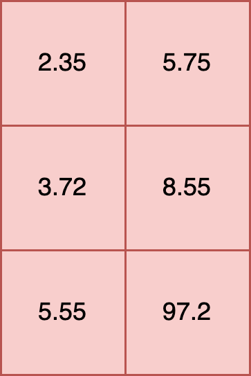
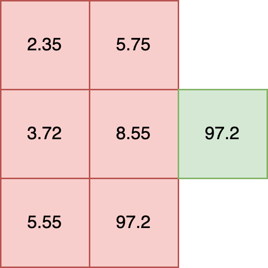
Data Type Consistency
All inputs into an ONNX model must have the same internal data type. For example, the following is valid because all of the data types within each element are float32.
t= [
[2.35, 5.75],
[3.72, 8.55],
[5.55, 97.2]
]
The following is invalid, as it mixes floats and strings in each element:
These requirements are <strong>not</strong> for Tensorflow Keras models, only for non-Keras Tensorflow models in the SavedModel format. For Tensorflow Keras deployment in Wallaroo, see the Tensorflow Keras requirements.
TensorFlow File Format
TensorFlow models are .zip file of the SavedModel format. For example, the Aloha sample TensorFlow model is stored in the directory alohacnnlstm:
Python models uploaded to Wallaroo are executed as a native runtime.
Note that Python models - aka “Python steps” - are standalone python scripts that use the python libraries natively supported by the Wallaroo platform. These are used for either simple model deployment (such as ARIMA Statsmodels), or data formatting such as the postprocessing steps. A Wallaroo Python model will be composed of one Python script that matches the Wallaroo requirements.
This is contrasted with Arbitrary Python models, also known as Bring Your Own Predict (BYOP) allow for custom model deployments with supporting scripts and artifacts. These are used with pre-trained models (PyTorch, Tensorflow, etc) along with whatever supporting artifacts they require. Supporting artifacts can include other Python modules, model files, etc. These are zipped with all scripts, artifacts, and a requirements.txt file that indicates what other Python models need to be imported that are outside of the typical Wallaroo platform.
Python Models Requirements
Python models uploaded to Wallaroo are Python scripts that must include the wallaroo_json method as the entry point for the Wallaroo engine to use it as a Pipeline step.
This method receives the results of the previous Pipeline step, and its return value will be used in the next Pipeline step.
If the Python model is the first step in the pipeline, then it will be receiving the inference request data (for example: a preprocessing step). If it is the last step in the pipeline, then it will be the data returned from the inference request.
In the example below, the Python model is used as a post processing step for another ML model. The Python model expects to receive data from a ML Model who’s output is a DataFrame with the column dense_2. It then extracts the values of that column as a list, selects the first element, and returns a DataFrame with that element as the value of the column output.
In line with other Wallaroo inference results, the outputs of a Python step that returns a pandas DataFrame or Arrow Table will be listed in the out. metadata, with all inference outputs listed as out.{variable 1}, out.{variable 2}, etc. In the example above, this results the output field as the out.output field in the Wallaroo inference result.
Input and output schemas for each Hugging Face pipeline are defined below. Note that adding additional inputs not specified below will raise errors, except for the following:
Framework.HUGGING-FACE-IMAGE-TO-TEXT
Framework.HUGGING-FACE-TEXT-CLASSIFICATION
Framework.HUGGING-FACE-SUMMARIZATION
Framework.HUGGING-FACE-TRANSLATION
Additional inputs added to these Hugging Face pipelines will be added as key/pair value arguments to the model’s generate method. If the argument is not required, then the model will default to the values coded in the original Hugging Face model’s source code.
Any parameter that is not part of the required inputs list will be forwarded to the model as a key/pair value to the underlying models generate method. If the additional input is not supported by the model, an error will be returned.
Any parameter that is not part of the required inputs list will be forwarded to the model as a key/pair value to the underlying models generate method. If the additional input is not supported by the model, an error will be returned.
Schemas:
input_schema=pa.schema([
pa.field('inputs', pa.string()),
pa.field('return_text', pa.bool_()),
pa.field('return_tensors', pa.bool_()),
pa.field('clean_up_tokenization_spaces', pa.bool_()),
# pa.field('extra_field', pa.int64()), # every extra field you specify will be forwarded as a key/value pair])
output_schema=pa.schema([
pa.field('summary_text', pa.string()),
])
input_schema=pa.schema([
pa.field('inputs', pa.string()), # requiredpa.field('top_k', pa.int64()), # optionalpa.field('function_to_apply', pa.string()), # optional])
output_schema=pa.schema([
pa.field('label', pa.list_(pa.string(), list_size=2)), # list with a number of items same as top_k, list_size can be skipped but may lead in worse performancepa.field('score', pa.list_(pa.float64(), list_size=2)), # list with a number of items same as top_k, list_size can be skipped but may lead in worse performance])
Any parameter that is not part of the required inputs list will be forwarded to the model as a key/pair value to the underlying models generate method. If the additional input is not supported by the model, an error will be returned.
Schemas:
input_schema=pa.schema([
pa.field('inputs', pa.string()), # requiredpa.field('return_tensors', pa.bool_()), # optionalpa.field('return_text', pa.bool_()), # optionalpa.field('clean_up_tokenization_spaces', pa.bool_()), # optionalpa.field('src_lang', pa.string()), # optionalpa.field('tgt_lang', pa.string()), # optional# pa.field('extra_field', pa.int64()), # every extra field you specify will be forwarded as a key/value pair])
output_schema=pa.schema([
pa.field('translation_text', pa.string()),
])
input_schema=pa.schema([
pa.field('inputs', pa.string()), # requiredpa.field('candidate_labels', pa.list_(pa.string(), list_size=2)), # requiredpa.field('hypothesis_template', pa.string()), # optionalpa.field('multi_label', pa.bool_()), # optional])
output_schema=pa.schema([
pa.field('sequence', pa.string()),
pa.field('scores', pa.list_(pa.float64(), list_size=2)), # same as number of candidate labels, list_size can be skipped by may result in slightly worse performancepa.field('labels', pa.list_(pa.string(), list_size=2)), # same as number of candidate labels, list_size can be skipped by may result in slightly worse performance])
input_schema=pa.schema([
pa.field('images',
pa.list_(
pa.list_(
pa.list_(
pa.int64(),
list_size=3 ),
list_size=640 ),
list_size=480 )),
pa.field('candidate_labels', pa.list_(pa.string(), list_size=3)),
pa.field('threshold', pa.float64()),
# pa.field('top_k', pa.int64()), # we want the model to return exactly the number of predictions, we shouldn't specify this])
output_schema=pa.schema([
pa.field('score', pa.list_(pa.float64())), # variable output, depending on detected objectspa.field('label', pa.list_(pa.string())), # variable output, depending on detected objectspa.field('box',
pa.list_( # dynamic output, i.e. dynamic number of boxes per input image, each sublist contains the 4 box coordinates pa.list_(
pa.int64(),
list_size=4 ),
),
),
])
Any parameter that is not part of the required inputs list will be forwarded to the model as a key/pair value to the underlying models generate method. If the additional input is not supported by the model, an error will be returned.
input_schema=pa.schema([
pa.field('inputs', pa.string()),
pa.field('return_tensors', pa.bool_()), # optionalpa.field('return_text', pa.bool_()), # optionalpa.field('return_full_text', pa.bool_()), # optionalpa.field('clean_up_tokenization_spaces', pa.bool_()), # optionalpa.field('prefix', pa.string()), # optionalpa.field('handle_long_generation', pa.string()), # optional# pa.field('extra_field', pa.int64()), # every extra field you specify will be forwarded as a key/value pair])
output_schema=pa.schema([
pa.field('generated_text', pa.list_(pa.string(), list_size=1))
])
SKLearn schema follows a different format than other models. To prevent inputs from being out of order, the inputs should be submitted in a single row in the order the model is trained to accept, with all of the data types being the same. For example, the following DataFrame has 4 columns, each column a float.
sepal length (cm)
sepal width (cm)
petal length (cm)
petal width (cm)
0
5.1
3.5
1.4
0.2
1
4.9
3.0
1.4
0.2
For submission to an SKLearn model, the data input schema will be a single array with 4 float values.
When submitting as an inference, the DataFrame is converted to rows with the column data expressed as a single array. The data must be in the same order as the model expects, which is why the data is submitted as a single array rather than JSON labeled columns: this insures that the data is submitted in the exact order as the model is trained to accept.
Original DataFrame:
sepal length (cm)
sepal width (cm)
petal length (cm)
petal width (cm)
0
5.1
3.5
1.4
0.2
1
4.9
3.0
1.4
0.2
Converted DataFrame:
inputs
0
[5.1, 3.5, 1.4, 0.2]
1
[4.9, 3.0, 1.4, 0.2]
SKLearn Schema Outputs
Outputs for SKLearn that are meant to be predictions or probabilities when output by the model are labeled in the output schema for the model when uploaded to Wallaroo. For example, a model that outputs either 1 or 0 as its output would have the output schema as follows:
TensorFlow Keras SavedModel models are .zip file of the SavedModel format. For example, the Aloha sample TensorFlow model is stored in the directory alohacnnlstm:
XGBoost schema follows a different format than other models. To prevent inputs from being out of order, the inputs should be submitted in a single row in the order the model is trained to accept, with all of the data types being the same. If a model is originally trained to accept inputs of different data types, it will need to be retrained to only accept one data type for each column - typically pa.float64() is a good choice.
For example, the following DataFrame has 4 columns, each column a float.
sepal length (cm)
sepal width (cm)
petal length (cm)
petal width (cm)
0
5.1
3.5
1.4
0.2
1
4.9
3.0
1.4
0.2
For submission to an XGBoost model, the data input schema will be a single array with 4 float values.
When submitting as an inference, the DataFrame is converted to rows with the column data expressed as a single array. The data must be in the same order as the model expects, which is why the data is submitted as a single array rather than JSON labeled columns: this insures that the data is submitted in the exact order as the model is trained to accept.
Original DataFrame:
sepal length (cm)
sepal width (cm)
petal length (cm)
petal width (cm)
0
5.1
3.5
1.4
0.2
1
4.9
3.0
1.4
0.2
Converted DataFrame:
inputs
0
[5.1, 3.5, 1.4, 0.2]
1
[4.9, 3.0, 1.4, 0.2]
XGBoost Schema Outputs
Outputs for XGBoost are labeled based on the trained model outputs. For this example, the output is simply a single output listed as output. In the Wallaroo inference result, it is grouped with the metadata out as out.output.
Arbitrary Python models, also known as Bring Your Own Predict (BYOP) allow for custom model deployments with supporting scripts and artifacts. These are used with pre-trained models (PyTorch, Tensorflow, etc) along with whatever supporting artifacts they require. Supporting artifacts can include other Python modules, model files, etc. These are zipped with all scripts, artifacts, and a requirements.txt file that indicates what other Python models need to be imported that are outside of the typical Wallaroo platform.
Contrast this with Wallaroo Python models - aka “Python steps”. These are standalone python scripts that use the python libraries natively supported by the Wallaroo platform. These are used for either simple model deployment (such as ARIMA Statsmodels), or data formatting such as the postprocessing steps. A Wallaroo Python model will be composed of one Python script that matches the Wallaroo requirements.
Arbitrary Python File Requirements
Arbitrary Python (BYOP) models are uploaded to Wallaroo via a ZIP file with the following components:
Artifact
Type
Description
Python scripts aka .py files with classes that extend mac.inference.Inference and mac.inference.creation.InferenceBuilder
Python Script
Extend the classes mac.inference.Inference and mac.inference.creation.InferenceBuilder. These are included with the Wallaroo SDK. Further details are in Arbitrary Python Script Requirements. Note that there is no specified naming requirements for the classes that extend mac.inference.Inference and mac.inference.creation.InferenceBuilder - any qualified class name is sufficient as long as these two classes are extended as defined below.
requirements.txt
Python requirements file
This sets the Python libraries used for the arbitrary python model. These libraries should be targeted for Python 3.8 compliance. These requirements and the versions of libraries should be exactly the same between creating the model and deploying it in Wallaroo. This insures that the script and methods will function exactly the same as during the model creation process.
Other artifacts
Files
Other models, files, and other artifacts used in support of this model.
For example, the if the arbitrary python model will be known as vgg_clustering, the contents may be in the following structure, with vgg_clustering as the storage directory:
Note the inclusion of the custom_inference.py file. This file name is not required - any Python script or scripts that extend the classes listed above are sufficient. This Python script could have been named vgg_custom_model.py or any other name as long as it includes the extension of the classes listed above.
The sample arbitrary python model file is created with the command zip -r vgg_clustering.zip vgg_clustering/.
Wallaroo Arbitrary Python uses the Wallaroo SDK mac module, included in the Wallaroo SDK 2023.2.1 and above. See the Wallaroo SDK Install Guides for instructions on installing the Wallaroo SDK.
Arbitrary Python Script Requirements
The entry point of the arbitrary python model is any python script that extends the following classes. These are included with the Wallaroo SDK. The required methods that must be overridden are specified in each section below.
mac.inference.Inference interface serves model inferences based on submitted input some input. Its purpose is to serve inferences for any supported arbitrary model framework (e.g. scikit, keras etc.).
classDiagram
    class Inference {
        <<Abstract>>
        +model Optional[Any]
        +expected_model_types()* Set
        +predict(input_data: InferenceData)*  InferenceData
        -raise_error_if_model_is_not_assigned() None
        -raise_error_if_model_is_wrong_type() None
    }
mac.inference.creation.InferenceBuilder builds a concrete Inference, i.e. instantiates an Inference object, loads the appropriate model and assigns the model to to the Inference object.
classDiagram
    class InferenceBuilder {
        +create(config InferenceConfig) * Inference
        -inference()* Any
    }
mac.inference.Inference
mac.inference.Inference Objects
Object
Type
Description
model Optional[Any]
An optional list of models that match the supported frameworks from wallaroo.framework.Framework included in the arbitrary python script. Note that this is optional - no models are actually required. A BYOP can refer to a specific model(s) used, be used for data processing and reshaping for later pipeline steps, or other needs.
mac.inference.Inference Methods
Method
Returns
Description
expected_model_types (Required)
Set
Returns a Set of models expected for the inference as defined by the developer. Typically this is a set of one. Wallaroo checks the expected model types to verify that the model submitted through the InferenceBuilder method matches what this Inference class expects.
The entry point for the Wallaroo inference with the following input and output parameters that are defined when the model is updated.
mac.types.InferenceData: The inputInferenceData is a dictionary of numpy arrays derived from the input_schema detailed when the model is uploaded, defined in PyArrow.Schema format.
mac.types.InferenceData: The output is a dictionary of numpy arrays as defined by the output parameters defined in PyArrow.Schema format.
The InferenceDataValidationError exception is raised when the input data does not match mac.types.InferenceData.
raise_error_if_model_is_not_assigned
N/A
Error when expected_model_types is not set.
raise_error_if_model_is_wrong_type
N/A
Error when the model does not match the expected_model_types.
mac.inference.creation.InferenceBuilder
InferenceBuilder builds a concrete Inference, i.e. instantiates an Inference object, loads the appropriate model and assigns the model to the Inference.
classDiagram
    class InferenceBuilder {
        +create(config InferenceConfig) * Inference
        -inference()* Any
    }
Each model that is included requires its own InferenceBuilder. InferenceBuilder loads one model, then submits it to the Inference class when created. The Inference class checks this class against its expected_model_types() Set.
Creates an Inference subclass, then assigns a model and attributes. The CustomInferenceConfig is used to retrieve the config.model_path, which is a pathlib.Path object pointing to the folder where the model artifacts are saved. Every artifact loaded must be relative to config.model_path. This is set when the arbitrary python .zip file is uploaded and the environment for running it in Wallaroo is set. For example: loading the artifact vgg_clustering\feature_extractor.h5 would be set with config.model_path \ feature_extractor.h5. The model loaded must match an existing module. For our example, this is from sklearn.cluster import KMeans, and this must match the Inferenceexpected_model_types.
inference
custom Inference instance.
Returns the instantiated custom Inference object created from the create method.
Arbitrary Python Runtime
Arbitrary Python always run in the containerized model runtime.
Wallaroo users can register their trained MLFlow ML Models from a containerized model container registry into their Wallaroo instance and perform inferences with it through a Wallaroo pipeline.
As of this time, Wallaroo only supports MLFlow 1.30.0 containerized models. For information on how to containerize an MLFlow model, see the MLFlow Documentation.
Wallaroo users can register their trained machine learning models from a model registry into their Wallaroo instance and perform inferences with it through a Wallaroo pipeline.
This guide details how to add ML Models from a model registry service into a Wallaroo instance.
Artifact Requirements
Models are uploaded to the Wallaroo instance as the specific artifact - the “file” or other data that represents the file itself. This must comply with the Wallaroo model requirements framework and version or it will not be deployed.
This tutorial will:
Create a Wallaroo workspace and pipeline.
Show how to connect a Wallaroo Registry that connects to a Model Registry Service.
Use the registry connection details to upload a sample model to Wallaroo.
We’ll start with importing the libraries we need for the tutorial.
importosimportwallaroo
Connect to the Wallaroo Instance through the User Interface
The next step is to connect to Wallaroo through the Wallaroo client. The Python library is included in the Wallaroo install and available through the Jupyter Hub interface provided with your Wallaroo environment.
This is accomplished using the wallaroo.Client() command, which provides a URL to grant the SDK permission to your specific Wallaroo environment. When displayed, enter the URL into a browser and confirm permissions. Store the connection into a variable that can be referenced later.
If logging into the Wallaroo instance through the internal JupyterHub service, use wl = wallaroo.Client(). For more information on Wallaroo Client settings, see the Client Connection guide.
The Wallaroo Registry stores the URL and authentication token to the Model Registry service, with the assigned name. Note that in this demonstration all URLs and token are examples.
For this demonstration, we will create a random Wallaroo workspace, then attach our registry to the workspace so it is accessible by other workspace users.
Add Registry to Workspace
Registries are assigned to a Wallaroo workspace with the Wallaroo.registry.add_registry_to_workspace method. This allows members of the workspace to access the registry connection. A registry can be associated with one or more workspaces.
Add Registry to Workspace Parameters
Parameter
Type
Description
name
string (Required)
The numerical identifier of the workspace.
# Make a random new workspaceimportmathimportrandomnum=math.floor(random.random()*1000)
workspace_id=wl.create_workspace(f"test{num}").id()
registry.add_registry_to_workspace(workspace_id=workspace_id)
Models uploaded to the Wallaroo workspace are uploaded from a MLFlow Registry with the Wallaroo.Registry.upload method.
Upload a Model from a Registry Parameters
Parameter
Type
Description
name
string (Required)
The name to assign the model once uploaded. Model names are unique within a workspace. Models assigned the same name as an existing model will be uploaded as a new model version.
path
string (Required)
The full path to the model artifact in the registry.
Once uploaded, the model will undergo conversion. The following will loop through the model status until it is ready. Once ready, it is available for deployment.
Once uploaded and converted, the model runtime is derived. This determines whether to allocate resources to pipeline’s native runtime environment or containerized runtime environment. For more details, see the Wallaroo SDK Essentials Guide: Pipeline Deployment Configuration guide.
model.config().runtime()
'mlflow'
Deploy Pipeline
The model is uploaded and ready for use. We’ll add it as a step in our pipeline, then deploy the pipeline. For this example we’re allocated 0.5 cpu to the runtime environment and 1 CPU to the containerized runtime environment.
A sample inference will be run. First the pandas DataFrame used for the inference is created, then the inference run through the pipeline’s infer method.
Arbitrary Python models, also known as Bring Your Own Predict (BYOP) allow for custom model deployments with supporting scripts and artifacts. These are used with pre-trained models (PyTorch, Tensorflow, etc) along with whatever supporting artifacts they require. Supporting artifacts can include other Python modules, model files, etc. These are zipped with all scripts, artifacts, and a requirements.txt file that indicates what other Python models need to be imported that are outside of the typical Wallaroo platform.
Contrast this with Wallaroo Python models - aka “Python steps”. These are standalone python scripts that use the python libraries natively supported by the Wallaroo platform. These are used for either simple model deployment (such as ARIMA Statsmodels), or data formatting such as the postprocessing steps. A Wallaroo Python model will be composed of one Python script that matches the Wallaroo requirements.
Arbitrary Python File Requirements
Arbitrary Python (BYOP) models are uploaded to Wallaroo via a ZIP file with the following components:
Artifact
Type
Description
Python scripts aka .py files with classes that extend mac.inference.Inference and mac.inference.creation.InferenceBuilder
Python Script
Extend the classes mac.inference.Inference and mac.inference.creation.InferenceBuilder. These are included with the Wallaroo SDK. Further details are in Arbitrary Python Script Requirements. Note that there is no specified naming requirements for the classes that extend mac.inference.Inference and mac.inference.creation.InferenceBuilder - any qualified class name is sufficient as long as these two classes are extended as defined below.
requirements.txt
Python requirements file
This sets the Python libraries used for the arbitrary python model. These libraries should be targeted for Python 3.8 compliance. These requirements and the versions of libraries should be exactly the same between creating the model and deploying it in Wallaroo. This insures that the script and methods will function exactly the same as during the model creation process.
Other artifacts
Files
Other models, files, and other artifacts used in support of this model.
For example, the if the arbitrary python model will be known as vgg_clustering, the contents may be in the following structure, with vgg_clustering as the storage directory:
Note the inclusion of the custom_inference.py file. This file name is not required - any Python script or scripts that extend the classes listed above are sufficient. This Python script could have been named vgg_custom_model.py or any other name as long as it includes the extension of the classes listed above.
The sample arbitrary python model file is created with the command zip -r vgg_clustering.zip vgg_clustering/.
Wallaroo Arbitrary Python uses the Wallaroo SDK mac module, included in the Wallaroo SDK 2023.2.1 and above. See the Wallaroo SDK Install Guides for instructions on installing the Wallaroo SDK.
Arbitrary Python Script Requirements
The entry point of the arbitrary python model is any python script that extends the following classes. These are included with the Wallaroo SDK. The required methods that must be overridden are specified in each section below.
mac.inference.Inference interface serves model inferences based on submitted input some input. Its purpose is to serve inferences for any supported arbitrary model framework (e.g. scikit, keras etc.).
classDiagram
    class Inference {
        <<Abstract>>
        +model Optional[Any]
        +expected_model_types()* Set
        +predict(input_data: InferenceData)*  InferenceData
        -raise_error_if_model_is_not_assigned() None
        -raise_error_if_model_is_wrong_type() None
    }
mac.inference.creation.InferenceBuilder builds a concrete Inference, i.e. instantiates an Inference object, loads the appropriate model and assigns the model to to the Inference object.
classDiagram
    class InferenceBuilder {
        +create(config InferenceConfig) * Inference
        -inference()* Any
    }
mac.inference.Inference
mac.inference.Inference Objects
Object
Type
Description
model Optional[Any]
An optional list of models that match the supported frameworks from wallaroo.framework.Framework included in the arbitrary python script. Note that this is optional - no models are actually required. A BYOP can refer to a specific model(s) used, be used for data processing and reshaping for later pipeline steps, or other needs.
mac.inference.Inference Methods
Method
Returns
Description
expected_model_types (Required)
Set
Returns a Set of models expected for the inference as defined by the developer. Typically this is a set of one. Wallaroo checks the expected model types to verify that the model submitted through the InferenceBuilder method matches what this Inference class expects.
The entry point for the Wallaroo inference with the following input and output parameters that are defined when the model is updated.
mac.types.InferenceData: The inputInferenceData is a dictionary of numpy arrays derived from the input_schema detailed when the model is uploaded, defined in PyArrow.Schema format.
mac.types.InferenceData: The output is a dictionary of numpy arrays as defined by the output parameters defined in PyArrow.Schema format.
The InferenceDataValidationError exception is raised when the input data does not match mac.types.InferenceData.
raise_error_if_model_is_not_assigned
N/A
Error when expected_model_types is not set.
raise_error_if_model_is_wrong_type
N/A
Error when the model does not match the expected_model_types.
mac.inference.creation.InferenceBuilder
InferenceBuilder builds a concrete Inference, i.e. instantiates an Inference object, loads the appropriate model and assigns the model to the Inference.
classDiagram
    class InferenceBuilder {
        +create(config InferenceConfig) * Inference
        -inference()* Any
    }
Each model that is included requires its own InferenceBuilder. InferenceBuilder loads one model, then submits it to the Inference class when created. The Inference class checks this class against its expected_model_types() Set.
Creates an Inference subclass, then assigns a model and attributes. The CustomInferenceConfig is used to retrieve the config.model_path, which is a pathlib.Path object pointing to the folder where the model artifacts are saved. Every artifact loaded must be relative to config.model_path. This is set when the arbitrary python .zip file is uploaded and the environment for running it in Wallaroo is set. For example: loading the artifact vgg_clustering\feature_extractor.h5 would be set with config.model_path \ feature_extractor.h5. The model loaded must match an existing module. For our example, this is from sklearn.cluster import KMeans, and this must match the Inferenceexpected_model_types.
inference
custom Inference instance.
Returns the instantiated custom Inference object created from the create method.
Arbitrary Python Runtime
Arbitrary Python always run in the containerized model runtime.
Wallaroo SDK Upload Arbitrary Python Tutorial: Generate Model
This tutorial demonstrates how to use arbitrary python as a ML Model in Wallaroo. Arbitrary Python allows organizations to use Python scripts that require specific libraries and artifacts as models in the Wallaroo engine. This allows for highly flexible use of ML models with supporting scripts.
Tutorial Goals
This tutorial is split into two parts:
Wallaroo SDK Upload Arbitrary Python Tutorial: Generate Model: Train a dummy KMeans model for clustering images using a pre-trained VGG16 model on cifar10 as a feature extractor. The Python entry points used for Wallaroo deployment will be added and described.
A copy of the arbitrary Python model models/model-auto-conversion-BYOP-vgg16-clustering.zip is included in this tutorial, so this step can be skipped.
Arbitrary Python Tutorial Deploy Model in Wallaroo Upload and Deploy: Deploys the KMeans model in an arbitrary Python package in Wallaroo, and perform sample inferences. The file models/model-auto-conversion-BYOP-vgg16-clustering.zip is provided so users can go right to testing deployment.
Arbitrary Python models, also known as Bring Your Own Predict (BYOP) allow for custom model deployments with supporting scripts and artifacts. These are used with pre-trained models (PyTorch, Tensorflow, etc) along with whatever supporting artifacts they require. Supporting artifacts can include other Python modules, model files, etc. These are zipped with all scripts, artifacts, and a requirements.txt file that indicates what other Python models need to be imported that are outside of the typical Wallaroo platform.
Contrast this with Wallaroo Python models - aka “Python steps”. These are standalone python scripts that use the python libraries natively supported by the Wallaroo platform. These are used for either simple model deployment (such as ARIMA Statsmodels), or data formatting such as the postprocessing steps. A Wallaroo Python model will be composed of one Python script that matches the Wallaroo requirements.
Arbitrary Python File Requirements
Arbitrary Python (BYOP) models are uploaded to Wallaroo via a ZIP file with the following components:
Artifact
Type
Description
Python scripts aka .py files with classes that extend mac.inference.Inference and mac.inference.creation.InferenceBuilder
Python Script
Extend the classes mac.inference.Inference and mac.inference.creation.InferenceBuilder. These are included with the Wallaroo SDK. Further details are in Arbitrary Python Script Requirements. Note that there is no specified naming requirements for the classes that extend mac.inference.Inference and mac.inference.creation.InferenceBuilder - any qualified class name is sufficient as long as these two classes are extended as defined below.
requirements.txt
Python requirements file
This sets the Python libraries used for the arbitrary python model. These libraries should be targeted for Python 3.8 compliance. These requirements and the versions of libraries should be exactly the same between creating the model and deploying it in Wallaroo. This insures that the script and methods will function exactly the same as during the model creation process.
Other artifacts
Files
Other models, files, and other artifacts used in support of this model.
For example, the if the arbitrary python model will be known as vgg_clustering, the contents may be in the following structure, with vgg_clustering as the storage directory:
Note the inclusion of the custom_inference.py file. This file name is not required - any Python script or scripts that extend the classes listed above are sufficient. This Python script could have been named vgg_custom_model.py or any other name as long as it includes the extension of the classes listed above.
The sample arbitrary python model file is created with the command zip -r vgg_clustering.zip vgg_clustering/.
Wallaroo Arbitrary Python uses the Wallaroo SDK mac module, included in the Wallaroo SDK 2023.2.1 and above. See the Wallaroo SDK Install Guides for instructions on installing the Wallaroo SDK.
Arbitrary Python Script Requirements
The entry point of the arbitrary python model is any python script that extends the following classes. These are included with the Wallaroo SDK. The required methods that must be overridden are specified in each section below.
mac.inference.Inference interface serves model inferences based on submitted input some input. Its purpose is to serve inferences for any supported arbitrary model framework (e.g. scikit, keras etc.).
classDiagram
    class Inference {
        <<Abstract>>
        +model Optional[Any]
        +expected_model_types()* Set
        +predict(input_data: InferenceData)*  InferenceData
        -raise_error_if_model_is_not_assigned() None
        -raise_error_if_model_is_wrong_type() None
    }
mac.inference.creation.InferenceBuilder builds a concrete Inference, i.e. instantiates an Inference object, loads the appropriate model and assigns the model to to the Inference object.
classDiagram
    class InferenceBuilder {
        +create(config InferenceConfig) * Inference
        -inference()* Any
    }
mac.inference.Inference
mac.inference.Inference Objects
Object
Type
Description
model Optional[Any]
An optional list of models that match the supported frameworks from wallaroo.framework.Framework included in the arbitrary python script. Note that this is optional - no models are actually required. A BYOP can refer to a specific model(s) used, be used for data processing and reshaping for later pipeline steps, or other needs.
mac.inference.Inference Methods
Method
Returns
Description
expected_model_types (Required)
Set
Returns a Set of models expected for the inference as defined by the developer. Typically this is a set of one. Wallaroo checks the expected model types to verify that the model submitted through the InferenceBuilder method matches what this Inference class expects.
The entry point for the Wallaroo inference with the following input and output parameters that are defined when the model is updated.
mac.types.InferenceData: The inputInferenceData is a dictionary of numpy arrays derived from the input_schema detailed when the model is uploaded, defined in PyArrow.Schema format.
mac.types.InferenceData: The output is a dictionary of numpy arrays as defined by the output parameters defined in PyArrow.Schema format.
The InferenceDataValidationError exception is raised when the input data does not match mac.types.InferenceData.
raise_error_if_model_is_not_assigned
N/A
Error when expected_model_types is not set.
raise_error_if_model_is_wrong_type
N/A
Error when the model does not match the expected_model_types.
mac.inference.creation.InferenceBuilder
InferenceBuilder builds a concrete Inference, i.e. instantiates an Inference object, loads the appropriate model and assigns the model to the Inference.
classDiagram
    class InferenceBuilder {
        +create(config InferenceConfig) * Inference
        -inference()* Any
    }
Each model that is included requires its own InferenceBuilder. InferenceBuilder loads one model, then submits it to the Inference class when created. The Inference class checks this class against its expected_model_types() Set.
Creates an Inference subclass, then assigns a model and attributes. The CustomInferenceConfig is used to retrieve the config.model_path, which is a pathlib.Path object pointing to the folder where the model artifacts are saved. Every artifact loaded must be relative to config.model_path. This is set when the arbitrary python .zip file is uploaded and the environment for running it in Wallaroo is set. For example: loading the artifact vgg_clustering\feature_extractor.h5 would be set with config.model_path \ feature_extractor.h5. The model loaded must match an existing module. For our example, this is from sklearn.cluster import KMeans, and this must match the Inferenceexpected_model_types.
inference
custom Inference instance.
Returns the instantiated custom Inference object created from the create method.
VGG16 Model Training Steps
This process will train a dummy KMeans model for clustering images using a pre-trained VGG16 model on cifar10 as a feature extractor. This model consists of the following elements:
All elements are stored in the folder models/vgg16_clustering. This will be converted to the zip file model-auto-conversion-BYOP-vgg16-clustering.zip.
models/vgg16_clustering will contain the following:
All necessary model artifacts
One or multiple Python files implementing the classes Inference and InferenceBuilder. The implemented classes can have any naming they desire as long as they inherit from the appropriate base classes.
a requirements.txt file with all necessary pip requirements to successfully run the inference
Import Libraries
The first step is to import the libraries we’ll be using. These are included by default in the Wallaroo instance’s JupyterHub service.
2023-07-07 16:16:26.511340: W tensorflow/stream_executor/platform/default/dso_loader.cc:64] Could not load dynamic library 'libcudart.so.11.0'; dlerror: libcudart.so.11.0: cannot open shared object file: No such file or directory
2023-07-07 16:16:26.511369: I tensorflow/stream_executor/cuda/cudart_stub.cc:29] Ignore above cudart dlerror if you do not have a GPU set up on your machine.
Variables
We’ll use these variables in later steps rather than hard code them in. In this case, the directory where we’ll store our artifacts.
model_directory='./models/vgg16_clustering'
Load Data Set
In this section, we will load our sample data and shape it.
# Load and preprocess the CIFAR-10 dataset(X_train, y_train), (X_test, y_test) =cifar10.load_data()
# Normalize the pixel values to be between 0 and 1X_train=X_train/255.0X_test=X_test/255.0
2023-07-07 16:16:30.207936: W tensorflow/stream_executor/platform/default/dso_loader.cc:64] Could not load dynamic library 'libcuda.so.1'; dlerror: libcuda.so.1: cannot open shared object file: No such file or directory
2023-07-07 16:16:30.207966: W tensorflow/stream_executor/cuda/cuda_driver.cc:269] failed call to cuInit: UNKNOWN ERROR (303)
2023-07-07 16:16:30.207987: I tensorflow/stream_executor/cuda/cuda_diagnostics.cc:156] kernel driver does not appear to be running on this host (jupyter-john-2ehummel-40wallaroo-2eai): /proc/driver/nvidia/version does not exist
2023-07-07 16:16:30.208169: I tensorflow/core/platform/cpu_feature_guard.cc:151] This TensorFlow binary is optimized with oneAPI Deep Neural Network Library (oneDNN) to use the following CPU instructions in performance-critical operations:  AVX2 AVX512F FMA
To enable them in other operations, rebuild TensorFlow with the appropriate compiler flags.
WARNING:tensorflow:Compiled the loaded model, but the compiled metrics have yet to be built. `model.compile_metrics` will be empty until you train or evaluate the model.
All needed model artifacts have been now saved under our model directory.
Sample Arbitrary Python Script
The following shows an example of extending the Inference and InferenceBuilder classes for our specific model. This script is located in our model directory under ./models/vgg16_clustering.
"""This module features an example implementation of a custom Inference and its
corresponding InferenceBuilder."""importpathlibimportpicklefromtypingimportAny, Setimporttensorflowastffrommac.config.inferenceimportCustomInferenceConfigfrommac.inferenceimportInferencefrommac.inference.creationimportInferenceBuilderfrommac.typesimportInferenceDatafromsklearn.clusterimportKMeansclassImageClustering(Inference):
"""Inference class for image clustering, that uses
a pre-trained VGG16 model on cifar10 as a feature extractor
and performs clustering on a trained KMeans model.
Attributes:
- feature_extractor: The embedding model we will use
as a feature extractor (i.e. a trained VGG16).
- expected_model_types: A set of model instance types that are expected by this inference.
- model: The model on which the inference is calculated.
"""def__init__(self, feature_extractor: tf.keras.Model):
self.feature_extractor=feature_extractorsuper().__init__()
@propertydefexpected_model_types(self) ->Set[Any]:
return {KMeans}
@Inference.model.setter# type: ignoredefmodel(self, model) ->None:
"""Sets the model on which the inference is calculated.
:param model: A model instance on which the inference is calculated.
:raises TypeError: If the model is not an instance of expected_model_types
(i.e. KMeans).
"""self._raise_error_if_model_is_wrong_type(model) # this will make sure an error will be raised if the model is of wrong typeself._model=modeldef_predict(self, input_data: InferenceData) ->InferenceData:
"""Calculates the inference on the given input data.
This is the core function that each subclass needs to implement
in order to calculate the inference.
:param input_data: The input data on which the inference is calculated.
It is of type InferenceData, meaning it comes as a dictionary of numpy
arrays.
:raises InferenceDataValidationError: If the input data is not valid.
Ideally, every subclass should raise this error if the input data is not valid.
:return: The output of the model, that is a dictionary of numpy arrays.
"""# input_data maps to the input_schema we have defined# with PyArrow, coming as a dictionary of numpy arraysinputs=input_data["images"]
# Forward inputs to the modelsembeddings=self.feature_extractor(inputs)
predictions=self.model.predict(embeddings.numpy())
# Return predictions as dictionary of numpy arraysreturn {"predictions": predictions}
classImageClusteringBuilder(InferenceBuilder):
"""InferenceBuilder subclass for ImageClustering, that loads
a pre-trained VGG16 model on cifar10 as a feature extractor
and a trained KMeans model, and creates an ImageClustering object."""@propertydefinference(self) ->ImageClustering:
returnImageClusteringdefcreate(self, config: CustomInferenceConfig) ->ImageClustering:
"""Creates an Inference subclass and assigns a model and additionally
needed attributes to it.
:param config: Custom inference configuration. In particular, we're
interested in `config.model_path` that is a pathlib.Path object
pointing to the folder where the model artifacts are saved.
Every artifact we need to load from this folder has to be
relative to `config.model_path`.
:return: A custom Inference instance.
"""feature_extractor=self._load_feature_extractor(
config.model_path/"feature_extractor.h5" )
inference=self.inference(feature_extractor)
model=self._load_model(config.model_path/"kmeans.pkl")
inference.model=modelreturninferencedef_load_feature_extractor(
self, file_path: pathlib.Path ) ->tf.keras.Model:
returntf.keras.models.load_model(file_path)
def_load_model(self, file_path: pathlib.Path) ->KMeans:
withopen(file_path.as_posix(), "rb") asfp:
model=pickle.load(fp)
returnmodel
Create Requirements File
As a last step we need to create a requirements.txt file and save it under our vgg_clustering/. The file should contain all the necessary pip requirements needed to run the inference. It will have this data inside.
Arbitrary Python Tutorial Deploy Model in Wallaroo Upload and Deploy
This tutorial demonstrates how to use arbitrary python as a ML Model in Wallaroo. Arbitrary Python allows organizations to use Python scripts that require specific libraries and artifacts as models in the Wallaroo engine. This allows for highly flexible use of ML models with supporting scripts.
Tutorial Goals
This tutorial is split into two parts:
Wallaroo SDK Upload Arbitrary Python Tutorial: Generate Model: Train a dummy KMeans model for clustering images using a pre-trained VGG16 model on cifar10 as a feature extractor. The Python entry points used for Wallaroo deployment will be added and described.
A copy of the arbitrary Python model models/model-auto-conversion-BYOP-vgg16-clustering.zip is included in this tutorial, so this step can be skipped.
Arbitrary Python Tutorial Deploy Model in Wallaroo Upload and Deploy: Deploys the KMeans model in an arbitrary Python package in Wallaroo, and perform sample inferences. The file models/model-auto-conversion-BYOP-vgg16-clustering.zip is provided so users can go right to testing deployment.
Arbitrary Python models, also known as Bring Your Own Predict (BYOP) allow for custom model deployments with supporting scripts and artifacts. These are used with pre-trained models (PyTorch, Tensorflow, etc) along with whatever supporting artifacts they require. Supporting artifacts can include other Python modules, model files, etc. These are zipped with all scripts, artifacts, and a requirements.txt file that indicates what other Python models need to be imported that are outside of the typical Wallaroo platform.
Contrast this with Wallaroo Python models - aka “Python steps”. These are standalone python scripts that use the python libraries natively supported by the Wallaroo platform. These are used for either simple model deployment (such as ARIMA Statsmodels), or data formatting such as the postprocessing steps. A Wallaroo Python model will be composed of one Python script that matches the Wallaroo requirements.
Arbitrary Python File Requirements
Arbitrary Python (BYOP) models are uploaded to Wallaroo via a ZIP file with the following components:
Artifact
Type
Description
Python scripts aka .py files with classes that extend mac.inference.Inference and mac.inference.creation.InferenceBuilder
Python Script
Extend the classes mac.inference.Inference and mac.inference.creation.InferenceBuilder. These are included with the Wallaroo SDK. Further details are in Arbitrary Python Script Requirements. Note that there is no specified naming requirements for the classes that extend mac.inference.Inference and mac.inference.creation.InferenceBuilder - any qualified class name is sufficient as long as these two classes are extended as defined below.
requirements.txt
Python requirements file
This sets the Python libraries used for the arbitrary python model. These libraries should be targeted for Python 3.8 compliance. These requirements and the versions of libraries should be exactly the same between creating the model and deploying it in Wallaroo. This insures that the script and methods will function exactly the same as during the model creation process.
Other artifacts
Files
Other models, files, and other artifacts used in support of this model.
For example, the if the arbitrary python model will be known as vgg_clustering, the contents may be in the following structure, with vgg_clustering as the storage directory:
Note the inclusion of the custom_inference.py file. This file name is not required - any Python script or scripts that extend the classes listed above are sufficient. This Python script could have been named vgg_custom_model.py or any other name as long as it includes the extension of the classes listed above.
The sample arbitrary python model file is created with the command zip -r vgg_clustering.zip vgg_clustering/.
Wallaroo Arbitrary Python uses the Wallaroo SDK mac module, included in the Wallaroo SDK 2023.2.1 and above. See the Wallaroo SDK Install Guides for instructions on installing the Wallaroo SDK.
Arbitrary Python Script Requirements
The entry point of the arbitrary python model is any python script that extends the following classes. These are included with the Wallaroo SDK. The required methods that must be overridden are specified in each section below.
mac.inference.Inference interface serves model inferences based on submitted input some input. Its purpose is to serve inferences for any supported arbitrary model framework (e.g. scikit, keras etc.).
classDiagram
    class Inference {
        <<Abstract>>
        +model Optional[Any]
        +expected_model_types()* Set
        +predict(input_data: InferenceData)*  InferenceData
        -raise_error_if_model_is_not_assigned() None
        -raise_error_if_model_is_wrong_type() None
    }
mac.inference.creation.InferenceBuilder builds a concrete Inference, i.e. instantiates an Inference object, loads the appropriate model and assigns the model to to the Inference object.
classDiagram
    class InferenceBuilder {
        +create(config InferenceConfig) * Inference
        -inference()* Any
    }
mac.inference.Inference
mac.inference.Inference Objects
Object
Type
Description
model Optional[Any]
An optional list of models that match the supported frameworks from wallaroo.framework.Framework included in the arbitrary python script. Note that this is optional - no models are actually required. A BYOP can refer to a specific model(s) used, be used for data processing and reshaping for later pipeline steps, or other needs.
mac.inference.Inference Methods
Method
Returns
Description
expected_model_types (Required)
Set
Returns a Set of models expected for the inference as defined by the developer. Typically this is a set of one. Wallaroo checks the expected model types to verify that the model submitted through the InferenceBuilder method matches what this Inference class expects.
The entry point for the Wallaroo inference with the following input and output parameters that are defined when the model is updated.
mac.types.InferenceData: The inputInferenceData is a dictionary of numpy arrays derived from the input_schema detailed when the model is uploaded, defined in PyArrow.Schema format.
mac.types.InferenceData: The output is a dictionary of numpy arrays as defined by the output parameters defined in PyArrow.Schema format.
The InferenceDataValidationError exception is raised when the input data does not match mac.types.InferenceData.
raise_error_if_model_is_not_assigned
N/A
Error when expected_model_types is not set.
raise_error_if_model_is_wrong_type
N/A
Error when the model does not match the expected_model_types.
mac.inference.creation.InferenceBuilder
InferenceBuilder builds a concrete Inference, i.e. instantiates an Inference object, loads the appropriate model and assigns the model to the Inference.
classDiagram
    class InferenceBuilder {
        +create(config InferenceConfig) * Inference
        -inference()* Any
    }
Each model that is included requires its own InferenceBuilder. InferenceBuilder loads one model, then submits it to the Inference class when created. The Inference class checks this class against its expected_model_types() Set.
Creates an Inference subclass, then assigns a model and attributes. The CustomInferenceConfig is used to retrieve the config.model_path, which is a pathlib.Path object pointing to the folder where the model artifacts are saved. Every artifact loaded must be relative to config.model_path. This is set when the arbitrary python .zip file is uploaded and the environment for running it in Wallaroo is set. For example: loading the artifact vgg_clustering\feature_extractor.h5 would be set with config.model_path \ feature_extractor.h5. The model loaded must match an existing module. For our example, this is from sklearn.cluster import KMeans, and this must match the Inferenceexpected_model_types.
inference
custom Inference instance.
Returns the instantiated custom Inference object created from the create method.
Tutorial Steps
Import Libraries
The first step is to import the libraries we’ll be using. These are included by default in the Wallaroo instance’s JupyterHub service.
2023-07-07 16:18:13.974516: W tensorflow/stream_executor/platform/default/dso_loader.cc:64] Could not load dynamic library 'libcudart.so.11.0'; dlerror: libcudart.so.11.0: cannot open shared object file: No such file or directory
2023-07-07 16:18:13.974543: I tensorflow/stream_executor/cuda/cudart_stub.cc:29] Ignore above cudart dlerror if you do not have a GPU set up on your machine.
Open a Connection to Wallaroo
The next step is connect to Wallaroo through the Wallaroo client. The Python library is included in the Wallaroo install and available through the Jupyter Hub interface provided with your Wallaroo environment.
This is accomplished using the wallaroo.Client() command, which provides a URL to grant the SDK permission to your specific Wallaroo environment. When displayed, enter the URL into a browser and confirm permissions. Store the connection into a variable that can be referenced later.
If logging into the Wallaroo instance through the internal JupyterHub service, use wl = wallaroo.Client(). If logging in externally, update the wallarooPrefix and wallarooSuffix variables with the proper DNS information. For more information on Wallaroo DNS settings, see the Wallaroo DNS Integration Guide.
wl=wallaroo.Client()
Set Variables and Helper Functions
We’ll set the name of our workspace, pipeline, models and files. Workspace names must be unique across the Wallaroo workspace. For this, we’ll add in a randomly generated 4 characters to the workspace name to prevent collisions with other users’ workspaces. If running this tutorial, we recommend hard coding the workspace name so it will function in the same workspace each time it’s run.
We’ll set up some helper functions that will either use existing workspaces and pipelines, or create them if they do not already exist.
importstringimportrandom# make a random 4 character suffix to prevent overwriting other user's workspacessuffix=''.join(random.choice(string.ascii_lowercase) foriinrange(4))
workspace_name=f'vgg16-clustering-workspace{suffix}'pipeline_name=f'vgg16-clustering-pipeline'model_name='vgg16-clustering'model_file_name='./models/model-auto-conversion-BYOP-vgg16-clustering.zip'
We will now create the Wallaroo workspace to store our model and set it as the current workspace. Future commands will default to this workspace for pipeline creation, model uploads, etc. We’ll create our Wallaroo pipeline that is used to deploy our arbitrary Python model.
Arbitrary Python models are uploaded to Wallaroo through the Wallaroo Client upload_model method.
Upload Arbitrary Python Model Parameters
The following parameters are required for Arbitrary Python models. Note that while some fields are considered as optional for the upload_model method, they are required for proper uploading of a Arbitrary Python model to Wallaroo.
Parameter
Type
Description
name
string (Required)
The name of the model. Model names are unique per workspace. Models that are uploaded with the same name are assigned as a new version of the model.
path
string (Required)
The path to the model file being uploaded.
framework
string (Upload Method Optional, Arbitrary Python model Required)
Set as Framework.CUSTOM.
input_schema
pyarrow.lib.Schema (Upload Method Optional, Arbitrary Python model Required)
The input schema in Apache Arrow schema format.
output_schema
pyarrow.lib.Schema (Upload Method Optional, Arbitrary Python model Required)
The output schema in Apache Arrow schema format.
convert_wait
bool (Upload Method Optional, Arbitrary Python model Optional) (Default: True)
True: Waits in the script for the model conversion completion.
False: Proceeds with the script without waiting for the model conversion process to display complete.
Once the upload process starts, the model is containerized by the Wallaroo instance. This process may take up to 10 minutes.
Upload Arbitrary Python Model Return
The following is returned with a successful model upload and conversion.
Field
Type
Description
name
string
The name of the model.
version
string
The model version as a unique UUID.
file_name
string
The file name of the model as stored in Wallaroo.
image_path
string
The image used to deploy the model in the Wallaroo engine.
last_update_time
DateTime
When the model was last updated.
For our example, we’ll start with setting the input_schema and output_schema that is expected by our ImageClustering._predict() method.
Now we’ll upload our model. The framework is Framework.CUSTOM for arbitrary Python models, and we’ll specify the input and output schemas for the upload.
model=wl.upload_model(model_name,
model_file_name,
framework=Framework.CUSTOM,
input_schema=input_schema,
output_schema=output_schema,
convert_wait=True)
model
Waiting for model conversion... It may take up to 10.0min.
Model is Pending conversion..Converting..................Ready.
The model is uploaded and ready for use. We’ll add it as a step in our pipeline, then deploy the pipeline. For this example we’re allocated 0.25 cpu and 4 Gi RAM to the pipeline through the pipeline’s deployment configuration.
Everything is in place - we’ll now run a sample inference with some toy data. In this case we’re randomly generating some values in the data shape the model expects, then submitting an inference request through our deployed pipeline.
Input and output schemas for each Hugging Face pipeline are defined below. Note that adding additional inputs not specified below will raise errors, except for the following:
Framework.HUGGING-FACE-IMAGE-TO-TEXT
Framework.HUGGING-FACE-TEXT-CLASSIFICATION
Framework.HUGGING-FACE-SUMMARIZATION
Framework.HUGGING-FACE-TRANSLATION
Additional inputs added to these Hugging Face pipelines will be added as key/pair value arguments to the model’s generate method. If the argument is not required, then the model will default to the values coded in the original Hugging Face model’s source code.
Any parameter that is not part of the required inputs list will be forwarded to the model as a key/pair value to the underlying models generate method. If the additional input is not supported by the model, an error will be returned.
Any parameter that is not part of the required inputs list will be forwarded to the model as a key/pair value to the underlying models generate method. If the additional input is not supported by the model, an error will be returned.
Schemas:
input_schema=pa.schema([
pa.field('inputs', pa.string()),
pa.field('return_text', pa.bool_()),
pa.field('return_tensors', pa.bool_()),
pa.field('clean_up_tokenization_spaces', pa.bool_()),
# pa.field('extra_field', pa.int64()), # every extra field you specify will be forwarded as a key/value pair])
output_schema=pa.schema([
pa.field('summary_text', pa.string()),
])
input_schema=pa.schema([
pa.field('inputs', pa.string()), # requiredpa.field('top_k', pa.int64()), # optionalpa.field('function_to_apply', pa.string()), # optional])
output_schema=pa.schema([
pa.field('label', pa.list_(pa.string(), list_size=2)), # list with a number of items same as top_k, list_size can be skipped but may lead in worse performancepa.field('score', pa.list_(pa.float64(), list_size=2)), # list with a number of items same as top_k, list_size can be skipped but may lead in worse performance])
Any parameter that is not part of the required inputs list will be forwarded to the model as a key/pair value to the underlying models generate method. If the additional input is not supported by the model, an error will be returned.
Schemas:
input_schema=pa.schema([
pa.field('inputs', pa.string()), # requiredpa.field('return_tensors', pa.bool_()), # optionalpa.field('return_text', pa.bool_()), # optionalpa.field('clean_up_tokenization_spaces', pa.bool_()), # optionalpa.field('src_lang', pa.string()), # optionalpa.field('tgt_lang', pa.string()), # optional# pa.field('extra_field', pa.int64()), # every extra field you specify will be forwarded as a key/value pair])
output_schema=pa.schema([
pa.field('translation_text', pa.string()),
])
input_schema=pa.schema([
pa.field('inputs', pa.string()), # requiredpa.field('candidate_labels', pa.list_(pa.string(), list_size=2)), # requiredpa.field('hypothesis_template', pa.string()), # optionalpa.field('multi_label', pa.bool_()), # optional])
output_schema=pa.schema([
pa.field('sequence', pa.string()),
pa.field('scores', pa.list_(pa.float64(), list_size=2)), # same as number of candidate labels, list_size can be skipped by may result in slightly worse performancepa.field('labels', pa.list_(pa.string(), list_size=2)), # same as number of candidate labels, list_size can be skipped by may result in slightly worse performance])
input_schema=pa.schema([
pa.field('images',
pa.list_(
pa.list_(
pa.list_(
pa.int64(),
list_size=3 ),
list_size=640 ),
list_size=480 )),
pa.field('candidate_labels', pa.list_(pa.string(), list_size=3)),
pa.field('threshold', pa.float64()),
# pa.field('top_k', pa.int64()), # we want the model to return exactly the number of predictions, we shouldn't specify this])
output_schema=pa.schema([
pa.field('score', pa.list_(pa.float64())), # variable output, depending on detected objectspa.field('label', pa.list_(pa.string())), # variable output, depending on detected objectspa.field('box',
pa.list_( # dynamic output, i.e. dynamic number of boxes per input image, each sublist contains the 4 box coordinates pa.list_(
pa.int64(),
list_size=4 ),
),
),
])
Any parameter that is not part of the required inputs list will be forwarded to the model as a key/pair value to the underlying models generate method. If the additional input is not supported by the model, an error will be returned.
input_schema=pa.schema([
pa.field('inputs', pa.string()),
pa.field('return_tensors', pa.bool_()), # optionalpa.field('return_text', pa.bool_()), # optionalpa.field('return_full_text', pa.bool_()), # optionalpa.field('clean_up_tokenization_spaces', pa.bool_()), # optionalpa.field('prefix', pa.string()), # optionalpa.field('handle_long_generation', pa.string()), # optional# pa.field('extra_field', pa.int64()), # every extra field you specify will be forwarded as a key/value pair])
output_schema=pa.schema([
pa.field('generated_text', pa.list_(pa.string(), list_size=1))
])
2.3.1 - Wallaroo API Upload Tutorial: Hugging Face Zero Shot Classification
How to upload a Hugging Face Zero Shot Classification model to Wallaroo via the MLOps API.
To perform the various Wallaroo MLOps API requests, we will use the Wallaroo SDK to generate the necessary tokens. For details on other methods of requesting and using authentication tokens with the Wallaroo MLOps API, see the Wallaroo API Connection Guide.
This is accomplished using the wallaroo.Client() command, which provides a URL to grant the SDK permission to your specific Wallaroo environment. When displayed, enter the URL into a browser and confirm permissions. Store the connection into a variable that can be referenced later.
If logging into the Wallaroo instance through the internal JupyterHub service, use wl = wallaroo.Client(). For more information on Wallaroo Client settings, see the Client Connection guide.
wl=wallaroo.Client()
Variables
The following variables will be set for the rest of the tutorial to set the following:
Wallaroo Workspace
Wallaroo Pipeline
Wallaroo Model name and path
Wallaroo Model Framework
The DNS prefix and suffix for the Wallaroo instance.
To allow this tutorial to be run multiple times or by multiple users in the same Wallaroo instance, a random 4 character prefix will be added to the workspace, pipeline, and model.
Verify that the DNS prefix and suffix match the Wallaroo instance used for this tutorial. See the DNS Integration Guide for more details.
importstringimportrandom# make a random 4 character suffix to prevent overwriting other user's workspacessuffix=''.join(random.choice(string.ascii_lowercase) foriinrange(4))
workspace_name=f'hugging-face-zero-shot-api{suffix}'pipeline_name=f'hugging-face-zero-shot'model_name=f'zero-shot-classification'model_file_name="./models/model-auto-conversion_hugging-face_dummy-pipelines_zero-shot-classification-pipeline.zip"framework="hugging-face-zero-shot-classification"wallarooPrefix="YOUR PREFIX."wallarooPrefix="YOUR SUFFIX"wallarooPrefix="doc-test."wallarooSuffix="wallarooexample.ai"APIURL=f"https://{wallarooPrefix}api.{wallarooSuffix}"APIURL
'https://doc-test.api.wallarooexample.ai'
Create the Workspace
In a production environment, the Wallaroo workspace that contains the pipeline and models would be created and deployed. We will quickly recreate those steps using the MLOps API.
Workspaces are created through the MLOps API with the /v1/api/workspaces/create command. This requires the workspace name be provided, and that the workspace not already exist in the Wallaroo instance.
# Retrieve the tokenheaders=wl.auth.auth_header()
# set Content-Type typeheaders['Content-Type']='application/json'# Create workspaceapiRequest=f"{APIURL}/v1/api/workspaces/create"data= {
"workspace_name": workspace_name}
response=requests.post(apiRequest, json=data, headers=headers, verify=True).json()
display(response)
# Stored for future examplesworkspaceId=response['workspace_id']
{'workspace_id': 9}
Upload the Model
Endpoint:
/v1/api/models/upload_and_convert
Headers:
Content-Type: multipart/form-data
Parameters
name (StringRequired): The model name.
visibility (StringRequired): Either public or private.
workspace_id (StringRequired): The numerical ID of the workspace to upload the model to.
conversion (StringRequired): The conversion parameters that include the following:
framework (StringRequired): The framework of the model being uploaded. See the list of supported models for more details.
python_version (StringRequired): The version of Python required for model.
requirements (StringRequired): Required libraries. Can be [] if the requirements are default Wallaroo JupyterHub libraries.
input_schema (StringOptional): The input schema from the Apache Arrow pyarrow.lib.Schema format, encoded with base64.b64encode. Only required for non-native runtime models.
output_schema (StringOptional): The output schema from the Apache Arrow pyarrow.lib.Schema format, encoded with base64.b64encode. Only required for non-native runtime models.
Set the Schemas
The input and output schemas will be defined according to the Wallaroo Hugging Face schema requirements. The inputs are then base64 encoded for attachment in the API request.
input_schema=pa.schema([
pa.field('inputs', pa.string()), # requiredpa.field('candidate_labels', pa.list_(pa.string(), list_size=2)), # requiredpa.field('hypothesis_template', pa.string()), # optionalpa.field('multi_label', pa.bool_()), # optional])
output_schema=pa.schema([
pa.field('sequence', pa.string()),
pa.field('scores', pa.list_(pa.float64(), list_size=2)), # same as number of candidate labels, list_size can be skipped by may result in slightly worse performancepa.field('labels', pa.list_(pa.string(), list_size=2)), # same as number of candidate labels, list_size can be skipped by may result in slightly worse performance])
We will now build the request to include the required data. We will be using the workspaceId returned when we created our workspace in a previous step, specifying the input and output schemas, and the framework.
# Get the model details# Retrieve the tokenheaders=wl.auth.auth_header()
# set Content-Type typeheaders['Content-Type']='application/json'apiRequest=f"{APIURL}/v1/api/models/list_versions"data= {
"model_id": model_name,
"models_pk_id" : modelId}
status=Nonewhilestatus!='ready':
response=requests.post(apiRequest, json=data, headers=headers, verify=True).json()
# verify we have the right versiondisplay(model)
model=next(modelformodelinresponseifmodel["id"] ==modelId)
display(model)
status=model['status']
The next step is connect to Wallaroo through the Wallaroo client. The Python library is included in the Wallaroo install and available through the Jupyter Hub interface provided with your Wallaroo environment.
This is accomplished using the wallaroo.Client() command, which provides a URL to grant the SDK permission to your specific Wallaroo environment. When displayed, enter the URL into a browser and confirm permissions. Store the connection into a variable that can be referenced later.
If logging into the Wallaroo instance through the internal JupyterHub service, use wl = wallaroo.Client(). If logging in externally, update the wallarooPrefix and wallarooSuffix variables with the proper DNS information. For more information on Wallaroo DNS settings, see the Wallaroo DNS Integration Guide.
wl=wallaroo.Client()
Set Variables and Helper Functions
We’ll set the name of our workspace, pipeline, models and files. Workspace names must be unique across the Wallaroo workspace. For this, we’ll add in a randomly generated 4 characters to the workspace name to prevent collisions with other users’ workspaces. If running this tutorial, we recommend hard coding the workspace name so it will function in the same workspace each time it’s run.
We’ll set up some helper functions that will either use existing workspaces and pipelines, or create them if they do not already exist.
defget_workspace(name):
workspace=Noneforwsinwl.list_workspaces():
ifws.name() ==name:
workspace=wsif(workspace==None):
workspace=wl.create_workspace(name)
returnworkspacedefget_pipeline(name):
try:
pipeline=wl.pipelines_by_name(name)[0]
exceptEntityNotFoundError:
pipeline=wl.build_pipeline(name)
returnpipelineimportstringimportrandom# make a random 4 character suffix to prevent overwriting other user's workspacessuffix=''.join(random.choice(string.ascii_lowercase) foriinrange(4))
workspace_name=f'hf-zero-shot-classification{suffix}'pipeline_name=f'hf-zero-shot-classification'model_name='hf-zero-shot-classification'model_file_name='./models/model-auto-conversion_hugging-face_dummy-pipelines_zero-shot-classification-pipeline.zip'
Create Workspace and Pipeline
We will now create the Wallaroo workspace to store our model and set it as the current workspace. Future commands will default to this workspace for pipeline creation, model uploads, etc. We’ll create our Wallaroo pipeline to deploy our model.
The following parameters are required for Hugging Face models. Note that while some fields are considered as optional for the upload_model method, they are required for proper uploading of a Hugging Face model to Wallaroo.
Parameter
Type
Description
name
string (Required)
The name of the model. Model names are unique per workspace. Models that are uploaded with the same name are assigned as a new version of the model.
path
string (Required)
The path to the model file being uploaded.
framework
string (Upload Method Optional, Hugging Face model Required)
Set as the framework.
input_schema
pyarrow.lib.Schema (Upload Method Optional, Hugging Face model Required)
The input schema in Apache Arrow schema format.
output_schema
pyarrow.lib.Schema (Upload Method Optional, Hugging Face model Required)
The output schema in Apache Arrow schema format.
convert_wait
bool (Upload Method Optional, Hugging Face model Optional) (Default: True)
True: Waits in the script for the model conversion completion.
False: Proceeds with the script without waiting for the model conversion process to display complete.
The input and output schemas will be configured for the data inputs and outputs. More information on the available inputs under the official 🤗 Hugging Face source code.
input_schema=pa.schema([
pa.field('inputs', pa.string()), # requiredpa.field('candidate_labels', pa.list_(pa.string(), list_size=2)), # requiredpa.field('hypothesis_template', pa.string()), # optionalpa.field('multi_label', pa.bool_()), # optional])
output_schema=pa.schema([
pa.field('sequence', pa.string()),
pa.field('scores', pa.list_(pa.float64(), list_size=2)), # same as number of candidate labels, list_size can be skipped by may result in slightly worse performancepa.field('labels', pa.list_(pa.string(), list_size=2)), # same as number of candidate labels, list_size can be skipped by may result in slightly worse performance])
Upload Model
The model will be uploaded with the framework set as Framework.HUGGING_FACE_ZERO_SHOT_CLASSIFICATION.
framework=Framework.HUGGING_FACE_ZERO_SHOT_CLASSIFICATIONmodel=wl.upload_model(model_name,
model_file_name,
framework=framework,
input_schema=input_schema,
output_schema=output_schema,
convert_wait=True)
model
Waiting for model conversion... It may take up to 10.0min.
Model is Pending conversion..Converting.............Ready.
The model is uploaded and ready for use. We’ll add it as a step in our pipeline, then deploy the pipeline. For this example we’re allocated 0.25 cpu and 4 Gi RAM to the pipeline through the pipeline’s deployment configuration.
pipeline=get_pipeline(pipeline_name)
# clear the pipeline if used previouslypipeline.undeploy()
pipeline.clear()
pipeline.add_model_step(model)
pipeline.deploy(deployment_config=deployment_config)
pipeline.status()
A sample inference will be run. First the pandas DataFrame used for the inference is created, then the inference run through the pipeline’s infer method.
input_data= {
"inputs": ["this is a test", "this is another test"], # required"candidate_labels": [["english", "german"], ["english", "german"]], # optional: using the defaults, similar to not passing this parameter"hypothesis_template": ["This example is {}.", "This example is {}."], # optional: using the defaults, similar to not passing this parameter"multi_label": [False, False], # optional: using the defaults, similar to not passing this parameter}
dataframe=pd.DataFrame(input_data)
dataframe
inputs
candidate_labels
hypothesis_template
multi_label
0
this is a test
[english, german]
This example is {}.
False
1
this is another test
[english, german]
This example is {}.
False
%timepipeline.infer(dataframe)
CPU times: user 3 µs, sys: 0 ns, total: 3 µs
Wall time: 3.81 µs
time
in.candidate_labels
in.hypothesis_template
in.inputs
in.multi_label
out.labels
out.scores
out.sequence
check_failures
0
2023-07-13 16:25:46.100
[english, german]
This example is {}.
this is a test
False
[english, german]
[0.5040545463562012, 0.49594542384147644]
this is a test
0
1
2023-07-13 16:25:46.100
[english, german]
This example is {}.
this is another test
False
[english, german]
[0.5037839412689209, 0.4962160289287567]
this is another test
0
Undeploy Pipelines
With the tutorial complete, the pipeline is undeployed to return the resources back to the cluster.
How to upload different Python Step Shape models to Wallaroo.
The following tutorials cover how to upload sample Python Step Shape models into a Wallaroo instance.
Python scripts are uploaded to Wallaroo and and treated like an ML Models in Pipeline steps. These will be referred to as Python steps.
Python steps can include:
Preprocessing steps to prepare the data received to be handed to ML Model deployed as another Pipeline step.
Postprocessing steps to take data output by a ML Model as part of a Pipeline step, and prepare the data to be received by some other data store or entity.
A model contained within a Python script.
In all of these, the requirements for uploading a Python script as a ML Model in Wallaroo are the same.
Python models uploaded to Wallaroo are executed as a native runtime.
Note that Python models - aka “Python steps” - are standalone python scripts that use the python libraries natively supported by the Wallaroo platform. These are used for either simple model deployment (such as ARIMA Statsmodels), or data formatting such as the postprocessing steps. A Wallaroo Python model will be composed of one Python script that matches the Wallaroo requirements.
This is contrasted with Arbitrary Python models, also known as Bring Your Own Predict (BYOP) allow for custom model deployments with supporting scripts and artifacts. These are used with pre-trained models (PyTorch, Tensorflow, etc) along with whatever supporting artifacts they require. Supporting artifacts can include other Python modules, model files, etc. These are zipped with all scripts, artifacts, and a requirements.txt file that indicates what other Python models need to be imported that are outside of the typical Wallaroo platform.
Python Models Requirements
Python models uploaded to Wallaroo are Python scripts that must include the wallaroo_json method as the entry point for the Wallaroo engine to use it as a Pipeline step.
This method receives the results of the previous Pipeline step, and its return value will be used in the next Pipeline step.
If the Python model is the first step in the pipeline, then it will be receiving the inference request data (for example: a preprocessing step). If it is the last step in the pipeline, then it will be the data returned from the inference request.
In the example below, the Python model is used as a post processing step for another ML model. The Python model expects to receive data from a ML Model who’s output is a DataFrame with the column dense_2. It then extracts the values of that column as a list, selects the first element, and returns a DataFrame with that element as the value of the column output.
In line with other Wallaroo inference results, the outputs of a Python step that returns a pandas DataFrame or Arrow Table will be listed in the out. metadata, with all inference outputs listed as out.{variable 1}, out.{variable 2}, etc. In the example above, this results the output field as the out.output field in the Wallaroo inference result.
time
in.tensor
out.output
check_failures
0
2023-06-20 20:23:28.395
[0.6878518042, 0.1760734021, -0.869514083, 0.3..
[12.886651039123535]
0
2.4.1 - Python Model Shape Upload to Wallaroo with the Wallaroo SDK
How to upload a Python Step Shape model to Wallaroo via the SDK
Python scripts can be deployed to Wallaroo as Python Models. These are treated like other models, and are used for:
ML Models: Models written entirely in Python script.
Data Formatting: Typically preprocess or post process modules that shape incoming data into what a ML model expects, or receives data output by a ML model and changes the data for other processes to accept.
Models are added to Wallaroo pipelines as pipeline steps, with the data from the previous step submitted to the next one. Python steps require the entry method wallaroo_json. These methods should be structured to receive and send pandas DataFrames as the inputs and outputs.
This allows inference requests to a Wallaroo pipeline to receive pandas DataFrames or Apache Arrow tables, and return the same for consistent results.
This tutorial will:
Create a Wallaroo workspace and pipeline.
Upload the sample Python model and ONNX model.
Demonstrate the outputs of the ONNX model to an inference request.
Demonstrate the functionality of the Python model in reshaping data after an inference request.
Use both the ONNX model and the Python model together as pipeline steps to perform an inference request and export the data for use.
Connect to the Wallaroo Instance through the User Interface
The next step is to connect to Wallaroo through the Wallaroo client. The Python library is included in the Wallaroo install and available through the Jupyter Hub interface provided with your Wallaroo environment.
This is accomplished using the wallaroo.Client() command, which provides a URL to grant the SDK permission to your specific Wallaroo environment. When displayed, enter the URL into a browser and confirm permissions. Store the connection into a variable that can be referenced later.
If logging into the Wallaroo instance through the internal JupyterHub service, use wl = wallaroo.Client(). For more information on Wallaroo Client settings, see the Client Connection guide.
# Login through local Wallaroo instancewl=wallaroo.Client()
Set Variables and Helper Functions
We’ll set the name of our workspace, pipeline, models and files. Workspace names must be unique across the Wallaroo workspace. For this, we’ll add in a randomly generated 4 characters to the workspace name to prevent collisions with other users’ workspaces. If running this tutorial, we recommend hard coding the workspace name so it will function in the same workspace each time it’s run.
We’ll set up some helper functions that will either use existing workspaces and pipelines, or create them if they do not already exist.
importstringimportrandom# make a random 4 character suffix to prevent overwriting other user's workspacessuffix=''.join(random.choice(string.ascii_lowercase) foriinrange(4))
workspace_name=f'python-demo{suffix}'pipeline_name=f'python-step-demo-pipeline'onnx_model_name='house-price-sample'onnx_model_file_name='./models/house_price_keras.onnx'python_model_name='python-step'python_model_file_name='./models/step.py'
./models/house_price_keras.onnx: A ML model trained to forecast hour prices based on inputs. This forecast is stored in the column dense_2.
./models/step.py: A Python script that accepts the data from the house price model, and reformats the output. We’ll be using it as a post-processing step.
For the Python step, it contains the method wallaroo_json as the entry point used by Wallaroo when deployed as a pipeline step. Our sample script has the following:
# take a dataframe output of the house price model, and reformat the `dense_2`# column as `output`defwallaroo_json(data: pd.DataFrame):
print(data)
return [{"output": [data["dense_2"].to_list()[0][0]]}]
As seen from the description, all those function will do it take the DataFrame output of the house price model, and output a DataFrame replacing the first element in the list from column dense_2 with output.
Upload Models
Both of these models will be uploaded to our current workspace using the method upload_model(name, path, framework).configure(framework, input_schema, output_schema).
For ./models/house_price_keras.onnx, we will specify it as Framework.ONNX. We do not need to specify the input and output schemas.
For ./models/step.py, we will set the input and output schemas in the required pyarrow.lib.Schema format.
With our models uploaded, we’ll perform different configurations of the pipeline steps.
First we’ll add just the house price model to the pipeline, deploy it, and submit a sample inference.
# used to restrict the resources needed for this demonstrationdeployment_config=DeploymentConfigBuilder() \
.cpus(0.25).memory('1Gi') \
.build()
# clear the pipeline if this tutorial was run beforepipeline.undeploy()
pipeline.clear()
pipeline.add_model_step(house_price_model)
pipeline.deploy(deployment_config=deployment_config)
Our inference result had the results in the out.dense_2 column. We’ll clear the pipeline, then add in as the pipeline step just the Python postprocessing step we’ve created. Then for our inference request, we’ll just submit the output of the house price model. Our result should be the first element in the array returned in the out.output column.
As the data was exported by the pipeline step as a pandas DataFrame, it will be reflected in the pipeline logs. We’ll retrieve the most recent log from our most recent inference.
With our tutorial complete, we’ll undeploy the pipeline and return the resources back to the cluster.
This process demonstrated how to structure a postprocessing Python script as a Wallaroo Pipeline step. This can be used for pre or post processing, Python based models, and other use cases.
The next step is connect to Wallaroo through the Wallaroo client. The Python library is included in the Wallaroo install and available through the Jupyter Hub interface provided with your Wallaroo environment.
This is accomplished using the wallaroo.Client() command, which provides a URL to grant the SDK permission to your specific Wallaroo environment. When displayed, enter the URL into a browser and confirm permissions. Store the connection into a variable that can be referenced later.
If logging into the Wallaroo instance through the internal JupyterHub service, use wl = wallaroo.Client(). If logging in externally, update the wallarooPrefix and wallarooSuffix variables with the proper DNS information. For more information on Wallaroo DNS settings, see the Wallaroo DNS Integration Guide.
We’ll set the name of our workspace, pipeline, models and files. Workspace names must be unique across the Wallaroo workspace. For this, we’ll add in a randomly generated 4 characters to the workspace name to prevent collisions with other users’ workspaces. If running this tutorial, we recommend hard coding the workspace name so it will function in the same workspace each time it’s run.
We’ll set up some helper functions that will either use existing workspaces and pipelines, or create them if they do not already exist.
defget_workspace(name):
workspace=Noneforwsinwl.list_workspaces():
ifws.name() ==name:
workspace=wsif(workspace==None):
workspace=wl.create_workspace(name)
returnworkspacedefget_pipeline(name):
try:
pipeline=wl.pipelines_by_name(name)[0]
exceptEntityNotFoundError:
pipeline=wl.build_pipeline(name)
returnpipelineimportstringimportrandom# make a random 4 character suffix to prevent overwriting other user's workspacessuffix=''.join(random.choice(string.ascii_lowercase) foriinrange(4))
workspace_name=f'pytorch-single-io{suffix}'pipeline_name=f'pytorch-single-io'model_name='pytorch-single-io'model_file_name="./models/model-auto-conversion_pytorch_single_io_model.pt"
Create Workspace and Pipeline
We will now create the Wallaroo workspace to store our model and set it as the current workspace. Future commands will default to this workspace for pipeline creation, model uploads, etc. We’ll create our Wallaroo pipeline to deploy our model.
The following parameters are required for PyTorch models. Note that while some fields are considered as optional for the upload_model method, they are required for proper uploading of a PyTorch model to Wallaroo.
Parameter
Type
Description
name
string (Required)
The name of the model. Model names are unique per workspace. Models that are uploaded with the same name are assigned as a new version of the model.
path
string (Required)
The path to the model file being uploaded.
framework
string (Upload Method Optional, PyTorch model Required)
Set as the Framework.PyTorch.
input_schema
pyarrow.lib.Schema (Upload Method Optional, PyTorch model Required)
The input schema in Apache Arrow schema format.
output_schema
pyarrow.lib.Schema (Upload Method Optional, PyTorch model Required)
The output schema in Apache Arrow schema format.
convert_wait
bool (Upload Method Optional, PyTorch model Optional) (Default: True)
True: Waits in the script for the model conversion completion.
False: Proceeds with the script without waiting for the model conversion process to display complete.
Once the upload process starts, the model is containerized by the Wallaroo instance. This process may take up to 10 minutes.
The model is uploaded and ready for use. We’ll add it as a step in our pipeline, then deploy the pipeline. For this example we’re allocated 0.25 cpu and 4 Gi RAM to the pipeline through the pipeline’s deployment configuration.
# clear the pipeline if it was used beforepipeline.undeploy()
pipeline.clear()
pipeline.add_model_step(model)
pipeline.deploy(deployment_config=deployment_config)
pipeline.status()
A sample inference will be run. First the pandas DataFrame used for the inference is created, then the inference run through the pipeline’s infer method.
The next step is connect to Wallaroo through the Wallaroo client. The Python library is included in the Wallaroo install and available through the Jupyter Hub interface provided with your Wallaroo environment.
This is accomplished using the wallaroo.Client() command, which provides a URL to grant the SDK permission to your specific Wallaroo environment. When displayed, enter the URL into a browser and confirm permissions. Store the connection into a variable that can be referenced later.
If logging into the Wallaroo instance through the internal JupyterHub service, use wl = wallaroo.Client(). If logging in externally, update the wallarooPrefix and wallarooSuffix variables with the proper DNS information. For more information on Wallaroo DNS settings, see the Wallaroo DNS Integration Guide.
wl=wallaroo.Client()
Set Variables and Helper Functions
We’ll set the name of our workspace, pipeline, models and files. Workspace names must be unique across the Wallaroo workspace. For this, we’ll add in a randomly generated 4 characters to the workspace name to prevent collisions with other users’ workspaces. If running this tutorial, we recommend hard coding the workspace name so it will function in the same workspace each time it’s run.
We’ll set up some helper functions that will either use existing workspaces and pipelines, or create them if they do not already exist.
defget_workspace(name):
workspace=Noneforwsinwl.list_workspaces():
ifws.name() ==name:
workspace=wsif(workspace==None):
workspace=wl.create_workspace(name)
returnworkspacedefget_pipeline(name):
try:
pipeline=wl.pipelines_by_name(name)[0]
exceptEntityNotFoundError:
pipeline=wl.build_pipeline(name)
returnpipelineimportstringimportrandom# make a random 4 character suffix to prevent overwriting other user's workspacessuffix=''.join(random.choice(string.ascii_lowercase) foriinrange(4))
workspace_name=f'pytorch-multi-io{suffix}'pipeline_name=f'pytorch-multi-io'model_name='pytorch-multi-io'model_file_name="./models/model-auto-conversion_pytorch_multi_io_model.pt"
Create Workspace and Pipeline
We will now create the Wallaroo workspace to store our model and set it as the current workspace. Future commands will default to this workspace for pipeline creation, model uploads, etc. We’ll create our Wallaroo pipeline to deploy our model.
The following parameters are required for PyTorch models. Note that while some fields are considered as optional for the upload_model method, they are required for proper uploading of a PyTorch model to Wallaroo.
Parameter
Type
Description
name
string (Required)
The name of the model. Model names are unique per workspace. Models that are uploaded with the same name are assigned as a new version of the model.
path
string (Required)
The path to the model file being uploaded.
framework
string (Upload Method Optional, PyTorch model Required)
Set as the Framework.PyTorch.
input_schema
pyarrow.lib.Schema (Upload Method Optional, PyTorch model Required)
The input schema in Apache Arrow schema format.
output_schema
pyarrow.lib.Schema (Upload Method Optional, PyTorch model Required)
The output schema in Apache Arrow schema format.
convert_wait
bool (Upload Method Optional, PyTorch model Optional) (Default: True)
True: Waits in the script for the model conversion completion.
False: Proceeds with the script without waiting for the model conversion process to display complete.
Once the upload process starts, the model is containerized by the Wallaroo instance. This process may take up to 10 minutes.
The model is uploaded and ready for use. We’ll add it as a step in our pipeline, then deploy the pipeline. For this example we’re allocated 0.25 cpu and 4 Gi RAM to the pipeline through the pipeline’s deployment configuration.
# clear the pipeline if it was used beforepipeline.undeploy()
pipeline.clear()
pipeline.add_model_step(model)
pipeline.deploy(deployment_config=deployment_config)
pipeline.status()
A sample inference will be run. First the pandas DataFrame used for the inference is created, then the inference run through the pipeline’s infer method.
SKLearn schema follows a different format than other models. To prevent inputs from being out of order, the inputs should be submitted in a single row in the order the model is trained to accept, with all of the data types being the same. For example, the following DataFrame has 4 columns, each column a float.
sepal length (cm)
sepal width (cm)
petal length (cm)
petal width (cm)
0
5.1
3.5
1.4
0.2
1
4.9
3.0
1.4
0.2
For submission to an SKLearn model, the data input schema will be a single array with 4 float values.
When submitting as an inference, the DataFrame is converted to rows with the column data expressed as a single array. The data must be in the same order as the model expects, which is why the data is submitted as a single array rather than JSON labeled columns: this insures that the data is submitted in the exact order as the model is trained to accept.
Original DataFrame:
sepal length (cm)
sepal width (cm)
petal length (cm)
petal width (cm)
0
5.1
3.5
1.4
0.2
1
4.9
3.0
1.4
0.2
Converted DataFrame:
inputs
0
[5.1, 3.5, 1.4, 0.2]
1
[4.9, 3.0, 1.4, 0.2]
SKLearn Schema Outputs
Outputs for SKLearn that are meant to be predictions or probabilities when output by the model are labeled in the output schema for the model when uploaded to Wallaroo. For example, a model that outputs either 1 or 0 as its output would have the output schema as follows:
The next step is connect to Wallaroo through the Wallaroo client. The Python library is included in the Wallaroo install and available through the Jupyter Hub interface provided with your Wallaroo environment.
This is accomplished using the wallaroo.Client() command, which provides a URL to grant the SDK permission to your specific Wallaroo environment. When displayed, enter the URL into a browser and confirm permissions. Store the connection into a variable that can be referenced later.
If logging into the Wallaroo instance through the internal JupyterHub service, use wl = wallaroo.Client(). If logging in externally, update the wallarooPrefix and wallarooSuffix variables with the proper DNS information. For more information on Wallaroo DNS settings, see the Wallaroo DNS Integration Guide.
wl=wallaroo.Client()
Set Variables and Helper Functions
We’ll set the name of our workspace, pipeline, models and files. Workspace names must be unique across the Wallaroo workspace. For this, we’ll add in a randomly generated 4 characters to the workspace name to prevent collisions with other users’ workspaces. If running this tutorial, we recommend hard coding the workspace name so it will function in the same workspace each time it’s run.
We’ll set up some helper functions that will either use existing workspaces and pipelines, or create them if they do not already exist.
defget_workspace(name):
workspace=Noneforwsinwl.list_workspaces():
ifws.name() ==name:
workspace=wsif(workspace==None):
workspace=wl.create_workspace(name)
returnworkspacedefget_pipeline(name):
try:
pipeline=wl.pipelines_by_name(name)[0]
exceptEntityNotFoundError:
pipeline=wl.build_pipeline(name)
returnpipelineimportstringimportrandom# make a random 4 character suffix to prevent overwriting other user's workspacessuffix=''.join(random.choice(string.ascii_lowercase) foriinrange(4))
workspace_name=f'sklearn-clustering-kmeans{suffix}'pipeline_name=f'sklearn-clustering-kmeans'model_name='sklearn-clustering-kmeans'model_file_name="models/model-auto-conversion_sklearn_kmeans.pkl"
Create Workspace and Pipeline
We will now create the Wallaroo workspace to store our model and set it as the current workspace. Future commands will default to this workspace for pipeline creation, model uploads, etc. We’ll create our Wallaroo pipeline to deploy our model.
SKLearn models are uploaded to Wallaroo through the Wallaroo Client upload_model method.
Upload SKLearn Model Parameters
The following parameters are required for SKLearn models. Note that while some fields are considered as optional for the upload_model method, they are required for proper uploading of a SKLearn model to Wallaroo.
Parameter
Type
Description
name
string (Required)
The name of the model. Model names are unique per workspace. Models that are uploaded with the same name are assigned as a new version of the model.
path
string (Required)
The path to the model file being uploaded.
framework
string (Upload Method Optional, SKLearn model Required)
Set as the Framework.SKLEARN.
input_schema
pyarrow.lib.Schema (Upload Method Optional, SKLearn model Required)
The input schema in Apache Arrow schema format.
output_schema
pyarrow.lib.Schema (Upload Method Optional, SKLearn model Required)
The output schema in Apache Arrow schema format.
convert_wait
bool (Upload Method Optional, SKLearn model Optional) (Default: True)
True: Waits in the script for the model conversion completion.
False: Proceeds with the script without waiting for the model conversion process to display complete.
Once the upload process starts, the model is containerized by the Wallaroo instance. This process may take up to 10 minutes.
The model is uploaded and ready for use. We’ll add it as a step in our pipeline, then deploy the pipeline. For this example we’re allocated 0.25 cpu and 4 Gi RAM to the pipeline through the pipeline’s deployment configuration.
# clear the pipeline if it was used beforepipeline.undeploy()
pipeline.clear()
pipeline.add_model_step(model)
pipeline.deploy(deployment_config=deployment_config)
pipeline.status()
SKLearn models must have all of the data as one line to prevent columns from being read out of order when submitting in JSON. The following will take in the data, convert the rows into a single inputs for the table, then perform the inference. From the output_schema we have defined the output as predictions which will be displayed in our inference result output as out.predictions.
data=pd.read_json('./data/test-sklearn-kmeans.json')
display(data)
# move the column values to a single array inputmock_dataframe=pd.DataFrame({"inputs": data[:2].values.tolist()})
display(mock_dataframe)
The next step is connect to Wallaroo through the Wallaroo client. The Python library is included in the Wallaroo install and available through the Jupyter Hub interface provided with your Wallaroo environment.
This is accomplished using the wallaroo.Client() command, which provides a URL to grant the SDK permission to your specific Wallaroo environment. When displayed, enter the URL into a browser and confirm permissions. Store the connection into a variable that can be referenced later.
If logging into the Wallaroo instance through the internal JupyterHub service, use wl = wallaroo.Client(). If logging in externally, update the wallarooPrefix and wallarooSuffix variables with the proper DNS information. For more information on Wallaroo DNS settings, see the Wallaroo DNS Integration Guide.
wl=wallaroo.Client()
Set Variables and Helper Functions
We’ll set the name of our workspace, pipeline, models and files. Workspace names must be unique across the Wallaroo workspace. For this, we’ll add in a randomly generated 4 characters to the workspace name to prevent collisions with other users’ workspaces. If running this tutorial, we recommend hard coding the workspace name so it will function in the same workspace each time it’s run.
We’ll set up some helper functions that will either use existing workspaces and pipelines, or create them if they do not already exist.
defget_workspace(name):
workspace=Noneforwsinwl.list_workspaces():
ifws.name() ==name:
workspace=wsif(workspace==None):
workspace=wl.create_workspace(name)
returnworkspacedefget_pipeline(name):
try:
pipeline=wl.pipelines_by_name(name)[0]
exceptEntityNotFoundError:
pipeline=wl.build_pipeline(name)
returnpipelineimportstringimportrandom# make a random 4 character suffix to prevent overwriting other user's workspacessuffix=''.join(random.choice(string.ascii_lowercase) foriinrange(4))
workspace_name=f'sklearn-clustering-svm{suffix}'pipeline_name=f'sklearn-clustering-svm'model_name='sklearn-clustering-svm'model_file_name='./models/model-auto-conversion_sklearn_svm_pipeline.pkl'
Create Workspace and Pipeline
We will now create the Wallaroo workspace to store our model and set it as the current workspace. Future commands will default to this workspace for pipeline creation, model uploads, etc. We’ll create our Wallaroo pipeline to deploy our model.
SKLearn models are uploaded to Wallaroo through the Wallaroo Client upload_model method.
Upload SKLearn Model Parameters
The following parameters are required for SKLearn models. Note that while some fields are considered as optional for the upload_model method, they are required for proper uploading of a SKLearn model to Wallaroo.
Parameter
Type
Description
name
string (Required)
The name of the model. Model names are unique per workspace. Models that are uploaded with the same name are assigned as a new version of the model.
path
string (Required)
The path to the model file being uploaded.
framework
string (Upload Method Optional, SKLearn model Required)
Set as the Framework.SKLEARN.
input_schema
pyarrow.lib.Schema (Upload Method Optional, SKLearn model Required)
The input schema in Apache Arrow schema format.
output_schema
pyarrow.lib.Schema (Upload Method Optional, SKLearn model Required)
The output schema in Apache Arrow schema format.
convert_wait
bool (Upload Method Optional, SKLearn model Optional) (Default: True)
True: Waits in the script for the model conversion completion.
False: Proceeds with the script without waiting for the model conversion process to display complete.
Once the upload process starts, the model is containerized by the Wallaroo instance. This process may take up to 10 minutes.
The model is uploaded and ready for use. We’ll add it as a step in our pipeline, then deploy the pipeline. For this example we’re allocated 0.25 cpu and 4 Gi RAM to the pipeline through the pipeline’s deployment configuration.
# clear the pipeline if it was used beforepipeline.undeploy()
pipeline.clear()
pipeline.add_model_step(model)
pipeline.deploy(deployment_config=deployment_config)
pipeline.status()
SKLearn models must have all of the data as one line to prevent columns from being read out of order when submitting in JSON. The following will take in the data, convert the rows into a single inputs for the table, then perform the inference. From the output_schema we have defined the output as predictions which will be displayed in our inference result output as out.predictions.
data=pd.read_json('./data/test_cluster-svm.json')
display(data)
# move the column values to a single array inputdataframe=pd.DataFrame({"inputs": data[:2].values.tolist()})
display(dataframe)
sepal length (cm)
sepal width (cm)
petal length (cm)
petal width (cm)
0
5.1
3.5
1.4
0.2
1
4.9
3.0
1.4
0.2
inputs
0
[5.1, 3.5, 1.4, 0.2]
1
[4.9, 3.0, 1.4, 0.2]
pipeline.infer(dataframe)
time
in.inputs
out.predictions
check_failures
0
2023-07-13 18:17:07.199
[5.1, 3.5, 1.4, 0.2]
0
0
1
2023-07-13 18:17:07.199
[4.9, 3.0, 1.4, 0.2]
0
0
Undeploy Pipelines
With the tutorial complete, the pipeline is undeployed to return the resources back to the cluster.
The next step is connect to Wallaroo through the Wallaroo client. The Python library is included in the Wallaroo install and available through the Jupyter Hub interface provided with your Wallaroo environment.
This is accomplished using the wallaroo.Client() command, which provides a URL to grant the SDK permission to your specific Wallaroo environment. When displayed, enter the URL into a browser and confirm permissions. Store the connection into a variable that can be referenced later.
If logging into the Wallaroo instance through the internal JupyterHub service, use wl = wallaroo.Client(). If logging in externally, update the wallarooPrefix and wallarooSuffix variables with the proper DNS information. For more information on Wallaroo DNS settings, see the Wallaroo DNS Integration Guide.
wl=wallaroo.Client()
Set Variables and Helper Functions
We’ll set the name of our workspace, pipeline, models and files. Workspace names must be unique across the Wallaroo workspace. For this, we’ll add in a randomly generated 4 characters to the workspace name to prevent collisions with other users’ workspaces. If running this tutorial, we recommend hard coding the workspace name so it will function in the same workspace each time it’s run.
We’ll set up some helper functions that will either use existing workspaces and pipelines, or create them if they do not already exist.
defget_workspace(name):
workspace=Noneforwsinwl.list_workspaces():
ifws.name() ==name:
workspace=wsif(workspace==None):
workspace=wl.create_workspace(name)
returnworkspacedefget_pipeline(name):
try:
pipeline=wl.pipelines_by_name(name)[0]
exceptEntityNotFoundError:
pipeline=wl.build_pipeline(name)
returnpipelineimportstringimportrandom# make a random 4 character suffix to prevent overwriting other user's workspacessuffix=''.join(random.choice(string.ascii_lowercase) foriinrange(4))
workspace_name=f'sklearn-linear-regression{suffix}'pipeline_name=f'sklearn-linear-regression'model_name='sklearn-linear-regression'model_file_name='models/model-auto-conversion_sklearn_linreg_diabetes.pkl'
Create Workspace and Pipeline
We will now create the Wallaroo workspace to store our model and set it as the current workspace. Future commands will default to this workspace for pipeline creation, model uploads, etc. We’ll create our Wallaroo pipeline to deploy our model.
SKLearn models are uploaded to Wallaroo through the Wallaroo Client upload_model method.
Upload SKLearn Model Parameters
The following parameters are required for SKLearn models. Note that while some fields are considered as optional for the upload_model method, they are required for proper uploading of a SKLearn model to Wallaroo.
Parameter
Type
Description
name
string (Required)
The name of the model. Model names are unique per workspace. Models that are uploaded with the same name are assigned as a new version of the model.
path
string (Required)
The path to the model file being uploaded.
framework
string (Upload Method Optional, SKLearn model Required)
Set as the Framework.SKLEARN.
input_schema
pyarrow.lib.Schema (Upload Method Optional, SKLearn model Required)
The input schema in Apache Arrow schema format.
output_schema
pyarrow.lib.Schema (Upload Method Optional, SKLearn model Required)
The output schema in Apache Arrow schema format.
convert_wait
bool (Upload Method Optional, SKLearn model Optional) (Default: True)
True: Waits in the script for the model conversion completion.
False: Proceeds with the script without waiting for the model conversion process to display complete.
Once the upload process starts, the model is containerized by the Wallaroo instance. This process may take up to 10 minutes.
The model is uploaded and ready for use. We’ll add it as a step in our pipeline, then deploy the pipeline. For this example we’re allocated 0.25 cpu and 4 Gi RAM to the pipeline through the pipeline’s deployment configuration.
# clear the pipeline if it was used beforepipeline.undeploy()
pipeline.clear()
pipeline.add_model_step(model)
pipeline.deploy(deployment_config=deployment_config)
pipeline.status()
SKLearn models must have all of the data as one line to prevent columns from being read out of order when submitting in JSON. The following will take in the data, convert the rows into a single inputs for the table, then perform the inference. From the output_schema we have defined the output as predictions which will be displayed in our inference result output as out.predictions.
data=pd.read_json('data/test_linear_regression_data.json')
display(data)
# move the column values to a single array inputdataframe=pd.DataFrame({"inputs": data[:2].values.tolist()})
display(dataframe)
age
sex
bmi
bp
s1
s2
s3
s4
s5
s6
0
0.038076
0.050680
0.061696
0.021872
-0.044223
-0.034821
-0.043401
-0.002592
0.019907
-0.017646
1
-0.001882
-0.044642
-0.051474
-0.026328
-0.008449
-0.019163
0.074412
-0.039493
-0.068332
-0.092204
inputs
0
[0.0380759064, 0.0506801187, 0.0616962065, 0.0...
1
[-0.0018820165, -0.0446416365, -0.051474061200...
pipeline.infer(dataframe)
time
in.inputs
out.predictions
check_failures
0
2023-07-13 18:20:51.820
[0.0380759064, 0.0506801187, 0.0616962065, 0.0...
206.116677
0
1
2023-07-13 18:20:51.820
[-0.0018820165, -0.0446416365, -0.0514740612, ...
68.071033
0
Undeploy Pipelines
With the tutorial complete, the pipeline is undeployed to return the resources back to the cluster.
The next step is connect to Wallaroo through the Wallaroo client. The Python library is included in the Wallaroo install and available through the Jupyter Hub interface provided with your Wallaroo environment.
This is accomplished using the wallaroo.Client() command, which provides a URL to grant the SDK permission to your specific Wallaroo environment. When displayed, enter the URL into a browser and confirm permissions. Store the connection into a variable that can be referenced later.
If logging into the Wallaroo instance through the internal JupyterHub service, use wl = wallaroo.Client(). If logging in externally, update the wallarooPrefix and wallarooSuffix variables with the proper DNS information. For more information on Wallaroo DNS settings, see the Wallaroo DNS Integration Guide.
wl=wallaroo.Client()
Set Variables and Helper Functions
We’ll set the name of our workspace, pipeline, models and files. Workspace names must be unique across the Wallaroo workspace. For this, we’ll add in a randomly generated 4 characters to the workspace name to prevent collisions with other users’ workspaces. If running this tutorial, we recommend hard coding the workspace name so it will function in the same workspace each time it’s run.
We’ll set up some helper functions that will either use existing workspaces and pipelines, or create them if they do not already exist.
defget_workspace(name):
workspace=Noneforwsinwl.list_workspaces():
ifws.name() ==name:
workspace=wsif(workspace==None):
workspace=wl.create_workspace(name)
returnworkspacedefget_pipeline(name):
try:
pipeline=wl.pipelines_by_name(name)[0]
exceptEntityNotFoundError:
pipeline=wl.build_pipeline(name)
returnpipelineimportstringimportrandom# make a random 4 character suffix to prevent overwriting other user's workspacessuffix=''.join(random.choice(string.ascii_lowercase) foriinrange(4))
workspace_name=f'sklearn-logistic-regression{suffix}'pipeline_name=f'sklearn-logistic-regression'model_name='sklearn-logistic-regression'model_file_name='models/logreg.pkl'
Create Workspace and Pipeline
We will now create the Wallaroo workspace to store our model and set it as the current workspace. Future commands will default to this workspace for pipeline creation, model uploads, etc. We’ll create our Wallaroo pipeline to deploy our model.
SKLearn models are uploaded to Wallaroo through the Wallaroo Client upload_model method.
Upload SKLearn Model Parameters
The following parameters are required for SKLearn models. Note that while some fields are considered as optional for the upload_model method, they are required for proper uploading of a SKLearn model to Wallaroo.
Parameter
Type
Description
name
string (Required)
The name of the model. Model names are unique per workspace. Models that are uploaded with the same name are assigned as a new version of the model.
path
string (Required)
The path to the model file being uploaded.
framework
string (Upload Method Optional, SKLearn model Required)
Set as the Framework.SKLEARN.
input_schema
pyarrow.lib.Schema (Upload Method Optional, SKLearn model Required)
The input schema in Apache Arrow schema format.
output_schema
pyarrow.lib.Schema (Upload Method Optional, SKLearn model Required)
The output schema in Apache Arrow schema format.
convert_wait
bool (Upload Method Optional, SKLearn model Optional) (Default: True)
True: Waits in the script for the model conversion completion.
False: Proceeds with the script without waiting for the model conversion process to display complete.
Once the upload process starts, the model is containerized by the Wallaroo instance. This process may take up to 10 minutes.
The model is uploaded and ready for use. We’ll add it as a step in our pipeline, then deploy the pipeline. For this example we’re allocated 0.25 cpu and 4 Gi RAM to the pipeline through the pipeline’s deployment configuration.
# clear the pipeline if it was used beforepipeline.undeploy()
pipeline.clear()
pipeline.add_model_step(model)
pipeline.deploy(deployment_config=deployment_config)
pipeline.status()
SKLearn models must have all of the data as one line to prevent columns from being read out of order when submitting in JSON. The following will take in the data, convert the rows into a single inputs for the table, then perform the inference. From the output_schema we have defined the output as predictions which will be displayed in our inference result output as out.predictions.
data=pd.read_json('data/test_logreg_data.json')
display(data)
# move the column values to a single array inputdataframe=pd.DataFrame({"inputs": data[:2].values.tolist()})
display(dataframe)
sepal length (cm)
sepal width (cm)
petal length (cm)
petal width (cm)
0
5.1
3.5
1.4
0.2
1
4.9
3.0
1.4
0.2
inputs
0
[5.1, 3.5, 1.4, 0.2]
1
[4.9, 3.0, 1.4, 0.2]
pipeline.infer(dataframe)
time
in.inputs
out.predictions
out.probabilities
check_failures
0
2023-07-13 18:24:26.268
[5.1, 3.5, 1.4, 0.2]
0
[0.9815821465852236, 0.018417838912958125, 1.4...
0
1
2023-07-13 18:24:26.268
[4.9, 3.0, 1.4, 0.2]
0
[0.9713374799347873, 0.028662489870060148, 3.0...
0
Undeploy Pipelines
With the tutorial complete, the pipeline is undeployed to return the resources back to the cluster.
Wallaroo Model Upload via the Wallaroo SDK: Sklearn Clustering SVM PCA
The following tutorial demonstrates how to upload a SKLearn Clustering Support Vector Machine(SVM) Principal Component Analysis (PCA) model to a Wallaroo instance.
Tutorial Goals
Demonstrate the following:
Upload a Sklearn Clustering SVM PCA model to a Wallaroo instance.
Create a pipeline and add the model as a pipeline step.
The next step is connect to Wallaroo through the Wallaroo client. The Python library is included in the Wallaroo install and available through the Jupyter Hub interface provided with your Wallaroo environment.
This is accomplished using the wallaroo.Client() command, which provides a URL to grant the SDK permission to your specific Wallaroo environment. When displayed, enter the URL into a browser and confirm permissions. Store the connection into a variable that can be referenced later.
If logging into the Wallaroo instance through the internal JupyterHub service, use wl = wallaroo.Client(). If logging in externally, update the wallarooPrefix and wallarooSuffix variables with the proper DNS information. For more information on Wallaroo DNS settings, see the Wallaroo DNS Integration Guide.
wl=wallaroo.Client()
Set Variables and Helper Functions
We’ll set the name of our workspace, pipeline, models and files. Workspace names must be unique across the Wallaroo workspace. For this, we’ll add in a randomly generated 4 characters to the workspace name to prevent collisions with other users’ workspaces. If running this tutorial, we recommend hard coding the workspace name so it will function in the same workspace each time it’s run.
We’ll set up some helper functions that will either use existing workspaces and pipelines, or create them if they do not already exist.
defget_workspace(name):
workspace=Noneforwsinwl.list_workspaces():
ifws.name() ==name:
workspace=wsif(workspace==None):
workspace=wl.create_workspace(name)
returnworkspacedefget_pipeline(name):
try:
pipeline=wl.pipelines_by_name(name)[0]
exceptEntityNotFoundError:
pipeline=wl.build_pipeline(name)
returnpipelineimportstringimportrandom# make a random 4 character suffix to prevent overwriting other user's workspacessuffix=''.join(random.choice(string.ascii_lowercase) foriinrange(4))
workspace_name=f'sklearn-clustering-svm-pca{suffix}'pipeline_name=f'sklearn-clustering-svm-pca'model_name='sklearn-clustering-svm-pca'model_file_name='models/model-auto-conversion_sklearn_svm_pca_pipeline.pkl'
Create Workspace and Pipeline
We will now create the Wallaroo workspace to store our model and set it as the current workspace. Future commands will default to this workspace for pipeline creation, model uploads, etc. We’ll create our Wallaroo pipeline to deploy our model.
SKLearn models are uploaded to Wallaroo through the Wallaroo Client upload_model method.
Upload SKLearn Model Parameters
The following parameters are required for SKLearn models. Note that while some fields are considered as optional for the upload_model method, they are required for proper uploading of a SKLearn model to Wallaroo.
Parameter
Type
Description
name
string (Required)
The name of the model. Model names are unique per workspace. Models that are uploaded with the same name are assigned as a new version of the model.
path
string (Required)
The path to the model file being uploaded.
framework
string (Upload Method Optional, SKLearn model Required)
Set as the Framework.SKLEARN.
input_schema
pyarrow.lib.Schema (Upload Method Optional, SKLearn model Required)
The input schema in Apache Arrow schema format.
output_schema
pyarrow.lib.Schema (Upload Method Optional, SKLearn model Required)
The output schema in Apache Arrow schema format.
convert_wait
bool (Upload Method Optional, SKLearn model Optional) (Default: True)
True: Waits in the script for the model conversion completion.
False: Proceeds with the script without waiting for the model conversion process to display complete.
Once the upload process starts, the model is containerized by the Wallaroo instance. This process may take up to 10 minutes.
The model is uploaded and ready for use. We’ll add it as a step in our pipeline, then deploy the pipeline. For this example we’re allocated 0.25 cpu and 4 Gi RAM to the pipeline through the pipeline’s deployment configuration.
# clear the pipeline if it was used beforepipeline.undeploy()
pipeline.clear()
pipeline.add_model_step(model)
pipeline.deploy(deployment_config=deployment_config)
pipeline.status()
SKLearn models must have all of the data as one line to prevent columns from being read out of order when submitting in JSON. The following will take in the data, convert the rows into a single inputs for the table, then perform the inference. From the output_schema we have defined the output as predictions which will be displayed in our inference result output as out.predictions.
data=pd.read_json('data/test-sklearn-kmeans.json')
display(data)
# move the column values to a single array inputdataframe=pd.DataFrame({"inputs": data[:2].values.tolist()})
display(dataframe)
sepal length (cm)
sepal width (cm)
petal length (cm)
petal width (cm)
0
5.1
3.5
1.4
0.2
1
4.9
3.0
1.4
0.2
inputs
0
[5.1, 3.5, 1.4, 0.2]
1
[4.9, 3.0, 1.4, 0.2]
pipeline.infer(dataframe)
time
in.inputs
out.predictions
check_failures
0
2023-07-13 18:11:14.856
[5.1, 3.5, 1.4, 0.2]
0
0
1
2023-07-13 18:11:14.856
[4.9, 3.0, 1.4, 0.2]
0
0
Undeploy Pipelines
With the tutorial complete, the pipeline is undeployed to return the resources back to the cluster.
These requirements are not for Tensorflow Keras models, only for non-Keras Tensorflow models in the SavedModel format. For Tensorflow Keras deployment in Wallaroo, see the Tensorflow Keras requirements.
TensorFlow File Format
TensorFlow models are .zip file of the SavedModel format. For example, the Aloha sample TensorFlow model is stored in the directory alohacnnlstm:
In this notebook we will walk through uploading a Tensorflow model to a Wallaroo instance and performing sample inferences. For this example we will be using an open source model that uses an Aloha CNN LSTM model for classifying Domain names as being either legitimate or being used for nefarious purposes such as malware distribution.
Prerequisites
An installed Wallaroo instance.
The following Python libraries installed:
os
wallaroo: The Wallaroo SDK. Included with the Wallaroo JupyterHub service by default.
The first step is to connect to Wallaroo through the Wallaroo client. The Python library is included in the Wallaroo install and available through the Jupyter Hub interface provided with your Wallaroo environment.
This is accomplished using the wallaroo.Client() command, which provides a URL to grant the SDK permission to your specific Wallaroo environment. When displayed, enter the URL into a browser and confirm permissions. Store the connection into a variable that can be referenced later.
If logging into the Wallaroo instance through the internal JupyterHub service, use wl = wallaroo.Client(). For more information on Wallaroo Client settings, see the Client Connection guide.e/wallaroo-sdk-essentials-client/).
importwallaroofromwallaroo.objectimportEntityNotFoundErrorfromwallaroo.frameworkimportFramework# to display dataframe tablesfromIPython.displayimportdisplay# used to display dataframe information without truncatingimportosos.environ["MODELS_ENABLED"] ="true"importpandasaspdpd.set_option('display.max_colwidth', None)
importpyarrowaspa
# Login through local Wallaroo instancewl=wallaroo.Client()
wallarooPrefix=""wallarooSuffix="autoscale-uat-ee.wallaroo.dev"wl=wallaroo.Client(api_endpoint=f"https://{wallarooPrefix}api.{wallarooSuffix}",
auth_endpoint=f"https://{wallarooPrefix}keycloak.{wallarooSuffix}",
auth_type="sso")
Create the Workspace
We will create a workspace to work in and call it the “alohaworkspace”, then set it as current workspace environment. We’ll also create our pipeline in advance as alohapipeline. The model name and the model file will be specified for use in later steps.
To allow this tutorial to be run multiple times or by multiple users in the same Wallaroo instance, a random 4 character prefix will be added to the workspace, pipeline, and model.
importstringimportrandom# make a random 4 character suffix to verify uniqueness in tutorialssuffix=''.join(random.choice(string.ascii_lowercase) foriinrange(4))
workspace_name=f'tensorflowuploadexampleworkspace{suffix}'pipeline_name=f'tensorflowuploadexample{suffix}'model_name=f'tensorflowuploadexample{suffix}'model_file_name='./models/alohacnnlstm.zip'
Now we will upload our models. Note that for this example we are applying the model from a .ZIP file. The Aloha model is a protobuf file that has been defined for evaluating web pages, and we will configure it to use data in the tensorflow format.
The following parameters are required for TensorFlow models. Tensorflow models are native runtimes in Wallaroo, so the input_schema and output_schema parameters are optional.
Parameter
Type
Description
name
string (Required)
The name of the model. Model names are unique per workspace. Models that are uploaded with the same name are assigned as a new version of the model.
path
string (Required)
The path to the model file being uploaded.
framework
string (Required)
Set as the Framework.TENSORFLOW.
input_schema
pyarrow.lib.Schema (Optional)
The input schema in Apache Arrow schema format.
output_schema
pyarrow.lib.Schema (Optional)
The output schema in Apache Arrow schema format.
convert_wait
bool (Optional) (Default: True)
Not required for native runtimes.
True: Waits in the script for the model conversion completion.
False: Proceeds with the script without waiting for the model conversion process to display complete.
TensorFlow File Format
TensorFlow models are .zip file of the SavedModel format. For example, the Aloha sample TensorFlow model is stored in the directory alohacnnlstm:
Now that the pipeline is deployed and our Aloha model is in place, we’ll perform a smoke test to verify the pipeline is up and running properly. We’ll use the infer_from_file command to load a single encoded URL into the inference engine and print the results back out.
The result should tell us that the tokenized URL is legitimate (0) or fraud (1). This sample data should return close to 1 in out.main.
When finished with our tests, we will undeploy the pipeline so we have the Kubernetes resources back for other tasks. Note that if the deployment variable is unchanged aloha_pipeline.deploy() will restart the inference engine in the same configuration as before.
TensorFlow Keras SavedModel models are .zip file of the SavedModel format. For example, the Aloha sample TensorFlow model is stored in the directory alohacnnlstm:
The next step is connect to Wallaroo through the Wallaroo client. The Python library is included in the Wallaroo install and available through the Jupyter Hub interface provided with your Wallaroo environment.
This is accomplished using the wallaroo.Client() command, which provides a URL to grant the SDK permission to your specific Wallaroo environment. When displayed, enter the URL into a browser and confirm permissions. Store the connection into a variable that can be referenced later.
If logging into the Wallaroo instance through the internal JupyterHub service, use wl = wallaroo.Client(). If logging in externally, update the wallarooPrefix and wallarooSuffix variables with the proper DNS information. For more information on Wallaroo DNS settings, see the Wallaroo DNS Integration Guide.
We’ll set the name of our workspace, pipeline, models and files. Workspace names must be unique across the Wallaroo workspace. For this, we’ll add in a randomly generated 4 characters to the workspace name to prevent collisions with other users’ workspaces. If running this tutorial, we recommend hard coding the workspace name so it will function in the same workspace each time it’s run.
We’ll set up some helper functions that will either use existing workspaces and pipelines, or create them if they do not already exist.
defget_workspace(name):
workspace=Noneforwsinwl.list_workspaces():
ifws.name() ==name:
workspace=wsif(workspace==None):
workspace=wl.create_workspace(name)
returnworkspacedefget_pipeline(name):
try:
pipeline=wl.pipelines_by_name(name)[0]
exceptEntityNotFoundError:
pipeline=wl.build_pipeline(name)
returnpipelineimportstringimportrandom# make a random 4 character suffix to prevent overwriting other user's workspacessuffix=''.join(random.choice(string.ascii_lowercase) foriinrange(4))
workspace_name=f'keras-sequential-single-io{suffix}'pipeline_name=f'keras-sequential-single-io'model_name='keras-sequential-single-io'model_file_name='models/model-auto-conversion_keras_single_io_keras_sequential_model.h5'
Create Workspace and Pipeline
We will now create the Wallaroo workspace to store our model and set it as the current workspace. Future commands will default to this workspace for pipeline creation, model uploads, etc. We’ll create our Wallaroo pipeline to deploy our model.
The following parameters are required for TensorFlow keras models. Note that while some fields are considered as optional for the upload_model method, they are required for proper uploading of a TensorFlow Keras model to Wallaroo.
Parameter
Type
Description
name
string (Required)
The name of the model. Model names are unique per workspace. Models that are uploaded with the same name are assigned as a new version of the model.
path
string (Required)
The path to the model file being uploaded.
framework
string (Upload Method Optional, TensorFlow keras model Required)
Set as the Framework.KERAS.
input_schema
pyarrow.lib.Schema (Upload Method Optional, TensorFlow Keras model Required)
The input schema in Apache Arrow schema format.
output_schema
pyarrow.lib.Schema (Upload Method Optional, TensorFlow Keras model Required)
The output schema in Apache Arrow schema format.
convert_wait
bool (Upload Method Optional, TensorFlow model Optional) (Default: True)
True: Waits in the script for the model conversion completion.
False: Proceeds with the script without waiting for the model conversion process to display complete.
Once the upload process starts, the model is containerized by the Wallaroo instance. This process may take up to 10 minutes.
The model is uploaded and ready for use. We’ll add it as a step in our pipeline, then deploy the pipeline. For this example we’re allocated 0.25 cpu and 4 Gi RAM to the pipeline through the pipeline’s deployment configuration.
# clear the pipeline if used in a previous tutorialpipeline.undeploy()
pipeline.clear()
pipeline.add_model_step(model)
pipeline.deploy(deployment_config=deployment_config)
pipeline.status()
A sample inference will be run. First the pandas DataFrame used for the inference is created, then the inference run through the pipeline’s infer method.
XGBoost schema follows a different format than other models. To prevent inputs from being out of order, the inputs should be submitted in a single row in the order the model is trained to accept, with all of the data types being the same. If a model is originally trained to accept inputs of different data types, it will need to be retrained to only accept one data type for each column - typically pa.float64() is a good choice.
For example, the following DataFrame has 4 columns, each column a float.
sepal length (cm)
sepal width (cm)
petal length (cm)
petal width (cm)
0
5.1
3.5
1.4
0.2
1
4.9
3.0
1.4
0.2
For submission to an XGBoost model, the data input schema will be a single array with 4 float values.
When submitting as an inference, the DataFrame is converted to rows with the column data expressed as a single array. The data must be in the same order as the model expects, which is why the data is submitted as a single array rather than JSON labeled columns: this insures that the data is submitted in the exact order as the model is trained to accept.
Original DataFrame:
sepal length (cm)
sepal width (cm)
petal length (cm)
petal width (cm)
0
5.1
3.5
1.4
0.2
1
4.9
3.0
1.4
0.2
Converted DataFrame:
inputs
0
[5.1, 3.5, 1.4, 0.2]
1
[4.9, 3.0, 1.4, 0.2]
XGBoost Schema Outputs
Outputs for XGBoost are labeled based on the trained model outputs. For this example, the output is simply a single output listed as output. In the Wallaroo inference result, it is grouped with the metadata out as out.output.
The next step is connect to Wallaroo through the Wallaroo client. The Python library is included in the Wallaroo install and available through the Jupyter Hub interface provided with your Wallaroo environment.
This is accomplished using the wallaroo.Client() command, which provides a URL to grant the SDK permission to your specific Wallaroo environment. When displayed, enter the URL into a browser and confirm permissions. Store the connection into a variable that can be referenced later.
If logging into the Wallaroo instance through the internal JupyterHub service, use wl = wallaroo.Client(). If logging in externally, update the wallarooPrefix and wallarooSuffix variables with the proper DNS information. For more information on Wallaroo DNS settings, see the Wallaroo DNS Integration Guide.
We’ll set the name of our workspace, pipeline, models and files. Workspace names must be unique across the Wallaroo workspace. For this, we’ll add in a randomly generated 4 characters to the workspace name to prevent collisions with other users’ workspaces. If running this tutorial, we recommend hard coding the workspace name so it will function in the same workspace each time it’s run.
We’ll set up some helper functions that will either use existing workspaces and pipelines, or create them if they do not already exist.
defget_workspace(name):
workspace=Noneforwsinwl.list_workspaces():
ifws.name() ==name:
workspace=wsif(workspace==None):
workspace=wl.create_workspace(name)
returnworkspacedefget_pipeline(name):
try:
pipeline=wl.pipelines_by_name(name)[0]
exceptEntityNotFoundError:
pipeline=wl.build_pipeline(name)
returnpipelineimportstringimportrandom# make a random 4 character suffix to prevent overwriting other user's workspacessuffix=''.join(random.choice(string.ascii_lowercase) foriinrange(4))
workspace_name=f'xgboost-rf-regressor{suffix}'pipeline_name=f'xgboost-rf-regressor'model_name='xgboost-rf-regressor'model_file_name='models/model-auto-conversion_xgboost_xgb_rf_regressor_diabetes.pkl'
Create Workspace and Pipeline
We will now create the Wallaroo workspace to store our model and set it as the current workspace. Future commands will default to this workspace for pipeline creation, model uploads, etc. We’ll create our Wallaroo pipeline to deploy our model.
XGBoost models are uploaded to Wallaroo through the Wallaroo Client upload_model method.
Upload XGBoost Model Parameters
The following parameters are required for XGBoost models. Note that while some fields are considered as optional for the upload_model method, they are required for proper uploading of a XGBoost model to Wallaroo.
Parameter
Type
Description
name
string (Required)
The name of the model. Model names are unique per workspace. Models that are uploaded with the same name are assigned as a new version of the model.
path
string (Required)
The path to the model file being uploaded.
framework
string (Upload Method Optional, SKLearn model Required)
Set as the Framework.XGBOOST.
input_schema
pyarrow.lib.Schema (Upload Method Optional, SKLearn model Required)
The input schema in Apache Arrow schema format.
output_schema
pyarrow.lib.Schema (Upload Method Optional, SKLearn model Required)
The output schema in Apache Arrow schema format.
convert_wait
bool (Upload Method Optional, SKLearn model Optional) (Default: True)
True: Waits in the script for the model conversion completion.
False: Proceeds with the script without waiting for the model conversion process to display complete.
Once the upload process starts, the model is containerized by the Wallaroo instance. This process may take up to 10 minutes.
XGBoost Schema Inputs
XGBoost schema follows a different format than other models. To prevent inputs from being out of order, the inputs should be submitted in a single row in the order the model is trained to accept, with all of the data types being the same. If a model is originally trained to accept inputs of different data types, it will need to be retrained to only accept one data type for each column - typically pa.float64() is a good choice.
For example, the following DataFrame has 4 columns, each column a float.
sepal length (cm)
sepal width (cm)
petal length (cm)
petal width (cm)
0
5.1
3.5
1.4
0.2
1
4.9
3.0
1.4
0.2
For submission to an XGBoost model, the data input schema will be a single array with 4 float values.
When submitting as an inference, the DataFrame is converted to rows with the column data expressed as a single array. The data must be in the same order as the model expects, which is why the data is submitted as a single array rather than JSON labeled columns: this insures that the data is submitted in the exact order as the model is trained to accept.
Original DataFrame:
sepal length (cm)
sepal width (cm)
petal length (cm)
petal width (cm)
0
5.1
3.5
1.4
0.2
1
4.9
3.0
1.4
0.2
Converted DataFrame:
inputs
0
[5.1, 3.5, 1.4, 0.2]
1
[4.9, 3.0, 1.4, 0.2]
XGBoost Schema Outputs
Outputs for XGBoost are labeled based on the trained model outputs. For this example, the output is simply a single output listed as output. In the Wallaroo inference result, it is grouped with the metadata out as out.output.
The model is uploaded and ready for use. We’ll add it as a step in our pipeline, then deploy the pipeline. For this example we’re allocated 0.25 cpu and 4 Gi RAM to the pipeline through the pipeline’s deployment configuration.
# clear the pipeline if it was used beforepipeline.undeploy()
pipeline.clear()
pipeline.add_model_step(model)
pipeline.deploy(deployment_config=deployment_config)
pipeline.status()
A sample inference will be run. First the pandas DataFrame used for the inference is created, then the inference run through the pipeline’s infer method.
The next step is connect to Wallaroo through the Wallaroo client. The Python library is included in the Wallaroo install and available through the Jupyter Hub interface provided with your Wallaroo environment.
This is accomplished using the wallaroo.Client() command, which provides a URL to grant the SDK permission to your specific Wallaroo environment. When displayed, enter the URL into a browser and confirm permissions. Store the connection into a variable that can be referenced later.
If logging into the Wallaroo instance through the internal JupyterHub service, use wl = wallaroo.Client(). If logging in externally, update the wallarooPrefix and wallarooSuffix variables with the proper DNS information. For more information on Wallaroo DNS settings, see the Wallaroo DNS Integration Guide.
wl=wallaroo.Client()
Set Variables and Helper Functions
We’ll set the name of our workspace, pipeline, models and files. Workspace names must be unique across the Wallaroo workspace. For this, we’ll add in a randomly generated 4 characters to the workspace name to prevent collisions with other users’ workspaces. If running this tutorial, we recommend hard coding the workspace name so it will function in the same workspace each time it’s run.
We’ll set up some helper functions that will either use existing workspaces and pipelines, or create them if they do not already exist.
defget_workspace(name):
workspace=Noneforwsinwl.list_workspaces():
ifws.name() ==name:
workspace=wsif(workspace==None):
workspace=wl.create_workspace(name)
returnworkspacedefget_pipeline(name):
try:
pipeline=wl.pipelines_by_name(name)[0]
exceptEntityNotFoundError:
pipeline=wl.build_pipeline(name)
returnpipelineimportstringimportrandom# make a random 4 character suffix to prevent overwriting other user's workspacessuffix=''.join(random.choice(string.ascii_lowercase) foriinrange(4))
workspace_name=f'xgboost-classification{suffix}'pipeline_name=f'xgboost-classification'model_name='xgboost-classification'model_file_name='./models/model-auto-conversion_xgboost_xgb_classification_iris.pkl'
Create Workspace and Pipeline
We will now create the Wallaroo workspace to store our model and set it as the current workspace. Future commands will default to this workspace for pipeline creation, model uploads, etc. We’ll create our Wallaroo pipeline to deploy our model.
XGBoost models are uploaded to Wallaroo through the Wallaroo Client upload_model method.
Upload XGBoost Model Parameters
The following parameters are required for XGBoost models. Note that while some fields are considered as optional for the upload_model method, they are required for proper uploading of a XGBoost model to Wallaroo.
Parameter
Type
Description
name
string (Required)
The name of the model. Model names are unique per workspace. Models that are uploaded with the same name are assigned as a new version of the model.
path
string (Required)
The path to the model file being uploaded.
framework
string (Upload Method Optional, SKLearn model Required)
Set as the Framework.XGBOOST.
input_schema
pyarrow.lib.Schema (Upload Method Optional, SKLearn model Required)
The input schema in Apache Arrow schema format.
output_schema
pyarrow.lib.Schema (Upload Method Optional, SKLearn model Required)
The output schema in Apache Arrow schema format.
convert_wait
bool (Upload Method Optional, SKLearn model Optional) (Default: True)
True: Waits in the script for the model conversion completion.
False: Proceeds with the script without waiting for the model conversion process to display complete.
Once the upload process starts, the model is containerized by the Wallaroo instance. This process may take up to 10 minutes.
XGBoost Schema Inputs
XGBoost schema follows a different format than other models. To prevent inputs from being out of order, the inputs should be submitted in a single row in the order the model is trained to accept, with all of the data types being the same. If a model is originally trained to accept inputs of different data types, it will need to be retrained to only accept one data type for each column - typically pa.float64() is a good choice.
For example, the following DataFrame has 4 columns, each column a float.
sepal length (cm)
sepal width (cm)
petal length (cm)
petal width (cm)
0
5.1
3.5
1.4
0.2
1
4.9
3.0
1.4
0.2
For submission to an XGBoost model, the data input schema will be a single array with 4 float values.
When submitting as an inference, the DataFrame is converted to rows with the column data expressed as a single array. The data must be in the same order as the model expects, which is why the data is submitted as a single array rather than JSON labeled columns: this insures that the data is submitted in the exact order as the model is trained to accept.
Original DataFrame:
sepal length (cm)
sepal width (cm)
petal length (cm)
petal width (cm)
0
5.1
3.5
1.4
0.2
1
4.9
3.0
1.4
0.2
Converted DataFrame:
inputs
0
[5.1, 3.5, 1.4, 0.2]
1
[4.9, 3.0, 1.4, 0.2]
XGBoost Schema Outputs
Outputs for XGBoost are labeled based on the trained model outputs. For this example, the output is simply a single output listed as output. In the Wallaroo inference result, it is grouped with the metadata out as out.output.
The model is uploaded and ready for use. We’ll add it as a step in our pipeline, then deploy the pipeline. For this example we’re allocated 0.25 cpu and 4 Gi RAM to the pipeline through the pipeline’s deployment configuration.
# clear the pipeline if it was used beforepipeline.undeploy()
pipeline.clear()
pipeline.add_model_step(model)
pipeline.deploy(deployment_config=deployment_config)
pipeline.status()
A sample inference will be run. First the pandas DataFrame used for the inference is created, then the inference run through the pipeline’s infer method.
The next step is connect to Wallaroo through the Wallaroo client. The Python library is included in the Wallaroo install and available through the Jupyter Hub interface provided with your Wallaroo environment.
This is accomplished using the wallaroo.Client() command, which provides a URL to grant the SDK permission to your specific Wallaroo environment. When displayed, enter the URL into a browser and confirm permissions. Store the connection into a variable that can be referenced later.
If logging into the Wallaroo instance through the internal JupyterHub service, use wl = wallaroo.Client(). If logging in externally, update the wallarooPrefix and wallarooSuffix variables with the proper DNS information. For more information on Wallaroo DNS settings, see the Wallaroo DNS Integration Guide.
We’ll set the name of our workspace, pipeline, models and files. Workspace names must be unique across the Wallaroo workspace. For this, we’ll add in a randomly generated 4 characters to the workspace name to prevent collisions with other users’ workspaces. If running this tutorial, we recommend hard coding the workspace name so it will function in the same workspace each time it’s run.
We’ll set up some helper functions that will either use existing workspaces and pipelines, or create them if they do not already exist.
defget_workspace(name):
workspace=Noneforwsinwl.list_workspaces():
ifws.name() ==name:
workspace=wsif(workspace==None):
workspace=wl.create_workspace(name)
returnworkspacedefget_pipeline(name):
try:
pipeline=wl.pipelines_by_name(name)[0]
exceptEntityNotFoundError:
pipeline=wl.build_pipeline(name)
returnpipelineimportstringimportrandom# make a random 4 character suffix to prevent overwriting other user's workspacessuffix=''.join(random.choice(string.ascii_lowercase) foriinrange(4))
workspace_name=f'xgboost-regressor{suffix}'pipeline_name=f'xgboost-regressor'model_name='xgboost-regressor'model_file_name='models/model-auto-conversion_xgboost_xgb_regressor_diabetes.pkl'
Create Workspace and Pipeline
We will now create the Wallaroo workspace to store our model and set it as the current workspace. Future commands will default to this workspace for pipeline creation, model uploads, etc. We’ll create our Wallaroo pipeline to deploy our model.
XGBoost models are uploaded to Wallaroo through the Wallaroo Client upload_model method.
Upload XGBoost Model Parameters
The following parameters are required for XGBoost models. Note that while some fields are considered as optional for the upload_model method, they are required for proper uploading of a XGBoost model to Wallaroo.
Parameter
Type
Description
name
string (Required)
The name of the model. Model names are unique per workspace. Models that are uploaded with the same name are assigned as a new version of the model.
path
string (Required)
The path to the model file being uploaded.
framework
string (Upload Method Optional, SKLearn model Required)
Set as the Framework.XGBOOST.
input_schema
pyarrow.lib.Schema (Upload Method Optional, SKLearn model Required)
The input schema in Apache Arrow schema format.
output_schema
pyarrow.lib.Schema (Upload Method Optional, SKLearn model Required)
The output schema in Apache Arrow schema format.
convert_wait
bool (Upload Method Optional, SKLearn model Optional) (Default: True)
True: Waits in the script for the model conversion completion.
False: Proceeds with the script without waiting for the model conversion process to display complete.
Once the upload process starts, the model is containerized by the Wallaroo instance. This process may take up to 10 minutes.
XGBoost Schema Inputs
XGBoost schema follows a different format than other models. To prevent inputs from being out of order, the inputs should be submitted in a single row in the order the model is trained to accept, with all of the data types being the same. If a model is originally trained to accept inputs of different data types, it will need to be retrained to only accept one data type for each column - typically pa.float64() is a good choice.
For example, the following DataFrame has 4 columns, each column a float.
sepal length (cm)
sepal width (cm)
petal length (cm)
petal width (cm)
0
5.1
3.5
1.4
0.2
1
4.9
3.0
1.4
0.2
For submission to an XGBoost model, the data input schema will be a single array with 4 float values.
When submitting as an inference, the DataFrame is converted to rows with the column data expressed as a single array. The data must be in the same order as the model expects, which is why the data is submitted as a single array rather than JSON labeled columns: this insures that the data is submitted in the exact order as the model is trained to accept.
Original DataFrame:
sepal length (cm)
sepal width (cm)
petal length (cm)
petal width (cm)
0
5.1
3.5
1.4
0.2
1
4.9
3.0
1.4
0.2
Converted DataFrame:
inputs
0
[5.1, 3.5, 1.4, 0.2]
1
[4.9, 3.0, 1.4, 0.2]
XGBoost Schema Outputs
Outputs for XGBoost are labeled based on the trained model outputs. For this example, the output is simply a single output listed as output. In the Wallaroo inference result, it is grouped with the metadata out as out.output.
The model is uploaded and ready for use. We’ll add it as a step in our pipeline, then deploy the pipeline. For this example we’re allocated 0.25 cpu and 4 Gi RAM to the pipeline through the pipeline’s deployment configuration.
# clear the pipeline if it was used beforepipeline.undeploy()
pipeline.clear()
pipeline.add_model_step(model)
pipeline.deploy(deployment_config=deployment_config)
pipeline.status()
A sample inference will be run. First the pandas DataFrame used for the inference is created, then the inference run through the pipeline’s infer method.
The next step is connect to Wallaroo through the Wallaroo client. The Python library is included in the Wallaroo install and available through the Jupyter Hub interface provided with your Wallaroo environment.
This is accomplished using the wallaroo.Client() command, which provides a URL to grant the SDK permission to your specific Wallaroo environment. When displayed, enter the URL into a browser and confirm permissions. Store the connection into a variable that can be referenced later.
If logging into the Wallaroo instance through the internal JupyterHub service, use wl = wallaroo.Client(). If logging in externally, update the wallarooPrefix and wallarooSuffix variables with the proper DNS information. For more information on Wallaroo DNS settings, see the Wallaroo DNS Integration Guide.
wl=wallaroo.Client()
Set Variables and Helper Functions
We’ll set the name of our workspace, pipeline, models and files. Workspace names must be unique across the Wallaroo workspace. For this, we’ll add in a randomly generated 4 characters to the workspace name to prevent collisions with other users’ workspaces. If running this tutorial, we recommend hard coding the workspace name so it will function in the same workspace each time it’s run.
We’ll set up some helper functions that will either use existing workspaces and pipelines, or create them if they do not already exist.
defget_workspace(name):
workspace=Noneforwsinwl.list_workspaces():
ifws.name() ==name:
workspace=wsif(workspace==None):
workspace=wl.create_workspace(name)
returnworkspacedefget_pipeline(name):
try:
pipeline=wl.pipelines_by_name(name)[0]
exceptEntityNotFoundError:
pipeline=wl.build_pipeline(name)
returnpipelineimportstringimportrandom# make a random 4 character suffix to prevent overwriting other user's workspacessuffix=''.join(random.choice(string.ascii_lowercase) foriinrange(4))
workspace_name=f'xgboost-rf-classification{suffix}'pipeline_name=f'xgboost-rf-classification'model_name='xgboost-rf-classification'model_file_name='./models/model-auto-conversion_xgboost_xgb_rf_classification_iris.pkl'
Create Workspace and Pipeline
We will now create the Wallaroo workspace to store our model and set it as the current workspace. Future commands will default to this workspace for pipeline creation, model uploads, etc. We’ll create our Wallaroo pipeline to deploy our model.
XGBoost models are uploaded to Wallaroo through the Wallaroo Client upload_model method.
Upload XGBoost Model Parameters
The following parameters are required for XGBoost models. Note that while some fields are considered as optional for the upload_model method, they are required for proper uploading of a XGBoost model to Wallaroo.
Parameter
Type
Description
name
string (Required)
The name of the model. Model names are unique per workspace. Models that are uploaded with the same name are assigned as a new version of the model.
path
string (Required)
The path to the model file being uploaded.
framework
string (Upload Method Optional, SKLearn model Required)
Set as the Framework.XGBOOST.
input_schema
pyarrow.lib.Schema (Upload Method Optional, SKLearn model Required)
The input schema in Apache Arrow schema format.
output_schema
pyarrow.lib.Schema (Upload Method Optional, SKLearn model Required)
The output schema in Apache Arrow schema format.
convert_wait
bool (Upload Method Optional, SKLearn model Optional) (Default: True)
True: Waits in the script for the model conversion completion.
False: Proceeds with the script without waiting for the model conversion process to display complete.
Once the upload process starts, the model is containerized by the Wallaroo instance. This process may take up to 10 minutes.
XGBoost Schema Inputs
XGBoost schema follows a different format than other models. To prevent inputs from being out of order, the inputs should be submitted in a single row in the order the model is trained to accept, with all of the data types being the same. If a model is originally trained to accept inputs of different data types, it will need to be retrained to only accept one data type for each column - typically pa.float64() is a good choice.
For example, the following DataFrame has 4 columns, each column a float.
sepal length (cm)
sepal width (cm)
petal length (cm)
petal width (cm)
0
5.1
3.5
1.4
0.2
1
4.9
3.0
1.4
0.2
For submission to an XGBoost model, the data input schema will be a single array with 4 float values.
When submitting as an inference, the DataFrame is converted to rows with the column data expressed as a single array. The data must be in the same order as the model expects, which is why the data is submitted as a single array rather than JSON labeled columns: this insures that the data is submitted in the exact order as the model is trained to accept.
Original DataFrame:
sepal length (cm)
sepal width (cm)
petal length (cm)
petal width (cm)
0
5.1
3.5
1.4
0.2
1
4.9
3.0
1.4
0.2
Converted DataFrame:
inputs
0
[5.1, 3.5, 1.4, 0.2]
1
[4.9, 3.0, 1.4, 0.2]
XGBoost Schema Outputs
Outputs for XGBoost are labeled based on the trained model outputs. For this example, the output is simply a single output listed as output. In the Wallaroo inference result, it is grouped with the metadata out as out.output.
The model is uploaded and ready for use. We’ll add it as a step in our pipeline, then deploy the pipeline. For this example we’re allocated 0.25 cpu and 4 Gi RAM to the pipeline through the pipeline’s deployment configuration.
# clear the pipeline if it was used beforepipeline.undeploy()
pipeline.clear()
pipeline.add_model_step(model)
pipeline.deploy(deployment_config=deployment_config)
pipeline.status()
A sample inference will be run. First the pandas DataFrame used for the inference is created, then the inference run through the pipeline’s infer method.
In this notebook we will walk through a simple pipeline deployment to inference on a model. For this example we will be using an open source model that uses an Aloha CNN LSTM model for classifying Domain names as being either legitimate or being used for nefarious purposes such as malware distribution.
Prerequisites
An installed Wallaroo instance.
The following Python libraries installed:
os
wallaroo: The Wallaroo SDK. Included with the Wallaroo JupyterHub service by default.
The first step is to connect to Wallaroo through the Wallaroo client. The Python library is included in the Wallaroo install and available through the Jupyter Hub interface provided with your Wallaroo environment.
This is accomplished using the wallaroo.Client() command, which provides a URL to grant the SDK permission to your specific Wallaroo environment. When displayed, enter the URL into a browser and confirm permissions. Store the connection into a variable that can be referenced later.
If logging into the Wallaroo instance through the internal JupyterHub service, use wl = wallaroo.Client(). For more information on Wallaroo Client settings, see the Client Connection guide.e/wallaroo-sdk-essentials-client/).
importwallaroofromwallaroo.objectimportEntityNotFoundError# to display dataframe tablesfromIPython.displayimportdisplay# used to display dataframe information without truncatingimportpandasaspdpd.set_option('display.max_colwidth', None)
importpyarrowaspa
# Login through local Wallaroo instancewl=wallaroo.Client()
Create the Workspace
We will create a workspace to work in and call it the “alohaworkspace”, then set it as current workspace environment. We’ll also create our pipeline in advance as alohapipeline. The model name and the model file will be specified for use in later steps.
To allow this tutorial to be run multiple times or by multiple users in the same Wallaroo instance, a random 4 character prefix will be added to the workspace, pipeline, and model.
importstringimportrandom# make a random 4 character suffix to verify uniqueness in tutorialssuffix=''.join(random.choice(string.ascii_lowercase) foriinrange(4))
workspace_name=f'alohaworkspace{suffix}'pipeline_name=f'alohapipeline{suffix}'model_name=f'alohamodel{suffix}'model_file_name='./alohacnnlstm.zip'
Now we will upload our models. Note that for this example we are applying the model from a .ZIP file. The Aloha model is a protobuf file that has been defined for evaluating web pages, and we will configure it to use data in the tensorflow format.
Now that we have a model that we want to use we will create a deployment for it.
We will tell the deployment we are using a tensorflow model and give the deployment name and the configuration we want for the deployment.
To do this, we’ll create our pipeline that can ingest the data, pass the data to our Aloha model, and give us a final output. We’ll call our pipeline aloha-test-demo, then deploy it so it’s ready to receive data. The deployment process usually takes about 45 seconds.
Note: If you receive an error that the pipeline could not be deployed because there are not enough resources, undeploy any other pipelines and deploy this one again. This command can quickly undeploy all pipelines to regain resources. We recommend not running this command in a production environment since it will cancel any running pipelines:
Now that the pipeline is deployed and our Aloha model is in place, we’ll perform a smoke test to verify the pipeline is up and running properly. We’ll use the infer_from_file command to load a single encoded URL into the inference engine and print the results back out.
The result should tell us that the tokenized URL is legitimate (0) or fraud (1). This sample data should return close to 1 in out.main.
This time, we’ll give it a bigger set of data to infer. ./data/data_1k.arrow is an Apache Arrow table with 1,000 records in it. Once submitted, we’ll turn the result into a DataFrame and display the first five results.
Now that our smoke test is successful, let’s really give it some data. We have two inference files we can use:
data_1k.arrow: Contains 10,000 inferences
data_25k.arrow: Contains 25,000 inferences
When Apache Arrow tables are submitted to a Wallaroo Pipeline, the inference is processed natively as an Arrow table, and the results are returned as an Arrow table. This allows for faster data processing than with JSON files or DataFrame objects.
We’ll pipe the data_25k.arrow file through the aloha_pipeline deployment URL, and place the results in a file named response.arrow. We’ll also display the time this takes. Note that for larger batches of 50,000 inferences or more can be difficult to view in Jupyter Hub because of its size, so we’ll only display the first five rows.
IMPORTANT NOTE: The _deployment._url() method will return an internal URL when using Python commands from within the Wallaroo instance - for example, the Wallaroo JupyterHub service. When connecting via an external connection, _deployment._url() returns an external URL. External URL connections requires the authentication be included in the HTTP request, and that Model Endpoints Guide external endpoints are enabled in the Wallaroo configuration options.
% Total % Received % Xferd Average Speed Time Time Time Current
Dload Upload Total Spent Left Speed
100 25.9M 100 21.1M 100 4874k 1740k 391k 0:00:12 0:00:12 --:--:-- 4647k
When finished with our tests, we will undeploy the pipeline so we have the Kubernetes resources back for other tasks. Note that if the deployment variable is unchanged aloha_pipeline.deploy() will restart the inference engine in the same configuration as before.
This tutorial demonstrates how to use the Wallaroo to detect objects in images through the following models:
rnn mobilenet: A single stage object detector that performs fast inferences. Mobilenet is typically good at identifying objects at a distance.
resnet50: A dual stage object detector with slower inferencing but but is able to detect objects that are closer to each other.
This tutorial series will demonstrate the following:
How to deploy a Wallaroo pipeline with trained rnn mobilenet model and perform sample inferences to detect objects in pictures, then display those objects.
How to deploy a Wallaroo pipeline with a trained resnet50 model and perform sample inferences to detect objects in pictures, then display those objects.
Use the Wallaroo feature shadow deploy to have both models perform inferences, then select the inference result with the higher confidence and show the objects detected.
This tutorial assumes that users have installed the Wallaroo SDK or are running these tutorials from within their Wallaroo instance’s JupyterHub service.
This demonstration should be run within a Wallaroo JupyterHub instance for best results.
Prerequisites
The included OpenCV class is included in this demonstration as CVDemoUtils.py, and requires the following dependencies:
ffmpeg
libsm
libxext
Internal JupyterHub Service
To install these dependencies in the Wallaroo JupyterHub service, use the following commands from a terminal shell via the following procedure:
Launch the JupyterHub Service within the Wallaroo install.
Select File->New->Terminal.
Enter the following:
sudo apt-get update
sudo apt-get install ffmpeg libsm6 libxext6 -y
External SDK Users
For users using the Wallaroo SDK to connect with a remote Wallaroo instance, the following commands will install the required dependancies:
MacOS users can prepare their environments using a package manager such as Brew with the following:
brew install ffmpeg libsm libxext
Libraries and Dependencies
This repository may use large file sizes for the models. If necessary, install Git Large File Storage (LFS) or use the Wallaroo Tutorials Releases to download a .zip file of the most recent computer vision tutorial that includes the models.
Import the following Python libraries into your environment:
These can be installed by running the command below in the Wallaroo JupyterHub service. Note the use of pip install torch --no-cache-dir for low memory environments.
The rest of the tutorials will rely on these libraries and applications, so finish their installation before running the tutorials in this series.
Models for Wallaroo Computer Vision Tutorials
In order for the wallaroo tutorial notebooks to run properly, models must be downloaded to the models directory. As they are too large for Git to contain without extra steps, this tutorial and all models are available as a separate download. These are downloaded via the following procedure:
The following tutorial demonstrates how to use a trained mobilenet model deployed in Wallaroo to detect objects. This process will use the following steps:
Create a Wallaroo workspace and pipeline.
Upload a trained mobilenet ML model and add it as a pipeline step.
Deploy the pipeline.
Perform an inference on a sample image.
Draw the detected objects, their bounding boxes, their classifications, and the confidence of the classifications on the provided image.
Review our results.
Steps
Import Libraries
The first step will be to import our libraries. Please check with Step 00: Introduction and Setup and verify that the necessary libraries and applications are added to your environment.
importtorchimportpickleimportwallaroofromwallaroo.objectimportEntityNotFoundErrorfromwallaroo.frameworkimportFrameworkimportnumpyasnpimportjsonimportrequestsimporttimeimportpandasaspdfromCVDemoUtilsimportCVDemo# used to display dataframe information without truncatingfromIPython.displayimportdisplayimportpandasaspdpd.set_option('display.max_colwidth', None)
# used for unique connection namesimportstringimportrandomsuffix=''.join(random.choice(string.ascii_lowercase) foriinrange(4))
Connect to the Wallaroo Instance
The first step is to connect to Wallaroo through the Wallaroo client. The Python library is included in the Wallaroo install and available through the Jupyter Hub interface provided with your Wallaroo environment.
This is accomplished using the wallaroo.Client() command, which provides a URL to grant the SDK permission to your specific Wallaroo environment. When displayed, enter the URL into a browser and confirm permissions. Store the connection into a variable that can be referenced later.
If logging into the Wallaroo instance through the internal JupyterHub service, use wl = wallaroo.Client(). For more information on Wallaroo Client settings, see the Client Connection guide.
# Login through local servicewl=wallaroo.Client()
Set Variables
The following variables and methods are used later to create or connect to an existing workspace, pipeline, and model.
The workspace will be created or connected to, and set as the default workspace for this session. Once that is done, then all models and pipelines will be set in that workspace.
With the model uploaded, we can add it is as a step in the pipeline, then deploy it. Once deployed, resources from the Wallaroo instance will be reserved and the pipeline will be ready to use the model to perform inference requests.
Next we will load a sample image and resize it to the width and height required for the object detector. Once complete, it the image will be converted to a numpy ndim array and added to a dictionary.
# The size the image will be resized towidth=640height=480# Only objects that have a confidence > confidence_target will be displayed on the imagecvDemo=CVDemo()
imagePath='data/images/input/example/dairy_bottles.png'# The image width and height needs to be set to what the model was trained for. In this case 640x480.tensor, resizedImage=cvDemo.loadImageAndResize(imagePath, width, height)
# get npArray from the tensorFloatnpArray=tensor.cpu().numpy()
#creates a dictionary with the wallaroo "tensor" key and the numpy ndim array representing image as the value.dictData= {"tensor":[npArray]}
dataframedata=pd.DataFrame(dictData)
Run Inference
With that done, we can have the model detect the objects on the image by running an inference through the pipeline, and storing the results for the next step.
startTime=time.time()
# pass the dataframe in infResults=pipeline.infer(dataframedata, dataset=["*", "metadata.elapsed"])
endTime=time.time()
Draw the Inference Results
With our inference results, we can take them and use the Wallaroo CVDemo class and draw them onto the original image. The bounding boxes and the confidence value will only be drawn on images where the model returned a 90% confidence rate in the object’s identity.
df=pd.DataFrame(columns=['classification','confidence','x','y','width','height'])
pd.options.mode.chained_assignment=None# default='warn'pd.options.display.float_format='{:.2%}'.format# Points to where all the inference results areboxList=infResults.loc[0]["out.output"]
# # reshape this to an array of bounding box coordinates converted to intsboxA=np.array(boxList)
boxes=boxA.reshape(-1, 4)
boxes=boxes.astype(int)
df[['x', 'y','width','height']] =pd.DataFrame(boxes)
classes=infResults.loc[0]["out.2519"]
confidences=infResults.loc[0]["out.2518"]
infResults= {
'model_name' : model_name,
'pipeline_name' : pipeline_name,
'width': width,
'height': height,
'image' : resizedImage,
'boxes' : boxes,
'classes' : classes,
'confidences' : confidences,
'confidence-target' : 0.90,
'inference-time': (endTime-startTime),
'onnx-time' : int(infResults.loc[0]["metadata.elapsed"][1]) /1e+9,
'color':(255,0,0)
}
image=cvDemo.drawAndDisplayDetectedObjectsWithClassification(infResults)
Extract the Inference Information
To show what is going on in the background, we’ll extract the inference results create a dataframe with columns representing the classification, confidence, and bounding boxes of the objects identified.
idx=0foridxinrange(0,len(classes)):
df['classification'][idx] =cvDemo.CLASSES[classes[idx]] # Classes contains the 80 different COCO classificaitonsdf['confidence'][idx] =confidences[idx]
df
classification
confidence
x
y
width
height
0
bottle
98.65%
0
210
85
479
1
bottle
90.12%
72
197
151
468
2
bottle
60.78%
211
184
277
420
3
bottle
59.22%
143
203
216
448
4
refrigerator
53.73%
13
41
640
480
5
bottle
45.13%
106
206
159
463
6
bottle
43.73%
278
1
321
93
7
bottle
43.09%
462
104
510
224
8
bottle
40.85%
310
1
352
94
9
bottle
39.19%
528
268
636
475
10
bottle
35.76%
220
0
258
90
11
bottle
31.81%
552
96
600
233
12
bottle
26.45%
349
0
404
98
13
bottle
23.06%
450
264
619
472
14
bottle
20.48%
261
193
307
408
15
bottle
17.46%
509
101
544
235
16
bottle
17.31%
592
100
633
239
17
bottle
16.00%
475
297
551
468
18
bottle
14.91%
368
163
423
362
19
book
13.66%
120
0
175
81
20
book
13.32%
72
0
143
85
21
bottle
12.22%
271
200
305
274
22
book
12.13%
161
0
213
85
23
bottle
11.96%
162
0
214
83
24
bottle
11.53%
310
190
367
397
25
bottle
9.62%
396
166
441
360
26
cake
8.65%
439
256
640
473
27
bottle
7.84%
544
375
636
472
28
vase
7.23%
272
2
306
96
29
bottle
6.28%
453
303
524
463
30
bottle
5.28%
609
94
635
211
Undeploy the Pipeline
With the inference complete, we can undeploy the pipeline and return the resources back to the Wallaroo instance.
The following tutorial demonstrates how to use a trained mobilenet model deployed in Wallaroo to detect objects. This process will use the following steps:
Create a Wallaroo workspace and pipeline.
Upload a trained resnet50 ML model and add it as a pipeline step.
Deploy the pipeline.
Perform an inference on a sample image.
Draw the detected objects, their bounding boxes, their classifications, and the confidence of the classifications on the provided image.
Review our results.
Steps
Import Libraries
The first step will be to import our libraries. Please check with Step 00: Introduction and Setup and verify that the necessary libraries and applications are added to your environment.
importtorchimportpickleimportwallaroofromwallaroo.objectimportEntityNotFoundErrorfromwallaroo.frameworkimportFrameworkimportnumpyasnpimportjsonimportrequestsimporttimeimportpandasaspdfromCVDemoUtilsimportCVDemo# used to display dataframe information without truncatingfromIPython.displayimportdisplayimportpandasaspdpd.set_option('display.max_colwidth', None)
# used for unique connection namesimportstringimportrandomsuffix=''.join(random.choice(string.ascii_lowercase) foriinrange(4))
Connect to the Wallaroo Instance
The first step is to connect to Wallaroo through the Wallaroo client. The Python library is included in the Wallaroo install and available through the Jupyter Hub interface provided with your Wallaroo environment.
This is accomplished using the wallaroo.Client() command, which provides a URL to grant the SDK permission to your specific Wallaroo environment. When displayed, enter the URL into a browser and confirm permissions. Store the connection into a variable that can be referenced later.
If logging into the Wallaroo instance through the internal JupyterHub service, use wl = wallaroo.Client(). For more information on Wallaroo Client settings, see the Client Connection guide.
# Login through local servicewl=wallaroo.Client()
Set Variables
The following variables and methods are used later to create or connect to an existing workspace, pipeline, and model. This example has both the resnet model, and a post process script.
The workspace will be created or connected to, and set as the default workspace for this session. Once that is done, then all models and pipelines will be set in that workspace.
With the model uploaded, we can add it is as a step in the pipeline, then deploy it. Once deployed, resources from the Wallaroo instance will be reserved and the pipeline will be ready to use the model to perform inference requests.
Test the pipeline by running inference on a sample image
Prepare input image
Next we will load a sample image and resize it to the width and height required for the object detector.
We will convert the image to a numpy ndim array and add it do a dictionary
#The size the image will be resized towidth=640height=480cvDemo=CVDemo()
imagePath='data/images/input/example/dairy_bottles.png'# The image width and height needs to be set to what the model was trained for. In this case 640x480.tensor, resizedImage=cvDemo.loadImageAndResize(imagePath, width, height)
# get npArray from the tensorFloatnpArray=tensor.cpu().numpy()
dictData= {"tensor":[npArray]}
dataframedata=pd.DataFrame(dictData)
Run Inference
With that done, we can have the model detect the objects on the image by running an inference through the pipeline, and storing the results for the next step.
IMPORTANT NOTE: If necessary, add timeout=60 to the infer method if more time is needed to upload the data file for the inference request.
startTime=time.time()
# pass the dataframe in infResults=pipeline.infer(dataframedata, dataset=["*", "metadata.elapsed"])
endTime=time.time()
Draw the Inference Results
With our inference results, we can take them and use the Wallaroo CVDemo class and draw them onto the original image. The bounding boxes and the confidence value will only be drawn on images where the model returned a 50% confidence rate in the object’s identity.
df=pd.DataFrame(columns=['classification','confidence','x','y','width','height'])
pd.options.mode.chained_assignment=None# default='warn'pd.options.display.float_format='{:.2%}'.format# Points to where all the inference results areboxList=infResults.loc[0]["out.output"]
# # reshape this to an array of bounding box coordinates converted to intsboxA=np.array(boxList)
boxes=boxA.reshape(-1, 4)
boxes=boxes.astype(int)
df[['x', 'y','width','height']] =pd.DataFrame(boxes)
classes=infResults.loc[0]["out.3070"]
confidences=infResults.loc[0]["out.3069"]
infResults= {
'model_name' : model_name,
'pipeline_name' : pipeline_name,
'width': width,
'height': height,
'image' : resizedImage,
'boxes' : boxes,
'classes' : classes,
'confidences' : confidences,
'confidence-target' : 0.90,
'inference-time': (endTime-startTime),
'onnx-time' : int(infResults.loc[0]["metadata.elapsed"][1]) /1e+9,
'color':(255,0,0)
}
image=cvDemo.drawAndDisplayDetectedObjectsWithClassification(infResults)
Extract the Inference Information
To show what is going on in the background, we’ll extract the inference results create a dataframe with columns representing the classification, confidence, and bounding boxes of the objects identified.
idx=0foridxinrange(0,len(classes)):
cocoClasses=cvDemo.getCocoClasses()
df['classification'][idx] =cocoClasses[classes[idx]] # Classes contains the 80 different COCO classificaitonsdf['confidence'][idx] =confidences[idx]
df
classification
confidence
x
y
width
height
0
bottle
99.65%
2
193
76
475
1
bottle
98.83%
610
98
639
232
2
bottle
97.00%
544
98
581
230
3
bottle
96.96%
454
113
484
210
4
bottle
96.48%
502
331
551
476
...
...
...
...
...
...
...
95
bottle
5.72%
556
287
580
322
96
refrigerator
5.66%
80
161
638
480
97
bottle
5.60%
455
334
480
349
98
bottle
5.46%
613
267
635
375
99
bottle
5.37%
345
2
395
99
100 rows × 6 columns
Undeploy the Pipeline
With the inference complete, we can undeploy the pipeline and return the resources back to the Wallaroo instance.
The following tutorial demonstrates how to use two trained models, one based on the resnet50, the other on mobilenet, deployed in Wallaroo to detect objects. This builds on the previous tutorials in this series, Step 01: Detecting Objects Using mobilenet" and “Step 02: Detecting Objects Using resnet50”.
For this tutorial, the Wallaroo feature Shadow Deploy will be used to submit inference requests to both models at once. The mobilnet object detector is the control and the faster-rcnn object detector is the challenger. The results between the two will be compared for their confidence, and that confidence will be used to draw bounding boxes around identified objects.
This process will use the following steps:
Create a Wallaroo workspace and pipeline.
Upload a trained resnet50 ML model and trained mobilenet model and add them as a shadow deployed step with the mobilenet as the control model.
Deploy the pipeline.
Perform an inference on a sample image.
Based on the
Draw the detected objects, their bounding boxes, their classifications, and the confidence of the classifications on the provided image.
Review our results.
Steps
Import Libraries
The first step will be to import our libraries. Please check with Step 00: Introduction and Setup and verify that the necessary libraries and applications are added to your environment.
importtorchimportpickleimportwallaroofromwallaroo.objectimportEntityNotFoundErrorfromwallaroo.frameworkimportFrameworkimportnumpyasnpimportjsonimportrequestsimporttimeimportpandasaspdfromCVDemoUtilsimportCVDemo# used to display dataframe information without truncatingfromIPython.displayimportdisplayimportpandasaspdpd.set_option('display.max_colwidth', None)
# used for unique connection namesimportstringimportrandomsuffix=''.join(random.choice(string.ascii_lowercase) foriinrange(4))
Connect to the Wallaroo Instance
The first step is to connect to Wallaroo through the Wallaroo client. The Python library is included in the Wallaroo install and available through the Jupyter Hub interface provided with your Wallaroo environment.
This is accomplished using the wallaroo.Client() command, which provides a URL to grant the SDK permission to your specific Wallaroo environment. When displayed, enter the URL into a browser and confirm permissions. Store the connection into a variable that can be referenced later.
If logging into the Wallaroo instance through the internal JupyterHub service, use wl = wallaroo.Client(). For more information on Wallaroo Client settings, see the Client Connection guide.
# Login through local servicewl=wallaroo.Client()
Set Variables
The following variables and methods are used later to create or connect to an existing workspace, pipeline, and model. This example has both the resnet model, and a post process script.
The workspace will be created or connected to, and set as the default workspace for this session. Once that is done, then all models and pipelines will be set in that workspace.
For this step, rather than deploying each model into a separate step, both will be deployed into a single step as a Shadow Deploy step. This will take the inference input data and process it through both pipelines at the same time. The inference results for the control will be stored in it’s ['outputs'] array, while the results for the challenger are stored the ['shadow_data'] array.
Next we will load a sample image and resize it to the width and height required for the object detector.
We will convert the image to a numpy ndim array and add it do a dictionary
imagePath='data/images/input/example/store-front.png'# The image width and height needs to be set to what the model was trained for. In this case 640x480.cvDemo=CVDemo()
# The size the image will be resized to meet the input requirements of the object detectorwidth=640height=480tensor, controlImage=cvDemo.loadImageAndResize(imagePath, width, height)
challengerImage=controlImage.copy()
# get npArray from the tensorFloatnpArray=tensor.cpu().numpy()
#creates a dictionary with the wallaroo "tensor" key and the numpy ndim array representing image as the value.# dictData = {"tensor": npArray.tolist()}dictData= {"tensor":[npArray]}
dataframedata=pd.DataFrame(dictData)
Run Inference using Shadow Deployment
Now lets have the model detect the objects on the image by running inference and extracting the results
First we’ll extract the inference result data for the control model and map it onto the image.
df=pd.DataFrame(columns=['classification','confidence','x','y','width','height'])
pd.options.mode.chained_assignment=None# default='warn'pd.options.display.float_format='{:.2%}'.format# Points to where all the inference results are# boxList = infResults[0]["out.output"]boxList=infResults.loc[0]["out.output"]
# # reshape this to an array of bounding box coordinates converted to intsboxA=np.array(boxList)
controlBoxes=boxA.reshape(-1, 4)
controlBoxes=controlBoxes.astype(int)
df[['x', 'y','width','height']] =pd.DataFrame(controlBoxes)
controlClasses=infResults.loc[0]["out.2519"]
controlConfidences=infResults.loc[0]["out.2518"]
results= {
'model_name' : control.name(),
'pipeline_name' : pipeline.name(),
'width': width,
'height': height,
'image' : controlImage,
'boxes' : controlBoxes,
'classes' : controlClasses,
'confidences' : controlConfidences,
'confidence-target' : 0.9,
'color':CVDemo.RED, # color to draw bounding boxes and the text in the statistics'inference-time': (endTime-startTime),
'onnx-time' : 0,
}
cvDemo.drawAndDisplayDetectedObjectsWithClassification(results)
Display the Control Results
Here we will use the Wallaroo CVDemo helper class to draw the control model results on the image.
The full results will be displayed in a dataframe with columns representing the classification, confidence, and bounding boxes of the objects identified.
Once extracted from the results we will want to reshape the flattened array into an array with 4 elements (x,y,width,height).
idx=0cocoClasses=cvDemo.getCocoClasses()
foridxinrange(0,len(controlClasses)):
df['classification'][idx] =cocoClasses[controlClasses[idx]] # Classes contains the 80 different COCO classificaitonsdf['confidence'][idx] =controlConfidences[idx]
df
classification
confidence
x
y
width
height
0
car
99.82%
278
335
494
471
1
person
95.43%
32
303
66
365
2
umbrella
81.33%
117
256
209
322
3
person
72.38%
183
310
203
367
4
umbrella
58.16%
213
273
298
309
5
person
47.49%
155
307
180
365
6
person
45.20%
263
315
303
422
7
person
44.17%
8
304
36
361
8
person
41.89%
608
330
628
375
9
person
40.04%
557
330
582
395
10
potted plant
39.22%
241
193
315
292
11
person
38.94%
547
329
573
397
12
person
38.50%
615
331
634
372
13
person
37.89%
553
321
576
374
14
person
37.04%
147
304
170
366
15
person
36.11%
515
322
537
369
16
person
34.55%
562
317
586
373
17
person
32.37%
531
329
557
399
18
person
32.19%
239
306
279
428
19
person
30.28%
320
308
343
359
20
person
26.50%
289
311
310
380
21
person
23.09%
371
307
394
337
22
person
22.66%
295
300
340
373
23
person
22.23%
1
306
25
362
24
person
21.88%
484
319
506
349
25
person
21.13%
272
327
297
405
26
person
20.15%
136
304
160
363
27
person
19.68%
520
338
543
392
28
person
16.86%
478
317
498
348
29
person
16.55%
365
319
391
344
30
person
16.22%
621
339
639
403
31
potted plant
16.18%
0
361
215
470
32
person
15.13%
279
313
300
387
33
person
10.62%
428
312
444
337
34
umbrella
10.01%
215
252
313
315
35
umbrella
9.10%
295
294
346
357
36
umbrella
7.95%
358
293
402
319
37
umbrella
7.81%
319
307
344
356
38
potted plant
7.18%
166
331
221
439
39
umbrella
6.38%
129
264
200
360
40
person
5.69%
428
318
450
343
Display the Challenger Results
Here we will use the Wallaroo CVDemo helper class to draw the challenger model results on the input image.
challengerDf=pd.DataFrame(columns=['classification','confidence','x','y','width','height'])
pd.options.mode.chained_assignment=None# default='warn'pd.options.display.float_format='{:.2%}'.format# Points to where all the inference results areboxList=infResults.loc[0][f"out_{challenger_model_name}.output"]
# outputs = results['outputs']# boxes = outputs[0]# # reshape this to an array of bounding box coordinates converted to ints# boxList = boxes['Float']['data']boxA=np.array(boxList)
challengerBoxes=boxA.reshape(-1, 4)
challengerBoxes=challengerBoxes.astype(int)
challengerDf[['x', 'y','width','height']] =pd.DataFrame(challengerBoxes)
challengerClasses=infResults.loc[0][f"out_{challenger_model_name}.3070"]
challengerConfidences=infResults.loc[0][f"out_{challenger_model_name}.3069"]
results= {
'model_name' : challenger.name(),
'pipeline_name' : pipeline.name(),
'width': width,
'height': height,
'image' : challengerImage,
'boxes' : challengerBoxes,
'classes' : challengerClasses,
'confidences' : challengerConfidences,
'confidence-target' : 0.9,
'color':CVDemo.RED, # color to draw bounding boxes and the text in the statistics'inference-time': (endTime-startTime),
'onnx-time' : 0,
}
cvDemo.drawAndDisplayDetectedObjectsWithClassification(results)
Display Challenger Results
The inference results for the objects detected by the challenger model will be displayed including the confidence values. Once extracted from the results we will want to reshape the flattened array into an array with 4 elements (x,y,width,height).
idx=0foridxinrange(0,len(challengerClasses)):
challengerDf['classification'][idx] =cvDemo.CLASSES[challengerClasses[idx]] # Classes contains the 80 different COCO classificaitonschallengerDf['confidence'][idx] =challengerConfidences[idx]
challengerDf
Notice the difference in the control confidence and the challenger confidence. Clearly we can see in this example the challenger resnet50 model is performing better than the control mobilenet model. This is likely due to the fact that frcnn resnet50 model is a 2 stage object detector vs the frcnn mobilenet is a single stage detector.
This completes using Wallaroo’s shadow deployment feature to compare different computer vision models.
3.3 - Computer Vision: Yolov8n Demonstration
How to use Wallaroo with the Yolov8n computer vision model to detect objects in images.
The Yolov8 computer vision model is used for fast recognition of objects in images. This tutorial demonstrates how to deploy a Yolov8n pre-trained model into a Wallaroo Ops server and perform inferences on it.
For this tutorial, the helper module CVDemoUtils and WallarooUtils are used to transform a sample image into a pandas DataFrame. This DataFrame is then submitted to the Yolov8n model deployed in Wallaroo.
This demonstration follows these steps:
Upload the Yolo8 model to Wallaroo
Add the Yolo8 model as a Wallaroo pipeline step
Deploy the Wallaroo pipeline and allocate cluster resources to the pipeline
Perform sample inferences
Undeploy and return the resources
References
Wallaroo Workspaces: Workspaces are environments were users upload models, create pipelines and other artifacts. The workspace should be considered the fundamental area where work is done. Workspaces are shared with other users to give them access to the same models, pipelines, etc.
Wallaroo Model Upload and Registration: ML Models are uploaded to Wallaroo through the SDK or the MLOps API to a workspace. ML models include default runtimes (ONNX, Python Step, and TensorFlow) that are run directly through the Wallaroo engine, and containerized runtimes (Hugging Face, PyTorch, etc) that are run through in a container through the Wallaroo engine.
Wallaroo Pipelines: Pipelines are used to deploy models for inferencing. Each model is a pipeline step in a pipelines, where the inputs of the previous step are fed into the next. Pipeline steps can be ML models, Python scripts, or Arbitrary Python (these contain necessary models and artifacts for running a model).
# Import Wallaroo Python SDKimportwallaroofromwallaroo.objectimportEntityNotFoundErrorfromwallaroo.frameworkimportFrameworkfromCVDemoUtilsimportCVDemofromWallarooUtilsimportUtilcvDemo=CVDemo()
util=Util()
# used to display DataFrame information without truncatingfromIPython.displayimportdisplayimportpandasaspdpd.set_option('display.max_colwidth', None)
Connect to the Wallaroo Instance through the User Interface
The next step is to connect to Wallaroo through the Wallaroo client. The Python library is included in the Wallaroo install and available through the Jupyter Hub interface provided with your Wallaroo environment.
This is accomplished using the wallaroo.Client() command, which provides a URL to grant the SDK permission to your specific Wallaroo environment. When displayed, enter the URL into a browser and confirm permissions. Store the connection into a variable that can be referenced later.
If logging into the Wallaroo instance through the internal JupyterHub service, use wl = wallaroo.Client(). For more information on Wallaroo Client settings, see the Client Connection guide.
wl=wallaroo.Client()
Create a New Workspace
We’ll use the SDK below to create our workspace , assign as our current workspace, then display all of the workspaces we have at the moment. We’ll also set up variables for our models and pipelines down the road, so we have one spot to change names to whatever fits your organization’s standards best.
To allow this tutorial to be run by multiple users in the same Wallaroo instance, a random 4 character prefix will be added to the workspace, pipeline, and model. Feel free to set suffix='' if this is not required.
# import string# import random# # make a random 4 character suffix to verify uniqueness in tutorials# suffix= ''.join(random.choice(string.ascii_lowercase) for i in range(4))suffix=''model_name='yolov8n'model_filename='models/yolov8n.onnx'pipeline_name='yolo8demonstration'workspace_name=f'yolo8-demonstration{suffix}'
When a model is uploaded to a Wallaroo cluster, it is optimized and packaged to make it ready to run as part of a pipeline. In many times, the Wallaroo Server can natively run a model without any Python overhead. In other cases, such as a Python script, a custom Python environment will be automatically generated. This is comparable to the process of “containerizing” a model by adding a small HTTP server and other wrapping around it.
Our pretrained model is in ONNX format, which is specified in the framework parameter. For this model, the tensor fields are set to images to match the input parameters, and the batch configuration is set to single - only one record will be submitted at a time.
The sample image dogbike.png was converted to a DataFrame using the cvDemo helper modules. The converted DataFrame is stored as ./data/dogbike.df.json to save time.
The code sample below demonstrates how to use this module to convert the sample image to a DataFrame.
# convert the image to a tensorwidth, height=640, 640tensor1, resizedImage1=cvDemo.loadImageAndResize('dogbike.png', width, height)
tensor1.flatten()
# add the tensor to a DataFrame and save the DataFrame in pandas record formatdf=util.convert_data(tensor1,'images')
df.to_json("data.json", orient='records')
# convert the image to a tensorwidth, height=640, 640tensor1, resizedImage1=cvDemo.loadImageAndResize('./data/dogbike.png', width, height)
tensor1.flatten()
# add the tensor to a DataFrame and save the DataFrame in pandas record formatdf=util.convert_data(tensor1,'images')
df.to_json("data.json", orient='records')
Inference Request
We submit the DataFrame to the pipeline using wallaroo.pipeline.infer_from_file, and store the results in the variable inf1.
Using our helper method cvDemo we’ll identify the objects detected in the photo and their bounding boxes. Only objects with a confidence threshold of 50% or more are shown.
Another method of performing an inference using the pipeline’s deployment url.
Performing an inference through an API requires the following:
The authentication token to authorize the connection to the pipeline.
The pipeline’s inference URL.
Inference data to sent to the pipeline - in JSON, DataFrame records format, or Apache Arrow.
Full details are available through the Wallaroo API Connection Guide on how retrieve an authorization token and perform inferences through the pipeline’s API.
For this demonstration we’ll submit the pandas record, request a pandas record as the return, and set the authorization header. The results will be stored in the file curl_response.df.
% Total % Received % Xferd Average Speed Time Time Time Current
Dload Upload Total Spent Left Speed
100 38.0M 100 22.9M 100 15.0M 5624k 3701k 0:00:04 0:00:04 --:--:-- 9334k
Image Detection for Health Care Computer Vision Tutorial Part 00: Prerequisites
The following tutorial demonstrates how to use Wallaroo to detect mitochondria from high resolution images. For this example we will be using a high resolution 1536x2048 image that is broken down into “patches” of 256x256 images that can be quickly analyzed.
Mitochondria are known as the “powerhouse” of the cell, and having a healthy amount of mitochondria indicates that a patient has enough energy to live a healthy life, or may have underlying issues that a doctor can check for.
Scanning high resolution images of patient cells can be used to count how many mitochondria a patient has, but the process is laborious. The following ML Model is trained to examine an image of cells, then detect which structures are mitochondria. This is used to speed up the process of testing patients and determining next steps.
Prerequisites
The included TiffImagesUtils class is included in this demonstration as CVDemoUtils.py, and requires the following dependencies:
ffmpeg
libsm
libxext
Internal JupyterHub Service
To install these dependencies in the Wallaroo JupyterHub service, use the following commands from a terminal shell via the following procedure:
Launch the JupyterHub Service within the Wallaroo install.
Select File->New->Terminal.
Enter the following:
sudo apt-get update
sudo apt-get install ffmpeg libsm6 libxext6 -y
External SDK Users
For users using the Wallaroo SDK to connect with a remote Wallaroo instance, the following commands will install the required dependancies:
MacOS users can prepare their environments using a package manager such as Brew with the following:
brew install ffmpeg libsm libxext
### Libraries and Dependencies1. This repository may use large file sizes for the models. If necessary, install [Git Large File Storage (LFS)](https://git-lfs.com) or use the [Wallaroo Tutorials Releases](https://github.com/WallarooLabs/Wallaroo_Tutorials/releases) to download a .zip file of the most recent computer vision tutorial that includes the models.
1. Import the following Python libraries into your environment:
1. [torch](https://pypi.org/project/torch/) 1. [wallaroo](https://pypi.org/project/wallaroo/) 1. [torchvision](https://pypi.org/project/torchvision/) 1. [opencv-python](https://pypi.org/project/opencv-python/) 1. [onnx](https://pypi.org/project/onnx/) 1. [onnxruntime](https://pypi.org/project/onnxruntime/) 1. [imutils](https://pypi.org/project/imutils/) 1. [pytz](https://pypi.org/project/pytz/) 1. [ipywidgets](https://pypi.org/project/ipywidgets/)These can be installed by running the command below in the Wallaroo JupyterHub service. Note the use of `pip install torch --no-cache-dir`for low memory environments.
```python
!pip install torchvision==0.15.2
!pip install torch==2.0.1 --no-cache-dir
!pip install opencv-python==4.7.0.72
!pip install onnx==1.12.0
!pip install onnxruntime==1.15.0
!pip install imutils==0.5.4
!pip install pytz
!pip install ipywidgets==8.0.6
!pip install patchify==0.2.3
!pip install tifffile==2023.4.12
!pip install piexif==1.1.3
Requirement already satisfied: torchvision==0.15.2 in /opt/conda/lib/python3.9/site-packages (0.15.2)
Requirement already satisfied: requests in /opt/conda/lib/python3.9/site-packages (from torchvision==0.15.2) (2.25.1)
Requirement already satisfied: pillow!=8.3.*,>=5.3.0 in /opt/conda/lib/python3.9/site-packages (from torchvision==0.15.2) (9.2.0)
Requirement already satisfied: torch==2.0.1 in /opt/conda/lib/python3.9/site-packages (from torchvision==0.15.2) (2.0.1)
Requirement already satisfied: numpy in /opt/conda/lib/python3.9/site-packages (from torchvision==0.15.2) (1.22.3)
Requirement already satisfied: nvidia-cuda-nvrtc-cu11==11.7.99 in /opt/conda/lib/python3.9/site-packages (from torch==2.0.1->torchvision==0.15.2) (11.7.99)
Requirement already satisfied: filelock in /opt/conda/lib/python3.9/site-packages (from torch==2.0.1->torchvision==0.15.2) (3.12.0)
Requirement already satisfied: jinja2 in /opt/conda/lib/python3.9/site-packages (from torch==2.0.1->torchvision==0.15.2) (3.1.2)
Requirement already satisfied: nvidia-cufft-cu11==10.9.0.58 in /opt/conda/lib/python3.9/site-packages (from torch==2.0.1->torchvision==0.15.2) (10.9.0.58)
Requirement already satisfied: nvidia-cudnn-cu11==8.5.0.96 in /opt/conda/lib/python3.9/site-packages (from torch==2.0.1->torchvision==0.15.2) (8.5.0.96)
Requirement already satisfied: nvidia-cublas-cu11==11.10.3.66 in /opt/conda/lib/python3.9/site-packages (from torch==2.0.1->torchvision==0.15.2) (11.10.3.66)
Requirement already satisfied: nvidia-cusparse-cu11==11.7.4.91 in /opt/conda/lib/python3.9/site-packages (from torch==2.0.1->torchvision==0.15.2) (11.7.4.91)
Requirement already satisfied: networkx in /opt/conda/lib/python3.9/site-packages (from torch==2.0.1->torchvision==0.15.2) (3.1)
Requirement already satisfied: nvidia-nccl-cu11==2.14.3 in /opt/conda/lib/python3.9/site-packages (from torch==2.0.1->torchvision==0.15.2) (2.14.3)
Requirement already satisfied: nvidia-curand-cu11==10.2.10.91 in /opt/conda/lib/python3.9/site-packages (from torch==2.0.1->torchvision==0.15.2) (10.2.10.91)
Requirement already satisfied: triton==2.0.0 in /opt/conda/lib/python3.9/site-packages (from torch==2.0.1->torchvision==0.15.2) (2.0.0)
Requirement already satisfied: nvidia-nvtx-cu11==11.7.91 in /opt/conda/lib/python3.9/site-packages (from torch==2.0.1->torchvision==0.15.2) (11.7.91)
Requirement already satisfied: typing-extensions in /opt/conda/lib/python3.9/site-packages (from torch==2.0.1->torchvision==0.15.2) (4.3.0)
Requirement already satisfied: sympy in /opt/conda/lib/python3.9/site-packages (from torch==2.0.1->torchvision==0.15.2) (1.12)
Requirement already satisfied: nvidia-cusolver-cu11==11.4.0.1 in /opt/conda/lib/python3.9/site-packages (from torch==2.0.1->torchvision==0.15.2) (11.4.0.1)
Requirement already satisfied: nvidia-cuda-cupti-cu11==11.7.101 in /opt/conda/lib/python3.9/site-packages (from torch==2.0.1->torchvision==0.15.2) (11.7.101)
Requirement already satisfied: nvidia-cuda-runtime-cu11==11.7.99 in /opt/conda/lib/python3.9/site-packages (from torch==2.0.1->torchvision==0.15.2) (11.7.99)
Requirement already satisfied: wheel in /opt/conda/lib/python3.9/site-packages (from nvidia-cublas-cu11==11.10.3.66->torch==2.0.1->torchvision==0.15.2) (0.37.1)
Requirement already satisfied: setuptools in /opt/conda/lib/python3.9/site-packages (from nvidia-cublas-cu11==11.10.3.66->torch==2.0.1->torchvision==0.15.2) (62.3.2)
Requirement already satisfied: cmake in /opt/conda/lib/python3.9/site-packages (from triton==2.0.0->torch==2.0.1->torchvision==0.15.2) (3.26.4)
Requirement already satisfied: lit in /opt/conda/lib/python3.9/site-packages (from triton==2.0.0->torch==2.0.1->torchvision==0.15.2) (16.0.5.post0)
Requirement already satisfied: urllib3<1.27,>=1.21.1 in /opt/conda/lib/python3.9/site-packages (from requests->torchvision==0.15.2) (1.26.9)
Requirement already satisfied: certifi>=2017.4.17 in /opt/conda/lib/python3.9/site-packages (from requests->torchvision==0.15.2) (2022.5.18.1)
Requirement already satisfied: idna<3,>=2.5 in /opt/conda/lib/python3.9/site-packages (from requests->torchvision==0.15.2) (2.10)
Requirement already satisfied: chardet<5,>=3.0.2 in /opt/conda/lib/python3.9/site-packages (from requests->torchvision==0.15.2) (4.0.0)
Requirement already satisfied: MarkupSafe>=2.0 in /opt/conda/lib/python3.9/site-packages (from jinja2->torch==2.0.1->torchvision==0.15.2) (2.1.1)
Requirement already satisfied: mpmath>=0.19 in /opt/conda/lib/python3.9/site-packages (from sympy->torch==2.0.1->torchvision==0.15.2) (1.3.0)
Requirement already satisfied: torch==2.0.1 in /opt/conda/lib/python3.9/site-packages (2.0.1)
Requirement already satisfied: jinja2 in /opt/conda/lib/python3.9/site-packages (from torch==2.0.1) (3.1.2)
Requirement already satisfied: nvidia-cusparse-cu11==11.7.4.91 in /opt/conda/lib/python3.9/site-packages (from torch==2.0.1) (11.7.4.91)
Requirement already satisfied: networkx in /opt/conda/lib/python3.9/site-packages (from torch==2.0.1) (3.1)
Requirement already satisfied: nvidia-cuda-nvrtc-cu11==11.7.99 in /opt/conda/lib/python3.9/site-packages (from torch==2.0.1) (11.7.99)
Requirement already satisfied: nvidia-curand-cu11==10.2.10.91 in /opt/conda/lib/python3.9/site-packages (from torch==2.0.1) (10.2.10.91)
Requirement already satisfied: triton==2.0.0 in /opt/conda/lib/python3.9/site-packages (from torch==2.0.1) (2.0.0)
Requirement already satisfied: nvidia-cuda-runtime-cu11==11.7.99 in /opt/conda/lib/python3.9/site-packages (from torch==2.0.1) (11.7.99)
Requirement already satisfied: nvidia-cufft-cu11==10.9.0.58 in /opt/conda/lib/python3.9/site-packages (from torch==2.0.1) (10.9.0.58)
Requirement already satisfied: nvidia-nccl-cu11==2.14.3 in /opt/conda/lib/python3.9/site-packages (from torch==2.0.1) (2.14.3)
Requirement already satisfied: filelock in /opt/conda/lib/python3.9/site-packages (from torch==2.0.1) (3.12.0)
Requirement already satisfied: nvidia-cuda-cupti-cu11==11.7.101 in /opt/conda/lib/python3.9/site-packages (from torch==2.0.1) (11.7.101)
Requirement already satisfied: nvidia-cublas-cu11==11.10.3.66 in /opt/conda/lib/python3.9/site-packages (from torch==2.0.1) (11.10.3.66)
Requirement already satisfied: sympy in /opt/conda/lib/python3.9/site-packages (from torch==2.0.1) (1.12)
Requirement already satisfied: nvidia-cudnn-cu11==8.5.0.96 in /opt/conda/lib/python3.9/site-packages (from torch==2.0.1) (8.5.0.96)
Requirement already satisfied: nvidia-cusolver-cu11==11.4.0.1 in /opt/conda/lib/python3.9/site-packages (from torch==2.0.1) (11.4.0.1)
Requirement already satisfied: nvidia-nvtx-cu11==11.7.91 in /opt/conda/lib/python3.9/site-packages (from torch==2.0.1) (11.7.91)
Requirement already satisfied: typing-extensions in /opt/conda/lib/python3.9/site-packages (from torch==2.0.1) (4.3.0)
Requirement already satisfied: setuptools in /opt/conda/lib/python3.9/site-packages (from nvidia-cublas-cu11==11.10.3.66->torch==2.0.1) (62.3.2)
Requirement already satisfied: wheel in /opt/conda/lib/python3.9/site-packages (from nvidia-cublas-cu11==11.10.3.66->torch==2.0.1) (0.37.1)
Requirement already satisfied: cmake in /opt/conda/lib/python3.9/site-packages (from triton==2.0.0->torch==2.0.1) (3.26.4)
Requirement already satisfied: lit in /opt/conda/lib/python3.9/site-packages (from triton==2.0.0->torch==2.0.1) (16.0.5.post0)
Requirement already satisfied: MarkupSafe>=2.0 in /opt/conda/lib/python3.9/site-packages (from jinja2->torch==2.0.1) (2.1.1)
Requirement already satisfied: mpmath>=0.19 in /opt/conda/lib/python3.9/site-packages (from sympy->torch==2.0.1) (1.3.0)
Requirement already satisfied: opencv-python==4.7.0.72 in /opt/conda/lib/python3.9/site-packages (4.7.0.72)
Requirement already satisfied: numpy>=1.19.3 in /opt/conda/lib/python3.9/site-packages (from opencv-python==4.7.0.72) (1.22.3)
Requirement already satisfied: onnx==1.12.0 in /opt/conda/lib/python3.9/site-packages (1.12.0)
Requirement already satisfied: typing-extensions>=3.6.2.1 in /opt/conda/lib/python3.9/site-packages (from onnx==1.12.0) (4.3.0)
Requirement already satisfied: protobuf<=3.20.1,>=3.12.2 in /opt/conda/lib/python3.9/site-packages (from onnx==1.12.0) (3.19.5)
Requirement already satisfied: numpy>=1.16.6 in /opt/conda/lib/python3.9/site-packages (from onnx==1.12.0) (1.22.3)
Requirement already satisfied: onnxruntime==1.15.0 in /opt/conda/lib/python3.9/site-packages (1.15.0)
Requirement already satisfied: packaging in /opt/conda/lib/python3.9/site-packages (from onnxruntime==1.15.0) (21.3)
Requirement already satisfied: flatbuffers in /opt/conda/lib/python3.9/site-packages (from onnxruntime==1.15.0) (1.12)
Requirement already satisfied: protobuf in /opt/conda/lib/python3.9/site-packages (from onnxruntime==1.15.0) (3.19.5)
Requirement already satisfied: numpy>=1.21.6 in /opt/conda/lib/python3.9/site-packages (from onnxruntime==1.15.0) (1.22.3)
Requirement already satisfied: coloredlogs in /opt/conda/lib/python3.9/site-packages (from onnxruntime==1.15.0) (15.0.1)
Requirement already satisfied: sympy in /opt/conda/lib/python3.9/site-packages (from onnxruntime==1.15.0) (1.12)
Requirement already satisfied: humanfriendly>=9.1 in /opt/conda/lib/python3.9/site-packages (from coloredlogs->onnxruntime==1.15.0) (10.0)
Requirement already satisfied: pyparsing!=3.0.5,>=2.0.2 in /opt/conda/lib/python3.9/site-packages (from packaging->onnxruntime==1.15.0) (3.0.9)
Requirement already satisfied: mpmath>=0.19 in /opt/conda/lib/python3.9/site-packages (from sympy->onnxruntime==1.15.0) (1.3.0)
Requirement already satisfied: imutils==0.5.4 in /opt/conda/lib/python3.9/site-packages (0.5.4)
Requirement already satisfied: pytz in /opt/conda/lib/python3.9/site-packages (2022.1)
Requirement already satisfied: ipywidgets==8.0.6 in /opt/conda/lib/python3.9/site-packages (8.0.6)
Requirement already satisfied: jupyterlab-widgets~=3.0.7 in /opt/conda/lib/python3.9/site-packages (from ipywidgets==8.0.6) (3.0.7)
Requirement already satisfied: ipython>=6.1.0 in /opt/conda/lib/python3.9/site-packages (from ipywidgets==8.0.6) (7.24.1)
Requirement already satisfied: ipykernel>=4.5.1 in /opt/conda/lib/python3.9/site-packages (from ipywidgets==8.0.6) (6.13.0)
Requirement already satisfied: traitlets>=4.3.1 in /opt/conda/lib/python3.9/site-packages (from ipywidgets==8.0.6) (5.2.1.post0)
Requirement already satisfied: widgetsnbextension~=4.0.7 in /opt/conda/lib/python3.9/site-packages (from ipywidgets==8.0.6) (4.0.7)
Requirement already satisfied: psutil in /opt/conda/lib/python3.9/site-packages (from ipykernel>=4.5.1->ipywidgets==8.0.6) (5.9.1)
Requirement already satisfied: matplotlib-inline>=0.1 in /opt/conda/lib/python3.9/site-packages (from ipykernel>=4.5.1->ipywidgets==8.0.6) (0.1.3)
Requirement already satisfied: debugpy>=1.0 in /opt/conda/lib/python3.9/site-packages (from ipykernel>=4.5.1->ipywidgets==8.0.6) (1.6.0)
Requirement already satisfied: nest-asyncio in /opt/conda/lib/python3.9/site-packages (from ipykernel>=4.5.1->ipywidgets==8.0.6) (1.5.5)
Requirement already satisfied: packaging in /opt/conda/lib/python3.9/site-packages (from ipykernel>=4.5.1->ipywidgets==8.0.6) (21.3)
Requirement already satisfied: tornado>=6.1 in /opt/conda/lib/python3.9/site-packages (from ipykernel>=4.5.1->ipywidgets==8.0.6) (6.1)
Requirement already satisfied: jupyter-client>=6.1.12 in /opt/conda/lib/python3.9/site-packages (from ipykernel>=4.5.1->ipywidgets==8.0.6) (7.3.1)
Requirement already satisfied: pexpect>4.3 in /opt/conda/lib/python3.9/site-packages (from ipython>=6.1.0->ipywidgets==8.0.6) (4.8.0)
Requirement already satisfied: backcall in /opt/conda/lib/python3.9/site-packages (from ipython>=6.1.0->ipywidgets==8.0.6) (0.2.0)
Requirement already satisfied: jedi>=0.16 in /opt/conda/lib/python3.9/site-packages (from ipython>=6.1.0->ipywidgets==8.0.6) (0.18.1)
Requirement already satisfied: pickleshare in /opt/conda/lib/python3.9/site-packages (from ipython>=6.1.0->ipywidgets==8.0.6) (0.7.5)
Requirement already satisfied: decorator in /opt/conda/lib/python3.9/site-packages (from ipython>=6.1.0->ipywidgets==8.0.6) (5.1.1)
Requirement already satisfied: prompt-toolkit!=3.0.0,!=3.0.1,<3.1.0,>=2.0.0 in /opt/conda/lib/python3.9/site-packages (from ipython>=6.1.0->ipywidgets==8.0.6) (3.0.29)
Requirement already satisfied: setuptools>=18.5 in /opt/conda/lib/python3.9/site-packages (from ipython>=6.1.0->ipywidgets==8.0.6) (62.3.2)
Requirement already satisfied: pygments in /opt/conda/lib/python3.9/site-packages (from ipython>=6.1.0->ipywidgets==8.0.6) (2.12.0)
Requirement already satisfied: parso<0.9.0,>=0.8.0 in /opt/conda/lib/python3.9/site-packages (from jedi>=0.16->ipython>=6.1.0->ipywidgets==8.0.6) (0.8.3)
Requirement already satisfied: entrypoints in /opt/conda/lib/python3.9/site-packages (from jupyter-client>=6.1.12->ipykernel>=4.5.1->ipywidgets==8.0.6) (0.4)
Requirement already satisfied: python-dateutil>=2.8.2 in /opt/conda/lib/python3.9/site-packages (from jupyter-client>=6.1.12->ipykernel>=4.5.1->ipywidgets==8.0.6) (2.8.2)
Requirement already satisfied: jupyter-core>=4.9.2 in /opt/conda/lib/python3.9/site-packages (from jupyter-client>=6.1.12->ipykernel>=4.5.1->ipywidgets==8.0.6) (4.10.0)
Requirement already satisfied: pyzmq>=22.3 in /opt/conda/lib/python3.9/site-packages (from jupyter-client>=6.1.12->ipykernel>=4.5.1->ipywidgets==8.0.6) (23.0.0)
Requirement already satisfied: ptyprocess>=0.5 in /opt/conda/lib/python3.9/site-packages (from pexpect>4.3->ipython>=6.1.0->ipywidgets==8.0.6) (0.7.0)
Requirement already satisfied: wcwidth in /opt/conda/lib/python3.9/site-packages (from prompt-toolkit!=3.0.0,!=3.0.1,<3.1.0,>=2.0.0->ipython>=6.1.0->ipywidgets==8.0.6) (0.2.5)
Requirement already satisfied: pyparsing!=3.0.5,>=2.0.2 in /opt/conda/lib/python3.9/site-packages (from packaging->ipykernel>=4.5.1->ipywidgets==8.0.6) (3.0.9)
Requirement already satisfied: six>=1.5 in /opt/conda/lib/python3.9/site-packages (from python-dateutil>=2.8.2->jupyter-client>=6.1.12->ipykernel>=4.5.1->ipywidgets==8.0.6) (1.16.0)
Requirement already satisfied: patchify==0.2.3 in /opt/conda/lib/python3.9/site-packages (0.2.3)
Requirement already satisfied: numpy<2,>=1 in /opt/conda/lib/python3.9/site-packages (from patchify==0.2.3) (1.22.3)
Requirement already satisfied: tifffile==2023.4.12 in /opt/conda/lib/python3.9/site-packages (2023.4.12)
Requirement already satisfied: numpy in /opt/conda/lib/python3.9/site-packages (from tifffile==2023.4.12) (1.22.3)
Requirement already satisfied: piexif==1.1.3 in /opt/conda/lib/python3.9/site-packages (1.1.3)
Wallaroo SDK
The Wallaroo SDK is provided by default with the Wallaroo instance’s JupyterHub service. To install the Wallaroo SDK manually, it is provided from the Python Package Index and is installed with pip. Verify that the same version of the Wallaroo SDK is the same version as the Wallaroo instance. For example for Wallaroo release 2023.2, the SDK install command is:
Image Detection for Health Care Computer Vision Tutorial Part 01: Mitochondria Detection
The following tutorial demonstrates how to use Wallaroo to detect mitochondria from high resolution images. For this example we will be using a high resolution 1536x2048 image that is broken down into “patches” of 256x256 images that can be quickly analyzed.
Mitochondria are known as the “powerhouse” of the cell, and having a healthy amount of mitochondria indicates that a patient has enough energy to live a healthy life, or may have underling issues that a doctor can check for.
Scanning high resolution images of patient cells can be used to count how many mitochondria a patient has, but the process is laborious. The following ML Model is trained to examine an image of cells, then detect which structures are mitochondria. This is used to speed up the process of testing patients and determining next steps.
Tutorial Goals
This tutorial will perform the following:
Upload and deploy the mitochondria_epochs_15.onnx model to a Wallaroo pipeline.
Randomly select from from a selection of 256x256 images that were originally part of a larger 1536x2048 image.
Convert the images into a numpy array inserted into a pandas DataFrame.
Submit the DataFrame to the Wallaroo pipeline and use the results to create a mask image of where the model detects mitochondria.
Compare the original image against a map of “ground truth” and the model’s mask image.
Undeploy the pipeline and return the resources back to the Wallaroo instance.
Prerequisites
Complete the steps from Mitochondria Detection Computer Vision Tutorial Part 00: Prerequisites.
Mitochondria Computer Vision Detection Steps
Import Libraries
The first step is to import the necessary libraries. Included with this tutorial are the following custom modules:
tiff_utils: Organizes the tiff images to perform random image selections and other tasks.
Note that tensorflow may return warnings depending on the environment.
importjsonimportIPython.displayasdisplayimporttimeimportmatplotlib.pyplotaspltfromIPython.displayimportclear_output, displayfromlib.TiffImageUtilsimportTiffUtilsimporttifffileastiffimportpandasaspdimportwallaroofromwallaroo.objectimportEntityNotFoundErrorimportnumpyasnpfrommatplotlibimportpyplotaspltimportcv2fromkeras.utilsimportnormalizetiff_utils=TiffUtils()
# used for unique connection namesimportstringimportrandomsuffix=''.join(random.choice(string.ascii_lowercase) foriinrange(4))
# ignoring warnings for demonstrationimportwarningswarnings.filterwarnings('ignore')
Open a Connection to Wallaroo
The next step is connect to Wallaroo through the Wallaroo client. The Python library is included in the Wallaroo install and available through the Jupyter Hub interface provided with your Wallaroo environment.
This is accomplished using the wallaroo.Client() command, which provides a URL to grant the SDK permission to your specific Wallaroo environment. When displayed, enter the URL into a browser and confirm permissions. Store the connection into a variable that can be referenced later.
If logging into the Wallaroo instance through the internal JupyterHub service, use wl = wallaroo.Client(). If logging in externally, update the wallarooPrefix and wallarooSuffix variables with the proper DNS information. For more information on Wallaroo DNS settings, see the Wallaroo DNS Integration Guide.
wl=wallaroo.Client()
Create Workspace and Pipeline
We will create a workspace to manage our pipeline and models. The following variables will set the name of our sample workspace then set it as the current workspace.
Workspace, pipeline, and model names should be unique to each Wallaroo instance, so we’ll add in a randomly generated suffix so multiple people can run this tutorial in a Wallaroo instance without affecting each other.
Randomly we will retrieve a 256x256 patch image and use it to do our semantic segmentation prediction.
We’ll then convert it into a numpy array and insert into a DataFrame for a single inference.
The following helper function loadImageAndConvertTiff is used to convert the image into a numpy, then insert that into the DataFrame. This allows a later command to take the randomly grabbed image perform the process on other images.
defloadImageAndConvertTiff(imagePath, width, height):
img=cv2.imread(imagePath, 0)
imgNorm=np.expand_dims(normalize(np.array(img), axis=1),2)
imgNorm=imgNorm[:,:,0][:,:,None]
imgNorm=np.expand_dims(imgNorm, 0)
resizedImage=None#creates a dictionary with the wallaroo "tensor" key and the numpy ndim array representing image as the value.dictData= {"tensor":[imgNorm]}
dataframedata=pd.DataFrame(dictData)
# display(dataframedata)returndataframedata, resizedImage
defrun_semantic_segmentation_inference(pipeline, input_tiff_image, width, height, threshold):
tensor, resizedImage=loadImageAndConvertTiff(input_tiff_image, width, height)
# print(tensor)# ## # run inference on the 256x256 patch image get the predicted mitochandria mask# #output=pipeline.infer(tensor)
# print(output)# # Obtain the flattened predicted mitochandria mask resultlist1d=output.loc[0]["out.conv2d_37"]
np1d=np.array(list1d)
# # unflatten itpredicted_mask=np1d.reshape(1,width,height,1)
# # perform the element-wise comaprison operation using the threshold providedpredicted_mask= (predicted_mask[0,:,:,0] >threshold).astype(np.uint8)
# return predicted_maskreturnpredicted_mask
Infer and Display Results
We will now perform our inferences and display the results. This results in a predicted mask showing us where the mitochondria cells are located.
The first image is the input image.
The 2nd image is the ground truth. The mask was created by a human who identified the mitochondria cells in the input image
The 3rd image is the predicted mask after running inference on the Wallaroo pipeline.
We’ll perform this 10 times to show how quickly the inferences can be submitted.
forxinrange(10):
# get a sample 256x256 mitochondria imagerandom_patch=tiff_utils.get_random_patch_sample(patches)
# build the path to the imagepatch_image_path=sample_mitochondria_patches_path+"/images/"+random_patch['patch_image_file']
# run inference in order to get the predicted 256x256 maskpredicted_mask=run_semantic_segmentation_inference(pipeline, patch_image_path, 256,256, 0.2)
# # plot the resultstest_image=random_patch['patch_image'][:,:,0]
test_image_title=f"Testing Image - {random_patch['index']}"ground_truth_image=random_patch['patch_mask'][:,:,0]
ground_truth_image_title="Ground Truth Mask"predicted_mask_title='Predicted Mask'tiff_utils.plot_test_results(test_image, test_image_title, \
ground_truth_image, ground_truth_image_title, \
predicted_mask, predicted_mask_title)
Complete Tutorial
With the demonstration complete, the pipeline is undeployed and the resources returned back to the Wallaroo instance.
Image Detection for Health Care Computer Vision Tutorial Part 02: External Data Connection Stores
The first example in this tutorial series showed selecting from 10 random images of cells and detecting mitochondria from within them.
This tutorial will expand on that by using a Wallaroo connection to retrieve a high resolution 1536x2048 image, break it down into 256x256 “patches” that can be quickly analyzed.
Wallaroo connections are definitions set by MLOps engineers that are used by other Wallaroo users for connection information to a data source. For this example, the data source will be a GitHub URL, but they could be Google BigQuery databases, Kafka topics, or any number of user defined examples.
Tutorial Goals
This tutorial will perform the following:
Upload and deploy the mitochondria_epochs_15.onnx model to a Wallaroo pipeline.
Create a Wallaroo connection pointing to a location for a high resolution image of cells.
Break down the image into 256x256 images based on the how the model was trained to detect mitochondria.
Convert the images into a numpy array inserted into a pandas DataFrame.
Submit the DataFrame to the Wallaroo pipeline and use the results to create a mask image of where the model detects mitochondria.
Compare the original image against a map of “ground truth” and the model’s mask image.
Undeploy the pipeline and return the resources back to the Wallaroo instance.
Prerequisites
Prerequisites
Complete the steps from Mitochondria Detection Computer Vision Tutorial Part 00: Prerequisites.
Mitochondria Computer Vision Detection Steps
Import Libraries
The first step is to import the necessary libraries. Included with this tutorial are the following custom modules:
tiff_utils: Organizes the tiff images to perform random image selections and other tasks.
importjsonimportIPython.displayasdisplayimporttimeimportmatplotlib.pyplotaspltfromIPython.displayimportclear_output, displayfromlib.TiffImageUtilsimportTiffUtilsimporttifffileastiffimportpandasaspdimportwallaroofromwallaroo.objectimportEntityNotFoundError, RequiredAttributeMissingimportnumpyasnpfrommatplotlibimportpyplotaspltimportcv2fromkeras.utilsimportnormalizetiff_utils=TiffUtils()
# used for unique connection namesimportstringimportrandomsuffix=''.join(random.choice(string.ascii_lowercase) foriinrange(4))
# ignoring warnings for demonstrationimportwarningswarnings.filterwarnings('ignore')
Open a Connection to Wallaroo
The next step is connect to Wallaroo through the Wallaroo client. The Python library is included in the Wallaroo install and available through the Jupyter Hub interface provided with your Wallaroo environment.
This is accomplished using the wallaroo.Client() command, which provides a URL to grant the SDK permission to your specific Wallaroo environment. When displayed, enter the URL into a browser and confirm permissions. Store the connection into a variable that can be referenced later.
If logging into the Wallaroo instance through the internal JupyterHub service, use wl = wallaroo.Client(). If logging in externally, update the wallarooPrefix and wallarooSuffix variables with the proper DNS information. For more information on Wallaroo DNS settings, see the Wallaroo DNS Integration Guide.
wl=wallaroo.Client()
Create Workspace and Pipeline
We will create a workspace to manage our pipeline and models. The following variables will set the name of our sample workspace then set it as the current workspace.
Workspace, pipeline, and model names should be unique to each Wallaroo instance, so we’ll add in a randomly generated suffix so multiple people can run this tutorial in a Wallaroo instance without effecting each other.
We’ll use our new connection to reach out, retrieve the images and store them locally for processing. The information is stored in the details() method for the connection, which is hidden by default when showing the connection, but the data can be retrieved when necessary.
Randomly we will retrieve a 256x256 patch image and use it to do our semantic segmentation prediction.
We’ll then convert it into a numpy array and insert into a DataFrame for a single inference.
The following helper function loadImageAndConvertTiff is used to convert the image into a numpy, then insert that into the DataFrame. This allows a later command to take the randomly grabbed image perform the process on other images.
defloadImageAndConvertTiff(imagePath, width, height):
img=cv2.imread(imagePath, 0)
imgNorm=np.expand_dims(normalize(np.array(img), axis=1),2)
imgNorm=imgNorm[:,:,0][:,:,None]
imgNorm=np.expand_dims(imgNorm, 0)
resizedImage=None#creates a dictionary with the wallaroo "tensor" key and the numpy ndim array representing image as the value.dictData= {"tensor":[imgNorm]}
dataframedata=pd.DataFrame(dictData)
# display(dataframedata)returndataframedata, resizedImage
defrun_semantic_segmentation_inference(pipeline, input_tiff_image, width, height, threshold):
tensor, resizedImage=loadImageAndConvertTiff(input_tiff_image, width, height)
# print(tensor)# ## # run inference on the 256x256 patch image get the predicted mitochandria mask# #output=pipeline.infer(tensor)
# print(output)# # Obtain the flattened predicted mitochandria mask resultlist1d=output.loc[0]["out.conv2d_37"]
np1d=np.array(list1d)
# # unflatten itpredicted_mask=np1d.reshape(1,width,height,1)
# # perform the element-wise comaprison operation using the threshold providedpredicted_mask= (predicted_mask[0,:,:,0] >threshold).astype(np.uint8)
# return predicted_maskreturnpredicted_mask
Infer and Display Results
We will now perform our inferences and display the results. This results in a predicted mask showing us where the mitochondria cells are located.
The first image is the input image.
The 2nd image is the ground truth. The mask was created by a human who identified the mitochondria cells in the input image
The 3rd image is the predicted mask after running inference on the Wallaroo pipeline.
We’ll perform this 10 times to show how quickly the inferences can be submitted.
forxinrange(10):
# get a sample 256x256 mitochondria imagerandom_patch=tiff_utils.get_random_patch_sample(patches)
# build the path to the imagepatch_image_path=sample_mitochondria_patches_path+"/images/"+random_patch['patch_image_file']
# run inference in order to get the predicted 256x256 maskpredicted_mask=run_semantic_segmentation_inference(pipeline, patch_image_path, 256,256, 0.2)
# # plot the resultstest_image=random_patch['patch_image'][:,:,0]
test_image_title=f"Testing Image - {random_patch['index']}"ground_truth_image=random_patch['patch_mask'][:,:,0]
ground_truth_image_title="Ground Truth Mask"predicted_mask_title='Predicted Mask'tiff_utils.plot_test_results(test_image, test_image_title, \
ground_truth_image, ground_truth_image_title, \
predicted_mask, predicted_mask_title)
Complete Tutorial
With the demonstration complete, the pipeline is undeployed and the resources returned back to the Wallaroo instance.
CLIP ViT-B/32 Transformer Demonstration with Wallaroo
The following tutorial demonstrates deploying and performing sample inferences with the Hugging Face CLIP ViT-B/32 Transformer model.
Prerequisites
This tutorial is geared towards the Wallaroo version 2023.2.1 and above. The model clip-vit-base-patch-32.zip must be downloaded and placed into the ./models directory. This is available from the following URL:
The first step is to connect to Wallaroo through the Wallaroo client. The Python library is included in the Wallaroo install and available through the Jupyter Hub interface provided with your Wallaroo environment.
This is accomplished using the wallaroo.Client() command, which provides a URL to grant the SDK permission to your specific Wallaroo environment. When displayed, enter the URL into a browser and confirm permissions. Store the connection into a variable that can be referenced later.
If logging into the Wallaroo instance through the internal JupyterHub service, use wl = wallaroo.Client(). For more information on Wallaroo Client settings, see the Client Connection guide.
## blank space to log in wl=wallaroo.Client()
## blank space to log in wl=wallaroo.Client()
Set Workspace and Pipeline
The next step is to create the Wallaroo workspace and pipeline used for the inference requests.
## convenience functions from the previous notebooks# return the workspace called <name> through the Wallaroo client.defget_workspace(name, client):
workspace=Noneforwsinclient.list_workspaces():
ifws.name() ==name:
workspace=wsreturnworkspace# if no workspaces were foundifworkspace==None:
workspace=wl.create_workspace(name)
returnworkspace# get a pipeline by name in the workspacedefget_pipeline(pipeline_name, workspace, client):
plist=workspace.pipelines()
pipeline= [pforpinplistifp.name() ==pipeline_name]
iflen(pipeline) <=0:
pipeline=client.build_pipeline(pipeline_name)
returnpipelinereturnpipeline[0]
# create the workspace and pipelineworkspace_name='clip-demo'pipeline_name='clip-demo'workspace=get_workspace(workspace_name, wl)
wl.set_current_workspace(workspace)
display(wl.get_current_workspace())
pipeline=get_pipeline(pipeline_name, workspace, wl)
pipeline
The 🤗 Hugging Face model is uploaded to Wallaroo by defining the input and output schema, and specifying the model’s framework as wallaroo.framework.Framework.HUGGING_FACE_ZERO_SHOT_IMAGE_CLASSIFICATION.
The data schemas are defined in Apache PyArrow Schema format.
The model is converted to the Wallaroo Containerized runtime after the upload is complete.
input_schema=pa.schema([
pa.field('inputs', # required, fixed image dimensionspa.list_(
pa.list_(
pa.list_(
pa.int64(),
list_size=3 ),
list_size=640 ),
list_size=480 )),
pa.field('candidate_labels', pa.list_(pa.string(), list_size=4)), # required, equivalent to `options` in the provided demo])
output_schema=pa.schema([
pa.field('score', pa.list_(pa.float64(), list_size=4)), # has to be same as number of candidate labelspa.field('label', pa.list_(pa.string(), list_size=4)), # has to be same as number of candidate labels])
Upload Model
model=wl.upload_model('clip-vit', './models/clip-vit-base-patch-32.zip',
framework=Framework.HUGGING_FACE_ZERO_SHOT_IMAGE_CLASSIFICATION,
input_schema=input_schema,
output_schema=output_schema)
model
Waiting for model loading - this will take up to 10.0min.
Model is pending loading to a container runtime..
Model is attempting loading to a container runtime............................................................successful
With the model uploaded and prepared, we add the model as a pipeline step and deploy it. For this example, we will allocate 4 Gi of RAM and 1 CPU to the model’s use through the pipeline deployment configuration.
We verify the pipeline is deployed by checking the status().
The sample images in the ./data directory are converted into numpy arrays, and the candidate labels added as inputs. Both are set as DataFrame arrays where the field inputs are the image values, and candidate_labels the labels.
The Containerized MLFlow Tutorial demonstrates how to use Wallaroo with containerized MLFlow models.
Setting Private Registry Configuration in Wallaroo
Configure Via Kots
If Wallaroo was installed via kots, use the following procedure to add the private model registry information.
Launch the Wallaroo Administrative Dashboard through a terminal linked to the Kubernetes cluster. Replace the namespace with the one used in your installation.
kubectl kots admin-console --namespace wallaroo
Launch the dashboard, by default at http://localhost:8800.
From the admin dashboard, select Config -> Private Model Container Registry.
Enable Provide private container registry credentials for model images.
Provide the following:
Registry URL: The URL of the Containerized Model Container Registry. Typically in the format host:port. In this example, the registry for GitHub is used. NOTE: When setting the URL for the Containerized Model Container Registry, only the actual service address is needed. For example: with the full URL of the model as ghcr.io/wallaroolabs/wallaroo_tutorials/mlflow-statsmodels-example:2022.4, the URL would be ghcr.io/wallaroolabs.
email: The email address of the user authenticating to the registry service.
username: The username of the user authentication to the registry service.
password: The password of the user authentication or token to the registry service.
Scroll down and select Save config.
Deploy the new version.
Once complete, the Wallaroo instance will be able to authenticate to the Containerized Model Container Registry and retrieve the images.
Configure via Helm
During either the installation process or updates, set the following in the local-values.yaml file:
privateModelRegistry:
enabled: true
secretName: model-registry-secret
registry: The URL of the private registry.
email: The email address of the user authenticating to the registry service.
username: The username of the user authentication to the registry service.
password: The password of the user authentication to the registry service.
For example:
# Other settings - DNS entries, etc.# The private registry settingsprivateModelRegistry:
enabled: truesecretName: model-registry-secret
registry: "YOUR REGISTRY URL:YOUR REGISTRY PORT"email: "YOUR EMAIL ADDRESS"username: "YOUR USERNAME"password: "Your Password here"
Wallaroo users can register their trained MLFlow ML Models from a containerized model container registry into their Wallaroo instance and perform inferences with it through a Wallaroo pipeline.
As of this time, Wallaroo only supports MLFlow 1.3.0 containerized models. For information on how to containerize an MLFlow model, see the MLFlow Documentation.
This tutorial assumes that you have a Wallaroo instance, and have either your own containerized model or use the one from the reference and are running this Notebook from the Wallaroo Jupyter Hub service.
MLFlow models are composed of two parts: the model, and the flavors. When submitting a MLFlow model to Wallaroo, both aspects must be part of the ML Model included in the container. For full information about MLFlow model structure, see the MLFlow Documentation.
Wallaroo registers the models from container registries. Organizations will either have to make their containers available in a public or through a private Containerized Model Container Registry service. For examples on setting up a private container registry service, see the Docker Documentation “Deploy a registry server”. For more details on setting up a container registry in a cloud environment, see the related documentation for your preferred cloud provider:
For this example, we will be using the MLFlow containers that was registered in a GitHub container registry service in MLFlow Creation Tutorial Part 03: Container Registration. The address of those containers are:
postprocess: ghcr.io/johnhansarickwallaroo/mlflowtests/mlflow-postprocess-example . Used for format data after the statsmodel inferences.
statsmodel: ghcr.io/johnhansarickwallaroo/mlflowtests/mlflow-statsmodels-example . The statsmodel generated in MLFlow Creation Tutorial Part 01: Model Creation.
Prerequisites
Before uploading and running an inference with a MLFlow model in Wallaroo the following will be required:
MLFlow Input Schema: The input schema with the fields and data types for each MLFlow model type uploaded to Wallaroo. In the examples below, the data types are imported using the pyarrow library.
An installed Wallaroo instance.
The following Python libraries installed:
os
wallaroo: The Wallaroo SDK. Included with the Wallaroo JupyterHub service by default.
IMPORTANT NOTE: Wallaroo supports MLFlow 1.3.0. Please ensure the MLFlow models used in Wallaroo meet this specification.
MLFlow Inference Steps
To register a containerized MLFlow ML Model into Wallaroo, use the following general step:
Import Libraries
Connect to Wallaroo
Set MLFlow Input Schemas
Register MLFlow Model
Create Pipeline and Add Model Steps
Run Inference
Import Libraries
We start by importing the libraries we will need to connect to Wallaroo and use our MLFlow models. This includes the wallaroo libraries, pyarrow for data types, and the json library for handling JSON data.
The first step is to connect to Wallaroo through the Wallaroo client. The Python library is included in the Wallaroo install and available through the Jupyter Hub interface provided with your Wallaroo environment.
This is accomplished using the wallaroo.Client() command, which provides a URL to grant the SDK permission to your specific Wallaroo environment. When displayed, enter the URL into a browser and confirm permissions. Store the connection into a variable that can be referenced later.
If logging into the Wallaroo instance through the internal JupyterHub service, use wl = wallaroo.Client(). For more information on Wallaroo Client settings, see the Client Connection guide.
# Login through local Wallaroo instancewl=wallaroo.Client()
Set the MLFlow input schemas through the pyarrow library. In the examples below, the input schemas for both the MLFlow model statsmodels-test and the statsmodels-test-postprocess model.
With the models registered, we can add the MLFlow models as steps in the pipeline. Once ready, we will deploy the pipeline so it is available for submitting data for running inferences.
Once the pipeline is running, we can submit our data to the pipeline and return our results. Once finished, we will undeploy the pipeline to return the resources back to the cluster.
# Initial container run may need extra time to finish deploying - adding 90 second timeout to compensateresults=pipeline.infer_from_file('./resources/bike_day_eval_engine.df.json', timeout=90)
display(results.loc[:,["out.predicted_mean"]])
The Demand Curve Quick Start Guide demonstrates how to use Wallaroo to chart a demand curve based on submitted data. This example uses a model plus preprocess and postprocessing steps.
This worksheet demonstrates a Wallaroo pipeline with data preprocessing, a model, and data postprocessing.
The model is a “demand curve” that predicts the expected number of units of a product that will be sold to a customer as a function of unit price and facts about the customer. Such models can be used for price optimization or sales volume forecasting. This is purely a “toy” demonstration, but is useful for detailing the process of working with models and pipelines.
Data preprocessing is required to create the features used by the model. Simple postprocessing prevents nonsensical estimates (e.g. negative units sold).
Prerequisites
An installed Wallaroo instance.
The following Python libraries installed:
os
wallaroo: The Wallaroo SDK. Included with the Wallaroo JupyterHub service by default.
importjsonimportwallaroofromwallaroo.objectimportEntityNotFoundErrorimportpandasimportnumpyimportconversionfromwallaroo.objectimportEntityNotFoundErrorimportpyarrowaspa# used to display dataframe information without truncatingfromIPython.displayimportdisplayimportpandasaspdpd.set_option('display.max_colwidth', None)
# ignoring warnings for demonstrationimportwarningswarnings.filterwarnings('ignore')
Connect to the Wallaroo Instance
The first step is to connect to Wallaroo through the Wallaroo client. The Python library is included in the Wallaroo install and available through the Jupyter Hub interface provided with your Wallaroo environment.
This is accomplished using the wallaroo.Client() command, which provides a URL to grant the SDK permission to your specific Wallaroo environment. When displayed, enter the URL into a browser and confirm permissions. Store the connection into a variable that can be referenced later.
If logging into the Wallaroo instance through the internal JupyterHub service, use wl = wallaroo.Client(). For more information on Wallaroo Client settings, see the Client Connection guide.
# Login through local Wallaroo instancewl=wallaroo.Client()
Now that the Wallaroo client has been initialized, we can create the workspace and call it demandcurveworkspace, then set it as our current workspace. We’ll also create our pipeline so it’s ready when we add our models to it.
We’ll set some variables and methods to create our workspace, pipelines and models. Note that as of the July 2022 release of Wallaroo, workspace names must be unique. Pipelines with the same name will be created as a new version when built.
With our workspace established, we’ll upload two models:
demand_curve_v1.onnx: Our demand_curve model. We’ll store the upload configuration into demand_curve_model.
postprocess.py: A Python step that will zero out any negative values and return the output variable as “prediction”.
Note that the order we upload our models isn’t important - we’ll be establishing the actual process of moving data from one model to the next when we set up our pipeline.
With our models uploaded, we’re going to create our own pipeline and give it three steps:
First, we apply the data to our demand_curve_model.
And finally, we prepare our data for output with the module_post.
# now make a pipelinedemandcurve_pipeline.undeploy()
demandcurve_pipeline.clear()
demandcurve_pipeline.add_model_step(preprocess_step)
demandcurve_pipeline.add_model_step(demand_curve_model)
demandcurve_pipeline.add_model_step(step)
name
demandcurvepipeline
created
2023-09-11 18:28:08.036841+00:00
last_updated
2023-09-11 18:28:08.036841+00:00
deployed
(none)
tags
versions
6e7452b9-1464-488b-9a28-85ff765f18d6
steps
published
False
And with that - let’s deploy our model pipeline. This usually takes about 45 seconds for the deployment to finish.
Everything is ready. Let’s feed our pipeline some data. We have some information prepared with the daily_purchasses.csv spreadsheet. We’ll start with just one row to make sure that everything is working correctly.
# read in some purchase datapurchases=pandas.read_csv('daily_purchases.csv')
# start with a one-row data frame for testingsubsamp_raw=purchases.iloc[0:1,: ]
subsamp_raw
We can see from the out.prediction field that the demand curve has a predicted slope of 6.68 from our sample data. We can isolate that by specifying just the data output below.
display(result.loc[0, ['out.prediction']][0])
[6.68025518653071]
Bulk Inference
The initial test went perfectly. Now let’s throw some more data into our pipeline. We’ll draw 10 random rows from our spreadsheet, perform an inference from that, and then display the results and the logs showing the pipeline’s actions.
The following example demonstrates how to use Wallaroo with chained models. In this example, we will be using information from the IMDB (Internet Movie DataBase) with a sentiment model to detect whether a given review is positive or negative. Imagine using this to automatically scan Tweets regarding your product and finding either customers who need help or have nice things to say about your product.
Note that this example is considered a “toy” model - only the first 100 words in the review were tokenized, and the embedding is very small.
polars: Polars for DataFrame with native Apache Arrow support
importwallaroofromwallaroo.objectimportEntityNotFoundError# to display dataframe tablesfromIPython.displayimportdisplay# used to display dataframe information without truncatingimportpandasaspdpd.set_option('display.max_colwidth', None)
importpyarrowaspa
print(wallaroo.__version__)
2023.2.1rc2
Connect to the Wallaroo Instance
The first step is to connect to Wallaroo through the Wallaroo client. The Python library is included in the Wallaroo install and available through the Jupyter Hub interface provided with your Wallaroo environment.
This is accomplished using the wallaroo.Client() command, which provides a URL to grant the SDK permission to your specific Wallaroo environment. When displayed, enter the URL into a browser and confirm permissions. Store the connection into a variable that can be referenced later.
If logging into the Wallaroo instance through the internal JupyterHub service, use wl = wallaroo.Client(). For more information on Wallaroo Client settings, see the Client Connection guide.
# Login through local Wallaroo instancewl=wallaroo.Client()
To test this model, we will perform the following:
Create a workspace for our models.
Upload two models:
embedder: Takes pre-tokenized text documents (model input: 100 integers/datum; output 800 numbers/datum) and creates an embedding from them.
sentiment: The second model classifies the resulting embeddings from 0 to 1, which 0 being an unfavorable review, 1 being a favorable review.
Create a pipeline that will take incoming data and pass it to the embedder, which will pass the output to the sentiment model, and then export the final result.
To test it, we will use information that has already been tokenized and submit it to our pipeline and gauge the results.
Just for the sake of this tutorial, we’ll use the SDK below to create our workspace , assign as our current workspace, then display all of the workspaces we have at the moment. We’ll also set up for our models and pipelines down the road, so we have one spot to change names to whatever fits your organization’s standards best.
To allow this tutorial to be run multiple times or by multiple users in the same Wallaroo instance, a random 4 character prefix will be added to the workspace, pipeline, and model.
When we create our new workspace, we’ll save it in the Python variable workspace so we can refer to it as needed.
First we’ll create a workspace for our environment, and call it imdbworkspace. We’ll also set up our pipeline so it’s ready for our models.
importstringimportrandom# make a random 4 character prefixprefix=''.join(random.choice(string.ascii_lowercase) foriinrange(4))
workspace_name=f'{prefix}imdbworkspace'pipeline_name=f'{prefix}imdbpipeline'
embedder.onnx: This will be used to embed the tokenized documents for evaluation.
sentiment_model.onnx: This will be used to analyze the review and determine if it is a positive or negative review. The closer to 0, the more likely it is a negative review, while the closer to 1 the more likely it is to be a positive review.
Since that works, let’s load up all 50,000 rows and do a full inference on each of them via an Apache Arrow file. Wallaroo pipeline inferences use Apache Arrow as their core data type, making this inference fast.
We’ll do a demonstration with a pandas DataFrame and display the first 5 results.
One of the biggest challenges facing organizations once they have a model trained is deploying the model: Getting all of the resources together, MLOps configured and systems prepared to allow inferences to run.
The next biggest challenge? Replacing the model while keeping the existing production systems running.
This tutorial demonstrates how Wallaroo model hot swap can update a pipeline step with a new model with one command. This lets organizations keep their production systems running while changing a ML model, with the change taking only milliseconds, and any inference requests in that time are processed after the hot swap is completed.
This example and sample data comes from the Machine Learning Group’s demonstration on Credit Card Fraud detection.
This tutorial provides the following:
Models:
rf_model.onnx: The champion model that has been used in this environment for some time.
xgb_model.onnx and gbr_model.onnx: Rival models that we will swap out from the champion model.
Data:
xtest-1.df.json and xtest-1k.df.json: DataFrame JSON inference inputs with 1 input and 1,000 inputs.
xtest-1.arrow and xtest-1k.arrow: Apache Arrow inference inputs with 1 input and 1,000 inputs.
polars: Polars for DataFrame with native Apache Arrow support
Steps
The following steps demonstrate the following:
Connect to a Wallaroo instance.
Create a workspace and pipeline.
Upload both models to the workspace.
Deploy the pipe with the rf_model.onnx model as a pipeline step.
Perform sample inferences.
Hot swap and replace the existing model with the xgb_model.onnx while keeping the pipeline deployed.
Conduct additional inferences to demonstrate the model hot swap was successful.
Hot swap again with gbr_model.onnx, and perform more sample inferences.
Undeploy the pipeline and return the resources back to the Wallaroo instance.
Load the Libraries
Load the Python libraries used to connect and interact with the Wallaroo instance.
importwallaroofromwallaroo.objectimportEntityNotFoundError# to display dataframe tablesfromIPython.displayimportdisplay# used to display dataframe information without truncatingimportpandasaspdpd.set_option('display.max_colwidth', None)
importpyarrowaspa
Connect to the Wallaroo Instance
The first step is to connect to Wallaroo through the Wallaroo client. The Python library is included in the Wallaroo install and available through the Jupyter Hub interface provided with your Wallaroo environment.
This is accomplished using the wallaroo.Client() command, which provides a URL to grant the SDK permission to your specific Wallaroo environment. When displayed, enter the URL into a browser and confirm permissions. Store the connection into a variable that can be referenced later.
If logging into the Wallaroo instance through the internal JupyterHub service, use wl = wallaroo.Client(). For more information on Wallaroo Client settings, see the Client Connection guide.
# Login through local Wallaroo instancewl=wallaroo.Client()
Set the Variables
The following variables are used in the later steps for creating the workspace, pipeline, and uploading the models. Modify them according to your organization’s requirements.
Just for the sake of this tutorial, we’ll use the SDK below to create our workspace , assign as our current workspace, then display all of the workspaces we have at the moment. We’ll also set up for our models and pipelines down the road, so we have one spot to change names to whatever fits your organization’s standards best.
To allow this tutorial to be run multiple times or by multiple users in the same Wallaroo instance, a random 4 character prefix will be added to the workspace, pipeline, and model.
importstringimportrandom# make a random 4 character prefixprefix=''.join(random.choice(string.ascii_lowercase) foriinrange(4))
workspace_name=f'{prefix}hotswapworkspace'pipeline_name=f'{prefix}hotswappipeline'original_model_name=f'{prefix}housingmodelcontrol'original_model_file_name='./models/rf_model.onnx'replacement_model_name01=f'{prefix}gbrhousingchallenger'replacement_model_file_name01='./models/gbr_model.onnx'replacement_model_name02=f'{prefix}xgbhousingchallenger'replacement_model_file_name02='./models/xgb_model.onnx'
We will create a workspace based on the variable names set above, and set the new workspace as the current workspace. This workspace is where new pipelines will be created in and store uploaded models for this session.
We can now upload both of the models. In a later step, only one model will be added as a pipeline step, where the pipeline will submit inference requests to the pipeline.
The pipeline is deployed with our model. The following will verify that the model is operating correctly. The high_fraud.json file contains data that the model should process as a high likelihood of being a fraudulent transaction.
The pipeline is currently deployed and is able to handle inferences. The model will now be replaced without having to undeploy the pipeline. This is done using the pipeline method replace_with_model_step(index, model). Steps start at 0, so the method called below will replace step 0 in our pipeline with the replacement model.
As an exercise, this deployment can be performed while inferences are actively being submitted to the pipeline to show how quickly the swap takes place.
To verify the swap, we’ll submit the same inferences and display the result. Note that out.variable has a different output than with the original model.
Wallaroo provides the ability to perform inferences through deployed pipelines via the Wallaroo SDK and the Wallaroo MLOps API. This tutorial demonstrates performing inferences using the Wallaroo SDK.
This tutorial provides the following:
ccfraud.onnx: A pre-trained credit card fraud detection model.
data/cc_data_1k.arrow, data/cc_data_10k.arrow: Sample testing data in Apache Arrow format with 1,000 and 10,000 records respectively.
wallaroo-model-endpoints-sdk.py: A code-only version of this tutorial as a Python script.
This tutorial and sample data comes from the Machine Learning Group’s demonstration on Credit Card Fraud detection.
wallaroo (Installed in the Wallaroo JupyterHub service by default).
Tutorial Goals
This demonstration provides a quick tutorial on performing inferences using the Wallaroo SDK using the Pipeline infer and infer_from_file methods. This following steps will be performed:
Connect to a Wallaroo instance using environmental variables. This bypasses the browser link confirmation for a seamless login. For more information, see the Wallaroo SDK Essentials Guide: Client Connection.
Create a workspace for our models and pipelines.
Upload the ccfraud model.
Create a pipeline and add the ccfraud model as a pipeline step.
Run a sample inference through SDK Pipeline infer method.
Run a batch inference through SDK Pipeline infer_from_file method.
Run a DataFrame and Arrow based inference through the pipeline Inference URL.
Open a Connection to Wallaroo
The first step is to connect to Wallaroo through the Wallaroo client. This example will store the user’s credentials into the file ./creds.json which contains the following:
Replace the username, password, and email fields with the user account connecting to the Wallaroo instance. This allows a seamless connection to the Wallaroo instance and bypasses the standard browser based confirmation link. For more information, see the Wallaroo SDK Essentials Guide: Client Connection.
If running this example within the internal Wallaroo JupyterHub service, use the wallaroo.Client(auth_type="user_password") method. If connecting externally via the Wallaroo SDK, use the following to specify the URL of the Wallaroo instance as defined in the Wallaroo DNS Integration Guide, replacing wallarooPrefix. and wallarooSuffix with your Wallaroo instance’s DNS prefix and suffix.
Note the . is part of the prefix. If there is no prefix, then wallarooPrefix = ""
importwallaroofromwallaroo.objectimportEntityNotFoundErrorimportpandasaspdimportosimportpyarrowaspa# used to display dataframe information without truncatingfromIPython.displayimportdisplaypd.set_option('display.max_colwidth', None)
importrequests# Used to create unique workspace and pipeline namesimportstringimportrandom# make a random 4 character suffix to prevent workspace and pipeline name clobberingsuffix=''.join(random.choice(string.ascii_lowercase) foriinrange(4))
# Retrieve the login credentials.os.environ["WALLAROO_SDK_CREDENTIALS"] ='./creds.json'# Client connection from local Wallaroo instancewl=wallaroo.Client(auth_type="user_password")
Create the Workspace
We will create a workspace to work in and call it the sdkinferenceexampleworkspace, then set it as current workspace environment. We’ll also create our pipeline in advance as sdkinferenceexamplepipeline.
The model to be uploaded and used for inference will be labeled as ccfraud.
In a production environment, the pipeline would already be set up with the model and pipeline steps. We would then select it and use it to perform our inferences.
For this example we will create the pipeline and add the ccfraud model as a pipeline step and deploy it. Deploying a pipeline allocates resources from the Kubernetes cluster hosting the Wallaroo instance and prepares it for performing inferences.
If this process was already completed, it can be commented out and skipped for the next step Select Pipeline.
Then we will list the pipelines and select the one we will be using for the inference demonstrations.
# Create or select the current pipelineccfraudpipeline=get_pipeline(pipeline_name)
# Add ccfraud model as the pipeline stepccfraud_model=wl.upload_model(model_name, model_file_name, framework=wallaroo.framework.Framework.ONNX).configure()
ccfraudpipeline.add_model_step(ccfraud_model).deploy()
This step assumes that the pipeline is prepared with ccfraud as the current step. The method pipelines_by_name(name) returns an array of pipelines with names matching the pipeline_name field. This example assumes only one pipeline is assigned the name sdkinferenceexamplepipeline.
# List the pipelines by name in the current workspace - just the first several to save space.display(wl.list_pipelines()[:5])
# Set the `pipeline` variable to our sample pipeline.pipeline=wl.pipelines_by_name(pipeline_name)[0]
display(pipeline)
Once a pipeline has been deployed, an inference can be run. This will submit data to the pipeline, where it is processed through each of the pipeline’s steps with the output of the previous step providing the input for the next step. The final step will then output the result of all of the pipeline’s steps.
Apache Arrow. The return value will be an Apache Arrow table.
Custom JSON. The return value will be a Wallaroo InferenceResult object.
Inferences are performed through the Wallaroo SDK via the Pipeline infer and infer_from_file methods.
infer Method
Now that the pipeline is deployed we’ll perform an inference using the Pipeline infer method, and submit a pandas DataFrame as our input data. This will return a pandas DataFrame as the inference output.
# use pyarrow to convert results to a pandas DataFrame and display only the results with > 0.75list= [0.75]
outputs=result.to_pandas()
# display(outputs)filter= [elt[0] >0.75foreltinoutputs['out.dense_1']]
outputs=outputs.loc[filter]
display(outputs)
Each pipeline has its own Inference URL that allows HTTP/S POST submissions of inference requests. Full details are available from the Inferencing via the Wallaroo MLOps API.
This example will demonstrate performing inferences with a DataFrame input and an Apache Arrow input.
Request JWT Token
There are two ways to retrieve the JWT token used to authenticate to the Wallaroo MLOps API.
Wallaroo SDK. This method requires a Wallaroo based user.
API Clent Secret. This is the recommended method as it is user independent. It allows any valid user to make an inference request.
This tutorial will use the Wallaroo SDK method Wallaroo Client wl.auth.auth_header() method, extracting the Authentication header from the response.
The Pipeline Inference URL is retrieved via the Wallaroo SDK with the Pipeline ._deployment._url() method.
IMPORTANT NOTE: The _deployment._url() method will return an internal URL when using Python commands from within the Wallaroo instance - for example, the Wallaroo JupyterHub service. When connecting via an external connection, _deployment._url() returns an external URL.
The following example performs a HTTP Inference request with a DataFrame input. The request will be made with first a Python requests method, then using curl.
# get authorization headerheaders=wl.auth.auth_header()
## Inference through external URL using dataframe# retrieve the json data to submitdata=pd.DataFrame.from_records([
{
"tensor":[
1.0678324729,
0.2177810266,
-1.7115145262,
0.682285721,
1.0138553067,
-0.4335000013,
0.7395859437,
-0.2882839595,
-0.447262688,
0.5146124988,
0.3791316964,
0.5190619748,
-0.4904593222,
1.1656456469,
-0.9776307444,
-0.6322198963,
-0.6891477694,
0.1783317857,
0.1397992467,
-0.3554220649,
0.4394217877,
1.4588397512,
-0.3886829615,
0.4353492889,
1.7420053483,
-0.4434654615,
-0.1515747891,
-0.2668451725,
-1.4549617756 ]
}
])
# set the content type for pandas recordsheaders['Content-Type']='application/json; format=pandas-records'# set accept as pandas-recordsheaders['Accept']='application/json; format=pandas-records'# submit the request via POST, import as pandas DataFrameresponse=pd.DataFrame.from_records(
requests.post(
deploy_url,
data=data.to_json(orient="records"),
headers=headers)
.json()
)
display(response.loc[:,["time", "out"]])
The following example performs a HTTP Inference request with an Apache Arrow input. The request will be made with first a Python requests method, then using curl.
Only the first 5 rows will be displayed for space purposes.
# get authorization headerheaders=wl.auth.auth_header()
# Submit arrow filedataFile="./data/cc_data_10k.arrow"data=open(dataFile,'rb').read()
# set the content type for Arrow tableheaders['Content-Type']="application/vnd.apache.arrow.file"# set accept as Apache Arrowheaders['Accept']="application/vnd.apache.arrow.file"response=requests.post(
deploy_url,
headers=headers,
data=data,
verify=True )
# Arrow table is retrieved withpa.ipc.open_file(response.content) asreader:
arrow_table=reader.read_all()
# convert to Polars DataFrame and display the first 5 rowsdisplay(arrow_table.to_pandas().head(5).loc[:,["time", "out"]])
% Total % Received % Xferd Average Speed Time Time Time Current
Dload Upload Total Spent Left Speed
100 4200k 100 3037k 100 1162k 1980k 757k 0:00:01 0:00:01 --:--:-- 2766k
Undeploy Pipeline
When finished with our tests, we will undeploy the pipeline so we have the Kubernetes resources back for other tasks.
Wallaroo provides the ability to perform inferences through deployed pipelines via the Wallaroo SDK and the Wallaroo MLOps API. This tutorial demonstrates performing inferences using the Wallaroo MLOps API.
This tutorial provides the following:
ccfraud.onnx: A pre-trained credit card fraud detection model.
data/cc_data_1k.arrow, data/cc_data_10k.arrow: Sample testing data in Apache Arrow format with 1,000 and 10,000 records respectively.
wallaroo-model-endpoints-api.py: A code-only version of this tutorial as a Python script.
This tutorial and sample data comes from the Machine Learning Group’s demonstration on Credit Card Fraud detection.
wallaroo (Installed in the Wallaroo JupyterHub service by default).
Tutorial Goals
This demonstration provides a quick tutorial on performing inferences using the Wallaroo MLOps API using a deployed pipeline’s Inference URL. This following steps will be performed:
Connect to a Wallaroo instance using the Wallaroo SDK and environmental variables. This bypasses the browser link confirmation for a seamless login, and provides a simple method of retrieving the JWT token used for Wallaroo MLOps API calls. For more information, see the Wallaroo SDK Essentials Guide: Client Connection and the Wallaroo MLOps API Essentials Guide.
Create a workspace for our models and pipelines.
Upload the ccfraud model.
Create a pipeline and add the ccfraud model as a pipeline step.
Run sample inferences with pandas DataFrame inputs and Apache Arrow inputs.
Retrieve Token
There are two methods of retrieving the JWT token used to authenticate to the Wallaroo instance’s API service:
Wallaroo SDK. This method requires a Wallaroo based user.
API Client Secret. This is the recommended method as it is user independent. It allows any valid user to make an inference request.
This tutorial will use the Wallaroo SDK method for convenience with environmental variables for a seamless login without browser validation. For more information, see the Wallaroo SDK Essentials Guide: Client Connection.
API Request Methods
All Wallaroo API endpoints follow the format:
https://$URLPREFIX.api.$URLSUFFIX/v1/api$COMMAND
Where $COMMAND is the specific endpoint. For example, for the command to list of workspaces in the Wallaroo instance would use the above format based on these settings:
Replace the username, password, and email fields with the user account connecting to the Wallaroo instance. This allows a seamless connection to the Wallaroo instance and bypasses the standard browser based confirmation link. For more information, see the Wallaroo SDK Essentials Guide: Client Connection.
Update wallarooPrefix = "YOUR PREFIX." and wallarooSuffix = "YOUR SUFFIX" to match the Wallaroo instance used for this demonstration. Note the . is part of the prefix. If there is no prefix, then wallarooPrefix = ""
importwallaroofromwallaroo.objectimportEntityNotFoundErrorimportpandasaspdimportosimportbase64importpyarrowaspaimportrequestsfromrequests.authimportHTTPBasicAuth# Used to create unique workspace and pipeline namesimportstringimportrandom# make a random 4 character prefixsuffix=''.join(random.choice(string.ascii_lowercase) foriinrange(4))
display(suffix)
importjson# used to display dataframe information without truncatingfromIPython.displayimportdisplaypd.set_option('display.max_colwidth', None)
'atwc'
# Retrieve the login credentials.os.environ["WALLAROO_SDK_CREDENTIALS"] ='./creds.json.example'# wl = wallaroo.Client(auth_type="user_password")# Client connection from local Wallaroo instancewallarooPrefix=""wallarooSuffix="autoscale-uat-ee.wallaroo.dev"wl=wallaroo.Client(api_endpoint=f"https://{wallarooPrefix}api.{wallarooSuffix}",
auth_endpoint=f"https://{wallarooPrefix}keycloak.{wallarooSuffix}",
auth_type="user_password")
As mentioned earlier, there are multiple methods of authenticating to the Wallaroo instance for MLOps API calls. This tutorial will use the Wallaroo SDK method Wallaroo Client wl.auth.auth_header() method, extracting the token from the response.
In a production environment, the Wallaroo workspace that contains the pipeline and models would be created and deployed. We will quickly recreate those steps using the MLOps API. If the workspace and pipeline have already been created through the Wallaroo SDK Inference Tutorial, then we can skip directly to Deploy Pipeline.
Workspaces are created through the MLOps API with the /v1/api/workspaces/create command. This requires the workspace name be provided, and that the workspace not already exist in the Wallaroo instance.
# Retrieve the tokenheaders=wl.auth.auth_header()
# set Content-Type typeheaders['Content-Type']='application/json'# Create workspaceapiRequest=f"{APIURL}/v1/api/workspaces/create"workspace_name=f"apiinferenceexampleworkspace{suffix}"data= {
"workspace_name": workspace_name}
response=requests.post(apiRequest, json=data, headers=headers, verify=True).json()
display(response)
# Stored for future examplesworkspaceId=response['workspace_id']
{'workspace_id': 374}
Upload Model
The model is uploaded using the /v1/api/models/upload_and_convert command. This uploads a ML Model to a Wallaroo workspace via POST with Content-Type: multipart/form-data and takes the following parameters:
Parameters
name - (REQUIRED string): Name of the model
visibility - (OPTIONAL string): The visibility of the model as either public or private.
workspace_id - (REQUIRED int): The numerical id of the workspace to upload the model to. Stored earlier as workspaceId.
Directly after we will use the /models/list_versions to retrieve model details used for later steps.
# Get the model details# Retrieve the tokenheaders=wl.auth.auth_header()
# set Content-Type typeheaders['Content-Type']='application/json'apiRequest=f"{APIURL}/v1/api/models/get_by_id"data= {
"id": modelId}
response=requests.post(apiRequest, json=data, headers=headers, verify=True).json()
display(response)
{'msg': 'The provided model id was not found.', 'code': 400}
# Get the model details# Retrieve the tokenheaders=wl.auth.auth_header()
# set Content-Type typeheaders['Content-Type']='application/json'apiRequest=f"{APIURL}/v1/api/models/list_versions"data= {
"model_id": model_name,
"models_pk_id" : modelId}
response=requests.post(apiRequest, json=data, headers=headers, verify=True).json()
display(response)
With the pipeline created and the model uploaded into the workspace, the pipeline can be deployed. This will allocate resources from the Kubernetes cluster hosting the Wallaroo instance and prepare the pipeline to process inference requests.
Pipelines are deployed through the MLOps API command /v1/api/pipelines/deploy which takes the following parameters:
Parameters
deploy_id (REQUIRED string): The name for the pipeline deployment.
engine_config (OPTIONAL string): Additional configuration options for the pipeline.
pipeline_version_pk_id (REQUIRED int): Pipeline version id. Captured earlier as pipeline_variant_id.
model_configs (OPTIONAL Array int): Ids of model configs to apply.
model_ids (OPTIONAL Array int): Ids of models to apply to the pipeline. If passed in, model_configs will be created automatically.
models (OPTIONAL Array models): If the model ids are not available as a pipeline step, the models’ data can be passed to it through this method. The options below are only required if models are provided as a parameter.
name (REQUIRED string): Name of the uploaded model that is in the same workspace as the pipeline. Captured earlier as the model_name variable.
version (REQUIRED string): Version of the model to use.
sha (REQUIRED string): SHA value of the model.
pipeline_id (REQUIRED int): Numerical value of the pipeline to deploy.
# Deploy Pipeline# Retrieve the tokenheaders=wl.auth.auth_header()
# set Content-Type typeheaders['Content-Type']='application/json'apiRequest=f"{APIURL}/v1/api/pipelines/deploy"exampleModelDeployId=pipeline_namedata= {
"deploy_id": exampleModelDeployId,
"pipeline_version_pk_id": pipeline_variant_id,
"model_ids": [
modelId ],
"pipeline_id": pipeline_id}
response=requests.post(apiRequest, json=data, headers=headers, verify=True).json()
display(response)
exampleModelDeploymentId=response['id']
# wait 45 seconds for the pipeline to complete deploymentimporttimetime.sleep(45)
{'id': 260}
Get Deployment Status
This returns the deployment status - we’re waiting until the deployment has the status “Ready.”
Parameters
name - (REQUIRED string): The deployment in the format {deployment_name}-{deploymnent-id}.
Example: The deployed empty and model pipelines status will be displayed.
# Retrieve the tokenheaders=wl.auth.auth_header()
# set Content-Type typeheaders['Content-Type']='application/json'# Get model pipeline deploymentapi_request=f"{APIURL}/v1/api/status/get_deployment"data= {
"name": f"{pipeline_name}-{exampleModelDeploymentId}"}
response=requests.post(api_request, json=data, headers=headers, verify=True).json()
response
The API command /admin/get_pipeline_external_url retrieves the external inference URL for a specific pipeline in a workspace.
Parameters
workspace_id (REQUIRED integer): The workspace integer id.
pipeline_name (REQUIRED string): The name of the pipeline.
In this example, a list of the workspaces will be retrieved. Based on the setup from the Internal Pipeline Deployment URL Tutorial, the workspace matching urlworkspace will have it’s workspace id stored and used for the /admin/get_pipeline_external_url request with the pipeline urlpipeline.
The External Inference URL will be stored as a variable for the next step.
The inference can now be performed through the External Inference URL. This URL will accept the same inference data file that is used with the Wallaroo SDK, or with an Internal Inference URL as used in the Internal Pipeline Inference URL Tutorial.
For this example, the externalUrl retrieved through the Get External Inference URL is used to submit a single inference request through the data file data-1.json.
# Retrieve the tokenheaders=wl.auth.auth_header()
# set Content-Type typeheaders['Content-Type']='application/json; format=pandas-records'## Inference through external URL using dataframe# retrieve the json data to submitdata= [
{
"tensor":[
1.0678324729,
0.2177810266,
-1.7115145262,
0.682285721,
1.0138553067,
-0.4335000013,
0.7395859437,
-0.2882839595,
-0.447262688,
0.5146124988,
0.3791316964,
0.5190619748,
-0.4904593222,
1.1656456469,
-0.9776307444,
-0.6322198963,
-0.6891477694,
0.1783317857,
0.1397992467,
-0.3554220649,
0.4394217877,
1.4588397512,
-0.3886829615,
0.4353492889,
1.7420053483,
-0.4434654615,
-0.1515747891,
-0.2668451725,
-1.4549617756 ]
}
]
# submit the request via POST, import as pandas DataFrameresponse=pd.DataFrame.from_records(
requests.post(
deployurl,
json=data,
headers=headers)
.json()
)
display(response.loc[:,["time", "out"]])
time
out
0
1688750664105
{'dense_1': [0.0014974177]}
# Retrieve the tokenheaders=wl.auth.auth_header()
# set Content-Type typeheaders['Content-Type']='application/vnd.apache.arrow.file'# set accept as apache arrow tableheaders['Accept']="application/vnd.apache.arrow.file"# Submit arrow filedataFile="./data/cc_data_10k.arrow"data=open(dataFile,'rb').read()
response=requests.post(
deployurl,
headers=headers,
data=data,
verify=True )
# Arrow table is retrieved withpa.ipc.open_file(response.content) asreader:
arrow_table=reader.read_all()
# convert to Polars DataFrame and display the first 5 rowsdisplay(arrow_table.to_pandas().head(5).loc[:,["time", "out"]])
time
out
0
1688750664889
{'dense_1': [0.99300325]}
1
1688750664889
{'dense_1': [0.99300325]}
2
1688750664889
{'dense_1': [0.99300325]}
3
1688750664889
{'dense_1': [0.99300325]}
4
1688750664889
{'dense_1': [0.0010916889]}
Undeploy the Pipeline
With the tutorial complete, we’ll undeploy the pipeline with /v1/api/pipelines/undeploy and return the resources back to the Wallaroo instance.
# Retrieve the tokenheaders=wl.auth.auth_header()
# set Content-Type typeheaders['Content-Type']='application/json'apiRequest=f"{APIURL}/v1/api/pipelines/undeploy"data= {
"pipeline_id": pipeline_id,
"deployment_id":exampleModelDeploymentId}
response=requests.post(apiRequest, json=data, headers=headers, verify=True).json()
display(response)
None
Wallaroo supports the ability to perform inferences through the SDK and through the API for each deployed pipeline. For more information on how to use Wallaroo, see the Wallaroo Documentation Site for full details.
4.3 - Onnx Deployment with Multi Input-Output Tutorial
How to deploy an ONNX model with multiple inputs and outputs in Wallaroo.
The first step is to import the libraries used for our demonstration - primarily the Wallaroo SDK, which is used to connect to the Wallaroo Ops instance, upload models, etc.
The next step is to connect to Wallaroo through the Wallaroo client. The Python library is included in the Wallaroo install and available through the Jupyter Hub interface provided with your Wallaroo environment.
This is accomplished using the wallaroo.Client() command, which provides a URL to grant the SDK permission to your specific Wallaroo environment. When displayed, enter the URL into a browser and confirm permissions. Store the connection into a variable that can be referenced later.
If logging into the Wallaroo instance through the internal JupyterHub service, use wl = wallaroo.Client(). For more information on Wallaroo Client settings, see the Client Connection guide.
# Login through local Wallaroo instancewl=wallaroo.Client()
Create Workspace
We will create a workspace to manage our pipeline and models. The following variables will set the name of our sample workspace then set it as the current workspace. If this tutorial has been run before, the helper function get_workspace will either create or connect to an existing workspace.
Workspace names must be unique; verify that no other workspaces have the same name when running this tutorial. We then set the current workspace to our new workspace; all model uploads and other requests will use this
The ONNX model ./models/multi_io.onnx will be uploaded with the wallaroo.client.upload_model method. This requires:
The designated model name.
The path for the file.
The framework aka what kind of model it is based on the wallaroo.framework.Framework options.
If we wanted to overwrite the name of the input fields, we could use the wallaroo.client.upload_model.configure(tensor_fields[field_names]) option. This ONNX model takes the inputs input_1 and input_2.
A new pipeline ‘multi-io-example’ is created with the wallaroo.client.build_pipeline method that creates a new Wallaroo pipeline within our current workspace. We then add our onnx-multi-io-model as a pipeline step.
pipeline_name='multi-io-example'pipeline=wl.build_pipeline(pipeline_name)
# in case this pipeline was run beforepipeline.clear()
pipeline.add_model_step(model)
With the model set, deploy the pipeline with a deployment configuration. This sets the number of resources that the pipeline will be allocated from the Wallaroo Ops cluster and makes it available for inference requests.
We now perform an inference with our sample inference request with the wallaroo.pipeline.infer method. The returning DataFrame displays the input variables as in.{variable_name}, and the output variables as out.{variable_name}. Each inference output row corresponds with an input row.
The Model Insights feature lets you monitor how the environment that your model operates within may be changing in ways that affect it’s predictions so that you can intervene (retrain) in an efficient and timely manner. Changes in the inputs, data drift, can occur due to errors in the data processing pipeline or due to changes in the environment such as user preference or behavior.
The validation framework performs per inference range checks with count frequency based thresholds for alerts and is ideal for catching many errors in input and output data.
In complement to the validation framework model insights focuses on the differences in the distributions of data in a time based window measured against a baseline for a given pipeline and can detect situations where values are still within the expected range but the distribution has shifted. For example, if your model predicts housing prices you might expect the predictions to be between \$200,000 and \$1,000,000 with a distribution centered around \$400,000. If your model suddenly starts predicting prices centered around \$250,000 or \$750,000 the predictions may still be within the expected range but the shift may signal something has changed that should be investigated.
Ideally we’d also monitor the quality of the predictions, concept drift. However this can be difficult as true labels are often not available or are severely delayed in practice. That is there may be a signficant lag between the time the prediction is made and the true (sale price) value is observed.
Consequently, model insights uses data drift detection techniques on both inputs and outputs to detect changes in the distributions of the data.
There are many useful statistical tests for calculating the difference between distributions; however, they typically require assumptions about the underlying distributions or confusing and expensive calculations. We’ve implemented a data drift framework that is easy to understand, fast to compute, runs in an automated fashion and is extensible to many specific use cases.
The methodology currently revolves around calculating the specific percentile-based bins of the baseline distribution and measuring how future distributions fall into these bins. This approach is both visually intuitive and supports an easy to calculate difference score between distributions. Users can tune the scoring mechanism to emphasize different regions of the distribution: for example, you may only care if there is a change in the top 20th percentile of the distribution, compared to the baseline.
You can specify the inputs or outputs that you want to monitor and the data to use for your baselines. You can also specify how often you want to monitor distributions and set parameters to define what constitutes a meaningful change in a distribution for your application.
Once you’ve set up a monitoring task, called an assay, comparisons against your baseline are then run automatically on a scheduled basis. You can be notified if the system notices any abnormally different behavior. The framework also allows you to quickly investigate the cause of any unexpected drifts in your predictions.
The rest of this notebook will shows how to create assays to monitor your pipelines.
NOTE: model insights operates over time and is difficult to demo in a notebook without pre-canned data. We assume you have an active pipeline that has been running and making predictions over time and show you the code you may use to analyze your pipeline.
Model Insights has the capability to perform interactive assays so that you can explore the data from a pipeline and learn how the data is behaving. With this information and the knowledge of your particular business use case you can then choose appropriate thresholds for persistent automatic assays as desired.
To get started lets import some libraries we’ll need.
importdatetimeasdtfromdatetimeimportdatetime, timedelta, timezone, tzinfoimportwallaroofromwallaroo.objectimportEntityNotFoundErrorimportwallaroo.assayfromwallaroo.assay_configimportBinMode, Aggregation, Metricimportpandasaspdimportmatplotlib.pyplotaspltimportmatplotlib.patchesasmpatchesimportjsonfromIPython.displayimportdisplay# used to display dataframe information without truncatingfromIPython.displayimportdisplaypd.set_option('display.max_colwidth', None)
plt.rcParams["figure.figsize"] = (12,6)
pd.options.display.float_format='{:,.2f}'.format# ignoring warnings for demonstrationimportwarningswarnings.filterwarnings('ignore')
wallaroo.__version__
'2023.2.0rc3'
Connect to the Wallaroo Instance
The first step is to connect to Wallaroo through the Wallaroo client. The Python library is included in the Wallaroo install and available through the Jupyter Hub interface provided with your Wallaroo environment.
This is accomplished using the wallaroo.Client() command, which provides a URL to grant the SDK permission to your specific Wallaroo environment. When displayed, enter the URL into a browser and confirm permissions. Store the connection into a variable that can be referenced later.
If logging into the Wallaroo instance through the internal JupyterHub service, use wl = wallaroo.Client(). For more information on Wallaroo Client settings, see the Client Connection guide.
# Client connection from local Wallaroo instancewl=wallaroo.Client()
Connect to Workspace and Pipeline
We will now connect to the existing workspace and pipeline. Update the variables below to match the ones used for past inferences.
workspace_name='housepricedrift'pipeline_name='housepricepipe'model_name='housepricemodel'# Used to generate a unique assay name for each runimportstringimportrandom# make a random 4 character prefixprefix=''.join(random.choice(string.ascii_lowercase) foriinrange(4))
assay_name=f"{prefix}example assay"
We assume the pipeline has been running for a while and there is a period of time that is free of errors that we’d like to use as the baseline. Lets note the start and end times. For this example we have 30 days of data from Jan 2023 and well use Jan 1 data as our baseline.
We don’t know much about our baseline data yet so lets examine the data and create a couple of visual representations. First lets get some basic stats on the baseline data.
Another option is the baseline_dataframe method to retrieve the baseline data with each field as a DataFrame column. To cut down on space, we’ll display just the output_dense_2_0 column, which corresponds to the output output_dense 2 iopath set earlier.
Now lets look at a histogram, kernel density estimate (KDE), and Emperical Cumulative Distribution (ecdf) charts of the baseline data. These will give us insite into the distributions of the predictions and features that the assay is configured for.
assay_builder.baseline_histogram()
assay_builder.baseline_kde()
assay_builder.baseline_ecdf()
List Assays
Assays are listed through the Wallaroo Client list_assays method.
wl.list_assays()
name
active
status
warning_threshold
alert_threshold
pipeline_name
api_assay
True
created
0.0
0.1
housepricepipe
Interactive Baseline Runs
We can do an interactive run of just the baseline part to see how the baseline data will be put into bins. This assay uses quintiles so all 5 bins (not counting the outlier bins) have 20% of the predictions. We can see the bin boundaries along the x-axis.
baseline_run.chart()
baseline mean = 12.940910643273655
baseline median = 12.884286880493164
bin_mode = Quantile
aggregation = Density
metric = PSI
weighted = False
We can also get a dataframe with the bin/edge information.
baseline_run.baseline_bins()
b_edges
b_edge_names
b_aggregated_values
b_aggregation
0
12.00
left_outlier
0.00
Density
1
12.55
q_20
0.20
Density
2
12.81
q_40
0.20
Density
3
12.98
q_60
0.20
Density
4
13.33
q_80
0.20
Density
5
14.97
q_100
0.20
Density
6
inf
right_outlier
0.00
Density
The previous assay used quintiles so all of the bins had the same percentage/count of samples. To get bins that are divided equally along the range of values we can use BinMode.EQUAL.
baseline mean = 12.940910643273655
baseline median = 12.884286880493164
bin_mode = Equal
aggregation = Density
metric = PSI
weighted = False
We now see very different bin edges and sample percentages per bin.
equal_baseline.baseline_bins()
b_edges
b_edge_names
b_aggregated_values
b_aggregation
0
12.00
left_outlier
0.00
Density
1
12.60
p_1.26e1
0.24
Density
2
13.19
p_1.32e1
0.49
Density
3
13.78
p_1.38e1
0.22
Density
4
14.38
p_1.44e1
0.04
Density
5
14.97
p_1.50e1
0.01
Density
6
inf
right_outlier
0.00
Density
Interactive Assay Runs
By default the assay builder creates an assay with some good starting parameters. In particular the assay is configured to run a new analysis for every 24 hours starting at the end of the baseline period. Additionally, it sets the number of bins to 5 so creates quintiles, and sets the target iopath to "outputs 0 0" which means we want to monitor the first column of the first output/prediction.
We can do an interactive run of just the baseline part to see how the baseline data will be put into bins. This assay uses quintiles so all 5 bins (not counting the outlier bins) have 20% of the predictions. We can see the bin boundaries along the x-axis.
We then run it with interactive_run and convert it to a dataframe for easy analysis with to_dataframe.
Now lets do an interactive run of the first assay as it is configured. Interactive runs don’t save the assay to the database (so they won’t be scheduled in the future) nor do they save the assay results. Instead the results are returned after a short while for further analysis.
Basic functionality for creating quick charts is included.
assay_results.chart_scores()
We see that the difference scores are low for a while and then jump up to indicate there is an issue. We can examine that particular window to help us decide if that threshold is set correctly or not.
We can generate a quick chart of the results. This chart shows the 5 quantile bins (quintiles) derived from the baseline data plus one for left outliers and one for right outliers. We also see that the data from the window falls within the baseline quintiles but in a different proportion and is skewing higher. Whether this is an issue or not is specific to your use case.
First lets examine a day that is only slightly different than the baseline. We see that we do see some values that fall outside of the range from the baseline values, the left and right outliers, and that the bin values are different but similar.
assay_results[0].chart()
baseline mean = 12.940910643273655
window mean = 12.969964654406132
baseline median = 12.884286880493164
window median = 12.899214744567873
bin_mode = Quantile
aggregation = Density
metric = PSI
weighted = False
score = 0.0029273068646199748
scores = [0.0, 0.000514261205558409, 0.0002139202456922972, 0.0012617897456473992, 0.0002139202456922972, 0.0007234154220295724, 0.0]
index = None
Other days, however are significantly different.
assay_results[12].chart()
baseline mean = 12.940910643273655
window mean = 13.06380216891949
baseline median = 12.884286880493164
window median = 13.027600288391112
bin_mode = Quantile
aggregation = Density
metric = PSI
weighted = False
score = 0.15060511096978788
scores = [4.6637149189075455e-05, 0.05969428191167242, 0.00806617426854112, 0.008316273402678306, 0.07090885609902021, 0.003572888138686759, 0.0]
index = None
assay_results[13].chart()
baseline mean = 12.940910643273655
window mean = 14.004728427908038
baseline median = 12.884286880493164
window median = 14.009637832641602
bin_mode = Quantile
aggregation = Density
metric = PSI
weighted = False
score = 2.9220486095961196
scores = [0.0, 0.7090936334784107, 0.7130482300184766, 0.33500731896676245, 0.12171058214520876, 0.9038825518183468, 0.1393062931689142]
index = None
If we want to investigate further, we can run interactive assays on each of the inputs to see if any of them show anything abnormal. In this example we’ll provide the feature labels to create more understandable titles.
The current assay expects continuous data. Sometimes categorical data is encoded as 1 or 0 in a feature and sometimes in a limited number of values such as 1, 2, 3. If one value has high a percentage the analysis emits a warning so that we know the scores for that feature may not behave as we expect.
We can chart each of the iopaths and do a visual inspection. From the charts we see that if any of the input features had significant differences in the first two days which we can choose to inspect further. Here we choose to show 3 charts just to save space in this notebook.
When we are comfortable with what alert threshold should be for our specific purposes we can create and save an assay that will be automatically run on a daily basis.
In this example we’re create an assay that runs everyday against the baseline and has an alert threshold of 0.5.
Once we upload it it will be saved and scheduled for future data as well as run against past data.
After a short while, we can get the assay results for further analysis.
When we get the assay results, we see that the assays analysis is similar to the interactive run we started with though the analysis for the third day does not exceed the new alert threshold we set. And since we called upload instead of interactive_run the assay was saved to the system and will continue to run automatically on schedule from now on.
Scheduling Assays
By default assays are scheduled to run every 24 hours starting immediately after the baseline period ends.
However, you can control the start time by setting start and the frequency by setting interval on the window.
So to recap:
The window width is the size of the window. The default is 24 hours.
The interval is how often the analysis is run, how far the window is slid into the future based on the last run. The default is the window width.
The window start is when the analysis should start. The default is the end of the baseline period.
For example to run an analysis every 12 hours on the previous 24 hours of data you’d set the window width to 24 (the default) and the interval to 12.
To start a weekly analysis of the previous week on a specific day, set the start date (taking care to specify the desired timezone), and the width and interval to 1 week and of course an analysis won’t be generated till a window is complete.
The assay can be configured in a variety of ways to help customize it to your particular needs. Specifically you can:
change the BinMode to evenly spaced, quantile or user provided
change the number of bins to use
provide weights to use when scoring the bins
calculate the score using the sum of differences, maximum difference or population stability index
change the value aggregation for the bins to density, cumulative or edges
Lets take a look at these in turn.
Default configuration
First lets look at the default configuration. This is a lot of information but much of it is useful to know where it is available.
We see that the assay is broken up into 4 sections. A top level meta data section, a section for the baseline specification, a section for the window specification and a section that specifies the summarization configuration.
In the meta section we see the name of the assay, that it runs on the first column of the first output "outputs 0 0" and that there is a default threshold of 0.25.
The summarizer section shows us the defaults of Quantile, Density and PSI on 5 bins.
The baseline section shows us that it is configured as a fixed baseline with the specified start and end date times.
And the window tells us what model in the pipeline we are analyzing and how often.
We can run the assay interactively and review the first analysis. The method compare_basic_stats gives us a dataframe with basic stats for the baseline and window data.
The method compare_bins gives us a dataframe with the bin information. Such as the number of bins, the right edges, suggested bin/edge names and the values for each bin in the baseline and the window.
baseline mean = 12.940910643273655
window mean = 12.969964654406132
baseline median = 12.884286880493164
window median = 12.899214744567873
bin_mode = Equal
aggregation = Density
metric = PSI
weighted = False
score = 0.011074287819376092
scores = [0.0, 7.3591419975306595e-06, 0.000773779195360713, 8.538514991838585e-05, 0.010207597078872246, 1.6725322721660374e-07, 0.0]
index = None
User Provided Bin Edges
The values in this dataset run from ~11.6 to ~15.81. And lets say we had a business reason to use specific bin edges. We can specify them with the BinMode.PROVIDED and specifying a list of floats with the right hand / upper edge of each bin and optionally the lower edge of the smallest bin. If the lowest edge is not specified the threshold for left outliers is taken from the smallest value in the baseline dataset.
baseline mean = 12.940910643273655
window mean = 12.956829186961135
baseline median = 12.884286880493164
window median = 12.929338455200195
bin_mode = Quantile
aggregation = Density
metric = PSI
weighted = False
score = 0.16591076620684958
scores = [0.0, 0.0002571306027792045, 0.044058279699182114, 0.009441459631493015, 0.03381618572319047, 0.0027335446937028877, 0.0011792419836838435, 0.051023062424253904, 0.009441459631493015, 0.008662563542113508, 0.0052978382749576496, 0.0]
index = None
Bin Weights
Now lets say we only care about differences at the higher end of the range. We can use weights to specify that difference in the lower bins should not be counted in the score.
If we stick with 10 bins we can provide 10 a vector of 12 weights. One weight each for the original bins plus one at the front for the left outlier bin and one at the end for the right outlier bin.
Note we still show the values for the bins but the scores for the lower 5 and left outlier are 0 and only the right half is counted and reflected in the score.
baseline mean = 12.940910643273655
window mean = 12.956829186961135
baseline median = 12.884286880493164
window median = 12.929338455200195
bin_mode = Quantile
aggregation = Density
metric = PSI
weighted = True
score = 0.012600694309416988
scores = [0.0, 0.0, 0.0, 0.0, 0.0, 0.0, 0.00019654033061397393, 0.00850384373737565, 0.0015735766052488358, 0.0014437605903522511, 0.000882973045826275, 0.0]
index = None
Metrics
The score is a distance or dis-similarity measure. The larger it is the less similar the two distributions are. We currently support summing the differences of each individual bin, taking the maximum difference and a modified Population Stability Index (PSI).
The following three charts use each of the metrics. Note how the scores change. The best one will depend on your particular use case.
baseline mean = 12.940910643273655
window mean = 12.969964654406132
baseline median = 12.884286880493164
window median = 12.899214744567873
bin_mode = Quantile
aggregation = Density
metric = MaxDiff
weighted = False
score = 0.01548175581324751
scores = [0.0, 0.009956893934794486, 0.006648048084512165, 0.01548175581324751, 0.006648048084512165, 0.012142553579017668, 0.0]
index = 3
Aggregation Options
Also, bin aggregation can be done in histogram Aggregation.DENSITY style (the default) where we count the number/percentage of values that fall in each bin or Empirical Cumulative Density Function style Aggregation.CUMULATIVE where we keep a cumulative count of the values/percentages that fall in each bin.
The first step is to import the libraries needed for this notebook.
importwallaroofromwallaroo.objectimportEntityNotFoundErrorimportpyarrowaspafromIPython.displayimportdisplay# used to display DataFrame information without truncatingfromIPython.displayimportdisplayimportpandasaspdpd.set_option('display.max_colwidth', None)
importdatetimeimportos
Connect to the Wallaroo Instance
The first step is to connect to Wallaroo through the Wallaroo client. The Python library is included in the Wallaroo install and available through the Jupyter Hub interface provided with your Wallaroo environment.
This is accomplished using the wallaroo.Client() command, which provides a URL to grant the SDK permission to your specific Wallaroo environment. When displayed, enter the URL into a browser and confirm permissions. Store the connection into a variable that can be referenced later.
If logging into the Wallaroo instance through the internal JupyterHub service, use wl = wallaroo.Client(). For more information on Wallaroo Client settings, see the Client Connection guide.
# Login through local Wallaroo instancewl=wallaroo.Client()
Create Workspace
We will create a workspace to manage our pipeline and models. The following variables will set the name of our sample workspace then set it as the current workspace.
For our example, we will upload the champion model that has been trained to derive house prices from a variety of inputs. The model file is rf_model.onnx, and is uploaded with the name housingcontrol.
This pipeline is made to be an example of an existing situation where a model is deployed and being used for inferences in a production environment. We’ll call it housepricepipeline, set housingcontrol as a pipeline step, then run a few sample inferences.
mainpipeline=wl.build_pipeline(main_pipeline_name)
mainpipeline.undeploy()
# in case this pipeline was run beforemainpipeline.clear()
mainpipeline.add_model_step(housing_model_control).deploy()
We’ll use two inferences as a quick sample test - one that has a house that should be determined around $700k, the other with a house determined to be around $1.5 million. We’ll also save the start and end periods for these events to for later log functionality.
As one last sample, we’ll run through roughly 1,000 inferences at once and show a few of the results. For this example we’ll use an Apache Arrow table, which has a smaller file size compared to uploading a pandas DataFrame JSON file. The inference result is returned as an arrow table, which we’ll convert into a pandas DataFrame to display the first 20 results.
Limits how many log records to display. Defaults to 100. If there are more pipeline logs than are being displayed, the Warning message Pipeline log record limit exceeded will be displayed. For example, if 100 log files were requested and there are a total of 1,000, the warning message will be displayed.
start_datetime and end_datetime
DateTime (Optional)
Limits logs to all logs between the start and end DateTime parameters. Both parameters must be provided. Submitting a logs() request with only start_datetime or end_datetime will generate an exception. If start_datetime and end_datetime are provided as parameters, then the records are returned in chronological order, with the oldest record displayed first.
dataset
List (OPTIONAL)
The datasets to be returned. The datasets available are:
*: Default. This translates to ["time", "in", "out", "check_failures"].
time: The DateTime of the inference request.
in: All inputs listed as in_{variable_name}.
out: All outputs listed as out_variable_name.
check_failures: Flags whether an Anomaly or Validation Check was triggered. 0 indicates no checks were triggered, 1 or greater indicates a check was triggered.
meta: Returns metadata. IMPORTANT NOTE: See Metadata RequestsRestrictions for specifications on how this dataset can be used with otherdatasets.
Returns in the metadata.elapsed field:
A list of time in nanoseconds for:
The time to serialize the input.
How long each step took.
Returns in the metadata.last_model field:
A dict with each Python step as:
model_name: The name of the model in the pipeline step.
model_sha : The sha hash of the model in the pipeline step.
Returns in the metadata.pipeline_version field:
The pipeline version as a UUID value.
metadata.elapsed: IMPORTANT NOTE: See Metadata Requests Restrictionsfor specifications on how this dataset can be used with other datasets.
Returns in the metadata.elapsed field:
A list of time in nanoseconds for:
The time to serialize the input.
How long each step took.
arrow
Boolean (Optional)
Defaults to False. If arrow is set to True, then the logs are returned as an Apache Arrow table. If arrow=False, then the logs are returned as a pandas DataFrame.
Pipeline Log Warnings
If the total number of logs the either the set limit or 10 MB in file size, the following warning is returned:
Warning: There are more logs available. Please set a larger limit or request a file using export_logs.
If the total number of logs requested either through the limit or through the start_datetime and end_datetime request is greater than 10 MB in size, the following error is displayed:
Warning: Pipeline log size limit exceeded. Only displaying 509 log messages. Please request a file using export_logs.
The following examples demonstrate displaying the logs, then displaying the logs between the control_model_start and control_model_end periods, then again retrieved as an Arrow table with the logs limited to only 5 entries.
# pipeline log retrieval - reverse chronological orderregular_logs=mainpipeline.logs()
display("Standard Logs")
display(len(regular_logs))
display(regular_logs)
# Display metadatametadatalogs=mainpipeline.logs(dataset=["time", "out.variable", "metadata"])
display("Metadata Logs")
# Only showing the pipeline version for space reasonsdisplay(metadatalogs.loc[:, ["time", "out.variable", "metadata.pipeline_version"]])
# Display logs restricted by date and limit display("Logs restricted by date")
arrow_logs=mainpipeline.logs(start_datetime=dataframe_start, end_datetime=dataframe_end, limit=50)
display(len(arrow_logs))
display(arrow_logs)
# # pipeline log retrieval limited to the last 5 an an arrow tabledisplay("Arrow logs by limit")
display(mainpipeline.logs(arrow=True))
Warning: There are more logs available. Please set a larger limit or request a file using export_logs.
In a previous step we performed 10,000 inferences at once. If we attempt to pull them at once, we’ll likely run into the size limit for this pipeline and receive the following warning message indicating that the pipeline size limits were exceeded and we should use export_logs instead.
Warning: Pipeline log size limit exceeded. Only displaying 1000 log messages (of 10000 requested). Please request a file using export_logs.
The export_logs method takes the following parameters:
Parameter
Type
Description
directory
String (Optional) (Default: logs)
Logs are exported to a file from current working directory to directory.
data_size_limit
String (Optional) ((Default: 100MB)
The maximum size for the exported data in bytes. Note that file size is approximate to the request; a request of 10MiB may return 10.3MB of data. The fields are in the format “{size as number} {unit value}”, and can include a space so “10 MiB” and “10MiB” are the same. The accepted unit values are:
KiB (for KiloBytes)
MiB (for MegaBytes)
GiB (for GigaBytes)
TiB (for TeraBytes)
file_prefix
String (Optional) (Default: The name of the pipeline)
The name of the exported files. By default, this will the name of the pipeline and is segmented by pipeline version between the limits or the start and end period. For example: ’logpipeline-1.json`, etc.
limit
Int (Optional)
Limits how many log records to display. Defaults to 100. If there are more pipeline logs than are being displayed, the Warning message Pipeline log record limit exceeded will be displayed. For example, if 100 log files were requested and there are a total of 1,000, the warning message will be displayed.
start and end
DateTime (Optional)
Limits logs to all logs between the start and end DateTime parameters. Both parameters must be provided. Submitting a logs() request with only start or end will generate an exception. If start and end are provided as parameters, then the records are returned in chronological order, with the oldest record displayed first.
dataset
List (OPTIONAL)
The datasets to be returned. The datasets available are:
*: Default. This translates to ["time", "in", "out", "check_failures"].
time: The DateTime of the inference request.
in: All inputs listed as in_{variable_name}.
out: All outputs listed as out_variable_name.
check_failures: Flags whether an Anomaly or Validation Check was triggered. 0 indicates no checks were triggered, 1 or greater indicates a check was triggered.
meta: Returns metadata. IMPORTANT NOTE: See Metadata RequestsRestrictions for specifications on how this dataset can be used with otherdatasets.
Returns in the metadata.elapsed field:
A list of time in nanoseconds for:
The time to serialize the input.
How long each step took.
Returns in the metadata.last_model field:
A dict with each Python step as:
model_name: The name of the model in the pipeline step.
model_sha : The sha hash of the model in the pipeline step.
Returns in the metadata.pipeline_version field:
The pipeline version as a UUID value.
metadata.elapsed: IMPORTANT NOTE: See Metadata Requests Restrictionsfor specifications on how this dataset can be used with other datasets.
Returns in the metadata.elapsed field:
A list of time in nanoseconds for:
The time to serialize the input.
How long each step took.
arrow
Boolean (Optional)
Defaults to False. If arrow is set to True, then the logs are returned as an Apache Arrow table. If arrow=False, then the logs are returned as JSON in pandas DataFrame format.
The following examples demonstrate saving a DataFrame version of the mainpipeline logs, then an Arrow version.
# Save the DataFrame version of the log filemainpipeline.export_logs()
display(os.listdir('./logs'))
mainpipeline.export_logs(arrow=True)
display(os.listdir('./logs'))
Warning: There are more logs available. Please set a larger limit to export more data.
[’logpipeline-1.json']
Warning: There are more logs available. Please set a larger limit to export more data.
[’logpipeline-1.arrow’, ’logpipeline-1.json’]
Shadow Deploy Pipelines
Let’s assume that after analyzing the assay information we want to test two challenger models to our control. We do that with the Shadow Deploy pipeline step.
In Shadow Deploy, the pipeline step is added with the add_shadow_deploy method, with the champion model listed first, then an array of challenger models after. All inference data is fed to all models, with the champion results displayed in the out.variable column, and the shadow results in the format out_{model name}.variable. For example, since we named our challenger models housingchallenger01 and housingchallenger02, the columns out_housingchallenger01.variable and out_housingchallenger02.variable have the shadow deployed model results.
For this example, we will remove the previous pipeline step, then replace it with a shadow deploy step with rf_model.onnx as our champion, and models xgb_model.onnx and gbr_model.onnx as the challengers. We’ll deploy the pipeline and prepare it for sample inferences.
# Upload the challenger modelsmodel_name_challenger01='logcontrolchallenger01'model_file_name_challenger01='./models/xgb_model.onnx'model_name_challenger02='logcontrolchallenger02'model_file_name_challenger02='./models/gbr_model.onnx'housing_model_challenger01=wl.upload_model(model_name_challenger01, model_file_name_challenger01, framework=wallaroo.framework.Framework.ONNX).configure()
housing_model_challenger02=wl.upload_model(model_name_challenger02, model_file_name_challenger02, framework=wallaroo.framework.Framework.ONNX).configure()
# Undeploy the pipelinemainpipeline.undeploy()
mainpipeline.clear()
# Add the new shadow deploy step with our challenger modelsmainpipeline.add_shadow_deploy(housing_model_control, [housing_model_challenger01, housing_model_challenger02])
# Deploy the pipeline with the new shadow stepmainpipeline.deploy()
We’ll now use our same sample data for an inference to our shadow deployed pipeline, then display the first 20 results with just the comparative outputs.
Pipelines with a shadow deployed step include the shadow inference result in the same format as the inference result: inference results from shadow deployed models are displayed as out_{model name}.{output variable}.
# Save shadow deployed log files as pandas DataFramemainpipeline.export_logs(directory="shadow", file_prefix="shadowdeploylogs")
display(os.listdir('./shadow'))
Warning: There are more logs available. Please set a larger limit to export more data.
[‘shadowdeploylogs-1.json’]
A/B Testing Pipeline
A/B testing allows inference requests to be split between a control model and one or more challenger models. For full details, see the Pipeline Management Guide: A/B Testing.
When the inference results and log entries are displayed, they include the column out._model_split which displays:
Field
Type
Description
name
String
The model name used for the inference.
version
String
The version of the model.
sha
String
The sha hash of the model version.
For this example, the shadow deployed step will be removed and replaced with an A/B Testing step with the ratio 1:1:1, so the control and each of the challenger models will be split randomly between inference requests. A set of sample inferences will be run, then the pipeline logs displayed.
mainpipeline.undeploy()
# remove the shadow deploy stepsmainpipeline.clear()
# Add the a/b test step to the pipelinemainpipeline.add_random_split([(1, housing_model_control), (1, housing_model_challenger01), (1, housing_model_challenger02)], "session_id")
mainpipeline.deploy()
# Perform sample inferences of 20 rows and display the resultsab_date_start=datetime.datetime.now()
abtesting_inputs=pd.read_json('./data/xtest-1k.df.json')
forindex, rowinabtesting_inputs.sample(20).iterrows():
display(mainpipeline.infer(row.to_frame('tensor').reset_index()).loc[:,["out._model_split", "out.variable"]])
ab_date_end=datetime.datetime.now()
## Get the logs with the a/b testing informationdisplay(mainpipeline.logs(start_datetime=ab_date_start, end_datetime=ab_date_end).loc[:, ["time", "out._model_split", "out.variable"]])
# Save a/b testing log files as DataFramemainpipeline.export_logs(limit=1000,directory="abtesting", file_prefix="abtests")
display(os.listdir('./abtesting'))
Note: The logs with different schemas are written to separate files in the provided directory.
This tutorial demonstrates Wallaroo Pipeline MLOps API for pipeline log retrieval.
This tutorial will demonstrate how to:
Select or create a workspace, pipeline and upload the control model, and additional testing models.
Add a pipeline step with the champion model, then deploy the pipeline and perform sample inferences.
Retrieve the logs via the Wallaroo MLOps API. These steps will be simplified to only show the API log retrieval method. See the Wallaroo Documentation site for full details.
Swap out the pipeline step with the champion model with a shadow deploy step that compares the champion model against two competitors.
Perform sample inferences with a shadow deployed step, then display the log files through the MLOps API for a shadow deployed pipeline.
Swap out the shadow deployed pipeline step with an A/B pipeline step.
Perform sample inferences with a A/B pipeline step, then display the log files through the MLOps API for an A/B pipeline step.
Undeploy the pipeline.
This tutorial provides the following:
Models:
models/rf_model.onnx: The champion model that has been used in this environment for some time.
models/xgb_model.onnx and models/gbr_model.onnx: Rival models that will be tested against the champion.
Data:
data/xtest-1.df.json and data/xtest-1k.df.json: DataFrame JSON inference inputs with 1 input and 1,000 inputs.
data/xtest-1k.arrow: Apache Arrow inference inputs with 1 input and 1,000 inputs.
Prerequisites
A deployed Wallaroo instance
The following Python libraries installed:
wallaroo: The Wallaroo SDK. Included with the Wallaroo JupyterHub service by default.
The first step is to import the libraries needed for this notebook.
importwallaroofromwallaroo.objectimportEntityNotFoundErrorimportpyarrowaspafromIPython.displayimportdisplay# used to display DataFrame information without truncatingfromIPython.displayimportdisplayimportpandasaspdpd.set_option('display.max_colwidth', None)
importdatetimeimportrequests
Connect to the Wallaroo Instance
The first step is to connect to Wallaroo through the Wallaroo client. The Python library is included in the Wallaroo install and available through the Jupyter Hub interface provided with your Wallaroo environment.
This is accomplished using the wallaroo.Client() command, which provides a URL to grant the SDK permission to your specific Wallaroo environment. When displayed, enter the URL into a browser and confirm permissions. Store the connection into a variable that can be referenced later.
If logging into the Wallaroo instance through the internal JupyterHub service, use wl = wallaroo.Client(). If logging in externally, update the wallarooPrefix and wallarooSuffix variables with the proper DNS information. For more information on Wallaroo Client settings, see the Client Connection guide.
# Login through local Wallaroo instancewl=wallaroo.Client()
Wallaroo MLOps API URL
API URL
The variable APIURL is used to specify the connection to the Wallaroo instance’s MLOps API URL, and is composed of the Wallaroo DNS prefix and suffix. For full details, see the Wallaroo API Connection Guide .
The variables wallarooPrefix. and wallarooSuffix variables will be used to derive the API url. For example, if the Wallaroo Prefix is doc-test. and the url is example.com, then the MLOps API URL would be doc-test.api.example.com/v1/api/{request}. Note that the . is part of the prefix; if there is no prefix, then wallarooPrefix = "".
Set the Wallaroo Prefix and Suffix in the code segment below based on your Wallaroo instance.
We will create a workspace to manage our pipeline and models. The following variables will set the name of our sample workspace then set it as the current workspace.
For our example, we will upload the champion model that has been trained to derive house prices from a variety of inputs. The model file is rf_model.onnx, and is uploaded with the name housingcontrol.
This pipeline is made to be an example of an existing situation where a model is deployed and being used for inferences in a production environment. We’ll call it housepricepipeline, set housingcontrol as a pipeline step, then run a few sample inferences.
mainpipeline=wl.build_pipeline(main_pipeline_name)
mainpipeline.undeploy()
# in case this pipeline was run beforemainpipeline.clear()
mainpipeline.add_model_step(housing_model_control).deploy()
We’ll pass in two DataFrame formatted inference requests which are returned as a pandas DataFrame. Then roughly 1,000 inferences as a batch as an Apache Arrow table, which is returned as an arrow table, which we’ll convert into a pandas DataFrame to display the first 20 results.
Pipeline logs are retrieved through the Wallaroo MLOps API with the following request.
REQUEST URL
v1/api/pipelines/get_logs
Headers
Accept:
application/json; format=pandas-records: For the logs returned as pandas DataFrame
application/vnd.apache.arrow.file: for the logs returned as Apache Arrow
PARAMETERS
pipeline_id (StringRequired): The name of the pipeline.
workspace_id (IntegerRequired): The numerical identifier of the workspace.
cursor (StringOptional): Cursor returned with a previous page of results from a pipeline log request, used to retrieve the next page of information.
order (StringOptional Default: Desc): The order for log inserts returned. Valid values are:
Asc: In chronological order of inserts.
Desc: In reverse chronological order of inserts.
page_size (IntegerOptional Default: 1000.): Max records per page.
start_time (StringOptional): The start time of the period to retrieve logs for in RFC 3339 format for DateTime. Must be combined with end_time.
end_time (StringOptional): The end time of the period to retrieve logs for in RFC 3339 format for DateTime. Must be combined with start_time.
RETURNS
The logs are returned by default as 'application/json; format=pandas-records' format. To request the logs as Apache Arrow tables, set the submission header Accept to application/vnd.apache.arrow.file.
Headers:
x-iteration-cursor: Used to retrieve the next page of results. This is not included if x-iteration-status is All.
x-iteration-status: Informs whether there are more records available outside of this log request parameters.
All: This page includes all logs available from this request. If x-iteration-status is All, then x-iteration-cursor is not provided.
SchemaChange: A change in the log schema caused by actions such as pipeline version, etc.
RecordLimited: The number of records exceeded from the page size, more records can be requested as the next page. There may be more records available to retrieve OR the record limit was reached for this request even if no more records are available in next cursor request.
ByteLimited: The number of records exceeded the pipeline log limit which is around 100K.
# Get next page of results as an arrow table# retrieve the authorization tokenheaders=wl.auth.auth_header()
headers['Accept']="application/vnd.apache.arrow.file"url=f"{APIURL}/v1/api/pipelines/get_logs"# Standard log retrievaldata= {
'pipeline_id': main_pipeline_name,
'workspace_id': workspace_id,
'cursor': cursor}
response=requests.post(url, headers=headers, json=data)
# Arrow table is retrieved withpa.ipc.open_file(response.content) asreader:
arrow_table=reader.read_all()
# convert to Polars DataFrame and display the first 5 rowsdisplay(arrow_table.to_pandas().head(5).loc[:,["time", "out"]])
time
out
0
1689349437595
{'variable': [718013.75]}
1
1689349437595
{'variable': [615094.56]}
2
1689349437595
{'variable': [448627.72]}
3
1689349437595
{'variable': [758714.2]}
4
1689349437595
{'variable': [513264.7]}
# Retrieve logs from specific date/time to only get the two DataFrame input inferences in ascending format# retrieve the authorization tokenheaders=wl.auth.auth_header()
url=f"{APIURL}/v1/api/pipelines/get_logs"# Standard log retrievaldata= {
'pipeline_id': main_pipeline_name,
'workspace_id': workspace_id,
'order': 'Asc',
'start_time': f'{dataframe_start.isoformat()}',
'end_time': f'{dataframe_end.isoformat()}'}
response=requests.post(url, headers=headers, json=data)
standard_logs=pd.DataFrame.from_records(response.json())
display(standard_logs.head(5).loc[:, ["time", "in", "out"]])
display(response.headers)
Let’s assume that after analyzing the assay information we want to test two challenger models to our control. We do that with the Shadow Deploy pipeline step.
In Shadow Deploy, the pipeline step is added with the add_shadow_deploy method, with the champion model listed first, then an array of challenger models after. All inference data is fed to all models, with the champion results displayed in the out.variable column, and the shadow results in the format out_{model name}.variable. For example, since we named our challenger models housingchallenger01 and housingchallenger02, the columns out_housingchallenger01.variable and out_housingchallenger02.variable have the shadow deployed model results.
For this example, we will remove the previous pipeline step, then replace it with a shadow deploy step with rf_model.onnx as our champion, and models xgb_model.onnx and gbr_model.onnx as the challengers. We’ll deploy the pipeline and prepare it for sample inferences.
# Upload the challenger modelsmodel_name_challenger01='logcontrolchallenger01'model_file_name_challenger01='./models/xgb_model.onnx'model_name_challenger02='logcontrolchallenger02'model_file_name_challenger02='./models/gbr_model.onnx'housing_model_challenger01=wl.upload_model(model_name_challenger01, model_file_name_challenger01, framework=wallaroo.framework.Framework.ONNX).configure()
housing_model_challenger02=wl.upload_model(model_name_challenger02, model_file_name_challenger02, framework=wallaroo.framework.Framework.ONNX).configure()
# Undeploy the pipelinemainpipeline.undeploy()
mainpipeline.clear()
# Add the new shadow deploy step with our challenger modelsmainpipeline.add_shadow_deploy(housing_model_control, [housing_model_challenger01, housing_model_challenger02])
# Deploy the pipeline with the new shadow stepmainpipeline.deploy()
We’ll now use our same sample data for an inference to our shadow deployed pipeline, then display the first 20 results with just the comparative outputs.
Pipelines with a shadow deployed step include the shadow inference result in the same format as the inference result: inference results from shadow deployed models are displayed as out_{model name}.{output variable}.
# Retrieve logs from specific date/time to only get the two DataFrame input inferences in ascending format# retrieve the authorization tokenheaders=wl.auth.auth_header()
url=f"{APIURL}/v1/api/pipelines/get_logs"# Standard log retrievaldata= {
'pipeline_id': main_pipeline_name,
'workspace_id': workspace_id,
'order': 'Asc',
'start_time': f'{shadow_date_start.isoformat()}',
'end_time': f'{shadow_date_end.isoformat()}'}
response=requests.post(url, headers=headers, json=data)
standard_logs=pd.DataFrame.from_records(response.json())
display(standard_logs.head(5).loc[:, ["time", "out", "out_logcontrolchallenger01", "out_logcontrolchallenger02"]])
time
out
out_logcontrolchallenger01
out_logcontrolchallenger02
0
1689349535135
{'variable': [718013.75]}
{'variable': [659806.0]}
{'variable': [704901.9]}
1
1689349535135
{'variable': [615094.56]}
{'variable': [732883.5]}
{'variable': [695994.44]}
2
1689349535135
{'variable': [448627.72]}
{'variable': [419508.84]}
{'variable': [416164.8]}
3
1689349535135
{'variable': [758714.2]}
{'variable': [634028.8]}
{'variable': [655277.2]}
4
1689349535135
{'variable': [513264.7]}
{'variable': [427209.44]}
{'variable': [426854.66]}
A/B Testing Pipeline
A/B testing allows inference requests to be split between a control model and one or more challenger models. For full details, see the Pipeline Management Guide: A/B Testing.
When the inference results and log entries are displayed, they include the column out._model_split which displays:
Field
Type
Description
name
String
The model name used for the inference.
version
String
The version of the model.
sha
String
The sha hash of the model version.
For this example, the shadow deployed step will be removed and replaced with an A/B Testing step with the ratio 1:1:1, so the control and each of the challenger models will be split randomly between inference requests. A set of sample inferences will be run, then the pipeline logs displayed.
ab_date_start=datetime.datetime.now(datetime.timezone.utc)
mainpipeline.undeploy()
# remove the shadow deploy stepsmainpipeline.clear()
# Add the a/b test step to the pipelinemainpipeline.add_random_split([(1, housing_model_control), (1, housing_model_challenger01), (1, housing_model_challenger02)], "session_id")
mainpipeline.deploy()
# Perform sample inferences of 20 rows and display the resultsabtesting_inputs=pd.read_json('./data/xtest-1k.df.json')
forindex, rowinabtesting_inputs.sample(20).iterrows():
display(mainpipeline.infer(row.to_frame('tensor').reset_index()).loc[:,["out._model_split", "out.variable"]])
ab_date_end=datetime.datetime.now(datetime.timezone.utc)
The log files for A/B Testing pipeline inference results contain the model information with the model outputs in the out field.
# Retrieve logs from specific date/time to only get the two DataFrame input inferences in ascending format# retrieve the authorization tokenheaders=wl.auth.auth_header()
url=f"{APIURL}/v1/api/pipelines/get_logs"# Standard log retrievaldata= {
'pipeline_id': main_pipeline_name,
'workspace_id': workspace_id,
'order': 'Asc',
'start_time': f'{ab_date_start.isoformat()}',
'end_time': f'{ab_date_end.isoformat()}'}
response=requests.post(url, headers=headers, json=data)
standard_logs=pd.DataFrame.from_records(response.json())
display(standard_logs.head(5).loc[:, ["time", "out"]])
A life cycle with a Statsmodel forecast model from model creation to automation.
This tutorial series demonstrates how to use Wallaroo to create a Statsmodel forecasting model based on bike rentals. This tutorial series is broken down into the following:
Create and Train the Model: This first notebook shows how the model is trained from existing data.
Deploy and Sample Inference: With the model developed, we will deploy it into Wallaroo and perform a sample inference.
Parallel Infer: A sample of multiple weeks of data will be retrieved and submitted as an asynchronous parallel inference. The results will be collected and uploaded to a sample database.
External Connection: A sample data connection to Google BigQuery to retrieve input data and store the results in a table.
ML Workload Orchestration: Take all of the previous steps and automate the request into a single Wallaroo ML Workload Orchestration.
4.7.1 - Statsmodel Forecast with Wallaroo Features: Model Creation
Statsmodel Forecast with Wallaroo Features: Model Creation
This tutorial series demonstrates how to use Wallaroo to create a Statsmodel forecasting model based on bike rentals. This tutorial series is broken down into the following:
Create and Train the Model: This first notebook shows how the model is trained from existing data.
Deploy and Sample Inference: With the model developed, we will deploy it into Wallaroo and perform a sample inference.
Parallel Infer: A sample of multiple weeks of data will be retrieved and submitted as an asynchronous parallel inference. The results will be collected and uploaded to a sample database.
External Connection: A sample data connection to Google BigQuery to retrieve input data and store the results in a table.
ML Workload Orchestration: Take all of the previous steps and automate the request into a single Wallaroo ML Workload Orchestration.
The resources to train the model will start with the local file day.csv. This data is load and prepared for use in training the model.
For this example, the simulated database is controled by the resources simbdb.
defmk_dt_range_query(*, tablename: str, seed_day: str) ->str:
assertisinstance(tablename, str)
assertisinstance(seed_day, str)
query=f"select cnt from {tablename} where date > DATE(DATE('{seed_day}'), '-1 month') AND date <= DATE('{seed_day}')"returnqueryconn=simdb.get_db_connection()
# create the queryquery=mk_dt_range_query(tablename=simdb.tablename, seed_day='2011-03-01')
print(query)
# read in the datatraining_frame=pd.read_sql_query(query, conn)
training_frame
select cnt from bikerentals where date > DATE(DATE('2011-03-01'), '-1 month') AND date <= DATE('2011-03-01')
cnt
0
1526
1
1550
2
1708
3
1005
4
1623
5
1712
6
1530
7
1605
8
1538
9
1746
10
1472
11
1589
12
1913
13
1815
14
2115
15
2475
16
2927
17
1635
18
1812
19
1107
20
1450
21
1917
22
1807
23
1461
24
1969
25
2402
26
1446
27
1851
Test the Forecast
The training frame is then loaded, and tested against our forecast model.
# testimportforecastimportjson# create the appropriate jsonjsonstr=json.dumps(training_frame.to_dict(orient='list'))
print(jsonstr)
forecast.wallaroo_json(jsonstr)
Statsmodel Forecast with Wallaroo Features: Deploy and Test Infer
This tutorial series demonstrates how to use Wallaroo to create a Statsmodel forecasting model based on bike rentals. This tutorial series is broken down into the following:
Create and Train the Model: This first notebook shows how the model is trained from existing data.
Deploy and Sample Inference: With the model developed, we will deploy it into Wallaroo and perform a sample inference.
Parallel Infer: A sample of multiple weeks of data will be retrieved and submitted as an asynchronous parallel inference. The results will be collected and uploaded to a sample database.
External Connection: A sample data connection to Google BigQuery to retrieve input data and store the results in a table.
ML Workload Orchestration: Take all of the previous steps and automate the request into a single Wallaroo ML Workload Orchestration.
In the previous step “Statsmodel Forecast with Wallaroo Features: Model Creation”, the statsmodel was trained and saved to the Python file forecast.py. This file will now be uploaded to a Wallaroo instance as a Python model, then used for sample inferences.
The first step is to import the libraries that we will need.
importjsonimportosimportdatetimeimportwallaroofromwallaroo.objectimportEntityNotFoundErrorfromwallaroo.frameworkimportFramework# used to display dataframe information without truncatingfromIPython.displayimportdisplayimportpandasaspdpd.set_option('display.max_colwidth', None)
wallaroo.__version__
'2023.2.1rc2'
Initialize connection
Start a connect to the Wallaroo instance and save the connection into the variable wl.
# Login through local Wallaroo instancewl=wallaroo.Client()
Set Configurations
The following will set the workspace, model name, and pipeline that will be used for this example. If the workspace or pipeline already exist, then they will assigned for use in this example. If they do not exist, they will be created based on the names listed below.
Workspace names must be unique. To allow this tutorial to run in the same Wallaroo instance for multiple users, the suffix variable is generated from a random set of 4 ASCII characters. To use the same workspace each time, hard code suffix and verify the workspace name created is is unique across the Wallaroo instance.
# used for unique connection namesimportstringimportrandomsuffix=''.join(random.choice(string.ascii_lowercase) foriinrange(4))
workspace_name=f'multiple-replica-forecast-tutorial-{suffix}'pipeline_name='bikedaypipe'model_name='bikedaymodel'
Set the Workspace and Pipeline
The workspace will be either used or created if it does not exist, along with the pipeline.
The Python model created in “Forecast and Parallel Infer with Statsmodel: Model Creation” will now be uploaded. Note that the Framework and runtime are set to python.
We will now add the uploaded model as a step for the pipeline, then deploy it. The pipeline configuration will allow for multiple replicas of the pipeline to be deployed and spooled up in the cluster. Each pipeline replica will use 0.25 cpu and 512 Gi RAM.
# Set the deployment to allow for additional engines to rundeploy_config= (wallaroo.DeploymentConfigBuilder()
.replica_count(1)
.replica_autoscale_min_max(minimum=2, maximum=5)
.cpus(0.25)
.memory("512Mi")
.build()
)
pipeline.add_model_step(bike_day_model).deploy(deployment_config=deploy_config)
Statsmodel Forecast with Wallaroo Features: Parallel Inference
This tutorial series demonstrates how to use Wallaroo to create a Statsmodel forecasting model based on bike rentals. This tutorial series is broken down into the following:
Create and Train the Model: This first notebook shows how the model is trained from existing data.
Deploy and Sample Inference: With the model developed, we will deploy it into Wallaroo and perform a sample inference.
Parallel Infer: A sample of multiple weeks of data will be retrieved and submitted as an asynchronous parallel inference. The results will be collected and uploaded to a sample database.
External Connection: A sample data connection to Google BigQuery to retrieve input data and store the results in a table.
ML Workload Orchestration: Take all of the previous steps and automate the request into a single Wallaroo ML Workload Orchestration.
This step will use the simulated database simdb to gather 4 weeks of inference data, then submit the inference request through the asynchronous Pipeline method parallel_infer. This receives a List of inference data, submits it to the Wallaroo pipeline, then receives the results as a separate list with each inference matched to the input submitted.
The results are then compared against the actual data to see if the model was accurate.
The first step is to import the libraries that we will need.
importjsonimportosimportdatetimeimportwallaroofromwallaroo.objectimportEntityNotFoundErrorfromwallaroo.frameworkimportFramework# used to display dataframe information without truncatingfromIPython.displayimportdisplayimportpandasaspdimportnumpyasnpfromresourcesimportsimdbfromresourcesimportutilpd.set_option('display.max_colwidth', None)
display(wallaroo.__version__)
'2023.2.1rc2'
Initialize connection
Start a connect to the Wallaroo instance and save the connection into the variable wl.
# Login through local Wallaroo instancewl=wallaroo.Client()
Set Configurations
The following will set the workspace, model name, and pipeline that will be used for this example. If the workspace or pipeline already exist, then they will assigned for use in this example. If they do not exist, they will be created based on the names listed below.
Workspace names must be unique. To allow this tutorial to run in the same Wallaroo instance for multiple users, the suffix variable is generated from a random set of 4 ASCII characters. To use the same workspace across the tutorial notebooks, hard code suffix and verify the workspace name created is is unique across the Wallaroo instance.
# used for unique connection namesimportstringimportrandomsuffix=''.join(random.choice(string.ascii_lowercase) foriinrange(4))
workspace_name=f'multiple-replica-forecast-tutorial-{suffix}'pipeline_name='bikedaypipe'model_name='bikedaymodel'
Set the Workspace and Pipeline
The workspace will be either used or created if it does not exist, along with the pipeline.
The Python model created in “Forecast and Parallel Infer with Statsmodel: Model Creation” will now be uploaded. Note that the Framework and runtime are set to python.
We will now add the uploaded model as a step for the pipeline, then deploy it. The pipeline configuration will allow for multiple replicas of the pipeline to be deployed and spooled up in the cluster. Each pipeline replica will use 0.25 cpu and 512 Gi RAM.
# Set the deployment to allow for additional engines to rundeploy_config= (wallaroo.DeploymentConfigBuilder()
.replica_count(1)
.replica_autoscale_min_max(minimum=2, maximum=5)
.cpus(0.25)
.memory("512Mi")
.build()
)
pipeline.deploy(deployment_config=deploy_config)
For this example, we will forecast bike rentals by looking back one month from “today” which will be set as 2011-02-22. The data from 2011-01-23 to 2011-01-27 (the 5 days starting from one month back) are used to generate a forecast for what bike sales will be over the next week from “today”, which will be 2011-02-23 to 2011-03-01.
# retrieve forecast schedulefirst_day, analysis_days=util.get_forecast_days()
print(f'Running analysis on {first_day}')
Running analysis on 2011-02-22
# connect to SQL data base conn=simdb.get_db_connection()
print(f'Bike rentals table: {simdb.tablename}')
# create the query and retrieve dataquery=util.mk_dt_range_query(tablename=simdb.tablename, forecast_day=first_day)
print(query)
data=pd.read_sql_query(query, conn)
data.head()
Bike rentals table: bikerentals
select cnt from bikerentals where date > DATE(DATE('2011-02-22'), '-1 month') AND date <= DATE('2011-02-22')
cnt
0
986
1
1416
2
1985
3
506
4
431
pd.read_sql_query("select date, cnt from bikerentals where date > DATE(DATE('2011-02-22'), '-1 month') AND date <= DATE('2011-02-22') LIMIT 5", conn)
date
cnt
0
2011-01-23
986
1
2011-01-24
1416
2
2011-01-25
1985
3
2011-01-26
506
4
2011-01-27
431
# send data to model for forecastresults=pipeline.infer(data.to_dict(orient='list'))[0]
results
# annotate with the appropriate dates (the next seven days)resultframe=pd.DataFrame({
'date' : util.get_forecast_dates(first_day),
'forecast' : results['forecast']
})
# write the new data to the db table "bikeforecast"resultframe.to_sql('bikeforecast', conn, index=False, if_exists='append')
# display the db tablequery="select date, forecast from bikeforecast"pd.read_sql_query(query, conn)
date
forecast
0
2011-02-23
1462
1
2011-02-24
1483
2
2011-02-25
1497
3
2011-02-26
1507
4
2011-02-27
1513
5
2011-02-28
1518
6
2011-03-01
1521
Four Weeks of Inference Data
Now we’ll go back staring at the “current data” of 2011-03-01, and fetch each week’s data across the month. This will be used to submit 5 inference requests through the Pipeline parallel_infer method.
The inference data is saved into the inference_data List - each element in the list will be a separate inference request.
# get our list of items to run throughinference_data= []
content_type="application/json"days= []
fordayinanalysis_days:
print(f"Current date: {day}")
days.append(day)
query=util.mk_dt_range_query(tablename=simdb.tablename, forecast_day=day)
print(query)
data=pd.read_sql_query(query, conn)
inference_data.append(data.to_dict(orient='list'))
Current date: 2011-03-01
select cnt from bikerentals where date > DATE(DATE('2011-03-01'), '-1 month') AND date <= DATE('2011-03-01')
Current date: 2011-03-08
select cnt from bikerentals where date > DATE(DATE('2011-03-08'), '-1 month') AND date <= DATE('2011-03-08')
Current date: 2011-03-15
select cnt from bikerentals where date > DATE(DATE('2011-03-15'), '-1 month') AND date <= DATE('2011-03-15')
Current date: 2011-03-22
select cnt from bikerentals where date > DATE(DATE('2011-03-22'), '-1 month') AND date <= DATE('2011-03-22')
Current date: 2011-03-29
select cnt from bikerentals where date > DATE(DATE('2011-03-29'), '-1 month') AND date <= DATE('2011-03-29')
Parallel Inference Request
The List inference_data will be submitted. Recall that the pipeline deployment can spool up to 5 replicas.
The pipeline parallel_infer(tensor_list, timeout, num_parallel, retries)asynchronous method performs an inference as defined by the pipeline steps and takes the following arguments:
tensor_list (REQUIRED List): The data submitted to the pipeline for inference as a List of the supported data types:
pandas.DataFrame: Data submitted as a pandas DataFrame are returned as a pandas DataFrame. For models that output one column based on the models outputs.
Apache Arrow (Preferred): Data submitted as an Apache Arrow are returned as an Apache Arrow.
timeout (OPTIONAL int): A timeout in seconds before the inference throws an exception. The default is 15 second per call to accommodate large, complex models. Note that for a batch inference, this is per list item - with 10 inference requests, each would have a default timeout of 15 seconds.
num_parallel (OPTIONAL int): The number of parallel threads used for the submission. This should be no more than four times the number of pipeline replicas.
retries (OPTIONAL int): The number of retries per inference request submitted.
parallel_infer is an asynchronous method that returns the Python callback list of tasks. Calling parallel_infer should be called with the await keyword to retrieve the callback results.
With our results, we’ll merge the results we have into the days we were looking to analyze. Then we can upload the results into the sample database and display the results.
# merge the days and the resultsdays_results=list(zip(days, parallel_results))
# upload to the databaseforday_resultindays_results:
resultframe=pd.DataFrame({
'date' : util.get_forecast_dates(day_result[0]),
'forecast' : day_result[1][0]['forecast']
})
resultframe.to_sql('bikeforecast', conn, index=False, if_exists='append')
On April 1st, we can compare March forecasts to actuals
query=f'''SELECT bikeforecast.date AS date, forecast, cnt AS actual
FROM bikeforecast LEFT JOIN bikerentals
ON bikeforecast.date = bikerentals.date
WHERE bikeforecast.date >= DATE('2011-03-01')
AND bikeforecast.date < DATE('2011-04-01')
ORDER BY 1'''print(query)
comparison=pd.read_sql_query(query, conn)
comparison
SELECT bikeforecast.date AS date, forecast, cnt AS actual
FROM bikeforecast LEFT JOIN bikerentals
ON bikeforecast.date = bikerentals.date
WHERE bikeforecast.date >= DATE('2011-03-01')
AND bikeforecast.date < DATE('2011-04-01')
ORDER BY 1
date
forecast
actual
0
2011-03-02
1764
2134
1
2011-03-03
1749
1685
2
2011-03-04
1743
1944
3
2011-03-05
1741
2077
4
2011-03-06
1740
605
5
2011-03-07
1740
1872
6
2011-03-08
1740
2133
7
2011-03-09
1735
1891
8
2011-03-10
1858
623
9
2011-03-11
1755
1977
10
2011-03-12
1841
2132
11
2011-03-13
1770
2417
12
2011-03-14
1829
2046
13
2011-03-15
1780
2056
14
2011-03-16
1878
2192
15
2011-03-17
1851
2744
16
2011-03-18
1858
3239
17
2011-03-19
1856
3117
18
2011-03-20
1857
2471
19
2011-03-21
1856
2077
20
2011-03-22
1856
2703
21
2011-03-23
2363
2121
22
2011-03-24
2316
1865
23
2011-03-25
2277
2210
24
2011-03-26
2243
2496
25
2011-03-27
2215
1693
26
2011-03-28
2192
2028
27
2011-03-29
2172
2425
28
2011-03-30
2225
1536
29
2011-03-31
2133
1685
Undeploy the Pipeline
Undeploy the pipeline and return the resources back to the Wallaroo instance.
Statsmodel Forecast with Wallaroo Features: Data Connection
This tutorial series demonstrates how to use Wallaroo to create a Statsmodel forecasting model based on bike rentals. This tutorial series is broken down into the following:
Create and Train the Model: This first notebook shows how the model is trained from existing data.
Deploy and Sample Inference: With the model developed, we will deploy it into Wallaroo and perform a sample inference.
Parallel Infer: A sample of multiple weeks of data will be retrieved and submitted as an asynchronous parallel inference. The results will be collected and uploaded to a sample database.
External Connection: A sample data connection to Google BigQuery to retrieve input data and store the results in a table.
ML Workload Orchestration: Take all of the previous steps and automate the request into a single Wallaroo ML Workload Orchestration.
For this step, we will use a Google BigQuery dataset to retrieve the inference information, predict the next month of sales, then store those predictions into another table. This will use the Wallaroo Connection feature to create a Connection, assign it to our workspace, then perform our inferences by using the Connection details to connect to the BigQuery dataset and tables.
Prerequisites
A Wallaroo instance version 2023.2.1 or greater.
Install the libraries from ./resources/requirements.txt that include the following:
The first step is to import the libraries that we will need.
importjsonimportosimportdatetimeimportwallaroofromwallaroo.objectimportEntityNotFoundErrorfromwallaroo.frameworkimportFramework# used to display dataframe information without truncatingfromIPython.displayimportdisplayimportpandasaspdimportnumpyasnpfromresourcesimportsimdbfromresourcesimportutilpd.set_option('display.max_colwidth', None)
# for Big Query connectionsfromgoogle.cloudimportbigqueryfromgoogle.oauth2importservice_accountimportdb_dtypesimporttime
display(wallaroo.__version__)
'2023.3.0+65834aca6'
Initialize connection
Start a connect to the Wallaroo instance and save the connection into the variable wl.
# Login through local Wallaroo instancewl=wallaroo.Client()
Set Configurations
The following will set the workspace, model name, and pipeline that will be used for this example. If the workspace or pipeline already exist, then they will assigned for use in this example. If they do not exist, they will be created based on the names listed below.
Workspace names must be unique. To allow this tutorial to run in the same Wallaroo instance for multiple users, the suffix variable is generated from a random set of 4 ASCII characters. To use the same workspace across the tutorial notebooks, hard code suffix and verify the workspace name created is is unique across the Wallaroo instance.
# used for unique connection namesimportstringimportrandomsuffix=''.join(random.choice(string.ascii_lowercase) foriinrange(4))
workspace_name=f'multiple-replica-forecast-tutorial-{suffix}'pipeline_name='bikedaypipe'model_name='bikedaymodel'
Set the Workspace and Pipeline
The workspace will be either used or created if it does not exist, along with the pipeline.
The Python model created in “Forecast and Parallel Infer with Statsmodel: Model Creation” will now be uploaded. Note that the Framework and runtime are set to python.
We will now add the uploaded model as a step for the pipeline, then deploy it. The pipeline configuration will allow for multiple replicas of the pipeline to be deployed and spooled up in the cluster. Each pipeline replica will use 0.25 cpu and 512 Gi RAM.
# Set the deployment to allow for additional engines to rundeploy_config= (wallaroo.DeploymentConfigBuilder()
.replica_count(4)
.cpus(0.25)
.memory("512Mi")
.build()
)
pipeline.deploy(deployment_config=deploy_config)
We have already demonstrated through the other notebooks in this series that we can use the statsmodel forecast model to perform an inference through a simulated database. Now we’ll create a Wallaroo connection that will store the credentials to a Google BigQuery database containining the information we’re looking for.
The details of the connection are stored in the file ./resources/bigquery_service_account_statsmodel.json that include the service account key file(SAK) information, as well as the dataset and table used. The details on how to generate the table and data for the sample bike_rentals table are stored in the file ./resources/create_bike_rentals.table, with the data used stored in ./resources/bike_rentals.csv.
With the credentials are three other important fields:
dataset: The BigQuery dataset from the project specified in the service account credentials file.
input_table: The table used for inference inputs.
output_table: The table used to store results.
We’ll add the helper method get_connection. If the connection already exists, then Wallaroo will return an error. If the connection with the same name already exists, it will retrieve it. Verify that the connection does not already exist in the Wallaroo instance for proper functioning of this tutorial.
We’ll now add the connection to our workspace so it can be retrieved by other workspace users. The method Workspace add_connection(connection_name) adds a Data Connection to a workspace.
To simulate a data scientist’s procedural flow, we’ll now retrieve the connection from the workspace.
The method Workspace list_connections() displays a list of connections attached to the workspace. By default the details field is obfuscated. Specific connections are retrieved by specifying their position in the returned list.
We’ll now retrieve sample data through the Wallaroo connection, and perform a sample inference. The connection details are retrieved through the Connection details() method.
inference_inputs=bigquery_statsmodel_client.query(
f"""
select dteday as date, cnt FROM {forecast_connection.details()['dataset']}.{forecast_connection.details()['input_table']} where dteday > DATE_SUB(DATE('2011-02-22'),
INTERVAL 1 month) AND dteday <= DATE('2011-02-22')
ORDER BY dteday
LIMIT 5
""" ).to_dataframe().apply({"date":str, "cnt":int}).to_dict(orient='list')
# the original table sends back the date schema as a date, not text. We'll convert it here.# inference_inputs = inference_inputs.apply({"date":str, "cnt":int})display(inference_inputs)
Now we’ll go back staring at the “current data” of the next month in 2011, and fetch the previous month to that date, then use that to predict what sales will be over the next 7 days.
The inference data is saved into the inference_data List - each element in the list will be a separate inference request.
# Start by getting the current month - we'll alway assume we're in 2011 to match the data storemonth=datetime.datetime.now().monthmonth=5start_date=f"{month+1}-1-2011"display(start_date)
# get our list of items to run throughinference_data= []
days= []
# get the days from the start date to the end datedefget_forecast_dates(forecast_day: str, nforecast=7):
days= [iforiinrange(nforecast)]
deltadays=pd.to_timedelta(pd.Series(days), unit='D')
last_day=pd.to_datetime(forecast_day)
dates=last_day+deltadaysdatestr=dates.dt.date.astype(str)
returndatestr# used to generate our queriesdefmk_dt_range_query(*, tablename: str, forecast_day: str) ->str:
assertisinstance(tablename, str)
assertisinstance(forecast_day, str)
query=f"""
select cnt from {tablename} where
dteday >= DATE_SUB(DATE('{forecast_day}'), INTERVAL 1 month)
AND dteday < DATE('{forecast_day}')
ORDER BY dteday
"""returnqueryfordayinforecast_dates:
print(f"Current date: {day}")
day_range=get_forecast_dates(day)
days.append({"date": day_range})
query=mk_dt_range_query(tablename=f"{forecast_connection.details()['dataset']}.{forecast_connection.details()['input_table']}", forecast_day=day)
print(query)
data=bigquery_statsmodel_client.query(query).to_dataframe().apply({"cnt":int}).to_dict(orient='list')
# add the date into the listinference_data.append(data)
Current date: 2011-06-01
select cnt from release_testing_2023_2.bike_rentals where
dteday >= DATE_SUB(DATE('2011-06-01'), INTERVAL 1 month)
AND dteday < DATE('2011-06-01')
ORDER BY dteday
Current date: 2011-06-08
select cnt from release_testing_2023_2.bike_rentals where
dteday >= DATE_SUB(DATE('2011-06-08'), INTERVAL 1 month)
AND dteday < DATE('2011-06-08')
ORDER BY dteday
Current date: 2011-06-15
select cnt from release_testing_2023_2.bike_rentals where
dteday >= DATE_SUB(DATE('2011-06-15'), INTERVAL 1 month)
AND dteday < DATE('2011-06-15')
ORDER BY dteday
Current date: 2011-06-22
select cnt from release_testing_2023_2.bike_rentals where
dteday >= DATE_SUB(DATE('2011-06-22'), INTERVAL 1 month)
AND dteday < DATE('2011-06-22')
ORDER BY dteday
Current date: 2011-06-29
select cnt from release_testing_2023_2.bike_rentals where
dteday >= DATE_SUB(DATE('2011-06-29'), INTERVAL 1 month)
AND dteday < DATE('2011-06-29')
ORDER BY dteday
# merge our parallel results into the predicted date sales# results_table = pd.DataFrame(list(zip(days, parallel_results)),# columns=["date", "forecast"])results_table=pd.DataFrame(columns=["date", "forecast"])
# display(days_results)fordateindays_results:
# display(date)new_days=date[0]['date'].tolist()
new_forecast=date[1][0]['forecast']
new_results=list(zip(new_days, new_forecast))
results_table=results_table.append(pd.DataFrame(list(zip(new_days, new_forecast)), columns=['date','forecast']))
Based on all of the predictions, here are the results for the next month.
results_table
date
forecast
0
2011-06-01
4373
1
2011-06-02
4385
2
2011-06-03
4379
3
2011-06-04
4382
4
2011-06-05
4380
5
2011-06-06
4381
6
2011-06-07
4380
0
2011-06-08
4666
1
2011-06-09
4582
2
2011-06-10
4560
3
2011-06-11
4555
4
2011-06-12
4553
5
2011-06-13
4553
6
2011-06-14
4552
0
2011-06-15
4683
1
2011-06-16
4634
2
2011-06-17
4625
3
2011-06-18
4623
4
2011-06-19
4622
5
2011-06-20
4622
6
2011-06-21
4622
0
2011-06-22
4732
1
2011-06-23
4637
2
2011-06-24
4648
3
2011-06-25
4646
4
2011-06-26
4647
5
2011-06-27
4647
6
2011-06-28
4647
0
2011-06-29
4692
1
2011-06-30
4698
2
2011-07-01
4699
3
2011-07-02
4699
4
2011-07-03
4699
5
2011-07-04
4699
6
2011-07-05
4699
Upload into DataBase
With our results, we’ll upload the results into the table listed in our connection as the results_table. To save time, we’ll just upload the dataframe directly with the Google Query insert_rows_from_dataframe method.
We’ll grab the last 5 results from our results table to verify the data was inserted.
# Get the last insert to the output table to verify# wait 10 seconds for the insert to finishtime.sleep(10)
task_inference_results=bigquery_statsmodel_client.query(
f"""
SELECT *
FROM {forecast_connection.details()['dataset']}.{forecast_connection.details()['results_table']} ORDER BY date DESC
LIMIT 5
""" ).to_dataframe()
display(task_inference_results)
date
forecast
0
2011-07-05
4699
1
2011-07-05
4699
2
2011-07-04
4699
3
2011-07-04
4699
4
2011-07-03
4699
Undeploy the Pipeline
Undeploy the pipeline and return the resources back to the Wallaroo instance.
pipeline.undeploy()
Waiting for undeployment - this will take up to 45s ..................................... ok
Statsmodel Forecast with Wallaroo Features: ML Workload Orchestration
This tutorial series demonstrates how to use Wallaroo to create a Statsmodel forecasting model based on bike rentals. This tutorial series is broken down into the following:
Create and Train the Model: This first notebook shows how the model is trained from existing data.
Deploy and Sample Inference: With the model developed, we will deploy it into Wallaroo and perform a sample inference.
Parallel Infer: A sample of multiple weeks of data will be retrieved and submitted as an asynchronous parallel inference. The results will be collected and uploaded to a sample database.
External Connection: A sample data connection to Google BigQuery to retrieve input data and store the results in a table.
ML Workload Orchestration: Take all of the previous steps and automate the request into a single Wallaroo ML Workload Orchestration.
This step will expand upon using the Connection and create a ML Workload Orchestration that automates requesting the inference data, submitting it in parallel, and storing the results into a database table.
Prerequisites
A Wallaroo instance version 2023.2.1 or greater.
Install the libraries from ./resources/requirements.txt that include the following:
We’ve details how Wallaroo Connections work. Now we’ll use Orchestrations, Tasks, and Task Runs.
Item
Description
Orchestration
ML Workload orchestration allows data scientists and ML Engineers to automate and scale production ML workflows in Wallaroo to ensure a tight feedback loop and continuous tuning of models from training to production. Wallaroo platform users (data scientists or ML Engineers) have the ability to deploy, automate and scale recurring batch production ML workloads that can ingest data from predefined data sources to run inferences in Wallaroo, chain pipelines, and send inference results to predefined destinations to analyze model insights and assess business outcomes.
Task
An implementation of an Orchestration. Tasks can be either Run Once: They run once and upon completion, stop. Run Scheduled: The task runs whenever a specific cron like schedule is reached. Scheduled tasks will run until the kill command is issued.
Task Run
The execusion of a task. For Run Once tasks, there will be only one Run Task. A Run Scheduled tasks will have multiple tasks, one for every time the schedule parameter is met. Task Runs have their own log files that can be examined to track progress and results.
Statsmodel Forecast Connection Steps
Import Libraries
The first step is to import the libraries that we will need.
importjsonimportosimportdatetimeimportwallaroofromwallaroo.objectimportEntityNotFoundErrorfromwallaroo.frameworkimportFramework# used to display dataframe information without truncatingfromIPython.displayimportdisplayimportpandasaspdimportnumpyasnpfromresourcesimportsimdbfromresourcesimportutilpd.set_option('display.max_colwidth', None)
# for Big Query connectionsfromgoogle.cloudimportbigqueryfromgoogle.oauth2importservice_accountimportdb_dtypesimporttime
display(wallaroo.__version__)
'2023.3.0+785595cda'
Initialize connection
Start a connect to the Wallaroo instance and save the connection into the variable wl.
# Login through local Wallaroo instancewl=wallaroo.Client()
Set Configurations
The following will set the workspace, model name, and pipeline that will be used for this example. If the workspace or pipeline already exist, then they will assigned for use in this example. If they do not exist, they will be created based on the names listed below.
Workspace names must be unique. To allow this tutorial to run in the same Wallaroo instance for multiple users, the suffix variable is generated from a random set of 4 ASCII characters. To use the same workspace across the tutorial notebooks, hard code suffix and verify the workspace name created is is unique across the Wallaroo instance.
# used for unique connection namesimportstringimportrandomsuffix=''.join(random.choice(string.ascii_lowercase) foriinrange(4))
workspace_name=f'multiple-replica-forecast-tutorial-{suffix}'pipeline_name='bikedaypipe'connection_name=f'statsmodel-bike-rentals-{suffix}'
Set the Workspace and Pipeline
The workspace will be either used or created if it does not exist, along with the pipeline.
The pipeline is already set witht the model. For our demo we’ll verify that it’s deployed.
# Set the deployment to allow for additional engines to rundeploy_config= (wallaroo.DeploymentConfigBuilder()
.replica_count(4)
.cpus(0.25)
.memory("512Mi")
.build()
)
pipeline.deploy(deployment_config=deploy_config)
Waiting for deployment - this will take up to 45s .................... ok
The orchestration that will automate this process is ./resources/forecast-bigquer-orchestration.zip. The files used are stored in the directory forecast-bigquery-orchestration, created with the command:
zip -r forecast-bigquery-connection.zip main.py requirements.txt.
This contains the following:
requirements.txt: The Python requirements file to specify the following libraries used:
main.py: The entry file that takes the previous statsmodel BigQuery connection and statsmodel Forecast model and uses it to predict the next month’s sales based on the previous month’s performance. The details are listed below. Since we are using the async parallel_infer, we’ll use the asyncio library to run our sample main method.
importjsonimportosimportdatetimeimportasyncioimportwallaroofromwallaroo.objectimportEntityNotFoundErrorfromwallaroo.frameworkimportFrameworkimportpandasaspdimportnumpyasnppd.set_option('display.max_colwidth', None)
# for Big Query connectionsfromgoogle.cloudimportbigqueryfromgoogle.oauth2importservice_accountimportdb_dtypesimporttimeasyncdefmain():
wl=wallaroo.Client()
# get the argumentsarguments=wl.task_args()
if"workspace_name"inarguments:
workspace_name=arguments['workspace_name']
else:
workspace_name="multiple-replica-forecast-tutorial"if"pipeline_name"inarguments:
pipeline_name=arguments['pipeline_name']
else:
pipeline_name="bikedaypipe"if"bigquery_connection_input_name"inarguments:
bigquery_connection_name=arguments['bigquery_connection_input_name']
else:
bigquery_connection_name="statsmodel-bike-rentals"print(bigquery_connection_name)
defget_workspace(name):
workspace=Noneforwsinwl.list_workspaces():
ifws.name() ==name:
workspace=wsreturnworkspacedefget_pipeline(name):
try:
pipeline=wl.pipelines_by_name(name)[0]
exceptEntityNotFoundError:
print(f"Pipeline not found:{name}")
returnpipelineprint(f"BigQuery Connection: {bigquery_connection_name}")
forecast_connection=wl.get_connection(bigquery_connection_name)
print(f"Workspace: {workspace_name}")
workspace=get_workspace(workspace_name)
wl.set_current_workspace(workspace)
print(workspace)
# the pipeline is assumed to be deployedprint(f"Pipeline: {pipeline_name}")
pipeline=get_pipeline(pipeline_name)
print(pipeline)
print("Getting date and input query.")
bigquery_statsmodel_credentials=service_account.Credentials.from_service_account_info(
forecast_connection.details())
bigquery_statsmodel_client=bigquery.Client(
credentials=bigquery_statsmodel_credentials,
project=forecast_connection.details()['project_id']
)
print("Get the current month and retrieve next month's forecasts")
month=datetime.datetime.now().monthstart_date=f"{month+1}-1-2011"print(f"Start date: {start_date}")
defget_forecast_days(firstdate) :
days= [i*7foriin [-1,0,1,2,3,4]]
deltadays=pd.to_timedelta(pd.Series(days), unit='D')
analysis_days= (pd.to_datetime(firstdate) +deltadays).dt.dateanalysis_days= [str(day) fordayinanalysis_days]
analysis_daysseed_day=analysis_days.pop(0)
returnanalysis_daysforecast_dates=get_forecast_days(start_date)
print(f"Forecast dates: {forecast_dates}")
# get our list of items to run throughinference_data= []
days= []
# get the days from the start date to the end datedefget_forecast_dates(forecast_day: str, nforecast=7):
days= [iforiinrange(nforecast)]
deltadays=pd.to_timedelta(pd.Series(days), unit='D')
last_day=pd.to_datetime(forecast_day)
dates=last_day+deltadaysdatestr=dates.dt.date.astype(str)
returndatestr# used to generate our queriesdefmk_dt_range_query(*, tablename: str, forecast_day: str) ->str:
assertisinstance(tablename, str)
assertisinstance(forecast_day, str)
query=f"""
select cnt from {tablename} where
dteday >= DATE_SUB(DATE('{forecast_day}'), INTERVAL 1 month)
AND dteday < DATE('{forecast_day}')
ORDER BY dteday
"""returnqueryfordayinforecast_dates:
print(f"Current date: {day}")
day_range=get_forecast_dates(day)
days.append({"date": day_range})
query=mk_dt_range_query(tablename=f"{forecast_connection.details()['dataset']}.{forecast_connection.details()['input_table']}", forecast_day=day)
print(query)
data=bigquery_statsmodel_client.query(query).to_dataframe().apply({"cnt":int}).to_dict(orient='list')
# add the date into the listinference_data.append(data)
print(inference_data)
parallel_results=awaitpipeline.parallel_infer(tensor_list=inference_data, timeout=20, num_parallel=16, retries=2)
days_results=list(zip(days, parallel_results))
print(days_results)
# merge our parallel results into the predicted date salesresults_table=pd.DataFrame(columns=["date", "forecast"])
# match the dates to predictions# display(days_results)fordateindays_results:
# display(date)new_days=date[0]['date'].tolist()
new_forecast=date[1][0]['forecast']
new_results=list(zip(new_days, new_forecast))
results_table=results_table.append(pd.DataFrame(list(zip(new_days, new_forecast)), columns=['date','forecast']))
print("Uploading results to results table.")
output_table=bigquery_statsmodel_client.get_table(f"{forecast_connection.details()['dataset']}.{forecast_connection.details()['results_table']}")
bigquery_statsmodel_client.insert_rows_from_dataframe(
output_table,
dataframe=results_table )
asyncio.run(main())
This orchestration allows a user to specify the workspace, pipeline, and data connection. As long as they all match the previous conditions, then the orchestration will run successfully.
Upload the Orchestration
Orchestrations are uploaded with the Wallaroo client upload_orchestration(path) method with the following parameters.
Parameter
Type
Description
path
string (Required)
The path to the ZIP file to be uploaded.
Once uploaded, the deployment will be prepared and any requirements will be downloaded and installed.
For this example, the orchestration ./bigquery_remote_inference/bigquery_remote_inference.zip will be uploaded and saved to the variable orchestration. Then we will loop until the uploaded orchestration’s status displays ready.
The orchestration is now ready to be implemented as a Wallaroo Task. We’ll just run it once as an example. This specific Orchestration that creates the Task assumes that the pipeline is deployed, and accepts the arguments:
workspace_name
pipeline_name
bigquery_connection_name
We’ll supply the workspaces, pipeline and connection created in previous steps and stored in the initial variables above. Verify these exist and match the existing workspace, pipeline and connection used in the previous notebooks in this series.
Tasks are generated and run once with the Orchestration run_once(name, json_args, timeout) method. Any arguments for the orchestration are passed in as a Dict. If there are no arguments, then an empty set {} is passed.
task=orchestration.run_once(name="statsmodel single run", json_args={"workspace_name":workspace_name, "pipeline_name": pipeline_name, "bigquery_connection_input_name":connection_name})
Monitor Run with Task Status
We’ll monitor the run first with it’s status.
For this example, the status of the previously created task will be generated, then looped until it has reached status started.
We’ll use the Wallaroo client list_tasks method to view the tasks currently running.
wl.list_tasks()
id
name
last run status
type
active
schedule
created at
updated at
c7279e5e-e162-42f8-90ce-b7c0c0bb30f8
statsmodel single run
running
Temporary Run
True
-
2023-30-Jun 16:53:41
2023-30-Jun 16:53:47
a47dbca0-e568-44d3-9715-1fed0f17b9a7
statsmodel single run
failure
Temporary Run
True
-
2023-30-Jun 16:49:44
2023-30-Jun 16:49:54
15c80ad0-537f-4e6a-84c6-6c2f35b5f441
statsmodel single run
failure
Temporary Run
True
-
2023-30-Jun 16:46:41
2023-30-Jun 16:46:51
d0935da6-480a-420d-a70c-570160b0b6b3
statsmodel single run
failure
Temporary Run
True
-
2023-30-Jun 16:44:50
2023-30-Jun 16:44:56
e510e8c5-048b-43b1-9524-974934a9e4f5
statsmodel single run
failure
Temporary Run
True
-
2023-30-Jun 16:43:30
2023-30-Jun 16:43:35
0f62befb-c788-4779-bcfb-0595e3ca6f24
statsmodel single run
failure
Temporary Run
True
-
2023-30-Jun 16:40:39
2023-30-Jun 16:40:50
f00c6a97-32f9-4124-bf86-34a0068c1314
statsmodel single run
failure
Temporary Run
True
-
2023-30-Jun 16:28:32
2023-30-Jun 16:28:38
10c8af33-8ff4-4aae-b08d-89665bcb0481
statsmodel single run
failure
Temporary Run
True
-
2023-30-Jun 16:13:30
2023-30-Jun 16:13:35
9ae4e6e6-3849-4039-acfe-6810699edef8
statsmodel single run
failure
Temporary Run
True
-
2023-30-Jun 16:00:05
2023-30-Jun 16:00:15
Display Task Run Results
The Task Run is the implementation of the task - the actual running of the script and it’s results. Tasks that are Run Once will only have one Task Run, while a Task set to Run Scheduled will have a Task Run for each time the task is executed. Each Task Run has its own set of logs and results that are monitoried through the Task Run logs() method.
We’ll wait 30 seconds, then retrieve the task run for our generated task, then start checking the logs for our task run. It may take longer than 30 seconds to launch the task, so be prepared to run the .logs() method again to view the logs.
#wait 30 seconds for the task to finishtime.sleep(30)
statsmodel_task_run=task.last_runs()[0]
The following tutorial demonstrates how to use Wallaroo Tags. Tags are applied to either model versions or pipelines. This allows organizations to track different versions of models, and search for what pipelines have been used for specific purposes such as testing versus production use.
The following will be demonstrated:
List all tags in a Wallaroo instance.
List all tags applied to a model.
List all tags applied to a pipeline.
Apply a tag to a model.
Remove a tag from a model.
Apply a tag to a pipeline.
Remove a tag from a pipeline.
Search for a model version by a tag.
Search for a pipeline by a tag.
This demonstration provides the following through the Wallaroo Tutorials Github Repository:
wallaroo: The Wallaroo SDK. Included with the Wallaroo JupyterHub service by default.
Steps
The following steps are performed use to connect to a Wallaroo instance and demonstrate how to use tags with models and pipelines.
Load Libraries
The first step is to load the libraries used to connect and use a Wallaroo instance.
importwallaroofromwallaroo.objectimportEntityNotFoundErrorimportpandasaspd# used to display dataframe information without truncatingfromIPython.displayimportdisplaypd.set_option('display.max_colwidth', None)
Connect to the Wallaroo Instance
The first step is to connect to Wallaroo through the Wallaroo client. The Python library is included in the Wallaroo install and available through the Jupyter Hub interface provided with your Wallaroo environment.
This is accomplished using the wallaroo.Client() command, which provides a URL to grant the SDK permission to your specific Wallaroo environment. When displayed, enter the URL into a browser and confirm permissions. Store the connection into a variable that can be referenced later.
If logging into the Wallaroo instance through the internal JupyterHub service, use wl = wallaroo.Client(). For more information on Wallaroo Client settings, see the Client Connection guide.
# Client connection from local Wallaroo instancewl=wallaroo.Client()
Set Variables
The following variables are used to create or connect to existing workspace and pipeline. The model name and model file are set as well. Adjust as required for your organization’s needs.
The methods get_workspace and get_pipeline are used to either create a new workspace and pipeline based on the variables below, or connect to an existing workspace and pipeline with the same name. Once complete, the workspace will be set as the current workspace where pipelines and models are used.
To allow this tutorial to be run multiple times or by multiple users in the same Wallaroo instance, a random 4 character prefix will be added to the workspace, pipeline, and model.
importstringimportrandom# make a random 4 character prefixprefix=''.join(random.choice(string.ascii_lowercase) foriinrange(4))
workspace_name=f'{prefix}tagtestworkspace'pipeline_name=f'{prefix}tagtestpipeline'model_name=f'{prefix}tagtestmodel'model_file_name='./models/ccfraud.onnx'
This tutorial assumes that no tags are currently existing, but that can be verified through the Wallaroo client list_pipelines and list_models commands. For this demonstration, it is recommended to use unique tags to verify each example.
Tags are created with the Wallaroo client command create_tag(String tagname). This creates the tag and makes it available for use.
The tag will be saved to the variable currentTag to be used in the rest of these examples.
# Now we create our tagcurrentTag=wl.create_tag("My Great Tag")
List Tags
Tags are listed with the Wallaroo client command list_tags(), which shows all tags and what models and pipelines they have been assigned to. Note that if a tag has not been assigned, it will not be displayed.
# List all tagswl.list_tags()
(no tags)
Assign Tag to a Model
Tags are assigned to a model through the Wallaroo Tag add_to_model(model_id) command, where model_id is the model’s numerical ID number. The tag is applied to the most current version of the model.
For this example, the currentTag will be applied to the tagtest_model. All tags will then be listed to show it has been assigned to this model.
# add tag to modelcurrentTag.add_to_model(tagtest_model.id())
Model versions can be searched via tags using the Wallaroo Client method search_models(search_term), where search_term is a string value. All models versions containing the tag will be displayed. In this example, we will be using the text from our tag to list all models that have the text from currentTag in them.
# Search models by tagwl.search_models('My Great Tag')
name
version
file_name
image_path
last_update_time
rehqtagtestmodel
53febe9a-bb4b-4a01-a6a2-a17f943d6652
ccfraud.onnx
None
2023-05-17 21:56:20.208454+00:00
Remove Tag from Model
Tags are removed from models using the Wallaroo Tag remove_from_model(model_id) command.
In this example, the currentTag will be removed from tagtest_model. A list of all tags will be shown with the list_tags command, followed by searching the models for the tag to verify it has been removed.
### remove tag from modelcurrentTag.remove_from_model(tagtest_model.id())
{'model_id': 29, 'tag_id': 1}
# list all tags to verify it has been removed from `tagtest_model`.wl.list_tags()
(no tags)
# search models for currentTag to verify it has been removed from `tagtest_model`.wl.search_models('My Great Tag')
(no model versions)
Add Tag to Pipeline
Tags are added to a pipeline through the Wallaroo Tag add_to_pipeline(pipeline_id) method, where pipeline_id is the pipeline’s integer id.
For this example, we will add currentTag to testtest_pipeline, then verify it has been added through the list_tags command and list_pipelines command.
# add this tag to the pipelinecurrentTag.add_to_pipeline(tagtest_pipeline.id())
{'pipeline_pk_id': 45, 'tag_pk_id': 1}
# list tags to verify it was added to tagtest_pipelinewl.list_tags()
Pipelines can be searched through the Wallaroo Client search_pipelines(search_term) method, where search_term is a string value for tags assigned to the pipelines.
In this example, the text “My Great Tag” that corresponds to currentTag will be searched for and displayed.
wl.search_pipelines('My Great Tag')
name
version
creation_time
last_updated_time
deployed
tags
steps
rehqtagtestpipeline
e259f6db-8ce2-45f1-b2d7-a719fde3b18f
2023-17-May 21:56:21
2023-17-May 21:56:21
(unknown)
My Great Tag
Remove Tag from Pipeline
Tags are removed from a pipeline with the Wallaroo Tag remove_from_pipeline(pipeline_id) command, where pipeline_id is the integer value of the pipeline’s id.
For this example, currentTag will be removed from tagtest_pipeline. This will be verified through the list_tags and search_pipelines command.
## remove from pipelinecurrentTag.remove_from_pipeline(tagtest_pipeline.id())
{'pipeline_pk_id': 45, 'tag_pk_id': 1}
wl.list_tags()
(no tags)
## Verify it was removedwl.search_pipelines('My Great Tag')
(no pipelines)
4.9 - Large Language Model with GPU Pipeline Deployment in Wallaroo Demonstration
A demonstration on allocating GPU resources from a cluster for use by a large language model (LLM).
Large Language Model with GPU Pipeline Deployment in Wallaroo Demonstration
Wallaroo supports the use of GPUs for model deployment and inferences. This demonstration demonstrates using a Hugging Face Large Language Model (LLM) stored in a registry service that creates summaries of larger text strings.
Tutorial Goals
For this demonstration, a cluster with GPU resources will be hosting the Wallaroo instance.
The containerized model hf-bart-summarizer3 will be registered to a Wallaroo workspace.
The model will be added as a step to a Wallaroo pipeline.
When the pipeline is deployed, the deployment configuration will specify the allocation of a GPU to the pipeline.
A sample inference summarizing a set of text is used as an inference input, and the sample results and time period displayed.
Connect to the Wallaroo Instance through the User Interface
The next step is to connect to Wallaroo through the Wallaroo client. The Python library is included in the Wallaroo install and available through the Jupyter Hub interface provided with your Wallaroo environment.
This is accomplished using the wallaroo.Client() command, which provides a URL to grant the SDK permission to your specific Wallaroo environment. When displayed, enter the URL into a browser and confirm permissions. Store the connection into a variable that can be referenced later.
If logging into the Wallaroo instance through the internal JupyterHub service, use wl = wallaroo.Client(). For more information on Wallaroo Client settings, see the Client Connection guide.
wl=wallaroo.Client()
Register MLFlow Model in Wallaroo
MLFlow Containerized Model require the input and output schemas be defined in Apache Arrow format. Both the input and output schema is a string.
Once complete, the MLFlow containerized model is registered to the Wallaroo workspace.
The registered model will be added to our sample pipeline as a pipeline step. When the pipeline is deployed, a specific resource configuration is applied that allocated a GPU to our MLFlow containerized model.
MLFlow models are run in the Containerized Runtime in the pipeline. As such, the DeploymentConfigBuilder method .sidekick_gpus(model: wallaroo.model.Model, core_count: int) is used to allocate 1 GPU to our model.
The pipeline is then deployed with our deployment configuration, and a GPU from the cluster is allocated for use by this model.
If DeploymentConfigBuilder.gpus or DeploymentConfigBuilder.gpus are called, then DeploymentConfigBuilder().deployment_label(label:string)must be called with the label set to the same name as the GPU nodepool. See Create GPU Nodepools for Kubernetes Clusters for more details on GPU nodepools with Wallaroo.
A sample inference is performed 10 times using the definition of LinkedIn, and the time to completion displayed. In this case, the total time to create a summary of the text multiple times is around 2 seconds per inference request.
input_data= {
"inputs": ["LinkedIn (/lɪŋktˈɪn/) is a business and employment-focused social media platform that works through websites and mobile apps. It launched on May 5, 2003. It is now owned by Microsoft. The platform is primarily used for professional networking and career development, and allows jobseekers to post their CVs and employers to post jobs. From 2015 most of the company's revenue came from selling access to information about its members to recruiters and sales professionals. Since December 2016, it has been a wholly owned subsidiary of Microsoft. As of March 2023, LinkedIn has more than 900 million registered members from over 200 countries and territories. LinkedIn allows members (both workers and employers) to create profiles and connect with each other in an online social network which may represent real-world professional relationships. Members can invite anyone (whether an existing member or not) to become a connection. LinkedIn can also be used to organize offline events, join groups, write articles, publish job postings, post photos and videos, and more."]
}
time in.inputs \
0 2023-07-11 19:27:50.806 LinkedIn (/lɪŋktˈɪn/) is a business and employ...
out.summary_text check_failures
0 LinkedIn is a business and employment-focused … 0 2.616016387939453 time in.inputs 0 2023-07-11 19:27:53.421 LinkedIn (/lɪŋktˈɪn/) is a business and employ…
out.summary_text check_failures
0 LinkedIn is a business and employment-focused … 0 2.478372097015381 time in.inputs 0 2023-07-11 19:27:55.901 LinkedIn (/lɪŋktˈɪn/) is a business and employ…
out.summary_text check_failures
0 LinkedIn is a business and employment-focused … 0 2.453855514526367 time in.inputs 0 2023-07-11 19:27:58.365 LinkedIn (/lɪŋktˈɪn/) is a business and employ…
out.summary_text check_failures
0 LinkedIn is a business and employment-focused … 0 2.4600493907928467 time in.inputs 0 2023-07-11 19:28:00.819 LinkedIn (/lɪŋktˈɪn/) is a business and employ…
out.summary_text check_failures
0 LinkedIn is a business and employment-focused … 0 2.461345672607422 time in.inputs 0 2023-07-11 19:28:03.273 LinkedIn (/lɪŋktˈɪn/) is a business and employ…
out.summary_text check_failures
0 LinkedIn is a business and employment-focused … 0 2.4581406116485596 time in.inputs 0 2023-07-11 19:28:05.732 LinkedIn (/lɪŋktˈɪn/) is a business and employ…
out.summary_text check_failures
0 LinkedIn is a business and employment-focused … 0 2.4555394649505615 time in.inputs 0 2023-07-11 19:28:08.192 LinkedIn (/lɪŋktˈɪn/) is a business and employ…
out.summary_text check_failures
0 LinkedIn is a business and employment-focused … 0 2.4681003093719482 time in.inputs 0 2023-07-11 19:28:10.657 LinkedIn (/lɪŋktˈɪn/) is a business and employ…
out.summary_text check_failures
0 LinkedIn is a business and employment-focused … 0 2.4639062881469727 time in.inputs 0 2023-07-11 19:28:13.120 LinkedIn (/lɪŋktˈɪn/) is a business and employ…
out.summary_text check_failures
0 LinkedIn is a business and employment-focused … 0 2.4664926528930664 Execution time: 24.782114267349243 seconds
elapsed_time/10
2.4782114267349242
Undeploy the Pipeline
With the inferences completed, the pipeline is undeployed. This returns the resources back to the cluster for use by other pipeline.
pipeline.undeploy()
Waiting for undeployment - this will take up to 45s ..............
4.10 - Simulated Edge Tutorial
The Shadow Deployment Tutorial demonstrates how restrain resources for pipelines to operate in an edge environment.
This notebook will explore “Edge ML”, meaning deploying a model intended to be run on “the edge”. What is “the edge”? This is typically defined as a resource (CPU, memory, and/or bandwidth) constrained environment or where a combination of latency requirements and bandwidth available requires the models to run locally.
Wallaroo provides two key capabilities when it comes to deploying models to edge devices:
Since the same engine is used in both environments, the model behavior can often be simulated accurately using Wallaroo in a data center for testing prior to deployment.
Wallaroo makes edge deployments “observable” so the same tools used to monitor model performance can be used in both kinds of deployments.
This notebook closely parallels the Aloha tutorial. The primary difference is instead of provide ample resources to a pipeline to allow high-throughput operation we will specify a resource budget matching what is expected in the final deployment. Then we can apply the expected load to the model and observe how it behaves given the available resources.
This example uses the open source Aloha CNN LSTM model for classifying Domain names as being either legitimate or being used for nefarious purposes such as malware distribution. This could be deployed on a network router to detect suspicious domains in real-time. Of course, it is important to monitor the behavior of the model across all of the deployments so we can see if the detect rate starts to drift over time.
Note that this example is not intended for production use and is meant of an example of running Wallaroo in a restrained environment. The environment is based on the Wallaroo AWS EC2 Setup guide.
Full details on how to configure a deployment through the SDK, see the Wallaroo SDK guides.
For our example, we will perform the following:
Create a workspace for our work.
Upload the Aloha model.
Define a resource budget for our inference pipeline.
Create a pipeline that can ingest our submitted data, submit it to the model, and export the results
Run a sample inference through our pipeline by loading a file
Run a batch inference through our pipeline’s URL and store the results in a file and find that the original memory allocation is too small.
Redeploy the pipeline with a larger memory budget and attempt sending the same batch of requests through again.
importwallaroofromwallaroo.objectimportEntityNotFoundError# to display dataframe tablesfromIPython.displayimportdisplay# used to display dataframe information without truncatingimportpandasaspdpd.set_option('display.max_colwidth', None)
importpyarrowaspa
Connect to the Wallaroo Instance
The first step is to connect to Wallaroo through the Wallaroo client. The Python library is included in the Wallaroo install and available through the Jupyter Hub interface provided with your Wallaroo environment.
This is accomplished using the wallaroo.Client() command, which provides a URL to grant the SDK permission to your specific Wallaroo environment. When displayed, enter the URL into a browser and confirm permissions. Store the connection into a variable that can be referenced later.
If logging into the Wallaroo instance through the internal JupyterHub service, use wl = wallaroo.Client(). For more information on Wallaroo Client settings, see the Client Connection guide.
# Login through local Wallaroo instancewl=wallaroo.Client()
Useful variables
The following variables and methods are used to create a workspace, the pipeline in the example workspace and upload models into it.
To allow this tutorial to be run multiple times or by multiple users in the same Wallaroo instance, a random 4 character prefix will be added to the workspace, pipeline, and model.
importstringimportrandom# make a random 4 character prefixprefix=''.join(random.choice(string.ascii_lowercase) foriinrange(4))
pipeline_name=f'{prefix}edgepipelineexample'workspace_name=f'{prefix}edgeworkspaceexample'model_name=f'{prefix}alohamodel'model_file_name='./alohacnnlstm.zip'
Now we will upload our models. Note that for this example we are applying the model from a .ZIP file. The Aloha model is a protobuf file that has been defined for evaluating web pages, and we will configure it to use data in the tensorflow format.
The DeploymentConfig object specifies the resources to allocate for a model pipeline. In this case, we’re going to set a very small budget, one that is too small for this model and then expand it based on testing. To start with, we’ll use 1 CPU and 250 MB of RAM.
Now that we have a model that we want to use we will create a deployment for it using the resource limits defined above.
We will tell the deployment we are using a tensorflow model and give the deployment name and the configuration we want for the deployment.
To do this, we’ll create our pipeline that can ingest the data, pass the data to our Aloha model, and give us a final output. We’ll call our pipeline edgepipeline, then deploy it so it’s ready to receive data. The deployment process usually takes about 45 seconds.
Note: If you receive an error that the pipeline could not be deployed because there are not enough resources, undeploy any other pipelines and deploy this one again. This command can quickly undeploy all pipelines to regain resources. We recommend not running this command in a production environment since it will cancel any running pipelines:
Now that the pipeline is deployed and our model is in place, we’ll perform a smoke test to verify the pipeline is up and running properly. We’ll use the infer_from_file command to load a single encoded URL into the inference engine and print the results back out.
The result should tell us that the tokenized URL is legitimate (0) or fraud (1). This sample data should return close to 1.
IMPORTANT NOTE: The _deployment._url() method will return an internal URL when using Python commands from within the Wallaroo instance - for example, the Wallaroo JupyterHub service. When connecting via an external connection, _deployment._url() returns an external URL. External URL connections requires the authentication be included in the HTTP request, and that Model Endpoints Guide external endpoints are enabled in the Wallaroo configuration options.
% Total % Received % Xferd Average Speed Time Time Time Current
Dload Upload Total Spent Left Speed
100 196k 100 95 100 196k 90 187k 0:00:01 0:00:01 --:--:-- 190k
Redeploy with a little larger budget
If you look in the file curl_response.df, you will see that the inference failed:
upstream connect error or disconnect/reset before headers. reset reason: connection termination
Even though a single inference passed, submitted a larger batch of work did not. If this is an expected usage case for this model, we need to add more memory. Let’s do that now.
The following DeploymentConfig is the same as the original, but increases the memory from 300MB to 600MB. This sort of budget would be available on some network routers.
% Total % Received % Xferd Average Speed Time Time Time Current
Dload Upload Total Spent Left Speed
100 1045k 100 849k 100 196k 411k 97565 0:00:02 0:00:02 --:--:-- 512k
It is important to note that increasing the memory was necessary to run a batch of 1,000 inferences at once. If this is not a design use case for your system, running with the smaller memory budget may be acceptable. Wallaroo allows you to easily test difference loading patterns to get a sense for what resources are required with sufficient buffer to allow for robust operation of your system while not over-provisioning scarce resources.
Undeploy Pipeline
When finished with our tests, we will undeploy the pipeline so we have the Kubernetes resources back for other tasks. Note that if the deployment variable is unchanged aloha_pipeline.deploy() will restart the inference engine in the same configuration as before.
A/B testing is a method that provides the ability to test out ML models for performance, accuracy or other useful benchmarks. A/B testing is contrasted with the Wallaroo Shadow Deployment feature. In both cases, two sets of models are added to a pipeline step:
Control or Champion model: The model currently used for inferences.
Challenger model(s): One or more models that are to be compared to the champion model.
The two feature are different in this way:
Feature
Description
A/B Testing
A subset of inferences are submitted to either the champion ML model or a challenger ML model.
Shadow Deploy
All inferences are submitted to the champion model and one or more challenger models.
So to repeat: A/B testing submits some of the inference requests to the champion model, some to the challenger model with one set of outputs, while shadow testing submits all of the inference requests to champion and shadow models, and has separate outputs.
This tutorial demonstrate how to conduct A/B testing in Wallaroo. For this example we will be using an open source model that uses an Aloha CNN LSTM model for classifying Domain names as being either legitimate or being used for nefarious purposes such as malware distribution.
For our example, we will perform the following:
Create a workspace for our work.
Upload the Aloha model and a challenger model.
Create a pipeline that can ingest our submitted data with the champion model and the challenger model set into a A/B step.
Run a series of sample inferences to display inferences that are run through the champion model versus the challenger model, then determine which is more efficient.
Here we will import the libraries needed for this notebook.
importwallaroofromwallaroo.objectimportEntityNotFoundErrorimportosimportpandasaspdimportjsonfromIPython.displayimportdisplay# used to display dataframe information without truncatingfromIPython.displayimportdisplaypd.set_option('display.max_colwidth', None)
wallaroo.__version__
'2023.2.0rc3'
Connect to the Wallaroo Instance
The first step is to connect to Wallaroo through the Wallaroo client. The Python library is included in the Wallaroo install and available through the Jupyter Hub interface provided with your Wallaroo environment.
This is accomplished using the wallaroo.Client() command, which provides a URL to grant the SDK permission to your specific Wallaroo environment. When displayed, enter the URL into a browser and confirm permissions. Store the connection into a variable that can be referenced later.
If logging into the Wallaroo instance through the internal JupyterHub service, use wl = wallaroo.Client(). For more information on Wallaroo Client settings, see the Client Connection guide.
# Login through local Wallaroo instancewl=wallaroo.Client()
Create Workspace
We will create a workspace to manage our pipeline and models. The following variables will set the name of our sample workspace then set it as the current workspace for all other commands.
To allow this tutorial to be run multiple times or by multiple users in the same Wallaroo instance, a random 4 character prefix will be added to the workspace, pipeline, and model.
Here we will configure a pipeline with two models and set the control model with a random split chance of receiving 2/3 of the data. Because this is a random split, it is possible for one model or the other to receive more inferences than a strict 2:1 ratio, but the more inferences are run, the more likely it is for the proper ratio split.
Now we have our deployment set up let’s run a single inference. In the results we will be able to see the inference results as well as which model the inference went to under model_id. We’ll run the inference request 5 times, with the odds are that the challenger model being run at least once.
We will submit 1000 rows of test data through the pipeline, then loop through the responses and display which model each inference was performed in. The results between the control and challenger should be approximately 2:1.
responses= []
test_data=pd.read_json('data/data-1k.df.json')
# For each row, submit that row as a separate dataframe# Add the results to the responses arrayforindex, rowintest_data.head(1000).iterrows():
responses.append(experiment_pipeline.infer(row.to_frame('text_input').reset_index()))
#now get our responses for each rowl= [json.loads(r.loc[0]["out._model_split"][0])["name"] forrinresponses]
df=pd.DataFrame({'model': l})
display(df.model.value_counts())
Now we have run a large amount of data we can compare the results.
For this experiment we are looking for a significant change in the fraction of inferences that predicted a probability of the seventh category being high than 0.5 so we can determine whether our challenger model is more “successful” than the champion model at identifying category 7.
control_count=0challenger_count=0control_success=0challenger_success=0forrinresponses:
ifjson.loads(r.loc[0]["out._model_split"][0])["name"] =="aloha-control":
control_count+=1if(r.loc[0]["out.main"][0] >.5):
control_success+=1else:
challenger_count+=1if(r.loc[0]["out.main"][0] >.5):
challenger_success+=1print("control class 7 prediction rate: "+str(control_success/control_count))
print("challenger class 7 prediction rate: "+str(challenger_success/challenger_count))
control class 7 prediction rate: 0.972972972972973
challenger class 7 prediction rate: 0.9850299401197605
Logs
Logs can be viewed with the Pipeline method logs(). For this example, only the first 5 logs will be shown. For Arrow enabled environments, the model type can be found in the column out._model_split.
Wallaroo provides multiple methods of analytical analysis to verify that the data received and generated during an inference is accurate. This tutorial will demonstrate how to use anomaly detection to track the outputs from a sample model to verify that the model is outputting acceptable results.
Anomaly detection allows organizations to set validation parameters in a pipeline. A validation is added to a pipeline to test data based on an expression, and flag any inferences where the validation failed inference result and the pipeline logs.
This tutorial will follow this process in setting up a validation to a pipeline and examining the results:
Create a workspace and upload the sample model.
Establish a pipeline and add the model as a step.
Add a validation to the pipeline.
Perform inferences and display anomalies through the InferenceResult object and the pipeline log files.
This tutorial provides the following:
Housing model: ./models/housingprice.onnx - a pretrained model used to determine standard home prices.
Test Data: ./data - sample data.
Prerequisites
A deployed Wallaroo instance
The following Python libraries installed:
os
json
wallaroo: The Wallaroo SDK. Included with the Wallaroo JupyterHub service by default.
The first step is to import the libraries needed for this notebook.
importwallaroofromwallaroo.objectimportEntityNotFoundErrorimportosimportjsonfromIPython.displayimportdisplay# used to display dataframe information without truncatingfromIPython.displayimportdisplayimportpandasaspdpd.set_option('display.max_colwidth', None)
importdatetime
Connect to the Wallaroo Instance
The first step is to connect to Wallaroo through the Wallaroo client. The Python library is included in the Wallaroo install and available through the Jupyter Hub interface provided with your Wallaroo environment.
This is accomplished using the wallaroo.Client() command, which provides a URL to grant the SDK permission to your specific Wallaroo environment. When displayed, enter the URL into a browser and confirm permissions. Store the connection into a variable that can be referenced later.
If logging into the Wallaroo instance through the internal JupyterHub service, use wl = wallaroo.Client(). For more information on Wallaroo Client settings, see the Client Connection guide.
# Login through local Wallaroo instancewl=wallaroo.Client()
Create Workspace
We will create a workspace to manage our pipeline and models. The following variables will set the name of our sample workspace then set it as the current workspace.
The pipeline anomaly-housing-pipeline will be created and the anomaly-housing-model added as a step. A validation will be created for outputs greater 100.0. This is interpreted as houses with a value greater than $350 thousand with the add_validation method. When houses greater than this value are detected, the InferenceObject will add it in the check_failures array with the message “price too high”.
Once complete, the pipeline will be deployed and ready for inferences.
p=p.add_validation('price too high', housing_model.outputs[0][0] <35.0)
pipeline=p.deploy()
Testing
Two data points will be fed used for an inference.
The first, labeled response_normal, will not trigger an anomaly detection. The other, labeled response_trigger, will trigger the anomaly detection, which will be shown in the InferenceResult check_failures array.
Note that multiple validations can be created to allow for multiple anomalies detected.
With the initial tests run, we can run the inferences against a larger set of data and identify anomalies that appear versus the expected results. These will be displayed into a graph so we can see where the anomalies occur. In this case with the house that came in at $350 million - outside of our validation range.
Note: Because this is splitting one batch inference into 500 separate inferences for this example, it may take longer to run.
Notice the one result that is outside the normal range - the one lonely result on the far right.
ifarrowEnabledisTrue:
test_data=pd.read_json("./data/houseprice_inputs_500.json", orient="records")
responses_anomaly=pd.DataFrame()
# For the first 1000 rows, submit that row as a separate DataFrame# Add the results to the responses_anomaly dataframeforindex, rowintest_data.head(500).iterrows():
responses_anomaly=responses_anomaly.append(pipeline.infer(row.to_frame('tensor').reset_index()))
else:
test_data=json.load("./data/houseprice_inputs_500.json")
responses_anomaly=[]
fornthinrange(500):
responses_anomaly.extend(pipeline.infer({ "tensor": [test_data['tensor'][0][nth]]}))
There are two primary methods for detecting anomalies with Wallaroo:
As demonstrated in the example above, from the InferenceObjectcheck_failures array in the output of each inference to see if anything has happened.
The other method is to view pipeline’s logs and see what anomalies have been detected.
View Logs
Anomalies can be displayed through the pipeline logs() method.
For Arrow enabled Wallaroo instances, the logs are returned as a dataframe. Filtering by the column check_failures greater than 0 displays any inferences that had an anomaly triggered.
For Arrow disabled Wallaroo instances, the parameter valid=False will show any validations that were flagged as False - in this case, houses that were above 350 thousand in value.
House Price Testing Life Cycle Comprehensive Tutorial
This tutorial simulates using Wallaroo for testing a model for inference outliers, potential model drift, and methods to test competitive models against each other and deploy the final version to use. This demonstrates using assays to detect model or data drift, then Wallaroo Shadow Deploy to compare different models to determine which one is most fit for an organization’s needs. These features allow organizations to monitor model performance and accuracy then swap out models as needed.
IMPORTANT NOTE: This tutorial assumes that the House Price Model Life Cycle Preparation notebook was run before this notebook, and that the workspace, pipeline and models used are the same. This is critical for the section on Assays below. If the preparation notebook has not been run, skip the Assays section as there will be no historical data for the assays to function on.
This tutorial will demonstrate how to:
Select or create a workspace, pipeline and upload the champion model.
Add a pipeline step with the champion model, then deploy the pipeline and perform sample inferences.
Create an assay and set a baseline, then demonstrate inferences that trigger the assay alert threshold.
Swap out the pipeline step with the champion model with a shadow deploy step that compares the champion model against two competitors.
Evaluate the results of the champion versus competitor models.
Change the pipeline step from a shadow deploy step to an A/B testing step, and show the different results.
Change the A/B testing step back to standard pipeline step with the original control model, then demonstrate hot swapping the control model with a challenger model without undeploying the pipeline.
Undeploy the pipeline.
This tutorial provides the following:
Models:
models/rf_model.onnx: The champion model that has been used in this environment for some time.
models/xgb_model.onnx and models/gbr_model.onnx: Rival models that will be tested against the champion.
Data:
data/xtest-1.df.json and data/xtest-1k.df.json: DataFrame JSON inference inputs with 1 input and 1,000 inputs.
data/xtest-1k.arrow: Apache Arrow inference inputs with 1 input and 1,000 inputs.
Prerequisites
A deployed Wallaroo instance
The following Python libraries installed:
wallaroo: The Wallaroo SDK. Included with the Wallaroo JupyterHub service by default.
The first step is to import the libraries needed for this notebook.
importwallaroofromwallaroo.objectimportEntityNotFoundErrorfromwallaroo.frameworkimportFrameworkfromIPython.displayimportdisplay# used to display DataFrame information without truncatingfromIPython.displayimportdisplayimportpandasaspdpd.set_option('display.max_colwidth', None)
importdatetimeimporttime# used for unique connection namesimportstringimportrandomsuffix=''.join(random.choice(string.ascii_lowercase) foriinrange(4))
importjson
Connect to the Wallaroo Instance
The first step is to connect to Wallaroo through the Wallaroo client. The Python library is included in the Wallaroo install and available through the Jupyter Hub interface provided with your Wallaroo environment.
This is accomplished using the wallaroo.Client() command, which provides a URL to grant the SDK permission to your specific Wallaroo environment. When displayed, enter the URL into a browser and confirm permissions. Store the connection into a variable that can be referenced later.
If logging into the Wallaroo instance through the internal JupyterHub service, use wl = wallaroo.Client(). For more information on Wallaroo Client settings, see the Client Connection guide.
# Login through local Wallaroo instancewl=wallaroo.Client()
Create Workspace
We will create a workspace to manage our pipeline and models. The following variables will set the name of our sample workspace then set it as the current workspace.
Workspace, pipeline, and model names should be unique to each user, so we’ll add in a randomly generated suffix so multiple people can run this tutorial in a Wallaroo instance without effecting each other.
defget_workspace(name):
workspace=Noneforwsinwl.list_workspaces():
ifws.name() ==name:
workspace=wsif(workspace==None):
workspace=wl.create_workspace(name)
returnworkspacedefget_pipeline(name, workspace):
pipelines=workspace.pipelines()
pipe_filter=filter(lambdax: x.name() ==name, pipelines)
pipes=list(pipe_filter)
# we can't have a pipe in the workspace with the same name, so it's always the firstifpipes:
pipeline=pipes[0]
else:
pipeline=wl.build_pipeline(name)
returnpipeline
For our example, we will upload the champion model that has been trained to derive house prices from a variety of inputs. The model file is rf_model.onnx, and is uploaded with the name housingcontrol.
This pipeline is made to be an example of an existing situation where a model is deployed and being used for inferences in a production environment. We’ll call it housepricepipeline, set housingcontrol as a pipeline step, then run a few sample inferences.
This pipeline will be a simple one - just a single pipeline step.
mainpipeline=get_pipeline(main_pipeline_name, workspace)
# clearing from previous runs and verifying it is undeployedmainpipeline.clear()
mainpipeline.undeploy()
mainpipeline.add_model_step(housing_model_control).deploy()
We’ll use two inferences as a quick sample test - one that has a house that should be determined around $700k, the other with a house determined to be around $1.5 million. We’ll also save the start and end periods for these events to for later log functionality.
As one last sample, we’ll run through roughly 1,000 inferences at once and show a few of the results. For this example we’ll use an Apache Arrow table, which has a smaller file size compared to uploading a pandas DataFrame JSON file. The inference result is returned as an arrow table, which we’ll convert into a pandas DataFrame to display the first 20 results.
Here’s a distribution plot of the inferences to view the values, with the X axis being the house price in millions, and the Y axis the number of houses fitting in a bin grouping. The majority of houses are in the $250,000 to $500,000 range, with some outliers in the far end.
importmatplotlib.pyplotasplthouseprices=pd.DataFrame({'sell_price': large_inference_result['out.variable'].apply(lambdax: x[0])})
houseprices.hist(column='sell_price', bins=75, grid=False, figsize=(12,8))
plt.axvline(x=0, color='gray', ls='--')
_=plt.title('Distribution of predicted home sales price')
time.sleep(5)
control_model_end=datetime.datetime.now()
Pipeline Logs
Pipeline logs with standard pipeline steps are retrieved either with:
Pipeline logs which returns either a pandas DataFrame or Apache Arrow table.
Pipeline export_logs which saves the logs either a pandas DataFrame JSON file or Apache Arrow table.
For full details, see the Wallaroo Documentation Pipeline Log Management guide.
Pipeline Log Methods
The Pipeline logs method accepts the following parameters.
Parameter
Type
Description
limit
Int (Optional)
Limits how many log records to display. Defaults to 100. If there are more pipeline logs than are being displayed, the Warning message Pipeline log record limit exceeded will be displayed. For example, if 100 log files were requested and there are a total of 1,000, the warning message will be displayed.
start_datetimert and end_datetime
DateTime (Optional)
Limits logs to all logs between the start_datetime and end_datetime DateTime parameters. Both parameters must be provided. Submitting a logs() request with only start_datetime or end_datetime will generate an exception. If start_datetime and end_datetime are provided as parameters, then the records are returned in chronological order, with the oldest record displayed first.
arrow
Boolean (Optional)
Defaults to False. If arrow is set to True, then the logs are returned as an Apache Arrow table. If arrow=False, then the logs are returned as a pandas DataFrame.
The following examples demonstrate displaying the logs, then displaying the logs between the control_model_start and control_model_end periods, then again retrieved as an Arrow table.
# pipeline log retrieval - reverse chronological orderdisplay(mainpipeline.logs())
# pipeline log retrieval between two dates - chronological orderdisplay(mainpipeline.logs(start_datetime=control_model_start, end_datetime=control_model_end))
# pipeline log retrieval limited to the last 5 an an arrow tabledisplay(mainpipeline.logs(arrow=True))
Warning: There are more logs available. Please set a larger limit or request a file using export_logs.
Anomaly detection allows organizations to set validation parameters in a pipeline. A validation is added to a pipeline to test data based on an expression, and flag any inferences where the validation failed inference result and the pipeline logs.
Validations are added through the Pipeline add_validation(name, validation) command which uses the following parameters:
The validation test command in the format model_name.outputs][field][index] {Operation} {Value}.
For this example, we want to detect the outputs of housing_model_control and validate that values are less than 1,500,000. Any outputs greater than that will trigger a check_failure which is shown in the output.
## Add the validation to the pipelinemainpipeline=mainpipeline.add_validation('price too high', housing_model_control.outputs[0][0] <1500000.0)
mainpipeline.deploy()
We’ll run through our previous batch, this time showing only those results outside of the validation, and a graph showing where the anomalies are against the other results.
batch_inferences=mainpipeline.infer_from_file('./data/xtest-1k.arrow')
large_inference_result=batch_inferences.to_pandas()
# Display only the anomalous resultsdisplay(large_inference_result[large_inference_result["check_failures"] >0].loc[:,["time", "out.variable", "check_failures"]])
time
out.variable
check_failures
30
2023-07-19 19:53:18.004
[1514079.8]
1
248
2023-07-19 19:53:18.004
[1967344.1]
1
255
2023-07-19 19:53:18.004
[2002393.5]
1
556
2023-07-19 19:53:18.004
[1886959.4]
1
698
2023-07-19 19:53:18.004
[1689843.2]
1
711
2023-07-19 19:53:18.004
[1946437.2]
1
722
2023-07-19 19:53:18.004
[2005883.1]
1
782
2023-07-19 19:53:18.004
[1910823.8]
1
965
2023-07-19 19:53:18.004
[2016006.0]
1
importmatplotlib.pyplotasplthouseprices=pd.DataFrame({'sell_price': large_inference_result['out.variable'].apply(lambdax: x[0])})
houseprices.hist(column='sell_price', bins=75, grid=False, figsize=(12,8))
plt.axvline(x=1500000, color='red', ls='--')
_=plt.title('Distribution of predicted home sales price')
Assays
Wallaroo assays provide a method for detecting input or model drift. These can be triggered either when unexpected input is provided for the inference, or when the model needs to be retrained from changing environment conditions.
Wallaroo assays can track either an input field and its index, or an output field and its index. For full details, see the Wallaroo Assays Management Guide.
For this example, we will:
Perform sample inferences based on lower priced houses.
Create an assay with the baseline set off those lower priced houses.
Generate inferences spread across all house values, plus specific set of high priced houses to trigger the assay alert.
Run an interactive assay to show the detection of values outside the established baseline.
Assay Generation
To start the demonstration, we’ll create a baseline of values from houses with small estimated prices and set that as our baseline. Assays are typically run on a 24 hours interval based on a 24 hour window of data, but we’ll bypass that by setting our baseline time even shorter.
small_houses_inputs=pd.read_json('./data/smallinputs.df.json')
baseline_size=500# Where the baseline data will startbaseline_start=datetime.datetime.now()
# These inputs will be random samples of small priced houses. Around 30,000 is a good numbersmall_houses=small_houses_inputs.sample(baseline_size, replace=True).reset_index(drop=True)
# Wait 30 seconds to set this data apart from the resttime.sleep(30)
mainpipeline.infer(small_houses)
# Set the baseline endbaseline_end=datetime.datetime.now()
# Set the name of the assayassay_name=f"small houses test {suffix}"# Now build the assay, based on the start and end of our baseline time, # and tracking the output variable index 0assay_builder=wl.build_assay(assay_name, mainpipeline, model_name_control, baseline_start, baseline_end ).add_iopath("output variable 0")
# Perform an interactive baseline run to set out baseline, then show the baseline statisticsbaseline_run=assay_builder.build().interactive_baseline_run()
Now we’ll perform some inferences with a spread of values, then a larger set with a set of larger house values to trigger our assay alert.
Because our assay windows are 1 minutes, we’ll need to stagger our inference values to be set into the proper windows. This will take about 4 minutes.
# set the number of inferences to useinference_size=1000# Get a spread of house valuesregular_houses_inputs=pd.read_json('./data/xtest-1k.df.json', orient="records")
regular_houses=regular_houses_inputs.sample(inference_size, replace=True).reset_index(drop=True)
# And a spread of large house valuesbig_houses_inputs=pd.read_json('./data/biginputs.df.json', orient="records")
big_houses=big_houses_inputs.sample(inference_size, replace=True).reset_index(drop=True)
# Set the start for our assay window period. Adjust date for the historical data usedassay_window_start=assay_window_start=datetime.datetime.now()
# Run a set of regular house values, spread across 90 seconds# Use to generate inferences now if historical data doesn't exitforxinrange(3):
mainpipeline.infer(regular_houses)
time.sleep(35)
mainpipeline.infer(big_houses)
time.sleep(35)
# End our assay window periodassay_window_end=datetime.datetime.now()
# now set up our interactive assay based on the window set above.assay_builder=assay_builder.add_run_until(assay_window_end)
# We don't have many records at the moment, so set the width to 1 minute so it'll slice each # one minute interval into a window to analyzeassay_builder.window_builder().add_width(minutes=1)
# Build the assay and then do an interactive run rather than waiting for the next intervalassay_config=assay_builder.build()
assay_results=assay_config.interactive_run()
# Show how many assay windows were analyzed, then show the chartprint(f"Generated {len(assay_results)} analyses")
assay_results.chart_scores()
Generated 8 analyses
# Display the results as a DataFrame - we're mainly interested in the score and whether the # alert threshold was triggereddisplay(assay_results.to_dataframe().loc[:, ["score", "start", "alert_threshold", "status"]])
score
start
alert_threshold
status
0
2.677746
2023-07-19T19:59:22.406972+00:00
0.25
Alert
1
2.677746
2023-07-19T20:00:22.406972+00:00
0.25
Alert
2
0.027453
2023-07-19T20:01:22.406972+00:00
0.25
Ok
3
8.868504
2023-07-19T20:02:22.406972+00:00
0.25
Alert
4
0.036661
2023-07-19T20:07:22.406972+00:00
0.25
Ok
5
2.660477
2023-07-19T20:08:22.406972+00:00
0.25
Alert
6
2.660477
2023-07-19T20:09:22.406972+00:00
0.25
Alert
7
0.026399
2023-07-19T20:10:22.406972+00:00
0.25
Ok
display(assay_name)
'small houses test'
assay_builder.upload()
2
The assay is now visible through the Wallaroo UI by selecting the workspace, then the pipeline, then Insights.
Shadow Deploy
Let’s assume that after analyzing the assay information we want to test two challenger models to our control. We do that with the Shadow Deploy pipeline step.
In Shadow Deploy, the pipeline step is added with the add_shadow_deploy method, with the champion model listed first, then an array of challenger models after. All inference data is fed to all models, with the champion results displayed in the out.variable column, and the shadow results in the format out_{model name}.variable. For example, since we named our challenger models housingchallenger01 and housingchallenger02, the columns out_housingchallenger01.variable and out_housingchallenger02.variable have the shadow deployed model results.
For this example, we will remove the previous pipeline step, then replace it with a shadow deploy step with rf_model.onnx as our champion, and models xgb_model.onnx and gbr_model.onnx as the challengers. We’ll deploy the pipeline and prepare it for sample inferences.
# Undeploy the pipelinemainpipeline.clear()
# Add the new shadow deploy step with our challenger modelsmainpipeline.add_shadow_deploy(housing_model_control, [housing_model_challenger01, housing_model_challenger02])
# Deploy the pipeline with the new shadow stepmainpipeline.deploy()
We’ll now use our same sample data for an inference to our shadow deployed pipeline, then display the first 20 results with just the comparative outputs.
A/B Testing is another method of comparing and testing models. Like shadow deploy, multiple models are compared against the champion or control models. The difference is that instead of submitting the inference data to all models, then tracking the outputs of all of the models, the inference inputs are off of a ratio and other conditions.
For this example, we’ll be using a 1:1:1 ratio with a random split between the champion model and the two challenger models. Each time an inference request is made, there is a random equal chance of any one of them being selected.
When the inference results and log entries are displayed, they include the column out._model_split which displays:
Field
Type
Description
name
String
The model name used for the inference.
version
String
The version of the model.
sha
String
The sha hash of the model version.
This is used to determine which model was used for the inference request.
# remove the shadow deploy stepsmainpipeline.clear()
# Add the a/b test step to the pipelinemainpipeline.add_random_split([(1, housing_model_control), (1, housing_model_challenger01), (1, housing_model_challenger02)], "session_id")
mainpipeline.deploy()
# Perform sample inferences of 20 rows and display the resultsab_date_start=datetime.datetime.now()
abtesting_inputs=pd.read_json('./data/xtest-1k.df.json')
df=pd.DataFrame(columns=["model", "value"])
forindex, rowinabtesting_inputs.sample(20).iterrows():
result=mainpipeline.infer(row.to_frame('tensor').reset_index())
value=result.loc[0]["out.variable"]
model=json.loads(result.loc[0]["out._model_split"][0])['name']
df=df.append({'model': model, 'value': value}, ignore_index=True)
display(df)
ab_date_end=datetime.datetime.now()
model
value
0
housepricesagacontrol
[435628.72]
1
housingchallenger02
[331885.06]
2
housepricesagacontrol
[987974.8]
3
housingchallenger01
[418809.63]
4
housepricesagacontrol
[765468.9]
5
housingchallenger01
[1497691.9]
6
housepricesagacontrol
[342604.47]
7
housingchallenger02
[280919.44]
8
housingchallenger01
[391736.7]
9
housingchallenger01
[420496.0]
10
housingchallenger01
[663045.3]
11
housingchallenger02
[617112.0]
12
housingchallenger01
[686057.06]
13
housepricesagacontrol
[712309.9]
14
housingchallenger02
[817921.4]
15
housepricesagacontrol
[642519.7]
16
housingchallenger02
[423905.3]
17
housingchallenger02
[731539.0]
18
housingchallenger01
[442630.16]
19
housingchallenger02
[719696.1]
Model Swap
Now that we’ve completed our testing, we can swap our deployed model in the original housepricingpipeline with one we feel works better.
We’ll start by removing the A/B Testing pipeline step, then going back to the single pipeline step with the champion model and perform a test inference.
When going from a testing step such as A/B Testing or Shadow Deploy, it is best to undeploy the pipeline, change the steps, then deploy the pipeline. In a production environment, there should be two pipelines: One for production, the other for testing models. Since this example uses one pipeline for simplicity, we will undeploy our main pipeline and reset it back to a one-step pipeline with the current champion model as our pipeline step.
Once done, we’ll perform the hot swap with the model gbr_model.onnx, which was labeled housing_model_challenger02 in a previous step. We’ll do an inference with the same data as used with the challenger model. Note that previously, the inference through the original model returned [718013.7].
Now we’ll “hot swap” the control model. We don’t have to deploy the pipeline - we can just swap the model out in that pipeline step and continue with only a millisecond or two lost while the swap was performed.
# Perform hot swapmainpipeline.replace_with_model_step(0, housing_model_challenger02).deploy()
# inference after model swapnormal_input=pd.DataFrame.from_records({"tensor": [[4.0,
2.25,
2200.0,
11250.0,
1.5,
0.0,
0.0,
5.0,
7.0,
1300.0,
900.0,
47.6845,
-122.201,
2320.0,
10814.0,
94.0,
0.0,
0.0]]})
challengerresult=mainpipeline.infer(normal_input)
display(challengerresult)
# Display the difference between the twodisplay(f'Original model output: {controlresult.loc[0]["out.variable"]}')
display(f'Hot swapped model output: {challengerresult.loc[0]["out.variable"]}')
'Original model output: [682284.56]'
‘Hot swapped model output: [770916.6]’
Undeploy Main Pipeline
With the examples and tutorial complete, we will undeploy the main pipeline and return the resources back to the Wallaroo instance.
Wallaroo provides a method of testing the same data against two different models or sets of models at the same time through shadow deployments otherwise known as parallel deployments. This allows data to be submitted to a pipeline with inferences running on two different sets of models. Typically this is performed on a model that is known to provide accurate results - the champion - and a model that is being tested to see if it provides more accurate or faster responses depending on the criteria known as the challengers. Multiple challengers can be tested against a single champion.
In data science, A/B tests can also be used to choose between two models in production, by measuring which model performs better in the real world. In this formulation, the control is often an existing model that is currently in production, sometimes called the champion. The treatment is a new model being considered to replace the old one. This new model is sometimes called the challenger….
Keep in mind that in machine learning, the terms experiments and trials also often refer to the process of finding a training configuration that works best for the problem at hand (this is sometimes called hyperparameter optimization).
When a shadow deployment is created, only the inference from the champion is returned in the InferenceResult Object data, while the result data for the shadow deployments is stored in the InferenceResult Object shadow_data.
The following tutorial will demonstrate how:
Upload champion and challenger models into a Wallaroo instance.
Create a shadow deployment in a Wallaroo pipeline.
Perform an inference through a pipeline with a shadow deployment.
View the data and shadow_data results from the InferenceResult Object.
View the pipeline logs and pipeline shadow logs.
This tutorial provides the following:
dev_smoke_test.json: Sample test data used for the inference testing.
The first step is to import the libraries required.
importwallaroofromwallaroo.objectimportEntityNotFoundError# used to display dataframe information without truncatingfromIPython.displayimportdisplayimportpandasaspdpd.set_option('display.max_colwidth', None)
Connect to the Wallaroo Instance
The first step is to connect to Wallaroo through the Wallaroo client. The Python library is included in the Wallaroo install and available through the Jupyter Hub interface provided with your Wallaroo environment.
This is accomplished using the wallaroo.Client() command, which provides a URL to grant the SDK permission to your specific Wallaroo environment. When displayed, enter the URL into a browser and confirm permissions. Store the connection into a variable that can be referenced later.
If logging into the Wallaroo instance through the internal JupyterHub service, use wl = wallaroo.Client(). For more information on Wallaroo Client settings, see the Client Connection guide.
# Login through local Wallaroo instancewl=wallaroo.Client()
Set Variables
The following variables are used to create or use existing workspaces, pipelines, and upload the models. Adjust them based on your Wallaroo instance and organization requirements.
The following creates or connects to an existing workspace based on the variable workspace_name, and creates or connects to a pipeline based on the variable pipeline_name.
A shadow deployment is created using the add_shadow_deploy(champion, challengers[]) method where:
champion: The model that will be primarily used for inferences run through the pipeline. Inference results will be returned through the Inference Object’s data element.
challengers[]: An array of models that will be used for inferences iteratively. Inference results will be returned through the Inference Object’s shadow_data element.
Using the data from sample_data_file, a test inference will be made.
For Arrow enabled Wallaroo instances the model outputs are listed by column. The output data is set by the term out, followed by the name of the model. For the default model, this is out.dense_1, while the shadow deployed models are in the format out_{model name}.variable, where {model name} is the name of the shadow deployed model.
For Arrow disabled environments, the output is from the Wallaroo InferenceResult object.### Run Test Inference
Using the data from sample_data_file, a test inference will be made. As mentioned earlier, the inference results from the champion model will be available in the returned InferenceResult Object’s data element, while inference results from each of the challenger models will be in the returned InferenceResult Object’s shadow_data element.
With the inferences complete, we can retrieve the log data from the pipeline with the pipeline logs method. Note that for each inference request, the logs return one entry per model. For this example, for one inference request three log entries will be created.
Another way of displaying the logs would be to specify the model.
For Arrow enabled Wallaroo instances the model outputs are listed by column. The output data is set by the term out, followed by the name of the model. For the default model, this is out.dense_1, while the shadow deployed models are in the format out_{model name}.variable, where {model name} is the name of the shadow deployed model.
For arrow disabled Wallaroo instances, to view the inputs and results for the shadow deployed models, use the pipeline logs_shadow_deploy() method. The results will be grouped by the inputs.
The following tutorials provide an example of an organization moving from experimentation to deployment in production using Jupyter Notebooks as the basis for code research and use. For this example, we can assume to main actors performing the following tasks.
Number
Notebook Sample
Task
Actor
Description
01
01_explore_and_train.ipynb
Data Exploration and Model Selection
Data Scientist
The data scientist evaluates the data and determines the best model to use to solve the proposed problems.
02
02_automated_training_process.ipynd
Training Process Automation Setup
Data Scientist
The data scientist has selected the model and tested how to train it. In this phase, the data scientist tests automating the training process based on a data store.
03
03_deploy_model.ipynb
Deploy the Model in Wallaroo
MLOps Engineer
The MLOps takes the trained model and deploys a Wallaroo pipeline with it to perform inferences on by feeding it data from a data store.
04
04_regular_batch_inferences.ipynb
Regular Batch Inference
MLOps Engineer
With the pipeline deployed, regular inferences can be made and the results reported to a data store.
Each Jupyter Notebook is arranged to demonstrate each step of the process.
Resources
The following resources are provided as part of this tutorial:
data
data/seattle_housing_col_description.txt: Describes the columns used as part data analysis.
data/seattle_housing.csv: Sample data of the Seattle, Washington housing market between 2014 and 2015.
code
preprocess.py: Formats the incoming data for the model.
simdb.py: A simulated database to demonstrate sending and receiving queries.
wallaroo_client.py: Additional methods used with the Wallaroo instance to create workspaces, etc.
When starting a project, the data scientist focuses on exploration and experimentation, rather than turning the process into an immediate production system. This notebook presents a simplified view of this stage.
Resources
The following resources are used as part of this tutorial:
data
data/seattle_housing_col_description.txt: Describes the columns used as part data analysis.
data/seattle_housing.csv: Sample data of the Seattle, Washington housing market between 2014 and 2015.
code
postprocess.py: Formats the data after inference by the model is complete.
preprocess.py: Formats the incoming data for the model.
simdb.py: A simulated database to demonstrate sending and receiving queries.
wallaroo_client.py: Additional methods used with the Wallaroo instance to create workspaces, etc.
Model Testing: Evaluate different models and determine which is best suited for the problem.
Import Libraries
First we’ll import the libraries we’ll be using to evaluate the data and test different models.
importnumpyasnpimportpandasaspdimportsklearnimportsklearn.ensembleimportxgboostasxgbimportseabornimportmatplotlibimportmatplotlib.pyplotaspltimportsimdb# module for the purpose of this demo to simulate pulling data from a databasematplotlib.rcParams["figure.figsize"] = (12,6)
# ignoring warnings for demonstrationimportwarningswarnings.filterwarnings('ignore')
Retrieve Training Data
For training, we will use the data on all houses sold in this market with the last two years. As a reminder, this data pulled from a simulated database as an example of how to pull from an existing data store.
Only a few columns will be shown for display purposes.
conn=simdb.simulate_db_connection()
tablename=simdb.tablenamequery=f"select * from {tablename} where date > DATE(DATE(), '-24 month') AND sale_price is not NULL"print(query)
# read in the datahousing_data=pd.read_sql_query(query, conn)
conn.close()
housing_data.loc[:, ["id", "date", "list_price", "bedrooms", "bathrooms", "sqft_living", "sqft_lot"]]
select * from house_listings where date > DATE(DATE(), '-24 month') AND sale_price is not NULL
id
date
list_price
bedrooms
bathrooms
sqft_living
sqft_lot
0
7129300520
2022-10-05
221900.0
3
1.00
1180
5650
1
6414100192
2022-12-01
538000.0
3
2.25
2570
7242
2
5631500400
2023-02-17
180000.0
2
1.00
770
10000
3
2487200875
2022-12-01
604000.0
4
3.00
1960
5000
4
1954400510
2023-02-10
510000.0
3
2.00
1680
8080
...
...
...
...
...
...
...
...
20518
263000018
2022-05-13
360000.0
3
2.50
1530
1131
20519
6600060120
2023-02-15
400000.0
4
2.50
2310
5813
20520
1523300141
2022-06-15
402101.0
2
0.75
1020
1350
20521
291310100
2023-01-08
400000.0
3
2.50
1600
2388
20522
1523300157
2022-10-07
325000.0
2
0.75
1020
1076
20523 rows × 7 columns
Data transformations
To improve relative error performance, we will predict on log10 of the sale price.
Predict on log10 price to try to improve relative error performance
Now we pick variables and split training data into training and holdout (test).
vars= ['bedrooms', 'bathrooms', 'sqft_living', 'sqft_lot', 'floors', 'waterfront', 'view',
'condition', 'grade', 'sqft_above', 'sqft_basement', 'lat', 'long', 'sqft_living15', 'sqft_lot15', 'house_age', 'renovated', 'yrs_since_reno']
outcome='logprice'runif=np.random.default_rng(2206222).uniform(0, 1, housing_data.shape[0])
gp=np.where(runif<0.2, 'test', 'training')
hd_train=housing_data.loc[gp=='training', :].reset_index(drop=True, inplace=False)
hd_test=housing_data.loc[gp=='test', :].reset_index(drop=True, inplace=False)
# split the training into training and val for xgboostrunif=np.random.default_rng(123).uniform(0, 1, hd_train.shape[0])
xgb_gp=np.where(runif<0.2, 'val', 'train')
# for xgboost, further split into train and valtrain_features=np.array(hd_train.loc[xgb_gp=='train', vars])
train_labels=np.array(hd_train.loc[xgb_gp=='train', outcome])
val_features=np.array(hd_train.loc[xgb_gp=='val', vars])
val_labels=np.array(hd_train.loc[xgb_gp=='val', outcome])
Postprocessing
Since we are fitting a model to predict log10 price, we need to convert predictions back into price units. We also want to round to the nearest dollar.
For the purposes of this demo, let’s say that we require a mean absolute percent error (MAPE) of 15% or less, and the we want to try a few models to decide which model we want to use.
One could also hyperparameter tune at this stage; for brevity, we’ll omit that in this demo.
In a Jupyter environment, please rerun this cell to show the HTML representation or trust the notebook. On GitHub, the HTML representation is unable to render, please try loading this page with nbviewer.org.
In a Jupyter environment, please rerun this cell to show the HTML representation or trust the notebook. On GitHub, the HTML representation is unable to render, please try loading this page with nbviewer.org.
Now that we have decided on the type and structure of the model from Stage 1: Data Exploration And Model Selection, this notebook modularizes the various steps of the process in a structure that is compatible with production and with Wallaroo.
We have pulled the preprocessing and postprocessing steps out of the training notebook into individual scripts that can also be used when the model is deployed.
Assuming no changes are made to the structure of the model, this notebook, or a script based on this notebook, can then be scheduled to run on a regular basis, to refresh the model with more recent training data. We’d expect to run this notebook in conjunction with the Stage 3 notebook, 03_deploy_model.ipynb. For clarity in this demo, we have split the training/upload task into two notebooks, 02_automated_training_process.ipynb and 03_deploy_model.ipynb.
Resources
The following resources are used as part of this tutorial:
data
data/seattle_housing_col_description.txt: Describes the columns used as part data analysis.
data/seattle_housing.csv: Sample data of the Seattle, Washington housing market between 2014 and 2015.
code
postprocess.py: Formats the data after inference by the model is complete.
preprocess.py: Formats the incoming data for the model.
simdb.py: A simulated database to demonstrate sending and receiving queries.
wallaroo_client.py: Additional methods used with the Wallaroo instance to create workspaces, etc.
Note that this connection is simulated to demonstrate how data would be retrieved from an existing data store. For training, we will use the data on all houses sold in this market with the last two years.
importnumpyasnpimportpandasaspdimportsklearnimportxgboostasxgbimportseabornimportmatplotlibimportmatplotlib.pyplotaspltimportpickleimportsimdb# module for the purpose of this demo to simulate pulling data from a databasefrompreprocessimportcreate_features# our custom preprocessingfrompostprocessimportpostprocess# our custom postprocessingmatplotlib.rcParams["figure.figsize"] = (12,6)
# ignoring warnings for demonstrationimportwarningswarnings.filterwarnings('ignore')
conn=simdb.simulate_db_connection()
tablename=simdb.tablenamequery=f"select * from {tablename} where date > DATE(DATE(), '-24 month') AND sale_price is not NULL"print(query)
# read in the datahousing_data=pd.read_sql_query(query, conn)
conn.close()
housing_data.loc[:, ["id", "date", "list_price", "bedrooms", "bathrooms", "sqft_living", "sqft_lot"]]
select * from house_listings where date > DATE(DATE(), '-24 month') AND sale_price is not NULL
id
date
list_price
bedrooms
bathrooms
sqft_living
sqft_lot
0
7129300520
2022-10-05
221900.0
3
1.00
1180
5650
1
6414100192
2022-12-01
538000.0
3
2.25
2570
7242
2
5631500400
2023-02-17
180000.0
2
1.00
770
10000
3
2487200875
2022-12-01
604000.0
4
3.00
1960
5000
4
1954400510
2023-02-10
510000.0
3
2.00
1680
8080
...
...
...
...
...
...
...
...
20518
263000018
2022-05-13
360000.0
3
2.50
1530
1131
20519
6600060120
2023-02-15
400000.0
4
2.50
2310
5813
20520
1523300141
2022-06-15
402101.0
2
0.75
1020
1350
20521
291310100
2023-01-08
400000.0
3
2.50
1600
2388
20522
1523300157
2022-10-07
325000.0
2
0.75
1020
1076
20523 rows × 7 columns
Data transformations
To improve relative error performance, we will predict on log10 of the sale price.
Predict on log10 price to try to improve relative error performance
# split data into training and testoutcome='logprice'runif=np.random.default_rng(2206222).uniform(0, 1, housing_data.shape[0])
gp=np.where(runif<0.2, 'test', 'training')
hd_train=housing_data.loc[gp=='training', :].reset_index(drop=True, inplace=False)
hd_test=housing_data.loc[gp=='test', :].reset_index(drop=True, inplace=False)
# split the training into training and val for xgboostrunif=np.random.default_rng(123).uniform(0, 1, hd_train.shape[0])
xgb_gp=np.where(runif<0.2, 'val', 'train')
Based on the experimentation and testing performed in Stage 1: Data Exploration And Model Selection, XGBoost was selected as the ML model and the variables for training were selected. The model will be generated and tested against sample data.
In a Jupyter environment, please rerun this cell to show the HTML representation or trust the notebook. On GitHub, the HTML representation is unable to render, please try loading this page with nbviewer.org.
This step converts the model to onnx for easy import into Wallaroo.
importonnxfromonnxmltools.convertimportconvert_xgboostfromskl2onnx.common.data_typesimportFloatTensorType, DoubleTensorTypeimportpreprocess# set the number of columnsncols=len(preprocess._vars)
# derive the opset valuefromonnx.defsimportonnx_opset_versionfromonnxconverter_common.onnx_eximportDEFAULT_OPSET_NUMBERTARGET_OPSET=min(DEFAULT_OPSET_NUMBER, onnx_opset_version())
# Convert the model to onnxonnx_model_converted=convert_xgboost(xgb_model, 'tree-based classifier',
[('input', FloatTensorType([None, ncols]))],
target_opset=TARGET_OPSET)
# Save the modelonnx.save_model(onnx_model_converted, "housing_model_xgb.onnx")
With the model trained and ready, we can now go to Stage 3: Deploy the Model in Wallaroo.
In this stage, we upload the trained model and the processing steps to Wallaroo, then set up and deploy the inference pipeline.
Once deployed we can feed the newest batch of data to the pipeline, do the inferences and write the results to a results table.
For clarity in this demo, we have split the training/upload task into two notebooks:
02_automated_training_process.ipynb: Train and pickle ML model.
03_deploy_model.ipynb: Upload the model to Wallaroo and deploy into a pipeline.
Assuming no changes are made to the structure of the model, these two notebooks, or a script based on them, can then be scheduled to run on a regular basis, to refresh the model with more recent training data and update the inference pipeline.
This notebook is expected to run within the Wallaroo instance’s Jupyter Hub service to provide access to all required Wallaroo libraries and functionality.
Resources
The following resources are used as part of this tutorial:
data
data/seattle_housing_col_description.txt: Describes the columns used as part data analysis.
data/seattle_housing.csv: Sample data of the Seattle, Washington housing market between 2014 and 2015.
code
postprocess.py: Formats the data after inference by the model is complete.
simdb.py: A simulated database to demonstrate sending and receiving queries.
wallaroo_client.py: Additional methods used with the Wallaroo instance to create workspaces, etc.
models
housing_model_xgb.onnx: Model created in Stage 2: Training Process Automation Setup.
Steps
The process of uploading the model to Wallaroo follows these steps:
Connect to Wallaroo: Connect to the Wallaroo instance and set up the workspace.
Upload The Model: Upload the model and autoconvert for use in the Wallaroo engine.
Test the Pipeline: Verify that the pipeline works with the sample data.
Connect to Wallaroo
First we import the required libraries to connect to the Wallaroo instance, then connect to the Wallaroo instance.
importjsonimportpickleimportpandasaspdimportnumpyasnpimportpyarrowaspaimportsimdb# module for the purpose of this demo to simulate pulling data from a database# from wallaroo.ModelConversion import ConvertXGBoostArgs, ModelConversionSource, ModelConversionInputTypeimportwallaroofromwallaroo.objectimportEntityNotFoundError# used to display dataframe information without truncatingfromIPython.displayimportdisplayimportpandasaspdpd.set_option('display.max_colwidth', None)
importdatetime
Connect to the Wallaroo Instance
The first step is to connect to Wallaroo through the Wallaroo client. The Python library is included in the Wallaroo install and available through the Jupyter Hub interface provided with your Wallaroo environment.
This is accomplished using the wallaroo.Client() command, which provides a URL to grant the SDK permission to your specific Wallaroo environment. When displayed, enter the URL into a browser and confirm permissions. Store the connection into a variable that can be referenced later.
If logging into the Wallaroo instance through the internal JupyterHub service, use wl = wallaroo.Client(). For more information on Wallaroo Client settings, see the Client Connection guide.
# Login through local Wallaroo instancewl=wallaroo.Client()
Create the pipeline with the preprocess module, housing model, and postprocess module as pipeline steps, then deploy the newpipeline.
pipeline=get_pipeline(pipeline_name)
# clear if the tutorial was run beforepipeline.clear()
pipeline.add_model_step(module_pre)
pipeline.add_model_step(hpmodel)
pipeline.add_model_step(module_post)
pipeline.deploy()
We will use a single query from the simulated housing_price table and infer. When successful, we will undeploy the pipeline to restore the resources back to the Kubernetes environment.
conn=simdb.simulate_db_connection()
# create the queryquery=f"select * from {simdb.tablename} limit 1"print(query)
# read in the datasingleton=pd.read_sql_query(query, conn)
conn.close()
display(singleton.loc[:, ["id", "date", "list_price", "bedrooms", "bathrooms", "sqft_living", "sqft_lot"]])
In Stage 3: Deploy the Model in Wallaroo, the housing model created and tested in Stage 2: Training Process Automation Setup was uploaded to a Wallaroo instance and added to the pipeline housing-pipe in the workspace housepricing. This pipeline can be deployed at any point and time and used with new inferences.
For the purposes of this demo, let’s say that every month we find the newly entered and still-unsold houses and predict their sale price.
The predictions are entered into a staging table, for further inspection before being joined to the primary housing data table.
We show this as a notebook, but this can also be scripted and scheduled, using CRON or some other process.
Resources
The following resources are used as part of this tutorial:
data
data/seattle_housing_col_description.txt: Describes the columns used as part data analysis.
data/seattle_housing.csv: Sample data of the Seattle, Washington housing market between 2014 and 2015.
code
postprocess.py: Formats the data after inference by the model is complete.
simdb.py: A simulated database to demonstrate sending and receiving queries.
wallaroo_client.py: Additional methods used with the Wallaroo instance to create workspaces, etc.
models
housing_model_xgb.onnx: Model created in Stage 2: Training Process Automation Setup.
Steps
This process will use the following steps:
Connect to Wallaroo: Connect to the Wallaroo instance and the housepricing workspace.
Connect to the Wallaroo instance and set the housepricing workspace as the current workspace.
importjsonimportpickleimportwallarooimportpandasaspdimportnumpyasnpimportpyarrowaspaimportdatetimeimportsimdb# module for the purpose of this demo to simulate pulling data from a databasefromwallaroo_clientimportget_workspace# used to display dataframe information without truncatingfromIPython.displayimportdisplaypd.set_option('display.max_colwidth', None)
Connect to the Wallaroo Instance
The first step is to connect to Wallaroo through the Wallaroo client. The Python library is included in the Wallaroo install and available through the Jupyter Hub interface provided with your Wallaroo environment.
This is accomplished using the wallaroo.Client() command, which provides a URL to grant the SDK permission to your specific Wallaroo environment. When displayed, enter the URL into a browser and confirm permissions. Store the connection into a variable that can be referenced later.
If logging into the Wallaroo instance through the internal JupyterHub service, use wl = wallaroo.Client(). For more information on Wallaroo Client settings, see the Client Connection guide.
# Login through local Wallaroo instancewl=wallaroo.Client()
From the data store, load the previous month’s house listing, prepare it as a DataFrame, then submit it for inferencing.
conn=simdb.simulate_db_connection()
# create the queryquery=f"select * from {simdb.tablename} where date > DATE(DATE(), '-1 month') AND sale_price is NULL"print(query)
# read in the data# can't have null values - turn them into 0newbatch=pd.read_sql_query(query, conn)
newbatch['sale_price'] =newbatch.sale_price.apply(lambdax: 0)
display(newbatch.shape)
display(newbatch.head(10).loc[:, ["id", "date", "list_price", "bedrooms", "bathrooms", "sqft_living", "sqft_lot"]])
select * from house_listings where date > DATE(DATE(), '-1 month') AND sale_price is NULL
From here, organizations can automate this process. Other features could be used such as data analysis using Wallaroo assays, or other features such as shadow deployments to test champion and challenger models to find which models provide the best results.
7 - ML Workload Orchestration Tutorials
Tutorials on using the Wallaroo ML Workload Orchestration.
The following tutorials show how to use the Wallaroo ML Workload Orchestration feature with different data connections and situations.
7.1 - Wallaroo ML Workload Orchestration API Tutorial
A tutorial on using the ML Workload Orchestration with the Wallaroo MLOps API
Wallaroo Connection and ML Workload Orchestration API Tutorial
This tutorial provides a quick set of methods and examples regarding Wallaroo Connections and Wallaroo ML Workload Orchestration. For full details, see the Wallaroo Documentation site.
Wallaroo provides Data Connections and ML Workload Orchestrations to provide organizations with a method of creating and managing automated tasks that can either be run on demand or a regular schedule.
Definitions
Orchestration: A set of instructions written as a python script with a requirements library. Orchestrations are uploaded to the Wallaroo instance as a .zip file.
Task: An implementation of an orchestration. Tasks are run either once when requested, on a repeating schedule, or as a service.
Connection: Definitions set by MLOps engineers that are used by other Wallaroo users for connection information to a data source. Usually paired with orchestrations.
Tutorial Goals
The tutorial will demonstrate the following:
Create a workspace and pipeline with a sample model.
Upload Wallaroo ML Workload Orchestration through the Wallaroo MLOps API.
List available orchestrations through the Wallaroo MLOps API.
Run the orchestration once as a Run Once Task through the Wallaroo MLOps API and verify that the information was saved the pipeline logs.
Prerequisites
An installed Wallaroo instance.
The following Python libraries installed. These are included by default in a Wallaroo instance’s JupyterHub service.
os
wallaroo: The Wallaroo SDK. Included with the Wallaroo JupyterHub service by default.
For this tutorial, we’ll create a workspace, upload our sample model and deploy a pipeline. We’ll perform some quick sample inferences to verify that everything it working.
Load Libraries
Here we’ll import the various libraries we’ll use for the tutorial.
importwallaroofromwallaroo.objectimportEntityNotFoundError, RequiredAttributeMissing# to display dataframe tablesfromIPython.displayimportdisplay# used to display dataframe information without truncatingimportpandasaspdpd.set_option('display.max_colwidth', None)
importpyarrowaspaimporttimeimportrequests# Used to create unique workspace and pipeline namesimportstringimportrandom# make a random 4 character suffixsuffix=''.join(random.choice(string.ascii_lowercase) foriinrange(4))
display(suffix)
'gsze'
Connect to the Wallaroo Instance
The first step is to connect to Wallaroo through the Wallaroo client. The Python library is included in the Wallaroo install and available through the Jupyter Hub interface provided with your Wallaroo environment.
This is accomplished using the wallaroo.Client() command, which provides a URL to grant the SDK permission to your specific Wallaroo environment. When displayed, enter the URL into a browser and confirm permissions. Store the connection into a variable that can be referenced later.
If logging into the Wallaroo instance through the internal JupyterHub service, use wl = wallaroo.Client(). If logging in externally, update the wallarooPrefix and wallarooSuffix variables with the proper DNS information. For more information on Wallaroo Client settings, see the Client Connection guide.
# Login through local Wallaroo instancewl=wallaroo.Client()
API URL
The variable APIURL is used to specify the connection to the Wallaroo instance’s MLOps API URL, and is composed of the Wallaroo DNS prefix and suffix. For full details, see the Wallaroo API Connection Guide .
The variables wallarooPrefix and wallarooSuffix variables will be used to derive the API url. For example, if the Wallaroo Prefix is doc-test and the url is example.com, then the MLOps API URL would be doc-test.api.example.com/v1/api/{request}.
Note the . is part of the prefix. If there is no prefix, then wallarooPrefix = ""
Set the Wallaroo Prefix and Suffix in the code segment below based on your Wallaroo instance.
# Setting variables for later stepswallarooPrefix="YOUR PREFIX."wallarooSuffix="YOUR SUFFIX"APIURL=f"https://{wallarooPrefix}api.{wallarooSuffix}"workspace_name=f'apiorchestrationworkspace{suffix}'pipeline_name=f'apipipeline{suffix}'model_name=f'apiorchestrationmodel{suffix}'model_file_name='./models/rf_model.onnx'
Helper Methods
The following helper methods are used to either create or get workspaces, pipelines, and connections.
We’ll now create our workspace and pipeline for the tutorial. If this tutorial has been run previously, then this will retrieve the existing ones with the assumption they’re for us with this tutorial.
We’ll set the retrieved workspace as the current workspace in the SDK, so all commands will default to that workspace.
We’ll upload our model into our sample workspace, then add it as a pipeline step before deploying the pipeline to it’s ready to accept inference requests.
# Upload the modelhousing_model_control=wl.upload_model(model_name, model_file_name, framework=wallaroo.framework.Framework.ONNX).configure()
# Add the model as a pipeline steppipeline.add_model_step(housing_model_control)
name
apipipelinegsze
created
2023-05-22 20:48:30.700499+00:00
last_updated
2023-05-22 20:48:30.700499+00:00
deployed
(none)
tags
versions
101b252a-623c-4185-a24d-ec00593dda79
steps
#deploy the pipelinepipeline.deploy()
Waiting for deployment - this will take up to 45s ......... ok
With the pipeline deployed and our connections set, we will now generate our ML Workload Orchestration. See the Wallaroo ML Workload Orchestrations guide for full details.
Orchestrations are uploaded to the Wallaroo instance as a ZIP file with the following requirements:
Parameter
Type
Description
User Code
(Required) Python script as .py files
If main.py exists, then that will be used as the task entrypoint. Otherwise, the firstmain.py found in any subdirectory will be used as the entrypoint.
Python Library Requirements
(Optional) requirements.txt file in the requirements file format. A standard Python requirements.txt for any dependencies to be provided in the task environment. The Wallaroo SDK will already be present and should not be included in the requirements.txt. Multiple requirements.txt files are not allowed.
Other artifacts
Other artifacts such as files, data, or code to support the orchestration.
For our example, our orchestration will:
Use the inference_results_connection to open a HTTP Get connection to the inference data file and use it in an inference request in the deployed pipeline.
Submit the inference results to the location specified in the external_inference_connection.
This sample script is stored in remote_inference/main.py with an empty requirements.txt file, and packaged into the orchestration as ./remote_inference/remote_inference.zip. We’ll display the steps in uploading the orchestration to the Wallaroo instance.
Note that the orchestration assumes the pipeline is already deployed.
API Upload the Orchestration
Orchestrations are uploaded via POST as a application/octet-stream with MLOps API route:
REQUEST
POST /v1/api/orchestration/upload
Content-Type multipart/form-data
PARAMETERS
file: The file uploaded as Content-Type as application/octet-stream.
metadata: Included as Content-Type as application/json with:
workspace_id: The numerical id of the workspace to upload the orchestration to.
name: The name of the orchestration.
The metadata specifying the workspace id and Content-Type as application/json.
Once uploaded, the deployment will be prepared and any requirements will be downloaded and installed.
User provides schedule. Task runs exits whenever schedule dictates.
Run Task Once via API
We’ll do both a Run Once task and generate our Run Once Task from our orchestration. Orchestrations are started as a run once task with the following request:
REQUEST
POST /v1/api/orchestration/task/run_once
PARAMETERS
name (StringRequired): The name to assign to the task.
workspace_id (IntegerRequired): The numerical identifier of the workspace associated with the orchestration.
orch_id(StringRequired): The orchestration ID represented by a UUID.
json(DictRequired): The parameters to pass to the task.
Tasks are generated and run once with the Orchestration run_once method. Any arguments for the orchestration are passed in as a Dict. If there are no arguments, then an empty set {} is passed.
# retrieve the authorization tokenheaders=wl.auth.auth_header()
data= {
"name": "api run once task",
"workspace_id": workspace_id,
"orch_id": orchestration_id,
"json": {
"workspace_name": workspace_name,
"pipeline_name": pipeline_name }
}
importdatetimetask_start=datetime.datetime.now()
url=f"{APIURL}/v1/api/task/run_once"response=requests.post(url, headers=headers, json=data).json()
display(response)
task_id=response['id']
{'id': 'c868aa44-f7fe-4e3d-b11d-e1e6af3ec150'}
Task Status via API
The list of tasks in the Wallaroo instance is retrieves through the Wallaroo MLOPs API request:
REQUEST
POST /v1/api/task/get_by_id
PARAMETERS
task: The numerical identifier of the workspace associated with the orchestration.
orch_id: The orchestration ID represented by a UUID.
json: The parameters to pass to the task.
For this example, the status of the previously created task will be generated, then looped until it has reached status started.
We can view the inferences from our logs and verify that new entries were added from our task. In our case, we’ll assume the task once started takes about 1 minute to run (deploy the pipeline, run the inference, undeploy the pipeline). We’ll add in a wait of 1 minute, then display the logs during the time period the task was running.
The history of a task, which each deployment of the task is known as a task run is retrieved with the Task last_runs method that takes the following arguments. It returns the reverse chronological order of tasks runs listed by updated_at.
REQUEST
POST /v1/api/task/list_task_runs
PARAMETERS
task_id: The numerical identifier of the task.
status: Filters the task history by the status. If all, returns all statuses. Status values are:
{'logs': ["2023-05-22T21:09:17.683428502Z stdout F {'pipeline_name': 'apipipelinegsze', 'workspace_name': 'apiorchestrationworkspacegsze'}",
'2023-05-22T21:09:17.683489102Z stdout F Getting the workspace apiorchestrationworkspacegsze',
'2023-05-22T21:09:17.683497403Z stdout F Getting the pipeline apipipelinegsze',
'2023-05-22T21:09:17.683504003Z stdout F Deploying the pipeline.',
'2023-05-22T21:09:17.683510203Z stdout F Performing sample inference.',
'2023-05-22T21:09:17.683516203Z stdout F time ... check_failures',
'2023-05-22T21:09:17.683521903Z stdout F 0 2023-05-22 21:08:37.779 ... 0',
'2023-05-22T21:09:17.683527803Z stdout F ',
'2023-05-22T21:09:17.683533603Z stdout F [1 rows x 4 columns]',
'2023-05-22T21:09:17.683540103Z stdout F Undeploying the pipeline']}
Run Task Scheduled via API
The other method of using tasks is as a scheduled run through the Orchestration run_scheduled(name, schedule, timeout, json_args). This sets up a task to run on an regular schedule as defined by the schedule parameter in the cron service format. For example:
schedule={'42 * * * *'}
Runs on the 42nd minute of every hour.
The following schedule runs every day at 12 noon from February 1 to February 15 2024 - and then ends.
schedule={'0 0 12 1-15 2 2024'}
The Run Scheduled Task request is available at the following address:
/v1/api/task/run_scheduled
And takes the following parameters.
name (StringRequired): The name to assign to the task.
orch_id (StringRequired): The UUID orchestration ID to create the task from.
workspace_id (IntegerRequired): The numberical identifier for the workspace.
schedule (StringRequired): The schedule as a single string in cron format.
timeout(IntegerOptional): The timeout to complete the task in seconds.
json (StringRequired): The arguments to pass to the task.
For our example, we will create a scheduled task to run every 5 minutes, display the inference results, then use the Orchestration kill task to keep the task from running any further.
It is recommended that orchestrations that have pipeline deploy or undeploy commands be spaced out no less than 5 minutes to prevent colliding with other tasks that use the same pipeline.
# retrieve the authorization tokenheaders=wl.auth.auth_header()
url=f"{APIURL}/v1/api/task/list_task_runs"data= {
"task_id": scheduled_task_id}
# loop until we have a single run tasklength=0whilelength==0:
response=requests.post(url, headers=headers, json=data).json()
display(response)
length=len(response)
time.sleep(10)
task_run_id=response[0]['run_id']
# retrieve the authorization tokenheaders=wl.auth.auth_header()
url=f"{APIURL}/v1/api/task/get_logs_for_run"data= {
"id": task_run_id}
# loop until we get a logresponse=requests.post(url, headers=headers, json=data).json()
display(response)
{'logs': ["2023-05-22T21:15:55.548754679Z stdout F {'pipeline_name': 'apipipelinegsze', 'workspace_name': 'apiorchestrationworkspacegsze'}",
'2023-05-22T21:15:55.54880928Z stdout F Getting the workspace apiorchestrationworkspacegsze',
'2023-05-22T21:15:55.54881708Z stdout F Getting the pipeline apipipelinegsze',
'2023-05-22T21:15:55.54882328Z stdout F Deploying the pipeline.',
'2023-05-22T21:15:55.54883088Z stdout F Performing sample inference.',
'2023-05-22T21:15:55.54883628Z stdout F time ... check_failures',
'2023-05-22T21:15:55.54884248Z stdout F 0 2023-05-22 21:15:17.420 ... 0',
'2023-05-22T21:15:55.54884788Z stdout F ',
'2023-05-22T21:15:55.54885348Z stdout F [1 rows x 4 columns]',
'2023-05-22T21:15:55.54885938Z stdout F Undeploying the pipeline']}
Cleanup
With the tutorial complete, we can undeploy the pipeline and return the resources back to the Wallaroo instance.
Kill Task via API
Started tasks are killed through the following request:
/v1/api/task/kill
And takes the following parameters.
orch_id (StringRequired): The UUID orchestration ID to create the task from.
Wallaroo Connection and ML Workload Orchestration with BigQuery House Price Model Tutorial
This tutorial provides a quick set of methods and examples regarding Wallaroo Connections. For full details, see the Wallaroo Documentation site.
Wallaroo provides Data Connections to organizations with a method of creating and managing automated tasks that can either be run on demand or a regular schedule.
Definitions
Orchestration: A set of instructions written as a python script with a requirements library. Orchestrations are uploaded to the Wallaroo instance as a .zip file.
Task: An implementation of an orchestration. Tasks are run either once when requested, on a repeating schedule, or as a service.
Connection: Definitions set by MLOps engineers that are used by other Wallaroo users for connection information to a data source. Usually paired with orchestrations.
This tutorial will focus on using Google BigQuery as the data source.
Tutorial Goals
The tutorial will demonstrate the following:
Create a Wallaroo connection to retrieving information from a Google BigQuery source table.
Create a Wallaroo connection to store inference results into a Google BigQuery destination table.
Upload Wallaroo ML Workload Orchestration that supports BigQuery connections with the connection details.
Run the orchestration once as a Run Once Task and verify that the inference request succeeded and the inference results were saved to the external data store.
Schedule the orchestration as a Scheduled Task and verify that the inference request succeeded and the inference results were saved to the external data store.
Prerequisites
An installed Wallaroo instance.
The following Python libraries installed. These are included by default in a Wallaroo instance’s JupyterHub service.
os
wallaroo: The Wallaroo SDK. Included with the Wallaroo JupyterHub service by default.
db-dtypes: Converts the BigQuery results to Apache Arrow table or pandas DataFrame.
Tutorial Resources
Models:
models/rf_model.onnx: A model that predicts house price values.
Data:
data/xtest-1.df.json and data/xtest-1k.df.json: DataFrame JSON inference inputs with 1 input and 1,000 inputs.
data/xtest-1k.arrow: Apache Arrow inference inputs with 1 input and 1,000 inputs.
Sample inference inputs in CSV that can be imported into Google BigQuery.
data/xtest-1k.df.json: Random sample housing prices.
data/smallinputs.df.json: Sample housing prices that return results lower than $1.5 million.
data/biginputs.df.json: Sample housing prices that return results higher than $1.5 million.
SQL queries to create the inputs/outputs tables with schema.
./resources/create_inputs_table.sql: Inputs table with schema.
./resources/create_outputs_table.sql: Outputs table with schema.
./resources/housrpricesga_inputs.avro: Avro container of inputs table.
Initial Steps
For this tutorial, we’ll create a workspace, upload our sample model and deploy a pipeline. We’ll perform some quick sample inferences to verify that everything it working.
Load Libraries
Here we’ll import the various libraries we’ll use for the tutorial.
importwallaroofromwallaroo.objectimportEntityNotFoundError, RequiredAttributeMissing# to display dataframe tablesfromIPython.displayimportdisplay# used to display dataframe information without truncatingimportpandasaspdpd.set_option('display.max_colwidth', None)
importpyarrowaspaimporttimeimportjson# for Big Query connectionsfromgoogle.cloudimportbigqueryfromgoogle.oauth2importservice_accountimportdb_dtypesimportrequests# used for unique connection namesimportstringimportrandomsuffix=''.join(random.choice(string.ascii_lowercase) foriinrange(4))
wallaroo.__version__
'2023.2.0rc3'
Connect to the Wallaroo Instance
The first step is to connect to Wallaroo through the Wallaroo client. The Python library is included in the Wallaroo install and available through the Jupyter Hub interface provided with your Wallaroo environment.
This is accomplished using the wallaroo.Client() command, which provides a URL to grant the SDK permission to your specific Wallaroo environment. When displayed, enter the URL into a browser and confirm permissions. Store the connection into a variable that can be referenced later.
If logging into the Wallaroo instance through the internal JupyterHub service, use wl = wallaroo.Client(). If logging in externally, update the wallarooPrefix and wallarooSuffix variables with the proper DNS information. For more information on Wallaroo Client settings, see the Client Connection guide.
# Login through local Wallaroo instancewl=wallaroo.Client()
API URL
The variable APIURL is used to specify the connection to the Wallaroo instance’s MLOps API URL, and is composed of the Wallaroo DNS prefix and suffix. For full details, see the Wallaroo API Connection Guide .
The variables wallarooPrefix and wallarooSuffix variables will be used to derive the API url. For example, if the Wallaroo Prefix is doc-test. and the url is example.com, then the MLOps API URL would be doc-test.api.example.com/v1/api/{request}.
Note the . is part of the prefix. If there is no prefix, then wallarooPrefix = ""
Set the Wallaroo Prefix and Suffix in the code segment below based on your Wallaroo instance.
Variable Declaration
The following variables will be used for our big query testing.
We’ll use two connections:
bigquery_input_connection: The connection that will draw inference input data from a BigQuery table.
bigquery_output_connection: The connection that will upload inference results into a BigQuery table.
Not that for the connection arguments, we’ll retrieve the information from the files ./bigquery_service_account_input_key.json and ./bigquery_service_account_output_key.json that include the service account key file(SAK) information, as well as the dataset and table used.
Field
Included in SAK
type
√
project_id
√
private_key_id
√
private_key
√
client_email
√
auth_uri
√
token_uri
√
auth_provider_x509_cert_url
√
client_x509_cert_url
√
database
🚫
table
🚫
# Setting variables for later stepswallarooPrefix="YOUR PREFIX."wallarooSuffix="YOUR SUFFIX"APIURL=f"https://{wallarooPrefix}api.{wallarooSuffix}"# Setting variables for later stepsworkspace_name='bigqueryapiworkspace'pipeline_name='bigqueryapipipeline'model_name='bigqueryapimodel'model_file_name='./models/rf_model.onnx'bigquery_connection_input_name=f"bigqueryhouseapiinput{suffix}"bigquery_connection_input_type="BIGQUERY"bigquery_connection_input_argument=json.load(open('./bigquery_service_account_input_key.json'))
bigquery_connection_output_name=f"bigqueryhouseapioutputs{suffix}"bigquery_connection_output_type="BIGQUERY"bigquery_connection_output_argument=json.load(open('./bigquery_service_account_output_key.json'))
Helper Methods
The following helper methods are used to either create or get workspaces, pipelines, and connections.
We’ll now create our workspace and pipeline for the tutorial. If this tutorial has been run previously, then this will retrieve the existing ones with the assumption they’re for us with this tutorial.
We’ll set the retrieved workspace as the current workspace in the SDK, so all commands will default to that workspace.
We’ll upload our model into our sample workspace, then add it as a pipeline step before deploying the pipeline to it’s ready to accept inference requests.
# Upload the modelhousing_model_control=wl.upload_model(model_name, model_file_name, framework=wallaroo.framework.Framework.ONNX).configure()
# Add the model as a pipeline steppipeline.add_model_step(housing_model_control)
The following steps will demonstration using the Wallaroo MLOps API to:
Create the BigQuery connections
Add the connections to the targeted workspace
Use the connections for inference requests and uploading the results to a BigQuery dataset table.
Create Connections via API
We will create the data source connection via the Wallaroo api request:
/v1/api/connections/create
This takes the following parameters:
name (StringRequired): The name of the connection.
type (StringRequired): The user defined type of connection.
details (StringRequired): User defined configuration details for the data connection. These can be {'username':'dataperson', 'password':'datapassword', 'port': 3339}, or {'token':'abcde123==', 'host':'example.com', 'port:1234'}, or other user defined combinations.
IMPORTANT NOTE: Data connections names must be unique. Attempting to create a data connection with the same name as an existing data connection will result in an error.
# retrieve the authorization tokenheaders=wl.auth.auth_header()
url=f"{APIURL}/v1/api/connections/create"# input connectiondata= {
'name': bigquery_connection_input_name,
'type' : bigquery_connection_input_type,
'details': bigquery_connection_input_argument}
response=requests.post(url, headers=headers, json=data).json()
display(response)
# saved for later stepsconnection_input_id=response['id']
{'id': '839779d7-d4b3-4e1c-953a-2f5ef55f1bb2'}
# retrieve the authorization tokenheaders=wl.auth.auth_header()
url=f"{APIURL}/v1/api/connections/create"# output connectiondata= {
'name': bigquery_connection_output_name,
'type' : bigquery_connection_output_type,
'details': bigquery_connection_output_argument}
response=requests.post(url, headers=headers, json=data).json()
display(response)
# saved for later stepsconnection_output_id=response['id']
{'id': 'ef0c62e7-e59f-4c43-bdff-05ed0976cffa'}
Add Connections to Workspace via API
The connections will be added to the sample workspace with the MLOps API request:
/v1/api/connections/add_to_workspace
This takes the following parameters:
workspace_id (StringRequired): The name of the connection.
connection_id (StringRequired): The UUID connection ID
With our connections set, we’ll now use them for an inference request through the following steps:
Retrieve the input data from a BigQuery request from the input connection details.
Perform the inference.
Upload the inference results into another BigQuery table from the output connection details.
Create Google Credentials
From our BigQuery request, we’ll create the credentials for our BigQuery connection.
We will use the MLOps API call:
/v1/api/connections/get
to retrieve the connection. This request takes the following parameters:
name (StringRequired): The name of the connection.
# get the connection input details# retrieve the authorization tokenheaders=wl.auth.auth_header()
url=f"{APIURL}/v1/api/connections/get"data= {
'name': bigquery_connection_input_name}
connection_input_details=requests.post(url, headers=headers, json=data).json()['details']
# get the connection output details# retrieve the authorization tokenheaders=wl.auth.auth_header()
url=f"{APIURL}/v1/api/connections/get"data= {
'name': bigquery_connection_output_name}
connection_output_details=requests.post(url, headers=headers, json=data).json()['details']
# Set the bigquery credentialsbigquery_input_credentials=service_account.Credentials.from_service_account_info(
connection_input_details)
bigquery_output_credentials=service_account.Credentials.from_service_account_info(
connection_output_details)
Connect to Google BigQuery
We can now generate a client from our connection details, specifying the project that was included in the big_query_connection details.
Now we’ll create our query and retrieve information from out dataset and table as defined in the file bigquery_service_account_key.json. The table is expected to be in the format of the file ./data/xtest-1k.df.json.
inference_dataframe_input=bigqueryinputclient.query(
f"""
SELECT tensor
FROM {connection_input_details['dataset']}.{connection_input_details['table']}""" ).to_dataframe()
We can verify the upload by requesting the last few rows of the output table.
task_inference_results=bigqueryoutputclient.query(
f"""
SELECT *
FROM {connection_output_details['dataset']}.{connection_output_details['table']} ORDER BY time DESC
LIMIT 5
""" ).to_dataframe()
display(task_inference_results)
Wallaroo Connection and ML Workload Orchestration Simple Tutorial
This tutorial provides a quick set of methods and examples regarding Wallaroo Connections and Wallaroo ML Workload Orchestration. For full details, see the Wallaroo Documentation site.
Wallaroo provides Data Connections and ML Workload Orchestrations to provide organizations with a method of creating and managing automated tasks that can either be run on demand or a regular schedule.
Definitions
Orchestration: A set of instructions written as a python script with a requirements library. Orchestrations are uploaded to the Wallaroo instance as a .zip file.
Task: An implementation of an orchestration. Tasks are run either once when requested, on a repeating schedule, or as a service.
Connection: Definitions set by MLOps engineers that are used by other Wallaroo users for connection information to a data source. Usually paired with orchestrations.
Tutorial Goals
The tutorial will demonstrate the following:
Create a Wallaroo connection to retrieving information from an external source.
Upload Wallaroo ML Workload Orchestration.
Run the orchestration once as a Run Once Task and verify that the information was saved the pipeline logs.
Schedule the orchestration as a Scheduled Task and verify that the information was saved to the pipeline logs.
Prerequisites
An installed Wallaroo instance.
The following Python libraries installed. These are included by default in a Wallaroo instance’s JupyterHub service.
os
wallaroo: The Wallaroo SDK. Included with the Wallaroo JupyterHub service by default.
For this tutorial, we’ll create a workspace, upload our sample model and deploy a pipeline. We’ll perform some quick sample inferences to verify that everything it working.
Load Libraries
Here we’ll import the various libraries we’ll use for the tutorial.
importwallaroofromwallaroo.objectimportEntityNotFoundError, RequiredAttributeMissing# to display dataframe tablesfromIPython.displayimportdisplay# used to display dataframe information without truncatingimportpandasaspdpd.set_option('display.max_colwidth', None)
importpyarrowaspaimporttime# Used to create unique workspace and pipeline namesimportstringimportrandom# make a random 4 character suffixsuffix=''.join(random.choice(string.ascii_lowercase) foriinrange(4))
display(suffix)
'dtzw'
Connect to the Wallaroo Instance
The first step is to connect to Wallaroo through the Wallaroo client. The Python library is included in the Wallaroo install and available through the Jupyter Hub interface provided with your Wallaroo environment.
This is accomplished using the wallaroo.Client() command, which provides a URL to grant the SDK permission to your specific Wallaroo environment. When displayed, enter the URL into a browser and confirm permissions. Store the connection into a variable that can be referenced later.
If logging into the Wallaroo instance through the internal JupyterHub service, use wl = wallaroo.Client(). For more information on Wallaroo Client settings, see the Client Connection guide.
# Login through local Wallaroo instancewl=wallaroo.Client()
# Setting variables for later stepsworkspace_name=f'simpleorchestrationworkspace{suffix}'pipeline_name=f'simpleorchestrationpipeline{suffix}'model_name=f'simpleorchestrationmodel{suffix}'model_file_name='./models/rf_model.onnx'inference_connection_name=f'external_inference_connection{suffix}'inference_connection_type="HTTP"inference_connection_argument= {'host':'https://github.com/WallarooLabs/Wallaroo_Tutorials/raw/main/wallaroo-testing-tutorials/houseprice-saga/data/xtest-1k.arrow'}
Helper Methods
The following helper methods are used to either create or get workspaces, pipelines, and connections.
# helper methods to retrieve workspaces and pipelinesdefget_workspace(name):
workspace=Noneforwsinwl.list_workspaces():
ifws.name() ==name:
workspace=wsif(workspace==None):
workspace=wl.create_workspace(name)
returnworkspacedefget_pipeline(name):
try:
pipeline=wl.pipelines_by_name(name)[0]
exceptEntityNotFoundError:
pipeline=wl.build_pipeline(name)
returnpipeline
Create the Workspace and Pipeline
We’ll now create our workspace and pipeline for the tutorial. If this tutorial has been run previously, then this will retrieve the existing ones with the assumption they’re for us with this tutorial.
We’ll set the retrieved workspace as the current workspace in the SDK, so all commands will default to that workspace.
We’ll upload our model into our sample workspace, then add it as a pipeline step before deploying the pipeline to it’s ready to accept inference requests.
# Upload the modelhousing_model_control=wl.upload_model(model_name, model_file_name, framework=wallaroo.framework.Framework.ONNX).configure()
# Add the model as a pipeline steppipeline.add_model_step(housing_model_control)
name
simpleorchestrationpipelinedtzw
created
2023-05-23 15:26:00.268667+00:00
last_updated
2023-05-23 15:26:00.268667+00:00
deployed
(none)
tags
versions
9a5afba3-c664-4d57-8c08-fc072d3f549c
steps
#deploy the pipelinepipeline.deploy()
Waiting for deployment - this will take up to 45s ....................... ok
We will create the data source connection via the Wallaroo client command create_connection.
Connections are created with the Wallaroo client command create_connection with the following parameters.
Parameter
Type
Description
name
string (Required)
The name of the connection. This must be unique - if submitting the name of an existing connection it will return an error.
type
string (Required)
The user defined type of connection.
details
Dict (Required)
User defined configuration details for the data connection. These can be {'username':'dataperson', 'password':'datapassword', 'port': 3339}, or {'token':'abcde123==', 'host':'example.com', 'port:1234'}, or other user defined combinations.
IMPORTANT NOTE: Data connections names must be unique. Attempting to create a data connection with the same name as an existing data connection will result in an error.
We’ll also create a data connection named inference_results_connection with our helper function get_connection that will either create or retrieve a connection if it already exists. From there we’ll create out connections:
houseprice_arrow_table: An Apache Arrow file stored on GitHub that will be used for our inference input.
The Wallaroo client method get_connection(name) retrieves the connection that matches the name parameter. We’ll retrieve our connection and store it as inference_source_connection.
With the pipeline deployed and our connections set, we will now generate our ML Workload Orchestration. See the Wallaroo ML Workload Orchestrations guide for full details.
Orchestrations are uploaded to the Wallaroo instance as a ZIP file with the following requirements:
Parameter
Type
Description
User Code
(Required) Python script as .py files
If main.py exists, then that will be used as the task entrypoint. Otherwise, the firstmain.py found in any subdirectory will be used as the entrypoint.
Python Library Requirements
(Optional) requirements.txt file in the requirements file format. A standard Python requirements.txt for any dependencies to be provided in the task environment. The Wallaroo SDK will already be present and should not be included in the requirements.txt. Multiple requirements.txt files are not allowed.
Other artifacts
Other artifacts such as files, data, or code to support the orchestration.
For our example, our orchestration will:
Use the inference_results_connection to open a HTTP Get connection to the inference data file and use it in an inference request in the deployed pipeline.
Submit the inference results to the location specified in the external_inference_connection.
This sample script is stored in remote_inference/main.py with an empty requirements.txt file, and packaged into the orchestration as ./remote_inference/remote_inference.zip. We’ll display the steps in uploading the orchestration to the Wallaroo instance.
Note that the orchestration assumes the pipeline is already deployed.
Upload the Orchestration
Orchestrations are uploaded with the Wallaroo client upload_orchestration(path) method with the following parameters.
Parameter
Type
Description
path
string (Required)
The path to the ZIP file to be uploaded.
Once uploaded, the deployment will be prepared and any requirements will be downloaded and installed.
For this example, the orchestration ./remote_inference/remote_inference.zip will be uploaded and saved to the variable orchestration.
Orchestration Status
We will loop until the uploaded orchestration’s status displays ready.
Another method to upload the orchestration is as a file object. For that, we will open the zip file as a binary, then upload it using the bytes_buffer parameter to specify the file object, and the file_name to give it a new name.
User provides schedule. Task runs exits whenever schedule dictates.
Run Task Once
We’ll do both a Run Once task and generate our Run Once Task from our orchestration.
Tasks are generated and run once with the Orchestration run_once(name, json_args, timeout) method. Any arguments for the orchestration are passed in as a Dict. If there are no arguments, then an empty set {} is passed.
We can view the inferences from our logs and verify that new entries were added from our task. We can do that with the task logs() method.
In our case, we’ll assume the task once started takes about 1 minute to run (deploy the pipeline, run the inference, undeploy the pipeline). We’ll add in a wait of 1 minute, then display the logs during the time period the task was running.
The other method of using tasks is as a scheduled run through the Orchestration run_scheduled(name, schedule, timeout, json_args). This sets up a task to run on an regular schedule as defined by the schedule parameter in the cron service format. For example:
schedule={'42 * * * *'}
Runs on the 42nd minute of every hour.
The following schedule runs every day at 12 noon from February 1 to February 15 2024 - and then ends.
schedule={'0 0 12 1-15 2 2024'}
For our example, we will create a scheduled task to run every 5 minutes, display the inference results, then use the Orchestration kill task to keep the task from running any further.
It is recommended that orchestrations that have pipeline deploy or undeploy commands be spaced out no less than 5 minutes to prevent colliding with other tasks that use the same pipeline.
#wait 420 seconds to give the scheduled event time to finishtime.sleep(420)
scheduled_task_end=datetime.datetime.now()
pipeline.logs(start_datetime=scheduled_task_start, end_datetime=scheduled_task_end)
With our testing complete, we will kill the scheduled task so it will not run again. First we’ll show all the tasks to verify that our task is there, then issue it the kill command.
wl.list_tasks()
id
name
last run status
type
active
schedule
created at
updated at
d0b6a83c-a3a1-41f0-98c9-92422d2544c4
simple_inference_schedule
success
Scheduled Run
True
*/5 * * * *
2023-23-May 15:28:30
2023-23-May 15:28:31
74046e01-68ab-42a0-bcd2-3493cbc66576
simpletaskdemo
success
Temporary Run
True
-
2023-23-May 15:27:15
2023-23-May 15:27:26
scheduled_task.kill()
<ArbexStatus.PENDING_KILL: 'pending_kill'>
wl.list_tasks()
id
name
last run status
type
active
schedule
created at
updated at
74046e01-68ab-42a0-bcd2-3493cbc66576
simpletaskdemo
success
Temporary Run
True
-
2023-23-May 15:27:15
2023-23-May 15:27:26
Cleanup
With the tutorial complete, we can undeploy the pipeline and return the resources back to the Wallaroo instance.
pipeline.undeploy()
Waiting for undeployment - this will take up to 45s ..................................... ok
Wallaroo ML Workload Orchestration House Price Model Tutorial
This tutorial provides a quick set of methods and examples regarding Wallaroo Connections and Wallaroo ML Workload Orchestration. For full details, see the Wallaroo Documentation site.
Wallaroo provides Data Connections and ML Workload Orchestrations to provide organizations with a method of creating and managing automated tasks that can either be run on demand or a regular schedule.
Definitions
Orchestration: A set of instructions written as a python script with a requirements library. Orchestrations are uploaded to the Wallaroo instance as a .zip file.
Task: An implementation of an orchestration. Tasks are run either once when requested, on a repeating schedule, or as a service.
Connection: Definitions set by MLOps engineers that are used by other Wallaroo users for connection information to a data source. Usually paired with orchestrations.
This tutorial will focus on using Google BigQuery as the data source.
Tutorial Goals
The tutorial will demonstrate the following:
Create a Wallaroo connection to retrieving information from a Google BigQuery source table.
Create a Wallaroo connection to store inference results into a Google BigQuery destination table.
Upload Wallaroo ML Workload Orchestration that supports BigQuery connections with the connection details.
Run the orchestration once as a Run Once Task and verify that the inference request succeeded and the inference results were saved to the external data store.
Schedule the orchestration as a Scheduled Task and verify that the inference request succeeded and the inference results were saved to the external data store.
Prerequisites
An installed Wallaroo instance.
The following Python libraries installed. These are included by default in a Wallaroo instance’s JupyterHub service.
os
wallaroo: The Wallaroo SDK. Included with the Wallaroo JupyterHub service by default.
db-dtypes: Converts the BigQuery results to Apache Arrow table or pandas DataFrame.
Tutorial Resources
Models:
models/rf_model.onnx: A model that predicts house price values.
Data:
data/xtest-1.df.json and data/xtest-1k.df.json: DataFrame JSON inference inputs with 1 input and 1,000 inputs.
data/xtest-1k.arrow: Apache Arrow inference inputs with 1 input and 1,000 inputs.
Sample inference inputs in CSV that can be imported into Google BigQuery.
data/xtest-1k.df.json: Random sample housing prices.
data/smallinputs.df.json: Sample housing prices that return results lower than $1.5 million.
data/biginputs.df.json: Sample housing prices that return results higher than $1.5 million.
SQL queries to create the inputs/outputs tables with schema.
./resources/create_inputs_table.sql: Inputs table with schema.
./resources/create_outputs_table.sql: Outputs table with schema.
./resources/housrpricesga_inputs.avro: Avro container of inputs table.
Initial Steps
For this tutorial, we’ll create a workspace, upload our sample model and deploy a pipeline. We’ll perform some quick sample inferences to verify that everything it working.
Load Libraries
Here we’ll import the various libraries we’ll use for the tutorial.
importwallaroofromwallaroo.objectimportEntityNotFoundError, RequiredAttributeMissing# to display dataframe tablesfromIPython.displayimportdisplay# used to display dataframe information without truncatingimportpandasaspdpd.set_option('display.max_colwidth', None)
importpyarrowaspaimporttimeimportjson# for Big Query connectionsfromgoogle.cloudimportbigqueryfromgoogle.oauth2importservice_accountimportdb_dtypes# used for unique connection namesimportstringimportrandomsuffix=''.join(random.choice(string.ascii_lowercase) foriinrange(4))
wallaroo.__version__
'2023.2.0+dfca0605e'
Connect to the Wallaroo Instance
The first step is to connect to Wallaroo through the Wallaroo client. The Python library is included in the Wallaroo install and available through the Jupyter Hub interface provided with your Wallaroo environment.
This is accomplished using the wallaroo.Client() command, which provides a URL to grant the SDK permission to your specific Wallaroo environment. When displayed, enter the URL into a browser and confirm permissions. Store the connection into a variable that can be referenced later.
If logging into the Wallaroo instance through the internal JupyterHub service, use wl = wallaroo.Client(). For more information on Wallaroo Client settings, see the Client Connection guide.
# Login through local Wallaroo instancewl=wallaroo.Client()
Variable Declaration
The following variables will be used for our big query testing.
We’ll use two connections:
bigquery_input_connection: The connection that will draw inference input data from a BigQuery table.
bigquery_output_connection: The connection that will upload inference results into a BigQuery table.
Not that for the connection arguments, we’ll retrieve the information from the files ./bigquery_service_account_input_key.json and ./bigquery_service_account_output_key.json that include the service account key file(SAK) information, as well as the dataset and table used.
Field
Included in SAK
type
√
project_id
√
private_key_id
√
private_key
√
client_email
√
auth_uri
√
token_uri
√
auth_provider_x509_cert_url
√
client_x509_cert_url
√
database
🚫
table
🚫
# Setting variables for later stepsworkspace_name=f'bigqueryworkspace{suffix}'pipeline_name=f'bigquerypipeline{suffix}'model_name=f'bigquerymodel{suffix}'model_file_name='./models/rf_model.onnx'bigquery_connection_input_name='bigqueryhouseinputs{suffix}'bigquery_connection_input_type="BIGQUERY"bigquery_connection_input_argument=json.load(open("./bigquery_service_account_input_key.json"))
bigquery_connection_output_name='bigqueryhouseoutputs{suffix}'bigquery_connection_output_type="BIGQUERY"bigquery_connection_output_argument=json.load(open("./bigquery_service_account_output_key.json"))
Helper Methods
The following helper methods are used to either create or get workspaces, pipelines, and connections.
# helper methods to retrieve workspaces and pipelinesdefget_workspace(name):
workspace=Noneforwsinwl.list_workspaces():
ifws.name() ==name:
workspace=wsif(workspace==None):
workspace=wl.create_workspace(name)
returnworkspacedefget_pipeline(name):
try:
pipeline=wl.pipelines_by_name(name)[0]
exceptEntityNotFoundError:
pipeline=wl.build_pipeline(name)
returnpipeline
Create the Workspace and Pipeline
We’ll now create our workspace and pipeline for the tutorial. If this tutorial has been run previously, then this will retrieve the existing ones with the assumption they’re for us with this tutorial.
We’ll set the retrieved workspace as the current workspace in the SDK, so all commands will default to that workspace.
We’ll upload our model into our sample workspace, then add it as a pipeline step before deploying the pipeline to it’s ready to accept inference requests.
# Upload the modelhousing_model_control=wl.upload_model(model_name, model_file_name, framework=wallaroo.framework.Framework.ONNX).configure()
# Add the model as a pipeline steppipeline.add_model_step(housing_model_control)
name
bigquerypipelinechbp
created
2023-05-23 15:17:30.123708+00:00
last_updated
2023-05-23 15:17:30.123708+00:00
deployed
(none)
tags
versions
fefa4278-04e0-4d1a-8d5b-9cc9c5275832
steps
#deploy the pipeline to set the pipeline stepspipeline.deploy()
Waiting for deployment - this will take up to 45s ............ ok
We will create the data source connection via the Wallaroo client command create_connection.
Connections are created with the Wallaroo client command create_connection with the following parameters.
Parameter
Type
Description
name
string (Required)
The name of the connection. This must be unique - if submitting the name of an existing connection it will return an error.
type
string (Required)
The user defined type of connection.
details
Dict (Required)
User defined configuration details for the data connection. These can be {'username':'dataperson', 'password':'datapassword', 'port': 3339}, or {'token':'abcde123==', 'host':'example.com', 'port:1234'}, or other user defined combinations.
IMPORTANT NOTE: Data connections names must be unique. Attempting to create a data connection with the same name as an existing data connection will result in an error.
The Wallaroo client method get_connection(name) retrieves the connection that matches the name parameter. We’ll retrieve our connection and store it as inference_source_connection.
We can test the BigQuery connection with a simple inference to our deployed pipeline. We’ll request the data, format the table into a pandas DataFrame, then submit it for an inference request.
Create Google Credentials
From our BigQuery request, we’ll create the credentials for our BigQuery connection.
Now we’ll create our query and retrieve information from out dataset and table as defined in the file bigquery_service_account_key.json. The table is expected to be in the format of the file ./data/xtest-1k.df.json.
inference_dataframe_input=bigqueryinputclient.query(
f"""
SELECT tensor
FROM {big_query_input_connection.details()['dataset']}.{big_query_input_connection.details()['table']}""" ).to_dataframe()
With the pipeline deployed and our connections set, we will now generate our ML Workload Orchestration. See the Wallaroo ML Workload Orchestrations guide for full details.
Orchestrations are uploaded to the Wallaroo instance as a ZIP file with the following requirements:
Parameter
Type
Description
User Code
(Required) Python script as .py files
If main.py exists, then that will be used as the task entrypoint. Otherwise, the firstmain.py found in any subdirectory will be used as the entrypoint.
Python Library Requirements
(Optional) requirements.txt file in the requirements file format. A standard Python requirements.txt for any dependencies to be provided in the task environment. The Wallaroo SDK will already be present and should not be included in the requirements.txt. Multiple requirements.txt files are not allowed.
Other artifacts
Other artifacts such as files, data, or code to support the orchestration.
For our example, our orchestration will:
Use the bigquery_remote_inference to open a connection to the input and output tables.
Deploy the pipeline.
Perform an inference with the input data.
Save the inference results to the output table.
Undeploy the pipeline.
This sample script is stored in bigquery_remote_inference/main.py with an requirements.txt file having the specific libraries for the Google BigQuery connection., and packaged into the orchestration as ./bigquery_remote_inference/bigquery_remote_inference.zip. We’ll display the steps in uploading the orchestration to the Wallaroo instance.
Note that the orchestration assumes the pipeline is already deployed.
Upload the Orchestration
Orchestrations are uploaded with the Wallaroo client upload_orchestration(path) method with the following parameters.
Parameter
Type
Description
path
string (Required)
The path to the ZIP file to be uploaded.
Once uploaded, the deployment will be prepared and any requirements will be downloaded and installed.
For this example, the orchestration ./bigquery_remote_inference/bigquery_remote_inference.zip will be uploaded and saved to the variable orchestration. Then we will loop until the uploaded orchestration’s status displays ready.
User provides schedule. Task runs exits whenever schedule dictates.
Run Task Once
We’ll do both a Run Once task and generate our Run Once Task from our orchestration.
Tasks are generated and run once with the Orchestration run_once(name, json_args, timeout) method. Any arguments for the orchestration are passed in as a Dict. If there are no arguments, then an empty set {} is passed.
We’ll display the last 5 rows of our BigQuery output table, then start the task that will perform the same inference we did above.
task_inference_results=bigqueryoutputclient.query(
f"""
SELECT *
FROM {big_query_output_connection.details()['dataset']}.{big_query_output_connection.details()['table']} ORDER BY time DESC
LIMIT 5
""" ).to_dataframe()
display(task_inference_results)
We can view the inferences from our logs and verify that new entries were added from our task. We’ll query the last 5 rows of our inference output table after a wait of 60 seconds.
time.sleep(60)
task_inference_results=bigqueryoutputclient.query(
f"""
SELECT *
FROM {big_query_output_connection.details()['dataset']}.{big_query_output_connection.details()['table']} ORDER BY time DESC LIMIT 5""" ).to_dataframe()
display(task_inference_results)
The other method of using tasks is as a scheduled run through the Orchestration run_scheduled(name, schedule, timeout, json_args). This sets up a task to run on an regular schedule as defined by the schedule parameter in the cron service format. For example:
schedule={'42 * * * *'}
Runs on the 42nd minute of every hour.
The following schedule runs every day at 12 noon from February 1 to February 15 2024 - and then ends.
schedule={'0 0 12 1-15 2 2024'}
For our example, we will create a scheduled task to run every 5 minutes, display the inference results, then use the Orchestration kill task to keep the task from running any further.
It is recommended that orchestrations that have pipeline deploy or undeploy commands be spaced out no less than 5 minutes to prevent colliding with other tasks that use the same pipeline.
task_inference_results=bigqueryoutputclient.query(
f"""
SELECT *
FROM {big_query_output_connection.details()['dataset']}.{big_query_output_connection.details()['table']} ORDER BY time DESC LIMIT 5""" ).to_dataframe()
display(task_inference_results.tail(5))
scheduled_task=orchestration.run_scheduled(name="simple_inference_schedule", schedule="*/5 * * * *", timeout=120, json_args={})
#wait 420 seconds to give the scheduled event time to finishtime.sleep(420)
task_inference_results=bigqueryoutputclient.query(
f"""
SELECT *
FROM {big_query_output_connection.details()['dataset']}.{big_query_output_connection.details()['table']} ORDER BY time DESC LIMIT 5""" ).to_dataframe()
display(task_inference_results.tail(5))
With our testing complete, we will kill the scheduled task so it will not run again. First we’ll show all the tasks to verify that our task is there, then issue it the kill command.
scheduled_task.kill()
<ArbexStatus.PENDING_KILL: 'pending_kill'>
Cleanup
With the tutorial complete, we can undeploy the pipeline and return the resources back to the Wallaroo instance.
pipeline.undeploy()
Waiting for undeployment - this will take up to 45s ..................................... ok
Wallaroo ML Workload Orchestrations and BigQuery Connections with Statsmodel Tutorial
This tutorial provides a quick set of methods and examples regarding Wallaroo Connections and Wallaroo ML Workload Orchestration. For full details, see the Wallaroo Documentation site.
Wallaroo provides Data Connections and ML Workload Orchestrations to provide organizations with a method of creating and managing automated tasks that can either be run on demand or a regular schedule.
Definitions
Orchestration: A set of instructions written as a python script with a requirements library. Orchestrations are uploaded to the Wallaroo instance as a .zip file.
Task: An implementation of an orchestration. Tasks are run either once when requested, on a repeating schedule, or as a service.
Connection: Definitions set by MLOps engineers that are used by other Wallaroo users for connection information to a data source. Usually paired with orchestrations.
This tutorial will focus on using Google BigQuery as the data source for supplying the inference data to perform inferences through a Statsmodel ML model.
Tutorial Goals
The tutorial will demonstrate the following:
Create a Wallaroo connection to retrieving information from a Google BigQuery source table.
Create a Wallaroo connection to store inference results into a Google BigQuery destination table.
Upload Wallaroo ML Workload Orchestration that supports BigQuery connections with the connection details.
Run the orchestration once as a Run Once Task and verify that the inference request succeeded and the inference results were saved to the external data store.
Schedule the orchestration as a Scheduled Task and verify that the inference request succeeded and the inference results were saved to the external data store.
Prerequisites
An installed Wallaroo instance.
The following Python libraries installed. These are included by default in a Wallaroo instance’s JupyterHub service.
os
wallaroo: The Wallaroo SDK. Included with the Wallaroo JupyterHub service by default.
db-dtypes: Converts the BigQuery results to Apache Arrow table or pandas DataFrame.
Tutorial Resources
Models:
models/bike_day_model.pkl: The statsmodel model predicts how many bikes will be rented on each of the next 7 days, based on the previous 7 days’ bike rentals, temperature, and wind speed. This model only accepts shapes (7,4) - 7 rows (representing the last 7 days) and 4 columns (representing the fields temp, holiday, workingday, windspeed). Additional files to support this example are:
infer.py: The inference script that is part of the statsmodel.
Data:
data/day.csv: Data used to train the sample statsmodel example.
data/bike_day_eval.json: Data used for inferences. This will be transferred to a BigQuery table as shown in the demonstration.
Resources:
resources/bigquery_service_account_input_key.json: Example service key to authenticate to a Google BigQuery project with the dataset and table used for the inference data.
resources/bigquery_service_account_output_key.json: Example service key to authenticate to a Google BigQuery project with the dataset and table used for the inference result data.
resources/statsmodel_forecast_inputs.sql: SQL script to create the inputs table schema, populated with the values from ./data/day.csv.
resources/statsmodel_forecast_outputs.sql: SQL script to create the outputs table schema.
Initial Steps
For this tutorial, we’ll create a workspace, upload our sample model and deploy a pipeline. We’ll perform some quick sample inferences to verify that everything it working.
Load Libraries
Here we’ll import the various libraries we’ll use for the tutorial.
importwallaroofromwallaroo.objectimportEntityNotFoundError, RequiredAttributeMissing# to display dataframe tablesfromIPython.displayimportdisplay# used to display dataframe information without truncatingimportpandasaspdpd.set_option('display.max_colwidth', None)
importpyarrowaspaimporttimeimportjson# for Big Query connectionsfromgoogle.cloudimportbigqueryfromgoogle.oauth2importservice_accountimportdb_dtypesimportstringimportrandomsuffix=''.join(random.choice(string.ascii_lowercase) foriinrange(4))
wallaroo.__version__
'2023.2.0+dfca0605e'
Connect to the Wallaroo Instance
The first step is to connect to Wallaroo through the Wallaroo client. The Python library is included in the Wallaroo install and available through the Jupyter Hub interface provided with your Wallaroo environment.
This is accomplished using the wallaroo.Client() command, which provides a URL to grant the SDK permission to your specific Wallaroo environment. When displayed, enter the URL into a browser and confirm permissions. Store the connection into a variable that can be referenced later.
If logging into the Wallaroo instance through the internal JupyterHub service, use wl = wallaroo.Client(). For more information on Wallaroo Client settings, see the Client Connection guide.
# Login through local Wallaroo instancewl=wallaroo.Client()
Variable Declaration
The following variables will be used for our big query testing.
We’ll use two connections:
bigquery_input_connection: The connection that will draw inference input data from a BigQuery table.
bigquery_output_connection: The connection that will upload inference results into a BigQuery table.
Not that for the connection arguments, we’ll retrieve the information from the files ./bigquery_service_account_input_key.json and ./bigquery_service_account_output_key.json that include the service account key file(SAK) information, as well as the dataset and table used.
Field
Included in SAK
type
√
project_id
√
private_key_id
√
private_key
√
client_email
√
auth_uri
√
token_uri
√
auth_provider_x509_cert_url
√
client_x509_cert_url
√
database
🚫
table
🚫
# Setting variables for later stepsworkspace_name=f'bigquerystatsmodelworkspace{suffix}'pipeline_name=f'bigquerystatsmodelpipeline{suffix}'model_name=f'bigquerystatsmodelmodel{suffix}'model_file_name='./models/bike_day_model.pkl'bigquery_connection_input_name=f'bigqueryforecastinputs{suffix}'bigquery_connection_input_type="BIGQUERY"bigquery_connection_input_argument=json.load(open('./resources/bigquery_service_account_input_key.json'))
bigquery_connection_output_name=f'bigqueryforecastoutputs{suffix}'bigquery_connection_output_type="BIGQUERY"bigquery_connection_output_argument=json.load(open('./resources/bigquery_service_account_output_key.json'))
Helper Methods
The following helper methods are used to either create or get workspaces, pipelines, and connections.
# helper methods to retrieve workspaces and pipelinesdefget_workspace(name):
workspace=Noneforwsinwl.list_workspaces():
ifws.name() ==name:
workspace=wsif(workspace==None):
workspace=wl.create_workspace(name)
returnworkspacedefget_pipeline(name):
try:
pipeline=wl.pipelines_by_name(name)[0]
exceptEntityNotFoundError:
pipeline=wl.build_pipeline(name)
returnpipeline
Create the Workspace and Pipeline
We’ll now create our workspace and pipeline for the tutorial. If this tutorial has been run previously, then this will retrieve the existing ones with the assumption they’re for us with this tutorial.
We’ll set the retrieved workspace as the current workspace in the SDK, so all commands will default to that workspace.
We’ll upload our model into our sample workspace, then add it as a pipeline step before deploying the pipeline to it’s ready to accept inference requests.
# Upload the modelbike_day_model=wl.upload_model(model_name, model_file_name, framework=wallaroo.framework.Framework.ONNX).configure(runtime="python")
# Add the model as a pipeline steppipeline.add_model_step(bike_day_model)
name
bigquerystatsmodelpipelinegztp
created
2023-05-23 15:19:43.097185+00:00
last_updated
2023-05-23 15:19:43.097185+00:00
deployed
(none)
tags
versions
fa33af33-3cf3-43c9-8e2a-4f0b549d84bf
steps
#deploy the pipelinepipeline.deploy()
Waiting for deployment - this will take up to 45s ............. ok
We’ll perform some quick sample inferences with the local file data to verity the pipeline deployed and is ready for inferences. Once done, we’ll undeploy the pipeline.
We will create the data source connection via the Wallaroo client command create_connection.
Connections are created with the Wallaroo client command create_connection with the following parameters.
Parameter
Type
Description
name
string (Required)
The name of the connection. This must be unique - if submitting the name of an existing connection it will return an error.
type
string (Required)
The user defined type of connection.
details
Dict (Required)
User defined configuration details for the data connection. These can be {'username':'dataperson', 'password':'datapassword', 'port': 3339}, or {'token':'abcde123==', 'host':'example.com', 'port:1234'}, or other user defined combinations.
IMPORTANT NOTE: Data connections names must be unique. Attempting to create a data connection with the same name as an existing data connection will result in an error.
See the statsmodel_forecast_inputs and statsmodel_forecast_outputs details listed above for the table schema used for our example.
The Wallaroo client method get_connection(name) retrieves the connection that matches the name parameter. We’ll retrieve our connection and store it as inference_source_connection.
We can test the BigQuery connection with a simple inference to our deployed pipeline. We’ll request the data, format the table into a pandas DataFrame, then submit it for an inference request.
Create Google Credentials
From our BigQuery request, we’ll create the credentials for our BigQuery connection.
Now we’ll create our query and retrieve information from out dataset and table as defined in the file bigquery_service_account_key.json.
We’ll grab the last 7 days of data - with every record assumed to be one day - and use that for our inference request.
inference_dataframe_input=bigqueryinputclient.query(
f"""
(select dteday, temp, holiday, workingday, windspeed
FROM {big_query_input_connection.details()['dataset']}.{big_query_input_connection.details()['table']} ORDER BY dteday DESC LIMIT 7)
ORDER BY dteday
""" ).to_dataframe().drop(columns=['dteday'])
# convert to a dict, show the first 7 rowsdisplay(inference_dataframe_input.to_dict())
# Get the last insert to the output table to verify# wait 10 seconds for the insert to finishtime.sleep(10)
task_inference_results=bigqueryoutputclient.query(
f"""
SELECT *
FROM {big_query_output_connection.details()['dataset']}.{big_query_output_connection.details()['table']} ORDER BY date DESC
LIMIT 5
""" ).to_dataframe()
display(task_inference_results)
With the pipeline deployed and our connections set, we will now generate our ML Workload Orchestration. See the Wallaroo ML Workload Orchestrations guide for full details.
Orchestrations are uploaded to the Wallaroo instance as a ZIP file with the following requirements:
Parameter
Type
Description
User Code
(Required) Python script as .py files
If main.py exists, then that will be used as the task entrypoint. Otherwise, the firstmain.py found in any subdirectory will be used as the entrypoint.
Python Library Requirements
(Optional) requirements.txt file in the requirements file format. A standard Python requirements.txt for any dependencies to be provided in the task environment. The Wallaroo SDK will already be present and should not be included in the requirements.txt. Multiple requirements.txt files are not allowed.
Other artifacts
Other artifacts such as files, data, or code to support the orchestration.
For our example, our orchestration will:
Use the bigquery_remote_inference to open a connection to the input and output tables.
Deploy the pipeline.
Perform an inference with the input data.
Save the inference results to the output table.
Undeploy the pipeline.
This sample script is stored in bigquery_statsmodel_remote_inference/main.py with an requirements.txt file having the specific libraries for the Google BigQuery connection., and packaged into the orchestration as ./bigquery_statsmodel_remote_inference/bigquery_statsmodel_remote_inference.zip. We’ll display the steps in uploading the orchestration to the Wallaroo instance.
Note that the orchestration assumes the pipeline is already deployed.
Upload the Orchestration
Orchestrations are uploaded with the Wallaroo client upload_orchestration(path) method with the following parameters.
Parameter
Type
Description
path
string (Required)
The path to the ZIP file to be uploaded.
Once uploaded, the deployment will be prepared and any requirements will be downloaded and installed.
For this example, the orchestration ./bigquery_remote_inference/bigquery_remote_inference.zip will be uploaded and saved to the variable orchestration. Then we will loop until the orchestration status is ready.
User provides schedule. Task runs exits whenever schedule dictates.
Run Task Once
We’ll do both a Run Once task and generate our Run Once Task from our orchestration.
Tasks are generated and run once with the Orchestration run_once(name, json_args, timeout) method. Any arguments for the orchestration are passed in as a Dict. If there are no arguments, then an empty set {} is passed.
We’ll display the last 5 rows of our BigQuery output table, then start the task that will perform the same inference we did above.
# Get the last insert to the output table to verifytask_inference_results=bigqueryoutputclient.query(
f"""
SELECT *
FROM {big_query_output_connection.details()['dataset']}.{big_query_output_connection.details()['table']} ORDER BY date DESC
LIMIT 5
""" ).to_dataframe()
display(task_inference_results)
We can view the inferences from our logs and verify that new entries were added from our task. We’ll query the last 5 rows of our inference output table after a wait of 60 seconds.
time.sleep(30)
# Get the last insert to the output table to verifytask_inference_results=bigqueryoutputclient.query(
f"""
SELECT *
FROM {big_query_output_connection.details()['dataset']}.{big_query_output_connection.details()['table']} ORDER BY date DESC
LIMIT 5
""" ).to_dataframe()
display(task_inference_results)
The other method of using tasks is as a scheduled run through the Orchestration run_scheduled(name, schedule, timeout, json_args). This sets up a task to run on an regular schedule as defined by the schedule parameter in the cron service format. For example:
schedule={'42 * * * *'}
Runs on the 42nd minute of every hour.
The following schedule runs every day at 12 noon from February 1 to February 15 2024 - and then ends.
schedule={'0 0 12 1-15 2 2024'}
For our example, we will create a scheduled task to run every 1 minute, display the inference results, then use the Orchestration kill task to keep the task from running any further.
task_inference_results=bigqueryoutputclient.query(
f"""
SELECT *
FROM {big_query_output_connection.details()['dataset']}.{big_query_output_connection.details()['table']} ORDER BY date DESC
LIMIT 5
""" ).to_dataframe()
display(task_inference_results)
scheduled_task=orchestration.run_scheduled(name="simple_statsmodel_inference_schedule", schedule="*/1 * * * *", timeout=120, json_args={})
#wait 120 seconds to give the scheduled event time to finishtime.sleep(60)
task_inference_results=bigqueryoutputclient.query(
f"""
SELECT *
FROM {big_query_output_connection.details()['dataset']}.{big_query_output_connection.details()['table']} ORDER BY date DESC
LIMIT 5
""" ).to_dataframe()
display(task_inference_results)
With our testing complete, we will kill the scheduled task so it will not run again. First we’ll show all the tasks to verify that our task is there, then issue it the kill command.
scheduled_task.kill()
<ArbexStatus.PENDING_KILL: 'pending_kill'>
Running Task with Custom Parameters
Right now, our task assumes the workspace, pipeline, and connections all have the names we defined above. For this example, we’ll set up a new pipeline with the same pipeline step, but name it bigquerystatsmodelpipeline02.
When we create our task, we’ll add that pipeline name as an argument to our task. Within our orchestrations main.py there is a code block that takes in the task arguments, then sets the pipeline name:
We’ll pass along our new pipeline name as { "pipeline_name": "bigquerystatsmodelpipeline02" } and track the task progress as before.
newpipeline_name='bigquerystatsmodelpipeline02'pipeline02=get_pipeline(newpipeline_name)
# add the model as the pipeline steppipeline02.add_model_step(bike_day_model)
name
bigquerystatsmodelpipeline02
created
2023-05-23 15:23:02.136077+00:00
last_updated
2023-05-23 15:23:02.136077+00:00
deployed
(none)
tags
versions
b2c56497-7a50-434a-8973-6d91af80f143
steps
# required to set the pipeline stepspipeline02.deploy()
Waiting for deployment - this will take up to 45s ........ ok
# Get the last insert to the output table to verifytask_inference_results=bigqueryoutputclient.query(
f"""
SELECT *
FROM {big_query_output_connection.details()['dataset']}.{big_query_output_connection.details()['table']} ORDER BY date DESC
LIMIT 5
""" ).to_dataframe()
display(task_inference_results)
# Generate the run once task with the new parametertask=orchestration.run_once(name="parameter sample", json_args={ "pipeline_name": newpipeline_name })
display(task)
# wait for the task to runwhiletask.status() !="started":
display(task.status())
time.sleep(5)
# wait 30 seconds then display the resultstime.sleep(30)
task_inference_results=bigqueryoutputclient.query(
f"""
SELECT *
FROM {big_query_output_connection.details()['dataset']}.{big_query_output_connection.details()['table']} ORDER BY date DESC
LIMIT 5
""" ).to_dataframe()
display(task_inference_results)
With that, our tutorial is over. Please feel free to use this tutorial code in your own Wallaroo related projects. Our last task will be to undeploy our pipelines to restore the resources back to the Wallaroo instance.
pipeline.undeploy()
pipeline02.undeploy()
ok
Waiting for undeployment - this will take up to 45s ..................................... ok
This tutorial provides a complete set of methods and examples regarding Wallaroo Connections and Wallaroo ML Workload Orchestration.
Wallaroo provides data connections, orchestrations, and tasks to provide organizations with a method of creating and managing automated tasks that can either be run on demand, on a regular schedule, or as a service so they respond to requests.
Object
Description
Orchestration
A set of instructions written as a python script with a requirements library. Orchestrations are uploaded to the Wallaroo instance
Task
An implementation of an orchestration. Tasks are run either once when requested, on a repeating schedule, or as a service.
Connection
Definitions set by MLOps engineers that are used by other Wallaroo users for connection information to a data source. Usually paired with orchestrations.
A typical flow in the orchestration, task and connection life cycle is:
(Optional) A connection is defined with information such as username, connection URL, tokens, etc.
One or more connections are applied to a workspace for users to implement in their code or orchestrations.
An orchestration is created to perform some set instructions. For example:
Deploy a pipeline, request data from an external service, store the results in an external database, then undeploy the pipeline.
Download a ML Model then replace a current pipeline step with the new version.
Collect log files from a deployed pipeline once every hour and submit it to a Kafka or other service.
A task is created that specifies the orchestration to perform and the schedule:
Run once.
Run on a schedule (based on cron like settings).
Run as a service to be run whenever requested.
Once the use for a task is complete, it is killed and its schedule or service removed.
Tutorial Goals
The tutorial will demonstrate the following:
Create a simple connection to retrieve an Apache Arrow table file from a GitHub registry.
Create an orchestration that retrieves the Apache Arrow table file from the location defined by the connection, deploy a pipeline, perform an inference, then undeploys the pipeline.
Implement the orchestration as a task that runs every minute.
Display the logs from the pipeline after 5 minutes to verify the task is running.
Tutorial Required Libraries
The following libraries are required for this tutorial, and included by default in a Wallaroo instance’s JupyterHub service.
IMPORTANT NOTE: These libraries are already installed in the Wallaroo JupyterHub service. Do not uninstall and reinstall the Wallaroo SDK with the command below.
The specific versions used are set in the file ./resources/requirements.txt. Supported libraries are automatically installed with the pypi or conda commands. For example, from the root of this tutorials folder:
pipinstall-r./resources/requirements.txt
Initialization
The first step is to connect to a Wallaroo instance. We’ll load the libraries and set our client connection settings
Workspace, Model and Pipeline Setup
For this tutorial, we’ll create a workspace, upload our sample model and deploy a pipeline. We’ll perform some quick sample inferences to verify that everything it working.
importwallaroofromwallaroo.objectimportEntityNotFoundError# to display dataframe tablesfromIPython.displayimportdisplay# used to display dataframe information without truncatingimportpandasaspdpd.set_option('display.max_colwidth', None)
importpyarrowaspaimportrequests# Used to create unique workspace and pipeline namesimportstringimportrandom# make a random 4 character suffixsuffix=''.join(random.choice(string.ascii_lowercase) foriinrange(4))
display(suffix)
'tgiq'
Connect to the Wallaroo Instance
The first step is to connect to Wallaroo through the Wallaroo client. The Python library is included in the Wallaroo install and available through the Jupyter Hub interface provided with your Wallaroo environment.
This is accomplished using the wallaroo.Client() command, which provides a URL to grant the SDK permission to your specific Wallaroo environment. When displayed, enter the URL into a browser and confirm permissions. Store the connection into a variable that can be referenced later.
If logging into the Wallaroo instance through the internal JupyterHub service, use wl = wallaroo.Client(). For more information on Wallaroo Client settings, see the Client Connection guide.
# Login through local Wallaroo instancewl=wallaroo.Client()
# Setting variables for later stepsworkspace_name=f'orchestrationworkspace{suffix}'pipeline_name=f'orchestrationpipeline{suffix}'model_name=f'orchestrationmodel{suffix}'model_file_name='./models/rf_model.onnx'connection_name=f'houseprice_arrow_table{suffix}'
Helper Methods
The following helper methods are used to either create or get workspaces and pipelines.
# helper methods to retrieve workspaces and pipelinesdefget_workspace(name):
workspace=Noneforwsinwl.list_workspaces():
ifws.name() ==name:
workspace=wsif(workspace==None):
workspace=wl.create_workspace(name)
returnworkspacedefget_pipeline(name):
try:
pipeline=wl.pipelines_by_name(name)[0]
exceptEntityNotFoundError:
pipeline=wl.build_pipeline(name)
returnpipeline
Create the Workspace and Pipeline
We’ll now create our workspace and pipeline for the tutorial. If this tutorial has been run previously, then this will retrieve the existing ones with the assumption they’re for us with this tutorial.
We’ll set the retrieved workspace as the current workspace in the SDK, so all commands will default to that workspace.
We’ll upload our model into our sample workspace, then add it as a pipeline step before deploying the pipeline to it’s ready to accept inference requests.
# Upload the modelhousing_model_control=wl.upload_model(model_name, model_file_name, framework=wallaroo.framework.Framework.ONNX).configure()
# Add the model as a pipeline steppipeline.add_model_step(housing_model_control)
name
orchestrationpipelinetgiq
created
2023-05-22 19:54:06.933674+00:00
last_updated
2023-05-22 19:54:06.933674+00:00
deployed
(none)
tags
versions
ed5bf4b1-1d5d-4ff9-8a23-2c1e44a8e672
steps
#deploy the pipelinepipeline.deploy()
Waiting for deployment - this will take up to 45s ........................ ok
We’ll perform some quick sample inferences using an Apache Arrow table as the input. Once that’s finished, we’ll undeploy the pipeline and return the resources back to the Wallaroo instance.
Connections are created at the Wallaroo instance level, typically by a MLOps or DevOps engineer, then applied to a workspace.
For this section:
We will create a sample connection that just has a URL to the same Arrow table file we used in the previous step.
We’ll apply the data connection to the workspace above.
For a quick demonstration, we’ll use the connection to retrieve the Arrow table file and use it for a quick sample inference.
Create Connection
Connections are created with the Wallaroo client command create_connection with the following parameters.
Parameter
Type
Description
name
string (Required)
The name of the connection. This must be unique - if submitting the name of an existing connection it will return an error.
type
string (Required)
The user defined type of connection.
details
Dict (Requires)
User defined configuration details for the data connection. These can be {'username':'dataperson', 'password':'datapassword', 'port': 3339}, or {'token':'abcde123==', 'host':'example.com', 'port:1234'}, or other user defined combinations.
We’ll create the connection named houseprice_arrow_table, set it to the type HTTPFILE, and provide the details as 'host':'https://github.com/WallarooLabs/Wallaroo_Tutorials/raw/main/wallaroo-testing-tutorials/houseprice-saga/data/xtest-1k.arrow' - the location for our sample Arrow table inference input.
For this example, the connection will be used to retrieve the Apache Arrow file referenced in the connection, and use that to turn it into an Apache Arrow table, then use that for a sample inference.
# Deploy the pipeline pipeline.deploy()
# Retrieve the file# set accept as apache arrow tableheaders= {
'Accept': 'application/vnd.apache.arrow.file'}
response=requests.get(
connection.details()['host'],
headers=headers )
# Arrow table is retrieved withpa.ipc.open_file(response.content) asreader:
arrow_table=reader.read_all()
results=pipeline.infer(arrow_table)
result_table=results.to_pandas()
display(result_table.head(20))
The Workspace method remove_connection(connection_name) removes the connection from the workspace, but does not delete the connection from the Wallaroo instance. This method takes the following parameters.
Parameter
Type
Description
name
String (Required)
The name of the connection to be removed
The previous connection will be removed from the workspace, then the workspace connections displayed to verify it has been removed.
The next series of examples will build on what we just did. So far we have:
Deployed a pipeline, performed sample inferences with a local Apache Arrow file, displayed the results, then undeployed the pipeline.
Deployed a pipeline, use a Wallaroo connection details to retrieve a remote Apache Arrow file, performed inferences and displayed the results, then undeployed the pipeline.
For the orchestration tutorial, we’ll do the same thing only package it into a separate python script and upload it to the Wallaroo instance, then create a task from that orchestration and perform our sample inferences again.
Orchestration Requirements
Orchestrations are uploaded to the Wallaroo instance as a ZIP file with the following requirements:
The ZIP file should not contain any directories - only files at the top level.
Parameter
Type
Description
User Code
(Required) Python script as .py files
Python scripts for the orchestration to run. If the file main.py exists, that will be the entrypoint. Otherwise, if only one .py exists, then that will be the entrypoint.
Python Library Requirements
(Required) requirements.txt file in the requirements file format. This is in the root of the zip file, and there can only be one requirements.txt file for the orchestration.
Other artifacts
Other artifacts such as files, data, or code to support the orchestration.
Zip Instructions
In a terminal with the zip command, assemble artifacts as above and then create the archive. The zip command is included by default with the Wallaroo JupyterHub service.
zip commands take the following format, with {zipfilename}.zip as the zip file to save the artifacts to, and each file thereafter as the files to add to the archive.
zip {zipfilename}.zip file1, file2, file3....
For example, the following command will add the files main.py and requirements.txt into the file hello.zip.
Orchestrations are listed with the Wallaroo Client list_orchestrations() which returns a list of available orchestrations.
wl.list_orchestrations()
id
name
status
filename
sha
created at
updated at
0f90e606-09f8-409b-a306-cb04ec4c011a
comprehensive sample
ready
remote_inference.zip
b88e93...2396fb
2023-22-May 19:55:15
2023-22-May 19:56:09
Task Management Tutorial
Once an Orchestration has the status ready, it can be run as a task. Tasks have three run options.
Type
SDK Call
How triggered
Purpose
Once
orchestration.run_once(name, json_args, timeout)
Task runs once and exits.
Single batch, experimentation
Scheduled
orchestration.run_scheduled()
User provides schedule. Task runs exits whenever schedule dictates.
Recurrent batch ETL.
Task Run Once
Tasks are generated and run once with the Orchestration run_once(name, json_args, timeout) method. Any arguments for the orchestration are passed in as a Dict. If there are no arguments, then an empty set {} is passed.
For our example, we will pass the workspace, pipeline, and connection into our task.
# Example: run onceimportdatetimetask_start=datetime.datetime.now()
task=orchestration.run_once(name="house price run once 2", json_args={"workspace_name": workspace_name,
"pipeline_name":pipeline_name,
"connection_name": connection_name }
)
task
Field
Value
ID
f0e27d6a-6a98-4d26-b240-266f08560c48
Name
house price run once 2
Last Run Status
unknown
Type
Temporary Run
Active
True
Schedule
-
Created At
2023-22-May 19:58:32
Updated At
2023-22-May 19:58:32
taskfail.last_runs()
task id
pod id
status
created at
updated at
5ee51c78-a1c6-41e4-86a6-77110ce26161
844902e0-5ff3-4c15-b497-e173aa3ce0d5
running
2023-22-May 20:15:08
2023-22-May 20:15:08
List Tasks
The list of tasks in the Wallaroo instance is retrieved through the Wallaroo Client list_tasks() method that accepts the following parameters.
Parameter
Type
Description
killed
Boolean (OptionalDefault: False)
Returns tasks depending on whether they have been issued the kill command. False returns all tasks whether killed or not. True only returns killed tasks.
This returns an array list of the following in reverse chronological order from updated at.
Parameter
Type
Description
id
string
The UUID identifier for the task.
last run status
string
The last reported status the task. Values are:
unknown: The task has not been started or is being prepared.
ready: The task is scheduled to execute.
running: The task has started.
failure: The task failed.
success: The task completed.
type
string
The type of the task. Values are:
Temporary Run: The task runs once then stop.
Scheduled Run: The task repeats on a cron like schedule.
Service Run: The task runs as a service and executes when its service port is activated.
active
Boolean
True: The task is scheduled or running. False: The task has completed or has been issued the kill command.
schedule
string
The cron style schedule for the task. If the task is not a scheduled one, then the schedule will be -.
created at
DateTime
The date and time the task was started.
updated at
DateTime
The date and time the task was updated.
wl.list_tasks()
id
name
last run status
type
active
schedule
created at
updated at
f0e27d6a-6a98-4d26-b240-266f08560c48
house price run once 2
running
Temporary Run
True
-
2023-22-May 19:58:32
2023-22-May 19:58:38
36509ef8-98da-42a0-913f-e6e929dedb15
house price run once
success
Temporary Run
True
-
2023-22-May 19:56:37
2023-22-May 19:56:48
Task Status
The status of the task is returned with the Task status() method that returned the tasks status. Tasks can have the following status.
pending: The task has not been started or is being prepared.
The history of a task, which each deployment of the task is known as a task run is retrieved with the Task last_runs method that takes the following arguments.
Parameter
Type
Description
status
String (Optional *Default: all)
Filters the task history by the status. If all, returns all statuses. Status values are:
running: The task has started.
failure: The task failed.
success: The task completed.
limit
Integer (Optional)
Limits the number of task runs returned.
This returns the following in reverse chronological order by updated at.
Parameter
Type
Description
task id
string
Task id in UUID format.
pod id
string
Pod id in UUID format.
status
string
Status of the task. Status values are:
running: The task has started.
failure: The task failed.
success: The task completed.
created at
DateTime
Date and time the task was created at.
updated at
DateTime
Date and time the task was updated.
task.last_runs()
task id
pod id
status
created at
updated at
f0e27d6a-6a98-4d26-b240-266f08560c48
7d9d73d5-df11-44ed-90c1-db0e64c7f9b8
success
2023-22-May 19:58:35
2023-22-May 19:58:35
Task Run Logs
The output of a task is displayed with the Task Run logs() method that takes the following parameters.
Parameter
Type
Description
limit
Integer (Optional)
Limits the lines returned from the task run log. The limit parameter is based on the log tail - starting from the last line of the log file, then working up until the limit of lines is reached. This is useful for viewing final outputs, exceptions, etc.
The Task Run logs() returns the log entries as a string list, with each entry as an item in the list.
IMPORTANT NOTE: It may take around a minute for task run logs to be integrated into the Wallaroo log database.
# give time for the task to complete and the log files enteredtime.sleep(60)
recent_run=task.last_runs()[0]
display(recent_run.logs())
2023-22-May 20:17:22 Getting the workspace bob
2023-22-May 20:17:22 File "/home/jovyan/main.py", line 43, in get_pipeline
2023-22-May 20:17:22 Traceback (most recent call last):
2023-22-May 20:17:22 Getting the pipeline does not exist
2023-22-May 20:17:22 pipeline = wl.pipelines_by_name(name)[0]
2023-22-May 20:17:22 File "/home/jovyan/venv/lib/python3.9/site-packages/wallaroo/client.py", line 1064, in pipelines_by_name
2023-22-May 20:17:22 raise EntityNotFoundError("Pipeline", {"pipeline_name": pipeline_name})
2023-22-May 20:17:22 wallaroo.object.EntityNotFoundError: Pipeline not found: {'pipeline_name': 'does not exist'}
2023-22-May 20:17:22
2023-22-May 20:17:22 During handling of the above exception, another exception occurred:
2023-22-May 20:17:22 Traceback (most recent call last):
2023-22-May 20:17:22
2023-22-May 20:17:22 File "/home/jovyan/main.py", line 54, in
2023-22-May 20:17:22 pipeline = get_pipeline(pipeline_name)
2023-22-May 20:17:22 pipeline = wl.build_pipeline(name)
2023-22-May 20:17:22 File "/home/jovyan/main.py", line 45, in get_pipeline
2023-22-May 20:17:22 File "/home/jovyan/venv/lib/python3.9/site-packages/wallaroo/client.py", line 1102, in build_pipeline
2023-22-May 20:17:22 require_dns_compliance(pipeline_name)
2023-22-May 20:17:22 File "/home/jovyan/venv/lib/python3.9/site-packages/wallaroo/checks.py", line 274, in require_dns_compliance
2023-22-May 20:17:22 wallaroo.object.InvalidNameError: Name 'does not exist is invalid: must be DNS-compatible (ASCII alpha-numeric plus dash (-))
2023-22-May 20:17:22 raise InvalidNameError(
Task Results
We can view the inferences from our logs and verify that new entries were added from our task. In our case, we’ll assume the task once started takes about 1 minute to run (deploy the pipeline, run the inference, undeploy the pipeline). We’ll add in a wait of 1 minute, then display the logs during the time period the task was running.
Scheduled tasks are run with the Orchestration run_scheduled method. We’ll set it up to run every 5 minutes, then check the results.
It is recommended that orchestrations that have pipeline deploy or undeploy commands be spaced out no less than 5 minutes to prevent colliding with other tasks that use the same pipeline.
Killing a task removes the schedule or removes it from a service. Tasks are killed with the Task kill() method, and returns a message with the status of the kill procedure.
If necessary, all tasks can be killed through the following script.
IMPORTANT NOTE: This command will kill all running tasks - scheduled or otherwise. Only use this if required.
# Kill all tasksfortinwl.list_tasks(): t.kill()
When listed with Wallaroo client task_list(killed=True) , the field active displays tasks that are killed (False) or either completed running or still scheduled to run (True).
task_scheduled.kill()
<ArbexStatus.PENDING_KILL: 'pending_kill'>
wl.list_tasks(killed=True)
id
name
last run status
type
active
schedule
created at
updated at
4af57c61-dfa9-43eb-944e-559135495df4
schedule example
success
Scheduled Run
False
*/5 * * * *
2023-22-May 20:08:25
2023-22-May 20:13:12
dc185e24-cf89-4a97-b6f0-33fc3d67da72
schedule example
unknown
Scheduled Run
False
*/5 * * * *
2023-22-May 20:05:47
2023-22-May 20:06:22
f0e27d6a-6a98-4d26-b240-266f08560c48
house price run once 2
success
Temporary Run
True
-
2023-22-May 19:58:32
2023-22-May 19:58:38
36509ef8-98da-42a0-913f-e6e929dedb15
house price run once
success
Temporary Run
True
-
2023-22-May 19:56:37
2023-22-May 19:56:48
Cleaning Up
With the tutorial complete we will undeploy the pipeline and ensure the resources are returned back to the Wallaroo instance.
pipeline.undeploy()
8 - Model Conversion Tutorials
How to convert ML models into a Wallaroo compatible format.
Wallaroo pipelines support the ONNX standard. The following guides offer tips on converting a ML model to ONNX.
The following tutorial is a brief example of how to convert a PyTorth (aka sk-learn) ML model to ONNX. This allows organizations that have trained sk-learn models to convert them and use them with Wallaroo.
This tutorial assumes that you have a Wallaroo instance and are running this Notebook from the Wallaroo Jupyter Hub service. This sample code is based on the guide Convert your PyTorch model to ONNX.
This tutorial provides the following:
pytorchbikeshare.pt: a RandomForestRegressor PyTorch model. This model has a total of 58 inputs, and uses the class BikeShareRegressor.
The first step is to import our libraries we will be using. For this example, the PyTorth torch library will be imported into this kernel.
# the Pytorch libraries# Import into this kernelimporttorchimporttorch.onnx
Load the Model
To load a PyTorch model into a variable, the model’s class has to be defined. For out example we are using the BikeShareRegressor class as defined below.
Now we will load the model into the variable pytorch_tobe_converted.
# load the Pytorch modelmodel=torch.load("./pytorch_bikesharingmodel.pt")
Convert_ONNX Inputs
Now we will define our method Convert_ONNX() which has the following inputs:
PyTorchModel: the PyTorch we are converting.
modelInputs: the model input or tuple for multiple inputs.
onnxPath: The location to save the onnx file.
opset_version: The ONNX version to export to.
input_names: Array of the model’s input names.
output_names: Array of the model’s output names.
dynamic_axes: Sets variable length axes in the format, replacing the batch_size as necessary: {'modelInput' : { 0 : 'batch_size'}, 'modelOutput' : {0 : 'batch_size'}}
export_params: Whether to store the trained parameter weight inside the model file. Defaults to True.
do_constant_folding: Sets whether to execute constant folding for optimization. Defaults to True.
#Function to Convert to ONNX defConvert_ONNX():
# set the model to inference mode model.eval()
# Export the model torch.onnx.export(model, # model being run dummy_input, # model input (or a tuple for multiple inputs) pypath, # where to save the model export_params=True, # store the trained parameter weights inside the model file opset_version=15, # the ONNX version to export the model to do_constant_folding=True, # whether to execute constant folding for optimization input_names= ['modelInput'], # the model's input names output_names= ['modelOutput'], # the model's output names dynamic_axes= {'modelInput' : {0 : 'batch_size'}, 'modelOutput' : {0 : 'batch_size'}} # variable length axes )
print(" ")
print('Model has been converted to ONNX')
Convert the Model
We’ll now set our variables and run our conversion. For out example, the input_size is known to be 58, and the device value we’ll derive from torch.cuda. We’ll also set the ONNX version for exporting to 15.
pypath="pytorchbikeshare.onnx"input_size=58iftorch.cuda.is_available():
device='cuda'else:
device='cpu'onnx_opset_version=15# Set up some dummy input tensor for the modeldummy_input=torch.randn(1, input_size, requires_grad=True).to(device)
Convert_ONNX()
The following tutorial is a brief example of how to convert a XGBoost ML model to the ONNX standard. This allows organizations that have trained XGBoost models to convert them and use them with Wallaroo.
This tutorial assumes that you have a Wallaroo instance and are running this Notebook from the Wallaroo Jupyter Hub service.
This tutorial provides the following:
housing_model_xgb.pkl: A pretrained model used as part of the Notebooks in Production tutorial. This model has a total of 18 columns.
Conversion Process
Libraries
The first step is to import our libraries we will be using.
The following tutorials are provided by Wallaroo to demonstrate different tools and techniques for working with MLModels and data with Wallaroo.
9.1 - Wallaroo JSON Inference Data to DataFrame and Arrow Tutorials
How to convert from inference inputs using Wallaroo proprietary JSON to Pandas DataFrame and Apache Arrow
The following guide on using inference data inputs from Wallaroo proprietary JSON to either Pandas DataFrame or Apache Arrow downloaded as part of the Wallaroo Tutorials repository.
Introduction
The following guide is to help users transition from using Wallaroo Proprietary JSON to Pandas DataFrame and Apache Arrow. The latter two formats allow data scientists to work natively with DataFrames, and when ready convert those into Arrow table files which provides greater file size efficiency and overall speed.
Using Pandas DataFrames for inference inputs requires typecasting into the Wallaroo inference engine. For models that are sensitive to data types, Arrow is the preferred format.
The demonstration code assumes a Wallaroo instance with Arrow support enabled and provides the following:
ccfraud.onnx: Sample trained ML Model trained to detect credit card fraud transactions.
data/high_fraud.json: Sample inference input formatted in the Wallaroo proprietary JSON format.
The following demonstrates how to convert Wallaroo Proprietary JSON to Pandas DataFrame. This example data and models are taken from the Wallaroo 101, which uses the CCFraud model examples.
Initialization
Connect to the Wallaroo Instance
Connect to the Wallaroo Instance
The first step is to connect to Wallaroo through the Wallaroo client. The Python library is included in the Wallaroo install and available through the Jupyter Hub interface provided with your Wallaroo environment.
This is accomplished using the wallaroo.Client() command, which provides a URL to grant the SDK permission to your specific Wallaroo environment. When displayed, enter the URL into a browser and confirm permissions. Store the connection into a variable that can be referenced later.
If logging into the Wallaroo instance through the internal JupyterHub service, use wl = wallaroo.Client(). For more information on Wallaroo Client settings, see the Client Connection guide.
importwallaroofromwallaroo.objectimportEntityNotFoundErrorfromIPython.displayimportdisplay# used to display dataframe information without truncatingfromIPython.displayimportdisplayimportpandasaspdpd.set_option('display.max_colwidth', None)
# Login through local Wallaroo instancewl=wallaroo.Client()
workspace_name='inferencedataexamplesworkspace'pipeline_name='inferencedataexamplespipeline'model_name='ccfraud'model_file_name='./ccfraud.onnx'defget_workspace(name):
workspace=Noneforwsinwl.list_workspaces():
ifws.name() ==name:
workspace=wsif(workspace==None):
workspace=wl.create_workspace(name)
returnworkspacedefget_pipeline(name):
try:
pipeline=wl.pipelines_by_name(name)[0]
exceptEntityNotFoundError:
pipeline=wl.build_pipeline(name)
returnpipeline# Create the workspaceworkspace=get_workspace(workspace_name)
wl.set_current_workspace(workspace)
# upload the modelmodel=wl.upload_model(model_name, model_file_name, framework=wallaroo.framework.Framework.ONNX).configure()
# Create the pipeline then deploy itpipeline=get_pipeline(pipeline_name)
pipeline.add_model_step(model).deploy()
The Wallaroo data will be saved to a variable. This sample input when run through the trained model as an inference returns a high probability of fraud.
For JSON data that is in the Pandas DataFrame format, the data can be turned into a Pandas DataFrame object through the same method. Note that the original variable is JSON, which could have come from a file, to a DataFrame object.
When working with files containing Wallaroo JSON data, these can be imported from their original JSON, then converted to a Pandas DataFrame object with the pandas method read_json.
The data can be used in an inference either with the infer method on the DataFrame object, or directly from the file. Note that in either case, the returned object is a DataFrame.
# Use this dataframe to inferresult=pipeline.infer(high_fraud_data_from_file)
display(result)
# Infer from file - it is read as a Pandas DataFrame object from the DataFrame JSONresult=pipeline.infer_from_file(high_fraud_filename)
display(result)
The helper file convert_wallaroo_data.py is used to convert from Pandas DataFrame to an Arrow Table with the following caveats:
Arrow requires the user to specify the exact datatypes of the array elements before passing the data to the engine. If you are aware of what data type the model expects, create a dictionary with column names as key and data type as the value and pass it as a param in place of data_type_dict. If not, the convert_to_pa_dtype function will try and guess the equivalent pyarrow data type and use it (this may or may not work as intended).
An inference can be done using the arrow table. The following shows the code sample and result. Note that when submitting an Arrow table to infer, that the returned object is an Arrow table.
# use the arrow table for infer:result=pipeline.infer(pa_table)
display(result)
pyarrow.Table
time: timestamp[ms]
in.tensor: list<item: float> not null
child 0, item: float
out.dense_1: list<inner: float not null> not null
child 0, inner: float not null
check_failures: int8
----
time: [[2023-05-18 14:06:22.107]]
in.tensor: [[[1.0678325,18.155556,-1.6589551,5.211179,2.345247,...,8.484355,14.64541,26.852377,2.7165291,3.0611956]]]
out.dense_1: [[[0.981199]]]
check_failures: [[0]]
Save Arrow Table to Arrow File
The converted Arrow table can be saved using the pyarrow library.
infer_from_file can be performed using the new arrow file. Note again that when submitting an inference with an Arrow object, the returning value is an Arrow object.
pyarrow.Table
time: timestamp[ms]
in.tensor: list<item: float> not null
child 0, item: float
out.dense_1: list<inner: float not null> not null
child 0, inner: float not null
check_failures: int8
----
time: [[2023-05-18 14:06:22.522]]
in.tensor: [[[1.0678325,18.155556,-1.6589551,5.211179,2.345247,...,8.484355,14.64541,26.852377,2.7165291,3.0611956]]]
out.dense_1: [[[0.981199]]]
check_failures: [[0]]
Read Arrow File to DataFrame
The data can go the opposite direction - reading from an Arrow binary file, and turning the data into either an Arrow table with the Arrow read_all method, or just the data into a DataFrame with the Arrow read_pandas method.
withpa.ipc.open_file(arrow_file_name) assource:
table=source.read_all() # to get pyarrow tabletable_df=source.read_pandas() # to get pandas dataframedisplay(table)
display(table_df)
Convert Flattened Arrow Table to Multi-Dimensional Pandas DataFrame
Some ML models use multi-dimensional DataFrames. Currently Wallaroo supports and outputs flattened tables for inferences.
For situations where the original data was in a multi-dimensional DataFrame, the following procedure will convert the flattened Arrow table back into a desired multi-dimensional pandas DataFrame.
Here is a sample infer result data in Arrow Table format.
Let’s suppose the shape of the output that natively comes out of the model is [2,5]. We can use that to make sure the shape is correct when translating from the 1 dimensional Arrow table.
# numpy array, shape [N, 2, 5] # In this case N = 1output_list= [elt.reshape(tensor_type['shape']) foreltinoutput_df]
output_tensor=np.stack(output_list)