Pipelines represent how data is submitted to your uploaded Machine Learning (ML) models. Pipelines allow you to:
Submit information through an uploaded file or through the Pipeline’s Deployment URL.
Have the Pipeline submit the information to one or more models in sequence.
Once complete, output the result from the model(s).
Pipeline Naming Requirements
Pipeline names map onto Kubernetes objects, and must be DNS compliant. Pipeline names must be ASCII alpha-numeric characters or dash (-) only. . and _ are not allowed.
How to Create a Pipeline and Use a Pipeline
Pipelines can be created through the Wallaroo Dashboard and the Wallaroo SDK. For specifics on using the SDK, see the Wallaroo SDK Guide. For more detailed instructions and step-by-step examples with real models and data, see the Wallaroo Tutorials.
The following instructions are focused on how to use the Wallaroo Dashboard for creating, deploying, and undeploying pipelines.
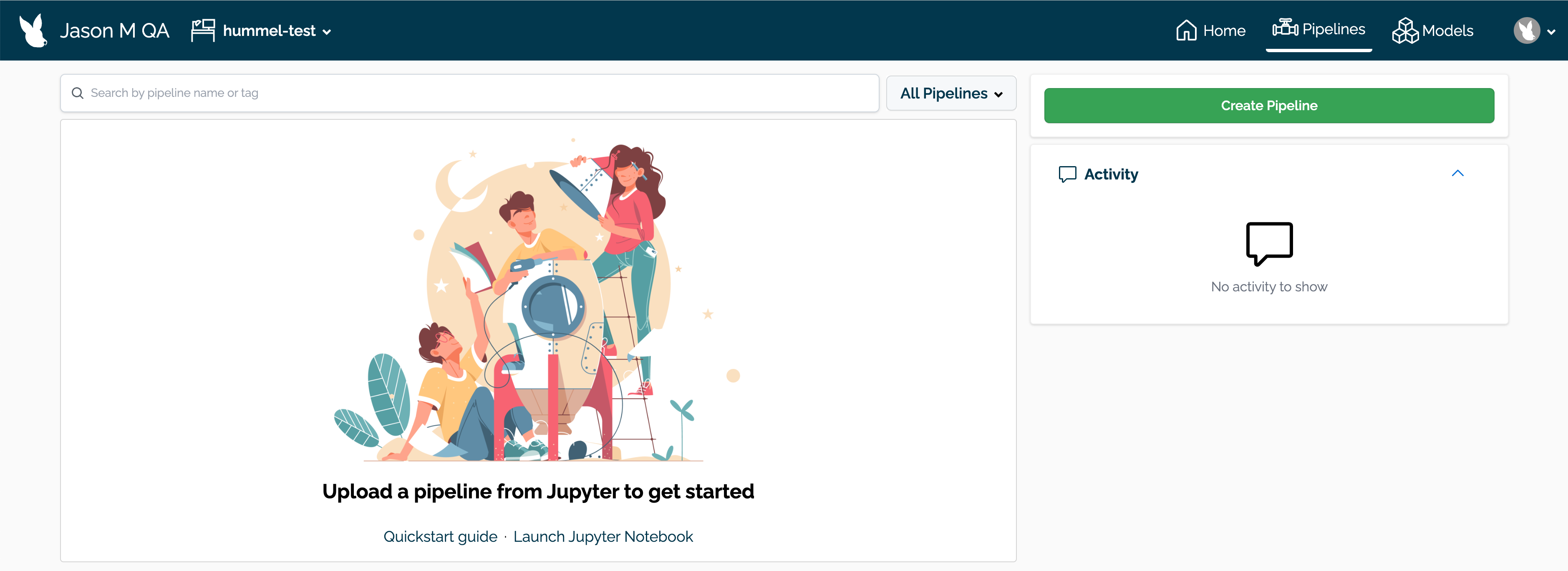
How to Create a Pipeline using the Wallaroo Dashboard
Prerequisites
Before creating a pipeline through the Wallaroo Dashboard, a model must be uploaded into the workspace through the SDK. For more information, see the Wallaroo SDK Essentials Guide.
IMPORTANT NOTICE
Pipeline names are not forced to be unique. You can have 50 pipelines all named my-pipeline, which can cause confusion in determining which pipeline to use.
It is recommended that organizations agree on a naming convention and select pipeline to use rather than creating a new one each time. See the SDK guides for more information on how to select an existing pipeline.
To create a pipeline:
From the Wallaroo Dashboard, set the current workspace from the top left dropdown list.
Select View Pipelines from the pipeline’s row.
From the upper right hand corner, select Create Pipeline.
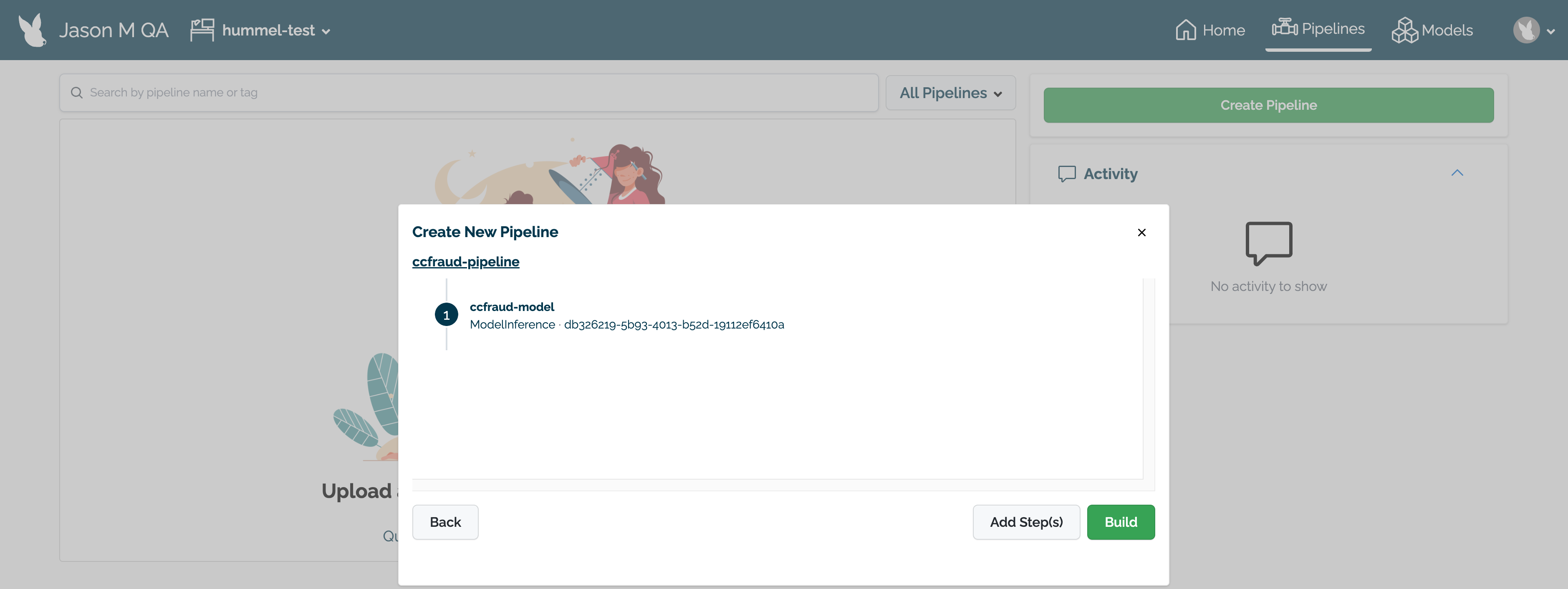
Enter the following:
Pipeline Name: The name of the new pipeline. Pipeline names should be unique across the Wallaroo instance.
Add Pipeline Step: Select the models to be used as the pipeline steps.
When finished, select Next.
Review the name of the pipeline and the steps. If any adjustments need to be made, select either Back to rename the pipeline or Add Step(s) to change the pipeline’s steps.
When finished, select Build to create the pipeline in this workspace. The pipeline will be built and be ready for deployment within a minute.
How to Deploy and Undeploy a Pipeline using the Wallaroo Dashboard
Deployed pipelines create new namespaces in the Kubernetes environment where the Wallaroo instance is deployed, and allocate resources from the Kubernetes environment to run the pipeline and its steps.
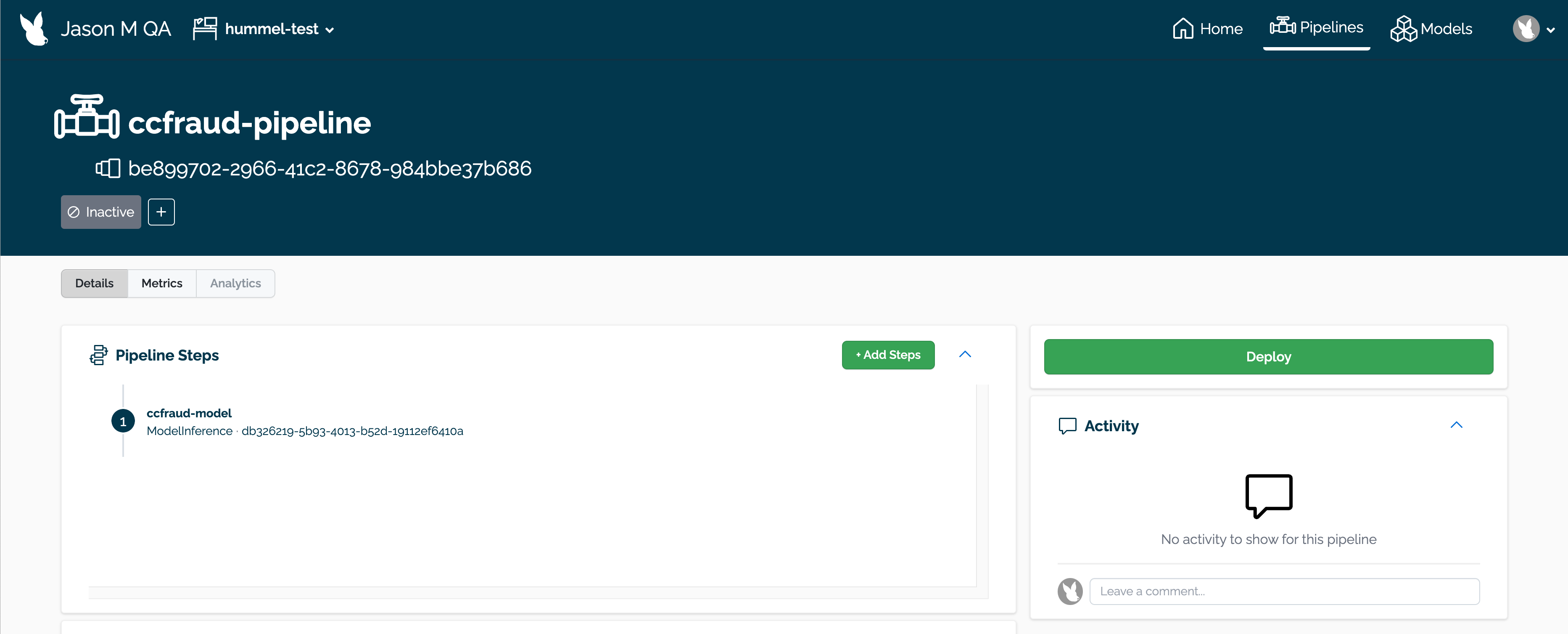
To deploy a pipeline:
From the Wallaroo Dashboard, set the current workspace from the top left dropdown list.
Select View Pipelines from the pipeline’s row.
Select the pipeline to deploy.
From the right navigation panel, select Deploy.
A popup module will request verification to deploy the pipeline. Select Deploy again to deploy the pipeline.
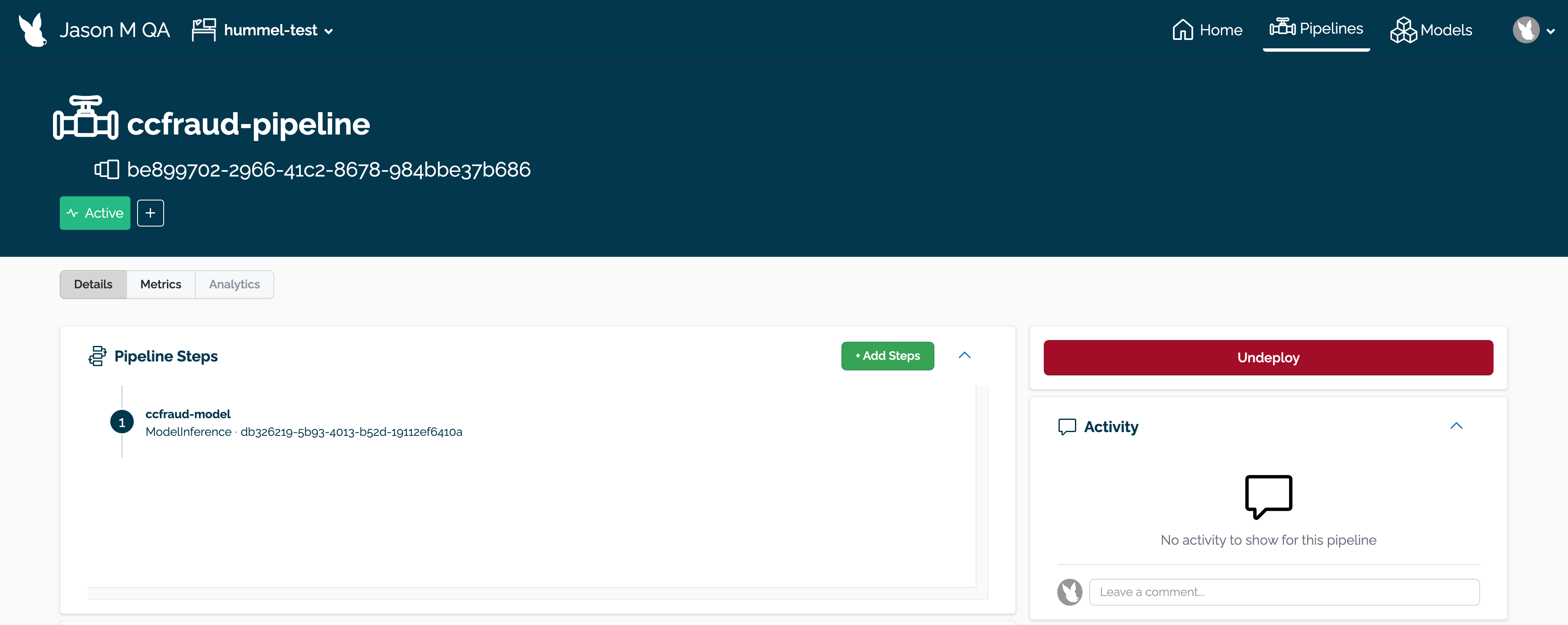
Undeploying a pipeline returns resources back to the Kubernetes environment and removes the namespaces created when the pipeline was deployed.
To undeploy a pipeline:
From the Wallaroo Dashboard, set the current workspace from the top left dropdown list.
Select View Pipelines from the pipeline’s row.
Select the pipeline to deploy.
From the right navigation panel, select Undeploy.
A popup module will request verification to undeploy the pipeline. Select Undeploy again to undeploy the pipeline.
How to View a Pipeline Details and Metrics
To view a pipeline’s details:
From the Wallaroo Dashboard, set the current workspace from the top left dropdown list.
Select View Pipelines from the pipeline’s row.
To view details on the pipeline, select the name of the pipeline.
A list of the pipeline’s details will be displayed.
To view a pipeline’s metrics:
From the Wallaroo Dashboard, set the current workspace from the top left dropdown list.
Select View Pipelines from the pipeline’s row.
To view details on the pipeline, select the name of the pipeline.
A list of the pipeline’s details will be displayed.
Select Metrics to view the following information. From here you can select the time period to display metrics from through the drop down to display the following:
Requests per second
Cluster inference rate
Inference latency
The Audit Log and Anomaly Log are available to view further details of the pipeline’s activities.
Pipeline Details
The following is available from the Pipeline Details page:
The name of the pipeline.
The pipeline ID: This is in UUID format.
Pipeline steps: The steps and the models in each pipeline step.
Version History: how the pipeline has been updated over time.
1 - Wallaroo Pipeline Tag Management
How to manage tags and pipelines.
Tags can be used to label, search, and track pipelines across a Wallaroo instance. The following guide will demonstrate how to:
Create a tag for a specific pipeline.
Remove a tag for a specific pipeline.
The example shown uses the pipeline ccfraudpipeline.
Steps
Add a New Tag to a Pipeline
To set a tag to pipeline using the Wallaroo Dashboard:
Log into your Wallaroo instance.
Select the workspace the pipelines are associated with.
Select View Pipelines.
From the Pipeline Select Dashboard page, select the pipeline to update.
From the Pipeline Dashboard page, select the + icon under the name of the pipeline and it’s hash value.
Enter the name of the new tag. When complete, select Enter. The tag will be set for this pipeline.
Remove a Tag from a Pipeline
To remove a tag from a pipeline:
IMPORTANT NOTE
Once a tag is deleted from a pipeline, it can not be undeleted.
Log into your Wallaroo instance.
Select the workspace the pipelines are associated with.
Select View Pipelines.
From the Pipeline Select Dashboard page, select the pipeline to update.
From the Pipeline Dashboard page, select the select the X for the tag to delete. The tag will be removed from the pipeline.
Wallaroo SDK Tag Management
Tags are applied to either model versions or pipelines. This allows organizations to track different versions of models, and search for what pipelines have been used for specific purposes such as testing versus production use.
Create Tag
Tags are created with the Wallaroo client command create_tag(String tagname). This creates the tag and makes it available for use.
The tag will be saved to the variable currentTag to be used in the rest of these examples.
# Now we create our tagcurrentTag=wl.create_tag("My Great Tag")
List Tags
Tags are listed with the Wallaroo client command list_tags(), which shows all tags and what models and pipelines they have been assigned to.
Tags are used with pipelines to track different pipelines that are built or deployed with different features or functions.
Add Tag to Pipeline
Tags are added to a pipeline through the Wallaroo Tag add_to_pipeline(pipeline_id) method, where pipeline_id is the pipeline’s integer id.
For this example, we will add currentTag to testtest_pipeline, then verify it has been added through the list_tags command and list_pipelines command.
# add this tag to the pipelinecurrentTag.add_to_pipeline(tagtest_pipeline.id())
{'pipeline_pk_id': 1, 'tag_pk_id': 1}
Search Pipelines by Tag
Pipelines can be searched through the Wallaroo Client search_pipelines(search_term) method, where search_term is a string value for tags assigned to the pipelines.
In this example, the text “My Great Tag” that corresponds to currentTag will be searched for and displayed.
wl.search_pipelines('My Great Tag')
name
version
creation_time
last_updated_time
deployed
tags
steps
tagtestpipeline
5a4ff3c7-1a2d-4b0a-ad9f-78941e6f5677
2022-29-Nov 17:15:21
2022-29-Nov 17:15:21
(unknown)
My Great Tag
Remove Tag from Pipeline
Tags are removed from a pipeline with the Wallaroo Tag remove_from_pipeline(pipeline_id) command, where pipeline_id is the integer value of the pipeline’s id.
For this example, currentTag will be removed from tagtest_pipeline. This will be verified through the list_tags and search_pipelines command.
## remove from pipelinecurrentTag.remove_from_pipeline(tagtest_pipeline.id())
{'pipeline_pk_id': 1, 'tag_pk_id': 1}
2 - Wallaroo Assays Management
How to create and use assays to monitor model inputs and outputs.
Model Insights and Interactive Analysis Introduction
Wallaroo provides the ability to perform interactive analysis so organizations can explore the data from a pipeline and learn how the data is behaving. With this information and the knowledge of your particular business use case you can then choose appropriate thresholds for persistent automatic assays as desired.
IMPORTANT NOTE
Model insights operates over time and is difficult to demo in a notebook without pre-canned data. We assume you have an active pipeline that has been running and making predictions over time and show you the code you may use to analyze your pipeline.
Monitoring tasks called assays monitors a model’s predictions or the data coming into the model against an established baseline. Changes in the distribution of this data can be an indication of model drift, or of a change in the environment that the model trained for. This can provide tips on whether a model needs to be retrained or the environment data analyzed for accuracy or other needs.
Assay Details
Assays contain the following attributes:
Attribute
Default
Description
Name
The name of the assay. Assay names must be unique.
Baseline Data
Data that is known to be “typical” (typically distributed) and can be used to determine whether the distribution of new data has changed.
Schedule
Every 24 hours at 1 AM
New assays are configured to run a new analysis for every 24 hours starting at the end of the baseline period. This period can be configured through the SDK.
Group Results
Daily
Groups assay results into groups based on either Daily (the default), Weekly, or Monthly.
Metric
PSI
Population Stability Index (PSI) is an entropy-based measure of the difference between distributions. Maximum Difference of Bins measures the maximum difference between the baseline and current distributions (as estimated using the bins). Sum of the difference of bins sums up the difference of occurrences in each bin between the baseline and current distributions.
Threshold
0.1
The threshold for deciding whether the difference between distributions, as evaluated by the above metric, is large (the distributions are different) or small (the distributions are similar). The default of 0.1 is generally a good threshold when using PSI as the metric.
Number of Bins
5
Sets the number of bins that will be used to partition the baseline data for comparison against how future data falls into these bins. By default, the binning scheme is percentile (quantile) based. The binning scheme can be configured (see Bin Mode, below). Note that the total number of bins will include the set number plus the left_outlier and the right_outlier, so the total number of bins will be the total set + 2.
Bin Mode
Quantile
Set the binning scheme. Quantile binning defines the bins using percentile ranges (each bin holds the same percentage of the baseline data). Equal binning defines the bins using equally spaced data value ranges, like a histogram. Custom allows users to set the range of values for each bin, with the Left Outlier always starting at Min (below the minimum values detected from the baseline) and the Right Outlier always ending at Max (above the maximum values detected from the baseline).
Bin Weight
Equally Weighted
The bin weights can be either set to Equally Weighted (the default) where each bin is weighted equally, or Custom where the bin weights can be adjusted depending on which are considered more important for detecting model drift.
Manage Assays via the Wallaroo Dashboard
Assays can be created and used via the Wallaroo Dashboard.
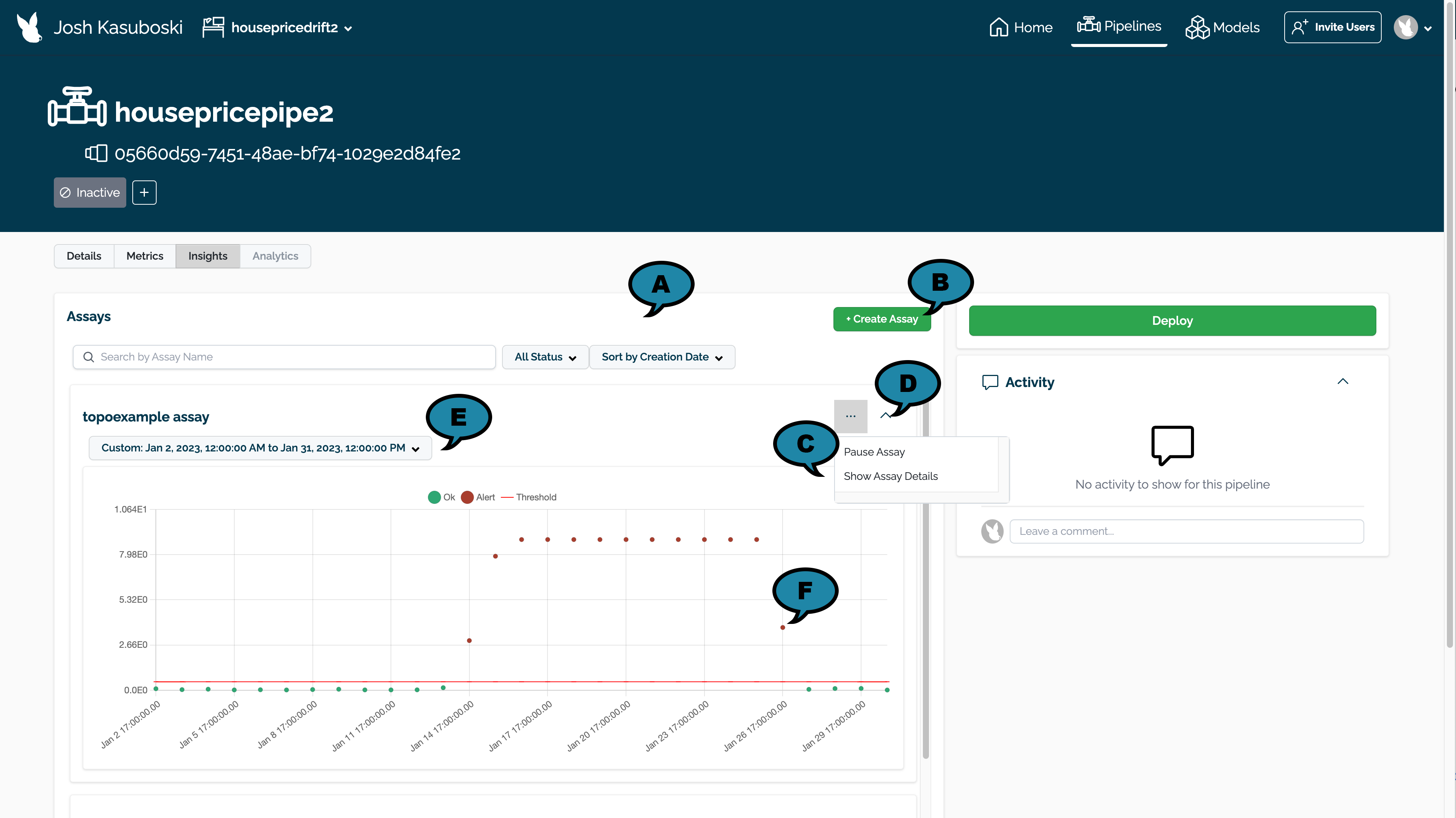
Accessing Assays Through the Pipeline Dashboard
Assays created through the Wallaroo Dashboard are accessed through the Pipeline Dashboard through the following process.
Log into the Wallaroo Dashboard.
Select the workspace containing the pipeline with the models being monitored from the Change Current Workspace and Workspace Management drop down.
Select View Pipelines.
Select the pipeline containing the models being monitored.
Select Insights.
The Wallaroo Assay Dashboard contains the following elements. For more details of each configuration type, see the Model Insights and Assays Introduction.
(A) Filter Assays: Filter assays by the following:
Name
Status:
Active: The assay is currently running.
Paused: The assay is paused until restarted.
Drift Detected: One or more drifts have been detected.
Sort By
Sort by Creation Date: Sort by the most recent Assays first.
Last Assay Run: Sort by the most recent Assay Last Run date.
(B) Create Assay: Create a new assay.
(C) Assay Controls:
Pause/Start Assay: Pause a running assay, or start one that was paused.
Show Assay Details: View assay details. See Assay Details View for more details.
(D) Collapse Assay: Collapse or Expand the assay for view.
(E) Time Period for Assay Data: Set the time period for data to be used in displaying the assay results.
(F) Assay Events: Select an individual assay event to see more details. See View Assay Alert Details for more information.
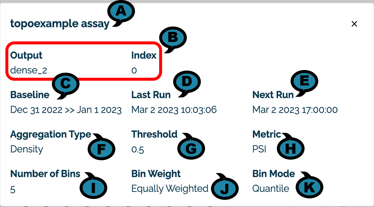
Assay Details View
The following details are visible by selecting the Assay View Details icon:
(A) Assay Name: The name of the assay displayed.
(B) Input / Output: The input or output and the index of the element being monitored.
(C) Baseline: The time period used to generate the baseline.
(D) Last Run: The date and time the assay was last run.
(E) Next Run: The future date and time the assay will be run again. NOTE: If the assay is paused, then it will not run at the scheduled time. When unpaused, the date will be updated to the next date and time that the assay will be run.
(F) Aggregation Type: The aggregation type used with the assay.
(G) Threshold: The threshold value used for the assay.
(H) Metric: The metric type used for the assay.
(I) Number of Bins: The number of bins used for the assay.
(J) Bin Weight: The weight applied to each bin.
(K) Bin Mode: The type of bin node applied to each bin.
View Assay Alert Details
To view details on an assay alert:
Select the data with available alert data.
Mouse hover of a specific Assay Event Alert to view the data and time of the event and the alert value.
Select the Assay Event Alert to view the Baseline and Window details of the alert including the left_outlier and right_outlier.
Hover over a bar chart graph to view additional details.
Select the ⊗ symbol to exit the Assay Event Alert details and return to the Assay View.
Build an Assay Through the Pipeline Dashboard
To create a new assay through the Wallaroo Pipeline Dashboard:
Log into the Wallaroo Dashboard.
Select the workspace containing the pipeline with the models being monitored from the Change Current Workspace and Workspace Management drop down.
Select View Pipelines.
Select the pipeline containing the models being monitored.
Select Insights.
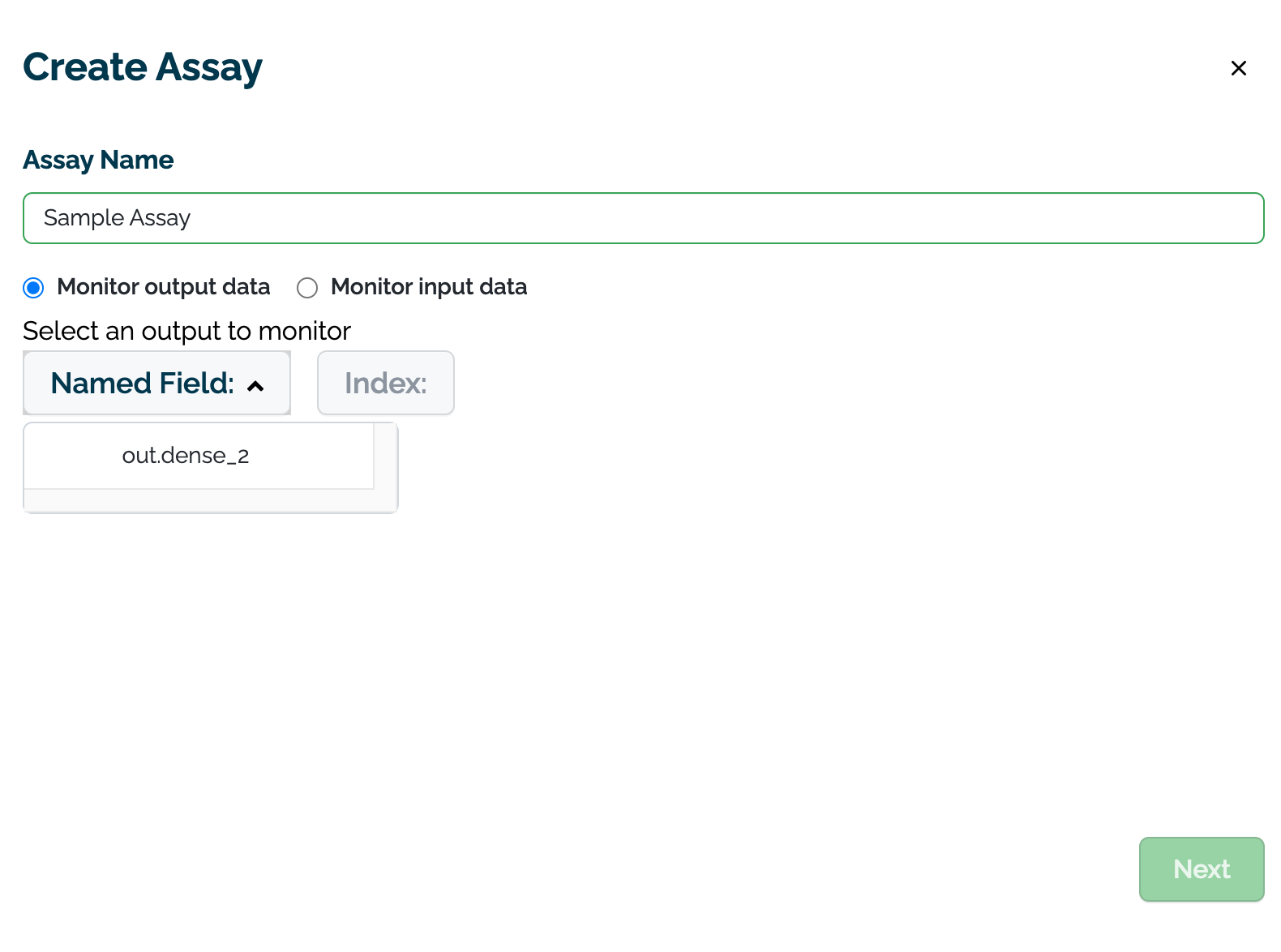
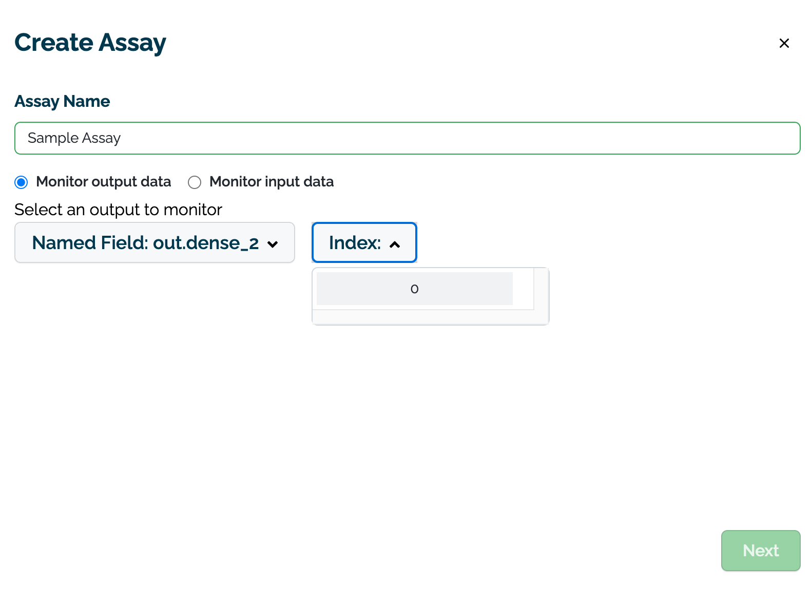
Select +Create Assay.
On the Assay Name module, enter the following:
Assay Name: The name of the new assay.
Monitor output data or Monitor input data: Select whether to monitor input or output data.
Select an output/input to monitor: Select the input or output to monitor.
Named Field: The name of the field to monitor.
Index: The index of the monitored field.
Select Next to continue.
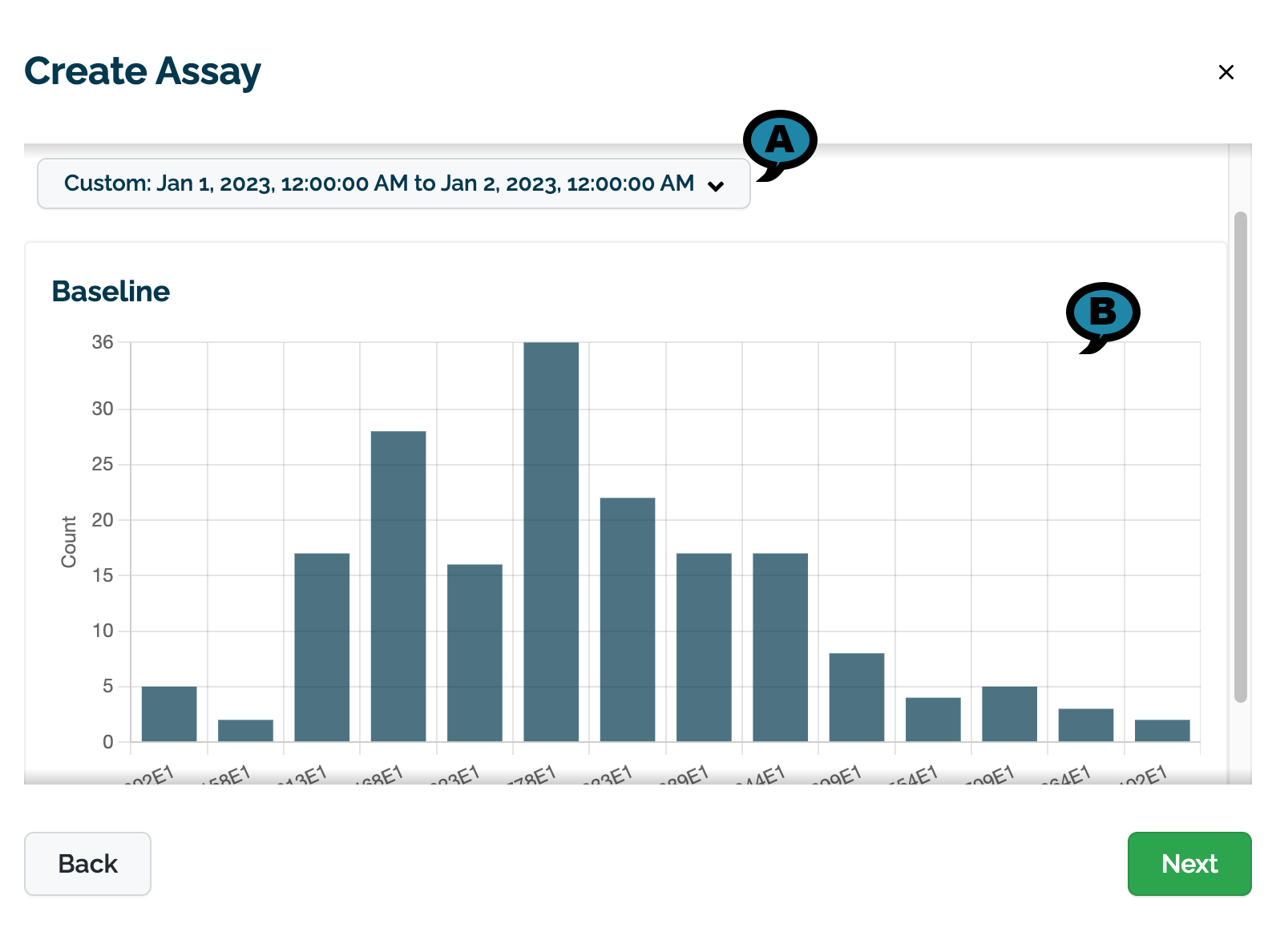
On the Specify Baseline Module:
(A) Select the data to use for the baseline. This can either be set with a preset recent time period (last 30 seconds, last 60 seconds, etc) or with a custom date range.
Once selected, a preview graph of the baseline values will be displayed (B). Note that this may take a few seconds to generate.
Select Next to continue.
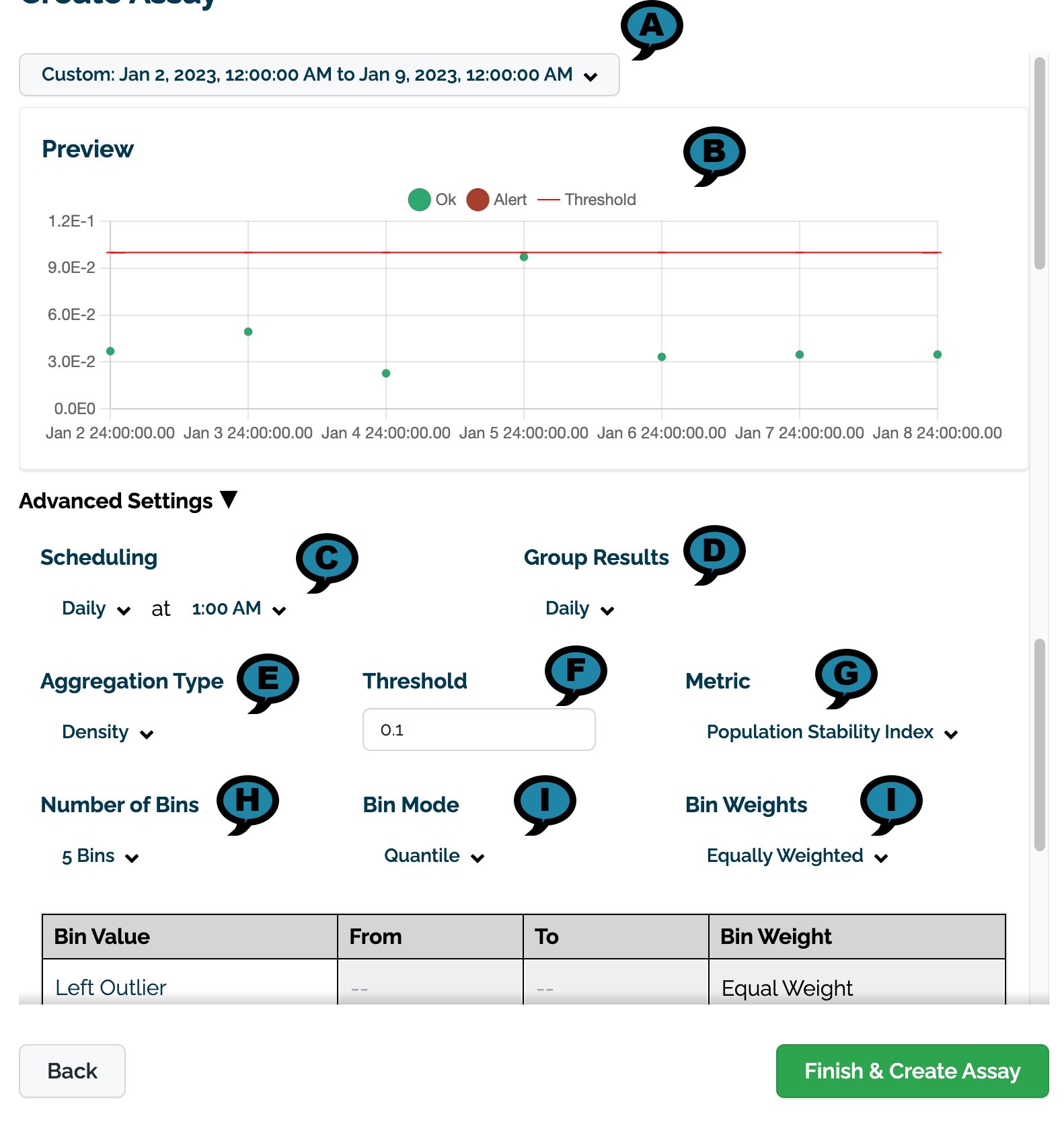
On the Settings Module:
Set the date and time range to view values generated by the assay. This can either be set with a preset recent time period (last 30 seconds, last 60 seconds, etc) or with a custom date range.
New assays are configured to run a new analysis for every 24 hours starting at the end of the baseline period. For information on how to adjust the scheduling period and other settings for the assay scheduling window, see the SDK section on how to Schedule Assay.
Set the following Advanced Settings.
(A) Preview Date Range: The date and times to for the preview chart.
(B) Preview: A preview of the assay results will be displayed based on the settings below.
(C) Scheduling: Set the Frequency (Daily, Every Minute, Hourly, Weekly, Default: Daily) and the Time (increments of one hour Default: 1:00 AM).
(D) Group Results: How the results are grouped: Daily, Weekly, or Monthly.
(E) Aggregation Type: Density or Cumulative.
(F) Threshold:
Default: 0.1
(G) Metric:
Default: Population Stability Index
Maximum Difference of Bins
Sum of the Difference of Bins
(H) Number of Bins: From 5 to 14. Default: 5
(F) Bin Mode:
Equally Spaced
Default: Quantile
(I) Bin Weights: The bin weights:
Equally Weighted (Default)
Custom: Users can assign their own bin weights as required.
Review the preview chart to verify the settings are correct.
Select Build to complete the process and build the new assay.
Once created, it may take a few minutes for the assay to complete compiling data. If needed, reload the Pipeline Dashboard to view changes.
Manage Assays via the Wallaroo SDK
List Assays
Assays are listed through the Wallaroo Client list_assays method.
wl.list_assays()
name
active
status
warning_threshold
alert_threshold
pipeline_name
api_assay
True
created
0.0
0.1
housepricepipe
Interactive Baseline Runs
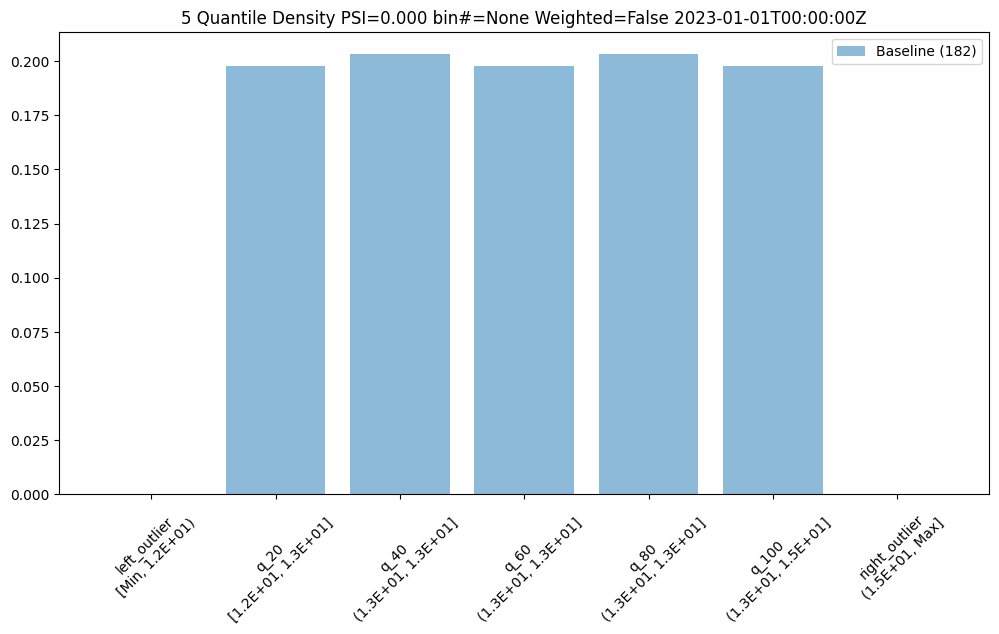
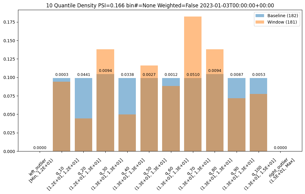
We can do an interactive run of just the baseline part to see how the baseline data will be put into bins. This assay uses quintiles so all 5 bins (not counting the outlier bins) have 20% of the predictions. We can see the bin boundaries along the x-axis.
baseline_run.chart()
baseline mean = 12.940910643273655
baseline median = 12.884286880493164
bin_mode = Quantile
aggregation = Density
metric = PSI
weighted = False
We can also get a dataframe with the bin/edge information.
baseline_run.baseline_bins()
b_edges
b_edge_names
b_aggregated_values
b_aggregation
0
12.00
left_outlier
0.00
Density
1
12.55
q_20
0.20
Density
2
12.81
q_40
0.20
Density
3
12.98
q_60
0.20
Density
4
13.33
q_80
0.20
Density
5
14.97
q_100
0.20
Density
6
inf
right_outlier
0.00
Density
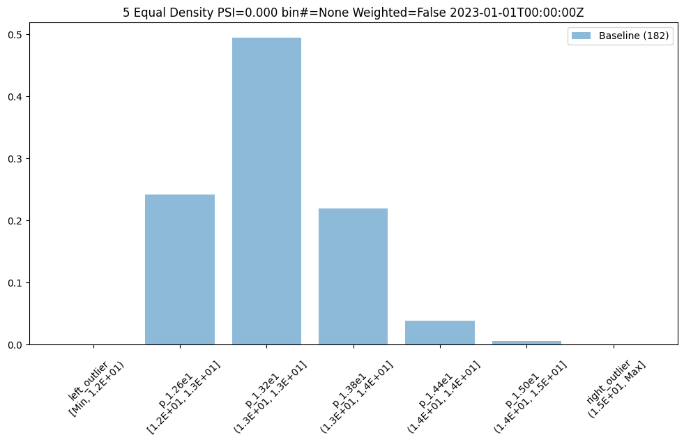
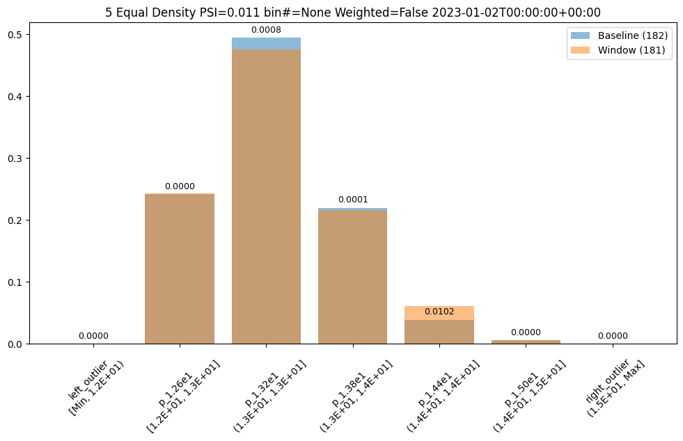
The previous assay used quintiles so all of the bins had the same percentage/count of samples. To get bins that are divided equally along the range of values we can use BinMode.EQUAL.
baseline mean = 12.940910643273655
baseline median = 12.884286880493164
bin_mode = Equal
aggregation = Density
metric = PSI
weighted = False
We now see very different bin edges and sample percentages per bin.
equal_baseline.baseline_bins()
b_edges
b_edge_names
b_aggregated_values
b_aggregation
0
12.00
left_outlier
0.00
Density
1
12.60
p_1.26e1
0.24
Density
2
13.19
p_1.32e1
0.49
Density
3
13.78
p_1.38e1
0.22
Density
4
14.38
p_1.44e1
0.04
Density
5
14.97
p_1.50e1
0.01
Density
6
inf
right_outlier
0.00
Density
Interactive Assay Runs
By default the assay builder creates an assay with some good starting parameters. In particular the assay is configured to run a new analysis for every 24 hours starting at the end of the baseline period. Additionally, it sets the number of bins to 5 so creates quintiles, and sets the target iopath to "outputs 0 0" which means we want to monitor the first column of the first output/prediction.
We can do an interactive run of just the baseline part to see how the baseline data will be put into bins. This assay uses quintiles so all 5 bins (not counting the outlier bins) have 20% of the predictions. We can see the bin boundaries along the x-axis.
We then run it with interactive_run and convert it to a dataframe for easy analysis with to_dataframe.
Now lets do an interactive run of the first assay as it is configured. Interactive runs don’t save the assay to the database (so they won’t be scheduled in the future) nor do they save the assay results. Instead the results are returned after a short while for further analysis.
Basic functionality for creating quick charts is included.
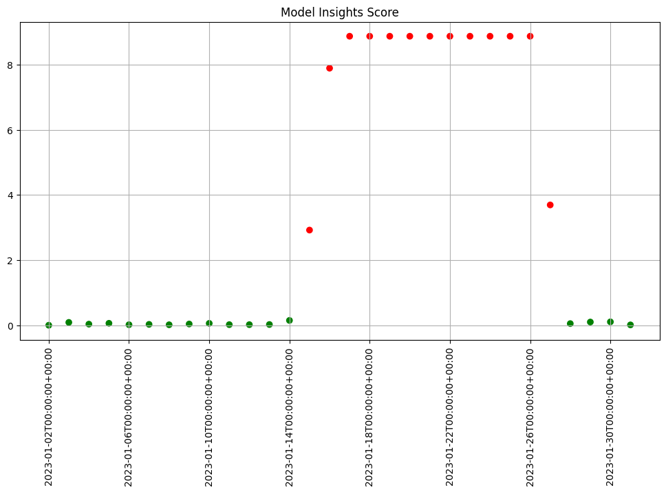
assay_results.chart_scores()
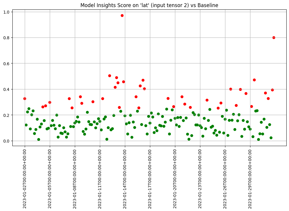
We see that the difference scores are low for a while and then jump up to indicate there is an issue. We can examine that particular window to help us decide if that threshold is set correctly or not.
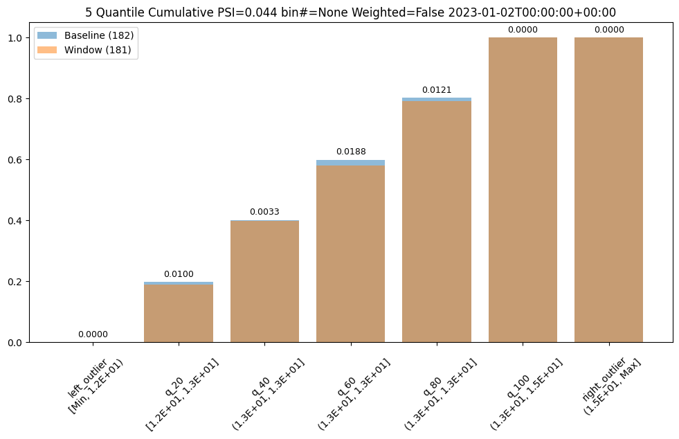
We can generate a quick chart of the results. This chart shows the 5 quantile bins (quintiles) derived from the baseline data plus one for left outliers and one for right outliers. We also see that the data from the window falls within the baseline quintiles but in a different proportion and is skewing higher. Whether this is an issue or not is specific to your use case.
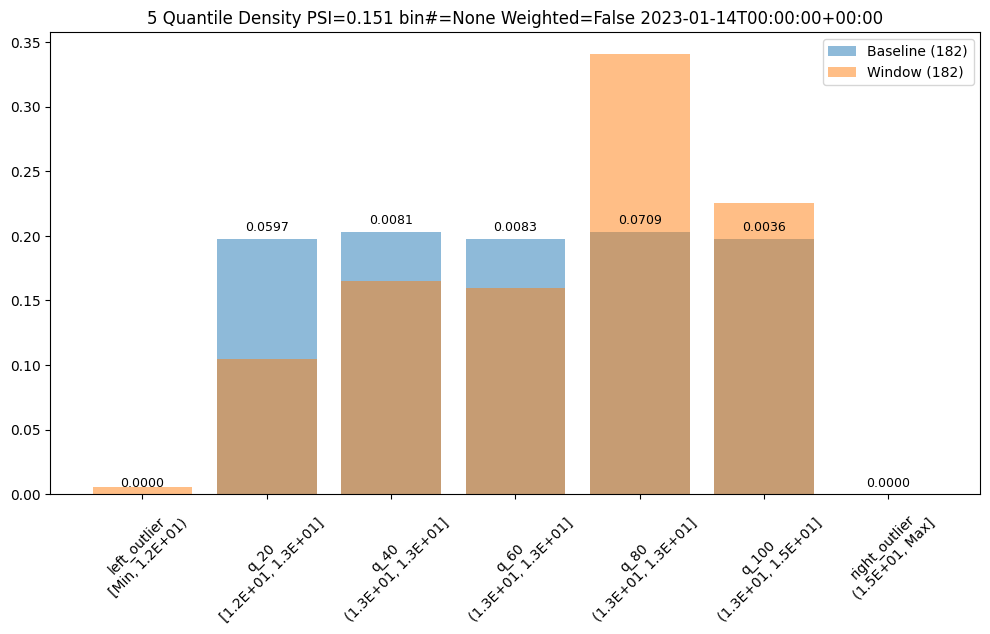
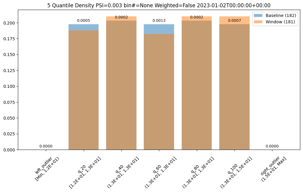
First lets examine a day that is only slightly different than the baseline. We see that we do see some values that fall outside of the range from the baseline values, the left and right outliers, and that the bin values are different but similar.
assay_results[0].chart()
baseline mean = 12.940910643273655
window mean = 12.969964654406132
baseline median = 12.884286880493164
window median = 12.899214744567873
bin_mode = Quantile
aggregation = Density
metric = PSI
weighted = False
score = 0.0029273068646199748
scores = [0.0, 0.000514261205558409, 0.0002139202456922972, 0.0012617897456473992, 0.0002139202456922972, 0.0007234154220295724, 0.0]
index = None
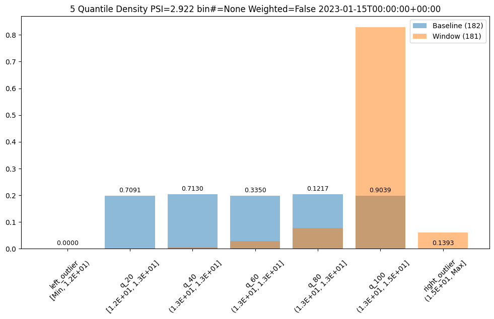
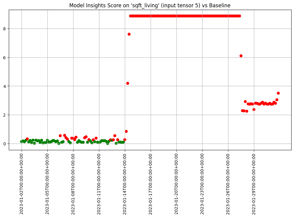
Other days, however are significantly different.
assay_results[12].chart()
baseline mean = 12.940910643273655
window mean = 13.06380216891949
baseline median = 12.884286880493164
window median = 13.027600288391112
bin_mode = Quantile
aggregation = Density
metric = PSI
weighted = False
score = 0.15060511096978788
scores = [4.6637149189075455e-05, 0.05969428191167242, 0.00806617426854112, 0.008316273402678306, 0.07090885609902021, 0.003572888138686759, 0.0]
index = None
assay_results[13].chart()
baseline mean = 12.940910643273655
window mean = 14.004728427908038
baseline median = 12.884286880493164
window median = 14.009637832641602
bin_mode = Quantile
aggregation = Density
metric = PSI
weighted = False
score = 2.9220486095961196
scores = [0.0, 0.7090936334784107, 0.7130482300184766, 0.33500731896676245, 0.12171058214520876, 0.9038825518183468, 0.1393062931689142]
index = None
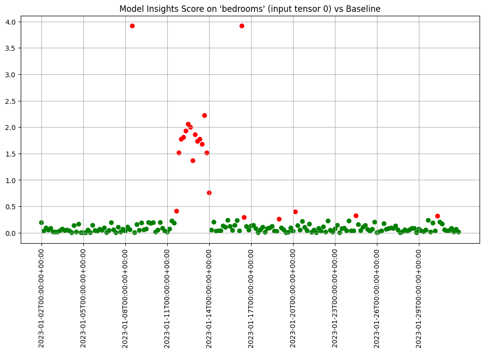
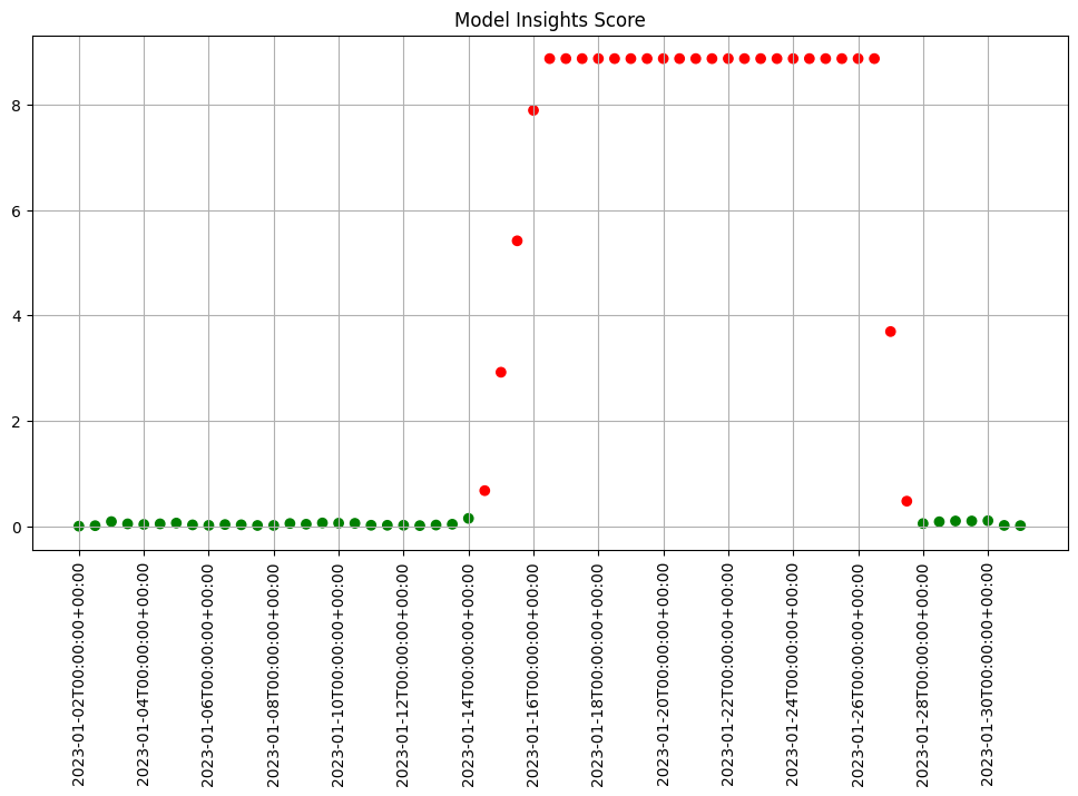
If we want to investigate further, we can run interactive assays on each of the inputs to see if any of them show anything abnormal. In this example we’ll provide the feature labels to create more understandable titles.
The current assay expects continuous data. Sometimes categorical data is encoded as 1 or 0 in a feature and sometimes in a limited number of values such as 1, 2, 3. If one value has high a percentage the analysis emits a warning so that we know the scores for that feature may not behave as we expect.
We can chart each of the iopaths and do a visual inspection. From the charts we see that if any of the input features had significant differences in the first two days which we can choose to inspect further. Here we choose to show 3 charts just to save space in this notebook.
When we are comfortable with what alert threshold should be for our specific purposes we can create and save an assay that will be automatically run on a daily basis.
In this example we’re create an assay that runs everyday against the baseline and has an alert threshold of 0.5.
Once we upload it it will be saved and scheduled for future data as well as run against past data.
After a short while, we can get the assay results for further analysis.
When we get the assay results, we see that the assays analysis is similar to the interactive run we started with though the analysis for the third day does not exceed the new alert threshold we set. And since we called upload instead of interactive_run the assay was saved to the system and will continue to run automatically on schedule from now on.
Scheduling Assays
By default assays are scheduled to run every 24 hours starting immediately after the baseline period ends.
However, you can control the start time by setting start and the frequency by setting interval on the window.
So to recap:
The window width is the size of the window. The default is 24 hours.
The interval is how often the analysis is run, how far the window is slid into the future based on the last run. The default is the window width.
The window start is when the analysis should start. The default is the end of the baseline period.
For example to run an analysis every 12 hours on the previous 24 hours of data you’d set the window width to 24 (the default) and the interval to 12.
To start a weekly analysis of the previous week on a specific day, set the start date (taking care to specify the desired timezone), and the width and interval to 1 week and of course an analysis won’t be generated till a window is complete.
The assay can be configured in a variety of ways to help customize it to your particular needs. Specifically you can:
change the BinMode to evenly spaced, quantile or user provided
change the number of bins to use
provide weights to use when scoring the bins
calculate the score using the sum of differences, maximum difference or population stability index
change the value aggregation for the bins to density, cumulative or edges
Lets take a look at these in turn.
Default configuration
First lets look at the default configuration. This is a lot of information but much of it is useful to know where it is available.
We see that the assay is broken up into 4 sections. A top level meta data section, a section for the baseline specification, a section for the window specification and a section that specifies the summarization configuration.
In the meta section we see the name of the assay, that it runs on the first column of the first output "outputs 0 0" and that there is a default threshold of 0.25.
The summarizer section shows us the defaults of Quantile, Density and PSI on 5 bins.
The baseline section shows us that it is configured as a fixed baseline with the specified start and end date times.
And the window tells us what model in the pipeline we are analyzing and how often.
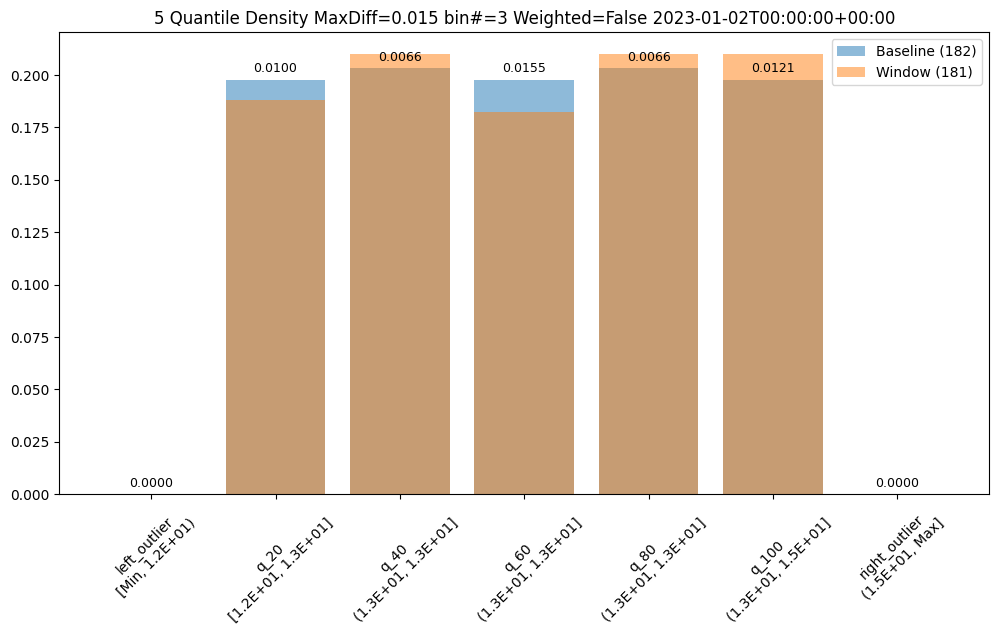
We can run the assay interactively and review the first analysis. The method compare_basic_stats gives us a dataframe with basic stats for the baseline and window data.
The method compare_bins gives us a dataframe with the bin information. Such as the number of bins, the right edges, suggested bin/edge names and the values for each bin in the baseline and the window.
baseline mean = 12.940910643273655
window mean = 12.969964654406132
baseline median = 12.884286880493164
window median = 12.899214744567873
bin_mode = Equal
aggregation = Density
metric = PSI
weighted = False
score = 0.011074287819376092
scores = [0.0, 7.3591419975306595e-06, 0.000773779195360713, 8.538514991838585e-05, 0.010207597078872246, 1.6725322721660374e-07, 0.0]
index = None
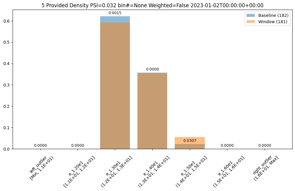
User Provided Bin Edges
The values in this dataset run from ~11.6 to ~15.81. And lets say we had a business reason to use specific bin edges. We can specify them with the BinMode.PROVIDED and specifying a list of floats with the right hand / upper edge of each bin and optionally the lower edge of the smallest bin. If the lowest edge is not specified the threshold for left outliers is taken from the smallest value in the baseline dataset.
baseline mean = 12.940910643273655
window mean = 12.956829186961135
baseline median = 12.884286880493164
window median = 12.929338455200195
bin_mode = Quantile
aggregation = Density
metric = PSI
weighted = False
score = 0.16591076620684958
scores = [0.0, 0.0002571306027792045, 0.044058279699182114, 0.009441459631493015, 0.03381618572319047, 0.0027335446937028877, 0.0011792419836838435, 0.051023062424253904, 0.009441459631493015, 0.008662563542113508, 0.0052978382749576496, 0.0]
index = None
Bin Weights
Now lets say we only care about differences at the higher end of the range. We can use weights to specify that difference in the lower bins should not be counted in the score.
If we stick with 10 bins we can provide 10 a vector of 12 weights. One weight each for the original bins plus one at the front for the left outlier bin and one at the end for the right outlier bin.
Note we still show the values for the bins but the scores for the lower 5 and left outlier are 0 and only the right half is counted and reflected in the score.
baseline mean = 12.940910643273655
window mean = 12.956829186961135
baseline median = 12.884286880493164
window median = 12.929338455200195
bin_mode = Quantile
aggregation = Density
metric = PSI
weighted = True
score = 0.012600694309416988
scores = [0.0, 0.0, 0.0, 0.0, 0.0, 0.0, 0.00019654033061397393, 0.00850384373737565, 0.0015735766052488358, 0.0014437605903522511, 0.000882973045826275, 0.0]
index = None
Metrics
The score is a distance or dis-similarity measure. The larger it is the less similar the two distributions are. We currently support summing the differences of each individual bin, taking the maximum difference and a modified Population Stability Index (PSI).
The following three charts use each of the metrics. Note how the scores change. The best one will depend on your particular use case.
baseline mean = 12.940910643273655
window mean = 12.969964654406132
baseline median = 12.884286880493164
window median = 12.899214744567873
bin_mode = Quantile
aggregation = Density
metric = MaxDiff
weighted = False
score = 0.01548175581324751
scores = [0.0, 0.009956893934794486, 0.006648048084512165, 0.01548175581324751, 0.006648048084512165, 0.012142553579017668, 0.0]
index = 3
Aggregation Options
Also, bin aggregation can be done in histogram Aggregation.DENSITY style (the default) where we count the number/percentage of values that fall in each bin or Empirical Cumulative Density Function style Aggregation.CUMULATIVE where we keep a cumulative count of the values/percentages that fall in each bin.